p1

Reference Manual

Original Publication: 08/01/2001

Last Revised: 03/24/2006

http://www.carlsonsw.com

© Carlson Software, 2005

p2

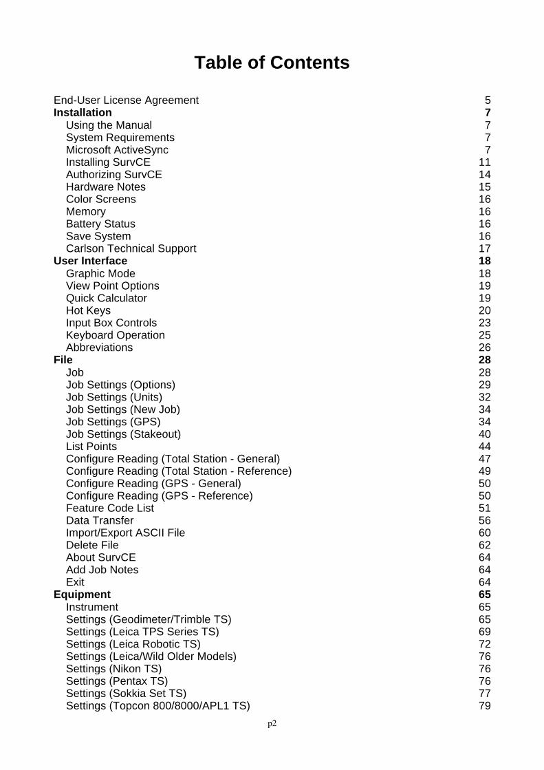
Table of Contents

End-User License Agreement 5Installation 7 Using the Manual 7 System Requirements 7 Microsoft ActiveSync 7 Installing SurvCE 11 Authorizing SurvCE 14 Hardware Notes 15 Color Screens 16 Memory 16 Battery Status 16 Save System 16 Carlson Technical Support 17User Interface 18 Graphic Mode 18 View Point Options 19 Quick Calculator 19 Hot Keys 20 Input Box Controls 23 Keyboard Operation 25 Abbreviations 26File 28 Job 28 Job Settings (Options) 29 Job Settings (Units) 32 Job Settings (New Job) 34 Job Settings (GPS) 34 Job Settings (Stakeout) 40 List Points 44 Configure Reading (Total Station - General) 47 Configure Reading (Total Station - Reference) 49 Configure Reading (GPS - General) 50 Configure Reading (GPS - Reference) 50 Feature Code List 51 Data Transfer 56 Import/Export ASCII File 60 Delete File 62 About SurvCE 64 Add Job Notes 64 Exit 64Equipment 65 Instrument 65 Settings (Geodimeter/Trimble TS) 65 Settings (Leica TPS Series TS) 69 Settings (Leica Robotic TS) 72 Settings (Leica/Wild Older Models) 76 Settings (Nikon TS) 76 Settings (Pentax TS) 76 Settings (Sokkia Set TS) 77 Settings (Topcon 800/8000/APL1 TS) 79

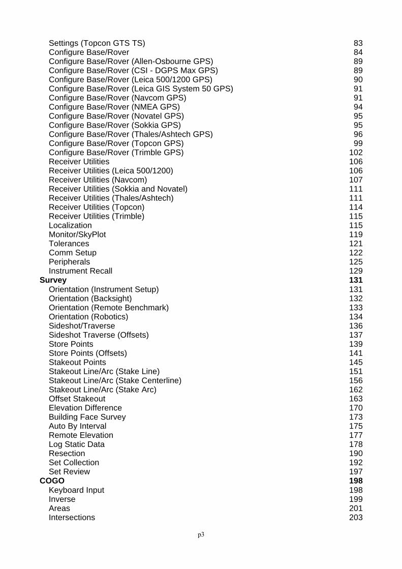
p3

Settings (Topcon GTS TS) 83 Configure Base/Rover 84 Configure Base/Rover (Allen-Osbourne GPS) 89 Configure Base/Rover (CSI - DGPS Max GPS) 89 Configure Base/Rover (Leica 500/1200 GPS) 90 Configure Base/Rover (Leica GIS System 50 GPS) 91 Configure Base/Rover (Navcom GPS) 91 Configure Base/Rover (NMEA GPS) 94 Configure Base/Rover (Novatel GPS) 95 Configure Base/Rover (Sokkia GPS) 95 Configure Base/Rover (Thales/Ashtech GPS) 96 Configure Base/Rover (Topcon GPS) 99 Configure Base/Rover (Trimble GPS) 102 Receiver Utilities 106 Receiver Utilities (Leica 500/1200) 106 Receiver Utilities (Navcom) 107 Receiver Utilities (Sokkia and Novatel) 111 Receiver Utilities (Thales/Ashtech) 111 Receiver Utilities (Topcon) 114 Receiver Utilities (Trimble) 115 Localization 115 Monitor/SkyPlot 119 Tolerances 121 Comm Setup 122 Peripherals 125 Instrument Recall 129Survey 131 Orientation (Instrument Setup) 131 Orientation (Backsight) 132 Orientation (Remote Benchmark) 133 Orientation (Robotics) 134 Sideshot/Traverse 136 Sideshot Traverse (Offsets) 137 Store Points 139 Store Points (Offsets) 141 Stakeout Points 145 Stakeout Line/Arc (Stake Line) 151 Stakeout Line/Arc (Stake Centerline) 156 Stakeout Line/Arc (Stake Arc) 162 Offset Stakeout 163 Elevation Difference 170 Building Face Survey 173 Auto By Interval 175 Remote Elevation 177 Log Static Data 178 Resection 190 Set Collection 192 Set Review 197COGO 198 Keyboard Input 198 Inverse 199 Areas 201 Intersections 203

p4

Point Projection 206 Station Store 209 Transformation 210 Calculator 213 Process Raw File 217 Point in Direction 230Road 233 Input-Edit Centerline 233 Draw Centerline 250 Input-Edit Profile 252 Draw Profile 254 Input-Edit Template 255 Draw Template 258 Slope Staking 259 Cross Section Survey 272 Road Utilities 281 Template Stakeout 296MAP 300 Basics 300 File 302 View 311 Draw 314 COGO 320 Tools 325Tutorials 330 Tutorial 1 330 Tutorial 2 331 Tutorial 3 331 Tutorial 4 335 Tutorial 5 348Troubleshooting 356 GPS Heights 356 Handheld Hardware 356 Miscellaneous Instrument Configuration 357 Supported File Formats 358Raw Data 360 File Format 360

p5

End-User License Agreement

Copyright © 2004 Carlson SoftwareAll Rights Reserved

CAUTION! READ THIS NOTICE CAREFULLY BEFORE USING SOFTWARE.

Use of this software indicates acceptance of the terms and conditions of the Software License Agreement.

SurvCE End-User License Agreement

This End-User License Agreement (henceforth "EULA") is a legal agreement between you, the individual or singleentity (henceforth "you"), and Carlson Software, Inc. (henceforth "Carlson Software") for the software accompanyingthis EULA, and may or may not include printed materials, associated media, and electronic documentation (henceforth"this software"). Exercising your right to use this software binds you to the terms of this EULA.  If you do not agree tothe terms contained herein, do not use this software.

SOFTWARE LICENSE:This software is protected by United States copyright laws and international copyright treaties, as well as applicableintellectual property laws and treaties.  This software is licensed, not sold.

GRANT OF LICENSE:This EULA grants you the following rights: You may install and use one copy of this software, or any prior version for the same operating system, on a single

computer.  The primary user of the computer on which this software is installed may make a second copy for hisor her exclusive use.

Additionally, you may store one copy of this software on a storage device, such as a network server, used only toinstall or run this software on other computer over an internal network.  However, you must acquire and dedicatea license for each separate computer on which this software is installed or run from the storage device.  A singlelicense for this software may not be shared or used concurrently on more than one computer, unless a licensemanager has been purchased from Carlson Software.

OTHER RIGHTS AND LIMITATIONS: You may not reverse engineer, decompile, or disassemble this software, except and only to the extent that such

activity is expressly permitted by applicable law notwithstanding this limitation. This software is licensed as a single product.  Its component parts may not be separated for use on more than one

computer. Under certain circumstances, you may permanently transfer all of your rights under this EULA, provided that the

recipient agrees to the terms of this EULA. Without prejudice to any other rights, Carlson Software may terminate this EULA if you fail to comply with the

terms and conditions of this EULA.  In this event, you are required to destroy all copies of this software, and all ofits component parts.

COPYRIGHT:All title and copyrights in and to this software, including, but not limited to, any images, photographs, animations,video, audio, music, text, or "applets" incorporated into this software, the accompanying printed materials, and anycopies of this software, are the sole property of Carlson Software and/or its suppliers.  This software is protected byUnited States copyright laws and international copyright treaties, as well as applicable intellectual property laws andtreaties. Treat this software as you would any other copyrighted material.

U.S. GOVERNMENT RESTRICTED RIGHTS:Use, duplication, or disclosure by the U.S. Government of this software or its documentation is subject to restrictions,as set forth in subparagraph (c)(1)(ii) of the Right in Technical Data and Computer Software clause at DFAARS252.227-7013, or subparagraph (c)(1) and (2) of the Commercial Computer Software Restricted Rights at 48 CFR52.227-19, as applicable.The manufacturer is:Carlson Software, Inc.102 W. Second StreetMaysville, KY 41056

p6

LIMITED WARRANTY: CARLSON SOFTWARE EXPRESSLY DISCLAIMS ANY WARRANTY, EITHER EXPRESSED OR

IMPLIED, INCLUDING BUT NOT LIMITED TO ANY IMPLIED WARRANTIES OFMERCHANTABILITY, FITNESS FOR A PARTICULAR PURPOSE, OR NONINFRINGEMENTREGARDING THESE MATERIALS.  CARLSON SOFTWARE MAKES SUCH MATERIALS AVAILABLESOLELY ON AN "AS-IS" BASIS.

IN NO EVENT SHALL CARLSON SOFTWARE BE LIABLE TO ANYONE FOR SPECIAL, COLLATERAL,INCIDENTAL, OR CONSEQUENTIAL DAMAGES IN CONNECTION WITH, OR ARISING OUT OF,PURCHASE, USE, OR INABILITY TO USE THESE MATERIALS. THIS INCLUDES, WITHOUTLIMITATION, DAMAGES FOR LOSS OF BUSINESS PROFITS, BUSINESS INTERRUPTION, LOSS OFBUSINESS INFORMATION OR ANY OTHER PECUNIARY LOSS. IN ALL INSTANCES, THEEXCLUSION OR LIMITATION OF LIABILITY IS SUBJECT TO ANY APPLICABLE JURISDICTION.

IF THIS SOFTWARE WAS ACQUIRED IN THE UNITED STATES, THIS EULA IS GOVERNED BY THELAWS OF THE COMMONWEALTH OF KENTUCKY. IF THIS PRODUCT WAS ACQUIRED OUTSIDE OFTHE UNITED STATES, THIS EULA IS GOVERNED BY THE LAWS IN ANY APPLICABLEJURISDICTION.

p7

InstallationUsing the ManualThis manual is designed as a reference guide. It contains a complete description of all commands in the CarlsonSurvCE product.

The chapters are organized by program menus, and they are arranged in the order that the menus appear in CarlsonSurvCE. Some commands are only applicable to either GPS or total station use and may not appear in your menu.

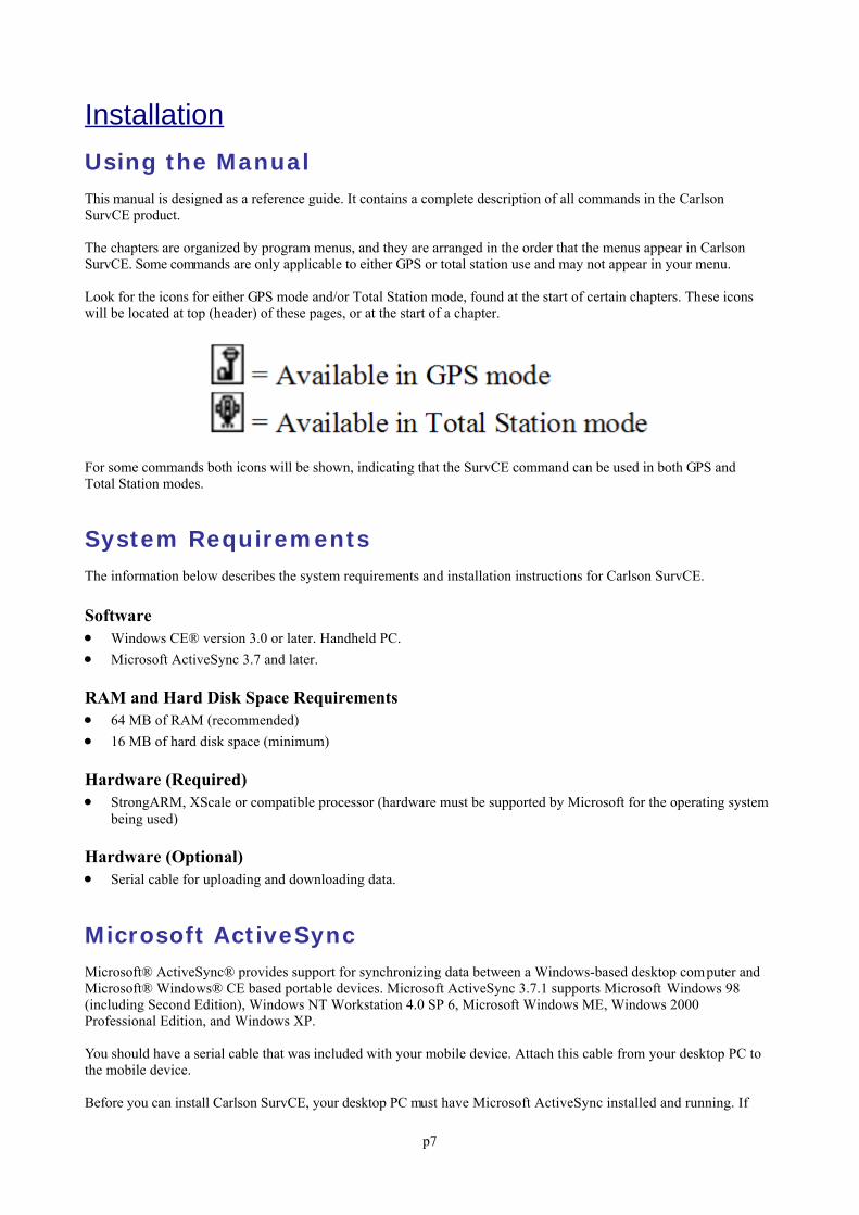
Look for the icons for either GPS mode and/or Total Station mode, found at the start of certain chapters. These iconswill be located at top (header) of these pages, or at the start of a chapter.

For some commands both icons will be shown, indicating that the SurvCE command can be used in both GPS andTotal Station modes.

System RequirementsThe information below describes the system requirements and installation instructions for Carlson SurvCE.

Software Windows CE® version 3.0 or later. Handheld PC. Microsoft ActiveSync 3.7 and later.

RAM and Hard Disk Space Requirements 64 MB of RAM (recommended) 16 MB of hard disk space (minimum)

Hardware (Required) StrongARM, XScale or compatible processor (hardware must be supported by Microsoft for the operating system

being used)

Hardware (Optional) Serial cable for uploading and downloading data.

Microsoft ActiveSyncMicrosoft® ActiveSync® provides support for synchronizing data between a Windows-based desktop computer andMicrosoft® Windows® CE based portable devices. Microsoft ActiveSync 3.7.1 supports Microsoft Windows 98(including Second Edition), Windows NT Workstation 4.0 SP 6, Microsoft Windows ME, Windows 2000Professional Edition, and Windows XP.

You should have a serial cable that was included with your mobile device. Attach this cable from your desktop PC tothe mobile device.

Before you can install Carlson SurvCE, your desktop PC must have Microsoft ActiveSync installed and running. If

p8

you have ActiveSync on your desktop PC, you should see an the ActiveSync icon in your system tray. If you do notsee this icon in the tray, choose the Windows Start button, choose Programs and then choose Microsoft ActiveSync. Ifyou do not have ActiveSync installed, insert the Carlson SurvCE CD-ROM and choose “Install ActiveSync”. You mayalso choose to download the latest version from Microsoft. After the ActiveSync installation starts, follow the prompts.If you need more assistance to install ActiveSync, visit Microsoft’s web site for the latest install details.

Auto ConnectionIf the default settings are correct, ActiveSync should automatically connect to the mobile device. When you see adialog on the mobile device that asks you if you want to connect, press Yes.

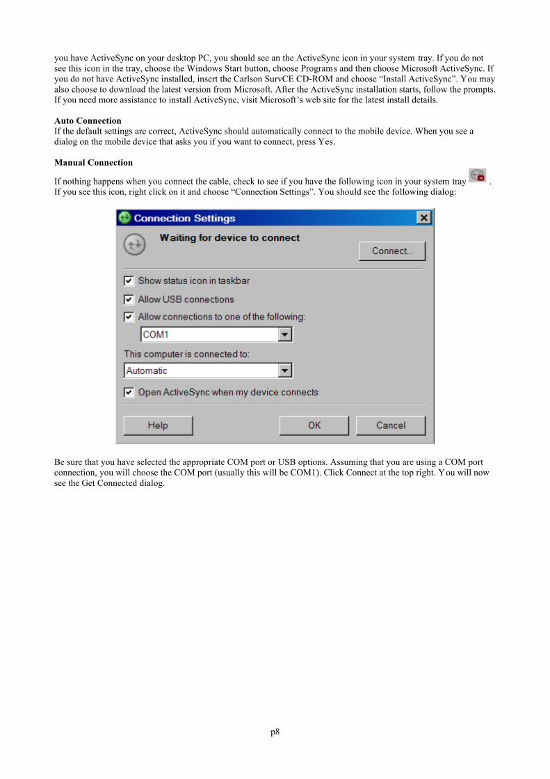
Manual Connection

If nothing happens when you connect the cable, check to see if you have the following icon in your system tray .If you see this icon, right click on it and choose “Connection Settings”. You should see the following dialog:

Be sure that you have selected the appropriate COM port or USB options. Assuming that you are using a COM portconnection, you will choose the COM port (usually this will be COM1). Click Connect at the top right. You will nowsee the Get Connected dialog.

p9

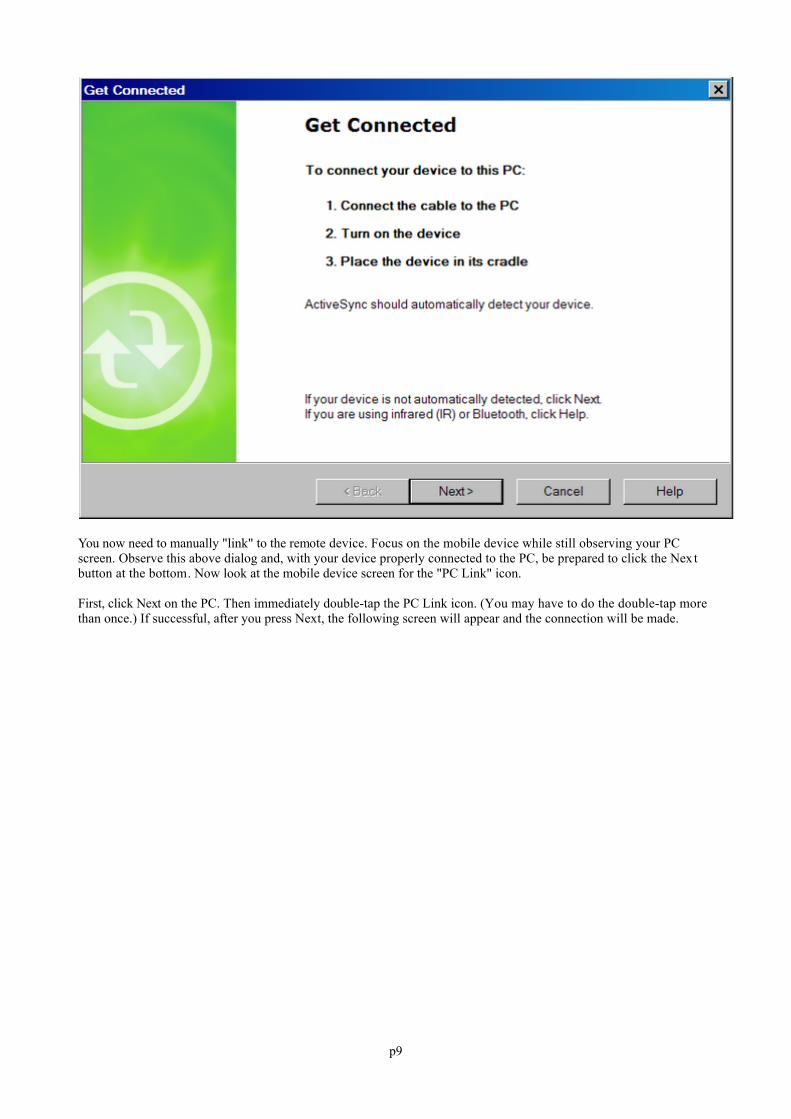
You now need to manually "link" to the remote device. Focus on the mobile device while still observing your PCscreen. Observe this above dialog and, with your device properly connected to the PC, be prepared to click the Nextbutton at the bottom. Now look at the mobile device screen for the "PC Link" icon.

First, click Next on the PC. Then immediately double-tap the PC Link icon. (You may have to do the double-tap morethan once.) If successful, after you press Next, the following screen will appear and the connection will be made.

p10

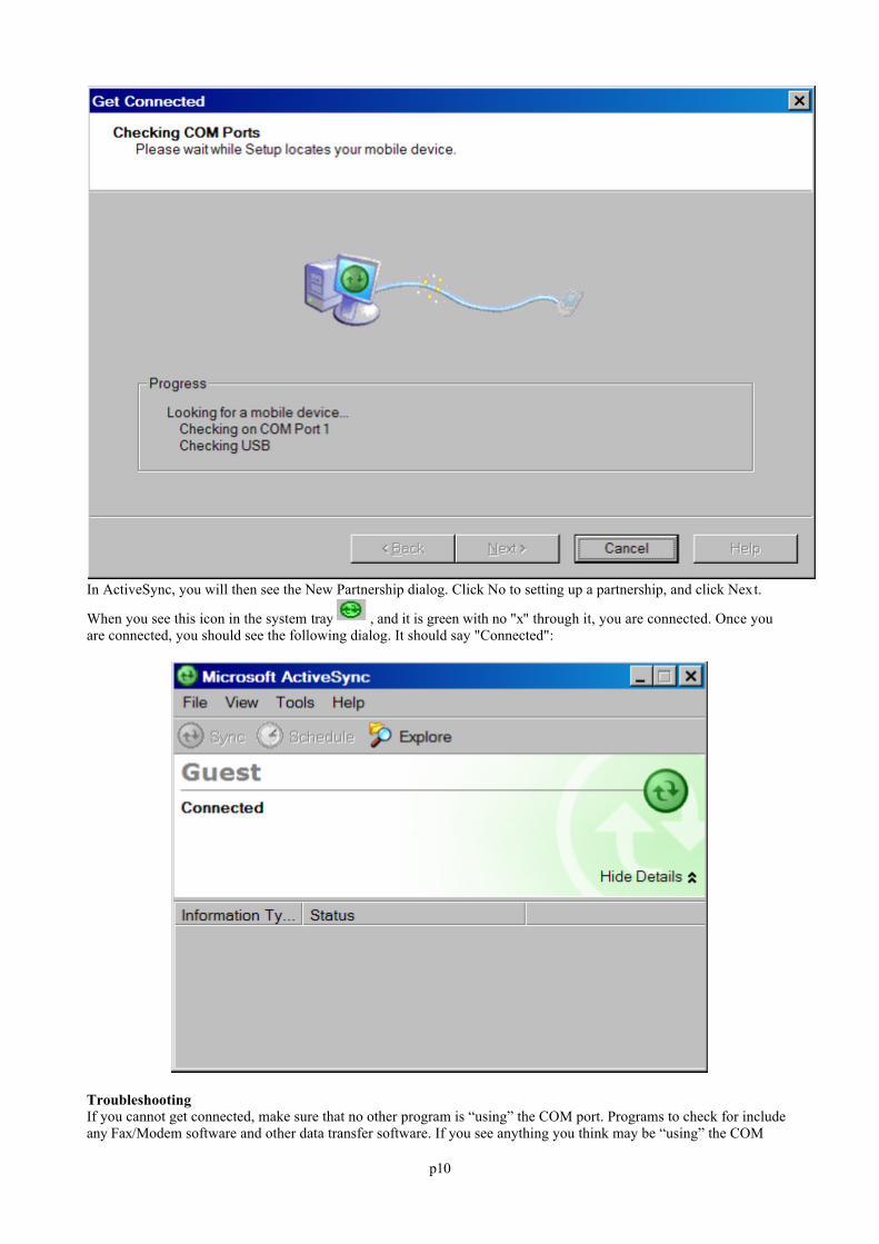
In ActiveSync, you will then see the New Partnership dialog. Click No to setting up a partnership, and click Next.

When you see this icon in the system tray , and it is green with no "x" through it, you are connected. Once youare connected, you should see the following dialog. It should say "Connected":

TroubleshootingIf you cannot get connected, make sure that no other program is “using” the COM port. Programs to check for includeany Fax/Modem software and other data transfer software. If you see anything you think may be “using” the COM

p11

port, shut it down and retry the connection with ActiveSync.

Enabling COM Port Communication for ActiveSync on Allegro, Panasonic Toughbook 01 and other CEdevicesIn order for ActiveSync to communicate, it may be necessary to direct the CE device to utilize the COM port as adefault. Some may come set default to USB. Go to Start (on Allegro, blue key and Start button), then Settings, thenControl Panel, then Communications icon, then PC Connection. Set to Com1 at a high baud rate, such as 57,600 baud.This will download programs and files at a high rate of speed. On the Allegro, use PC Link to connect to PC withActiveSync. On the Panasonic Toughbook, do Start, Run, and in the Open window, type in “autosync –go” (autosyncthen spacebar then “minus” go). Then do Start, Settings, Control Panel, Communications, do PC Connection, ChangeConnection to Serial Port @ 115K. Make sure “Enable direct connections to the desktop computer” is checked.

Note: When using SurvCE’s Data Transfer option, you will need to disable Serial Port Connection (click off AllowSerial Cable). This is done with Connection Settings in ActiveSync. Click back on to use ActiveSync.

Installing SurvCEBefore you install Carlson SurvCE, close all running applications on the mobile device.

1. Connect the mobile device to the desktop PC and ensure that the ActiveSync connection is made.2. Insert the CD into the CD-ROM drive on the desktop PC. If Autorun is enabled, the startup program begins. The

startup program lets you choose the version of SurvCE to install. To start the installation process without usingAutorun, choose Run from the Windows Start Menu. Enter the CD-ROM drive letter, and setup. For example,enter d:\setup (where d is your CD-ROM drive letter).

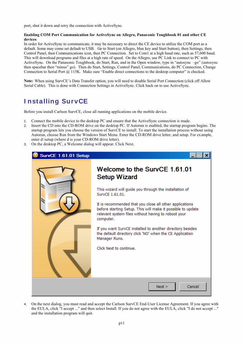
3. On the desktop PC, a Welcome dialog will appear. Click Next.

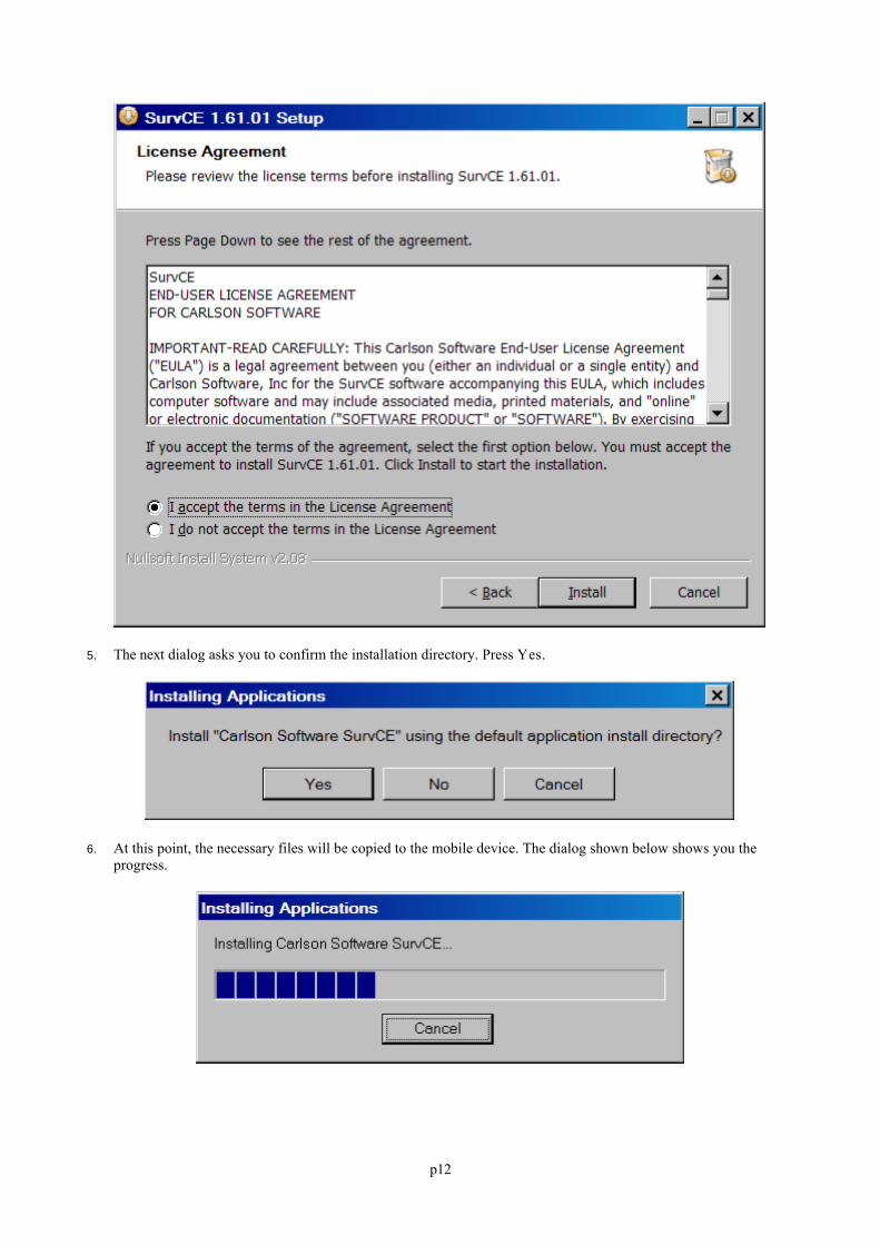
4. On the next dialog, you must read and accept the Carlson SurvCE End-User License Agreement. If you agree withthe EULA, click "I accept ..." and then select Install. If you do not agree with the EULA, click "I do not accept ..."and the installation program will quit.

p12

5. The next dialog asks you to confirm the installation directory. Press Yes.

6. At this point, the necessary files will be copied to the mobile device. The dialog shown below shows you theprogress.

p13

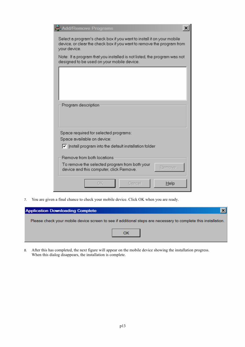
7. You are given a final chance to check your mobile device. Click OK when you are ready.

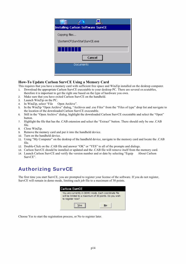
8. After this has completed, the next figure will appear on the mobile device showing the installation progress. When this dialog disappears, the installation is complete.

p14

How-To Update Carlson SurvCE Using a Memory CardThis requires that you have a memory card with sufficient free space and WinZip installed on the desktop computer.1. Download the appropriate Carlson SurvCE executable to your desktop PC. There are several ex ecutables,

therefore it is important to get the right one based on the type of hardware you own.2. Make sure that you have exited Carlson SurvCE on the handheld.3. Launch WinZip on the PC.4. In WinZip, select “File Open Archive”.5. In the WinZip “Open Archive” dialog, “Archives and .exe Files” from the “Files of type” drop list and navigate to

the location of the downloaded Carlson SurvCE executable.6. Still in the “Open Archive” dialog, highlight the downloaded Carlson SurvCE executable and select the “Open”

button.7. Highlight the file that has the .CAB extension and select the “Extract” button. There should only be one .CAB

file.8. Close WinZip.9. Remove the memory card and put it into the handheld device.10. Turn on the handheld device.11. Using “My Computer” on the desktop of the handheld device, navigate to the memory card and locate the .CAB

file.12. Double-Click on the .CAB file and answer “OK” or “YES” to all of the prompts and dialogs.13. Carlson SurvCE should be installed or updated and the .CAB file will remove itself from the memory card.14. Launch Carlson SurvCE and verify the version number and or date by selecting “Equip About Carlson

SurvCE”.

Authorizing SurvCEThe first time you start SurvCE, you are prompted to register your license of the software. If you do not register,SurvCE will remain in demo mode, limiting each job file to a maximum of 30 points.

Choose Yes to start the registration process, or No to register later.

p15

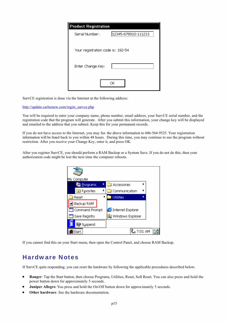
SurvCE registration is done via the Internet at the following address:

http://update.carlsonsw.com/regist_survce.php

You will be required to enter your company name, phone number, email address, your SurvCE serial number, and theregistration code that the program will generate. After you submit this information, your change key will be displayedand emailed to the address that you submit. Keep this for your permanent records.

If you do not have access to the Internet, you may fax the above information to 606-564-9525. Your registrationinformation will be faxed back to you within 48 hours. During this time, you may continue to use the program withoutrestriction. After you receive your Change Key, enter it, and press OK.

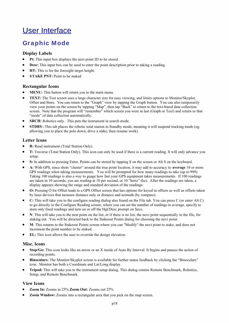
After you register SurvCE, you should perform a RAM Backup or a System Save. If you do not do this, then yourauthorization code might be lost the next time the computer reboots.

If you cannot find this on your Start menu, then open the Control Panel, and choose RAM Backup.

Hardware NotesIf SurvCE quits responding, you can reset the hardware by following the applicable procedures described below.

Ranger: Tap the Start button, then choose Programs, Utilities, Reset, Soft Reset. You can also press and hold thepower button down for approximately 5 seconds.

Juniper Allegro: You press and hold the On\Off button down for approximately 5 seconds. Other hardware: See the hardware documentation.

p16

Color ScreensSurvCE 1.21 or greater enables viewing of color. Any red, green, blue or other colored entities in DXF files willretain the color when viewed within SurvCE. Points will appear with black point numbers, green descriptions and blueelevations. Dialogs and prompting will utilize color throughout SurvCE.

MemoryMemory on Allegros and Rangers, and other similar CE devices, can be allocated for best results. We recommendsetting “storage memory” to a minimum of 16,000 to 18,000 KB. The following discussion outlines the procedure forsetting that memory on the Allegro. An equivalent process should be used for other CE devices, as available.

The SurvCE controller will function better during topo and stakeout with the "Storage Memory" set to around 18,000KB. To check and/or change the settings:

Hit the Blue Key and Start, then Settings => Control Panel => Double click on System => Touch the Memorytab => Slide the pointer toward the left, which is the Storage Memory side, so that the " Allocated " is around18,000 KB .

Keep in mind that to upgrade software, this setting may need to be changed back, so that the "Program Memory" hasmore available. To change, do as above but => Slide the pointer toward the Right, which is the Program side, so thatthe "Allocated" is around 18,000 KB. This assures that there is enough Program memory, so that the new updates canbe saved.

Once the upgrade or additional software is added, you can change it back so that the pointer is more toward theStorage Memory -- around 18,000 KB.

After changing these settings, or updating software, it's a good idea to do a "Save System".

Battery StatusThe black icon that appears at the top of every screen is designed to indicate battery status. Full black should indicatefull battery. As battery levels decrease the black recedes to full white (out of battery).

On some CE devices, there is no way to detect battery status, so the battery icon does not change. On some devicessuch as the Jett CE (Carlson Explorer), a partial indication of battery status is detected as follows:

Good - 100% Low - 50% Critical – 10%

Save SystemAfter installing SurvCE or making any system level changes (e.g. memory settings), its highly recommended that youperform a Save System on the device.

Carlson ExplorerStart - Programs - SaveReg

p17

AllegroStart - Programs - Utilities - Save System

Carlson Technical SupportContact information for tech support for SurvCE is provided below:

Carlson Software, Inc.Corporate HeadquartersMaysville, KY, USATel (606) 564-5028Fax (606) 564-6422e-mail: support@carlsonsw.com

Customer Service, Technical Support, Repair:If you need assistance with your Carlson Software products, please call by telephone, or send an e-mail to the addressabove. Support hours are Monday through Friday, 7:00 A.M. to 9:00 P.M. (EST, GMT -5 hours).

p18

User InterfaceGraphic Mode

Display Labels Pt: This input box displays the next point ID to be stored. Desc: This input box can be used to enter the point description prior to taking a reading. HT: This is for the foresight target height. STAKE PNT: Point to be staked

Rectangular Icons MENU: This button will return you to the main menu. TEXT: The Text screen uses a large character size for easy viewing, and limits options to Monitor/Skyplot,

Offset and Store. You can return to the “Graph” view by tapping the Graph button. You can also temporarilyview your points on the screen by tapping “Map”, then tap “Back” to return to the text-based data collectionscreen. Note that the program will “remember” which screen you were in last (Graph or Text) and return to that“mode” of data collection automatically.

SRCH: Robotics only. This puts the instrument in search mode. STDBY: This tab places the robotic total station in Standby mode, meaning it will suspend tracking mode (eg.

allowing you to place the pole down, drive a stake, then resume work).

Letter Icons R: Read instrument (Total Station Only). T: Traverse (Total Station Only). This icon can only be used if there is a current reading. It will only advance you

setup. S: In addition to pressing Enter, Points can be stored by tapping S on the screen or Alt S on the keyboard. A: With GPS, since shots “cluster” around the true point location, it may add to accuracy to average 10 or more

GPS readings when taking measurements. You will be prompted for how many readings to take (up to 999). Taking 100 readings is also a way to guage how fast your GPS equipment takes measurements. If 100 readingsare taken in 10 seconds, you are reading at 10 per second, or 10 “hertz” (hz). After the readings are taken, adisplay appears showing the range and standard deviation of the readings:

O: Pressing O for Offset leads to a GPS Offset screen that has options for keyed in offsets as well as offsets takenby laser devices that measure distance only or distance and azimuth (by compass).

C: This will take you to the configure reading dialog also found on the File tab. You can press C (or enter Alt C)to go directly to the Configure Reading screen, where you can set the number of readings to average, specify tostore only fixed readings and turn on or off the Hgt/Desc prompt on Save.

N: This will take you to the next point on the list, or if there is no list, the next point sequentially in the file, forstaking out. You will be directed back to the Stakeout Points dialog for choosing the next point

M: This returns to the Stakeout Points screen where you can "Modify" the next point to stake, and does notincrement the point number to be staked.

EL: This icon allows the user to override the design elevation.

Misc. Icons Stop/Go: This icon looks like an arrow or an X inside of Auto By Interval. It begins and pauses the action of

recording points. Binoculars: The Monitor/Skyplot screen is available for further status feedback by clicking the “Binoculars”

icon. Monitor has both a Coordinate and Lat/Long display. Tripod: This will take you to the instrument setup dialog. This dialog cotains Remote Benchmark, Robotics,

Setup, and Remote Benchmark.

View Icons Zoom In: Zooms in 25%.Zoom Out: Zooms out 25% Zoom Window: Zooms into a rectangular area that you pick on the map screen.

p19

Zoom Previous: Zooms to the previous view, SurvCE remembers up to 50 views. View Point Options: Displays the View Point Options dialog box, where you can control aspects of points such

as the symbol, the style of the plot and the freezing or thawing of attributes such as descriptions and elevations. To avoid “point clutter”, you can even set it to show only the last stored point along with setup and BS. See "ViewPoint Options" section of this manual.

Pan: You can also “pan” the screen simply by touching it, holding and dragging your finger or stylus along thescreen surface. Pan is automatic and needs no prior command.

View Point OptionsThe graphic view has all of the standard zoom icon as well as a view setting icon. This icon allows you to change theway the graphical items will be displayed.

Show Only Last Stored Point (ALT F): This toggle will result in SurvCE only displaying the lineworkcollected, the instrument and backsight points and the last point collected. This is a popular setting to reduce theclutter of numerous points displayed all at once.

Freeze All: This toggle will freeze (hide from view) the point attrributes (i.e. Point ID, Elevation andDescription. Each attribute can be toggled off separately as well.

Decimal in Point Location: This toggle will adjust the text location so that the point location is the decimal pointof the elevation.

Redraw: After adjusting the settings, exit and commit your changes by selecting redraw. Set Color Attributes: This button will allow users to specify the colors of the point text (color units only).

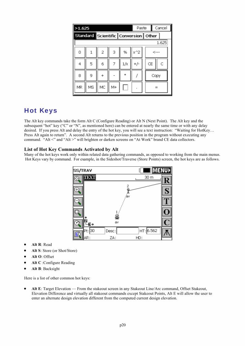
Quick CalculatorFrom virtually any dialog entry line in the program, the “?” command will go to the Calculator routines, and allow“copying” and “pasting” of any selected calculation result back into the dialog entry line.

For example, if you were grading a site that had 19.5” of subgrade, and had modeled the top surface, you need tograde to the top surface with a vertical offset of -19.5/12. You could quickly obtain the value in feet by entering ? inthe Vertical Offset field within the Elevation Difference dialog, as shown in this next figure.

This leads immediately to the Calculator screen, with its four “tabs”, or options, many with sub-options. Using theStandard tab, we can enter 19.5/12 and get 1.625 as shown. Then select the “Copy” button, which places the value inthe “banner” line at the very top of the screen. Then choose Paste in the upper right to past it back into the VerticalOffset dialog “edit” box. It can also be pointed out that this value could be entered two additional ways, withinVertical Offset: (1) as 19.5 in for “inches”, which would auto-convert to feet or the current units setting, or (2)19.5/12, which would do the division directly in this edit box. This figure shows the Calculator screen.

p20

Hot KeysThe Alt key commands take the form Alt C (Configure Reading) or Alt N (Next Point). The Alt key and thesubsequent “hot” key (“C” or “N”, as mentioned here) can be entered at nearly the same time or with any delaydesired. If you press Alt and delay the entry of the hot key, you will see a text instruction: “Waiting for HotKey… Press Alt again to return”. A second Alt returns to the previous position in the program without executing anycommand. “Alt <” and “Alt >” will brighten or darken screens on “At Work” brand CE data collectors.

List of Hot Key Commands Activated by AltMany of the hot keys work only within related data gathering commands, as opposed to working from the main menus. Hot Keys vary by command. For example, in the Sideshot/Traverse (Store Points) screen, the hot keys are as follows.

Alt R: Read Alt S: Store (or Shot/Store) Alt O: Offset Alt C :Configure Reading Alt B: Backsight

Here is a list of other common hot keys:

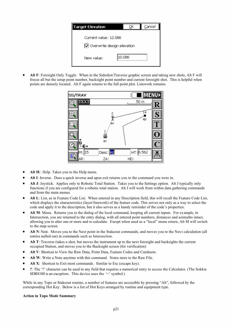
Alt E: Target Elevation — From the stakeout screen in any Stakeout Line/Arc command, Offset Stakeout,Elevation Difference and virtually all stakeout commands except Stakeout Points, Alt E will allow the user toenter an alternate design elevation different from the computed current design elevation.

p21

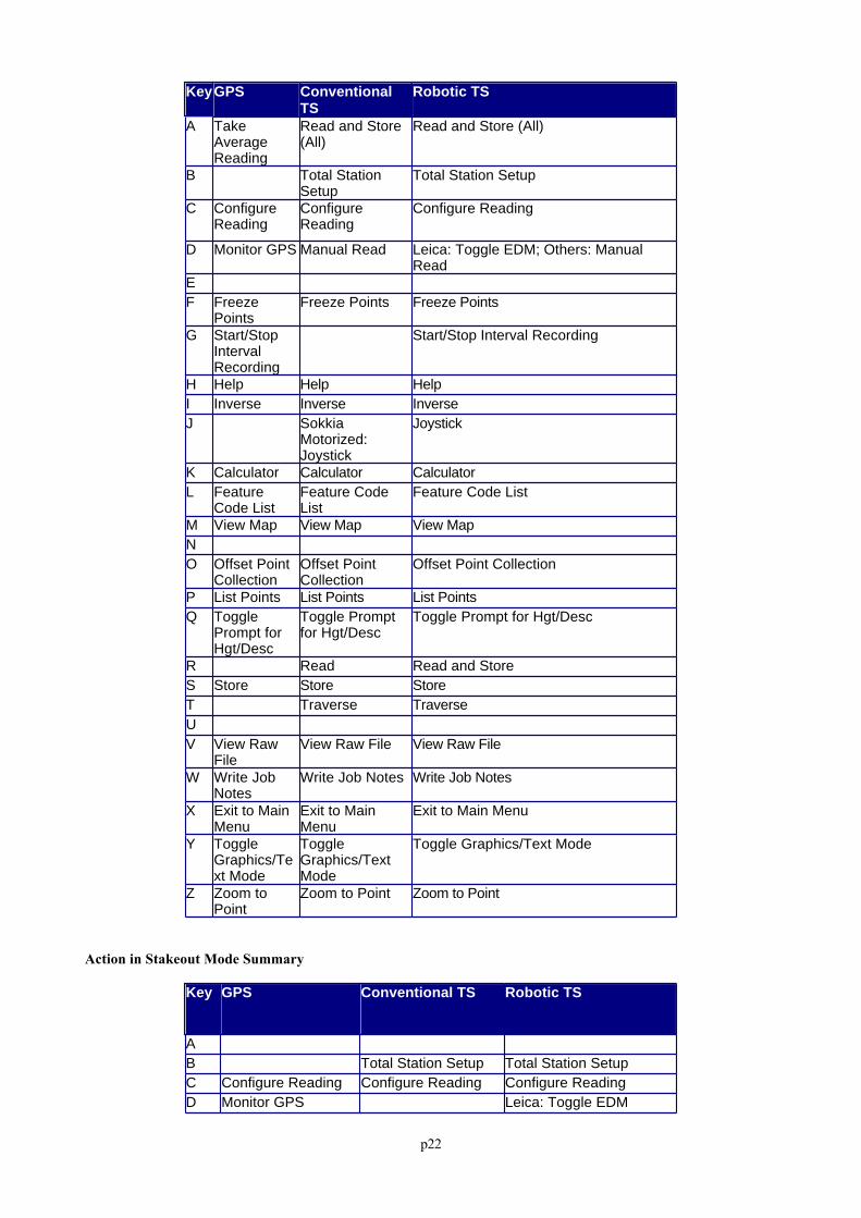
Alt F: Foresight Only Toggle. When in the Sideshot/Traverse graphic screen and taking new shots, Alt F willfreeze all but the setup point number, backsight point number and current foresight shot. This is helpful whenpoints are densely located. Alt F again returns to the full point plot. Linework remains.

Alt H: Help. Takes you to the Help menu. Alt I: Inverse. Does a quick inverse and upon exit returns you to the command you were in. Alt J: Joystick. Applies only to Robotic Total Station. Takes you to the Settings option. Alt J typically only

functions if you are configured for a robotic total station. Alt J will work from within data gathering commandsand from the main menus.

Alt L: List, as in Feature Code List. When entered in any Description field, this will recall the Feature Code List,which displays the characteristics (layer/linework) of the feature code. This serves not only as a way to select thecode and apply it to the description, but it also serves as a handy reminder of the code’s properties.

Alt M: Menu. Returns you to the dialog of the local command, keeping all current inputs. For example, inIntersection, you are returned to the entry dialog, with all entered point numbers, distances and azimuths intact,allowing you to alter one or more and re-calculate. Except when used as a “local” menu return, Alt M will switchto the map screen.

Alt N: Next. Moves you to the Next point in the Stakeout commands, and moves you to the Nex t calculation (allentries nulled out) in commands such as Intersection.

Alt T: Traverse (takes a shot, but moves the instrument up to the next foresight and backsights the currentoccupied Station, and moves you to the Backsight screen (for verification)

Alt V: Shortcut to View the Raw Data, Point Data, Feature Codes and Cutsheets. Alt W: Write a Note anytime with this command. Notes store to the Raw File. Alt X: Shortcut to Exit most commands. Similar to Esc (escape key). ?: The ‘?’ character can be used in any field that requires a numerical entry to access the Calculator. (The Sokkia

SDR8100 is an exception. This device uses the ‘=’ symbol.)

While in any Topo or Stakeout routine, a number of features are accessible by pressing “Alt”, followed by thecorresponding Hot Key. Below is a list of Hot Keys arranged by routine and equipment type.

Action in Topo Mode Summary

p22

KeyGPS ConventionalTS

Robotic TS

A TakeAverageReading

Read and Store(All)

Read and Store (All)

B Total StationSetup

Total Station Setup

C ConfigureReading

ConfigureReading

Configure Reading

D Monitor GPS Manual Read Leica: Toggle EDM; Others: ManualRead

EF Freeze

PointsFreeze Points Freeze Points

G Start/StopIntervalRecording

Start/Stop Interval Recording

H Help Help HelpI Inverse Inverse InverseJ Sokkia

Motorized:Joystick

Joystick

K Calculator Calculator CalculatorL Feature

Code ListFeature CodeList

Feature Code List

M View Map View Map View MapNO Offset Point

CollectionOffset PointCollection

Offset Point Collection

P List Points List Points List PointsQ Toggle

Prompt forHgt/Desc

Toggle Promptfor Hgt/Desc

Toggle Prompt for Hgt/Desc

R Read Read and StoreS Store Store StoreT Traverse TraverseUV View Raw

FileView Raw File View Raw File

W Write JobNotes

Write Job Notes Write Job Notes

X Exit to MainMenu

Exit to MainMenu

Exit to Main Menu

Y ToggleGraphics/Text Mode

ToggleGraphics/TextMode

Toggle Graphics/Text Mode

Z Zoom toPoint

Zoom to Point Zoom to Point

Action in Stakeout Mode Summary

Key GPS Conventional TS Robotic TS

AB Total Station Setup Total Station SetupC Configure Reading Configure Reading Configure ReadingD Monitor GPS Leica: Toggle EDM

p23

E Set Target Elevation Set Target Elevation Set Target ElevationF Freeze Points Freeze Points Freeze PointsGH Help Help HelpI Inverse Inverse InverseJ Sokkia Motorized:

JoystickJoystick

K Calculator Calculator CalculatorL Feature Code List Feature Code List Feature Code ListM View Map View Map View MapN Next Point/Station to

StakeNext Point/Station toStake

Next Point/Station toStake

OP List Points List Points List PointsQR Read Read and StoreS Store Store StoreTUV View Raw File View Raw File View Raw FileW Write Job Notes Write Job Notes Write Job NotesX Exit to Main Menu Exit to Main Menu Exit to Main MenuY Toggle

Graphics/Text ModeToggle Graphics/TextMode

Toggle Graphics/TextMode

Z Zoom to Point Zoom to Point Zoom to Point

Input Box ControlsWhen point ID’s are used to determine a value, the program will search for the point ID’s in the current job and if notfound search in the control job, if active.

Formatted Distance/Height EntriesEntries for distances or heights that include certain special or commonly understood “measurement” extensions areautomatically interpreted as a unit of measurement and converted to the “working” units. For example, a target heightentry of 2m is converted to 6.5617 feet if units are configured for feet. The “extension” can appear after the numberseparated by a space or can be directly appended to the number as in 2m. For feet and inch conversion the seconddecimal point informs the software that the user in entering fractions (See Below). Recognized text and theircorresponding units are shown below:

f or ft: US Feet i or ift: International Feet in: Inches cm: Centimeters m: Meters #.#.#.#: Feet and Inches (e.g. 1.5.3.8 = 1'5 3/8" either entry format is supported)

These extensions can be caps or lower case, or any combination (entries are not case-sensitive). These extensions areautomatically recognized for target heights and instrument heights and within certain distance entry dialogs.

Formatted Bearing/Azimuth EntriesMost directional commands within SurvCE allow for the entry of both azimuths and bearings. Azimuth entries are inthe form 350.2531 (DDD.MMSS), representing 350 degrees, 25 minutes and 31 seconds. But that same directioncould be entered as N9.3429W or alternately as NW9.3429. SurvCE will accept both forms. Additional directionalentry options, which might apply to commands such as Intersection under Cogo, are outlined below:

If Job Settings is set to Bearing and Degrees (360 circle), the user can enter the quadrant number before the angle

p24

value.

Example120.1234

The result is N20°12’34’’E.

Quadrants1 NE 2 SE 3 SW4 NW

In the case where Job Settings is set to Bearing and the user would like to enter an Azimuth, the letter A can be placedbefore the azimuth value and the program will convert it to a Bearing.

ExampleA20.1234

The result is N20°12’34’’E.

In the case where Job Settings is set to Azimuth and the user would like to enter a bearing, the quadrant letters can beused before the bearing value.

ExampleNW45.0000

The result is 315°00’00”.

Formatted Angle EntriesInterior Angle: The user can compute an angle defined by three points by entering the point ID’s as <PointID>,<Point ID>,Point ID>. The program will return the interior angle created by the three points using theAT-FROM-TO logic. Such entries might apply to the Angle Right input box in Sideshot/Traverse when configured toManual Total Station.

Example1,2,3

Using the coordinates below, the result is 90°00’00”. Point 2 would be the vertex point.

Pt. North East1 5500 50002 5000 50003 5000 5500

Mathematical ExpressionsMath expressions can be used in nearly all angle and distance edit boxes. For example, within the Intersection routine,an azimuth can be entered in the form 255.35-90, which means 255 degrees, 35 minutes minus 90 degrees. Additionally, point-defined distances and directions can be entered with the comma as separator, as in 4,5. If point 4to point 5 has an azimuth of 255 degrees, 35 minutes, then the same expression above could be entered as 4,5-90. Formath, the program handles “/”, “*”, “-“ and “+”. To go half the distance from 103 to 10, enter 103,10/2.

Point RangesWhen ranges of points are involved such as in stakeout lists, a dash is used. You can enter ranges in reverse (eg.75-50), which would create a list of points from 75 down to 50 in reverse order.

Survey Data Display ControlsANGLEThe angle control will display the angle as defined by the current settings from File Job Settings.

Options are available for Azimuth (North or South) or Bearing combined with the option of Degrees or Grads.

Format

p25

The display format of degrees uses the degree, minute, second symbols. For the case of a bearing we display thequadrant using the characters N, S, W, E.

Example BearingN7°09'59"EExample Azimuth7°09'59"

All angular values entered by the user should be in the DD.MMSS format.

Example7.0959The result is 7°09'59".

FormulasThe user can use formulas for working with angles. The format must have the operator after the angle value.Example90.0000 * 0.5The result would be 45°00’00”

DISTANCEThe distance control will display the value using the current File Job Settings unit. The user can enter a formulausing the mathematical operators as described above.

InverseThe user can compute a distance from a point to point inverse by entering <Point ID>,<Point ID>.Example1,2Using the coordinates listed below, the result is 500’.Pt. North East1 5500 50002 5000 5000

STATIONThe station control will display the value using the current File Job Settings format.The same options described above for distance input boxes apply.

SLOPEThe slope control will display the value using the current File Job Settings format.

Keyboard OperationCarlson SurvCE allows the user to operate the interface completely from keyboard navigation, as well as touch screennavigation. The rules for keyboard navigation are outlined below:

Controls

Button (Radio Buttons, Check Boxes and Standard Buttons)o Enter: Select the button.o Right/Left Arrows: Move to the next tab stop.

Right [Tab] Left [Shift+Tab]

o Up/Down Arrows: Move to the next tab stop. Down [Tab] Up [Shift+Tab]

o Tab: Move to the next tab stop.

Drop Listo Enter: Move to the next tab stop.

p26

o Right/Left Arrows: Move to the next tab stop. Right [Tab] Left [Shift+Tab]

o Up/Down Arrows: Move through the list items.o Tab: Move to the next tab stop.

Edit Boxo Enter: Move to the next tab stop. For any measurement screen, if focus is in the description edit

box, take a reading. For all other edit boxes, ENTER moves through the tab stops.o Right/Left Arrows: Move through the text like standard windows.o Up/Down Arrows: Move to the next tab stop.

Down [Tab] Up [Shift+Tab]

o Tab: Move to the next tab stop.

Tabo Enter: Move to the next tab stop.o Right/Left Arrows: Move through the tabs.

Right Next Tab Left Previous Tab

o Up/Down Arrows: Move to the next tab stop. Down [Tab] Up [Shift+Tab]

o Tab: Move to the next tab stop.

Abbreviations

Adr: Address AR: Angle Right Avg: Average Az: Azimuth Bk: Back Calc: Calculate Char: Character Chk: Check cm: Centimeter Coord(s): Coordinate(s) Ctrl: Control Desc: Description Dev: Deviation Diff: Difference Dist: Distance El: Elevation Fst: Fast ft: Foot Fwd: Forward HD: Horizontal Distance HI: Height of Instrument. Horiz: Horizontal

p27

Ht: Height or Height of Antenna with GPS. HT: Height of Target. ID: Identifier ift: International Foot in: Inch Inst: Instrument Int: Interval L: Left m: Meter No: Number OS: Offset Prev: Previous Pt: Point ID Pts: Points R: Right Rdg: Reading SD: Slope Distance Sta: Station Std: Standard Vert: Vertical ZE: Zenith

p28

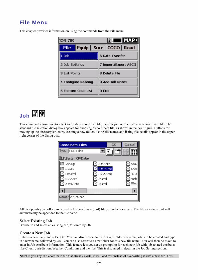
File MenuThis chapter provides information on using the commands from the File menu.

Job This command allows you to select an existing coordinate file for your job, or to create a new coordinate file. Thestandard file selection dialog box appears for choosing a coordinate file, as shown in the next figure. Buttons formoving up the directory structure, creating a new folder, listing file names and listing file details appear in the upperright corner of the dialog box.

All data points you collect are stored in the coordinate (.crd) file you select or create. The file ex tension .crd willautomatically be appended to the file name.

Select Existing JobBrowse to and select an existing file, followed by OK.

Create a New JobEnter is a new name and select OK. You can also browse to the desired folder where the job is to be created and typein a new name, followed by OK. You can also recreate a new folder for this new file name. You will then be asked toenter in Job Attribute information. This feature lets you set up prompting for each new job with job-related attributeslike Client, Jurisdiction, Weather Conditions and the like. This is discussed in detail in the Job Setting section.

Note: If you key in a coordinate file that already exists, it will load this instead of overwriting it with a new file. This

p29

benefit to this feature is that you cannot overwrite an existing coordinate file from within Carlson SurvCE.

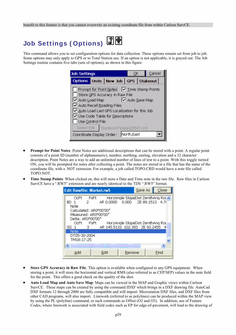
Job Settings (Options) This command allows you to set configuration options for data collection. These options remain set from job to job.Some options may only apply to GPS or to Total Station use. If an option is not applicable, it is grayed out. The JobSettings routine contains five tabs (sets of options), as shown in this figure:

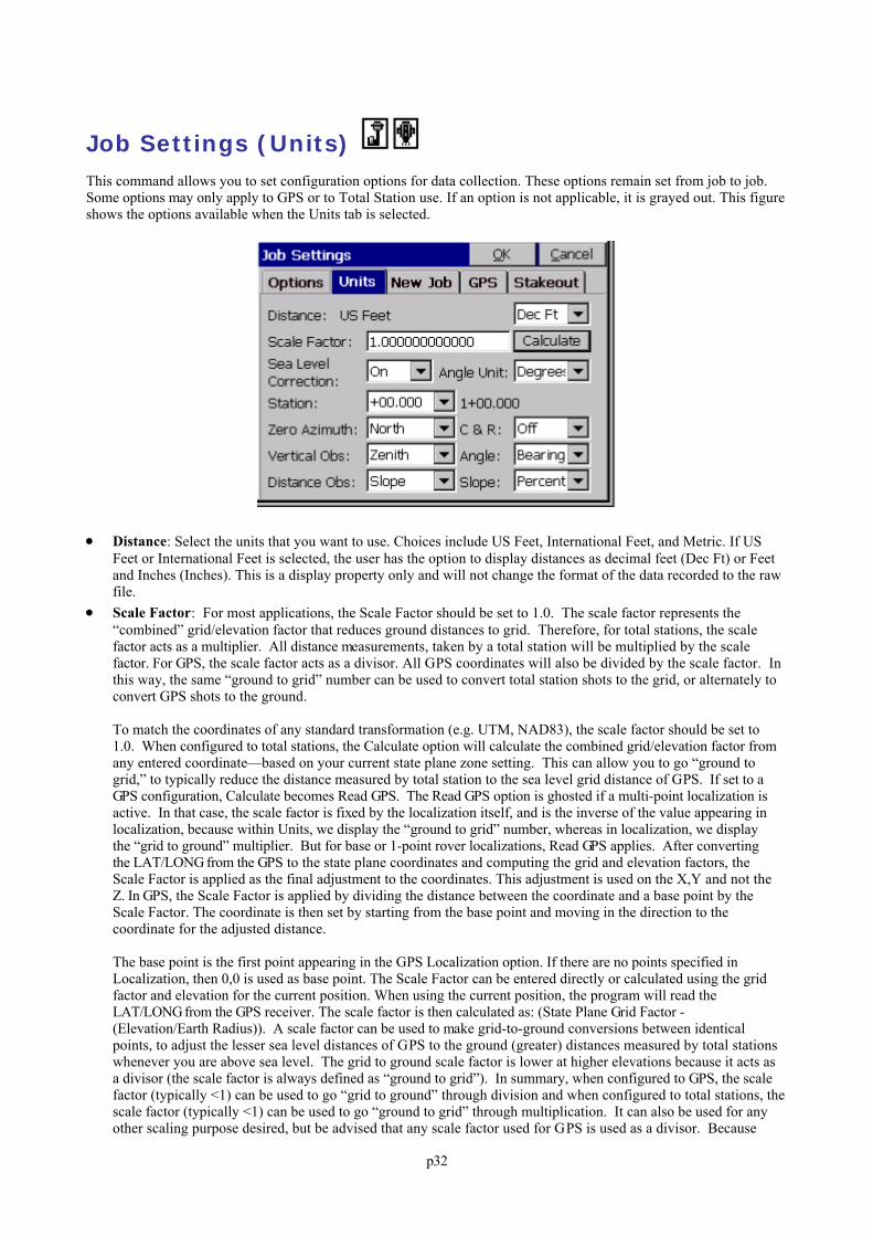
Prompt for Point Notes: Point Notes are additional descriptions that can be stored with a point. A regular pointconsists of a point ID (number of alphanumeric), number, northing, easting, elevation and a 32 characterdescription. Point Notes are a way to add an unlimited number of lines of text to a point. With this toggle turnedON, you will be prompted for notes after collecting a point. The notes are stored in a file that has the name of thecoordinate file, with a .NOT extension. For example, a job called TOPO.CRD would have a note file calledTOPO.NOT.

Time Stamp Points: When clicked on, this will store a Date and Time note in the raw file. Raw files in CarlsonSurvCE have a “.RW5” extension and are nearly identical to the TDS “.RW5” format.

Store GPS Accuracy in Raw File: This option is available when configured to any GPS equipment. Whenstoring a point, it will store the horizontal and vertical RMS (also referred to as CEP/SEP) values in the note fieldfor the point. This offers a good check on the quality of the shot.

Auto Load Map and Auto Save Map: Maps can be viewed in the MAP and Graphic views within CarlsonSurvCE. These maps can be created by using the command IDXF which brings in a DXF drawing file. AutoCadDXF formats 12 through 2000 are fully compatible and will import. Microstation DXF files, and DXF files fromother CAD programs, will also import. Linework (referred to as polylines) can be produced within the MAP viewby using the PL (polyline) command, or such commands as Offset (O2 and O3). In addition, use of FeatureCodes, where linework is associated with field codes such as EP for edge-of-pavement, will lead to the drawing of

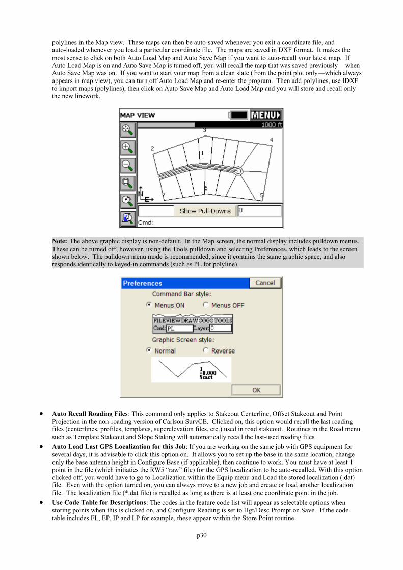
p30

polylines in the Map view. These maps can then be auto-saved whenever you exit a coordinate file, andauto-loaded whenever you load a particular coordinate file. The maps are saved in DXF format. It makes themost sense to click on both Auto Load Map and Auto Save Map if you want to auto-recall your latest map. IfAuto Load Map is on and Auto Save Map is turned off, you will recall the map that was saved previously—whenAuto Save Map was on. If you want to start your map from a clean slate (from the point plot only—which alwaysappears in map view), you can turn off Auto Load Map and re-enter the program. Then add polylines, use IDXFto import maps (polylines), then click on Auto Save Map and Auto Load Map and you will store and recall onlythe new linework.

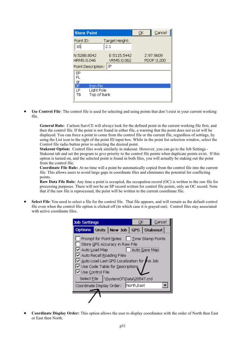
Note: The above graphic display is non-default. In the Map screen, the normal display includes pulldown menus.These can be turned off, however, using the Tools pulldown and selecting Preferences, which leads to the screenshown below. The pulldown menu mode is recommended, since it contains the same graphic space, and alsoresponds identically to keyed-in commands (such as PL for polyline).

Auto Recall Roading Files: This command only applies to Stakeout Centerline, Offset Stakeout and PointProjection in the non-roading version of Carlson SurvCE. Clicked on, this option would recall the last roadingfiles (centerlines, profiles, templates, superelevation files, etc.) used in road stakeout. Routines in the Road menusuch as Template Stakeout and Slope Staking will automatically recall the last-used roading files

Auto Load Last GPS Localization for this Job: If you are working on the same job with GPS equipment forseveral days, it is advisable to click this option on. It allows you to set up the base in the same location, changeonly the base antenna height in Configure Base (if applicable), then continue to work. You must have at least 1point in the file (which initiaties the RW5 “raw” file) for the GPS localization to be auto-recalled. With this optionclicked off, you would have to go to Localization within the Equip menu and Load the stored localization (.dat)file. Even with the option turned on, you can always move to a new job and create or load another localizationfile. The localization file (*.dat file) is recalled as long as there is at least one coordinate point in the job.

Use Code Table for Descriptions: The codes in the feature code list will appear as selectable options whenstoring points when this is clicked on, and Configure Reading is set to Hgt/Desc Prompt on Save. If the codetable includes FL, EP, IP and LP for example, these appear within the Store Point routine.

p31

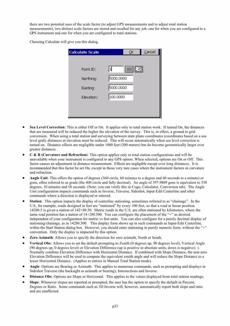
Use Control File: The control file is used for selecting and using points that don’t exist in your current workingfile.

General Rule: Carlson SurvCE will always look for the defined point in the current working file first, andthen the control file. If the point is not found in either file, a warning that the point does not exist will bedisplayed. You can force a point to come from the control file or the current file, regardless of settings, byusing the List icon to the right of the point ID input box. While in the point list selection window, select theControl file radio button prior to selecting the desired point.Stakeout Option: Control files work similarly in stakeout. However, you can go to the Job Settings -Stakeout tab and set the program to give priority to the control file points when duplicate points exist. If thisoption is turned on, and the selected point is found in both files, you will actually be staking out the pointfrom the control file.Coordinate File Rule: At no time will a point be automatically copied from the control file into the currentfile. This allows users to avoid large gaps in coordinate files and eliminates the potential for conflictingpoints.Raw Data File Rule: Any time a point is occupied, the occupation record (OC) is written to the raw file forprocessing purposes. There will not be an SP record written for control file points, only an OC record. Notethat if the raw file is reprocessed, the point will be written to the current coordinate file.

Select File: You need to select a file for the control file. That file appears, and will remain as the default controlfile even when the control file option is clicked off (in which case it is grayed out). Control files stay associatedwith active coordinate files.

Coordinate Display Order: This option allows the user to display coordinates with the order of North then Eastor East then North.

p32

Job Settings (Units) This command allows you to set configuration options for data collection. These options remain set from job to job.Some options may only apply to GPS or to Total Station use. If an option is not applicable, it is grayed out. This figureshows the options available when the Units tab is selected.

Distance: Select the units that you want to use. Choices include US Feet, International Feet, and Metric. If USFeet or International Feet is selected, the user has the option to display distances as decimal feet (Dec Ft) or Feetand Inches (Inches). This is a display property only and will not change the format of the data recorded to the rawfile.

Scale Factor: For most applications, the Scale Factor should be set to 1.0. The scale factor represents the“combined” grid/elevation factor that reduces ground distances to grid. Therefore, for total stations, the scalefactor acts as a multiplier. All distance measurements, taken by a total station will be multiplied by the scalefactor. For GPS, the scale factor acts as a divisor. All GPS coordinates will also be divided by the scale factor. Inthis way, the same “ground to grid” number can be used to convert total station shots to the grid, or alternately toconvert GPS shots to the ground.

To match the coordinates of any standard transformation (e.g. UTM, NAD83), the scale factor should be set to1.0. When configured to total stations, the Calculate option will calculate the combined grid/elevation factor fromany entered coordinate—based on your current state plane zone setting. This can allow you to go “ground togrid,” to typically reduce the distance measured by total station to the sea level grid distance of GPS. If set to aGPS configuration, Calculate becomes Read GPS. The Read GPS option is ghosted if a multi-point localization isactive. In that case, the scale factor is fixed by the localization itself, and is the inverse of the value appearing inlocalization, because within Units, we display the “ground to grid” number, whereas in localization, we displaythe “grid to ground” multiplier. But for base or 1-point rover localizations, Read GPS applies. After convertingthe LAT/LONG from the GPS to the state plane coordinates and computing the grid and elevation factors, theScale Factor is applied as the final adjustment to the coordinates. This adjustment is used on the X,Y and not theZ. In GPS, the Scale Factor is applied by dividing the distance between the coordinate and a base point by theScale Factor. The coordinate is then set by starting from the base point and moving in the direction to thecoordinate for the adjusted distance.

The base point is the first point appearing in the GPS Localization option. If there are no points specified inLocalization, then 0,0 is used as base point. The Scale Factor can be entered directly or calculated using the gridfactor and elevation for the current position. When using the current position, the program will read theLAT/LONG from the GPS receiver. The scale factor is then calculated as: (State Plane Grid Factor -(Elevation/Earth Radius)). A scale factor can be used to make grid-to-ground conversions between identicalpoints, to adjust the lesser sea level distances of GPS to the ground (greater) distances measured by total stationswhenever you are above sea level. The grid to ground scale factor is lower at higher elevations because it acts asa divisor (the scale factor is always defined as “ground to grid”). In summary, when configured to GPS, the scalefactor (typically <1) can be used to go “grid to ground” through division and when configured to total stations, thescale factor (typically <1) can be used to go “ground to grid” through multiplication. It can also be used for anyother scaling purpose desired, but be advised that any scale factor used for GPS is used as a divisor. Because

p33

there are two potential uses of the scale factor (to adjust GPS measurements and to adjust total stationmeasurements), two distinct scale factors are stored and recalled for any job, one for when you are configured to aGPS instrument and one for when you are configured to total stations.

Choosing Calculate will give you this dialog.

Sea Level Correction: This is either Off or On. It applies only to total station work. If turned On, the distancesthat are measured will be reduced the higher the elevation of the survey. This is, in effect, a ground to gridconversion. When using a total station and surveying between state plane coordinates (coordinates based on a sealevel grid), distances at elevation must be reduced. This will occur automatically when sea level correction isturned on. Distance effects are negligible under 1000 feet (300 meters) but do become geometrically larger overgreater distances.

C & R (Curvature and Refraction): This option applies only to total station configurations and will beunavailable when your instrument is configured to any GPS option. When selected, options are On or Off. Thisfactor causes an adjustment in distance measurement. Effects are negligible except over long distances. It isrecommended that this factor be set On, except in those very rare cases where the instrument factors in curvatureand refraction.

Angle Unit: This offers the option of degrees (360 circle, 60 minutes to a degree and 60 seconds to a minute) orgons, often referred to as grads (the 400 circle and fully decimal). An angle of 397.9809 gons is equivalent to 358degrees, 10 minutes and 58 seconds. (Note: you can verify this in Cogo, Calculator, Conversion tab). The AngleUnit configuration impacts commands such as Inverse, Traverse, Sideshot, Input-Edit Centerline and othercommands where a direction is displayed or entered.

Station: This option impacts the display of centerline stationing, sometimes referred to as “chainage”. In theU.S., for example, roads designed in feet are “stationed” by every 100 feet, so that a road at linear position14280.5 is given a station of 142+80.50. Metric roads in the U.S. are often stationed by kilometers, where thesame road position has a station of 14+280.500. You can configure the placement of the “+” as desired,independent of your configuration for metric vs feet units. You can also configure for a purely decimal display ofstationing/chainage, as in 14280.500. This display form shows up in such commands as Input-Edit Centerline,within the Start Station dialog box. However, you should enter stationing in purely numeric form, without the “+”convention. Only the display is impacted by this option.

Zero Azimuth: Allows you to specify the direction for zero azimuth, North or South. Vertical Obs: Allows you to set the default prompting to Zenith (0 degrees up, 90 degrees level), Vertical Angle

(90 degrees up, 0 degrees level) or Elevation Difference (up is positive in absolute units, down is negative). ). Normally combine Elevation Difference with Horizontal Distance. If combined with Slope Distance, the non-zeroElevation Difference will be used to compute the equivalent zenith angle and will reduce the Slope Distance to alesser Horizontal Distance. (Applies to entries in Manual Total Station mode).

Angle: Options are Bearing or Azimuth. This applies to numerous commands, such as prompting and displays inSideshot Traverse (the backsight as azimuth or bearing), Intersections and Inverse.

Distance Obs: Options are Slope or Horizontal. This applies to the values displayed from total station readings. Slope: Whenever slopes are reported or prompted, the user has the option to specify the default in Percent,

Degrees or Ratio. Some commands such as 3D Inverse will, however, automatically report both slope and ratioand are unaffected.

p34

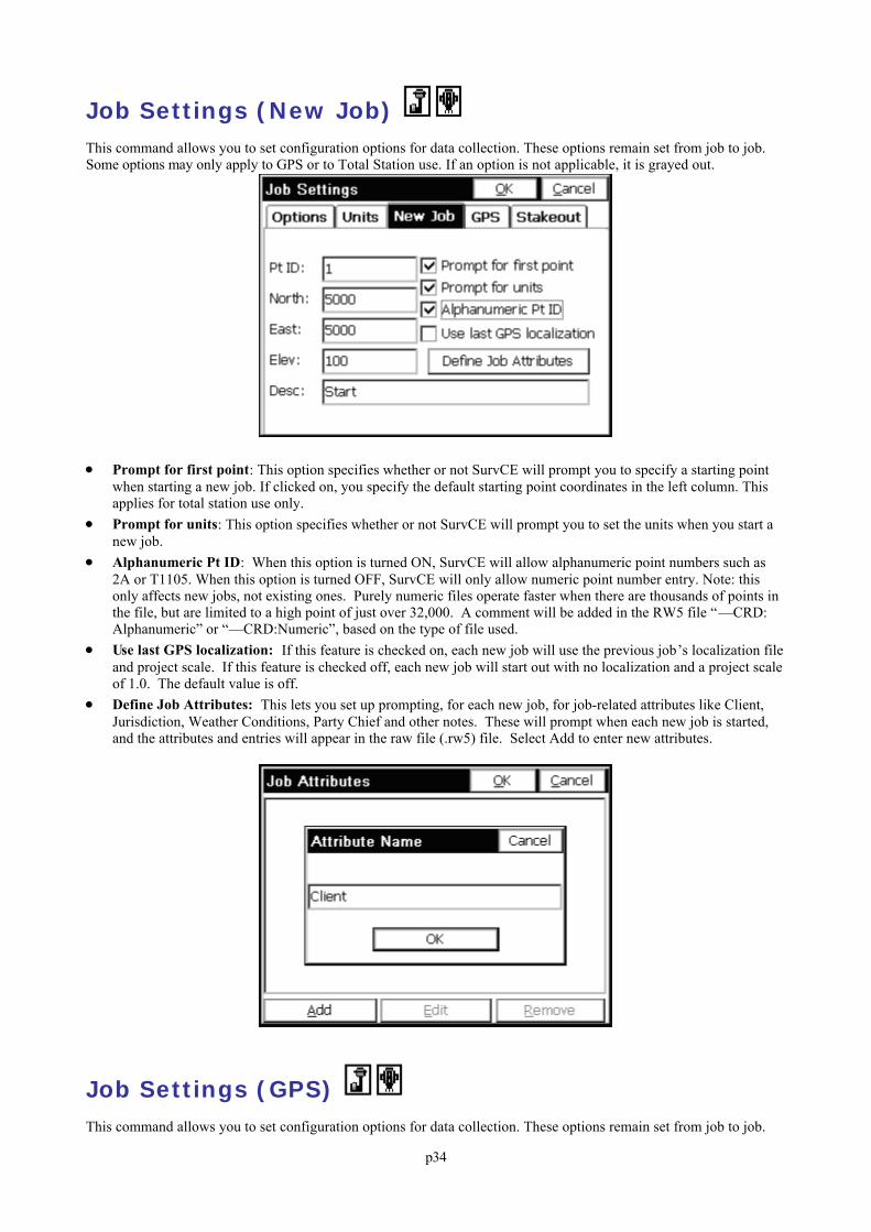
Job Settings (New Job) This command allows you to set configuration options for data collection. These options remain set from job to job.Some options may only apply to GPS or to Total Station use. If an option is not applicable, it is grayed out.

Prompt for first point: This option specifies whether or not SurvCE will prompt you to specify a starting pointwhen starting a new job. If clicked on, you specify the default starting point coordinates in the left column. Thisapplies for total station use only.

Prompt for units: This option specifies whether or not SurvCE will prompt you to set the units when you start anew job.

Alphanumeric Pt ID: When this option is turned ON, SurvCE will allow alphanumeric point numbers such as2A or T1105. When this option is turned OFF, SurvCE will only allow numeric point number entry. Note: thisonly affects new jobs, not existing ones. Purely numeric files operate faster when there are thousands of points inthe file, but are limited to a high point of just over 32,000. A comment will be added in the RW5 file “—CRD:Alphanumeric” or “—CRD:Numeric”, based on the type of file used.

Use last GPS localization: If this feature is checked on, each new job will use the previous job’s localization fileand project scale. If this feature is checked off, each new job will start out with no localization and a project scaleof 1.0. The default value is off.

Define Job Attributes: This lets you set up prompting, for each new job, for job-related attributes like Client,Jurisdiction, Weather Conditions, Party Chief and other notes. These will prompt when each new job is started,and the attributes and entries will appear in the raw file (.rw5) file. Select Add to enter new attributes.

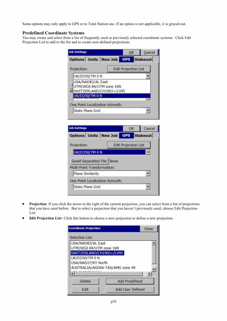
Job Settings (GPS) This command allows you to set configuration options for data collection. These options remain set from job to job.

p35

Some options may only apply to GPS or to Total Station use. If an option is not applicable, it is grayed out.

Predefined Coordinate SystemsYou may create and select from a list of frequently used or previously selected coordinate systems. Click EditProjection List to add to the list and to create user-defined projections.

Projection: If you click the arrow to the right of the current projection, you can select from a list of projectionsthat you have used before. But to select a projection that you haven’t previously used, choose Edit ProjectionList.

Edit Projection List: Click this button to choose a new projection or define a new projection.

p36

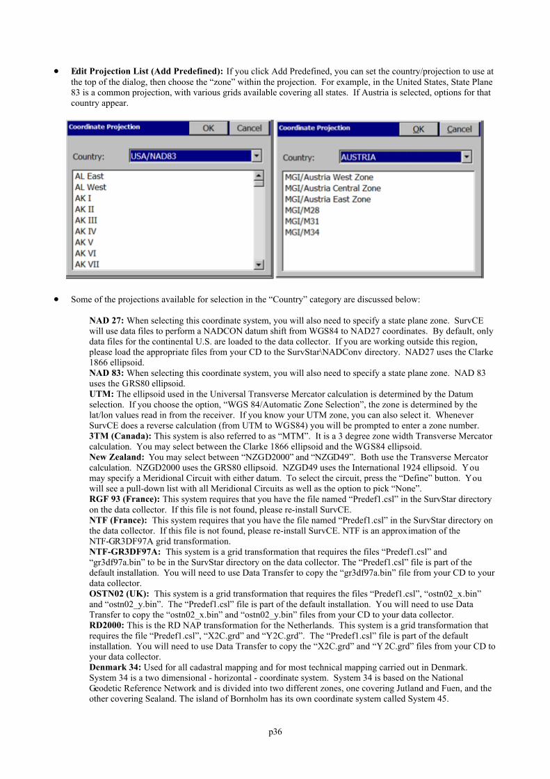
Edit Projection List (Add Predefined): If you click Add Predefined, you can set the country/projection to use atthe top of the dialog, then choose the “zone” within the projection. For example, in the United States, State Plane83 is a common projection, with various grids available covering all states. If Austria is selected, options for thatcountry appear.

Some of the projections available for selection in the “Country” category are discussed below:

NAD 27: When selecting this coordinate system, you will also need to specify a state plane zone. SurvCEwill use data files to perform a NADCON datum shift from WGS84 to NAD27 coordinates. By default, onlydata files for the continental U.S. are loaded to the data collector. If you are working outside this region,please load the appropriate files from your CD to the SurvStar\NADConv directory. NAD27 uses the Clarke1866 ellipsoid.NAD 83: When selecting this coordinate system, you will also need to specify a state plane zone. NAD 83uses the GRS80 ellipsoid.UTM: The ellipsoid used in the Universal Transverse Mercator calculation is determined by the Datumselection. If you choose the option, “WGS 84/Automatic Zone Selection”, the zone is determined by thelat/lon values read in from the receiver. If you know your UTM zone, you can also select it. WheneverSurvCE does a reverse calculation (from UTM to WGS84) you will be prompted to enter a zone number.3TM (Canada): This system is also referred to as “MTM”. It is a 3 degree zone width Transverse Mercatorcalculation. You may select between the Clarke 1866 ellipsoid and the WGS84 ellipsoid.New Zealand: You may select between “NZGD2000” and “NZGD49”. Both use the Transverse Mercatorcalculation. NZGD2000 uses the GRS80 ellipsoid. NZGD49 uses the International 1924 ellipsoid. Youmay specify a Meridional Circuit with either datum. To select the circuit, press the “Define” button. Youwill see a pull-down list with all Meridional Circuits as well as the option to pick “None”.RGF 93 (France): This system requires that you have the file named “Predef1.csl” in the SurvStar directoryon the data collector. If this file is not found, please re-install SurvCE. NTF (France): This system requires that you have the file named “Predef1.csl” in the SurvStar directory onthe data collector. If this file is not found, please re-install SurvCE. NTF is an approximation of theNTF-GR3DF97A grid transformation.NTF-GR3DF97A: This system is a grid transformation that requires the files “Predef1.csl” and“gr3df97a.bin” to be in the SurvStar directory on the data collector. The “Predef1.csl” file is part of thedefault installation. You will need to use Data Transfer to copy the “gr3df97a.bin” file from your CD to yourdata collector.OSTN02 (UK): This system is a grid transformation that requires the files “Predef1.csl”, “ostn02_x.bin”and “ostn02_y.bin”. The “Predef1.csl” file is part of the default installation. You will need to use DataTransfer to copy the “ostn02_x.bin” and “ostn02_y.bin” files from your CD to your data collector.RD2000: This is the RD NAP transformation for the Netherlands. This system is a grid transformation thatrequires the file “Predef1.csl”, “X2C.grd” and “Y2C.grd”. The “Predef1.csl” file is part of the defaultinstallation. You will need to use Data Transfer to copy the “X2C.grd” and “Y 2C.grd” files from your CD toyour data collector.Denmark 34: Used for all cadastral mapping and for most technical mapping carried out in Denmark.System 34 is a two dimensional - horizontal - coordinate system. System 34 is based on the NationalGeodetic Reference Network and is divided into two different zones, one covering Jutland and Fuen, and theother covering Sealand. The island of Bornholm has its own coordinate system called System 45.

p37

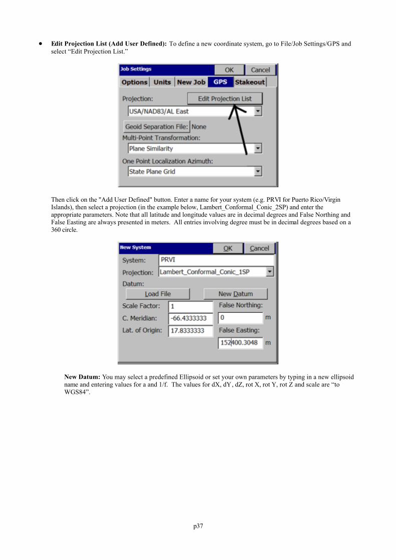
Edit Projection List (Add User Defined): To define a new coordinate system, go to File/Job Settings/GPS andselect “Edit Projection List.”

Then click on the "Add User Defined" button. Enter a name for your system (e.g. PRVI for Puerto Rico/VirginIslands), then select a projection (in the example below, Lambert_Conformal_Conic_2SP) and enter theappropriate parameters. Note that all latitude and longitude values are in decimal degrees and False Northing andFalse Easting are always presented in meters. All entries involving degree must be in decimal degrees based on a360 circle.

New Datum: You may select a predefined Ellipsoid or set your own parameters by typing in a new ellipsoidname and entering values for a and 1/f. The values for dX, dY, dZ, rot X, rot Y, rot Z and scale are “toWGS84”.

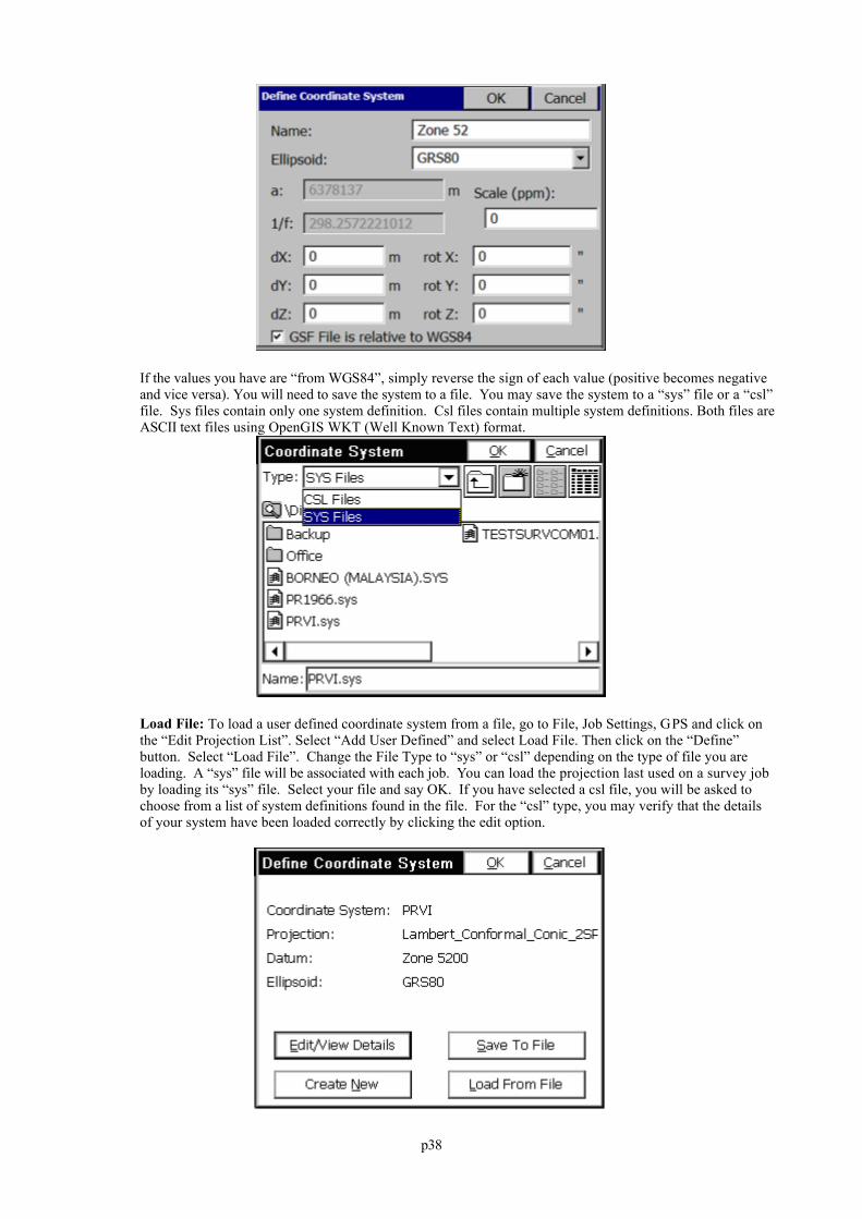
p38

If the values you have are “from WGS84”, simply reverse the sign of each value (positive becomes negativeand vice versa). You will need to save the system to a file. You may save the system to a “sys” file or a “csl”file. Sys files contain only one system definition. Csl files contain multiple system definitions. Both files areASCII text files using OpenGIS WKT (Well Known Text) format.

Load File: To load a user defined coordinate system from a file, go to File, Job Settings, GPS and click onthe “Edit Projection List”. Select “Add User Defined” and select Load File. Then click on the “Define”button. Select “Load File”. Change the File Type to “sys” or “csl” depending on the type of file you areloading. A “sys” file will be associated with each job. You can load the projection last used on a survey jobby loading its “sys” file. Select your file and say OK. If you have selected a csl file, you will be asked tochoose from a list of system definitions found in the file. For the “csl” type, you may verify that the detailsof your system have been loaded correctly by clicking the edit option.

p39

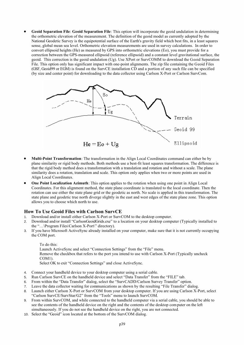
Geoid Separation File: Geoid Separation File: This option will incorporate the geoid undulation in determiningthe orthometric elevation of the measurement. The definition of the geoid model as currently adopted by theNational Geodetic Survey is the equipotential surface of the Earth's gravity field which best fits, in a least squaressense, global mean sea level. Orthometric elevation measurements are used in survey calculations. In order toconvert ellipsoid heights (He) as measured by GPS into orthometric elevations (Eo), you must provide for acorrection between the GPS-measured ellipsoid (reference ellipsoid) and a constant level gravitational surface, thegeoid. This correction is the geoid undulation (Ug). Use XPort or SurvCOMM to download the Geoid SeparationFile. This option only has significant impact with one-point alignments. The zip file containing the Geoid Files(GSF, Geoid99 or EGM) is found on the SurvCE installation CD and a portion of any such file can be specified(by size and center point) for downloading to the data collector using Carlson X-Port or Carlson SurvCom.

Multi-Point Transformation: The transformation in the Align Local Coordinates command can either be byplane similarity or rigid body methods. Both methods use a best-fit least squares transformation. The difference isthat the rigid body method does a transformation with a translation and rotation and without a scale. The planesimilarity does a rotation, translation and scale. This option only applies when two or more points are used inAlign Local Coordinates.

One Point Localization Azimuth: This option applies to the rotation when using one point in Align LocalCoordinates. For this alignment method, the state plane coordinate is translated to the local coordinate. Then therotation can use either the state plane grid or the geodetic as north. No scale is applied in this transformation. Thestate plane and geodetic true north diverge slightly in the east and west edges of the state plane zone. This optionallows you to choose which north to use.

How To Use Geoid Files with Carlson SurvCE1. Download and/or install either Carlson X-Port or SurvCOM to the desktop computer.2. Download and/or install “CarlsonGeoidGrids.exe” to a location on your desktop computer (Typically installed to

the “…\Program Files\Carlson X-Port\” directory).3. If you have Microsoft ActiveSync already installed on your computer, make sure that it is not currently occupying

the COM port.

To do this:Launch ActiveSync and select “Connection Settings” from the “File” menu. Remove the checkbox that refers to the port you intend to use with Carlson X-Port (Typically uncheckCOM1). Select OK to exit “Connection Settings” and close ActiveSync.

4. Connect your handheld device to your desktop computer using a serial cable.5. Run Carlson SurvCE on the handheld device and select “Data Transfer” from the “FILE” tab.6. From within the “Data Transfer” dialog, select the “SurvCADD/Carlson Survey Transfer” option.7. Leave the data collector waiting for communications as shown by the resulting “File Transfer” dialog.8. Launch either Carlson X-Port or SurvCOM from your desktop computer. If you are using Carlson X-Port, select

“Carlson SurvCE/SurvStar/G2” from the “Tools” menu to launch SurvCOM.9. From within SurvCOM, and while connected to the handheld computer via a serial cable, you should be able to

see the contents of the handheld device on the right and the contents of the desktop com puter on the leftsimultaneously. If you do not see the handheld device on the right, you are not connected.

10. Select the “Geoid” icon located at the bottom of the SurvCOM dialog.

p40

11. From within the “Set Geoid Area” dialog, verify the path to the geoid files is set to the installed location of thesefiles as defined in step 2 of this document (Typically “…Program Files\Carlson X-Port\”).

12. Select the desired geoid model to extract an area from.13. Key in the approximate latitude and longitude of the center of the area.14. Define the grid size for the area you want the model to cover (Supported sizes are 50-250 miles, 80-400

kilometers and 1-5 degrees, however, keep the size 100 miles or smaller for better performance).15. Name the geoid model with any name that you want (e.g. geoid). You may want to name this file with a logical

name for the location of the area for future reference (e.g. geoid-LA).16. Select the “OK” button to automatically transfer the file to the “…\Survstar\” directory of the handheld device. A

copy of the file will also be created on your desktop computer in the currently selected folder.17. On the handheld device, select “Job Settings” from the “FILE” tab and view the “GPS” tab.18. Select the “Geoid Separation File” button and choose the geoid file you created and transferred with SurvCOM.19. You have now completed the definition and selection of the geoid file. Select “OK” to exit the “Job Setting”

dialog.

Job Settings (Stakeout) This command allows you to set configuration options for data collection. These options remain set from job to job.Some options may only apply to GPS or to Total Station use. If you are configured for total station, selecting theStakeout tab will give you the options shown on the left. If you are configured for GPS, the Stakeout tab will appear asshown at the right. If an option is not applicable, it is grayed out.

Store Carlson Cutsheet Data in Note File: This option specifies whether or not to store the stakeout data in thenote file (.NOT) for the current job. At the end of staking out a point, there is an option to store the stakedcoordinates in the current job. Note (.NOT) files are associated with points, so you must store the point to alsostore the cutsheet note. This additional data includes the target coordinates for reference. Keep in mind that thecut and fill data is also stored in the raw file, plus you can store an ASCII cutsheet file using the button at thebottom of the dialog, so storing into the note file is somewhat redundant. SurvCE does not show the cutsheet notewithin List Points (notes turned on), since this feature only shows notes that begin with “Note:” The oneadvantage of the note file is that notes are viewable in association with points using Carlson Software officeproducts such as Carlson SurvCadd, Carlson Survey, or Carlson Survey Desktop. See command “CutsheetReport”, option “Note File”.

Zero Hz Angle to Target: This option specifies whether or not SurvCE will set the horizontal angle of the totalstation to zero in the direction towards the stakeout point. When stakeout is completed, the horizontal angle is setback to the original value. This option only applies to Sokkia total stations or to total stations such as Nikon whichhave a “Sokkia emulation” mode.

Control File Points have Priority for Stakeout: This option, which applies to both total stations and GPS, willchoose the point in the control file for stakeout, when the point requested exists in both the current file and thecontrol file.

Note: Use this option with care. You may not realize that this option is set, and will discover that directions toyour expected stakeout point of 10 are really based on a point 10 from another file altogether – the control file.

p41

Decimals: Use this to control the decimal precision reported during stakeout routines. Increment Station Interval from Beg. Station: For centerlines that start on an “odd” station such as 1020

(10+20 in U.S. stationing format), this option would conduct stakeout by interval measured from station 1020. Soa 50 interval stakeout, instead of being 1050, 1100, 1150 would be 1020, 1070, 1120, etc.

Apply Station Limits: When selected, the program will not automatically advance beyond the natural start andend of a given centerline.

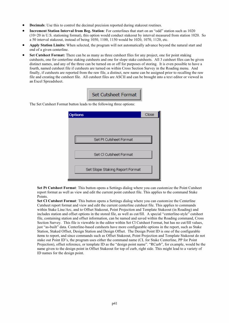
Set Cutsheet Format: There can be as many as three cutsheet files for any project, one for point stakingcutsheets, one for centerline staking cutsheets and one for slope stake cutsheets. All 3 cutsheet files can be givendistinct names, and any of the three can be turned on or off for purposes of storing. It is even possible to have afourth, named cutsheet file if cutsheets are turned on within Cross Section Survey in the Roading menu. Andfinally, if cutsheets are reported from the raw file, a distinct, new name can be assigned prior to recalling the rawfile and creating the cutsheet file. All cutsheet files are ASCII and can be brought into a text editor or viewed inan Excel Spreadsheet.

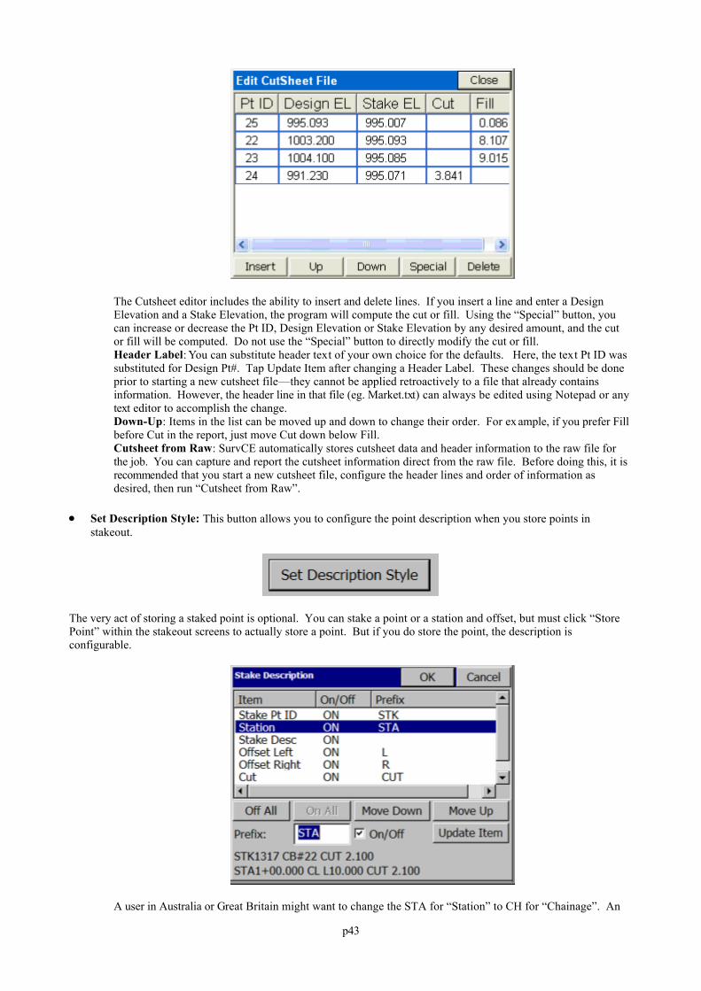
The Set Cutsheet Format button leads to the following three options:

Set Pt Cutsheet Format: This button opens a Settings dialog where you can customize the Point Cutsheetreport format as well as view and edit the current point cutsheet file. This applies to the command StakePoints.Set Cl Cutsheet Format: This button opens a Settings dialog where you can customize the CenterlineCutsheet report format and view and edit the current centerline cutsheet file. This applies to commandswithin Stake Line/Arc, and to Offset Stakeout, Point Projection and Template Stakeout (in Roading) andincludes station and offset options in the stored file, as well as cut/fill. A special “centerline-style” cutsheetfile, containing station and offset information, can be named and saved within the Roading command, CrossSection Survey. This file is viewable in the editor within Set Cl Cutsheet Format, but has no cut/fill values,just “as-built” data. Centerline-based cutsheets have more configurable options in the report, such as StakeStation, Staked Offset, Design Station and Design Offset. The Design Point ID is one of the configurableitems to report, and since commands such as Offset Stakeout, Point Projection and Template Stakeout do notstake out Point ID’s, the program uses either the command name (CL for Stake Centerline, PP for PointProjection), offset reference, or template ID as the “design point name”. “RCurb”, for example, would be thename given to the design point in Offset Stakeout for top of curb, right side. This might lead to a variety ofID names for the design point.

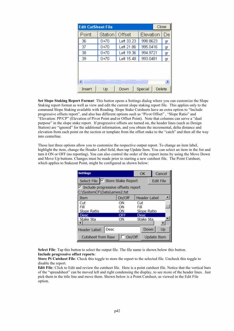
p42

Set Slope Staking Report Format: This button opens a Settings dialog where you can customize the SlopeStaking report format as well as view and edit the current slope staking report file. This applies only to thecommand Slope Staking available with Roading. Slope Stake Cutsheets have an extra option to “Includeprogressive offsets report”, and also has different options such as “Pivot Offset” , “Slope Ratio” and“Elevation: PP/CP” (Elevation of Pivot Point and/or Offset Point). Note that columns can serve a “dualpurpose” in the slope stake report. If progressive offsets are turned on, the header lines (such as DesignStation) are “ignored” for the additional information, and you obtain the incremental, delta distance andelevation from each point on the section or template from the offset stake to the “catch” and then all the wayinto centerline.

These last three options allow you to customize the respective output report. To change an item label,highlight the item, change the Header Label field, then tap Update Item. You can select an item in the list andturn it ON or OFF (no reporting). You can also control the order of the report items by using the Move Downand Move Up buttons. Changes must be made prior to starting a new cutsheet file. The Point Cutsheet,which applies to Stakeout Point, might be configured as shown below:

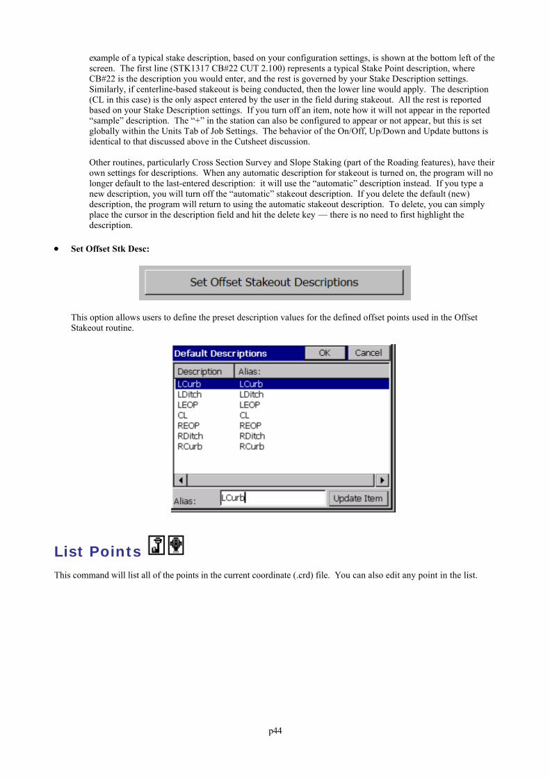
Select File: Tap this button to select the output file. The file name is shown below this button.Include progressive offset reports: Store Pt Cutsheet File: Check this toggle to store the report to the selected file. Uncheck this toggle todisable the report.Edit File: Click to Edit and review the cutsheet file. Here is a point cutsheet file. Notice that the vertical barsof the “spreadsheet” can be moved left and right condensing the display, to see more of the header lines. Justpick them in the title line and move them. Shown below is a Point Cutsheet, as viewed in the Edit Fileoption.

p43

The Cutsheet editor includes the ability to insert and delete lines. If you insert a line and enter a DesignElevation and a Stake Elevation, the program will compute the cut or fill. Using the “Special” button, youcan increase or decrease the Pt ID, Design Elevation or Stake Elevation by any desired amount, and the cutor fill will be computed. Do not use the “Special” button to directly modify the cut or fill.Header Label: You can substitute header text of your own choice for the defaults. Here, the text Pt ID wassubstituted for Design Pt#. Tap Update Item after changing a Header Label. These changes should be doneprior to starting a new cutsheet file—they cannot be applied retroactively to a file that already containsinformation. However, the header line in that file (eg. Market.txt) can always be edited using Notepad or anytext editor to accomplish the change.Down-Up: Items in the list can be moved up and down to change their order. For ex ample, if you prefer Fillbefore Cut in the report, just move Cut down below Fill.Cutsheet from Raw: SurvCE automatically stores cutsheet data and header information to the raw file forthe job. You can capture and report the cutsheet information direct from the raw file. Before doing this, it isrecommended that you start a new cutsheet file, configure the header lines and order of information asdesired, then run “Cutsheet from Raw”.

Set Description Style: This button allows you to configure the point description when you store points instakeout.

The very act of storing a staked point is optional. You can stake a point or a station and offset, but must click “StorePoint” within the stakeout screens to actually store a point. But if you do store the point, the description isconfigurable.

A user in Australia or Great Britain might want to change the STA for “Station” to CH for “Chainage”. An

p44

example of a typical stake description, based on your configuration settings, is shown at the bottom left of thescreen. The first line (STK1317 CB#22 CUT 2.100) represents a typical Stake Point description, whereCB#22 is the description you would enter, and the rest is governed by your Stake Description settings. Similarly, if centerline-based stakeout is being conducted, then the lower line would apply. The description(CL in this case) is the only aspect entered by the user in the field during stakeout. All the rest is reportedbased on your Stake Description settings. If you turn off an item, note how it will not appear in the reported“sample” description. The “+” in the station can also be configured to appear or not appear, but this is setglobally within the Units Tab of Job Settings. The behavior of the On/Off, Up/Down and Update buttons isidentical to that discussed above in the Cutsheet discussion.

Other routines, particularly Cross Section Survey and Slope Staking (part of the Roading features), have theirown settings for descriptions. When any automatic description for stakeout is turned on, the program will nolonger default to the last-entered description: it will use the “automatic” description instead. If you type anew description, you will turn off the “automatic” stakeout description. If you delete the default (new)description, the program will return to using the automatic stakeout description. To delete, you can simplyplace the cursor in the description field and hit the delete key — there is no need to first highlight thedescription.

Set Offset Stk Desc:

This option allows users to define the preset description values for the defined offset points used in the OffsetStakeout routine.

List Points This command will list all of the points in the current coordinate (.crd) file. You can also edit any point in the list.

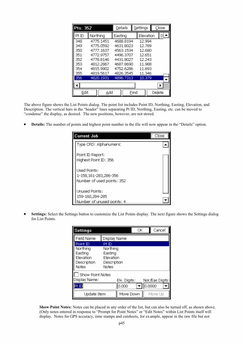
p45

The above figure shows the List Points dialog. The point list includes Point ID, Northing, Easting, Elevation, andDescription. The vertical bars in the “header” lines separating Pt ID, Northing, Easting, etc. can be moved to“condense” the display, as desired. The new positions, however, are not stored.

Details: The number of points and highest point number in the file will now appear in the “Details” option.

Settings: Select the Settings button to customize the List Points display. The next figure shows the Settings dialogfor List Points.

Show Point Notes: Notes can be placed in any order of the list, but can also be turned off, as shown above.(Only notes entered in response to “Prompt for Point Notes” or “Edit Notes” within List Points itself willdisplay. Notes for GPS accuracy, time stamps and cutsheets, for example, appear in the raw file but not

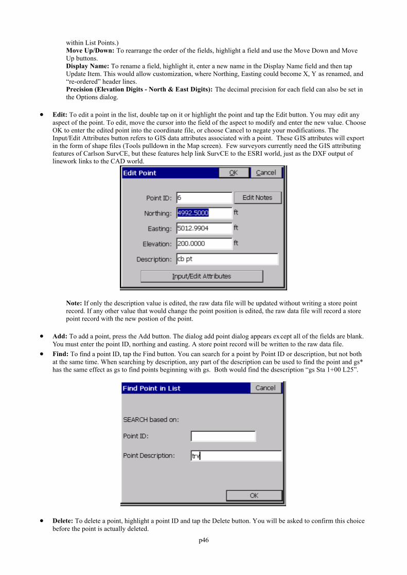
p46

within List Points.)Move Up/Down: To rearrange the order of the fields, highlight a field and use the Move Down and MoveUp buttons.Display Name: To rename a field, highlight it, enter a new name in the Display Name field and then tapUpdate Item. This would allow customization, where Northing, Easting could become X, Y as renamed, and“re-ordered” header lines. Precision (Elevation Digits - North & East Digits): The decimal precision for each field can also be set inthe Options dialog.

Edit: To edit a point in the list, double tap on it or highlight the point and tap the Edit button. You may edit anyaspect of the point. To edit, move the cursor into the field of the aspect to modify and enter the new value. ChooseOK to enter the edited point into the coordinate file, or choose Cancel to negate your modifications. TheInput/Edit Attributes button refers to GIS data attributes associated with a point. These GIS attributes will exportin the form of shape files (Tools pulldown in the Map screen). Few surveyors currently need the GIS attributingfeatures of Carlson SurvCE, but these features help link SurvCE to the ESRI world, just as the DXF output oflinework links to the CAD world.

Note: If only the description value is edited, the raw data file will be updated without writing a store pointrecord. If any other value that would change the point position is edited, the raw data file will record a storepoint record with the new postion of the point.

Add: To add a point, press the Add button. The dialog add point dialog appears except all of the fields are blank.You must enter the point ID, northing and easting. A store point record will be written to the raw data file.

Find: To find a point ID, tap the Find button. You can search for a point by Point ID or description, but not bothat the same time. When searching by description, any part of the description can be used to find the point and gs*has the same effect as gs to find points beginning with gs. Both would find the dsescription “gs Sta 1+00 L25”.

Delete: To delete a point, highlight a point ID and tap the Delete button. You will be asked to confirm this choicebefore the point is actually deleted.

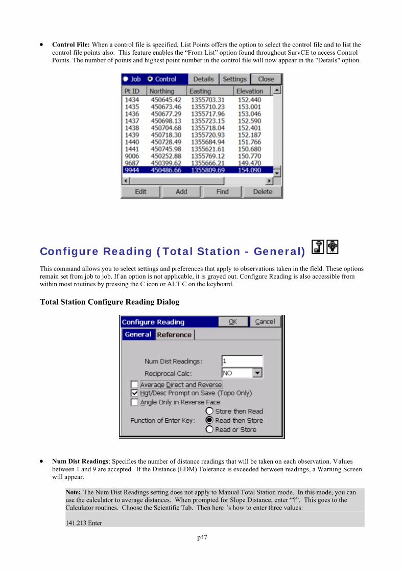
p47

Control File: When a control file is specified, List Points offers the option to select the control file and to list thecontrol file points also. This feature enables the “From List” option found throughout SurvCE to access ControlPoints. The number of points and highest point number in the control file will now appear in the "Details" option.

Configure Reading (Total Station - General) This command allows you to select settings and preferences that apply to observations taken in the field. These optionsremain set from job to job. If an option is not applicable, it is grayed out. Configure Reading is also accessible fromwithin most routines by pressing the C icon or ALT C on the keyboard.

Total Station Configure Reading Dialog

Num Dist Readings: Specifies the number of distance readings that will be taken on each observation. Valuesbetween 1 and 9 are accepted. If the Distance (EDM) Tolerance is exceeded between readings, a Warning Screenwill appear.

Note: The Num Dist Readings setting does not apply to Manual Total Station mode. In this mode, you canuse the calculator to average distances. When prompted for Slope Distance, enter “?”. This goes to theCalculator routines. Choose the Scientific Tab. Then here ’s how to enter three values:

141.213 Enter

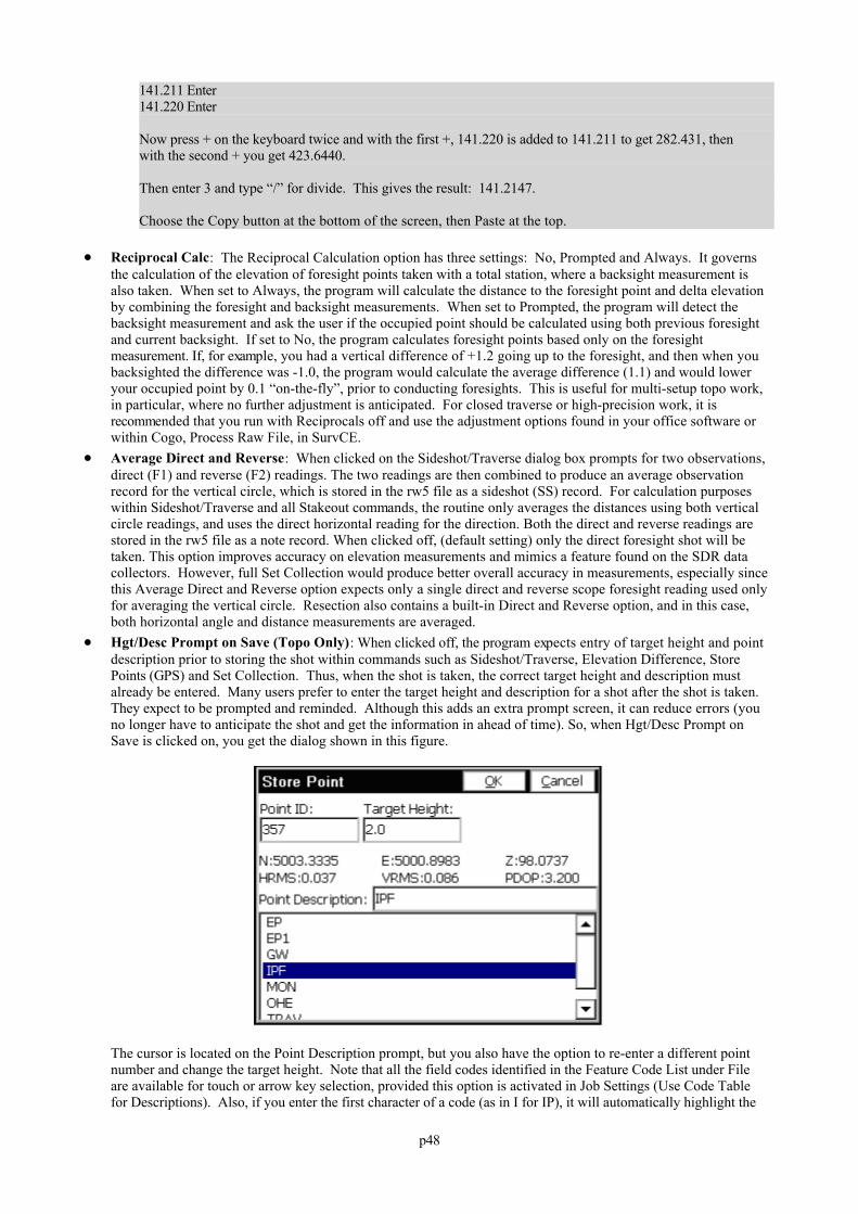
p48

141.211 Enter141.220 Enter

Now press + on the keyboard twice and with the first +, 141.220 is added to 141.211 to get 282.431, thenwith the second + you get 423.6440.

Then enter 3 and type “/” for divide. This gives the result: 141.2147.

Choose the Copy button at the bottom of the screen, then Paste at the top.

Reciprocal Calc: The Reciprocal Calculation option has three settings: No, Prompted and Always. It governsthe calculation of the elevation of foresight points taken with a total station, where a backsight measurement isalso taken. When set to Always, the program will calculate the distance to the foresight point and delta elevationby combining the foresight and backsight measurements. When set to Prompted, the program will detect thebacksight measurement and ask the user if the occupied point should be calculated using both previous foresightand current backsight. If set to No, the program calculates foresight points based only on the foresightmeasurement. If, for example, you had a vertical difference of +1.2 going up to the foresight, and then when youbacksighted the difference was -1.0, the program would calculate the average difference (1.1) and would loweryour occupied point by 0.1 “on-the-fly”, prior to conducting foresights. This is useful for multi-setup topo work,in particular, where no further adjustment is anticipated. For closed traverse or high-precision work, it isrecommended that you run with Reciprocals off and use the adjustment options found in your office software orwithin Cogo, Process Raw File, in SurvCE.

Average Direct and Reverse: When clicked on the Sideshot/Traverse dialog box prompts for two observations,direct (F1) and reverse (F2) readings. The two readings are then combined to produce an average observationrecord for the vertical circle, which is stored in the rw5 file as a sideshot (SS) record. For calculation purposeswithin Sideshot/Traverse and all Stakeout commands, the routine only averages the distances using both verticalcircle readings, and uses the direct horizontal reading for the direction. Both the direct and reverse readings arestored in the rw5 file as a note record. When clicked off, (default setting) only the direct foresight shot will betaken. This option improves accuracy on elevation measurements and mimics a feature found on the SDR datacollectors. However, full Set Collection would produce better overall accuracy in measurements, especially sincethis Average Direct and Reverse option expects only a single direct and reverse scope foresight reading used onlyfor averaging the vertical circle. Resection also contains a built-in Direct and Reverse option, and in this case,both horizontal angle and distance measurements are averaged.

Hgt/Desc Prompt on Save (Topo Only): When clicked off, the program expects entry of target height and pointdescription prior to storing the shot within commands such as Sideshot/Traverse, Elevation Difference, StorePoints (GPS) and Set Collection. Thus, when the shot is taken, the correct target height and description mustalready be entered. Many users prefer to enter the target height and description for a shot after the shot is taken. They expect to be prompted and reminded. Although this adds an extra prompt screen, it can reduce errors (youno longer have to anticipate the shot and get the information in ahead of time). So, when Hgt/Desc Prompt onSave is clicked on, you get the dialog shown in this figure.

The cursor is located on the Point Description prompt, but you also have the option to re-enter a different pointnumber and change the target height. Note that all the field codes identified in the Feature Code List under Fileare available for touch or arrow key selection, provided this option is activated in Job Settings (Use Code Tablefor Descriptions). Also, if you enter the first character of a code (as in I for IP), it will automatically highlight the

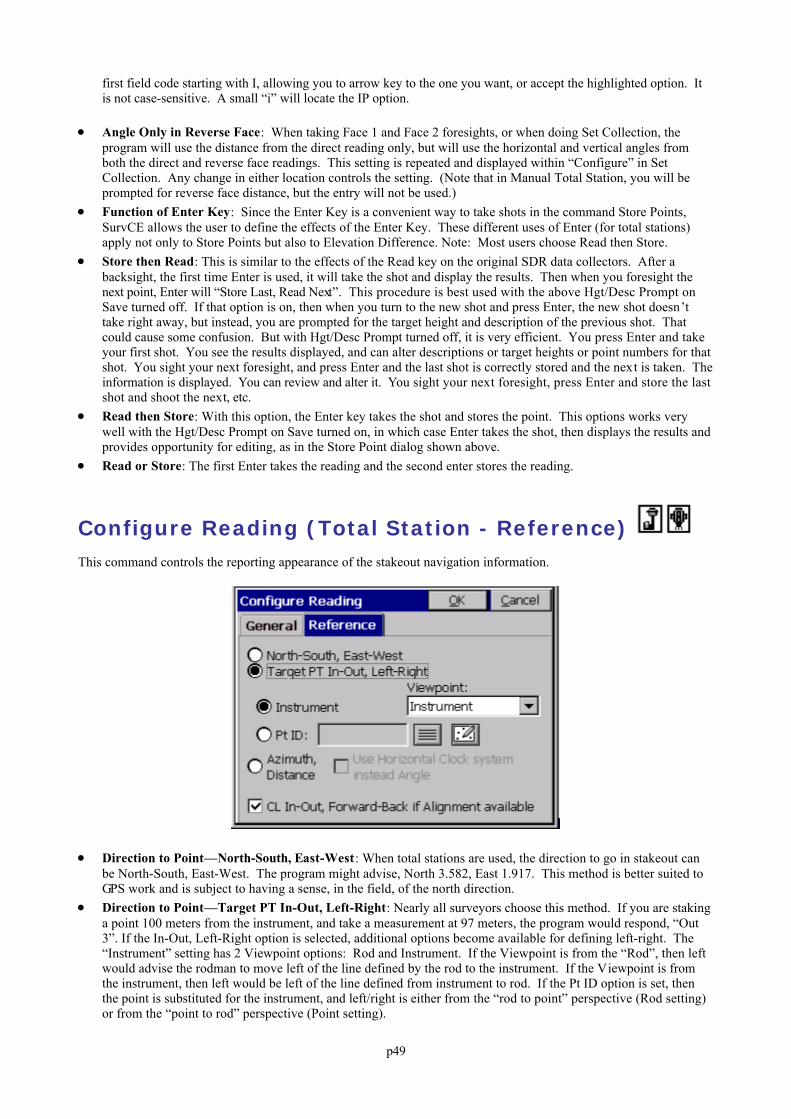
p49

first field code starting with I, allowing you to arrow key to the one you want, or accept the highlighted option. Itis not case-sensitive. A small “i” will locate the IP option.

Angle Only in Reverse Face: When taking Face 1 and Face 2 foresights, or when doing Set Collection, theprogram will use the distance from the direct reading only, but will use the horizontal and vertical angles fromboth the direct and reverse face readings. This setting is repeated and displayed within “Configure” in SetCollection. Any change in either location controls the setting. (Note that in Manual Total Station, you will beprompted for reverse face distance, but the entry will not be used.)

Function of Enter Key: Since the Enter Key is a convenient way to take shots in the command Store Points,SurvCE allows the user to define the effects of the Enter Key. These different uses of Enter (for total stations)apply not only to Store Points but also to Elevation Difference. Note: Most users choose Read then Store.

Store then Read: This is similar to the effects of the Read key on the original SDR data collectors. After abacksight, the first time Enter is used, it will take the shot and display the results. Then when you foresight thenext point, Enter will “Store Last, Read Next”. This procedure is best used with the above Hgt/Desc Prompt onSave turned off. If that option is on, then when you turn to the new shot and press Enter, the new shot doesn’ttake right away, but instead, you are prompted for the target height and description of the previous shot. Thatcould cause some confusion. But with Hgt/Desc Prompt turned off, it is very efficient. You press Enter and takeyour first shot. You see the results displayed, and can alter descriptions or target heights or point numbers for thatshot. You sight your next foresight, and press Enter and the last shot is correctly stored and the next is taken. Theinformation is displayed. You can review and alter it. You sight your next foresight, press Enter and store the lastshot and shoot the next, etc.

Read then Store: With this option, the Enter key takes the shot and stores the point. This options works verywell with the Hgt/Desc Prompt on Save turned on, in which case Enter takes the shot, then displays the results andprovides opportunity for editing, as in the Store Point dialog shown above.

Read or Store: The first Enter takes the reading and the second enter stores the reading.

Configure Reading (Total Station - Reference) This command controls the reporting appearance of the stakeout navigation information.

Direction to Point—North-South, East-West: When total stations are used, the direction to go in stakeout canbe North-South, East-West. The program might advise, North 3.582, East 1.917. This method is better suited toGPS work and is subject to having a sense, in the field, of the north direction.

Direction to Point—Target PT In-Out, Left-Right: Nearly all surveyors choose this method. If you are stakinga point 100 meters from the instrument, and take a measurement at 97 meters, the program would respond, “Out3”. If the In-Out, Left-Right option is selected, additional options become available for defining left-right. The“Instrument” setting has 2 Viewpoint options: Rod and Instrument. If the Viewpoint is from the “Rod”, then leftwould advise the rodman to move left of the line defined by the rod to the instrument. If the Viewpoint is fromthe instrument, then left would be left of the line defined from instrument to rod. If the Pt ID option is set, thenthe point is substituted for the instrument, and left/right is either from the “rod to point” perspective (Rod setting)or from the “point to rod” perspective (Point setting).

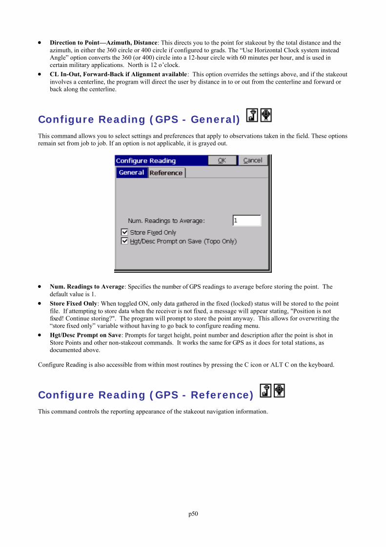
p50

Direction to Point—Azimuth, Distance: This directs you to the point for stakeout by the total distance and theazimuth, in either the 360 circle or 400 circle if configured to grads. The “Use Horizontal Clock system insteadAngle” option converts the 360 (or 400) circle into a 12-hour circle with 60 minutes per hour, and is used incertain military applications. North is 12 o’clock.

CL In-Out, Forward-Back if Alignment available: This option overrides the settings above, and if the stakeoutinvolves a centerline, the program will direct the user by distance in to or out from the centerline and forward orback along the centerline.

Configure Reading (GPS - General) This command allows you to select settings and preferences that apply to observations taken in the field. These optionsremain set from job to job. If an option is not applicable, it is grayed out.

Num. Readings to Average: Specifies the number of GPS readings to average before storing the point. Thedefault value is 1.

Store Fixed Only: When toggled ON, only data gathered in the fixed (locked) status will be stored to the pointfile. If attempting to store data when the receiver is not fixed, a message will appear stating, "Position is notfixed! Continue storing?". The program will prompt to store the point anyway. This allows for overwriting the“store fixed only” variable without having to go back to configure reading menu.

Hgt/Desc Prompt on Save: Prompts for target height, point number and description after the point is shot inStore Points and other non-stakeout commands. It works the same for GPS as it does for total stations, asdocumented above.

Configure Reading is also accessible from within most routines by pressing the C icon or ALT C on the keyboard.

Configure Reading (GPS - Reference) This command controls the reporting appearance of the stakeout navigation information.

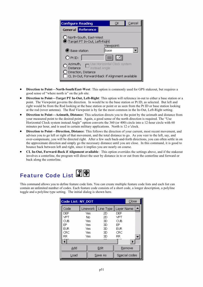
p51

Direction to Point—North-South/East-West: This option is commonly used for GPS stakeout, but requires agood sense of “where north is” on the job site.

Direction to Point—Target PT In-Out, Left-Right: This option will reference in-out to either a base station or apoint. The Viewpoint governs the direction. In would be to the base station or Pt ID, as selected. But left andright would be from the Rod looking at the base station or point or as seen from the Pt ID or base station lookingat the rod (rover antenna). The Rod Viewpoint is by far the most common in the In-Out, Left-Right setting.

Direction to Point—Azimuth, Distance: This selection directs you to the point by the azimuth and distance fromyour measured point to the desired point. Again, a good sense of the north direction is required. The “UseHorizontal Clock system instead Angle” option converts the 360 (or 400) circle into a 12-hour circle with 60minutes per hour, and is used in certain military applications. North is 12 o’clock.

Direction to Point—Direction, Distance: This follows the direction of your current, most recent movement, andadvises you to go left or right of that movement, and the total distance to go. As you veer to the left, say, andover-compensate, you will be directed right. After a few such back-and-forth directions, you can often settle in onthe approximate direction and simply go the necessary distance until you are close. In this command, it is good tobounce back between left and right, since it implies you are nearly on course.

CL In-Out, Forward-Back if Alignment available: This option overrides the settings above, and if the stakeoutinvolves a centerline, the program will direct the user by distance in to or out from the centerline and forward orback along the centerline.

Feature Code List This command allows you to define feature code lists. You can create multiple feature code lists and each list cancontain an unlimited number of codes. Each feature code consists of a short code, a longer description, a polylinetoggle and a polyline type setting. The initial dialog is shown here.

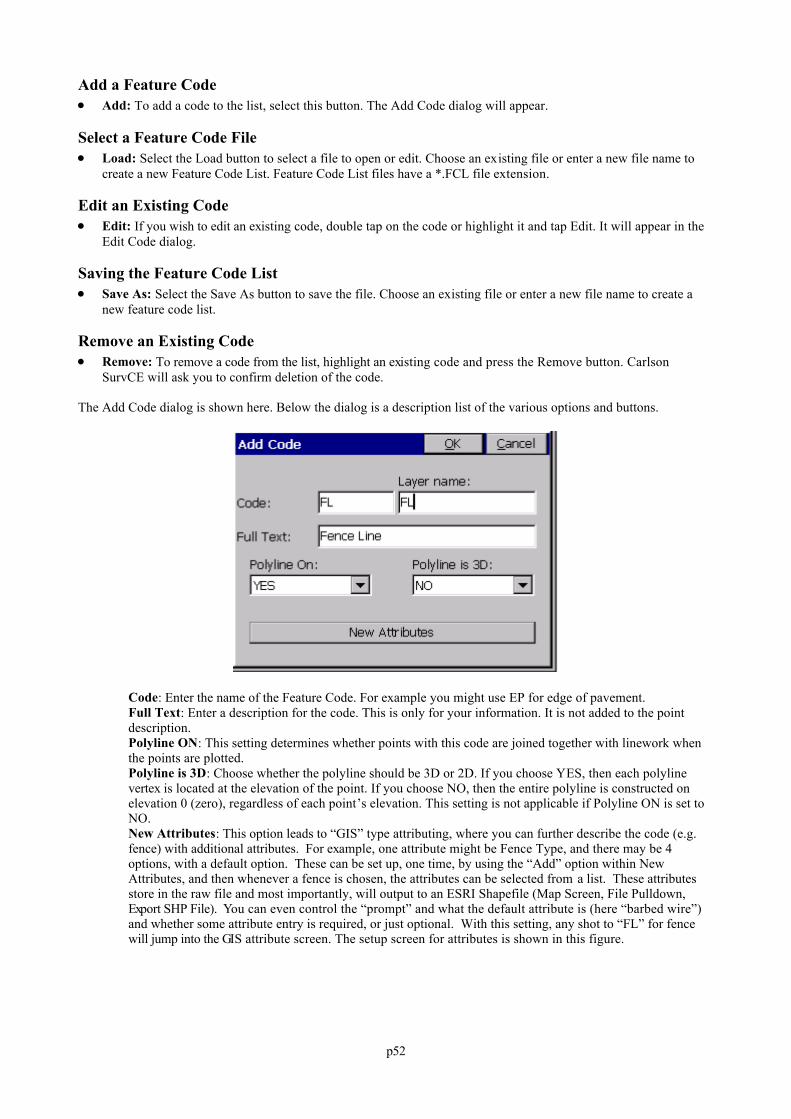
p52

Add a Feature Code Add: To add a code to the list, select this button. The Add Code dialog will appear.

Select a Feature Code File Load: Select the Load button to select a file to open or edit. Choose an existing file or enter a new file name to

create a new Feature Code List. Feature Code List files have a *.FCL file extension.

Edit an Existing Code Edit: If you wish to edit an existing code, double tap on the code or highlight it and tap Edit. It will appear in the

Edit Code dialog.

Saving the Feature Code List Save As: Select the Save As button to save the file. Choose an existing file or enter a new file name to create a

new feature code list.

Remove an Existing Code Remove: To remove a code from the list, highlight an existing code and press the Remove button. Carlson

SurvCE will ask you to confirm deletion of the code.

The Add Code dialog is shown here. Below the dialog is a description list of the various options and buttons.

Code: Enter the name of the Feature Code. For example you might use EP for edge of pavement.Full Text: Enter a description for the code. This is only for your information. It is not added to the pointdescription.Polyline ON: This setting determines whether points with this code are joined together with linework whenthe points are plotted.Polyline is 3D: Choose whether the polyline should be 3D or 2D. If you choose YES, then each polylinevertex is located at the elevation of the point. If you choose NO, then the entire polyline is constructed onelevation 0 (zero), regardless of each point’s elevation. This setting is not applicable if Polyline ON is set toNO.New Attributes: This option leads to “GIS” type attributing, where you can further describe the code (e.g.fence) with additional attributes. For example, one attribute might be Fence Type, and there may be 4options, with a default option. These can be set up, one time, by using the “Add” option within NewAttributes, and then whenever a fence is chosen, the attributes can be selected from a list. These attributesstore in the raw file and most importantly, will output to an ESRI Shapefile (Map Screen, File Pulldown,Export SHP File). You can even control the “prompt” and what the default attribute is (here “barbed wire”)and whether some attribute entry is required, or just optional. With this setting, any shot to “FL” for fencewill jump into the GIS attribute screen. The setup screen for attributes is shown in this figure.

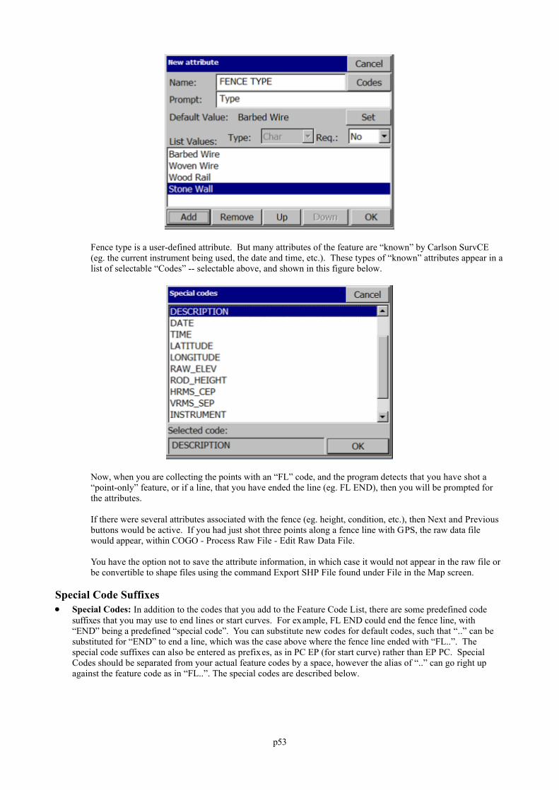
p53

Fence type is a user-defined attribute. But many attributes of the feature are “known” by Carlson SurvCE(eg. the current instrument being used, the date and time, etc.). These types of “known” attributes appear in alist of selectable “Codes” -- selectable above, and shown in this figure below.

Now, when you are collecting the points with an “FL” code, and the program detects that you have shot a“point-only” feature, or if a line, that you have ended the line (eg. FL END), then you will be prompted forthe attributes.

If there were several attributes associated with the fence (eg. height, condition, etc.), then Next and Previousbuttons would be active. If you had just shot three points along a fence line with GPS, the raw data filewould appear, within COGO - Process Raw File - Edit Raw Data File.

You have the option not to save the attribute information, in which case it would not appear in the raw file orbe convertible to shape files using the command Export SHP File found under File in the Map screen.

Special Code Suffixes Special Codes: In addition to the codes that you add to the Feature Code List, there are some predefined code

suffixes that you may use to end lines or start curves. For example, FL END could end the fence line, with“END” being a predefined “special code”. You can substitute new codes for default codes, such that “..” can besubstituted for “END” to end a line, which was the case above where the fence line ended with “FL..”. Thespecial code suffixes can also be entered as prefixes, as in PC EP (for start curve) rather than EP PC. SpecialCodes should be separated from your actual feature codes by a space, however the alias of “..” can go right upagainst the feature code as in “FL..”. The special codes are described below.

p54

PC & PT: Used to specify the point of curvature (PC) and point of tangency (PT) of a curve. If you aretaking shots on a curve, use PC to specify the beginning of the curve and PT to specify the end of the curve.The PC special code will activate a 3-point arc automatically, so use of the PT code in a 3-point arc isredundant and therefore it is not necessary. However, if you are picking up a meandering stream or treeline,PT is useful to end the curving feature, and the program will “best fit” a curve through all the surveyed pointsbetween the PC and PT codes.

CLO: Use this code to close a figure. This tells the software to close from the last point coded as CLO backto the first point of the figure.

SMO: Use this code to smooth the line through all of the points. This code must occur on the first point ofthe line.

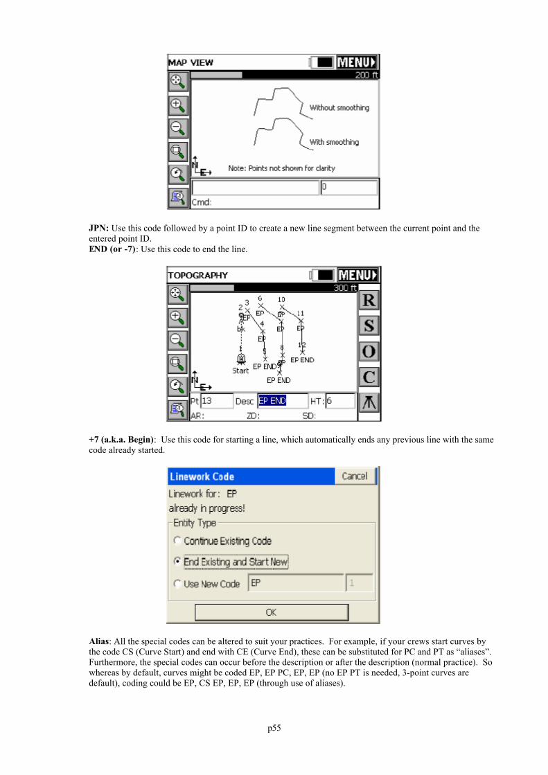
p55

JPN: Use this code followed by a point ID to create a new line segment between the current point and theentered point ID.END (or -7): Use this code to end the line.

+7 (a.k.a. Begin): Use this code for starting a line, which automatically ends any previous line with the samecode already started.

Alias: All the special codes can be altered to suit your practices. For example, if your crews start curves bythe code CS (Curve Start) and end with CE (Curve End), these can be substituted for PC and PT as “aliases”.Furthermore, the special codes can occur before the description or after the description (normal practice). Sowhereas by default, curves might be coded EP, EP PC, EP, EP (no EP PT is needed, 3-point curves aredefault), coding could be EP, CS EP, EP, EP (through use of aliases).

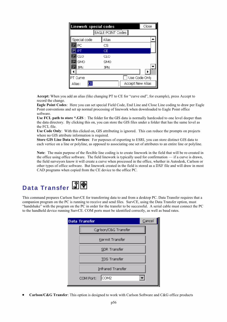
p56

Accept: When you add an alias (like changing PT to CE for “curve end”, for example), press Accept torecord the change.Eagle Point Codes: Here you can set special Field Code, End Line and Close Line coding to draw per EaglePoint conventions and set up normal processing of linework when downloaded to Eagle Point officesoftware.Use FCL path to store *.GIS : The folder for the GIS data is normally hardcoded to one level deeper thanthe data directory. By clicking this on, you can store the GIS files under a folder that has the same level asthe FCL file.Use Code Only: With this clicked on, GIS attributing is ignored. This can reduce the prompts on projectswhere no GIS attribute information is required.Store GIS Line Data to Vertices: For purposes of exporting to ESRI, you can store distinct GIS data toeach vertice on a line or polyline, as opposed to associating one set of attributes to an entire line or polyline.

Note: The main purpose of the flexible line coding is to create linework in the field that will be re-created inthe office using office software. The field linework is typically used for confirmation — if a curve is drawn,the field surveyors know it will create a curve when processed in the office, whether in Autodesk, Carlson orother types of office software. But linework created in the field is stored as a DXF file and will draw in mostCAD programs when copied from the CE device to the office PC.

Data Transfer This command prepares Carlson SurvCE for transferring data to and from a desktop PC. Data Transfer requires that acompanion program on the PC is running to receive and send files. SurvCE, using the Data Transfer option, must“handshake” with the program on the PC in order for the transfer to be successful. A serial cable must connect the PCto the handheld device running SurvCE. COM ports must be identified correctly, as well as baud rates.

Carlson/C&G Transfer: This option is designed to work with Carlson Software and C&G office products

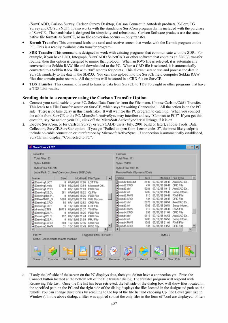
p57

(SurvCADD, Carlson Survey, Carlson Survey Desktop, Carlson Connect in Autodesk products, X-Port, CGSurvey and CG SurvNET). It also works with the standalone SurvCom program that is included with the purchaseof SurvCE. The handshake is designed for simplicity and robustness. Carlson Software products use the samenative file formats as SurvCE, so no file conversion occurs — only transfer.

Kermit Transfer: This command leads to a send and receive screen that works with the Kermit program on thePC. This is a readily available data transfer program.

SDR Transfer: This command is designed to work with existing programs that communicate with the SDR. Forexample, if you have LDD, Integraph, SurvCADD SelectCAD or other software that contains an SDR33 transferroutine, then this option is designed to mimic that protocol. When an RW5 file is selected, it is automaticallyconverted to a Sokkia RAW file and downloaded to the PC. When a CRD file is selected, it is automaticallyconverted to a Sokkia RAW file with “08” records for points. This allows users to use and process the data inSurvCE similarly to the data in the SDR33. You can also upload into the SurvCE field computer Sokkia RAWfiles that contain point records. All the points will be stored in a CRD file on SurvCE.

TDS Transfer: This command is used to transfer data from SurvCE to TDS Foresight or other programs that havea TDS Link routine.

Sending data to a computer using the Carlson Transfer Option1. Connect your serial cable to your PC. Select Data Transfer from the File menu. Choose Carlson/C&G Transfer.

This leads to a File Transfer screen on SurvCE, which says “Awaiting Connection”. All the action is on the PCside. There is no time delay in this handshake. It will wait for the PC program to catch up. When you connectthe cable from SurvCE to the PC, MicroSoft ActiveSync may interfere and say “Connect to PC?” If you get thisquestion, say No and on your PC, click off the MicroSoft ActiveSync serial linkage if it is on.

2. Execute SurvCom, or for Carlson Survey or SurvCADD users (July, 2001 build or later), choose Tools, DataCollectors, SurvCE/SurvStar option. If you get “Failed to open Com 1 error code -3”, the most likely culpritsinclude no cable connection or interference by Microsoft ActiveSync. If connection is automatically established,SurvCE will display, “Connected to PC”.

3. If only the left side of the screen on the PC displays data, then you do not have a connection yet. Press theConnect button located at the bottom left of the file transfer dialog. The transfer program will respond withRetrieving File List. Once the file list has been retrieved, the left side of the dialog box will show files located inthe specified path on the PC and the right side of the dialog displays the files located in the designated path on theremote. You can change directories by scrolling to the top of the file list and choosing Up One Level (just like inWindows). In the above dialog, a filter was applied so that the only files in the form of *.crd are displayed. Filters

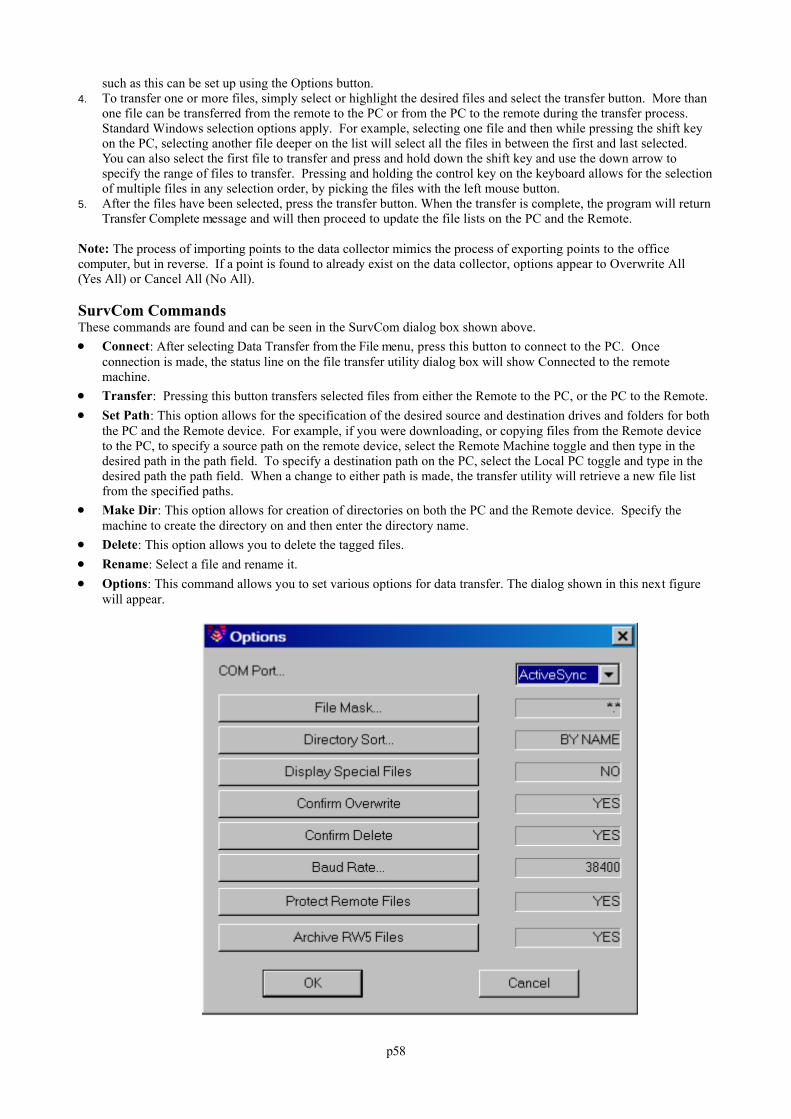
p58

such as this can be set up using the Options button.4. To transfer one or more files, simply select or highlight the desired files and select the transfer button. More than

one file can be transferred from the remote to the PC or from the PC to the remote during the transfer process. Standard Windows selection options apply. For example, selecting one file and then while pressing the shift keyon the PC, selecting another file deeper on the list will select all the files in between the first and last selected. You can also select the first file to transfer and press and hold down the shift key and use the down arrow tospecify the range of files to transfer. Pressing and holding the control key on the keyboard allows for the selectionof multiple files in any selection order, by picking the files with the left mouse button.

5. After the files have been selected, press the transfer button. When the transfer is complete, the program will returnTransfer Complete message and will then proceed to update the file lists on the PC and the Remote.

Note: The process of importing points to the data collector mimics the process of exporting points to the officecomputer, but in reverse. If a point is found to already exist on the data collector, options appear to Overwrite All(Yes All) or Cancel All (No All).

SurvCom Commands These commands are found and can be seen in the SurvCom dialog box shown above. Connect: After selecting Data Transfer from the File menu, press this button to connect to the PC. Once

connection is made, the status line on the file transfer utility dialog box will show Connected to the remotemachine.

Transfer: Pressing this button transfers selected files from either the Remote to the PC, or the PC to the Remote. Set Path: This option allows for the specification of the desired source and destination drives and folders for both

the PC and the Remote device. For example, if you were downloading, or copying files from the Remote deviceto the PC, to specify a source path on the remote device, select the Remote Machine toggle and then type in thedesired path in the path field. To specify a destination path on the PC, select the Local PC toggle and type in thedesired path the path field. When a change to either path is made, the transfer utility will retrieve a new file listfrom the specified paths.

Make Dir: This option allows for creation of directories on both the PC and the Remote device. Specify themachine to create the directory on and then enter the directory name.

Delete: This option allows you to delete the tagged files. Rename: Select a file and rename it. Options: This command allows you to set various options for data transfer. The dialog shown in this next figure

will appear.

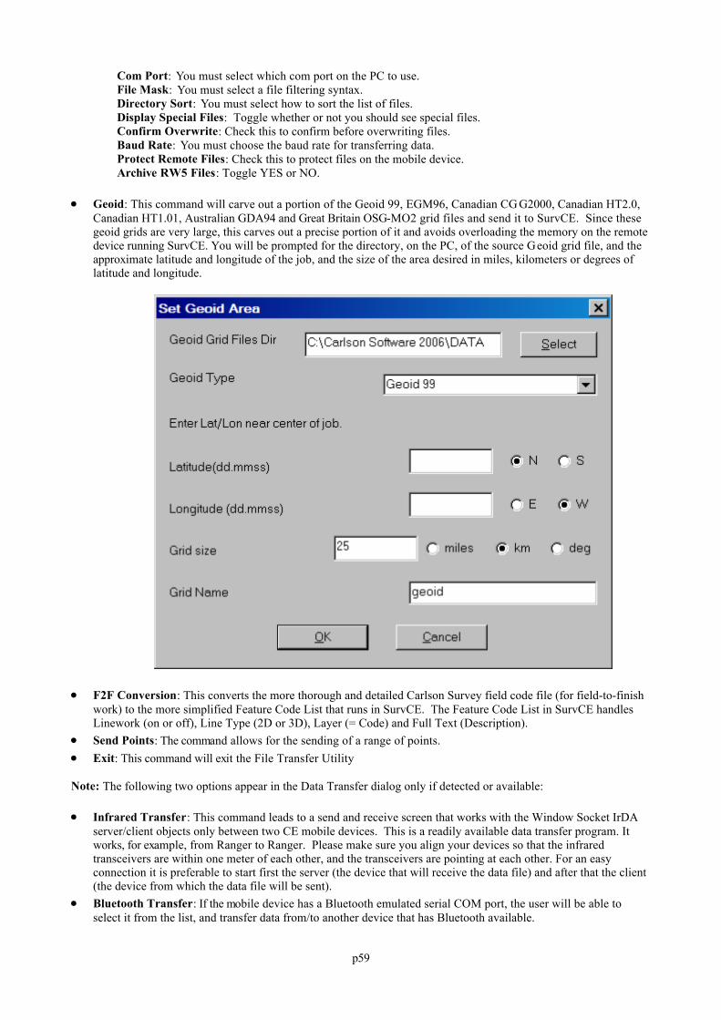
p59

Com Port: You must select which com port on the PC to use.File Mask: You must select a file filtering syntax.Directory Sort: You must select how to sort the list of files.Display Special Files: Toggle whether or not you should see special files.Confirm Overwrite: Check this to confirm before overwriting files.Baud Rate: You must choose the baud rate for transferring data.Protect Remote Files: Check this to protect files on the mobile device.Archive RW5 Files: Toggle YES or NO.

Geoid: This command will carve out a portion of the Geoid 99, EGM96, Canadian CG G2000, Canadian HT2.0,Canadian HT1.01, Australian GDA94 and Great Britain OSG-MO2 grid files and send it to SurvCE. Since thesegeoid grids are very large, this carves out a precise portion of it and avoids overloading the memory on the remotedevice running SurvCE. You will be prompted for the directory, on the PC, of the source Geoid grid file, and theapproximate latitude and longitude of the job, and the size of the area desired in miles, kilometers or degrees oflatitude and longitude.

F2F Conversion: This converts the more thorough and detailed Carlson Survey field code file (for field-to-finishwork) to the more simplified Feature Code List that runs in SurvCE. The Feature Code List in SurvCE handlesLinework (on or off), Line Type (2D or 3D), Layer (= Code) and Full Text (Description).

Send Points: The command allows for the sending of a range of points. Exit: This command will exit the File Transfer Utility

Note: The following two options appear in the Data Transfer dialog only if detected or available:

Infrared Transfer: This command leads to a send and receive screen that works with the Window Socket IrDAserver/client objects only between two CE mobile devices. This is a readily available data transfer program. Itworks, for example, from Ranger to Ranger. Please make sure you align your devices so that the infraredtransceivers are within one meter of each other, and the transceivers are pointing at each other. For an easyconnection it is preferable to start first the server (the device that will receive the data file) and after that the client(the device from which the data file will be sent).

Bluetooth Transfer: If the mobile device has a Bluetooth emulated serial COM port, the user will be able toselect it from the list, and transfer data from/to another device that has Bluetooth available.

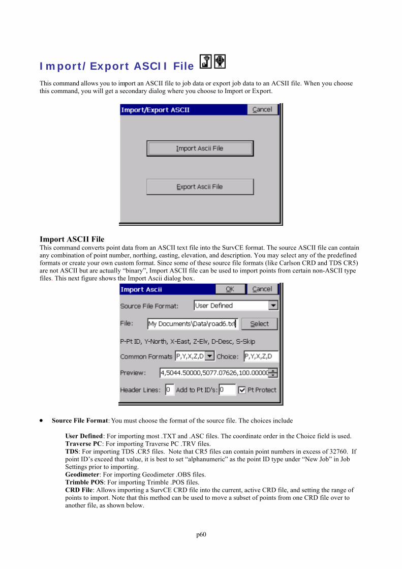
p60

Import/Export ASCII File This command allows you to import an ASCII file to job data or export job data to an ACSII file. When you choosethis command, you will get a secondary dialog where you choose to Import or Export.

Import ASCII File This command converts point data from an ASCII text file into the SurvCE format. The source ASCII file can containany combination of point number, northing, easting, elevation, and description. You may select any of the predefinedformats or create your own custom format. Since some of these source file formats (like Carlson CRD and TDS CR5)are not ASCII but are actually “binary”, Import ASCII file can be used to import points from certain non-ASCII typefiles. This next figure shows the Import Ascii dialog box.

Source File Format: You must choose the format of the source file. The choices include

User Defined: For importing most .TXT and .ASC files. The coordinate order in the Choice field is used.Traverse PC: For importing Traverse PC .TRV files.TDS: For importing TDS .CR5 files. Note that CR5 files can contain point numbers in excess of 32760. Ifpoint ID’s exceed that value, it is best to set “alphanumeric” as the point ID type under “New Job” in JobSettings prior to importing.Geodimeter: For importing Geodimeter .OBS files.Trimble POS: For importing Trimble .POS files.CRD File: Allows importing a SurvCE CRD file into the current, active CRD file, and setting the range ofpoints to import. Note that this method can be used to move a subset of points from one CRD file over toanother file, as shown below.

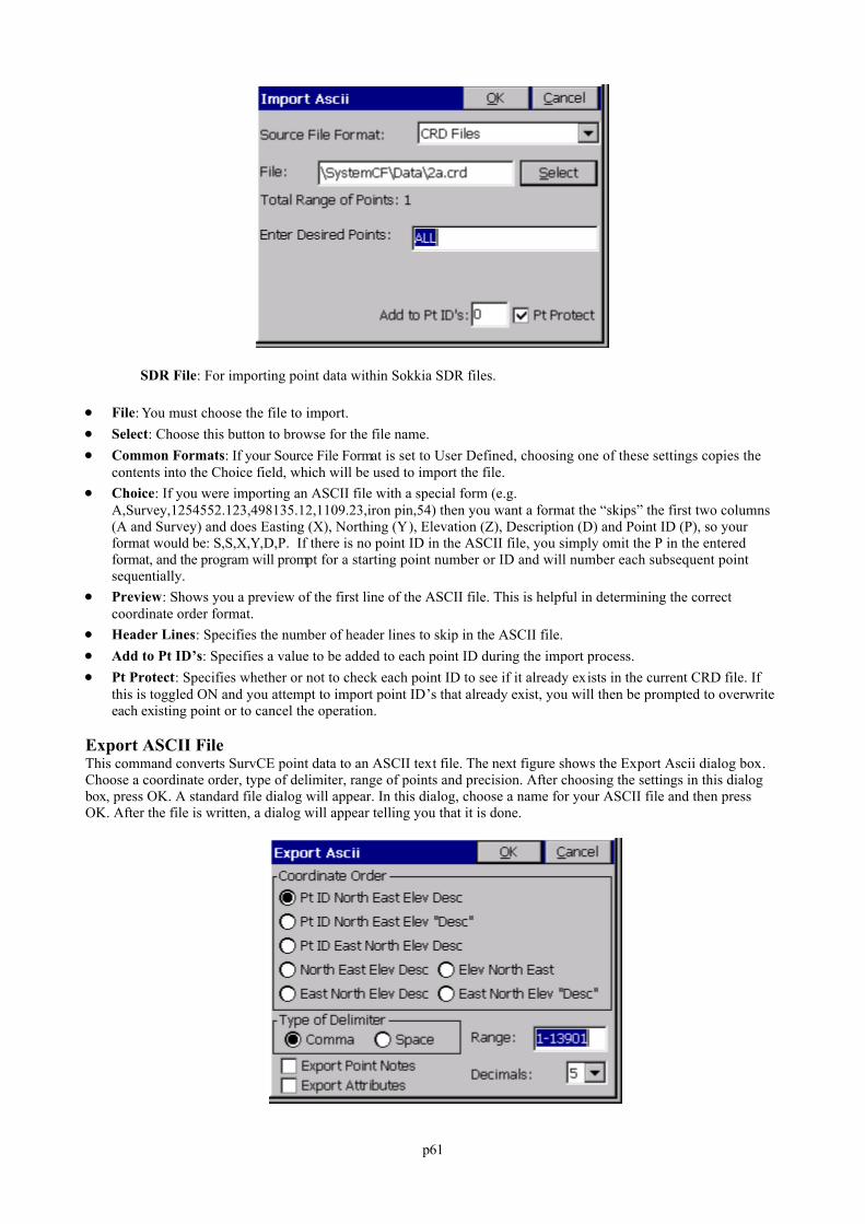
p61

SDR File: For importing point data within Sokkia SDR files.

File: You must choose the file to import. Select: Choose this button to browse for the file name. Common Formats: If your Source File Format is set to User Defined, choosing one of these settings copies the

contents into the Choice field, which will be used to import the file. Choice: If you were importing an ASCII file with a special form (e.g.

A,Survey,1254552.123,498135.12,1109.23,iron pin,54) then you want a format the “skips” the first two columns(A and Survey) and does Easting (X), Northing (Y), Elevation (Z), Description (D) and Point ID (P), so yourformat would be: S,S,X,Y,D,P. If there is no point ID in the ASCII file, you simply omit the P in the enteredformat, and the program will prompt for a starting point number or ID and will number each subsequent pointsequentially.

Preview: Shows you a preview of the first line of the ASCII file. This is helpful in determining the correctcoordinate order format.

Header Lines: Specifies the number of header lines to skip in the ASCII file. Add to Pt ID’s: Specifies a value to be added to each point ID during the import process. Pt Protect: Specifies whether or not to check each point ID to see if it already exists in the current CRD file. If

this is toggled ON and you attempt to import point ID’s that already exist, you will then be prompted to overwriteeach existing point or to cancel the operation.

Export ASCII FileThis command converts SurvCE point data to an ASCII text file. The next figure shows the Export Ascii dialog box.Choose a coordinate order, type of delimiter, range of points and precision. After choosing the settings in this dialogbox, press OK. A standard file dialog will appear. In this dialog, choose a name for your ASCII file and then pressOK. After the file is written, a dialog will appear telling you that it is done.

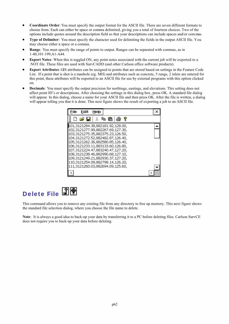
p62

Coordinate Order: You must specify the output format for the ASCII file. There are seven different formats tochoose from. Each can either be space or comma delimited, giving you a total of fourteen choices. Two of theoptions include quotes around the description field so that your descriptions can include spaces and/or com mas.

Type of Delimiter: You must specify the character used for delimiting the fields in the output ASCII file. Youmay choose either a space or a comma.

Range: You must specify the range of points to output. Ranges can be separated with commas, as in1-40,101-199,A1-A44.

Export Notes: When this is toggled ON, any point notes associated with the current job will be exported to a.NOT file. These files are used with SurvCADD (and other Carlson office software products).

Export Attributes: GIS attributes can be assigned to points that are stored based on settings in the Feature CodeList. If a point that is shot is a manhole (eg. MH) and attributes such as concrete, 5 rungs, 2 inlets are entered forthis point, these attributes will be exported to an ASCII file for use by external programs with this option clickedon.

Decimals: You must specify the output precision for northings, eastings, and elevations. This setting does notaffect point ID’s or descriptions. After choosing the settings in this dialog box, press OK. A standard file dialogwill appear. In this dialog, choose a name for your ASCII file and then press OK. After the file is written, a dialogwill appear telling you that it is done. This next figure shows the result of exporting a job to an ASCII file.

Delete File This command allows you to remove any existing file from any directory to free up memory. This next figure showsthe standard file selection dialog, where you choose the file name to delete.

Note: It is always a good idea to back-up your data by transferring it to a PC before deleting files. Carlson SurvCEdoes not require you to back-up your data before deleting.

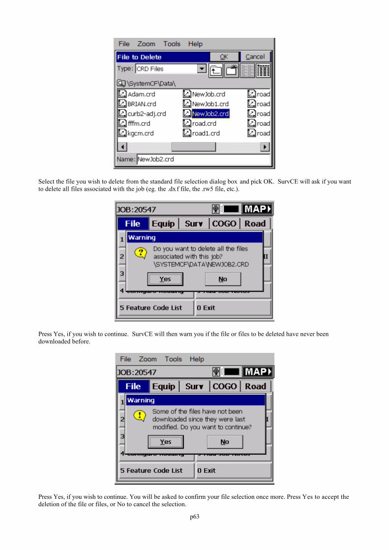
p63

Select the file you wish to delete from the standard file selection dialog box and pick OK. SurvCE will ask if you wantto delete all files associated with the job (eg. the .dx f file, the .rw5 file, etc.).

Press Yes, if you wish to continue. SurvCE will then warn you if the file or files to be deleted have never beendownloaded before.

Press Yes, if you wish to continue. You will be asked to confirm your file selection once more. Press Yes to accept thedeletion of the file or files, or No to cancel the selection.

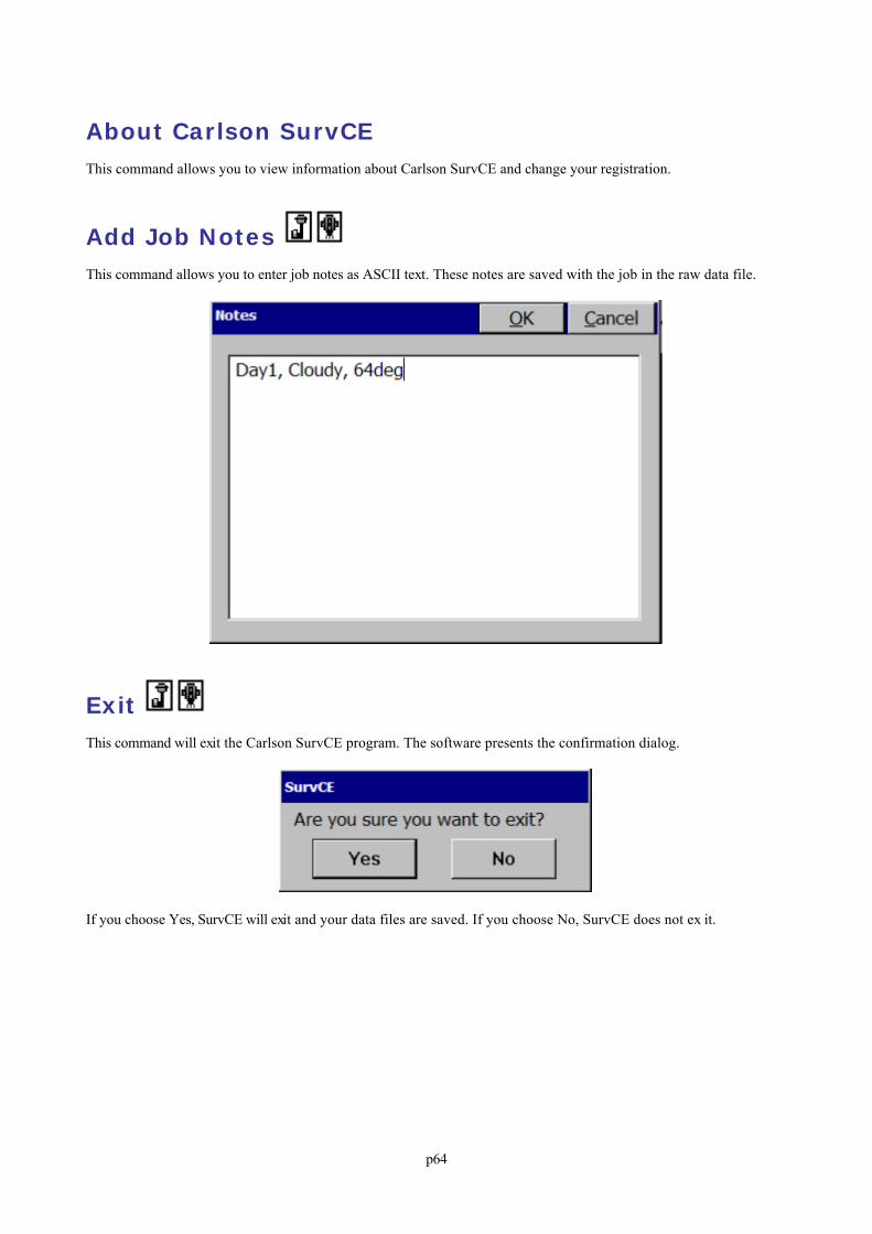
p64

About Carlson SurvCEThis command allows you to view information about Carlson SurvCE and change your registration.

Add Job Notes This command allows you to enter job notes as ASCII text. These notes are saved with the job in the raw data file.

Exit This command will exit the Carlson SurvCE program. The software presents the confirmation dialog.

If you choose Yes, SurvCE will exit and your data files are saved. If you choose No, SurvCE does not ex it.

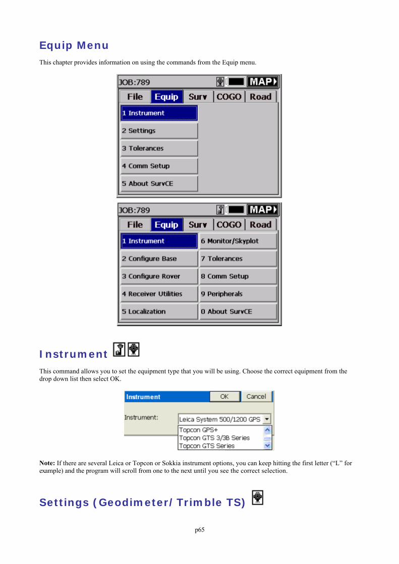
p65

Equip MenuThis chapter provides information on using the commands from the Equip menu.

Instrument This command allows you to set the equipment type that you will be using. Choose the correct equipment from thedrop down list then select OK.

Note: If there are several Leica or Topcon or Sokkia instrument options, you can keep hitting the first letter (“L” forexample) and the program will scroll from one to the next until you see the correct selection.

Settings (Geodimeter/Trimble TS)

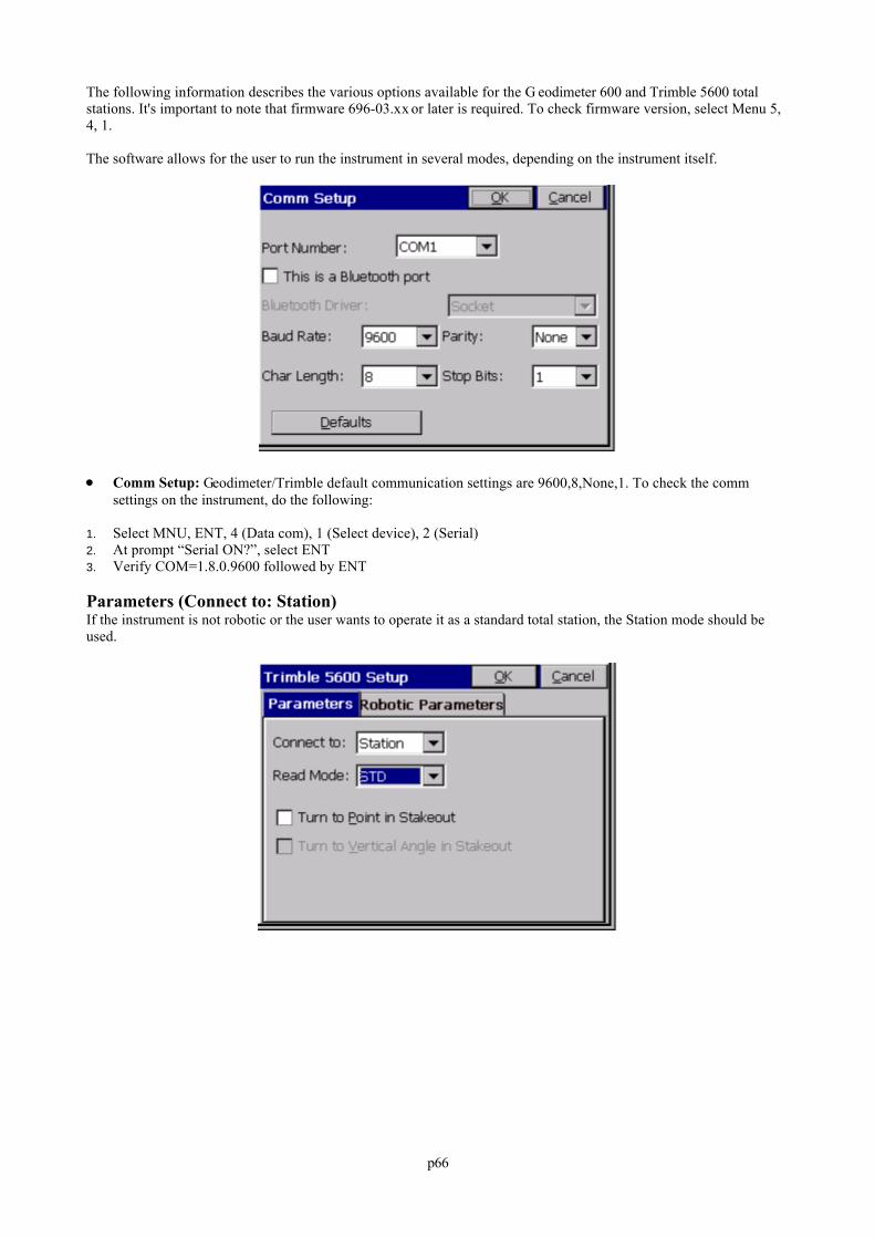
p66

The following information describes the various options available for the G eodimeter 600 and Trimble 5600 totalstations. It's important to note that firmware 696-03.xx or later is required. To check firmware version, select Menu 5,4, 1.

The software allows for the user to run the instrument in several modes, depending on the instrument itself.

Comm Setup: Geodimeter/Trimble default communication settings are 9600,8,None,1. To check the commsettings on the instrument, do the following:

1. Select MNU, ENT, 4 (Data com), 1 (Select device), 2 (Serial)2. At prompt “Serial ON?”, select ENT3. Verify COM=1.8.0.9600 followed by ENT

Parameters (Connect to: Station)If the instrument is not robotic or the user wants to operate it as a standard total station, the Station mode should beused.

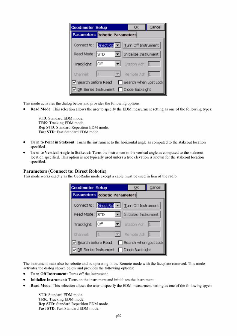
p67

This mode activates the dialog below and provides the following options: Read Mode: This selection allows the user to specify the EDM measurment setting as one of the following types:

STD: Standard EDM mode.TRK: Tracking EDM mode.Rep STD: Standard Repetition EDM mode.Fast STD: Fast Standard EDM mode.

Turn to Point in Stakeout: Turns the instrument to the horizontal angle as computed to the stakeout locationspecified.

Turn to Vertical Angle in Stakeout: Turns the instrument to the vertical angle as computed to the stakeoutlocation specified. This option is not typically used unless a true elevation is known for the stakeout locationspecified.

Parameters (Connect to: Direct Robotic)This mode works exactly as the GeoRadio mode except a cable must be used in lieu of the radio.

The instrument must also be robotic and be operating in the Remote mode with the faceplate removed. This modeactivates the dialog shown below and provides the following options: Turn Off Instrument: Turns off the instrument. Initialize Instrument: Turns on the instrument and initializes the instrument. Read Mode: This selection allows the user to specify the EDM measurment setting as one of the following tpyes:

STD: Standard EDM mode.TRK: Tracking EDM mode.Rep STD: Standard Repetition EDM mode.Fast STD: Fast Standard EDM mode.

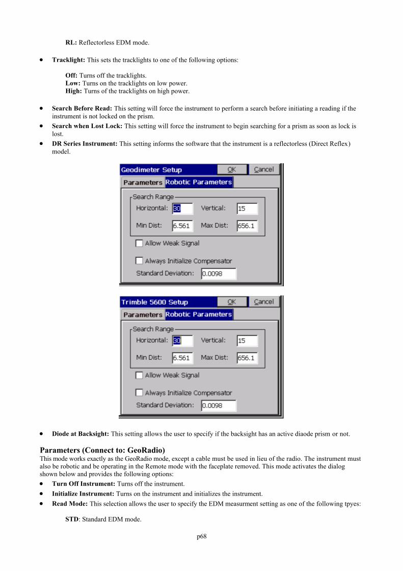
p68

RL: Reflectorless EDM mode.

Tracklight: This sets the tracklights to one of the following options:

Off: Turns off the tracklights.Low: Turns on the tracklights on low power.High: Turns of the tracklights on high power.

Search Before Read: This setting will force the instrument to perform a search before initiating a reading if theinstrument is not locked on the prism.

Search when Lost Lock: This setting will force the instrument to begin searching for a prism as soon as lock islost.

DR Series Instrument: This setting informs the software that the instrument is a reflectorless (Direct Reflex)model.

Diode at Backsight: This setting allows the user to specify if the backsight has an active diaode prism or not.

Parameters (Connect to: GeoRadio)This mode works exactly as the GeoRadio mode, except a cable must be used in lieu of the radio. The instrument mustalso be robotic and be operating in the Remote mode with the faceplate removed. This mode activates the dialogshown below and provides the following options: Turn Off Instrument: Turns off the instrument. Initialize Instrument: Turns on the instrument and initializes the instrument. Read Mode: This selection allows the user to specify the EDM measurment setting as one of the following tpyes:

STD: Standard EDM mode.

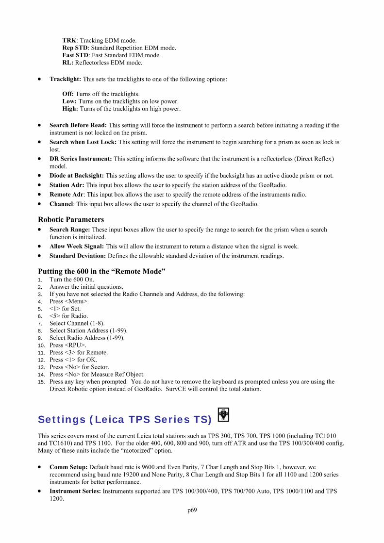
p69

TRK: Tracking EDM mode.Rep STD: Standard Repetition EDM mode.Fast STD: Fast Standard EDM mode.RL: Reflectorless EDM mode.

Tracklight: This sets the tracklights to one of the following options:

Off: Turns off the tracklights.Low: Turns on the tracklights on low power.High: Turns of the tracklights on high power.

Search Before Read: This setting will force the instrument to perform a search before initiating a reading if theinstrument is not locked on the prism.

Search when Lost Lock: This setting will force the instrument to begin searching for a prism as soon as lock islost.

DR Series Instrument: This setting informs the software that the instrument is a reflectorless (Direct Reflex)model.

Diode at Backsight: This setting allows the user to specify if the backsight has an active diaode prism or not. Station Adr: This input box allows the user to specify the station address of the GeoRadio. Remote Adr: This input box allows the user to specify the remote address of the instruments radio. Channel: This input box allows the user to specify the channel of the GeoRadio.

Robotic Parameters Search Range: These input boxes allow the user to specify the range to search for the prism when a search

function is initialized. Allow Week Signal: This will allow the instrument to return a distance when the signal is week. Standard Deviation: Defines the allowable standard deviation of the instrument readings.

Putting the 600 in the “Remote Mode”1. Turn the 600 On.2. Answer the initial questions.3. If you have not selected the Radio Channels and Address, do the following:4. Press <Menu>.5. <1> for Set.6. <5> for Radio.7. Select Channel (1-8).8. Select Station Address (1-99).9. Select Radio Address (1-99).10. Press <RPU>.11. Press <3> for Remote.12. Press <1> for OK.13. Press <No> for Sector.14. Press <No> for Measure Ref Object.15. Press any key when prompted. You do not have to remove the keyboard as prompted unless you are using the

Direct Robotic option instead of GeoRadio. SurvCE will control the total station.

Settings (Leica TPS Series TS) This series covers most of the current Leica total stations such as TPS 300, TPS 700, TPS 1000 (including TC1010and TC1610) and TPS 1100. For the older 400, 600, 800 and 900, turn off ATR and use the TPS 100/300/400 config.Many of these units include the “motorized” option.

Comm Setup: Default baud rate is 9600 and Even Parity, 7 Char Length and Stop Bits 1, however, werecommend using baud rate 19200 and None Parity, 8 Char Length and Stop Bits 1 for all 1100 and 1200 seriesinstruments for better performance.

Instrument Series: Instruments supported are TPS 100/300/400, TPS 700/700 Auto, TPS 1000/1100 and TPS1200.

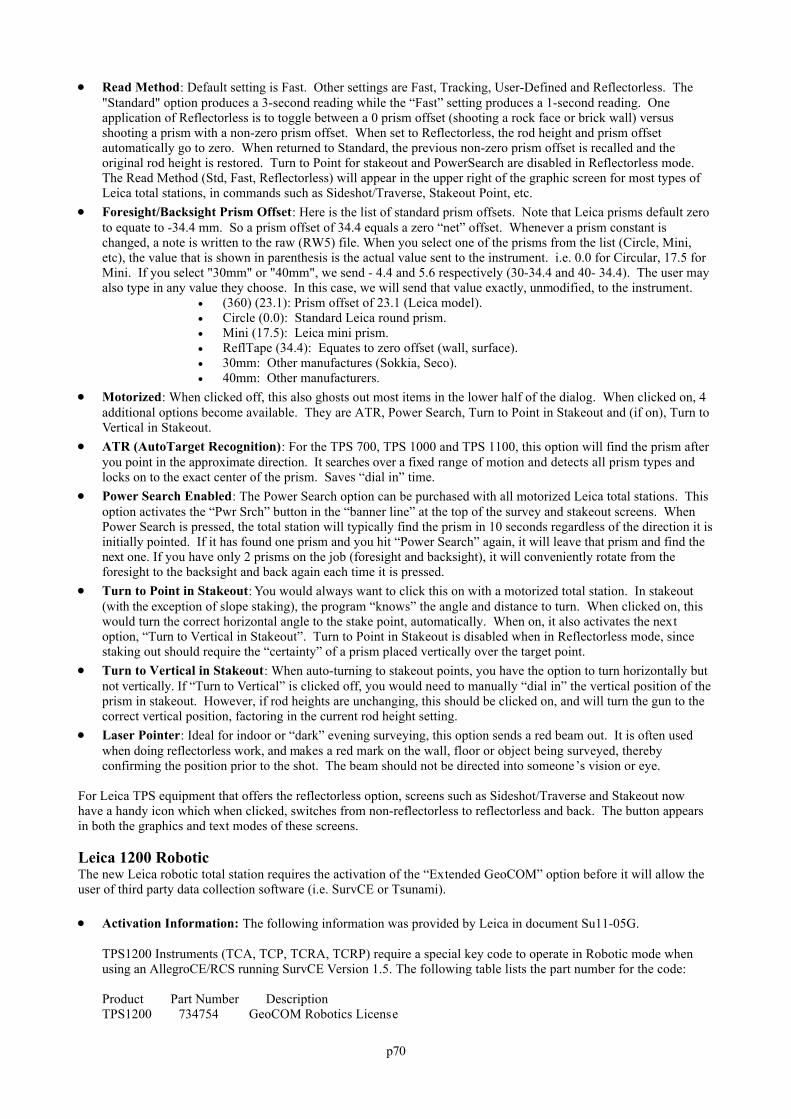
p70

Read Method: Default setting is Fast. Other settings are Fast, Tracking, User-Defined and Reflectorless. The"Standard" option produces a 3-second reading while the “Fast” setting produces a 1-second reading. Oneapplication of Reflectorless is to toggle between a 0 prism offset (shooting a rock face or brick wall) versusshooting a prism with a non-zero prism offset. When set to Reflectorless, the rod height and prism offsetautomatically go to zero. When returned to Standard, the previous non-zero prism offset is recalled and theoriginal rod height is restored. Turn to Point for stakeout and PowerSearch are disabled in Reflectorless mode. The Read Method (Std, Fast, Reflectorless) will appear in the upper right of the graphic screen for most types ofLeica total stations, in commands such as Sideshot/Traverse, Stakeout Point, etc.

Foresight/Backsight Prism Offset: Here is the list of standard prism offsets. Note that Leica prisms default zeroto equate to -34.4 mm. So a prism offset of 34.4 equals a zero “net” offset. Whenever a prism constant ischanged, a note is written to the raw (RW5) file. When you select one of the prisms from the list (Circle, Mini,etc), the value that is shown in parenthesis is the actual value sent to the instrument. i.e. 0.0 for Circular, 17.5 forMini. If you select "30mm" or "40mm", we send - 4.4 and 5.6 respectively (30-34.4 and 40- 34.4). The user mayalso type in any value they choose. In this case, we will send that value exactly, unmodified, to the instrument.

(360) (23.1): Prism offset of 23.1 (Leica model). Circle (0.0): Standard Leica round prism. Mini (17.5): Leica mini prism. ReflTape (34.4): Equates to zero offset (wall, surface). 30mm: Other manufactures (Sokkia, Seco). 40mm: Other manufacturers.

Motorized: When clicked off, this also ghosts out most items in the lower half of the dialog. When clicked on, 4additional options become available. They are ATR, Power Search, Turn to Point in Stakeout and (if on), Turn toVertical in Stakeout.

ATR (AutoTarget Recognition): For the TPS 700, TPS 1000 and TPS 1100, this option will find the prism afteryou point in the approximate direction. It searches over a fixed range of motion and detects all prism types andlocks on to the exact center of the prism. Saves “dial in” time.

Power Search Enabled: The Power Search option can be purchased with all motorized Leica total stations. Thisoption activates the “Pwr Srch” button in the “banner line” at the top of the survey and stakeout screens. WhenPower Search is pressed, the total station will typically find the prism in 10 seconds regardless of the direction it isinitially pointed. If it has found one prism and you hit “Power Search” again, it will leave that prism and find thenext one. If you have only 2 prisms on the job (foresight and backsight), it will conveniently rotate from theforesight to the backsight and back again each time it is pressed.

Turn to Point in Stakeout: You would always want to click this on with a motorized total station. In stakeout(with the exception of slope staking), the program “knows” the angle and distance to turn. When clicked on, thiswould turn the correct horizontal angle to the stake point, automatically. When on, it also activates the nextoption, “Turn to Vertical in Stakeout”. Turn to Point in Stakeout is disabled when in Reflectorless mode, sincestaking out should require the “certainty” of a prism placed vertically over the target point.

Turn to Vertical in Stakeout: When auto-turning to stakeout points, you have the option to turn horizontally butnot vertically. If “Turn to Vertical” is clicked off, you would need to manually “dial in” the vertical position of theprism in stakeout. However, if rod heights are unchanging, this should be clicked on, and will turn the gun to thecorrect vertical position, factoring in the current rod height setting.

Laser Pointer: Ideal for indoor or “dark” evening surveying, this option sends a red beam out. It is often usedwhen doing reflectorless work, and makes a red mark on the wall, floor or object being surveyed, therebyconfirming the position prior to the shot. The beam should not be directed into someone’s vision or eye.

For Leica TPS equipment that offers the reflectorless option, screens such as Sideshot/Traverse and Stakeout nowhave a handy icon which when clicked, switches from non-reflectorless to reflectorless and back. The button appearsin both the graphics and text modes of these screens.

Leica 1200 RoboticThe new Leica robotic total station requires the activation of the “Extended GeoCOM” option before it will allow theuser of third party data collection software (i.e. SurvCE or Tsunami).

Activation Information: The following information was provided by Leica in document Su11-05G.

TPS1200 Instruments (TCA, TCP, TCRA, TCRP) require a special key code to operate in Robotic mode whenusing an AllegroCE/RCS running SurvCE Version 1.5. The following table lists the part number for the code:

Product Part Number DescriptionTPS1200 734754 GeoCOM Robotics License

p71

Note: When ordering a TPS1200 Robotic Instrument, AllegroCE/RCS and SurvCE, you must order part number734754 – this is a no charge item.

Procedures for Checking Activation Status: A simple way to know that the “Extended GeoCOM” option is notactivated is to enter the Robotics dialog of SurvCE and attempt a power search. The instrument will communicatebut the power search feature will fail. If you suspect this to be the case, on the newer firmware you can also checkthe status using the following steps:

o Power on the instrument.o Select the “User” button on the keyboard.o Select the F3 button for “STAT”.o Select list item number 3 for “System Information”.o Use the down arrow key to scroll to the bottom of the “Instrument” page.o Verify that “Extended GeoCOM” is on.

Defining the Port: The Leica 1200 needs to know that you intend to use the GeoCOM interface through theexternal port. The following steps will set the Leica to communicate with SurvCE:

o Power on the instrument.o Select “Config”.o Select menu item 4 for “Interfaces”.o Arrow down to “GeoCOM Mode” and select F3 for “Edit”.o Select F5 for “DEVCE”.o Select “RS232 Geocom”o Select F3 for “Edit” and verify the communication settings.

Baud Rate: 19,200 Parity: None Data Bits: 8 Stop Bit: 1

o Select F1 for “STORE”.o Select F1 for “CONT” and verify the following option on the GeoCOM Mode page:

Use Interface: Yes Port: Port 1 Device: RS232 GeoCOM Protocol: RS232 GeoCOM

o Select F1 for “CONT”.o Verify that the only device active is RS232 GeoCOM and select F1 for “CONT”.

Prediction Settings: The Leica 1200 has several prediction modes for when the instrument has lost lock. Thefollowing are the recommended settings while using SurvCE:

o Select 3 for “Manage”.o Select 5 for “Configuration Sets”o Pick New or Edit (Recommend New for First Time)

New - Input Name, Desc and Creator Initials then F1 Store/Conto Select F1 for “CONT” 8 times until the "Automatic Prism Search" screen appears.o Select the down arrow one time and set "After Prediction Search With:" to "No Search" by tapping

the right arrow key one time.o Select F1 for “CONT”.o Select F1 for “CONT” 2 more times until the "Interfaces" screen appears.o Select the down arrow key to highlight GeoCOM mode and press F5 for “Use”. Make sure no other

mode is set. To toggle off any other mode highlight and press F5 for “Use” to toggle off.o Select F1 for “CONT” 5 times to save and exit to the Main Menu.

TC1010/1610For the Leica TC1010/1610 series instruments, it's important that the following settings are true: Communications Settings (SurvCE & Instrument): 9600,7,even,1 Communication Mode: Make sure you set the instrument to communciate RS232 mode, not module.

SurvCE Settings

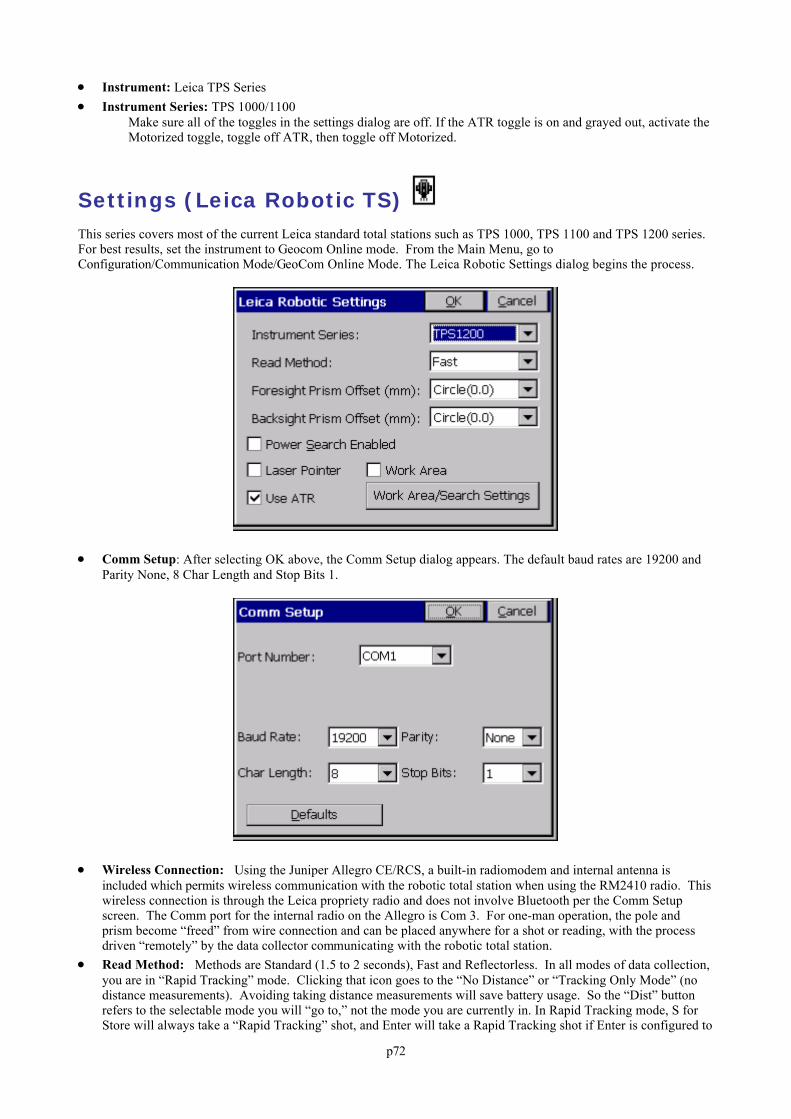
p72

Instrument: Leica TPS Series Instrument Series: TPS 1000/1100

Make sure all of the toggles in the settings dialog are off. If the ATR toggle is on and grayed out, activate theMotorized toggle, toggle off ATR, then toggle off Motorized.

Settings (Leica Robotic TS) This series covers most of the current Leica standard total stations such as TPS 1000, TPS 1100 and TPS 1200 series. For best results, set the instrument to Geocom Online mode. From the Main Menu, go toConfiguration/Communication Mode/GeoCom Online Mode. The Leica Robotic Settings dialog begins the process.

Comm Setup: After selecting OK above, the Comm Setup dialog appears. The default baud rates are 19200 andParity None, 8 Char Length and Stop Bits 1.

Wireless Connection: Using the Juniper Allegro CE/RCS, a built-in radiomodem and internal antenna isincluded which permits wireless communication with the robotic total station when using the RM2410 radio. Thiswireless connection is through the Leica propriety radio and does not involve Bluetooth per the Comm Setupscreen. The Comm port for the internal radio on the Allegro is Com 3. For one-man operation, the pole andprism become “freed” from wire connection and can be placed anywhere for a shot or reading, with the processdriven “remotely” by the data collector communicating with the robotic total station.

Read Method: Methods are Standard (1.5 to 2 seconds), Fast and Reflectorless. In all modes of data collection,you are in “Rapid Tracking” mode. Clicking that icon goes to the “No Distance” or “Tracking Only Mode” (nodistance measurements). Avoiding taking distance measurements will save battery usage. So the “Dist” buttonrefers to the selectable mode you will “go to,” not the mode you are currently in. In Rapid Tracking mode, S forStore will always take a “Rapid Tracking” shot, and Enter will take a Rapid Tracking shot if Enter is configured to

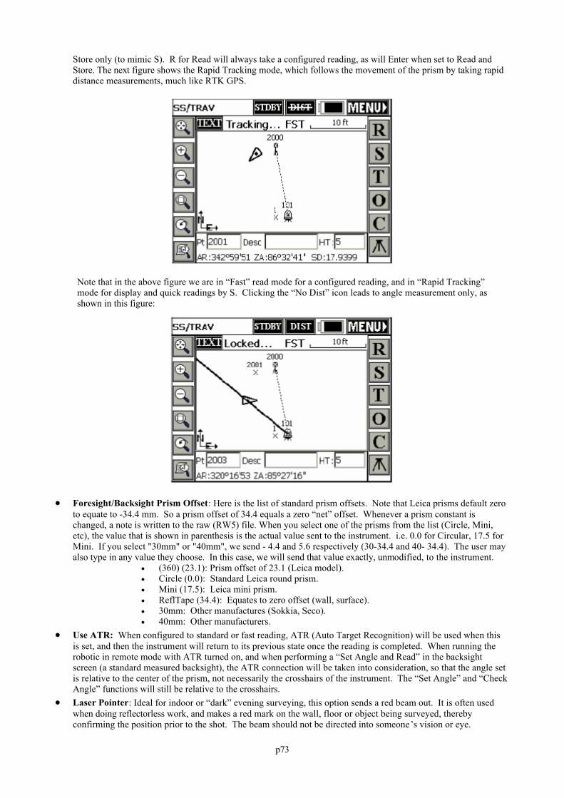
p73

Store only (to mimic S). R for Read will always take a configured reading, as will Enter when set to Read andStore. The next figure shows the Rapid Tracking mode, which follows the movement of the prism by taking rapiddistance measurements, much like RTK GPS.

Note that in the above figure we are in “Fast” read mode for a configured reading, and in “Rapid Tracking”mode for display and quick readings by S. Clicking the “No Dist” icon leads to angle measurement only, asshown in this figure:

Foresight/Backsight Prism Offset: Here is the list of standard prism offsets. Note that Leica prisms default zeroto equate to -34.4 mm. So a prism offset of 34.4 equals a zero “net” offset. Whenever a prism constant ischanged, a note is written to the raw (RW5) file. When you select one of the prisms from the list (Circle, Mini,etc), the value that is shown in parenthesis is the actual value sent to the instrument. i.e. 0.0 for Circular, 17.5 forMini. If you select "30mm" or "40mm", we send - 4.4 and 5.6 respectively (30-34.4 and 40- 34.4). The user mayalso type in any value they choose. In this case, we will send that value exactly, unmodified, to the instrument.

(360) (23.1): Prism offset of 23.1 (Leica model). Circle (0.0): Standard Leica round prism. Mini (17.5): Leica mini prism. ReflTape (34.4): Equates to zero offset (wall, surface). 30mm: Other manufactures (Sokkia, Seco). 40mm: Other manufacturers.

Use ATR: When configured to standard or fast reading, ATR (Auto Target Recognition) will be used when thisis set, and then the instrument will return to its previous state once the reading is completed. When running therobotic in remote mode with ATR turned on, and when performing a “Set Angle and Read” in the backsightscreen (a standard measured backsight), the ATR connection will be taken into consideration, so that the angle setis relative to the center of the prism, not necessarily the crosshairs of the instrument. The “Set Angle” and “CheckAngle” functions will still be relative to the crosshairs.

Laser Pointer: Ideal for indoor or “dark” evening surveying, this option sends a red beam out. It is often usedwhen doing reflectorless work, and makes a red mark on the wall, floor or object being surveyed, therebyconfirming the position prior to the shot. The beam should not be directed into someone’s vision or eye.

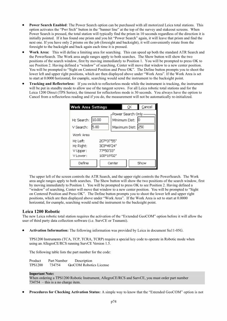
p74

Power Search Enabled: The Power Search option can be purchased with all motorized Leica total stations. Thisoption activates the “Pwr Srch” button in the “banner line” at the top of the survey and stakeout screens. WhenPower Search is pressed, the total station will typically find the prism in 10 seconds regardless of the direction it isinitially pointed. If it has found one prism and you hit “Power Search” again, it will leave that prism and find thenext one. If you have only 2 prisms on the job (foresight and backsight), it will conveniently rotate from theforesight to the backsight and back again each time it is pressed.

Work Area: This will define a limiting area for searching. This can speed up both the standard ATR Search andthe PowerSearch. The Work area angle ranges apply to both searches. The Show button will show the twopositions of the search window, first by moving immediately to Position 1. You will be prompted to press OK tosee Position 2. Having defined a “window” of searching, Center will move that window to a new center position. You will be prompted to “Sight on Centered Position and Press OK”. The Define button prompts you to shoot thelower left and upper right positions, which are then displayed above under “Work Area”. If the Work Area is setto start at 0.0000 horizontal, for example, searching would send the instrument to the backsight point.

Tracking and Reflectorless: If you switch to reflectorless mode while the instrument is tracking, the instrumentwill be put in standby mode to allow use of the tangent screws. For all Leica robotic total stations and for theLeica 1200 Direct (TPS Series), the timeout for reflectorless mode is 30 seconds. You always have the option toCancel from a reflectorless reading and if you do, the measurement will not be automatically re-initialized.

The upper left of the screen controls the ATR Search, and the upper right controls the PowerSearch. The Workarea angle ranges apply to both searches. The Show button will show the two positions of the search window, firstby moving immediately to Position 1. You will be prompted to press OK to see Position 2. Having defined a“window” of searching, Center will move that window to a new center position. You will be prompted to “Sighton Centered Position and Press OK”. The Define button prompts you to shoot the lower left and upper rightpositions, which are then displayed above under “Work Area”. If the Work Area is set to start at 0.0000horizontal, for example, searching would send the instrument to the backsight point.

Leica 1200 RoboticThe new Leica robotic total station requires the activation of the “Extended GeoCOM” option before it will allow theuser of third party data collection software (i.e. SurvCE or Tsunami).

Activation Information: The following information was provided by Leica in document Su11-05G.

TPS1200 Instruments (TCA, TCP, TCRA, TCRP) require a special key code to operate in Robotic mode whenusing an AllegroCE/RCS running SurvCE Version 1.5.

The following table lists the part number for the code:

Product Part Number DescriptionTPS1200 734754 GeoCOM Robotics License

Important Note:When ordering a TPS1200 Robotic Instrument, AllegroCE/RCS and SurvCE, you must order part number734754 – this is a no charge item.

Procedures for Checking Activation Status: A simple way to know that the “Extended GeoCOM” option is not

p75

activated is to enter the Robotics dialog of SurvCE and attempt a power search. The instrument will communicatebut the power search feature will fail. If you suspect this to be the case, on the newer firmware you can also checkthe status using the following steps:

o Power on the instrument.o Select the “User” button on the keyboard.o Select the F3 button for “STAT”.o Select list item number 3 for “System Information”.o Use the down arrow key to scroll to the bottom of the “Instrument” page.o Verify that “Extended GeoCOM” is on.

Defining the Port: The Leica 1200 needs to know that you intend to use the GeoCOM interface through theexternal port. The following steps will set the Leica to communicate with SurvCE:

o Power on the instrument.o Select “Config”.o Select menu item 4 for “Interfaces”.o Arrow down to “GeoCOM Mode” and select F3 for “Edit”.o Select F5 for “DEVCE”.o Select “RS232 Geocom”o Select F3 for “Edit” and verify the communication settings.

Baud Rate: 19,200 Parity: None Data Bits: 8 Stop Bit: 1

o Select F1 for “STORE”.o Select F1 for “CONT” and verify the following option on the GeoCOM Mode page:

Use Interface: Yes Port: Port 1 Device: RS232 GeoCOM Protocol: RS232 GeoCOM

o Select F1 for “CONT”.o Verify that the only device active is RS232 GeoCOM and select F1 for “CONT”.

Prediction Settings: The Leica 1200 has several prediction modes for when the instrument has lost lock. Thefollowing are the recommended settings while using SurvCE:

o Select 3 for “Manage”.o Select 5 for “Configuration Sets”o Pick New or Edit (Recommend New for First Time)

New - Input Name, Desc and Creator Initials then F1 Store/Conto Select F1 for “CONT” 8 times until the "Automatic Prism Search" screen appears.o Select the down arrow one time and set "After Prediction Search With:" to "No Search" by tapping

the right arrow key one time.o Select F1 for “CONT”.o Select F1 for “CONT” 2 more times until the "Interfaces" screen appears.o Select the down arrow key to highlight GeoCOM mode and press F5 for “Use”. Make sure no other

mode is set. To toggle off any other mode highlight and press F5 for “Use” to toggle off.o Select F1 for “CONT” 5 times to save and exit to the Main Menu.

Troubleshooting: If your Leica robotic total station has any communication issues, it is typically a matter of verifyingfirmware and configuration settings. Investigate and note down the firmware version of the various components onyour instrument, if calling or emailing for tech support. Most important is the GeoCom Version, which you can checkfor this instrument by going to Configuration, then Info (F5). For ex ample, a Leica TCRA 1103 with PowerSearchmight display the following firmware settings:

System Version: Sept. 17, 2002, 2.20 EDM Version 2.02 ATR Version 2.02 PS Version 1.01 GeoCom Version 1.07

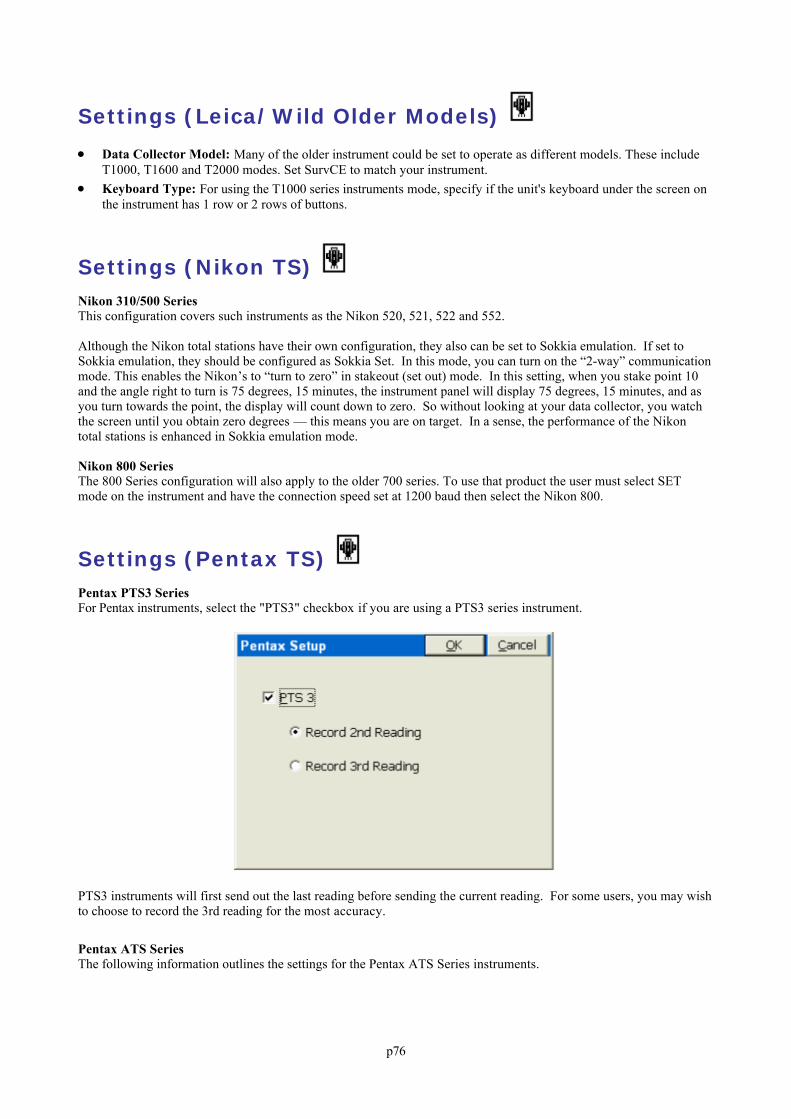
p76

Settings (Leica/Wild Older Models)

Data Collector Model: Many of the older instrument could be set to operate as different models. These includeT1000, T1600 and T2000 modes. Set SurvCE to match your instrument.

Keyboard Type: For using the T1000 series instruments mode, specify if the unit's keyboard under the screen onthe instrument has 1 row or 2 rows of buttons.

Settings (Nikon TS) Nikon 310/500 SeriesThis configuration covers such instruments as the Nikon 520, 521, 522 and 552.

Although the Nikon total stations have their own configuration, they also can be set to Sokkia emulation. If set toSokkia emulation, they should be configured as Sokkia Set. In this mode, you can turn on the “2-way” communicationmode. This enables the Nikon’s to “turn to zero” in stakeout (set out) mode. In this setting, when you stake point 10and the angle right to turn is 75 degrees, 15 minutes, the instrument panel will display 75 degrees, 15 minutes, and asyou turn towards the point, the display will count down to zero. So without looking at your data collector, you watchthe screen until you obtain zero degrees — this means you are on target. In a sense, the performance of the Nikontotal stations is enhanced in Sokkia emulation mode.

Nikon 800 SeriesThe 800 Series configuration will also apply to the older 700 series. To use that product the user must select SETmode on the instrument and have the connection speed set at 1200 baud then select the Nikon 800.

Settings (Pentax TS) Pentax PTS3 SeriesFor Pentax instruments, select the "PTS3" checkbox if you are using a PTS3 series instrument.

PTS3 instruments will first send out the last reading before sending the current reading. For some users, you may wishto choose to record the 3rd reading for the most accuracy.

Pentax ATS SeriesThe following information outlines the settings for the Pentax ATS Series instruments.

p77

This information was compiled using an ATS-105.

1. Power up the Unit & Level it up.

2. Set the baud rate in the instrument. Hold down the Blue “S” key and press the number 6 key in the upper right. Thiswill open the Configuration Menu for Baud Settings.

3. Set the baud rate in SurvCE by selecting the Equip tab, and then select the Comm Setup button. SurvCE defaults to1200 / None / 8 / 1. Match the Baud, Parity, Char Length & Stop Bits with whatever the instrument is currently set to.

4. Connect the data collector, hold down the Blue "S" key and press the "F5" button. This puts the Total Station intoRemote Mode for use with external data collectors. [RM] blinks in the upper left corner.

NOTE: SurvCE has advanced options for setting the Read Method, Number of Readings & use of the instrumentlights. Not all models or firmware support these features. If these options do not work, you might be able to update thefirmware, or manually adjust the settings using the instrument.

Settings (Sokkia Set TS) The following information describes the various options available for the Sokkia Set total stations.

1-Way vs 2-Way: The 1-Way option mimics the operation of most total station instruments using SurvCE. The2-Way option has the one big advantage of sending the angle to turn into the instrument during stakeout, so thatlooking at the instrument panel, you “turn to zero” to aim at the target point. It is recommended that Nikoninstruments be run in Sokkia Set emulation mode, enabling the 2-Way communication.

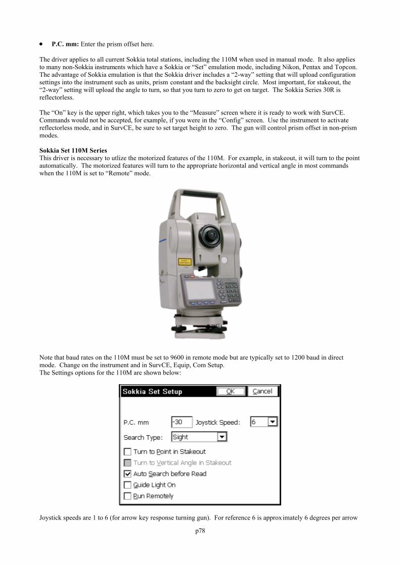
p78

P.C. mm: Enter the prism offset here.

The driver applies to all current Sokkia total stations, including the 110M when used in manual mode. It also appliesto many non-Sokkia instruments which have a Sokkia or “Set” emulation mode, including Nikon, Pentax and Topcon. The advantage of Sokkia emulation is that the Sokkia driver includes a “2-way” setting that will upload configurationsettings into the instrument such as units, prism constant and the backsight circle. Most important, for stakeout, the“2-way” setting will upload the angle to turn, so that you turn to zero to get on target. The Sokkia Series 30R isreflectorless.

The “On” key is the upper right, which takes you to the “Measure” screen where it is ready to work with SurvCE. Commands would not be accepted, for example, if you were in the “Config” screen. Use the instrument to activatereflectorless mode, and in SurvCE, be sure to set target height to zero. The gun will control prism offset in non-prismmodes.

Sokkia Set 110M SeriesThis driver is necessary to utlize the motorized features of the 110M. For example, in stakeout, it will turn to the pointautomatically. The motorized features will turn to the appropriate horizontal and vertical angle in most commandswhen the 110M is set to “Remote” mode.

Note that baud rates on the 110M must be set to 9600 in remote mode but are typically set to 1200 baud in directmode. Change on the instrument and in SurvCE, Equip, Com Setup. The Settings options for the 110M are shown below:

Joystick speeds are 1 to 6 (for arrow key response turning gun). For reference 6 is approximately 6 degrees per arrow

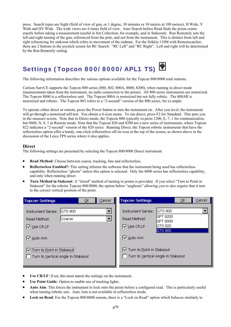
p79

press. Search types are Sight (field of view of gun, or 1 degree, 30 minutes or 10 meters at 100 meters), H Wide, VWide and HV Wide. The wide views are 6 times field of view. Auto Search before Read finds the prism centerexactly before taking a measurement (useful in Set Collection, for example, and in Stakeout). Run Remotely sets theleft and right turning of the gun, referenced from the pole, and not from the instrument. This is distinct from left andright referencing for stakeout which refers to movement of the rodman. For the Sokkia 110M with Remotocatcher,there are 2 buttons in the joystick screen for RC Search: “RC Left” and “RC Right”. Left and right will be determinedby the Run Remotely setting.

Settings (Topcon 800/8000/APL1 TS) The following information describes the various options available for the Topcon 800/8000 total stations.

Carlson SurvCE supports the Topcon 800 series (800, 802, 800A, 8000, 8200), when running in direct mode(measurements taken from the instrument, no radio connection to the prism). All 800 series instruments are motorized.The Topcon 8000 is a reflectorless unit. The Topcon 800A is motorized but not fully robitic. The 800AR ismotorized and robotic. The Topcon 802 refers to a “2-second” version of the 800 series, for ex ample.

To operate either direct or remote, press the Power button to turn the instrument on. After you level, the instrumentwill go through a motorized self-test. You obtain a 6-icon menu. To run direct, press F2 for Standard. This puts youin the measure screen. Note that in Direct mode, the Topcon 800 typically ex pects 1200, E, 7, 1 for communication,but 9600, N, 8, 1 in Remote mode. Note that the Topcon 820 and 8200 are a new series of instruments, where Topcon822 indicates a “2-second” version of the 820 series. Running Direct, the Topcon robotic instruments that have thereflectorless option offer a handy, one-click reflectorless off-on icon at the top of the screen, as shown above in thediscussion of the Leica TPS series where it also applies.

DirectThe following settings are presented by selecting the Topcon 800/8000 Direct instrument.

Read Method: Choose between coarse, tracking, fine and reflectorless. Reflectorless Enabled?: This setting informs the software that the instrument being used has relfectorless

capability. Reflectorless “ghosts” unless this option is selected. Only the 8000 series has reflectorless capability,and only when running direct.

Turn Method in Stakeout: A “tiered” method of turning to points is provided. If you select “Turn to Point inStakeout” for the robotic Topcon 800/8000, the option below “unghosts” allowing you to also require that it turnto the correct vertical position of the point.

Use CR/LF: If set, this must match the settings on the instrument. Use Point Guide: Option to enable use of tracking lights. Auto Aim: This forces the instrument to lock onto the prism before a configured read. This is particularly useful

when turning robotic sets. Auto Aim is not available in reflectorless mode. Lock on Read: For the Topcon 800/8000 remote, there is a “Lock on Read” option which behaves similarly to

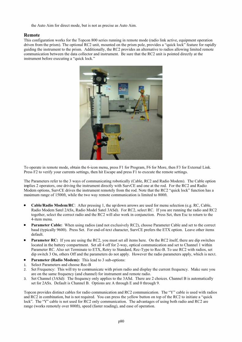
p80

the Auto Aim for direct mode, but is not as precise as Auto Aim.

RemoteThis configuration works for the Topcon 800 series running in remote mode (radio link active, equipment operationdriven from the prism). The optional RC2 unit, mounted on the prism pole, provides a “quick lock” feature for rapidlyguiding the instrument to the prism. Additionally, the RC2 provides an alternative to radios allowing limited remotecommunication between the data collector and instrument. Be sure that the RC2 unit is pointed directly at theinstrument before executing a “quick lock.”

To operate in remote mode, obtain the 6-icon menu, press F1 for Program, F6 for More, then F3 for External Link. Press F2 to verify your currents settings, then hit Escape and press F1 to execute the remote settings.

The Parameters refer to the 3 ways of communicating robotically (Cable, RC2 and Radio Modem). The Cable optionimplies 2 operators, one driving the instrument directly with SurvCE and one at the rod. For the RC2 and RadioModem options, SurvCE drives the instrument remotely from the rod. Note that the RC2 “quick lock” function has amaximum range of 1500ft, while the two way remote communication is limited to 800ft.

Cable/Radio Modem/RC: After pressing 1, the up/down arrows are used for menu selection (e.g. RC, Cable,Radio Modem Satel 2ASx, Radio Model Satel 3ASd). For RC2, select RC. If you are running the radio and RC2together, select the correct radio and the RC2 will also work in conjunction. Press Set, then Esc to return to the4-item menu.

Parameter Cable: When using radios (and not exclusively RC2), choose Parameter Cable and set to the correctbaud (typically 9600). Press Set. For end-of-text character, SurvCE prefers the ETX option. Leave other itemsdefault.

Parameter RC: If you are using the RC2, you must set all items here. On the RC2 itself, there are dip switcheslocated in the battery compartment. Set all 4 off for 2-way, optical communication and set to Channel 1 withinParameter RC. Also set Terminate to ETX, Retry to Standard, Rec-Type to Rec-B. To use RC2 with radios, setdip switch 3 On, others Off and the parameters do not apply. However the radio parameters apply, which is next.

Parameter (Radio Modem): This lead to 3 sub-options:1. Select Parameters and choose Rec-B2. Set Frequency: This will try to communicate with prism radio and display the current frequency. Make sure you

are on the same frequency (and channel) for instrument and remote radio.3. Set Channel (3ASd): The frequency only applies to the 3ASd. There are 2 choices. Channel B is automatically

set for 2ASx. Default is Channel B. Options are A through E and 0 through 9.

Topcon provides distinct cables for radio communication and RC2 communication. The “Y” cable is used with radiosand RC2 in combination, but is not required. You can press the yellow button on top of the RC2 to initiate a “quicklock”. The “Y” cable is not used for RC2 only communication. The advantages of using both radio and RC2 arerange (works remotely over 800ft), speed (faster reading), and ease of operation.

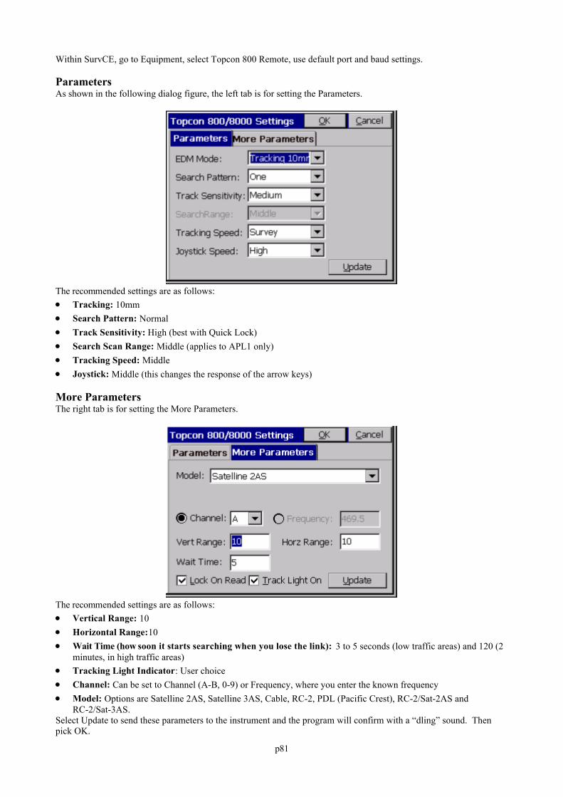
p81

Within SurvCE, go to Equipment, select Topcon 800 Remote, use default port and baud settings.

ParametersAs shown in the following dialog figure, the left tab is for setting the Parameters.

The recommended settings are as follows: Tracking: 10mm Search Pattern: Normal Track Sensitivity: High (best with Quick Lock) Search Scan Range: Middle (applies to APL1 only) Tracking Speed: Middle Joystick: Middle (this changes the response of the arrow keys)

More ParametersThe right tab is for setting the More Parameters.

The recommended settings are as follows: Vertical Range: 10 Horizontal Range:10 Wait Time (how soon it starts searching when you lose the link): 3 to 5 seconds (low traffic areas) and 120 (2

minutes, in high traffic areas) Tracking Light Indicator: User choice Channel: Can be set to Channel (A-B, 0-9) or Frequency, where you enter the known frequency Model: Options are Satelline 2AS, Satelline 3AS, Cable, RC-2, PDL (Pacific Crest), RC-2/Sat-2AS and

RC-2/Sat-3AS. Select Update to send these parameters to the instrument and the program will confirm with a “dling” sound. Thenpick OK.

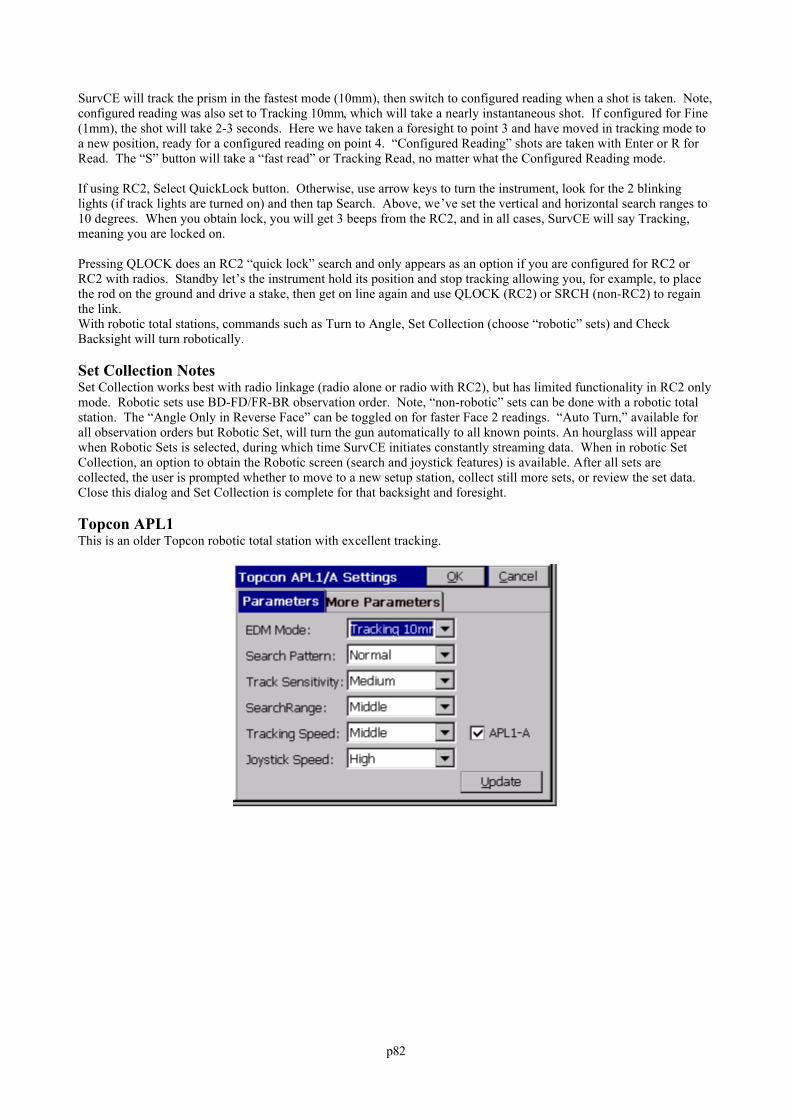
p82

SurvCE will track the prism in the fastest mode (10mm), then switch to configured reading when a shot is taken. Note,configured reading was also set to Tracking 10mm, which will take a nearly instantaneous shot. If configured for Fine(1mm), the shot will take 2-3 seconds. Here we have taken a foresight to point 3 and have moved in tracking mode toa new position, ready for a configured reading on point 4. “Configured Reading” shots are taken with Enter or R forRead. The “S” button will take a “fast read” or Tracking Read, no matter what the Configured Reading mode.

If using RC2, Select QuickLock button. Otherwise, use arrow keys to turn the instrument, look for the 2 blinkinglights (if track lights are turned on) and then tap Search. Above, we’ve set the vertical and horizontal search ranges to10 degrees. When you obtain lock, you will get 3 beeps from the RC2, and in all cases, SurvCE will say Tracking,meaning you are locked on.

Pressing QLOCK does an RC2 “quick lock” search and only appears as an option if you are configured for RC2 orRC2 with radios. Standby let’s the instrument hold its position and stop tracking allowing you, for example, to placethe rod on the ground and drive a stake, then get on line again and use QLOCK (RC2) or SRCH (non-RC2) to regainthe link. With robotic total stations, commands such as Turn to Angle, Set Collection (choose “robotic” sets) and CheckBacksight will turn robotically.

Set Collection NotesSet Collection works best with radio linkage (radio alone or radio with RC2), but has limited functionality in RC2 onlymode. Robotic sets use BD-FD/FR-BR observation order. Note, “non-robotic” sets can be done with a robotic totalstation. The “Angle Only in Reverse Face” can be toggled on for faster Face 2 readings. “Auto Turn,” available forall observation orders but Robotic Set, will turn the gun automatically to all known points. An hourglass will appearwhen Robotic Sets is selected, during which time SurvCE initiates constantly streaming data. When in robotic SetCollection, an option to obtain the Robotic screen (search and joystick features) is available. After all sets arecollected, the user is prompted whether to move to a new setup station, collect still more sets, or review the set data. Close this dialog and Set Collection is complete for that backsight and foresight.

Topcon APL1This is an older Topcon robotic total station with excellent tracking.

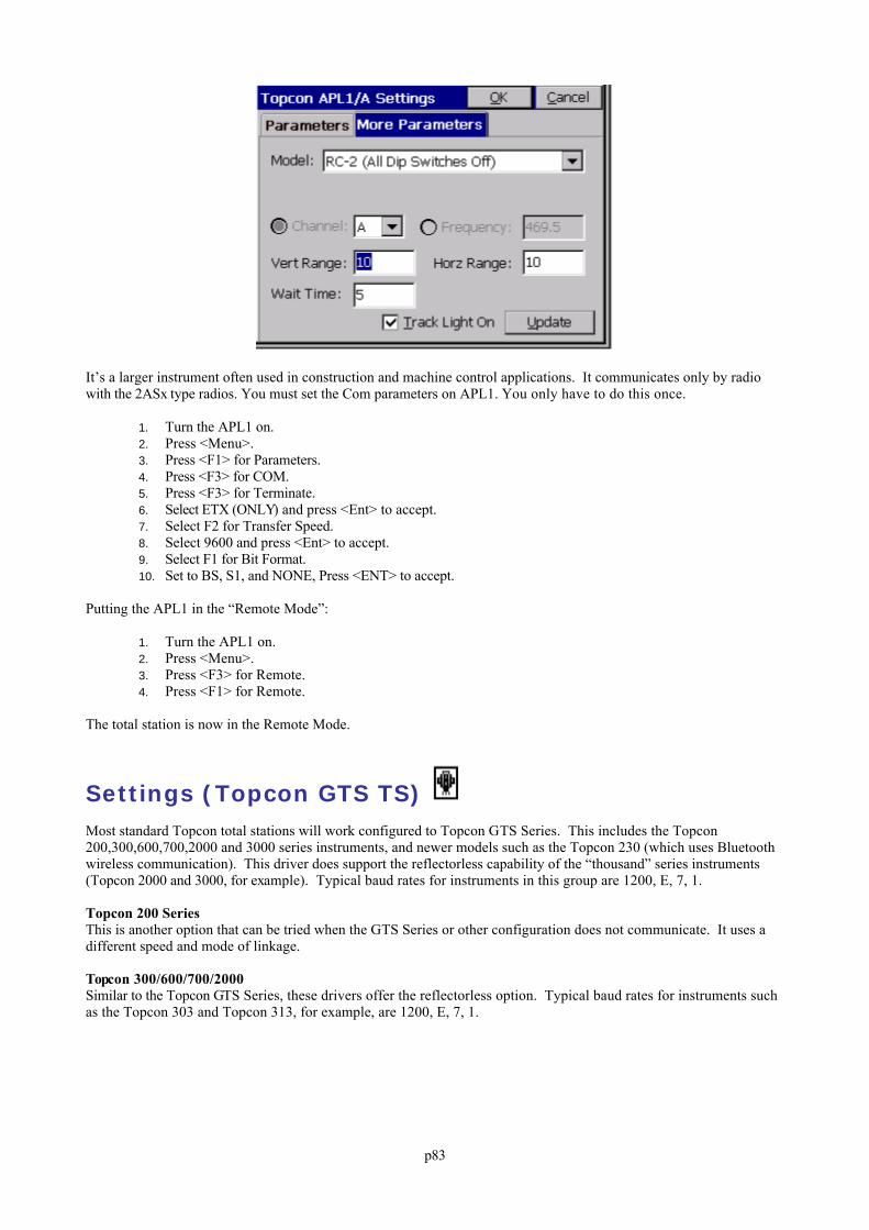
p83

It’s a larger instrument often used in construction and machine control applications. It communicates only by radiowith the 2ASx type radios. You must set the Com parameters on APL1. You only have to do this once.

1. Turn the APL1 on.2. Press <Menu>.3. Press <F1> for Parameters.4. Press <F3> for COM.5. Press <F3> for Terminate.6. Select ETX (ONLY) and press <Ent> to accept.7. Select F2 for Transfer Speed.8. Select 9600 and press <Ent> to accept.9. Select F1 for Bit Format.10. Set to BS, S1, and NONE, Press <ENT> to accept.

Putting the APL1 in the “Remote Mode”:

1. Turn the APL1 on.2. Press <Menu>.3. Press <F3> for Remote.4. Press <F1> for Remote.

The total station is now in the Remote Mode.

Settings (Topcon GTS TS) Most standard Topcon total stations will work configured to Topcon GTS Series. This includes the Topcon200,300,600,700,2000 and 3000 series instruments, and newer models such as the Topcon 230 (which uses Bluetoothwireless communication). This driver does support the reflectorless capability of the “thousand” series instruments(Topcon 2000 and 3000, for example). Typical baud rates for instruments in this group are 1200, E, 7, 1.

Topcon 200 SeriesThis is another option that can be tried when the GTS Series or other configuration does not communicate. It uses adifferent speed and mode of linkage.

Topcon 300/600/700/2000Similar to the Topcon GTS Series, these drivers offer the reflectorless option. Typical baud rates for instruments suchas the Topcon 303 and Topcon 313, for example, are 1200, E, 7, 1.

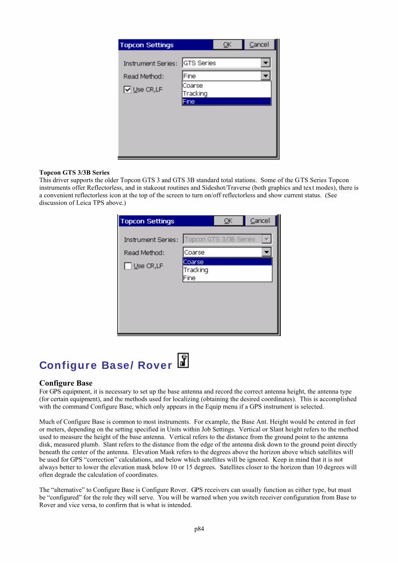
p84

Topcon GTS 3/3B SeriesThis driver supports the older Topcon GTS 3 and GTS 3B standard total stations. Some of the GTS Series Topconinstruments offer Reflectorless, and in stakeout routines and Sideshot/Traverse (both graphics and text modes), there isa convenient reflectorless icon at the top of the screen to turn on/off reflectorless and show current status. (Seediscussion of Leica TPS above.)

Configure Base/Rover

Configure BaseFor GPS equipment, it is necessary to set up the base antenna and record the correct antenna height, the antenna type(for certain equipment), and the methods used for localizing (obtaining the desired coordinates). This is accomplishedwith the command Configure Base, which only appears in the Equip menu if a GPS instrument is selected.

Much of Configure Base is common to most instruments. For example, the Base Ant. Height would be entered in feetor meters, depending on the setting specified in Units within Job Settings. Vertical or Slant height refers to the methodused to measure the height of the base antenna. Vertical refers to the distance from the ground point to the antennadisk, measured plumb. Slant refers to the distance from the edge of the antenna disk down to the ground point directlybeneath the center of the antenna. Elevation Mask refers to the degrees above the horizon above which satellites willbe used for GPS “correction” calculations, and below which satellites will be ignored. Keep in mind that it is notalways better to lower the elevation mask below 10 or 15 degrees. Satellites closer to the horizon than 10 degrees willoften degrade the calculation of coordinates.

The “alternative” to Configure Base is Configure Rover. GPS receivers can usually function as either type, but mustbe “configured” for the role they will serve. You will be warned when you switch receiver configuration from Base toRover and vice versa, to confirm that is what is intended.

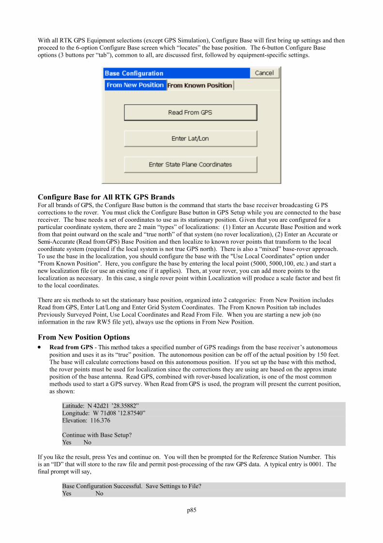
p85

With all RTK GPS Equipment selections (except GPS Simulation), Configure Base will first bring up settings and thenproceed to the 6-option Configure Base screen which “locates” the base position. The 6-button Configure Baseoptions (3 buttons per “tab”), common to all, are discussed first, followed by equipment-specific settings.

Configure Base for All RTK GPS BrandsFor all brands of GPS, the Configure Base button is the command that starts the base receiver broadcasting G PScorrections to the rover. You must click the Configure Base button in GPS Setup while you are connected to the basereceiver. The base needs a set of coordinates to use as its stationary position. Given that you are configured for aparticular coordinate system, there are 2 main “types” of localizations: (1) Enter an Accurate Base Position and workfrom that point outward on the scale and “true north” of that system (no rover localization), (2) Enter an Accurate orSemi-Accurate (Read from GPS) Base Position and then localize to known rover points that transform to the localcoordinate system (required if the local system is not true GPS north). There is also a “mixed” base-rover approach. To use the base in the localization, you should configure the base with the "Use Local Coordinates" option under"From Known Position". Here, you configure the base by entering the local point (5000, 5000,100, etc.) and start anew localization file (or use an existing one if it applies). Then, at your rover, you can add more points to thelocalization as necessary. In this case, a single rover point within Localization will produce a scale factor and best fitto the local coordinates.

There are six methods to set the stationary base position, organized into 2 categories: From New Position includesRead from GPS, Enter Lat/Long and Enter Grid System Coordinates. The From Known Position tab includesPreviously Surveyed Point, Use Local Coordinates and Read From File. When you are starting a new job (noinformation in the raw RW5 file yet), always use the options in From New Position.

From New Position Options Read from GPS - This method takes a specified number of GPS readings from the base receiver’s autonomous

position and uses it as its “true” position. The autonomous position can be off of the actual position by 150 feet.The base will calculate corrections based on this autonomous position. If you set up the base with this method,the rover points must be used for localization since the corrections they are using are based on the approx imateposition of the base antenna. Read GPS, combined with rover-based localization, is one of the most commonmethods used to start a GPS survey. When Read from GPS is used, the program will present the current position,as shown:

Latitude: N 42d21 ’28.35882”Longitude: W 71d08 ’12.87540”Elevation: 116.376

Continue with Base Setup?Yes No

If you like the result, press Yes and continue on. You will then be prompted for the Reference Station Number. Thisis an “ID” that will store to the raw file and permit post-processing of the raw GPS data. A typical entry is 0001. Thefinal prompt will say,

Base Configuration Successful. Save Settings to File?Yes No

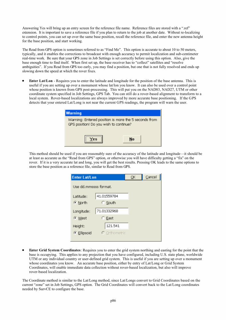
p86

Answering Yes will bring up an entry screen for the reference file name. Reference files are stored with a “.ref”extension. It is important to save a reference file if you plan to return to the job at another date. Without re-localizingto control points, you can set up over the same base position, recall the reference file, and enter the new antenna heightfor the base position, and start working.

The Read from GPS option is sometimes referred to as “Find Me”. This option is accurate to about 10 to 50 meters,typically, and it enables the corrections to broadcast with enough accuracy to permit localization and sub-centimeterreal-time work. Be sure that your GPS zone in Job Settings is set correctly before using this option. Also, give thebase enough time to find itself. When first set up, the base receiver has to “collect” satellites and “resolveambiguities”. If you Read from GPS too early, you may find a position, but one that is not fully resolved and ends upslowing down the speed at which the rover fixes.

Enter Lat/Lon - Requires you to enter the latitude and longitude for the position of the base antenna. This isuseful if you are setting up over a monument whose lat/lon you know. It can also be used over a control pointwhose position is known from GPS post-processing. This will put you on the NAD83, NAD27, UTM or othercoordinate system specified in Job Settings, GPS Tab. You can still do a rover-based alignment to transform to alocal system. Rover-based localizations are always improved by more accurate base positioning. If the GPSdetects that your entered Lat/Long is not near the current GPS readings, the program will warn the user.

This method should be used if you are reasonably sure of the accuracy of the latitude and longitude—it should beat least as accurate as the “Read from GPS” option, or otherwise you will have difficulty getting a “fix” on therover. If it is a very accurate lat and long, you will get the best results. Pressing OK leads to the same options tostore the base position as a reference file, similar to Read from GPS.

Enter Grid System Coordinates: Requires you to enter the grid system northing and easting for the point that thebase is occupying. This applies to any projection that you have configured, including U.S. state plane, worldwideUTM or any individual country or user-defined grid system. This is useful if you are setting up over a monumentwhose coordinates you know. An accurate base position, either by entry of Lat/Long or Grid SystemCoordinates, will enable immediate data collection without rover-based localization, but also will improverover-based localization.

The Coordinate method is similar to the Lat/Long method, since Lat/Longs convert to Grid Coordinates based on thecurrent “zone” set in Job Settings, GPS option. The Grid Coordinates will convert back to the Lat/Long coordinatesneeded by SurvCE to configure the base.

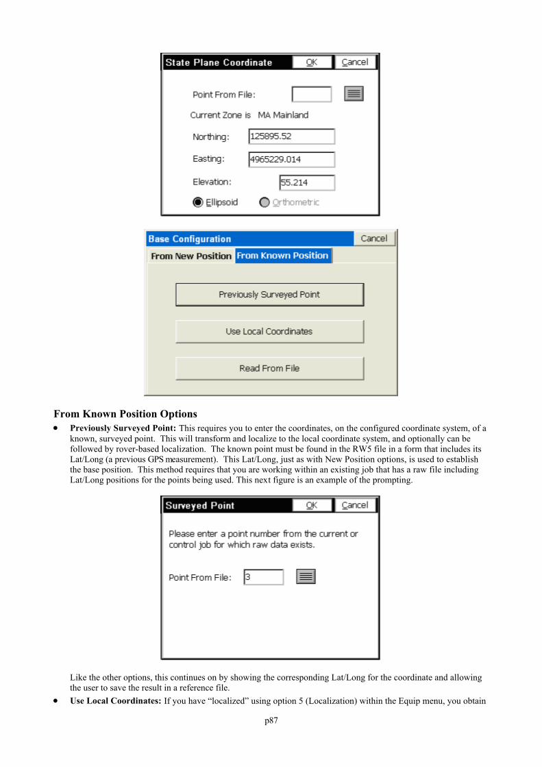
p87

From Known Position Options Previously Surveyed Point: This requires you to enter the coordinates, on the configured coordinate system, of a

known, surveyed point. This will transform and localize to the local coordinate system, and optionally can befollowed by rover-based localization. The known point must be found in the RW5 file in a form that includes itsLat/Long (a previous GPS measurement). This Lat/Long, just as with New Position options, is used to establishthe base position. This method requires that you are working within an existing job that has a raw file includingLat/Long positions for the points being used. This next figure is an example of the prompting.

Like the other options, this continues on by showing the corresponding Lat/Long for the coordinate and allowingthe user to save the result in a reference file.

Use Local Coordinates: If you have “localized” using option 5 (Localization) within the Equip menu, you obtain

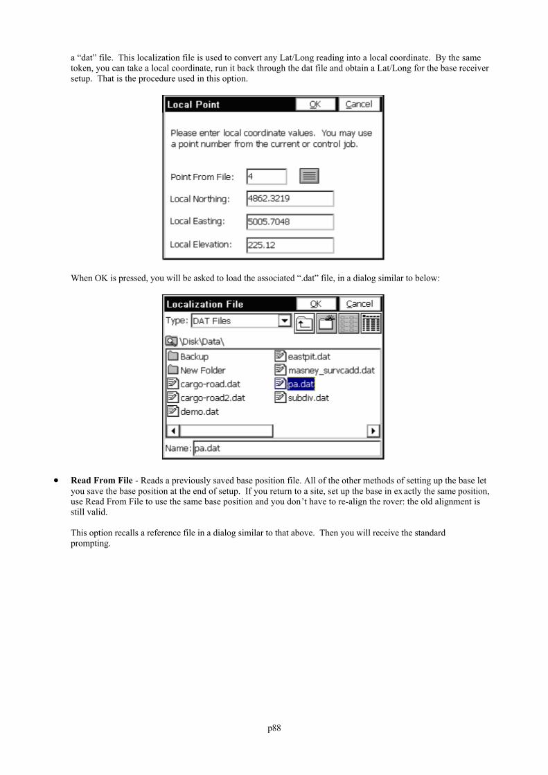
p88

a “dat” file. This localization file is used to convert any Lat/Long reading into a local coordinate. By the sametoken, you can take a local coordinate, run it back through the dat file and obtain a Lat/Long for the base receiversetup. That is the procedure used in this option.

When OK is pressed, you will be asked to load the associated “.dat” file, in a dialog similar to below:

Read From File - Reads a previously saved base position file. All of the other methods of setting up the base letyou save the base position at the end of setup. If you return to a site, set up the base in ex actly the same position,use Read From File to use the same base position and you don’t have to re-align the rover: the old alignment isstill valid.

This option recalls a reference file in a dialog similar to that above. Then you will receive the standardprompting.

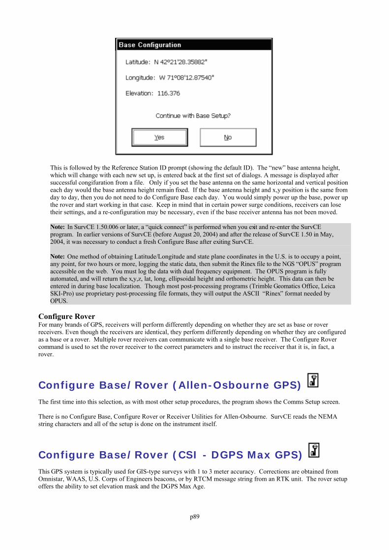
p89

This is followed by the Reference Station ID prompt (showing the default ID). The “new” base antenna height,which will change with each new set up, is entered back at the first set of dialogs. A message is displayed aftersuccessful congifuration from a file. Only if you set the base antenna on the same horizontal and vertical positioneach day would the base antenna height remain fixed. If the base antenna height and x,y position is the same fromday to day, then you do not need to do Configure Base each day. You would simply power up the base, power upthe rover and start working in that case. Keep in mind that in certain power surge conditions, receivers can losetheir settings, and a re-configuration may be necessary, even if the base receiver antenna has not been moved.

Note: In SurvCE 1.50.006 or later, a “quick connect” is performed when you exit and re-enter the SurvCEprogram. In earlier versions of SurvCE (before August 20, 2004) and after the release of SurvCE 1.50 in May,2004, it was necessary to conduct a fresh Configure Base after exiting SurvCE.

Note: One method of obtaining Latitude/Longitude and state plane coordinates in the U.S. is to occupy a point,any point, for two hours or more, logging the static data, then submit the Rinex file to the NGS “OPUS” programaccessible on the web. You must log the data with dual frequency equipment. The OPUS program is fullyautomated, and will return the x,y,z, lat, long, ellipsoidal height and orthometric height. This data can then beentered in during base localization. Though most post-processing programs (Trimble Geomatics Office, LeicaSKI-Pro) use proprietary post-processing file formats, they will output the ASCII “Rinex” format needed byOPUS.

Configure RoverFor many brands of GPS, receivers will perform differently depending on whether they are set as base or roverreceivers. Even though the receivers are identical, they perform differently depending on whether they are configuredas a base or a rover. Multiple rover receivers can communicate with a single base receiver. The Configure Rovercommand is used to set the rover receiver to the correct parameters and to instruct the receiver that it is, in fact, arover.

Configure Base/Rover (Allen-Osbourne GPS) The first time into this selection, as with most other setup procedures, the program shows the Comms Setup screen.

There is no Configure Base, Configure Rover or Receiver Utilities for Allen-Osbourne. SurvCE reads the NEMAstring characters and all of the setup is done on the instrument itself.

Configure Base/Rover (CSI - DGPS Max GPS) This GPS system is typically used for GIS-type surveys with 1 to 3 meter accuracy. Corrections are obtained fromOmnistar, WAAS, U.S. Corps of Engineers beacons, or by RTCM message string from an RTK unit. The rover setupoffers the ability to set elevation mask and the DGPS Max Age.

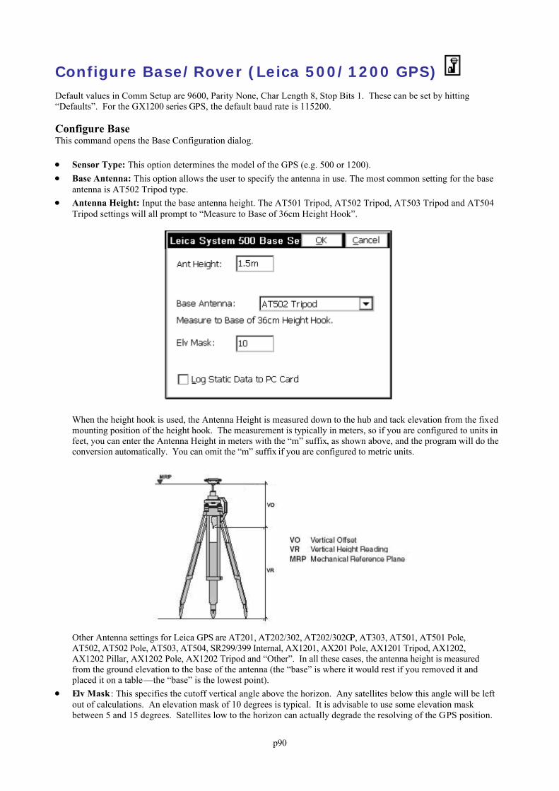
p90

Configure Base/Rover (Leica 500/1200 GPS) Default values in Comm Setup are 9600, Parity None, Char Length 8, Stop Bits 1. These can be set by hitting“Defaults”. For the GX1200 series GPS, the default baud rate is 115200.

Configure BaseThis command opens the Base Configuration dialog.

Sensor Type: This option determines the model of the GPS (e.g. 500 or 1200). Base Antenna: This option allows the user to specify the antenna in use. The most common setting for the base

antenna is AT502 Tripod type. Antenna Height: Input the base antenna height. The AT501 Tripod, AT502 Tripod, AT503 Tripod and AT504

Tripod settings will all prompt to “Measure to Base of 36cm Height Hook”.

When the height hook is used, the Antenna Height is measured down to the hub and tack elevation from the fixedmounting position of the height hook. The measurement is typically in meters, so if you are configured to units infeet, you can enter the Antenna Height in meters with the “m” suffix, as shown above, and the program will do theconversion automatically. You can omit the “m” suffix if you are configured to metric units.

Other Antenna settings for Leica GPS are AT201, AT202/302, AT202/302GP, AT303, AT501, AT501 Pole,AT502, AT502 Pole, AT503, AT504, SR299/399 Internal, AX1201, AX201 Pole, AX1201 Tripod, AX1202,AX1202 Pillar, AX1202 Pole, AX1202 Tripod and “Other”. In all these cases, the antenna height is measuredfrom the ground elevation to the base of the antenna (the “base” is where it would rest if you removed it andplaced it on a table—the “base” is the lowest point).

Elv Mask : This specifies the cutoff vertical angle above the horizon. Any satellites below this angle will be leftout of calculations. An elevation mask of 10 degrees is typical. It is advisable to use some elevation maskbetween 5 and 15 degrees. Satellites low to the horizon can actually degrade the resolving of the GPS position.

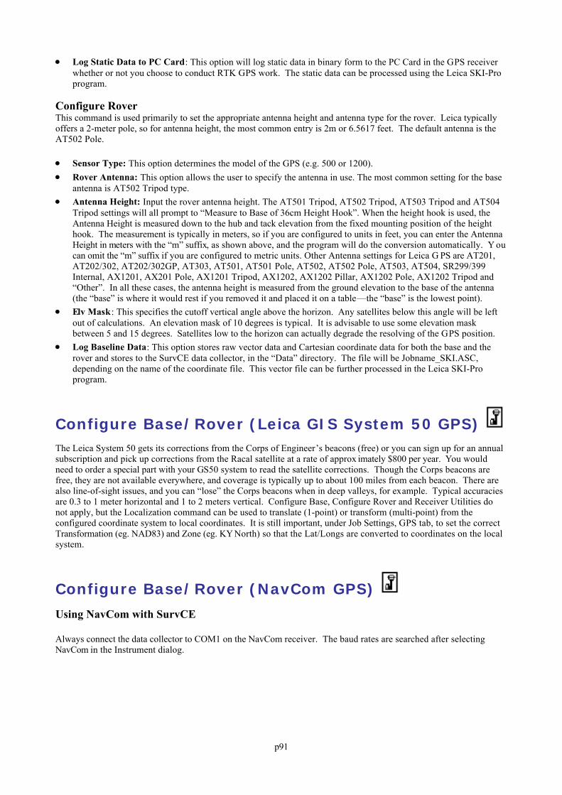
p91

Log Static Data to PC Card: This option will log static data in binary form to the PC Card in the GPS receiverwhether or not you choose to conduct RTK GPS work. The static data can be processed using the Leica SKI-Proprogram.

Configure RoverThis command is used primarily to set the appropriate antenna height and antenna type for the rover. Leica typicallyoffers a 2-meter pole, so for antenna height, the most common entry is 2m or 6.5617 feet. The default antenna is theAT502 Pole.

Sensor Type: This option determines the model of the GPS (e.g. 500 or 1200). Rover Antenna: This option allows the user to specify the antenna in use. The most common setting for the base

antenna is AT502 Tripod type. Antenna Height: Input the rover antenna height. The AT501 Tripod, AT502 Tripod, AT503 Tripod and AT504

Tripod settings will all prompt to “Measure to Base of 36cm Height Hook”. When the height hook is used, theAntenna Height is measured down to the hub and tack elevation from the fixed mounting position of the heighthook. The measurement is typically in meters, so if you are configured to units in feet, you can enter the AntennaHeight in meters with the “m” suffix, as shown above, and the program will do the conversion automatically. Y oucan omit the “m” suffix if you are configured to metric units. Other Antenna settings for Leica G PS are AT201,AT202/302, AT202/302GP, AT303, AT501, AT501 Pole, AT502, AT502 Pole, AT503, AT504, SR299/399Internal, AX1201, AX201 Pole, AX1201 Tripod, AX1202, AX1202 Pillar, AX1202 Pole, AX1202 Tripod and“Other”. In all these cases, the antenna height is measured from the ground elevation to the base of the antenna(the “base” is where it would rest if you removed it and placed it on a table—the “base” is the lowest point).

Elv Mask : This specifies the cutoff vertical angle above the horizon. Any satellites below this angle will be leftout of calculations. An elevation mask of 10 degrees is typical. It is advisable to use some elevation maskbetween 5 and 15 degrees. Satellites low to the horizon can actually degrade the resolving of the GPS position.

Log Baseline Data: This option stores raw vector data and Cartesian coordinate data for both the base and therover and stores to the SurvCE data collector, in the “Data” directory. The file will be Jobname_SKI.ASC,depending on the name of the coordinate file. This vector file can be further processed in the Leica SKI-Proprogram.

Configure Base/Rover (Leica GIS System 50 GPS) The Leica System 50 gets its corrections from the Corps of Engineer’s beacons (free) or you can sign up for an annualsubscription and pick up corrections from the Racal satellite at a rate of approx imately $800 per year. You wouldneed to order a special part with your GS50 system to read the satellite corrections. Though the Corps beacons arefree, they are not available everywhere, and coverage is typically up to about 100 miles from each beacon. There arealso line-of-sight issues, and you can “lose” the Corps beacons when in deep valleys, for example. Typical accuraciesare 0.3 to 1 meter horizontal and 1 to 2 meters vertical. Configure Base, Configure Rover and Receiver Utilities donot apply, but the Localization command can be used to translate (1-point) or transform (multi-point) from theconfigured coordinate system to local coordinates. It is still important, under Job Settings, GPS tab, to set the correctTransformation (eg. NAD83) and Zone (eg. KY North) so that the Lat/Longs are converted to coordinates on the localsystem.

Configure Base/Rover (NavCom GPS)

Using NavCom with SurvCE

Always connect the data collector to COM1 on the NavCom receiver. The baud rates are searched after selectingNavCom in the Instrument dialog.

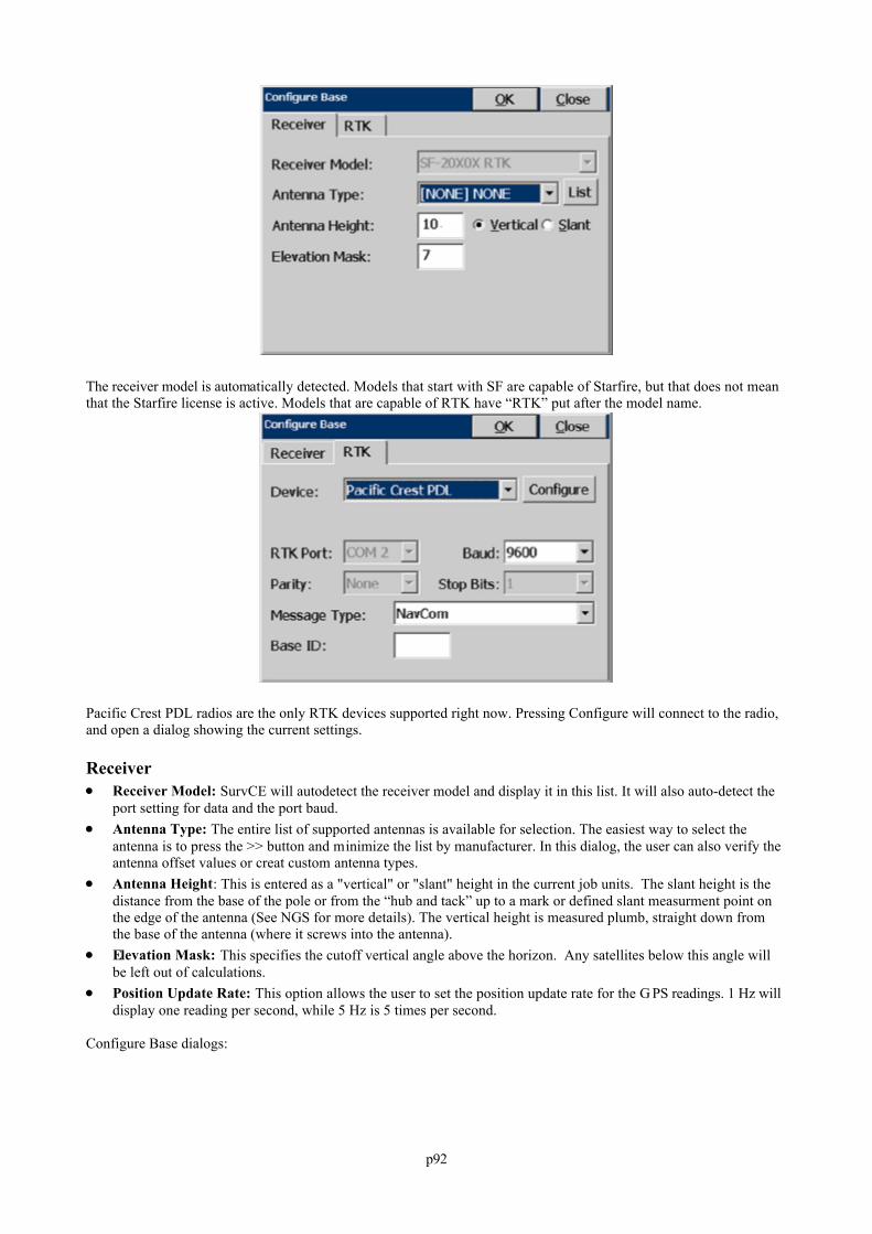
p92

The receiver model is automatically detected. Models that start with SF are capable of Starfire, but that does not meanthat the Starfire license is active. Models that are capable of RTK have “RTK” put after the model name.

Pacific Crest PDL radios are the only RTK devices supported right now. Pressing Configure will connect to the radio,and open a dialog showing the current settings.

Receiver Receiver Model: SurvCE will autodetect the receiver model and display it in this list. It will also auto-detect the

port setting for data and the port baud. Antenna Type: The entire list of supported antennas is available for selection. The easiest way to select the

antenna is to press the >> button and minimize the list by manufacturer. In this dialog, the user can also verify theantenna offset values or creat custom antenna types.

Antenna Height: This is entered as a "vertical" or "slant" height in the current job units. The slant height is thedistance from the base of the pole or from the “hub and tack” up to a mark or defined slant measurment point onthe edge of the antenna (See NGS for more details). The vertical height is measured plumb, straight down fromthe base of the antenna (where it screws into the antenna).

Elevation Mask: This specifies the cutoff vertical angle above the horizon. Any satellites below this angle willbe left out of calculations.

Position Update Rate: This option allows the user to set the position update rate for the G PS readings. 1 Hz willdisplay one reading per second, while 5 Hz is 5 times per second.

Configure Base dialogs:

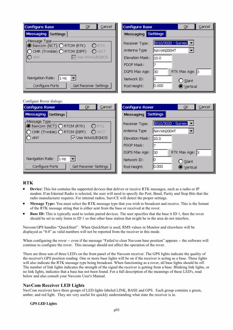
p93

Configure Rover dialogs:

RTK Device: This list contains the supported devices that deliver or receive RTK messages, such as a radio or IP

modem. If an External Radio is selected, the user will need to specify the Port, Baud, Parity and Stop Bits that theradio manufacturer requires. For internal radios, SurvCE will detect the proper settings.

Message Type: You must select the RTK message type that you wish to broadcast and receive. This is the formatof the RTK message string that is either sent from the base or received at the rover.

Base ID: This is typically used to isolate paired devices. The user specifies that the base it ID 1, then the rovershould be set to only listen to ID 1 so that other base station that might be in the area do not interfere.

Navcom GPS handles “QuickStart”. When QuickStart is used, RMS values in Monitor and elsewhere will bedisplayed as “0.0” as valid numbers will not be reported from the receiver in this mode.

When configuring the rover -- even if the message “Failed to clear Navcom base position” appears -- the software willcontinue to configure the rover. This message should not affect the operation of the rover.

There are three sets of three LED's on the front panel of the Navcom receiver. The GPS lights indicate the quality ofthe receiver's GPS position reading. One or more base lights will be on if the receiver is acting as a base. These lightswill also indicate the RTK message type being broadcast. When functioning as a rover, all base lights should be off.The number of link lights indicates the strength of the signal the receiver is getting from a base. Blinking link lights, orno link lights, indicates that a base has not been found. For a full description of the meanings of these LED's, readbelow and also consult your Navcom User's Manual.

NavCom Receiver LED LightsNavCom receivers have three groups of LED lights labeled LINK, BASE and GPS. Each group contains a green,amber, and red light. They are very useful for quickly understanding what state the receiver is in.

GPS LED Lights

p94

Whatever GPS LED lights are on, they blink at the rate of position calculation (1Hz, 5Hz, etc.). If the red LED ison then there are not enough satellites to calculate a position. The amber LED blinking by itself indicates that anon-differential position is being calculated. Blinking green and amber means there is a differential position(WAAS, DGPS, StarFire, or RTK Float). If the receiver has StarFire capability, then when the green LED is theonly GPS LED blinking, the receiver has a StarFire position. If the receiver does not have StarFire, the singlegreen LED indicates RTK Fixed mode. If the receiver has both StarFire and RTK ability, then a single greenLED indicates either StarFire or RTK Fixed mode.

Base LED LightsThe Base LED lights blink at the rate RTK corrections are being sent. If the receiver is configured as a rover, allBase LED lights will be off. Which color of LED is blinking depends on the RTK correction format being sent. Green indicates NavCom proprietary format, amber indicates CMR and red indicates RTCM.

Link LED LightsCarlson Software programs the behavior of the Link LED lights to depend on whether the receiver is configuredas a base or rover and whether using an internal or external radio for RTK corrections. The following tablesummarizes the possible configurations:

  Base Rover

Internal Radio LED’s off Signal Strength

External Radio Sent correction Received correction

When using an internal radio on a rover, the LED ’s show radio signal strength. Full strength is shown by all LinkLED’s being on and not blinking. As signal strength fades, The green LED will start blinking then turn off, thenthe amber LED will start blinking and turn off, then the red LED will blink when signal is lost.

Every time a correction is sent or received when using an external radio, a Link LED blinks. The color of theLink LED that blinks depends on the RTK correction format. Green indicates NavCom proprietary format, amberindicates CMR and red indicates RTCM.

Troubleshooting

Not able to establish connection to receiverIf the data collector is connected to COM2 and configures COM1 to receive CMR corrections, the receiver will nolonger recognize commands on COM1. To correct the problem, connect the data collector to COM2, go to theConfigure Rover window, set the correction type to NavCom and press OK. Now connect to COM1, go to the CommSetup window and press OK. It will then search through the baud rates to find the right one.

Unable to update NavCom firmwareA common problem people have when updating the firmware on the NavCom is they connect the computer to COM1on the NavCom instead of COM2. They must connect to COM2 to update the firmware. The transfer will go faster ifthey set COM2 to run at 115200 baud before starting the firmware update utility.

Configure Base/Rover (NMEA GPS) This GPS configuration is typically used to pick up the standard, commonly output NMEA string from a variety ofreceivers, including Magellan, the Sokkia GPS01 Toughbook and some brands of Trimble equipment.

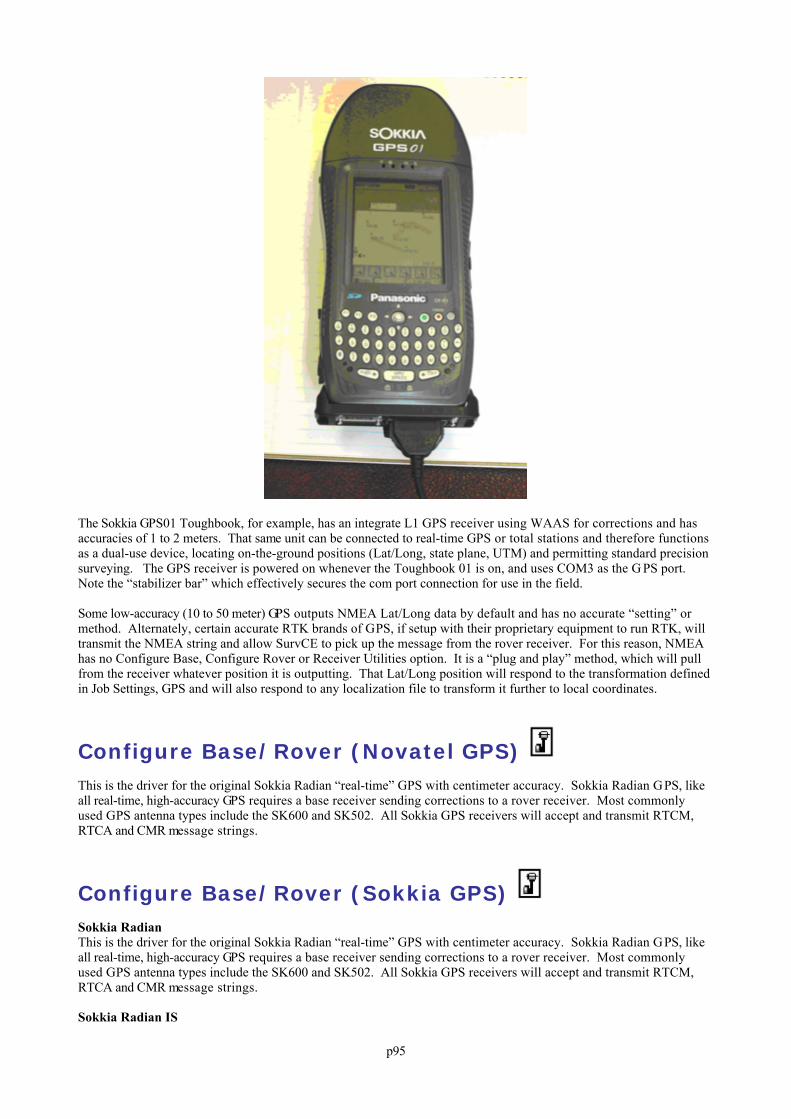
p95

The Sokkia GPS01 Toughbook, for example, has an integrate L1 GPS receiver using WAAS for corrections and hasaccuracies of 1 to 2 meters. That same unit can be connected to real-time GPS or total stations and therefore functionsas a dual-use device, locating on-the-ground positions (Lat/Long, state plane, UTM) and permitting standard precisionsurveying. The GPS receiver is powered on whenever the Toughbook 01 is on, and uses COM3 as the G PS port. Note the “stabilizer bar” which effectively secures the com port connection for use in the field.

Some low-accuracy (10 to 50 meter) GPS outputs NMEA Lat/Long data by default and has no accurate “setting” ormethod. Alternately, certain accurate RTK brands of GPS, if setup with their proprietary equipment to run RTK, willtransmit the NMEA string and allow SurvCE to pick up the message from the rover receiver. For this reason, NMEAhas no Configure Base, Configure Rover or Receiver Utilities option. It is a “plug and play” method, which will pullfrom the receiver whatever position it is outputting. That Lat/Long position will respond to the transformation definedin Job Settings, GPS and will also respond to any localization file to transform it further to local coordinates.

Configure Base/Rover (Novatel GPS) This is the driver for the original Sokkia Radian “real-time” GPS with centimeter accuracy. Sokkia Radian GPS, likeall real-time, high-accuracy GPS requires a base receiver sending corrections to a rover receiver. Most commonlyused GPS antenna types include the SK600 and SK502. All Sokkia GPS receivers will accept and transmit RTCM,RTCA and CMR message strings.

Configure Base/Rover (Sokkia GPS) Sokkia RadianThis is the driver for the original Sokkia Radian “real-time” GPS with centimeter accuracy. Sokkia Radian GPS, likeall real-time, high-accuracy GPS requires a base receiver sending corrections to a rover receiver. Most commonlyused GPS antenna types include the SK600 and SK502. All Sokkia GPS receivers will accept and transmit RTCM,RTCA and CMR message strings.

Sokkia Radian IS

p96

The Radian IS is an “integrated” GPS receiver with a fixed antenna type, the SK600. Antenna height on the integratedRadian IS with built-in SK600 antenna is measured to the base of the rubber bumper around the antenna. Sokkiaprovides a measuring tape that connects to the rectangular indentations for precise height measurement. A diagram ofthe phase center offset (antenna height) is included on the receiver. Similar “hook points” exist on all Sokkiaantennas.

Sokkia GSR2600 GPSThe GSR2600 is a modular version of the Radian IS, with a variety of antenna types available. The Log Static Dataroutine in SurvCE will initialize the storing of raw data to the receiver. This raw data can be post-processed in SokkiaSpectrum Survey.

Sokkia Axis/Axis 3 GPSThe Sokkia Axis 3 is the current GIS-level GPS product from Sokkia and obtains corrections from Coast Guardbeacons, WAAS and OmniStar. There is no subscription fee for beacons or WAAS, but there is for OmniStar. Thesubscription can be by month or year or any other time period (even “weekend” use). Accuracy varies on correctionmethod used, but is typically sub-meter to 3 meters. For example, 0.5 meter accuracy (1.5 feet) is common withbeacon corrections when located within 60 miles of a Coast Guard beacon. The Axis 3 is designed for GIS andenvironmental applications, which are effectively addressed by SurvCE through use of attributing on feature codes andthrough ESRI import and export features.

Configure Base/Rover (Thales/Ashtech GPS) The following information describes the various options available for Thales/Ashtech GPS.

SurvCE works with the following high precision, centimeter accurate RTK GPS equipment produced byThales/Ashtech: Z12/Sensor, ZSurveyor, GG24, Z-Xtreme and Z-Max. SurvCE also works with the Ashtech RelianceUSCG/DGPS RTCM sub-meter RTK GPS receivers.

Shown below is the front panel view of the Ashtech Z-Xtreme, as it appears in the top of the backpack.

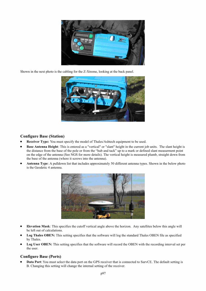
p97

Shown in the next photo is the cabling for the Z-Xtreme, looking at the back panel.

Configure Base (Station) Receiver Type: You must specify the model of Thales/Ashtech equipment to be used. Base Antenna Height: This is entered as a "vertical" or "slant" height in the current job units. The slant height is

the distance from the base of the pole or from the “hub and tack” up to a mark or defined slant measurment pointon the edge of the antenna (See NGS for more details). The vertical height is measured plumb, straight down fromthe base of the antenna (where it screws into the antenna).

Antenna Type: A pulldown list that includes approximately 50 different antenna types. Shown in the below photois the Geodetic 4 antenna.

Elevation Mask: This specifies the cutoff vertical angle above the horizon. Any satellites below this angle willbe left out of calculations.

Log Thales OBEN: This setting specifies that the software will log the standard Thales OBEN file as specifiedby Thales.

Log User OBEN: This setting specifies that the software will record the OBEN with the recording interval set perthe user.

Configure Base (Ports) Data Port: You must select the data port on the GPS receiver that is connected to SurvCE. The default setting is

B. Changing this setting will change the internal setting of the receiver.

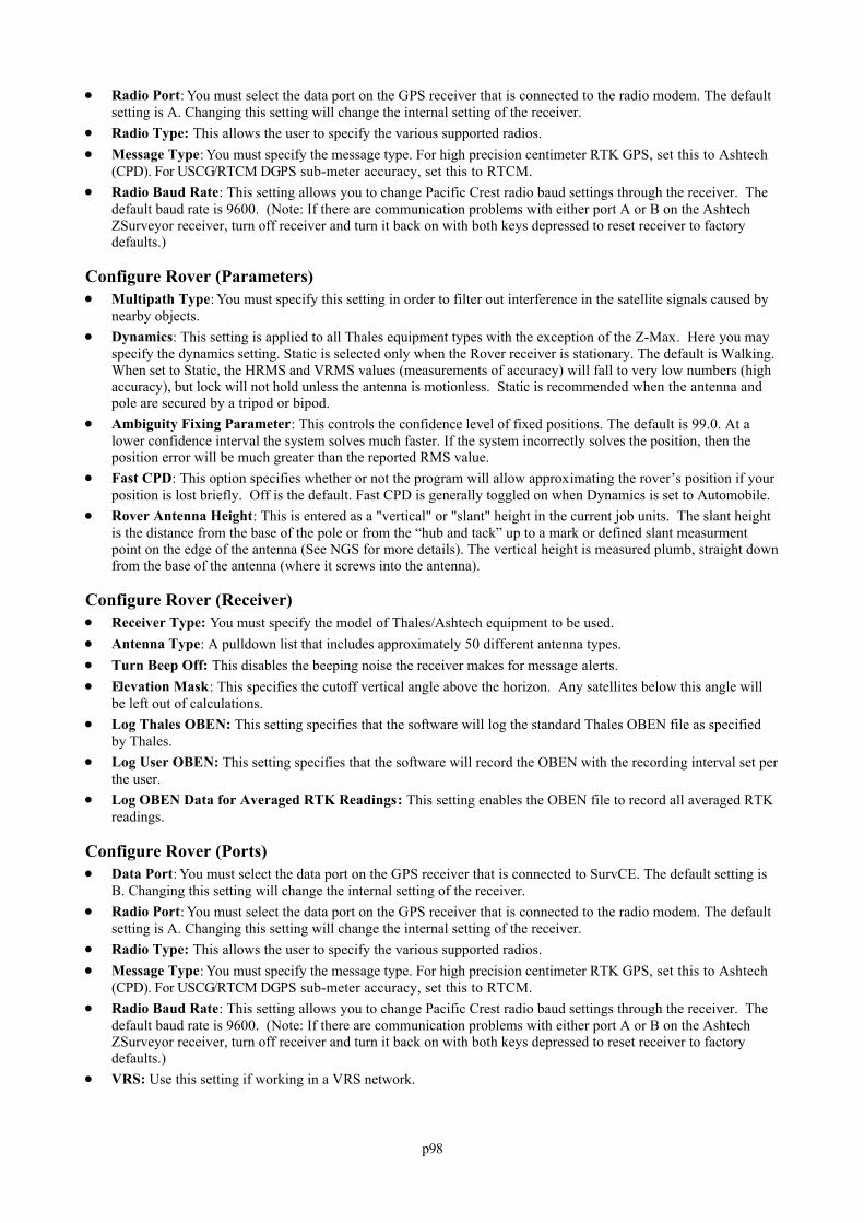
p98

Radio Port: You must select the data port on the GPS receiver that is connected to the radio modem. The defaultsetting is A. Changing this setting will change the internal setting of the receiver.

Radio Type: This allows the user to specify the various supported radios. Message Type: You must specify the message type. For high precision centimeter RTK GPS, set this to Ashtech

(CPD). For USCG/RTCM DGPS sub-meter accuracy, set this to RTCM. Radio Baud Rate: This setting allows you to change Pacific Crest radio baud settings through the receiver. The

default baud rate is 9600. (Note: If there are communication problems with either port A or B on the AshtechZSurveyor receiver, turn off receiver and turn it back on with both keys depressed to reset receiver to factorydefaults.)

Configure Rover (Parameters) Multipath Type: You must specify this setting in order to filter out interference in the satellite signals caused by

nearby objects. Dynamics: This setting is applied to all Thales equipment types with the exception of the Z-Max. Here you may

specify the dynamics setting. Static is selected only when the Rover receiver is stationary. The default is Walking.When set to Static, the HRMS and VRMS values (measurements of accuracy) will fall to very low numbers (highaccuracy), but lock will not hold unless the antenna is motionless. Static is recommended when the antenna andpole are secured by a tripod or bipod.

Ambiguity Fixing Parameter: This controls the confidence level of fixed positions. The default is 99.0. At alower confidence interval the system solves much faster. If the system incorrectly solves the position, then theposition error will be much greater than the reported RMS value.

Fast CPD: This option specifies whether or not the program will allow approximating the rover’s position if yourposition is lost briefly. Off is the default. Fast CPD is generally toggled on when Dynamics is set to Automobile.

Rover Antenna Height: This is entered as a "vertical" or "slant" height in the current job units. The slant heightis the distance from the base of the pole or from the “hub and tack” up to a mark or defined slant measurmentpoint on the edge of the antenna (See NGS for more details). The vertical height is measured plumb, straight downfrom the base of the antenna (where it screws into the antenna).

Configure Rover (Receiver) Receiver Type: You must specify the model of Thales/Ashtech equipment to be used. Antenna Type: A pulldown list that includes approximately 50 different antenna types. Turn Beep Off: This disables the beeping noise the receiver makes for message alerts. Elevation Mask: This specifies the cutoff vertical angle above the horizon. Any satellites below this angle will

be left out of calculations. Log Thales OBEN: This setting specifies that the software will log the standard Thales OBEN file as specified

by Thales. Log User OBEN: This setting specifies that the software will record the OBEN with the recording interval set per

the user. Log OBEN Data for Averaged RTK Readings: This setting enables the OBEN file to record all averaged RTK

readings.

Configure Rover (Ports) Data Port: You must select the data port on the GPS receiver that is connected to SurvCE. The default setting is

B. Changing this setting will change the internal setting of the receiver. Radio Port: You must select the data port on the GPS receiver that is connected to the radio modem. The default

setting is A. Changing this setting will change the internal setting of the receiver. Radio Type: This allows the user to specify the various supported radios. Message Type: You must specify the message type. For high precision centimeter RTK GPS, set this to Ashtech

(CPD). For USCG/RTCM DGPS sub-meter accuracy, set this to RTCM. Radio Baud Rate: This setting allows you to change Pacific Crest radio baud settings through the receiver. The

default baud rate is 9600. (Note: If there are communication problems with either port A or B on the AshtechZSurveyor receiver, turn off receiver and turn it back on with both keys depressed to reset receiver to factorydefaults.)

VRS: Use this setting if working in a VRS network.

p99

Configure Base/Rover (Topcon GPS) This configuration covers all Topcon GPS receiver types. Some of these receivers utilize Glonass satellites as well asthe standard U.S. satellites. In the Configure Base routine for Topcon GPS, the firmware version of the receiver willbe checked and the correct message for setting the base position will be sent according to the firmware version in use.

Note: Glonass refers to the Russian satellite constellation (Global Navigation Satellite System). There areapproximately 24 U.S. satellites active (more will launch over time) and there are approximately 10 Glonasssatellites currently active. A full “24 satellite constellation” is anticipated by 2006 for the Glonass satellites. With a minimum of 2 Glonass satellites available or “seen” by the base and rover receivers, satellite coverage isimproved, and work is sometimes possible in canopy, urban or deep pit environments where non-Glonassreceivers do not have coverage. All Topcon GPS receivers have a "stat" light on the front panel that flashes greenindicating number of U.S. satellites and orange indicating the number of Russian satellites.

Comm Setup Port Number: This drop list allows the user to select the communications port of the data collector. This is a Bluetooth Port: This toggle allows the user to specify that the selected port number is in fact the

communications port that the Bluetooth device in the data collector is assigned to. Find Bluetooth Port: This button will auto-detect the Bluetooth port number in most devices. Bluetooth Type: Select the manufacturer of the bluetooth device if known. Typically, Socket will be the

preferred brand and often the installed brand, but if the brand is not known, select Other. Baud Rate: Set this value to match the data baud rate of the GPS serial port. Typically this will be 115200 but

may also be 9600 or 38400. Character Length: Set this value to match the data Character Length of the GPS serial port. Typically this will

be 8. Parity: Set this value to match the data Parity of the GPS serial port. Typically this will be None. Stop Bits: Set this value to match the data Stop Bits of the GPS serial port. Typically this will be 1.

BluetoothIn addition to the discussion of Bluetooth (wireless) connection found under the help subject Equip - Comm Setup,there are additional trouble-shooting considerations with Topcon Bluetooth. Note that the PIN for all Topcon devices is 11111. If the OAF file is not current the Bluetooth will not work. An OAF file is used by Topcon for the firmware of their

receivers. With an expired OAF file, many features (including Bluetooth) will not work. Normally the Bluetooth port (usually B) must be enabled in the OAF file for the Bluetooth to work. It is possible to set the Bluetooth port baud rate. Normally it is 9600, 38400 or 115200. This can be checked from

the “A” com port using GRIL (command manual for Topcon receivers) commands. The baud rate in the ComSetup should be the same.

Configure Base Station Receiver Type: You must select the receiver type (e.g. Hiper Lite). Antenna Type: You must select the Antenna Type (e.g. Hiper Lite). See the figure below.

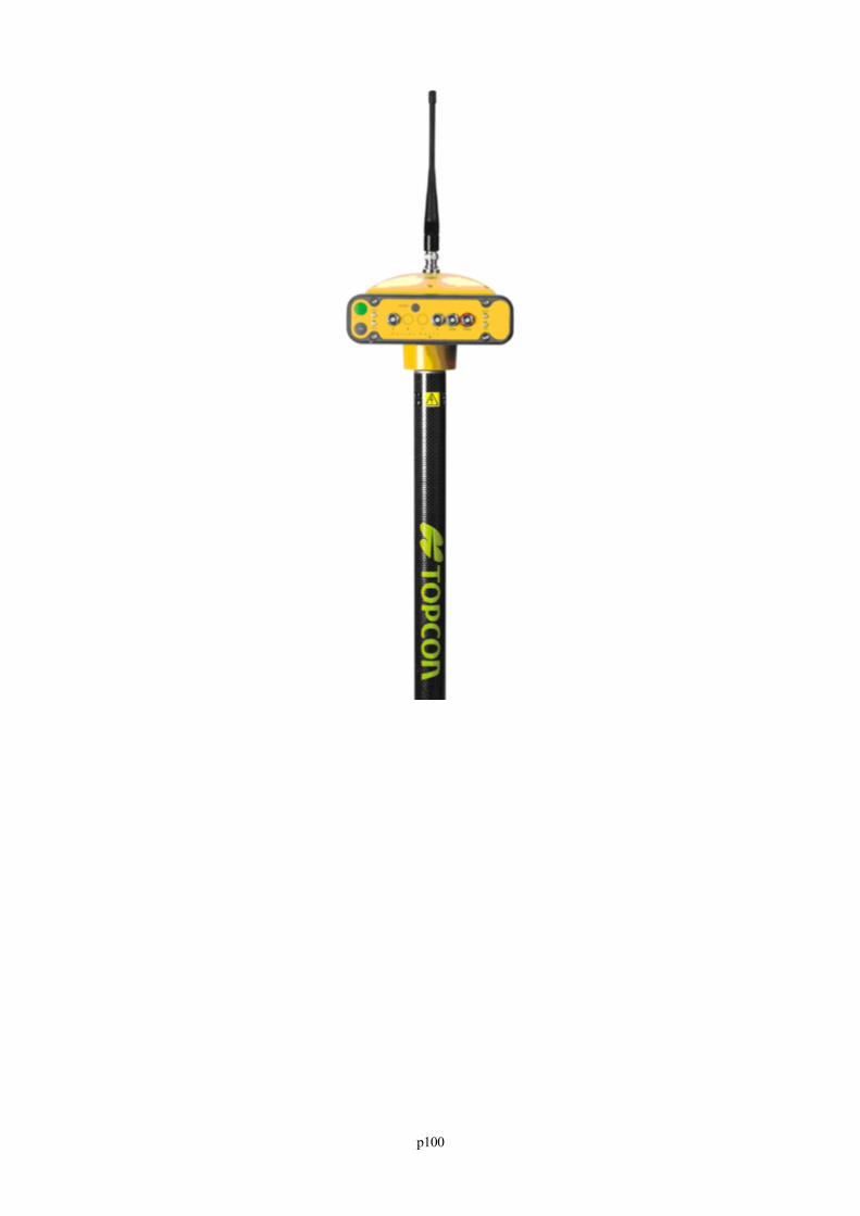
p100

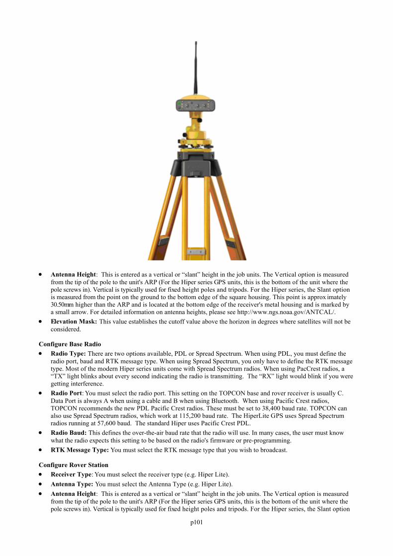
p101

Antenna Height: This is entered as a vertical or “slant” height in the job units. The Vertical option is measuredfrom the tip of the pole to the unit's ARP (For the Hiper series GPS units, this is the bottom of the unit where thepole screws in). Vertical is typically used for fixed height poles and tripods. For the Hiper series, the Slant optionis measured from the point on the ground to the bottom edge of the square housing. This point is approx imately30.50mm higher than the ARP and is located at the bottom edge of the receiver's metal housing and is marked bya small arrow. For detailed information on antenna heights, please see http://www.ngs.noaa.gov/ANTCAL/.

Elevation Mask: This value establishes the cutoff value above the horizon in degrees where satellites will not beconsidered.

Configure Base Radio Radio Type: There are two options available, PDL or Spread Spectrum. When using PDL, you must define the

radio port, baud and RTK message type. When using Spread Spectrum, you only have to define the RTK messagetype. Most of the modern Hiper series units come with Spread Spectrum radios. When using PacCrest radios, a“TX” light blinks about every second indicating the radio is transmitting. The “RX” light would blink if you weregetting interference.

Radio Port: You must select the radio port. This setting on the TOPCON base and rover receiver is usually C.Data Port is always A when using a cable and B when using Bluetooth. When using Pacific Crest radios,TOPCON recommends the new PDL Pacific Crest radios. These must be set to 38,400 baud rate. TOPCON canalso use Spread Spectrum radios, which work at 115,200 baud rate. The HiperLite GPS uses Spread Spectrumradios running at 57,600 baud. The standard Hiper uses Pacific Crest PDL.

Radio Baud: This defines the over-the-air baud rate that the radio will use. In many cases, the user must knowwhat the radio expects this setting to be based on the radio's firmware or pre-programming.

RTK Message Type: You must select the RTK message type that you wish to broadcast.

Configure Rover Station Receiver Type: You must select the receiver type (e.g. Hiper Lite). Antenna Type: You must select the Antenna Type (e.g. Hiper Lite). Antenna Height: This is entered as a vertical or “slant” height in the job units. The Vertical option is measured

from the tip of the pole to the unit's ARP (For the Hiper series GPS units, this is the bottom of the unit where thepole screws in). Vertical is typically used for fixed height poles and tripods. For the Hiper series, the Slant option

p102

is measured from the point on the ground to the bottom edge of the square housing. This point is approx imately30.50mm higher than the ARP and is located at the bottom edge of the receiver's metal housing and is marked bya small arrow. For detailed information on antenna heights, please see http://www.ngs.noaa.gov/ANTCAL/.

Elevation Mask: This value establishes the cutoff value above the horizon in degrees where satellites will not beconsidered.

Configure Rover Radio Radio Type: There are two options available, PDL or Spread Spectrum. When using PDL, you must define the

radio port, baud and RTK message type. When using Spread Spectrum, you only have to define the RTK messagetype. Most of the modern Hiper series units come with Spread Spectrum radios. When using PacCrest radios, a“TX” light blinks about every second indicating the radio is transmitting. The “RX” light would blink if you weregetting interference.

Radio Port: You must select the radio port. This setting on the TOPCON base and rover receiver is usually C.Data Port is always A when using a cable and B when using Bluetooth. When using Pacific Crest radios,TOPCON recommends the new PDL Pacific Crest radios. These must be set to 38,400 baud rate. TOPCON canalso use Spread Spectrum radios, which work at 115,200 baud rate. The HiperLite GPS uses Spread Spectrumradios running at 57,600 baud. The standard Hiper uses Pacific Crest PDL.

Radio Baud: This defines the over-the-air baud rate that the radio will receive. In many cases, the user mustknow what the radio expects this setting to be based on the radio's firmware or pre-programming.

RTK Message Type: You must select the RTK message type that you wish to receive.

Configure Rover Parameters Position Update Rate: In Configure Rover, the RTK Calculation Mode should be set to Delay, which forces a

fresh reading, as opposed to Extrapolate, which will project the next reading by your direction of movement, andmay apply to difficult shots in tree lines.

Ambiguity Fixing Parameter: This determines how tight the ambiguities of the RTK solution must be before afixed position is achieved. It is recommended that High be used for greater accuracy.

RTK Calculation Mode: In Configure Rover, the RTK Calculation Mode should be set to Delay, which forces afresh reading, as opposed to Extrapolate which will project the next reading by your direction of movement.Extrapolate may apply to difficult shots near obstructions such as trees or buildings.

Receiver Utilities Power Cycle Receiver: Use this button to power cycle the receiver. At times this may help if communications fail

and cannot be restarted by Configure Base or Rover. Restore Factory Defaults: Use this button to re-boot the receiver back to factory default settings. Clear Non-Volatile Memory: Use this option to clear the unit's non-volatile memory. Send Command to Receiver: This button allow the user to send command directly to the receiver if necessary. Set Base/Rover Radio: Use Set Base Radio and Set Rover Radio to be sure that both radios are on the same

channel. Recommended settings are base on low “digisquelch” (low sensitivity) and rover on medium or highdigisquelch.

Set Satellite Status: This command enables you to “turn off” particular satellites, both U.S. and Russian. InSurvCE's Monitor/SkyPlot command, located on the Equip tab, the Sat Info screen displays the Russian satellitesnumbered 45 and up and the U.S. satellites numbered from 1 to 24.

Initialize to Known Point: Use this option to speed up the initialization process.

Post-ProcessingAll Topcon GPS receivers can be used for post processing and will store raw GPS data on the on-board RAM in thereceiver. The post-processing can be activated by the Log Static Data command found in the Surv menu of SurvCE. On every receiver, you can also activate logging purely through hardware by holding down the FN key, watch the lightturn orange to green, then release. To turn off by hardware, press FN until the light turns off. Since SurvCE willprompt for antenna height, type and other parameters, it is recommended that software be used to initiate logging. Topcon logging files typically start off with the word “Log” followed by the date, and are post-processed usingTopcon Tools. Topcon Tools will output a Rinex ASCII file of the logging data for use with programs such as NGS’sOPUS.

Configure Base/Rover (Trimble GPS)

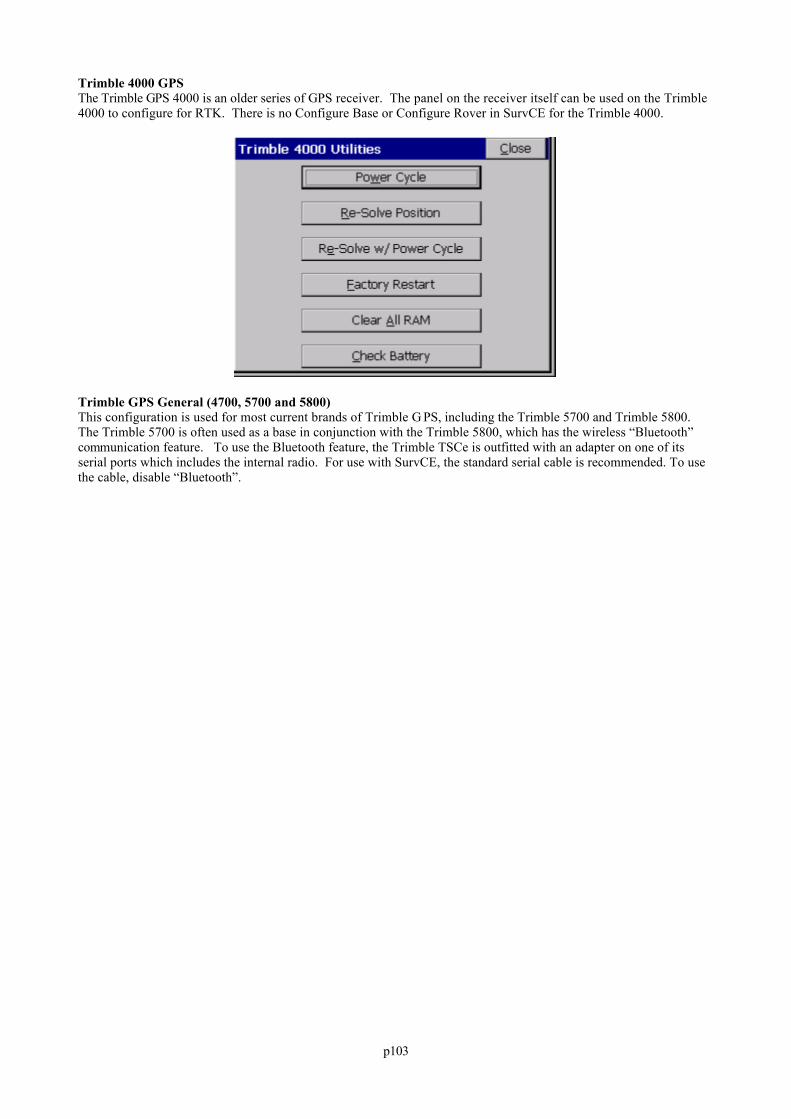
p103

Trimble 4000 GPSThe Trimble GPS 4000 is an older series of GPS receiver. The panel on the receiver itself can be used on the Trimble4000 to configure for RTK. There is no Configure Base or Configure Rover in SurvCE for the Trimble 4000.

Trimble GPS General (4700, 5700 and 5800)This configuration is used for most current brands of Trimble G PS, including the Trimble 5700 and Trimble 5800. The Trimble 5700 is often used as a base in conjunction with the Trimble 5800, which has the wireless “Bluetooth”communication feature. To use the Bluetooth feature, the Trimble TSCe is outfitted with an adapter on one of itsserial ports which includes the internal radio. For use with SurvCE, the standard serial cable is recommended. To usethe cable, disable “Bluetooth”.

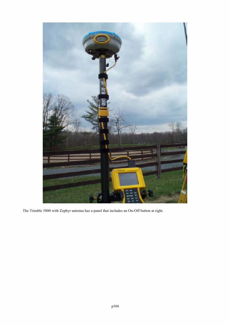
p104

The Trimble 5800 with Zephyr antenna has a panel that includes an On-Off button at right.

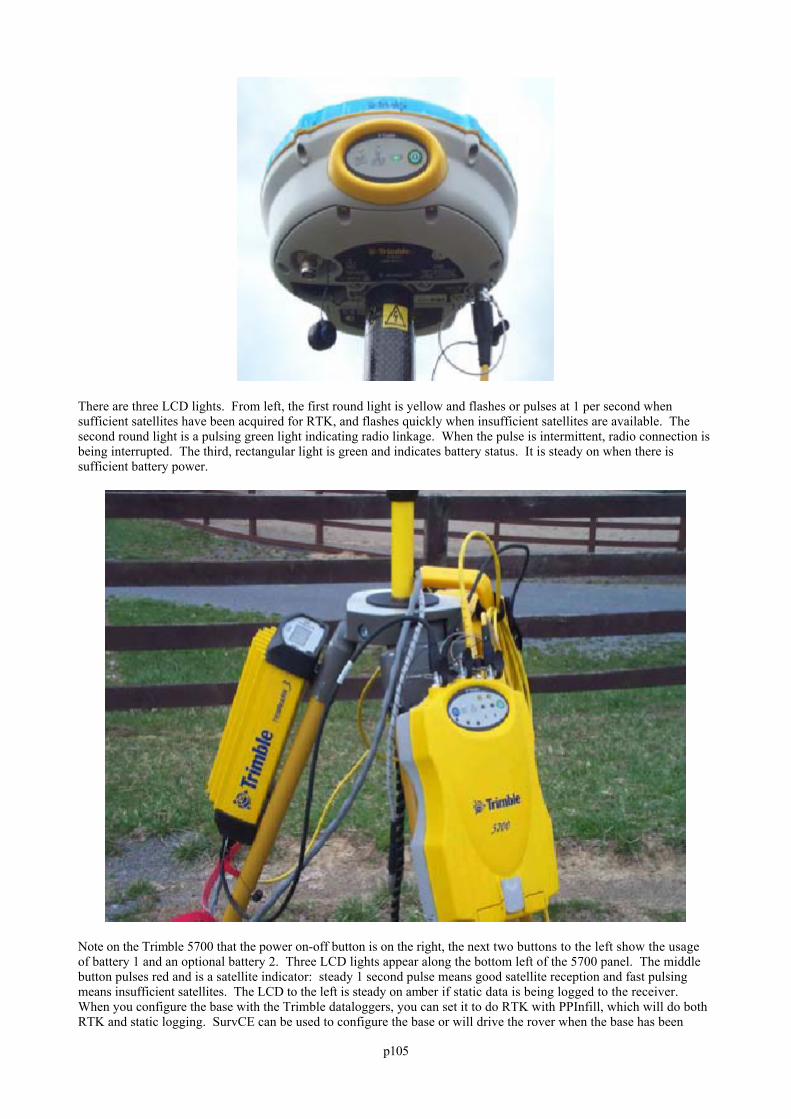
p105

There are three LCD lights. From left, the first round light is yellow and flashes or pulses at 1 per second whensufficient satellites have been acquired for RTK, and flashes quickly when insufficient satellites are available. Thesecond round light is a pulsing green light indicating radio linkage. When the pulse is intermittent, radio connection isbeing interrupted. The third, rectangular light is green and indicates battery status. It is steady on when there issufficient battery power.

Note on the Trimble 5700 that the power on-off button is on the right, the next two buttons to the left show the usageof battery 1 and an optional battery 2. Three LCD lights appear along the bottom left of the 5700 panel. The middlebutton pulses red and is a satellite indicator: steady 1 second pulse means good satellite reception and fast pulsingmeans insufficient satellites. The LCD to the left is steady on amber if static data is being logged to the receiver. When you configure the base with the Trimble dataloggers, you can set it to do RTK with PPInfill, which will do bothRTK and static logging. SurvCE can be used to configure the base or will drive the rover when the base has been

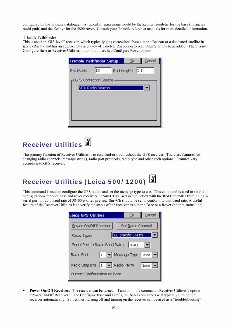
p106

configured by the Trimble datalogger. A typical antenna usage would be the Zephyr Geodetic for the base (mitigatesmulti-path) and the Zephyr for the 5800 rover. Consult your Trimble reference manuals for more detailed information.

Trimble PathFinderThis is another “GIS-level” receiver, which typically gets corrections from either a Beacon or a dedicated satellite inspace (Racal), and has an approximate accuracy of 1 meter. An option to read OmniStar has been added. There is noConfigure Base or Receiver Utilities option, but there is a Configure Rover option.

Receiver Utilities The primary function of Receiver Utilities is to reset and/or troubleshoot the GPS receiver. There are features forchanging radio channels, message strings, radio port protocols, radio type and other such options. Features varyaccording to GPS receiver.

Receiver Utilities (Leica 500/1200) This command is used to configure the GPS radios and set the message type to use. This command is used to set radioconfigurations for both base and rover receivers. If SurvCE is used in conjuction with the Red Controller from Leica, aserial port to radio baud rate of 38400 is often pre-set. SurvCE should be set to conform to that baud rate. A usefulfeature of the Receiver Utilities is to verify the status of the receiver as either a Base or a Rover (bottom status line).

Power On/Off Receiver: The receiver can be turned off and on in the command “Receiver Utilities”, option“Power On/Off Receiver”. The Configure Base and Configure Rover commands will typically turn on thereceiver automatically. Sometimes, turning off and turning on the receiver can be used as a “troubleshooting”

p107

technique to clear conditions and start from a clean slate. Radio Type: The Pacific Crest PDL radio type is the default setting, operating at 38400 baud rate. Older Pacific

Crest radios are often type RFM96W, defaulting to 9600 baud rate. Other options include Motorola Cell Phone,3COM Faxmodem, RS232 and User Defined Modem. Phone numbers for cell modems will accept up to 49characters. When using Freewave or Tait “spread spectrum” radios, the radio type doesn’t matter, but can be setto “User Defined Modem”. Baud rate for Freewaves is often 19600 baud.

Motorola Cell Phone: With Freewave and other spread spectrum radio linkages, communication must occurwithin a line-of-sight distance, typically no more than 2 to 5 kilometers except in very flat terrain. With PacCrest radios, the signal can “bend” somewhat, and achieve maximum distances of 10 kilometers, typically. Cell phone linkage allows corrections to be transmitted within the coverage of the cell phones themselves andmaintains accuracy up to as much as 50 kilometers. Contact your Leica GPS vendor for appropriate cablesfor connectivity details. When you select the Motorola configuration, the “Set Radio Channel” buttonbecomes “Connect Modem”, and when tapped, you are prompted for a Phone Number for the actual cellphone (for the rover to call the base). The base must also be hooked to a cell phone. The base can actuallybe set to both cell phone and radio linkage, with the rover set to either cell or radio as preferred. The roverwill go from autonomous to float (cell phones are communicating) to fixed with cell phones just like withradio linkage.Note: Base and rover GPS receivers must have matching radio configurations. If cell phones are used forthe rover, then the base must be configured for cell phone use. If Pac Crest PDL radios are used on therover, than Pac Crest PDL radios must be used on the base. Also note that cell phone switching is madepossible through the C icon or Alt C “on the fly” from commands such as Store Points or Stakeout Points. This is because of the availability of a “Utilities Tab” in Configure Reading when configured Leica GPS.Reference Station: To obtain corrections from a reference station to a single rover, you typically must set tocell phone or modem linkage, depending on what is required by the reference station.

Set Radio Channel: This is normally set to channel 0 or channel 1. SurvCE allows up to 16 radio channels (0 to15). The procedure is to pick the channel, then tap “Set Radio Channel”. Radios on base and rover must be set tothe same channel.

Radio Ports: The Leica GPS 500 series receiver has 2 main radio ports (ports 1 and 3). Radio Stop Bits: Typically set to 1. Message Type: Standard setting is Leica Proprietary. Other message string options are RTCM (an industry

standard) and CMR (Trimble message string). RTCM and CMR are used when it is necessary to communicatewith non-Leica GPS.

Radio Parity: Typically set to None.

Receiver Utilities (NavCom)

p108

Configure RTK Device: Use this page to change your RTK data port settings. This can also be done during baseor rover configuration.

Check RTK: This tells the user why they aren’t in RTK fixed. Quickstart (Starfire Only): Starfire corrections often take some time to acquire high levels of accuracy. If you’re

returning to a previously surveyed area, you can save time by storing a known position to a reference file. Thenyou can initialize the Starfire system with this position upon returning to the site by performing a Quickstart.

At the end of the first day, verify that you’re receiving Dual-Frequency Starfire corrections (RTG or WCT)by entering the Navigation Status utility. Enter the Quickstart menu, and press Read GPS. Be sure tophysically mark this position in some way so that the exact position can be returned to later. When you havea GPS position, click Save to save the position to a reference file. When you return to the site, first ensurethat you’re receiving dual-frequency Starfire corrections, and that you're set up on the position marked theprevious day. Then enter the Quickstart menu and choose Load to select the previously stored reference file.Press Initiate to input the loaded starting position to the receiver. To disable an input position, press Disable. Note that if the input position is inaccurate, using the Quickstart routine will slow down the processing ofacquiring an accurate position.

Reset Receiver: Use this tool to reset your receiver (soft reset) Factory Reset: Use this tool to reset your receiver (factory reset).

The buttons available in Receiver Utilities depends on the capabilities of the receiver. If a Starfire license is notactive, the Quickstart button is not shown.

Check RTK is a very useful tool. It tells the user why they aren’t in RTK fixed and, if connected to a base whenpressed, it determines if the base is transmitting corrections, and if not, tells the user why. If connected to the rover, ittells the user if in RTK Fixed and if not, and it tells the user why. Configure RTK Device is the same as the Configurebutton in the RTK tab of the Base and Rover dialogs.

p109

“Quickstart” allows the user to save a quickstart point or to quickstart from a previously saved quickstart point.

StarFire and QuickstartStarFire is a space-based GPS correction system capable of 10 cm horizontal accuracy. Vertical will be 1.5 to 2 timesas much. It is kind of like WAAS on steroids. The positions that it calculates are ITRF 2000. This is different fromthe positions calculated in RTK surveys. Since the RTK survey is based on a base point on the ground and the Starfireposition is a space based position, they do not match. A localization created from an RTK system cannot be used by aStarFire receiver. The localization must be created using StarFire positions.

It normally takes about an hour to get to the 10cm accuracy. The receiver does not have to be stationary during thattime. Quickstart is a method of reducing the “pull in” time to 50 seconds. If a Quickstart point has been saved usingthe Quickstart dialog, it can be loaded and used to perform a Quickstart. Best results are obtained by performing theQuickstart 5 minutes after turning on the receiver.

Performing a Quickstart to point with a position that is wrong will increase the “pull in” time to 2-3 hours. It will startat the bad position and then drift toward the correct position. It is better to not perform a Quickstart if the receiver hasalready been on for 30-40 minutes.

RTK Extend™

IntroductionAn industry first from NavCom, RTK Extend™ enables continuous RTK position accuracy during radiocommunication outages by utilizing NavCom’s global StarFire™ corrections. Traditionally, when an RTK rover losescommunication with the base station, it is unable to continue to provide position updates for more than a few seconds,resulting in user down-time and reduced productivity. A NavCom StarFire receiver, operating in RTK mode, cantransition to RTK Extend mode and maintain centimeter accurate positioning during communication loss for up to 15minutes or in some cases even longer. RTK Extend allows the user to work more efficiently and without interruption,thus enabling them to concentrate on the work rather than the tools.

The ConceptUsing a receiver capable of StarFire and RTK at both the base and the rover locations allows the receivers to computeStarFire and RTK solutions (or corrections) simultaneously. If a communication outage occurs and the rover stopsreceiving RTK corrections from the base station, the receiver automatically and seamlessly transitions to RTK Extendmode by employing the StarFire signal.

Using RTK Extend, the receiver is able to compute an RTK equivalent position for up to 15 minutes. If the receiverremains in RTK extend mode for more than 15 minutes, the position solution will slowly degrade to the typical 10cmaccuracy of the StarFire system. Once the communication link is restored, the rover automatically switches back to thestandard RTK solution. The break in communications and the seamless mode transition of RTK Extend is designed to

p110

go unnoticed by the user with the exception of the mode flag indicating the receiver is operating in the StarFire-aidedRTK Extend mode rather than standard RTK.

How it WorksTo enable the RTK Extend process, the base station must compute a StarFire solution and constantly difference thisposition against the known RTK base station position. This difference information is transmitted to the rover as anadditional RTK message. The difference results from two different sources: 1) The StarFire system inherentlyoperates on the ITRF coordinate system and the solution will differ for the known base station position if it wasentered using a different coordinate system. 2) Because RTK and StarFire use different techniques to compute aposition solution at any given time there will be a few centimeters difference between the two solutions. The roveruses this difference information to prevent any position jumps from occurring when transitioning into or out of RTKExtend mode such that the geodetic datum of the rover position will always be the same as the RTK base stationposition.

The RTK extend process works by continually forcing agreement between the StarFire and RTK rover solutions atevery epoch while receiving a signal from the base station. Prior to initializing StarFire at each epoch, the RTKsolution is modified by the delta received from the base station. By first applying the delta, StarFire is initialized to atrue StarFire position but with a known offset from the desired RTK position.

When the system transitions to the RTK extend mode all that is required is to subtract the delta prior to outputting theposition. Had the delta not first been applied to the RTK position prior to initialization, StarFire would immediatelyattempt to return to the correct StarFire position once it was no longer locked to the RTK position. In addition to theloss of accuracy that would result if the StarFire solution diverged from the RTK position there would also be a suddenposition jump when the link to the base station was restored. Thus by making use of this additional information, therover is able to extend RTK through position gaps that would normally result from loss of communication with thebase station.

SetupSetting up an RTK system to take advantage of RTK Extend involves very little additional effort. TheStarFire-activated receiver at the base station is setup exactly the same as if it were a standard RTK receiver using anexternal communication link with the addition of two key steps:

1. The unit will be configured to navigate as a StarFire™ rover in addition to operating as an RTK base station.

2. The unit will be configured to output a third RTK message , namely NavCom ’s binary 0x5D message, whichcarries the Delta between the fixed RTK position and the StarFire-aided navigation position to the rover.

The rover, being able to translate and adjust for the bias mentioned in item two above, is able to instantaneouslyQuickStart to the StarFire-aided navigation solution when standard RTK corrections are unavailable. While thereceiver is navigating in StarFire mode, the position is flagged in its binary output indicating that the StarFire solutionis actually “coasting” through an RTK communication dropout.

Frequently Asked Questions

Q: How long are the near-RTK level accuracies maintained if the communication link is lost?A: To allow a StarFire receiver to work anywhere in the world, rather than just within a few kilometers of an RTKbase station, unique processing techniques must be used and the typically obtainable accuracy is around 10 cm ratherthan the 1-2 cm obtainable with an RTK system. The errors that cause StarFire to fluctuate around the true position bya few centimeters change very slowly. As a result, once StarFire is initialized to a known position, it will stay within1-2 cm of truth for many minutes, but within an hour or so will begin varying from the true position by a greateramount. Testing has determined that once initialized the StarFire position will stay within 1-2 cm of the true positionfor at least 15 minutes and in many cases even longer depending on the number of satellites visible and their geometry.Every time the receiver reestablishes the link to the base station and is able to compute an RTK position the 15 minuteperiod is restarted. Thus RTK Extend will coast through several back to back outages as long as none of them arelonger than 15 minutes.

Q: Does the base station send more than standard RTK messages to the rover?A: Yes. The RTK Extend base outputs an additional correction which allows the rover to resolve any biases betweenthe StarFire and RTK solutions. The rover makes use of this information to seamlessly transition between modes ofoperation.

Q: Can another manufacturer’s receiver or NavCom receiver without StarFire capability be used as a base station?

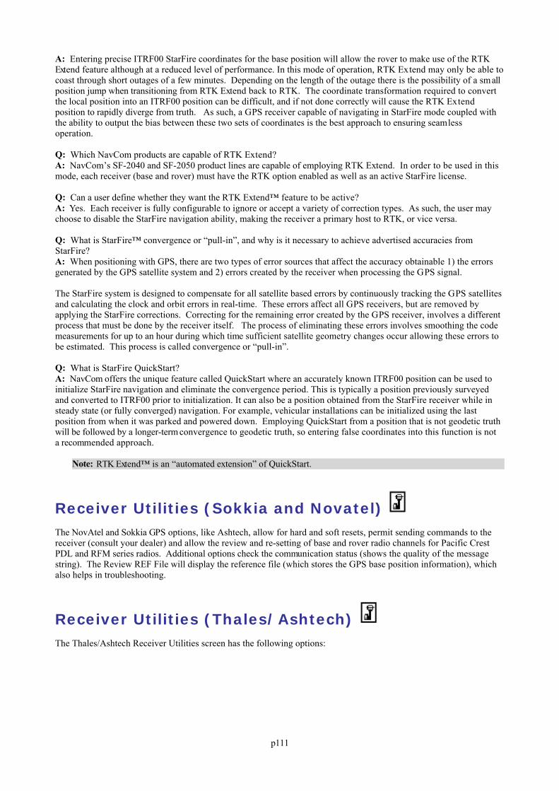
p111

A: Entering precise ITRF00 StarFire coordinates for the base position will allow the rover to make use of the RTKExtend feature although at a reduced level of performance. In this mode of operation, RTK Extend may only be able tocoast through short outages of a few minutes. Depending on the length of the outage there is the possibility of a smallposition jump when transitioning from RTK Extend back to RTK. The coordinate transformation required to convertthe local position into an ITRF00 position can be difficult, and if not done correctly will cause the RTK Extendposition to rapidly diverge from truth. As such, a GPS receiver capable of navigating in StarFire mode coupled withthe ability to output the bias between these two sets of coordinates is the best approach to ensuring seamlessoperation.

Q: Which NavCom products are capable of RTK Extend?A: NavCom’s SF-2040 and SF-2050 product lines are capable of employing RTK Extend. In order to be used in thismode, each receiver (base and rover) must have the RTK option enabled as well as an active StarFire license.

Q: Can a user define whether they want the RTK Extend™ feature to be active?A: Yes. Each receiver is fully configurable to ignore or accept a variety of correction types. As such, the user maychoose to disable the StarFire navigation ability, making the receiver a primary host to RTK, or vice versa.

Q: What is StarFire™ convergence or “pull-in”, and why is it necessary to achieve advertised accuracies fromStarFire?A: When positioning with GPS, there are two types of error sources that affect the accuracy obtainable 1) the errorsgenerated by the GPS satellite system and 2) errors created by the receiver when processing the GPS signal.

The StarFire system is designed to compensate for all satellite based errors by continuously tracking the GPS satellitesand calculating the clock and orbit errors in real-time. These errors affect all GPS receivers, but are removed byapplying the StarFire corrections. Correcting for the remaining error created by the GPS receiver, involves a differentprocess that must be done by the receiver itself. The process of eliminating these errors involves smoothing the codemeasurements for up to an hour during which time sufficient satellite geometry changes occur allowing these errors tobe estimated. This process is called convergence or “pull-in”.

Q: What is StarFire QuickStart?A: NavCom offers the unique feature called QuickStart where an accurately known ITRF00 position can be used toinitialize StarFire navigation and eliminate the convergence period. This is typically a position previously surveyedand converted to ITRF00 prior to initialization. It can also be a position obtained from the StarFire receiver while insteady state (or fully converged) navigation. For example, vehicular installations can be initialized using the lastposition from when it was parked and powered down. Employing QuickStart from a position that is not geodetic truthwill be followed by a longer-term convergence to geodetic truth, so entering false coordinates into this function is nota recommended approach.

Note: RTK Extend™ is an “automated extension” of QuickStart.

Receiver Utilities (Sokkia and Novatel) The NovAtel and Sokkia GPS options, like Ashtech, allow for hard and soft resets, permit sending commands to thereceiver (consult your dealer) and allow the review and re-setting of base and rover radio channels for Pacific CrestPDL and RFM series radios. Additional options check the communication status (shows the quality of the messagestring). The Review REF File will display the reference file (which stores the GPS base position information), whichalso helps in troubleshooting.

Receiver Utilities (Thales/Ashtech) The Thales/Ashtech Receiver Utilities screen has the following options:

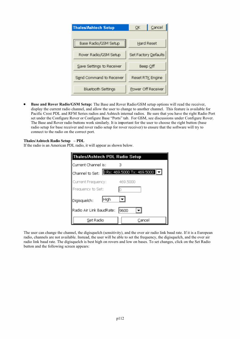
p112

Base and Rover Radio/GSM Setup: The Base and Rover Radio/GSM setup options will read the receiver,display the current radio channel, and allow the user to change to another channel. This feature is available forPacific Crest PDL and RFM Series radios and Ashtech internal radios. Be sure that you have the right Radio Portset under the Configure Rover or Configure Base “Ports” tab. For GSM, see discussions under Configure Rover. The Base and Rover radio buttons work similarly. It is important for the user to choose the right button (baseradio setup for base receiver and rover radio setup for rover receiver) to ensure that the software will try toconnect to the radio on the correct port.

Thales/Ashtech Radio Setup – PDLIf the radio is an American PDL radio, it will appear as shown below.

The user can change the channel, the digisquelch (sensitivity), and the over air radio link baud rate. If it is a Europeanradio, channels are not available. Instead, the user will be able to set the frequency, the digisquelch, and the over airradio link baud rate. The digisquelch is best high on rovers and low on bases. To set changes, click on the Set Radiobutton and the following screen appears:

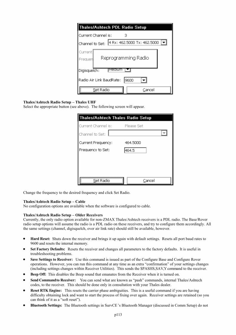
p113

Thales/Ashtech Radio Setup – Thales UHFSelect the appropriate button (see above). The following screen will appear.

Change the frequency to the desired frequency and click Set Radio.

Thales/Ashtech Radio Setup – CableNo configuration options are available when the software is configured to cable.

Thales/Ashtech Radio Setup – Older ReceiversCurrently, the only radio option available for non-ZMAX Thales/Ashtech receivers is a PDL radio. The Base/Roverradio setup options will assume the radio is a PDL radio on these receivers, and try to configure them accordingly. Allthe same settings (channel, digisquelch, over air link rate) should still be available, however.

Hard Reset: Shuts down the receiver and brings it up again with default settings. Resets all port baud rates to9600 and resets the internal memory.

Set Factory Defaults: Resets the receiver and changes all parameters to the factory defaults. It is useful introubleshooting problems.

Save Settings to Receiver: Use this command is issued as part of the Configure Base and Configure Roveroperations. However, you can run this command at any time as an extra “confirmation” of your settings changes(including settings changes within Receiver Utilities). This sends the $PASHS,SAV,Y command to the receiver.

Beep Off: This disables the Beep sound that emanates from the Receiver when it is turned on. Send Command to Receiver: You can send what are known as “pash” commands, internal Thales/Ashtech

codes, to the receiver. This should be done only in consultation with your Thales dealer. Reset RTK Engine: This resets the carrier phase ambiguities. This is a useful command if you are having

difficulty obtaining lock and want to start the process of fixing over again. Receiver settings are retained (so youcan think of it as a “soft reset”).

Bluetooth Settings: The Bluetooth settings in SurvCE ’s Bluetooth Manager (discussed in Comm Setup) do not

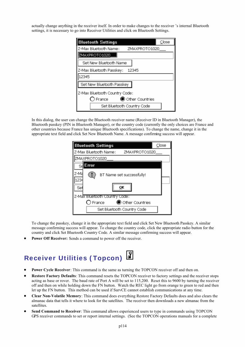
p114

actually change anything in the receiver itself. In order to make changes to the receiver ’s internal Bluetoothsettings, it is necessary to go into Receiver Utilities and click on Bluetooth Settings.

In this dialog, the user can change the Bluetooth receiver name (Receiver ID in Bluetooth Manager), theBluetooth passkey (PIN in Bluetooth Manager), or the country code (currently the only choices are France andother countries because France has unique Bluetooth specifications). To change the name, change it in theappropriate text field and click Set New Bluetooth Name. A message confirming success will appear.

To change the passkey, change it in the appropriate text field and click Set New Bluetooth Passkey. A similarmessage confirming success will appear. To change the country code, click the appropriate radio button for thecountry and click Set Bluetooth Country Code. A similar message confirming success will appear.

Power Off Receiver: Sends a command to power off the receiver.

Receiver Utilities (Topcon)

Power Cycle Receiver: This command is the same as turning the TOPCON receiver off and then on. Restore Factory Defaults: This command resets the TOPCON receiver to factory settings and the receiver stops

acting as base or rover. The baud rate of Port A will be set to 115,200. Reset this to 9600 by turning the receiveroff and then on while holding down the FN button. Watch the REC light go from orange to green to red and thenlet up the FN button. This method can be used if SurvCE cannot establish communications at any time.

Clear Non-Volatile Memory: This command does everything Restore Factory Defaults does and also clears thealmanac data that tells it where to look for the satellites. The receiver then downloads a new almanac from thesatellites.

Send Command to Receiver: This command allows experienced users to type in commands using TOPCONGPS receiver commands to set or report internal settings. (See the TOPCON operations manuals for a complete

p115

list of TOPCON GPS receiver commands). Set Satellite Status: This feature allows the user to disable a satellite if necessary. Initialize to Known Point: The Topcon GPS has a special feature to Initialize to a Known Point which can

greatly speed up “move ups” from one base position to another.

Receiver Utilities (Trimble)

Reset Receiver: This will reset the receiver. Select Rover Input: If you choose Select Rover Input, you can identify the “station id” of the base to avoid

picking up inappropriate base corrections from the wrong base receiver. Check Battery: This will display the condition of the receiver's battery. Power On/Off Receiver: This will turn on and off the receiver.

Localization This command allows you to align on a local coordinate system using the GPS rover receiver. The base receiver canbe on a known point but may also be on an unknown point and located using Read from GPS within Configure Base. The Localization command is essentially “Rover-Based Localization”. Further discussions on localization are foundin Tutorial 2 near the back of the manual.

View: Shown, by default, are the local coordinates. Pressing “View” would show the geodetic, Lat/Loncoordinates.

Scale: The Scale Factor, shown in the Localization dialog when two or more localization points are used, is amultiplier factor and represents “grid to ground”. In release 1.50.004 or higher of SurvCE, and when configuredfor GPS, any GPS localization scale factor is displayed within Job Settings, Units in inverse form to represent“ground to grid”.

Add: Enter the alignment or localization points by coordinate values or by entering a point number. If you choosethe point number method, you can enter a point number or select them from the point list. If you choose the“from list” method, you can access points in the Control File, if a Control File is active (See Job Settings,Options). You can average as many readings as you like when you add points, and view the range and residuals. It is recommended that you use the point number option and carefully hand-enter your local grid systemcoordinates first, using either List Points, option Add, or Keyboard Input. Entry of coordinates “on-the-fly”, inthe field, provides opportunity for error. Once you click OK in the coordinate dialog, the user will have threeoptions for establishing the GPS position for the named local point.

Add Method 1--Read GPS: This allows the user to collect measurements from the GPS receiver andaverage as many readings as preferred. Once the readings are complete, the software will present a dialogthat displays the range and residuals of the averaged readings.

p116

Add Method 2--Enter Latitude/Longitude: This allows the user to hand-enter known geodetic coordinatesfor the local position. The elevation should be the ellipsoid elevation in the jobs current units if a geoidmodel is not applied. If a geoid model is applied, then the elevation should be the orthometric elevation inthe current job units. This method allows manual entry of a localization file without occupying points in thefield. Note that you do not enter the decimal for decimal seconds.

If you use manual entry of a localization data set, it is important that you either utilize an existing base GPSreceiver with the fixed antenna location that was used to survey the original geodetic positions, or that youset up your base on a known GPS position measured previously using that localization data set. Good surveypractice would include checking into known positions to verify the quality of your hand-entered GPSlocalization, and verifying low residuals in the Localization screen. With all data pairs used for bothhorizontal and vertical control (none turned off), the resolutions for this data set would appear.

Add Method 3--From Raw File: This allows the user to use a point from the raw data file that has beenpreviously collected via GPS. This is just like “Read from GPS” except you are recalling a point previouslymeasured and stored in the raw file. For this to work, you must have the base antenna in the same position aswhen the original raw file was collected, or you need to set your base antenna over a known coordinate fromthe original survey, and enter those original coordinates and the new base antenna height within the commandConfigure Base.

Delete: Allows you to delete the selected item from the list. Note that it is not necessary to delete a localizationpoint if you simply want to avoid using it. You can turn “Off” both the horizontal and vertical component of thepoint, but keep it available for use later.

Edit: Allows you to edit the selected item in the list. It will display the northing, easting and elevation of thelocalization point, which can be changed.

On/Off: Allows you to remove the horizontal or vertical components of your localization points. This is afrequently used feature that enables the use of one point for vertical control only (turn off its horizontalcomponent) and other points for horizontal control (turn off their vertical, if appropriate). Points with no knownelevation (0 for example), would obviously be used only for horizontal control, as shown in this ex ample.

p117

Note that in this example, it takes three horizontal control points, active “H On = Y” to get horizontal residualresults, and four vertical control points, active “V On = Y” to get vertical residual results. You can on a trial basisremove different points from consideration both vertically and horizontally and watch the residuals of theremaining control points improve or degrade. In this way, if you have four or more total control points, you candetermine the best combination to use as horizontal and vertical control.

Load: This allows the user to load any localization file for modifying or for the purpose of associating it to thecurrent job. Note that the OK button must be used if the intention is to associate the loaded file to the current job.

Monitor: Goes to the standard Monitor screen. This is particularly useful to verify the quality of your satellitecoverage and your fixed or float status. You always want the best possible fixed status when conducting arover-based localization.

Save: Allows you to save the control points in a file. 2 pt Rotate Only: Allows you to use the second point in the localization file for direction but not for scaling. In

this case, any scale factor set in Job Settings, Units, would be active. OK: Pressing OK will temporarily recall the current Localization as you work. If you change the Localization

file, Save, then Cancel, the original Localization file will still be active. Pressing OK is what makes it active, andcurrent. In this case, you would need to Load the new Localization file and press OK to make it active. Youcould choose to “add” localization points midway on a job, and not actually use them by pressing Save, thenCancel. Then when the job is complete, you could recall the Localization file with all the old and addedlocalization points, go to Process Raw File, and re-calculate all surveying points according to the newLocalization.

Discussion of Localization TechniquesIf you do a base localization by entering Latitude and Longitude or known coordinates on the designated coordinatesystem, then you do not need to add localization points. A base localization would put you on grid north and gridscale and would work for any new job where you are not trying to “match” existing coordinates. However, any timeyou are working on a project that has existing coordinates, you will most likely need to do a Localization. Even if thatexisting job is supposedly on state plane, UTM or another known coordinate system, the project coordinates often failto match grid scale and grid north exactly, requiring localization. When localizing, it is advisable to use at least threepoints for horizontal control and four points for vertical control, in order to get a measure of “residuals” or accuracy. The program will “best fit” a plane through all activated (H=On and/or V=On) control points. The residuals are howmuch each activated point is “off” of the plane surface. Because multiple elevation points may create a slightly“tilted” plane, some surveyors will verify that the vertical control has low residuals and is accurate using multiplevertical control points, then turn off all but one (V=Off) and use only the nearest vertical (elevation) as they progressthrough the job.

Note: The Scale Factor set in Job Settings, Units, will cause all GPS measurements to be adjusted by the scalefactor. For GPS, scale factors can only be entered for 1-point localizations (base or rover). For multi-point roverlocalizations, the scale factor is computed by the localization and fixed. It appears ghosted under Job Settings,Units. When a scale factor is used for 1-point localizations, scaling occurs along the vector outward from thesingle localization point in the direction of the measured point. For GPS, the scale factor acts as a divisor. Ascale factor of 0.9 would calculate the measured point 1/0.9 units further away from the single localization point.Therefore, it is recommended that you keep the scale factor set to 1.0. When configured to total stations, the scalefactor is sometimes used to go “ground to grid”. When configured to GPS, the scale factor in Job Settings, Unitsis sometimes used to go “grid to ground”, to better match total station scaling. The scale factor is defined as“ground to grid”. To go “ground to grid” from high elevations, for example, it would be less than 1. It would

p118

multiply total station measurements and reduce them to grid. It would divide GPS measurements and expandthem to ground. If your goal is to work on the specified state plane, UTM or other grid coordinate system, andyou are planning to use a 1-point localization, then the scale factor should be set to 1, unless you are trying tomatch “ground” coordinates, where the coordinates are “true north” but not “true scale”. In all other cases,matching ground coordinates with GPS is best accomplished with a multi-point rover-based localization. Theresulting “effective” scale factor multipler will appear in the localization screen, such as the 0.999779 valueshown in the last figure.

After a change in a localization file, any points measured in the field by GPS will be converted from Lat/Long to localcoordinates by using the new localization file. For this reason, it is a good idea to re-convert older GPS measurementsto the same, compatible coordinate system by going to Process Raw Data, option Process GPS, within the Cogo menu.

Geoid FilesThe Geoid file is loaded onto SurvCE using Carlson X-Port. You first select the area of interest, then X-Port “carvesout” the geoid for that area and downloads it to SurvCE. You set the Geoid file to use in Job Settings, GPS tab. TheGeoid should be used principally with 1-point localizations. Starting with a known position for the base (or using a1-point rover localization and approximate base position), the program will add or deduct the geoidal separation fromthe computed Z value on all measurements, and will match more closely to geoid-based surface elevations. The G eoidcan also be used with multiple-point rover localizations, since the added accuracy provided by the geoidal calculationcan reduce vertical residuals. This is true, however, only if the points being matched had Z values that, themselves,considered the geoid. Since you will get a best-fit plane that minimizes vertical residuals with or without use of thegeoid, it is often not used with rover-based localizations.

Changing or Updating the Localization FileThere are two ways to change a localization file: one is to edit an existing file by deleting elements, to add additionallocalization points. In either case, whenever a change in the “.dat” localization file is detected, you are promptedwhether you would like to re-process any previously stored GPS points found in the raw file. A dialog appears.

If you answer “Yes”, it takes you to the Process GPS command found within Cogo, Process Raw File.

Recalculating Stored GPS PointsThere is no requirement to survey all localization points first, unless you are doing stakeout. For simple topo or datagathering, you can set up your base, survey in one or two localization points with the rover, then gather data in StorePoints as needed. As you move cross country and encounter another known, or even unex pected control point, youcan localize on it and add it to the list, verify residuals, and if the results are good, you can reprocess the raw file andkeep your entire survey fully updated. If the residuals are disappointing, you can choose not to include the new pointin the localization file. Either remove it or turn its H and V components off. You can also choose Process Raw File torecalculate all GPS measurements at any time.

Including the Base Position in the Localization FileTo use the base in the localization, you should configure the base with the "Use Local Coordinates" option under"From Known Position". Here, you configure the base by entering the local point (5000,5000,100, etc.) and start anew localization file (or use an existing one if it applies). Then, at your rover, you can add more points to thelocalization as necessary.

Localization and the Raw FileIf the scale for GPS is determined from the localization, a “GPS Scale” record of 1.0 and a “Localization Scale” equalto the calculated scale appearing in the Localization screen will be written to the RW5 file.

Using the Localization File to Improve Base Localizations through Logging Static DataThe Localization File (.dat) typically applies to rover-based localizations. But if you did a “Read GPS” on your baseantenna position and then took GPS shots with no rover localization, and logged static data on the base in themeantime, it is possible to submit that logged information to the OPUS program and obtain an accurate base position.

p119

But is it too late to recalculate all the field shots taken earlier from the less accurate base? No. Follow this procedure:1. Store the Base Point (Reference Tab in the Monitor screen). 2. Add a point to the now-empty Localization File. For the local point, enter the grid system coordinate computed

by OPUS or other program. For the geodetic Lat/Lon point, review the raw file and select the point you stored forthe base.

3. Reprocess the raw file through the localization. All CRD points should then be relative to the new calculated (eg.OPUS-generated) coordinate.

Monitor/SkyPlot The Monitor/Skyplot command allows you to review local position and quality of data.

Monitor: Under the Monitor tab you see values for northing, easting, and elevation. Additionally, you canmonitor horizontal and vertical RMS values, as well as PDOP, HDOP, and TDOP values. Some instruments referto RMS values as CEP and SEP. For the CSI DGPS and the Sokkia Axis 3 receivers using OmniStar, the BERvalue will be shown to give indication of the strength of corrections received. When set to CSI DGPS, the age ofcorrections is also displayed. The number of satellites (SATS) is shown.

The Status is shown as either:AUTONOMOUS: No radio communication between base and rover.FLOAT: Communication has been established, but ambiguities have not been resolved.FIXED: Position has been resolved.

Lat/Lon: Under the Lat/Lon tab you see the current position given in latitude, longitude, and elevation. Stateplane northing (SP North) and easting (SP East) values are shown.

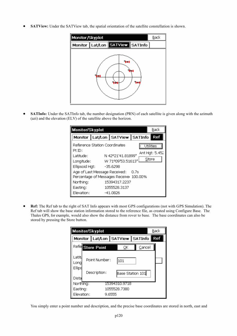
p120

SATView: Under the SATView tab, the spatial orientation of the satellite constellation is shown.

SATInfo: Under the SATInfo tab, the number designation (PRN) of each satellite is given along with the azimuth(azi) and the elevation (ELV) of the satellite above the horizon.

Ref: The Ref tab to the right of SAT Info appears with most GPS configurations (not with GPS Simulation). TheRef tab will show the base station information stored to the reference file, as created using Configure Base. TheThales GPS, for example, would also show the distance from rover to base. The base coordinates can also bestored by pressing the Store button.

You simply enter a point number and description, and the precise base coordinates are stored in north, east and

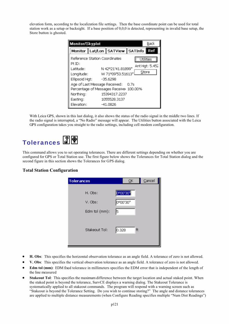
p121

elevation form, according to the localization file settings. Then the base coordinate point can be used for totalstation work as a setup or backsight. If a base position of 0,0,0 is detected, representing in invalid base setup, theStore button is ghosted.

With Leica GPS, shown in this last dialog, it also shows the status of the radio signal in the middle two lines. Ifthe radio signal is interrupted, a “No Radio” message will appear. The Utilities button associated with the LeicaGPS configuration takes you straight to the radio settings, including cell modem configuration.

Tolerances This command allows you to set operating tolerances. There are different settings depending on whether you areconfigured for GPS or Total Station use. The first figure below shows the Tolerances for Total Station dialog and thesecond figure in this section shows the Tolerances for GPS dialog.

Total Station Configuration

H. Obs: This specifies the horizontal observation tolerance as an angle field. A tolerance of zero is not allowed. V. Obs: This specifies the vertical observation tolerance as an angle field. A tolerance of zero is not allowed. Edm tol (mm): EDM fixed tolerance in millimeters specifies the EDM error that is independent of the length of

the line measured Stakeout Tol: This specifies the maximum difference between the target location and actual staked point. When

the staked point is beyond the tolerance, SurvCE displays a warning dialog. The Stakeout Tolerance issystematically applied to all stakeout commands. The program will respond with a warning screen such as“Stakeout is beyond the Tolerance Setting. Do you wish to continue storing?” The angle and distance tolerancesare applied to multiple distance measurements (when Configure Reading specifies multiple “Num Dist Readings”)

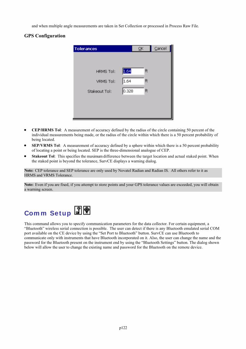
p122

and when multiple angle measurements are taken in Set Collection or processed in Process Raw File.

GPS Configuration

CEP/HRMS Tol: A measurement of accuracy defined by the radius of the circle containing 50 percent of theindividual measurements being made, or the radius of the circle within which there is a 50 percent probability ofbeing located.

SEP/VRMS Tol: A measurement of accuracy defined by a sphere within which there is a 50 percent probabilityof locating a point or being located. SEP is the three-dimensional analogue of CEP.

Stakeout Tol: This specifies the maximum difference between the target location and actual staked point. Whenthe staked point is beyond the tolerance, SurvCE displays a warning dialog.

Note: CEP tolerance and SEP tolerance are only used by Novatel Radian and Radian IS. All others refer to it asHRMS and VRMS Tolerance.

Note: Even if you are fixed, if you attempt to store points and your GPS tolerance values are exceeded, you will obtaina warning screen.

Comm Setup This command allows you to specify communication parameters for the data collector. For certain equipment, a“Bluetooth” wireless serial connection is possible. The user can detect if there is any Bluetooth emulated serial COMport available on the CE device by using the “Set Port to Bluetooth” button. SurvCE can use Bluetooth tocommunicate only with instruments that have Bluetooth incorporated on it. Also, the user can change the name and thepassword for the Bluetooth present on the instrument end by using the “Bluetooth Settings” button. The dialog shownbelow will allow the user to change the existing name and password for the Bluetooth on the remote device.

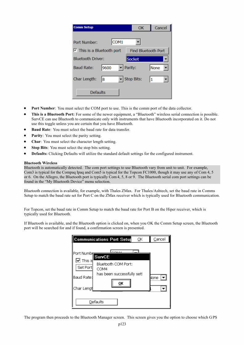
p123

Port Number: You must select the COM port to use. This is the comm port of the data collector. This is a Bluetooth Port: For some of the newer equipment, a “Bluetooth” wireless serial connection is possible.

SurvCE can use Bluetooth to communicate only with instruments that have Bluetooth incorporated on it. Do notuse this toggle unless you are certain that you have Bluetooth.

Baud Rate: You must select the baud rate for data transfer. Parity: You must select the parity setting. Char: You must select the character length setting. Stop Bits: You must select the stop bits setting. Defaults: Clicking Defaults will utilize the standard default settings for the configured instrument.

Bluetooth WirelessBluetooth is automatically detected. The com port settings to use Bluetooth vary from unit to unit. For example,Com3 is typical for the Compaq Ipaq and Com5 is typical for the Topcon FC1000, though it may use any of Com 4, 5or 6. On the Allegro, the Bluetooth port is typically Com 4, 5, 8 or 9. The Bluetooth serial com port settings can befound in the “My Bluetooth Device” menu selection.

Bluetooth connection is available, for example, with Thales ZMax. For Thales/Ashtech, set the baud rate in CommsSetup to match the baud rate set for Port C on the ZMax receiver which is typically used for Bluetooth communication.

For Topcon, set the baud rate in Comm Setup to match the baud rate for Port B on the Hiper receiver, which istypically used for Bluetooth.

If Bluetooth is available, and the Bluetooth option is clicked on, when you OK the Comm Setup screen, the Bluetoothport will be searched for and if found, a confirmation screen is presented.

The program then proceeds to the Bluetooth Manager screen. This screen gives you the option to choose which G PS

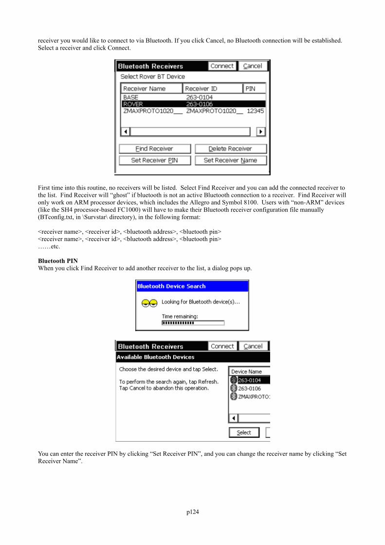
p124

receiver you would like to connect to via Bluetooth. If you click Cancel, no Bluetooth connection will be established. Select a receiver and click Connect.

First time into this routine, no receivers will be listed. Select Find Receiver and you can add the connected receiver tothe list. Find Receiver will “ghost” if bluetooth is not an active Bluetooth connection to a receiver. Find Receiver willonly work on ARM processor devices, which includes the Allegro and Symbol 8100. Users with “non-ARM” devices(like the SH4 processor-based FC1000) will have to make their Bluetooth receiver configuration file manually(BTconfig.txt, in \Survstar\ directory), in the following format:

<receiver name>, <receiver id>, <bluetooth address>, <bluetooth pin><receiver name>, <receiver id>, <bluetooth address>, <bluetooth pin>……etc.

Bluetooth PINWhen you click Find Receiver to add another receiver to the list, a dialog pops up.

You can enter the receiver PIN by clicking “Set Receiver PIN”, and you can change the receiver name by clicking “SetReceiver Name”.

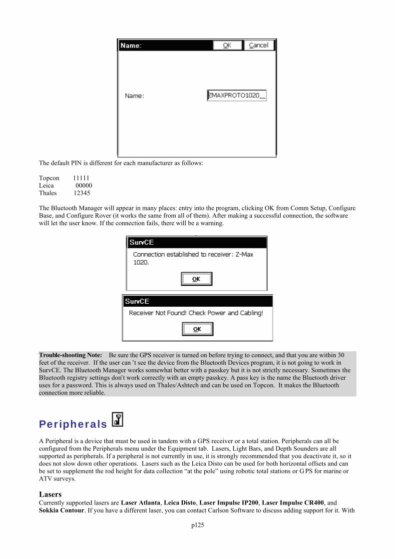
p125

The default PIN is different for each manufacturer as follows:

Topcon 11111Leica 00000Thales 12345

The Bluetooth Manager will appear in many places: entry into the program, clicking OK from Comm Setup, ConfigureBase, and Configure Rover (it works the same from all of them). After making a successful connection, the softwarewill let the user know. If the connection fails, there will be a warning.

Trouble-shooting Note: Be sure the GPS receiver is turned on before trying to connect, and that you are within 30feet of the receiver. If the user can ’t see the device from the Bluetooth Devices program, it is not going to work inSurvCE. The Bluetooth Manager works somewhat better with a passkey but it is not strictly necessary. Sometimes theBluetooth registry settings don’t work correctly with an empty passkey. A pass key is the name the Bluetooth driveruses for a password. This is always used on Thales/Ashtech and can be used on Topcon. It makes the Bluetoothconnection more reliable.

Peripherals A Peripheral is a device that must be used in tandem with a GPS receiver or a total station. Peripherals can all beconfigured from the Peripherals menu under the Equipment tab. Lasers, Light Bars, and Depth Sounders are allsupported as peripherals. If a peripheral is not currently in use, it is strongly recommended that you deactivate it, so itdoes not slow down other operations. Lasers such as the Leica Disto can be used for both horizontal offsets and canbe set to supplement the rod height for data collection “at the pole” using robotic total stations or G PS for marine orATV surveys.

LasersCurrently supported lasers are Laser Atlanta, Leica Disto, Laser Impulse IP200, Laser Impulse CR400, andSokkia Contour. If you have a different laser, you can contact Carlson Software to discuss adding support for it. With

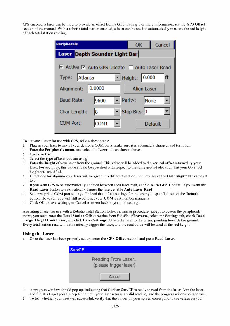
p126

GPS enabled, a laser can be used to provide an offset from a GPS reading. For more information, see the GPS Offsetsection of the manual. With a robotic total station enabled, a laser can be used to automatically measure the rod heightof each total station reading.

To activate a laser for use with GPS, follow these steps:1. Plug in your laser to any of your device’s COM ports, make sure it is adequately charged, and turn it on.2. Enter the Peripherals menu, and select the Laser tab, as shown above.3. Check Active4. Select the type of laser you are using.5. Enter the height of your laser from the ground. This value will be added to the vertical offset returned by your

laser. For accuracy, this value should be specified with respect to the same ground elevation that your GPS rodheight was specified.

6. Directions for aligning your laser will be given in a different section. For now, leave the laser alignment value setto 0.

7. If you want GPS to be automatically updated between each laser read, enable Auto GPS Update. If you want theRead Laser button to automatically trigger the laser, enable Auto Laser Read.

8. Set appropriate COM port settings. To load the default settings for the laser you specified, select the Defaultbutton. However, you will still need to set your COM port number manually.

9. Click OK to save settings, or Cancel to revert back to yoru old settings.

Activating a laser for use with a Robotic Total Station follows a similar procedure, except to access the peripheralsmenu, you must enter the Total Station Offset routine from SideShot/Traverse, select the Settings tab, check ReadTarget Height from Laser, and click Laser Settings. Attach the laser to the prism, pointing towards the ground.Every total station read will automatically trigger the laser, and the read value will be used as the rod height.

Using the Laser1. Once the laser has been properly set up, enter the GPS Offset method and press Read Laser.

2. A progress window should pop up, indicating that Carlson SurvCE is ready to read from the laser. Aim the laserand fire at a target point. Keep firing until your laser returns a valid reading, and the progress window disappears.

3. To test whether your shot was successful, verify that the values on your screen correspond to the values on your

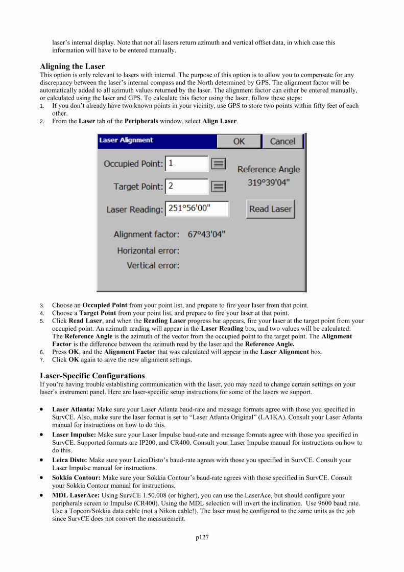
p127

laser’s internal display. Note that not all lasers return azimuth and vertical offset data, in which case thisinformation will have to be entered manually.

Aligning the LaserThis option is only relevant to lasers with internal. The purpose of this option is to allow you to compensate for anydiscrepancy between the laser’s internal compass and the North determined by GPS. The alignment factor will beautomatically added to all azimuth values returned by the laser. The alignment factor can either be entered manually,or calculated using the laser and GPS. To calculate this factor using the laser, follow these steps:1. If you don’t already have two known points in your vicinity, use GPS to store two points within fifty feet of each

other.2. From the Laser tab of the Peripherals window, select Align Laser.

3. Choose an Occupied Point from your point list, and prepare to fire your laser from that point.4. Choose a Target Point from your point list, and prepare to fire your laser at that point.5. Click Read Laser, and when the Reading Laser progress bar appears, fire your laser at the target point from your

occupied point. An azimuth reading will appear in the Laser Reading box, and two values will be calculated:The Reference Angle is the azimuth of the vector from the occupied point to the target point. The AlignmentFactor is the difference between the azimuth read by the laser and the Reference Angle.

6. Press OK, and the Alignment Factor that was calculated will appear in the Laser Alignment box.7. Click OK again to save the new alignment settings.

Laser-Specific ConfigurationsIf you’re having trouble establishing communication with the laser, you may need to change certain settings on yourlaser’s instrument panel. Here are laser-specific setup instructions for some of the lasers we support.

Laser Atlanta: Make sure your Laser Atlanta baud-rate and message formats agree with those you specified inSurvCE. Also, make sure the laser format is set to “Laser Atlanta Original” (LA1KA). Consult your Laser Atlantamanual for instructions on how to do this.

Laser Impulse: Make sure your Laser Impulse baud-rate and message formats agree with those you specified inSurvCE. Supported formats are IP200, and CR400. Consult your Laser Impulse manual for instructions on how todo this.

Leica Disto: Make sure your LeicaDisto’s baud-rate agrees with those you specified in SurvCE. Consult yourLaser Impulse manual for instructions.

Sokkia Contour: Make sure your Sokkia Contour’s baud-rate agrees with those specified in SurvCE. Consultyour Sokkia Contour manual for instructions.

MDL LaserAce: Using SurvCE 1.50.008 (or higher), you can use the LaserAce, but should configure yourperipherals screen to Impulse (CR400). Using the MDL selection will invert the inclination. Use 9600 baud rate. Use a Topcon/Sokkia data cable (not a Nikon cable!). The laser must be configured to the same units as the jobsince SurvCE does not convert the measurement.

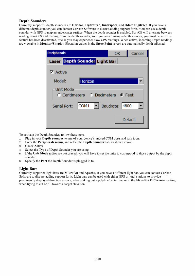
p128

Depth SoundersCurrently supported depth sounders are Horizon, Hydrotrac, Innerspace, and Odom Digitrace. If you have adifferent depth sounder, you can contact Carlson Software to discuss adding support for it. You can use a depthsounder with GPS to map an underwater surface. When the depth sounder is enabled, SurvCE will alternate betweenreading from GPS and reading from the depth sounder, so if you aren ’t using a depth sounder, you must be sure thisfeature has been deactivated, or else you may experience slow GPS readings. When active, incoming Depth readingsare viewable in Monitor/Skyplot. Elevation values in the Store Point screen are automatically depth adjusted.

To activate the Depth Sounder, follow these steps:1. Plug in your Depth Sounder to any of your device’s unused COM ports and turn it on.2. Enter the Peripherals menu, and select the Depth Sounder tab, as shown above.3. Check Active4. Select the Type of Depth Sounder you are using.5. If the Unit Mode radios are not grayed, you will have to set the units to correspond to those output by the depth

sounder.6. Specify the Port the Depth Sounder is plugged in to.

Light BarsCurrently supported light bars are Mikrofyn and Apache. If you have a different light bar, you can contact CarlsonSoftware to discuss adding support for it. Light bars can be used with either GPS or total stations to provideprominently displayed direction arrows, when staking out a polyline/centerline, or in the Elevation Difference routine,when trying to cut or fill toward a target elevation.

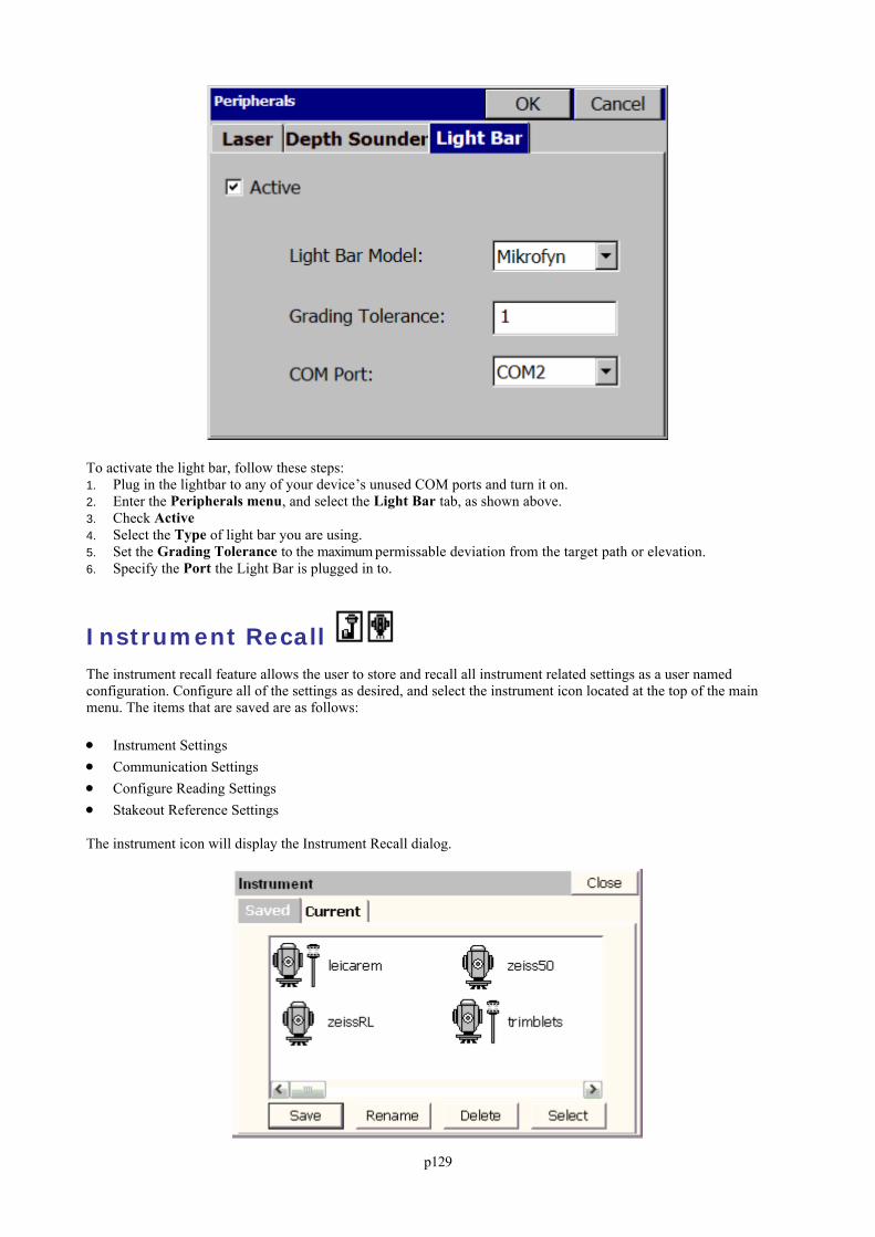
p129

To activate the light bar, follow these steps:1. Plug in the lightbar to any of your device’s unused COM ports and turn it on.2. Enter the Peripherals menu, and select the Light Bar tab, as shown above.3. Check Active4. Select the Type of light bar you are using.5. Set the Grading Tolerance to the maximum permissable deviation from the target path or elevation.6. Specify the Port the Light Bar is plugged in to.

Instrument Recall The instrument recall feature allows the user to store and recall all instrument related settings as a user namedconfiguration. Configure all of the settings as desired, and select the instrument icon located at the top of the mainmenu. The items that are saved are as follows:

Instrument Settings Communication Settings Configure Reading Settings Stakeout Reference Settings

The instrument icon will display the Instrument Recall dialog.

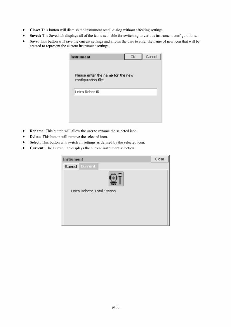
p130

Close: This button will dismiss the instrument recall dialog without affecting settings. Saved: The Saved tab displays all of the icons available for switching to various instrument configurations. Save: This button will save the current settings and allows the user to enter the name of new icon that will be

created to represent the current instrument settings.

Rename: This button will allow the user to rename the selected icon. Delete: This button will remove the selected icon. Select: This button will switch all settings as defined by the selected icon. Current: The Current tab displays the current instrument selection.

p131

Surv MenuThis chapter provides information on using the commands from the Surv menu.

Orientation (Instrument Setup) The instrument setup dialog is displayed upon entering ever routine.

SurvCE 1.21 borrowed from the old SDR style backsight. When you selected the command, you were immediatelyqueried whether you wanted to accept the current occupied point and backsight point information. If everything wasOK, (you simply turned off the instrument for lunch and are starting up again), then you could answer “Yes” andproceed straight to the foresight screen. If the occupied point, backsight point or instrument height had changed, youcould revise the setup information. If only the target height had changed, that can be revised within the foresightscreen.

SurvCE 1.5 simplified the backsight by going straight to the backsight setup/point entry screen. You can verifyeverything, and simply press Enter or OK to continue to the Foresight. Now you can even go to Configure Readingprior to pressing Enter for the Foresight Screen. Note that once in the Foresight Screen, you can select the “Tripod”icon and return to the instrument setup screen for a Check Backsight reading or to re-set the setup information.

When configured to robotic total stations, the “Tripod” icon takes you first to the robotics control screen for quickadjustments and then back to more foresights, or from there, you can tab to the backsight screen and access all thebacksight functions, returning when done to the Foresight Screen.

Occupy Point: Enter the occupied point ID (occupied/setup point). You can also click the list icon (dashed line

p132

icon) and select the point from a list of points, or click the map icon (dots with pointer icon) and select the pointsfrom the map itself, literally by touching point 1031.

Instr. Height: This is the height of the instrument from the center of measurement (typically middle of the lens) tothe tack in the hub or ground elevation over which the instrument is set. If you are configured English, this heightis in feet. If you are configured to Metric, this height is in meters. The units for the job are displayed (ft, ift orm).

Backsight point: Here you enter your backsight point ID, or pick it from a list or from the map itself, using theicons to the right. A backsight point ID is required, even if you choose to enter an azimuth or bearing only.

Backsight Bearing or Azimuth: This displays the bearing or azimuth between the two entered points, when bothpoints have coordinates. If Job Settings, Units, is set to “Angle Type” equals Bearing, then a backsight bearingwill appear. If set to “Angle Type” equals Azimuth, then the backsight azimuth is shown. (Azimuth shouldalways be used with a 400 circle/gons configuration). When both point IDs have coordinates, the backsight isfixed and predetermined and therefore the bearing/azimuth field is disabled since it cannot be altered. However,if the backsight point has no coordinates, then you must enter a backsight bearing or azimuth, which will be usedto calculate the null or zero coordinate point ID.

Target Height: This is the height in feet or meters (depending on your configuration) of the target, from groundelevation to the center of the lens for example.

Note: The backsight target height will default to the previous backsight target height on future setups. Theforesight target height is kept distinct and will default to previous foresight target heights, but will notautomatically match the backsight target height. So if you prefer to survey by setting the prism pole to afixed height for both backsights and foresights, be aware that you will have to put in 2 initial target heights: one for the first backsight in the backsight screen and one for the first foresight in the foresight screen, inorder to get both “remembered” values established.

Use Backsight Ht for Foresights: This option will link the backsight height and the foresight height toaccomodate the use of a single prism for both the backsight and foresight readings, rather than a fixed tripod at thebacksight and roving pole scenario.

Confirm NEZ: This option will display the full coordinates and description of both the setup and backsightpoints. By default, the Setup coordinates will be displayed. You can tab to the backsight coordinates. Press Enteror tap OK to exit this dialog.

Configure: This accesses the Configure Reading screen for a variety of condition or settings changes (eg.Hgt/Desc prompt on save).

Backsight: Continues to the “Take Backsight” screen. OK or pressing Enter: Continues straight to the Foresight screen. If OK is not highlighted and not ghosted,

pressing OK will still go to the Foresight screen, even if Enter does not.

Orientation (Backsight) The backsight dialog has “Setup” and “Results” tabs showing the results of a measurement to the backsight.

Set Angle Option List: There are 4 backsight options for setting the reference angle. They are found in theoption list in the upper left of the Take BS screen:

Set to Zero: This is the most common usage. A message is sent to the instrument to set it to zero, then thebacksight is taken at a zero reference angle, and angles then are typically turned to the right from zero.Set to Backsight Azimuth: In this scenario, the backsight direction in the gun is set to the azimuth of thebacksight. If the backsight azimuth was 180 degree, then an angle to the right of 10 degrees would read 190degrees from the instrument. This is useful in underground mine surveying because it keeps the readingsdisplayed by the total station always referring to true azimuth. Some surveyors are “azimuth” surveyors andothers prefer “set zero”.Set to: User-Entered Azimuth: This option allows the user to “force” a particular backsight azimuth intothe total station as a reference direction. Sometimes non-zero backsight angles are deliberately entered in setcollection, to use different quadrants of the 360 circle.Use Current (Do Not Set Angle): Uses whatever direction reading is already in the instrument.

Set Angle and Read: This button will set the horizontal angle and read the distance to the backsight. Theprogram defaults to the “Set Angle and Read” option (the large, lower button), on the assumption that most often,

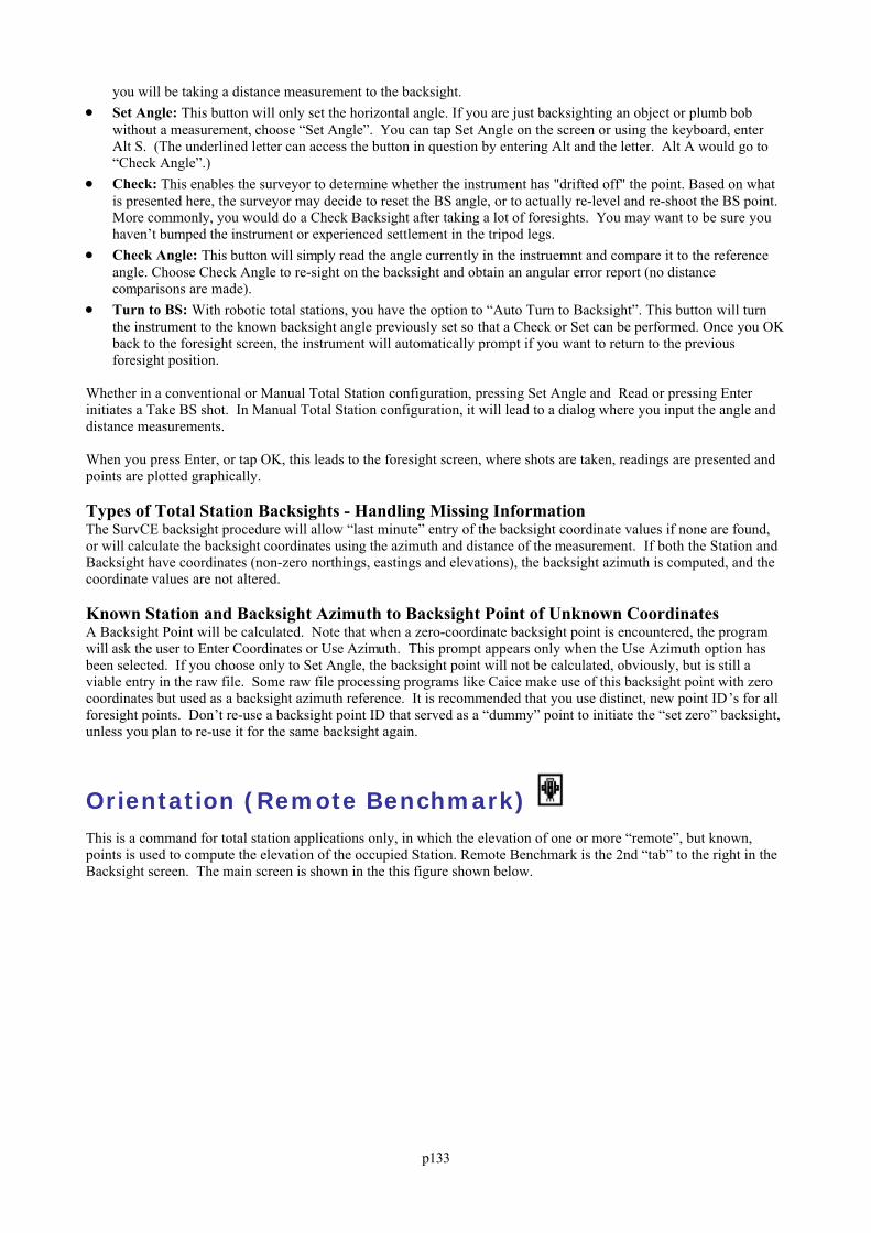
p133

you will be taking a distance measurement to the backsight. Set Angle: This button will only set the horizontal angle. If you are just backsighting an object or plumb bob

without a measurement, choose “Set Angle”. You can tap Set Angle on the screen or using the keyboard, enterAlt S. (The underlined letter can access the button in question by entering Alt and the letter. Alt A would go to“Check Angle”.)

Check: This enables the surveyor to determine whether the instrument has "drifted off" the point. Based on whatis presented here, the surveyor may decide to reset the BS angle, or to actually re-level and re-shoot the BS point. More commonly, you would do a Check Backsight after taking a lot of foresights. You may want to be sure youhaven’t bumped the instrument or experienced settlement in the tripod legs.

Check Angle: This button will simply read the angle currently in the instruemnt and compare it to the referenceangle. Choose Check Angle to re-sight on the backsight and obtain an angular error report (no distancecomparisons are made).

Turn to BS: With robotic total stations, you have the option to “Auto Turn to Backsight”. This button will turnthe instrument to the known backsight angle previously set so that a Check or Set can be performed. Once you OKback to the foresight screen, the instrument will automatically prompt if you want to return to the previousforesight position.

Whether in a conventional or Manual Total Station configuration, pressing Set Angle and Read or pressing Enterinitiates a Take BS shot. In Manual Total Station configuration, it will lead to a dialog where you input the angle anddistance measurements.

When you press Enter, or tap OK, this leads to the foresight screen, where shots are taken, readings are presented andpoints are plotted graphically.

Types of Total Station Backsights - Handling Missing InformationThe SurvCE backsight procedure will allow “last minute” entry of the backsight coordinate values if none are found,or will calculate the backsight coordinates using the azimuth and distance of the measurement. If both the Station andBacksight have coordinates (non-zero northings, eastings and elevations), the backsight azimuth is computed, and thecoordinate values are not altered.

Known Station and Backsight Azimuth to Backsight Point of Unknown CoordinatesA Backsight Point will be calculated. Note that when a zero-coordinate backsight point is encountered, the programwill ask the user to Enter Coordinates or Use Azimuth. This prompt appears only when the Use Azimuth option hasbeen selected. If you choose only to Set Angle, the backsight point will not be calculated, obviously, but is still aviable entry in the raw file. Some raw file processing programs like Caice make use of this backsight point with zerocoordinates but used as a backsight azimuth reference. It is recommended that you use distinct, new point ID’s for allforesight points. Don’t re-use a backsight point ID that served as a “dummy” point to initiate the “set zero” backsight,unless you plan to re-use it for the same backsight again.

Orientation (Remote Benchmark) This is a command for total station applications only, in which the elevation of one or more “remote”, but known,points is used to compute the elevation of the occupied Station. Remote Benchmark is the 2nd “tab” to the right in theBacksight screen. The main screen is shown in the this figure shown below.

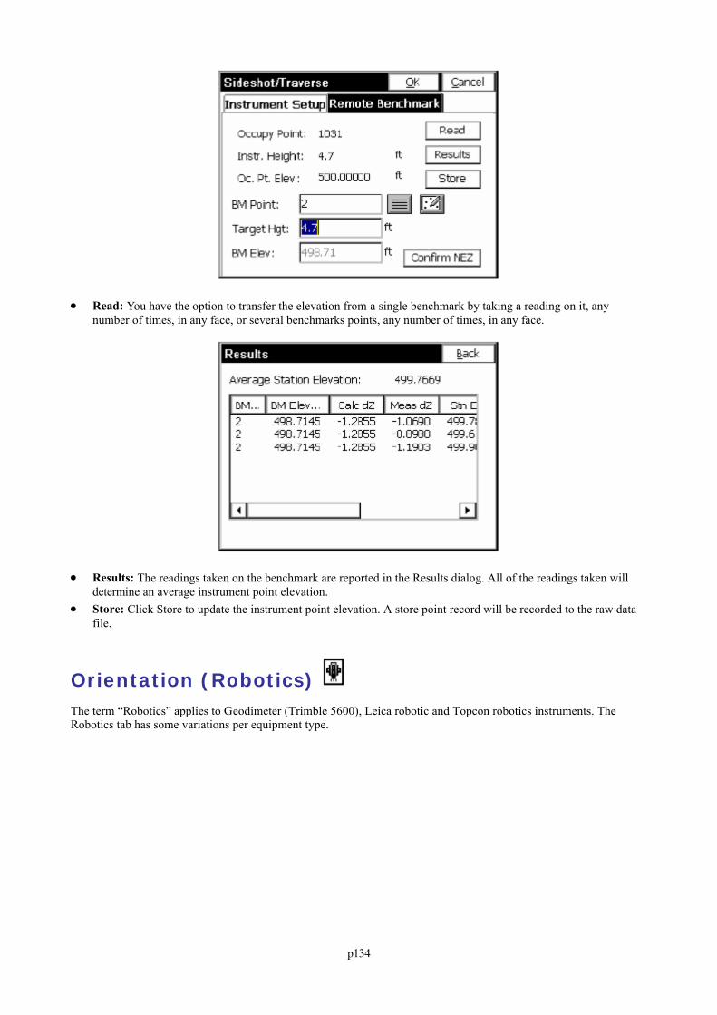
p134

Read: You have the option to transfer the elevation from a single benchmark by taking a reading on it, anynumber of times, in any face, or several benchmarks points, any number of times, in any face.

Results: The readings taken on the benchmark are reported in the Results dialog. All of the readings taken willdetermine an average instrument point elevation.

Store: Click Store to update the instrument point elevation. A store point record will be recorded to the raw datafile.

Orientation (Robotics) The term “Robotics” applies to Geodimeter (Trimble 5600), Leica robotic and Topcon robotics instruments. TheRobotics tab has some variations per equipment type.

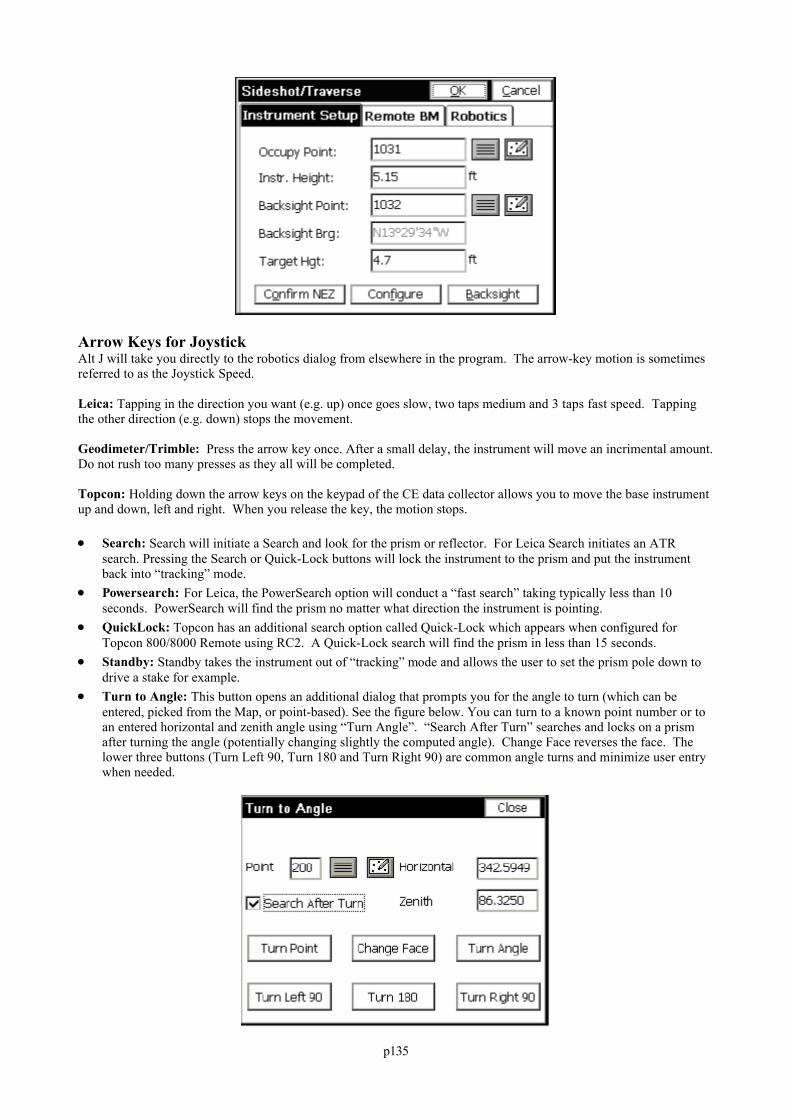
p135

Arrow Keys for JoystickAlt J will take you directly to the robotics dialog from elsewhere in the program. The arrow-key motion is sometimesreferred to as the Joystick Speed.

Leica: Tapping in the direction you want (e.g. up) once goes slow, two taps medium and 3 taps fast speed. Tappingthe other direction (e.g. down) stops the movement.

Geodimeter/Trimble: Press the arrow key once. After a small delay, the instrument will move an incrimental amount.Do not rush too many presses as they all will be completed.

Topcon: Holding down the arrow keys on the keypad of the CE data collector allows you to move the base instrumentup and down, left and right. When you release the key, the motion stops.

Search: Search will initiate a Search and look for the prism or reflector. For Leica Search initiates an ATRsearch. Pressing the Search or Quick-Lock buttons will lock the instrument to the prism and put the instrumentback into “tracking” mode.

Powersearch: For Leica, the PowerSearch option will conduct a “fast search” taking typically less than 10seconds. PowerSearch will find the prism no matter what direction the instrument is pointing.

QuickLock: Topcon has an additional search option called Quick-Lock which appears when configured forTopcon 800/8000 Remote using RC2. A Quick-Lock search will find the prism in less than 15 seconds.

Standby: Standby takes the instrument out of “tracking” mode and allows the user to set the prism pole down todrive a stake for example.

Turn to Angle: This button opens an additional dialog that prompts you for the angle to turn (which can beentered, picked from the Map, or point-based). See the figure below. You can turn to a known point number or toan entered horizontal and zenith angle using “Turn Angle”. “Search After Turn” searches and locks on a prismafter turning the angle (potentially changing slightly the computed angle). Change Face reverses the face. Thelower three buttons (Turn Left 90, Turn 180 and Turn Right 90) are common angle turns and minimize user entrywhen needed.

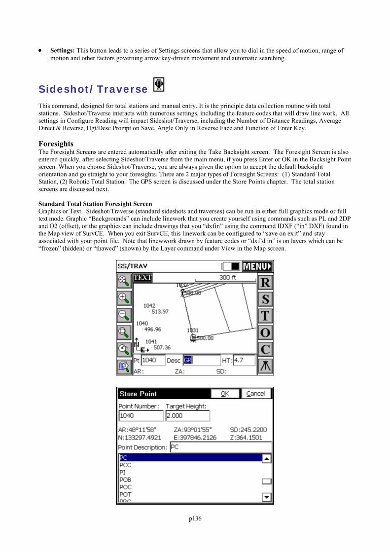
p136

Settings: This button leads to a series of Settings screens that allow you to dial in the speed of motion, range ofmotion and other factors governing arrow key-driven movement and automatic searching.

Sideshot/Traverse This command, designed for total stations and manual entry. It is the principle data collection routine with totalstations. Sideshot/Traverse interacts with numerous settings, including the feature codes that will draw line work. Allsettings in Configure Reading will impact Sideshot/Traverse, including the Number of Distance Readings, AverageDirect & Reverse, Hgt/Desc Prompt on Save, Angle Only in Reverse Face and Function of Enter Key.

ForesightsThe Foresight Screens are entered automatically after exiting the Take Backsight screen. The Foresight Screen is alsoentered quickly, after selecting Sideshot/Traverse from the main menu, if you press Enter or OK in the Backsight Pointscreen. When you choose Sideshot/Traverse, you are always given the option to accept the default backsightorientation and go straight to your foresights. There are 2 major types of Foresight Screens: (1) Standard TotalStation, (2) Robotic Total Station. The GPS screen is discussed under the Store Points chapter. The total stationscreens are discussed next.

Standard Total Station Foresight ScreenGraphics or Text. Sideshot/Traverse (standard sideshots and traverses) can be run in either full graphics mode or fulltext mode. Graphic “Backgrounds” can include linework that you create yourself using commands such as PL and 2DPand O2 (offset), or the graphics can include drawings that you “dxfin” using the command IDXF (“in” DXF) found inthe Map view of SurvCE. When you exit SurvCE, this linework can be configured to “save on exit” and stayassociated with your point file. Note that linewwork drawn by feature codes or “dxf’d in” is on layers which can be“frozen” (hidden) or “thawed” (shown) by the Layer command under View in the Map screen.

p137

Unless the “rod hgt/description” prompt is clicked on, the Sideshot/Traverse screen is designed to “quick-store”points, with the user expected to enter, ahead of time, the correct description and rod heights in the edit boxes shownat the bottom of the dialog.

Sokkia-Style: The SDR33 and earlier SDR data collectors had a convenient concept for “Store Last, Read Next”.You get your descriptions set up and take a shot. The reading is displayed at the bottom line of the screen. Y ouexamine it, satisfy yourself it is correct, move to the next point, and take another shot. This was done on the SDRcollectors with the “Read” key, but with SurvCE, can be accomplished with Enter.

Normal Foresight Style: Most popular collectors are known for their Read & Store procedure, with an“after-shot” pop-up box for entering descriptions and rod height values for the point just measured. Enter Key forRead First, Store Later. This is the “Read or Store” version. Your first Enter is a Read only (like pressing R orentering Alt R). Your second Enter is a Store, which can be followed by the Hgt/Desc Prompt on Save. This isthe “most cautious” designation of the use of the Enter key for taking shots. Note below that after the Read, thepoint is displayed with a question mark, and the raw data is displayed. It is saved only when Enter is pressedagain (or S is pressed, or even Alt S—all of which store a previous Read). In the final Store Point dialog (withRod Hgt/Desc prompt turned on), you are placed in the Point Description field, where Enter continues on. Alldescriptions entered for this job will accumulate in the available Point Description List (here showing PC, PCC,PI, POB, etc.), allowing the user to select the text graphically, arrow key to the desired text, or highlight and selectthe correct text after entering the first character in the edit box. An entry of “P” goes right to all text starting withthe letter “P”. Then you can pick the one you want.

Robotic FeaturesThe “status” of the robot is displayed in the upper left-center, next to TEXT and above the Map. Status modesinclude: Tracking: Locked onto the prism and following it. Standby: Stopped in the last position it was in and ready to resume Tracking. Searching: Looking for the prism. No Data: Brief mode between losing the prism and beginning an automatic Search.

The upper left buttons will display “SRCH” and "STDBY" (Leica will display a combo button "SRCH" or "STDBY"and "DIST") The search and standby buutons let you initiate a Search after a “Lost Lock” condition, or go to Standbyif Tracking was active (to drive a hub and stop the gun from moving), or go back to Search, leading to Tracking, fromStandby (after driving the hub).

For Leica The “DIST” button, takes the EDM signal on and off. With the signal on, more power is used, but you gaina lot by seeing continuous, real-time distance readings and by seeing your position on the screen, in the form of atriangle. Shots are nearly instantaneous, but respond to the “fast-tracking” mode of the EDM (typically 10mm). Iftaken out of EDM Tracking, you lose your real-time movement on the screen, but measurements will respond to theaccuracy of your Equipment Settings, which may call for standard or fine mode.

Note: The response to losing lock when taking foresights with robotic total stations is for the instrument to stop whereit is. If you have set “Search when Lost Lock” on, the instrument will start searching immediately on loss of lock. Alternately, when running remote, you can use the joystick-arrow controls to move the instrument towards you andobtain lock again.

Sideshot Traverse (Offsets) To make offset points using a Total Station requires entry of Alt O or selecting the O/Offset button within theSideshot/Traverse Foresight Screen. This works from both the Graphic and Text screens when foresighting. There isno distinct Total Station “Offset” command—it is an offshoot (literally) of standard Sideshot/Traverse. The Totalstation Offset command must be selected each time it is used. It has three options:

Distance/Angle (sometimes referred to as “Shoot a Big Tree”): The Distance/Angle method requires twomeasurements. The first measurement is the distance followed by the prompt to read the angle. Note how thedialog, shown in the next figure, prompts you to “Read Distance” first.

p138

In the case of shooting a large tree, where the goal is to shoot the center of the tree, you would take a shot to themiddle-side of the tree, equivalent to the distance to the center of the tree. Then you would take a second shot, asprompted, to the middle of the tree, for horizontal angle only. Note that for the elevation of the shot, you can use thedistance measurement or the angle measurement (second reading), and apply the vertical offset, if any, accordingly. After both measurements are taken, the results are displayed as shown in the next figure. You are then returned to thedialog to take your next offset. Tap Close to exit to the main Foresight screen.

Point (Plus/Minus): The Point Offset takes a shot and deducts or adds a distance relative to the line-of-sight in allthree directions (L/R, In/Out, Vertically Up/Down) using the dialog shown in the nex t figure.

Before the shot, tap Read. After the shot, when the raw data is displayed in the lower left, tap Store. You willremain in the command until you tap Close.

p139

2-Point Offset: This creates a 2-point 3D “vector”, where the offset direction, distance and vertical offset iscomputed from the delta N, delta E and Delta Z of the 2 points that are measured or entered. If “Read Inst” isclicked on, then the 2 points are measured in the field. If instead you wish to obtain the offset vector from 2points, then click off Read Inst. and enter the 2 point numbers. The offset entered will extend the vector frompoint “P2” in the direction of “P1” to “P2”. The vector offset will also impact the elevation that is calculated. This might be used to calculate a point at the top of a cliff, for example, where you stand above the cliff top andpick up 2 points on the slope to the cliff edge, and estimate the distance to the cliff face from the second point. The offset by 2 points routine will write an SS record in the RW5 file (raw file), which enables re-processing.

Settings: The Settings tab permits reading the target height from a laser and accesses the entire range of laserdevices found in the Peripherals menu option under Equip.

Store Points Store Points is the principle data collection routine for GPS equipment. Store Points interacts with numerous settings,including the feature codes, and will draw line work. The Store Points screen in GPS shows the cursor moving on thescreen in real-time. Shots can be taken anytime by pressing Enter. The screen will pan automatically, so you arealways in view as you move. Points will plot on the screen as shots are taken.

In GPS mode, Enter has only one function: Read & Store. If you want the “after-shot” antenna height and descriptionprompt, then that can be turned on in Configure Reading (C or Alt C from the Store Points screen). If you don’t havethe height and description prompt turned on, then each shot is a single press of Enter, and you must put any antennaheight changes or description or point ID changes in ahead of time, prior to pressing Enter.

Coordinates are displayed at all times, as well as the Status (Fixed, Float, Autonomous) and HRMS and VRMSaccuracy estimates. The icons at the left are for zooming and panning. From top to bottom, they are zoom extents,

p140

zoom in, zoom out, zoom window, zoom previous and point display control. If you prefer to work in a pure “Text”screen, without graphics, you can tap the “TEXT” button in the upper left. The following dialog will appear.

The Text screen uses a large character size for easy viewing, and limits options to Monitor/Skyplot, Offset and Store. You can return to the “Graph” view by tapping the Graph button. You can also temporarily view your points on thescreen by tapping “Map”, then tap “Back” to return to the text-based data collection screen. Note that the programwill “remember” which screen you were in last (Graph or Text) and return to that “mode” of data collectionautomatically.

In addition to pressing Enter, points can be stored by tapping S on the screen, or Alt S on the keyboard.

Pressing O for Offset leads to a GPS Offset screen that has options for keyed in offsets, as well as offsets takenby laser devices that measure distance only, or distance and azimuth (by compass).

With GPS, since shots “cluster” around the true point location, it may add to accuracy to average 10 or moreGPS readings when taking measurements. You will be prompted for how many readings to take (up to 999). Taking100 readings is also a way to guage how fast your GPS equipment takes measurements. If 100 readings are taken in10 seconds, you are reading at 10 per second, or 10 “hertz” (hz). After the readings are taken, a display appearsshowing the range and standard deviation of the readings.

You can press C (or enter Alt C) to go directly to the Configure Reading screen, where you can set the numberof readings to average, specify to store only fixed readings and turn on or off the Hgt/Desc prompt on Save.

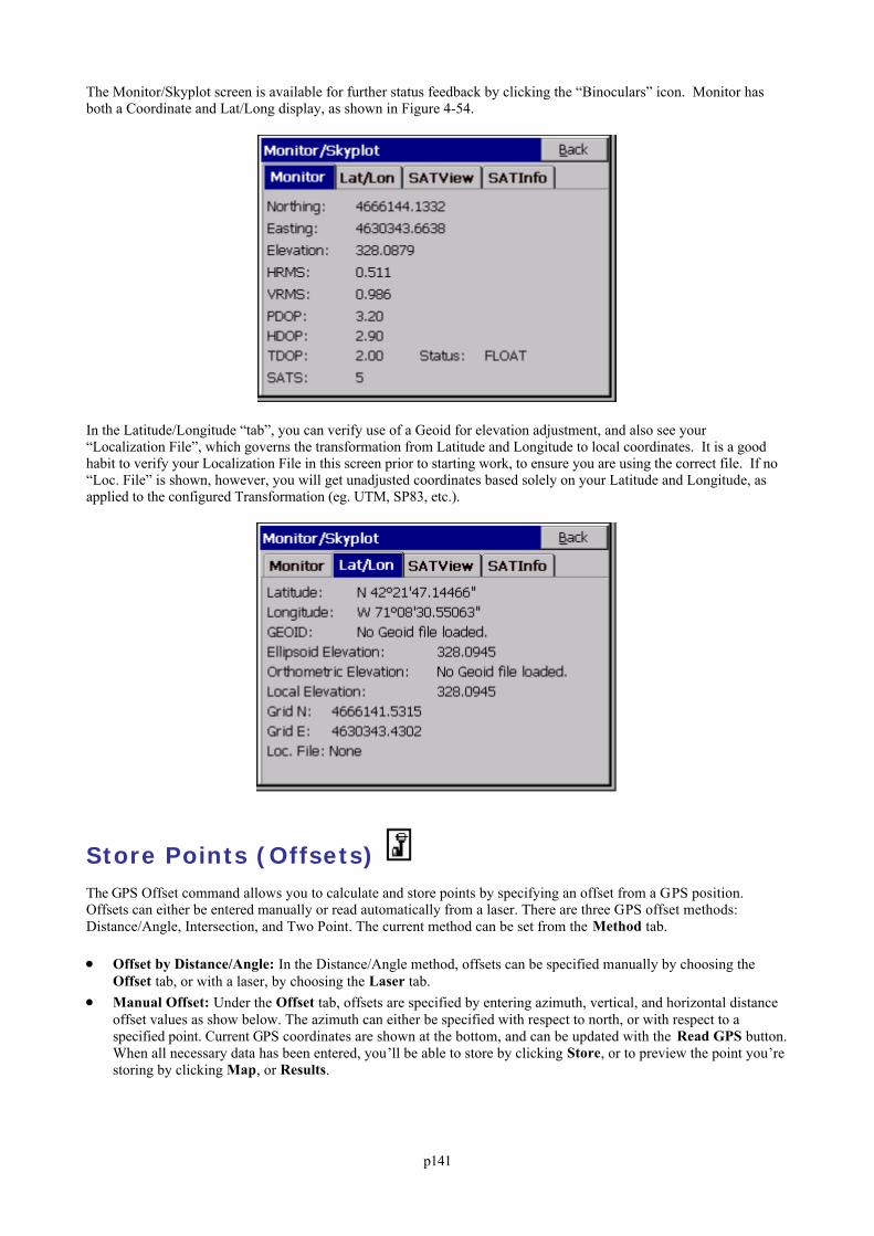
p141

The Monitor/Skyplot screen is available for further status feedback by clicking the “Binoculars” icon. Monitor hasboth a Coordinate and Lat/Long display, as shown in Figure 4-54.

In the Latitude/Longitude “tab”, you can verify use of a Geoid for elevation adjustment, and also see your“Localization File”, which governs the transformation from Latitude and Longitude to local coordinates. It is a goodhabit to verify your Localization File in this screen prior to starting work, to ensure you are using the correct file. If no“Loc. File” is shown, however, you will get unadjusted coordinates based solely on your Latitude and Longitude, asapplied to the configured Transformation (eg. UTM, SP83, etc.).

Store Points (Offsets) The GPS Offset command allows you to calculate and store points by specifying an offset from a GPS position.Offsets can either be entered manually or read automatically from a laser. There are three GPS offset methods:Distance/Angle, Intersection, and Two Point. The current method can be set from the Method tab.

Offset by Distance/Angle: In the Distance/Angle method, offsets can be specified manually by choosing theOffset tab, or with a laser, by choosing the Laser tab.

Manual Offset: Under the Offset tab, offsets are specified by entering azimuth, vertical, and horizontal distanceoffset values as show below. The azimuth can either be specified with respect to north, or with respect to aspecified point. Current GPS coordinates are shown at the bottom, and can be updated with the Read GPS button.When all necessary data has been entered, you’ll be able to store by clicking Store, or to preview the point you’restoring by clicking Map, or Results.

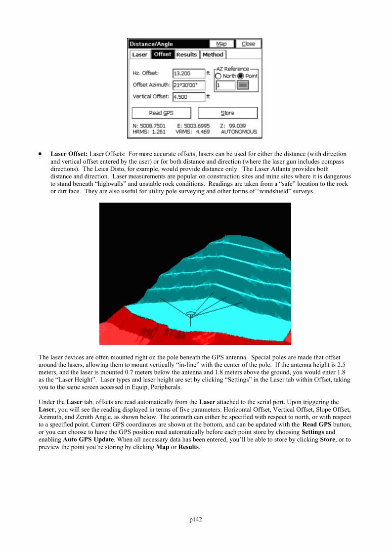
p142

Laser Offset: Laser Offsets: For more accurate offsets, lasers can be used for either the distance (with directionand vertical offset entered by the user) or for both distance and direction (where the laser gun includes compassdirections). The Leica Disto, for example, would provide distance only. The Laser Atlanta provides bothdistance and direction. Laser measurements are popular on construction sites and mine sites where it is dangerousto stand beneath “highwalls” and unstable rock conditions. Readings are taken from a “safe” location to the rockor dirt face. They are also useful for utility pole surveying and other forms of “windshield” surveys.

The laser devices are often mounted right on the pole beneath the GPS antenna. Special poles are made that offsetaround the lasers, allowing them to mount vertically “in-line” with the center of the pole. If the antenna height is 2.5meters, and the laser is mounted 0.7 meters below the antenna and 1.8 meters above the ground, you would enter 1.8as the “Laser Height”. Laser types and laser height are set by clicking “Settings” in the Laser tab within Offset, takingyou to the same screen accessed in Equip, Peripherals.

Under the Laser tab, offsets are read automatically from the Laser attached to the serial port. Upon triggering theLaser, you will see the reading displayed in terms of five parameters: Horizontal Offset, Vertical Offset, Slope Offset,Azimuth, and Zenith Angle, as shown below. The azimuth can either be specified with respect to north, or with respectto a specified point. Current GPS coordinates are shown at the bottom, and can be updated with the Read GPS button,or you can choose to have the GPS position read automatically before each point store by choosing Settings andenabling Auto GPS Update. When all necessary data has been entered, you’ll be able to store by clicking Store, or topreview the point you’re storing by clicking Map or Results.

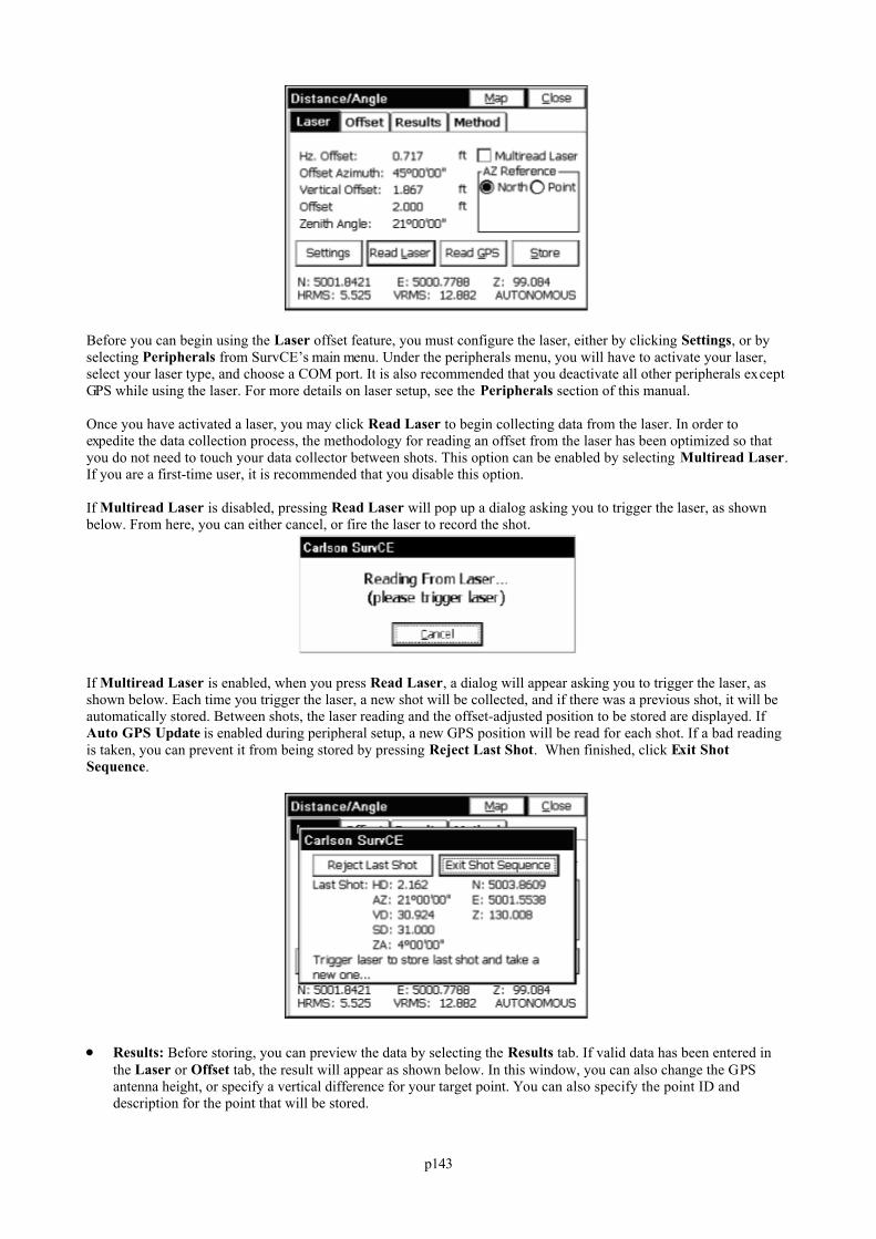
p143

Before you can begin using the Laser offset feature, you must configure the laser, either by clicking Settings, or byselecting Peripherals from SurvCE’s main menu. Under the peripherals menu, you will have to activate your laser,select your laser type, and choose a COM port. It is also recommended that you deactivate all other peripherals exceptGPS while using the laser. For more details on laser setup, see the Peripherals section of this manual.

Once you have activated a laser, you may click Read Laser to begin collecting data from the laser. In order toexpedite the data collection process, the methodology for reading an offset from the laser has been optimized so thatyou do not need to touch your data collector between shots. This option can be enabled by selecting Multiread Laser.If you are a first-time user, it is recommended that you disable this option.

If Multiread Laser is disabled, pressing Read Laser will pop up a dialog asking you to trigger the laser, as shownbelow. From here, you can either cancel, or fire the laser to record the shot.

If Multiread Laser is enabled, when you press Read Laser, a dialog will appear asking you to trigger the laser, asshown below. Each time you trigger the laser, a new shot will be collected, and if there was a previous shot, it will beautomatically stored. Between shots, the laser reading and the offset-adjusted position to be stored are displayed. If Auto GPS Update is enabled during peripheral setup, a new GPS position will be read for each shot. If a bad readingis taken, you can prevent it from being stored by pressing Reject Last Shot. When finished, click Exit ShotSequence.

Results: Before storing, you can preview the data by selecting the Results tab. If valid data has been entered inthe Laser or Offset tab, the result will appear as shown below. In this window, you can also change the GPSantenna height, or specify a vertical difference for your target point. You can also specify the point ID anddescription for the point that will be stored.

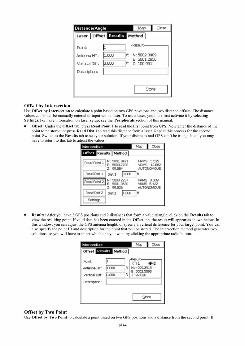
p144

Offset by IntersectionUse Offset by Intersection to calculate a point based on two GPS positions and two distance offsets. The distancevalues can either be manually entered or input with a laser. To use a laser, you must first activate it by selecting Settings. For more information on laser setup, see the Peripherals section of this manual. Offset: Under the Offset tab, press Read Point 1 to read the first point from GPS. Now enter the distance of the

point to be stored, or press Read Dist 1 to read this distance from a laser. Repeat this process for the secondpoint. Switch to the Results tab to see your solution. If your distances and GPS can’t be triangulated, you mayhave to return to this tab to adjust the values.

Results: After you have 2 GPS positions and 2 distances that form a valid triangle, click on the Results tab toview the resulting point. If valid data has been entered in the Offset tab, the result will appear as shown below. Inthis window, you can adjust the GPS antenna height, or specify a vertical difference for your target point. You canalso specify the point ID and description for the point that will be stored. The intersection method generates twosolutions, so you will have to select which one you want by clicking the appropriate radio button.

Offset by Two PointUse Offset by Two Point to calculate a point based on two GPS positions and a distance from the second point. If

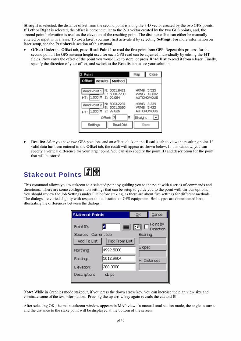
p145

Straight is selected, the distance offset from the second point is along the 3-D vector created by the two GPS points.If Left or Right is selected, the offset is perpendicular to the 2-D vector created by the two GPS points, and, thesecond point’s elevation is used as the elevation of the resulting point. The distance offset can either be manuallyentered or input with a laser. To use a laser, you must first activate it by selecting Settings. For more information onlaser setup, see the Peripherals section of this manual. Offset: Under the Offset tab, press Read Point 1 to read the first point from GPS. Repeat this process for the

second point. The GPS antenna height used for each GPS read can be adjusted individually by editing the HTfields. Now enter the offset of the point you would like to store, or press Read Dist to read it from a laser. Finally,specify the direction of your offset, and switch to the Results tab to see your solution.

Results: After you have two GPS positions and an offset, click on the Results tab to view the resulting point. Ifvalid data has been entered in the Offset tab, the result will appear as shown below. In this window, you canspecify a vertical difference for your target point. You can also specify the point ID and description for the pointthat will be stored.

Stakeout Points This command allows you to stakeout to a selected point by guiding you to the point with a series of commands anddirections. There are some configuration settings that can be setup to guide you to the point with various options. You should review the Job Settings under File before staking, as there are about five settings for different methods. The dialogs are varied slightly with respect to total station or GPS equipment. Both types are documented here,illustrating the differences between the dialogs.

Note: While in Graphics mode stakeout, if you press the down arrow key, you can increase the plan view size andeliminate some of the text information. Pressing the up arrow key again reveals the cut and fill.

After selecting OK, the main stakeout window appears in MAP view. In manual total station mode, the angle to turn toand the distance to the stake point will be displayed at the bottom of the screen.

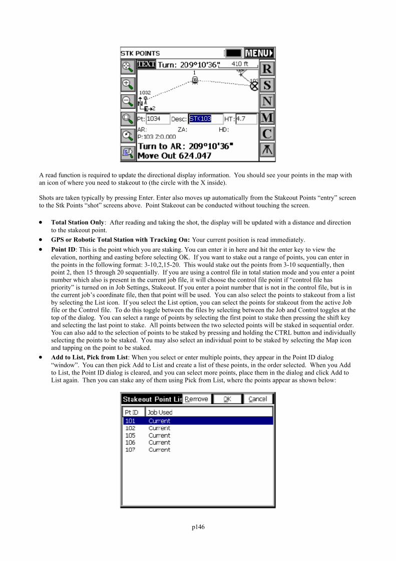
p146

A read function is required to update the directional display information. You should see your points in the map withan icon of where you need to stakeout to (the circle with the X inside).

Shots are taken typically by pressing Enter. Enter also moves up automatically from the Stakeout Points “entry” screento the Stk Points “shot” screens above. Point Stakeout can be conducted without touching the screen.

Total Station Only: After reading and taking the shot, the display will be updated with a distance and directionto the stakeout point.

GPS or Robotic Total Station with Tracking On: Your current position is read immediately. Point ID: This is the point which you are staking. You can enter it in here and hit the enter key to view the

elevation, northing and easting before selecting OK. If you want to stake out a range of points, you can enter inthe points in the following format: 3-10,2,15-20. This would stake out the points from 3-10 sequentially, thenpoint 2, then 15 through 20 sequentially. If you are using a control file in total station mode and you enter a pointnumber which also is present in the current job file, it will choose the control file point if “control file haspriority” is turned on in Job Settings, Stakeout. If you enter a point number that is not in the control file, but is inthe current job’s coordinate file, then that point will be used. You can also select the points to stakeout from a listby selecting the List icon. If you select the List option, you can select the points for stakeout from the active Jobfile or the Control file. To do this toggle between the files by selecting between the Job and Control toggles at thetop of the dialog. You can select a range of points by selecting the first point to stake then pressing the shift keyand selecting the last point to stake. All points between the two selected points will be staked in sequential order. You can also add to the selection of points to be staked by pressing and holding the CTRL button and individuallyselecting the points to be staked. You may also select an individual point to be staked by selecting the Map iconand tapping on the point to be staked.

Add to List, Pick from List: When you select or enter multiple points, they appear in the Point ID dialog“window”. You can then pick Add to List and create a list of these points, in the order selected. When you Addto List, the Point ID dialog is cleared, and you can select more points, place them in the dialog and click Add toList again. Then you can stake any of them using Pick from List, where the points appear as shown below:

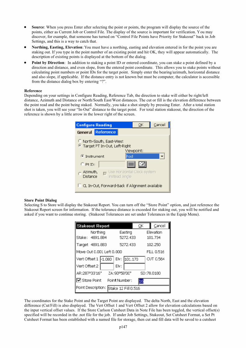
p147

Source: When you press Enter after selecting the point or points, the program will display the source of thepoints, either as Current Job or Control File. The display of the source is important for verification. You maydiscover, for example, that someone has turned on “Control File Points have Priority for Stakeout” back in JobSettings, and this is a way to catch that.

Northing, Easting, Elevation: You must have a northing, easting and elevation entered in for the point you arestaking out. If you type in the point number of an existing point and hit OK, they will appear automatically. Thedescription of existing points is displayed at the bottom of the dialog.

Point by Direction: In addition to staking a point ID or entered coordinate, you can stake a point defined by adirection and distance, and even slope, from the entered point coordinate. This allows you to stake points withoutcalculating point numbers or point IDs for the target point. Simply enter the bearing/azimuth, horizontal distanceand also slope, if applicable. If the distance entry is not known but must be computer, the calculator is accessiblefrom the distance dialog box by entering “?”.

ReferenceDepending on your settings in Configure Reading, Reference Tab, the direction to stake will either be right/leftdistance, Azimuth and Distance or North/South East/West distances. The cut or fill is the elevation difference betweenthe point read and the point being staked. Normally, you take a shot simply by pressing Enter. After a total stationshot is taken, you will see your “In-Out” distance to the target point. For total station stakeout, the direction of thereference is shown by a little arrow in the lower right of the screen.

Store Point DialogSelecting S to Store will display the Stakeout Report. You can turn off the “Store Point” option, and just reference theStakeout Report screen for information. If the tolerance distance is exceeded for staking out, you will be notified andasked if you want to continue storing. (Stakeout Tolerances are set under Tolerances in the Equip Menu).

The coordinates for the Stake Point and the Target Point are displayed. The delta North, East and the elevationdifference (Cut/Fill) is also displayed. The Vert Offset 1 and Vert Offset 2 allow for elevation calculations based onthe input vertical offset values. If the Store Carlson Cutsheet Data in Note File has been toggled, the vertical offset(s)specified will be recorded in the .not file for the job. If under Job Settings, Stakeout, Set Cutsheet Format, a Set PtCutsheet Format has been established with a named file for storage, then cut and fill data will be saved to a cutsheet

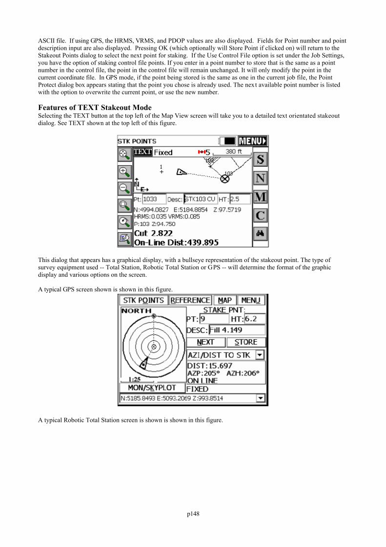
p148

ASCII file. If using GPS, the HRMS, VRMS, and PDOP values are also displayed. Fields for Point number and pointdescription input are also displayed. Pressing OK (which optionally will Store Point if clicked on) will return to theStakeout Points dialog to select the next point for staking. If the Use Control File option is set under the Job Settings,you have the option of staking control file points. If you enter in a point number to store that is the same as a pointnumber in the control file, the point in the control file will remain unchanged. It will only modify the point in thecurrent coordinate file. In GPS mode, if the point being stored is the same as one in the current job file, the PointProtect dialog box appears stating that the point you chose is already used. The next available point number is listedwith the option to overwrite the current point, or use the new number.

Features of TEXT Stakeout ModeSelecting the TEXT button at the top left of the Map View screen will take you to a detailed text orientated stakeoutdialog. See TEXT shown at the top left of this figure.

This dialog that appears has a graphical display, with a bullseye representation of the stakeout point. The type ofsurvey equipment used -- Total Station, Robotic Total Station or GPS -- will determine the format of the graphicdisplay and various options on the screen.

A typical GPS screen shown is shown in this figure.

A typical Robotic Total Station screen is shown is shown in this figure.

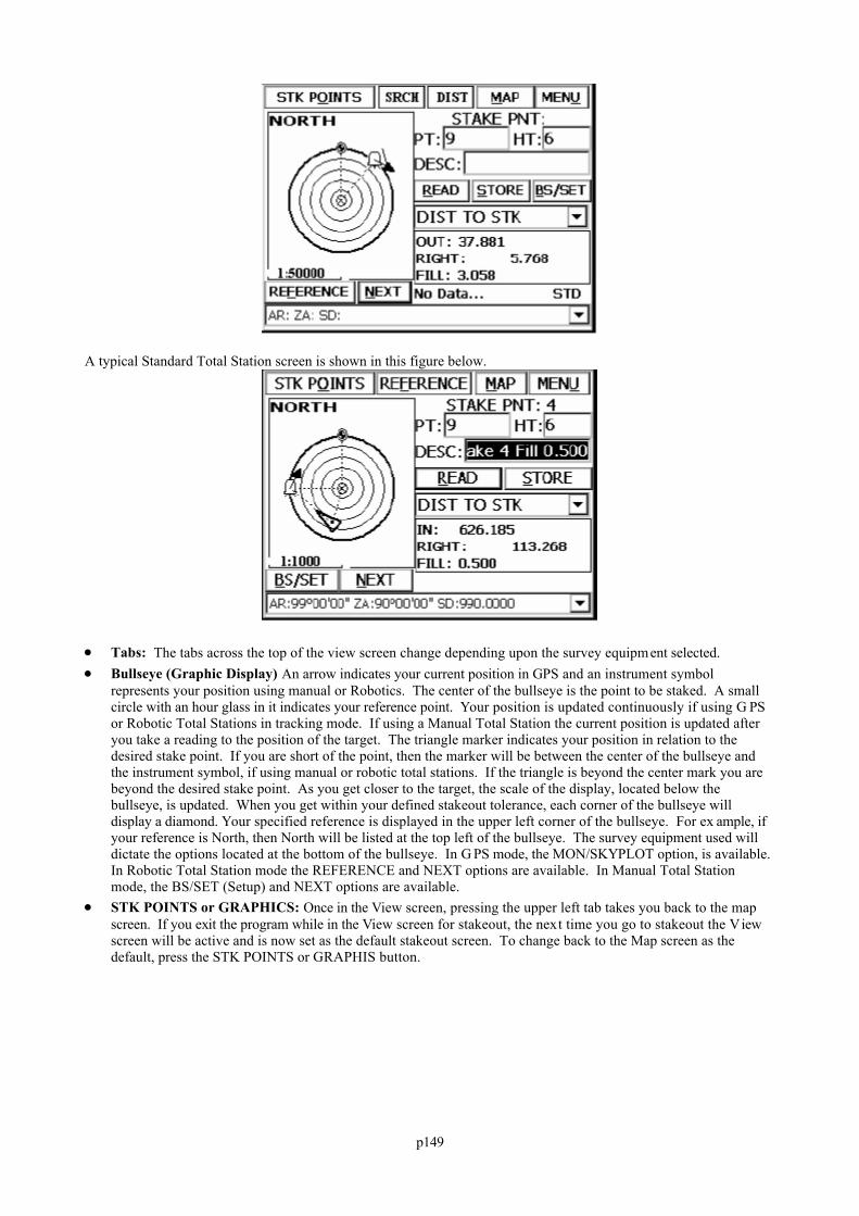
p149

A typical Standard Total Station screen is shown in this figure below.

Tabs: The tabs across the top of the view screen change depending upon the survey equipment selected. Bullseye (Graphic Display) An arrow indicates your current position in GPS and an instrument symbol

represents your position using manual or Robotics. The center of the bullseye is the point to be staked. A smallcircle with an hour glass in it indicates your reference point. Your position is updated continuously if using G PSor Robotic Total Stations in tracking mode. If using a Manual Total Station the current position is updated afteryou take a reading to the position of the target. The triangle marker indicates your position in relation to thedesired stake point. If you are short of the point, then the marker will be between the center of the bullseye andthe instrument symbol, if using manual or robotic total stations. If the triangle is beyond the center mark you arebeyond the desired stake point. As you get closer to the target, the scale of the display, located below thebullseye, is updated. When you get within your defined stakeout tolerance, each corner of the bullseye willdisplay a diamond. Your specified reference is displayed in the upper left corner of the bullseye. For ex ample, ifyour reference is North, then North will be listed at the top left of the bullseye. The survey equipment used willdictate the options located at the bottom of the bullseye. In G PS mode, the MON/SKYPLOT option, is available. In Robotic Total Station mode the REFERENCE and NEXT options are available. In Manual Total Stationmode, the BS/SET (Setup) and NEXT options are available.

STK POINTS or GRAPHICS: Once in the View screen, pressing the upper left tab takes you back to the mapscreen. If you exit the program while in the View screen for stakeout, the next time you go to stakeout the Viewscreen will be active and is now set as the default stakeout screen. To change back to the Map screen as thedefault, press the STK POINTS or GRAPHIS button.

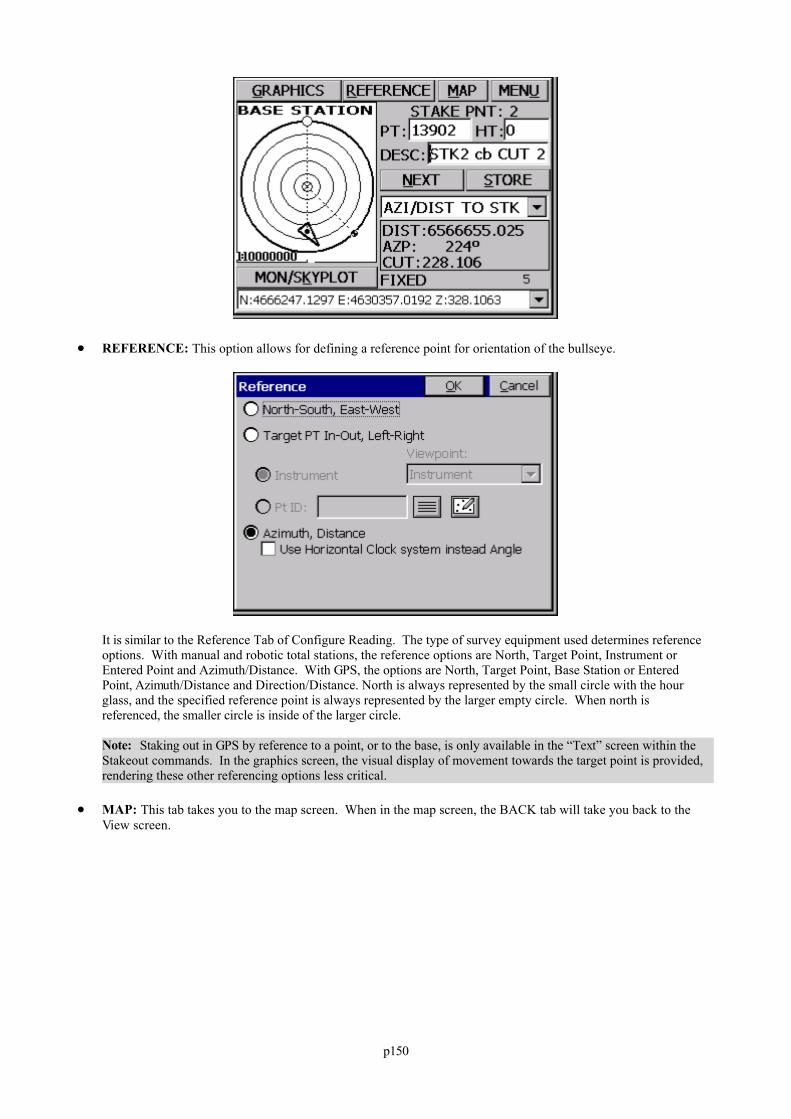
p150

REFERENCE: This option allows for defining a reference point for orientation of the bullseye.

It is similar to the Reference Tab of Configure Reading. The type of survey equipment used determines referenceoptions. With manual and robotic total stations, the reference options are North, Target Point, Instrument orEntered Point and Azimuth/Distance. With GPS, the options are North, Target Point, Base Station or EnteredPoint, Azimuth/Distance and Direction/Distance. North is always represented by the small circle with the hourglass, and the specified reference point is always represented by the larger empty circle. When north isreferenced, the smaller circle is inside of the larger circle.

Note: Staking out in GPS by reference to a point, or to the base, is only available in the “Text” screen within theStakeout commands. In the graphics screen, the visual display of movement towards the target point is provided,rendering these other referencing options less critical.

MAP: This tab takes you to the map screen. When in the map screen, the BACK tab will take you back to theView screen.

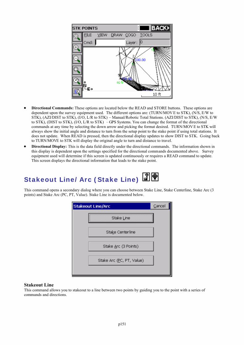
p151

Directional Commands: These options are located below the READ and STORE buttons. These options aredependent upon the survey equipment used. The different options are: (TURN/MOV E to STK), (N/S, E/W toSTK), (AZI/DIST to STK), (I/O, L/R to STK) – Manual/Robotic Total Stations. (AZI/DIST to STK), (N/S, E/Wto STK), (DIST to STK), (I/O, L/R to STK) – GPS Systems. You can change the format of the directionalcommands at any time by selecting the down arrow and picking the format desired. TURN/MOV E to STK willalways show the initial angle and distance to turn from the setup point to the stake point if using total stations. Itdoes not update. When READ is pressed, then the directional display updates to show DIST to STK. Going backto TURN/MOVE to STK will display the original angle to turn and distance to travel.

Directional Display: This is the data field directly under the directional commands. The information shown inthis display is dependent upon the settings specified for the directional commands documented above. Surveyequipment used will determine if this screen is updated continuously or requires a READ command to update. This screen displays the directional information that leads to the stake point.

Stakeout Line/Arc (Stake Line) This command opens a secondary dialog where you can choose between Stake Line, Stake Centerline, Stake Arc (3points) and Stake Arc (PC, PT, Value). Stake Line is documented below.

Stakeout LineThis command allows you to stakeout to a line between two points by guiding you to the point with a series ofcommands and directions.

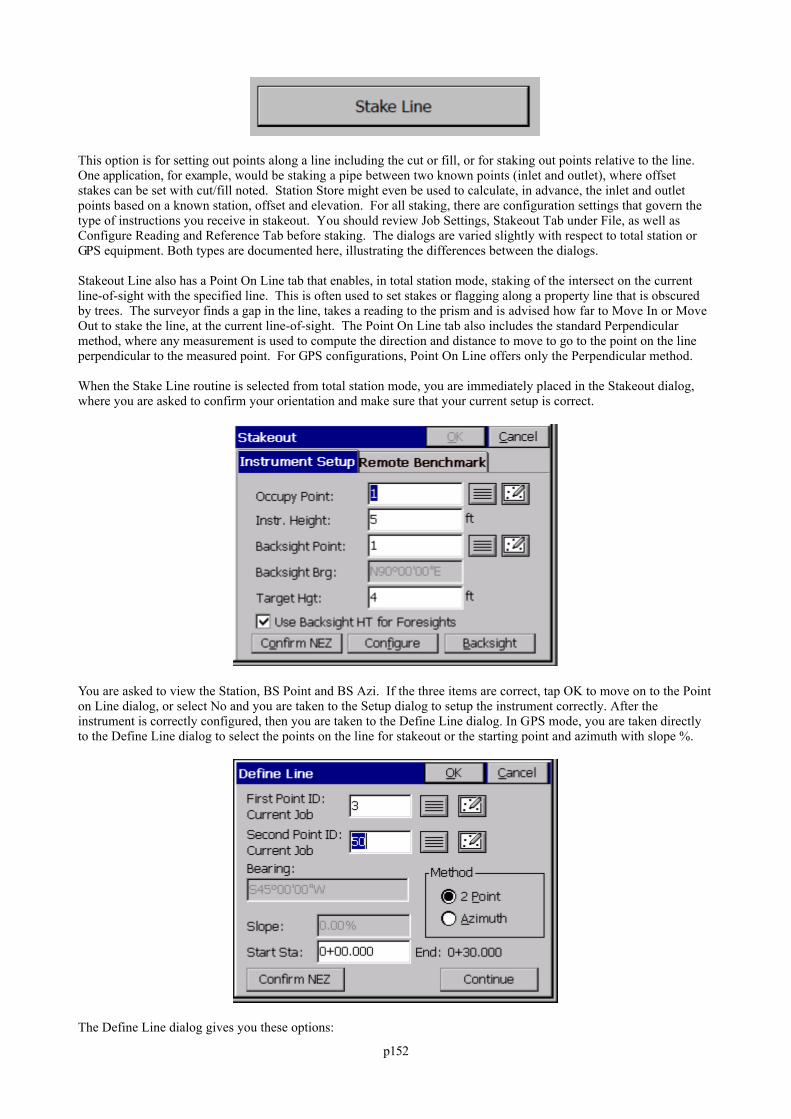
p152

This option is for setting out points along a line including the cut or fill, or for staking out points relative to the line. One application, for example, would be staking a pipe between two known points (inlet and outlet), where offsetstakes can be set with cut/fill noted. Station Store might even be used to calculate, in advance, the inlet and outletpoints based on a known station, offset and elevation. For all staking, there are configuration settings that govern thetype of instructions you receive in stakeout. You should review Job Settings, Stakeout Tab under File, as well asConfigure Reading and Reference Tab before staking. The dialogs are varied slightly with respect to total station orGPS equipment. Both types are documented here, illustrating the differences between the dialogs.

Stakeout Line also has a Point On Line tab that enables, in total station mode, staking of the intersect on the currentline-of-sight with the specified line. This is often used to set stakes or flagging along a property line that is obscuredby trees. The surveyor finds a gap in the line, takes a reading to the prism and is advised how far to Move In or MoveOut to stake the line, at the current line-of-sight. The Point On Line tab also includes the standard Perpendicularmethod, where any measurement is used to compute the direction and distance to move to go to the point on the lineperpendicular to the measured point. For GPS configurations, Point On Line offers only the Perpendicular method.

When the Stake Line routine is selected from total station mode, you are immediately placed in the Stakeout dialog,where you are asked to confirm your orientation and make sure that your current setup is correct.

You are asked to view the Station, BS Point and BS Azi. If the three items are correct, tap OK to move on to the Pointon Line dialog, or select No and you are taken to the Setup dialog to setup the instrument correctly. After theinstrument is correctly configured, then you are taken to the Define Line dialog. In GPS mode, you are taken directlyto the Define Line dialog to select the points on the line for stakeout or the starting point and azimuth with slope %.

The Define Line dialog gives you these options:

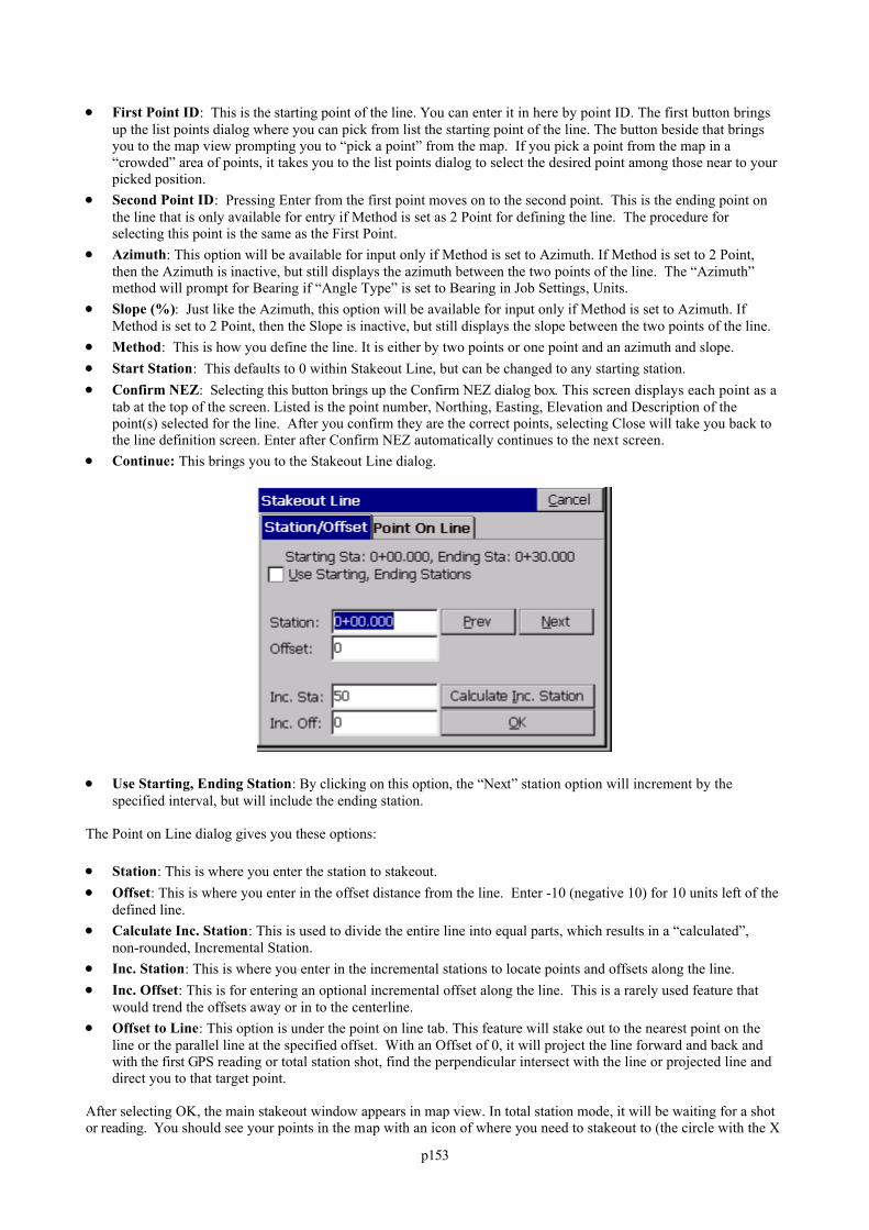
p153

First Point ID: This is the starting point of the line. You can enter it in here by point ID. The first button bringsup the list points dialog where you can pick from list the starting point of the line. The button beside that bringsyou to the map view prompting you to “pick a point” from the map. If you pick a point from the map in a“crowded” area of points, it takes you to the list points dialog to select the desired point among those near to yourpicked position.

Second Point ID: Pressing Enter from the first point moves on to the second point. This is the ending point onthe line that is only available for entry if Method is set as 2 Point for defining the line. The procedure forselecting this point is the same as the First Point.

Azimuth: This option will be available for input only if Method is set to Azimuth. If Method is set to 2 Point,then the Azimuth is inactive, but still displays the azimuth between the two points of the line. The “Azimuth”method will prompt for Bearing if “Angle Type” is set to Bearing in Job Settings, Units.

Slope (%): Just like the Azimuth, this option will be available for input only if Method is set to Azimuth. IfMethod is set to 2 Point, then the Slope is inactive, but still displays the slope between the two points of the line.

Method: This is how you define the line. It is either by two points or one point and an azimuth and slope. Start Station: This defaults to 0 within Stakeout Line, but can be changed to any starting station. Confirm NEZ: Selecting this button brings up the Confirm NEZ dialog box. This screen displays each point as a

tab at the top of the screen. Listed is the point number, Northing, Easting, Elevation and Description of thepoint(s) selected for the line. After you confirm they are the correct points, selecting Close will take you back tothe line definition screen. Enter after Confirm NEZ automatically continues to the next screen.

Continue: This brings you to the Stakeout Line dialog.

Use Starting, Ending Station: By clicking on this option, the “Next” station option will increment by thespecified interval, but will include the ending station.

The Point on Line dialog gives you these options:

Station: This is where you enter the station to stakeout. Offset: This is where you enter in the offset distance from the line. Enter -10 (negative 10) for 10 units left of the

defined line. Calculate Inc. Station: This is used to divide the entire line into equal parts, which results in a “calculated”,

non-rounded, Incremental Station. Inc. Station: This is where you enter in the incremental stations to locate points and offsets along the line. Inc. Offset: This is for entering an optional incremental offset along the line. This is a rarely used feature that

would trend the offsets away or in to the centerline. Offset to Line: This option is under the point on line tab. This feature will stake out to the nearest point on the

line or the parallel line at the specified offset. With an Offset of 0, it will project the line forward and back andwith the first GPS reading or total station shot, find the perpendicular intersect with the line or projected line anddirect you to that target point.

After selecting OK, the main stakeout window appears in map view. In total station mode, it will be waiting for a shotor reading. You should see your points in the map with an icon of where you need to stakeout to (the circle with the X

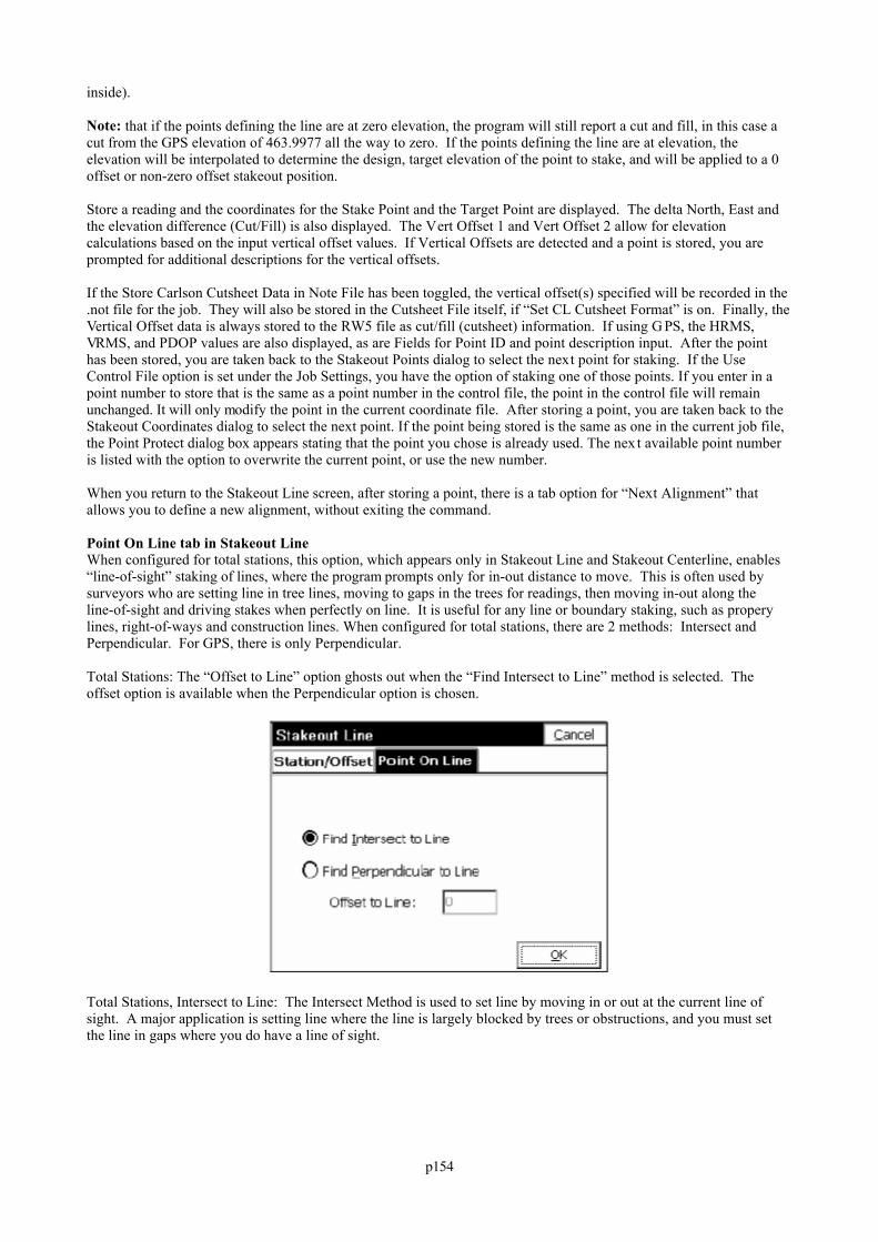
p154

inside).

Note: that if the points defining the line are at zero elevation, the program will still report a cut and fill, in this case acut from the GPS elevation of 463.9977 all the way to zero. If the points defining the line are at elevation, theelevation will be interpolated to determine the design, target elevation of the point to stake, and will be applied to a 0offset or non-zero offset stakeout position.

Store a reading and the coordinates for the Stake Point and the Target Point are displayed. The delta North, East andthe elevation difference (Cut/Fill) is also displayed. The Vert Offset 1 and Vert Offset 2 allow for elevationcalculations based on the input vertical offset values. If Vertical Offsets are detected and a point is stored, you areprompted for additional descriptions for the vertical offsets.

If the Store Carlson Cutsheet Data in Note File has been toggled, the vertical offset(s) specified will be recorded in the.not file for the job. They will also be stored in the Cutsheet File itself, if “Set CL Cutsheet Format” is on. Finally, theVertical Offset data is always stored to the RW5 file as cut/fill (cutsheet) information. If using G PS, the HRMS,VRMS, and PDOP values are also displayed, as are Fields for Point ID and point description input. After the pointhas been stored, you are taken back to the Stakeout Points dialog to select the next point for staking. If the UseControl File option is set under the Job Settings, you have the option of staking one of those points. If you enter in apoint number to store that is the same as a point number in the control file, the point in the control file will remainunchanged. It will only modify the point in the current coordinate file. After storing a point, you are taken back to theStakeout Coordinates dialog to select the next point. If the point being stored is the same as one in the current job file,the Point Protect dialog box appears stating that the point you chose is already used. The nex t available point numberis listed with the option to overwrite the current point, or use the new number.

When you return to the Stakeout Line screen, after storing a point, there is a tab option for “Next Alignment” thatallows you to define a new alignment, without exiting the command.

Point On Line tab in Stakeout LineWhen configured for total stations, this option, which appears only in Stakeout Line and Stakeout Centerline, enables“line-of-sight” staking of lines, where the program prompts only for in-out distance to move. This is often used bysurveyors who are setting line in tree lines, moving to gaps in the trees for readings, then moving in-out along theline-of-sight and driving stakes when perfectly on line. It is useful for any line or boundary staking, such as properylines, right-of-ways and construction lines. When configured for total stations, there are 2 methods: Intersect andPerpendicular. For GPS, there is only Perpendicular.

Total Stations: The “Offset to Line” option ghosts out when the “Find Intersect to Line” method is selected. Theoffset option is available when the Perpendicular option is chosen.

Total Stations, Intersect to Line: The Intersect Method is used to set line by moving in or out at the current line ofsight. A major application is setting line where the line is largely blocked by trees or obstructions, and you must setthe line in gaps where you do have a line of sight.

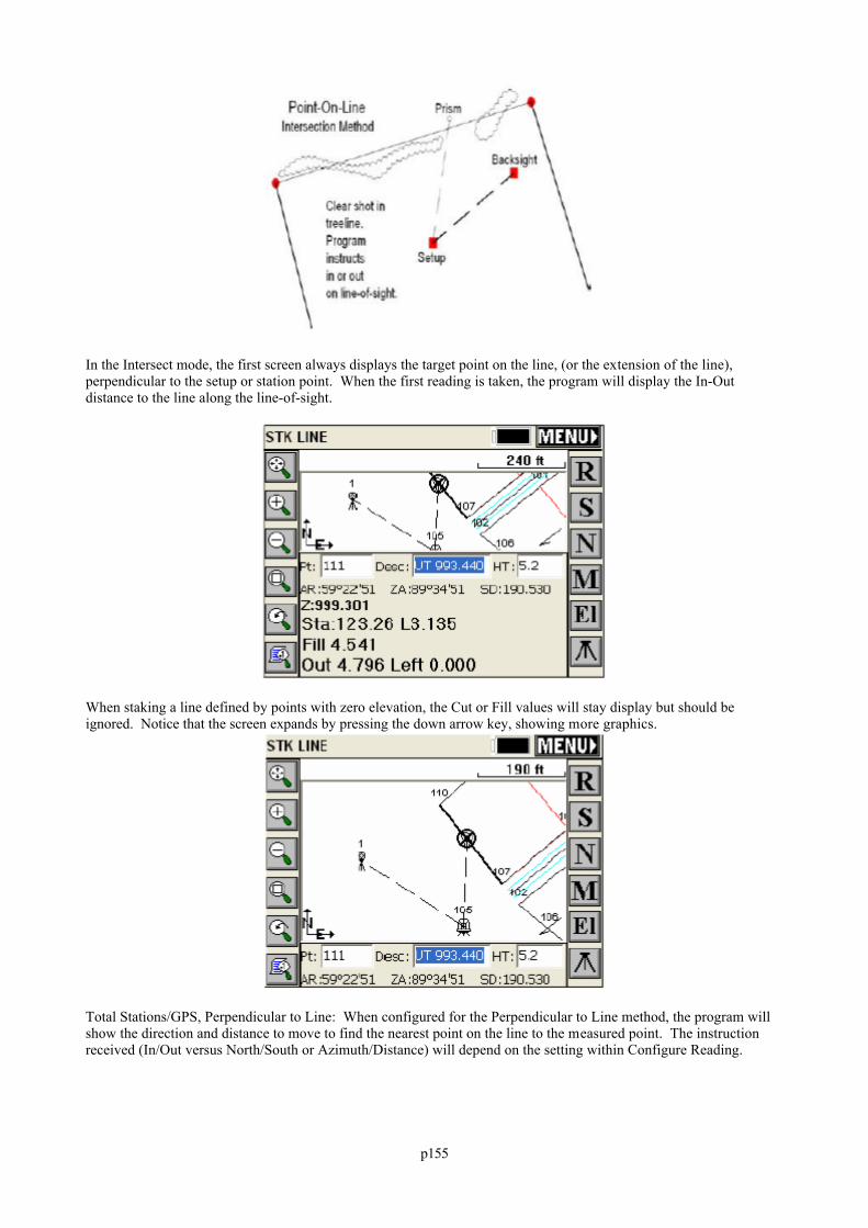
p155

In the Intersect mode, the first screen always displays the target point on the line, (or the extension of the line),perpendicular to the setup or station point. When the first reading is taken, the program will display the In-Outdistance to the line along the line-of-sight.

When staking a line defined by points with zero elevation, the Cut or Fill values will stay display but should beignored. Notice that the screen expands by pressing the down arrow key, showing more graphics.

Total Stations/GPS, Perpendicular to Line: When configured for the Perpendicular to Line method, the program willshow the direction and distance to move to find the nearest point on the line to the measured point. The instructionreceived (In/Out versus North/South or Azimuth/Distance) will depend on the setting within Configure Reading.

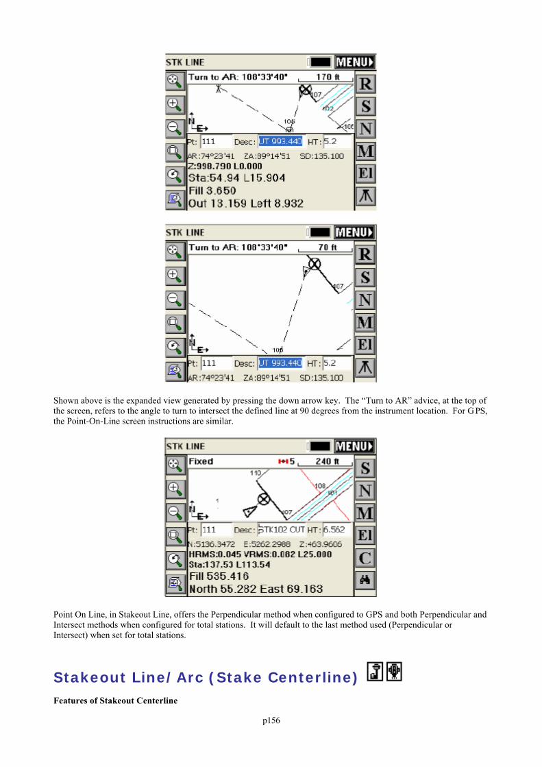
p156

Shown above is the expanded view generated by pressing the down arrow key. The “Turn to AR” advice, at the top ofthe screen, refers to the angle to turn to intersect the defined line at 90 degrees from the instrument location. For G PS,the Point-On-Line screen instructions are similar.

Point On Line, in Stakeout Line, offers the Perpendicular method when configured to GPS and both Perpendicular andIntersect methods when configured for total stations. It will default to the last method used (Perpendicular orIntersect) when set for total stations.

Stakeout Line/Arc (Stake Centerline) Features of Stakeout Centerline

p157

When the routine is run in total station mode, you are immediately placed in a confirm orientation dialog. Afterorientation confirmation, you must choose a centerline file (.CL) from a standard file selection dialog. When thisroutine is run in GPS mode, you will immediately be prompted to select the centerline (.CL) file. Stakeout Centerlineonly requires a horizontal alignment, but you have the option to specify a vertical alignment which will lead to cut andfill results as well. See this figure.

Defining the Horizontal Alignment (Centerline)

Load Centerline: Select a centerline file defined in the Roads Menu or uploaded and converted to “.cl” format. Select Polyline: Select a polyline on the screen to define the alignment. Sequence of Points: Enter a sequence of points to define the alignment. Preview: Displays the alignment graphically. Save: If an alignment was defined by points or a polyline, you can optionally save it as a centerline file. Starting Station: Enter the starting station unless it was pre-determined by a centerline file.

Defining the Vertical Alignment (Profile)This is optional in this command. If your goal is to ignore elevations and you are auto-recalling roading files, theVertical Alignment will be used and cut/fill will appear unless you turn off “Apply Elevations”.

There are three methods of defining the vertical alignment. Load Profile: Select a profile file defined in the Roads Menu or uploaded and converted to “.pro” format. Select Polyline: Select a 3D polyline on the screen to define the profile. Sequence of Points: Enter a sequence of points that have elevation to define the profile. Preview: Displays the profile graphically. Save: If the profile was defined by points or a polyline, you can optionally save it as a profile file.

p158

Starting Station: Enter the starting station unless it was pre-determined by a profile file. Apply Vertical Alignment: Toggles on/off the vertical alignment for 2D or 3D staking.

Note : For file names to be recalled, Auto Recall Files needs to be clicked on within the File Menu, Job Settings.

Here is an example of what will you see when you tap Preview in either tab. Notice that the centerline is shown alongwith any existing point numbers in the vicinity.

Stakeout Centerline DialogAfter you select the centerline file, the Stakeout Centerline dialog appears. If no profile was defined, elevations can beentered, leading to cut/fill reporting.

By contrast, if a Vertical Alignment is entered, and toggled on, you'll notice that the elevation is computed from theVertical Alignment. If the “Override design elevation” box is clicked on, the computed Elevation can be changed. The Elevation is used for cut/fill reporting.

Use PC, PT, TS, SC, CS, ST, Start/End Stations: With this toggle checked on, each PC, point of curve, PT,point of tangent, TS, tangent to spiral point, SC, spiral to curve point, and ST, spiral to tangent point will bestaked. Start and End stations will also be used. When the N, next icon is pressed during stakeout, if one of theabove curve elements is encountered, the station of the point will be displayed in the Station/Offset dialog. Theoption to skip this point is available by pressing the Next button.

Station: This is where you enter the station to stake. The Prev and Next buttons allow for advancement to theNext station or to the Previous station. The default station advancement distance is defined by the Inc. Stationdefined below.

Offset: This is where you enter in the offset distance from the line. Inc. Station: This is where you enter in the incremental stations to locate points and offsets along the line. Inc. Offset: This is for entering an optional incremental offset along the line.

p159

Elevation: This option enables reporting of cut and fill data on the staked point.

After you define the station to stake, the display will change to the map view. Note that your current station and offsetare displayed on the third line from the bottom, just above your target (design) station. Also recall that, as in allstakeout screens, the down arrow will increase the graphic space and reduce the text display.

In the total station example shown below, the target station is 300 at an offset of 50 units to the right.

Point On CL in Stakeout CenterlineThis command is identical to the Perpendicular Offset option in Point On Line within Stakeout Line. You aredirected to the perpendicular intersect point on the centerline (or specified offset from centerline) from the pointmeasured. With GPS, the directions are presented real-time, continuously.

p160

Note that the Turn to AR advice refers to the angle to turn to contact the centerline at 90 degrees (right angles) to theinstrument setup. Note also that the instructions (out 13.8, Left 23.1) are from the rodman ’s viewpoint (the triangleposition looking at the instrument), as set in Configure Reading, Reference Tab.

Stakeout Arc (3 Points)

This routine requests 3 points to define a unique arc, which is then used for stakeout by station and offset. The firstpoint becomes the beginning of the arc. The prompting is shown below.

The points can be entered in, chosen from the list points button, or selected with the pick from the screen button. Afterselecting the three points, choose OK to go to the Stakeout Arc dialog. Please refer to Stake Centerline above forStakeout Arc dialog definitions, which are identical. The only difference is that the “special stations” are limited toPC (start) and PT (end). There are no spiral-oriented or PI (point of intersection) special stations. After choosing astation and offset to stake and selecting OK, the main stakeout window appears in map view below. Here we arestaking station 100, 25 units right. In total station mode, an angle to turn to and a distance to go will be displayed atthe bottom of the screen. Taking a reading to the current target position will update the display with a distance out/inand a right/left distance depending upon your job settings. You should see your points and centerline or curve in themap with an icon of the point you need to stakeout to (the circle with the X inside). When using GPS, after selectingOK to the Stakeout Arc dialog, you will be placed in the Map screen at your current position with directionalinstructions to the target point continually updating.

See Features of Stakeout Centerline above for information on the available commands while in the dialog shownabove. See below for discussion on Point on Arc feature.

Stakeout Arc (PC, PT Value)

This option for defining the arc requires four input parameters, the Start point, End Point, Curve Direction, and any ofthe following: Radius Point, Radius Length, Arc Length, Delta Angle or Degree of Curvature. The starting stationdefaults to 0, but can also be changed. See this figure.

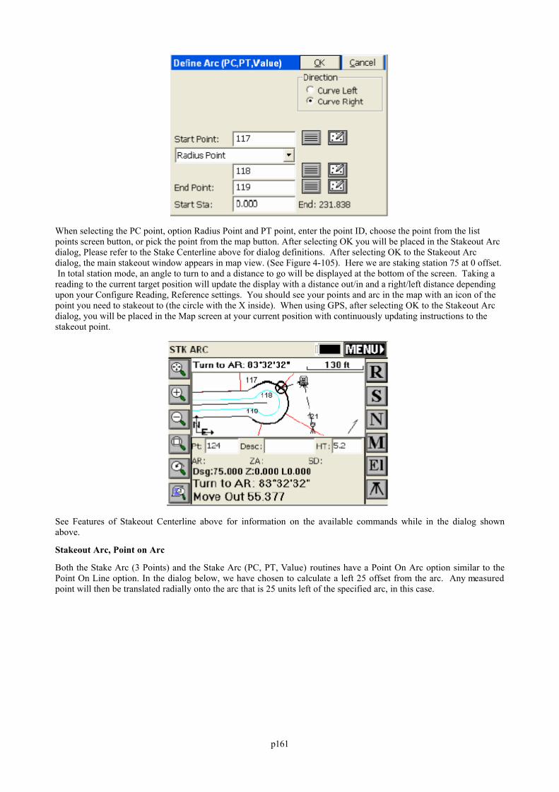
p161

When selecting the PC point, option Radius Point and PT point, enter the point ID, choose the point from the listpoints screen button, or pick the point from the map button. After selecting OK you will be placed in the Stakeout Arcdialog, Please refer to the Stake Centerline above for dialog definitions. After selecting OK to the Stakeout Arcdialog, the main stakeout window appears in map view. (See Figure 4-105). Here we are staking station 75 at 0 offset. In total station mode, an angle to turn to and a distance to go will be displayed at the bottom of the screen. Taking areading to the current target position will update the display with a distance out/in and a right/left distance dependingupon your Configure Reading, Reference settings. You should see your points and arc in the map with an icon of thepoint you need to stakeout to (the circle with the X inside). When using GPS, after selecting OK to the Stakeout Arcdialog, you will be placed in the Map screen at your current position with continuously updating instructions to thestakeout point.

See Features of Stakeout Centerline above for information on the available commands while in the dialog shownabove.

Stakeout Arc, Point on Arc

Both the Stake Arc (3 Points) and the Stake Arc (PC, PT, Value) routines have a Point On Arc option similar to thePoint On Line option. In the dialog below, we have chosen to calculate a left 25 offset from the arc. Any measuredpoint will then be translated radially onto the arc that is 25 units left of the specified arc, in this case.

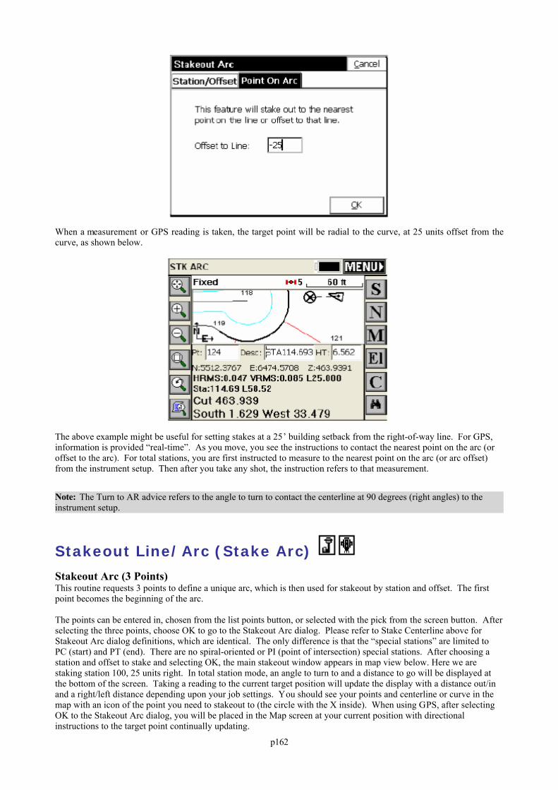
p162

When a measurement or GPS reading is taken, the target point will be radial to the curve, at 25 units offset from thecurve, as shown below.

The above example might be useful for setting stakes at a 25’ building setback from the right-of-way line. For GPS,information is provided “real-time”. As you move, you see the instructions to contact the nearest point on the arc (oroffset to the arc). For total stations, you are first instructed to measure to the nearest point on the arc (or arc offset)from the instrument setup. Then after you take any shot, the instruction refers to that measurement.

Note: The Turn to AR advice refers to the angle to turn to contact the centerline at 90 degrees (right angles) to theinstrument setup.

Stakeout Line/Arc (Stake Arc)

Stakeout Arc (3 Points)This routine requests 3 points to define a unique arc, which is then used for stakeout by station and offset. The firstpoint becomes the beginning of the arc.

The points can be entered in, chosen from the list points button, or selected with the pick from the screen button. Afterselecting the three points, choose OK to go to the Stakeout Arc dialog. Please refer to Stake Centerline above forStakeout Arc dialog definitions, which are identical. The only difference is that the “special stations” are limited toPC (start) and PT (end). There are no spiral-oriented or PI (point of intersection) special stations. After choosing astation and offset to stake and selecting OK, the main stakeout window appears in map view below. Here we arestaking station 100, 25 units right. In total station mode, an angle to turn to and a distance to go will be displayed atthe bottom of the screen. Taking a reading to the current target position will update the display with a distance out/inand a right/left distance depending upon your job settings. You should see your points and centerline or curve in themap with an icon of the point you need to stakeout to (the circle with the X inside). When using GPS, after selectingOK to the Stakeout Arc dialog, you will be placed in the Map screen at your current position with directionalinstructions to the target point continually updating.

p163

See Features of Stakeout Centerline above for information on the available commands while in the dialogs.See below for discussion on Point on Arc feature.

Stakeout Arc (PC, PT Value)This option for defining the arc requires four input parameters, the Start point, End Point, Curve Direction, and any ofthe following: Radius Point, Radius Length, Arc Length, Delta Angle or Degree of Curvature. The starting stationdefaults to 0, but can also be changed.

When selecting the PC point, option Radius Point and PT point, enter the point ID, choose the point from the listpoints screen button, or pick the point from the map button. After selecting OK you will be placed in the Stakeout Arcdialog, Please refer to the Stake Centerline above for dialog definitions. After selecting OK to the Stakeout Arcdialog, the main stakeout window appears in map view. In total station mode, an angle to turn to and a distance to gowill be displayed at the bottom of the screen. Taking a reading to the current target position will update the displaywith a distance out/in and a right/left distance depending upon your Configure Reading, Reference settings. Youshould see your points and arc in the map with an icon of the point you need to stakeout to (the circle with the Xinside). When using GPS, after selecting OK to the Stakeout Arc dialog, you will be placed in the Map screen at yourcurrent position with continuously updating instructions to the stakeout point.

See Features of Stakeout Centerline above for information on the available commands while in the dialogs.

Stakeout Arc, Point on ArcBoth the Stake Arc (3 Points) and the Stake Arc (PC, PT, Value) routines have a Point On Arc option similar to thePoint On Line option. In the dialog, you can chose to calculate a left (-) or right (+) offset from the arc. Any measuredpoint will then be translated radially onto the arc.

For GPS, information is provided “real-time”. As you move, you see the instructions to contact the nearest point onthe arc (or offset to the arc). For total stations, you are first instructed to measure to the nearest point on the arc (or arcoffset) from the instrument setup. Then after you take any shot, the instruction refers to that measurement.

Offset Stakeout This command will stake out up to two user defined horizontal offsets to a centerline at any station, as well as anunlimited number of offsets per station, if you are using a predefined Cutsheet Station and Offset List (loaded usingthe Settings button). It will also stake out the centerline itself. Station intervals can be entered, and the program willauto-detect, at the user’s option, special stations such as the TS, SC, PC, PT, CS, ST and vertical curve points(including high and low points). Because individual stations and offsets can be entered, and also because pre-madestation and offset lists can be recalled in the field, Offset Stakeout can be applied to virtually any offset point along acenterline.

Prerequisites and ProceduresOffset Stakeout requires both a horizontal and vertical alignment. If total stations are involved, Offset Stakeout passesthrough the normal backsight confirmation screens that Sideshot/Traverse and other forms of Stakeout require.

The Offset Stakeout command is a 3-screen program. The first screen identifies and loads in the alignment files. Thesecond screen identifies the offset points to stake (slopes and distances) and the intervals or lists of stations/offsets tostake, and the final screen goes to the standard graphics, shows the target points, and guides the user to the destination,with N for Next continuing onto the next station in the interval or list.

Identifying the AlignmentsThe first screen has tabs for selecting both the horizontal and vertical alignments. See this next figure.

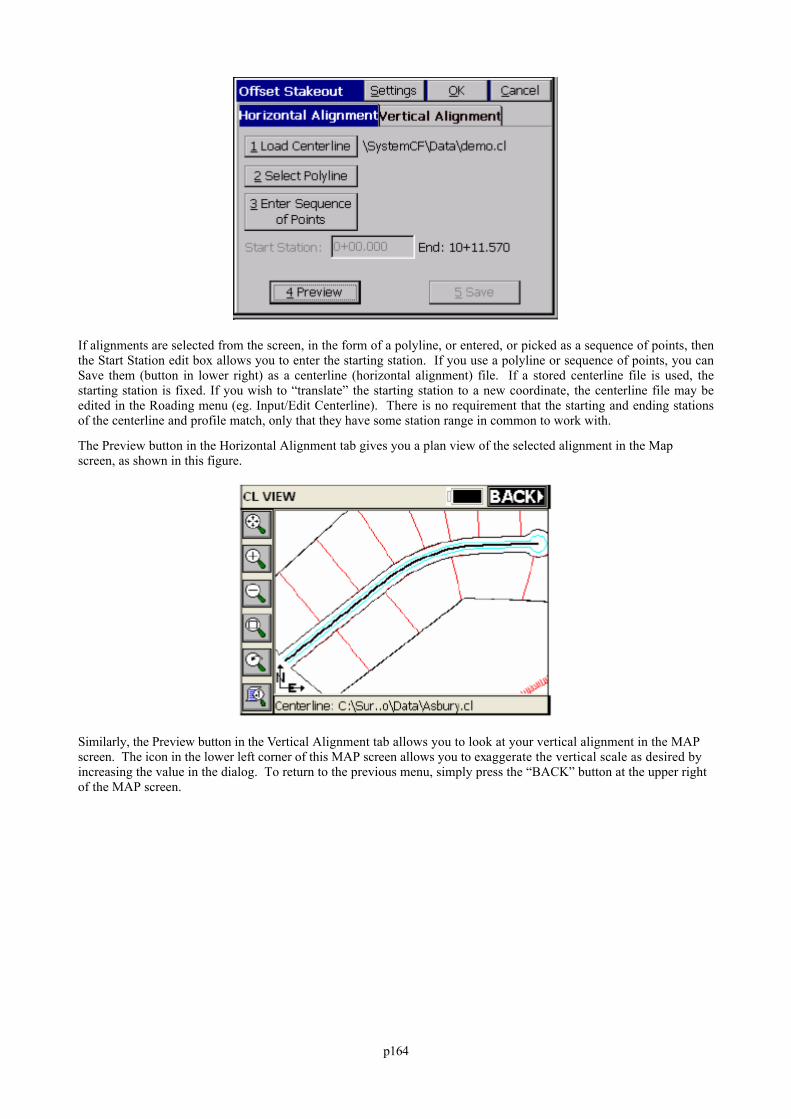
p164

If alignments are selected from the screen, in the form of a polyline, or entered, or picked as a sequence of points, thenthe Start Station edit box allows you to enter the starting station. If you use a polyline or sequence of points, you canSave them (button in lower right) as a centerline (horizontal alignment) file. If a stored centerline file is used, thestarting station is fixed. If you wish to “translate” the starting station to a new coordinate, the centerline file may beedited in the Roading menu (eg. Input/Edit Centerline). There is no requirement that the starting and ending stationsof the centerline and profile match, only that they have some station range in common to work with.

The Preview button in the Horizontal Alignment tab gives you a plan view of the selected alignment in the Mapscreen, as shown in this figure.

Similarly, the Preview button in the Vertical Alignment tab allows you to look at your vertical alignment in the MAPscreen. The icon in the lower left corner of this MAP screen allows you to exaggerate the vertical scale as desired byincreasing the value in the dialog. To return to the previous menu, simply press the “BACK” button at the upper rightof the MAP screen.

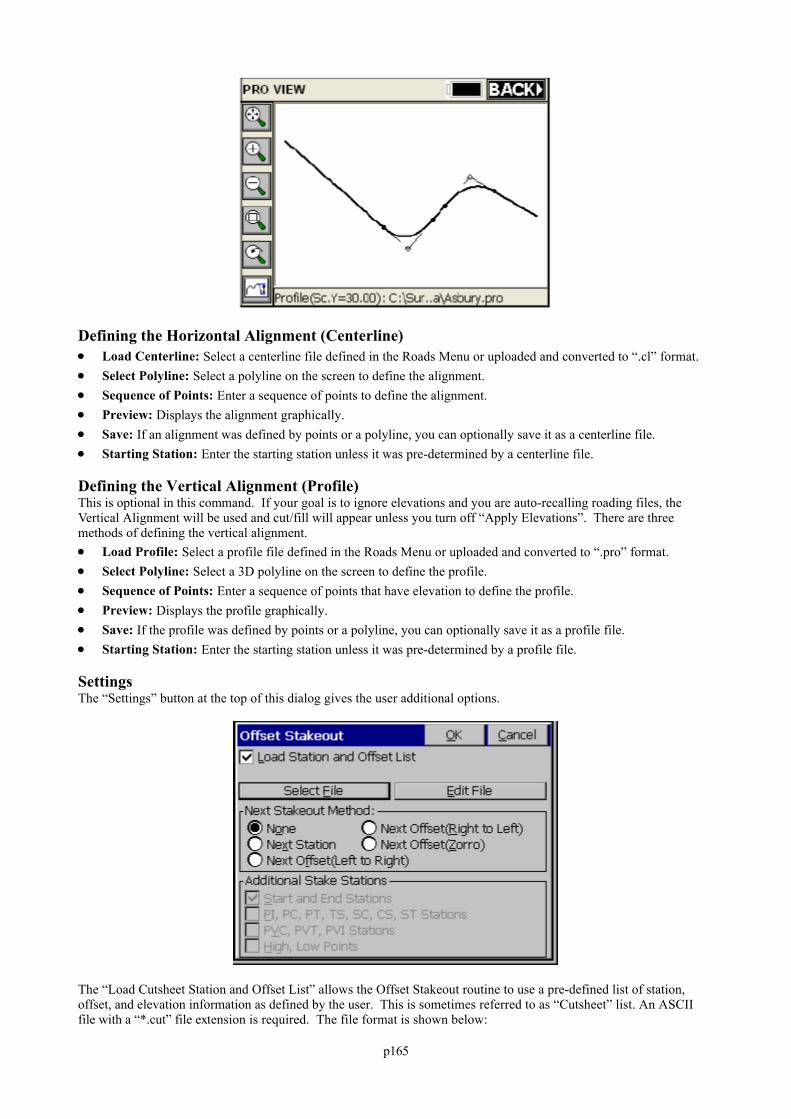
p165

Defining the Horizontal Alignment (Centerline) Load Centerline: Select a centerline file defined in the Roads Menu or uploaded and converted to “.cl” format. Select Polyline: Select a polyline on the screen to define the alignment. Sequence of Points: Enter a sequence of points to define the alignment. Preview: Displays the alignment graphically. Save: If an alignment was defined by points or a polyline, you can optionally save it as a centerline file. Starting Station: Enter the starting station unless it was pre-determined by a centerline file.

Defining the Vertical Alignment (Profile)This is optional in this command. If your goal is to ignore elevations and you are auto-recalling roading files, theVertical Alignment will be used and cut/fill will appear unless you turn off “Apply Elevations”. There are threemethods of defining the vertical alignment. Load Profile: Select a profile file defined in the Roads Menu or uploaded and converted to “.pro” format. Select Polyline: Select a 3D polyline on the screen to define the profile. Sequence of Points: Enter a sequence of points that have elevation to define the profile. Preview: Displays the profile graphically. Save: If the profile was defined by points or a polyline, you can optionally save it as a profile file. Starting Station: Enter the starting station unless it was pre-determined by a profile file.

SettingsThe “Settings” button at the top of this dialog gives the user additional options.

The “Load Cutsheet Station and Offset List” allows the Offset Stakeout routine to use a pre-defined list of station,offset, and elevation information as defined by the user. This is sometimes referred to as “Cutsheet” list. An ASCIIfile with a “*.cut” file extension is required. The file format is shown below:

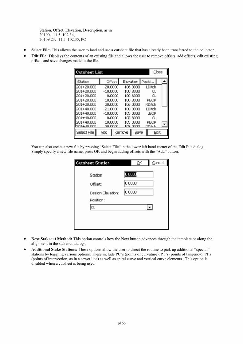
p166

Station, Offset, Elevation, Description, as in20100, -11.5, 102.34, 20109.23, -11.5, 102.35, PC

Select File: This allows the user to load and use a cutsheet file that has already been transferred to the collector. Edit File: Displays the contents of an existing file and allows the user to remove offsets, add offsets, edit existing

offsets and save changes made to the file.

You can also create a new file by pressing “Select File” in the lower left hand corner of the Edit File dialog. Simply specify a new file name, press OK and begin adding offsets with the “Add” button.

Next Stakeout Method: This option controls how the Next button advances through the template or along thealignment in the stakeout dialogs.

Additional Stake Stations: These options allow the user to direct the routine to pick up additional “special”stations by toggling various options. These include PC’s (points of curvature), PT’s (points of tangency), PI’s(points of intersection, as in a sewer line) as well as spiral curve and vertical curve elements. This option isdisabled when a cutsheet is being used.

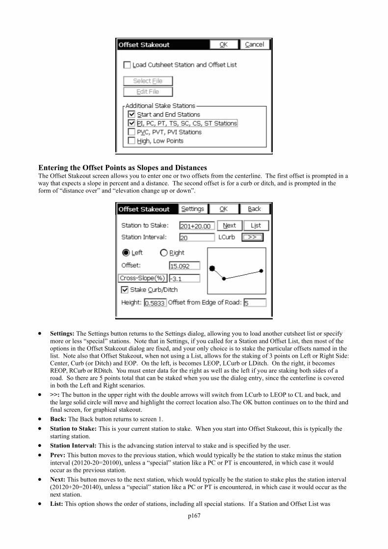
p167

Entering the Offset Points as Slopes and DistancesThe Offset Stakeout screen allows you to enter one or two offsets from the centerline. The first offset is prompted in away that expects a slope in percent and a distance. The second offset is for a curb or ditch, and is prompted in theform of “distance over” and “elevation change up or down”.

Settings: The Settings button returns to the Settings dialog, allowing you to load another cutsheet list or specifymore or less “special” stations. Note that in Settings, if you called for a Station and Offset List, then most of theoptions in the Offset Stakeout dialog are fixed, and your only choice is to stake the particular offsets named in thelist. Note also that Offset Stakeout, when not using a List, allows for the staking of 3 points on Left or Right Side:Center, Curb (or Ditch) and EOP. On the left, is becomes LEOP, LCurb or LDitch. On the right, it becomesREOP, RCurb or RDitch. You must enter data for the right as well as the left if you are staking both sides of aroad. So there are 5 points total that can be staked when you use the dialog entry, since the centerline is coveredin both the Left and Right scenarios.

>>: The button in the upper right with the double arrows will switch from LCurb to LEOP to CL and back, andthe large solid circle will move and highlight the correct location also.The OK button continues on to the third andfinal screen, for graphical stakeout.

Back: The Back button returns to screen 1. Station to Stake: This is your current station to stake. When you start into Offset Stakeout, this is typically the

starting station. Station Interval: This is the advancing station interval to stake and is specified by the user. Prev: This button moves to the previous station, which would typically be the station to stake minus the station

interval (20120-20=20100), unless a “special” station like a PC or PT is encountered, in which case it wouldoccur as the previous station.

Next: This button moves to the next station, which would typically be the station to stake plus the station interval(20120+20=20140), unless a “special” station like a PC or PT is encountered, in which case it would occur as thenext station.

List: This option shows the order of stations, including all special stations. If a Station and Offset List was

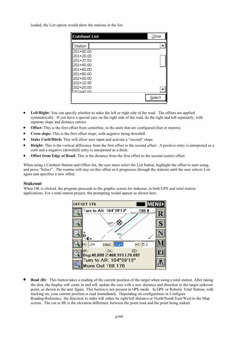
p168

loaded, the List option would show the stations in the list.

Left/Right: You can specify whether to stake the left or right side of the road. The offsets are appliedsymmetrically. If you have a special case on the right side of the road, do the right and left separately, withseparate slope and distance entries.

Offset: This is the first offset from centerline, in the units that are configured (feet or meters). Cross slope: This is the first offset slope, with negative being downhill. Stake Curb/Ditch: This will allow user input and activate a “second” slope. Height: This is the vertical difference from the first offset to the second offset. A positive entry is interpreted as a

curb and a negative (downhill) entry is interpreted as a ditch. Offset from Edge of Road: This is the distance from the first offset to the second (outer) offset.

When using a Cutsheet Station and Offset list, the user must select the List button, highlight the offset to start using,and press “Select”. The routine will stay on this offset as it progresses through the stations until the user selects Listagain and specifies a new offset.

StakeoutWhen OK is clicked, the program proceeds to the graphic screen for stakeout, in both GPS and total stationapplications. For a total station project, the prompting would appear as shown here.

Read (R) : This button takes a reading of the current position of the target when using a total station. After takingthe shot, the display will zoom in and will update the user with a new distance and direction to the target stakeoutpoint, as shown in the next figure. This button is not present in GPS mode. In GPS or Robotic Total Station, withtracking on, your current position is read immediately. Depending on configuration in ConfigureReading-Reference, the direction to stake will either be right/left distance or North/South East/West in the Mapscreen. The cut or fill is the elevation difference between the point read and the point being staked.

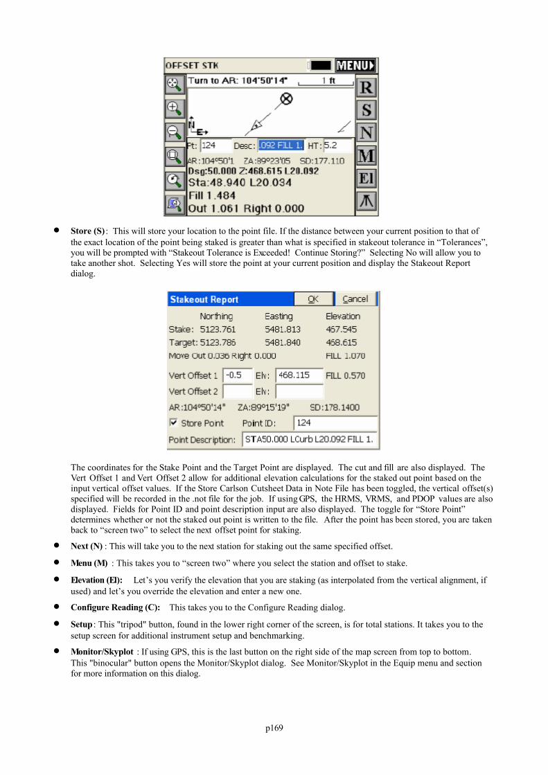
p169

Store (S) : This will store your location to the point file. If the distance between your current position to that ofthe exact location of the point being staked is greater than what is specified in stakeout tolerance in “Tolerances”,you will be prompted with “Stakeout Tolerance is Exceeded! Continue Storing?” Selecting No will allow you totake another shot. Selecting Yes will store the point at your current position and display the Stakeout Reportdialog.

The coordinates for the Stake Point and the Target Point are displayed. The cut and fill are also displayed. TheVert Offset 1 and Vert Offset 2 allow for additional elevation calculations for the staked out point based on theinput vertical offset values. If the Store Carlson Cutsheet Data in Note File has been toggled, the vertical offset(s)specified will be recorded in the .not file for the job. If using GPS, the HRMS, VRMS, and PDOP values are alsodisplayed. Fields for Point ID and point description input are also displayed. The toggle for “Store Point”determines whether or not the staked out point is written to the file. After the point has been stored, you are takenback to “screen two” to select the next offset point for staking.

Next (N) : This will take you to the next station for staking out the same specified offset.

Menu (M) : This takes you to “screen two” where you select the station and offset to stake.

Elevation (El): Let’s you verify the elevation that you are staking (as interpolated from the vertical alignment, ifused) and let’s you override the elevation and enter a new one.

Configure Reading (C): This takes you to the Configure Reading dialog.

Setup : This "tripod" button, found in the lower right corner of the screen, is for total stations. It takes you to thesetup screen for additional instrument setup and benchmarking.

Monitor/Skyplot : If using GPS, this is the last button on the right side of the map screen from top to bottom. This "binocular" button opens the Monitor/Skyplot dialog. See Monitor/Skyplot in the Equip menu and sectionfor more information on this dialog.

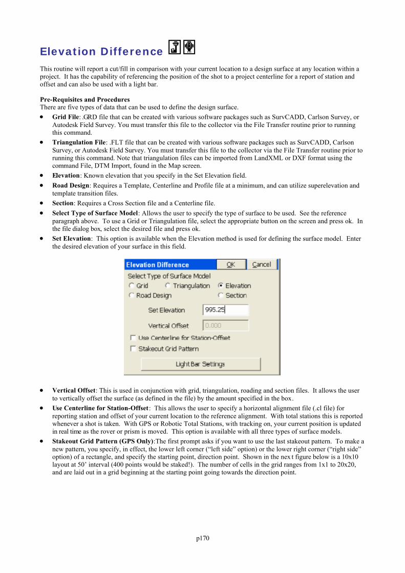
p170

Elevation Difference This routine will report a cut/fill in comparison with your current location to a design surface at any location within aproject. It has the capability of referencing the position of the shot to a project centerline for a report of station andoffset and can also be used with a light bar.

Pre-Requisites and ProceduresThere are five types of data that can be used to define the design surface. Grid File: .GRD file that can be created with various software packages such as SurvCADD, Carlson Survey, or

Autodesk Field Survey. You must transfer this file to the collector via the File Transfer routine prior to runningthis command.

Triangulation File: .FLT file that can be created with various software packages such as SurvCADD, CarlsonSurvey, or Autodesk Field Survey. You must transfer this file to the collector via the File Transfer routine prior torunning this command. Note that triangulation files can be imported from LandXML or DXF format using thecommand File, DTM Import, found in the Map screen.

Elevation: Known elevation that you specify in the Set Elevation field. Road Design: Requires a Template, Centerline and Profile file at a minimum, and can utilize superelevation and

template transition files. Section: Requires a Cross Section file and a Centerline file. Select Type of Surface Model: Allows the user to specify the type of surface to be used. See the reference

paragraph above. To use a Grid or Triangulation file, select the appropriate button on the screen and press ok. Inthe file dialog box, select the desired file and press ok.

Set Elevation: This option is available when the Elevation method is used for defining the surface model. Enterthe desired elevation of your surface in this field.

Vertical Offset: This is used in conjunction with grid, triangulation, roading and section files. It allows the userto vertically offset the surface (as defined in the file) by the amount specified in the box.

Use Centerline for Station-Offset: This allows the user to specify a horizontal alignment file (.cl file) forreporting station and offset of your current location to the reference alignment. With total stations this is reportedwhenever a shot is taken. With GPS or Robotic Total Stations, with tracking on, your current position is updatedin real time as the rover or prism is moved. This option is available with all three types of surface models.

Stakeout Grid Pattern (GPS Only):The first prompt asks if you want to use the last stakeout pattern. To make anew pattern, you specify, in effect, the lower left corner (“left side” option) or the lower right corner (“right side”option) of a rectangle, and specify the starting point, direction point. Shown in the nex t figure below is a 10x10layout at 50’ interval (400 points would be staked!). The number of cells in the grid ranges from 1x1 to 20x20,and are laid out in a grid beginning at the starting point going towards the direction point.

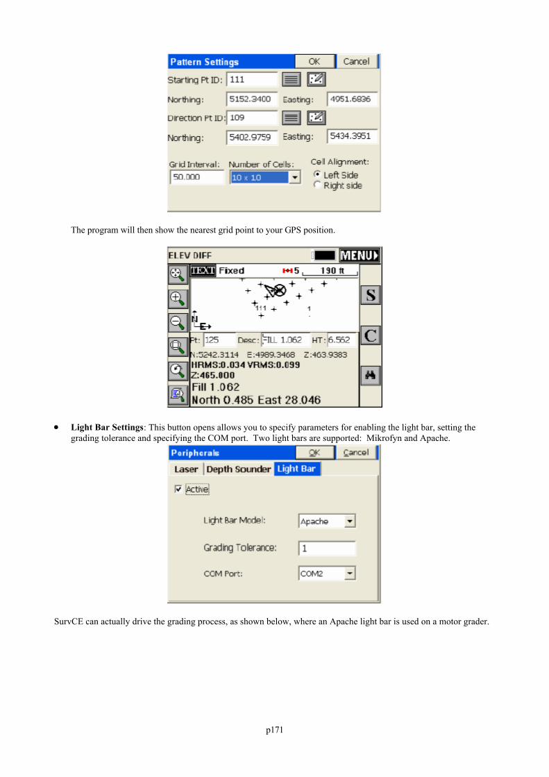
p171

The program will then show the nearest grid point to your GPS position.

Light Bar Settings: This button opens allows you to specify parameters for enabling the light bar, setting thegrading tolerance and specifying the COM port. Two light bars are supported: Mikrofyn and Apache.

SurvCE can actually drive the grading process, as shown below, where an Apache light bar is used on a motor grader.

p172

Pressing OK from the main Elevation Difference screen will first prompt the user to load the surface files involved(unless elevation method was selected). Then, when OK is chosen, the following ELEV DIFF screen comes up. Thisscreen provides the user with a plan view of the project. When a shot is taken, cut or fill from the current verticallocation to the design surface is reported in the lower left portion of the screen. The computed design surfaceelevation for your current location is also reported.

Options on the right side of the screen are shown below:Read (R): This allows the user to take a shot without storing it to the job file. Cut or fill is immediately reported.This button is not present with GPS.Store (S): This button immediately reports cut or fill and stores the current shot to the job file. Pressing the enter keywill simultaneously read and store your current shot as well. Shots store like topo shots, and respond to the setting inHeight/Description Prompt on Save, within Configure Reading.El: This allows you to set the elevation. Configure (C): This takes the user to the Configure Reading dialog that is standard throughout the program. Monitor/Skyplot: If using GPS, this is the last button on the right side of the map screen from top to bottom. This"binocular" button opens the Monitor/Skyplot dialog.

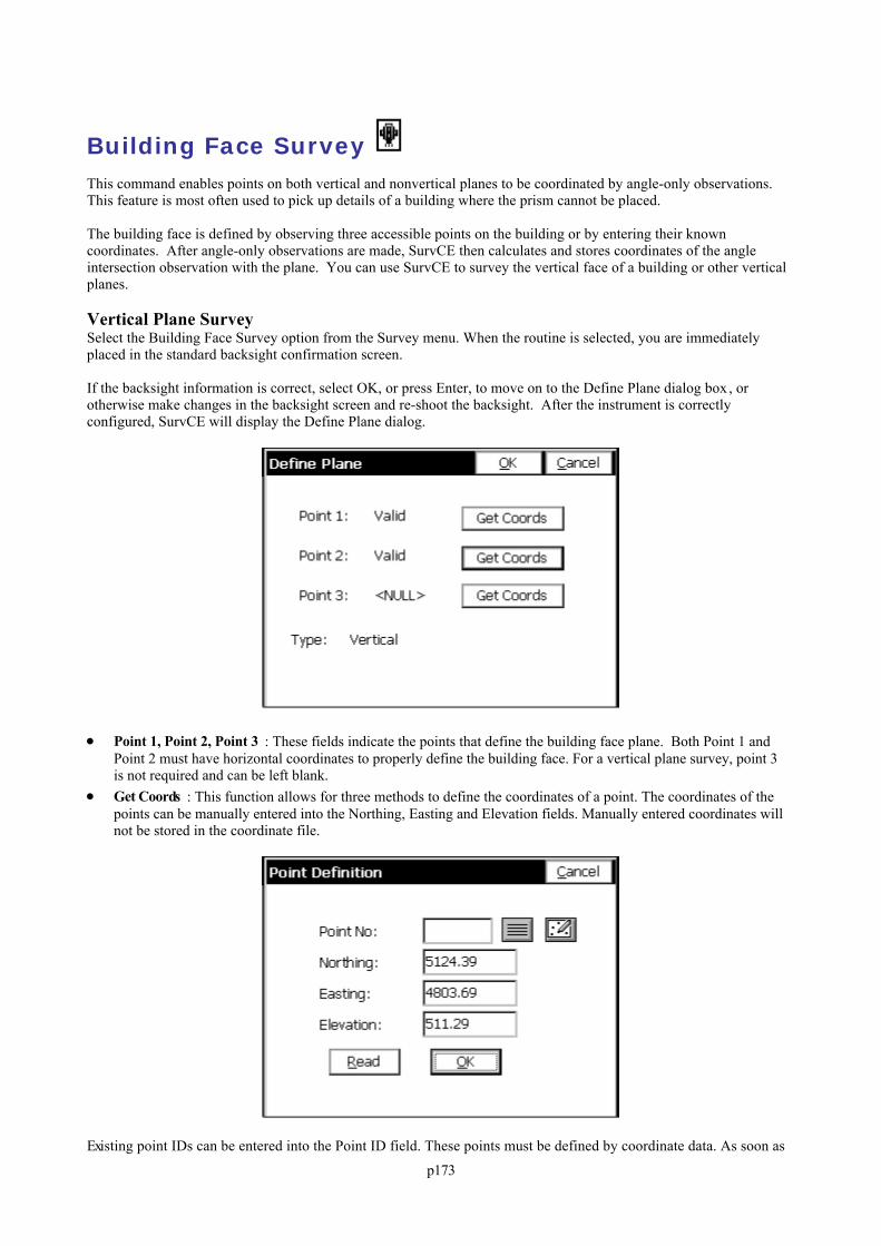
p173

Building Face Survey This command enables points on both vertical and nonvertical planes to be coordinated by angle-only observations. This feature is most often used to pick up details of a building where the prism cannot be placed.

The building face is defined by observing three accessible points on the building or by entering their knowncoordinates. After angle-only observations are made, SurvCE then calculates and stores coordinates of the angleintersection observation with the plane. You can use SurvCE to survey the vertical face of a building or other verticalplanes.

Vertical Plane SurveySelect the Building Face Survey option from the Survey menu. When the routine is selected, you are immediatelyplaced in the standard backsight confirmation screen.

If the backsight information is correct, select OK, or press Enter, to move on to the Define Plane dialog box , orotherwise make changes in the backsight screen and re-shoot the backsight. After the instrument is correctlyconfigured, SurvCE will display the Define Plane dialog.

Point 1, Point 2, Point 3 : These fields indicate the points that define the building face plane. Both Point 1 andPoint 2 must have horizontal coordinates to properly define the building face. For a vertical plane survey, point 3is not required and can be left blank.

Get Coords : This function allows for three methods to define the coordinates of a point. The coordinates of thepoints can be manually entered into the Northing, Easting and Elevation fields. Manually entered coordinates willnot be stored in the coordinate file.

Existing point IDs can be entered into the Point ID field. These points must be defined by coordinate data. As soon as

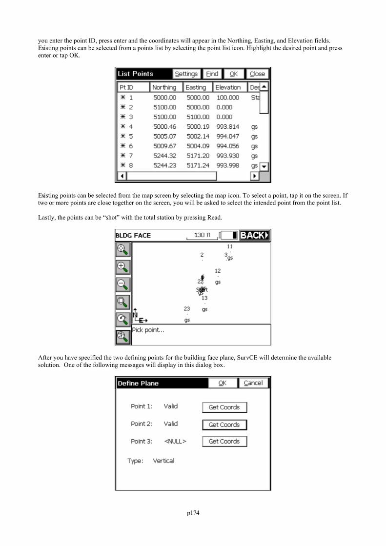
p174

you enter the point ID, press enter and the coordinates will appear in the Northing, Easting, and Elevation fields.Existing points can be selected from a points list by selecting the point list icon. Highlight the desired point and pressenter or tap OK.

Existing points can be selected from the map screen by selecting the map icon. To select a point, tap it on the screen. Iftwo or more points are close together on the screen, you will be asked to select the intended point from the point list.

Lastly, the points can be “shot” with the total station by pressing Read.

After you have specified the two defining points for the building face plane, SurvCE will determine the availablesolution. One of the following messages will display in this dialog box.

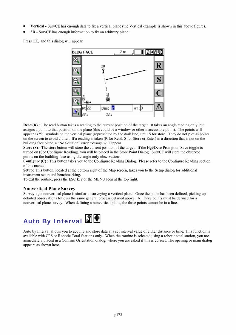
p175

Vertical - SurvCE has enough data to fix a vertical plane (the Vertical example is shown in this above figure). 3D - SurvCE has enough information to fix an arbitrary plane.

Press OK, and this dialog will appear.

Read (R) : The read button takes a reading to the current position of the target. It takes an angle reading only, butassigns a point to that position on the plane (this could be a window or other inaccessible point). The points willappear as “?” symbols on the vertical plane (represented by the dark line) until S for store. They do not plot as pointson the screen to avoid clutter. If a reading is taken (R for Read, S for Store or Enter) in a direction that is not on thebuilding face plane, a “No Solution” error message will appear.Store (S) : The store button will store the current position of the target. If the Hgt/Desc Prompt on Save toggle isturned on (See Configure Reading), you will be placed in the Store Point Dialog. SurvCE will store the observedpoints on the building face using the angle only observations. Configure (C) : This button takes you to the Configure Reading Dialog. Please refer to the Configure Reading sectionof this manual.Setup : This button, located at the bottom right of the Map screen, takes you to the Setup dialog for additionalinstrument setup and benchmarking.To exit the routine, press the ESC key or the MENU Icon at the top right.

Nonvertical Plane SurveySurveying a nonvertical plane is similar to surveying a vertical plane. Once the plane has been defined, picking updetailed observations follows the same general process detailed above. All three points must be defined for anonvertical plane survey. When defining a nonvertical plane, the three points cannot be in a line.

Auto By Interval Auto by Interval allows you to acquire and store data at a set interval value of either distance or time. This function isavailable with GPS or Robotic Total Stations only. When the routine is selected using a robotic total station, you areimmediately placed in a Confirm Orientation dialog, where you are asked if this is correct. The opening or main dialogappears as shown here.

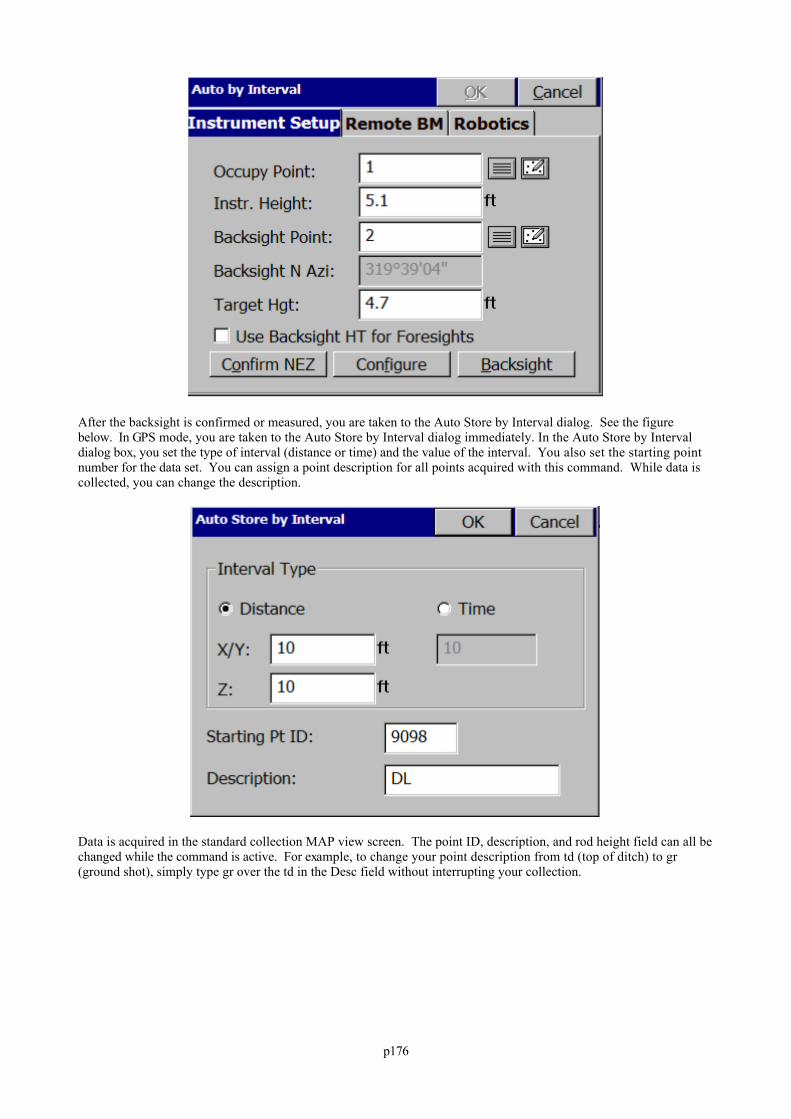
p176

After the backsight is confirmed or measured, you are taken to the Auto Store by Interval dialog. See the figurebelow. In GPS mode, you are taken to the Auto Store by Interval dialog immediately. In the Auto Store by Intervaldialog box, you set the type of interval (distance or time) and the value of the interval. You also set the starting pointnumber for the data set. You can assign a point description for all points acquired with this command. While data iscollected, you can change the description.

Data is acquired in the standard collection MAP view screen. The point ID, description, and rod height field can all bechanged while the command is active. For example, to change your point description from td (top of ditch) to gr(ground shot), simply type gr over the td in the Desc field without interrupting your collection.

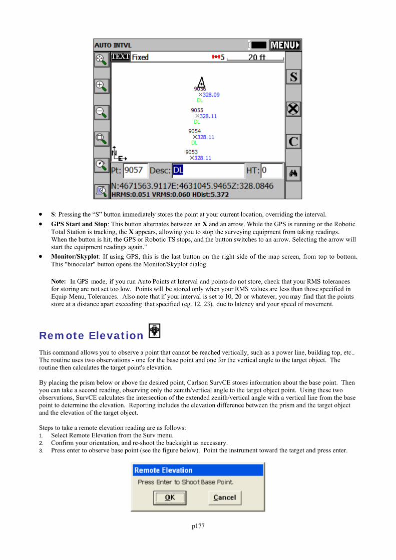
p177

S: Pressing the “S” button immediately stores the point at your current location, overriding the interval. GPS Start and Stop: This button alternates between an X and an arrow. While the GPS is running or the Robotic

Total Station is tracking, the X appears, allowing you to stop the surveying equipment from taking readings.When the button is hit, the GPS or Robotic TS stops, and the button switches to an arrow. Selecting the arrow willstart the equipment readings again."

Monitor/Skyplot: If using GPS, this is the last button on the right side of the map screen, from top to bottom.This "binocular" button opens the Monitor/Skyplot dialog.

Note: In GPS mode, if you run Auto Points at Interval and points do not store, check that your RMS tolerancesfor storing are not set too low. Points will be stored only when your RMS values are less than those specified inEquip Menu, Tolerances. Also note that if your interval is set to 10, 20 or whatever, you may find that the pointsstore at a distance apart exceeding that specified (eg. 12, 23), due to latency and your speed of movement.

Remote Elevation This command allows you to observe a point that cannot be reached vertically, such as a power line, building top, etc.. The routine uses two observations - one for the base point and one for the vertical angle to the target object. Theroutine then calculates the target point's elevation.

By placing the prism below or above the desired point, Carlson SurvCE stores information about the base point. Thenyou can take a second reading, observing only the zenith/vertical angle to the target object point. Using these twoobservations, SurvCE calculates the intersection of the extended zenith/vertical angle with a vertical line from the basepoint to determine the elevation. Reporting includes the elevation difference between the prism and the target objectand the elevation of the target object.

Steps to take a remote elevation reading are as follows:1. Select Remote Elevation from the Surv menu.2. Confirm your orientation, and re-shoot the backsight as necessary.3. Press enter to observe base point (see the figure below). Point the instrument toward the target and press enter.

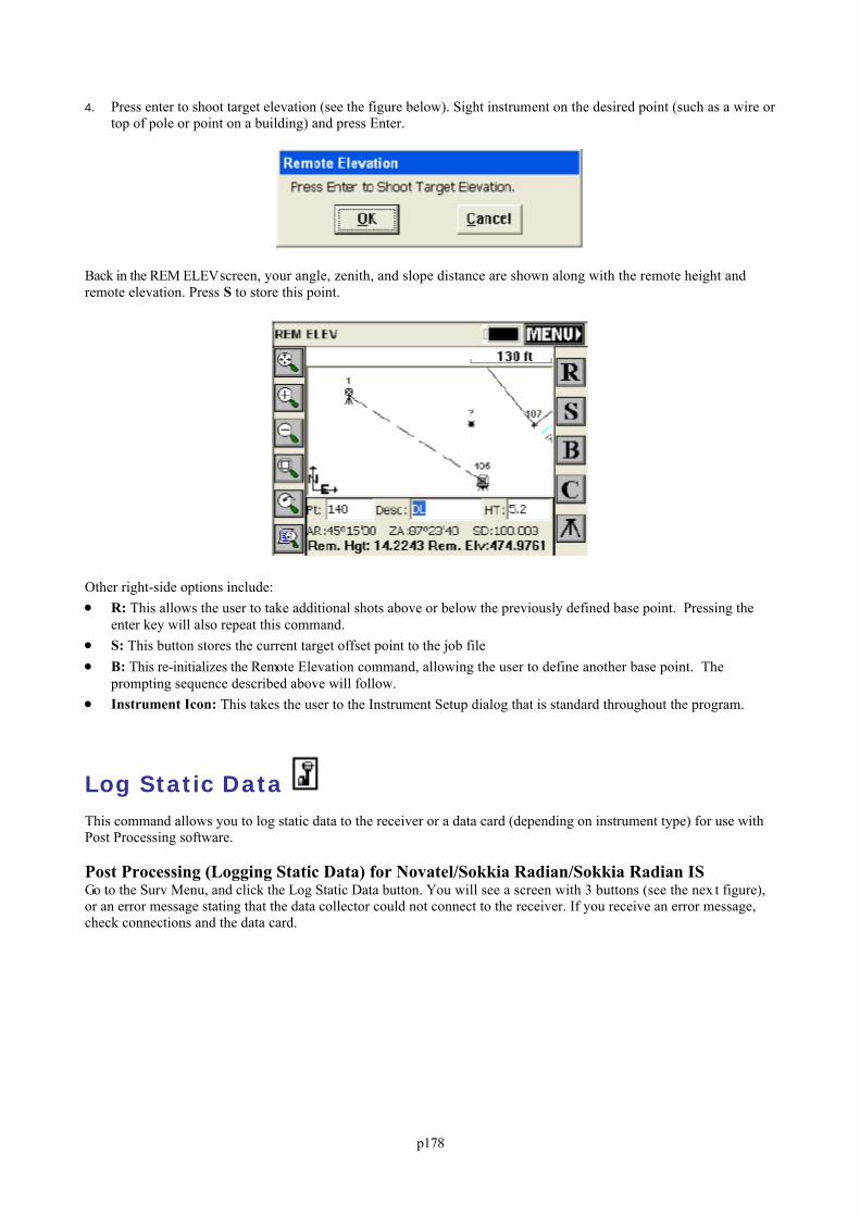
p178

4. Press enter to shoot target elevation (see the figure below). Sight instrument on the desired point (such as a wire ortop of pole or point on a building) and press Enter.

Back in the REM ELEV screen, your angle, zenith, and slope distance are shown along with the remote height andremote elevation. Press S to store this point.

Other right-side options include: R: This allows the user to take additional shots above or below the previously defined base point. Pressing the

enter key will also repeat this command. S: This button stores the current target offset point to the job file B: This re-initializes the Remote Elevation command, allowing the user to define another base point. The

prompting sequence described above will follow. Instrument Icon: This takes the user to the Instrument Setup dialog that is standard throughout the program.

Log Static Data This command allows you to log static data to the receiver or a data card (depending on instrument type) for use withPost Processing software.

Post Processing (Logging Static Data) for Novatel/Sokkia Radian/Sokkia Radian ISGo to the Surv Menu, and click the Log Static Data button. You will see a screen with 3 buttons (see the nex t figure),or an error message stating that the data collector could not connect to the receiver. If you receive an error message,check connections and the data card.

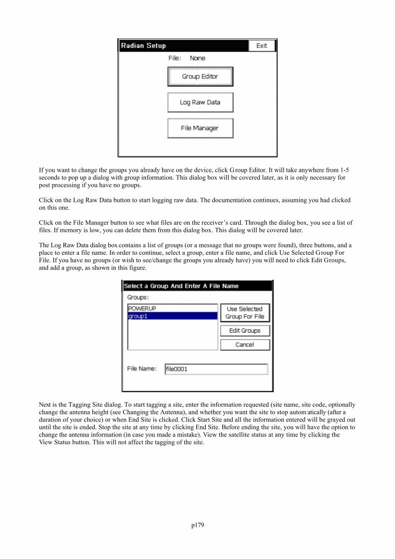
p179

If you want to change the groups you already have on the device, click Group Editor. It will take anywhere from 1-5seconds to pop up a dialog with group information. This dialog box will be covered later, as it is only necessary forpost processing if you have no groups.

Click on the Log Raw Data button to start logging raw data. The documentation continues, assuming you had clickedon this one.

Click on the File Manager button to see what files are on the receiver’s card. Through the dialog box, you see a list offiles. If memory is low, you can delete them from this dialog box. This dialog will be covered later.

The Log Raw Data dialog box contains a list of groups (or a message that no groups were found), three buttons, and aplace to enter a file name. In order to continue, select a group, enter a file name, and click Use Selected Group ForFile. If you have no groups (or wish to see/change the groups you already have) you will need to click Edit Groups,and add a group, as shown in this figure.

Next is the Tagging Site dialog. To start tagging a site, enter the information requested (site name, site code, optionallychange the antenna height (see Changing the Antenna), and whether you want the site to stop autom atically (after aduration of your choice) or when End Site is clicked. Click Start Site and all the information entered will be grayed outuntil the site is ended. Stop the site at any time by clicking End Site. Before ending the site, you will have the option tochange the antenna information (in case you made a mistake). View the satellite status at any time by clicking theView Status button. This will not affect the tagging of the site.

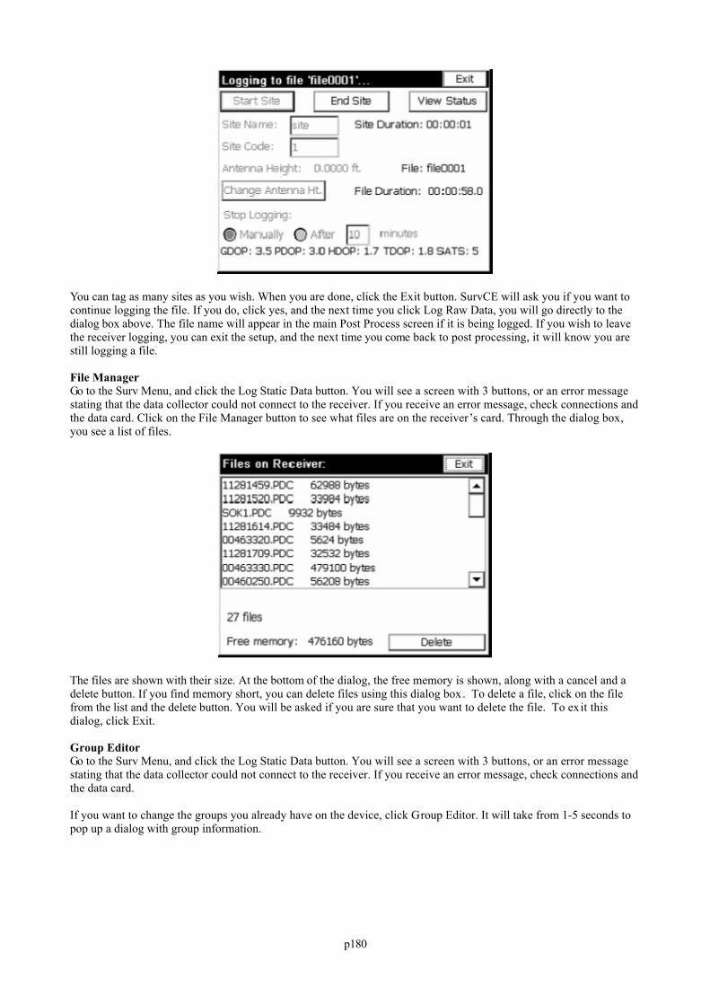
p180

You can tag as many sites as you wish. When you are done, click the Exit button. SurvCE will ask you if you want tocontinue logging the file. If you do, click yes, and the next time you click Log Raw Data, you will go directly to thedialog box above. The file name will appear in the main Post Process screen if it is being logged. If you wish to leavethe receiver logging, you can exit the setup, and the next time you come back to post processing, it will know you arestill logging a file.

File ManagerGo to the Surv Menu, and click the Log Static Data button. You will see a screen with 3 buttons, or an error messagestating that the data collector could not connect to the receiver. If you receive an error message, check connections andthe data card. Click on the File Manager button to see what files are on the receiver’s card. Through the dialog box,you see a list of files.

The files are shown with their size. At the bottom of the dialog, the free memory is shown, along with a cancel and adelete button. If you find memory short, you can delete files using this dialog box. To delete a file, click on the filefrom the list and the delete button. You will be asked if you are sure that you want to delete the file. To exit thisdialog, click Exit.

Group EditorGo to the Surv Menu, and click the Log Static Data button. You will see a screen with 3 buttons, or an error messagestating that the data collector could not connect to the receiver. If you receive an error message, check connections andthe data card.

If you want to change the groups you already have on the device, click Group Editor. It will take from 1-5 seconds topop up a dialog with group information.

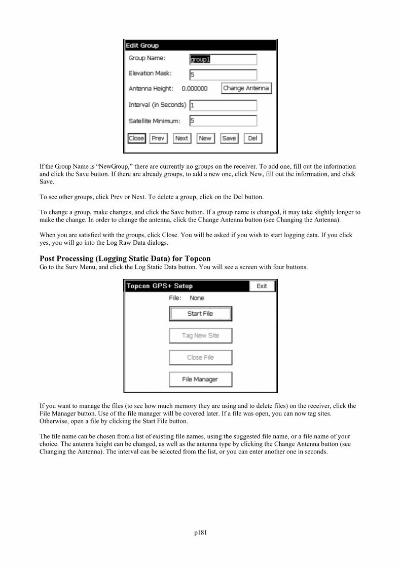
p181

If the Group Name is “NewGroup,” there are currently no groups on the receiver. To add one, fill out the informationand click the Save button. If there are already groups, to add a new one, click New, fill out the information, and clickSave.

To see other groups, click Prev or Next. To delete a group, click on the Del button.

To change a group, make changes, and click the Save button. If a group name is changed, it may take slightly longer tomake the change. In order to change the antenna, click the Change Antenna button (see Changing the Antenna).

When you are satisfied with the groups, click Close. You will be asked if you wish to start logging data. If you clickyes, you will go into the Log Raw Data dialogs.

Post Processing (Logging Static Data) for TopconGo to the Surv Menu, and click the Log Static Data button. You will see a screen with four buttons.

If you want to manage the files (to see how much memory they are using and to delete files) on the receiver, click theFile Manager button. Use of the file manager will be covered later. If a file was open, you can now tag sites.Otherwise, open a file by clicking the Start File button.

The file name can be chosen from a list of existing file names, using the suggested file name, or a file name of yourchoice. The antenna height can be changed, as well as the antenna type by clicking the Change Antenna button (seeChanging the Antenna). The interval can be selected from the list, or you can enter another one in seconds.

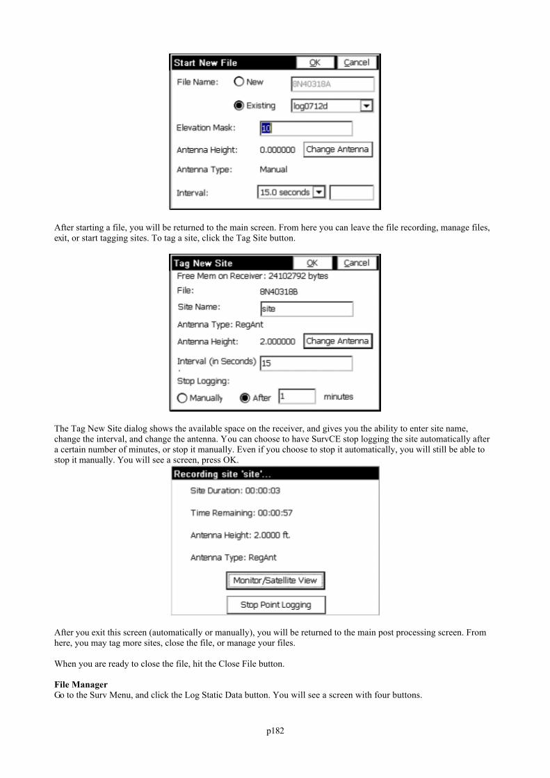
p182

After starting a file, you will be returned to the main screen. From here you can leave the file recording, manage files,exit, or start tagging sites. To tag a site, click the Tag Site button.

The Tag New Site dialog shows the available space on the receiver, and gives you the ability to enter site name,change the interval, and change the antenna. You can choose to have SurvCE stop logging the site automatically aftera certain number of minutes, or stop it manually. Even if you choose to stop it automatically, you will still be able tostop it manually. You will see a screen, press OK.

After you exit this screen (automatically or manually), you will be returned to the main post processing screen. Fromhere, you may tag more sites, close the file, or manage your files.

When you are ready to close the file, hit the Close File button.

File ManagerGo to the Surv Menu, and click the Log Static Data button. You will see a screen with four buttons.

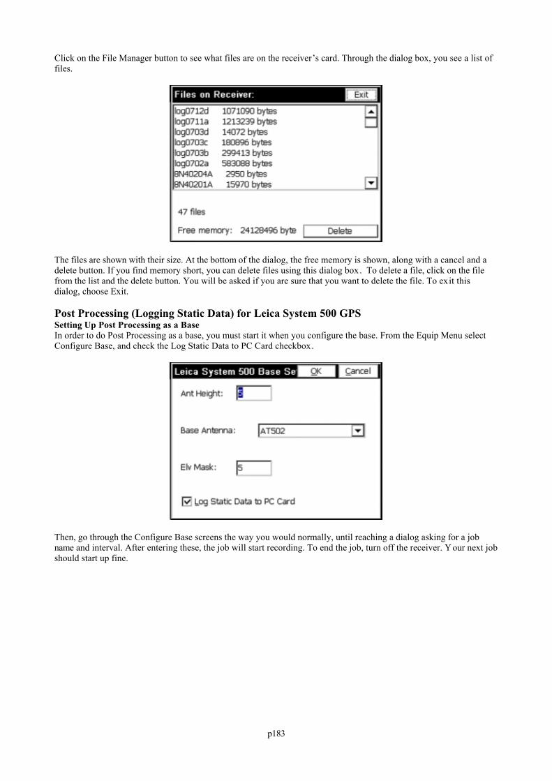
p183

Click on the File Manager button to see what files are on the receiver’s card. Through the dialog box, you see a list offiles.

The files are shown with their size. At the bottom of the dialog, the free memory is shown, along with a cancel and adelete button. If you find memory short, you can delete files using this dialog box. To delete a file, click on the filefrom the list and the delete button. You will be asked if you are sure that you want to delete the file. To exit thisdialog, choose Exit.

Post Processing (Logging Static Data) for Leica System 500 GPSSetting Up Post Processing as a BaseIn order to do Post Processing as a base, you must start it when you configure the base. From the Equip Menu selectConfigure Base, and check the Log Static Data to PC Card checkbox.

Then, go through the Configure Base screens the way you would normally, until reaching a dialog asking for a jobname and interval. After entering these, the job will start recording. To end the job, turn off the receiver. Y our next jobshould start up fine.

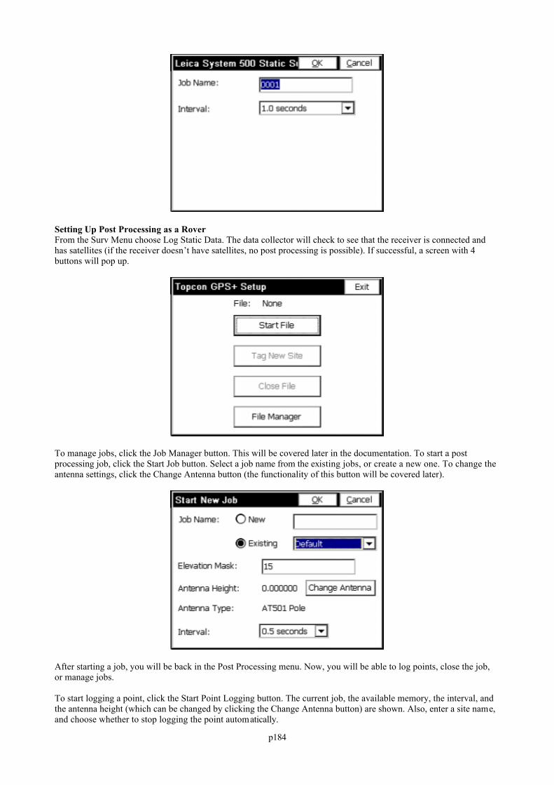
p184

Setting Up Post Processing as a RoverFrom the Surv Menu choose Log Static Data. The data collector will check to see that the receiver is connected andhas satellites (if the receiver doesn’t have satellites, no post processing is possible). If successful, a screen with 4buttons will pop up.

To manage jobs, click the Job Manager button. This will be covered later in the documentation. To start a postprocessing job, click the Start Job button. Select a job name from the existing jobs, or create a new one. To change theantenna settings, click the Change Antenna button (the functionality of this button will be covered later).

After starting a job, you will be back in the Post Processing menu. Now, you will be able to log points, close the job,or manage jobs.

To start logging a point, click the Start Point Logging button. The current job, the available memory, the interval, andthe antenna height (which can be changed by clicking the Change Antenna button) are shown. Also, enter a site name,and choose whether to stop logging the point automatically.

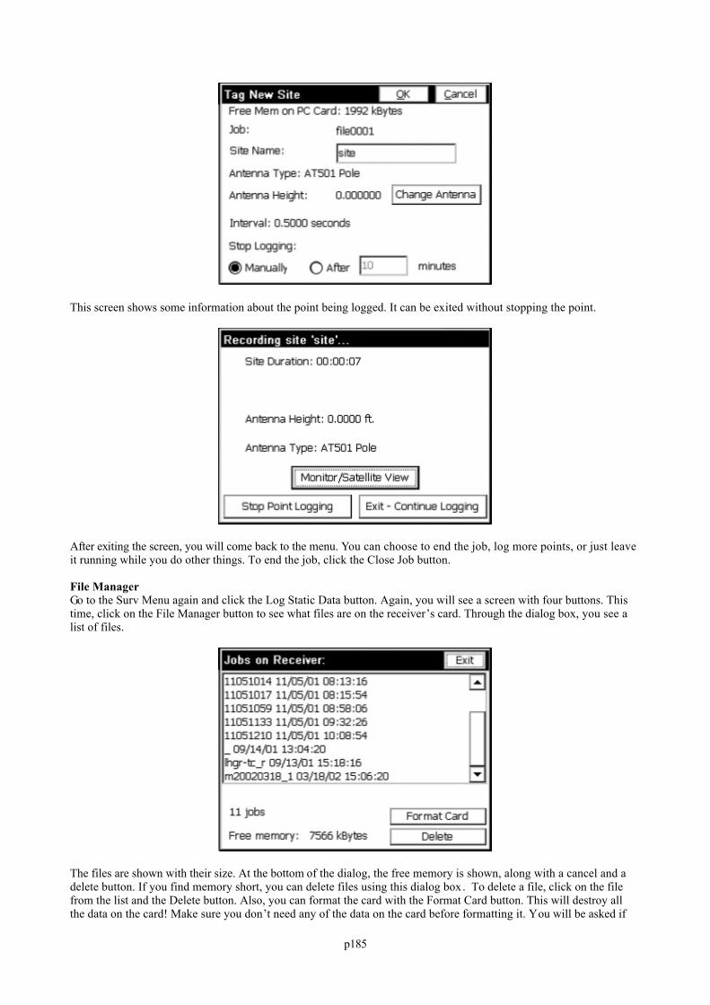
p185

This screen shows some information about the point being logged. It can be exited without stopping the point.

After exiting the screen, you will come back to the menu. You can choose to end the job, log more points, or just leaveit running while you do other things. To end the job, click the Close Job button.

File ManagerGo to the Surv Menu again and click the Log Static Data button. Again, you will see a screen with four buttons. Thistime, click on the File Manager button to see what files are on the receiver’s card. Through the dialog box, you see alist of files.

The files are shown with their size. At the bottom of the dialog, the free memory is shown, along with a cancel and adelete button. If you find memory short, you can delete files using this dialog box. To delete a file, click on the filefrom the list and the Delete button. Also, you can format the card with the Format Card button. This will destroy allthe data on the card! Make sure you don’t need any of the data on the card before formatting it. You will be asked if

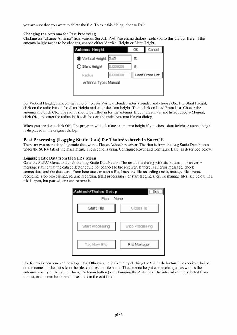
p186

you are sure that you want to delete the file. To exit this dialog, choose Exit.

Changing the Antenna for Post ProcessingClicking on “Change Antenna” from various SurvCE Post Processing dialogs leads you to this dialog. Here, if theantenna height needs to be changes, choose either Vertical Height or Slant Height.

For Vertical Height, click on the radio button for Vertical Height, enter a height, and choose OK. For Slant Height,click on the radio button for Slant Height and enter the slant height. Then, click on Load From List. Choose theantenna and click OK. The radius should be filled in for the antenna. If your antenna is not listed, choose Manual,click OK, and enter the radius in the edit box on the main Antenna Height dialog.

When you are done, click OK. The program will calculate an antenna height if you chose slant height. Antenna heightis displayed in the original dialog.

Post Processing (Logging Static Data) for Thales/Ashtech in SurvCEThere are two methods to log static data with a Thales/Ashtech receiver. The first is from the Log Static Data buttonunder the SURV tab of the main menu. The second is using Configure Rover and Configure Base, as described below.

Logging Static Data from the SURV MenuGo to the SURV Menu, and click the Log Static Data button. The result is a dialog with six buttons, or an errormessage stating that the data collector could not connect to the receiver. If there is an error message, checkconnections and the data card. From here one can start a file, leave the file recording (exit), manage files, pauserecording (stop processing), resume recording (start processing), or start tagging sites. To manage files, see below. If afile is open, but paused, one can resume it.

If a file was open, one can now tag sites. Otherwise, open a file by clicking the Start File button. The receiver, basedon the names of the last site in the file, chooses the file name. The antenna height can be changed, as well as theantenna type by clicking the Change Antenna button (see Changing the Antenna). The interval can be selected fromthe list, or one can be entered in seconds in the edit field.

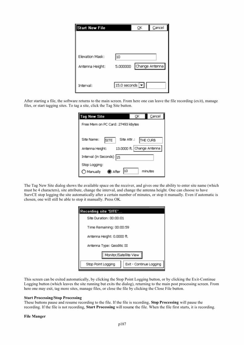
p187

After starting a file, the software returns to the main screen. From here one can leave the file recording (exit), managefiles, or start tagging sites. To tag a site, click the Tag Site button.

The Tag New Site dialog shows the available space on the receiver, and gives one the ability to enter site name (whichmust be 4 characters), site attribute, change the interval, and change the antenna height. One can choose to haveSurvCE stop logging the site automatically after a certain number of minutes, or stop it manually. Even if automatic ischosen, one will still be able to stop it manually. Press OK.

This screen can be exited automatically, by clicking the Stop Point Logging button, or by clicking the Exit-ContinueLogging button (which leaves the site running but exits the dialog), returning to the main post processing screen. Fromhere one may exit, tag more sites, manage files, or close the file by clicking the Close File button.

Start Processing/Stop ProcessingThese buttons pause and resume recording to the file. If the file is recording, Stop Processing will pause therecording. If the file is not recording, Start Processing will resume the file. When the file first starts, it is recording.

File Manger

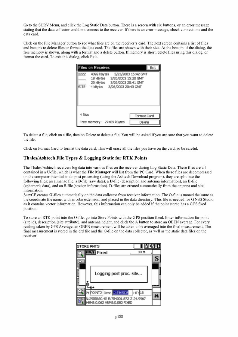
p188

Go to the SURV Menu, and click the Log Static Data button. There is a screen with six buttons, or an error messagestating that the data collector could not connect to the receiver. If there is an error message, check connections and thedata card.

Click on the File Manager button to see what files are on the receiver’s card. The next screen contains a list of filesand buttons to delete files or format the data card. The files are shown with their size. At the bottom of the dialog, thefree memory is shown, along with a format and a delete button. If memory is short, delete files using this dialog, orformat the card. To exit this dialog, click Exit.

To delete a file, click on a file, then on Delete to delete a file. You will be asked if you are sure that you want to deletethe file.

Click on Format Card to format the data card. This will erase all the files you have on the card, so be careful.

Thales/Ashtech File Types & Logging Static for RTK Points

The Thales/Ashtech receivers log data into various files on the receiver during Log Static Data. These files are allcontained in a U-file, which is what the File Manager will list from the PC Card. When these files are decompressedon the computer intended to do post processing (using the Ashtech Download program), they are split into thefollowing files: an almanac file, a B-file (raw data), a D-file (description and antenna information), an E-file(ephemeris data), and an S-file (session information). D-files are created automatically from the antenna and siteinformation.SurvCE creates O-files automatically on the data collector from receiver information. The O-file is named the same asthe coordinate file name, with an .obn extension, and placed in the data directory. This file is needed for G NSS Studio,as it contains vector information. However, this information can only be added if the point stored has a G PS fixedposition.

To store an RTK point into the O-file, go into Store Points with the GPS position fixed. Enter information for point(site id), description (site attribute), and antenna height, and click the A button to store an OBEN average. For everyreading taken by GPS Average, an OBEN measurement will be taken to be averaged into the final measurement. Thefinal measurement is stored in the crd file and the O-file on the data collector, as well as the static data files on thereceiver.

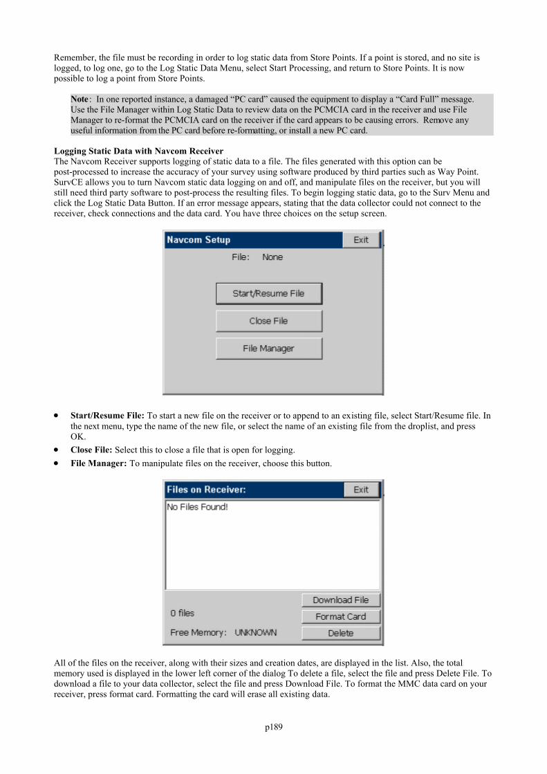
p189

Remember, the file must be recording in order to log static data from Store Points. If a point is stored, and no site islogged, to log one, go to the Log Static Data Menu, select Start Processing, and return to Store Points. It is nowpossible to log a point from Store Points.

Note : In one reported instance, a damaged “PC card” caused the equipment to display a “Card Full” message.Use the File Manager within Log Static Data to review data on the PCMCIA card in the receiver and use FileManager to re-format the PCMCIA card on the receiver if the card appears to be causing errors. Remove anyuseful information from the PC card before re-formatting, or install a new PC card.

Logging Static Data with Navcom ReceiverThe Navcom Receiver supports logging of static data to a file. The files generated with this option can bepost-processed to increase the accuracy of your survey using software produced by third parties such as Way Point.SurvCE allows you to turn Navcom static data logging on and off, and manipulate files on the receiver, but you willstill need third party software to post-process the resulting files. To begin logging static data, go to the Surv Menu andclick the Log Static Data Button. If an error message appears, stating that the data collector could not connect to thereceiver, check connections and the data card. You have three choices on the setup screen.

Start/Resume File: To start a new file on the receiver or to append to an existing file, select Start/Resume file. Inthe next menu, type the name of the new file, or select the name of an existing file from the droplist, and pressOK.

Close File: Select this to close a file that is open for logging. File Manager: To manipulate files on the receiver, choose this button.

All of the files on the receiver, along with their sizes and creation dates, are displayed in the list. Also, the totalmemory used is displayed in the lower left corner of the dialog To delete a file, select the file and press Delete File. Todownload a file to your data collector, select the file and press Download File. To format the MMC data card on yourreceiver, press format card. Formatting the card will erase all existing data.

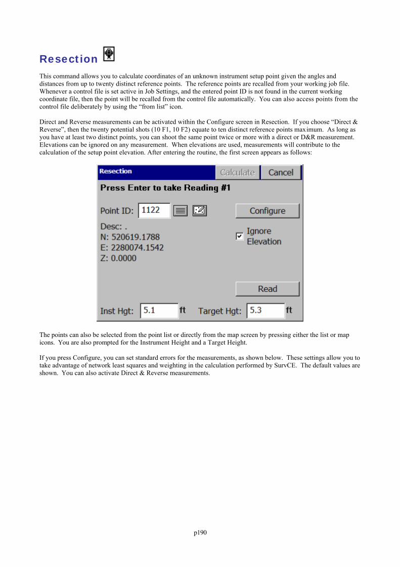
p190

Resection This command allows you to calculate coordinates of an unknown instrument setup point given the angles anddistances from up to twenty distinct reference points. The reference points are recalled from your working job file. Whenever a control file is set active in Job Settings, and the entered point ID is not found in the current workingcoordinate file, then the point will be recalled from the control file automatically. You can also access points from thecontrol file deliberately by using the “from list” icon.

Direct and Reverse measurements can be activated within the Configure screen in Resection. If you choose “Direct &Reverse”, then the twenty potential shots (10 F1, 10 F2) equate to ten distinct reference points maximum. As long asyou have at least two distinct points, you can shoot the same point twice or more with a direct or D&R measurement. Elevations can be ignored on any measurement. When elevations are used, measurements will contribute to thecalculation of the setup point elevation. After entering the routine, the first screen appears as follows:

The points can also be selected from the point list or directly from the map screen by pressing either the list or mapicons. You are also prompted for the Instrument Height and a Target Height.

If you press Configure, you can set standard errors for the measurements, as shown below. These settings allow you totake advantage of network least squares and weighting in the calculation performed by SurvCE. The default values areshown. You can also activate Direct & Reverse measurements.

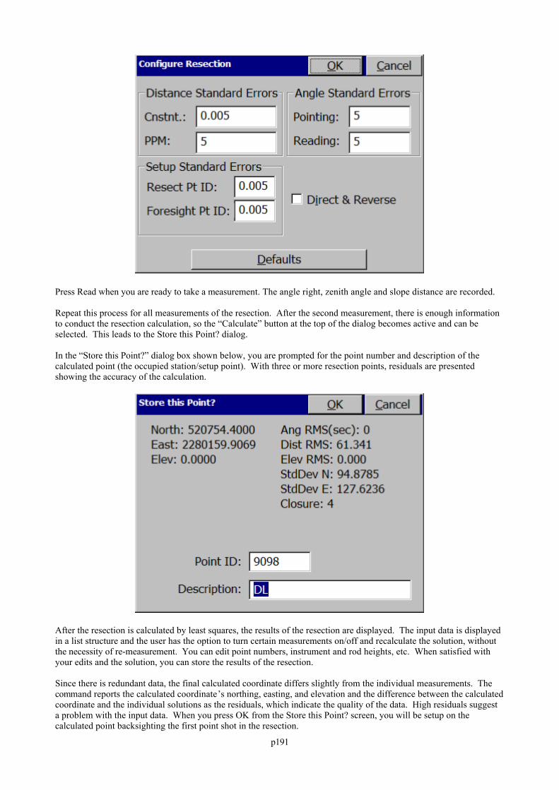
p191

Press Read when you are ready to take a measurement. The angle right, zenith angle and slope distance are recorded.

Repeat this process for all measurements of the resection. After the second measurement, there is enough informationto conduct the resection calculation, so the “Calculate” button at the top of the dialog becomes active and can beselected. This leads to the Store this Point? dialog.

In the “Store this Point?” dialog box shown below, you are prompted for the point number and description of thecalculated point (the occupied station/setup point). With three or more resection points, residuals are presentedshowing the accuracy of the calculation.

After the resection is calculated by least squares, the results of the resection are displayed. The input data is displayedin a list structure and the user has the option to turn certain measurements on/off and recalculate the solution, withoutthe necessity of re-measurement. You can edit point numbers, instrument and rod heights, etc. When satisfied withyour edits and the solution, you can store the results of the resection.

Since there is redundant data, the final calculated coordinate differs slightly from the individual measurements. Thecommand reports the calculated coordinate’s northing, easting, and elevation and the difference between the calculatedcoordinate and the individual solutions as the residuals, which indicate the quality of the data. High residuals suggesta problem with the input data. When you press OK from the Store this Point? screen, you will be setup on thecalculated point backsighting the first point shot in the resection.

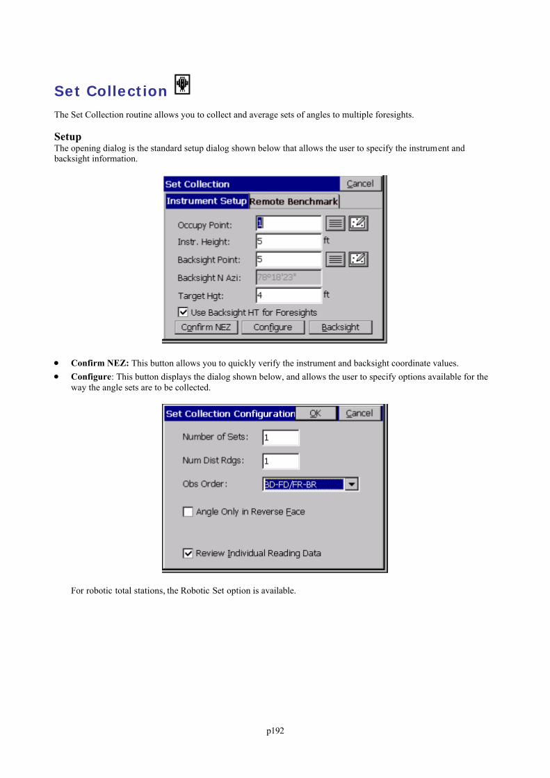
p192

Set Collection The Set Collection routine allows you to collect and average sets of angles to multiple foresights.

SetupThe opening dialog is the standard setup dialog shown below that allows the user to specify the instrument andbacksight information.

Confirm NEZ: This button allows you to quickly verify the instrument and backsight coordinate values. Configure: This button displays the dialog shown below, and allows the user to specify options available for the

way the angle sets are to be collected.

For robotic total stations, the Robotic Set option is available.

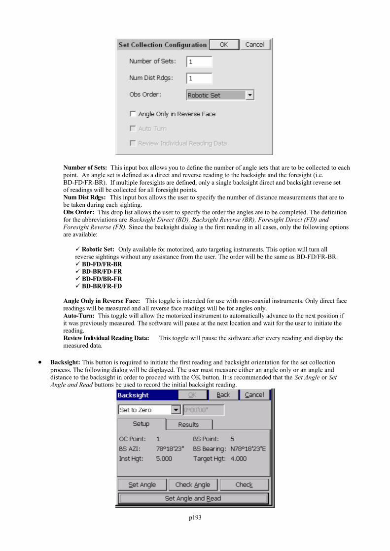
p193

Number of Sets: This input box allows you to define the number of angle sets that are to be collected to eachpoint. An angle set is defined as a direct and reverse reading to the backsight and the foresight (i.e.BD-FD/FR-BR). If multiple foresights are defined, only a single backsight direct and backsight reverse setof readings will be collected for all foresight points.Num Dist Rdgs: This input box allows the user to specify the number of distance measurements that are tobe taken during each sighting.Obs Order: This drop list allows the user to specify the order the angles are to be completed. The definitionfor the abbreviations are Backsight Direct (BD), Backsight Reverse (BR), Foresight Direct (FD) andForesight Reverse (FR). Since the backsight dialog is the first reading in all cases, only the following optionsare available:

Robotic Set: Only available for motorized, auto targeting instruments. This option will turn allreverse sightings without any assistance from the user. The order will be the same as BD-FD/FR-BR. BD-FD/FR-BR BD-BR/FD-FR BD-FD/BR-FR BD-BR/FR-FD

Angle Only in Reverse Face: This toggle is intended for use with non-coaxial instruments. Only direct facereadings will be measured and all reverse face readings will be for angles only.Auto-Turn: This toggle will allow the motorized instrument to automatically advance to the next position ifit was previously measured. The software will pause at the next location and wait for the user to initiate thereading.Review Individual Reading Data: This toggle will pause the software after every reading and display themeasured data.

Backsight: This button is required to initiate the first reading and backsight orientation for the set collectionprocess. The following dialog will be displayed. The user must measure either an angle only or an angle anddistance to the backsight in order to proceed with the OK button. It is recommended that the Set Angle or SetAngle and Read buttons be used to record the initial backsight reading.

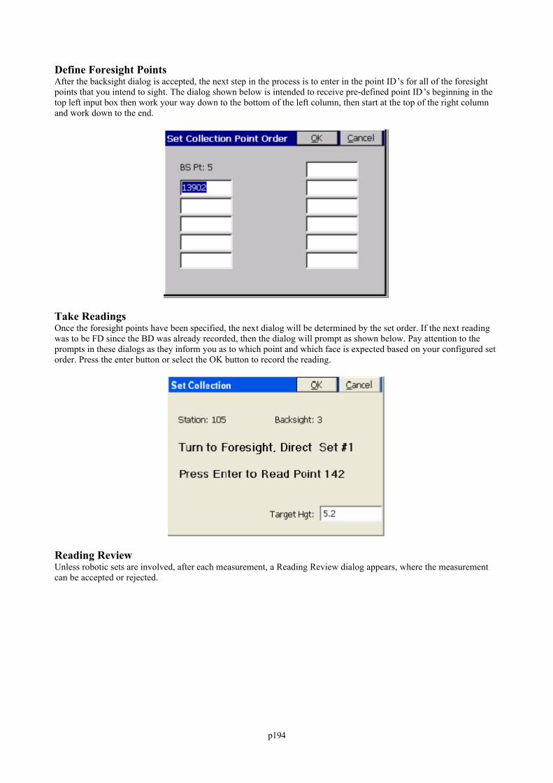
p194

Define Foresight PointsAfter the backsight dialog is accepted, the next step in the process is to enter in the point ID’s for all of the foresightpoints that you intend to sight. The dialog shown below is intended to receive pre-defined point ID’s beginning in thetop left input box then work your way down to the bottom of the left column, then start at the top of the right columnand work down to the end.

Take ReadingsOnce the foresight points have been specified, the next dialog will be determined by the set order. If the next readingwas to be FD since the BD was already recorded, then the dialog will prompt as shown below. Pay attention to theprompts in these dialogs as they inform you as to which point and which face is expected based on your configured setorder. Press the enter button or select the OK button to record the reading.

Reading ReviewUnless robotic sets are involved, after each measurement, a Reading Review dialog appears, where the measurementcan be accepted or rejected.

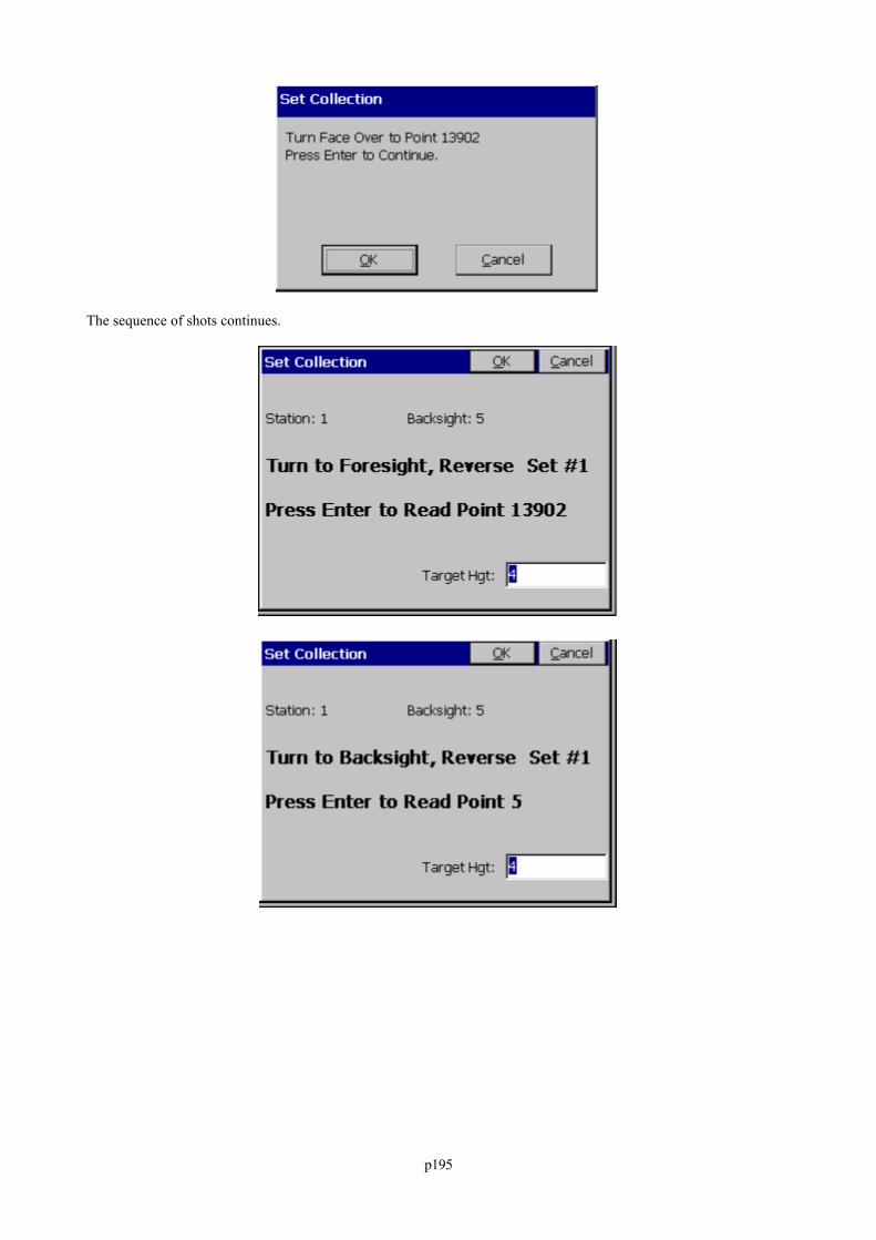
p195

The sequence of shots continues.

p196

Completed SetAt the end of the set collection process is the dialog displayed below. This will be presented after all of the reciprocalcalculation and store point dialogs have been dismissed.

Change Station: This button will take the user to the instrument setup dialog and advance the point numbers sothat the originally occupied point is the backsight and the last foresight point is now the occupied point.

Collect More Sets: This button will take the user to the backsight dialog and maintain all of the previous setupinformation.

Review Direct-Reverse Report: This button will allow the user to select the occupied point ID from a list ofpoints that were used with set collection. The software will then generate a report of all of the sets measure fromthe specified occupation point.

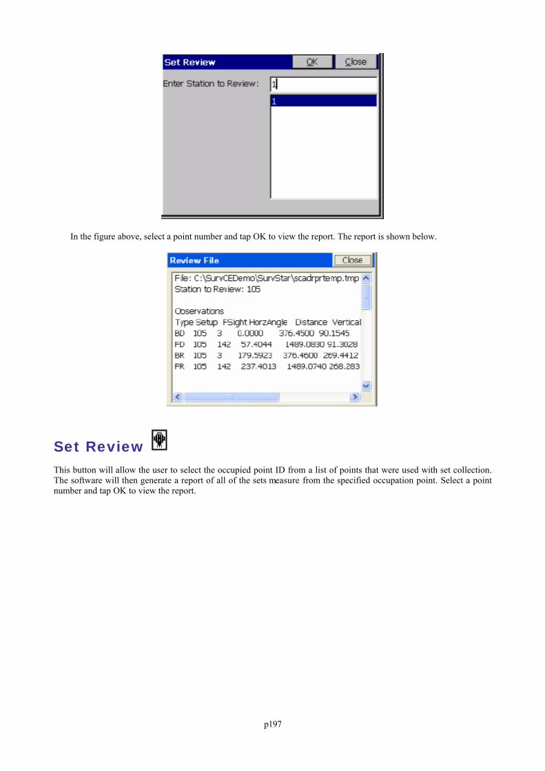
p197

In the figure above, select a point number and tap OK to view the report. The report is shown below.

Set Review This button will allow the user to select the occupied point ID from a list of points that were used with set collection.The software will then generate a report of all of the sets measure from the specified occupation point. Select a pointnumber and tap OK to view the report.

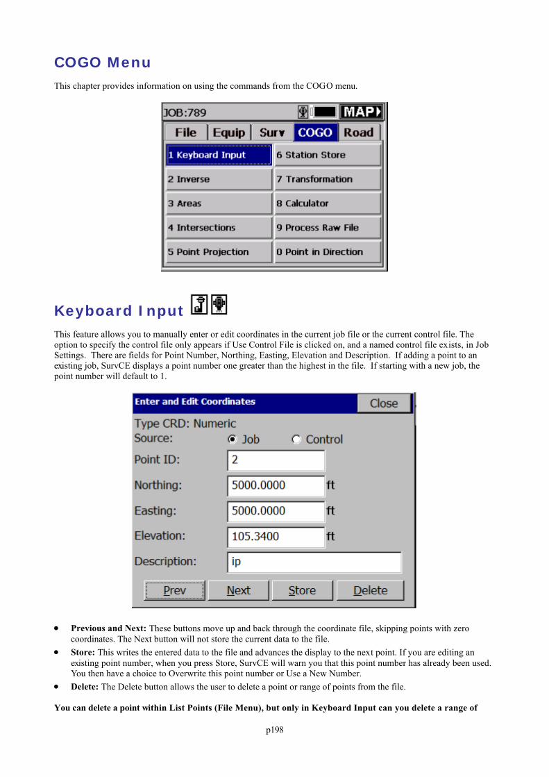
p198

COGO MenuThis chapter provides information on using the commands from the COGO menu.

Keyboard Input This feature allows you to manually enter or edit coordinates in the current job file or the current control file. Theoption to specify the control file only appears if Use Control File is clicked on, and a named control file exists, in JobSettings. There are fields for Point Number, Northing, Easting, Elevation and Description. If adding a point to anexisting job, SurvCE displays a point number one greater than the highest in the file. If starting with a new job, thepoint number will default to 1.

Previous and Next: These buttons move up and back through the coordinate file, skipping points with zerocoordinates. The Next button will not store the current data to the file.

Store: This writes the entered data to the file and advances the display to the next point. If you are editing anexisting point number, when you press Store, SurvCE will warn you that this point number has already been used. You then have a choice to Overwrite this point number or Use a New Number.

Delete: The Delete button allows the user to delete a point or range of points from the file.

You can delete a point within List Points (File Menu), but only in Keyboard Input can you delete a range of

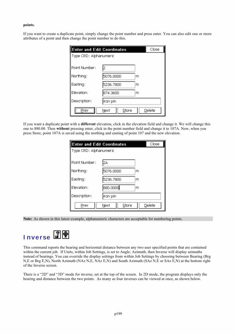
p199

points.

If you want to create a duplicate point, simply change the point number and press enter. You can also edit one or moreattributes of a point and then change the point number to do this.

If you want a duplicate point with a different elevation, click in the elevation field and change it. We will change thisone to 880.00. Then without pressing enter, click in the point number field and change it to 107A. Now, when youpress Store, point 107A is saved using the northing and easting of point 107 and the new elevation.

Note: As shown in this latest example, alphanumeric characters are acceptable for numbering points.

Inverse This command reports the bearing and horizontal distance between any two user specified points that are containedwithin the current job. If Units, within Job Settings, is set to Angle: Azimuth, then Inverse will display azimuthsinstead of bearings. You can override the display settings from within Job Settings by choosing between Bearing (BrgN,E or Brg E,N), North Azimuth (NAz N,E, NAz E,N) and South Azimuth (SAz N,E or SAz E,N) at the bottom rightof the Inverse screen.

There is a “2D” and “3D” mode for inverse, set at the top of the screen. In 2D mode, the program displays only thebearing and distance between the two points. As many as four inverses can be viewed at once, as shown below.

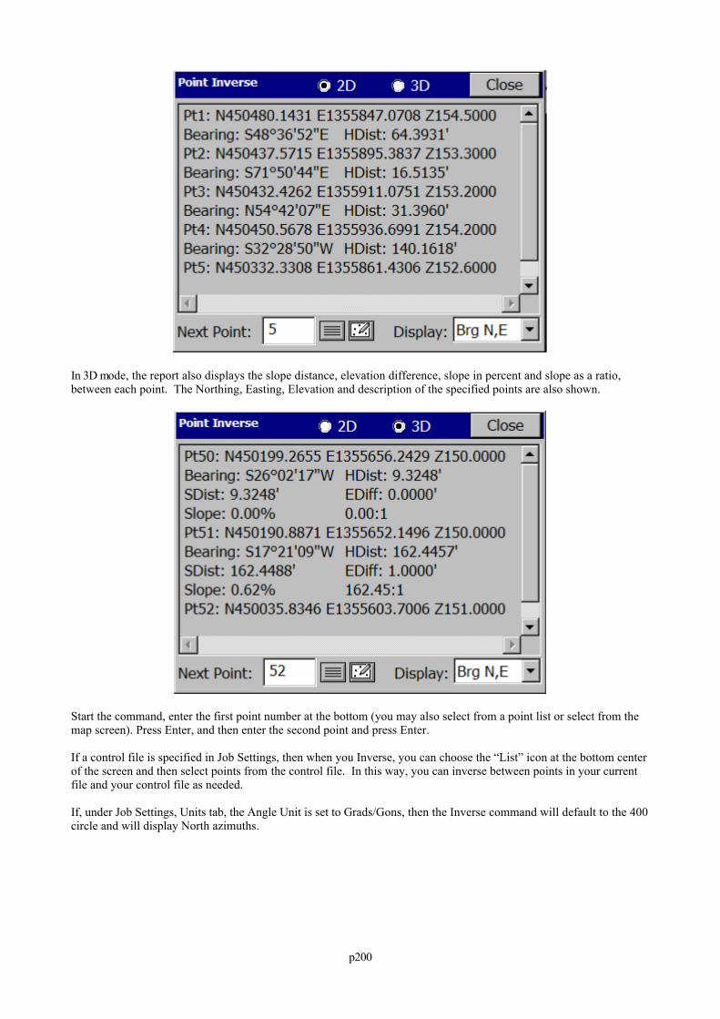
p200

In 3D mode, the report also displays the slope distance, elevation difference, slope in percent and slope as a ratio,between each point. The Northing, Easting, Elevation and description of the specified points are also shown.

Start the command, enter the first point number at the bottom (you may also select from a point list or select from themap screen). Press Enter, and then enter the second point and press Enter.

If a control file is specified in Job Settings, then when you Inverse, you can choose the “List” icon at the bottom centerof the screen and then select points from the control file. In this way, you can inverse between points in your currentfile and your control file as needed.

If, under Job Settings, Units tab, the Angle Unit is set to Grads/Gons, then the Inverse command will default to the 400circle and will display North azimuths.

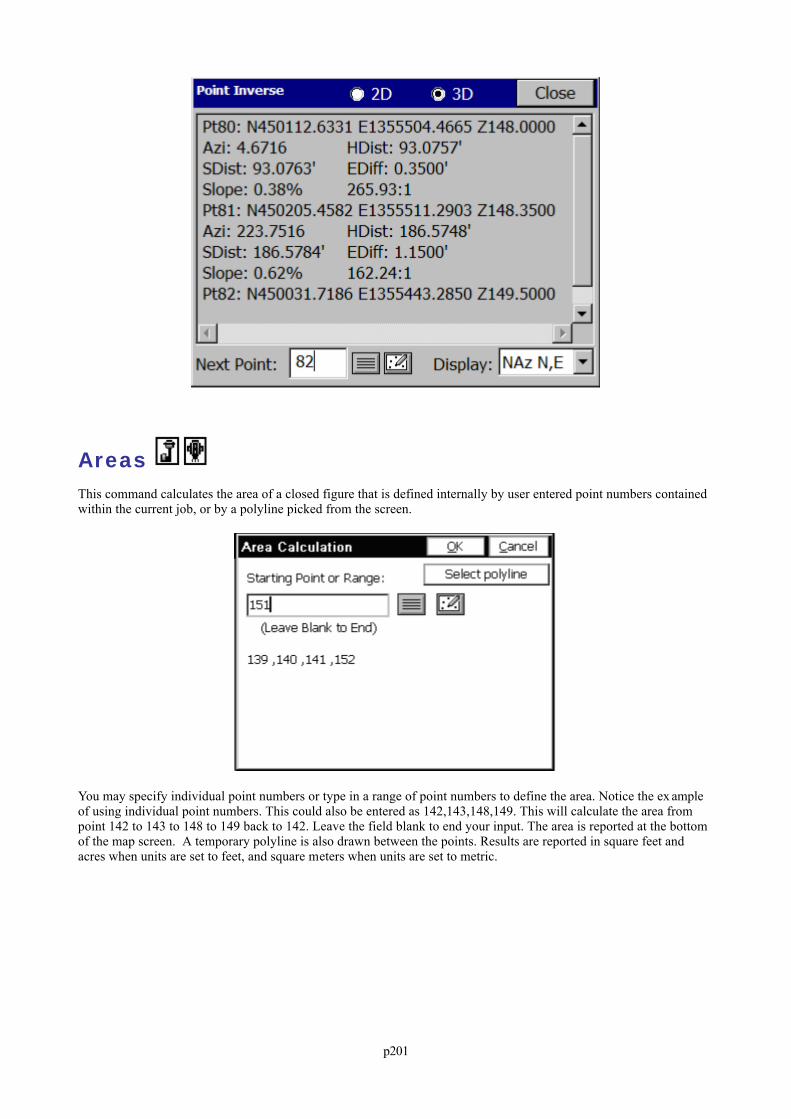
p201

Areas This command calculates the area of a closed figure that is defined internally by user entered point numbers containedwithin the current job, or by a polyline picked from the screen.

You may specify individual point numbers or type in a range of point numbers to define the area. Notice the ex ampleof using individual point numbers. This could also be entered as 142,143,148,149. This will calculate the area frompoint 142 to 143 to 148 to 149 back to 142. Leave the field blank to end your input. The area is reported at the bottomof the map screen. A temporary polyline is also drawn between the points. Results are reported in square feet andacres when units are set to feet, and square meters when units are set to metric.

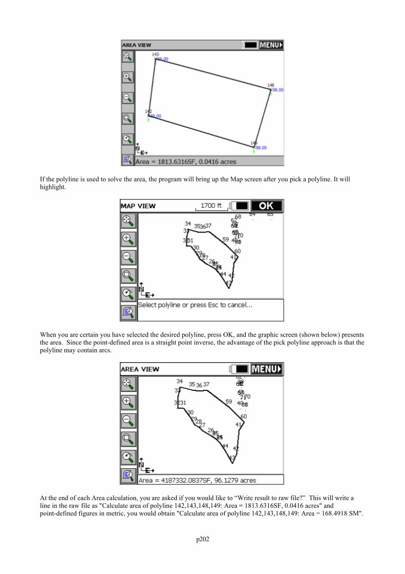
p202

If the polyline is used to solve the area, the program will bring up the Map screen after you pick a polyline. It willhighlight.

When you are certain you have selected the desired polyline, press OK, and the graphic screen (shown below) presentsthe area. Since the point-defined area is a straight point inverse, the advantage of the pick polyline approach is that thepolyline may contain arcs.

At the end of each Area calculation, you are asked if you would like to “Write result to raw file?” This will write aline in the raw file as "Calculate area of polyline 142,143,148,149: Area = 1813.6316SF, 0.0416 acres" andpoint-defined figures in metric, you would obtain "Calculate area of polyline 142,143,148,149: Area = 168.4918 SM".

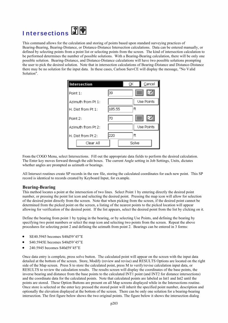
p203

Intersections This command allows for the calculation and storing of points based upon standard surveying practices ofBearing-Bearing, Bearing-Distance, or Distance-Distance Intersection calculations. Data can be entered manually, ordefined by selecting points from a point list or selecting points from the screen. The kind of intersection calculation tobe performed determines the number of possible solutions. With a Bearing-Bearing calculation, there will be only onepossible solution. Bearing-Distance, and Distance-Distance calculations will have two possible solutions promptingthe user to pick the desired solution. Note that in intersection calculations of Bearing-Distance and Distance-Distancethere may be no solution for the input data. In these cases, Carlson SurvCE will display the message, "No ValidSolution".

From the COGO Menu, select Intersections. Fill out the appropriate data fields to perform the desired calculation. The Enter key moves forward through the edit boxes. The current Angle setting in Job Settings, Units, dictateswhether angles are prompted as azimuth or bearings.

All Intersect routines create SP records in the raw file, storing the calculated coordinates for each new point. This SPrecord is identical to records created by Keyboard Input, for example.

Bearing-BearingThis method locates a point at the intersection of two lines. Select Point 1 by entering directly the desired pointnumber, or pressing the point list icon and selecting the desired point. Pressing the map icon will allow for selectionof the desired point directly from the screen. Note that when picking from the screen, if the desired point cannot bedetermined from the picked point on the screen, a listing of the nearest points to the picked location will appearallowing for verification of the desired point. If the list appears, select the desired point from the list by clicking on it.

Define the bearing from point 1 by typing in the bearing, or by selecting Use Points, and defining the bearing byspecifying two point numbers or select the map icon and selecting two points from the screen. Repeat the aboveprocedures for selecting point 2 and defining the azimuth from point 2. Bearings can be entered in 3 forms:

SE40.5945 becomes S40d59’45”E S40.5945E becomes S40d59’45”E 240.5945 becomes S40d59’45”E

Once data entry is complete, press solve button. The calculated point will appear on the screen with the input datadetailed at the bottom of the screen. Store, Modify (review and revise) and RESULTS Options are located on the rightside of the Map screen. Press S to store the calculated point, press M to verify/revise calculation input data, orRESULTS to review the calculation results. The results screen will display the coordinates of the base points, theinverse bearing and distance from the base points to the calculated INT1 point (and INT2 for distance intersections)and the coordinate data for the calculated points. Note that calculated points are labeled as Int1 and Int2 until thepoints are stored. These Option Buttons are present on all Map screens displayed while in the Intersections routine. Once store is selected or the enter key pressed the stored point will inherit the specified point number, description andoptionally the elevation displayed at the bottom of the screen. There can be only one solution for a bearing-bearingintersection. The first figure below shows the two original points. The figure below it shows the intersection dialog

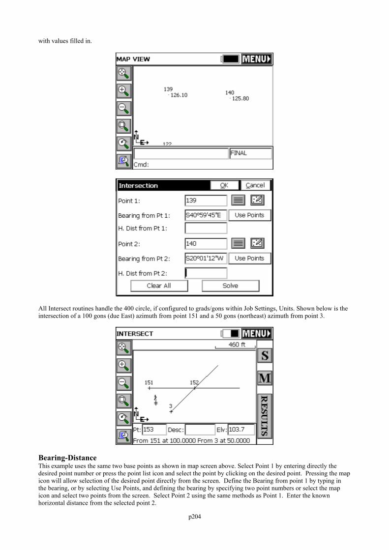
p204

with values filled in.

All Intersect routines handle the 400 circle, if configured to grads/gons within Job Settings, Units. Shown below is theintersection of a 100 gons (due East) azimuth from point 151 and a 50 gons (northeast) azimuth from point 3.

Bearing-DistanceThis example uses the same two base points as shown in map screen above. Select Point 1 by entering directly thedesired point number or press the point list icon and select the point by clicking on the desired point. Pressing the mapicon will allow selection of the desired point directly from the screen. Define the Bearing from point 1 by typing inthe bearing, or by selecting Use Points, and defining the bearing by specifying two point numbers or select the mapicon and select two points from the screen. Select Point 2 using the same methods as Point 1. Enter the knownhorizontal distance from the selected point 2.

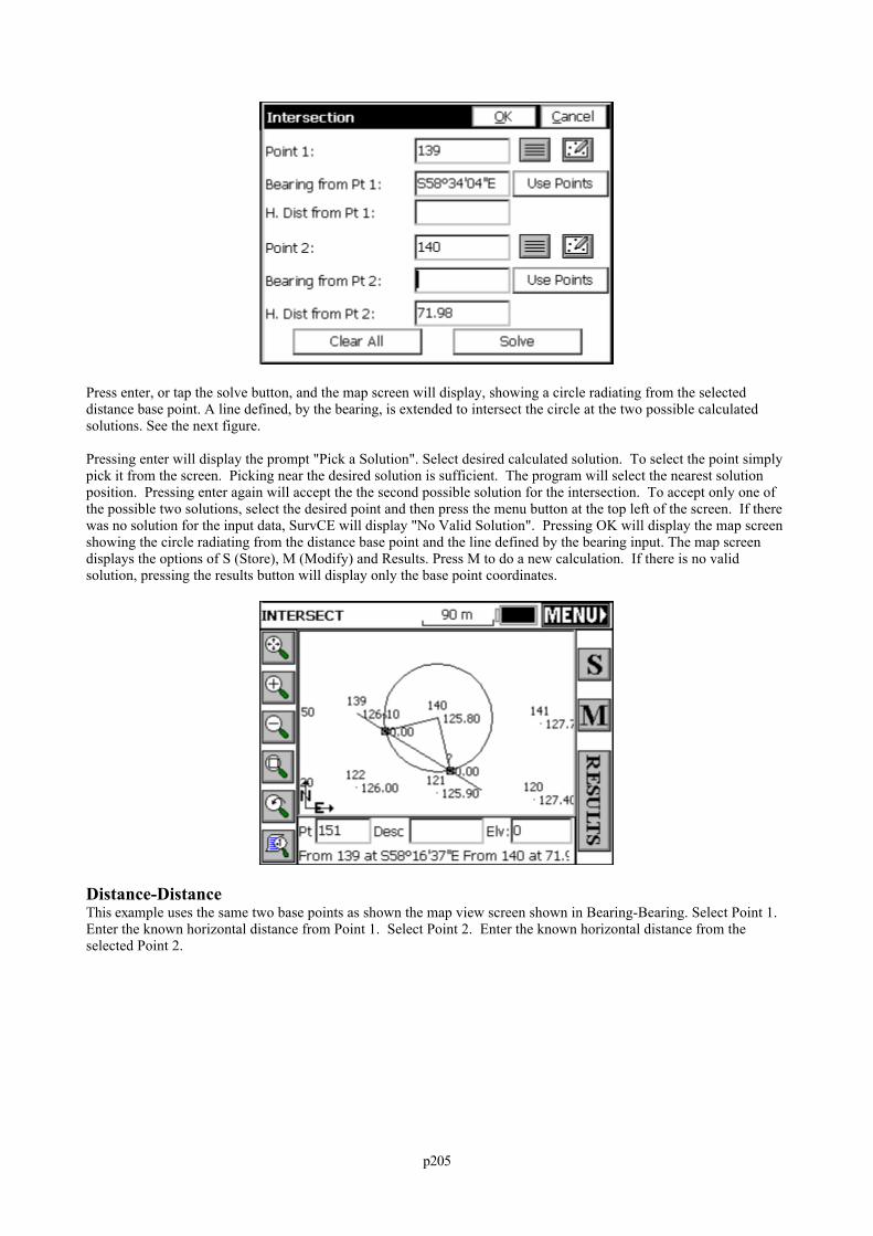
p205

Press enter, or tap the solve button, and the map screen will display, showing a circle radiating from the selecteddistance base point. A line defined, by the bearing, is extended to intersect the circle at the two possible calculatedsolutions. See the next figure.

Pressing enter will display the prompt "Pick a Solution". Select desired calculated solution. To select the point simplypick it from the screen. Picking near the desired solution is sufficient. The program will select the nearest solutionposition. Pressing enter again will accept the the second possible solution for the intersection. To accept only one ofthe possible two solutions, select the desired point and then press the menu button at the top left of the screen. If therewas no solution for the input data, SurvCE will display "No Valid Solution". Pressing OK will display the map screenshowing the circle radiating from the distance base point and the line defined by the bearing input. The map screendisplays the options of S (Store), M (Modify) and Results. Press M to do a new calculation. If there is no validsolution, pressing the results button will display only the base point coordinates.

Distance-DistanceThis example uses the same two base points as shown the map view screen shown in Bearing-Bearing. Select Point 1.Enter the known horizontal distance from Point 1. Select Point 2. Enter the known horizontal distance from theselected Point 2.

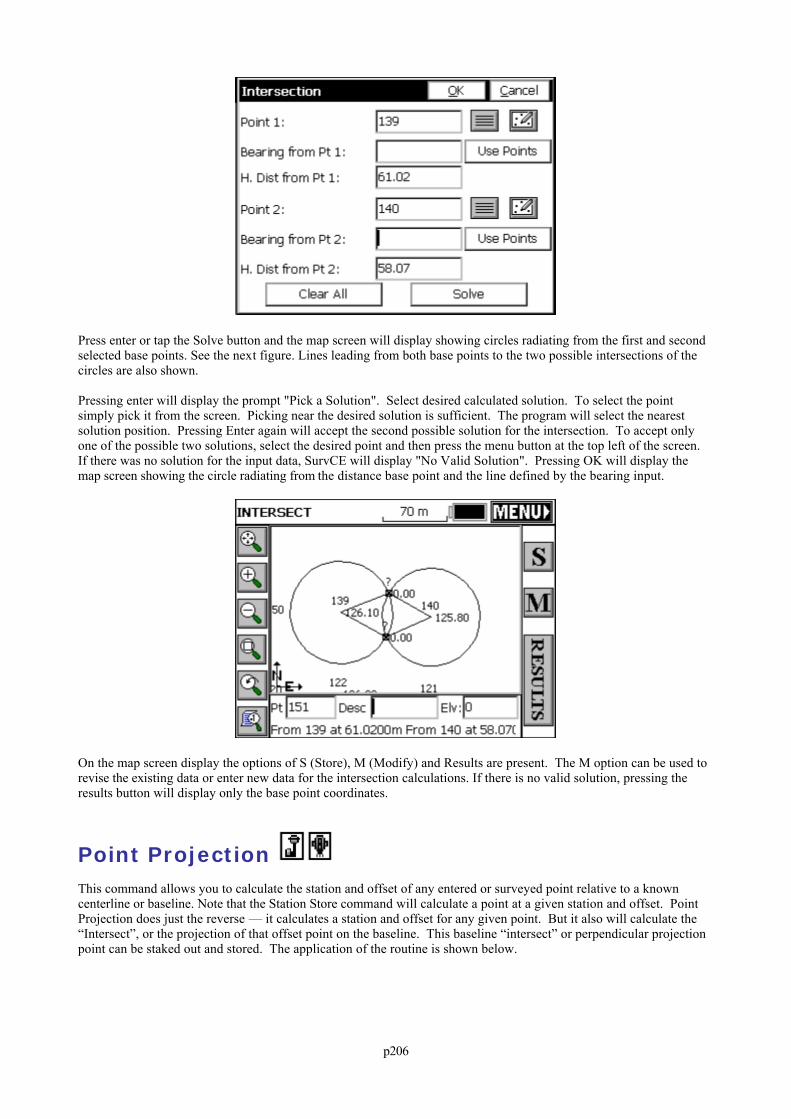
p206

Press enter or tap the Solve button and the map screen will display showing circles radiating from the first and secondselected base points. See the next figure. Lines leading from both base points to the two possible intersections of thecircles are also shown.

Pressing enter will display the prompt "Pick a Solution". Select desired calculated solution. To select the pointsimply pick it from the screen. Picking near the desired solution is sufficient. The program will select the nearestsolution position. Pressing Enter again will accept the second possible solution for the intersection. To accept onlyone of the possible two solutions, select the desired point and then press the menu button at the top left of the screen. If there was no solution for the input data, SurvCE will display "No Valid Solution". Pressing OK will display themap screen showing the circle radiating from the distance base point and the line defined by the bearing input.

On the map screen display the options of S (Store), M (Modify) and Results are present. The M option can be used torevise the existing data or enter new data for the intersection calculations. If there is no valid solution, pressing theresults button will display only the base point coordinates.

Point Projection This command allows you to calculate the station and offset of any entered or surveyed point relative to a knowncenterline or baseline. Note that the Station Store command will calculate a point at a given station and offset. PointProjection does just the reverse — it calculates a station and offset for any given point. But it also will calculate the“Intersect”, or the projection of that offset point on the baseline. This baseline “intersect” or perpendicular projectionpoint can be staked out and stored. The application of the routine is shown below.

p207

The coordinates to project from are entered one of three ways:

By Point Number By Entering the Coordinate Values By Taking a GPS or Total Station Reading

The Station and Offset of the point is then calculated, and the Intersect button (see the above figure) will calculate theprojected perpendicular intersect point on the baseline. This Intersect can be staked out. Point Projection can be used,crudely, to set line, where you sight a manual total station in a gap in a tree line or row of bushes, and note the stationand offset. However, since the offset is perpendicular, the “out” or “in” distance to the desired line will not be alongthe line of sight, as shown above. The best “set line” method is Point on Line within Stakeout Line/Arc.

Procedure: You must first define the baseline as shown in the next figure. You can designate the baseline by pickingtwo points on a line or by choosing a predefined centerline file (.cl file).

If you choose Two Points, you must then define the line in the Point Projection dialog box as shown below.

p208

With the Two Points method, you simply enter two point numbers, or choose them from the point list or MAP. Theazimuth and slope between them is calculated, along with the ending station, based on the entered start station. Withthe Azimuth method, you define the line by entering a first point and then entering an azimuth and slope. You canconfirm the coordinate values of the points by choosing Confirm NEZ. When the line is defined, choose Continue.You must now define, or designate the point that is offset from the line in the Point Definition dialog box .

You can enter a point ID, select one from the list, or select one from the map. You can also enter coordinates to definea new point, or read values for a new point. As soon as enough information is entered, the Station/Offset is displayedor the message OFF CENTERLINE is displayed, to let you know that a station/offset cannot be computed for thecoordinates entered. Read: This command reads the instrument to gather coordinates for point projection. Store: Store after Read stores the offset coordinate. Store after Intersect is selected stores the coordinates for the

intersect point on the centerline (perpendicular from the offset point). Store after entering coordinates or a pointnumber for the offset point, without selecting Intersect, would simply store the offset point coordinates again as anew point number. Store is most often used to save the calculated intersect points to the coordinate file. PressingStore will save an SP (store point) record in the raw file and a note record will indicate tha the point wascalculated within Point Projection.

StakeOut: This command will allow you to stakeout the displayed coordinates (typically used to stakeout theintersect points).

Intersect: This command will project the coordinates entered perpendicular, back to the centerline and enter thesenew coordinates into the Point Projection dialog box. From there you can store or stakeout the intersect points.

p209

This stakeout screen represents a metric, grads/gons display (400 circle). The target point is 198.864 metersalong the baseline, 30.2722 gons angle right from the backsight point 1, a distance of 72.207 meters from theinstrument. Point 1 itself was also the offset point used in this example.

Stakeout Note: During stakeout, you will obtain the standard stakeout screen, where option M returns to theprevious coordinate screen with the same data shown, and option N returns to the same previous screen with thedata cleared, ready for entry of the next offset point.

Station Store Station Store is a pure calculation routine that will create points based on a station and offset from an alignment. Thealignment may be defined as a centerline, a 3-point arc, an arc defined by a PC, Radius and PT, a selected polyline ora sequence of points. The user may also assign an elevation to the calculated point. Station Store might be used toenter elevations of pipe culverts, for example, where inlets and outlets are located at distinct stations, offsets andelevations. Then the two calculated points at the inlet and outlet can be used within Stakeout Line to stake any pointalong the culvert, with the cut/fill calculated. Although the command Stake Centerline, found within StakeoutLine/Arc, will directly stakeout a particular station and offset to a centerline, some users prefer to pre-calculate thestation and offset and assign a point ID, then stake by point ID. Station Store permits this pre-calculation of points atany station and offset.

The very first screen within Station Store offers several methods of defining an alignment.

The routine defaults to the most automatic of the methods—use of a pre-defined centerline file. To review, centerlinefiles can be made by use of the command Input-Edit Centerline File (item 1 within the Road menu). Alternately,centerlines can be uploaded to the SurvCE program from a PC in forms including LandXML, SDR, TDS, ASCII LDD,TM (Terramodel) and Carlson/AutoDesk Field Survey. Unless the file format is Carlson/Autodesk Field Survey, the

p210

command Centerline Conversion within Road Utilities should be used to convert the “foreign” centerline format to the“.cl” form used by SurvCE.

You can follow along by loading the file demo.cl within the command Station Store. Then, on the data entry screen,enter a station of 101.25, offset of -35.5, and elevation of 996.04, as shown below (any unused point ID will do).

Pressing Enter will move through the dialog and store the point, leaving the screen up for more entries, whiledefaulting to the previous data and the next point ID. The description is fixed as the station and offset, but could beedited using the command Keyboard Input. You could continue by entering a right-side station and offset, such asstation 117.25, offset 29.71, elevation 1003.67 for point number 7. Then the 2 calculated points might define a“skewed” pipe culvert, ready for stakeout using the command Stakeout Line/Arc. You could also choose to stakeoutthe endpoints of the culvert by point ID using the command Stakeout Points.

You can draw the demo.cl by doing the command CL2P at the “command” line in the MAP view. It is also foundunder the “Tools” pulldown in the MAP view.

The line representing the culvert is drawn by the command 2DP, which stands for “2D polyline”.

Transformation This command allows you to translate, rotate, and/or scale points in the current job. Any point drawn on the mapscreen will be updated automatically in addition to updating the coordinates.

All three transformations can be performed individually or all at once if desired.

p211

Range of Points: Enter the range of points to translate. Ranges can be entered in the following format: 1-20,32,40-45,etc..Add to Point Numbers: Enter a number to add to existing point numbers when creating new point numbers. Thisoption is not available when overwriting your existing point numbers. Seeexample below under Use New Point Numbers.Overwrite Existing Point Numbers: Overwrites the existing point coordinate data with the new coordinate data.Use New Point Numbers: Uses new point numbers for the new coordinate positions while keeping the existing pointnumbers and coordinate data. Each time a point is to be overwritten, you will be prompted whether to overwrite or usea new point number. This method is only recommended when you are transforming very few points, and wish to givethem specific point number assignments.Store in New CRD File: This option writes the transformed points to a new CRD file while keeping the existingpoint numbers and coordinate data. You may also choose to input a number for Add to Point Numbers, but this is notrequired.

Translate

On the translate dialog, enter in the Delta North, Delta East, and the Delta Elevation. These values represent thechange in the original coordinate values and the desired coordinate values. When complete, select the ok button onthe dialog, or press the Rotate or Scale Tabs for further data input.

The lower portion of the screen, is an alternate method of defining a translation, by comparing an original point to adestination point. Data entered there, as point ID or directly entered northing, easting and elevation, will lead tocomputation and display of the delta N, delta E and delta Z in the upper portion of the screen.

When OK is pressed, a second screen appears which controls then range ofpoints to be translated.

Assuming you have 55 points in your file, you could "preserve" these 55 points by adding 100 to the point numbers,and saving the transformed points as 101 through 155. If you choose "Overwrite", the Add to Point Numbers option isnot available. If you choose "Use New Point Numbers", then you will be prompted to enter a new point number for

p212

each existing point to be overwritten (recommended only when you are overwriting a few points). You can even storethe "transformed" points in a completely new CRD file by selecting "Store in New CRD File".

Raising and Lowering Elevations: Users often ask, "How do I raise or lower elevations on a range of points?" Theanswer is, Transformation, option Translate, enter only the delta elevation (leave Northing and Easting at 0translation). Rather than have a special command for raising or lowering elevations, it is just a subset of the Translateoption within Transformation.

Rotate

The rotate tab is used to rotate points in a coordinate file. Enter thedesired degree of rotation into the degree of rotation data field. Specify the rotation base point. This can be accomplished by eitherentering the point number of the desired point manually, or by selectingthe point list icon and selecting the point from the list, or using themap icon and selecting the point from the screen. You may also enter incoordinates for the rotation point if the point is not present in thecoordinate file. You can also define the rotation by referencing 2points (such as ?From? 1, ?To? 2), then specifying the desired newbearing for these points. Even the new bearing itself can be computedfrom 2 points used as a reference.

The ?second? screen appears, which allows you to set the range of pointsto transform and how to store the newly calculated points. For allrotations, the rotation value is written into the RW5 file as dd.mmss(the current angle format).

Scale

The scale tab is used to scale the points in a coordinate file. The northing, easting and optionally the elevation aremultiplied by the specified scale factor. Enter the desired scale factor in the scale factor field. Select the base point byentering the point number of the desired point manually, or by selecting the point list icon andselecting the point from the list, or by using the map icon andselecting the point from the screen. You may also enter in coordinatesfor the scale base point if the base point for scaling is not present inthe coordinate file. The coordinate of the base point will remainunchanged. All other points will scale. If the Ignore Elevations toggleis checked ON, then only the Northing and Easting values are scaled.

Raw Data Records (CC)

The transformation raw data records are expressed as one string percommand with the values separated by spaces. These records will berecorded to the raw data file for processing purposes so that allCarlson processors will recognize the records and perform thetransformation during re-processing.

* TRANSLATE: Range Dx Dy Dz Process_Zero_Z * ROTATE: Range Angle Base_Y Base_X * SCALE: Range Scale Base_Y Base_X Use_Z * ALIGN: Range From1 To1 From2 To2

Example:

CC,Translate,8-9 200 50 0 0

CC,Rotate,7 33.1234 79613.662 15619.725

CC,Scale,7 1.5 79613.662 15619.725

CC,Align,8-9 8 6 9 7

p213

Calculator This command eliminates the need to carry a separate calculator in the field. The calculator can be used to doscientific computations, standard calculations, conversions, triangle calculations including angles and curvecalculations.

Standard CalculatorThis calculator allows for most basic calculations to be done with this tool. Memory functions are also available.

Scientific CalculatorValues can be entered on the X register by typing on the keypad. The values can be rolled up and down with the upand down arrow keys and the Roll and RollD buttons on the screen. The Enter key finishes the entry of a number andpushes the stack. The C on the touch screen clears an entry. Additional functions on the screen can be obtainedthrough touching the scroll [<] and [>] area of the screen.

p214

Conversion CalculatorConversion values can be entered for various unit types and scenarios. M to Ft: Conversion calculator for converting between the following units. Enter a value in any field and press

enter to find the conversion value.Feet, Meters and International FeetDegrees, Minutes, Seconds and Gons/Grads and Decimal Degrees

Slope Distance to Horizontal Distance: This option allows you to convert slope distances with zenith angles tohorizontal distances and vertical differences, and vice versa. See this figure.

Lat/Lon-SP: This option allows you to convert from Latitude/Longitude to grid system coordinates and viceversa. If you are configured for U.S. State Plane Coordinates, the routine conveniently displays your zone, andyou can even change zones for quick calculations without altering your GPS zone settings in Job Settings.Otherwise, the calculation is based on your Job Settings GPS Zone. To solve for northing and easting, fill in the

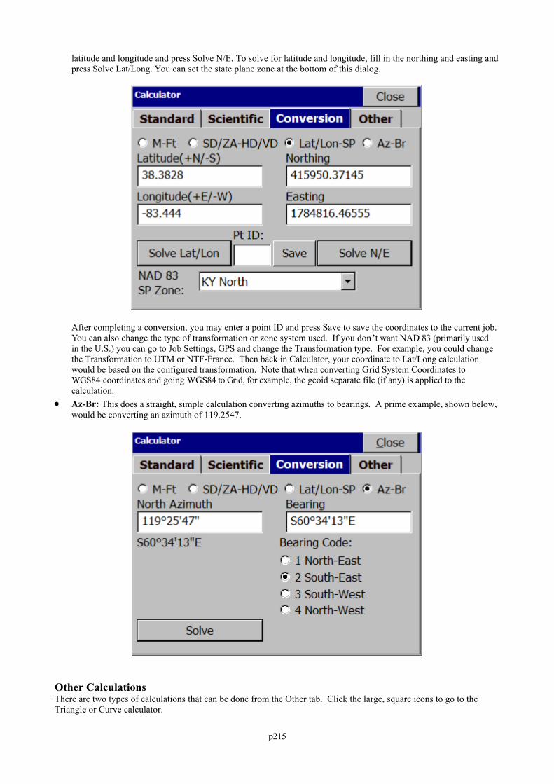
p215

latitude and longitude and press Solve N/E. To solve for latitude and longitude, fill in the northing and easting andpress Solve Lat/Long. You can set the state plane zone at the bottom of this dialog.

After completing a conversion, you may enter a point ID and press Save to save the coordinates to the current job.You can also change the type of transformation or zone system used. If you don’t want NAD 83 (primarily usedin the U.S.) you can go to Job Settings, GPS and change the Transformation type. For example, you could changethe Transformation to UTM or NTF-France. Then back in Calculator, your coordinate to Lat/Long calculationwould be based on the configured transformation. Note that when converting Grid System Coordinates toWGS84 coordinates and going WGS84 to Grid, for example, the geoid separate file (if any) is applied to thecalculation.

Az-Br: This does a straight, simple calculation converting azimuths to bearings. A prime example, shown below,would be converting an azimuth of 119.2547.

Other CalculationsThere are two types of calculations that can be done from the Other tab. Click the large, square icons to go to theTriangle or Curve calculator.

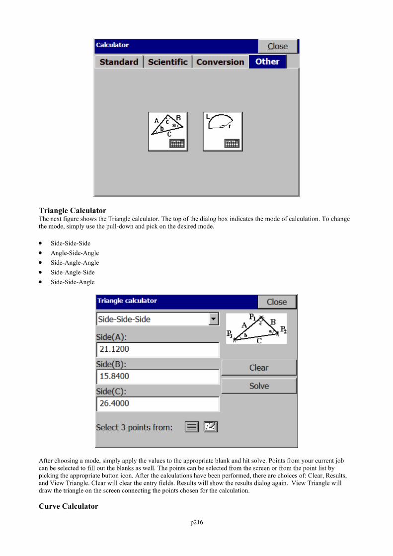
p216

Triangle CalculatorThe next figure shows the Triangle calculator. The top of the dialog box indicates the mode of calculation. To changethe mode, simply use the pull-down and pick on the desired mode.

Side-Side-Side Angle-Side-Angle Side-Angle-Angle Side-Angle-Side Side-Side-Angle

After choosing a mode, simply apply the values to the appropriate blank and hit solve. Points from your current jobcan be selected to fill out the blanks as well. The points can be selected from the screen or from the point list bypicking the appropriate button icon. After the calculations have been performed, there are choices of: Clear, Results,and View Triangle. Clear will clear the entry fields. Results will show the results dialog again. View Triangle willdraw the triangle on the screen connecting the points chosen for the calculation.

Curve Calculator

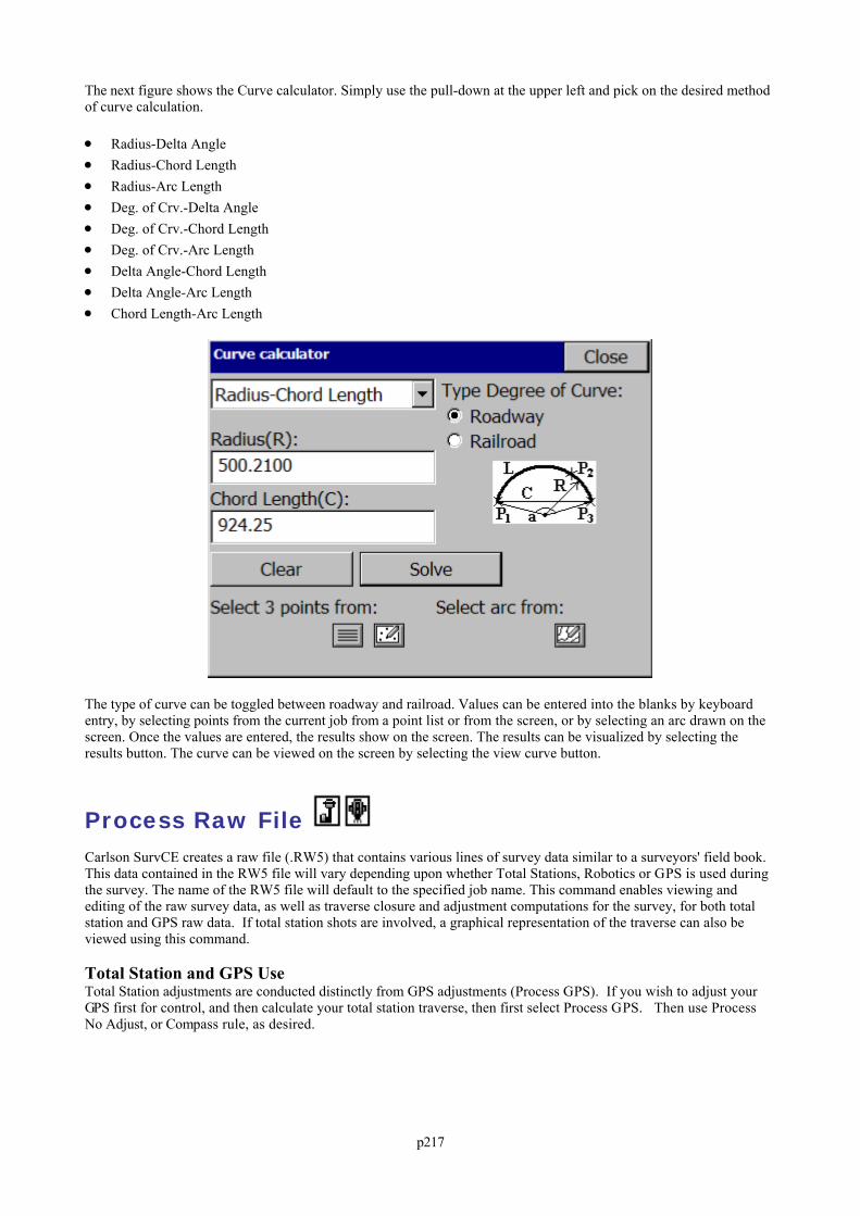
p217

The next figure shows the Curve calculator. Simply use the pull-down at the upper left and pick on the desired methodof curve calculation.

Radius-Delta Angle Radius-Chord Length Radius-Arc Length Deg. of Crv.-Delta Angle Deg. of Crv.-Chord Length Deg. of Crv.-Arc Length Delta Angle-Chord Length Delta Angle-Arc Length Chord Length-Arc Length

The type of curve can be toggled between roadway and railroad. Values can be entered into the blanks by keyboardentry, by selecting points from the current job from a point list or from the screen, or by selecting an arc drawn on thescreen. Once the values are entered, the results show on the screen. The results can be visualized by selecting theresults button. The curve can be viewed on the screen by selecting the view curve button.

Process Raw File Carlson SurvCE creates a raw file (.RW5) that contains various lines of survey data similar to a surveyors' field book. This data contained in the RW5 file will vary depending upon whether Total Stations, Robotics or GPS is used duringthe survey. The name of the RW5 file will default to the specified job name. This command enables viewing andediting of the raw survey data, as well as traverse closure and adjustment computations for the survey, for both totalstation and GPS raw data. If total station shots are involved, a graphical representation of the traverse can also beviewed using this command.

Total Station and GPS UseTotal Station adjustments are conducted distinctly from GPS adjustments (Process GPS). If you wish to adjust yourGPS first for control, and then calculate your total station traverse, then first select Process GPS. Then use ProcessNo Adjust, or Compass rule, as desired.

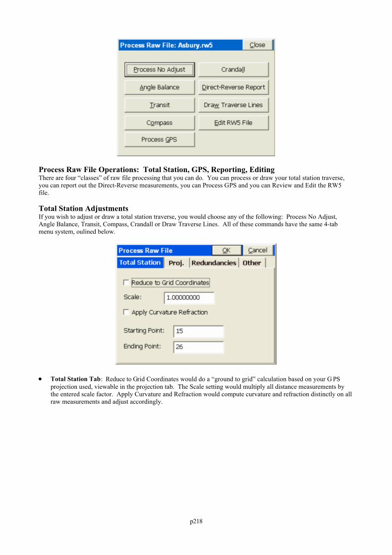
p218

Process Raw File Operations: Total Station, GPS, Reporting, EditingThere are four “classes” of raw file processing that you can do. You can process or draw your total station traverse,you can report out the Direct-Reverse measurements, you can Process GPS and you can Review and Edit the RW5file.

Total Station AdjustmentsIf you wish to adjust or draw a total station traverse, you would choose any of the following: Process No Adjust,Angle Balance, Transit, Compass, Crandall or Draw Traverse Lines. All of these commands have the same 4-tabmenu system, oulined below.

Total Station Tab: Reduce to Grid Coordinates would do a “ground to grid” calculation based on your G PSprojection used, viewable in the projection tab. The Scale setting would multiply all distance measurements bythe entered scale factor. Apply Curvature and Refraction would compute curvature and refraction distinctly on allraw measurements and adjust accordingly.

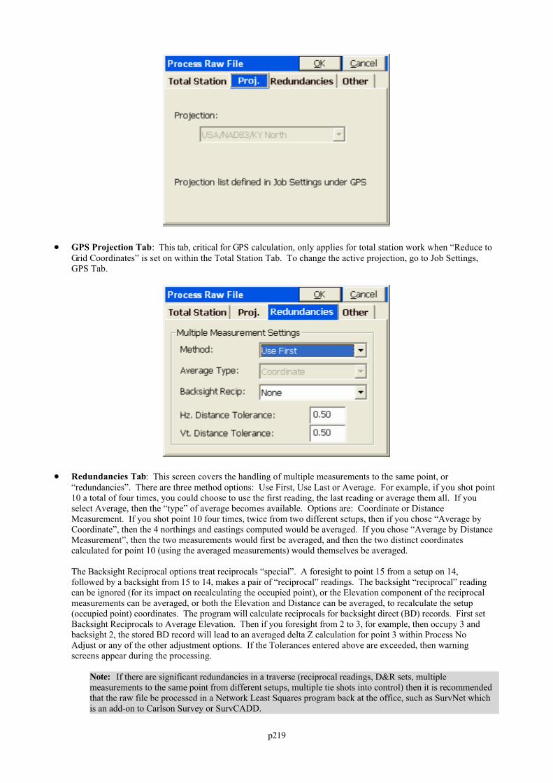
p219

GPS Projection Tab: This tab, critical for GPS calculation, only applies for total station work when “Reduce toGrid Coordinates” is set on within the Total Station Tab. To change the active projection, go to Job Settings,GPS Tab.

Redundancies Tab: This screen covers the handling of multiple measurements to the same point, or“redundancies”. There are three method options: Use First, Use Last or Average. For example, if you shot point10 a total of four times, you could choose to use the first reading, the last reading or average them all. If youselect Average, then the “type” of average becomes available. Options are: Coordinate or DistanceMeasurement. If you shot point 10 four times, twice from two different setups, then if you chose “Average byCoordinate”, then the 4 northings and eastings computed would be averaged. If you chose “Average by DistanceMeasurement”, then the two measurements would first be averaged, and then the two distinct coordinatescalculated for point 10 (using the averaged measurements) would themselves be averaged.

The Backsight Reciprocal options treat reciprocals “special”. A foresight to point 15 from a setup on 14,followed by a backsight from 15 to 14, makes a pair of “reciprocal” readings. The backsight “reciprocal” readingcan be ignored (for its impact on recalculating the occupied point), or the Elevation component of the reciprocalmeasurements can be averaged, or both the Elevation and Distance can be averaged, to recalculate the setup(occupied point) coordinates. The program will calculate reciprocals for backsight direct (BD) records. First setBacksight Reciprocals to Average Elevation. Then if you foresight from 2 to 3, for example, then occupy 3 andbacksight 2, the stored BD record will lead to an averaged delta Z calculation for point 3 within Process NoAdjust or any of the other adjustment options. If the Tolerances entered above are exceeded, then warningscreens appear during the processing.

Note: If there are significant redundancies in a traverse (reciprocal readings, D&R sets, multiplemeasurements to the same point from different setups, multiple tie shots into control) then it is recommendedthat the raw file be processed in a Network Least Squares program back at the office, such as SurvNet whichis an add-on to Carlson Survey or SurvCADD.

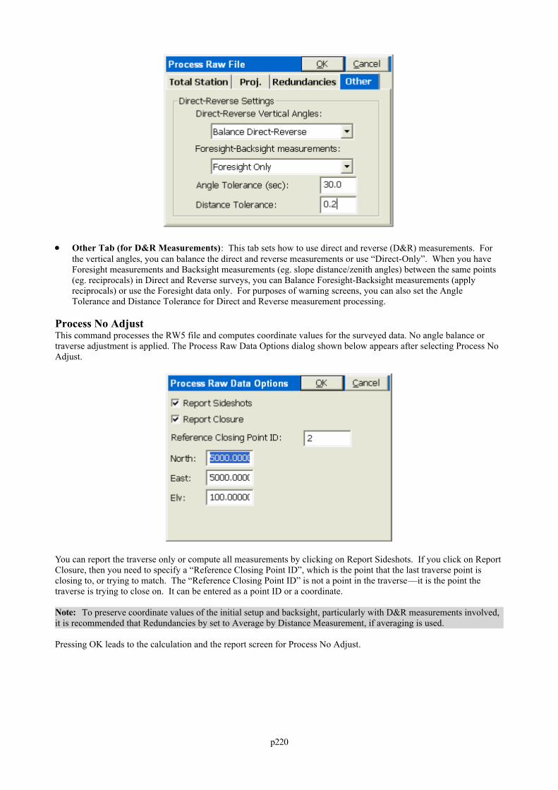
p220

Other Tab (for D&R Measurements): This tab sets how to use direct and reverse (D&R) measurements. Forthe vertical angles, you can balance the direct and reverse measurements or use “Direct-Only”. When you haveForesight measurements and Backsight measurements (eg. slope distance/zenith angles) between the same points(eg. reciprocals) in Direct and Reverse surveys, you can Balance Foresight-Backsight measurements (applyreciprocals) or use the Foresight data only. For purposes of warning screens, you can also set the AngleTolerance and Distance Tolerance for Direct and Reverse measurement processing.

Process No AdjustThis command processes the RW5 file and computes coordinate values for the surveyed data. No angle balance ortraverse adjustment is applied. The Process Raw Data Options dialog shown below appears after selecting Process NoAdjust.

You can report the traverse only or compute all measurements by clicking on Report Sideshots. If you click on ReportClosure, then you need to specify a “Reference Closing Point ID”, which is the point that the last traverse point isclosing to, or trying to match. The “Reference Closing Point ID” is not a point in the traverse—it is the point thetraverse is trying to close on. It can be entered as a point ID or a coordinate.

Note: To preserve coordinate values of the initial setup and backsight, particularly with D&R measurements involved,it is recommended that Redundancies by set to Average by Distance Measurement, if averaging is used.

Pressing OK leads to the calculation and the report screen for Process No Adjust.

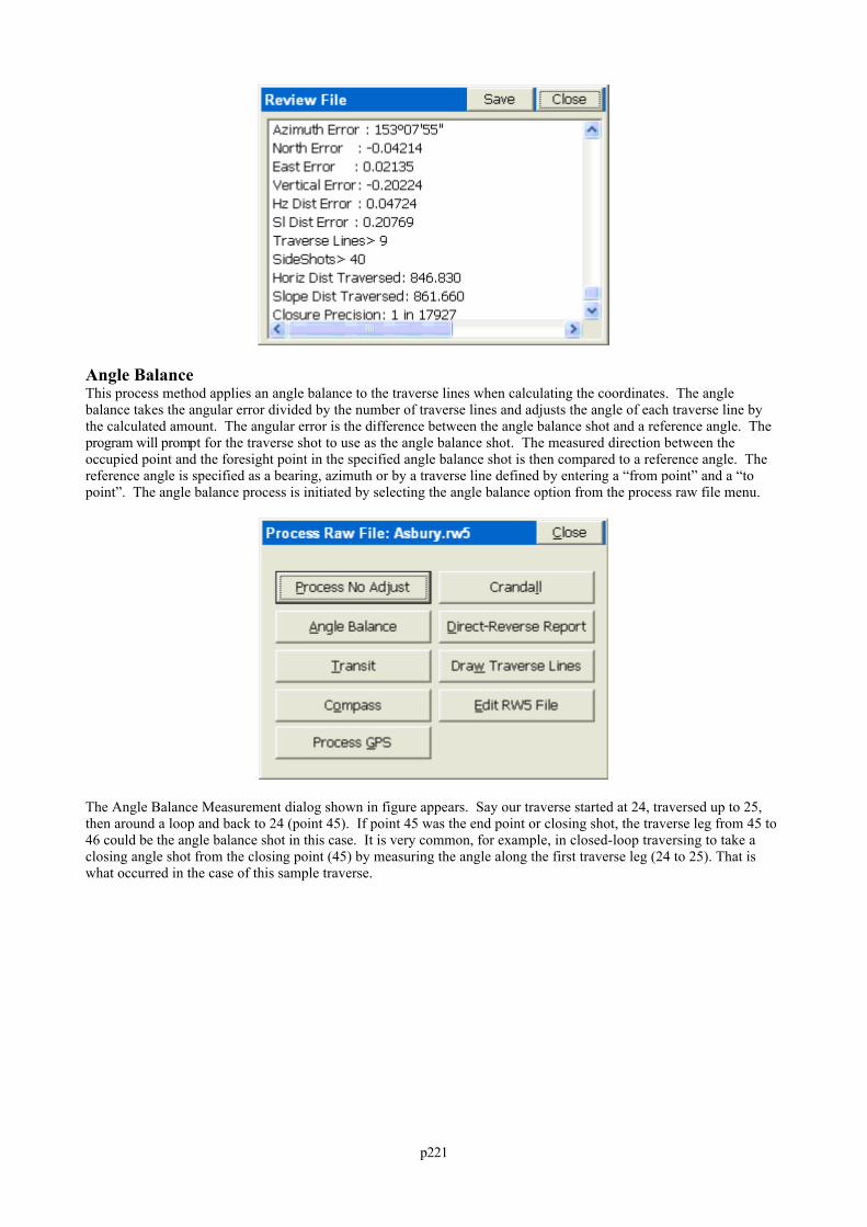
p221

Angle BalanceThis process method applies an angle balance to the traverse lines when calculating the coordinates. The anglebalance takes the angular error divided by the number of traverse lines and adjusts the angle of each traverse line bythe calculated amount. The angular error is the difference between the angle balance shot and a reference angle. Theprogram will prompt for the traverse shot to use as the angle balance shot. The measured direction between theoccupied point and the foresight point in the specified angle balance shot is then compared to a reference angle. Thereference angle is specified as a bearing, azimuth or by a traverse line defined by entering a “from point” and a “topoint”. The angle balance process is initiated by selecting the angle balance option from the process raw file menu.

The Angle Balance Measurement dialog shown in figure appears. Say our traverse started at 24, traversed up to 25,then around a loop and back to 24 (point 45). If point 45 was the end point or closing shot, the traverse leg from 45 to46 could be the angle balance shot in this case. It is very common, for example, in closed-loop traversing to take aclosing angle shot from the closing point (45) by measuring the angle along the first traverse leg (24 to 25). That iswhat occurred in the case of this sample traverse.

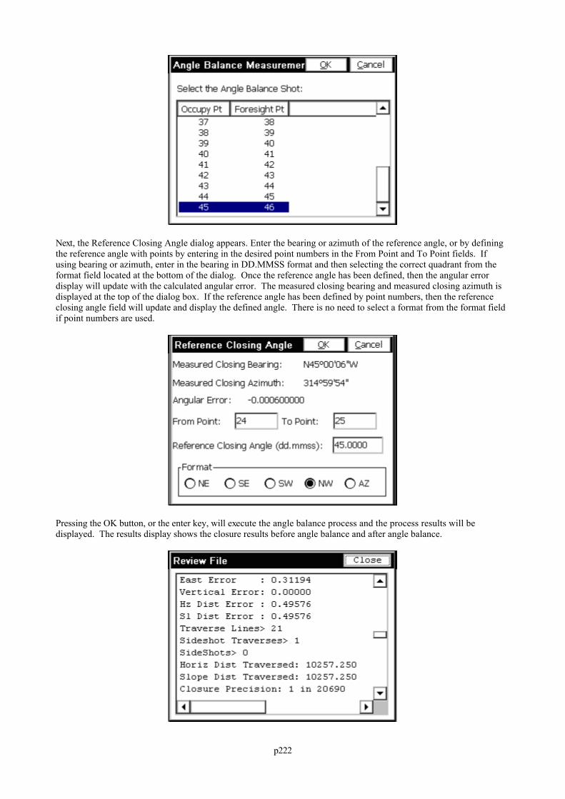
p222

Next, the Reference Closing Angle dialog appears. Enter the bearing or azimuth of the reference angle, or by definingthe reference angle with points by entering in the desired point numbers in the From Point and To Point fields. Ifusing bearing or azimuth, enter in the bearing in DD.MMSS format and then selecting the correct quadrant from theformat field located at the bottom of the dialog. Once the reference angle has been defined, then the angular errordisplay will update with the calculated angular error. The measured closing bearing and measured closing azimuth isdisplayed at the top of the dialog box. If the reference angle has been defined by point numbers, then the referenceclosing angle field will update and display the defined angle. There is no need to select a format from the format fieldif point numbers are used.

Pressing the OK button, or the enter key, will execute the angle balance process and the process results will bedisplayed. The results display shows the closure results before angle balance and after angle balance.

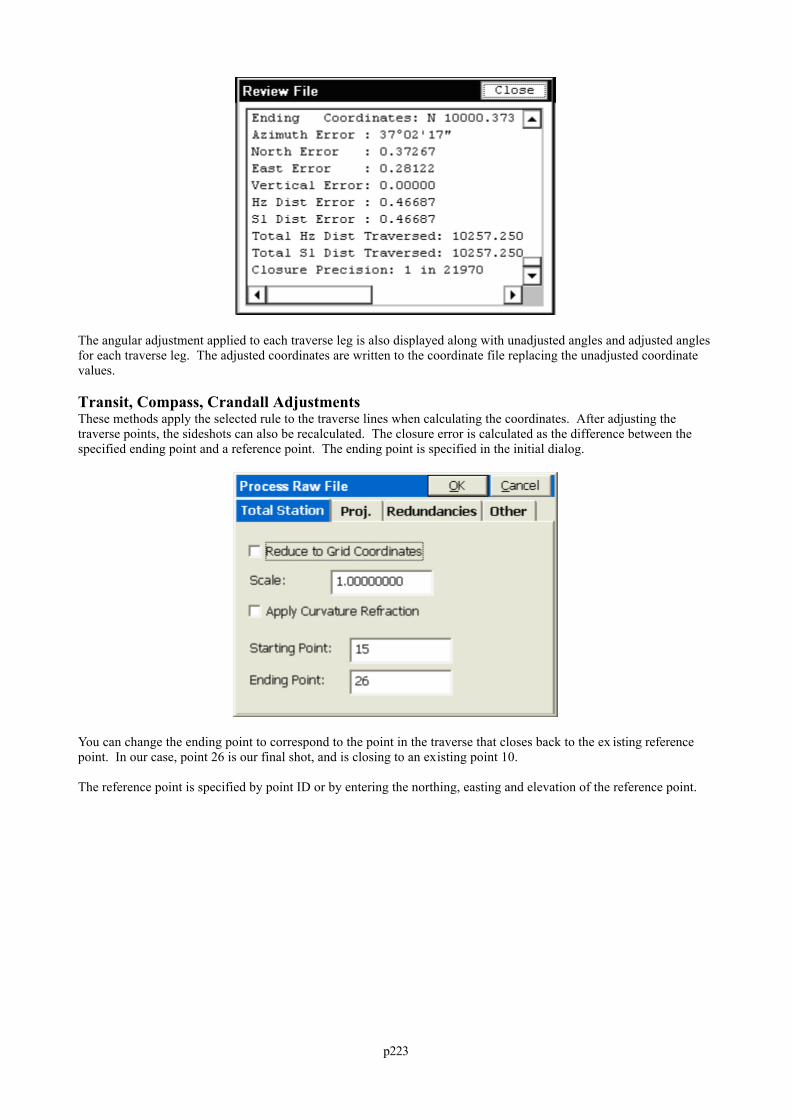
p223

The angular adjustment applied to each traverse leg is also displayed along with unadjusted angles and adjusted anglesfor each traverse leg. The adjusted coordinates are written to the coordinate file replacing the unadjusted coordinatevalues.

Transit, Compass, Crandall AdjustmentsThese methods apply the selected rule to the traverse lines when calculating the coordinates. After adjusting thetraverse points, the sideshots can also be recalculated. The closure error is calculated as the difference between thespecified ending point and a reference point. The ending point is specified in the initial dialog.

You can change the ending point to correspond to the point in the traverse that closes back to the ex isting referencepoint. In our case, point 26 is our final shot, and is closing to an existing point 10.

The reference point is specified by point ID or by entering the northing, easting and elevation of the reference point.

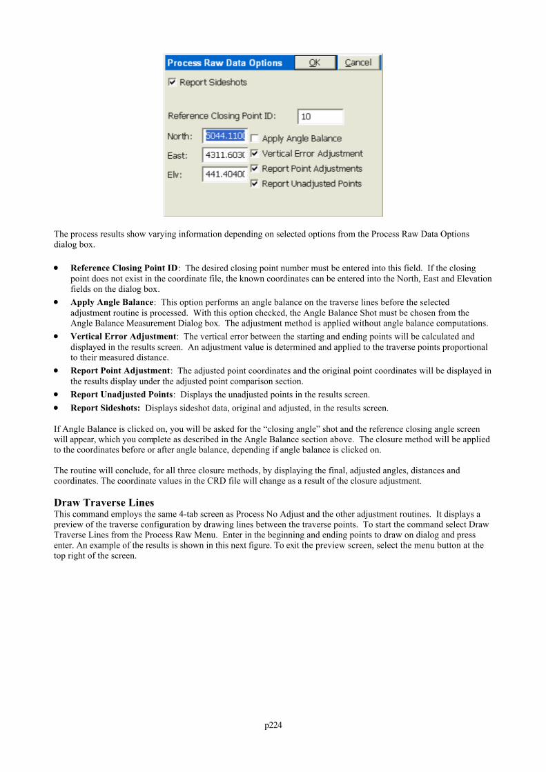
p224

The process results show varying information depending on selected options from the Process Raw Data Optionsdialog box.

Reference Closing Point ID: The desired closing point number must be entered into this field. If the closingpoint does not exist in the coordinate file, the known coordinates can be entered into the North, East and Elevationfields on the dialog box.

Apply Angle Balance: This option performs an angle balance on the traverse lines before the selectedadjustment routine is processed. With this option checked, the Angle Balance Shot must be chosen from theAngle Balance Measurement Dialog box. The adjustment method is applied without angle balance computations.

Vertical Error Adjustment: The vertical error between the starting and ending points will be calculated anddisplayed in the results screen. An adjustment value is determined and applied to the traverse points proportionalto their measured distance.

Report Point Adjustment: The adjusted point coordinates and the original point coordinates will be displayed inthe results display under the adjusted point comparison section.

Report Unadjusted Points: Displays the unadjusted points in the results screen. Report Sideshots: Displays sideshot data, original and adjusted, in the results screen.

If Angle Balance is clicked on, you will be asked for the “closing angle” shot and the reference closing angle screenwill appear, which you complete as described in the Angle Balance section above. The closure method will be appliedto the coordinates before or after angle balance, depending if angle balance is clicked on.

The routine will conclude, for all three closure methods, by displaying the final, adjusted angles, distances andcoordinates. The coordinate values in the CRD file will change as a result of the closure adjustment.

Draw Traverse LinesThis command employs the same 4-tab screen as Process No Adjust and the other adjustment routines. It displays apreview of the traverse configuration by drawing lines between the traverse points. To start the command select DrawTraverse Lines from the Process Raw Menu. Enter in the beginning and ending points to draw on dialog and pressenter. An example of the results is shown in this next figure. To exit the preview screen, select the menu button at thetop right of the screen.

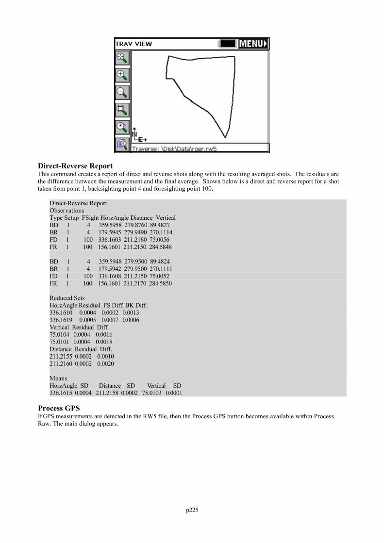
p225

Direct-Reverse ReportThis command creates a report of direct and reverse shots along with the resulting averaged shots. The residuals arethe difference between the measurement and the final average. Shown below is a direct and reverse report for a shottaken from point 1, backsighting point 4 and foresighting point 100.

Direct-Reverse ReportObservationsType Setup FSight HorzAngle Distance VerticalBD 1 4 359.5958 279.8760 89.4827BR 1 4 179.5945 279.9490 270.1114FD 1 100 336.1603 211.2160 75.0056FR 1 100 156.1601 211.2150 284.5848

BD 1 4 359.5948 279.9500 89.4824BR 1 4 179.5942 279.9500 270.1111FD 1 100 336.1608 211.2150 75.0052FR 1 100 156.1601 211.2170 284.5850

Reduced SetsHorzAngle Residual FS Diff. BK Diff.336.1610 0.0004 0.0002 0.0013 336.1619 0.0005 0.0007 0.0006 Vertical Residual Diff.75.0104 0.0004 0.0016 75.0101 0.0004 0.0018 Distance Residual Diff.211.2155 0.0002 0.0010 211.2160 0.0002 0.0020

MeansHorzAngle SD Distance SD Vertical SD336.1615 0.0004 211.2158 0.0002 75.0103 0.0001

Process GPSIf GPS measurements are detected in the RW5 file, then the Process GPS button becomes available within ProcessRaw. The main dialog appears.

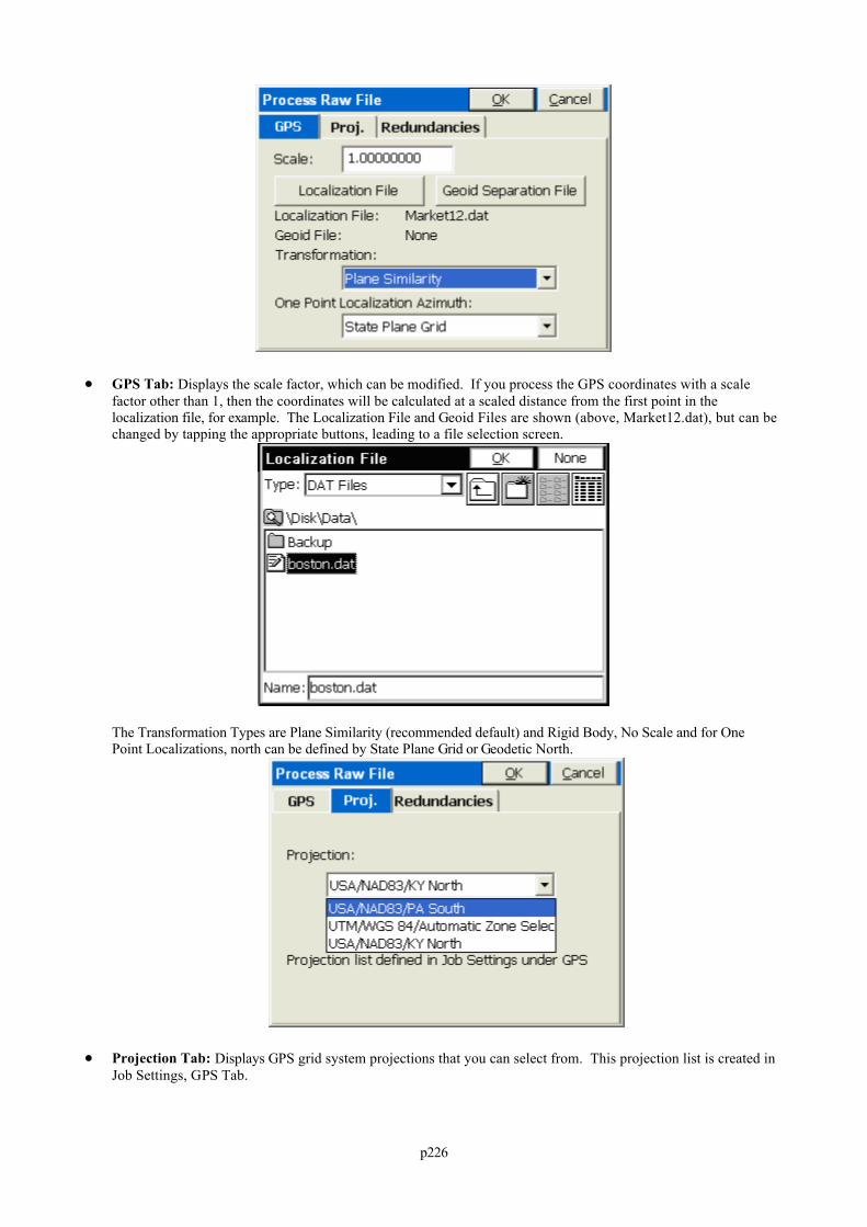
p226

GPS Tab: Displays the scale factor, which can be modified. If you process the GPS coordinates with a scalefactor other than 1, then the coordinates will be calculated at a scaled distance from the first point in thelocalization file, for example. The Localization File and Geoid Files are shown (above, Market12.dat), but can bechanged by tapping the appropriate buttons, leading to a file selection screen.

The Transformation Types are Plane Similarity (recommended default) and Rigid Body, No Scale and for OnePoint Localizations, north can be defined by State Plane Grid or Geodetic North.

Projection Tab: Displays GPS grid system projections that you can select from. This projection list is created inJob Settings, GPS Tab.

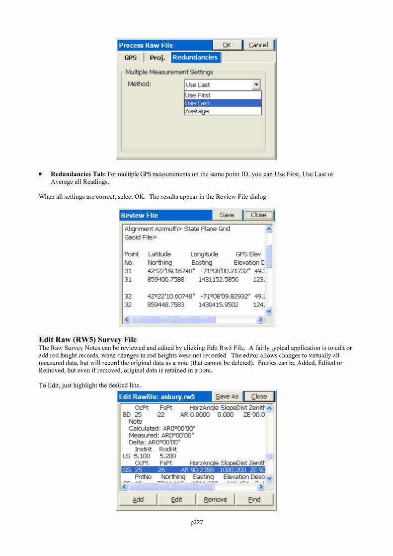
p227

Redundancies Tab: For multiple GPS measurements on the same point ID, you can Use First, Use Last orAverage all Readings.

When all settings are correct, select OK. The results appear in the Review File dialog.

Edit Raw (RW5) Survey FileThe Raw Survey Notes can be reviewed and edited by clicking Edit Rw5 File. A fairly typical application is to edit oradd rod height records, when changes in rod heights were not recorded. The editor allows changes to virtually allmeasured data, but will record the original data as a note (that cannot be deleted). Entries can be Added, Edited orRemoved, but even if removed, original data is retained in a note.

To Edit, just highlight the desired line.

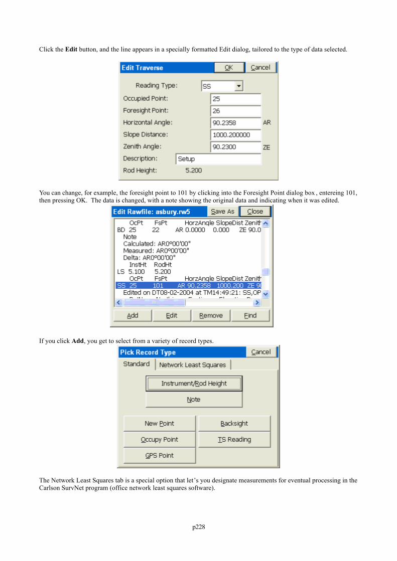
p228

Click the Edit button, and the line appears in a specially formatted Edit dialog, tailored to the type of data selected.

You can change, for example, the foresight point to 101 by clicking into the Foresight Point dialog box , entereing 101,then pressing OK. The data is changed, with a note showing the original data and indicating when it was edited.

If you click Add, you get to select from a variety of record types.

The Network Least Squares tab is a special option that let’s you designate measurements for eventual processing in theCarlson SurvNet program (office network least squares software).

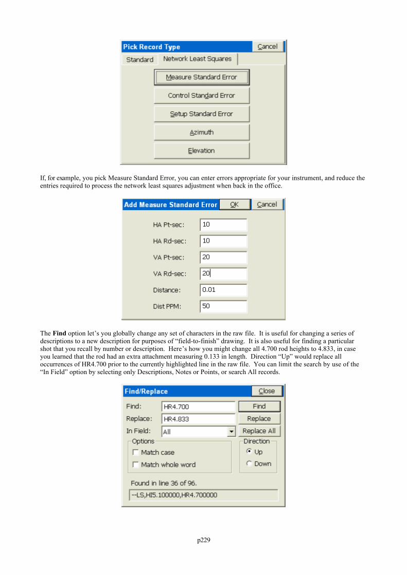
p229

If, for example, you pick Measure Standard Error, you can enter errors appropriate for your instrument, and reduce theentries required to process the network least squares adjustment when back in the office.

The Find option let’s you globally change any set of characters in the raw file. It is useful for changing a series ofdescriptions to a new description for purposes of “field-to-finish” drawing. It is also useful for finding a particularshot that you recall by number or description. Here’s how you might change all 4.700 rod heights to 4.833, in caseyou learned that the rod had an extra attachment measuring 0.133 in length. Direction “Up” would replace alloccurrences of HR4.700 prior to the currently highlighted line in the raw file. You can limit the search by use of the“In Field” option by selecting only Descriptions, Notes or Points, or search All records.

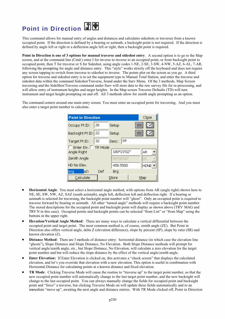
p230

Point in Direction This command allows for manual entry of angles and distances and calculates sideshots or traverses from a knownoccupied point. If the direction is defined by a bearing or azimuth, a backsight point is not required. If the direction isdefined by angle left or right or a deflection angle left or right, then a backsight point is required.

Point in Direction is one of 3 options for manual traverse and sideshot entry . A second option is to go to the Mapscreen, and at the command line (Cmd:) enter I for inverse to inverse to an occupied point, or from backsight point tooccupied point, then T for traverse or S for Sideshot, using angle codes 1-NE, 2-SE, 3-SW, 4-NW, 5-AZ, 6-AL, 7-AR,following the prompting for angle and distance entry. This “style” works strictly off the keyboard and does not requireany screen tapping to switch from traverse to sideshot to inverse. The points plot on the screen as you go. A thirdoption for traverse and sideshot entry is to set the equipment type to Manual Total Station, and enter the traverse andsideshot data within the command Sideshot/Traverse, found under the Surv Menu. Of the 3 methods, Map Screentraversing and the SideShot/Traverse command under Surv will store data to the raw survey file for re-processing, andwill allow entry of instrument heights and target heights. In the Map screen Traverse Defaults (TD) will turninstrument and target height prompting on and off. All 3 methods allow for zenith angle prompting as an option.

The command centers around one main entry screen. You must enter an occupied point for traversing. And you mustalso enter a target point number to calculate.

Horizontal Angle: You must select a horizontal angle method, with options from AR (angle right) shown here toNE, SE, SW, NW, AZ, SAZ (south azimuth), angle left, deflection left and deflection right. If a bearing orazimuth is selected for traversing, the backsight point number will “ghost”. Only an occupied point is required totraverse forward by bearing or azimuth. All other “turned angle” methods will require a backsight point number. The stored descriptions for the occupied point and backsight point will display as shown above (TRV MAG andTRV N in this case). Occupied points and backsight points can be selected “from List” or “from Map” using thebuttons in the upper right.

Elevation/Vertical Angle Method : There are many ways to calculate a vertical differential between theoccupied point and target point. The most common method is, of course, zenith angle (ZE). But Point inDirection also offers vertical angle, delta Z (elevation difference), slope by percent (SP), slope by ratio (SR) andknown elevation (Z).

Distance Method: There are 3 methods of distance entry: horizontal distance (in which case the elevation line“ghosts”), Slope Distance and Slope Distance, No Elevation. Both Slope Distance methods will prompt forvertical angle/zenith angle, etc., but Slope Distance, No Elevation, will calculate a zero elevation for the targetpoint number and but will reduce the slope distance by the effect of the vertical angle/zenith angle.

Enter Elevation: If Enter Elevation is clicked on, this activates a “check screen” that displays the calculatedelevation, and let’s you override that elevation with a new elevation. This option is useful in combination withHorizontal Distance for calculating points at a known distance and fixed elevation.

TR Mode: Clicking Traverse Mode will cause the routine to “traverse up” to the target point number, so that thenew occupied point number will automatically change to the last target point number, and the new backsight willchange to the last occupied point. You can always manually change the fields for occupied point and backsightpoint and “force” a traverse, but clicking Traverse Mode on will update these fields automatically and to animmediate “move up”, awaiting the next angle and distance entries. With TR Mode clicked off, Point in Direction

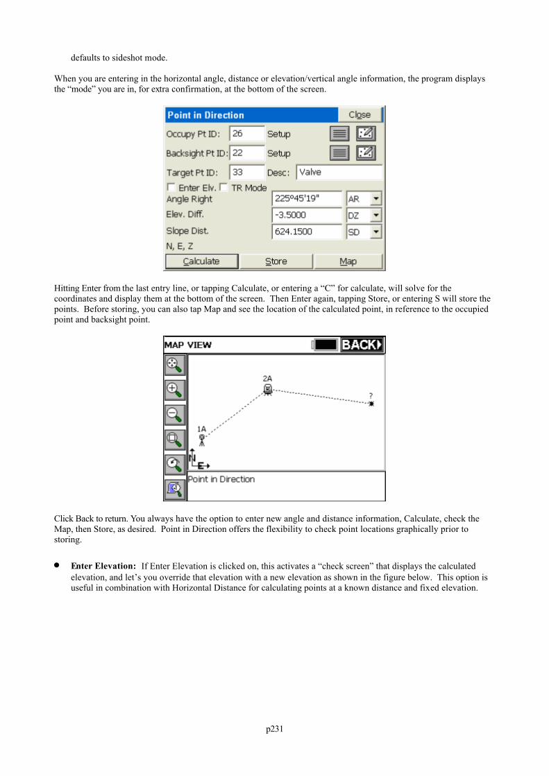
p231

defaults to sideshot mode.

When you are entering in the horizontal angle, distance or elevation/vertical angle information, the program displaysthe “mode” you are in, for extra confirmation, at the bottom of the screen.

Hitting Enter from the last entry line, or tapping Calculate, or entering a “C” for calculate, will solve for thecoordinates and display them at the bottom of the screen. Then Enter again, tapping Store, or entering S will store thepoints. Before storing, you can also tap Map and see the location of the calculated point, in reference to the occupiedpoint and backsight point.

Click Back to return. You always have the option to enter new angle and distance information, Calculate, check theMap, then Store, as desired. Point in Direction offers the flexibility to check point locations graphically prior tostoring.

Enter Elevation: If Enter Elevation is clicked on, this activates a “check screen” that displays the calculatedelevation, and let’s you override that elevation with a new elevation as shown in the figure below. This option isuseful in combination with Horizontal Distance for calculating points at a known distance and fixed elevation.

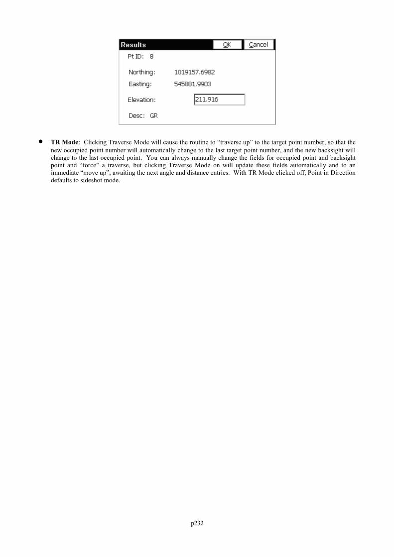
p232

TR Mode: Clicking Traverse Mode will cause the routine to “traverse up” to the target point number, so that thenew occupied point number will automatically change to the last target point number, and the new backsight willchange to the last occupied point. You can always manually change the fields for occupied point and backsightpoint and “force” a traverse, but clicking Traverse Mode on will update these fields automatically and to animmediate “move up”, awaiting the next angle and distance entries. With TR Mode clicked off, Point in Directiondefaults to sideshot mode.

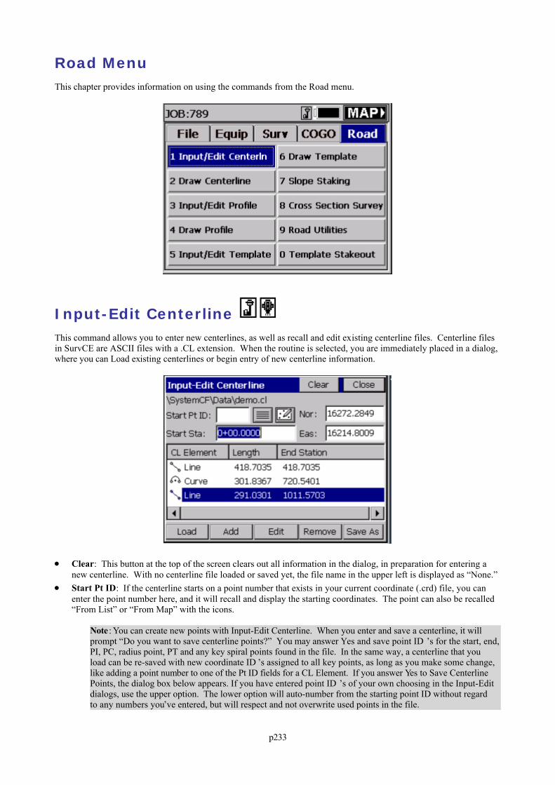
p233

Road MenuThis chapter provides information on using the commands from the Road menu.

Input-Edit Centerline This command allows you to enter new centerlines, as well as recall and edit existing centerline files. Centerline filesin SurvCE are ASCII files with a .CL extension. When the routine is selected, you are immediately placed in a dialog,where you can Load existing centerlines or begin entry of new centerline information.

Clear: This button at the top of the screen clears out all information in the dialog, in preparation for entering anew centerline. With no centerline file loaded or saved yet, the file name in the upper left is displayed as “None.”

Start Pt ID: If the centerline starts on a point number that exists in your current coordinate (.crd) file, you canenter the point number here, and it will recall and display the starting coordinates. The point can also be recalled“From List” or “From Map” with the icons.

Note : You can create new points with Input-Edit Centerline. When you enter and save a centerline, it willprompt “Do you want to save centerline points?” You may answer Yes and save point ID ’s for the start, end,PI, PC, radius point, PT and any key spiral points found in the file. In the same way, a centerline that youload can be re-saved with new coordinate ID ’s assigned to all key points, as long as you make some change,like adding a point number to one of the Pt ID fields for a CL Element. If you answer Yes to Save CenterlinePoints, the dialog box below appears. If you have entered point ID ’s of your own choosing in the Input-Editdialogs, use the upper option. The lower option will auto-number from the starting point ID without regardto any numbers you’ve entered, but will respect and not overwrite used points in the file.

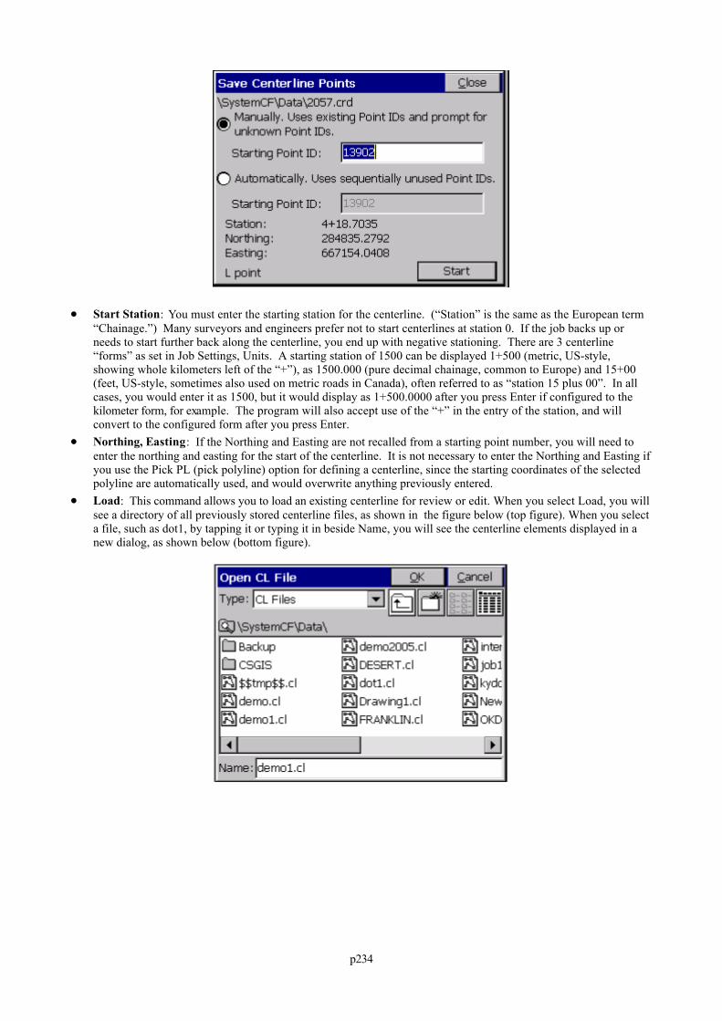
p234

Start Station: You must enter the starting station for the centerline. (“Station” is the same as the European term“Chainage.”) Many surveyors and engineers prefer not to start centerlines at station 0. If the job backs up orneeds to start further back along the centerline, you end up with negative stationing. There are 3 centerline“forms” as set in Job Settings, Units. A starting station of 1500 can be displayed 1+500 (metric, US-style,showing whole kilometers left of the “+”), as 1500.000 (pure decimal chainage, common to Europe) and 15+00(feet, US-style, sometimes also used on metric roads in Canada), often referred to as “station 15 plus 00”. In allcases, you would enter it as 1500, but it would display as 1+500.0000 after you press Enter if configured to thekilometer form, for example. The program will also accept use of the “+” in the entry of the station, and willconvert to the configured form after you press Enter.

Northing, Easting: If the Northing and Easting are not recalled from a starting point number, you will need toenter the northing and easting for the start of the centerline. It is not necessary to enter the Northing and Easting ifyou use the Pick PL (pick polyline) option for defining a centerline, since the starting coordinates of the selectedpolyline are automatically used, and would overwrite anything previously entered.

Load: This command allows you to load an existing centerline for review or edit. When you select Load, you willsee a directory of all previously stored centerline files, as shown in the figure below (top figure). When you selecta file, such as dot1, by tapping it or typing it in beside Name, you will see the centerline elements displayed in anew dialog, as shown below (bottom figure).

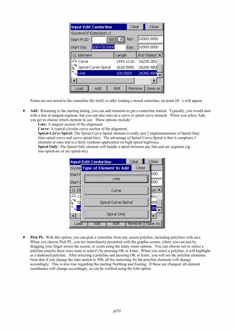
p235

Points are not stored to the centerline file itself, so after loading a stored centerline, no point ID ’s will appear.

Add: Returning to the starting dialog, you can add elements to get a centerline started. Typically, you would startwith a line or tangent segment, but you can also start on a curve or spiral curve element. When you select Add,you get to choose which element to use. These options include:

Line: A tangent section of the alignment.Curve: A typical circular curve section of the alignment.Spiral-Curve-Spiral: The Spiral-Curve-Spiral element is really just 2 implementations of Spiral Only(line-spiral-curve and curve-spiral-line). The advantage of Spiral-Curve-Spiral is that it completes 3elements at once and is a fairly common application on high-speed highways.Spiral Only: The Spiral Only element will handle a spiral between any line and arc segment (eg.line-spiral-arc or arc-spiral-arc).

Pick PL: With this option, you can pick a centerline from any screen polyline, including polylines with arcs.When you choose Pick PL, you are immediately presented with the graphic screen, where you can pan bydragging your finger across the screen, or zoom using the many zoom options. You can choose not to select apolyline (maybe there were none to select!) by pressing OK or Enter. When you select a polyline, it will highlightas a darkened polyline. After selecting a polyline and pressing OK or Enter, you will see the polyline elements. Note that if you change the start station to 500, all the stationing for the polyline elements will changeaccordingly. This is also true regarding the starting Northing and Easting. If these are changed, all elementcoordinates will change accordingly, as can be verified using the Edit option.

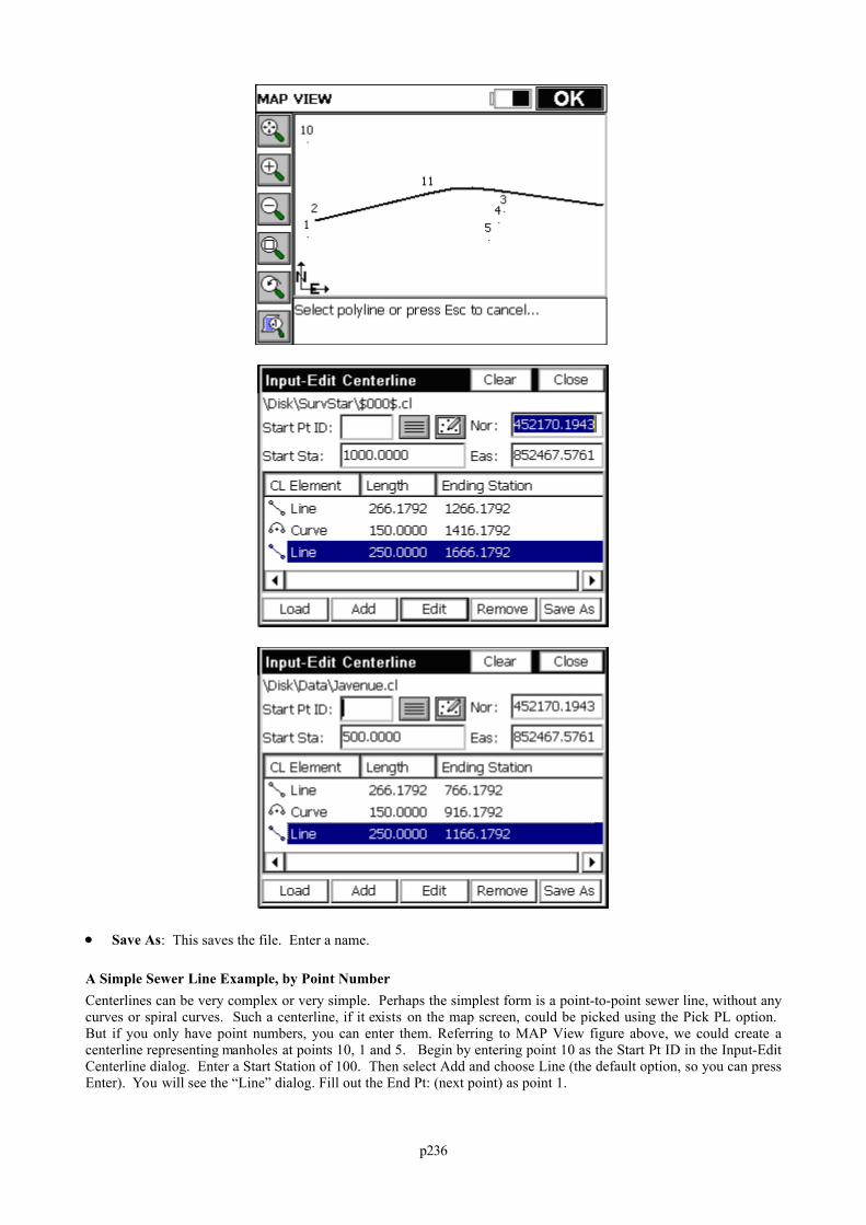
p236

Save As: This saves the file. Enter a name.

A Simple Sewer Line Example, by Point NumberCenterlines can be very complex or very simple. Perhaps the simplest form is a point-to-point sewer line, without anycurves or spiral curves. Such a centerline, if it exists on the map screen, could be picked using the Pick PL option. But if you only have point numbers, you can enter them. Referring to MAP View figure above, we could create acenterline representing manholes at points 10, 1 and 5. Begin by entering point 10 as the Start Pt ID in the Input-EditCenterline dialog. Enter a Start Station of 100. Then select Add and choose Line (the default option, so you can pressEnter). You will see the “Line” dialog. Fill out the End Pt: (next point) as point 1.

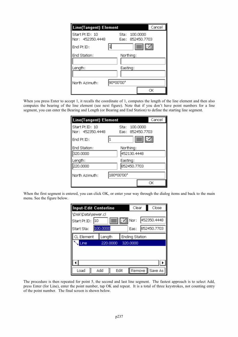
p237

When you press Enter to accept 1, it recalls the coordinate of 1, computes the length of the line element and then alsocomputes the bearing of the line element (see next figure). Note that if you don’t have point numbers for a linesegment, you can enter the Bearing and Length (or Bearing and End Station) to define the starting line segment.

When the first segment is entered, you can click OK, or enter your way through the dialog items and back to the mainmenu. See the figure below.

The procedure is then repeated for point 5, the second and last line segment. The fastest approach is to select Add,press Enter (for Line), enter the point number, tap OK and repeat. It is a total of three keystrokes, not counting entryof the point number. The final screen is shown below.

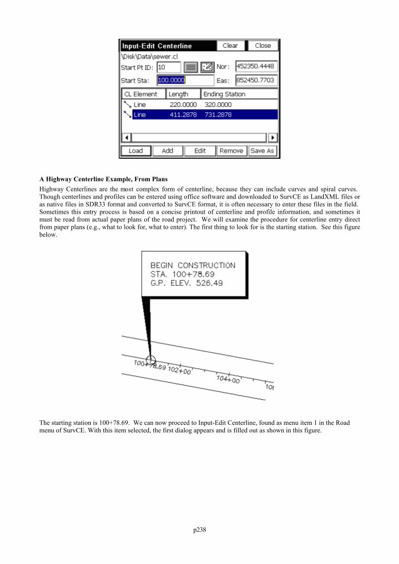
p238

A Highway Centerline Example, From PlansHighway Centerlines are the most complex form of centerline, because they can include curves and spiral curves. Though centerlines and profiles can be entered using office software and downloaded to SurvCE as LandXML files oras native files in SDR33 format and converted to SurvCE format, it is often necessary to enter these files in the field. Sometimes this entry process is based on a concise printout of centerline and profile information, and sometimes itmust be read from actual paper plans of the road project. We will examine the procedure for centerline entry directfrom paper plans (e.g., what to look for, what to enter). The first thing to look for is the starting station. See this figurebelow.

The starting station is 100+78.69. We can now proceed to Input-Edit Centerline, found as menu item 1 in the Roadmenu of SurvCE. With this item selected, the first dialog appears and is filled out as shown in this figure.

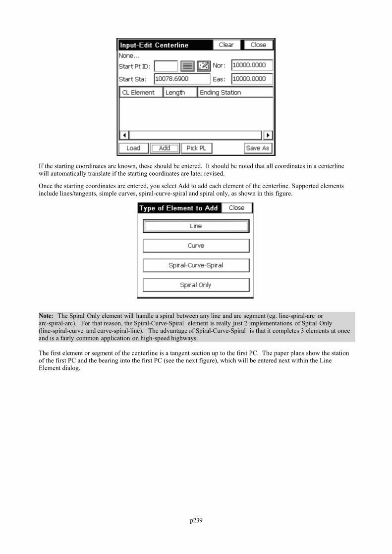
p239

If the starting coordinates are known, these should be entered. It should be noted that all coordinates in a centerlinewill automatically translate if the starting coordinates are later revised.

Once the starting coordinates are entered, you select Add to add each element of the centerline. Supported elementsinclude lines/tangents, simple curves, spiral-curve-spiral and spiral only, as shown in this figure.

Note: The Spiral Only element will handle a spiral between any line and arc segment (eg. line-spiral-arc orarc-spiral-arc). For that reason, the Spiral-Curve-Spiral element is really just 2 implementations of Spiral Only(line-spiral-curve and curve-spiral-line). The advantage of Spiral-Curve-Spiral is that it completes 3 elements at onceand is a fairly common application on high-speed highways.

The first element or segment of the centerline is a tangent section up to the first PC. The paper plans show the stationof the first PC and the bearing into the first PC (see the next figure), which will be entered next within the LineElement dialog.

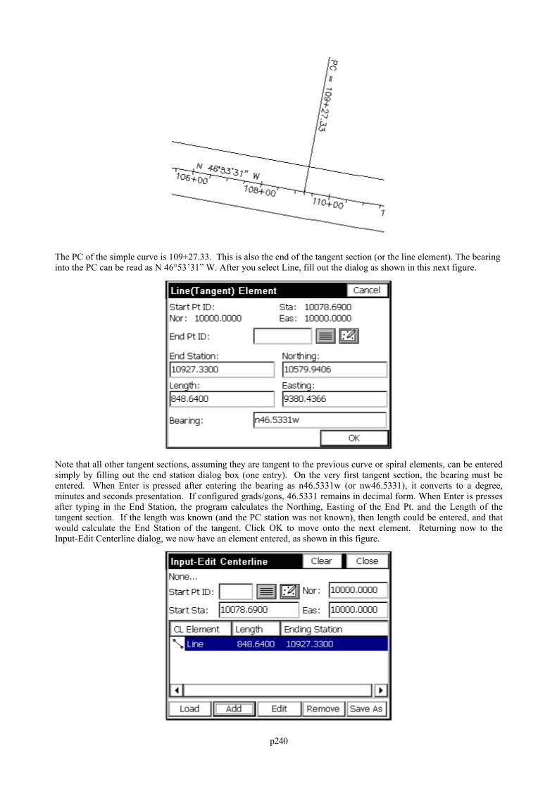
p240

The PC of the simple curve is 109+27.33. This is also the end of the tangent section (or the line element). The bearinginto the PC can be read as N 46°53’31” W. After you select Line, fill out the dialog as shown in this next figure.

Note that all other tangent sections, assuming they are tangent to the previous curve or spiral elements, can be enteredsimply by filling out the end station dialog box (one entry). On the very first tangent section, the bearing must beentered. When Enter is pressed after entering the bearing as n46.5331w (or nw46.5331), it converts to a degree,minutes and seconds presentation. If configured grads/gons, 46.5331 remains in decimal form. When Enter is pressesafter typing in the End Station, the program calculates the Northing, Easting of the End Pt. and the Length of thetangent section. If the length was known (and the PC station was not known), then length could be entered, and thatwould calculate the End Station of the tangent. Click OK to move onto the next element. Returning now to theInput-Edit Centerline dialog, we now have an element entered, as shown in this figure.

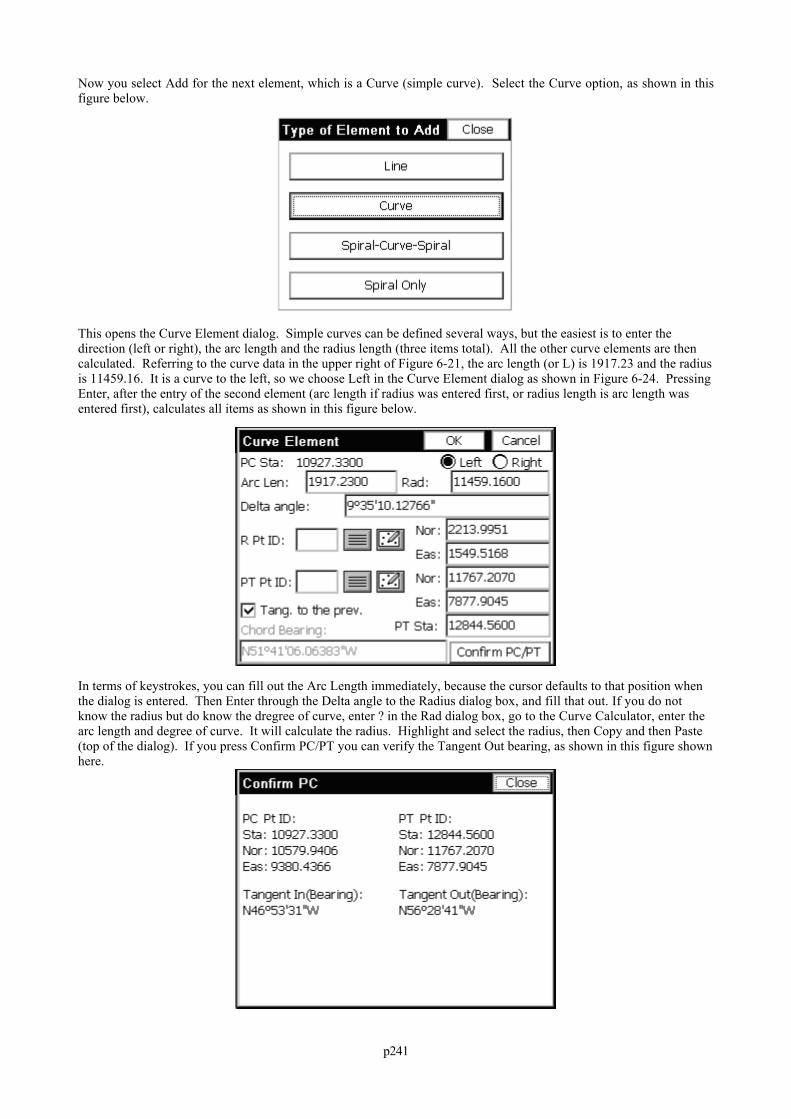
p241

Now you select Add for the next element, which is a Curve (simple curve). Select the Curve option, as shown in thisfigure below.

This opens the Curve Element dialog. Simple curves can be defined several ways, but the easiest is to enter thedirection (left or right), the arc length and the radius length (three items total). All the other curve elements are thencalculated. Referring to the curve data in the upper right of Figure 6-21, the arc length (or L) is 1917.23 and the radiusis 11459.16. It is a curve to the left, so we choose Left in the Curve Element dialog as shown in Figure 6-24. PressingEnter, after the entry of the second element (arc length if radius was entered first, or radius length is arc length wasentered first), calculates all items as shown in this figure below.

In terms of keystrokes, you can fill out the Arc Length immediately, because the cursor defaults to that position whenthe dialog is entered. Then Enter through the Delta angle to the Radius dialog box, and fill that out. If you do notknow the radius but do know the dregree of curve, enter ? in the Rad dialog box, go to the Curve Calculator, enter thearc length and degree of curve. It will calculate the radius. Highlight and select the radius, then Copy and then Paste(top of the dialog). If you press Confirm PC/PT you can verify the Tangent Out bearing, as shown in this figure shownhere.

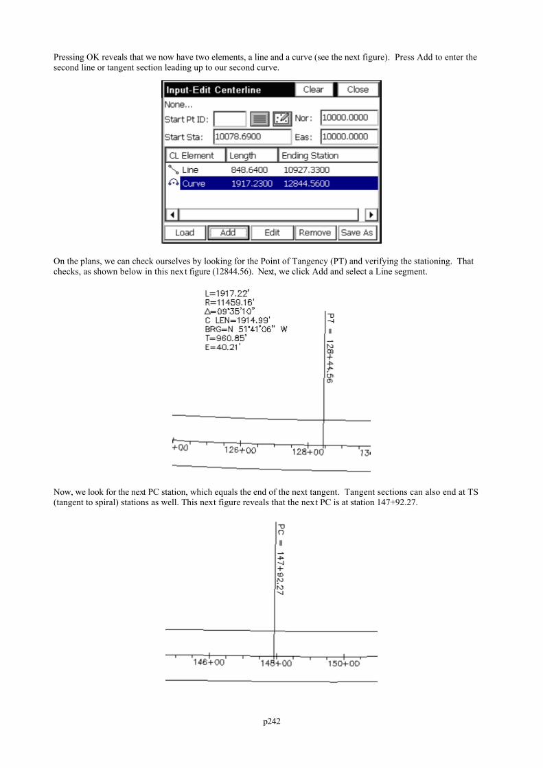
p242

Pressing OK reveals that we now have two elements, a line and a curve (see the next figure). Press Add to enter thesecond line or tangent section leading up to our second curve.

On the plans, we can check ourselves by looking for the Point of Tangency (PT) and verifying the stationing. Thatchecks, as shown below in this nex t figure (12844.56). Next, we click Add and select a Line segment.

Now, we look for the next PC station, which equals the end of the next tangent. Tangent sections can also end at TS(tangent to spiral) stations as well. This next figure reveals that the next PC is at station 147+92.27.

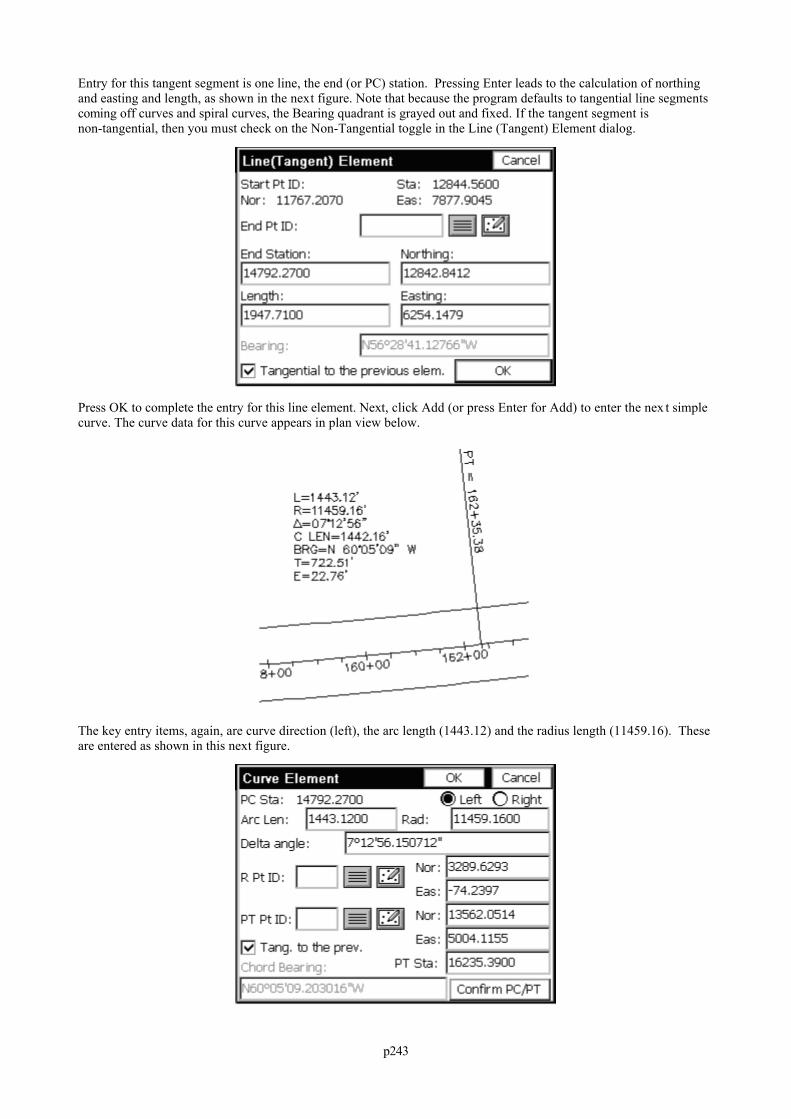
p243

Entry for this tangent segment is one line, the end (or PC) station. Pressing Enter leads to the calculation of northingand easting and length, as shown in the next figure. Note that because the program defaults to tangential line segmentscoming off curves and spiral curves, the Bearing quadrant is grayed out and fixed. If the tangent segment isnon-tangential, then you must check on the Non-Tangential toggle in the Line (Tangent) Element dialog.

Press OK to complete the entry for this line element. Next, click Add (or press Enter for Add) to enter the nex t simplecurve. The curve data for this curve appears in plan view below.

The key entry items, again, are curve direction (left), the arc length (1443.12) and the radius length (11459.16). Theseare entered as shown in this next figure.

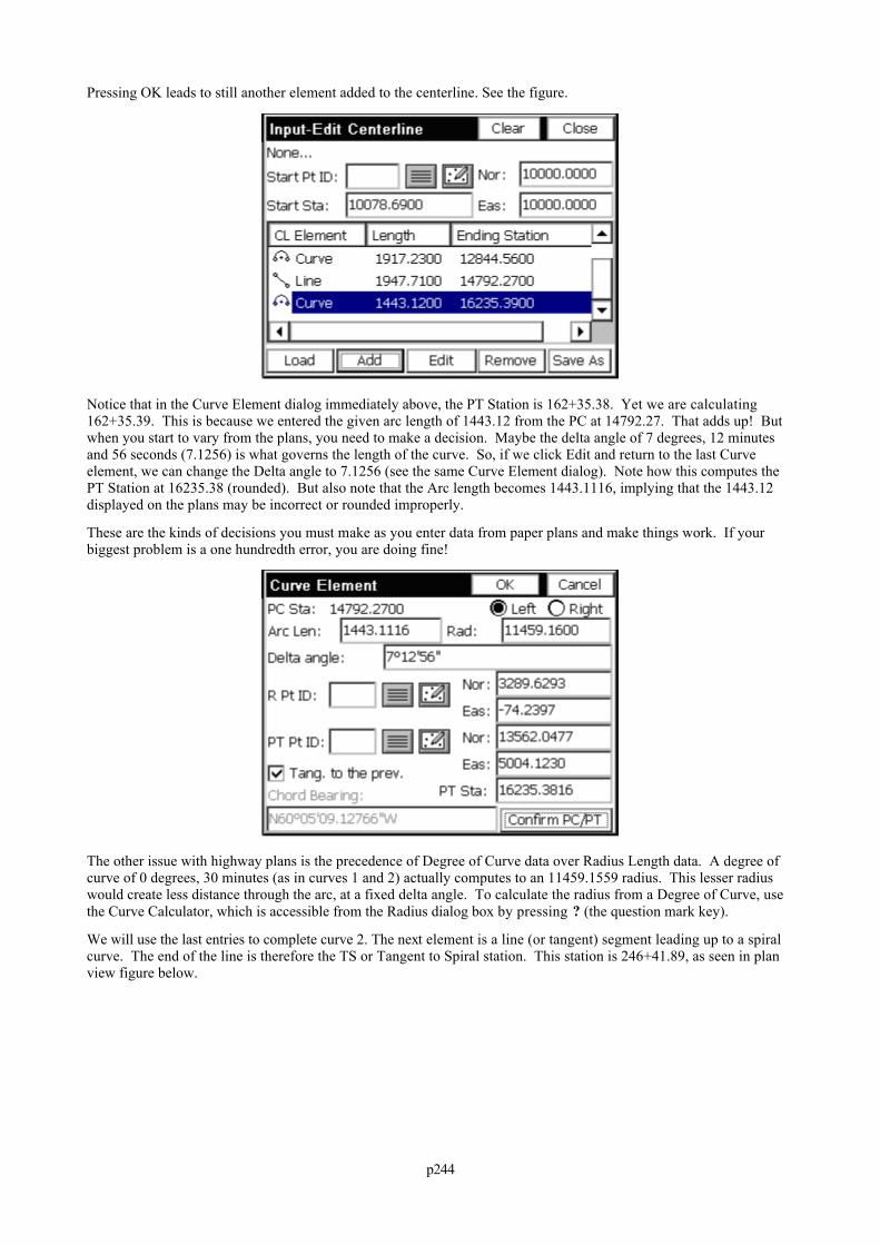
p244

Pressing OK leads to still another element added to the centerline. See the figure.

Notice that in the Curve Element dialog immediately above, the PT Station is 162+35.38. Yet we are calculating162+35.39. This is because we entered the given arc length of 1443.12 from the PC at 14792.27. That adds up! Butwhen you start to vary from the plans, you need to make a decision. Maybe the delta angle of 7 degrees, 12 minutesand 56 seconds (7.1256) is what governs the length of the curve. So, if we click Edit and return to the last Curveelement, we can change the Delta angle to 7.1256 (see the same Curve Element dialog). Note how this computes thePT Station at 16235.38 (rounded). But also note that the Arc length becomes 1443.1116, implying that the 1443.12displayed on the plans may be incorrect or rounded improperly.

These are the kinds of decisions you must make as you enter data from paper plans and make things work. If yourbiggest problem is a one hundredth error, you are doing fine!

The other issue with highway plans is the precedence of Degree of Curve data over Radius Length data. A degree ofcurve of 0 degrees, 30 minutes (as in curves 1 and 2) actually computes to an 11459.1559 radius. This lesser radiuswould create less distance through the arc, at a fixed delta angle. To calculate the radius from a Degree of Curve, usethe Curve Calculator, which is accessible from the Radius dialog box by pressing ? (the question mark key).

We will use the last entries to complete curve 2. The next element is a line (or tangent) segment leading up to a spiralcurve. The end of the line is therefore the TS or Tangent to Spiral station. This station is 246+41.89, as seen in planview figure below.

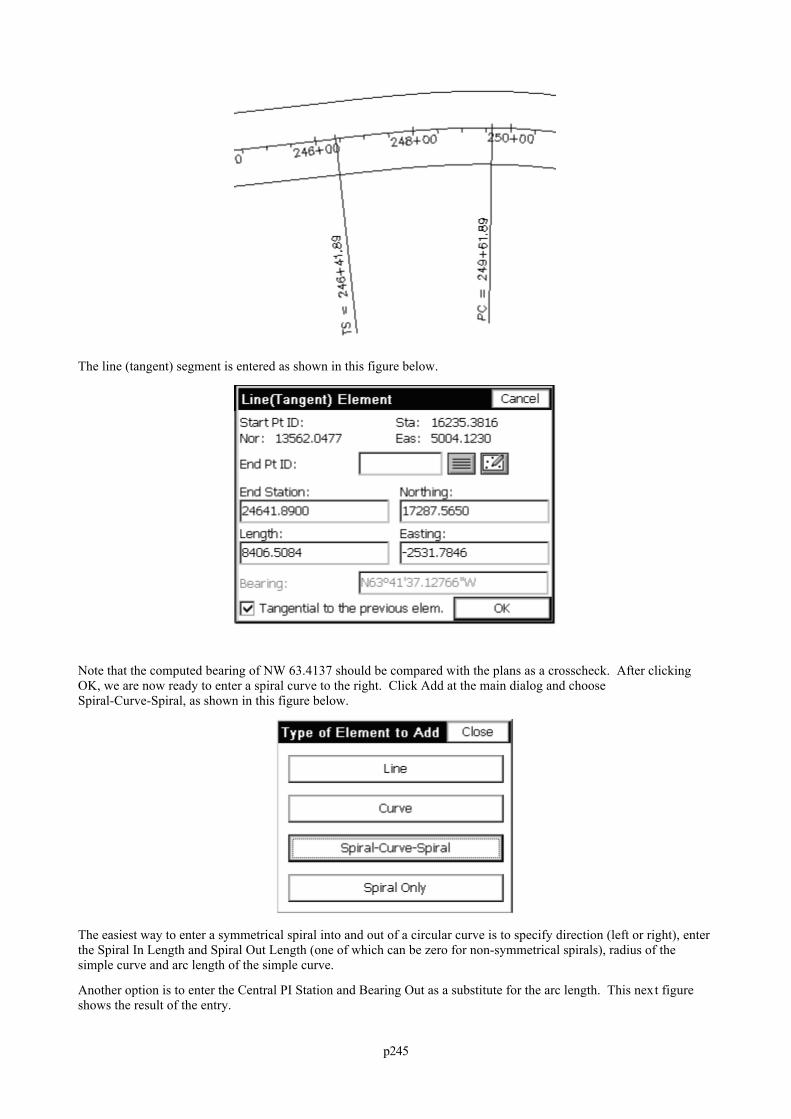
p245

The line (tangent) segment is entered as shown in this figure below.

Note that the computed bearing of NW 63.4137 should be compared with the plans as a crosscheck. After clickingOK, we are now ready to enter a spiral curve to the right. Click Add at the main dialog and chooseSpiral-Curve-Spiral, as shown in this figure below.

The easiest way to enter a symmetrical spiral into and out of a circular curve is to specify direction (left or right), enterthe Spiral In Length and Spiral Out Length (one of which can be zero for non-symmetrical spirals), radius of thesimple curve and arc length of the simple curve.

Another option is to enter the Central PI Station and Bearing Out as a substitute for the arc length. This next figureshows the result of the entry.

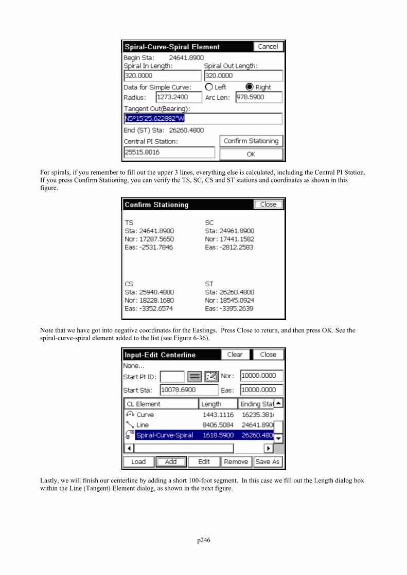
p246

For spirals, if you remember to fill out the upper 3 lines, everything else is calculated, including the Central PI Station.If you press Confirm Stationing, you can verify the TS, SC, CS and ST stations and coordinates as shown in thisfigure.

Note that we have got into negative coordinates for the Eastings. Press Close to return, and then press OK. See thespiral-curve-spiral element added to the list (see Figure 6-36).

Lastly, we will finish our centerline by adding a short 100-foot segment. In this case we fill out the Length dialog boxwithin the Line (Tangent) Element dialog, as shown in the next figure.

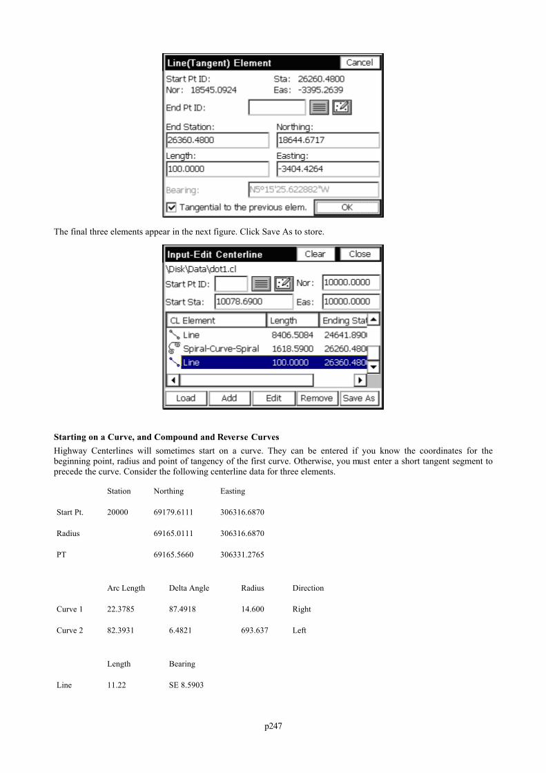
p247

The final three elements appear in the next figure. Click Save As to store.

Starting on a Curve, and Compound and Reverse CurvesHighway Centerlines will sometimes start on a curve. They can be entered if you know the coordinates for thebeginning point, radius and point of tangency of the first curve. Otherwise, you must enter a short tangent segment toprecede the curve. Consider the following centerline data for three elements.

Station Northing Easting

Start Pt. 20000 69179.6111 306316.6870

Radius 69165.0111 306316.6870

PT 69165.5660 306331.2765

Arc Length Delta Angle Radius Direction

Curve 1 22.3785 87.4918 14.600 Right

Curve 2 82.3931 6.4821 693.637 Left

Length Bearing

Line 11.22 SE 8.5903

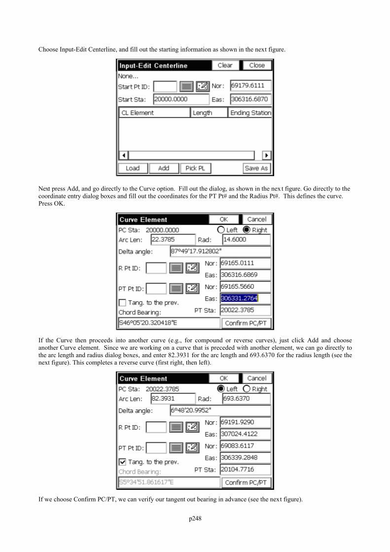
p248

Choose Input-Edit Centerline, and fill out the starting information as shown in the next figure.

Next press Add, and go directly to the Curve option. Fill out the dialog, as shown in the nex t figure. Go directly to thecoordinate entry dialog boxes and fill out the coordinates for the PT Pt# and the Radius Pt#. This defines the curve. Press OK.

If the Curve then proceeds into another curve (e.g., for compound or reverse curves), just click Add and chooseanother Curve element. Since we are working on a curve that is preceded with another element, we can go directly tothe arc length and radius dialog boxes, and enter 82.3931 for the arc length and 693.6370 for the radius length (see thenext figure). This completes a reverse curve (first right, then left).

If we choose Confirm PC/PT, we can verify our tangent out bearing in advance (see the next figure).

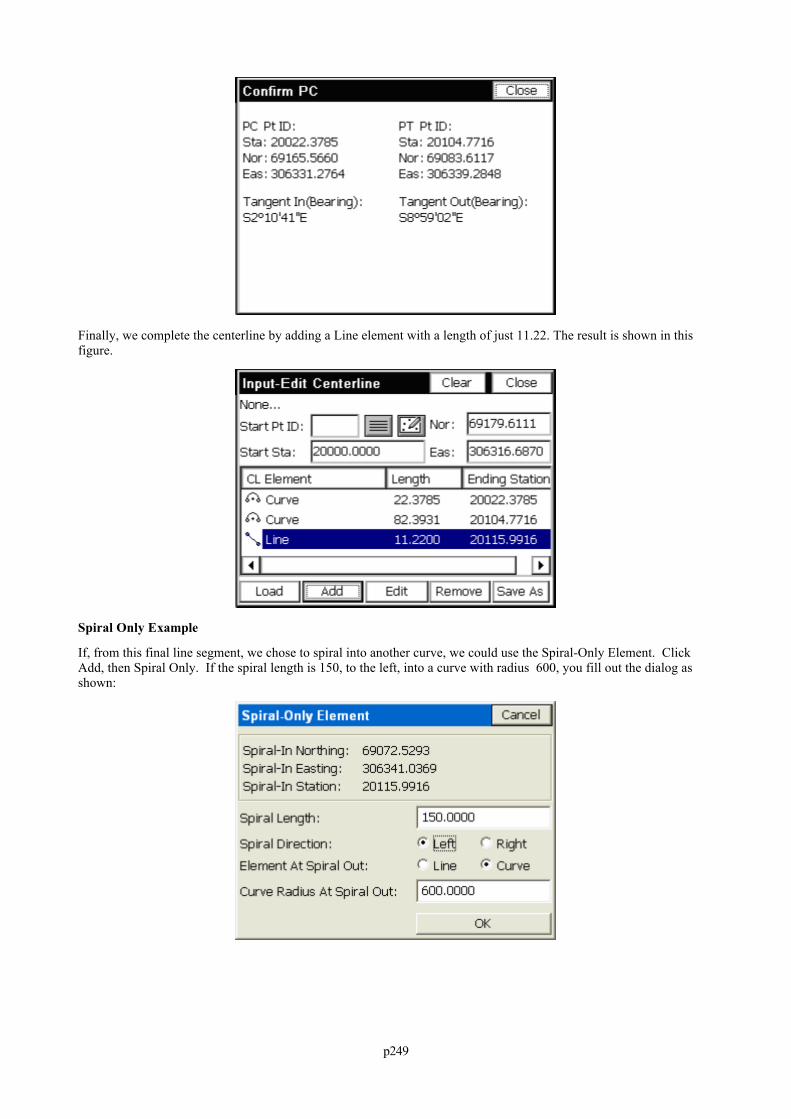
p249

Finally, we complete the centerline by adding a Line element with a length of just 11.22. The result is shown in thisfigure.

Spiral Only Example

If, from this final line segment, we chose to spiral into another curve, we could use the Spiral-Only Element. ClickAdd, then Spiral Only. If the spiral length is 150, to the left, into a curve with radius 600, you fill out the dialog asshown:

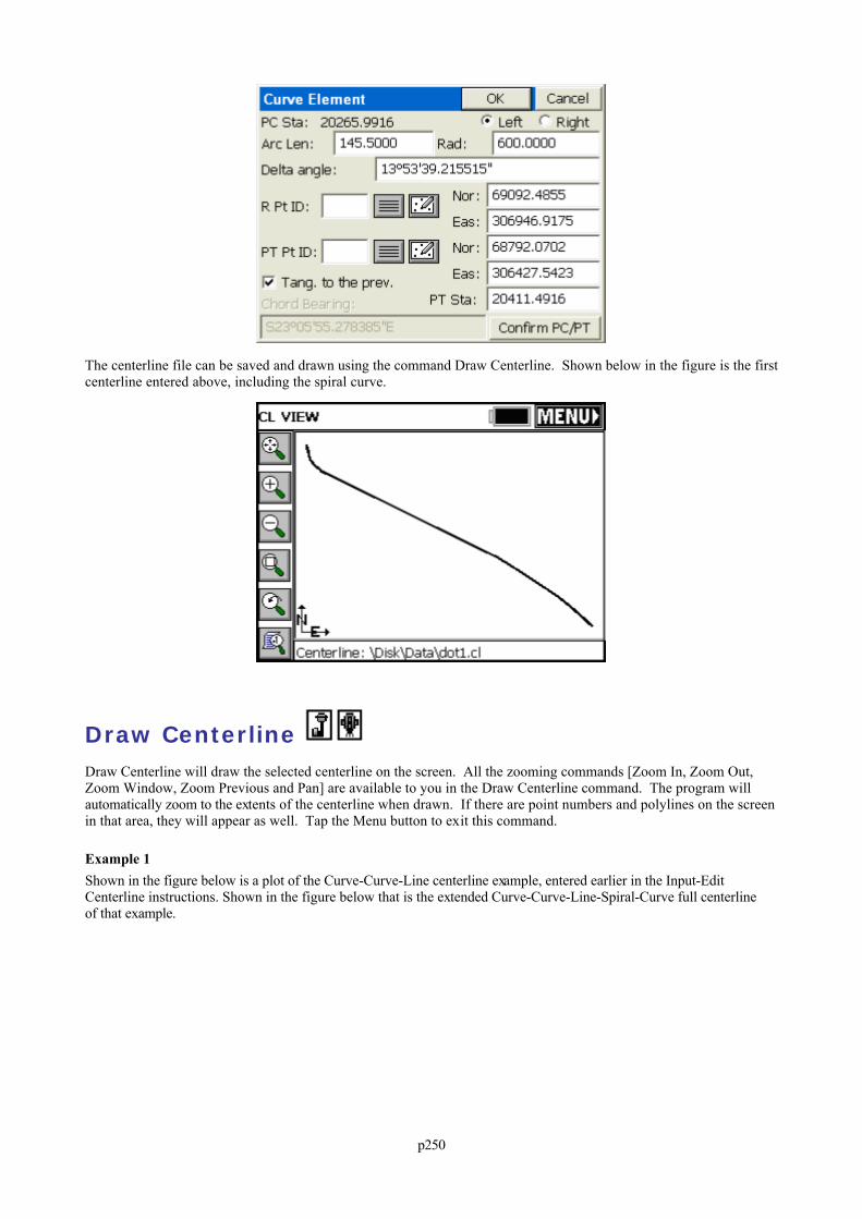
p250

The centerline file can be saved and drawn using the command Draw Centerline. Shown below in the figure is the firstcenterline entered above, including the spiral curve.

Draw Centerline Draw Centerline will draw the selected centerline on the screen. All the zooming commands [Zoom In, Zoom Out,Zoom Window, Zoom Previous and Pan] are available to you in the Draw Centerline command. The program willautomatically zoom to the extents of the centerline when drawn. If there are point numbers and polylines on the screenin that area, they will appear as well. Tap the Menu button to exit this command.

Example 1Shown in the figure below is a plot of the Curve-Curve-Line centerline example, entered earlier in the Input-EditCenterline instructions. Shown in the figure below that is the extended Curve-Curve-Line-Spiral-Curve full centerlineof that example.

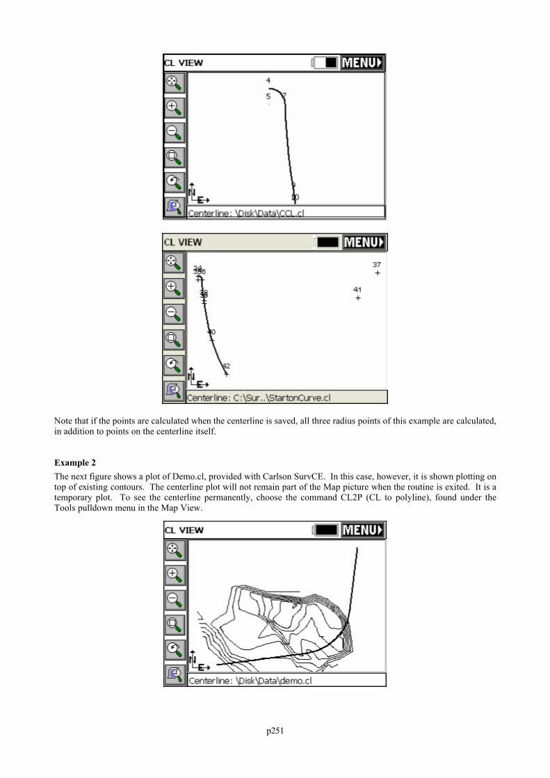
p251

Note that if the points are calculated when the centerline is saved, all three radius points of this example are calculated,in addition to points on the centerline itself.

Example 2The next figure shows a plot of Demo.cl, provided with Carlson SurvCE. In this case, however, it is shown plotting ontop of existing contours. The centerline plot will not remain part of the Map picture when the routine is exited. It is atemporary plot. To see the centerline permanently, choose the command CL2P (CL to polyline), found under theTools pulldown menu in the Map View.

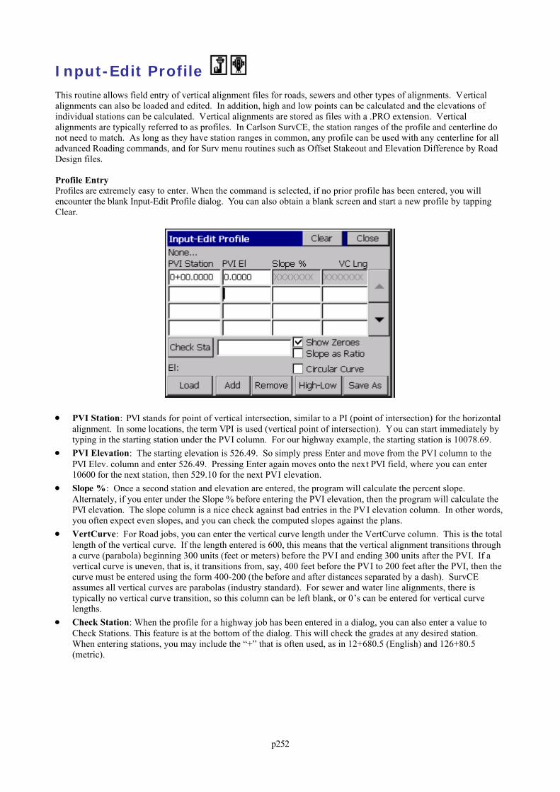
p252

Input-Edit Profile This routine allows field entry of vertical alignment files for roads, sewers and other types of alignments. Verticalalignments can also be loaded and edited. In addition, high and low points can be calculated and the elevations ofindividual stations can be calculated. Vertical alignments are stored as files with a .PRO extension. Verticalalignments are typically referred to as profiles. In Carlson SurvCE, the station ranges of the profile and centerline donot need to match. As long as they have station ranges in common, any profile can be used with any centerline for alladvanced Roading commands, and for Surv menu routines such as Offset Stakeout and Elevation Difference by RoadDesign files.

Profile EntryProfiles are extremely easy to enter. When the command is selected, if no prior profile has been entered, you willencounter the blank Input-Edit Profile dialog. You can also obtain a blank screen and start a new profile by tappingClear.

PVI Station: PVI stands for point of vertical intersection, similar to a PI (point of intersection) for the horizontalalignment. In some locations, the term VPI is used (vertical point of intersection). You can start immediately bytyping in the starting station under the PVI column. For our highway example, the starting station is 10078.69.

PVI Elevation: The starting elevation is 526.49. So simply press Enter and move from the PVI column to thePVI Elev. column and enter 526.49. Pressing Enter again moves onto the next PVI field, where you can enter10600 for the next station, then 529.10 for the next PVI elevation.

Slope %: Once a second station and elevation are entered, the program will calculate the percent slope.Alternately, if you enter under the Slope % before entering the PVI elevation, then the program will calculate thePVI elevation. The slope column is a nice check against bad entries in the PVI elevation column. In other words,you often expect even slopes, and you can check the computed slopes against the plans.

VertCurve: For Road jobs, you can enter the vertical curve length under the VertCurve column. This is the totallength of the vertical curve. If the length entered is 600, this means that the vertical alignment transitions througha curve (parabola) beginning 300 units (feet or meters) before the PVI and ending 300 units after the PVI. If avertical curve is uneven, that is, it transitions from, say, 400 feet before the PVI to 200 feet after the PVI, then thecurve must be entered using the form 400-200 (the before and after distances separated by a dash). SurvCEassumes all vertical curves are parabolas (industry standard). For sewer and water line alignments, there istypically no vertical curve transition, so this column can be left blank, or 0’s can be entered for vertical curvelengths.

Check Station: When the profile for a highway job has been entered in a dialog, you can also enter a value toCheck Stations. This feature is at the bottom of the dialog. This will check the grades at any desired station. When entering stations, you may include the “+” that is often used, as in 12+680.5 (English) and 126+80.5(metric).

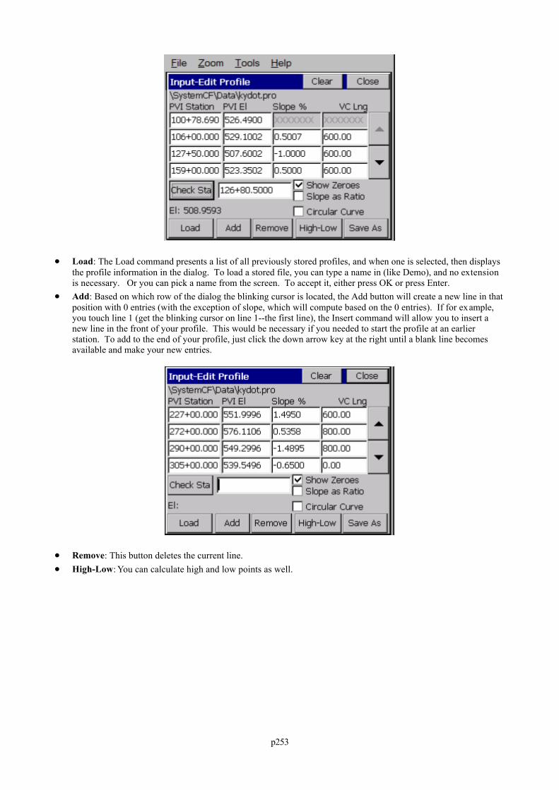
p253

Load: The Load command presents a list of all previously stored profiles, and when one is selected, then displaysthe profile information in the dialog. To load a stored file, you can type a name in (like Demo), and no extensionis necessary. Or you can pick a name from the screen. To accept it, either press OK or press Enter.

Add: Based on which row of the dialog the blinking cursor is located, the Add button will create a new line in thatposition with 0 entries (with the exception of slope, which will compute based on the 0 entries). If for example,you touch line 1 (get the blinking cursor on line 1--the first line), the Insert command will allow you to insert anew line in the front of your profile. This would be necessary if you needed to start the profile at an earlierstation. To add to the end of your profile, just click the down arrow key at the right until a blank line becomesavailable and make your new entries.

Remove: This button deletes the current line. High-Low: You can calculate high and low points as well.

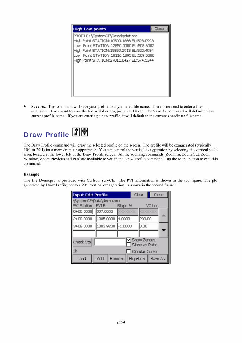
p254

Save As: This command will save your profile to any entered file name. There is no need to enter a fileextension. If you want to save the file as Baker.pro, just enter Baker. The Save As command will default to thecurrent profile name. If you are entering a new profile, it will default to the current coordinate file name.

Draw Profile The Draw Profile command will draw the selected profile on the screen. The profile will be exaggerated (typically10:1 or 20:1) for a more dramatic appearance. You can control the vertical exaggeration by selecting the vertical scaleicon, located at the lower left of the Draw Profile screen. All the zooming commands [Zoom In, Zoom Out, ZoomWindow, Zoom Previous and Pan] are available to you in the Draw Profile command. Tap the Menu button to exit thiscommand.

ExampleThe file Demo.pro is provided with Carlson SurvCE. The PVI information is shown in the top figure. The plotgenerated by Draw Profile, set to a 20:1 vertical exaggeration, is shown in the second figure.

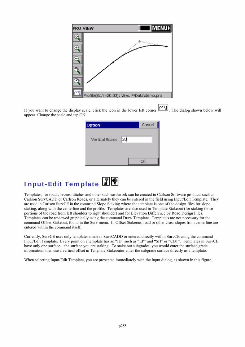
p255

If you want to change the display scale, click the icon in the lower left corner . The dialog shown below willappear. Change the scale and tap OK.

Input-Edit Template Templates, for roads, levees, ditches and other such earthwork can be created in Carlson Software products such asCarlson SurvCADD or Carlson Roads, or alternately they can be entered in the field using Input/Edit Template. Theyare used in Carlson SurvCE in the command Slope Staking where the template is one of the design files for slopestaking, along with the centerline and the profile. Templates are also used in Template Stakeout (for staking thoseportions of the road from left shoulder to right shoulder) and for Elevation Difference by Road Design Files. Templates can be reviewed graphically using the command Draw Template. Templates are not necessary for thecommand Offset Stakeout, found in the Surv menu. In Offset Stakeout, road or other cross slopes from centerline areentered within the command itself.

Currently, SurvCE uses only templates made in SurvCADD or entered directly within SurvCE using the commandInput/Edit Template. Every point on a template has an “ID” such as “EP” and “SH” or “CB1”. Templates in SurvCEhave only one surface—the surface you are staking. To stake out subgrades, you would enter the surface gradeinformation, then use a vertical offset in Template Stakeoutor enter the subgrade surface directly as a template.

When selecting Input/Edit Template, you are presented immediately with the input dialog, as shown in this figure.

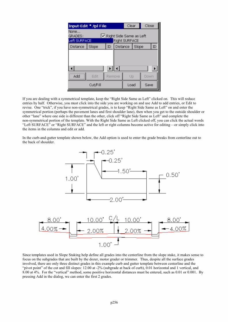
p256

If you are dealing with a symmetrical template, keep the “Right Side Same as Left” clicked on. This will reduceentries by half. Otherwise, you must click into the side you are working on and use Add to add entries, or Edit torevise. One “trick”, if you have non-symmetrical grades, is to keep “Right Side Same as Left” on and enter thesymmetrical portion (perhaps the pavement lanes and first shoulder lane), then when you get to the outside shoulder orother “lane” where one side is different than the other, click off “Right Side Same as Left” and complete thenon-symmetrical portion of the template. With the Right Side Same as Left clicked off, you can click the actual words“Left SURFACE” or “Right SURFACE” and the left or right columns become active for editing—or simply click intothe items in the columns and edit or add.

In the curb-and-gutter template shown below, the Add option is used to enter the grade breaks from centerline out tothe back of shoulder.

Since templates used in Slope Staking help define all grades into the centerline from the slope stake, it makes sense tofocus on the subgrades that are built by the dozer, motor grader or trimmer. Thus, despite all the surface gradesinvolved, there are only three distinct grades in this example curb and gutter template between centerline and the“pivot point” of the cut and fill slopes: 12.00 at -2% (subgrade at back of curb), 0.01 horizontal and 1 vertical, and8.00 at 4%. For the “vertical” method, some positive horizontal distances must be entered, such as 0.01 or 0.001. Bypressing Add in the dialog, we can enter the first 2 grades.

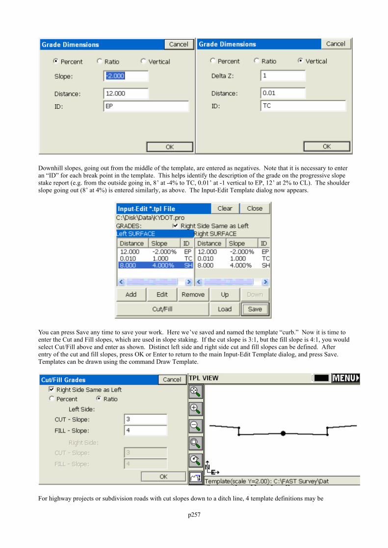
p257

Downhill slopes, going out from the middle of the template, are entered as negatives. Note that it is necessary to enteran “ID” for each break point in the template. This helps identify the description of the grade on the progressive slopestake report (e.g. from the outside going in, 8’ at -4% to TC, 0.01’ at -1 vertical to EP, 12’ at 2% to CL). The shoulderslope going out (8’ at 4%) is entered similarly, as above. The Input-Edit Template dialog now appears.

You can press Save any time to save your work. Here we’ve saved and named the template “curb.” Now it is time toenter the Cut and Fill slopes, which are used in slope staking. If the cut slope is 3:1, but the fill slope is 4:1, you wouldselect Cut/Fill above and enter as shown. Distinct left side and right side cut and fill slopes can be defined. Afterentry of the cut and fill slopes, press OK or Enter to return to the main Input-Edit Template dialog, and press Save. Templates can be drawn using the command Draw Template.

For highway projects or subdivision roads with cut slopes down to a ditch line, 4 template definitions may be

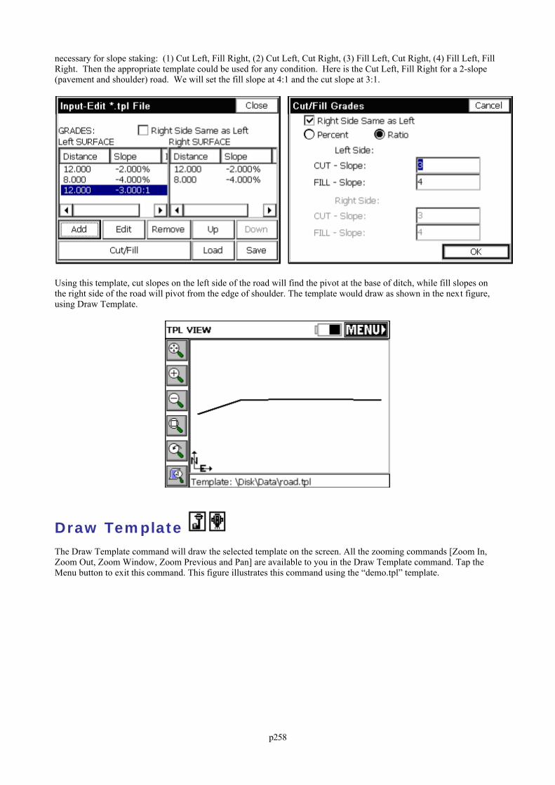
p258

necessary for slope staking: (1) Cut Left, Fill Right, (2) Cut Left, Cut Right, (3) Fill Left, Cut Right, (4) Fill Left, FillRight. Then the appropriate template could be used for any condition. Here is the Cut Left, Fill Right for a 2-slope(pavement and shoulder) road. We will set the fill slope at 4:1 and the cut slope at 3:1.

Using this template, cut slopes on the left side of the road will find the pivot at the base of ditch, while fill slopes onthe right side of the road will pivot from the edge of shoulder. The template would draw as shown in the next figure,using Draw Template.

Draw Template The Draw Template command will draw the selected template on the screen. All the zooming commands [Zoom In,Zoom Out, Zoom Window, Zoom Previous and Pan] are available to you in the Draw Template command. Tap theMenu button to exit this command. This figure illustrates this command using the “demo.tpl” template.

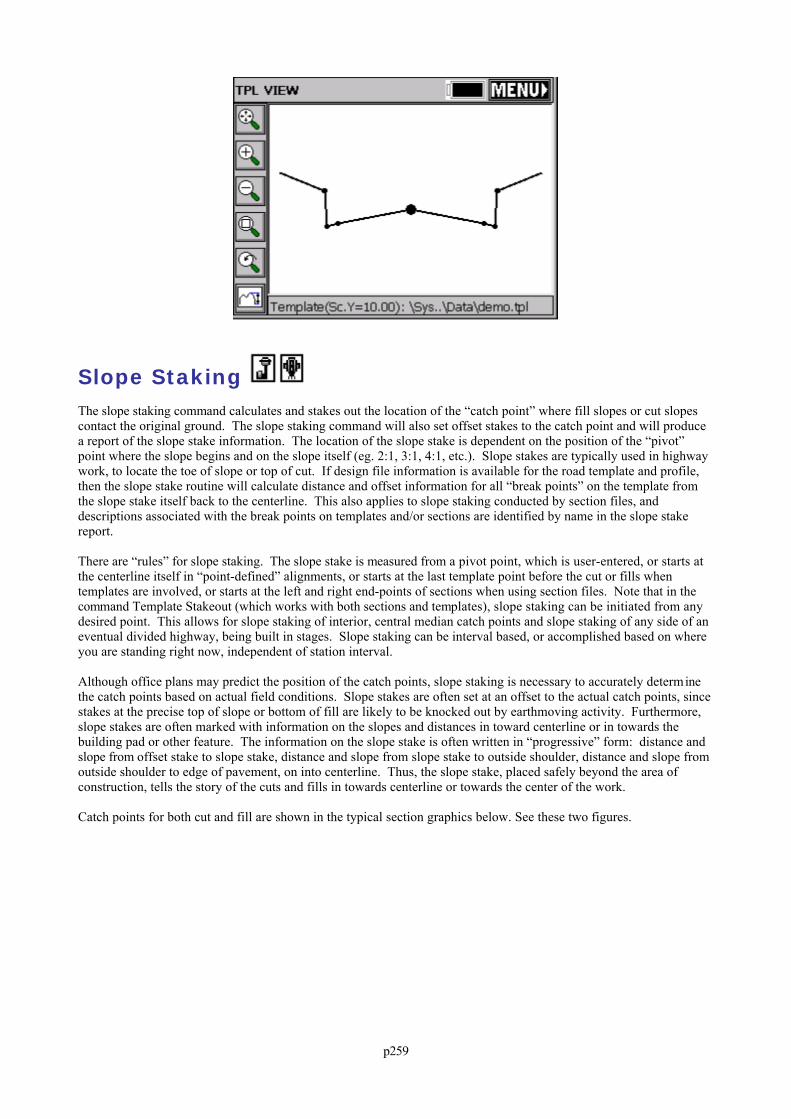
p259

Slope Staking The slope staking command calculates and stakes out the location of the “catch point” where fill slopes or cut slopescontact the original ground. The slope staking command will also set offset stakes to the catch point and will producea report of the slope stake information. The location of the slope stake is dependent on the position of the “pivot”point where the slope begins and on the slope itself (eg. 2:1, 3:1, 4:1, etc.). Slope stakes are typically used in highwaywork, to locate the toe of slope or top of cut. If design file information is available for the road template and profile,then the slope stake routine will calculate distance and offset information for all “break points” on the template fromthe slope stake itself back to the centerline. This also applies to slope staking conducted by section files, anddescriptions associated with the break points on templates and/or sections are identified by name in the slope stakereport.

There are “rules” for slope staking. The slope stake is measured from a pivot point, which is user-entered, or starts atthe centerline itself in “point-defined” alignments, or starts at the last template point before the cut or fills whentemplates are involved, or starts at the left and right end-points of sections when using section files. Note that in thecommand Template Stakeout (which works with both sections and templates), slope staking can be initiated from anydesired point. This allows for slope staking of interior, central median catch points and slope staking of any side of aneventual divided highway, being built in stages. Slope staking can be interval based, or accomplished based on whereyou are standing right now, independent of station interval.

Although office plans may predict the position of the catch points, slope staking is necessary to accurately determinethe catch points based on actual field conditions. Slope stakes are often set at an offset to the actual catch points, sincestakes at the precise top of slope or bottom of fill are likely to be knocked out by earthmoving activity. Furthermore,slope stakes are often marked with information on the slopes and distances in toward centerline or in towards thebuilding pad or other feature. The information on the slope stake is often written in “progressive” form: distance andslope from offset stake to slope stake, distance and slope from slope stake to outside shoulder, distance and slope fromoutside shoulder to edge of pavement, on into centerline. Thus, the slope stake, placed safely beyond the area ofconstruction, tells the story of the cuts and fills in towards centerline or towards the center of the work.

Catch points for both cut and fill are shown in the typical section graphics below. See these two figures.

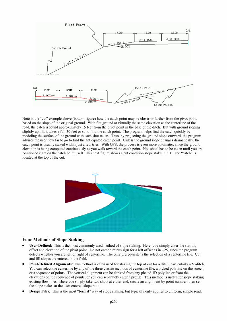
p260

Note in the “cut” example above (bottom figure) how the catch point may be closer or farther from the pivot pointbased on the slope of the original ground. With flat ground at virtually the same elevation as the centerline of theroad, the catch is found approximately 15 feet from the pivot point in the base of the ditch. But with ground slopingslightly uphill, it takes a full 30 feet or so to find the catch point. The program helps find the catch quickly bymodeling the surface of the ground with each shot taken. Thus, by projecting the ground slope outward, the programadvises the user how far to go to find the anticipated catch point. Unless the ground slope changes dramatically, thecatch point is usually staked within just a few tries. With GPS, the process is even more automatic, since the groundelevation is being computed continuously as you walk toward the catch point. No “shot” has to be taken until you arepositioned right on the catch point itself. This next figure shows a cut condition slope stake in 3D. The “catch” islocated at the top of the cut.

Four Methods of Slope Staking User-Defined: This is the most commonly used method of slope staking. Here, you simply enter the station,

offset and elevation of the pivot point. Do not enter a minus sign for a left offset as in –25, since the programdetects whether you are left or right of centerline. The only prerequisite is the selection of a centerline file. Cutand fill slopes are entered in the field.

Point-Defined Alignments: This method is often used for staking the top of cut for a ditch, particularly a V-ditch.You can select the centerline by any of the three classic methods of centerline file, a picked polyline on the screen,or a sequence of points. The vertical alignment can be derived from any picked 3D polyline or from theelevations on the sequence of points, or you can separately enter a profile. This method is useful for slope stakingexisting flow lines, where you simply take two shots at either end, create an alignment by point number, then setthe slope stakes at the user-entered slope ratio.

Design Files: This is the most “formal” way of slope staking, but typically only applies to uniform, simple road,

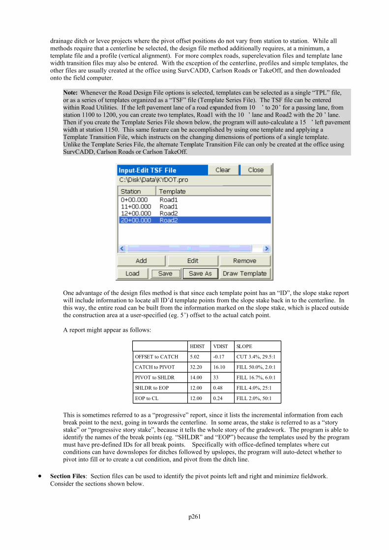
p261

drainage ditch or levee projects where the pivot offset positions do not vary from station to station. While allmethods require that a centerline be selected, the design file method additionally requires, at a minimum, atemplate file and a profile (vertical alignment). For more complex roads, superelevation files and template lanewidth transition files may also be entered. With the exception of the centerline, profiles and simple templates, theother files are usually created at the office using SurvCADD, Carlson Roads or TakeOff, and then downloadedonto the field computer.

Note: Whenever the Road Design File options is selected, templates can be selected as a single “TPL” file,or as a series of templates organized as a “TSF” file (Template Series File). The TSF file can be enteredwithin Road Utilities. If the left pavement lane of a road expanded from 10 ’ to 20’ for a passing lane, fromstation 1100 to 1200, you can create two templates, Road1 with the 10 ’ lane and Road2 with the 20 ’ lane.Then if you create the Template Series File shown below, the program will auto-calculate a 15 ’ left pavementwidth at station 1150. This same feature can be accomplished by using one template and applying aTemplate Transition File, which instructs on the changing dimensions of portions of a single template. Unlike the Template Series File, the alternate Template Transition File can only be created at the office usingSurvCADD, Carlson Roads or Carlson TakeOff.

One advantage of the design files method is that since each template point has an “ID”, the slope stake reportwill include information to locate all ID’d template points from the slope stake back in to the centerline. Inthis way, the entire road can be built from the information marked on the slope stake, which is placed outsidethe construction area at a user-specified (eg. 5’) offset to the actual catch point.

A report might appear as follows:

HDIST VDIST SLOPE

OFFSET to CATCH 5.02 -0.17 CUT 3.4%, 29.5:1

CATCH to PIVOT 32.20 16.10 FILL 50.0%, 2.0:1

PIVOT to SHLDR 14.00 33 FILL 16.7%, 6.0:1

SHLDR to EOP 12.00 0.48 FILL 4.0%, 25:1

EOP to CL 12.00 0.24 FILL 2.0%, 50:1

This is sometimes referred to as a “progressive” report, since it lists the incremental information from eachbreak point to the next, going in towards the centerline. In some areas, the stake is referred to as a “storystake” or “progressive story stake”, because it tells the whole story of the gradework. The program is able toidentify the names of the break points (eg. “SHLDR” and “EOP”) because the templates used by the programmust have pre-defined IDs for all break points. Specifically with office-defined templates where cutconditions can have downslopes for ditches followed by upslopes, the program will auto-detect whether topivot into fill or to create a cut condition, and pivot from the ditch line.

Section Files: Section files can be used to identify the pivot points left and right and minimize fieldwork.Consider the sections shown below.

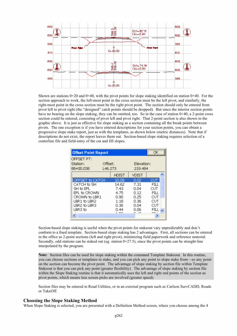
p262

Shown are stations 0+20 and 0+40, with the pivot points for slope staking identified on station 0+40. For thesection approach to work, the left-most point in the cross section must be the left pivot, and similarly, theright-most point in the cross section must be the right pivot point. The section should only be entered frompivot left to pivot right (the “designed” catch points should be dropped). But since the interior section pointshave no bearing on the slope staking, they can be omitted, too. So in the case of station 0+40, a 2-point crosssection could be entered, consisting of pivot left and pivot right. That 2-point section is also shown in thegraphic above. It is just as effective for slope staking as a section containing all the break points betweenpivots. The one exception is if you have entered descriptions for your section points, you can obtain aprogressive slope stake report, just as with the templates, as shown below (metric distances). Note that ifdescriptions do not exist, the report leaves them out. Section-based slope staking requires selection of acenterline file and field-entry of the cut and fill slopes.

Section-based slope staking is useful when the pivot points for stakeout vary unpredictably and don’tconform to a fixed template. Section-based slope staking has 2 advantages. First, all sections can be enteredin the office as 2-point sections (left and right pivot), minimizing field paperwork and reference material. Secondly, odd stations can be staked out (eg. station 0+27.5), since the pivot points can be straight-lineinterpolated by the program.

Note: Section files can be used for slope staking within the command Template Stakeout. In this routine,you can choose sections or templates to stake, and you can pick any point to slope stake from—so any pointon the section can become the pivot point. The advantage of slope staking by section file within TemplateStakeout is that you can pick any point (greater flexibility). The advantage of slope staking by section filewithin the Slope Staking routine is that it automatically uses the left and right end points of the section aspivot points, which means less screen picks are involved (greater speed).

Section files may be entered in Road Utilities, or in an external program such as Carlson SurvCADD, Roadsor TakeOff.

Choosing the Slope Staking MethodWhen Slope Staking is selected, you are presented with a Definition Method screen, where you choose among the 4

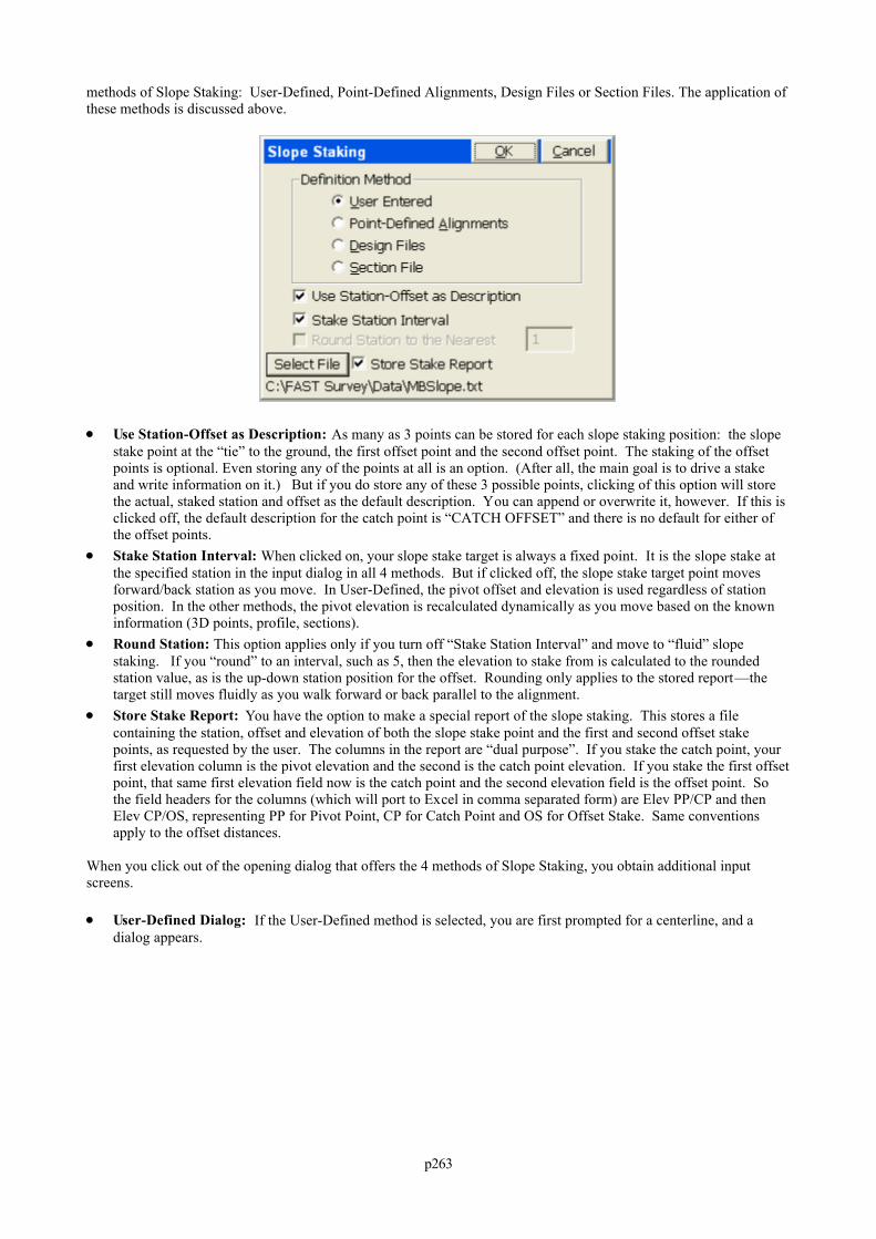
p263

methods of Slope Staking: User-Defined, Point-Defined Alignments, Design Files or Section Files. The application ofthese methods is discussed above.

Use Station-Offset as Description: As many as 3 points can be stored for each slope staking position: the slopestake point at the “tie” to the ground, the first offset point and the second offset point. The staking of the offsetpoints is optional. Even storing any of the points at all is an option. (After all, the main goal is to drive a stakeand write information on it.) But if you do store any of these 3 possible points, clicking of this option will storethe actual, staked station and offset as the default description. You can append or overwrite it, however. If this isclicked off, the default description for the catch point is “CATCH OFFSET” and there is no default for either ofthe offset points.

Stake Station Interval: When clicked on, your slope stake target is always a fixed point. It is the slope stake atthe specified station in the input dialog in all 4 methods. But if clicked off, the slope stake target point movesforward/back station as you move. In User-Defined, the pivot offset and elevation is used regardless of stationposition. In the other methods, the pivot elevation is recalculated dynamically as you move based on the knowninformation (3D points, profile, sections).

Round Station: This option applies only if you turn off “Stake Station Interval” and move to “fluid” slopestaking. If you “round” to an interval, such as 5, then the elevation to stake from is calculated to the roundedstation value, as is the up-down station position for the offset. Rounding only applies to the stored report—thetarget still moves fluidly as you walk forward or back parallel to the alignment.

Store Stake Report: You have the option to make a special report of the slope staking. This stores a filecontaining the station, offset and elevation of both the slope stake point and the first and second offset stakepoints, as requested by the user. The columns in the report are “dual purpose”. If you stake the catch point, yourfirst elevation column is the pivot elevation and the second is the catch point elevation. If you stake the first offsetpoint, that same first elevation field now is the catch point and the second elevation field is the offset point. Sothe field headers for the columns (which will port to Excel in comma separated form) are Elev PP/CP and thenElev CP/OS, representing PP for Pivot Point, CP for Catch Point and OS for Offset Stake. Same conventionsapply to the offset distances.

When you click out of the opening dialog that offers the 4 methods of Slope Staking, you obtain additional inputscreens.

User-Defined Dialog: If the User-Defined method is selected, you are first prompted for a centerline, and adialog appears.

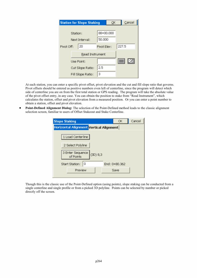
p264

At each station, you can enter a specific pivot offset, pivot elevation and the cut and fill slope ratio that governs. Pivot offsets should be entered as positive numbers even left of centerline, since the program will detect whichside of centerline you are on from the first total station or GPS reading. The program will take the absolute valueof the pivot offset entry, in any case. You can obtain the position to stake from “Read Instrument”, whichcalculates the station, offset and pivot elevation from a measured position. Or you can enter a point number toobtain a station, offset and pivot elevation.

Point-Defined Alignment Dialog: The selection of the Point-Defined method leads to the classic alignmentselection screen, familiar to users of Offset Stakeout and Stake Centerline.

Though this is the classic use of the Point-Defined option (using points), slope staking can be conducted from asingle centerline and single profile or from a picked 3D polyline. Points can be selected by number or pickeddirectly off the screen.

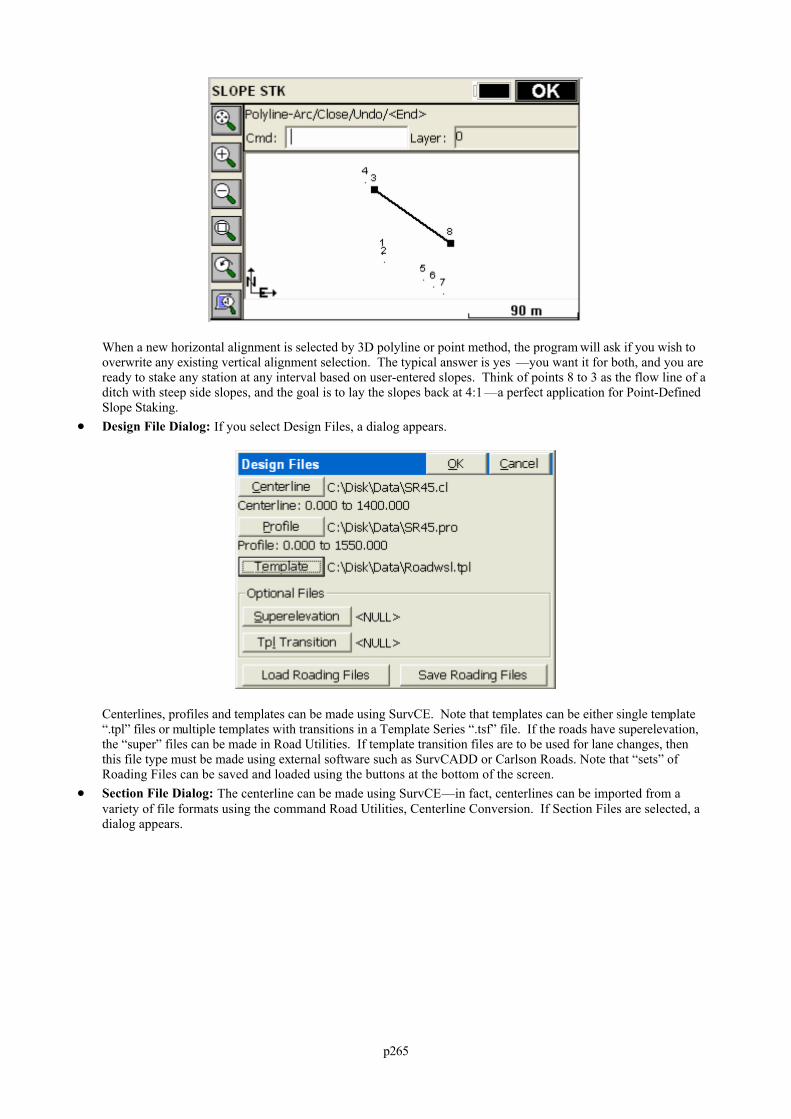
p265

When a new horizontal alignment is selected by 3D polyline or point method, the program will ask if you wish tooverwrite any existing vertical alignment selection. The typical answer is yes —you want it for both, and you areready to stake any station at any interval based on user-entered slopes. Think of points 8 to 3 as the flow line of aditch with steep side slopes, and the goal is to lay the slopes back at 4:1 —a perfect application for Point-DefinedSlope Staking.

Design File Dialog: If you select Design Files, a dialog appears.

Centerlines, profiles and templates can be made using SurvCE. Note that templates can be either single template“.tpl” files or multiple templates with transitions in a Template Series “.tsf” file. If the roads have superelevation,the “super” files can be made in Road Utilities. If template transition files are to be used for lane changes, thenthis file type must be made using external software such as SurvCADD or Carlson Roads. Note that “sets” ofRoading Files can be saved and loaded using the buttons at the bottom of the screen.

Section File Dialog: The centerline can be made using SurvCE—in fact, centerlines can be imported from avariety of file formats using the command Road Utilities, Centerline Conversion. If Section Files are selected, adialog appears.

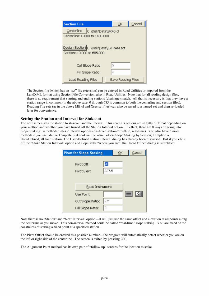
p266

The Section file (which has an “sct” file extension) can be entered in Road Utilities or impored from theLandXML format using Section File Conversion, also in Road Utilities. Note that for all roading design files,there is no requirement that starting and ending stations (chainage) match. All that is necessary is that they have astation range in common (in the above case, 0 through 685 is common to both the centerline and section files). Roading File sets (as in the above MB.cl and Xsec.sct files) can also be saved to a named set and then re-loadedlater for convenience.

Setting the Station and Interval for StakeoutThe next screen sets the station to stakeout and the interval. This screen’s options are slightly different depending onyour method and whether you have turned off the Station Interval option. In effect, there are 8 ways of going intoSlope Staking: 4 methods times 2 interval options (on=fixed station/off=fluid, real-time). You also have 3 moremethods if you include the Template Stakeout routine which offers Slope Staking by Section, Template orUser-Defined, all fixed station. The User-Defined station interval dialog has already been discussed. But if you clickoff the “Stake Station Interval” option and slope stake “where you are”, the User-Defined dialog is simplified.

Note there is no “Station” and “Next Interval” option—it will just use the same offset and elevation at all points alongthe centerline as you move. This non-interval method could be called “real-time” slope staking. You are freed of theconstraints of staking a fixed point at a specified station.

The Pivot Offset should be entered as a positive number—the program will automatically detect whether you are onthe left or right side of the centerline. The screen is exited by pressing OK.

The Alignment Point method has its own pair of “follow-up” screens for the location to stake.

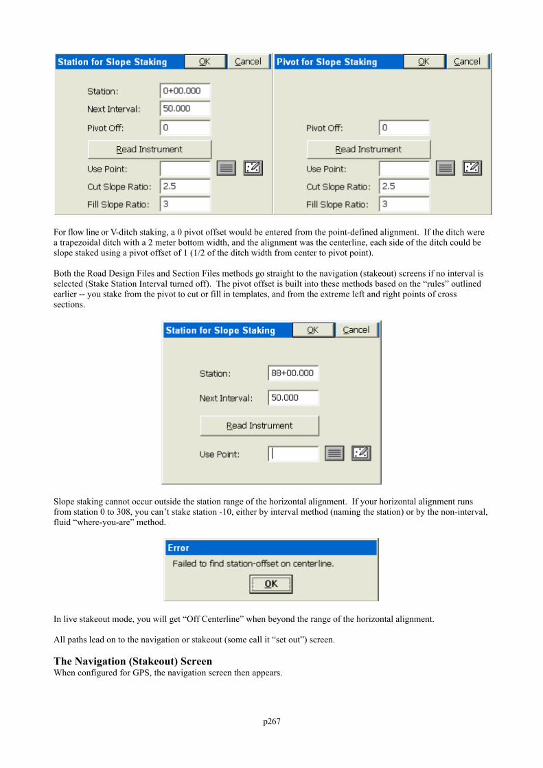
p267

For flow line or V-ditch staking, a 0 pivot offset would be entered from the point-defined alignment. If the ditch werea trapezoidal ditch with a 2 meter bottom width, and the alignment was the centerline, each side of the ditch could beslope staked using a pivot offset of 1 (1/2 of the ditch width from center to pivot point).

Both the Road Design Files and Section Files methods go straight to the navigation (stakeout) screens if no interval isselected (Stake Station Interval turned off). The pivot offset is built into these methods based on the “rules” outlinedearlier -- you stake from the pivot to cut or fill in templates, and from the extreme left and right points of crosssections.

Slope staking cannot occur outside the station range of the horizontal alignment. If your horizontal alignment runsfrom station 0 to 308, you can’t stake station -10, either by interval method (naming the station) or by the non-interval,fluid “where-you-are” method.

In live stakeout mode, you will get “Off Centerline” when beyond the range of the horizontal alignment.

All paths lead on to the navigation or stakeout (some call it “set out”) screen.

The Navigation (Stakeout) ScreenWhen configured for GPS, the navigation screen then appears.

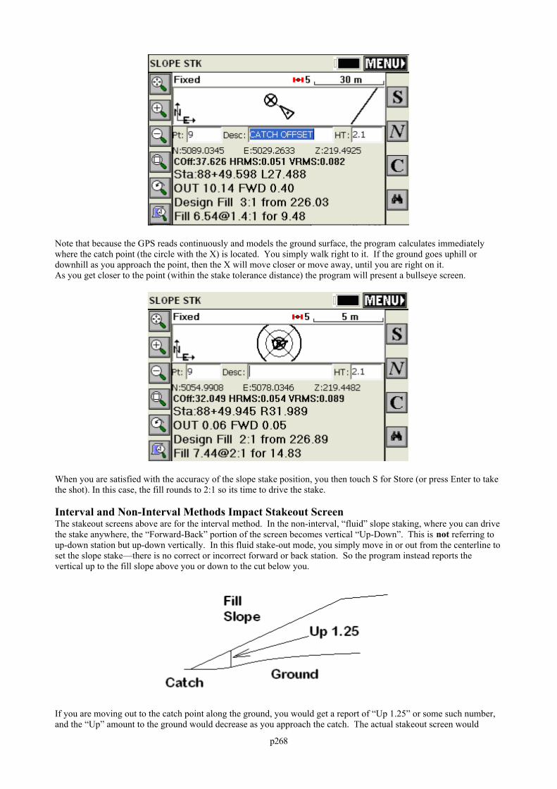
p268

Note that because the GPS reads continuously and models the ground surface, the program calculates immediatelywhere the catch point (the circle with the X) is located. You simply walk right to it. If the ground goes uphill ordownhill as you approach the point, then the X will move closer or move away, until you are right on it.As you get closer to the point (within the stake tolerance distance) the program will present a bullseye screen.

When you are satisfied with the accuracy of the slope stake position, you then touch S for Store (or press Enter to takethe shot). In this case, the fill rounds to 2:1 so its time to drive the stake.

Interval and Non-Interval Methods Impact Stakeout ScreenThe stakeout screens above are for the interval method. In the non-interval, “fluid” slope staking, where you can drivethe stake anywhere, the “Forward-Back” portion of the screen becomes vertical “Up-Down”. This is not referring toup-down station but up-down vertically. In this fluid stake-out mode, you simply move in or out from the centerline toset the slope stake—there is no correct or incorrect forward or back station. So the program instead reports thevertical up to the fill slope above you or down to the cut below you.

If you are moving out to the catch point along the ground, you would get a report of “Up 1.25” or some such number,and the “Up” amount to the ground would decrease as you approach the catch. The actual stakeout screen would

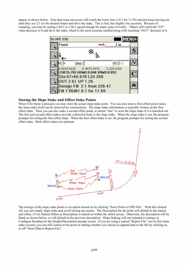
p269

appear as shown below. Note that some surveyors will watch the lower line (1.6:1 for 11.59) and just keep moving outuntil they see 2:1 (or the desired slope) and drive the stake. This is fast, but slightly less accurate. Because ofrounding, you may be setting 2.04:1 or 1.96:1 (good enough for many types of work). Others will watch the “UP”value decrease to 0 and drive the stake, which is the most accurate method along with watching “OUT” decrease to 0.

Storing the Slope Stake and Offset Stake PointsWhen S for Store is pressed, you may store the actual slope stake point. You can also store a first offset point (sincethe slope stake itself can be removed by construction). The slope stake information is typically written on the firstoffset stake. Then you can also stake a second offset point, to obtain “line” to reset the slope stake if it is knocked out.The first and second offset stakes provide a direction back to the slope stake. When the slope stake is set, the programprompts for setting the first offset stake. When the first offset stake is set, the program prompts for setting the secondoffset stake. Both offset stakes are optional.

The storage of the slope stake points is an option turned on by clicking “Store Point to CRD File”. With this clickedoff, you can simply slope stake and avoid storing any points. The Description for the point will default to the stationand offset, if Use Station Offset as Description is turned on within the initial screen. Otherwise, the description will beblank as shown below, or will default to the previous description. Slope Staking will not respond to settings inConfigure Reading for the Height/Description prompt screen. If you are using a named “Report File” (set in first slopestake screen), you can still control at the point of staking whether you choose to append data to the file by clicking onor off “Store Data to Report File”.

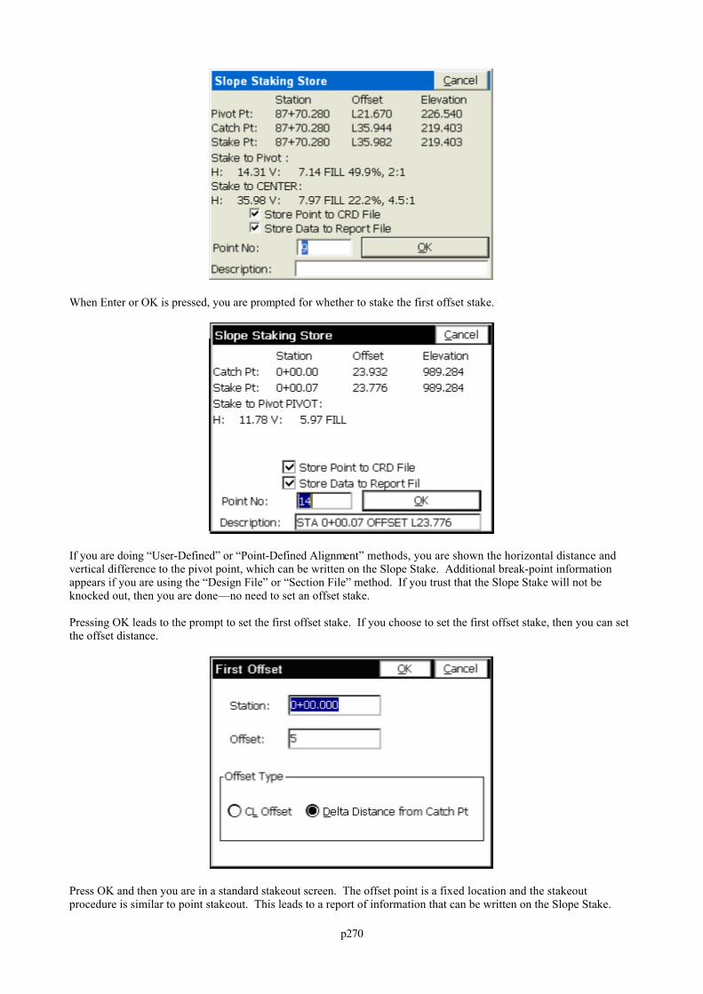
p270

When Enter or OK is pressed, you are prompted for whether to stake the first offset stake.

If you are doing “User-Defined” or “Point-Defined Alignment” methods, you are shown the horizontal distance andvertical difference to the pivot point, which can be written on the Slope Stake. Additional break-point informationappears if you are using the “Design File” or “Section File” method. If you trust that the Slope Stake will not beknocked out, then you are done—no need to set an offset stake.

Pressing OK leads to the prompt to set the first offset stake. If you choose to set the first offset stake, then you can setthe offset distance.

Press OK and then you are in a standard stakeout screen. The offset point is a fixed location and the stakeoutprocedure is similar to point stakeout. This leads to a report of information that can be written on the Slope Stake.

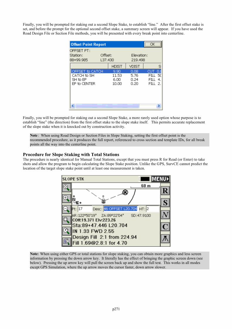
p271

Finally, you will be prompted for staking out a second Slope Stake, to establish “line.” After the first offset stake isset, and before the prompt for the optional second offset stake, a summary screen will appear. If you have used theRoad Design File or Section File methods, you will be presented with every break point into centerline.

Finally, you will be prompted for staking out a second Slope Stake, a more rarely used option whose purpose is toestablish “line” (the direction) from the first offset stake to the slope stake itself. This permits accurate replacementof the slope stake when it is knocked out by construction activity.

Note : When using Road Design or Section Files in Slope Staking, setting the first offset point is therecommended procedure, as it produces the full report, referenced to cross section and template IDs, for all breakpoints all the way into the centerline point.

Procedure for Slope Staking with Total StationsThe procedure is nearly identical for Manual Total Stations, except that you must press R for Read (or Enter) to takeshots and allow the program to begin calculating the Slope Stake position. Unlike the GPS, SurvCE cannot predict thelocation of the target slope stake point until at least one measurement is taken.

Note: When using either GPS or total stations for slope staking, you can obtain more graphics and less screeninformation by pressing the down arrow key. It literally has the effect of bringing the graphic screen down (seebelow). Pressing the up arrow key will pull the screen back up and show the full text. This works in all modesexcept GPS Simulation, where the up arrow moves the cursor faster, down arrow slower.

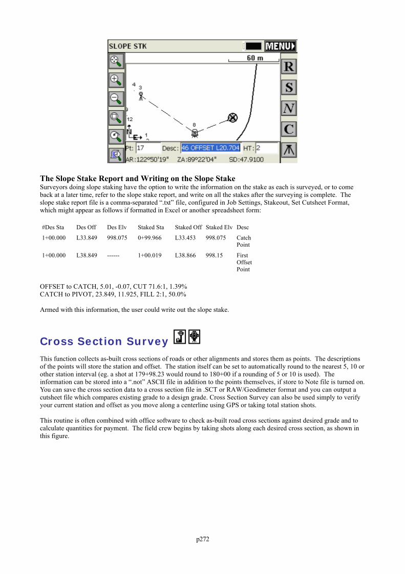
p272

The Slope Stake Report and Writing on the Slope StakeSurveyors doing slope staking have the option to write the information on the stake as each is surveyed, or to comeback at a later time, refer to the slope stake report, and write on all the stakes after the surveying is complete. Theslope stake report file is a comma-separated “.txt” file, configured in Job Settings, Stakeout, Set Cutsheet Format,which might appear as follows if formatted in Excel or another spreadsheet form:

#Des Sta Des Off Des Elv Staked Sta Staked Off Staked Elv Desc

1+00.000 L33.849 998.075 0+99.966 L33.453 998.075 CatchPoint

1+00.000 L38.849 ------ 1+00.019 L38.866 998.15 FirstOffsetPoint

OFFSET to CATCH, 5.01, -0.07, CUT 71.6:1, 1.39%CATCH to PIVOT, 23.849, 11.925, FILL 2:1, 50.0%

Armed with this information, the user could write out the slope stake.

Cross Section Survey This function collects as-built cross sections of roads or other alignments and stores them as points. The descriptionsof the points will store the station and offset. The station itself can be set to automatically round to the nearest 5, 10 orother station interval (eg. a shot at 179+98.23 would round to 180+00 if a rounding of 5 or 10 is used). Theinformation can be stored into a “.not” ASCII file in addition to the points themselves, if store to Note file is turned on.You can save the cross section data to a cross section file in .SCT or RAW/Geodimeter format and you can output acutsheet file which compares existing grade to a design grade. Cross Section Survey can also be used simply to verifyyour current station and offset as you move along a centerline using GPS or taking total station shots.

This routine is often combined with office software to check as-built road cross sections against desired grade and tocalculate quantities for payment. The field crew begins by taking shots along each desired cross section, as shown inthis figure.

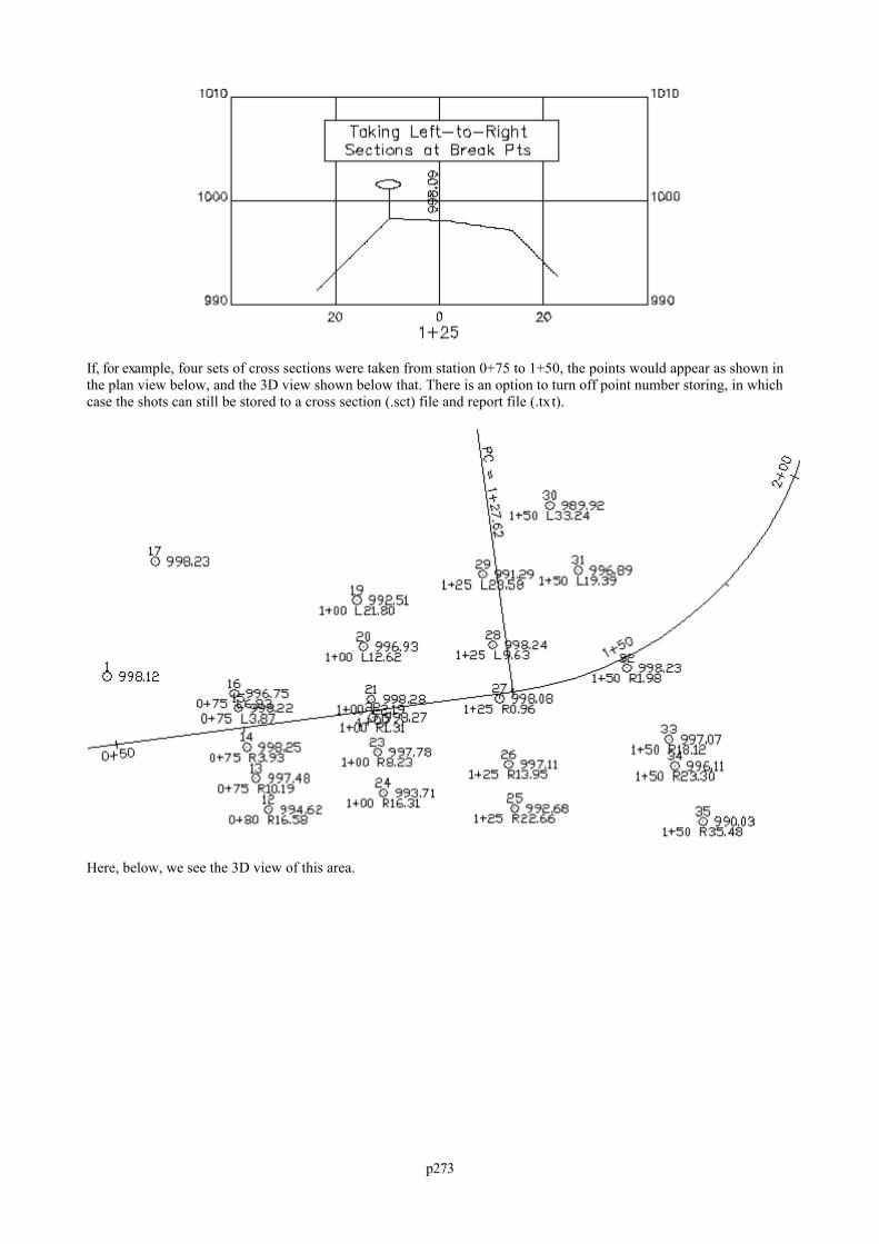
p273

If, for example, four sets of cross sections were taken from station 0+75 to 1+50, the points would appear as shown inthe plan view below, and the 3D view shown below that. There is an option to turn off point number storing, in whichcase the shots can still be stored to a cross section (.sct) file and report file (.txt).

Here, below, we see the 3D view of this area.

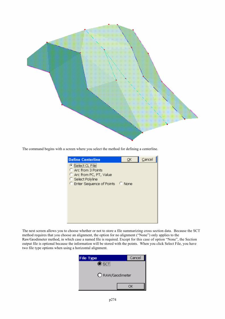
p274

The command begins with a screen where you select the method for defining a centerline.

The next screen allows you to choose whether or not to store a file summarizing cross section data. Because the SCTmethod requires that you choose an alignment, the option for no alignment (“None”) only applies to theRaw/Geodimeter method, in which case a named file is required. Except for this case of option “None”, the Sectionoutput file is optional because the information will be stored with the points. When you click Select File, you havetwo file type options when using a horizontal alignment.

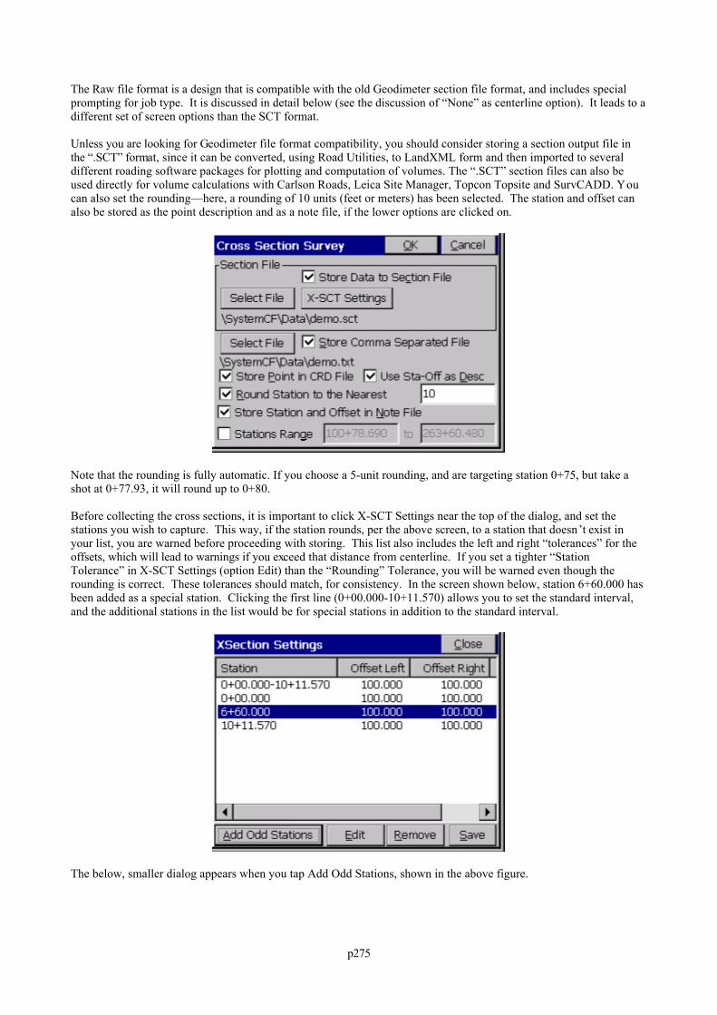
p275

The Raw file format is a design that is compatible with the old Geodimeter section file format, and includes specialprompting for job type. It is discussed in detail below (see the discussion of “None” as centerline option). It leads to adifferent set of screen options than the SCT format.

Unless you are looking for Geodimeter file format compatibility, you should consider storing a section output file inthe “.SCT” format, since it can be converted, using Road Utilities, to LandXML form and then imported to severaldifferent roading software packages for plotting and computation of volumes. The “.SCT” section files can also beused directly for volume calculations with Carlson Roads, Leica Site Manager, Topcon Topsite and SurvCADD. Youcan also set the rounding—here, a rounding of 10 units (feet or meters) has been selected. The station and offset canalso be stored as the point description and as a note file, if the lower options are clicked on.

Note that the rounding is fully automatic. If you choose a 5-unit rounding, and are targeting station 0+75, but take ashot at 0+77.93, it will round up to 0+80.

Before collecting the cross sections, it is important to click X-SCT Settings near the top of the dialog, and set thestations you wish to capture. This way, if the station rounds, per the above screen, to a station that doesn’t exist inyour list, you are warned before proceeding with storing. This list also includes the left and right “tolerances” for theoffsets, which will lead to warnings if you exceed that distance from centerline. If you set a tighter “StationTolerance” in X-SCT Settings (option Edit) than the “Rounding” Tolerance, you will be warned even though therounding is correct. These tolerances should match, for consistency. In the screen shown below, station 6+60.000 hasbeen added as a special station. Clicking the first line (0+00.000-10+11.570) allows you to set the standard interval,and the additional stations in the list would be for special stations in addition to the standard interval.

The below, smaller dialog appears when you tap Add Odd Stations, shown in the above figure.

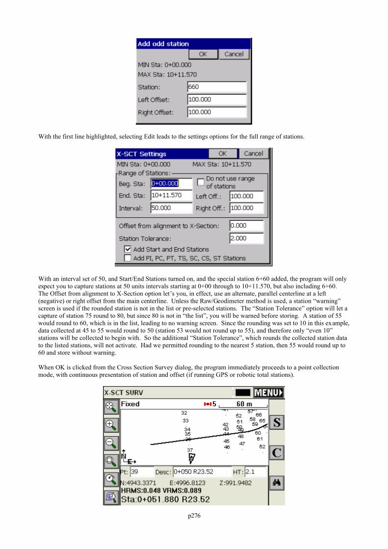
p276

With the first line highlighted, selecting Edit leads to the settings options for the full range of stations.

With an interval set of 50, and Start/End Stations turned on, and the special station 6+60 added, the program will onlyexpect you to capture stations at 50 units intervals starting at 0+00 through to 10+11.570, but also including 6+60. The Offset from alignment to X-Section option let’s you, in effect, use an alternate, parallel centerline at a left(negative) or right offset from the main centerline. Unless the Raw/Geodimeter method is used, a station “warning”screen is used if the rounded station is not in the list or pre-selected stations. The “Station Tolerance” option will let acapture of station 75 round to 80, but since 80 is not in “the list”, you will be warned before storing. A station of 55would round to 60, which is in the list, leading to no warning screen. Since the rounding was set to 10 in this example,data collected at 45 to 55 would round to 50 (station 53 would not round up to 55), and therefore only “even 10”stations will be collected to begin with. So the additional “Station Tolerance”, which rounds the collected station datato the listed stations, will not activate. Had we permitted rounding to the nearest 5 station, then 55 would round up to60 and store without warning.

When OK is clicked from the Cross Section Survey dialog, the program immediately proceeds to a point collectionmode, with continuous presentation of station and offset (if running GPS or robotic total stations).

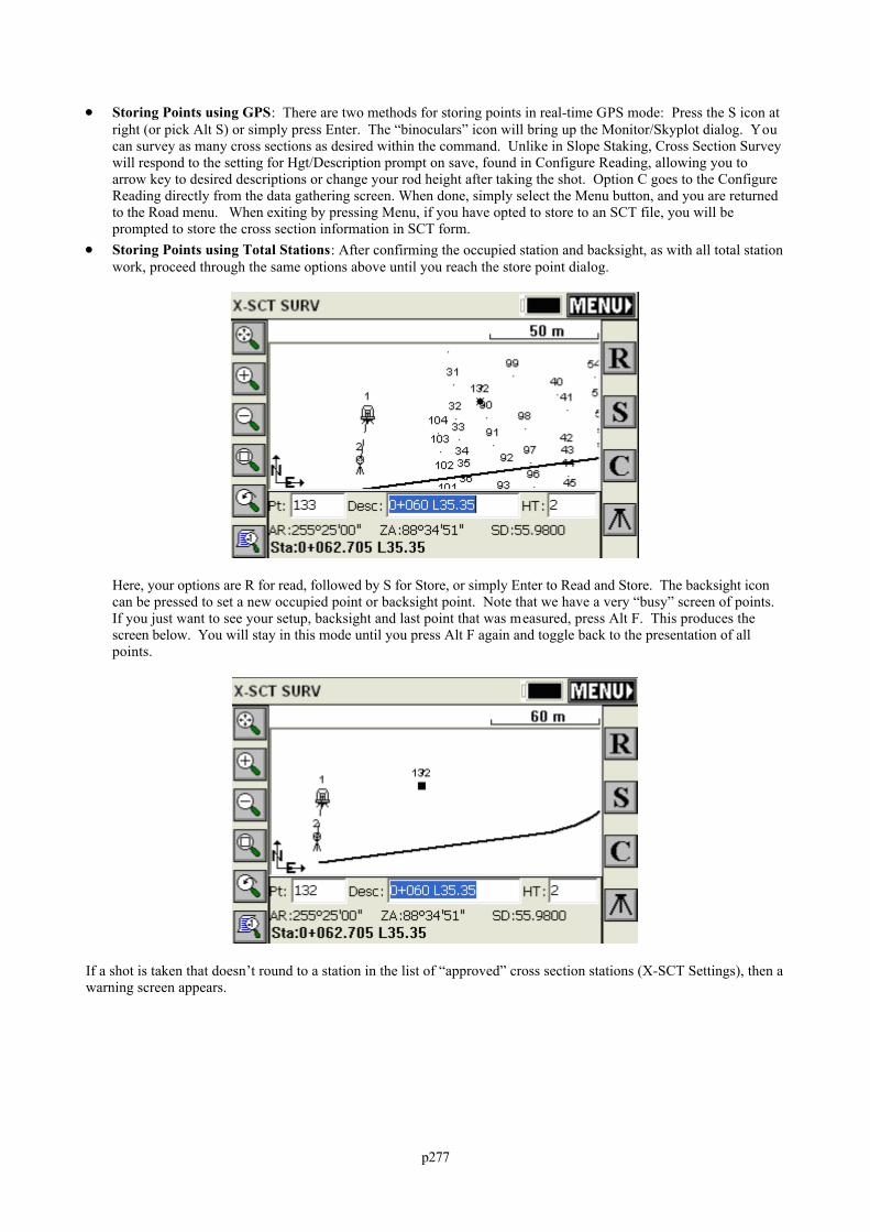
p277

Storing Points using GPS: There are two methods for storing points in real-time GPS mode: Press the S icon atright (or pick Alt S) or simply press Enter. The “binoculars” icon will bring up the Monitor/Skyplot dialog. Youcan survey as many cross sections as desired within the command. Unlike in Slope Staking, Cross Section Surveywill respond to the setting for Hgt/Description prompt on save, found in Configure Reading, allowing you toarrow key to desired descriptions or change your rod height after taking the shot. Option C goes to the ConfigureReading directly from the data gathering screen. When done, simply select the Menu button, and you are returnedto the Road menu. When exiting by pressing Menu, if you have opted to store to an SCT file, you will beprompted to store the cross section information in SCT form.

Storing Points using Total Stations: After confirming the occupied station and backsight, as with all total stationwork, proceed through the same options above until you reach the store point dialog.

Here, your options are R for read, followed by S for Store, or simply Enter to Read and Store. The backsight iconcan be pressed to set a new occupied point or backsight point. Note that we have a very “busy” screen of points. If you just want to see your setup, backsight and last point that was measured, press Alt F. This produces thescreen below. You will stay in this mode until you press Alt F again and toggle back to the presentation of allpoints.

If a shot is taken that doesn’t round to a station in the list of “approved” cross section stations (X-SCT Settings), then awarning screen appears.

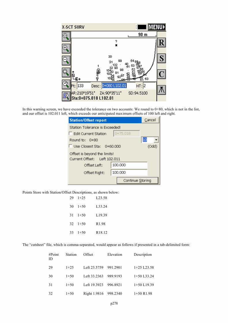
p278

In this warning screen, we have exceeded the tolerance on two accounts: We round to 0+80, which is not in the list,and our offset is 102.011 left, which exceeds our anticipated maximum offsets of 100 left and right.

Points Store with Station/Offset Descriptions, as shown below:29 1+25 L23.58

30 1+50 L33.24

31 1+50 L19.39

32 1+50 R1.98

33 1+50 R18.12

The “cutsheet” file, which is comma-separated, would appear as follows if presented in a tab-delimited form:

#PointID

Station Offset Elevation Description

29 1+25 Left 23.5759 991.2901 1+25 L23.58

30 1+50 Left 33.2363 989.9193 1+50 L33.24

31 1+50 Left 19.3923 996.8921 1+50 L19.39

32 1+50 Right 1.9816 998.2340 1+50 R1.98

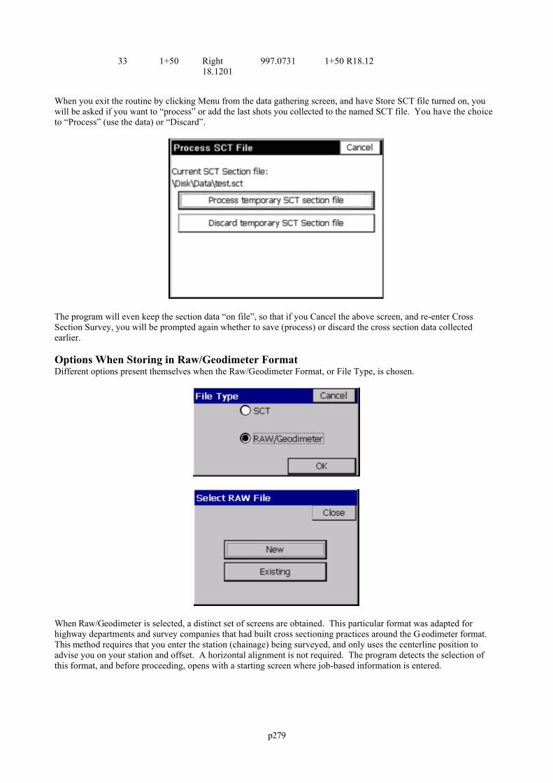
p279

33 1+50 Right18.1201

997.0731 1+50 R18.12

When you exit the routine by clicking Menu from the data gathering screen, and have Store SCT file turned on, youwill be asked if you want to “process” or add the last shots you collected to the named SCT file. You have the choiceto “Process” (use the data) or “Discard”.

The program will even keep the section data “on file”, so that if you Cancel the above screen, and re-enter CrossSection Survey, you will be prompted again whether to save (process) or discard the cross section data collectedearlier.

Options When Storing in Raw/Geodimeter FormatDifferent options present themselves when the Raw/Geodimeter Format, or File Type, is chosen.

When Raw/Geodimeter is selected, a distinct set of screens are obtained. This particular format was adapted forhighway departments and survey companies that had built cross sectioning practices around the G eodimeter format. This method requires that you enter the station (chainage) being surveyed, and only uses the centerline position toadvise you on your station and offset. A horizontal alignment is not required. The program detects the selection ofthis format, and before proceeding, opens with a starting screen where job-based information is entered.

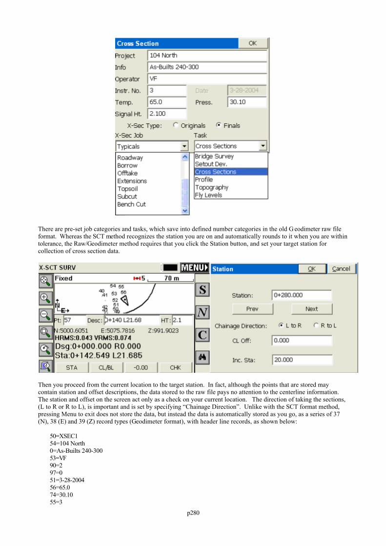
p280

There are pre-set job categories and tasks, which save into defined number categories in the old G eodimeter raw fileformat. Whereas the SCT method recognizes the station you are on and automatically rounds to it when you are withintolerance, the Raw/Geodimeter method requires that you click the Station button, and set your target station forcollection of cross section data.

Then you proceed from the current location to the target station. In fact, although the points that are stored maycontain station and offset descriptions, the data stored to the raw file pays no attention to the centerline information.The station and offset on the screen act only as a check on your current location. The direction of taking the sections,(L to R or R to L), is important and is set by specifying “Chainage Direction”. Unlike with the SCT format method,pressing Menu to exit does not store the data, but instead the data is automatically stored as you go, as a series of 37(N), 38 (E) and 39 (Z) record types (Geodimeter format), with header line records, as shown below:

50=XSEC154=104 North0=As-Builts 240-30053=VF90=297=051=3-28-200456=65.074=30.1055=3

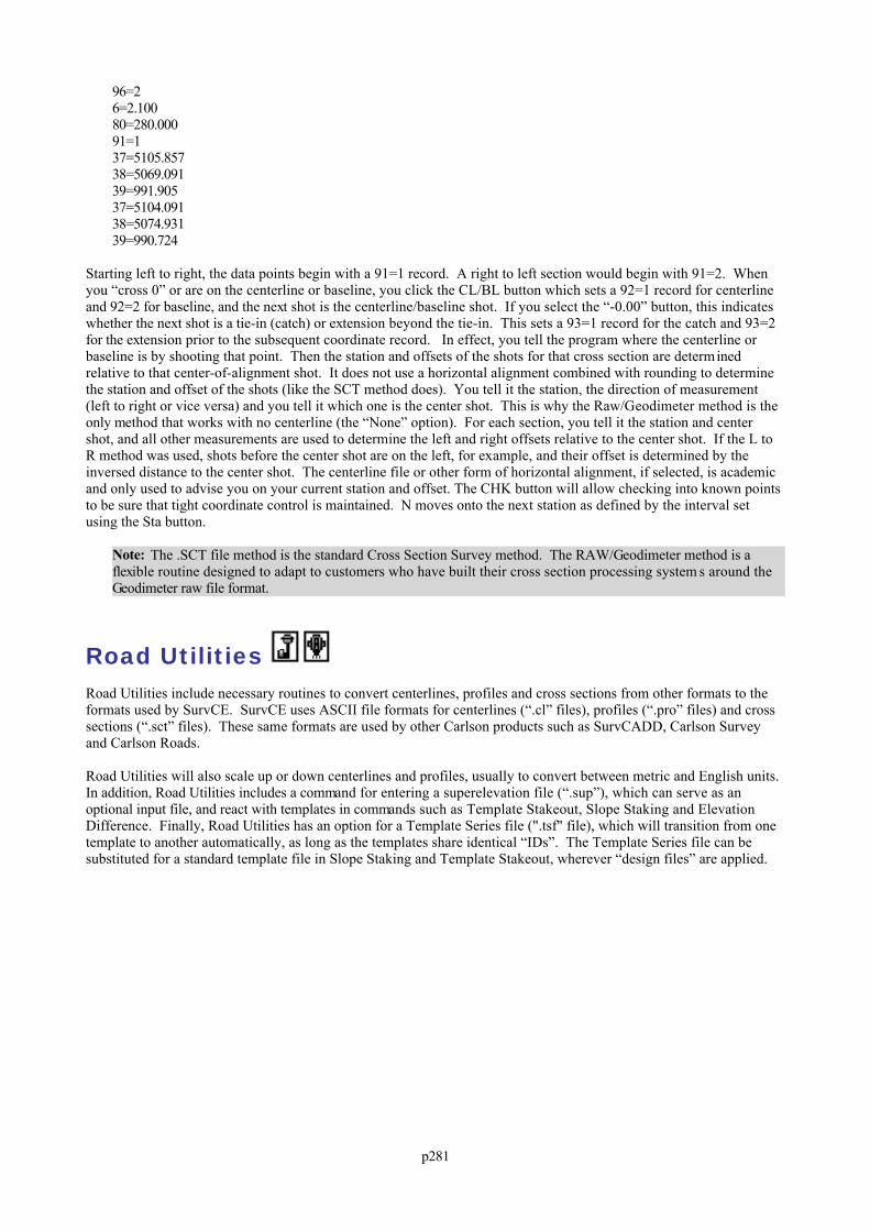
p281

96=26=2.10080=280.00091=137=5105.85738=5069.09139=991.90537=5104.09138=5074.93139=990.724

Starting left to right, the data points begin with a 91=1 record. A right to left section would begin with 91=2. Whenyou “cross 0” or are on the centerline or baseline, you click the CL/BL button which sets a 92=1 record for centerlineand 92=2 for baseline, and the next shot is the centerline/baseline shot. If you select the “-0.00” button, this indicateswhether the next shot is a tie-in (catch) or extension beyond the tie-in. This sets a 93=1 record for the catch and 93=2for the extension prior to the subsequent coordinate record. In effect, you tell the program where the centerline orbaseline is by shooting that point. Then the station and offsets of the shots for that cross section are determinedrelative to that center-of-alignment shot. It does not use a horizontal alignment combined with rounding to determinethe station and offset of the shots (like the SCT method does). You tell it the station, the direction of measurement(left to right or vice versa) and you tell it which one is the center shot. This is why the Raw/Geodimeter method is theonly method that works with no centerline (the “None” option). For each section, you tell it the station and centershot, and all other measurements are used to determine the left and right offsets relative to the center shot. If the L toR method was used, shots before the center shot are on the left, for example, and their offset is determined by theinversed distance to the center shot. The centerline file or other form of horizontal alignment, if selected, is academicand only used to advise you on your current station and offset. The CHK button will allow checking into known pointsto be sure that tight coordinate control is maintained. N moves onto the next station as defined by the interval setusing the Sta button.

Note: The .SCT file method is the standard Cross Section Survey method. The RAW/Geodimeter method is aflexible routine designed to adapt to customers who have built their cross section processing system s around theGeodimeter raw file format.

Road Utilities Road Utilities include necessary routines to convert centerlines, profiles and cross sections from other formats to theformats used by SurvCE. SurvCE uses ASCII file formats for centerlines (“.cl” files), profiles (“.pro” files) and crosssections (“.sct” files). These same formats are used by other Carlson products such as SurvCADD, Carlson Surveyand Carlson Roads.

Road Utilities will also scale up or down centerlines and profiles, usually to convert between metric and English units. In addition, Road Utilities includes a command for entering a superelevation file (“.sup”), which can serve as anoptional input file, and react with templates in commands such as Template Stakeout, Slope Staking and ElevationDifference. Finally, Road Utilities has an option for a Template Series file (".tsf" file), which will transition from onetemplate to another automatically, as long as the templates share identical “IDs”. The Template Series file can besubstituted for a standard template file in Slope Staking and Template Stakeout, wherever “design files” are applied.

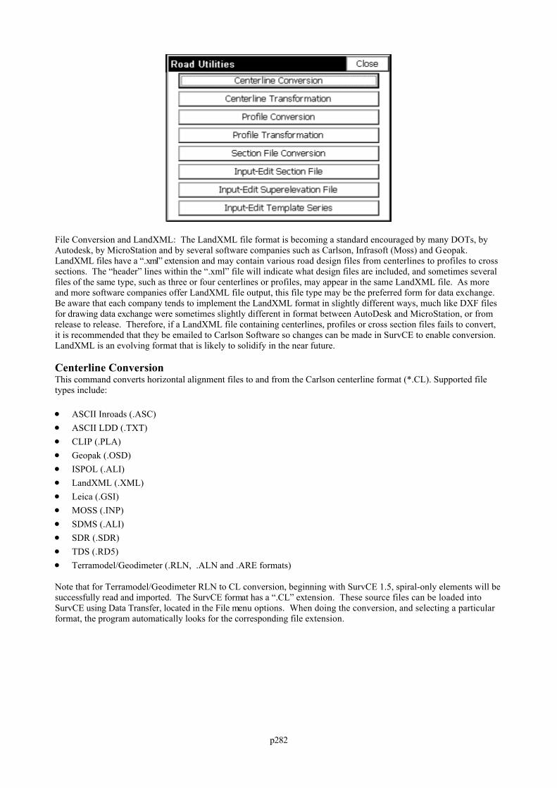
p282

File Conversion and LandXML: The LandXML file format is becoming a standard encouraged by many DOTs, byAutodesk, by MicroStation and by several software companies such as Carlson, Infrasoft (Moss) and Geopak. LandXML files have a “.xml” extension and may contain various road design files from centerlines to profiles to crosssections. The “header” lines within the “.xml” file will indicate what design files are included, and sometimes severalfiles of the same type, such as three or four centerlines or profiles, may appear in the same LandXML file. As moreand more software companies offer LandXML file output, this file type may be the preferred form for data exchange. Be aware that each company tends to implement the LandXML format in slightly different ways, much like DXF filesfor drawing data exchange were sometimes slightly different in format between AutoDesk and MicroStation, or fromrelease to release. Therefore, if a LandXML file containing centerlines, profiles or cross section files fails to convert,it is recommended that they be emailed to Carlson Software so changes can be made in SurvCE to enable conversion. LandXML is an evolving format that is likely to solidify in the near future.

Centerline ConversionThis command converts horizontal alignment files to and from the Carlson centerline format (*.CL). Supported filetypes include:

ASCII Inroads (.ASC) ASCII LDD (.TXT) CLIP (.PLA) Geopak (.OSD) ISPOL (.ALI) LandXML (.XML) Leica (.GSI) MOSS (.INP) SDMS (.ALI) SDR (.SDR) TDS (.RD5) Terramodel/Geodimeter (.RLN, .ALN and .ARE formats)

Note that for Terramodel/Geodimeter RLN to CL conversion, beginning with SurvCE 1.5, spiral-only elements will besuccessfully read and imported. The SurvCE format has a “.CL” extension. These source files can be loaded intoSurvCE using Data Transfer, located in the File menu options. When doing the conversion, and selecting a particularformat, the program automatically looks for the corresponding file extension.

p283

Clicking “Existing” in the upper right will load the file and clicking “Select New .CL” will save the centerline file inthe correct format for use in SurvCE. Reversing the direction, clicking “Select Existing .CL” would recall a SurvCEcenterline file, and then clicking “New” in the upper left would save it back to a converted file, for use in othersoftware.

For file types where both Import and Export options are available, the conversion procedure forms a “criss-cross”:You bring the files into SurvCE by going upper right (“Existing”) to lower left (“Select New”). You send the filesback to the “non-SurvCE” format by going lower right (“Select Existing”) to upper left “New” as shown in the nex tfigure.

When the files have been selected, the appropriate action is highlighted below. When the process is completed, theprogram announces “Process Done,” and you are free to move on to the next command. Most formats only convert toSurvCE and not back again, and therefore only have “one-way” dialogs. These include ASCII-Inroads, ASCII-LDD,Geopak, Moss, TDS and Terramodel/Geodimeter. When only 1-way conversion (to SurvCE) is available.

If the SDR format is selected, the dialog automatically changes.

p284

When the process is completed, the program announces “Process Done,” and you are free to move on to the nextcommand. Most formats only convert to SurvCE and not back again, and therefore only have “one-way” dialogs. These include ASCII-Inroads, ASCII-LDD, Geopak, Moss, TDS and Terramodel/Geodimeter. When only 1-wayconversion (to SurvCE) is available, the dialog appears as shown in this figure.

Importing TDS RD5 FilesImporting TDS RD5 Files: If TDS is selected, centerlines can be converted “1-way” to SurvCE centerlines. It isimportant to note that the TDS RD5 file is a dual centerline and profile file. Because the TDS RD5 file does notdisplay the starting station, an extra dialog will appear requesting starting coordinates and a starting station.

Verify the ConversionIt is recommended that after converting centerlines, profiles or cross section files to SurvCE format, that you go to theInput-Edit options for these file types, and review the data to verify that the correct file was converted and that theconversion was successful. So, for example, after converting a centerline from, say, Inroads format to SurvCE “.cl”format, go directly to Input-Edit Centerline in the Roads menu and verify that data.

Recognizing File FormatsFor reference, portions of four of the file types are shown below, as they might display in a Text Editor. TheLandXML, SurvCE and SDR examples all reference the file DOT1.CL. These displays may help you recognize thesefile types in the future. The new LandXML format, endorsed by many Departments of Transportation in the UnitedStates, may soon become the standard in the future for internet transfer of roading and other types of design files.

p285

Centerline TransformationThis routine is designed primarily to convert centerline data from Metric to Survey Feet or from Survey Feet to Metric.Here is the dialog, and scale factor, when converting from Metric to Survey Feet.

p286

Apply scale factor for start station: If this option is clicked on, as shown, then a starting station of 1000, for example,would become a start station of 3280.833. If clicked off, the start station would remain at 1000. If the goal is tochange the starting station by a certain amount unrelated to the scale factor, then you must use Input-Edit Centerlineand enter a new start station in the initial dialog. This will automatically translate all stations in the centerline by theappropriate amount.

When “Apply Scale Factor” is selected, the centerline is adjusted by the scale factor, after a confirming “warning”screen.

Profile ConversionThis command converts vertical alignments to and from the Carlson profile format (*.PRO). Supported file typesinclude: ASCII-LDD (.TXT) Caice (.KCP) CLIP (.ALZ) ISPOL (.RAS) LandXML (.XML) Leica (.GSI) MOSS (.INP) SDR (.SDR) TDS (.RD5) Terramodel/Geodimeter (.RLN, .ALN and .ARE)

The SurvCE format has a .PRO extension. These source files can be loaded into SurvCE using Data Transfer, locatedin the File menu options. The conversion screen is similar to Centerline Conversion, with the characteristic“criss-cross” logic for 2-way conversion (LandXML and Leica) and one-way conversion for the other options.

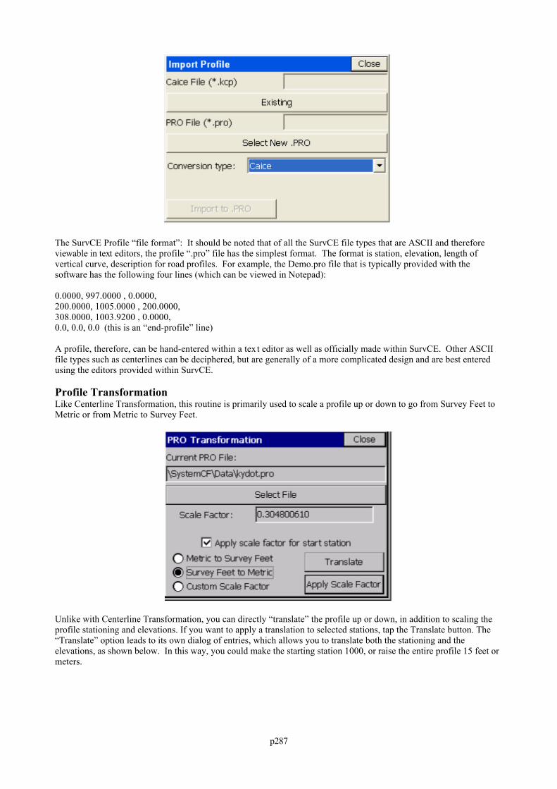
p287

The SurvCE Profile “file format”: It should be noted that of all the SurvCE file types that are ASCII and thereforeviewable in text editors, the profile “.pro” file has the simplest format. The format is station, elevation, length ofvertical curve, description for road profiles. For example, the Demo.pro file that is typically provided with thesoftware has the following four lines (which can be viewed in Notepad):

0.0000, 997.0000 , 0.0000, 200.0000, 1005.0000 , 200.0000, 308.0000, 1003.9200 , 0.0000, 0.0, 0.0, 0.0 (this is an “end-profile” line)

A profile, therefore, can be hand-entered within a tex t editor as well as officially made within SurvCE. Other ASCIIfile types such as centerlines can be deciphered, but are generally of a more complicated design and are best enteredusing the editors provided within SurvCE.

Profile TransformationLike Centerline Transformation, this routine is primarily used to scale a profile up or down to go from Survey Feet toMetric or from Metric to Survey Feet.

Unlike with Centerline Transformation, you can directly “translate” the profile up or down, in addition to scaling theprofile stationing and elevations. If you want to apply a translation to selected stations, tap the Translate button. The“Translate” option leads to its own dialog of entries, which allows you to translate both the stationing and theelevations, as shown below. In this way, you could make the starting station 1000, or raise the entire profile 15 feet ormeters.

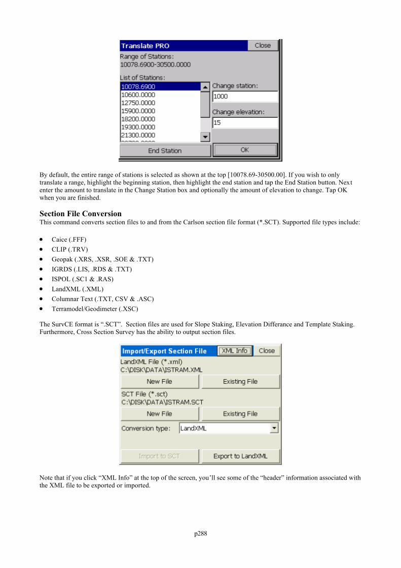
p288

By default, the entire range of stations is selected as shown at the top [10078.69-30500.00]. If you wish to onlytranslate a range, highlight the beginning station, then highlight the end station and tap the End Station button. Nextenter the amount to translate in the Change Station box and optionally the amount of elevation to change. Tap OKwhen you are finished.

Section File ConversionThis command converts section files to and from the Carlson section file format (*.SCT). Supported file types include: Caice (.FFF) CLIP (.TRV) Geopak (.XRS, .XSR, .SOE & .TXT) IGRDS (.LIS, .RDS & .TXT) ISPOL (.SC1 & .RAS) LandXML (.XML) Columnar Text (.TXT, CSV & .ASC) Terramodel/Geodimeter (.XSC)

The SurvCE format is “.SCT”. Section files are used for Slope Staking, Elevation Differance and Template Staking. Furthermore, Cross Section Survey has the ability to output section files.

Note that if you click “XML Info” at the top of the screen, you’ll see some of the “header” information associated withthe XML file to be exported or imported.

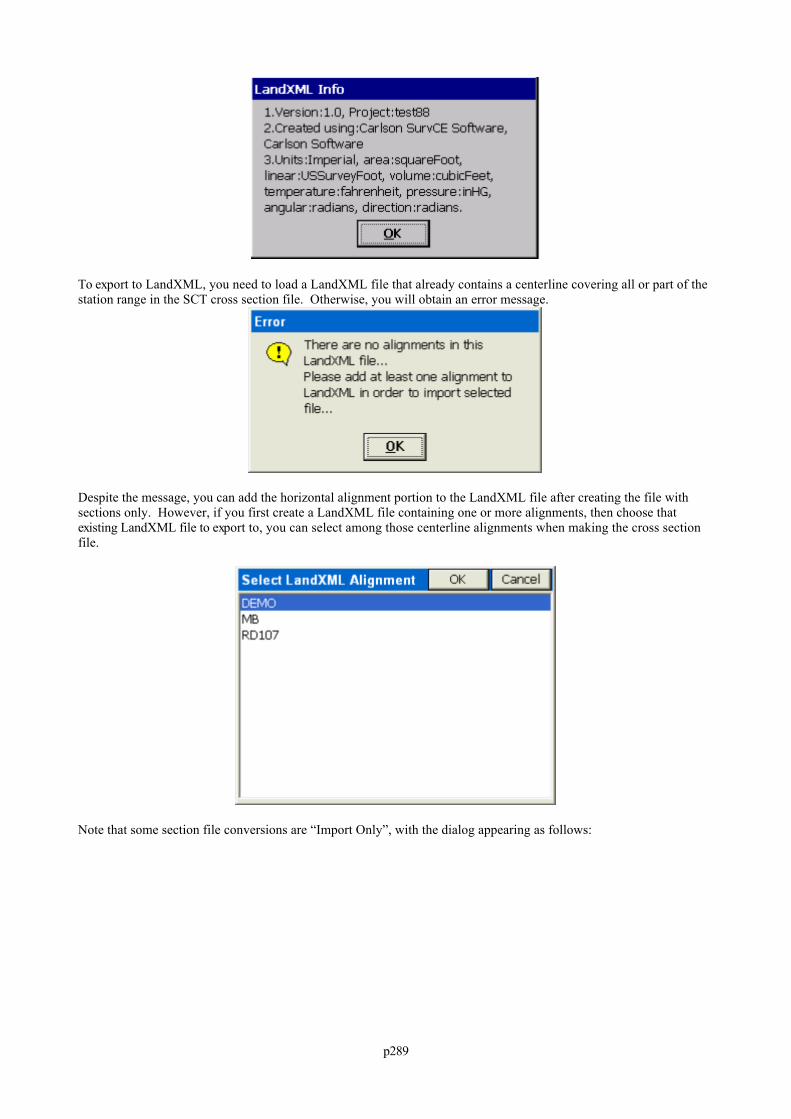
p289

To export to LandXML, you need to load a LandXML file that already contains a centerline covering all or part of thestation range in the SCT cross section file. Otherwise, you will obtain an error message.

Despite the message, you can add the horizontal alignment portion to the LandXML file after creating the file withsections only. However, if you first create a LandXML file containing one or more alignments, then choose thatexisting LandXML file to export to, you can select among those centerline alignments when making the cross sectionfile.

Note that some section file conversions are “Import Only”, with the dialog appearing as follows:

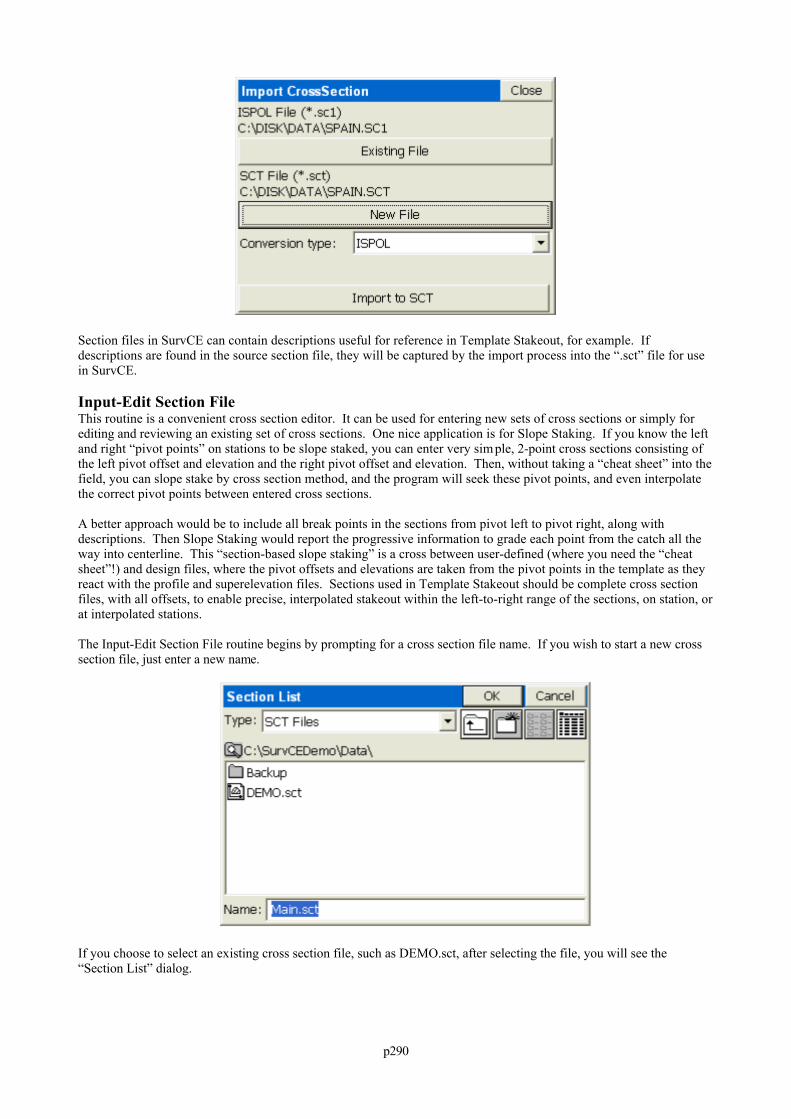
p290

Section files in SurvCE can contain descriptions useful for reference in Template Stakeout, for example. Ifdescriptions are found in the source section file, they will be captured by the import process into the “.sct” file for usein SurvCE.

Input-Edit Section FileThis routine is a convenient cross section editor. It can be used for entering new sets of cross sections or simply forediting and reviewing an existing set of cross sections. One nice application is for Slope Staking. If you know the leftand right “pivot points” on stations to be slope staked, you can enter very sim ple, 2-point cross sections consisting ofthe left pivot offset and elevation and the right pivot offset and elevation. Then, without taking a “cheat sheet” into thefield, you can slope stake by cross section method, and the program will seek these pivot points, and even interpolatethe correct pivot points between entered cross sections.

A better approach would be to include all break points in the sections from pivot left to pivot right, along withdescriptions. Then Slope Staking would report the progressive information to grade each point from the catch all theway into centerline. This “section-based slope staking” is a cross between user-defined (where you need the “cheatsheet”!) and design files, where the pivot offsets and elevations are taken from the pivot points in the template as theyreact with the profile and superelevation files. Sections used in Template Stakeout should be complete cross sectionfiles, with all offsets, to enable precise, interpolated stakeout within the left-to-right range of the sections, on station, orat interpolated stations.

The Input-Edit Section File routine begins by prompting for a cross section file name. If you wish to start a new crosssection file, just enter a new name.

If you choose to select an existing cross section file, such as DEMO.sct, after selecting the file, you will see the“Section List” dialog.

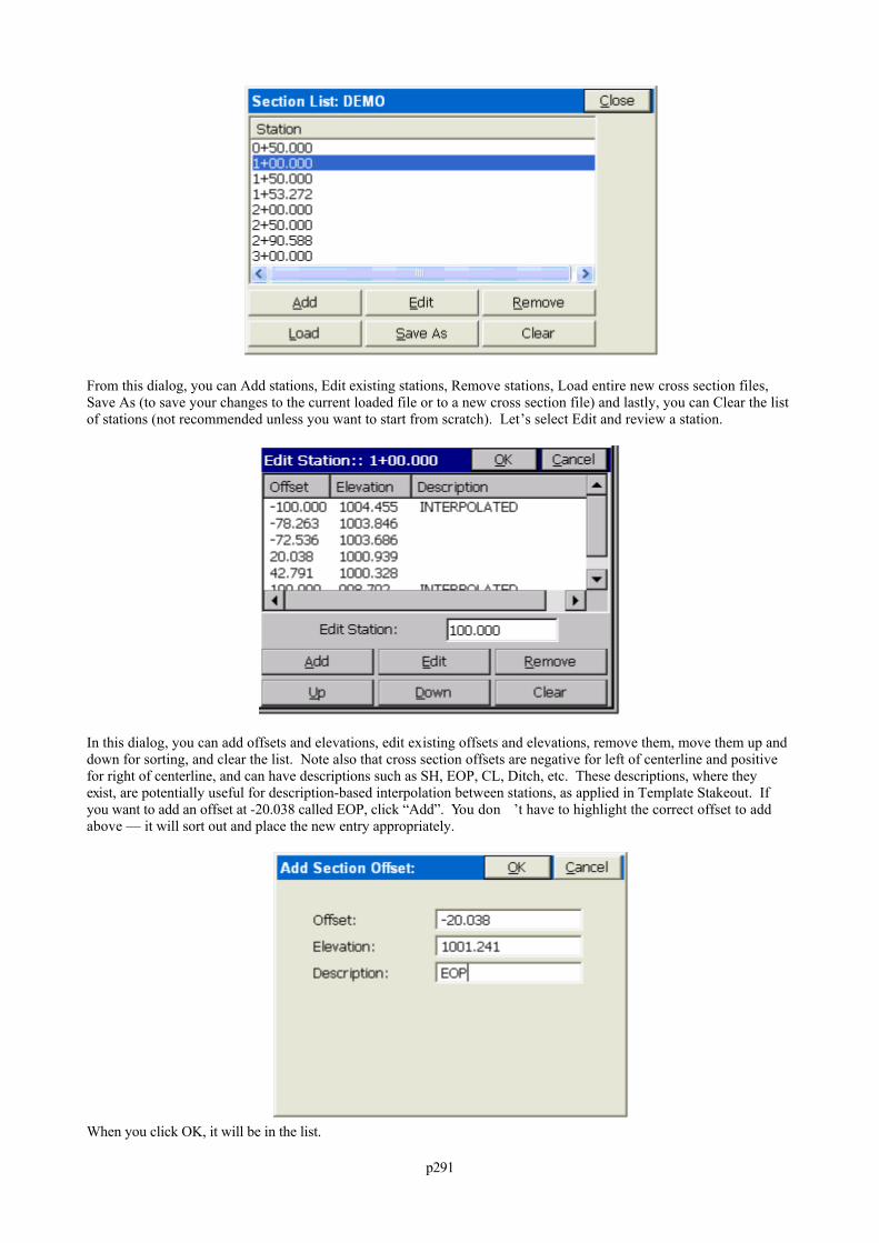
p291

From this dialog, you can Add stations, Edit existing stations, Remove stations, Load entire new cross section files,Save As (to save your changes to the current loaded file or to a new cross section file) and lastly, you can Clear the listof stations (not recommended unless you want to start from scratch). Let’s select Edit and review a station.

In this dialog, you can add offsets and elevations, edit existing offsets and elevations, remove them, move them up anddown for sorting, and clear the list. Note also that cross section offsets are negative for left of centerline and positivefor right of centerline, and can have descriptions such as SH, EOP, CL, Ditch, etc. These descriptions, where theyexist, are potentially useful for description-based interpolation between stations, as applied in Template Stakeout. Ifyou want to add an offset at -20.038 called EOP, click “Add”. You don ’t have to highlight the correct offset to addabove — it will sort out and place the new entry appropriately.

When you click OK, it will be in the list.

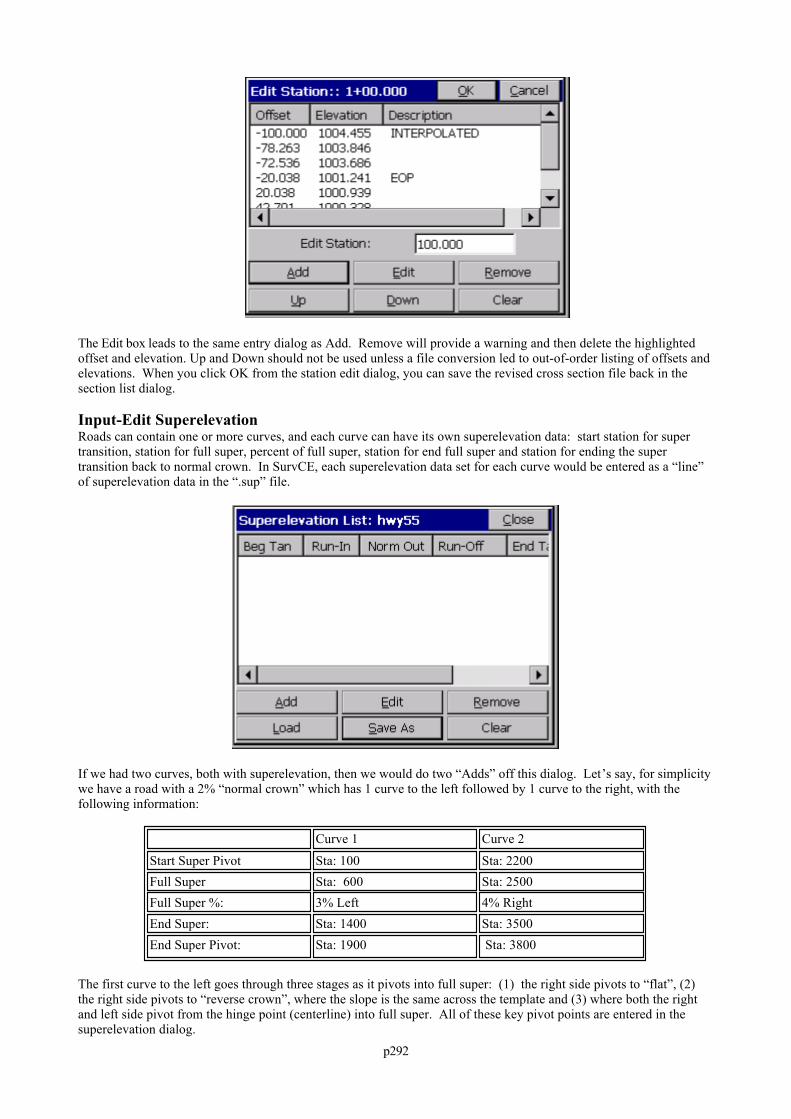
p292

The Edit box leads to the same entry dialog as Add. Remove will provide a warning and then delete the highlightedoffset and elevation. Up and Down should not be used unless a file conversion led to out-of-order listing of offsets andelevations. When you click OK from the station edit dialog, you can save the revised cross section file back in thesection list dialog.

Input-Edit SuperelevationRoads can contain one or more curves, and each curve can have its own superelevation data: start station for supertransition, station for full super, percent of full super, station for end full super and station for ending the supertransition back to normal crown. In SurvCE, each superelevation data set for each curve would be entered as a “line”of superelevation data in the “.sup” file.

If we had two curves, both with superelevation, then we would do two “Adds” off this dialog. Let’s say, for simplicitywe have a road with a 2% “normal crown” which has 1 curve to the left followed by 1 curve to the right, with thefollowing information:

Curve 1 Curve 2

Start Super Pivot Sta: 100 Sta: 2200Full Super Sta: 600 Sta: 2500Full Super %: 3% Left 4% RightEnd Super: Sta: 1400 Sta: 3500End Super Pivot: Sta: 1900 Sta: 3800

The first curve to the left goes through three stages as it pivots into full super: (1) the right side pivots to “flat”, (2)the right side pivots to “reverse crown”, where the slope is the same across the template and (3) where both the rightand left side pivot from the hinge point (centerline) into full super. All of these key pivot points are entered in thesuperelevation dialog.

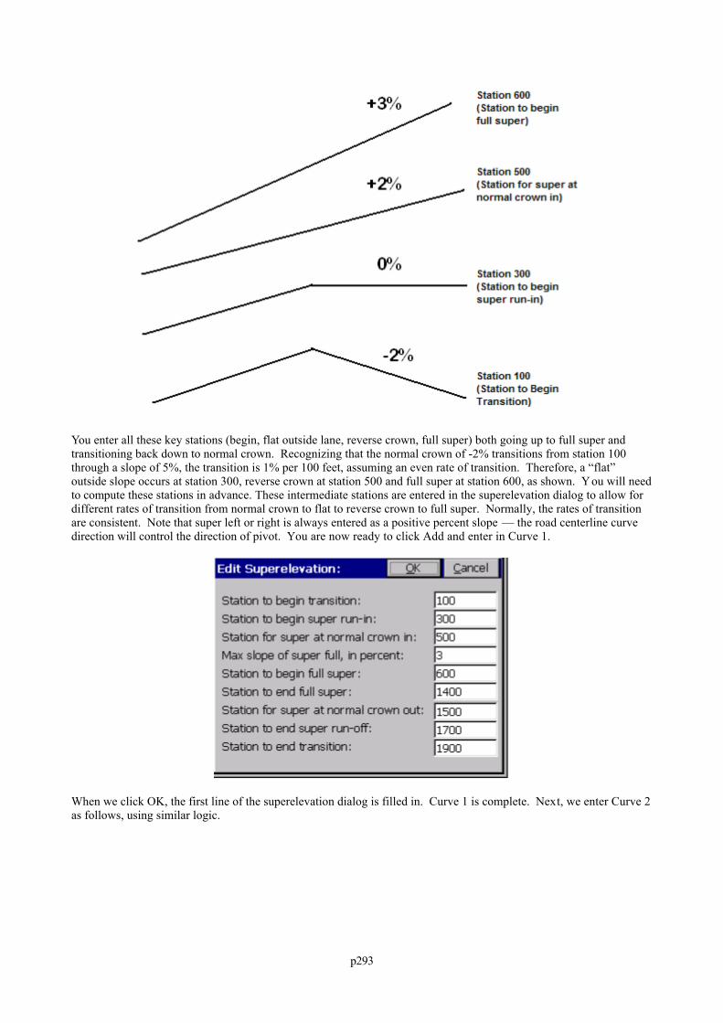
p293

You enter all these key stations (begin, flat outside lane, reverse crown, full super) both going up to full super andtransitioning back down to normal crown. Recognizing that the normal crown of -2% transitions from station 100through a slope of 5%, the transition is 1% per 100 feet, assuming an even rate of transition. Therefore, a “flat”outside slope occurs at station 300, reverse crown at station 500 and full super at station 600, as shown. You will needto compute these stations in advance. These intermediate stations are entered in the superelevation dialog to allow fordifferent rates of transition from normal crown to flat to reverse crown to full super. Normally, the rates of transitionare consistent. Note that super left or right is always entered as a positive percent slope — the road centerline curvedirection will control the direction of pivot. You are now ready to click Add and enter in Curve 1.

When we click OK, the first line of the superelevation dialog is filled in. Curve 1 is complete. Next, we enter Curve 2as follows, using similar logic.

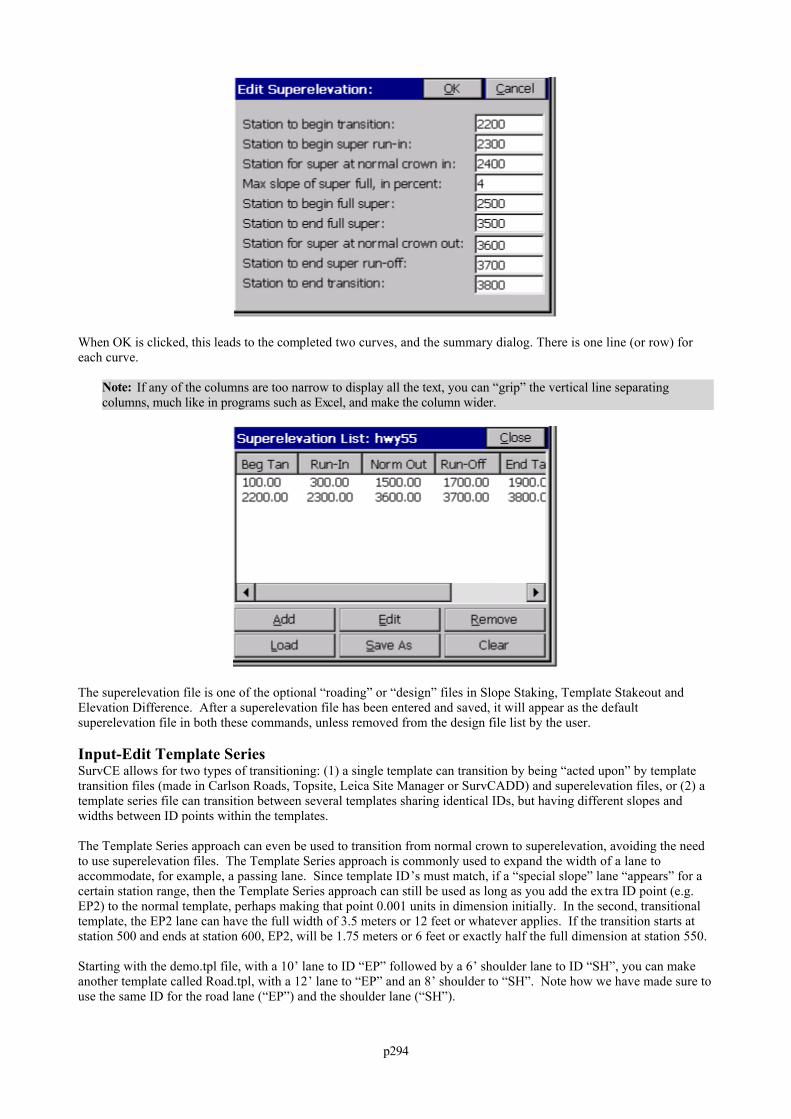
p294

When OK is clicked, this leads to the completed two curves, and the summary dialog. There is one line (or row) foreach curve.

Note: If any of the columns are too narrow to display all the text, you can “grip” the vertical line separatingcolumns, much like in programs such as Excel, and make the column wider.

The superelevation file is one of the optional “roading” or “design” files in Slope Staking, Template Stakeout andElevation Difference. After a superelevation file has been entered and saved, it will appear as the defaultsuperelevation file in both these commands, unless removed from the design file list by the user.

Input-Edit Template SeriesSurvCE allows for two types of transitioning: (1) a single template can transition by being “acted upon” by templatetransition files (made in Carlson Roads, Topsite, Leica Site Manager or SurvCADD) and superelevation files, or (2) atemplate series file can transition between several templates sharing identical IDs, but having different slopes andwidths between ID points within the templates.

The Template Series approach can even be used to transition from normal crown to superelevation, avoiding the needto use superelevation files. The Template Series approach is commonly used to expand the width of a lane toaccommodate, for example, a passing lane. Since template ID’s must match, if a “special slope” lane “appears” for acertain station range, then the Template Series approach can still be used as long as you add the extra ID point (e.g.EP2) to the normal template, perhaps making that point 0.001 units in dimension initially. In the second, transitionaltemplate, the EP2 lane can have the full width of 3.5 meters or 12 feet or whatever applies. If the transition starts atstation 500 and ends at station 600, EP2, will be 1.75 meters or 6 feet or exactly half the full dimension at station 550.

Starting with the demo.tpl file, with a 10’ lane to ID “EP” followed by a 6’ shoulder lane to ID “SH”, you can makeanother template called Road.tpl, with a 12’ lane to “EP” and an 8’ shoulder to “SH”. Note how we have made sure touse the same ID for the road lane (“EP”) and the shoulder lane (“SH”).

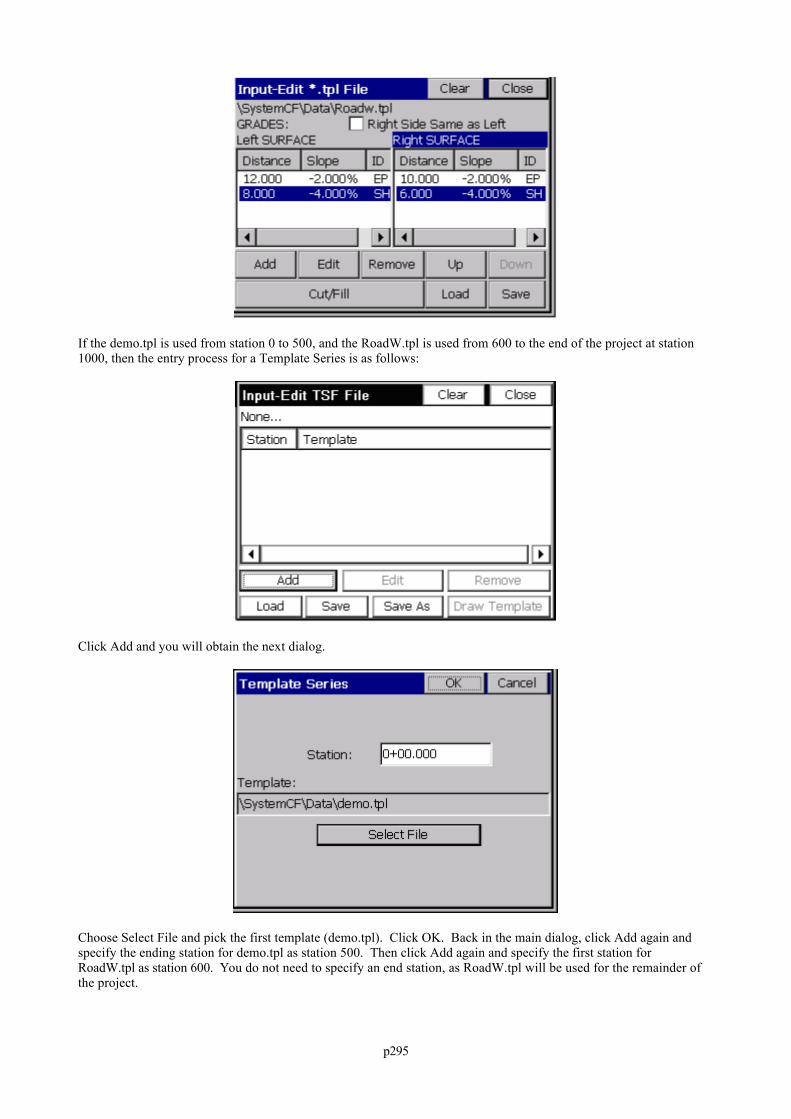
p295

If the demo.tpl is used from station 0 to 500, and the RoadW.tpl is used from 600 to the end of the project at station1000, then the entry process for a Template Series is as follows:

Click Add and you will obtain the next dialog.

Choose Select File and pick the first template (demo.tpl). Click OK. Back in the main dialog, click Add again andspecify the ending station for demo.tpl as station 500. Then click Add again and specify the first station forRoadW.tpl as station 600. You do not need to specify an end station, as RoadW.tpl will be used for the remainder ofthe project.

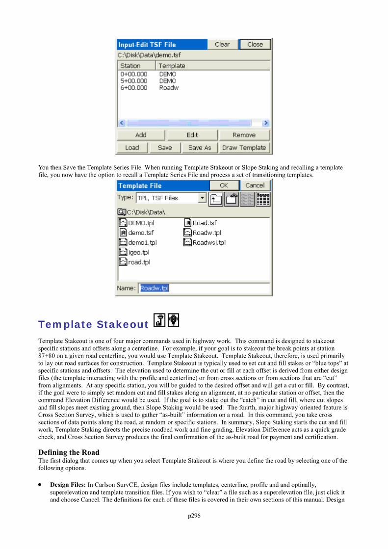
p296

You then Save the Template Series File. When running Template Stakeout or Slope Staking and recalling a templatefile, you now have the option to recall a Template Series File and process a set of transitioning templates.

Template Stakeout Template Stakeout is one of four major commands used in highway work. This command is designed to stakeoutspecific stations and offsets along a centerline. For example, if your goal is to stakeout the break points at station87+80 on a given road centerline, you would use Template Stakeout. Template Stakeout, therefore, is used primarilyto lay out road surfaces for construction. Template Stakeout is typically used to set cut and fill stakes or “blue tops” atspecific stations and offsets. The elevation used to determine the cut or fill at each offset is derived from either designfiles (the template interacting with the profile and centerline) or from cross sections or from sections that are “cut”from alignments. At any specific station, you will be guided to the desired offset and will get a cut or fill. By contrast,if the goal were to simply set random cut and fill stakes along an alignment, at no particular station or offset, then thecommand Elevation Difference would be used. If the goal is to stake out the “catch” in cut and fill, where cut slopesand fill slopes meet existing ground, then Slope Staking would be used. The fourth, major highway-oriented feature isCross Section Survey, which is used to gather “as-built” information on a road. In this command, you take crosssections of data points along the road, at random or specific stations. In summary, Slope Staking starts the cut and fillwork, Template Staking directs the precise roadbed work and fine grading, Elevation Difference acts as a quick gradecheck, and Cross Section Survey produces the final confirmation of the as-built road for payment and certification.

Defining the RoadThe first dialog that comes up when you select Template Stakeout is where you define the road by selecting one of thefollowing options.

Design Files: In Carlson SurvCE, design files include templates, centerline, profile and and optinally,superelevation and template transition files. If you wish to “clear” a file such as a superelevation file, just click itand choose Cancel. The definitions for each of these files is covered in their own sections of this manual. Design

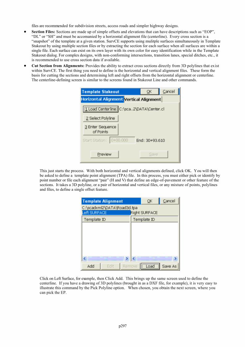
p297

files are recommended for subdivision streets, access roads and simpler highway designs. Section Files: Sections are made up of simple offsets and elevations that can have descriptions such as “EOP”,

“DL” or “SH” and must be accomanied by a horizontal alignment file (centerline). Every cross section is a“snapshot” of the template at a given station. SurvCE supports using mulitple surfaces simultaneously in TemplateStakeout by using multiple section files or by extracting the section for each surface when all surfaces are within asingle file. Each surface can exist on its own layer with its own color for easy identification while in the TemplateStakeout dialog. For complex designs, with non-conforming intersections, transition lanes, special ditches, etc., itis recommended to use cross section data if available.

Cut Section from Alignments: Provides the ability to extract cross sections directly from 3D polylines that existwithin SurvCE. The first thing you need to define is the horizontal and vertical alignment files. These form thebasis for cutting the sections and determining left and right offsets from the horizontal alignment or centerline. The centerline-defining screen is similar to the screens found in Stakeout Line and other commands.

This just starts the process. With both horizontal and vertical alignments defined, click OK. You will thenbe asked to define a template point alignment (TPA) file. In this process, you must either pick or identify bypoint number or file each alignment “pair” (H and V) that define an edge-of-pavement or other feature of thesections. It takes a 3D polyline, or a pair of horizontal and vertical files, or any mixture of points, polylinesand files, to define a single offset feature.

Click on Left Surface, for example, then Click Add. This brings up the same screen used to define thecenterline. If you have a drawing of 3D polylines (brought in as a DXF file, for example), it is very easy toillustrate this command by the Pick Polyline option. When chosen, you obtain the next screen, where youcan pick the EP.

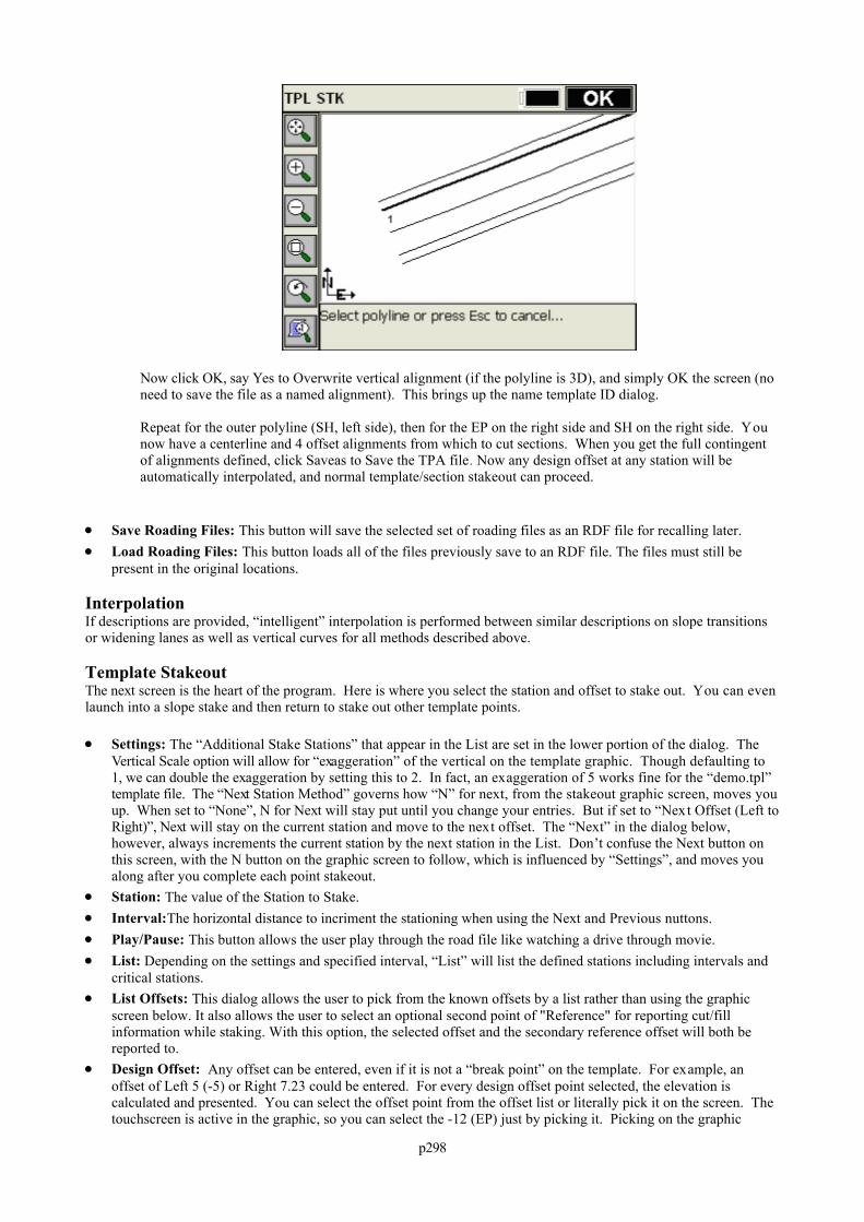
p298

Now click OK, say Yes to Overwrite vertical alignment (if the polyline is 3D), and simply OK the screen (noneed to save the file as a named alignment). This brings up the name template ID dialog.

Repeat for the outer polyline (SH, left side), then for the EP on the right side and SH on the right side. Younow have a centerline and 4 offset alignments from which to cut sections. When you get the full contingentof alignments defined, click Saveas to Save the TPA file. Now any design offset at any station will beautomatically interpolated, and normal template/section stakeout can proceed.

Save Roading Files: This button will save the selected set of roading files as an RDF file for recalling later. Load Roading Files: This button loads all of the files previously save to an RDF file. The files must still be

present in the original locations.

InterpolationIf descriptions are provided, “intelligent” interpolation is performed between similar descriptions on slope transitionsor widening lanes as well as vertical curves for all methods described above.

Template StakeoutThe next screen is the heart of the program. Here is where you select the station and offset to stake out. You can evenlaunch into a slope stake and then return to stake out other template points.

Settings: The “Additional Stake Stations” that appear in the List are set in the lower portion of the dialog. TheVertical Scale option will allow for “exaggeration” of the vertical on the template graphic. Though defaulting to1, we can double the exaggeration by setting this to 2. In fact, an exaggeration of 5 works fine for the “demo.tpl”template file. The “Next Station Method” governs how “N” for next, from the stakeout graphic screen, moves youup. When set to “None”, N for Next will stay put until you change your entries. But if set to “Next Offset (Left toRight)”, Next will stay on the current station and move to the next offset. The “Next” in the dialog below,however, always increments the current station by the next station in the List. Don’t confuse the Next button onthis screen, with the N button on the graphic screen to follow, which is influenced by “Settings”, and moves youalong after you complete each point stakeout.

Station: The value of the Station to Stake. Interval:The horizontal distance to incriment the stationing when using the Next and Previous nuttons. Play/Pause: This button allows the user play through the road file like watching a drive through movie. List: Depending on the settings and specified interval, “List” will list the defined stations including intervals and

critical stations. List Offsets: This dialog allows the user to pick from the known offsets by a list rather than using the graphic

screen below. It also allows the user to select an optional second point of "Reference" for reporting cut/fillinformation while staking. With this option, the selected offset and the secondary reference offset will both bereported to.

Design Offset: Any offset can be entered, even if it is not a “break point” on the template. For example, anoffset of Left 5 (-5) or Right 7.23 could be entered. For every design offset point selected, the elevation iscalculated and presented. You can select the offset point from the offset list or literally pick it on the screen. Thetouchscreen is active in the graphic, so you can select the -12 (EP) just by picking it. Picking on the graphic

p299

screen will take you to the “Offset List” screen for verification, where you can confirm your pick by pressingEnter or selecting another offset.

Stk Off(H): Horizontal offset from the design offset. If you enter an stake offset of 2 and the design offset pointwas at 12, then the stake would go in at offset 14 off of CL, but the cut/fill would refer to the elevation at thedesign offset location of 12. The stake offset and Off. to CL inter-react. A stake offset entry of 15 with a designoffset of 12 left calculates to a setback of 3.

[...] Button: This button allows the user to specify the horizontal and verical offsets relative to the design offset.Various methods can be used for computing the offsets based on the template or section points and theirelevations.

Off to CL: This is the total distance that the stakeout position is from the defined road centerline. Vert. Off (V): Vertical offset from the design elevation. Elevation: Elevation to be staked. This value is based on the combined design elevation and vertical offset. Run Slope Stake: This feature allows for dynamic slope staking in the middle of the Template Stakeout routine.

This option is very useful for road staging, and also for staking interior catch points like central median ditches. When the slope stake is completed, the program returns to the main Template Stakeout dialog. Any point in thetemplate or section can be used for running in a slope stake. You are asked to specify the desired cut and fill sloperatios. The slope can be auto-defined or user defined as follows:

Define Slope by Next Section Point: This option allows you to select the edge of the road and use theproposed design catch point for auto-dermining the slope rate.

Define Slope by Previous Section Point: This option allows you to select the proposed design catch pointand then use the next point towards CL for auto-dermining the slope rate.

Extend Current Slope: This option will allow you to pick the edge of the road or catch point and use thenext point towards CL to end the slope between then away from CL.

User Defined Slope: Allow you to enter the slope ratio by hand for on-the-fly slope changes.

Slopes by Template: This option extracts the slope definitions from the template file itself.

Pivot Point: This option allows the user perform on-the-fly offsets releative to the stakeout position defined in thefrom end of the routine.

Stakeout ViewsTemplate Stakeout now allows you to navigate to the point in either plan view or cross section view. Select theX-SCT/PLAN icon to switch back and forth.

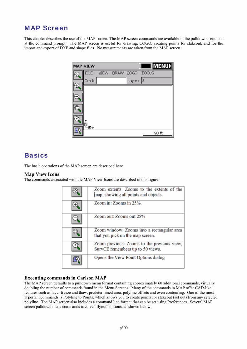
p300

MAP ScreenThis chapter describes the use of the MAP screen. The MAP screen commands are available in the pulldown menus orat the command prompt. The MAP screen is useful for drawing, COGO, creating points for stakeout, and for theimport and export of DXF and shape files. No measurements are taken from the MAP screen.

BasicsThe basic operations of the MAP screen are described here.

Map View IconsThe commands associated with the MAP View Icons are described in this figure:

Executing commands in Carlson MAPThe MAP screen defaults to a pulldown menu format containing approximately 60 additional commands, virtuallydoubling the number of commands found in the Menu Screens. Many of the commands in MAP offer CAD-likefeatures such as layer freeze and thaw, predetermined area, polyline offsets and even contouring. One of the mostimportant commands is Polyline to Points, which allows you to create points for stakeout (set out) from any selectedpolyline. The MAP screen also includes a command line format that can be set using Preferences. Several MAPscreen pulldown menu commands involve “flyout” options, as shown below.

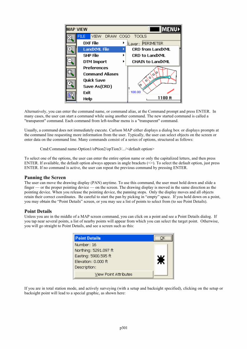
p301

Alternatively, you can enter the command name, or command alias, at the Command prompt and press ENTER. Inmany cases, the user can start a command while using another command. The new started command is called a"transparent" command. Each command from left-toolbar menu is a "transparent" command.

Usually, a command does not immediately execute. Carlson MAP either displays a dialog box or displays prompts atthe command line requesting more information from the user. Typically, the user can select objects on the screen orenter data on the command line. Many commands consist of a series of options, structured as follows:

Cmd:Command name-Option1/oPtion2/opTion3/.../<default option>

To select one of the options, the user can enter the entire option name or only the capitalized letters, and then pressENTER. If available, the default option always appears in angle brackets (<>). To select the default option, just pressENTER. If no command is active, the user can repeat the previous command by pressing ENTER.

Panning the ScreenThe user can move the drawing display (PAN) anytime. To use this command, the user must hold down and slide afinger — or the proper pointing device — on the screen. The drawing display is moved in the same direction as thepointing device. When you release the pointing device, the panning stops. Only the display moves and all objectsretain their correct coordinates. Be careful to start the pan by picking in “empty” space. If you hold down on a point,you may obtain the “Point Details” screen, or you may see a list of points to select from (to see Point Details).

Point DetailsUnless you are in the middle of a MAP screen command, you can click on a point and see a Point Details dialog. Ifyou tap near several points, a list of nearby points will appear from which you can select the target point. Otherwise,you will go straight to Point Details, and see a screen such as this:

If you are in total station mode, and actively surveying (with a setup and backsight specified), clicking on the setup orbacksight point will lead to a special graphic, as shown here:

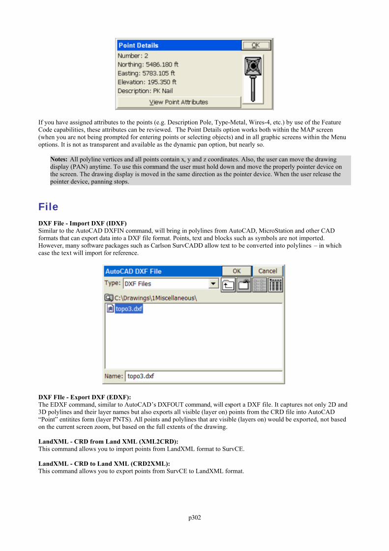
p302

If you have assigned attributes to the points (e.g. Description Pole, Type-Metal, Wires-4, etc.) by use of the FeatureCode capabilities, these attributes can be reviewed. The Point Details option works both within the MAP screen(when you are not being prompted for entering points or selecting objects) and in all graphic screens within the Menuoptions. It is not as transparent and available as the dynamic pan option, but nearly so.

Notes: All polyline vertices and all points contain x, y and z coordinates. Also, the user can move the drawingdisplay (PAN) anytime. To use this command the user must hold down and move the properly pointer device onthe screen. The drawing display is moved in the same direction as the pointer device. When the user release thepointer device, panning stops.

FileDXF File - Import DXF (IDXF)Similar to the AutoCAD DXFIN command, will bring in polylines from AutoCAD, MicroStation and other CADformats that can export data into a DXF file format. Points, text and blocks such as symbols are not imported. However, many software packages such as Carlson SurvCADD allow text to be converted into polylines – in whichcase the text will import for reference.

DXF FIle - Export DXF (EDXF): The EDXF command, similar to AutoCAD’s DXFOUT command, will export a DXF file. It captures not only 2D and3D polylines and their layer names but also exports all visible (layer on) points from the CRD file into AutoCAD“Point” entitites form (layer PNTS). All points and polylines that are visible (layers on) would be exported, not basedon the current screen zoom, but based on the full extents of the drawing.

LandXML - CRD from Land XML (XML2CRD): This command allows you to import points from LandXML format to SurvCE.

LandXML - CRD to Land XML (CRD2XML): This command allows you to export points from SurvCE to LandXML format.

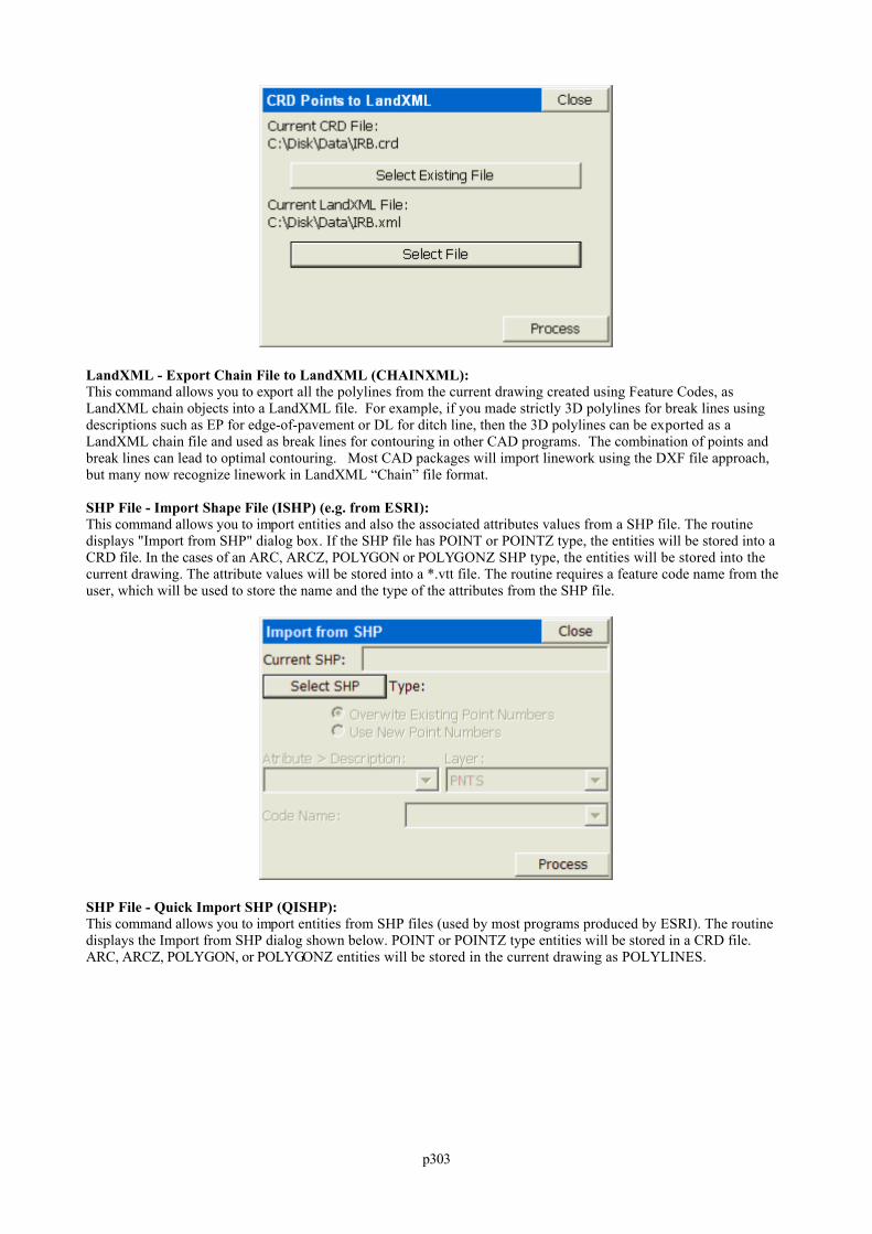
p303

LandXML - Export Chain File to LandXML (CHAINXML): This command allows you to export all the polylines from the current drawing created using Feature Codes, asLandXML chain objects into a LandXML file. For example, if you made strictly 3D polylines for break lines usingdescriptions such as EP for edge-of-pavement or DL for ditch line, then the 3D polylines can be exported as aLandXML chain file and used as break lines for contouring in other CAD programs. The combination of points andbreak lines can lead to optimal contouring. Most CAD packages will import linework using the DXF file approach,but many now recognize linework in LandXML “Chain” file format.

SHP File - Import Shape File (ISHP) (e.g. from ESRI): This command allows you to import entities and also the associated attributes values from a SHP file. The routinedisplays "Import from SHP" dialog box. If the SHP file has POINT or POINTZ type, the entities will be stored into aCRD file. In the cases of an ARC, ARCZ, POLYGON or POLYGONZ SHP type, the entities will be stored into thecurrent drawing. The attribute values will be stored into a *.vtt file. The routine requires a feature code name from theuser, which will be used to store the name and the type of the attributes from the SHP file.

SHP File - Quick Import SHP (QISHP): This command allows you to import entities from SHP files (used by most programs produced by ESRI). The routinedisplays the Import from SHP dialog shown below. POINT or POINTZ type entities will be stored in a CRD file.ARC, ARCZ, POLYGON, or POLYGONZ entities will be stored in the current drawing as POLYLINES.

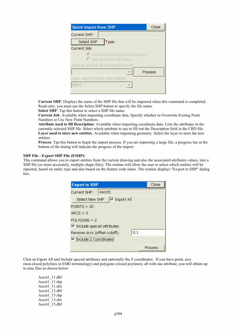
p304

Current SHP: Displays the name of the SHP file that will be imported when this command is completed.Read-only, you must use the Select SHP button to specify the file name.Select SHP: Tap this button to select a SHP file name.Current Job: Available when importing coordinate data. Specify whether to Overwrite Exiting PointNumbers or Use New Point Numbers. Attribute used to fill Description: Available when importing coordinate data. Lists the attributes in thecurrently selected SHP file. Select which attribute to use to fill out the Description field in the CRD file.Layer used to store new entities: Available when importing geometry. Select the layer to store the newentities.Process: Tap this button to begin the import process. If you are importing a large file, a progress bar at thebottom of the dialog will indicate the progress of the import.

SHP File - Export SHP File (ESHP): This command allows you to export entities from the current drawing and also the associated attributes values, into aSHP file (or more accurately, multiple shape files). The routine will allow the user to select which entities will beexported, based on entity type and also based on the feature code name. The routine displays "Export to SHP" dialogbox.

Click on Export All and Include special attributes and optionally the Z coordinates. If you have point, arcs(non-closed polylines in ESRI terminology) and polygons (closed poylines), all with one attribute, you will obtain upto nine files as shown below:

Ascot1_11.dbfAscot1_11.shpAscot1_11.shxAscot1_13.dbfAscot1_13.shpAscot1_13.shxAscot1_15.dbf

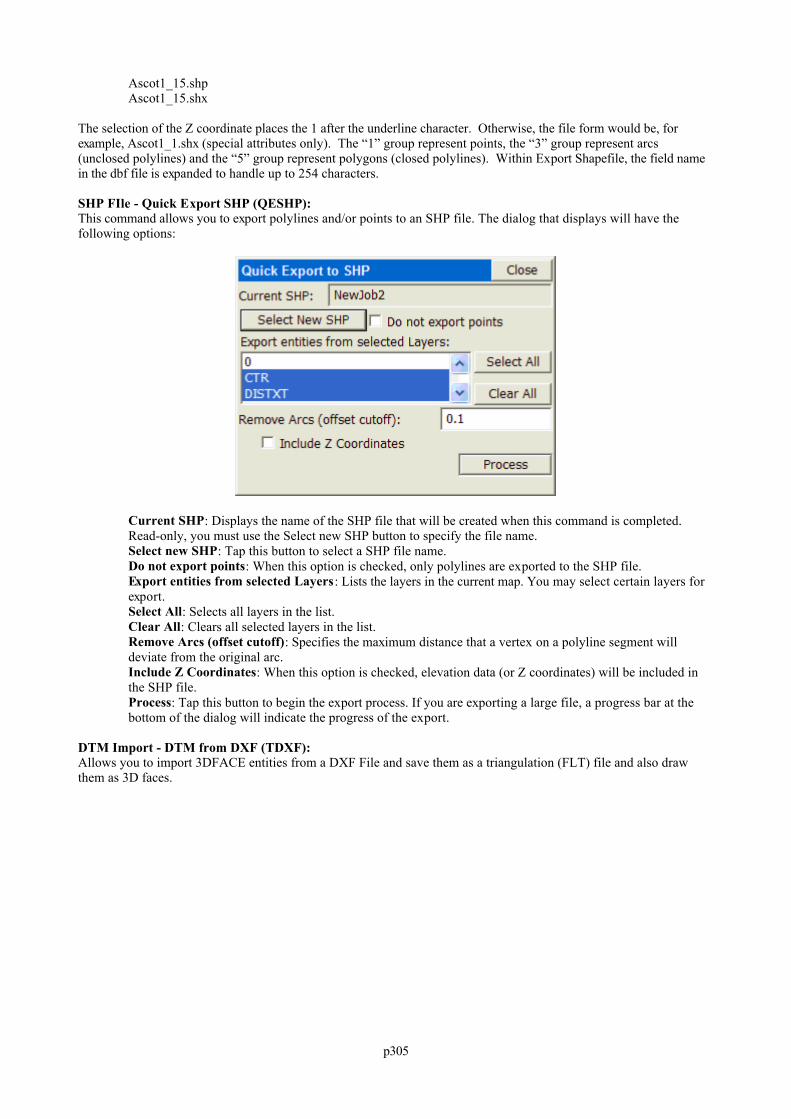
p305

Ascot1_15.shpAscot1_15.shx

The selection of the Z coordinate places the 1 after the underline character. Otherwise, the file form would be, forexample, Ascot1_1.shx (special attributes only). The “1” group represent points, the “3” group represent arcs(unclosed polylines) and the “5” group represent polygons (closed polylines). Within Export Shapefile, the field namein the dbf file is expanded to handle up to 254 characters.

SHP FIle - Quick Export SHP (QESHP): This command allows you to export polylines and/or points to an SHP file. The dialog that displays will have thefollowing options:

Current SHP: Displays the name of the SHP file that will be created when this command is completed.Read-only, you must use the Select new SHP button to specify the file name.Select new SHP: Tap this button to select a SHP file name.Do not export points: When this option is checked, only polylines are exported to the SHP file.Export entities from selected Layers: Lists the layers in the current map. You may select certain layers forexport.Select All: Selects all layers in the list.Clear All: Clears all selected layers in the list.Remove Arcs (offset cutoff): Specifies the maximum distance that a vertex on a polyline segment willdeviate from the original arc.Include Z Coordinates: When this option is checked, elevation data (or Z coordinates) will be included inthe SHP file.Process: Tap this button to begin the export process. If you are exporting a large file, a progress bar at thebottom of the dialog will indicate the progress of the export.

DTM Import - DTM from DXF (TDXF): Allows you to import 3DFACE entities from a DXF File and save them as a triangulation (FLT) file and also drawthem as 3D faces.

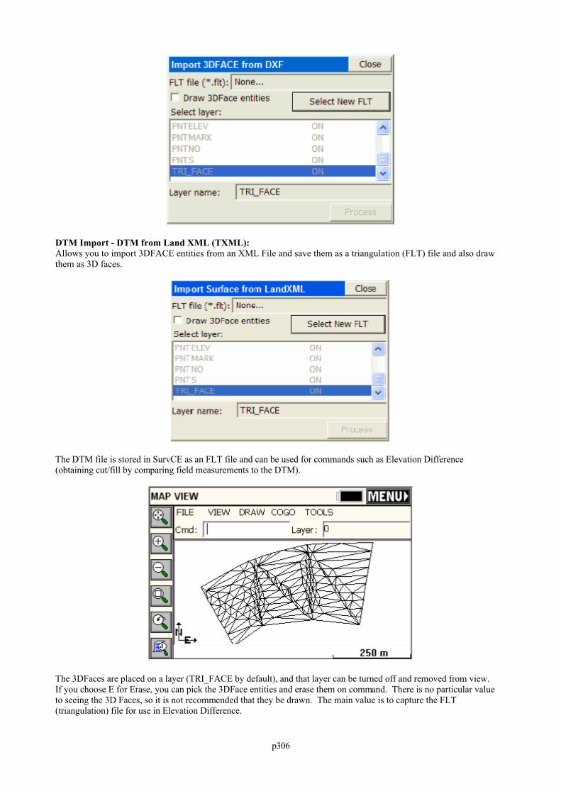
p306

DTM Import - DTM from Land XML (TXML): Allows you to import 3DFACE entities from an XML File and save them as a triangulation (FLT) file and also drawthem as 3D faces.

The DTM file is stored in SurvCE as an FLT file and can be used for commands such as Elevation Difference(obtaining cut/fill by comparing field measurements to the DTM).

The 3DFaces are placed on a layer (TRI_FACE by default), and that layer can be turned off and removed from view. If you choose E for Erase, you can pick the 3DFace entities and erase them on command. There is no particular valueto seeing the 3D Faces, so it is not recommended that they be drawn. The main value is to capture the FLT(triangulation) file for use in Elevation Difference.

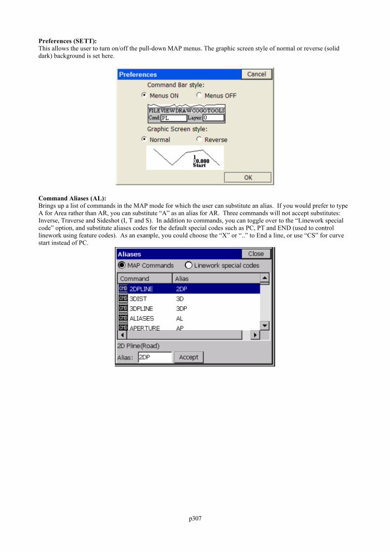
p307

Preferences (SETT): This allows the user to turn on/off the pull-down MAP menus. The graphic screen style of normal or reverse (soliddark) background is set here.

Command Aliases (AL): Brings up a list of commands in the MAP mode for which the user can substitute an alias. If you would prefer to typeA for Area rather than AR, you can substitute “A” as an alias for AR. Three commands will not accept substitutes: Inverse, Traverse and Sideshot (I, T and S). In addition to commands, you can toggle over to the “Linework specialcode” option, and substitute aliases codes for the default special codes such as PC, PT and END (used to controllinework using feature codes). As an example, you could choose the “X” or “..” to End a line, or use “CS” for curvestart instead of PC.

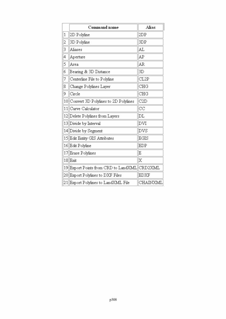
p308

p309

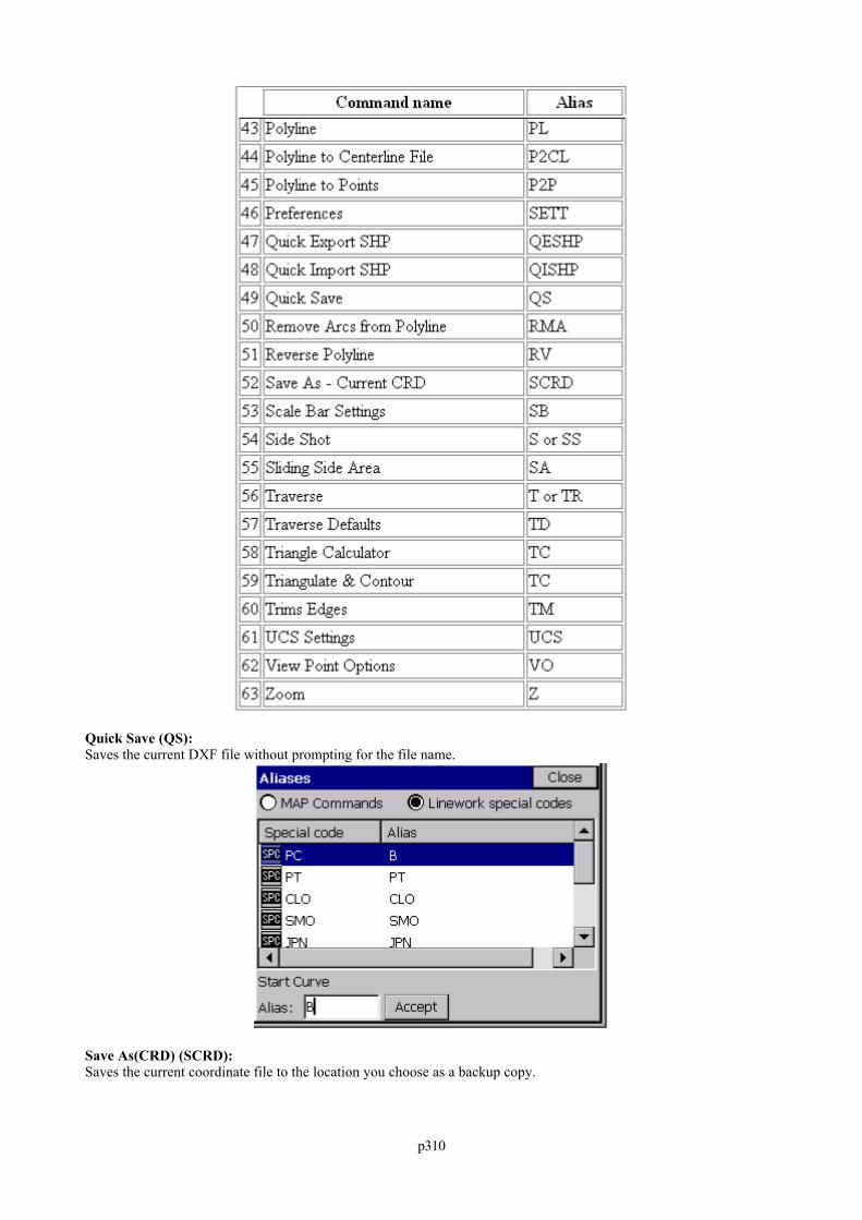
p310

Quick Save (QS): Saves the current DXF file without prompting for the file name.

Save As(CRD) (SCRD): Saves the current coordinate file to the location you choose as a backup copy.

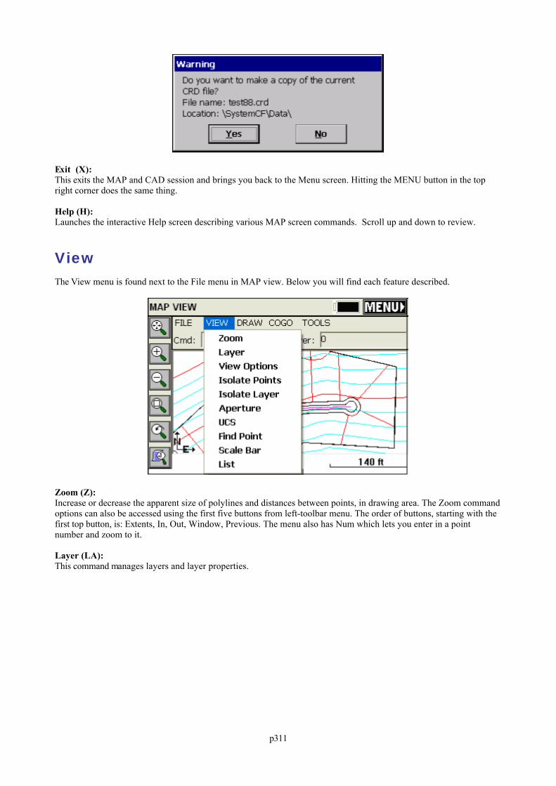
p311

Exit (X): This exits the MAP and CAD session and brings you back to the Menu screen. Hitting the MENU button in the topright corner does the same thing.

Help (H): Launches the interactive Help screen describing various MAP screen commands. Scroll up and down to review.

ViewThe View menu is found next to the File menu in MAP view. Below you will find each feature described.

Zoom (Z): Increase or decrease the apparent size of polylines and distances between points, in drawing area. The Zoom commandoptions can also be accessed using the first five buttons from left-toolbar menu. The order of buttons, starting with thefirst top button, is: Extents, In, Out, Window, Previous. The menu also has Num which lets you enter in a pointnumber and zoom to it.

Layer (LA): This command manages layers and layer properties.

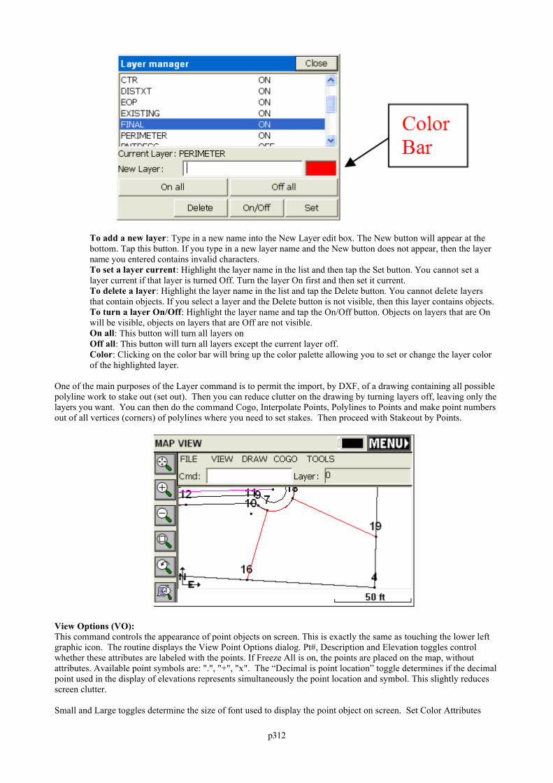
p312

To add a new layer: Type in a new name into the New Layer edit box. The New button will appear at thebottom. Tap this button. If you type in a new layer name and the New button does not appear, then the layername you entered contains invalid characters.To set a layer current: Highlight the layer name in the list and then tap the Set button. You cannot set alayer current if that layer is turned Off. Turn the layer On first and then set it current.To delete a layer: Highlight the layer name in the list and tap the Delete button. You cannot delete layersthat contain objects. If you select a layer and the Delete button is not visible, then this layer contains objects.To turn a layer On/Off: Highlight the layer name and tap the On/Off button. Objects on layers that are Onwill be visible, objects on layers that are Off are not visible.On all: This button will turn all layers onOff all: This button will turn all layers except the current layer off.Color: Clicking on the color bar will bring up the color palette allowing you to set or change the layer colorof the highlighted layer.

One of the main purposes of the Layer command is to permit the import, by DXF, of a drawing containing all possiblepolyline work to stake out (set out). Then you can reduce clutter on the drawing by turning layers off, leaving only thelayers you want. You can then do the command Cogo, Interpolate Points, Polylines to Points and make point numbersout of all vertices (corners) of polylines where you need to set stakes. Then proceed with Stakeout by Points.

View Options (VO): This command controls the appearance of point objects on screen. This is exactly the same as touching the lower leftgraphic icon. The routine displays the View Point Options dialog. Pt#, Description and Elevation toggles controlwhether these attributes are labeled with the points. If Freeze All is on, the points are placed on the map, withoutattributes. Available point symbols are: ".", "+", "x". The “Decimal is point location” toggle determines if the decimalpoint used in the display of elevations represents simultaneously the point location and symbol. This slightly reducesscreen clutter.

Small and Large toggles determine the size of font used to display the point object on screen. Set Color Attributes

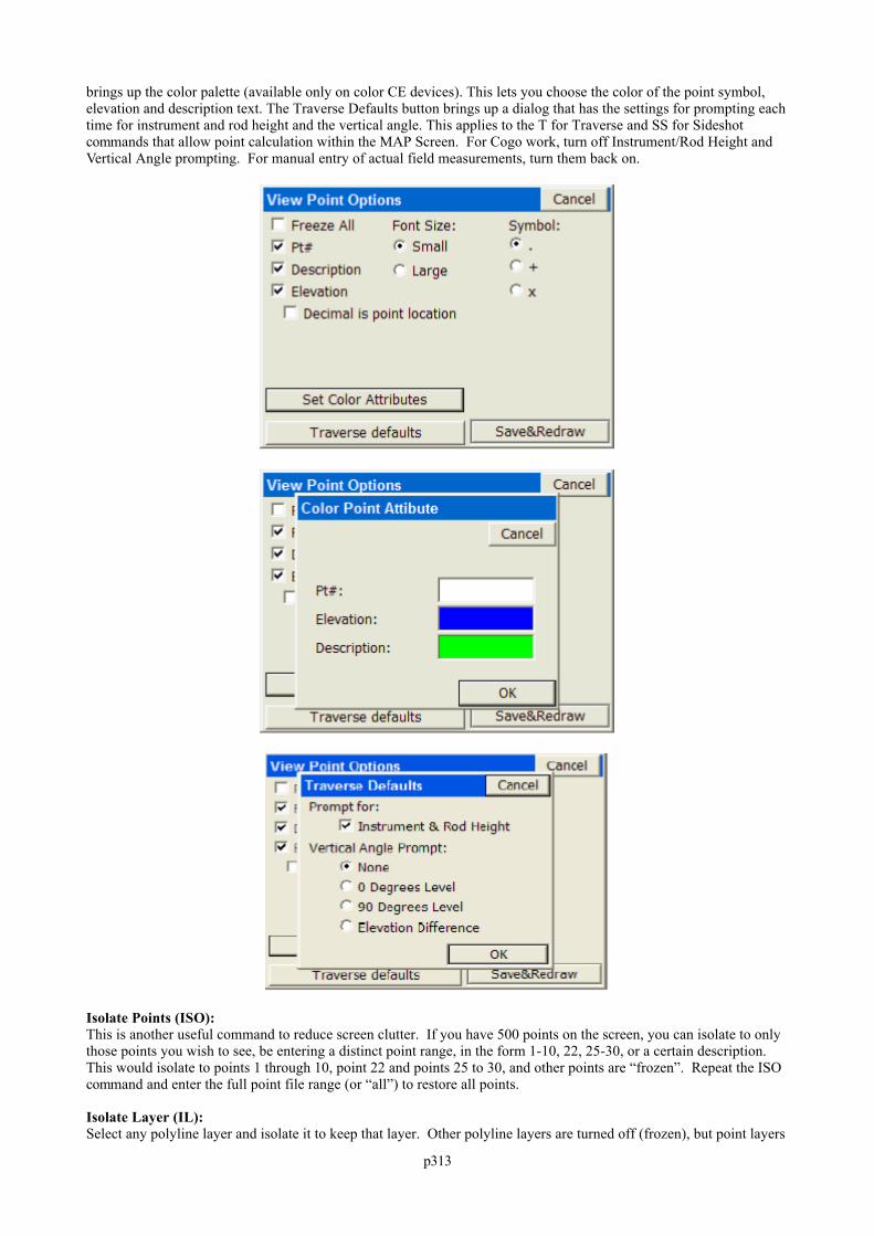
p313

brings up the color palette (available only on color CE devices). This lets you choose the color of the point symbol,elevation and description text. The Traverse Defaults button brings up a dialog that has the settings for prompting eachtime for instrument and rod height and the vertical angle. This applies to the T for Traverse and SS for Sideshotcommands that allow point calculation within the MAP Screen. For Cogo work, turn off Instrument/Rod Height andVertical Angle prompting. For manual entry of actual field measurements, turn them back on.

Isolate Points (ISO): This is another useful command to reduce screen clutter. If you have 500 points on the screen, you can isolate to onlythose points you wish to see, be entering a distinct point range, in the form 1-10, 22, 25-30, or a certain description. This would isolate to points 1 through 10, point 22 and points 25 to 30, and other points are “frozen”. Repeat the ISOcommand and enter the full point file range (or “all”) to restore all points.

Isolate Layer (IL):Select any polyline layer and isolate it to keep that layer. Other polyline layers are turned off (frozen), but point layers

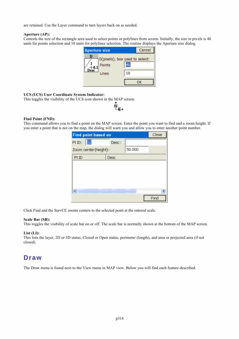
p314

are retained. Use the Layer command to turn layers back on as needed.

Aperture (AP): Controls the size of the rectangle area used to select points or polylines from screen. Initially, the size in pixels is 40units for points selection and 10 units for polylines selection. The routine displays the Aperture size dialog.

UCS (UCS) User Coordinate System Indicator: This toggles the visibility of the UCS icon shown in the MAP screen.

Find Point (FND): This command allows you to find a point on the MAP screen. Enter the point you want to find and a zoom height. Ifyou enter a point that is not on the map, the dialog will warn you and allow you to enter another point number.

Click Find and the SurvCE zooms centers to the selected point at the entered scale.

Scale Bar (SB): This toggles the visibility of scale bar on or off. The scale bar is normally shown at the bottom of the MAP screen.

List (LI): This lists the layer, 2D or 3D status, Closed or Open status, perimeter (length), and area or projected area (if notclosed).

DrawThe Draw menu is found next to the View menu in MAP view. Below you will find each feature described.

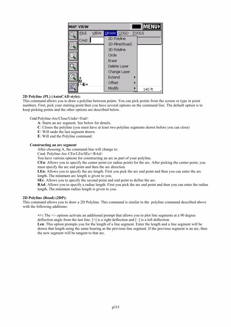
p315

2D Polyline (PL) (AutoCAD style): This command allows you to draw a polyline between points. You can pick points from the screen or type in pointnumbers. First, pick your starting point then you have several options on the command line. The default option is tokeep picking points and the other options are described below.

Cmd:Polyline-Arc/Close/Undo/<End>A: Starts an arc segment. See below for details.C: Closes the polyline (you must have at least two polyline segments drawn before you can close)U: Will undo the last segment drawn.E: Will end the Polyline command.

Constructing an arc segmentAfter choosing A, the command line will change to:Cmd: Polyline-Arc CEn/LEn/SEc/<RAd>You have various options for constructing an arc as part of your polyline.CEn: Allows you to specify the center point (or radius point) for the arc. After picking the center point, youmust specify the arc end point and then the arc direction.LEn: Allows you to specify the arc length. First you pick the arc end point and then you can enter the arclength. The minimum arc length is given to you.SEc: Allows you to specify the second point and end point to define the arc.RAd: Allows you to specify a radius length. First you pick the arc end point and then you can enter the radiuslength. The minimum radius length is given to you.

2D Polyline (Road) (2DP):This command allows you to draw a 2D Polyline. This command is similar to the polyline command described abovewith the following additions:

+/-: The +/- options activate an additional prompt that allows you to plot line segments at a 90 degreedeflection angle from the last line. [+] is a right deflection and [–] is a left deflection.Len: This option prompts you for the length of a line segment. Enter the length and a line segment will bedrawn that length using the same bearing as the previous line segment. If the previous segment is an arc, thenthe new segment will be tangent to that arc.

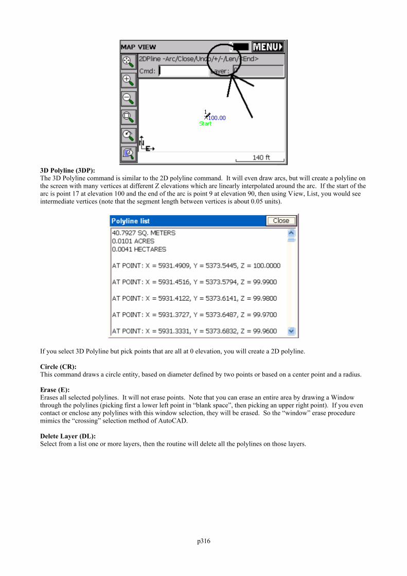
p316

3D Polyline (3DP): The 3D Polyline command is similar to the 2D polyline command. It will even draw arcs, but will create a polyline onthe screen with many vertices at different Z elevations which are linearly interpolated around the arc. If the start of thearc is point 17 at elevation 100 and the end of the arc is point 9 at elevation 90, then using View, List, you would seeintermediate vertices (note that the segment length between vertices is about 0.05 units).

If you select 3D Polyline but pick points that are all at 0 elevation, you will create a 2D polyline.

Circle (CR): This command draws a circle entity, based on diameter defined by two points or based on a center point and a radius.

Erase (E): Erases all selected polylines. It will not erase points. Note that you can erase an entire area by drawing a Windowthrough the polylines (picking first a lower left point in “blank space”, then picking an upper right point). If you evencontact or enclose any polylines with this window selection, they will be erased. So the “window” erase proceduremimics the “crossing” selection method of AutoCAD.

Delete Layer (DL): Select from a list one or more layers, then the routine will delete all the polylines on those layers.

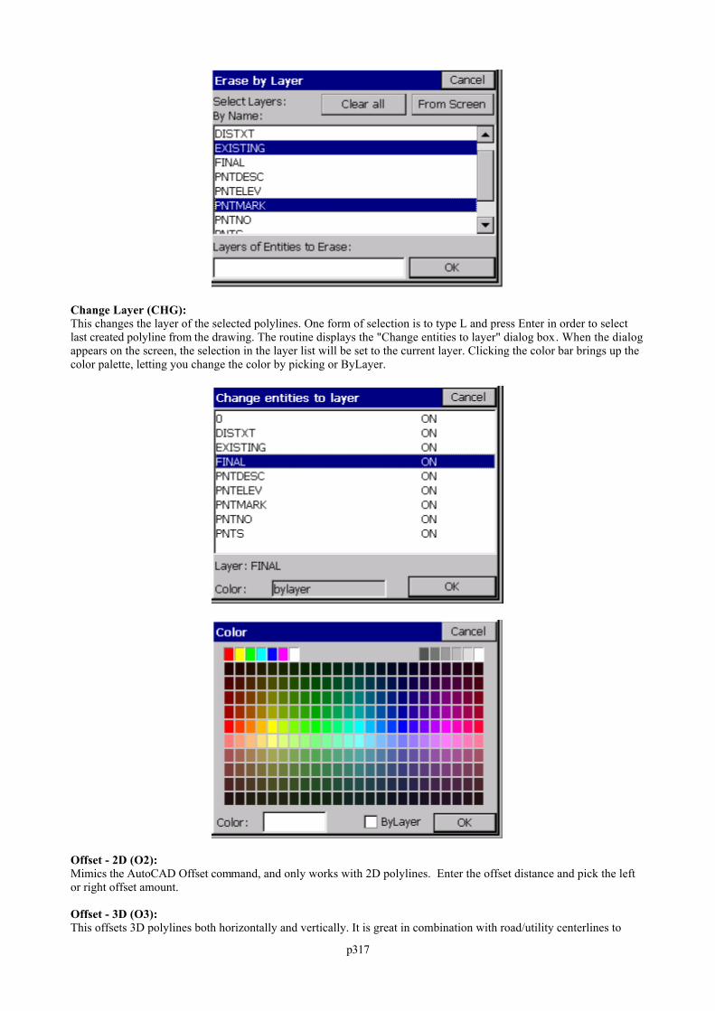
p317

Change Layer (CHG): This changes the layer of the selected polylines. One form of selection is to type L and press Enter in order to selectlast created polyline from the drawing. The routine displays the "Change entities to layer" dialog box. When the dialogappears on the screen, the selection in the layer list will be set to the current layer. Clicking the color bar brings up thecolor palette, letting you change the color by picking or ByLayer.

Offset - 2D (O2): Mimics the AutoCAD Offset command, and only works with 2D polylines. Enter the offset distance and pick the leftor right offset amount.

Offset - 3D (O3): This offsets 3D polylines both horizontally and vertically. It is great in combination with road/utility centerlines to

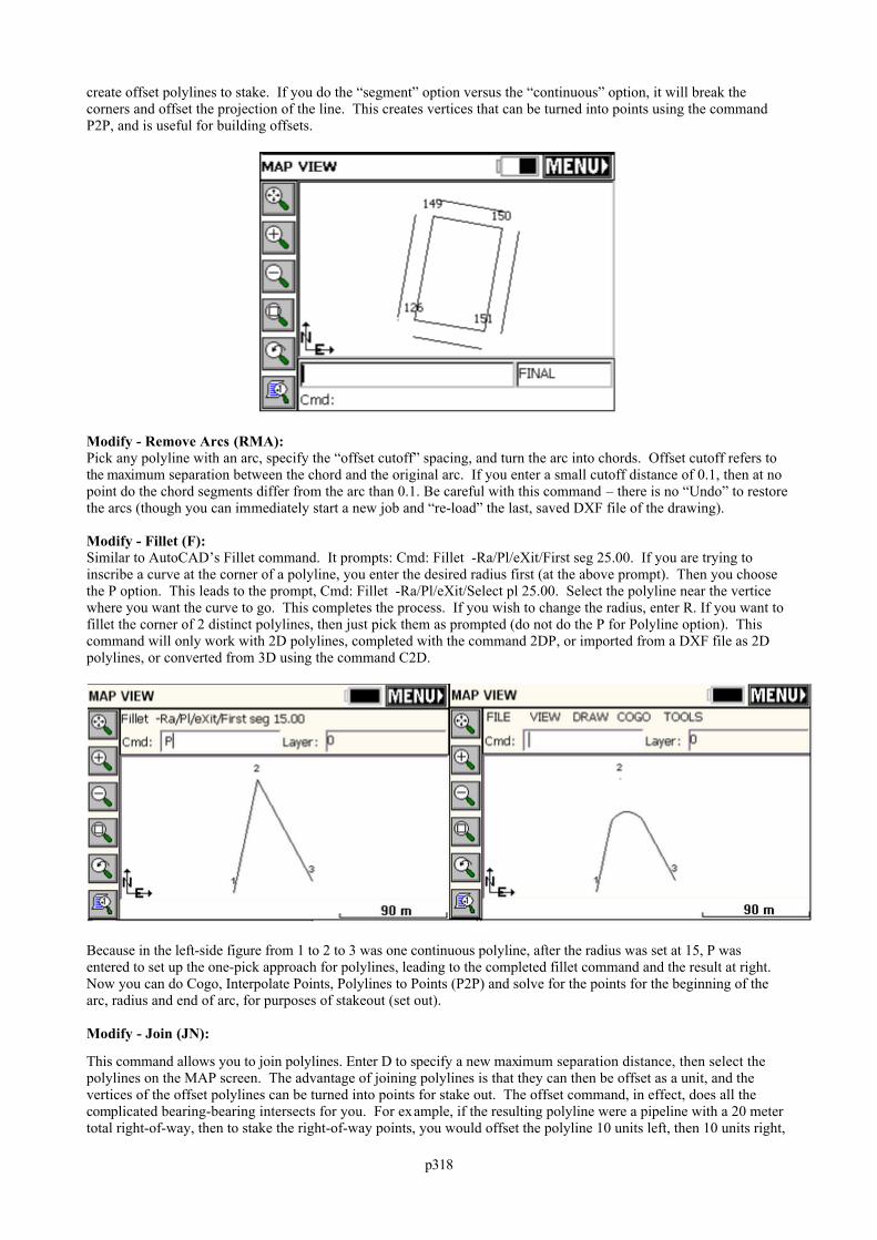
p318

create offset polylines to stake. If you do the “segment” option versus the “continuous” option, it will break thecorners and offset the projection of the line. This creates vertices that can be turned into points using the commandP2P, and is useful for building offsets.

Modify - Remove Arcs (RMA): Pick any polyline with an arc, specify the “offset cutoff” spacing, and turn the arc into chords. Offset cutoff refers tothe maximum separation between the chord and the original arc. If you enter a small cutoff distance of 0.1, then at nopoint do the chord segments differ from the arc than 0.1. Be careful with this command – there is no “Undo” to restorethe arcs (though you can immediately start a new job and “re-load” the last, saved DXF file of the drawing).

Modify - Fillet (F): Similar to AutoCAD’s Fillet command. It prompts: Cmd: Fillet -Ra/Pl/eXit/First seg 25.00. If you are trying toinscribe a curve at the corner of a polyline, you enter the desired radius first (at the above prompt). Then you choosethe P option. This leads to the prompt, Cmd: Fillet -Ra/Pl/eXit/Select pl 25.00. Select the polyline near the verticewhere you want the curve to go. This completes the process. If you wish to change the radius, enter R. If you want tofillet the corner of 2 distinct polylines, then just pick them as prompted (do not do the P for Polyline option). Thiscommand will only work with 2D polylines, completed with the command 2DP, or imported from a DXF file as 2Dpolylines, or converted from 3D using the command C2D.

Because in the left-side figure from 1 to 2 to 3 was one continuous polyline, after the radius was set at 15, P wasentered to set up the one-pick approach for polylines, leading to the completed fillet command and the result at right. Now you can do Cogo, Interpolate Points, Polylines to Points (P2P) and solve for the points for the beginning of thearc, radius and end of arc, for purposes of stakeout (set out).

Modify - Join (JN):

This command allows you to join polylines. Enter D to specify a new maximum separation distance, then select thepolylines on the MAP screen. The advantage of joining polylines is that they can then be offset as a unit, and thevertices of the offset polylines can be turned into points for stake out. The offset command, in effect, does all thecomplicated bearing-bearing intersects for you. For example, if the resulting polyline were a pipeline with a 20 metertotal right-of-way, then to stake the right-of-way points, you would offset the polyline 10 units left, then 10 units right,

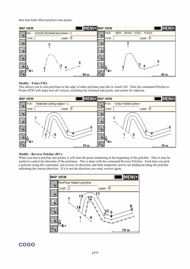
p319

then turn both offset polylines into points.

Modify - Trim (TM): This allows you to trim polylines to the edge of other polylines just like in AutoCAD. Then the command Polyline toPoints (P2P) will make turn all vertices, including the trimmed end points, into points for stakeout.

Modify - Reverse Polyline (RV): When you turn a polyline into points, it will start the point numbering at the beginning of the polyline. Thus it may beuseful to control the direction of the polylines. This is done with the command Reverse Polyline. Each time you picka polyline using this command, you reverse its direction, and little temporary arrows are displayed along the polylineindicating the current direction. If it is not the direction you want, reverse again.

COGO

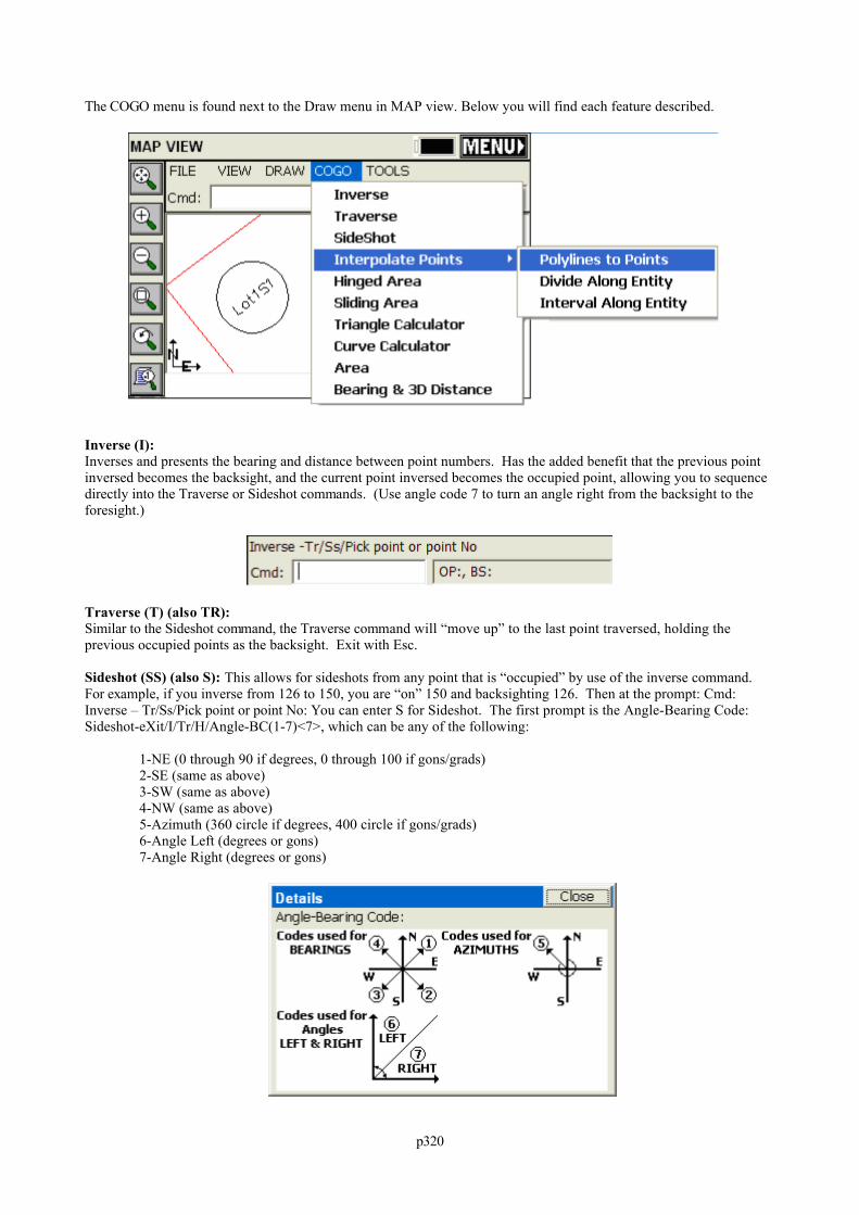
p320

The COGO menu is found next to the Draw menu in MAP view. Below you will find each feature described.

Inverse (I): Inverses and presents the bearing and distance between point numbers. Has the added benefit that the previous pointinversed becomes the backsight, and the current point inversed becomes the occupied point, allowing you to sequencedirectly into the Traverse or Sideshot commands. (Use angle code 7 to turn an angle right from the backsight to theforesight.)

Traverse (T) (also TR): Similar to the Sideshot command, the Traverse command will “move up” to the last point traversed, holding theprevious occupied points as the backsight. Exit with Esc.

Sideshot (SS) (also S): This allows for sideshots from any point that is “occupied” by use of the inverse command.For example, if you inverse from 126 to 150, you are “on” 150 and backsighting 126. Then at the prompt: Cmd:Inverse – Tr/Ss/Pick point or point No: You can enter S for Sideshot. The first prompt is the Angle-Bearing Code:Sideshot-eXit/I/Tr/H/Angle-BC(1-7)<7>, which can be any of the following:

1-NE (0 through 90 if degrees, 0 through 100 if gons/grads)2-SE (same as above)3-SW (same as above)4-NW (same as above)5-Azimuth (360 circle if degrees, 400 circle if gons/grads)6-Angle Left (degrees or gons)7-Angle Right (degrees or gons)

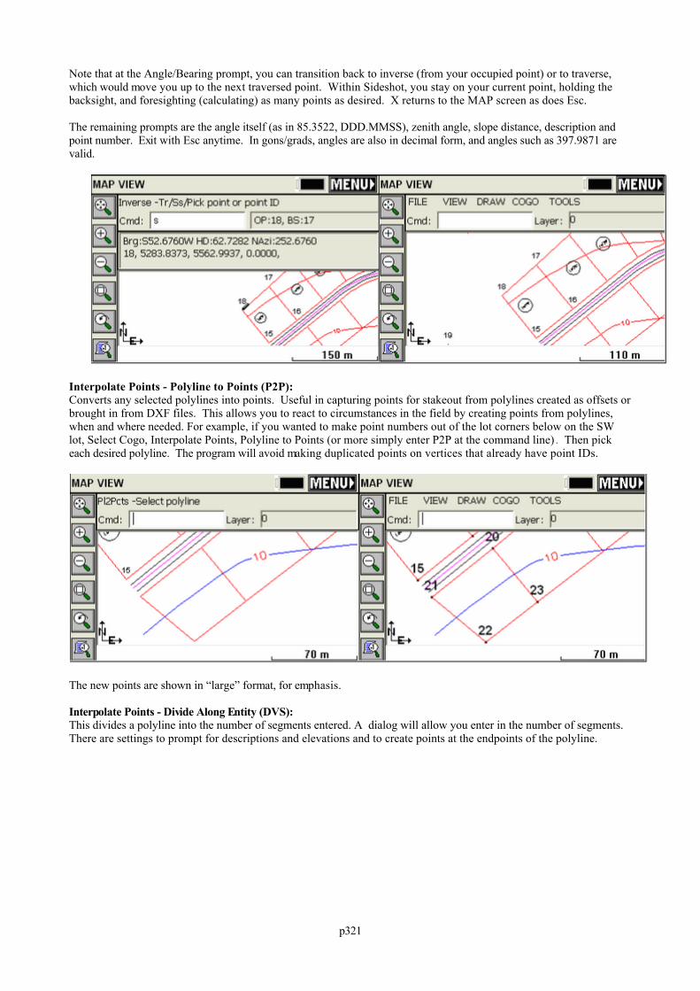
p321

Note that at the Angle/Bearing prompt, you can transition back to inverse (from your occupied point) or to traverse,which would move you up to the next traversed point. Within Sideshot, you stay on your current point, holding thebacksight, and foresighting (calculating) as many points as desired. X returns to the MAP screen as does Esc.

The remaining prompts are the angle itself (as in 85.3522, DDD.MMSS), zenith angle, slope distance, description andpoint number. Exit with Esc anytime. In gons/grads, angles are also in decimal form, and angles such as 397.9871 arevalid.

Interpolate Points - Polyline to Points (P2P): Converts any selected polylines into points. Useful in capturing points for stakeout from polylines created as offsets orbrought in from DXF files. This allows you to react to circumstances in the field by creating points from polylines,when and where needed. For example, if you wanted to make point numbers out of the lot corners below on the SWlot, Select Cogo, Interpolate Points, Polyline to Points (or more simply enter P2P at the command line) . Then pickeach desired polyline. The program will avoid making duplicated points on vertices that already have point IDs.

The new points are shown in “large” format, for emphasis.

Interpolate Points - Divide Along Entity (DVS): This divides a polyline into the number of segments entered. A dialog will allow you enter in the number of segments.There are settings to prompt for descriptions and elevations and to create points at the endpoints of the polyline.

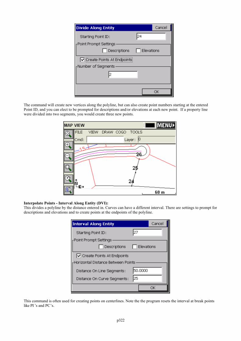
p322

The command will create new vertices along the polyline, but can also create point numbers starting at the enteredPoint ID, and you can elect to be prompted for descriptions and/or elevations at each new point. If a property linewere divided into two segments, you would create three new points.

Interpolate Points - Interval Along Entity (DVI): This divides a polyline by the distance entered in. Curves can have a different interval. There are settings to prompt fordescriptions and elevations and to create points at the endpoints of the polyline.

This command is often used for creating points on centerlines. Note the the program resets the interval at break pointslike PI ’s and PC’s.

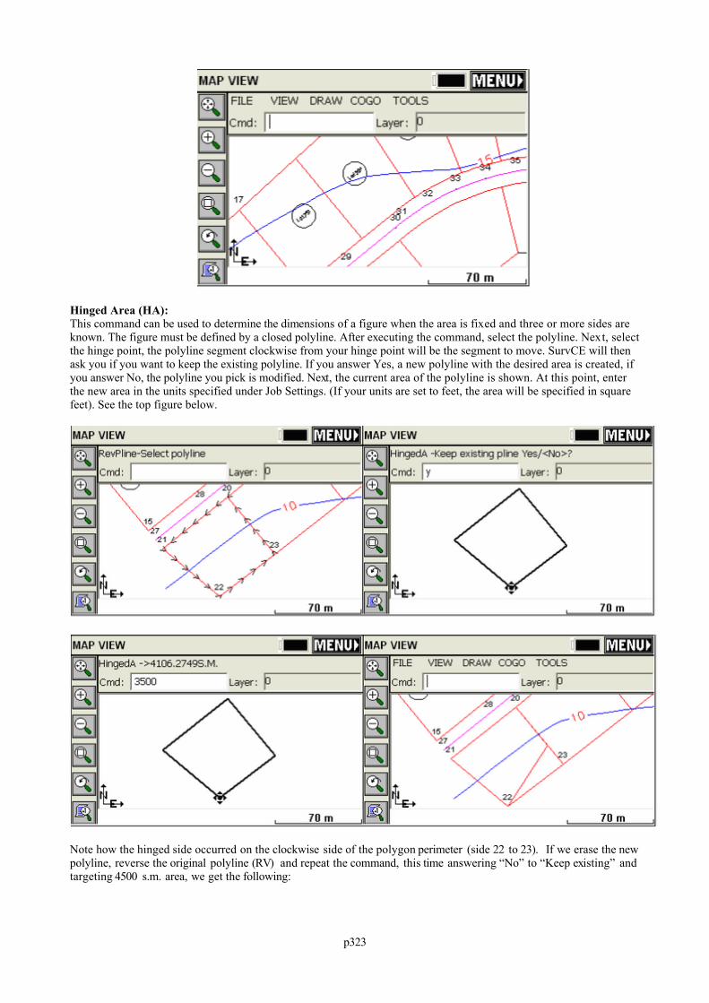
p323

Hinged Area (HA): This command can be used to determine the dimensions of a figure when the area is fixed and three or more sides areknown. The figure must be defined by a closed polyline. After executing the command, select the polyline. Next, selectthe hinge point, the polyline segment clockwise from your hinge point will be the segment to move. SurvCE will thenask you if you want to keep the existing polyline. If you answer Yes, a new polyline with the desired area is created, ifyou answer No, the polyline you pick is modified. Next, the current area of the polyline is shown. At this point, enterthe new area in the units specified under Job Settings. (If your units are set to feet, the area will be specified in squarefeet). See the top figure below.

Note how the hinged side occurred on the clockwise side of the polygon perimeter (side 22 to 23). If we erase the newpolyline, reverse the original polyline (RV) and repeat the command, this time answering “No” to “Keep existing” andtargeting 4500 s.m. area, we get the following:

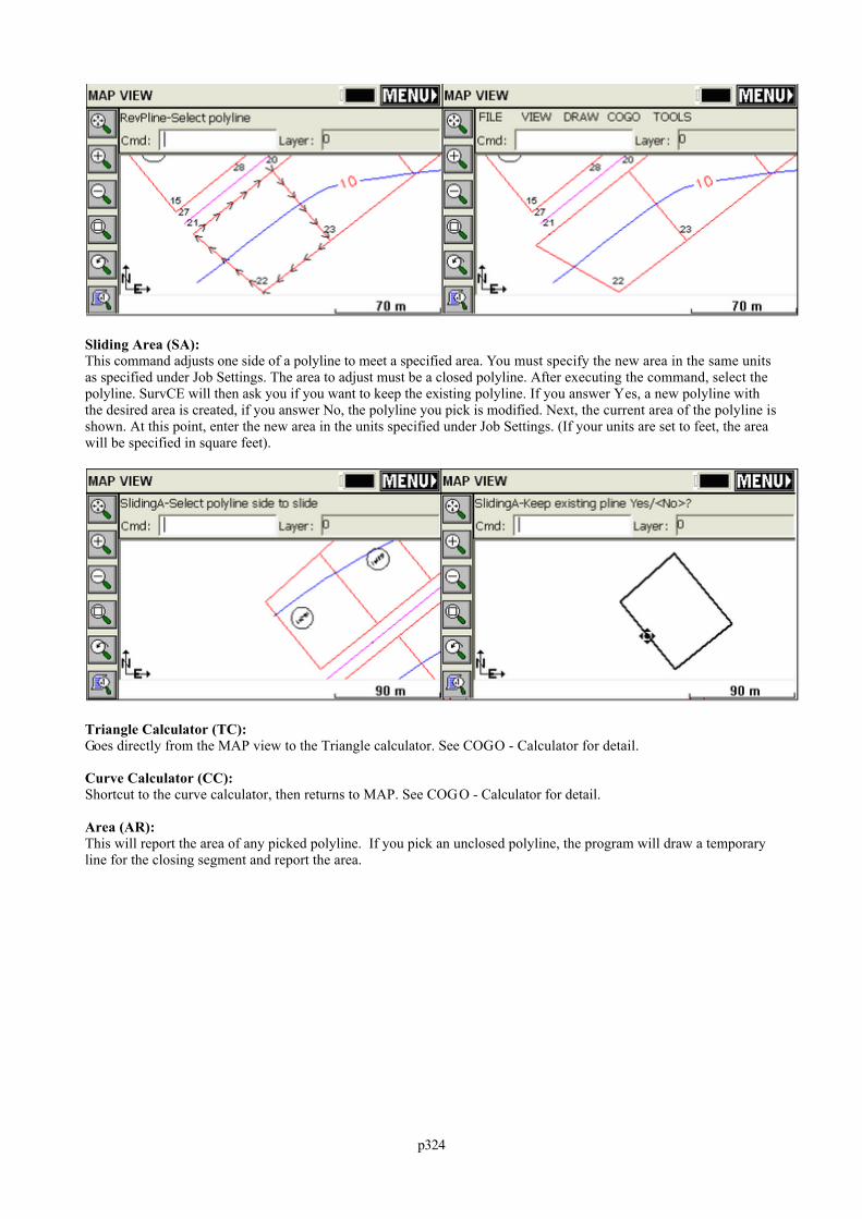
p324

Sliding Area (SA): This command adjusts one side of a polyline to meet a specified area. You must specify the new area in the same unitsas specified under Job Settings. The area to adjust must be a closed polyline. After executing the command, select thepolyline. SurvCE will then ask you if you want to keep the existing polyline. If you answer Yes, a new polyline withthe desired area is created, if you answer No, the polyline you pick is modified. Next, the current area of the polyline isshown. At this point, enter the new area in the units specified under Job Settings. (If your units are set to feet, the areawill be specified in square feet).

Triangle Calculator (TC): Goes directly from the MAP view to the Triangle calculator. See COGO - Calculator for detail.

Curve Calculator (CC): Shortcut to the curve calculator, then returns to MAP. See COGO - Calculator for detail.

Area (AR): This will report the area of any picked polyline. If you pick an unclosed polyline, the program will draw a temporaryline for the closing segment and report the area.

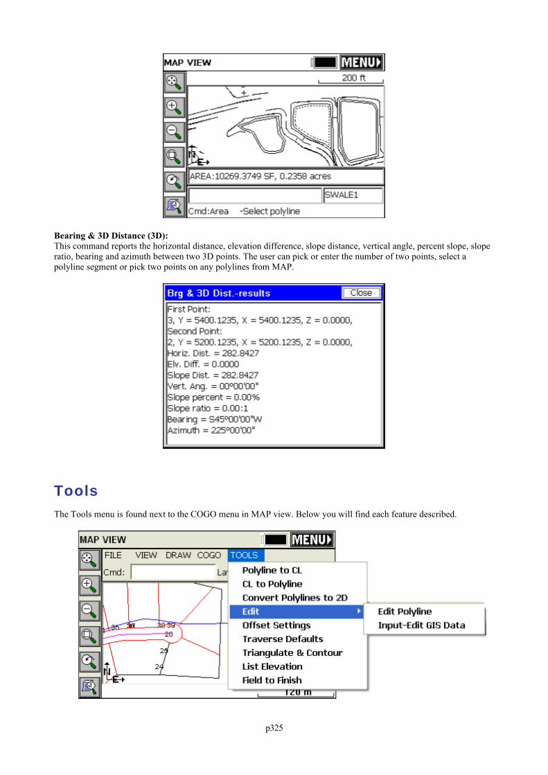
p325

Bearing & 3D Distance (3D): This command reports the horizontal distance, elevation difference, slope distance, vertical angle, percent slope, sloperatio, bearing and azimuth between two 3D points. The user can pick or enter the number of two points, select apolyline segment or pick two points on any polylines from MAP.

ToolsThe Tools menu is found next to the COGO menu in MAP view. Below you will find each feature described.

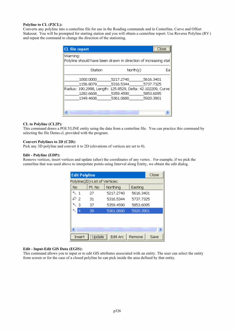
p326

Polyline to CL (P2CL): Converts any polyline into a centerline file for use in the Roading commands and in Centerline, Curve and OffsetStakeout. You will be prompted for starting station and you will obtain a centerline report. Use Reverse Polyline (RV )and repeat the command to change the direction of the stationing.

CL to Polyline (CL2P): This command draws a POLYLINE entity using the data from a centerline file. You can practice this command byselecting the file Demo.cl, provided with the program.

Convert Polylines to 2D (C2D): Pick any 3D polyline and convert it to 2D (elevations of vertices are set to 0).

Edit - Polyline (EDP): Remove vertices, insert vertices and update (alter) the coordinates of any vertex . For example, if we pick thecenterline that was used above to interpolate points using Interval along Entity, we obtain the edit dialog.

Edit - Input-Edit GIS Data (EGIS): This command allows you to input or to edit GIS attributes associated with an entity. The user can select the entityfrom screen or for the case of a closed polyline he can pick inside the area defined by that entity.

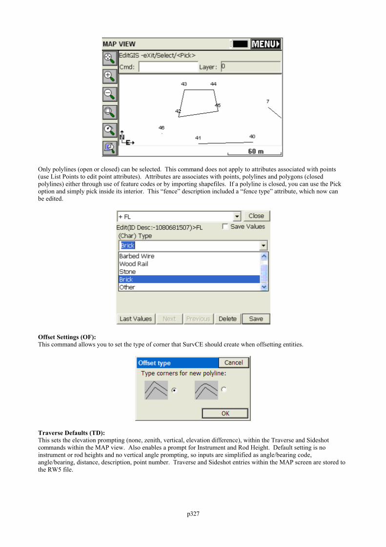
p327

Only polylines (open or closed) can be selected. This command does not apply to attributes associated with points(use List Points to edit point attributes). Attributes are associates with points, polylines and polygons (closedpolylines) either through use of feature codes or by importing shapefiles. If a polyline is closed, you can use the Pickoption and simply pick inside its interior. This “fence” description included a “fence type” attribute, which now canbe edited.

Offset Settings (OF): This command allows you to set the type of corner that SurvCE should create when offsetting entities.

Traverse Defaults (TD): This sets the elevation prompting (none, zenith, vertical, elevation difference), within the Traverse and Sideshotcommands within the MAP view. Also enables a prompt for Instrument and Rod Height. Default setting is noinstrument or rod heights and no vertical angle prompting, so inputs are simplified as angle/bearing code,angle/bearing, distance, description, point number. Traverse and Sideshot entries within the MAP screen are stored tothe RW5 file.

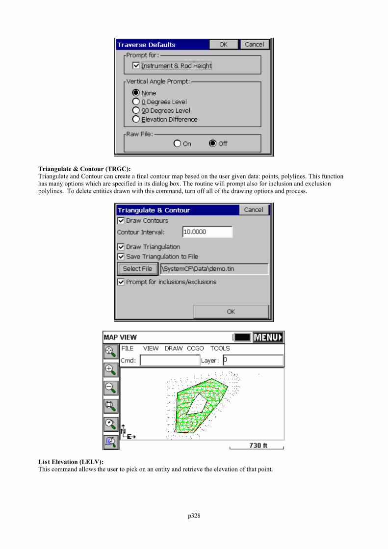
p328

Triangulate & Contour (TRGC): Triangulate and Contour can create a final contour map based on the user given data: points, polylines. This functionhas many options which are specified in its dialog box. The routine will prompt also for inclusion and exclusionpolylines. To delete entities drawn with this command, turn off all of the drawing options and process.

List Elevation (LELV): This command allows the user to pick on an entity and retrieve the elevation of that point.

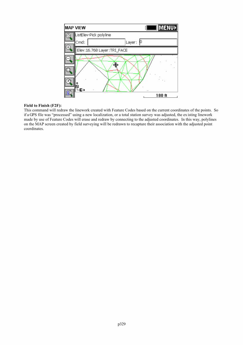
p329

Field to Finish (F2F): This command will redraw the linework created with Feature Codes based on the current coordinates of the points. Soif a GPS file was “processed” using a new localization, or a total station survey was adjusted, the ex isting lineworkmade by use of Feature Codes will erase and redraw by connecting to the adjusted coordinates. In this way, polylineson the MAP screen created by field surveying will be redrawn to recapture their association with the adjusted pointcoordinates.

p330

Tutorials

This section contains five tutorials designed to assist you in learning Carlson SurvCE.

Tutorial 1: Calculating a Traverse (By Hand) with SurvCETo do a hand traverse with SurvCE, go to the MAP screen. To get there, click the icon in the upper right corner ofyour screen labeled MAP. Once there, you will set your defaults for traversing.

Tutorial 2: Performing Math Functions in SurvCE Input BoxesVarious input boxes in SurvCE allow the user to calculate math functions "on-the-fly". The basic steps for gettingstarted are shown here.

Tutorial 3: Performing a Compass Rule AdjustmentThis tutorial shows a compass rule adjustment, with various SurvCE screen captures to guide you.

Tutorial 4: Defining Field Codes, Line/Layer Properties & GIS PromptingThis tutorial will assist users in defining Field Codes in SurvCE. SurvCE can have one pre-defined FCL (Feature CodeList) file loaded with the job coordinate CRD file. The Feature Code List file stores pre-defined field codes that defineLine/Layer drawing properties and, optionally, GIS prompting. More than one FCL file can exist, but only one can beloaded at a time per job coordinate CRD file. The operator builds this FCL file using option 5 “Feature Code List” inthe File main menu.

Tutorial 5: Standard Procedures for Conducting GPS LocalizationsThis tutorial is intended to assist users with the recommended localization method for SurvCE. Other methods can beused, and it is up to the individual users to determine which is best for them.

Tutorial 1

Calculating a Traverse (By Hand) with SurvCEIn order to do a hand traverse with SurvCE, go to the MAP screen by clicking the icon in the upper right corner

labeled MAP. While in the map screen, select the map settings icon to set your Traverse Defaults .

Traverse Steps:

1 To begin, you must key in the command for inverse by typing “I” (Without the quotes) to establish youroccupied and backsight points. The command prompt will display the following:

Cmd:Inverse - Tr/Ss/Pick point or point No2 Key in the backsight point number followed by the [ENTER] key.3 Key in the occupied point number followed by the [ENTER] key.4 Key “T” for Traverse or “S” for Sideshot followed by the [ENTER] key.5 If you keyed in “T” for traverse the command prompt will be waiting for an angle code by displaying the

following:

Cmd:Traverse - eXit/I/Ss/Angle-BC(1-7)<7>

If you keyed in “S” for sideshot the command prompt will also be waiting for an angle code by displaying thefollowing:

Cmd:Sideshot - eXit/I/Tr/Angle-BC(1-7)<7>

The code choices you can key in are as follows:

1 - Northeast Bearing

2 - Southeast Bearing

3 - Southwest Bearing

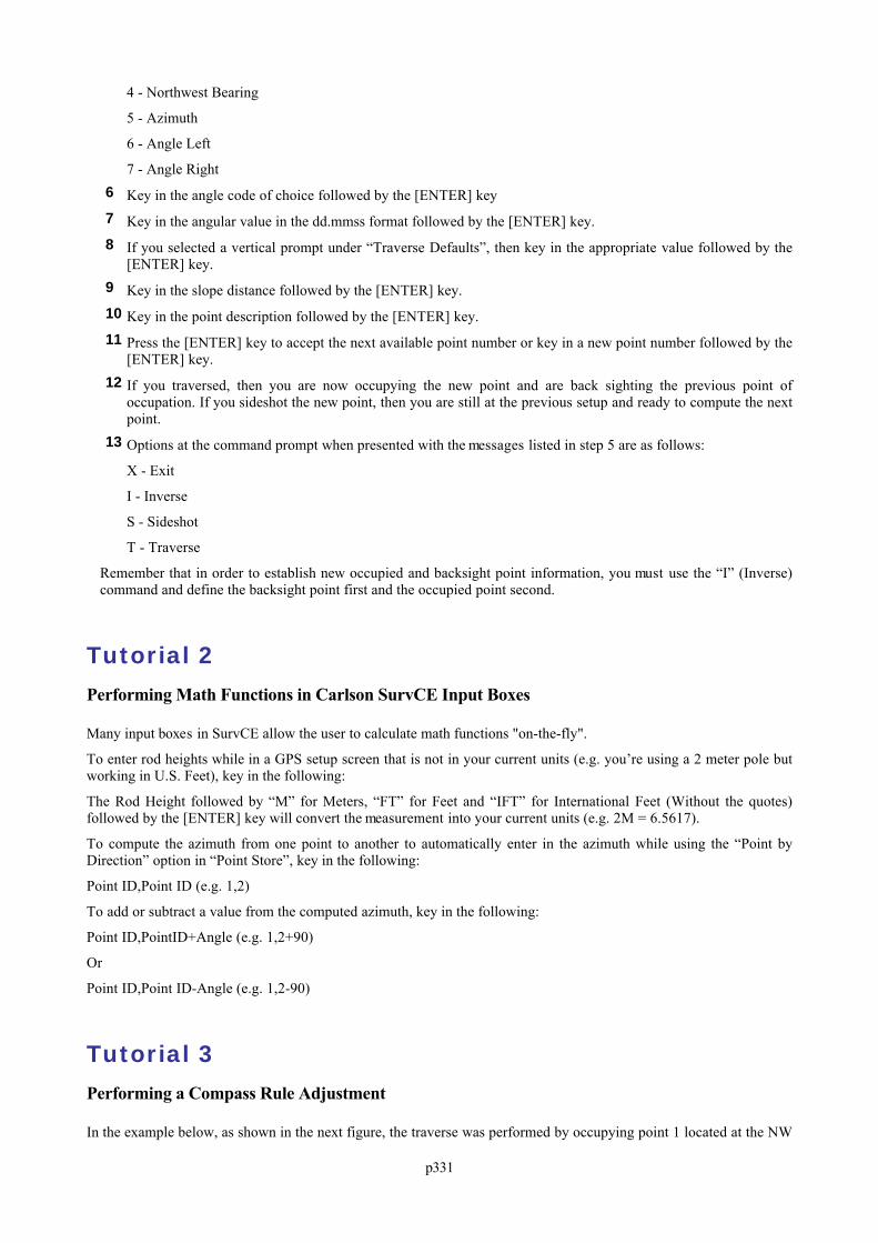
p331

4 - Northwest Bearing

5 - Azimuth

6 - Angle Left

7 - Angle Right6 Key in the angle code of choice followed by the [ENTER] key7 Key in the angular value in the dd.mmss format followed by the [ENTER] key.8 If you selected a vertical prompt under “Traverse Defaults”, then key in the appropriate value followed by the

[ENTER] key.9 Key in the slope distance followed by the [ENTER] key.10 Key in the point description followed by the [ENTER] key.11 Press the [ENTER] key to accept the next available point number or key in a new point number followed by the

[ENTER] key.12 If you traversed, then you are now occupying the new point and are back sighting the previous point of

occupation. If you sideshot the new point, then you are still at the previous setup and ready to compute the nextpoint.

13 Options at the command prompt when presented with the messages listed in step 5 are as follows:

X - Exit

I - Inverse

S - Sideshot

T - Traverse

Remember that in order to establish new occupied and backsight point information, you must use the “I” (Inverse)command and define the backsight point first and the occupied point second.

Tutorial 2

Performing Math Functions in Carlson SurvCE Input Boxes

Many input boxes in SurvCE allow the user to calculate math functions "on-the-fly".

To enter rod heights while in a GPS setup screen that is not in your current units (e.g. you’re using a 2 meter pole butworking in U.S. Feet), key in the following:

The Rod Height followed by “M” for Meters, “FT” for Feet and “IFT” for International Feet (Without the quotes)followed by the [ENTER] key will convert the measurement into your current units (e.g. 2M = 6.5617).

To compute the azimuth from one point to another to automatically enter in the azimuth while using the “Point byDirection” option in “Point Store”, key in the following:

Point ID,Point ID (e.g. 1,2)

To add or subtract a value from the computed azimuth, key in the following:

Point ID,PointID+Angle (e.g. 1,2+90)

Or

Point ID,Point ID-Angle (e.g. 1,2-90)

Tutorial 3

Performing a Compass Rule Adjustment

In the example below, as shown in the next figure, the traverse was performed by occupying point 1 located at the NW

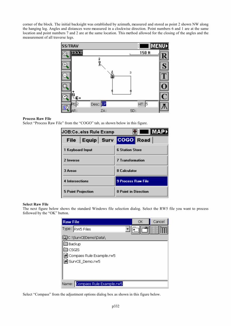
p332

corner of the block. The initial backsight was established by azimuth, measured and stored as point 2 shown NW alongthe hanging leg. Angles and distances were measured in a clockwise direction. Point numbers 6 and 1 are at the samelocation and point numbers 7 and 2 are at the same location. This method allowed for the closing of the angles and themeasurement of all traverse legs.

Process Raw FileSelect “Process Raw File” from the “COGO” tab, as shown below in this figure.

Select Raw FileThe next figure below shows the standard Windows file selection dialog. Select the RW5 file you want to processfollowed by the “OK” button.

Select “Compass” from the adjustment options dialog box as shown in this figure below.

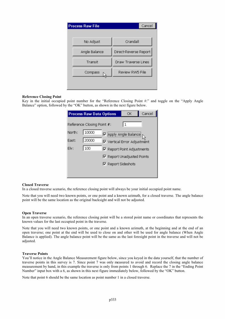
p333

Reference Closing PointKey in the initial occupied point number for the “Reference Closing Point #:” and toggle on the “Apply AngleBalance” option, followed by the “OK” button, as shown in the next figure below.

Closed TraverseIn a closed traverse scenario, the reference closing point will always be your initial occupied point name.

Note that you will need two known points, or one point and a known azimuth, for a closed traverse. The angle balancepoint will be the same location as the original backsight and will not be adjusted.

Open TraverseIn an open traverse scenario, the reference closing point will be a stored point name or coordinates that represents theknown values for the last occupied point in the traverse.

Note that you will need two known points, or one point and a known azimuth, at the beginning and at the end of anopen traverse; one point at the end will be used to close on and other will be used for angle balance (When AngleBalance is applied). The angle balance point will be the same as the last foresight point in the traverse and will not beadjusted.

Traverse PointsYou’ll notice in the Angle Balance Measurement figure below, since you keyed in the data yourself, that the number oftraverse points in this survey is 7. Since point 7 was only measured to avoid and record the closing angle balancemeasurement by hand, in this example the traverse is only from points 1 through 6. Replace the 7 in the “Ending PointNumber” input box with a 6, as shown in this next figure immediately below, followed by the “OK” button.

Note that point 6 should be the same location as point number 1 in a closed traverse.

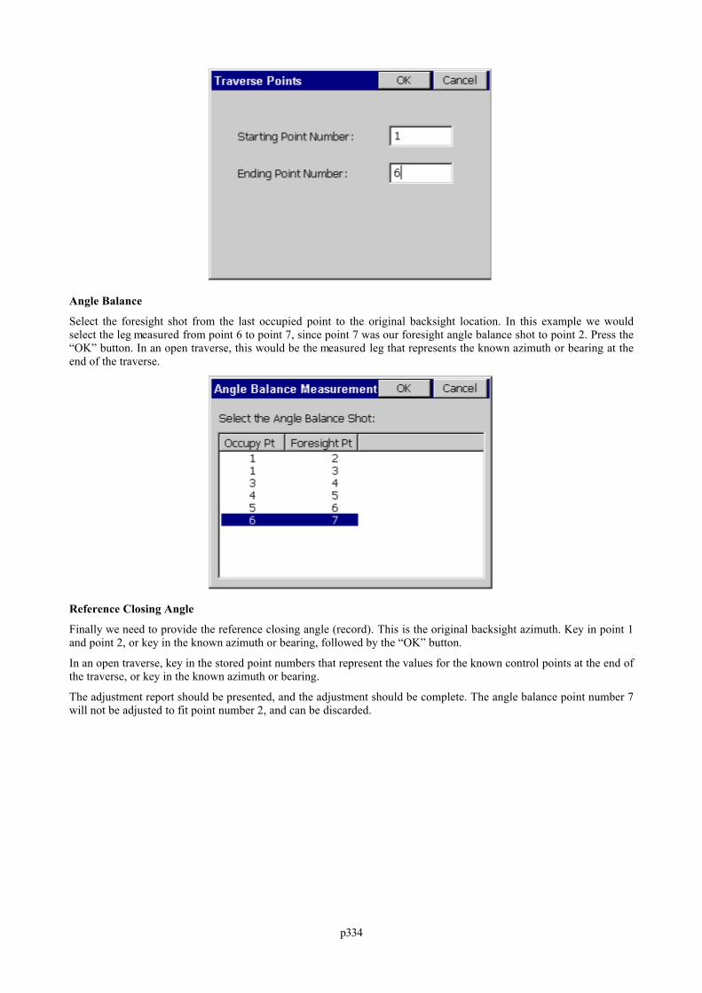
p334

Angle Balance

Select the foresight shot from the last occupied point to the original backsight location. In this example we wouldselect the leg measured from point 6 to point 7, since point 7 was our foresight angle balance shot to point 2. Press the“OK” button. In an open traverse, this would be the measured leg that represents the known azimuth or bearing at theend of the traverse.

Reference Closing Angle

Finally we need to provide the reference closing angle (record). This is the original backsight azimuth. Key in point 1and point 2, or key in the known azimuth or bearing, followed by the “OK” button.

In an open traverse, key in the stored point numbers that represent the values for the known control points at the end ofthe traverse, or key in the known azimuth or bearing.

The adjustment report should be presented, and the adjustment should be complete. The angle balance point number 7will not be adjusted to fit point number 2, and can be discarded.

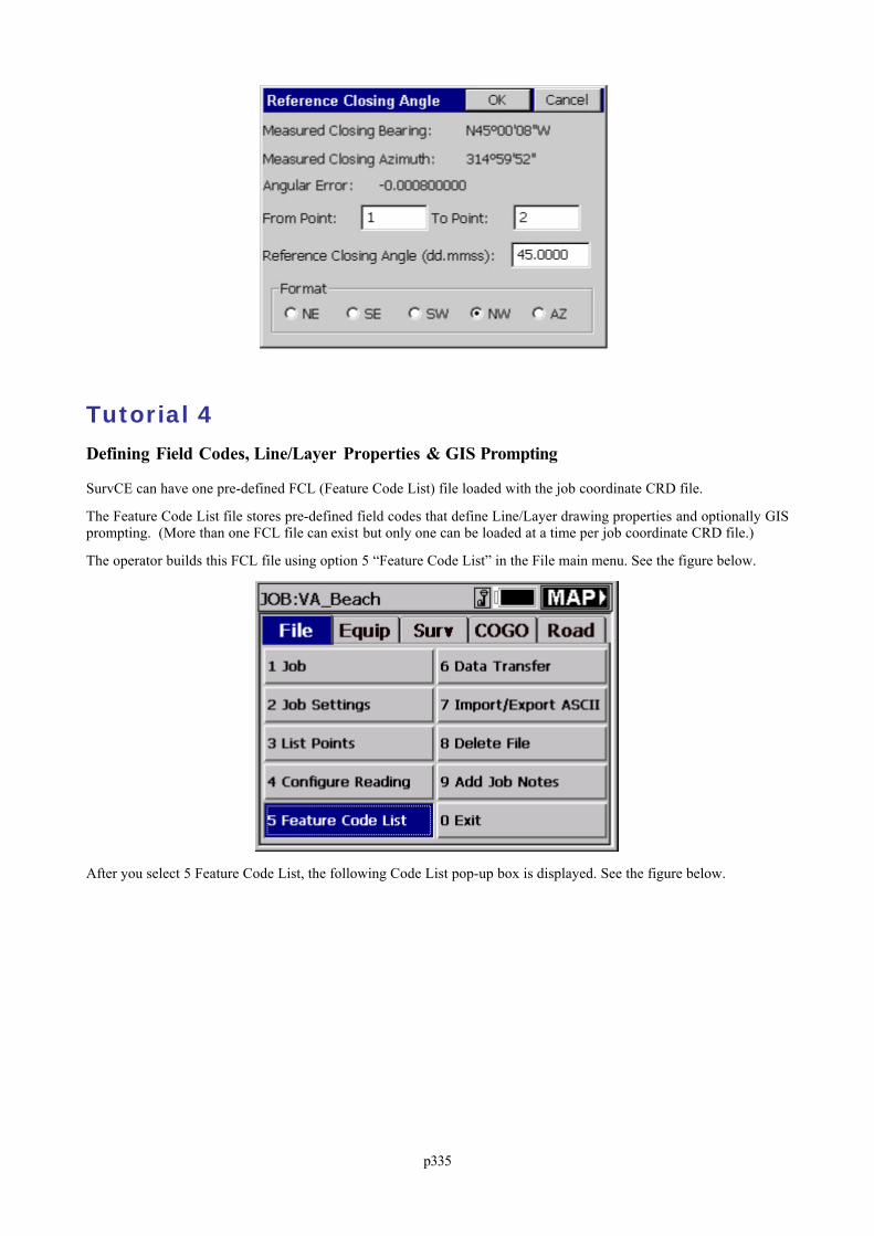
p335

Tutorial 4

Defining Field Codes, Line/Layer Properties & GIS Prompting

SurvCE can have one pre-defined FCL (Feature Code List) file loaded with the job coordinate CRD file.

The Feature Code List file stores pre-defined field codes that define Line/Layer drawing properties and optionally GISprompting. (More than one FCL file can exist but only one can be loaded at a time per job coordinate CRD file.)

The operator builds this FCL file using option 5 “Feature Code List” in the File main menu. See the figure below.

After you select 5 Feature Code List, the following Code List pop-up box is displayed. See the figure below.

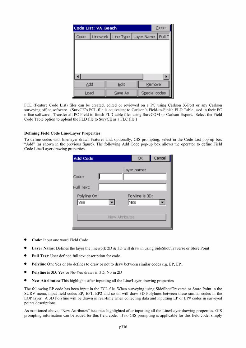
p336

FCL (Feature Code List) files can be created, edited or reviewed on a PC using Carlson X-Port or any Carlsonsurveying office software. (SurvCE’s FCL file is equivalent to Carlson’s Field-to-Finish FLD Table used in their PCoffice software. Transfer all PC Field-to-finish FLD table files using SurvCOM or Carlson Export. Select the FieldCode Table option to upload the FLD file to SurvCE as a FLC file.)

Defining Field Code Line/Layer PropertiesTo define codes with line/layer drawn features and, optionally, GIS prompting, select in the Code List pop-up box“Add” (as shown in the previous figure). The following Add Code pop-up box allows the operator to define FieldCode Line/Layer drawing properties.

Code: Input one word Field Code

Layer Name: Defines the layer the linework 2D & 3D will draw in using SideShot/Traverse or Store Point

Full Text: User defined full text description for code

Polyline On: Yes or No defines to draw or not to draw between similar codes e.g. EP, EP1

Polyline is 3D: Yes or No-Yes draws in 3D, No in 2D

New Attributes: This highlights after inputting all the Line/Layer drawing properties

The following EP code has been input in the FCL file. When surveying using SideShot/Traverse or Store Point in theSURV menu, input field codes EP, EP1, EP2 and so on will draw 3D Polylines between these similar codes in theEOP layer. A 3D Polyline will be drawn in real-time when collecting data and inputting EP or EP# codes in surveyedpoints descriptions.

As mentioned above, “New Attributes” becomes highlighted after inputting all the Line/Layer drawing properties. GISprompting information can be added for this field code. If no GIS prompting is applicable for this field code, simply

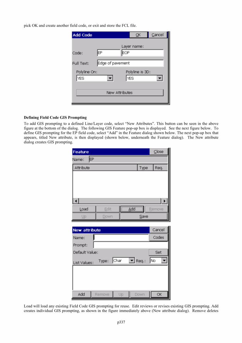
p337

pick OK and create another field code, or exit and store the FCL file.

Defining Field Code GIS PromptingTo add GIS prompting to a defined Line/Layer code, select “New Attributes”. This button can be seen in the abovefigure at the bottom of the dialog. The following GIS Feature pop-up box is displayed. See the next figure below. Todefine GIS prompting for the EP field code, select “Add” in the Feature dialog shown below. The next pop-up box thatappears, titled New attribute, is then displayed (shown below, underneath the Feature dialog). The New attributedialog creates GIS prompting.

Load will load any existing Field Code GIS prompting for reuse. Edit reviews or revises existing GIS prompting. Addcreates individual GIS prompting, as shown in the figure immediately above (New attribute dialog). Remove deletes

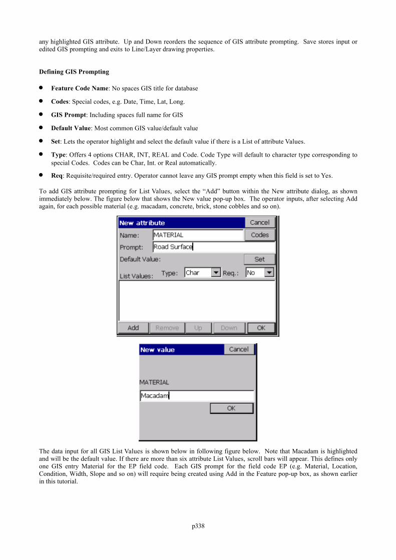
p338

any highlighted GIS attribute. Up and Down reorders the sequence of GIS attribute prompting. Save stores input oredited GIS prompting and exits to Line/Layer drawing properties.

Defining GIS Prompting

Feature Code Name: No spaces GIS title for database

Codes: Special codes, e.g. Date, Time, Lat, Long.

GIS Prompt: Including spaces full name for GIS

Default Value: Most common GIS value/default value

Set: Lets the operator highlight and select the default value if there is a List of attribute Values.

Type: Offers 4 options CHAR, INT, REAL and Code. Code Type will default to character type corresponding tospecial Codes. Codes can be Char, Int. or Real automatically.

Req: Requisite/required entry. Operator cannot leave any GIS prompt empty when this field is set to Yes.

To add GIS attribute prompting for List Values, select the “Add” button within the New attribute dialog, as shownimmediately below. The figure below that shows the New value pop-up box. The operator inputs, after selecting Addagain, for each possible material (e.g. macadam, concrete, brick, stone cobbles and so on).

The data input for all GIS List Values is shown below in following figure below. Note that Macadam is highlightedand will be the default value. If there are more than six attribute List Values, scroll bars will appear. This defines onlyone GIS entry Material for the EP field code. Each GIS prompt for the field code EP (e.g. Material, Location,Condition, Width, Slope and so on) will require being created using Add in the Feature pop-up box, as shown earlierin this tutorial.

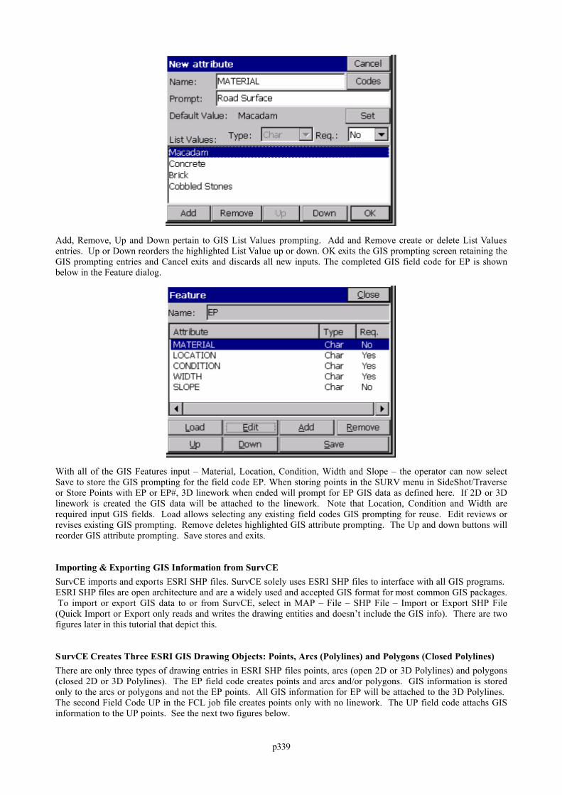
p339

Add, Remove, Up and Down pertain to GIS List Values prompting. Add and Remove create or delete List Valuesentries. Up or Down reorders the highlighted List Value up or down. OK exits the GIS prompting screen retaining theGIS prompting entries and Cancel exits and discards all new inputs. The completed GIS field code for EP is shownbelow in the Feature dialog.

With all of the GIS Features input – Material, Location, Condition, Width and Slope – the operator can now selectSave to store the GIS prompting for the field code EP. When storing points in the SURV menu in SideShot/Traverseor Store Points with EP or EP#, 3D linework when ended will prompt for EP GIS data as defined here. If 2D or 3Dlinework is created the GIS data will be attached to the linework. Note that Location, Condition and Width arerequired input GIS fields. Load allows selecting any existing field codes GIS prompting for reuse. Edit reviews orrevises existing GIS prompting. Remove deletes highlighted GIS attribute prompting. The Up and down buttons willreorder GIS attribute prompting. Save stores and exits.

Importing & Exporting GIS Information from SurvCESurvCE imports and exports ESRI SHP files. SurvCE solely uses ESRI SHP files to interface with all GIS programs. ESRI SHP files are open architecture and are a widely used and accepted GIS format for most common GIS packages. To import or export GIS data to or from SurvCE, select in MAP – File – SHP File – Import or Export SHP File(Quick Import or Export only reads and writes the drawing entities and doesn’t include the GIS info). There are twofigures later in this tutorial that depict this.

SurvCE Creates Three ESRI GIS Drawing Objects: Points, Arcs (Polylines) and Polygons (Closed Polylines)There are only three types of drawing entries in ESRI SHP files points, arcs (open 2D or 3D Polylines) and polygons(closed 2D or 3D Polylines). The EP field code creates points and arcs and/or polygons. GIS information is storedonly to the arcs or polygons and not the EP points. All GIS information for EP will be attached to the 3D Polylines. The second Field Code UP in the FCL job file creates points only with no linework. The UP field code attachs GISinformation to the UP points. See the next two figures below.

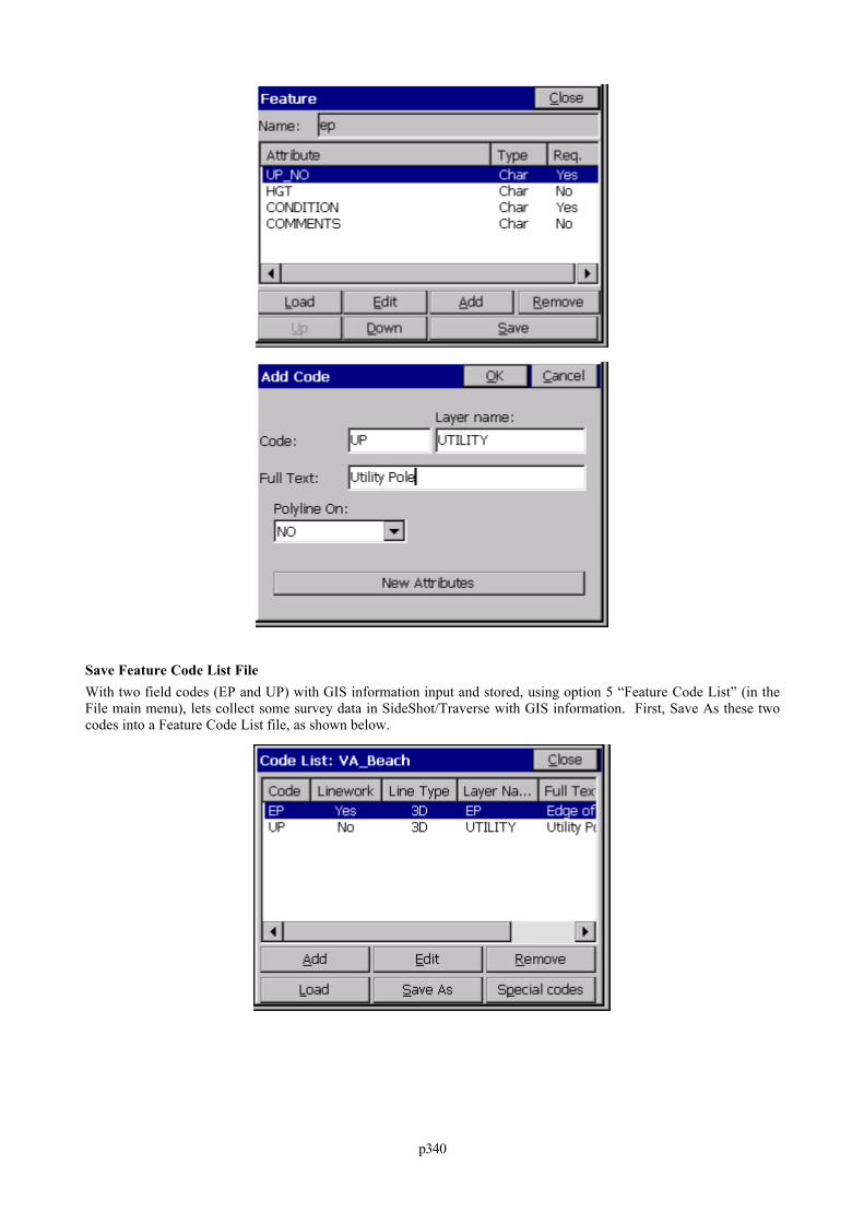
p340

Save Feature Code List FileWith two field codes (EP and UP) with GIS information input and stored, using option 5 “Feature Code List” (in theFile main menu), lets collect some survey data in SideShot/Traverse with GIS information. First, Save As these twocodes into a Feature Code List file, as shown below.

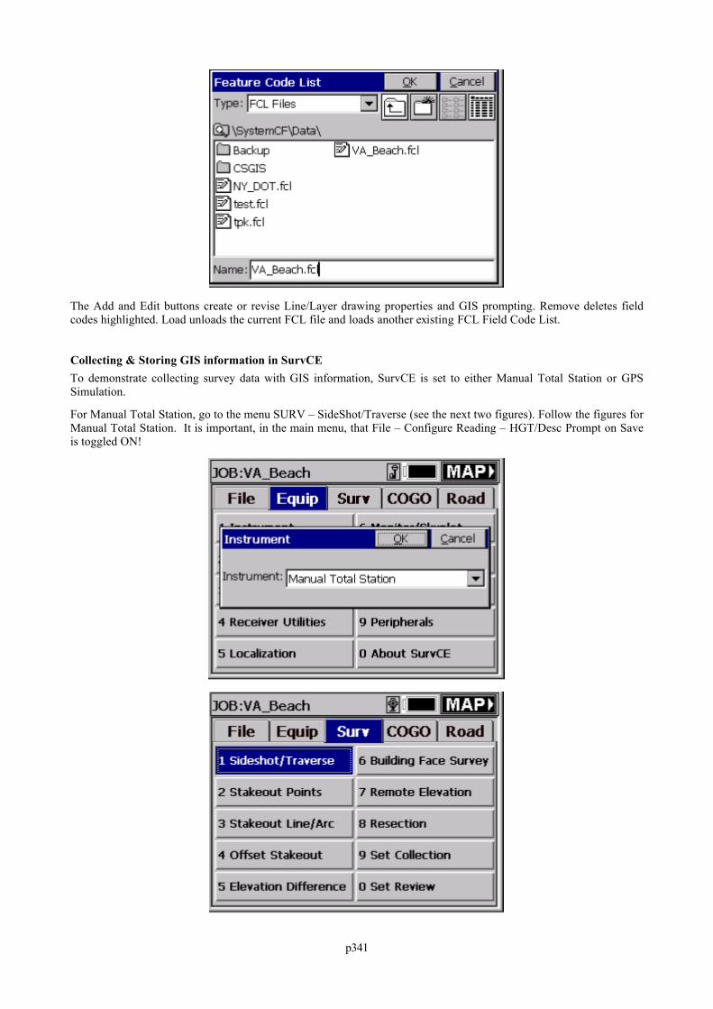
p341

The Add and Edit buttons create or revise Line/Layer drawing properties and GIS prompting. Remove deletes fieldcodes highlighted. Load unloads the current FCL file and loads another existing FCL Field Code List.

Collecting & Storing GIS information in SurvCETo demonstrate collecting survey data with GIS information, SurvCE is set to either Manual Total Station or GPSSimulation.

For Manual Total Station, go to the menu SURV – SideShot/Traverse (see the next two figures). Follow the figures forManual Total Station. It is important, in the main menu, that File – Configure Reading – HGT/Desc Prompt on Saveis toggled ON!

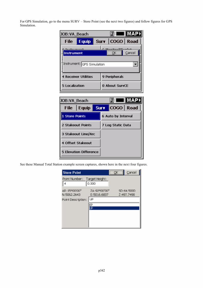
p342

For GPS Simulation, go to the menu SURV – Store Point (see the next two figures) and follow figures for GPSSimulation.

See these Manual Total Station example screen captures, shown here in the next four figures.

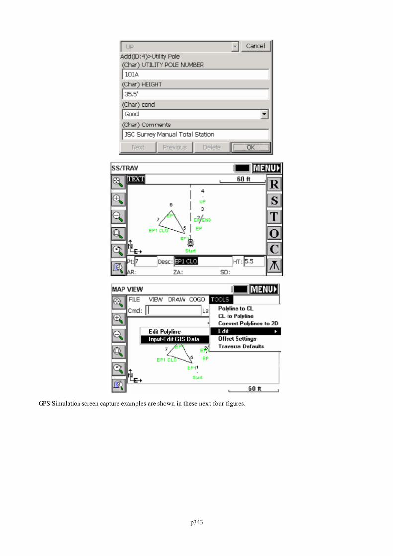
p343

GPS Simulation screen capture examples are shown in these next four figures.

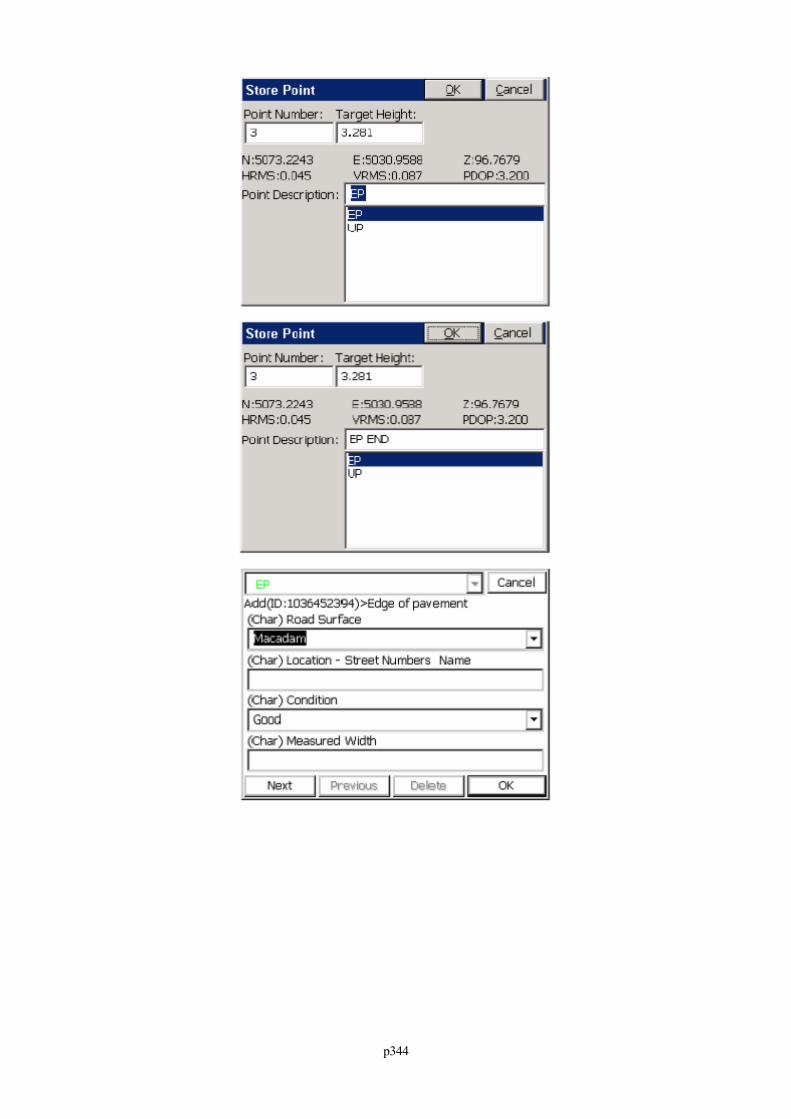
p344

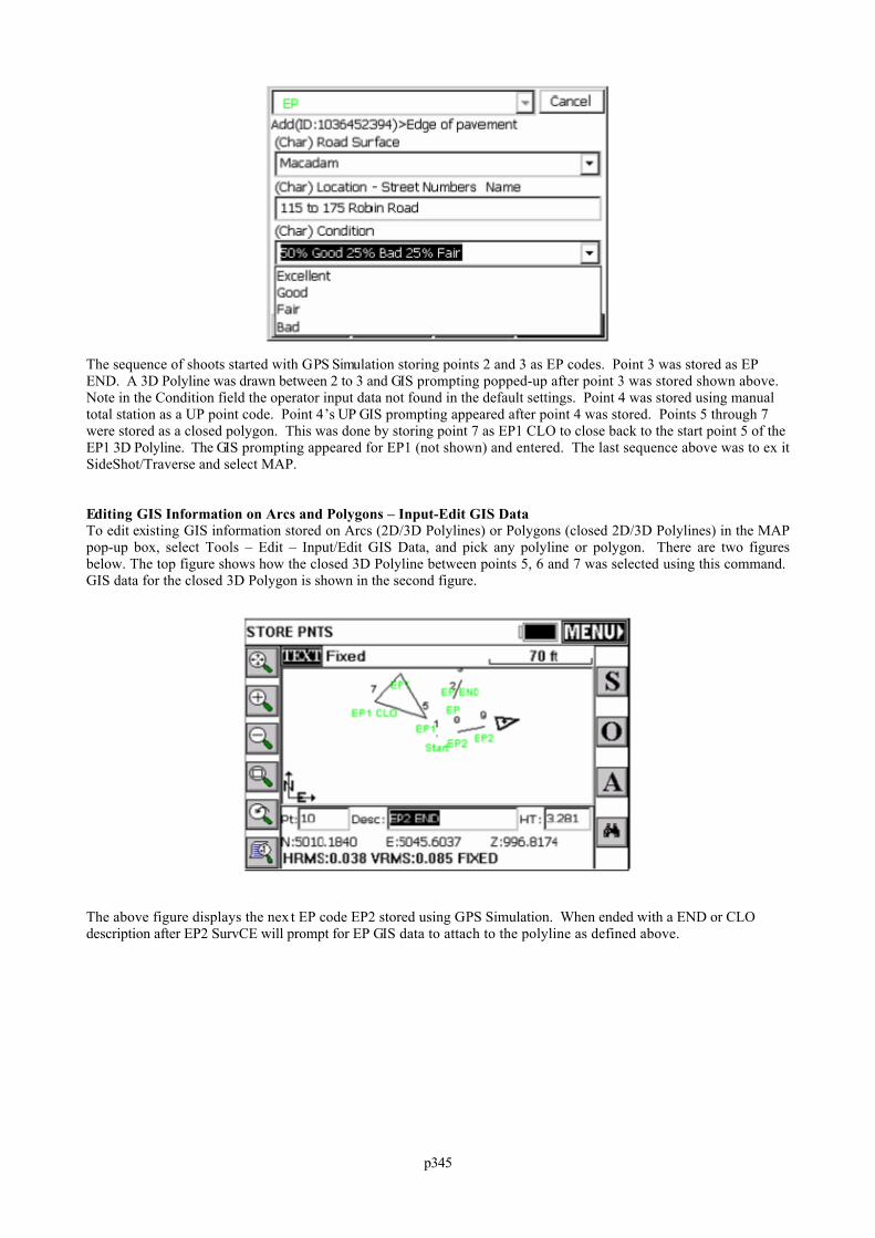
p345

The sequence of shoots started with GPS Simulation storing points 2 and 3 as EP codes. Point 3 was stored as EPEND. A 3D Polyline was drawn between 2 to 3 and GIS prompting popped-up after point 3 was stored shown above. Note in the Condition field the operator input data not found in the default settings. Point 4 was stored using manualtotal station as a UP point code. Point 4’s UP GIS prompting appeared after point 4 was stored. Points 5 through 7were stored as a closed polygon. This was done by storing point 7 as EP1 CLO to close back to the start point 5 of theEP1 3D Polyline. The GIS prompting appeared for EP1 (not shown) and entered. The last sequence above was to ex itSideShot/Traverse and select MAP.

Editing GIS Information on Arcs and Polygons – Input-Edit GIS DataTo edit existing GIS information stored on Arcs (2D/3D Polylines) or Polygons (closed 2D/3D Polylines) in the MAPpop-up box, select Tools – Edit – Input/Edit GIS Data, and pick any polyline or polygon. There are two figuresbelow. The top figure shows how the closed 3D Polyline between points 5, 6 and 7 was selected using this command. GIS data for the closed 3D Polygon is shown in the second figure.

The above figure displays the nex t EP code EP2 stored using GPS Simulation. When ended with a END or CLOdescription after EP2 SurvCE will prompt for EP GIS data to attach to the polyline as defined above.

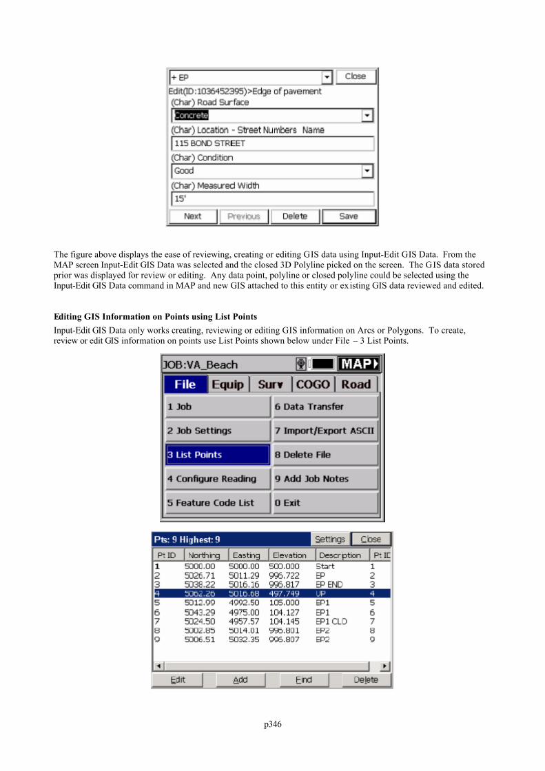
p346

The figure above displays the ease of reviewing, creating or editing GIS data using Input-Edit GIS Data. From theMAP screen Input-Edit GIS Data was selected and the closed 3D Polyline picked on the screen. The GIS data storedprior was displayed for review or editing. Any data point, polyline or closed polyline could be selected using theInput-Edit GIS Data command in MAP and new GIS attached to this entity or existing GIS data reviewed and edited.

Editing GIS Information on Points using List PointsInput-Edit GIS Data only works creating, reviewing or editing GIS information on Arcs or Polygons. To create,review or edit GIS information on points use List Points shown below under File – 3 List Points.

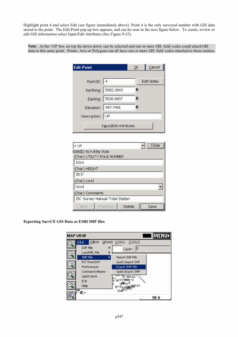
p347

Highlight point 4 and select Edit (see figure immediately above). Point 4 is the only surveyed number with GIS datastored to the point. The Edit Point pop-up box appears, and can be seen in the next figure below. To create, review oredit GIS information select Input/Edit Attributes (See Figure 9-32).

Note: At the +UP box on top the down arrow can be selected and one or more GIS field codes could attach GISdata to this same point. Points, Arcs or Polygons can all have one or more GIS field codes attached to these entities.

Exporting SurvCE GIS Data as ESRI SHP files

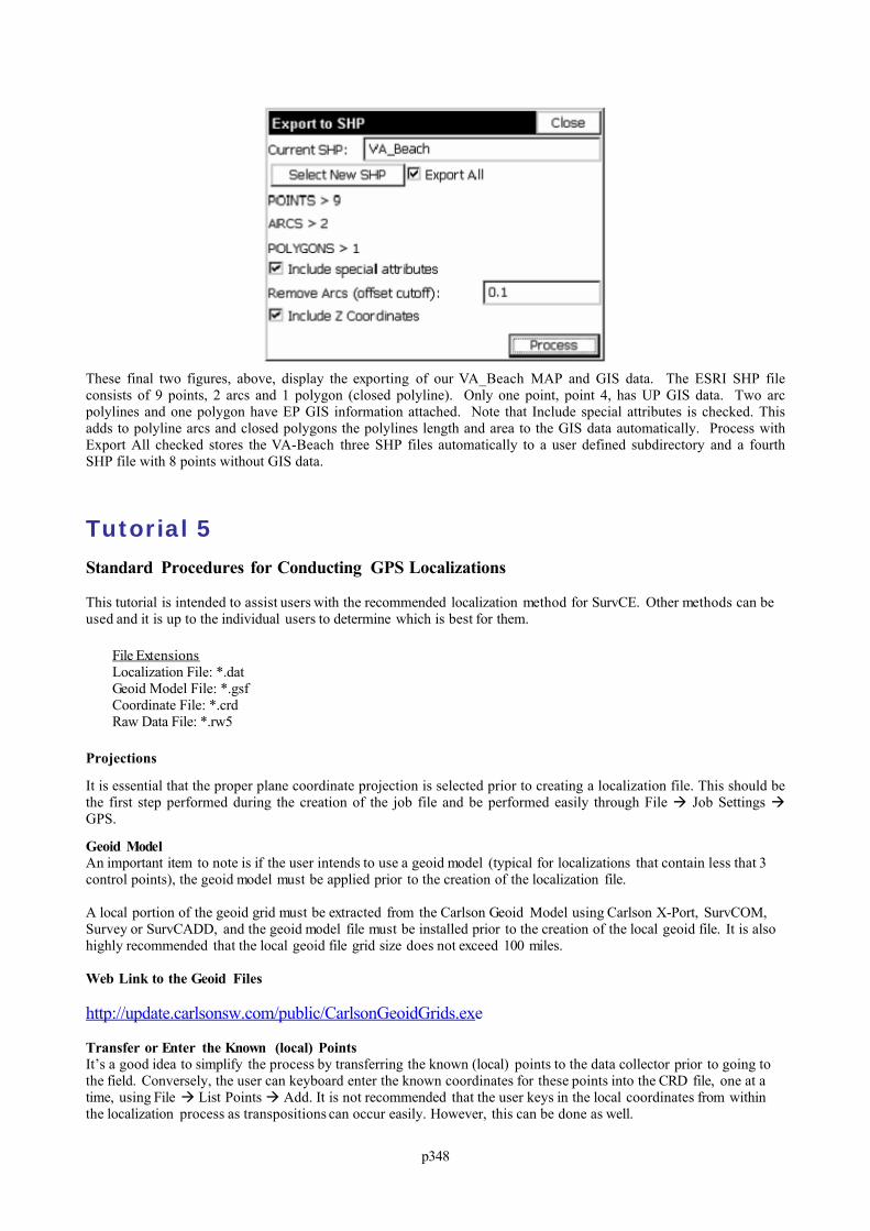
p348

These final two figures, above, display the exporting of our VA_Beach MAP and GIS data. The ESRI SHP fileconsists of 9 points, 2 arcs and 1 polygon (closed polyline). Only one point, point 4, has UP GIS data. Two arcpolylines and one polygon have EP GIS information attached. Note that Include special attributes is checked. Thisadds to polyline arcs and closed polygons the polylines length and area to the GIS data automatically. Process withExport All checked stores the VA-Beach three SHP files automatically to a user defined subdirectory and a fourthSHP file with 8 points without GIS data.

Tutorial 5

Standard Procedures for Conducting GPS Localizations

This tutorial is intended to assist users with the recommended localization method for SurvCE. Other methods can beused and it is up to the individual users to determine which is best for them.

File ExtensionsLocalization File: *.datGeoid Model File: *.gsfCoordinate File: *.crdRaw Data File: *.rw5

Projections

It is essential that the proper plane coordinate projection is selected prior to creating a localization file. This should bethe first step performed during the creation of the job file and be performed easily through File Job Settings GPS.

Geoid ModelAn important item to note is if the user intends to use a geoid model (typical for localizations that contain less that 3control points), the geoid model must be applied prior to the creation of the localization file.

A local portion of the geoid grid must be extracted from the Carlson Geoid Model using Carlson X-Port, SurvCOM,Survey or SurvCADD, and the geoid model file must be installed prior to the creation of the local geoid file. It is alsohighly recommended that the local geoid file grid size does not exceed 100 miles.

Web Link to the Geoid Files

http://update.carlsonsw.com/public/CarlsonGeoidGrids.exe

Transfer or Enter the Known (local) PointsIt’s a good idea to simplify the process by transferring the known (local) points to the data collector prior to going tothe field. Conversely, the user can keyboard enter the known coordinates for these points into the CRD file, one at atime, using File List Points Add. It is not recommended that the user keys in the local coordinates from withinthe localization process as transpositions can occur easily. However, this can be done as well.

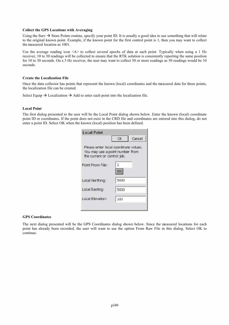
p349

Collect the GPS Locations with AveragingUsing the Surv Store Points routine, specify your point ID. It is usually a good idea to use something that will relateto the original known point. Example, if the known point for the first control point is 1, then you may want to collectthe measured location as 1001.

Use the average reading icon <A> to collect several epochs of data at each point. Typically when using a 1 Hzreceiver, 10 to 30 readings will be collected to ensure that the RTK solution is consistently reporting the same positionfor 10 to 30 seconds. On a 5 Hz receiver, the user may want to collect 50 or more readings as 50 readings would be 10seconds.

Create the Localization FileOnce the data collector has points that represent the known (local) coordinates and the measured data for these points,the localization file can be created.

Select Equip Localization Add to enter each point into the localization file.

Local PointThe first dialog presented to the user will be the Local Point dialog shown below. Enter the known (local) coordinatepoint ID or coordinates. If the point does not exist in the CRD file and coordinates are entered into this dialog, do notenter a point ID. Select OK when the known (local) position has been defined.

GPS Coordinates

The next dialog presented will be the GPS Coordinates dialog shown below. Since the measured locations for eachpoint has already been recorded, the user will want to use the option From Raw File in this dialog. Select OK tocontinue.

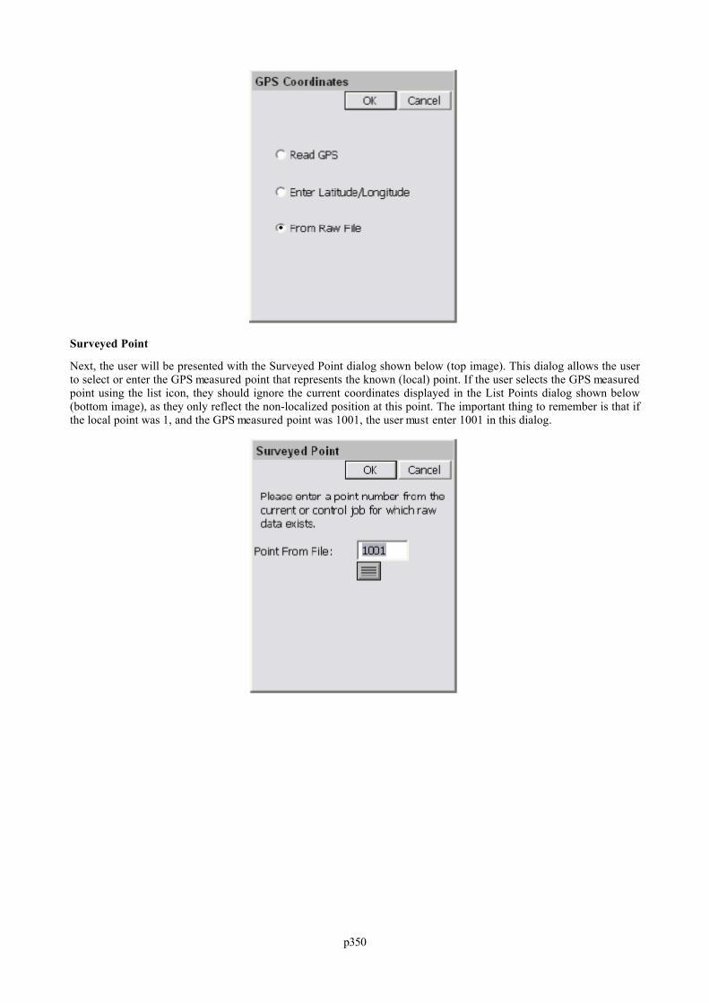
p350

Surveyed Point

Next, the user will be presented with the Surveyed Point dialog shown below (top image). This dialog allows the userto select or enter the GPS measured point that represents the known (local) point. If the user selects the GPS measuredpoint using the list icon, they should ignore the current coordinates displayed in the List Points dialog shown below(bottom image), as they only reflect the non-localized position at this point. The important thing to remember is that ifthe local point was 1, and the GPS measured point was 1001, the user must enter 1001 in this dialog.

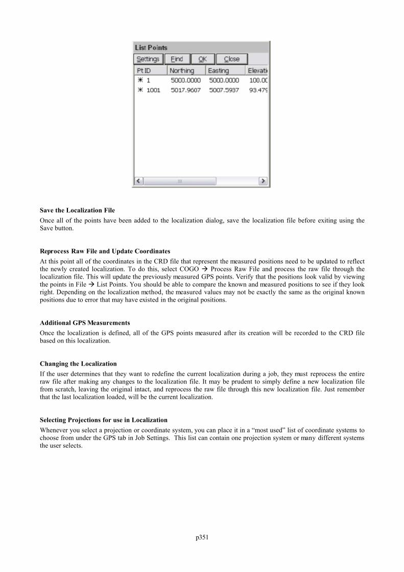
p351

Save the Localization FileOnce all of the points have been added to the localization dialog, save the localization file before exiting using theSave button.

Reprocess Raw File and Update CoordinatesAt this point all of the coordinates in the CRD file that represent the measured positions need to be updated to reflectthe newly created localization. To do this, select COGO Process Raw File and process the raw file through thelocalization file. This will update the previously measured GPS points. Verify that the positions look valid by viewingthe points in File List Points. You should be able to compare the known and measured positions to see if they lookright. Depending on the localization method, the measured values may not be exactly the same as the original knownpositions due to error that may have existed in the original positions.

Additional GPS MeasurementsOnce the localization is defined, all of the GPS points measured after its creation will be recorded to the CRD filebased on this localization.

Changing the LocalizationIf the user determines that they want to redefine the current localization during a job, they must reprocess the entireraw file after making any changes to the localization file. It may be prudent to simply define a new localization filefrom scratch, leaving the original intact, and reprocess the raw file through this new localization file. Just rememberthat the last localization loaded, will be the current localization.

Selecting Projections for use in LocalizationWhenever you select a projection or coordinate system, you can place it in a “most used” list of coordinate systems tochoose from under the GPS tab in Job Settings. This list can contain one projection system or many different systemsthe user selects.

p352

This is a special list of either predefined (eg. KY North NAD83) or user-defined coordinates systems. To get the liststarted or add to the list, select Edit Projection List and click Add Predefined. In the U.S., for example, surveyorsmight want to keep the UTM (WGS84) system plus the NAD83 and NAD27 “state plane” zones in the list for quickaccess, covering the region of your work. European and other worldwide zones can be added. When setting up aUTM selection, you can choose your zone, referencing the graphic below for the US:

You can see a map of the UTM zones online at:

http://www.dmap.co.uk/utmworld.htm

To edit the list of saved projections, click on Edit Projection List. Here we select a user-defined UTM system fromthe list to Delete or Edit.

p353

Choosing Edit will bring you to the screen below:

From this screen, you can select the Projection calculation method as well as calculation parameters. Projectionsinclude:

Lambert Conformal_Conic_2SP, Transverse_Mercator, Oblique_Sterographic (Double), Lambert_Conformal_Conic_1SP, Oblique_Mercator_83, Stereographic, Oblique_Mercator_27, Transverse_Mercator_OSTN02, Oblique_Stereographic_RD2000, Oblique_Mercator, Cassini_Soldner, Transverse_Mercator_27, Lambert_Conformal_Conic_27, Transverse_Mercator_Alaska_27 Transverse_Mercator_34.

You may also use the buttons on this screen to edit the existing datum or create a new datum definition.

p354

The Datum definition screen is where you select the ellipsoid and Helmert parameters to apply.

If you select Add User Defined within the Coordinate Projection List screen, you proceed to the screen below:

Here you enter the name of the new system and select the projection type and parameters, or you can “Load File” toload a pre-defined system stored earlier (in the form *.sys or *.csl).

If you select “Add Predefined” to create a new, stored projection system, you will be presented with this screen:

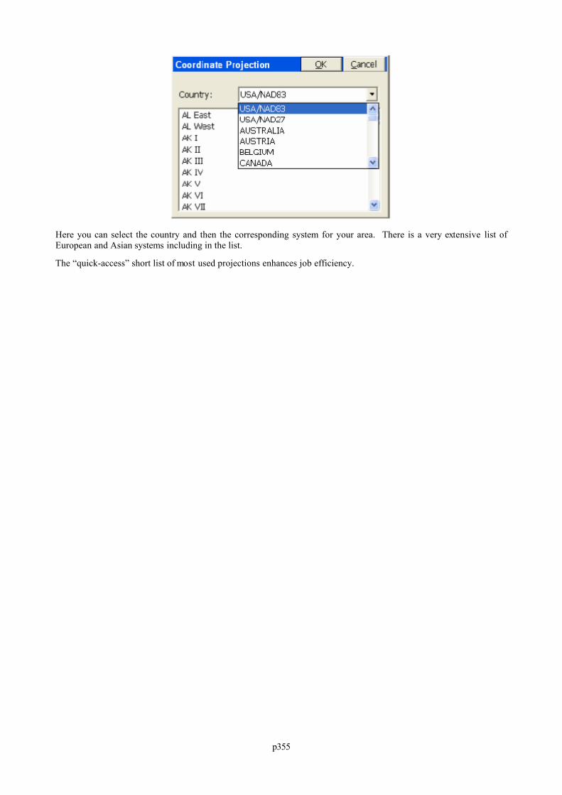
p355

Here you can select the country and then the corresponding system for your area. There is a very extensive list ofEuropean and Asian systems including in the list.

The “quick-access” short list of most used projections enhances job efficiency.

p356

TroubleshootingThis chapter contains troubleshooting tips for Carlson SurvCE, and the various hardware devices supported bySurvCE.

GPS HeightsSurvCE records GPS heights as the ellipsoid height, expressed in meters, at either the phase center or the ARP of theantenna, depending on the GPS make. If the position is recorded to the ARP, then the LS record (antenna height) willonly reflect the user entered value. If the position is recorded to the phase center, then the LS record (antenna height)will reflect the user entered value plus the phase center offset.

SurvCE records the ARP position for the following GPS makes: Leica Geodetics

Handheld Hardware

How do I reset the computer after a lock up?RangerHold down the power button until the computer resets or instructs you to hold it for 5 more seconds to reset.

AllegroHold down the power button until the computer resets.

Why can’t I load the software?The computer may disconnect from ActiveSync when there is not enough memory allocated to “Storage Memory”. Inthe control panel, select the “System” icon followed by the Memory tab. Position the slider so that there is 5mb (5120kb) allocated and not in use (i.e. if the “In Use” value says 1024 kb then add 1024 & 5120 to determine what the“Allocated” value should be.

How do I clear the RAM backup and why?Clearing the RAM backup seems to improve performance on the Ranger platform after new programs have beeninstalled or removed. Make sure that all software applications are closed and select the “RAM Backup” icon from thecontrol panel. Select the “Delete” button and answer “Yes” to the three resulting message boxes.

Why can’t I communicate through the COM port?If you cannot communicate with the instrument, verify all COM settings in SurvCE and make sure that they match theCOM settings on the instrument. If it happens to be that you were communicating fine and the COM settings have notbeen altered, try one of the following until it clears up the COM port:

Exit SurvCE, turn off the computer, turn back on the computer and re-enter SurvCE. Exit SurvCE and perform a soft reset on the device (Verify that all applications have been closed). Exit SurvCE and perform a hard reset on the device (Verify that all applications have been closed).

How do I set the CAPS LOCK status?RangerHold down the yellow shift button [ ^ ] and the [ALT] buttons, then press and release the power button.A small keyboard should be showing. On the small keyboard, press the [CAPS] button then repeat step 1 to dismissthe keyboard.

AllegroPress and release the blue function button followed by the CapLk/Shift button located at the lower left side of thekeyboard.

How frequently should I charge the device?

p357

Refer to your hardware manual for specifics, but most of the newer CE devices are coming with lithium ion batteriesthat do not establish a “memory” based on your charging habits after the initial charge has been established per themanufacturers suggestions. Charge the device as necessary which will likely be nightly to ensure a full battery for thenext day in the field.

How do I calibrate the touch screen?In the control panel of the CE device, select the “Stylus” icon to configure the “Double Tab” and “Calibration” of thetouch screen.

How do I turn on/off the backlight?RangerHold down the shift button [ ^ ] and then press and release the power button.

AllegroPress and release the yellow function button followed by the F3/F8 button located at the top center of the keyboard.

How can I speed up the Allegro performance?In the control panel of the Allegro, select the “System” icon and then the “Memory” tab. Set your “Storage Memory”allocation to 8000 KB or 8 MB +/-. This should provide more RAM to the system for operating the programs andincrease performance.

How can I Recover the SurvCE Icon if it Disappears?It may be possible to lose the SurvCE Icon off the desktop if, for example, the power drains out of the CE device. There are safeguards against this, but if it happens, follow these steps to restore the icon:1. Select Start (lower left on most CE devices, Ctrl Esc on the Ranger) and choose Windows Explorer under

Programs.2. Navigate to the SurvStar directory (the directory containing SurvCE), which on some devices is \Disk\SurvStar.3. Look for the SurvCE Shortcut and highlight it (select it).4. Choose the Edit Pulldown in Windows Explorer and choose Copy.5. Then return to the desktop where the icons are visible and press Alt then tap into blank space on the screen

(sometimes referred to as Alt Click).6. Choose Paste Shortcut. That should restore it.

If the icon disappears, this indicates some problem in the original installation of SurvCE, since a process occurs tomake the icon permanent. You can help ensure that your restored icon is permanent by going to Start, Settings,Control Panel and choosing Perform Ram Backup. Select Backup Now, as prompted. This should make the SurvCEicon remain even after full loss of battery.

Can I lose data or get bad data if I Re-Boot my CE device?If you re-boot your Allegro or Carlson Explorer or Ipaq or any other CE device you are using, you can lose yourantenna height or prism height information, for the following reasons:

SurvCE does not store to memory changes in antenna height or prism height, except in the following scenarios:

The hard save of antenna/prism heights is done when the user exits the program, when you save a configuration fromthe instrument icon at the top of the screen, when you say OK to Configure Rover, Configure Base or Equip/Settings(for TS), when you change jobs and when you enter Equip/Comm Settings.  Prior to release 1.50.007, in November,2004, even Configure Rover did not save the height information "to disk".

Therefore, if you re-boot, hard reset or otherwise exit the program by any method other than the normal File, Exitmethod, recent changes to the prism height or antenna height may not be saved.  On re-entering the program, the x,yposition for GPS work, for example, will very likely be correct, but elevations may be in error.  When using GPS, it isrecommended, after a re-boot, that you do the command Configure Rover to re-establish the correct elevations, and inall cases (GPS and Total Station) it is recommended that you double-check your antenna or prism heights beforeproceeding.

Miscellaneous Instrument ConfigurationLeica Robotic - Do I need to be in RCS (Remote Control) mode?You must verify that you are NOT in RCS mode when using SurvCE with Leica robotic equipment. It will appear as

p358

though you are not communicating with the instrument if this mode is active. Refer to the Leica documentation forhow to exit RCS mode.

Leica GPS - What firmware will allow radio channel changing?Firmware version 3.52 or later is required for SurvCE to have radio channel changing functionality.

Geodimeter 600 - What firmware version is required?Firmware version 696-03.xx or later is required for SurvCE to operate with this instrument. To check the firmware onthe instrument, follow the key strokes below: Menu, 5, 4, 1

Supported File Formats

What file types does SurvCE use or convert?

ALI ISPOL Centerline File (Spain)

ALN TerraModel Road Alignment File

ALZ Form of CLIP Vertical Alignment File (Spain)

ASC ASCII text file for point imports or Inroads Centerline File

CL Carlson Horizontal Road Alignment File

CR5 TDS Binary Coordinate File

CRD Carlson coordinate file in binary form.

DAT Carlson Localization File

DXF Drawing file format that can be used for exchanging drawings.

EGM Carlson EGM Geoid File

FCL Carlson Field Code Library file.

FFF Older form of Caice Cross Section File

FLT Carlson Triangulation Mesh File

G99 Carlson Geoid99 File

GRD Carlson Grid File

GSI Leica file extension for Raw files, Roading files, etc.

INF Carlson User Preferences Settings File

INP MOSS Roading Files (Horizontal and Vertical Alignment)

LIS Form of IGRDS Cross Section File

NOT Carlson Note File

OBS Geodimeter Coordinate File

OSD A form of Geopak Centerline File

PLT Horizontal Alignment Report file from CLIP (Spain)

POS Sokkia or Trimble Coordinate File

PRO Carlson Vertical Road Alignment File

RAS ISPOL Vertical Road Alignment File (Spain)

RD5 TDS Road Alignment File

RDS IGRDS Cross Section File

REF Carlson Base Station Reference File

RLN TerraModel Road Alignment File

RW5 Carlson Raw Data File, TDS Raw Data File

SC1 ISPOL Cross Section File (Spain)

SCT Carlson Cross Section File

SDR Sokkia file extension for Raw Files, Roading files, etc.

SHP ESRI Shape File

SUP Carlson Road Superelevation File

p359

TPL Carlson Road Template File

TPT Carlson Road Template Transition File

TRV Traverse PC Coordinate File and CLIP Format for Sections (Spain)

XML LandXML File may contain a variety of file types (eg. Roading/DTM)

XRS Form of Geopak Cross Section File

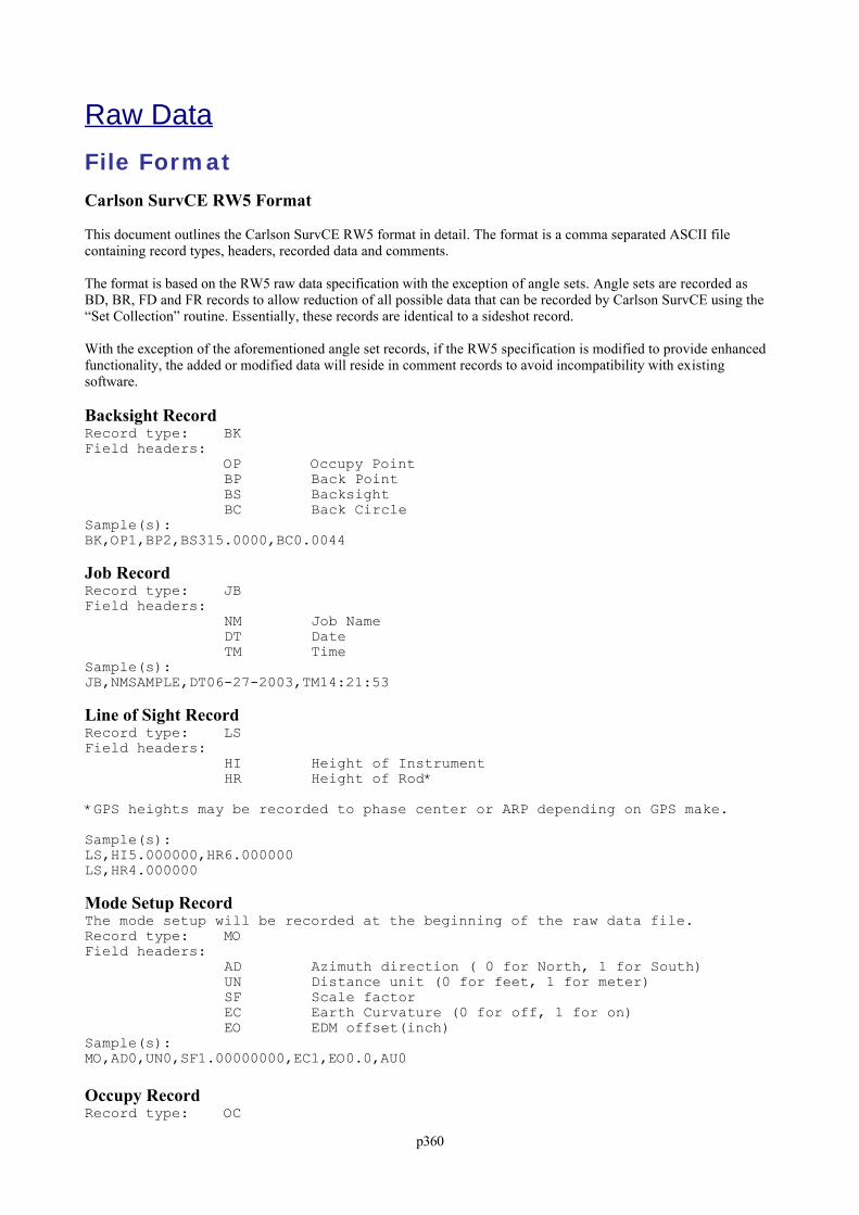
p360

Raw DataFile Format

Carlson SurvCE RW5 Format

This document outlines the Carlson SurvCE RW5 format in detail. The format is a comma separated ASCII filecontaining record types, headers, recorded data and comments.

The format is based on the RW5 raw data specification with the exception of angle sets. Angle sets are recorded asBD, BR, FD and FR records to allow reduction of all possible data that can be recorded by Carlson SurvCE using the“Set Collection” routine. Essentially, these records are identical to a sideshot record.

With the exception of the aforementioned angle set records, if the RW5 specification is modified to provide enhancedfunctionality, the added or modified data will reside in comment records to avoid incompatibility with existingsoftware.

Backsight RecordRecord type: BK

Field headers:

OP Occupy Point

BP Back Point

BS Backsight

BC Back Circle

Sample(s):

BK,OP1,BP2,BS315.0000,BC0.0044

Job RecordRecord type: JB

Field headers:

NM Job Name

DT Date

TM Time

Sample(s):

JB,NMSAMPLE,DT06-27-2003,TM14:21:53

Line of Sight RecordRecord type: LS

Field headers:

HI Height of Instrument

HR Height of Rod*

*GPS heights may be recorded to phase center or ARP depending on GPS make.

Sample(s):

LS,HI5.000000,HR6.000000

LS,HR4.000000

Mode Setup RecordThe mode setup will be recorded at the beginning of the raw data file.

Record type: MO

Field headers:

AD Azimuth direction ( 0 for North, 1 for South)

UN Distance unit (0 for feet, 1 for meter)

SF Scale factor

EC Earth Curvature (0 for off, 1 for on)

EO EDM offset(inch)

Sample(s):

MO,AD0,UN0,SF1.00000000,EC1,EO0.0,AU0

Occupy RecordRecord type: OC

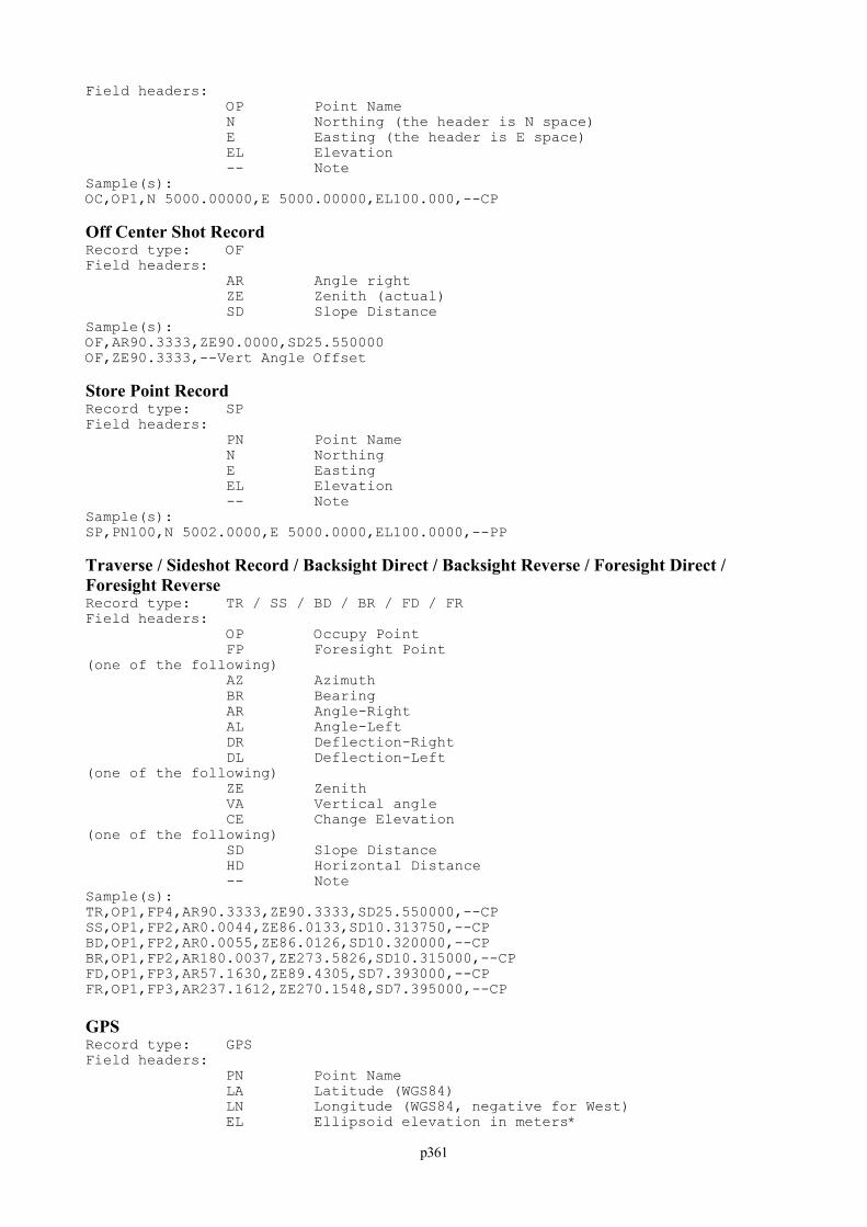
p361

Field headers:

OP Point Name

N Northing (the header is N space)

E Easting (the header is E space)

EL Elevation

-- Note

Sample(s):

OC,OP1,N 5000.00000,E 5000.00000,EL100.000,--CP

Off Center Shot RecordRecord type: OF

Field headers:

AR Angle right

ZE Zenith (actual)

SD Slope Distance

Sample(s):

OF,AR90.3333,ZE90.0000,SD25.550000

OF,ZE90.3333,--Vert Angle Offset

Store Point RecordRecord type: SP

Field headers:

PN Point Name

N Northing

E Easting

EL Elevation

-- Note

Sample(s):

SP,PN100,N 5002.0000,E 5000.0000,EL100.0000,--PP

Traverse / Sideshot Record / Backsight Direct / Backsight Reverse / Foresight Direct /Foresight ReverseRecord type: TR / SS / BD / BR / FD / FR

Field headers:

OP Occupy Point

FP Foresight Point

(one of the following)

AZ Azimuth

BR Bearing

AR Angle-Right

AL Angle-Left

DR Deflection-Right

DL Deflection-Left

(one of the following)

ZE Zenith

VA Vertical angle

CE Change Elevation

(one of the following)

SD Slope Distance

HD Horizontal Distance

-- Note

Sample(s):

TR,OP1,FP4,AR90.3333,ZE90.3333,SD25.550000,--CP

SS,OP1,FP2,AR0.0044,ZE86.0133,SD10.313750,--CP

BD,OP1,FP2,AR0.0055,ZE86.0126,SD10.320000,--CP

BR,OP1,FP2,AR180.0037,ZE273.5826,SD10.315000,--CP

FD,OP1,FP3,AR57.1630,ZE89.4305,SD7.393000,--CP

FR,OP1,FP3,AR237.1612,ZE270.1548,SD7.395000,--CP

GPSRecord type: GPS

Field headers:

PN Point Name

LA Latitude (WGS84)

LN Longitude (WGS84, negative for West)

EL Ellipsoid elevation in meters*

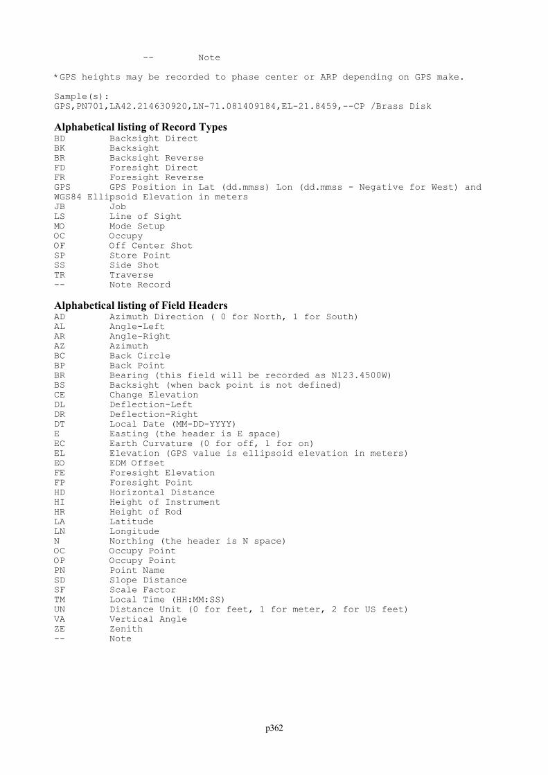
p362

-- Note

*GPS heights may be recorded to phase center or ARP depending on GPS make.

Sample(s):

GPS,PN701,LA42.214630920,LN-71.081409184,EL-21.8459,--CP /Brass Disk

Alphabetical listing of Record TypesBD Backsight Direct

BK Backsight

BR Backsight Reverse

FD Foresight Direct

FR Foresight Reverse

GPS GPS Position in Lat (dd.mmss) Lon (dd.mmss - Negative for West) and

WGS84 Ellipsoid Elevation in meters

JB Job

LS Line of Sight

MO Mode Setup

OC Occupy

OF Off Center Shot

SP Store Point

SS Side Shot

TR Traverse

-- Note Record

Alphabetical listing of Field HeadersAD Azimuth Direction ( 0 for North, 1 for South)

AL Angle-Left

AR Angle-Right

AZ Azimuth

BC Back Circle

BP Back Point

BR Bearing (this field will be recorded as N123.4500W)

BS Backsight (when back point is not defined)

CE Change Elevation

DL Deflection-Left

DR Deflection-Right

DT Local Date (MM-DD-YYYY)

E Easting (the header is E space)

EC Earth Curvature (0 for off, 1 for on)

EL Elevation (GPS value is ellipsoid elevation in meters)

EO EDM Offset

FE Foresight Elevation

FP Foresight Point

HD Horizontal Distance

HI Height of Instrument

HR Height of Rod

LA Latitude

LN Longitude

N Northing (the header is N space)

OC Occupy Point

OP Occupy Point

PN Point Name

SD Slope Distance

SF Scale Factor

TM Local Time (HH:MM:SS)

UN Distance Unit (0 for feet, 1 for meter, 2 for US feet)

VA Vertical Angle

ZE Zenith

-- Note

p363

Index

- A -Abbreviations 26About SurvCE 64Add Job Notes 64Areas 201Authorizing SurvCE 14Auto By Interval 175

- B -Basics 300Battery Status 16Building Face Survey 173

- C -Calculator 213Carlson Technical Support 17COGO 320Color Screens 16Comm Setup 122Configure Base/Rover 84Configure Base/Rover (Allen-Osbourne GPS) 89Configure Base/Rover (CSI - DGPS Max GPS) 89Configure Base/Rover (Leica 500/1200 GPS) 90Configure Base/Rover (Leica GIS System 50 GPS) 91Configure Base/Rover (Navcom GPS) 91Configure Base/Rover (NMEA GPS) 94Configure Base/Rover (Novatel GPS) 95Configure Base/Rover (Sokkia GPS) 95Configure Base/Rover (Thales/Ashtech GPS) 96Configure Base/Rover (Topcon GPS) 99Configure Base/Rover (Trimble GPS) 102Configure Reading (GPS - General) 50Configure Reading (GPS - Reference) 50Configure Reading (Total Station - General) 47Configure Reading (Total Station - Reference) 49Cross Section Survey 272

- D -Data Transfer 56Delete File 62Draw 314Draw Centerline 250Draw Profile 254Draw Template 258

- E -Elevation Difference 170End-User License Agreement 5Exit 64

- F -Feature Code List 51File 302

p364

File Format 360

- G -GPS Heights 356Graphic Mode 18

- H -Handheld Hardware 356Hardware Notes 15Hot Keys 20

- I -Import/Export ASCII File 60Input Box Controls 23Input-Edit Centerline 233Input-Edit Profile 252Input-Edit Template 255Installing SurvCE 11Instrument 65Instrument Recall 129Intersections 203Inverse 199

- J -Job 28Job Settings (GPS) 34Job Settings (New Job) 34Job Settings (Options) 29Job Settings (Stakeout) 40Job Settings (Units) 32

- K -Keyboard Input 198Keyboard Operation 25

- L -List Points 44Localization 115Log Static Data 178

- M -Memory 16Microsoft ActiveSync 7Miscellaneous Instrument Configuration 357Monitor/SkyPlot 119

- O -Offset Stakeout 163Orientation (Backsight) 132Orientation (Instrument Setup) 131Orientation (Remote Benchmark) 133Orientation (Robotics) 134

- P -Peripherals 125Point in Direction 230

p365

Point Projection 206Process Raw File 217

- Q -Quick Calculator 19

- R -Receiver Utilities 106Receiver Utilities (Leica 500/1200) 106Receiver Utilities (Navcom) 107Receiver Utilities (Sokkia and Novatel) 111Receiver Utilities (Thales/Ashtech) 111Receiver Utilities (Topcon) 114Receiver Utilities (Trimble) 115Remote Elevation 177Resection 190Road Utilities 281

- S -Save System 16Set Collection 192Set Review 197Settings (Geodimeter/Trimble TS) 65Settings (Leica Robotic TS) 72Settings (Leica TPS Series TS) 69Settings (Leica/Wild Older Models) 76Settings (Nikon TS) 76Settings (Pentax TS) 76Settings (Sokkia Set TS) 77Settings (Topcon 800/8000/APL1 TS) 79Settings (Topcon GTS TS) 83Sideshot Traverse (Offsets) 137Sideshot/Traverse 136Slope Staking 259Stakeout Line/Arc (Stake Arc) 162Stakeout Line/Arc (Stake Centerline) 156Stakeout Line/Arc (Stake Line) 151Stakeout Points 145Station Store 209Store Points 139Store Points (Offsets) 141Supported File Formats 358System Requirements 7

- T -Template Stakeout 296Tolerances 121Tools 325Transformation 210Tutorial 1 330Tutorial 2 331Tutorial 3 331Tutorial 4 335Tutorial 5 348

- U -Using the Manual 7

p366

- V -View 311View Point Options 19