
Oracle8i - Oracle Help Center
412
Oracle8i Data Warehousing Guide Release 2 (8.1.6) December 1999 Part No. A76994-01
-
Upload
khangminh22 -
Category
Documents
-
view
2 -
download
0
Transcript of Oracle8i - Oracle Help Center

Oracle8 i
Data Warehousing Guide
Release 2 (8.1.6)
December 1999
Part No. A76994-01

Data Warehousing Guide, Release 2 (8.1.6)
Part No. A76994-01
Copyright © 1996, 1999, Oracle Corporation. All rights reserved.
Primary Author: Paul Lane
Contributing Author: George Lumpkin
Contributors: Patrick Amor, Tolga Bozkaya, Karl Dias, Yu Gong, Ira Greenberg, Helen Grembowicz,John Haydu, Meg Hennington, Lilian Hobbs, Hakan Jakobsson, Jack Raitto, Ray Roccaforte, AndyWitkowski, Zia Ziauddin
Graphic Designer: Valarie Moore
The Programs are not intended for use in any nuclear, aviation, mass transit, medical, or otherinherently dangerous applications. It shall be the licensee’s responsibility to take all appropriatefail-safe, backup, redundancy and other measures to ensure the safe use of such applications if thePrograms are used for such purposes, and Oracle disclaims liability for any damages caused by suchuse of the Programs.
The Programs (which include both the software and documentation) contain proprietary information ofOracle Corporation; they are provided under a license agreement containing restrictions on use anddisclosure and are also protected by copyright, patent, and other intellectual and industrial propertylaws. Reverse engineering, disassembly, or decompilation of the Programs is prohibited.
The information contained in this document is subject to change without notice. If you find anyproblems in the documentation, please report them to us in writing. Oracle Corporation does notwarrant that this document is error free. Except as may be expressly permitted in your license agreementfor these Programs, no part of these Programs may be reproduced or transmitted in any form or by anymeans, electronic or mechanical, for any purpose, without the express written permission of OracleCorporation.
If the Programs are delivered to the U.S. Government or anyone licensing or using the Programs onbehalf of the U.S. Government, the following notice is applicable:
Restricted Rights Notice Programs delivered subject to the DOD FAR Supplement are "commercialcomputer software" and use, duplication, and disclosure of the Programs including documentation, shallbe subject to the licensing restrictions set forth in the applicable Oracle license agreement. Otherwise,Programs delivered subject to the Federal Acquisition Regulations are "restricted computer software"and use, duplication, and disclosure of the Programs shall be subject to the restrictions in FAR 52.227-19,Commercial Computer Software - Restricted Rights (June, 1987). Oracle Corporation, 500 OracleParkway, Redwood City, CA 94065.
Oracle is a registered trademark, and Enterprise Manager, Pro*COBOL, Server Manager, SQL*Forms,SQL*Net, and SQL*Plus, Net8, Oracle Call Interface, Oracle7, Oracle7 Server, Oracle8, Oracle8 Server,Oracle8i, Oracle Forms, PL/SQL, Pro*C, Pro*C/C++, and Trusted Oracle are registered trademarks ortrademarks of Oracle Corporation. All other company or product names mentioned are used foridentification purposes only and may be trademarks of their respective owners.
Send Us Your Comments .................................................................................................................. xv
Preface ......................................................................................................................................................... xvii
Audience............................................................................................................................................... xviiKnowledge Assumed of the Reader .......................................................................................... xviiInstallation and Migration Information .................................................................................... xviiApplication Design Information ................................................................................................ xvii
How Oracle8i Data Warehousing Guide Is Organized .............................................................. xviiiConventions Used in This Manual ................................................................................................... xx
Part I Concepts
1 Data Warehousing Concepts
What is a Data Warehouse? ............................................................................................................... 1-2Subject Oriented............................................................................................................................ 1-2Integrated....................................................................................................................................... 1-2Nonvolatile .................................................................................................................................... 1-2Time Variant.................................................................................................................................. 1-3Contrasting a Data Warehouse with an OLTP System ........................................................... 1-3
Typical Data Warehouse Architectures........................................................................................... 1-5
Part II Logical Design
2 Overview of Logical Design
Logical vs. Physical............................................................................................................................. 2-2Create a Logical Design ..................................................................................................................... 2-2Data Warehousing Schemas ............................................................................................................. 2-3
Star Schemas.................................................................................................................................. 2-3Other Schemas .............................................................................................................................. 2-4Data Warehousing Objects.......................................................................................................... 2-4Fact Tables ..................................................................................................................................... 2-5Dimensions .................................................................................................................................... 2-5
Part III Physical Design
iii

3 Overview of Physical Design
Moving from Logical to Physical Design ....................................................................................... 3-2Physical Design ................................................................................................................................... 3-3
Physical Design Structures .......................................................................................................... 3-3Tablespaces .................................................................................................................................... 3-3Partitions ........................................................................................................................................ 3-3Indexes............................................................................................................................................ 3-4Constraints..................................................................................................................................... 3-4
4 Hardware and I/O
Striping ................................................................................................................................................. 4-2Input/Output Considerations ........................................................................................................... 4-9
Staging File Systems ..................................................................................................................... 4-9
5 Parallelism and Partitioning
Overview of Parallel Execution Tuning.......................................................................................... 5-2When to Implement Parallel Execution..................................................................................... 5-2
Tuning Physical Database Layouts .................................................................................................. 5-3Types of Parallelism ..................................................................................................................... 5-3Partitioning Data........................................................................................................................... 5-4Partition Pruning ........................................................................................................................ 5-10Partition-wise Joins..................................................................................................................... 5-12
6 Indexes
Bitmap Indexes .................................................................................................................................... 6-2B-tree Indexes ...................................................................................................................................... 6-6Local Versus Global ............................................................................................................................ 6-6
7 Constraints
Why Constraints are Useful in a Data Warehouse ....................................................................... 7-2Overview of Constraint States.......................................................................................................... 7-2Typical Data Warehouse Constraints .............................................................................................. 7-3
Unique Constraints in a Data Warehouse................................................................................. 7-3
iv

Foreign Key Constraints in a Data Warehouse ........................................................................ 7-5RELY Constraints ......................................................................................................................... 7-5Constraints and Parallelism ........................................................................................................ 7-6Constraints and Partitioning....................................................................................................... 7-6
8 Materialized Views
Overview of Data Warehousing with Materialized Views......................................................... 8-2Materialized Views for Data Warehouses ................................................................................ 8-3Materialized Views for Distributed Computing...................................................................... 8-3Materialized Views for Mobile Computing.............................................................................. 8-3
The Need for Materialized Views ................................................................................................... 8-3Components of Summary Management ................................................................................... 8-5Terminology .................................................................................................................................. 8-7Schema Design Guidelines for Materialized Views ................................................................ 8-8
Types of Materialized Views .......................................................................................................... 8-10Materialized Views with Joins and Aggregates..................................................................... 8-11Single-Table Aggregate Materialized Views .......................................................................... 8-12Materialized Views Containing Only Joins ............................................................................ 8-13
Creating a Materialized View......................................................................................................... 8-16Naming......................................................................................................................................... 8-17Storage Characteristics............................................................................................................... 8-17Build Methods............................................................................................................................. 8-18Used for Query Rewrite............................................................................................................. 8-18Query Rewrite Restrictions ....................................................................................................... 8-18Refresh Options .......................................................................................................................... 8-19ORDER BY................................................................................................................................... 8-22Using Oracle Enterprise Manager............................................................................................ 8-23
Nested Materialized Views............................................................................................................. 8-23Why Use Nested Materialized Views? .................................................................................... 8-23Rules for Using Nested Materialized Views........................................................................... 8-24Restrictions when Using Nested Materialized Views........................................................... 8-24Limitations of Nested Materialized Views ............................................................................. 8-25Example of a Nested Materialized View................................................................................. 8-26Nesting Materialized Views with Joins and Aggregates...................................................... 8-28Nested Materialized View Usage Guidelines......................................................................... 8-28
v

Registration of an Existing Materialized View ........................................................................... 8-29Partitioning a Materialized View................................................................................................... 8-31
Partitioning the Materialized View.......................................................................................... 8-32Partitioning a Prebuilt Table ..................................................................................................... 8-33
Indexing Selection for Materialized Views ................................................................................. 8-34Invalidating a Materialized View .................................................................................................. 8-34
Security Issues ............................................................................................................................. 8-35Guidelines for Using Materialized Views in a Data Warehouse............................................. 8-35Altering a Materialized View ......................................................................................................... 8-36Dropping a Materialized View....................................................................................................... 8-36Overview of Materialized View Management Tasks................................................................. 8-37
9 Dimensions
What is a Dimension? ........................................................................................................................ 9-2Drilling Across .............................................................................................................................. 9-5
Creating a Dimension ........................................................................................................................ 9-6Multiple Hierarchies..................................................................................................................... 9-8Using Normalized Dimension Tables...................................................................................... 9-10Dimension Wizard...................................................................................................................... 9-11
Viewing Dimensions........................................................................................................................ 9-11Using The DEMO_DIM Package.............................................................................................. 9-12Using Oracle Enterprise Manager ............................................................................................ 9-13
Dimensions and Constraints .......................................................................................................... 9-13Validating a Dimension ................................................................................................................... 9-14Altering a Dimension....................................................................................................................... 9-14Deleting a Dimension ...................................................................................................................... 9-15
Part IV Managing the Warehouse Environment
10 ETT Overview
ETT Overview.................................................................................................................................... 10-2ETT Tools ............................................................................................................................................ 10-2ETT Sample Schema......................................................................................................................... 10-3
vi

11 Extraction
Overview of Extraction .................................................................................................................... 11-2Extracting Via Data Files ................................................................................................................. 11-2
Extracting into Flat Files Using SQL*Plus............................................................................... 11-3Extracting into Flat Files Using OCI or Pro*C Programs...................................................... 11-4Exporting into Oracle Export Files Using Oracle's EXP Utility ........................................... 11-4Copying to Another Oracle Database Using Transportable Tablespaces .......................... 11-5
Extracting Via Distributed Operations ......................................................................................... 11-5Change Capture................................................................................................................................. 11-6
Timestamps ................................................................................................................................. 11-7Partitioning.................................................................................................................................. 11-7Triggers ........................................................................................................................................ 11-7
12 Transportation
Transportation Overview ................................................................................................................ 12-2Transportation of Flat Files ....................................................................................................... 12-2Transportation Via Distributed Operations............................................................................ 12-2Transportable Tablespaces ........................................................................................................ 12-3
13 Transformation
Techniques for Data Transformation Inside the Database ....................................................... 13-2Transformation Flow.................................................................................................................. 13-2Transformations Provided by SQL*Loader ............................................................................ 13-3Transformations Using SQL and PL/SQL.............................................................................. 13-4Data Substitution ........................................................................................................................ 13-5Key Lookups................................................................................................................................ 13-5Pivoting ........................................................................................................................................ 13-7Emphasis on Transformation Techniques .............................................................................. 13-9
14 Loading and Refreshing
Refreshing a Data Warehouse ........................................................................................................ 14-2Using Partitioning to Improve Data Warehouse Refresh..................................................... 14-2Populating Databases Using Parallel Load........................................................................... 14-10
Refreshing Materialized Views ................................................................................................... 14-16
vii

Complete Refresh...................................................................................................................... 14-18Fast Refresh................................................................................................................................ 14-18Tips for Refreshing Using Refresh ......................................................................................... 14-22Complex Materialized Views.................................................................................................. 14-27Recommended Initialization Parameters for Parallelism ................................................... 14-27Monitoring a Refresh................................................................................................................ 14-28Tips after Refreshing Materialized Views............................................................................. 14-28
15 Summary Advisor
Summary Advisor ............................................................................................................................. 15-2Collecting Structural Statistics .................................................................................................. 15-3Collection of Dynamic Workload Statistics ............................................................................ 15-3Recommending Materialized Views........................................................................................ 15-5Estimating Materialized View Size .......................................................................................... 15-7Summary Advisor Wizard ........................................................................................................ 15-8
Is a Materialized View Being Used?.............................................................................................. 15-8
Part V Warehouse Performance
16 Schemas
Schemas............................................................................................................................................... 16-2Star Schemas ................................................................................................................................ 16-2
Optimizing Star Queries ................................................................................................................. 16-4Tuning Star Queries.................................................................................................................... 16-4Star Transformation.................................................................................................................... 16-5
17 SQL for Analysis
Overview............................................................................................................................................. 17-2Analyzing Across Multiple Dimensions ................................................................................. 17-2Optimized Performance............................................................................................................. 17-4A Scenario .................................................................................................................................... 17-5
ROLLUP .............................................................................................................................................. 17-6Syntax ........................................................................................................................................... 17-6Details ........................................................................................................................................... 17-6
viii

Example........................................................................................................................................ 17-6Interpreting NULLs in Results ................................................................................................. 17-8Partial Rollup .............................................................................................................................. 17-8Calculating Subtotals without ROLLUP ................................................................................. 17-9When to Use ROLLUP ............................................................................................................. 17-10
CUBE ................................................................................................................................................. 17-10Syntax ......................................................................................................................................... 17-11Details......................................................................................................................................... 17-11Example...................................................................................................................................... 17-11Partial Cube ............................................................................................................................... 17-13Calculating Subtotals without CUBE .................................................................................... 17-14When to Use CUBE .................................................................................................................. 17-14
Using Other Aggregate Functions with ROLLUP and CUBE ................................................ 17-15GROUPING Function.................................................................................................................... 17-15
Syntax ......................................................................................................................................... 17-15Examples.................................................................................................................................... 17-16When to Use GROUPING ....................................................................................................... 17-18
Other Considerations when Using ROLLUP and CUBE ........................................................ 17-19Hierarchy Handling in ROLLUP and CUBE........................................................................ 17-19Column Capacity in ROLLUP and CUBE............................................................................. 17-20HAVING Clause Used with ROLLUP and CUBE............................................................... 17-20ORDER BY Clause Used with ROLLUP and CUBE............................................................ 17-21
Analytic Functions.......................................................................................................................... 17-21Ranking Functions.................................................................................................................... 17-24Windowing Functions.............................................................................................................. 17-35Reporting Functions................................................................................................................. 17-43Lag/Lead Functions................................................................................................................. 17-46Statistics Functions ................................................................................................................... 17-46
Case Expressions ............................................................................................................................. 17-52CASE Example .......................................................................................................................... 17-52Creating Histograms with User-defined Buckets ................................................................ 17-53
18 Tuning Parallel Execution
Introduction to Parallel Execution Tuning................................................................................... 18-2When to Implement Parallel Execution................................................................................... 18-2
ix

Initializing and Tuning Parameters for Parallel Execution ...................................................... 18-3Selecting Automated or Manual Tuning of Parallel Execution ............................................... 18-3
Automatically Derived Parameter Settings under Fully Automated Parallel Execution 18-4Setting the Degree of Parallelism and Enabling Adaptive Multi-User ................................. 18-5
Degree of Parallelism and Adaptive Multi-User and How They Interact ......................... 18-5Enabling Parallelism for Tables and Queries.......................................................................... 18-6Forcing Parallel Execution for a Session.................................................................................. 18-7Controlling Performance with PARALLEL_THREADS_PER_CPU................................... 18-7
Tuning General Parameters............................................................................................................. 18-8Parameters Establishing Resource Limits for Parallel Operations ...................................... 18-8Parameters Affecting Resource Consumption ..................................................................... 18-17Parameters Related to I/O....................................................................................................... 18-25
Example Parameter Setting Scenarios for Parallel Execution ................................................ 18-27Example One: Small Datamart................................................................................................ 18-28Example Two: Medium-sized Data Warehouse................................................................... 18-29Example Three: Large Data Warehouse ................................................................................ 18-30Example Four: Very Large Data Warehouse ........................................................................ 18-31
Miscellaneous Tuning Tips ........................................................................................................... 18-33Formula for Memory, Users, and Parallel Execution Server Processes............................ 18-33Setting Buffer Pool Size for Parallel Operations................................................................... 18-36Balancing the Formula ............................................................................................................. 18-37Examples: Balancing Memory, Users, and Parallel Execution Servers............................. 18-40Parallel Execution Space Management Issues ...................................................................... 18-43Tuning Parallel Execution on Oracle Parallel Server........................................................... 18-44Overriding the Default Degree of Parallelism...................................................................... 18-48Rewriting SQL Statements....................................................................................................... 18-49Creating and Populating Tables in Parallel .......................................................................... 18-50Creating Temporary Tablespaces for Parallel Sort and Hash Join .................................... 18-51Executing Parallel SQL Statements ........................................................................................ 18-53Using EXPLAIN PLAN to Show Parallel Operations Plans............................................... 18-54Additional Considerations for Parallel DML ....................................................................... 18-54Creating Indexes in Parallel .................................................................................................... 18-57Parallel DML Tips..................................................................................................................... 18-59Incremental Data Loading in Parallel .................................................................................... 18-62Using Hints with Cost-Based Optimization ......................................................................... 18-64
x

Monitoring and Diagnosing Parallel Execution Performance ............................................... 18-64Is There Regression?................................................................................................................. 18-66Is There a Plan Change?........................................................................................................... 18-67Is There a Parallel Plan?........................................................................................................... 18-67Is There a Serial Plan? .............................................................................................................. 18-67Is There Parallel Execution? .................................................................................................... 18-68Is The Workload Evenly Distributed? ................................................................................... 18-68Monitoring Parallel Execution Performance with Dynamic Performance Views .......... 18-69Monitoring Session Statistics .................................................................................................. 18-72Monitoring Operating System Statistics................................................................................ 18-75
19 Query Rewrite
Overview of Query Rewrite............................................................................................................ 19-2Cost-Based Rewrite .......................................................................................................................... 19-3Enabling Query Rewrite.................................................................................................................. 19-4
Initialization Parameters for Query Rewrite .......................................................................... 19-5Privileges for Enabling Query Rewrite ................................................................................... 19-6
When Does Oracle Rewrite a Query? ........................................................................................... 19-6Query Rewrite Methods .................................................................................................................. 19-8
SQL Text Match Rewrite Methods........................................................................................... 19-8General Query Rewrite Methods ............................................................................................. 19-9Query Rewrite with CUBE/ROLLUP Operator .................................................................. 19-20
When are Constraints and Dimensions Needed?..................................................................... 19-21Complex Materialized Views.................................................................................................. 19-21View-based Materialized View .............................................................................................. 19-22Rewrite with Nested Materialized Views ............................................................................. 19-22
Expression Matching...................................................................................................................... 19-23Date Folding .............................................................................................................................. 19-24
Accuracy of Query Rewrite ........................................................................................................... 19-26Did Query Rewrite Occur?............................................................................................................ 19-27
Explain Plan............................................................................................................................... 19-27Controlling Query Rewrite ..................................................................................................... 19-28
Guidelines for Using Query Rewrite.......................................................................................... 19-29Constraints................................................................................................................................. 19-29Dimensions ................................................................................................................................ 19-29
xi

Outer Joins ................................................................................................................................. 19-29SQL Text Match......................................................................................................................... 19-30Aggregates ................................................................................................................................. 19-30Grouping Conditions ............................................................................................................... 19-30Expression Matching................................................................................................................ 19-31Date Folding .............................................................................................................................. 19-31Statistics...................................................................................................................................... 19-31
Part VI Miscellaneous
20 Data Marts
What Is a Data Mart? ........................................................................................................................ 20-2How Is It Different from a Data Warehouse? ......................................................................... 20-2Dependent, Independent, and Hybrid Data Marts ............................................................... 20-2Extraction, Transformation, and Transportation ................................................................... 20-5
A Glossary
xii

xiii

xiv

Send Us Your Comments
Oracle8 i Data Warehousing Guide, Release 2 (8.1.6)
Part No. A76994-01
Oracle Corporation welcomes your comments and suggestions on the quality and usefulness of this
publication. Your input is an important part of the information used for revision.
■ Did you find any errors?
■ Is the information clearly presented?
■ Do you need more information? If so, where?
■ Are the examples correct? Do you need more examples?
■ What features did you like most about this manual?
If you find any errors or have any other suggestions for improvement, please indicate the chapter,
section, and page number (if available). You can send comments to us in the following ways:
■ E-mail - [email protected]
■ FAX - (650) 506-7228
■ Postal service:
Oracle Corporation
Server Technologies Documentation Manager
500 Oracle Parkway
Redwood Shores, CA 94065
USA
If you would like a reply, please give your name, address, and telephone number below.
If you have problems with the software, please contact your local Oracle Support Services.
xv

xvi

Preface
This manual provides reference information about Oracle8i’s data warehousing
capabilities.
AudienceThis manual is written for database administrators, system administrators, and
database application developers who need to deal with data warehouses.
Knowledge Assumed of the ReaderIt is assumed that readers of this manual are familiar with relational database
concepts, basic Oracle server concepts, and the operating system environment
under which they are running Oracle.
Installation and Migration InformationThis manual is not an installation or migration guide. If your primary interest is
installation, refer to your operating-system-specific Oracle documentation. If your
primary interest is database and application migration, refer to Oracle8i Migration.
Application Design InformationIn addition to administrators, experienced users of Oracle and advanced database
application designers will find information in this manual useful. However,
database application developers should also refer to the Oracle8i ApplicationDeveloper’s Guide - Fundamentals and to the documentation for the tool or language
product they are using to develop Oracle database applications.
xvii
How Oracle8 i Data Warehousing Guide Is OrganizedThis manual is organized as follows:
Chapter 1, "Data Warehousing Concepts"This chapter contains an overview of data warehousing concepts.
Chapter 2, "Overview of Logical Design"This chapter contains an explanation of how to do logical design.
Chapter 3, "Overview of Physical Design"This chapter contains an explanation of how to do physical design.
Chapter 4, "Hardware and I/O"This chapter describes some hardware and input/output issues.
Chapter 5, "Parallelism and Partitioning"This chapter describes the basics of parallelism and partitioning in data
warehouses.
Chapter 6, "Indexes"This chapter describes how to use indexes in data warehouses.
Chapter 7, "Constraints"This chapter describes some issues involving constraints.
Chapter 8, "Materialized Views"This chapter describes how to use materialized views in data warehouses.
Chapter 9, "Dimensions"This chapter describes how to use dimensions in data warehouses.
Chapter 10, "ETT Overview"This chapter describes an overview of the ETT process.
Chapter 11, "Extraction"This chapter describes issues involved with extraction.
xviii
Chapter 12, "Transportation"This chapter describes issues involved with transporting data in data warehouses.
Chapter 13, "Transformation"This chapter describes issues involved with transforming data in data warehouses.
Chapter 14, "Loading and Refreshing"This chapter describes how to refresh in a data warehousing environment.
Chapter 15, "Summary Advisor"This chapter describes how to use the Summary Advisor utility.
Chapter 16, "Schemas"This chapter describes the schemas useful in data warehousing environments.
Chapter 17, "SQL for Analysis"This chapter explains how to use analytic functions in data warehouses.
Chapter 18, "Tuning Parallel Execution"This chapter describes how to tune data warehouses using parallel execution.
Chapter 19, "Query Rewrite"This chapter describes using Query Rewrite.
Chapter 20, "Data Marts"This chapter contains an introduction to Data Marts, and how they differ from
warehouses.
Appendix A, "Glossary"This chapter defines commonly used data warehousing terms.
xix

Conventions Used in This ManualThe following sections describe the conventions used in this manual.
Text of the ManualThe text of this manual uses the following conventions.
UPPERCASE CharactersUppercase text is used to call attention to command keywords, database object
names, parameters, filenames, and so on.
For example, "After inserting the default value, Oracle checks the FOREIGN KEY
integrity constraint defined on the DEPTNO column," or "If you create a private
rollback segment, the name must be included in the ROLLBACK_SEGMENTS
initialization parameter."
Italicized CharactersItalicized words within text are book titles or emphasized words.
Code ExamplesCommands or statements of SQL, Oracle Enterprise Manager line mode (Server
Manager), and SQL*Plus appear in a monospaced font.
For example:
INSERT INTO emp (empno, ename) VALUES (1000, 'SMITH');ALTER TABLESPACE users ADD DATAFILE 'users2.ora' SIZE 50K;
Example statements may include punctuation, such as commas or quotation marks.
All punctuation in example statements is required. All example statements
terminate with a semicolon (;). Depending on the application, a semicolon or other
terminator may or may not be required to end a statement.
UPPERCASE in Code ExamplesUppercase words in example statements indicate the keywords within Oracle SQL.
When you issue statements, however, keywords are not case sensitive.
lowercase in Code ExamplesLowercase words in example statements indicate words supplied only for the
context of the example. For example, lowercase words may indicate the name of a
table, column, or file.
xx

Your Comments Are WelcomeWe value and appreciate your comment as an Oracle user and reader of our
manuals. As we write, revise, and evaluate our documentation, your opinions are
the most important feedback we receive.
You can send comments and suggestions about this manual to the Information
Development department at the following e-mail address:
If you prefer, you can send letters or faxes containing your comments to:
Server Technologies Documentation Manager
Oracle Corporation
500 Oracle Parkway Redwood Shores, CA 94065
Fax: (650) 506-7228 Attn: Data Warehousing Guide
xxi

xxii

Part I
ConceptsThis section introduces basic data warehousing concepts.
It contains the following chapter:
■ Data Warehousing Concepts


Data Warehousing Con
1
Data Warehousing ConceptsThis chapter provides an overview of the Oracle implementation of data
warehousing. Its sections include:
■ What is a Data Warehouse?
■ Typical Data Warehouse Architectures
Note that this book is meant as a supplement to standard texts covering data
warehousing, and is not meant to reproduce in detail material of a general nature.
This book, therefore, focuses on Oracle-specific material. Two standard texts of a
general nature are:
■ The Data Warehouse Toolkit by Ralph Kimball
■ Building the Data Warehouse by William Inmon
cepts 1-1

What is a Data Warehouse?
What is a Data Warehouse?A data warehouse is a relational database that is designed for query and analysis
rather than transaction processing. It usually contains historical data that is derived
from transaction data, but it can include data from other sources. It separates
analysis workload from transaction workload and enables an organization to
consolidate data from several sources.
In addition to a relational database, a data warehouse environment often consists of
an Extraction, Transportation, and Transformation (ETT) solution, an online
analytical processing (OLAP) engine, client analysis tools, and other applications
that manage the process of gathering data and delivering it to business users. See
Chapter 10, "ETT Overview", for further information regarding the ETT process.
A common way of introducing data warehousing is to refer to Inmon’s
characteristics of a data warehouse, who says that they are:
■ Subject Oriented
■ Integrated
■ Nonvolatile
■ Time Variant
Subject OrientedData warehouses are designed to help you analyze your data. For example, you
might want to learn more about your company’s sales data. To do this, you could
build a warehouse concentrating on sales. In this warehouse, you could answer
questions like "Who was our best customer for this item last year?" This kind of
focus on a topic, sales in this case, is what is meant by subject oriented.
IntegratedIntegration is closely related to subject orientation. Data warehouses need to have
the data from disparate sources put into a consistent format. This means that
naming conflicts have to be resolved and problems like data being in different units
of measure must be resolved.
NonvolatileNonvolatile means that the data should not change once entered into the warehouse.
This is logical because the purpose of a warehouse is to analyze what has occurred.
1-2 Oracle8i Data Warehousing Guide

What is a Data Warehouse?
Time VariantMost business analysis requires analyzing trends. Because of this, analysts tend to
need large amounts of data. This is very much in contrast to OLTP systems, where
performance requirements demand that historical data be moved to an archive.
Contrasting a Data Warehouse with an OLTP SystemFigure 1–1 illustrates some of the key differences between a data warehouse’s
model and an OLTP system’s.
Figure 1–1 Contrasting OLTP and Data Warehousing Environments
One major difference between the types of system is that data warehouses are not
usually in third-normal form.
Data warehouses and OLTP systems have vastly different requirements. Here are
some examples of the notable differences between typical data warehouses and
OLTP systems:
■ Workload
Data warehouses are designed to accommodate ad hoc queries. The workload
of a data warehouse may not be completely understood in advance, and the
data warehouse is optimized to perform well for a wide variety of possible
query operations.
Few
Rare
NormalizedDBMS
Many
Indexes
Derived dataand Aggregates
DuplicatedData
Joins
Many
Complex datastructures
(3NF databases)Multidimensionaldata structures
OLTP Data Warehouse
Common
DenormalizedDBMS
Some
Data Warehousing Concepts 1-3

What is a Data Warehouse?
OLTP systems support only predefined operations. The application may be
specifically tuned or designed to support only these operations.
■ Data Modifications
The data in a data warehouse is updated on a regular basis by the ETT process
(often, every night or every week) using bulk data-modification techniques. The
end users of a data warehouse do not directly update the data warehouse.
In an OLTP system, end users routinely issue individual data-modification
statements in the database. The OLTP database is always up-to-date, and
reflects the current state of each business transaction.
■ Schema Design
Data warehouses often use denormalized or partially denormalized schemas
(such as a star schema) to optimize query performance.
OLTP systems often use fully normalized schemas to optimize
update/insert/delete performance, and guarantee data consistency.
■ Typical Operations
A typical data warehouse query may scan thousands or millions of rows. For
example, "Find the total sales for all customers last month."
A typical OLTP operation may access only a handful of records. For example,
"Retrieve the current order for a given customer."
■ Historical Data
Data warehouses usually store many months or years of historical data. This is
to support historical analysis of business data.
OLTP systems usually store only a few weeks' or months' worth of data. The
OLTP system only stores as much historical data as is necessary to successfully
meet the current transactional requirements.
1-4 Oracle8i Data Warehousing Guide

Typical Data Warehouse Architectures
Typical Data Warehouse ArchitecturesAs you might expect, data warehouses and their architectures can vary depending
upon the specifics of each organization's situation. Figure 1–2 shows the most basic
architecture for a data warehouse. In it, a data warehouse is fed from one or more
source systems, and end users directly access the data warehouse.
Figure 1–2 Typical Architecture for a Data Warehouse
Figure 1–3 illustrates a more complex data warehouse environment. In addition to a
central database, there is a staging system used to cleanse and integrate data, as
well as multiple data marts, which are systems designed for a particular line of
business.
AccessStoreFeed
Personal
Personal
Personal
SummaryData
Raw Data
Metadata
Operational Data
External Data
Data Warehousing Concepts 1-5

Typical Data Warehouse Architectures
Figure 1–3 Typical Architecture for a Complex Data Warehouse
Operationalsystem
Datasources
StagingArea
Integration/warehouse
Datamarts Users
Operationalsystem
Flat files
Normalized DW
Sales
Purchasing
Inventory
Analysis
Reporting
Mining
1-6 Oracle8i Data Warehousing Guide

Part II
Logical DesignThis section deals with the issues in logical design in a data warehouse.
It contains the following chapter:
■ Overview of Logical Design


Overview of Logical D
2
Overview of Logical DesignThis chapter tells how to design a data warehousing environment, and includes the
following topics:
■ Logical vs. Physical
■ Create a Logical Design
■ Data Warehousing Schemas
esign 2-1
Logical vs. Physical
Logical vs. PhysicalIf you are reading this guide, it is likely that your organization has already decided
to build a data warehouse. Moreover, it is likely that the business requirements are
already defined, the scope of your application has been agreed upon, and you have
a conceptual design. So now you need to translate your requirements into a system
deliverable. In this step, you create the logical and physical design for the data
warehouse and, in the process, define the specific data content, relationships within
and between groups of data, the system environment supporting your data
warehouse, the data transformations required, and the frequency with which data is
refreshed.
The logical design is more conceptual and abstract than the physical design. In the
logical design, you look at the logical relationships among the objects. In the physicaldesign, you look at the most effective way of storing and retrieving the objects.
Your design should be oriented toward the needs of the end users. End users
typically want to perform analysis and look at aggregated data, rather than at
individual transactions. Your design is driven primarily by end-user utility, but the
end users may not know what they need until they see it. A well-planned design
allows for growth and changes as the needs of users change and evolve.
By beginning with the logical design, you focus on the information requirements
without getting bogged down immediately with implementation detail.
Create a Logical DesignA logical design is a conceptual, abstract design. You do not deal with the physical
implementation details yet; you deal only with defining the types of information
that you need.
The process of logical design involves arranging data into a series of logical
relationships called entities and attributes. An entity represents a chunk of
information. In relational databases, an entity often maps to a table. An attribute is a
component of an entity and helps define the uniqueness of the entity. In relational
databases, an attribute maps to a column.
You can create the logical design using a pen and paper, or you can use a design
tool such as Oracle Warehouse Builder or Oracle Designer.
While entity-relationship diagramming has traditionally been associated with
highly normalized models such as online transaction processing (OLTP)
applications, the technique is still useful in dimensional modeling. You just
approach it differently. In dimensional modeling, instead of seeking to discover
2-2 Oracle8i Data Warehousing Guide

Data Warehousing Schemas
atomic units of information and all of the relationships between them, you try to
identify which information belongs to a central fact table(s) and which information
belongs to its associated dimension tables.
One output of the logical design is a set of entities and attributes corresponding to
fact tables and dimension tables. Another output of mapping is operational data
from your source into subject-oriented information in your target data warehouse
schema. You identify business subjects or fields of data, define relationships
between business subjects, and name the attributes for each subject.
The elements that help you to determine the data warehouse schema are the model
of your source data and your user requirements. Sometimes, you can get the source
model from your company’s enterprise data model and reverse-engineer the logical
data model for the data warehouse from this. The physical implementation of the
logical data warehouse model may require some changes due to your system
parameters—size of machine, number of users, storage capacity, type of network,
and software.
Data Warehousing SchemasA schema is a collection of database objects, including tables, views, indexes, and
synonyms. There are a variety of ways of arranging schema objects in the schema
models designed for data warehousing. Most data warehouses use a dimensional
model.
Star SchemasThe star schema is the simplest data warehouse schema. It is called a star schema
because the diagram of a star schema resembles a star, with points radiating from a
center. The center of the star consists of one or more fact tables and the points of the
star are the dimension tables shown in Figure 2–1:
Overview of Logical Design 2-3

Data Warehousing Schemas
Figure 2–1 Star Schema
Unlike other database structures, in a star schema, the dimensions are
denormalized. That is, the dimension tables have redundancy which eliminates the
need for multiple joins on dimension tables. In a star schema, only one join is
needed to establish the relationship between the fact table and any one of the
dimension tables.
The main advantage to a star schema is optimized performance. A star schema
keeps queries simple and provides fast response time because all the information
about each level is stored in one row. See Chapter 16, "Schemas", for further
information regarding schemas.
Other SchemasSome schemas use third normal form rather than star schemas or the dimensional
model.
Data Warehousing ObjectsThe following types of objects are commonly used in data warehouses:
• Fact tables are the central tables in your warehouse schema. Fact tables typically
contain facts and foreign keys to the dimension tables. Fact tables represent
data usually numeric and additive that can be analyzed and examined.
Examples include Sales, Cost, and Profit.
Note: Oracle recommends you choose a star schema unless you
have a clear reason not to.
Customer
Products
Dimension Table Dimension Table
Channel
Sales(units, price)
Time
Fact Table
2-4 Oracle8i Data Warehousing Guide

Data Warehousing Schemas
• Dimension tables, also known as lookup or reference tables, contain the
relatively static data in the warehouse. Examples are stores or products.
Fact TablesA fact table is a table in a star schema that contains facts. A fact table typically has
two types of columns: those that contain facts, and those that are foreign keys to
dimension tables. A fact table might contain either detail-level facts or facts that
have been aggregated. Fact tables that contain aggregated facts are often called
summary tables. A fact table usually contains facts with the same level of
aggregation.
Values for facts or measures are usually not known in advance; they are observed
and stored.
Fact tables are the basis for the data queried by OLAP tools.
Creating a New Fact TableYou must define a fact table for each star schema. A fact table typically has two
types of columns: those that contain facts, and those that are foreign keys to
dimension tables. From a modeling standpoint, the primary key of the fact table is
usually a composite key that is made up of all of its foreign keys; in the physical
data warehouse, the data warehouse administrator may or may not choose to create
this primary key explicitly.
Facts support mathematical calculations used to report on and analyze the business.
Some numeric data are dimensions in disguise, even if they seem to be facts. If you
are not interested in a summarization of a particular item, the item may actually be
a dimension. Database size and overall performance improve if you categorize
borderline fields as dimensions.
DimensionsA dimension is a structure, often composed of one or more hierarchies, that
categorizes data. Several distinct dimensions, combined with measures, enable you
to answer business questions. Commonly used dimensions are Customer, Product,
and Time. Figure 2–2 shows some a typical dimension hierarchy.
Overview of Logical Design 2-5

Data Warehousing Schemas
Figure 2–2 Typical Levels in a Dimension Hierarchy
Dimension data is typically collected at the lowest level of detail and then
aggregated into higher level totals, which is more useful for analysis. For example,
in the Total_Customer dimension, there are four levels: Total_Customer, Regions,
Territories, and Customers. Data collected at the Customers level is aggregated to
the Territories level. For the Regions dimension, data collected for several regions
such as Western Europe or Eastern Europe might be aggregated as a fact in the fact
table into totals for a larger area such as Europe.
See Chapter 9, "Dimensions", for further information regarding dimensions.
HierarchiesHierarchies are logical structures that use ordered levels as a means of organizing
data. A hierarchy can be used to define data aggregation. For example, in a Time
dimension, a hierarchy might be used to aggregate data from the Month level to the
Quarter level to the Year level. A hierarchy can also be used to define a navigational
drill path and establish a family structure.
Within a hierarchy, each level is logically connected to the levels above and below it;
data values at lower levels aggregate into the data values at higher levels. For
example, in the Product dimension, there might be two hierarchies—one for
product identification and one for product responsibility.
Dimension hierarchies also group levels from very general to very granular.
Hierarchies are utilized by query tools, allowing you to drill down into your data to
view different levels of granularity—one of the key benefits of a data warehouse.
RootTotal_Customer
Level
Customers Level
Territories Level
Regions Level
2-6 Oracle8i Data Warehousing Guide

Data Warehousing Schemas
When designing your hierarchies, you must consider the relationships defined in
your source data. For example, a hierarchy design must honor the foreign key
relationships between the source tables in order to properly aggregate data.
Hierarchies imposes a family structure on dimension values. For a particular level
value, a value at the next higher level is its parent, and values at the next lower level
are its children. These familial relationships allow analysts to access data quickly.
See Chapter 9, "Dimensions", for further information regarding hierarchies.
Levels Levels represent a position in a hierarchy. For example, a Time dimension
might have a hierarchy that represents data at the Month, Quarter, and Year levels.
Levels range from general to very specific, with the root level as the highest, or most
general level. The levels in a dimension are organized into one or more hierarchies.
Level Relationships Level relationships specify top-to-bottom ordering of levels from
most general (the root) to most specific information and define the parent-child
relationship between the levels in a hierarchy.
You can define hierarchies where each level rolls up to the previous level in the
dimension or you can define hierarchies that skip one or multiple levels.
Overview of Logical Design 2-7

Data Warehousing Schemas
2-8 Oracle8i Data Warehousing Guide

Part III
Physical DesignThis section deals with physical design in a data warehouse.
It contains the following chapters:
■ Overview of Physical Design
■ Hardware and I/O
■ Parallelism and Partitioning
■ Indexes
■ Constraints
■ Materialized Views
■ Dimensions


Overview of Physical D
3
Overview of Physical DesignThis chapter describes physical design in a data warehousing environment, and
includes the following:
■ Moving from Logical to Physical Design
■ Physical Design
esign 3-1

Moving from Logical to Physical Design
Moving from Logical to Physical DesignIn a sense, logical design is what you draw with a pencil before building your
warehouse and physical design is when you create the database with SQL
statements.
During the physical design process, you convert the data gathered during the
logical design phase into a description of the physical database, including tables
and constraints. Physical design decisions, such as the type of index or partitioning
have a large impact on query performance. See Chapter 6, "Indexes" for further
information regarding indexes. See Chapter 5, "Parallelism and Partitioning" for
further information regarding partitioning.
Logical models use fully normalized entities. The entities are linked together using
relationships. Attributes are used to describe the entities. The UID distinguishes
between one instance of an entity and another.
A graphical way of looking at the differences between logical and physical designs
is in Figure 3–1:
Figure 3–1 Logical Design Compared with Physical Design
Entity
UniqueIdentifier
Attribute
Relationship
Table
Logical Physical
Primary Key
Column
Foreign Key
3-2 Oracle8i Data Warehousing Guide
Physical Design
Physical DesignPhysical design is where you translate the expected schemas into actual database
structures. At this time, you have to map:
■ Entities to Tables
■ Relationships to Foreign Keys
■ Attributes to Columns
■ Primary Unique Identifiers to the Primary Key
■ Unique Identifiers to Unique Keys
You will have to decide whether to use a one-to-one mapping as well.
Physical Design StructuresTranslating your schemas into actual database structures requires creating the
following:
■ Tablespaces
■ Partitions
■ Indexes
■ Constraints
TablespacesTablespaces need to be separated by differences. For example, tables should be
separated from their indexes and small tables should be separated from large tables.
See Chapter 4, "Hardware and I/O", for further information regarding tablespaces.
PartitionsPartitioning large tables improves performance because each partitioned piece is
more manageable. Typically, you partition based on transaction dates in a data
warehouse. For example, each month. This month’s worth of data can be assigned
its own partition. See Chapter 5, "Parallelism and Partitioning", for further details.
Overview of Physical Design 3-3

Physical Design
IndexesData warehouses' indexes resemble OLTP indexes. An important point is that
bitmap indexes are quite common. See Chapter 6, "Indexes", for further information.
ConstraintsConstraints are somewhat different in data warehouses than in OLTP environments
because data integrity is reasonably ensured due to the limited sources of data and
because you can check the data integrity of large files for batch loads. Not null
constraints are particularly common in data warehouses. See Chapter 7,
"Constraints", for further details.
3-4 Oracle8i Data Warehousing Guide

Hardware an
4
Hardware and I/OThis chapter explains some of the hardware and input/output issues in a data
warehousing environment, and includes the following topics:
■ Striping
■ Input/Output Considerations
d I/O 4-1

Striping
Striping
Striping DataTo avoid I/O bottlenecks during parallel processing or concurrent query access, all
tablespaces accessed by parallel operations should be striped. As shown in
Figure 4–1, tablespaces should always stripe over at least as many devices as CPUs; in
this example, there are four CPUs.
Stripe tablespaces for tables, indexes, rollback segments, and temporary
tablespaces. You must also spread the devices over controllers, I/O channels,
and/or internal buses.
Figure 4–1 Striping Objects Over at Least as Many Devices as CPUs
It is also important to ensure that data is evenly distributed across these files. One
way to stripe data during loads, use the FILE= clause of parallel loader to load data
from multiple load sessions into different files in the tablespace. To make striping
effective, ensure that enough controllers and other I/O components are available to
support the bandwidth of parallel data movement into and out of the striped
tablespaces.
Your operating system or volume manager may perform striping (operating system
striping), or you can perform striping manually through careful data file allocation
to tablespaces.
We recommend using a large stripe size of at least 64KB with OS striping when
possible. This approach always performs better than manual striping, especially in
multi-user environments.
4
0001
0002
tablespace 1
3
2
1
tablespace 2
tablespace 3
tablespace 44
0001
0002
3
2
1
4
0001
0002
3
2
1
4
0001
0002
3
2
1
Controller 2Controller 1
4-2 Oracle8i Data Warehousing Guide

Striping
Operating System Striping Operating system striping is usually flexible and easy to
manage. It supports multiple users running sequentially as well as single users
running in parallel. Two main advantages make OS striping preferable to manual
striping, unless the system is very small or availability is the main concern:
■ For parallel scan operations (such as full table scan or fast full scan), operating
system striping increases the number of disk seeks. Nevertheless, this is largely
compensated by the large I/O size (DB_BLOCK_SIZE * MULTIBLOCK_READ_
COUNT) that should enable this operation to reach the maximum I/O
throughput for your platform. This maximum is in general limited by the
number of controllers or I/O buses of the platform, not by the number of disks
(unless you have a small configuration and/or are using large disks.
■ For index probes (for example, within a nested loop join or parallel index range
scan), operating system striping enables you to avoid hot spots: I/O is more
evenly distributed across the disks.
Stripe size must be at least as large as the I/O size. If stripe size is larger than I/O
size by a factor of 2 or 4, then certain trade-offs may arise. The large stripe size can
be beneficial because it allows the system to perform more sequential operations on
each disk; it decreases the number of seeks on disk. The disadvantage is that it
reduces the I/O parallelism so fewer disks are simultaneously active. If you
encounter problems, increase the I/O size of scan operations (going, for example,
from 64KB to 128KB), instead of changing the stripe size. The maximum I/O size is
platform-specific (in a range, for example, of 64KB to 1MB).
With OS striping, from a performance standpoint, the best layout is to stripe data,
indexes, and temporary tablespaces across all the disks of your platform. For
availability reasons, it may be more practical to strip over fewer disks to prevent a
single disk value from affecting the entire data warehouse. However, for
performance, it is crucial to strip all objects over multiple disks. In this way,
maximum I/O performance (both in terms of throughput and number of I/Os per
second) can be reached when one object is accessed by a parallel operation. If
multiple objects are accessed at the same time (as in a multi-user configuration),
striping automatically limits the contention.
Manual Striping You can use manual striping on all platforms. To do this, add
multiple files to each tablespace, each on a separate disk. If you use manual striping
correctly, your system will experience significant performance gains. However, you
should be aware of several drawbacks that may adversely affect performance if you
do not stripe correctly.
First, when using manual striping, the degree of parallelism (DOP) is more a
function of the number of disks than of the number of CPUs. This is because it is
Hardware and I/O 4-3

Striping
necessary to have one server process per datafile to drive all the disks and limit the
risk of experiencing I/O bottlenecks. Also, manual striping is very sensitive to
datafile size skew which can affect the scalability of parallel scan operations.
Second, manual striping requires more planning and set up effort that operating
system striping.
Local and Global StripingLocal striping, which applies only to partitioned tables and indexes, is a form of
non-overlapping disk-to-partition striping. Each partition has its own set of disks
and files, as illustrated in Figure 4–2. There is no overlapping disk access, and no
overlapping of files.
An advantage of local striping is that if one disk fails, it does not affect other
partitions. Moreover, you still have some striping even if you have data in only one
partition.
A disadvantage of local striping is that you need many more disks to implement
it—each partition requires multiple disks of its own. Another major disadvantage is
that after partition pruning to only a single or a few partitions, the system will have
limited I/O bandwidth. As a result, local striping is not optimal for parallel
operations. For this reason, consider local striping only if your main concern is
availability, and not parallel execution.
See Also: Oracle8i Concepts for information on disk striping and
partitioning. For MPP systems, see your platform-specific Oracle
documentation regarding the advisability of disabling disk affinity
when using operating system striping.
4-4 Oracle8i Data Warehousing Guide

Striping
Figure 4–2 Local Striping
Global striping, illustrated in Figure 4–3, entails overlapping disks and partitions.
Figure 4–3 Global Striping
Global striping is advantageous if you have partition pruning and need to access
data only in one partition. Spreading the data in that partition across many disks
improves performance for parallel execution operations. A disadvantage of global
striping is that if one disk fails, all partitions are affected.
Analyzing StripingThere are two considerations when analyzing striping issues for your applications.
First, consider the cardinality of the relationships among the objects in a storage
system. Second, consider what you can optimize in your striping effort: full table
scans, general tablespace availability, partition scans, or some combinations of these
goals. These two topics are discussed under the following headings.
Stripe 1
Stripe 2
Partition 1 Partition 2
Stripe 3
Stripe 4������������������
Stripe 1
Stripe 2
Partition 1 Partition 2
Hardware and I/O 4-5

Striping
Cardinality of Storage Object Relationships To analyze striping, consider the following
relationships:
Figure 4–4 Cardinality of Relationships
Figure 4–4 shows the cardinality of the relationships among objects in a typical
Oracle storage system. For every table there may be:
■ p partitions, shown in Figure 4–4 as a one-to-many relationship
■ s partitions for every tablespace, shown in Figure 4–4 as a many-to-one
relationship
■ f files for every tablespace, shown in Figure 4–4 as a one-to-many relationship
■ m files to n devices, shown in Figure 4–4 as a many-to-many relationship
Goals. You may wish to stripe an object across devices to achieve one of three goals:
■ Goal 1: To optimize full table scans. This means placing a table on many
devices.
■ Goal 2: To optimize availability. This means restricting the tablespace to a few
devices.
■ Goal 3: To optimize partition scans. This means achieving intra-partition
parallelism by placing each partition on many devices.
To attain both Goal 1 and Goal 2, having the table reside on many devices, with the
highest possible availability, you can maximize the number of partitions p and
minimize the number of partitions per tablespace s.
For highest availability but the least intra-partition parallelism, place each partition
in its own tablespace. Do not used striped files, and use one file per tablespace. To
minimize Goal 2 and thereby minimize availability, set f and n equal to 1.
When you minimize availability you maximize intra-partition parallelism. Goal 3
conflicts with Goal 2 because you cannot simultaneously maximize the formula for
Goal 3 and minimize the formula for Goal 2. You must compromise to achieve some
benefits of both goals.
table partitions tablespace devicesfiles
1 p s 1 1 f m n
4-6 Oracle8i Data Warehousing Guide

Striping
Goal 1: To optimize full table scans. Having a table on many devices is beneficial
because full table scans are scalable.
Calculate the number of partitions multiplied by the number of files in the
tablespace multiplied by the number of devices per file. Divide this product by the
number of partitions that share the same tablespace, multiplied by the number of
files that share the same device. The formula is as follows:
You can do this by having t partitions, with every partition in its own tablespace, if
every tablespace has one file, and these files are not striped.
If the table is not partitioned, but is in one tablespace in one file, stripe it over ndevices.
There are a maximum of t partitions, every partition in its own tablespace, f files in
each tablespace, each tablespace on a striped device:
Number of devices per table = p x f x ns x m
t x 1 / p x 1 x 1, up to t devices
1 x 1 x n devices
t x f x n devices
Hardware and I/O 4-7

Striping
Goal 2: To optimize availability. Restricting each tablespace to a small number of
devices and having as many partitions as possible helps you achieve high
availability.
Availability is maximized when f = n = m = 1 and p is much greater than 1.
Goal 3: To optimize partition scans. Achieving intra-partition parallelism is
beneficial because partition scans are scalable. To do this, place each partition on
many devices.
Partitions can reside in a tablespace that can have many files. There could be either
■ Many files per tablespace or
■ Striped file
Striping and Media RecoveryStriping affects media recovery. Loss of a disk usually means loss of access to all
objects stored on that disk. If all objects are striped over all disks, then loss of any
disk stops the entire database. Furthermore, you may need to restore all database
files from backups, even if each file has only a small fraction of its total data stored
on the failed disk.
Often, the same OS subsystem that provides striping also provides mirroring. With
the declining price of disks, mirroring can provide an effective supplement to
backups and log archival, but not a substitute for them. Mirroring can help your
system recover from device failures more quickly than with a backup, but is not as
robust. Mirroring does not protect against software faults and other problems that
an independent backup would protect your system against.
You can effectively use mirroring if you are able to reload read-only data from the
original source tapes. If you have a disk failure, restoring data from backups could
involve lengthy downtime, whereas restoring it from a mirrored disk would enable
your system to get back online quickly.
Number of devices per tablespace = f x nm
Number of devices per partition = f x ns x m
4-8 Oracle8i Data Warehousing Guide
Input/Output Considerations
RAID-5 technology is even less expensive than mirroring. RAID-5 avoids full
duplication in favor of more expensive write operations. For "read-mostly"
applications, this may suffice.
For more information about automatic file striping and tools you can use to
determine I/O distribution among your devices, refer to your operating system,
server, and storage documentation.
Input/Output ConsiderationsBe careful when configuring the I/O subsystem that the throughput capacity of the
disks that you will be accessing at any given time does not exceed the throughput
capacity of the I/O controllers. You must balance the number of disks with the total
number of I/O controllers to prevent bottlenecks at the controller level.
Staging File SystemsIt is important for data warehouses that the staging file systems perform well.
Staging file systems are used to store flat files while these files are loaded into the
data warehouse. Most operating systems that support OS striping support creating
file systems on striped devices.
If you intend to have more than one process reading from or writing to a file system
simultaneously, you should create the file system on a device that is striped over the
same number of devices as the number of processes that you intend to use. For
example, if you will be using five Parallel SQL*Loader processes to load five flat
files into the database, the file system where the flat files reside should be striped
over five devices. Alternatively, place each flat file in a separate unstriped file
system.
Note: RAID-5 technology is particularly slow on write operations.
Performance of write operations, such as loading, should be
considered when evaluating RAID-5.
Hardware and I/O 4-9

Input/Output Considerations
4-10 Oracle8i Data Warehousing Guide

Parallelism and Partit
5
Parallelism and PartitioningData warehouses often contain large tables, and require techniques for both
managing these large tables and providing good query performance across these
large tables. This chapter discusses two key techniques for addressing these needs.
Parallel execution dramatically reduces response time for data-intensive operations
on large databases typically associated with decision support systems (DSS). You
can also implement parallel execution on certain types of online transaction
processing (OLTP) and hybrid systems.
This chapter explains how to implement parallel execution and tune your system to
optimize parallel execution performance. The following topics are discussed:
■ Overview of Parallel Execution Tuning
■ Tuning Physical Database Layouts
Note: Parallel execution is available only with the Oracle8iEnterprise Edition.
ioning 5-1

Overview of Parallel Execution Tuning
Overview of Parallel Execution TuningParallel execution is useful for many types of operations accessing significant
amounts of data. Parallel execution improves processing for:
■ Large table scans and joins
■ Creation of large indexes
■ Partitioned index scans
■ Bulk inserts, updates, and deletes
■ Aggregations and copying
You can also use parallel execution to access object types within an Oracle database.
For example, you can use parallel execution to access LOBs (large binary objects).
Parallel execution benefits systems if they have all of the following characteristics:
■ Symmetric multi-processors (SMP), clusters, or massively parallel systems
■ Sufficient I/O bandwidth
■ Underutilized or intermittently used CPUs (for example, systems where CPU
usage is typically less than 30%)
■ Sufficient memory to support additional memory-intensive processes such as
sorts, hashing, and I/O buffers
If your system lacks any of these characteristics, parallel execution may notsignificantly improve performance. In fact, parallel execution can reduce system
performance on overutilized systems or systems with small I/O bandwidth.
When to Implement Parallel ExecutionParallel execution provides the greatest performance improvements in decision
support systems (DSS). Online transaction processing (OLTP) systems also benefit
from parallel execution, but usually only during batch processing.
Note: The term parallel execution server designates server
processes, or threads on NT systems, that perform parallel
operations. This is not the same as the Oracle Parallel Server option,
which refers to multiple Oracle instances accessing the same
database.
5-2 Oracle8i Data Warehousing Guide
Tuning Physical Database Layouts
During the day, most OLTP systems should probably not use parallel execution.
During off-hours, however, parallel execution can effectively process high-volume
batch operations. For example, a bank might use parallelized batch programs to
perform millions of updates to apply interest to accounts.
The more common example of using parallel execution is for DSS. Complex queries,
such as those involving joins of several tables or searches of very large tables, are
often best executed in parallel.
See Chapter 18, "Tuning Parallel Execution", for further information regarding
parallel execution.
Tuning Physical Database LayoutsThis section describes how to tune the physical database layout for optimal
performance of parallel execution. The following topics are discussed:
■ Types of Parallelism
■ Partitioning Data
■ Partition Pruning
■ Partition-wise Joins
Types of ParallelismDifferent parallel operations use different types of parallelism. The optimal physical
database layout depends on what parallel operations are most prevalent in your
application.
The basic unit of parallelism is a called a granule. The operation being parallelized (a
table scan, table update, or index creation, for example) is divided by Oracle into
granules. Parallel execution processes execute the operation one granule at a time.
The number of granules and their size affect the degree of parallelism (DOP) you
can use. It also affects how well the work is balanced across query server processes.
Block Range GranulesBlock range granules are the basic unit of most parallel operations. This is true even
on partitioned tables; it is the reason why, on Oracle, the parallel degree is not
related to the number of partitions.
Block range granules are ranges of physical blocks from a table. Because they are
based on physical data addresses, Oracle can size block range granules to allow
Parallelism and Partitioning 5-3

Tuning Physical Database Layouts
better load balancing. Block range granules permit dynamic parallelism that does
not depend on static preallocation of tables or indexes. On SMP (symmetric
multi-processors) systems, granules are located on different devices to drive as
many disks as possible. On many MPP (massively parallel processing) systems,
block range granules are preferentially assigned to query server processes that have
physical proximity to the disks storing the granules. Block range granules are also
used with global striping.
When block range granules are used predominantly for parallel access to a table or
index, administrative considerations (such as recovery or using partitions for
deleting portions of data) may influence partition layout more than performance
considerations. The number of disks that you stripe partitions over should be at
least equal to the value of the DOP so that parallel execution efficiency is not
reduced when or if partition pruning occurs.
Partition GranulesWhen partition granules are used, a query server process works on an entire
partition or subpartition of a table or index. Because partition granules are statically
determined when a table or index is created, partition granules do not allow as
much flexibility in parallelizing an operation. This means that the allowable DOP
might be limited, and that load might not be well balanced across query server
processes.
Partition granules are the basic unit of parallel index range scans and parallel
operations that modify multiple partitions of a partitioned table or index. These
operations include parallel update, parallel delete, parallel direct-load insert into
partitioned tables, parallel creation of partitioned indexes, and parallel creation of
partitioned tables.
When partition granules are used for parallel access to a table or index, it is
important that there be a relatively large number of partitions (ideally, three times
the DOP), so Oracle can effectively balance work across the query server processes.
Partitioning DataThis section describes the partitioning features that significantly enhance data
access and greatly improve overall applications performance. This is especially true
for applications accessing tables and indexes with millions of rows and many
gigabytes of data.
See Also: Oracle8i Concepts for information on disk striping and
partitioning.
5-4 Oracle8i Data Warehousing Guide

Tuning Physical Database Layouts
Partitioned tables and indexes facilitate administrative operations by allowing these
operations to work on subsets of data. For example, you can add a new partition,
organize an existing partition, or drop a partition with less than a second of
interruption to a read-only application.
Using the partitioning methods described in this section can help you tune SQL
statements to avoid unnecessary index and table scans (using partition pruning).
You can also improve the performance of massive join operations when large
amount of data (for example, several million rows) are joined together by using
partition-wise joins. Finally, partitioning data greatly improves manageability of
very large databases and dramatically reduces the time required for administrative
tasks such as backup and restore.
Types of PartitioningOracle offers three partitioning methods:
■ Range
■ Hash
■ Composite
Each partitioning method has a different set of advantages and disadvantages.
Thus, each method is appropriate for a particular situation.
Range Partitioning Range partitioning maps data to partitions based on boundaries
identified by ranges of column values that you establish for each partition. This
method is often useful for applications that manage historical data, especially data
warehouses.
Hash Partitioning Hash partitioning maps data to partitions based on a hashing
algorithm that Oracle applies to a partitioning key identified by the user. The
hashing algorithm evenly distributes rows among partitions. Therefore, the
resulting set of partitions should be approximately of the same size. This makes
hash partitioning ideal for distributing data evenly across devices. Hash
partitioning is also a good and easy-to-use alternative to range partitioning when
data is not historical in content.
Note: You cannot define alternate hashing algorithms for
partitions.
Parallelism and Partitioning 5-5

Tuning Physical Database Layouts
Composite Partitioning Composite partitioning combines the features of range and
hash partitioning. With composite partitioning, Oracle first distributes data into
partitions according to boundaries established by the partition ranges. Then Oracle
further divides the data into subpartitions within each range partition. Oracle uses a
hashing algorithm to distribute data into the subpartitions.
Index PartitioningYou can create both local and global indexes on a table partitioned by range, hash,
or composite. Local indexes inherit the partitioning attributes of their related tables.
For example, if you create a local index on a composite table, Oracle automatically
partitions the local index using the composite method.
Oracle supports only range partitioning for global indexes. You cannot partition
global indexes using the hash or composite partitioning methods.
Performance Issues for Range, Hash, and Composite PartitioningThe following section describes performance issues for range, hash, and composite
partitioning.
Performance Considerations for Range Partitioning Range partitioning is a convenient
method for partitioning historical data. The boundaries of range partitions define
the ordering of the partitions in the tables or indexes.
The most common use of range partitioning leverages the partitioning of data into
time intervals on a column of type DATE. Because of this, SQL statements accessing
range partitions tend to focus on time frames. An example of this is a SQL
statement similar to "select data from a particular period in time". In such a
scenario, if each partition represents one month's worth of data, the query "find data
of month 98-DEC" needs to access only the December partition of year 98. This
reduces the amount of data scanned to a fraction of the total data available. This
optimization method is called 'partition pruning'.
Range partitioning is also ideal when you periodically load new data and purge old
data. This adding or dropping of partitions is a major manageability enhancement.
It is common to keep a rolling window of data, for example keeping the past 36
months of data online. Range partitioning simplifies this process. To add a new
month's data you load it into a separate table, clean the data, index it, and then add
it to the range-partitioned table using the EXCHANGE PARTITION command, all
while the table remains online. Once you add the new partition, you can drop the
trailing month with the DROP PARTITION command.
In conclusion, consider using range partitioning when:
5-6 Oracle8i Data Warehousing Guide
Tuning Physical Database Layouts
■ Very large tables are frequently scanned by a range predicate on a column that
is a good partitioning column, such as ORDER_DATE or PURCHASE_DATE.
Partitioning the table on that column would enable partitioning pruning.
■ You want to maintain a rolling window of data
■ You cannot complete administrative operations on large tables, such as backup
and restore, in an allotted time frame
■ You need to implement parallel DML (PDML) operations
The following SQL example creates the table Sales for a period of two years, 1994
and 1995, and partitions it by range according to the column s_saledate to separate
the data into eight quarters, each corresponding to a partition:
CREATE TABLE sales (s_productid NUMBER, s_saledate DATE, s_custid NUMBER, s_totalprice NUMBER)PARTITION BY RANGE(s_saledate) (PARTITION sal94q1 VALUES LESS THAN TO_DATE (01-APR-1994, DD-MON-YYYY), PARTITION sal94q2 VALUES LESS THAN TO_DATE (01-JUL-1994, DD-MON-YYYY), PARTITION sal94q3 VALUES LESS THAN TO_DATE (01-OCT-1994, DD-MON-YYYY), PARTITION sal94q4 VALUES LESS THAN TO_DATE (01-JAN-1995, DD-MON-YYYY), PARTITION sal95q1 VALUES LESS THAN TO_DATE (01-APR-1995, DD-MON-YYYY), PARTITION sal95q2 VALUES LESS THAN TO_DATE (01-JUL-1995, DD-MON-YYYY), PARTITION sal95q3 VALUES LESS THAN TO_DATE (01-OCT-1995, DD-MON-YYYY), PARTITION sal95q4 VALUES LESS THAN TO_DATE (01-JAN-1996, DD-MON-YYYY));
Performance Considerations for Hash Partitioning Unlike range partitioning, the way in
which Oracle distributes data in hash partitions does not correspond to a business,
or logical, view of the data. Therefore, hash partitioning is not an effective way to
manage historical data. However, hash partitions share some performance
characteristics of range partitions, such as using partition pruning is limited to
equality predicates. You can also use partition-wise joins, parallel index access and
PDML.
As a general rule, use hash partitioning:
See Also: Partition-wise joins are described later in this chapter
under the heading "Partition-wise Joins" on page 5-12.
Parallelism and Partitioning 5-7

Tuning Physical Database Layouts
■ To improve the availability and manageability of large tables or to enable
PDML, in tables that do not store historical data (where range partitioning is
not appropriate).
■ To avoid data skew among partitions. Hash partitioning is an effective means of
distributing data, because Oracle hashes the data into a number of partitions,
each of which can reside on a separate device. Thus, data is evenly spread over
as many devices as required to maximize I/O throughput. Similarly, you can
use hash partitioning to evenly distribute data among the nodes of an MPP
platform that uses the Oracle Parallel Server.
■ If it is important to use partition pruning and partition-wise joins according to a
partitioning key.
If you add or merge a hashed partition, Oracle automatically rearranges the rows to
reflect the change in the number of partitions and subpartitions. The hash function
that Oracle uses is especially designed to limit the cost of this reorganization.
Instead of reshuffling all the rows in the table, Oracles uses an 'add partition' logic
that splits one and only one of the existing hashed partitions. Conversely, Oracle
coalesces a partition by merging two existing hashed partitions.
Although this dramatically improves the manageability of hash partitioned tables, it
means that the hash function can cause a skew if the number of partitions of a hash
partitioned table, or the number of subpartitions in each partition of a composite
table, is not a power of 2. If you do not quantify the number of partitions by a
power of 2, in the worst case the largest partition can be twice the size of the
smallest. So for optimal performance, create partitions, or subpartitions per
partition, using a power of two. For example, 2, 4, 8, 16, 32, 64, 128, and so on.
The following example creates four hashed partitions for the table Sales using the
column s_productid as the partition key:
CREATE TABLE sales (s_productid NUMBER, s_saledate DATE, s_custid NUMBER, s_totalprice NUMBER)PARTITION BY HASH(s_productid)PARTITIONS 4;
Note: In hash partitioning, partition pruning is limited to using
equality or IN-list predicates.
5-8 Oracle8i Data Warehousing Guide

Tuning Physical Database Layouts
Specify the partition names only if you want some of the partitions to have different
properties than the table. Otherwise, Oracle automatically generates internal names
for the partitions. Also, you can use the STORE IN clause to assign partitions to
tablespaces in a round-robin manner.
Performance Considerations for Composite Partitioning Composite partitioning offers the
benefits of both range and hash partitioning. With composite partitioning, Oracle
first partitions by range, and then within each range Oracle creates subpartitions
and distributes data within them using a hashing algorithm. Oracle uses the same
hashing algorithm to distribute data among the hash subpartitions of composite
partitioned tables as it does for hash partitioned tables.
Data placed in composite partitions is logically ordered only in terms of the
partition boundaries you use to define the range level partitions. The partitioning of
data within each partition has no logical organization beyond the identity of the
partition to which the subpartitions belong.
Consequently, tables and local indexes partitioned using the composite method:
■ Support historical data at the partition level
■ Support the use of subpartitions as units of parallelism for parallel operations
such as PDML, for example, space management and backup and recovery
■ Are eligible for partition pruning and partition-wise joins on the range and hash
dimensions
Using Composite Partitioning Use the composite partitioning method for tables and
local indexes if:
■ Partitions must have a logical meaning to efficiently support historical data
■ The contents of a partition may be spread across multiple tablespaces, devices,
or nodes (of an MPP system)
■ You need to use both partition pruning and partition-wise joins even when the
pruning and join predicates use different columns of the partitioned table
■ You want to use a degree of parallelism that is greater than the number of
partitions for backup, recovery, and parallel operations
Most large tables in a data warehouse should use range partitioning. Composite
partitioning should be used for very large tables, or for data warehouses with a
well-defined need for the conditions above. When using the composite method,
Oracle stores each subpartition on a different segment. Thus, the subpartitions may
Parallelism and Partitioning 5-9

Tuning Physical Database Layouts
have properties that are different from the properties of the table or the partition to
which the subpartitions belong.
The following SQL example partitions the table Sales by range on the column s_saledate to create four partitions. This takes advantage of ordering data by a time
frame. Then within each range partition, the data is further subdivided into four
subpartitions by hash on the column s_productid.
CREATE TABLE sales( s_productid NUMBER, s_saledate DATE, s_custid NUMBER, s_totalprice) PARTITION BY RANGE (s_saledate) SUBPARTITION BY HASH (s_productid) SUBPARTITIONS 4 (PARTITION sal94q1 VALUES LESS THAN TO_DATE (01-APR-1994, DD-MON-YYYY), PARTITION sal94q2 VALUES LESS THAN TO_DATE (01-JUL-1994, DD-MON-YYYY), PARTITION sal94q3 VALUES LESS THAN TO_DATE (01-OCT-1994, DD-MON-YYYY), PARTITION sal94q4 VALUES LESS THAN TO_DATE (01-JAN-1995, DD-MON-YYYY));
Each hashed subpartition contains sales of a single quarter ordered by product
code. The total number of subpartitions is 16.
Partition PruningPartition pruning is a very important performance feature for data warehouses. In
partition pruning, the cost-based optimizer analyzes FROM and WHERE clauses in
SQL statements to eliminate unneeded partitions when building the partition access
list. This allows Oracle to perform operations only on partitions relevant to the SQL
statement. Oracle does this when you use range, equality, and IN-list predicates on
the range partitioning columns, and equality and IN-list predicates on the hash
partitioning columns.
Partition pruning can also dramatically reduce the amount of data retrieved from
disk and reduce processing time. This results in substantial improvements in query
performance and resource utilization. If you partition the index and table on
different columns (with a global, partitioned index), partition pruning also
eliminates index partitions even when the underlying table's partitions cannot be
eliminated.
On composite partitioned objects, Oracle can prune at both the range partition level
and hash subpartition level using the relevant predicates. For example, referring to
the table Sales from the previous example, partitioned by range on the column
5-10 Oracle8i Data Warehousing Guide
Tuning Physical Database Layouts
s_saledate and subpartitioned by hash on column s_productid, consider the following
SQL statement:
SELECT * FROM salesWHERE s_saledate BETWEEN TO_DATE(01-JUL-1994, DD-MON-YYYY) ANDTO_DATE(01-OCT-1994, DD-MON-YYYY) AND s_productid = 1200;
Oracle uses the predicate on the partitioning columns to perform partition pruning
as follows:
■ When using range partitioning, Oracle accesses only partitions sal94q2 and
sal94q3
■ When using hash partitioning, Oracle accesses only the third partition, h3,
where rows with s_productid equal to 1200 are mapped
Pruning Using DATE ColumnsIn the previous example, the date value was fully specified, 4 digits for year, using
the TO_DATE function. While this is the recommended format for specifying date
values, the optimizer can prune partitions using the predicates on s_saledate when
you use other formats, as in the following examples:
SELECT * FROM salesWHERE s_saledate BETWEEN TO_DATE(01-JUL-1994, DD-MON-YY) ANDTO_DATE(01-OCT-1994, DD-MON-YY) AND s_productid = 1200;
SELECT * FROM salesWHERE s_saledate BETWEEN '01-JUL-1994' AND'01-OCT-1994' AND s_productid = 1200;
However, you will not be able to see which partitions Oracle is accessing as is
usually shown on the partition_start and partition_stop columns of the EXPLAIN
PLAN command output on the SQL statement. Instead, you will see the keyword
'KEY' for both columns.
Avoiding I/O BottlenecksTo avoid I/O bottlenecks, when Oracle is not scanning all partitions because some
have been eliminated by pruning, spread each partition over several devices. On
MPP systems, spread those devices over multiple nodes.
Parallelism and Partitioning 5-11

Tuning Physical Database Layouts
Partition-wise JoinsPartition-wise joins reduce query response time by minimizing the amount of data
exchanged among query servers when joins execute in parallel. This significantly
reduces response time and resource utilization, both in terms of CPU and memory.
In Oracle Parallel Server (OPS) environments, it also avoids or at least limits the
data traffic over the interconnect, which is the key to achieving good scalability for
massive join operations.
There are two variations of partition-wise join, full and partial, as discussed under
the following headings.
Full Partition-wise JoinsA full partition-wise join divides a large join into smaller joins between a pair of
partitions from the two joined tables. To use this feature, you must equi-partition
both tables on their join keys. For example, consider a large join between a sales
table and a customer table on the column customerid. The query “find the records of
all customers who bought more than 100 articles in Quarter 3 of 1994" is a typical
example of a SQL statement performing such a join. The following is an example of
this:
SELECT c_customer_name, COUNT(*)FROM sales, customer WHERE s_customerid = c_customerid
AND s_saledate BETWEEN TO_DATE(01-jul-1994, DD-MON-YYYY) AND TO_DATE(01-oct-1994, DD-MON-YYYY)GROUP BY c_customer_name HAVINGCOUNT(*) > 100;
This is a very large join typical in data warehousing environments. The entire
customer table is joined with one quarter of the sales data. In large data warehouse
applications, it might mean joining millions of rows. The join method to use in that
case is obviously a hash join. But you can reduce the processing time for this hash
join even more if both tables are equi-partitioned on the customerid column. This
enables a full partition-wise join.
When you execute a full partition-wise join in parallel, the granule of parallelism, as
described under "Types of Parallelism" on page 5-3, is a partition. As a result, the
degree of parallelism is limited to the number of partitions. For example, you
should have at least 16 partitions to set the degree of parallelism of the query to 16.
You can use various partitioning methods to equi-partition both tables on the
column customerid with 16 partitions. These methods are described in the following
subsections.
5-12 Oracle8i Data Warehousing Guide
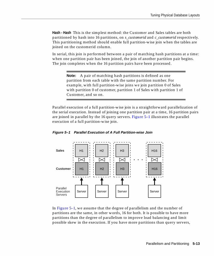
Tuning Physical Database Layouts
Hash - Hash This is the simplest method: the Customer and Sales tables are both
partitioned by hash into 16 partitions, on s_customerid and c_customerid respectively.
This partitioning method should enable full partition-wise join when the tables are
joined on the customerid column.
In serial, this join is performed between a pair of matching hash partitions at a time:
when one partition pair has been joined, the join of another partition pair begins.
The join completes when the 16 partition pairs have been processed.
Parallel execution of a full partition-wise join is a straightforward parallelization of
the serial execution. Instead of joining one partition pair at a time, 16 partition pairs
are joined in parallel by the 16 query servers. Figure 5–1 illustrates the parallel
execution of a full partition-wise join.
Figure 5–1 Parallel Execution of A Full Partition-wise Join
In Figure 5–1, we assume that the degree of parallelism and the number of
partitions are the same, in other words, 16 for both. It is possible to have more
partitions than the degree of parallelism to improve load balancing and limit
possible skew in the execution. If you have more partitions than query servers,
Note: A pair of matching hash partitions is defined as one
partition from each table with the same partition number. For
example, with full partition-wise joins we join partition 0 of Sales
with partition 0 of customer, partition 1 of Sales with partition 1 of
Customer, and so on.
Server
H1
H1
Server
H2
H2
Server
H3
H3
Server
H16
H16
. . .Sales
Customer
ParallelExecutionServers
Parallelism and Partitioning 5-13

Tuning Physical Database Layouts
when one query server is done with the join of one pair of partitions, it requests that
the query coordinator give it another pair to join. This process repeats until all pairs
have been processed. This method allows dynamic load balancing when the
number of partition pairs is greater than the degree of parallelism, for example, 64
partitions with a degree of parallelism of 16.
In Oracle Parallel Server environments running on shared-nothing platforms or
MPPs, partition placements on nodes is critical to achieving good scalability. To
avoid remote I/O, both matching partitions should have affinity to the same node.
Partition pairs should be spread over all nodes to avoid bottlenecks and to use all
CPU resources available on the system.
You can, however, have node host multiple pairs when there are more pairs than
nodes. For example, with an 8-node system and 16 partition pairs, each node should
receive two pairs.
Composite - Hash This method is a variation of the hash-hash method. The sales
table is a typical example of a table storing historical data. For all the reasons
mentioned under the heading "Performance Considerations for Range Partitioning"
on page 5-6, a more logical partitioning method for sales is probably the range
method, not the hash method.
For example, assume you want to partition the Sales table by range on the column
s_saledate into 8 partitions. Also assume you have two years' of data and each
partition represents a quarter. Instead of range partitioning you can use composite
to enable a full partition-wise join while preserving the partitioning on s_saledate.
Do this by partitioning the Sales table by range on s_saledate and then by
subpartitioning each partition by hash on s_customerid using 16 subpartitions per
partition, for a total of 128 subpartitions. The customer table can still use hash
partitioning with 16 partitions.
With that new partitioning method, a full partition-wise join works similarly to the
hash/hash method. The join is still divided into 16 smaller joins between hash
partition pairs from both tables. The difference is that now each hash partition in
Note: Always use a number of partitions that is a multiple of the
degree of parallelism.
See Also: For more information on data affinity, please refer to
Oracle8i Parallel Server Concepts.
5-14 Oracle8i Data Warehousing Guide

Tuning Physical Database Layouts
the Sales table is composed of a set of 8 subpartitions, one from each range
partition.
Figure 5–2 illustrates how the hash partitions are formed in the Sales table. In it,
each cell represents a subpartition. Each row corresponds to one range partition, for
a total of 8 range partitions. Each range partition has 16 subpartitions.
Symmetrically, each column on the figure corresponds to one hash partition for a
total of 16 hash partitions; each hash partition has 8 subpartitions. Note that hash
partitions can be defined only if all partitions have the same number of
subpartitions, in this case, 16.
Hash partitions in a composite table are implicit. However, Oracle does not record
them in the data dictionary, and you cannot manipulate them with DDL commands
as you can range partitions.
Parallelism and Partitioning 5-15

Tuning Physical Database Layouts
Figure 5–2 Range and Hash Partitions of A Composite Table
This partitioning method is effective because it allows you to combine pruning (on
s_salesdate) with a full partition-wise join (on customerid). In the previous example
query, pruning is achieved by only scanning the subpartitions corresponding to Q3
of 1994, in other words, row number 3 on Figure 5–2. Oracle them joins these
subpartitions with the customer table using a full partition-wise join.
All characteristics of the hash-hash method also apply to the composite-hash
method. In particular for this example, these two points are common to both
methods:
■ The degree of parallelism for this full partition-wise join cannot exceed 16. This
is because even though the Sales table has 128 subpartitions, it has only 16 hash
partitions.
94 - Q1
94 - Q2
94 - Q3
94 - Q4
95 - Q1
95 - Q2
95 - Q3
95 - Q4
Hash partition #9
H1
H2
H3
H4
H5
H6
H7
H8
H9
H10
H11
H12
H13
H14
H15
H16
Sal
esd
ate
Customerid
5-16 Oracle8i Data Warehousing Guide

Tuning Physical Database Layouts
■ The same rules for data placement on MPP systems apply here. The only
difference is that a hash partition is now a collection of subpartitions. You must
ensure that all these subpartitions are placed on the same node with the
matching hash partition from the other table. For example, in Figure 5–2, you
should store hash partition 9 of the Sales table shown by the eight circled
subpartitions, on the same node as hash partition 9 of the Customer table.
Composite - Composite (Hash Dimension) If needed, you can also partition the
Customer table by composite. For example, you can partition it by range on a zip
code column to enable pruning based on zip code. You should then subpartition it
by hash on customerid to enable a partition-wise join on the hash dimension.
Range - Range You can also use partition-wise joins for range partitioning. However,
this is more complex to implement because you must know your data's distribution
before performing the join. Furthermore, this can lead to data skew during the
execution if you do not correctly identify the partition bounds so that you have
partitions of equal size.
The basic principle for using range-range is the same as for hash-hash: you must
equi-partition both tables. This means that the number of partitions must be the
same and the partition bounds must be identical. For example, assume that you
know in advance that you have 10 million customers, and the values for customeridvary from 1 to 10000000. In other words, you have possibly 10 million different
values. To create 16 partitions, you can range partition both tables, Sales on
s_customerid and Customer on c_customerid. You should define partition bounds for
both tables to generate partitions of the same size. In this example, partition bounds
should be defined as 625001, 1250001, 1875001, ..., 10000001, so each partition
contains 625000 rows.
Range - Composite, Composite - Composite (Range Dimension) Finally, you can also
subpartition one or both tables on another column. Therefore, the range/composite
and composite/composite methods on the range dimension are also valid for
enabling a full partition-wise join on the range dimension.
Partial Partition-wise JoinsOracle can only perform partial partition-wise joins in parallel. Unlike full
partition-wise joins, partial partition-wise joins require you to partition only one
table on the join key, not both. The partitioned table is referred to as the reference
table. The other table may or may not be partitioned. Partial partition-wise joins are
more common than full partition-wise joins, because they require that you partition
only one of the joined tables on the join key.
Parallelism and Partitioning 5-17
Tuning Physical Database Layouts
To execute a partial partition-wise join, Oracle dynamically repartitions the other
table based on the partitioning of the reference table. Once the other table is
repartitioned, the execution is similar to a full partition-wise join.
The performance advantage that partial partition-wise joins have over conventional
parallel joins is that the reference table is not moved during the join operation.
Conventional parallel joins require both input tables to be redistributed on the join
key. This redistribution operation involves exchanging rows between query servers.
This is a very CPU-intensive operation and can lead to excessive interconnect traffic
in OPS environments. Partitioning large tables on a join key, either a foreign or
primary key, prevents this re-distribution every time the table is joined on that key.
Of course, if you choose a foreign key to partition the table, which is the most
common scenario, select a foreign key that is involved in many queries.
To illustrate partial partition-wise joins, consider the previous Sales/Customer
example. Assume that Customer is not partitioned or partitioned on a column other
than c_customerid. Because Sales is often joined with Customer on customerid, and
because this join dominates our application workload, partition Sales on
s_customerid to enable partial partition-wise join every time Customer and Sales are
joined. As in full partition-wise join, we have several alternatives:
Hash The simplest method to enable a partial partition-wise join is to partition Sales
by hash on c_customerid. The number of partitions determines the maximum degree
of parallelism, because the partition is the smallest granule of parallelism for partial
partition-wise join operations.
The parallel execution of a partial partition-wise join is illustrated in Figure 5–3,
"Partial Partition-wise Join", which assumes that both the degree of parallelism and
the number of partitions of Sales are 16. The execution involves two sets of query
servers: one set, labeled set 1 on the figure, scans the customer table in parallel. The
granule of parallelism for the scan operation is a range of blocks.
Rows from Customer that are selected by the first set, in this case all rows, are
redistributed to the second set of query servers by hashing customerid. For
example, all rows in Customer that could have matching rows in partition H1 of
Sales are sent to query server 1 in the second set. Rows received by the second set of
query servers are joined with the rows from the corresponding partitions in Sales.
Query server number 1 in the second set joins all Customer rows that it receives
with partition H1 of Sales.
5-18 Oracle8i Data Warehousing Guide

Tuning Physical Database Layouts
Figure 5–3 Partial Partition-wise Join
Considerations for full partition-wise joins also apply to partial partition-wise joins:
■ The degree of parallelism does not need to equal the number of partitions. In
Figure 5–3, the query executes with 8 query server sets. In this case, Oracle
assigns 2 partitions to each query server of the second set. Again, the number of
partitions should always be a multiple of the degree of parallelism.
■ In Oracle Parallel Server environments on shared-nothing platforms (MPPs),
each hash partition of sales should preferably have affinity to only one node to
avoid remote I/Os. Also, spread partitions over all nodes to avoid bottlenecks
and use all CPU resources available on the system. It is adequate for a node to
host multiple partitions when there are more partitions than nodes.
Composite As with full partition-wise joins, the prime partitioning method for the
Sales table is to use the range method on column s_salesdate. This is because Sales is
a typical example of a table that stores historical data. To enable a partial
See Also: For more information on data affinity, please refer to
Oracle8i Parallel Server Concepts.
Server
H1
Server
H2
Server
H16
. . .
. . .
. . .
Sales
Parallelexecutionserverset 2
Parallelexecutionserverset 1
Customer
Parallelexecutionserverset 1
re-distributionhash(c_customerid)
join
select
Parallelism and Partitioning 5-19
Tuning Physical Database Layouts
partition-wise join while preserving this range partitioning, you can subpartition
Sales by hash on column s_customerid using 16 subpartitions per partition. Pruning
and partial partition-wise joins can be used together if a query joins Customer and
Sales and if the query has a selection predicate on s_salesdate.
When Sales is composite, the granule of parallelism for a partial-partition wise join
is a hash partition and not a subpartition. Refer to Figure 5–2 for the definition of a
hash partition in a composite table. Again, the number of hash partitions should be
a multiple of the degree of parallelism. Also, on an MPP system, ensure that each
hash partition has affinity to a single node. In the previous example, the 8
subpartitions composing a hash partition should have affinity to the same node.
Range Finally, you can use range partitioning on s_customerid to enable a partial
partition-wise join. This works similarly to the hash method, although it is not
recommended. The resulting data distribution could be skewed if the size of the
partitions differs. Moreover, this method is more complex to implement because it
requires prior knowledge of the values of the partitioning column which is also a
join key.
Benefits of Partition-wise JoinsPartition-wise joins offer benefits as described in this section:
■ Reduction of Communications Overhead
■ Reduction of Memory Requirements
Reduction of Communications Overhead Partition-wise joins reduce communications
overhead when they are executed in parallel. This is because in the default case,
parallel execution of a join operation by a set of parallel execution servers requires
the redistribution of each table on the join column into disjoint subsets of rows.
These disjoint subsets of rows are then joined pair-wise by a single parallel
execution server.
Oracle can avoid redistributing the partitions because the two tables are already
partitioned on the join column. This allows each parallel execution server to join a
pair of matching partitions.
This performance enhancement is even more noticeable in OPS configurations with
internode parallel execution. This is because partition-wise joins can dramatically
reduce interconnect traffic. Using this feature is an almost mandatory optimization
measure for large DSS configurations that use OPS.
Currently, most OPS platforms, such as MPP and SMP clusters, provide limited
interconnect bandwidths compared to their processing powers. Ideally, interconnect
5-20 Oracle8i Data Warehousing Guide
Tuning Physical Database Layouts
bandwidth should be comparable to disk bandwidth, but this is seldom the case. As
a result, most join operations in OPS experience high interconnect latencies without
this optimization.
Reduction of Memory Requirements Partition-wise joins require less memory. In the
case of serial joins, the join is performed on a pair of matching partitions at the same
time. Thus, if data is evenly distributed across partitions, the memory requirement
is divided by the number of partitions. In this case, there is no skew.
In the parallel case, it depends on the number of partition pairs that are joined in
parallel. For example, if the degree of parallelism is 20 and the number of partitions
is 100, 5 times less memory is required because only 20 joins of two partitions are
performed at the same time. The fact that partition-wise joins require less memory
has a direct effect on performance. For example, the join does not need to write
blocks to disk during the build phase of a hash join.
Performance Considerations for Parallel Partition-wise JoinsThe performance improvements from parallel partition-wise joins also come with
disadvantages. The cost-based optimizer weighs the advantages and disadvantages
when deciding whether to use partition-wise joins.
■ In the case of range partitioning, data skew may increase response time if the
partitions are of different sizes. This is because some parallel execution servers
take longer than others to finish their joins. Oracle recommends the use of hash
(sub)partitioning to enable partition-wise joins because hash partitioning limits
the risk of skew, assuming that the number of partitions is a power of 2.
■ The number of partitions used for partition-wise joins should, if possible, be a
multiple of the number of query servers. With a degree of parallelism of 16, for
example, it is acceptable to have 16, 32, or even 64 partitions (or subpartitions).
But Oracle will serially execute the last phase of the join if the degree of
parallelism is, for example, 17. This is because in the beginning of the execution,
each parallel execution server works on a different partition pair. At the end of
this first phase, only one pair is left. Thus, a single query server joins this
remaining pair while all other query servers are idle.
■ Sometimes, parallel joins can cause remote I/Os. For example, on Oracle
Parallel Server environments running on MPP configurations, if a pair of
matching partitions is not collocated on the same node, a partition-wise join
requires extra inter-node communication due to remote I/Os. This is because
Oracle must transfer at least one partition to the node where the join is
Parallelism and Partitioning 5-21

Tuning Physical Database Layouts
performed. In this case, it is better to explicitly redistribute the data than to use
a partition-wise join.
5-22 Oracle8i Data Warehousing Guide

In
6
IndexesThis chapter tells how to use indexes in a data warehousing environment, and
discusses the following types of index:
■ Bitmap Indexes
■ B-tree Indexes
■ Local Versus Global
dexes 6-1

Bitmap Indexes
Bitmap IndexesBitmap indexes are widely used in data warehousing applications, which have large
amounts of data and ad hoc queries but a low level of concurrent transactions. For
such applications, bitmap indexing provides:
■ Reduced response time for large classes of ad hoc queries
■ A substantial reduction of space usage compared to other indexing techniques
■ Dramatic performance gains even on hardware with a relatively small number
of CPUs or small amount of memory
■ Very efficient maintenance during parallel DML and loads
Fully indexing a large table with a traditional B-tree index can be prohibitively
expensive in terms of space because the indexes can be several times larger than the
data in the table. Bitmap indexes are typically only a fraction of the size of the
indexed data in the table.
The purpose of an index is to provide pointers to the rows in a table that contain a
given key value. In a regular index, this is achieved by storing a list of rowids for
each key corresponding to the rows with that key value. In a bitmap index, a bitmap
for each key value is used instead of a list of rowids.
Each bit in the bitmap corresponds to a possible rowid, and if the bit is set, it means
that the row with the corresponding rowid contains the key value. A mapping
function converts the bit position to an actual rowid, so the bitmap index provides
the same functionality as a regular index even though it uses a different
representation internally. If the number of different key values is small, bitmap
indexes are very space efficient.
Bitmap indexes are most effective for queries that contain multiple conditions in the
WHERE clause. Rows that satisfy some, but not all conditions are filtered out before
the table itself is accessed. This improves response time, often dramatically.
Attention: Bitmap indexes are available only if you have
purchased the Oracle8i Enterprise Edition. See Getting to KnowOracle8i for more information about the features available in
Oracle8i and the Oracle8i Enterprise Edition.
6-2 Oracle8i Data Warehousing Guide

Bitmap Indexes
Benefits for Data Warehousing ApplicationsBitmap indexes are not suitable for OLTP applications with large numbers of
concurrent transactions modifying the data. These indexes are primarily intended
for decision support (DSS) in data warehousing applications where users typically
query the data rather than update it.
Parallel query and parallel DML work with bitmap indexes as with traditional
indexes. (Bitmap indexes on partitioned tables must be local indexes; see "Index
Partitioning" on page 5-6 for more information.) Parallel create index and
concatenated indexes are also supported.
CardinalityThe advantages of using bitmap indexes are greatest for low cardinality columns:
that is, columns in which the number of distinct values is small compared to the
number of rows in the table. A gender column, which only has two distinct values
(male and female), is ideal for a bitmap index. However, data warehouse
administrators will also choose to build bitmap indexes on columns with much
higher cardinalities.
For example, on a table with one million rows, a column with 10,000 distinct values
is a candidate for a bitmap index. A bitmap index on this column can out-perform a
B-tree index, particularly when this column is often queried in conjunction with
other columns.
B-tree indexes are most effective for high-cardinality data: that is, data with many
possible values, such as CUSTOMER_NAME or PHONE_NUMBER. In a data
warehouse, B-tree indexes should only be used for unique columns or other
columns with very high cardinalities (that is, columns that are almost unique). The
majority of indexes in a data warehouse should be bitmap indexes.
In ad hoc queries and similar situations, bitmap indexes can dramatically improve
query performance. AND and OR conditions in the WHERE clause of a query can
be quickly resolved by performing the corresponding boolean operations directly
on the bitmaps before converting the resulting bitmap to rowids. If the resulting
number of rows is small, the query can be answered very quickly without resorting
to a full table scan of the table.
Bitmap Index ExampleTable 6–1 shows a portion of a company's customer data.
Indexes 6-3
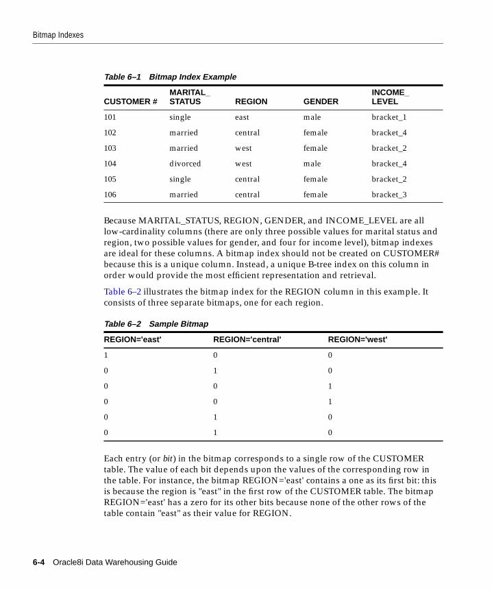
Bitmap Indexes
Because MARITAL_STATUS, REGION, GENDER, and INCOME_LEVEL are all
low-cardinality columns (there are only three possible values for marital status and
region, two possible values for gender, and four for income level), bitmap indexes
are ideal for these columns. A bitmap index should not be created on CUSTOMER#
because this is a unique column. Instead, a unique B-tree index on this column in
order would provide the most efficient representation and retrieval.
Table 6–2 illustrates the bitmap index for the REGION column in this example. It
consists of three separate bitmaps, one for each region.
Each entry (or bit) in the bitmap corresponds to a single row of the CUSTOMER
table. The value of each bit depends upon the values of the corresponding row in
the table. For instance, the bitmap REGION='east' contains a one as its first bit: this
is because the region is "east" in the first row of the CUSTOMER table. The bitmap
REGION='east' has a zero for its other bits because none of the other rows of the
table contain "east" as their value for REGION.
Table 6–1 Bitmap Index Example
CUSTOMER #MARITAL_STATUS REGION GENDER
INCOME_LEVEL
101 single east male bracket_1
102 married central female bracket_4
103 married west female bracket_2
104 divorced west male bracket_4
105 single central female bracket_2
106 married central female bracket_3
Table 6–2 Sample Bitmap
REGION='east' REGION='central' REGION='west'
1 0 0
0 1 0
0 0 1
0 0 1
0 1 0
0 1 0
6-4 Oracle8i Data Warehousing Guide

Bitmap Indexes
An analyst investigating demographic trends of the company's customers might
ask, "How many of our married customers live in the central or west regions?" This
corresponds to the following SQL query:
SELECT COUNT(*) FROM customer WHERE MARITAL_STATUS = 'married' AND REGION IN ('central','west');
Bitmap indexes can process this query with great efficiency by merely counting the
number of ones in the resulting bitmap, as illustrated in Figure 6–1. To identify the
specific customers who satisfy the criteria, the resulting bitmap would be used to
access the table.
Figure 6–1 Executing a Query Using Bitmap Indexes
Bitmap Indexes and NullsBitmap indexes include rows that have NULL values, unlike most other types of
indexes. Indexing of nulls can be useful for some types of SQL statements, such as
queries with the aggregate function COUNT.
Example
SELECT COUNT(*) FROM emp;
Any bitmap index can be used for this query because all table rows are indexed,
including those that have NULL data. If nulls were not indexed, the optimizer
would only be able to use indexes on columns with NOT NULL constraints.
AND OR = AND =
0
1
1
0
0
1
0
1
0
0
1
1
0
0
1
1
0
0
0
1
1
0
0
1
0
1
1
1
1
1
0
1
1
0
0
1
status ='married'
region ='central'
region ='west'
Indexes 6-5

B-tree Indexes
Bitmap Indexes on Partitioned TablesYou can create bitmap indexes on partitioned tables. The only restriction is that
bitmap indexes must be local to the partitioned table—they cannot be global
indexes. (Global bitmap indexes are supported only on nonpartitioned tables).
B-tree IndexesA B-tree index is organized like an upside-down tree. The bottommost level of the
index holds the actual data values and pointers to the corresponding rows, much
like the index in a book has a page number associated with each index entry. See
Oracle8i Concepts for an explanation of B-tree structures.
In general, you use B-tree indexes when you know that your typical query refers to
the indexed column and retrieves a few rows. In these queries, it is faster to find the
rows by looking at the index. However, there is a tricky issue here—return to the
analogy of a book index to understand it. If you plan to look at every single topic in
a book, you might not want to look in the index for the topic and then look up the
page. It might be faster to read through every chapter in the book. Similarly, if you
are retrieving most of the rows in a table, it might not make sense to look up the
index to find the table rows. Instead, you might want to read or scan the table.
B-tree indexes are most commonly used in a data warehouse to index keys which
are unique or near-unique. In many cases, it may not be necessary to index these
columns in a data warehouse, because unique constraints can be maintained
without an index, and since typical data warehouse queries may not yield better
performance with such indexes. Bitmap indexes should be more common that
B-tree indexes in most data warehouse environments.
Local Versus GlobalA B-tree index on a partitioned table can be local or global. Global indexes must be
fully rebuilt after a direct load, which can be very costly when loading a relatively
small number of rows into a large table. For this reason, it is strongly recommended
that indexes on partitioned tables should be defined as local indexes unless there is
a well-justified performance requirement for a global index. Bitmap indexes on
partitioned tables are always local. See "Partitioning Data" on page 5-4 for further
details.
6-6 Oracle8i Data Warehousing Guide

Const
7
ConstraintsThis chapter describes constraints, and discusses:
■ Why Constraints are Useful in a Data Warehouse
■ Overview of Constraint States
■ Typical Data Warehouse Constraints
raints 7-1

Why Constraints are Useful in a Data Warehouse
Why Constraints are Useful in a Data WarehouseConstraints provide a mechanism for ensuring that data conforms to guidelines
specified by the database administrator. The most common types of constraints
include unique constraints (ensuring that a given column is unique), not-null
constraints, and foreign-key constraints (which ensure that two keys share a
primary key-foreign key relationship).
Constraints can be used for the following basic purposes in a data warehouse:
■ Data cleanliness: Constraints can be used to verify that the data in the data
warehouse conforms to basic level of data consistency and correctness. Thus,
constraints are often used in a data warehouse to prevent the introduction of
dirty data.
■ Supporting query optimization: The Oracle database will utilize constraints
when optimizing SQL queries. Although constraints can be useful in many
aspects of query optimization, constraints are particularly important for
query-rewrite of materialized views.
Unlike many relational-database environments, data in a data warehouse is
typically added and/or modified under very controlled circumstances during the
ETT process. Multiple users typically do not update the data warehouse directly;
this is considerably different from the usage of a typical operational system.
Thus, the specific usage of constraints in a data warehouse may vary considerably
from the usage of constraints in operational systems. Oracle8i provides a wide
breadth of constraint functionality to address both the needs of data warehouses as
well as the needs to operational systems.
Many significant constraint features for data warehousing were introduced in
Oracle8i, so that readers familiar with Oracle’s constraint functionality in Oracle7
and Oracle8 should take special note of the new functionality described in this
chapter. In fact, many Oracle7 and Oracle8-based data warehouses lacked
constraints because of concerns about constraint performance. The new Oracle8ifunctionality for constraints is designed to address these concerns for data
warehouses.
Overview of Constraint StatesIn order to understand how to best utilize constraints in a data warehouse, it is
important to first understand the basic purposes of constraints:
■ Enforcement: In order to use a constraint for enforcement, the constraint must
be in the ENABLE state. An ENABLEd constraint can be used to ensure that all
7-2 Oracle8i Data Warehousing Guide

Typical Data Warehouse Constraints
data-modifications upon a given table (or tables) will satisfy the conditions of
the constraints. Data-modification operations, which would result in data that
violated the constraint, will fail with a constraint-violation error.
■ Validation: In order to use a constraint for validation, the constraint must be in
the VALIDATE state. If the constraint is validated, then all of the data that
currently resides in the table satisfies the constraint.
Note that validation is independent of enforcement. Although the typical
constraint in an operational system is both enabled and validated, any
constraint could be validated but not enforced or vice versa (enforced but not
validated). These latter two cases can be very useful for data warehouses, and
are discussed in the examples below.
■ Belief: In order to use a constraint for belief, the constraint must be in the RELY
state. In some cases, the data-warehouse administrator may know that a given
constraint is true. The RELY state provides the data-warehouse administrator
with a mechanism for telling Oracle8i that a given constraint is believed to be
true.
Note that the RELY state is only meaningful for constraints that have not been
validated.
Typical Data Warehouse ConstraintsThis section assumes that most readers are familiar with the typical usage of
constraints; that is, constraints that are both enabled and validated. For data
warehousing, many users have discovered the such constraints may not be
effective, because it may be prohibitively costly to build and maintain such
constraints.
Unique Constraints in a Data WarehouseA unique constraint is typically enforced using a unique index. However, in a data
warehouse, in which tables can be extremely large, creating a unique index may be
very costly both in terms of processing time and disk space.
Suppose that a data warehouse contained a table SALES, with includes a column
SALES_ID. SALES_ID uniquely identifies a single sales transaction, and the
data-warehouse wants to ensure that this column is unique within the data
warehouse.
One way to create the constraint is:
Constraints 7-3

Typical Data Warehouse Constraints
ALTER TABLE sales ADD CONSTRAINT sales_unique UNIQUE(sales_id);
By default, this constraint is both enabled and validated. Oracle will implicitly
create a unique index on sales_id to support this constraint. However, this index
may be problematic in a data warehouse for three reasons:
■ The unique index can be very large, since the SALES table could easily have
millions or even billions of rows.
■ The unique index is rarely used for query execution; most typical data
warehousing queries will not have predicates on unique keys, so this index will
probably not improve performance.
■ If SALES is partitioned along a column other than SALES_ID, the unique index
must be a global index. This can detrimentally affect all maintenance operations
on the SALES table.
Why is an index required for unique constraints? The index is used for enforcement.
That is, the unique index is necessary to ensure that each individual row that is
modified in the SALES table will satisfy the unique constraint.
For data warehousing tables, an alternative mechanism for unique constraints is:
ALTER TABLE sales ADD CONSTRAINT sales_unique UNIQUE (sales_id) DISABLE VALIDATE;
This statement will create a unique constraint, but since the constraint is disabled,
there is no need for a unique index. This approach can be advantageous for many
data warehousing environments, because the constraint now ensures uniqueness
without the shortcomings of a unique index.
However, there are trade-offs for the data warehouse administrator to consider with
DISABLE VALIDATE constraints. Since this constraint is disabled, no DML
statements which may modify the unique column are permitted against the SALES
table. Thus, there are two strategies for modifying this table in the presence of a
constraint:
■ Use DDL to add data to this table (such as exchanging partitions). See the
example in Chapter 14, "Loading and Refreshing".
■ Prior to the modifying this table, drop the constraint. Then, make all of the
necessary data modifications. Finally, recreate the disabled constraint. Note that
recreating the constraint will be much more efficient that re-creating an enabled
constraint. This approach will not guarantee that the data in the SALES table is
unique while the constraint has been dropped.
7-4 Oracle8i Data Warehousing Guide

Typical Data Warehouse Constraints
Foreign Key Constraints in a Data WarehouseIn a star schema data warehouse, foreign-key constraints are typically created in
order to validate the relationship between the fact table and the dimension tables.
An example constraint might be:
ALTER TABLE sales ADD CONSTRAINT fk_sales_timeFOREIGN KEY (sales_time_id) REFERENCES time (time_id)ENABLE VALIDATE;
However, there are several different requirements in which a data warehouse
administrator may choose to use different states for the foreign-key constraints. In
particular, the ENABLE NOVALIDATE state can be useful for data warehousing. A
data warehouse administrator may choose to use an ENABLE NOVALIDATE
constraint when either:
■ There is data in the tables that currently disobeys the constraint, but the data
warehouse administrator wishes to create a constraint for enforcement.
■ There is a requirement to quickly create an enforced constraint.
Suppose that the data warehouse loaded new data into the fact table(s) every day,
but only refreshed the dimension tables on the weekend. Then, during the week, it
is possible that the dimension tables and fact tables may in fact disobey the
foreign-key constraints. Nevertheless, the data warehouse administrator may wish
to maintain the enforcement of this constraint to prevent any changes that might
affect the foreign key constraint outside of the ETT process. Thus, the foreign key
constraints could be created every night, following the ETT process, as:
ALTER TABLE sales ADD CONSTRAINT fk_sales_timeFOREIGN KEY (sales_time_id) REFERENCES time (time_id)ENABLE NOVALIDATE;
Another usage of ENABLE NOVALIDATE is for quickly creating an enforced
constraint, even when the constraint is believed to be true. Suppose that the ETT
process verifies that a foreign-key constraint is true. Rather than have the database
re-verify this foreign-key constraint (which would require time and database
resources), the data-warehouse administrator could instead create a foreign-key
constraint using ENABLE NOVALIDATE.
RELY ConstraintsIt is not uncommon for the ETT process to verify that certain constraints are true.
For example, the ETT process may validate all of the foreign keys in the incoming
data for the fact table. In these environments, the data warehouse administrator
Constraints 7-5

Typical Data Warehouse Constraints
may choose to trust the ETT process to provide clean data, instead of implementing
constraints in the data warehouse.
For example, during the ETT process, the data warehouse administrator may have
verified that a foreign-key constraint is true. Rather than have the database re-verify
this foreign-key constraint (which would require time and database resources), the
data warehouse administrator could instead create a foreign-key constraint with the
RELY state:
ALTER TABLE sales add CONSTRAINT fk_sales_timeFOREIGN KEY (sales_time_id) REFERENCES time (time_id)DISABLE NOVALIDATE rely;
The existence of RELY constraints, even though they are not used for
data-validation, may be important for several purposes, including:
■ constraints may be used to enable more sophisticated query-rewrites for
materialized views. See Chapter 19, "Query Rewrite", for further details.
■ other data-warehousing tools may retrieve information regarding constraints
directly from the Oracle data dictionary.
Creating a RELY constraint is very inexpensive. Because the constraint is not being
validated, there is no data processing necessary to create such a constraint.
Constraints and ParallelismAll constraints can be validated in parallel. When validating constraints on very
large tables, parallelism is often necessary to meet performance goals. The degree of
parallelism for a given constraint operation is determined by the default degree of
parallelism of the underlying table.
Constraints and PartitioningMany aspects of creating and maintaining constraints can be executed on a
per-partition basis. Later chapters will discuss the significance of partitioning for
data warehousing, and partitioning can provide benefits to constraint management
(just as partitioning provide benefits to managing of many other operations). For
example, Chapter 14, "Loading and Refreshing", provides a scenario example of
creating unique and foreign-key constraints on a separate staging table, and these
constraints are maintained during the EXCHANGE PARTITION statement.
7-6 Oracle8i Data Warehousing Guide

Materialize
8
Materialized ViewsThis chapter introduces you to the use of materialized views and discusses:
■ Overview of Data Warehousing with Materialized Views
■ The Need for Materialized Views
■ Types of Materialized Views
■ Creating a Materialized View
■ Nested Materialized Views
■ Registration of an Existing Materialized View
■ Partitioning a Materialized View
■ Indexing Selection for Materialized Views
■ Invalidating a Materialized View
■ Guidelines for Using Materialized Views in a Data Warehouse
■ Altering a Materialized View
■ Dropping a Materialized View
■ Overview of Materialized View Management Tasks
d Views 8-1

Overview of Data Warehousing with Materialized Views
Overview of Data Warehousing with Materialized ViewsTypically, data flows from one or more online transaction processing (OLTP)
databases into a data warehouse on a monthly, weekly, or daily basis. The data is
usually processed in a staging file before being added to the data warehouse. Data
warehouses typically range in size from tens of gigabytes to a few terabytes, usually
with the vast majority of the data stored in a few very large fact tables.
One technique employed in data warehouses to improve performance is the
creation of summaries, or aggregates. They are a special kind of aggregate view that
improves query execution times by precalculating expensive joins and aggregation
operations prior to execution and storing the results in a table in the database. For
example, a table could be created to contain the sum of sales by region and by
product.
Prior to Oracle8i, organizations using summaries spent a significant amount of time
manually creating summaries, identifying which ones to create, indexing the
summaries, updating them, and advising their users on which ones to use. The
introduction of summary management in the Oracle server eases the workload of
the DBA and means the end user no longer has to be aware of which summaries
have been defined. The DBA creates one or more materialized views, which are the
equivalent of a summary. The end user queries the tables and views in the database
and the query rewrite mechanism in the Oracle server automatically rewrites the
SQL query to use the summary tables. This mechanism significantly improves the
response time for returning results from the query and eliminates the need for the
end user or database application to be aware of the materialized views that exist
within the data warehouse.
The summaries or aggregates that are referred to in this book and in literature on
data warehousing are created in Oracle using a schema object called a materializedview. Materialized views can perform a number of roles, such as improving query
performance or providing replicated data, as described below.
Although materialized views are usually accessed via the query rewrite mechanism,
an end-user or database application can construct queries that directly access the
summaries. However, serious consideration should be given to whether users
should be allowed to do this, because, once the summaries are directly referenced in
queries, the DBA will not be free to drop and create summaries without affecting
applications.
8-2 Oracle8i Data Warehousing Guide

The Need for Materialized Views
Materialized Views for Data WarehousesIn data warehouses, materialized views can be used to precompute and store
aggregated data such as the sum of sales. Materialized views in these environments
are typically referred to as summaries, because they store summarized data. They
can also be used to precompute joins with or without aggregations. A materialized
view eliminates the overhead associated with expensive joins or aggregations for a
large or important class of queries.
Materialized Views for Distributed ComputingIn distributed environments, materialized views are used to replicate data at
distributed sites and to synchronize updates done at several sites with conflict
resolution methods. The materialized views as replicas provide local access to data
which otherwise would have to be accessed from remote sites. Materialized views
are also useful in remote data marts.
Materialized Views for Mobile ComputingYou can also use materialized views to download a subset of data from central
servers to mobile clients, with periodic refreshes from the central servers and
propagation of updates by clients back to the central servers.
This chapter focuses on the use of materialized views in data warehouses. See also
Oracle8i Replication and Oracle8i Distributed Database Systems for details on
distributed and mobile computing.
The Need for Materialized ViewsMaterialized views are used in data warehouses to increase the speed of queries on
very large databases. Queries to large databases often involve joins between tables
or aggregations such as SUM, or both. These operations are very expensive in terms
of time and processing power. The type of materialized view that is created
determines how the materialized view can be refreshed and used by query rewrite.
Materialized views can be used in a number of ways and almost identical syntax
can be used to perform a number of roles. For example, a materialized view can be
used to replicate data, which was formerly achieved by using the CREATE
SNAPSHOT statement. Now CREATE MATERIALIZED VIEW is a synonym for
CREATE SNAPSHOT.
Materialized views improve query performance by precalculating expensive join
and aggregation operations on the database prior to execution time and storing the
Materialized Views 8-3
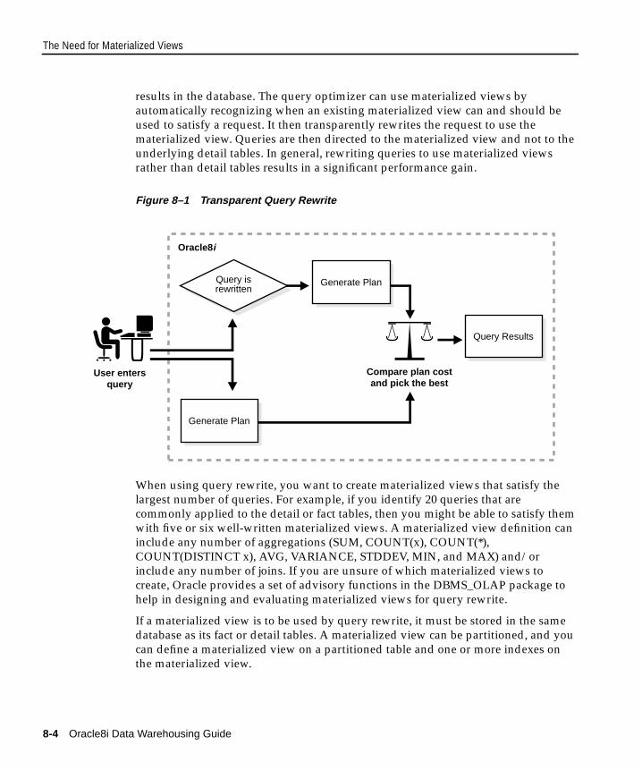
The Need for Materialized Views
results in the database. The query optimizer can use materialized views by
automatically recognizing when an existing materialized view can and should be
used to satisfy a request. It then transparently rewrites the request to use the
materialized view. Queries are then directed to the materialized view and not to the
underlying detail tables. In general, rewriting queries to use materialized views
rather than detail tables results in a significant performance gain.
Figure 8–1 Transparent Query Rewrite
When using query rewrite, you want to create materialized views that satisfy the
largest number of queries. For example, if you identify 20 queries that are
commonly applied to the detail or fact tables, then you might be able to satisfy them
with five or six well-written materialized views. A materialized view definition can
include any number of aggregations (SUM, COUNT(x), COUNT(*),
COUNT(DISTINCT x), AVG, VARIANCE, STDDEV, MIN, and MAX) and/or
include any number of joins. If you are unsure of which materialized views to
create, Oracle provides a set of advisory functions in the DBMS_OLAP package to
help in designing and evaluating materialized views for query rewrite.
If a materialized view is to be used by query rewrite, it must be stored in the same
database as its fact or detail tables. A materialized view can be partitioned, and you
can define a materialized view on a partitioned table and one or more indexes on
the materialized view.
StrategyGenerate PlanStrategy
Query isrewritten
User entersquery
Compare plan costand pick the best
StrategyGenerate Plan
StrategyQuery Results
Oracle8i
8-4 Oracle8i Data Warehousing Guide

The Need for Materialized Views
Materialized views are similar to indexes in several ways: they consume storage
space, they must be refreshed when the data in their master tables changes, and,
when used for query rewrite, they improve the performance of SQL execution and
their existence is transparent to SQL applications and users. Unlike indexes,
materialized views can be accessed directly using a SELECT statement. Depending
on the type of refresh that is required, they can also be accessed directly in an
INSERT, UPDATE, or DELETE statement.
Components of Summary ManagementSummary management consists of:
■ Mechanisms to define materialized views and dimensions
■ A refresh mechanism to ensure that all materialized views contain the latest
data
■ A query rewrite capability to transparently rewrite a query to use a
materialized view
■ An advisor utility to recommend which materialized views to create, retain, and
drop
Many large decision support system (DSS) databases have schemas that do not
closely resemble a conventional data warehouse schema, but that still require joins
and aggregates. The use of summary management features imposes no schema
restrictions, and may enable some existing DSS database applications to achieve
large gains in performance without requiring a redesign of the database or
application. This functionality is thus available to all database users.
Figure 8–2 illustrates where summary management is used in the warehousing
cycle. After the data has been transformed, staged, and loaded into the detail data
in the warehouse, the summary management process can be invoked. This means
that summaries can be created, queries can be rewritten, and the advisor can be
used to plan summary usage and creation.
Note: Materialized views can also be used by Oracle Replication.
The techniques shown in this chapter illustrate how to use
materialized views in data warehouses. See Oracle8i Replication for
further information.
Materialized Views 8-5
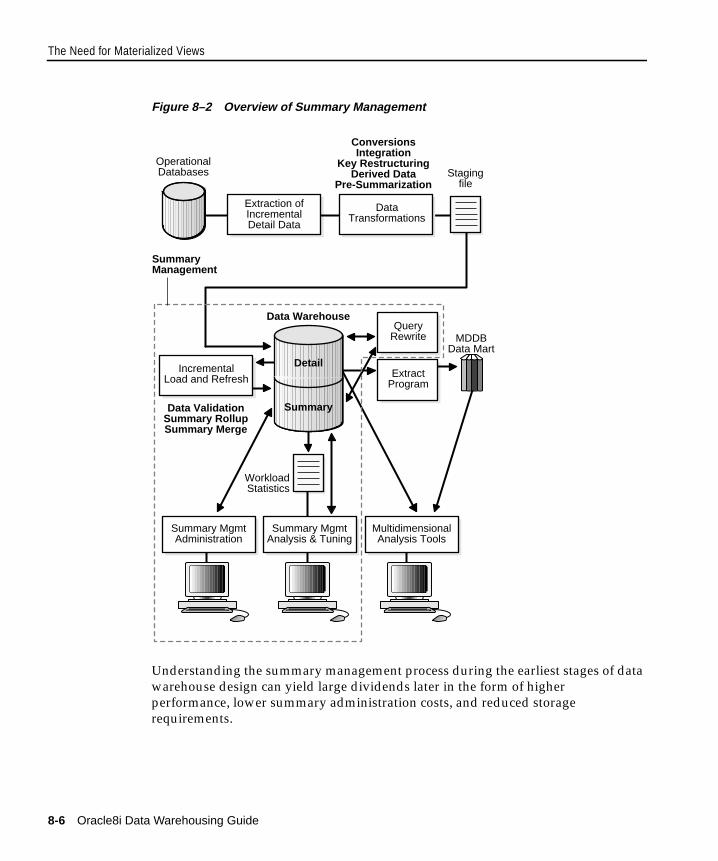
The Need for Materialized Views
Figure 8–2 Overview of Summary Management
Understanding the summary management process during the earliest stages of data
warehouse design can yield large dividends later in the form of higher
performance, lower summary administration costs, and reduced storage
requirements.
OperationalDatabases
Extraction ofIncrementalDetail Data
IncrementalLoad and Refresh
DataTransformations
Stagingfile
Detail
Data Warehouse
Summary
QueryRewrite
ExtractProgram
Summary MgmtAdministration
Summary MgmtAnalysis & Tuning
MultidimensionalAnalysis Tools
WorkloadStatistics
MDDBData Mart
Data ValidationSummary RollupSummary Merge
ConversionsIntegration
Key RestructuringDerived Data
Pre-Summarization
SummaryManagement
8-6 Oracle8i Data Warehousing Guide

The Need for Materialized Views
The summary management process begins with the creation of dimensions and
hierarchies that describe the business relationships and common access patterns in
the database. An analysis of the dimensions, combined with an understanding of
the typical work load, can then be used to create materialized views. Materialized
views improve query execution performance by precalculating expensive join or
aggregation operations prior to execution time. Query rewrite then automatically
recognizes when an existing materialized view can and should be used to satisfy a
request, and can transparently rewrite a request to use a materialized view, thus
improving performance.
TerminologySome basic data warehousing terms are defined as follows:
■ Dimension tables describe the business entities of an enterprise, which usually
represent hierarchical, categorical information such as time, departments,
locations, and products. Dimension tables are sometimes called lookup or
reference tables.
Dimension tables usually change slowly over time and are not modified on a
periodic schedule. They are typically not large, but they affect the performance
of long-running decision support queries that consist of joins of fact tables with
dimension tables, followed by aggregation to specific levels of the dimension
hierarchies. Dimensions and dimension tables are discussed in Chapter 9,
"Dimensions".
■ Fact tables describe the business transactions of an enterprise. Fact tables are
sometimes called detail tables.
The vast majority of data in a data warehouse is stored in a few very large fact
tables. They are updated periodically with data from one or more operational
online transaction processing (OLTP) databases.
Fact tables include measures such as sales, units, and inventory.
– A simple measure is a numeric or character column of one table such as
FACT.SALES.
– A computed measure is an expression involving only simple measures of
one table, for example, FACT.REVENUES - FACT.EXPENSES.
– A multi-table measure is a computed measure defined on multiple tables,
for example, FACT_A.REVENUES - FACT_B.EXPENSES.
Materialized Views 8-7

The Need for Materialized Views
Fact tables also contain one or more keys that organize the business transactions
by the relevant business entities such as time, product, and market. In most
cases, the fact keys are non-null, form a unique compound key of the fact table,
and join with exactly one row of a dimension table.
■ A materialized view is a pre-computed table comprising aggregated and/or
joined data from fact and possibly dimension tables. Builders of data
warehouses will know a materialized view as a summary or aggregation.
Schema Design Guidelines for Materialized ViewsA materialized view definition can include any number of aggregates, as well as
any number of joins. In several ways, a materialized view behaves like an index:
■ The purpose of a materialized view is to increase request execution
performance.
■ The existence of a materialized view is transparent to SQL applications, so a
DBA can create or drop materialized views at any time without affecting the
validity of SQL applications.
■ A materialized view consumes storage space.
■ The contents of the materialized view must be updated when the underlying
detail tables are modified.
Before starting to define and use the various components of summary management,
you should review your schema design to, wherever possible, abide by the
following guidelines:
Guideline 1: Your dimensions should either be denormalized (each dimension
contained in one table) or the joins between tables in a normalized
or partially normalized dimension should guarantee that each
child-side row joins with exactly one parent-side row. The benefits
of maintaining this condition are described in "Creating a
Dimension" on page 9-6.
8-8 Oracle8i Data Warehousing Guide

The Need for Materialized Views
If desired, this condition can be enforced by adding FOREIGN
KEY and NOT NULL constraints on the child-side join key(s) and
PRIMARY KEY constraints on the parent-side join key(s). If your
materialized view contains only a single detail table, or if it
performs no aggregation, a preferred alternative would be to use
queries containing outer joins in place of inner joins. In this case,
the Oracle optimizer can guarantee the integrity of the result
without enforced referential integrity constraints.
Guideline 2: If dimensions are denormalized or partially denormalized,
hierarchical integrity must be maintained between the key
columns of the dimension table. Each child key value must
uniquely identify its parent key value, even if the dimension table is
denormalized. Hierarchical integrity in a denormalized dimension
can be verified by calling the VALIDATE_DIMENSION procedure
of the DBMS_OLAP package.
Guideline 3: Fact tables and dimension tables should similarly guarantee that
each fact table row joins with exactly one dimension table row.
This condition must be declared, and optionally enforced, by
adding FOREIGN KEY and NOT NULL constraints on the fact
key column(s) and PRIMARY KEY constraints on the dimension
key column(s), or by using outer joins as described in Guideline 1.
In a data warehouse, constraints are typically enabled with the
NOVALIDATE and RELY options to avoid constraint enforcement
performance overhead.
Guideline 4: Incremental loads of your detail data should be done using the
SQL*Loader direct-path option, or any bulk loader utility that
uses Oracle's direct path interface (including INSERT AS SELECT
with the APPEND or PARALLEL hints). Fast refresh after
conventional DML is not supported with views with aggregates
and joins, but it is for single-table aggregate views. See Oracle8iSQL Reference for further details.
Guideline 5: Range-partition your tables by a monotonically increasing time
column if possible (preferably of type DATE). Different
materialized views have different requirements for speeding up
refresh.
Guideline 6: After each load and before refreshing your materialized view, use
the VALIDATE_DIMENSION procedure of the DBMS_OLAP
package to incrementally verify dimensional integrity.
Materialized Views 8-9

Types of Materialized Views
Guidelines 1 and 2 are more important than guideline 3. If your schema design does
not follow guidelines 1 and 2, it does not then matter whether it follows guideline 3.
Guidelines 1, 2, and 3 affect both query rewrite performance and materialized view
refresh performance.
If you are concerned with the time required to enable constraints and whether any
constraints may be violated, use the ENABLE NOVALIDATE clause to turn on
constraint checking without validating any of the existing constraints. The risk with
this approach is that incorrect query results could occur if any constraints are
broken. Therefore, the designer must determine how clean the data is and whether
the risk of wrong results is too great.
Summary management can perform many useful functions, including query rewrite
and materialized view refresh, even if your data warehouse design does not follow
these guidelines. However, you will realize significantly greater query execution
performance and materialized view refresh performance benefits and you will
require fewer materialized views if your schema design complies with these
guidelines.
Types of Materialized ViewsThe SELECT clause in the materialized view creation statement defines the data that
the materialized view is to contain. There are only a few restrictions on what may
be specified. Any number of tables can be joined together, however, they cannot be
remote tables if you wish to take advantage of query rewrite or the warehouse
refresh facility (part of the DBMS_OLAP package). Besides tables, views, inline
views, subqueries, and materialized views may all be joined or referenced in the
SELECT clause.
The types of materialized views are:
■ Materialized Views with Joins and Aggregates
■ Single-Table Aggregate Materialized Views
■ Materialized Views Containing Only Joins
Guideline 7: Horizontally partition and index the materialized view as you
have the fact tables. Include a local concatenated index on all the
materialized view keys.
8-10 Oracle8i Data Warehousing Guide
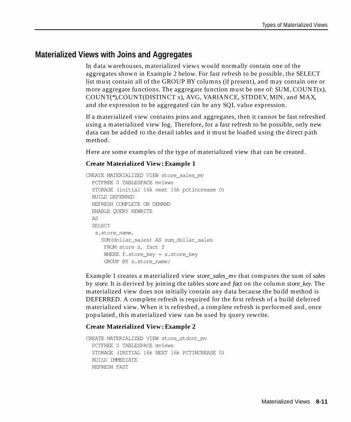
Types of Materialized Views
Materialized Views with Joins and AggregatesIn data warehouses, materialized views would normally contain one of the
aggregates shown in Example 2 below. For fast refresh to be possible, the SELECT
list must contain all of the GROUP BY columns (if present), and may contain one or
more aggregate functions. The aggregate function must be one of: SUM, COUNT(x),
COUNT(*),COUNT(DISTINCT x), AVG, VARIANCE, STDDEV, MIN, and MAX,
and the expression to be aggregated can be any SQL value expression.
If a materialized view contains joins and aggregates, then it cannot be fast refreshed
using a materialized view log. Therefore, for a fast refresh to be possible, only new
data can be added to the detail tables and it must be loaded using the direct path
method.
Here are some examples of the type of materialized view that can be created.
Create Materialized View: Example 1
CREATE MATERIALIZED VIEW store_sales_mv PCTFREE 0 TABLESPACE mviews STORAGE (initial 16k next 16k pctincrease 0) BUILD DEFERRED REFRESH COMPLETE ON DEMAND ENABLE QUERY REWRITE AS SELECT s.store_name, SUM(dollar_sales) AS sum_dollar_sales FROM store s, fact f WHERE f.store_key = s.store_key GROUP BY s.store_name;
Example 1 creates a materialized view store_sales_mv that computes the sum of salesby store. It is derived by joining the tables store and fact on the column store_key. The
materialized view does not initially contain any data because the build method is
DEFERRED. A complete refresh is required for the first refresh of a build deferred
materialized view. When it is refreshed, a complete refresh is performed and, once
populated, this materialized view can be used by query rewrite.
Create Materialized View: Example 2
CREATE MATERIALIZED VIEW store_stdcnt_mv PCTFREE 0 TABLESPACE mviews STORAGE (INITIAL 16k NEXT 16k PCTINCREASE 0) BUILD IMMEDIATE REFRESH FAST
Materialized Views 8-11

Types of Materialized Views
ENABLE QUERY REWRITE AS SELECT store_name, t.time_key, STDDEV(unit_sales) AS stdcnt_unit_sales AVG(unit_sales) AS avgcnt_unit_sales COUNT(unit_sales) AS count_days SUM(unit_sales) AS sum_unit_sales FROM store s, fact f, time t WHERE s.store_key = f.store_key AND f.time_key = t.time_key GROUP BY store_name, t.time_key;
The statement above creates a materialized view store_stdcnt_mv that computes the
standard deviation for the number of units sold by a store on a given date. It is
derived by joining the tables store, time, and fact on the columns store_key and
time_key. The materialized view is populated with data immediately because the
build method is immediate and it is available for use by query rewrite. In this
example, the default refresh method is FAST, which is allowed because the COUNT
and SUM aggregates have been included to support fast refresh of the STDDEV
aggregate.
Single-Table Aggregate Materialized Views A materialized view that contains one or more aggregates (SUM, AVG,
VARIANCE, STDDEV, COUNT) and a GROUP BY clause may be based on a single
table. The aggregate function can involve an expression on the columns such as
SUM(a*b). If this materialized view is to be incrementally refreshed, then a
materialized view log must be created on the detail table with the INCLUDING
NEW VALUES option, and the log must contain all columns referenced in the
materialized view query definition.
CREATE MATERIALIZED VIEW log on fact with rowid (store_key, time_key, dollar_sales, unit_sales) including new values;
CREATE MATERIALIZED VIEW sum_sales PARALLEL BUILD IMMEDIATE REFRESH FAST ON COMMIT AS SELECT f.store_key, f.time_key, COUNT(*) AS count_grp, SUM(f.dollar_sales) AS sum_dollar_sales, COUNT(f.dollar_sales) AS count_dollar_sales,
8-12 Oracle8i Data Warehousing Guide

Types of Materialized Views
SUM(f.unit_sales) AS sum_unit_sales, COUNT(f.unit_sales) AS count_unit_sales FROM fact f GROUP BY f.store_key, f.time_key;
In this example, a materialized view has been created which contains aggregates on
a single table. Because the materialized view log has been created, the materialized
view is fast refreshable. If DML is applied against the fact table, then, when the
commit is issued, the changes will be reflected in the materialized view.
Table 8–1 illustrates the aggregate requirements for a single-table aggregate
materialized view.
Note that COUNT(*) must always be present.
Incremental refresh for a single-table aggregate materialized view is possible after
any type of DML to the base tables (direct load or conventional INSERT, UPDATE,
or DELETE).
A single-table aggregate materialized view can be defined to be refreshed ON
COMMIT or ON DEMAND. If it is ON COMMIT, the refresh is performed at
commit time of the transaction that does DML on one of the materialized view's
detail tables.
After a refresh ON COMMIT, you are urged to check the alert log and trace files to
see if any error occurred during the refresh.
Materialized Views Containing Only JoinsMaterialized views may contain only joins and no aggregates, such as in the next
example where a materialized view is created which joins the fact table to the store
Table 8–1 Single-Table Aggregate Requirements
If aggregate X is present, aggregate Y is required and aggregate Z is optional
X Y Z
COUNT(expr) - -
SUM(expr) COUNT(expr) -
AVG(expr) COUNT(expr) SUM(expr)
STDDEV(expr) COUNT(expr) SUM(expr * expr)
VARIANCE(expr) COUNT(expr) SUM(expr * expr)
Materialized Views 8-13

Types of Materialized Views
table. The advantage of creating this type of materialized view is that expensive
joins will be precalculated.
Incremental refresh for a materialized view containing only joins is possible after
any type of DML to the base tables (direct load or conventional INSERT, UPDATE,
or DELETE).
A materialized view containing only joins can be defined to be refreshed ON
COMMIT or ON DEMAND. If it is ON COMMIT, the refresh is performed at
commit time of the transaction that does DML on the materialized view's detail
table.
If you specify REFRESH FAST, Oracle performs further verification of the query
definition to ensure that fast refresh can be performed if any of the detail tables
change. These additional checks include:
1. A materialized view log must be present for each detail table.
2. The rowids of all the detail tables must appear in the SELECT list of the
materialized view query definition.
3. If there are outer joins, unique constraints must exist on the join columns of the
inner table.
For example, if you are joining the fact and a dimension table and the join is an
outer join with the fact table being the outer table, there must exist unique
constraints on the join columns of the dimension table.
If some of the above restrictions are not met, then the materialized view should be
created as REFRESH FORCE to take advantage of incremental refresh when it is
possible. If the materialized view is created as ON COMMIT, Oracle performs all of
the fast refresh checks. If one of the tables did not meet all of the criteria, but the
other tables did, the materialized view would still be incrementally refreshable with
respect to the other tables for which all the criteria are met.
In a data warehouse star schema, if space is at a premium, you can include the
rowid of the fact table only because this is the table that will be most frequently
updated, and the user can specify the FORCE option when the materialized view is
created.
A materialized view log should contain the rowid of the master table. It is not
necessary to add other columns.
To speed up refresh, it is recommended that the user create indexes on the columns
of the materialized view that stores the rowids of the fact table.
8-14 Oracle8i Data Warehousing Guide
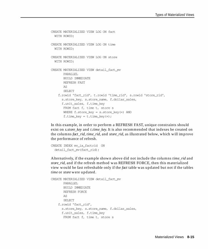
Types of Materialized Views
CREATE MATERIALIZED VIEW LOG ON fact WITH ROWID;
CREATE MATERIALIZED VIEW LOG ON time WITH ROWID;
CREATE MATERIALIZED VIEW LOG ON store WITH ROWID;
CREATE MATERIALIZED VIEW detail_fact_mv PARALLEL BUILD IMMEDIATE REFRESH FAST AS SELECT f.rowid "fact_rid", t.rowid "time_rid", s.rowid "store_rid", s.store_key, s.store_name, f.dollar_sales, f.unit_sales, f.time_key FROM fact f, time t, store s WHERE f.store_key = s.store_key(+) AND f.time_key = t.time_key(+);
In this example, in order to perform a REFRESH FAST, unique constraints should
exist on s.store_key and t.time_key. It is also recommended that indexes be created on
the columns fact_rid, time_rid, and store_rid, as illustrated below, which will improve
the performance of refresh.
CREATE INDEX mv_ix_factrid ON detail_fact_mv(fact_rid);
Alternatively, if the example shown above did not include the columns time_rid and
store_rid, and if the refresh method was REFRESH FORCE, then this materialized
view would be fast refreshable only if the fact table was updated but not if the tables
time or store were updated.
CREATE MATERIALIZED VIEW detail_fact_mv PARALLEL BUILD IMMEDIATE REFRESH FORCE AS SELECT f.rowid "fact_rid", s.store_key, s.store_name, f.dollar_sales, f.unit_sales, f.time_key FROM fact f, time t, store s
Materialized Views 8-15

Creating a Materialized View
WHERE f.store_key = s.store_key(+) AND f.time_key = t.time_key(+);
Creating a Materialized ViewA materialized view can be created with the CREATE MATERIALIZED VIEW
statement or using Oracle Enterprise Manager. The following command creates the
materialized view store_sales_mv.
CREATE MATERIALIZED VIEW store_sales_mv PCTFREE 0 TABLESPACE mviews STORAGE (INITIAL 16k NEXT 16k PCTINCREASE 0) PARALLEL BUILD IMMEDIATE REFRESH COMPLETE ENABLE QUERY REWRITE AS SELECT s.store_name, SUM(dollar_sales) AS sum_dollar_sales FROM store s, fact f WHERE f.store_key = s.store_key GROUP BY s.store_name;
It is not uncommon in a data warehouse to have already created summary or
aggregation tables, and the DBA may not wish to repeat this work by building a
new materialized view. In this instance, the table that already exists in the database
can be registered as a prebuilt materialized view. This technique is described in
"Registration of an Existing Materialized View" on page 8-29.
Once you have selected the materialized views you want to create, follow the steps
below for each materialized view.
1. Do the physical design of the materialized view (existing user-defined
materialized views do not require this step). If the materialized view contains
many rows, then, if appropriate, the materialized view should be partitioned by
a time attribute (if possible) and should match the partitioning of the largest or
most frequently updated detail or fact table (if possible). Refresh performance
generally benefits from a large number of partitions because it can take
advantage of the parallel DML capabilities in Oracle.
See Also: For a complete description of CREATE
MATERIALIZED VIEW, see the Oracle8i SQL Reference.
8-16 Oracle8i Data Warehousing Guide
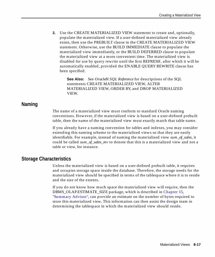
Creating a Materialized View
2. Use the CREATE MATERIALIZED VIEW statement to create and, optionally,
populate the materialized view. If a user-defined materialized view already
exists, then use the PREBUILT clause in the CREATE MATERIALIZED VIEW
statement. Otherwise, use the BUILD IMMEDIATE clause to populate the
materialized view immediately, or the BUILD DEFERRED clause to populate
the materialized view at a more convenient time. The materialized view is
disabled for use by query rewrite until the first REFRESH, after which it will be
automatically enabled, provided the ENABLE QUERY REWRITE clause has
been specified.
NamingThe name of a materialized view must conform to standard Oracle naming
conventions. However, if the materialized view is based on a user-defined prebuilt
table, then the name of the materialized view must exactly match that table name.
If you already have a naming convention for tables and indexes, you may consider
extending this naming scheme to the materialized views so that they are easily
identifiable. For example, instead of naming the materialized view sum_of_sales, it
could be called sum_of_sales_mv to denote that this is a materialized view and not a
table or view, for instance.
Storage CharacteristicsUnless the materialized view is based on a user-defined prebuilt table, it requires
and occupies storage space inside the database. Therefore, the storage needs for the
materialized view should be specified in terms of the tablespace where it is to reside
and the size of the extents.
If you do not know how much space the materialized view will require, then the
DBMS_OLAP.ESTIMATE_SIZE package, which is described in Chapter 15,
"Summary Advisor", can provide an estimate on the number of bytes required to
store this materialized view. This information can then assist the design team in
determining the tablespace in which the materialized view should reside.
See Also: See Oracle8i SQL Reference for descriptions of the SQL
statements CREATE MATERIALIZED VIEW, ALTER
MATERIALIZED VIEW, ORDER BY, and DROP MATERIALIZED
VIEW.
Materialized Views 8-17
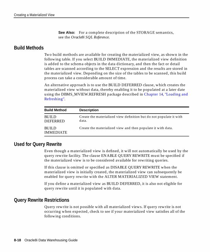
Creating a Materialized View
Build MethodsTwo build methods are available for creating the materialized view, as shown in the
following table. If you select BUILD IMMEDIATE, the materialized view definition
is added to the schema objects in the data dictionary, and then the fact or detail
tables are scanned according to the SELECT expression and the results are stored in
the materialized view. Depending on the size of the tables to be scanned, this build
process can take a considerable amount of time.
An alternative approach is to use the BUILD DEFERRED clause, which creates the
materialized view without data, thereby enabling it to be populated at a later date
using the DBMS_MVIEW.REFRESH package described in Chapter 14, "Loading and
Refreshing".
Used for Query RewriteEven though a materialized view is defined, it will not automatically be used by the
query rewrite facility. The clause ENABLE QUERY REWRITE must be specified if
the materialized view is to be considered available for rewriting queries.
If this clause is omitted or specified as DISABLE QUERY REWRITE when the
materialized view is initially created, the materialized view can subsequently be
enabled for query rewrite with the ALTER MATERIALIZED VIEW statement.
If you define a materialized view as BUILD DEFERRED, it is also not eligible for
query rewrite until it is populated with data.
Query Rewrite RestrictionsQuery rewrite is not possible with all materialized views. If query rewrite is not
occurring when expected, check to see if your materialized view satisfies all of the
following conditions.
See Also: For a complete description of the STORAGE semantics,
see the Oracle8i SQL Reference.
Build Method Description
BUILDDEFERRED
Create the materialized view definition but do not populate it withdata.
BUILDIMMEDIATE
Create the materialized view and then populate it with data.
8-18 Oracle8i Data Warehousing Guide

Creating a Materialized View
Materialized View Restrictions1. There cannot be non-repeatable expressions (ROWNUM, SYSDATE,
non-repeatable PL/SQL functions, and so on) anywhere in the defining query.
2. There cannot be references to RAW or LONG RAW datatypes or object REFs.
3. The query must be a single-block query, that is, it cannot contain set functions
(UNION, MINUS, and so on). However, a materialized view can have multiple
query blocks (for example, inline views in the FROM clause and subselects in
the WHERE or HAVING clauses).
4. If the materialized view was registered as PREBUILT, the precision of the
columns must agree with the precision of the corresponding SELECT
expressions unless overridden by WITH REDUCED PRECISION.
Query Rewrite Restrictions1. If a query has both local and remote tables, only local tables will be considered
for potential rewrite.
2. None of the detail tables can be owned by SYS, and the materialized view
cannot be owned by SYS.
Non-SQL Text Rewrite Restrictions1. SELECT and GROUP BY lists, if present, must be the same in the query and the
materialized view and must contain straight columns, that is, no expressions
are allowed in the columns.
2. Aggregate operators must occur only as the outermost part of the expression;
that is, aggregates such as AVG(AVG(x)) or AVG(x)+AVG(x) are not allowed.
3. The WHERE clause must contain only inner or outer equijoins, and they can be
connected only by ANDs. No ORs and no selections on single tables are
allowed in the WHERE clause.
4. HAVING or CONNECT BY clauses are not allowed.
Refresh OptionsWhen you define a materialized view, you can specify its two refresh options: how
to refresh and what type of refresh. If unspecified, the defaults are assumed as ON
DEMAND and FORCE.
The two refresh execution modes are: ON COMMIT and ON DEMAND. The
method you select will affect the type of materialized view that can be defined.
Materialized Views 8-19

Creating a Materialized View
If you think the materialized view did not refresh, check the alert log or trace file.
If a materialized view fails during refresh at COMMIT time, the user has to
explicitly invoke the refresh procedure using the DBMS_MVIEW package after
addressing the errors specified in the trace files. Until this is done, the view will no
longer be refreshed automatically at commit time.
You can specify how you want your materialized views to be refreshed from the
detail tables by selecting one of four options: FORCE, COMPLETE, FAST, and
NEVER.
Whether the fast refresh option is available will depend upon the type of
materialized view. Fast refresh is available for three general classes of materialized
views: materialized views with joins only, materialized views with joins and
aggregates, and materialized views with aggregates on a single table.
General Restrictions on Fast RefreshThe materialized view’s defining query is restricted as follows:
■ The FROM list must contain base tables only (that is, no views).
Refresh Mode Description
ON COMMIT Refresh occurs automatically when a transaction that modified one ofthe materialized view’s fact tables commits. Can be used withmaterialized views on single table aggregates and materialized viewscontaining joins only.
ON DEMAND Refresh occurs when a user manually executes one of the availablerefresh procedures contained in the DBMS_MVIEW package(REFRESH, REFRESH_ALL_MVIEWS, REFRESH_DEPENDENT).
Refresh Option Description
COMPLETE Refreshes by recalculating the materialized view's defining query.
FAST Refreshes by incrementally adding the new data that has beeninserted into the tables. The new data is obtained from the directpath log or from the materialized view logs.
FORCE Applies fast refresh if possible; otherwise, it applies COMPLETErefresh.
NEVER Indicates that the materialized view will not be refreshed with theOracle refresh mechanisms.
8-20 Oracle8i Data Warehousing Guide

Creating a Materialized View
■ It cannot contain references to non-repeating expressions like SYSDATE and
ROWNUM.
■ It cannot contain references to RAW or LONG RAW data types.
■ It cannot contain HAVING or CONNECT BY clauses.
■ The WHERE clause can contain only joins and they must be equi-joins (inner or
outer) and all join predicates must be connected with ANDs. No selection
predicates on individual tables are allowed.
■ It cannot have subqueries, inline views, or set functions like UNION or MINUS.
Restrictions on Fast Refresh on Materialized Views with Joins OnlyDefining queries for materialized views with joins only and no aggregates have
these restrictions on fast refresh:
■ All restrictions from "General Restrictions on Fast Refresh" on page 8-20.
■ They cannot have GROUP BY clauses or aggregates.
■ If the WHERE clause of the query contains outer joins, then unique constraints
must exist on the join columns of the inner join table.
■ Rowids of all the tables in the FROM list must appear in the SELECT list of the
query.
■ Materialized view logs must exist with rowids for all the base tables in the
FROM list of the query.
■ Materialized views from this category are FAST refreshable after DML or Direct
Load to the base tables.
Restrictions on Fast Refresh on Materialized Views with Single-Table AggregatesDefining queries for materialized views with single-table aggregates have these
restrictions on fast refresh:
■ All restrictions from "General Restrictions on Fast Refresh" on page 8-20.
■ They can only have a single table.
■ The SELECT list must contain all GROUP BY columns.
■ Expressions are allowed in the GROUP BY and SELECT clauses provided they
are the same.
■ They cannot have a WHERE clause.
Materialized Views 8-21

Creating a Materialized View
■ COUNT(*) must be present.
■ They cannot have a MIN or MAX function.
■ For a materialized view with an aggregate with a single table, a materialized
view log must exist on the table and must contain all columns referenced in the
materialized view. The log must have been created with the INCLUDING NEW
VALUES clause.
■ If AVG(expr) or SUM(expr) is specified, you must have COUNT(expr).
■ If VARIANCE(expr) or STDDEV(expr) is specified, you must have
COUNT(expr) and SUM(expr).
Restrictions on Fast Refresh on Materialized Views with Joins and Aggregates:Defining queries for materialized views with joins and aggregates have these
restrictions on fast refresh:
■ All restrictions from "General Restrictions on Fast Refresh" on page 8-20.
■ The WHERE clause can contain inner equi-joins only (that is, no outer joins)
■ Materialized views from this category are FAST refreshable after Direct Load to
the base tables; they are not FAST refreshable after conventional DML to the
base tables.
■ Materialized views from this category can have only the ON DEMAND option
(that is, no ON COMMIT refresh option is allowed).
ORDER BYAn ORDER BY clause is allowed in the CREATE MATERIALIZED VIEW statement.
It is only used during the initial creation of the materialized view. It is not used
during a full refresh or an incremental refresh.
To improve the performance of queries against large materialized views, store the
rows in the materialized view in the order specified in the ORDER BY clause. This
initial ordering provides physical clustering of the data. If indexes are built on the
columns by which the materialized view is ordered, accessing the rows of the
materialized view using the index will significantly reduce the time for disk I/O
due to the physical clustering.
The ORDER BY clause is not considered part of the materialized view definition. As
a result, there is no difference in the manner in which Oracle detects the various
types of materialized views (for example, materialized join views with no
aggregates). For the same reason, query rewrite is not affected by the ORDER BY
8-22 Oracle8i Data Warehousing Guide

Nested Materialized Views
clause. This feature is similar to the CREATE TABLE ... ORDER BY ... capability that
exists in Oracle. For example:
CREATE MATERIALIZED VIEW sum_sales REFRESH FAST ON DEMAND AS SELECT cityid, COUNT(*) count_all, SUM(sales) sum_sales, COUNT(sales) cnt_sales FROM city_sales ORDER BY cityid;
In the above example, we would use the "ORDER BY cityid" clause only during the
creation of the materialized view. The materialized view definition is not affected by
the ORDER BY clause. The definition is:
SELECT cityid, COUNT(*) count_all,SUM(sales) sum_sales, COUNT(sales) cnt_salesFROM city_sales
Using Oracle Enterprise ManagerA materialized view can also be created using Oracle Enterprise Manager by
selecting the materialized view object type. There is no difference in the information
required if this approach is used. However, there are three property sheets which
must be completed and you need to ensure that the option "Enable Query Rewrite"
on the General sheet is selected.
Nested Materialized ViewsA nested materialized view is a materialized view whose definition is based on
another materialized view. A nested materialized view may reference other
relations in the database in addition to materialized views.
Why Use Nested Materialized Views?In a data warehouse, you typically create many aggregate views on a single join (for
example, rollups along different dimensions). Incrementally maintaining these
distinct materialized aggregate views can take a long time because the underlying
join has to be performed many times. By using nested materialized views, the join is
performed just once (while maintaining the materialized view containing joins
only) and incremental maintenance of single-table aggregate materialized views is
very fast due to the self-maintenance refresh operations on this class of views.
Using nested materialized views also overcomes the limitation posed by
Materialized Views 8-23

Nested Materialized Views
materialized aggregate views, where incremental maintenance can only be done
with direct-load insert.
Rules for Using Nested Materialized ViewsYou should keep a couple of points in mind when deciding whether to use nested
materialized views.
1. If you do not need the FAST REFRESH clause, then you can define a nested
materialized view.
2. Materialized views with joins only and single-table aggregate materialized
views can be REFRESH FAST and nested if all the materialized views that they
depend on are either materialized join views or single-table aggregate
materialized views.
Restrictions when Using Nested Materialized ViewsOnly nested materialized join views and nested single-table aggregate materialized
views can use incremental refresh. If you want complete refresh for all of your
materialized views, then you can still nest these materialized views.
Materialized join views and single-table aggregate materialized views can be
incrementally refreshed in the presence of arbitrary DML. In addition, the ON
COMMIT refresh mode can be used with these types of materialized views. To
maximize performance with materialized join views and single-table aggregate
materialized views, you should first combine the two together. That is, define a
single-table aggregate materialized view on top of a materialized join view. Such a
composition yields a materialized aggregate view with respect to the base tables. Thus,
logically:
single-table aggregate materialized view (materialized join view (<tables>))
is equivalent to:
materialized view with joins and aggregates(<tables>)
8-24 Oracle8i Data Warehousing Guide

Nested Materialized Views
Figure 8–3 Nested Materialized View Equivalents
Figure 8–3 is just one of many possible ways to nest materialized views, but it is
likely to be the most frequent and practical. Cyclic dependencies (a materialized
view that indirectly references itself) are caught at creation time and an error is
generated. Some restrictions are placed on the way you can nest materialized views.
Oracle allows nesting a materialized view only when all the immediate
dependencies of the materialized view do not have any dependencies amongst
themselves. Thus, in the dependency tree, a materialized view can never be a parent
as well as a grandparent of an object. For example, Figure 8–4, shows an
impermissible materialized view because it is both a parent and grandparent of the
same object.
Figure 8–4 Nested Materialized View Restriction
Limitations of Nested Materialized ViewsNested materialized views incur the space overhead of materializing the join and
having a materialized view log. This is in contrast to materialized aggregate views
Materializedjoin view
Single tableAggregate
materialized view
Table 2 Table 3Table 1
Materializedview with joins
and Aggregates
Table 2 Table 3Table 1
=
MV2
MV1
Table2Table1
Materialized Views 8-25
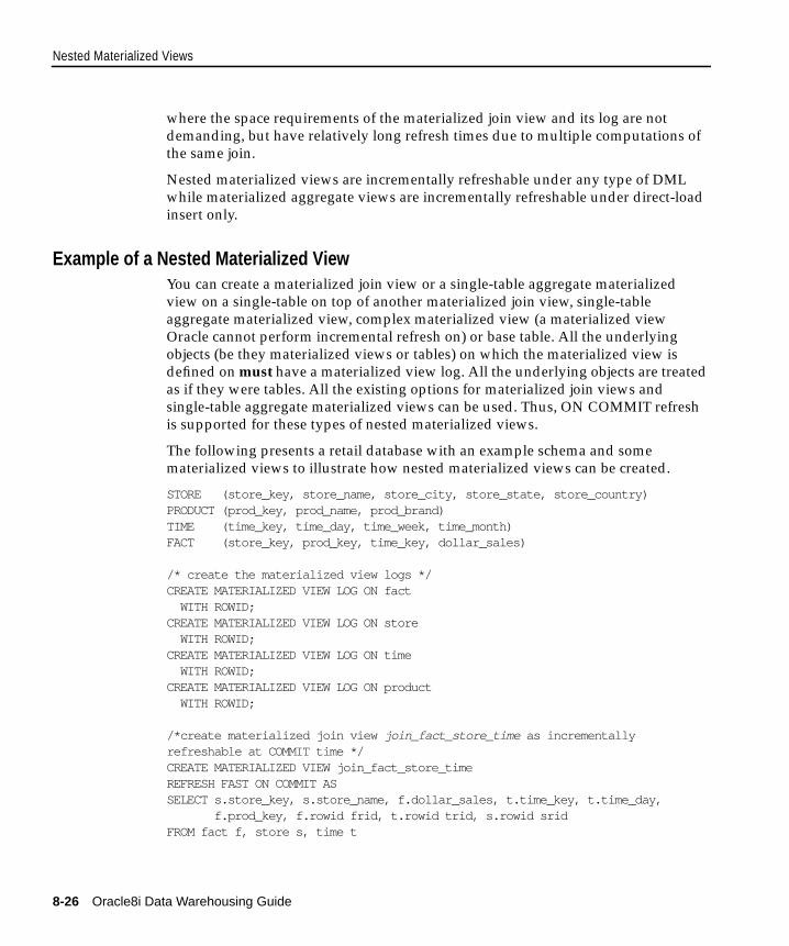
Nested Materialized Views
where the space requirements of the materialized join view and its log are not
demanding, but have relatively long refresh times due to multiple computations of
the same join.
Nested materialized views are incrementally refreshable under any type of DML
while materialized aggregate views are incrementally refreshable under direct-load
insert only.
Example of a Nested Materialized ViewYou can create a materialized join view or a single-table aggregate materialized
view on a single-table on top of another materialized join view, single-table
aggregate materialized view, complex materialized view (a materialized view
Oracle cannot perform incremental refresh on) or base table. All the underlying
objects (be they materialized views or tables) on which the materialized view is
defined on must have a materialized view log. All the underlying objects are treated
as if they were tables. All the existing options for materialized join views and
single-table aggregate materialized views can be used. Thus, ON COMMIT refresh
is supported for these types of nested materialized views.
The following presents a retail database with an example schema and some
materialized views to illustrate how nested materialized views can be created.
STORE (store_key, store_name, store_city, store_state, store_country)PRODUCT (prod_key, prod_name, prod_brand)TIME (time_key, time_day, time_week, time_month)FACT (store_key, prod_key, time_key, dollar_sales)
/* create the materialized view logs */CREATE MATERIALIZED VIEW LOG ON fact WITH ROWID;CREATE MATERIALIZED VIEW LOG ON store WITH ROWID;CREATE MATERIALIZED VIEW LOG ON time WITH ROWID;CREATE MATERIALIZED VIEW LOG ON product WITH ROWID;
/*create materialized join view join_fact_store_time as incrementallyrefreshable at COMMIT time */CREATE MATERIALIZED VIEW join_fact_store_timeREFRESH FAST ON COMMIT ASSELECT s.store_key, s.store_name, f.dollar_sales, t.time_key, t.time_day, f.prod_key, f.rowid frid, t.rowid trid, s.rowid sridFROM fact f, store s, time t
8-26 Oracle8i Data Warehousing Guide

Nested Materialized Views
WHERE f.time_key = t.time_key AND f.store_key = s.store_key;
To create a nested materialized view on the table join_fact_store_time, you would
have to create a materialized view log on the table. Because this will be a
single-table aggregate materialized view on join_fact_store_time, you need to log all
the necessary columns and use the INCLUDING NEW VALUES clause.
/* create materialized view log on join_fact_store_time */CREATE MATERIALIZED VIEW log on join_fact_store_time WITH rowid (store_name, time_day, dollar_sales) INCLUDING new values;
/* create the single-table aggregate materialized view sum_sales_store_time onjoin_fact_store_time as incrementally refreshable at COMMIT time. */CREATE MATERIALIZED VIEW sum_sales_store_time REFRESH FAST ON COMMIT AS SELECT COUNT(*) cnt_all, SUM(dollar_sales) sum_sales, COUNT(dollar_sales) cnt_sales, store_name, time_day FROM join_fact_store_time GROUP BY store_name, time_day;
Note that the above single-table aggregate materialized view sum_sales_store_time is
logically equivalent to a multi-table aggregate on the tables fact, time, and store
whose definition is
SELECT COUNT(*) cnt_all, SUM(f.dollar_sales) sum_sales, COUNT(f.dollar_sales) cnt_sales, s.store_name, t.time_dayFROM fact f, time t , store sWHERE f.time_key = t.time_key AND f.store_key = s.store_keyGROUP BY store_name, time_day;
You can now define a materialized join view join_fact_store_time_prod as a join
between join_fact_store_time and table product.
CREATE MATERIALIZED VIEW join_fact_store_time_prod REFRESH FAST ON COMMIT AS SELECT j.rowid jrid, p.rowid prid, j.store_name, j.prod_key, j.prod_name, j.dollar_sales FROM join_fact_store_time j, product p WHERE j.prod_key = p.prod_key;
Materialized Views 8-27

Nested Materialized Views
The above schema can be diagrammatically represented as in Figure 8–5.
Figure 8–5 Nested Materialized View Schema
Nesting Materialized Views with Joins and AggregatesMaterialized views with joins and aggregates can be nested if they are refreshed as
COMPLETE REFRESH. Thus, a user can arbitrarily nest materialized views having
joins and aggregates. No incremental maintenance is possible for these materialized
views.
Note that the ON COMMIT refresh option is not available for complex materialized
views. Because you have to invoke the refresh functions manually, ordering has to
be taken into account. This is because the refresh for a materialized view that is
built on other materialized views will use the current state of the other materialized
views, whether they are fresh or not. You can find the dependent materialized
views for a particular object using the PL/SQL function
GET_MV_DEPENDENCIES() in the DBMS_MVIEW package.
Nested Materialized View Usage GuidelinesHere are some guidelines on how to use nested materialized views:
1. If incremental refresh is desired when a materialized view contains joins and
aggregates and standard fast refresh cannot be used because DML is occurring
on the tables, consider creating a single-table aggregate materialized view
nested on a materialized join view.
2. If incremental refresh is desired, you should incrementally refresh all the
materialized views along any chain. It makes little sense to define an
join_fact_store_time
store fact time
sum_sales_store_time join_fact_store_time
product
8-28 Oracle8i Data Warehousing Guide

Registration of an Existing Materialized View
incrementally refreshable materialized view on top of a materialized view that
must be refreshed with a complete refresh.
3. When using materialized join views and single-table aggregate materialized
views, you can define them to be ON COMMIT or ON DEMAND. The choice
would depend on the application using the materialized views. If one expects
the materialized views to always remain fresh, then all the materialized views
should have the ON COMMIT refresh option. If the time window for refresh
does not permit refreshing all the materialized views at commit time, then the
appropriate materialized views could be created with (or altered to have) the
ON DEMAND refresh option.
Registration of an Existing Materialized ViewSome data warehouses have implemented materialized views in ordinary user
tables. Although this solution provides the performance benefits of materialized
views, it does not:
■ provide query rewrite to all SQL applications
■ enable materialized views defined in one application to be transparently
accessed in another application
■ generally support fast parallel or fast incremental materialized view refresh
Because of these problems, and because existing materialized views may be
extremely large and expensive to rebuild, you should register your existing
materialized view tables with Oracle whenever possible. You can register a
user-defined materialized view with the CREATE MATERIALIZED VIEW ... ON
PREBUILT TABLE statement. Once registered, the materialized view can be used
for query rewrites or maintained by one of the refresh methods, or both.
In some cases, user-defined materialized views are refreshed on a schedule that is
longer than the update cycle; for example, a monthly materialized view may be
updated only at the end of each month, and the materialized view values always
refer to complete time periods. Reports written directly against these materialized
views implicitly select only data that is not in the current (incomplete) time period.
If a user-defined materialized view already contains a time dimension:
■ It should be registered and then incrementally refreshed each update cycle.
■ A view should be created that selects the complete time period of interest.
Materialized Views 8-29
Registration of an Existing Materialized View
For example, if a materialized view was formerly refreshed monthly at the end
of each month, then the view would contain the selection WHERE time.month <
CURRENT_MONTH().
■ The reports should be modified to refer to the view instead of referring directly
to the user-defined materialized view.
If the user-defined materialized view does not contain a time dimension, then:
■ A new materialized view should be created that does include the time
dimension (if possible).
■ The view should aggregate over the time column in the new materialized view.
The contents of the table must reflect the materialization of the defining query at the
time you register it as a materialized view, and each column in the defining query
must correspond to a column in the table that has a matching datatype. However,
you can specify WITH REDUCED PRECISION to allow the precision of columns in
the defining query to be different from that of the table columns.
The table and the materialized view must have the same name, but the table retains
its identity as a table and can contain columns that are not referenced in the
defining query of the materialized view. These extra columns are known as
unmanaged columns. If rows are inserted during a refresh operation, each
unmanaged column of the row is set to its default value. Therefore, the unmanaged
columns cannot have NOT NULL constraints unless they also have default values.
Unmanaged columns are not supported by single-table aggregate materialized
views or materialized views containing joins only.
Materialized views based on prebuilt tables are eligible for selection by query
rewrite provided the parameter QUERY_REWRITE_INTEGRITY is set to at least the
level of TRUSTED. See Chapter 19, "Query Rewrite", for details about integrity
levels.
When you drop a materialized view that was created on a prebuilt table, the table
still exists—only the materialized view is dropped.
When a prebuilt table is registered as a materialized view and query rewrite is
desired, the parameter QUERY_REWRITE_INTEGRITY must be set to at least
STALE_TOLERATED because, when it is created, the materialized view is marked
as unknown. Therefore, only stale integrity modes can be used.
CREATE TABLE sum_sales_tab PCTFREE 0 TABLESPACE mviews STORAGE (INITIAL 16k NEXT 16k PCTINCREASE 0) AS
8-30 Oracle8i Data Warehousing Guide

Partitioning a Materialized View
SELECT f.store_key SUM(dollar_sales) AS dollar_sales, SUM(unit_sales) AS unit_sales, SUM(dollar_cost) AS dollar_cost FROM fact f GROUP BY f.store_key;
CREATE MATERIALIZED VIEW sum_sales_tabON PREBUILT TABLE WITHOUT REDUCED PRECISIONENABLE QUERY REWRITEASSELECT f.store_key, SUM(dollar_sales) AS dollar_sales, SUM(unit_sales) AS unit_sales, SUM(dollar_cost) AS dollar_cost FROM fact f GROUP BY f.store_key;
This example illustrates the two steps required to register a user-defined table. First,
the table is created, then the materialized view is defined using exactly the same
name as the table. This materialized view sum_sales_tab is eligible for use in query
rewrite.
Partitioning a Materialized ViewBecause of the large volume of data held in a data warehouse, partitioning is an
extremely useful option that can be used by the database designer.
Partitioning the fact tables improves scalability, simplifies system administration,
and makes it possible to define local indexes that can be efficiently rebuilt. See
Chapter 5, "Parallelism and Partitioning", for further details about partitioning.
Partitioning a materialized view also has benefits for refresh, since the refresh
procedure can use parallel DML to maintain the materialized view. To realize these
benefits, the materialized view has to be defined as PARALLEL and parallel DML
must be enabled in the session.
When the data warehouse or data mart contains a time dimension, it is often
desirable to archive the oldest information, and then reuse the storage for new
information, the rolling window scenario. If the fact tables or materialized views
include a time dimension and are horizontally partitioned by the time attribute,
then management of rolling materialized views can be reduced to a few fast
partition maintenance operations provided that the unit of data that is rolled out
equals, or is at least aligned with, the range partitions.
Materialized Views 8-31

Partitioning a Materialized View
If you plan to have rolling materialized views in your warehouse, then you should
determine how frequently you plan to perform partition maintenance operations,
and you should plan to partition fact tables and materialized views to reduce the
amount of system administration overhead required when old data is aged out.
With the introduction of new partitioning options in Oracle8i, you are not restricted
to using range partitions. For example, a composite partition using both a time
value and, say, a key value could result in an ideal partition solution for your data.
An ideal case for using partitions is when a materialized view contains a subset of
the data. For example, this can be achieved by defining an expression of the form
WHERE time_key < '1-OCT-1998' in the SELECT expression for the materialized
view. However, if a WHERE clause of this type is included, then query rewrite will
be restricted to the exact match case, which severely restricts when the materialized
view is used. To overcome this problem, use a partitioned materialized view with
no WHERE clause and then query rewrite will be able to use the materialized view
and it will only search the appropriate partition, thus improving query
performance.
There are two approaches to partitioning a materialized view:
■ Partitioning the Materialized View
■ Partitioning a Prebuilt Table
Partitioning the Materialized ViewPartitioning a materialized view involves defining the materialized view with the
standard Oracle partitioning clauses as illustrated in the example below. This
example creates a materialized view called part_sales_mv which uses three
partitions, is, by default, fast refreshed, and is eligible for query rewrite.
CREATE MATERIALIZED VIEW part_sales_mv PARALLEL PARTITION by RANGE (time_key) ( PARTITION time_key VALUES LESS THAN (TO_DATE('31-12-1997', 'DD-MM-YYYY')) PCTFREE 0 PCTUSED STORAGE (INITIAL 64k NEXT 16k PCTINCREASE 0) TABLESPACE sf1, PARTITION month2 VALUES LESS THAN (TO_DATE('31-01-1998', 'DD-MM-YYYY')) PCTFREE 0 PCTUSED STORAGE INITIAL 64k NEXT 16k PCTINCREASE 0)
8-32 Oracle8i Data Warehousing Guide

Partitioning a Materialized View
TABLESPACE sf2, PARTITION month3 VALUES LESS THAN (TO_DATE('31-01-1998', 'DD-MM-YYYY')) PCTFREE 0 PCTUSED STORAGE (INITIAL 64k NEXT 16k PCTINCREASE 0) TABLESPACE sf3)BUILD DEFERREDREFRESH FASTENABLE QUERY REWRITEASSELECT f.store_key, f.time_key, SUM(f.dollar_sales) AS sum_dol_sales, SUM(f.unit_sales) AS sum_unit_sales FROM fact f GROUP BY f.time_key, f.store_key;
Partitioning a Prebuilt TableAlternatively, a materialized view can be registered to a partitioned prebuilt table as
illustrated in the following example:
CREATE TABLE part_fact_tab( time_key, store_key, sum_dollar_sales, sum_unit_sale) PARALLEL PARTITION by RANGE (time_key) ( PARTITION month1 VALUES LESS THAN (TO_DATE('31-12-1997', 'DD-MM-YYYY')) PCTFREE 0 PCTUSED 99 STORAGE (INITITAL 64k NEXT 16k PCTINCREASE 0) TABLESPACE sf1, PARTITIION month2 VALUES LESS THAN (TO_DATE('31-01-1998', 'DD-MM-YYYY')) PCTFREE 0 PCTUSED 99 STORAGE (INITIAL 64k NEXT 16k PCTINCREASE 0) TABLESPACE sf2, PARTITION month3 VALUES LESS THAN (TO_DATE('31-01-1998', DD-MM-YYYY')) PCTFREE 0 PCTUSED 99 STORAGE INITIAL 64k NEXT 16k PCTINCREASE 0) TABLESPACE sf3)ASSELECT f.time_key, f.store_key, SUM(f.dollar_sales) AS sum_dollar_sales, SUM(f.unit_sales) AS sum_unit_sales
Materialized Views 8-33

Indexing Selection for Materialized Views
FROM fact f GROUP BY f.time_key, f.store_key;
CREATE MATERIALIZED VIEW part_fact_tabON PREBUILT TABLEENABLE QUERY REWRITEASSELECT f.time_key, f.store_key, SUM(f.dollar_sales) AS sum_dollar_sales, SUM(f.unit_sales) AS sum_unit_sales FROM fact f GROUP BY f.time_key , f.store_key;
In this example, the table part_fact_tab has been partitioned over three months and
then the materialized view was registered to use the prebuilt table. This
materialized view is eligible for query rewrite because the ENABLE QUERY
REWRITE clause has been included.
Indexing Selection for Materialized ViewsThe two main operations on a materialized view are query execution and
incremental refresh, and each operation has different performance requirements.
Query execution may need to access any subset of the materialized view key
columns, and may need to join and aggregate over a subset of those columns.
Consequently, query execution usually performs best if there is a single-column
bitmap index defined on each materialized view key column.
In the case of materialized views containing only joins using the fast refresh option,
it is highly recommended that indexes be created on the columns that contain the
rowids to improve the performance of the refresh operation.
If a materialized view using joins and aggregates is fast refreshable, then an index is
automatically created and cannot be disabled.
See Chapter 18, "Tuning Parallel Execution", for further details.
Invalidating a Materialized ViewDependencies related to materialized views are automatically maintained to ensure
correct operation. When a materialized view is created, the materialized view
depends on the detail tables referenced in its definition. Any DDL operation, such
as a DROP or ALTER, on any dependency in the materialized view will cause it to
become invalid.
8-34 Oracle8i Data Warehousing Guide

Guidelines for Using Materialized Views in a Data Warehouse
A materialized view is automatically revalidated when it is referenced. In many
cases, the materialized view will be successfully and transparently revalidated.
However, if a column has been dropped in a table referenced by a materialized view
or the owner of the materialized view did not have one of the query rewrite
privileges and that has now been granted to the owner, the command:
ALTER MATERIALIZED VIEW mview_name ENABLE QUERY REWRITE
should be used to revalidate the materialized view. If there are any problems, an
error will be returned.
The state of a materialized view can be checked by querying the tables
USER_MVIEWS or ALL_MVIEWS. The column STALENESS will show one of the
values FRESH, STALE, UNUSABLE, UNKNOWN, or UNDEFINED to indicate
whether the materialized view can be used.
Security IssuesTo create a materialized view, the privilege CREATE MATERIALIZED VIEW is
required, and to create a materialized view that references a table in another
schema, you must have SELECT privileges on that table. Moreover, if you enable
query rewrite, you must have the QUERY REWRITE or GLOBAL QUERY
REWRITE privilege to reference tables in your own schema. To enable query rewrite
on a materialized view that references tables outside your schema, you must have
the GLOBAL QUERY REWRITE privilege.
If you continue to get a privilege error while trying to create a materialized view
and you believe that all the required privileges have been granted, then the problem
is most likely due to a privilege not being granted explicitly and trying to inherit the
privilege from a role instead. The owner of the materialized view must have
explicitly been granted SELECT access to the referenced tables if they are in a
different schema.
Guidelines for Using Materialized Views in a Data WarehouseDetermining what materialized views would be most beneficial for performance
gains is aided by the analysis tools of the DBMS_OLAP package. Specifically, you
can call the DBMS_OLAP.RECOMMEND_MV procedure to see a list of
materialized views that Oracle recommends based on the statistics and the usage of
the target database. See Chapter 15, "Summary Advisor", for further details.
If you are going to write your own materialized views without the aid of Oracle
analysis tools, then use these guidelines to achieve maximum performance:
Materialized Views 8-35

Altering a Materialized View
1. Instead of defining multiple materialized views on the same tables with the
same GROUP BY columns but with different measures, define a single
materialized view including all of the different measures.
2. If your materialized view includes the aggregated measure AVG(x), also
include COUNT(x) to support incremental refresh. Similarly, if VARIANCE(x)
or STDDEV(x) is present, then always include COUNT(x) and SUM(x) to
support incremental refresh.
Altering a Materialized ViewThere are five amendments that can be made to a materialized view:
■ change its refresh option (FAST/FORCE/COMPLETE/NEVER)
■ change its refresh mode (ON COMMIT/ ON DEMAND)
■ recompile
■ enable/disable its use for query rewrite
■ consider fresh
All other changes are achieved by dropping and then recreating the materialized
view.
The COMPILE clause of the ALTER MATERIALIZED VIEW statement can be used
when the materialized view has been invalidated as described in "Invalidating a
Materialized View" on page 8-34. This compile process is quick, and allows the
materialized view to be used by query rewrite again.
For further information about ALTER MATERIALIZED VIEW, see Oracle8i SQLReference.
Dropping a Materialized ViewUse the DROP MATERIALIZED VIEW statement to drop a materialized view. For
example:
DROP MATERIALIZED VIEW sales_sum_mv;
This command drops the materialized view sales_sum_mv . If the materialized
view was prebuilt on a table, then the table is not dropped but it can no longer be
maintained with the refresh mechanism. Alternatively, you can drop a materialized
view using Oracle Enterprise Manager.
8-36 Oracle8i Data Warehousing Guide

Overview of Materialized View Management Tasks
Overview of Materialized View Management TasksThe motivation for using materialized views is to improve performance, but the
overhead associated with materialized view management can become a significant
system management problem. Materialized view management activities include:
■ Identifying what materialized views to create initially
■ Indexing the materialized views
■ Ensuring that all materialized views and materialized view indexes are
refreshed properly each time the database is updated
■ Checking which materialized views have been used
■ Determining how effective each materialized view has been on workload
performance
■ Measuring the space being used by materialized views
■ Determining which new materialized views should be created
■ Determining which existing materialized views should be dropped
■ Archiving old detail and materialized view data that is no longer useful
After the initial effort of creating and populating the data warehouse or data mart,
the major administration overhead is the update process, which involves the
periodic extraction of incremental changes from the operational systems;
transforming the data; verification that the incremental changes are correct,
consistent, and complete; bulk-loading the data into the warehouse; and refreshing
indexes and materialized views so that they are consistent with the detail data.
The update process must generally be performed within a limited period of time
known as the update window. The update window depends on the update frequency(such as daily or weekly) and the nature of the business. For a daily update
frequency, an update window of two to six hours might be typical.
The update window usually displays the time for the following activities:
1. Loading the detail data.
2. Updating or rebuilding the indexes on the detail data.
3. Performing quality assurance tests on the data.
4. Refreshing the materialized views.
5. Updating the indexes on the materialized views.
Materialized Views 8-37

Overview of Materialized View Management Tasks
A popular and efficient way to load data into a warehouse or data mart is to use
SQL*Loader with the DIRECT or PARALLEL option or to use another loader tool
that uses the Oracle direct path API.
Loading strategies can be classified as one-phase or two-phase. In one-phase loading,
data is loaded directly into the target table, quality assurance tests are performed,
and errors are resolved by performing DML operations prior to refreshing
materialized views. If a large number of deletions are possible, then storage
utilization may be adversely affected, but temporary space requirements and load
time are minimized. The DML that may be required after one-phase loading causes
multi-table aggregate materialized views to become unusable in the safest rewrite
integrity level.
In a two-phase loading process:
■ Data is first loaded into a temporary table in the warehouse.
■ Quality assurance procedures are applied to the data.
■ Referential integrity constraints on the target table are disabled, and the local
index in the target partition is marked unusable.
■ The data is copied from the temporary area into the appropriate partition of the
target table using INSERT AS SELECT with the PARALLEL or APPEND hint.
■ The temporary table is dropped.
■ The constraints are enabled, usually with the NOVALIDATE option.
Immediately after loading the detail data and updating the indexes on the detail
data, the database can be opened for operation, if desired. Query rewrite can be
disabled by default (with ALTER SYSTEM SET QUERY_REWRITE_ENABLED =
FALSE) until all the materialized views are refreshed, but enabled at the session
level for any users who do not require the materialized views to reflect the data
from the latest load (with ALTER SESSION SET QUERY_REWRITE_ENABLED =
TRUE). However, as long as QUERY_REWRITE_INTEGRITY = ENFORCED or
TRUSTED, this is not necessary because the system ensures that only materialized
views with updated data participate in a query rewrite.
See Also: See Oracle8i Utilities for the restrictions and
considerations when using SQL*Loader with the DIRECT or
PARALLEL keywords.
8-38 Oracle8i Data Warehousing Guide

Dimen
9
DimensionsThe following sections will help you create and manage a data warehouse:
■ What is a Dimension?
■ Creating a Dimension
■ Viewing Dimensions
■ Dimensions and Constraints
■ Validating a Dimension
■ Altering a Dimension
■ Deleting a Dimension
sions 9-1

What is a Dimension?
What is a Dimension?A dimension is a structure that categorizes data in order to enable end users to
answer business questions. Commonly used dimensions are Customer, Product,
and Time. For example, each store of a video chain might gather and store data
regarding sales and rentals of video tapes at the check-out counter. The video chain
management can build a data warehouse to analyze the sales of its products across
all stores over time and help answer questions such as:
■ What is the effect of promoting one product on the sale of a related product that
is not promoted?
■ What are the product sales before and after the promotion?
The data in the video chain's data warehouse system has two important
components: dimensions and facts. The dimensions are products, locations (stores),
promotions, and time. One approach for identifying your dimensions is to review
your reference tables, such as a product table that contains everything about a
product, or a store table containing all information about a store. The facts are sales
(units sold or rented) and profits. A data warehouse contains facts about the sales of
each product at each store on a daily basis.
A typical dimensional cube is shown in Figure 9–1:
9-2 Oracle8i Data Warehousing Guide

What is a Dimension?
Figure 9–1 Sample Dimensional Cube
Dimensions do not have to be defined, but spending time creating them can yield
significant benefits because they help query rewrite perform more complex types of
rewrite. They are mandatory if you use the Summary Advisor to recommend which
materialized views to create, drop, or retain. See Chapter 19, "Query Rewrite", for
further details regarding query rewrite. See Chapter 15, "Summary Advisor", for
further details regarding the Summary Advisor.
Dimension values are usually organized into hierarchies. Going up a level in the
hierarchy is called rolling up the data and going down a level in the hierarchy is
called drilling down the data. In the video chain example:
■ Within the time dimension, months roll up to quarters, quarters roll up to years,
and years roll up to all years.
■ Within the product dimension, products roll up to categories, categories roll up
to departments, and departments roll up to all departments.
■ Within the location dimension, stores roll up to cities, cities roll up to states,
states roll up to regions, regions roll up to countries, and countries roll up to all
countries, as shown in Figure 9–2.
Region
Time
Product
Dimensions 9-3

What is a Dimension?
Figure 9–2 Geography Dimension
Data analysis typically starts at higher levels in the dimensional hierarchy and
gradually drills down if the situation warrants such analysis.
You can visualize the dimensions of a business process as an n-dimensional data
cube. In the video chain example, the business dimensions product, location, and
time can be represented along the three axes of the cube. Each unit along the
product axis represents a different product, each unit along the location axis
represents a store, and each unit along the time axis represents a month. At the
intersection of these values is a cell that contains factual information, such as units
sold and profits made. Higher-level analysis consists of selecting and aggregating
the factual information within a subcube, such as rentals of comedy videos in
California stores during the second quarter of 1998.
Therefore, the first step towards creating a dimension is to identify the dimensions
within your data warehouse and then draw the hierarchies as shown in Figure 9–2.
For example, city is a child of state (because you can aggregate city-level data up to
state), and state. Using this approach, you should find it easier to translate this into
an actual dimension.
In the case of normalized or partially normalized dimensions (a dimension that is
stored in more than one table), identify how these tables are joined. Note whether
the joins between the dimension tables can guarantee that each child-side row joins
with one and only one parent-side row. In the case of denormalized dimensions,
determine whether the child-side columns uniquely determine the parent-side (or
attribute) columns. These constraints can be enabled with the NOVALIDATE and
RELY options if the relationships represented by the constraints are guaranteed by
Country
All
State
City
9-4 Oracle8i Data Warehousing Guide
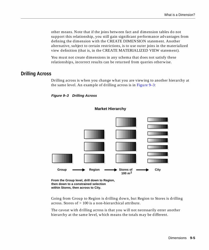
What is a Dimension?
other means. Note that if the joins between fact and dimension tables do not
support this relationship, you still gain significant performance advantages from
defining the dimension with the CREATE DIMENSION statement. Another
alternative, subject to certain restrictions, is to use outer joins in the materialized
view definition (that is, in the CREATE MATERIALIZED VIEW statement).
You must not create dimensions in any schema that does not satisfy these
relationships, incorrect results can be returned from queries otherwise.
Drilling AcrossDrilling across is when you change what you are viewing to another hierarchy at
the same level. An example of drilling across is in Figure 9–3:
Figure 9–3 Drilling Across
Going from Group to Region is drilling down, but Region to Stores is drilling
across. Stores of > 100 is a non-hierarchical attribute.
The caveat with drilling across is that you will not necessarily enter another
hierarchy at the same level, which means the totals may be different.
Market Hierarchy
Region Stores of 100 m
CityGroup
From the Group level, drill down to Region, then down to a constrained selection within Stores, then across to City.
2
Dimensions 9-5
Creating a Dimension
Creating a DimensionBefore you can create a dimension, tables must exist in the database which contain
this dimension data. For example, if you create a dimension called LOCATION, one
or more tables must exist which contains the city, state, and country information. In
a star-schema data warehouse, these dimension tables already exist. It is therefore a
simple task to identify which ones will be used.
You create a dimension using either the CREATE DIMENSION statement or the
Dimension wizard in Oracle Enterprise Manager. Within the CREATE DIMENSION
statement, use the LEVEL...IS clause to identify the names of the dimension levels.
The location dimension contains a single hierarchy, with arrows drawn from the
child level to the parent level. At the top of this dimension graph is the special level
ALL, that represents aggregation over all rows. Each arrow in this graph indicates
that for any child there is one and only one parent. For example, each city must be
contained in exactly one state and each state must be contained in exactly one
country. States that belong to more than one country, or that belong to no country,
violate hierarchical integrity. Hierarchical integrity is necessary for the correct
operation of management functions for materialized views that include aggregates.
For example, you can declare a dimension LOCATION which contains levels CITY,
STATE, and COUNTRY:
CREATE DIMENSION location_dimLEVEL city IS location.cityLEVEL state IS location.stateLEVEL country IS location.country
Each level in the dimension must correspond to one or more columns in a table in
the database. Thus, level city is identified by the column city in the table called
location and level country is identified by a column called country in the same table.
In this example, the database tables are denormalized and all the columns exist in
the same table. However, this is not a prerequisite for creating dimensions. "Using
Normalized Dimension Tables" on page 9-10 shows how to create a dimension that
has a normalized schema design using the JOIN KEY clause.
The next step is to declare the relationship between the levels with the
HIERARCHY statement and give that hierarchy a name. A hierarchical relationship
is a functional dependency from one level of a hierarchy to the next level in the
hierarchy. Using the level names defined previously, the CHILD OF relationship
denotes that each child's level value is associated with one and only one parent
level value. Again, using the entities in Figure 9–4 on page 9-9, the following
9-6 Oracle8i Data Warehousing Guide

Creating a Dimension
statements declare a hierarchy LOC_ROLLUP and define the relationship between
CITY, STATE, and COUNTRY.
HIERARCHY loc_rollup (city CHILD OFstate CHILD OFcountry )
In addition to the 1:n hierarchical relationships, dimensions also include 1:1
attribute relationships between the hierarchy levels and their dependent dimension
attributes. For example, if there are columns governor and mayor, then the
ATTRIBUTE...DETERMINES statement would be state to governor and city to
mayor.
In our example, suppose a query were issued that queried by mayor instead of city.
Since this 1:1 relationship exists between the attribute and the level, city can be used
to identify the data.
ATTRIBUTE city DETERMINES mayor
The complete dimension definition, including the creation of the location table,
follows:
CREATE TABLE location (city VARCHAR2(30),state VARCHAR2(30),country VARCHAR2(30),mayor VARCHAR2(30),governor VARCHAR2(30) );
CREATE DIMENSION location_dimLEVEL city IS location.cityLEVEL state IS location.stateLEVEL country IS location.country
HIERARCHY loc_rollup (city CHILD OFstate CHILD OFcountry )
ATTRIBUTE city DETERMINES location.mayorATTRIBUTE state DETERMINES location.governor;
The design, creation, and maintenance of dimensions is part of the design, creation,
and maintenance of your data warehouse schema. Once the dimension has been
created, check that it meets these requirements:
Dimensions 9-7

Creating a Dimension
■ There must be a 1:n relationship between a parent and children. A parent can
have one or more children, but a child can have only one parent.
■ There must be a 1:1 attribute relationship between hierarchy levels and theirdependent dimension attributes. For example, if there is a column corporation,
then a possible attribute relationship would be corporation to president.
■ If the columns of a parent level and child level are in different relations, thenthe connection between them also requires a 1:n join relationship. Each row
of the child table must join with one and only one row of the parent table. This
relationship is stronger than referential integrity alone because it requires that
the child join key must be non-null, that referential integrity must be
maintained from the child join key to the parent join key, and that the parent
join key must be unique.
■ Ensure (using database constraints if necessary) that the columns of eachhierarchy level are non-null and that hierarchical integrity is maintained.
■ The hierarchies of a dimension may overlap or be disconnected from eachother. However, the columns of a hierarchy level cannot be associated with
more than one dimension.
■ Join relationships that form cycles in the dimension graph are not supported.For example, a hierarchy level cannot be joined to itself either directly or
indirectly.
Multiple HierarchiesA single dimension definition can contain multiple hierarchies as illustrated below.
Suppose a department store wants to track the sales of certain items over time. The
first step is to define the time dimension over which sales will be tracked.
Figure 9–4 on page 9-9 illustrates a dimension "Time_dim" with three time
hierarchies.
9-8 Oracle8i Data Warehousing Guide

Creating a Dimension
Figure 9–4 Time_dim Dimension with Three Time Hierarchies
From the illustration, you can construct the following denormalized Time
dimension statement. The associated CREATE TABLE statement is also shown.
CREATE TABLE time (curDate DATE,month INTEGER,quarter INTEGER,year INTEGER,season INTEGER,week_num INTEGER,dayofweek VARCHAR2(30),month_name VARCHAR2(30) );
CREATE DIMENSION Time_dimLEVEL curDate IS time.curDateLEVEL month IS time.monthLEVEL quarter IS time.quarterLEVEL year IS time.yearLEVEL season IS time.seasonLEVEL week_num IS time.week_num
All
Season
curDate
Quarter
Year
Month
Week
Dimensions 9-9

Creating a Dimension
HIERARCHY calendar_rollup (curDate CHILD OFmonth CHILD OFquarter CHILD OFyear )
HIERARCHY weekly_rollup ( curDate CHILD OF week_num )
HIERARCHY seasonal_rollup ( curDate CHILD OF season )
ATTRIBUTE curDate DETERMINES time.dayofweekATTRIBUTE month DETERMINES time.month_name;
Using Normalized Dimension TablesThe tables used to define a dimension may be normalized or denormalized and the
individual hierarchies can be normalized or denormalized. If the levels of a
hierarchy come from the same table, it is called a fully denormalized hierarchy. For
example, CALENDAR_ROLLUP in the Time dimension is a denormalized
hierarchy. If levels of a hierarchy come from different tables, such a hierarchy is
either a fully or partially normalized hierarchy. This section shows how to define a
normalized hierarchy.
Suppose the tracking of products is done by product, brand, and department. This
data is stored in the tables PRODUCT, BRAND, and DEPARTMENT. The product
dimension is normalized because the data entities ITEM_NAME, BRAND_ID, and
DEPT_ID are taken from different tables. The clause JOIN KEY within the
dimension definition specifies how to join together the levels in the hierarchy. The
dimension statement and the associated CREATE TABLE statements for the
PRODUCT, BRAND, and DEPARTMENT tables are shown below.
CREATE TABLE product (item_name VARCHAR2(30),brand_id INTEGER );
CREATE TABLE brand (brand_id INTEGER,brand_name VARCHAR2(30),dept_id INTEGER);
CREATE TABLE department (dept_id INTEGER,dept_name VARCHAR2(30),
9-10 Oracle8i Data Warehousing Guide

Viewing Dimensions
dept_type INTEGER);
CREATE DIMENSION product_dimLEVEL item IS product.item_nameLEVEL brand_id IS brand.brand_idLEVEL dept_id IS department.dept_id
HIERARCHY merchandise_rollup(
item CHILD OFbrand_id CHILD OFdept_id
JOIN KEY product.brand_id REFERENCES brand_idJOIN KEY brand.dept_id REFERENCES dept_id
)ATTRIBUTE brand_id DETERMINES product.brand_nameATTRIBUTE dept_id DETERMINES (product.dept_name, product.dept_type);
Dimension WizardThe dimension wizard is automatically invoked whenever a request is made to
create a dimension object in Oracle Enterprise Manager. The user is then guided
step by step through the information required for a dimension.
A dimension created via the wizard may contain any of the attributes described in
"Creating a Dimension" on page 9-6, such as join keys, multiple hierarchies and
attributes. Some users may prefer to use the wizard because it will graphically
display the hierarchical relationships as they are being constructed. When it is time
to describe the hierarchy, the dimension wizard will automatically display a default
hierarchy based on the column values, which the user can subsequently amend. See
the Oracle Enterprise Manager documentation set for further details.
Viewing DimensionsDimensions can be viewed through one of two methods:
■ Using The DEMO_DIM Package
■ Using Oracle Enterprise Manager
Dimensions 9-11

Viewing Dimensions
Using The DEMO_DIM PackageTwo procedures are available which allow you to display the dimensions that have
been defined. First, the file smdim.sql must be executed to provide the DEMO_DIM
package, which includes:
■ DEMO_DIM.PRINT_DIM to print a specific dimension
■ DEMO_DIM.PRINT_ALLDIMS to print all dimensions
The DEMO_DIM.PRINT_DIM procedure has only one parameter, the name of the
dimension to display. The example below shows how to display the dimension
TIME_PD.
DEMO_DIM.PRINT_DIM ('TIME_PD');
To display all of the dimensions that have been defined, call the procedure DEMO_
DIM.PRINT_ALLDIMS without any parameters as shown below.
DEMO_DIM.PRINT_ALLDIMS ();
Irrespective of which procedure is called, the output format is identical. A sample
display is shown below.
DIMENSION GROCERY.TIME_PDLEVEL FISCAL_QTR IS GROCERY.WEEK.FISCAL_QTRLEVEL MONTH IS GROCERY.MONTH.MONTHLEVEL QUARTER IS GROCERY.QUARTER.QUARTERLEVEL TIME_KEY IS GROCERY.TIME.TIME_KEYLEVEL WEEK IS GROCERY.WEEK.WEEKLEVEL YEAR IS GROCERY.YEAR.YEARHIERARCHY WEEKLY_ROLLUP ( TIME_KEY CHILD OF WEEK JOIN KEY GROCERY.TIME.WEEK REFERENCES WEEK ) HIERARCHY FISCAL_ROLLUP ( TIME_KEY CHILD OF WEEK CHILD OF FISCAL_QTR JOIN KEY GROCERY.TIME.WEEK REFERENCES WEEK ) HIERARCHY CALENDAR_ROLLUP ( TIME_KEY CHILD OF MONTH CHILD OF QUARTER CHILD OF YEAR
9-12 Oracle8i Data Warehousing Guide

Dimensions and Constraints
JOIN KEY GROCERY.TIME.MONTH REFERENCES MONTH JOIN KEY GROCERY.MONTH.QUARTER REFERENCES QUARTER JOIN KEY GROCERY.QUARTER.YEAR REFERENCES YEAR )
ATTRIBUTE TIME_KEY DETERMINES GROCERY.TIME.DAY_NUMBER_IN_MONTH ATTRIBUTE TIME_KEY DETERMINES GROCERY.TIME.DAY_NUMBER_IN_YEAR ATTRIBUTE WEEK DETERMINES GROCERY.WEEK.WEEK_NUMBER_OF_YEAR ATTRIBUTE MONTH DETERMINES GROCERY.MONTH.FULL_MONTH_NAME
Using Oracle Enterprise ManagerAll of the dimensions which exist in the data warehouse can be easily viewed using
Oracle Enterprise Manager. Selecting the Dimension object from within the Schema
icon, will display all of the dimensions. Selecting a specific dimension will
graphically display its hierarchy, levels and any attributes which may have been
defined. See the Oracle Enterprise Manager documentation set for further details.
Dimensions and ConstraintsConstraints play an important role with dimensions. In most cases, full referential
integrity is enforced on the operational databases, and operational procedures can
be used to ensure that data flowing into the data warehouse (after data cleansing)
never violates referential integrity; so, in practice, referential integrity constraints
may or may not be enabled in the data warehouse.
It is recommended that constraints be enabled and, if validation time is a concern,
then the NOVALIDATE clause should be used as follows:
ENABLE NOVALIDATE CONSTRAINT pk_time;
Primary and foreign keys should be implemented as described. Referential integrity
constraints and NOT NULL constraints on the fact tables provide information that
query rewrite can use to extend the usefulness of materialized views.
In addition, the RELY clause should be used to advise query rewrite that it can rely
upon the constraints being correct as follows:
ALTER TABLE time MODIFY CONSTRAINT pk_time RELY;
Dimensions 9-13

Validating a Dimension
Validating a DimensionIf the relationships described by the dimensions are incorrect, wrong results could
occur. Therefore, you should verify the relationships specified by CREATE
DIMENSION using the DBMS_OLAP.VALIDATE_DIMENSION procedure
periodically.
This procedure is easy to use and only has four parameters:
■ dimension name
■ owner name
■ set to TRUE to check only the new rows for tables of this dimension
■ set to TRUE to verify that all columns are not null
The following example validates the dimension time_fn in the Grocery schema
DBMS_OLAP.VALIDATE_DIMENSION ('TIME_FN', 'GROCERY', FALSE, TRUE);
All exceptions encountered by the VALIDATE_DIMENSION procedure are placed
in the table MVIEW$_EXCEPTIONS, which is created in the user's schema.
Querying this table will identify the exceptions that were found. For example:
OWNER TABLE_NAME DIMENSION_NAME RELATIONSHIP BAD_ROWID-------- ----------- -------------- ------------ ------------------GROCERY MONTH TIME_FN FOREIGN KEY AAAAuwAAJAAAARwAAA
However, rather than query this table, it may be better to query as follows where
the rowid of the invalid row is used to retrieve the actual row that has violated the
constraint. In this example, the dimension TIME_FD is checking a table called
month. It has found a row that violates the constraints and using the rowid, we can
see exactly which row in the month table is causing the problem.
SELECT * FROM monthWHERE rowid IN (SELECT bad_rowid FROM mview$_exceptions);
MONTH QUARTER FISCAL_QTR YEAR FULL_MONTH_NAME MONTH_NUMB---------- ---------- ---------- ---------- -------------------- ----------199903 19981 19981 1998 March 3
Altering a DimensionSome modification can be made to the dimension using the ALTER DIMENSION
statement. You can add or drop a level, hierarchy, or attribute from the dimension
using this command.
9-14 Oracle8i Data Warehousing Guide

Deleting a Dimension
Referring to the time dimension in Figure 9–4, you could remove the attribute
month, drop the hierarchy weekly_rollup, and remove the level week. In addition,
you could add a new level called qtr1.
ALTER DIMENSION time_dim DROP ATTRIBUTE month;ALTER DIMENSION time_dim DROP HIERARCHY weekly_rollup;ALTER DIMENSION time_dim DROP LEVEL week;ALTER DIMENSION time_dim ADD LEVEL qtr1 IS time.fiscal_qtr;
A dimension becomes invalid if you change any schema object which the
dimension is referencing. For example, if the table on which the dimension is
defined is altered, the dimension becomes invalid.
To check the status of a dimension, view the contents of the column invalid in the
table ALL_DIMENSIONS.
To revalidate the dimension, use the COMPILE option as follows:
ALTER DIMENSION time_dim COMPILE;
Dimensions can also be modified using Oracle Enterprise Manager.
Deleting a DimensionA dimension is removed using the DROP DIMENSION command. For example:
DROP DIMENSION time_dim;
Dimensions can also be deleted using Oracle Enterprise Manager.
Dimensions 9-15

Deleting a Dimension
9-16 Oracle8i Data Warehousing Guide
PartIV
Managing the Warehouse EnvironmentThis section deals with the tasks for managing a data warehouse.
It contains the following chapters:
■ ETT Overview
■ Extraction
■ Transportation
■ Transformation
■ Loading and Refreshing
■ Summary Advisor

ETT Ov
10
ETT OverviewThis chapter discusses extracting, transporting, and transforming in a data
warehousing environment:
■ ETT Overview
■ ETT Tools
■ ETT Sample Schema
erview 10-1

ETT Overview
ETT OverviewYou need to load your data warehouse regularly so that it can serve its purpose of
allowing business analysis. To do this, however, data from one or more operational
systems needs to be extracted and copied into the warehouse. This process of
reading and preparing the data is relatively difficult, and needs to be performed on
a regular basis.
The process of extracting data from source systems and bringing it into the data
warehouse is commonly called ETT, which stands for Extraction, Transformation,
and Transportation. Indeed, the acronym ETT is perhaps too simplistic, since it
omits one important phase, the loading of the data warehouse, and implies that
each of other phases of the process is distinct. Rather than introduce new
terminology, we will instead refer to the entire process as ETT. You should
understand that ETT refers to a broad process, and not three well-defined steps.
The emphasis in many of the examples in this section is scalability. While many
longtime users of Oracle are experts in programming complex data-transformation
logic using PL/SQL, these chapters seek to suggest alternatives for many such
data-manipulation operations, with a particular emphasis on implementations that
leverage Oracle’s existing parallel-query infrastructure.
ETT ToolsBuilding and maintaining the ETT process is often considered one of the most
difficult and resource-intensive portions of a data-warehouse project. Many
data-warehousing projects use ETT tools to manage this process. Oracle Warehouse
Builder, for example, provides ETT capabilities. Other data warehouse builders
choose to create their own ETT tools and processes.
Oracle8i is not an ETT tool, and does not provide a complete solution for ETT.
However, Oracle8i does provide a rich set of capabilities which can be leveraged by
both ETT tools and home-grown ETT solutions. Oracle8i offers techniques for
transporting data between Oracle databases, for transforming large volumes of
data, and for quickly loading new data into a data warehouse.
10-2 Oracle8i Data Warehousing Guide

ETT Sample Schema
ETT Sample SchemaMany examples in the ETT section of this guide (Chapter 10 through Chapter 15)
use the same, simple star schema. This schema consists of a single fact table (called
sales) partitioned by month and four dimension tables. The definitions of these
tables follow:
CREATE TABLE product( product_id VARCHAR2(6) NOT NULL, product_oe_id VARCHAR2(6), product_name VARCHAR2(60), product_language VARCHAR2(30), product_media VARCHAR2(8), product_category VARCHAR2(30))
CREATE TABLE time( time_id DATE NOT NULL, time_month VARCHAR2(5) NOT NULL, time_quarter VARCHAR2(4) NOT NULL, time_year NUMBER NOT NULL, time_dayno NUMBER NOT NULL, time_weekno NUMBER NOT NULL, time_day_of_week VARCHAR2(9) NOT NULL)
CREATE TABLE customer( customer_id VARCHAR2(6) NOT NULL, customer_name VARCHAR2(25), customer_address VARCHAR2(40), customer_city VARCHAR2(30), customer_subregion VARCHAR2(30), customer_region VARCHAR2(15), customer_postalcode NUMBER(9), customer_age NUMBER(2), customer_gender VARCHAR2(1))CREATE TABLE channel( channel_id VARCHAR2(2) NOT NULL, channel_description VARCHAR2(10))
ETT Overview 10-3
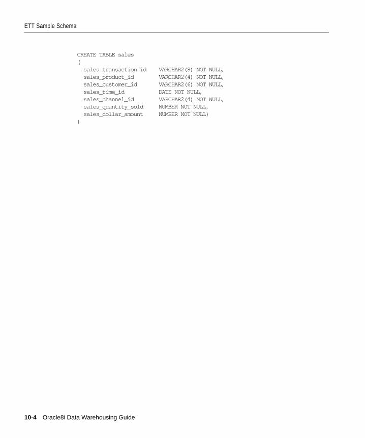
ETT Sample Schema
CREATE TABLE sales( sales_transaction_id VARCHAR2(8) NOT NULL, sales_product_id VARCHAR2(4) NOT NULL, sales_customer_id VARCHAR2(6) NOT NULL, sales_time_id DATE NOT NULL, sales_channel_id VARCHAR2(4) NOT NULL, sales_quantity_sold NUMBER NOT NULL, sales_dollar_amount NUMBER NOT NULL))
10-4 Oracle8i Data Warehousing Guide

Ex
11
ExtractionThis chapter discusses extraction, which is when you take data from an operational
system and move it to your warehouse. The chapter discusses:
■ Overview of Extraction
■ Extracting Via Data Files
■ Extracting Via Distributed Operations
■ Change Capture
traction 11-1
Overview of Extraction
Overview of ExtractionExtraction is the operation of copying data from a database into a file or onto a
network connection. This is the first step of the ETT process: data must be extracted
from the source system(s) so that this data may be subsequently transformed and
loaded into the data warehouse.
The source systems for a data warehouse are typically transaction-processing
database applications. For example, one of the source systems for a sales-analysis
data warehouse may be the order-entry system which records all of the current
order activities.
Designing and creating the extraction process is often one of the most
time-consuming tasks in the ETT process and, indeed, in the entire data
warehousing process. The source systems may be very complex, and thus
determining which data needs to be extracted can be difficult. Moreover, the source
system typically cannot be modified, nor can its performance or availability be
impacted, to accommodate the needs of the data warehouse extraction process.
These are very important considerations for extraction, and ETT in general.
This chapter, however, focuses on the technical considerations for extracting data. It
assumes that the data warehouse team has already identified the data that will be
extracted, and discusses common techniques used for extracting data from source
databases. The techniques for extraction fall into two broad categories:
■ Techniques which extract data from an operational system and place the data
into a file. Examples are data-unloads and exports.
■ Techniques which extract data from an operational system and directly
transport data into the target database (a data warehouse or a staging database).
Examples are gateways and distributed queries.
Extracting Via Data FilesMost database systems provide mechanisms for exporting and/or unloading data
from the internal database format into flat files. Extracts from mainframe systems
often use COBOL programs, but many databases, as well as third-party software
vendors, provide export and/or unload utilities.
Data extraction does not necessarily mean that entire database structures are
unloaded in flat files. In many cases, it may be appropriate to unload entire
database tables or objects. In other cases, it may be more appropriate to unload only
a subset of a given table, or unload the results of joining multiple tables together.
11-2 Oracle8i Data Warehousing Guide

Extracting Via Data Files
Different extraction techniques may vary in their capabilities to support these two
scenarios.
When the source system is an Oracle database, there are several alternatives for
extracting data into files:
■ Extracting into Flat Files Using SQL*Plus
■ Extracting into Flat Files Using OCI or Pro*C Programs
■ Exporting into Oracle Export Files Using Oracle's EXP Utility
■ Copying to Another Oracle Database Using Transportable Tablespaces
Extracting into Flat Files Using SQL*PlusThe most basic technique for extracting data is to execute a SQL query in SQL*Plus
and direct the output of the query to a file. For example, to extract a flat file,
empdept.log, containing a list of employee names and department names from the
EMP and DEPT tables, the following SQL script could be run:
SET echo offSET pagesize 0SPOOL empdept.datSELECT ename, dname FROM emp, deptWHERE emp.deptno = dept.deptno;SPOOL off
The exact format of the output file can be specified using SQL*Plus's system
variables.
Note that this extraction technique offers the advantage of being able to extract the
output of any SQL statement. The example above extracts the results of a join.
This extraction technique can be parallelized. Parallelization can be achieved by
initiating multiple, concurrent SQL*Plus sessions, each session running a separate
query representing a different portion of the data to be extracted. For example,
suppose that you wish to extract data from an ORDERS table, and that the ORDERS
table has been range partitioned by month, with partitions ORDERS_JAN1998,
ORDER_FEB1998, and so on. Then, in order to extract a single year of data from the
ORDERS table, you could initiate 12 concurrent SQL*Plus sessions, each extracting
a single partition. The SQL script for one such session could be:
SPOOL order_jan.datSELECT * FROM orders PARTITION (orders_jan1998);SPOOL OFF
Extraction 11-3

Extracting Via Data Files
These 12 SQL*Plus processes would concurrently spool data to 12 separate files.
These files may need to be concatenated (using OS utilities) following the
extraction.
Even if the ORDERS table is not partitioned, it is still possible to parallelize the
extraction. By viewing the data dictionary, it is possible to identify the Oracle data
blocks that make up the ORDERS table. Using this information, you could then
derive a set of ROWID-range queries for extracting data from the ORDERS table:
SELECT * FROM orders WHERE rowid BETWEEN <value1> and <value2>;
Parallelization of the extraction of complex SQL queries may also be possible,
although the process of breaking a single complex query into multiple components
can be challenging.
Note that all parallel techniques can use considerably more CPU and I/O resources
on the source system, and the impact on the source system should be evaluated
before parallelizing any extraction technique.
Extracting into Flat Files Using OCI or Pro*C ProgramsOCI programs (or other program using Oracle call interfaces, such as Pro*C
programs), can also be used to extract data. These techniques typically provide
improved performance over the SQL*Plus approach, although they also require
additional programming. Like the SQL*Plus approach, an OCI program can be used
to extract the results of any SQL query. Furthermore, the parallelization techniques
described for the SQL*Plus approach can be readily applied to OCI programs as
well.
Exporting into Oracle Export Files Using Oracle's EXP UtilityOracle's export utility allows tables (including data) to be exported into Oracle
export files. Unlike the SQL*Plus and OCI approaches, which describe the
extraction of the results of a SQL statement, EXP provides a mechanism for
extracting database objects. Thus, EXP differs from the previous approaches in
several important ways:
■ The export files contain metadata as well as data. An export file contains, not
only the raw data of a table, but also information on how to recreate the table,
potentially including any indexes, constraints, grants, and other attributes
associated with that table.
■ A single export file may contain many database objects, and even an entire
schema.
11-4 Oracle8i Data Warehousing Guide

Extracting Via Distributed Operations
■ Export cannot be directly used to export portions of a database object, or to
export the results of a complex SQL query. Export can only be used to extract
entire database objects.
■ The output of the export utility can only be processed using the Oracle import
utility.
Oracle provides a direct-path export, which is quite efficient for extracting data.
Note that in Oracle8i, there is no direct-path import, which should be considered
when evaluating the overall performance of an export-based extraction strategy.
Although the SQL*Plus and OCI extraction techniques are more common, EXP may
be useful for certain ETT environments that require extraction of metadata as well
as data.
See Oracle8i Utilities for more information on using export.
Copying to Another Oracle Database Using Transportable TablespacesOne of the most powerful features for extracting and moving large volumes of data
between Oracle database is transportable tablespaces. A more detailed example of
using this feature to extract and transport data is provided in Chapter 12,
"Transportation". When possible, transportable tablespaces are very highly
recommended for data extraction, because they often provide considerable
advantages in performance and manageability over other extraction techniques.
Extracting Via Distributed OperationsUsing distributed-query technology, one Oracle database can directly query tables
located in another Oracle database. Specifically, a data warehouse or staging
database could directly access tables and data located in an Oracle-based source
system. This is perhaps the simplest method for moving data between two Oracle
databases because it combines the extraction and transformation into a single step,
and, moreover, requires minimal programming.
Continuing our example from above, suppose that we wanted to extract a list of
employee names with department names from a source database, and store it into
our data warehouse. Using a Net8 connection, and distributed-query technology,
this can be achieved using a single SQL statement:
CREATE TABLE empdeptASSELECT ename, dname FROM emp@source_db, dept@source_dbWHERE emp.deptno = dept.deptno;
Extraction 11-5

Change Capture
This statement creates a local table in the data warehouse, EMPDEPT, and
populates it with data from the EMP and DEPT tables on the source system.
This technique is ideal for moving small volumes of data. However, the data is
transported from the source system to the data warehouse via a single Net8
connection. Thus, the scalability of this technique is limited. For larger data
volumes, file-based data extraction and transportation techniques are often more
scalable and thus more appropriate.
Gateways are another form of distributed-query technology, except that gateways
allow an Oracle database (such as a data warehouse) to access database tables
stored in remote, non-Oracle databases. Like distributed queries, gateways are very
easy to set up and use, but also lack scalability for very large data volumes.
For more information on distributed queries, see Oracle8i Distributed DatabaseSystems and Oracle8i Concepts.
Change CaptureAn important consideration for extraction is incremental extraction, also called
change data capture. If a data warehouse extracts data from an operational system on
a nightly basis, then the only data which that data warehouse requires is the data
that has changed since the last extraction (that is, the data that has been modified in
the last 24 hours).
If it was possible to efficiently identify and extract only the most recently-changed
data, the extraction process (as well as all downstream operations in the ETT
process) could be much more efficient since it would only need to extract a much
smaller volume of data. Unfortunately, for many source systems, identifying the
recently modified data may be difficult or intrusive to the operation of the system.
Change data capture is typically the most challenging technical issue in data
extraction.
Many data warehouses do not use any change-capture techniques as part of the
extraction process. Instead, entire tables from the source systems are extracted to the
data warehouse or staging area, and these tables are compared with a previous
extract from the source system to identify the changed data. While this approach
may not have significant impact on the source systems, it clearly can place a
considerable burden on the data-warehouse processes particularly if the data
volumes are large.
Thus, change data capture as part of the extraction process is often desirable. This
section describes several techniques for implementing change-data-capture on
Oracle source systems:
11-6 Oracle8i Data Warehousing Guide

Change Capture
■ Timestamps
■ Partitioning
■ Triggers
These techniques are based upon the characteristics of the source systems, or may
require modifications to the source systems. Thus, each of these techniques must be
carefully evaluated by the owners of the source system prior to implementation.
Each of these change-capture techniques will work in conjunction with the
data-extraction technique discussed above. For example, timestamps can be used
whether the data is being unloaded to a file or accessed via distributed query.
TimestampsThe tables in some operational systems have timestamp columns. The timestamp
specifies the time and date that a given row was last modified. If the tables in an
operational system have columns containing timestamps, then the latest data can
easily be identified using the timestamp columns. For example, the following query
might be useful for extracting today's data from an ORDERS table:
SELECT * FROM orders WHERE TIMESTAMP = TO_DATE(sysdate, 'mm-dd-yyyy');
If timestamps are not available in an operational system, the system may be able to
be modified to include timestamps. This would require, first, modifying the
operational system's tables to include a new timestamp column, and second,
creating a trigger (see "Triggers" on page 11-7) to update the timestamp column
following every operation which modifies a given row.
PartitioningSome source systems may utilize Oracle's range-partitioning, such that the source
tables are partitioned along a date key, which allows for easy identification of new
data. For example, if you are extracting from an ORDERS table, and the ORDERS
table is partitioned by week, then it is easy to identify the current week's data.
TriggersTriggers can be created in operational systems to keep track of recently updated
records. They can then be used in conjunction with timestamp columns to allow
you to identify the exact time and date when a given row was last modified. You do
this by creating a trigger on each source table that requires change-data-capture.
Following each DML statement that is executed on the source table, this trigger
Extraction 11-7

Change Capture
updates the timestamp column with the current time. Thus, the timestamp column
provides the exact time and date when a given row was last modified.
A similar trigger-based technique is to use Oracle's materialized view logs. These
logs are used by materialized views to identify changed data, and these logs are
accessible to end users. A materialized view log can be created on each source table
requiring change-data-capture. Then, whenever any modifications are made to the
source table, a record will be inserted into the materialized-view log indicating
which row(s) were modified. The materialized view log can then be subsequently
queried by the extraction process to identify the changed data.
Materialized view logs rely on triggers, but they provide an advantage in that the
creation and maintenance of this change-data system is largely managed by Oracle.
Both of these trigger-based techniques will impact performance on the source
systems, and this impact should be carefully consider prior to implementing on a
production source system.
11-8 Oracle8i Data Warehousing Guide

Trans
12
TransportationThe following topics provide information about transporting data into a data
warehouse:
■ Transportation Overview
portation 12-1

Transportation Overview
Transportation OverviewTransportation is, literally, the act of moving data from one system to another system.
In a data warehouse environment, the most common requirements for
transportation are in moving data from a source system to a staging database or a
data warehouse database; from a staging database to a data warehouse; or from a
data warehouse to a data mart.
Transportation is often one of the simplest portions of the ETT process, and is
commonly integrated with other portions of the process. For example, as shown in
Chapter 11, "Extraction", distributed query technology provides a mechanism for
both extracting and transporting data.
There are various techniques for transporting data, each with its own distinct
advantages. This chapter introduces some of these techniques, and includes:
■ Transportation of Flat Files
■ Transportation Via Distributed Operations
■ Transportable Tablespaces
Transportation of Flat FilesThe most common method for transporting data is by the transfer of flat files, using
mechanisms such as FTP or other remote file-system access protocols. Data is
unloaded or exported from the source system into flat files using techniques
discussed in Chapter 11, "Extraction", and is then transported to the target platform
using FTP or similar mechanisms.
Because source systems and data warehouses often use different operating systems
and database systems, flat files are often the simplest mechanism to exchange data
between heterogeneous systems with minimal transformations. However, even
when transporting data between homogeneous systems, flat files are often the most
efficient and most easy-to-manage mechanism for data transfer.
Transportation Via Distributed OperationsDistributed queries and gateways can be an effective mechanism for extracting
data. These mechanisms also transport the data directly to the target systems, thus
providing both extracting and transformation in a single step. For relatively small
volumes of data, these mechanisms are very well-suited for both extraction and
transformation. See Chapter 11, "Extraction", for further details.
12-2 Oracle8i Data Warehousing Guide
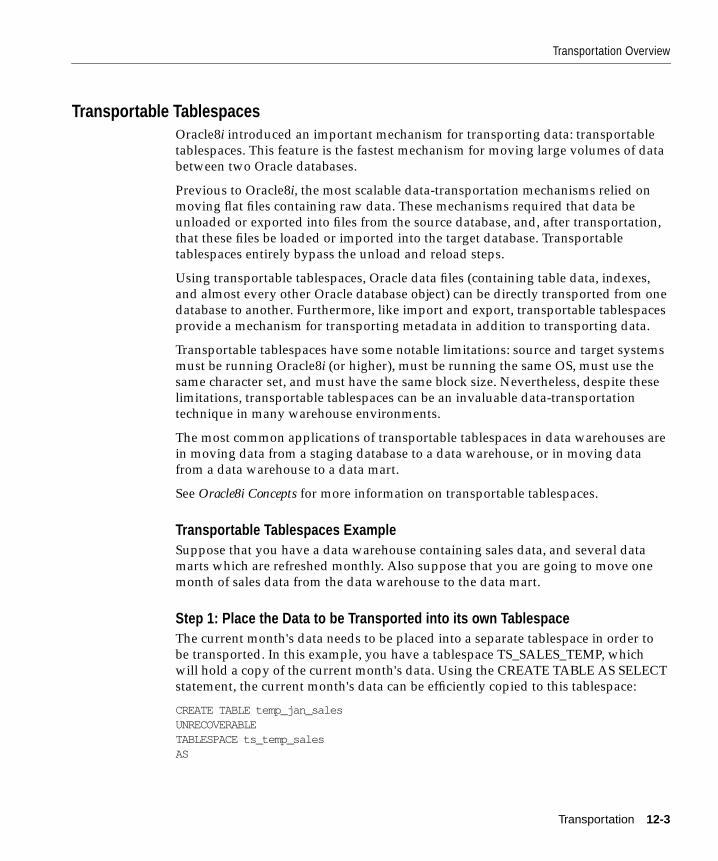
Transportation Overview
Transportable TablespacesOracle8i introduced an important mechanism for transporting data: transportable
tablespaces. This feature is the fastest mechanism for moving large volumes of data
between two Oracle databases.
Previous to Oracle8i, the most scalable data-transportation mechanisms relied on
moving flat files containing raw data. These mechanisms required that data be
unloaded or exported into files from the source database, and, after transportation,
that these files be loaded or imported into the target database. Transportable
tablespaces entirely bypass the unload and reload steps.
Using transportable tablespaces, Oracle data files (containing table data, indexes,
and almost every other Oracle database object) can be directly transported from one
database to another. Furthermore, like import and export, transportable tablespaces
provide a mechanism for transporting metadata in addition to transporting data.
Transportable tablespaces have some notable limitations: source and target systems
must be running Oracle8i (or higher), must be running the same OS, must use the
same character set, and must have the same block size. Nevertheless, despite these
limitations, transportable tablespaces can be an invaluable data-transportation
technique in many warehouse environments.
The most common applications of transportable tablespaces in data warehouses are
in moving data from a staging database to a data warehouse, or in moving data
from a data warehouse to a data mart.
See Oracle8i Concepts for more information on transportable tablespaces.
Transportable Tablespaces ExampleSuppose that you have a data warehouse containing sales data, and several data
marts which are refreshed monthly. Also suppose that you are going to move one
month of sales data from the data warehouse to the data mart.
Step 1: Place the Data to be Transported into its own TablespaceThe current month's data needs to be placed into a separate tablespace in order to
be transported. In this example, you have a tablespace TS_SALES_TEMP, which
will hold a copy of the current month's data. Using the CREATE TABLE AS SELECT
statement, the current month's data can be efficiently copied to this tablespace:
CREATE TABLE temp_jan_salesUNRECOVERABLETABLESPACE ts_temp_salesAS
Transportation 12-3

Transportation Overview
SELECT * FROM salesWHERE sales_date BETWEEN '31-DEC-1999' AND '01-FEB-2000';
Following this create-table operation, the tablespace TS_TEMP_SALES is set to read
only:
ALTER TABLESPACE ts_temp_sales READ ONLY;
A tablespace cannot be transported unless there are no active transactions
modifying the tablespace; setting the tablespace to read only enforces this.
The tablespace TS_TEMP_SALES may be a tablespace that has been especially
created to temporarily store data for use by the transportable tablespace features.
Following "Step 3: Copy the Datafiles and Export File to the Target System", this
tablespace can be set to read-write, and, if desired, the table TEMP_JAN_SALES can
be deleted, and the tablespace can be re-used for other transportations or for other
purposes.
In a given transportable tablespace operation, all of the objects in a given tablespace
are transported. Although only one table is being transported in this example, the
tablespace TS_TEMP_SALES could contain multiple tables. For example, perhaps
the data mart is refreshed not only with the new month's worth of sales
transactions, but also with a new copy of the customer table. Both of these tables
could be transported in the same tablespace. Moreover, this tablespace could also
contain other database objects such as indexes, which would also be transported.
Additionally, in a given transportable-tablespace operation, multiple tablespaces
can be transported at the same time. This makes it easier to move very large
volumes of data between databases. Note, however, that the transportable
tablespace feature can only transport a set of tablespaces which contain an complete
set of database objects without dependencies on other tablespaces. For example, an
index cannot be transported without its table, nor can a partition be transported
without the rest of the table.
In this step, we have copied the January sales data into a separate tablespace;
however, in some cases, it may be possible to leverage the transportable tablespace
feature without even moving data to a separate tablespace. If the sales table has
been partitioned by month in the data warehouse and if each partition is in its own
tablespace, then it may be possible to directly transport the tablespace containing
the January data. Suppose the January partition, sales_jan2000, is located in the
tablespace TS_SALES_JAN2000. Then the tablespace TS_SALES_JAN2000 could
potentially be transported, rather than creating a temporary copy of the January
sales data in the TS_TEMP_SALES.
12-4 Oracle8i Data Warehousing Guide

Transportation Overview
However, two conditions must be satisfied in order to transport the tablespace TS_
SALES_JAN2000. First, this tablespace must be set to read only. Second, since a
single partition of a partitioned table cannot be transported without the remainder
of the partitioned table also being transported, it is necessary to exchange the
January partition into a separate table (using the ALTER TABLE statement), in order
to transport the January data. The EXCHANGE operation is very quick; however,
the January data will no longer be a part of the underlying SALES table, and thus
may be unavailable to users until this data is exchanged back into the SALES table.
The January data can be exchanged back into the SALES table following step 3.
Step 2: Export the MetadataThe EXPORT utility is used to export the metadata describing the objects contained
in the transported tablespace. For our example scenario, the EXPORT command
could be:
EXP TRANSPORT_TABLESPACE=y TABLESPACES=ts_temp_sales FILE=jan_sales.dmp
This operation will generate an export file, jan_sales.dmp. The export file will be
small, because it only contains metadata. In this case, the export file will contain
information describing the table TEMP_JAN_SALES, such as the column names,
column datatype, and all other information which the target Oracle database will
need in order to access the objects in TS_TEMP_SALES.
Step 3: Copy the Datafiles and Export File to the Target SystemThe data files that make up TS_TEMP_SALES, as well as the export file jan_
sales.dmp, should be copied to the data mart platform, using any transportation
mechanism for flat files.
Once the datafiles have been copied, the tablespace TS_TEMP_SALES can be set to
READ WRITE mode if desired.
Step 4: Import the MetadataOnce the files have been copied to the data mart, the metadata should be imported
into the data mart:
IMP TRANSPORT_TABLESPACE=y DATAFILES='/db/tempjan.f'TABLESPACES=ts_temp_salesFILE=jan_sales.dmp
Transportation 12-5

Transportation Overview
Like the export operation in step 2, the import operation in this step should be very
fast.
At this point, the tablespace TS_TEMP_SALES and the table TEMP_SALES_JAN are
accessible in the data mart.
There are two potential scenarios for incorporating this new data into the data
mart's tables.
First, the data from the TEMP_SALES_JAN table could be inserted into the data
mart's sales table:
INSERT /*+ APPEND */ INTO sales SELECT * FROM temp_sales_jan;
Following this operation, the temp_sales_jan table (and even the entire ts_temp_
sales tablespace) could be deleted.
Second, if the data mart's sales table is partitioned by month, then the new
transported tablespace and the TEMP_SALES_JAN table could become a
permanent part of the data mart. The TEMP_SALES_JAN table could become a
partition of the data mart's sales table:
ALTER TABLE sales ADD PARTITION sales_00jan VALUES LESS THAN (TO_DATE('01-feb-2000','dd-mon-yyyy'));ALTER TABLE sales EXCHANGE PARTITION sales_00jan WITH TABLE temp_sales_janINCLUDING INDEXES WITH VALIDATION;
Other Uses of Transportable TablespacesThe above example illustrated a typical scenario for transporting data in a data
warehouse. However, transportable tablespaces can be used for many other
purposes. In a data warehousing environment, transportable tablespaces should be
viewed as a utility (much like import/export or SQL*Loader), whose purpose is to
move large volumes of data between Oracle databases. When used in conjunction
with parallel data-movement operations such as the CREATE TABLE AS SELECT
and INSERT AS SELECT statements, transportable tablespaces provide an
important mechanism for quickly transporting data for many purposes.
12-6 Oracle8i Data Warehousing Guide

Transf
13
TransformationThis chapter helps you create and manage a data warehouse, and discusses:
■ Techniques for Data Transformation Inside the Database
ormation 13-1

Techniques for Data Transformation Inside the Database
Techniques for Data Transformation Inside the DatabaseData transformations are often the most complex and, in terms of processing time,
the most costly part of the ETT process. They can run the gamut from simple data
conversions to extremely complex data-scrubbing techniques. Many, if not all, data
transformations can occur within an Oracle8i database, although transformations
are also often implemented outside of the database (for example, on flat files) as
well.
This chapter discusses the techniques used to implement data transformation
within Oracle8i and special considerations for choosing among these techniques,
and includes:
■ Transformation Flow
■ Transformations Provided by SQL*Loader
■ Transformations Using SQL and PL/SQL
■ Data Substitution
■ Key Lookups
■ Pivoting
■ Emphasis on Transformation Techniques
Transformation FlowThe data-transformation logic for most data warehouses consists of multiple steps.
For example, in transforming new records to be inserted into a sales table, there
may be separate logical transformation steps to validate each dimension key.
A graphical way of looking at the transformation logic is presented in Figure 13–1:
13-2 Oracle8i Data Warehousing Guide

Techniques for Data Transformation Inside the Database
Figure 13–1 Data Transformation
When using Oracle8i as a transformation engine, a common strategy is to
implement each different transformation as a separate SQL operation, and to create
a separate, temporary table (such as the tables new_sales_step1 and new_sales_
step2 in Figure 13–1) to store the incremental results for each step. This strategy also
provides a natural checkpointing scheme to the entire transformation process, which
enables to the process to be more easily monitored and restarted.
It may also be possible to combine many simple logical transformations into a
single SQL statement or single PL/SQL procedure. While this may provide better
performance than performing each step independently, it may also introduce
difficulties in modifying, adding or dropping individual transformations, and,
moreover, prevents any effective checkpointing.
Transformations Provided by SQL*LoaderBefore any data-transformations can occur within the database, the raw data must
first be loaded into the database. Chapter 12, "Transportation", discussed several
techniques for transporting data to an Oracle data warehouse. Perhaps the most
common technique for transporting data is via flat files.
Load into staging table
Insert into sales warehouse table
Convert source product keys
to warehouse product keys
Flat Files Table
new_sales_step1
new_sales_step2 new_sales_step3
sales
Validate customer keys (lookup in
customer dimension table)
TableTable
Table
Transformation 13-3

Techniques for Data Transformation Inside the Database
SQL*Loader is used to move data from flat files into an Oracle data warehouse.
During this data load, SQL*Loader can also be used to implement basic data
transformations. When using direct-path SQL*Loader, datatype conversion and
simple NULL handling can be automatically resolved during the data load. Most
data warehouses choose to use direct-path loading for performance reasons.
Oracle's conventional-path loader provides broader capabilities for data
transformation than direct-path loader: SQL functions can be applied to any column
as those values are being loaded. This provides a rich capability for transformations
during the data load. However, the conventional-path loader is less efficient than
direct-path loader and is not parallelizable. For these reasons, the conventional-path
loader should be considered primarily for loading and transforming smaller
amounts of data.
For more information on SQL*Loader, see Oracle8i Utilities.
Transformations Using SQL and PL/SQLOnce data is loaded into an Oracle8i database, data transformations can be executed
using SQL and PL/SQL operations. There are two basic techniques for
implementing data-transformations within Oracle8i.
Technique 1: The CREATE TABLE ... AS SELECT ... statement
The CREATE TABLE ... AS SELECT ... statement (CTAS) is a very powerful tool for
manipulating large sets of data. As we shall see in the examples below, many data
transformations can be expressed in standard SQL, and Oracle's implementation of
CTAS provides a mechanism for efficiently executing a SQL query, and storing the
results of that query in a database table.
In a data warehouse environment, CTAS is typically run in parallel and using
NOLOGGING mode for best performance.
Technique 2: PL/SQL Procedures
In a data warehouse environment, PL/SQL can be used to implement complex
transformations in the Oracle8i database.
While CTAS operates on entire tables and emphasizes parallelism, PL/SQL
provides a row-based approached and can accommodate very sophisticated
transformation rules. For example, a PL/SQL procedure could open multiple
cursors and read data from multiple source tables, combine this data using complex
business rules, and finally insert the transformed data into one or more target
tables; it may be difficult or impossible to express the same sequence of operations
using standard SQL commands.
13-4 Oracle8i Data Warehousing Guide

Techniques for Data Transformation Inside the Database
The following examples demonstrate transformations using SQL and PL/SQL.
Data SubstitutionA simple and common type of data transformation is a data substitution. In a
data-substitution transformation, some or all of the values of a single column are
modified. For example, our sales table has a sales_channel_id column. This column
is used to specify whether a given sales transaction was made by our company’s
own sales force (a direct sale) or via a distributor (an indirect sale).
We may receive data from multiple source systems for our data warehouse. Let us
suppose that one of those source systems processes only direct sales, and thus the
source system does not know indirect sales channels. When the data warehouse
initially receives sales data from this system, all of sales records have a null value
for the sales_channel_id field. These null values must be modified, and set to the
proper key value.
This can be efficiently done using a CTAS statement:
CREATE TABLE temp_sales_step2NOLOGGING PARALLEL ASSELECT sales_product_id, NVL(sales_channel_id, 1) sales_channel_id, sales_customer_id, sales_time_id, sales_quantity_sold, sales_dollar_amountFROM temp_sales_step1;
Another possible technique for implementing a data-substitution is to use an
UPDATE statement to modify the sales_channel_id column. An UPDATE will
provide the correct result. However, many data-substitution transformations
require that a very large percentage of the rows (often all of the rows) be modified.
In these cases, it may be more efficient to use a CTAS statement than an UPDATE.
Key LookupsAnother simple transformation is a key lookup For example, suppose that, in a
retail data warehouse, sales transaction data has been loaded into the data
warehouse. Although the data warehouse’s SALES table contains a PRODUCT_ID
column, the sales transaction data extracted from the source system contains UPC
codes instead of PRODUCT_IDs. Therefore, it is necessary to transform the UPC
codes into PRODUCT_IDs before the new sales transaction data can be inserted into
the SALES table.
In order to execute this transformation, there must be a lookup table which relates
the PRODUCT_ID values to the UPC codes. This may be the PRODUCT dimension
Transformation 13-5

Techniques for Data Transformation Inside the Database
table, or perhaps there is another table in the data warehouse that has been created
specifically to support this transformation. For this example, we assume that there
is a table named PRODUCT, which has a PRODUCT_ID and an UPC_CODE
column.
This data-substitution transformation can be implemented using the following
CTAS statement:
CREATE TABLE temp_sales_step2NOLOGGING PARALLELASSELECT sales_transaction_id, product.product_id sales_product_id, sales_customer_id, sales_time_id, sales_channel_id, sales_quantity_sold, sales_dollar_amountFROM temp_sales_step1, productWHERE temp_sales_step1.upc_code = product.upc_code;
This CTAS statement will convert each valid UPC code to a valid PRODUCT_ID
value. If the ETT process has guaranteed that each UPC code is valid, then this
statement alone may be sufficient to implement the entire transformation.
Exception Handling: Invalid DataHowever, it can be important to handle new sales data that does not have valid
UPC codes.
One approach is to use an additional CTAS statement to identify the invalid rows:
CREATE TABLE temp_sales_step1_invalidNOLOGGING PARALLELASSELECT * FROM temp_sales_step1WHERE temp_sales_step1.upc_code NOT IN (SELECT upc_code FROM product);
This invalid data is now stored in a separate table, TEMP_SALES_STEP1_INVALID,
and can be handled separately by the ETT process.
A second approach is to modify the original CTAS to use an outer join:
CREATE TABLE temp_sales_step2NOLOGGING PARALLELAS
13-6 Oracle8i Data Warehousing Guide

Techniques for Data Transformation Inside the Database
SELECT sales_transaction_id, product.product_id sales_product_id, sales_customer_id, sales_time_id, sales_channel_id, sales_quantity_sold, sales_dollar_amountFROM temp_sales_step1, productWHERE temp_sales_step1.upc_code = product.upc_code (+);
Using this outer join, the sales transactions that originally contained invalidated
UPC codes will be assigned a PRODUCT_ID of NULL. These PRODUCT_IDs can
be handled later.
There are other possible approaches to handling invalid UPC codes. Some data
warehouses may choose to insert null-valued PRODUCT_IDs into their SALES
table, while other data warehouses may not allow any new data from the entire
batch to be inserted into the SALES table until all invalid UPC codes have been
addressed. The correct approach is determined by the business requirements of the
data warehouse. Regardless of the specific requirements, exception handling can be
addressed by the same basic SQL techniques as transformations.
PivotingA data warehouse can receive data from many different sources. Some of these
source systems may not be relational databases, and may store data in very different
formats from the data warehouse. For example, suppose that you receive a set of
sales records from a non-relational database having the form:
product_id, store_id, week_id, sales_sun, sales_mon, sales_tue,sales_wed, sales_thu, sales_fri, sales_sat
In your data warehouse, you would want to store the records in a more typical
relational form:
product_id, store_id, time_id, sales_amount
Thus, you need to build a transformation such that each record in the input stream
must be converted into seven records for the data warehouse's SALES table. This
operation is commonly referred to as pivoting.
The CTAS approach to pivoting would require a UNION-ALL query:
Transformation 13-7

Techniques for Data Transformation Inside the Database
CREATE table temp_sales_step2NOLOGGING PARALLELASSELECT product_id, time_id, sales_amountFROM(SELECT product_id, store_id, TO_DATE(week_id,'WW') time_id, sales_sun sales_amount FROM temp_sales_step1 UNION ALL SELECT product_id, store_id, TO_DATE(week_id,'WW')+1 time_id, sales_mon sales_amount FROM temp_sales_step1 UNION ALL SELECT product_id, store_id, TO_DATE(week_id,'WW')+2 time_id, sales_tue sales_amount FROM temp_sales_step1 UNION ALL SELECT product_id, store_id, TO_DATE(week_id,'WW')+3 time_id, sales_web sales_amount FROM temp_sales_step1 UNION ALL SELECT product_id, store_id, TO_DATE(week_id,'WW')+4 time_id, sales_thu sales_amount FROM temp_sales_step1 UNION ALL SELECT product_id, store_id, TO_DATE(week_id,'WW')+5 time_id, sales_fri sales_amount FROM temp_sales_step1 UNION ALL SELECT product_id, store_id, TO_DATE(week_id,'WW')+6 time_id, sales_sat sales_amount FROM temp_sales_step1);
Like all CTAS operations, this operation can be fully parallelized. However, the
CTAS approach also requires seven separate scans of the data, one for each day of
the week. Even with parallelism, the CTAS approach may be time-consuming.
An alternative implementation is PL/SQL. A very basic PL/SQL function to
implement the pivoting operation would be:
DECLARE CURSOR c1 is SELECT product_id, store_id, week_id, sales_sun, sales_mon, sales_tue, sales_wed, sales_thu, sales_fri, sales_sat FROM temp_sales_step1;BEGIN FOR next IN c1 LOOP INSERT INTO temp_sales_step2 VALUES (product_id, store_id, TO_DATE(week_id,'WW') time_id, sales_sun ); INSERT INTO temp_sales_step2 VALUES (product_id, store_id, TO_DATE(week_id,'WW')+1 time_id, sales_mon );
13-8 Oracle8i Data Warehousing Guide

Techniques for Data Transformation Inside the Database
INSERT INTO temp_sales_step2 VALUES (product_id, store_id, TO_DATE(week_id,'WW')+2 time_id, sales_tue ); INSERT INTO temp_sales_step2 VALUES (product_id, store_id, TO_DATE(week_id,'WW')+3 time_id, sales_wed ); INSERT INTO temp_sales_step2 VALUES (product_id, store_id, TO_DATE(week_id,'WW')+4 time_id, sales_thu ); INSERT INTO temp_sales_step2 VALUES (product_id, store_id, TO_DATE(week_id,'WW')+5 time_id, sales_fri ); INSERT INTO temp_sales_step2 VALUES (product_id, store_id, TO_DATE(week_id,'WW')+6 time_id, sales_sat ); END LOOP; COMMIT;END;
This PL/SQL procedure could be modified to provide even better performance.
Array inserts could accelerate the insertion phase of the procedure. Further
performance could be gained by parallelizing this transformation operation,
particularly if the TEMP_SALES_STEP1 table is partitioned, using techniques
similar to the parallelization of data-unloading described in Chapter 11,
"Extraction".
The primary advantage of this PL/SQL procedure over a CTAS approach is that it
only requires a single scan of the data. Pivoting is an example of a complex
transformation that may be more amenable to PL/SQL.
Emphasis on Transformation TechniquesThis chapter is designed to introduce techniques for implementing scalable and
efficient data transformations within Oracle8i. The examples in this chapter are
relatively simple; real-world data transformations are often considerably more
complex. However, the transformation techniques introduced in this chapter meet
the majority of real-world data transformation requirements, often with more
scalability and less programming than alternative approaches.
This chapter does not seek to illustrate all of the typical transformations that would
be encountered in a data warehouse, but to demonstrate the types of techniques
that can be applied to implement these transformations and to provide guidance in
how to choose the best techniques.
Transformation 13-9

Techniques for Data Transformation Inside the Database
13-10 Oracle8i Data Warehousing Guide

Loading and Ref
14
Loading and RefreshingThis chapter discusses how to load and refresh a data warehouse, and discusses:
■ Refreshing a Data Warehouse
■ Refreshing Materialized Views
reshing 14-1

Refreshing a Data Warehouse
Refreshing a Data WarehouseFollowing extraction and transformation, the final step of the ETT process is to
physically insert the new, clean data into the production data warehouse schema,
and take all of the other steps necessary (such as building indexes, validating
constraints, taking backups) to make this new data available to the end-users.
Using Partitioning to Improve Data Warehouse RefreshThe partitioning scheme of the data warehouse is often crucial in determining the
efficiency of refresh operations in the data warehouse load process. In fact, the load
process is often the primary consideration in choosing the partitioning scheme of
data-warehouse tables and indexes.
The partitioning scheme of the largest data-warehouse tables (for example, the fact
table in a star schema) should be based upon the loading paradigm of the data
warehouse.
Most data warehouses are loaded on a regular schedule: every night, every week or
every month, new data is brought into the data warehouse. The data being loaded
at the end of the week or month typically corresponds to the transactions for the
week or month week. In this very common scenario, the data warehouse is being
loaded by time. This suggests that the data-warehouse tables should be partitioned
by a date key. In our data warehouse example, suppose the new data is loaded into
the SALES table every month. Furthermore, the SALES table has been partitioned
by month. These steps show how the load process will proceed to add the data for a
new month (January, 2000) to SALES table:
Step 1: Place the new data into a separate table, SALES_00JAN. This data may be
directly loaded into SALES_00JAN from outside the data warehouse, or this data
may be the result of previous data-transformation operations that have already
occurred in the data warehouse. SALES_00JAN has the exact same columns,
datatypes, etc. as the SALES table. Gather statistics on the SALES_00JAN table.
Step 2: Create indexes and add constraints on SALES_00JAN. Again, the indexes
and constraints on SALES_00JAN should be identical to the indexes and constraints
on SALES.
Indexes can be built in parallel, and should use the NOLOGGING and the
COMPUTE STATISTICS options. For example:
CREATE BITMAP INDEX sales_00jan_customer_id_bix tablespace (sales_index) NOLOGGING parallel (degree 8) COMPUTE STATISTICS;
14-2 Oracle8i Data Warehousing Guide

Refreshing a Data Warehouse
All constraints should be applied to the SALES_00JAN table that are present on the
SALES table. This includes referential integrity constraints. Some typical constraints
would be:
ALTER TABLE sales_00jan add CONSTRAINT sales_pk unique(sales_transaction_id) disable validate;ALTER TABLE sales_00jan add constraint sales_customer_ri sales_customer_id REFERENCES customer(customer_id);
Step 3: Add the SALES_00JAN table to the SALES table.
In order to add this new data to the SALES table, we need to do two things. First,
we need to add a new partition to the SALES table. We will use the ALTER TABLE
... ADD PARTITION statement. This will add an empty partition to the SALES table:
ALTER TABLE sales ADD PARTITION sales_00janVALUES LESS THAN (TO_DATE('01-FEB-2000', 'dd-mon-yyyy'));
Then, we can add our newly created table to this partition using the exchange
partition operation. This will exchange the new, empty partition with the
newly-loaded table.
ALTER TABLE sales EXCHANGE PARTITiON sales_00jan WITH TABLE sales_00janINCLUDING INDEXES WITHOUT VALIDATION;
The exchange operator will preserve the indexes and constraints that were already
present on the SALES_00JAN table. For unique constraints (such as the unique
constraint on SALES_TRANSACTION_ID), the exchange operator might need to do
additional processing to ensure consistency. If there were only foreign-key
constraints, the exchange operation would be instantaneous.
The benefits of this partitioning technique are significant. First, the new data is
loaded with minimal resource utilization. The new data is loaded into an entirely
separate table, and the index-processing and constraint-processing are only applied
to the new partition. If the SALES table was 50GB and had 12 partitions, then a new
month's worth of data contains approximately 4 GB. Only the new month's worth of
data needs to be indexed; none of the indexes on the remaining 46GB of data needs
to be modified at all.
This partitioning scheme additionally ensures that the load-processing time is
directly proportional to the amount of new data being loaded, not to the total size of
the SALES table.
Second, the new data is loaded with minimal impact on concurrent queries. Since
all of the operations associated with data loading are occurring on a separate
Loading and Refreshing 14-3

Refreshing a Data Warehouse
SALES_00JAN table, none of the existing data or indexes of the SALES table is
impacted during this data-refresh process. The SALES table, and its indexes, remain
entirely untouched throughout this refresh process.
The EXCHANGE operator can be viewed as a publishing mechanism. Until the
data-warehouse administrator exchanges the SALES_00JAN table into the SALES
table, end-user cannot see the new data. Once the EXCHANGE has occurred, than
any end-user query accessing the SALES table will immediately be able to see the
SALES_00JAN data.
Note that partitioning is not only useful for adding new data, but also for removing
data. Many data warehouses maintain a rolling window of data; that is, the data
warehouse stores the most recent 12-months of SALES data for example. Just as a
new partition can be added to the SALES table (as described above), an old
partition can be quickly (and independently) removed from the SALES table. The
above two benefits (reduced resources utilization and minimal end-user impact) are
just as pertinent to removing a partition as they are to adding a partition.
This example is a simplification of the data warehouse load scenario. Real-world
data-warehouse refresh characteristics are always more complex. However, the
advantages of this rolling window approach are not diminished in more complex
scenarios.
Consider two typical scenarios:
1. Data is loaded daily. However, the data warehouse contains two years of data,
so that partitioning by day might not be desired.
SOLUTION: Partition by week or month (as appropriate). Use INSERT to add
the new data to an existing partition. Since INSERT is only affecting a single
partition, the benefits described above remain intact. The INSERT could occur
while the partition remains a part of the table. INSERT into a single partition
can be parallelized:
INSERT INTO SALES PARTITION (SALES_00JAN) SELECT * FROM NEW_SALES;
The indexes of this SALES partition will be maintained in parallel as well.
Alternatively, the SALES_00JAN partition could be EXCHANGEd out of the
SALES table, and the INSERT could occur there (this approach could be used,
for example, if it was determined that based on data volumes it would be more
efficient to drop and rebuild the indexes on this partition rather than maintain
them)
2. New data feeds, although consisting primarily of data for the most recent
day/week/month, also contain some data from previous time periods.
14-4 Oracle8i Data Warehousing Guide

Refreshing a Data Warehouse
SOLUTION: Use parallel SQL operations (such as CREATE TABLE ... AS
SELECT) to separate the new data from the data in previous time periods.
Process the old data separately using other techniques.
New data feeds are not solely time-based. This can occur when a data
warehouse receives data from multiple operational systems. For example, the
sales data from DIRECT channels may come into the data warehouse separately
from the data from INDIRECT channels. For business reasons, it may
furthermore make sense to keep the DIRECT and INDIRECT data in separate
partitions.
SOLUTION: Oracle supports concatenated partitioning keys. The SALES table
could be partitioned by (month, channel). Care must be taken with this
approach to ensure that the partition-pruning techniques (when querying the
SALES table) are understood prior to implementation.
Another possibility is composite (range/hash) partitioning. This approach is
only feasible if the second key has a high cardinality. In this example,
CHANNEL has only two possible values, so that it would not be a good
candidate for a hash-partitioning key.
The rolling window approach is the most basic technique for refreshing a data
warehouse.
Example: Implementing an Efficient UpsertCommonly, the data that is extracted from a source system is not simply a list of
new records that needs to be inserted into the data warehouse. Instead, this new
data set is a combination of new records as well as modified records. For example,
suppose that most of data extracted from the OLTP systems will be new sales
transactions. These records will be inserted into the warehouse’s SALES table,
however, some records may reflect modifications of previous transactions, such as
returned merchandise or transactions that may have been incomplete or incorrect
when initially loaded into the data warehouse. The records require updates to the
SALES table.
As a typical scenario, suppose that there is a table, called NEW_SALES, which
contains both inserts and updates that will be applied to the data warehouse's
SALES table. When designing the entire data-warehouse load process, it was
determined that the NEW_SALES table would contain records with the following
semantics:
■ if a given SALES_TRANSACTION_ID of a record in NEW_SALES already
exists in SALES, then update the SALES table by adding the SALES_DOLLAR_
Loading and Refreshing 14-5

Refreshing a Data Warehouse
AMOUNT and SALES_QUANTITY_SOLD values from the NEW_SALES table
to the existing row in the SALES table
■ otherwise, insert the entire new record from the NEW_SALES table into the
SALES table
This UPDATE-ELSE-INSERT operation is often called an upsert. Upsert can be
executed using two SQL statements. The first SQL statement updates the
appropriate rows in the SALES tables, while the second SQL statement inserts the
rows:
UPDATE sales SET sales.sales_dollar_amount = sales.sales_dollar_amount + new_sales.sales_dollar_amount, sales.sales_quantity_sold = sales.sales_quantity_sold + new_sales.sales_quantity_soldWHERE new_sales.sales_transaction_id = sales.transaction_id;
INSERT INTO salesSELECT * FROM new_salesWHERE new_sales.sales_transaction_id NOT IN (SELECT sales_transaction_id FROM sales);
Both of these SQL statements can be parallelized, and this provides a very scalable
mechanism for handling large amounts of changes.
An alternative implementation of upserts is to utilize a PL/SQL package, which
successively reads each row of the NEW_SALES table, and applies if-then logic to
either update or insert the new row into the SALES table. A PL/SQL-based
implementation will certainly be effective if the NEW_SALES table is small,
although the above approach will often be more efficient for larger data volumes.
Example: Maintaining Referential IntegrityIn some data warehousing environments, the data warehouse administrator may
wish to insert new data into tables in order to guarantee referential integrity. For
example, a data warehouse may derive SALES from an operational system that
retrieves data directly from cash registers. The SALES is refreshed nightly. However,
the data for the PRODUCT dimension table may be derived from a separate
operational system. The PRODUCT dimension table may only be refreshed once
per week, since the PRODUCT table changes relatively slowly. If a new product was
introduced on Monday, then it is possible for that product's PRODUCT_ID to
appear in the SALES data of the data warehouse before that PRODUCT_ID has
been inserted into the data warehouses PRODUCT table.
14-6 Oracle8i Data Warehousing Guide

Refreshing a Data Warehouse
Although the sales transactions of the new product may be valid, this sales data will
not satisfy the referential-integrity constraint between the PRODUCT dimension
table and the SALES fact table.
Rather than disallow the new sales transactions, the data warehouse administrator
may choose to insert the sales transactions into the SALES table.
However, the administrator may also wish to maintain the referential-integrity
relationship between the SALES and PRODUCT tables. This can be accomplished
by inserting new rows into the PRODUCT table as placeholders for the unknown
products.
As in previous examples, we assume that the new data for the SALES table will be
staged in a separate table, NEW_SALES. Using a single INSERT statement (which
can be parallelized), the PRODUCT table can be altered to reflect the new products:
INSERT INTO PRODUCT_ID (SELECT SALES_PRODUCT_ID, 'Unknown Product Name', NULL, NULL ... FROM NEW_SALES WHERE SALES_PRODUCT_ID NOT IN (SELECT PRODUCT_ID FROM PRODUCT));
Example: Purging DataOccasionally, it is necessary to remove large amounts of data from a data
warehouse.
A very common scenario was discussed above with the rolling window, in which
older data is rolled out of the data warehouse to make room for new data.
However, sometimes other data may need to removed from a data warehouse. Let's
suppose that a retail company has previously sold products from 'MS Software',
and that 'MS Software' has subsequently gone out of business. The business users of
the warehouse may decide that they are no longer interested in seeing any data
related to 'MS Software', so this data should be deleted.
One approach to removing a large volume of data is via parallel delete:
DELETE FROM SALES WHERE SALES_PRODUCT_ID IN (SELECT PRODUCT_ID FROMPRODUCT WHERE PRODUCT_CATEGORY = 'MS Software');
This SQL statement will spawn one parallel process per partition. The advantage to
this approach is that this will be much more efficient than a serial DELETE
statement, and that none of the data in the SALES table will need to moved.
However, this approach also has some disadvantages. When removing a large
percentage of rows, the delete statement will leave many empty row-slots in the
existing partitions. If new data is being loaded using a rolling-window technique
Loading and Refreshing 14-7
Refreshing a Data Warehouse
(or is being loaded using direct-path insert or load), then this storage will not be
reclaimed. Moreover, even though the DELETE statement is parallelized, there may
be more efficient methods. An alternative method is to recreate the entire SALES
table, keeping the data for all product categories except 'MS Software'.
CREATE TABLE SALES2 ASSELECT * FROM SALES, PRODUCTWHERE SALES.SALES_PRODUCT_ID = PRODUCT.PRODUCT_IDAND PRODUCT_CATEGORY <> 'MS Software'NOLOGGING PARALLEL (DEGREE 8)PARTITION ... ;CREATE INDEXES, constraints, etc.DROP TABLE SALES;RENAME SALES2 TO SALES;
This approach may be more efficient than a parallel delete. However, this approach
is also costly in terms of the amount of disk space, since the SALES table must
effectively be instantiated twice.
An alternative method to utilize less space is to recreate the SALES table one
partition at a time:
CREATE TABLE SALES_TEMP AS SELECT * FROM SALES WHERE 1=0;
INSERT INTO SALES_TEMP PARTITION (SALES_99JAN)SELECT * FROM SALES, PRODUCTWHERE SALES.SALES_PRODUCT_ID = PRODUCT.PRODUCT_IDAND PRODUCT_CATEGORY <> 'MS Software';<CREATE appropriate indexes and constraints on SALES_TEMP>ALTER TABLE SALES EXCHANGE PARTITION (SALES_99JAN) WITH TABLE SALES_TEMP;
Continue this process for each partition in the SALES table.
Example: Re-synchronizing a Materialized ViewAnother major component of loading and refreshing a data warehouse is the
refreshing of materialized views. Because many of the previous examples in this
chapter relied on partition-maintenance operations, this section will initially discuss
how to maintain materialized views following these operations. The following
example demonstrates how you can manually re-synchronize a materialized view
with its detail tables after performing partition maintenance operations on one of its
detail tables. The method shown requires the materialized view to be partitioned on
the same key column(s) as that of detail table and that the materialized view
partitions have a one to one correspondence with the detail table partitions.
14-8 Oracle8i Data Warehousing Guide

Refreshing a Data Warehouse
Drop an old partition from table FACT
ALTER TABLE fact DROP PARTITION month1;
Drop the corresponding old partition from materialized view DAILY_SUM using
ALTER MATERIALIZED VIEW is currently not allowed, but ALTER TABLE
works.)
ALTER TABLE daily_sum DROP PARTITION daily_sum_month1;
The materialized view is now stale and requires a complete refresh because of the
partition operations. However, the materialized view is in fact fresh since we have
manually re-synchronized it with its detail tables by dropping the corresponding
materialized view partition. Therefore, we can alter the materialized view to tell
Oracle to consider it fresh.
ALTER MATERIALIZED VIEW daily_sum CONSIDER FRESH;
DAILY_SUM's status is now neither known fresh nor known stale. Instead, it is
UNKNOWN, enabling it to be used in QUERY_REWRITE_INTEGRITY =
TRUSTED mode (if the materialized view is enabled for query rewrite). Moreover,
the materialized view is again eligible for fast refresh after any subsequent updates.
In addition to re-synchronizing materialized views, this technique is also useful
when the materialized view is intended to accumulate historical, aggregated data
after it has been removed from the detail table. For example, you might wish to
store 12 months of detail sales data in your warehouse, but also store 36 months of
aggregate data in your materialized views. Oracle does not recommend you enable
such a materialized view for query rewrite since the contents of the materialized
view are deliberately not synchronized with its detail tables. This scenario can be
implemented as shown above, except you omit the following statement:
ALTER TABLE daily_sum DROP PARTITION daily_sum_month1;
In order to deliberately not synchronize the materialized view with its detail tables.
So long as the materialized view is not enabled for query rewrite, it is safe to use the
following statement:
ALTER MATERIALIZED VIEW daily_sum CONSIDER FRESH;
This statement informs Oracle that DAILY_SUM is fresh for your purposes, and
thereby re-enable fast refresh after subsequent updates.
Loading and Refreshing 14-9

Refreshing a Data Warehouse
Populating Databases Using Parallel LoadThis section presents a case study illustrating how to create, load, index, and
analyze a large data warehouse fact table with partitions in a typical star schema.
This example uses SQL Loader to explicitly stripe data over 30 disks.
■ The example 120 GB table is named FACTS.
■ The system is a 10-CPU shared memory computer with more than 100 disk
drives.
■ Thirty disks (4 GB each) will be used for base table data, 10 disks for index, and
30 disks for temporary space. Additional disks are needed for rollback
segments, control files, log files, possible staging area for loader flat files, and so
on.
■ The FACTS table is partitioned by month into 12 logical partitions. To facilitate
backup and recovery, each partition is stored in its own tablespace.
■ Each partition is spread evenly over 10 disks, so a scan accessing few partitions
or a single partition can proceed with full parallelism. Thus there can be
intra-partition parallelism when queries restrict data access by partition
pruning.
■ Each disk has been further subdivided using an OS utility into 4 OS files with
names like /dev/D1.1, /dev/D1.2, ... , /dev/D30.4.
■ Four tablespaces are allocated on each group of 10 disks. To better balance I/O
and parallelize table space creation (because Oracle writes each block in a
datafile when it is added to a tablespace), it is best if each of the four tablespaces
on each group of 10 disks has its first datafile on a different disk. Thus the first
tablespace has /dev/D1.1 as its first datafile, the second tablespace has /dev/D4.2as its first datafile, and so on, as illustrated in Figure 14–1.
14-10 Oracle8i Data Warehousing Guide

Refreshing a Data Warehouse
Figure 14–1 Datafile Layout for Parallel Load Example
Step 1: Create the Tablespaces and Add Datafiles in ParallelBelow is the command to create a tablespace named "Tsfacts1". Other tablespaces
are created with analogous commands. On a 10-CPU machine, it should be possible
to run all 12 CREATE TABLESPACE commands together. Alternatively, it might be
better to run them in two batches of 6 (two from each of the three groups of disks).
CREATE TABLESPACE Tsfacts1DATAFILE /dev/D1.1' SIZE 1024MB REUSEDATAFILE /dev/D2.1' SIZE 1024MB REUSEDATAFILE /dev/D3.1' SIZE 1024MB REUSEDATAFILE /dev/D4.1' SIZE 1024MB REUSEDATAFILE /dev/D5.1' SIZE 1024MB REUSEDATAFILE /dev/D6.1' SIZE 1024MB REUSEDATAFILE /dev/D7.1' SIZE 1024MB REUSEDATAFILE /dev/D8.1' SIZE 1024MB REUSEDATAFILE /dev/D9.1' SIZE 1024MB REUSEDATAFILE /dev/D10.1 SIZE 1024MB REUSEDEFAULT STORAGE (INITIAL 100MB NEXT 100MB PCTINCREASE 0)CREATE TABLESPACE Tsfacts2DATAFILE /dev/D4.2' SIZE 1024MB REUSE
����TSfacts1
����TSfacts2
��TSfacts3
��TSfacts4
����TSfacts5��TSfacts6����
TSfacts7
��TSfacts8
��TSfacts9����
TSfacts10
��TSfacts11
��TSfacts12
/dev/D1.1
/dev/D1.2
/dev/D1.3
/dev/D1.4
/dev/D11.1
/dev/D11.2
/dev/D11.3
/dev/D11.4
/dev/D21.1
/dev/D21.2
/dev/D21.3
/dev/D21.4
����������������������������������
/dev/D2.1
/dev/D2.2
/dev/D2.3
/dev/D2.4
/dev/D12.1
/dev/D12.2
/dev/D12.3
/dev/D12.4
/dev/D22.1
/dev/D22.2
/dev/D22.3
/dev/D22.4
����������������������������������
/dev/D10.1
/dev/D10.2
/dev/D10.3
/dev/D10.4
/dev/D20.1
/dev/D20.2
/dev/D20.3
/dev/D20.4
/dev/D30.1
/dev/D30.2
/dev/D30.3
/dev/D30.4
. . .
. . .
. . .
. . .
. . .
. . .
. . .
. . .
. . .
. . .
. . .
. . .
Loading and Refreshing 14-11

Refreshing a Data Warehouse
DATAFILE /dev/D5.2' SIZE 1024MB REUSEDATAFILE /dev/D6.2' SIZE 1024MB REUSEDATAFILE /dev/D7.2' SIZE 1024MB REUSEDATAFILE /dev/D8.2' SIZE 1024MB REUSEDATAFILE /dev/D9.2' SIZE 1024MB REUSEDATAFILE /dev/D10.2 SIZE 1024MB REUSEDATAFILE /dev/D1.2' SIZE 1024MB REUSEDATAFILE /dev/D2.2' SIZE 1024MB REUSEDATAFILE /dev/D3.2' SIZE 1024MB REUSEDEFAULT STORAGE (INITIAL 100MB NEXT 100MB PCTINCREASE 0)...CREATE TABLESPACE Tsfacts4DATAFILE /dev/D10.4' SIZE 1024MB REUSEDATAFILE /dev/D1.4' SIZE 1024MB REUSEDATAFILE /dev/D2.4' SIZE 1024MB REUSEDATAFILE /dev/D3.4 SIZE 1024MB REUSEDATAFILE /dev/D4.4' SIZE 1024MB REUSEDATAFILE /dev/D5.4' SIZE 1024MB REUSEDATAFILE /dev/D6.4' SIZE 1024MB REUSEDATAFILE /dev/D7.4' SIZE 1024MB REUSEDATAFILE /dev/D8.4' SIZE 1024MB REUSEDATAFILE /dev/D9.4' SIZE 1024MB REUSEDEFAULT STORAGE (INITIAL 100MB NEXT 100MB PCTINCREASE 0)...CREATE TABLESPACE Tsfacts12DATAFILE /dev/D30.4' SIZE 1024MB REUSEDATAFILE /dev/D21.4' SIZE 1024MB REUSEDATAFILE /dev/D22.4' SIZE 1024MB REUSEDATAFILE /dev/D23.4 SIZE 1024MB REUSEDATAFILE /dev/D24.4' SIZE 1024MB REUSEDATAFILE /dev/D25.4' SIZE 1024MB REUSEDATAFILE /dev/D26.4' SIZE 1024MB REUSEDATAFILE /dev/D27.4' SIZE 1024MB REUSEDATAFILE /dev/D28.4' SIZE 1024MB REUSEDATAFILE /dev/D29.4' SIZE 1024MB REUSEDEFAULT STORAGE (INITIAL 100MB NEXT 100MB PCTINCREASE 0)
14-12 Oracle8i Data Warehousing Guide

Refreshing a Data Warehouse
Extent sizes in the STORAGE clause should be multiples of the multiblock read size,
where:
blocksize * MULTIBLOCK_READ_COUNT = multiblock read size
INITIAL and NEXT should normally be set to the same value. In the case of parallel
load, make the extent size large enough to keep the number of extents reasonable,
and to avoid excessive overhead and serialization due to bottlenecks in the data
dictionary. When PARALLEL=TRUE is used for parallel loader, the INITIAL extent
is not used. In this case you can override the INITIAL extent size specified in the
tablespace default storage clause with the value specified in the loader control file,
for example, 64KB.
Tables or indexes can have an unlimited number of extents provided you have set
the COMPATIBLE system parameter to match the current release number, and use
the MAXEXTENTS keyword on the CREATE or ALTER command for the
tablespace or object. In practice, however, a limit of 10,000 extents per object is
reasonable. A table or index has an unlimited number of extents, so set the
PERCENT_INCREASE parameter to zero to have extents of equal size.
Step 2: Create the Partitioned TableWe create a partitioned table with 12 partitions, each in its own tablespace. The
table contains multiple dimensions and multiple measures. The partitioning column
is named "dim_2" and is a date. There are other columns as well.
CREATE TABLE fact (dim_1 NUMBER, dim_2 DATE, ...meas_1 NUMBER, meas_2 NUMBER, ... )PARALLEL(PARTITION BY RANGE (dim_2)PARTITION jan95 VALUES LESS THAN ('02-01-1995') TABLESPACETSfacts1
Note: It is not desirable to allocate extents faster than about 2 or 3
per minute. Thus, each process should get an extent that lasts for 3
to 5 minutes. Normally such an extent is at least 50MB for a large
object. Too small an extent size incurs significant overhead and this
affects performance and scalability of parallel operations. The
largest possible extent size for a 4GB disk evenly divided into 4
partitions is 1GB. 100MB extents should perform well. Each
partition will have 100 extents. You can then customize the default
storage parameters for each object created in the tablespace, if
needed.
Loading and Refreshing 14-13

Refreshing a Data Warehouse
PARTITION feb95 VALUES LESS THAN ('03-01-1995') TABLESPACETSfacts2...PARTITION dec95 VALUES LESS THAN ('01-01-1996') TABLESPACETSfacts12);
Step 3: Load the Partitions in ParallelThis section describes four alternative approaches to loading partitions in parallel.
The different approaches to loading help you manage the ramifications of the
PARALLEL=TRUE keyword of SQL*Loader that controls whether individual
partitions are loaded in parallel. The PARALLEL keyword entails restrictions such
as the following:
■ Indexes cannot be defined.
■ You need to set a small initial extent, because each loader session gets a new
extent when it begins, and it does not use any existing space associated with the
object.
■ Space fragmentation issues arise.
However, regardless of the setting of this keyword, if you have one loader process
per partition, you are still effectively loading into the table in parallel.
Case 1
In this approach, assume 12 input files are partitioned in the same way as your
table. The DBA has 1 input file per partition of the table to be loaded. The DBA
starts 12 SQL*Loader sessions concurrently in parallel, entering statements like
these:
SQLLDR DATA=jan95.dat DIRECT=TRUE CONTROL=jan95.ctlSQLLDR DATA=feb95.dat DIRECT=TRUE CONTROL=feb95.ctl . . .SQLLDR DATA=dec95.dat DIRECT=TRUE CONTROL=dec95.ctl
In the example, the keyword PARALLEL=TRUE is not set. A separate control file
per partition is necessary because the control file must specify the partition into
which the loading should be done. It contains a statement such as:
LOAD INTO fact partition(jan95)
The advantages of this approach are that local indexes are maintained by
SQL*Loader. You still get parallel loading, but on a partition level—without the
restrictions of the PARALLEL keyword.
14-14 Oracle8i Data Warehousing Guide
Refreshing a Data Warehouse
A disadvantage is that you must partition the input prior to loading manually.
Case 2
In another common approach, assume an arbitrary number of input files that are
not partitioned in the same way as the table. The DBA can adopt a strategy of
performing parallel load for each input file individually. Thus if there are 7 input
files, the DBA can start 7 SQL*Loader sessions, using statements like the following:
SQLLDR DATA=file1.dat DIRECT=TRUE PARALLEL=TRUE
Oracle partitions the input data so that it goes into the correct partitions. In this case
all the loader sessions can share the same control file, so there is no need to mention
it in the statement.
The keyword PARALLEL=TRUE must be used because each of the 7 loader sessions
can write into every partition. In case 1, every loader session would write into only
1 partition, because the data was partitioned prior to loading. Hence all the
PARALLEL keyword restrictions are in effect.
In this case, Oracle attempts to spread the data evenly across all the files in each of
the 12 tablespaces—however an even spread of data is not guaranteed. Moreover,
there could be I/O contention during the load when the loader processes are
attempting to write to the same device simultaneously.
Case 3
In Case 3 (illustrated in the example), the DBA wants precise control over the load.
To achieve this, the DBA must partition the input data in the same way as the
datafiles are partitioned in Oracle.
This example uses 10 processes loading into 30 disks. To accomplish this, the DBA
must split the input into 120 files beforehand. The 10 processes will load the first
partition in parallel on the first 10 disks, then the second partition in parallel on the
second 10 disks, and so on through the 12th partition. The DBA runs the following
commands concurrently as background processes:
SQLLDR DATA=jan95.file1.dat DIRECT=TRUE PARALLEL=TRUE FILE=/dev/D1.1...SQLLDR DATA=jan95.file10.dat DIRECT=TRUE PARALLEL=TRUE FILE=/dev/D10.1WAIT;...SQLLDR DATA=dec95.file1.dat DIRECT=TRUE PARALLEL=TRUE FILE=/dev/D30.4...SQLLDR DATA=dec95.file10.dat DIRECT=TRUE PARALLEL=TRUE FILE=/dev/D29.4
Loading and Refreshing 14-15

Refreshing Materialized Views
For Oracle Parallel Server, divide the loader session evenly among the nodes. The
datafile being read should always reside on the same node as the loader session.
The keyword PARALLEL=TRUE must be used, because multiple loader sessions
can write into the same partition. Hence all the restrictions entailed by the
PARALLEL keyword are in effect. An advantage of this approach, however, is that
it guarantees that all of the data is precisely balanced, exactly reflecting your
partitioning.
Case 4
For this approach, all partitions must be in the same tablespace. You need to have
the same number of input files as datafiles in the tablespace, but you do not need to
partition the input the same way in which the table is partitioned.
For example, if all 30 devices were in the same tablespace, then you would
arbitrarily partition your input data into 30 files, then start 30 SQL*Loader sessions
in parallel. The statement starting up the first session would be similar to the
following:
SQLLDR DATA=file1.dat DIRECT=TRUE PARALLEL=TRUE FILE=/dev/D1. . .SQLLDR DATA=file30.dat DIRECT=TRUE PARALLEL=TRUE FILE=/dev/D30
The advantage of this approach is that as in Case 3, you have control over the exact
placement of datafiles because you use the FILE keyword. However, you are not
required to partition the input data by value because Oracle does that for you.
A disadvantage is that this approach requires all the partitions to be in the same
tablespace. This minimizes availability.
Refreshing Materialized ViewsWhen creating a materialized view, you have the option of specifying whether the
refresh occurs ON DEMAND or ON COMMIT. When ON_DEMAND refresh is
used, then the materialized view can be refreshed by calling one of the procedures
in DBMS_MVIEW.
The DBMS_MVIEW package provides three different types of refresh operations.
Note: Although this example shows parallel load used with
partitioned tables, the two features can be used independent of one
another.
14-16 Oracle8i Data Warehousing Guide
Refreshing Materialized Views
■ DBMS_MVIEW.REFRESH
Refresh one or more materialized views.
■ DBMS_MVIEW.REFRESH_ALL_MVIEWS
Refresh all materialized views.
■ DBMS_MVIEW.REFRESH_DEPENDENT
Refresh all table-based materialized views that depend on a specified detail
table or list of detail tables.
See "Manual Refresh Using the DBMS_MVIEW Package" on page 14-18 for more
information about this package.
Performing a refresh operation requires temporary space to rebuild the indexes, and
can require additional space for performing the refresh operation itself.
Some sites may prefer to not refresh all of their materialized views at the same time.
Therefore, if you defer refreshing your materialized views, you can temporarily
disable query rewrite with ALTER SYSTEM SET QUERY_REWRITE_ENABLED =
FALSE. Users who still want access to the stale materialized views can override this
default with ALTER SESSION SET QUERY_REWRITE_ENABLED = TRUE. After
refreshing the materialized views, you can re-enable query rewrite as the default for
all sessions in the current database instance by setting ALTER SYSTEM SET
QUERY_REWRITE_ENABLED = TRUE.
Refreshing a materialized view automatically updates all of its indexes; in the case
of full refresh, this requires temporary sort space. If insufficient temporary space is
available to rebuild the indexes, then you must explicitly drop each index or mark it
unusable prior to performing the refresh operation.
When a materialized view is refreshed, one of four refresh methods may be
specified as shown in the table below.
Refresh Option Description
COMPLETE C Refreshes by recalculating the materialized view's definingquery.
FAST F Refreshes by incrementally applying changes to the detail tables.
FORCE ? Tries to do a fast refresh. If that is not possible, it does acomplete refresh.
ALWAYS A Unconditionally does a complete refresh.
Loading and Refreshing 14-17

Refreshing Materialized Views
Complete RefreshA complete refresh occurs when the materialized view is initially defined, unless
the materialized view references a prebuilt table, and complete refresh may be
requested at any time during the life of the materialized view. Because the refresh
involves reading the detail table to compute the results for the materialized view,
this can be a very time-consuming process, especially if there are huge amounts of
data to be read and processed. Therefore, one should always consider the time
required to process a complete refresh before requesting it. See Oracle8i Designingand Tuning for Performance for further details.
However, there are cases when the only refresh method available is complete
refresh because the materialized view does not satisfy the conditions specified in
the following section for a fast refresh.
Fast RefreshMost data warehouses require periodic incremental updates to their detail data. As
described in "Schema Design Guidelines for Materialized Views" on page 8-8, you
can use the SQL*Loader direct path option, or any bulk load utility that uses
Oracle's direct path interface, to perform incremental loads of detail data. Use of
Oracle's direct path interface makes fast refresh of your materialized views efficient
because, instead of having to recompute the entire materialized view, the changes
are added to the existing data. Thus, applying only the changes can result in a very
fast refresh time.
The time required to perform incremental refresh is sensitive to several factors:
■ Whether the data in the materialized view container table is partitioned
■ The number of inner joins in the materialized view that have not been declared
as part of a referential integrity constraint or JOIN KEY declaration in a
CREATE or ALTER DIMENSION statement
The first factors can be addressed by partitioning the materialized view container
by time, like the fact tables, and by creating a local concatenated index on the
materialized view keys. The third factor can be addressed by creating dimensions
and hierarchies for your schema, and by ensuring that all materialized view inner
joins are strict 1:n relationships whenever possible, as described below.
Manual Refresh Using the DBMS_MVIEW PackageThree different refresh procedures are available in the DBMS_MVIEW package for
performing ON DEMAND refresh and they each have their own unique set of
parameters. To use this package, Oracle8 queues must be available, which means
14-18 Oracle8i Data Warehousing Guide

Refreshing Materialized Views
that the following parameters must be set in the initialization parameter file. If
queues are unavailable, refresh will fail with an appropriate message.
Required Initialization Parameters for Refresh
■ JOB_QUEUE_PROCESSES
The number of background processes. Determines how many materialized
views can be refreshed concurrently.
■ JOB_QUEUE_INTERVAL
In seconds, the interval between which the job queue scheduler checks to see if
a new job has been submitted to the job queue.
■ UTL_FILE_DIR
Determines the directory where the refresh log is written. If unspecified, no
refresh log will be created.
These packages also create a log which, by default, is called refresh.log and is useful
in helping to diagnose problems during the refresh process. This log file can be
renamed by calling the procedure DBMS_OLAP.SET_LOGFILE_NAME ('log
filename').
Refresh Specific Materialized ViewsThe DBMS_MVIEW.REFRESH procedure is used to refresh one or more
materialized views that are explicitly defined in the FROM list. This refresh
procedure can also be used to refresh materialized views used by replication, so not
all of the parameters are required. The required parameters to use this procedure
are:
■ The list of materialized views to refresh, delimited by a comma
■ The refresh method: A-Always, F-Fast, ?-Force, C-Complete
■ The rollback segment to use
■ Continue after errors
When refreshing multiple materialized views, if one of them has an error while
being refreshed, the job will continue if set to TRUE.
See Also: See Oracle8i Supplied PL/SQL Packages Reference for
detailed information about the DBMS_MVIEW package. Oracle8iReplication explains how to use it in a replication environment.
Loading and Refreshing 14-19

Refreshing Materialized Views
■ The following four parameters should be set to FALSE, 0,0,0
These are the values required by warehouse refresh, since these parameters are
used by the replication process.
■ Atomic refresh
If set to TRUE, all refreshes are done in one transaction. If set to FALSE, then
each refresh is done in a separate transaction.
Therefore, to perform a fast refresh on the materialized view store_mv, the package
would be called as follows:
DBMS_MVIEW.REFRESH('STORE_MV', 'A', '', TRUE, FALSE, 0,0,0, FALSE);
Multiple materialized views can be refreshed at the same time and they don't all
have to use the same refresh method. To give them different refresh methods,
specify multiple method codes in the same order as the list of materialized views
(without commas). For example, the following specifies that store_mv will be
completely refreshed and product_mv will receive a fast refresh.
DBMS_MVIEW.REFRESH('STORE_MV,PRODUCT_MV', 'AF', '', TRUE, FALSE, 0,0,0, FALSE);
Refresh All Materialized ViewsAn alternative to specifying the materialized views to refresh is to use the
procedure DBMS_MVIEW.REFRESH_ALL_MVIEWS. This will result in all
materialized views being refreshed. If any of the materialized views fails to refresh,
then the number of failures is reported.
The parameters for this procedure are:
■ The number of failures
■ The datatype number
■ The refresh method: A-Always, F-Fast, ?-Force, C-Complete
■ The rollback segment to use
■ Continue after errors
An example of refreshing all materialized views is:
DBMS_MVIEW.REFRESH_ALL_MVIEWS ( failures,'A','',FALSE,FALSE);
14-20 Oracle8i Data Warehousing Guide

Refreshing Materialized Views
Refresh DependentThe third option is the ability to refresh only those materialized views that depend
on a specific table using the procedure DBMS_MVIEW. REFRESH_DEPENDENT.
For example, suppose the changes have been received for the orders table but not
customer payments. The refresh dependent procedure can be called to refresh only
those materialized views that reference the ORDER table.
The parameters for this procedure are:
■ The number of failures
■ The dependent table
■ The refresh method: A-Always, F-Fast, ?-Force, C-Complete
■ The rollback segment to use
■ Continue after errors
A Boolean parameter. If set to TRUE, the number_of_failures output parameter
will be set to the number of refreshes that failed, and a generic error message
will indicate that failures occurred. The refresh log will give details of each of
the errors, as will the alert log for the instance. If set to FALSE, the default, then
refresh, will stop after it encounters the first error, and any remaining
materialized views in the list will not be refreshed.
■ Atomic refresh
A Boolean parameter.
In order to perform a full refresh on all materialized views that reference the
ORDERS table, use:
DBMS_mview.refresh_dependent (failures, 'ORDERS', 'A', '', FALSE, FALSE );
To provide the list of materialized views that are directly dependent on a given
object (table/MV), use:
DBMS_mview.get_mv_dependencies ( mvlist IN VARCHAR2, deplist OUT VARCHAR2)
The input to the above functions is the name(s) of the materialized view and the
output is a comma separated list of the materialized views that are defined on it.
For example:
get_mv_dependencies ( "JOHN.SALES_REG, SCOTT.PROD_TIME", deplist)
would populate deplist with the list of materialized views defined on the input
arguments
Loading and Refreshing 14-21

Refreshing Materialized Views
deplist <= "JOHN.SUM_SALES_WEST, JOHN.SUM_SALES_EAST, SCOTT.SUM_PROD_MONTH".
Tips for Refreshing Using RefreshIf the process that is executing DBMS_MVIEW.REFRESH is interrupted or the
instance is shut down, any refresh jobs that were executing in job queue processes
will be requeued and will continue running. To remove these jobs, use the DBMS_
JOB.REMOVE procedure.
Materialized Views with Joins and Aggregates1-Enable Parallel DML.
2-Use atomic=FALSE, which will use TRUNCATE instead of DELETE to delete
existing rows.
Here are some guidelines for using the refresh mechanism for materialized views
with joins and aggregates.
1. Always load new data using the direct-path option if possible. Avoid deletes
and updates because a complete refresh will be necessary (for aggregates only).
However, you can drop a partition on a materialized view and do a fast refresh.
2. Place fixed key constraints on the fact table, and primary key constraints from
the fact table to the dimension table. Doing this enables refresh to identify the
fact table, which helps fast refresh.
3. During loading, disable all constraints and re-enable when finished loading.
4. Index the materialized view on the foreign key columns using a concatenated
index.
5. To speed up fast refresh, make the number of job queue processes greater than
the number of processors.
6. If there are many materialized views to refresh, it is faster to refresh all in a
single command than to call them individually.
7. Make use of the "?" refresh method to ensure getting a refreshed materialized
view that can be used to query rewrite. If a fast refresh cannot be done, a
complete refresh will be performed. Whereas, if a fast refresh had been
requested and there was no need for a refresh, the materialized view would not
be refreshed at all.
8. Try to create materialized views that are fast refreshable because it refreshes
more quickly.
14-22 Oracle8i Data Warehousing Guide

Refreshing Materialized Views
9. If a materialized view contains data that is based on data which is no longer in
the fact table, maintain the materialized view using fast refresh. If no job queues
are started, two job queue processes will be started by the refresh. This can be
modified by:
ALTER SYSTEM SET JOB_QUEUE_PROCESSES = value
10. In general, the more processors there are, the more job queue processes should
be created. Also, if you are doing mostly complete refreshes, reduce the number
of job queue processes, since each refresh consumes more system resources than
a fast refresh. The number of job queue processes limits the number of
materialized views that can be refreshed concurrently. In contrast, if you
perform mostly fast refreshes, increase the number of job queue processes.
Refresh of Materialized Views Containing a Single Table with AggregatesA materialized view which contains aggregates and is based on a single table may
be fast refreshable, provided it adheres to the rules in Requirements for Fast Refresh
when data changes are made using either direct path or SQL DML statements. At
refresh time, Oracle detects the type of DML that has been done (direct-load or SQL
DML) and uses either the materialized view log or information available from the
direct-path to determine the new data. If changes will be made to your data using
both methods, then refresh should be performed after each type of data change
rather than issuing one refresh at the end. This is because Oracle can perform
significant optimizations if it detects that only one type of DML is done. It is
therefore recommended that scenario 2 be followed rather than scenario 1.
To improve fast refresh performance, it is highly recommended that indexes be
created on the columns which contain the rowids.
Scenario 1■ Direct-load data to detail table
■ SQL DML such as INSERT or DELETE to detail table
■ Refresh materialized view
Scenario 2■ Direct-load data to detail table
■ Refresh materialized view
■ SQL DML such as INSERT or DELETE to detail table
Loading and Refreshing 14-23

Refreshing Materialized Views
■ Refresh materialized view
Furthermore, for refresh ON COMMIT, Oracle keeps track of the type of DML done
in the committed transaction. It is thus recommended that the user does not do
direct-path load and SQL DML to other tables in the same transaction as Oracle
may not be able to optimize the refresh phase.
If the user has done a lot of updates to the table, it is better to bunch them in one
transaction, so that refresh of the materialized view will be performed just once at
commit time rather than after each update. In the warehouse, after a bulk load, the
user should enable parallel DML in the session and perform the refresh. Oracle will
use parallel DML to do the refresh, which will enhance performance tremendously.
There is more to gain if the materialized view is partitioned.
As an example, assume that a materialized view is partitioned and has a parallel
clause. The following sequence would be recommended in a data warehouse
1. Bulk load into detail table
2. ALTER SESSION ENABLE PARALLEL DML;
3. Refresh materialized view
Refresh of Materialized Views Containing only JoinsIf a materialized view contains joins but no aggregates, then having an index on
each of the join column rowids in the detail table will enhance refresh performance
greatly because this type of materialized view tends to be much larger than
materialized views containing aggregates. For example, referring to the following
materialized view:
CREATE MATERIALIZED VIEW detail_fact_mvBUILD IMMEDIATEREFRESH FAST ON COMMIT AS SELECT f.rowid "fact_rid", t.rowid "time_rid", s.rowid "store_rid", s.store_key, s.store_name, f.dollar_sales, f.unit_sales, f.time_key FROM fact f, time t, store s WHERE f.store_key = s.store_key(+) and f.time_key = t.time_key(+);
Indexes should be created on columns FACT_RID, TIME_RID and STORE_RID.
Partitioning is highly recommended as is enabling parallel DML in the session
before invoking refresh because it will greatly enhance refresh performance.
14-24 Oracle8i Data Warehousing Guide
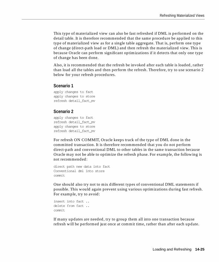
Refreshing Materialized Views
This type of materialized view can also be fast refreshed if DML is performed on the
detail table. It is therefore recommended that the same procedure be applied to this
type of materialized view as for a single table aggregate. That is, perform one type
of change (direct-path load or DML) and then refresh the materialized view. This is
because Oracle can perform significant optimizations if it detects that only one type
of change has been done.
Also, it is recommended that the refresh be invoked after each table is loaded, rather
than load all the tables and then perform the refresh. Therefore, try to use scenario 2
below for your refresh procedures.
Scenario 1apply changes to factapply changes to storerefresh detail_fact_mv
Scenario 2apply changes to factrefresh detail_fact_mvapply changes to storerefresh detail_fact_mv
For refresh ON COMMIT, Oracle keeps track of the type of DML done in the
committed transaction. It is therefore recommended that you do not perform
direct-path and conventional DML to other tables in the same transaction because
Oracle may not be able to optimize the refresh phase. For example, the following is
not recommended:
direct path new data into factConventional dml into storecommit
One should also try not to mix different types of conventional DML statements if
possible. This would again prevent using various optimizations during fast refresh.
For example, try to avoid:
insert into fact ..delete from fact ..commit
If many updates are needed, try to group them all into one transaction because
refresh will be performed just once at commit time, rather than after each update.
Loading and Refreshing 14-25

Refreshing Materialized Views
Scenario 1update factcommitupdate factcommitupdate factcommit
Scenario 2update factupdate factupdate factcommit
Note that if, when you use the DBMS_MVIEW package to refresh a number of
materialized views containing only joins with the "atomic" parameter set to TRUE,
parallel DML is disabled, which could lead to poorer refresh performance.
In a data warehousing environment, assuming that the materialized view has a
parallel clause, the following sequence of steps is recommended:
1. Bulk load into fact
2. ALTER SESSION ENABLE PARALLEL DML;
3. Refresh materialized view
Refreshing Nested Materialized ViewsRefreshing materialized join views and single-table aggregate materialized views
uses the same algorithms irrespective of whether or not the views are nested. All
underlying objects are treated as ordinary tables. If the ON COMMIT refresh option
is specified, then all the materialized views are refreshed in the appropriate order at
commit time.
Example: Consider the schema in Figure 8–5. Assume all the materialized views are
defined for ON COMMIT refresh. If table fact changes, at commit time, you could
refresh join_fact_store_time first and then sum_sales_store_time and join_fact_store_time_prod (with no specific order for sum_sales_store_time and join_fact_store_time_prod because they do not have any dependencies between them).
In other words, Oracle builds a partially ordered set of materialized views and
refreshes them such that, after the successful completion of the refresh, all the
materialized views are fresh. The status of the materialized views can be checked by
querying the appropriate (USER, DBA, ALL)_MVIEWS view.
14-26 Oracle8i Data Warehousing Guide

Refreshing Materialized Views
If any of the materialized views is defined as ON DEMAND refresh (irrespective of
whether the refresh method is fast, force, or complete), you will need to refresh
them in the correct order (taking into account the dependencies between the
materialized views) since the nested materialized view will be refreshed with
respect to the current state of the other materialized views (whether fresh or not).
You can find out dependent materialized views for a particular object using the
PL/SQL function GET_MVIEW_DEPENDENCIES() in the DBMS_MVIEWS
package.
If a refresh fails during commit time, the list of materialized views that have not
been refreshed will be written to the alert log and the user will have to manually
refresh them along with all their dependent materialized views.
APIs As is the case with all materialized views, the functions in the DBMS_MVIEW
package have to be used to refresh a nested materialized view on demand. These
functions have the following behavior when used with nested materialized views:
■ If REFRESH() is used to refresh a materialized view M that is built on other
materialized views, then M will be refreshed with respect to the current state of
the other materialized views (that is, they won't be made fresh first).
■ If REFRESH_DEPENDENT() is used to refresh with respect to the materialized
view M, then only materialized views that directly depend on M will be
refreshed (that is, a materialized view that depends on a materialized view that
depends on M will not be refreshed).
■ If REFRESH_ALL_MVIEWS() is used, the order in which the materialized
views will be refreshed is not guaranteed.
■ GET_MV_DEPENDENCIES() is a new function provided to list the immediate
(or direct) materialized view dependencies for an object.
Complex Materialized ViewsA complex materialized view is one which cannot be fast refreshed. If you will be
using only COMPLETE REFRESH, you can create a materialized view with any
definition.
Recommended Initialization Parameters for ParallelismThe following parameters
■ PARALLEL_MAX_SERVERS should be set high enough to take care of
parallelism.
Loading and Refreshing 14-27

Refreshing Materialized Views
■ SORT_AREA_SIZE should be less than HASH_AREA_SIZE.
■ OPTIMIZER_MODE should equal ALL_ROWS (cost based optimization).
■ OPTIMIZER_PERCENT_PARALLEL should equal 100.
Analyze all tables and indexes for better costing.
Monitoring a RefreshWhile a job is running, a SELECT * FROM V$SESSION_LONGOPS statement will
tell you the progress of each materialized view being refreshed.
To look at the progress of which jobs are on which queue, use a SELECT * FROM
DBA_JOBS_RUNNING statement.
The table ALL_MVIEWS contains the values, as a moving average, for the time
most recently refreshed and the average time to refresh using both full and
incremental methods.
Refresh will schedule the long running jobs first. Use the refresh log to check what
each refresh did.
Tips after Refreshing Materialized ViewsAfter you have performed a load or incremental load and rebuilt the detail table
indexes, you need to re-enable integrity constraints (if any) and refresh the
materialized views and materialized view indexes that are derived from that detail
data. In a data warehouse environment, referential integrity constraints are
normally enabled with the NOVALIDATE or RELY options. An important decision
to make before performing a refresh operation is whether the refresh needs to be
recoverable. Because materialized view data is redundant and can always be
reconstructed from the detail tables, it may be preferable to disable logging on the
materialized view. To disable logging and run incremental refresh non-recoverably,
use the ALTER MATERIALIZED VIEW...NOLOGGING statement prior to
REFRESH.
If the materialized view is being refreshed using the ON COMMIT method, then,
following refresh operations, the alert log (alert_ <SID>.log) and the trace file (ora_
<SID>_number.trc) should be consulted to check that no errors have occurred.
14-28 Oracle8i Data Warehousing Guide

Summary A
15
Summary AdvisorThis chapter can help you create and manage a data warehouse, and includes:
■ Summary Advisor
■ Is a Materialized View Being Used?
dvisor 15-1

Summary Advisor
Summary AdvisorTo help you select from among the many materialized views that are possible in
your schema, Oracle provides a collection of materialized view analysis and
advisory functions in the DBMS_OLAP package. These functions are callable from
any PL/SQL program.
Figure 15–1 Materialized Views and the Summary Advisor
From within the DBMS_OLAP package, several facilities are available to:
■ Estimate the size of a materialized view
■ Recommend a materialized view
■ Recommend materialized views based on collected workload information
■ Report actual utilization of materialized views based on collected workload
Whenever the summary advisor is run, with the exception of reporting the size of a
materialized view, the results are placed in a table in the database which means that
they can be queried, thereby saving the need to keep running the advisor process.
Summary Advisor
Discoverer orThird Party Tool
DBMS_OLAPPL/SQL Package
Workload Collection(optional)
ConfigFile
TraceLog
format
collect
defineevents
Oracle TraceManager
Warehouse
Oracle8i
MaterializedView and
Dimensions
Workload
15-2 Oracle8i Data Warehousing Guide

Summary Advisor
Collecting Structural StatisticsThe advisory functions of the DBMS_OLAP package require you to gather
structural statistics about fact table cardinalities, dimension table cardinalities, and
the distinct cardinalities of every dimension LEVEL column, JOIN KEY column,
and fact table key column. This can be accomplished by loading your data
warehouse, then gathering either exact or estimated statistics with the DBMS_
STATS package or the ANALYZE TABLE statement. Because gathering statistics is
time-consuming and extreme statistical accuracy is not required, it is generally
preferable to estimate statistics. The advisor cannot be used if no dimensions have
been defined, which is a good reason for ensuring that some time is spent creating
them.
Collection of Dynamic Workload StatisticsOptionally, if you have purchased the Oracle Enterprise Manager Performance Pack,then you may also run Oracle Trace to gather dynamic information about your
query work load, which can then be used by an advisory function. If Oracle Trace is
available, serious consideration should be given to collecting materialized view
usage. Not only does it enable the DBA to see which materialized views are in use,
but it also means that the advisor may detect some unusual query requests from the
users which would result in recommending some different materialized views.
Oracle Trace gathers the following work load statistics for the analysis of
materialized views:
■ The name of each materialized view selected by query rewrite
■ The estimated benefit obtained by using the materialized view, which is
roughly the ratio of the fact table cardinality to the materialized view
cardinality, adjusted for the need to further aggregate over the materialized
view or join it back to other relations
■ The ideal materialized view that could have been used by the request
Oracle Trace includes two new point events for collecting runtime statistics about
materialized views: one event that records the selected materialized view names at
request execution time, and another event that records the estimated benefit and
ideal materialized view at compile time. You can log just these two events for
materialized view analysis if desired, or you can join this information with other
information collected by Oracle Trace, such as the SQL text or the execution time of
the request, if other Trace events are also collected. A collection option in the Oracle
Trace Manager GUI provides a way to collect materialized view management
statistics.
Summary Advisor 15-3

Summary Advisor
To collect and analyze the summary event set, you must do the following:
1. Set six initialization parameters to collect data via Oracle Trace. Enabling these
parameters incurs some additional overhead at database connection, but is
otherwise transparent.
■ ORACLE_TRACE_COLLECTION_NAME = oraclesm
■ ORACLE_TRACE_COLLECTION_PATH = location of collection files
■ ORACLE_TRACE_COLLECTION_SIZE = 0
■ ORACLE_TRACE_ENABLE = TRUE turns on Trace collecting
■ ORACLE_TRACE_FACILITY_NAME = oraclesm
■ ORACLE_TRACE_FACILITY_PATH = location of trace facility files
For further information on these parameters, refer to the Oracle Trace UsersGuide.
2. Run the Oracle Trace Manager GUI, specify a collection name, and select the
SUMMARY_EVENT set. Oracle Trace Manager reads information from the
associated configuration file and registers events to be logged with Oracle.
While collection is enabled, the workload information defined in the event set
gets written to a flat log file.
3. When collection is complete, Oracle Trace automatically formats the Oracle
Trace log file into a set of relations, which have the predefined synonyms V_
192216243_F_5_E_14_8_1 and V_192216243_F_5_E_15_8_1. The workload tables
should be located in the same schema that the subsequent workload analysis
will be performed in. Alternatively, the collection file, which usually has an
extension of .CDF, can be formatted manually using otrcfmt. A manual
collection command is illustrated below:
otrcfmt collection_name.cdf user/password@database
4. Run the GATHER_TABLE_STATS procedure of the DBMS_STATS package or
ANALYZE...ESTIMATE STATISTICS to collect cardinality statistics on all fact
tables, dimension tables, and key columns (any column that appears in a
dimension LEVEL clause or JOIN KEY clause of a CREATE DIMENSION
statement).
Once these four steps have been completed, you will be ready to make
recommendations about your materialized views.
15-4 Oracle8i Data Warehousing Guide

Summary Advisor
Recommending Materialized ViewsThe analysis and advisory functions for materialized views are RECOMMEND_MV
and RECOMMEND_MV_W in the DBMS_OLAP package. These functions
automatically recommend which materialized views to create, retain, or drop.
■ RECOMMEND_MV uses structural statistics, but not workload statistics, to
generate recommendations.
■ RECOMMEND_MV_W uses both workload statistics and structural statistics.
You can call these functions to obtain a list of materialized view recommendations
that you can select, modify, or reject. Alternatively, you can use the DBMS_OLAP
package directly in your PL/SQL programs for the same purpose.
The summary advisor will not be able to recommend summaries if the following
conditions are not met:
1. All tables including existing materialized views must have been analyzed as
described in step 4 above.
2. Dimensions must exist.
3. The advisor should be able to identify the fact table because it will contain
foreign key references to other tables.
Four parameters are required to use these functions:
■ Fact table names or null to analyze all fact tables
■ The maximum storage that can be used for storing materialized views
■ A list or materialized views that you want to retain
■ A number between 0 to 100 that specifies the percentage of materialized views
that must be retained
A typical call to the package, where the main fact table is called FACT, would be:
DBMS_OLAP.RECOMMEND_MV('fact', 100000, '', 10);
No workload statistics are used in this example.
The results from calling this package are put in the table MVIEWS$_
RECOMMENDATIONS. The contents of this table can be queried or they can be
See Also: See Oracle8i Supplied PL/SQL Packages Reference for
detailed information about the DBMS_OLAP package.
Summary Advisor 15-5

Summary Advisor
displayed using the SQL file sadvdemo.sql. The output from calling this procedure
is the same irrespective of whether the workload statistics are used.
The recommendations can be viewed by calling the procedure DEMO_
SUMADV.PRETTYPRINT_RECOMMENDATIONS, but first you need to run
sadvdemo.sql. It is suggested that SET SERVEROUTPUT ON SIZE 900000 be used
to ensure that all the information can be displayed. A sample recommendation that
resulted from calling this package is shown below.
Recommendation Number 1Recommended Action is DROP existing summary GROCERY.QTR_STORE_PROMO_SUMStorage in bytes is 196020Percent performance gain is nullBenefit-to-cost ratio is null
Recommendation Number 2Recommended Action is RETAIN existing summary GROCERY.STORE_SUMStorage in bytes is 21Percent performance gain is nullBenefit-to-cost ratio is null
To call the package and use the workload statistics, the only difference is the
procedure name that is called. For example, instead of recommend_mv, it's
recommend_mv_w.
DBMS_OLAP.RECOMMEND_MV_W('fact', 100000, '', 10);
Recommendation Number 3Recommendation Number = 3Recommended Action is CREATE new summary:SELECT PROMOTION.PROMOTION_KEY, STORE.STORE_KEY, STORE.STORE_NAME, STORE.DISTRICT, STORE.REGION , COUNT(*), SUM(FACT.CUSTOMER_COUNT), COUNT(FACT.CUSTOMER_COUNT), SUM(FACT.DOLLAR_COST),COUNT(FACT.DOLLAR_COST), SUM(FACT.DOLLAR_SALES), COUNT(FACT.DOLLAR_SALES), MIN(FACT.DOLLAR_SALES), MAX(FACT.DOLLAR_SALES), SUM(FACT.RANDOM1), COUNT(FACT.RANDOM1), SUM(FACT.RANDOM2), COUNT(FACT.RANDOM2), SUM(FACT.RANDOM3), COUNT(FACT.RANDOM3), SUM(FACT.UNIT_SALES), COUNT(FACT.UNIT_SALES)FROM GROCERY.FACT, GROCERY.PROMOTION, GROCERY.STOREWHERE FACT.PROMOTION_KEY = PROMOTION.PROMOTION_KEY AND FACT.STORE_KEY = STORE.STORE_KEYGROUP BY PROMOTION.PROMOTION_KEY, STORE.STORE_KEY, STORE.STORE_NAME, STORE.DISTRICT, STORE.REGION
15-6 Oracle8i Data Warehousing Guide
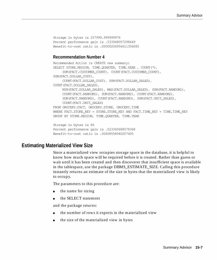
Summary Advisor
Storage in bytes is 257999.999999976Percent performance gain is .533948057298649Benefit-to-cost ratio is .00000206956611356085
Recommendation Number 4Recommended Action is CREATE new summary:SELECT STORE.REGION, TIME.QUARTER, TIME.YEAR , COUNT(*), SUM(FACT.CUSTOMER_COUNT), COUNT(FACT.CUSTOMER_COUNT),SUM(FACT.DOLLAR_COST), COUNT(FACT.DOLLAR_COST), SUM(FACT.DOLLAR_SALES),COUNT(FACT.DOLLAR_SALES), MIN(FACT.DOLLAR_SALES), MAX(FACT.DOLLAR_SALES), SUM(FACT.RANDOM1), COUNT(FACT.RANDOM1), SUM(FACT.RANDOM2), COUNT(FACT.RANDOM2), SUM(FACT.RANDOM3), COUNT(FACT.RANDOM3), SUM(FACT.UNIT_SALES), COUNT(FACT.UNIT_SALES)FROM GROCERY.FACT, GROCERY.STORE, GROCERY.TIMEWHERE FACT.STORE_KEY = STORE.STORE_KEY AND FACT.TIME_KEY = TIME.TIME_KEYGROUP BY STORE.REGION, TIME.QUARTER, TIME.YEAR
Storage in bytes is 86Percent performance gain is .523360688578368Benefit-to-cost ratio is .00608558940207405
Estimating Materialized View SizeSince a materialized view occupies storage space in the database, it is helpful to
know how much space will be required before it is created. Rather than guess or
wait until it has been created and then discoverer that insufficient space is available
in the tablespace, use the package DBMS_ESTIMATE_SIZE. Calling this procedure
instantly returns an estimate of the size in bytes that the materialized view is likely
to occupy.
The parameters to this procedure are:
■ the name for sizing
■ the SELECT statement
and the package returns:
■ the number of rows it expects in the materialized view
■ the size of the materialized view in bytes
Summary Advisor 15-7

Is a Materialized View Being Used?
In the example shown below, the query that will be specified in the materialized
view is passed into the ESTIMATE_SUMMARY_SIZE package. Note that the SQL
statement is passed in without a ";".
DBMS_OLAP.estimate_summary_size ('simple_store', 'SELECT product_key1, product_key2, SUM(dollar_sales) AS sum_dollar_sales, SUM(unit_sales) AS sum_unit_sales, SUM(dollar_cost) AS sum_dollar_cost, SUM(customer_count) AS no_of_customers FROM fact GROUP BY product_key1, product_key2' , no_of_rows, mv_size );
The procedure returns two values, an estimate for the number of rows and the size
of the materialized view in bytes, as shown below.
No of Rows: 17284Size of Materialized view (bytes): 2281488
Summary Advisor WizardThe Summary Advisor Wizard, which can be found in Oracle Enterprise Manager,
provides an interactive environment to recommend and build materialized views.
Using this approach, you will be asked where the materialized views are to be
placed, which fact tables to use, and which of the existing materialized views are to
be retained. If a workload exists, it will be automatically selected, otherwise, it will
display the recommendations that are generated from the advisor functions
RECOMMEND_MV or RECOMMEND_MV_W.
By using the wizard, all of the steps required to maintain your materialized views
can be completed by answering the wizard's questions and no subsequent DML
operations are required. See the Oracle Enterprise Manager documentation set for
further details.
Is a Materialized View Being Used?One of the major administrative problems with materialized views is knowing
whether they are being used. Materialized views could be in regular use or they
could have been created for a one-time problem that has now been resolved.
However, the usergroup who requested this level of analysis might never have told
the DBA that it was no longer required, so the materialized view remains in the
database occupying storage space and possibly being regularly refreshed.
15-8 Oracle8i Data Warehousing Guide

Is a Materialized View Being Used?
If the Oracle Trace option is available, then it can advise the DBA which
materialized views are in use, using exactly the same procedure as for collecting
workload statistics. Trace collection is enabled and in this case the collection period
is likely to be longer that for query collection because Trace will only report on
materialized views that were used while it was collecting statistics. Therefore, if too
small a window is chosen, not all the materialized views that are in use will be
reported.
Once you are satisfied that you have collected sufficient data, the data is formatted
by Oracle Trace, just as if it were workload information, and then the package
EVALUATE_UTILIZATION_W is called. It analyzes the data and then the results
are placed in the table MVIEWS$_EVALUATIONS.
In the example below, the utilization of materialized views is analyzed and the
results are displayed.
DBMS_OLAP.EVALUATE_UTILIZATION_W();
Note that no parameters are passed into the package.
Shown below is a sample output obtained by querying the table
MVIEW$EVALUATIONS which is providing the following information:
■ Materialized view owner and name
■ Rank of this materialized view in descending benefit-to-cost ratio
■ Size of the materialized view in bytes
■ The number of times the materialized view appears in the workload
■ The cumulative benefit is calculated each time the materialized view is used as
■ The benefit-to-cost ratio is calculated as the incremental improvement in
performance to the size of the materialized view
MVIEW_OWNER MVIEW_NAME RANK SIZE FREQ CUMULATIVE BENEFIT----------- ------------------- ----- ------ ---- ---------- ----------GROCERY STORE_MIN_SUM 1 340 1 9001 26.4735294GROCERY STORE_MAX_SUM 2 380 1 9001 23.6868421GROCERY STORE_STDCNT_SUM 3 3120 1 3000.38333 .961661325GROCERY QTR_STORE_PROMO_SUM 4 196020 2 0 0GROCERY STORE_SALES_SUM 5 340 1 0 0GROCERY STORE_SUM 6 21 10 0 0
Summary Advisor 15-9

Is a Materialized View Being Used?
15-10 Oracle8i Data Warehousing Guide

Part V
Warehouse PerformanceThis section deals with ways to improve your data warehouse’s performance, and
contains the following chapters:
■ Schemas
■ SQL for Analysis
■ Tuning Parallel Execution
■ Query Rewrite


S
16
SchemasThe following topics provide information about schemas in a data warehouse:
■ Schemas
■ Optimizing Star Queries
chemas 16-1

Schemas
SchemasA schema is a collection of database objects, including tables, views, indexes, and
synonyms.
There is a variety of ways of arranging schema objects in the schema models
designed for data warehousing. The most common data-warehouse schema model
is a star schema. For this reason, most of the examples in this book utilize a star
schema. However, a significant but smaller number of data warehouses use
third-normal-form (3NF) schemas, or other schemas which are more highly
normalized than star schemas. These 3NF data warehouses are typically very large
data warehouses, which are used primarily for loading data and for feeding data
marts. These data warehouses are not typically used for heavy end-user query
workloads.
Some features of the Oracle8i database, such as the star transformation feature
described in this chapter, are specific to star schemas, however, the vast majority of
Oracle8i's data warehousing features are equally applicable to both star schemas
and 3NF schemas.
Star SchemasThe star schema is the simplest data warehouse schema. It is called a star schema
because the diagram of a star schema resembles a star, with points radiating from a
center. The center of the star consists of one or more fact tables and the points of the
star are the dimension tables.
A star schema is characterized by one or more very large fact tables that contain the
primary information in the data warehouse and a number of much smaller
dimension tables (or lookup tables), each of which contains information about the
entries for a particular attribute in the fact table.
A star query is a join between a fact table and a number of lookup tables. Each
lookup table is joined to the fact table using a primary-key to foreign-key join, but
the lookup tables are not joined to each other.
Cost-based optimization recognizes star queries and generates efficient execution
plans for them. (Star queries are not recognized by rule-based optimization.)
A typical fact table contains keys and measures. For example, a simple fact table
might contain the measure Sales, and keys Time, Product, and Market. In this case,
there would be corresponding dimension tables for Time, Product, and Market. The
Product dimension table, for example, would typically contain information about
each product number that appears in the fact table. A measure is typically a
16-2 Oracle8i Data Warehousing Guide

Schemas
numeric or character column, and can be taken from one column in one table or
derived from two columns in one table or two columns in more than one table.
A star join is a primary-key to foreign-key join of the dimension tables to a fact table.
The fact table normally has a concatenated index on the key columns to facilitate
this type of join.
The main advantages of star schemas are that they:
■ Provide a direct and intuitive mapping between the business entities being
analyzed by end users and the schema design.
■ Provides highly optimized performance for typical data warehouse queries.
Figure 16–1 presents a graphical representation of a star schema.
Figure 16–1 Star Schema
Snowflake SchemasThe snowflake schema is a more complex data warehouse model than a star
schema, and is a type of star schema. It is called a snowflake schema because the
diagram of the schema resembles a snowflake.
Snowflake schemas normalize dimensions to eliminate redundancy. That is, the
dimension data has been grouped into multiple tables instead of one large table. For
example, a product dimension table in a star schema might be normalized into a
Product table, a Product_Category table, and a Product_Manufacturer table in a
snowflake schema. While this saves space, it increases the number of dimension
tables and requires more foreign key joins. The result is more complex queries and
reduced query performance. Figure 16–2 presents a graphical representation of a
snowflake schema.
Customer
Products
Dimension Table Dimension Table
Channel
Sales(units, price)
Time
Fact Table
Schemas 16-3

Optimizing Star Queries
Figure 16–2 Snowflake Schema
Optimizing Star Queries
Tuning Star QueriesIn order to get the best possible performance for star queries, it is important to
follow some basic guidelines:
■ A bitmap index should be built on each of the foreign-key columns of the fact
table(s).
■ The initialization parameter STAR_TRANSFORMATION_ENABLED should be
set to TRUE. This enables an important optimizer feature for star-queries; it is
set to FALSE by default for backwards-compatibility.
■ The cost-based optimizer should be used. [This does not apply solely to star
schemas: all data warehouses should always use the cost-based optimizer].
When a data warehouse satisfies these conditions, the majority of the star queries
running in the data warehouse will use a query-execution strategy known as the
star transformation. The star transformation provides very efficient query
performance for star queries.
Note: Oracle recommends you choose a star schema over a
snowflake schema unless you have a clear reason not to.
Customer
Products
Channel
Sales(units, price)
Time
Category Time Period
Segment
16-4 Oracle8i Data Warehousing Guide

Optimizing Star Queries
Star TransformationThe star transformation is a cost-based query transformation aimed at executing
star queries efficiently. Whereas the star optimization works well for schemas with a
small number of dimensions and dense fact tables, the star transformation may be
considered as an alternative if any of the following holds true:
■ The number of dimensions is large
■ The fact table is sparse
■ There are queries where not all dimension tables have constraining predicates
The star transformation does not rely on computing a Cartesian product of the
dimension tables, which makes it better suited for cases where fact table sparsity
and/or a large number of dimensions would lead to a large Cartesian product with
few rows having actual matches in the fact table. In addition, rather than relying on
concatenated indexes, the star transformation is based on combining bitmap
indexes on individual fact table columns.
The transformation can thus combine indexes corresponding precisely to the
constrained dimensions. There is no need to create many concatenated indexes
where the different column orders match different patterns of constrained
dimensions in different queries.
Star Transformation ExampleThis section provides an example of the star transformation. The star
transformation is a powerful, and interesting, optimization technique which relies
upon implicitly rewriting (or transforming) the SQL of the original star query.
The end user never needs to know any of the details about the star transformation;
Oracle's cost-based optimizer will automatically choose the star transformation
where appropriate.
However, the DBA may be interested to learn the details of the star transformation.
This section will enable the DBA to understand how the star transformation
algorithm works, and moreover, the DBA will be able to recognize the execution
plans of star queries which are using the star transformation.
Attention: Bitmap indexes are available only if you have
purchased the Oracle8i Enterprise Edition. In Oracle8i, bitmap
indexes and star transformation are not available.
Schemas 16-5

Optimizing Star Queries
Oracle processes a star query using two basic phases. The first phase retrieves
exactly the necessary rows from the fact table (the result set). Because this retrieval
utilizes bitmap indexes, it is very efficient.
The second phase joins this result set to the dimension tables. Below is an example
of how an end-user may query this data warehouse: "What were the sales and
profits for the grocery department of stores in the west and southwest sales districts
over the last three quarters?" This is a simple star query. The SQL generated by an
end-user tool could look like:
SELECT store.sales_district, time.fiscal_period, SUM(sales.dollar_sales) revenue, SUM(dollar_sales) - SUM(dollar_cost) incomeFROM sales, store, time, productWHERE sales.store_key = store.store_key AND sales.time_key = time.time_key AND sales.product_key = product.product_key AND time.fiscal_period IN ('3Q95', '4Q95', '1Q96') and product.department = 'Grocery' AND store.sales_district IN ('San Francisco', 'Los Angeles')GROUP BY store.sales_district, time.fiscal_period;
Oracle will process this query in two phases. In the first phase, Oracle will use the
bitmap indexes on the foreign-key columns of the fact table to identify and retrieve
the only the necessary rows from the fact table. That is, Oracle will retrieve the
result set from the fact table using essentially the following query:
SELECT ... FROM salesWHERE store_key IN (SELECT store_key FROM store WHERE sales_district IN ('WEST', 'SOUTHWEST')) AND time_key IN (SELECT time_key FROM time WHERE quarter IN ('3Q96', '4Q96', '1Q97')) AND product_key IN (SELECT product_key FROM product WHERE department = 'GROCERY');
This is the transformation step of the algorithm, because the original star query has
been transformed into this subquery representation. This method of accessing the
fact table leverages the strengths of Oracle's bitmap indexes. Intuitively, bitmap
indexes provide a set-based processing scheme within a relational database. Oracle
16-6 Oracle8i Data Warehousing Guide

Optimizing Star Queries
has implemented very fast methods for doing set operations such as AND (an
intersection in standard set-based terminology), OR (a set-based union), MINUS,
and COUNT.
In this star query, a bitmap index on store_key is used to identify the set of all rows
in the fact table corresponding to sales in the West sales district. This set is
represented as a bitmap (a string of 1's and 0's that indicates which rows of the fact
table are members of the set).
A similar bitmap is retrieved for the fact-table rows corresponding to the sale in the
Southwest sales district. The bitmap OR operation is used to combine this set of
Southwest sales with the set of West sales.
Additional set operations will be done for the time dimension and the product
dimension. At this point in the star query processing, there are three bitmaps: each
bitmap corresponds to a separate dimension table, and each bitmap represents the
set of rows of the fact table that satisfy that individual dimension's constraints.
These three bitmaps are combined into a single bitmap using the bitmap AND
operation. This final bitmap represents the set of rows in the fact table that satisfy
all of the constraints on the dimension table; this is the result set, the exact set of
rows from the fact table needed to evaluate the query. Note that none of the actual
data in the fact table has been accessed; all of these operations rely solely on the
bitmap indexes and the dimension tables. Because of the bitmap indexes' patented,
compressed data representations, the bitmap set-based operations are extremely
efficient.
Once the result set is identified, the bitmap is used to access the actual data from the
sales table. Only those rows that are required for the end-user's query are retrieved
from the fact table.
The second phase of this query is to join these rows from the fact table to the
dimension tables. Oracle will use the most efficient method for accessing and
joining the dimension tables. Many dimension are very small, and table scans are
typically the most efficient access method for these dimension tables. For large
dimension tables, table scans may not be the most efficient access method. In the
example above, a bitmap index on product.department may be used to quickly
identify all of those products in the grocery department. Oracle8's cost-based
optimizer will automatically determine which access method is most appropriate
for a given dimension table, based upon the cost-based optimizer's knowledge
about the sizes and data distributions of each dimension table.
The specific join method (as well as indexing method) for each dimension tables
will likewise be intelligently determined by the cost-based optimizer. A hash join is
often the most efficient algorithm for joining the dimension tables. The final answer
Schemas 16-7

Optimizing Star Queries
is returned to the user once all of the dimension tables have been joined. The query
technique of retrieving only the matching rows from one table and then joining to
another table is commonly known as a semi-join.
Execution PlanThe following execution plan might result from "Star Transformation Example" on
page 16-5:
SELECT STATEMENT HASH JOIN HASH JOIN HASH JOIN TABLE ACCESS SALES BY INDEX ROWID BITMAP CONVERSION TO ROWIDS BITMAP AND BITMAP MERGE BITMAP KEY ITERATION TABLE ACCESS STORE FULL BITMAP INDEX SALES_STORE_KEY RANGE SCAN BITMAP MERGE BITMAP KEY ITERATION TABLE ACCESS TIME FULL BITMAP INDEX SALES_TIME_KEY RANGE SCAN BITMAP MERGE BITMAP KEY ITERATION TABLE ACCESS PRODUCTS FULL BITMAP INDEX SALES_PRODUCT_KEY RANGE SCAN TABLE ACCESS TIME FULL TABLE ACCESS PRODUCTS FULL TABLE ACCESS STORE FULL
In this plan, the fact table is accessed through a bitmap access path based on a
bitmap AND of three merged bitmaps. The three bitmaps are generated by the
BITMAP MERGE row source being fed bitmaps from row source trees underneath
it. Each such row source tree consists of a BITMAP KEY ITERATION row source
which fetches values from the subquery row source tree, which in this example is
just a full table access. For each such value, the BITMAP KEY ITERATION row
source retrieves the bitmap from the bitmap index. After the relevant fact table rows
have been retrieved using this access path, they are joined with the dimension
tables and temporary tables to produce the answer to the query.
The star transformation is a cost-based transformation in the following sense. The
optimizer generates and saves the best plan it can produce without the
transformation. If the transformation is enabled, the optimizer then tries to apply it
16-8 Oracle8i Data Warehousing Guide
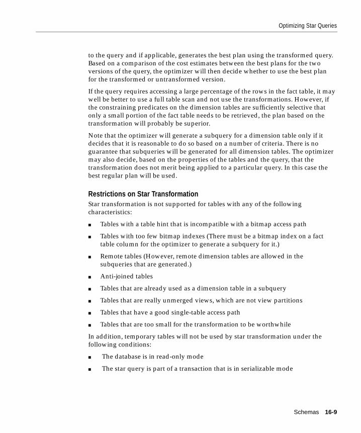
Optimizing Star Queries
to the query and if applicable, generates the best plan using the transformed query.
Based on a comparison of the cost estimates between the best plans for the two
versions of the query, the optimizer will then decide whether to use the best plan
for the transformed or untransformed version.
If the query requires accessing a large percentage of the rows in the fact table, it may
well be better to use a full table scan and not use the transformations. However, if
the constraining predicates on the dimension tables are sufficiently selective that
only a small portion of the fact table needs to be retrieved, the plan based on the
transformation will probably be superior.
Note that the optimizer will generate a subquery for a dimension table only if it
decides that it is reasonable to do so based on a number of criteria. There is no
guarantee that subqueries will be generated for all dimension tables. The optimizer
may also decide, based on the properties of the tables and the query, that the
transformation does not merit being applied to a particular query. In this case the
best regular plan will be used.
Restrictions on Star TransformationStar transformation is not supported for tables with any of the following
characteristics:
■ Tables with a table hint that is incompatible with a bitmap access path
■ Tables with too few bitmap indexes (There must be a bitmap index on a fact
table column for the optimizer to generate a subquery for it.)
■ Remote tables (However, remote dimension tables are allowed in the
subqueries that are generated.)
■ Anti-joined tables
■ Tables that are already used as a dimension table in a subquery
■ Tables that are really unmerged views, which are not view partitions
■ Tables that have a good single-table access path
■ Tables that are too small for the transformation to be worthwhile
In addition, temporary tables will not be used by star transformation under the
following conditions:
■ The database is in read-only mode
■ The star query is part of a transaction that is in serializable mode
Schemas 16-9

Optimizing Star Queries
16-10 Oracle8i Data Warehousing Guide

SQL for
17
SQL for AnalysisThe following topics provide information about how to improve analytical SQL
queries in a data warehouse:
■ Overview
■ ROLLUP
■ CUBE
■ Using Other Aggregate Functions with ROLLUP and CUBE
■ GROUPING Function
■ Other Considerations when Using ROLLUP and CUBE
■ Analytic Functions
■ Case Expressions
Analysis 17-1

Overview
OverviewOracle has enhanced SQL's analytical processing power along several paths:
■ The CUBE and ROLLUP extensions to the GROUP BY clause of the SELECT
statement
■ A new family of analytic SQL functions
■ Linear regression functions
■ CASE expressions
The CUBE and ROLLUP extensions to SQL make querying and reporting easier in
data warehousing environments. ROLLUP creates subtotals at increasing levels of
aggregation, from the most detailed up to a grand total. CUBE is an extension
similar to ROLLUP, enabling a single statement to calculate all possible
combinations of subtotals. CUBE can generate the information needed in
cross-tabulation reports with a single query.
Analytic functions enable rankings, moving window calculations, and lead/lag
analysis. Ranking functions include cumulative distributions, percent rank, and
N-tiles. Moving window calculations allow you to find moving and cumulative
aggregations, such as sums and averages. Lead/lag analysis enables direct
inter-row references so you can calculate period-to-period changes.
Other enhancements to SQL include a family of regression functions and the CASE
expression. Regression functions offer a full set of linear regression calculations.
CASE expressions provide if-then logic useful in many situations.
These CUBE and ROLLUP extensions and analytic functions are part of the core
SQL processing. To enhance performance, CUBE, ROLLUP, and analytic functions
can be parallelized: multiple processes can simultaneously execute all of these
statements. These capabilities make calculations easier and more efficient, thereby
enhancing database performance, scalability, and simplicity.
Analyzing Across Multiple DimensionsOne of the key concepts in decision support systems is multi-dimensional analysis:
examining the enterprise from all necessary combinations of dimensions. We use
the term dimension to mean any category used in specifying questions. Among the
most commonly specified dimensions are time, geography, product, department,
and distribution channel, but the potential dimensions are as endless as the varieties
See Also: For information on parallel execution, see Chapter 18,
"Tuning Parallel Execution".
17-2 Oracle8i Data Warehousing Guide

Overview
of enterprise activity. The events or entities associated with a particular set of
dimension values are usually referred to as facts. The facts may be sales in units or
local currency, profits, customer counts, production volumes, or anything else
worth tracking.
Here are some examples of multidimensional requests:
■ Show total sales across all products at increasing aggregation levels for a
geography dimension: from state to country to region for 1998 and 1999.
■ Create a cross-tabular analysis of our operations showing expenses by territory
in South America for 1998 and 1999. Include all possible subtotals.
■ List the top 10 sales representatives in Asia according to 1999 sales revenue for
automotive products, and rank their commissions.
All the requests above involve multiple dimensions. Many multidimensional
questions require aggregated data and comparisons of data sets, often across time,
geography or budgets.
To visualize data that has many dimensions, analysts commonly use the analogy of
a data cube, that is, a space where facts are stored at the intersection of ndimensions. Figure 17–1 shows a data cube and how it could be used differently by
various groups. The cube stores sales data organized by the dimensions of Product,
Market, and Time.
SQL for Analysis 17-3

Overview
Figure 17–1 Cubes and Views by Different Users
We can retrieve slices of data from the cube. These correspond to cross-tabular
reports such as the one shown in Table 17–1. Regional managers might study the
data by comparing slices of the cube applicable to different markets. In contrast,
product managers might compare slices that apply to different products. An ad hoc
user might work with a wide variety of constraints, working in a subset cube.
Answering multidimensional questions often involves accessing and querying huge
quantities of data, sometimes millions of rows. Because the flood of detailed data
generated by large organizations cannot be interpreted at the lowest level,
aggregated views of the information are essential. Subtotals across many
dimensions are vital to multidimensional analyses. Therefore, analytical tasks
require convenient and efficient data aggregation.
Optimized PerformanceNot only multidimensional issues, but all types of processing can benefit from
enhanced aggregation facilities. Transaction processing, financial and
manufacturing systems—all of these generate large numbers of production reports
Regional Mgr. View
Financial Mgr. View Ad Hoc View
PROD
Time
Mar
ket
SALESProduct Mgr. View
17-4 Oracle8i Data Warehousing Guide

Overview
needing substantial system resources. Improved efficiency when creating these
reports will reduce system load. In fact, any computer process that aggregates data
from details to higher levels needs optimized performance.
Oracle8i extensions provide aggregation features and bring many benefits,
including:
■ Simplified programming requiring less SQL code for many tasks
■ Quicker and more efficient query processing
■ Reduced client processing loads and network traffic because aggregation work
is shifted to servers
■ Opportunities for caching aggregations because similar queries can leverage
existing work
Oracle8i provides all these benefits with the new CUBE and ROLLUP extensions to
the GROUP BY clause. These extensions adhere to the ANSI and ISO proposals for
SQL3, a draft standard for enhancements to SQL.
A ScenarioTo illustrate CUBE and ROLLUP queries, this chapter uses a hypothetical videotape
sales and rental company. All the examples given refer to data from this scenario.
The hypothetical company has stores in several regions and tracks sales and profit
information. The data is categorized by three dimensions: Time, Department, and
Region. The time dimension members are 1996 and 1997, the departments are Video
Sales and Video Rentals, and the regions are East, West, and Central.
Table 17–1 is a sample cross-tabular report showing the total profit by region and
department in 1999:
Table 17–1 Simple Cross-Tabular Report, with Subtotals Shaded
1999
Region Department
Video Rental Profit Video Sales Profit Total Profit
Central 82,000 85,000 167,000
East 101,000 137,000 238,000
West 96,000 97,000 193,000
Total 279,000 319,000 598,000
SQL for Analysis 17-5

ROLLUP
Consider that even a simple report like Table 17–1, with just twelve values in its
grid, generates five subtotals and a grand total. The subtotals are the shaded
numbers. Half of the values needed for this report would not be calculated with a
query that used standard SUM() and GROUP BY operations. Database commands
that offer improved calculation of subtotals bring major benefits to querying,
reporting, and analytical operations.
ROLLUPROLLUP enables a SELECT statement to calculate multiple levels of subtotals
across a specified group of dimensions. It also calculates a grand total. ROLLUP is a
simple extension to the GROUP BY clause, so its syntax is extremely easy to use.
The ROLLUP extension is highly efficient, adding minimal overhead to a query.
SyntaxROLLUP appears in the GROUP BY clause in a SELECT statement. Its form is:
SELECT … GROUP BY ROLLUP(grouping_column_reference_list )
DetailsROLLUP's action is straightforward: it creates subtotals which roll up from the most
detailed level to a grand total, following a grouping list specified in the ROLLUP
clause. ROLLUP takes as its argument an ordered list of grouping columns. First, it
calculates the standard aggregate values specified in the GROUP BY clause. Then, it
creates progressively higher-level subtotals, moving from right to left through the
list of grouping columns. Finally, it creates a grand total.
ROLLUP creates subtotals at n+1 levels, where n is the number of grouping
columns. For instance, if a query specifies ROLLUP on grouping columns of Time,
Region, and Department (n=3), the result set will include rows at four aggregation
levels.
ExampleThis example of ROLLUP uses the data in the video store database, the same
database as was used in Table 17–1, "Simple Cross-Tabular Report, with Subtotals
Shaded".
SELECT Time, Region, Department, SUM(Profit) AS Profit FROM sales GROUP BY ROLLUP(Time, Region, Dept);
17-6 Oracle8i Data Warehousing Guide

ROLLUP
As you can see in Output 15-1, this query returns the following sets of rows:
■ Regular aggregation rows that would be produced by GROUP BY without
using ROLLUP
■ First-level subtotals aggregating across Department for each combination of
Time and Region
■ Second-level subtotals aggregating across Region and Department for each
Time value
■ A grand total row
Output 15-1ROLLUP Aggregation across Three Dimensions
Time Region Department Profit---- ------ ---------- ------1996 Central VideoRental 75,0001996 Central VideoSales 74,0001996 Central NULL 149,0001996 East VideoRental 89,0001996 East VideoSales 115,0001996 East NULL 204,0001996 West VideoRental 87,0001996 West VideoSales 86,0001996 West NULL 173,0001996 NULL NULL 526,0001997 Central VideoRental 82,0001997 Central VideoSales 85,0001997 Central NULL 167,0001997 East VideoRental 101,0001997 East VideoSales 137,0001997 East NULL 238,0001997 West VideoRental 96,0001997 West VideoSales 97,0001997 West NULL 193,0001997 NULL NULL 598,000NULL NULL NULL 1,124,000
Note: The NULLs shown in the figures of this chapter are
displayed only for clarity: in standard Oracle output, these cells
would be blank.
SQL for Analysis 17-7

ROLLUP
Interpreting NULLs in ResultsNULLs returned by ROLLUP and CUBE are not always the traditional null
meaning value unknown. Instead, a NULL may indicate that its row is a subtotal. For
instance, the first NULL value shown in Output 15-1 is in the Department column.
This NULL means that the row is a subtotal for "All Departments" for the Central
region in 1996. To avoid introducing another non-value in the database system,
these subtotal values are not given a special tag.
See the section "GROUPING Function" on page 17-15 for details on how the NULLs
representing subtotals are distinguished from NULLs stored in the data.
Partial RollupYou can also ROLLUP so that only some of the sub-totals will be included. This
partial rollup uses the following syntax:
GROUP BY expr1, ROLLUP(expr2, expr3);
In this case, ROLLUP creates subtotals at (2+1=3) aggregation levels. That is, at level
(expr1, expr2, expr3), (expr1, expr2), and (expr1). It does not produce a grand total.
Example:
This example of partial ROLLUP uses the data in the video store database.
SELECT Time, Region, Department, SUM(Profit) AS Profit FROM sales GROUP BY Time, ROLLUP(Region, Dept);
As you can see in Output 15-2, this query returns the following sets of rows:
■ Regular aggregation rows that would be produced by GROUP BY without
using ROLLUP
■ First-level subtotals aggregating across Department for each combination of
Time and Region
■ Second-level subtotals aggregating across Region and Department for each
Time value
■ It does not produce a grand total row
17-8 Oracle8i Data Warehousing Guide

ROLLUP
Output 15-2Partial ROLLUP
Time Region Department Profit---- ------ ---------- ------1996 Central VideoRental 75,0001996 Central VideoSales 74,0001996 Central NULL 149,0001996 East VideoRental 89,0001996 East VideoSales 115,0001996 East NULL 204,0001996 West VideoRental 87,0001996 West VideoSales 86,0001996 West NULL 173,0001996 NULL NULL 526,0001997 Central VideoRental 82,0001997 Central VideoSales 85,0001997 Central NULL 167,0001997 East VideoRental 101,0001997 East VideoSales 137,0001997 East NULL 238,0001997 West VideoRental 96,0001997 West VideoSales 97,0001997 West NULL 193,0001997 NULL NULL 598,000
Calculating Subtotals without ROLLUPThe result set in Table 17–1 could be generated by the UNION of four SELECT
statements, as shown below. This is a subtotal across three dimensions. Notice that
a complete set of ROLLUP-style subtotals in n dimensions would require n+1
SELECT statements linked with UNION ALL.
SELECT Time, Region, Department, SUM(Profit) FROM Sales GROUP BY Time, Region, DepartmentUNION ALL SELECT Time, Region, '' , SUM(Profit) FROM Sales GROUP BY Time, RegionUNION ALL SELECT Time, '', '', SUM(Profits) FROM Sales GROUP BY TimeUNION ALL
SQL for Analysis 17-9

CUBE
SELECT '', '', '', SUM(Profits) FROM Sales;
The approach shown in the SQL above has two shortcomings compared with the
ROLLUP operator. First, the syntax is complex, requiring more effort to generate
and understand. Second, and more importantly, query execution is inefficient
because the optimizer receives no guidance about the user's overall goal. Each of
the four SELECT statements above causes table access even though all the needed
subtotals could be gathered with a single pass. The ROLLUP extension makes thedesired result explicit and gathers its results with just one table access.
The more columns used in a ROLLUP clause, the greater the savings compared to
the UNION ALL approach. For instance, if a four-column ROLLUP replaces a
UNION of five SELECT statements, the reduction in table access is four-fifths or
80%.
Some data access tools calculate subtotals on the client side and thereby avoid the
multiple SELECT statements described above. While this approach can work, it
places significant loads on the computing environment. For large reports, the client
must have substantial memory and processing power to handle the subtotaling
tasks. Even if the client has the necessary resources, a heavy processing burden for
subtotal calculations may slow down the client in its performance of other activities.
When to Use ROLLUPUse the ROLLUP extension in tasks involving subtotals.
■ It is very helpful for subtotaling along a hierarchical dimension such as time or
geography. For instance, a query could specify a ROLLUP(y, m, day) or
ROLLUP(country, state, city).
■ For data warehouse administrators using summary tables, but not yet utilizing
materialized views, ROLLUP may simplify and speed up the maintenance of
summary tables.
CUBEThe subtotals created by ROLLUP represent only a fraction of possible subtotal
combinations. For instance, in the cross-tabulation shown in Table 17–1, the
departmental totals across regions (279,000 and 319,000) would not be calculated by
See Also: For information on parallel execution, see Chapter 18,
"Tuning Parallel Execution".
17-10 Oracle8i Data Warehousing Guide

CUBE
a ROLLUP(Time, Region, Department) clause. To generate those numbers would
require a ROLLUP clause with the grouping columns specified in a different order:
ROLLUP(Time, Department, Region). The easiest way to generate the full set of
subtotals needed for cross-tabular reports such as those needed for Table 17–1 is to
use the CUBE extension.
CUBE enables a SELECT statement to calculate subtotals for all possible
combinations of a group of dimensions. It also calculates a grand total. This is the
set of information typically needed for all cross-tabular reports, so CUBE can
calculate a cross-tabular report with a single SELECT statement. Like ROLLUP,
CUBE is a simple extension to the GROUP BY clause, and its syntax is also easy to
learn.
SyntaxCUBE appears in the GROUP BY clause in a SELECT statement. Its form is:
SELECT … GROUP BY CUBE (grouping_column_reference_list)
DetailsCUBE takes a specified set of grouping columns and creates subtotals for all
possible combinations of them. In terms of multi-dimensional analysis, CUBE
generates all the subtotals that could be calculated for a data cube with the specified
dimensions. If you have specified CUBE(Time, Region, Department), the result set
will include all the values that would be included in an equivalent ROLLUP
statement plus additional combinations. For instance, in Table 17–1, the
departmental totals across regions (279,000 and 319,000) would not be calculated by
a ROLLUP(Time, Region, Department) clause, but they would be calculated by a
CUBE(Time, Region, Department) clause. If n columns are specified for a CUBE,
there will be 2n combinations of subtotals returned. Output 15-3 gives an example
of a three-dimension CUBE.
ExampleThis example of CUBE uses the data in the video store database.
SELECT Time, Region, Department, SUM(Profit) AS Profit FROM sales GROUP BY CUBE (Time, Region, Dept);
Output 15-3 shows the results of this query.
SQL for Analysis 17-11

CUBE
Output 15-3CUBE Aggregation across Three Dimensions
Time Region Department Profit---- ------ ---------- ------1996 Central VideoRental 75,0001996 Central VideoSales 74,0001996 Central NULL 149,0001996 East VideoRental 89,0001996 East VideoSales 115,0001996 East NULL 204,0001996 West VideoRental 87,0001996 West VideoSales 86,0001996 West NULL 173,0001996 NULL VideoRental 251,0001996 NULL VideoSales 275,0001996 NULL NULL 526,0001997 Central VideoRental 82,0001997 Central VideoSales 85,0001997 Central NULL 167,0001997 East VideoRental 101,0001997 East VideoSales 137,0001997 East NULL 238,0001997 West VideoRental 96,0001997 West VideoSales 97,0001997 West NULL 193,0001997 NULL VideoRental 279,0001997 NULL VideoSales 319,0001997 NULL NULL 598,000NULL Central VideoRental 157,000NULL Central VideoSales 159,000NULL Central NULL 316,000NULL East VideoRental 190,000NULL East VideoSales 252,000NULL East NULL 442,000NULL West VideoRental 183,000NULL West VideoSales 183,000NULL West NULL 366,000NULL NULL VideoRental 530,000NULL NULL VideoSales 594,000NULL NULL NULL 1,124,000
17-12 Oracle8i Data Warehousing Guide

CUBE
Partial CubePartial cube resembles partial rollup in that you can limit it to certain dimensions. In
this case, subtotals of all possible combinations are limited to the dimensions within
the cube list (in parentheses).
SyntaxGROUP BY expr1, CUBE(expr2, expr3)
The above syntax example calculates 2*2, or 4, subtotals. That is:
■ (expr1, expr2, expr3)
■ (expr1, expr2)
■ (expr1, expr3)
■ (expr1)
Using the video store database, we can issue the following statement:
SELECT Time, Region, Department, SUM(Profit) AS Profit FROM sales GROUP BY Time CUBE(Region, Dept);
Output 15-4 shows the results of this query.
Output 15-4Partial CUBE
Time Region Department Profit---- ------ ---------- ------1996 Central VideoRental 75,0001996 Central VideoSales 74,0001996 Central NULL 149,0001996 East VideoRental 89,0001996 East VideoSales 115,0001996 East NULL 204,0001996 West VideoRental 87,0001996 West VideoSales 86,0001996 West NULL 173,0001996 NULL VideoRental 251,0001996 NULL VideoSales 275,0001996 NULL NULL 526,0001997 Central VideoRental 82,0001997 Central VideoSales 85,000
SQL for Analysis 17-13

CUBE
1997 Central NULL 167,0001997 East VideoRental 101,0001997 East VideoSales 137,0001997 East NULL 238,0001997 West VideoRental 96,0001997 West VideoSales 97,0001997 West NULL 193,0001997 NULL VideoRental 279,0001997 NULL VideoSales 319,0001997 NULL NULL 598,000
Calculating Subtotals without CUBEJust as for ROLLUP, multiple SELECT statements combined with UNION ALL
statements could provide the same information gathered through CUBE. However,
this might require many SELECT statements. For an n-dimensional cube, 2n
SELECT statements are needed. In our three-dimension example, this would mean
issuing eight SELECTS linked with UNION ALL.
Consider the impact of adding just one more dimension when calculating all
possible combinations: the number of SELECT statements would double to 16. The
more columns used in a CUBE clause, the greater the savings compared to the
UNION ALL approach. For instance, if a four-column CUBE replaces UNION ALL
of 16 SELECT statements, the reduction in table access is fifteen-sixteenths or
93.75%.
When to Use CUBE■ Use CUBE in any situation requiring cross-tabular reports. The data needed for
cross-tabular reports can be generated with a single SELECT using CUBE. Like
ROLLUP, CUBE can be helpful in generating summary tables. Note that
population of summary tables is even faster if the CUBE query executes in
parallel.
■ CUBE is especially valuable in queries that use columns from multiple
dimensions rather than columns representing different levels of a single
dimension. For instance, a commonly requested cross-tabulation might need
subtotals for all the combinations of month, state, and product. These are three
independent dimensions, and analysis of all possible subtotal combinations is
commonplace. In contrast, a cross-tabulation showing all possible combinations
See Also: For information on parallel execution, see Chapter 18,
"Tuning Parallel Execution".
17-14 Oracle8i Data Warehousing Guide

GROUPING Function
of year, month, and day would have several values of limited interest, since
there is a natural hierarchy in the time dimension. Subtotals such as profit by
day of month summed across year would be unnecessary in most analyses.
Using Other Aggregate Functions with ROLLUP and CUBEThe examples in this chapter show ROLLUP and CUBE used with the SUM()
function. While this is the most common type of aggregation, these extensions can
also be used with all other functions available to the GROUP BY clause, for
example, COUNT, AVG, MIN, MAX, STDDEV, and VARIANCE. COUNT, which is
often needed in cross-tabular analyses, is likely to be the second most helpful
function.
GROUPING FunctionTwo challenges arise with the use of ROLLUP and CUBE. First, how can we
programmatically determine which result set rows are subtotals, and how do we
find the exact level of aggregation of a given subtotal? We will often need to use
subtotals in calculations such as percent-of-totals, so we need an easy way to
determine which rows are the subtotals we seek. Second, what happens if query
results contain both stored NULL values and "NULL" values created by a ROLLUP
or CUBE? How does an application or developer differentiate between the two?
To handle these issues, Oracle 8i provides a function called GROUPING. Using a
single column as its argument, GROUPING returns 1 when it encounters a NULL
value created by a ROLLUP or CUBE operation. That is, if the NULL indicates the
row is a subtotal, GROUPING returns a 1. Any other type of value, including a
stored NULL, returns a 0.
SyntaxGROUPING appears in the selection list portion of a SELECT statement. Its form is:
SELECT … [GROUPING(dimension_column)…] … GROUP BY … {CUBE | ROLLUP} (dimension_column)
Note: The DISTINCT qualifier has ambiguous semantics when
combined with ROLLUP and CUBE. To minimize confusion and
opportunities for error, DISTINCT is not permitted together with
the extensions.
SQL for Analysis 17-15

GROUPING Function
ExamplesThis example uses GROUPING to create a set of mask columns for the result set
shown in Output 15-3. The mask columns are easy to analyze programmatically.
SELECT Time, Region, Department, SUM(Profit) AS Profit, GROUPING (Time) as T,
GROUPING (Region) as R, GROUPING (Department) as D FROM SalesGROUP BY ROLLUP (Time, Region, Department);
Output 15-5 shows the results of this query.
Output 15-5Use of GROUPING Function:
Time Region Department Profit T R D---- ------ ---------- ------ - - -1996 Central VideoRental 75,000 0 0 01996 Central VideoSales 74,000 0 0 01996 Central NULL 149,000 0 0 11996 East VideoRental 89,000 0 0 01996 East VideoSales 115,000 0 0 01996 East NULL 204,000 0 0 11996 West VideoRental 87,000 0 0 01996 West VideoSales 86,000 0 0 01996 West NULL 173,000 0 0 11996 NULL NULL 526,000 0 1 11997 Central VideoRental 82,000 0 0 01997 Central VideoSales 85,000 0 0 01997 Central NULL 167,000 0 0 11997 East VideoRental 101,000 0 0 01997 East VideoSales 137,000 0 0 01997 East NULL 238,000 0 0 11997 West VideoRental 96,000 0 0 01997 West VideoSales 97,000 0 0 01997 West NULL 193,000 0 0 11997 NULL VideoRental 598,000 0 1 1NULL NULL NULL 1,124,000 1 1 1
A program can easily identify the detail rows above by a mask of "0 0 0" on the T, R,
and D columns. The first level subtotal rows have a mask of "0 0 1", the second level
subtotal rows have a mask of "0 1 1", and the overall total row has a mask of "1 1 1".
17-16 Oracle8i Data Warehousing Guide
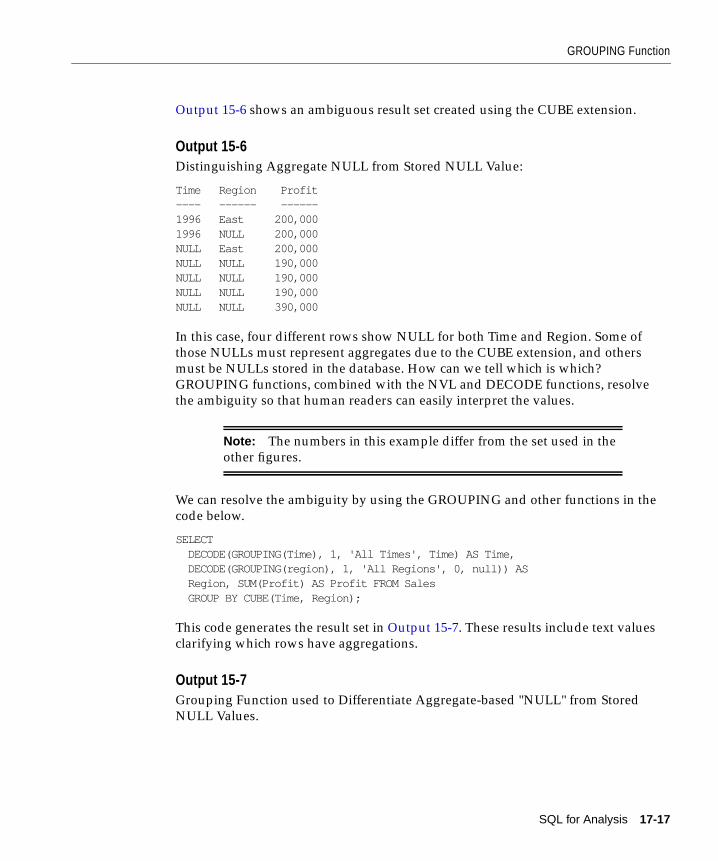
GROUPING Function
Output 15-6 shows an ambiguous result set created using the CUBE extension.
Output 15-6Distinguishing Aggregate NULL from Stored NULL Value:
Time Region Profit---- ------ ------1996 East 200,0001996 NULL 200,000NULL East 200,000NULL NULL 190,000NULL NULL 190,000NULL NULL 190,000NULL NULL 390,000
In this case, four different rows show NULL for both Time and Region. Some of
those NULLs must represent aggregates due to the CUBE extension, and others
must be NULLs stored in the database. How can we tell which is which?
GROUPING functions, combined with the NVL and DECODE functions, resolve
the ambiguity so that human readers can easily interpret the values.
We can resolve the ambiguity by using the GROUPING and other functions in the
code below.
SELECT DECODE(GROUPING(Time), 1, 'All Times', Time) AS Time, DECODE(GROUPING(region), 1, 'All Regions', 0, null)) AS Region, SUM(Profit) AS Profit FROM Sales GROUP BY CUBE(Time, Region);
This code generates the result set in Output 15-7. These results include text values
clarifying which rows have aggregations.
Output 15-7Grouping Function used to Differentiate Aggregate-based "NULL" from Stored
NULL Values.
Note: The numbers in this example differ from the set used in the
other figures.
SQL for Analysis 17-17

GROUPING Function
Time Region Profit---- ------ ------1996 East 200,0001996 All Regions 200,000All Times East 200,000NULL NULL 190,000NULL All Regions 190,000All Times NULL 190,000All Times All Regions 390,000
To explain the SQL statement above, we will examine its first column specification,
which handles the Time column. Look at the first line of the SQL code above,
namely,
DECODE(GROUPING(Time), 1, 'All Times', Time) as Time,
The Time value is determined with a DECODE function that contains a GROUPING
function. The GROUPING function returns a 1 if a row value is an aggregate
created by ROLLUP or CUBE, otherwise it returns a 0. The DECODE function then
operates on the GROUPING function's results. It returns the text "All Times" if it
receives a 1 and the time value from the database if it receives a 0. Values from the
database will be either a real value such as 1996 or a stored NULL. The second
column specification, displaying Region, works the same way.
When to Use GROUPINGThe GROUPING function is not only useful for identifying NULLs, it also enables
sorting subtotal rows and filtering results. In the next example (Output 15-8), we
retrieve a subset of the subtotals created by a CUBE and none of the base-level
aggregations. The HAVING clause constrains columns which use GROUPING
functions.
SELECT Time, Region, Department, SUM(Profit) AS Profit, GROUPING (Time) AS T, GROUPING (Region) AS R, GROUPING (Department) AS D FROM Sales GROUP BY CUBE (Time, Region, Department) HAVING (GROUPING(Department)=1 AND GROUPING(Region)=1 AND GROUPING(Time)=1) OR (GROUPING(Region)=1 AND (GROUPING(Department)=1) OR (GROUPING(Time)=1 AND GROUPING(department)=1);
Output 15-8 shows the results of this query.
17-18 Oracle8i Data Warehousing Guide

Other Considerations when Using ROLLUP and CUBE
Output 15-8Example of GROUPING Function Used to Filter Results to Subtotals and Grand
Total:
Time Region Department Profit---- ------ ---------- ------1996 NULL NULL 526,0001997 NULL NULL 598,000NULL Central NULL 316,000NULL East NULL 442,000NULL West NULL 366,000NULL NULL NULL 1,124,000
Compare the result set of Output 15-8 with that in Output 15-3 to see how Output
15-8 is a precisely specified group: it contains only the yearly totals, regional totals
aggregated over time and department, and the grand total.
Other Considerations when Using ROLLUP and CUBEThis section discusses the following topics.
■ Hierarchy Handling in ROLLUP and CUBE
■ Column Capacity in ROLLUP and CUBE
■ HAVING Clause Used with ROLLUP and CUBE
Hierarchy Handling in ROLLUP and CUBEThe ROLLUP and CUBE extensions work independently of any hierarchy metadata
in your system. Their calculations are based entirely on the columns specified in the
SELECT statement in which they appear. This approach enables CUBE and
ROLLUP to be used whether or not hierarchy metadata is available. The simplest
way to handle levels in hierarchical dimensions is by using the ROLLUP extension
and indicating levels explicitly through separate columns. The code below shows a
simple example of this with months rolled up to quarters and quarters rolled up to
years.
SELECT Year, Quarter, Month, SUM(Profit) AS Profit FROM sales GROUP BY ROLLUP(Year, Quarter, Month)
This query returns the rows in Output 15-9.
SQL for Analysis 17-19

Other Considerations when Using ROLLUP and CUBE
Output 15-9Example of ROLLUP across Time Levels:
Year Quarter Month Profit---- ------- ----- ------1997 Winter January 55,0001997 Winter February 64,0001997 Winter March 71,0001997 Winter NULL 190,0001997 Spring April 75,0001997 Spring May 86,0001997 Spring June 88,0001997 Spring NULL 249,0001997 Summer July 91,0001997 Summer August 87,0001997 Summer September 101,0001997 Summer NULL 279,0001997 Fall October 109,0001997 Fall November 114,0001997 Fall December 133,0001997 Fall NULL 356,0001997 NULL NULL 1,074,000
Column Capacity in ROLLUP and CUBECUBE and ROLLUP do not restrict the GROUP BY clause column capacity. The
GROUP BY clause, with or without the extensions, can work with up to 255
columns. However, the combinatorial explosion of CUBE makes it unwise to specify
a large number of columns with the CUBE extension. Consider that a 20-column list
for CUBE would create 220 combinations in the result set. A very large CUBE list
could strain system resources, so any such query needs to be tested carefully for
performance and the load it places on the system.
HAVING Clause Used with ROLLUP and CUBEThe HAVING clause of SELECT statements is unaffected by the use of ROLLUP and
CUBE. Note that the conditions specified in the HAVING clause apply to both the
subtotal and non-subtotal rows of the result set. In some cases a query may need to
exclude the subtotal rows or the non-subtotal rows from the HAVING clause. This
Note: The numbers in this example differ from the set used in the
other figures.
17-20 Oracle8i Data Warehousing Guide

Analytic Functions
can be achieved by using the GROUPING function together with the HAVING
clause. See Output 15-8 on page 17-19 and its associated SQL for an example.
ORDER BY Clause Used with ROLLUP and CUBEThe ORDER BY clause of a SELECT statement is unaffected by the use of ROLLUP
and CUBE. Note that the conditions specified in the ORDER BY clause apply to
both subtotal and non-subtotal rows of the result set. In some cases, a query may
need to order the rows in a certain way. This can be achieved by using a grouping
function in the ORDER BY clause.
Analytic FunctionsThe SQL language, while extremely capable in many areas, has never provided
strong support for analytic tasks. Basic business intelligence calculations such as
moving averages, rankings, and lead/lag comparisons have required extensive
programming outside of standard SQL, often with performance problems. Oracle8inow provides a new set of functions which address this longstanding need. These
functions are referred to as analytic functions because they are useful in all types of
analyses. The analytic functions improve performance. In addition, the functions
are now under review by ANSI for addition to the SQL standard during 2000.
Analytic functions are classified in the following categories:
■ Ranking Functions
■ Windowing Functions
■ Reporting Functions
■ Lag/Lead Functions
■ Statistics Functions
They are used as follows:
Table 17–2 Analytic Functions and Their Uses
Type Used for
Ranking Calculating ranks, percentiles, and n-tiles of the valuesin a result set.
SQL for Analysis 17-21

Analytic Functions
To perform these operations, the analytic functions add several new elements to
SQL processing. These elements build on existing SQL to allow flexible and
powerful calculation expressions. The processing flow is represented in Figure 17–2.
Figure 17–2 Processing Order
Here are the essential concepts used in the analytic functions:
■ Processing Order - Query processing using analytic functions takes place in
three stages. First, all joins, WHERE, GROUP BY and HAVING clauses are
performed. Second, the result set is made available to the analytic functions,
and all their calculations take place. Third, if the query has an ORDER BY
clause at its end, the ORDER BY is processed to allow for precise output
ordering. The processing order is shown in Figure 17–2.
Windowing Calculating cumulative and moving averages. Workswith these functions:
SUM, AVG, MIN, MAX, COUNT, VARIANCE,STDDEV, FIRST_VALUE, LAST_VALUE, and newstatistical functions
Reporting Calculating shares. For example, market share. Workswith these functions:
SUM, AVG, MIN, MAX, COUNT (with/withoutDISTINCT), VARIANCE, STDDEV, RATIO_TO_REPORT, and new statistical functions
LAG/LEAD Finding a value in a row a specified number of rowsfrom a current row.
Statistics Calculating linear regression and other statistics (slope,intercept, etc.).
Table 17–2 Analytic Functions and Their Uses
Type Used for
Joins,WHERE, GROUP BY, and HAVING clauses
Partitions created;Analytic functionsapplied to each row ineach partition
FinalORDER BY
17-22 Oracle8i Data Warehousing Guide
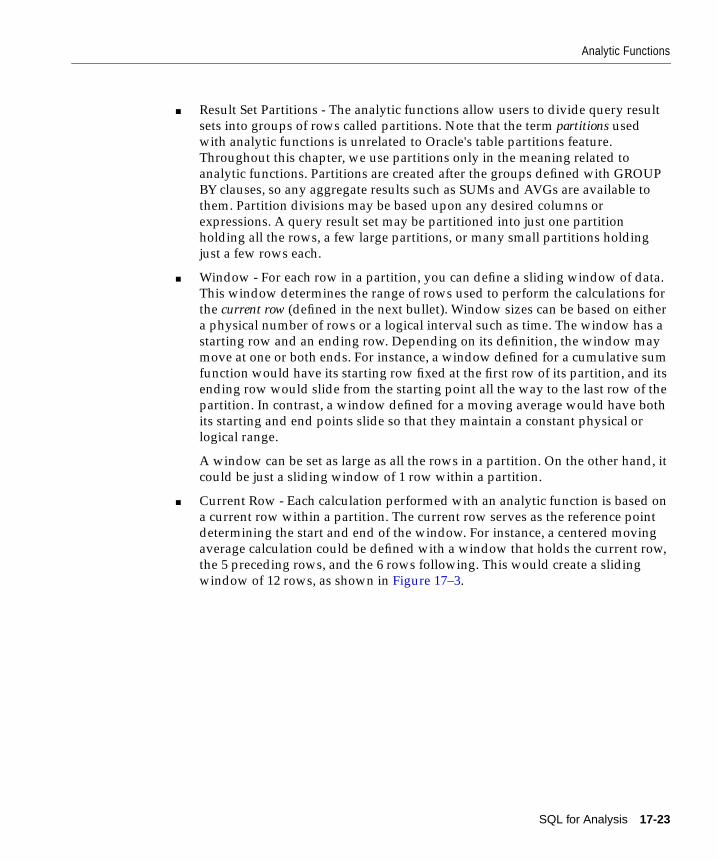
Analytic Functions
■ Result Set Partitions - The analytic functions allow users to divide query result
sets into groups of rows called partitions. Note that the term partitions used
with analytic functions is unrelated to Oracle's table partitions feature.
Throughout this chapter, we use partitions only in the meaning related to
analytic functions. Partitions are created after the groups defined with GROUP
BY clauses, so any aggregate results such as SUMs and AVGs are available to
them. Partition divisions may be based upon any desired columns or
expressions. A query result set may be partitioned into just one partition
holding all the rows, a few large partitions, or many small partitions holding
just a few rows each.
■ Window - For each row in a partition, you can define a sliding window of data.
This window determines the range of rows used to perform the calculations for
the current row (defined in the next bullet). Window sizes can be based on either
a physical number of rows or a logical interval such as time. The window has a
starting row and an ending row. Depending on its definition, the window may
move at one or both ends. For instance, a window defined for a cumulative sum
function would have its starting row fixed at the first row of its partition, and its
ending row would slide from the starting point all the way to the last row of the
partition. In contrast, a window defined for a moving average would have both
its starting and end points slide so that they maintain a constant physical or
logical range.
A window can be set as large as all the rows in a partition. On the other hand, it
could be just a sliding window of 1 row within a partition.
■ Current Row - Each calculation performed with an analytic function is based on
a current row within a partition. The current row serves as the reference point
determining the start and end of the window. For instance, a centered moving
average calculation could be defined with a window that holds the current row,
the 5 preceding rows, and the 6 rows following. This would create a sliding
window of 12 rows, as shown in Figure 17–3.
SQL for Analysis 17-23
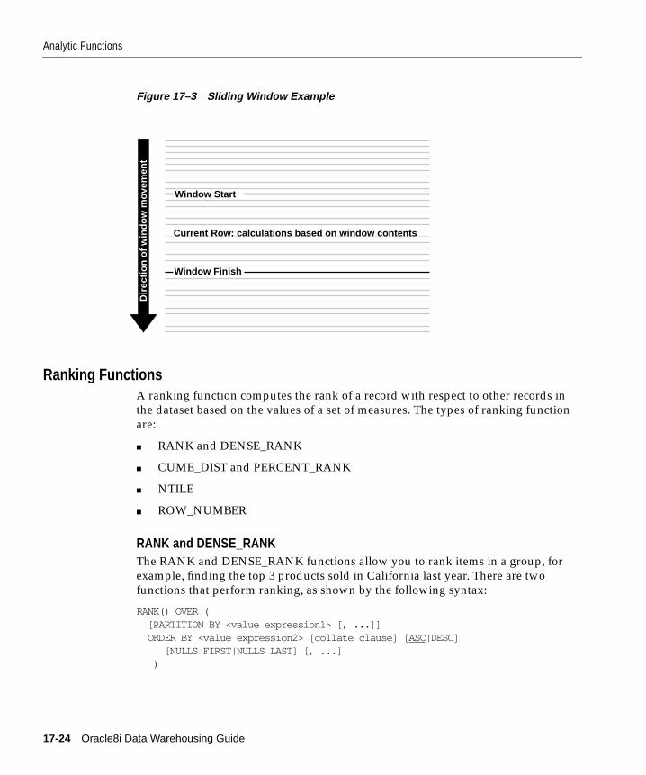
Analytic Functions
Figure 17–3 Sliding Window Example
Ranking FunctionsA ranking function computes the rank of a record with respect to other records in
the dataset based on the values of a set of measures. The types of ranking function
are:
■ RANK and DENSE_RANK
■ CUME_DIST and PERCENT_RANK
■ NTILE
■ ROW_NUMBER
RANK and DENSE_RANKThe RANK and DENSE_RANK functions allow you to rank items in a group, for
example, finding the top 3 products sold in California last year. There are two
functions that perform ranking, as shown by the following syntax:
RANK() OVER ( [PARTITION BY <value expression1> [, ...]] ORDER BY <value expression2> [collate clause] [ ASC|DESC] [NULLS FIRST|NULLS LAST] [, ...] )
Dir
ecti
on
of
win
do
w m
ove
men
t
Window Start
Current Row: calculations based on window contents
Window Finish
17-24 Oracle8i Data Warehousing Guide

Analytic Functions
DENSE_RANK() OVER ( [PARTITION BY <value expression1> [, ...]] ORDER BY <value expression2> [collate clause] [ ASC|DESC] [NULLS FIRST|NULLS LAST] [, ...] )
The difference between RANK and DENSE_RANK is that DENSE_RANK leaves no
gaps in ranking sequence when there are ties. That is, if we were ranking a
competition using DENSE_RANK and had three people tie for second place, we
would say that all three were in second place and that the next person came in
third. The RANK function would also give three people in second place, but the
next person would be in fifth place.
Some relevant points about RANK:
■ Ascending is the default sort order, which you may want to change to
descending.
■ The expressions in the optional PARTITION BY clause divide the query result
set into groups within which the RANK function operates. That is, RANK gets
reset whenever the group changes. In effect, the <value expression>s of the
PARTITION BY clause define the reset boundaries.
■ If the PARTITION BY clause is missing, then ranks are computed over the entire
query result set.
■ <value expression1> can be any valid expression involving column references,
constants, aggregates, or expressions invoking these items.
■ The ORDER BY clause specifies the measures (<value expression>s) on which
ranking is done and defines the order in which rows are sorted in each group
(or partition). Once the data is sorted within each partition, ranks are given to
each row starting from 1.
■ <value expression2> can be any valid expression involving column references,
aggregates, or expressions invoking these items.
■ The NULLS FIRST | NULLS LAST clause indicates the position of NULLs in
the ordered sequence, either first or last in the sequence. The order of the
sequence would make NULLs compare either high or low with respect to
non-NULL values. If the sequence were in ascending order, then NULLS FIRST
implies that NULLs are smaller than all other non-NULL values and NULLS
LAST implies they are larger than non-NULL values. It is the opposite for
descending order. See the example in "Treatment of NULLs" on page 17-29.
SQL for Analysis 17-25

Analytic Functions
■ If the NULLS FIRST | NULLS LAST clause is omitted, then the ordering of the
null values depends on the ASC or DESC arguments. Null values are
considered larger than any other values. If the ordering sequence is ASC, then
nulls will appear last; nulls will appear first otherwise. Nulls are considered
equal to other nulls and, therefore, the order in which nulls are presented is
non-deterministic.
Ranking Order The following example shows how the [ASC | DESC] option changes
the ranking order.
SELECT s_productkey, s_amount, RANK() OVER (ORDER BY s_amount) AS default_rank, RANK() OVER (ORDER BY s_amount DESC NULLS LAST) AS custom_rankFROM sales;
This statement gives:
S_PRODUCTKEY S_AMOUNT DEFAULT_RANK CUSTOM_RANK------------ -------- ------------ -----------SHOES 130 6 1JACKETS 95 5 2SWEATERS 80 4 3SHIRTS 75 3 4PANTS 60 2 5TIES 45 1 6
Note: While the data in this result is ordered on the measure s_amount , in general,
it is not guaranteed by the RANK function that the data will be sorted on the
measures. If you want the data to be sorted on s_amount in your result, you must
specify it explicitly with an ORDER BY clause, at the end of the SELECT statement.
Ranking on Multiple Expressions Ranking functions need to resolve ties between
values in the set. If the first expression cannot resolve ties, the second expression is
used to resolve ties and so on. For example, to rank products based on their dollar
sales within each region, breaking ties with the profits, we would say:
SELECT r_regionkey, p_productkey, s_amount, s_profit, RANK() OVER (ORDER BY s_amount DESC, s_profit DESC) AS rank_in_eastFROM region, product, salesWHERE r_regionkey = s_regionkey AND p_productkey = s_productkey AND r_regionkey= 'east';
The result would be:
17-26 Oracle8i Data Warehousing Guide

Analytic Functions
R_REGIONKEY S_PRODUCTKEY S_AMOUNT S_PROFIT RANK_IN_EAST----------- ------------ -------- -------- ------------EAST SHOES 130 30 1EAST JACKETS 100 28 2EAST PANTS 100 24 3EAST SWEATERS 75 24 4EAST SHIRTS 75 24 4EAST TIES 60 12 6EAST T-SHIRTS 20 10 7
For jackets and pants, the s_profit column resolves the tie in the s_amount column.
But for sweaters and shirts, s_profit cannot resolve the tie in s_amount column.
Hence, they are given the same rank.
RANK and DENSE_RANK Difference The difference between RANK() and DENSE_
RANK() functions is illustrated below:
SELECT s_productkey, SUM(s_amount) as sum_s_amount, RANK() OVER (ORDER BY SUM(s_amount) DESC) AS rank_all, DENSE_RANK() OVER (ORDER BY SUM(s_amount) DESC) AS rank_denseFROM salesGROUP BY s_productkey;
This statement produces this result:
S_PRODUCTKEY SUM_S_AMOUNT RANK_ALL RANK_DENSE------------ ------------ -------- ----------SHOES 100 1 1JACKETS 100 1 1SHIRTS 89 3 2SWEATERS 75 4 3SHIRTS 75 4 3TIES 66 6 4PANTS 66 6 4
Note that, in the case of DENSE_RANK(), the largest rank value gives the number
of distinct values in the dataset.
Per Group Ranking The RANK function can be made to operate within groups, that
is, the rank gets reset whenever the group changes. This is accomplished with the
PARTITION BY option. The group expressions in the PARTITION BY subclause
divide the dataset into groups within which RANK operates. For example, to rank
products within each region by their dollar sales, we say:
SELECT r_regionkey, p_productkey, SUM(s_amount),
SQL for Analysis 17-27

Analytic Functions
RANK() OVER (PARTITION BY r_regionkey ORDER BY SUM(s_amount) DESC) AS rank_of_product_per_regionFROM product, region, salesWHERE r_regionkey = s_regionkey AND p_productkey = s_productkeyGROUP BY r_regionkey, p_productkey;
A single query block can contain more than one ranking function, each partitioning
the data into different groups (that is, reset on different boundaries). The groups can
be mutually exclusive. The following query ranks products based on their dollar
sales within each region (rank_of_product_per_region ) and over all regions
(rank_of_product_total ).
SELECT r_regionkey, p_productkey, SUM(s_amount) AS SUM_S_AMOUNT, RANK() OVER (PARTITION BY r_regionkey ORDER BY SUM(s_amount) DESC)AS rank_of_product_per_region, RANK() OVER (ORDER BY SUM(s_amount) DESC) AS rank_of_product_totalFROM product, region, salesWHERE r_regionkey = s_regionkey AND p_productkey = s_productkeyGROUP BY r_regionkey, p_productkeyORDER BY r_regionkey;
The query produces this result:
R_REGIONKEY P_PRODUCTKEY SUM_S_AMOUNT RANK_OF_PRODUCT_PER_REGION RANK_OF_PRODUCT_TOTAL----------- ------------ ------------ -------------------------- ---------------------EAST SHOES 130 1 1EAST JACKETS 95 2 4EAST SHIRTS 80 3 6EAST SWEATERS 75 4 7EAST T-SHIRTS 60 5 11EAST TIES 50 6 12EAST PANTS 20 7 14WEST SHOES 100 1 2WEST JACKETS 99 2 3WEST T-SHIRTS 89 3 5WEST SWEATERS 75 4 7WEST SHIRTS 75 4 7WEST TIES 66 6 10WEST PANTS 45 7 13
Per Cube- and Rollup-group Ranking Analytic functions, RANK for example, can be
reset based on the groupings provided by a CUBE or ROLLUP operator.
17-28 Oracle8i Data Warehousing Guide

Analytic Functions
It is useful to assign ranks to the groups created by CUBE and ROLLUP queries. See
the CUBE/ROLLUP section, which includes information about the GROUPING
function for further details. A sample query is:
SELECT r_regionkey, p_productkey, SUM(s_amount) AS SUM_S_AMOUNT, RANK() OVER (PARTITION BY GROUPING(r_regionkey), GROUPING(p_productkey) ORDER BY SUM(s_amount) DESC) AS rank_per_cubeFROM product, region, salesWHERE r_regionkey = s_regionkey AND p_productkey = s_productkeyGROUP BY CUBE(r_regionkey, p_productkey)ORDER BY GROUPING(r_regionkey), GROUPING(p_productkey), r_regionkey;
It produces this result:
R_REGIONKEY P_PRODUCTKEY SUM_S_AMOUNT RANK_PER_CUBE----------- ------------ ------------ -------------EAST SHOES 130 1EAST JACKETS 50 12EAST SHIRTS 80 6EAST SWEATERS 75 7EAST T-SHIRTS 60 11EAST TIES 95 4EAST PANTS 20 14WEST SHOES 100 2WEST JACKETS 99 3WEST SHIRTS 89 5WEST SWEATERS 75 7WEST T-SHIRTS 75 7WEST TIES 66 10WEST PANTS 45 13EAST NULL 510 2WEST NULL 549 1NULL SHOES 230 1NULL JACKETS 149 5NULL SHIRTS 169 2NULL SWEATERS 150 4NULL T-SHIRTS 135 6NULL TIES 161 3NULL PANTS 65 7NULL NULL 1059 1
Treatment of NULLs NULLs are treated like normal values. Also, for the purpose of
rank computation, a NULL value is assumed to be equal to another NULL value.
Depending on the ASC | DESC options provided for measures and the NULLS
SQL for Analysis 17-29
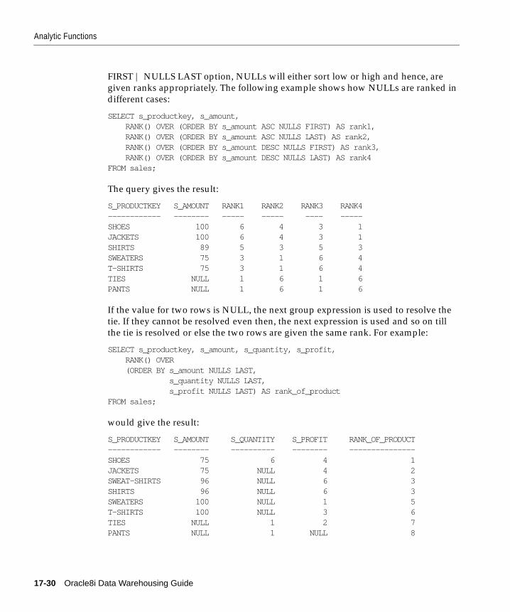
Analytic Functions
FIRST | NULLS LAST option, NULLs will either sort low or high and hence, are
given ranks appropriately. The following example shows how NULLs are ranked in
different cases:
SELECT s_productkey, s_amount, RANK() OVER (ORDER BY s_amount ASC NULLS FIRST) AS rank1, RANK() OVER (ORDER BY s_amount ASC NULLS LAST) AS rank2, RANK() OVER (ORDER BY s_amount DESC NULLS FIRST) AS rank3, RANK() OVER (ORDER BY s_amount DESC NULLS LAST) AS rank4FROM sales;
The query gives the result:
S_PRODUCTKEY S_AMOUNT RANK1 RANK2 RANK3 RANK4------------ -------- ----- ----- ---- -----SHOES 100 6 4 3 1JACKETS 100 6 4 3 1SHIRTS 89 5 3 5 3SWEATERS 75 3 1 6 4T-SHIRTS 75 3 1 6 4TIES NULL 1 6 1 6PANTS NULL 1 6 1 6
If the value for two rows is NULL, the next group expression is used to resolve the
tie. If they cannot be resolved even then, the next expression is used and so on till
the tie is resolved or else the two rows are given the same rank. For example:
SELECT s_productkey, s_amount, s_quantity, s_profit, RANK() OVER (ORDER BY s_amount NULLS LAST, s_quantity NULLS LAST, s_profit NULLS LAST) AS rank_of_productFROM sales;
would give the result:
S_PRODUCTKEY S_AMOUNT S_QUANTITY S_PROFIT RANK_OF_PRODUCT------------ -------- ---------- -------- ---------------SHOES 75 6 4 1JACKETS 75 NULL 4 2SWEAT-SHIRTS 96 NULL 6 3SHIRTS 96 NULL 6 3SWEATERS 100 NULL 1 5T-SHIRTS 100 NULL 3 6TIES NULL 1 2 7PANTS NULL 1 NULL 8
17-30 Oracle8i Data Warehousing Guide

Analytic Functions
HATS NULL 6 2 9SOCKS NULL 6 2 9SUITS NULL 6 NULL 10JEANS NULL NULL NULL 11BELTS NULL NULL NULL 11
TOP_NYou can easily obtain top N ranks by enclosing the RANK function in a subquery
and then applying a filter condition outside the subquery. For example, to obtain
the top four sales items per region, you can issue:
SELECT region, product, sum_s_amount FROM (SELECT r_regionkey AS region, p_product_key AS product, SUM(s_amount) AS sum_s_amount, RANK() OVER(PARTITION BYr_region_key ORDER BY SUM(s_amount) DESC AS rank1,FROM product, region, salesWHERE r_region_key = s_region_key AND p_product_key = s_product_keyGROUP BY r_region_key ORDER BY r_region_key)WHERE rank1 <= 4;
The query produces this result:
R_REGIONKEY P_PRODUCTKEY SUM_S_AMOUNT----------- ------------ ------------EAST SHOES 130EAST JACKETS 95EAST SHIRTS 80EAST SWEATERS 75WEST SHOES 100WEST JACKETS 99WEST T-SHIRTS 89WEST SWEATERS 75WEST SHIRTS 75
BOTTOM_NBOTTOM_N is similar to TOP_N except for the ordering sequence within the rank
expression. In the previous example, you can order SUM(s_amount) ASC instead of
DESC.
CUME_DISTThe CUME_DIST function (defined as the inverse of percentile in some statistical
books) computes the position of a specified value relative to a set of values. The
order can be ascending or descending. Ascending is the default. The range of values
SQL for Analysis 17-31

Analytic Functions
for CUME_DIST is from greater than 0 to 1. To compute the CUME_DIST of a value
x in a set S of size N, we use the formula:
CUME_DIST(x) = number of values (different from, or equal to, x) in S coming before x in thespecified order/ N
Its syntax is:
CUME_DIST() OVER ( [PARTITION BY <value expression1> [, ...]] ORDER BY <value expression2> [collate clause] [ ASC|DESC] [NULLS FIRST | NULLS LAST] [, ...])
The semantics of various options in the CUME_DIST function are similar to those in
the RANK function. The default order is ascending, implying that the lowest value
gets the lowest cume_dist (as all other values come later than this value in the
order). NULLS are treated the same as they are in the RANK function. They are
counted towards both the numerator and the denominator as they are treated like
non-NULL values. To assign cume_dists to products per region based on their sales
and profits, we would say:
SELECT r_regionkey, p_productkey, SUM(s_amount) AS SUM_S_AMOUNT, CUME_DIST() OVER (PARTITION BY r_regionkey ORDER BY SUM(s_amount)) AS cume_dist_per_regionFROM region, product, salesWHERE r_regionkey = s_regionkey AND p_productkey = s_productkeyGROUP BY r_regionkey, p_productkeyORDER BY r_regionkey, s_amount DESC;
It will produce this result:
R_REGIONKEY P_PRODUCTKEY SUM_S_AMOUNT CUME_DIST_PER_REGION----------- ------------ ------------ --------------------EAST SHOES 130 1.00EAST JACKETS 95 .84EAST SHIRTS 80 .70EAST SWEATERS 75 .56EAST T-SHIRTS 60 .42EAST TIES 50 .28EAST PANTS 20 .14WEST SHOES 100 1.00WEST JACKETS 99 .84WEST T-SHIRTS 89 .70
17-32 Oracle8i Data Warehousing Guide
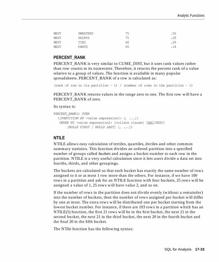
Analytic Functions
WEST SWEATERS 75 .56WEST SHIRTS 75 .28WEST TIES 66 .28WEST PANTS 45 .14
PERCENT_RANKPERCENT_RANK is very similar to CUME_DIST, but it uses rank values rather
than row counts in its numerator. Therefore, it returns the percent rank of a value
relative to a group of values. The function is available in many popular
spreadsheets. PERCENT_RANK of a row is calculated as:
(rank of row in its partition - 1) / (number of rows in the partition - 1)
PERCENT_RANK returns values in the range zero to one. The first row will have a
PERCENT_RANK of zero.
Its syntax is:
PERCENT_RANK() OVER ( [PARTITION BY <value expression1> [, ...]] ORDER BY <value expression2> [collate clause] [ ASC|DESC] [NULLS FIRST | NULLS LAST] [, ...])
NTILENTILE allows easy calculation of tertiles, quartiles, deciles and other common
summary statistics. This function divides an ordered partition into a specified
number of groups called buckets and assigns a bucket number to each row in the
partition. NTILE is a very useful calculation since it lets users divide a data set into
fourths, thirds, and other groupings.
The buckets are calculated so that each bucket has exactly the same number of rows
assigned to it or at most 1 row more than the others. For instance, if we have 100
rows in a partition and ask for an NTILE function with four buckets, 25 rows will be
assigned a value of 1, 25 rows will have value 2, and so on.
If the number of rows in the partition does not divide evenly (without a remainder)
into the number of buckets, then the number of rows assigned per bucket will differ
by one at most. The extra rows will be distributed one per bucket starting from the
lowest bucket number. For instance, if there are 103 rows in a partition which has an
NTILE(5) function, the first 21 rows will be in the first bucket, the next 21 in the
second bucket, the next 21 in the third bucket, the next 20 in the fourth bucket and
the final 20 in the fifth bucket.
The NTile function has the following syntax:
SQL for Analysis 17-33

Analytic Functions
NTILE(N) OVER ( [PARTITION BY <value expression1> [, ...]] ORDER BY <value expression2> [collate clause] [ ASC|DESC] [NULLS FIRST | NULLS LAST] [, ...])
where the N in NTILE(N) can be a constant (e.g., 5) or an expression. The
expression can include expressions in the PARTITION BY clause. For example, (5*2)
or (5*c1) OVER (PARTITION BT c1)).
This function, like RANK and CUME_DIST, has a PARTITION BY clause for pergroup computation, an ORDER BY clause for specifying the measures and their sort
order, and NULLS FIRST | NULLS LAST clause for the specific treatment of
NULLs. For example,
SELECT p_productkey, s_amount, NTILE(4) (ORDER BY s_amount DESC NULLS FIRST) AS 4_tileFROM product, salesWHERE p_productkey = s_productkey;
This query would give:
P_PRODUCTKEY S_AMOUNT 4_TILE------------ -------- ------SUITS NULL 1SHOES 100 1JACKETS 90 1SHIRTS 89 2T-SHIRTS 84 2SWEATERS 75 2JEANS 75 3TIES 75 3PANTS 69 3BELTS 56 4SOCKS 45 4
NTILE is a nondeterministic function. Equal values can get distributed across
adjacent buckets (75 is assigned to buckets 2 and 3) and buckets '1', '2' and '3' have 3
elements - one more than the size of bucket '4'. In the above table, "JEANS" could as
well be assigned to bucket 2 (instead of 3) and "SWEATERS" to bucket 3 (instead of
2), because there is no ordering on the p_PRODUCT_KEY column. To ensure
deterministic results, you must order on a unique key.
17-34 Oracle8i Data Warehousing Guide
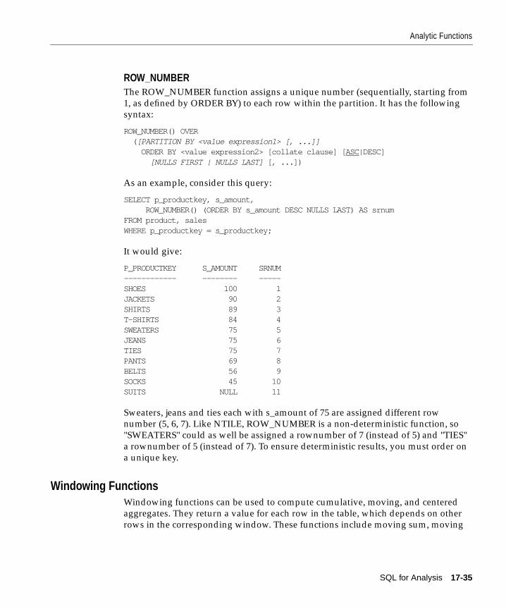
Analytic Functions
ROW_NUMBERThe ROW_NUMBER function assigns a unique number (sequentially, starting from
1, as defined by ORDER BY) to each row within the partition. It has the following
syntax:
ROW_NUMBER() OVER ( [PARTITION BY <value expression1> [, ...]] ORDER BY <value expression2> [collate clause] [ ASC|DESC] [NULLS FIRST | NULLS LAST] [, ...])
As an example, consider this query:
SELECT p_productkey, s_amount, ROW_NUMBER() (ORDER BY s_amount DESC NULLS LAST) AS srnumFROM product, salesWHERE p_productkey = s_productkey;
It would give:
P_PRODUCTKEY S_AMOUNT SRNUM------------ -------- -----SHOES 100 1JACKETS 90 2SHIRTS 89 3T-SHIRTS 84 4SWEATERS 75 5JEANS 75 6TIES 75 7PANTS 69 8BELTS 56 9SOCKS 45 10SUITS NULL 11
Sweaters, jeans and ties each with s_amount of 75 are assigned different row
number (5, 6, 7). Like NTILE, ROW_NUMBER is a non-deterministic function, so
"SWEATERS" could as well be assigned a rownumber of 7 (instead of 5) and "TIES"
a rownumber of 5 (instead of 7). To ensure deterministic results, you must order on
a unique key.
Windowing FunctionsWindowing functions can be used to compute cumulative, moving, and centered
aggregates. They return a value for each row in the table, which depends on other
rows in the corresponding window. These functions include moving sum, moving
SQL for Analysis 17-35

Analytic Functions
average, moving min/max, cumulative sum, as well as statistical functions. They
can be used only in the SELECT and ORDER BY clauses of the query. Two other
functions are available: FIRST_VALUE, which returns the first value in the window;
and LAST_VALUE, which returns the last value in the window. These functions
provide access to more than one row of a table without a self-join. The syntax of the
windowing functions is:
{SUM|AVG|MAX|MIN|COUNT|STDDEV|VARIANCE|FIRST_VALUE|LAST_VALUE} ({<value expression1> | *}) OVER ([PARTITION BY <value expression2>[,...]] ORDER BY <value expression3> [collate clause>] [ASC| DESC] [NULLS FIRST | NULLS LAST] [,...] ROWS | RANGE {{UNBOUNDED PRECEDING | <value expression4> PRECEDING} | BETWEEN {UNBOUNDED PRECEDING | <value expression4> PRECEDING} AND{CURRENT ROW | <value expression4> FOLLOWING}}
where:
OVER indicates that the function operates on a query result set. That is, it iscomputed after the FROM, WHERE, GROUP BY, and HAVINGclauses. OVER isused to define the window of the rows to be included while computing thefunction.
query_partition_clause
PARTITION BY partitions the query result set into groups based on one or more value_expr.If you omit this clause, the function treats all rows of the query result set asa single group.
You can specify multiple analytic functions in the same query, each withthe same or different PARTITION BY keys.
Note: If the objects being queried have the parallel attribute, and if youspecify an analytic function with the query_partition_clause, then thefunction computations are parallelized as well.
value_expr Valid value expressions are constants, columns, nonanalytic functions,function expressions, or expressions involving any of these.
ORDER_BY_clause
17-36 Oracle8i Data Warehousing Guide

Analytic Functions
ORDER BY specifies how data is ordered within a partition. You can order the valuesin a partition on multiple keys, each defined by a value_expr and eachqualified by an ordering sequence.
Within each function, you can specify multiple ordering expressions. Doingso is especially useful when using functions that rank values, because thesecond expression can resolve ties between identical values for the firstexpression.
Note: Analytic functions always operate on rows in the order specified inthe ORDER_BY_clause of the function. However, the ORDER_BY_clause ofthe function does not guarantee the order of the result. Use theORDER_BY_clause of the query to guarantee the final result ordering.
Restriction: When used in an analytic function, the ORDER_BY_clausemust take an expression (expr). Position (position) and column aliases(c_alias) are invalid. Otherwise this ORDER_BY_clause is the same as thatused to order the overall query or subquery.
ASC | DESC specifies the ordering sequence (ascending or descending). ASC is thedefault.
NULLS FIRST| NULLS LAST
specifies whether returned rows containing null values should appear firstor last in the ordering sequence.
NULLS LAST is the default for ascending order, and NULLS FIRST is thedefault for descending order.
windowing_clause
ROWS | RANGE These keywords define for each row a "window" (a physical or logical setof rows) used for calculating the function result. The function is thenapplied to all the rows in the window. The window "slides" through thequery result set or partition from top to bottom.
■ ROWS specifies the window in physical units (rows)
■ RANGE specifies the window as a logical offset.
You cannot specify this clause unless you have specified theORDER_BY_clause.
Note: The value returned by an analytic function with a logical offset isalways deterministic. However, the value returned by an analytic functionwith a physical offset may produce nondeterministic results unless theordering expression(s) results in a unique ordering. You may have tospecify multiple columns in the ORDER_BY_clause to achieve this uniqueordering.
BETWEEN ...AND
lets you specify a start point and end point for the window. The firstexpression (before AND) defines the start point and the second expression(after AND) defines the end point.
SQL for Analysis 17-37

Analytic Functions
If you omit BETWEEN and specify only one end point, Oracle considers itthe start point, and the end point defaults to the current row.
UNBOUNDEDPRECEDING
specifies that the window starts at the first row of the partition. This is thestart point specification and cannot be used as an end point specification.
UNBOUNDED PRECEDING - specifies that the window starts at the firstrow of the partition. If the PARTITION BY clause is absent, then it refers tothe first row in the dataset.
UNBOUNDEDFOLLOWING
specifies that the window ends at the last row of the partition. This is theend point specification and cannot be used as a start point specification.
CURRENT ROW As a start point, CURRENT ROW specifies that the window begins at thecurrent row or value (depending on whether you have specified ROW orRANGE, respectively). In this case the end point cannot be value_exprPRECEDING.
As an end point, CURRENT ROW specifies that the window ends at thecurrent row or value (depending on whether you have specified ROW orRANGE, respectively). In this case the start point cannot be value_exprFOLLOWING.
value_exprPRECEDING
value_exprFOLLOWING
For RANGE or ROW:
■ If value_expr FOLLOWING is the start point, then the end point must bevalue_expr FOLLOWING or UNBOUNDED FOLLOWING.
■ If value_expr PRECEDING is the end point, then the start point must bevalue_expr PRECEDING or UNBOUNDED FOLLOWING.
If you are defining a logical window defined by an interval of time innumeric format, you may need to use conversion functions, likeNUMTODS or NUMTOYM.
If you specify ROWS:
■ value_expr is a physical offset. It must be a constant or expression andmust evaluate to a positive numeric value.
If you specify RANGE:
■ value_expr is a logical offset. It must be a constant or expression thatevaluates to a positive numeric value or an interval literal.
■ You can specify only one expression in the ORDER_BY_clause if thestart or end point is specified using <value_expr> PRECEDING orFOLLOWING.
■ If value_expr evaluates to a numeric value, the ORDER BYexpr must bea NUMBER or DATE datatype.
■ If value_expr evaluates to an interval value, the ORDER BYexpr must bea DATE datatype.
17-38 Oracle8i Data Warehousing Guide

Analytic Functions
Treatment of NULLs on Input to Window Functions Window functions' NULL semantics
match the NULL semantics for SQL aggregate functions. Other semantics can be
obtained by user-defined functions, or by using the DECODE or a CASE expression
within the window function.
Windowing functions with Logical Offset: A logical offset can be specified with constants
such as "RANGE 10 PRECEDING", or an expression that evaluates to a constant, or
by an interval specification like "RANGE INTERVAL N DAYS/MONTHS/YEARS
PRECEDING" or an expression that evaluates to an interval. With logical offset,
there can only be one expression in the ORDER BY expression list in the function,
with type compatible to NUMERIC if offset is numeric, or DATE if an interval is
specified.
Some examples of windowing functions follow:
Example of Cumulative Aggregate Function The following is an example of a cumulative
balance per account ordered by deposit date.
SELECT Acct_number, Trans_date, Trans_amount, SUM(Trans_amount) OVER (PARTITION BY Acct_number ORDER BY Trans_date ROWS UNBOUNDED PRECEDING) AS BalanceFROM LedgerORDER BY Acct_number, Trans_date;
Acct_number Trans_date Trans_amount Balance----------- ---------- ------------ ------- 73829 1998-11-01 113.45 113.45 73829 1998-11-05 -52.01 61.44 73829 1998-11-13 36.25 97.69 82930 1998-11-01 10.56 10.56 82930 1998-11-21 32.55 43.11 82930 1998-11-29 -5.02 38.09
In this example, the analytic function SUM defines, for each row, a window that
starts at the beginning of the partition(UNBOUNDED PRECEDING) and ends, by
default, at the current row.
Example of Moving Aggregate functionHere is an example of a time-based window that shows, for each transaction, the
moving average of transaction amount for the preceding 7 days of transactions:
If you omit the windowing_clause entirely, the default is RANGE BETWEEN UNBOUNDEDPRECEDING AND CURRENT ROW.
SQL for Analysis 17-39

Analytic Functions
SELECT Account_number, Trans_date, Trans_amount, AVG (Trans_amount) OVER (PARTITION BY Account_number ORDER BY Trans_date RANGE INTERVAL '7' DAY PRECEDING) AS mavg_7dayFROM Ledger;
Acct_number Trans_date Trans_amount mavg_7day----------- ---------- ------------ --------- 73829 1998-11-03 113.45 113.45 73829 1998-11-09 -52.01 30.72 73829 1998-11-13 36.25 -7.88 73829 1998-11-14 10.56 -1.73 73829 1998-11-20 32.55 26.45 82930 1998-11-01 100.25 100.25 82930 1998-11-10 10.01 10.01 82930 1998-11-25 11.02 11.02 82930 1998-11-26 100.56 55.79 82930 1998-11-30 -5.02 35.52
Example of Centered Aggregate function Calculating windowing aggregate functions
centered around the current row is straightforward. This example computes for
each account a centered moving average of the transaction amount for the 1 month
preceding the current row and 1 month following the current row including the
current row as well.
SELECT Account_number, Trans_date, Trans_amount, AVG (Trans_amount) OVER (PARTITION BY Account_number ORDER BY Trans_date RANGE BETWEEN INTERVAL '1' MONTH PRECEDING AND INTERVAL '1' MONTH FOLLOWING) as c_avgFROM Ledger;
Windowing Aggregate Functions with Logical Offsets The following example illustrates
how window aggregate functions compute values in the presence of duplicates.
SELECT r_rkey, p_pkey, s_amt SUM(s_amt) OVER (ORDER BY p_pkey RANGE BETWEEN 1 PRECEDING AND CURRENT ROW) AS current_group_sumFROM product, region, salesWHERE r_rkey = s_rkey AND p_pkey = s_pkey AND r_rkey = 'east'ORDER BY r_rkey, p_pkey;
R_RKEY P_PKEY S_AMT CURRENT_GROUP_SUM /*Source numbers for the current_group_sum column*/------ ------ ----- ----------------- /*------- */EAST 1 130 130 /* 130 */EAST 2 50 180 /*130+50 */
17-40 Oracle8i Data Warehousing Guide

Analytic Functions
EAST 3 80 265 /*50+(80+75+60) */EAST 3 75 265 /*50+(80+75+60) */EAST 3 60 265 /*50+(80+75+60) */EAST 4 20 235 /*80+75+60+20 */
Values within parentheses indicate ties.
Let us consider the row with the output of "EAST, 3, 75" from the above table. In
this case, all the other rows with p_pkey of 3 (ties) are considered to belong to one
group. So, it should include itself (that is, 75) to the window and its ties (that is, 80,
60); hence the result 50 + (80 + 75 + 60). This is only true because you used RANGE
rather than ROWS. It is important to note that the value returned by the window
aggregate function with logical offsets is deterministic in all the cases. In fact, all the
windowing functions (except FIRST_VALUE and LAST_VALUE) with logical
offsets are deterministic.
Example of Variable Sized Window Assume that you want to calculate the moving
average of stock price over 3 working days. If the data is dense (that is, you have
data for all working days) then you can use a physical window function. However,
if there are holidays and no data is available for those days, here is how you can
calculate moving average under those circumstances.
SELECT t_timekey, AVG(stock_price) OVER (ORDER BY t_timekey RANGE fn(t_timekey ) PRECEDING) av_priceFROM stock, timeWHERE st_timekey = t_timekeyORDER BY t_timekey;
Here, fn could be a PL/SQL function with the following specification:
fn(t_timekey) returns
■ 4 if t_timekey is Monday, Tuesday
■ 2 otherwise
If any of the previous days are holidays, it adjusts the count appropriately.
Note that, when window is specified using a number in a window function with
ORDER BY on a date column, then it is implicitly the number of days. We could
have also used the interval literal conversion function, as:
NUMTODSINTERVAL(fn(t_timekey), 'DAY')
instead of just
SQL for Analysis 17-41

Analytic Functions
fn(t_timekey)
to mean the same thing.
Windowing Aggregate Functions with Physical Offsets For windows expressed in
physical units (ROWS), the ordering expressions should be unique to produce
deterministic results. For example, the query below is not deterministic since t_timekey is not unique.
SELECT t_timekey, s_amount, FIRST_VALUE(s_amount) OVER (ORDER BY t_timekey ROWS 1 PRECEDING) AS LAG_physical, SUM(s_amount) OVER (ORDER BY t_timekey ROWS 1 PRECEDING) AS MOVINGSUM,FROM sales, timeWHERE sales.s_timekey = time.t_timekeyORDER BY t_timekey;
It can yield either of the following:
T_TIMEKEY S_AMOUNT LAG_PHYSICAL MOVINGSUM--------- -------- ----------- ---------92-10-11 1 1 192-10-12 4 1 592-10-12 3 4 792-10-12 2 3 592-10-15 5 2 7
T_TIMEKEY S_AMOUNT LAG_PHYSICAL MOVINGSUM--------- -------- ----------- ---------92-10-11 1 1 192-10-12 3 1 492-10-12 4 3 792-10-12 2 4 692-10-15 5 2 7
FIRST_VALUE AND LAST_VALUE FUNCTIONS The FIRST_VALUE and LAST_VALUE
functions help users derive full power and flexibility from the window aggregate
functions. They allow queries to select the first and last rows from a window. These
rows are specially valuable since they are often used as the baselines in calculations.
For instance, with a partition holding sales data ordered by day, we might ask
"How much was each day's sales compared to the first sales day (FIRST_VALUE) of
the period?" Or we might wish to know, for a set of rows in increasing sales order,
17-42 Oracle8i Data Warehousing Guide

Analytic Functions
"What was the percentage size of each sale in the region compared to the largest
sale (LAST_VALUE) in the region?"
Reporting FunctionsAfter a query has been processed, aggregate values like the number of resulting
rows or an average value in a column can be easily computed within a partition and
made available to other reporting functions. Reporting aggregate functions return
the same aggregate value for every row in a partition. Their behavior with respect
to NULLs is the same as the SQL aggregate functions. Here is the syntax:
{SUM | AVG | MAX | MIN | COUNT | STDDEV | VARIANCE} ([ ALL | DISTINCT] {<value expression1> | *}) OVER ([PARTITION BY <value expression2>[,...]])
where
■ An asterisk (*) is only allowed in COUNT(*)
■ DISTINCT is supported only if corresponding aggregate functions allow it
■ <value expression1> and <value expression2> can be any valid expression
involving column references or aggregates.
■ The PARTITION BY clause defines the groups on which the windowing
functions would be computed. If the PARTITION BY clause is absent, then the
function is computed over the whole query result set.
Reporting functions can appear only in the SELECT clause or the ORDER BY clause.
The major benefit of reporting functions is their ability to do multiple passes of data
in a single query block. Queries such as "Count the number of salesmen with sales
more than 10% of city sales" do not require joins between separate query blocks.
For example, consider the question "For each product, find the region in which it
had maximum sales". The equivalent SQL query using the MAX reporting function
would look like this:
SELECT s_productkey, s_regionkey, sum_s_amountFROM (SELECT s_productkey, s_regionkey, SUM(s_amount) AS sum_s_amount, MAX(SUM(s_amount)) OVER (PARTITION BY s_productkey) AS max_sum_s_amount FROM sales GROUP BY s_productkey, s_regionkey)WHERE sum_s_amount = max_sum_s_amount;
SQL for Analysis 17-43

Analytic Functions
Given this aggregated (sales grouped by s_productkey and s_regionkey) data for
the first three columns below, the reporting aggregate function MAX(SUM(s_
amount)) returns:
S_PRODUCTKEY S_REGIONKEY SUM_S_AMOUNT MAX_SUM_S_AMOUNT------------ ----------- ------------ ----------------JACKETS WEST 99 99JACKETS EAST 50 99PANTS EAST 20 45PANTS WEST 45 45SHIRTS EAST 60 80SHIRTS WEST 80 80SHOES WEST 100 130SHOES EAST 130 130SWEATERS WEST 75 75SWEATERS EAST 75 75TIES EAST 95 95TIES WEST 66 95
The outer query would return:
S_PRODUCTKEY S_REGIONKEY SUM_S_AMOUNT------------ ----------- ------------JACKETS WEST 99PANTS WEST 45SHIRTS WEST 80SWEATERS WEST 75SWEATERS EAST 75SHOES EAST 130TIES EAST 95
Complex example Here is an example of computing the top 10 items in sales within
those product lines which contribute more than 10% within their product category.
The first column is the key in each of the tables.
SELECT *FROM ( SELECT item_name, prod_line_name, prod_cat_name, SUM(sales) OVER (PARTITION BY prod_cat_table.cat_id) cat_sales, SUM(sales) OVER (PARTITION BY prod_line_table.line_id) line_sales, RANK(sales) OVER (PARTITION BY prod_line_table.line_id ORDER BY sales DESC NULLS LAST) rnk FROM item_table, prod_line_table, prod_cat_table WHERE item_table.line_id = prod_line_table.line_id AND prod_line_table.cat_id = prod_cat_table.cat_id
17-44 Oracle8i Data Warehousing Guide

Analytic Functions
)WHERE line_sales > 0.1 * cat_sales AND rnk <= 10;
RATIO_TO_REPORTThe RATIO_TO_REPORT function computes the ratio of a value to the sum of a set
of values. If the expression value expression evaluates to NULL, RATIO_TO_REPORT
also evaluates to NULL, but it is treated as zero for computing the sum of values for
the denominator. Its syntax is:
RATIO_TO_REPORT(<value expression1>) OVER ([PARTITION BY <value expression2>[,...]])
where
■ <value expression1> and <value expression2> can be any valid expression
involving column references or aggregates.
■ The PARTITION BY clause defines the groups on which the RATIO_TO_
REPORT function is to be computed. If the PARTITION BY clause is absent,
then the function is computed over the whole query result set.
To calculate RATIO_TO_REPORT of sales per product, we might use the following
syntax:
SELECT s_productkey, SUM(s_amount) AS sum_s_amount, SUM(SUM(s_amount)) OVER () AS sum_total, RATIO_TO_REPORT(SUM(s_amount)) OVER () AS ratio_to_reportFROM salesGROUP BY s_productkey;
with this result:
S_PRODUCTKEY SUM_S_AMOUNT SUM_TOTAL RATIO_TO_REPORT------------ ------------ --------- ---------------SHOES 100 520 0.19JACKETS 90 520 0.17SHIRTS 80 520 0.15SWEATERS 75 520 0.14SHIRTS 75 520 0.14TIES 10 520 0.01PANTS 45 520 0.08SOCKS 45 520 0.08
SQL for Analysis 17-45

Analytic Functions
Lag/Lead FunctionsThe LAG and LEAD functions are useful for comparing values in different time
periods—for example, March 98 to March 99.
These functions provide access to more than one row of a table at the same time
without a self-join. The LAG function provides access to a row at a given offset
prior to the position and the LEAD function provides access to a row at a given
offset after the current position.
The functions have the following syntax:
{LAG | LEAD} (<value expression1>, [<offset> [, <default>]]) OVER ([PARTITION BY <value expression2>[,...]] ORDER BY <value expression3> [collate clause>] [ ASC | DESC] [NULLS FIRST | NULLS LAST] [,...])
<offset> is an optional parameter and defaults to 1. <default> is an optional
parameter and is the value returned if the <offset> falls outside the bounds of the
table or partition.
If column sales.s_amount contains values 1,2,3,..., then:
SELECT t_timekey, s_amount, LAG(s_amount,1) OVER (ORDER BY t_timekey) AS LAG_amount, LEAD(s_amount,1) OVER (ORDER BY t_timekey) AS LEAD_amountFROM sales, timeWHERE sales.s_timekey = time.t_timekeyORDER BY t_timekey;
gives:
T_TIMEKEY S_AMOUNT LAG_AMOUNT LEAD_AMOUNT--------- -------- ---------- -----------99-10-11 1 NULL 299-10-12 2 1 399-10-13 3 2 499-10-14 4 4 599-10-15 5 2 NULL
Statistics FunctionsOracle has statistics functions you can use to compute covariance, correlation, and
linear regression statistics. Each of these functions operates on an unordered set.
17-46 Oracle8i Data Warehousing Guide

Analytic Functions
They also can be used as windowing and reporting functions. They differ from the
aggregate functions (such as AVG(x)) in that most of them take two arguments.
VAR_POPVAR_POP returns the population variance of a set of numbers after discarding the
nulls in this set.
The argument is a number expression. The result is of type number and can be null.
For a given expression e, population variance of e is defined as:
(SUM(e*e) - SUM(e)*SUM(e)/COUNT(e))/COUNT(e)
If the function is applied to an empty set, the result is a null value.
VAR_SAMPVAR_SAMP returns the sample variance of a set of numbers after discarding the
NULLs in this set.
The argument is a number expression. The result is of type NUMBER and can be
null.
For a given expression e, the sample variance of e is defined as:
(SUM(e*e) - SUM(e)*SUM(e)/COUNT(e))/(COUNT(e)-1)
If the function is applied to an empty set or a set with a single element, the result is
a null value.
The VAR_SAMP function is similar to the existing VARIANCE function. The only
difference is when the function takes a single argument. In this case, VARIANCE
returns 0 and VAR_SAMP returns NULL.
STDDEV_POP/STDDEV_SAMPThe STDDEV_POP and STDDEV_SAMP functions compute the population
standard deviation and the sample standard deviation, respectively.
For both functions, the argument is a number expression. Population standard
deviation is simply defined as the square root of population variance. Similarly,
sample standard deviation is defined as the square root of sample variance.
COVAR_POPCOVAR_POP returns the population covariance of a set of number pairs.
SQL for Analysis 17-47

Analytic Functions
Argument values e1 and e2 are number expressions. Oracle applies the function to
the set of (e1, e2) pairs after eliminating all pairs for which either e1 or e2 is null.
Then Oracle makes the following computation:
(SUM(e1 * e2) - SUM(e2) * SUM(e1) / n) / n
where n is the number of (e1, e2) pairs where neither e1 nor e2 is null.
The function returns a value of type NUMBER. If the function is applied to an empty
set, it returns null.
COVAR_SAMPCOVAR_SAMP returns the sample variance of a set of number pairs.
Argument values e1 and e2 are number expressions. Oracle applies the function to
the set of (e1, e2) pairs after eliminating all pairs for which either e1 or e2 is null.
Then Oracle makes the following computation:
(SUM(e1*e2)-SUM(e1)*SUM(e2)/n)/(n-1)
where n is the number of (e1, e2) pairs where neither e1 nor e2 is null.
The function returns a value of type NUMBER.
CORRThe CORR function returns the coefficient of correlation of a set of number pairs.
The argument values e1 and e2 are number expressions.
The datatype of the result is NUMBER and can be null. When not null, the result is
between -1 and 1.
The function is applied to the set of (e1, e2) pairs after eliminating all the pairs for
which either e1 or e2 is null. Then Oracle makes the following computation:
COVAR_POP(e1, e2)/(STDDEV_POP(e1)*STDDEV_POP(e2))
If the function is applied to an empty set, or if either STDDEV_POP(e1) or
STDDEV_POP(e2) is equal to zero after null elimination, the result is a null value.
LINEAR REGRESSION FUNCTIONSThe regression functions support the fitting of an ordinary-least-squares regression
line to a set of number pairs. You can use them as both aggregate functions or
windowing or reporting functions.
The functions are:
17-48 Oracle8i Data Warehousing Guide

Analytic Functions
■ REGR_COUNT
■ REGR_AVGX
■ REGR_AVGY
■ REGR_SLOPE
■ REGR_INTERCEPT
■ REGR_R2
■ REGR_SXX
■ REGR_SYY
■ REGR_SXY
Oracle applies the function to the set of (e1, e2) pairs after eliminating all pairs for
which either of e1 or e2 is null. e1 is interpreted as a value of the dependent variable
(a "y value"), and e2 is interpreted as a value of the independent variable (an "x
value"). Both expressions must be numbers.
The regression functions are all computed simultaneously during a single pass
through the data.
For further information regarding syntax and semantics, see Oracle8i SQL Reference.
REGR_COUNTREGR_COUNT returns the number of non-null number pairs used to fit the
regression line. If applied to an empty set (or if there are no (e1, e2) pairs where
neither of e1 or e2 is null), the function returns 0.
REGR_AVGY, REGR_AVGXREGR_AVGY and REGR_AVGX compute the averages of the dependent variable
and the independent variable of the regression line, respectively. REGR_AVGY
computes the average of its first argument (e1) after eliminating (e1, e2) pairs where
either of e1 or e2 is null. Similarly, REGR_AVGX computes the average of its second
argument (e2) after null elimination. Both functions return NULL if applied to an
empty set.
REGR_SLOPE, REGR_INTERCEPTThe REGR_SLOPE function computes the slope of the regression line fitted to
non-null (e1, e2) pairs. For this, it makes the following computation after
eliminating (e1, e2) pairs where either of e1 or e2 is null:
SQL for Analysis 17-49

Analytic Functions
COVAR_POP(e1, e2) / VAR_POP(e2)
If VAR_POP(e2) is 0 (a vertical regression line), REGR_SLOPE returns NULL.
The REGR_INTERCEPT function computes the y-intercept of the regression line.
For this, it makes the following computation:
REGR_AVGY(e1, e2) - REGR_SLOPE(e1, e2) * REGR_AVGX(e1, e2)
REGR_INTERCEPT returns NULL whenever slope or the regression averages are
NULL.
REGR_R2The REGR_R2 function computes the coefficient of determination (also called
"R-squared" or "goodness of fit") for the regression line. It computes and returns one
of the following values after eliminating (e1, e2) pairs where either e1 or e2 is null:
■ POWER(CORR(e1, e2), 2)
when VAR_POP(e1) > 0 and VAR_POP(e2) > 0
■ 1
when VAR_POP(e1) = 0 and VAR_POP(e2) > 0
■ NULL
otherwise
REGR_R2 returns values between 0 and 1 when the regression line is defined (slope
of the line is not null), and it returns NULL otherwise.
REGR_SXX, REGR_SYY, REGR_SXYREGR_SXX, REGR_SYY and REGR_SXY functions are used in computing various
diagnostic statistics for regression analysis. After eliminating (e1, e2) pairs where
either of e1 or e2 is null, these functions make the following computations:
REGR_SXX: REGR_COUNT(e1,e2) * VAR_POP(e2)
REGR_SYY: REGR_COUNT(e1,e2) * VAR_POP(e1)
REGR_SXY: REGR_COUNT(e1,e2) * COVAR_POP(e1, e2)
Examples of Linear Regression Statistics Some common diagnostic statistics that
accompany linear regression analysis are given in Table 17–3, "Common Diagnostic
Statistics and Their Expressions".
17-50 Oracle8i Data Warehousing Guide

Analytic Functions
Sample Linear Regression CalculationIn this example, you can compute an ordinary-least-squares regression line that
expresses the bonus of an employee as a linear function of the employee's salary.
The values SLOPE, ICPT, RSQR are slope, intercept, and coefficient of
determination of the regression line, respectively. The values AVGSAL and
AVGBONUS are the average salary and average bonus, respectively, of the
employees, and the (integer) value CNT is the number of employees in the
department for whom both salary and bonus data are available. The remaining
regression statistics are named SXX, SYY, and SXY.
Consider the following Employee table with 8 employees:
SELECT * FROM employee;EMPNO NAME DEPT SALARY BONUS HIREDATE---------- ---------- ---------- ---------- ---------- --------- 45 SAM SALES 4500 500 20-SEP-97 52 MILES SALES 4300 450 01-FEB-98 41 CLAIRE SALES 5600 800 14-JUN-96 65 MOLLY SALES 3200 07-AUG-99 36 FRANK HARDWARE 6700 1150 01-MAY-95 58 DEREK HARDWARE 3000 350 20-JUL-98 25 DIANA HARDWARE 8200 1860 12-APR-94 54 BILL HARDWARE 6000 900 05-MAR-988 rows selected.
Table 17–3 Common Diagnostic Statistics and Their Expressions
Type of Statistic Expression
Adjusted R2 1 - ((1 - REGR_R2) * ((REGR_COUNT - 1) /(REGR_COUNT - 2)))
Standard error SQRT((REGR_SYY - (POWER(REGR_SXY,2)/REGR_SXX)) / (REGR_COUNT-2))
Total sum of squares REGR_SYY
Regression sum of squares POWER(REGR_SXY,2) / REGR_SXX
Residual sum of squares (Total sum of squares) - (Regression sum of squares)
t statistic for slope REGR_SLOPE * SQRT(REGR_SXX) / (Standard error)
t statistic for y-intercept REGR_INTERCEPT / ((Standard error)*SQRT((1/REGR_COUNT)+(POWER(REGR_AVGX,2)/REGR_SXX))
SQL for Analysis 17-51

Case Expressions
We can then calculate:
SELECT REGR_SLOPE(BONUS, SALARY) SLOPE, REGR_INTERCEPT(BONUS, SALARY) ICPT, REGR_R2(BONUS, SALARY) RSQR, REGR_COUNT(BONUS, SALARY) COUNT, REGR_AVGX(BONUS, SALARY) AVGSAL, REGR_AVGY(BONUS, SALARY) AVGBONUS, REGR_SXX(BONUS, SALARY) SXX, REGR_SXY(BONUS, SALARY) SXY, REGR_SYY(BONUS, SALARY) SXYFROM employeeGROUP BY dept;
SLOPE ICPT RSQR COUNT AVGSAL AVGBONUS SXX SXY SXY-------- -------- -------- ----- ------ --------- -------- ------- ----------.2759379 -583.729 .9263144 4 5975 1065 14327500 3953500 1177700.2704082 -714.626 .9998813 3 4800 583.33333 980000 265000 71666.6667
Case ExpressionsOracle now supports searched CASE statements. CASE statements are similar in
purpose to the Oracle DECODE statement, but they offer more flexibility and
logical power. They are also easier to read than traditional DECODE statements,
and offer better performance as well. They are commonly used when breaking
categories into buckets like age (for example, 20-29, 30-39, etc.). The syntax is:
CASE WHEN <cond1> THEN <v1> WHEN <cond2> THEN <v2> ... [ ELSE <v n+1> ] END
You can specify only 255 arguments and each WHEN...THEN pair counts as two
arguments. For a workaround to this limit, see Oracle8i SQL Reference.
CASE ExampleSuppose you wanted to find the average salary of all employees in the company. If
an employee's salary is less than $2000, then use $2000 instead. Currently, you
would have to write this query as follows,
SELECT AVG(foo(e.sal)) FROM emps e;
where foo is a function that returns its input if the input is greater than 2000, and
returns 2000 otherwise. The query has performance implications because it needs to
invoke a PL/SQL function for each row.
17-52 Oracle8i Data Warehousing Guide

Case Expressions
Using CASE expressions natively in the RDBMS, the above query can be rewritten
as:
SELECT AVG(CASE when e.sal > 2000 THEN e.sal ELSE 2000 end) FROM emps e;
Because this query does not require a PL/SQL function invocation, it is much faster.
Creating Histograms with User-defined BucketsYou can use the CASE statement when you want to obtain histograms with
user-defined buckets (both in number of buckets and width of each bucket). Below
are two examples of histograms created with CASE statements. In the first example,
the histogram totals are shown in multiple columns and a single row is returned. In
the second example, the histogram is shown with a label column and a single
column for totals, and multiple rows are returned.
Given the following dataset, we wish to create a histogram which includes the
following four buckets: 70-79, 80-89 and 90-99, 100+.
Example 1:
SELECTSUM(CASE WHEN age BETWEEN 70 AND 79 THEN 1 ELSE 0 END) as "70-79",SUM(CASE WHEN age BETWEEN 80 AND 89 THEN 1 ELSE 0 END) as "80-89",SUM(CASE WHEN age BETWEEN 90 AND 99 THEN 1 ELSE 0 END) as "90-99",
Ages
100
96
93
90
88
85
79
76
76
72
SQL for Analysis 17-53

Case Expressions
SUM(CASE WHEN age > 99 THEN 1 ELSE 0 END) as "100+"FROM customer;
The output is:
70-79 80-89 90-99 100+----- ----- ----- ---- 4 2 3 1
Example 2:
SELECTCASE WHEN age BETWEEN 70 AND 79 THEN '70-79' WHEN age BETWEEN 80 and 89 THEN '80-89' WHEN age BETWEEN 90 and 99 THEN '90-99' WHEN age > 99 THEN '100+' END) as age_group,COUNT(*) as age_countFROM customerGROUP BYCASE WHEN age BETWEEN 70 AND 79 THEN '70-79' WHEN age BETWEEN 80 and 89 THEN '80-89' WHEN age BETWEEN 90 and 99 THEN '90-99' WHEN age > 99 THEN '100+' END);
The output is:
age_group age_count--------- ---------70-79 480-89 290-99 3100+ 1
17-54 Oracle8i Data Warehousing Guide

Tuning Parallel Ex
18
Tuning Parallel ExecutionThis chapter covers tuning in a parallel execution environment, and discusses:
■ Introduction to Parallel Execution Tuning
■ Initializing and Tuning Parameters for Parallel Execution
■ Selecting Automated or Manual Tuning of Parallel Execution
■ Setting the Degree of Parallelism and Enabling Adaptive Multi-User
■ Tuning General Parameters
■ Example Parameter Setting Scenarios for Parallel Execution
■ Miscellaneous Tuning Tips
■ Monitoring and Diagnosing Parallel Execution Performance
ecution 18-1

Introduction to Parallel Execution Tuning
Introduction to Parallel Execution TuningParallel execution dramatically reduces response time for data-intensive operations
on large databases typically associated with Decision Support Systems (DSS). You
can also implement parallel execution on certain types of OLTP (Online Transaction
Processing) and hybrid systems. Parallel execution improves processing for:
■ Queries requiring large table scans, joins, and/or partitioned index scans
■ Creation of large indexes
■ Creation of large tables (including materialized views)
■ Bulk inserts, updates, and deletes
You can also use parallel execution to access object types within an Oracle database.
For example, you can use parallel execution to access LOBs (Large Binary Objects).
Parallel execution benefits systems if they have all of the following characteristics:
■ Symmetric Multi-processors (SMP), clusters, or massively parallel systems
■ Sufficient I/O bandwidth
■ Under utilized or intermittently used CPUs (for example, systems where CPU
usage is typically less than 30%)
■ Sufficient memory to support additional memory-intensive processes such as
sorts, hashing, and I/O buffers
If your system lacks any of these characteristics, parallel execution might notsignificantly improve performance. In fact, parallel execution can reduce system
performance on over-utilized systems or systems with small I/O bandwidth.
When to Implement Parallel ExecutionParallel execution provides the greatest performance improvements in Decision
Support Systems (DSS). Online Transaction Processing (OLTP) systems also benefit
from parallel execution, but usually only during batch processing.
During the day, most OLTP systems should probably not use parallel execution.
During off-hours, however, parallel execution can effectively process high-volume
batch operations. For example, a bank might use parallelized batch programs to
perform millions of updates to apply interest to accounts.
The more common use of parallel execution is for DSS. Complex queries, such as
those involving joins of several tables or searches for very large tables, are often best
executed in parallel.
18-2 Oracle8i Data Warehousing Guide

Selecting Automated or Manual Tuning of Parallel Execution
Initializing and Tuning Parameters for Parallel ExecutionYou can initialize and automatically tune parallel execution by setting the
initialization parameter PARALLEL_AUTOMATIC_TUNING to TRUE. Once
enabled, automated parallel execution controls values for all parameters related to
parallel execution. These parameters affect several aspects of server processing,
namely, the DOP (degree of parallelism), the adaptive multi-user feature, and
memory sizing.
With parallel automatic tuning enabled, Oracle determines parameter settings for
each environment based on the number of CPUs on your system and the value set
for PARALLEL_THREADS_PER_CPU. The default values Oracle sets for parallel
execution processing when PARALLEL_AUTOMATIC_TUNING is TRUE are
usually optimal for most environments. In most cases, Oracle's automatically
derived settings are at least as effective as manually derived settings.
You can also manually tune parallel execution parameters, however, Oracle
recommends using automated parallel execution. Manual tuning of parallel
execution is more complex than using automated tuning for two reasons: Manual
parallel execution tuning requires more attentive administration than automated
tuning, and manual tuning is prone to user load and system resource
miscalculations.
Initializing and tuning parallel execution involves the three steps described under
the following headings. These are:
■ Selecting Automated or Manual Tuning of Parallel Execution
■ Setting the Degree of Parallelism and Enabling Adaptive Multi-User
■ Tuning General Parameters
Step Three is a discussion of tuning general parameters. You may find the general
parameters information useful if your parallel execution performance requires
further tuning after you complete the first two steps.
Several examples describing parallel execution tuning appear at the end of this
section. The example scenarios describe configurations that range from completely
automated to completely manual systems.
Selecting Automated or Manual Tuning of Parallel ExecutionThere are several ways to initialize and tune parallel execution. You can make your
environment fully automated for parallel execution, as mentioned, by setting
Tuning Parallel Execution 18-3

Selecting Automated or Manual Tuning of Parallel Execution
PARALLEL_AUTOMATIC_TUNING to TRUE. You can further customize this type
of environment by overriding some of the automatically derived values.
You can also leave PARALLEL_AUTOMATIC_TUNING at its default value of
FALSE and manually set the parameters that affect parallel execution. For most
OLTP environments and other types of systems that would not benefit from parallel
execution, do not enable parallel execution.
Automatically Derived Parameter Settings under Fully Automated Parallel ExecutionWhen PARALLEL_AUTOMATIC_TUNING is TRUE, Oracle automatically sets
other parameters as shown in Table 18–1. For most systems, you do not need to
make further adjustments to have an adequately tuned, fully automated parallel
execution environment.
Note: Well established, manually tuned systems that achieve
desired resource use patterns may not benefit from automated
parallel execution.
Table 18–1 Parameters Affected by PARALLEL_AUTOMATIC_TUNING
Parameter Default
Default if PARALLEL_AUTOMATIC_TUNING = TRUE Comments
PARALLEL_ADAPTIVE_MULTI_USER
FALSE TRUE -
PROCESSES 6 The greater of: 1.2 xPARALLEL_ MAX_SERVERSorPARALLEL_MAX_SERVERS+ 6 + 5 + (CPUs x 4)
Value is forced up tominimum ifPARALLEL_AUTOMATIC_TUNING is TRUE.
SESSIONS (PROCESSES x1.1) + 5
(PROCESSES x 1.1) + 5 Automatic parallel tuningindirectly affects SESSIONS.If you do not set SESSIONS,Oracle sets it based on thevalue for PROCESSES.
18-4 Oracle8i Data Warehousing Guide

Setting the Degree of Parallelism and Enabling Adaptive Multi-User
As mentioned, you can manually adjust the parameters shown in Table 18–1, even if
you set PARALLEL_AUTOMATIC_TUNING to TRUE. You might need to do this if
you have a highly customized environment or if your system does not perform
optimally using the completely automated settings.
Because parallel execution improves performance for a wide range of system types,
you might want to use the examples at the end of this section as starting points.
After observing your system's performance using these initial settings, you can
further customize your system for parallel execution.
Setting the Degree of Parallelism and Enabling Adaptive Multi-UserIn this step, establish your system's degree of parallelism (DOP) and consider
whether to enable adaptive multi-user.
Degree of Parallelism and Adaptive Multi-User and How They InteractDOP specifies the number of available processes, or threads, used in parallel
operations. Each parallel thread may use one or two query processes depending on
the query's complexity.
PARALLEL_MAX_SERVERS
5 CPU x 10 Use this limit to maximize thenumber of processes thatparallel execution uses. Thevalue for this parameter isport-specific so processingmay vary from system tosystem.
LARGE_POOL_SIZE None PARALLEL_EXECUTION_POOL +MTS heap requirements +Backup buffer requests +600KB
Oracle does not allocateparallel execution buffersfrom the SHARED_POOL.
PARALLEL_EXECUTION_MESSAGE_SIZE
2KB (portspecific)
4KB (port specific) Default increased sinceOracle allocates memory fromthe LARGE_POOL.
Table 18–1 Parameters Affected by PARALLEL_AUTOMATIC_TUNING
Parameter Default
Default if PARALLEL_AUTOMATIC_TUNING = TRUE Comments
Tuning Parallel Execution 18-5

Setting the Degree of Parallelism and Enabling Adaptive Multi-User
The adaptive multi-user feature adjusts DOP based on user load. For example, you
may have a table with a DOP of 5. This DOP may be acceptable with 10 users. But if
10 more users enter the system and you enable the
PARALLEL_ADAPTIVE_MULTI_USER feature, Oracle reduces the DOP to spread
resources more evenly according to the perceived system load.
It is best to use the parallel adaptive multi-user feature when users process
simultaneous parallel execution operations. If you enable
PARALLEL_AUTOMATIC_TUNING, Oracle automatically sets
PARALLEL_ADAPTIVE_MULTI_USER to TRUE.
How the Adaptive Multi-User Algorithm WorksThe adaptive multi-user algorithm has several inputs. The algorithm first considers
the number of allocated threads as calculated by the database resource manager.
The algorithm then considers the default settings for parallelism as set in INIT.ORA,
as well as parallelism options used in CREATE TABLE and ALTER TABLE
commands and SQL hints.
When a system is overloaded and the input DOP is larger than the default DOP, the
algorithm uses the default degree as input. The system then calculates a reduction
factor that it applies to the input DOP. For example, using a 16-CPU system, when
the first user enters the system and it is idle, it will be granted a DOP of 32. the next
user will be give a DOP of 8, the next 4, and so on. If the system settles into a steady
state of eight users issuing queries, all the users will eventually be given a DOP of 4,
thus dividing the system evenly among all the parallel users.
Enabling Parallelism for Tables and QueriesThe DOP of tables involved in parallel operations affect the DOP for operations on
those tables. Therefore, after setting parallel tuning-related parameters, enable
parallel execution for each table you want parallelized using the PARALLEL option
of the CREATE TABLE or ALTER TABLE commands. You can also use the
Note: Once Oracle determines the DOP for a query, the DOP does
not change for the duration of the query.
Note: Disable adaptive multi-user for single-user, batch
processing systems or if your system already provides optimal
performance.
18-6 Oracle8i Data Warehousing Guide

Setting the Degree of Parallelism and Enabling Adaptive Multi-User
PARALLEL hint with SQL statements to enable parallelism for that operation only,
or use the FORCE option of the ALTER SESSION statement to enable parallelism
for all subsequent operations in the session.
When you parallelize tables, you can also specify the DOP or allow Oracle to set it
automatically based on the value of PARALLEL_THREADS_PER_CPU.
Forcing Parallel Execution for a SessionIf you are sure you want to execute in parallel and want to avoid setting the degree
of a table or modifying the queries involved, you can force parallelism with the
following statement:
ALTER SESSION FORCE PARALLEL QUERY;
All subsequent queries will be executed in parallel. You can also force DML and
DDL statements. This clause overrides any parallel clause specified in subsequent
statements in the session, but is overridden by a parallel hint. See Oracle8i SQLReference for further details.
Controlling Performance with PARALLEL_THREADS_PER_CPUThe initialization parameter PARALLEL_THREADS_PER_CPU affects algorithms
controlling both the DOP and the adaptive multi-user feature. Oracle multiplies the
value of PARALLEL_THREADS_PER_CPU by the number of CPUs per instance to
derive the number of threads to use in parallel operations.
The adaptive multi-user feature also uses the default DOP to compute the target
number of query server processes that should exist in a system. When a system is
running more processes than the target number, the adaptive algorithm reduces the
DOP of new queries as required. Therefore, you can also use
PARALLEL_THREADS_PER_CPU to control the adaptive algorithm.
The default for PARALLEL_THREADS_PER_CPU is appropriate for most systems.
However, if your I/O subsystem cannot keep pace with the processors, you may
need to increase the value for PARALLEL_THREADS_PER_CPU. In this case, you
need more processes to achieve better system scalability. If too many processes are
running, reduce the number.
The default for PARALLEL_THREADS_PER_CPU on most platforms is 2. However,
the default for machines with relatively slow I/O subsystems can be as high as 8.
Tuning Parallel Execution 18-7

Tuning General Parameters
Tuning General ParametersThis section discusses the following types of parameters:
■ Parameters Establishing Resource Limits for Parallel Operations
■ Parameters Affecting Resource Consumption
■ Parameters Related to I/O
Parameters Establishing Resource Limits for Parallel OperationsThe parameters that establish resource limits are:
■ PARALLEL_MAX_SERVERS
■ PARALLEL_MIN_SERVERS
■ LARGE_POOL_SIZE/SHARED_POOL_SIZE
■ SHARED_POOL_SIZE
■ PARALLEL_MIN_PERCENT
■ PARALLEL_SERVER_INSTANCES
PARALLEL_MAX_SERVERSThe recommended value is 2 x DOP x number_of_concurrent_users.
The PARALLEL_MAX_SEVERS parameter sets a resource limit on the maximum
number of processes available for parallel execution. If you set
PARALLEL_AUTOMATIC_TUNING to FALSE, you need to manually specify a
value for PARALLEL_MAX_SERVERS.
Most parallel operations need at most twice the number of query server processes
as the maximum DOP attributed to any table in the operation.
If PARALLEL_AUTOMATIC_TUNING is FALSE, the default value for
PARALLEL_MAX_SERVERS is 5. This is sufficient for some minimal operations,
but not enough for executing parallel execution. If you manually set the parameter
PARALLEL_MAX_SERVERS, set it to 10 times the number of CPUs. This is a
reasonable starting value.
To support concurrent users, add more query server processes. You probably want
to limit the number of CPU-bound processes to be a small multiple of the number of
CPUs: perhaps 4 to 16 times the number of CPUs. This would limit the number of
concurrent parallel execution statements to be in the range of 2 to 8.
18-8 Oracle8i Data Warehousing Guide

Tuning General Parameters
If a database's users initiate too many concurrent operations, Oracle may not have
enough query server processes. In this case, Oracle executes the operations
sequentially or displays an error if PARALLEL_MIN_PERCENT is set to another
value other than the default value of 0 (zero).
This condition can be verified through the GV$SYSSTAT view and comparing the
statistics for parallel operations not downgraded and Parallel operations
downgraded to serial. For example:
SQL> SELECT * FROM GV$SYSSTAT WHERE name like 'Parallel operation%';
When Users Have Too Many Processes When concurrent users have too many query
server processes, memory contention (paging), I/O contention, or excessive context
switching can occur. This contention can reduce system throughput to a level lower
than if parallel execution were not used. Increase the PARALLEL_MAX_SERVERS
value only if your system has sufficient memory and I/O bandwidth for the
resulting load. You can find by using operating system performance monitoring
tools to determine how much memory, swap space and I/O bandwidth is free. Look
at the runq lengths for both your CPUs and disks, as well as the service time for
I/Os on the system. Verify that sufficient swap space exists on the machine to add
more processes. Limiting the total number of query server processes might restrict
the number of concurrent users that can execute parallel operations, but system
throughput tends to remain stable.
Increasing the Number of Concurrent UsersTo increase the number of concurrent users, you can restrict the number of
concurrent sessions that resource consumer groups can have. For example:
■ You can enable PARALLEL_ADAPTIVE_MULTI_USER
■ You can set a large limit for users running batch jobs
■ You can set a medium limit for users performing analyses
■ You can prohibit a particular class of user from using parallelism
Limiting the Number of Resources for a UserYou can limit the amount of parallelism available to a given user by establishing a
resource consumer group for the user. Do this to limit the number of sessions,
See Also: For more information about resource consumer groups,
refer to discussions on the Database Resource Manager in the
Oracle8i Administrator’s Guide and Oracle8i Concepts.
Tuning Parallel Execution 18-9

Tuning General Parameters
concurrent logons, and the number of parallel processes that any one or group of
users can have.
Each query server process working on a parallel execution statement is logged on
with a session ID; each process counts against the user's limit of concurrent
sessions. For example, to limit a user to 10 parallel execution processes, set the
user's limit to 11. One process is for the parallel coordinator and there remain 10
parallel processes that consist of two sets of query server servers. This would allow
1 session for the parallel coordinator and 10 sessions for the parallel execution
processes.
PARALLEL_MIN_SERVERSThe recommended value is 0 (zero).
The system parameter PARALLEL_MIN_SERVERS allows you to specify the
number of processes to be started and reserved for parallel operations at startup in
a single instance. The syntax is:
PARALLEL_MIN_SERVERS=n
Where n is the number of processes you want to start and reserve for parallel
operations.
Setting PARALLEL_MIN_SERVERS balances the startup cost against memory
usage. Processes started using PARALLEL_MIN_SERVERS do not exit until the
database is shut down. This way, when a query is issued the processes are likely to
be available. It is desirable, however, to recycle query server processes periodically
since the memory these processes use can become fragmented and cause the high
water mark to slowly increase. When you do not set PARALLEL_MIN_SERVERS,
processes exit after they are idle for 5 minutes.
LARGE_POOL_SIZE/SHARED_POOL_SIZEThe following discussion of how to tune the large pool is also true for tuning the
shared pool, except as noted under the heading "SHARED_POOL_SIZE" on
page 18-16. You must also increase the value for this memory setting by the amount
you determine.
See Also: Refer to the Oracle8i Administrator’s Guide for more
information about managing resources with user profiles and
Oracle8i Parallel Server Concepts for more information on querying
GV$ views.
18-10 Oracle8i Data Warehousing Guide

Tuning General Parameters
There is no recommended value for LARGE_POOL_SIZE. Instead, Oracle
recommends leaving this parameter unset and having Oracle set it for you by
setting the PARALLEL_AUTOMATIC_TUNING parameter to TRUE. The exception
to this is when the system-assigned value is inadequate for your processing
requirements.
Oracle automatically computes LARGE_POOL_SIZE if
PARALLEL_AUTOMATIC_TUNING is TRUE. To manually set a value for
LARGE_POOL_SIZE, query the V$SGASTAT view and increase or decrease the
value for LARGE_POOL_SIZE depending on your needs.
For example, if Oracle displays the following error on startup:
ORA-27102: out of memorySVR4 Error: 12: Not enough space
Consider reducing the value for LARGE_POOL_SIZE low enough so your database
starts. If, after lowering the value of LARGE_POOL_SIZE, you see the error:
ORA-04031: unable to allocate 16084 bytes of shared memory ("largepool","unknown object","large pool hea","PX msg pool")
Execute the following query to determine why Oracle could not allocate the 16,084
bytes:
SELECT NAME, SUM(BYTES) FROM V$SGASTAT WHERE POOL='LARGE POOL' GROUP BYROLLUP (NAME);
Oracle should respond with output similar to:
NAME SUM(BYTES)-------------------------- ----------PX msg pool 1474572free memory 562132------------------------------20367043 rows selected.
To resolve this, increase the value for LARGE_POOL_SIZE. This example shows the
LARGE_POOL_SIZE to be about 2MB. Depending on the amount of memory
Note: When PARALLEL_AUTOMATIC_TUNING is set to TRUE,
Oracle allocates parallel execution buffers from the large pool.
When this parameter is FALSE, Oracle allocates parallel execution
buffers from the shared pool.
Tuning Parallel Execution 18-11

Tuning General Parameters
available, you could increase the value of LARGE_POOL_SIZE to 4MB and attempt
to start your database. If Oracle continues to display an ORA-4031 message,
gradually increase the value for LARGE_POOL_SIZE until startup is successful.
Computing Additional Memory Requirements for Message BuffersAfter you determine the initial setting for the large or shared pool, you must
calculate additional memory requirements for message buffers and determine how
much additional space you need for cursors.
Adding Memory for Message Buffers You must increase the value for the
LARGE_POOL_SIZE or the SHARED_POOL_SIZE parameters to accommodate
message buffers. The message buffers allow query server processes to communicate
with each other. If you enable automatic parallel tuning, Oracle allocates space for
the message buffer from the large pool. Otherwise, Oracle allocates space from the
shared pool.
Oracle uses a fixed number of buffers per virtual connection between producer and
consumer query servers. Connections increase as the square of the DOP increases.
For this reason, the maximum amount of memory used by parallel execution is
bound by the highest DOP allowed on your system. You can control this value
using either the PARALLEL_MAX_SERVERS parameter or by using policies and
profiles.
Calculate how much additional memory you need for message buffers according
the following five steps. These steps are nearly the same steps Oracle performs
when you set the PARALLEL_AUTOMATIC_TUNING parameter to TRUE. If you
enable automatic tuning and check the computed value, you will get the same
result.
1. Determine the maximum DOP possible on your system. When determining this
value, consider how you parallelize your batch jobs: you use more memory for
a single job using a large DOP than you use for multiple jobs with smaller
DOPs. Thus, to ensure you have enough memory for message buffers, calculate
an upper bound DOP. This DOP should also take multiple instances into
account. In other words, to use a degree of 4 in 2 instances, the number you
calculate should be 8, not 4. A conservative way to compute the maximum
value is to take the value of PARALLEL_MAX_SERVERS multiplied by the
number of instances and divide by 4. This number is the DOP in the formula
appearing after step 5.
2. Determine the number of instances participating in the SQL statements. For
most installations, this number will be 1. This value is INSTANCES in the
formula.
18-12 Oracle8i Data Warehousing Guide

Tuning General Parameters
3. Estimate the maximum number of concurrent queries executing at this DOP. A
number of 1 is a reasonable value if either
PARALLEL_ADAPTIVE_MULTI_USER is set to TRUE or if you have set DOP
to be a value which is either greater than or equal to the value for
PARALLEL_MAX_SERVERS divided by 4. This is because your DOP is then
bound by the number of servers. This number is USERS in the formula below.
4. Calculate the maximum number of query server process groups per query.
Normally, Oracle uses only one group of query server processes per query.
Sometimes with subqueries, however, Oracle uses one group of query server
processes for each subquery. A conservative starting value for this number is 2.
This number is GROUPS in the formula appearing after step 5.
5. Determine the parallel message size using the value for the parameter
PARALLEL_MESSAGE_SIZE. This is usually 2KB or 4KB. Use the SQL*Plus
SHOW PARAMETERS command to see the current value for
PARALLEL_MESSAGE_SIZE.
Memory Formula for SMP Systems Most SMP systems use the following formula:
Where CONNECTIONS = (DOP2 + 2 x DOP).
Memory Formula for MPP Systems If you are using OPS and the value for INSTANCES
is greater than 1, use the following formula. This formula calculates the number of
buffers needed for local virtual connections as well as for remote physical
connections. You can use the value of REMOTE as the number of remote
connections among nodes to help tune your operating system. The formula is:
Where:
■ CONNECTIONS = (DOP2 + 2 x DOP)
■ LOCAL = CONNECTIONS/INSTANCES
■ REMOTE = CONNECTIONS - LOCAL
Each instance uses the memory computed by the formula.
Memory in bytes = (3 x SETS x USERS x SIZE x CONNECTIONS)
Memory in bytes = (GROUPS x USERS x SIZE) x ((LOCAL x 3) + (REMOTE x 2))
Tuning Parallel Execution 18-13

Tuning General Parameters
Add this amount to your original setting for the large or shared pool. However,
before setting a value for either of these memory structures, you must also consider
additional memory for cursors as explained under the following heading.
Calculating Additional Memory for Cursors Parallel execution plans consume more space
in the SQL area than serial execution plans. You should regularly monitor shared
pool resource use to ensure both structures have enough memory to accommodate
your system's processing requirements.
Adjusting Memory After Processing BeginsThe formulae in this section are just starting points. Whether you are using
automated or manual tuning, you should monitor usage on an on-going basis to
make sure the size of memory is not too large or too small. To do this, tune the large
and shared pools pool after examining the size of structures in the large pool using
the following query:
SELECT POOL, NAME, SUM(BYTES) FROM V$SGASTAT WHERE POOL LIKE '%pool%'GROUP BY ROLLUP (POOL, NAME);
Sample output:
POOL NAME SUM(BYTES)----------- -------------------------- ----------large pool PX msg pool 38092812large pool free memory 299988large pool 38392800shared pool Checkpoint queue 38496shared pool KGFF heap 1964shared pool KGK heap 4372shared pool KQLS heap 1134432shared pool LRMPD SGA Table 23856shared pool PLS non-lib hp 2096shared pool PX subheap 186828shared pool SYSTEM PARAMETERS 55756shared pool State objects 3907808shared pool character set memory 30260shared pool db_block_buffers 200000
Note: If you used parallel execution in previous releases and now
intend to manually tune it, reduce the amount of memory allocated
for LARGE_POOL_SIZE to account for the decreased demand on
this pool.
18-14 Oracle8i Data Warehousing Guide

Tuning General Parameters
shared pool db_block_hash_buckets 33132shared pool db_files 122984shared pool db_handles 52416shared pool dictionary cache 198216shared pool dlm shared memory 5387924shared pool enqueue_resources 29016shared pool event statistics per sess 264768shared pool fixed allocation callback 1376shared pool free memory 26329104shared pool gc_* 64000shared pool latch nowait fails or sle 34944shared pool library cache 2176808shared pool log_buffer 24576shared pool log_checkpoint_timeout 24700shared pool long op statistics array 30240shared pool message pool freequeue 116232shared pool miscellaneous 267624shared pool processes 76896shared pool session param values 41424shared pool sessions 170016shared pool sql area 9549116shared pool table columns 148104shared pool trace_buffers_per_process 1476320shared pool transactions 18480shared pool trigger inform 24684shared pool 52248968 9064176841 rows selected.
Evaluate the memory used as shown in your output and alter the setting for
LARGE_POOL_SIZE based on your processing needs.
To obtain more memory usage statistics, execute the query:
SELECT * FROM V$PX_PROCESS_SYSSTAT WHERE STATISTIC LIKE 'Buffers%';
Oracle responds with output similar to:
STATISTIC VALUE------------------------------ ----------Buffers Allocated 23225Buffers Freed 23225Buffers Current 0Buffers HWM 36204 Rows selected.
Tuning Parallel Execution 18-15

Tuning General Parameters
The amount of memory used appears in the statistics "Buffers Current" and "Buffers
HWM". Calculate a value in bytes by multiplying the number of buffers by the
value for PARALLEL_EXECUTION_MESSAGE_SIZE. Compare the high water
mark to the parallel execution message pool size to determine if you allocated too
much memory. For example, in the first output, the value for large pool as shown in
"px msg pool" is 38092812 or 38MB. The "BuffersHWM" from the second output is
3,620, which when multiplied by a parallel execution message size of 4,096 is
14,827,520, or approximately 15MB. In this case, the high water mark has reached
approximately 40% of its capacity.
SHARED_POOL_SIZEAs mentioned earlier, if PARALLEL_AUTOMATIC_TUNING is FALSE, Oracle
allocates query server processes from the shared pool. In this case, tune the shared
pool as described under the previous heading for large pool except for the
following:
■ Allow for other clients of the shared pool such as shared cursors and stored
procedures
■ Larger values improve performance in multi-user systems but smaller values
use less memory
You must also take into account that using parallel execution generates more
cursors. Look at statistics in the V$SQLAREA view to determine how often Oracle
recompiles cursors. If the cursor hit ratio is poor, increase the size of the pool.
You can then monitor the number of buffers used by parallel execution in the same
way as explained previously, and compare the "shared pool PX msg pool" to the
current high water mark reported in output from the view
V$PX_PROCESS_SYSSTAT.
PARALLEL_MIN_PERCENTThe recommended value for this parameter is 0 (zero).
This parameter allows users to wait for an acceptable DOP depending on the
application in use. Setting this parameter to values other than 0 (zero) causes Oracle
to return an error when the required minimum DOP cannot be satisfied by the
system at a given time.
For example, if you set PARALLEL_MIN_PERCENT to 50, which translates to
"50%", and the DOP is reduced by 50% or greater because of the adaptive algorithm
or because of a resource limitation, then Oracle returns ORA-12827. For example:
SELECT /*+ PARALLEL(e, 4, 1) */ d.deptno, SUM(SAL)
18-16 Oracle8i Data Warehousing Guide

Tuning General Parameters
FROM emp e, dept d WHERE e.deptno = d.deptnoGROUP BY d.deptno ORDER BY d.deptno;
Oracle responds with this message:
ORA-12827: INSUFFICIENT PARALLEL QUERY SLAVES AVAILABLE
PARALLEL_SERVER_INSTANCESThe recommended value is to set this parameter equal to the number of instances in
your parallel server environment.
The PARALLEL_SERVER_INSTANCES parameter specifies the number of instances
configured in a parallel server environment. Oracle uses the value of this parameter
to compute values for LARGE_POOL_SIZE when
PARALLEL_AUTOMATIC_TUNING is set to TRUE.
Parameters Affecting Resource ConsumptionThe first group of parameters discussed in this section affects memory and resource
consumption for all parallel operations, and in particular for parallel execution.
These parameters are:
■ HASH_AREA_SIZE
■ SORT_AREA_SIZE
■ PARALLEL_EXECUTION_MESSAGE_SIZE
■ OPTIMIZER_PERCENT_PARALLEL
■ PARALLEL_BROADCAST_ENABLE
A second subset of parameters discussed in this section explains parameters
affecting parallel DML and DDL.
To control resource consumption, configure memory at two levels:
■ At the Oracle level, so the system uses an appropriate amount of memory from
the operating system.
■ At the operating system level for consistency. On some platforms you may need
to set operating system parameters that control the total amount of virtual
memory available, summed across all processes.
The SGA is typically part of real physical memory. The SGA is static and of fixed
size; if you want to change its size, shut down the database, make the change, and
restart the database. Oracle allocates the large and shared pools out of the SGA.
Tuning Parallel Execution 18-17

Tuning General Parameters
A large percentage of the memory used in data warehousing operations is more
dynamic. This memory comes from process memory and both the size of process
memory and the number of processes can vary greatly. This memory is controlled
by the HASH_AREA_SIZE and SORT_AREA_SIZE parameters. Together these
parameters affect the amount of virtual memory used by Oracle.
Process memory comes from virtual memory. Total virtual memory should be
somewhat larger than available real memory, which is the physical memory minus
the size of the SGA. Virtual memory generally should not exceed twice the size of
the physical memory minus the SGA size. If you set virtual memory to a value
several times greater than real memory, the paging rate may increase when the
machine is overloaded.
As a general rule for memory sizing, each process requires adequate address space
for hash joins. A dominant factor in high volume data warehousing operations is
the relationship between memory, the number of processes, and the number of hash
join operations. Hash joins and large sorts are memory-intensive operations, so you
may want to configure fewer processes, each with a greater limit on the amount of
memory it can use. Sort performance, however, degrades with increased memory
use.
HASH_AREA_SIZESet HASH_AREA_SIZE using one of two approaches. The first approach examines
how much memory is available after configuring the SGA and calculating the
amount of memory processes the system uses during normal loads.
The total amount of memory that Oracle processes are allowed to use should be
divided by the number of processes during the normal load. These processes
include parallel execution servers. This number determines the total amount of
working memory per process. This amount then needs to be shared among different
operations in a given query. For example, setting HASH_AREA_SIZE or
SORT_AREA_SIZE to half or one third of this number is reasonable.
Set these parameters to the highest number that does not cause swapping. After
setting these parameters as described, you should watch for swapping and free
memory. If there is swapping, decrease the values for these parameters. If a
significant amount of free memory remains, you may increase the values for these
parameters.
The second approach to setting HASH_AREA_SIZE requires a thorough
understanding of the types of hash joins you execute and an understanding of the
amount of data you will be querying against. If the queries and query plans you
execute are well understood, this approach is reasonable.
18-18 Oracle8i Data Warehousing Guide

Tuning General Parameters
HASH_AREA_SIZE should be approximately half of the square root of S, where S is
the size in megabytes of the smaller of the inputs to the join operation. In any case,
the value for HASH_AREA_SIZE should not be less than 1MB.
This relationship can be expressed as follows:
For example, if S equals 16MB, a minimum appropriate value for
HASH_AREA_SIZE might be 2MB summed over all parallel processes. Thus if you
have 2 parallel processes, a minimum value for HASH_AREA_SIZE might be 1MB.
A smaller hash area is not advisable.
For a large data warehouse, HASH_AREA_SIZE may range from 8MB to 32MB or
more. This parameter provides for adequate memory for hash joins. Each process
performing a parallel hash join uses an amount of memory equal to
HASH_AREA_SIZE.
Hash join performance is more sensitive to HASH_AREA_SIZE than sort
performance is to SORT_AREA_SIZE. As with SORT_AREA_SIZE, too large a hash
area may cause the system to run out of memory.
The hash area does not cache blocks in the buffer cache; even low values of
HASH_AREA_SIZE will not cause this to occur. Too small a setting, however, could
adversely affect performance.
HASH_AREA_SIZE is relevant to parallel execution operations and to the query
portion of DML or DDL statements.
SORT_AREA_SIZEThe recommended values for this parameter fall in the range from 256KB to 4MB.
This parameter specifies the amount of memory to allocate per query server process
for sort operations. If you have a lot of system memory, you can benefit from setting
SORT_AREA_SIZE to a large value. This can dramatically increase the performance
of sort operations because the entire process is more likely to be performed in
memory. However, if memory is a concern for your system, you may want to limit
the amount of memory allocated for sort and hash operations.
If the sort area is too small, an excessive amount of I/O is required to merge a large
number of sort runs. If the sort area size is smaller than the amount of data to sort,
then the sort will move to disk, creating sort runs. These must then be merged again
HASH_AREA_SIZE >= S2
Tuning Parallel Execution 18-19

Tuning General Parameters
using the sort area. If the sort area size is very small, there will be many runs to
merge and multiple passes may be necessary. The amount of I/O increases as
SORT_AREA_SIZE decreases.
If the sort area is too large, the operating system paging rate will be excessive. The
cumulative sort area adds up quickly because each query server process can allocate
this amount of memory for each sort. For such situations, monitor the operating
system paging rate to see if too much memory is being requested.
SORT_AREA_SIZE is relevant to parallel execution operations and to the query
portion of DML or DDL statements. All CREATE INDEX statements must do some
sorting to generate the index. Commands that require sorting include:
■ CREATE INDEX
■ Direct-load INSERT (if an index is involved)
■ ALTER INDEX ... REBUILD
PARALLEL_EXECUTION_MESSAGE_SIZEThe recommended value for PARALLEL_EXECUTION_MESSAGE_SIZE is 4KB. If
PARALLEL_AUTOMATIC_TUNING is TRUE, the default is 4KB. If
PARALLEL_AUTOMATIC_TUNING is FALSE, the default is slightly greater than
2KB.
The PARALLEL_EXECUTION_MESSAGE_SIZE parameter specifies the upper limit
for the size of parallel execution messages. The default value is operating system
specific and this value should be adequate for most applications. Larger values for
PARALLEL_EXECUTION_MESSAGE_SIZE require larger values for
LARGE_POOL_SIZE or SHARED_POOL_SIZE, depending on whether you've
enabled parallel automatic tuning.
While you may experience significantly improved response time by increasing the
value for PARALLEL_EXECUTION_ MESSAGE_SIZE, memory use also drastically
increases. For example, if you double the value for PARALLEL_EXECUTION_
MESSAGE_SIZE, parallel execution requires a message source pool that is twice as
large.
Therefore, if you set PARALLEL_AUTOMATIC_TUNING to FALSE, then you must
adjust the SHARED_POOL_SIZE to accommodate parallel execution messages. If
you have set PARALLEL_AUTOMATIC_TUNING to TRUE, but have set
LARGE_POOL_SIZE manually, then you must adjust the LARGE_POOL_SIZE to
accommodate parallel execution messages.
See Also: "HASH_AREA_SIZE" on page 18-18.
18-20 Oracle8i Data Warehousing Guide

Tuning General Parameters
OPTIMIZER_PERCENT_PARALLELThe recommended value is 100/number_of_concurrent_users.
This parameter determines how aggressively the optimizer attempts to parallelize a
given execution plan. OPTIMIZER_PERCENT_PARALLEL encourages the
optimizer to use plans with low response times because of parallel execution, even
if total resource used is not minimized.
The default value of OPTIMIZER_PERCENT_PARALLEL is 0 (zero), which, if
possible, parallelizes the plan using the fewest resources. Here, the execution time
of the operation may be long because only a small amount of resource is used.
A nonzero setting of OPTIMIZER_PERCENT_PARALLEL is overridden if you use a
FIRST_ROWS hint or set OPTIMIZER_MODE to FIRST_ROWS.
PARALLEL_BROADCAST_ENABLEThe default value is FALSE.
Set this parameter to TRUE if you are joining a very large join result set with a very
small result set (size being measured in bytes, rather than number of rows). In this
case, the optimizer has the option of broadcasting the small set's rows to each of the
query server processes that are processing the rows of the larger set. The result is
enhanced performance. If the result set is large, the optimizer will not broadcast,
which is to avoid excessive communication overhead.
You cannot dynamically set the parameter PARALLEL_BROADCAST_ENABLE as
it only affects hash joins and merge joins.
Note: Given an appropriate index, Oracle can quickly select a
single record from a table; Oracle does not require parallelism to do
this. A full scan to locate the single row can be executed in parallel.
Normally, however, each parallel process examines many rows. In
this case, the response time of a parallel plan will be longer and
total system resource use will be much greater than if it were done
by a serial plan using an index. With a parallel plan, the delay is
shortened because more resources are used. The parallel plan could
use up to n times more resources where n is equal to the value set
for the degree of parallelism. A value between 0 and 100 sets an
intermediate trade-off between throughput and response time. Low
values favor indexes; high values favor table scans.
Tuning Parallel Execution 18-21

Tuning General Parameters
Parameters Affecting Resource Consumption for Parallel DML and Parallel DDLThe parameters that affect parallel DML and parallel DDL resource consumption
are:
■ TRANSACTIONS
■ ROLLBACK_SEGMENTS
■ FAST_START_PARALLEL_ROLLBACK
■ LOG_BUFFER
■ DML_LOCKS
■ ENQUEUE_RESOURCES
Parallel inserts, updates, and deletes require more resources than serial DML
operations require. Likewise, PARALLEL CREATE TABLE ... AS SELECT and
PARALLEL CREATE INDEX may require more resources. For this reason you may
need to increase the value of several additional initialization parameters. These
parameters do not affect resources for queries.
TRANSACTIONSFor parallel DML and DDL, each query server process starts a transaction. The
parallel coordinator uses the two-phase commit protocol to commit transactions;
therefore the number of transactions being processed increases by the DOP. You
may thus need to increase the value of the TRANSACTIONS initialization
parameter.
The TRANSACTIONS parameter specifies the maximum number of concurrent
transactions. The default assumes no parallelism. For example, if you have a DOP
of 20, you will have 20 more new server transactions (or 40, if you have two server
sets) and 1 coordinator transaction; thus you should increase TRANSACTIONS by
21 (or 41), if they are running in the same instance. If you do not set this parameter,
Oracle sets it to 1.1 x SESSIONS.
ROLLBACK_SEGMENTSThe increased number of transactions for parallel DML and DDL requires more
rollback segments. For example, one command with a DOP of 5 uses 5 server
transactions distributed among different rollback segments. The rollback segments
should belong to tablespaces that have free space. The rollback segments should
also be unlimited, or you should specify a high value for the MAXEXTENTS
parameter of the STORAGE clause. In this way they can extend and not run out of
space.
18-22 Oracle8i Data Warehousing Guide

Tuning General Parameters
FAST_START_PARALLEL_ROLLBACKIf a system crashes when there are uncommitted parallel DML or DDL transactions,
you can speed up transaction recovery during startup by using the
FAST_START_PARALLEL_ROLLBACK parameter.
This parameter controls the DOP used when recovering "dead transactions." Dead
transactions are transactions that are active before a system crash. By default, the
DOP is chosen to be at most two times the value of the CPU_COUNT parameter.
If the default DOP is insufficient, set the parameter to the HIGH. This gives a
maximum DOP to be at most 4 times the value of the CPU_COUNT parameter. This
feature is available by default.
LOG_BUFFERCheck the statistic "redo buffer allocation retries" in the V$SYSSTAT view. If this
value is high relative to "redo blocks written", try to increase the LOG_BUFFER size.
A common LOG_BUFFER size for a system generating numerous logs is 3 to 5MB.
If the number of retries is still high after increasing LOG_BUFFER size, a problem
may exist with the disk on which the log files reside. In that case, tune the I/O
subsystem to increase the I/O rates for redo. One way of doing this is to use
fine-grained striping across multiple disks. For example, use a stripe size of 16KB. A
simpler approach is to isolate redo logs on their own disk.
DML_LOCKSThis parameter specifies the maximum number of DML locks. Its value should
equal the total of locks on all tables referenced by all users. A parallel DML
operation's lock and enqueue resource requirement is very different from serial
DML. Parallel DML holds many more locks, so you should increase the value of the
ENQUEUE_RESOURCES and DML_LOCKS parameters by equal amounts.
Table 18–2 shows the types of locks acquired by coordinator and query server
processes for different types of parallel DML statements. Using this information,
you can determine the value required for these parameters. A query server process
can work on one or more partitions or subpartitions, but a partition or subpartition
can only be worked on by one server process (this is different from parallel
execution).
Tuning Parallel Execution 18-23

Tuning General Parameters
Consider a table with 600 partitions running with a DOP of 100. Assume all
partitions are involved in a parallel UPDATE/DELETE statement with no
row-migrations.
Table 18–2 Locks Acquired by Parallel DML Statements
Type of statementCoordinator processacquires:
Each parallel executionserver acquires:
Parallel UPDATE or DELETEinto partitioned table; WHEREclause pruned to a subset ofpartitions/subpartitions
1 table lock SX
1 partition lock X perpruned (sub)partition
1 table lock SX
1 partition lock NULL perpruned (sub)partition ownedby the query server process
1 partition-wait lock S perpruned (sub)partition ownedby the query server process
Parallel row-migratingUPDATE into partitioned table;WHERE clause pruned to asubset of (sub)partitions
1 table lock SX 1 table lock SX
1 partition X lock perpruned (sub)partition
1 partition lock NULL perpruned (sub)partition ownedby the query server process
1 partition-wait lock S perpruned partition owned by thequery server process
1 partition lock SX for allother (sub)partitions
1 partition lock SX for all other(sub)partitions
Parallel UPDATE, DELETE, orINSERT into partitioned table
1 table lock SX
Partition locks X for all(sub)partitions
1 table lock SX
1 partition lock NULL per(sub)partition owned by thequery server process
1 partition-wait lock S per(sub)partition owned by thequery server process
Parallel INSERT intononpartitioned table
1 table lock X None
Note: Table, partition, and partition-wait DML locks all appear as
TM locks in the V$LOCK view.
The coordinator acquires: 1 table lock SX.
18-24 Oracle8i Data Warehousing Guide

Tuning General Parameters
ENQUEUE_RESOURCESThis parameter sets the number of resources that can be locked by the lock manager.
Parallel DML operations require many more resources than serial DML. Therefore,
increase the value of the ENQUEUE_RESOURCES and DML_LOCKS parameters
by equal amounts.
Parameters Related to I/OThe parameters that affect I/O are:
■ DB_BLOCK_BUFFERS
■ DB_BLOCK_SIZE
■ DB_FILE_MULTIBLOCK_READ_COUNT
■ HASH_MULTIBLOCK_IO_COUNT
■ SORT_MULTIBLOCK_READ_COUNT
■ DISK_ASYNCH_IO and TAPE_ASYNCH_IO
These parameters also affect the optimizer which ensures optimal performance for
parallel execution I/O operations.
DB_BLOCK_BUFFERSWhen you perform parallel updates and deletes, the buffer cache behavior is very
similar to any system running a high volume of updates.
DB_BLOCK_SIZEThe recommended value is 8KB or 16KB.
Set the database block size when you create the database. If you are creating a new
database, use a large block size.
600 partition locks X.
Total server processes acquire: 100 table locks SX.
600 partition locks NULL.
600 partition-wait locks S.
See Also: "DML_LOCKS" on page 18-23.
Tuning Parallel Execution 18-25

Tuning General Parameters
DB_FILE_MULTIBLOCK_READ_COUNTThe recommended value is 8 for 8KB block size, or 4 for 16KB block size.
This parameter determines how many database blocks are read with a single
operating system READ call. The upper limit for this parameter is
platform-dependent. If you set DB_FILE_MULTIBLOCK_READ_COUNT to an
excessively high value, your operating system will lower the value to the highest
allowable level when you start your database. In this case, each platform uses the
highest value possible. Maximum values generally range from 64KB to 1MB.
HASH_MULTIBLOCK_IO_COUNTThe recommended value is 4.
This parameter specifies how many blocks a hash join reads and writes at once.
Increasing the value of HASH_MULTIBLOCK_IO_COUNT decreases the number
of hash buckets. If a system is I/O bound, you can increase the efficiency of I/O by
having larger transfers per I/O.
Because memory for I/O buffers comes from the HASH_AREA_SIZE, larger I/O
buffers mean fewer hash buckets. There is a trade-off, however. For large tables
(hundreds of gigabytes in size) it is better to have more hash buckets and slightly
less efficient I/Os. If you find an I/O bound condition on temporary space during
hash joins, consider increasing the value of HASH_MULTIBLOCK_IO_COUNT.
SORT_MULTIBLOCK_READ_COUNTThe recommended value is to use the default value.
The SORT_MULTIBLOCK_READ_COUNT parameter specifies the number of
database blocks to read each time a sort performs a read from a temporary segment.
Temporary segments are used by a sort when the data does not fit in
SORT_AREA_SIZE of memory.
If the system is performing too many I/Os per second during sort operations and
the CPUs are relatively idle during that time, consider increasing the
SORT_MUTLIBLOCK_READ_COUNT parameter to force the sort operations to
perform fewer, larger I/Os.
DISK_ASYNCH_IO and TAPE_ASYNCH_IOThe recommended value is TRUE.
These parameters enable or disable the operating system's asynchronous I/O
facility. They allow query server processes to overlap I/O requests with processing
18-26 Oracle8i Data Warehousing Guide

Example Parameter Setting Scenarios for Parallel Execution
when performing table scans. If the operating system supports asynchronous I/O,
leave these parameters at the default value of TRUE.
Figure 18–1 Asynchronous Read
Asynchronous operations are currently supported for parallel table scans, hash
joins, sorts, and serial table scans. However, this feature may require operating
system specific configuration and may not be supported on all platforms. Check
your Oracle operating system-specific documentation.
Example Parameter Setting Scenarios for Parallel ExecutionThe following examples describe a limited variety of parallel execution
implementation possibilities. Each example begins by using either automatic or
manual parallel execution tuning. Oracle automatically sets other parameters based
on each sample system's characteristics and on how parallel execution tuning was
initialized. The examples then describe setting the degree of parallelism and the
enabling of the adaptive multi-user feature.
The effects that the parameter settings in these examples have on internally-derived
settings and overall performance are only approximations. Your system's
performance characteristics will vary depending on operating system dependencies
and user workloads.
With additional adjustments, you can fine tune these examples to make them more
closely resemble your environment. To further analyze the consequences of setting
PARALLEL_AUTOMATIC_TUNING to TRUE, refer to Table 18–1 on page 18-4.
I/O: read block #1
CPU: process block #1
I/O: read block #2
CPU: process block #2
Synchronous read
I/O: read block #1
CPU: process block #1
I/O: read block #2
CPU: process block #2
Asynchronous read
Tuning Parallel Execution 18-27

Example Parameter Setting Scenarios for Parallel Execution
In your production environment, after you set the DOP for your tables and enable
the adaptive multi-user feature, you may want to analyze system performance as
explained in "Monitoring and Diagnosing Parallel Execution Performance" on
page 18-64. If your system performance remains poor, refer to the explanation of
"Tuning General Parameters" on page 18-8.
The following four examples describe different system types in ascending order of
size and complexity.
Example One: Small DatamartIn this example, the DBA has limited parallel execution experience and does not
have time to closely monitor the system.
The database is mostly a star type schema with some summary tables and a few
tables in third normal form. The workload is mostly ad hoc in nature. Users expect
parallel execution to improve the performance of their high-volume queries.
Other facts about the system are:
■ CPUs = 4
■ Main Memory = 750MB
■ Disk = 40GB
■ Users = 16
The DBA makes the following settings:
■ PARALLEL_AUTOMATIC_TUNING = TRUE
■ SHARED_POOL_SIZE = 12MB
■ TRANSACTIONS = Left unset to use system default
Oracle automatically makes the following default settings:
■ PARALLEL_MAX_SERVERS = 64
■ PARALLEL_ADAPTIVE_MULTI_USER = TRUE
■ PARALLEL_THREADS_PER_CPU = 2
■ PROCESSES = 76
■ SESSIONS = 88
■ TRANSACTIONS = 96
■ LARGE_POOL_SIZE = 29MB
18-28 Oracle8i Data Warehousing Guide

Example Parameter Setting Scenarios for Parallel Execution
Parameter Settings for DOP and the Adaptive Multi-User FeatureThe DBA parallelizes every table having more than 10,000 rows using a command
similar to the following:
ALTER TABLE employee PARALLEL;
In this example, because PARALLEL_THREADS_PER_CPU is 2 and the number of
CPUs is 4, the DOP is 8. Because PARALLEL_ADAPTIVE_MULTI_USER is set to
TRUE, Oracle may reduce this DOP in response to the system load that exists at the
time of the query's initiation.
Example Two: Medium-sized Data WarehouseIn this example, the DBA is experienced but is also busy with other responsibilities.
The DBA knows how to organize users into resource consumer groups and uses
views and other roles to control access to parallelism. The DBA also has
experimented with manually adjusting the settings that automated parallel tuning
generates and has chosen to use all of the generated settings except for the
PARALLEL_ADAPTIVE_MULTI_USER parameter, which the DBA sets to FALSE.
The system workload involves some ad hoc queries and a high volume of batch
operations to convert a central repository into summary tables and star schemas.
Most queries on this system are generated by Oracle Express and other tools.
The database has source tables in third normal form and end-user tables in a star
schema and summary form only.
Other facts about the system are:
■ CPUS = 8
■ Main Memory = 2GB
■ Disk = 80GB
■ Users = 40
The DBA makes the following settings:
■ PARALLEL_AUTOMATIC_TUNING = TRUE
■ PARALLEL_ADAPTIVE_MULTI_USER = FALSE
■ PARALLEL_THREADS_PER_CPU = 4
■ SHARED_POOL_SIZE = 20MB
Tuning Parallel Execution 18-29

Example Parameter Setting Scenarios for Parallel Execution
The DBA also sets other parameters unrelated to parallelism. As a result, Oracle
responds by automatically adjusting the following parameter settings:
■ PROCESSES = 307
■ SESSIONS = 342
■ TRANSACTIONS = 376
■ PARALLEL_MAX_SERVERS = 256
■ LARGE_POOL_SIZE = 78MB
Parameter Settings for DOP and the Adaptive Multi-User FeatureThe DBA parallelizes some tables in the data warehouse while creating other views
for special users:
ALTER TABLE sales PARALLEL;CREATE VIEW invoice_parallel AS SELECT /*+ PARALLEL(P) */ * FROM invoices P;
The DBA allows the system to use the PARALLEL_THREADS_PER_CPU setting of
4 with 8 CPUs. The DOP for the tables is 32. This means a simple query uses 32
processes while more complex queries use 64.
Example Three: Large Data WarehouseIn this example, the DBA is experienced and is occupied primarily with managing
this system. The DBA has good control over resources and understands how to tune
the system. The DBA schedules large queries in batch mode.
The workload includes some ad hoc parallel queries. In addition, a large number of
serial queries are processed against a star schema. There is also some batch
processing that generates summary tables and indexes. The database is completely
denormalized and the Oracle Parallel Server option is in use.
Other facts about the system are:
■ 24 Nodes, 1 CPU per node
■ Uses MPP Architecture (Massively Parallel Processing)
■ Main Memory = 750MB per node
■ Disk = 200GB
■ Users = 256
The DBA uses manual parallel tuning by setting the following:
18-30 Oracle8i Data Warehousing Guide

Example Parameter Setting Scenarios for Parallel Execution
■ PARALLEL_AUTOMATIC_TUNING = FALSE
■ PARALLEL_THREADS_PER_CPU = 1
■ PARALLEL_MAX_SERVERS = 10
■ SHARED_POOL_SIZE = 75MB
■ PARALLEL_SERVER_INSTANCES = 24
■ PARALLEL_SERVER = TRUE
■ PROCESSES = 40
■ SESSIONS = 50
■ TRANSACTIONS = 60
The DBA also sets other parameters unrelated to parallel execution. Because
PARALLEL_AUTOMATIC_TUNING is set to FALSE, Oracle allocates parallel
execution buffers from the SHARED_POOL.
Parameter Settings for DOP and the Adaptive Multi-User FeatureThe DBA parallelizes tables in the data warehouse by explicitly setting the DOP
using syntax similar to the following:
ALTER TABLE department1 PARALLEL 10;ALTER TABLE department2 PARALLEL 5;CREATE VIEW current_sales AS SELECT /*+ PARALLEL(P, 20) */ * FROM sales P;
In this example, Oracle does not make calculations for parallel execution because
the DBA has manually set all parallel execution parameters.
Example Four: Very Large Data WarehouseIn this example, the DBA is very experienced and is dedicated to administering this
system. The DBA has good control over the environment, but the variety of users
requires the DBA to devote constant attention to the system.
The DBA sets PARALLEL_AUTOMATIC_TUNING to TRUE, which makes Oracle
allocate parallel execution buffers from the large pool.
PARALLEL_ADAPTIVE_MULTI_USER is automatically enabled. After gaining
experience with the system, the DBA fine-tunes the system supplied defaults to
further improve performance.
The database is a very large data warehouse with data marts residing on the same
machine. The data marts are generated and refreshed from data in the warehouse.
Tuning Parallel Execution 18-31

Example Parameter Setting Scenarios for Parallel Execution
The warehouse is mostly normalized while the marts are mostly star schemas and
summary tables. The DBA has carefully customized system parameters through
experimentation.
Other facts about the system are:
■ CPUS = 64
■ Main Memory 32GB
■ Disk = 3TB
■ Users = 1,000
The DBA makes the following settings:
■ PARALLEL_AUTOMATIC_TUNING = TRUE
■ PARALLEL_MAX_SERVERS = 600
■ PARALLEL_MIN_SERVERS = 600
■ LARGE_POOL_SIZE = 1,300MB
■ SHARED_POOL_SIZE = 500MB
■ PROCESSES = 800
■ SESSIONS = 900
■ TRANSACTIONS = 1,024
Parameter Settings for DOP and the Adaptive Multi-User FeatureThe DBA has carefully evaluated which users and tables require parallelism and
has set the values according to their requirements. The DBA has taken all steps
mentioned in the earlier examples, but in addition, the DBA also uses the following
command during peak user hours to enable the adaptive DOP algorithms:
ALTER SYSTEM SET PARALLEL_ADAPTIVE_MULTI_USER = TRUE;
During off hours when batch processing is about to begin, the DBA disables
adaptive processing by issuing the command:
ALTER SYSTEM SET PARALLEL_ADAPTIVE_MULTI_USER = FALSE;
18-32 Oracle8i Data Warehousing Guide

Miscellaneous Tuning Tips
Miscellaneous Tuning TipsThis section contains some ideas for improving performance in a parallel execution
environment, and includes:
■ Formula for Memory, Users, and Parallel Execution Server Processes
■ Setting Buffer Pool Size for Parallel Operations
■ Balancing the Formula
■ Examples: Balancing Memory, Users, and Parallel Execution Servers
■ Parallel Execution Space Management Issues
■ Tuning Parallel Execution on Oracle Parallel Server
■ Overriding the Default Degree of Parallelism
■ Rewriting SQL Statements
■ Creating and Populating Tables in Parallel
■ Creating Temporary Tablespaces for Parallel Sort and Hash Join
■ Executing Parallel SQL Statements
■ Using EXPLAIN PLAN to Show Parallel Operations Plans
■ Additional Considerations for Parallel DML
■ Creating Indexes in Parallel
■ Parallel DML Tips
■ Incremental Data Loading in Parallel
■ Using Hints with Cost-Based Optimization
Formula for Memory, Users, and Parallel Execution Server ProcessesA key to the tuning of parallel operations is an understanding of the relationship
between memory requirements, the number of users (processes) a system can
support, and the maximum number of parallel execution servers. The goal is to
obtain dramatic performance enhancements made possible by parallelizing certain
operations, and by using hash joins rather than sort merge joins. You must balance
this performance goal with the need to support multiple users.
Tuning Parallel Execution 18-33

Miscellaneous Tuning Tips
In considering the maximum number of processes a system can support, it is useful
to divide the processes into three classes, based on their memory requirements.
Table 18–3 defines high, medium, and low memory processes.
Analyze the maximum number of processes that can fit in memory as follows:
Figure 18–2 Formula for Memory/Users/Server Relationship
sga_size+ (# low_memory_processes * low_memory_required)+ (# medium_memory_processes * medium_memory_required)+ (# high_memory_processes * high_memory_required)
total memory required
18-34 Oracle8i Data Warehousing Guide

Miscellaneous Tuning Tips
Table 18–3 Memory Requirements for Three Classes of Process
Class Description
Low Memory Processes:
100KB to 1MB
Low Memory Processes include table scans, index lookups, index nested loopjoins; single-row aggregates (such as sum or average with no GROUP BYs, orvery few groups), and sorts that return only a few rows; and direct loading.
This class of Data Warehousing process is similar to OLTP processes in theamount of memory required. Process memory could be as low as a fewhundred kilobytes of fixed overhead. You could potentially support thousandsof users performing this kind of operation. You can take this requirement evenlower by using the multi-threaded server, and support even more users.
Medium Memory Processes:
1MB to 10MB
Medium Memory Processes include large sorts, sort merge join, GROUP BY orORDER BY operations returning a large number of rows, parallel insertoperations that involve index maintenance, and index creation.
These processes require the fixed overhead needed by a low memory process,plus one or more sort areas, depending on the operation. For example, a typicalsort merge join would sort both its inputs—resulting in two sort areas. GROUPBY or ORDER BY operations with many groups or rows also require sort areas.
Look at the EXPLAIN PLAN output for the operation to identify the numberand type of joins, and the number and type of sorts. Optimizer statistics in theplan show the size of the operations. When planning joins, remember that youhave several choices. The EXPLAIN PLAN statement is described in Oracle8iDesigning and Tuning for Performance.
High Memory Processes:
10MB to 100MB
High memory processes include one or more hash joins, or a combination ofone or more hash joins with large sorts.
These processes require the fixed overhead needed by a low memory process,plus hash area. The hash area size required might range from 8MB to 32MB,and you might need two of them. If you are performing 2 or more serial hashjoins, each process uses 2 hash areas. In a parallel operation, each parallelexecution server does at most 1 hash join at a time; therefore, you would need 1hash area size per server.
In summary, the amount of hash join memory for an operation equals the DOPmultiplied by hash area size, multiplied by the lesser of either 2 or the numberof hash joins in the operation.
Note: The process memory requirements of parallel DML (Data
Manipulation Language) and parallel DDL (Data Definition
Language) operations also depend upon the query portion of the
statement.
Tuning Parallel Execution 18-35
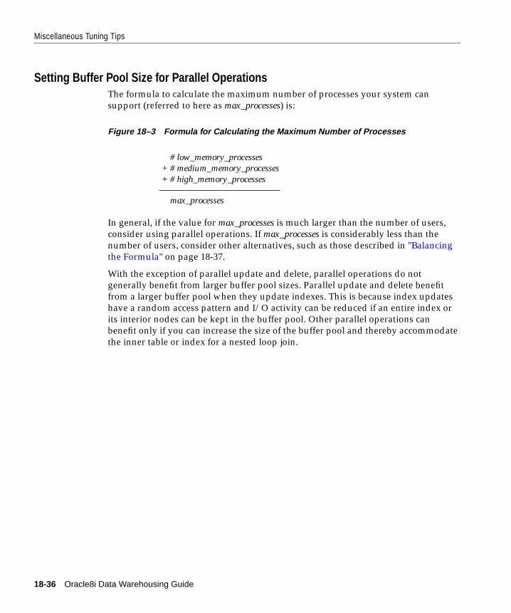
Miscellaneous Tuning Tips
Setting Buffer Pool Size for Parallel OperationsThe formula to calculate the maximum number of processes your system can
support (referred to here as max_processes) is:
Figure 18–3 Formula for Calculating the Maximum Number of Processes
In general, if the value for max_processes is much larger than the number of users,
consider using parallel operations. If max_processes is considerably less than the
number of users, consider other alternatives, such as those described in "Balancing
the Formula" on page 18-37.
With the exception of parallel update and delete, parallel operations do not
generally benefit from larger buffer pool sizes. Parallel update and delete benefit
from a larger buffer pool when they update indexes. This is because index updates
have a random access pattern and I/O activity can be reduced if an entire index or
its interior nodes can be kept in the buffer pool. Other parallel operations can
benefit only if you can increase the size of the buffer pool and thereby accommodate
the inner table or index for a nested loop join.
# low_memory_processes+ # medium_memory_processes+ # high_memory_processes
max_processes
18-36 Oracle8i Data Warehousing Guide

Miscellaneous Tuning Tips
Balancing the FormulaUse the following techniques to balance the memory/users/server formula given in
Figure 18–2:
■ Oversubscribing with Attention to Paging
■ Reducing the Number of Memory-Intensive Processes
■ Decreasing Data Warehousing Memory per Process
■ Decreasing Parallelism for Multiple Users
Oversubscribing with Attention to PagingYou can permit the potential workload to exceed the limits recommended in the
formula. Total memory required, minus the SGA size, can be multiplied by a factor
of 1.2, to allow for 20% oversubscription. Thus, if you have 1GB of memory, you
might be able to support 1.2GB of demand: the other 20% could be handled by the
paging system.
You must, however, verify that a particular degree of oversubscription is viable on
your system. Do this by monitoring the paging rate and making sure you are not
spending more than a very small percent of the time waiting for the paging
subsystem. Your system may perform acceptably even if oversubscribed by 60%, if
on average not all of the processes are performing hash joins concurrently. Users
might then try to use more than the available memory, so you must continually
monitor paging activity in such a situation. If paging dramatically increases,
consider other alternatives.
On average, no more than 5% of the time should be spent simply waiting in the
operating system on page faults. More than 5% wait time indicates your paging
subsystem is I/O bound. Use your operating system monitor to check wait time.
If wait time for paging devices exceeds 5%, you can reduce memory requirements
in one of these ways:
■ Reducing the memory required for each class of process
■ Reducing the number of processes in memory-intensive classes
■ Adding memory
If the wait time indicates an I/O bottleneck in the paging subsystem, you could
resolve this by striping.
Tuning Parallel Execution 18-37

Miscellaneous Tuning Tips
Reducing the Number of Memory-Intensive ProcessesThis section describes two things you can do to reduce the number of
memory-intensive processes:
■ Adjusting the Degree of Parallelism
■ Scheduling Parallel Jobs
Adjusting the Degree of Parallelism. You can adjust not only the number of operations
that run in parallel, but also the DOP (degree of parallelism) with which operations
run. To do this, issue an ALTER TABLE statement with a PARALLEL clause, or use
a hint.
You can limit the parallel pool by reducing the value of
PARALLEL_MAX_SERVERS. Doing so places a system-level limit on the total
amount of parallelism. It also makes your system easier to administer. More
processes are then forced to run in serial mode.
If you enable the parallel adaptive multi-user feature by setting the
PARALLEL_ADAPTIVE_MULTI_USER parameter to TRUE, Oracle adjusts DOP
based on user load.
Scheduling Parallel Jobs Queuing jobs is another way to reduce the number of
processes but not reduce parallelism. Rather than reducing parallelism for all
operations, you may be able to schedule large parallel batch jobs to run with full
parallelism one at a time, rather than concurrently. Queries at the head of the queue
would have a fast response time, those at the end of the queue would have a slow
response time. However, this method entails a certain amount of administrative
overhead.
Decreasing Data Warehousing Memory per ProcessThe following discussion focuses upon the relationship of HASH_AREA_SIZE to
memory, but all the same considerations apply to SORT_AREA_SIZE. The lower
bound of SORT_AREA_SIZE, however, is not as critical as the 8MB recommended
minimum HASH_AREA_SIZE.
If every operation performs a hash join and a sort, the high memory requirement
limits the number of processes you can have. To allow more users to run
concurrently you may need to reduce the data warehouse's process memory.
18-38 Oracle8i Data Warehousing Guide

Miscellaneous Tuning Tips
Moving Processes from High to Medium Memory Requirements You can move a process
from the high-memory to the medium-memory class by reducing the value for
HASH_AREA_SIZE. With the same amount of memory, Oracle always processes
hash joins faster than sort merge joins. Therefore, Oracle does not recommend that
you make your hash area smaller than your sort area.
Moving Processes from High or Medium Memory Requirements to Low Memory RequirementsIf you need to support thousands of users, create access paths so operations do not
access data unnecessarily. To do this, perform one or more of the following:
■ Decrease the demand for index joins by creating indexes and/or summary
tables.
■ Decrease the demand for GROUP BY sorting by creating summary tables and
encouraging users and applications to reference summaries and materialized
views rather than detailed data.
■ Decrease the demand for ORDER BY sorts by creating indexes on frequently
sorted columns.
Decreasing Parallelism for Multiple UsersThe easiest way to decrease parallelism for multiple users is to enable the parallel
adaptive multi-user feature.
If you decide to control this manually, however, there is a trade-off between
parallelism for fast single-user response time and efficient use of resources for
multiple users. For example, a system with 2GB of memory and a
HASH_AREA_SIZE of 32MB can support about 60 parallel execution servers. A 10
CPU machine can support up to 3 concurrent parallel operations (2 * 10 * 3 = 60). To
support 12 concurrent parallel operations, you could override the default
parallelism (reduce it), decrease HASH_AREA_SIZE, buy more memory, or you
could use some combination of these three strategies. Thus you could ALTER
TABLE t PARALLEL (DOP = 5) for all parallel tables t, set HASH_AREA_SIZE to
16MB, and increase PARALLEL_MAX_SERVERS to 120. By reducing the memory of
each parallel server by a factor of 2, and reducing the parallelism of a single
operation by a factor of 2, the system can accommodate 2 * 2 = 4 times more
concurrent parallel operations.
The penalty for using such an approach is that, when a single operation happens to
be running, the system uses just half the CPU resource of the 10 CPU machine. The
other half is idle until another operation is started.
Tuning Parallel Execution 18-39

Miscellaneous Tuning Tips
To determine whether your system is being fully utilized, use one of the graphical
system monitors available on most operating systems. These monitors often give
you a better idea of CPU utilization and system performance than monitoring the
execution time of an operation. Consult your operating system documentation to
determine whether your system supports graphical system monitors.
Examples: Balancing Memory, Users, and Parallel Execution ServersThe examples in this section show how to evaluate the relationship between
memory, users, and parallel execution servers, and balance the formula given in
Figure 18–2. They show concretely how you might adjust your system workload to
accommodate the necessary number of processes and users.
Example 1Assume your system has 1GB of memory, the DOP is 10, and that your users
perform 2 hash joins with 3 or more tables. If you need 300MB for the SGA, that
leaves 700MB to accommodate processes. If you allow a generous hash area size,
such as 32MB, then your system can support:
Figure 18–4 Formula for Balancing Memory, Users, and Processes
This makes a total of 704MB. In this case, the memory is not significantly
oversubscribed.
Remember that every parallel, hash, or sort merge join operation takes a number of
parallel execution servers equal to twice the DOP, utilizing 2 server sets, and often
each individual process of a parallel operation uses a significant amount of memory.
Thus you can support many more users by running their processes serially, or by
using less parallelism to run their processes.
To service more users, you can reduce hash area size to 2MB. This configuration can
support 17 parallel operations, or 170 serial operations, but response times may be
significantly higher than if you were using hash joins.
The trade-off in this example reveals that by reducing memory per process by a
factor of 16, you can increase the number of concurrent users by a factor of 16. Thus
1 parallel operation (32MB * 10 * 2 = 640MB)
1 serial operation (32MB * 2 = 64MB)
18-40 Oracle8i Data Warehousing Guide

Miscellaneous Tuning Tips
the amount of physical memory on the machine imposes another limit on the total
number of parallel operations you can run involving hash joins and sorts.
Example 2In a mixed workload example, consider a user population with diverse needs, as
described in Table 18–4. In this situation, you would have to allocate resources
selectively. You could not allow everyone to run hash joins—even though they
outperform sort merge joins—because you do not have adequate memory to
support workload level.
You might consider it safe to oversubscribe by 50%, because of the infrequent batch
jobs that run during the day: 700MB * 1.5 = 1.05GB. This gives you enough virtual
memory for the total workload.
Example 3Suppose your system has 2GB of memory and you have 200 query server processes
and 100 users doing performing heavy data warehousing operations involving hash
joins. You decide not to consider tasks such as index retrievals and small sorts.
Instead, you concentrate on the high memory processes. You might have 300
processes, of which 200 must come from the parallel pool and 100 are single
threaded. One quarter of the total 2GB of memory might be used by the SGA,
leaving 1.5GB of memory to handle all the processes. You could apply the formula
Table 18–4 How to Accommodate a Mixed Workload
User Needs How to Accommodate
DBA: runs nightly batch jobs, andoccasional batch jobs during the day.These might be parallel operations thatperform hash joins and thus use a lot ofmemory.
You might take 20 parallel execution servers, and setHASH_AREA_SIZE to a mid-range value, perhaps 20MB, for a singlepowerful batch job in the high memory class. This might be a largeGROUP BY operation with a join to produce a summary of data.Twenty servers multiplied by 20MB equals 400MB of memory.
Analysts: interactive users who extractdata for their spreadsheets.
You might plan for 10 analysts running serial operations that usecomplex hash joins accessing a large amount of data. You would notallow them to perform parallel operations because of memoryrequirements. Ten such serial processes at 40MB each equals 400MBof memory.
Users: Several hundred usersperforming simple lookups ofindividual customer accounts, andmaking reports on already joined,partially summarized data.
To support hundreds of users performing low memory processes atabout 0.5MB each, you might reserve 200MB.
Tuning Parallel Execution 18-41

Miscellaneous Tuning Tips
considering only the high memory requirements, including a factor of 20%
oversubscription:
Figure 18–5 Formula for Memory/User/Server Relationship: High-Memory Processes
Here, 5MB = 1.8GB/300. Less than 5MB of hash area would be available for each
process, whereas 8MB is the recommended minimum. If you must have 300
processes, you may need to reduce hash area size to change them from the highly
memory-intensive class to the moderately memory-intensive class. Then they may
fit within your system's constraints.
Example 4Consider a system with 2GB of memory and 10 users who want to run intensive
data warehousing parallel operations concurrently and still have good
performance. If you choose a DOP of 10, then the 10 users will require 200
processes. (Processes running large joins need twice the number of parallel
execution servers as the DOP, so you would set PARALLEL_MAX_SERVERS to 10 *
10 * 2.) In this example each process would get 1.8GB/200—or about 9MB of hash
area—which should be adequate.
With only 5 users doing large hash joins, each process would get over 16MB of hash
area, which would be fine. But if you want 32MB available for lots of hash joins, the
system could only support 2 or 3 users. By contrast, if users are just computing
aggregates, the system needs adequate sort area size—and can have many more
users.
Example 5If a system with 2GB of memory needs to support 1000 users, all of them running
large queries, you must evaluate the situation carefully. Here, the per-user memory
budget is only 1.8MB (that is, 1.8GB divided by 1,000). Since this figure is at the low
end of the medium memory process class, you must rule out parallel operations,
which use even more resources. You must also rule out large hash joins. Each
sequential process could require up to 2 hash areas plus the sort area, so you would
have to set HASH_AREA_SIZE to the same value as SORT_AREA_SIZE, which
would be 600KB(1.8MB/3). Such a small hash area size is likely to be ineffective.
high_memory_req’d = 1.2 = =*total_memory
#_high-memory_processes
1.5GB * 1.2
300
1.8GB
300
18-42 Oracle8i Data Warehousing Guide

Miscellaneous Tuning Tips
Given the organization's resources and business needs, is it reasonable for you to
upgrade your system's memory? If memory upgrade is not an option, then you
must change your expectations. To adjust the balance, you might:
■ Accept the fact that the system will actually support a limited number of users
executing large hash joins.
■ Give the users access to summary tables, rather than to the whole database.
■ Classify users into different groups, and give some groups more memory than
others. Instead of all users doing sorts with a small sort area, you could have a
few users doing high-memory hash joins, while most users use summary tables
or do low-memory index joins. (You could accomplish this by forcing users in
each group to use hints in their queries such that operations are performed in a
particular way.)
Parallel Execution Space Management IssuesThis section describes space management issues that occur when using parallel
execution. These issues are:
■ ST (Space Transaction) Enqueue for Sorts and Temporary Data
■ External Fragmentation
These problems become particularly important for parallel operations in an OPS
(Oracle Parallel Server) environment; the more nodes that are involved, the more
tuning becomes critical.
If you can implement locally-managed tablespaces, you can avoid these issues
altogether.
ST (Space Transaction) Enqueue for Sorts and Temporary DataEvery space management transaction in the database (such as creation of temporary
segments in PARALLEL CREATE TABLE, or parallel direct-load inserts of
non-partitioned tables) is controlled by a single ST enqueue. A high transaction rate,
for example, more than 2 or 3 transactions per minute, on ST enqueues may result
in poor scalability on OPS with many nodes, or a timeout waiting for space
management resources. Use the V$ROWCACHE and V$LIBRARYCACHE views to
locate this type of contention.
Note: For more information about locally-managed tablespaces,
please refer to the Oracle8i Administrator’s Guide.
Tuning Parallel Execution 18-43
Miscellaneous Tuning Tips
Try to minimize the number of space management transactions, in particular:
■ The number of sort space management transactions
■ The creation and removal of objects
■ Transactions caused by fragmentation in a tablespace
Use dedicated temporary tablespaces to optimize space management for sorts. This
is particularly beneficial on OPS. You can monitor this using V$SORT_SEGMENT.
Set INITIAL and NEXT extent size to a value in the range of 1MB to 10MB.
Processes may use temporary space at a rate of up to 1MB per second. Do not accept
the default value of 40KB for next extent size, because this will result in many
requests for space per second.
External FragmentationExternal fragmentation is a concern for parallel load, direct-load insert, and
PARALLEL CREATE TABLE ... AS SELECT. Memory tends to become fragmented
as extents are allocated and data is inserted and deleted. This may result in a fair
amount of free space that is unusable because it consists of small, non-contiguous
chunks of memory.
To reduce external fragmentation on partitioned tables, set all extents to the same
size. Set the value for NEXT equal to the value for INITIAL and set
PERCENT_INCREASE to zero. The system can handle this well with a few
thousand extents per object. Therefore, set MAXEXTENTS to, for example, 1,000 to
3,000; never attempt to use a value for MAXEXTENS in excess of 10,000. For tables
that are not partitioned, the initial extent should be small.
Tuning Parallel Execution on Oracle Parallel ServerThis section describe several aspects of parallel execution for OPS.
Lock AllocationThis section provides parallel execution tuning guidelines for optimal lock
management on OPS.
To optimize parallel execution on OPS, you need to correctly set
GC_FILES_TO_LOCKS. On OPS, a certain number of parallel cache management
(PCM) locks are assigned to each data file. Data block address locking in its default
behavior assigns one lock to each block. During a full table scan, a PCM lock must
then be acquired for each block read into the scan. To speed up full table scans, you
have three possibilities:
18-44 Oracle8i Data Warehousing Guide

Miscellaneous Tuning Tips
■ For data files containing truly read-only data, set the tablespace to read only.
Then PCM locking does not occur.
■ Alternatively, for data that is mostly read-only, assign very few hashed PCM
locks (for example, 2 shared locks) to each data file. Then these are the only
locks you have to acquire when you read the data.
■ If you want data block address or fine-grain locking, group together the blocks
controlled by each lock, using the ! option. This has advantages over default
data block address locking because with the default, you would need to acquire
one million locks in order to read one million blocks. When you group the
blocks, you reduce the number of locks allocated by the grouping factor. Thus a
grouping of !10 would mean that you would only have to acquire one tenth as
many PCM locks as with the default. Performance improves due to the
dramatically reduced amount of lock allocation. As a rule of thumb,
performance with a grouping of !10 is comparable to the speed of hashed
locking.
To speed up parallel DML operations, consider using hashed locking or a high
grouping factor rather than database address locking. A parallel execution
server works on non-overlapping partitions; it is recommended that partitions
not share files. You can thus reduce the number of lock operations by having
only 1 hashed lock per file. Because the parallel execution server only works on
non-overlapping files, there are no lock pings.
The following guidelines effect memory usage, and thus indirectly affect
performance:
■ Never allocate PCM locks for datafiles of temporary tablespaces.
■ Never allocate PCM locks for datafiles that contain only rollback segments.
These are protected by GC_ROLLBACK_LOCKS and
GC_ROLLBACK_SEGMENTS.
■ Allocate specific PCM locks for the SYSTEM tablespace. This practice ensures
that data dictionary activity such as space management never interferes with
the data tablespaces at a cache management level (error 1575).
For example, on a read-only database with a data warehousing application's
query-only workload, you might create 500 PCM locks on the SYSTEM
tablespace in file 1, then create 50 more locks to be shared for all the data in the
other files. Space management work will never interfere with the rest of the
database.
Tuning Parallel Execution 18-45

Miscellaneous Tuning Tips
Load Balancing for Multiple Concurrent Parallel OperationsLoad balancing distributes query server processes to spread CPU and memory use
evenly among nodes. It also minimizes communication and remote I/O among
nodes. Oracle does this by allocating servers to the nodes that are running the
fewest number of processes.
The load balancing algorithm attempts to maintain an even load across all nodes.
For example, if a DOP of 8 is requested on an 8-node MPP (Massively Parallel
Processing) system with 1 CPU per node, the algorithm places 2 servers on each
node.
If the entire query server group fits on one node, the load balancing algorithm
places all the processes on a single node to avoid communications overhead. For
example, if a DOP of 8 is requested on a 2-node cluster with 16 CPUs per node, the
algorithm places all 16 query server processes on one node.
Using Parallel Instance GroupsA user or the DBA can control which instances allocate query server processes by
using Instance Group functionality. To use this feature, you must first assign each
active instance to at least one or more instance groups. Then you can dynamically
control which instances spawn parallel processes by activating a particular group of
instances.
Establish instance group membership on an instance-by-instance basis by setting
the initialization parameter INSTANCE_GROUPS to a name representing one or
more instance groups. For example, on a 32-node MPP system owned by both a
Marketing and a Sales organization, you could assign half the nodes to one
organization and the other half to the other organization using instance group
names. To do this, assign nodes 1-16 to the Marketing organization using the
following parameter syntax in each initialization parameter file:
INSTANCE_GROUPS=marketing
Then assign nodes 17-32 to Sales using this syntax in the remaining INIT.ORA files:
INSTANCE_GROUPS=sales
Then a user or the DBA can activate the nodes owned by Sales to spawn a query
server process by entering the following:
See Also: Oracle8i Parallel Server Concepts for a thorough
discussion of PCM locks and locking parameters.
18-46 Oracle8i Data Warehousing Guide
Miscellaneous Tuning Tips
ALTER SESSION SET PARALLEL_INSTANCE_GROUP = 'sales';
In response, Oracle allocates query server processes to nodes 17-32. The default
value for PARALLEL_INSTANCE_GROUP is all active instances.
Disk AffinitySome OPS platforms use disk affinity. Without disk affinity, Oracle tries to balance
the allocation evenly across instances; with disk affinity, Oracle tries to allocate
parallel execution servers for parallel table scans on the instances that are closest to
the requested data. Disk affinity minimizes data shipping and internode
communication on a shared nothing architecture. Disk affinity can thus significantly
increase parallel operation throughput and decrease response time.
Disk affinity is used for parallel table scans, parallel temporary tablespace
allocation, parallel DML, and parallel index scan. It is not used for parallel table
creation or parallel index creation. Access to temporary tablespaces preferentially
uses local datafiles. It guarantees optimal space management extent allocation.
Disks striped by the operating system are treated by disk affinity as a single unit.
In the following example of disk affinity, table T is distributed across 3 nodes, and a
full table scan on table T is being performed.
Note: An instance can belong to one or more groups. You can
enter multiple instance group names with the INSTANCE_GROUP
parameter using a comma as a separator.
Tuning Parallel Execution 18-47

Miscellaneous Tuning Tips
Figure 18–6 Disk Affinity Example
■ If a query requires 2 instances, then two instances from the set 1, 2, and 3 are
used.
■ If a query requires 3 instances, then instances 1, 2, and 3 are used.
■ If a query requires 4 instances, then all four instances are used.
■ If there are two concurrent operations against table T, each requiring 3 instances
(and enough processes are available on the instances for both operations), then
both operations use instances 1, 2, and 3. Instance 4 is not used. In contrast,
without disk affinity instance 4 is used.
Overriding the Default Degree of ParallelismThe default DOP is appropriate for reducing response time while guaranteeing use
of CPU and I/O resources for any parallel operations. If an operation is I/O bound,
consider increasing the default DOP. If it is memory bound, or several concurrent
parallel operations are running, you might want to decrease the default DOP.
Oracle uses the default DOP for tables that have PARALLEL attributed to them in
the data dictionary, or when the PARALLEL hint is specified. If a table does not
have parallelism attributed to it, or has NOPARALLEL (the default) attributed to it,
then that table is never scanned in parallel—regardless of the default DOP that
would be indicated by the number of CPUs, instances, and devices storing that
table.
See Also: Oracle8i Parallel Server Concepts for more information on
instance affinity.
Instance1
Table T
Instance2
Table T
Instance3
Table T
Instance4
18-48 Oracle8i Data Warehousing Guide

Miscellaneous Tuning Tips
Use the following guidelines when adjusting the DOP:
■ You can modify the default DOP by changing the value for the
PARALLEL_THREADS_PER_CPU parameter.
■ You can adjust the DOP either by using ALTER TABLE, ALTER SESSION, or by
using hints.
■ To increase the number of concurrent parallel operations, reduce the DOP, or set
the parameter PARALLEL_ADAPTIVE_MULTI_USER to TRUE.
■ For I/O-bound parallel operations, first spread the data over more disks than
there are CPUs. Then, increase parallelism in stages. Stop when the query
becomes CPU bound.
For example, assume a parallel indexed nested loop join is I/O bound
performing the index lookups, with #CPUs=10 and #disks=36. The default DOP
is 10, and this is I/O bound. You could first try a DOP of 12. If the application is
still I/O bound, try a DOP of 24; if still I/O bound, try 36.
Rewriting SQL StatementsThe most important issue for parallel execution is ensuring that all parts of the
query plan that process a substantial amount of data execute in parallel. Use
EXPLAIN PLAN to verify that all plan steps have an OTHER_TAG of
PARALLEL_TO_PARALLEL, PARALLEL_TO_SERIAL,
PARALLEL_COMBINED_WITH_PARENT, or
PARALLEL_COMBINED_WITH_CHILD. Any other keyword (or null) indicates
serial execution, and a possible bottleneck.
By making the following changes you can increase the optimizer's ability to
generate parallel plans:
■ Convert subqueries, especially correlated subqueries, into joins. Oracle can
parallelize joins more efficiently than subqueries. This also applies to updates.
■ Use a PL/SQL function in the WHERE clause of the main query instead of a
correlated subquery.
■ Rewrite queries with distinct aggregates as nested queries. For example, rewrite
SELECT COUNT(DISTINCT C) FROM T;
To:
SELECT COUNT(*)FROM (SELECT DISTINCT C FROM T);
Tuning Parallel Execution 18-49

Miscellaneous Tuning Tips
Creating and Populating Tables in ParallelOracle cannot return results to a user process in parallel. If a query returns a large
number of rows, execution of the query may indeed be faster; however, the user
process can only receive the rows serially. To optimize parallel execution
performance with queries that retrieve large result sets, use PARALLEL CREATE
TABLE ... AS SELECT or direct-load insert to store the result set in the database. At
a later time, users can view the result set serially.
When combined with the NOLOGGING option, the parallel version of CREATE
TABLE ... AS SELECT provides a very efficient intermediate table facility.
For example:
CREATE TABLE summary PARALLEL NOLOGGING AS SELECT dim_1, dim_2 ..., SUM (meas_1) FROM facts GROUP BY dim_1, dim_2;
These tables can also be incrementally loaded with parallel insert. You can take
advantage of intermediate tables using the following techniques:
■ Common subqueries can be computed once and referenced many times. This
may allow some queries against star schemas (in particular, queries without
selective WHERE-clause predicates) to be better parallelized. Note that star
queries with selective WHERE-clause predicates using the star-transformation
technique can be effectively parallelized automatically without any
modification to the SQL.
■ Decompose complex queries into simpler steps in order to provide
application-level checkpoint/restart. For example, a complex multi-table join on
a database 1 terabyte in size could run for dozens of hours. A crash during this
query would mean starting over from the beginning. Using CREATE TABLE ...
AS SELECT and/or PARALLEL INSERT AS SELECT, you can rewrite the query
as a sequence of simpler queries that run for a few hours each. If a system
failure occurs, the query can be restarted from the last completed step.
See Also: "Updating the Table" on page 18-62.
Note: Parallelism of the SELECT does not influence the CREATE
statement. If the CREATE is parallel, however, the optimizer tries to
make the SELECT run in parallel also.
18-50 Oracle8i Data Warehousing Guide

Miscellaneous Tuning Tips
■ Materialize a Cartesian product. This may allow queries against star schemas to
execute in parallel. It may also increase scalability of parallel hash joins by
increasing the number of distinct values in the join column.
Consider a large table of retail sales data that is joined to region and to
department lookup tables. There are 5 regions and 25 departments. If the huge
table is joined to regions using parallel hash partitioning, the maximum
speedup is 5. Similarly, if the huge table is joined to departments, the maximum
speedup is 25. But if a temporary table containing the Cartesian product of
regions and departments is joined with the huge table, the maximum speedup
is 125.
■ Efficiently implement manual parallel deletes by creating a new table that omits
the unwanted rows from the original table, and then dropping the original
table. Alternatively, you can use the convenient parallel delete feature, which
can directly delete rows from the original table.
■ Create summary tables for efficient multidimensional drill-down analysis. For
example, a summary table might store the sum of revenue grouped by month,
brand, region, and salesperson.
■ Reorganize tables, eliminating chained rows, compressing free space, and so on,
by copying the old table to a new table. This is much faster than export/import
and easier than reloading.
Creating Temporary Tablespaces for Parallel Sort and Hash JoinFor optimal space management performance, use dedicated temporary tablespaces.
As with the TStemp tablespace, first add a single datafile and later add the
remainder in parallel as in this example:
CREATE TABLESPACE TStemp TEMPORARY DATAFILE '/dev/D31'SIZE 4096MB REUSEDEFAULT STORAGE (INITIAL 10MB NEXT 10MB PCTINCREASE 0);
Note: Be sure to use the ANALYZE statement on newly created
tables. Also consider creating indexes. To avoid I/O bottlenecks,
specify a tablespace with at least as many devices as CPUs. To
avoid fragmentation in allocating space, the number of files in a
tablespace should be a multiple of the number of CPUs.
Tuning Parallel Execution 18-51

Miscellaneous Tuning Tips
Size of Temporary ExtentsTemporary extents are all the same size, because the server ignores the
PCTINCREASE and INITIAL settings and only uses the NEXT setting for
temporary extents. This helps avoid fragmentation.
As a general rule, temporary extents should be smaller than permanent extents,
because there are more demands for temporary space, and parallel processes or
other operations running concurrently must share the temporary tablespace.
Normally, temporary extents should be in the range of 1MB to 10MB. Once you
allocate an extent it is yours for the duration of your operation. If you allocate a
large extent but only need to use a small amount of space, the unused space in the
extent is tied up.
At the same time, temporary extents should be large enough that processes do not
have to spend all their time waiting for space. Temporary tablespaces use less
overhead than permanent tablespaces when allocating and freeing a new extent.
However, obtaining a new temporary extent still requires the overhead of acquiring
a latch and searching through the SGA structures, as well as SGA space
consumption for the sort extent pool. Also, if extents are too small, SMON may take
a long time dropping old sort segments when new instances start up.
Operating System Striping of Temporary TablespacesOperating system striping is an alternative technique you can use with temporary
tablespaces. Media recovery, however, offers subtle challenges for large temporary
tablespaces. It does not make sense to mirror, use RAID, or back up a temporary
tablespace. If you lose a disk in an OS striped temporary space, you will probably
have to drop and recreate the tablespace. This could take several hours for the
120GB example. With Oracle striping, simply remove the defective disk from the
tablespace. For example, if /dev/D50 fails, enter:
ALTER DATABASE DATAFILE '/dev/D50' RESIZE 1K;ALTER DATABASE DATAFILE '/dev/D50' OFFLINE;
Because the dictionary sees the size as 1KB, which is less than the extent size, the
corrupt file is not accessed. Eventually, you may wish to recreate the tablespace.
Be sure to make your temporary tablespace available for use:
ALTER USER scott TEMPORARY TABLESPACE TStemp;
See Also: For MPP systems, see your platform-specific
documentation regarding the advisability of disabling disk affinity
when using operating system striping.
18-52 Oracle8i Data Warehousing Guide

Miscellaneous Tuning Tips
Executing Parallel SQL StatementsAfter analyzing your tables and indexes, you should see performance
improvements based on the degree of parallelism used. The following operations
should scale:
■ Table scans
■ NESTED LOOP JOIN
■ SORT MERGE JOIN
■ HASH JOIN
■ NOT IN
■ GROUP BY
■ SELECT DISTINCT
■ UNION and UNION ALL
■ AGGREGATION
■ PL/SQL functions called from SQL
■ ORDER BY
■ CREATE TABLE AS SELECT
■ CREATE INDEX
■ REBUILD INDEX
■ REBUILD INDEX PARTITION
■ MOVE PARTITION
■ SPLIT PARTITION
■ UPDATE
■ DELETE
■ INSERT ... SELECT
■ ENABLE CONSTRAINT
■ STAR TRANSFORMATION
Start with simple parallel operations. Evaluate total I/O throughput with SELECT
COUNT(*) FROM facts. Evaluate total CPU power by adding a complex WHERE
clause. I/O imbalance may suggest a better physical database layout. After you
Tuning Parallel Execution 18-53

Miscellaneous Tuning Tips
understand how simple scans work, add aggregation, joins, and other operations
that reflect individual aspects of the overall workload. Look for bottlenecks.
Besides query performance you should also monitor parallel load, parallel index
creation, and parallel DML, and look for good utilization of I/O and CPU resources.
Using EXPLAIN PLAN to Show Parallel Operations PlansUse the EXPLAIN PLAN command to see the execution plans for parallel queries.
EXPLAIN PLAN output shows optimizer information in the COST, BYTES, and
CARDINALITY columns. For more information on using EXPLAIN PLAN, refer to
Oracle8i Designing and Tuning for Performance.
There are several ways to optimize the parallel execution of join statements. You can
alter your system's configuration, adjust parameters as discussed earlier in this
chapter, or use hints, such as the DISTRIBUTION hint.
Additional Considerations for Parallel DMLWhen you want to refresh your data warehouse database using parallel insert,
update, or delete on a data warehouse, there are additional issues to consider when
designing the physical database. These considerations do not affect parallel
execution operations. These issues are:
■ PDML and Direct-load Restrictions
■ Limitation on the Degree of Parallelism
■ Using Local and Global Striping
■ Increasing INITRANS and MAXTRANS
■ Limitation on Available Number of Transaction Free Lists
■ Using Multiple Archivers
■ Database Writer Process (DBWn) Workload
■ [NO]LOGGING Clause
PDML and Direct-load RestrictionsA complete listing of PDML and direct-load insert restrictions is found in Oracle8iConcepts. If a parallel restriction is violated, the operation is simply performed
serially. If a direct-load insert restriction is violated, then the APPEND hint is
ignored and a conventional insert is performed. No error message is returned.
18-54 Oracle8i Data Warehousing Guide

Miscellaneous Tuning Tips
Limitation on the Degree of ParallelismIf you are performing parallel insert, update, or delete operations, the DOP is equal
to or less than the number of partitions in the table.
Using Local and Global StripingParallel DML works mostly on partitioned tables. It does not use asynchronous I/O
and may generate a high number of random I/O requests during index
maintenance of parallel UPDATE and DELETE operations. For local index
maintenance, local striping is most efficient in reducing I/O contention, because one
server process only goes to its own set of disks and disk controllers. Local striping
also increases availability in the event of one disk failing.
For global index maintenance, (partitioned or non-partitioned), globally striping the
index across many disks and disk controllers is the best way to distribute the
number of I/Os.
Increasing INITRANS and MAXTRANSIf you have global indexes, a global index segment and global index blocks are
shared by server processes of the same parallel DML statement. Even if the
operations are not performed against the same row, the server processes may share
the same index blocks. Each server transaction needs one transaction entry in the
index block header before it can make changes to a block. Therefore, in the CREATE
INDEX or ALTER INDEX statements, you should set INITRANS, the initial number
of transactions allocated within each data block, to a large value, such as the
maximum DOP against this index. Leave MAXTRANS, the maximum number of
concurrent transactions that can update a data block, at its default value, which is
the maximum your system can support. This value should not exceed 255.
If you run a DOP of 10 against a table with a global index, all 10 server processes
might attempt to change the same global index block. For this reason, you must set
MAXTRANS to at least 10 so all server processes can make the change at the same
time. If MAXTRANS is not large enough, the parallel DML operation fails.
Limitation on Available Number of Transaction Free ListsOnce a segment has been created, the number of process and transaction free lists is
fixed and cannot be altered. If you specify a large number of process free lists in the
segment header, you may find that this limits the number of transaction free lists
that are available. You can abate this limitation the next time you recreate the
segment header by decreasing the number of process free lists; this leaves more
room for transaction free lists in the segment header.
Tuning Parallel Execution 18-55

Miscellaneous Tuning Tips
For UPDATE and DELETE operations, each server process may require its own
transaction free list. The parallel DML DOP is thus effectively limited by the
smallest number of transaction free lists available on any of the global indexes the
DML statement must maintain. For example, if you have two global indexes, one
with 50 transaction free lists and one with 30 transaction free lists, the DOP is
limited to 30.
The FREELISTS parameter of the STORAGE clause is used to set the number of
process free lists. By default, no process free lists are created.
The default number of transaction free lists depends on the block size. For example,
if the number of process free lists is not set explicitly, a 4KB block has about 80
transaction free lists by default. The minimum number of transaction free lists is 25.
Using Multiple ArchiversParallel DDL and parallel DML operations may generate a large amount of redo
logs. A single ARCH process to archive these redo logs might not be able to keep
up. To avoid this problem, you can spawn multiple archiver processes. This can be
done manually or by using a job queue.
Database Writer Process (DBWn) WorkloadParallel DML operations dirty a large number of data, index, and undo blocks in the
buffer cache during a short period of time. If you see a high number of
"free_buffer_waits" after querying the V$SYSTEM_EVENT view as in the following
syntax:
SELECT TOTAL_WAITS FROM V$SYSTEM_EVENT WHERE EVENT = 'FREE BUFFER WAITS';
Tune the DBWn process(es). If there are no waits for free buffers, the above query
does not return any rows.
[NO]LOGGING ClauseThe [NO]LOGGING clause applies to tables, partitions, tablespaces, and indexes.
Virtually no log is generated for certain operations (such as direct-load INSERT) if
the NOLOGGING clause is used. The NOLOGGING attribute is not specified at the
INSERT statement level, but is instead specified when using the ALTER or CREATE
command for the table, partition, index, or tablespace.
See Also: Oracle8i Parallel Server Concepts for information about
transaction free lists.
18-56 Oracle8i Data Warehousing Guide

Miscellaneous Tuning Tips
When a table or index has NOLOGGING set, neither parallel nor serial direct-load
INSERT operations generate undo or redo logs. Processes running with the
NOLOGGING option set run faster because no redo is generated. However, after a
NOLOGGING operation against a table, partition, or index, if a media failure
occurs before a backup is taken, then all tables, partitions, and indexes that have
been modified may be corrupted.
For backward compatibility, [UN]RECOVERABLE is still supported as an alternate
keyword with the CREATE TABLE command. This alternate keyword may not be
supported, however, in future releases.
At the tablespace level, the logging clause specifies the default logging attribute for
all tables, indexes, and partitions created in the tablespace. When an existing
tablespace logging attribute is changed by the ALTER TABLESPACE statement,
then all tables, indexes, and partitions created after the ALTER statement will have
the new logging attribute; existing ones will not change their logging attributes. The
tablespace level logging attribute can be overridden by the specifications at the
table, index, or partition level.
The default logging attribute is LOGGING. However, if you have put the database
in NOARCHIVELOG mode, by issuing ALTER DATABASE NOARCHIVELOG,
then all operations that can be done without logging will not generate logs,
regardless of the specified logging attribute.
Creating Indexes in ParallelMultiple processes can work together simultaneously to create an index. By
dividing the work necessary to create an index among multiple server processes,
the Oracle Server can create the index more quickly than if a single server process
created the index sequentially.
Parallel index creation works in much the same way as a table scan with an ORDER
BY clause. The table is randomly sampled and a set of index keys is found that
equally divides the index into the same number of pieces as the DOP. A first set of
Note: Direct-load INSERT operations (except for dictionary
updates) never generate undo logs. The NOLOGGING attribute
does not affect undo, but only redo. To be precise, NOLOGGING
allows the direct-load INSERT operation to generate a negligible
amount of redo (range-invalidation redo, as opposed to full image
redo).
Tuning Parallel Execution 18-57

Miscellaneous Tuning Tips
query processes scans the table, extracts key, ROWID pairs, and sends each pair to a
process in a second set of query processes based on key. Each process in the second
set sorts the keys and builds an index in the usual fashion. After all index pieces are
built, the parallel coordinator simply concatenates the pieces (which are ordered) to
form the final index.
Parallel local index creation uses a single server set. Each server process in the set is
assigned a table partition to scan, and for which to build an index partition. Because
half as many server processes are used for a given DOP, parallel local index creation
can be run with a higher DOP.
You can optionally specify that no redo and undo logging should occur during
index creation. This can significantly improve performance, but temporarily renders
the index unrecoverable. Recoverability is restored after the new index is backed
up. If your application can tolerate this window where recovery of the index
requires it to be re-created, then you should consider using the NOLOGGING
clause.
The PARALLEL clause in the CREATE INDEX statement is the only way in which
you can specify the DOP for creating the index. If the DOP is not specified in the
parallel clause of CREATE INDEX, then the number of CPUs is used as the DOP. If
there is no parallel clause, index creation is done serially.
When you add or enable a UNIQUE key or PRIMARY KEY constraint on a table,
you cannot automatically create the required index in parallel. Instead, manually
create an index on the desired columns using the CREATE INDEX statement and an
appropriate PARALLEL clause and then add or enable the constraint. Oracle then
uses the existing index when enabling or adding the constraint.
Multiple constraints on the same table can be enabled concurrently and in parallel if
all the constraints are already in the enabled novalidate state. In the following
example, the ALTER TABLE ... ENABLE CONSTRAINT statement performs the
table scan that checks the constraint in parallel:
Note: When creating an index in parallel, the STORAGE clause
refers to the storage of each of the subindexes created by the query
server processes. Therefore, an index created with an INITIAL of
5MB and a DOP of 12 consumes at least 60MB of storage during
index creation because each process starts with an extent of 5MB.
When the query coordinator process combines the sorted
subindexes, some of the extents may be trimmed, and the resulting
index may be smaller than the requested 60MB.
18-58 Oracle8i Data Warehousing Guide

Miscellaneous Tuning Tips
CREATE TABLE a (a1 NUMBER CONSTRAINT ach CHECK (a1 > 0) ENABLE NOVALIDATE)PARALLEL;INSERT INTO a values (1); COMMIT; ALTER TABLE a ENABLE CONSTRAINT ach;
Parallel DML TipsThis section provides an overview of parallel DML functionality.
■ INSERT
■ Direct-Load INSERT
■ Parallelizing INSERT, UPDATE, and DELETE
INSERTOracle INSERT functionality can be summarized as follows:
If parallel DML is enabled and there is a PARALLEL hint or PARALLEL attribute
set for the table in the data dictionary, then inserts are parallel and appended,
unless a restriction applies. If either the PARALLEL hint or PARALLEL attribute is
missing, then the insert is performed serially.
See Also: For more information on how extents are allocated
when using the parallel execution feature, see Oracle8i Concepts.Also refer to the Oracle8i SQL Reference for the complete syntax of
the CREATE INDEX statement.
See Also: Oracle8i Concepts for a detailed discussion of parallel
DML and DOP. For a discussion of parallel DML affinity, please see
Oracle8i Parallel Server Concepts.
Table 18–5 Summary of INSERT Features
Insert Type Parallel Serial NOLOGGING
Conventional No Yes No
Direct LoadInsert(Append)
Yes: requires:
■ ALTER SESSION ENABLE PARALLEL DML
■ Table PARALLEL attribute or PARALLEL hint
■ APPEND hint (optional)
Yes: requires:
■ APPEND hint
Yes: requires:
■ NOLOGGINGattribute set fortable orpartition
Tuning Parallel Execution 18-59

Miscellaneous Tuning Tips
Direct-Load INSERTAppend mode is the default during a parallel insert: data is always inserted into a
new block which is allocated to the table. Therefore the APPEND hint is optional.
You should use append mode to increase the speed of insert operations—but not
when space utilization needs to be optimized. You can use NOAPPEND to override
append mode.
The APPEND hint applies to both serial and parallel insert: even serial inserts are
faster if you use this hint. APPEND, however, does require more space and locking
overhead.
You can use NOLOGGING with APPEND to make the process even faster.
NOLOGGING means that no redo log is generated for the operation. NOLOGGING
is never the default; use it when you wish to optimize performance. It should not
normally be used when recovery is needed for the table or partition. If recovery is
needed, be sure to take a backup immediately after the operation. Use the ALTER
TABLE [NO]LOGGING statement to set the appropriate value.
Parallelizing INSERT, UPDATE, and DELETEWhen the table or partition has the PARALLEL attribute in the data dictionary, that
attribute setting is used to determine parallelism of INSERT, UPDATE, and DELETE
statements as well as queries. An explicit PARALLEL hint for a table in a statement
overrides the effect of the PARALLEL attribute in the data dictionary.
You can use the NOPARALLEL hint to override a PARALLEL attribute for the table
in the data dictionary. In general, hints take precedence over attributes.
DML operations are considered for parallelization only if the session is in a
PARALLEL DML enabled mode. (Use ALTER SESSION ENABLE PARALLEL DML
to enter this mode.) The mode does not affect parallelization of queries or of the
query portions of a DML statement.
Parallelizing INSERT ... SELECT In the INSERT... SELECT statement you can specify a
PARALLEL hint after the INSERT keyword, in addition to the hint after the SELECT
keyword. The PARALLEL hint after the INSERT keyword applies to the insert
operation only, and the PARALLEL hint after the SELECT keyword applies to the
select operation only. Thus parallelism of the INSERT and SELECT operations are
independent of each other. If one operation cannot be performed in parallel, it has
no effect on whether the other operation can be performed in parallel.
See Also: Oracle8i Concepts for more information on parallel
INSERT, UPDATE and DELETE.
18-60 Oracle8i Data Warehousing Guide
Miscellaneous Tuning Tips
The ability to parallelize INSERT causes a change in existing behavior, if the user
has explicitly enabled the session for parallel DML, and if the table in question has a
PARALLEL attribute set in the data dictionary entry. In that case existing INSERT ...
SELECT statements that have the select operation parallelized may also have their
insert operation parallelized.
If you query multiple tables, you can specify multiple SELECT PARALLEL hints
and multiple PARALLEL attributes.
Example
Add the new employees who were hired after the acquisition of ACME.
INSERT /*+ PARALLEL(EMP) */ INTO EMPSELECT /*+ PARALLEL(ACME_EMP) */ *FROM ACME_EMP;
The APPEND keyword is not required in this example, because it is implied by the
PARALLEL hint.
Parallelizing UPDATE and DELETE The PARALLEL hint (placed immediately after the
UPDATE or DELETE keyword) applies not only to the underlying scan operation,
but also to the update/delete operation. Alternatively, you can specify
update/delete parallelism in the PARALLEL clause specified in the definition of the
table to be modified.
If you have explicitly enabled PDML (Parallel Data Manipulation Language) for the
session or transaction, UPDATE/DELETE statements that have their query
operation parallelized may also have their UPDATE/DELETE operation
parallelized. Any subqueries or updatable views in the statement may have their
own separate parallel hints or clauses, but these parallel directives do not affect the
decision to parallelize the update or delete. If these operations cannot be performed
in parallel, it has no effect on whether the UPDATE or DELETE portion can be
performed in parallel.
You can only use parallel UPDATE and DELETE on partitioned tables.
Example 1
Give a 10% salary raise to all clerks in Dallas.
UPDATE /*+ PARALLEL(EMP) */ EMPSET SAL=SAL * 1.1 WHERE JOB='CLERK' AND DEPTNO IN (SELECT DEPTNO FROM DEPT WHERE LOCATION='DALLAS');
Tuning Parallel Execution 18-61

Miscellaneous Tuning Tips
The PARALLEL hint is applied to the update operation as well as to the scan.
Example 2
Remove all products in the grocery category, because the grocery business line was
recently spun off into a separate company.
DELETE /*+ PARALLEL(PRODUCTS) */ FROM PRODUCTSWHERE PROCUT_CATEGORY ='GROCERY';
Again, the parallelism is applied to the scan as well as update operation on table
EMP.
Incremental Data Loading in ParallelParallel DML combined with the updatable join views facility provides an efficient
solution for refreshing the tables of a data warehouse system. To refresh tables is to
update them with the differential data generated from the OLTP production system.
In the following example, assume that you want to refresh a table named
CUSTOMER(c_key, c_name, c_addr). The differential data contains either new rows
or rows that have been updated since the last refresh of the data warehouse. In this
example, the updated data is shipped from the production system to the data
warehouse system by means of ASCII files. These files must be loaded into a
temporary table, named DIFF_CUSTOMER, before starting the refresh process. You
can use SQL Loader with both the parallel and direct options to efficiently perform
this task.
Once DIFF_CUSTOMER is loaded, the refresh process can be started. It is
performed in two phases:
■ Updating the table
■ Inserting the new rows in parallel
Updating the TableA straightforward SQL implementation of the update uses subqueries:
UPDATE CUSTOMERSET(C_NAME, C_ADDR) = (SELECT C_NAME, C_ADDR FROM DIFF_CUSTOMER WHERE DIFF_CUSTOMER.C_KEY = CUSTOMER.C_KEY) WHERE C_KEY IN(SELECT C_KEY FROM DIFF_CUSTOMER);
18-62 Oracle8i Data Warehousing Guide

Miscellaneous Tuning Tips
Unfortunately, the two subqueries in the preceding statement affect the
performance.
An alternative is to rewrite this query using updatable join views. To do this you
must first add a primary key constraint to the DIFF_CUSTOMER table to ensure
that the modified columns map to a key-preserved table:
CREATE UNIQUE INDEX DIFF_PKEY_IND ON DIFF_CUSTOMER(C_KEY) PARALLEL NOLOGGING; ALTER TABLE DIFF_CUSTOMER ADD PRIMARY KEY (C_KEY);
Update the CUSTOMER table with the following SQL statement:
UPDATE /*+ PARALLEL(CUST_JOINVIEW) */(SELECT /*+ PARALLEL(CUSTOMER) PARALLEL(DIFF_CUSTOMER) */CUSTOMER.C_NAME as C_NAMECUSTOMER.C_ADDR as C_ADDR,DIFF_CUSTOMER.C_NAME as C_NEWNAME,DIFF_CUSTOMER.C_ADDR as C_NEWADDR WHERE CUSTOMER.C_KEY = DIFF_CUSTOMER.C_KEY) CUST_JOINVIEW SET C_NAME = C_NEWNAME, C_ADDR = C_NEWADDR;
The base scans feeding the join view CUST_JOINVIEW are done in parallel. You can
then parallelize the update to further improve performance but only if the
CUSTOMER table is partitioned.
Inserting the New Rows into the Table in ParallelThe last phase of the refresh process consists of inserting the new rows from the
DIFF_CUSTOMER to the CUSTOMER table. Unlike the update case, you cannot
avoid having a subquery in the insert statement:
INSERT /*+PARALLEL(CUSTOMER)*/ INTO CUSTOMERSELECT * FROM DIFF_CUSTOMERWHERE DIFF_CUSTOMER.C_KEY NOT IN (SELECT /*+ HASH_AJ */ KEY FROM CUSTOMER);
But here, the HASH_AJ hint transforms the subquery into an anti-hash join. (The
hint is not required if the parameter ALWAYS_ANTI_JOIN is set to hash in the
initialization file). Doing so allows you to use parallel insert to execute the
preceding statement very efficiently. Parallel insert is applicable even if the table is
not partitioned.
See Also: "Rewriting SQL Statements" on page 18-49. Also see the
Oracle8i Application Developer’s Guide - Fundamentals for information
about key-preserved tables.
Tuning Parallel Execution 18-63
Monitoring and Diagnosing Parallel Execution Performance
Using Hints with Cost-Based OptimizationCost-based optimization is a sophisticated approach to finding the best execution
plan for SQL statements. Oracle automatically uses cost-based optimization with
parallel execution.
Use discretion in employing hints. If used, hints should come as a final step in
tuning, and only when they demonstrate a necessary and significant performance
advantage. In such cases, begin with the execution plan recommended by
cost-based optimization, and go on to test the effect of hints only after you have
quantified your performance expectations. Remember that hints are powerful; if
you use them and the underlying data changes you may need to change the hints.
Otherwise, the effectiveness of your execution plans may deteriorate.
Always use cost-based optimization unless you have an existing application that
has been hand-tuned for rule-based optimization. If you must use rule-based
optimization, rewriting a SQL statement can greatly improve application
performance.
Monitoring and Diagnosing Parallel Execution PerformanceUse the decision tree in Figure 18–7 to diagnose parallel performance problems. The
questions in the decision points of Figure 18–7 are discussed in more detail after the
figure.
Some key issues in diagnosing parallel execution performance problems are the
following:
■ Quantify your performance expectations to determine whether there is a
problem.
Note: You must use the DBMS_STATS package to gather current
statistics for cost-based optimization. In particular, tables used in
parallel should always be analyzed. Always keep your statistics
current by using the DBMS_STATS package.
Note: If any table in a query has a DOP greater than one
(including the default DOP), Oracle uses the cost-based optimizer
for that query—even if OPTIMIZER_MODE = RULE, or if there is a
RULE hint in the query itself.
18-64 Oracle8i Data Warehousing Guide

Monitoring and Diagnosing Parallel Execution Performance
■ Determine whether a problem pertains to optimization, such as inefficient plans
that may require re-analyzing tables or adding hints, or whether the problem
pertains to execution, such as simple operations like scanning, loading,
grouping, or indexing running much slower than published guidelines.
■ Determine whether the problem occurs when running in parallel, such as load
imbalance or resource bottlenecks, or whether the problem is also present for
serial operations.
This phase discusses the following topics for monitoring parallel execution
performance:
■ Monitoring Parallel Execution Performance with Dynamic Performance Views
■ Monitoring Session Statistics
■ Monitoring Operating System Statistics
Tuning Parallel Execution 18-65

Monitoring and Diagnosing Parallel Execution Performance
Figure 18–7 Parallel Execution Performance Checklist
Is There Regression?Does parallel execution's actual performance deviate from what you expected? If
performance is as you expected, could there be an underlying performance
problem? Perhaps you have a desired outcome in mind to which you are comparing
the current outcome. Perhaps you have justifiable performance expectations that the
system does not achieve. You might have achieved this level of performance or
particular execution plan in the past, but now, with a similar environment and
operation, your system is not meeting this goal.
If performance is not as you expected, can you quantify the deviation? For data
warehousing operations, the execution plan is key. For critical data warehousing
Memory(paging, buffer, sort, and hash area sizing)
Quantify/justifyperformance expectations
ParallelExecution?
- device contention- I/O bound and too little parallelism- CPU bound and too much parallelism- too many concurrent users
Skew?
No
Yes
No
Regression?
PlanChange?
No
Yes
Yes
No
Yes
- Number of distinct values < degree of parallelism- diagnose with V$PQ_TQSTAT- create temp tables- I/O: reorg base tables, add devices to temp
ParallelPlan?
Yes
- OPTIMIZER_PERCENT_ PARALLEL = 100 - study parallel portion of EXPLAIN PLAN output
- analyze tables- use index hints if CPU bound- use index-only access- use create table as select- convert subqueries to joins- study EXPLAIN PLAN output
No
Start
18-66 Oracle8i Data Warehousing Guide

Monitoring and Diagnosing Parallel Execution Performance
operations, save the EXPLAIN PLAN results. Then, as you analyze the data,
reanalyze, upgrade Oracle, and load new data, over time you can compare new
execution plans with old plans. Take this approach either proactively or reactively.
Alternatively, you may find that plan performance improves if you use hints. You
may want to understand why hints were necessary, and determine how to get the
optimizer to generate the desired plan without the hints. Try increasing the
statistical sample size: better statistics may give you a better plan. If you had to use
a PARALLEL hint, determine whether you had
OPTIMIZER_PERCENT_PARALLEL set to 100%.
Is There a Plan Change?If there has been a change in the execution plan, determine whether the plan is (or
should be) parallel or serial.
Is There a Parallel Plan?If the execution plan is or should be parallel:
■ Try increasing OPTIMIZER_PERCENT_PARALLEL to 100 if you want a
parallel plan, but the optimizer has not given you one.
■ Study the EXPLAIN PLAN output. Did you analyze all the tables? Perhaps you
need to use hints in a few cases. Verify that the hint provides better
performance.
Is There a Serial Plan?If the execution plan is or should be serial, consider the following strategies:
■ Use an index. Sometimes adding an index can greatly improve performance.
Consider adding an extra column to the index: perhaps your operation could
obtain all its data from the index, and not require a table scan. Perhaps you
need to use hints in a few cases. Verify that the hint gives better results.
■ If you do not analyze often, and you can spare the time, it is a good practice to
compute statistics. This is particularly important if you are performing many
joins and it will result in better plans. Alternatively, you can estimate statistics.
See Also: For information on preserving plans throughout
changes to your system using Plan Stability and outlines, please
refer to Oracle8i Designing and Tuning for Performance.
Tuning Parallel Execution 18-67

Monitoring and Diagnosing Parallel Execution Performance
■ Use histograms for non-uniform distributions.
■ Check initialization parameters to be sure the values are reasonable.
■ Replace bind variables with literals.
■ Determine whether execution is I/O or CPU bound. Then check the optimizer
cost model.
■ Convert subqueries to joins.
■ Use the CREATE TABLE ... AS SELECT statement to break a complex operation
into smaller pieces. With a large query referencing five or six tables, it may be
difficult to determine which part of the query is taking the most time. You can
isolate bottlenecks in the query by breaking it into steps and analyzing each
step.
Is There Parallel Execution?If the cause of regression cannot be traced to problems in the plan, then the problem
must be an execution issue. For data warehousing operations, both serial and
parallel, consider how your plan uses memory. Check the paging rate and make
sure the system is using memory as effectively as possible. Check buffer, sort, and
hash area sizing. After you run a query or DML operation, look at the V$SESSTAT,
V$PX_SESSTAT, and V$PQ_SYSSTAT views to see the number of server processes
used and other information for the session and system.
Is The Workload Evenly Distributed?If you are using parallel execution, is there unevenness in workload distribution?
For example, if there are 10 CPUs and a single user, you can see whether the
workload is evenly distributed across CPUs. This may vary over time, with periods
that are more or less I/O intensive, but in general each CPU should have roughly
the same amount of activity.
Note: Using different sample sizes can cause the plan to change.
Generally, the higher the sample size, the better the plan.
See Also: Oracle8i Concepts regarding the CREATE TABLE ... AS
SELECT statement.
18-68 Oracle8i Data Warehousing Guide

Monitoring and Diagnosing Parallel Execution Performance
The statistics in V$PQ_TQSTAT show rows produced and consumed per parallel
execution server. This is a good indication of skew and does not require single user
operation.
Operating system statistics show you the per-processor CPU utilization and
per-disk I/O activity. Concurrently running tasks make it harder to see what is
going on, however. It can be useful to run in single-user mode and check operating
system monitors that show system level CPU and I/O activity.
When workload distribution is unbalanced, a common culprit is the presence of
skew in the data. For a hash join, this may be the case if the number of distinct
values is less than the degree of parallelism. When joining two tables on a column
with only 4 distinct values, you will not get scaling on more than 4. If you have 10
CPUs, 4 of them will be saturated but 6 will be idle. To avoid this problem, change
the query: use temporary tables to change the join order such that all operations
have more values in the join column than the number of CPUs.
If I/O problems occur you may need to reorganize your data, spreading it over
more devices. If parallel execution problems occur, check to be sure you have
followed the recommendation to spread data over at least as many devices as CPUs.
If there is no skew in workload distribution, check for the following conditions:
■ Is there device contention? Are there enough disk controllers to provide
adequate I/O bandwidth?
■ Is the system I/O bound, with too little parallelism? If so, consider increasing
parallelism up to the number of devices.
■ Is the system CPU bound, with too much parallelism? Check the operating
system CPU monitor to see whether a lot of time is being spent in system calls.
The resource may be overcommitted, and too much parallelism may cause
processes to compete with themselves.
■ Are there more concurrent users than the system can support?
Monitoring Parallel Execution Performance with Dynamic Performance ViewsAfter your system has run for a few days, monitor parallel execution performance
statistics to determine whether your parallel processing is optimal. Do this using
any of the views discussed in this phase.
Tuning Parallel Execution 18-69

Monitoring and Diagnosing Parallel Execution Performance
View Names in Oracle Parallel ServerIn Oracle Parallel Server, global versions of views described in this phase aggregate
statistics from multiple instances. The global views have names beginning with "G",
such as GV$FILESTAT for V$FILESTAT, and so on.
V$PX_SESSIONThe V$PX_SESSION view shows data about query server sessions, groups, sets, and
server numbers. Displays real-time data about the processes working on behalf of
parallel execution. This table includes information about the requested DOP and
actual DOP granted to the operation.
V$PX_SESSTATThe V$PX_SESSTAT view provides a join of the session information from
V$PX_SESSION and the V$SESSTAT table. Thus, all session statistics available to a
normal session are available for all sessions performed using parallel execution.
V$PX_PROCESSThe V$PX_PROCESS view contains information about the parallel processes.
Includes status, session ID, Process ID and other information.
V$PX_PROCESS_SYSSTATThe V$PX_PROCESS_SYSSTAT view shows the status of query servers and
provides buffer allocation statistics.
V$PQ_SESSTATThe V$PQ_SESSTAT view shows the status of all current server groups in the
system such as data about how queries allocate processes and how the multi-user
and load balancing algorithms are affecting the default and hinted values.
V$PQ_SESSTAT will be obsolete in a future release.
You may need to adjust some parameter settings to improve performance after
reviewing data from these views. In this case, refer to the discussion of "Tuning
General Parameters" on page 18-8. Query these views periodically to monitor the
progress of long-running parallel operations.
18-70 Oracle8i Data Warehousing Guide

Monitoring and Diagnosing Parallel Execution Performance
V$FILESTATThe V$FILESTAT view sums read and write requests, the number of blocks, and
service times for every datafile in every tablespace. Use V$FILESTAT to diagnose
I/O and workload distribution problems.
You can join statistics from V$FILESTAT with statistics in the DBA_DATA_FILES
view to group I/O by tablespace or to find the filename for a given file number.
Using a ratio analysis, you can determine the percentage of the total tablespace
activity used by each file in the tablespace. If you make a practice of putting just one
large, heavily accessed object in a tablespace, you can use this technique to identify
objects that have a poor physical layout.
You can further diagnose disk space allocation problems using the DBA_EXTENTS
view. Ensure that space is allocated evenly from all files in the tablespace.
Monitoring V$FILESTAT during a long-running operation and then correlating I/O
activity to the EXPLAIN PLAN output is a good way to follow progress.
V$PARAMETERThe V$PARAMETER view lists the name, current value, and default value of all
system parameters. In addition, the view shows whether a parameter is a session
parameter that you can modify online with an ALTER SYSTEM or ALTER SESSION
command.
V$PQ_TQSTATThe V$PQ_TQSTAT view provides a detailed report of message traffic at the table
queue level. V$PQ_TQSTAT data is valid only when queried from a session that is
executing parallel SQL statements. A table queue is the pipeline between query
server groups or between the parallel coordinator and a query server group or
between a query server group and the coordinator. Table queues are represented in
EXPLAIN PLAN output by the row labels of PARALLEL_TO_PARALLEL,
SERIAL_TO_PARALLEL, or PARALLEL_TO_SERIAL, respectively.
V$PQ_TQSTAT has a row for each query server process that reads from or writes to
in each table queue. A table queue connecting 10 consumer processes to 10
Note: For many dynamic performance views, you must set the
parameter TIMED_STATISTICS to TRUE in order for Oracle to
collect statistics for each view. You can use the ALTER SYSTEM or
ALTER SESSION commands to turn TIMED_STATISTICS on and
off.
Tuning Parallel Execution 18-71
Monitoring and Diagnosing Parallel Execution Performance
producer processes has 20 rows in the view. Sum the bytes column and group by
TQ_ID, the table queue identifier, to obtain the total number of bytes sent through
each table queue. Compare this with the optimizer estimates; large variations may
indicate a need to analyze the data using a larger sample.
Compute the variance of bytes grouped by TQ_ID. Large variances indicate
workload imbalances. You should investigate large variances to determine whether
the producers start out with unequal distributions of data, or whether the
distribution itself is skewed. If the data itself is skewed, this may indicate a low
cardinality, or low number of distinct values.
V$SESSTAT and V$SYSSTATThe V$SESSTAT view provides parallel execution statistics for each session. The
statistics include total number of queries, DML and DDL statements executed in a
session and the total number of intra- and inter-instance messages exchanged
during parallel execution during the session.
V$SYSSTAT does the same as V$SESSTAT for the entire system.
Monitoring Session StatisticsThese examples use the dynamic performance views just described.
Use V$PX_SESSION to determine the configuration of the server group executing in
parallel. In this example, Session ID 9 is the query coordinator, while sessions 7 and
21 are in the first group, first set. Sessions 18 and 20 are in the first group, second
set. The requested and granted DOP for this query is 2 as shown by Oracle's
response to the following query:
SELECT QCSID, SID, INST_ID "Inst",SERVER_GROUP "Group", SERVER_SET "Set",DEGREE "Degree", REQ_DEGREE "Req Degree"FROM GV$PX_SESSIONORDER BY QCSID, QCINST_ID, SERVER_GROUP, SERVER_SET;
Note: The V$PQ_TQSTAT view will be renamed in a future
release to V$PX_TQSTSAT.
18-72 Oracle8i Data Warehousing Guide

Monitoring and Diagnosing Parallel Execution Performance
Oracle responds with:
QCSID SID Inst Group Set Degree Req Degree---------- ---------- ---------- ---------- ---------- ---------- ---------- 9 9 1 9 7 1 1 1 2 2 9 21 1 1 1 2 2 9 18 1 1 2 2 2 9 20 1 1 2 2 25 rows selected.
The processes shown in the output from the previous example using
GV$PX_SESSION collaborate to complete the same task. The next example shows
the execution of a join query to determine the progress of these processes in terms
of physical reads. Use this query to track any specific statistic:
SELECT QCSID, SID, INST_ID "Inst",SERVER_GROUP "Group", SERVER_SET "Set" ,NAME "Stat Name", VALUEFROM GV$PX_SESSTAT A, V$STATNAME BWHERE A.STATISTIC# = B.STATISTIC#AND NAME LIKE 'PHYSICAL READS'AND VALUE > 0ORDER BY QCSID, QCINST_ID, SERVER_GROUP, SERVER_SET;
Oracle responds with output similar to:
QCSID SID Inst Group Set Stat Name VALUE------ ----- ------ ------ ------ ------------------ ---------- 9 9 1 physical reads 3863 9 7 1 1 1 physical reads 2 9 21 1 1 1 physical reads 2 9 18 1 1 2 physical reads 2 9 20 1 1 2 physical reads 25 rows selected.
Use the previous type of query to track statistics in V$STATNAME. Repeat this
query as often as required to observe the progress of the query server processes.
Note: For a single instance, select from V$PX_SESSION and do
not include the column name "Instance ID".
Tuning Parallel Execution 18-73

Monitoring and Diagnosing Parallel Execution Performance
The next query uses V$PX_PROCESS to check the status of the query servers.
SELECT * FROM V$PX_PROCESS;
Your output should be similar to the following:
SERV STATUS PID SPID SID SERIAL---- --------- ------ --------- ------ ------P002 IN USE 16 16955 21 7729P003 IN USE 17 16957 20 2921P004 AVAILABLE 18 16959P005 AVAILABLE 19 16962P000 IN USE 12 6999 18 4720P001 IN USE 13 7004 7 2346 rows selected.
Monitoring System StatisticsThe V$SYSSTAT and V$SESSTAT views contain several statistics for monitoring
parallel execution. Use these statistics to track the number of parallel queries,
DMLs, DDLs, DFOs, and operations. Each query, DML, or DDL can have multiple
parallel operations and multiple DFOs.
In addition, statistics also count the number of query operations for which the DOP
was reduced, or downgraded, due to either the adaptive multi-user algorithm or
due to the depletion of available parallel execution servers.
Finally, statistics in these views also count the number of messages sent on behalf of
parallel execution. The following syntax is an example of how to display these
statistics:
SELECT NAME, VALUE FROM GV$SYSSTATWHERE UPPER (NAME) LIKE '%PARALLEL OPERATIONS%'OR UPPER (NAME) LIKE '%PARALLELIZED%'OR UPPER (NAME) LIKE '%PX%' ;
See Also: For more details about these views, please refer to the
Oracle8i Reference.
18-74 Oracle8i Data Warehousing Guide

Monitoring and Diagnosing Parallel Execution Performance
Oracle responds with output similar to:
NAME VALUE-------------------------------------------------- ----------queries parallelized 347DML statements parallelized 0DDL statements parallelized 0DFO trees parallelized 463Parallel operations not downgraded 28Parallel operations downgraded to serial 31Parallel operations downgraded 75 to 99 pct 252Parallel operations downgraded 50 to 75 pct 128Parallel operations downgraded 25 to 50 pct 43Parallel operations downgraded 1 to 25 pct 12PX local messages sent 74548PX local messages recv'd 74128PX remote messages sent 0PX remote messages recv'd 0
14 rows selected.
Monitoring Operating System StatisticsThere is considerable overlap between information available in Oracle and
information available though operating system utilities (such as sar and vmstat on
UNIX-based systems). Operating systems provide performance statistics on I/O,
communication, CPU, memory and paging, scheduling, and synchronization
primitives. The V$SESSTAT view provides the major categories of OS statistics as
well.
Typically, operating system information about I/O devices and semaphore
operations is harder to map back to database objects and operations than is Oracle
information. However, some operating systems have good visualization tools and
efficient means of collecting the data.
Operating system information about CPU and memory usage is very important for
assessing performance. Probably the most important statistic is CPU usage. The
goal of low-level performance tuning is to become CPU bound on all CPUs. Once
this is achieved, you can move up a level and work at the SQL level to find an
alternate plan that might be more I/O intensive but use less CPU.
Operating system memory and paging information is valuable for fine tuning the
many system parameters that control how memory is divided among
memory-intensive warehouse subsystems like parallel communication, sort, and
hash join.
Tuning Parallel Execution 18-75

Monitoring and Diagnosing Parallel Execution Performance
18-76 Oracle8i Data Warehousing Guide

Query R
19
Query RewriteThis chapter contains:
■ Overview of Query Rewrite
■ Cost-Based Rewrite
■ Enabling Query Rewrite
■ When Does Oracle Rewrite a Query?
■ Query Rewrite Methods
■ When are Constraints and Dimensions Needed?
■ Expression Matching
■ Accuracy of Query Rewrite
■ Did Query Rewrite Occur?
■ Guidelines for Using Query Rewrite
ewrite 19-1

Overview of Query Rewrite
Overview of Query RewriteOne of the major benefits of creating and maintaining materialized views is the
ability to take advantage of query rewrite, which transforms a SQL statement
expressed in terms of tables or views into a statement accessing one or more
materialized views that are defined on the detail tables. The transformation is
transparent to the end user or application, requiring no intervention and no
reference to the materialized view in the SQL statement. Because query rewrite is
transparent, materialized views can be added or dropped just like indexes without
invalidating the SQL in the application code.
Before the query is rewritten, it is subjected to several checks to determine whether
it is a candidate for query rewrite. If the query fails any of the checks, then the
query is applied to the detail tables rather than the materialized view. This can be
costly in terms of response time and processing power.
The Oracle optimizer uses two different methods to recognize when to rewrite a
query in terms of one or more materialized views. The first method is based on
matching the SQL text of the query with the SQL text of the materialized view
definition. If the first method fails, the optimizer uses the more general method in
which it compares join conditions, data columns, grouping columns, and aggregate
functions between the query and a materialized view.
Query rewrite operates on queries and subqueries in the following types of SQL
statements:
■ SELECT
■ CREATE TABLE … AS SELECT
■ INSERT INTO … SELECT
It also operates on subqueries in the set operators UNION, UNION ALL,
INTERSECT, and MINUS, and subqueries in DML statements such as INSERT,
DELETE, and UPDATE.
Several factors affect whether or not a given query is rewritten to use one or more
materialized views:
■ Enabling/disabling query rewrite
– by the CREATE or ALTER statement for individual materialized views
– by the initialization parameter QUERY_REWRITE_ENABLED
– by the REWRITE and NOREWRITE hints in SQL statements
19-2 Oracle8i Data Warehousing Guide

Cost-Based Rewrite
■ Rewrite integrity levels
■ Dimensions and constraints
Cost-Based RewriteQuery rewrite is available with cost-based optimization. Oracle optimizes the input
query with and without rewrite and selects the least costly alternative. The
optimizer rewrites a query by rewriting one or more query blocks, one at a time.
If the rewrite logic has a choice between multiple materialized views to rewrite a
query block, it will select one to optimize the ratio of the sum of the cardinality of
the tables in the rewritten query block to that in the original query block. Therefore,
the materialized view selected would be the one which can result in reading in the
least amount of data.
After a materialized view has been picked for a rewrite, the optimizer performs the
rewrite, and then tests whether the rewritten query can be rewritten further with
another materialized view. This process continues until no further rewrites are
possible. Then the rewritten query is optimized and the original query is optimized.
The optimizer compares these two optimizations and selects the least costly
alternative.
Since optimization is based on cost, it is important to collect statistics both on tables
involved in the query and on the tables representing materialized views. Statistics
are fundamental measures, such as the number of rows in a table, that are used to
calculate the cost of a rewritten query. They are created with the ANALYZE
statement or by using the DBMS_STATISTICS package.
Queries that contain in-line or named views are also candidates for query rewrite.
When a query contains a named view, the view name is used to do the matching
between a materialized view and the query. That is, the set of named views in a
materialized view definition should match exactly with the set of views in the
query. When a query contains an inline view, the inline view may be merged into
the query before matching between a materialized view and the query occurs.
The following presents a graphical view of the cost-based approach.
Query Rewrite 19-3

Enabling Query Rewrite
Figure 19–1 The Query Rewrite Process
Enabling Query RewriteSeveral steps must be followed to enable query rewrite:
1. Individual materialized views must have the ENABLE QUERY REWRITE
clause.
2. The initialization parameter QUERY_REWRITE_ENABLED must be set to
TRUE.
Rewrite
Generateplan
User's SQL
Generateplan
Choose(based on cost)
Execute
Oracle8i
19-4 Oracle8i Data Warehousing Guide
Enabling Query Rewrite
3. Cost-based optimization must be used either by setting the initialization
parameter OPTIMIZER_MODE to ALL_ROWS or FIRST_ROWS, or by
analyzing the tables and setting OPTIMIZER_MODE to "CHOOSE".
If step 1 has not been completed, a materialized view will never be eligible for
query rewrite. ENABLE QUERY REWRITE can be specified either when the
materialized view is created, as illustrated below, or via the ALTER
MATERIALIZED VIEW statement.
CREATE MATERIALIZED VIEW store_sales_mv ENABLE QUERY REWRITE AS SELECT s.store_name, SUM(dollar_sales) AS sum_dollar_sales FROM store s, fact f WHERE f.store_key = s.store_key GROUP BY s.store_name;
You can use the initialization parameter QUERY_REWRITE_ENABLED to disable
query rewrite for all materialized views, or to enable it again for all materialized
views that are individually enabled. However, the QUERY_REWRITE_ENABLED
parameter cannot enable query rewrite for materialized views that have disabled it
with the CREATE or ALTER statement.
The NOREWRITE hint disables query rewrite in a SQL statement, overriding the
QUERY_REWRITE_ENABLED parameter, and the REWRITE (mview_name, ...) hint
restricts the eligible materialized views to those named in the hint.
Initialization Parameters for Query RewriteQuery rewrite requires the following initialization parameter settings:
■ OPTIMIZER_MODE = ALL_ROWS, FIRST_ROWS, or CHOOSE
■ QUERY_REWRITE_ENABLED = TRUE
■ COMPATIBLE = 8.1.0 (or greater)
The QUERY_REWRITE_INTEGRITY parameter is optional, but must be set to
STALE_TOLERATED, TRUSTED, or ENFORCED if it is specified (see "Accuracy of
Query Rewrite" on page 19-26). It will default to ENFORCED if it is undefined.
Because the integrity level is set by default to ENFORCED, all constraints must be
validated. Therefore, if you use ENABLE NOVALIDATE, certain types of query
rewrite may not work. So you should set your integrity level to a lower level of
granularity such as TRUSTED or STALE_TOLERATED.
Query Rewrite 19-5

When Does Oracle Rewrite a Query?
With OPTIMIZER_MODE set to CHOOSE, a query will not be rewritten unless at
least one table referenced by it has been analyzed. This is because the rule-based
optimizer is used when OPTIMIZER_MODE is set to CHOOSE and none of the
tables referenced in a query have been analyzed.
Privileges for Enabling Query RewriteA materialized view is used based not on privileges the user has on that
materialized view, but based on privileges the user has on detail tables or views in
the query.
The system privilege GRANT REWRITE allows you to enable materialized views in
your own schema for query rewrite only if all tables directly referenced by the
materialized view are in that schema. The GRANT GLOBAL REWRITE privilege
allows you to enable materialized views for query rewrite even if the materialized
view references objects in other schemas.
The privileges for using materialized views for query rewrite are similar to those for
definer-rights procedures. See Oracle8i Concepts for further information.
When Does Oracle Rewrite a Query?A query is rewritten only when a certain number of conditions are met:
■ Query rewrite must be enabled for the session.
■ A materialized view must be enabled for query rewrite.
■ The rewrite integrity level should allow the use of the materialized view. For
example, if a materialized view is not fresh and query rewrite integrity is set to
ENFORCED, then the materialized view will not be used.
■ Either all or part of the results requested by the query must be obtainable from
the precomputed result stored in the materialized view.
To determine this, the optimizer may depend on some of the data relationships
declared by the user via constraints and dimensions. Such data relationships
include hierarchies, referential integrity, and uniqueness of key data, and so on.
The following sections use an example schema and a few materialized views to
illustrate how the data relationships are used by the optimizer to rewrite queries. A
retail database consists of these tables:
STORE (store_key, store_name, store_city, store_state, store_country)PRODUCT (prod_key, prod_name, prod_brand)TIME (time_key, time_day, time_week, time_month)
19-6 Oracle8i Data Warehousing Guide

When Does Oracle Rewrite a Query?
FACT (store_key, prod_key, time_key, dollar_sales)
Two materialized views created on these tables contain only joins:
CREATE MATERIALIZED VIEW join_fact_store_time ENABLE QUERY REWRITE AS SELECT s.store_key, s.store_name, f.dollar_sales, t.time_key, t.time_day, f.prod_key, f.rowid, t.rowid FROM fact f, store s, time t WHERE f.time_key = t.time_key AND f.store_key = s.store_key;
CREATE MATERIALIZED VIEW join_fact_store_time_oj ENABLE QUERY REWRITE AS SELECT s.store_key, s.store_name, f.dollar_sales, t.time_key, f.rowid, t.rowid FROM fact f, store s, time t WHERE f.time_key = t.time_key(+) AND f.store_key = s.store_key(+);
and two materialized views contain joins and aggregates:
CREATE MATERIALIZED VIEW sum_fact_store_time_prod ENABLE QUERY REWRITE AS SELECT s.store_name, time_week, p.prod_key, SUM(f.dollar_sales) AS sum_sales, COUNT(f.dollar_sales) AS count_sales FROM fact f, store s, time t, product p WHERE f.time_key = t.time_key AND f.store_key = s.store_key AND f.prod_key = p.prod_key GROUP BY s.store_name, time_week, p.prod_key;
CREATE MATERIALIZED VIEW sum_fact_store_prod ENABLE QUERY REWRITE AS SELECT s.store_city, p.prod_name SUM(f.dollar_sales) AS sum_sales, COUNT(f.dollar_sales) AS count_sales FROM fact f, store s, product p WHERE f.store_key = s.store_key AND f.prod_key = p.prod_key GROUP BY store_city, p.prod_name;
You must collect statistics on the materialized views so that the optimizer can
determine based on cost whether to rewrite the queries.
Query Rewrite 19-7

Query Rewrite Methods
ANALYZE TABLE join_fact_store_time COMPUTE STATISTICS;ANALYZE TABLE join_fact_store_time_oj COMPUTE STATISTICS;ANALYZE TABLE sum_fact_store_time_prod COMPUTE STATISTICS;ANALYZE TABLE sum_fact_store_prod COMPUTE STATISTICS;
Query Rewrite MethodsThe optimizer uses a number of different methods to rewrite a query. The first, most
important step is to determine if all or part of the results requested by the query can
be obtained from the precomputed results stored in a materialized view.
The simplest case occurs when the result stored in a materialized view exactly
matches what is requested by a query. The Oracle optimizer makes this type of
determination by comparing the SQL text of the query with the SQL text of the
materialized view definition. This method is most straightforward and also very
limiting.
When the SQL text comparison test fails, the Oracle optimizer performs a series of
generalized checks based on the joins, grouping, aggregates, and column data
fetched. This is accomplished by individually comparing various clauses (SELECT,
FROM, WHERE, GROUP BY) of a query with those of a materialized view.
SQL Text Match Rewrite MethodsTwo methods are used by the optimizer:
1. Full SQL text match
2. Partial SQL text match
In full SQL text match, the entire SQL text of a query is compared against the entire
SQL text of a materialized view definition (that is, the entire SELECT expression),
ignoring the white space during SQL text comparison. The following query
SELECT s.store_name, time_week, p.prod_key, SUM(f.dollar_sales) AS sum_sales, COUNT(f.dollar_sales) AS count_salesFROM fact f, store s, time t, product pWHERE f.time_key = t.time_key AND f.store_key = s.store_key AND f.prod_key = p.prod_keyGROUP BY s.store_name, time_week, p.prod_key;
which matches sum_fact_store_time_prod (white space excluded) will be rewritten as:
SELECT store_name, time_week, product_key, sum_sales, count_sales
19-8 Oracle8i Data Warehousing Guide

Query Rewrite Methods
FROM sum_fact_store_time_prod;
When full SQL text match fails, the optimizer then attempts a partial SQL text
match. In this method, the SQL text starting from the FROM clause of a query is
compared against the SQL text starting from the FROM clause of a materialized
view definition. Therefore, this query:
SELECT s.store_name, time_week, p.prod_key, AVG(f.dollar_sales) AS avg_salesFROM fact f, store s, time t, product pWHERE f.time_key = t.time_key AND f.store_key = s.store_key AND f.prod_key = p.prod_keyGROUP BY s.store_name, time_week, p.prod_key;
will be rewritten as:
SELECT store_name, time_week, prod_key, sum_sales/count_sales AS avg_salesFROM sum_fact_store_time_prod;
Note that, under the partial SQL text match rewrite method, the average of sales
aggregate required by the query is computed using sum of sales and count of sales
aggregates stored in the materialized view.
When neither SQL text match succeeds, the optimizer uses a general query rewrite
method.
General Query Rewrite MethodsThe general query rewrite methods are much more powerful than SQL text match
methods because they can enable the use of a materialized view even if it contains
only part of the data requested by a query, or it contains more data than what is
requested by a query, or it contains data in a different form which can be converted
into a form required by a query. To achieve this, the optimizer compares the SQL
clauses (SELECT, FROM, WHERE, GROUP BY) individually between a query and a
materialized view.
The Oracle optimizer employs four different checks called:
■ Join Compatibility
■ Data Sufficiency
■ Grouping Compatibility
■ Aggregate Computability
Query Rewrite 19-9

Query Rewrite Methods
Depending on the type of a materialized view, some or all four checks are made to
determine if the materialized view can be used to rewrite a query as illustrated in
Table 19–1.
To perform these checks, the optimizer uses data relationships on which it can
depend. For example, primary key and foreign key relationships tell the optimizer
that each row in the foreign key table joins with at most one row in the primary key
table. Furthermore, if there is a NOT NULL constraint on the foreign key, it
indicates that each row in the foreign key table joins with exactly one row in the
primary key table.
Data relationships such as these are very important for query rewrite because they
tell what type of result is produced by joins, grouping, or aggregation of data.
Therefore, to maximize the rewritability of a large set of queries when such data
relationships exist in a database, they should be declared by the user.
Join Compatibility CheckIn this check, the joins in a query are compared against the joins in a materialized
view. In general, this comparison results in the classification of joins into three
categories:
1. Common joins that occur in both the query and the materialized view. These
joins form the common subgraph.
2. Delta joins that occur in the query but not in the materialized view. These joins
form the query delta subgraph.
3. Delta joins that occur in the materialized view but not in the query. These joins
form the materialized view delta subgraph.
They can be visualized as follows:
Table 19–1 Materialized View Types and General Query Rewrite Methods
MV withJoins Only
MV with Joins andAggregates
MV with Aggregateson a Single Table
Join Compatibility X X -
Data Sufficiency X X X
Grouping Compatibility - X X
Aggregate Computability - X X
19-10 Oracle8i Data Warehousing Guide

Query Rewrite Methods
Figure 19–2 Query Rewrite Subgraphs
Common Joins The common join pairs between the two must be of the same type, or
the join in the query must be derivable from the join in the materialized view. For
example, if a materialized view contains an outer join of table A with table B, and a
query contains an inner join of table A with table B, the result of the inner join can
be derived by filtering the anti-join rows from the result of the outer join.
For example, consider this query:
SELECT s.store_name, t.time_day, SUM(f.dollar_sales)FROM fact f, store s, time tWHERE f.time_key = t.time_key AND f.store_key = s.store_key AND t.time_day BETWEEN '01-DEC-1997' AND '31-DEC-1997'GROUP BY s.store_name, t.time_day;
The common joins between this query and the materialized view join_fact_store_timeare:
f.time_key = t.time_key AND f.store_key = s.store_key
They match exactly and the query can be rewritten as:
SELECT store_name, time_day, SUM(dollar_sales)FROM join_fact_store_time
Querydelta
Commonsubgraph
MVdelta
City
Store Product
Facttable
Time
Query joingraph
Materializedview joingraph
Query Rewrite 19-11

Query Rewrite Methods
WHERE time_day BETWEEN '01-DEC-1997' AND '31-DEC-1997'GROUP BY store_name, time_day;
The query could also be answered using the join_fact_store_time_oj materialized
view where inner joins in the query can be derived from outer joins in the
materialized view. The rewritten version will (transparently to the user) filter out
the anti-join rows. The rewritten query will have the structure:
SELECT store_name, time_day, SUM(f.dollar_sales)FROM join_fact_store_time_ojWHERE time_key IS NOT NULL AND store_key IS NOT NULL AND time_day BETWEEN '01-DEC-1997' AND '31-DEC-1997'GROUP BY store_name, time_day;
In general, if you use an outer join in a materialized view containing only joins, you
should put in the materialized view either the primary key or the rowid on the right
side of the outer join. For example, in the previous example, join_fact_store_time_ojthere is a primary key on both store and time.
Another example of when a materialized view containing only joins is used is the
case of a semi-join rewrites. That is, a query contains either an EXISTS or an IN
subquery with a single table.
Consider this query, which reports the stores that had sales greater than $10,000
during the 1997 Christmas season.
SELECT DISTINCT store_nameFROM store sWHERE EXISTS (SELECT * FROM fact f WHERE f.store_key = s.store_key AND f.dollar_sales > 10000 AND f.time_key BETWEEN '01-DEC-1997' AND '31-DEC-1997');
This query could also be seen as:
SELECT DISTINCT store_nameFROM store sWHERE s.store_key IN (SELECT f.store_key FROM fact f WHERE f.dollar_sales > 10000);
This query contains a semi-join 'f.store_key = s.store_key' between the store and the
fact table. This query can be rewritten to use either the join_fact_store_timematerialized view, if foreign key constraints are active or join_fact_store_time_ojmaterialized view, if primary keys are active. Observe that both materialized views
19-12 Oracle8i Data Warehousing Guide

Query Rewrite Methods
contain 'f.store_key = s.store_key' which can be used to derive the semi-join in the
query.
The query is rewritten with join_fact_store_time as follows:
SELECT store_nameFROM (SELECT DISTINCT store_name, store_key FROM join_fact_store_time WHERE dollar_sales > 10000 AND f.time_key BETWEEN '01-DEC-1997' AND '31-DEC-1997');
If the materialized view join_fact_store_time is partitioned by time_key, then this
query is likely to be more efficient than the original query because the original join
between store and fact has been avoided.
The query could be rewritten using join_fact_store_time_oj as follows.
SELECT store_nameFROM (SELECT DISTINCT store_name, store_key FROM join_fact_store_time_oj WHERE dollar_sales > 10000 AND store_key IS NOT NULL AND time_key BETWEEN '01-DEC-1997' AND '31-DEC-1997');
Rewrites with semi-joins are currently restricted to materialized views with joins
only and are not available for materialized views with joins and aggregates.
Query Delta Joins A query delta join is a join that appears in the query but not in the
materialized view. Any number and type of delta joins in a query are allowed and
they are simply retained when the query is rewritten with a materialized view.
Upon rewrite, the materialized view is joined to the appropriate tables in the query
delta.
For example, consider this query:
SELECT store_name, prod_name, SUM(f.dollar_sales)FROM fact f, store s, time t, product pWHERE f.time_key = t.time_key AND f.store_key = s.store_key AND f.prod_key = p.prod_key AND t.time_day BETWEEN '01-DEC-1997' AND '31-DEC-1997'GROUP BY store_name, prod_name;
Using the materialized view join_fact_store_time, common joins are: f.time_key =
t.time_key AND f.store_key = s.store_key. The delta join in the query is f.prod_key
= p.prod_key.
Query Rewrite 19-13

Query Rewrite Methods
The rewritten form will then join the join_fact_store_time materialized view with the
product table:
SELECT store_name, prod_name, SUM(f.dollar_sales)FROM join_fact_store_time mv, product pWHERE mv.prod_key = p.prod_key AND mv.time_day BETWEEN '01-DEC-1997' AND '31-DEC-1997'GROUP BY store_name, prod_name;
Materialized View Delta Joins A materialized view delta join is a join that appears in the
materialized view but not the query. All delta joins in a materialized view are
required to be lossless with respect to the result of common joins. A lossless join
guarantees that the result of common joins is not restricted. A lossless join is one
where, if two tables called A and B are joined together, rows in table A will always
match with rows in table B and no data will be lost, hence the term lossless join. For
example, every row with the foreign key matches a row with a primary key
provided no nulls are allowed in the foreign key. Therefore, to guarantee a lossless
join, it is necessary to have FOREIGN KEY, PRIMARY KEY, and NOT NULL
constraints on appropriate join keys. Alternatively, if the join between tables A and
B is an outer join (A being the outer table), it is lossless as it preserves all rows of
table A.
All delta joins in a materialized view are required to be non-duplicating with
respect to the result of common joins. A non-duplicating join guarantees that the
result of common joins is not duplicated. For example, a non-duplicating join is one
where, if table A and table B are joined together, rows in table A will match with at
most one row in table B and no duplication occurs. To guarantee a non-duplicating
join, the key in table B must be constrained to unique values by using a primary key
or unique constraint.
Consider this query which joins FACT and TIME:
SELECT t.time_day, SUM(f.dollar_sales)FROM fact f, time tWHERE f.time_key = t.time_key AND t.time_day BETWEEN '01-DEC-1997' AND '31-DEC-1997'GROUP t.time_day;
The materialized view join_fact_store_time has an additional join between FACT and
STORE: 'f.store_key = s.store_key'. This is the delta join in join_fact_store_time.
We can rewrite the query if this join is lossless and non-duplicating. This is the case
if f.store_key is a foreign key to s.store_key and is not null. The query is therefore
rewritten as:
19-14 Oracle8i Data Warehousing Guide

Query Rewrite Methods
SELECT time_day, SUM(f.dollar_sales)FROM join_fact_store_timeWHERE time_day BETWEEN '01-DEC-1997' AND '31-DEC-1997'GROUP BY time_day;
The query could also be rewritten with the materialized view join_fact_store_time_ojwhere foreign key constraints are not needed. This view contains an outer join
between fact and store: 'f.store_key = s.store_key(+)' which makes the join lossless.
If s.store_key is a primary key, then the non-duplicating condition is satisfied as
well and optimizer will rewrite the query as:
SELECT time_day, SUM(f.dollar_sales)FROM join_fact_store_time_ojWHERE time_key IS NOT NULL AND time_day BETWEEN '01-DEC-1997' AND '31-DEC-1997'GROUP BY time_day;
The current limitations restrict most rewrites with outer joins to materialized views
with joins only. There is very limited support for rewrites with materialized
aggregate views with outer joins. Those views should rely on foreign key
constraints to assure losslessness of materialized view delta joins.
Data Sufficiency CheckIn this check, the optimizer determines if the necessary column data requested by a
query can be obtained from a materialized view. For this, the equivalence of one
column with another is used. For example, if an inner join between table A and
table B is based on a join predicate A.X = B.X, then the data in column A.X will
equal the data in column B.X in the result of the join. This data property is used to
match column A.X in a query with column B.X in a materialized view or vice versa.
For example, consider this query:
SELECT s.store_name, f.time_key, SUM(f.dollar_sales)FROM fact f, store s, time tWHERE f.time_key = t.time_key AND f.store_key = s.store_keyGROUP BY s.store_name, f.time_key;
This query can be answered with join_fact_store_time even though the materialized
view doesn't have f.time_key. Instead, it has t.time_key which, through a join
condition 'f.time_key = t.time_key', is equivalent to f.time_key.
Thus, the optimizer may select this rewrite:
Query Rewrite 19-15

Query Rewrite Methods
SELECT store_name, time_key, SUM(dollar_sales)FROM join_fact_store_timeGROUP BY store_name, time_key;
If some column data requested by a query cannot be obtained from a materialized
view, the optimizer further determines if it can be obtained based on a data
relationship called functional dependency. When the data in a column can
determine data in another column, such a relationship is called functional
dependency or functional determinance. For example, if a table contains a primary
key column called prod_key and another column called prod_name, then, given a
prod_key value, it is possible to look up the corresponding prod_name. The opposite
is not true, which means a prod_name value need not relate to a unique prod_key.
When the column data required by a query is not available from a materialized
view, such column data can still be obtained by joining the materialized view back
to the table that contains required column data provided the materialized view
contains a key that functionally determines the required column data.
For example, consider this query:
SELECT s.store_name, t.time_week, p.prod_name, SUM(f.dollar_sales) AS sum_sales,FROM fact f, store s, time t, product pWHERE f.time_key = t.time_key AND f.store_key = s.store_key AND f.prod_key = p.prod_key AND p.prod_brand = 'KELLOGG'GROUP BY s.store_name, t.time_week, p.prod_name;
The materialized view sum_fact_store_time_prod contains p.prod_key, but not
p.prod_brand. However, we can join sum_fact_store_time_prod back to PRODUCT to
retrieve prod_brand because prod_key functionally determines prod_brand. The
optimizer rewrites this query using sum_fact_store_time_prod as:
SELECT mv.store_name, mv.time_week, p.product_key, mv.sum_sales,FROM sum_fact_store_time_prod mv, product pWHERE mv.prod_key = p.prod_key AND p.prod_brand = 'KELLOGG'GROUP BY mv.store_name, mv.time_week, p.prod_key;
Here the PRODUCT table is called a joinback table because it was originally joined
in the materialized view but joined again in the rewritten query.
There are two ways to declare functional dependency:
■ Using the primary key constraint
■ Using the DETERMINES clause of a dimension
19-16 Oracle8i Data Warehousing Guide
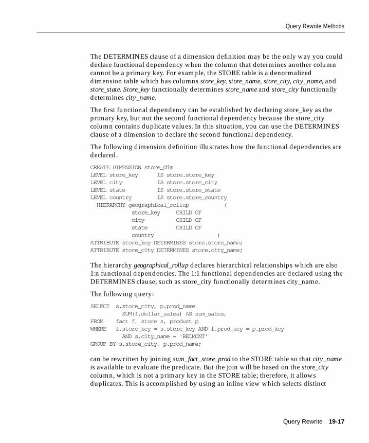
Query Rewrite Methods
The DETERMINES clause of a dimension definition may be the only way you could
declare functional dependency when the column that determines another column
cannot be a primary key. For example, the STORE table is a denormalized
dimension table which has columns store_key, store_name, store_city, city_name, and
store_state. Store_key functionally determines store_name and store_city functionally
determines city_name.
The first functional dependency can be established by declaring store_key as the
primary key, but not the second functional dependency because the store_city
column contains duplicate values. In this situation, you can use the DETERMINES
clause of a dimension to declare the second functional dependency.
The following dimension definition illustrates how the functional dependencies are
declared.
CREATE DIMENSION store_dimLEVEL store_key IS store.store_keyLEVEL city IS store.store_cityLEVEL state IS store.store_stateLEVEL country IS store.store_country HIERARCHY geographical_rollup ( store_key CHILD OF city CHILD OF state CHILD OF country )ATTRIBUTE store_key DETERMINES store.store_name;ATTRIBUTE store_city DETERMINES store.city_name;
The hierarchy geographical_rollup declares hierarchical relationships which are also
1:n functional dependencies. The 1:1 functional dependencies are declared using the
DETERMINES clause, such as store_city functionally determines city_name.
The following query:
SELECT s.store_city, p.prod_name SUM(f.dollar_sales) AS sum_sales,FROM fact f, store s, product pWHERE f.store_key = s.store_key AND f.prod_key = p.prod_key AND s.city_name = 'BELMONT'GROUP BY s.store_city, p.prod_name;
can be rewritten by joining sum_fact_store_prod to the STORE table so that city_nameis available to evaluate the predicate. But the join will be based on the store_citycolumn, which is not a primary key in the STORE table; therefore, it allows
duplicates. This is accomplished by using an inline view which selects distinct
Query Rewrite 19-17

Query Rewrite Methods
values and this view is joined to the materialized view as shown in the rewritten
query below.
SELECT iv.store_city, mv.prod_name, mv.sum_salesFROM sum_fact_store_prod mv, (SELECT DISTINCT store_city, city_name FROM store) ivWHERE mv.store_city = iv.store_city AND iv.city_name = 'BELMONT'GROUP BY iv.store_city, mv.prod_name;
This type of rewrite is possible because of the fact that store_city functionally
determines city_name as declared in the dimension.
Grouping Compatibility CheckThis check is required only if both the materialized view and the query contain a
GROUP BY clause. The optimizer first determines if the grouping of data requested
by a query is exactly the same as the grouping of data stored in a materialized view.
In other words, the level of grouping is the same in both the query and the
materialized view. For example, a query requests data grouped by store_city and a
materialized view stores data grouped by store_city and store_state. The grouping is
the same in both provided store_city functionally determines store_state, such as the
functional dependency shown in the dimension example above.
If the grouping of data requested by a query is at a coarser level compared to the
grouping of data stored in a materialized view, the optimizer can still use the
materialized view to rewrite the query. For example, the materialized view
sum_fact_store_time_prod groups by store_name, time_week, and prod_key. This query
groups by store_name, a coarser grouping granularity:
SELECT s.store_name, SUM(f.dollar_sales) AS sum_sales,FROM fact f, store sWHERE f.store_key = s.store_keyGROUP BY s.store_name;
Therefore, the optimizer will rewrite this query as:
SELECT store_name, SUM(sum_dollar_sales) AS sum_sales,FROM sum_fact_store_time_prodGROUP BY s.store_name;
In another example, a query requests data grouped by store_state whereas a
materialized view stores data grouped by store_city. If store_city is a CHILD OF
store_state (see the dimension example above), the grouped data stored in the
materialized view can be further grouped by store_state when the query is rewritten.
19-18 Oracle8i Data Warehousing Guide

Query Rewrite Methods
In other words, aggregates at store_city level (finer granularity) stored in a
materialized view can be rolled up into aggregates at store_state level (coarser
granularity).
For example, consider the following query:
SELECT store_state, prod_name, SUM(f.dollar_sales) AS sum_salesFROM fact f, store s, product pWHERE f.store_key = s.store_key AND f.prod_key = p.prod_keyGROUP BY store_state, prod_name;
Because store_city functionally determines store_state, sum_fact_store_prod can be
used with a joinback to store table to retrieve store_state column data, and then
aggregates can be rolled up to store_state level, as shown below:
SELECT store_state, prod_name, sum(mv.sum_sales) AS sum_salesFROM sum_fact_store_prod mv, (SELECT DISTINCT store_city, store_state FROM store) ivWHERE mv.store_city = iv.store_cityGROUP BY store_state, prod_name;
Note that for this rewrite, the data sufficiency check determines that a joinback to
the STORE table is necessary, and the grouping compatibility check determines that
aggregate rollup is necessary.
Aggregate Computability CheckThis check is required only if both the query and the materialized view contain
aggregates. Here the optimizer determines if the aggregates requested by a query
can be derived or computed from one or more aggregates stored in a materialized
view. For example, if a query requests AVG(X) and a materialized view contains
SUM(X) and COUNT(X), then AVG(X) can be computed as SUM(X) / COUNT(X).
If the grouping compatibility check determined that the rollup of aggregates stored
in a materialized view is required, then the aggregate computability check
determines if it is possible to roll up each aggregate requested by the query using
aggregates in the materialized view.
For example, SUM(sales) at the city level can be rolled up to SUM(sales) at the state
level by summing all SUM(sales) aggregates in a group with the same state value.
However, AVG(sales) cannot be rolled up to a coarser level unless COUNT(sales) is
also available in the materialized view. Similarly, VARIANCE(sales) or
STDDEV(sales) cannot be rolled up unless COUNT(sales) and SUM(sales) are also
available in the materialized view. For example, given the query:
Query Rewrite 19-19

Query Rewrite Methods
SELECT p.prod_name, AVG(f.dollar_sales) AS avg_salesFROM fact f, product pWHERE f.prod_key = p.prod_keyGROUP BY p.prod_name;
The materialized view sum_fact_store_prod can be used to rewrite it provided the
join between FACT and STORE is lossless and non-duplicating. Further, the query
groups by prod_name whereas the materialized view groups by store_city, prod_name,
which means the aggregates stored in the materialized view will have to be rolled
up. The optimizer will rewrite the query as:
SELECT mv.prod_name, SUM(mv.sum_sales)/SUM(mv.count_sales) AS avg_salesFROM sum_fact_store_prod mvGROUP BY mv.prod_name;
The argument of an aggregate such as SUM can be an arithmetic expression like
A+B. The optimizer will try to match an aggregate SUM(A+B) in a query with an
aggregate SUM(A+B) or SUM(B+A) stored in a materialized view. In other words,
expression equivalence is used when matching the argument of an aggregate in a
query with the argument of a similar aggregate in a materialized view. To
accomplish this, Oracle converts the aggregate argument expression into a
canonical form such that two different but equivalent expressions convert into the
same canonical form. For example, A*(B-C), A*B-C*A, (B-C)*A, and -A*C+A*B all
convert into the same canonical form and, therefore, they are successfully matched.
Query Rewrite with CUBE/ROLLUP OperatorA query that contains GROUP BY CUBE or GROUP BY ROLLUP clauses can be
rewritten in terms of a materialized view as long as the grouping of the query is
compatible with the grouping in a materialized view. For example, consider the
following query:
SELECT store_city, prod_name, AVG(f.dollar_sales) AS avg_salesFROM fact f, store s, product pWHERE f.store_key = s.store_key AND f.prod_key = p.prod_keyGROUP BY CUBE(store_city, prod_name);
This query can be rewritten in terms of the materialized view sum_fact_store_prod
as follows:
SELECT store_city, prod_name, SUM(sum_sales)/SUM(count_sales) AS avg_salesFROM sum_fact_store_prodGROUP BY CUBE (store_city, prod_name);
19-20 Oracle8i Data Warehousing Guide

When are Constraints and Dimensions Needed?
Note that the grouping in sum_fact_store_prod matches with the grouping in the
query. However, the query requires a cube result which means super aggregates
should be computed from the base aggregates available from the materialized view.
This is accomplished by retaining the GROUP BY CUBE clause in the rewritten
query.
A cube or rollup query can be also rewritten in terms of a materialized view which
groups data at a finer granularity level. In this type of rewrite, the rewritten query
will compute both the base aggregates (from finer to coarser granularity level) and
the super aggregates.
When are Constraints and Dimensions Needed?To clarify when dimensions and constraints are required for the different types of
query rewrite, refer to Table 19–2.
Complex Materialized ViewsRewrite capability with complex materialized views is limited to SQL text
match-based rewrite (partial or full). A materialized view can be defined using
arbitrarily complex SQL query expressions, but such a materialized view is treated
as complex by query rewrite. For example, some of the constructs that make a
materialized view complex are: selection predicates in the WHERE clause, a
HAVING clause, inline views, multiple instances of same table or view, set
operators (UNION, UNION ALL, INTERSECT, MINUS), START WITH clause,
CONNECT BY clause, etc. Therefore, a complex materialized view limits
rewritability but can be used to rewrite specific queries that are highly complex and
execute very slowly.
Table 19–2 Dimension and Constraint Requirements for Query Rewrite
Rewrite Checks DimensionsPrimary Key/Foreign Key/NotNull Constraints
Matching SQL Text Not Required Not Required
Join Compatibility Not Required Required
Data Sufficiency Required OR Required
Grouping Compatibility Required Required
Aggregate Computability Not Required Not Required
Query Rewrite 19-21

When are Constraints and Dimensions Needed?
View-based Materialized ViewA view-based materialized view contains one or more named views in the FROM
clause of its SQL expression. Such a materialized view is subject to some important
query rewrite restrictions. In order for the view-based materialized view to be
eligible to rewrite a query, all views referenced in it must also be referenced in the
query. However, the query can have additional views and this will not make a
view-based materialized view ineligible.
Another important restriction with view-based materialized views is related to the
determination of the lossless joins. Any join based on view columns in a view-based
materialized view is considered a lossy join by the join compatibility check. This
means that if there are some delta joins in a view-based materialized view and if at
least one of the delta joins is based on view columns, the join compatibility check
will fail.
View-based materialized views are useful when you want to materialize only a
subset of table data. For example, if you want to summarize the data only for the
year 1996 and store it in a materialized view, it can be done in two ways.
■ Define a materialized view with a selection predicate year=1996 in the WHERE
clause. This makes the materialized view complex so only SQL text match
rewrite is possible.
■ Define a regular view with a selection predicate year=1996 and then define a
materialized view on this view. This produces a view-based materialized view
for which both SQL text match and general query rewrite methods can be used.
Rewrite with Nested Materialized ViewsQuery rewrite is attempted recursively to take advantage of nested materialized
views. Oracle first tries to rewrite a query Q with a materialized view having
aggregates and joins, then with a materialized join view. If any of the rewrites
succeeds, Oracle repeats that process again until no rewrites have occurred.
For example, assume that you had created materialized views join_fact_store_timeand sum_sales_store_time as in "Example of a Nested Materialized View" on
page 8-26.
Consider this query:
SELECT store_name, time_day, SUM(dollar_sales)FROM fact f, store s, time tWHERE f.time_key = t.time_key AND f.store_key = s.store_keyGROUP BY store_name, time_day;
19-22 Oracle8i Data Warehousing Guide

Expression Matching
Oracle first tries to rewrite it with a materialized aggregate view and finds there is
none eligible (note that single-table aggregate materialized view,
sum_sales_store_time cannot yet be used), and then tries a rewrite with a
materialized join view and finds that join_fact_store_time is eligible for rewrite. The
rewritten query has this form:
SELECT store_name, time_day, SUM(dollar_sales)FROM join_fact_store_timeGROUP BY store_name, time_day;
Because a rewrite occurred, Oracle tries the process again. This time the above
query can be rewritten with single-table aggregate materialized view
sum_sales_store_time into this form:
SELECT store_name, time_day, sum_salesFROM sum_sales_store_time;
Expression MatchingAn expression that appears in a query can be replaced with a simple column in a
materialized view provided the materialized view column represents a
precomputed expression that matches with the expression in the query. Because a
materialized view stores pre-computed results of an expression, any query that is
rewritten to use such a materialized view will benefit through performance
improvement achieved by obviating the need for expression computation.
The expression matching is done by first converting the expressions into canonical
forms and then comparing them for equality. Therefore, two different expressions
will be matched as long as they are equivalent to each other. Further, if the entire
expression in a query fails to match with an expression in a materialized view, then
subexpressions of it are tried to find a match. The subexpressions are tried in a
top-down order to get maximal expression matching.
Consider a query that asks for sum of sales by age brackets (1-10, 11-20, 21-30,...).
SELECT (age+9)/10 AS age_bracket, SUM(sales) AS sum_salesFROM fact, customerWHERE fact.cust_id = customer.cust_idGROUP BY (age+9)/10;
Assume that there is a materialized view MV1 that summarizes sales by same age
brackets as shown below:
CREATE MATERIALIZED VIEW sum_sales_mv
Query Rewrite 19-23

Expression Matching
ENABLE QUERY REWRITEASSELECT (9+age)/10 AS age_bracket, SUM(sales) AS sum_salesFROM fact, customerWHERE fact.cust_id = customer.cust_idGROUP BY (9+age)/10;
The above query is rewritten in terms of sum_sales_mv based on the matching of
the canonical forms of the age bracket expressions (i.e. (9+age)/10 and (age+9)/10)
as follows.
SELECT age_bracket, sum_salesFROM sum_sales_mv;
Date FoldingDate folding rewrite is a specific form of expression matching rewrite. In this type
of rewrite, a date range in a query is folded into an equivalent date range
representing higher date granules. The resulting expressions representing higher
date granules in the folded date range are matched with equivalent expressions in a
materialized view. The folding of date range into higher date granules such as
months, quarters, or years is done when the underlying datatype of the column is
an Oracle DATE. The expression matching is done based on the use of canonical
forms for the expressions.
DATE is a built-in datatype which represents ordered time units such as seconds,
days, and months, and incorporates a time hierarchy (second -> minute -> hour ->
day -> month -> quarter -> year). This hard-coded knowledge about DATE is used
in folding date ranges from lower-date granules to higher-date granules.
Specifically, folding a date value to the beginning of a month, quarter, year, or to the
end of a month, quarter, year is supported. For example, the date value '1-jan-1999'
can be folded into the beginning of either year '1999' or quarter '1999-1' or month
'1999-01'. And, the date value '30-sep-1999' can be folded into the end of either
quarter '1999-03' or month '1999-09'.
Because date values are ordered, any range predicate specified on date columns can
be folded from lower level granules into higher level granules provided the date
range represents an integral number of higher level granules. For example, the
range predicate date_col BETWEEN '1-jan-1999' AND '30-jun-1999' can be folded
into either a month range or a quarter range using the TO_CHAR function, which
extracts specific date components from a date value.
The advantage of aggregating data by folded date values is the compression of data
achieved. Without date folding, the data is aggregated at the lowest granularity
19-24 Oracle8i Data Warehousing Guide

Expression Matching
level, resulting in increased disk space for storage and increased I/O to scan the
materialized view.
Consider a query that asks for the sum of sales by product types for the years 1991,
1992, 1993.
SELECT prod_type, sum(sales) AS sum_salesFROM fact, productWHERE fact.prod_id = product.prod_id AND sale_date BETWEEN '1-jan-1991' AND '31-dec-1993'GROUP BY prod_type;
The date range specified in the query represents an integral number of years,
quarters, or months. Assume that there is a materialized view MV3 that contains
pre-summarized sales by prod_type and is defined as follows:
CREATE MATERIALIZED VIEW MV3 ENABLE QUERY REWRITEASSELECT prod_type, TO_CHAR(sale_date,'yyyy-mm') AS month, SUM(sales) AS sum_salesFROM fact, productWHERE fact.prod_id = product.prod_idGROUP BY prod_type, TO_CHAR(sale_date, 'yyyy-mm');
The query can be rewritten by first folding the date range into the month range and
then matching the expressions representing the months with the month expression
in MV3. This rewrite is shown below in two steps (first folding the date range
followed by the actual rewrite).
SELECT prod_type, SUM(sales) AS sum_salesFROM fact, productWHERE fact.prod_id = product.prod_id AND TO_CHAR(sale_date, 'yyyy-mm') BETWEEN TO_CHAR('1-jan-1991', 'yyyy-mm') AND TO_CHAR('31-dec-1993', 'yyyy-mm')GROUP BY prod_type;
SELECT prod_type, sum_salesFROM MV3WHERE month BETWEEN TO_CHAR('1-jan-1991', 'yyyy-mm') AND TO_CHAR('31-dec-1993', 'yyyy-mm');GROUP BY prod_type;
If MV3 had pre-summarized sales by prod_type and year instead of prod_type and
month, the query could still be rewritten by folding the date range into year range
and then matching the year expressions.
Query Rewrite 19-25

Accuracy of Query Rewrite
Accuracy of Query RewriteQuery rewrite offers three levels of rewrite integrity that are controlled by the
initialization parameter QUERY_REWRITE_INTEGRITY, which can either be set in
your parameter file or controlled using the ALTER SYSTEM or ALTER SESSION
command. The three values it can take are:
■ ENFORCED
This is the default mode. The optimizer will only use materialized views which
it knows contain fresh data and only use those relationships that are based on
enforced constraints.
■ TRUSTED
In TRUSTED mode, the optimizer trusts that the data in the materialized views
based on prebuilt tables is correct, and the relationships declared in dimensions
and RELY constraints are correct. In this mode, the optimizer uses prebuilt
materialized views, and uses relationships that are not enforced as well as those
that are enforced. In this mode, the optimizer also 'trusts' declared but not
enforced constraints and data relationships specified using dimensions.
■ STALE_TOLERATED
In STALE_TOLERATED mode, the optimizer uses materialized views that are
valid but contain stale data as well as those that contain fresh data. This mode
offers the maximum rewrite capability but creates the risk of generating wrong
results.
If rewrite integrity is set to the safest level, ENFORCED, the optimizer uses only
enforced primary key constraints and referential integrity constraints to ensure that
the results of the query are the same as the results when accessing the detail tables
directly.
If the rewrite integrity is set to levels other than ENFORCED, then there are several
situations where the output with rewrite may be different from that without it.
1. A materialized view can be out of synchronization with the master copy of the
data. This generally happens because the materialized view refresh procedure is
pending following bulk load or DML operations to one or more detail tables of
a materialized view. At some data warehouse sites, this situation is desirable
because it is not uncommon for some materialized views to be refreshed at
certain time intervals.
2. The relationships implied by the dimension objects are invalid. For example,
values at a certain level in a hierarchy do not roll up to exactly one parent value.
19-26 Oracle8i Data Warehousing Guide
Did Query Rewrite Occur?
3. The values stored in a PREBUILT materialized view table may be incorrect.
4. Partition operations such as DROP and MOVE PARTITION on the detail table
could affect the results of the materialized view.
Did Query Rewrite Occur?Since query rewrite occurs transparently, special steps have to be taken to verify
that a query has been rewritten. Of course, if the query runs faster, this should
indicate that rewrite has occurred but that is not proof. Therefore, to confirm that
query rewrite does occur, use the EXPLAIN PLAN statement.
Explain PlanThe EXPLAIN PLAN facility is used as described in Oracle8i SQL Reference. For
query rewrite, all you need to check is that the object_name column in PLAN_TABLE
contains the materialized view name. If it does, then query rewrite will occur when
this query is executed.
In this example, the materialized view store_mv has been created.
CREATE MATERIALIZED VIEW store_mv ENABLE QUERY REWRITE AS SELECT s.region, SUM(grocery_sq_ft) AS sum_floor_plan FROM store s GROUP BY s.region;
If EXPLAIN PLAN is used on this SQL statement, the results are placed in the
default table PLAN_TABLE.
EXPLAIN PLANFORSELECT s.region, SUM(grocery_sq_ft)FROM store sGROUP BY s.region;
For the purposes of query rewrite, the only information of interest from
PLAN_TABLE is the OBJECT_NAME, which identifies the objects that will be used
to execute this query. Therefore, you would expect to see the object name
STORE_MV in the output as illustrated below.
Query Rewrite 19-27

Did Query Rewrite Occur?
SELECT object_name FROM plan_table;
OBJECT_NAME------------------------------STORE_MV
2 rows selected.
Controlling Query RewriteA materialized view is only eligible for query rewrite if the ENABLE QUERY
REWRITE clause has been specified, either initially when the materialized view was
first created or subsequently via an ALTER MATERIALIZED VIEW command.
The initialization parameters described above can be set using the ALTER SYSTEM
SET command. For a given user's session, ALTER SESSION can be used to disable
or enable query rewrite for that session only. For example:
ALTER SESSION SET QUERY_REWRITE_ENABLED = TRUE;
The correctness of query rewrite can be set for a session, thus allowing different
users to work at different integrity levels.
ALTER SESSION SET QUERY_REWRITE_INTEGRITY = STALE_TOLERATED;ALTER SESSION SET QUERY_REWRITE_INTEGRITY = TRUSTED;ALTER SESSION SET QUERY_REWRITE_INTEGRITY = ENFORCED;
Rewrite HintsHints may be included in SQL statements to control whether query rewrite occurs.
Using the NOREWRITE hint in a query prevents the optimizer from rewriting it.
The REWRITE hint with no argument in a query forces the optimizer to use a
materialized view (if any) to rewrite it regardless of the cost.
The REWRITE (mv1, mv2, ...) hint with argument(s) forces rewrite to select the most
suitable materialized view from the list of names specified.
For example, to prevent a rewrite, you can use:
SELECT /*+ NOREWRITE */ s.city, SUM(s.grocery_sq_ft)FROM store sGROUP BY s.city;
To force a rewrite using mv1, you can use:
19-28 Oracle8i Data Warehousing Guide

Guidelines for Using Query Rewrite
SELECT /*+ REWRITE (mv1) */ s.city, SUM(s.grocery_sq_ft)FROM store sGROUP BY s.city;
Note that the scope of a rewrite hint is a query block. If a SQL statement consists of
several query blocks (SELECT clauses), you may need to specify rewrite hint on
each query block to control the rewrite for the entire statement.
Guidelines for Using Query RewriteThe following guidelines will help in getting the maximum benefit from query
rewrite. They are not mandatory for using query rewrite and rewrite is not
guaranteed if you follow them. They are general rules of thumb.
ConstraintsMake sure all inner joins referred to in a materialized view have referential integrity
(foreign key - primary key constraints) with additional NOT NULL constraints on
the foreign key columns. Since constraints tend to impose a large overhead, you
could make them NONVALIDATE and RELY and set the parameter
QUERY_REWRITE_INTEGRITY to STALE_TOLERATED or TRUSTED. However, if
you set QUERY_REWRITE_INTEGRITY to ENFORCED, all constraints must be
enforced to get maximum rewritability.
DimensionsYou can express the hierarchical relationships and functional dependencies in
normalized or denormalized dimension tables using the HIERARCHY and
DETERMINES clauses of a dimension. Dimensions can express intra-table
relationships which cannot be expressed by any constraints. Set the parameter
QUERY_REWRITE_INTEGRITY to TRUSTED or STALE_TOLERATED for query
rewrite to take advantage of the relationships declared in dimensions.
Outer JoinsAnother way of avoiding constraints is to use outer joins in the materialized view.
Query rewrite will be able to derive an inner join in the query, such as (A.a = B.b),
from an outer join in the materialized view (A.a = B.b(+)), as long as the rowid of B
or column B.b is available in the materialized view. Most of the support for rewrites
with outer joins is provided for materialized views with joins only. To exploit it, a
materialized view with outer joins should store the rowid or primary key of the
Query Rewrite 19-29

Guidelines for Using Query Rewrite
inner table of an outer join. For example, the materialized view
join_fact_store_time_oj stores the primary keys store_key and time_key of the inner
tables of outer joins.
SQL Text MatchIf you need to speed up an extremely complex, long-running query, you could
create a materialized view with the exact text of the query.
AggregatesIn order to get the maximum benefit from query rewrite, make sure that all
aggregates which are needed to compute ones in the targeted set of queries are
present in the materialized view. The conditions on aggregates are quite similar to
those for incremental refresh. For instance, if AVG(x) is in the query, then you
should store COUNT(x) and AVG(x) or store SUM(x) and COUNT(x) in the
materialized view. Refer to Requirements for Fast Refresh in "General Restrictions
on Fast Refresh" on page 8-20.
Grouping ConditionsAggregating data at lower levels in the hierarchy is better than aggregating at
higher levels because lower levels can be used to rewrite more queries. Note,
however, that doing so will also take up more space. For example, instead of
grouping on state, group on city (unless space constraints prohibit it).
Instead of creating multiple materialized views with overlapping or hierarchically
related GROUP BY columns, create a single materialized view with all those
GROUP BY columns. For example, instead of using a materialized view that groups
by city and another materialized view that groups by month, use a materialized
view that groups by city and month.
Use GROUP BY on columns which correspond to levels in a dimension but not on
columns that are functionally dependent, because query rewrite will be able to use
the functional dependencies automatically based on the DETERMINES clause in a
dimension. For example, instead of grouping on city_name, group on city_id (as
long as there is a dimension which indicates that the attribute city_id determines
city_name, you will enable the rewrite of a query involving city_name).
19-30 Oracle8i Data Warehousing Guide

Guidelines for Using Query Rewrite
Expression MatchingIf several queries share the same common subexpression, it is advantageous to
create a materialized view with the common subexpression as one of its SELECT
columns. This way, the performance benefit due to precomputation of the common
subexpression can be obtained across several queries.
Date FoldingWhen creating a materialized view which aggregates data by folded date granules
such as months or quarters or years, always use the year component as the prefix
but not as the suffix. For example, TO_CHAR(date_col, 'yyyy-q') folds the date into
quarters, which collate in year order, whereas TO_CHAR(date_col, 'q-yyyy') folds
the date into quarters, which collate in quarter order. The former preserves the
ordering while the latter does not. For this reason, any materialized view created
without a year prefix will not be eligible for date folding rewrite.
StatisticsOptimization with materialized views is based on cost and the optimizer needs
statistics of both the materialized view and the tables in the query to make a
cost-based choice. Materialized views should thus have statistics collected using
either the ANALYZE TABLE statement or the DBMS_STATISTICS package.
Query Rewrite 19-31

Guidelines for Using Query Rewrite
19-32 Oracle8i Data Warehousing Guide

PartVI
MiscellaneousThis section deals with other topics of interest in a data warehousing environment.
It contains the following chapters:
■ Data Marts


20
Data MartsThis chapter contains information useful for building and using data marts,
including:
■ What Is a Data Mart?
This chapter is not meant to be a substitute for other Oracle or non-Oracle
documentation regarding data marts. It is simply an overview. See the Data MartSuites documentation for further details.
Data Marts 20-1

What Is a Data Mart?
What Is a Data Mart?A data mart is a simple form of a data warehouse that is focused on a single subject
(or functional area), such as Sales or Finance or Marketing. Data marts are often
built and controlled by a single department within an organization. Given their
single-subject focus, data marts usually draw data from only a few sources. The
sources could be internal operational systems, a central data warehouse, or external
data.
How Is It Different from a Data Warehouse?A data warehouse, in contrast, deals with multiple subject areas and is typically
implemented and controlled by a central organizational unit such as the Corporate
Information Technology (IT) group. Often, it is called a central or enterprise data
warehouse. Typically, a data warehouse assembles data from multiple source
systems.
Nothing in these basic definitions limits the size of a data mart or the complexity of
the decision-support data that it contains. Nevertheless, data marts are typically
smaller and less complex than data warehouses; hence, they are typically easier to
build and maintain. The following table summarizes the basic differences between a
data warehouse and a data mart:
Dependent, Independent, and Hybrid Data MartsThree basic types of data marts are dependent, independent, and hybrid. The
categorization is based primarily on the data source that feeds the data mart.
Dependent data marts draw data from a central data warehouse that has already been
created. Independent data marts, in contrast, are standalone systems built by drawing
data directly from operational or external sources of data or both. Hybrid data martscan draw data from operational systems or data warehouses.
Data Warehouse Data Mart
Scope Corporate Line-of-Business (LoB)
Subjects Multiple Single Subject
Data Sources Many Few
Size (typical) 100 GB-TB+ < 100GB
Implementation Time Months to years Months
20-2 Oracle8i Data Warehousing Guide

What Is a Data Mart?
Dependent Data MartsA dependent data mart allows you to unite your organization’s data in one data
warehouse. This gives you the usual advantages of centralization. Figure 20–1
illustrates a dependent data mart.
Figure 20–1 Dependent Data Mart
Independent Data MartsAn independent data mart is created without the use of a central data warehouse.
This could be desirable for smaller groups within an organization. It is not,
however, the focus of this Guide. See the Data Mart Suites documentation for further
details regarding this architecture. Figure 20–2 illustrates an independent data mart.
Enterprise datawarehouse
Operational sources
Dependent departmentaldatamarts
Data Marts 20-3

What Is a Data Mart?
Figure 20–2 Independent Data Marts
Hybrid Data MartsA hybrid data mart allows you to combine input from sources other than a data
warehouse. This could be useful for many situations, especially when you need ad
hoc integration, such as after a new group or product is added to the organization.
Figure 20–3 illustrates a hybrid data mart.
Operational sources
Independentdatamarts
20-4 Oracle8i Data Warehousing Guide

What Is a Data Mart?
Figure 20–3 Hybrid Data Mart
Extraction, Transformation, and TransportationThe main difference between independent and dependent data marts is how you
populate the data mart; that is, how you get data out of the sources and into the
data mart. This step, called the Extraction-Transformation-Transportation (ETT)
process, involves moving data from operational systems, filtering it, and loading it
into the data mart.
With dependent data marts, this process is somewhat simplified because formatted
and summarized (clean) data has already been loaded into the central data
warehouse. The ETT process for dependent data marts is mostly a process of
identifying the right subset of data relevant to the chosen data mart subject and
moving a copy of it, perhaps in a summarized form.
With independent data marts, however, you must deal with all aspects of the ETT
process, much as you do with a central data warehouse. The number of sources are
likely to be fewer and the amount of data associated with the data mart is less than
the warehouse, given your focus on a single subject.
Enterprise datawarehouse
Operational sources
Dependent departmentaldatamarts
3
2
1
Data Marts 20-5

What Is a Data Mart?
The motivations behind the creation of these two types of data marts are also
typically different. Dependent data marts are usually built to achieve improved
performance and availability, better control, and lower telecommunication costs
resulting from local access of data relevant to a specific department. The creation of
independent data marts is often driven by the need to have a solution within a
shorter time.
Hybrid data marts simply combine the issues of independent and independent data
marts.
See Chapter 10, "ETT Overview", for further details regarding the ETT process.
20-6 Oracle8i Data Warehousing Guide

Gloss
A
Glossaryadditive
Describes a fact (or measure) that can be summarized through addition. An additive
fact is the most common type of fact. Examples include Sales, Cost, and Profit.
(Contrast with nonadditive, semi-additive.)
advisor
The Summary Advisor recommends which materialized views to retain, create, and
drop. It helps database administrators manage materialized views.
attribute
A descriptive characteristic of one or more levels. Attributes represent logical
groupings that enable end users to select data based on like characteristics. Note
that in relational modeling, an attribute is defined as a characteristic of an entity. In
Oracle 8i, an attribute is a column in a dimension that characterizes elements of a
single level.
aggregation
The process of consolidating data values into a single value. For example, sales data
could be collected on a daily basis and then be aggregated to the week level, the
week data could be aggregated to the month level, and so on. The data can then be
referred to as aggregate data. Aggregation is synonymous with summarization, and
aggregate data is synonymous with summary data.
aggregate
Summarized data. For example, unit sales of a particular product could be
aggregated by day, month, quarter and yearly sales.
ary A-1

ancestor
A value at any level above a given value in a hierarchy. For example, in a Time
dimension, the value “1999” might be the ancestor of the values “Q1-99” and
“Jan-99.” (See also descendant, hierarchy, level.)
attribute
A descriptive characteristic of one or more levels. For example, the Product
dimension for a clothing manufacturer might contain a level called Item, one of
whose attributes is Color. Attributes represent logical groupings that enable end
users to select data based on like characteristics.
Note that in relational modeling, an attribute is defined as a characteristic of an
entity. In Oracle 8i, an attribute is a column in a dimension that characterizes
elements of a single level.
child
A value at the level below a given value in a hierarchy. For example, in a Time
dimension, the value “Jan-99” might be the child of the value “Q1-99.” A value can
be a child for more than one parent if the child value belongs to multiple
hierarchies. (See also hierarchy, level, parent.)
cleansing
The process of resolving inconsistencies and fixing the anomalies in source data,
typically as part of the ETT process. (See also ETT.)
Common Warehouse Metadata (CWM)
A repository standard used by Oracle data warehousing, decision support, and
OLAP tools including Oracle Warehouse Builder. The CWM repository schema is a
stand-alone product that other products can share—each product owns only the
objects within the CWM repository that it creates.
data source
A database, application, repository, or file that contributes data to a warehouse.
data mart
A data warehouse that is designed for a particular line of business, such as sales,
marketing, or finance. In a dependent data mart, the data can be derived from an
enterprise-wide data warehouse. In an independent data mart, data can be collected
directly from sources. (See also data warehouse.)
A-2 Oracle8i Data Warehousing Guide

data warehouse
A relational database that is designed for query and analysis rather than transaction
processing. A data warehouse usually contains historical data that is derived from
transaction data, but it can include data from other sources. It separates analysis
workload from transaction workload and enables a business to consolidate data
from several sources.
In addition to a relational database, a data warehouse environment often consists of
an ETT solution, an OLAP engine, client analysis tools, and other applications that
manage the process of gathering data and delivering it to business users. (See also
ETT, OLAP.)
denormalize
The process of allowing redundancy in a table so that it can remain flat. (Contrast
with normalize.)
derived fact (or measure)
A fact (or measure) that is generated from existing data using a mathematical
operation or a data transformation. Examples include averages, totals, percentages,
and differences.
dimension
A structure, often composed of one or more hierarchies, that categorizes data.
Several distinct dimensions, combined with measures, enable end users to answer
business questions. Commonly used dimensions are Customer, Product, and Time.
In Oracle 8i, a dimension is a database object that defines hierarchical (parent/child)
relationships between pairs of column sets. In Oracle Express, a dimension is a
database object that consists of a list of values.
dimension value
One element in the list that makes up a dimension. For example, a computer
company might have dimension values in the Product dimension called “LAPPC”
and “DESKPC.” Values in the Geography dimension might include “Boston” and
“Paris.” Values in the Time dimension might include “MAY96” and “JAN97.”
drill
To navigate from one item to a set of related items. Drilling typically involves
navigating up and down through the levels in a hierarchy. When selecting data, you
can expand or collapse a hierarchy by drilling down or up in it, respectively. (See
also drill down, drill up.)
Glossary A-3

drill down
To expand the view to include child values that are associated with parent values in
the hierarchy. (See also drill, drill up.)
drill up
To collapse the list of descendant values that are associated with a parent value in
the hierarchy.
element
An object or process. For example, a dimension is an object, a mapping is a process,
and both are elements.
ETT
Extraction, transformation, and transportation. ETT refers to the methods involved
in accessing and manipulating source data and loading it into a data warehouse.
The order in which these processes are performed varies.
Note that ETL (extraction, transformation, load) and ETM (extraction,
transformation, move) are sometimes used instead of ETT. (See also data warehouse,extraction, transformation, transportation.)
extraction
The process of taking data out of a source as part of an initial phase of ETT. (See also
ETT.)
fact table
A table in a star schema that contains facts. A fact table typically has two types of
columns: those that contain facts and those that are foreign keys to dimension
tables. The primary key of a fact table is usually a composite key that is made up of
all of its foreign keys.
A fact table might contain either detail level facts or facts that have been aggregated
(fact tables that contain aggregated facts are often instead called summary tables). A
fact table usually contains facts with the same level of aggregation.
fact/measure
Data, usually numeric and additive, that can be examined and analyzed. Values for
facts or measures are usually not known in advance; they are observed and stored.
Examples include Sales, Cost, and Profit. Fact and measure are synonymous; fact ismore commonly used with relational environments, measure is more commonly
used with multidimensional environments. (See also derived fact.)
A-4 Oracle8i Data Warehousing Guide

fast refresh
An operation that applies only the data changes to a materialized view, thus
eliminating the need to rebuild the materialized view from scratch.
file-to-table mapping
Maps data from flat files to tables in the warehouse.
hierarchy
A logical structure that uses ordered levels as a means of organizing data. A
hierarchy can be used to define data aggregation; for example, in a Time dimension,
a hierarchy might be used to aggregate data from the “Month” level to the
“Quarter” level to the “Year” level. A hierarchy can also be used to define a
navigational drill path, regardless of whether the levels in the hierarchy represent
aggregated totals. (See also dimension, level.)
hub module
The metadata container for process data.
level
A position in a hierarchy. For example, a Time dimension might have a hierarchy
that represents data at the “Month,” “Quarter,” and “Year” levels.
(See also hierarchy.)
level value table
A database table that stores the values or data for the levels you created as part of
your dimensions and hierarchies.
mapping
The definition of the relationship and data flow between source and target objects.
materialized view
A pre-computed table comprising aggregated and/or joined data from fact and
possibly dimension tables. Also known as a summary or aggregation.
metadata
Data that describes data and other structures, such as objects, business rules, and
processes. For example, the schema design of a data warehouse is typically stored in
a repository as metadata, which is used to generate scripts used to build and
populate the data warehouse. A repository contains metadata.
Glossary A-5

Examples include: for data, the definition of a source to target transformation that is
used to generate and populate the data warehouse; for information, definitions of
tables, columns and associations that are stored inside a relational modeling tool;
for business rules, discount by 10 percent after selling 1,000 items.
model
An object that represents something to be made. A representative style, plan, or
design. Metadata that defines the structure of the data warehouse.
nonadditive
Describes a fact (or measure) that cannot be summarized through addition. An
example includes Average. (Contrast with additive, semi-additive.)
normalize
In a relational database, the process of removing redundancy in data by separating
the data into multiple tables. (Contrast with denormalize.)
The process of removing redundancy in data by separating the data into multiple
tables. (Kimball)
operational data store (ODS)
The cleaned, transformed data from a particular source database.
OLAP
Online analytical processing. OLAP functionality is characterized by dynamic,
multidimensional analysis of historical data, which supports activities such as the
following:
• Calculating across dimensions and through hierarchies
• Analyzing trends
• Drilling up and down through hierarchies
• Rotating to change the dimensional orientation
OLAP tools can run against a multidimensional database or interact directly with a
relational database.
parent
A value at the level above a given value in a hierarchy. For example, in a Time
dimension, the value “Q1-99” might be the parent of the value “Jan-99.” (See also
child, hierarchy, level.)
A-6 Oracle8i Data Warehousing Guide

refresh
The mechanism whereby materialized views are populated with data.
schema
A collection of related database objects. Relational schemas are grouped by database
user ID and include tables, views, and other objects. (See also snowflake schema, starschema.)
semi-additive
Describes a fact (or measure) that can be summarized through addition along some,
but not all, dimensions. Examples include Headcount and On Hand Stock.
(Contrast with additive, nonadditive.)
snowflake schema
A type of star schema in which the dimension tables are partly or fully normalized.
(See also schema, star schema.)
source
A database, application, file, or other storage facility from which the data in a data
warehouse is derived.
star schema
A relational schema whose design represents a multidimensional data model. The
star schema consists of one or more fact tables and one or more dimension tables
that are related through foreign keys. (See also schema, snowflake schema.)
subject area
A classification system that represents or distinguishes parts of an organization or
areas of knowledge. A data mart is often developed to support a subject area such
as sales, marketing, or geography. (See also data mart.)
table
A layout of data in columns.
target
Holds the intermediate or final results of any part of the ETT process. The target of
the entire ETT process is the data warehouse. (See also data warehouse, ETT.)
Glossary A-7

transformation
The process of manipulating data. Any manipulation beyond copying is a
transformation. Examples include cleansing, aggregating, and integrating data
from multiple sources.
transportation
The process of moving copied or transformed data from a source to a data
warehouse. (See also transformation.)
validation
The process of verifying metadata definitions and configuration parameters.
versioning
The ability to create new versions of a data warehouse project for new requirements
and changes.
A-8 Oracle8i Data Warehousing Guide

Index
Aadaptive multi-useralgorithm for, 18-6
definition, 18-6
aggregate computability check, 19-19
aggregates, 8-8, 8-11, 18-49, 19-30
ALTER MATERIALIZED VIEW statement, 8-17
enabling query rewrite, 19-5
ALTER TABLE statement
NOLOGGING clause, 18-60
altering dimensions, 9-14
analytic functions, 17-21
ANALYZE statement, 18-51
ANALYZE TABLE statement, 15-3
analyzing data
for parallel processing, 18-69
APPEND hint, 18-60
applications
data warehouses
star queries, 16-2
decision support, 18-2
decision support systems, 6-3
ARCH processes
multiple, 18-56
asynchronous I/O, 18-26
attributes, 9-7
Bbackups
disk mirroring, 4-8
bandwidth, 5-2, 18-2
bitmap indexes, 6-2
nulls and, 6-5
on partitioned tables, 6-6
parallel query and DML, 6-3
block range granules, 5-3
BOTTOM_N function, 17-31
B-tree indexes, 6-6
bitmap indexes versus, 6-3
buffer pools
setting for parallel operations, 18-36
build methods, 8-18
Ccardinality, 6-3
CASE expressions, 17-52
change
capture, 11-6
data capture, 11-6
columns
cardinality, 6-3
common joins, 19-11
COMPATIBLE parameter, 14-13, 19-5
COMPLETE clause, 8-20
complete refresh, 14-18
complex materialized views, 14-27
complex queries
snowflake schemas, 16-3
composite partitioning, 5-6
performance considerations, 5-9
concurrent users
increasing the number of, 18-9
constraints, 7-2, 9-13
foreign key, 7-5
RELY, 7-5
Index-1

unique, 7-3
with partitioning, 7-6
with query rewrite, 19-29
CORR function, 17-48
cost-based optimizations, 18-64
parallel execution, 18-64
star queries, 16-2
cost-based rewrite, 19-3
COVAR_POP function, 17-47
COVAR_SAMP function, 17-48
CPU
utilization, 5-2, 18-2
CREATE DIMENSION statement, 9-6
CREATE INDEX statement, 18-58
CREATE MATERIALIZED VIEW statement, 8-17
enabling query rewrite, 19-5
CREATE SNAPSHOT statement, 8-3
CREATE TABLE AS SELECT statement, 18-50,
18-68
CUBE, 17-10
partial, 17-13
when to use, 17-14
CUBE/ROLLUP
with query rewrite, 19-20
CUME_DIST function, 17-31
Ddata
partitioning, 5-4
purging, 14-7
substitutions, 13-5
sufficiency check, 19-15
data marts
definition of, 20-2
dependent, 20-2
differences from data warehouse, 20-2
independent, 20-2
data warehouses, 8-2
definition of, 20-2
differences from data marts, 20-2
dimension tables
(lookup tables), 8-7
dimensions, 16-2
fact tables (detail tables), 8-7
partitioned tables, 5-6
refresh tips, 14-22
refreshing, 14-2
star queries, 16-2
database writer process (DBWn)
tuning, 18-56
databases
layout, 5-3
staging, 8-2
date folding
with query rewrite, 19-24
DB_BLOCK_SIZE parameter, 18-25
and parallel query, 18-25
DB_FILE_MULTIBLOCK_READ_COUNT
parameter, 18-26
DBA_DATA_FILES view, 18-71
DBA_EXTENTS view, 18-71
DBMS_MVIEW package, 14-18
DBMS_MVIEW.REFRESH procedure, 14-17, 14-19
DBMS_MVIEW.REFRESH_ALL_MVIEWS
procedure, 14-17
DBMS_MVIEW.REFRESH_DEPENDENT
procedure, 14-17
DBMS_OLAP package, 8-35, 15-2, 15-3, 15-5
DBMS_OLAP.RECOMMEND_MV procedure, 8-35
DBMS_STATISTICS package, 19-3
DBMS_STATS package, 15-3
decision support
processes, 18-35
decision support systems
bitmap indexes, 6-3
degree of parallelism
and adaptive multi-user, 18-5
setting, 18-5
DEMO_DIM package, 9-12
denormalized
star schemas, 2-4
DENSE_RANK function, 17-24
dependent data marts, 20-2
detail tables, 8-7
dimension tables, 8-8, 16-2
normalized, 9-10
dimension wizard, 9-11
dimensions, 2-5, 9-2, 9-13
altering, 9-14
Index-2

creating, 9-6
definition, 9-2
dimension tables (lookup tables), 8-7
dropping, 9-15
hierarchies, 2-6
hierarchies overview, 2-6
multiple, 17-2
star joins, 16-3
star queries, 16-2
validating, 9-14
with query rewrite, 19-29
direct-load inserts
external fragmentation, 18-44
disk affinities
and parallel query, 18-47
disabling with MPP, 4-4
with MPP, 18-52
DISK_ASYNCH_IO parameter, 18-26
DML_LOCKS parameter, 18-23, 18-25
drilling across, 9-5
drilling down, 9-3
hierarchies, 9-3
DROP MATERIALIZED VIEW statement, 8-17
prebuilt tables, 8-30
dropping
dimensions, 9-15
materialized views, 8-36
EENFORCED mode, 19-26
ENQUEUE_RESOURCES parameter, 18-23, 18-25
estimating materialized view size, 15-7
ETT
overview, 10-2
process, 7-2, 20-5
tools, 10-2
EVALUATE_UTILIZATION_W package, 15-9
EXCHANGE PARTITION statement, 7-6
execution plans
parallel operations, 18-67
star transformations, 16-8
EXPLAIN PLAN statement, 18-67, 19-27
query parallelization, 18-54
star transformations, 16-8
exporting
EXP utility, 11-4
expression matching
with query rewrite, 19-23
extents
size, 14-13
temporary, 18-52
extractions
data files, 11-2
distributed operations, 11-5
OCI, 11-4
overview, 11-2
Pro*C, 11-4
SQL*Plus, 11-3
Ffact tables, 2-4, 2-5
star joins, 16-3
star queries, 16-2
facts, 9-2
FAST clause, 8-20
fast refresh, 14-18
FAST REFRESH restrictions, 8-20
FAST_START_PARALLEL_ROLLBACK
parameter, 18-23
FIRST_ROWS hint, 18-21
FIRST_VALUE function, 17-42
FORCE clause, 8-20
foreign key constraints, 7-5
foreign key joins
snowflake schemas, 16-3
fragmentation
external, 18-44
FREELISTS parameter, 18-56
full partition-wise joins, 5-12
functions
LAG/LEAD, 17-46
linear regression, 17-48
ranking, 17-24
reporting, 17-43
statistics, 17-46
windowing, 17-35
Index-3

GGC_FILES_TO_LOCKS parameter, 18-44
GC_ROLLBACK_LOCKS parameter, 18-45
GC_ROLLBACK_SEGMENTS parameter, 18-45
global
indexes, 6-6, 18-55
striping, 4-5
granules, 5-3
block range, 5-3
partition, 5-4
GROUP BY clause
decreasing demand for, 18-39
grouping
compatibility check, 19-18
conditions, 19-30
GROUPING function, 17-15
when to use, 17-18
GV$FILESTAT view, 18-70
Hhash areas, 18-35
hash joins, 18-19, 18-35
hash partitioning, 5-5
HASH_AREA_SIZE parameter, 18-39
and parallel execution, 18-18, 18-19
relationship to memory, 18-38
HASH_MULTIBLOCK_IO_COUNT
parameter, 18-26
hierarchies, 9-3
drilling across, 9-5
how used, 2-6
multiple, 9-8
overview, 2-6
rolling up and drilling down, 9-3
hints
query rewrite, 19-5, 19-28
histograms
creating with user-defined buckets, 17-53
II/O
asynchronous, 18-26
parallel execution, 5-2, 18-2
striping to avoid bottleneck, 4-2
independent data marts, 20-2
index joins, 18-39
indexes
bitmap indexes, 6-6
B-tree, 6-6
cardinality, 6-3
creating in parallel, 18-57
global, 18-55
local, 18-55
nulls and, 6-5
parallel creation, 18-57, 18-58
parallel local, 18-58
partitioned tables, 6-6
partitioning, 5-6
STORAGE clause, 18-58
INITIAL extent size, 14-13, 18-44
INSERT
functionality, 18-59
invalidating
materialized views, 8-34
JJOB_QUEUE_INTERVALS parameter, 14-19
JOB_QUEUE_PROCESSES parameter, 14-19
join compatibility, 19-10
joins, 8-11
full partition-wise, 5-12
partial partition-wise, 5-17
partition-wise, 5-12
star joins, 16-3
star queries, 16-2
Kkey lookups, 13-5
keys, 8-8, 16-2
LLAG/LEAD functions, 17-46
LARGE_POOL_SIZE parameter, 18-10
LAST_VALUE function, 17-42
level relationships, 2-7
Index-4

purpose, 2-7
levels, 2-6, 2-7
linear regression functions, 17-48
load
parallel, 14-15
local indexes, 6-3, 6-6, 18-55
local striping, 4-4
LOG_BUFFER parameter
and parallel execution, 18-23
LOGGING clause, 18-56
lookup tables, 8-7, 16-2
star queries, 16-2
Mmanual
refresh, 14-18
striping, 4-3
massively parallel systems, 5-2, 18-2
materialized views
altering, 8-36
build methods, 8-18
complex, 14-27
containing only joins, 8-13
creating, 8-16
delta joins, 19-14
dropping, 8-30, 8-36
estimating size, 15-7
guidelines, 8-35
invalidating, 8-34
joins and aggregates, 8-11
logs, 11-8
naming, 8-17
nested, 8-23
partitioning, 8-31
prebuilt, 8-16
query rewrite
hints, 19-5, 19-28
matching join graphs, 8-18
parameters, 19-5
privileges, 19-6
recommending, 15-5
refresh dependent, 14-21
refreshing, 8-20, 14-16
refreshing all, 14-20
registration, 8-29
restrictions, 8-19
rewrites
enabling, 19-5
schema design guidelines, 8-8
security, 8-35
single table aggregate, 8-12
storage characteristics, 8-17
types of, 8-10
uses for, 8-2
MAXEXTENTS keyword, 14-13, 18-44
measures, 8-7, 16-2
media recoveries, 18-52
memory
configure at 2 levels, 18-17
process classification, 18-35
virtual, 18-18
mirroring
disks, 4-8
monitoring
parallel processing, 18-70
refresh, 14-28
MPP
disk affinity, 4-4
MULTIBLOCK_READ_COUNT parameter, 14-13
multiple archiver processes, 18-56
multiple hierarchies, 9-8
multi-threaded server, 18-35
Nnested loop joins, 18-35
nested materialized views, 8-23
refreshing, 14-26
restrictions, 8-24
nested queries, 18-49
NEVER clause, 8-20
NEXT extent, 18-44
NOAPPEND hint, 18-60
NOARCHIVELOG mode, 18-57
NOLOGGING clause, 18-50, 18-56, 18-58
with APPEND hint, 18-60
NOPARALLEL attribute, 18-48
NOREWRITE hint, 19-5, 19-28
NTILE function, 17-33
Index-5

nulls
indexes and, 6-5
OOLAP tools, 2-5
ON COMMIT clause, 8-20
ON DEMAND clause, 8-20
online transaction processing (OLTP)
processes, 18-35
operating systems
striping, 4-3
optimizations
cost-based
star queries, 16-2
query rewrite
enabling, 19-5
hints, 19-5, 19-28
matching join graphs, 8-18
query rewrites
privileges, 19-6
OPTIMIZER_MODE parameter, 14-28, 18-64, 19-5
OPTIMIZER_PERCENT_PARALLEL
parameter, 14-28, 18-21, 18-67
optimizers
with rewrite, 19-2
Oracle Parallel Server
disk affinities, 18-47
parallel execution, 18-44
parallel load, 14-16
Oracle Trace, 15-3
ORDER BY clause, 8-22
decreasing demand for, 18-39
outer joins
with query rewrite, 19-29
oversubscribing resources, 18-37, 18-41
Ppaging, 18-37
rate, 18-18
subsystem, 18-37
PARALLEL clause, 18-59, 18-60
PARALLEL CREATE INDEX statement, 18-22
PARALLEL CREATE TABLE AS SELECT statement
external fragmentation, 18-44
resources required, 18-22
parallel DML
bitmap indexes, 6-3
parallel execution
adjusting workloads, 18-40
cost-based optimization, 18-64
I/O parameters, 18-25
index creation, 18-57
introduction, 5-2
maximum processes, 18-34
method of, 18-3
parallel server, 18-44
plans, 18-67
process classification, 4-4
resource parameters, 18-17
rewriting SQL, 18-49
solving problems, 18-48
space management, 18-43
tuning, 5-1, 18-2
understanding performance issues, 18-33
PARALLEL hint, 18-48, 18-59, 18-67
parallel load
example, 14-15
Oracle Parallel Server, 14-16
using, 14-10
parallel partition-wise joins
performance considerations, 5-21
parallel query
bitmap indexes, 6-3
parallel scan operations, 4-3
parallel server
disk affinities, 18-47
parallel execution tuning, 18-44
PARALLEL_ADAPTIVE_MULTI_USER
parameter, 18-6, 18-29
PARALLEL_AUTOMATIC_TUNING
parameter, 18-3
PARALLEL_BROADCAST_ENABLE
parameter, 18-21
PARALLEL_EXECUTION_MESSAGE_SIZE
parameter, 18-20
PARALLEL_MAX_SERVERS parameter, 14-27,
18-8, 18-9, 18-38
and parallel execution, 18-8
Index-6

PARALLEL_MIN_PERCENT parameter, 18-9,
18-16
PARALLEL_MIN_SERVERS parameter, 18-10
PARALLEL_SERVER_INSTANCES parameter
and parallel execution, 18-17
PARALLEL_THREADS_PER_CPU
parameter, 18-3, 18-7
parallelism
degree, overriding, 18-48
enabing for tables and queries, 18-6
parameters
COMPATIBLE, 14-13, 19-5
DB_BLOCK_SIZE, 18-25
DB_FILE_MULTIBLOCK_READ_
COUNT, 18-26
DISK_ASYNCH_IO, 18-26
DML_LOCKS, 18-23, 18-25
ENQUEUE_RESOURCES, 18-23, 18-25
FAST_START_PARALLEL_ROLLBACK, 18-23
FREELISTS, 18-56
GC_FILES_TO_LOCKS, 18-44
GC_ROLLBACK_LOCKS, 18-45
GC_ROLLBACK_SEGMENTS, 18-45
HASH_AREA_SIZE, 18-18, 18-38, 18-39
HASH_MULTIBLOCK_IO_COUNT, 18-26
JOB_QUEUE_INTERVAL, 14-19
JOB_QUEUE_PROCESSES, 14-19
LARGE_POOL_SIZE, 18-10
LOG_BUFFER, 18-23
MULTIBLOCK_READ_COUNT, 14-13
OPTIMIZED_PERCENT_PARALLEL, 18-67
OPTIMIZER_MODE, 14-28, 18-64, 19-5
OPTIMIZER_PERCENT_PARALLEL, 14-28,
18-21
PARALLEL_ADAPTIVE_MULTI_USER, 18-29
PARALLEL_AUTOMATIC_TUNING, 18-3
PARALLEL_BROADCAST_ENABLE, 18-21
PARALLEL_EXECUTION_MESSAGE_
SIZE, 18-20
PARALLEL_MAX_SERVERS, 14-27, 18-8, 18-9,
18-38
PARALLEL_MIN_PERCENT, 18-9, 18-16
PARALLEL_MIN_SERVERS, 18-10
PARALLEL_SERVER_INSTANCES, 18-17
PARALLEL_THREADS_PER_CPU, 18-3
QUERY_REWRITE_ENABLED, 19-5
ROLLBACK_SEGMENTS, 18-22
SHARED_POOL_SIZE, 18-10, 18-16
SORT_AREA_SIZE, 14-28, 18-19
SORT_MULTIBLOCK_READ_COUNT, 18-26
STAR_TRANSFORMATION_ENABLED, 16-4
TAPE_ASYNCH_IO, 18-26
TRANSACTIONS, 18-22
UTL_FILE_DIR, 14-19
partial partition-wise joins, 5-17
partition granules, 5-4
partitioned tables
data warehouses, 5-6
example, 14-13
partitioning, 11-7
composite, 5-6
data, 5-4
hash, 5-5
indexes, 5-6
materialized views, 8-31
prebuilt tables, 8-33
range, 5-5
partitions
bitmap indexes, 6-6
pruning, 5-10
partition-wise joins, 5-12
benefits of, 5-20
PCM lock, 18-44
PERCENT_RANK function, 17-33
physical database layouts, 5-3
pivoting, 13-7
plans
star transformations, 16-8
prebuilt materialized views, 8-16
PRIMARY KEY constraints, 18-58
processes
and memory contention in parallel
processing, 18-9
classes of parallel execution, 4-4
DSS, 18-35
maximum number, 18-34
maximum number for parallel query, 18-34
OLTP, 18-35
pruning
partitions, 5-10
Index-7

using DATE columns, 5-11
purging data, 14-7
Qqueries
enabling parallelism for, 18-6
star queries, 16-2
query delta joins, 19-13
query rewrite
controlling, 19-28
correctness, 19-26
enabling, 19-4, 19-5
hints, 19-5, 19-28
matching join graphs, 8-18
methods, 19-8
parameters, 19-5
privileges, 19-6
restrictions, 8-19
when it occurs, 19-6
QUERY_REWRITE_ENABLED parameter, 19-5
RRAID, 4-9, 18-52
range partitioning, 5-5
performance considerations, 5-6
RANK function, 17-24
ranking functions, 17-24
RATIO_TO_REPORT function, 17-45
RECOMMEND_MV function, 15-5
RECOMMEND_MV_W function, 15-5
recovery
media, with striping, 4-8
redo buffer allocation retries, 18-23
redundancy
star schemas, 2-4
reference tables, 8-7
refresh
monitoring, 14-28
options, 8-19
refreshing
materialized views, 14-16
nested materialized views, 14-26
partitioning, 14-2
REGR_AVGX function, 17-49
REGR_AVGY function, 17-49
REGR_COUNT function, 17-49
REGR_INTERCEPT function, 17-49
REGR_R2 function, 17-50
REGR_SLOPE function, 17-49
REGR_SXX function, 17-50
REGR_SXY function, 17-50
REGR_SYY function, 17-50
regression
detecting, 18-66
RELY constraints, 7-5
reporting functions, 17-43
resources
consumption, parameters affecting, 18-17
consumption, parameters affecting parallel
DML/DDL, 18-22
limiting for users, 18-9
limits, 18-8
oversubscribing, 18-37
oversubscription, 18-41
parallel query usage, 18-17
restrictions
FAST REFRESH, 8-20
nested materialized views, 8-24
query rewrite, 8-19
REWRITE hint, 19-5, 19-28
rewrites
hints, 19-28
parameters, 19-5
privileges, 19-6
query optimizations
hints, 19-5, 19-28
matching join graphs, 8-18
rollback segments, 18-22
ROLLBACK_SEGMENTS parameter, 18-22
rolling up hierarchies, 9-3
ROLLUP, 17-6
partial, 17-8
when to use, 17-10
root level, 2-7
ROW_NUMBER function, 17-35
RULE hint, 18-64
Index-8

Ssar UNIX command, 18-75
scalable operations, 18-53
schemas, 16-2
design guidelines for materialized views, 8-8
snowflake, 2-3
star, 2-3
star schemas, 16-2
third-normal form, 16-2
SGA size, 18-18
SHARED_POOL_SIZE parameter, 18-10, 18-16
single table aggregate requirements, 8-13
snowflake schemas, 16-3
complex queries, 16-3
SORT_AREA_SIZE parameter, 14-28, 18-19
and parallel execution, 18-19
SORT_MULTIBLOCK_READ_COUNT
parameter, 18-26
source systems, 11-2
space management, 18-51
parallel execution, 18-43
reducing transactions, 18-44
SQL functions
COUNT, 6-5
SQL Loader, 14-10
SQL text match, 19-8
with query rewrite, 19-30
staging
databases, 8-2
file systems, 4-9
files, 8-2
staging databases, 8-2
STALE_TOLERATED mode, 19-26
star joins, 16-3
star queries, 16-2
star transformation, 16-5
star schemas
advantages, 2-4
defining fact tables, 2-5
dimensional model, 2-3, 16-2
redundancy, 2-4
star transformation, 16-2
star transformations, 16-5
restrictions, 16-9
STAR_TRANSFORMATION_ENABLED
parameter, 16-4
statistics, 19-31
estimating, 18-67
functions, 17-46
operating system, 18-75
STDDEV_POP function, 17-47
STDDEV_SAMP function, 17-47
STORAGE clause
parallel query, 18-58
striping
analyzing, 4-5
and disk affinity, 18-47
example, 14-10
local, 4-4
manual, 4-3
media recovery, 4-8
operating systems, 4-3
temporary tablespace, 18-52
subqueries
correlated, 18-49
summary advisor, 15-2
wizard, 15-8
summary management, 8-5
symmetric multiprocessors, 5-2, 18-2
Ttable queues, 18-71
tables
detail tables, 8-7
dimension tables (lookup tables), 8-7
dimensions
star queries, 16-2
enabling parallelism for, 18-6
fact tables, 8-7
star queries, 16-2
lookup tables (dimension tables), 16-2
tablespaces
creating, example, 14-11
dedicated temporary, 18-51
transportable, 11-5, 12-3
TAPE_ASYNCH_IO parameter, 18-26
temporary extents, 18-52
temporary tablespaces
Index-9

striping, 18-52
third-normal-form schemas, 16-2
TIMED_STATISTICS parameter, 18-71
timestamps, 11-7
TOP_N function, 17-31
transactions
rate, 18-43
TRANSACTIONS parameter, 18-22
transformations, 13-2
SQL and PL/SQL, 13-4
SQL*Loader, 13-3
star, 16-2
transportable tablespaces, 11-5, 12-3
transportation
definition, 12-2
distributed operations, 12-2
flat files, 12-2
triggers, 11-7
TRUSTED mode, 19-26
tuning
parallel execution, 5-3
two-phase commit, 18-22
Uunique constraints, 7-3, 18-58
unusable indexes, 14-17
update frequencies, 8-37
update windows, 8-37
UPSERT statement, 14-5
user resources
limiting, 18-9
UTL_FILE_DIR parameter, 14-19
VV$FILESTAT view
and parallel query, 18-71
V$PARAMETER view, 18-71
V$PQ_SESSTAT view, 18-68, 18-70
V$PQ_SYSSTAT view, 18-68
V$PQ_TQSTAT view, 18-69, 18-71
V$PX_PROCESS view, 18-70
V$PX_SESSION view, 18-70
V$PX_SESSTAT view, 18-70
V$SESSTAT view, 18-72, 18-75
V$SORT_SEGMENT view, 18-44
V$SYSSTAT view, 18-23, 18-56, 18-72
validating dimensions, 9-14
VAR_POP function, 17-47
VAR_SAMP function, 17-47
virtual memory, 18-18
vmstat UNIX command, 18-75
Wwait times, 18-37
windowing functions, 17-35
workloads
adjusting, 18-40
distribution, 18-68
exceeding, 18-37
Index-10