Quantum Stochastic Linearization of Multi-Linear Interactions
Upload
khangminh22Category
view
3download
0
On Connection, Linearization and DuplicationCoefficients of Classical Orthogonal Polynomials
By
Daniel Duviol Tcheutia
zur Erlangung des akademischen Gradeseines Doktors der Naturwissenschaften
(Dr. rer. nat.)im Fachbereich Mathematik und Naturwissenschaften
der Universität Kassel
Ph.D. thesis co-supervised by:
Prof. Dr. Wolfram KoepfUniversity of Kassel, Germany
and
Prof. Dr. Mama FoupouagnigniUniversity of Yaounde I, Cameroon.
July 2014

Tag der mündlichen Prüfung14. Juli 2014
Erstgutachter
Prof. Dr. Wolfram KoepfUniversität Kassel
Zweitgutachter
Prof. Dr. Mama FoupouagnigniUniversity of Yaounde I
Acknowledgments
A work of this nature could not have been possible without the contributions of manypersons whom I would like to acknowledge here. I am highly indebted to Prof. Dr. MamaFoupouagnigni and Prof. Dr. Wolfram Koepf for the efforts and sacrifices made to co-supervise this work. They are models to follow for a good research carreer. I would likethem to find in these words my sincere gratitude.
I am very grateful to Prof. Dr. Mama Foupouagnigni for his constant support, adviceand encouragement.
My sincere thanks go to Prof. Dr. Wolfram Koepf and his wife Angelika Wolf. Theformer for offering me the opportunities to visit the University of Kassel where the mainpart of this work has been written and the latter for her warm welcome at Potsdam in2013.
My stays in Kassel in 2011 and 2013 were decisive for the finalization of this dis-sertation. I acknowledge the support of a STIBET fellowship of DAAD of 2011, thefinancial support of the Mathematics Department of the University of Kassel, and theResearch-Group Linkage Programme 2009-2012 between the University of Kassel (Ger-many) and the University of Yaounde I (Cameroon) sponsored by the Alexander vonHumboldt Foundation. All these institutions receive my sincere thanks.
Thanks also to my former professors of the Mathematics Department of the Facultyof Sciences of the University of Yaounde I and the Higher Teachers’ Training College ofYaounde.
I thank my colleagues of the Alexander von Humboldt Laboratory of Computationaland Educational Mathematics (University of Yaounde I, Cameroon): Patrick Njionou,Maurice Kenfack, Salifou Mboutngam, Yves Guemo, Marlyse Njinkeu for the good work-ing climate and the exciting moments we usually spent. Special thanks go to Pr. DavidSimo, the Manager of the “Centre for German-African Scientific Cooperation” for hostingthis laboratory.
Furthermore, thanks go to the whole Department of Mathematics of the University ofKassel for their warm hospitality during my visits and especially to Dr. Torsten Sprengerfor his tireless attention whenever I had any algorithmic problem.
My profound gratitude goes to Dr. Etienne Le Grand Nana Chiadjeu and M. Em-manuel Michel Touko who guided and took care of me during my visits in Kassel.
Special thanks are owed to my whole family, and particulary my wife Charlotte Mazeu-fouo and my children (Tcheutia Fokeng Nelsy, Tcheutia Tchinda Daniella and TcheutiaNgouana Cherine) for their relentless support.

Contents
Acknowledgments i
Abstract v
List of abbreviations vi
0 General Introduction 1
1 Connection, Linearization and Duplication Coefficients of CCOP 91.1 Introduction . . . . . . . . . . . . . . . . . . . . . . . . . . . . . . . . . . . 91.2 Connection and Linearization Coefficient Using Structural Relations . . . . 12
1.2.1 Structural Formulas for Classical Orthogonal Polynomials of a Con-tinuous Variable . . . . . . . . . . . . . . . . . . . . . . . . . . . . 12
1.2.2 First Method . . . . . . . . . . . . . . . . . . . . . . . . . . . . . . 141.2.3 Second Method: The NaViMa Algorithm . . . . . . . . . . . . . . 18
1.3 Integral Evaluation of the Connection and Linearization Coefficients of CCOP 221.4 Other Methods . . . . . . . . . . . . . . . . . . . . . . . . . . . . . . . . . 26
1.4.1 Using the Fields and Wimp Expansion Formula . . . . . . . . . . . 271.4.2 Using Generating Functions . . . . . . . . . . . . . . . . . . . . . . 27
1.5 Connection and Linearization Coefficients of CCOP . . . . . . . . . . . . . 271.6 Duplication Coefficients of CCOP . . . . . . . . . . . . . . . . . . . . . . . 301.7 Applications of Connection and Linearization Formulae of CCOP . . . . . 34
1.7.1 Parameter Derivatives . . . . . . . . . . . . . . . . . . . . . . . . . 341.7.2 Logarithmic Potential of Hermite Polynomials and Information En-
tropies of the Harmonic Oscillator Eigenstates (see [Sánchez-Ruiz,1997] and References Therein) . . . . . . . . . . . . . . . . . . . . . 36
2 Connection, Linearization and Duplication Coefficients of CDOP 392.1 Introduction . . . . . . . . . . . . . . . . . . . . . . . . . . . . . . . . . . . 392.2 Evaluation of Connection and Linearization Coefficients . . . . . . . . . . . 422.3 Connection and Linearization Coefficients of CDOP Using Structural Re-
lations . . . . . . . . . . . . . . . . . . . . . . . . . . . . . . . . . . . . . . 442.3.1 First Method . . . . . . . . . . . . . . . . . . . . . . . . . . . . . . 462.3.2 Second Method: The NaViMa Algorithm . . . . . . . . . . . . . . . 462.3.3 Linearization Problem for CDOP: the NaViMa Algorithm . . . . . 48
2.4 Connection and Linearization Coefficients of CDOP . . . . . . . . . . . . . 492.5 Duplication Problem for CDOP . . . . . . . . . . . . . . . . . . . . . . . . 552.6 Application of Connection Formulae of CDOP: Parameter Derivatives . . . 57
iv Contents
3 Connection, Linearization and Duplication Coefficients of q-COP 593.1 Introduction . . . . . . . . . . . . . . . . . . . . . . . . . . . . . . . . . . . 593.2 Structural Formulas for q-Orthogonal Polynomials of the q-Hahn Class . . 633.3 Inversion Problem of q-COP . . . . . . . . . . . . . . . . . . . . . . . . . . 70
3.3.1 The case Vn(x) = xn . . . . . . . . . . . . . . . . . . . . . . . . . . 713.3.2 The cases Vn(x) = (x; q)n and Vn(x) = (ix; q)n . . . . . . . . . . . . 713.3.3 The case Vn(x) = (x 1)nq . . . . . . . . . . . . . . . . . . . . . . . 72
3.4 Connection Problem of q-COP . . . . . . . . . . . . . . . . . . . . . . . . . 733.4.1 Connection Coefficients for σ(x) = σ(x) . . . . . . . . . . . . . . . . 733.4.2 Connection Coefficients Using Inversion Formulas . . . . . . . . . . 763.4.3 Parameter Derivatives . . . . . . . . . . . . . . . . . . . . . . . . . 82
3.5 Linearization Problem of q-COP . . . . . . . . . . . . . . . . . . . . . . . . 853.5.1 Representation Basis xn . . . . . . . . . . . . . . . . . . . . . . . 853.5.2 Representation Basis (x; q)n or (ix; q)n . . . . . . . . . . . . . 873.5.3 Representation Basis (x 1)nq . . . . . . . . . . . . . . . . . . . . 92
3.6 Duplication Problem of q-COP . . . . . . . . . . . . . . . . . . . . . . . . 943.6.1 First Method . . . . . . . . . . . . . . . . . . . . . . . . . . . . . . 953.6.2 Second Method . . . . . . . . . . . . . . . . . . . . . . . . . . . . . 97
4 Connection, Linearization and Duplication Coefficients of OP on QQL 1034.1 Introduction . . . . . . . . . . . . . . . . . . . . . . . . . . . . . . . . . . . 1044.2 Inversion Formula of Askey-Wilson Polynomials . . . . . . . . . . . . . . . 109
4.2.1 Three-Term Recurrence Equation of the Family (pn(x; a, b, c, d|q))n . 1094.2.2 Three-Term Recurrence Equation of the Family (D2
xpn(x; a, b, c, d|q))n110
4.2.3 Inversion Formula of Askey-Wilson Polynomials . . . . . . . . . . . 1114.3 Connection, Duplication, Linearization Formulae of Askey-Wilson Polyno-
mials . . . . . . . . . . . . . . . . . . . . . . . . . . . . . . . . . . . . . . . 1124.3.1 Connection Coefficients Between (pn(x; a, b, c, d|q))n
and (pm(x; a, β, γ, δ|q))m . . . . . . . . . . . . . . . . . . . . . . . . 1124.3.2 Connection Coefficients Between (pn(x; a, b, c, d|q))n
and (pm(x;α, β, γ, δ|q))m . . . . . . . . . . . . . . . . . . . . . . . . 1144.3.3 Duplication Formula of Askey-Wilson Polynomials . . . . . . . . . . 1184.3.4 Linearization Formula of Askey-Wilson Polynomials . . . . . . . . . 120
4.4 I.C.L.D. Formulae for the q-Racah, Wilson and Racah Polynomials . . . . 1244.4.1 Inversion, Connection, Duplication and Linearization Coefficients
for the q-Racah Orthogonal Polynomials . . . . . . . . . . . . . . . 1244.4.2 Inversion, Connection, Duplication and Linearization Coefficients
for the Wilson Orthogonal Polynomials . . . . . . . . . . . . . . . . 1264.4.3 Inversion, Connection and Linearization Coefficients for the Racah
Orthogonal Polynomials . . . . . . . . . . . . . . . . . . . . . . . . 130
5 Conclusion and Perspectives 133
Bibliography 141
Index 144
Abstract
In this work, we have mainly achieved the following:
1. we provide a review of the main methods used for the computation of the connectionand linearization coefficients between orthogonal polynomials of a continuous vari-able, moreover using a new approach, the duplication problem of these polynomialfamilies is solved;
2. we review the main methods used for the computation of the connection and lin-earization coefficients of orthogonal polynomials of a discrete variable, we solve theduplication and linearization problem of all orthogonal polynomials of a discretevariable;
3. we propose a method to generate the connection, linearization and duplication co-efficients for q-orthogonal polynomials;
4. we propose a unified method to obtain these coefficients in a generic way for orthog-onal polynomials on the quadratic and q-quadratic lattices.
Our algorithmic approach to compute linearization, connection and duplication coeffi-cients is based on the one used by Koepf and Schmersau [1998] and on the NaViMaalgorithm (see e.g. [Ronveaux et al., 1995], [Godoy et al., 1997]). Our main techniqueis to use explicit formulas for structural identities of classical orthogonal polynomial sys-tems. We find our results by an application of computer algebra. The major algorithmictools for our development are Zeilberger’s algorithm ([Petkovšek et al., 1996], [Koepf,1998]), q-Zeilberger’s algorithm ([Koornwinder, 1993], [Koepf, 1998], [Riese, 2003]), thePetkovšek-van-Hoeij algorithm ([Petkovšek, 1992], [van Hoeij, 1999]), the q-Petkovšek-van-Hoeij algorithm, Algorithm 2.2, p. 20 of Koepf [1998] and it q-analogue.
List of abbreviations
OP: orthogonal polynomialsCCOP: classical continuous orthogonal polynomialsCDOP: classical discrete orthogonal polynomialsq-COP: q-classical orthogonal polynomialsN = 1, 2, 3, . . .N0 = N ∪ 0C= set of complex numbersQQL: quadratic and q-quadratic latticesI.C.L.D.: inversion, connection, linearization and duplication
Chapter 0
General Introduction
The addition formula for cosine given by
cosmθ cosnθ =1
2cos(m+ n)θ +
1
2cos(m− n)θ
pertains to Chebyshev polynomials of the first kind Tn(x) = cosnθ, where x = cos θ,0 < θ < π. It is called a linearization formula since it represents a product of twopolynomials as a linear combination of other polynomials of the same kind
Tn(x)Tm(x) =1
2Tm+n(x) +
1
2Tm−n(x).
The linearization problem is the problem of finding the coefficients Lk(m,n) in the ex-pansion of the product pn(x)qm(x) of two polynomial systems pn(x)n∈N0 and qm(x)m∈N0
in terms of a third sequence of polynomials yk(x)k∈N0
pn(x)qm(x) =n+m∑k=0
Lk(m,n)yk(x). (1)
These coefficients exist and are unique since deg pn = n, deg qm = m, deg yk = k andthe polynomials yk(x), k = 0, 1, . . . , n+m are linearly independent. Note that, in thissetting, the polynomials pn(x), qm(x) and yk(x) may belong to three different polyno-mial families. When the polynomials pn, qm and yk are solutions of the same differentialequation, this is usually called the (standard) linearization [Askey, 1975] or Clebsch-Gordan-type problem for hypergeometric polynomials (the name Clebsch-Gordan is at-tached because the structure is similar to the Clebsch-Gordan series for spherical functions[Edmonds, 1957]). On the other hand, if qm(x) := 1 in (1), we are faced with the so-calledconnection problem,
pn(x) =n∑k=0
Ck(n)yk(x), (2)
which for pn(x) = xn is known as the inversion problem
xn =n∑k=0
Ik(n)yk(x), (3)
2 General Introduction
for the family yk(x). If we substitute x by ax in the left hand side of (2) and yk by pk,we get the duplication problem
pn(ax) =n∑k=0
Dk(n, a)pk(x). (4)
Linearization, connection and duplication problems are not only important from a fun-damental point of view, but also because they are used in the computation of physicaland chemical properties of quantum-mechanical systems. As example, in the evaluationof the logarithmic potentials of orthogonal polynomials Vn(t) = −
∫[pn(x)]2 log |x− t|dx,
which appears in the calculation of the position and momentum information entropiesof quantum systems ([Dehesa et al., 1997a], [Sánchez-Ruiz, 1997]), the linearization for-
mula (pn(x))2 =2n∑j=0
Lj(m,n)pj(x) is used to reduce the above integral into the form
Vn(t) = −2n∑j=0
Lj(m,n)∫pj(x) log |x− t|dx which can be easily computed.
In many applications of orthogonal polynomials, it is often important to know whetherthe linearization, connection or duplication coefficients are positive or non-negative (seee.g. [Askey, 1968], [Askey, 1975], [Gasper, 1975], [Ismail, 2005, Chapter 9]). This propertyhas many important consequences. It gives rise to a convolution structure associatedwith the polynomial set pn(x) ([Gasper, 1970], [Askey and Gasper, 1971b], [Askey andGasper, 1977], [Szwarc, 1992]). During the last decades, several sufficient conditions forthese sign properties to hold have been derived (see e.g. [Askey, 1965], [Askey and Gasper,1971a], [Gasper, 1975], [Askey, 1975], [Trench, 1976], [Koornwinder, 1978], [Szwarc, 1996],[Sánchez-Ruiz et al., 1999], [Szwarc, 2003], [Ismail, 2005]).
The literature on the standard linearization and connection problems is extremelyvast, and a variety of methods and approaches for computing the coefficients have beendeveloped for classical continuous, discrete, q-discrete orthogonal polynomials and alsofor orthogonal polynomials on a nonuniform lattice.
Classical orthogonal polynomials of a continuous, a discrete and a q-discrete variable,and on a nonuniform lattice x = x(s) are known to satisfy, respectively, the followingsecond-order holonomic differential, difference, q-difference and divided-difference equa-tions (see e.g. [Nikiforov and Uvarov, 1988], [Foupouagnigni, 2008], [Koekoek et al., 2010]):
σ(x) d2
dx2y(x) + τ(x) d
dxy(x) + λn y(x) = 0,
σ(x) ∆∇y(x) + τ(x) ∆ y(x) + λn y(x) = 0,
σ(x)DqD 1qy(x) + τ(x)Dq y(x) + λn,q y(x) = 0,
σ(x(s))D2xyn(x(s)) + τ(x(s))SxDxyn(x(s)) + λnyn(x(s)) = 0,
where ∆, ∇, and Dq are, respectively, the forward, the backward and the Hahn operatorsdefined by
∆f(x) = f(x+1)−f(x), ∇f(x) = f(x)−f(x−1), Dqf(x) =f(qx)− f(x)
(q − 1)x, q 6= 1, x 6= 0,
withDqf(0) = limx→0
Dqf(x) = f ′(0), provided that f ′(0) exists, Dx and Sx are the operatorsdefined by [Foupouagnigni, 2008]
Dxf(x(s)) =f(x(s+ 1
2))− f(x(s− 1
2))
x(s+ 12)− x(s− 1
2)
, Sxf(x(s)) =f(x(s+ 1
2)) + f(x(s− 1
2))
2,
3
σ(x) = ax2+bx+c, τ(x) = dx+e, are polynomials of maximum degree 2 and 1 respectively,and λn, λn,q are constants.
For the classical continuous or discrete polynomials families, representations of lin-earization, connection and duplication coefficients have been obtained, usually in termsof generalized hypergeometric series or as a hypergeometric term (to be defined be-low), exploiting for this purpose several of their characterizing properties: Rodrigues’formula, generating functions, orthogonality weights, structure relations etc. (see for in-stance [Szegö, 1939], [Gasper, 1974], [Askey, 1975], [Rahman, 1981a], [Niukkanen, 1985],[Markett, 1994], [Area et al., 1998], [Koepf and Schmersau, 1998], [Lewanowicz, 2003a],[Sánchez-Ruiz et al., 1999]).
Definition 0.1. The generalized hypergeometric series is defined by
pFq
a1, . . . , ap
b1, . . . , bq
∣∣∣∣∣∣x :=
∞∑m=0
Amxm =
∞∑m=0
(a1)m · · · (ap)m(b1)m · · · (bq)m
xm
m!, (5)
where (a)m denotes the Pochhammer symbol (or shifted factorial) defined by
(a)m =
1 if m = 0
a(a+ 1)(a+ 2) · · · (a+m− 1) = Γ(a+m)Γ(a)
if m ∈ N.
We say that a term Am is a hypergeometric term with respect to m if Am+1
Am∈ Q(m),
i.e. is a rational function in the variable m.
The summand αm = Amxm of a generalized hypergeometric series is a hypergeometric
term sinceαm+1
αm=
(m+ a1) · · · (m+ ap)
(m+ b1) · · · (m+ bq)
x
m+ 1.
If any numerator parameter ai is zero or a negative integer, the series terminates.An application of the elementary ratio test to the power series on the right in (5)
shows at once that:
a) If p ≤ q, the series converges for all x ∈ C;
b) If p = q + 1, the series converges for |x| < 1 and diverges for |x| > 1;
c) If p > q + 1, the series diverges for x 6= 0.
If the series terminates, there is no question of convergence, and the conclusions (b) and(c) do not apply. If p = q + 1, the series in (5) is absolutely convergent on the circle|x| = 1 if
Re( q∑j=1
bj −p∑i=1
ai
)> 0.
Ferrers [1877] and Adams [1878] found the linearization formula of the Legendre poly-nomials Pn(x) = P
(0,0)n (x)1
Pn(x)Pm(x) =
min(m,n)∑k=0
m+ n− 2k + 12
m+ n− k + 12
AkAm−kAn−kAm+n−k
Pm+n−2k(x), Am =
(12
)m
m!
1The general notation for specific orthogonal systems are given in Chapter 1
4 General Introduction
by finding the coefficients for small values of m (Adams derived these coefficients form = 1, 2, 3, 4 in his paper, guessing what the result would be for arbitrary m and n, andproving it by induction). Bailey [1933] gave the first proof of this formula by means ofWhipple’s transformation of a Saalschützian 4F3 to a well-poised 7F6 and Dougall [1953]gave a second proof. But a more systematic method should be found. Hylleraas [1962]computed a fourth order differential equation satisfied by the product C(α)
m (x)C(α)n (x) of
ultraspherical polynomials and used it to set up a recurrence relation for the linearizationcoefficients. Then he solved this recurrence relation and obtained Dougall’s linearizationformula [Dougall, 1919]
C(α)n (x)C(α)
m (x) =
min(m,n)∑k=0
(n+m− 2k + α)(n+m− 2k)!(α)kk!(n+m− k + α)(n− k)!(m− k)!
×(α)n−k(α)m−k(2α)n+m−k
(α)n+m−k(2α)n+m−2k
C(α)n+m−2k(x).
For Jacobi polynomials the situation was far from satisfaction.Rainville [1960] combined the hypergeometric representation and inversion formulas
to get connection coefficients of continuous orthogonal polynomials. The technique heused was based on generating functions of the polynomials involved.
Recently, it has been shown by Lewanowicz [2003a] that the connection problem be-tween two families of orthogonal polynomials can sometimes be solved by taking advantageof known theorems from the theory of generalized hypergeometric functions.
Koepf and Schmersau [1998] gave a general algorithmic method to solve connectionproblems for classical orthogonal polynomials of a continuous and a discrete variable.Their main technique was to use explicit formulas for structural identities of the givenpolynomial systems. Sánchez-Ruiz et al. [1999], by an integral evaluation, obtained gen-eral representations for the linearization coefficients, and the particular cases of the stan-dard linearization and connection problems were singled out. Their method was based onthe Rodrigues’ formula and the orthogonality of the polynomial families. Alvarez-Nodarseet al. [1997] used the same approach to solve linearization and connection problems fordiscrete hypergeometric polynomials.
Another, rather general, approach allows the computation of the standard linearizationand connection coefficients recursively (see e.g. [Markett, 1994], [Ronveaux et al., 1995],[Lewanowicz, 1996b], [Godoy et al., 1997]). For this purpose, an algorithm called NaViMahas been developed by Ronveaux et al. [1995], Godoy et al. [1997].
In contrast, the general linearization, connection and duplication problem has notyet been solved, to the best of our knowledge, for q-orthogonal polynomials and orthog-onal polynomials on a quadratic and q-quadratic lattice, although some partial resultsare known for the linearization of the following families: little q-Jacobi [Andrews andAskey, 1977], Continuous q-Jacobi [Rahman, 1981b], q-Ultraspherical [Gasper and Rah-man, 1990], q-Hermite [Markett, 1994]. Moreover for classical continuous othogonal poly-nomials the duplication problem is not completely solved whereas for classical discreteorthogonal polynomials, it is solved only for a = −1 and also the linearization problem isnot completely solved.
In this work:
1. we provide a review of the main methods used for the computation of the connec-tion, linearization and duplication coefficients between orthogonal polynomials of a
5
continuous variable, we solve the duplication problem of these polynomial familiesusing a new approach. We recover known duplication formulas and moreover, weget new results for Jacobi and Gegenbauer polynomials (see Theorem 1.13).
2. we review the main methods used for the computation of the connection and lin-earization coefficients of orthogonal polynomials of a discrete variable. The dupli-cation problem of the polynomials belonging to this family is solved for any valueof a, therefore generalizing known results for a = −1 (see Theorem 2.13). Further-more the linearization problem of all orthogonal polynomials of a discrete variableis solved and we get a hypergeometric series representation of their linearizationcoefficients (see Theorem 2.8); these results are new as far as we know.
3. we propose a method to generate the connection, linearization and duplication coef-ficients for q-orthogonal polynomials. To the best of our knowledge these results arenew and we have already published some of them in [Foupouagnigni et al., 2012].
4. we propose a unified method to obtain the connection, linearization and duplicationcoefficients in a generic way for the Askey-Wilson polynomials. In [Foupouagnigniet al., 2013b], we have already published part of these results.
5. we use limiting and/or special cases to recover from the results obtained for theAskey-Wilson polynomials, the representation of connection, linearization and du-plication coefficients for all the classical orthogonal polynomials on a quadratic andq-quadratic lattice. However, due to space limitation, we have provided these coef-ficients only for the q-Racah, Wilson and Racah orthogonal polynomials which arethe most representative for the different types of quadratic and q-quadratic lattices.
Our algorithmic approach to compute linearization, connection and duplication coeffi-cients is based on the one used by Koepf and Schmersau [1998] and on the NaViMaalgorithm [Ronveaux et al., 1995], [Godoy et al., 1997]. We find our results by an applica-tion of the Maple and Mathematica computer algebra systems. Our main technique is touse explicit formulas for structural identities of classical orthogonal polynomial systems.The major algorithmic tools for our development are Zeilberger’s algorithm, q-Zeilberger’salgorithm, the Petkovšek-van-Hoeij algorithm, the q-Petkovšek-van-Hoeij algorithm, Al-gorithm 2.2, p. 20 of Koepf [1998] and it q-analogue.
Marko Petkovšek [Petkovšek, 1992] developed an algorithm to find all hypergeometricterm solutions of a holonomic recurrence equation, i.e., homogeneous linear recurrenceequation with polynomial coefficients. In some cases this algorithm is not very efficient.However Mark van Hoeij [van Hoeij, 1999] gave a very efficient version of such an algo-rithm. Cluzeau and van Hoeij [2006] described the complete algorithm to compute thehypergeometric term solutions of linear recurrence relations with rational function coeffi-cients. An efficient version of this algorithm was implemented in Maple by van Hoeij. Inthe sequel, the Petkovšek-van-Hoeij algorithm refers to this efficient version of van Hoeij.
Zeilberger’s algorithm (see e.g. [Petkovšek et al., 1996], [Koepf, 1998]) deals with sumsof the form
Sn =∞∑
m=−∞
A(n,m).
Zeilberger’s algorithm applies if A(n,m) is a hypergeometric term with respect to both nand m. It generates a holonomic recurrence equation for Sn. If the recurrence equation
6 General Introduction
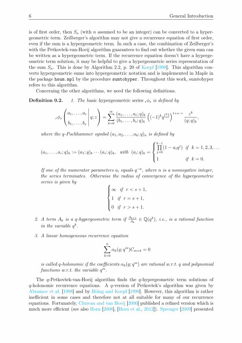
is of first order, then Sn (with n assumed to be an integer) can be converted to a hyper-geometric term. Zeilberger’s algorithm may not give a recurrence equation of first order,even if the sum is a hypergeometric term. In such a case, the combination of Zeilberger’swith the Petkovšek-van-Hoeij algorithm guarantees to find out whether the given sum canbe written as a hypergeometric term. If the recurrence equation doesn’t have a hyperge-ometric term solution, it may be helpful to give a hypergeometric series representation ofthe sum Sn. This is done by Algorithm 2.2, p. 20 of Koepf [1998]. This algorithm con-verts hypergeometric sums into hypergeometric notation and is implemented in Maple inthe package hsum.mpl by the procedure sumtohyper. Throughout this work, sumtohyperrefers to this algorithm.
Concerning the other algorithms, we need the following definitions.
Definition 0.2. 1. The basic hypergeometric series rφs is defined by
rφs
a1, . . . , ar
b1, . . . , bs
∣∣∣∣∣∣ q; z =
∞∑k=0
(a1, . . . , ar; q)k(b1, . . . , bs; q)k
((−1)kq(
k2))1+s−r zk
(q; q)k,
where the q-Pochhammer symbol (a1, a2, . . . , ak; q)n is defined by
(a1, . . . , ar; q)k := (a1; q)k · · · (ar; q)k, with (ai; q)k =
k−1∏j=0
(1− aiqj) if k = 1, 2, 3, . . .
1 if k = 0.
If one of the numerator parameters ai equals q−n, where n is a nonnegative integer,the series terminates. Otherwise the radius of convergence of the hypergeometricseries is given by
∞ if r < s+ 1,
1 if r = s+ 1,
0 if r > s+ 1.
2. A term Ak is a q-hypergeometric term if Ak+1
Ak∈ Q(qk), i.e., is a rational function
in the variable qk.
3. A linear homogeneous recurrence equationn∑k=0
αk(q; qm)Cm+k = 0
is called q-holonomic if the coefficients αk(q; qm) are rational w.r.t. q and polynomialfunctions w.r.t. the variable qm.
The q-Petkovšek-van-Hoeij algorithm finds the q-hypergeometric term solutions ofq-holonomic recurrence equations. A q-version of Petkovšek’s algorithm was given byAbramov et al. [1998] and by Böing and Koepf [1999]. However, this algorithm is ratherinefficient in some cases and therefore not at all suitable for many of our recurrenceequations. Fortunately, Cluzeau and van Hoeij [2006] published a refined version which ismuch more efficient (see also Horn [2008], [Horn et al., 2012]). Sprenger [2009] presented
7
a Maple implementation of this refined version qHypergeomSolveRE in his package qFPS(see also [Sprenger and Koepf, 2012]). It is worth noting that in the sequel, q-Petkovšek-van-Hoeij algorithm refers to this implementation.
The q-version of Zeilberger’s algorithm (see e.g. [Koepf, 1998]) also deals with definitesums of the form
Sn =∞∑
m=−∞
A(n,m)
and applies if A(n,m) is a q-hypergeometric term with respect to both n and m. Itgenerates a q-holonomic recurrence equation for Sn. If the recurrence equation is of firstorder, then Sn (with n assumed to be an integer) can be converted to a q-hypergeometricterm. If the recurrence if of order greater than one, q-Petkovšek-van-Hoeij algorithmis used. If the recurrence equation doesn’t have a q-hypergeometric term solution, itmay be helpful to give a q-hypergeometric representation of the sum Sn. This is doneby the q-analogue of Algorithm 2.2, p. 20 of Koepf [1998]. This algorithm converts q-hypergeometric sums into q-hypergeometric notation and is implemented in Maple in thepackage qsum.mpl by the procedure sum2qhyper. Throughout this work, sum2qhyperrefers to this algorithm.

8 General Introduction
Chapter 1
Connection, Linearization andDuplication Coefficients of ClassicalOrthogonal Polynomials of aContinuous Variable
In this chapter, we recall known results on connection and linearization coefficients ofclassical orthogonal polynomials on the real line. We are interested in reviewing here somedifferent general methods used to obtain these results. Furthermore we use a new approachto compute duplication coefficients of classical continuous orthogonal polynomials. Werecover known results and get some new ones.
1.1 Introduction
Here, we recall some definitions and results which will be useful in the sequel.Let P denotes the linear space of polynomials with coefficients in C, the set of complexnumbers.
Definition 1.1. 1. A polynomial sequence yn(x)n≥0 in P is called a polynomial fam-ily (system or set) if yn(x) is of degree precisely n in x, n = 0, 1, 2, . . ..
2. A positive function ρ(x) defined on (A,B) (with −∞ ≤ A < B ≤ +∞) is a weightfunction if ρ(x) is continuous on (A,B) and
∫ BAρ(x)xndx ∈ R , for all n ∈ N0.
3. We say that a polynomial family yn(x)n≥0 of a continuous variable is orthogonalwith respect to the weight function ρ(x) defined on (A,B) if∫ B
A
yn(x)ym(x)ρ(x)dx = h2nδmn, (1.1)
where h2n is a nonnegative real and δmn =
0 if m 6= n
1 if m = n,designates the Kronecker
symbol.
10 Connection, Linearization and Duplication Coefficients of CCOP
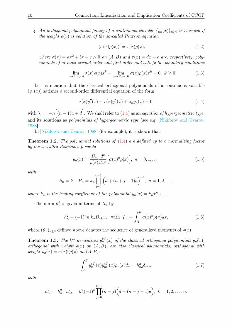
4. An orthogonal polynomial family of a continuous variable yn(x)n≥0 is classical ifthe weight ρ(x) is solution of the so-called Pearson equation
(σ(x)ρ(x))′ = τ(x)ρ(x), (1.2)
where σ(x) = ax2 + bx+ c > 0 on (A,B) and τ(x) = dx+ e are, respectively, poly-nomials of at most second order and first order and satisfy the boundary conditions
limx→A, x>A
σ(x)ρ(x)xk = limx→B, x<B
σ(x)ρ(x)xk = 0, k ≥ 0. (1.3)
Let us mention that the classical orthogonal polynomials of a continuous variable(yn(x)) satisfies a second-order differential equation of the form
σ(x)y′′n(x) + τ(x)y′n(x) + λnyn(x) = 0, (1.4)
with λn = −n[(n− 1)a+ d
]. We shall refer to (1.4) as an equation of hypergeometric type,
and its solutions as polynomials of hypergeometric type (see e.g. [Nikiforov and Uvarov,1988]).
In [Nikiforov and Uvarov, 1988] (for example), it is shown that:
Theorem 1.2. The polynomial solutions of (1.4) are defined up to a normalizing factorby the so-called Rodrigues formula
yn(x) =Bn
ρ(x)
dn
dxn
[σ(x)nρ(x)
], n = 0, 1, . . . , (1.5)
with
B0 = k0, Bn = kn
n−1∏j=0
(d+ (n+ j − 1)a
)−1
, n = 1, 2, . . . ,
where kn is the leading coefficient of the polynomial yn(x) = knxn + . . ..
The norm h2n is given in terms of Bn by
h2n = (−1)nn!knBnµn, with µn =
∫ B
A
σ(x)nρ(x)dx, (1.6)
where (µn)n≥0 defined above denotes the sequence of generalized moments of ρ(x).
Theorem 1.3. The kth derivatives y(k)n (x) of the classical orthogonal polynomials yn(x),
orthogonal with weight ρ(x) on (A,B), are also classical polynomials, orthogonal withweight ρk(x) = σ(x)kρ(x) on (A,B):∫ B
A
y(k)n (x)y(k)
m (x)ρk(x)dx = h2nkδm,n, (1.7)
with
h2n0 = h2
n, h2nk = h2
n(−1)kk−1∏j=0
(n− j)(d+ (n+ j − 1)a
), k = 1, 2, . . . , n.
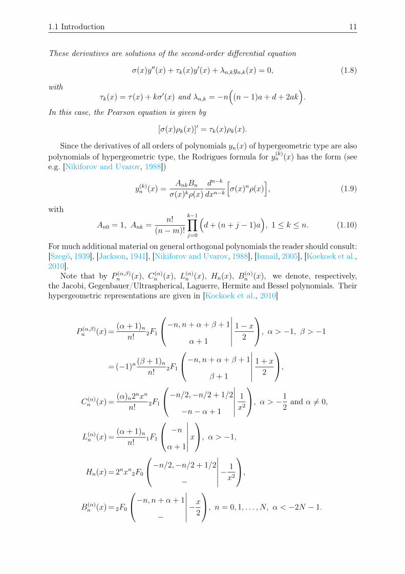
1.1 Introduction 11
These derivatives are solutions of the second-order differential equation
σ(x)y′′(x) + τk(x)y′(x) + λn,kyn,k(x) = 0, (1.8)
withτk(x) = τ(x) + kσ′(x) and λn,k = −n
((n− 1)a+ d+ 2ak
).
In this case, the Pearson equation is given by
[σ(x)ρk(x)]′ = τk(x)ρk(x).
Since the derivatives of all orders of polynomials yn(x) of hypergeometric type are alsopolynomials of hypergeometric type, the Rodrigues formula for y(k)
n (x) has the form (seee.g. [Nikiforov and Uvarov, 1988])
y(k)n (x) =
AnkBn
σ(x)kρ(x)
dn−k
dxn−k
[σ(x)nρ(x)
], (1.9)
with
An0 = 1, Ank =n!
(n−m)!
k−1∏j=0
(d+ (n+ j − 1)a
), 1 ≤ k ≤ n. (1.10)
For much additional material on general orthogonal polynomials the reader should consult:[Szegö, 1939], [Jackson, 1941], [Nikiforov and Uvarov, 1988], [Ismail, 2005], [Koekoek et al.,2010].
Note that by P (α,β)n (x), C(α)
n (x), L(α)n (x), Hn(x), B(α)
n (x), we denote, respectively,the Jacobi, Gegenbauer/Ultraspherical, Laguerre, Hermite and Bessel polynomials. Theirhypergeometric representations are given in [Koekoek et al., 2010]
P (α,β)n (x) =
(α + 1)nn!
2F1
−n, n+ α + β + 1
α + 1
∣∣∣∣∣∣ 1− x2
, α > −1, β > −1
= (−1)n(β + 1)n
n!2F1
−n, n+ α + β + 1
β + 1
∣∣∣∣∣∣ 1 + x
2
,C(α)n (x) =
(α)n2nxn
n!2F1
−n/2,−n/2 + 1/2
−n− α + 1
∣∣∣∣∣∣ 1
x2
, α > −1
2and α 6= 0,
L(α)n (x) =
(α + 1)nn!
1F1
−n
α + 1
∣∣∣∣∣∣x, α > −1,
Hn(x) = 2nxn2F0
−n/2,−n/2 + 1/2
−
∣∣∣∣∣∣− 1
x2
,B(α)n (x) = 2F0
−n, n+ α + 1
−
∣∣∣∣∣∣−x2, n = 0, 1, . . . , N, α < −2N − 1.
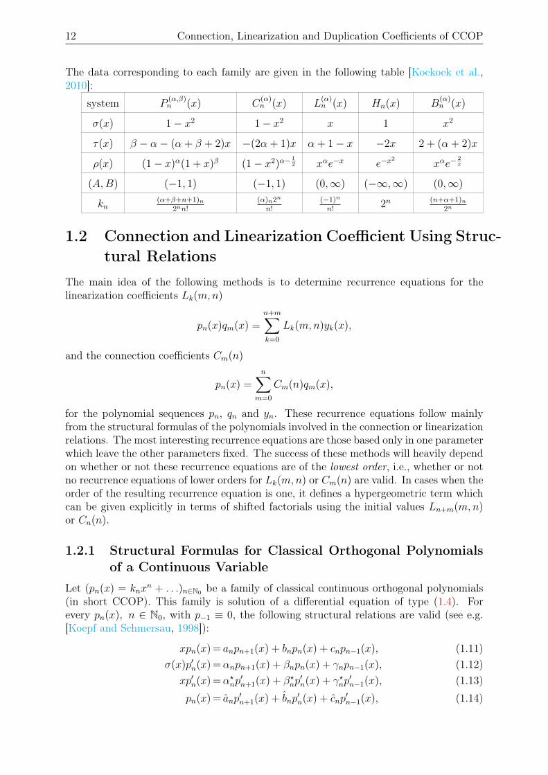
12 Connection, Linearization and Duplication Coefficients of CCOP
The data corresponding to each family are given in the following table [Koekoek et al.,2010]:
system P(α,β)n (x) C
(α)n (x) L
(α)n (x) Hn(x) B
(α)n (x)
σ(x) 1− x2 1− x2 x 1 x2
τ(x) β − α− (α + β + 2)x −(2α + 1)x α + 1− x −2x 2 + (α + 2)x
ρ(x) (1− x)α(1 + x)β (1− x2)α−12 xαe−x e−x
2xαe−
2x
(A,B) (−1, 1) (−1, 1) (0,∞) (−∞,∞) (0,∞)
kn(α+β+n+1)n
2nn!(α)n2n
n!(−1)n
n!2n (n+α+1)n
2n
1.2 Connection and Linearization Coefficient Using Struc-tural Relations
The main idea of the following methods is to determine recurrence equations for thelinearization coefficients Lk(m,n)
pn(x)qm(x) =n+m∑k=0
Lk(m,n)yk(x),
and the connection coefficients Cm(n)
pn(x) =n∑
m=0
Cm(n)qm(x),
for the polynomial sequences pn, qn and yn. These recurrence equations follow mainlyfrom the structural formulas of the polynomials involved in the connection or linearizationrelations. The most interesting recurrence equations are those based only in one parameterwhich leave the other parameters fixed. The success of these methods will heavily dependon whether or not these recurrence equations are of the lowest order, i.e., whether or notno recurrence equations of lower orders for Lk(m,n) or Cm(n) are valid. In cases when theorder of the resulting recurrence equation is one, it defines a hypergeometric term whichcan be given explicitly in terms of shifted factorials using the initial values Ln+m(m,n)or Cn(n).
1.2.1 Structural Formulas for Classical Orthogonal Polynomialsof a Continuous Variable
Let (pn(x) = knxn + . . .)n∈N0 be a family of classical continuous orthogonal polynomials
(in short CCOP). This family is solution of a differential equation of type (1.4). Forevery pn(x), n ∈ N0, with p−1 ≡ 0, the following structural relations are valid (see e.g.[Koepf and Schmersau, 1998]):
xpn(x) = anpn+1(x) + bnpn(x) + cnpn−1(x), (1.11)σ(x)p′n(x) =αnpn+1(x) + βnpn(x) + γnpn−1(x), (1.12)
xp′n(x) =α?np′n+1(x) + β?np
′n(x) + γ?np
′n−1(x), (1.13)
pn(x) = anp′n+1(x) + bnp
′n(x) + cnp
′n−1(x), (1.14)
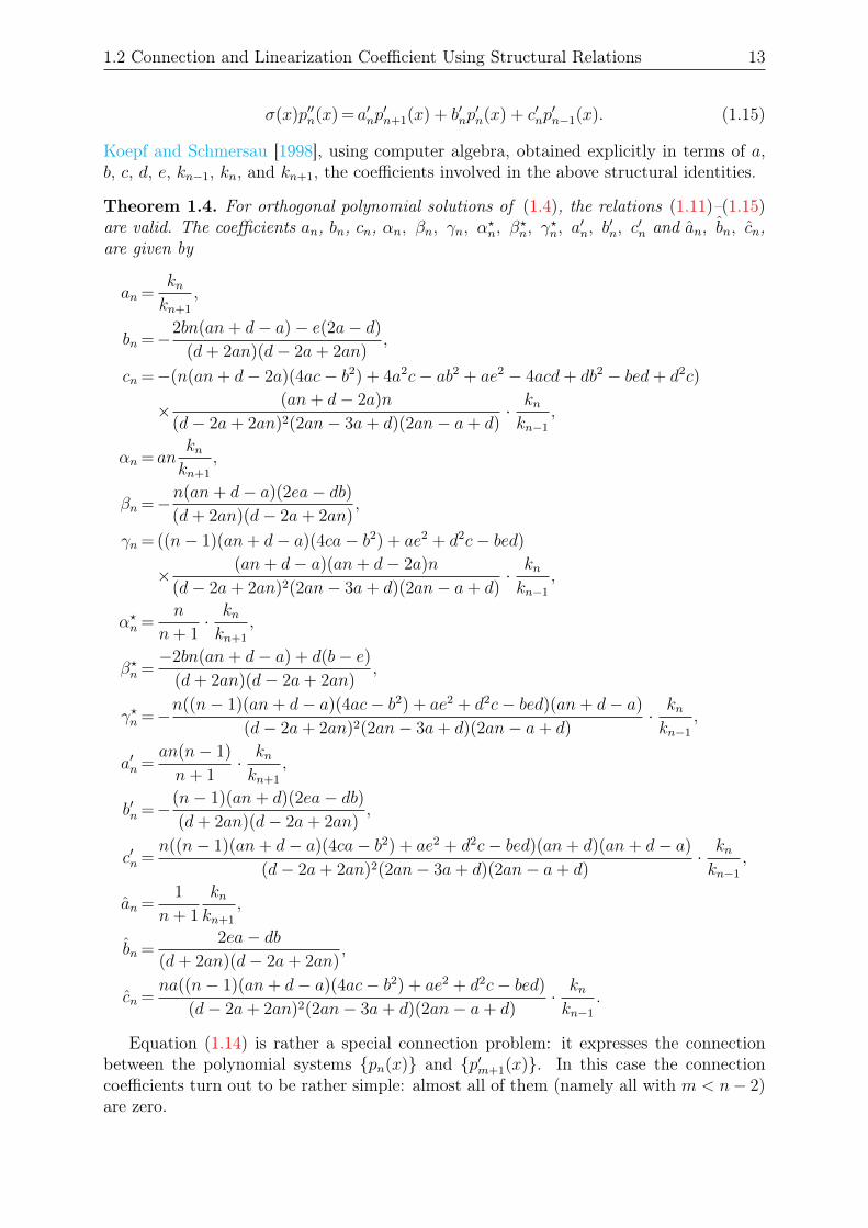
1.2 Connection and Linearization Coefficient Using Structural Relations 13
σ(x)p′′n(x) = a′np′n+1(x) + b′np
′n(x) + c′np
′n−1(x). (1.15)
Koepf and Schmersau [1998], using computer algebra, obtained explicitly in terms of a,b, c, d, e, kn−1, kn, and kn+1, the coefficients involved in the above structural identities.
Theorem 1.4. For orthogonal polynomial solutions of (1.4), the relations (1.11)–(1.15)are valid. The coefficients an, bn, cn, αn, βn, γn, α?n, β?n, γ?n, a′n, b′n, c′n and an, bn, cn,are given by
an =knkn+1
,
bn =−2bn(an+ d− a)− e(2a− d)
(d+ 2an)(d− 2a+ 2an),
cn =−(n(an+ d− 2a)(4ac− b2) + 4a2c− ab2 + ae2 − 4acd+ db2 − bed+ d2c)
× (an+ d− 2a)n
(d− 2a+ 2an)2(2an− 3a+ d)(2an− a+ d)· knkn−1
,
αn = anknkn+1
,
βn =−n(an+ d− a)(2ea− db)(d+ 2an)(d− 2a+ 2an)
,
γn = ((n− 1)(an+ d− a)(4ca− b2) + ae2 + d2c− bed)
× (an+ d− a)(an+ d− 2a)n
(d− 2a+ 2an)2(2an− 3a+ d)(2an− a+ d)· knkn−1
,
α?n =n
n+ 1· knkn+1
,
β?n =−2bn(an+ d− a) + d(b− e)
(d+ 2an)(d− 2a+ 2an),
γ?n =−n((n− 1)(an+ d− a)(4ac− b2) + ae2 + d2c− bed)(an+ d− a)
(d− 2a+ 2an)2(2an− 3a+ d)(2an− a+ d)· knkn−1
,
a′n =an(n− 1)
n+ 1· knkn+1
,
b′n =−(n− 1)(an+ d)(2ea− db)(d+ 2an)(d− 2a+ 2an)
,
c′n =n((n− 1)(an+ d− a)(4ca− b2) + ae2 + d2c− bed)(an+ d)(an+ d− a)
(d− 2a+ 2an)2(2an− 3a+ d)(2an− a+ d)· knkn−1
,
an =1
n+ 1
knkn+1
,
bn =2ea− db
(d+ 2an)(d− 2a+ 2an),
cn =na((n− 1)(an+ d− a)(4ac− b2) + ae2 + d2c− bed)
(d− 2a+ 2an)2(2an− 3a+ d)(2an− a+ d)· knkn−1
.
Equation (1.14) is rather a special connection problem: it expresses the connectionbetween the polynomial systems pn(x) and p′m+1(x). In this case the connectioncoefficients turn out to be rather simple: almost all of them (namely all with m < n− 2)are zero.
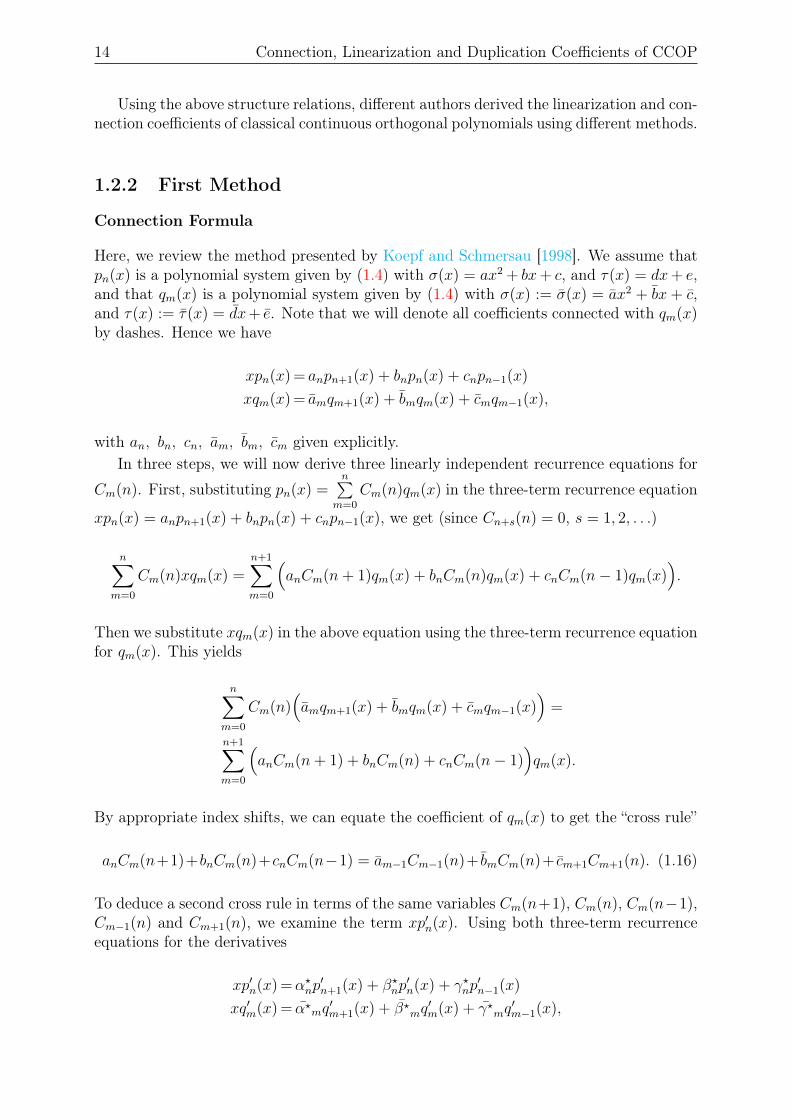
14 Connection, Linearization and Duplication Coefficients of CCOP
Using the above structure relations, different authors derived the linearization and con-nection coefficients of classical continuous orthogonal polynomials using different methods.
1.2.2 First Method
Connection Formula
Here, we review the method presented by Koepf and Schmersau [1998]. We assume thatpn(x) is a polynomial system given by (1.4) with σ(x) = ax2 + bx+ c, and τ(x) = dx+ e,and that qm(x) is a polynomial system given by (1.4) with σ(x) := σ(x) = ax2 + bx + c,and τ(x) := τ(x) = dx+ e. Note that we will denote all coefficients connected with qm(x)by dashes. Hence we have
xpn(x) = anpn+1(x) + bnpn(x) + cnpn−1(x)
xqm(x) = amqm+1(x) + bmqm(x) + cmqm−1(x),
with an, bn, cn, am, bm, cm given explicitly.In three steps, we will now derive three linearly independent recurrence equations for
Cm(n). First, substituting pn(x) =n∑
m=0
Cm(n)qm(x) in the three-term recurrence equation
xpn(x) = anpn+1(x) + bnpn(x) + cnpn−1(x), we get (since Cn+s(n) = 0, s = 1, 2, . . .)
n∑m=0
Cm(n)xqm(x) =n+1∑m=0
(anCm(n+ 1)qm(x) + bnCm(n)qm(x) + cnCm(n− 1)qm(x)
).
Then we substitute xqm(x) in the above equation using the three-term recurrence equationfor qm(x). This yields
n∑m=0
Cm(n)(amqm+1(x) + bmqm(x) + cmqm−1(x)
)=
n+1∑m=0
(anCm(n+ 1) + bnCm(n) + cnCm(n− 1)
)qm(x).
By appropriate index shifts, we can equate the coefficient of qm(x) to get the “cross rule”
anCm(n+1)+bnCm(n)+cnCm(n−1) = am−1Cm−1(n)+ bmCm(n)+ cm+1Cm+1(n). (1.16)
To deduce a second cross rule in terms of the same variables Cm(n+1), Cm(n), Cm(n−1),Cm−1(n) and Cm+1(n), we examine the term xp′n(x). Using both three-term recurrenceequations for the derivatives
xp′n(x) =α?np′n+1(x) + β?np
′n(x) + γ?np
′n−1(x)
xq′m(x) = α?mq′m+1(x) + β?mq
′m(x) + γ?mq
′m−1(x),
1.2 Connection and Linearization Coefficient Using Structural Relations 15
we get
xp′n(x) = α?np′n+1(x) + β?np
′n(x) + γ?np
′n−1(x)
mn∑
m=0
Cm(n)xq′m(x) =n+1∑m=0
(α?nCm(n+ 1) + β?nCm(n) + γ?nCm(n− 1)
)q′m(x)
mn∑
m=0
Cm(n)(α?mq
′m+1(x) + β?mq
′m(x) + γ?mq
′m−1(x)
)=
n+1∑m=0
(α?nCm(n+ 1) + β?nCm(n) + γ?nCm(n− 1)
)q′m(x).
Again, by appropriate index shifts, we can equate the coefficient of q′m(x) to get the crossrule
α?nCm(n+1)+β?nCm(n)+γ?nCm(n−1) = α?m−1Cm−1(n)+β?mCm(n)+γ?m+1Cm+1(n). (1.17)
In a similar way the cross rule
anCm(n+1)+ bnCm(n)+ cnCm(n−1) = ¯am−1Cm−1(n)+¯bmCm(n)+ ¯cm+1Cm+1(n) (1.18)
can be obtained from (1.14). It turns out, however, that this relation is linearly dependentfrom (1.16) and (1.17), and hence does not yield new information. To obtain reasonablysimple results, we now assume furthermore that σ(x) = σ(x).
Connection Formula with σ(x) = σ(x)
Using both derivatives rules
σ(x)p′n(x) =αnpn+1(x) + βnpn(x) + γnpn−1(x),
σ(x)q′m(x) = αmqm+1(x) + βmqm(x) + γmqm−1(x),
we get
σ(x)p′n(x) = αnpn+1(x) + βnpn(x) + γnpn−1(x)
mn∑
m=0
Cm(n)σ(x)q′m(x) =n+1∑m=0
(αnCm(n+ 1) + βnCm(n) + γnCm(n− 1)
)qm(x)
mn∑
m=0
Cm(n)(αmqm+1(x) + βmqm(x) + γmqm−1(x)
)=
n+1∑m=0
(αnCm(n+ 1) + βnCm(n) + γnCm(n− 1)
)qm(x).
Again, by appropriate index shifts, this results in the cross rule
αnCm(n+1)+βnCm(n)+γnCm(n−1) = αm−1Cm−1(n)+βmCm(n)+γm−1Cm−1(n). (1.19)
To obtain a pure recurrence equation with respect to m, from the three cross rules (1.16),(1.17), and (1.19) by linear algebra we eliminate the variables Cm(n+ 1) and Cm(n− 1),and to obtain a pure recurrence equation with respect to n, we eliminate the variablesCm−1(n) and Cm+1(n). This yields a second-order recurrence equation satisfied by theconnection coefficients Cm(n).
In different cases where σ(x) 6= σ(x), we need the power representation.
16 Connection, Linearization and Duplication Coefficients of CCOP
Power Representation or Inversion Formula
In many applications, one wants to develop a given polynomial in terms of a given or-thogonal polynomial system. In this case handy formulas for the power xn like
xn =n∑
m=0
Im(n)qm(x)
are very welcome. We remark that this formula is the connection formula for the specificcase pn(x) = xn, and is called inversion formula.
For qm(x), we have the differential equation
σ(x)q′′m(x) + τ(x)q′m(x) + λmqm(x) = 0
with σ(x) = ax2 + bx+ c, and the derivative rule
σ(x)q′m(x) = αmqm+1(x) + βmqm(x) + γmqm−1(x).
Our current pn(x) = xn satisfies
σ(x)p′n(x) = (ax2 + bx+ c)nxn−1
= anxn+1 + bnxn + cnxn−1
= anpn+1(x) + bnpn(x) + cnpn−1(x),
xpn(x) = pn+1(x), xp′n(x) =n
n+ 1p′n+1(x), pn(x) =
1
n+ 1p′n+1(x).
Hence in our situation, we get the cross rule (1.16) with an = 1, bn = cn = 0
Im(n+ 1) = am−1Im−1(n) + bmIm(n) + cm+1Im+1(n), (1.20)
the cross rule (1.17) with α?n = nn+1
, β?n = γ?n = 0
n
n+ 1Im(n+ 1) = α?m−1Im−1(n) + β?mIm(n) + γ?m+1Im+1(n), (1.21)
the cross rule (1.18) with an = 1n+1
, bn = cn = 0
1
n+ 1Im(n+ 1) = ¯am−1Im−1(n) +
¯bmIm(n) + ¯cm+1Im+1(n),
and the cross rule
anIm(n+ 1) + bnIm(n) + cnIm(n− 1) = αm−1Im−1(n) + βmIm(n) + γm−1Im−1(n).
We substitute the cross rule (1.20) in (1.21), and then we obtain a pure recurrence equationwith respect to m.
Remark 1.5. In many instances the recurrence equations reduce to two terms. Thentheir hypergeometric term solutions are identified. If the recurrence equation is of ordergreater than 1, we use the Petkovšek-van-Hoeij algorithm to get its hypergeometric termsolutions.
Using the hypergeometric representation of the polynomial pn(x) and the inversionformula of qm(x), we get the general connection formula.
1.2 Connection and Linearization Coefficient Using Structural Relations 17
Connection Formula: General Case
In general, to find the coefficients Cm(n) in the relation
pn(x) =n∑
m=0
Cm(n)qm(x),
we combine
pn(x) =n∑j=0
Aj(n)xj and xj =
j∑m=0
Im(j)qm(x),
which yields the representation
pn(x) =n∑j=0
j∑m=0
Aj(n)Im(j)qm(x),
and then, interchanging the order of summation gives
Cm(n) =n−m∑j=0
Aj+m(n)Im(j +m).
For orthogonal polynomials with even weight such as Hermite and Gegenbauer polyno-mials, we have the relations
pn(x) =
bn2c∑
j=0
Aj(n)xn−2j and xj =
b j2c∑
m=0
Im(j)qj−2m(x),
from which we deduce
xn−2j =
bn2c−j∑
m=0
Im(n− 2j)qn−2j−2m(x).
Finally, we combine the above two expressions and substitute m by m− j to get
Cm(n) =m∑j=0
Aj(n)Im−j(n− 2j),
with
pn(x) =n∑
m=0
Cm(n)qn−2m(x).
Since the summand F (j,m, n) := Aj(n)Im(j) of Cm(n) turns out to be a hypergeo-metric term with respect to (j,m, n), i.e., the term ratios F (j + 1,m, n)/F (j,m, n),F (j,m+1, n)/F (j,m, n), and F (j,m, n+1)/F (j,m, n) are rational functions, Zeilberger’s(combined with the Petkovšek-van-Hoeij) algorithm applies. If a hypergeometric term so-lution exists, the representation of Cm(n) follows then from the initial values Cn(n) =kn/kn, Cn+s(n) = 0, s = 1, 2, . . ., where kn, kn are, respectively, the leading coefficientsof pn(x) and qn(x).
18 Connection, Linearization and Duplication Coefficients of CCOP
Linearization Formula
The linearization formula
pn(x)qm(x) =n+m∑k=0
Lk(m,n)yk(x)
follows from the hypergeometric representation of the polynomials pn(x), qm(x) and theinversion formula of the polynomials yk(x).
In fact, if
pn(x) =n∑i=0
Ai(n)xi and qm(x) =m∑j=0
Bj(m)xj,
then by the Cauchy product
pn(x)qm(x) =n+m∑l=0
Gl(m,n)xl,
with
Gl(m,n) =l∑
i=0
Ai(n)Bl−i(m).
Combining the preceding result with the inversion formula
xl =l∑
k=0
Ik(l)yk(x),
we get
Lk(m,n) =n+m−k∑l=0
Gl+k(m,n)Ik(l + k)
=n+m−k∑l=0
l+k∑i=0
Ik(l + k)Ai(n)Bl+k−i(m).
We note that we can apply Zeilberger’s and the Petkovšek-van-Hoeij algorithm to reduce(if possible) Gl(m,n) into a hypergeometric term and/or Lk(m,n) into a single sum or ahypergeometric term.
1.2.3 Second Method: The NaViMa Algorithm
In this section, we describe a recurrent algorithm (called NaViMa) to compute recursivelythe connection and linearization coefficients of CCOP [Ronveaux et al., 1995], [Godoyet al., 1997]. We note that the name NaViMa comes from their authors’ institutionswhich are Namur (in Belgium), Vigo and Madrid (in Spain). This method also uses thestructural relations (1.11)-(1.15) of CCOP.
1.2 Connection and Linearization Coefficient Using Structural Relations 19
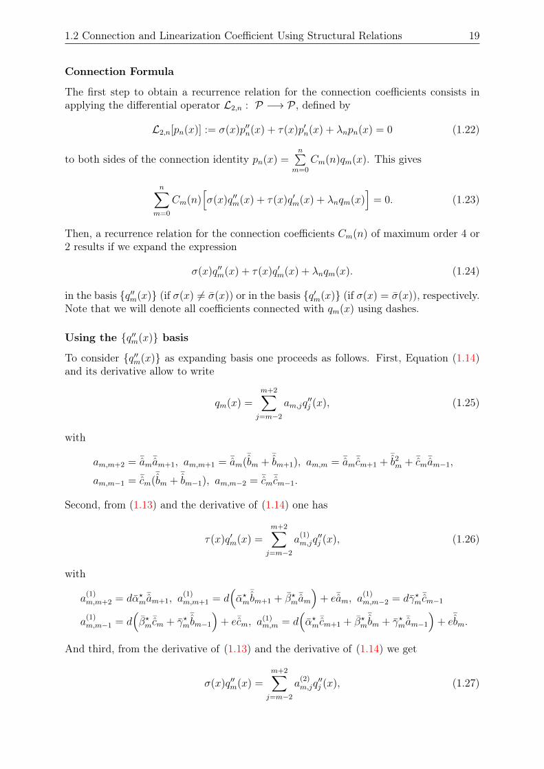
Connection Formula
The first step to obtain a recurrence relation for the connection coefficients consists inapplying the differential operator L2,n : P −→ P , defined by
L2,n[pn(x)] := σ(x)p′′n(x) + τ(x)p′n(x) + λnpn(x) = 0 (1.22)
to both sides of the connection identity pn(x) =n∑
m=0
Cm(n)qm(x). This gives
n∑m=0
Cm(n)[σ(x)q′′m(x) + τ(x)q′m(x) + λnqm(x)
]= 0. (1.23)
Then, a recurrence relation for the connection coefficients Cm(n) of maximum order 4 or2 results if we expand the expression
σ(x)q′′m(x) + τ(x)q′m(x) + λnqm(x). (1.24)
in the basis q′′m(x) (if σ(x) 6= σ(x)) or in the basis q′m(x) (if σ(x) = σ(x)), respectively.Note that we will denote all coefficients connected with qm(x) using dashes.
Using the q′′m(x) basis
To consider q′′m(x) as expanding basis one proceeds as follows. First, Equation (1.14)and its derivative allow to write
qm(x) =m+2∑j=m−2
am,jq′′j (x), (1.25)
with
am,m+2 = ¯am¯am+1, am,m+1 = ¯am(¯bm +
¯bm+1), am,m = ¯am¯cm+1 +
¯b2m + ¯cm¯am−1,
am,m−1 = ¯cm(¯bm +
¯bm−1), am,m−2 = ¯cm¯cm−1.
Second, from (1.13) and the derivative of (1.14) one has
τ(x)q′m(x) =m+2∑j=m−2
a(1)m,jq
′′j (x), (1.26)
with
a(1)m,m+2 = dα?m
¯am+1, a(1)m,m+1 = d
(α?m
¯bm+1 + β?m
¯am
)+ e¯am, a
(1)m,m−2 = dγ?m
¯cm−1
a(1)m,m−1 = d
(β?m
¯cm + γ?m¯bm−1
)+ e¯cm, a
(1)m,m = d
(α?m
¯cm+1 + β?m¯bm + γ?m
¯am−1
)+ e
¯bm.
And third, from the derivative of (1.13) and the derivative of (1.14) we get
σ(x)q′′m(x) =m+2∑j=m−2
a(2)m,jq
′′j (x), (1.27)
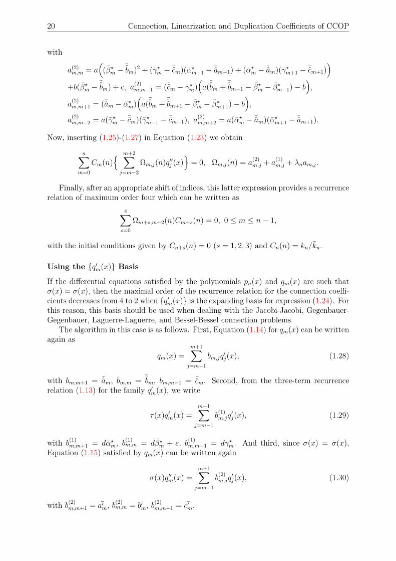
20 Connection, Linearization and Duplication Coefficients of CCOP
with
a(2)m,m = a
((β?m −
¯bm)2 + (γ?m − ¯cm)(α?m−1 − ¯am−1) + (α?m − ¯am)(γ?m+1 − ¯cm+1)
)+b(β?m −
¯bm) + c, a
(2)m,m−1 = (¯cm − γ?m)
(a(
¯bm +
¯bm−1 − β?m − β?m−1)− b
),
a(2)m,m+1 = (¯am − α?m)
(a(
¯bm +
¯bm+1 − β?m − β?m+1)− b
),
a(2)m,m−2 = a(γ?m − ¯cm)(γ?m−1 − ¯cm−1), a
(2)m,m+2 = a(α?m − ¯am)(α?m+1 − ¯am+1).
Now, inserting (1.25)-(1.27) in Equation (1.23) we obtain
n∑m=0
Cm(n) m+2∑j=m−2
Ωm,j(n)q′′j (x)
= 0, Ωm,j(n) = a(2)m,j + a
(1)m,j + λnam,j.
Finally, after an appropriate shift of indices, this latter expression provides a recurrencerelation of maximum order four which can be written as
4∑s=0
Ωm+s,m+2(n)Cm+s(n) = 0, 0 ≤ m ≤ n− 1,
with the initial conditions given by Cn+s(n) = 0 (s = 1, 2, 3) and Cn(n) = kn/kn.
Using the q′m(x) Basis
If the differential equations satisfied by the polynomials pn(x) and qm(x) are such thatσ(x) = σ(x), then the maximal order of the recurrence relation for the connection coeffi-cients decreases from 4 to 2 when q′m(x) is the expanding basis for expression (1.24). Forthis reason, this basis should be used when dealing with the Jacobi-Jacobi, Gegenbauer-Gegenbauer, Laguerre-Laguerre, and Bessel-Bessel connection problems.
The algorithm in this case is as follows. First, Equation (1.14) for qm(x) can be writtenagain as
qm(x) =m+1∑j=m−1
bm,jq′j(x), (1.28)
with bm,m+1 = ¯am, bm,m =¯bm, bm,m−1 = ¯cm. Second, from the three-term recurrence
relation (1.13) for the family q′m(x), we write
τ(x)q′m(x) =m+1∑j=m−1
b(1)m,jq
′j(x), (1.29)
with b(1)m,m+1 = dα?m, b
(1)m,m = dβ?m + e, b(1)
m,m−1 = dγ?m. And third, since σ(x) = σ(x),Equation (1.15) satisfied by qm(x) can be written again
σ(x)q′′m(x) =m+1∑j=m−1
b(2)m,jq
′j(x), (1.30)
with b(2)m,m+1 = a′m, b
(2)m,m = b′m, b
(2)m,m−1 = c′m.
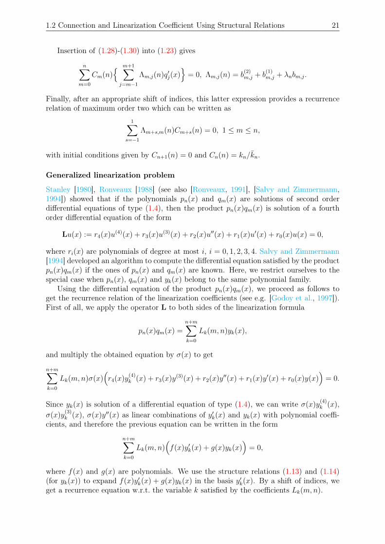
1.2 Connection and Linearization Coefficient Using Structural Relations 21
Insertion of (1.28)-(1.30) into (1.23) gives
n∑m=0
Cm(n) m+1∑j=m−1
Λm,j(n)q′j(x)
= 0, Λm,j(n) = b(2)m,j + b
(1)m,j + λnbm,j.
Finally, after an appropriate shift of indices, this latter expression provides a recurrencerelation of maximum order two which can be written as
1∑s=−1
Λm+s,m(n)Cm+s(n) = 0, 1 ≤ m ≤ n,
with initial conditions given by Cn+1(n) = 0 and Cn(n) = kn/kn.
Generalized linearization problem
Stanley [1980], Ronveaux [1988] (see also [Ronveaux, 1991], [Salvy and Zimmermann,1994]) showed that if the polynomials pn(x) and qm(x) are solutions of second orderdifferential equations of type (1.4), then the product pn(x)qm(x) is solution of a fourthorder differential equation of the form
Lu(x) := r4(x)u(4)(x) + r3(x)u(3)(x) + r2(x)u′′(x) + r1(x)u′(x) + r0(x)u(x) = 0,
where ri(x) are polynomials of degree at most i, i = 0, 1, 2, 3, 4. Salvy and Zimmermann[1994] developed an algorithm to compute the differential equation satisfied by the productpn(x)qm(x) if the ones of pn(x) and qm(x) are known. Here, we restrict ourselves to thespecial case when pn(x), qm(x) and yk(x) belong to the same polynomial family.
Using the differential equation of the product pn(x)qm(x), we proceed as follows toget the recurrence relation of the linearization coefficients (see e.g. [Godoy et al., 1997]).First of all, we apply the operator L to both sides of the linearization formula
pn(x)qm(x) =n+m∑k=0
Lk(m,n)yk(x),
and multiply the obtained equation by σ(x) to get
n+m∑k=0
Lk(m,n)σ(x)(r4(x)y
(4)k (x) + r3(x)y(3)(x) + r2(x)y′′(x) + r1(x)y′(x) + r0(x)y(x)
)= 0.
Since yk(x) is solution of a differential equation of type (1.4), we can write σ(x)y(4)k (x),
σ(x)y(3)k (x), σ(x)y′′(x) as linear combinations of y′k(x) and yk(x) with polynomial coeffi-
cients, and therefore the previous equation can be written in the form
n+m∑k=0
Lk(m,n)(f(x)y′k(x) + g(x)yk(x)
)= 0,
where f(x) and g(x) are polynomials. We use the structure relations (1.13) and (1.14)(for yk(x)) to expand f(x)y′k(x) + g(x)yk(x) in the basis y′k(x). By a shift of indices, weget a recurrence equation w.r.t. the variable k satisfied by the coefficients Lk(m,n).
22 Connection, Linearization and Duplication Coefficients of CCOP
Remark 1.6. Hylleraas [1962] computed the differential equation satisfied by the productof Jacobi polynomials and used it to set up a recurrence relation for the linearizationcoefficients of Gegenbauer polynomials. For Jacobi polynomials, the situation was farfrom satisfactory.
Lewanowicz [1996b] obtained by a method which is alternative to NaViMa a second-order recurrence relation for the linearization coefficients.
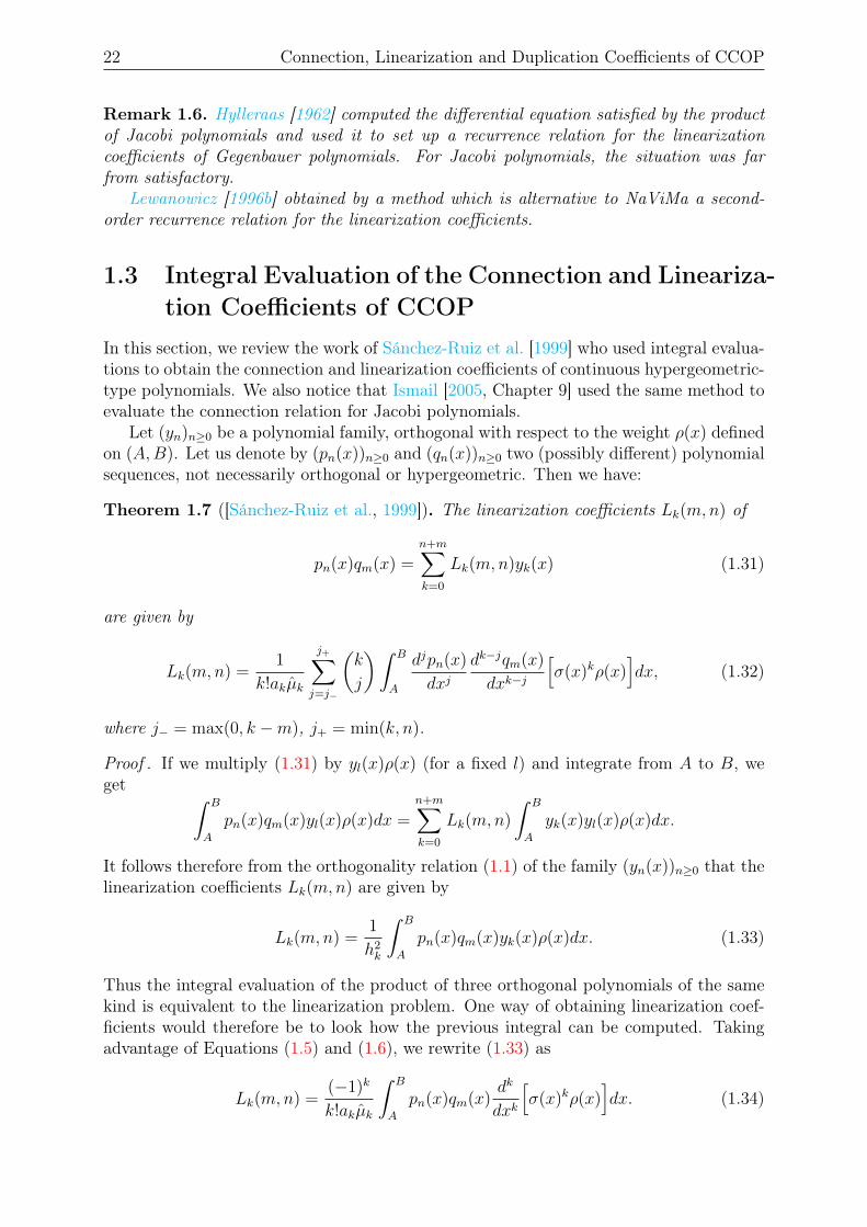
1.3 Integral Evaluation of the Connection and Lineariza-tion Coefficients of CCOP
In this section, we review the work of Sánchez-Ruiz et al. [1999] who used integral evalua-tions to obtain the connection and linearization coefficients of continuous hypergeometric-type polynomials. We also notice that Ismail [2005, Chapter 9] used the same method toevaluate the connection relation for Jacobi polynomials.
Let (yn)n≥0 be a polynomial family, orthogonal with respect to the weight ρ(x) definedon (A,B). Let us denote by (pn(x))n≥0 and (qn(x))n≥0 two (possibly different) polynomialsequences, not necessarily orthogonal or hypergeometric. Then we have:
Theorem 1.7 ([Sánchez-Ruiz et al., 1999]). The linearization coefficients Lk(m,n) of
pn(x)qm(x) =n+m∑k=0
Lk(m,n)yk(x) (1.31)
are given by
Lk(m,n) =1
k!akµk
j+∑j=j−
(k
j
)∫ B
A
djpn(x)
dxjdk−jqm(x)
dxk−j
[σ(x)kρ(x)
]dx, (1.32)
where j− = max(0, k −m), j+ = min(k, n).
Proof . If we multiply (1.31) by yl(x)ρ(x) (for a fixed l) and integrate from A to B, weget ∫ B
A
pn(x)qm(x)yl(x)ρ(x)dx =n+m∑k=0
Lk(m,n)
∫ B
A
yk(x)yl(x)ρ(x)dx.
It follows therefore from the orthogonality relation (1.1) of the family (yn(x))n≥0 that thelinearization coefficients Lk(m,n) are given by
Lk(m,n) =1
h2k
∫ B
A
pn(x)qm(x)yk(x)ρ(x)dx. (1.33)
Thus the integral evaluation of the product of three orthogonal polynomials of the samekind is equivalent to the linearization problem. One way of obtaining linearization coef-ficients would therefore be to look how the previous integral can be computed. Takingadvantage of Equations (1.5) and (1.6), we rewrite (1.33) as
Lk(m,n) =(−1)k
k!akµk
∫ B
A
pn(x)qm(x)dk
dxk
[σ(x)kρ(x)
]dx. (1.34)
1.3 Integral Evaluation of the Connection and Linearization Coefficients of CCOP 23
We show by induction on j ∈ N that for every P ∈ P , there exists Q ∈ P such that
dj
dxj
[σ(x)kρ(x)P (x)
]= σ(x)k−jρ(x)Q(x), j ≤ k. (1.35)
Indeed, for j = 1, using Pearson’s equation (1.2), we have
d
dx
[σ(x)kρ(x)P (x)
]=σ(x)k−1ρ(x)
(τ(x)P (x) + (k − 1)σ′(x)P (x) + σ(x)P ′(x)
)=σ(x)k−1ρ(x)Q1,k(x)
with Q1,k(x) = τ(x)P (x) + (k − 1)σ′(x)P (x) + σ(x)P ′(x). We suppose that (1.35) is truefor j ≥ 2, and then it follows that
dj+1
dxj+1
[σ(x)kρ(x)P (x)
]=
d
dx
(σ(x)k−jρ(x)Q(x)
)=σ(x)k−j−1ρ(x)Q1,k−j(x).
Thus, integrating by parts and taking into account, respectively, (1.35) and the boundaryconditions (1.3), we rewrite (1.34) in the form
Lk(m,n) =(−1)k
k!akµk
(pn(x)qm(x)
dk−1
dxk−1
[σ(x)kρ(x)
]∣∣∣BA
−∫ B
A
d
dx
(pn(x)qm(x)
) dk−1
dxk−1
[σ(x)kρ(x)
]dx)
=(−1)k
k!akµk
(pn(x)qm(x)σ(x)ρ(x)Q(x)
∣∣∣BA
−∫ B
A
d
dx
(pn(x)qm(x)
) dk−1
dxk−1
[σ(x)kρ(x)
]dx)
=(−1)k+1
k!akµk
∫ B
A
d
dx
(pn(x)qm(x)
) dk−1
dxk−1
[σ(x)kρ(x)
]dx.
We repeat the integration by parts k − 1 times and use again (1.35) and (1.3) to obtain
Lk(m,n) =1
k!akµk
∫ B
A
dk
dxk
(pn(x)qm(x)
)[σ(x)kρ(x)
]dx. (1.36)
If j > n,dj
dxjpn(x) = 0 and if j < k −m, k − j > m and then
dk−j
dxk−jqm(x) = 0 such that
from Leibniz’s rule
dk
dxk(pn(x)qm(x)) =
k∑j=0
(k
j
)dj
dxjpn(x)
dk−j
dxk−jqm(x)
the result follows. In particular, taking pn(x) = xn and qm(x) = 1, we obtain the solution of the inversion
problem in terms of the moments of the weights ρk(x):
24 Connection, Linearization and Duplication Coefficients of CCOP
Proposition 1.8 ([Sánchez-Ruiz et al., 1999]). The coefficients Ik(n) of the inversionproblem
xn =n∑k=0
Ik(n)yk(x)
are given by
Ik(n) =
(n
k
)1
akµk
∫ B
A
xn−kρk(x)dx.
Proof . Since qm(x) = 1, dk−jqm(x)dxk−j
=
0 if j 6= k
1 if j = k.Thus for Pn(x) = xn, we get
Ik(n) =1
k!akµk
∫ b
a
dkxn
dxkσ(x)kρ(x)dx
=
(n
k
)1
akµk
∫ b
a
xn−kσ(x)kρ(x)dx.
We note that Sánchez-Ruiz and Dehesa [1997], Ismail [2005] used the above proposition
to solve the inversion problem for CCOP.Let us assume now that both pn(x) and qm(x) are also polynomials of hypergeometric
type. Equation (1.32) is practical for the computation of the generalized linearizationcoefficients whenever the explicit expressions of the polynomials djpn(x)
dxjand dk−jqm(x)
dxk−jare
known, as is the case, e.g., for the classical hypergeometric families. For general familiesof polynomials, when only the coefficients of the corresponding differential operators areavailable, we can make one more step and find an equivalent expression for Lk(m,n) thatdoes not require the knowledge of the explicit expressions of the polynomials. We restrictour attention to the particular case when the three families of hypergeometric polynomialscoincide
(pn(x) = qn(x) = yn(x)
), for which we have the following
Theorem 1.9 ([Sánchez-Ruiz et al., 1999]). If pn(x) = qn(x) = yn(x), the linearizationcoefficients Lk(m,n) in (1.31) are given by
Lk(m,n) =(Bn)2
k!akµk
j+∑j=j−
Anj(−1)m+k+j
(k
j
) i+∑i=i−
(−1)iAm(n+k−i−2j)
(n− ji
)×
∫ B
A
ρm(x)dm−n+i+2j−k
dxm−n+i+2j−k
(σ(x)2j−k+id
iσ(x)k−i
dxi
). (1.37)
Proof . Since pn(x) = qn(x) = yn(x), then
Lk(m,n) =1
k!akµk
j+∑j=j−
(k
j
)∫ B
A
y(j)n (x)yk−jm (x)ρk(x)dx.
Using Equation (1.9) for y(j)n (x), the above expression can be written as
Lk(m,n) =Bn
k!akµk
j+∑j=j−
Anj
(k
j
)∫ B
A
dn−jρn(x)
dxn−jy(k−j)m (x)σ(x)k−jdx.
1.3 Integral Evaluation of the Connection and Linearization Coefficients of CCOP 25
Observe that by (1.9) and (1.35), there exist two polynomials Q1(x) and Q2(x) such thatfor 0 ≤ l ≤ n− j,
term :=dl
dxl
(y(k−j)m (x)σ(x)k−j
) dn−j−l−1
dxn−j−l−1(ρn(x))
= Am(k−j)Bmdl
dxl
( 1
ρ(x)
dm−k+jρm(x)
dxm−k+j
)σ(x)j+l+1ρ(x)Q2(x)
= Am(k−j)Bmdl
dxl
(σ(x)k−jQ1(x)
)σ(x)j+l+1ρ(x)Q2(x)
=N∑i=0
aiσ(x)ρ(x)xi, ai ∈ R, N ∈ N.
Thus, integrating by parts n− j times and taking into account the boundary conditions(1.3),
Lk(m,n) =Bn
k!akµk
j+∑j=j−
Anj(−1)n−j(k
j
)∫ B
A
ρn(x)dn−j
dxn−j(y(k−j)m (x)σ(x)k−j)dx.
Using the Leibniz rule,
Lk(m,n) =Bn
k!akµk
j+∑j=j−
Anj(−1)n−j(k
j
) i+∑i=i−
(n− ji
)∫ B
A
ρn(x)diσ(x)k−j
dxiy(n+k−2j−i)m dx,
where i− = max0, n−m+k−2j, i+ = minn−j, (k−j) deg[σ(x)]. In fact, diσ(x)k−j
dxi6= 0
if and only if i ≤ (k− j) deg[σ(x)] and y(n+k−2j−i)m 6= 0 if and only if n+ k− 2j− i ≤ m⇔
i ≥ n −m + k − 2j. We substitute the expression of y(n+k−2j−i)m given by the Rodrigues
formula (1.9), integrate by parts again, use Equation (1.35) and the boundary conditions(1.3) to get the result. In spite of its apparent complexity, this formula has the advantage that no derivativesof the weight functions are involved; it does not make use of the expressions of thepolynomials either. In fact, if we know σ(x) we can express the integrals appearing in(1.37) as a linear combination of the moments of the weight function ρm(x), which makesthis equation suitable for symbolic manipulation.
Let us consider now the connection problem
pn(x) =n∑k=0
Ck(n)yk(x) (1.38)
where pn(x) is the sequence of polynomial of degree n, solution of the differential equa-tion
σ(x)p′′n(x) + τ(x)p′n(x) + λnpn(x) = 0.
Taking qm(x) := 1 in (1.31), we readily see that Ck(n) = Lk(0, n), so that the connectioncoefficients Ck(n) can be obtained as the particular case m = 0 of both (1.33) and (1.32).Again, it turns out to be much more convenient to use (1.32), which leads to
Ck(n) =1
k!akµk
∫ B
A
p(k)n (x)ρk(x)dx, (1.39)
26 Connection, Linearization and Duplication Coefficients of CCOP
which does not require the use of the representation for yk(x). We note that the previousformula was already proved by [Rainville, 1960, Theorem 56, p. 151].
By Equation (1.9), the previous formula for Ck(n) can be written as
Ck(n) =AnkBn
k!akµk
∫ B
A
ρk(x)
ρk(x)
dn−kρn(x)
dxn−kdx
or, equivalently, integrating by parts n− k times (using (1.35), (1.3)),
Ck(n) =(−1)n−kAnkBn
k!akµk
∫ B
A
ρn(x)dn−k
dxn−k
(ρk(x)
ρk(x)
)dx.
A common situation in connecting polynomials of the same family, but with differentparameters, is when σ(x) = σ(x). In this case, if we put ρ(x) = f(x)ρ(x), the previousequation takes the form
Ck(n) =(−1)n−kAnkBn
k!akµk
∫ B
A
f(x)ρn(x)dn−k
dxn−k
( 1
f(x)
)dx,
which may be useful if the derivatives of 1f(x)
have simple representations.It is a remarkable fact that, in the case when all the involved polynomials are of
hypergeometric type, Equation (1.32) enables us to express the linearization coefficientsin terms of two connection coefficients, namely those corresponding to the expansions ofthe polynomials p(j)
n (x) and q(k−j)m (x) in series of y(r)
k (x),
p(j)n (x) =
n−j∑r=0
C(j,k)r,n (p)y(k)
r (x), q(k−j)m (x) =
m+j−k∑s=0
C(k−j,k)s,m (q)y(k)
s .
Substituting these expressions into (1.32) and using the orthogonality relation (1.7), weobtain
Lk(m,n) =1
k!akµk
j+∑j=j−
(k
j
) n−j∑r=0
m+j−k∑s=0
C(j,k)r,n (p)C(k−j,k)
s,m (q)
∫ B
A
y(k)r (x)y(k)
s ρk(x)dx
=1
k!akµk
j+∑j=j−
(k
j
) r+∑r=0
C(j,k)r,n (p)C(k−j,k)
r,m (q)h2rk,
where r+ = min(n−j,m+j−k). In particular, for the standard linearization coefficients,the previous formula does apply with p = q = y, and we can omit the arguments of theconnection coefficients to simplify the notation.
1.4 Other Methods
Besides the methods cited above, there exist some other methods regularly used in theliterature to compute connection and inversion coefficients of CCOP. In this section, werecall two of them.
1.5 Connection and Linearization Coefficients of CCOP 27
1.4.1 Using the Fields and Wimp Expansion Formula
One approach to evaluate the connection coefficients is to think of pn(x) =n∑
m=0
Cm(n)qm(x)
as a polynomial expansion problem. One of the most important general expansion for-mulas for hypergeometric series is the Fields and Wimp [1961] expansion given by
p+rFq+s
a1, . . . , ap, c1, . . . , cr
b1, . . . , bq, d1, . . . , ds
∣∣∣∣∣∣ zw =
∞∑n=0
(a1, . . . , ap)n(α)n(−z)n
(b1, . . . , bq)n(γ + n)nn!(1.40)
×p+1Fq+1
n+ α, n+ a1, . . . , n+ ap
2n+ γ + 1, n+ b1, . . . , n+ bq
∣∣∣∣∣∣ zr+2Fs+1
−n, n+ γ, c1, . . . , cr
α, d1, . . . , ds
∣∣∣∣∣∣w.
The letters p, q, r and s stand for nonnegative integers.Proceeding as in [Njionou Sadjang, 2013], we choose p = q = 0, w = x and γ = 0. Weexpand both sides of (1.40) in the basis (zn)n and then equate the coefficients of zn toobtain
r∏j=1
(cj)n
s∏j=1
(dj)n
xn =n∑k=0
(−1)k(n
k
)r+1Fs
−k, c1, . . . , cr
d1, . . . , ds
∣∣∣∣∣∣x.
Using this relation, Njionou Sadjang [2013] derived inversion formulas of some CCOP.Sánchez-Ruiz [2001], by making the substitutions r = s = 0, z = 1, w = 1 − x2 and bya suitable identification of the remaining parameters, derived from (1.40) connection andlinearization formulas involving squares of Gegenbauer polynomials. Lewanowicz [2003a]used the formula (1.40) to obtain hypergeometric term representations and recurrencerelations for the connection coefficients of CCOP.
1.4.2 Using Generating Functions
Andrews et al. [1999, p. 318] used a method based on generating functions to find thelinearization coefficients of the Hermite polynomials. Rainville [1960] also used generatingfunctions to get inversion and connection formulas of classical continuous orthogonal poly-nomials. Chaggara and Koepf [2010] starting from the generating function of the Jacobipolynomials and using symbolic computation, in particular Zeilberger’s and Petkovšek-van-Hoeij algorithms, computed the linearization coefficients of Jacobi and Gegenbauerpolynomials.
1.5 Connection and Linearization Coefficients of CCOPAs an immediate consequence of the above methods, we get the following connection,linearization and inversion coefficient of classical continuous orthogonal polynomials.
Theorem 1.10. The following representations for the powers in terms of the classicalcontinuous orthogonal polynomials are valid:
(1− x)n = 2nΓ(α + n+ 1)n∑
m=0
(α + β + 2m+ 1)Γ(α + β +m+ 1)
Γ(α +m+ 1)Γ(α + β + n+m+ 2)(−n)mP
(α,β)m (x)
28 Connection, Linearization and Duplication Coefficients of CCOP
(see e.g. [Koepf and Schmersau, 1998], [Ismail, 2005]),
(1 + x)n = 2nΓ(β + n+ 1)n∑
m=0
(−1)m(−n)m(α + β + 2m+ 1)Γ(α + β +m+ 1)
Γ(β +m+ 1)Γ(α + β + n+m+ 2)P (α,β)m (x)
(see e.g. [Askey, 1975], [Koepf and Schmersau, 1998], [Ismail, 2005]),
xn =n!
(α)n2n
bn2c∑
m=0
(−n2− α
2+ 1)m(−n− α)m
(−n2− α
2)mm!
(−1)mCαn−2m(x)
=n!
2n
bn2c∑
m=0
n+ α− 2m
m!(α)n+1−mC
(α)n−2m(x)
(see e.g. [Rainville, 1960], [Koepf and Schmersau, 1998]),
xn = (1 + α)n
n∑m=0
(−n)m(1 + α)m
L(α)m (x) = n!
n∑m=0
(n+ α
n−m
)(−1)mL(α)
m (x)
(see e.g. [Sánchez-Ruiz and Dehesa, 1997], [Koepf and Schmersau, 1998], [Ismail, 2005]),
xn =
bn2c∑
m=0
(−n2)m(−n
2+ 1
2)m
m!2n−2mHn−2m(x) =
n!
2n
bn2c∑
m=0
1
m!(n− 2m)!Hn−2m(x)
(see e.g. [Koepf and Schmersau, 1998], [Ismail, 2005]),
xn =(−2)n
(α + 2)n
n∑m=0
(−n)m(α + 1)m(α2
+ 32)m
(n+ 2 + α)m(α2
+ 12)mm!
B(α)m (x)
= (−2)nn∑
m=0
(2m+ α + 1)(−n)mΓ(α +m+ 1)
m!Γ(n+m+ α + 2)B(α)m (x)
(see e.g. [Sánchez-Ruiz and Dehesa, 1997], [Koepf and Schmersau, 1998]).
Theorem 1.11. The following connection relations between classical orthogonal polyno-mials are valid:
P (α,β)n (x) =
n∑m=0
(2m+ γ + β + 1)Γ(n+ β + 1)Γ(n+m+ α + β + 1)
Γ(m+ β + 1)Γ(n+ α + β + 1)
× Γ(m+ γ + β + 1)(α− γ)n−mΓ(n+m+ γ + β + 2)(n−m)!
P (γ,β)m (x)
(see e.g. [Askey, 1975, p. 63], [Koepf and Schmersau, 1998]),
P (α,β)n =
n∑m=0
(−1)n−m(2m+ α + δ + 1)Γ(n+ α + 1)Γ(n+m+ α + β + 1)
Γ(m+ α + 1)Γ(n+ α + β + 1)
× Γ(m+ α + δ + 1)(β − δ)n−mΓ(n+m+ α + δ + 2)(n−m)!
P (α,δ)m (x)
1.5 Connection and Linearization Coefficients of CCOP 29
(see e.g. [Askey, 1975, p. 63], [Koepf and Schmersau, 1998], [Ismail, 2005, p. 258]),
P (α,β)n (x) =
n∑m=0
(m+ α + 1)n−m(n+ α + β + 1)m(n−m)!(m+ γ + δ + 1)m
×3F2
m− n, n+m+ α + β + 1,m+ γ + 1
m+ α + 1, 2m+ γ + δ + 2
∣∣∣∣∣∣ 1P (γ,δ)
m (x)
(see e.g. [Gasper, 1974], [Lewanowicz, 2003a], [Ismail, 2005, p. 257], compare [Sánchez-Ruizet al., 1999]),
C(α)n (x) =
Γ(β)
Γ(α)Γ(α− β)
bn2c∑
m=0
(n− 2m+ β)Γ(m+ α− β)Γ(n−m+ α)
m!Γ(n−m+ β + 1)C
(β)n−2m(x)
(see e.g. [Koepf and Schmersau, 1998], [Sánchez-Ruiz et al., 1999], [Ismail, 2005, p. 257]),
L(α)n (x) =
n∑m=0
(α− β)n−m(n−m)!
L(β)m (x)
(see e.g. [Koepf and Schmersau, 1998], [Sánchez-Ruiz et al., 1999]),
B(α)n (x) =
n∑m=0
(−1)m(2m+ β + 1)(−n)m(n+ α + 1)mΓ(m+ β + 1)Γ(β − α + 1)
m!Γ(n+m+ β + 2)Γ(m− n+ β − α + 1)B(β)m (x)
(see e.g. [Godoy et al., 1997], [Koepf and Schmersau, 1998], [Sánchez-Ruiz et al., 1999]).
Theorem 1.12. The following linearization formulas between classical orthogonal poly-nomials are valid:
P (λ,δ)n (x)P (µ,γ)
m (x) =n+m∑k=0
(α + β + 1)n+m−k(α + 1)n+m(2(n+m− k) + α + β + 1)
(α + 1)n+m−k(α + β + 1)2(n+m)−k+1
×(−1)k(n+m)!(λ+ δ + 1)2n(µ+ γ + 1)2m
n!m!k!(λ+ δ + 1)n(µ+ γ + 1)m
×∞∑
r,s=0
(−k,−α− β − 1− 2(n+m) + k)r+s(−n,−λ− n)r(−m,−µ−m)s(−n−m,−α− n−m)r+s(−2n− λ− δ)r(−2m− µ− γ)sr!s!
P(α,β)n+m−k(x),
see [Chaggara and Koepf, 2010],
P (λ,δ)n (x)P (µ,γ)
m (x) =n+m∑k=0
(µ+ λ+ δ + γ + 1)n+m−k(2(n+m− k) + µ+ λ+ δ + γ + 1)
(µ+ λ+ 1)n+m−k(µ+ λ+ δ + γ + 1)2(n+m)−k+1
×(µ+ λ+ 1)n+m(n+m)!(λ+ δ + 1)2n(µ+ γ + 1)2m(−2n− λ− δ)kn!m!k!(λ+ δ + 1)n(µ+ γ + 1)m(−2m− µ− γ)k
×3F2
−k,−λ− µ− δ − γ − 1− 2(n+m) + k,−n
−2n− λ− δ,−n−m
∣∣∣∣∣∣ 1
×3F2
−k,−λ− µ− δ − γ − 1− 2(n+m) + k,−λ− n
−2n− λ− δ,−λ− µ− n−m
∣∣∣∣∣∣ 1P (λ+µ,δ+γ)
n+m−k (x),
30 Connection, Linearization and Duplication Coefficients of CCOP
compare [Park and Kim, 2006], see [Chaggara and Koepf, 2010],
C(α)n (x)C(α)
m (x) =
min(m,n)∑k=0
(n+m− 2k + α)(n+m− 2k)!(α)kk!(n+m− k + α)(n− k)!(m− k)!
×(α)n−k(α)m−k(2α)n+m−k
(α)n+m−k(2α)n+m−2k
C(α)n+m−2k(x)
(see e.g. [Askey, 1975, p. 39], [Sánchez-Ruiz et al., 1999]),
Hn(x)Hm(x) =
min(n,m)∑k=0
(n
k
)(m
k
)2kk!Hn+m−2k(x)
(see e.g. [Watson, 1938], [Askey, 1975, p. 42], [Sánchez-Ruiz et al., 1999]),
L(α)n (x)L(α)
m (x) =n+m∑
k=|n−m|
(−2)n+m−kk!
(n+m− k)!(k − n)!(k −m)!
×3F2
k−m−n2
, k−m−n+12
, k + α + 1
k − n+ 1, k −m+ 1
∣∣∣∣∣∣ 1L(α)
k (x)
(see e.g. [Watson, 1938]).
We note that in the above theorems, we gave only connection and linearization formu-lae between CCOP of the same family. In general we can obtain all the other connectionand linearization coefficients using for example the first method of Section 1.2.2. In thecase they aren’t hypergeometric terms, we can use the sumtohyper algorithm if the coef-ficient is a single sum. If the coefficient is a double sum, Zeilberger’s algorithm combinedwith Petkovšek-van-Hoeij algorithm may be used to simplify this double sum to a singlesum or to a hypergeometric term (if possible).
1.6 Duplication Coefficients of CCOP
Given a polynomial system pnn≥0, we use a new approach to solve the so-called duplica-tion problem associated to this system which consists in finding the coefficients Dm(n, a)in the expansion
pn(ax) =n∑
m=0
Dm(n, a)pm(x),
where a designates a nonzero complex number. In the following theorem, using the hyper-geometric representations given in page 11 and the inversion formulas given in Theorem1.10, we provide known duplication formulas and moreover, we get new results for Jacobiand Gegenbauer polynomials.
1.6 Duplication Coefficients of CCOP 31
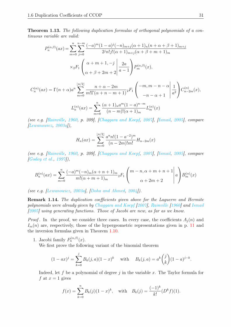
Theorem 1.13. The following duplication formulas of orthogonal polynomials of a con-tinuous variable are valid:
P (α,β)n (ax) =
n∑m=0
n−m∑j=0
(−a)m(1− a)j(−n)m+j(α + 1)n(n+ α + β + 1)m+j
2jn!j!(α + 1)m+j(α + β +m+ 1)m
×2F1
α +m+ 1,−j
α + β + 2m+ 2
∣∣∣∣∣∣ 2a
a− 1
P (α,β)m (x),
C(α)n (ax) = Γ(n+ α)an
bn/2c∑m=0
n+ α− 2m
m!Γ(α + n−m+ 1)2F1
−m,m− n− α−n− α + 1
∣∣∣∣∣∣ 1
a2
C(α)n−2m(x),
L(α)n (ax) =
n∑m=0
(α + 1)nam(1− a)n−m
(n−m)!(α + 1)mL(α)m (x)
(see e.g. [Rainville, 1960, p. 209], [Chaggara and Koepf, 2007], [Ismail, 2005], compare[Lewanowicz, 2003a]),
Hn(ax) =
bn/2c∑m=0
ann!(1− a−2)m
(n− 2m)!m!Hn−2m(x)
(see e.g. [Rainville, 1960, p. 209], [Chaggara and Koepf, 2007], [Ismail, 2005], compare[Godoy et al., 1997]),
B(α)n (ax) =
n∑m=0
(−a)m(−n)m(α + n+ 1)mm!(α +m+ 1)m
2F1
m− n, α +m+ n+ 1
α + 2m+ 2
∣∣∣∣∣∣ aB(α)
m (x)
(see e.g. [Lewanowicz, 2003a], [Doha and Ahmed, 2004]).
Remark 1.14. The duplication coefficients given above for the Laguerre and Hermitepolynomials were already given by Chaggara and Koepf [2007], Rainville [1960] and Ismail[2005] using generating functions. Those of Jacobi are new, as far as we know.
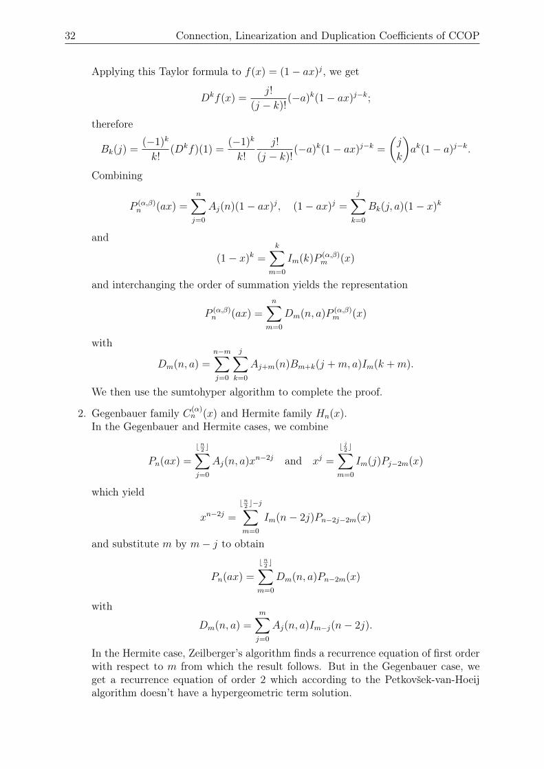
Proof . In the proof, we consider three cases. In every case, the coefficients Aj(n) andIm(n) are, respectively, those of the hypergeometric representations given in p. 11 andthe inversion formulas given in Theorem 1.10.
1. Jacobi family P (α,β)n (x).
We first prove the following variant of the binomial theorem
(1− ax)j =
j∑k=0
Bk(j, a)(1− x)k with Bk(j, a) = ak(j
k
)(1− a)j−k.
Indeed, let f be a polynomial of degree j in the variable x. The Taylor formula forf at x = 1 gives
f(x) =n∑k=0
Bk(j)(1− x)k, with Bk(j) =(−1)k
k!(Dkf)(1).
32 Connection, Linearization and Duplication Coefficients of CCOP
Applying this Taylor formula to f(x) = (1− ax)j, we get
Dkf(x) =j!
(j − k)!(−a)k(1− ax)j−k;
therefore
Bk(j) =(−1)k
k!(Dkf)(1) =
(−1)k
k!
j!
(j − k)!(−a)k(1− ax)j−k =
(j
k
)ak(1− a)j−k.
Combining
P (α,β)n (ax) =
n∑j=0
Aj(n)(1− ax)j, (1− ax)j =
j∑k=0
Bk(j, a)(1− x)k
and
(1− x)k =k∑
m=0
Im(k)P (α,β)m (x)
and interchanging the order of summation yields the representation
P (α,β)n (ax) =
n∑m=0
Dm(n, a)P (α,β)m (x)
with
Dm(n, a) =n−m∑j=0
j∑k=0
Aj+m(n)Bm+k(j +m, a)Im(k +m).
We then use the sumtohyper algorithm to complete the proof.
2. Gegenbauer family C(α)n (x) and Hermite family Hn(x).
In the Gegenbauer and Hermite cases, we combine
Pn(ax) =
bn2c∑
j=0
Aj(n, a)xn−2j and xj =
b j2c∑
m=0
Im(j)Pj−2m(x)
which yield
xn−2j =
bn2c−j∑
m=0
Im(n− 2j)Pn−2j−2m(x)
and substitute m by m− j to obtain
Pn(ax) =
bn2c∑
m=0
Dm(n, a)Pn−2m(x)
with
Dm(n, a) =m∑j=0
Aj(n, a)Im−j(n− 2j).
In the Hermite case, Zeilberger’s algorithm finds a recurrence equation of first orderwith respect to m from which the result follows. But in the Gegenbauer case, weget a recurrence equation of order 2 which according to the Petkovšek-van-Hoeijalgorithm doesn’t have a hypergeometric term solution.
1.6 Duplication Coefficients of CCOP 33
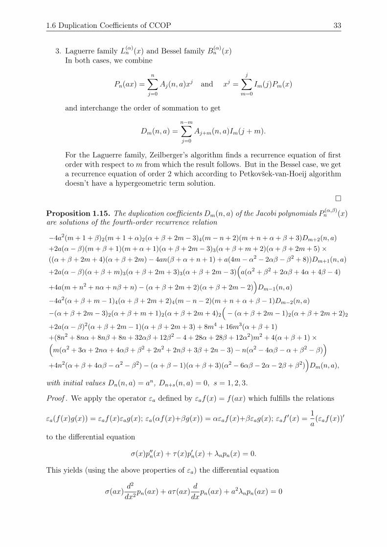
3. Laguerre family L(α)n (x) and Bessel family B(α)
n (x)In both cases, we combine
Pn(ax) =n∑j=0
Aj(n, a)xj and xj =
j∑m=0
Im(j)Pm(x)
and interchange the order of sommation to get
Dm(n, a) =n−m∑j=0
Aj+m(n, a)Im(j +m).
For the Laguerre family, Zeilberger’s algorithm finds a recurrence equation of firstorder with respect to m from which the result follows. But in the Bessel case, we geta recurrence equation of order 2 which according to Petkovšek-van-Hoeij algorithmdoesn’t have a hypergeometric term solution.
Proposition 1.15. The duplication coefficients Dm(n, a) of the Jacobi polynomials P (α,β)n (x)
are solutions of the fourth-order recurrence relation
−4a2(m+ 1 + β)2(m+ 1 + α)2(α+ β + 2m− 3)4(m− n+ 2)(m+ n+ α+ β + 3)Dm+2(n, a)
+2a(α− β)(m+ β + 1)(m+ α+ 1)(α+ β + 2m− 3)3(α+ β +m+ 2)(α+ β + 2m+ 5)×((α+ β + 2m+ 4)(α+ β + 2m)− 4an(β + α+ n+ 1) + a(4m− α2 − 2αβ − β2 + 8))Dm+1(n, a)
+2a(α− β)(α+ β +m)3(α+ β + 2m+ 3)3(α+ β + 2m− 3)(a(α2 + β2 + 2αβ + 4α+ 4β − 4)
+4a(m+ n2 + nα+ nβ + n)− (α+ β + 2m+ 2)(α+ β + 2m− 2))Dm−1(n, a)
−4a2(α+ β +m− 1)4(α+ β + 2m+ 2)4(m− n− 2)(m+ n+ α+ β − 1)Dm−2(n, a)
−(α+ β + 2m− 3)2(α+ β +m+ 1)2(α+ β + 2m+ 4)2
(− (α+ β + 2m− 1)2(α+ β + 2m+ 2)2
+2a(α− β)2(α+ β + 2m− 1)(α+ β + 2m+ 3) + 8m4 + 16m3(α+ β + 1)
+(8n2 + 8nα+ 8nβ + 8n+ 32αβ + 12β2 − 4 + 28α+ 28β + 12α2)m2 + 4(α+ β + 1)×(m(α2 + 3α+ 2nα+ 4αβ + β2 + 2n2 + 2nβ + 3β + 2n− 3)− n(α2 − 4αβ − α+ β2 − β)
)+4n2(α+ β + 4αβ − α2 − β2)− (α+ β − 1)(α+ β + 3)(α2 − 6αβ − 2α− 2β + β2)
)Dm(n, a),
with initial values Dn(n, a) = an, Dn+s(n, a) = 0, s = 1, 2, 3.
Proof . We apply the operator εa defined by εaf(x) = f(ax) which fulfills the relations
εa(f(x)g(x)) = εaf(x)εag(x); εa(αf(x)+βg(x)) = αεaf(x)+βεag(x); εaf′(x) =
1
a(εaf(x))′
to the differential equation
σ(x)p′′n(x) + τ(x)p′n(x) + λnpn(x) = 0.
This yields (using the above properties of εa) the differential equation
σ(ax)d2
dx2pn(ax) + aτ(ax)
d
dxpn(ax) + a2λnpn(ax) = 0
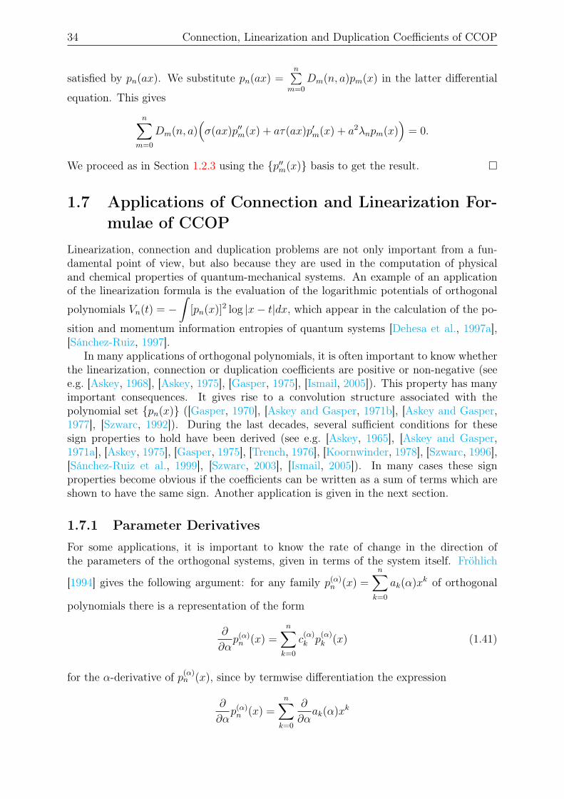
34 Connection, Linearization and Duplication Coefficients of CCOP
satisfied by pn(ax). We substitute pn(ax) =n∑
m=0
Dm(n, a)pm(x) in the latter differential
equation. This gives
n∑m=0
Dm(n, a)(σ(ax)p′′m(x) + aτ(ax)p′m(x) + a2λnpm(x)
)= 0.
We proceed as in Section 1.2.3 using the p′′m(x) basis to get the result.
1.7 Applications of Connection and Linearization For-mulae of CCOP
Linearization, connection and duplication problems are not only important from a fun-damental point of view, but also because they are used in the computation of physicaland chemical properties of quantum-mechanical systems. An example of an applicationof the linearization formula is the evaluation of the logarithmic potentials of orthogonal
polynomials Vn(t) = −∫
[pn(x)]2 log |x− t|dx, which appear in the calculation of the po-
sition and momentum information entropies of quantum systems [Dehesa et al., 1997a],[Sánchez-Ruiz, 1997].
In many applications of orthogonal polynomials, it is often important to know whetherthe linearization, connection or duplication coefficients are positive or non-negative (seee.g. [Askey, 1968], [Askey, 1975], [Gasper, 1975], [Ismail, 2005]). This property has manyimportant consequences. It gives rise to a convolution structure associated with thepolynomial set pn(x) ([Gasper, 1970], [Askey and Gasper, 1971b], [Askey and Gasper,1977], [Szwarc, 1992]). During the last decades, several sufficient conditions for thesesign properties to hold have been derived (see e.g. [Askey, 1965], [Askey and Gasper,1971a], [Askey, 1975], [Gasper, 1975], [Trench, 1976], [Koornwinder, 1978], [Szwarc, 1996],[Sánchez-Ruiz et al., 1999], [Szwarc, 2003], [Ismail, 2005]). In many cases these signproperties become obvious if the coefficients can be written as a sum of terms which areshown to have the same sign. Another application is given in the next section.
1.7.1 Parameter Derivatives
For some applications, it is important to know the rate of change in the direction ofthe parameters of the orthogonal systems, given in terms of the system itself. Fröhlich
[1994] gives the following argument: for any family p(α)n (x) =
n∑k=0
ak(α)xk of orthogonal
polynomials there is a representation of the form
∂
∂αp(α)n (x) =
n∑k=0
c(α)k p
(α)k (x) (1.41)
for the α-derivative of p(α)n (x), since by termwise differentiation the expression
∂
∂αp(α)n (x) =
n∑k=0
∂
∂αak(α)xk
1.7 Applications of Connection and Linearization Formulae of CCOP 35
is seen to be a polynomial of degree n with respect to x, and since any polynomial ofdegree n has a representation of the form (1.41). We call the derivative with respect to theparameter α a parameter derivative of p(α)
n (x). These parameter derivative representationscan be obtained from the connection formulas as shown by Koepf and Schmersau [1998].
Corollary 1.16. The following representations for the parameter derivatives of the clas-sical continuous orthogonal polynomials are valid:
∂
∂αP (α,β)n (x) =
n−1∑m=0
1
α + β +m+ n+ 1
×(P (α,β)n (x) +
α + β + 1 + 2m
n−m(β +m+ 1)n−m
(α + β +m+ 1)n−mP (α,β)m (x)
)(see [Fröhlich, 1994, Theorem 3], [Koepf and Schmersau, 1998]),
∂
∂βP (α,β)n (x) =
n−1∑m=0
1
α + β +m+ n+ 1
×(P (α,β)n (x) + (−1)n−m
α + β + 1 + 2m
n−m(α +m+ 1)n−m
(α + β +m+ 1)n−mP (α,β)m (x)
)(see [Fröhlich, 1994, Theorem 3], [Koepf and Schmersau, 1998]),
∂
∂αC(α)n (x) =
n−1∑m=0
( 2(m+ 1)
(2α +m)(2α + 1 + 2m)+
2
2α +m+ n
)C(α)n (x)
+n−1∑m=0
2(1 + (−1)n−m)(α +m)
(2α +m+ n)(n−m)C(α)m (x)
(see [Koepf, 1997, Theorem 10], [Koepf and Schmersau, 1998]),
∂
∂αL(α)n (x) =
n−1∑m=0
1
n−mL(α)m (x)
(see [Koepf, 1997, Theorem 10], [Koepf and Schmersau, 1998]),
∂
∂αBαn (x) =
n−1∑m=0
1
α + n+m+ 1
×(Bαn (x) + (−1)n−m
2m+ α + 1
n−mn!
(α +m+ 1)n−mm!Bαm(x)
)(see [Koepf and Schmersau, 1998]).
Proof (See [Koepf and Schmersau, 1998]). Given the connection relation
pαn(x) =n∑
m=0
Cm(n;α, β)pβm(x),
36 Connection, Linearization and Duplication Coefficients of CCOP
we build the difference quotient
pαn(x)− pβn(x)
α− β=
n∑m=0
Cm(n;α, β)
α− βpβm(x)− pβn(x)
α− β
=Cn(n;α, β)− 1
α− βpβn(x) +
n−1∑m=0
Cm(n;α, β)
α− βpβm(x)
so that with β → α
∂
∂αpαn(x) = lim
β→α
Cn(n;α, β)− 1
α− βpβn(x) +
n−1∑m=0
limβ→α
Cm(n;α, β)
α− βpβm(x)
since the systems pαn(x) are continuous with respect to α. This gives the results.
Remark 1.17. Lewanowicz [2002] also gave a general procedure to produce iterativelyexplicit parameter derivative representations for almost all the classical orthogonal poly-nomial families.
1.7.2 Logarithmic Potential of Hermite Polynomials and Infor-mation Entropies of the Harmonic Oscillator Eigenstates(see [Sánchez-Ruiz, 1997] and References Therein)
For the nth eigenstate of the one-dimensional harmonic oscillator Hamiltonian
H =p2
2m+
1
2mω2x2,
the probability densities ρ for position and momentum γ are expressed in terms of theHermite polynomials Hn(x),
ρ(x) =α
2nn!√π
(Hn(αx))2e−α2x2 , γ(p) =
1
2nn!√πα
(Hn(x))2e−p2
α2 ,
where α := (mω)2. The corresponding entropies of position and momentum can be writtenas
Sρ = − lnα + Sn, Sγ = lnα + Sn,
whereSn = ln(2nn!
√π) + n+
1
2+
1
2nn!√πEn(H)
is given in terms of En(H), the so-called entropy of the Hermite polynomials, whoserepresentation is
En(H) = −∫ ∞−∞
(Hn(x))2 ln(Hn(x))2e−x2
dx.
Dehesa et al. [1997b] showed that En(H) can be written in the form
En(H) = −2nn!√π ln(22n) + 2
n∑i=1
Vn(xn,i),
1.7 Applications of Connection and Linearization Formulae of CCOP 37
where xn,i (i = 1, . . . , n) is the ith root of Hn(x), and Vn(t) is the logarithmic potential ofthe Hermite polynomial Hn(x), defined as
Vn(t) = −∫ ∞−∞
(Hn(x))2 ln |x− t|e−x2dx. (1.42)
To calculate Vn(t), Sánchez-Ruiz [1997] make use of the linearization formula for theHermite polynomials
Hm(x)Hn(x) =
min(m,n)∑j=0
m!n!2j
(m− j)!(n− j)!j!Hm+n−2j(x)
which in the particular case m = n gives, writing j = n− k,
(Hn(x))2 = 2nn!n∑k=0
(n
k
)H2k(x)
2kk!.
Substituting this equation in the expression (1.42) of the logarithmic potential Vn(t) hegets
Vn(t) = 2nn!n∑k=0
(n
k
)W2k(t)
2kk!, W2k(t) = −
∫ ∞−∞
H2k(x) ln |x− t|e−x2dx.
After some calculations, he obtains a representation for Vn(t) which in turn yields arepresentation for the entropies when the exact location of the zeros of Hn(x) are known.
38 Connection, Linearization and Duplication Coefficients of CCOP
Chapter 2
Connection, Linearization andDuplication Coefficients of OrthogonalPolynomials of a Discrete Variable
The first purpose of this chapter is to review some general methods used to computelinearization and connection coefficients of classical discrete orthogonal polynomials (inshort CDOP). On the other hand, by an algorithmic approach, we solve the duplicationproblem for CDOP. Hypergeometric series representations of linearization coefficients ofCDOP are also given.
2.1 IntroductionLet us consider the second-order difference equation of hypergeometric type, i.e. the equa-tion [Nikiforov and Uvarov, 1988],
σ(x)∆∇y(x) + τ(x)∆y(x) + λy(x) = 0, (2.1)
where ∆y(x) = y(x+ 1)− y(x) and ∇y(x) = y(x)− y(x− 1) denote the forward andbackward difference operators, respectively, σ(x) = ax2 + bx + c and τ(x) = dx + e arepolynomials of degree not greater than 2 and 1, respectively, and λ is a constant. Thisequation can be written in the form
∆[σ(x)ρ(x)∇y(x)
]+ λρ(x)y(x) = 0,
where the function ρ(x) satisfies the Pearson-type difference equation
∆[σ(x)ρ(x)
]= τ(x)ρ(x).
The solutions of Equation (2.1) with
λ ≡ λn = −n(
(n− 1)a+ d)
are polynomials of degree n, usually called hypergeometric type “discrete” polynomialsy = yn(x). These polynomials are orthogonal with respect to the weight function ρ(x),x = A, A+ 1, . . . , B − 1 [Nikiforov et al., 1991], i.e.,
B−1∑x=A
yn(x)ym(x)ρ(x) = h2nδn,m, (2.2)
40 Connection, Linearization and Duplication Coefficients of CDOP
provided that ρ(x) > 0 for A ≤ x ≤ B − 1 and
σ(x)ρ(x)xk∣∣∣x=A,B
= 0, ∀k ≥ 0. (2.3)
The square of the norm of the polynomial yn(x) is given by (see e.g. [Nikiforov et al.,1991])
h2n = (−1)nknBn
B−n−1∑x=A
ρn(x), (2.4)
where kn is the leading coefficient of the polynomial yn(x) = knxn + . . ., and Bn is the
normalization constant of the Rodrigues-type formula
yn(x) =Bn
ρ(x)∇n[ρn(x)
], n = 0, 1, 2, . . . , (2.5)
with
ρn(x) = ρ(x+ n)n∏
m=1
σ(x+m), n = 1, 2, . . . , ρ0(x) = ρ(x).
The use of Equation (2.5) together with the formula
∇n[f(x)] =n∑k=0
(−1)k(n
k
)f(x− k) (2.6)
allows one to obtain an explicit expression for the polynomials [Nikiforov et al., 1991].The constants kn and Bn are related by
kn = Bn
n−1∏k=0
[d+ (n+ k − 1)a
], k = 1, 2, . . . , k0 = B0.
The kth difference derivative of the polynomials yn(x) also fulfills a Rodrigues-typeformula [Nikiforov et al., 1991]
∆kyn(x) =AnkBn
ρk(x)∇n−k[ρn(x)], (2.7)
where
Anm =n!
(n−m)!
m−1∏k=0
[d+ (n+ k − 1)a] ≡ n!
(n−m)!
kmBm
, An0 = 1.
The four referred families of discrete hypergeometric polynomials are the so-calledCDOP. We denote by Qn(x;α, β,N), Mn(x; γ, µ), Kn(x; p,N) and Cn(x;µ), the Hahn,Meixner, Krawtchouk and Charlier polynomials, respectively. The hypergeometric repre-sentations of the above polynomials are given by Koekoek et al. [2010]
Qn(x;α, β,N) = 3F2
−n,−x, n+ 1 + α + β
α + 1,−N
∣∣∣∣∣∣ 1,
n, x = 0, 1, . . . , N, α > −1 and β > −1, or α < −N and β < −N,
Mn(x; γ, µ) = 2F1
−n,−xγ
∣∣∣∣∣∣ 1− 1
µ
, γ > 0, 0 < µ < 1, x = 0, 1, . . . ,
2.1 Introduction 41
Kn(x; p,N) = 2F1
−n,−x−N
∣∣∣∣∣∣ 1
p
, 0 < p < 1, n, x = 0, 1, . . . , N,
Cn(x;µ) = 2F0
−n,−x−
∣∣∣∣∣∣− 1
µ
, µ > 0, x = 0, 1, . . . .
The data corresponding to each family are given in the following table [Koekoek et al.,2010]:
system Qn(x;α, β,N) Mn(x; γ, µ) Kn(x; p,N) Cn(x;µ)
σ(x) x(N + α− x) x x x
τ(x) (β + 1)(N − 1)− (α + β + 2)x (µ− 1)x+ µγ Np−x1−p µ− x
ρ(x) (α+1)xx!
(β+1)N−x(N−x)!
(γ)xx!µx
(Nx
)px(1− p)N−x e−µµx
x!
kn(α+β+n+1)n(−N)n(α+1)n
(1− 1µ
)n
(γ)n1
(−N)npn(− 1
µ)n
In the continuous case, the polynomials were represented in terms of the powers xn. Thecorresponding choice in the discrete case is a representation in terms of the falling facto-rials
xn = x(x− 1) · · · (x− n+ 1) = (−1)n(−x)n.
The falling factorials satisfy the equations
∆mxn =n!
(n−m)!xn−m, ∇mxn =
n!
(n−m)!(x−m)n−m, m ≤ n. (2.8)
The expansion of any arbitrary discrete polynomial pn(x) as a series w.r.t. a generalset of discrete hypergeometric polynomials qn(x) is a matter of great interest. This isparticulary true for the problem of linearization of a product of any two discrete poly-nomials. General and widely applicable strategies begin to appear about 20 years ago[Lewanowicz, 1996a], [Alvarez-Nodarse et al., 1997], [Koepf and Schmersau, 1998].
To solve the connection problem, Ronveaux et al. [1996] proposed a method whichrequires the knowledge of the three-term recurrence relation, the second-order differenceequation, satisfied by the polynomials of the orthogonal set of the expansion problem inconsideration, see [Lewanowicz and Ronveaux, 1996], [Zarzo et al., 1997], [Belmehdi et al.,1997], [Area et al., 1998], for further description and application of this method.
Koepf and Schmersau [1998] proposed a computer-algebra-based method which, start-ing from the second-order hypergeometric difference equation, produces by symbolicmeans and in a recurrent way the expansion coefficients of the CDOP in terms of thefalling factorial polynomials as well as the expansion coefficients of the corresponding in-verse problem. The combination of these two expansion problems allows these authors tosolve the connection problems within each specific CDOP set.
All the previous methods provide the expansion coefficients via recursion relation-ships, which is very useful for the symbolic and/or numerical computation of their values.Starting from the second-order hypergeometric difference equation satisfied by the setof discrete orthogonal polynomials yn(x), Alvarez-Nodarse et al. [1997] found the rep-resentations of the expansion coefficients of any polynomial pn(x) and of the productpn(x)qm(x) as a series w.r.t. the set yn(x).
42 Connection, Linearization and Duplication Coefficients of CDOP
In this chapter, we review some of the above general methods used to find the con-nection and linearization coefficients of CDOP. In addition as new results, we solve thegeneral duplication problem for CDOP and we propose a method to generate hypergeo-metric series representations of the linearization coefficients of CDOP.
2.2 Evaluation of Connection and Linearization Coeffi-cients
In this section, we review the method used by Alvarez-Nodarse et al. [1997] to find repre-sentations for connection and linearization coefficients of discrete orthogonal polynomials.
We want to find the expansion coefficients Lk(m,n) of the relation
pn(x)qm(x) =n+m∑k=0
Lk(m,n)yk(x), (2.9)
where yk(x) is a discrete orthogonal set of hypergeometric polynomials which satisfythe difference equation (2.1), and pn(x) and qm(x) are arbitrary polynomial families.
Theorem 2.1 ([Alvarez-Nodarse et al., 1997]). The coefficients Lk(m,n) in the expansion(2.9) are given by
Lk(m,n) =(−1)kBk
h2k
B−1∑x=A
ρk(x− k)∇k[pn(x)qm(x)
]. (2.10)
Proof . Multiplying both sides of Eq. (2.9) by ρ(x)yl(x), and summing between A andB − 1, the orthogonality relation (2.2) gives
Lk(m,n) =1
h2k
B−1∑x=A
pn(x)qm(x)yk(x)ρ(x).
Using the Rodrigues formula (2.5) for yk(x) gives
Lk(m,n) =Bk
h2k
B−1∑x=A
pn(x)qm(x)∇k[ρk(x)].
From the following summation by parts formula
B−1∑x=A
f(x)∇g(x) = (f(x)g(x))∣∣∣B−1
A−1−
B−1∑x=A
g(x− 1)∇f(x),
we get
Lk(m,n) =Bk
h2k
pn(x)qm(x)∇k−1[ρk(x)]
∣∣∣B−1
A−1−
B−1∑x=A
∇[pn(x)qm(x)]∇k−1[ρk(x− 1)].
2.2 Evaluation of Connection and Linearization Coefficients 43
For any integer j with 0 ≤ j < k, we have from Equation (2.6)
∇j[ρk(x)] =
j∑i=0
(−1)i(j
i
)ρk(x− i)
=
j∑i=0
(−1)i(j
i
)ρ(x− i+ k)
k∏l=1
σ(x− i+ l).
We remark from the definition of the weight function of CDOP that for k ≥ 1, ρ(x+k) =ρ(x + 1) × f(x) where f(x) is a rational function with finite limits at A − 1 and B − 1.It follows that for j < k, ∇j[ρk(x)] is proportional to σ(x+ 1)ρ(x+ 1). Thus taking intoaccount the boundary condition (2.3) we get
Lk(m,n) = −Bk
h2k
B−1∑x=A
∇[pn(x)qm(x)]∇k−1[ρk(x− 1)].
Repeating this process k − 1 times, we obtain the desired expression (2.10). In the special case pn(x) = xn and qm(x) = 1, we derive the following inversion
formula from (2.10) and (2.8).
Corollary 2.2 ([Alvarez-Nodarse et al., 1997]).
xn =n∑k=0
Ik(n)yk(x), with Ik(n) =(−1)kk!Bk
(n− k)!h2k
B−1∑x=A
(x− k)n−kρk(x− k). (2.11)
In the special case when pn(x) is a hypergeometric polynomial satisfying the followingsecond-order difference equation
σ(x)∆∇pn(x) + τ(x)∆pn(x) + λnpn(x) = 0,
we get
Theorem 2.3 ([Alvarez-Nodarse et al., 1997]). The coefficients Lk(m,n) in the expansion(2.9) are given by
Lk(m,n) =(−1)kBkBn
h2k
j+∑j=j−
(k
j
)Anj
B−1∑x=A
n−j∑l=0
(−1)l(n− jl
)×
ρk(x− k)
ρj(x− j)ρn(x− j − l)
[∇k−jqm(x− j)
], (2.12)
where j− = max(0, k − n) and j+ = min(k, n).
Proof . Applying Leibniz’s rule for the nth difference derivative of a product
∇n[f(x)g(x)
]=
n∑j=0
(n
j
)[∇jf(x)
][∇n−jg(x− j)
]to pn(x)qm(x), it follows from Equation (2.10) that
Lk(m,n) =(−1)kBk
h2k
B−1∑x=A
ρk(x− k)
j+∑j=j−
(k
j
)[∇jpn(x)
][∇k−jqm(x− j)
].
44 Connection, Linearization and Duplication Coefficients of CDOP
From the Rodrigues-type formula (2.7), we deduce
∇jpn(x) ≡ ∆jpn(x− j) =AnjBn
ρj(x− j)∇n−j
[ρn(x− j)
],
where Anj and Bn are defined in terms of the coefficients of σ(x) and τ(x). It follows that
Lk(m,n) =(−1)kBkBn
h2k
j+∑j=j−
(k
j
)Anj
B−1∑x=A
ρk(x− k)
ρj(x− j)∇n−j
[ρn(x− j)
][∇k−jqm(x− j)
].
Using (2.6), we substitute the expression for ∇n−j[ρn(x − j)
]in the previous equation
and (2.12) follows. A very important particular case of the expansion (2.9) is the case m = 0, i.e. the
connection problem
pn(x) =n∑k=0
Ck(n)yk(x).
It can be deduced that the connection coefficients are given by
Ck(n) = Lk(0, n) =(−1)kBkBnAnk
h2k
B−1∑x=A
n−k∑l=0
(−1)l(n− kl
)ρk(x− k)
ρk(x− k)ρn(x− k− l). (2.13)
If σ(x) = σ(x), the above expansion coefficients reduce to
Ck(n) =(−1)kBkBnAnk
h2k
B−1∑x=A
n−k∑l=0
(−1)l(n− kl
)ρ(x)
ρ(x)ρn(x− k − l). (2.14)
Using relations (2.13) and (2.14), Alvarez-Nodarse et al. [1997] provided formulas con-necting the different monic families of CDOP.
2.3 Connection and Linearization Coefficients of CDOPUsing Structural Relations
For any classical discrete orthogonal polynomial system pn(x)n∈N0 with p−1 ≡ 0, thefollowing structure relations are valid (see e.g. [Nikiforov et al., 1991], [García et al., 1995],[Koepf and Schmersau, 1998]):
xpn(x) = anpn+1(x) + bnpn(x) + cnpn−1(x), (2.15)σ(x)∇pn(x) = αnpn+1(x) + βnpn(x) + γnpn−1(x) or (2.16)(σ(x) + τ(x))∇pn(x) = Snpn+1(x) + Tnpn(x) +Rnpn−1(x), (2.17)x∆pn(x) = α?n∆pn+1(x) + β?n∆pn(x) + γ?n∆pn−1(x), (2.18)pn(x) = an∆pn+1(x) + bn∆pn(x) + cn∆pn−1(x), (2.19)σ(x)∆∇pn(x) = a′n∆pn+1(x) + b′n∆pn(x) + c′n∆pn−1(x). (2.20)
Koepf and Schmersau [1998] obtained explicitly the coefficients appearing in the previousequations.
2.3 Connection and Linearization Coefficients of CDOP Using Structural Relations 45
Theorem 2.4 ([Koepf and Schmersau, 1998]). For the polynomial solutions of (2.1), therelations (2.15)-(2.20) are valid. The coefficients an, bn, cn, αn, βn, γn, α?n, β?n, γ?n, an,bn, cn, a′n, b′n, c′n, Sn, Tn, Rn, are given in terms of the coefficients a, b, c, d, e of thedifference equation (2.1) by
an =knkn+1
,
bn =−n(d+ 2b)(d+ an− a) + e(d− 2a)
(2an− 2a+ d)(d+ 2an),
cn =−(
(and− db− ad+ a2n2 − 2a2n+ 4ac+ a2 + 2ea− b2)
×(n− 1)(d+ an− a)− dbe+ d2c+ ae2)
(an+ d− 2a)n
(d− a+ 2an)(d+ 2an− 3a)(2an− 2a+ d)2· knkn−1
,
αn = anknkn+1
,
βn =−n(an+ d− a)(2and− ad− db+ 2ea− 2a2n+ 2a2n2)
(d+ 2an)(d− 2a+ 2an),
γn =(
(n− 1)(an+ d− a)(and− db− ad+ a2n2 − 2a2n+ 4ac+ a2 + 2ea− b2)
−dbe+ d2c+ ae2)× (an+ d− a)(an+ d− 2a)n
(d− 2a+ 2an)2(2an− 3a+ d)(2an− a+ d)· knkn−1
,
α?n =n
n+ 1
knkn+1
,
β?n =−n(d+ 2a+ 2b)(d+ an− a) + d(e− a− b)(2an− 2a+ d)(d+ 2an)
,
γ?n =−(
(n− 1)(d+ an− a)(and− db− ad+ a2n2 − 2a2n+ 4ac+ a2 + 2ea− b2)
−dbe+ d2c+ ae2)× (d+ an− a)n
(2an− 2a+ d)2(2an− 3a+ d)(d− a+ 2an)· knkn−1
,
a′n =an(n− 1)
n+ 1· knkn+1
,
b′n =−(n− 1)(an+ d)(2and− ad− db+ 2ea− 2a2n+ 2a2n2)
(2an− 2a+ d)(d+ 2an)
c′n =(
(n− 1)(d+ an− a)(and− db− ad+ a2n2 − 2a2n+ 4ac+ a2 + 2ea− b2)
−dbe+ d2c+ ae2)× (d+ an− a)(an+ d)n
(2an− 2a+ d)2(2an− 3a+ d)(2an− a+ d)· knkn−1
,
an =1
n+ 1· knkn+1
,
bn =−2an(d+ an− a)− db+ ad− d2 + 2ea
(2an− 2a+ d)(d+ 2an),
cn =(
(n− 1)(d+ an− a)(and− db− ad+ a2n2 − 2a2n+ 4ac+ a2 + 2ea− b2)
−dbe+ d2c+ ae2)× an
(2an− 2a+ d)2(2an− 3a+ d)(2an− a+ d)· knkn−1
,
46 Connection, Linearization and Duplication Coefficients of CDOP
Sn =αn, Tn = βn − λn, Rn = γn.
2.3.1 First Method
We assume that pn(x) is a polynomial system given by (2.1) with σ(x) = ax2 + bx + c,and τ(x) = dx + e, and that qm(x) is a polynomial system given by (2.1) with σ(x) =ax2 + bx+ c, and τ(x) = dx+ e.
If σ(x) = σ(x) or σ(x) + τ(x) = σ(x) + τ(x) we proceed similarly as in the Section1.2.1 by replacing, respectively, the structural formulas
xp′n(x) =α?np′n+1(x) + β?np
′n(x) + γ?np
′n−1(x)
σ(x)p′n(x) =αnpn+1(x) + βnpn(x) + γnpn−1(x)
by
x∆pn(x) =α?n∆pn+1(x) + β?n∆pn(x) + γ?n∆pn−1(x),
σ(x)∇pn(x) =αnpn+1(x) + βnpn(x) + γnpn−1(x).
If σ(x) 6= σ(x) and σ(x) + τ(x) 6= σ(x) + τ(x), similarly as in Section 1.2.1, we solve thefalling factorial representation
xn =n∑
m=0
Im(n)qm(x),
using the following structure relations for pn(x) = xn:
xpn(x) = pn+1(x)+npn(x), pn(x) =1
n+ 1∆pn+1(x), x∆pn(x) =
n
n+ 1∆pn+1(x)+(n−1)∆pn(x).
From the identity xn = (−1)n(−x)n and the definition of the generalized hypergeo-metric function, we have for all CDOP
pn(x) =n∑j=0
Aj(n)xj.
By the combination of the above formula with the inversion formula
xj =
j∑m=0
Im(j)qm(x)
we get the connection formula as in Section 1.2.1.
2.3.2 Second Method: The NaViMa Algorithm
It is also possible to use the NaViMa algorithm to compute recursively the connectioncoefficients between two families of CDOP [Ronveaux et al., 1996], [Area et al., 1998].
In the first step, we apply the difference operator L2,n : P −→ P , defined by
L2,n[pn(x)] := σ(x)∆∇pn(x) + τ(x)∆pn(x) + λnpn(x) = 0
2.3 Connection and Linearization Coefficients of CDOP Using Structural Relations 47
to both sides of the connection identity pn(x) =n∑
m=0
Cm(n)qm(x). This gives
n∑m=0
Cm(n)(σ(x)∆∇qm(x) + τ(x)∆qm(x) + λnqm(x)
)= 0. (2.21)
To obtain a recurrence relation for the coefficients Cm(n) of maximum order 4 or 2, weexpand the expression
σ(x)∆∇qm(x) + τ(x)∆qm(x) + λnqm(x) (2.22)
in the basis ∆∇qm(x) if σ(x) 6= σ(x), or in the basis ∆qm(x) if σ(x) = σ(x), respectively.Note that we denote all coefficients connected with qm(x) by dashes.
Using the ∆∇qm(x) basis (σ(x) 6= σ(x))
We proceed as follows. In the first step, we apply ∇ to (2.19) and use the properties
∆∇ = ∇∆, ∆ = ∇+ ∆∇
to get∆qm(x) = ¯am∆∇qm+1(x) + (
¯bm + 1)∆∇qm(x) + ¯cm∆∇qm−1(x). (2.23)
Then, this expression together with (2.19) yields
qm(x) =m+2∑j=m−2
am,j∆∇qj(x), (2.24)
with
am,m+2 = ¯am¯am+1, am,m+1 = ¯am(¯bm +
¯bm+1 + 1), am,m = ¯am¯cm+1 +
¯b2m +
¯bm + ¯cm¯am−1,
am,m−1 = ¯cm(¯bm +
¯bm−1 + 1), am,m−2 = ¯cm¯cm−1.
Second, from (2.18) we have
τ(x)∆qm(x) = α?md∆qm+1(x) + (e+ dβ?m)∆qm(x) + γ?md∆qm−1(x),
and using (2.23) this yields
τ(x)∆qm(x) =m+2∑j=m−2
a(1)m,j∆∇qj(x), (2.25)
with
a(1)m,m+2 = dα?m
¯am+1, a(1)m,m+1 = d
(α?m(
¯bm+1 + 1) + β?m
¯am
)+ e¯am,
a(1)m,m−2 = dγ?m
¯cm−1, a(1)m,m−1 = d
(β?m
¯cm + γ?m(¯bm−1 + 1)
)+ e¯cm,
a(1)m,m = d
(α?m
¯cm+1 + β?m(¯bm + 1) + γ?m
¯am−1
)+ e(
¯bm + 1).
48 Connection, Linearization and Duplication Coefficients of CDOP
And third, we apply ∇ to both sides of (2.18) and use the properties
∇(p(x)q(x)) = ∇p(x) · q(x) + p(x− 1)∇q(x), ∆∇ = ∇∆
and (2.23) to get
x∆∇qm(x) = α?m∆∇qm+1(x) + (β?m + 1)∆∇qm(x) + γ?m∆∇qm−1(x)−∆qm(x)
= (α?m − ¯am)∆∇qm+1(x) + (β?m −¯bm)∆∇qm(x) + (γ?m − ¯cm)∆∇qm−1(x).
It follows that
σ(x)∆∇qm(x) =m+2∑j=m−2
a(2)m,j∆∇qj(x), (2.26)
with the coefficients a(2)m,j given as in (1.27).
Now, we substitute (2.24)-(2.26) in Equation (2.21) and proceed as in Section 1.2.3.
Using the ∆qm(x) basis (σ(x) = σ(x))
The procedure is the same as in Section 1.2.3 with Equations (1.28), (1.29) and (1.30)replaced, respectively, by
qm(x) =m+1∑j=m−1
bm,j∆qj(x),
τ(x)∆qm(x) =m+1∑j=m−1
b(1)m,j∆qj(x),
and
σ(x)∆∇qm(x) = σ(x)∆∇qm(x) =m+1∑j=m−1
b(2)m,j∆qj(x).
with the same coefficients.
2.3.3 Linearization Problem for CDOP: the NaViMa Algorithm
Every CDOP family satisfies a difference equation of type (2.1) which can be easily rewrit-ten as
A(x)y(x+ 1) +B(x)y(x) + C(x)y(x− 1) = 0, (2.27)
where A(x) = σ(x) + τ(x), B(x) = λn − 2σ(x)− τ(x) and C(x) = σ(x) are polynomialsof maximum degree 2. Salvy and Zimmermann [1994] (see also [Stanley, 1980]) developedan algorithm to compute the difference equation of the product of two CDOP pn(x)qm(x).This algorithm is implemented in Maple in the package gfun by the procedure rec∗rec.If pn(x) and qm(x) are solutions of a difference equation of type (2.27), then using thisalgorithm, we obtain a fourth order difference equation
r4(x)y(x+ 4) + r3(x)y(x+ 3) + r2(x)y(x+ 2) + r1(x)y(x+ 1) + r0(x)y(x) = 0, (2.28)
satisfies by the product y(x) = pn(x)pm(x). To solve recursively the linearization problem
pn(x)pm(x) =n+m∑k=0
Lk(m,n)pk(x),
2.4 Connection and Linearization Coefficients of CDOP 49
we substitute the above expression in (2.28), and then from (2.27), pk(x + 4), pk(x +3), pk(x + 2) are given as linear combinations of pk(x + 1) and pk(x). This yields adifference equation of the form
n+m∑k=0
f(x)pk(x+ 1) + g(x)pk(x) = 0,
where f(x) and g(x) are polynomials. Substituting pk(x+ 1) by ∆pk(x) + pk(x) and thenusing structural formulae (2.18) and (2.19), we obtain after an appropriate shift of indicesa recurrence relation in the variable k satisfied by the linearization coefficients Lk(m,n).
Remark 2.5. 1. Ronveaux et al. [1996], Lewanowicz [1996a] also proposed an algorith-mic method of obtaining recurrence relations satisfied by the connection coefficientsbetween two families of the CDOP, and using the same approach,Belmehdi et al. [1997] gave a recurrence relation for the linearization coefficientsof CDOP. Their method uses again structure formulas of CDOP.
2. Zarzo et al. [1997] used the NaViMa algorithm to solve the inversion problem ofmonic CDOP.
3. Using theorems from the theory of generalized hypergeometric functions of Section1.4, Chapter 1, Lewanowicz [2003a] obtained a representation of the connectioncoefficients of some CDOP.
2.4 Connection and Linearization Coefficients of CDOP
Gasper [1974], Ronveaux et al. [1996], Koepf and Schmersau [1998] (compare[Zarzo et al., 1997], [Alvarez-Nodarse et al., 1997]) proved that
Theorem 2.6. The following representations for the falling factorials in terms of theclassical discrete orthogonal polynomials are valid:
xn =n∑
m=0
(1 + α)n(−N)n(−1)n
(α + β + 2)n
(α + β + 1 + 2m)
(α + β + 1)
(−n)m(α + β + 1)m(n+ 2 + α + β)mm!
Qm(x;α, β,N),
xn =n∑
m=0
(−1)n(γ)n( µµ−1
)n(−n)m
m!Mm(x; γ, µ),
xn =n∑
m=0
(−1)n(−N)npn(−n)m
m!Km(x; p,N),
xn =n∑
m=0
µn(−n)mm!
Cm(x;µ).
In [Gasper, 1974], [Koepf and Schmersau, 1998], [Lewanowicz, 2003a] (compare[Lewanowicz, 1996a], [Area et al., 1998]), the connection coefficients within the samefamily of CDOP were given.
50 Connection, Linearization and Duplication Coefficients of CDOP
Theorem 2.7. The following connection relations between the classical discrete orthogo-nal polynomials are valid:
Qn(x;α, β,N) =n∑
m=0
(β − δ)n(−1)n
(2 + α + δ)n
(α + δ + 1 + 2m)
(α + δ + 1)
×(−n)m(1 + α + δ)m(n+ 1 + α + β)m(−1)m
(α + 2 + n+ δ)m(1− β + δ − n)mm!Qm(x;α, δ,N),
Qn(x;α, β,N) =n∑
m=0
(α− γ)n(β + 1)n(α + 1)n(2 + β + γ)n
(β + γ + 1 + 2m)
(β + γ + 1)
× (−n)m(1 + β + γ)m(γ + 1)m(n+ 1 + α + β)m(β + 1)m(β + γ + n+ 2)m(γ − α− n+ 1)mm!
Qm(x; γ, β,N),
Qn(x;α, β,N) =n∑
m=0
n!(γ + 1)m(n+ α + β + 1)mm!(n−m)!(α + 1)m(m+ γ + δ + 1)m
×3F2
m− n,m+ γ + 1, n+m+ α + β + 1
m+ α + 1, 2m+ γ + δ + 2
∣∣∣∣∣∣ 1Qm(x; γ, δ,N),
if n = 0, 1, . . . ,M and x = 0, 1, . . . ,min(M,N), then
Qn(x;α, β,M) =
min(n,N)∑m=0
n!(−N)m(γ + 1)m(n+ α + β + 1)mm!(n−m)!(−M)m(α + 1)m(m+ γ + δ + 1)m
×4F3
m− n,m−N,m+ γ + 1, n+m+ α + β + 1
m−M,m+ α + 1, 2m+ γ + δ + 2
∣∣∣∣∣∣ 1Qm(x; γ, δ,N),
Mn(x; γ, µ) =n∑
m=0
(γ − δ)n(−n)m(δ)m(δ − n+ 1− γ)m(γ)nm!
Mm(x; δ, µ),
Mn(x; γ, µ) =n∑
m=0
( ν − µµ(ν − 1)
)n (−n)mm!
(− ν(µ− 1)
ν − µ
)mMm(x; γ, ν),
Mn(x; γ, µ) =n∑
m=0
n!(δ)mm!(n−m)!(γ)m
[ν(1− µ)
µ(1− ν)
]m2F1
m− n,m+ δ
m+ γ
∣∣∣∣∣∣ ν(1− µ)
µ(1− ν)
Mm(x; δ, ν),
Kn(x; p,N) =n∑
m=0
qm(p− q)n−m(nm
)pn
Km(x; q,N),
Kn(x; p,N) =n∑
m=0
(−M)m(M −N)n−m(nm
)(−N)n
Km(x; p,M),
if n = 0, 1, . . . ,M and x = 0, 1, . . . ,min(M,N), then
Kn(x; q,M) =
min(n,N)∑m=0
(−N)mpm(nm
)(−M)mqm
2F1
m− n,m−Nm−M
∣∣∣∣∣∣ pqKm(x; p,N),
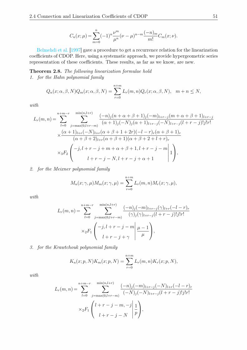
2.4 Connection and Linearization Coefficients of CDOP 51
Cn(x;µ) =n∑
m=0
(−1)nνm
µn(ν − µ)n−m
(−n)mm!
Cm(x; ν).
Belmehdi et al. [1997] gave a procedure to get a recurrence relation for the linearizationcoefficients of CDOP. Here, using a systematic approach, we provide hypergeometric seriesrepresentation of these coefficients. These results, as far as we know, are new.
Theorem 2.8. The following linearization formulae hold1. for the Hahn polynomial family
Qn(x;α, β,N)Qm(x;α, β,N) =n+m∑r=0
Lr(m,n)Qr(x;α, β,N), m+ n ≤ N,
with
Lr(m,n) =n+m−r∑l=0
min(n,l+r)∑j=max(0,l+r−m)
(−n)j(n+ α + β + 1)j(−m)l+r−j(m+ α + β + 1)l+r−j(α + 1)j(−N)j(α + 1)l+r−j(−N)l+r−j(l + r − j)!j!r!
×(α + 1)l+r(−N)l+r(α + β + 1 + 2r)(−l − r)r(α + β + 1)r(α + β + 2)l+r(α + β + 1)(α + β + 2 + l + r)r
×3F2
−j, l + r − j +m+ α + β + 1, l + r − j −m
l + r − j −N, l + r − j + α + 1
∣∣∣∣∣∣ 1,
2. for the Meixner polynomial family
Mn(x; γ, µ)Mm(x; γ, µ) =n+m∑r=0
Lr(m,n)Mr(x; γ, µ),
with
Lr(m,n) =n+m−r∑l=0
min(n,l+r)∑j=max(0,l+r−m)
(−n)j(−m)l+r−j(γ)l+r(−l − r)r(γ)j(γ)l+r−j(l + r − j)!j!r!
×2F1
−j, l + r − j −m
l + r − j + γ
∣∣∣∣∣∣ µ− 1
µ
,3. for the Krawtchouk polynomial family
Kn(x; p,N)Km(x; p,N) =n+m∑r=0
Lr(m,n)Kr(x; p,N),
with
Lr(m,n) =n+m−r∑l=0
min(n,l+r)∑j=max(0,l+r−m)
(−n)j(−m)l+r−j(−N)l+r(−l − r)r(−N)j(−N)l+r−j(l + r − j)!j!r!
×2F1
l + r − j −m,−j
l + r − j −N
∣∣∣∣∣∣ 1
p
,
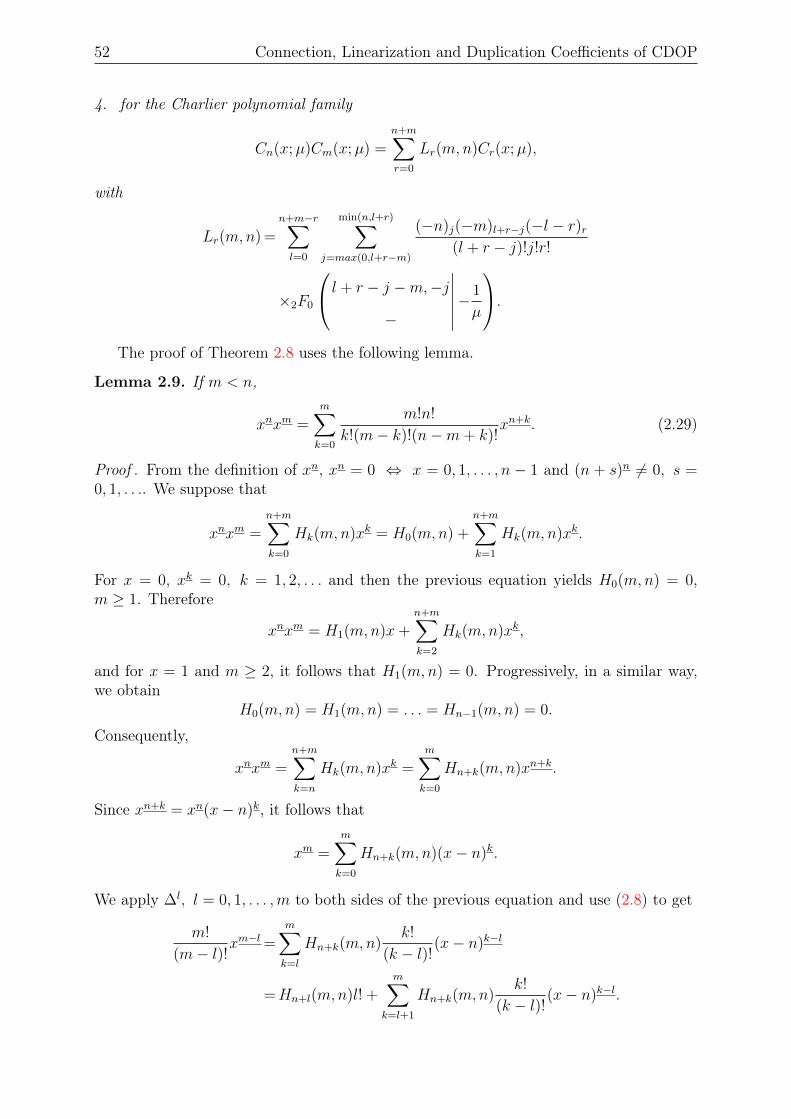
52 Connection, Linearization and Duplication Coefficients of CDOP
4. for the Charlier polynomial family
Cn(x;µ)Cm(x;µ) =n+m∑r=0
Lr(m,n)Cr(x;µ),
with
Lr(m,n) =n+m−r∑l=0
min(n,l+r)∑j=max(0,l+r−m)
(−n)j(−m)l+r−j(−l − r)r(l + r − j)!j!r!
×2F0
l + r − j −m,−j
−
∣∣∣∣∣∣− 1
µ
.The proof of Theorem 2.8 uses the following lemma.
Lemma 2.9. If m < n,
xnxm =m∑k=0
m!n!
k!(m− k)!(n−m+ k)!xn+k. (2.29)
Proof . From the definition of xn, xn = 0 ⇔ x = 0, 1, . . . , n − 1 and (n + s)n 6= 0, s =0, 1, . . .. We suppose that
xnxm =n+m∑k=0
Hk(m,n)xk = H0(m,n) +n+m∑k=1
Hk(m,n)xk.
For x = 0, xk = 0, k = 1, 2, . . . and then the previous equation yields H0(m,n) = 0,m ≥ 1. Therefore
xnxm = H1(m,n)x+n+m∑k=2
Hk(m,n)xk,
and for x = 1 and m ≥ 2, it follows that H1(m,n) = 0. Progressively, in a similar way,we obtain
H0(m,n) = H1(m,n) = . . . = Hn−1(m,n) = 0.
Consequently,
xnxm =n+m∑k=n
Hk(m,n)xk =m∑k=0
Hn+k(m,n)xn+k.
Since xn+k = xn(x− n)k, it follows that
xm =m∑k=0
Hn+k(m,n)(x− n)k.
We apply ∆l, l = 0, 1, . . . ,m to both sides of the previous equation and use (2.8) to get
m!
(m− l)!xm−l =
m∑k=l
Hn+k(m,n)k!
(k − l)!(x− n)k−l
=Hn+l(m,n)l! +m∑
k=l+1
Hn+k(m,n)k!
(k − l)!(x− n)k−l.
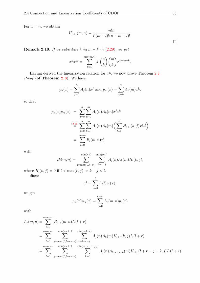
2.4 Connection and Linearization Coefficients of CDOP 53
For x = n, we obtain
Hn+l(m,n) =m!n!
l!(m− l)!(n−m+ l)!.
Remark 2.10. If we substitute k by m− k in (2.29), we get
xnxm =
min(m,n)∑k=0
k!
(n
k
)(m
k
)xn+m−k.
Having derived the linearization relation for xn, we now prove Theorem 2.8.Proof (of Theorem 2.8). We have
pn(x) =n∑j=0
Aj(n)xj and pm(x) =m∑k=0
Ak(m)xk,
so that
pn(x)pm(x) =n∑j=0
m∑k=0
Aj(n)Ak(m)xjxk
(2.29)=
n∑j=0
m∑k=0
Aj(n)Ak(m)( k∑l=0
Hj+l(k, j)xj+l)
=n+m∑l=0
Bl(m,n)xl,
with
Bl(m,n) =
min(n,l)∑j=max(0,l−m)
min(m,l)∑k=l−j
Aj(n)Ak(m)Hl(k, j),
where Hl(k, j) = 0 if l < max(k, j) or k + j < l.Since
xl =l∑
r=0
Ir(l)pr(x),
we get
pn(x)pm(x) =n+m∑r=0
Lr(m,n)pr(x)
with
Lr(m,n) =n+m−r∑l=0
Bl+r(m,n)Ir(l + r)
=n+m−r∑l=0
min(n,l+r)∑j=max(0,l+r−m)
min(m,l+r)∑k=l+r−j
Aj(n)Ak(m)Hl+r(k, j)Ir(l + r)
=n+m−r∑l=0
min(n,l+r)∑j=max(0,l+r−m)
min(m−l−r+j,j)∑k=0
Aj(n)Al+r−j+k(m)Hl+r(l + r − j + k, j)Ir(l + r).
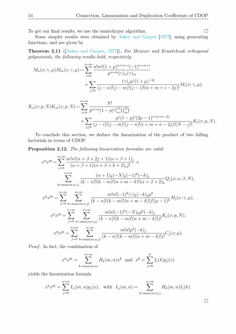
54 Connection, Linearization and Duplication Coefficients of CDOP
To get our final results, we use the sumtohyper algorithm. Some simpler results were obtained by Askey and Gasper [1977], using generating
functions, and are given by
Theorem 2.11 ([Askey and Gasper, 1977]). For Meixner and Krawtchouk orthogonalpolynomials, the following results hold, respectively:
Mn(x; γ, µ)Mm(x; γ, µ) =n+m∑i=0
n!m!(1 + µ)n+m+i(−1)n+m+i
µn+m(γ)n(γ)m
×∑j≥0
(γ)jµj(1 + µ)−2j
(j − n)!(j −m)!(j − i)!(n+m+ i− 2j)!Mi(x; γ, µ),
Kn(x; p,N)Km(x; p,N) =n+m∑i=0
N !
pn+m(1− p)i(Nn
)(Nm
)×∑j≥0
pj(1− p)j(2p− 1)i+m+n−2j
(j − i)!(j −m)!(j − n)!(i+m+ n− 2j)!(N − j)!Ki(x; p,N).
To conclude this section, we deduce the linearization of the product of two fallingfactorials in terms of CDOP.
Proposition 2.12. The following linearization formulae are valid:
xnxm =n+m∑j=0
m!n!(α + β + 2j + 1)(α + β + 1)j(α + β + 1)(α + β + k + 2)jj!
×
n+m∑k=max(m,n,j)
(α + 1)k(−N)k(−1)k(−k)j(k − n)!(k −m)!(n+m− k)!(α + β + 2)k
Qj(x;α, β,N),
xnxm =n+m∑j=0
n+m∑k=max(m,n,j)
m!n!(−1)k(γ)k(−k)jµk
(k − n)!(k −m)!(n+m− k)!j!(µ− 1)kMj(x; γ, µ),
xnxm =n+m∑j=0
n+m∑k=max(m,n,j)
m!n!(−1)k(−N)kpk(−k)j
(k − n)!(k −m)!(n+m− k)!j!Kj(x; p,N),
xnxm =n+m∑j=0
n+m∑k=max(m,n,j)
m!n!µk(−k)j(k − n)!(k −m)!(n+m− k)!j!
Cj(x;µ).
Proof . In fact, the combination of
xnxm =n+m∑
k=max(m,n)
Hk(m,n)xk and xk =k∑j=0
Ij(k)pj(x)
yields the linearization formula
xnxm =n+m∑j=0
Lj(m,n)pj(x), with Lj(m,n) =n+m∑
k=max(m,n,j)
Hk(m,n)Ij(k).
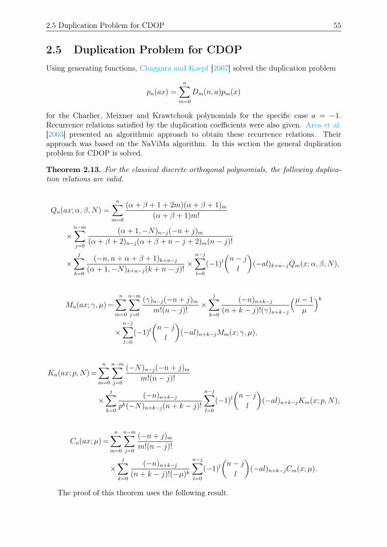
2.5 Duplication Problem for CDOP 55
2.5 Duplication Problem for CDOP
Using generating functions, Chaggara and Koepf [2007] solved the duplication problem
pn(ax) =n∑
m=0
Dm(n, a)pm(x)
for the Charlier, Meixner and Krawtchouk polynomials for the specific case a = −1.Recurrence relations satisfied by the duplication coefficients were also given. Area et al.[2003] presented an algorithmic approach to obtain these recurrence relations. Theirapproach was based on the NaViMa algorithm. In this section the general duplicationproblem for CDOP is solved.
Theorem 2.13. For the classical discrete orthogonal polynomials, the following duplica-tion relations are valid.
Qn(ax;α, β,N) =n∑
m=0
(α + β + 1 + 2m)(α + β + 1)m(α + β + 1)m!
×n−m∑j=0
(α + 1,−N)n−j(−n+ j)m(α + β + 2)n−j(α + β + n− j + 2)m(n− j)!
×j∑
k=0
(−n, n+ α + β + 1)k+n−j
(α + 1,−N)k+n−j(k + n− j)!×
n−j∑l=0
(−1)l(n− jl
)(−al)k+n−jQm(x;α, β,N),
Mn(ax; γ, µ) =n∑
m=0
n−m∑j=0
(γ)n−j(−n+ j)mm!(n− j)!
×j∑
k=0
(−n)n+k−j
(n+ k − j)!(γ)n+k−j
(µ− 1
µ
)k×
n−j∑l=0
(−1)l(n− jl
)(−al)n+k−jMm(x; γ, µ),
Kn(ax; p,N) =n∑
m=0
n−m∑j=0
(−N)n−j(−n+ j)mm!(n− j)!
×j∑
k=0
(−n)n+k−j
pk(−N)n+k−j(n+ k − j)!
n−j∑l=0
(−1)l(n− jl
)(−al)n+k−jKm(x; p,N),
Cn(ax;µ) =n∑
m=0
n−m∑j=0
(−n+ j)mm!(n− j)!
×j∑
k=0
(−n)n+k−j
(n+ k − j)!(−µ)k
n−j∑l=0
(−1)l(n− jl
)(−al)n+k−jCm(x;µ).
The proof of this theorem uses the following result.
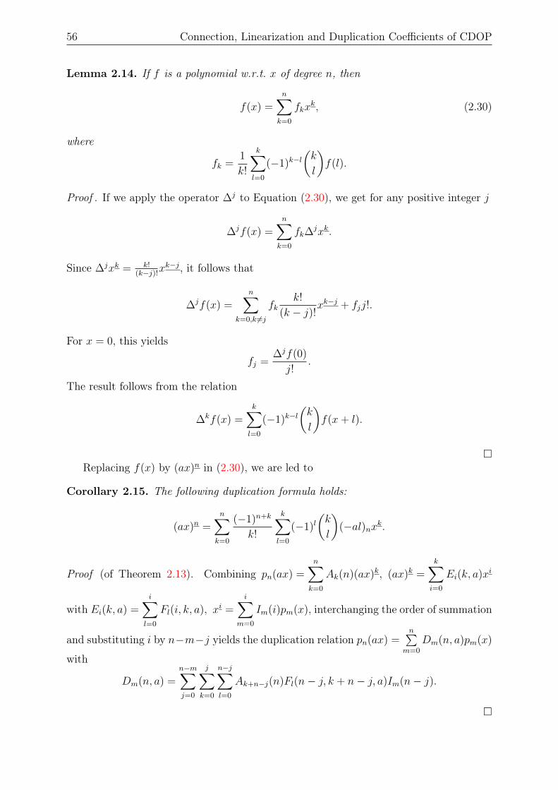
56 Connection, Linearization and Duplication Coefficients of CDOP
Lemma 2.14. If f is a polynomial w.r.t. x of degree n, then
f(x) =n∑k=0
fkxk, (2.30)
where
fk =1
k!
k∑l=0
(−1)k−l(k
l
)f(l).
Proof . If we apply the operator ∆j to Equation (2.30), we get for any positive integer j
∆jf(x) =n∑k=0
fk∆jxk.
Since ∆jxk = k!(k−j)!x
k−j, it follows that
∆jf(x) =n∑
k=0,k 6=j
fkk!
(k − j)!xk−j + fjj!.
For x = 0, this yields
fj =∆jf(0)
j!.
The result follows from the relation
∆kf(x) =k∑l=0
(−1)k−l(k
l
)f(x+ l).
Replacing f(x) by (ax)n in (2.30), we are led to
Corollary 2.15. The following duplication formula holds:
(ax)n =n∑k=0
(−1)n+k
k!
k∑l=0
(−1)l(k
l
)(−al)nxk.
Proof (of Theorem 2.13). Combining pn(ax) =n∑k=0
Ak(n)(ax)k, (ax)k =k∑i=0
Ei(k, a)xi
with Ei(k, a) =i∑l=0
Fl(i, k, a), xi =i∑
m=0
Im(i)pm(x), interchanging the order of summation
and substituting i by n−m−j yields the duplication relation pn(ax) =n∑
m=0
Dm(n, a)pm(x)
with
Dm(n, a) =n−m∑j=0
j∑k=0
n−j∑l=0
Ak+n−j(n)Fl(n− j, k + n− j, a)Im(n− j).
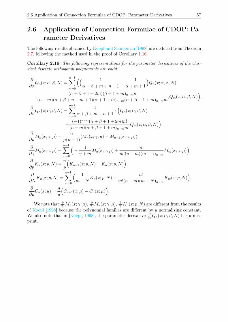
2.6 Application of Connection Formulae of CDOP: Parameter Derivatives 57
2.6 Application of Connection Formulae of CDOP: Pa-rameter Derivatives
The following results obtained by Koepf and Schmersau [1998] are deduced from Theorem2.7, following the method used in the proof of Corollary 1.16.
Corollary 2.16. The following representations for the parameter derivatives of the clas-sical discrete orthogonal polynomials are valid:
∂
∂αQn(x;α, β,N) =
n−1∑m=0
(( 1
α + β +m+ n+ 1− 1
α +m+ 1
)Qn(x;α, β,N)
+(α + β + 1 + 2m)(β + 1 +m)n−mn!
(n−m)(α + β + n+m+ 1)(α + 1 +m)n−m(α + β + 1 +m)n−mm!Qm(x;α, β,N)
),
∂
∂βQn(x;α, β,N) =
n−1∑m=0
1
α + β +m+ n+ 1·(Qn(x;α, β,N)
+(−1)n−m(α + β + 1 + 2m)n!
(n−m)(α + β + 1 +m)n−mm!Qm(x;α, β,N)
),
∂
∂µMn(x; γ, µ) =
n
µ(µ− 1)(Mn(x; γ, µ)−Mn−1(x; γ, µ)),
∂
∂γMn(x; γ, µ) =
n−1∑m=0
(− 1
γ +mMn(x; γ, µ) +
n!
m!(n−m)(m+ γ)n−mMm(x; γ, µ)
),
∂
∂pKn(x; p,N) =
n
p
(Kn−1(x; p,N)−Kn(x; p,N)
),
∂
∂NKn(x; p,N) =
n−1∑m=0
( 1
m−NKn(x; p,N)− n!
m!(n−m)(m−N)n−mKm(x; p,N)
),
∂
∂µCn(x;µ) =
n
µ
(Cn−1(x;µ)− Cn(x;µ)
).
We note that ∂∂µMn(x; γ, µ), ∂
∂γMn(x; γ, µ), ∂
∂pKn(x; p,N) are different from the results
of Koepf [1998] because the polynomial families are different by a normalizing constant.We also note that in [Koepf, 1998], the parameter derivative ∂
∂αQn(x;α, β,N) has a mis-
print.

58 Connection, Linearization and Duplication Coefficients of CDOP
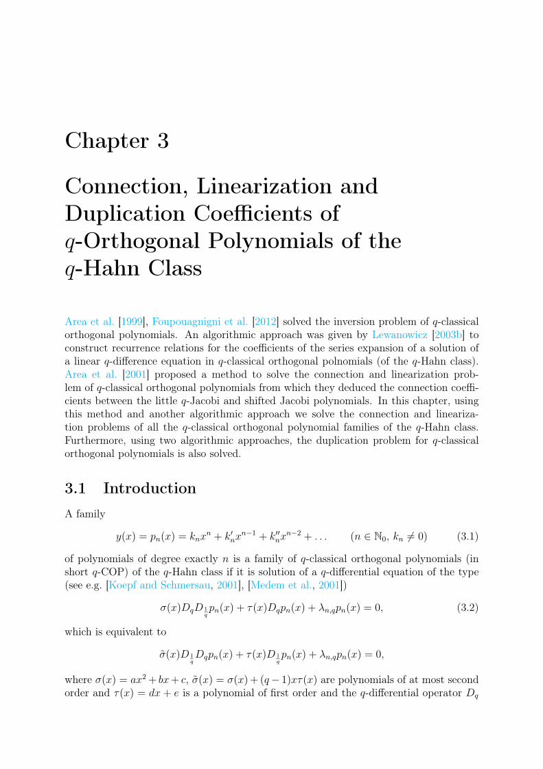
Chapter 3
Connection, Linearization andDuplication Coefficients ofq-Orthogonal Polynomials of theq-Hahn Class
Area et al. [1999], Foupouagnigni et al. [2012] solved the inversion problem of q-classicalorthogonal polynomials. An algorithmic approach was given by Lewanowicz [2003b] toconstruct recurrence relations for the coefficients of the series expansion of a solution ofa linear q-difference equation in q-classical orthogonal polnomials (of the q-Hahn class).Area et al. [2001] proposed a method to solve the connection and linearization prob-lem of q-classical orthogonal polynomials from which they deduced the connection coeffi-cients between the little q-Jacobi and shifted Jacobi polynomials. In this chapter, usingthis method and another algorithmic approach we solve the connection and lineariza-tion problems of all the q-classical orthogonal polynomial families of the q-Hahn class.Furthermore, using two algorithmic approaches, the duplication problem for q-classicalorthogonal polynomials is also solved.
3.1 IntroductionA family
y(x) = pn(x) = knxn + k′nx
n−1 + k′′nxn−2 + . . . (n ∈ N0, kn 6= 0) (3.1)
of polynomials of degree exactly n is a family of q-classical orthogonal polynomials (inshort q-COP) of the q-Hahn class if it is solution of a q-differential equation of the type(see e.g. [Koepf and Schmersau, 2001], [Medem et al., 2001])
σ(x)DqD 1qpn(x) + τ(x)Dqpn(x) + λn,qpn(x) = 0, (3.2)
which is equivalent to
σ(x)D 1qDqpn(x) + τ(x)D 1
qpn(x) + λn,qpn(x) = 0,
where σ(x) = ax2 + bx+ c, σ(x) = σ(x) + (q− 1)xτ(x) are polynomials of at most secondorder and τ(x) = dx + e is a polynomial of first order and the q-differential operator Dq
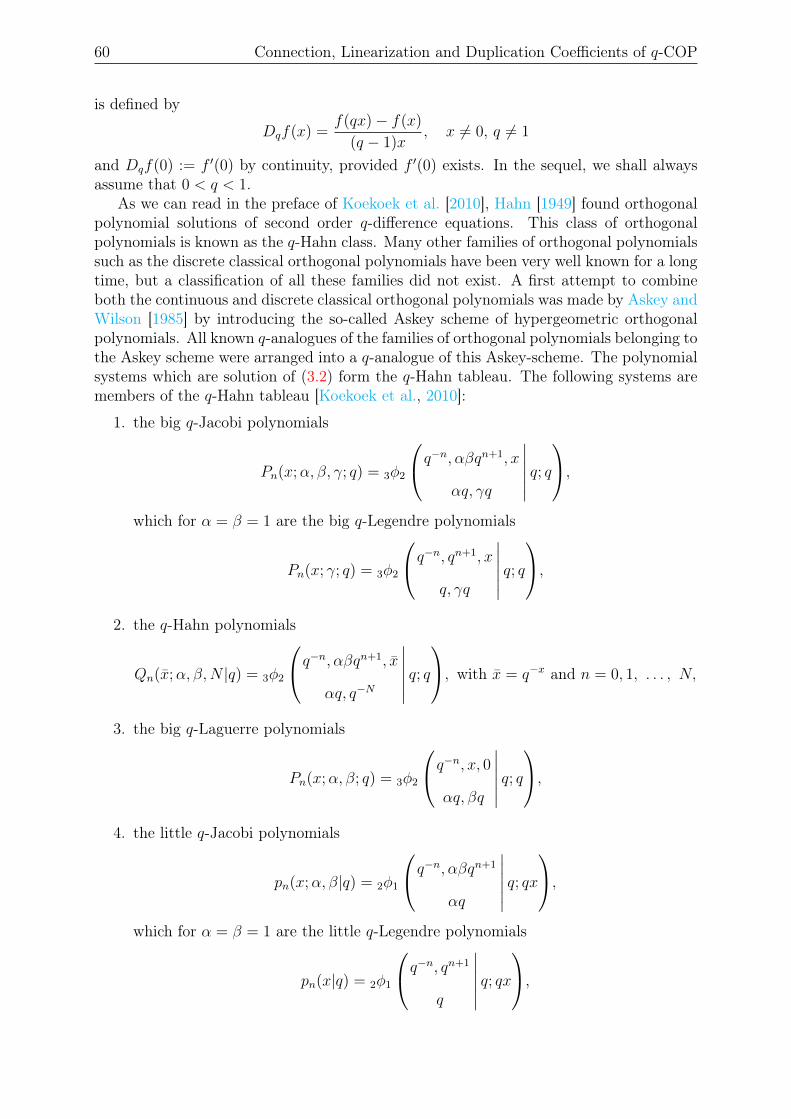
60 Connection, Linearization and Duplication Coefficients of q-COP
is defined by
Dqf(x) =f(qx)− f(x)
(q − 1)x, x 6= 0, q 6= 1
and Dqf(0) := f ′(0) by continuity, provided f ′(0) exists. In the sequel, we shall alwaysassume that 0 < q < 1.
As we can read in the preface of Koekoek et al. [2010], Hahn [1949] found orthogonalpolynomial solutions of second order q-difference equations. This class of orthogonalpolynomials is known as the q-Hahn class. Many other families of orthogonal polynomialssuch as the discrete classical orthogonal polynomials have been very well known for a longtime, but a classification of all these families did not exist. A first attempt to combineboth the continuous and discrete classical orthogonal polynomials was made by Askey andWilson [1985] by introducing the so-called Askey scheme of hypergeometric orthogonalpolynomials. All known q-analogues of the families of orthogonal polynomials belonging tothe Askey scheme were arranged into a q-analogue of this Askey-scheme. The polynomialsystems which are solution of (3.2) form the q-Hahn tableau. The following systems aremembers of the q-Hahn tableau [Koekoek et al., 2010]:
1. the big q-Jacobi polynomials
Pn(x;α, β, γ; q) = 3φ2
q−n, αβqn+1, x
αq, γq
∣∣∣∣∣∣ q; q,
which for α = β = 1 are the big q-Legendre polynomials
Pn(x; γ; q) = 3φ2
q−n, qn+1, x
q, γq
∣∣∣∣∣∣ q; q,
2. the q-Hahn polynomials
Qn(x;α, β,N |q) = 3φ2
q−n, αβqn+1, x
αq, q−N
∣∣∣∣∣∣ q; q, with x = q−x and n = 0, 1, . . . , N,
3. the big q-Laguerre polynomials
Pn(x;α, β; q) = 3φ2
q−n, x, 0αq, βq
∣∣∣∣∣∣ q; q,
4. the little q-Jacobi polynomials
pn(x;α, β|q) = 2φ1
q−n, αβqn+1
αq
∣∣∣∣∣∣ q; qx,
which for α = β = 1 are the little q-Legendre polynomials
pn(x|q) = 2φ1
q−n, qn+1
q
∣∣∣∣∣∣ q; qx,
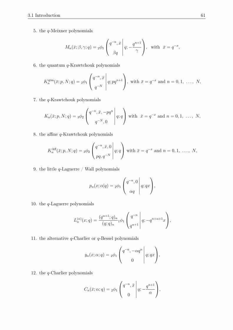
3.1 Introduction 61
5. the q-Meixner polynomials
Mn(x; β, γ; q) = 2φ1
q−n, xβq
∣∣∣∣∣∣ q;−qn+1
γ
, with x = q−x,
6. the quantum q-Krawtchouk polynomials
Kqtmn (x; p,N ; q) = 2φ1
q−n, xq−N
∣∣∣∣∣∣ q; pqn+1
, with x = q−x and n = 0, 1, . . . , N,
7. the q-Krawtchouk polynomials
Kn(x; p,N ; q) = 3φ2
q−n, x,−pqnq−N , 0
∣∣∣∣∣∣ q; q with x = q−x and n = 0, 1, . . . , N,
8. the affine q-Krawtchouk polynomials
KAffn (x; p,N ; q) = 3φ2
q−n, x, 0pq, q−N
∣∣∣∣∣∣ q; q with x = q−x and n = 0, 1, . . . , N,
9. the little q-Laguerre / Wall polynomials
pn(x;α|q) = 2φ1
q−n, 0αq
∣∣∣∣∣∣ q; qx,
10. the q-Laguerre polynomials
L(α)n (x; q) =
(qα+1; q)n(q; q)n
1φ1
q−n
qα+1
∣∣∣∣∣∣ q;−qn+α+1x
,11. the alternative q-Charlier or q-Bessel polynomials
yn(x;α; q) = 2φ1
q−n,−αqn0
∣∣∣∣∣∣ q; qx,
12. the q-Charlier polynomials
Cn(x;α; q) = 2φ1
q−n, x0
∣∣∣∣∣∣ q;−qn+1
α
,
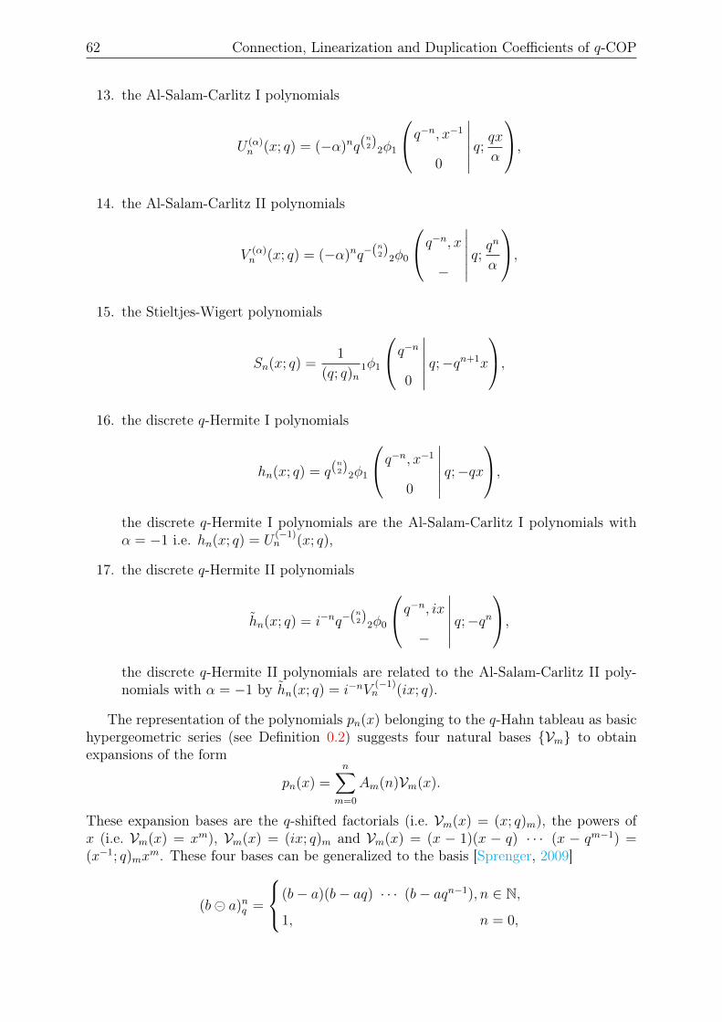
62 Connection, Linearization and Duplication Coefficients of q-COP
13. the Al-Salam-Carlitz I polynomials
U (α)n (x; q) = (−α)nq(
n2)2φ1
q−n, x−1
0
∣∣∣∣∣∣ q; qxα,
14. the Al-Salam-Carlitz II polynomials
V (α)n (x; q) = (−α)nq−(n2)2φ0
q−n, x−
∣∣∣∣∣∣ q; qn
α
,15. the Stieltjes-Wigert polynomials
Sn(x; q) =1
(q; q)n1φ1
q−n0
∣∣∣∣∣∣ q;−qn+1x
,16. the discrete q-Hermite I polynomials
hn(x; q) = q(n2)2φ1
q−n, x−1
0
∣∣∣∣∣∣ q;−qx,
the discrete q-Hermite I polynomials are the Al-Salam-Carlitz I polynomials withα = −1 i.e. hn(x; q) = U
(−1)n (x; q),
17. the discrete q-Hermite II polynomials
hn(x; q) = i−nq−(n2)2φ0
q−n, ix−
∣∣∣∣∣∣ q;−qn,
the discrete q-Hermite II polynomials are related to the Al-Salam-Carlitz II poly-nomials with α = −1 by hn(x; q) = i−nV
(−1)n (ix; q).
The representation of the polynomials pn(x) belonging to the q-Hahn tableau as basichypergeometric series (see Definition 0.2) suggests four natural bases Vm to obtainexpansions of the form
pn(x) =n∑
m=0
Am(n)Vm(x).
These expansion bases are the q-shifted factorials (i.e. Vm(x) = (x; q)m), the powers ofx (i.e. Vm(x) = xm), Vm(x) = (ix; q)m and Vm(x) = (x − 1)(x − q) · · · (x − qm−1) =(x−1; q)mx
m. These four bases can be generalized to the basis [Sprenger, 2009]
(b a)nq =
(b− a)(b− aq) · · · (b− aqn−1), n ∈ N,
1, n = 0,
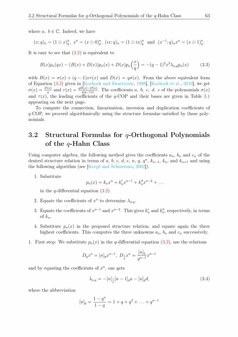
3.2 Structural Formulas for q-Orthogonal Polynomials of the q-Hahn Class 63
where a, b ∈ C. Indeed, we have
(x; q)n = (1 x)nq , xn = (x 0)nq , (ix; q)n = (1 ix)nq and (x−1; q)nx
n = (x 1)nq .
It is easy to see that (3.2) is equivalent to
B(x)pn(qx)− (B(x) +D(x))pn(x) +D(x)pn
(xq
)= −(q − 1)2x2λn,qpn(x) (3.3)
with B(x) = σ(x) + (q − 1)xτ(x) and D(x) = qσ(x). From the above equivalent formof Equation (3.2) given in [Koekoek and Swarttouw, 1998], [Koekoek et al., 2010], we getσ(x) = D(x)
qand τ(x) = qB(x)−D(x)
q(q−1)x. The coefficients a, b, c, d, e of the polynomials σ(x)
and τ(x), the leading coefficients of the q-COP and their bases are given in Table 3.1appearing on the next page.
To compute the connection, linearization, inversion and duplication coefficients ofq-COP, we proceed algorithmically using the structure formulae satisfied by these poly-nomials.
3.2 Structural Formulas for q-Orthogonal Polynomialsof the q-Hahn Class
Using computer algebra, the following method gives the coefficients an, bn and cn of thedesired structure relation in terms of a, b, c, d, e, n, q, qn, kn−1, kn, and kn+1 and usingthe following algorithm (see [Koepf and Schmersau, 2002]).
1. Substitutepn(x) = knx
n + k′nxn−1 + k′′nx
n−2 + . . .
in the q-differential equation (3.2).
2. Equate the coefficients of xn to determine λn,q.
3. Equate the coefficients of xn−1 and xn−2. This gives k′n and k′′n, respectively, in termsof kn.
4. Substitute pn(x) in the proposed structure relation, and equate again the threehighest coefficients. This computes the three unknowns an, bn and cn successively.
1. First step: We substitute pn(x) in the q-differential equation (3.2), use the relations
Dqxn = [n]qx
n−1, D 1qxn =
[n]qqn−1
xn−1
and by equating the coefficients of xn, one gets
λn,q = −[n] 1q[n− 1]qa− [n]qd, (3.4)
where the abbreviation
[n]q =1− qn
1− q= 1 + q + q2 + . . .+ qn−1
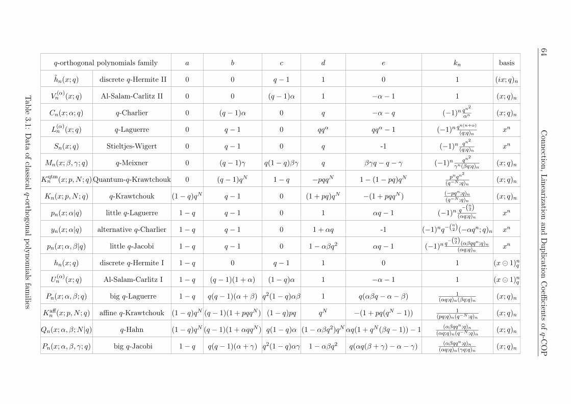
64Connection,Linearization
andDuplication
Coeffi
cientsofq-C
OP
q-orthogonal polynomials family a b c d e kn basis
hn(x; q) discrete q-Hermite II 0 0 q − 1 1 0 1 (ix; q)n
V(α)n (x; q) Al-Salam-Carlitz II 0 0 (q − 1)α 1 −α− 1 1 (x; q)n
Cn(x;α; q) q-Charlier 0 (q − 1)α 0 q −α− q (−1)n qn2
αn (x; q)n
L(α)n (x; q) q-Laguerre 0 q − 1 0 qqα qqα − 1 (−1)n q
n(n+α)
(q;q)nxn
Sn(x; q) Stieltjes-Wigert 0 q − 1 0 q -1 (−1)n qn2
(q;q)nxn
Mn(x;β, γ; q) q-Meixner 0 (q − 1)γ q(1− q)βγ q βγq − q − γ (−1)n qn2
γn(βq;q)n(x; q)n
Kqtmn (x; p,N ; q)Quantum-q-Krawtchouk 0 (q − 1)qN 1− q −pqqN 1− (1− pq)qN pnqn
2
(q−N ;q)n(x; q)n
Kn(x; p,N ; q) q-Krawtchouk (1− q)qN q − 1 0 (1 + pq)qN −(1 + pqqN ) (−pqn;q)n(q−N ;q)n
(x; q)n
pn(x;α|q) little q-Laguerre 1− q q − 1 0 1 αq − 1 (−1)n q−(n2)
(αq;q)nxn
yn(x;α|q) alternative q-Charlier 1− q q − 1 0 1 + αq -1 (−1)nq−(n2)(−αqn; q)n xn
pn(x;α, β|q) little q-Jacobi 1− q q − 1 0 1− αβq2 αq − 1 (−1)n q−(n2)(αβqqn;q)n
(αq;q)nxn
hn(x; q) discrete q-Hermite I 1− q 0 q − 1 1 0 1 (x 1)nq
U(α)n (x; q) Al-Salam-Carlitz I 1− q (q − 1)(1 + α) (1− q)α 1 −α− 1 1 (x 1)nq
Pn(x;α, β; q) big q-Laguerre 1− q q(q − 1)(α+ β) q2(1− q)αβ 1 q(αβq − α− β) 1(αq;q)n(βq;q)n
(x; q)n
Kaffn (x; p,N ; q) affine q-Krawtchouk (1− q)qN (q − 1)(1 + pqqN ) (1− q)pq qN −(1 + pq(qN − 1)) 1
(pq;q)n(q−N ;q)n(x; q)n
Qn(x;α, β;N |q) q-Hahn (1− q)qN (q − 1)(1 + αqqN ) q(1− q)α (1− αβq2)qN αq(1 + qN (βq − 1))− 1 (αβqqn;q)n(αq;q)n(q−N ;q)n
(x; q)n
Pn(x;α, β, γ; q) big q-Jacobi 1− q q(q − 1)(α+ γ) q2(1− q)αγ 1− αβq2 q(αq(β + γ)− α− γ) (αβqqn;q)n(αq;q)n(γq;q)n
(x; q)n
Table3.1:
Data
ofclassicalq-orthogonalpolynom
ialsfam
ilies
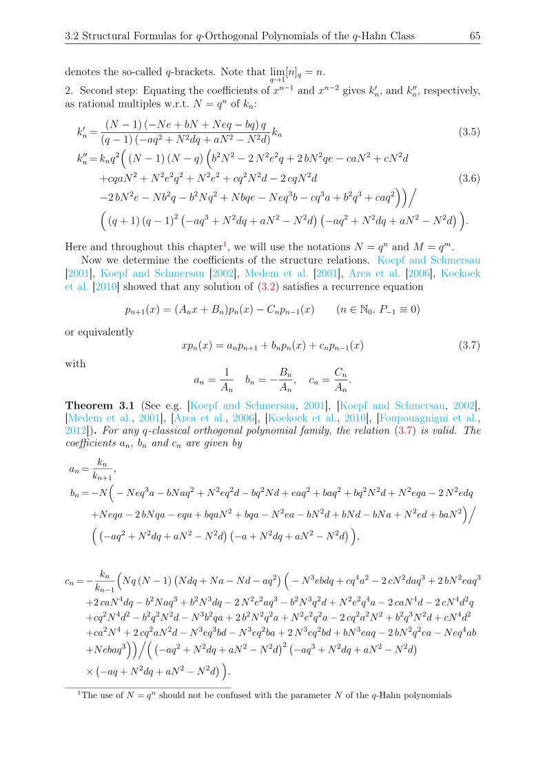
3.2 Structural Formulas for q-Orthogonal Polynomials of the q-Hahn Class 65
denotes the so-called q-brackets. Note that limq→1
[n]q = n.
2. Second step: Equating the coefficients of xn−1 and xn−2 gives k′n, and k′′n, respectively,as rational multiples w.r.t. N = qn of kn:
k′n =(N − 1) (−Ne+ bN +Neq − bq) q
(q − 1) (−aq2 +N2dq + aN2 −N2d)kn (3.5)
k′′n = knq2(
(N − 1) (N − q)(b2N2 − 2N2e2q + 2 bN2qe− caN2 + cN2d
+cqaN2 +N2e2q2 +N2e2 + cq2N2d− 2 cqN2d (3.6)
−2 bN2e−Nb2q − b2Nq2 +Nbqe−Neq3b− cq3a+ b2q3 + caq2))/
((q + 1) (q − 1)2 (−aq3 +N2dq + aN2 −N2d
) (−aq2 +N2dq + aN2 −N2d
) ).
Here and throughout this chapter1, we will use the notations N = qn and M = qm.Now we determine the coefficients of the structure relations. Koepf and Schmersau
[2001], Koepf and Schmersau [2002], Medem et al. [2001], Area et al. [2006], Koekoeket al. [2010] showed that any solution of (3.2) satisfies a recurrence equation
pn+1(x) = (Anx+Bn)pn(x)− Cnpn−1(x) (n ∈ N0, P−1 ≡ 0)
or equivalentlyxpn(x) = anpn+1 + bnpn(x) + cnpn−1(x) (3.7)
withan =
1
Anbn = −Bn
An, cn =
CnAn
.
Theorem 3.1 (See e.g. [Koepf and Schmersau, 2001], [Koepf and Schmersau, 2002],[Medem et al., 2001], [Area et al., 2006], [Koekoek et al., 2010], [Foupouagnigni et al.,2012]). For any q-classical orthogonal polynomial family, the relation (3.7) is valid. Thecoefficients an, bn and cn are given by
an =knkn+1
,
bn =−N(−Neq3a− bNaq2 +N2eq2d− bq2Nd+ eaq2 + baq2 + bq2N2d+N2eqa− 2N2edq
+Neqa− 2 bNqa− eqa+ bqaN2 + bqa−N2ea− bN2d+ bNd− bNa+N2ed+ baN2)/
( (−aq2 +N2dq + aN2 −N2d
) (−a+N2dq + aN2 −N2d
) ),
cn =− knkn−1
(Nq (N − 1)
(Ndq +Na−Nd− aq2
) (−N3ebdq + cq4a2 − 2 cN2daq3 + 2 bN2eaq3
+2 caN4dq − b2Naq3 + b2N3dq − 2N2e2aq3 − b2N3q2d+N2e2q4a− 2 caN4d− 2 cN4d2q
+cq2N4d2 − b2q2N2d−N3b2qa+ 2 b2N2q2a+N2e2q2a− 2 cq2a2N2 + b2q3N2d+ cN4d2
+ca2N4 + 2 cq2aN2d−N3eq3bd−N3eq2ba+ 2N3eq2bd+ bN3eaq − 2 bN2q2ea−Neq4ab
+Nebaq3))/( (
−aq2 +N2dq + aN2 −N2d)2 (−aq3 +N2dq + aN2 −N2d
)×(−aq +N2dq + aN2 −N2d
) ).
1The use of N = qn should not be confused with the parameter N of the q-Hahn polynomials
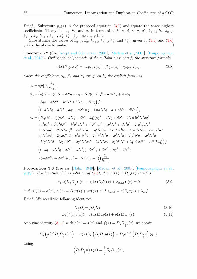
66 Connection, Linearization and Duplication Coefficients of q-COP
Proof . Substitute pn(x) in the proposed equation (3.7) and equate the three highestcoefficients. This yields an, bn, and cn in terms of a, b, c, d, e, q, qn, kn−1, kn, kn+1,k′n−1, k′n, k′n+1, k′′n−1, k′′n, k′′n+1 by linear algebra.
Substituting the values of k′n−1, k′n, k′n+1, k′′n−1, k′′n, and k′′n+1 given by (3.5) and (3.6)yields the above formulas.
Theorem 3.2 (See [Koepf and Schmersau, 2001], [Medem et al., 2001], [Foupouagnigniet al., 2012]). Orthogonal polynomials of the q-Hahn class satisfy the structure formula
σ(x)D 1qpn(x) = αnpn+1(x) + βnpn(x) + γnpn−1(x), (3.8)
where the coefficients αn, βn and γn are given by the explicit formulas
αn = a[n]1/qknkn+1
,
βn =(q(N − 1)(aN + dNq − aq −Nd)(eNaq2 − bdN2q +Nqbq
−bqa+ bdN2 − baN2 + bNa− eNa))/
((−dN2q + dN2 + aq2 − aN2)(q − 1)(dN2q − a+ aN2 − dN2)
),
γn =(Nq(N − 1)(aN + dNq − dN − aq)(aq2 − dNq + dN − aN)(2b2N2aq2
+q4ca2 + b2q3dN2 − b2q2dN2 + e2N2aq2 + cq2N4 + cN4a2 − 2cq3adN2
+eNbaq3 − 2eN2baq2 − eq4Nba− eq2N3ba+ 2eq2N3bd+ 2bq3N2ea− eq3N3bd
+eN3baq + 2cqaN4d+ e2q4N2a− 2e2q3N2a+ qb2N3d− q3b2Na− qb2N3a
−b2q2N3d− 2cqd2N4 − 2q2N2ca2 − 2dN4ca+ cq2d2N4 + 2q2dcaN2 − eN3bdq))/
((−aq + dN2q + aN2 − dN2)(−dN2q + dN2 + aq3 − aN2)
×(−dN2q + dN2 + aq2 − aN2)2(q − 1)) knkn−1
.
Proposition 3.3 (See e.g. [Hahn, 1949], [Medem et al., 2001], [Foupouagnigni et al.,2012]). If a function y(x) is solution of (3.2), then Y (x) = Dqy(x) satisfies
σ1(x)DqD 1qY (x) + τ1(x)DqY (x) + λn,q,1Y (x) = 0 (3.9)
with σ1(x) = σ(x), τ1(x) = Dqσ(x) + qτ(qx) and λn,q,1 = q(Dqτ(x) + λn,q).
Proof . We recall the following identities
D 1qDq = qDqD 1
q, (3.10)
Dq(f(x)g(x)) = f(qx)Dqg(x) + g(x)Dqf(x). (3.11)
Applying identity (3.11) with g(x) = σ(x) and f(x) = DqD 1qy(x), we obtain
Dq
(σ(x)DqD 1
qy(x)
)= σ(x)Dq
(DqD 1
qy(x)
)+Dqσ(x)
(DqD 1
qy)
(qx).
Using (DqD 1
qy)
(qx) =1
qDqDqy(x),
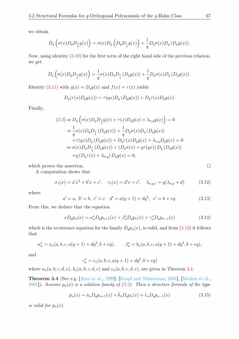
3.2 Structural Formulas for q-Orthogonal Polynomials of the q-Hahn Class 67
we obtain
Dq
(σ(x)DqD 1
qy(x)
)= σ(x)Dq
(DqD 1
qy(x)
)+
1
qDqσ(x)Dq (Dqy(x)) .
Now, using identity (3.10) for the first term of the right hand side of the previous relation,we get
Dq
(σ(x)DqD 1
qy(x)
)=
1
qσ(x)DqD 1
q(Dqy(x)) +
1
qDqσ(x)Dq (Dqy(x)) .
Identity (3.11) with g(x) = Dqy(x) and f(x) = τ(x) yields
Dq(τ(x)Dqy(x)) = τ(qx)Dq (Dqy(x)) +Dqτ(x)Dqy(x).
Finally,
(3.2)⇒Dq
(σ(x)DqD 1
qy(x) + τ(x)Dqy(x) + λn,qy(x)
)= 0
⇒ 1
qσ(x)DqD 1
q(Dqy(x)) +
1
qDqσ(x)Dq (Dqy(x))
+τ(qx)Dq (Dqy(x)) +Dqτ(x)Dqy(x) + λn,qDqy(x) = 0
⇒σ(x)DqD 1q
(Dqy(x)) + (Dqσ(x) + qτ(qx))Dq (Dqy(x))
+q (Dqτ(x) + λn,q)Dqy(x) = 0,
which proves the assertion. A computation shows that
σ1(x) = a′x2 + b′x+ c′, τ1(x) = d′x+ c′, λn,q,1 = q(λn,q + d) (3.12)
wherea′ = a, b′ = b, c′ = c d′ = a(q + 1) + dq2, e′ = b+ eq. (3.13)
From this, we deduce that the equation
xDqpn(x) = α?nDqpn+1(x) + β?nDqpn(x) + γ?nDqpn−1(x) (3.14)
which is the recurrence equation for the family Dqpn(x), is valid, and from (3.13) it followsthat
α?n = an(a, b, c, a(q + 1) + dq2, b+ eq), β?n = bn(a, b, c, a(q + 1) + dq2, b+ eq),
andγ?n = cn(a, b, c, a(q + 1) + dq2, b+ eq)
where an(a, b, c, d, e), bn(a, b, c, d, e) and cn(a, b, c, d, e), are given in Theorem 3.1.
Theorem 3.4 (See e.g. [Area et al., 1999], [Koepf and Schmersau, 2001], [Medem et al.,2001]). Assume pn(x) is a solution family of (3.2). Then a structure formula of the type
pn(x) = anDqpn+1(x) + bnDqpn(x) + cnDqpn−1(x) (3.15)
is valid for pn(x).
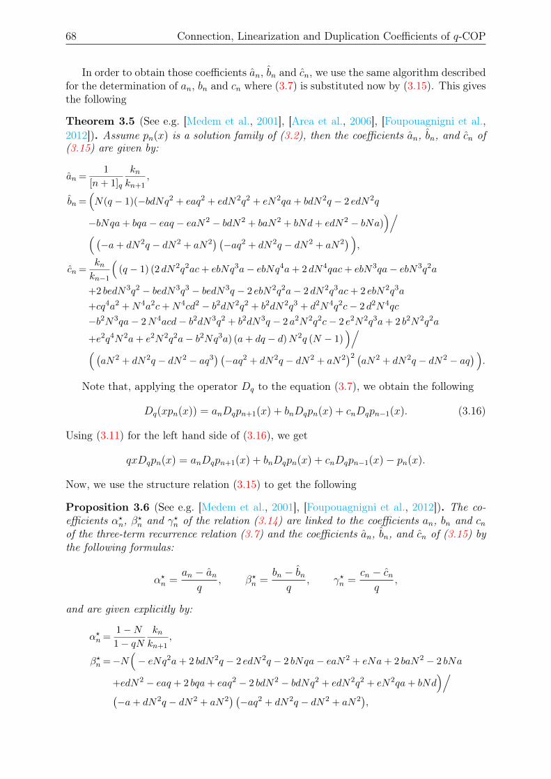
68 Connection, Linearization and Duplication Coefficients of q-COP
In order to obtain those coefficients an, bn and cn, we use the same algorithm describedfor the determination of an, bn and cn where (3.7) is substituted now by (3.15). This givesthe following
Theorem 3.5 (See e.g. [Medem et al., 2001], [Area et al., 2006], [Foupouagnigni et al.,2012]). Assume pn(x) is a solution family of (3.2), then the coefficients an, bn, and cn of(3.15) are given by:
an =1
[n+ 1]q
knkn+1
,
bn =(N(q − 1)(−bdNq2 + eaq2 + edN2q2 + eN2qa+ bdN2q − 2 edN2q
−bNqa+ bqa− eaq − eaN2 − bdN2 + baN2 + bNd+ edN2 − bNa))/
( (−a+ dN2q − dN2 + aN2
) (−aq2 + dN2q − dN2 + aN2
) ),
cn =knkn−1
((q − 1) (2 dN2q2ac+ ebNq3a− ebNq4a+ 2 dN4qac+ ebN3qa− ebN3q2a
+2 bedN3q2 − bedN3q3 − bedN3q − 2 ebN2q2a− 2 dN2q3ac+ 2 ebN2q3a
+cq4a2 +N4a2c+N4cd2 − b2dN2q2 + b2dN2q3 + d2N4q2c− 2 d2N4qc
−b2N3qa− 2N4acd− b2dN3q2 + b2dN3q − 2 a2N2q2c− 2 e2N2q3a+ 2 b2N2q2a
+e2q4N2a+ e2N2q2a− b2Nq3a) (a+ dq − d)N2q (N − 1))/
( (aN2 + dN2q − dN2 − aq3
) (−aq2 + dN2q − dN2 + aN2
)2 (aN2 + dN2q − dN2 − aq
) ).
Note that, applying the operator Dq to the equation (3.7), we obtain the following
Dq(xpn(x)) = anDqpn+1(x) + bnDqpn(x) + cnDqpn−1(x). (3.16)
Using (3.11) for the left hand side of (3.16), we get
qxDqpn(x) = anDqpn+1(x) + bnDqpn(x) + cnDqpn−1(x)− pn(x).
Now, we use the structure relation (3.15) to get the following
Proposition 3.6 (See e.g. [Medem et al., 2001], [Foupouagnigni et al., 2012]). The co-efficients α?n, β?n and γ?n of the relation (3.14) are linked to the coefficients an, bn and cnof the three-term recurrence relation (3.7) and the coefficients an, bn, and cn of (3.15) bythe following formulas:
α?n =an − an
q, β?n =
bn − bnq
, γ?n =cn − cnq
,
and are given explicitly by:
α?n =1−N1− qN
knkn+1
,
β?n =−N(− eNq2a+ 2 bdN2q − 2 edN2q − 2 bNqa− eaN2 + eNa+ 2 baN2 − 2 bNa
+edN2 − eaq + 2 bqa+ eaq2 − 2 bdN2 − bdNq2 + edN2q2 + eN2qa+ bNd)/
(−a+ dN2q − dN2 + aN2
) (−aq2 + dN2q − dN2 + aN2
),
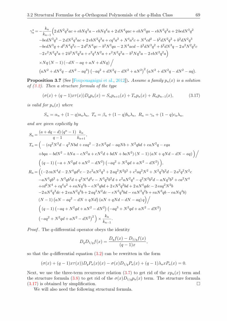
3.2 Structural Formulas for q-Orthogonal Polynomials of the q-Hahn Class 69
γ?n =− knkn−1
(2 dN2q2ac+ ebNq3a− ebNq4a+ 2 dN4qac+ ebN3qa− ebN3q2a+ 2 bedN3q2
−bedN3q3 − 2 dN2q3ac+ 2 ebN2q3a+ cq4a2 +N4a2c+N4cd2 − b2dN2q2 + b2dN2q3
−bedN3q + d2N4q2c− 2 d2N4qc− b2N3qa− 2N4acd− b2dN3q2 + b2dN3q − 2 a2N2q2c
−2 e2N2q3a+ 2 b2N2q2a+ e2q4N2a+ e2N2q2a− b2Nq3a− 2 ebN2q2a)
×Nq (N − 1) (−dN − aq + aN + dNq)/
(aN2 + dN2q − dN2 − aq3
) (−aq2 + dN2q − dN2 + aN2
)2 (aN2 + dN2q − dN2 − aq
).
Proposition 3.7 (See [Foupouagnigni et al., 2012]). Assume a family pn(x) is a solutionof (3.2). Then a structure formula of the type
(σ(x) + (q − 1)xτ(x))Dqpn(x) = Snpn+1(x) + Tnpn(x) +Rnpn−1(x), (3.17)
is valid for pn(x) where
Sn = αn + (1− q)anλn, Tn = βn + (1− q)bnλn, Rn = γn + (1− q)cnλn,
and are given explicitly by
Sn =(a+ dq − d) (qn − 1)
q − 1
knkn+1
,
Tn =(− (eq2N2d− q2Nbd+ eaq2 − 2 eN2qd− aqNb+N2qbd+ eaN2q − eqa
+bqa− bdN2 − bNa− eN2a+ eN2d+ bdN + baN2) (N − 1) (aN + qNd− dN − aq))/
((q − 1)
(−a+N2qd+ aN2 − dN2
) (−aq2 +N2qd+ aN2 − dN2
) ),
Rn =(
(−2 caN4d− 2N4qd2c− 2 e2aN2q3 + 2 aq2N2b2 + e2aq2N2 +N2q3b2d− 2 a2q2N2c
−aN3qb2 +N3qb2d+ q2N4d2c−N3q2b2d+ e2aN2q4 − q2N2b2d− aNq3b2 + ca2N4
+cd2N4 + cq4a2 + eaNq3b− eN3qbd+ 2 eN3q2bd+ 2 aN4qdc− 2 eaq2N2b
−2 aN2q3dc+ 2 eaN2q3b+ 2 aq2N2dc− eN3q3bd− eaN3q2b+ eaN3qb− eaNq4b)
(N − 1)(aN − aq2 − dN + qNd
)(aN + qNd− dN − aq) q
)/(
(q − 1)(−aq +N2qd+ aN2 − dN2
) (−aq3 +N2qd+ aN2 − dN2
)(−aq2 +N2qd+ aN2 − dN2
)2 )× knkn−1
.
Proof . The q-differential operator obeys the identity
DqD1/qf(x) =Dqf(x)−D1/qf(x)
(q − 1)x,
so that the q-differential equation (3.2) can be rewritten in the form
(σ(x) + (q − 1)xτ(x))DqPn(x)(x)− σ(x)D1/qPn(x) + (q − 1)λnxPn(x) = 0.
Next, we use the three-term recurrence relation (3.7) to get rid of the xpn(x) term andthe structure formula (3.8) to get rid of the σ(x)D1/qpn(x) term. The structure formula(3.17) is obtained by simplification.
We will also need the following structural formula.
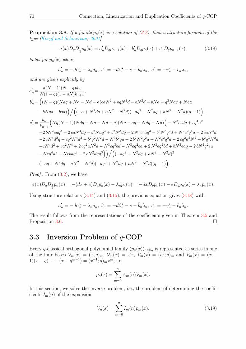
70 Connection, Linearization and Duplication Coefficients of q-COP
Proposition 3.8. If a family pn(x) is a solution of (3.2), then a structure formula of thetype [Koepf and Schmersau, 2001]
σ(x)DqD 1qpn(x) = a′nDqpn+1(x) + b′nDqpn(x) + c′nDqpn−1(x), (3.18)
holds for pn(x) where
a′n = −dα?n − λnan, b′n = −dβ?n − e− bnλn, c′n = −γ?n − cnλn,
and are given explicitly by
a′n =a(N − 1)(N − q)kn
N(1− q)(1− qN)k1+n,
b′n =(
(N − q)(Ndq +Na−Nd− a(baN2 + bqN2d− bN2d− bNa− q2Nae+Nea
−bNqa+ bqa))/(
(−a+N2dq + aN2 −N2d)(−aq2 +N2dq + aN2 −N2d)(q − 1)),
c′n =knkn−1
(Nq(N − 1)(Ndq +Na−Nd− a)(Na− aq +Ndq −Nd)
(−N3ebdq + cq4a2
+2 bN2eaq3 + 2 caN4dq − b2Naq3 + b2N3dq − 2N2e2aq3 − b2N3q2d+N2e2q4a− 2 caN4d
−2 cN4d2q + cq2N4d2 − b2q2N2d−N3b2qa+ 2 b2N2q2a+N2e2q2a− 2 cq2a2N2 + b2q3N2d
+cN4d2 + ca2N4 + 2 cq2aN2d−N3eq3bd−N3eq2ba+ 2N3eq2bd+ bN3eaq − 2 bN2q2ea
−Neq4ab+Nebaq3 − 2 cN2daq3))/(
(−aq2 +N2dq + aN2 −N2d)2
(−aq +N2dq + aN2 −N2d)(−aq3 +N2dq + aN2 −N2d)(q − 1)).
Proof . From (3.2), we have
σ(x)DqD 1qpn(x) = −(dx+ e)Dqpn(x)− λnpn(x) = −dxDqpn(x)− eDqpn(x)− λnpn(x).
Using structure relations (3.14) and (3.15), the previous equation gives (3.18) with
a′n = −dα?n − λnan, b′n = −dβ?n − e− bnλn, c′n = −γ?n − cnλn.
The result follows from the representations of the coefficients given in Theorem 3.5 andProposition 3.6.
3.3 Inversion Problem of q-COPEvery q-classical orthogonal polynomial family (pn(x))n∈N0 is represented as series in oneof the four bases Vm(x) = (x; q)m, Vm(x) = xm, Vm(x) = (ix; q)m and Vm(x) = (x −1)(x− q) · · · (x− qm−1) = (x−1; q)mx
m, i.e.
pn(x) =n∑
m=0
Am(n)Vm(x).
In this section, we solve the inverse problem, i.e., the problem of determining the coeffi-cients Im(n) of the expansion
Vn(x) =n∑
m=0
Im(n)pm(x). (3.19)
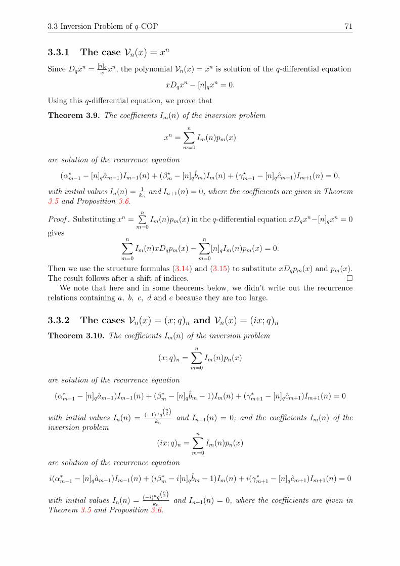
3.3 Inversion Problem of q-COP 71
3.3.1 The case Vn(x) = xn
Since Dqxn = [n]q
xxn, the polynomial Vn(x) = xn is solution of the q-differential equation
xDqxn − [n]qx
n = 0.
Using this q-differential equation, we prove that
Theorem 3.9. The coefficients Im(n) of the inversion problem
xn =n∑
m=0
Im(n)pm(x)
are solution of the recurrence equation
(α?m−1 − [n]qam−1)Im−1(n) + (β?m − [n]q bm)Im(n) + (γ?m+1 − [n]q cm+1)Im+1(n) = 0,
with initial values In(n) = 1kn
and In+1(n) = 0, where the coefficients are given in Theorem3.5 and Proposition 3.6.
Proof . Substituting xn =n∑
m=0
Im(n)pm(x) in the q-differential equation xDqxn−[n]qx
n = 0
givesn∑
m=0
Im(n)xDqpm(x)−n∑
m=0
[n]qIm(n)pm(x) = 0.
Then we use the structure formulas (3.14) and (3.15) to substitute xDqpm(x) and pm(x).The result follows after a shift of indices.
We note that here and in some theorems below, we didn’t write out the recurrencerelations containing a, b, c, d and e because they are too large.
3.3.2 The cases Vn(x) = (x; q)n and Vn(x) = (ix; q)n
Theorem 3.10. The coefficients Im(n) of the inversion problem
(x; q)n =n∑
m=0
Im(n)pn(x)
are solution of the recurrence equation
(α∗m−1 − [n]qam−1)Im−1(n) + (β∗m − [n]q bm − 1)Im(n) + (γ∗m+1 − [n]q cm+1)Im+1(n) = 0
with initial values In(n) = (−1)nq(n2)
knand In+1(n) = 0; and the coefficients Im(n) of the
inversion problem
(ix; q)n =n∑
m=0
Im(n)pn(x)
are solution of the recurrence equation
i(α∗m−1 − [n]qam−1)Im−1(n) + (iβ∗m − i[n]q bm − 1)Im(n) + i(γ∗m+1 − [n]q cm+1)Im+1(n) = 0
with initial values In(n) = (−i)nq(n2)
knand In+1(n) = 0, where the coefficients are given in
Theorem 3.5 and Proposition 3.6.
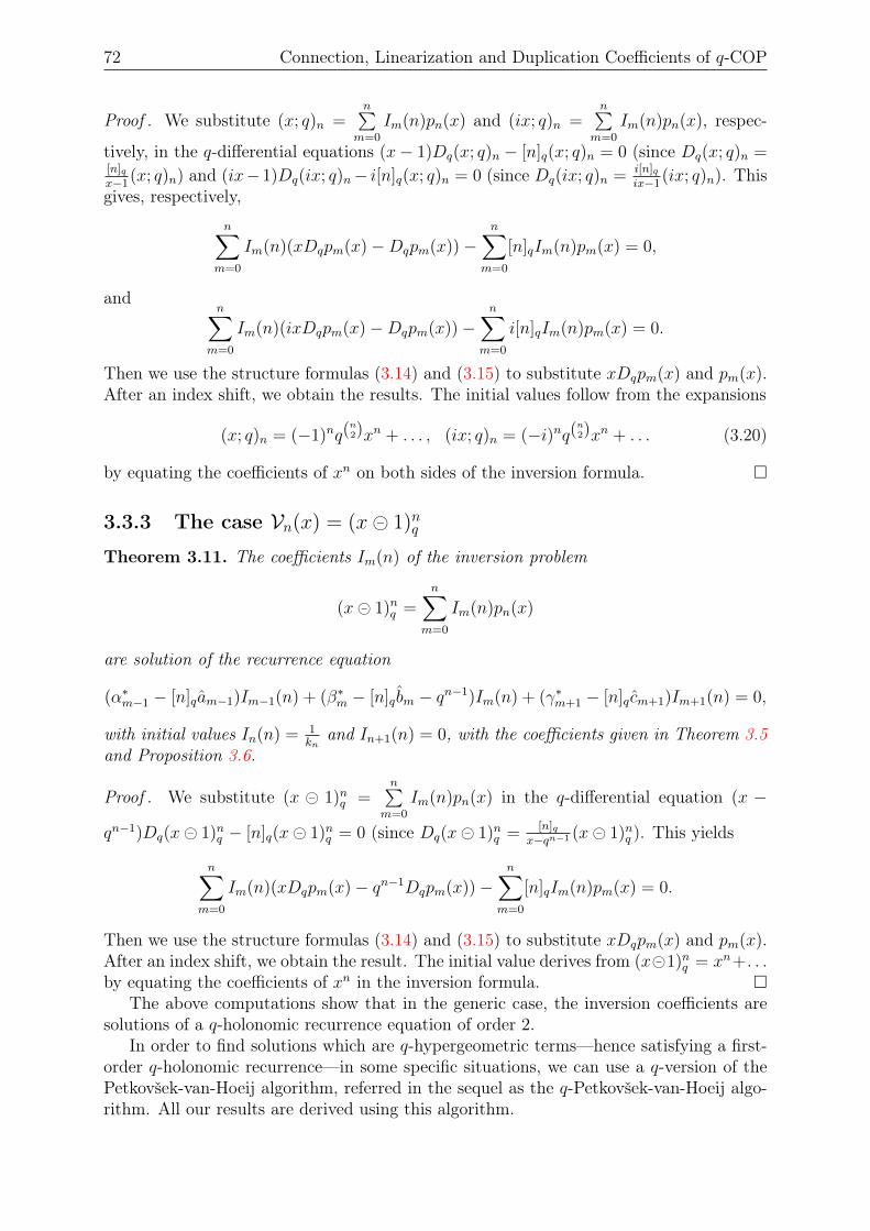
72 Connection, Linearization and Duplication Coefficients of q-COP
Proof . We substitute (x; q)n =n∑
m=0
Im(n)pn(x) and (ix; q)n =n∑
m=0
Im(n)pn(x), respec-
tively, in the q-differential equations (x− 1)Dq(x; q)n − [n]q(x; q)n = 0 (since Dq(x; q)n =[n]qx−1
(x; q)n) and (ix− 1)Dq(ix; q)n− i[n]q(x; q)n = 0 (since Dq(ix; q)n = i[n]qix−1
(ix; q)n). Thisgives, respectively,
n∑m=0
Im(n)(xDqpm(x)−Dqpm(x))−n∑
m=0
[n]qIm(n)pm(x) = 0,
andn∑
m=0
Im(n)(ixDqpm(x)−Dqpm(x))−n∑
m=0
i[n]qIm(n)pm(x) = 0.
Then we use the structure formulas (3.14) and (3.15) to substitute xDqpm(x) and pm(x).After an index shift, we obtain the results. The initial values follow from the expansions
(x; q)n = (−1)nq(n2)xn + . . . , (ix; q)n = (−i)nq(
n2)xn + . . . (3.20)
by equating the coefficients of xn on both sides of the inversion formula.
3.3.3 The case Vn(x) = (x 1)nq
Theorem 3.11. The coefficients Im(n) of the inversion problem
(x 1)nq =n∑
m=0
Im(n)pn(x)
are solution of the recurrence equation
(α∗m−1 − [n]qam−1)Im−1(n) + (β∗m − [n]q bm − qn−1)Im(n) + (γ∗m+1 − [n]q cm+1)Im+1(n) = 0,
with initial values In(n) = 1kn
and In+1(n) = 0, with the coefficients given in Theorem 3.5and Proposition 3.6.
Proof . We substitute (x 1)nq =n∑
m=0
Im(n)pn(x) in the q-differential equation (x −
qn−1)Dq(x 1)nq − [n]q(x 1)nq = 0 (since Dq(x 1)nq = [n]qx−qn−1 (x 1)nq ). This yields
n∑m=0
Im(n)(xDqpm(x)− qn−1Dqpm(x))−n∑
m=0
[n]qIm(n)pm(x) = 0.
Then we use the structure formulas (3.14) and (3.15) to substitute xDqpm(x) and pm(x).After an index shift, we obtain the result. The initial value derives from (x1)nq = xn+. . .by equating the coefficients of xn in the inversion formula.
The above computations show that in the generic case, the inversion coefficients aresolutions of a q-holonomic recurrence equation of order 2.
In order to find solutions which are q-hypergeometric terms—hence satisfying a first-order q-holonomic recurrence—in some specific situations, we can use a q-version of thePetkovšek-van-Hoeij algorithm, referred in the sequel as the q-Petkovšek-van-Hoeij algo-rithm. All our results are derived using this algorithm.
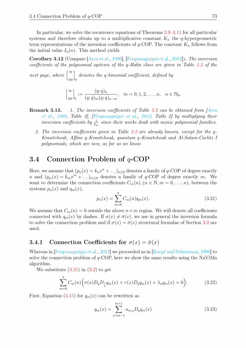
3.4 Connection Problem of q-COP 73
In particular, we solve the recurrence equations of Theorems 3.9–3.11 for all particularsystems and therefore obtain up to a multiplicative constant Kn the q-hypergeometricterm representations of the inversion coefficients of q-COP. The constant Kn follows fromthe initial value In(n). This method yields
Corollary 3.12 (Compare [Area et al., 1999], [Foupouagnigni et al., 2012]). The inversioncoefficients of the polynomial systems of the q-Hahn class are given in Table 3.2 of the
next page, where[ nm
]qdenotes the q-binomial coefficient, defined by
[ nm
]q
:=(q; q)n
(q; q)m(q; q)n−m, m = 0, 1, 2, . . . , n, n ∈ N0.
Remark 3.13. 1. The inversion coefficients of Table 3.2 can be obtained from [Areaet al., 1999, Table 3], [Foupouagnigni et al., 2012, Table 2] by multiplying theirinversion coefficients by 1
kmsince their works dealt with monic polynomial families.
2. The inversion coefficients given in Table 3.2 are already known, except for the q-Krawtchouk, Affine q-Krawtchouk, quantum q-Krawtchouk and Al-Salam-Carlitz Ipolynomials, which are new, as far as we know.
3.4 Connection Problem of q-COPHere, we assume that (pn(x) = knx
n + . . .)n≥0 denotes a family of q-COP of degree exactlyn and (qm(x) = kmx
m + . . .)m≥0 denotes a family of q-COP of degree exactly m. Wewant to determine the connection coefficients Cm(n), (n ∈ N,m = 0, . . . , n), between thesystems pn(x) and qm(x),
pn(x) =n∑
m=0
Cm(n)qm(x). (3.21)
We assume that Cm(n) = 0 outside the above n×m region. We will denote all coefficientsconnected with qm(x) by dashes. If σ(x) 6= σ(x), we use in general the inversion formulato solve the connection problem and if σ(x) = σ(x) structural formulae of Section 3.2 areused.
3.4.1 Connection Coefficients for σ(x) = σ(x)
Whereas in [Foupouagnigni et al., 2012] we proceeded as in [Koepf and Schmersau, 1998] tosolve the connection problem of q-COP, here we show the same results using the NaViMaalgorithm.
We substitute (3.21) in (3.2) to getn∑
m=0
Cm(n)(σ(x)DqD 1
qqm(x) + τ(x)Dqqm(x) + λnqm(x) = 0
). (3.22)
First, Equation (3.15) for qm(x) can be rewritten as
qm(x) =m+1∑j=m−1
am,jDqqm(x) (3.23)
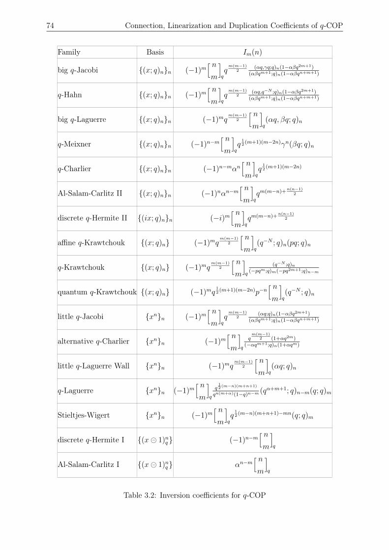
74 Connection, Linearization and Duplication Coefficients of q-COP
Family Basis Im(n)
big q-Jacobi (x; q)nn (−1)m[ nm
]qqm(m−1)
2(αq,γq;q)n(1−αβq2m+1)
(αβqm+1;q)n(1−αβqn+m+1)
q-Hahn (x; q)nn (−1)m[ nm
]qqm(m−1)
2(αq,q−N ;q)n(1−αβq2m+1)
(αβqm+1;q)n(1−αβqn+m+1)
big q-Laguerre (x; q)nn (−1)mqm(m−1)
2
[ nm
]q(αq, βq; q)n
q-Meixner (x; q)nn (−1)n−m[ nm
12
(m+1)(m−2n)γn(βq; q)n
q-Charlier (x; q)nn (−1)n−mαn[ nm
12
(m+1)(m−2n)
Al-Salam-Carlitz II (x; q)nn (−1)nαn−m[ nm
]qqm(m−n)+
n(n−1)2
discrete q-Hermite II (ix; q)nn (−i)m[ nm
]qqm(m−n)+
n(n−1)2
affine q-Krawtchouk (x; q)n (−1)mqm(m−1)
2
[ nm
]q(q−N ; q)n(pq; q)n
q-Krawtchouk (x; q)n (−1)mqm(m−1)
2
[ nm
]q
(q−N ;q)n(−pqm;q)m(−pq2m+1;q)n−m
quantum q-Krawtchouk (x; q)n (−1)mq12
(m+1)(m−2n)p−n[ nm
]q(q−N ; q)n
little q-Jacobi xnn (−1)m[ nm
]qqm(m−1)
2(αq;q)n(1−αβq2m+1)
(αβqm+1;q)n(1−αβqn+m+1)
alternative q-Charlier xnn (−1)m[ nm
]q
qm(m−1)
2 (1+αq2m)(−αqm+1;q)n(1+αqm)
little q-Laguerre Wall xnn (−1)mqm(m−1)
2
[ nm
]q(αq; q)n
q-Laguerre xnn (−1)m[ nm
]q
q12 (m−n)(m+n+1)
qn(m+α)(1−q)n−m (qα+m+1; q)n−m(q; q)m
Stieltjes-Wigert xnn (−1)m[ nm
12
(m−n)(m+n+1)−mn(q; q)m
discrete q-Hermite I (x 1)nq (−1)n−m[ nm
]q
Al-Salam-Carlitz I (x 1)nq αn−m[ nm
]q
Table 3.2: Inversion coefficients for q-COP
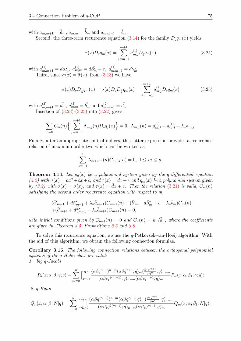
3.4 Connection Problem of q-COP 75
with am,m+1 = ¯am, am,m =¯bm and am,m−1 = ¯cm.
Second, the three-term recurrence equation (3.14) for the family Dqqm(x) yields
τ(x)Dqqm(x) =m+1∑j=m−1
a(1)m,jDqqm(x) (3.24)
with a(1)m,m+1 = dα?m, a
(1)m,m = dβ?m + e, a
(1)m,m−1 = dγ?m.
Third, since σ(x) = σ(x), from (3.18) we have
σ(x)DqD 1qqm(x) = σ(x)DqD 1
qqm(x) =
m+1∑j=m−1
a(2)m,jDqqm(x) (3.25)
with a(2)m,m+1 = a′m, a
(2)m,m = b′m and a(2)
m,m−1 = c′m.Insertion of (3.23)-(3.25) into (3.22) gives
n∑m=0
Cm(n) m+1∑j=m−1
Λm,j(n)Dqqj(x)
= 0, Λm,j(n) = a(2)m,j + a
(1)m,j + λnam,j.
Finally, after an appropriate shift of indices, this latter expression provides a recurrencerelation of maximum order two which can be written as
1∑s=−1
Λm+s,m(n)Cm+s(n) = 0, 1 ≤ m ≤ n.
Theorem 3.14. Let pn(x) be a polynomial system given by the q-differential equation(3.2) with σ(x) = ax2 + bx+ c, and τ(x) = dx+e and qm(x) be a polynomial system givenby (3.2) with σ(x) = σ(x), and τ(x) = dx + e. Then the relation (3.21) is valid, Cm(n)satisfying the second order recurrence equation with respect to m
(a′m−1 + dα?m−1 + λn¯am−1)Cm−1(n) + (b′m + dβ?m + e+ λn¯bm)Cm(n)
+(c′m+1 + dγ?m+1 + λn¯cm+1)Cm+1(n) = 0,
with initial conditions given by Cn+1(n) = 0 and Cn(n) = kn/kn, where the coefficientsare given in Theorem 3.5, Propositions 3.6 and 3.8.
To solve this recurrence equation, we use the q-Petkovšek-van-Hoeij algorithm. Withthe aid of this algorithm, we obtain the following connection formulae.
Corollary 3.15. The following connection relations between the orthogonal polynomialsystems of the q-Hahn class are valid:1. big q-Jacobi
Pn(x;α, β, γ; q) =
n∑m=0
[ nm
]q
(αβqn+1)n−m(αβqn+1; q)m(β1qm+1
βqn ; q)n−m
(αβ1q2(m+1); q)n−m(αβ1qm+1; q)mPm(x;α, β1, γ; q);
2. q-Hahn
Qn(x;α, β,N |q) =n∑
m=0
[ nm
]q
(αβq(n+1))n−m(αβqn+1; q)m(β1qm+1
βqn; q)n−m
(αβ1q2(m+1); q)n−m(αβ1qm+1; q)mQm(x;α, β1, N |q);
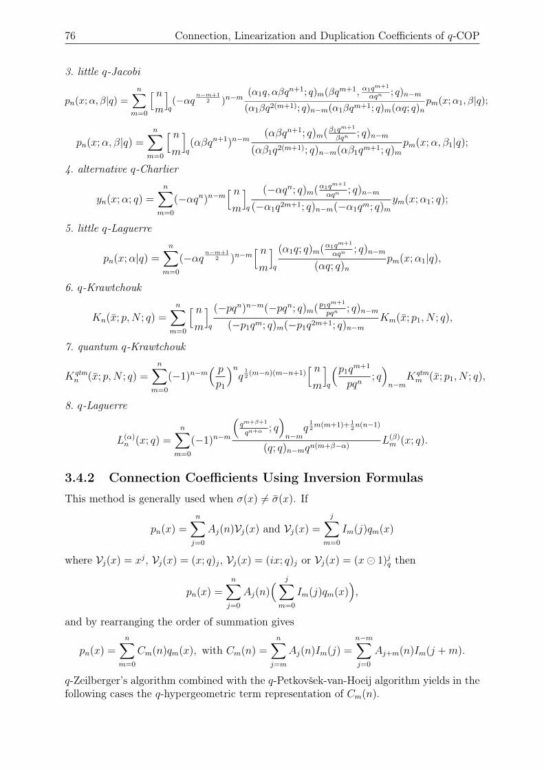
76 Connection, Linearization and Duplication Coefficients of q-COP
3. little q-Jacobi
pn(x;α, β|q) =
n∑m=0
[ nm
]q(−αq
n−m+12 )n−m
(α1q, αβqn+1; q)m(βqm+1, α1qm+1
αqn ; q)n−m
(α1βq2(m+1); q)n−m(α1βqm+1; q)m(αq; q)npm(x;α1, β|q);
pn(x;α, β|q) =n∑
m=0
[ nm
]q(αβqn+1)n−m
(αβqn+1; q)m(β1qm+1
βqn; q)n−m
(αβ1q2(m+1); q)n−m(αβ1qm+1; q)mpm(x;α, β1|q);
4. alternative q-Charlier
yn(x;α; q) =n∑
m=0
(−αqn)n−m[ nm
]q
(−αqn; q)m(α1qm+1
αqn; q)n−m
(−α1q2m+1; q)n−m(−α1qm; q)mym(x;α1; q);
5. little q-Laguerre
pn(x;α|q) =n∑
m=0
(−αqn−m+1
2 )n−m[ nm
]q
(α1q; q)m(α1qm+1
αqn; q)n−m
(αq; q)npm(x;α1|q),
6. q-Krawtchouk
Kn(x; p,N ; q) =n∑
m=0
[ nm
]q
(−pqn)n−m(−pqn; q)m(p1qm+1
pqn; q)n−m
(−p1qm; q)m(−p1q2m+1; q)n−mKm(x; p1, N ; q),
7. quantum q-Krawtchouk
Kqtmn (x; p,N ; q) =
n∑m=0
(−1)n−m( pp1
)nq
12
(m−n)(m−n+1)[ nm
]q
(p1qm+1
pqn; q)n−m
Kqtmm (x; p1, N ; q),
8. q-Laguerre
L(α)n (x; q) =
n∑m=0
(−1)n−m
(qm+β+1
qn+α; q)n−m
q12m(m+1)+ 1
2n(n−1)
(q; q)n−mqn(m+β−α)L(β)m (x; q).
3.4.2 Connection Coefficients Using Inversion Formulas
This method is generally used when σ(x) 6= σ(x). If
pn(x) =n∑j=0
Aj(n)Vj(x) and Vj(x) =
j∑m=0
Im(j)qm(x)
where Vj(x) = xj, Vj(x) = (x; q)j, Vj(x) = (ix; q)j or Vj(x) = (x 1)jq then
pn(x) =n∑j=0
Aj(n)( j∑m=0
Im(j)qm(x)),
and by rearranging the order of summation gives
pn(x) =n∑
m=0
Cm(n)qm(x), with Cm(n) =n∑
j=m
Aj(n)Im(j) =n−m∑j=0
Aj+m(n)Im(j +m).
q-Zeilberger’s algorithm combined with the q-Petkovšek-van-Hoeij algorithm yields in thefollowing cases the q-hypergeometric term representation of Cm(n).
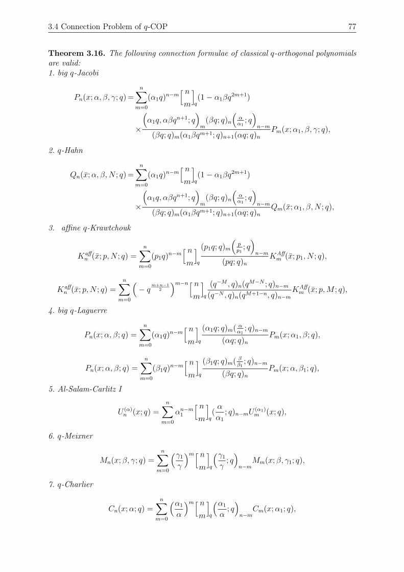
3.4 Connection Problem of q-COP 77
Theorem 3.16. The following connection formulae of classical q-orthogonal polynomialsare valid:1. big q-Jacobi
Pn(x;α, β, γ; q) =n∑
m=0
(α1q)n−m
[ nm
]q(1− α1βq
2m+1)
×
(α1q, αβq
n+1; q)m
(βq; q)n
(αα1
; q)n−m
(βq; q)m(α1βqm+1; q)n+1(αq; q)nPm(x;α1, β, γ; q),
2. q-Hahn
Qn(x;α, β,N ; q) =n∑
m=0
(α1q)n−m
[ nm
]q(1− α1βq
2m+1)
×
(α1q, αβq
n+1; q)m
(βq; q)n
(αα1
; q)n−m
(βq; q)m(α1βqm+1; q)n+1(αq; q)nQm(x;α1, β,N ; q),
3. affine q-Krawtchouk
Kaffn (x; p,N ; q) =
n∑m=0
(p1q)n−m
[ nm
]q
(p1q; q)m
(pp1
; q)n−m
(pq; q)nKAffm (x; p1, N ; q),
Kaffn (x; p,N ; q) =
n∑m=0
(− q
m+n−12
)m−n[ nm
]q
(q−M , q)n(qM−N ; q)n−m(q−N , q)n(qM+1−n, q)n−m
KAffm (x; p,M ; q),
4. big q-Laguerre
Pn(x;α, β; q) =n∑
m=0
(α1q)n−m
[ nm
]q
(α1q; q)m( αα1
; q)n−m
(αq; q)nPm(x;α1, β; q),
Pn(x;α, β; q) =n∑
m=0
(β1q)n−m
[ nm
]q
(β1q; q)m( ββ1
; q)n−m
(βq; q)nPm(x;α, β1; q),
5. Al-Salam-Carlitz I
U (α)n (x; q) =
n∑m=0
αn−m1
[ nm
]q(α
α1
; q)n−mU(α1)m (x; q),
6. q-Meixner
Mn(x; β, γ; q) =n∑
m=0
(γ1
γ
)m[ nm
]q
(γ1
γ; q)n−m
Mm(x; β, γ1; q),
7. q-Charlier
Cn(x;α; q) =n∑
m=0
(α1
α
)m[ nm
]q
(α1
α; q)n−m
Cm(x;α1; q),
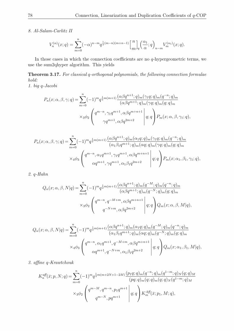
78 Connection, Linearization and Duplication Coefficients of q-COP
8. Al-Salam-Carlitz II
V (α)n (x; q) =
n∑m=0
(−α)n−mq12
(m−n)(m+n−1)[ nm
]q
(α1
α; q)n−m
V (α1)m (x; q).
In those cases in which the connection coefficients are no q-hypergeometric terms, weuse the sum2qhyper algorithm. This yields
Theorem 3.17. For classical q-orthogonal polynomials, the following connection formulaehold:1. big q-Jacobi
Pn(x;α, β, γ; q) =n∑
m=0
(−1)mq12m(m+1) (αβqn+1; q)m(γ1q; q)m(q−n; q)m
(αβqm+1; q)m(γq; q)m(q; q)m
×3φ2
qm−n, γ1qm+1, αβqm+n+1
γqm+1, αβq2m+2
∣∣∣∣∣∣ q; qPm(x;α, β, γ1; q),
Pn(x;α, β, γ; q) =n∑
m=0
(−1)mq12m(m+1) (αβqn+1; q)m(α1q; q)m(γ1q; q)m(q−n; q)m
(α1β1qm+1; q)m(αq; q)m(γq; q)m(q; q)m
×4φ3
qm−n, α1qm+1, γ1q
m+1, αβqm+n+1
αqm+1, γqm+1, α1β1q2m+2
∣∣∣∣∣∣ q; qPm(x;α1, β1, γ1; q),
2. q-Hahn
Qn(x;α, β,N |q) =n∑
m=0
(−1)mq12m(m+1) (αβqn+1; q)m(q−M ; q)m(q−n; q)m
(αβqm+1; q)m(q−N ; q)m(q; q)m
×3φ2
qm−n, q−M+m, αβqm+n+1
q−N+m, αβq2m+2
∣∣∣∣∣∣ q; qQm(x;α, β,M |q),
Qn(x;α, β,N |q) =n∑
m=0
(−1)mq12m(m+1) (αβqn+1; q)m(α1q; q)m(q−M ; q)m(q−n; q)m
(α1β1qm+1; q)m(αq; q)m(q−N ; q)m(q; q)m
×4φ3
qm−n, α1qm+1, q−M+m, αβqm+n+1
αqm+1, q−N+m, α1β1q2m+2
∣∣∣∣∣∣ q; qQm(x;α1, β1,M |q),
3. affine q-Krawtchouk
Kaffn (x; p,N ; q) =
n∑m=0
(−1)mq12m(m+2N+1−2M) (p1q; q)m(q−n; q)m(q1−m; q)N(q; q)M
(pq; q)m(q; q)m(q; q)N(q1−m; q)M
×3φ2
qm−M , qm−n, p1qm+1
qm−N , pqm+1
∣∣∣∣∣∣ q; qKAff
m (x; p1,M ; q),
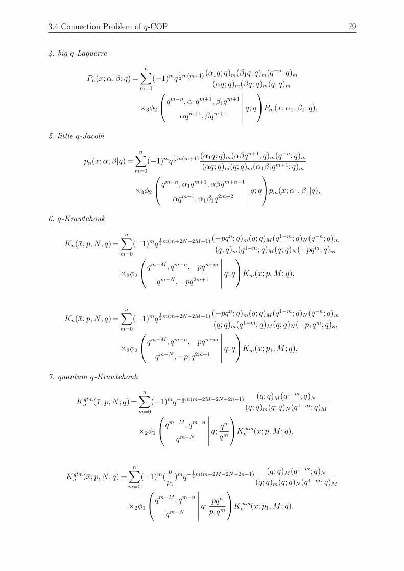
3.4 Connection Problem of q-COP 79
4. big q-Laguerre
Pn(x;α, β; q) =n∑
m=0
(−1)mq12m(m+1) (α1q; q)m(β1q; q)m(q−n; q)m
(αq; q)m(βq; q)m(q; q)m
×3φ2
qm−n, α1qm+1, β1q
m+1
αqm+1, βqm+1
∣∣∣∣∣∣ q; qPm(x;α1, β1; q),
5. little q-Jacobi
pn(x;α, β|q) =n∑
m=0
(−1)mq12m(m+1) (α1q; q)m(αβqn+1; q)m(q−n; q)m
(αq; q)m(q; q)m(α1β1qm+1; q)m
×3φ2
qm−n, α1qm+1, αβqm+n+1
αqm+1, α1β1q2m+2
∣∣∣∣∣∣ q; qpm(x;α1, β1|q),
6. q-Krawtchouk
Kn(x; p,N ; q) =n∑
m=0
(−1)mq12m(m+2N−2M+1) (−pqn; q)m(q; q)M(q1−m; q)N(q−n; q)m
(q; q)m(q1−m; q)M(q; q)N(−pqm; q)m
×3φ2
qm−M , qm−n,−pqn+m
qm−N ,−pq2m+1
∣∣∣∣∣∣ q; qKm(x; p,M ; q),
Kn(x; p,N ; q) =n∑
m=0
(−1)mq12m(m+2N−2M+1) (−pqn; q)m(q; q)M(q1−m; q)N(q−n; q)m
(q; q)m(q1−m; q)M(q; q)N(−p1qm; q)m
×3φ2
qm−M , qm−n,−pqn+m
qm−N ,−p1q2m+1
∣∣∣∣∣∣ q; qKm(x; p1,M ; q),
7. quantum q-Krawtchouk
Kqtmn (x; p,N ; q) =
n∑m=0
(−1)mq−12m(m+2M−2N−2n−1) (q; q)M(q1−m; q)N
(q; q)m(q; q)N(q1−m; q)M
×2φ1
qm−M , qm−nqm−N
∣∣∣∣∣∣ q; qn
qm
Kqtmn (x; p,M ; q),
Kqtmn (x; p,N ; q) =
n∑m=0
(−1)m(p
p1
)mq−12m(m+2M−2N−2n−1) (q; q)M(q1−m; q)N
(q; q)m(q; q)N(q1−m; q)M
×2φ1
qm−M , qm−nqm−N
∣∣∣∣∣∣ q; pqn
p1qm
Kqtmn (x; p1,M ; q),
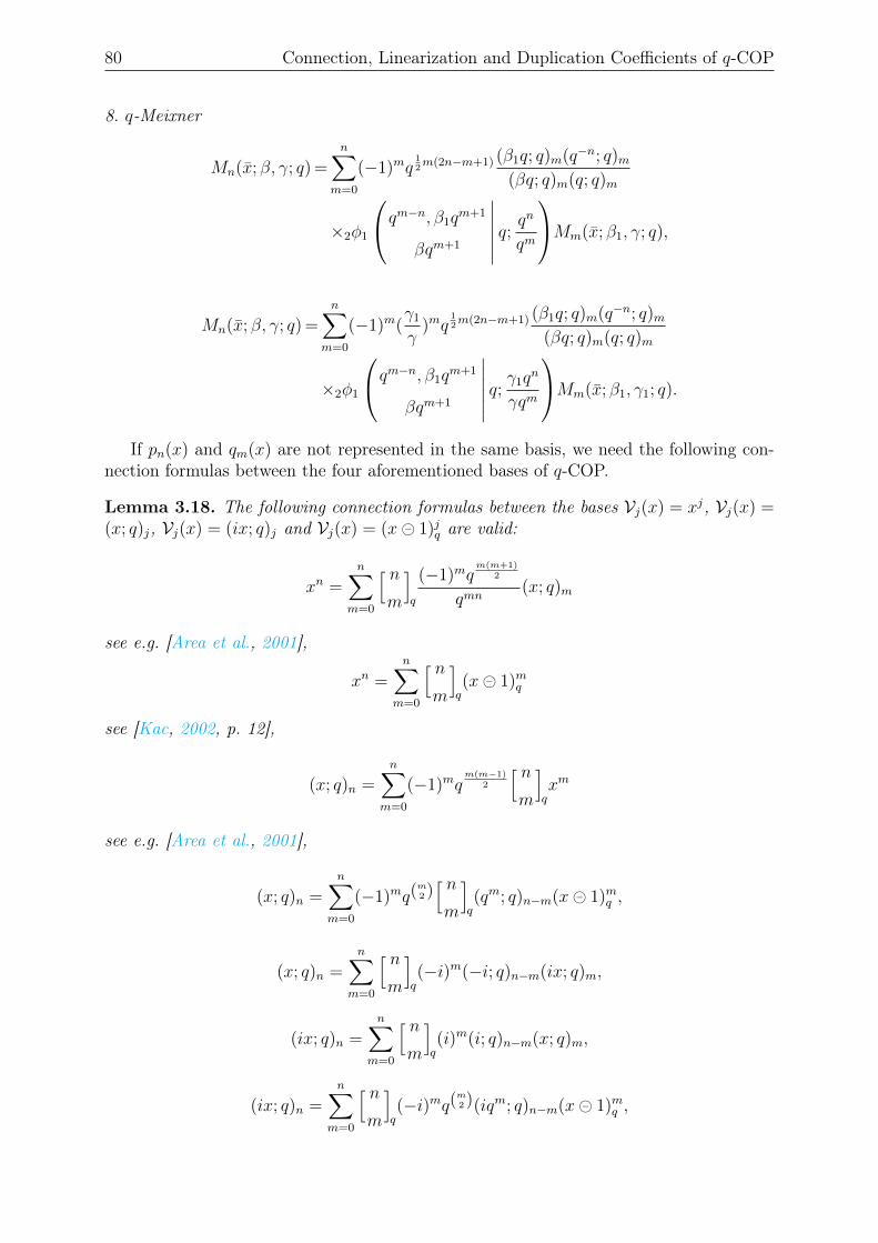
80 Connection, Linearization and Duplication Coefficients of q-COP
8. q-Meixner
Mn(x; β, γ; q) =n∑
m=0
(−1)mq12m(2n−m+1) (β1q; q)m(q−n; q)m
(βq; q)m(q; q)m
×2φ1
qm−n, β1qm+1
βqm+1
∣∣∣∣∣∣ q; qn
qm
Mm(x; β1, γ; q),
Mn(x; β, γ; q) =n∑
m=0
(−1)m(γ1
γ)mq
12m(2n−m+1) (β1q; q)m(q−n; q)m
(βq; q)m(q; q)m
×2φ1
qm−n, β1qm+1
βqm+1
∣∣∣∣∣∣ q; γ1qn
γqm
Mm(x; β1, γ1; q).
If pn(x) and qm(x) are not represented in the same basis, we need the following con-nection formulas between the four aforementioned bases of q-COP.
Lemma 3.18. The following connection formulas between the bases Vj(x) = xj, Vj(x) =(x; q)j, Vj(x) = (ix; q)j and Vj(x) = (x 1)jq are valid:
xn =n∑
m=0
[ nm
]q
(−1)mqm(m+1)
2
qmn(x; q)m
see e.g. [Area et al., 2001],
xn =n∑
m=0
[ nm
]q(x 1)mq
see [Kac, 2002, p. 12],
(x; q)n =n∑
m=0
(−1)mqm(m−1)
2
[ nm
]qxm
see e.g. [Area et al., 2001],
(x; q)n =n∑
m=0
(−1)mq(m2 )[ nm
]q(qm; q)n−m(x 1)mq ,
(x; q)n =n∑
m=0
[ nm
]q(−i)m(−i; q)n−m(ix; q)m,
(ix; q)n =n∑
m=0
[ nm
]q(i)m(i; q)n−m(x; q)m,
(ix; q)n =n∑
m=0
[ nm
]q(−i)mq(
m2 )(iqm; q)n−m(x 1)mq ,
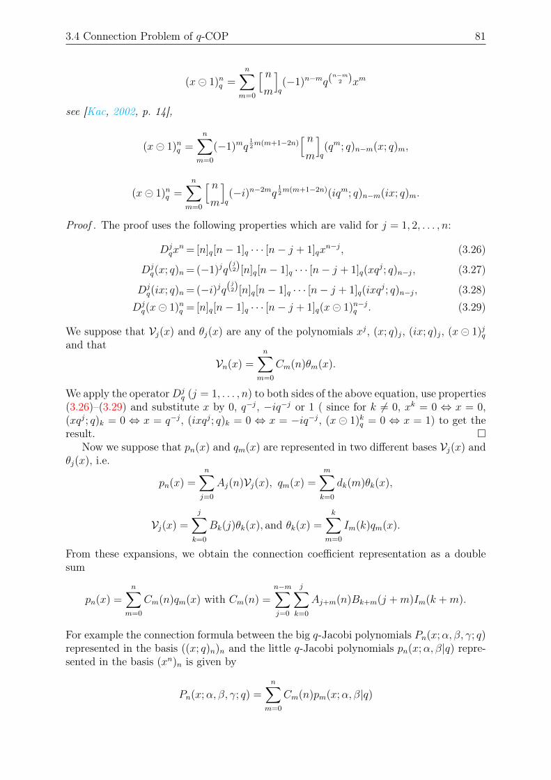
3.4 Connection Problem of q-COP 81
(x 1)nq =n∑
m=0
[ nm
]q(−1)n−mq(
n−m2 )xm
see [Kac, 2002, p. 14],
(x 1)nq =n∑
m=0
(−1)mq12m(m+1−2n)
[ nm
]q(qm; q)n−m(x; q)m,
(x 1)nq =n∑
m=0
[ nm
]q(−i)n−2mq
12m(m+1−2n)(iqm; q)n−m(ix; q)m.
Proof . The proof uses the following properties which are valid for j = 1, 2, . . . , n:
Djqx
n = [n]q[n− 1]q · · · [n− j + 1]qxn−j, (3.26)
Djq(x; q)n = (−1)jq(
j2)[n]q[n− 1]q · · · [n− j + 1]q(xq
j; q)n−j, (3.27)
Djq(ix; q)n = (−i)jq(
j2)[n]q[n− 1]q · · · [n− j + 1]q(ixq
j; q)n−j, (3.28)Djq(x 1)nq = [n]q[n− 1]q · · · [n− j + 1]q(x 1)n−jq . (3.29)
We suppose that Vj(x) and θj(x) are any of the polynomials xj, (x; q)j, (ix; q)j, (x 1)jqand that
Vn(x) =n∑
m=0
Cm(n)θm(x).
We apply the operatorDjq (j = 1, . . . , n) to both sides of the above equation, use properties
(3.26)–(3.29) and substitute x by 0, q−j, −iq−j or 1 ( since for k 6= 0, xk = 0 ⇔ x = 0,(xqj; q)k = 0 ⇔ x = q−j, (ixqj; q)k = 0 ⇔ x = −iq−j, (x 1)kq = 0 ⇔ x = 1) to get theresult.
Now we suppose that pn(x) and qm(x) are represented in two different bases Vj(x) andθj(x), i.e.
pn(x) =n∑j=0
Aj(n)Vj(x), qm(x) =m∑k=0
dk(m)θk(x),
Vj(x) =
j∑k=0
Bk(j)θk(x), and θk(x) =k∑
m=0
Im(k)qm(x).
From these expansions, we obtain the connection coefficient representation as a doublesum
pn(x) =n∑
m=0
Cm(n)qm(x) with Cm(n) =n−m∑j=0
j∑k=0
Aj+m(n)Bk+m(j +m)Im(k +m).
For example the connection formula between the big q-Jacobi polynomials Pn(x;α, β, γ; q)represented in the basis ((x; q)n)n and the little q-Jacobi polynomials pn(x;α, β|q) repre-sented in the basis (xn)n is given by
Pn(x;α, β, γ; q) =n∑
m=0
Cm(n)pm(x;α, β|q)
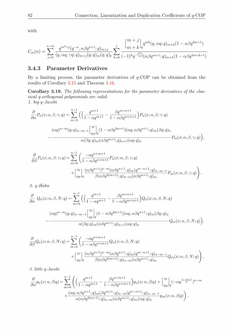
82 Connection, Linearization and Duplication Coefficients of q-COP
with
Cm(n) =n−m∑j=0
qm2+j(q−n, αβqn+1; q)m+j
(q, αq, γq; q)m+j(q; q)m(q; q)k
j∑k=0
[m+ j
m+ k
]qqmk(q, αq; q)m+k(1− αβq2m+1)
(−1)kq−(k2)(αβqm+1; q)m+k(1− αβq2m+k+1).
3.4.3 Parameter Derivatives
By a limiting process, the parameter derivatives of q-COP can be obtained from theresults of Corollary 3.15 and Theorem 3.16.
Corollary 3.19. The following representations for the parameter derivatives of the clas-sical q-orthogonal polynomials are valid:1. big q-Jacobi
∂
∂αPn(x;α, β, γ; q) =
n−1∑m=0
(( qm+1
1− αqm+1− βqm+n+1
1− αβqm+n+1
)Pn(x;α, β, γ; q)
−
(αq)n−m(q; q)n−m−1
[ nm
]q(1− αβq2m+1)(αq, αβqn+1; q)m(βq; q)n
α(βq; q)m(αβqm+1; q)n+1(αq; q)nPm(x;α, β, γ; q)
),
∂
∂βPn(x;α, β, γ; q) =
n−1∑m=0
(−αqn+m+1
1− αβqn+m+1Pn(x;α, β, γ; q)
+[ nm
]q
(αβqn+1)n−m(αβqn+1; q)m(qm−n+1; q)n−m−1
β(αβq2(m+1); q)n−m(αβqm+1; q)mPm(x;α, β, γ; q)
),
2. q-Hahn
∂
∂αQn(x;α, β,N ; q) =
n−1∑m=0
(( qm+1
1− αqm+1− βqm+n+1
1− αβqm+n+1
)Qn(x;α, β,N ; q)
−
(αq)n−m(q; q)n−m−1
[ nm
]q(1− αβq2m+1)(αq, αβqn+1; q)m(βq; q)n
α(βq; q)m(αβqm+1; q)n+1(αq; q)nQm(x;α, β,N ; q)
),
∂
∂βQn(x;α, β,N ; q) =
n−1∑m=0
(−αqn+m+1
1− αβqn+m+1Qn(x;α, β,N ; q)
+[ nm
]q
(αβqn+1)n−m(αβqn+1; q)m(qm−n+1; q)n−m−1
β(αβq2(m+1); q)n−m(αβqm+1; q)mQm(x;α, β,N ; q)
),
3. little q-Jacobi
∂
∂αpn(x;α, β|q) =
n−1∑m=0
(( qm+1
1− αqm+1− βqn+m+1
1− αβqn+m+1
)pn(x;α, β|q) +
[ nm
]q(−αq
n−m+12 )n−m
×(αq, αβqn+1; q)m(βqm+1; q)n−m(qm−n+1; q)n−m−1
α(αβq2(m+1); q)n−m(αβqm+1; q)m(αq; q)npm(x;α, β|q)
),
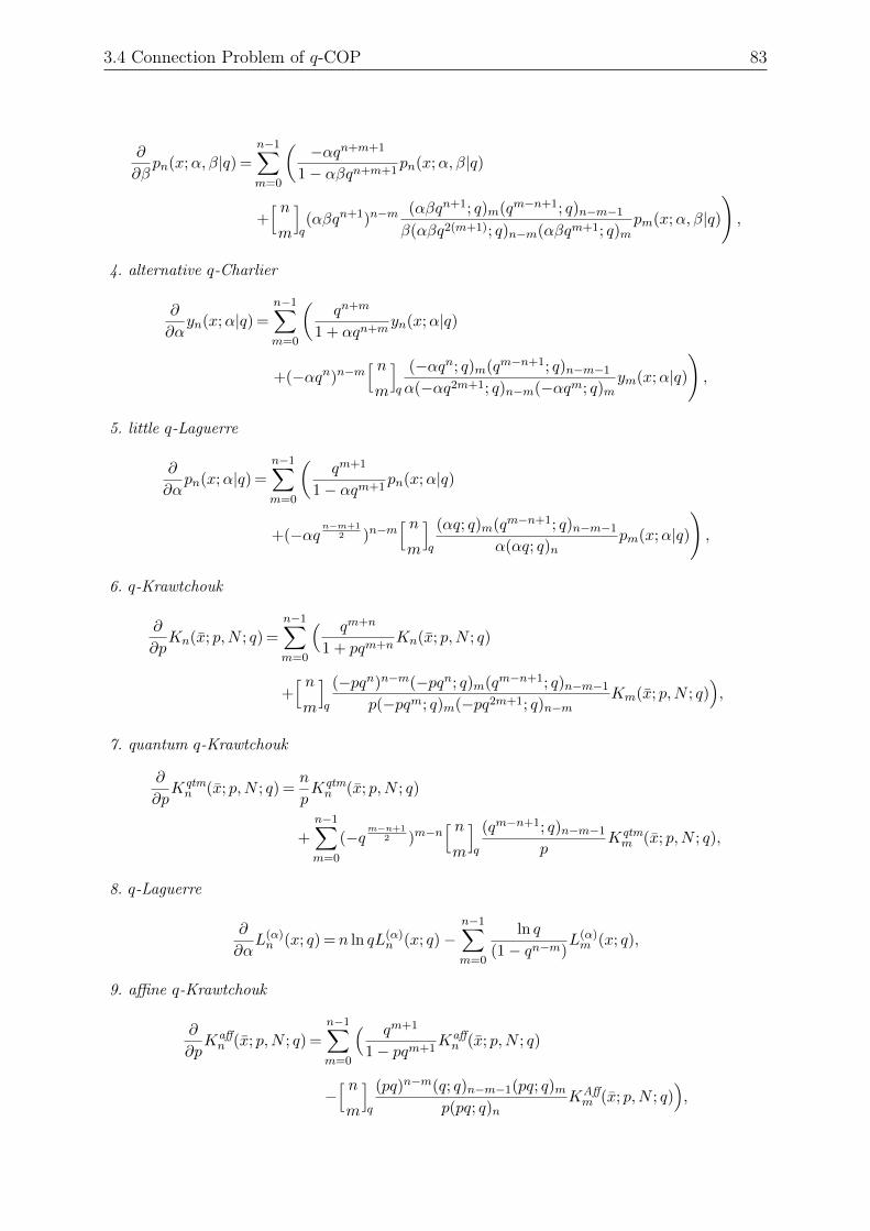
3.4 Connection Problem of q-COP 83
∂
∂βpn(x;α, β|q) =
n−1∑m=0
(−αqn+m+1
1− αβqn+m+1pn(x;α, β|q)
+[ nm
]q(αβqn+1)n−m
(αβqn+1; q)m(qm−n+1; q)n−m−1
β(αβq2(m+1); q)n−m(αβqm+1; q)mpm(x;α, β|q)
),
4. alternative q-Charlier
∂
∂αyn(x;α|q) =
n−1∑m=0
(qn+m
1 + αqn+myn(x;α|q)
+(−αqn)n−m[ nm
]q
(−αqn; q)m(qm−n+1; q)n−m−1
α(−αq2m+1; q)n−m(−αqm; q)mym(x;α|q)
),
5. little q-Laguerre
∂
∂αpn(x;α|q) =
n−1∑m=0
(qm+1
1− αqm+1pn(x;α|q)
+(−αqn−m+1
2 )n−m[ nm
]q
(αq; q)m(qm−n+1; q)n−m−1
α(αq; q)npm(x;α|q)
),
6. q-Krawtchouk
∂
∂pKn(x; p,N ; q) =
n−1∑m=0
( qm+n
1 + pqm+nKn(x; p,N ; q)
+[ nm
]q
(−pqn)n−m(−pqn; q)m(qm−n+1; q)n−m−1
p(−pqm; q)m(−pq2m+1; q)n−mKm(x; p,N ; q)
),
7. quantum q-Krawtchouk
∂
∂pKqtmn (x; p,N ; q) =
n
pKqtmn (x; p,N ; q)
+
n−1∑m=0
(−qm−n+1
2 )m−n[ nm
]q
(qm−n+1; q)n−m−1
pKqtmm (x; p,N ; q),
8. q-Laguerre
∂
∂αL(α)n (x; q) = n ln qL(α)
n (x; q)−n−1∑m=0
ln q
(1− qn−m)L(α)m (x; q),
9. affine q-Krawtchouk
∂
∂pKaffn (x; p,N ; q) =
n−1∑m=0
( qm+1
1− pqm+1Kaffn (x; p,N ; q)
−[ nm
]q
(pq)n−m(q; q)n−m−1(pq; q)mp(pq; q)n
KAffm (x; p,N ; q)
),
84 Connection, Linearization and Duplication Coefficients of q-COP
∂
∂NKaffn (x; p,N ; q) =
n−1∑m=0
(−qm−N ln q
1− qm−NKAffn (x; p,N ; q)
+(−qm+n−1
2 )m−n ln q[ nm
]q
(q; q)n−m−1
(qN+1−n; q)n−mKaffm (x; p,N ; q)
),
10. big q-Laguerre
∂
∂αPn(x;α, β; q) =
n−1∑m=0
( qm+1
1− αqm+1Pn(x;α, β; q)
−[ nm
]q
(αq)n−m(αq; q)m(q; q)n−m−1
α(αq; q)nPm(x;α, β; q)
),
∂
∂βPn(x;α, β; q) =
n−1∑m=0
( qm+1
1− βqm+1Pn(x;α, β; q)
−[ nm
]q
(βq)n−m(βq; q)m(q; q)n−m−1
β(βq; q)nPm(x;α, β; q)
),
11. Al-Salam-Carlitz I
∂
∂αU (α)n (x; q) =−
n−1∑m=0
αn−m−1(q; q)n−m−1
[ nm
]qU (α)m (x; q),
12. q-Meixner
∂
∂γMn(x;β, γ; q) =−n
γMn(x;β, γ; q) +
1
γ
n−1∑m=0
(q; q)n−m−1
[ nm
]qMm(x;β, γ; q),
13. q-Charlier
∂
∂αCn(x;α; q) =−n
αCn(x;α; q) +
1
α
n−1∑m=0
(q; q)n−m−1
[ nm
]qCm(x;α; q),
14. Al-Salam-CArlitz II
∂
∂αV (α)n (x; q) =
1
α
n−1∑m=0
(−α)n−mq(m−n)(m+n−1)
2 (q; q)n−m−1
[ nm
]qV (α)n (x; q).
Proof . If
pαn(x) =n∑
m=0
Cm(n, α, β)pβm(x),
then∂
∂αpαn(x) = lim
β→α
Cn(n, α, β)− 1
α− βpβn(x) +
n−1∑m=0
limβ→α
Cm(n, α, β)
α− βP βm(x).
3.5 Linearization Problem of q-COP 85
We know thatd
dx
n∏j=1
fj(x) =n∑
m=1
f ′m(x)
fm(x)
n∏j=1
fj(x),
from which we get for a parameter γ
∂
∂α(αγqn+1; q)n =
n−1∑m=0
−γqn+m+1
1− αγqn+m+1(αγqn+1; q)n.
Using l’Hospital’s rule, we obtain
limβ→α
(αγqn+1; q)n − (βγqn+1; q)n(βγqn+1; q)n(α− β)
=n−1∑m=0
−γqn+m+1
1− αγqn+m+1.
We also have
limβ→α
(βqm+1
αqn; q)n−m
α− β=
1
α(qm−n+1; q)n−m−1
and
limβ→α
(αβ; q)n−m
α− β= − 1
α(q; q)n−m−1.
From all the preceding, the result follows.
Remark 3.20. Lewanowicz [2003b] gave an algorithmic approach to construct recurrence
relations for the coefficients Ck of the expansion of the form ∂∂αPn(x;α; q) =
n−1∑k=0
CkPk(x;α; q),
where Pn(x;α; q) is a q-COP. He solved this recurrence relation for the big q-Jacobi poly-nomials Pk(x;α, β, γ; q) and gave explicitly the coefficients Ck.
3.5 Linearization Problem of q-COP
The linearization problem of the q-COP family (pn(x))n depends on the basis xn,(x; q)n, (ix; q)n or (x 1)nq in which pn(x) is represented.
3.5.1 Representation Basis xnTheorem 3.21. The following linearization relations between the orthogonal polynomialsystems of the q-Hahn class represented in the basis xn are valid:1. little q-Jacobi
pn(x;α, β|q)pm(x;α1, β1|q) =n+m∑l=0
n+m−l∑k=0
(−1)lqk+l(l+1)
2 (q, α2q; q)k+l(1− α2β2q2l+1)
(q; q)l(q; q)k(α2β2ql+1; q)k+l(1− α2β2qk+2l+1)
×k+l∑r=0
(q−n, αβqn+1; q)r(q−m, α1β1q
m+1; q)k+l−r
(q, αq; q)r(q, α1q; q)k+l−rpl(x;α2, β2|q),
86 Connection, Linearization and Duplication Coefficients of q-COP
2. alternative q-Charlier
yn(x;α|q)ym(x;α1|q) =n+m∑l=0
n+m−l∑k=0
(−1)lqk+l(l+1)
2 (q; q)k+l(1 + α2q2l)
(q; q)k(q; q)l(−α2ql+1; q)k+l(1 + α2ql)
×k+l∑r=0
(q−n,−αqn; q)r(q−m,−α1q
m; q)k+l−r
(q; q)r(q; q)k+l−ryl(x;α2|q),
3. little q-Laguerre/Wall
pn(x;α|q)pm(x;α1|q) =n+m∑l=0
n+m−l∑k=0
(−1)lqk+l(l+1)
2 (q; q)k+l(α2q; q)k+l
(q; q)k(q; q)l
×k+l∑r=0
(q−n; q)r(q−m; q)k+l−r
(q, αq; q)r(q, α1q; q)k+l−rpl(x;α2|q),
4. q-Laguerre
L(α)n (x; q)L(β)
m (x; q) =n+m∑l=0
n+m−l∑k=0
(−1)lq(m+β−γ)(k+l)(qα+1; q)n(qβ+1; q)m(q; q)k+l(qγ+l+1; q)k
q12l(l+2k−1)(q; q)n(q; q)m(q; q)k
×k+l∑r=0
qr(n+α+r)(q−n; q)r(q−m; q)k+l−r
qr(m+k+l+β)(q, qα+1; q)r(q, qβ+1; q)k+l−rL
(γ)l (x; q),
5. Stieltjes-Wigert
Sn(x; q)Sm(x; q) =n+m∑l=0
n+m−l∑k=0
k+l∑r=0
(−1)lqm(k+l)+r(n+r)(q; q)k+l(q−n; q)r(q
−m; q)k+l−r
q12l(l+2k−1)+r(m+k+l)(q; q)n(q; q)m(q; q)k(q; q)r(q; q)k+l−r
Sl(x; q).
Proof . We suppose
pn(x) =n∑i=0
Ai(n)xi, qm(x) =m∑j=0
Bj(m)xj, and xk =k∑l=0
Il(k)yl(x)
where pn(x), qm(x), yl(x) are three families of classical q-orthogonal polynomials.We then obtain the Cauchy product
pn(x)qm(x) =n+m∑k=0
Ck(m,n)xk, where Ck(m,n) =k∑r=0
Ar(n)Bk−r(m).
Using the inversion formula, this can be rewritten as
pn(x)qm(x) =n+m∑l=0
Ll(m,n)yl(x)
with
Ll(m,n) =n+m−l∑k=0
Ck+l(m,n)Il(k + l) =n+m−l∑k=0
k+l∑r=0
Ar(n)Bk+l−r(m)Il(k + l).
We consider here the standard linearization problem of Clebsch-Gordan-type where pn(x),qm(x), yl(x) belong to the same q-orthogonal family.
3.5 Linearization Problem of q-COP 87
3.5.2 Representation Basis (x; q)n or (ix; q)nIn these cases, we need the following linearization coefficients of the basis (x; q)n or(ix; q)n.
Proposition 3.22. The basis (x; q)n fulfils the linearization relation
(x; q)n(x; q)m =n+m∑
k=max(m,n)
(q; q)n(q; q)m(−1)n+m−kq(n+m−k
2 )−nm
(q; q)k−n(q; q)k−m(q; q)n+m−k(x; q)k. (3.30)
Proof . Without loss of generality, we suppose n ≥ m.(x; q)n = 0⇔ x = q−j, j = 0, 1, . . . , n− 1. For x = 1, the equation
(x; q)n(x; q)m =n+m∑k=0
Hk(m,n)(x; q)k (3.31)
yields H0(m,n) = 0, m ≥ 1 so that
(x; q)n(x; q)m =n+m∑k=1
Hk(m,n)(x; q)k.
Next for x = q−1, the above equation gives H1(m,n)(q−1, q)1 = 0, m ≥ 2. Since(q−n; q)n 6= 0 therefore H1(m,n) = 0.Progressively, it follows in a similar way that
H0(m,n) = H1(m,n) = . . . = Hn−1(m,n) = 0.
Consequently
(x; q)n(x; q)m =n+m∑k=n
Hk(m,n)(x; q)k =m∑k=0
Hn+k(m,n)(x; q)n+k.
Since (x; q)n+k = (x; q)n(xqn; q)k it follows that
(x; q)m =m∑k=0
Hn+k(m,n)(xqn; q)k. (3.32)
For x = q−n, (3.32) gives Hn(m,n) = (q−n; q)m, m ≥ 1. From the property
Dq(xqn; q)k = −[k]qq
n(xqn+1; q)k−1
it follows that for any j = 1, 2, . . . ,m
Djq(xq
n; q)k = (−1)j[k]q[k − 1]q · · · [k − j + 1]qqnj+(j2)(xqn+j; q)k−j.
We apply Djq to both sides of (3.32) to get
[m]q[m− 1]q · · · [m− j + 1]q(xqj ; q)m−j =
m∑k=0
[k]q[k − 1]q · · · [k − j + 1]qqnj(xqn+j ; q)k−j
=
m∑k=0,k 6=j
[k]q[k − 1]q · · · [k − j + 1]qqnj(xqn+j ; q)k−j
+qnj [j]q!Hn+j(m,n)
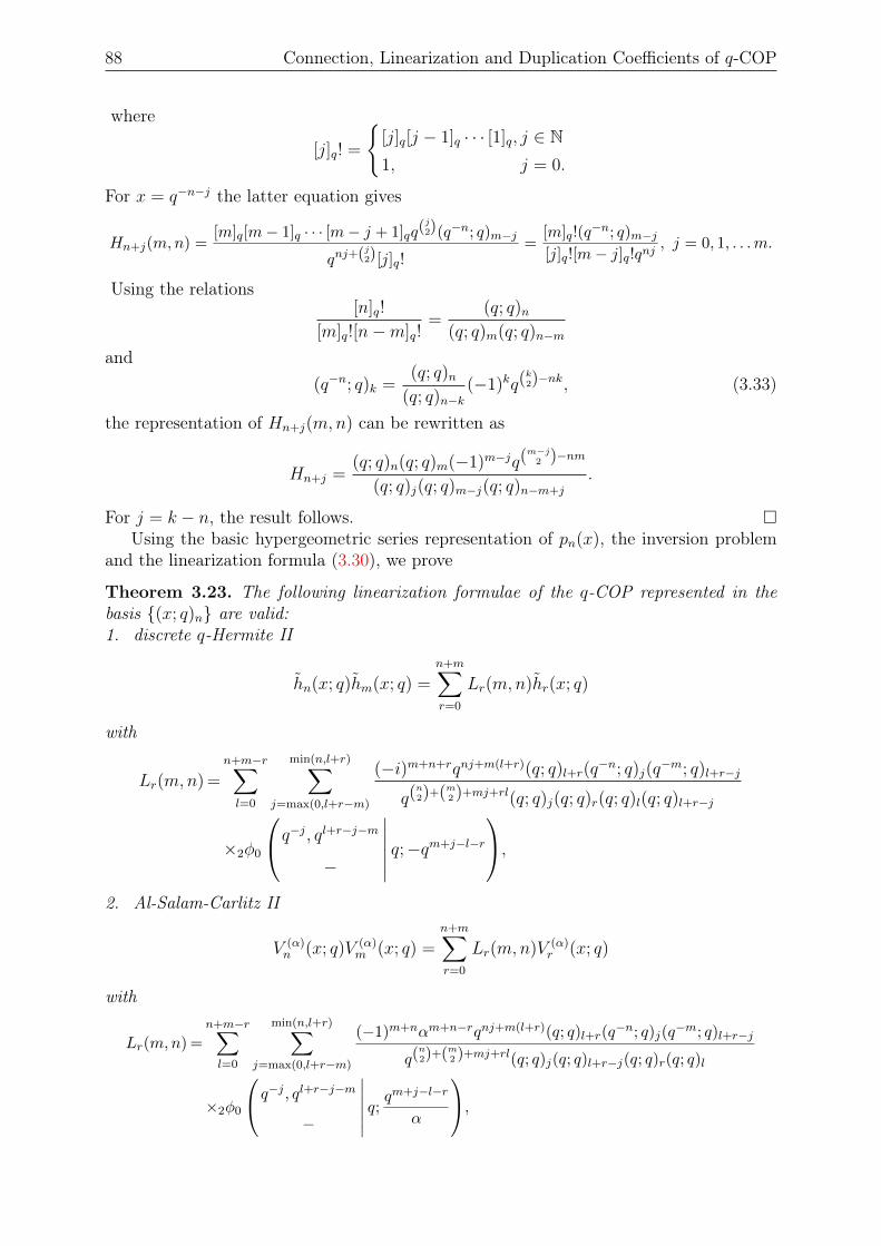
88 Connection, Linearization and Duplication Coefficients of q-COP
where
[j]q! =
[j]q[j − 1]q · · · [1]q, j ∈ N1, j = 0.
For x = q−n−j the latter equation gives
Hn+j(m,n) =[m]q[m− 1]q · · · [m− j + 1]qq
(j2)(q−n; q)m−j
qnj+(j2)[j]q!=
[m]q!(q−n; q)m−j
[j]q![m− j]q!qnj, j = 0, 1, . . .m.
Using the relations[n]q!
[m]q![n−m]q!=
(q; q)n(q; q)m(q; q)n−m
and(q−n; q)k =
(q; q)n(q; q)n−k
(−1)kq(k2)−nk, (3.33)
the representation of Hn+j(m,n) can be rewritten as
Hn+j =(q; q)n(q; q)m(−1)m−jq(
m−j2 )−nm
(q; q)j(q; q)m−j(q; q)n−m+j
.
For j = k − n, the result follows. Using the basic hypergeometric series representation of pn(x), the inversion problem
and the linearization formula (3.30), we prove
Theorem 3.23. The following linearization formulae of the q-COP represented in thebasis (x; q)n are valid:1. discrete q-Hermite II
hn(x; q)hm(x; q) =n+m∑r=0
Lr(m,n)hr(x; q)
with
Lr(m,n) =n+m−r∑l=0
min(n,l+r)∑j=max(0,l+r−m)
(−i)m+n+rqnj+m(l+r)(q; q)l+r(q−n; q)j(q
−m; q)l+r−j
q(n2)+(m2 )+mj+rl(q; q)j(q; q)r(q; q)l(q; q)l+r−j
×2φ0
q−j, ql+r−j−m−
∣∣∣∣∣∣ q;−qm+j−l−r
,2. Al-Salam-Carlitz II
V (α)n (x; q)V (α)
m (x; q) =n+m∑r=0
Lr(m,n)V (α)r (x; q)
with
Lr(m,n) =n+m−r∑l=0
min(n,l+r)∑j=max(0,l+r−m)
(−1)m+nαm+n−rqnj+m(l+r)(q; q)l+r(q−n; q)j(q
−m; q)l+r−j
q(n2)+(m2 )+mj+rl(q; q)j(q; q)l+r−j(q; q)r(q; q)l
×2φ0
q−j , ql+r−j−m−
∣∣∣∣∣∣ q; qm+j−l−r
α
,
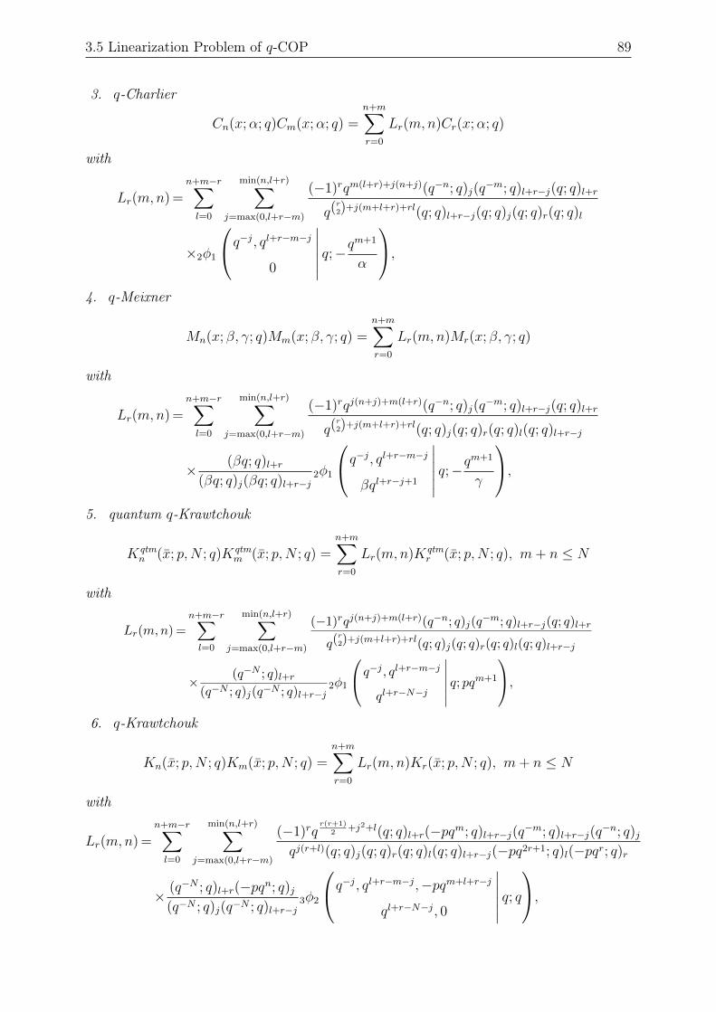
3.5 Linearization Problem of q-COP 89
3. q-Charlier
Cn(x;α; q)Cm(x;α; q) =n+m∑r=0
Lr(m,n)Cr(x;α; q)
with
Lr(m,n) =n+m−r∑l=0
min(n,l+r)∑j=max(0,l+r−m)
(−1)rqm(l+r)+j(n+j)(q−n; q)j(q−m; q)l+r−j(q; q)l+r
q(r2)+j(m+l+r)+rl(q; q)l+r−j(q; q)j(q; q)r(q; q)l
×2φ1
q−j, ql+r−m−j0
∣∣∣∣∣∣ q;−qm+1
α
,4. q-Meixner
Mn(x; β, γ; q)Mm(x; β, γ; q) =n+m∑r=0
Lr(m,n)Mr(x; β, γ; q)
with
Lr(m,n) =n+m−r∑l=0
min(n,l+r)∑j=max(0,l+r−m)
(−1)rqj(n+j)+m(l+r)(q−n; q)j(q−m; q)l+r−j(q; q)l+r
q(r2)+j(m+l+r)+rl(q; q)j(q; q)r(q; q)l(q; q)l+r−j
× (βq; q)l+r(βq; q)j(βq; q)l+r−j
2φ1
q−j, ql+r−m−jβql+r−j+1
∣∣∣∣∣∣ q;−qm+1
γ
,5. quantum q-Krawtchouk
Kqtmn (x; p,N ; q)Kqtm
m (x; p,N ; q) =n+m∑r=0
Lr(m,n)Kqtmr (x; p,N ; q), m+ n ≤ N
with
Lr(m,n) =n+m−r∑l=0
min(n,l+r)∑j=max(0,l+r−m)
(−1)rqj(n+j)+m(l+r)(q−n; q)j(q−m; q)l+r−j(q; q)l+r
q(r2)+j(m+l+r)+rl(q; q)j(q; q)r(q; q)l(q; q)l+r−j
× (q−N ; q)l+r(q−N ; q)j(q−N ; q)l+r−j
2φ1
q−j , ql+r−m−jql+r−N−j
∣∣∣∣∣∣ q; pqm+1
,6. q-Krawtchouk
Kn(x; p,N ; q)Km(x; p,N ; q) =n+m∑r=0
Lr(m,n)Kr(x; p,N ; q), m+ n ≤ N
with
Lr(m,n) =n+m−r∑l=0
min(n,l+r)∑j=max(0,l+r−m)
(−1)rqr(r+1)
2+j2+l(q; q)l+r(−pqm; q)l+r−j(q
−m; q)l+r−j(q−n; q)j
qj(r+l)(q; q)j(q; q)r(q; q)l(q; q)l+r−j(−pq2r+1; q)l(−pqr; q)r
× (q−N ; q)l+r(−pqn; q)j(q−N ; q)j(q−N ; q)l+r−j
3φ2
q−j, ql+r−m−j,−pqm+l+r−j
ql+r−N−j, 0
∣∣∣∣∣∣ q; q,
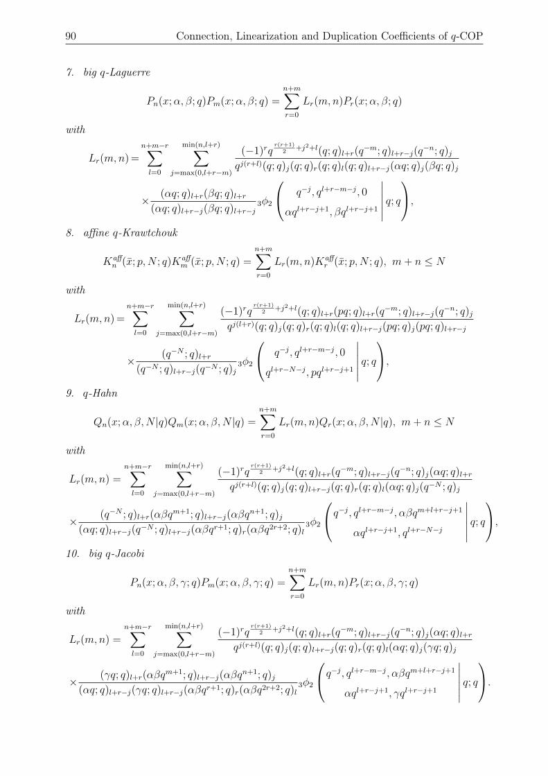
90 Connection, Linearization and Duplication Coefficients of q-COP
7. big q-Laguerre
Pn(x;α, β; q)Pm(x;α, β; q) =n+m∑r=0
Lr(m,n)Pr(x;α, β; q)
with
Lr(m,n) =n+m−r∑l=0
min(n,l+r)∑j=max(0,l+r−m)
(−1)rqr(r+1)
2+j2+l(q; q)l+r(q
−m; q)l+r−j(q−n; q)j
qj(r+l)(q; q)j(q; q)r(q; q)l(q; q)l+r−j(αq; q)j(βq; q)j
× (αq; q)l+r(βq; q)l+r(αq; q)l+r−j(βq; q)l+r−j
3φ2
q−j, ql+r−m−j, 0
αql+r−j+1, βql+r−j+1
∣∣∣∣∣∣ q; q,
8. affine q-Krawtchouk
Kaffn (x; p,N ; q)Kaff
m (x; p,N ; q) =n+m∑r=0
Lr(m,n)Kaffr (x; p,N ; q), m+ n ≤ N
with
Lr(m,n) =n+m−r∑l=0
min(n,l+r)∑j=max(0,l+r−m)
(−1)rqr(r+1)
2+j2+l(q; q)l+r(pq; q)l+r(q
−m; q)l+r−j(q−n; q)j
qj(l+r)(q; q)j(q; q)r(q; q)l(q; q)l+r−j(pq; q)j(pq; q)l+r−j
× (q−N ; q)l+r(q−N ; q)l+r−j(q−N ; q)j
3φ2
q−j, ql+r−m−j, 0
ql+r−N−j, pql+r−j+1
∣∣∣∣∣∣ q; q,
9. q-Hahn
Qn(x;α, β,N |q)Qm(x;α, β,N |q) =n+m∑r=0
Lr(m,n)Qr(x;α, β,N |q), m+ n ≤ N
with
Lr(m,n) =n+m−r∑l=0
min(n,l+r)∑j=max(0,l+r−m)
(−1)rqr(r+1)
2+j2+l(q; q)l+r(q
−m; q)l+r−j(q−n; q)j(αq; q)l+r
qj(r+l)(q; q)j(q; q)l+r−j(q; q)r(q; q)l(αq; q)j(q−N ; q)j
× (q−N ; q)l+r(αβqm+1; q)l+r−j(αβq
n+1; q)j(αq; q)l+r−j(q−N ; q)l+r−j(αβqr+1; q)r(αβq2r+2; q)l
3φ2
q−j, ql+r−m−j, αβqm+l+r−j+1
αql+r−j+1, ql+r−N−j
∣∣∣∣∣∣ q; q,
10. big q-Jacobi
Pn(x;α, β, γ; q)Pm(x;α, β, γ; q) =n+m∑r=0
Lr(m,n)Pr(x;α, β, γ; q)
with
Lr(m,n) =n+m−r∑l=0
min(n,l+r)∑j=max(0,l+r−m)
(−1)rqr(r+1)
2+j2+l(q; q)l+r(q
−m; q)l+r−j(q−n; q)j(αq; q)l+r
qj(r+l)(q; q)j(q; q)l+r−j(q; q)r(q; q)l(αq; q)j(γq; q)j
× (γq; q)l+r(αβqm+1; q)l+r−j(αβq
n+1; q)j(αq; q)l+r−j(γq; q)l+r−j(αβqr+1; q)r(αβq2r+2; q)l
3φ2
q−j, ql+r−m−j, αβqm+l+r−j+1
αql+r−j+1, γql+r−j+1
∣∣∣∣∣∣ q; q.
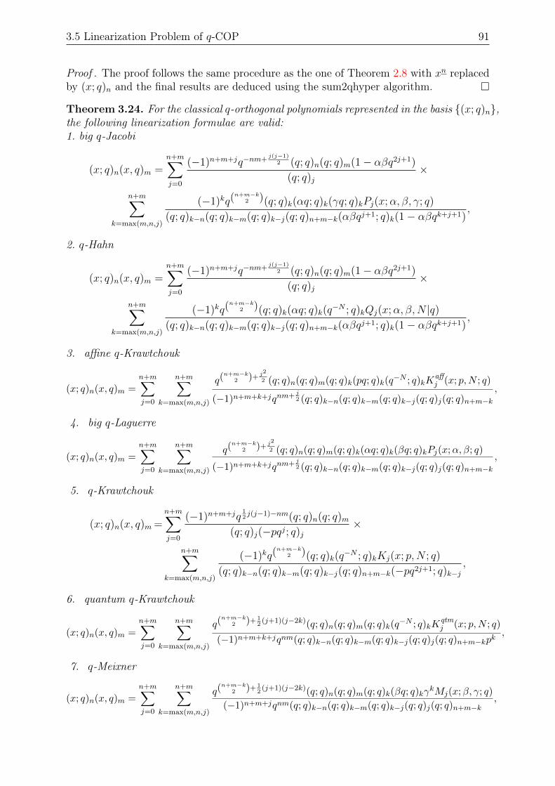
3.5 Linearization Problem of q-COP 91
Proof . The proof follows the same procedure as the one of Theorem 2.8 with xn replacedby (x; q)n and the final results are deduced using the sum2qhyper algorithm.
Theorem 3.24. For the classical q-orthogonal polynomials represented in the basis (x; q)n,the following linearization formulae are valid:1. big q-Jacobi
(x; q)n(x, q)m =n+m∑j=0
(−1)n+m+jq−nm+j(j−1)
2 (q; q)n(q; q)m(1− αβq2j+1)
(q; q)j×
n+m∑k=max(m,n,j)
(−1)kq(n+m−k
2 )(q; q)k(αq; q)k(γq; q)kPj(x;α, β, γ; q)
(q; q)k−n(q; q)k−m(q; q)k−j(q; q)n+m−k(αβqj+1; q)k(1− αβqk+j+1),
2. q-Hahn
(x; q)n(x, q)m =n+m∑j=0
(−1)n+m+jq−nm+j(j−1)
2 (q; q)n(q; q)m(1− αβq2j+1)
(q; q)j×
n+m∑k=max(m,n,j)
(−1)kq(n+m−k
2 )(q; q)k(αq; q)k(q−N ; q)kQj(x;α, β,N |q)
(q; q)k−n(q; q)k−m(q; q)k−j(q; q)n+m−k(αβqj+1; q)k(1− αβqk+j+1),
3. affine q-Krawtchouk
(x; q)n(x, q)m =n+m∑j=0
n+m∑k=max(m,n,j)
q(n+m−k
2 )+ j2
2 (q; q)n(q; q)m(q; q)k(pq; q)k(q−N ; q)kK
affj (x; p,N ; q)
(−1)n+m+k+jqnm+ j2 (q; q)k−n(q; q)k−m(q; q)k−j(q; q)j(q; q)n+m−k
,
4. big q-Laguerre
(x; q)n(x, q)m =n+m∑j=0
n+m∑k=max(m,n,j)
q(n+m−k
2 )+ j2
2 (q; q)n(q; q)m(q; q)k(αq; q)k(βq; q)kPj(x;α, β; q)
(−1)n+m+k+jqnm+ j2 (q; q)k−n(q; q)k−m(q; q)k−j(q; q)j(q; q)n+m−k
,
5. q-Krawtchouk
(x; q)n(x, q)m =n+m∑j=0
(−1)n+m+jq12j(j−1)−nm(q; q)n(q; q)m
(q; q)j(−pqj; q)j×
n+m∑k=max(m,n,j)
(−1)kq(n+m−k
2 )(q; q)k(q−N ; q)kKj(x; p,N ; q)
(q; q)k−n(q; q)k−m(q; q)k−j(q; q)n+m−k(−pq2j+1; q)k−j,
6. quantum q-Krawtchouk
(x; q)n(x, q)m =
n+m∑j=0
n+m∑k=max(m,n,j)
q(n+m−k
2 )+ 12
(j+1)(j−2k)(q; q)n(q; q)m(q; q)k(q−N ; q)kK
qtmj (x; p,N ; q)
(−1)n+m+k+jqnm(q; q)k−n(q; q)k−m(q; q)k−j(q; q)j(q; q)n+m−kpk,
7. q-Meixner
(x; q)n(x, q)m =
n+m∑j=0
n+m∑k=max(m,n,j)
q(n+m−k
2 )+ 12
(j+1)(j−2k)(q; q)n(q; q)m(q; q)k(βq; q)kγkMj(x;β, γ; q)
(−1)n+m+jqnm(q; q)k−n(q; q)k−m(q; q)k−j(q; q)j(q; q)n+m−k,
92 Connection, Linearization and Duplication Coefficients of q-COP
8. q-Charlier
(x; q)n(x, q)m =
n+m∑j=0
n+m∑k=max(m,n,j)
q(n+m−k
2 )+ 12
(j+1)(j−2k)(q; q)n(q; q)m(q; q)kαkCj(x;α; q)
(−1)n+m+jqnm(q; q)k−n(q; q)k−m(q; q)k−j(q; q)j(q; q)n+m−k,
9. Al-Salam-Carlitz II
(x; q)n(x, q)m =
n+m∑j=0
n+m∑k=max(m,n,j)
q(n+m−k
2 )+ 12k(k−1)+j(j−k)(q; q)n(q; q)m(q; q)kα
k−jV(α)j (x; q)
(−1)n+mqnm(q; q)k−n(q; q)k−m(q; q)k−j(q; q)j(q; q)n+m−k,
10. discrete q-Hermite II
(x; q)n(x, q)m =n+m∑j=0
n+m∑k=max(m,n,j)
q(n+m−k
2 )+ 12k(k−1)+j(j−k)(q; q)n(q; q)m(q; q)k(−i)j hj(x; q)
(−1)n+m−kqnm(q; q)k−n(q; q)k−m(q; q)k−j(q; q)j(q; q)n+m−k.
Proof . The combination of
(x; q)n(x; q)m =n+m∑
k=max(m,n)
Hk(m,n)(x; q)k and (x; q)k =k∑j=0
Ij(k)pj(x)
yields the linearization formula
(x; q)n(x; q)m =n+m∑j=0
Lj(m,n)pj(x), with Lj(m,n) =n+m∑
k=max(m,n,j)
Hk(m,n)Ij(k).
3.5.3 Representation Basis (x 1)nqTo solve the linearization problem of q-COP represented in the basis (x 1)nq , thefollowing linearization formula for this basis is necessary.
Proposition 3.25. For the basis (x a)nq , the linearization formula
(x a)nq (x a)mq =n+m∑
k=max(m,n)
(q; q)m(q; q)n(−a)n+m−kq(n+m−k
2 )
(q; q)k−n(q; q)k−m(q; q)n+m−k(x a)kq (3.34)
holds.
Proof . Without loss of generality, we suppose n ≥ m. For every positive integer n
(x a)nq =n−1∏j=0
(x− aqj) = 0⇔ x = aqj, j = 0, 1, . . . , n− 1. (3.35)
For x = a and m ≥ 1, the linearization formula
(x a)nq (x a)mq =n+m∑k=0
Hk(m,n)(x a)kq
3.5 Linearization Problem of q-COP 93
gives thanks to (3.35) H0(m,n) = 0, so that
(x a)nq (x a)mq =n+m∑k=1
Hk(m,n)(x a)kq .
For x = aq and m ≥ 2 the above equation yields (using (3.35)) H1(m,n)(aq a)1q = 0.
Since by definition (aqn a)nq 6= 0, it follows that H1(m,n) = 0. In a similar way, we canshow that
H0(m,n) = H1(m,n) = · · · = Hn−1(m,n) = 0.
Therefore
(x a)nq (x a)mq =n+m∑k=n
Hk(m,n)(x a)kq =m∑k=0
Hn+k(m,n)(x a)n+kq .
Since(x a)n+k
q = (x a)nq (x aqn)kq
the latter equation becomes
(x a)mq =m∑k=0
Hn+k(m,n)(x aqn)kq . (3.36)
For x = aqn and using (3.35), (3.36) gives Hn(m,n) = (aqn a)mq .We have
Dq(x a)mq = [m]q(x a)m−1q
from which for any integer j = 1, 2, . . . ,m,
Djq(x a)mq = [m]q[m− 1]q · · · [m− j + 1]q(x a)m−jq .
Applying Djq to both sides of (3.36), we get
[m]q[m− 1]q · · · [m− j + 1]q(x a)m−jq =m∑k=0
Hn+k(m,n)[k]q[k − 1]q · · · [k − j + 1]q(x aqn)k−jq
=m∑
k=0,k 6=jHn+k(m,n)
[k]q!
[k − j]q!(x aqn)k−jq +Hn+j(m,n)[j]q!.
For x = aqn, the previous equation yields thanks to (3.35)
Hn+j(m,n) =[m]q[m− 1]q · · · [m− j + 1]q(aq
n a)m−jq
[j]q!
=(q; q)m(aqn a)m−jq
(q; q)j(q; q)m−j.
We show that
(aqn a)m−jq = (aqn)m−j(q−n; q)m−j(3.33)=
(−a)m−jq(m−j
2 )(q; q)n(q; q)n−m+j
,
therefore
Hn+j(m,n) =(q; q)m(−a)m−jq(
m−j2 )(q; q)n
(q; q)j(q; q)m−j(q; q)n−m+j
.
Substituting j by k − n, the result follows. Proceeding as in the proof of Theorem 3.23, we get
94 Connection, Linearization and Duplication Coefficients of q-COP
Theorem 3.26. For the q-COP represented in the basis (x 1)nq , the following lineariza-tion formulae are valid:1. Al-Salam-Carlitz I
U (α)n (x; q)U (α)
m (x; q) =n+m∑r=0
n+m−r∑l=0
min(n,l+r)∑j=max(0,l+r−m)
(−1)n+mαm+n−rq(n2)+(m2 )+l+r(q−n; q)j
(q; q)j(q; q)r(q; q)l
×(q−m; q)l+r−j(q; q)l+r(q; q)l+r−j
2φ1
q−j, q−m−j+l+r0
∣∣∣∣∣∣ q; qj+1
α
U (α)r (x; q),
2. discrete q-Hermite I polynomials
hn(x; q)hm(x; q) =n+m∑r=0
n+m−r∑l=0
min(n,l+r)∑j=max(0,l+r−m)
(−1)rq(n2)+(m2 )+l+r(q−n; q)j
(q; q)j(q; q)r(q; q)l
×(q−m; q)l+r−j(q; q)l+r(q; q)l+r−j
2φ1
q−j, q−m−j+l+r0
∣∣∣∣∣∣ q;−qj+1
hr(x; q).
Theorem 3.27. For the classical q-orthogonal polynomials represented in the basis(x 1)nq , the following linearization formulae are valid:1. Al-Salam-Carlitz I
(x 1)nq (x 1)mq =n+m∑j=0
n+m∑k=max(m,n,j)
(−1)n+m−kαk−jq(n+m−k
2 )(q, q)n(q, q)m(q, q)k(q, q)k−n(q, q)k−m(q, q)k−j(q, q)n+m−k(q, q)j
U(α)j (x; q),
2. discrete q-Hermite I
(x 1)nq (x 1)mq =n+m∑j=0
n+m∑k=max(m,n,j)
(−1)n+m−jq(n+m−k
2 )(q, q)n(q, q)m(q, q)k(q, q)k−n(q, q)k−m(q, q)k−j(q, q)n+m−k(q, q)j
hj(x; q).
Proof . The combination of
(x 1)nq (x 1)mq =n+m∑
k=max(m,n)
Hk(m,n)(x 1)kq and (x 1)kq =k∑j=0
Ij(k)pj(x)
yields the linearization formula
(x 1)nq (x 1)mq =n+m∑j=0
Lj(m,n)pj(x), with Lj(m,n) =n+m∑
k=max(m,n,j)
Hk(m,n)Ij(k).
3.6 Duplication Problem of q-COPFor q-COP, we propose two different methods to solve the duplication problem
pn(ax) =n∑
m=0
Dm(n, a)pm(x). (3.37)
3.6 Duplication Problem of q-COP 95
3.6.1 First Method
First we determine a q-differential equation satisfied by pn(ax). For this purpose, we needthe operator εa acting on a function f defined by
εaf(x) := f(ax).
Sprenger [2009] showed that the operator εa has the following properties for any constantb, c:
εa(bf(x) + cg(x)) = bεaf(x) + cεag(x), (3.38)εa(f(x) · g(x)) = εaf(x) · εag(x), (3.39)
εaDq =1
aDqεa. (3.40)
Using the operator εa, we prove
Proposition 3.28. If a q-COP family pn(x) is a solution of the q-differential equation(3.2), then pn(ax) = εapn(x) is a solution of the q-differential equation
σ(ax)DqD 1qpn(ax) + aτ(ax)Dqpn(ax) + a2λn,qpn(ax) = 0. (3.41)
Proof . We apply the operator εa to Equation (3.2) and use the properties (3.38)–(3.40)to get the result.
Using this q-differential equation, we show
Theorem 3.29. Let pn(x) be a q-COP solution of Equation (3.2) with deg(σ) ≤ 1. Theduplication coefficients Dm(n,A) of the duplication problem (3.37) fulfill the recurrencerelations
(a′m−1 + A2(dα?m−1 + λn,qam−1))Dm−1(n,A) + (b′m + A(Adβ?m + e+ Aλn,q bm))Dm(n,A)
+(c′m+1 + A2(dγ?m+1 + λn,q cm+1))Dm+1(n,A) = 0
if σ is a constant and
(a′m−1 + A(dα?m−1 + λnam−1))Dm−1(n,A) + (b′m + Adβ?m + e+ Aλnbm)Dm(n,A)
+(c′m+1 + A(dγ?m+1 + λncm+1))Dm+1(n,A) = 0
if σ is linear, with initial conditions given by Dn+1(n,A) = 0 and Dn(n,A) = An, wherethe coefficients are given in Theorem 3.5 and Propositions 3.6 and 3.8.
Proof . We substitute (3.37) with a = A in (3.41) to get
n∑m=0
Dm(n,A)(σ(Ax)DqD 1
qpm(x) + Aτ(Ax)Dqpm(x) + A2λnpm(x)
)= 0 (3.42)
and proceed as in Subsection 3.4.1.First, for pm(x) Equation (3.15) can be rewritten as
pm(x) =m+1∑j=m−1
am,jDqpm(x) (3.43)
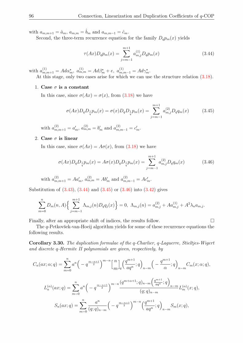
96 Connection, Linearization and Duplication Coefficients of q-COP
with am,m+1 = am, am,m = bm and am,m−1 = cm.Second, the three-term recurrence equation for the family Dqpm(x) yields
τ(Ax)Dqpm(x) =m+1∑j=m−1
a(1)m,jDqpm(x) (3.44)
with a(1)m,m+1 = Adα?m, a
(1)m,m = Adβ?m + e, a
(1)m,m−1 = Adγ?m.
At this stage, only two cases arise for which we can use the structure relation (3.18).
1. Case σ is a constant
In this case, since σ(Ax) = σ(x), from (3.18) we have
σ(Ax)DqD 1qpm(x) = σ(x)DqD 1
qpm(x) =
m+1∑j=m−1
a(2)m,jDqqm(x) (3.45)
with a(2)m,m+1 = a′m, a
(2)m,m = b′m and a(2)
m,m−1 = c′m.
2. Case σ is linear
In this case, since σ(Ax) = Aσ(x), from (3.18) we have
σ(Ax)DqD 1qpm(x) = Aσ(x)DqD 1
qpm(x) =
m+1∑j=m−1
a(2)m,jDqqm(x) (3.46)
with a(2)m,m+1 = Aa′m, a
(2)m,m = Ab′m and a(2)
m,m−1 = Ac′m.
Substitution of (3.43), (3.44) and (3.45) or (3.46) into (3.42) gives
n∑m=0
Dm(n,A) m+1∑j=m−1
Λm,j(n)Dqqj(x)
= 0, Λm,j(n) = a(2)m,j + Aa
(1)m,j + A2λnam,j.
Finally, after an appropriate shift of indices, the results follow. The q-Petkovšek-van-Hoeij algorithm yields for some of these recurrence equations the
following results.
Corollary 3.30. The duplication formulae of the q-Charlier, q-Laguerre, Stieltjes-Wigertand discrete q-Hermite II polynomials are given, respectively, by
Cn(ax;α; q) =n∑
m=0
an(− q
m−n+12
)m−n[ nm
]q
(qm+1
aqn; q)n−m
(− qm+1
α; q)n−m
Cm(x;α; q),
L(α)n (ax; q) =
n∑m=0
an(− q
m−n+12
)m−n (qm+α+1; q)n−m
(qm+1
aqn; q)n−m
(q; q)n−mL(α)m (x; q),
Sn(ax; q) =n∑
m=0
an
(q; q)n−m
(− q
m−n+12
)m−n(qm+1
aqn; q)n−m
Sm(x; q),
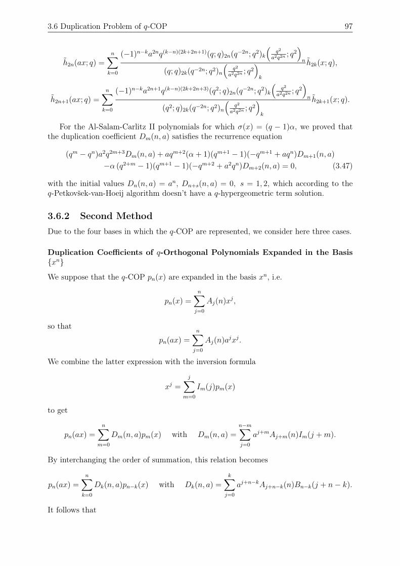
3.6 Duplication Problem of q-COP 97
h2n(ax; q) =n∑k=0
(−1)n−ka2nq(k−n)(2k+2n+1)(q; q)2n(q−2n; q2)k
(q2
a2q2n; q2)n
(q; q)2k(q−2n; q2)n
(q2
a2q2n; q2)k
h2k(x; q),
h2n+1(ax; q) =n∑k=0
(−1)n−ka2n+1q(k−n)(2k+2n+3)(q2; q)2n(q−2n; q2)k
(q2
a2q2n; q2)n
(q2; q)2k(q−2n; q2)n
(q2
a2q2n; q2)k
h2k+1(x; q).
For the Al-Salam-Carlitz II polynomials for which σ(x) = (q − 1)α, we proved thatthe duplication coefficient Dm(n, a) satisfies the recurrence equation
(qm − qn)a2q2m+3Dm(n, a) + aqm+2(α + 1)(qm+1 − 1)(−qm+1 + aqn)Dm+1(n, a)
−α (q2+m − 1)(qm+1 − 1)(−qm+2 + a2qn)Dm+2(n, a) = 0, (3.47)
with the initial values Dn(n, a) = an, Dn+s(n, a) = 0, s = 1, 2, which according to theq-Petkovšek-van-Hoeij algorithm doesn’t have a q-hypergeometric term solution.
3.6.2 Second Method
Due to the four bases in which the q-COP are represented, we consider here three cases.
Duplication Coefficients of q-Orthogonal Polynomials Expanded in the Basisxn
We suppose that the q-COP pn(x) are expanded in the basis xn, i.e.
pn(x) =n∑j=0
Aj(n)xj,
so that
pn(ax) =n∑j=0
Aj(n)ajxj.
We combine the latter expression with the inversion formula
xj =
j∑m=0
Im(j)pm(x)
to get
pn(ax) =n∑
m=0
Dm(n, a)pm(x) with Dm(n, a) =n−m∑j=0
aj+mAj+m(n)Im(j +m).
By interchanging the order of summation, this relation becomes
pn(ax) =n∑k=0
Dk(n, a)pn−k(x) with Dk(n, a) =k∑j=0
aj+n−kAj+n−k(n)Bn−k(j + n− k).
It follows that
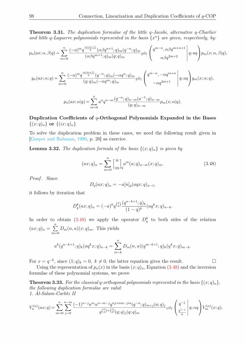
98 Connection, Linearization and Duplication Coefficients of q-COP
Theorem 3.31. The duplication formulae of the little q-Jacobi, alternative q-Charlierand little q-Laguerre polynomials represented in the basis xn are given, respectively, by:
pn(ax;α, β|q) =n∑
m=0
(−a)mqm(m+1)
2 (αβqn+1; q)m(q−n; q)m(αβqm+1; q)m(q; q)m
2φ1
qm−n, αβqm+n+1
αβq2m+2
∣∣∣∣∣∣ q; aqpm(x;α, β|q),
yn(ax;α; q) =
n∑m=0
(−a)mqm(m+1)
2 (q−n; q)m(−αqn; q)m(q; q)m(−αqm; q)m
2φ1
qm−n,−αqm+n
−αq2m+1
∣∣∣∣∣∣ q; aqym(x;α; q),
pn(ax;α|q) =n∑
m=0
anqn−m(q−n; q)n−m(a−1; q)n−m
(q; q)n−mpm(x;α|q).
Duplication Coefficients of q-Orthogonal Polynomials Expanded in the Bases(x; q)n or (ix; q)n
To solve the duplication problem in these cases, we need the following result given in[Gasper and Rahman, 1990, p. 20] as exercice.
Lemma 3.32. The duplication formula of the basis (x; q)n is given by
(ax; q)n =n∑
m=0
[ nm
]qam(a; q)n−m(x; q)m. (3.48)
Proof . SinceDq(ax; q)n = −a[n]q(aqx; q)n−1,
it follows by iteration that
Dkq (ax; q)n = (−a)kq(
k2) (qn−k+1; q)k
(1− q)k(aqkx; q)n−k.
In order to obtain (3.48) we apply the operator Dkq to both sides of the relation
(ax; q)n =n∑
m=0
Dm(n, a)(x; q)m. This yields
ak(qn−k+1; q)k(aqkx; q)n−k =
n∑m=k
Dm(n, a)(qm−k+1; q)k(qkx; q)m−k.
For x = q−k, since (1; q)k = 0, k 6= 0, the latter equation gives the result. Using the representation of pn(x) in the basis (x; q)n, Equation (3.48) and the inversion
formulae of these polynomial systems, we prove
Theorem 3.33. For the classical q-orthogonal polynomials represented in the basis (x; q)n,the following duplication formulae are valid:1. Al-Salam-Carlitz II
V (α)n (ax; q) =
n∑m=0
n−m∑j=0
(−1)n−jamαn−m−jqnj+nm−jm(q−n; q)m+j(a; q)j
q(n2)+(j2)(q; q)j(q; q)m
1φ1
q−j
q1−j
a
∣∣∣∣∣∣ q;αqV (α)
m (x; q),
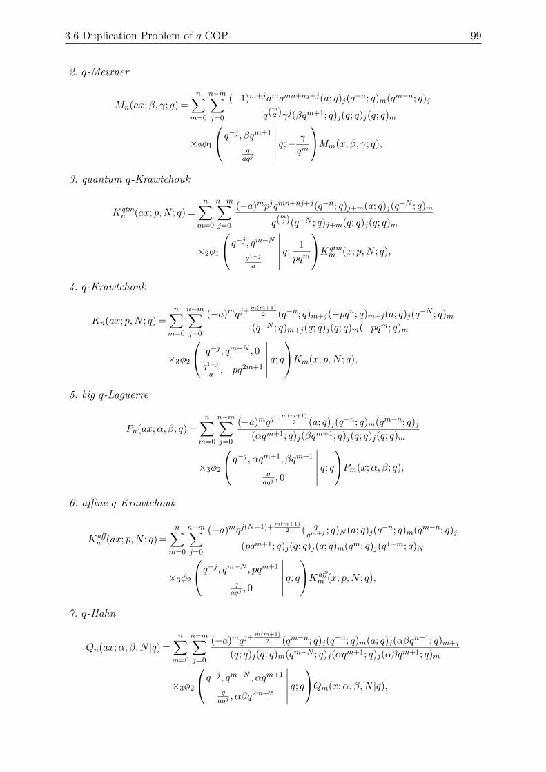
3.6 Duplication Problem of q-COP 99
2. q-Meixner
Mn(ax;β, γ; q) =
n∑m=0
n−m∑j=0
(−1)m+jamqmn+nj+j(a; q)j(q−n; q)m(qm−n; q)j
q(m2 )γj(βqm+1; q)j(q; q)j(q; q)m
×2φ1
q−j , βqm+1
qaqj
∣∣∣∣∣∣ q;− γ
qm
Mm(x;β, γ; q),
3. quantum q-Krawtchouk
Kqtmn (ax; p,N ; q) =
n∑m=0
n−m∑j=0
(−a)mpjqmn+nj+j(q−n; q)j+m(a; q)j(q−N ; q)m
q(m2 )(q−N ; q)j+m(q; q)j(q; q)m
×2φ1
q−j , qm−Nq1−j
a
∣∣∣∣∣∣ q; 1
pqm
Kqtmm (x; p,N ; q),
4. q-Krawtchouk
Kn(ax; p,N ; q) =
n∑m=0
n−m∑j=0
(−a)mqj+m(m+1)
2 (q−n; q)m+j(−pqn; q)m+j(a; q)j(q−N ; q)m
(q−N ; q)m+j(q; q)j(q; q)m(−pqm; q)m
×3φ2
q−j , qm−N , 0
q1−j
a ,−pq2m+1
∣∣∣∣∣∣ q; qKm(x; p,N ; q),
5. big q-Laguerre
Pn(ax;α, β; q) =n∑
m=0
n−m∑j=0
(−a)mqj+m(m+1)
2 (a; q)j(q−n; q)m(qm−n; q)j
(αqm+1; q)j(βqm+1; q)j(q; q)j(q; q)m
×3φ2
q−j , αqm+1, βqm+1
qaqj, 0
∣∣∣∣∣∣ q; qPm(x;α, β; q),
6. affine q-Krawtchouk
Kaffn (ax; p,N ; q) =
n∑m=0
n−m∑j=0
(−a)mqj(N+1)+m(m+1)
2 ( qqm+j ; q)N (a; q)j(q
−n; q)m(qm−n; q)j
(pqm+1; q)j(q; q)j(q; q)m(qm; q)j(q1−m; q)N
×3φ2
q−j , qm−N , pqm+1
qaqj, 0
∣∣∣∣∣∣ q; qKaff
m (x; p,N ; q),
7. q-Hahn
Qn(ax;α, β,N |q) =
n∑m=0
n−m∑j=0
(−a)mqj+m(m+1)
2 (qm−n; q)j(q−n; q)m(a; q)j(αβq
n+1; q)m+j
(q; q)j(q; q)m(qm−N ; q)j(αqm+1; q)j(αβqm+1; q)m
×3φ2
q−j , qm−N , αqm+1
qaqj, αβq2m+2
∣∣∣∣∣∣ q; qQm(x;α, β,N |q),
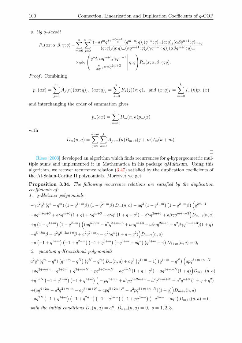
100 Connection, Linearization and Duplication Coefficients of q-COP
8. big q-Jacobi
Pn(ax;α, β, γ; q) =
n∑m=0
n−m∑j=0
(−a)mqj+m(m+1)
2 (qm−n; q)j(q−n; q)m(a; q)j(αβq
n+1; q)m+j
(q; q)j(q; q)m(αqm+1; q)j(γqm+1; q)j(αβqm+1; q)m
×3φ2
q−j , αqm+1, γqm+1
qaqj, αβq2m+2
∣∣∣∣∣∣ q; qPm(x;α, β, γ; q).
Proof . Combining
pn(ax) =n∑j=0
Aj(n)(ax; q)j, (ax; q)j =
j∑k=0
Bk(j)(x; q)k and (x; q)k =k∑
m=0
Im(k)pm(x)
and interchanging the order of summation gives
pn(ax) =n∑
m=0
Dm(n, a)pm(x)
with
Dm(n, a) =n−m∑j=0
j∑k=0
Aj+m(n)Bm+k(j +m)Im(k +m).
Riese [2003] developed an algorithm which finds recurrences for q-hypergeometric mul-
tiple sums and implemented it in Mathematica in his package qMultisum. Using thisalgorithm, we recover recurrence relation (3.47) satisfied by the duplication coefficients ofthe Al-Salam-Carlitz II polynomials. Moreover we get
Proposition 3.34. The following recurrence relations are satisfied by the duplicationcoefficients of:1. q-Meixner polynomials
−γa2q6 (qn − qm)(1− q1+mβ
) (1− q2+mβ
)Dm(n, a)− aq3
(1− q1+m
) (1− q2+mβ
) (q2m+4
−aqm+n+3 + aγqm+1(1 + q) + γqm+3 − aγqn(1 + q + q2)− βγq2m+4 + aβγqm+n+3)Dm+1(n, a)
+q(1− q1+m
) (1− q2+m
) ((aq5+2m − a2q3+m+n + aγqm+3 − aβγq2m+5 + a2βγqm+n+3)(1 + q)
−q8+3mβ + a2q6+2m+nβ + a2q2+mγ − a2γqn(1 + q + q2))Dm+2(n, a)
−a(−1 + q1+m
) (−1 + q2+m
) (−1 + q3+m
) (−q3+m + aqn
) (q3+m + γ
)D3+m(n, a) = 0,
2. quantum q-Krawtchouk polynomials
a2q6 (qm − qn)(q1+m − qN
) (qN − qm
)Dm(n, a) + aq3
(q1+m − 1
) (q1+m − qN
) (apq3+m+n+N
+aq2+m+n − q3+2m + q3+m+N − pq4+2m+N − aqn+N (1 + q + q2) + aq1+m+N (1 + q))Dm+1(n, a)
+q1+N(−1 + q1+m
) (−1 + q2+m
) (− pq7+3m + a2pq5+2m+n − a2q2+m+N + a2qn+N (1 + q + q2)
+(aq4+2m − a2q2+m+n − aq3+m+N + apq5+2m+N − a2pq3+m+n+N )(1 + q))Dm+2(n, a)
−aq2N(−1 + q1+m
) (−1 + q2+m
) (−1 + q3+m
) (−1 + pq3+m
) (−q3+m + aqn
)Dm+3(n, a) = 0,
with the initial conditions Dn(n, a) = an, Dn+s(n, a) = 0, s = 1, 2, 3.
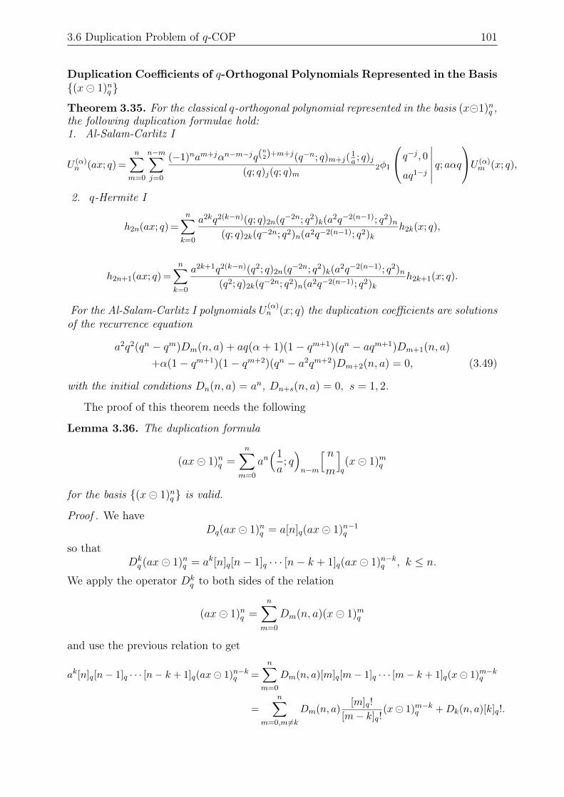
3.6 Duplication Problem of q-COP 101
Duplication Coefficients of q-Orthogonal Polynomials Represented in the Basis(x 1)nq
Theorem 3.35. For the classical q-orthogonal polynomial represented in the basis (x1)nq ,the following duplication formulae hold:1. Al-Salam-Carlitz I
U (α)n (ax; q) =
n∑m=0
n−m∑j=0
(−1)nam+jαn−m−jq(n2)+m+j(q−n; q)m+j(
1a ; q)j
(q; q)j(q; q)m2φ1
q−j , 0aq1−j
∣∣∣∣∣∣ q; aαqU (α)
m (x; q),
2. q-Hermite I
h2n(ax; q) =
n∑k=0
a2kq2(k−n)(q; q)2n(q−2n; q2)k(a2q−2(n−1); q2)n
(q; q)2k(q−2n; q2)n(a2q−2(n−1); q2)kh2k(x; q),
h2n+1(ax; q) =n∑k=0
a2k+1q2(k−n)(q2; q)2n(q−2n; q2)k(a2q−2(n−1); q2)n
(q2; q)2k(q−2n; q2)n(a2q−2(n−1); q2)kh2k+1(x; q).
For the Al-Salam-Carlitz I polynomials U (α)n (x; q) the duplication coefficients are solutions
of the recurrence equation
a2q2(qn − qm)Dm(n, a) + aq(α + 1)(1− qm+1)(qn − aqm+1)Dm+1(n, a)
+α(1− qm+1)(1− qm+2)(qn − a2qm+2)Dm+2(n, a) = 0, (3.49)
with the initial conditions Dn(n, a) = an, Dn+s(n, a) = 0, s = 1, 2.
The proof of this theorem needs the following
Lemma 3.36. The duplication formula
(ax 1)nq =n∑
m=0
an(1
a; q)n−m
[ nm
]q(x 1)mq
for the basis (x 1)nq is valid.
Proof . We haveDq(ax 1)nq = a[n]q(ax 1)n−1
q
so thatDkq (ax 1)nq = ak[n]q[n− 1]q · · · [n− k + 1]q(ax 1)n−kq , k ≤ n.
We apply the operator Dkq to both sides of the relation
(ax 1)nq =n∑
m=0
Dm(n, a)(x 1)mq
and use the previous relation to get
ak[n]q[n− 1]q · · · [n− k + 1]q(ax 1)n−kq =
n∑m=0
Dm(n, a)[m]q[m− 1]q · · · [m− k + 1]q(x 1)m−kq
=n∑
m=0,m6=kDm(n, a)
[m]q!
[m− k]q!(x 1)m−kq +Dk(n, a)[k]q!.
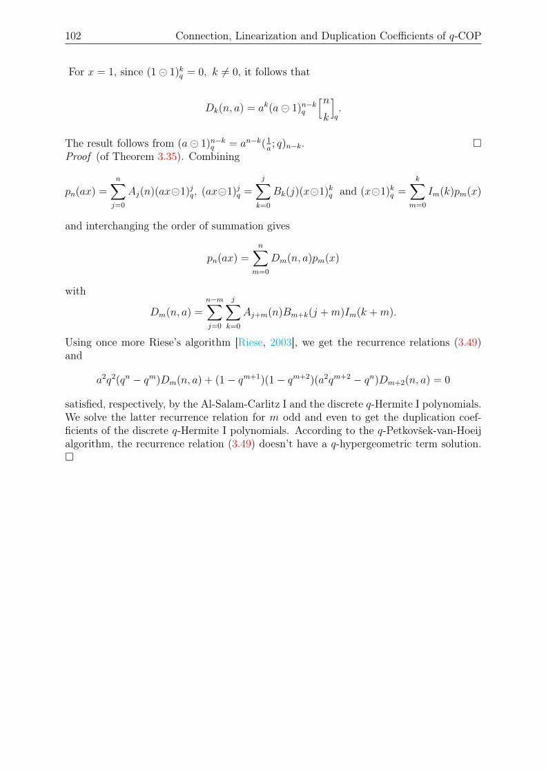
102 Connection, Linearization and Duplication Coefficients of q-COP
For x = 1, since (1 1)kq = 0, k 6= 0, it follows that
Dk(n, a) = ak(a 1)n−kq
[nk
]q.
The result follows from (a 1)n−kq = an−k( 1a; q)n−k.
Proof (of Theorem 3.35). Combining
pn(ax) =n∑j=0
Aj(n)(ax1)jq, (ax1)jq =
j∑k=0
Bk(j)(x1)kq and (x1)kq =k∑
m=0
Im(k)pm(x)
and interchanging the order of summation gives
pn(ax) =n∑
m=0
Dm(n, a)pm(x)
with
Dm(n, a) =n−m∑j=0
j∑k=0
Aj+m(n)Bm+k(j +m)Im(k +m).
Using once more Riese’s algorithm [Riese, 2003], we get the recurrence relations (3.49)and
a2q2(qn − qm)Dm(n, a) + (1− qm+1)(1− qm+2)(a2qm+2 − qn)Dm+2(n, a) = 0
satisfied, respectively, by the Al-Salam-Carlitz I and the discrete q-Hermite I polynomials.We solve the latter recurrence relation for m odd and even to get the duplication coef-ficients of the discrete q-Hermite I polynomials. According to the q-Petkovšek-van-Hoeijalgorithm, the recurrence relation (3.49) doesn’t have a q-hypergeometric term solution.
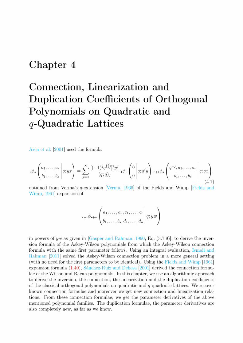
Chapter 4
Connection, Linearization andDuplication Coefficients of OrthogonalPolynomials on Quadratic andq-Quadratic Lattices
Area et al. [2001] used the formula
rφs
a1, . . . , ar
b1, . . . , bs
∣∣∣∣∣∣ q; yx =
∞∑j=0
[(−1)jq(j2)]2yj
(q; q)j1φ1
0
0
∣∣∣∣∣∣ q; qjy r+1φs
q−j , a1, . . . , ar
b1, . . . , bs
∣∣∣∣∣∣ q; qx,
(4.1)obtained from Verma’s q-extension [Verma, 1966] of the Fields and Wimp [Fields andWimp, 1961] expansion of
r+tφs+u
a1, . . . , ar, c1, . . . , ct
b1, . . . , bs, d1, . . . , du
∣∣∣∣∣∣ q; yw
in powers of yw as given in [Gasper and Rahman, 1990, Eq. (3.7.9)], to derive the inver-sion formula of the Askey-Wilson polynomials from which the Askey-Wilson connectionformula with the same first parameter follows. Using an integral evaluation, Ismail andRahman [2011] solved the Askey-Wilson connection problem in a more general setting(with no need for the first parameters to be identical). Using the Fields and Wimp [1961]expansion formula (1.40), Sánchez-Ruiz and Dehesa [2001] derived the connection formu-lae of the Wilson and Racah polynomials. In this chapter, we use an algorithmic approachto derive the inversion, the connection, the linearization and the duplication coefficientsof the classical orthogonal polynomials on quadratic and q-quadratic lattices. We recoverknown connection formulae and moreover we get new connection and linearization rela-tions. From these connection formulae, we get the parameter derivatives of the abovementioned polynomial families. The duplication formulae, the parameter derivatives arealso completely new, as far as we know.
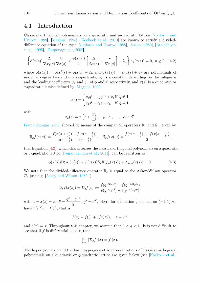
104 Connection, Linearization and Duplication Coefficients of OP on QQL
4.1 IntroductionClassical orthogonal polynomials on a quadratic and q-quadratic lattice [Nikiforov andUvarov, 1988], [Magnus, 1995], [Koekoek et al., 2010] are known to satisfy a divided-difference equation of the type [Nikiforov and Uvarov, 1988], [Suslov, 1989], [Atakishiyevet al., 1995], [Foupouagnigni, 2008],
φ(x(s))∆
∇x1(s)
∇∇x(s)
+ψ(x(s))
2
[∆
∆x(s)+∇∇x(s)
]+ λn
pn(x(s)) = 0, n ≥ 0, (4.2)
where φ(x(s)) = φ2x2(s) + φ1x(s) + φ0 and ψ(x(s)) = ψ1x(s) + ψ0 are polynomials of
maximal degree two and one respectively, λn is a constant depending on the integer nand the leading coefficients φ2 and ψ1 of φ and ψ respectively, and x(s) is a quadratic orq-quadratic lattice defined by [Magnus, 1995]
x(s) =
c1q
s + c2q−s + c3 if q 6= 1,
c4s2 + c5s+ c6 if q = 1,
withxµ(s) = x
(s+
µ
2
), µ, c1, . . . , c6 ∈ C.
Foupouagnigni [2008] showed by means of the companion operators Dx and Sx, given by
Dxf(x(s)) =f(x(s+ 1
2))− f(x(s− 1
2))
x(s+ 12)− x(s− 1
2)
, Sxf(x(s)) =f(x(s+ 1
2)) + f(x(s− 1
2))
2,
that Equation (4.2), which characterizes the classical orthogonal polynomials on a quadraticor q-quadratic lattice [Foupouagnigni et al., 2011], can be rewritten as
φ(x(s))D2xpn(x(s)) + ψ(x(s))SxDxpn(x(s)) + λnpn(x(s)) = 0. (4.3)
We note that the divided-difference operator Dx is equal to the Askey-Wilson operatorDq (see e.g. [Askey and Wilson, 1985] )
Dxf(x(s)) = Dqf(x) :=f(q1/2eiθ)− f(q−1/2eiθ)
e(q1/2eiθ)− e(q−1/2eiθ),
with x = x(s) = cos θ =qs + q−s
2, qs = eiθ, where for a function f defined on (−1, 1) we
have f(eiθ) := f(x), that is
f(z) = f((z + 1/z)/2), z = eiθ,
and e(x) = x. Throughout this chapter, we assume that 0 < q < 1. It is not difficult tosee that if f is differentiable at x, then
limq→1
(Dqf)(x) = f ′(x).
The hypergeometric and the basic hypergeometric representations of classical orthogonalpolynomials on a quadratic or q-quadratic lattice are given below (see [Koekoek et al.,
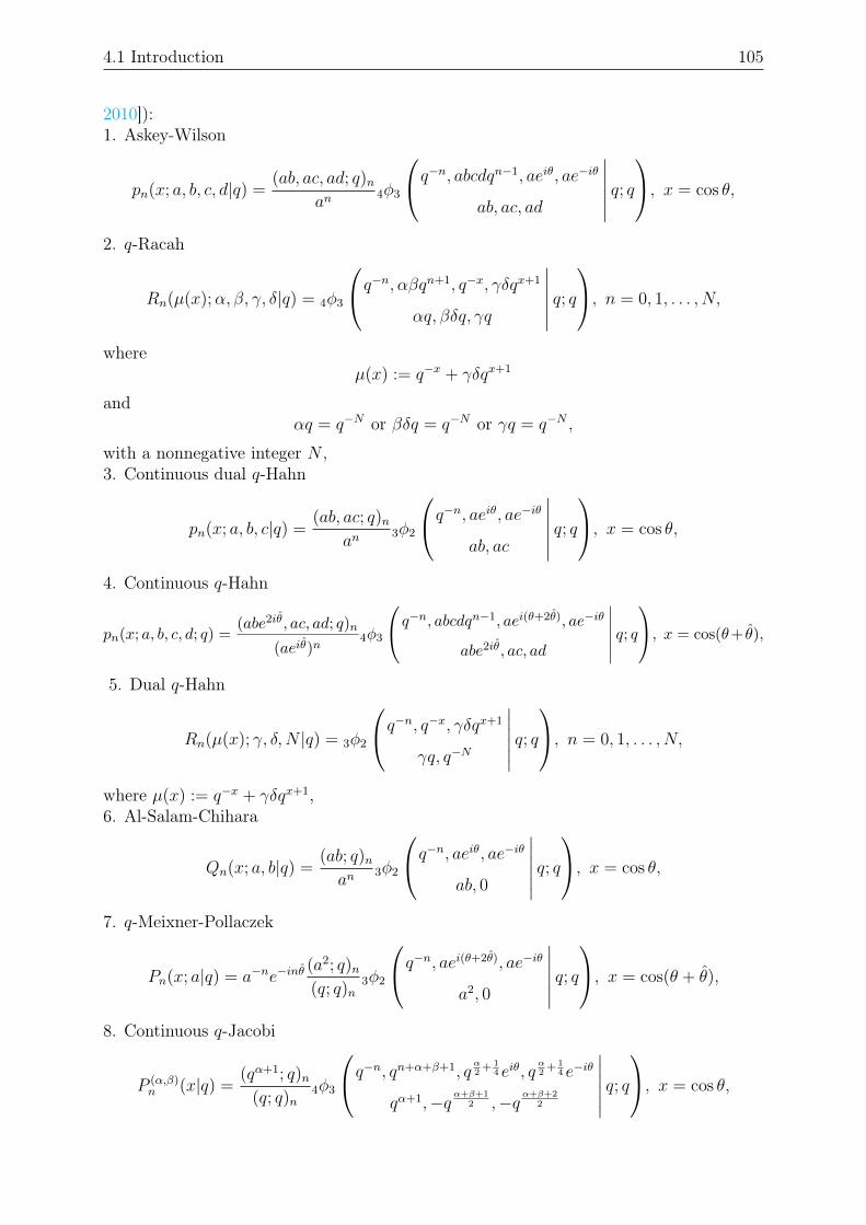
4.1 Introduction 105
2010]):1. Askey-Wilson
pn(x; a, b, c, d|q) =(ab, ac, ad; q)n
an4φ3
q−n, abcdqn−1, aeiθ, ae−iθ
ab, ac, ad
∣∣∣∣∣∣ q; q, x = cos θ,
2. q-Racah
Rn(µ(x);α, β, γ, δ|q) = 4φ3
q−n, αβqn+1, q−x, γδqx+1
αq, βδq, γq
∣∣∣∣∣∣ q; q, n = 0, 1, . . . , N,
whereµ(x) := q−x + γδqx+1
andαq = q−N or βδq = q−N or γq = q−N ,
with a nonnegative integer N ,3. Continuous dual q-Hahn
pn(x; a, b, c|q) =(ab, ac; q)n
an3φ2
q−n, aeiθ, ae−iθab, ac
∣∣∣∣∣∣ q; q, x = cos θ,
4. Continuous q-Hahn
pn(x; a, b, c, d; q) =(abe2iθ, ac, ad; q)n
(aeiθ)n4φ3
q−n, abcdqn−1, aei(θ+2θ), ae−iθ
abe2iθ, ac, ad
∣∣∣∣∣∣ q; q, x = cos(θ+ θ),
5. Dual q-Hahn
Rn(µ(x); γ, δ,N |q) = 3φ2
q−n, q−x, γδqx+1
γq, q−N
∣∣∣∣∣∣ q; q, n = 0, 1, . . . , N,
where µ(x) := q−x + γδqx+1,6. Al-Salam-Chihara
Qn(x; a, b|q) =(ab; q)nan
3φ2
q−n, aeiθ, ae−iθab, 0
∣∣∣∣∣∣ q; q, x = cos θ,
7. q-Meixner-Pollaczek
Pn(x; a|q) = a−ne−inθ(a2; q)n(q; q)n
3φ2
q−n, aei(θ+2θ), ae−iθ
a2, 0
∣∣∣∣∣∣ q; q, x = cos(θ + θ),
8. Continuous q-Jacobi
P (α,β)n (x|q) =
(qα+1; q)n(q; q)n
4φ3
q−n, qn+α+β+1, qα2
+ 14 eiθ, q
α2
+ 14 e−iθ
qα+1,−q α+β+12 ,−q α+β+2
2
∣∣∣∣∣∣ q; q, x = cos θ,
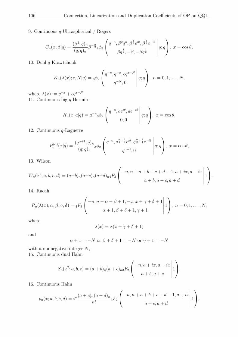
106 Connection, Linearization and Duplication Coefficients of OP on QQL
9. Continuous q-Ultraspherical / Rogers
Cn(x; β|q) =(β2; q)n(q; q)n
β−n2 4φ3
q−n, β2qn, β12 eiθ, β
12 e−iθ
βq12 ,−β,−βq 1
2
∣∣∣∣∣∣ q; q, x = cos θ,
10. Dual q-Krawtchouk
Kn(λ(x); c,N |q) = 3φ2
q−n, q−x, cqx−Nq−N , 0
∣∣∣∣∣∣ q; q, n = 0, 1, . . . , N,
where λ(x) := q−x + cqx−N ,11. Continuous big q-Hermite
Hn(x; a|q) = a−n3φ2
q−n, aeiθ, ae−iθ0, 0
∣∣∣∣∣∣ q; q, x = cos θ,
12. Continuous q-Laguerre
P (α)n (x|q) =
(qα+1; q)n(q; q)n
3φ2
q−n, q α2 + 14 eiθ, q
α2
+ 14 e−iθ
qα+1, 0
∣∣∣∣∣∣ q; q, x = cos θ,
13. Wilson
Wn(x2; a, b, c, d) = (a+b)n(a+c)n(a+d)n4F3
−n, n+ a+ b+ c+ d− 1, a+ ix, a− ix
a+ b, a+ c, a+ d
∣∣∣∣∣∣ 1,
14. Racah
Rn(λ(x);α, β, γ, δ) = 4F3
−n, n+ α + β + 1,−x, x+ γ + δ + 1
α + 1, β + δ + 1, γ + 1
∣∣∣∣∣∣ 1, n = 0, 1, . . . , N,
whereλ(x) = x(x+ γ + δ + 1)
andα + 1 = −N or β + δ + 1 = −N or γ + 1 = −N
with a nonnegative integer N ,15. Continuous dual Hahn
Sn(x2; a, b, c) = (a+ b)n(a+ c)n3F2
−n, a+ ix, a− ix
a+ b, a+ c
∣∣∣∣∣∣ 1,
16. Continuous Hahn
pn(x; a, b, c, d) = in(a+ c)n(a+ d)n
n!3F2
−n, n+ a+ b+ c+ d− 1, a+ ix
a+ c, a+ d
∣∣∣∣∣∣ 1,
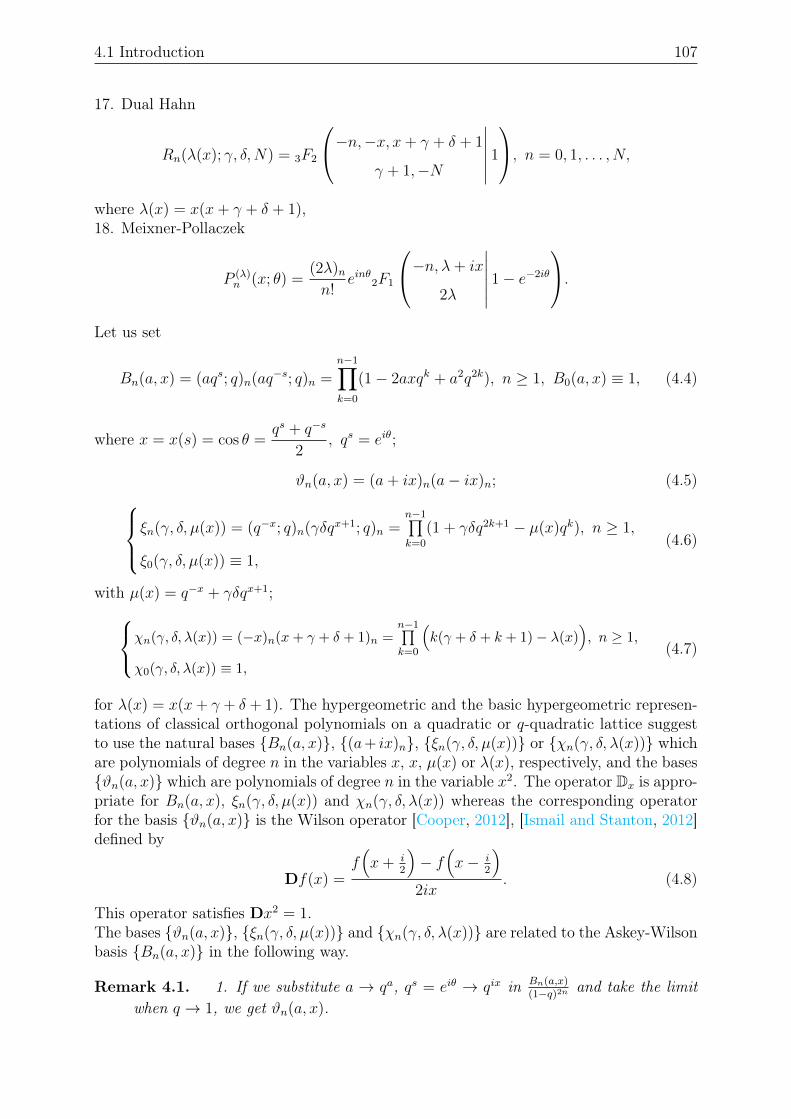
4.1 Introduction 107
17. Dual Hahn
Rn(λ(x); γ, δ,N) = 3F2
−n,−x, x+ γ + δ + 1
γ + 1,−N
∣∣∣∣∣∣ 1, n = 0, 1, . . . , N,
where λ(x) = x(x+ γ + δ + 1),18. Meixner-Pollaczek
P (λ)n (x; θ) =
(2λ)nn!
einθ2F1
−n, λ+ ix
2λ
∣∣∣∣∣∣ 1− e−2iθ
.Let us set
Bn(a, x) = (aqs; q)n(aq−s; q)n =n−1∏k=0
(1− 2axqk + a2q2k), n ≥ 1, B0(a, x) ≡ 1, (4.4)
where x = x(s) = cos θ =qs + q−s
2, qs = eiθ;
ϑn(a, x) = (a+ ix)n(a− ix)n; (4.5)ξn(γ, δ, µ(x)) = (q−x; q)n(γδqx+1; q)n =n−1∏k=0
(1 + γδq2k+1 − µ(x)qk), n ≥ 1,
ξ0(γ, δ, µ(x)) ≡ 1,
(4.6)
with µ(x) = q−x + γδqx+1;χn(γ, δ, λ(x)) = (−x)n(x+ γ + δ + 1)n =n−1∏k=0
(k(γ + δ + k + 1)− λ(x)
), n ≥ 1,
χ0(γ, δ, λ(x)) ≡ 1,
(4.7)
for λ(x) = x(x+ γ + δ + 1). The hypergeometric and the basic hypergeometric represen-tations of classical orthogonal polynomials on a quadratic or q-quadratic lattice suggestto use the natural bases Bn(a, x), (a+ ix)n, ξn(γ, δ, µ(x)) or χn(γ, δ, λ(x)) whichare polynomials of degree n in the variables x, x, µ(x) or λ(x), respectively, and the basesϑn(a, x) which are polynomials of degree n in the variable x2. The operator Dx is appro-priate for Bn(a, x), ξn(γ, δ, µ(x)) and χn(γ, δ, λ(x)) whereas the corresponding operatorfor the basis ϑn(a, x) is the Wilson operator [Cooper, 2012], [Ismail and Stanton, 2012]defined by
Df(x) =f(x+ i
2
)− f
(x− i
2
)2ix
. (4.8)
This operator satisfies Dx2 = 1.The bases ϑn(a, x), ξn(γ, δ, µ(x)) and χn(γ, δ, λ(x)) are related to the Askey-Wilsonbasis Bn(a, x) in the following way.
Remark 4.1. 1. If we substitute a → qa, qs = eiθ → qix in Bn(a,x)(1−q)2n and take the limit
when q → 1, we get ϑn(a, x).
108 Connection, Linearization and Duplication Coefficients of OP on QQL
2. If we substitute a → (γδq)12 and qs = eiθ → (γδq)
12 qx in Bn(a, x) we obtain
ξn(γ, δ, µ(x)).
3. If we substitute γ → qγ, δ → qδ in ξn(γ,δ,µ(x))(1−q)2n and take the limit as q → 1, we get
χn(γ, δ, λ(x)).
4. If we set a = 12(γ+δ+1) and ix→ x+ 1
2(γ+δ+1) in ϑn(a, x) we get χn(γ, δ, λ(x)).
5. We also havelimt→∞
ϑn(a− it, x+ t)
(−2it)n= (a+ ix)n.
In this chapter we find the inversion, connection, duplication and linearization formu-lae for the Askey-Wilson polynomials. The results can be extended to other families ofclassical orthogonal polynomials on a quadratic or q-quadratic lattice by means of spe-cialization and/or by limiting processes following the Askey scheme and it q-analogue. Toillustrate this, we solve the inversion, connection, duplication and linearization problemfor the q-Racah, Wilson and Racah polynomials.
The Askey-Wilson orthogonal polynomial family pn(x; a, b, c, d|q) satisfies the divided-difference equation of type (4.3) with [Foupouagnigni, 2008]
φ(x(s)) = 2(abcd+ 1)x2(s)− (a+ b+ c+ d+ abc+ abd+ acd+ bcd)x(s)
+ab+ ac+ ad+ bc+ bd+ cd− abcd− 1,
ψ(x(s)) =4(abcd− 1)q
12x(s)
q − 1+
2(a+ b+ c+ d− abc− abd− acd− bcd)q12
q − 1.
The Askey-Wilson basis Bn(a, x) has the following properties.
Proposition 4.2 ([Foupouagnigni et al., 2013a], [Foupouagnigni et al., 2013b]). Theq-quadratic lattice x(s) = qs+q−s
2and the corresponding polynomial basis
Bn(a, x) = (aqs; q)n(aq−s; q)n, n ≥ 1, B0(a, x) ≡ 1,
fulfil the relations
DxBn(a, x) = η(a, n)Bn−1(a√q, x); (4.9)
SxBn(a, x) = β1(a, n)Bn−1(a√q, x) + β2(n)Bn(a
√q, x);
B1(a, x)D2xBn(a, x) = η(a, n)η(a
√q, n− 1)Bn−1(a, x); (4.10)
B1(a, x)SxDxBn(a, x) = η(a, n) (β1(a√q, n− 1)Bn−1(a, x) + β2(n− 1)Bn(a, x)) ; (4.11)
xBn(a, x) =µ1(a, n)Bn(a, x) + µ2(a, n)Bn+1(a, x); (4.12)B1(a, x)Bn(a, x) = ν1(a, n)Bn(a, x) + ν2(n)Bn+1(a, x); (4.13)B1(a, x)Bn(aq, x) =Bn+1(a, x),
where
η(a, n) = 2a(1−qn)q−1
, β1(a, n) = 12(1− a2q2n−1)(1− q−n), β2(n) = 1
2+ 1
2qn,
µ1(a, n) = 1+a2q2n
2aqn, µ2(a, n) = −1
2aqn, ν1(a, n) = (1− q−n)(1− a2qn), ν2(n) = q−n.
Using these properties of the basis Bn(a, x), we will derive the inversion formulaeof Askey-Wilson polynomials.
4.2 Inversion Formula of Askey-Wilson Polynomials 109
4.2 Inversion Formula of Askey-Wilson Polynomials
To solve the inversion problem of the Askey-Wilson polynomials we need the coefficientsof the three-term recurrence relation of the Askey-Wilson polynomials pn(x; a, b, c, d|q),and the coefficients of the three-term recurrence relation of the second divided-derivativeof the Askey-Wilson polynomials D2
xpn(x; a, b, c, d|q).
4.2.1 Three-Term Recurrence Equation of the Family (pn(x; a, b, c, d|q))n
Proposition 4.3 (See e.g. [Koekoek et al., 2010]). The Askey-Wilson polynomial familysatisfies a three-term recurrence equation of the form
xpn(x; a, b, c, d|q) = αnpn+1(x; a, b, c, d|q) + βnpn(x; a, b, c, d|q) + γnpn−1(x; a, b, c, d|q),(4.14)
with
αn =− 1
2aqnknkn+1
, (4.15)
βn =1
2
qn
(−q2 + dcbaq2n) (−1 + dcbaq2n)
((q2 + abcdq2n+1 + abcdqn+1 − abcdqn)×
(a+ b+ c+ d)− (qn+1 + qn+2 − q − abcdq2n)(abc+ abd+ acd+ bcd)), (4.16)
γn =− kn2kn−1
(qndc− q) (dbqn − q) (qnbc− q) (dcbaqn − q2) qna (baqn − q) (caqn − q)q (−q2 + dcbaq2n)2 (−q3 + dcbaq2n)
×(aqnd− q) (−1 + qn)
(−q + dcbaq2n),
where kn is the leading coefficient of the polynomial pn(x; a, b, c, d|q) represented in thebasis (Bn(a, x))n
pn(x; a, b, c, d|q) = knBn(a, x) + k′nBn−1(a, x) + k′′nBn−2(a, x) + . . . (4.17)
and is given explicitly by kn =(abcdqn−1; q)n
(−a)nq(n2)
.
Proof . We will first need to compute, in terms of the leading coefficient kn, the coefficientsk′n and k′′n of the expansion (4.17) of pn(x; a, b, c, d|q) in the appropriate basis (Bn(a, x))n.In order to compute these coefficients, first we substitute (4.17) in the divided-differenceequation (4.3). Next we multiply this equation by B1(a, x) and use Relations (4.10), (4.11)and (4.13). To eliminate the terms xBk(a, x) and x2Bk(a, x), we use Relations (4.12) and
x2Bn(a, x) =µ21(a, n)Bn(a, x) + µ2(a, n)(µ1(a, n) + µ1(a, n+ 1))Bn+1(a, x)
+µ2(a, n)µ2(a, n+ 1)Bn+2(a, x). (4.18)
Equating the coefficients of Bn+1(a, x) gives (compare [Foupouagnigni, 2008, p. 158,(104)])
λn = −4(−1 + qn)
√q (abcdqn − q)
(q − 1)2 qn. (4.19)
110 Connection, Linearization and Duplication Coefficients of OP on QQL
Equating the coefficients of Bn(a, x), we deduce using (4.19) that
k′n = −(−1 + qn) (−q + aqnd) (aqnc− q) (aqnb− q)q (q − 1) (−q2 + abcdq2n)
kn. (4.20)
By equating the coefficients of Bn−1(a, x) and using (4.19)-(4.20), one gets
k′′n =(−1 + qn) (−q + aqnd) (aqnc− q) (aqnb− q) (−q + qn) (aqnd− q2)
(1 + q) (q − 1)2 (−q3 + abcdq2n) (−q2 + abcdq2n)
×(aqnc− q2) (aqnb− q2)
q4kn. (4.21)
To get the coefficients αn, βn and γn of Equation (4.14), we substitute the expressionof pn given by (4.17) in the recurrence equation (4.14) and use Equations (4.12), (4.19)-(4.21). By equating the coefficients of Bn+1(a, x), one gets αn. Equating the coefficientsof Bn(a, x) and using (4.15) yields βn. Similarly, equating the coefficients of Bn−1(a, x)and using (4.15)-(4.16) gives γn.
Remark 4.4. The recurrence equation (4.14) was also given in [Koekoek et al., 2010, p.417] in the form
2xpn(x) = Anpn+1(x) + [a+ a−1 − (An + Cn)]pn(x) + Cnpn−1(x), (4.22)
wherepn(x) :=
anpn(x; a, b, c, d|q)(ab, ac, ad : q)n
and
An =(1− abqn)(1− acqn)(1− adqn)(1− abcdqn−1)
a(1− abcdq2n−1)(1− abcdq2n)
Cn =a(1− qn)(1− bcqn−1)(1− bdqn−1)(1− cdqn−1)
(1− abcdq2n−2)(1− abcdq2n−1).
It can be proved by direct computation that Equation (4.22) is equivalent to Equation(4.14) with
αn = Ana(ab, ac, ad; q)n
2(ab, ac, ad; q)n+1
, βn =[a+ a−1 − (An + Cn)]
2, γn = Cn
(ab, ac, ad; q)n2a(ab, ac, ad; q)n−1
.
4.2.2 Three-Term Recurrence Equation of the Family (D2xpn(x; a, b, c, d|q))n
Foupouagnigni et al. [2011] proved that if (pn)n is an orthogonal polynomial family satis-fying (4.3), then the families (Dm
x pn)n are also orthogonal, for all m ∈ N. Consequently,they also satisfy a three-term recurrence equation.
Proposition 4.5. The second-order divided-difference D2xpn of the Askey-Wilson orthog-
onal polynomials defined by (4.17) satisfies the following recurrence equation
xD2xpn(x; a, b, c, d|q) =α?nD2
xpn+1(x; a, b, c, d|q) + β?nD2xpn(x; a, b, c, d|q)
+γ?nD2xpn−1(x; a, b, c, d|q), (4.23)
4.2 Inversion Formula of Askey-Wilson Polynomials 111
with
α?n =−1
2
−q + qn
aqn (−1 + qn+1)
knkn+1
, (4.24)
β?n =1
2
qn
(−q2 + abcdq2n) (−1 + abcdq2n)
((a+ b+ c+ d)(q − abcdqn+1 − abcdqn+2 + abcdq2n)
+(abc+ abd+ acd+ bcd)(q2 − qn − qn+1 + abcdq2n+1)), (4.25)
γ?n =− kn2kn−1
(−q + qndc) (qnbd− q) (qnbc− q) (abcdqn − 1) qna (−1 + qn) (baqn − q)(−q2 + abcdq2n)2 (−q3 + abcdq2n)
×(acqn − q) (−q + aqnd)
(−q + abcdq2n).
Proof . We substitute the expression of pn given by (4.17) in the recurrence equation (4.23),and then multiply the equation obtained by B1(a, x). Next we use (4.10) and (4.12),respectively, to eliminate B1(a, x)D2
xBn(a, x) and xBn(a, x). By equating the coefficientsof Bn(a, x), one gets α?n. Equating the coefficients of Bn−1(a, x) and using (4.24) yields β?n.Similarly, equating the coefficients of Bn−2(a, x) and using (4.24) and (4.25), we obtainγ?n.
4.2.3 Inversion Formula of Askey-Wilson Polynomials
Since the family (pk(x; a, b, c, d|q))k=0,...,n is a basis of polynomials of degree less than orequal to n, and since Bn(a, x) is a polynomial of degree n w.r.t. x, it follows that
Bn(a, x) =n∑
m=0
Im(n)pm(x; a, b, c, d|q), (4.26)
which is called the inversion formula for the family (pn(x; a, b, c, d|q))n represented in thebasis (Bn(a, x))n. We prove that
Proposition 4.6 (See e.g. [Area et al., 2001], [Foupouagnigni et al., 2013b]). The inver-sion formula of the Askey-Wilson orthogonal polynomial family is given by
Bn(a, x) =n∑
m=0
[ nm
]qqm(m−1)
2(−a)m(abqm, acqm, adqm; q)n−m(abcdqm−1; q)m(abcdq2m; q)n−m
pm(x; a, b, c, d|q). (4.27)
The proof of this proposition uses the following
Lemma 4.7. The second Dx-derivative of the basis (Bn(a, x))n satisfies the recurrencerelation
xD2xBn(a, x) = µ1(a, n− 1)D2
xBn(a, x) + µ2(a, n− 1)η(a, n)η(a
√q, n− 1)
η(a, n+ 1)η(a√q, n)
D2xBn+1(a, x),
(4.28)with the coefficients given in Proposition 4.2.
Proof (of the lemma). From (4.10) we obtain Bn(a, x) in terms of D2xBn+1(a, x). If we
substitute this in the recurrence equation (4.12), the result follows.
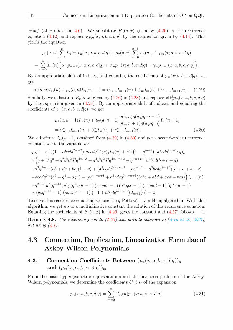
112 Connection, Linearization and Duplication Coefficients of OP on QQL
Proof (of Proposition 4.6). We substitute Bn(a, x) given by (4.26) in the recurrenceequation (4.12) and replace xpm(x; a, b, c, d|q) by the expression given by (4.14). Thisyields the equation
µ1(a, n)n∑
m=0
Im(n)pm(x; a, b, c, d|q) + µ2(a, n)n+1∑m=0
Im(n+ 1)pm(x; a, b, c, d|q)
=n∑
m=0
Im(n)(αmpm+1(x; a, b, c, d|q) + βmpm(x; a, b, c, d|q) + γmpm−1(x; a, b, c, d|q)
).
By an appropriate shift of indices, and equating the coefficients of pm(x; a, b, c, d|q), weget
µ1(a, n)Im(n) + µ2(a, n)Im(n+ 1) = αm−1Im−1(n) + βmIm(n) + γm+1Im+1(n). (4.29)
Similarly, we substitute Bn(a, x) given by (4.26) in (4.28) and replace xD2xpm(x; a, b, c, d|q)
by the expression given in (4.23). By an appropriate shift of indices, and equating thecoefficients of pm(x; a, b, c, d|q), we get
µ1(a, n− 1)Im(n) + µ2(a, n− 1)η(a, n)η(a
√q, n− 1)
η(a, n+ 1)η(a√q, n)
Im(n+ 1)
= α?m−1Im−1(n) + β?mIm(n) + γ?m+1Im+1(n). (4.30)
We substitute Im(n+ 1) obtained from (4.29) in (4.30) and get a second-order recurrenceequation w.r.t. the variable m:
q(qn − qm)(1− abcdq2m+2)(abcdq2m; q)4Im(n) + qm(1− qm+1
)(abcdq2m+1; q)3
×(q + a2qn + a2b2c2d2q4m+3 + a4b2c2d2q4m+n+2 + q2m+n+2a2bcd(b+ c+ d)
+a2q2m+1(db+ dc+ bc)(1 + q) + (a2bcdq2m+n+1 − aqm+1 − a2bcdq3m+2)(d+ a+ b+ c)
−abcdq2m(q3 − q2 + aqn)− (aqm+n+1 + a2bdcq3m+n+2)(abc+ abd+ acd+ bcd))Im+1(n)
+q2m+1a2(qm+1; q)2 (qmqdc− 1) (qmqdb− 1) (qmqbc− 1) (qmqad− 1) (qmqac− 1)
×(abqm+1 − 1
) (abcdq2m − 1
) (−1 + abcdqm+n+1
)Im+2(n) = 0.
To solve this recurrence equation, we use the q-Petkovšek-van-Hoeij algorithm. With thisalgorithm, we get up to a multiplicative constant the solution of this recurrence equation.Equating the coefficients of Bn(a, x) in (4.26) gives the constant and (4.27) follows.
Remark 4.8. The inversion formula (4.27) was already obtained in [Area et al., 2001],but using (4.1).
4.3 Connection, Duplication, Linearization Formulae ofAskey-Wilson Polynomials
4.3.1 Connection Coefficients Between (pn(x; a, b, c, d|q))nand (pm(x; a, β, γ, δ|q))m
From the basic hypergeometric representation and the inversion problem of the Askey-Wilson polynomials, we determine the coefficients Cm(n) of the expansion
pn(x; a, b, c, d|q) =n∑
m=0
Cm(n)pm(x; a, β, γ, δ|q). (4.31)
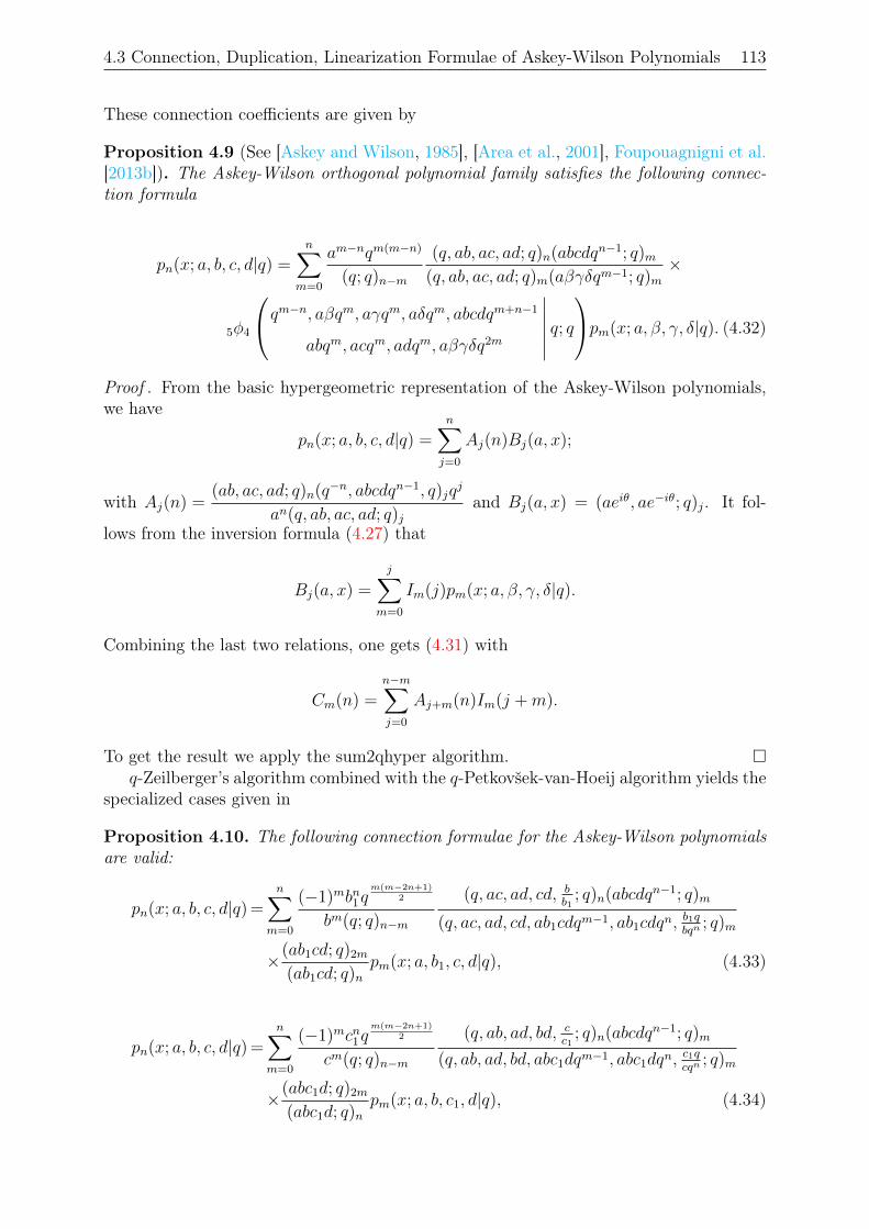
4.3 Connection, Duplication, Linearization Formulae of Askey-Wilson Polynomials 113
These connection coefficients are given by
Proposition 4.9 (See [Askey and Wilson, 1985], [Area et al., 2001], Foupouagnigni et al.[2013b]). The Askey-Wilson orthogonal polynomial family satisfies the following connec-tion formula
pn(x; a, b, c, d|q) =n∑
m=0
am−nqm(m−n)
(q; q)n−m
(q, ab, ac, ad; q)n(abcdqn−1; q)m(q, ab, ac, ad; q)m(aβγδqm−1; q)m
×
5φ4
qm−n, aβqm, aγqm, aδqm, abcdqm+n−1
abqm, acqm, adqm, aβγδq2m
∣∣∣∣∣∣ q; qpm(x; a, β, γ, δ|q). (4.32)
Proof . From the basic hypergeometric representation of the Askey-Wilson polynomials,we have
pn(x; a, b, c, d|q) =n∑j=0
Aj(n)Bj(a, x);
with Aj(n) =(ab, ac, ad; q)n(q−n, abcdqn−1, q)jq
j
an(q, ab, ac, ad; q)jand Bj(a, x) = (aeiθ, ae−iθ; q)j. It fol-
lows from the inversion formula (4.27) that
Bj(a, x) =
j∑m=0
Im(j)pm(x; a, β, γ, δ|q).
Combining the last two relations, one gets (4.31) with
Cm(n) =n−m∑j=0
Aj+m(n)Im(j +m).
To get the result we apply the sum2qhyper algorithm. q-Zeilberger’s algorithm combined with the q-Petkovšek-van-Hoeij algorithm yields the
specialized cases given in
Proposition 4.10. The following connection formulae for the Askey-Wilson polynomialsare valid:
pn(x; a, b, c, d|q) =n∑
m=0
(−1)mbn1qm(m−2n+1)
2
bm(q; q)n−m
(q, ac, ad, cd, bb1
; q)n(abcdqn−1; q)m
(q, ac, ad, cd, ab1cdqm−1, ab1cdqn,b1qbqn
; q)m
×(ab1cd; q)2m
(ab1cd; q)npm(x; a, b1, c, d|q), (4.33)
pn(x; a, b, c, d|q) =n∑
m=0
(−1)mcn1qm(m−2n+1)
2
cm(q; q)n−m
(q, ab, ad, bd, cc1
; q)n(abcdqn−1; q)m
(q, ab, ad, bd, abc1dqm−1, abc1dqn,c1qcqn
; q)m
×(abc1d; q)2m
(abc1d; q)npm(x; a, b, c1, d|q), (4.34)
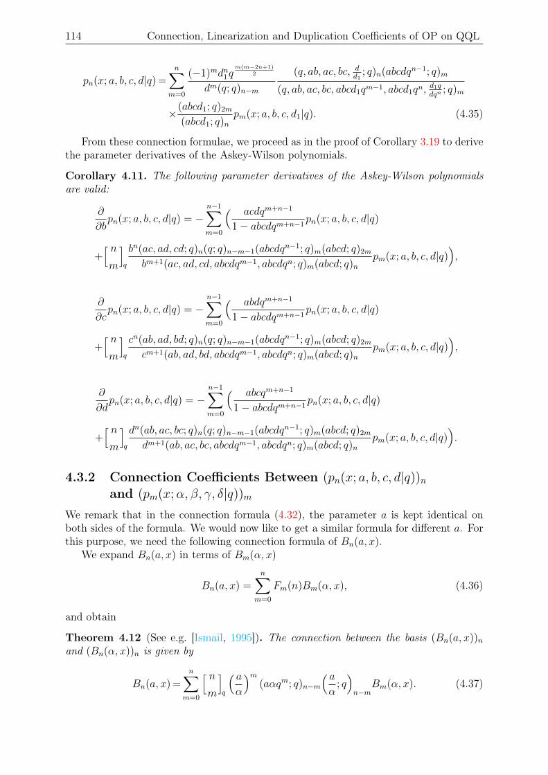
114 Connection, Linearization and Duplication Coefficients of OP on QQL
pn(x; a, b, c, d|q) =n∑
m=0
(−1)mdn1qm(m−2n+1)
2
dm(q; q)n−m
(q, ab, ac, bc, dd1
; q)n(abcdqn−1; q)m
(q, ab, ac, bc, abcd1qm−1, abcd1qn,d1qdqn
; q)m
×(abcd1; q)2m
(abcd1; q)npm(x; a, b, c, d1|q). (4.35)
From these connection formulae, we proceed as in the proof of Corollary 3.19 to derivethe parameter derivatives of the Askey-Wilson polynomials.
Corollary 4.11. The following parameter derivatives of the Askey-Wilson polynomialsare valid:
∂
∂bpn(x; a, b, c, d|q) = −
n−1∑m=0
( acdqm+n−1
1− abcdqm+n−1pn(x; a, b, c, d|q)
+[ nm
]q
bn(ac, ad, cd; q)n(q; q)n−m−1(abcdqn−1; q)m(abcd; q)2m
bm+1(ac, ad, cd, abcdqm−1, abcdqn; q)m(abcd; q)npm(x; a, b, c, d|q)
),
∂
∂cpn(x; a, b, c, d|q) = −
n−1∑m=0
( abdqm+n−1
1− abcdqm+n−1pn(x; a, b, c, d|q)
+[ nm
]q
cn(ab, ad, bd; q)n(q; q)n−m−1(abcdqn−1; q)m(abcd; q)2m
cm+1(ab, ad, bd, abcdqm−1, abcdqn; q)m(abcd; q)npm(x; a, b, c, d|q)
),
∂
∂dpn(x; a, b, c, d|q) = −
n−1∑m=0
( abcqm+n−1
1− abcdqm+n−1pn(x; a, b, c, d|q)
+[ nm
]q
dn(ab, ac, bc; q)n(q; q)n−m−1(abcdqn−1; q)m(abcd; q)2m
dm+1(ab, ac, bc, abcdqm−1, abcdqn; q)m(abcd; q)npm(x; a, b, c, d|q)
).
4.3.2 Connection Coefficients Between (pn(x; a, b, c, d|q))nand (pm(x;α, β, γ, δ|q))m
We remark that in the connection formula (4.32), the parameter a is kept identical onboth sides of the formula. We would now like to get a similar formula for different a. Forthis purpose, we need the following connection formula of Bn(a, x).
We expand Bn(a, x) in terms of Bm(α, x)
Bn(a, x) =n∑
m=0
Fm(n)Bm(α, x), (4.36)
and obtain
Theorem 4.12 (See e.g. [Ismail, 1995]). The connection between the basis (Bn(a, x))nand (Bn(α, x))n is given by
Bn(a, x) =n∑
m=0
[ nm
]q
( aα
)m(aαqm; q)n−m
( aα
; q)n−m
Bm(α, x). (4.37)
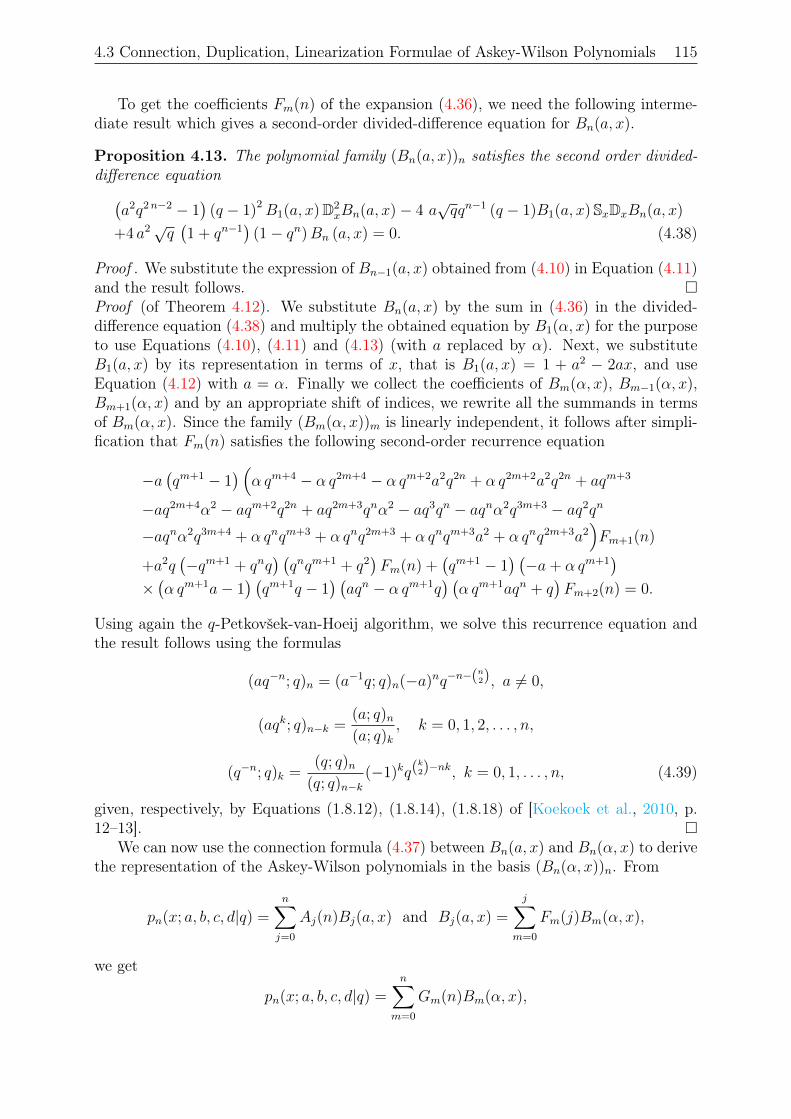
4.3 Connection, Duplication, Linearization Formulae of Askey-Wilson Polynomials 115
To get the coefficients Fm(n) of the expansion (4.36), we need the following interme-diate result which gives a second-order divided-difference equation for Bn(a, x).
Proposition 4.13. The polynomial family (Bn(a, x))n satisfies the second order divided-difference equation(
a2q2n−2 − 1)
(q − 1)2B1(a, x)D2xBn(a, x)− 4 a
√qqn−1 (q − 1)B1(a, x)SxDxBn(a, x)
+4 a2√q(1 + qn−1
)(1− qn)Bn (a, x) = 0. (4.38)
Proof . We substitute the expression of Bn−1(a, x) obtained from (4.10) in Equation (4.11)and the result follows. Proof (of Theorem 4.12). We substitute Bn(a, x) by the sum in (4.36) in the divided-difference equation (4.38) and multiply the obtained equation by B1(α, x) for the purposeto use Equations (4.10), (4.11) and (4.13) (with a replaced by α). Next, we substituteB1(a, x) by its representation in terms of x, that is B1(a, x) = 1 + a2 − 2ax, and useEquation (4.12) with a = α. Finally we collect the coefficients of Bm(α, x), Bm−1(α, x),Bm+1(α, x) and by an appropriate shift of indices, we rewrite all the summands in termsof Bm(α, x). Since the family (Bm(α, x))m is linearly independent, it follows after simpli-fication that Fm(n) satisfies the following second-order recurrence equation
−a(qm+1 − 1
) (α qm+4 − α q2m+4 − α qm+2a2q2n + α q2m+2a2q2n + aqm+3
−aq2m+4α2 − aqm+2q2n + aq2m+3qnα2 − aq3qn − aqnα2q3m+3 − aq2qn
−aqnα2q3m+4 + α qnqm+3 + α qnq2m+3 + α qnqm+3a2 + α qnq2m+3a2)Fm+1(n)
+a2q(−qm+1 + qnq
) (qnqm+1 + q2
)Fm(n) +
(qm+1 − 1
) (−a+ α qm+1
)×(α qm+1a− 1
) (qm+1q − 1
) (aqn − α qm+1q
) (α qm+1aqn + q
)Fm+2(n) = 0.
Using again the q-Petkovšek-van-Hoeij algorithm, we solve this recurrence equation andthe result follows using the formulas
(aq−n; q)n = (a−1q; q)n(−a)nq−n−(n2), a 6= 0,
(aqk; q)n−k =(a; q)n(a; q)k
, k = 0, 1, 2, . . . , n,
(q−n; q)k =(q; q)n
(q; q)n−k(−1)kq(
k2)−nk, k = 0, 1, . . . , n, (4.39)
given, respectively, by Equations (1.8.12), (1.8.14), (1.8.18) of [Koekoek et al., 2010, p.12–13].
We can now use the connection formula (4.37) between Bn(a, x) and Bn(α, x) to derivethe representation of the Askey-Wilson polynomials in the basis (Bn(α, x))n. From
pn(x; a, b, c, d|q) =n∑j=0
Aj(n)Bj(a, x) and Bj(a, x) =
j∑m=0
Fm(j)Bm(α, x),
we get
pn(x; a, b, c, d|q) =n∑
m=0
Gm(n)Bm(α, x),
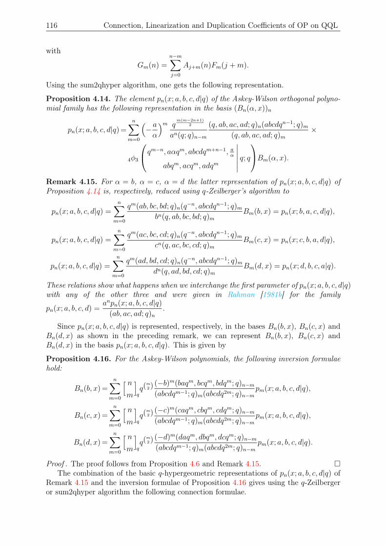
116 Connection, Linearization and Duplication Coefficients of OP on QQL
with
Gm(n) =n−m∑j=0
Aj+m(n)Fm(j +m).
Using the sum2qhyper algorithm, one gets the following representation.
Proposition 4.14. The element pn(x; a, b, c, d|q) of the Askey-Wilson orthogonal polyno-mial family has the following representation in the basis (Bn(α, x))n
pn(x; a, b, c, d|q) =n∑
m=0
(− aα
)m qm(m−2n+1)
2
an(q; q)n−m
(q, ab, ac, ad; q)n(abcdqn−1; q)m(q, ab, ac, ad; q)m
×
4φ3
qm−n, aαqm, abcdqm+n−1, aα
abqm, acqm, adqm
∣∣∣∣∣∣ q; qBm(α, x).
Remark 4.15. For α = b, α = c, α = d the latter representation of pn(x; a, b, c, d|q) ofProposition 4.14 is, respectively, reduced using q-Zeilberger’s algorithm to
pn(x; a, b, c, d|q) =n∑
m=0
qm(ab, bc, bd; q)n(q−n, abcdqn−1; q)mbn(q, ab, bc, bd; q)m
Bm(b, x) = pn(x; b, a, c, d|q),
pn(x; a, b, c, d|q) =n∑
m=0
qm(ac, bc, cd; q)n(q−n, abcdqn−1; q)mcn(q, ac, bc, cd; q)m
Bm(c, x) = pn(x; c, b, a, d|q),
pn(x; a, b, c, d|q) =n∑
m=0
qm(ad, bd, cd; q)n(q−n, abcdqn−1; q)mdn(q, ad, bd, cd; q)m
Bm(d, x) = pn(x; d, b, c, a|q).
These relations show what happens when we interchange the first parameter of pn(x; a, b, c, d|q)with any of the other three and were given in Rahman [1981b] for the family
pn(x; a, b, c, d) =anpn(x; a, b, c, d|q)
(ab, ac, ad; q)n.
Since pn(x; a, b, c, d|q) is represented, respectively, in the bases Bn(b, x), Bn(c, x) andBn(d, x) as shown in the preceding remark, we can represent Bn(b, x), Bn(c, x) andBn(d, x) in the basis pn(x; a, b, c, d|q). This is given by
Proposition 4.16. For the Askey-Wilson polynomials, the following inversion formulaehold:
Bn(b, x) =n∑
m=0
[ nm
]qq(
m2 ) (−b)m(baqm, bcqm, bdqm; q)n−m
(abcdqm−1; q)m(abcdq2m; q)n−mpm(x; a, b, c, d|q),
Bn(c, x) =n∑
m=0
[ nm
]qq(
m2 ) (−c)m(caqm, cbqm, cdqm; q)n−m
(abcdqm−1; q)m(abcdq2m; q)n−mpm(x; a, b, c, d|q),
Bn(d, x) =n∑
m=0
[ nm
]qq(
m2 ) (−d)m(daqm, dbqm, dcqm; q)n−m
(abcdqm−1; q)m(abcdq2m; q)n−mpm(x; a, b, c, d|q).
Proof . The proof follows from Proposition 4.6 and Remark 4.15. The combination of the basic q-hypergeometric representations of pn(x; a, b, c, d|q) of
Remark 4.15 and the inversion formulae of Proposition 4.16 gives using the q-Zeilbergeror sum2qhyper algorithm the following connection formulae.
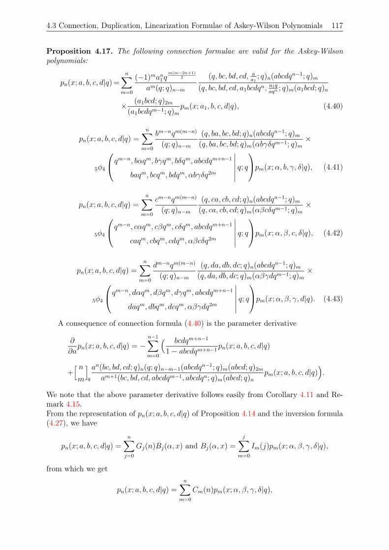
4.3 Connection, Duplication, Linearization Formulae of Askey-Wilson Polynomials 117
Proposition 4.17. The following connection formulae are valid for the Askey-Wilsonpolynomials:
pn(x; a, b, c, d|q) =n∑
m=0
(−1)man1qm(m−2n+1)
2
am(q; q)n−m
(q, bc, bd, cd, aa1
; q)n(abcdqn−1; q)m
(q, bc, bd, cd, a1bcdqn,a1qaqn
; q)m(a1bcd; q)n
× (a1bcd; q)2m
(a1bcdqm−1; q)mpm(x; a1, b, c, d|q), (4.40)
pn(x; a, b, c, d|q) =n∑
m=0
bm−nqm(m−n)
(q; q)n−m
(q, ba, bc, bd; q)n(abcdqn−1; q)m(q, ba, bc, bd; q)m(αbγδqm−1; q)m
×
5φ4
qm−n, bαqm, bγqm, bδqm, abcdqm+n−1
baqm, bcqm, bdqm, αbγδq2m
∣∣∣∣∣∣ q; qpm(x;α, b, γ, δ|q), (4.41)
pn(x; a, b, c, d|q) =n∑
m=0
cm−nqm(m−n)
(q; q)n−m
(q, ca, cb, cd; q)n(abcdqn−1; q)m(q, ca, cb, cd; q)m(αβcδqm−1; q)m
×
5φ4
qm−n, cαqm, cβqm, cδqm, abcdqm+n−1
caqm, cbqm, cdqm, αβcδq2m
∣∣∣∣∣∣ q; qpm(x;α, β, c, δ|q), (4.42)
pn(x; a, b, c, d|q) =n∑
m=0
dm−nqm(m−n)
(q; q)n−m
(q, da, db, dc; q)n(abcdqn−1; q)m(q, da, db, dc; q)m(αβγdqm−1; q)m
×
5φ4
qm−n, dαqm, dβqm, dγqm, abcdqm+n−1
daqm, dbqm, dcqm, αβγdq2m
∣∣∣∣∣∣ q; qpm(x;α, β, γ, d|q). (4.43)
A consequence of connection formula (4.40) is the parameter derivative
∂
∂apn(x; a, b, c, d|q) = −
n−1∑m=0
( bcdqm+n−1
1− abcdqm+n−1pn(x; a, b, c, d|q)
+[ nm
]q
an(bc, bd, cd; q)n(q; q)n−m−1(abcdqn−1; q)m(abcd; q)2m
am+1(bc, bd, cd, abcdqm−1, abcdqn; q)m(abcd; q)npm(x; a, b, c, d|q)
).
We note that the above parameter derivative follows easily from Corollary 4.11 and Re-mark 4.15.From the representation of pn(x; a, b, c, d|q) of Proposition 4.14 and the inversion formula(4.27), we have
pn(x; a, b, c, d|q) =n∑j=0
Gj(n)Bj(α, x) and Bj(α, x) =
j∑m=0
Im(j)pm(x;α, β, γ, δ|q),
from which we get
pn(x; a, b, c, d|q) =n∑
m=0
Cm(n)pm(x;α, β, γ, δ|q),
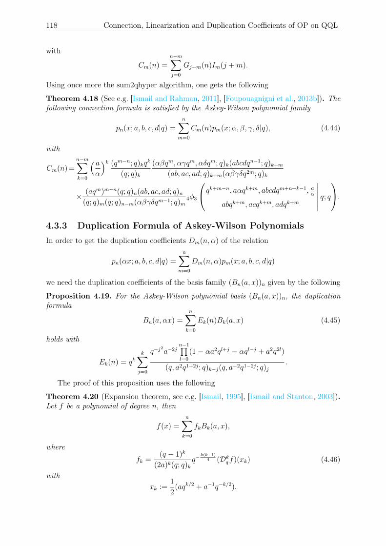
118 Connection, Linearization and Duplication Coefficients of OP on QQL
with
Cm(n) =n−m∑j=0
Gj+m(n)Im(j +m).
Using once more the sum2qhyper algorithm, one gets the following
Theorem 4.18 (See e.g. [Ismail and Rahman, 2011], [Foupouagnigni et al., 2013b]). Thefollowing connection formula is satisfied by the Askey-Wilson polynomial family
pn(x; a, b, c, d|q) =n∑
m=0
Cm(n)pm(x;α, β, γ, δ|q), (4.44)
with
Cm(n) =n−m∑k=0
( aα
)k (qm−n; q)kqk
(q; q)k
(αβqm, αγqm, αδqm; q)k(abcdqn−1; q)k+m
(ab, ac, ad; q)k+m(αβγδq2m; q)k
× (aqm)m−n(q; q)n(ab, ac, ad; q)n(q; q)m(q; q)n−m(αβγδqm−1; q)m
4φ3
qk+m−n, aαqk+m, abcdqm+n+k−1, aα
abqk+m, acqk+m, adqk+m
∣∣∣∣∣∣ q; q.
4.3.3 Duplication Formula of Askey-Wilson Polynomials
In order to get the duplication coefficients Dm(n, α) of the relation
pn(αx; a, b, c, d|q) =n∑
m=0
Dm(n, α)pm(x; a, b, c, d|q)
we need the duplication coefficients of the basis family (Bn(a, x))n given by the following
Proposition 4.19. For the Askey-Wilson polynomial basis (Bn(a, x))n, the duplicationformula
Bn(a, αx) =n∑k=0
Ek(n)Bk(a, x) (4.45)
holds with
Ek(n) = qkk∑j=0
q−j2a−2j
n−1∏l=0
(1− αa2ql+j − αql−j + a2q2l)
(q, a2q1+2j; q)k−j(q, a−2q1−2j; q)j.
The proof of this proposition uses the following
Theorem 4.20 (Expansion theorem, see e.g. [Ismail, 1995], [Ismail and Stanton, 2003]).Let f be a polynomial of degree n, then
f(x) =n∑k=0
fkBk(a, x),
where
fk =(q − 1)k
(2a)k(q; q)kq−
k(k−1)4 (Dkqf)(xk) (4.46)
withxk :=
1
2(aqk/2 + a−1q−k/2).
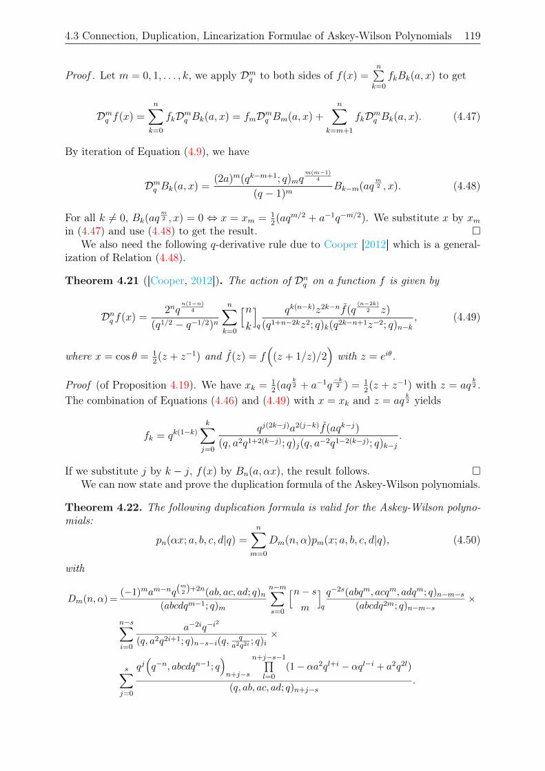
4.3 Connection, Duplication, Linearization Formulae of Askey-Wilson Polynomials 119
Proof . Let m = 0, 1, . . . , k, we apply Dmq to both sides of f(x) =n∑k=0
fkBk(a, x) to get
Dmq f(x) =n∑k=0
fkDmq Bk(a, x) = fmDmq Bm(a, x) +n∑
k=m+1
fkDmq Bk(a, x). (4.47)
By iteration of Equation (4.9), we have
Dmq Bk(a, x) =(2a)m(qk−m+1; q)mq
m(m−1)4
(q − 1)mBk−m(aq
m2 , x). (4.48)
For all k 6= 0, Bk(aqm2 , x) = 0⇔ x = xm = 1
2(aqm/2 + a−1q−m/2). We substitute x by xm
in (4.47) and use (4.48) to get the result. We also need the following q-derivative rule due to Cooper [2012] which is a general-
ization of Relation (4.48).
Theorem 4.21 ([Cooper, 2012]). The action of Dnq on a function f is given by
Dnq f(x) =2nq
n(1−n)4
(q1/2 − q−1/2)n
n∑k=0
[nk
]q
qk(n−k)z2k−nf(q(n−2k)
2 z)
(q1+n−2kz2; q)k(q2k−n+1z−2; q)n−k, (4.49)
where x = cos θ = 12(z + z−1) and f(z) = f
((z + 1/z)/2
)with z = eiθ.
Proof (of Proposition 4.19). We have xk = 12(aq
k2 + a−1q
−k2 ) = 1
2(z + z−1) with z = aq
k2 .
The combination of Equations (4.46) and (4.49) with x = xk and z = aqk2 yields
fk = qk(1−k)
k∑j=0
qj(2k−j)a2(j−k)f(aqk−j)
(q, a2q1+2(k−j); q)j(q, a−2q1−2(k−j); q)k−j.
If we substitute j by k − j, f(x) by Bn(a, αx), the result follows. We can now state and prove the duplication formula of the Askey-Wilson polynomials.
Theorem 4.22. The following duplication formula is valid for the Askey-Wilson polyno-mials:
pn(αx; a, b, c, d|q) =n∑
m=0
Dm(n, α)pm(x; a, b, c, d|q), (4.50)
with
Dm(n, α) =(−1)mam−nq(
m2 )+2n(ab, ac, ad; q)n
(abcdqm−1; q)m
n−m∑s=0
[n− sm
]q
q−2s(abqm, acqm, adqm; q)n−m−s(abcdq2m; q)n−m−s
×
n−s∑i=0
a−2iq−i2
(q, a2q2i+1; q)n−s−i(q,q
a2q2i; q)i×
s∑j=0
qj(q−n, abcdqn−1; q
)n+j−s
n+j−s−1∏l=0
(1− αa2ql+i − αql−i + a2q2l)
(q, ab, ac, ad; q)n+j−s.
120 Connection, Linearization and Duplication Coefficients of OP on QQL
Proof . From the basic hypergeometric representation of the Askey-Wilson polynomials
given on p. 105, since pn(x; a, b, c, d|q) =n∑j=0
Aj(n)Bj(a, x) with Bj(a, x) defined by (4.4),
we have
pn(αx; a, b, c, d|q) =n∑j=0
Aj(n)Bj(a, αx).
From (4.45) and from the inversion formula (4.27), we have
Bj(a, αx) =
j∑k=0
Ek(j)Bk(a, x) and Bk(a, x) =k∑
m=0
Im(k)pm(x; a, b, c, d|q),
respectively. The combination of the above representations yields
pn(αx; a, b, c, d|q) =n∑
m=0
Dm(n, α)pm(x; a, b, c, d|q)
with
Dm(n, α) =n−m∑k=0
n−m−k∑j=0
Im(k +m)Aj+k+m(n)Ek+m(j + k +m).
Since
Ek(n) =k∑i=0
Fi(k, n) with Fi(k, n) = qkq−i
2a−2i
n−1∏l=0
(1− αa2ql+i − αql−i + a2q2l)
(q, a2q1+2i; q)k−i(q, a−2q1−2i; q)i,
it follows that
Dm(n, α) =n−m∑k=0
n−m−k∑j=0
Im(k +m)Aj+k+m(n)k+m∑i=0
Fi(k +m, j + k +m).
From the substitution n−m− k = s, we get
Dm(n, α) =n−m∑s=0
Im(n− s)s∑j=0
n−s∑i=0
Aj+n−s(n)Fi(n− s, j + n− s)
=n−m∑s=0
Im(n− s)n−s∑i=0
s∑j=0
Aj+n−s(n)Fi(n− s, j + n− s).
4.3.4 Linearization Formula of Askey-Wilson Polynomials
We want to determine the linearization coefficients Lk(m,n) of the formula
pn(x; a, b, c, d|q)pm(x; a, b, c, d|q) =n+m∑k=0
Lk(m,n)pk(x; a, b, c, d|q).
For this purpose we need to derive the linearization relation for the basis (Bn(a, x))n.
4.3 Connection, Duplication, Linearization Formulae of Askey-Wilson Polynomials 121
Proposition 4.23 (See [Ismail and Stanton, 2003]). The basis (Bn(a, x))n of the Askey-Wilson orthogonal polynomial family satisfies the following linearization formula
Bn(a, x)Bm(a1, x) =m∑k=0
Hn+k(m,n)Bn+k(a, x), m, n ∈ N, (4.51)
with
Hn+k(m,n) =[mk
]qq−nk
(a1
a
)k ( a1
aqn; q
)m−k
(aa1q
n+k; q)m−k , k = 0, 1, . . . ,m.
Proof . We recall that
Bn(a, x) =n−1∏j=0
(1− 2aqjx+ a2q2j).
Forx = εj(a) ≡ 1 + a2q2j
2aqj=
1
2(aqj + a−1q−j),
we getBn(a, εj(a)) = 0, n ≥ 1, j = 0, 1, . . . , n− 1 (4.52)
and for j = n,Bn(a, εn(a)) 6= 0. (4.53)
In the first step, we expand Bn(a, x)Bm(a1, x), n ≥ 1 in the basis (Bk(a, x))k
Bn(a, x)Bm(a1, x) =n+m∑k=0
Hk(m,n)Bk(a, x), (4.54)
and use Relation (4.52) to get H0(m,n) = Bn(a, ε0(a))Bm(a1, ε0(a)) = 0, n ≥ 1.Considering (4.54) for x = ε1(a) and observing that H0(m,n) = 0, we get using again
(4.52) that
H1(m,n)B1(a, ε1(a)) = Bn(a, ε1(a))Bm(a1, ε1(a)) = 0, n ≥ 2.
Therefore, H1(m,n) = 0 thanks to (4.53). Progressively, we obtain in a similar way for afixed integer j using (4.52), (4.53) and (4.54) that
H0(m,n) = H1(m,n) = · · · = Hj(m,n) = 0, j ≤ n− 1.
In the second step, we rewrite Relation (4.54) accordingly with the previous result
Bn(a, x)Bm(a1, x) =m∑k=0
Hn+k(m,n)Bn+k(a, x). (4.55)
Using the relationBn+k(a, x) = Bn(a, x)Bk(aq
n, x),
derived from the definition
Bn(a, x) =n−1∏j=0
(1− aqsqj)(1− aq−sqj),
122 Connection, Linearization and Duplication Coefficients of OP on QQL
we get from (4.55) that
Bm(a1, x) =m∑k=0
Hn+k(m,n)Bn+k(a, x)
Bn(a, x)=
m∑k=0
Hn+k(m,n)Bk(aqn, x). (4.56)
For x = ε0(aqn), Equation (4.56) gives Hn(m,n) = Bm(a1, ε0(aqn)).Iterating Relation (4.9), we have for fixed l
DlxBn(a, x) =
l−1∏j=0
η(aqj2 , n− j)Bn−l(aq
l2 , x), 1 ≤ l ≤ n.
Applying the operator Dlx to Relation (4.56), we get
l−1∏j=0
η(a1qj2 ,m−j)Bm−l(a1q
l2 , x) =
m∑k=l
Hn+k(m,n)l−1∏j=0
η(aqn+ j2 , k−j)Bk−l(aq
n+ l2 , x), 1 ≤ l ≤ m.
For x = ε0(aqn+ l2 ), the preceding relation gives, taking into account (4.52)
Hn+l(m,n) =
l−1∏j=0
η(a1qj2 ,m− j)
l−1∏j=0
η(aqn+ j2 , l − j)
Bm−l(a1ql2 , ε0(aqn+ l
2 )), l = 1, 2, . . . ,m.
We replace η(a1qn+ j
2 , l − j), η(a1qj2 ,m − j) and Bm−l(a1q
l2 , ε0(aqn+ l
2 )) by their values
obtained from Proposition 4.2 and from the definition Bn(a, x) =n−1∏j=0
(1− 2aqjx+ a2q2j).
This yields
Hn+k(m,n) =(a1
a
)kq(m−n−k)k (q−m; q)k
(q−k; q)k
(a1
aqn; q
)m−k
(aa1q
n+k; q)m−k .
The result follows by using the transformation (4.39).
Remark 4.24. 1. Substituting a1 = a in Relation (4.51) yields
Bn(a, x)Bm(a, x) =m∑k=0
[mk
]qq−nk(q−n; q)m−k(a
2qn+k; q)m−kBn+k(a, x) (4.57)
=n+m∑k=n
[ m
k − n
]qq−n(k−n)(q−n; q)m+n−k(a
2qk; q)m+n−kBk(a, x).
For negative subscripts we define [Koekoek et al., 2010, Eq. (1.8.5)]
(a; q)−n =1∏n
k=1(1− aq−k), a 6= q, q2, . . . , qn, n = 1, 2, 3, . . . ,
so that1
(q; q)−n= 0, n = 1, 2, 3, . . . .
4.3 Connection, Duplication, Linearization Formulae of Askey-Wilson Polynomials 123
It follows from this remark that we can write again
Bn(a, x)Bm(a, x) =n+m∑k=0
[ m
k − n
]qq−n(k−n)(q−n; q)m+n−k(a
2qk; q)m+n−kBk(a, x).
(4.58)
2. If we take m = 1 in (4.57), we recover Relation (4.13). We also remark that forn = 0, (4.51) is the connection formula (4.37) with a = a1 and α = a.
Having derived the linearization relation for Bn(a, x), we now state and prove:
Theorem 4.25. The Askey-Wilson orthogonal polynomial family satisfies the lineariza-tion formula
pn(x; a, b, c, d|q)pm(x; a, b, c, d|q) =n+m∑r=0
Lr(m,n)pr(x; a, b, c, d|q), (4.59)
with
Lr(m,n) =q
12r(r+1)(ab, ac, ad; q)n(ab, ac, ad; q)m
(−1)ram+n−r(abcdqr−1; q)r
n+m−r∑l=0
[ l + r
r
]q
ql(abqr, acqr, adqr; q)l(abcdq2r; q)l
×
min(n,l+r)∑j=max(0,l+r−m)
qj(j−l−r)(q−n, abcdqn−1; q)j(q; q)l+r−j(q, ab, ac, ad; q)j
min(j,m−l−r+j)∑k=0
qk(q−m, abcdqm−1; q)k+l+r−j(q−j , a2ql+r; q)k
(ab, ac, ad; q)k+l+r−j(q; q)k.
Proof . We proceed as in the proof of Theorem 2.8 with xn replaced by Bn(a, x).
Remark 4.26. By an integral evaluation, Rahman [1981b] solved the linearization prob-lem of the polynomial family
pn(x; a, b, c, d) = 4φ3
q−n, abcdqn−1, aeiθ, ae−iθ
ab, ac, ad
∣∣∣∣∣∣ q; q
and got the linearization coefficients as a triple sum, see [Rahman, 1981b, Eq. (1.27)].From these coefficients, he solved the linearization problem
P (α,β)n (x; q)P
(α,β)n−s (x; q) =
2n−2s∑j=0
bjP(α,β)s+j (x; q)
for the continuous q-Jacobi polynomials defined by
P (α,β)n (x; q) =
(qα+1; q)n(−qβ+1; q)n(q; q)n(−q; q)n
pn(x;√q, qα+ 1
2 ,−qβ+ 12 ,−√q)
and gave the linearization coefficients as a 10φ9 series.
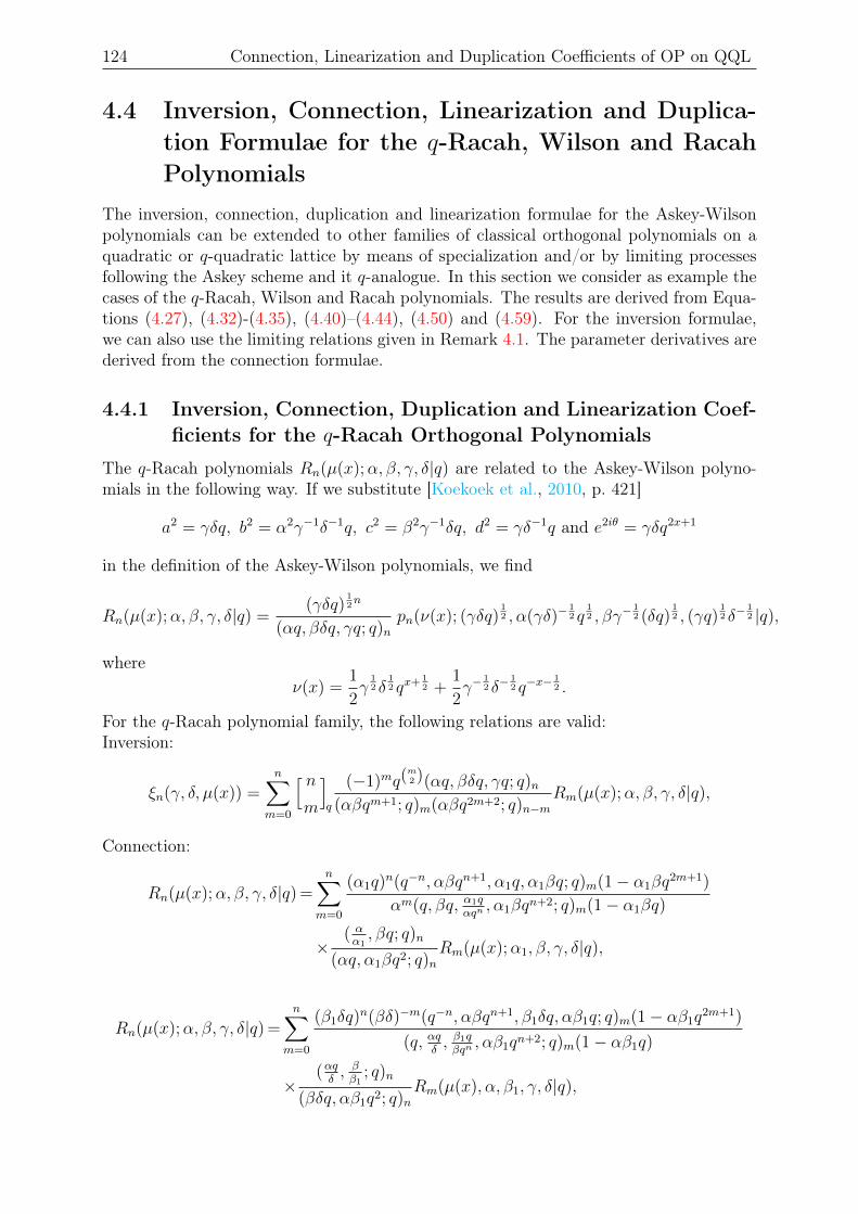
124 Connection, Linearization and Duplication Coefficients of OP on QQL
4.4 Inversion, Connection, Linearization and Duplica-tion Formulae for the q-Racah, Wilson and RacahPolynomials
The inversion, connection, duplication and linearization formulae for the Askey-Wilsonpolynomials can be extended to other families of classical orthogonal polynomials on aquadratic or q-quadratic lattice by means of specialization and/or by limiting processesfollowing the Askey scheme and it q-analogue. In this section we consider as example thecases of the q-Racah, Wilson and Racah polynomials. The results are derived from Equa-tions (4.27), (4.32)-(4.35), (4.40)–(4.44), (4.50) and (4.59). For the inversion formulae,we can also use the limiting relations given in Remark 4.1. The parameter derivatives arederived from the connection formulae.
4.4.1 Inversion, Connection, Duplication and Linearization Coef-ficients for the q-Racah Orthogonal Polynomials
The q-Racah polynomials Rn(µ(x);α, β, γ, δ|q) are related to the Askey-Wilson polyno-mials in the following way. If we substitute [Koekoek et al., 2010, p. 421]
a2 = γδq, b2 = α2γ−1δ−1q, c2 = β2γ−1δq, d2 = γδ−1q and e2iθ = γδq2x+1
in the definition of the Askey-Wilson polynomials, we find
Rn(µ(x);α, β, γ, δ|q) =(γδq)
12n
(αq, βδq, γq; q)npn(ν(x); (γδq)
12 , α(γδ)−
12 q
12 , βγ−
12 (δq)
12 , (γq)
12 δ−
12 |q),
whereν(x) =
1
2γ
12 δ
12 qx+ 1
2 +1
2γ−
12 δ−
12 q−x−
12 .
For the q-Racah polynomial family, the following relations are valid:Inversion:
ξn(γ, δ, µ(x)) =n∑
m=0
[ nm
]q
(−1)mq(m2 )(αq, βδq, γq; q)n
(αβqm+1; q)m(αβq2m+2; q)n−mRm(µ(x);α, β, γ, δ|q),
Connection:
Rn(µ(x);α, β, γ, δ|q) =n∑
m=0
(α1q)n(q−n, αβqn+1, α1q, α1βq; q)m(1− α1βq
2m+1)
αm(q, βq, α1qαqn
, α1βqn+2; q)m(1− α1βq)
×( αα1, βq; q)n
(αq, α1βq2; q)nRm(µ(x);α1, β, γ, δ|q),
Rn(µ(x);α, β, γ, δ|q) =n∑
m=0
(β1δq)n(βδ)−m(q−n, αβqn+1, β1δq, αβ1q; q)m(1− αβ1q
2m+1)
(q, αqδ, β1qβqn
, αβ1qn+2; q)m(1− αβ1q)
×(αqδ, ββ1
; q)n
(βδq, αβ1q2; q)nRm(µ(x), α, β1, γ, δ|q),
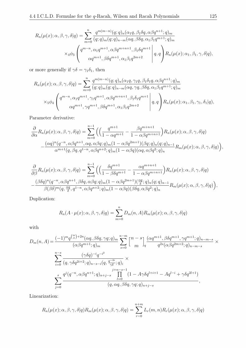
4.4 I.C.L.D. Formulae for the q-Racah, Wilson and Racah Polynomials 125
Rn(µ(x);α, β, γ, δ|q) =n∑
m=0
qm(m−n)(q; q)n(α1q, β1δq, αβqn+1; q)m
(q; q)m(q; q)n−m(αq, βδq, α1β1qm+1; q)m
×4φ3
qm−n, α1qm+1, αβqm+n+1, β1δq
m+1
αqm+1, βδqm+1, α1β1q2m+2
∣∣∣∣∣∣ q, qRn(µ(x);α1, β1, γ, δ|q),
or more generally if γδ = γ1δ1, then
Rn(µ(x);α, β, γ, δ|q) =n∑
m=0
qm(m−n)(q; q)n(α1q, γ1q, β1δ1q, αβqn+1; q)m
(q; q)m(q; q)n−m(αq, γq, βδq, α1β1qm+1; q)m
×5φ4
qm−n, α1qm+1, γ1q
m+1, αβqm+n+1, β1δ1qm+1
αqm+1, γqm+1, βδqm+1, α1β1q2m+2
∣∣∣∣∣∣ q, qRn(µ(x);α1, β1, γ1, δ1|q),
Parameter derivative:
∂
∂αRn(µ(x);α, β, γ, δ|q) =
n−1∑m=0
(( qm+1
1− αqm+1− βqm+n+1
1− αβqm+n+1
)Rn(µ(x);α, β, γ, δ|q)
−(αq)n(q−n, αβqn+1, αq, αβq; q)m(1− αβq2m+1)(βq; q)n(q; q)n−1
αm+1(q, βq, q1−n, αβqn+2; q)m(1− αβq)(αq, αβq2; q)nRm(µ(x);α, β, γ, δ|q)
),
∂
∂βRn(µ(x);α, β, γ, δ|q) =
n−1∑m=0
(( δqm+1
1− βδqm+1− αqm+n+1
1− αβqm+n+1
)Rn(µ(x);α, β, γ, δ|q)
−(βδq)n(q−n, αβqn+1, βδq, αβq; q)m(1− αβq2m+1)(αq
δ; q)n(q; q)n−1
β(βδ)m(q, αqδ, q1−n, αβqn+2; q)m(1− αβq)(βδq, αβq2; q)n
Rm(µ(x);α, β, γ, δ|q)),
Duplication:
Rn(A · µ(x);α, β, γ, δ|q) =n∑
m=0
Dm(n,A)Rm(µ(x);α, β, γ, δ|q)
with
Dm(n,A) =(−1)mq(
m2 )+2n(αq, βδq, γq; q)m(αβqm+1; q)m
n−m∑s=0
[n− sm
]q
(αqm+1, βδqm+1, γqm+1; q)n−m−sq2s(αβq2m+2; q)n−m−s
×
n−s∑i=0
(γδq)−iq−i2
(q, γδq2i+2; q)n−s−i(q,q−2i
γδ; q)i×
s∑j=0
qj(q−n, αβqn+1; q)n+j−s
j+n−s−1∏l=0
(1− Aγδql+i+1 − Aql−i + γδq2l+1)
(q, αq, βδq, γq; q)n+j−s,
Linearization:
Rn(µ(x);α, β, γ, δ|q)Rm(µ(x);α, β, γ, δ|q) =n+m∑r=0
Lr(m,n)Rr(µ(x);α, β, γ, δ|q)
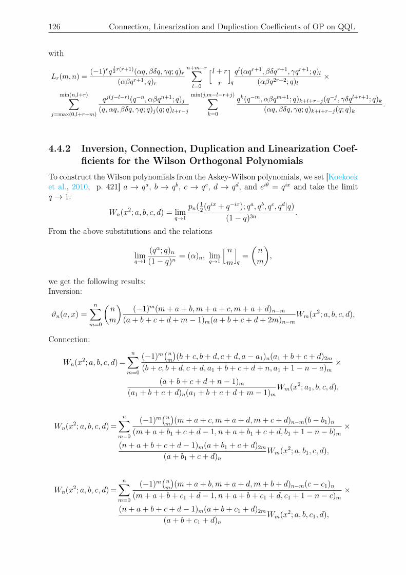
126 Connection, Linearization and Duplication Coefficients of OP on QQL
with
Lr(m,n) =(−1)rq
12r(r+1)(αq, βδq, γq; q)r(αβqr+1; q)r
n+m−r∑l=0
[ l + r
r
]q
ql(αqr+1, βδqr+1, γqr+1; q)l(αβq2r+2; q)l
×
min(n,l+r)∑j=max(0,l+r−m)
qj(j−l−r)(q−n, αβqn+1; q)j(q, αq, βδq, γq; q)j(q; q)l+r−j
min(j,m−l−r+j)∑k=0
qk(q−m, αβqm+1; q)k+l+r−j(q−j , γδql+r+1; q)k
(αq, βδq, γq; q)k+l+r−j(q; q)k.
4.4.2 Inversion, Connection, Duplication and Linearization Coef-ficients for the Wilson Orthogonal Polynomials
To construct the Wilson polynomials from the Askey-Wilson polynomials, we set [Koekoeket al., 2010, p. 421] a → qa, b → qb, c → qc, d → qd, and eiθ = qix and take the limitq → 1:
Wn(x2; a, b, c, d) = limq→1
pn(12(qix + q−ix); qa, qb, qc, qd|q)
(1− q)3n.
From the above substitutions and the relations
limq→1
(qα; q)n(1− q)n
= (α)n, limq→1
[ nm
]q
=
(n
m
),
we get the following results:Inversion:
ϑn(a, x) =n∑
m=0
(n
m
)(−1)m(m+ a+ b,m+ a+ c,m+ a+ d)n−m
(a+ b+ c+ d+m− 1)m(a+ b+ c+ d+ 2m)n−mWm(x2; a, b, c, d),
Connection:
Wn(x2; a, b, c, d) =n∑
m=0
(−1)m(nm
)(b+ c, b+ d, c+ d, a− a1)n(a1 + b+ c+ d)2m
(b+ c, b+ d, c+ d, a1 + b+ c+ d+ n, a1 + 1− n− a)m×
(a+ b+ c+ d+ n− 1)m(a1 + b+ c+ d)n(a1 + b+ c+ d+m− 1)m
Wm(x2; a1, b, c, d),
Wn(x2; a, b, c, d) =n∑
m=0
(−1)m(nm
)(m+ a+ c,m+ a+ d,m+ c+ d)n−m(b− b1)n
(m+ a+ b1 + c+ d− 1, n+ a+ b1 + c+ d, b1 + 1− n− b)m×
(n+ a+ b+ c+ d− 1)m(a+ b1 + c+ d)2m
(a+ b1 + c+ d)nWm(x2; a, b1, c, d),
Wn(x2; a, b, c, d) =n∑
m=0
(−1)m(nm
)(m+ a+ b,m+ a+ d,m+ b+ d)n−m(c− c1)n
(m+ a+ b+ c1 + d− 1, n+ a+ b+ c1 + d, c1 + 1− n− c)m×
(n+ a+ b+ c+ d− 1)m(a+ b+ c1 + d)2m
(a+ b+ c1 + d)nWm(x2; a, b, c1, d),
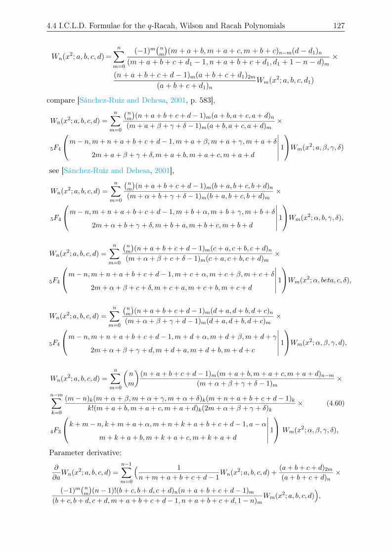
4.4 I.C.L.D. Formulae for the q-Racah, Wilson and Racah Polynomials 127
Wn(x2; a, b, c, d) =n∑
m=0
(−1)m(nm
)(m+ a+ b,m+ a+ c,m+ b+ c)n−m(d− d1)n
(m+ a+ b+ c+ d1 − 1, n+ a+ b+ c+ d1, d1 + 1− n− d)m×
(n+ a+ b+ c+ d− 1)m(a+ b+ c+ d1)2m
(a+ b+ c+ d1)nWm(x2; a, b, c, d1)
compare [Sánchez-Ruiz and Dehesa, 2001, p. 583],
Wn(x2; a, b, c, d) =n∑
m=0
(nm
)(n+ a+ b+ c+ d− 1)m(a+ b, a+ c, a+ d)n
(m+ a+ β + γ + δ − 1)m(a+ b, a+ c, a+ d)m×
5F4
m− n,m+ n+ a+ b+ c+ d− 1,m+ a+ β,m+ a+ γ,m+ a+ δ
2m+ a+ β + γ + δ,m+ a+ b,m+ a+ c,m+ a+ d
∣∣∣∣∣∣ 1Wm(x2; a, β, γ, δ)
see [Sánchez-Ruiz and Dehesa, 2001],
Wn(x2; a, b, c, d) =n∑
m=0
(nm
)(n+ a+ b+ c+ d− 1)m(b+ a, b+ c, b+ d)n
(m+ α+ b+ γ + δ − 1)m(b+ a, b+ c, b+ d)m×
5F4
m− n,m+ n+ a+ b+ c+ d− 1,m+ b+ α,m+ b+ γ,m+ b+ δ
2m+ α+ b+ γ + δ,m+ b+ a,m+ b+ c,m+ b+ d
∣∣∣∣∣∣ 1Wm(x2;α, b, γ, δ),
Wn(x2; a, b, c, d) =n∑
m=0
(nm
)(n+ a+ b+ c+ d− 1)m(c+ a, c+ b, c+ d)n
(m+ α+ β + c+ δ − 1)m(c+ a, c+ b, c+ d)m×
5F4
m− n,m+ n+ a+ b+ c+ d− 1,m+ c+ α,m+ c+ β,m+ c+ δ
2m+ α+ β + c+ δ,m+ c+ a,m+ c+ b,m+ c+ d
∣∣∣∣∣∣ 1Wm(x2;α, beta, c, δ),
Wn(x2; a, b, c, d) =n∑
m=0
(nm
)(n+ a+ b+ c+ d− 1)m(d+ a, d+ b, d+ c)n
(m+ α+ β + γ + d− 1)m(d+ a, d+ b, d+ c)m×
5F4
m− n,m+ n+ a+ b+ c+ d− 1,m+ d+ α,m+ d+ β,m+ d+ γ
2m+ α+ β + γ + d,m+ d+ a,m+ d+ b,m+ d+ c
∣∣∣∣∣∣ 1Wm(x2;α, β, γ, d),
Wn(x2; a, b, c, d) =n∑
m=0
(n
m
)(n+ a+ b+ c+ d− 1)m(m+ a+ b,m+ a+ c,m+ a+ d)n−m
(m+ α+ β + γ + δ − 1)m×
n−m∑k=0
(m− n)k(m+ α+ β,m+ α+ γ,m+ α+ δ)k(m+ n+ a+ b+ c+ d− 1)kk!(m+ a+ b,m+ a+ c,m+ a+ d)k(2m+ α+ β + γ + δ)k
× (4.60)
4F3
k +m− n, k +m+ a+ α,m+ n+ k + a+ b+ c+ d− 1, a− α
m+ k + a+ b,m+ k + a+ c,m+ k + a+ d
∣∣∣∣∣∣ 1 Wm(x2;α, β, γ, δ),
Parameter derivative:
∂
∂aWn(x2; a, b, c, d) =
n−1∑m=0
( 1
n+m+ a+ b+ c+ d− 1Wn(x2; a, b, c, d) +
(a+ b+ c+ d)2m
(a+ b+ c+ d)n×
(−1)m(nm
)(n− 1)!(b+ c, b+ d, c+ d)n(n+ a+ b+ c+ d− 1)m
(b+ c, b+ d, c+ d,m+ a+ b+ c+ d− 1, n+ a+ b+ c+ d, 1− n)mWm(x2; a, b, c, d)
),
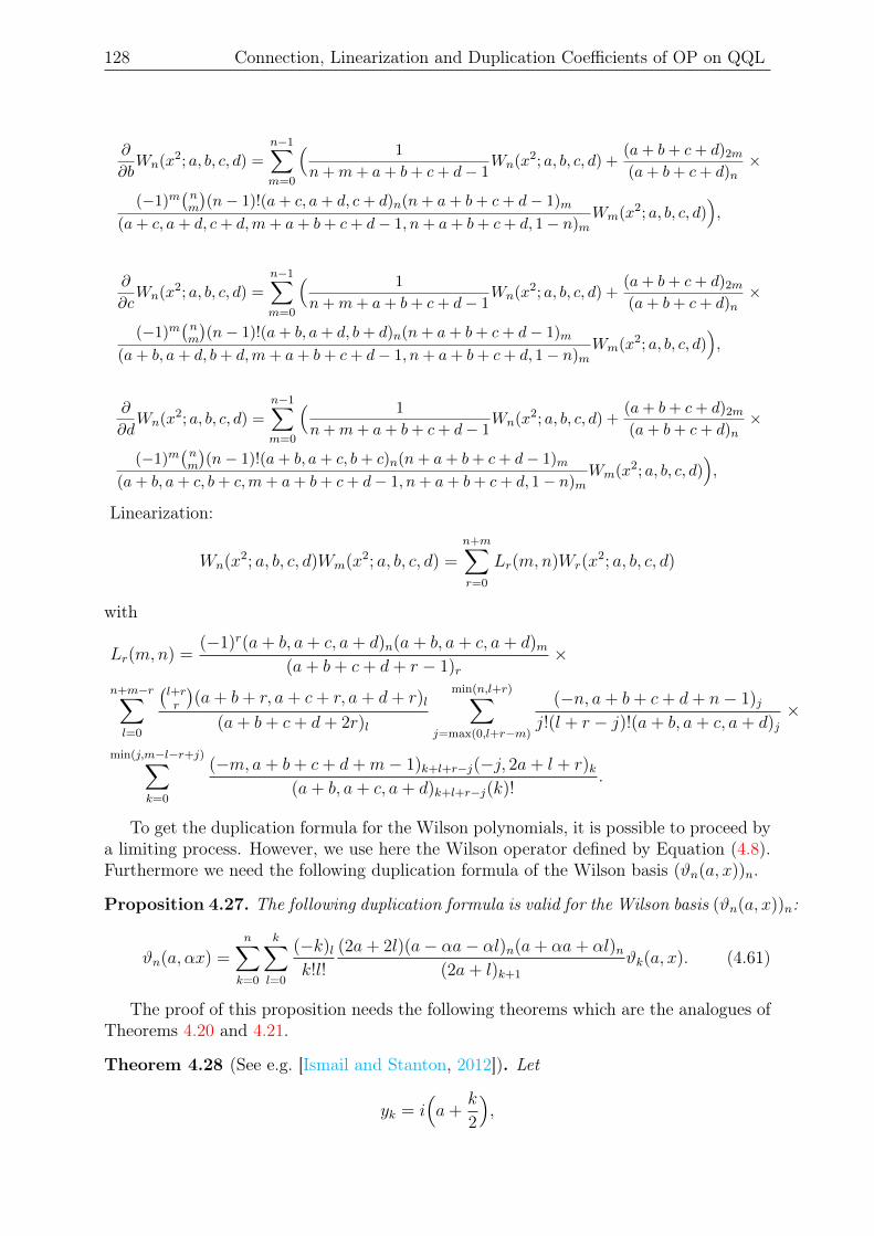
128 Connection, Linearization and Duplication Coefficients of OP on QQL
∂
∂bWn(x2; a, b, c, d) =
n−1∑m=0
( 1
n+m+ a+ b+ c+ d− 1Wn(x2; a, b, c, d) +
(a+ b+ c+ d)2m
(a+ b+ c+ d)n×
(−1)m(nm
)(n− 1)!(a+ c, a+ d, c+ d)n(n+ a+ b+ c+ d− 1)m
(a+ c, a+ d, c+ d,m+ a+ b+ c+ d− 1, n+ a+ b+ c+ d, 1− n)mWm(x2; a, b, c, d)
),
∂
∂cWn(x2; a, b, c, d) =
n−1∑m=0
( 1
n+m+ a+ b+ c+ d− 1Wn(x2; a, b, c, d) +
(a+ b+ c+ d)2m
(a+ b+ c+ d)n×
(−1)m(nm
)(n− 1)!(a+ b, a+ d, b+ d)n(n+ a+ b+ c+ d− 1)m
(a+ b, a+ d, b+ d,m+ a+ b+ c+ d− 1, n+ a+ b+ c+ d, 1− n)mWm(x2; a, b, c, d)
),
∂
∂dWn(x2; a, b, c, d) =
n−1∑m=0
( 1
n+m+ a+ b+ c+ d− 1Wn(x2; a, b, c, d) +
(a+ b+ c+ d)2m
(a+ b+ c+ d)n×
(−1)m(nm
)(n− 1)!(a+ b, a+ c, b+ c)n(n+ a+ b+ c+ d− 1)m
(a+ b, a+ c, b+ c,m+ a+ b+ c+ d− 1, n+ a+ b+ c+ d, 1− n)mWm(x2; a, b, c, d)
),
Linearization:
Wn(x2; a, b, c, d)Wm(x2; a, b, c, d) =n+m∑r=0
Lr(m,n)Wr(x2; a, b, c, d)
with
Lr(m,n) =(−1)r(a+ b, a+ c, a+ d)n(a+ b, a+ c, a+ d)m
(a+ b+ c+ d+ r − 1)r×
n+m−r∑l=0
(l+rr
)(a+ b+ r, a+ c+ r, a+ d+ r)l
(a+ b+ c+ d+ 2r)l
min(n,l+r)∑j=max(0,l+r−m)
(−n, a+ b+ c+ d+ n− 1)jj!(l + r − j)!(a+ b, a+ c, a+ d)j
×
min(j,m−l−r+j)∑k=0
(−m, a+ b+ c+ d+m− 1)k+l+r−j(−j, 2a+ l + r)k(a+ b, a+ c, a+ d)k+l+r−j(k)!
.
To get the duplication formula for the Wilson polynomials, it is possible to proceed bya limiting process. However, we use here the Wilson operator defined by Equation (4.8).Furthermore we need the following duplication formula of the Wilson basis (ϑn(a, x))n.
Proposition 4.27. The following duplication formula is valid for the Wilson basis (ϑn(a, x))n:
ϑn(a, αx) =n∑k=0
k∑l=0
(−k)lk!l!
(2a+ 2l)(a− αa− αl)n(a+ αa+ αl)n(2a+ l)k+1
ϑk(a, x). (4.61)
The proof of this proposition needs the following theorems which are the analogues ofTheorems 4.20 and 4.21.
Theorem 4.28 (See e.g. [Ismail and Stanton, 2012]). Let
yk = i(a+
k
2
),
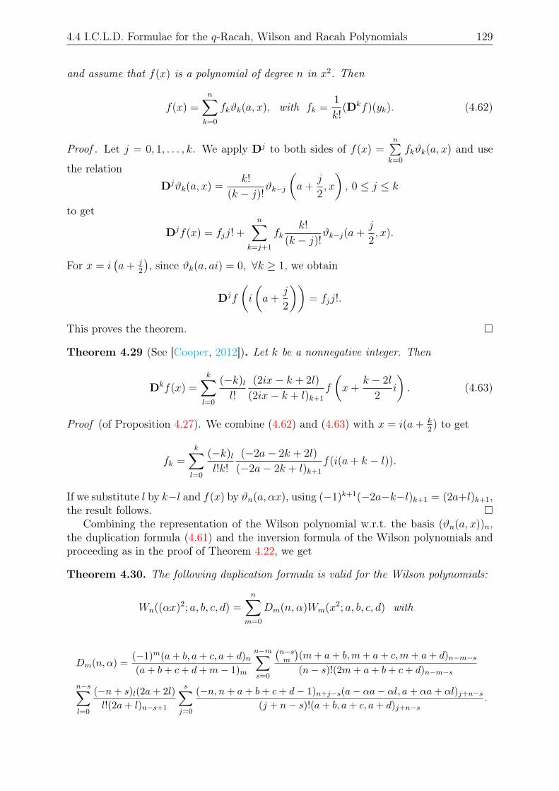
4.4 I.C.L.D. Formulae for the q-Racah, Wilson and Racah Polynomials 129
and assume that f(x) is a polynomial of degree n in x2. Then
f(x) =n∑k=0
fkϑk(a, x), with fk =1
k!(Dkf)(yk). (4.62)
Proof . Let j = 0, 1, . . . , k. We apply Dj to both sides of f(x) =n∑k=0
fkϑk(a, x) and use
the relationDjϑk(a, x) =
k!
(k − j)!ϑk−j
(a+
j
2, x
), 0 ≤ j ≤ k
to get
Djf(x) = fjj! +n∑
k=j+1
fkk!
(k − j)!ϑk−j(a+
j
2, x).
For x = i(a+ j
2
), since ϑk(a, ai) = 0, ∀k ≥ 1, we obtain
Djf
(i
(a+
j
2
))= fjj!.
This proves the theorem.
Theorem 4.29 (See [Cooper, 2012]). Let k be a nonnegative integer. Then
Dkf(x) =k∑l=0
(−k)ll!
(2ix− k + 2l)
(2ix− k + l)k+1
f
(x+
k − 2l
2i
). (4.63)
Proof (of Proposition 4.27). We combine (4.62) and (4.63) with x = i(a+ k2) to get
fk =k∑l=0
(−k)ll!k!
(−2a− 2k + 2l)
(−2a− 2k + l)k+1
f(i(a+ k − l)).
If we substitute l by k−l and f(x) by ϑn(a, αx), using (−1)k+1(−2a−k−l)k+1 = (2a+l)k+1,the result follows.
Combining the representation of the Wilson polynomial w.r.t. the basis (ϑn(a, x))n,the duplication formula (4.61) and the inversion formula of the Wilson polynomials andproceeding as in the proof of Theorem 4.22, we get
Theorem 4.30. The following duplication formula is valid for the Wilson polynomials:
Wn((αx)2; a, b, c, d) =n∑
m=0
Dm(n, α)Wm(x2; a, b, c, d) with
Dm(n, α) =(−1)m(a+ b, a+ c, a+ d)n(a+ b+ c+ d+m− 1)m
n−m∑s=0
(n−sm
)(m+ a+ b,m+ a+ c,m+ a+ d)n−m−s
(n− s)!(2m+ a+ b+ c+ d)n−m−s
n−s∑l=0
(−n+ s)l(2a+ 2l)
l!(2a+ l)n−s+1
s∑j=0
(−n, n+ a+ b+ c+ d− 1)n+j−s(a− αa− αl, a+ αa+ αl)j+n−s(j + n− s)!(a+ b, a+ c, a+ d)j+n−s
.
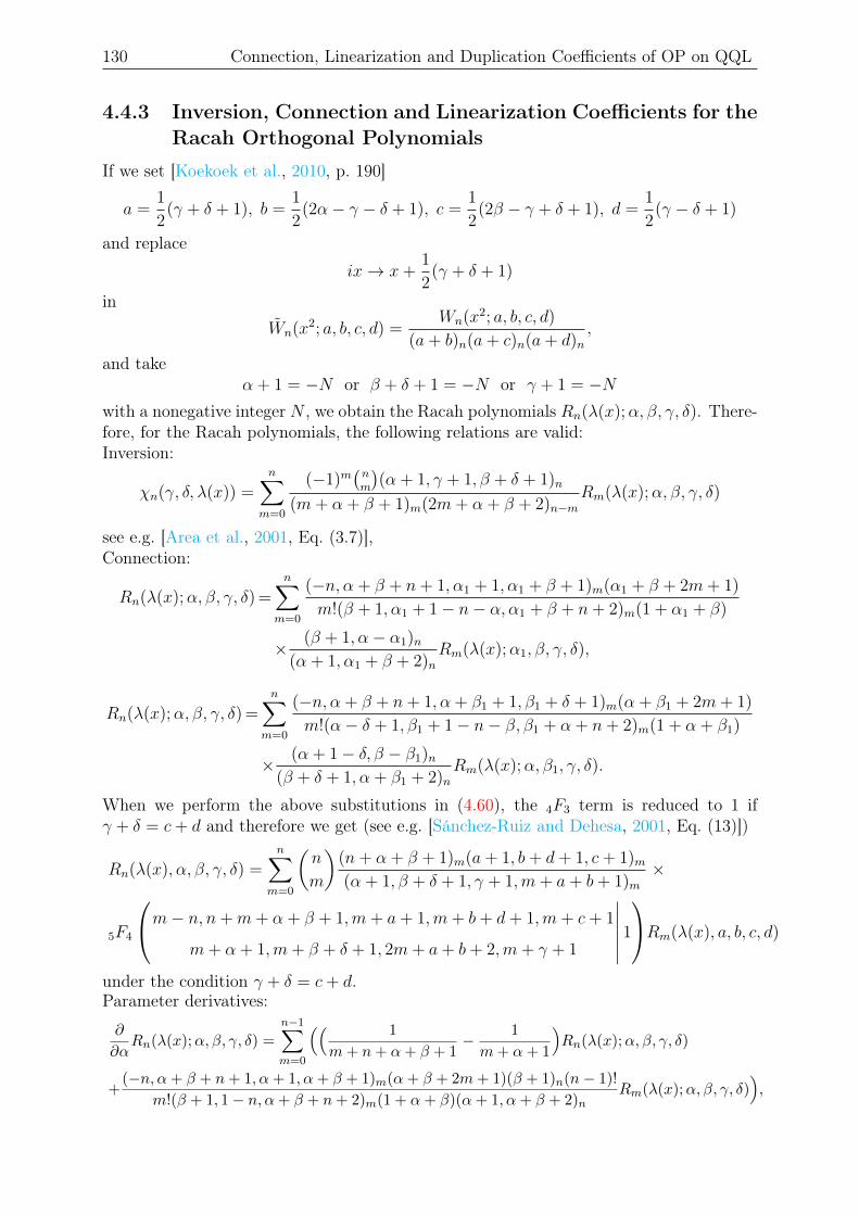
130 Connection, Linearization and Duplication Coefficients of OP on QQL
4.4.3 Inversion, Connection and Linearization Coefficients for theRacah Orthogonal Polynomials
If we set [Koekoek et al., 2010, p. 190]
a =1
2(γ + δ + 1), b =
1
2(2α− γ − δ + 1), c =
1
2(2β − γ + δ + 1), d =
1
2(γ − δ + 1)
and replace
ix→ x+1
2(γ + δ + 1)
inWn(x2; a, b, c, d) =
Wn(x2; a, b, c, d)
(a+ b)n(a+ c)n(a+ d)n,
and takeα + 1 = −N or β + δ + 1 = −N or γ + 1 = −N
with a nonegative integer N , we obtain the Racah polynomials Rn(λ(x);α, β, γ, δ). There-fore, for the Racah polynomials, the following relations are valid:Inversion:
χn(γ, δ, λ(x)) =n∑
m=0
(−1)m(nm
)(α + 1, γ + 1, β + δ + 1)n
(m+ α + β + 1)m(2m+ α + β + 2)n−mRm(λ(x);α, β, γ, δ)
see e.g. [Area et al., 2001, Eq. (3.7)],Connection:
Rn(λ(x);α, β, γ, δ) =n∑
m=0
(−n, α + β + n+ 1, α1 + 1, α1 + β + 1)m(α1 + β + 2m+ 1)
m!(β + 1, α1 + 1− n− α, α1 + β + n+ 2)m(1 + α1 + β)
× (β + 1, α− α1)n(α + 1, α1 + β + 2)n
Rm(λ(x);α1, β, γ, δ),
Rn(λ(x);α, β, γ, δ) =n∑
m=0
(−n, α + β + n+ 1, α + β1 + 1, β1 + δ + 1)m(α + β1 + 2m+ 1)
m!(α− δ + 1, β1 + 1− n− β, β1 + α + n+ 2)m(1 + α + β1)
× (α + 1− δ, β − β1)n(β + δ + 1, α + β1 + 2)n
Rm(λ(x);α, β1, γ, δ).
When we perform the above substitutions in (4.60), the 4F3 term is reduced to 1 ifγ + δ = c+ d and therefore we get (see e.g. [Sánchez-Ruiz and Dehesa, 2001, Eq. (13)])
Rn(λ(x), α, β, γ, δ) =n∑
m=0
(n
m
)(n+ α + β + 1)m(a+ 1, b+ d+ 1, c+ 1)m(α + 1, β + δ + 1, γ + 1,m+ a+ b+ 1)m
×
5F4
m− n, n+m+ α + β + 1,m+ a+ 1,m+ b+ d+ 1,m+ c+ 1
m+ α + 1,m+ β + δ + 1, 2m+ a+ b+ 2,m+ γ + 1
∣∣∣∣∣∣ 1Rm(λ(x), a, b, c, d)
under the condition γ + δ = c+ d.Parameter derivatives:
∂
∂αRn(λ(x);α, β, γ, δ) =
n−1∑m=0
(( 1
m+ n+ α+ β + 1− 1
m+ α+ 1
)Rn(λ(x);α, β, γ, δ)
+(−n, α+ β + n+ 1, α+ 1, α+ β + 1)m(α+ β + 2m+ 1)(β + 1)n(n− 1)!
m!(β + 1, 1− n, α+ β + n+ 2)m(1 + α+ β)(α+ 1, α+ β + 2)nRm(λ(x);α, β, γ, δ)
),
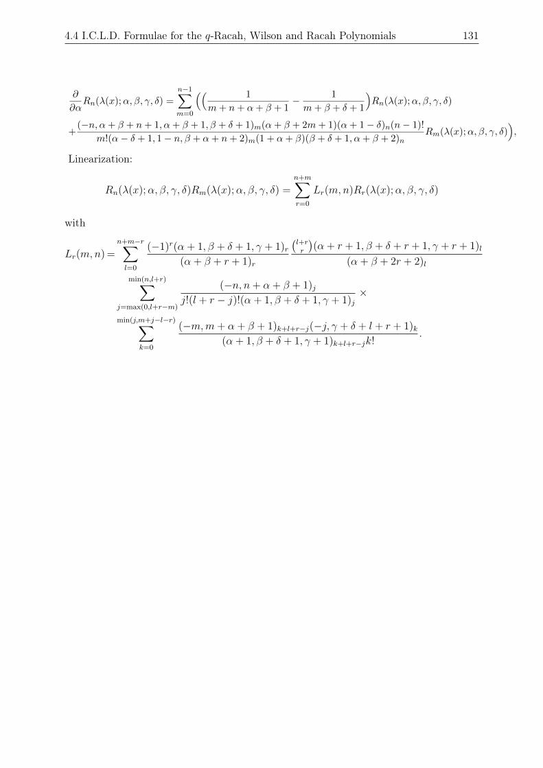
4.4 I.C.L.D. Formulae for the q-Racah, Wilson and Racah Polynomials 131
∂
∂αRn(λ(x);α, β, γ, δ) =
n−1∑m=0
(( 1
m+ n+ α+ β + 1− 1
m+ β + δ + 1
)Rn(λ(x);α, β, γ, δ)
+(−n, α+ β + n+ 1, α+ β + 1, β + δ + 1)m(α+ β + 2m+ 1)(α+ 1− δ)n(n− 1)!
m!(α− δ + 1, 1− n, β + α+ n+ 2)m(1 + α+ β)(β + δ + 1, α+ β + 2)nRm(λ(x);α, β, γ, δ)
),
Linearization:
Rn(λ(x);α, β, γ, δ)Rm(λ(x);α, β, γ, δ) =n+m∑r=0
Lr(m,n)Rr(λ(x);α, β, γ, δ)
with
Lr(m,n) =n+m−r∑l=0
(−1)r(α + 1, β + δ + 1, γ + 1)r(α + β + r + 1)r
(l+rr
)(α + r + 1, β + δ + r + 1, γ + r + 1)l
(α + β + 2r + 2)l
min(n,l+r)∑j=max(0,l+r−m)
(−n, n+ α + β + 1)jj!(l + r − j)!(α + 1, β + δ + 1, γ + 1)j
×
min(j,m+j−l−r)∑k=0
(−m,m+ α + β + 1)k+l+r−j(−j, γ + δ + l + r + 1)k(α + 1, β + δ + 1, γ + 1)k+l+r−jk!
.

132 Connection, Linearization and Duplication Coefficients of OP on QQL
Chapter 5
Conclusion and Perspectives
We have provided in this thesis representations for the inversion, connection, linearizationand duplication coefficients of all classical orthogonal polynomials of a continuous, dis-crete and q-discrete variable listed in [Koekoek et al., 2010]. We also solved the inversion,connection, linearization and duplication problem for the Askey-Wilson polynomials andshowed how the results can be extended to other families of classical orthogonal polynomi-als on quadratic or q-quadratic lattice. From the various connection formulae parameterderivatives have been derived.
Using our algorithmic approach, we recovered known results and obtained many newones.
As perspectives, it would be interesting:
1. to find conditions on the parameters to simplify the coefficients appearing in doubleand triple summation,
2. to compute by means of limit and/or specialization the inversion, connection, lin-earization and duplication coefficients for other families of classical orthogonal poly-nomials on a quadratic or q-quadratic lattice,
3. to extend our method to other classes of orthogonal polynomials that are obtainedby a modification of the three-term recurrence relations of the classical orthogonalpolynomials, for example [Foupouagnigni, 2006]: the associated orthogonal polyno-mials, the co-recursive orthogonal polynomials,
4. to implement in Maple for example an algorithm which solves the inversion, connec-tion, linearization or duplication problem for the classical orthogonal polynomials.

134 Conclusion and Perspectives
Bibliography
S. Abramov, P. Paule, and M. Petkovšek. q-hypergeometric solutions of q-differenceequations. Discrete Math., 180:3–22, 1998. 6
J. C. Adams. On the expression of the product of any two Legendre’s coefficients bymeans of a series of Legendre’s coefficients. Proc. R. Soc. Lond., 27:63–71, 1878. 3
R. Alvarez-Nodarse, R. J. Yáñez, and J. S. Dehesa. Modified Clebsch-Gordan-type ex-pansions for products of discrete hypergeometric polynomials. J. Comput. Appl. Math.,89:171–197, 1997. 4, 41, 42, 43, 44, 49
G. E. Andrews and R. Askey. Enumeration of partitions: the role of Eulerian series and q-orthogonal polynomials. In Higher Combinatorics (ed. M. Aigner), pages 3–26, Boston,1977. Reidel Publications. 4
G. E. Andrews, R. Askey, and R. Roy. Special Functions, volume 71. Encyclopedia Math.Appl., Cambridge University Press, Cambridge, 1999. 27
I. Area, E. Godoy, A. Ronveaux, and A. Zarzo. Minimal recurrence relations for connectioncoefficients between classical orthogonal polynomials: Discrete case. J. Comput. Appl.Math., 89:309–325, 1998. 3, 41, 46, 49
I. Area, E. Godoy, A. Ronveaux, and A. Zarzo. Inversion problems in the q-Hahn tableau.J. Symbolic Comput., 28:767–776, 1999. 59, 67, 73
I. Area, E. Godoy, A. Ronveaux, and A. Zarzo. Solving connection and linearizationproblems within the Askey scheme and its q-analogue via inversion formulas. J. Comput.Appl. Math., 136:152–162, 2001. 59, 80, 103, 111, 112, 113, 130
I. Area, E. Godoy, A. Ronveaux, and A. Zarzo. Classical discrete orthogonal polynomials,Lah numbers, and involutory matrices. Appl. Math. Lett., 16:383–387, 2003. 55
I. Area, E. Godoy, A. Ronveaux, and A. Zarzo. Extensions of some results of P. Humberton Bezout’s identity for classical orthogonal polynomials. J. Comput. Appl. Math., 196:212–228, 2006. 65, 68
R. Askey. Orthogonal expansions with positive coefficients. Proc. Amer. Math. Soc., 26:1191–1194, 1965. 2, 34
R. Askey. Jacobi polynomial expansions with positive coefficients and embeddings ofprojective spaces. Bull. Amer. Math. Soc., 74:301–304, 1968. 2, 34
R. Askey. Orthogonal Polynomials and Special Functions, volume 21. CBMS RegionalConf. Ser. in Appl. Math., Philadelphia, 1975. 1, 2, 3, 28, 29, 30, 34
136 Bibliography
R. Askey and G. Gasper. Jacobi polynomial expansions of Jacobi polynomials with non-negative coefficients. Proc. Camb. Phil. Soc., 70:243–255, 1971a. 2, 34
R. Askey and G. Gasper. Linearization of the product of Jacobi polynomials III. Canad.J. Math., 23:332–338, 1971b. 2, 34
R. Askey and G. Gasper. Convolution structures for Laguerre polynomials. J. Anal.Math., 31:48–68, 1977. 2, 34, 54
R. Askey and J. A. Wilson. Some basic hypergeometric orthogonal polynomials thatgeneralize Jacobi polynomials. Mem. Amer. Math. Soc., 319, 1985. 60, 104, 113
N. M. Atakishiyev, M. Rahman, and S. K. Suslov. On classical orthogonal polynomials.Constr. Approx., 11:181–226, 1995. 104
W. N. Bailey. On the product of two Legendre polynomials. Proc. Cambridge Phil. Soc.,29:173–177, 1933. 4
S. Belmehdi, S. Lewanowicz, and A. Ronveaux. Linearization of products of orthogonalpolynomials of a discrete variable. Appl. Math., 24:445–455, 1997. 41, 49, 51
H. Böing andW. Koepf. Algorithms for q-hypergeometric summation in computer algebra.J. Symbolic Comput., 11:1–23, 1999. 6
H. Chaggara and W. Koepf. Duplication coefficients via generating functions. ComplexVar. Elliptic Equ., 52:537–549, 2007. 31, 55
H. Chaggara and W. Koepf. On linearization coefficients of Jacobi polynomials. Appl.Math. Lett., 23:609–614, 2010. 27, 29, 30
T. Cluzeau and M. van Hoeij. Computing hypergeometric solutions of linear recurrenceequations. Appl. Algebra Engrg. Comm. Comput., 17:83–115, 2006. 5, 6
S. Cooper. The Askey-Wilson operator and the 6φ5 summation formula. Preprint, 2012.107, 119, 129
J. S. Dehesa, W. Van Assche, and R. J. Yáñez. Information entropy of classical orthogonalpolynomials and their application to the harmonic oscillator and Coulomb potentials.Methods Appl. Anal., 4:91–110, 1997a. 2, 34
J. S. Dehesa, W. Van Assche, and R. J. Yáñez. Logarithmic potential of Hermite polyno-mials and information entropies of the harmonic oscillator eigenstates. J. Math. Phys.,38:5031–5043, 1997b. 36
E. H. Doha and H. M. Ahmed. Recurrences and explicit formulae for the expansion andconnection coefficients in series of Bessel polynomials. J. Phys. A, 37:8045–8063, 2004.31
J. Dougall. A theorem of Sonine in Bessel functions, with two extensions to sphericalharmonics. Proc. Edinb. Math. Soc., 37:33–47, 1919. 4
J. Dougall. The product of two Legendre polynomials. Proc. Glasgow Math. Assoc., 37:121–125, 1953. 4
Bibliography 137
A. R. Edmonds. Angular Momentum in Quantum Mechanics. Princeton University Press,Princeton, New Jersey, 1957. 1
N. M. Ferrers. An Elementary Treatise on Spherical Harmonics and Subjects Connectedthem. Macmillan, London, 1877. 3
J. L. Fields and J. Wimp. Expansions of hypergeometric functions in hypergeometricfunctions. Math. Comp., 15:390–395, 1961. 27, 103
M. Foupouagnigni. On difference and differential equations for modifications of classicalorthogonal polynomials. Habilitation thesis, Fachbereich Mathematik der UniversitätKassel, 2006. 133
M. Foupouagnigni. On difference equations for orthogonal polynomials on non-uniformlattices. J. Difference Equ. Appl., 14:127–174, 2008. 2, 104, 108, 109
M. Foupouagnigni, M. Kenfack-Nangho, and S. Mboutngam. Characterization theoremof classical orthogonal polynomials on non-uniform lattices: The functional approach.Integral Transforms Spec. Funct., 22:739–758, 2011. 104, 110
M. Foupouagnigni, W. Koepf, D. D. Tcheutia, and P. Njionou Sadjang. Representationsof q-orthogonal polynomials. J. Symbolic Comput., 47:1347–1371, 2012. 5, 59, 65, 66,68, 69, 73
M. Foupouagnigni, W. Koepf, M. Kenfack-Nangho, and S. Mboutngam. On solutionsof holonomic divided-difference equations on nonuniform lattices. Axioms, 3:404–434,2013a. 108
M. Foupouagnigni, W. Koepf, and D. D. Tcheutia. Connection and linearization coeffi-cients of the Askey-Wilson polynomials. J. Symbolic Comput., 53:96–118, 2013b. 5,108, 111, 113, 118
J. Fröhlich. Parameter derivatives of the Jacobi polynomials and the Gaussian hyperge-ometric function. Integral Transforms Spec. Funct., 2:252–266, 1994. 34, 35
A. G. García, F. Marcellán, and L. Salto. A distributional study of discrete classicalorthogonal polynomials. J. Comput. Appl. Math., 57:147–162, 1995. 44
G. Gasper. Linearization of the product of Jacobi polynomials I. Canad. J. Math., 22:171–175, 1970. 2, 34
G. Gasper. Projection formulas for orthogonal polynomials of a discrete variable. J. Math.Anal. Appl., 45:176–198, 1974. 3, 29, 49
G. Gasper. Positivity and special functions, Theory and Application of Special Functions.In ed. R. Askey, pages 375–433. Academic Press, New York, 1975. 2, 34
G. Gasper and M. Rahman. Basic Hypergeometric Series, volume 35. Encyclopedia Math.Appl., Cambridge University Press, Cambridge, 1990. 4, 98, 103
E. Godoy, A. Ronveaux, A. Zarzo, and I. Area. Minimal recurrence relations for connectioncoefficients between classical orthogonal polynomials: Continuous case. J. Comput.Appl. Math., 84:257–275, 1997. v, 4, 5, 18, 21, 29, 31
138 Bibliography
W. Hahn. Über Orthogonalpolynome, die q-Differenzengleichungen genügen. Math.Nachr., 2:4–34, 1949. 60, 66
P. Horn. Faktorisierung in Schief-Polynomringen. Ph.D. dissertation, Universität Kassel,2008. 6
P. Horn, W. Koepf, and T. Sprenger. m-fold hypergeometric solutions of linear recurrenceequations revisited. Math. Comput. Sci., 6:61–77, 2012. 6
E. Hylleraas. Linearization of products of Jacobi polynomials. Math. Scand., 10:189–200,1962. 4, 22
M. E. H. Ismail. The Askey-Wilson operator and summation theorems. Contemp. Math.,190:171–178, 1995. 114, 118
M. E. H. Ismail. Classical and Quantum Orthogonal Polynomials in One Variable, vol-ume 98. Encyclopedia Math. Appl., Cambridge University Press, Cambridge, 2005. 2,11, 22, 24, 28, 29, 31, 34
M. E. H. Ismail and M. Rahman. Connection relations and expansions. Pacific J. Math.,252:427–446, 2011. 103, 118
M. E. H. Ismail and D. Stanton. Application of q−Taylor theorems. J. Comput. Appl.Math., 153:259–272, 2003. 118, 121
M. E. H. Ismail and D. Stanton. Some combinatorial and analytical identities. Ann.Comb., 16:755–771, 2012. 107, 128
D. Jackson. Fourier Series and Orthogonal Polynomials, volume 6. Math. Assoc. of Amer.,Oberlin, Ohio, 1941. 11
V. Kac. Quantum Calculus. Springer-Verlag, New York, 2002. 80, 81
R. Koekoek and R. F. Swarttouw. The Askey-scheme of hypergeometric orthogonal poly-nomials and its q-analogue. Report no. 98-17, Delft University of Technology, 1998.63
R. Koekoek, P. A. Lesky, and R. F. Swarttouw. Hypergeometric Orthogonal Polynomialsand Their q-Analogues. Springer, Berlin, 2010. 2, 11, 12, 40, 41, 60, 63, 65, 104, 109,110, 115, 122, 124, 126, 130, 133
W. Koepf. Identities for families of orthogonal polynomials and special functions. IntegralTransforms Spec. Funct., 5:69–102, 1997. 35
W. Koepf. Hypergeometric Summation. Vieweg, Braunschweig/Wiesbaden, 1998. v, 5, 6,7, 57
W. Koepf and D. Schmersau. Representations of orthogonal polynomials. J. Comput.Appl. Math., 90:57–94, 1998. v, 3, 4, 5, 12, 13, 14, 28, 29, 35, 41, 44, 45, 49, 57, 73
W. Koepf and D. Schmersau. On a structure formula for classical q-orthogonal polyno-mials. J. Comput. Appl. Math., 136:99–107, 2001. 59, 65, 66, 67, 70
Bibliography 139
W. Koepf and D. Schmersau. Recurrence equations and their classical orthogonal poly-nomials solutions. Appl. Math. Comput., 128:303–327, 2002. 63, 65
T. Koornwinder. Positivity proofs for linearization and connection coefficients of orthogo-nal polynomials satisfying an addition formula. J. Lond. Math. Soc., 18:101–114, 1978.2, 34
T. H. Koornwinder. On Zeilberger’s algorithm and its q-analogue: a rigorous description.J. Comput. Appl. Math., 48:91–111, 1993. v
S. Lewanowicz. Recurrence relations for the connection coefficients of orthogonal polyno-mials of a discrete variable. J. Comput. Appl. Math., 76:213–229, 1996a. 41, 49
S. Lewanowicz. Second-order recurrence relation for the linearization coefficients of theclassical orthogonal polynomials. J. Comput. Appl. Math., 69:159–170, 1996b. 4, 22
S. Lewanowicz. Representations for the derivatives of the classical orthogonal polynomials.Rend. Cir. Math. Palermo, 68:599–613, 2002. 36
S. Lewanowicz. The hypergeometric functions approach to the connection problem forthe classical orthogonal polynomials. Techn. report, Inst. of Computer Sci., Univ. ofWroclaw, 2003a. 3, 4, 27, 29, 31, 49
S. Lewanowicz. Construction of recurrences for the coefficients of expansions in q-classicalorthogonal polynomials. J. Comput. Appl. Math., 153:295–309, 2003b. 59, 85
S. Lewanowicz and A. Ronveaux. Linearization of powers of an orthogonal polynomial ofa discrete variable. J. Math. Phys. Sci., 1996. 41
A. P. Magnus. Special nonuniform lattice (snul) orthogonal polynomials on discrete densesets of points. J. Comput. Appl. Math., 65:253–265, 1995. 104
C. Markett. Linearization of the product of symmetric orthogonal polynomials. Constr.Approx., 10:317–338, 1994. 3, 4
J. C. Medem, R. Álvarez Nordarse, and F. Marcellán. On the q-polynomials: A distribu-tional study. J. Comput. Appl. Math., 135:157–196, 2001. 59, 65, 66, 67, 68
A. F. Nikiforov and V. B. Uvarov. Special Functions of Mathematical Physics. BirkhäuserVerlag, Basel, 1988. 2, 10, 11, 39, 104
A. F. Nikiforov, S. Suslov, and V. B. Uvarov. Classical Orthogonal Polynomials of aDiscrete Variable. Springer Ser. Comput. Phys., Springer-Verlag, New York, 1991. 39,40, 44
A. W. Niukkanen. Clebsch-Gordan-type linearization for the product of Laguerre poly-nomials and hydrogen-like functions. J. Phys. A, 18:1399–1417, 1985. 3
P. Njionou Sadjang. Moments of classical orthogonal polynomials. Phd dissertation,Universität Kassel, 2013. 27
S. B. Park and J. H. Kim. Integral evaluation of the linearization coefficients of theproduct of two Legendre polynomials. J. Appl. Math. Comput., 20:623–635, 2006. 30
140 Bibliography
M. Petkovšek. Hypergeometric solutions of linear recurrences with polynomial coefficients.J. Symbolic Comput., 14:243–264, 1992. v, 5
M. Petkovšek, H. Wilf, and D. Zeilberger. A = B. A. K. Peters, Wellesley, 1996. v, 5
M. Rahman. A non-negative representation of the linearization coefficients of the productof Jacobi polynomials. Canad. J. Math., 33:915–928, 1981a. 3
M. Rahman. The linearization of the product of continuous q-Jacobi polynomials. Canad.J. Math., 33:961–987, 1981b. 4, 116, 123
E. D. Rainville. Special Functions. The Macmillan Company, New York, 1960. 4, 26, 27,28, 31
A. Riese. qmultisum—a package for proving q-hypergeometric multiple summation iden-tities. J. Symbolic Comput., 35:349–376, 2003. v, 100, 102
A. Ronveaux. Some fourth order differential equations related to the classical orthogonalpolynomials. In A. Cachafeiro, E. Godoy (Eds.), Actas del V Simposium sobre Poli-nomios Orthogonales y sus Aplicaciones, pages 159–169, Uni. Santiago de Compostela,Spain, 1988. 21
A. Ronveaux. 4th order differential equations and orthogonal polynomials of the Laguerre-Hahn class. In C. Brezinski, L. Gori, A. Ronveaux (Eds.), Orthogonal polynomials andtheir applications, IMACS Annals on Computing and Applied Math., volume 9, pages379–385, 1991. 21
A. Ronveaux, A. Zarzo, and E. Godoy. Recurrence relations for connection between twofamilies of orthogonal polynomials. J. Comput. Appl. Math., 62:67–73, 1995. v, 4, 5,18
A. Ronveaux, S. Belmehdi, E. Godoy, and A. Zarzo. Recurrence relation approach forconnection coefficients. Applications to classical discrete orthogonal polynomials. InD. Levi, L. Vinet, P. Winternitz (Eds.), Proceedings of the International Workshop onsymmetries and Integrability of Difference Equations, CRM Proceedings and LectureNotes Series, volume 9, pages 321–337, 1996. 41, 46, 49
B. Salvy and P. Zimmermann. Gfun: A package for the manipulation of generating andholonomic functions in one variable. ACM Trans. Math. Software, 20:163–177, 1994.21, 48
J. Sánchez-Ruiz. Logarithmic potential of Hermite polynomials and information entropiesof the harmonic oscillator eigenstates. J. Math. Phys., 38:5031–5043, 1997. iii, 2, 34,36, 37
J. Sánchez-Ruiz. Linearization and connection formulae involving squares of Gegenbauerpolynomials. Appl. Math. Lett., 14:261–267, 2001. 27
J. Sánchez-Ruiz and J. S. Dehesa. Expansions in series of orthogonal hypergeometricpolynomials. J. Comput. Appl. Math., 89:155–170, 1997. 24, 28
Bibliography 141
J. Sánchez-Ruiz and J. S. Dehesa. Some connection and linearization problems for thepolynomials in and beyond the Askey scheme. J. Comput. Appl. Math., 133:579–591,2001. 103, 127, 130
J. Sánchez-Ruiz, P. L. Artés, A. Martínez-Finkelshtein, and J. S. Dehesa. General lin-earization formulae for products of continuous hypergeometric-type polynomials. J.Phys. A, 32:7345–7366, 1999. 2, 3, 4, 22, 24, 29, 30, 34
T. Sprenger. Algorithmen für q-holonome Funktionen und q-hypergeometrische Reihen.Ph.D. dissertation, Universität Kassel, 2009. 6, 62, 95
T. Sprenger and W. Koepf. Algorithmic determination of q-power series for q-holonomicfunctions. J. Symbolic Comput., 47:519–535, 2012. 7
R. P. Stanley. Differentiably finite power series. European J. Combin., 1:175–188, 1980.21, 48
S. K. Suslov. The theory of difference analogues of special functions of hypergeometrictype. Russian Math. Surveys, 44:227–278, 1989. 104
G. Szegö. Orthogonal Polynomials, volume 23. Amer. Math. Soc. Colloq. Publ., Provi-dence, Rhode Island, 1939. 3, 11
R. Szwarc. Convolution structures associated with orthogonal polynomials. J. Math.Anal. Appl., 170:158–170, 1992. 2, 34
R. Szwarc. Nonnegative linearization and quadratic transformation of Askey-Wilson poly-nomials. Canad. Math. Bull., 39:241–249, 1996. 2, 34
R. Szwarc. A necessary and sufficient condition for nonnegative product linearization oforthogonal polynomials. Constr. Approx., 19:565–573, 2003. 2, 34
W. F. Trench. Orthogonal polynomial expansions with non-negative coefficients. SIAMJ. Math. Anal., 7:824–833, 1976. 2, 34
M. van Hoeij. Finite singularities and hypergeometric solutions of linear recurrence equa-tions. J. Pure Appl. Algebra, 139:109–131, 1999. v, 5
A. Verma. Certain expansions of the basic hypergeometric functions. Math. Comp., 20:151–157, 1966. 103
G. N. Watson. A note on the polynomials of Hermite and Laguerre. J. Lond. Math. Soc.,106:29–32, 1938. 30
A. Zarzo, I. Area, E. Godoy, and A. Ronveaux. Results for some inversion problems forclassical continuous and discrete orthogonal polynomials. J. Phys. A, 30:35–40, 1997.41, 49

142 Bibliography
Index
Dq, 59Dx, 104D, 107Dq, 104Sx, 104q-Hahn tableau, 60q-Petkovšek-van-Hoeij algorithm, 6, 72q-Pochhammer symbol, 6q-Racah polynomials, 124q-binomial coefficient, 73q-brackets, 65q-classical orthogonal polynomials, 59q-hypergeometric term, 6
Askey-Wilson polynomials, 105
basic hypergeometric series, 6
classicalcontinuous orthogonal polynomial, 10discrete orthogonal polynomials, 40orthogonal polynomials, 2orthogonal polynomials on a quadratic
and q-quadratic lattice, 104connection
formula, 15, 17, 113formulae, 113, 117problem, 1, 73relations, 28, 50
duplicationformula, 119formulas, 31problem, 2, 94relations, 55
Expansion theorem, 118
falling factorial, 41Fields and Wimp expansion formula, 27
generalized hypergeometric series, 3
Hahn operators, 2holonomic recurrence equation, 5hypergeometric term, 3
inversionformula, 111formulae, 116problem, 1, 70relations, 27, 49
linearizationformula, 1, 3, 4, 18, 120formulae, 51formulas, 29problem, 1, 21, 85
NaViMa algorithm, 18, 46
parameter derivatives, 35, 57, 82, 114Petkovšek-van-Hoeij algorithm, 5Pochhammer symbol, 3power representation, 16
quadratic or q-quadratic lattice, 104
Racah polynomials, 130
second-order difference equation, 39structural formulas, 12, 63structure relations, 44sum2qhyper algorithm, 7sumtohyper algorithm, 6
Wilson polynomials, 126
Zeilberger’s algorithm, 5

144 Index

Eidesstattliche Erklärung
Hiermit versichere ich, dass ich die vorliegende Dissertation selbständig und ohne uner-laubte Hilfe angefertigt und andere als die in der Dissertation angegebenen Hilfsmittelnicht benutzt habe. Alle Stellen, die wörtlich oder sinngemäß aus veröffentlichten oderunveröffentlichten Schriften entnommen sind, habe ich als solche kenntlich gemacht. KeinTeil dieser Arbeit ist in einem anderen Promotions- oder Habilitationsverfahren verwendetworden.
Copyright © 2022 FDOKUMEN