Linearization of Nonlinear Fractional Differential Systems with ...

Progr. Fract. Differ. Appl. 6, No. 1, 11-22 (2020) 11

Progress in Fractional Differentiation and ApplicationsAn International Journal

http://dx.doi.org/10.18576/pfda/060102

Linearization of Nonlinear Fractional Differential

Systems with Riemann-Liouville and Hadamard

Derivatives⋆

Changpin Li1 and Shahzad Sarwar2,∗

1 Department of Mathematics, Shanghai University, 200444, People’s Republic of China2 Department of Mathematics & Statistics, King Fahd University of Petroleum and Minerals, Dhahran, 31261, Kingdom of Saudi

Arabia

Received: 2 Jul. 2019, Revised: 2 Aug. 2019, Accepted: 15 Aug. 2019

Published online: 1 Jan. 2020

Abstract: The present paper addresses the system of nonlinear fractional differential systems involving Riemann-Liouville and

Hadamard derivatives with different types of initial value conditions. However, these initial value conditions are not equivalent with

each other. We construct the new linearization theorems for nonlinear fractional differential systems defined by fractional differential

equations with Riemann-Liouville and Hadamard derivatives which have never been explored before.

Keywords: Fractional differential system, Riemann-Liouville derivative, Hadamard derivative, Linearization theorem.

1 Introduction

Fractional calculus, including fractional integral and fractional derivative, has recently become a topic of interest becauseof its wide applications in various areas of science and engineering. These phenomena in science and engineeringproblems can be effectively described by models using mathematical tools from fractional calculus [1,2,3,4,6,7,8,9]. Ithas been shown that the behaviors of many systems can be described using fractional differential systems [11,12,13,14]for instance, modelingi anomalousi diffusion [15], timei dependenti materialsi and processi with longi rangeidependence [16], dielectric relaxation phenomena in polymeric materials [17], transport of passive tracers carried byfluid flow in a porous medium in groundwater hydrology [18], viscoelastic behavior [19], transport dynamics in systemsgoverned by anomalous diffusion [20], self-similar processes such as protein dynamics [21], long-time memory infinancial time series [22] using fractional Langevin equations [23] etc. Recently, fractional order models of happiness[24] and love [25] have been derived. The authors claim that these models provide a better representation than theinteger-order dynamical systems. In recent years, the study of fractional derivatives has gained a significant development,but the development of the theory of fractional dynamics is still poor because fractional derivative has weak singularityand does not obey the semigroup property. Thus the well-established results for ordinary dynamical system cannotalways be applied in the same way [26,27,28,29].

The solution to a fractionali differential systemi cannot definei a dynamicali systemi in thei sense ofi semigroupipropertyi because of the ihistoryi memoryi inducedi by thei weaklyi singulari kernel. However, wei can still iexplore it inai similar manner. Fori example, wei can definei the Lyapunov exponentsi for the fractionali differentiali system thoughborrowingi ideas from the ordinaryi differential system [27]. Recently, Li. et al. [30] addressed fractional dynamicalsystem with Caputo derivative and established some results. Motivated by that work, we pose the following question:Can we establish some results of fractional dynamical system with Riemann-Liouville and/or Hadamard derivatives withdifferent initial conditions? The present paper presents an appropriate answer.

⋆ The present job was in partially supported by the National Natural Science Foundation of China under grant no. 11872234.

∗ Corresponding author e-mail: [email protected]

c© 2020 NSP

Natural Sciences Publishing Cor.

http://dx.doi.org/10.18576/pfda/060102

12 C. P. Li, S. Sarwar: Linearization of Nonlinear Fractional Differential Systems

The paper is outlined as follows: Section 2, comprises some definitions and previous results that will be used lateron. In Section 3, linearization theorems of the nonlinear fractional differential systems are constructed. Conclusion ispresented in the last section.

2 Preliminaries

In thisi section, we recall somei definitions and results from the theory of ordinary dynamical system [31] and fractionalcalculus [1,2,3,4,6,7,8,9,10] which will be frequently used in our main analysis.

First, R denotes the set of real numbers, R+ represents the set of non negative real numbers, R

n is the realn−dimensionali Euclidean space, Z indicates the set of integeri numbers, Z+ denotes the set of non negativei integernumbers, N stands for the set of natural numbers, and C is the set of complex numbers.

Second, we recall thei relationshipi between a vectori field andi a flow of diffeomorphisms [32]. Wei restrict theattentioni to Euclideani space Ω ⊂ Rn.

There are several definitions of fractional integrals and derivatives, such as Riemann-Liouville and Hadamardintegrals; Grunwald-Letnikov, Riemann-Liouville, Caputo, Riesz, and Hadamard derivatives, etc. However, they are notequivalent with each other. In this paper, we only focus on two definitions i.e. Riemann-Liouville and Hadamardderivatives, which are mostly used in our analysis. Since Riesz derivative is a linear combination of the leftRiemann-Liouville derivative and the right one, it is unnecessary to deal with the Riesz case.

Definition 1. The Riemann-Liouville integral of function f (t) with order α > 0 is defined as

RLD−αt0,t

f (t) =1

Γ (α)

∫ t

t0

(t − s)α−1 f (s)ds, t > t0. (1)

Definition 2. The Riemann-Liouville derivative of function f (t) with order α > 0 is defined as

RLDαt0,t

f (t) =1

Γ (n−α)

dn

dtn

∫ t

t0

(t − s)n−α−1 f (s)ds, (2)

where t > t0, and n− 1 ≤ α < n ∈ Z+.

Definition 3. The Caputo derivative of function f (t) with order α > 0 is defined as

CDαt0,t

f (t) =1

Γ (n−α)

∫ t

t0

(t − s)α−1 f (n)(s)ds, t > t0, (3)

where n− 1 < α ≤ n ∈ Z+.

Proposition 1. From the above-mentioned definitioni and integrationi by parts, we iobtain

RLDpt0,t

(

RLDqt0,tx(t)

)

= RLDp+qt0,t x(t)−

m

∑j=1

[

RLDq− jt0,t

]

t=t0

t−p− j

Γ (1− p− j),

RLDqt0,t

(

RLDpt0,tx(t)

)

= RLDp+qt0,t x(t)−

n

∑j=1

[

RLDp− jt0,t

]

t=t0

t−q− j

Γ (1− q− j),

where n−1i ≤ pi < n, m−1i ≤ q < im, m, n ∈N, so RLDpt0,t

(

RLDqt0,tx(t)

)

, RLDqt0,t

(

RLDpt0,tx(t)

)

, and RLDp+qt0,t x(t) are not

generally equal to each other.

Proposition 2. Suppose thati x(t) satisfies thei definitions of Riemanni-Liouville derivativei and Caputoi derivativei with

order α , n− 1 < α < n ∈ Z+, then they havei the followingi connection

CDαt0,t

x(t) = RLDαt0,t

x(t)−n−1

∑j=0

x( j)(t0)

Γ ( j−α + 1)(t − t0)

j−α , (4)

CDαt0,t

x(t) = RLDαt0,t

x(t) holds if andi onlyi if x′(t0) = x′′(t0) = · · ·= x(n−1)(t0) = 0.

c© 2020 NSP


Progr. Fract. Differ. Appl. 6, No. 1, 11-22 (2020) / www.naturalspublishing.com/Journals.asp 13

Remark. Becausei ofi Propositions 1i and 2, thei Riemann-Liouvillei and the Caputoi fractionali differentiali operatorsido not satisfyi the classical semigroup property. In most situations, t0 is always set to 0. We will not specifically state thisif no confusion appears.

Definition 4. The Hadamard fractional integral of order α ∈ Rn of a function f (x), for all x > a is defined as

HD−αa,x f (x) =

1

Γ (α)

∫ x

a

(

lnx

t

)α−1

f (t)dt

t, x > a ≥ 0. (5)

Definition 5. The Hadamard derivative of order α ∈ [n− 1,n), n ∈ Z+, of function f (x) is given as follows

HDαa+ f (x) = δ n

(

HD−(n−α)a+

f (x))

, (6)

where, x > a, δ = x ddx, n− 1 ≤ α < n ∈ Z+.

Remark. The kernel in Riemann-Liouville integral has the form (x− t) whenever Hadamard integral has the form of ln xt.

Second, the Riemann-Liouville derivative has the operator dn

dtn , while the Hadamard derivative has(

x ddx

)noperator whose

construction is well suited to the case of the half-axis.

Theorem 1. Ifi n−1<α < n, n∈ iN, CDα0,tx(t)≥ CDα

0,ty(t), and x(k)(0)≥ y(k)(0), (k = i0,1, · · · i,n−1), then x(t)≥ y(t).

Paralleli, if n−1 < α < n, n ∈N, RLDα0,tx(t)≥ RLDα

0,ty(t), and RLDα−k−10,t x(t)|t=0 ≥ RLDα−k−1

0,t y(t)|t=0, (k = 0,1, · · · ,n−

1), then x(t)≥ y(t).

Proof. Thei proof of this theoremi can bei referredi to [33].

Definition 6. The Mittagi-Leffleri function of two parameters isi defined by

Eα ,β (z)i =∞

∑k=0

zk

Γ (kα +β ), α,β > 0. (7)

Now, we consider the initial value problems (IVPs) of FDEs are in Riemann-Liouville derivative sense

RLDα0,ty(t) = f (y), t > 0,

RLDα−10,t y(t)

∣

∣

∣

t=0= y0,

(8)

or equivalently,

RLDα0,ty(t) = f (y), t > 0,

limt→0+[

t1−αy(t)]

t=0= y0

Γ (α) ,(9)

and in Hadamard derivative sense

HDαa+

y(t) = f (y), t > a > 0,

HDα−1a+

y(t)∣

∣

t=a= ya,

(10)

or equivalently,

HDαa+

y(t) = f (y), t > a > 0,(

ln ta

)1−αy(t)∣

∣

∣

t=a= ya

Γ (α),

(11)

respectively, where 0 < α < 1, f (y) = ( f1(y), · · · , fn(y))T , y ∈ Rn. We always assume that they have unique solutions

respectively.

Lemma 1. [4] If f (y) isi continuous,i the IVP (8) is equivalent to the following nonlinear Volterra integral equation of

the second kind

y(t) =y0

Γ (α)tα−1 +

1

Γ (α)

t∫

0

(t − ξ )α−1 f (ξ )dξ . (12)

In other words, every solution of the Volterra integral equation (12) is also the solution of IVP (8) and vise versa.

c© 2020 NSP


www.naturalspublishing.com/Journals.asp


Lemma 2. [4,5] The initial value problem

RLDα0,tu(t) = f (t), t > 0,

t1−αu(t)∣

∣

t=0= u0,

(13)

has following integral form

u(t) = u0tα−1 +1

Γ (α)

t∫

0

(t − τ)α−1 f (τ)dτ, (14)

where 0 < α < 1 and q ∈C ([0,T ]×R).

Lemma 3. [4,5] The initial value problem

RLDα0,tu(t) = f (t,u),

u(a) = b, t > a > 0,(15)

has unique solution in C(R+)∩L1loc(R

+) given by

u(t) =

b−1

Γ (α)

a∫

0

(a− τ)α−1 f (τ,u(τ))dτ

tα−1

aα−1+

1

Γ (α)

t∫

0

(t − τ)α−1 f (τ,u(τ))dτ, (16)

where 0 < α < 1, f (t,u) ∈C(R+)∩L1loc(R

+) for all (a,b) ∈R+×R.

Lemma 4. [4,10] Let G be an open set in R and let f : (a,b]×G→R be a function such that f (y)∈Cγ,ln[a,b], 0≤ γ < 1,for any y ∈ G, y(x) ∈C1−α ,ln[a,b]. Then the IVP (10) is equivalent to the following nonlinear integral equation

y(t) =ya

Γ (α)

(

lnt

a

)α−1

+1

Γ (α)

t∫

a

(

lnt

ω

)α−1

f (ω)dω

ω. (17)

Lemma 5. [9] The initial value problem

HDαa+

u(t) = f (t), a < t ≤ b

u(t0) = u0, a < t0 ≤ b,(18)

has unique solution. Then

u(t) =

u0 −1

Γ (α)

t0∫

a

(

lnt0

s

)α−1

f (s)ds

s

(

lnt0

a

)1−α (

lnt

a

)α−1

+1

Γ (α)

t∫

a

(

lnt

s

)α−1

f (s)ds

s, (19)

where 0 < α < 1 and u(t) ∈C1−α ,ln[a,b].

3 The linerarization theorems

Some authors [34,35,36,37] investigated the linearization theorems of dynamical systems with integer orders. However,this section addressesi thei linearization theoremsi of fractionali dynamical systemi defined byi fractionali differentialequationsi with Riemann-Liouville and Hadamard derivatives.

Consider the homogenous linear system of FDEs in Riemann-Liouville derivative sense

RLDα0,ty(t) = Ay(t), t > 0,

RLDα−10,t y(t)

∣

∣

∣

t=0= y0,

(20)

and in Hadamard derivative sense

HDαa+

y(t) = Ay(t), t > a > 0,

HDα−1a+

y(t)∣

∣

t=a= ya,

(21)

where A is an n× n constant matrix, 0 < α < 1 and y(t) ∈ Rn.

c© 2020 NSP



Definition 7. The autonomous systems (20) and (21) are said to be (i) stable if and only if for any y0 , ya. Then, therei

exists ε > 0 such ithat ‖y(t)‖ ≤ ε fori t ≥ 0 respectively and (ii) asymptotically stable if and only if limt→∞ ‖y(t)‖= 0.

Definition 8. If all the eigenvaluesi λ (A) ofi Ai satisfy: |iλ (A)| 6= 0 and |arg(λ (A))| 6= απ2, the iorigin O of the autonomous

systems (20) and (21) arei called a hyperbolici equilibriumi point.

Now we consider the autonomous nonlinear differential system with Riemann-Liouville derivative

RLDα0,ty(t) = f (y(t)), t > 0,

RLDα−10,t y(t)

∣

∣

∣

t=0= y0,

(22)

and Hadamard derivative

HDαa+

y(t) = f (y(t)), t > a > 0,

HDα−1a+

y(t)∣

∣

t=a= ya,

(23)

where 0 < α < 1 and f (y) is continuous function.

Definition 9. The yeq = 0 is said to be equilibrium point of fractional differential systems (22) and (23) if and only if

f (yeq) = 0.

Definition 10. Supposei that yeq = 0 is ani equilibriumi pointsi of i the systems (22) and (23) and all thei eigenvalues

λ (D f (yeq)) of the ilinearized matrix D f (yeq) at the equilibriumi point yeq satisfy:∣

∣λ (D f (yeq))∣

∣ i 6= 0 and∣

∣λ (D f (yeq))∣

∣ 6=πα2

, theni we call a hyperbolici equilibriumi point.

Definition 11.

(1) Thei equilibriumi points yeq = 0 of systems (22) and (23) arei said to be: (i) locallyi stable if for all εi> 0, therei exists

a δ > 0 suchi that∥

∥y(t)− yeq

∥

∥< ε holdsi for all y0 ∈ z :∥

∥z− yeq

∥

∥< δ and fori all t > 0 and t > a respectively; (ii)

locallyi asymptoticallyi stablei if the equilibrium point is locally stable and limt→+∞ y(t) = yeq.

(2) Consideri y(t) and y(t) arei thei solutionsi of systems (22) and (23) withi initiali values y0(t) and y0(t) respectively.

Thei solution y(t) isi said to be: (i) locallyi stable ifi for all ε > 0, therei exist a δ > 0 suchi that ‖y(t)− y(t)‖ < εholdsi for all ‖y(t)− y(t)‖ < δ and fori all t ≥ 0 and t ≥ a, respectively; (ii) locallyi asymptoticallyi stable if the

equilibriumi point is locallyi stablei and limt→+∞(y(t)− y(t)) = 0.

Suppose f (x) and ig(y) are continuous vectori fields definedi on U,V ⊆ Rn and generatei flows ψt, f : U → U,ψt,g :

V →V, respectively.

Definition 12. If there isi a homeomorphismi h : Ui →V, isatisfying: hψt, f (x)i = ψt,g h(x), x ∈ δ (x0,r)⊂U, x0 ∈U,

f (x)i and g(y) are locallyi topologicallyi equivalent. If the iabove relationi holds in ithe wholei space U, then they arei

globally topologicallyi equivalent.

Next, we give the linearizationi theorems of fractionali differentiali equation with Riemann-Liouvillei and Hadamardderivatives. The equilibrium yeq is always in the origin.

Theorem 2. If thei origini O is a hyperbolici equilibrium point of Riemann-Liouvillei fractionali differentiali system (22),

ivector field f (y) is topologicallyi equivalent with iits linearization ivector field V f (0)y in thei neighbourhood δ (0) of the

origin O.

Proof. Let λ1,λ2, · · · ,λn be the eigenvalues of V f (0), |arg(λi)| > απ2, i = 1,2, · · · ,n1,

|arg(λi)| <απ2, i = n1 + 1,n1 + 2, · · · ,n. Let n = n1 + n2, then by non singular linear transformation T :

Rn → Rn1 ×Rn2 , y(t) → g(t) = (g1(t),g2(t)), (g1(t) ∈ Rn1 , g2(t) ∈ Rn2), fractional differential system (22) can betransformed into the following system

RLDα0,tg1(t) = A1g1(t)+F1(g1(t),g2(t)),

RLDα0,tg2(t) = A2g2(t)+F2(g1(t),g2(t)),

(24)

where the eigenvalues of A1,A2 are λ1,λ2, · · · ,λn1and λn1+1,λn1+2, · · · ,λn, respectively. Moreover, ‖Eα ,α(A1)‖ = a,

(‖Eα ,α(A2)‖)−1 = b. Without lossi of generality, suppose b < 1

a, F1,F2 = o(‖g1(t)‖+ ‖g2(t)‖) as (g1(t),g2(t))→ 0.

c© 2020 NSP




The solution ψt(g) = (g1(t),g2(t)) of (24) can be written as

g1(t) = g01tα−1Eα ,α(A1tα)+

t∫

0

(t − τ)α−1Eα ,α(A1(t − τ)α) F1(g1(τ),g2(τ)) dτ

= g01tα−1Eα ,α(A1tα)+G1(t,g

01,g

02),

g2(t) = g02tα−1Eα ,α(A2tα)+

t∫

0

(t − τ)α−1Eα ,α(A2(t − τ)α) F2(g1(τ),g2(τ)) dτ

= g02tα−1Eα ,α(A2tα)+G2(t,g

01,g

02).

Our theorem refers only to the neighbourhood δ (0) of the origin O, when (g01,g

02) /∈ δ (0), we set F1(g

01,g

02) ≡ 0,

F2(g01,g

02)≡ 0, consequently, G1,G2 ≡ 0,(g0

1,g02) /∈ δ (0). Thus omit the case when (g0

1,g02) ∈ δ (0)

Consider the homogenous linear system of (24)

RLDα0,tw1(t) = A1w1(t),

RLDα0,tw2(t) = A2w2(t),

(25)

where w(t) = (w1(t),w2(t)) ∈ Rn1 ×Rn2 , w1(t) ∈ Rn1 , w2(t) ∈ Rn2 . The solution ϕt(w)(t) = (w1(t),w2(t)) of (25) canbe expressed as

w1(t) = w01tα−1Eα ,α(A1tα),

w2(t) = w02tα−1Eα ,α(A2tα),

(26)

If we can find a homeomorphism h : Rn →Rn, satisfying hψt = ϕt h, theni the theorem isi true. For ithis, we dividei

the proof iinto threei steps.

Step 1: For t = 1, we find ia continuousi map h1 : Rn → Rn satisfying

θs ϕt h1 = h1 θs ψ1, s ∈ (0,1). (27)

Suppose that h1 which satisfies (27) is expressed by the following coordinate transformation

w01 =U(g0

1,g02), w0

2 =V (g01,g

02). (28)

By (27) and (28), we have

θsEα ,α(A1)U(g01,g

02) = U(θs(g

01Eα ,α(A1)+G1(1,g

01,g

02)),θs(g

02Eα ,α(A2)+G2(1,g

01,g

02))), (29)

θsEα ,α(A2)V (g01,g

02) = V (θs(g

01Eα ,α(A1)+G1(1,g

01,g

02)),θs(g

02Eα ,α(A2)+G2(1,g

01,g

02))), (30)

So V satisfies the following equation

V (g01,g

02) = (θs)

−1(Eα ,α(A2))−1V (θs(g

01Eα ,α(A1)+G1(1,g

01,g

02)),θs(g

02Eα ,α(A2)+G2(1,g

01,g

02))), (31)

Next, wei use successive iapproximations to iobtain isolution to (31). Put

V0(g01,g

02) = g0

2,Vk(g

01,g

02) = (θs)

−1(Eα ,α(A2))−1Vk−1(θs(g

01Eα ,α(A1)+G1(1,g

01,g

02)),θs(g

02Eα ,α(A2)+G2(1,g

01,g

02))),

(32)

for k = 1,2, · · · . We get

V1(g01,g

02) = (θs)

−1(Eα ,α(A2))−1(θs(g

02Eα ,α(A2)+G2(1,g

01,g

02))),

= g02 +(Eα ,α(A2))

−1G2(1,g01,g

02).

Let δ i > 0 enough small, then iti is easily iknown that

r = b‖θ‖−1 (2maxa‖θ‖ ,2c‖θ‖ ,‖Eα ,α(A2)‖‖θ‖)δ < 1. (33)

c© 2020 NSP



Since G2 = o(∥

∥g01

∥

∥+∥

∥g02

∥

∥) as g01,g

02 → 0, there exists a constant L > 0 satisfying

∥

∥V1(g01,g

02)−V0(g

01,g

02)∥

∥< Lr(∥

∥g01

∥

∥+∥

∥g02

∥

∥

)δ. (34)

Suppose∥

∥Vk(g01,g

02)−Vk−1(g

01,g

02)∥

∥< Lrk(∥

∥g01

∥

∥+∥

∥g02

∥

∥

)δ. One has

∥

∥Vk+1(g01,g

02)−Vk(g

01,g

02)∥

∥ =∥

∥(θs)−1(Eα ,α(A2))

−1Vk(θs(g01Eα ,α(A1)+G1(1,g

01,g

02)),θs(g

02Eα ,α(A2)

+G2(1,g01,g

02)))− (θs)

−1(Eα ,α(A2))−1Vk−1(θs × (g0

1Eα ,α(A1)

+G1(1,g01,g

02)),θs(g

02Eα ,α(A2)+G2(1,g

01,g

02)))∥

∥

∥

∥Vk+1(g01,g

02)−Vk(g

01,g

02)∥

∥ ≤ ‖(Eα ,α(A2))‖−1 ‖θ‖−1

Lrk(∥

∥θs(g01Eα ,α(A1)+G1(1,g

01,g

02))∥

∥

+θs(g02Eα ,α(A2)+G2(1,g

01,g

02)))

δ

≤ Lrkb‖θ‖−1 (‖θ‖(a∥

∥g01

∥

∥+∥

∥g01Eα ,α(A1)

∥

∥×∥

∥g02

∥

∥)+ 2c(∥

∥g01

∥

∥+∥

∥g02

∥

∥)‖θ‖)δ

≤ Lrkb‖θ‖−1 (2maxa‖θ‖ ,2c‖θ‖ ,‖Eα ,α(A2)‖‖θ‖)δ(∥

∥g01

∥

∥+∥

∥g02

∥

∥

)δ

≤ Lrk+1(∥

∥g01

∥

∥+∥

∥g02

∥

∥

)δ.

where b < ‖θ‖< 1a.

So Vk(g01,g

02) uniformly converges to a continuous function V (g0

1,g02) and we get

V (g01,g

02) = V0(g

01,g

02)+

∞

∑k=1

[Vk(g01,g

02)−Vk−1(g

01,g

02)]

= g02 +V ∗(g0

1,g02),

where V ∗(g01,g

02) = o(

∥

∥g01

∥

∥+∥

∥g02

∥

∥).

Furthermore, U satisfies the following equation

θsEα ,α(A1)U(g01,g

02) = U(θs(g

01Eα ,α(A1)+G1(1,g

01,g

02)),θs(g

02Eα ,α(A2)+G2(1,g

01,g

02))),

= U(u1,u2), (35)

and

u1 = θs(g01Eα ,α(A1)+G1(1,g

01,g

02)),

u2 = θs(g02Eα ,α(A2)+G2(1,g

01,g

02)).

(36)

We can provei that therei exists thei inverse itransformation iof (36), namely

g01 = (θs)

−1(Eα ,α(A1))−1u1 +P1((θs)

−1u1,(θs)−1u2),

g02 = (θs)

−1(Eα ,α(A2))−1u2 +P2((θs)

−1u1,(θs)−1u2).

(37)

So, function U satisfies

U(u1,u2) = θsEα ,α(A1)U((Eα ,α(A1))−1(θs)

−1u1 +P1((θs)−1u1,(θs)

−1u2),(Eα ,α(A2))−1(θs)

−1u2

+P2((θs)−1u1,(θs)

−1u2)). (38)

By successivei approximation similar to functioni V , we obtain the solution of U(g01,g

02) satisfying

U(g01,g

02) = g0

1 +U∗(g01,g

02), (39)

where U∗(g01,g

02) = o(

∥

∥g01

∥

∥+∥

∥g02

∥

∥).

If b > 1a, namely ‖(Eα ,α(A1))‖= ‖(Eα ,α(A2))‖, similar to (29), we cani also use successivei approximationi to obtain

the solution of (30). If b > 1a, the process iis similar to b < 1

a. As a result we geti a continuousi map h1 satisfying

h1(0,0) = i(0,0), and when (g01,g

02) /∈ δ (0), h1(g

01,g

02) = (g0

1,g02). Moreover, thei uniqueness is easilyi proved.

Step 2: h1 is ai homeomorphism, Based on step i1, there also exists ai continuousi map h2 satisfying h2 θs ϕ1 =θs ψ1 h2.

h1 h2 θs ϕ1 = h1 θs ψ1 h2 = θs ψ1 h1 h2, (40)

c© 2020 NSP




θs ψ1 h2 h1 = h2 θs ψ1 h1 = h2 h1 θs ψ1. (41)

By the uniqueness of h1 and h2, so (h1)−1 = h2, and (h1)

−1 is continuous.i Therefore, h1 is ai homeomorphism.Step 3: Let

h =

1∫

0

ϕs h1 (ψ1)−1ds. (42)

For t ∈ R+, similar to Step 2, we cani prove h is a homeomorphism.

ϕt θt h =

1+t∫

t

ϕt θt ϕs−t h1 (ψs−t)−1ds

=

1+t∫

t

ϕs h1 (ψs)−1 ψt θt ψs−t (ψs−t)

−1ds

=

1∫

t

ϕs h1 (ψs)−1dsψt θt +

1+t∫

1

ϕs h1 (ψs)−1dsψt θt

=

1∫

t


t∫

0

ϕs+1 h1 (ψs+1)−1dsψt θt

=

1∫

t


t∫

0

ϕs θs ϕ1 h1 (ψ1)−1 (θs)

−1 (ψs)−1dsψt θt

=

1∫

t


t∫

0

ϕs h1 (ψs)−1dsψt θt

=

1∫

0

ϕs h1 (ψs)−1dsψt θt = h ψt θt .

Thus, the conclusioni is true.

Remark.

(i) The above itheorem is the fractional form of the Hartman theorem [34,35,36,37].(ii) The conditioni hyperbolici equilibrium isi necessary. If the origin O is not a hyperbolici equilibrium then thei

conclusioni does not hold.

Lemma 6. If n−1<α < n∈N, HDαa,tx(t)≥H Dα

a,ty(t), and HDα−k−1a,t x(t)

∣

∣

t=a≥ HDα−k−1

a,t y(t)∣

∣

t=a, for k = 0,1, · · · ,n−1,

then x(t)≥ y(t).

Proof. Setting HDαa,tx(t) = σ(t)+H Dα

a,ty(t), and taking the Mellin transform [4] on both sides, one has

(−s)α (M x) (s) = (M σ)(s)+ (−s)α(M y)(s)

dividing by (−s)α taking the inverse Mellin transform in both sides, one can get

x(t) = y(t)+M−1 ((−s)α

M (σ)(s))

The right hand side of the above equality is positive. This completes the proof.

Theorem 3. If thei origin O is a hyperbolici equilibrium pointi of Hadamard fractionali differential isystem (23), theni

vector field f (y) is itopologicallyi equivalent with its linearization ivector field V f (y) in the neighbourhood δ (0) of the

origin O.

c© 2020 NSP



Proof. Fractional differential system (23) can be transformed into the following system

HDαa+

u1(t) = A1u1(t)+F1(u1(t),u2(t)),

HDαa+

u2(t) = A2u2(t)+F2(u1(t),u2(t)),(43)

where the eigenvalues of A1,A2 are λ1,λ2, · · · ,λn1and λn1+1,λn1+2, · · · ,λn, respectively. Let n = n1 + n2, then by non

singular linear transformation T : Rn → Rn1 ×R

n2 , y(t) → u(t) = (u1(t),u2(t)), (u1(t) ∈ Rn1 ,u2(t) ∈ R

n2). Moreover,(

log 1a

)α−1Eα ,α

[

A1

(

log 1a

)α]

= b and(

(

log 1a

)α−1Eα ,α

[

A2

(

log 1a

)α])−1

= c.

Without loss of generality, suppose c < 1b,F1,F2 = o(‖u1(t)‖+ ‖u2(t)‖) as u1(t),u2(t)→ 0.

The solution ψt(u) = (u1(t),u2(t)) of (43) can be written as

u1(t) = u01

(

logt

a

)α−1

Eα ,α

[

A1

(

logt

a

)α]

+

t∫

a

(

logt

τ

)α−1

Eα ,α

[

A1

(

logt

τ

)α]

F1(u1(τ),u2(τ))dτ

= u01

(

logt

a

)α−1

Eα ,α

[

A1

(

logt

a

)α]

+ S1(t,u01,u

02),

u2(t) = u02

(

logt

a

)α−1

Eα ,α

[

A2

(

logt

a

)α]

+

t∫

a

(

logt

τ

)α−1

Eα ,α

[

A2

(

logt

τ

)α]

F2(u1(τ),u2(τ))dτ

= u02

(

logt

a

)α−1

Eα ,α

[

A2

(

logt

a

)α]

+ S2(t,u01,u

02),

Our this theorem refers only to the neighbourhood δ (0) of the origin O, when (u01,u

02) /∈ δ (0), we set F1(u

01,g

02) ≡

0, F2(u01,u

02)≡ 0, consequently, S1,S2 ≡ 0,(u0

1,u02) /∈ δ (0). So we omit the case when (u0

1,u02) ∈ δ (0).

Consider the homogenous linear system of (43)

HDαa+

w1(t) = A1w1(t),

HDαa+

w2(t) = A2w2(t),(44)

where w(t) = (w1(t),w2(t)) ∈ Rn1 ×Rn2 , w1(t) ∈ Rn1 , w2(t) ∈ Rn2 . The solution ϕt(w)(t) = (w1(t),w2(t)) of (44) canbe expressed as

w1(t) = w01

(

log ta

)α−1Eα ,α

[

A1

(

log ta

)α]

,

w2(t) = w02

(

log ta

)α−1Eα ,α

[

A2

(

log ta

)α]

,

If we can find a homeomorphism h : Rn → Rn, satisfying h ψt = ϕt h, then the theorem is true. For this, we dividethe proof into three steps.

Step 1: For t = 1, we find a continuous map h1 : Rn → Rn satisfying

θs ϕt h1 = h1 θs ψ1, s ∈ (0,1). (45)

Suppose that h1 which satisfies (45) is expressed by the following coordinate transformation

w01 =U(u0

1,u02), w0

2 =V (u01,u

02). (46)

By (45) and (46), we have

θs(log1

a)α−1Eα ,α [A1(log

1

a)α ]U(u0

1,u02) = U(θs(u

01(log

1


1

a)α ]+ S1(1,u

01,u

02)),θs(u

02(log

1

a)α−1

×Eα ,α [A2(log1

a)α ]+ S2(1,u

01,u

02))), (47)

θs(log1


1

a)α ]V (u0

1,u02) = V (θs(u

01(log

1


1

a)α ]+ S1(1,u

01,u

02)),θs(u

02(log

1

a)α−1

×Eα ,α [A2(log1

a)α ]+ S2(1,u

01,u

02))). (48)

c© 2020 NSP




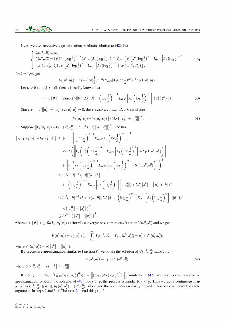
Next, we use successive approximations to obtain solution to (48). Put

V0(u01,u

02) = u0

2,

Vk(u01,u

02) = (θs)

−1(

log 1a

)1−α(Eα ,α(A2

(

log 1a

)α))−1Vk−1

(

θs

(

u01

(

log 1a

)α−1Eα ,α

[

A1

(

log 1a

)α]

+ S1(1,u01,u

02))

,θs

(

u02

(

log 1a

)α−1Eα ,α

[

A2

(

log 1a

)α]

+ S2(1,u01,u

02))

)

,

(49)

for k = 1,we get

V1(u01,u

02) = u0

2 +(log1

a)1−α(Eα ,α [A2(log

1

a)α ])−1S2(1,u

01,u

02).

Let δ > 0 enough small, then it is easily known that

r = c‖θ‖−1 (2maxb‖θ‖ ,2d ‖θ‖ ,

∥

∥

∥

∥

∥

(

log1

a

)α−1

Eα ,α

[

A2

(

log1

a

)α]∥

∥

∥

∥

∥

‖θ‖)δ < 1. (50)

Since S2 = o(∥

∥u01

∥

∥+∥

∥u02

∥

∥) as u01,u

02 → 0, there exists a constant L > 0 satisfying

∥

∥V1(u01,u

02)−V0(u

01,u

02)∥

∥< Lr(∥

∥u01

∥

∥+∥

∥u02

∥

∥

)δ. (51)

Suppose∥

∥Vk(u01,u

02)−Vk−1(u

01,u

02)∥

∥< Lrk(∥

∥u01

∥

∥+∥

∥u02

∥

∥

)δ. One has

∥

∥Vk+1(u01,u

02)−Vk(u

01,u

02)∥

∥ ≤ ‖θ‖−1

∥

∥

∥

∥

∥

(

log1

a

)α−1

Eα ,α(A2

(

log1

a

)α

)

∥

∥

∥

∥

∥

−1

×Lrk

(∥

∥

∥

∥

∥

θs

(

u01

(

log1

a

)α−1

Eα ,α

[

A1

(

log1

a

)α]

+ S1(1,u01,u

02)

)∥

∥

∥

∥

∥

+

∥

∥

∥

∥

∥

θs

(

u02

(

log1

a

)α−1

Eα ,α

[

A2

(

log1

a

)α]

+ S2(1,u01,u

02)

)∥

∥

∥

∥

∥

)δ

≤ Lrkc‖θ‖−1(

‖θ‖(

b∥

∥u01

∥

∥

+

∥

∥

∥

∥

∥

(

log1

a

)α−1

Eα ,α

[

A2

(

log1

a

)α]∥

∥

∥

∥

∥

∥

∥u02

∥

∥)+ 2d(∥

∥u01

∥

∥+∥

∥u02

∥

∥)‖θ‖)δ

≤ Lrkc‖θ‖−1 (2maxb‖θ‖ ,2d ‖θ‖ ,

∥

∥

∥

∥

∥

(

log1

a

)α−1

Eα ,α

[

A2

(

log1

a

)α]∥

∥

∥

∥

∥

‖θ‖)δ

×(∥

∥u01

∥

∥+∥

∥u02

∥

∥

)δ

≤ Lrk+1(∥

∥u01

∥

∥+∥

∥u02

∥

∥

)δ.

where c < ‖θ‖< 1b. So Vk(u

01,u

02) uniformly converges to a continuous function V (u0

1,u02) and we get

V (u01,u

02) =V0(u

01,u

02)+

∞

∑k=1

[Vk(u01,u

02)−Vk−1(u

01,u

02)] = u0

2 +V ∗(u01,u

02),

where V ∗(u01,u

02) = o(

∥

∥u01

∥

∥+∥

∥u02

∥

∥).

By successive approximation similar to function V , we obtain the solution of U(u01,u

02) satisfying

U(u01,u

02) = u0

1 +U∗(u01,u

02), (52)

where U∗(u01,u

02) = o(

∥

∥u01

∥

∥+∥

∥u02

∥

∥).

If c > 1b, namely,

∥

∥

∥(Eα ,α(A1

(

log 1a

)α))∥

∥

∥ =∥

∥

∥(Eα ,α(A2

(

log 1a

)α))∥

∥

∥, similarly to (47), we can also use successive

approximation to obtain the solution of (48). For c > 1b, the process is similar to c < 1

b. Thus we get a continuous map

h1 when (u01,u

02) /∈ δ (0), h1(u

01,u

02) = (u0

1,u02). Moreover, the uniqueness is easily proved. Then one can utilize the same

arguments in steps 2 and 3 of Theorem 2 to end this proof.

c© 2020 NSP



4 Conclusion

The present paper has addressed non linear fractional differential systems involving Riemann-Liouville and Hadamardderivatives with different types of initial value conditions whenever such initial conditions are not equal with each other.We also have proved the new linearization theorems of those nonlinear fractional differential systems.

Acknowledgement

The authors are grateful to thank Prof. Dumitru Baleanu, Editor in Chief of PFDA for his invitation to submit the paper inthis well-reputed journal.

References

[1] C. P.Li, F. H.Zeng, Numerical Methods for Fractional Calculus, 1st ed. Chapman and Hall/CRC, Boca Raton, USA, (2015).

[2] K. Oldham, Spanier, J., The Fractional Calculus: Integrations and Differentiations to Arbitrary Order, Academic Press, New York

(1974).

[3] I. Podlubny, Fractional differential equations, Academic Press New York, (1999).

[4] A. A. Kilbas, H. M. Srivastava, J. J. Trujillo, Theory and Applications of Fractional Differential Equations, Elsevier, New York,

(2006).

[5] S. Q. Zhang, Monotone iterative method for initial value problem involving Riemann-Liouville fractional derivatives, Nonlinear

Anal. TMA 71, pp. 2087-2093, (2009.

[6] S. G. Samko, A. A. Kilbas, O. I.Marichev, Fractional Integrals and Derivatives, Theory and Applications, Gordon & Breach,

Switzerland, (1993).

[7] K. S. Miller, B. Ross, An Introduction to the Fractional Calculus and Differential Equations, John Wiley & Sons, New York,

(1993).

[8] V. Lakshmikantham, S. Leela, J. V.Devi, Theory of Fractional Dynamic Systems, Cambridge Academic, Cambridge, UK, (2009).

[9] Ma Li, C. P. Li, On Hadamard fractional calculus, Fractals, 25(3), 1750033, (2017).

[10] Q. Z. Gong, D. L.Qian, C. P. Li, P. Guo, On the Hadamard type fractional differential system, Fractional Dynamics and Control,

eds. D. Baleanu et al. (Springer, New York, USA), pp. 159-171, (2012).

[11] D. Kusnezov, A. Bulgac, G. D. Dang, Quantum Levy Processes and Fractional Kinetics, Phys. Rev. Lett., 82(6), pp. 1136-1139,

(1999).

[12] H. H. Sun,, A. A. Abdelwahab,, B. Onaral, Linear Approximation of Transfer Function with a Pole of Fractional Order, IEEE

Transactions on Automatic Control, 29(5), pp. 441-444, (1984).

[13] M. Ichisea, Y. Nagayanagia, T. Kojima, An analog simulation of non-integer order transfer functions for analysis of electrode

processes, J. Electroanal. Chem., 33(2), pp. 253-265, (1971).

[14] N. Laskin,, Fractional market dynamics, Phys. A: Stat. Mech. Appl., 287, pp. 482-492, (2000).

[15] H. Sheng, Y. Q. Chen, T. S. Qiu, Fractional Processes and Fractional-Order Signal Processing, New York: Springer-Verlag, (2012).

[16] R. Metzler, J. Klafter, The random walks guide to anomalous diffusion: a fractional dynamic approach, Physics Reports, 339(1),

pp. 1-77, (2000).

[17] E. Reyes-Melo, J. Martinez-Vega, C. Guerrero-Salazar, U. Ortiz-Mendez, Application of fractional calculus to the modeling of

dielectric relaxation phenomena in polymeric materials, Journal of Applied Polymer Science, 98, pp. 923-935, (2005).

[18] R. Schumer, D. Benson, Eulerian derivation of the fractional advection-dispersion equation, J. Contaminant Hydrology, 48, pp.

69-88, (2001).

[19] N. Heymans, J. C. Bauwens, Fractal rheological models and fractional differential equations for viscoelastic behavior, Rheologica

Acta, 33, pp. 210-219, (1994).

[20] B. Henry, S. Wearne, Existence of turing instabilities in a two-species fractional reactiondiffusion system, SIAM Journal on Applied

Mathematics, 62, pp. 870-887, (2002).

[21] W. Glockle, T. Nonnenmacher, A fractional calculus approach to self-similar protein dynamics, Biophysical Journal, 68, pp. 46-53,

(1995).

[22] S. Picozzi, B. J. West, Fractional Langevin model of memory in financial markets, Physics Review E, 66, pp. 46-118, (2002).

[23] B. Ahmad, J. J. Nieto, A. Alsaedi, M. El-Shahed, A study of nonlinear Langevin equation involving two fractional orders in

different intervals, Nonlinear Analysis: Real World Applications, 13, pp. 599-606, (2012).

[24] R. Gu, Y. Xu, Chaos in a fractional-order dynamical model of love and its control, In: S. Li, X. Wang, Y. Okazaki, J. Kawabe, T.

Murofushi, L. Guan (eds) Nonlinear Mathematics for Uncertainty and Its Applications, Berlin/Heidelberg: Springer-Verlag, 100,

pp. 349-356, (2011).

[25] L. Song, S. Xu, J. Yang, Dynamical models of happiness with fractional order, Communica- tions in Nonlinear Science and

Numerical Simulation, 15, pp. 616-628, (2010).

c© 2020 NSP




[26] R. L. Bagley, R. A. Calico, Fractional order state equations for control of viscoelastic structures, J. Guid. Cont. and Dyn., 14(2),

pp. 304-311, (1991).

[27] C. P. Li, Z. Q. Gong, D. L. Qian,, Y. Q. Chen,, On the Bound of the Lyapunov Exponents for the Fractional Differential Systems,

Chaos, 20(1), 013127, (2010).

[28] N. D. Cong, T. S.Doan, S. Siegmund, H. T.Tuan, On Stable Manifolds for Planar Fractional Differential Equations, Appl. Math.

Comput, 226(1), pp. 157-168, (2014).

[29] C. P. Li, F. R. Zhang, A survey on the stability of fractional differential equations, Eur. Phys. J. Special Topics, 193, pp. 27-47,

(2011).

[30] C. P. Li, Y. T.Ma, Fractional dynamical system and its linearization theorem. Nonlinear Dynamics, 71(4), pp. 621-633, (2013).

[31] Y. A. Kuznetsov, Elements of Applied Bifurcation Theory, Springer-Verlag, New York, (1995).

[32] H. Kunita, Stochastic differential equations and stochastic flows of diffeomorphisms, Lect. Notes Math., 1097, pp. 143-303, (1984).

[33] C. P. Li, D. L.Qian, Y. Q.Chen, On Riemann-Liouville and Caputo derivatives,Discrete Dyn. Nat. Soc., 2011, pp. 562494, (2011).

[34] P. Hartman, A lemma in the theory of structural stability of differential equations, Proc. Am. Math. Soc., 11(4), pp. 610-620,

(1960).

[35] P. Hartman, On the local linearization of differential equations, Proc. Am. Math. Soc., 14(4), pp. 568-573, (1963).

[36] C. C. Pugh, On a theorem of P. Hartman, Am. J. Math., 91(2), pp. 363-367, (1969).

[37] P. Hartman, Ordinary Differential Equations, 2nd ed., Birkhauser, Basel, (1982).

c© 2020 NSP


Linearization of Nonlinear Fractional Differential Systems with ...

Documents

Transcript of Linearization of Nonlinear Fractional Differential Systems with ...