Int. J. Appl. Math. Comput. Sci., 2009, Vol. 19, No. 2, 219–232DOI: 10.2478/v10006-009-0018-2

INPUT CONSTRAINTS HANDLING IN AN MPC/FEEDBACK LINEARIZATIONSCHEME

JIAMEI DENG ∗ , VICTOR M. BECERRA ∗∗, RICHARD STOBART ∗

∗ Department of Aeronautical and Automotive EngineeringLoughborough University, Leicestershire LE11 3TU, UKe-mail: j.deng,r.k.stobart@lboro.ac.uk

∗∗ School of Systems EngineeringUniversity of Reading, Reading, RG6 6AY, UKe-mail: v.m.becerra@reading.ac.uk

The combination of model predictive control based on linear models (MPC) with feedback linearization (FL) has attractedinterest for a number of years, giving rise to MPC+FL control schemes. An important advantage of such schemes isthat feedback linearizable plants can be controlled with a linear predictive controller with a fixed model. Handling inputconstraints within such schemes is difficult since simple bound contraints on the input become state dependent because ofthe nonlinear transformation introduced by feedback linearization. This paper introduces a technique for handling inputconstraints within a real time MPC/FL scheme, where the plant model employed is a class of dynamic neural networks. Thetechnique is based on a simple affine transformation of the feasible area. A simulated case study is presented to illustratethe use and benefits of the technique.

Keywords: predictive control, feedback linearization, neural networks, nonlinear systems, constraints.

1. Introduction

The great success of predictive control is mainly due toits handling of constraints in an optimal way. There isearly work on the integration of a feedback linearizingcontroller in an unconstrained MPC scheme (Henson andSeborg, 1993). However, in practical control schemesconstraints have to be dealt with. Del-Re et al. (1993)dealt with the integration of output constraints by map-ping the problem into a linear MPC problem. The ba-sic idea of this method is to linearize the process us-ing feedback linearization so that linear MPC solutionscan be employed. However, in most of the cases, thismapping transforms the original input constraints of theprocess into nonlinear and state-dependent constraints,which cannot be handled by means of quadratic program-ming (Nevistic, 1994; Oliveiria et al., 1995). Some meth-ods have been presented in order to deal with such non-linear constraints mapping while using QP routines tosolve an approximate linear MPC problem (Henson andKurtz, 1994; Oliveiria et al., 1995). However, these ap-proaches suffer from an important limitation as conver-gence to a feasible solution over the optimization horizon

within the available time becomes a problem (Nevistic andMorari, 1995).

Ayala-Botto et al. (1999) proposed a new optimiza-tion procedure that guarantees a feasible control solu-tion without input constraints violation over the completeoptimization horizon, in a finite number of steps, whileallowing only a small overall closed-loop performancedegradation. Ayala-Botto et al. (1996) integrated in twocomplementary iterative procedures the solution of theQP optimization converting the nonlinear state-dependentconstraints into linear ones. Van den Boom (1997) de-rived a robust MPC algorithm using feedback lineariza-tion at the cost of possibly conservative constraint han-dling. Nevistic and Primbs (1996) considered the problemof model/plant mismatch of MPC with feedback lineariza-tion. Guemghar et al. (2005) proposed a cascade structureof predictive control and feedback linearization for unsta-ble systems. Scattolini and Colaneri (2007) presented amulti-layer cascaded predictive controller to guaranteedstability and feasibility. Ayala-Botto et al. (1999) pre-sented a new solution for the problem of incorporating aninput-output linearization scheme based on static neural

220 J. Deng et al.

networks in a predictive controller, considering the pres-ence of level and rate inequality constraints applied to theplant input. However, this scheme can only handle single-input single-output systems. Moreover, Kurtz and Hen-son (1997) presented an input constraint mapping tech-nology, the transformed constraints at each sampling timewere decided by solving a constrained optimization prob-lem. Also Casavola and Mosca (1996) tried to find boxconstraints by employing an optimization algorithm.

In this paper, focus will be positioned on input con-straint handling on an integrated MPC+FL scheme basedon dynamic neural networks. The aim is to find a con-straint handling method that is suitable for real time ap-plication and avoids the shortcomings of the method byAyala-Botto et al. (1999). Solving an additional optimiza-tion problem to find the transformed constraints is avoidedin the proposed method.

The paper is organised as follows: Section 2 brieflydescribes the model predictive control formulation em-ployed in this work. Section 3 describes the neural net-work structure used and discusses the training problem.Section 4 discusses the feedback linearization techniqueemployed. Section 5 presents the proposed method forhandling input constraints within an MPC/FL scheme.Section 6 discusses how the dynamic neural network isemployed as a closed-loop observer. Section 7 presentsa simulated case study. Concluding remarks are given inSection 8.

2. Model-based predictive control

The predictive control formulation employed(Maciejowski, 2002) is based on a linear, discrete-time state-space model of the plant. This makes sensewithin the framework of this paper as the plant is assumedto be feedback linearized prior to the application ofpredictive control. The model has the form

xm(k + 1) = Axm(k) + Bu(k),ym(k) = Cyxm(k),

z(k) = Czx(k),(1)

where xm(k) ∈ RN is the state vector at time k, u(k) ∈

Rm is the vector of inputs, ym(k) ∈ R

n is the vector ofmeasured outputs, and z(k) ∈ R

γ is the vector of outputswhich are to be controlled to satisfy some constraints, orto particular set-points, or both. In this work, a Kalmanfilter was used that can be described as follows:

xm(k + 1|k) = Axm(k|k − 1) + Bu(k) + Le(k|k),ym(k|k − 1) = Cyxm(k|k − 1),

z(k|k − 1) = Cz xm(k|k − 1),(2)

where xm(k + 1|k) is the estimate of the state at futuretime k + 1 based on the information available at time k,

ym(k|k − 1) is the estimate of the plant output at time kbased on information at time k − 1, L is the Kalman filtergain matrix and e(k|k) is the estimated error: e(k|k) =ym(k) − ym(k|k − 1).

The prediction model of MPC is similiar to Eqn. (2),without e(k|k). This formulation is inspired in the con-strained algorithm presented in (Maciejowski, 2002). Thecost function V minimised by the predictive controllerpenalises deviations of the predicted controlled outputsz(k + i|k) from a reference trajectory r(k + i|k), and italso penalises changes in the future manipulated inputsΔu(k + i|k). Define the cost function as follows:

V (k) =p∑

i=1

||z(k + i|k) − r(k + i|k)||2Qw(i)

+m−1∑

i=0

||Δu(k + i|k)||2Rw(i),

(3)

where the prediction and control horizons are p and m,respectively, Qw(i) and Rw(i) are output weight and inputweight matrices, respectively. The cost function is subjectto the inequality constraints:

umax(k) ≥ u(k + i − 1|k) ≥ umin(k),Δumax(k) ≥ Δu(k + i − 1|k) ≥ Δumin(k),

zmax(k) ≥ z(k + j|k) ≥ zmin(k),(4)

where i = 1, 2, . . . , m and j = 1, 2, . . . , p. Theconstrained predictive control algorithm has been imple-mented in the C programming language using quadraticprogramming (Deng and Becerra, 2004), and it has beeninterfaced to SIMULINK through an S-Function as itis difficult to handle constraints using the MPC toolboxavailable in Matlab and in a real time case.

3. Dynamic neural networks

A dynamic neural network is used as a model of the plantfor control synthesis in this paper as it can easily approxi-mate any nonlinear systems. It can be expressed as a vec-tor differential equation:

x(t) = f(x(t), u(t), θ),y(t) = h(x(t), θ),

(5)

where x ∈ RN represents the state vector, y ∈ R

n isthe output vector, u ∈ R

m is the external input vector,θ ∈ R

l is a parameter vector. Here f is a vector-valuedfunction that represents the structure of the network, andh is a vector-valued function that represents the relation-ships between the state vector and the output vector.

The structure of the dynamic neural network used inthis paper is a particular case of Eqn. (5). Any finite timetrajectory of a given dynamic system can be approximated

Input constraints handling in an MPC/feedback linearization scheme 221

vi

i1

u1

um

(x1)

im

i1

iN

Neuron's

outputs

Input

vector

xi

M

M

( )ixσ

(xN)

1

is β+

( ) tanh( )σ ⋅ = ⋅

Fig. 1. Illustration of a dynamic neuron.

by the internal state of the output units of a continuoustime dynamic neural network with N dynamic units, minputs and n outputs (Garces et al., 2003). These networksare neural unit arrays which have connections both waysbetween a pair of units, and from a unit to itself. Themodel is defined by a one-dimensional array of N neu-rons or units, in which each neuron of the dynamic neuralnetwork can be described as follows:

xi = −βixi +N∑

j=1

ωijσ(xj) +m∑

j=1

γijuj , (6)

where βi, ωij and γij are adjustable weights, with 1/βi asa positive time constant and n ≤ N , xi the activation stateof Unit i, and u1, . . . , um the input signals (see Fig. 1).

The states of the first n neurons are taken as the out-put of the network, leaving N−n units as hidden neurons.The network is defined by the vectorised expression of (6)as follows:

x = −βx + ωσ(x) + γu, (7)

y = Cx, (8)

where x are the coordinates on RN , β ∈ R

N×N , γ ∈R

N×m , u ∈ Rm, σ(x) = [σ(x1), . . . , σ(xN )]T , σ(·)

is a sigmoidal function, such as the hyperbolic tangent,In×n is the n × n identity matrix, 0n×(N−n) is an n ×(N − n) matrix of zeros. C = [In×n 0n×(N−n)], andβ = diag(β1, . . . , βN ) is a diagonal matrix. This paperused a dynamic neural network described by Eqns. (7)–(8). The state vector x of the dynamic neural network ofEqn. (7) can be partitioned into the output state xo and thehidden states xh:

x =[

xo

xh

]. (9)

A dynamic neural network training problem can be

cast as a nonlinear unconstrained optimization problem:

minθ

FM (θ, ZM ) =1

2M

M∑

k=1

||y(tk) − y(tk|θ)||2,(10)

where ZM = [y(tk), u(tk)]k=1,M is a training data set,y(tk) represents the measured output, y(tk|θ) is the dy-namic neural network output, and θ is a parameter vector.

The optimization problem associated with trainingusually exhibits local minima. Hence, training dynamicneural networks is typically performed using uncon-strained local optimization with multiple random starts,global optimization methods, or hybrid methods. Globaloptimization or hybrid methods are usually better choicesfor training DNNs when dealing with multivariable plants(Garces et al., 2003).

In this work dynamic networks are trained us-ing a hybrid method involving the DIRECT algorithm(Perttunen et al., 1993), which is a deterministic globaloptimization method, and a gradient based local optimiza-tion method. The solutions obtained by DIRECT are im-proved using gradient based local optimization. The train-ing algorithm will find the parameters of the network inEqn. (7) for which the error function FM is minimized.The weight vector θ used by the algorithm is the aggre-gate of the neurons feedback weight matrix ωN×N , the in-put weight matrix γN×m, the state feedback weight vectorβN×1 = [β1, . . . , βN ]T and the initial values of the hid-den states of the dynamic neural network, xh(t0). Thatis,

θ =

⎡

⎢⎢⎣

βN×1

vec(γN×m)vec(ωN×N )

xh(t0)(N−n)×1

⎤

⎥⎥⎦ , (11)

where vec(.) transfers a matrix into a vector.

4. Approximate input-output feedbacklinearization and MPC integration

Many nonlinear control methods are based on state spacemodels where the time derivative of the states dependsnonlinearly on the states and linearly on the control inputs(Isidori, 1995), which are known as control affine systemsand are described as follows:

x = f(x) + g(x)u,

y = h(x),(12)

where x ∈ RN is a state vector, u ∈ R

m is a vector of ma-nipulated inputs, f and g are differentiable vector fields,and y ∈ R

n is a vector of outputs variables.The purpose of input-output linearization is to intro-

duce a new input variable v and a nonlinear transformationthat uses state feedback to compute the original input u, so

222 J. Deng et al.

that a system described by Eqn. (12) behaves linearly fromthe new input v to the output y.

It is of considerable importance to assess which sys-tems can be input-output linearized. The necessary andsufficient conditions for the existence of a feedback laware presented in (Isidori, 1995).

Input-output linearization and decoupling is a partic-ular case of input-output linearization. An appropriate se-lection of the design parameters leads to a feedback lin-earized system where the i-th output depends on the i-th external input only. The basic linearizing-decouplingtechnique is described in (Isidori, 1995). In this paper, weapply the linearizing-decoupling technique to the dynamicneural network model, which is a control affine system,as formulated by Garces et al. (2002). The control affinesystem mappings related to Eqn. (12) can be related to thedynamic neural network parameters as follows:

f(x) = −βx + ωσ(x),g(x) = γ,

h(x) = Cx.

(13)

Consider the dynamic neural network described byEqns. (7) and (8), and suppose that the dynamic neu-ral network has a vector relative degree given by r =[r1, r2, . . . , rn] at a point x0. Assume that the dynamicneural network has the same number of inputs and outputs(n = m). For arbitrary values λik (i = 1, . . . , n and k =0, . . . , ri), a state feedback law with

u = −S(x)−1E(x) + S(x)−1v, (14)

where

S(x)

=

⎡

⎢⎣λ1r1Lg1L

r1−1f x1 · · · λ1r1LgnLr1−1

f x1

.... . .

...λnrnLg1L

rn−1f xn · · · λnrnLgnLrn−1

f xn

⎤

⎥⎦

n×n

(15)

and

E(x) =

⎡

⎢⎢⎢⎢⎢⎣

r1∑k=0

λ1kLkfx1

...rn∑

k=0

λnkLkfxn

⎤

⎥⎥⎥⎥⎥⎦

n×1

, (16)

where Lkfh denotes a Lie derivative of order k of a scalar

function h(x) along vector field f , λiks are scalar designparameters, and ri is the relative degree of the i-th outputyi, produced when applied to a dynamic neural networkdescribed by Eqns. (7) and (8) a linearized-decoupled sys-tem that obeys

ri∑

k=0

λikdkyi

dtk= vi , i = 1 . . . n, (17)

where yi, not yi, is used as it is based on a neural network.If the relative vector is well defined, S(x) is invert-

ible and

det[diag

(λ1r1 , λ2r2 , . . . , λnrn

)]= 0. (18)

It should be noted that the approximate feedback lin-earization and decoupling laws described above requirestate information. Since the model employed in this workto generate the linearizing-decoupling laws is a dynamicneural network, the same model can also be used as aclosed loop observer to provide state information to thefeedback linearizing laws.

Once the feedback linearization is tested and val-idated on the actual plant, the constrained predictivecontroller can be used to control the linearized system.This controller can deal with disturbances arising frommodelling errors and other sources, and it can handleconstraints on plant variables. While handling outputconstraints using the method presented in this paper isstraightforward, input constraints require special treat-ment due to the presence of the nonlinear transformationsassociated with feedback linearization. This aspect will bediscussed in detail in Section 5. The scheme is illustratedin Fig. 2.

5. Algorithm for handling input constraints

Output constraints are straightforward for feedback lin-earization. Therefore, only input constraints are discussedin this paper. The feedback linearization-decoupling law(14) can be written as follows in discrete time based onthe sampling time Ts, which is chosen using the Nyquist-Shannon theorem:

u(k + 1|k)

= S(x(k + 1|k))−1

· (v(k + 1|k) − E(x(k + 1|k))),

(19)

where i = 1, 2, . . . , m, S(x(k + 1|k)) and E(x(k + 1|k))are given by Eqns. (15) and (16), and x(k +1|k) is a sam-pled state estimate obtained from an observer as as de-scribed in Section 6. Consider the following constraintson the input uk:

umin(k) ≤uk ≤ umax(k),Δumin(k) ≤Δuk ≤ Δumax(k). (20)

From Eqns. (19) and (20), it is possible to see that theresulting constraints on v(k + i−1|k) are state dependentand hence are not suitable to be enforced by means of anMPC algorithm such as the one presented in Section 2,which assumes constant bounds. Although MPC based onquadratic programming could solve linear-variant, evennonlinear-variant constraints, it is not suitable for a real-time control purpose. This paper proposes the use of an

Input constraints handling in an MPC/feedback linearization scheme 223

Feedback linearization-

Feedback Linearized Process

decoupling

Nonlinear

process

Predictive

Controllerreference

DNN

x

uv y

Fig. 2. Hybrid MPC/FL control scheme based on a dynamic neural network.

affine transformation to solve this problem for a real-timeapplication. In order to describe the technique in a simpleway, this paper considers a two-input two-output system.However, this technique can be used in cases with moreinputs and outputs, simply by increasing the dimensions.

Assume that u = [u1(k + i−1|k) u2(k + i−1|k)]T .Then, at sampling time k,

u1min ≤u1(k + i − 1|k) ≤ u1max,

u2min ≤u2(k + i − 1|k) ≤ u2max,

Δu1min ≤Δu1(k + i − 1|k) ≤ Δu1max,

Δu2min ≤Δu2(k + i − 1|k) ≤ Δu2max. (21)

Figure 3 illustrates the feasible area of u1(k+ i−1|k) andu2(k + i − 1|k) at sampling time k. It has four cornerslabelled by O, R, S, T . The coordinates of the cornersare (u1min, u2min), (u1min, u2max), (u1max, u2max),(u1max, u2min), respectively. Note that since these arebound constraints, the sides of the box are parallel to theco-ordinates axes xc and yc. Figure 4 illustrates the feasi-ble area of v1 and v2 after each point in the feasible area ofu1(k+i−1|k) and u2(k+i−1|k) is multiplied by the ma-trix S(x(k + 1|k)) and translated by E(x(k + 1|k)). Thecoordinates of these four corners O, R, S, T have changedinto (a1, a2), (b1, b2), (c1, c2), (d1, d2). The new coordi-nates have the following relationship with the old ones:

[a1

a2

]= S(x(k + 1|k))

[u1min

u2min

]

+ E(x(k + 1|k)),[

b1

b2

]= S(x(k + 1|k))

[u1min

u2max

]

+ E(x(k + 1|k)),[

c1

c2

]= S(x(k + 1|k))

[u1max

u2max

]

+ E(x(k + 1|k)),

(22)

[d1

d2

]= S(x(k + 1|k))

[u1max

u2min

]

+ E(x(k + 1|k)).

The feasible area in Fig. 4 of the transformed inputsis not suitable for use with the predictive control algorithmdescribed in Section 2, as the box is oblique with respectto the co-ordinate system xc–yc. From Eqn. (22), it is notdifficult to see that the side OT is parallel with the sideRS; the side OR is parallel with the side TS. There-fore, the feasible area of the transformed inputs can beexpressed in a suitable form for the predictive control al-gorithm described in Section 2, after an affine change ofcoordinates, which involves in the 2D case a rotation and atranslation. Figure 5 shows the new co-ordinates. Axis x′

c

is parallel with sides OT and RS. Axis y′c is parallel with

the sides OR and TS. In the new coordinates, the pointsO, R, S, T map into (a′

1, a′2), (b

′1, b

′2), (c

′1, c

′2), (d

′1, d

′2). It

is not difficult to prove that a′1 = b′1, a′

2 = d′2, b′2 = c′2and c′1 = d′1.

Suppose the affine change of variables is done bymeans of a 2×2 affine matrix H and a translation. MatrixH can be obtained using the following equations:

[a′1

a′2

]= H

[a1

a2

]− E(x(k + 1|k))

,

[b′1b′2

]= H

[b1

b2

]− E(x(k + 1|k))

, (23)

[c′1c′2

]= H

[c1

c2

]− E(x(k + 1|k))

,

[d′1d′2

]= H

[d1

d2

]− E(x(k + 1|k))

.

Notice that by choosing to have the origin of the x′c–

y′c co-ordinate system centered in the box, the effect of

the shift E(x(k + 1|k)) from Eqn. (22) is cancelled byEqn. (23). Hence it is safe to ignore the effect of theshift E(x(k + 1|k)) when computing the new bounds for

224 J. Deng et al.

Fig. 3. Illustration of the feasible area of the manipulated inputs: Feedback linearization incorporated in a predictive control schemeafter the affine transformation.

Fig. 4. Illustration of the feasible area of the transformed inputs.

Fig. 5. New coordinates after the affine transformation.

v(k + i − 1|k)′ in the x′c–y′

c co-ordinates. The followingrelationships are also true:

b′2 − a′2 =

√(b1 − a1)2 + (b2 − a2)2,

c′1 − b′1 =√

(b1 − c1)2 + (b2 − c2)2, (24)

c′2 − d′2 =√

(d1 − c1)2 + (d2 − c2)2,

d′1 − a′1 =

√(d1 − a1)2 + (d2 − a2)2.

After a′1, a′

2, b′1, b′2, c′1, c′2, d′1, and d′2 are obtained from

Eqn. (24), H can be easily obtained from Eqn. (23).Thus any vector z in the xc–yc co-ordinates can be

transformed into a vector z′c in the x′c–y′

c co-ordinates asfollows:

z′ = H(z − E(x(k + 1|k))), (25)

while any vector z′ in the x′c–y′

c co-ordinates can be trans-formed into a vector in the xc–yc co-ordinates as

z = H−1z′ + E(x(k + 1|k)). (26)

Input constraints handling in an MPC/feedback linearization scheme 225

After the affine transformation, for a given time k,v(k + i − 1|k)′ will be bounded as follows:

[a′1

a′2

]≤ v(k + i − 1|k)′ ≤

[c′1c′2

]. (27)

Therefore, we could change the first line of Eqn. (4) intoEqn. (27) as this is the real input constraint for MPC.

For a given k,

v(k − 1|k − 2) = S(x(k − 1|k − 2))u(k − 1|k − 2)+ E(x(k − 1|k − 2)),

v(k|k − 1) = S(x(k|k − 1))uk + E(x(k|k − 1)).(28)

Hence,

Δv(k + i − 1|k)= v(k + i − 1|k) − v(k − 1|k − 2)= S(x(k + 1|k))uk

− S(u(k − 1|k − 2))u(k − 1|k − 2)+ E(x(k + 1|k))− E(x(k − 1|k − 2)).

(29)

Δv(k + i − 1|k)′ is obtained by transformingΔv(k + i − 1|k) into the new coordinates x′

c andy′

c, i.e.,

Δv(k + i − 1|k)′ = HΔv(k + i − 1|k). (30)

Combining Eqns. (29) and (30), we get

Δv(k + i − 1|k)′

= HS(x(k + 1|k))Δu(k + 1|k)+ Hu(k − 1|k − 2)(S(x(k + 1|k))− S(x(k − 1|k − 2)))+ H(E(x(k + 1|k))− E(x(k − 1|k − 2)).

(31)

Equation (31) also can be writen as

Δv(k + i − 1|k)′

= HΔv(k + i − 1|k)+ Hu(k − 1|k − 2)(S(x(k + 1|k))− S(x(k − 1|k − 2)))+ H(E(x(k + 1|k))− E(x(k − 1|k − 2))).

(32)

The following two equations will be obtained by usingconstraints on Eqn. (31):

Δv′min

= HΔvmin(k + i − 1|k)+ Hu(k − 1|k − 2)(S(x(k + 1|k))− S(x(k − 1|k − 2)))+ H(E(x(k + 1|k)) − E(x(k − 1|k − 2))).

(33)

Δv′max

= HΔvmax(k + i − 1|k)+ Hu(k − 1|k − 2)(S(x(k + 1|k))− S(x(k − 1|k − 2)))+ H(E(x(k + 1|k)) − E(x(k − 1|k − 2))).

(34)

Therefore, we could change the second line ofEqn. (4) into Eqns. (33) and (34) as this is the real rateconstraint for MPC. Now that the constraints have beentransformed into a new coordinate frame. The next step isto transform the inputs to the predictive controller. Figure6 illustrates the control scheme, where the forward trans-formation and its inverse are denoted by H blocks andH−1 blocks, respectively.

The use of the affine transformation to define thebounds for v(k + i − 1|k) does not affect the transferfunction of the plant seen by the predictive controller, pro-vided the output and the reference signals undergo thesame transformation. This can be proved as follows. Forthe scheme in Fig. 6, the matrix transfer function can bewritten as follows:y(s)v(s)

=[ 1

c1nsn+···+c11s+c100

0 1c2nsn+···+c21s+c20

],

(35)

Here, c1n, . . . , c10 and c2n, . . . , c20 are the arbitraryvalues chosen when applying feedback linearization-decoupling. From Fig. 6, y1(s) can be obtained by

y1(s) = H × G(s) × H−1v1(s), (36)

LetG1(s) = H × G(s) × H−1, (37)

where G1 is the new transfer function for the predictivecontroller, which can easily be transformed into a statespace form. Table 1 gives a step-by-step summary ofthe method for handling input constraints in an MPC/FL.Consider now the multi-input multi-output case and sup-pose the number of inputs and outputs is m. The numberof inequalities in Eqn. (21) will be 2m. The dimension ofFig. 3 should be m and the corner number of the feasiblearea will be 2m. The dimension of Fig. 4 is also m andthe corner number of new coordinates is 2m. The num-ber of equations in Eqn. (22) will become 2m, so will thenumber of equations in Eqn. (23). H can still be obtainedusing equations which are similar to (22) and (23). There-fore, the multi-input and multi-output case can easily besolved.

6. Using the dynamic neural network modelas a closed-loop observer

Poznyak et al. (2001) proposed the use of dynamic neu-ral networks as closed loop observers. In this paper, a

226 J. Deng et al.

Nonlinear

process

Feedback

linearization-

decoupling

Predictive

Controllerreference

Feedback Linearized Process

yu

v

v1

y1

H

H

H-1

Fig. 6. Feedback linearization incorporated in a predictive control scheme after the affine transformation.

Table 1. Method for handling input constraints in an MPC/FLscheme.

Step Description

Step 1 Set k = 0. Obtain a′1, a′

2, b′1, b′2, c′1, c′2, d′1,and d′2 according to Eqn. (24) given thata′1 = b′1, a′

2 = d′2, b′2 = c′2 and c′1 = d′1.Step 2 Obtain H is from Eqn. (23).Step 3 Define the bounds for v(k + i − 1|k)′

as given in Eqn. (27).Step 5 Calculate Δvmin

′ and Δvmax′

according to Eqns. (33) and (34).Step 6 Measure the current plant output yk and

transform it using Eqn. (25) to obtain y′k.

Step 7 Transform the current reference rk

using Eqn. (25) to obtain r′k.Step 8 Execute one step of the predictive control

algorithm to obtain v(k + i − 1|k)′.Step 8 Transform v(k + i − 1|k)′ to obtain

v(k + i − 1|k) using Eqn. (26).Step 9 Provide v(k + i − 1|k) to

the feedback linearization/decoupling algorithm.Step 10 Set k = k + 1 and return to Step 1.

dynamic neural network is employed as a closed-loopobserver to provide state information to be used by thefeedback linearization laws. A dynamic neural networkcan be used as either an open-loop observer or a closed-loop observer. A dynamic neural network was used as anopen-loop observer in (Garces et al., 2003; Garces, 2000),where the state vector of the dynamic neural networkwas used to provide state information to the feedback lin-earization law, with no plant output information used tocorrect the state estimates. A closed-loop observer withoutput feedback can reduce the state estimation error andimprove the robustness of the estimator. An extendedKalman filter algorithm (Maybeck, 1982) is employed in

this work as a state estimator, where a dynamic neural net-work is employed to represent the plant dynamics.

We used a simplified extended Kalman filter whichassumes the following stochastic model of the plant dy-namics and discrete observations with a sampling intervalTs:

x(t) = F (x, u) + Gw(t)= −βx(t) + ωσ(x(t)) + γu(t) + Gw(t),

x(0) = x0,

y(tk) = Cx(tk) + v(tk),

(38)

where x is the state vector, y is the measurement vector,u is the external input vector, w is assumed to be zeromean continuous white noise with covariance matrix Q,v is assumed to be zero mean discrete white noise withcovariance matrix R, and x0 is a random vector with zeromean and covariance matrix P0.

The algorithm assumes that the Jacobian matrix re-mains constant between samples, so that

Φ(k) = exp

([∂F (x, u))

∂x

]

tk

Ts

). (39)

A summary of the algorithm is as follows:

• Algorithm initialisation: Give values to Q, R, P0 andG. Set t = 0, k = 0, P (0) = P0, x(0) = x0.

• Step 1: Time update. Integrate from tk−1 to tk thefollowing differential equation to obtain x(k)−:

x = −βx(t) + ωσ(x(t)) + γu(t). (40)

Also compute the a priori state covariance from

P−(k) = Φ(k)P (k − 1)Φ(k)T + Q. (41)

• Step 2: Measurement update. Measure the currentoutput y(k) and then compute the Kalman filter gain

Input constraints handling in an MPC/feedback linearization scheme 227

Qc,Tc Qh,Th

TI

hI

T2

h2

Tank1 Tank2

K1 K2Qo1 Qo2

Fig. 7. Schematic diagram of the two tank mixing process.

K(k), the corrected state estimate x(k), and the cor-rected covariance matrix P (k):

K(k) = P−(k)CT (CP−(k)CT + R)−1, (42)

x(k) = x−(k) + K(k)(y(k) − y−(k)), (43)

P (k) = (I − K(k)C)P−(k). (44)

Set k = k + 1 and return to Step 1.

7. Case study

This section describes a case study based on a simulatedmixing process. A section of the process is shown inFig. 7.

Two streams of cold and hot water enter the first tank,where a motorized mixer operates. These streams are con-trolled by means of two pneumatic valves. The two tanksare interconnected via a lower pipe with a manual valvethat is normally open. The outlet valve from Tank 2 isalso normally open. The two measured variables are thelevel of Tank 1 and the temperature of Tank 2. A simplemodular model of the mixing process is described below(Becerra et al., 2001). The model is obtained from massand energy balances. The main simplifying assumptionsthat were made to derive this model were as follows:

• The mixing is perfect.

• Heat losses are negligible.

• The valves have linear characteristics.

• The temperatures of the cold and hot water streamsare constant.

The model for the first tank is given by the following

algebraic and differential equations:

Qc = Ccvc/100,

Qh = Chvh/100,

Qo1 = K1

√h1 − h2, (45)

dh1

dt= (Qc + Qh − Qo1)/A1,

dT1

dt= [Qc(Tc − T1) + Qh(Th − T1)]/(A1h1),

where vc is the opening of the cold water control valve(%), vh is the opening of the hot water control valve(%), Cc is the constant of the cold water control valve(cm3/s%), Ch is the constant of the cold water controlvalve (cm3/s)%), Qc is the cold water flow rate (cm3/s),Qh is the hot water flow rate (cm3/s), Qo1 is the outletflow rate from Tank 1 (cm3/s), h1 is the liquid level inTank 1 (cm), T1 is the liquid temperature in Tank 1 (oC),Tc is the temperature of the cold water stream (oC), Th isthe temperature of the hot water stream (oC), K1 is the re-striction of the interconnection valve and pipe (cm5/2/s),A1 is the cross-sectional area of Tank 1 (cm2).

The model for the second tank is given by the follow-ing algebraic and differential equations:

Qo2 = K2

√h2,

dh2

dt= (Q1 − Qo2)/A2, (46)

dT2

dt= [Qo1(T1 − T2)]/(A2h2),

where Qo2 is the outlet flow rate from Tank 2 (cm3/s), h2

is the liquid level in Tank 2 (cm), T2 is the liquid temper-ature in Tank 2 (oC), K2 is the restriction of the Tank 2outlet valve and pipe (cm5/2/s), A2 is the cross-sectionalarea of Tank 2 (cm2).

The following values were used for the model pa-rameters: A1 = 289 cm2, A2 = 144 cm2, Cc =280.0 cm3/s%, C − h = 100.0 cm3/s%, T = 20oC,Th = 72oC, K1 = 30 cm5/2/s, K2 = 30 cm5/2/s. Qh

228 J. Deng et al.

Normalize the domain to be the

unit hyper-cube with center c1

Find f(c1), set f

min =f(c

1)

Choose a rectangle Ei

Sample the center of the

rectangle Ei Update f

min

Identify the set E of potentially

optimal rectangle

E-Ei=0

Reach

target

Gradient descent algorithm

for the fine-tuning result

End

No

Yes

No Yes

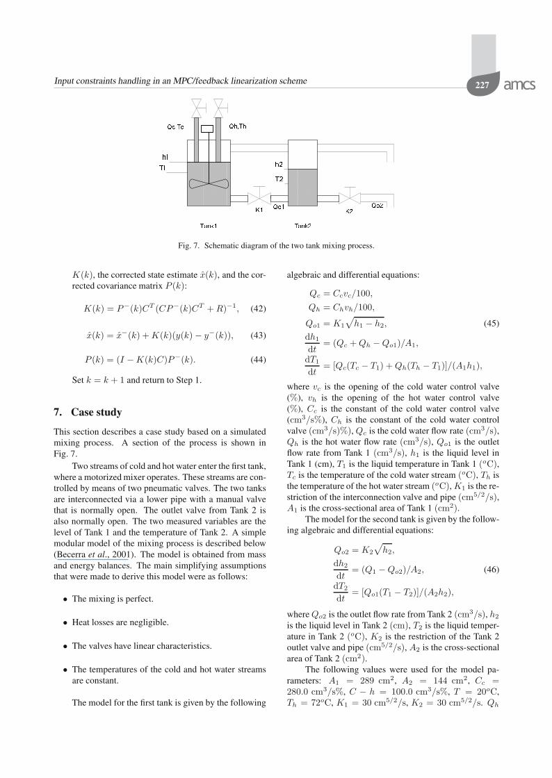
Fig. 8. Descriptive diagram of a combined DIRECT gradientbased training algorithm.

and Qc are the manipulated inputs. An identification ex-periment was carried out on this two-tank system modelby using random steps in the inputs u1(k + i − 1|k) andu2(k + i−1|k) over 4000 sampling points. The first 2000sampling points data were used for training and the sec-ond 2000 sampling points data were used for validation.The sampling time is 20 s. Training was carried out bymeans of the DIRECT algorithm combined with the gra-dient descent algorithm. Fifty training runs were carriedfor each network size, starting from the random initialweights, and the best network in terms of mean squareerror for the training data was selected for each networksize. The values of the parameters of the best model foundwere

β =[

0.0059 00 0.0106

], (47)

γ =[

0.0084 0.0030−0.0034 0.0038

], (48)

ω =[ −0.0891 −0.0783

0.1488 0.1850

], (49)

C = [1 0]. (50)

In order to explore a reduced region of the error sur-face, some methods, such as Quasi-Newton ones, resultin finding a local minimum from the given initial parame-

ters. At the same time, values obtained from the DIRECTalgorithm are close to different local minima. A combinedalgorithm starts with the DIRECT algorithm and then fine-tunes the result using a faster local search procedure. Thisis illustrated in Fig. 8.

Figure 9 compares the network output obtained forthe training input with the training output using the DI-RECT algorithm combined with the gradient descent al-gorithm. Figure 10 compares the network output obtainedfor the validation input with the validation output usingthe DIRECT algorithm combined with the gradient de-scent algorithm. After identifying the dynamic neural net-work model, a feedback linearization based on this DNNhas being calculated. In order to improve the feedbacklinearization, the dynamic neural network is also used asa closed loop observer. The two-tank system yields a 2-unit network:

h(x) = x =[

x1

x2

],

g(x) = γ =[

γ11 γ12

γ21 γ22

], (51)

f(x) = −βx + ωσ(x).

It has the relative degree of

r = [1 1]. (52)

The control law is given by

u(t) = − S(x(k + 1|k))−1E(x(k + 1|k))

+ S(x(k + 1|k))−1v(t),

(53)

where

S(x(k + 1|k)) =[

λ11Lg1L0fx1,k λ11Lg2L

0fx1,k

λ21Lg1L0fx2,k λ21Lg2L

0fx2,k

]

=[

λ11γ11 λ11γ12

λ21γ21 λ21γ22

], (54)

E(x(k + 1|k))

=[

λ10L0fx1,k + λ11Lfx1,k

λ20L0fx2,k + λ21Lfx2,k

]

=

[λ10x(k + 1|k) + λ11(−β1x(k + 1|k)λ20x(k + 1|k) + λ21(−β1x(k + 1|k)σ(x(k + 1|k)))

+w11σ(x(k + 1|k)) + w12σ(x(k + 1|k)))+w21σ(x(k + 1|k)) + w22σ(x(k + 1|k)))

], (55)

where λ10 = 0.000062861, λ11 = 0.0165, λ20 =0.000062861, λ21 = 0.0165. The design parameters λij

are chosen so that λ10 = λ20 and λ11 = λ21, and the staticgain and dominant time constant of the linearized systemv − y is as near to that of the Jacobian linearization of the

Input constraints handling in an MPC/feedback linearization scheme 229

0 500 1000 1500 20000

20

40

Sampling Points

Tem

pera

ture

DNNTank

0 500 1000 1500 200020

30

40

Sampling Points

Leve

l

DNNTank

Fig. 9. Comparison of training trajectories using the DIRECT algorithm combined with the gradient descent algorithm.

0 500 1000 1500 200010

20

30

40

50

Sampling Points

Tem

pera

ture

DNNTank

0 500 1000 1500 200025

30

35

40

Sampling Points

Leve

l

DNNTank

Fig. 10. Comparison of validation trajectories using the DIRECT algorithm combined with the gradient descent algorithm.

dynamic neural network model as possible. For this case,S(x(k + 1|k)) is a constant matrix:

S(x(k + 1|k)) =[

0.0001394 0.0000485−0.0000565 0.0000628

]. (56)

The input constraints are given as

[00

]≤ u ≤

[100100

]. (57)

After the constraint area is transformed using

S(x(k + 1|k)), the coordinates of the four corners are

(a1, a2) = (0, 0),(b1, b2) = (0.004983, 0.0062799),(c1, c2) = (0.01889, 0.00063129),(d1, d2) = (0.0139387,−0.0056489). (58)

Therefore,

(a′1, a

′2) = (0, 0),

230 J. Deng et al.

(b′1, b′2) = (0, 0.0079984),

(c′1, c′2) = (0.01504, 0.0079984),

(d′1, d′2) = (0.01504, 0). (59)

According to Eqn. (23),

H =[

0.81764 −0.644920.391138 0.96513

]. (60)

In this example, S(x(k + 1|k)) and H are constant matri-ces. However, if S(x(k+1|k)) and H are state-dependent,the proposed method for handling input constraints withinan MPC/FL scheme remains applicable, only that the con-straint values change at every sampling time.

The Kalman filter gain was computed using thelinearized model and the covarience matrices Qf =diag(1, 1), Rf = diag(0.001, 0.001). The referencesused in the simulation were two square waves with dif-ferent frequencies. The sampling time is Ts = 20 s,the control horizon is m = 2, the prediction horizon isp = 320, the input and output weights are uwt = [1, 1]T ,ywt = [0.0001, 0.0001]T , the manipulated variablesconstraints are umin = [0, 0]T , umax = [100, 100]T ,the incremental constraints on the manipulated variableare Δumax = [0.01, 0.01]T . The tuning parametersof the extended Kalman filter are P0 = diag(0.1, 0.1),Q = diag(0.1, 0.1), R = diag(100, 100). The diagonalelements of the output noise covariance matrix R werechosen to account for the covariance of the measurementnoise. The diagonal elements of the process noise covari-ance matrix Q were chosen small and positive in order toprevent the covariance of the state error from becomingzero. The initial covariance of the state error P0 is chosento reflect some uncertainty in the initial state estimate.

Figure 11 shows the outputs responses under theMPC/FL scheme. Figure 12 shows the actual inputs tothe process under the MPC/FL control method. In thiscase, the input magnitude constraints do not become ac-tive. Figures 13 and 14 show the output of the controllerand input to the process under the proposed scheme in ascenario where one of the input magnitude constraints be-comes active as can be seen in Fig. 13.

8. Conclusion

This paper has introduced a technique for handling inputconstraints within a real time MPC/FL scheme, where theplant model employed is a class of dynamic neural net-work. Handling input constraints within such schemes isdifficult since simple bound contraints on the input be-come state dependent because of the nonlinear transfor-mation introduced by feedback linearization. The tech-nique is based on a simple affine transformation of thefeasible area. A simulated case study was presented toillustrate the use of the technique. The issue of recursive

feasiblity of MPC is important (Rossiter, 2003) in the con-text of the work presented in this paper. This is currentlybeing investigated by the authors and will be the subjectof a future paper.

Acknowledgment

This project is co-funded by the UK Technology Strat-egy Board’s Collaborative Research and Developmentprogramme, following an open competition. The au-thors would like to thank the Technology Strategy BoardProgram under Grant Reference No. TP/3/DSM/6/I/152.Thanks also are given to the UK Engineering and Phys-ical Science Research Council under Grant ReferenceNo. GR/R64193 and the University of Reading ChineseStudentship Programme for their support.

ReferencesAyala-Botto, M., Boom, T. V. D., Krijgsman, A. and da Costa,

J. S. (1999). Predictive control based on neural net-work models with I/O feedback linearization, InternationalJournal of Control 72(17): 1538–1554.

Ayala-Botto, M., Braake, H. T., da Costa, J. S. and Verbruggen,H. (1996). Constrained nonlinear predictive control basedon input-output linearization using a neural network, Pro-ceedings of the 13-th IFAC World Congress, San Francisco,CA, USA, pp. 175–180.

Becerra, V. M., Roberts, P. D. and Griffiths, G. W. (2001). Ap-plying the extended Kalman filter to systems desribed bynonlinear differential-algebraic equations, Control Engi-neering Practice 9(3): 267–281.

Casavola, A. and Mosca, E. (1996). Reference governor for con-strained uncertain linear systems subject to bounded inputdisturbances, Preceedings of the 35-th Conference on De-cision and Control, Kobe, Japan, pp. 3531–3536.

Del-Re, L., Chapuis, J. and Nevistic, V. (1993). Stability of neu-ral net based model predivtive control, Proceedings of the32-nd Conference on Decision and Control, San Antonio,TX, USA, pp. 2984–2989.

Deng, J. and Becerra, V. M. (2004). Real-time constrainedpredictive control of a 3d crane system, Proceedings ofthe 2004 IEEE Conference on Robotics, Automation andMechatronics, Singapore, pp. 583–587.

Garces, F. (2000). Dynamic Neural Networks for ApproximateInput-Output Linearisation-Decoupling of Dynamic Sys-tems, Ph.D. thesis, University of Reading.

Garces, F., Becerra, V., Kambhampati, C. and Warwick, K.(2003). Strategies for Feedback Linearisation: A DynamicNeural Network Approach, Springer, London.

Guemghar, K., Srinivasan, B., Mullhaupt, P. and Bonvin, D.(2005). Analysis of cascade structure with predictive con-trol and feedback linearisation, IEE Proceedings: ControlTheory and Applications 152(3): 317–324.

Henson, M. A. and Kurtz, M. J. (1994). Input-output linearisa-tion of constrained nonlinear processes, Nonlinear Control,AICHE Annual Meeting, San Franciso, CA, USA, pp. 1–20.

Input constraints handling in an MPC/feedback linearization scheme 231

0 200 400 600 800 1000 1200 1400 1600 1800 200020

30

40

Sampling Points

Le

ve

l(cm

)

LevelReference

0 200 400 600 800 1000 1200 1400 1600 1800 200030

40

50

Sampling PointsTe

mp

era

ture

(Ce

lsiu

s)

TemperatureReference

Fig. 11. Mixing process outputs under the MPC/FL method. The reference signals are square waves.

0 500 1000 1500 20000

50

Sampling Points

Qc(c

m3 /s

)

0 500 1000 1500 20000

50

100

Sampling Points

Qh(c

m3 /h

)

Fig. 12. Inputs applied to the mixing process the MPC/FL method.

0 500 1000 1500 200015

20

25

30

35

0 500 1000 1500 200030

40

50

60

Sampling Points

Leve

l (cm)

Te

mper

ature

(Cels

ius)

LevelReference

TemperatureReference

Fig. 13. Mixing process outputs under the MPC/FL control method.

Henson, M. A. and Seborg, D. E. (1993). Theoretical analysis ofunconstrained nonlinear model predictive control, Interna-tional Journal of Control 58(5): 1053–1080.

Isidori, A. (1995). Nonlinear Control Systems, 2nd Edition,Springer, Berlin/New York, NY.

Kurtz, M. and Henson, M. (1997). Input-output linearizing con-trol of constrained nonlinear processes, Journal of ProcessControl 7(1): 3–17.

Maciejowski, J. M. (2002). Predictive Control with Constraints,Prentice Hall, London.

Maybeck, P. S. (1982). Stochastic Models, Estimation and Con-trol, Academic Press, New York, NY.

Nevistic, V. (1994). Feasible Suboptimal Model Predictive Con-trol for Linear Plants with State Dependent Constraints,Postdiploma thesis, Swiss Federal Institute of Technology,Automatica Control Laboratory, ETH, Zurich.

Nevistic, V. and Morari, M. (1995). Constrained control offeedback-linearizable systems, Proceedings of the Euro-pean Control Conference, Rome, Italy, pp. 1726–1731.

Nevistic, V. and Primbs, J. A. (1996). Model predictive con-

232 J. Deng et al.

0 200 400 600 800 1000 1200 1400 1600 1800 2000−20

0

20

40

0 200 400 600 800 1000 1200 1400 1600 1800 2000−50

0

50

100Q

c(cm

3 /s)

Qh(c

m3 /s

)

Sampling Points

Sampling Points

Fig. 14. Inputs applied to the mixing process under the MPC/FL control method.

trol: Breaking through constraints, Proceedings of the35-th Conference on Decision and Control, Kobe, Japan,pp. 3932–3937.

Oliveiria, S. D., Nevistic, V. and Morari, M. (1995). Control ofnonlinear systems subject to input constraints, Preprints ofthe IFAC Symposium on Nonlinear Control Systems, NOL-COS’95, Tahoe City, CA, USA, Vol. 1, pp. 15–20.

Perttunen, C. D., Jones, D. R. and Stuckman, B. E. (1993). Lips-chitzian optimization without the Lipschitz constant, Jour-nal of Optimization Theory and Application 79(1): 157–181.

Poznyak, A. S., Sanchez, E. N. and Yu, W. (2001). Differen-tial Neural Networks for Robust Nonlinear Control, WorldScientific, Singapore.

Rossiter, J. A. (2003). Model Based Predictive Control: A Prac-tical Approach, CRC Press, Boca Raton, FL, USA.

Scattolini, R. and Colaneri, P. (2007). Hierarchical model pre-dictive control, Proceedings of the 46-th IEEE Confer-ence on Decision and Control, New Orleans, LA, USA,pp. 4803–4808.

van den Boom, T. (1997). Robust nonlinear predictive controlusing feedback linearization and linear matrix inequalities,Proceedings of the American Control Conference, Albu-querque, NM, USA, pp. 3068–3072.

Jiamei Deng received the Ph.D. degree in cy-bernetics from the University of Reading in2005, the B.Eng. degree in electrical engineer-ing from the Hua Zhong University of Scienceand Technology, Wuhan, China, in 1988, andthe M.Eng. degree in mechanical engineeringfrom the Shanghai Institute of Mechanical En-gineering, China, in 1991. She currently worksas a research associate at Loughborough Uni-versity. She was a research fellow at the Uni-

versity of Sussex between 2006 and 2007. Her research interests includepredictive control, nonlinear control, sliding mode control, optimal con-trol, system identification, optimization, process control, power control,black-box modeling, automotive control, and energy systems.

Victor M. Becerra obtained his Ph.D. degreein control engineering from City University,London, in 1994, for the development of noveloptimal control algorithms, a B.Eng. degreein electrical engineering (Cum Laude) from Si-mon Bolivar University, Caracas, Venezuela, in1990, and an M.Sc. degree in financial man-agement from Middesex University, London, in2001. He worked in power systems analysis forCVG Edelca, Caracas, between 1989 and 1991.

He was a research fellow at City University between 1994 and 1999, be-fore joining the University of Reading, UK, as a lecturer in 2000, wherehe is currently a reader in cybernetics. His main research areas includeoptimal control, nonlinear control, intelligent control, and system iden-tification. Dr. Becerra has published over 100 papers in internationaljournals and conferences, and he has co-authored a Springer book onneural network based control. Since 2003 he has been the head of theCybernetics Intelligence Research Group at the University of Reading.He is a member of the Technical Committees on Optimal Control aswell as Adaptive Control and Learning of the International Federationof Automatic Control (IFAC). He is a member of the IASTED techni-cal committee on robotics. He is also a Senior Member of the IEEE, amember of the IET, and a Chartered Engineer.

Richard Stobart is a Ford professor of au-tomotive engineering at Loughborough Univer-sity in the Department of Aeronautical and Au-tomotive Engineering. As a professor, he is re-sponsible for the development of research andeducation in the field of vehicle engineering,with a particular focus on propulsion and powergeneration systems. In 2007 he completed histerm as the chair of the Powertrain, Fuels andLubricants Activity of the US based Society of

Automotive Engineers (SAE) and was a programme co-chair (with Prof.Li of Tongji University) for the 2008 SAE Congress on Powertrain Fuelsand Lubricants in Shanghai in 2008. He was a professor of automotiveengineering at the University of Sussex (Brighton, UK) from 2001 to2007, where he was also the head of Engineering and Design from 2003to 2006. Professor Stobart was a member of the team who in 1997 re-ceived Arthur D Little’s Ketteringham prize for their work in developingfuel cell technology. He is a graduate from the University of Cambridgewith a first class honours degree in mechanical engineering. He waselected a Fellow of the Institution of Mechanical Engineers in 2000.

Received: 12 May 2008Revised: 11 November 2008Re-revised: 18 November 2008