
Materials Handling - AnalysisChamp.com
231
Section 10 Materials Handling BY VINCENT M. ALTAMURO President, VMA Inc., Toms River, NJ ERNST K. H. MARBURG Vice President, Total Quality and Standards, Retired, Columbus McKinnon Corp. 10-1 10.1 MATERIAL HOLDING, FEEDING, AND METERING by Vincent M. Altamuro Factors and Considerations . . . . . . . . . . . . . . . . . . . . . . . . . . . . . . . . . . . . . 10-2 Flow Analysis . . . . . . . . . . . . . . . . . . . . . . . . . . . . . . . . . . . . . . . . . . . . . . . 10-2 Classifications . . . . . . . . . . . . . . . . . . . . . . . . . . . . . . . . . . . . . . . . . . . . . . . 10-3 Forms of Material . . . . . . . . . . . . . . . . . . . . . . . . . . . . . . . . . . . . . . . . . . . . 10-3 Holding Devices . . . . . . . . . . . . . . . . . . . . . . . . . . . . . . . . . . . . . . . . . . . . . 10-3 Material Feeding and Metering Modes . . . . . . . . . . . . . . . . . . . . . . . . . . . . 10-3 Feeding and Metering Devices. . . . . . . . . . . . . . . . . . . . . . . . . . . . . . . . . . . 10-4 Transferring and Positioning . . . . . . . . . . . . . . . . . . . . . . . . . . . . . . . . . . . . 10-4 10.2 LIFTING, HOISTING, AND ELEVATING by Ernst K. H. Marburg and Associates Chain (BY JOSEPH S. DORSON AND ERNST K. H. MARBURG) . . . . . . . . . . . . . 10-4 Wire Rope (BY LARRY D. MEANS) . . . . . . . . . . . . . . . . . . . . . . . . . . . . . . . . 10-8 Holding Mechanisms? . . . . . . . . . . . . . . . . . . . . . . . . . . . . . . . . . . . . . . . . 10-11 Lifting Tongs . . . . . . . . . . . . . . . . . . . . . . . . . . . . . . . . . . . . . . . . . . . . . 10-11 Special Mechanical and Vacuum Holding Mechanisms . . . . . . . . . . . . . 10-12 Lifting Magnets (BY RICHARD ADAHLIN). . . . . . . . . . . . . . . . . . . . . . . . 10-12 Buckets and Scrapers . . . . . . . . . . . . . . . . . . . . . . . . . . . . . . . . . . . . . . . 10-14 Hoists . . . . . . . . . . . . . . . . . . . . . . . . . . . . . . . . . . . . . . . . . . . . . . . . . . . . 10-15 Mine Hoists and Skips (BY BURT GAROFAB) . . . . . . . . . . . . . . . . . . . 10-19 Elevators, Dumbwaiters, Escalators (BY LOUIS BIALY) . . . . . . . . . . . . 10-20 10.3 DRAGGING, PULLING, AND PUSHING by Harold V. Hawkins revised by Ernst K. H. Marburg and Associates Hoists, Pullers, and Winches . . . . . . . . . . . . . . . . . . . . . . . . . . . . . . . . . . . 10-22 Locomotive Haulage, Coal Mines (BY BURT GAROFAB) . . . . . . . . . . . . . . . 10-22 Industrial Cars . . . . . . . . . . . . . . . . . . . . . . . . . . . . . . . . . . . . . . . . . . . . . . 10-24 Dozers, Draglines . . . . . . . . . . . . . . . . . . . . . . . . . . . . . . . . . . . . . . . . . . . 10-25 Moving Sidewalks . . . . . . . . . . . . . . . . . . . . . . . . . . . . . . . . . . . . . . . . . . . 10-25 Car-Unloading Machinery . . . . . . . . . . . . . . . . . . . . . . . . . . . . . . . . . . . . . 10-25 10.4 LOADING, CARRYING, AND EXCAVATING by Ernst K. H. Marburg and Associates Containerization . . . . . . . . . . . . . . . . . . . . . . . . . . . . . . . . . . . . . . . . . . . . 10-26 Surface Handling (BY COLIN K. LARSEN) . . . . . . . . . . . . . . . . . . . . . . . . . . 10-26 Lift Trucks and Palletized Loads . . . . . . . . . . . . . . . . . . . . . . . . . . . . . . 10-26 Off-Highway Vehicles and Earthmoving Equipment (BY B. DOUGLAS BODE) . . . . . . . . . . . . . . . . . . . . . . . . . . . . . . . . . . . 10-27 Above-Surface Handling . . . . . . . . . . . . . . . . . . . . . . . . . . . . . . . . . . . . . . 10-29 Monorails (BY DAVID T. HOLMS) . . . . . . . . . . . . . . . . . . . . . . . . . . . . . . 10-29 Overhead Traveling Cranes (BY DAVID T. HOLMES) . . . . . . . . . . . . . . . . 10-30 Gantry Cranes . . . . . . . . . . . . . . . . . . . . . . . . . . . . . . . . . . . . . . . . . . . . 10-32 Special-Purpose Overhead Traveling Cranes . . . . . . . . . . . . . . . . . . . . . 10-34 Jib Cranes . . . . . . . . . . . . . . . . . . . . . . . . . . . . . . . . . . . . . . . . . . . . . . . 10-34 Derricks (BY RONALD M. KOHNER) . . . . . . . . . . . . . . . . . . . . . . . . . . . . . 10-34 Mobile Cranes . . . . . . . . . . . . . . . . . . . . . . . . . . . . . . . . . . . . . . . . . . . . 10-35 Cableways . . . . . . . . . . . . . . . . . . . . . . . . . . . . . . . . . . . . . . . . . . . . . . . 10-37 Cable Tramways . . . . . . . . . . . . . . . . . . . . . . . . . . . . . . . . . . . . . . . . . . 10-38 Below-Surface Handling (Excavation) . . . . . . . . . . . . . . . . . . . . . . . . . . . . 10-40 10.5 CONVEYOR MOVING AND HANDLING by Vincent M. Altamuro Overhead Conveyors (BY IVAN L. ROSS) . . . . . . . . . . . . . . . . . . . . . . . . . . . 10-42 Noncarrying Conveyors . . . . . . . . . . . . . . . . . . . . . . . . . . . . . . . . . . . . . . . 10-47 Carrying Conveyors . . . . . . . . . . . . . . . . . . . . . . . . . . . . . . . . . . . . . . . . . . 10-51 Changing Direction of Materials on a Conveyor . . . . . . . . . . . . . . . . . . . . 10-61 10.6 AUTOMATIC GUIDED VEHICLES AND ROBOTS by Vincent M. Altamuro Automatic Guided Vehicles . . . . . . . . . . . . . . . . . . . . . . . . . . . . . . . . . . . . 10-63 Robots . . . . . . . . . . . . . . . . . . . . . . . . . . . . . . . . . . . . . . . . . . . . . . . . . . . . 10-63 10.7 MATERIAL STORAGE AND WAREHOUSING by Vincent M. Altamuro Identification and Control of Materials . . . . . . . . . . . . . . . . . . . . . . . . . . . 10-69 Storage Equipment . . . . . . . . . . . . . . . . . . . . . . . . . . . . . . . . . . . . . . . . . . 10-79 Automated Storage/Retrieval Systems . . . . . . . . . . . . . . . . . . . . . . . . . . . . 10-80 Order Picking . . . . . . . . . . . . . . . . . . . . . . . . . . . . . . . . . . . . . . . . . . . . . . 10-81 Loading Dock Design . . . . . . . . . . . . . . . . . . . . . . . . . . . . . . . . . . . . . . . . 10-81
-
Upload
khangminh22 -
Category
Documents
-
view
0 -
download
0
Transcript of Materials Handling - AnalysisChamp.com

Section 10Materials Handling
BY
VINCENT M. ALTAMURO President, VMA Inc., Toms River, NJERNST K. H. MARBURG Vice President, Total Quality and Standards, Retired, ColumbusMcKinnon Corp.
10-1
10.1 MATERIAL HOLDING, FEEDING, AND METERINGby Vincent M. Altamuro
Factors and Considerations . . . . . . . . . . . . . . . . . . . . . . . . . . . . . . . . . . . . . 10-2
Flow Analysis . . . . . . . . . . . . . . . . . . . . . . . . . . . . . . . . . . . . . . . . . . . . . . . 10-2
Classifications . . . . . . . . . . . . . . . . . . . . . . . . . . . . . . . . . . . . . . . . . . . . . . . 10-3
Forms of Material . . . . . . . . . . . . . . . . . . . . . . . . . . . . . . . . . . . . . . . . . . . . 10-3
Holding Devices . . . . . . . . . . . . . . . . . . . . . . . . . . . . . . . . . . . . . . . . . . . . . 10-3
Material Feeding and Metering Modes . . . . . . . . . . . . . . . . . . . . . . . . . . . . 10-3
Feeding and Metering Devices. . . . . . . . . . . . . . . . . . . . . . . . . . . . . . . . . . . 10-4
Transferring and Positioning . . . . . . . . . . . . . . . . . . . . . . . . . . . . . . . . . . . . 10-4
10.2 LIFTING, HOISTING, AND ELEVATINGby Ernst K. H. Marburg and Associates
Chain (BY JOSEPH S. DORSON AND ERNST K. H. MARBURG) . . . . . . . . . . . . . 10-4
Wire Rope (BY LARRY D. MEANS) . . . . . . . . . . . . . . . . . . . . . . . . . . . . . . . . 10-8
Holding Mechanisms? . . . . . . . . . . . . . . . . . . . . . . . . . . . . . . . . . . . . . . . . 10-11
Lifting Tongs . . . . . . . . . . . . . . . . . . . . . . . . . . . . . . . . . . . . . . . . . . . . . 10-11
Special Mechanical and Vacuum Holding Mechanisms . . . . . . . . . . . . . 10-12
Lifting Magnets (BY RICHARD A DAHLIN). . . . . . . . . . . . . . . . . . . . . . . . 10-12
Buckets and Scrapers . . . . . . . . . . . . . . . . . . . . . . . . . . . . . . . . . . . . . . . 10-14
Hoists . . . . . . . . . . . . . . . . . . . . . . . . . . . . . . . . . . . . . . . . . . . . . . . . . . . . 10-15
Mine Hoists and Skips (BY BURT GAROFAB) . . . . . . . . . . . . . . . . . . . 10-19Elevators, Dumbwaiters, Escalators (BY LOUIS BIALY) . . . . . . . . . . . . 10-20
10.3 DRAGGING, PULLING, AND PUSHINGby Harold V. Hawkins
revised by Ernst K. H. Marburg and Associates
Hoists, Pullers, and Winches . . . . . . . . . . . . . . . . . . . . . . . . . . . . . . . . . . . 10-22
Locomotive Haulage, Coal Mines (BY BURT GAROFAB) . . . . . . . . . . . . . . . 10-22
Industrial Cars . . . . . . . . . . . . . . . . . . . . . . . . . . . . . . . . . . . . . . . . . . . . . . 10-24
Dozers, Draglines . . . . . . . . . . . . . . . . . . . . . . . . . . . . . . . . . . . . . . . . . . . 10-25
Moving Sidewalks . . . . . . . . . . . . . . . . . . . . . . . . . . . . . . . . . . . . . . . . . . . 10-25
Car-Unloading Machinery . . . . . . . . . . . . . . . . . . . . . . . . . . . . . . . . . . . . . 10-25
10.4 LOADING, CARRYING, AND EXCAVATINGby Ernst K. H. Marburg and Associates
Containerization . . . . . . . . . . . . . . . . . . . . . . . . . . . . . . . . . . . . . . . . . . . . 10-26
Surface Handling (BY COLIN K. LARSEN) . . . . . . . . . . . . . . . . . . . . . . . . . . 10-26
Lift Trucks and Palletized Loads . . . . . . . . . . . . . . . . . . . . . . . . . . . . . . 10-26
Off-Highway Vehicles and Earthmoving Equipment
(BY B. DOUGLAS BODE) . . . . . . . . . . . . . . . . . . . . . . . . . . . . . . . . . . . 10-27
Above-Surface Handling . . . . . . . . . . . . . . . . . . . . . . . . . . . . . . . . . . . . . . 10-29
Monorails (BY DAVID T. HOLMS) . . . . . . . . . . . . . . . . . . . . . . . . . . . . . . 10-29
Overhead Traveling Cranes (BY DAVID T. HOLMES) . . . . . . . . . . . . . . . . 10-30
Gantry Cranes . . . . . . . . . . . . . . . . . . . . . . . . . . . . . . . . . . . . . . . . . . . . 10-32
Special-Purpose Overhead Traveling Cranes . . . . . . . . . . . . . . . . . . . . . 10-34
Jib Cranes . . . . . . . . . . . . . . . . . . . . . . . . . . . . . . . . . . . . . . . . . . . . . . . 10-34
Derricks (BY RONALD M. KOHNER). . . . . . . . . . . . . . . . . . . . . . . . . . . . . 10-34
Mobile Cranes . . . . . . . . . . . . . . . . . . . . . . . . . . . . . . . . . . . . . . . . . . . . 10-35
Cableways . . . . . . . . . . . . . . . . . . . . . . . . . . . . . . . . . . . . . . . . . . . . . . . 10-37
Cable Tramways . . . . . . . . . . . . . . . . . . . . . . . . . . . . . . . . . . . . . . . . . . 10-38
Below-Surface Handling (Excavation) . . . . . . . . . . . . . . . . . . . . . . . . . . . . 10-40
10.5 CONVEYOR MOVING AND HANDLINGby Vincent M. Altamuro
Overhead Conveyors (BY IVAN L. ROSS) . . . . . . . . . . . . . . . . . . . . . . . . . . . 10-42
Noncarrying Conveyors . . . . . . . . . . . . . . . . . . . . . . . . . . . . . . . . . . . . . . . 10-47
Carrying Conveyors. . . . . . . . . . . . . . . . . . . . . . . . . . . . . . . . . . . . . . . . . . 10-51
Changing Direction of Materials on a Conveyor . . . . . . . . . . . . . . . . . . . . 10-61
10.6 AUTOMATIC GUIDED VEHICLES AND ROBOTSby Vincent M. Altamuro
Automatic Guided Vehicles . . . . . . . . . . . . . . . . . . . . . . . . . . . . . . . . . . . . 10-63
Robots . . . . . . . . . . . . . . . . . . . . . . . . . . . . . . . . . . . . . . . . . . . . . . . . . . . . 10-63
10.7 MATERIAL STORAGE AND WAREHOUSINGby Vincent M. Altamuro
Identification and Control of Materials . . . . . . . . . . . . . . . . . . . . . . . . . . . 10-69
Storage Equipment . . . . . . . . . . . . . . . . . . . . . . . . . . . . . . . . . . . . . . . . . . 10-79
Automated Storage/Retrieval Systems . . . . . . . . . . . . . . . . . . . . . . . . . . . . 10-80
Order Picking . . . . . . . . . . . . . . . . . . . . . . . . . . . . . . . . . . . . . . . . . . . . . . 10-81
Loading Dock Design . . . . . . . . . . . . . . . . . . . . . . . . . . . . . . . . . . . . . . . . 10-81

FACTORS AND CONSIDERATIONS
The movement of material from the place where it is to the place whereit is needed can be time consuming, expensive, and troublesome. Thematerial can be damaged or lost in transit. It is important, therefore, thatit be done smoothly, directly, with the proper equipment and so that itis under control at all times. The several factors that must be knownwhen a material handling system is designed include:1. Form of material at point of origin, e.g., liquid, granular, sheets,
etc.2. Characteristics of the material, e.g., fragile, radioactive, oily, etc.3. Original position of the material, e.g., under the earth, in cartons,
etc.4. Flow demands, e.g., amount needed, continuous or intermittent,
timing, etc.5. Final position, where material is needed, e.g., distance, elevation
differences, etc.6. In-transit conditions, e.g., transocean, jungle, city traffic, inplant,
etc., and any hazards, perils, special events or situations that couldoccur during transit7. Handling equipment available, e.g., devices, prices, reliability,
maintenance needs, etc.8. Form and position needed at destination9. Integration with other equipment and systems10. Degree of control required
Other factors to be considered include:1. Labor skills available2. Degree of mechanization desired3. Capital available4. Return on investment5. Expected life of installationSince material handling adds expense, but not value, it should be
reduced as much as possible with respect to time, distance, frequency,and overall cost. A straight steady flow of material is usually most effi-cient. The use of mechanical equipment rather than humans is usually,but not always, desirable—depending upon the duration of the job, fre-quency of trips, load factors, and characteristics of the material. Whenequipment is used, maximizing its utilization, using the correct equip-ment, proper maintenance, and safety are important considerations.The proper material handling equipment can be selected by analyz-
ing the material, the route it must take from point of origin to destina-tion, and knowing what equipment is available.
FLOW ANALYSIS
The path materials take through a plant or process can be shown on a flowchart and floor plan. See. Figs. 10.1.1 and 10.1.2. These show notonly distances and destinations, but also time required, loads, and otherinformation to suggest which type of handling equipment will beneeded.
10-2 MATERIAL HOLDING, FEEDING, AND METERING
10.1 MATERIAL HOLDING, FEEDING, AND METERINGby Vincent M. Altamuro
Fig. 10.1.1 Material flowchart.

MATERIAL FEEDING AND METERING MODES 10-3
CLASSIFICATIONS
Material handling may be divided into classifications or actions relatedto the stage of the process. For some materials the first stage is its exis-tence in its natural state in nature, e.g., in the earth or ocean. In othercases the first stage would be its receipt at the factory’s receiving dock.Subsequent material handling actions might be:1. Holding, feeding, metering2. Transferring, positioning3. Lifting, hoisting, elevating4. Dragging, pulling, pushing5. Loading, carrying, excavating6. Conveyor moving and handling7. Automatic guided vehicle transporting8. Robot manipulating9. Identifying, sorting, controlling10. Storing, warehousing11. Order picking, packing12. Loading, shipping
FORMS OF MATERIAL
Material may be in solid, liquid, or gaseous form. Solid material maybe in end-product shapes or in intermediate forms of slabs, sheets, bars,wire, etc., which may be rigid, soft, or amorphous. Further, each itemmay be unique or all may be the same, allowing for indiscriminateselection and handling. Items may be segregated according to somecharacteristic or all may be commingled in a mixed container. Theymight have to be handled as discrete items, or portions of a bulk supplymay be handled. If bulk, as coal or powder, their size, size distribution,flowability, angle of repose, abrasiveness, contaminants, weight, etc.,must be known. In short, before any material can be held, fed, sorted,and transported, all important characteristics of its form must be known.
HOLDING DEVICES
Devices used to hold material should be selected on the basis of theform of the material, what operations, if any, are to be done to it while
being held (e.g., heated, mixed, macerated, dyed, etc.), and how it is tobe fed out of the device. Some such devices are tanks, bins, hoppers,reels, spools, bobbins, trays, racks, magazines, tubes, and totes. Suchdevices may be stationary—either with or without moving parts—ormoving, e.g., vibrating, rotating, oscillating, or jogging. The material holding system is the first stage of a material handling
system. Efforts should be made to assure that the holding devices neverbecome empty, lest the entire system’s flow stops. They can be refilledmanually or automatically and have signals to call for refills at carefullycalculated trigger points.
Fig. 10.1.2 Material flow floor plan.
Fig. 10.1.3 Reciprocating feeder. Either hopper or tube reciprocates to obtain,
orient, and feed items.
MATERIAL FEEDING AND METERING MODES
Material can be fed from its holding devices to processing areas inseveral modes:1. Randomly or by selection of individual items2. Pretested or untested3. Linked together or separated4. Oriented or in any orientation5. Continuous flow or interruptible flow6. Specified feed rate or any rate of flow7. Live (powered) or unpowered action8. With specific spaces between items or not
Fig. 10.1.4 Centerboard feeder. Board, with edge shaped to match part, dips
and then rises through parts to select part, which then slides into feed groove.

FEEDING AND METERING DEVICES
The feeding and metering devices selected depend on the above factorsand the properties of the material. Some, but not all, possible devicesinclude:1. Pumps, dispensers, applicators2. Feedscrews, reciprocating rams, pistons 3. Oscillating blades, sweeps, arms4. Belts, chains, rotaries, turntables5. Vibratory bowl feeders, shakers6. Escapements, mechanisms, pick-and-place devices
TRANSFERRING AND POSITIONING
There is frequently a need to transfer material from one machine toanother, to reposition it within a machine, or to move it a short distance.This can be accomplished through the use of ceiling-, wall-, column-,or floor-mounted hoists, mechanical-advantage linkages, powered
10-4 LIFTING, HOISTING, AND ELEVATING
Fig. 10.1.5 Rotary centerboard feeder. Blade, with edge shaped to match part,
rotates through parts, catching those oriented correctly. Parts slide on contour of
blade to exit onto feeder rail.
Figures 10.1.3 to 10.1.8 illustrate some possible feeding and meter-ing devices.
Fig. 10.1.6 Escapement feeder. One of several variations. Escapement is
weighted or spring-loaded to stop part from leaving track until it is snared by the
work carrier. Slope of track feeds next part into position.
Fig. 10.1.7 Spring blade escapement. Advancing work carrier strips off one
part. Remainder of parts slide down feed track. Work carrier may be another part
of the product being assembled, resulting in an automated assembly.
manipulators, robots, airflow units, or special devices. Also turrets,dials, indexers, carousels, or conveyors can be used; their motion andaction can be:1. In-line (straight line)
a. Plain (without pallets or platens)b. Pallet or platen equipped
Fig. 10.1.8 Lead screw feeder. Parts stack up behind the screw. Rotation of
screw feeds parts with desired separation and timing.
2. Rotary (dial, turret, or table)a. Horizontalb. Vertical
3. Shuttle table4. Trunnion5. Indexing or continuous motion6. Synchronous or nonsynchronous movement7. Single- or multistation
10.2 LIFTING, HOISTING, AND ELEVATINGby Ernst K. H. Marburg and Associates
CHAIN
by Joseph S. Dorson and Ernst K. H. Marburg
Columbus McKinnon Corporation
Chain, because of its energy absorption properties, flexibility, and abil-ity to follow contours, is a versatile medium for lifting, towing, pulling,and securing. The American Society for Testing and Materials (ASTM)and National Association of Chain Manufacturers (NACM) have dividedchain into two groups: welded and weldless. Welded chain is furthercategorized into grades by strength and used for many high-strengthindustrial applications, while weldless chain is used for light-duty low-strength industrial and commercial applications. The grade designationsrecognized by ASTM and NACM for welded steel chain are 30, 43, 70,80, and 100. These grade numbers relate the mean stress in newtons persquare millimeter (N/mm2) at the minimum breaking load. As an exam-ple, the mean stress of Grade 30 chain at its minimum breaking load is300 N/mm2 while that for Grades 100, 80, 70, and 43 is 1000, 800, 700and 430 N/mm2, respectively.Graded welded steel chain is further divided by material and use.
Grades 30, 43, and 70 are welded carbon-steel chains intended for a
variety of uses in the trucking, construction, agricultural, and lumberindustries, while Grade 80 is welded alloy-steel chain used primarilyfor overhead lifting (sling) applications.As a matter of convenience when discussing graded steel chains,
chain designers have developed an expression that contains a constantfor each given grade of chain regardless of the material size. Thisexpression is where M is the chain mini-mum ultimate strength in pounds; N is a constant: 114 for Grade 100,91 for Grade 80, 80 for Grade 70, 49 for Grade 43, and 34 for Grade 30.Note that N has units of lb/in2 and diam. is the actual material stockdiameter in inches.Note that the foregoing expression can also be stated as chain ulti-
mate where short tons 2,000. Therefore, knowing the value of the constant N and thestock diameter of the chain, the minimum ultimate strength can bedetermined.As an example, the ultimate strength of -in. Grade 80 chain can be
verified as follows by using the information contained in Table 10.2.1:
M 5 s91 lb/in2ds0.512 ind2 3 2000 5 47,700 lb s214 kNd
1⁄2
strength 5 N 3 sdiam.d2 3 sshort tonsd
M 5 N 3 sdiam.d2 3 2000

CHAIN 10-5
While graded steel chains are not classified as calibrated chain, sincelinks are manufactured to accepted commercial tolerances, they aresometimes used for power transmission in pocket wheel applications. Inmost such applications, however, power transmission chain is special inthat link dimensions are held to very close tolerances and the chain isprocessed to achieve special wear and strength properties. More in-depth discussions of chain, chain fittings, power transmission, and spe-cial chain follow in this section.
Grade 80 and Grade 100 Welded Alloy-SteelChain (Sling Chain)
The ASTM and NACM specifications for alloy-steel chain (sling chain)have evolved over a period of many years dating back to the mid-1950s.The load and strength requirements for slings and sling chain have uni-fied and are currently specified at Grade 80 and Grade 100 levels in theASME standard for slings, and the NACM and ASTM specifications foralloy-steel chain. Table 10.2.1 relates the ASTM and NACM Grade 80and Grade 100 specifications. As noted, the working load limit or max-imum load to be applied during use is approximately 25 percent of theminimum breaking force. Because the endurance limit is approximately18 percent of the minimum breaking strength for these grades, applica-tions that call for a high number of load cycles near the working load limitshould be reconsidered to maintain the load within the endurance limit. Asan alternative, a larger size chain with a higher working load limit couldbe applied.Alloy-steel chain manufactured to the Grade 80 specification varies
in hardness among producers from about 360 to 400 Brinell. Similarly,Grade 100 chain varies among producers from about 400 to 440 Brinell.The hardness range for Grade 80 chain has narrowed, on average, inrecent years from a wider range of 250 to 450 Brinell that was commonin the 1960s. The current values for Grade 80 equate to a material ten-sile strength of about 175,000 lb/in2 or an average chain tensile strengthof approximately 116,000 lb/in2 (800 N/mm2). Thus, the tensile strengthexpressed for Grade 80 chain provides a breaking strength of
short tons. Similarly, the material tensile strength forGrade 100 is about 215,000 lb/in2 for an average chain tensile strengthof approximately 145,000 lb/in2 (1000 N/mm2). Grade 100 chain for the
91 3 sdiamd2
tensile strength expressed thus has a breaking strength of short tons. Note that the approximate conversion from USCS units to SIunits is 1.0 (diam)2 short tons 8.78 N/mm2. As an example, 91(diam)2 short tons 800 N/mm2.As is the case with chain strength, chain dimensions have become
standardized in the interest of interchangeability of chain and chain fit-tings. Thus, the dimensions presented in Table 10.2.1 are intended toassure interchangeability of products between manufacturers.Present ASTM and NACM chain specifications call for a minimum
elongation of 20 percent at rupture. An original value of 15 percent wasestablished in 1924 as an attempt to guarantee against brittle fracture andto give visible warning of overloading. For low-hardness carbon steelchains (under 200 Brinell) in use prior to the advent of hardened alloysteel, the requirement for sling chains to have a 15 percent minimumelongation at rupture provided some usefulness as an overload warningsignal. However, since high-quality Grade 80 and Grade 100 alloy-steelchain of 360 Brinell and higher has replaced carbon steel chain in high-strength applications, elongation as an indicator of overload is not soapparent. Hardened steel chain achieves about 50 percent of its total elon-gation during the final 10 percent of loading just prior to rupture. For thisreason, only about 50 percent of the total elongation is useful as a visualindicator of overloading. Thus, it is increasingly important that slingchain and slings of optimum strength, toughness, and durability be prop-erly selected, applied, and maintained as advised in applicable standards.Total deformation (plastic plus elastic) at fracture is important as one
of the determinants of energy absorption capability and therefore ofimpact resistance. However, its companion determinant—breakingstrength—is equally important. The only way to measure their compositeeffect is by impact tests carried out on actual chain samples—not bytests on Charpy or other prepared specimens of material. Special impacttesters equipped with high-speed measuring and integration deviceshave been developed for this purpose.
General-Purpose Welded Carbon-Steel Chains
Grade 30 (proof coil) chain is made from low-carbon steel containingabout 0.08 percent carbon. It has a minimum breaking strength ofapproximately 34 ! (diam)2 short tons at 125 Brinell, while its working
114 3 sdiamd2
Table 10.2.1 Grade 80 and Grade 100 Alloy Chain SpecificationsNote: For overhead lifting applications, only alloy chain should be used.
Grade 80
Nominal Material Working load Proof test* Minimum Inside length
chain size diameter limit (max.) (min.) breaking force* (max.) Inside width range
in mm in mm lb kg lb kN lb kN in mm in mm
5.5 0.217 5.5 2,100 970 4,200 19.0 8,400 38.0 0.69 17.6 0.281–0.325 7.14–8.25
7.0 0.276 7.0 3,500 1,570 7,000 30.8 14,000 61.6 0.90 22.9 0.375–0.430 9.53–10.92
8.0 0.315 8.0 4,500 2,000 9,000 40.3 18,000 80.6 1.04 26.4 0.430–0.500 10.92–12.70
10.0 0.394 10.0 7,100 3,200 14,200 63.0 28,400 126.0 1.26 32.0 0.512–0.600 13.00–15.20
13.0 0.512 13.0 12,000 5,400 24,000 107.0 48,000 214.0 1.64 41.6 0.688–0.768 17.48–19.50
16.0 0.630 16.0 18,100 8,200 36,200 161.0 72,400 322.0 2.02 51.2 0.812–0.945 20.63–24.00
20.0 0.787 20.0 28,300 12,800 56,600 252.0 113,200 504.0 2.52 64.0 0.984–1.180 25.00–30.00
22.0 0.866 22.0 34,200 15,500 68,400 305.0 136,800 610.0 2.77 70.4 1.080–1.300 27.50–33.00
1 26.0 1.020 26.0 47,700 21,600 95,400 425.0 190,800 850.0 3.28 83.2 1.280–1.540 32.50–39.00
32.0 1.260 32.0 72,300 32,800 144,600 644.0 289,200 1,288.0 4.03 102.4 1.580–1.890 40.00–48.00
Grade 100
5.5 0.217 5.5 2,700 1,220 5,400 23.8 10,800 47.6 0.69 17.6 0.281–0.325 7.14–8.25
7.0 0.276 7.0 4,300 1,950 8,600 38.5 17,200 77.0 0.90 22.9 0.375–0.430 9.53–10.92
8.0 0.315 8.0 5,700 2,600 11,400 51.0 22,800 102.0 1.04 26.4 0.430–0.500 10.92–12.70
10.0 0.394 10.0 8,800 4,000 17,600 79.0 35,200 158.0 1.26 32.0 0.512–0.600 13.00–15.20
13.0 0.512 13.0 15,000 6,800 30,000 134.0 60,000 268.0 1.64 41.6 0.688–0.768 17.48–19.50
16.0 0.630 16.0 22,600 10,300 45,200 201.0 90,400 402.0 2.02 51.2 0.812–0.945 20.63–24.00
20.0 0.787 20.0 35,300 16,000 70,600 315.0 141,200 630.0 2.52 64.0 0.984–1.180 25.00–30.00
22.0 0.866 22.0 42,700 19,400 85,400 381.0 170,800 762.0 2.77 70.4 1.080–1.300 27.50–33.00
1 26.0 1.020 26.0 59,700 27,100 119,400 531.0 238,800 1,062.0 3.28 83.2 1.280–1.540 32.50–39.00
32.0 1.260 32.0 90,400 41,000 180,800 805.0 361,600 1,610.0 4.03 102.4 1.580–1.890 40.00–48.00
*The proof test and minimum breaking force loads shall not be used as criteria for service or design purposes.SOURCE: National Association of Chain Manufacturers; copyright material reprinted with permission.
11⁄4
7⁄8
3⁄4
5⁄8
1⁄2
3⁄8
5⁄16
9⁄32
7⁄32
11⁄4
7⁄8
3⁄4
5⁄8
1⁄2
3⁄8
5⁄16
9⁄32
7⁄32

load limit is 25 percent of its minimum breaking force. Applicationsinclude load securement, guard rail chain, and boat mooring. It is notfor use in critical or lifting applications. Table 10.2.2 gives pertinentASTM-NACM size and load data.Grade 43 (high test) chain is made from medium carbon steel having
a carbon content of 0.15 to 0.22 percent. It is typically heat-treated to aminimum breaking strength of 49 ! (diam)2 short tons at a hardness of200 Brinell. Table 10.2.3 presents the ASTM-NACM specifications forGrade 43 chain. As shown, the working load limit is approximately35 percent of the minimum breaking force. The major use of this chaingrade is load securement, although it also finds use for towing and drag-ging in the logging industry.
Grade 70 (transport) chain was previously designated binding chainby NACM. This is a high-strength chain which finds use as a loadsecurement medium on log and cargo transport trucks. It may be madefrom carbon or low-alloy steel with boron or manganese added in somecases to provide a uniformly hardened cross section. Carbon content isin the range of 0.22 to 0.30 percent. The chain is heat-treated to a min-imum breaking force of 80 ! (diam)2 short tons with the working loadlimit at 25 percent of the minimum breaking force. Although this chainapproaches the strength of Grade 80, it is not recommended for over-head lifting because of the greater energy absorption capability andtoughness demanded of sling chain. Table 10.2.4 presents the ASTM-NACM specifications for Grade 70 chain.
10-6 LIFTING, HOISTING, AND ELEVATING
Table 10.2.2 Grade 30 Proof Coil Chain SpecificationsNote: Not to be used in overhead lifting applications.
Working Minimum Inside Inside
Nominal Material load limit Proof test* breaking length width
chain size diameter (max.) (min.) force* (max.) (min.)
in mm in mm lb kg lb kN lb kN in mm in mm
4.0 0.156 4.0 400 180 800 3.6 1,600 7.2 0.94 23.9 0.25 6.4
5.5 0.217 5.5 800 365 1,600 7.2 3,200 14.4 0.98 24.8 0.30 7.7
7.0 0.276 7.0 1,300 580 2,600 11.6 5,200 23.2 1.24 31.5 0.38 9.8
8.0 0.331 8.4 1,900 860 3,800 16.9 7,600 33.8 1.29 32.8 0.44 11.2
10.0 0.394 10.0 2,650 1,200 5,300 23.6 10,600 47.2 1.38 35.0 0.55 14.0
11.9 0.488 11.9 3,700 1,680 7,400 32.9 14,800 65.8 1.64 41.6 0.65 16.6
13.0 0.512 13.0 4,500 2,030 9,000 40.0 18,000 80.0 1.79 45.5 0.72 18.2
16.0 0.630 16.0 6,900 3,130 13,800 61.3 27,600 122.6 2.20 56.0 0.79 20.0
20.0 0.787 20.0 10,600 4,800 21,200 94.3 42,400 188.6 2.76 70.0 0.98 25.0
22.0 0.866 22.0 12,800 5,810 25,600 114.1 51,200 228.2 3.03 77.0 1.08 27.5
1 26.0 1.020 26.0 17,900 8,140 35,800 159.1 71,600 318.2 3.58 90.9 1.25 31.7
*The proof test and minimum breaking force loads shall not be used as criteria for service or design purposes.SOURCE: National Association of Chain Manufacturers; copyright material reprinted with permission.
7⁄8
3⁄4
5⁄8
1⁄2
7⁄16
3⁄8
5⁄16
1⁄4
3⁄16
1⁄8
Table 10.2.3 Grade 43 High-Test Chain SpecificationsNote: Not to be used in overhead lifting applications.
Working Minimum Inside Inside
Nominal Material load limit Proof test* breaking length width
chain size diameter (max.) (min.) force* (max.) (min.)
in mm in mm lb kg lb kN lb kN in mm in mm
7.0 0.276 7.0 2,600 1,180 3,900 17.3 7,800 34.6 1.24 31.5 0.38 9.8
8.7 0.343 8.7 3,900 1,770 5,850 26.0 11,700 52.0 1.29 32.8 0.44 11.2
10.0 0.406 10.3 5,400 2,450 8,100 36.0 16,200 72.0 1.38 35.0 0.55 14.0
11.9 0.468 11.9 7,200 3,270 10,800 48.0 21,600 96.0 1.64 41.6 0.65 16.6
13.0 0.531 13.5 9,200 4,170 13,800 61.3 27,600 122.6 1.79 45.5 0.72 18.2
16.0 0.630 16.0 13,000 5,910 19,500 86.5 39,000 173.0 2.20 56.0 0.79 20.0
20.0 0.787 20.0 20,200 9,180 30,300 134.7 60,600 269.4 2.76 70.0 0.98 25.0
22.0 0.866 22.0 24,500 11,140 36,750 163.3 73,500 326.6 3.03 77.0 1.08 27.5
* The proof test and minimum breaking force loads shall not be used as criteria for service or design purposes.SOURCE: National Association of Chain Manufacturers; copyright material reprinted with permission.
7⁄8
3⁄4
5⁄8
1⁄2
7⁄16
3⁄8
5⁄16
1⁄4
Table 10.2.4 Grade 70 Transport Chain SpecificationsNote: Not to be used in overhead lifting applications.
Working Minimum Inside Inside
Nominal Material load limit Proof test* breaking length width
chain size diameter (max.) (min.) force* (max.) (min.)
in mm in mm lb kg lb kN lb kN in mm in mm
7.0 0.281 7.0 3,150 1,430 6,300 28.0 12,600 56.0 1.24 31.5 0.38 9.8
8.7 0.343 8.7 4,700 2,130 9,400 41.8 18,800 83.6 1.29 32.8 0.44 11.2
10.0 0.406 10.3 6,600 2,990 13,200 58.7 26,400 117.4 1.38 35.0 0.55 14.0
11.9 0.468 11.9 8,750 3,970 17,500 77.8 35,000 155.4 1.64 41.6 0.65 16.6
13.0 0.531 13.5 11,300 5,130 22,600 100.4 45,200 200.8 1.79 45.5 0.72 18.2
16.0 0.630 16.0 15,800 7,170 31,600 140.4 63,200 280.8 2.20 56.0 0.79 20.0
20.0 0.787 20.0 24,700 11,200 49,400 219.6 98,800 439.2 2.76 70.0 0.98 25.0
* The proof test and minimum breaking force loads shall not be used as criteria for service or design purposes.SOURCE: National Association of Chain Manufacturers; copyright material reprinted with permission.
3⁄4
5⁄8
1⁄2
7⁄16
3⁄8
5⁄16
1⁄4

CHAIN 10-7
Chain Strength
Welded chain links are complex, statically indeterminate structures sub-jected to combinations of bending, shear, and tension under normalaxial load. When a link is loaded, the maximum tensile stress normal tothe section occurs in the outside fiber at the end of the link (seeFig. 10.2.1), which shows the stress distribution in a -in (10-mm) Grade80 chain link with rated load, determined by finite element analysis(FEA). In Fig. 10.2.1, stress distribution is obtained from FEA byassuming that peak stress is below the elastic limit of the material. If thematerial is ductile and the peak stress from linear static FEA exceedsthe elastic limit, plastic deformation will occur, resulting in a distribu-tion of stresses over a larger area and a reduction of peak stress.It is interesting to note that the highest stress in the chain link is com-
pressive and occurs at the point of loading on the inside end of the link.Conversely, traveling around the curved portion of the link, the compres-sive and tensile stresses reverse and the outside of the link barrels are incompression. Since the outside of the barrels of the link, unlike the linkends, are unprotected, they are vulnerable to damage such as wear fromabrasion, nicks, and gouges. Fortunately, since the damage occurs in anarea of compressive stress, their potentially harmful effects are reduced.Maximum shear stress, as indicated in Fig. 10.2.1, occurs on a plane
approximately 45" to the x axis of the link where the bending moment iszero. Chains such as Grade 80 with low to medium hardness (BHN 400or less) normally break when overloaded in this region. As hardnessincreases, there is a tendency for the fracture mode to shift from one ofshear as described above to one of tension bending through the end of thelink where the maximum tensile stress occurs. A member made of ductilematerial and subjected to uniaxial stress fails only after extensive plasticdeformation of the material. The yielding results in deformation, causinga reduction in the link’s cross section until final failure occurs in shear.Combined stresses referred to initially in this section result in higher
stresses than those computed by considering the load applied uniformly
3⁄8
in simple tension across both barrels. For example, a -in (10-mm)Grade 80 alloy chain with a BHN of 360 has a material strength of180,000 lb/in2 (1240.9 MN/m2). Based on a specified ultimate strengthof the chain of 91 ! (diam)2 tons, which is 28,300 lb (12,800 kg), theaverage stress in each barrel of the chain would be 116,000 lb/in2
(799.7 MN/m2). The actual breaking strength, however, because of theeffects of the combined stresses, is magnified by a factor of180,000/116,000 1.5 over the average stress in each barrel. Most chain manufacturers now manufacture a through-hardened com-
mercial alloy sling chain, discussed in this section. Although designedprimarily for sling service, it is used in many original equipmentapplications. Typical strength of this Grade 80 chain is 91 ! (diam)2
tons with a BHN of 360 and a minimum elongation of 15 percent. Thiscombination of strength, wear resistance, and energy absorption char-acteristics makes it ideal for applications where the utmost dependabil-ity is required under rugged conditions. Typical inside width and pitchdimensions are 1.25 ! diam and 3.20 ! diam.
Chain End Fittings
Most industrial chains must be equipped with some type of end fittings.These usually consist of oblong links, pear-shaped links, or rings(called masters) on one end to fit over a crane hook and some variety ofhook or enlarged link at the other end to engage the load. The hooks arenormally drop-forged from carbon or alloy steel and subsequently heat-treated. They are designed (using curve-beam theories) to be compati-ble in strength with the chain for which they are recommended. Masterlinks or rings must fit over the rather large section thicknesses of cranehooks, and they therefore must have large inside dimensions. For thisreason they are subjected to higher bending moments, requiring largersection diameters than those on links with a narrower configuration.CM Chain Division of Columbus McKinnon recommends that
oblong master links be designed with an inside width of 3.5 ! diam and
3⁄8
Fig. 10.2.1 Stress distribution in a -in (10-mm) Grade 80 chain link at rated load.3⁄8

an inside length of 7.0 ! diam, where diam is the section diameter ininches. Using a material with a yield strength of 100,000 lb/in2, thediameter can be calculated from the relationship diam (WLL)/20,0001/2, where WLL is the working load limit in pounds. Rings require a somewhat greater section diameter than oblong links
to withstand the same load without deforming because of the higherbending moment. Master rings with an inside diameter of 4 ! diam canbe sized from the relationship diam (WLL)/15,0001/2 in. Ringsrequire a 15 percent larger section diameter and a 33 percent greaterinside width than oblong links for the same load-carrying capacity, andthe use of the less bulky oblong links is therefore preferred.Pear-shaped master links are not nearly as widely in demand as oblong
master links. Some users, however, prefer them for special applications.They are less versatile than oblong links and can be inadvertentlyreversed, leading to undesirable bending stresses in the narrow end dueto jamming around the thick saddle of the crane hook.Hooks and end links are attached to sling chains by means of coupling
links, either welded or mechanical. Welded couplers require specialequipment and skill to produce quality and reliability compatible withthe other components of a sling and, consequently, must be installed bysling chain manufacturers in their plants. The advent of reliablemechanical couplers such as Hammerloks (CM Chain Division), madefrom high-strength alloy forgings, have enabled users to repair and alterthe sling in the field. With such attachments, customized slings can beassembled by users from component parts carried in local distributorstocks.
Welded-Link Wheel Chains
These differ from sling chains and general-purpose chains in two prin-cipal aspects: (1) they are precisely calibrated to function with pocketor sprocket wheels and (2) they are usually provided with considerablyhigher surface hardness to provide adequate wear life.The most widely used variety is hoist load wheel chain, a short link
style used as the lifting chain in hand, electric, and air-powered hoists.Some roller chain is still used for this purpose, but its use is steadilydeclining because of the higher strength per weight ratio and three-dimensional flexibility of welded link chain. Wire rope is also sometimesused in hoist applications. However, it is much less flexible than eitherwelded link or roller chain and consequently requires a drum of 20 to 50times the rope diameter to maintain bending stresses within safe limits.Welded link chain is used most frequently in hoists with three- or four-pocket wheels; however, it is also used in hoists with multipocket wheels.Pocket wheels, as opposed to cable drums, permit the use of much smallergear reductions and thus reduce the hoist weight, bulk, and cost.Welded load wheel chain also has 3 times as much impact absorption
capability as a wire rope of equal static tensile strength. As a result, wirerope of equal impact strength costs much more than load wheel chain.Since average wire rope life in a hoist is only about 5 percent of the lifeof chain, overall economics are greatly in favor of chain for hoistingpurposes.To achieve maximum flexibility, hoist load wheel chain is made with
link inside dimensions of pitch 3 ! diam and width 1.25 ! diam.Breaking strength is 90 ! (diam)2 tons, and endurance limit is about18! (diam)2 tons. In hand-operated hoists, it can be used safely at work-ing loads up to one-fourth the ultimate strength (a design factor of 4). Inpowered hoists, the higher operating speeds and expectancy of morelifts during the life of the hoist require a somewhat higher design factorof safety. CM Chain Division recommends a factor of 7 for such unitswhere starting, stopping, and resonance effects do not cause the dynamicload to exceed the static chain load by more than 25 percent. For thiscondition, chain fatigue life will exceed 500,000 lifts, the normal max-imum requirement for a powered hoist. Standard hoist load wheelchains, now produced in sizes from 0.125-in (3-mm) through 0.562-in(14-mm) diameter, meet requirements for working load limits up toapproximately 5 or 6 short tons (5 long tons) for hand-operated hoistsand 3 short tons (2.5 long tons) for power-operated hoists. More com-plete technical information on this special chain product and on chain-hoist design considerations is available from CM Chain Division.
Another widespread use of welded link chain is in conveyor applica-tions where high loads and moderate speeds are encountered. As con-trasted to link-wheel chain used in hoists, conveyor chain requires alonger pitch. For example, the pitch of hoist chain is approximately3.0 ! diam and conveyor chain is 3.5 ! diam. The longer-pitch chain,in addition to being more economical, accommodates the use of shackleconnectors between sections of the chain to which flight bars areattached.CM Corporation, for example, manufactures conveyor chains in four
metric sizes and in two different thermal treatments (Table 10.2.5).These chains are precisely calibrated to operate in pocket wheels. Theymay have a high surface hardness (500 Brinell) to provide adequatewear life for ash conveyors in power generating plants and to providehigh strength and good wear properties for drive chain applications.Also, the long-pitch chain is used extensively in longwall mining oper-ations to move coal in the mines.
Power Transmission
Power transmission, in the sense used to describe the transfer of powerin machines from one shaft to another one close by, is a relatively newfield of application for welded-link chain. Roller chain and other pin-link chains have been widely used for this purpose for many years.However, recent studies have shown that welded-link chain can be oper-ated at speeds to 3,000 ft/min. Its three-dimensional flexibility, whichcan sometimes eliminate the need for direction-change components,and its high strength-weight ratio suggest the possibility for significantcost savings in some power-transmission applications.
Miscellaneous Special Chains
Special requirements calling for corrosion or heat resistance, nonmag-netic properties, noncontamination of dyes and foodstuffs, and sparkresistance have resulted in the development of many special chains. Theyhave been produced from beryllium copper, bronze, monel, Inconel,Hadfield’s manganese, and aluminum and from a wide variety of AISIanalyses of stainless and nonstainless alloys. However, the need forsuch special chains, other than those of stainless steel, is so infrequentthat they are seldom carried as stock items.
WIRE ROPE
by Larry D. Means
Means Engineering and Consulting
Wire rope is a machine composed of many moving parts (Fig. 10.2.2). Ithas three main segments, the wires that make up the individual strands,the multiwire strands helically laid around the central core, and the core.The combination of these three components varies in both complexityand configuration to produce many different wire ropes designed forspecific applications and having special characteristics. A typical 6 by 25filler wire construction has 150 wires in its outer strands alone. Thesewires and the strands they compose act together and independentlyaround the core as the wire rope operates. The allowed tolerances for theindividual wires and the clearances between the wires in the strands arein the same range as those found associated with engine bearings.The basic component of a wire rope is the wires. These are normally
round, but in some ropes may be shaped. These wires are drawn in a
10-8 LIFTING, HOISTING, AND ELEVATING
Table 10.2.5 Conveyor Chain Specifications
Minimum breaking force,
1000 lb (454 kg)
Chain size, Link pitch, Case- Through-
mm mm hardened hardened
14 50 36.5 50.0
18 64 65.0 92.2
22 86 75.0 121.5
26 92 90.0 169.8
SOURCE: Columbus McKinnon Corporation.

WIRE ROPE 10-9
process called “cold forming” or “cold wire drawing” subsequent to thebase material having been subjected to special heat treating called“patenting.” Uncoated high-carbon steel is by far the most predominantbase material. Wire ropes manufactured utilizing these wires are nor-mally referred to as “bright” ropes. High-carbon steel wires are avail-able in various strength levels defined by ASTM A-1007-00, StandardSpecification for Carbon Steel Wire for Wire Rope. The wire levels areselected by the wire rope manufacturer to optimize the performance andoperating characteristics of the finished product.Other types of wire are available. Galvanized wire is used to enhance
the wire rope’s corrosion resistance. Galvanized wire is produced bytwo different procedures. Wires produced by the “galvanized to finishedsize” wire process is first cold drawn to a predetermined bright wirediameter then coated in a galvanizing line to the required finished wirediameter. Wires produced with wire manufactured in this manner havea 10 percent lower tensile strength than the comparable diameter brightwire. Therefore, wire ropes made from this type wire have a 10 percentlower minimum breaking force than the same size and grade of brightrope. Wires produced by the drawn galvanized process are galvanizedprior to being drawn to the required final diameter and, consequently,have the same tensile strength as the same diameter and grade brightwire. Therefore, wire ropes produced by utilizing drawn galvanizedwires have the same minimum breaking force as the same diameter andgrade bright wire rope.In addition to galvanized wire ropes, various stainless steel wire
ropes are available. To meet the requirements of numerous corrosive-type environments, several grades are typically available. Most of thecommon grades are typically the 18 percent chromium and 8 percentnickel alloys. The wire rope manufacturer should be consulted for thespecific stainless steel wire ropes available to meet the specific require-ments of any situation. It should be noted that the majority of the stain-less steel wire ropes are not normally available from stock and willrequire ample times for production and minimum production lengths.The first thing usually identified with a wire rope is its diameter. This
characteristic defines the strength and the ancillary equipment, i.e.,sheaves, drums, and fittings, that can be used with the rope. The diam-eter normally refers to a rope’s nominal diameter, which is the diameterthat will be found in tables, specifications, etc. The actual diameter of anew, unused wire rope will normally be larger than the nominal diameter.Most specifications allow a tolerance of of nominal diameter.20/15%
This is an important factor when it comes to inspection and evaluationfor continued service. Methods for measuring a wire rope’s diameterare available in industry publications.Wire ropes are available with strand constructions numbering in the
hundreds. The number of strands and the construction of the individualstrands play a major role in determining the wire rope’s operating char-acteristics. Standard wire ropes are available with 6 to 8 outer strandsvarying. Special rotation resistant wire ropes are available with from 12to 17 or more outer strands and total strands numbering 40 or more. Theapplications for wire rope are so varied it is impractical to attempt to listspecifics in this section. Particulars on these ropes can be obtained fromwire rope distributors and manufacturers. An excellent source of infor-mation on this subject is the Wire Rope User’s Manual, published by theWire Rope Technical Board. Specifications for most of the typical wireropes are covered in Federal Specification RR-W-410, Wire Rope andStrand, and in ASTM A 1023, Standard Specification for Carbon SteelWire Ropes for General Purposes.The wire rope manufacturers have devised a system to group their
products into segments of similar products. These are called rope clas-sifications. The more common wire ropes fall into classifications shownin Table 10.2.6
Fig. 10.2.2 Components of a wire rope.
Table 10.2.6 Classifications of Wire Rope
Standard wire rope Number of Wires per Maximum number of
classification outer strands strand outer wires
6 3–14 9
6 15–26 12
6 27–49 18
7 15–26 12
7 27–49 18
8 15–26 12
8 27–49 18
Rotation resistant wire Number of Wires per Maximum number of
rope classification outer strands strand outer wires
9 max. 15–26 12
10 min. 6–9 8
10 min. 15–26 12
15 min. 6–9 8
15 min. 15–26 1235 3 19
35 3 7
19 3 19
19 3 7
8 3 19
8 3 36
8 3 19
7 3 36
7 3 19
6 3 36
6 3 19
6 3 7
There are numerous specialty wire ropes with added features toenhance certain operating characteristics. These include compactedropes, ropes with compacted strands, plastic-filled ropes, plastic-coatedropes, plastic-coated-core ropes, flattened-strand ropes, and others.Additionally, many rope manufacturers combine more than one of theseoperating enhancing production methods to produce highly specializedwire ropes for specific applications.Wire rope “lay” defines three different properties of a specific wire
rope. Each of them has important bearing on the rope’s operation and use.The first is the direction the strands lie in the rope. When you look at
a wire rope, the strands will either have a right-hand spiral, right lay,or a left-hand spiral, left lay. This characteristic can have importancewith respect to proper spooling on a drum and in balancing torque inmultiple rope lifts or suspension. While left lay is available in somerope constructions, right lay is much more common.The second meaning of lay indicates the relationship between the
direction the wires are laid in the strands compared to the direction thestrands are laid in the rope. In regular lay ropes, the wires in the strandsare laid in the opposite direction as those strands are laid in the rope.The wires in a regular lay rope appear to run straight down the lengthof the rope almost parallel to the longitudinal axis of the rope. Regularlay rope is the rope commonly used in most applications. In lang layropes, the wires in the strands lie in the same direction as those strandslie in the rope. The wires in a lang lay rope appear to angle across theaxis of the rope. Lang lay ropes are available in many rope constructions

but are normally associated with applications where abrasion is the pre-dominant mode of degradation.The third meaning of lay means the distance along the length of a wire
rope that it takes any strand to make one complete spiral around the rope(Fig. 10.2.3). This measurement is one that is commonly used in inspec-tion and removal criteria relating to the number of broken wires allow-able for continued utilization. It has other significance in specializeduses, i.e., mine hoisting, that are particular to those industries.
other equipment or to drums; mechanical, pressed, or swaged end fit-tings for attachment or joining; wire rope clips for forming attachmentpoints; and many others. One of the most important factors to considerin making an attachment with any fitting or end termination is that theconnection may not develop the full strength of the wire rope. The effi-ciency of fittings is readily available from the manufacturers of theseitems or from most wire rope manufacturers’ catalogs.A drum is a cylindrical-shaped member with plates, called flanges,
attached to both ends used as the means to transmit power to the ropeand allow that power to move objects. Drums can either be smooth-faced or grooved. They can be welded, cast, or machined of variousmaterials, but they are almost always metallic. The method of wire ropeattachment varies by drum manufacturer and by application. Again, it isimportant for the designer to determine the efficiency of the drumattachment. Another thing the designer should consider is that mostindustry standards specify a minimum number of wraps that mustremain on the drum during normal operation. Hoisting drums are illus-trated in Figs. 10.2.4 and 10.2.5
10-10 LIFTING, HOISTING, AND ELEVATING
Fig. 10.2.3 Wire rope lay.
The grade of a wire rope is used to define the wire rope minimumbreaking force. In standard wire ropes, several grades are normallyavailable. The most common grade for standard wire ropes is extraimproved plow steel, or EIPS.Another grade available is extra extra improvedplow steel, or EEIPS, which normally has a 10 percent higher minimumbreaking force than the same diameter and construction EIPS wire rope.See Table 10.2.7 for minimum breaking forces of a few typical wirerope diameters. Other grades may be available from the manufacturers.The minimum breaking forces for different wire ropes are listed in man-ufacturer’s brochures, RR-W-410, ASTM A 1023, and numerous othersources. This section does not address the grades associated with theelevator industry, as they have special grades and specifications for wireropes utilized in elevators.
Table 10.2.7 Minimum Breaking Force, 6 19 and 6 36Classification Uncoated IWRC Wire Rope
Nominal diameter, Approx. weight,
in lb/ft EIPS, tons EEIPS, tons
0.42 13.3 14.6
0.95 29.4 32.4
1 1.68 51.7 56.9
2.63 79.9 87.9
3.78 114 125
2 6.72 198 217
3 15.1 425 468
11⁄2
11⁄4
3⁄4
1⁄2
The core of a wire rope is the central element of the rope that providesthe foundation and support for the finished wire rope. There are com-mon cores used in the majority of wire ropes. The first is a fiber core.While it may be natural fiber for special application, synthetic fibercores are the most prevalent in wire ropes produced today. In mostropes, the fiber core is made up of filaments stranded into a fiber ropeof the synthetic material, but, in some special ropes, the core can be asolid synthetic core. The second core type is the independent wire ropecore commonly referred to as IWRC. The name identifies what this is.In this case, the core is actually a small-diameter wire rope used as thecore of a larger-diameter finished rope. IWRC ropes make up themajority of the wire ropes in use today. The third core type is a wirestrand core or WSC. Again, the name describes the process in which asingle strand is used as the core of a larger diameter rope.The terms and descriptions listed above are the language of wire
rope. While they are used in specific ways to describe certain charac-teristics of the wire rope, they are important in communicating withothers about the product. Once the rope has been identified, the nextthing to consider is the equipment on which it is going to be used. Oneof the first things to consider is how and with what the wire rope isgoing to be terminated or attached to other equipment. Fittings are nor-mally used for this purpose. There are a multitude of these attachmentdevices available. They include thimbles to minimize the damage to therope at termination points; wedge-type sockets to attach the rope to
Fig. 10.2.4 Hoisting drum.
Fig. 10.2.5 Hoisting drum.
Where there is side draft on the rope, movable idlers are provided toalign the rope and groove. The idlers may be moved parallel to the faceof the drum by the side pressure of the rope or may be driven positivelysideways, thus eliminating friction and increasing the life of rope. InFig. 10.2.4, idlers sheave c revolves between fixed collars on shaft a,which is connected to the drum shaft by sprocket and chain. The shaftis prevented from rotating by a feather key. On sprocket b, a nut is heldfrom moving sideways by flanges; the shaft a with sheave c moves inthe direction of its axis. In an alternative construction, the idler shaft isthreaded but held stationary, and the sheave hub is a nut. The sheave isturned by the friction of the rope, which causes it to travel back andforth. Figure 10.2.5 shows a construction used when the side draft isexcessive. The upright rollers a are moved sideways by screw b, whichis driven by sprocket and chain c from the drum shaft. For winding therope on the drum in several layers, a clutch is provided that reverses thedirection at the end of travel.A sheave is a grooved wheel or pulley used with either wire rope or a
fiber rope to change the direction and the point of application of apulling force. Sheaves utilized with wire ropes must be maintained ingood condition to minimize the wear on the wire rope and the sheave.When bent over a sheave, the rope’s load-induced stretch causes wearto both the rope and the groove. This wear is also influenced by thesheave material and the radial pressure between the wire rope and

HOLDING MECHANISMS 10-11
the groove. It should be noted that these factors are also relative todrums and rollers on which the rope operates. Values for radial pres-sures with various materials are available in the Wire Rope User’sManual, published by the Wire Rope Technical Board.Sheaves, drums, and rollers must be of the correct design if opti-
mum service is to be obtained. All wire ropes operating over sheavesare subjected to contact cyclic bending stresses, resulting in fatigue-type deterioration to the rope. The relationship between the ropediameter d and the sheave diameter D, expressed as D/d, is a criticalfactor that will determine the rope’s service life. Values for this ratiovary by rope construction and should be maximized when possible. Itshould be noted that, in addition to causing accelerated wear, a D/dsmaller than recommended can result in a loss of efficiency of thewire rope itself. Values of D/d and loss of efficiency reductions areavailable in the Wire Rope User’s Manual, published by the WireRope Technical Board.Since most wire ropes are used in conjunction with drums and
sheaves, the grooves in the drums or sheaves used with wire ropes mustbe properly sized to facilitate the optimum service life of the wire rope.In addition to the sheave overall diameter, the groove configuration isalso critical for optimum service life. For general-purpose wire ropes,grooves in new drums and sheaves should nominally be 6 percent largerthan the nominal diameter of the rope to be used in them. The diameterof a groove should never exceed 10 percent larger than the nominal wirerope diameter to be used in it. Any time a groove has worn to a diame-ter percent greater than the rope’s nominal diameter, it should beregrooved or replaced. Sheave and drum grooves should be checkedperiodically with groove gauges. Gauges for measuring the worn con-dition are available and should be used during the normal inspection ofthe equipment utilizing wire rope.Another factor of rope wear is directly related to the wire rope align-
ment with the sheaves and/or the drum, referred to as fleet angle. Fleetangles should be in the range of to for smooth faced drums and
to for grooved drums. Angles smaller than should be avoided,as this will cause the rope to pile up. Angles larger than recommendedresult in poor spooling, accelerated rope wear in both the sheave and onthe drum, plus accelerated wear to the sheave itself.Blocks consisting of one or more sheaves are used in many wire rope
applications. When the wire rope is used in these blocks, there is aresultant loss in efficiency due to the friction in the sheave bearings.This loss is dependent upon the bearing material being used. When mul-tipart reeving is used, these factors should be considered. Values for theefficiency of various bearing materials are available from the bearingmanufacturer.
Wire Rope Hoist Brakes
Small wire rope hoists are provided with hand-operated band brakes orelectrically operated disk brakes; larger wire rope hoists have mechan-ically operated post brakes. On electric hoists, it is usual to apply thebrake with a weight or spring and to remove it by a solenoid. Wherecontrolled rate of application of a brake is desirable, a thrustor is fre-quently used. This is a self-contained unit consisting of a vertical motor,a centrifugal pump in a piston, and a cylinder filled with oil. Starting themotor raises the piston and connected counterweight. Stopping themotor permits the weight to fall. An adjustable range of several secondsin falling sets the brake slowly. Thrustors are built with considerablygreater load capacities and stroke lengths than solenoids. Should thecurrent fail, the brakes are automatically applied. On steam hoists, thebrake is taken off by a steam piston and cylinder instead of by a sole-noid. On overhead cranes, load brakes are used to sustain the load auto-matically at any point and occasionally to regulate the speed whenlowering.In one type of load brake (Fig. 10.2.6), the motor A drives drum B
through the load brake on intermediate shaft D. A spider C is keyed toshaft D, its inner end supporting one end of a coiled bronze spring ofsquare section E. The opposite end of the spring is fixed in flange F,which is loosely fitted to shaft D and directly attached to pinion G.Anyrelative angular motion of flange F and spider C alters the closeness of
1⁄28281⁄2811⁄281⁄28
21⁄2
the coiling of spring E, consequently altering its outside diameter(considered as a drum). This outer surface is one of the friction surfacesof the brake, the other being provided by the internal face of drum H,which revolves loosely on shaft D at one end and on flange F at the
Fig. 10.2.6 Load brake.
other. Drum H is restrained from moving in one direction by ratchet Iand pawls J. The exterior of drum H is grooved for heat dissipation. The action of the load brake in Fig. 10.2.6 is as follows: When hoist-
ing, the brake revolves as shown by the arrow. Pawls J permit drum Hto revolve; consequently, the whole mechanism is locked and revolvesas one piece. When stopping the load, the downward pull of the loadreacts to drive drum H against pawl J. Flange F therefore moves slightlyin an angular direction relative to spider C, and spring E consequentlyuntwists until it grips the interior of drum H, thus locking the load. Theaction is such that the grip is slightly more than necessary to hold theload. Reversing the motor for lowering the load drives the interior of thebrake surface against drum H so that the power consumed is the amountnecessary to overcome the excess holding power of the brake over theload reaction.Load brakes of the disk and cone types are also used and embody the
same principle of pawl locks and differential action. The choice ofbrake type should be based on considerations of smoothness of work-ing and lack of chatter, as well as on the power requirements for lower-ing at different values of load within the range of the crane.In regenerative braking, the motor, when overhauled, acts as a gener-
ator to pump current back into the line.
HOLDING MECHANISMS
Lifting Tongs
Figure 10.2.7 shows the type of clamps used for lifting plates. The camsa grip the plate when the chains tighten, preventing slipping. Self-closing
Fig. 10.2.7 Lifting clamps.

tongs (Fig. 10.2.8) are used for handling logs, manure, straw, etc. Therope a is attached to and makes several turns around drum b; chains care attached to the bucket head e and to drum b.When power is appliedto rope a, drum b is revolved, winding itself upon chains c and closingthe tongs. To open, slack off on rope a, holding tongs on rope d,attached to head e.
the load limits the flow of magnetic lines of force and reduces the liftingcapacity of a magnet. The greater the number of lines of magnetic forceflowing from a magnet into the load, the greater the effectiveness of themagnet. The thicker the load, the more lines of magnetic force are ableto flow. However, after a certain thickness of load, no additional lines offorce will flow because the magnet has reached its full capacity. Thethinner the load, the less iron is available, and fewer lines of magneticforce flow from the magnet into the load. Therefore, the lifting capcacityof the magnet is reduced. Low-carbon steels, such as AISI 1020 steel, arealmost as good conductors of magnetic lines of force as pure iron.However, many other alloys contain nonmagnetic materials, whichreduce the ability of magnetic lines of force to flow into the load. Analloy such as AISI 300 series of stainless steel is almost as poor a con-ductor of magnetic lines of force as air. AISI 416 stainless steel is con-sidered magnetic, but it contains enough chromium that a magnet candevelop only one-half as much force on an AISI 416 stainless steel loadas it can on an AISI 1020 steel load. Elevated temperatures can reducethe ability of magnetic lines of force to flow into the load. When low-carbon steel is heated above its curie temperature of itwill become austenitic and lose its magnetic properties.There are basically three types of lifting magnets: electromagnets,
permanent magnets, and electro-permanent lifting magnets.Electromagnets (Figs. 10.2.9 and 10.2.10) become magnetized when
electrical direct current (dc) is passed through an insulated electrical
7008C s13908Fd,
10-12 LIFTING, HOISTING, AND ELEVATING
Fig. 10.2.8 Lifting tongs.
Special Mechanical and Vacuum HoldingMechanisms
There are many specially fabricated holding mechanisms used in generalindustrial applications. They may be mechanical or vacuum and are usedfor many differing applications. Mechanical devices include clamps,grabs, grips, beams, tongs, and lifters used to hold such objects assheets, coils, ingots, drums, and many other objects including thosesupported by slings suspended from a beam. A grip force may beapplied to the object via mechanical or electrical means. Design con-siderations include grip force, grip ratio, and mechanical design factors.Vacuum devices usually consist of one or more suction pads attached
to a framework capable of supporting the object to be held. A vacuumis applied to attach and then shut off to release the object. Vacuumdevices are used to lift sheets, bags, boxes, and many other objects thathave a sufficiently smooth surface upon which the suction pad can beattached. Design considerations include those for the mechanicalframework plus the suction pad’s capacity, which is a function of thearea of the pad and the vacuum applied.
Lifting Magnets
By Richard A. Dahlin,Walker Magnetics
Lifting magnets are used in many different industries for handling alltypes of magnetic materials, and they are available in many differentsizes and shapes to accommodate the various lifting applications. In thescrap handling and reclamation industries, magnets lift all types ofscrap iron, castings, and steel shredding. The steel industry uses mag-nets to handle hot billets, tubes, rails, plates, and pipes, and to load andunload large coils of steel into annealing ovens. In material warehousesthey lift structural steel materials singly, in bundles or layers, and loadand unload flame and plasma tables. Lifting magnets are used through-out industrial plants, machine shops, steel supply, and die shops in thereceiving and shipping areas, storeroom, near cutoff saws, buring andwelding tables, and for loading and unloading various machine tools.They are often the fastest and the only way for a single operator to load,handle, and unload magnetic material.To help in understanding the lifting power of magnets, magnetic
power is often illustrated as lines of magnetic force flowing from themagnet’s north pole to south pole. Anything that limits the flow of thesemagnetic lines of force reduces the magnet’s lifting capacity. Many fac-tors limit the flow of these lines of force. For instance, magnetic linesof force do not flow easily through air. They need iron in order to flowfreely. Anything that creates a space or an air gap between a magnet and
Fig. 10.2.9 Circular lifting electromagnet. (Walker.)
WALKER
MASTER
720
wire or strip conductor that is wound around the low-carbon or caststeel core of the magnet. The strength of the magnetic field developedis dependent on the amount of the current and the number of turns ofthe conductor wrapped around the magnet’s core. Electromagnets canbe designed to overcome significant air gaps that allow them to gatherand lift scrap material and bundles of steel that often provide minimumcontact with the poles of the lifting magnet. Because of the amount ofheat that can be generated within these magnets by the electrical cur-rent, electromagnets are not usually designed for continuous operationin order to protect their electrical insulation. Exceeding the typical dutycycles of 50 to 75 percent that match the lifting application will result

HOLDING MECHANISMS 10-13
in reduced lifting capacity because of the excessive heat that will bebuilt up in the magnet. Duty cycle rating (D.C.%) is defined as (timeon 100)#(time off $ time on) D.C.%. It is expressed as a percent,with a maximum of 10 minutes time on to avoid overheating the mag-net. When these magnets are used on high-temperature loads it isimportant to keep the magnet-coil temperature within the design limitsof the electrical insulation. While energized, an electromagnet is a high-ly inductive device that requires a special magnet controller that allowsthe current to be reversed in order to effectively release the load andalso absorb the large amounts of energy stored within the magnet. Also,to prevent the load from being dropped in the event of a power inter-ruption, many electromagnets are supplied with a battery backup sys-tem that provides instantaneous power transfer to battery power.Battery-powered electromagnets and other compact electromagnets areself-contained magnets that are used in many industrial applications.These magnets are considered close-proximity lifting magnets becausethe operator is required to manually position the lifting magnet on theload, and/or manually guide the load during its movement. Magnets thatare remotely controlled and operated close to people are also consideredclose-proximity magnets.Permanent lifting magnets (Fig. 10.2.11) utilize permanent-magnet
materials such as ferrite (ceramic), Alnico, and the newer rare-earth
3
magnet material neodymium iron boron to produce the magnetic hold-ing force. These lifting magnets are manually turned on and off by mov-ing a handle that in turn internally redirects the magnetic alignment ofthe magnetic lines of force. To turn on the magnet, the permanentmagnets within the lifting magnet are positioned to direct the magneticlines of force to the lifting magnets’ lifting surfaces (poles) in order tocomplete the magnetic circuit through the load to be lifted. To turn offthe magnet, the permanent magnets are positioned to direct the mag-netic lines of force to remain within the lifting magnet. Turning thesemagnets on and off requires the interruption of internal magnetic forcesthat can become quite large. Thus the maximum rated lifting capacityof permanent lifting magnets is limited to acceptable actuation forces.The strength of the magnetic field developed is dependent on the mag-net design and the properties of the permanent-magnet material used inthe magnet. With the introduction of the newer higher-energy magnetmaterial neodymium iron boron, it has been possible to reduce the over-all size and weight of permanent lifting magnets. Permanent liftingmagnets can be operated with a 100 percent duty cycle without any con-cerns for an electrical power interruption or the generation of internalheat. However, the permanent-magnet material is affected by highertemperatures. Its magnetic properties are reduced as the temperature isincreased, thus permanent lifting magnets are not recommended for use onhot material. These lifting magnets are primarily used as self-containedclose-proximity lifting magnets.Electro-permanent lifting magnets (Fig. 10.2.12) are permanent lifting
magnets that are energized and de-energized electrically withoutmoving any internal parts. These lifting magnets use two types of per-manent magnets, fixed (or static) magnets and reversible magnets,along with an electrical coil that surrounds the reversible magnets tochange their polarity orientation. In the past, fixed magnets were
Fig. 10.2.10 DC battery-powered lifting electromagnet. (Walker.)
NEO2000
Fig. 10.2.11 Permanent lifting magnet. (Walker.) Fig. 10.2.12 Electro-permanent lifting magnet. (Walker.)
WALKER
usually made of ferrite, but today the newer higher-energy neodymiumiron boron is becoming more common. The reversible magnets are usu-ally made of Alnico. The fixed and reversible magnets are oriented sothey can combine their magnetic lines of force into the load to be liftedor direct the magnetic lines of force to remain within the lifting magnetto release the load when the polarity is reversed. Turning the magnet onis achieved by placing the electro-permanent magnet on the load andthen applying a short dc pulse to the coil to reverse the polarity of thereversible magnet to direct the magnetic lines of force from within themagnet body to the load. Electro-permanent lifting magnets will remainon, without the need of any battery backup systems, until another elec-trical dc pulse is applied to turn it off.Electro-permanent lifting magnets, like permanent lifting magnets,
have been significantly larger and heavier than electromagnets of equiv-alent lifting capacity. However, this difference has been greatly reducedwith the development of the newer, higher-energy rare-earth permanentmagnetic materials. Electro-permanent magnets perform well in liftinglarge solid loads such as plates, slabs, coils, and rounds. They are alsoused as self-contained close-proximity lifting magnets.Lifting magnets can lift and move steel very efficiently without the
need for the attachment of slings, hooks, or cables. They are often thefastest and the only way for a single operator to load, handle, andunload magnetic material. Electromagnets, permanent lifting magnets,and electro-permanent lifting magnets have different benefits and limi-tations. Therefore, all aspects of the lifting application must be under-stood when choosing the appropriate lifting magnet.
Buckets and Scrapers
One type ofWilliams self-filling dragline bucket (Fig. 10.2.13) consists ofa bowl with the top and digging end open. The shackles at c are soattached that the cutting edge will penetrate the material. When filled,
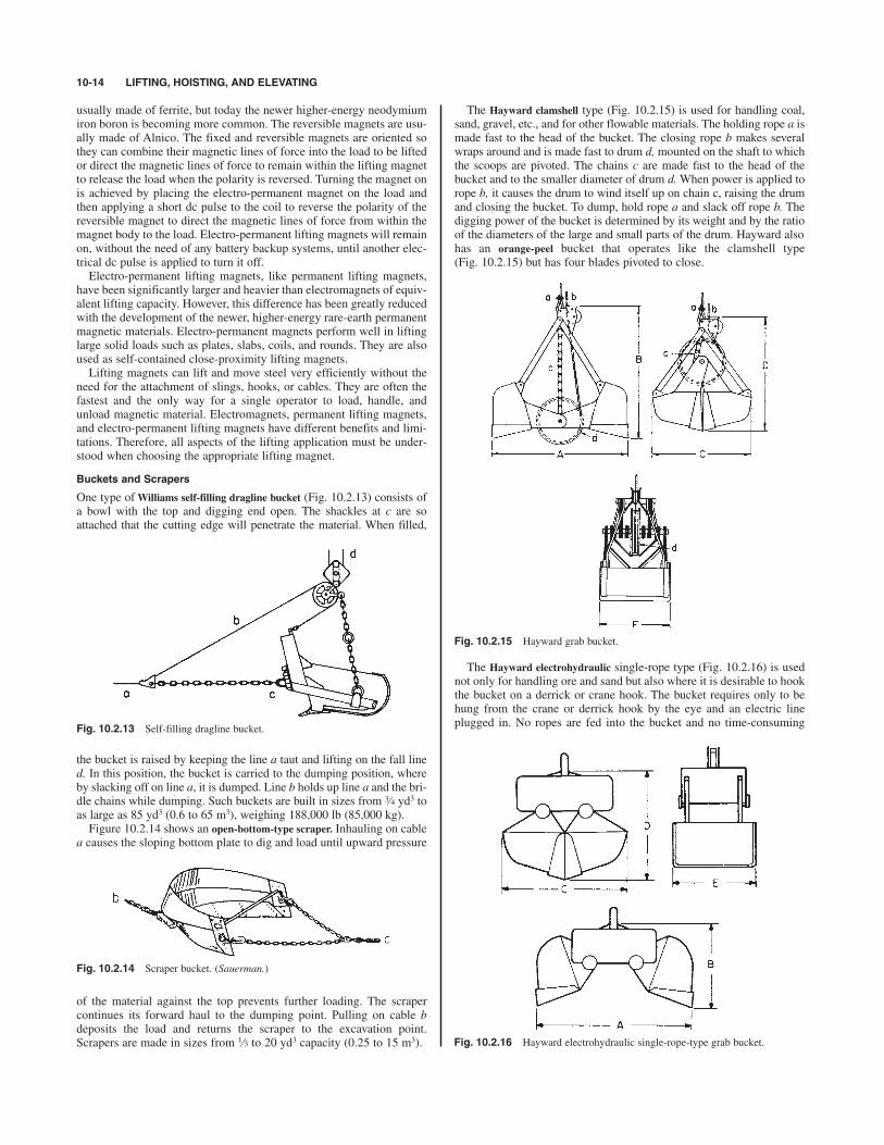
The Hayward clamshell type (Fig. 10.2.15) is used for handling coal,sand, gravel, etc., and for other flowable materials. The holding rope a ismade fast to the head of the bucket. The closing rope b makes severalwraps around and is made fast to drum d, mounted on the shaft to whichthe scoops are pivoted. The chains c are made fast to the head of thebucket and to the smaller diameter of drum d.When power is applied torope b, it causes the drum to wind itself up on chain c, raising the drumand closing the bucket. To dump, hold rope a and slack off rope b. Thedigging power of the bucket is determined by its weight and by the ratioof the diameters of the large and small parts of the drum. Hayward alsohas an orange-peel bucket that operates like the clamshell type(Fig. 10.2.15) but has four blades pivoted to close.
10-14 LIFTING, HOISTING, AND ELEVATING
Fig. 10.2.13 Self-filling dragline bucket.
the bucket is raised by keeping the line a taut and lifting on the fall lined. In this position, the bucket is carried to the dumping position, whereby slacking off on line a, it is dumped. Line b holds up line a and the bri-dle chains while dumping. Such buckets are built in sizes from yd3 toas large as 85 yd3 (0.6 to 65 m3), weighing 188,000 lb (85,000 kg).Figure 10.2.14 shows an open-bottom-type scraper. Inhauling on cable
a causes the sloping bottom plate to dig and load until upward pressure
3⁄4
Fig. 10.2.14 Scraper bucket. (Sauerman.)
of the material against the top prevents further loading. The scrapercontinues its forward haul to the dumping point. Pulling on cable bdeposits the load and returns the scraper to the excavation point.Scrapers are made in sizes from to 20 yd3 capacity (0.25 to 15 m3).1⁄3
Fig. 10.2.15 Hayward grab bucket.
The Hayward electrohydraulic single-rope type (Fig. 10.2.16) is usednot only for handling ore and sand but also where it is desirable to hookthe bucket on a derrick or crane hook. The bucket requires only to behung from the crane or derrick hook by the eye and an electric lineplugged in. No ropes are fed into the bucket and no time-consuming
Fig. 10.2.16 Hayward electrohydraulic single-rope-type grab bucket.

HOISTS 10-15
shifting of lines is required—thus facilitating changing from magnet tobucket. The bowls are suspended from the head, which contains a com-plete electrohydraulic power unit consisting of an ac or dc motor,hydraulic pump, directional valve, sump, filters, and cylinders. Whencurrent is turned on, the motor drives the pump which provides systempressure. Energizing the solenoids in the directional valve directs thefluid flow to either end of the cylinders, which are attached to the bladearms, thus opening or closing the bucket. The system uses a pressure-compensated variable-displacement pump which enters a no-deliverymode when system pressure is reached during the closing or openingaction, thus avoiding any heat generation and reducing the load on themotor while maintaining system pressure. The 1 yd3 (0.76 m3) bucket isprovided with a 15-hp (11.2-kW) motor and 15 gal/min (0.95 1/s) pump.The 2 and 3 yd3 (1.5 to 2.3 m3) buckets have motors of 20 to 25 hp(15 to 19 kW), according to duty.
HOISTS
Hand-Chain Hoists
Hand chain hoists are portable lifting devices suspended from a hookand operated by pulling on a hand chain. There are two types currently
in common use, the high-speed, high-efficiency hand hoist (Fig. 10.2.17) andthe economy hand hoist. The economyhand hoist is similar in appearance to thehigh-efficiency hand hoist except thehandwheel diameter is smaller. Thissmaller diameter accounts for a smallerheadroom dimension for the economyhoist. High-speed hoists have mechanicalefficiency as high as 80 percent, employWeston self-energizing brakes for loadcontrol, and can incorporate load-limitingdevices which prevent the lifting of exces-sive overloads. They require less handchain pull and less chain overhaul formovement of a given load at the expenseof the larger head size when compared toeconomy hoists. As noted, this larger headsize also creates a minimum headroomdimension somewhat greater than that forthe economy hoists. High-speed hoistsfind application in production operationswhere low operating effort and long lifeare important. Economy hoists find appli-cation in construction and shop use wheremore compact size and lower unit costcompensate for the higher operating effortand lower efficiency.Both hoist types function in a similar
manner. The hand chain operates over ahandwheel which is connected via thebrake mechanism and gear train to apocket wheel over which the load chaintravels. The brake is disengaged duringhoisting by a one-way ratchet mecha-
nism. In lowering, the hand chain is pulled continuously in a reversedirection to overcome brake torque, thus allowing the load to descend.Although a majority of hand chain hoist applications are fixed hook-
suspended applications, sometimes a hand hoist is mounted to a trolleyto permit horizontal movement of the load, as in a forklift battery-changing operation. This is accomplished by directly attaching the hoisthook to the trolley load bar, or by using an integrated trolley hoist whichcombines a high-speed hoist with a trolley to save headroom(Fig. 10.2.18).Hand chain hoists are available in capacities to 50 tons (45 tonnes).
Tables 10.2.8 and 10.2.9 provide data for high-speed and economyhoists in readily available capacities to 10 tons (9 tonnes), respectively.
Pullers or Come-Alongs
Pullers, or come-alongs, are lever-operated chain or wire rope hoists(Fig. 10.2.19). Because they are smaller in size and lower in weight than
equivalent capacity hand chain hoists,they find use in applications where thetravel (take-up) distance is short and thelever is within easy reach of the opera-tor. They may be used for lifting orpulling at any angle as long as the loadis applied in a straight line betweenhooks. There are two types of lever-operated chain or wire rope hoists cur-rently in use: long handle and shorthandle. The long-handle variety,because of direct drive or numericallylower gear ratios, allows a greater loadchain take-up per handle stroke than theshort-handle version. Conversely, theshort-handle variety requires less han-dle force at the expense of chain take-up distance because of numericallyhigher gear ratios. Both types find usein construction, electrical utilities andindustrial maintenance for wire ten-
sioning, machinery skidding, and lifting applications.A reversible ratchet mechanism in the lever permits operation for both
tensioning and relaxing. The load is held in place by a Weston-type brakeor a releasable ratchet. Lever tools incorporating load-limiting devices viaslip clutch, spring deflection, or handle-collapsing means are also avail-able. Table 10.2.10 provides data for lever operated chain hoists.
Electric Hoists
Electric hoists are used for repetitive or high-speed lifting. Two typesare available: chain (see Fig. 10.2.20) (both link and roller), in capaci-ties to 15 tons (13.6 tonnes); wire rope (see Fig. 10.2.21), in ratings to25 tons (22.7 tonnes). The typical hoist has a drum or sprocket centeredin the frame, with the motor and gearing at opposite ends, the motorshaft passing through or alongside the drum or sprocket. Many have anintegral load-limiting device to prevent the lifting of gross overloads.Electric hoists are equipped with at least two independent braking
means. An electrically released brake causes spring-loaded disk brake
Fig. 10.2.17 High-speed
hand hoist. (CM Hoist Div.,
Columbus McKinnon.)
Fig. 10.2.18 Trolley hoist. Shown with hand chain removed for clarity. (CM
Hoist Div., Columbus McKinnon.)
Fig. 10.2.19 Puller or come-
along hoist. (CM Hoist Div.,
Columbus McKinnon.)

10-16 LIFTING, HOISTING, AND ELEVATING
Table 10.2.8 Typical Data for High-Speed Hand Chain Hoists with 8-ft Chain Lift
Hand chain pull Retracted distance Hand chain
Capacity to lift rated between hooks overhaul to lift
capacity load (headroom) Net weight load 1 ft
short
tons tonnes lb kg in mm lb kg ft m
0.23 23 10.4 13 330.2 33 15.0 22.5 6.9
0.45 46 20.9 13 330.2 33 15.0 22.5 6.9
1 0.91 69 31.3 14 355.6 36 16.3 30 9.1
1.36 80 36.3 17.5 444.5 59 26.8 40.5 12.3
2 1.81 83 37.6 17.5 444.5 60 27.2 52 15.8
3 2.7 85 38.6 21.5 546.1 84 38.1 81 24.7
4 3.6 88 39.9 21.5 546.1 91 41.3 104 31.7
5 4.5 75 34.0 24.5 622.3 122 55.3 156 47.5
6 5.4 90 40.8 25.5 647.7 127 57.6 156 47.5
8 7.3 89 40.3 35.5 901.7 207 93.9 208 63.4
10 9.1 95 43.1 35.5 901.7 219 99.3 260 79.2
SOURCE: CM Hoist Division, Columbus McKinnon.
11⁄2
1⁄2
1⁄4
Fig. 10.2.21 Electric wire-rope hoist. (CM Hoist Div., Columbus McKinnon.)
Table 10.2.9 Typical Data for Economy Hand Chain Hoist with 8-ft Chain Lift
Hand chain pull Retracted distance Hand chain
Capacity to lift rated between hooks overhaul to lift
capacity load (headroom) Net weight load 1 ft
short
tons tonnes lb kg in mm lb kg ft m
0.45 45 20 10 254 15 7 32 9.8
1 0.91 74 34 12 305 22 10 39 11.9
2 1.81 70 32 17 432 53 24 77 23.5
3 2.7 54 25 22 559 69 31 154 46.9
5 4.5 88 40 24 610 74 34 154 46.9
10 9.1 90 41 32 813 139 63 308 93.9
SOURCE: CM Hoist Division, Columbus McKinnon.
1⁄2
Table 10.2.10 Typical Data for Short- and Long-Handle Lever-Operated Chain Hoists
Retracted
distance Handle pull to lift
between rated capacity Net weight*
Capacity hooks
(headroom) Short Long Short Long
shorttons tonnes in mm lb kg lb kg lb kg lb kg
0.68 11 279 35 15.8 58 26.3 18 8.2 14 6.4
1.4 14 356 40 18.1 83 37.6 27 12.2 24 10.9
3 2.7 18 457 73 33.1 95 43.1 45 20.4 44 20.0
6 5.4 23 584 77 35.0 96 43.5 66 30.0 65 29.5
* With chain to allow 52 in (1322 mm) of hook travel.SOURCE: CM Hoist Division, Columbus McKinnon.
11⁄2
3⁄4
Fig. 10.2.20 Electric chain hoist. (CM Hoist Div., Columbus McKinnon.)

HOISTS 10-17
electric hoists have upper-limit devices; lower-limit devices are standardon chain hoists, optional on wire-rope hoists. Control is usually by pushbutton: pendant ropes from the controller are obsolescent. Control is“deadman” type, the hoist stopping instantly upon release. Modernmultiple-speed and variable-speed ac controls have made dc hoists obso-lete. Single-phase ac hoists are available to 1 hp, polyphase in all sizes.The hoist may be suspended by an integral hook or bolt-type lug or may
be attached to a trolley rolling on an I beam or monorail. The trolley maybe plain (push type), geared (operated by a hand chain), or motor-driven;the latter types are essential for heavier loads.Table 10.2.11 gives data forelectric chain hoists, and Table 10.2.12 for wire-rope hoists.
plates to engage when current is off. When the hoist motor is activated,a solenoid overcomes the springs to release the brake. In the loweringdirection, the motor acts as a generator, putting current back into the lineand controlling the lowering speed. Some electric hoists use the sametype of Weston brake as is used in hand hoists, but with this type, themotor must drive the load downward so as to try to release the brake.This type of brake generates considerable heat that must be dissipated—usually through an oil bath. The heat generated may also lower the use-ful-duty cycle of the hoist. If the Weston brake is used, an additionalauxiliary hand-released or electrically released friction brake must beprovided since the Weston brake will not act in the raising direction. All
Table 10.2.11 Typical Data for Electric Chain Hoists*
Retracted distance
between hooks
Capacity Lifting speed (headroom) Net weight Motor
short tons tonnes ft/min m/min in mm lb kg hp kW
0.11 32 10 15 381 62 28 0.19
0.11 60 18 15 381 68 31 0.37
0.23 16 5 15 381 62 28 0.19
0.23 32 10 15 381 68 31 0.37
0.45 8 2.5 18 457 73 33 0.19
0.45 16 5 15 381 68 31 0.37
0.45 32 10 16 406 114 52 1 0.75
0.45 64 20 16 406 121 55 2 1.49
1 .91 8 2.5 18 457 79 36 0.37
1 .91 16 5 16 406 114 52 1 0.75
1 .91 32 10 16 406 121 55 2 1.49
2 1.81 8 2.5 23 584 139 63 1 0.75
2 1.81 16 5 23 584 146 66 2 1.49
3 2.7 5.5 1.5 25 635 163 74 1 0.75
3 2.7 11 3.3 25 635 170 77 2 1.49
5 4.5 10 3 37 940 668 303 5 3.73
5 4.5 24 7 37 940 684 310 5.59
6.8 7 2 40 1016 929 421 5 3.73
6.8 16 5 40 1016 957 434 5.59
10 9.1 7 2 42 1067 945 429 5 3.73
10 9.1 13 4 42 1067 961 436 5.59
15 13.6 4 1.2 48 1219 1155 524 5 3.73
15 13.6 8 2.5 48 1219 1167 529 5.59
*Up to and including 3-ton hook suspended with 10-ft lift. 5- through 15-ton plain trolley suspended with 20-ft lift. Headroom distance is beam to high hook.SOURCE: CM Hoist Division, Columbus McKinnon Corporation.
71⁄2
71⁄2
71⁄271⁄2
71⁄2
71⁄2
1⁄2
1⁄2
1⁄2
1⁄21⁄2
1⁄41⁄2
1⁄21⁄4
1⁄41⁄4
1⁄21⁄8
1⁄41⁄8
Table 10.2.12 Typical Data for Electric Wire Rope Hoists*
Beam to
high hook
Capacity Lifting speed distance Net weight Motor
short tons tonnes ft/min m/min in mm lb kg hp kW
0.45 60 18 27 686 430 195 4.5 3.36
0.68 37 11 27 686 430 195 4.5 3.36
1 0.91 30 9 25 635 465 211 4.5 3.36
1 0.91 37 11 27 686 435 197 4.5 3.36
1 0.91 60 18 27 686 445 202 4.5 3.36
1.36 18 5.5 25 635 465 211 4.5 3.36
1.36 30 9 25 635 465 211 4.5 3.36
1.36 37 11 27 686 445 202 4.5 3.36
2 1.81 18 5.5 25 635 465 211 4.5 3.36
2 1.81 30 9 25 635 480 218 4.5 3.36
3 2.7 18 5.5 25 635 560 254 4.5 3.36
5 4.5 13 4 30 762 710 322 4.5 3.36
6.8 15 4.6 36 914 1100 499 7.5 5.59
10 9.1 13.5 4.1 40 1016 1785 810 10 7.46
15 13.6 13 4 49 1245 2510 1139 15 11.19
*Up to and including 5-ton with plain trolley. - to 15-ton with motor-driven trolley.SOURCE: CM Hoist Division, Columbus McKinnon.
71⁄2
71⁄2
11⁄2
11⁄2
11⁄2
3⁄4
1⁄2

Air Hoists
Air hoists are similar to electric hoists except that air motors are used.Hoists with roller chain are available to 1 ton capacity, with link chain to3 short tons (2.7 tonnes), and with wire rope to 15 short tons (13.6 tonnes)capacity. The motor may be of the rotary-vane or piston type. Thepiston motor is more costly but provides the best starting and low-speedperformance and is preferred for larger-capacity hoists. A brake, inter-locked with the controls, automatically holds the load in neutral; con-trol movement releases the brake, either mechanically or by airpressure. Some air hoists also include a Weston-type load brake. Thehoist may be suspended by a hook, lug, or trolley; the latter may beplain, geared, or air-motor-driven. Horizontal movement is limited toabout 25 ft (7.6 m) because of the air hose, although a runway systemis available with a series of normally closed ports that are opened by aspecial trolley to supply air to the hoist.Air hoists provide infinitely variable speed, according to the movement
of the control valve. Very high speeds are possible with light loads.When severely overloaded, the air motor stalls without damage. Airhoists are smaller and lighter than electric hoists of equal capacity andcan be operated in explosive atmospheres. They are more expensivethan electric hoists, require mufflers for reasonably quiet operation, andnormally are fitted with automatic lubricators in the air supply.
Jacks and Power Screw Actuators
Jacks are portable, hand-operated devices for moving heavy loadsthrough short distances. There are three types in common use: screwjacks, ratchet jacks, and hydraulic jacks. Bell-bottom screw jacks(Fig. 10.2.22) are available in capacities to 24 tons and lifting ranges to14 in. The screw is rotated by a bar inserted in holes in the screw head.Geared journal jacks will lift up to 75 short tons (68 tonnes). A leverratchet mechanism turns a pinion which drives a gear affixed to a liftingscrew causing an internally threaded nut affixed to the jack head to travel.Ductile iron jacks (Fig. 10.2.23) consist of a cast-steel housing in which
are: translating screw, rotating screw (translating nut), and translatingtube. Gearing types are: worm gearing, bevel gearing, and spur/helicalgearing. Mounting methods are: base mounting, trunnion mounting andclevis mounting. Available options include: stop nuts, bellows boots,limit switches, motor mounts, and integral speed reducers and motors.Perhaps the greatest single advantage of power screw actuators is thatmultiple units can be tied together mechanically for synchronized trav-el. Power screw actuators are of three basic types.Machine screw actuators (Fig. 10.2.25) feature a sliding-contact
power thread (ACME, STUB ACME, modified square, or metric trape-zoidal) mechanism. Advantages are: lowest cost, self-locking opera-tion (most machine screw actuators will not backdrive), quietestoperation, availability of widest range of lifting capacities, availabilityof internal keying of translating screw models, availability of anantibacklash feature (to control power screw axial free movement), andavailability of stainless steel construction. Disadvantages are: lowestefficiency, lowest duty cycle capability, highest power usage, require-ment for largest drives, and increasing backlash from wear during life.Machine screw actuators are available in lifting capacities to 250 tons(228 tonnes).
10-18 LIFTING, HOISTING, AND ELEVATING
Fig. 10.2.25 Upright translating machine screw actuator. (Duff Norton.)
Fig. 10.2.22 Bell-bottom
screw jack.Fig. 10.2.23 Ratchet jack.
the lever pivots. The rack-toothed bar passes through the hollow hous-ing; the load may be lifted either on the top or on a toe extending fromthe bottom of the bar. The lever pawl may be biased either to raise or tolower the bar, the housing pawl holding the load on the return leverstroke. Track jacks are ratchet jacks that may be tripped to release theload. They are used for railroad-track work but not for industrial servicewhere the tripping features might be hazardous. Hydraulic jacks(Fig. 10.2.24) consist of a cylinder, a piston, and a lever-operated pump.Capacities to 100 short tons (91 tonnes) and lifting heights to 22 in.(0.56 m) are available. Jacks 25 short tons (22.7 tonnes) and larger maybe provided with two pumps, the second pump being a high-speed unitfor rapid travel at partial load.Power screw actuators are integral gear-driven power screw devices
that convert rotary motion and power into linear movement of a load.Power screw actuators are available in many variations. Configurations
Fig. 10.2.24 Hydraulic jack.
Ball screw actuators (Fig. 10.2.26) feature a rolling contact recirculat-ing ball power thread mechanism. Advantages are: highest efficiency,faster speed capability, highest duty cycle capability, lowest powerusage, requirement for smallest drives, near-constant backlash duringlife, and predictable power thread life. Disadvantages are higher cost

MINE HOISTS AND SKIPS 10-19
and self-lowering operation (most ball screw actuators require brakes toprevent backdriving). Ball screw actuators are available in lifting capac-ities to 50 tons (45 tonnes).Roller screw actuators feature a rolling contact planetary roller
power thread mechanism. Advantages are: higher efficiency, highestload capacity, longest life, highest speed and acceleration capability,high stiffness, high positional accuracy, near-constant backlash dur-ing life, predictable power thread life, and quieter operation.Disadvantages are highest cost and self-lowering operation (mostroller screw actuators require brakes to prevent backdriving). Rollerscrew actuators are available with lifting capacities to 90 tons(82 tonnes).
MINE HOISTS AND SKIPS
by Burt Garofab
Pittston Corporation
There are two types of hoists, the drum hoist and the friction hoist.On a drum hoist, the rope is attached to the drum and is woundaround and stored on the drum. A drum hoist may be single-drum ordouble-drum. There are also several different configurations of boththe single-drum and the double-drum hoist. A drum hoist may befurther divided as either unbalanced, partially balanced, or fullybalanced.On a friction hoist, which is often referred to as a Koepe hoist, the rope
is not wound around the drum, but rather passes over the drum. A fric-tion hoist may utilize a single rope or multiple ropes.The operation of hoists may be controlled manually, automatically, or
semiautomatically. There are also arrangements that use combinationsof the different control types.There are currently three types of grooving being used on new drums
for drum hoists. They are helical grooving, counterbalance (Lebus)grooving, and antisynchronous grooving. Helical grooving is used pri-marily for applications where only a single layer of rope is woundaround the drum. Counterbalance and antisynchronous grooving areused for applications where multiple layers of rope are wound aroundthe drum.Mine hoists are generally divided into (1) metal-mine hoists (e.g., iron,
copper, zinc, salt, gypsum, silver, gold, ores) and (2) coal-mine hoists.These classes subdivide into main hoists (for handling ores or coal) andhoists for men, timbers, and supplies. They are designed for operating
(1) mine shafts, vertical and inclined, balanced and unbalanced; and(2) slopes, balanced and unbalanced. When an empty cage or platformdescends while the loaded cage or platform ascends, as when bothcables are wound on a single drum, the machine is referred to as abalanced hoist. Most medium- and large-sized hoists normally operatein balance, as the tonnage obtained for a given load and rope speed isabout double that for an unbalanced hoist and the power consumptionper ton hoisted is lower. Balanced operation can also be obtained by acounterweight. The counterweight (approximately equal to all thedead loads plus one-half the live load) is usually installed in guideswithin a single shaft compartment. The average depth of ore mines isabout 2,000 ft (610 m), and that of coal mines is close to 500 ft (152 m).Most ore-mine hoists are of the double-drum type, normally hostingin balance, each drum being provided with a friction clutch for chang-ing the relative positions of the two skips when operating from vari-ous levels.Hoists for coal mines are principally of the keyed-drum type, for
operating in balance from one level. For high rope speeds in shallowshafts, it is generally advantageous to use combined cylindrical and con-ical drums. The cylindroconical drum places the maximum rope pull(weight of rope and loaded skip) on the small diameter so that duringthe acceleration period of the cycle, the weight of the opposing skipis offering the greatest counterbalance torque, reducing motor peakloads and slightly reducing the power consumption. The peak reduc-tion obtained becomes greater when shafts are shallower and hoistingspeeds are higher, provided that the proportion between the smallerand the large diameters is increased as these conditions increase. Byvarying the ratio of diameters and the distribution of rope on the drumprofiles with respect to the periods of acceleration, retardation, andconstant speed, static and dynamic torques can be modified to pro-duce the most economical power consumption and the minimum sizeof motor. The conical drum is not applicable for multiple-level oper-ation, and except in very special cases, only a single layer of rope canbe used.Skip hoists for industrial purposes such as power-plant fuel handling
and blast-furnace charging are similar to shallow-lift slow-speedcoal-mine hoists in that they operate from a single level. Speeds of 100to 400 ft/min (0.5 to 2 m/s) are usual. For blast-furnace charging withcombined bucket and load weights up to 31,000 lb (14,000 kg) and aspeed of 500 ft/min (2.5 m/s), modern plants consist of straight-drumgeared engines, frequently with Ward Leonard control.Industrial skip hoists may be specified where the lift is too high for a
bucket elevator, where the lumps are too large for elevator buckets, orwhere the material is pulverized and extremely abrasive or actively cor-rosive. For high lifts having a vertical or nearly vertical path, the skipwith supporting structure usually costs less than a bucket elevator or aninclined-belt conveyor with bridge. Typical paths are shown inFig. 10.2.27, paths C and D being suitable when the load is receivedthrough a track hopper.
Fig. 10.2.26 Inverted rotating ball screw actuator. (Duff Norton.)
Fig. 10.2.27 Typical paths for skip hoists. (a) Vertical with discharge to
either side; (b) straight inclined run; (c) incline and vertical; (d) incline, vertical,
incline.

The skip may be manually loaded direct from a dump car orautomatically loaded by a pivoted chute, which is actuated by the bucketand which, when upturned, serves as a cutoff gate (Fig. 10.2.28).For small capacities, the skip can be manually loaded with semiauto-
matic control. When the bucket has been filled, the operator pushes thestart button and the bucket ascends, dumps, and returns to loading posi-tion. With automatic loading and larger capacity, the skip may have full automatic control. For economy, the bucket is counterbalanced by aweight, usually equaling the weight of the empty bucket plus half theload. For large capacity, a balanced skip in which one bucket rises as theother descends may be used. High-speed skips usually have automaticslowdown (two-speed motor) as the bucket nears the loading and dis-charge points.
Conservative maximum hoisting speeds, as recommended by Bu. MinesBull. 75, are as follows:
10-20 LIFTING, HOISTING, AND ELEVATING
Fig. 10.2.28 Automatic loader (in loading position).
There are various types of wire ropes used in hoisting. Hoist ropescan be categorized into three main types: round strand, flattened strand,and locked coil. Round strand rope is used on drum hoists in applica-tions when a single layer of rope is wound on the drum. Flattened strandrope is used on drum hoists when multiple layers of rope are wound onthe drum. Flattened strand rope can also be used on friction hoists.Locked coil rope is used on friction hoists.Plow steel and improved plow steel are the most commonly used
grades; the latter is used where the service is severe. Some state miningregulations require higher factors of safety than the usual hoistingrequirements. The working capacity of new ropes is usually computedby using the minimum breaking strength given in the manufacturer’stables and the following factors of safety: rope lengths of 500 ft (152 m)or less, minimum factor 8; 500 to 1,000 ft (152 to 305 m), 7; 1,000 to2,000 ft (305 to 610 m), 6; 2,000 to 3,000 ft (610 to 914 m), 5; 3,000 ft(914 m) or over, . These are gross factors between the rated mini-mum breaking strength of the rope and the maximum static pull due tosuspended load plus rope weight. The net factor, which should be usedin dealing with large capacities and great depth, must take into consid-eration stresses due to acceleration and bending around the drum,together with suitable allowances for shock. With 6-by-19 wire con-struction, the pitch diameter of the drums is generally not less than sixtytimes the diameter of the rope. Drums are made of either cast iron orcast steel machine-grooved to suit the size of rope (see above). In largehoists, a lifting device is installed at the free rope end of the drum toassist the rope in doubling back over the first layer.Brakes There are three main types of brakes used on hoists: the jaw
brake, the parallel motion brake, and disk brakes. Brake control is accom-plished through air or hydraulics. Brake shoes are steel with attachedfriction material surfaces. Hoist Motors Determining the proper size of motor for driving a
hoist calls for setting up a definite cycle of duty based upon the requireddaily or hourly tonnage.The permissible hoisting speed for mine hoists largely depends upon the
depth of the shaft; the greater the depth, the higher the allowable speed.
41⁄2
Depth of shaft Hoisting speed
ft m ft/min m/s
500 or less 150 or less 1,200 6
500–1,000 150–300 1,600 8
1,000–2,000 300–600 2,000 10
2,000–3,000 600–900 3,000 15
High hoisting speeds call for rapid acceleration and retardation. Forsmall hoists, the rate of acceleration may be made as low as 0.5 ft/s2
(0.15 m/s2). An average value of 3 ft/s2 is adopted for large hoists withfairly high speeds. Exceptional cases may require up to 6 ft/s2 (1.9 m/s2).The speed should also be considered with regard to the weight of thematerial to be hoisted per trip. The question of whether the load shouldbe increased and the speed reduced or vice versa is controlled by localconditions, mining laws, and practical experience. The rest periodassigned to the duty cycle, i.e., the requisite time for loading at the bot-tom and unloading at the top, is dependent upon the equipmentemployed. With skips loaded from underground ore-storage hoppers, 5to 6 s is the minimum that can be assumed. Unless special or automaticprovision is made, the loading time should be taken as 8 to 10 s mini-mum. When the (1) hoisting speed, (2) weight of skip or cage, (3) weightof load, (4) periods of acceleration, (5) retardation, and (6) time for load-ing have been decided upon, the next step is to ascertain the “root-mean-square” equivalent continuous load-heating effect on the motor, takinginto account rope and load weights, acceleration and deceleration of allhanging and rotating masses, and friction of sheaves, machines, etc. Thefriction load is usually taken as constant throughout the running periodof the cycle. The overall efficiency of the mechanical parts of a single-reduction-geared hoist averages 80 percent; that of a first-motion hoist iscloser to 85 percent. The motor selected must have sufficient startingtorque to meet the temporary peaks of any cycle, including, in the caseof balanced hoists, the requirements of trips out of balance.Electrical equipment for driving mine hoists is of four classes:1. Direct-current motors with resistance control for small hoists, usu-
ally series-wound but occasionally compound-wound in conjunctionwith dynamic braking control.2. Alternating-current slip-ring-type motor with secondary resis-
tance.3. Ward Leonard system of control for higher efficiency, particularly
on short lifts at high rope speeds, where the rheostatic losses duringacceleration and retardation represent a large proportion of the net workdone during the cycle; for accuracy of speeds, with high-speed hoists;and for equalization of power demands. Complete control of the speedfrom standstill to maximum is obtained for all values of load from max-imum positive to maximum negative. The lowering of unbalanced loadswithout the use of brakes is as readily accomplished as hoisting.4. The Ilgner Ward Leonard system consists of a flywheel directly
connected to a Ward Leonard motor-generator set and a device for auto-matically varying the speed through the secondary rheostatic control ofthe slip-ring induction motor driving the set. This form of equipment isused under conditions that prohibit the carrying of heavy loads or wherepower is purchased under heavy reservation charges for peak loads. Itlimits the power taken from the supply circuit to a certain predeter-mined value; whatever is required in excess of this value is produced bythe energy given up by the flywheel as its speed is reduced.
ELEVATORS, DUMBWAITERS, ESCALATORS
by Louis Bialy
Otis Elevator Corporation
The advent of the safety elevator changed the concept of the city by mak-ing high-rise buildings possible. Elevators are widely used to transport

ELEVATORS, DUMBWAITERS, ESCALATORS 10-21
passengers and freight vertically or at an incline in buildings and struc-tures. Elevators are broadly classified as low-rise, medium-rise, and high-rise units. Low-rise elevators typically serve buildings with between 2and 7 floors, medium-rise elevators serve buildings with between 5 and20 floors, while high-rise elevators serve buildings with more than15 floors. The speed of the elevator is indexed to the rise of the buildingso that the overall flight time from bottom to top, or vice versa, is approx-imately the same. A typical flight time is about one minute. Typical speedsfor low-rise elevators are up to 200 ft/min (1.0 m/s). Typical speeds formedium rise elevators are up to 400 ft/min (2.0 m/s). High rise elevatorstypically travel at speeds of up to 1,800 ft/min (9.0 m/s).Low rise elevators are usually oil-power hydraulic devices. The sim-
plest version consists of a hydraulic jack buried in the ground beneaththe elevator car. The jack is approximately centrally located beneath thecar and the ram or plunger is connected to the platform or structurewhich supports the car. The car is guided by guiderails which coverthe full rise of the elevator hoistway. Guideshoes or guiderollers typi-cally guide the elevator as it ascends and descends the hoistway. Thehydraulic cylinder is equipped with a cylinder head which houses theseals and bearing rings which locate the ram. The ram typically runsclear of the inner cylinder wall. Buried cylinders are typically protectedagainst corrosion.Hydraulic power is usually supplied by a screw-type positive-
displacement pump driven by an induction motor. It is common for themotor and pump to be coaxially mounted and submersed in the hydraulicreservoir. Operating pressures are typically 300 to 600 lb/in2 (2 to 4 MPa).A hydraulic control valve controls the flow of oil to the hydraulic jackand hence the speed of the elevator. In the down direction, the pump isnot powered, and the elevator speed is controlled by bleeding fluidthrough the control valve.Another manifestation of the hydraulic elevator is called the holeless
hydraulic elevator. These typically have one or more hydraulic jacksmounted vertically alongside the elevator car, the plunger being eitherdirectly attached to the car or connected to the car by steel wire cables(also known as wire ropes). Elevators of the latter type are known asroped hydraulic elevators. These elevators are often roped 1 : 2 so that theelevator moves at twice the speed of the hydraulic ram. The rise of theelevator is also twice the stroke of the ram. Holeless hydraulic elevatorswith the ram directly connected to the elevator car may have single-stagejacks or multistage telescopic jacks, depending on the required rise.Medium- and high-rise elevators are typically traction-driven units,
i.e., the rotary motion of the drive sheave is transmitted to the suspen-sion system via friction. The suspension system usually comprises steelwire cables or ropes, although other systems are emerging. Example ofthese include: ropes manufactured from synthetic fibers (such asaramid) encased in an elastomeric jacket and flat belts comprising sev-eral steel wire cords (each consisting of multiple wires) encased in anelastomeric coating. The elevators are typically counterweighted so thatthe motor and drive need overcome only the unbalanced load. The coun-terweight mass is typically the car mass plus approximately half the dutyload (load of passengers or freight). With high-rise elevators, the weightof the rope is neutralized by compensating chains hung from the under-side of the counterweight and looped to the bottom of the car. If thecompensation weight matches the suspension rope weight, then irre-spective of the position of the car, there will be no imbalance due torope weight. The drive sheave is usually grooved to guide the rope andenhance the traction. Roping ratios may be 1 : 1 or 2 : 1. With 1 : 1 ratiosthe car speed is the same as the rope speed. With 2 : 1 ratios the eleva-tor speed is half of the rope speed.Medium-rise elevators are typically driven by geared machines that
transmit the motor power to the drive sheave. Gear reduction ratios aretypically in the range from 12 : 1 to 30 : 1.Right-angle worm reduction gear sets are most common; however,
helical gears are also used. These have higher operating efficiency andlow wear characteristics.High-rise elevators are typically driven by gearless machines which
provide the smoothest and most precise performance of all elevators(see Fig. 10.2.29).
Fig. 10.2.29 Electric traction elevator.
Motors AC motors have virtually completely replaced dc motors topower the driving sheave on new elevators. A large population of dcmotors still exists on old elevators, and some new elevators still use thistechnology. Direct current motors have the advantages of good startingtorque and ease of speed control. Elevator motors are obliged to developdouble-rated torques at 125 percent rated current and have frequentstarts, stops, reversals, and runs at constant speed. With sparkless commu-tation required under all conditions, commercial motors cannot as a rulemeet these requirements. For constant voltage, cumulative-compoundmotors with heavy series fields are used. The series fields are gradual-ly short-circuited as the motor comes up to speed, after which the motoroperates shunt. The shunt field is excited permanently, the current beingreduced to a low value with increased resistance instead of the circuitopening when the motor is not in operation.Drive Control for DC Motors The relatively few new elevators
being supplied with dc drive motors are equipped with thyristor [siliconcontrolled rectifier (SCR)] drive controls. Older elevators still opera-tional in the field are equipped with Ward Leonard (voltage control)systems using motor/generator sets. With voltage control, an individualdc generator is used for each behavior. The generator may be driven byeither a dc or an ac motor (see Ward Leonard and Ilgner systems,above).AC Motor and Control Squirrel-cage induction motors are exten-
sively used for elevators because of their ruggedness and simplicity.The absence of brushes is considered a distinct advantage. The motorsare typically three-phase machines driven by variable-voltage, variable-frequency (VVVF) drives. The VVVF current is provided by an inverter.High-current-capacity power transistors modulate the power to themotor. Motion of the rotor or the elevator is often monitored by devicessuch as optical encoders that provide feedback to the control system forclosed loop control. Permanent-magnet-rotor synchronous motors withwound field coils are becoming more prevalent for elevator use,because of their high efficiency, compact design, and reliability. Theseare invariably driven by VVVF drives.Elevators installed in the United States are usually required to com-
ply with the ANSI/ASME A17.1 Safety Code or other applicable localcodes. The A17.1 code imposes specific safety requirements pertainingto the mechanical, structural, and electrical integrity of the elevator.Examples of code requirements include: factors of safety for mechanicaland structural elements; the number and type of wire ropes to be used;the means of determining the load capacity of the elevator; the require-ments for speed governors and independent safety devices to arrest thecar should the car descend at excessive speeds; the requirements forbrakes to hold the stationary car with loads of up to 125 percent of ratedload; the requirements for buffers at the bottom of the elevator shaft todecelerate the elevator or counterweight should they descendbeyond the lowest landing; the type and motion of elevator and hoist-way doors; the requirement that doors not open if the elevator is not ata landing; the requirement that door motion cease or reverse if a pas-senger or obstruction is in their path and that the kinetic energy of the

door motion be limited so as to minimize the impact with a passengeror obstruction should they fail to stop in time. The code also requireselectrical protective devices which stop the car should it transcendeither upper or lower terminal landings, remove power to the motor, andcause the brake to apply should the speed exceed governor settings, etc.The A17.1 code also provides special requirements for elevators locat-ed in high seismic risk zones.Loads Table 10.2.13 shows the rated load of passenger elevators.
Operational Control of Elevators Most modern passenger elevatorsare on fully automatic group collective control. Each group of elevatorsis controlled by a dispatching system which assigns specific elevators toanswer specific hall calls. Modern dispatch systems are microprocessor-based or have some equivalent means of processing information so thateach call registered for an elevator is answered in a timely manner. Thedetermination as to which elevator is assigned to answer a specific callis a complex process which in the case of microprocessor-controlleddispatch systems requires the use of sophisticated algorithms whichemulate the building dynamics. Some dispatch systems use advanceddecision-making processes based on artificial intelligence such asexpert systems and fuzzy logic to optimize group collective service inbuildings. With better dispatching systems it is possible to achieveexcellent elevator service in buildings with the minimum number of ele-vators, or the efficient service of taller buildings without devoting morespace to elevators.The operational control systems also provide signals for door open-
ing and closing.Dumbwaiters follow the general design philosophy of elevators except
that code requirements are somewhat more relaxed. For example, roller-link chain can be used for support instead of wire rope. Moreover, a sin-gle steel wire rope can be used instead of the mandatory minimum ofthree for traction-type elevators and two for drum-type elevators.Dumbwaiters are not intended for the transportation of people.Escalators have the advantages of continuity of motion, great capaci-
ty, and small amounts of space occupied and current consumed for eachpassenger carried. Escalators are built with step widths of 24, 32, and40 in (610, 810, and 1015 mm). The angle of incline is 308 from the hor-izontal, and the speed is 90 to 120 ft/min (0.45 to 0.6 m/s).Approximate average handling capacities for escalators traveling at
90 ft/min are 2,000, 2,300, and 4,000 passengers per hour for 24-in, 32-in,and 40-in (610-, 810-, and 1015-mm) escalator step sizes, respectively.Higher-speed escalators have proportionally higher passenger-carryingcapacity.Escalators are equipped with a handrail on each side, mounted on the
balustrade. The handrail moves at the same speed as the escalator.Escalator steps are so arranged that as they approach the upper andlower landings they recede so that they are substantially level with thefloor for safe embarkation and disembarkation of the escalator.
10-22 DRAGGING, PULLING, AND PUSHING
Table 10.2.13 Rated Load of Passenger Elevators
Rated Capacity, lb 2,500 3,500 4,500 6,000 9,000 12,000
kg 1,135 1,590 2,045 2,725 4,085 5,450
Net inside area, ft2 29.1 38.0 46.2 57.7 80.5 103.0
Platform area, m2 2.7 3.5 4.3 5.4 7.5 9.6
Efficiencies and Energy Dissipation per Car Mile The overall effi-ciency and hence the energy dissipation varies greatly from ele-vator to elevator, depending on the design, hoistway conditions, load-ing conditions, acceleration and deceleration profiles, number ofstops, etc.For a load of 2,500 lb (1,130 kg) for geared traction elevators driven
at 350 ft/min (1.75 m/s) by SCR-controlled dc motor or VVVF-con-trolled ac motor, typical values are as follows: efficiency 60 percent,energy dissipation 4.5 kWh (16 MJ).Under same conditions for gearless traction elevators traveling at
700 ft/min (3.5 m/s), the efficiency may be 70 percent and the energydissipation 4 kWh (14.5 MJ).Note that efficiencies are based on net load, i.e., full load minus
overbalance.Car Mileage and Stops (per elevator, 8-h day)Office buildings, local elevators: intensive service, 12 to 20 car miles
(19 to 32 car kilometers), making about 150 regular stops per mileExpress elevators: 20 to 40 car miles (32 to 64 car kilometers), mak-
ing about 75 to 100 regular stops per mileDepartment store elevators: 4 to 8 car miles (6 to 13 car kilometers),
making about 350 regular stops per mile.
10.3 DRAGGING, PULLING, AND PUSHINGby Harold V. Hawkins
revised by Ernst K. H. Marburg and Associates
HOISTS, PULLERS, AND WINCHES
Many of the fundamental portable lifting mechanisms such as hoists orpullers (see above) can also be used forcefully to drag or pull materials.In addition, nonmobile versions, called winches, utilizing hoistingdrums can also be used.
LOCOMOTIVE HAULAGE, COAL MINES
by Burt Garofab
Pittston Corporation
The haulage system of an underground mine is used to transport per-sonnel and material between the face and the portal. It can be subdivid-ed into face haulage and main haulage. The main haulage systemextends from the end of the face haulage system to the outside.Rubber-tired haulage at the coal face was introduced in 1935 and
received further impetus with the introduction of the rubber-tired shuttle
car in 1938. Crawler-mounted loaders and rubber-tired universal coalcutters completed the equipment needed for complete off-track mining.This off-track mining caused a revolution in face haulage, since it elim-inated the expense of laying track in the rooms and advancing the trackas the face of the coal advanced. It also made gathering locomotives ofthe cable-reel, crab-reel, and battery types obsolete. Practically all thegathering duty is now performed by rubber-tired shuttle cars, chain con-veyors, extensible belt conveyors, and other methods involving offtrackequipment. Some mines eliminated track completely by having beltconveyors carry the coal to the outside. Most coal mines today utilize a combination of haulage systems.
Personnel and supplies are transported by either rail or rubber-tiredhaulage. Coal is transported by belt or rail, predominantly belt.Locomotives used in rail haulage may be trolley wire powered, battery
powered, or diesel powered. Battery and diesel powered locomotives arecommonly used to transport supplies in mines which utilize belt as themain coal haulage system. Trolley-wire-powered locomotives are

LOCOMOTIVE HAULAGE, COAL MINES 10-23
used when rail is the main coal haulage system. The sleek, streamlined,fast, and easy-riding Jeffrey eight-wheel four-motor locomotives areavailable in 27-, 37-, and 50-short ton (24-, 34-, and 45-tonne) sizes.This type of locomotive has two four-wheel trucks, each having twomotors. The trucks, having Pullman or longitudinal-type equalizerswith snubbers, will go around a 50 ft (15 m) radius curve, have shortoverhang, and provide a very easy ride. This construction is easy on thetrack, with consequent low track-maintenance cost. Speed at full loadranges from 10 to 12.5 mi/h (4.5 to 5.6 m/s), and the maximum safespeed is approximately 30 mi/h (13.4 m/s).The eight-wheel locomotive usually has a box frame; series-wound
motors with single-reduction spur gearing; 10 steps of straight parallel,full electropneumatic contactor control; dynamic braking; 32-V battery-operated control and headlights, with the battery charged automaticallyfrom the trolley; straight air brakes; air-operated sanders; air horn; auto-matic couplers; one trolley pole; two headlights at each end; and blow-ers to ventilate the traction motors. The equipment is located so that itis easily accessible for repair and maintenance.The eight-wheel type of locomotive has, to a great extent, superseded
the tandem type, consisting of two four-wheel two-motor locomotivescoupled together and controlled from the cab of one of the units of thetandem.The older Jeffrey four-wheel-type locomotive is available in 11-, 15-, 20-,
and 27-short ton (10-, 13.6-, 18-, 24.5-tonne) nominal weights. The20- and 27-short ton (18- and 24.5-tonne) sizes have electrical equip-ment very much like that of the eight-wheel-type locomotive. Speedsare also comparable. The 15-short ton (13.6-tonne) locomotive usuallyhas semielectropneumatic contactor control, rather than full electro-pneumatic control, and dynamic braking but usually does not have the32-V battery-operated control. The 11-short ton (10-tonne) locomotivehas manual control, with manual brakes and sanders, although contac-tor control, air brakes, blowers, etc., are optional.Locomotive motors have a horsepower rating on the basis of 1 h at
75"C above an ambient temperature of 40"C. Sizes range from a total of100 hp (75 kW) for the 11-ton (10-tonne) to a total of 720 hp for the50-ton.The following formulas are recommended by the Jeffrey Mining
Machinery Co. to determine the weight of a locomotive required to haul aload. Table 10.3.1 gives haulage capacities of various weights of loco-motives on grades up to 5 percent. The tabulation of haulage capacitiesshows how drastically the tons of trailing load decrease as the gradeincreases. For example, a 50-ton locomotive can haul 1,250 tons trail-ing load on the level but only 167 tons up a 5 percent grade.The following formulas are based on the use of steel-tired or rolled-
steel wheels on clean, dry rail.Weight of locomotive required on level track:
W 5 LsR 1 Ad> s0.3 3 2,000 2 Ad
Weight of locomotive required to haul train up the grade:
Weight of locomotive necessary to start train on the grade:
where W is the weight in tons of locomotive required; R is the frictionalresistance of the cars in pounds per ton and is taken as 20 lb for cars withantifriction bearings and 30 lb for plain-bearing cars; L is the weight ofthe load in tons; A is the acceleration resistance [this is 100 for1 mi/(h % s) and is usually taken at 20 for less than 10 mi/h or at 30 from10 to 12 mi/h, corresponding to an acceleration of 0.2 or 0.3 mi/(h % s)];G is the grade resistance in pounds per ton or 20 lb/ton for each percent ofgrade (25 percent is the running adhesion of the locomotive, 30 percentis the starting adhesion using sand); 2,000 is the factor to give adhesionin pounds per ton.Where the grade is in favor of the load:
To brake the train to a stop on grade:
where B is the braking (or decelerating) effort in pounds per ton andequals 100 lb/ton for a braking rate of 1 mi/(h % s) or 20 lb/ton for abraking rate of 0.2 mi/(h % s) or 30 lb for a braking rate of 0.3 mi/(h % s).The adhesion is taken from a safety standpoint as 20 percent. It is notadvisable to rely on using sand to increase the adhesion, since the sand-boxes may be empty when sand is needed.Time in seconds to brake the train to stop:
Distance in feet to brake the train to a stop:
Storage-battery locomotives are used for hauling muck cars in tunnelconstruction where it is inconvenient to install trolley wires and bondthe track as the tunnel advances. They are also used to some extent inmetal mines and in mines of countries where trolley locomotives are notpermitted. They are often used in coal mines in the United States forhauling supplies. Their first cost is frequently less than that for a trolleyinstallation. They also possess many of the advantages of the trolleylocomotive and eliminate the danger and obstruction of the trolley wire.Storage-battery locomotives are limited by the energy that is stored inthe battery and should not be used on steep grades or where large,continuous overloads are required. Best results are obtained where light
ft 5 [mi/h sstartd 2 mi/h sfinishd] 3 s 3 1.46/2
s 5mi/h sstartd 2 mi/h sfinishddeceleration in mi/sh # sd
W 5 LsG 1 B 2 Rd> s0.20 3 2,000 2 G 2 Bd
W 5 LsG 2 Rd> s0.20 3 2,000 2 Gd
W 5 LsR 1 G 1 Ad> s0.30 3 2,000 2 G 2 Ad
W 5 LsR 1 Gd> s0.25 3 2,000 2 Gd
Table 10.3.1 Haulage Capacities of Locomotives with Steel-Tired or Rolled-Steel Wheels*
Weight of locomotive, tons†
Grade 11 15 20 27 37 50
Level Drawber pull, lb 5,500 7,500 10,000 13,500 18,500 25,000
Haulage capacity, gross tons 275 375 500 675 925 1,250
1% Drawbar pull, lb 5,280 7,200 9,600 12,960 17,760 24,000
Haulage capacity, gross tons 132 180 240 324 444 600
2% Drawbar pull, lb 5,260 6,900 9,200 12,420 17,020 23,000
Haulage capacity, gross tons 88 115 153 207 284 384
3% Drawbar pull, lb 4,840 6,600 8,800 11,880 16,280 22,000
Haulage capacity, gross tons 67 82 110 149 204 275
4% Drawbar pull, lb 4,620 6,300 8,400 11,340 15,540 21,000
Haulage capacity, gross tons 46 63 84 113 155 210
5% Drawbar pull, lb 4,400 6,000 8,000 10,800 14,800 20,000
Haulage capacity, gross tons 31 50 67 90 123 167
* Jeffrey Mining Machinery Co.† Haulage capacities are based on 20 lb/ton rolling friction, which is conservative for roller-bearing cars. Multiply lb by 0.45 to get kg and tons
by 0.91 to get tonnes.
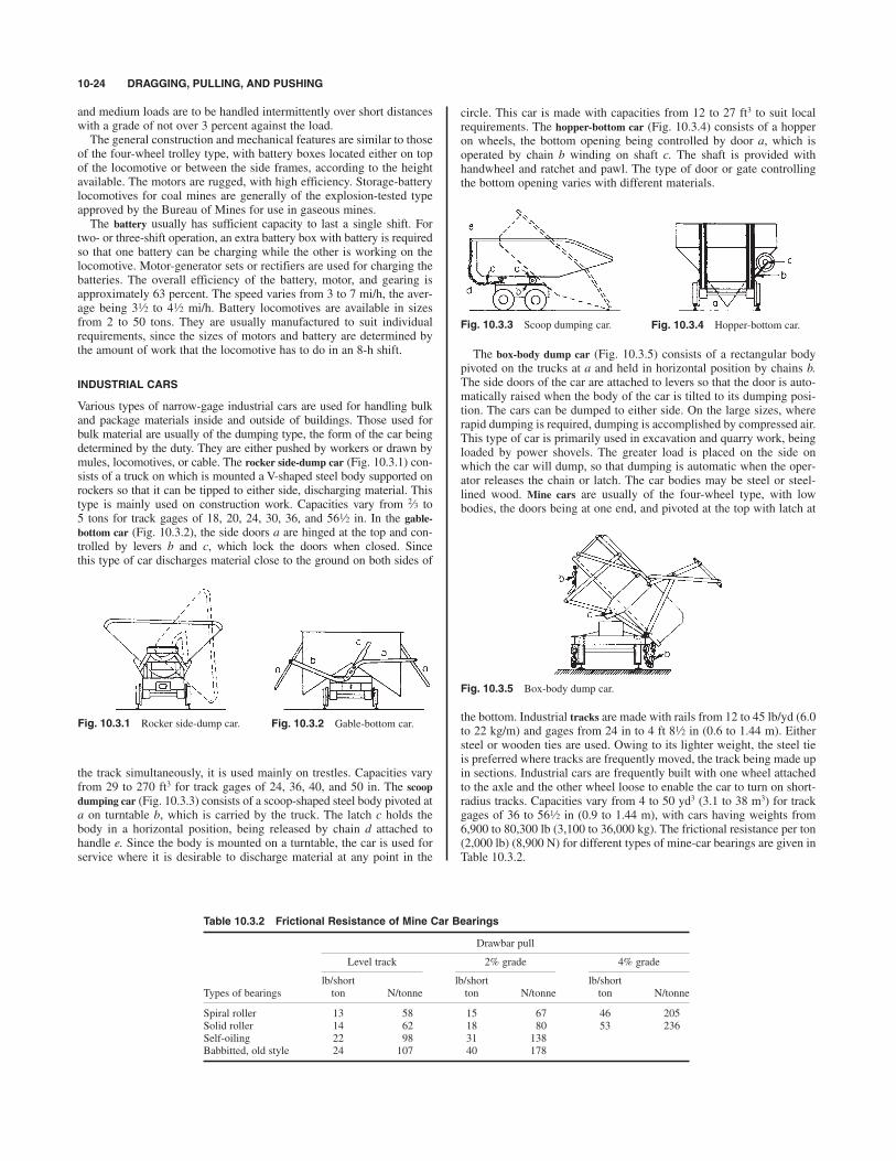
and medium loads are to be handled intermittently over short distanceswith a grade of not over 3 percent against the load. The general construction and mechanical features are similar to those
of the four-wheel trolley type, with battery boxes located either on topof the locomotive or between the side frames, according to the heightavailable. The motors are rugged, with high efficiency. Storage-batterylocomotives for coal mines are generally of the explosion-tested typeapproved by the Bureau of Mines for use in gaseous mines.The battery usually has sufficient capacity to last a single shift. For
two- or three-shift operation, an extra battery box with battery is requiredso that one battery can be charging while the other is working on thelocomotive. Motor-generator sets or rectifiers are used for charging thebatteries. The overall efficiency of the battery, motor, and gearing isapproximately 63 percent. The speed varies from 3 to 7 mi/h, the aver-age being to mi/h. Battery locomotives are available in sizesfrom 2 to 50 tons. They are usually manufactured to suit individualrequirements, since the sizes of motors and battery are determined bythe amount of work that the locomotive has to do in an 8-h shift.
INDUSTRIAL CARS
Various types of narrow-gage industrial cars are used for handling bulkand package materials inside and outside of buildings. Those used forbulk material are usually of the dumping type, the form of the car beingdetermined by the duty. They are either pushed by workers or drawn bymules, locomotives, or cable. The rocker side-dump car (Fig. 10.3.1) con-sists of a truck on which is mounted a V-shaped steel body supported onrockers so that it can be tipped to either side, discharging material. Thistype is mainly used on construction work. Capacities vary from to5 tons for track gages of 18, 20, 24, 30, 36, and in. In the gable-bottom car (Fig. 10.3.2), the side doors a are hinged at the top and con-trolled by levers b and c, which lock the doors when closed. Sincethis type of car discharges material close to the ground on both sides of
561⁄2
2⁄3
41⁄231⁄2
circle. This car is made with capacities from 12 to 27 ft3 to suit localrequirements. The hopper-bottom car (Fig. 10.3.4) consists of a hopperon wheels, the bottom opening being controlled by door a, which isoperated by chain b winding on shaft c. The shaft is provided withhandwheel and ratchet and pawl. The type of door or gate controllingthe bottom opening varies with different materials.
10-24 DRAGGING, PULLING, AND PUSHING
Fig. 10.3.2 Gable-bottom car.Fig. 10.3.1 Rocker side-dump car.
the track simultaneously, it is used mainly on trestles. Capacities varyfrom 29 to 270 ft3 for track gages of 24, 36, 40, and 50 in. The scoopdumping car (Fig. 10.3.3) consists of a scoop-shaped steel body pivoted ata on turntable b, which is carried by the truck. The latch c holds thebody in a horizontal position, being released by chain d attached tohandle e. Since the body is mounted on a turntable, the car is used forservice where it is desirable to discharge material at any point in the
Fig. 10.3.3 Scoop dumping car. Fig. 10.3.4 Hopper-bottom car.
The box-body dump car (Fig. 10.3.5) consists of a rectangular bodypivoted on the trucks at a and held in horizontal position by chains b.The side doors of the car are attached to levers so that the door is auto-matically raised when the body of the car is tilted to its dumping posi-tion. The cars can be dumped to either side. On the large sizes, whererapid dumping is required, dumping is accomplished by compressed air.This type of car is primarily used in excavation and quarry work, beingloaded by power shovels. The greater load is placed on the side onwhich the car will dump, so that dumping is automatic when the oper-ator releases the chain or latch. The car bodies may be steel or steel-lined wood. Mine cars are usually of the four-wheel type, with lowbodies, the doors being at one end, and pivoted at the top with latch at
Fig. 10.3.5 Box-body dump car.
the bottom. Industrial tracks are made with rails from 12 to 45 lb/yd (6.0to 22 kg/m) and gages from 24 in to 4 ft in (0.6 to 1.44 m). Eithersteel or wooden ties are used. Owing to its lighter weight, the steel tieis preferred where tracks are frequently moved, the track being made upin sections. Industrial cars are frequently built with one wheel attachedto the axle and the other wheel loose to enable the car to turn on short-radius tracks. Capacities vary from 4 to 50 yd3 (3.1 to 38 m3) for trackgages of 36 to in (0.9 to 1.44 m), with cars having weights from6,900 to 80,300 lb (3,100 to 36,000 kg). The frictional resistance per ton(2,000 lb) (8,900 N) for different types of mine-car bearings are given inTable 10.3.2.
561⁄2
81⁄2
Table 10.3.2 Frictional Resistance of Mine Car Bearings
Drawbar pull
Level track 2% grade 4% grade
lb/short lb/short lb/short
Types of bearings ton N/tonne ton N/tonne ton N/tonne
Spiral roller 13 58 15 67 46 205
Solid roller 14 62 18 80 53 236
Self-oiling 22 98 31 138
Babbitted, old style 24 107 40 178

CAR-UNLOADING MACHINERY 10-25
DOZERS, DRAGLINES
The dual capability of some equipment, such as dozers and draglines,suggests that it should be mentioned as prime machinery in the area ofmaterials handling by dragging, pulling, or pushing. Dozers are describedin the discussion on earthmoving equipment since their basic frames arealso used for power shovels and backhoes. In addition, dozers performthe auxiliary function of pushing carryall earthmovers to assist themin scraping up their load. Dragline equipment is discussed with below-surface handling or excavation. The same type of equipment that woulddrag or scrape may also have a lifting function.
MOVING SIDEWALKS
Moving horizontal belts with synchronized balustrading have beenintroduced to expedite the movement of passengers to or from railroadtrains in depots or planes at airports (see belt conveyors). A necessaryfeature is the need to prevent the clothing of anyone (e.g., a child) sit-ting on the moving walk from being caught in the mechanism at the endof the walk. Use of a comblike stationary end fence protruding downinto longitudinal slots in the belt is an effective preventive.
CAR-UNLOADING MACHINERY
Four types of devices are in common use for unloading material fromall types of open-top cars: crossover and horn dumps, used to unloadmine cars with swinging end doors; rotary car dumps, for mine carswithout doors; and tipping car dumps, for unloading standard-gage carswhere large unloading capacity is required.Crossover Dump Figure 10.3.6 shows a car in the act of dumping.
Figure 10.3.7 shows a loaded car pushing an empty car off the dump.A section of track is carried by a platform supported on rockers a. Anextension bar b carries the weight c and the brake friction bar d.A handlever controls the brake, acting on the friction bar and placing thedumping under the control of the operator. A section of track e in front
The loaded car b is to one side of the center and causes the cylinder torotate, the material rolling to the chute beneath. The band brake c, withcounterweight d, is operated by lever e, putting the dumping under con-trol of the operator. No power is required; one operator can dump twoor three cars per minute.
Fig. 10.3.7 Crossover dump: empty car being pushed away.
Fig. 10.3.6 Crossover dump: car unloading.
of the dump is pivoted on a parallel motion and counterbalanced so thatit is normally raised. The loaded car depresses the rails e and, throughlevers, pivots the horns f around the shafts g, releasing the empty car.The loaded car strikes the empty car, starting it down the inclined track.After the loaded car has passed the rails e, the springs return the hornsf so that they stop the loaded car in the position to dump. Buffer springson the shaft g absorb the shock of stopping the car. Since the center ofgravity of the loaded car is forward of the rockers, the car will dumpautomatically under control of the brake. No power is required for thisdump, and one operator can dump three or four cars per minute.Rotary Gravity Dump (Fig. 10.3.8) This consists of a steel cylinder
supported by a shaft a, its three compartments carrying three tracks.
Fig. 10.3.8 Rotary gravity dump.
Rotary-power dumpers are also built to take any size of open-top rail-road car and are frequently used in power plants, coke plants, ports, andore mines to dump coal, coke, ore, bauxite, and other bulk material. Theyare mainly of two types: (1) single barrel, and (2) tandem.The McDowell-Wellman Engineering Co. dumper consists of a revolv-
ing cradle supporting a platen (with rails in line with the approach andrunoff car tracks in the upright position), which carries the car to bedumped. A blocking on the dumping side supports the side of the car asthe cradle starts rotating. Normally, the platen is movable and the block-ing is fixed, but in some cases the platen is fixed and the blocking mov-able. Where there is no variation in the car size, the platen and blockingare both fixed. The cradle is supported on two end rings, which arebound with a rail and a gear rack. The rail makes contact with rollersmounted in sills resting on the foundation. Power through the motorrotates the cradle by means of two pinions meshing with the gear racks.The angle of rotation for a complete dump is 155" for a normal opera-tion, but occasionally, a dumper is designed for 180" rotation. Theclamps, supported by the cradle, start moving down as the dumper startsto rotate. These clamps are lowered, locked, released, and raised eitherby a gravity-powered mechanism or by hydraulic cylinders.With the advent of the unit-train system, the investment and operating
costs for a dumper have been reduced considerably. The design ofdumpers for unit train has improved and results in fewer maintenanceproblems. The use of rotary couplers on unit train eliminates uncou-pling of cars while dumping because the center of the rotary coupler isin line with the center of rotation of the dumper.Car Shakers As alternatives to rotating or tilting the car, several
types of car shakers are used to hasten the discharge of the load. Usuallythe shaker is a heavy yoke equipped with an unbalanced pulley rotatedat 2,000 r/min by a 20-hp (15-kW) motor. The yoke rests upon the cartop sides, and the load is actively vibrated and rapidly discharged.While a car shaker provides a discharge rate about half that of a rotarydumper, the smaller investment is advantageous.Car Positioner As the popularity of unit-train systems consisting of
rail cars connected by rotary couplers has increased, more rotary dump-ing stations have been equipped with an automatic train positionerdeveloped by McDowell-Wellman Engineering Company. This deviceconsists of a carriage moving parallel to the railroad track actuated byeither hydraulic cylinders or wire rope driven by a winch, which carriesan arm that rotates in a vertical plane to engage the coupling betweenthe cars. The machines are available in many sizes, the largest of whichare capable of indexing 200-car trains in one- or two-car incrementsthrough the rotary dumper. These machines or similar ones are alsoavailable from FMC/Materials Handling System Division, Heyl andPatterson, Inc., and Whiting Corp.

CONTAINERIZATION
The proper packaging of material to assist in handling can significantlyminimize the handling cost and can also have a marked influence on thetype of handling equipment employed. For example, partial carload lots ofliquid or granular material may be shipped in rigid or nonrigid containersequipped with proper lugs to facilitate in-transit handling. Heavy-duty rub-berized containers that are inert to most cargo are available for repeateduse in shipping partial carloads. The nonrigid container reduces returnshipping costs, since it can be collapsed to reduce space. Disposable light-weight corrugated-cardboard shipping containers for small and medium-sized packages both protect the cargo and permit stacking to economize onspace requirements. The type of container to be used should be planned orconsidered when the handling mechanism is selected.
SURFACE HANDLING
by Colin K. Larsen
Blue Giant Equipment Co.
Lift Trucks and Palletized Loads
The basis of all efficient handling, storage, and movement of unitizedgoods is the cube concept. Building a cube enables a large quantity ofunit goods to be handled and stored at one time. This provides greaterefficiency by increasing the volume of goods movement for a givenamount of work. Examples of cube-facilitating devices include pallets,skids, slip sheets, bins, drums, and crates.The most widely applied cube device is the pallet. A pallet is a low
platform, usually constructed of wood, incorporating openings for theforks of a lift truck to enter. Such openings are designed to enable a lifttruck to pick up and transport the pallet containing the cubed goods.Lift truck is a loose term for a family of pallet handling/transporting
machines. Such machines range from manually propelled low-lift devices(Fig. 10.4.1) to internal combustion and electric powered ride-on high-lift devices (Fig. 10.4.2). While some machines are substitutes in termsof function, each serves its own niche when viewed in terms of indi-vidual budgets and applications.Pallet trucks are low-lift machines designed to raise loaded pallets
sufficiently off the ground to enable the truck to transport the pallet hor-izontally. Pallet trucks are available as manually operated and propelledmodels that incorporate a hydraulic pump and handle assembly(Fig. 10.4.1). This pump and handle assembly enables the operator toraise the truck forks, and push/pull the load. Standard manual pallettrucks are available in lifting capacities from 4,500 to 5,500 lb
(2,045 to 2,500 kg), with customer manufactured models to 8,000 lb(3,636 kg). While available in a variety of fork sizes, by far the most com-mon is 27 in wide ! 48 in long (686 mm ! 1,219 mm). This size accom-modates the most common pallet sizes of 40 in ! 48 in (1,016 mm !1,219 mm) and 48 in ! 48 in (1,219 mm ! 1,219 mm). Pallet trucksare also available in motorized versions, equipped with dc electricmotors to electrically raise and transport. The power supply for these
10-26
10.4 LOADING, CARRYING, AND EXCAVATINGby Ernst K. H. Marburg and Associates
Fig. 10.4.1 Manually operated and propelled pallet truck.
trucks is an on-board lead-acid traction battery that is rechargeablewhen the truck is not in use. Control of these trucks is through a set oflift, lower, speed, and direction controls fitted into the steering handleassembly. Powered pallet trucks are available in walk and ride models.Capacities range from 4,000 to 10,000 lb (1,818 to 4,545 kg), with forksup to 96 in (2,438 mm) long. The longer fork models are designed toallow the truck to transport two pallets, lined up end to end.Stackers, as the name implies, are high lift machines designed to raise
and stack loaded pallets in addition to providing horizontal transportation.
Fig. 10.4.3 Counterbalanced electric-battery-powered pallet truck. (Blue
Giant.)
Fig. 10.4.2 Lift truck powered by an internal-combustion engine.

SURFACE HANDLING 10-27
Stackers are separated into two classes: straddle and counterbalanced.Straddle stackers are equipped with legs which straddle the pallet andprovide load and truck stability. The use of the straddle leg systemresults in a very compact chassis which requires minimal aisle space forturning. This design, however, does have its trade-offs insomuch as thestraddles limit the truck’s usage to smooth level floors. The limited legunderclearance inherent in these machines prohibits their use on docklevelers for loading/unloading transport trucks. Straddle stackers areavailable from 1,000 to 4,000 lb (455 to 1,818 kg) capacity with liftheights to 16 ft (4,877 mm). Counterbalanced stackers utilize a counter-weight system in lieu of straddle legs for load and vehicle stability (Fig.10.4.3). The absence of straddle legs results in a chassis with increasedunderclearance which can be used on ramps, including dock levelers.The counterbalanced chassis, however, is longer than its straddlecounterpart, and this requires greater aisle space for maneuvering. Formaterials handling operations that require one machine to perform amultitude of tasks, and are flexible in floor layout of storage areas, thecounterbalanced stacker is the recommended machine.
Off-Highway Vehicles and EarthmovingEquipment
by B. Douglas Bode, John Deere and Co.
The movement of large quantities of bulk materials, earth, gravel, andbroken rock in road building, mining, construction, quarrying, and landclearing may be handled by off-highway vehicles. Such vehicles aremounted on large pneumatic tires or on crawler tracks if heavy pullingand pushing are required on poor or steep terrain. Width and weight ofthe rubber-tired equipment often exceed highway legal limits, and useof grouser tracks on highways is prohibited. A wide range of workingtool attachments, which can be added (and removed) without modifica-tion to the basic machine, are available to enhance the efficiency andversatility of the equipment.Proper selection of size and type of equipment depends on the
amount, kind, and density of the material to be moved in a specifiedtime and on the distances, direction, and steepness of grades, footing fortraction, and altitude above sea level. Time cycles and pay loads for pro-duction per hour can then be estimated from manufacturers’ perfor-mance data and job experience. This production per hour, together withthe corresponding owning, operating, and labor costs per hour, enablesselection by favorable cost per cubic yard, ton, or other pay unit.Current rapid progress in the development of off-highway equipment
will soon make any description of size, power, and productivity obso-lete. However, the following brief description of major off-highwayvehicles will serve as a guide to their applications.Crawler Tractors These are track-type prime movers for use with
mounted bulldozers, rippers, winches, cranes, cable layers, and sidebooms rated by net engine horsepower in sizes from 40 to over 500 hp;maximum traveling speeds, 5 to 7 mi/h (8 to 11 km/h). Crawler tractorsdevelop drawbar pulls up to 90 percent or more of their weight withmounted equipment.Wheel Tractors Sizes range from rubber-tired industrial tractors for
small scoops, loaders, and backhoes to large, diesel-powered, two- andfour-wheel drive pneumatic-tired prime movers for propelling scrapersand wagons. Large, four-wheel-drive, articulated-steering types alsopower bulldozers.Bulldozer—Crawler Type (Fig. 10.4.4) This is a crawler tractor with
a front-mounted blade, which is lifted by hydraulic or cable power con-trol. There are four basic types of moldboards: straight, semi-U and U(named by top-view shape), and angling. The angling type, often calledbullgrader or angledozer, can be set for side casting 25" to the right or leftof perpendicular to the tractor centerline, while the other blades can betipped forward or back through about 10" for different diggingconditions. All blades can be tilted for ditching, with hydraulic-powertilt available for all blades.
APPLICATION. This is the best machine for pioneering access roads,for boulder and tree removal, and for short-haul earthmoving in roughterrain. It push-loads self-propelled scrapers and is often used with arear-mounted ripper to loosen firm or hard materials, including rock, for
Fig. 10.4.4 Crawler tractor with dozer blade. (John Deere.)
scraper loading. U blades drift 15 to 20 percent more loose material thanstraight blades but have poor digging ability. Angling blades expeditesidehill benching and backfilling of trenches. Loose-material capacity ofstraight blades varies approximately as the blade height squared, multi-plied by length. Average capacity of digging blades is about 1 yd3 loosemeasure per 30 net hp rating of the crawler tractor. Payload is 60 to 90percent of loose measure, depending on material swell variations.Bulldozer—Wheel Type This is a four-wheel-drive, rubber-tired
tractor, generally of the hydraulic articulated-steering type, with front-mounted blade that can be hydraulically raised, lowered, tipped, andtilted. Its operating weights range to 150,000 lb, with up to 700 hp, andits traveling speeds range from stall to about 20 mi/h for pushing andmobility.
APPLICATION. It is excellent for push-loading self-propelled scrapers,for grading the cut, spreading and compacting the fill, and for driftingloose materials on firm or sandy ground for distances up to 500 ft.Useful tractive effort on firm earth surfaces is limited to about 60 percentof weight, as compared with 90 percent for crawler dozers.Compaction Equipment Compactors are machines, either self-
propelled or pull-type, consisting of drums, rollers, or wheels and com-binations of wheels and drums. Drums can be smooth or sheepsfoot(drums with protrusions to provide a blunt point of contact with thesoil), standard or vibrating. They contact the surface, causing pressureto compact the soil. Sizes range from small walk-behind units to land-fill compactors weighing 100,000 lb (45.4 tonnes) or more.
APPLICATION. Sheepsfoot compactors are used to compact soil inroad building, dams, and site preparation. Smooth drums and rubber-tired wheels are used to finish compacting granular surfaces and asphaltpavement. Compaction is needed to increase soil and surface density tosupport heavy loads.Loader—Crawler Type (Fig. 10.4.5) This is a track-type prime
mover with front-mounted bucket that can be raised, dumped, lowered,and tipped by power control. Capacities range from 0.7 to 5.0 yd3 (0.5to 3.8 m3), SAE rated. It is also available with grapples for pulpwood,logs, and lumber.
Fig. 10.4.5 Crawler tractor with loader bucket. (John Deere.)

APPLICATION. It is used for digging basements, pools, ponds, andditches; for loading trucks and hoppers; for placing, spreading, andcompacting earth over garbage in sanitary fills; for stripping sod; forremoving steel-mill slag; and for carrying and loading pulpwood andlogs.Loader—Wheel Type (Fig. 10.4.6) This is a four-wheel, rubber-
tired, articulated-steer machine equipped with a front-mounted,hydraulic-powered bucket and loader linkage that loads material into thebucket through forward motion of the machine and which lifts, trans-ports, and discharges the material. The machine is commonly referred toas a four-wheel-drive loader tractor. Bucket sizes range from yd3
(0.4 m3) to more than 20 yd3 (15 m3), SAE rated capacity. The addition
1⁄2
and commercial construction, bridge and road repair, and agriculture.They are used to lift, transport, load materials with buckets or forks,break concrete with hammers, plane high spots, and grade and smootha landscape. They are a true multipurpose utility unit.Backhoe Loader (Fig. 10.4.8) This is a self-propelled, highly
mobile machine with a main frame to support and accommodate boththe rear-mounted backhoe and front-mounted loader. The machine wasdesigned with the intention that the backhoe will normally remain inplace when the machine is being used as a loader and vice versa. Thebackhoe digs, lifts, swings, and discharges material while the machineis stationary. When used in the loader mode, the machine loads materialinto the bucket through forward motion of the machine and lifts, trans-ports, and discharges the material. Backhoe loaders are categorizedaccording to digging depth of the backhoe. Backhoe loader typesinclude variations of front/rear/articulated and all-wheel steer andrear/four-wheel drive.
10-28 LOADING, CARRYING, AND EXCAVATING
Fig. 10.4.6 Four-wheel-drive loader. (John Deere.)
of a quick coupler to the loader linkage permits convenient interchangeof buckets and other working tool attachments, adding versatility to theloader. Rigid-frame machines with variations and combinations offront/rear/skid steer, front/rear drive, and front/rear engine are also usedin various applications.
APPLICATION. Four-wheel-drive loaders are used primarily in con-struction, aggregate, and utility industries. Typical operations includetruck loading, filling hoppers, trenching and backfilling, land clearing,and snow removal.Loader—Skid Steer (Fig. 10.4.7) This is a four-wheel or rubber-
tracked skid-steer unit equipped with a hydraulically operated loaderlinkage and bucket that loads material into the bucket by forward move-ment of the unit and which lifts, transports loads, and dumps material.Bucket sizes range from to with theweight of these units ranging from 4000 lb (1.8 tonnes) to 10,000 lb(4.5 tonnes). These units use a quick coupler on the front to accommo-date a large variety of other attachments such as forks, blades, rakes,and a host of hydraulically driven attachments such as brooms, ham-mers, planers, augers, and trenchers. The small size and the versatilityof the unit contribute to its increased popularity.
APPLICATION. Skid-steer loaders are used in all types of job sites wheresmall power units are required, such as landscaping and nurseries, home
13⁄4 yd3 s1.34 m3d,1⁄2 yd3 s0.38 m3d
Fig. 10.4.7 Skid-steer loader. (John Deere.)
Fig. 10.4.8 Backhoe loader. (John Deere.)
APPLICATION. Backhoe loaders are used primarily for trenching andbackfilling operations in the construction and utility industries. Quickcouplers for the loader and backhoe are available which quickly inter-change the working tool attachments, thus expanding machine capabil-ities. Backhoe loader mobility allows the unit to be driven to nearby jobsites, thus minimizing the need to load and haul the machine.Scrapers (Fig. 10.4.9) This is a self-propelled machine, having a
cutting edge positioned between the front and rear axles which loads,transports, discharges, and spreads material. Tractor scrapers includeopen-bowl and self-loading types, with multiple steer and drive axlevariations. Scraper rear wheels may also be driven by a separate rear-mounted engine which minimizes the need for a push tractor. Scraperratings are provided in cubic yard struck/heaped capacities. Payloadcapacities depend on loadability and swell of materials but approximatethe struck capacity. Crawler tractor-drawn, four-wheel rubber-tiredscrapers have traditionally been used in a similar manner—normally insituations with shorter haul distances or under tractive and terrain con-ditions that are unsuitable for faster, self-propelled scrapers.
APPLICATION. Scrapers are used for high-speed earth moving, primarily inroad building and other construction work where there is a need to movelarger volumes of material relatively short distances. The convenient
Fig. 10.4.9 Two-axle articulated self-propelled elevating scraper.
(John Deere.)

ABOVE-SURFACE HANDLING 10-29
control of the cutting edge height allows for accurate control of thegrade in either a cut or fill mode. The loaded weight of the scraper cancontribute to compaction of fill material. All-wheel-drive units can alsoload each other through a push-pull type of attachment. Two-axle, four-wheel types have the best maneuverability; however, the three-axle typeis sometimes preferred for operator comfort on longer, higher-speedhauls.Motor Grader (Fig. 10.4.10) This is a six-wheel, articulated-frame
self-propelled machine characterized by a long wheelbase and mid-mounted blade. The blade can be hydraulically positioned by rotationabout a vertical axis—pitching fore/aft, shifting laterally, and indepen-dently raising each end—in the work process of cutting, moving, andspreading material, to rough- or finish-grade requirements. Motorgraders range in size to 60,000 lb (27,000 kg) and 275 hp (205 kW)with typical transport speeds in the 25-mi/h (40-km/h) range. Rigid-frame machines with various combinations of four/six wheels, two/four-wheel drive, front/rear-wheel steer are used as dictated by the oper-ating requirements.
generally downward) and the shovel type (bucket cuts toward the unitand generally upward). Weight of the machines range from mini [2000lb (0.9 tonnes)] to giant [1,378,000 lb (626 tonnes)] with power ratingsfrom 8 to 3644 hp (5.9 to 2717 kW).
APPLICATION. The typical attachment for the unit is the bucket, whichis used for trenching for the placement of pipe and other underground util-ities, digging basements and footings for building foundations, loadingtrucks in mass excavation sites, and maintaining and grading steep slopesof retention ponds. Other specialized attachments include hydraulic ham-mers and compactors, thumbs, clamshells, grapples, and long-reachfronts that expand the capabilities of the excavator.Dump Trucks (Fig. 10.4.12) A dump truck is a self-propelled
machine, having an open body or bin, that is designed to transport anddump or spread material. Loading is accomplished by means external tothe dumper with another machine. Types are generally categorized intorigid-frame or articulated-steer. Most rigid-frame trucks are rear dumpwith two axles and front axle steer while articulated trucks most com-monly are rear dump with three axles and front frame steer. Some bot-tom dumps are configured as a tractor trailer with up to five axles.
Fig. 10.4.10 Six-wheel articulated-frame motor grader. (John Deere.)
APPLICATION. Motor graders are the machine of choice for buildingpaved and unpaved roads. The long wheelbase in conjunction with themidmounted blade and precise hydraulic controls allows the unit to fin-ish-grade road beds within 0.25 in (6 mm) prior to paving. The weight,power, and blade maneuverability enable the unit to perform all the nec-essary work, including creating the initial road shape, cutting the ditch-es, finishing the bank slopes, and spreading the gravel. The motorgrader is also a cost-effective and vital part of any road maintenancefleet.Excavators (Fig. 10.4.11) This is a mobile machine that is pro-
pelled by either a crawler-track or rubber-tired undercarriage, with theunique feature being an upper structure that is capable of continuousrotation and a wide working range. The unit digs, lifts, swings, anddumps material by action of the boom, arm, or telescoping boom andbucket. Excavators include the hoe type (bucket cuts toward the unit and
Fig. 10.4.11 Excavator with tracked undercarriage. (John Deere.)
Fig. 10.4.12 Articulated dump truck. (John Deere.)
APPLICATION. Dump trucks are used for hauling and dumping blastedmaterials in mines and quarries and earth, sand and gravel for buildingroads and dams, and materials for site development. The units are capa-ble of 30 to 40 mi/h (50 to 65 km/h) when loaded, depending on terrainand slope.Owning and Operating Costs These include depreciation; interest,
insurance, taxes; parts, labor, repairs, and tires; fuel, lubricant, filters,hydraulic-system oil, and other operating supplies. This is reduced tocost per hour over a service life of 4 to 6 years of 2,000 h each—average5 years, 10,000 h. Owning and operating costs of diesel-powered bull-dozers and scrapers, excluding operator’s wages, average 3 to 4 timesthe delivered price in 10,000 h.
ABOVE-SURFACE HANDLING
Monorails
by David T. Holmes, Lift-Tech International
Materials can be moved from point to point on an overhead fixed trackby wheeled carriers or trolleys that roll on the top surface of the tracklower flange. Track members supporting the trolleys can be structuralI beams, wide-flange or H beams, and specially fabricated rails havingan I shape and special lower flat flanges for improved rolling character-istics. Track sections may be straight, curved, or a combination thereof.The wheel tread diameter and surface finish determine the ease withwhich it rolls on a track. Figure 10.4.13 illustrates a typical trolley thatwill negotiate both straight and curved track sections. Typicaldimensions are given in Table 10.4.1. The trolley may be plain handpush, geared hand wheel with hand chain, or motor driven. To raise and

lower a load, a hoist must be attached to the trolley. For low headroom, thetrolley can be built into the hoist and is known as a monorail trolley hoist.
Overhead Traveling Cranes
by David T. Holmes, Lift-Tech International
An overhead crane is a mechanism used to lift, transport, and lowerloads. It consists of a traveling bridge that supports a movable trolley ora stationary hoist mechanism. The bridge structure has single or multi-ple horizontal girders supported at each end by a structural end truckassembly. This assembly incorporates wheels, axles, and bearings andrides on an overhead fixed runway structure installed at right angles tothe bridge girders. The movable trolley travels the full length of thebridge girders and incorporates a hoist mechanism for lifting and low-ering loads. When the bridge is equipped with a stationary hoist it maybe mounted at any position in the length of the bridge girders.Overhead cranes are provided as top-running or under-running. This
refers to the structural section on which the wheel of the structural endtruck assembly travels. Top-running cranes utilize single- or double-flange wheels that ride on the top surface of a railroad-type rail or squarebar. Under-running cranes utilize single-flange wheels that ride on thetop surface of the lower flange of a structural I beam, wide-flange beam,or H beam like the trolley on the monorail illustrated in Figure 10.4.13.Overhead cranes provide three directions of motion at right angles to
each other. This permits access to any point in the cube of space overwhich the crane operates. Light-capacity bridge and trolley horizontaltraverse motions may be propelled by hand or geared wheel with handchain, while electric or pneumatic motors may drive all capacities. Thehoist motion, which is entirely independent of the trolley motion, maybe propelled by a geared wheel with hand chain or a motor like thebridge or trolley. Overhead cranes are most commonly powered byelectricity. In hazardous atmospheres, as identified in the NationalElectrical Code, cranes are frequently powered by compressed air andare provided with spark-resistant features. Occasionally overheadcranes are powered by hydraulics.
Specifications 70 and 74 of the Crane Manufacturers Association ofAmerica (CMAA) have established crane service classes for overheadcranes so that the most economical crane can be obtained for the instal-lation. Service classifications A through F are defined as follows:Class A (Standby or Infrequent Service) This service class covers
cranes that may be used in installations such as powerhouses, publicutilities, turbine rooms, and transformer stations where precise handlingof equipment at slow speeds with long idle periods between lifts isrequired. Capacity loads may be handled for initial installation ofequipment and for infrequent maintenance.Class B (Light Service) This service covers cranes that may be
used in repair shops, light assembly operations, service buildings, lightwarehousing, etc., where service requirements are light and the speed isslow. Loads may vary from no load to occasional full-rated loads with2 to 5 lifts per hour, averaging 10 feet per lift.Class C (Moderate Service) This service covers cranes that may be
used in machine shops or papermill machine rooms, etc., where servicerequirements are moderate. In this type of service the crane will handleloads that average 50 percent of the rated capacity with 5 to 10 lifts perhour, averaging 15 feet, not over 50 percent of the lift at rated capacity.Class D (Heavy Service) This service covers cranes that may be
used in heavy machine shops, foundries, fabricating plants, steel ware-houses, container yards, lumber mills, etc., and standard-duty bucketand magnet operations where heavy-duty production is required. In thistype of service, loads approaching 50 percent of the rated capacity willbe handled constantly during the working period. High speeds are desir-able for this type of service, with 10 to 20 lifts per hour averaging15 feet, not over 65 percent of the lifts at rated capacity.Class E (Severe Service) This type of service requires a crane
capable of handling loads approaching rated capacity throughout itslife. Applications may include magnet, bucket, magnet/bucket combi-nation cranes for scrap yards, cement mills, lumber mills, fertilizerplants, container handling, etc., with 20 or more lifts per hour at or nearthe rated capacity.Class F (Continuous Severe Service) This type of service requires
a crane capable of handling loads approaching rated capacity continu-ously under severe service conditions throughout its life. Applicationsmay include custom-designed specialty cranes essential to performingthe critical work tasks affecting the total production facility. Thesecranes must provide the highest reliability with special attention to easeof maintenance features.Single-girder cranes have capacities from to 30 tons with spans up to
60 feet in length. Typical speeds for motions of motor-driven single-girder cranes as suggested by the Crane Manufactures Association ofAmerica are given in Table 10.4.2. Single-girder cranes are provided forservice classes A through D.A basic top-running single-girder crane is illustrated in Figure 10.4.14.
It consists of an I-beam girder a supported at each end by a two-wheeled structural end truck assembly b. The trolley c traverses thelength of the girder on the top surface of the lower flange of the I beam.
1⁄2
10-30 LOADING, CARRYING, AND EXCAVATING
Fig. 10.4.13 Monorail trolley. (CM Hoist Div., Columbus McKinnon.)
Table 10.4.1 Typical Monorail Trolley Dimensions
Capacity, I-beam Wheel- Net
short range tread weight, B,* C, H, M, N, Min beam
tons (depth), in diam, in lb in in in in in radius, * in
5—10 32 21
1 5—10 32 21
6—10 4 52 30
2 6—10 4 52 30
3 8—15 5 88 42
4 8—15 5 88 42
5 10—18 6 137 48
6 10—18 6 137 48
8 12—24 8 279 60
10 12—24 8 279 60
Metric values, multiply tons by 907 for kg, inches by 25.4 for mm, and lb by 0.45 for kg.* These dimensions are given for minimum beam.SOURCE: CM Hoist Division, Columbus McKinnon.
133⁄443⁄16213⁄877⁄1651⁄2
133⁄443⁄16213⁄877⁄1651⁄2
101⁄835⁄16153⁄863⁄1653⁄16
101⁄835⁄16153⁄863⁄1653⁄16
715⁄16213⁄16131⁄253⁄847⁄16
715⁄16213⁄16131⁄253⁄847⁄16
77⁄16215⁄16113⁄845⁄837⁄8
77⁄16215⁄16113⁄845⁄837⁄811⁄2
61⁄423⁄897⁄841⁄831⁄431⁄2
61⁄423⁄897⁄841⁄831⁄431⁄21⁄2

ABOVE-SURFACE HANDLING 10-31
A hoist is attached to the trolley to provide the lifting mechanism. Thetrolley and hoist may be an integral unit. The bridge travels on the run-way by pulling on the hand chain d, turning sprocket wheel that isattached to shaft f. The pinions at each end of the crane attached to shaftfmesh with the gears g which are attached to the wheel axles. An under-running crane is similar except for having two wheels at each wheellocation that travel on the top surface of the lower flange of an I beam,wide-flange beam, or H beam. In lieu of the hand-geared drive, thebridge may be driven by a motor through a gear reduction to the shaft f.When the bridge is motor-driven, a pendant push-button station sus-pended from the crane or hoist operates the motions.
Double-girder cranes have capacities up to 200 tons, with spans of 20to 200 feet. Larger capacities and spans are built for special applica-tions. Typical speeds for motions of motor-driven double-girder cranesas suggested by the Crane Manufacturers Association of American aregiven in Tables 10.4.3 for floor-controlled cranes and in Table 10.4.4 forcab-controlled cranes. Double-girder cranes are provided for serviceclasses A through F.A basic top-running double-girder crane is illustrated in Figure 10.4.15.
Two bridge girders a are supported at each end by structural end truckshaving two or more wheels depending upon the capacity of the crane.The bridge travels on the runway by motor c driving shaft d through agear reduction. Shaft d is coupled to the wheel axle directly or througha gear mesh. The top-running integral trolley hoist b is set on the railsmounted to the top of the girders a traversing their length. Both trolleyand hoist are motor-driven. An operator’s cab e may be suspended atany position along the length of the girders. It contains the motor con-trols, master switches or push-button station, hydraulic brake, andwarning device.The two girders are standard structural shapes for low-capacity
cranes up to 60 feet in span. High-capacity and long-span cranes willuse box girders fabricated of plates or plates and channels to providestrength and stiffness. Provisions are made in the structural end truck toprevent it dropping more than 1 inch if there is an axle failure.A hydraulic brake mounted to the bridge motor shaft is used on cab-operated cranes to stop the crane. Floor-operated cranes use a spring-set,electrically-released brake.The top-running trolley hoist has the following basic parts: structural
frame, hoist mechanism, and trolley traverse drive. The structural framesupports the hoist mechanism and imparts the load to the trolley drive.
Table 10.4.2 Single-girder crane speeds
Suggested operating speeds, ft/min
Hoist Trolley Bridge
Capacity,
tons Slow Medium Fast Slow Medium Fast Slow Medium Fast
3 14 35 45 50 80 125 50 115 175
5 14 27 40 50 80 125 50 115 175
7.5 13 27 38 50 80 125 50 115 175
10 13 21 35 50 80 125 50 115 175
15 13 19 31 50 80 125 50 115 175
20 10 17 30 50 80 125 50 115 175
25 8 14 29 50 80 125 50 115 175
30 7 14 28 50 80 125 50 115 150
Fig. 10.4.14 Hand-powered crane.
Table 10.4.3 Double-girder crane speeds—floor-controlled
Suggested operating speeds, ft/min
Capacity,Hoist Trolley Bridge
tons Slow Medium Fast Slow Medium Fast Slow Medium Fast
3 14 35 45 50 80 125 50 115 175
5 14 27 40 50 80 125 50 115 175
7.5 13 27 38 50 80 125 50 115 175
10 13 21 35 50 80 125 50 115 175
15 13 19 31 50 80 125 50 115 175
20 10 17 30 50 80 125 50 115 175
25 8 14 29 50 80 125 50 115 175
30 7 14 28 50 80 125 50 115 150
35 7 12 25 50 80 125 50 115 150
40 7 12 25 40 70 100 40 100 150
50 5 11 20 40 70 100 40 100 150
60 5 9 18 40 70 100 40 75 125
75 4 9 15 40 70 100 30 75 125
100 4 8 13 30 60 80 25 50 100
150 3 6 11 25 60 80 25 50 100
NOTE: Consideration must be given to length of runway for the bridge speed, span of bridge for the trolley speed, average travel, distance and spotting charac-teristics required.

The hoist mechanism includes the motor, motor brake, load brake, gear-ing, helically grooved rope drum, upper sheave assembly, lower blockwith hook, and wire rope. The wire rope is reeved from the drum overthe sheaves of the upper sheave assembly and the lower block. To pre-vent over wrapping of the wire rope on the drum and the engagement ofthe frame by the lower block, limit switches are provided to stop themotors at the upper limit of travel. Frequently, limit switches are alsoprovided to limit the lower travel of the lower block to prevent the ropefrom totally unwinding and reverse winding onto the rope drum. Thetrolley traverse drive includes the motor, motor brake, gearing, axles,and wheels. On large-capacity trolleys, an auxiliary hoist of lowercapacity and higher lifting speed is provided. For low headroom appli-cations, an under-running trolley is used, placing the hoisting mecha-nism up between the girders. Table 10.4.5 provides capacities anddimensions for standard industrial cranes.Electrically powered cranes use either alternating current or direct
current power sources. Alternating current is predominately used.Power is delivered to the crane bridge by rolling or sliding collectors incontact with the electrical conductors mounted on the runway or by fes-tooned multiconductor cables. In a similar manner, power is deliveredto the trolley hoist with the conductor system being supported from thebridge girders. The motors and controls are designed for crane and hoistservice to operate specifically on one of the power sources. Alternating
current motors are generally of the single or two-speed squirrel cage orwound-rotor type designed for operation on a 230 or 460-V, three-phase, 60-Hz power source. Standard crane and hoist motor controluses contactors, relays, and resistors. Variable-frequency drives provideprecise load control with a wide range of speeds when used with squir-rel cage motors. Direct current motors can be either series-wound orshunt-wound type designed for operation on a 250-V power source.
Gantry Cranes
A gantry crane is an adaptation of an overhead crane. Most gantry craneinstallations are outdoors where an elevated runway is long and notcost-effective to erect. Figure 10.4.16 illustrates a double leg gantrycrane. A structural leg a is attached to each end of the bridge and is sup-ported by structural end trucks having two or more wheels, dependingupon the capacity of the crane. The crane rides on railroad-type railsmounted on the ground and is driven by motor b through a gear reduction
10-32 LOADING, CARRYING, AND EXCAVATING
Table 10.4.4 Double-girder crane speeds—cab-controlled
Suggested operating speeds, ft/min
Capacity, Hoist Trolley Bridge
tons Slow Medium Fast Slow Medium Fast Slow Medium Fast
3 14 35 45 125 150 200 200 300 400
5 14 27 40 125 150 200 200 300 400
7.5 13 27 38 125 150 200 200 300 400
10 13 21 35 125 150 200 200 300 400
15 13 19 31 125 150 200 200 300 400
20 10 17 30 125 150 200 200 300 400
25 8 14 29 100 150 175 200 300 400
30 7 14 28 100 125 175 150 250 350
35 7 12 25 100 125 150 150 250 350
40 7 12 25 100 125 150 150 250 350
50 5 11 20 75 125 150 100 200 300
60 5 9 18 75 100 150 100 200 300
75 4 9 15 50 100 125 75 150 200
100 4 8 13 50 100 125 50 100 150
150 3 6 11 30 75 100 50 75 100
NOTE: Consideration must be given to length of runway for the bridge speed, span of bridge for the trolley speed, average travel, distance and spotting charac-teristics required.
Fig. 10.4.15 Electric traveling crane.
Fig. 10.4.16 Gantry crane.

Table 10.4.5
Dimensions,Loads,and Speeds for Industrial-Type Cranes a,d,e
Std.
Max
Capacity
lift,
load
main hoist,
main
Dimensions, refer to Fig. 10.4.13
per
Runway
No. of
tons, 2,000
Span,
hoist,
wheel,
rail,
X,
bridge
lbft
ftb
AB min
CD
Eb
FH
lbc
lb/yd
inwheels
640
36
9,470
25
12
4
60
53
12,410
25
12
4
80
86
15,440
25
12
4
100
118
19,590
40
12
4
10
40
36
15,280
25
12
4
60
53
18,080
40
12
4
80
86
20,540
40
12
4
100
118
24,660
60
12
4
16
40
28
20,950
60
12
4
60
40
23,680
60
12
4
80
62
26,140
60
12
4
100
84
30,560
80
12
4
20
40
22
26,350
60
18
4
5 ton aux
60
30
30,000
80
18
4
80
46
33,370
60
18
4
100
63
38,070
80
18
4
30
40
22
37,300
80
24
4
5 ton aux
60
22
40,050
135
24
4
80
34
44,680
80
24
4
100
48
51,000
135
24
4
40
40
25
48,630
135
24
4
5 ton aux
60
25
52,860
135
24
4
80
40
59,040
135
24
4
100
54
65,200
135
24
4
50
40
25
55,810
135
24
4
10 ton aux
60
25
62,050
135
24
4
80
32
68,790
135
24
4
100
46
76,160
176
24
4
60
40
25
65,970
135
24
4
10 ton aux
60
25
72,330
135
24
4
80
32
79,230
175
24
4
100
46
89,250
175
24
4
aLift-Tech International, Inc.
bFor each 10 ft extra lift, increase H
byX.
cDirect loads, no impact.
dThese figures should be used for preliminary work only as the data varies am
ong manufacturers.
eMultiply ft by 0.30 for m, ft/min by 0.0051 for m/s, in by 25.4 for mm, lb by 0.45 for kg, lb/yd by 0.50 for kg/m.
14
r6s
3r5
1⁄4
s281⁄8
s551⁄4
s7
r6s
6r10
s9
s
11
r6s
3r5
1⁄4
s281⁄8
s551⁄4
s7
r6s
6r8
s9
s
10
r6s
3r5
1⁄4
s281⁄8
s551⁄4
s7
r6s
6r8
s9
s
10
r6s
3r5
1⁄4
s281⁄8
s551⁄4
s7
r6s
6r8
s9
s
14
r6s
3r5
1⁄4
s281⁄8
s551⁄4
s7
r6s
6r7
s9
s
11
r6s
3r5
1⁄4
s281⁄8
s551⁄4
s7
r6s
6r7
s9
s
10
r6s
3r5
1⁄4
s291⁄4
s563⁄8
s7
r6s
6r7
s77⁄8
s
10
r6s
3r5
1⁄4
s291⁄4
s563⁄8
s7
r6s
6r10
s77⁄8
s
14
r6s
2r6
3⁄4
s175⁄8
s467⁄8
s6
r6s
5r5
s77⁄8
s
11
r6s
2r6
3⁄4
s175⁄8
s467⁄8
s6
r6s
5r5
s77⁄8
s
9r6
s2
r63⁄4
s175⁄8
s467⁄8
s6
r6s
5r5
s77⁄8
s
9r6
s2
r63⁄4
s175⁄8
s467⁄8
s6
r6s
5r5
s77⁄8
s
14
r6s
1r111⁄2
s273⁄8
s403⁄8
s4
r6s
3r11
s77⁄8
s
11
r6s
1r111⁄2
s273⁄8
s403⁄8
s4
r6s
3r11
s77⁄8
s
9r6
s1
r111⁄2
s287⁄8
s417⁄8
s4
r6s
3r11
s63⁄8
s
9r6
s1
r111⁄2
s287⁄8
s417⁄8
s4
r6s
3r11
s63⁄8
s
14
r6s
2r2
s281⁄8
s401⁄8
s4
r0s
3r11
s63⁄8
s
11
r6s
2r2
s281⁄8
s401⁄8
s4
r0s
3r11
s63⁄8
s
9r6
s2
r2s
285⁄8
s405⁄8
s4
r0s
3r9
s57⁄8
s
8r0
s2
r2s
285⁄8
s405⁄8
s4
r0s
3r9
s57⁄8
s
14
r6s
381⁄2
s281⁄8
s4
r0s
3r10
s57⁄8
s
11
r6s
381⁄2
s281⁄8
s4
r0s
3r9
s57⁄8
s
9r6
s381⁄2
s281⁄8
s4
r0s
3r9
s57⁄8
s
8r0
s381⁄2
s281⁄8
s4
r0s
3r9
s57⁄8
s
14
r6s
317⁄8
s297⁄8
s3
r1⁄4
s3
r9s
57⁄8
s
11
r6s
317⁄8
s297⁄8
s3
r1⁄4
s3
r9s
57⁄8
s
9r6
s317⁄8
s297⁄8
s3
r1⁄4
s3
r9s
57⁄8
s
8r0
s317⁄8
s297⁄8
s3
r1⁄4
s3
r9s
57⁄8
s
14
r6s
317⁄8
s297⁄8
s3
r1⁄4
s3
r9s
57⁄8
s
11
r6s
317⁄8
s297⁄8
s3
r1⁄4
s3
r9s
57⁄8
s
9r6
s317⁄8
s297⁄8
s3
r1⁄4
s3
r9s
57⁄8
s
8r0
s317⁄8
s297⁄8
s3
r1⁄4
s3
r9s
57⁄8
s
10-33

to shaft c, which drives the vertical shafts d through a bevel gear set.Shaft d is coupled to the wheel axles by bevel and spur gear reductions.Gantry cranes are also driven with separate motors, brakes, and gearreductions mounted adjacent to the drive wheels of the structural endtruck in lieu of the bridge-mounted cross-shaft drive. Gantry cranes areavailable with similar capacities and spans as overhead cranes.
Special-Purpose Overhead Traveling Cranes
Overhead and gantry cranes can be specially designed to meet specialapplication requirements: furnace charging cranes that charge scrapmetal into electric furnaces, wall traveling cranes that use a runway sys-tem on one wall of a building, lumber handling cranes that travel atextremely high speeds and are equipped with special reeving systems toprovide stability of the loads, polar cranes that operate on a single railcircular runway, and stacker cranes that move materials in and out ofracks are examples of these applications.
Jib Cranes
Jib cranes find common use in manufacturing. Figure 10.4.17 shows acolumn jib crane, consisting of pivoted post a and carrying boom b, onwhich travels either an electric or a hand hoist c. The post a is attachedto building column d so that it can swing through approximately .Cranes of this type have been replaced by such other methods ofhandling materials as the mobile lift truck and other types of cranes.Column jib cranes are built with radii up to 20 ft (6 m) and for loads up
2708
to 5 tons (4.5 tonnes). Yard jib cranes are generally designed to meetspecial conditions.
Derricks
by Ronald M. Kohner, Landmark Engineering Services, Ltd.
Derricks are stationary lifting devices used to raise and reposition heavyloads. A diagonal latticed strut, or boom, from which loads are sus-pended is typically pinned near the base of a second vertical latticedstrut, or mast. The object to be lifted is raised or lowered vertically bymeans of a pulley and rope system suspended from the tip of the boom.When one end of the rope is spooled onto a drum, the object is raisedvertically toward the boom tip. When the rope is unspooled from thedrum, the object is lowered. The bottom end of the boom is pinned nearthe base of the mast to allow it to be pivoted through a vertical arc usu-ally slightly less than A second rope and pulley system connects thetop of the boom to the top of the vertical mast. Spooling or unspoolingthis second rope from another drum moves the boom through its verti-cal arc. As the boom pivots in the vertical plane, any load that is sus-pended from the tip of the boom will be moved horizontally—eithercloser to or farther away from the base of the mast and boom. The topof the derrick mast is typically held in place either by two rigid tensionlegs fastened to anchor sills, as in a stiff-leg derrick (Fig. 10.4.18), orby a system of guy lines anchored some distance from the derrick, as ina guy derrick (Fig. 10.4.19). Both the boom and mast can be rotatedhorizontally about the mast’s vertical axis to provide lateral movementof any load suspended from the boom tip. A derrick can therefore beused to move a load up or down (hoisting), closer or farther away fromthe derrick base (luffing), and side to side (swinging).The term derrick is originally derived from a London hangman who
achieved such notoriety that his name became synonymous with the tallgallows on which he plied his gruesome trade. In early days derricksconsisted of booms and masts that were simply large timbers fittedwith steel end caps to which the base pins or pulley systems could beattached. Drum power was supplied by manually operated cranks. Steelsoon replaced timber as the primary material for booms and masts.Power was provided first by steam boiler then by electric motors orinternal combustion engines. Lifting capacities grew from a few hun-dred pounds for the earliest manually powered derricks to over 600tons. Some guy derricks have even been adapted to mount on mobile
908.
10-34 LOADING, CARRYING, AND EXCAVATING
Fig. 10.4.17 Column jib crane.
Fig. 10.4.18 Steel stiff-leg derrick. (HydraLift AmClyde.)

ABOVE-SURFACE HANDLING 10-35
crawler and truck type cranes to increase the inherent lifting capacity ofthese machines (Fig. 10.4.20). Due to their fixed location and the effortrequired to assemble/disassemble them, the use of derricks in recentyears has been limited to a relatively few special-purpose applications.They have largely been overshadowed by mobile-type cranes in the lift-ing industry.
Mobile Cranes
Mobile cranes are characterized by their ability to move from lifting jobto lifting job with relative ease. This is accomplished by mounting thecrane structure and hoist machinery on some sort of mobile base.Another distinguishing feature of this type of crane is the strut, or boom,that protrudes diagonally upward from the crane body to provide a lift-ing point from which heavy loads can be suspended. A rope and pulleysystem is hung from the tip of this boom to provide a means for raisingand lowering loads. Internal combustion engines provide power tospool the pulley rope onto drums to raise heavy loads.The diagonal position of the boom is controlled by one of two basic
systems. With the first arrangement, the tip of the boom is tied back tothe rear of the crane with a second rope and pulley system. Spoolingthis rope on or off a drum raises or lowers the tip of the boom, therebychanging its angle in a vertical arc about hinge pins at the bottom of the
boom. Booms suspended by ropes in this fashion are typically lattice-type structures built in sections that can be fastened together to lengthenor shorten the boom (Fig. 10.4.21). Boom systems of this type reachlengths of over 500 ft.
Fig. 10.4.19 Self-slewing steel guy derrick. (HydraLift AmClyde.)
Fig. 10.4.20 Guy derrick.
Fig. 10.4.21 Lattice boom crane. (Construction Safety Association
of Ontario.)
The second type of boom system uses hydraulic cylinders pushing upon the bottom of the boom to support it at the desired angle. Extendingor retracting the hydraulic boom support cylinder raises or lowers thetip of the boom in a vertical arc about its bottom hinge pins. Booms sup-ported in this fashion are typically composed of several nested rectan-gular box sections that can be telescoped in or out with another internalhydraulic cylinder to change the length of the boom (Fig. 10.4.22).Boom systems of this type reach lengths of several hundred feet. Witheither type of boom system, sideways movement of a suspended load isachieved by rotating the boom horizontally on a swing roller system.The first mobile cranes were associated with the railroads and moved
from location to location on their tracks. As time progressed the need totravel beyond the confines of the rail bed gave rise to crane mountingsthat could move over virtually any reasonably solid and level terrain.
Fig. 10.4.22 Telescoping boom crane. (Crane Institute of America, Inc.)

Today, mobile cranes are grouped into one of two general categoriesbased on the travel system on which the crane is mounted.One category of cranes is mounted on crawler tracks much like those
on a military tank (Fig. 10.4.23). The second category is mounted onvarious types of rubber-tired vehicles. Crawler mountings offer theadvantage of a more rigid base for the boom system and allow the entirecrane to move forward or backward while a load remains suspendedfrom the boom. The disadvantage of crawlers is their very slow travelspeed, which imposes a practical limit on the distance that can be trav-eled. Crawler-mounted cranes are typically loaded on trucks or railcarsfor extended travel distances between jobs. Crawler cranes range incapacity from a few tons to over 1,000 tons.
originally geared for travel only on improved roads. Today, with both off-road and highway gearing, truck-mounted cranes are available in an all-terrain (AT) configuration. They are available with either rope-supportedlattice booms or hydraulic telescopic-type booms. They range in capacityfrom a few tons to over 1,000 tons.A third category of rubber-tire-mounted mobile crane is the rough
terrain (RT) crane (Fig. 10.4.26). It is distinguished by higher groundclearance with much larger tires than other wheel-mounted cranes.Unlike conventional truck cranes, the steering and travel controls aretypically located at the same operator’s station as the hoist, therebyplacing all crane movements under the control of a single individual.Like most other wheel-mounted cranes, an integral outrigger systemprovides the necessary stability for lifting heavy loads but confines thecrane to a fixed location when on outriggers. Rough terrain cranes aretypically configured only with hydraulic telescopic-type booms. Thesecranes in the 30- to 60-ton capacity range have become the general-purpose workhorses for most job sites where cranes are required.Capacities range from a few tons to over 100 tons.
10-36 LOADING, CARRYING, AND EXCAVATING
Fig. 10.4.23 Crawler-mounted lattice boom crane. (Crane Institute of America.
Inc.)
The second category of mobile cranes is mounted on rubber-tiredvehicles and can be further subdivided by the configuration of that vehi-cle. Boom-and-hoist systems that are mounted on relatively standard,commercially available flatbed trucks are commonly termed boomtrucks (Fig. 10.4.24). They are generally shorter in boom length andlower in lifting capacity than other rubber-tired cranes. Booming andhoisting functions are powered by the truck’s own engine. These cranesare equipped with hydraulic telescopic booms and are light enough totravel easily over most roads for rapid deployment. They range incapacity from a few tons to near 35 tons.
Fig. 10.4.24 Boom truck. (Construction Safety Association of Ontario.)
Larger rubber-tired cranes are mounted on truck carriers speciallybuilt to support the swing roller system on which bigger cranes must bemounted (Fig. 10.4.25). These truck carriers are built stronger than con-ventional trucks to withstand the heavier loads imposed by crane ser-vice. They are driven from a second control location remote from theposition where the operator of the crane is seated. Like all wheel-mounted cranes, they are equipped with self-contained outriggers toincrease the crane’s stability beyond that provided by the relatively narrowtire system. Deployment of the outriggers for maximum lifting stabili-ty generally raises the crane off its wheels, thereby fixing the crane’slocation when loads are being lifted. Truck-mounted cranes were
Fig. 10.4.25 Carrier-mounted lattice boom crane. (Crane Institute of America,
Inc.)
Fig. 10.4.26 Rough terrain crane. (Construction Safety Association of
Ontario.)
Numerous attachments other than simple booms have been devel-oped for rope-supported lattice-boom-type mobile cranes to addressspecific problems associated with lifting work. Several of these attach-ments are as follows:1. Jib. A smaller, lighter strut mounted on top of a standard crane
boom. It is typically offset at some slight angle forward from the mainboom. It allows lighter loads to be lifted to higher elevations than is pos-sible on a standard boom alone (Fig. 10.4.21). Jibs are also used on topof hydraulic telescopic booms.2. Luffing jib. A smaller, lighter strut mounted on top of a standard
crane boom. With a luffing jib, the angle that the jib is offset forward ofthe main boom can be varied with a rope-and-pulley system. This offersa wider selection of boom angle/jib angle combinations than are possi-ble with a fixed jib. Luffing-type jibs are available on either lattice orhydraulic telescopic-type booms (Fig. 10.4.27).

ABOVE-SURFACE HANDLING 10-37
3. Tower attachment. The normal diagonally oriented working boomis mounted on the top of a second strut, or tower, that rises verticallyfrom the crane body. Protruding up and out from the vertical towerallows the working boom to maintain sufficient clearance to reach upover the corner of tall structures and handle loads while the crane basestands close to the front of the structure. Tower attachments are typi-cally available only on some lattice boom cranes (Fig. 10.4.28).
5. Sky Horse attachment. The first of several similar attachmentsoffered by different crane manufacturers that place an auxiliary coun-terweight on a wheeled trailer system directly behind the crane. A sec-ond strut, or mast, is mounted behind the Sky Horse boom andprotrudes up diagonally to the rear (Fig. 10.4.30). The purpose of thisattachment is to increase the capacity of a standard crawler-mountedcrane by adding extra counterweight while maintaining mobility with asuspended load as the auxiliary counterweight follows behind on itsown wheels. The mast provides improved geometry for the boom sus-pension system. The patented Sky Horse attachment approximatelydoubles the capacity of a standard crawler crane. Other similar attach-ments are known by names such as Maxer and Superlift (Fig. 10.4.31).
Fig. 10.4.27 Telescoping boom crane with luffing jib. (Crane Institute of
America, Inc.)
Fig. 10.4.28 Mobile tower crane. (Construction Safety Association of
Ontario.)
4. Ringer attachment. A rail-like structural ring is placed completelyaround the tracks of a conventional crawler-mounted crane. A large sup-
plemental counterweight is placed ontop of a roller bed on the rear of the ringto increase the crane’s stability. Thecrane’s boom is mounted on a similarroller bed on top of the ring in front ofthe crane. A second strut, or mast, ismounted behind the ringer boom andprotrudes up diagonally to the rear. Thetip of the boom is attached by a ropeand pulley system to the tip of the mast.The purpose of this attachment is toincrease the capacity of a standardcrawler-mounted crane by adding extracounterweight to the crane along with amast to provide more advantageousgeometry for the boom suspension sys-tem. When equipped with a Ringerattachment, the crane can no longer
move with a load suspended. The patented Ringer attachment increasesa standard crawler crane’s capacity from 300 tons to over 1,000 tons(Fig. 10.4.29).
Fig. 10.4.29 Ringer crane.
(Construction Safety Association
of Ontario.)
Fig. 10.4.30 Sky Horse crane.
Fig. 10.4.31 Superlift crane.
(Construction Safety Association of
Ontario.)
Mobile cranes have grown from capacities of 20 or 30 tons severaldecades ago to well over 1,000 tons today. Boom lengths can reach ele-vations over 500 ft. Sizes are largely limited by the weight and externaldimensions of crane components when moving the machines betweenjob sites. Current equipment can move rapidly between work sites anddeploy for lifting in a matter of minutes. They have become one of themost popular and necessary tools in the industry’s toolbox.
Cableways
Cableways are aerial hoisting and conveying devices using suspended steelcable for their tracks, the loads being suspended from carriages andmoved by gravity or power. The most common uses are transportingmaterial from open pits and quarries to the surface; handling construc-tion material in the building of dams, docks, and other structures wherethe construction of tracks across rivers or valleys would be uneconom-ical; and loading logs on cars. The maximum clear span is 2,000 to3,000 ft (610 to 914 m); the usual spans, 300 to 1,500 ft (91 to 457 m).The gravity type is limited to conditions where a grade of at least20 percent is obtainable on the track cable. Transporting cablewaysmove the load from one point to another. Hoisting transporting cable-ways hoist the load as well as transport it.A transporting cableway may have one or two fixed track cables,
inclined or horizontal, on which the carriage operates by gravity orpower. The gravity transporting type (Fig. 10.4.32-I) will either raise orlower material. It consists of one track cable a on which travels thewheeled carriage b carrying the bucket. The traction rope c attached tothe carriage is made fast to power drum d. The inclination must be suf-ficient for the carriage to coast down and pull the traction rope after it.The carriage is hauled up by traction rope c. Drum d is provided with abrake to control the lowering speed, and material may be either raisedor lowered. When it is not possible to obtain sufficient fall to operate theload by gravity, traction rope c (Fig. 10.4.32-II) is made endless so thatcarriage b is drawn in either direction by power drum d. Another typeof inclined cableway, shown in Fig. 10.4.32-III, consists of two trackcables aa, with an endless traction rope c, driven and controlled bydrum d.When material is being lowered, the loaded bucket b raises theempty carriage bb, the speed being controlled by the brake on the drum.

When material is being raised, the drum is driven by power, the descend-ing empty carriage assisting the engine in raising the loaded carriage.This type has twice the capacity of that shown in Fig. 10.4.32-I.A hoisting and conveying cableway (Fig. 10.4.32-IV) hoists the material
at any point under the track cable and transports it to any other point. Itconsists of a track cable a and carriage b, moved by the endless tractionrope c and by power drum d. The hoisting of the load is accomplishedby power drum e through fall rope f, which raises the fall block g sus-pended from the carriage. The fall-rope carriers h support the fall rope;otherwise, the weight of this sagging rope would prevent fall block gfrom lowering when without load. Where it is possible to obtain a min-imum inclination of 20" on the track cable, the traction-rope drum d isprovided with a brake and is not power-driven. The carriage then
Cable Tramways
Cable tramways are aerial conveying devices using suspended cables,carriages, and buckets for transporting material over level or mountain-ous country or across rivers, valleys, or hills (they transport but do nothoist). They are used for handling small quantities over long distances,and their construction cost is insignificant compared with the construc-tion costs of railroads and bridges. Five types are in use: Monocable, or Single-Rope, Saddle-Clip Tramway Operates on
grades to 50 percent gravity grip or on higher grades with spring gripand has capacity of 250 tons/h (63 kg/s) in each direction and speeds to500 ft/min. Single section lengths to 16 miles without intermediate sta-tions or tension points. Can operate in multiple sections without trans-shipment to any desired length [monocables to 170 miles (274 km) overjungle terrain are practical]. Loads automatically leave the carryingmoving rope and travel by overhead rail at angle stations and transferpoints between sections with no detaching or attaching device required.Main rope constantly passes through stations for inspection and oiling.Cars are light and safe for passenger transportation.Single-Rope Fixed-Clip Tramway Endless rope traveling at low
speed, having buckets or carriers fixed to the rope at intervals. Ropepasses around horizontal sheaves at each terminal and is provided witha driving gear and constant tension device.Bicable, or Double-Rope,Tramway Standing track cable and a mov-
ing endless hauling or traction rope traveling up to 500 ft/min (2.5 m/s).Used on excessively steep grades. A detacher and attacher is required toopen and close the car grip on the traction rope at stations. Track cableis usually in sections of 6,000 to 7,000 ft (1,830 to 2,130 m) and coun-terweighted because of friction of stiff cable over tower saddles.Jigback, or Two-Bucket, Reversing Tramway Usually applied to
hillside operations for mine workings so that on steep slopes loadedbucket will pull unloaded one up as loaded one descends under controlof a brake. Loads to 10 tons (9 tonnes) are carried using a pair of trackcables and an endless traction rope fixed to the buckets.To-and-Fro, or Single-Bucket, Reversing Tramway A single track
rope and a single traction rope operated on a winding or hoist drum.Suitable for light loads to 3 tons (2.7 tonnes) for intermittent workingon a hillside, similar to a hoisting and conveying cableway without thehoisting feature.The monocable tramway (Fig. 10.4.33) consists of an endless cable a
passing over horizontal sheaves d and e at the ends and supported atintervals by towers. This cable is moved continuously, and it both sup-ports and propels carriages b and c. The carriages either are attachedpermanently to the cable (as in the single-rope fixed clip tramway), in
10-38 LOADING, CARRYING, AND EXCAVATING
Fig. 10.4.32 Cableways.
descends by gravity, pulling the fall and traction ropes to the desiredpoint. Brakes are applied to drum d, stopping the carrier. The fall blockis lowered, loaded, and raised. If the load is to be carried up the incline,the carriage is hauled up by the fall rope. With this type, the friction ofthe carriage must be greater than that of the fall block or the load willrun down. A novel development is the use of self-filling grab bucketsoperated from the carriages of cableways, which are lowered, automat-ically filled, hoisted, carried to dumping position, and discharged. The carriage speed is 300 to 1,400 ft/min (1.5 to 7.1 m/s) [in special
cases, up to 1,800 ft/min (9.1 m/s)]; average hoisting speed is 100 to700 ft/min. The average loads for coal and earth are 1 to 5 tons (0.9 to4.5 tonnes); for rock from quarries, 5 to 20 tons; for concrete, to 12 yd3
(9.1 m3) at 50 tons.The deflection of track cables with their maximum gross loads at mid-
span is usually taken as to 6 percent of the span. Let S spanbetween supports, ft; L one-half the span, ft; w weight of rope,lb/ft; P total concentrated load on rope, lb; h deflection, ft; H horizontal tension in rope, lb. Then h (wL$ P)L/2H; P (2h' wL2)/L (8hH ' wS2)/2S.For track cables, a factor of safety of at least 4 is advised, though this
may be as low as 3 for locked smooth-coil strands that use outer wiresof high ultimate strength. For traction and fall ropes, the sum of the loadand bending stress should be well within the elastic limit of the rope or,for general hoisting, about two-thirds the elastic limit (which is taken at65 percent of the breaking strength). Let P load on the rope, lb; A area of metal in rope section, in2; E 29,500,000; R radius of curva-ture of hoisting drum or sheave, whichever is smaller, in; d diameterof individual wires in rope, in (for six-strand 19-wire rope, d ropediam; for six-strand 7-wire rope, d 1/9 rope diam). Then load stress perin2 T1 P/A, and bending stress per in2 Tb Ed/2R. The radius ofcurvature of saddles, sheaves, and driving drums is thus important tofatigue life of the cable. In determining the horsepower required, theload on the traction ropes or on the fall ropes will govern, dependingupon the degree of inclination.
1⁄15
51⁄2Fig. 10.4.33 Single-rope cable tramway.
which case they must be loaded and dumped while in motion, or areattached by friction grips so that they may be connected automaticallyor by hand at the loading and dumping points. When the tramway islowering material from a higher to a lower level, the grade is frequentlysufficient for the loaded buckets b to raise the empty buckets c, operat-ing the tramway by gravity, the speed being controlled by a brake ongrip wheel d.The bicable tramway (Fig. 10.4.34) consists of two stationary track
cables a, on which the wheeled carriages c and d travel. The endlesstraction rope b propels the carriages, being attached by friction grips.Figure 10.4.35 shows the arrangement of the overhead type. The trackcable a is supported at intervals by towers b, which carry the saddles c
Fig. 10.4.34 Double-rope cable tramway.

ABOVE-SURFACE HANDLING 10-39
in which the track cable rests. Each tower also carries the sheave d forsupporting traction rope e. The self-dumping bucket f is suspended fromcarriage g. The grip h, which attaches the carriage to traction rope e, iscontrolled by lever k. In the underhung type, shown in Fig. 10.4.36, trackcable a is carried above traction rope e. Saddle c on top of the tower sup-ports the track cable, and sheave d supports the traction cable. Thesheave is provided with a rope guard m. The lever h, with a roller on theend, automatically attaches and detaches the grip by coming in contactwith guides at the loading and dumping points. The carriages move in
traction cable f, and pass on the track cable a. Traction cable f passesaround and is driven by drum g. When the carriages are permanentlyattached to the traction cable, they are loaded by a moving hopper, whichis automatically picked up by the carriage and carried with it a short dis-tance while the bucket is being filled. Figure 10.4.38 shows a dischargeterminal. The carriage rolls off from the track cable a to the fixed trackc, being automatically ungripped. It is pushed around the 180" bend oftrack c, discharging into the bin underneath and continuing on track c
Fig. 10.4.35 Overhead-type double-rope cable tramway.
only one direction on each track. On steep downgrades, specialhydraulic speed controllers are used to fix the speed of the carriages. The track cables are of the special locked-joint smooth-coil, or
tramway, type. Nearly all wire rope is made of plow steel, with the oldcast-steel type no longer being in use. The track cable is usually pro-vided with a smooth outer surface of Z-shaped wires for full lock type
or with a surface with half the wires H-shaped and the rest round.Special tramway couplers are attached in the shops with zinc or areattached in the field by driving little wedges into the strand end afterinserting the end into the coupler. The second type of coupling is knownas a dry socket and, though convenient for field installation, is not heldin as high regard for developing full cable strength. The usual spans forlevel ground are 200 to 300 ft (61 to 91 m). One end of the track cableis anchored; the other end is counterweighted to one-quarter the break-ing strength of the rope so that the horizontal tension is a known quan-tity. The traction ropes are made six-strand 7-wire or six-strand 19-wire,of cast or plow steel on hemp core. The maximum diameter is 1 in,which limits the length of the sections. The traction rope is endless andis driven by a drum at one end, passing over a counterweighted sheaveat the other end.Figure 10.4.37 shows a loading terminal. The track cables a are
anchored at b. The carriage runs off the cable to the fixed track c, whichmakes a 180" bend at d. The empty buckets are loaded by chute e fromthe loading bin, continue around track c, are automatically gripped to
Fig. 10.4.36 Underhung-type double-rope cable tramway.
Fig. 10.4.37 Cable-tramway loading terminal.
Fig. 10.4.38 Cable-tramway discharge terminal.
until it is automatically gripped to traction cable f. The counterweightsh are attached to track cables a, and the counterweight k is attached tothe carriage of the traction-rope sheave m. The supporting towers areA frames of steel or wood. At abrupt vertical angles the supports areplaced close together and steel tracks installed in place of the cable.Spacing of towers will depend upon the capacity of the track cables andsheaves and upon the terrain as well as the bucket spacing. Stress In Ropes (Roebling) The deflection for track cables of
tramways is taken as one-fortieth to one-fiftieth of the span to reducethe grade at the towers. Let S span between supports, ft; h deflec-tion, ft; P gross weight of buckets and carriages, lb; Z distancebetween buckets, ft; W1 total load per ft of rope, lb; H horizontaltension of rope, lb. The formulas given for cableways then apply. Whenseveral buckets come in the span at the same time, special treatment isrequired for each span. For large capacities, the buckets are spacedclose together, the load may be assumed to be uniformly distributed,and the live load per linear foot of span P/Z. Then H W1S
2/8h,where W1 (weight of rope per ft) $ (P/Z). When the buckets are notspaced closely, the equilibrium curve can be plotted with known hori-zontal tension and vertical reactions at points of support.For figuring the traction rope, t0 tension on counterweight rope, lb;
t1, t2, t3, t4 tensions, lb, at points shown in Fig. 10.4.39; n numberof carriers in motion; a angle subtended between the line connectingthe tower supports and the horizontal; W1 weight of each loaded car-rier, lb; W2 weight of each empty carrier, lb; w weight of traction
Fig. 10.4.39 Diagram showing traction rope tensions.
rope, lb/ft; L length of tramway of each grade a, ft; D diameter ofend sheave, ft; d diameter of shaft of sheave, ft; f1 0.015 coef-ficient of friction of shaft; f2 0.025 rolling friction of carriagewheels. Then, if the loads descend, the maximum stress on the loadedside of the traction rope is
where t1 t0[1 ' f1(d/D)]. If the load ascends, there are two cases:(1) driving power located at the lower terminal, (2) driving power at theupper terminal. If the line has no reverse grades, it will operate by
1⁄2
2 f2g sLw cos a 1 1⁄2nW1 cos ad
t2 5 t1 1 g sLw sin a 1 1⁄2nW1 sin ad

gravity at a 10 percent incline to 10 tons/h capacity and at a 4 percentgrade for 80 tons/h. The preceding formula will determine whether itwill operate by gravity. The power required or developed by tramways is as follows: Let V
velocity of traction rope, ft/min; P gross weight of loaded carriage,lb; p weight of empty carriage, lb; N number of carriages on onetrack cable; P/50 friction of loaded carriage; p/50 friction of emptycarriage;W weight of moving parts, lb; E length of tramway dividedby difference in levels between terminals, ft. Then, power required is
Where power is developed by tramways, use 80 instead of 50 underP $ p.
BELOW-SURFACE HANDLING (EXCAVATION)
Power Shovels
Power shovels stand upon the bottom of the pit being dug and dig abovethis level. Small machines are used for road grading, basement excava-tion, clay mining, and trench digging; larger sizes are used in quarries,mines, and heavy construction; and the largest are used for removingoverburden in opencut mining of coal and ore. The uses for thesemachines may be divided into two groups: (1) loading, where sturdymachines with comparatively short working ranges are used to excavatematerial and load it for transportation; (2) stripping, where a machine ofvery great dumping and digging reaches is used to both excavate thematerial and transport it to the dump or wastepile. The full-revolvingshovel, which is the only type built at the present (having entirely dis-placed the old railroad shovel), is usually composed of a crawler-mounted truck frame with a center pintle and roller track upon whichthe revolving frame can rotate. The revolving frame carries the swingand hoisting machinery and supports, by means of a socket at the lowerend and cable guys at the upper end, a boom carrying guides for the dip-per handles and machinery to thrust the dipper into the material beingdug.Figure 10.4.40 shows a full-revolving shovel. The dipper a, of cast or
plate steel, is provided with special wear-resisting teeth. It is pulledthrough the material by a steel cable b wrapped on a main drum c.Gasoline engines are used almost exclusively in the small sizes, anddiesel, diesel-electric, or electric power units, with Ward Leonard con-trol, in the large machines. The commonly used sizes are from to 5 yd3
(0.4 to 3.8 m3) capacity, but special machines for coal-mine strippingare built with buckets holding up to 33 yd3 (25 m3) or even more. Thevery large machines are not suited for quarry or heavy rock work. Sizesup to 5 yd3 (3.8 m3) are known as quarry machines. Stripping shovels arecrawler-mounted, with double-tread crawlers under each of the fourcorners and with power means for keeping the turntable level whentraveling over uneven ground. The crowd motion consists of a chain
1⁄2
hp 5NV
33,000¢P 2 p
E6P 1 p
50≤ 6 0.0000001 WV
10-40 LOADING, CARRYING, AND EXCAVATING
Fig. 10.4.40 Revolving power shovel.
which, through the rack-and-pinion mechanism, forces the dipper intothe material as the dipper is hoisted and withdraws it on its downwardswing. On the larger sizes, a separate engine or motor is mounted on theboom for crowding. A separate engine working through a pinion andhorizontal gear g swings the entire frame and machinery to bring thedipper into position for dumping and to return it to a new digging posi-tion. Dumping is accomplished by releasing the hinged dipper bottom,which drops upon the pulling of a latch. With gasoline-engine or diesel-engine drives, there is only one prime mover, the power for all opera-tions being taken off by means of clutches. Practically all power shovels are readily converted for operation as
dragline excavators, or cranes. The changes necessary are very simple inthe case of the small machines; in the case of the larger machines, theinstallation of extra drums, shafts, and gears is required, in addition tothe boom and bucket change.The telescoping boom, hydraulically operated excavator shown in Fig.
10.4.41 is a versatile machine that can be quickly converted from therotating-boom power shovel shown in Fig. 10.4.41a to one with a craneboom (Fig. 10.4.41b) or backhoe shovel boom (Fig. 10.4.41c). It can digditches reaching to 22 ft (6.7 m) horizontally and 9 ft 6 in (2.9 m) belowgrade; it can cut slopes, rip, scrape, dig to a depth of 12 ft 6 in (3.8 m),and load to a height of 11 ft 2 in (3.4 m). It is completely hydraulic inall powerized functions.
Dredges
Placer dredges are used for the mining of gold, platinum, and tin fromplacer deposits. The usual maximum digging depth of most existingdredges is 65 to 70 ft (20 to 21 m), but one dredge is digging to 125 ft(38 m). The dredge usually works with a bank above the water of 8 to20 ft (2.4 to 6 m). Sometimes hydraulic jets are employed to breakdown these banks ahead of the dredge. The excavated material isdeposited astern, and as the dredge advances, the pond in which thedredge floats is carried along with it.The digging element consists of a chain of closely connected buckets
passing over an idler tumbler and an upper or driving tumbler. Thechain is mounted on a structural-steel ladder which carries a series of
Fig. 10.4.41 Hydraulically operated excavator. (Link-Belt.)

BELOW-SURFACE HANDLING (EXCAVATION) 10-41
rollers to provide a bearing track for the chain of buckets. The uppertumbler is placed 10 to 40 ft (3 to 13 m) above the deck, dependingupon the size of the dredge. Its fore-and-aft location is about 65 percentof the length of the ladder from the bow of the dredge. The ladder oper-ates through a well in the hull, which extends from the bow practicallyto the upper-tumbler center. The material excavated by the buckets isdumped by the inversion of the buckets at the upper tumbler into a hop-per, which feeds it to a revolving screen.Placer dredges are made with buckets ranging in capacity from 2 to
20 ft3 (0.06 to 0.6 m3). The usual speed of operation is 15 to 30 bucketsper min, in the inverse order of size.The digging reaction is taken by stern spuds, which act as pivots
upon which the dredge, while digging, is swung from side to side of thecut by swinging lines which lead off the dredge near the bow and areanchored ashore or pass over shore sheaves and are dead-ended near thelower tumbler on the digging ladder. By using each spud alternately asa pivot, the dredge is fed forward into the bank.Elevator dredges, of which dredges are a special classification, are
used principally for the excavation of sand and gravel beds from rivers,lakes, or ocean deposits. Since this type of dredge is not as a rulerequired to cut its own flotation, the bow corners of the hull may bemade square and the digging ladder need not extend beyond the bow.The bucket chain may be of the close-connected placer-dredge type orof the open-connected type with one or more links between the buck-ets. The dredge is more of an elevator than a digging type, and for thisreason the buckets may be flatter across the front and much lighter thanthe placer-dredge bucket.The excavated material is usually fed to one or more revolving
screens for classification and grading to the various commercial sizes ofsand and gravel. Sometimes it is delivered to sumps or settling tanks inthe hull, where the silt or mud is washed off by an overflow. Secondaryelevators raise the material to a sufficient height to spout it by gravityor to load it by belt conveyors to the scows.Hydraulic dredges are used most extensively in river and harbor work,
where extremely heavy digging is not encountered and spoil areas areavailable within a reasonable radius of the dredge. The radius may varyfrom a few hundred feet to a mile or more, and with the aid of boosterpumps in the pipeline, hydraulic dredges have pumped material throughdistances in excess of 2 mi (3.2 km), at the same time elevating it morethan 100 ft (30 m). This type of dredge is also used for sand-and-gravel-plant operations and for land-reclamation work. Levees and dams can bebuilt with hydraulic dredges. The usual maximum digging depth is about50 ft (16 m). Hydraulic dredges are reclaiming copper stamp-mill tail-ings from a depth of 115 ft (35 m) below the water, and a depth of 165ft (50 m) has been reached in a land-reclamation job.The usual type of hydraulic dredge has a digging ladder suspended
from the bow at an angle of 45" for the maximum digging depth. Thisladder carries the suction pipe and cutter, with its driving machinery,and the swinging-line sheaves. The cutter head may have applied to it25 to 1,000 hp (3.7 to 746 kW). The 20-in (0.5-m) dredge, which is thestandard, general-purpose machine, has a cutter drive of about 300 hp.The usual operating speed of the cutter is 5 to 20 r/min.The material excavated by the cutter enters the mouth of the suction
pipe, which is located within and at the lower side of the cutter head.The material is sucked up by a centrifugal pump, which discharges it tothe dump through a pipeline. The shore discharge pipe is usually of thetelescopic type, made of No. 10 to -in (3- to 7.5-mm) plates inlengths of 16 ft (5 m) so that it can be readily handled by the shore crew.Floating pipelines are usually made of plates from to in (6 to13 mm) thick and in lengths of 40 to 100 ft (12 to 30 m), which arefloated on pontoons and connected together through rubber sleeves or,preferably, ball joints. The floating discharge line is flexibly connectedto the hull in order to permit the dredge to swing back and forth acrossthe cut while working without disturbing the pipeline.Pump efficiency is usually sacrificed to make an economical unit for
the handling of material, which may run from 2 to 25 percent of the totalvolume of the mixture pumped. Most designs have generous clearancesand will permit the passage of stone which is 70 percent of the pipeline
1⁄21⁄4
3⁄10
diameter. The pump efficiencies vary widely but in general may runfrom 50 to 70 percent.Commercial dredges vary in size and discharge-pipe diameters from
12 to 30 in (0.3 to 0.8 m). Smaller or larger dredges are usually special-purpose machines. A number of 36-in (0.9-m) dredges are used to main-tain the channel of the Mississippi River. The power applied to pumpsvaries from 100 to 3,000 hp (75 to 2,200 kW). The modern 20-in(0.5-m) commercial dredge has about 1,350 bhp (1,007 kW) applied tothe pump.Diesel dredges are built for direct-connected or electric drives, and
modern steam dredges have direct-turbine or turboelectric drives. Thesteam turbine and the dc electric motor have the advantage that they arecapable of developing full rating at reduced speeds.Within its scope, the hydraulic dredge can work more economically
than any other excavating machine or combination of machines.
Dragline Excavators
Dragline excavators are typically used for digging open cuts, drainageditches, canals, sand, and gravel pits, where the material is to be moved20 to 1,000 ft (6 to 305 m) before dumping. They cannot handle rockunless the rock is blasted. Since they are provided with long booms andmounted on turntables, permitting them to swing through a full circle,these excavators can deposit material directly on the spoil bank fartherfrom the point of excavation than any other type of machine. Whereasa shovel stands below the level of the material it is digging, a draglineexcavator stands above and can be used to excavate material underwater.Figure 10.4.42 shows a self-contained dragline mounted on crawler
treads. The drive is almost exclusively gasoline in the small sizes anddiesel, diesel-electric, or electric, frequently with Ward Leonard con-trol, in the large sizes. The boom a is pivoted at its lower end to theturntable, the outer end being supported by cables b, so that it can beraised or lowered to the desired angle. The scraper bucket c is supported
Fig. 10.4.42 Dragline excavator.
by cable d, which is attached to a bail on the bucket, passes over asheave at the head of the boom, and is made fast to the engine. A sec-ond cable e is attached to the front of the bucket and made fast to thesecond drum of the engine. The bucket is dropped and dragged alongthe surface of the material by cable e until filled. It is then hoisted bycable d, drawn back to its dumping position, e being kept tight until thedumping point is reached, when e is slacked, allowing the bucketto dump by gravity. After the bucket is filled, the boom is swung to thedumping position while the bucket is being hauled out. A good opera-tor can throw the bucket 10 to 40 ft (3 to 12 m) beyond the end of theboom, depending on the size of machine and the working conditions.The depth of the cut varies from 12 to 75 ft (3.7 to 23 m), again depend-ing on the size of machine and the working conditions. With the smallermachines and under favorable conditions, two or even three trips perminute are possible; but with the largest machines, even one trip perminute may not be attained. The more common sizes are for handing- to 4-yd3 (0.6- to 3-m3) buckets with boom lengths up to 100 or 125
ft (30 to 38 m), but machines have been built to handle an 8-yd3 (6-m3)bucket with a boom length of 200 ft (60 m). The same machine can handle a 12-yd3 (9-m3) bucket with the boom shortened to 165 ft (50 m).
3⁄4

Slackline Cableways
Used widely in sand-and-gravel plants, the slackline cableway employs anopen-ended dragline bucket suspended from a carrier (Fig. 10.4.43)which runs upon a track cable. It will dig, elevate, and convey materi-als in one continuous operation.
10-42 CONVEYOR MOVING AND HANDLING
Fig. 10.4.43 Slackline-cable bucket and trolley.
Figure 10.4.44 shows a typical slackline-cableway operation. Thebucket and carrier is a; b is the track cable, inclined to return the bucketand carrier by gravity; c is a tension cable for raising or lowering thetrack cable; d is the load cable; and e is a power unit with two frictiondrums having variable speeds. A mast or tower f is used to support guideand tension blocks at the high end of the track cable; a movable tail
Fig. 10.4.44 Slackline-cable plant. (Sauerman.)
tower g supports the lower end of the track cable. The bucket is raisedand lowered by tensioning or slacking off the track cable. The bucket isloaded, after lowering, by pulling on the load cable. The loaded bucket,after raising, is conveyed at high speed to the dumping point and is
10.5 CONVEYOR MOVING AND HANDLINGby Vincent M. Altamuro
OVERHEAD CONVEYORS
By Ivan L. Ross
Acco Chain Conveyor Division
Conveyors are primarily horizontal-movement, fixed-path, constant-speed material handling systems. However, they often contain inclinedsections to change the elevation of the material as it is moving, switch-es to permit alternate paths and “power-and-free” capabilities to allowthe temporary slowing, stopping, or accumulating of material.Conveyors are used, not only for transporting material, but also for
in-process storage. To the extent possible, materials should beprocessed while being moved, so that value is added to it as it iscontinuously transported. They may be straight, curved, closed-loop,irreversible, or reversible. Some types of conveyors are:
air blower monorailapron pneumatic tubebelt power-and-freebucket rollercar-on-track screwcarousel skate wheelchain slatflight spiralhydraulic towlinemagnetic trolley
Tables 10.5.1 and 10.5.2 describe and compare some of these. Conveyors are often used as integral components of assembly systems.
They bring the correct material, at the required rate, to each worker andthen to the next operator in the assembly sequence. Figure 10.5.1 showsways conveyors can be used in assembly.Overhead conveyor systems are defined in two general classifica-
tions: the basic trolley conveyor and the power-and-free conveyor, eachof which serves a definite purpose.Trolley conveyors, often referred to as overhead power conveyors,
consist of a series of trolleys or wheels supported from or within an
overhead track and connected by an endless propelling means, such aschain, cable, or other linkages. Individual loads are usually suspendedfrom the trolleys or wheels (Fig. 10.5.2). Trolley conveyors are utilizedfor transportation or storage of loads suspended from one conveyorwhich follows a single fixed path. They are normally used in applica-tions where a balanced, continuous production is required. Track sec-tions range from lightweight “tee” members or tubular sections, tomedium- and heavy-duty I-beam sections. The combinations and sizesof trolley-propelling means and track sections are numerous. Normallythis type of conveyor is continually in motion at a selected speed to suitits function.Power-and-free conveyor systems consist of at least one power con-
veyor, but usually more, where the individual loads are suspended fromone or more free trolleys (not permanently connected to the propellingmeans) which are conveyor-propelled through all or part of the system.Additional portions of the system may have manual or gravity means ofpropelling the trolleys.Worldwide industrial, institutional, and warehousing requirements
of in-process and finished products have affected the considerablegrowth and development of power-and-free conveyors. Endless vari-eties of size, style, and color, in all imaginable product combinations,have extended the use of power-and-free conveyors. The power-and-free system combines the advantages of continuously driven chainswith the versatile traffic system exemplified by traditional monorailunpowered systems. Thus, high-density load-transportation capabili-ties are coupled each with complex traffic patterns and in-process orworkstation requirements to enable production requirements to be metwith a minimum of manual handling or transferring. Automatic dis-patch systems for coding and programming of the load routing aregenerally used.
Trolley Conveyors
The load-carrying member of a trolley conveyor is the trolley or seriesof wheels. The wheels are sized and spaced as a function of the imposed
returned at a still higher speed by gravity to the digging point. The cable-way can be operated in radial lines from a mast or in parallel lines betweentwo moving towers. It will not dig rock unless the rock is blasted. Thedepth of digging may vary from 5 to 100 ft.

OVERHEAD CONVEYORS 10-43
Table 10.5.1 Types of Conveyors Used in Factories
Type of conveyor Description Features/limitations
Overhead
Power-and-free Carriers hold parts and move on overhead track. With inverted Accumulation; flexible routing; live storage; can hold parts
designs, track is attached to factory floor. Carriers can be while production steps are performed; can travel around
transferred from powered to “free” track. corners and up inclines.
Trolley Similar to power and free, but carriers cannot move off Same as power and free, but flexible routing is not possible
powered track. without additional equipment
Above-floor
Roller, powered Load-carrying rollers are driven by a chain or belt. Handles only flat-bottomed packages, boxes, pallets or parts;
can accumulate loads; can also be suspended from ceiling for
overhead handling.
Roller, gravity Free-turning rollers; loads are moved either by gravity or When inclined, loads advance automatically.
manual force.
Skate wheel Free-turning wheels spaced on parallel shafts. For lightweight packages and boxes; less expensive than
gravity rollers.
Spiral tower Helix-shaped track which supports parts or small “pallets” Buffer storage; provides surge of parts to machine tools when
that move down track. needed.
Magnetic Metal belt conveyor with magnetized bed. Handles ferromagnetic parts, or separates ferromagnetic parts
from nonferrous scrap.
Pneumatic Air pressure propels cylindrical containers through metal tubes. Moves loads quickly; can be used overhead to free floor space.
Car-on-track Platforms powered by rotating shaft move along track. Good for flexible manufacturing systems; precise positioning
of platforms; flexible routing.
In-floor
Towline Carts are advanced by a chain in the floor. High throughput; flexible routing possible by incorporating
spurs in towline; tow carts can be manually removed from
track; carts can travel around corners.
SOURCE: Modern Materials Handling, Aug. 5, 1983, p. 55.
Table 10.5.2 Transportation Equipment Features
Most practical Automatic Throughput
Equipment travel distance load or unload Typical load rate Travel path Typical application
Conveyors
Belt Short to medium No Cases, small parts High Fixed Take-away from picking,
sorting
Chain Short to medium Yes Unit High Fixed Deliver to and from automatic
storage and retrieval systems
Roller Short to long Yes Unit, case High Fixed Unit: same as chain
Case: sorting, delivery
between pick station
Towline Medium to long Yes Carts High Fixed Delivery to and from shipping
or receiving
Wire-guided vehicles
Cart Short to long Yes Unit Low Fixed Delivery between two
drop points
Pallet truck Short to long Yes Unit Low Fixed Delivery between two
drop points
Tractor train Short to long Yes Unit Medium Fixed Delivery to multiple drop
points
Operator-guided vehicles
Walkie pallet Short No Unit Low Flexible Short hauls at shipping
and receiving
Rider pallet Medium No Unit Low Flexible Dock-to-warehouse deliveries
Tractor train Short to long No Unit Medium Flexible Delivery to multiple drop
points
SOURCE: Modern Materials Handling, Feb. 22, 1980, p. 106.

load, the propelling means, and the track capability. The load hanger(carrier) is attached to the conveyor and generally remains attachedunless manually removed. However, in a few installations, the loadhanger is transferred to and from the conveyor automatically. where A fw [where w total weight of chain, carriers, and live load,
lb (kg) and f coefficient of friction]; B wS [where w averagecarrier load per ft (m), lb/ft (kg/m) and S total vertical rise, ft (m)];C 0.017f(A $ B)N (where N sum of all horizontal and verticalcurves, deg); and D w(S( [where w( average carrier load per ft (m),lb/ft (kg/m) and s( total vertical drop, ft (m)].For conveyors with antifriction wheels, with clean operating condi-
tion, the coefficient of friction f may be 0.13.
Net drive effort, N 5 sA 1 B 1 C 2 Dd 9.81 Max drive effort, N 5 sA 1 B 1 Cd 9.81
10-44 CONVEYOR MOVING AND HANDLING
Fig. 10.5.1 Conveyors used in assembly operations. (a) Belt conveyor, with
diverters at each station; (b) carousel circulates assembly materials to workers; (c)
multiple-path conveyors allow several products to be built at once; (d) gravity
roller conveyors; (e) towline conveyor, moving assemblies from one group of
assemblers to another. (Modern Materials Handling, Nov. 1979, page 116.)
The trolley conveyor can employ any chain length consistent withallowable propelling means and drive(s) capability. The track layoutalways involves horizontal turns and commonly has vertical inclinesand declines.When a dimensional layout, load spacing, weights of moving loads,
function, and load and unload points are determined, the chain or cablepull can be calculated. Manufacturer’s data should be used for frictionalvalues. A classical point-to-point analysis should be made, using themost unfavorable loading condition.In the absence of precise data, the following formulas can be used to
find the approximate drive effort:
Net drive effort, lb 5 A 1 B 1 C 2 D
Max drive effort, lb 5 A 1 B 1 C
Fig. 10.5.2 Typical conveyor chains or cable.
Where drive calculations indicate that the allowable chain or cabletension may be exceeded, multiple-drive units are used. When multipledrives are used for constant speed, high-slip motors or fluid couplingsare commonly used. If variable speed is required with multiple drives,it is common to use direct-current motors with direct-current supplyand controls. For both constant and variable speed, drives are balancedto share drive effort. Other than those mentioned, many various meth-ods of balancing are available for use.Complexities of overhead conveyors, particularly with varying loads
on inclines and declines, as well as other influencing factors (e.g., con-veyor length, environment, lubrication, and each manufacturer’s designrecommendations), usually require detail engineering analysis to selectthe proper number of drives and their location. Particular care is alsorequired to locate the take-up properly.The following components or devices are used on trolley-conveyor
applications:Trolley Assembly Wheels and their attachment portion to the pro-
pelling means (chain or cable) are adapted to particular applications,depending upon loading, duty cycle, environment, and manufacturer’sdesign.Carrier Attachments These are made in three main styles: (1) en-
closed tubular type, where the wheels and propelling means are carriedinside; (2) semienclosed tubular type, where the wheels are enclosed andthe propelling means is external; and (3) open-tee or I-beam type, wherethe wheels and propelling means are carried externally.Sprocket or Traction Wheel Turn Any arc of horizontal turn is
available. Standards usually vary in increments of 15" from 15 to 180".Roller Turns Any arc of horizontal turn is available. Standards usu-
ally vary in increments of 15" from 15 to 180".Track Turns These are horizontal track bends without sprockets,
traction wheels, or rollers; they are normally used on enclosed-trackconveyors where the propelling means is fitted with horizontal guidewheels.

OVERHEAD CONVEYORS 10-45
Track Hangers, Brackets, and Bracing These conform to track sizeand shape, spaced at intervals consistent with allowable track stress anddeflection applied by loading and chain or cable tensions.Track Expansion Joints For use in variable ambient conditions,
such as ovens, these are also applied in many instances where convey-or track crosses building expansion joints.Chain Take-Up Unit Required to compensate for chain wear and/or
variable ambient conditions, this unit may be traction-wheel, sprocket,roller, or track-turn type. Adjustment is maintained by screw, screwspring, counterweight, or air cylinder.Incline and Decline Safety Devices An “anti-back-up” device will
ratchet into a trolley or the propelling means in case of unexpectedreversal of a conveyor on an incline. An “anti-runaway” device willsense abnormal conveyor velocity on a decline and engage a ratchet intoa trolley or the propelling means. Either device will arrest the uncon-trolled movement of the conveyor. The anti-runaway is commonly con-nected electrically to cut the power to the drive unit.Drive Unit Usually sprocket or caterpillar type, these units are avail-
able for constant-speed or manual variable-speed control. Commonspeed variation is 1 : 3; e.g., 5 to 15 ft/min (1.5 to 4.5 m/min). Drivemotors commonly range from fractional to 15 hp (11 kW).Drive Unit Overload Overload is detected by electrical, torque, or
pull detection by any one of many available means. Usually overload willdisconnect power to the drive, stopping the conveyor. When the reason foroverload is determined and corrected, the conveyor may be restarted.Equipment Guards Often it is desirable or necessary to guard the
conveyor from hostile environment and contaminants. Also employeesmust be protected from accidental engagement with the conveyorcomponents.Transfer Devices Usually unique to each application, automatic
part or carrier loading, unloading, and transfer devices are available.With growth in the use of power-and-free, carrier transfer devices havebecome rare.
Power-and-Free Conveyor
The power-and-free conveyor has the highest potential applicationwherever there is a requirement for other than a single fixed-path flow(trolley conveyor). Power-and-free conveyors may have any number ofautomatic or manual switch points. A system will permit scheduledtransit and delivery of work to the next assigned station automatically.Accumulation (storage) areas are designed to accommodate in-processinventory between operations.The components and chain-pull calculation discussed for powered
overhead conveyors are basically applicable to the power-and-free con-veyor. Addition of a secondary free track surface is provided for thework carrier to traverse. This free track is usually disposed directlybelow the power rail but is sometimes found alongside the power rail.(This arrangement is often referred to as a “side pusher” or “drop finger.”)The power-and-free rails are joined by brackets for rail (free-track)
continuity. The power chain is fitted with pushers to engage the work-carrier trolley. Track sections are available in numerous configurationsfor both the power portion and the free portion. Sections will beenclosed, semienclosed, or open in any combinations. Two of the mostcommon types are shown in Fig. 10.5.3.As an example of one configuration of power-and-free, Fig. 10.5.4
shows the ACCO Chain Conveyor Division enclosed-track power-and-free rail. In the cutaway portion, the pushers are shown engaged withthe work-carrier trolley.The pushers are pivoted on an axis parallel to the chain path and
swing aside to engage the pusher trolley. The pusher trolley remainsengaged on level and sloped sections. At automatic or manual switchingpoints, the leading dispatch trolley head which is not engaged with the
Fig. 10.5.3 Conveyor tracks.
Fig. 10.5.4 Power-and-free conveyor rail and trolley heads. (ACCO Chain
Conveyor Division.)
chain is propelled through the switch to the branch line. As the chainpasses the switching point, the pusher trolley departs to the right or leftfrom pusher engagement and arrives on a free line, where it is subjectto manual or controlled gravity flow.The distance between pushers on the chain for power-and-free use is
established in accordance with conventional practice, except that theminimum allowable pusher spacing must take into account the wheel-base of the trolley, the bumper length, the load size, the chain velocity,and the action of the carrier at automatic switching and reentry points.A switching headway must be allowed between work carriers. Anapproximation of the minimum allowable pusher spacing is that thepusher spacing will equal twice the work-carrier bumper length.Therefore, a 4-ft (1.2-m) work carrier would indicate a minimum pusherspacing of 8 ft (2.4 m).The load-transmission capabilities are a function of velocity and
pusher spacing. At the 8-ft (2.4-m) pusher spacing and a velocity of40 ft/min (0.22 m/s), five pushers per minute are made available. Theload-transmission capability is five loads per minute, or 300 loadsper hour.Method of Automatic Switching from a Powered Line to a Free Line
Power-and-free work carriers are usually switched automatically. To dothis, it is necessary to have a code device on the work carrier and adecoding (reading) device along the track in advance of the trackswitch. Figure 10.5.5 shows the equipment relationship. On each carrier,the free trolley carries the code selection, manually or automaticallyintroduced, which identifies it for a particular destination or routing. Asthe free trolley passes the reading station, the trolley intelligence isdecoded and compared with a preset station code and its current knowl-edge of the switch position and branch-line condition; a decision is thenreached which results in correct positioning of the rail switch.In Fig. 10.5.5, the equipment illustrated includes a transistorized
readout station a, which supplies 12 V direct current at stainless-steelcode brushes b. The code brushes are “matched” by contacts on theencoded trolley head c.When a trolley is in register and matches the code-brush positioning, it will be allowed to enter branch line d if the line is notfull. If carrier e is to be entered, the input signal is rectified and

amplified so as to drive a power relay at junction box f, which in turnactuates solenoid g to operate track switch h to the branch-line position.A memory circuit is established in the station, indicating that a full-linecondition exists. This condition is maintained until the pusher pin of theswitched carrier clears reset switch j.
space provision for arriving and departing carriers. (Considerableknowledge of work-rate standards and production-schedule require-ments is needed for accurate sizing.) (4) As manned or automatic stor-age lines, especially for handling production imbalance for laterconsumption.Nonmanned automatic free lines require that the carrier be controlled
in conformance with desired conveyor function and with regard to thecommodity being handled. The two principal ways to control carriers innonmanned free rails are (1) to slope the free rail so that all carriers willstart from rest and use incremental spot retarders to check velocity, and(2) to install horizontal or sloped rails and use auxiliary power convey-or(s) to accumulate carriers arriving in the line.In manned free lines, it is usual to have slope at the automatic arrival
and automatic departure sections only. These sections are designed forautomatic accumulation of a finite number of carriers, and retarding orfeeding devices may be used. Throughout the remainder of the mannedstation, the carrier is propelled by hand.Method of Automatic Switching from a Free Line to a Powered
Line Power-and-free work carriers can be reentered into the poweredlines either manually or automatically. The carrier must be integratedwith traffic already on the powered line and must be entered so that itwill engage with a pusher on the powered chain. Figure 10.5.6 illus-trates a typical method of automatic reentry. The carrier a is held at arest on a slope in the demand position by the electric trolley stop b. Thedemand to enter enables the sensing switches c and d mounted on thepowered rail to test for the availability of a pusher. When a pusher thatis not propelling a load is sensed, all conditions are met and the carrieris released by the electric trolley stop such that it arrives in the pickupposition in advance of the pusher. A retarding or choke device can beused to keep the entering carrier from overrunning the next switch posi-tion or another carrier in transit. The chain pusher engages the pushertrolley and departs the carrier. The track switch f can remain in thebranch-line position until a carrier on the main line g would cause thetrack switch to reset. Automatic reentry control ensures that no oppor-tunity to use a pusher is overlooked and does not require the time of anoperator.Power-and-Free Conveyor Components All components used on
trolley conveyors are applied to power-and-free conveyors. Listedbelow are a few of the various components unique to power-and-freesystems.
TRACK SWITCH. This is used for diverting work carriers either auto-matically or manually from one line or path to another. Any one systemmay have both. Switching may be either to the right or to the left.Automatically, stops are usually operated pneumatically or electro-mechanically. Track switches are also used to merge two lines into one.
10-46 CONVEYOR MOVING AND HANDLING
Fig. 10.5.5 Switch mechanism exiting trolley from power rail to free rail.
(ACCO Chain Conveyor Division.)
The situations which can be handled by the decoding stations are asfollows: (1) A trolley with a matching code is in register; there is spacein the branch line. The carrier is allowed to enter the branch line. (2) Atrolley with a matching code is in register; there is no space in thebranch line. The carrier is automatically recirculated on the poweredsystem and will continue to test its assigned destination until it can beaccommodated. (3) A trolley with a matching code is in register; thereis no space in the branch line. The powered conveyor is automaticallystopped, and visual and/or audible signals are started. The conveyor canbe automatically restarted when the full-line condition is cleared, andthe waiting carrier will be allowed to enter. (4) A trolley with a non-matching code is in register; in this case, the decoding station alwaysreturns the track switch to the main-line position, if necessary, andbypasses the carrier.Use and Control of Carriers on Free and Gravity Lines Free and
gravity lines are used as follows: (1) To connect multiple power-and-free conveyors, thus making systems easily extensible and permittingdifferent conveyor designs for particular use. (2) To connect two auxil-iary devices such as vertical conveyors and drop-lift stations. (3) Asmanned or automatic workstations. In this case, the size of the stationdepends on the number of carriers processed at one time, with additional
Fig. 10.5.6 Switch mechanism reentering trolley from free rail to power rail. (ACCO Chain Conveyor Division.)

NONCARRYING CONVEYORS 10-47
TROLLEY STOPS. Used to stop work carriers, these operate either auto-matically or manually on a free track section or on a powered section.Automatically, stops are usually operated pneumatically or electro-mechanically.
STORAGE. Portions or spurs of power-and-free conveyors are usuallydedicated to the storage (accumulation) of work carriers. Unique to thedesign, type, or application, storage may be accomplished on (1) levelhand-pushed lines, (2) gravity sloped lines (usually with overspeed-control retarders), (3) power lines with spring-loaded pusher dogs, or(4) powered lines with automatic accumulating free trolleys.
INCLINES AND DECLINES. As in the case of trolley conveyors, verticalinclines and declines are common to power-and-free. In addition tosafety devices used on trolley conveyors, similar devices may beapplied to free trolleys.
LOAD BARS AND CARRIERS. The design of load bars, bumpers, swiveldevices, index devices, hooks, or carriers is developed at the time of theinitial power-and-free investigation. The system will see only the carrier,and all details of system design are a function of its design. How thecommodity is being handled on or in the carrier is carefully consideredto facilitate its use throughout the system, manually, automatically, orboth.
VERTICAL CONVEYOR SECTIONS. Vertical conveyor sections are oftenused as an accessory to power-and-free. For practical purposes, the ver-tical conveyor can be divided into two classes of devices:
DROP (LIFT) SECTION. This device is used to drop (or lift) the workcarrier vertically to a predetermined level in lieu of vertical inclines ordeclines. One common reason for its use is to conserve space. The unitmay be powered by a cylinder or hoist, depending on the travel dis-tance, cycle time, and load. One example of the use of a drop (lift) sec-tion is to receive a carrier on a high level and lower it to an operationslevel. The lower level may be a load-unload station or processing sta-tion. Automatic safety stops are used to close open rail ends.
INTERFLOORVERTICAL CONVEYOR. When used for interfloor service andlong lifts, the vertical conveyor may be powered by high-speed hoistsor elevating machines. In any case, the carriers are automatically trans-ferred to and from the lift, and the dispatch control on the carrier caninstruct the machine as to the destination of the carrier. Machines canbe equipped with a variety of speeds and operating characteristics.Multiple carriers may be handled, and priority-call control systems canbe fitted to suit individual requirements.
NONCARRYING CONVEYORS
Flight Conveyors Flight conveyors are used for moving granular,lumpy, or pulverized materials along a horizontal path or on an inclineseldom greater than about 40". Their principal application is in handlingcoal. The flight conveyor of usual construction should not be specifiedfor a material that is actively abrasive, such as damp sand and ashes.The drag-chain conveyor (Fig. 10.5.7) has an open-link chain, whichserves, instead of flights, to push the material along. With a hard-facedconcrete or cast-iron trough, it serves well for handling ashes. Thereturn run is, if possible, above the carrying run, so that the dribble willbe back into the loaded run. A feeder must be provided unless the feed is
otherwise controlled, as from a tandem elevator or conveyor. As thefeeder is interlocked, either mechanically or electrically, the feed stopsif the conveyor stops. Flight conveyors may be classified as scraper type(Fig. 10.5.8), in which the element (chain and flights) rests on thetrough; suspended-flight type (Fig. 10.5.9), in which the flights are carriedclear of the trough by shoes resting on guides; and suspended-chaintype (Fig. 10.5.10), in which the chain rests on guides, again carrying theflights clear of the trough. These types are further differentiated assingle-strand (Figs. 10.5.8 and 10.5.9) and double-strand (Fig. 10.5.10).For lumpy material, the latter has the advantage since the lumpswill enter the trough without interference. For heavy duty also, thedouble strand has the advantage, in that the pull is divided between
Fig. 10.5.7 Drag chain.
Fig. 10.5.8 Single-strand
scraper-flight conveyor.
Fig. 10.5.9 Single-strand
suspended-flight conveyor.Fig. 10.5.10 Double-strand
roller-chain flight conveyor.
two chains. A special type for simultaneous handling of several materi-als may have the trough divided by longitudinal partitions. The materi-al having the greatest coefficient of friction is then carried, if possible,in the central zone to equalize chain wear and stretch.Improvements in the welding and carburizing of welded-link chain
have made possible its use in flight conveyors, offering several signifi-cant advantages, including economy and flexibility in all directions.Figure 10.5.11 shows a typical scraper-type flight cast from malleableiron incorporated onto a slotted conveyor bed. The small amount offines that fall through the slot are returned to the top of the bed by thereturning flights. Figure 10.5.12 shows a double-chain scraper conveyorin which the ends of the flights ride in a restrictive channel. These typesof flight conveyors are driven by pocket wheels.
Fig. 10.5.11 Scraper flight with welded chain.
Flight conveyors of small capacity operate usually at 100 to150 ft/min (0.51 to 0.76 m/s). Large-capacity conveyors operate at100 ft/min (0.51 m/s) or slower; their long-pitch chains hammerheavily against the drive-sprocket teeth or pocket wheels at higher speeds.
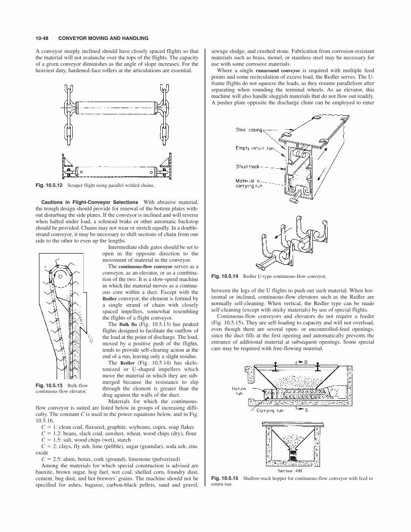
A conveyor steeply inclined should have closely spaced flights so thatthe material will not avalanche over the tops of the flights. The capacityof a given conveyor diminishes as the angle of slope increases. For theheaviest duty, hardened-face rollers at the articulations are essential.
sewage sludge, and crushed stone. Fabrication from corrosion-resistantmaterials such as brass, monel, or stainless steel may be necessary foruse with some corrosive materials. Where a single runaround conveyor is required with multiple feed
points and some recirculation of excess load, the Redler serves. The U-frame flights do not squeeze the loads, as they resume parallelism afterseparating when rounding the terminal wheels. As an elevator, thismachine will also handle sluggish materials that do not flow out readily.A pusher plate opposite the discharge chute can be employed to enter
10-48 CONVEYOR MOVING AND HANDLING
Fig. 10.5.12 Scraper flight using parallel welded chains.
Cautions in Flight-Conveyor Selections With abrasive material,the trough design should provide for renewal of the bottom plates with-out disturbing the side plates. If the conveyor is inclined and will reversewhen halted under load, a solenoid brake or other automatic backstopshould be provided. Chains may not wear or stretch equally. In a double-strand conveyor, it may be necessary to shift sections of chain from oneside to the other to even up the lengths.
Intermediate slide gates should be set toopen in the opposite direction to themovement of material in the conveyor.The continuous-flow conveyor serves as a
conveyor, as an elevator, or as a combina-tion of the two. It is a slow-speed machinein which the material moves as a continu-ous core within a duct. Except with theRedler conveyor, the element is formed bya single strand of chain with closelyspaced impellers, somewhat resemblingthe flights of a flight conveyor.The Bulk flo (Fig. 10.5.13) has peaked
flights designed to facilitate the outflow ofthe load at the point of discharge. The load,moved by a positive push of the flights,tends to provide self-clearing action at theend of a run, leaving only a slight residue.The Redler (Fig. 10.5.14) has skele-
tonized or U-shaped impellers whichmove the material in which they are sub-merged because the resistance to slipthrough the element is greater than thedrag against the walls of the duct.Materials for which the continuous-
flow conveyor is suited are listed below in groups of increasing diffi-culty. The constant C is used in the power equations below, and in Fig.10.5.16.C 1: clean coal, flaxseed, graphite, soybeans, copra, soap flakesC 1.2: beans, slack coal, sawdust, wheat, wood chips (dry), flourC 1.5: salt, wood chips (wet), starchC 2: clays, fly ash, lime (pebble), sugar (granular), soda ash, zinc
oxideC 2.5: alum, borax, cork (ground), limestone (pulverized)Among the materials for which special construction is advised are
bauxite, brown sugar, hog fuel, wet coal, shelled corn, foundry dust,cement, bug dust, and hot brewers’ grains. The machine should not bespecified for ashes, bagasse, carbon-black pellets, sand and gravel,
Fig. 10.5.13 Bulk-flow
continuous-flow elevator.
Fig. 10.5.14 Redler U-type continuous-flow conveyor.
between the legs of the U flights to push out such material. When hor-izontal or inclined, continuous-flow elevators such as the Redler arenormally self-cleaning. When vertical, the Redler type can be madeself-cleaning (except with sticky materials) by use of special flights.Continuous-flow conveyors and elevators do not require a feeder
(Fig. 10.5.15). They are self-loading to capacity and will not overload,even though there are several open- or uncontrolled-feed openings,since the duct fills at the first opening and automatically prevents theentrance of additional material at subsequent openings. Some specialcare may be required with free-flowing material.
Fig. 10.5.15 Shallow-track hopper for continuous-flow conveyor with feed to
return run.

NONCARRYING CONVEYORS 10-49
The duct is easily insulated by sheets of asbestos cement or similarmaterial to reduce cooling in transit. As the duct is completely sealed,there is no updraft where the lift is high. The material is protected fromexposure and contamination or contact with lubricants. The handlingcapacity for horizontal or inclined lengths (nearly to the angle of reposeof the material) approximates 100 percent of the volume swept throughby the movement of the element. For steeper inclines or elevators, it isbetween 50 and 90 percent.If the material is somewhat abrasive, as with wet bituminous coal, the
duct should be of corrosion-resistant steel, of extra thickness, and thechain pins should be both extremely hard and of corrosion-resistantmaterial.A long horizontal run followed by an upturn is inadvisable because
of radial thrust. Lumpy material is difficult to feed from a track hopper.An automatic brake is unnecessary, as an elevator will reverse only afew inches when released.The motor horsepower P required by continuous-flow conveyors for
the five arrangements shown in Fig. 10.5.16 is given in the accompany-ing formulas in terms of the capacity T, in tons per h; the horizontal runH, ft; the vertical lift V, ft; and the constant C, values for which are givenabove. If loading from a track hopper, add 10 percent.
Screw Conveyors
The screw, or spiral, conveyor is used quite widely for pulverized orgranular, noncorrosive, nonabrasive materials when the required capac-ity is moderate, when the distance is not more than about 200 ft (61 m),and when the path is not too steep. It usually costs substantially lessthan any other type of conveyor and is readily made dusttight by a sim-ple cover plate.The conveyor will handle lumpy material if the lumps are not large
in proportion to the diameter of the helix. If the length exceeds thatadvisable for a single conveyor, separate or tandem units are readilyarranged. Screw conveyors may be inclined. A standard-pitch helix willhandle material on inclines up to 35". The reduction in capacity as com-pared with the capacity when horizontal is indicated in the followingtable:
Inclination, deg 10 15 20 25 30 35
Reduction in capacity, percent 10 26 45 58 70 78
Abrasive or corrosive materials can be handled with suitable con-struction of the helix and trough.The standard screw-conveyor helix (Fig. 10.5.17) has a pitch approx-
imately equal to its outside diameter. Other forms are used for specialcases.
Fig. 10.5.16 Continuous-flow-conveyor arrangements.
Fig. 10.5.17 Spiral conveyor.
Short-pitch screws are advisable for inclines above 29".Variable-pitch screws, with short pitch at the feed end, automatically
control the flow to the conveyor so that the load is correctly propor-tioned for the length beyond the feed point. With a short section eitherof shorter pitch or of smaller diameter, the conveyor is self-loading tocapacity and does not require a feeder.
Fig. 10.5.18 Cut-flight conveyor.
Cut flights (Fig. 10.5.18) are used for conveying and mixing cereals,grains, and other light materials.Ribbon screws (Fig. 10.5.19) are used for wet and sticky materials,
such as molasses, hot tar, and asphalt, which might otherwise build upon the spindle.Paddle screws are used primarily for mixing such materials as mortar
and bitulithic paving mixtures. One typical application is to churn ashesand water to eliminate dust.
Fig. 10.5.19 Ribbon conveyor.
Standard constructions have a plain or galvanized-steel helix andtrough. For abrasives and corrosives such as wet ashes, both helix andtrough may be of hard-faced cast iron. For simple abrasives, the outeredge of the helix may be faced with a renewable strip of Stellite or

similar extremely hard material. For food products, aluminum, bronze,monel metal, or stainless steel is suitable but expensive.Table 10.5.3 gives the capacities, allowable speeds, percentages of
helix loading for five groups of materials, and the factor F used in esti-mating the power requirement.Table 10.5.4 gives the handling capacities for standard-pitch screw
conveyors in each of the five groups of materials when the conveyorsare operating at the maximum advised speeds and in the horizontalposition. The capacity at any lower speed is in the ratio of the speeds.Power Requirements The power requirements for horizontal screw
conveyors of standard design and pitch are determined by the Link-BeltCo. by the formula that follows. Additional allowances should be madefor inclined conveyors, for starting under load, and for materials thattend to stick or pack in the trough, as with cement.
where A factor for size of conveyor (see Table 10.5.5); C quantityof material, ft3/h; L length of conveyor, ft; F factor for material(see Table 10.5.3); N r/min of conveyor; W density of material,lb/ft3.The motor size depends on the efficiency E of the drive (usually close
to 90 percent); a further allowance G, depending on the horsepower, ismade:
H 5 hp at conveyor head shaft 5 sALN 1 CWLFd 3 1026
and lengths, the alternatives—a flight conveyor or a belt conveyor—should receive consideration.
EXAMPLES. 1. Slack coal 50 lb/ft3 (800 kg/m3); desired capacity 50 tons/h (2,000
ft3/h) (45 tonnes/h); conveyor length, 60 ft (18 m); 14-in (0.36-m) conveyor at
80 r/min. F for slack coal 0.9 (group 2).
Use 7 -hp motor.2. Limestone screenings, 90 lb/ft3; desired capacity, 10 tons/h (222 ft3/h); con-
veyor length, 50 ft; 9-in conveyor at 50 r/min. F for limestone screenings 2.0
(group 4).
Use 3-hp motor.
Chutes
Bulk Material If the material is fragile and cannot be set through asimple vertical chute, a retarding chute may be specified. Figure 10.5.20shows a ladder chute in which the material trickles over shelves insteadof falling freely. If it is necessary to minimize breakage when materialis fed from a bin, a vertical box chute with flap doors opening inward,as shown in Fig. 10.5.21, permits the material to flow downward onlyfrom the top surface and eliminates the degradation that results from aconverging flow from the bottom of the mass.Straight inclined chutes for coal should have a slope of 40 to 45". If
it is found that the coal accelerates objectionably, the chute may be pro-vided with cross angles over which the material cascades at reducedspeed (Fig. 10.5.22).Lumpy material such as coke and large coal, difficult to control when
flowing from a bin, can be handled by a chain-controlled feeder chutewith a screen of heavy endless chains hung on a sprocket shaft (Fig.10.5.23). The weight of the chain curtain holds the material in the chute.When a feed is desired, the sprocket shaft is revolved slowly, eithermanually or by a motorized reducer.Unit Loads Mechanical handling of unit loads, such as boxes, barrels,
packages, castings, crates, and palletized loads, calls for methods and
Motor hp 5 s2.24 3 1.25d>0.90 5 2.8
H 5 s96 3 50 3 50 1 222 3 90 3 50 3 2.0d>1,000,000 5 2.24
1⁄2
Motor hp 5 s6.6 3 1.0d>0.90 5 7.3 s5.4 kWd
H 5 s255 3 60 3 80 1 2,000 3 50 3 60 3 0.9d>1,000,000 5 6.6
10-50 CONVEYOR MOVING AND HANDLING
Table 10.5.3 Capacities and Speed of Spiral Conveyors
Max percent of cross Max density Max r/min for diameters
section occupied by of material, lb/
Group the material ft3 (kg/m3) 6 in (152 mm) 20 in (508 mm)
1 45 50 (800) 170 110
2 38 50 (800) 120 75
3 31 75 (1,200) 90 60
4 25 100 (1,600) 70 50
5 30 25
Group 1 includes light materials such as barley, beans, brewers grains (dry), coal (pulv.), corn meal, cottonseedmeal, flaxseed, flour, malt, oats, rice, wheat. The value of the factor F is 0.5.Group 2 includes fines and granular materials. The values of F are alum (pulv.), 0.6, coal (slack or fines), 0.9; cof-
fee beans, 0.4; sawdust, 0.7; soda ash (light), 0.7; soybeans, 0.5; fly ash, 0.4.Group 3 includes materials with small lumps mixed with fines. Values of F are alum, 1.4; ashes (dry), 4.0; borax,
0.7; brewers grains (wet), 0.6; cottonseed, 0.9; salt, course or fine, 1.2; soda ash (heavy), 0.7.Group 4 includes semiabrasive materials, fines, granular and small lumps. Values of F are acid phosphate (dry), 1.4;
bauxite (dry), 1.8; cement (dry), 1.4; clay, 2.0; fuller’s earth, 2.0; lead salts, 1.0; limestone screenings, 2.0; sugar (raw),1.0; white lead, 1.0; sulfur (lumpy), 0.8; zinc oxide, 1.0.Group 5 includes abrasive lumpy materials which must be kept from contact with hanger bearings. Values of F are
wet ashes, 5.0; flue dirt, 4.0; quartz (pulv.), 2.5; silica sand, 2.0; sewage sludge (wet and sandy), 6.0.
121⁄2
H 1 1–2 2–4 4–5 5
G 2 1.5 1.25 1.1 1.0
Motor hp HG/E
When the material is distributed into a bunker, the conveyor has anopen-bottom trough to discharge progressively over the crest of the pileso formed. This trough reduces the capacity and increases the requiredpower, since the material drags over the material instead of over a pol-ished trough.If the material contains unbreakable lumps, the helix should clear the
trough by at least the diameter of the average lump. For a given capac-ity, a conveyor of larger size and slower speed is preferable to aconveyor of minimum size and maximum speed. For large capacities
Table 10.5.4 Screw-Conveyor Capacities
(ft3/h)
Conveyor size, in*
Group 6 9 10 12 14 16 18 20
1 350 1,100 1,600 2,500 4,000 5,500 7,600 10,000
2 220 700 950 1,600 2,400 3,400 4,500 6,000
3 150 460 620 1,100 1,600 2,200 3,200 4,000
4 90 300 400 650 1,000 1,500 2,000 2,600
5 20 68 90 160 240 350 500 650
*Multiply by 25.4 to obtain mm.

CARRYING CONVEYORS 10-51
mechanisms entirely different from those adapted to the movement ofbulk materials.
maximum size of package that can be handled. These chutes may havereceive and discharge points at any desired floors. There are certainkinds of commodities, such as those made of metal or bound with wireor metal bands, that cannot be handled satisfactorily unless the spiralchute is designed to handle only that particular commodity. Sheet-metalspirals can be built with double or triple blades, all mounted on thesame standpipe. Another form of sheet-metal spiral is the open-coretype, which is especially adaptable for handling long and narrow arti-cles or bulky classes of merchandise or for use where the spiral mustwind around an existing column or pass through floors in locations lim-ited by beams or girders that cannot be conveniently cut or moved. Forhandling bread or other food products, it is customary to have the spi-ral tread made from monel metal or aluminum.
Table 10.5.5 Factor A(Self-lubricating bronze bearings assumed)
Diam of conveyor, in 6 9 10 12 14 16 18 20 24
mm 152 229 254 305 356 406 457 508 610
Factor A 54 96 114 171 255 336 414 510 690
Fig. 10.5.20 Ladder chute. Fig. 10.5.21 Box chute with
flap doors. Chute is always full
up to discharging point.
Spiral chutes are adapted for the direct lowering of unit loads of variousshapes, sizes, and weights, so long as their slide characteristics do not varywidely. If they do vary, care must be exercised to see that items accelerat-ing on the selected helix pitch do not crush or damage those ahead.
Fig. 10.5.22 Inclined chute
with cross angles.
Fig. 10.5.23 Chain-controlled
feeder chute.
A spiral chute may extend through several floors, e.g., for loweringparcels in department stores to a basement shipping department. Theopening at each floor must be provided with automatic closure doors,and the design must be approved by the Board of Fire Underwriters.At the discharge end, it is usual to extend the chute plate horizontally
to a length in which the loads can come to rest. A tandem gravity rollconveyor may be advisable for distribution of the loads.The sheet-metal spiral (Fig. 10.5.24) has a fixed blade and can be fur-
nished in varying diameters and pitches, both of which determine the
Fig. 10.5.24 Metal spiral chute.
CARRYING CONVEYORS
Apron Conveyors
Apron conveyors are specified for granular or lumpy materials. Since theload is carried and not dragged, less power is required than for screw orscraper conveyors. Apron conveyors may have stationary skirt or sideplates to permit increased depth of material on the apron, e.g., when usedas a feeder for taking material from a track hopper (Fig. 10.5.25) with
Fig. 10.5.25 Track hopper and apron feeder supplying a gravity-discharge bucket-elevator boot.

controlled rate of feed. They are not often specified if the length isgreat, since other types of conveyor are substantially lower in cost.Sizes of lumps are limited by the width of the pans and the ability of theconveyor to withstand the impact of loading. Only end discharge is pos-sible. The apron conveyor (Fig. 10.5.26) consists of two strands ofroller chain separated by overlapping apron plates, which form the car-rying surface, with sides 2 to 6 in (51 to 152 mm) high. The chains aredriven by sprockets at one end, take-ups being provided at the otherend. The conveyors always pull the material toward the driving end. Forlight duty, flangeless rollers on flat rails are used; for heavy duty, single-flanged rollers and T rails are used. Apron conveyors may be run with-out feeders, provided that the opening of the feeding hopper is madesufficiently narrow to prevent material from spilling over the sides ofthe conveyor after passing from the opening. When used as a conveyor,the speed should not exceed 60 ft/min (0.30 m/s); when used as a feed-er, 30 ft/min (0.15 m/s). Table 10.5.6 gives the capacities of apron feed-ers with material weighing 50 lb/ft3 (800 kg/m3) at a speed of 10 ft/min(0.05 m/s). Chain pull for horizontal-apron conveyor:
Chain pull for inclined-apron conveyor:
where L conveyor length, ft; W weight of chain and pans per ft, lb;W1 weight of material per ft of conveyor, lb; u angle of inclination,deg; F coefficient of rolling friction, usually 0.1 for plain roller bear-ings or 0.05 for antifriction bearings.
LsW 1 W1dsF cos u 1 sin ud 1 WLsF cos u 2 sin ud
2LFsW 1 W1d
separated by V-shaped steel buckets. Figure 10.5.28 shows the mostcommon form, where material is received on the lower horizontal run,elevated, and discharged through openings in the bottom of the troughof the upper horizontal run. The material is scraped along the horizontaltrough of the conveyor, as in a flight conveyor. The steel guard plates a
10-52 CONVEYOR MOVING AND HANDLING
Fig. 10.5.26 Apron conveyor. Fig. 10.5.27 Open-top carrier.
Bucket Conveyors and Elevators
Open-top bucket carriers (Fig. 10.5.27) are similar to apron conveyors,except that dished or bucket-shaped receptacles take the place of the flator corrugated apron plates used on the apron conveyor. The carriers willoperate on steeper inclines than apron conveyors (up to 70"), as thebuckets prevent material from sliding back. Neither sides extendingabove the tops of buckets nor skirtboards are necessary. Speed,when loaded by a feeder, 60 ft/min (max)(0.30 m/s) and when drag-ging the load from a hopper or bin, )30 ft/min. The capacity should becalculated on the basis of the buckets being three-fourths full, the angleof inclination of the conveyor determining the loading condition of thebucket.V-bucket carriers are used for elevating and conveying nonabrasive
materials, principally coal when it must be elevated and conveyed withone piece of apparatus. The length and height lifted are limited by thestrength of the chains and seldom exceed 75 ft (22.9 m). These carrierscan operate on any incline and can discharge at any point on the hori-zontal run. The size of lumps carried is limited by the size and spacingof the buckets. The carrier consists of two strands of roller chain
Fig. 10.5.28 V-bucket carrier.
at the right prevent spillage at the bends. Figure 10.5.29 shows a differ-ent form, where material is dug by the elevator from a boot, elevatedvertically, scraped along the horizontal run, and discharged throughgates in the bottom of the trough. Figure 10.5.30 shows a variation ofthe type shown in Fig. 10.5.29, requiring one less bend in the conveyor.The troughs are of steel or steel-lined wood. When feeding material tothe horizontal run, it is advisable to use an automatic feeder driven by
Fig. 10.5.29 and 10.5.30 V-bucket carriers.
power from one of the bend shafts to prevent overloading. Should thebuckets of this type of conveyor be overloaded, they will spill on thevertical section. The drive is located at b, with take-up at c. The speedshould not exceed 100 ft/min (0.51 m/s) when large material is beinghandled, but when material is small, speed may be increased to125 ft/min (0.64 m/s). The best results are obtained when speeds arekept low. Table 10.5.7 gives the capacities and weights based on aneven and continuous feed. Pivoted-bucket carriers are used primarily where the path is a run-
around in a vertical plane. Their chief application has been for the dual
Table 10.5.6 Capacities of Apron Conveyors
Width betweenCapacity, 50 lb/ft3 (800 kg/m3) material at 10 ft/min (0.05 m/s) speed
skirt plates Depth of load, in (mm)
in mm 12 (305) 16 (406) 20 (508) 24 (610)
24 610 22 (559) 30 (762)
30 762 26 (660) 37 (940) 47 (1,194) 56 (1,422)
36 914 34 (864) 45 (1,143) 56 (1,422) 67 (1,702)
42 1,067 39 (991) 52 (1,321) 65 (1,651) 79 (2,007)

CARRYING CONVEYORS 10-53
duty of handling coal and ashes in boiler plants. They require lesspower than V-bucket carriers, as the material is carried and not draggedon the horizontal run. The length and height lifted are limited by thestrength of the chains. The length seldom exceeds 500 ft (152 m) andthe height lifted 100 ft (30 m). They can be operated on any incline andcan discharge at any point on the horizontal run. The size of lumps islimited by the size of buckets. The maintenance cost is extremely low.Many carrier installations are still in operation after 40 years of service.Other applications are for hot clinker, granulated and pulverized chem-icals, cement, and stone.The carrier consists of two strands of roller chain, with flanged
rollers, between which are pivoted buckets, usually of malleable iron.The drive (Fig. 10.5.31) is located at a or a(, the take-up at b. The mate-rial is fed to the buckets by a feeder at any point along the lower hori-zontal run, is elevated, and is discharged on the upper horizontal run.
the turns, the buckets swing in a larger-radius curve, automaticallyunlatch, and then lap correctly as they enter the straight run. The pivoted-bucket carrier requires little attention beyond periodic
lubrication and adjustment of take-ups. For the dual service of coal andash handling, its only competitor is the skip hoist.
Table 10.5.7 Capacities and Weights of V-Bucket Carriers*
Buckets Capacity, tons Weight per ft
of coal per of chains
Length, Width, Depth, Spacing, hour at 100 ft/ and buckets,
in in in in min lb
12 12 6 18 29 36
16 12 6 18 32 40
20 15 8 24 43 55
24 20 10 24 100 65
30 20 10 24 126 70
36 24 12 30 172 94
42 24 12 30 200 105
48 24 12 36 192 150
* Multiply in by 25.4 for mm, ton/h by 0.25 for kg/s or by 0.91 for tonnes/h.
Fig. 10.5.31 Pivoted-bucket carrier.
The tripper c, mounted on wheels so that it can be moved to the desireddumping position, engages the cams on the buckets and tips them untilthe material runs out. The buckets always remain vertical except whentripped. The chain rollers run on T rails on the horizontal sections andbetween guides on the vertical runs. Speeds range from 30 to 60 ft/min(0.15 to 0.30 m/s).After dumping, the overlapping bucket lips are in the wrong position
to round the far corner; after rounding the take-up wheels, the lap iswrong for making the upturn. The Link-Belt Peck carrier eliminates thisby suspending the buckets from trunnions attached to rearward can-tilever extensions of the inner links (Fig. 10.5.32). As the chain rounds
Fig. 10.5.32 Link-Belt Peck carrier buckets.
Table 10.5.8 shows the capacities of pivoted-bucket carriers withmaterials weighing 50 lb/ft3 (800 kg/m3), with carriers operating at 40to 50 ft/min (0.20 to 0.25 m/s), and with buckets loaded to 80 percentcapacity.Bucket elevators are of two types: (1) chain-and-bucket, where the
buckets are attached to one or two chains; and (2) belt-and-bucket,where the buckets are attached to canvas or rubber belts. Either typemay be vertical or inclined and may have continuous or noncontinuousbuckets. Bucket elevators are used to elevate any bulk material that willnot adhere to the bucket. Belt-and-bucket elevators are particularly welladapted to handling abrasive materials which would produce excessivewear on chains. Chain-and-bucket elevators are frequently used with per-forated buckets when handling wet material, to drain off surplus water.The length of elevators is limited by the strength of the chains or belts.They may be built up to 100 ft (30 m) long, but they average 25 to 75 ft(7.6 to 23 m). Inclined-belt elevators operate best on an angle of about30" to the vertical. At greater angles, the sag of the return belt is exces-sive, as it cannot be supported by rollers between the head and footpulleys. This applies also to single-strand chain elevators. Double-strand chain elevators, however, if provided with roller chain, can runon an angle, as both the upper and return chains are supported by rails.
Table 10.5.8 Capacities of Pivoted-Bucket Carriers with Coal or Similar MaterialsWeighing 50 lb/ft3 (800 kg/m3) at Speeds Noted
Bucket pitch ! width Capacity of coal Speed
in mm Short ton/h tonne/h ft/min m/s
24 ! 18 610 ! 457 35–45 32–41 40–50 0.20–0.25
24 ! 24 610 ! 610 50–60 45–54 40–50 0.20–0.25
24 ! 30 610 ! 762 60–75 54–68 40–50 0.20–0.25
24 ! 36 610 ! 914 70–90 63–82 40–50 0.20–0.25

The size of lumps is limited by the size and spacing of the buckets andby the speed of the elevator.
Continuous-bucket elevators (Fig. 10.5.33and Table 10.5.9) usually operateat 100 ft/min (0.51 m/s) or less and aresingle- or double-strand. The contentsof each bucket discharge over the back ofthe preceding bucket. For maximumcapacity and a large proportion of lumps,the buckets extend rearward behind thechain runs. The elevator is then called asupercapacity elevator (Fig. 10.5.34 andTable 10.5.10).Gravity-discharge elevators operate at
100 ft/min (0.51 m/s) or less and aredouble-strand, with spaced V buckets.The path may be an L, an inverted L,or a runaround in a vertical plane(Fig. 10.5.28). Along the horizontal run,the buckets function as pushers within a
trough. An elevator with a tandem flight conveyor costs less. For arunaround path, the pivoted-bucket carrier requires less power and haslower maintenance costs.
with structural-steel boot and casing. Elevators of this type must be run atsufficient speed to throw the discharging material clear of the bucketahead.Capacity Elevators are rated for capacity with the buckets 75 percent
loaded. The buckets must be large enough to accommodate the lumps,even though the capacity is small.
10-54 CONVEYOR MOVING AND HANDLING
Fig. 10.5.33 Continuous
bucket.
Table 10.5.9 Continuous Bucket Elevators*
Max lump size, in Capacity with
50 lb material
Bucket size, All 10% at 100 ft/min
in lumps lumps tons/h
10 ! 5 ! 8 17
10 ! 7 ! 12 1 3 21
12 ! 7 ! 12 1 3 25
14 ! 7 ! 12 1 3 30
14 ! 8 ! 12 4 36
16 ! 8 ! 12 42
18 ! 8 ! 12 46
* Multiply in by 25.4 for mm, lb by 0.45 for kg, tons by 0.91 for tonnes.
41⁄211⁄241⁄211⁄2
11⁄4
21⁄23⁄4
As bucket elevators have no feed control, an interlocked feeder isdesirable for a gravity flow. Some types scoop up the load as the buck-ets round the foot end and can take care of momentary surges byspilling the excess back into the boot. The continuous-bucket elevator,however, must be loaded after the buckets line up for the lift, i.e., whenthe gaps between buckets have closed.
Belt-and-bucket elevators are advan-tageous for grain, cereals, glass batch,clay, coke breeze, sand, and other abra-sives if the temperature is not highenough to scorch the belt [below 250"F(121"C) for natural rubber].Elevator casings usually are sectional
and dusttight, either of -in (4.8-mm)sheet steel or, better, of aluminum.If the elevator has considerable height,its cross section must be sufficientlylarge to prevent sway contact betweenbuckets and casing. Chain guidesextending the length of both runs maybe provided to control sway and to pre-vent piling up of the element, at theboot, should the chain break. Caution:Indoor high elevators may develop
considerable updraft tending to sweep up light, pulverized material.Provision to neutralize the pressure differential at the top and bottom maybe essential. Figure 10.5.35 shows the cast-iron boot used with centrifugal-discharge and V-bucket chain elevators and belt elevators.Figure 10.5.36 shows the general form of a belt-and-bucket elevator
3⁄16
Fig. 10.5.34 Supercapacity
bucket.
Table 10.5.10 Supercapacity Elevators*(Link-Belt Co.)
Max lump size, large lumps Capacity with
Bucket, in length ! not more than 20%, 50 lb material
width ! depth in tons/h
16 ! 12 ! 18 8 115
20 ! 12 ! 18 8 145
24 ! 12 ! 18 8 175
30 ! 12 ! 18 8 215
24 ! 17 ! 24 10 230
36 ! 17 ! 24 10 345
* Multiply in by 25.4 for mm, lb by 0.45 for kg, tons by 0.91 for tonnes.
Fig. 10.5.35 Cast-iron boot.
Power Requirements The motor horsepower for the continuous-bucket and supercapacity elevators can be approximated as
The motor horsepower of gravity-discharge elevators can be approxi-mated by using the same formula for the lift and adding for the horse-power of the horizontal run the power as estimated for a flight conveyor.For a vertical runaround path, add a similar allowance for the lower hor-izontal run.
Motor hp 5 s2 3 tons/h 3 lift, ftd/1,000
Fig. 10.5.36 Structural-steel boot and casing.
Belt Conveyors
The belt conveyor is a heavy-duty conveyor available for transportinglarge tonnages over paths beyond the range of any other type ofmechanical conveyor. The capacity may be several thousand tons perhour, and the distance several miles. It may be horizontal or inclinedupward or downward, or it may be a combination of these, as outlinedin Fig. 10.5.37. The limit of incline is reached when the material tendsto slip on the belt surface. There are special belts with molded designsto assist in keeping material from slipping on inclines. They will han-dle pulverized, granular, or lumpy material. Special compounds areavailable if material is hot or oily.In its simplest form, the conveyor consists of a head or drive pulley, a
take-up pulley, an endless belt, and carrying and return idlers. The spac-ing of the carrying idlers varies with the width and loading of the belt

CARRYING CONVEYORS 10-55
and usually is 5 ft (1.5 m) or less. Return idlers are spaced on 10-ft(3.0-m) centers or slightly less with wide belts. Sealed antifriction idlerbearings are used almost exclusively, with pressure-lubrication fittingsrequiring attention about once a year.
somewhat lower tensile ratings of 90 (1.61), 120 (2.14), 155 (2.77), 195(3.48), and 240 (4.29) lb/in (kg/mm) per ply ratings. The B. F. Goodrich Company has developed a steel-cable-reinforced
belt rated 700 to 4,400 lb/in (12.5 to 78.6 kg/mm) of belt width. Thebelt has parallel brass-plated 7 by 19 steel airplane cables ranging from
to in (4.0 to 9.5 mm) diameter placed on - to -in (12.7-to 19.0-mm) centers.These belts are used for long single-length conveyors and for high-
lift, extremely heavy duty service, e.g., for taking ore from deep openpits, thus providing an alternative to a spiraling railway or truck route.Synthetic rubber is in use for belts. Combinations of synthetic and
natural rubbers have been found satisfactory. Synthetics are superiorunder special circumstances, e.g., neoprene for flame resistance andresistance to petroleum-based oils, Buna N for resistance to vegetable,animal, and petroleum oils, and butyl for resistance to heat (per RMA).Belt Life With lumpy material, the impact at the loading point may
be destructive. Heavy lumps, such as ore and rock, cut through the pro-tective cover and expose the carcass. The impact shock is reduced bymaking the belt supports flexible. This can be done by the use of idlerswith cushion or pneumatic tires (Fig. 10.5.39) or by supporting theidlers on rubber mountings. Chuting the load vertically against the beltshould be avoided. Where possible, the load should be given a move-ment in the direction of belt travel. When the material is a mixture oflumps and fines, the fines should be screened through to form a cush-ion for the lumps. Other destructive factors are belt overstressing, belts
3⁄41⁄23⁄85⁄32
Fig. 10.5.37 Typical arrangements of belt conveyors.
Belts Belt width is governed by the desired conveyor capacityand maximum lump size. The standard rubber belt construction(Fig. 10.5.38) has several plies of square woven cotton duck or syntheticfabric such as rayon, nylon, or polyester cemented together with a rub-ber compound called “friction” and covered both top and bottom withrubber to resist abrasion and keep out moisture. Top cover thickness is
Fig. 10.5.38 Rubber-covered conveyor belt.
determined by the severity of the job and varies from to in (1.6to 19 mm). The bottom cover is usually in (1.6 mm). By placing alayer of loosely woven fabric, called the breaker strip, between thecover and outside fabric ply, it is often possible to double the adhesionof the cover to the carcass. The belt is rated according to the tension towhich it may safely be subjected, and this is a function of the length andlift of the conveyor. The standard Rubber Manufacturers Association(RMA) multiple ply ratings in lb/in (kg/mm) of width per ply are asfollows:
RMA multiple ply No. MP35 MP43 MP50 MP60 MP70
Permissible pull, lb/in (kg/mm) 35 43 50 60 70
of belt width per ply, vulcanized (0.63) (0.77) (0.89) (1.07) (1.25)
splice
Permissible pull, lb/in (kg/mm) 27 33 40 45 55
of belt width per ply, mechanical (0.48) (0.60) (0.71) (0.80) (0.98)
splice
Thus, for a pull of 4,200 lb (1,905 kg) and 24-in (0.61-m) belt width, afive-ply MP35 could be used with a vulcanized splice or a five-plyMP50 could be used with a mechanical splice.High-Strength Belts For belt conveyors of extremely great length, a
greater strength per inch of belt width is available now through the useof improved weaving techniques that provide straight-warp syntheticfabric to support the tensile forces (Uniflex by Uniroyal, Inc., or Flexsealby B. F. Goodrich). Strengths go to 1,500 lb/in width tension rating.They are available in most cover and bottom combinations and havegood bonding to carcass. The number of plies is reduced to two insteadof as many as eight so as to give excellent flexibility. Widths to 60 in areavailable. Other conventional high-strength fabric belts are available to
1⁄16
3⁄41⁄16
Fig. 10.5.39 Pneumatic-tired idlers applied to belt feeder at loading point of
belt conveyor.
running out of line and rubbing against supports, broken idlers, and fail-ure to clean the belt surface thoroughly before it comes in contact withthe snub and tripper pulleys. Introduction of a 180" twist in the returnbelt (B. F. Goodrich Co.) at both head and tail ends can be used to keepthe clean side of the belt against the return idlers and to prevent buildup.Using one 180" twist causes both sides of the belt to wear evenly. Foreach twist, 1 ft of length/in of belt width is required.Idler Pulleys Troughing idlers are usually of the three-pulley type
(Fig. 10.5.40), with the troughing pulleys at 20". There is a growing ten-dency toward the use of 35 and 45" idlers to increase the volume capac-ity of a belt; 35" idlers will increase the volume capacity of a given belt25 to 35 percent over 20" idlers, and 45" idlers, 35 to 40 percent.
Fig. 10.5.40 Standard assembly of three-pulley troughing idler and
return idler.
The bearings, either roller or ball type, are protected by felt or labyrinthgrease seals against the infiltration of abrasive dust. A belt running outof line may be brought into alignment by shifting slightly forward oneend or the other with a few idler sets. Self-aligning idlers (Fig. 10.5.41)should be spaced not more than 75 ft (23 m) apart. These call attentionto the necessity of lining up the belt and should not serve as continuingcorrectives.

Drive Belt slip on the conveyor-drive pulley is destructive. There islittle difference in tendency to slip between a bare pulley and a rubber-lagged pulley when the belt is clean and dry. A wet belt will adhere toa lagged pulley much better, especially if the lagging is grooved.Heavy-duty conveyors exposed to the possibility of wetting the belt are
downward (retarding conveyor), when the take-up is located at thedownhill end. Trippers The load may be removed from the belt by a diagonal or
V plow, but a tripper that snubs the belt backward is standard equip-ment. Trippers may be (1) stationary, (2) manually propelled by crank,or (3) propelled by power from one of the snubbing pulleys or by anindependent motor. The discharge may be chuted to either side or backto the belt by a deflector plate. When the tripper must move back to theload-receiving end of the conveyor, it is usual to incline the belt forabout 15 ft (4.6 m) to match the slope up to the tripper top pulley. Asthe lower tripper snub pulleys are in contact with the dirty side of thebelt, a cleaner must be provided between the pulleys. A scraper in lightcontact with the face of the pulley may be advisable.Belt Slope The slopes (in degrees) given in Table 10.5.11 are the
maximum permissible angles for various materials.
10-56 CONVEYOR MOVING AND HANDLING
Fig. 10.5.41 Self-aligning idler.
generally driven by a head pulley lagged with a -in (12.7-mm) rubberbelt and with - by -in (6.4- by 6.4-mm) grooves spaced in(12.7 mm) apart and, preferably, diagonally as a herringbone gear.A snub pulley can be employed to increase the arc of contact on the headpulley, and since the pulley is in contact with the dirty side of the belt, abelt cleaner is essential. The belt cleaner may be a high-speed bristlebrush, a spiral rubber wiper (resembling an elongated worm pinion), cir-cular disks mounted slantwise on a shaft to give a wiping effect whenrotated, or a scraper. Damp deposits such as clay or semifrozen coal dirtare best removed by multiple diagonal scrapers of stainless steel.A belt conveyor should be emptied after each run to avoid a heavy
starting strain. The motor should have high starting torque, moderatestarting-current inrush, and good characteristics when operating underfull load. The double-squirrel-cage ac motor fulfills these requirements.Heavy-Duty Belt-Conveyor Drives For extremely heavy duty, it is
essential that the drive torque be built up slowly, or serious belt damagewill occur. The hydraulic clutch, derived from the hydraulic automobileclutch, serves nicely. The best drive developed to date is the dynamaticclutch (Fig. 10.5.42). This has a magnetized rotor on the extended motorshaft, revolving within an iron ring keyed to the reduction gearing of theconveyor. The energizing current is automatically built up over a periodthat may extend to 2 min, and the increasing magnetic pull on the ringbuilds up the belt speed.
1⁄21⁄41⁄4
1⁄2
Fig. 10.5.42 Operating principle of the dynamic clutch.
Take-ups For short conveyors, a screw take-up is satisfactory. Forlong conveyors, the expansion and contraction of the belt with tempera-ture changes and the necessity of occasional cutting and resplicing makea weighted gravity take-up preferable, especially if a vulcanized splice isused. The take-up should, if possible, be located where the slack firstoccurs, usually just back of the drive except in a conveyor inclined
Table 10.5.11 Maximum Belt Slopes for Various Materials,Degrees
Coal: anthracite, sized; mined, 50 mesh and under; or mined 16
and sized
Coal, bituminous, mined, run of mine 18
Coal: bituminous, stripping, not cleaned; or lignite 22
Earth, as excavated, dry 20
Earth, wet, containing clay 23
Gravel, bank run 20
Gravel, dry, sharp 15–17
Gravel, pebbles 12
Grain, distillery, spent, dry 15
Sand, bank, damp 20–22
Sand, bank, dry 16–18
Wood chips 27
SOURCE: Uniroyal, Inc.
Determination of Motor Horsepower The power required to drivea belt conveyor is the sum of the powers required (1) to move theempty belt, (2) to move the load horizontally, and (3) to lift the load ifthe conveyor is inclined upward. If (3) is larger than the other two, anautomatic brake must be provided to hold the conveyor if the currentfails. A solenoid brake is usual. The power required to move the emptybelt is given by Fig. 10.5.43. The power to move 100 tons/h horizon-tally is given by the formula hp 0.4 $ 0.00325L, where L is the dis-tance between centers, ft. For other capacities the horsepower isproportional.
Fig. 10.5.43 Horsepower required to move belt conveyor empty at 100 ft/
min (0.15 m/s).

10-57
Table 10.5.12
Troughed Conveyor-Belt Capacities*
Tons per hour (TPH) with belt speed of 100 ft/min (0.51 m/s).
Belt shape:
Equal length, 3 roll
Long center, 3 roll
Belt
Idler angle:
20º
35º
45º
35º
45%
width,
inSCA†:
0º
10º
30º
0º
10º
30º
0º
10º
30º
CED‡
0º
10º
30º
0º
10º
30º
CED‡
12
10
14
24
16
20
28
19
29
35
.770
24
52
74
120
83
102
143
98
115
150
1.050
82
101
141
96
113
149
1.05
30
86
121
195
137
167
232
161
188
244
1.095
111
144
212
133
163
225
1.12
42
177
249
400
282
345
476
332
386
500
1.130
179
248
394
216
281
417
1.22
60
375
526
843
598
729
1,003
702
815
1,053
1.187
266
417
734
324
468
772
1.35
72
548
768
1,232
874
1,064
1,464
1,026
1,190
1,535
1.205
291
516
987
356
573
1,030
1.44
*
Surcharge angle (see Fig 10.5.44).
‡ Capacity calculated for standard distance of load from belt edge:
whereb= belt width, inches. For constant 2-in edge distance (CED) multiply by CED constant as given in this table.
For slumping materials (very free flowing), use capacities based upon 2-in CED. This includes dry silica sand, dry aerated portland cem
ent, wet concrete, etc., with surcharge angle
or less. For metric units multiply in by 25.4 for mm; tons per hour by
0.91 for tonne per hour; ft/min by 0.0051 for m/s.
58
s0.55
b1
0.9
d,†
Tons per hour sTPH
d5
value from table3
sactual material wt., lb/ft3d
100
3sactual belt speed, ft/min
d
100

The capacity in tons per hour for materials of various weights percubic foot is given by Table 10.5.12. Table 10.5.13 gives minimum beltwidths for lumps of various sizes. Table 10.5.14 gives advisable maxi-mum belt speeds for various belt widths and materials. The speedshould ensure full-capacity loading so that the entire belt width isutilized.Drive Calculations From the standpoint of the application of power
to the belt, a conveyor is identical with a power belt. The determiningfactors are the coefficient of friction between the drive pulley and thebelt, the tension in the belt, and the arc of contact between the pulley andthe belt. The arc of the contact is increased up to about 240" by using a
For a belt with 6,000-lb (26,700-N) max tension running on a barepulley drive with 180" wrap (Table 10.5.15), T 1.857Te 6,000 lb;Te 3,200 lb (14,200 N). Such a belt, 30 in wide, might be a five-plyMP50, a reduced-ply belt rated at 200 lb/in, or a steel-cable belt with
-in (4-mm) cables spaced on 0.650-in (16.5-mm) centers. The last isthe most costly.
5⁄32
10-58 CONVEYOR MOVING AND HANDLING
Table 10.5.13 Minimum Belt Width for Lumps
Belt width, in 12 18 24 30 42 60 72
mm 305 457 610 762 1,067 1,524 1,829
Sized material, in 2 4 5 6 8 12 14
mm 51 102 127 152 203 305 356
Unsized material, in 4 6 8 10 14 20 24
mm 102 152 203 254 356 508 610
SOURCE: Uniroyal, Inc.
Table 10.5.14 Maximum Belt Speeds, ft/min, for Various Materials*
Light or Moderately Heavy sharp
free-flowing free-flowing Lump coal, lumpy materials,
Width of materials, grains, sand, gravel, coarse stone, heavy ores,
belt, in dry sand, etc. fine stone, etc. crushed ore lump coke
12–14 400 250
16–18 500 300 250
20–24 600 400 350 250
30–36 750 500 400 300
42–60 850 550 450 350
* Multiply in by 25.4 for mm, ft/min by 0.005 for m/s.
Fig. 10.5.44 (a) Troughed belt; (b) flat belt. (Uniroyal, Inc.)
(a) (b)
snub pulley and up to 410" by using two pulleys geared together or dri-ven by separate motors and having the belt wrapped around them in theform of a letter S. The resistance to be overcome is the sum of all thefrictional resistances throughout the length of the conveyor plus, inthe case of a rising conveyor, the resistance due to lifting the load. The sumof the conveyor and load resistances determines the working pull that hasto be transmitted to the belt at the drive pulley. The total pull is increasedby the slack-side tension necessary to keep the belt from slipping on thepulley. Other factors adding to the belt pull are the component of theweight of the belt if the conveyor is inclined and a take-up pull to keepthe belt from sagging between the idlers at the loading point. These,however, do not add to the working pull. The maximum belt pull deter-mines the length of conveyor that can be used. If part of the conveyorruns downgrade, the load on it will reduce the working pull. In moderate-length conveyors, stresses due to acceleration or deceleration are safelycarried by the factor of safety used for belt-life calculations.The total or maximum tension Tmax must be known to specify a suit-
able belt. The effective tension Te is the difference between tight-side
tension and slack-side tension, or Te T1 ' T2. The coefficient of fric-
tion between rubber and steel is 0.25; with a lagged pulley, betweenrubber and rubber, it is 0.55 for ideal conditions but should be taken as0.35 to allow for loss due to dirty conditions.Except for extremely heavy belt pulls, the tandem drive is seldom
used since it is costly; the lagged-and-grooved drive pulley is used formost industrial installations.
Table 10.5.15 Ratio T1 to Te for Various Arcs of Contact withBare Pulleys and Lagged Pulleys(Coefficients of friction 0.25 and 0.35, respectively)
Belt wrap, deg 180 200 210 215 220 240
Bare pulley 1.85 1.72 1.67 1.64 1.62 1.54
Lagged pulley 1.50 1.42 1.38 1.36 1.35 1.30
In an inclined belt with single pulley drive, the Tmax is lowest if the driveis at the head end and increases as the drive shifts toward the foot end.Allowance for Tripper The belt lifts about 5 ft to pass over the top
snub pulley of the tripper. Allowance should be made for this lift indetermining the power requirement of the conveyor. If the tripper is pro-pelled by the belt, an allowance of 1 hp (0.75 kW) for a 16-in (406-mm)belt, 3 hp (2.2 kW) for a 36-in (914-mm) belt, or 7 hp (5.2 kW) for a60-in (1,524-mm) belt is ample. If a rotary cleaning brush is drivenfrom one of the snub shafts, an allowance should be made which isapproximately the same as that for the propulsion of the tripper.Magnetic pulleys are frequently used as head pulleys on belt convey-
ors to remove tramp iron, such as stray nuts or bolts, before crushing;to concentrate magnetic ores, such as magnetic or nickeliferouspyrrhotite, from nonmagnetic material; and to reclaim iron fromfoundry refuse. A chute or hopper automatically receives the extractedmaterial as it is drawn down through the other nonmagnetic material,drawn around the end pulley on the belt, and finally released as the beltleaves the pulley. Light-duty permanent-magnet types [for pulleys 12 to24 in (305 to 610 mm) in diameter] will separate material through a 2-in (51-mm) layer on the belt. Heavy-duty permanent-magnet units (12to 24 in in diameter) will separate material if the belt carries over 2 inof material or if the magnetic content is very fine. Even larger units areavailable for special applications. So effective and powerful are thepermanent-magnet types that electromagnetic pulleys are available onlyin the larger sizes, from 18 to 48 in in diameter. The permanent-magnettype requires no slip rings, external power, or upkeep.Overhead magnetic separators (Dings), both electromagnetic and
Ceramox permanent-magnet types, for suspension above a belt conveyorare also available for all commercial belt widths to pull magnetic materi-al from burden as thick as 40 in and at belt speeds to 750 ft/min. Thesemay or may not be equipped with a separately encompassing belt to be

CARRYING CONVEYORS 10-59
self-cleaning. Wattages vary from 1,600 to 17,000. The permanent-magnettype requires no electric power and has nonvarying magnet strength. Analternate type of belt protection is to use a Ferro Guard Detector (Dings)to stop belt motion if iron is detected.Trippers of the fixed or movable type are used for discharging mate-
rial between the ends of a belt conveyor. A self-propelling tripper con-sists of two pulleys, over which the belt passes, the material beingdischarged into the chute as the belt bends around the upper pulley. Thepulleys are mounted on a frame carried by four wheels and power-driven.A lever on the frame and stops alongside the rails enable the tripper,taking power from the conveyor belt, to move automatically betweenthe stops, thus distributing the material. Rail clamps are provided tohold the tripper in a fixed position when discharging. Motor-driven trip-pers are used when it is desirable to move the tripper independently ofthe conveyor belt. Fixed trippers have their pulleys mounted on the con-veyor framework instead of on a movable carriage.Shuttle conveyors are frequently used in place of trippers for distribut-
ing materials. They consist of a reversible belt conveyor mounted upona movable frame and discharging over either end.Belt-Conveyor Arrangements Figure 10.5.37 shows typical
arrangements of belt conveyors. a is a level conveyor receiving material atone end and discharging at the other. b shows a level conveyor withtraveling tripper. The receiving end of the conveyor is depressed so thatthe belt will not be lifted against the chute when the tripper is at itsextreme loading end. c is a level conveyor with fixed trippers. d showsan inclined end combined with a level section. e is a combination oflevel conveyor, vertical curve, and horizontal section. The radius of thevertical curve depends upon the weight of the belt and the tension in thebelt at the point of tangency. This must be figured in each case and isfound by the formula: min radius, ft belt tension at lowest point ofcurve divided by weight per ft of belt. The belt weight should be for theworn belt with not over -in (1.6-mm) top cover. f is a combination oflevel conveyor receiving material from a bin, a fixed dump, and inclinedsection, and a series of fixed trippers.Portable conveyors are widely used around retail coal yards, small
power plants, and at coal mines for storing coal and reclaiming it forloading into trucks or cars. They are also used for handling other bulkmaterials. They consist of a short section of chain or belt conveyorsmounted on large wheels or crawler treads and powered with a gasolineengine or electric motor. They vary in length from 20 to 90 ft and canhandle up to 250 tons/h (63 kg/s) of coal. For capacities greater thanwhat two people can shovel onto a belt, some form of power loader isnecessary.Sectional-belt conveyors have come into wide use in coal mines for
bringing the coal from the face and loading it into cars in the entry. Theyconsist of short sections (6 ft or more) of light frame of special low-typeconstruction. The sections are designed for ease of connecting anddisconnecting for transfer from one part of the mine to another. Theyare built in lengths up to 1,000 ft (305 m) or more under favorable con-ditions and can handle 125 tons/h (32 kg/s) of coal.Sliding-belt conveyors use belts sliding on decks instead of troughed
belts carried on rollers. Sliding belts are used in the shipping rooms ofdepartment stores for handling miscellaneous parcels, in post offices forhandling mail bags, in chemical plants for miscellaneous light waste,etc. The decking preferably is of maple strips. If of steel, the deckshould be perforated at intervals to relieve the vacuum effect betweenthe bottom of the belt and the deck. Cotton or balata belts are best. Thespeed should be low. The return run may be carried on 4-in straight-faceidlers. The power requirement is greater than with idler rollers.The oscillating conveyor is a horizontal trough varying in width from
12 to 48 in (305 to 1,219 mm), mounted on rearward-inclined cantileversupports, and driven from an eccentric at 400 to 500 r/min. The effectis to “bounce” the material along at about 50 ft/min (0.25 m/s) withminimum wear on the trough. The conveyor is adapted to abrasive orhot fragmentary materials, such as scrap metals, castings, or metalchips. The trough bottom may be a screen plate to cull fine material, aswhen cleaning sand from castings, or the trough may have louvers anda ventilating hood to cool the moving material. These oscillating
1⁄16
conveyors may have unit lengths up to 100 ft (30 m). Capacities rangefrom a few tons to 100 tons/h (25 kg/s) with high efficiency and lowmaintenance.
Feeders
When material is drawn from a hopper or bin to a conveyor, an auto-matic feeder should be used (unless the material is dry and free-running,e.g., grain). The satisfactory operation of any conveyor depends on thematerial being fed to it in an even and continuous stream. The automat-ic feeder not only ensures a constant and controlled feed, irrespective ofthe size of material, but saves the expense of an operator who wouldotherwise be required at the feeding point. Figure 10.5.45 shows areciprocating-plate feeder, consisting of a plate mounted on four wheelsand forming the bottom of the hopper. When the plate is moved for-ward, it carries the material with it; when moved back, the plate is with-drawn from under the material, allowing it to fall into the chute. Theplate is moved by connecting rods from cranks or eccentrics. Thecapacity of this feeder is determined by the length and number ofstrokes, width of plate, and location of the adjustable gate. The numberof strokes should not exceed 60 to 70 per min. When used under a trackhopper, the material remaining on the plate may freeze in winter, as thistype of feeder is not self-clearing.
Fig. 10.5.45 Reciprocating-plate feeder.
Vibrating Feeders The vibrating feeder consists of a plate inclineddownward slightly and vibrated (1) by a high-speed unbalanced pulley,(2) by electromagnetic vibrations from one or more solenoids, as in theJeffrey Manufacturing Co. feeder, or (3) by the slower pulsationssecured by mounting the plate on rearward-inclined leaf springs.The electric vibrating feeder (Fig. 10.5.46) operates magnetically with
a large number of short strokes (7,200 per min from an alternating cur-rent in the small sizes and 3,600 from a pulsating direct current in thelarger sizes). It is built to feed from a few pounds per minute to 1,250tons/h (315 kg/s) and will handle any material that does not adhere tothe pan. It is self-cleaning, instantaneously adjustable for capacity, andcontrollable from any point near or remote. It is usually supported fromabove with spring shock absorbers a in each hanger, but it may besupported from below with similar springs in the supports. A modifiedform can be set to feed a weighed constant amount hourly for processcontrol.
Fig. 10.5.46 Electric vibrating feeder.
Roller Conveyors
The principle involved in gravity roller conveyors is the control of motiondue to gravity by interposing an antifriction trackage set at a definitegrade. Roller conveyors are used in the movement of all sorts of pack-age goods with smooth surfaces which are sufficiently rigid to preventsagging between rollers—in warehouses, brickyards, building-supply

yards, department stores, post offices, and the manufacturing and ship-ping departments of industrial manufacturers. The rollers vary in diameter and strength from 1 in, with a capacity of
5 lb (2.3 kg) per roller, up to 4 in (102 mm), with a capacity of1,800 lb (816 kg) per roller. The heavier rollers are generally used infoundries and steel mills for moving large molds, castings, or stacks ofsheet steel. The small roller is used for handling small, light objects.The spacing of the rollers in the frames varies with the size and weightof the objects to be moved. Three rollers should be in contact with thepackage to prevent hobbling. The grade of fall required to move theobject varies from to 7 percent, depending on the weight and char-acter of the material in contact with the rollers.Figure 10.5.47 shows a typical cross section of a roller conveyor.
Curved sections are similar in construction to straight sections, exceptthat in the majority of cases multiple rollers (Fig. 10.5.48) are used tokeep the package properly lined up and in the center of the conveyor.
11⁄2
contamination-free conditions has increased the use of pneumaticconveying.Dust Collection All pipes should be as straight and short as possi-
ble, and bends, if necessary, should have a radius of at least three diam-eters of the pipe. Pipes should be proportioned to keep down frictionlosses and yet maintain the air velocities that will prevent settling of thematerial. Frequent cleanout openings must be provided. Branch con-nections should go into the sides of the main and deliver the incomingstream as nearly as possible in the direction of flow of the main stream.Sudden changes in diameter should be avoided to prevent eddy losses.When vertical runs are short in proportion to the horizontal runs, the
size of the riser is locally restricted, thereby increasing the air velocityand producing sufficient lifting power to elevate the material. If the ver-tical pipes are comparatively long, they are not restricted, but the nec-essary lifting power is secured by increased velocity and suctionthroughout the entire system.The area of the main at any point should be 20 to 25 percent in excess
of the sums of the branches entering it between the point in questionand the dead end of the main. Floor sweepers, if equipped with efficientblast gates, need not be included in computing the main area. The diam-eter of the connecting pipe from machine to main and the sectionrequired at each hood are determined by experience. The sum of thevolumes of each branch gives the total volume to be handled by the fan.Fan Suction The maintained resistance at the fan is composed of
(1) suctions of the various hoods, which must be chosen from experi-ence, (2) collector loss, and (3) loss due to pipe friction.The pipe loss for any machine is the sum of the losses in the corre-
sponding branch and in the main from that branch to the fan. For eachelbow, add a length equal to 10 diameters of straight pipe. The total lossin the system, or static pressure required at the fan, is equal to the sumof (1), (2), and (3).For conveying soft materials, a fan is used to create a suction. The sus-
pended material is collected at the terminal point by a separatorupstream from the fan. The material may be moved from one locationto another or may be unloaded from barge or rail car. Required convey-ing velocity ranges from 2,000 ft/min (10.2 m/s) for light materials, suchas sawdust, to 3,000 to 4,000 ft/min (15.2 to 20.3 m/s) for medium-weight materials, such as grain. Since abrasion is no problem, steel pipeor galvanized-metal ducts are satisfactory. Unnecessary bends and fit-tings should be avoided to minimize power consumption.For conveying hard materials, a water-jet exhauster or steam exhauster
is used on suction systems, and a positive-displacement blower on pres-sure systems. A mechanical exhauster may also be used on suction sys-tems if there is a bag filter or air washer ahead of the exhauster. Thelargest tonnage of hard material handled is fly ash. A single coal-fired,steam-electric plant may collect more than 1,000 tons (907 tonnes) offly ash per day. Fly ash can be conveyed several miles pneumatically at30 tons (27 tonnes) or more per hour using a pressure conveyor. Anotherhigh-tonnage material conveyed pneumatically is cement. Individualtransfer conveyors may handle several hundred tons per hour. Hardmaterials are usually also heavy and abrasive. Required conveyingvelocities vary from 4,000 to 5,000 ft/min (20.3 to 25.4 m/s).Heavy cast-iron or alloy pipe and fittings are required to prevent exces-sive wear.Vacuum pneumatic ash-handling systems have the airflow induced by
steam- or water-jet exhausters, or by mechanical blowers. Cyclone-typeNuveyor receivers collect the ash for storage in a dry silo. A typicalNuveyor system is shown in Fig. 10.5.51. The conveying velocity isdependent upon material handled in the system. Fly ash is handled atapproximately 3,800 ft/min (19.3 m/s) and capacity up to 60 tons/h(15.1 kg/s). Positive-pressure pneumatic ash systems are becoming morecommon because of higher capacities required. These systems can con-vey fly ash up to mi (2.4 km) and capacities of 100 tons/h (25.2 kg/s)for shorter systems.The power requirement for pneumatic conveyors is much greater than
for a mechanical conveyor of equal capacity, but the duct can be ledalong practically any path. There are no moving parts and no risk ofinjury to the attendant. The vacuum-cleaner action provides dustless
11⁄2
10-60 CONVEYOR MOVING AND HANDLING
Fig. 10.5.48 Multiple-roller
conveyor.
Fig. 10.5.47 Gravity roller
conveyor.
Figure 10.5.49 illustrates a wheel conveyor, used for handling bundlesof shingles, fruit boxes, bundles of fiber cartons, and large, light cases.The wheels are of ball-bearing type, bolted to flat-bar or angle-framerails.
Fig. 10.5.49 Wheel-type conveyor.
When an installation involves a trunk line with several tributary runs,a simple two-arm deflector at each junction point holds back the item onone run until the item on the other has cleared. Power-operated rollerconveyors permit handling up an incline. Usually the rolls are driven bysprockets on the spindle ends. An alternative of a smooth deck andpusher flights should be considered as costing less and permittingsteeper inclines.Platform conveyors are single- or double-strand conveyors
(Fig. 10.5.50) with plates of steel or hardwood forming a continuousplatform on which the loads are placed. They are adapted to handlingheavy drums or barrels and miscellaneous freight.
Fig. 10.5.50 Double-strand platform conveyor.
Pneumatic Conveyors
The pneumatic conveyor transports dry, free-flowing, granular materialin suspension within a pipe or duct by means of a high-velocityairstream or by the energy of expanding compressed air within a com-paratively dense column of fluidized or aerated material. Principal usesare (1) dust collection; (2) conveying soft materials, such as grain, dryfoodstuff (flour and feeds), chemicals (soda ash, lime, salt cake), woodchips, carbon black, and sawdust; (3) conveying hard materials, such asfly ash, cement, silica metallic ores, and phosphate. The need in pro-cessing of bulk-transporting plastic pellets, powders, and flour under

CHANGING DIRECTION OF MATERIALS ON A CONVEYOR 10-61
operation, sometimes important when pulverized material is unloadedfrom boxcars through flexible hose and nozzle. A few materials buildup a state-electric charge which may introduce an explosion risk. Sulfuris an outstanding example. Sticky materials tend to pack at the elbowsand are unsuitable for pneumatic handling. The performance of a pneumatic conveyor cannot be predicted with
the accuracy usual with the various types of mechanical conveyorsand elevators. It is necessary to rely on the advice of experiencedengineers.The Fuller-Kinyon system for transporting dry pulverized material
consists of a motor- or engine-driven pump, a source of compressed airfor fluidizing the material, a conduit or pipe-line, distributing valves(operated manually, electropneumatically, or by motor), and electricbin-level indicators (high-level, low-level, or both). The impeller is a spe-cially designed differential-pitch screw normally turning at 1,200 r/min.The material enters the feed hopper and is compressed in the decreas-ing pitch of the screw flights. At the discharge end of the screw, themass is introduced through a check valve to a mixing chamber, whereit is aerated by the introduction of compressed air. The fluidized mate-rial is conveyed in the transport line by the continuing action of theimpeller screw and the energy of expanding air. Practical distance oftransportation by the system depends upon the material to be handled.Cement has been handled in this manner for distances up to a mile. Themost important field of application is the handling of portland cement.For this material, the Fuller-Kinyon pump is used for such operationsas moving both raw material and finished cement within the cement-manufacturing process; loading out; unloading ships, barges, and rail-way cars; and transferring from storage to mixer plant on largeconstruction jobs.The Airslide (registered trademark of the Fuller Company) conveyor
system is an air-activated gravity-type conveyor using low-pressure airto aerate or fluidize pulverized material to a degree which will permit itto flow on a slight incline by the force of gravity. The conveyor com-prises an enclosed trough, the bottom of which has an inclined air-permeable surface. Beneath this surface is a plenum chamber throughwhich air is introduced at low pressure, depending upon the application.Various control devices for controlling and diverting material flow andfor controlling air supply may be provided as part of complete systems.For normal conveying applications, the air is supplied by an appropri-ate fan; for operation under a head of material (as in a storage bin), theair is supplied by a rotary positive blower. The Airslide conveyor iswidely used for horizontal conveying, discharge of storage bins, andspecial railway-car and truck-trailer transport, as well as in stationaryblow-tank-type conveying systems. An important feature of this con-veyor is low power requirement.
Hydraulic Conveyors
Hydraulic conveyors are used for handling boiler-plant ash or slag froman ash hopper or slag tank located under the furnace. The material isflushed from the hopper to a grinder, which discharges to a jet pump ora mechanical pump for conveying to a disposal area or a dewatering bin(Fig. 10.5.52). Water requirements average 1 gal/lb of ash.
Fig. 10.5.51 Nuveyor pneumatic ash-handling system. (United Conveyor Corp.)
Fig. 10.5.52 Ash-sluicing system with jet pump. (United Conveyor Corp.)
CHANGING DIRECTION OF MATERIALSON A CONVEYOR
Some material in transit can be made to change direction by being bentaround a curve. Metal being rolled, wire, strip, material on webs, andthe like, can be guided to new directions by channels, rollers, wheels,pulleys, etc.Some conveyors can be given curvatures, such as in overhead mono-
rails, tow car grooves, tracks, pneumatic tube bends, etc. Other, straightsections of conveyors can be joined by curved sections to accomplishdirectional changes. Figures 10.5.53 to 10.5.56 show some examples ofthese. In some cases, the simple intersection, or overlapping, at an angleof two conveyors can result in a direction change. See Figs. 10.5.57 and10.5.58. When not all of the material on the first section of conveyor isto be diverted, sweeps or switches may be used. Figure 10.5.59 showshow fixed diverters set at decreasing heights can direct boxes of certain

sizes onto other conveyors. Switches allow the material to be sent in onedirection at one time and in another at other times. In Fig. 10.5.60 thediverter can swing to one side or the other. In Fig. 10.5.61, the switch-ing section has a dual set of wheels, with the set being made higher atthe time carrying the material in their angled direction. Pushers, asshown in Fig. 10.5.62 can selectively divert material, as can air blastsfor lightweight items (Fig. 10.5.63) and tipping sections (Fig. 10.5.64).
10-62 CONVEYOR MOVING AND HANDLING
Fig. 10.5.53 Fixed curve turn section. Joins two conveyors and changes
direction and level of material flow.
Fig. 10.5.54 Fixed curve turn section. Joins two conveyors and changes direction
of material flow. Turn section has no power. Incoming items push those ahead of
them around curve. Wheels, balls, rollers, etc. may be added to turn section to reduce
friction of dead plate section shown.
Fig. 10.5.55 Fixed curve turn section. Uses tapered rollers, skate wheels,
balls, or belt. May be level or inclined, “dead” or powered.
Fig. 10.5.56 Fixed curve turn section. Disk receives item from incoming con-
veyor section, rotates it, and directs it onto outgoing conveyor section.
Fig. 10.5.57 Simple intersection. Incoming conveyor section overlaps outgo-
ing section and merely dumps material onto lower conveyor.
Fig. 10.5.58 Simple intersection. Both incoming and outgoing sections are
powered. Rotating post serves as a guide.
Fig. 10.5.59 Fixed diverters. Diverters do not move. They are preset at
heights to catch and divert items of given heights.
Fig. 10.5.60 Moving diverter. Material on incoming conveyor section can be
sent to either outgoing section by pivoting the diverter to one side or the other.
Fig. 10.5.61 Wheel switch. Fixed wheels carry material on incoming convey-
or to outgoing conveyor until movable set of wheels is raised above the fixed
set. Then material is carried in the other direction.
Fig. 10.5.62 Pusher diverter. When triggered, the pusher advances and moves
item onto another conveyor. A movable sweep can also be used.
Fig. 10.5.63 Air diverter. When activated, a jet of air pushes a lightweight
item onto another conveyor.
Fig. 10.5.64 Tilting section. Sections of main conveyor move along, level,
until activated to tilt at chosen location to dump material onto another conveyor.

AUTOMATIC GUIDED VEHICLES
Driverless towing tractors guided by wires embedded into or affixedonto the floor have been available since the early 1950s. Currently, theaddition of computer controls, sensors that can monitor remote condi-tions, real-time feedback, switching capabilities, and a whole new fam-ily of vehicles have created automatic guided vehicle systems (AGVs)that compete with industrial trucks and conveyors as material handlingdevices.Most AGVs have only horizontal motion capabilities. Any vertical
motion is limited. Fork lift trucks usually have more vertical motioncapabilities than do standard AGVs. Automatic storage and retrievalsystems (AS/RS) usually have very high rise vertical capabilities, withhorizontal motions limited only to moving to and down the proper aisle.Power for the automatic guided vehicle is usually a battery, like that ofthe electric industrial truck. Guidance may be provided several ways. Inelectrical or magnetic guidance, a wire network is usually embedded ina narrow, shallow slot cut in the floor along the possible paths. The elec-tromagnetic field emitted by the conductor wire is sensed by deviceson-board the vehicle which activate a steering mechanism, causing thevehicle to follow the wire. An optical guidance system has a similarsteering mechanism, but the path is detected by a photosensor pickingout the bright path (paint, tape, or fluorescent chemicals) previouslylaid down. The embedded wire system seems more popular in factories,as it is in a protective groove, whereas the optical tape or painted linecan get dirty and/or damaged. In offices, where the AGV may be usedto pick up and deliver mail, the optical system may be preferred, as it isless expensive to install and less likely to deteriorate in such an envi-ronment. However, in carpeted areas, a wire can easily be laid under thecarpet and operate invisibly. That wire can be relocated if the desiredpath of the AGV changes.In a laser beam guidance system, a laser scanner on the vehicle trans-
mits and receives back an infrared laser beam that reads passive retrore-flective targets that are placed at strategic points on x and y coordinatesin the facility. The vehicle’s on-board computers take the locations anddistances of the targets and calculate the vehicle’s position by triangu-lation. The locations of the loads to be picked up, the destinations atwhich they are to be dropped off, and the paths the vehicle is to travelare transmitted from the system’s base station. Instructions are convert-ed to inputs to the vehicle’s steering and driving motors. A variation ofthe system is for the laser scanner to read bar codes or radio-frequencyidentification (RFID) targets to get more information regarding theirmission than merely their current location. Other, less used, guidancemethods are infrared, whereby line-of-sight signals are sent to the vehi-cle, and dead reckoning, whereby a vehicle is programmed to traverse acertain path and then turned loose.The directions that an AGV can travel may be classified as unidirec-
tional (one way), bidirectional (forward or backward along its path), oromnidirectional (all directions). Omnidirectional AGVs with five ormore on-board microprocessors and a multitude of sensors are some-times called self-guided vehicles (SGVs).Automatic guided vehicles require smooth and level floors in order
to operate properly. They can be weatherized so as to be able to run out-doors between buildings but there, too, the surface they travel on mustbe smooth and level.AGV equipment can be categorized as:1. Driverless tractors2. Guided pallet trucks3. Unit load transporters and platform carriers4. Assembly or tool bed robot transporters
Driverless tractors can be used to tow a series of powerless materialhandling carts, like a locomotive pulls a train. They can be routed,stopped, coupled, uncoupled, and restarted either manually, by a pro-grammed sequence, or from a central control computer. They are suit-ed to low-volume, heavy or irregularly shaped loads which have to bemoved over longer distances than would be economical for a conveyor.Guided pallet trucks, like the conventional manually operated trucks
they replace, are available in a wide range of sizes and configurations.In operation, they usually are loaded under the control of a person, whothen drives them over the guide wire, programs in their desired destination,then switches them to automatic. At their destination, they can turn off themain guidepath onto a siding, automatically drop off their load, thencontinue back onto the main guidepath. The use of guided pallet trucksreduces the need for conventional manually operated trucks and theiroperators.Unit load transporters and platform carriers are designed so as to
carry their loads directly on their flat or specially contoured surface,rather than on forks or on carts towed behind. They can either carrymaterial or work-in-process from workstation to workstation or theycan be workstations themselves and process the material while theytransport it.The assembly or tool bed type of AGV is used to carry either work-in-
process or tooling to machines. It may also be used to carry equipmentfor an entire process step—a machine plus its tooling—to large, heavy,or immovable products.Robot transporters are used to make robots mobile. A robot can be
fitted atop the transporter and carried to the work. Further, the robot canprocess the work as the transporter carries it along to the next station,thereby combining productive work with material handling and trans-portation.Most AGVs and SGVs have several safety devices, including flashing
in-motion lights, infrared scanners to slow them down when approach-ing an obstacle, sound warnings and alarms, stop-on-impact bumpers,speed regulators, and the like.
ROBOTS
A robot is a machine constructed as an assemblage of links joined sothat they can be articulated into desired positions by a reprogrammablecontroller and precision actuators to perform a variety of tasks. Robotsrange from simple devices to very complex and “intelligent” systems byvirtue of added sensors, computers, and special features. See Figure 10.6.1for the possible components of a robotic system.Robots, being programmable multijointed machines, fall between
humans and fixed-purpose machines in their utility. In general, they aremost useful in replacing humans in jobs that are dangerous, dirty, dull,or demeaning, and for doing things beyond human capabilities. Theyare usually better than conventional “hard” automation in short-run jobsand those requiring different tasks on a variety of products. They areideal for operations calling for high consistency, cycle after cycle, yetare changeable when necessary. In contrast to “fixed” machines, theyare “flexible,” meaning that they are reprogrammable.There are several hundred types and models of robots. They are avail-
able in a wide range of shapes, sizes, speeds, load capacities, and othercharacteristics. Care must be taken to select a robot to match the require-ments of the tasks to be done. One way to classify them is by theirintended application. In general, there are industrial, commercial, labo-ratory, mobile, military, security, medical, service, hobby, home, andpersonal robots. While they are programmable to do a wide variety of
10-63
10.6 AUTOMATIC GUIDED VEHICLES AND ROBOTSby Vincent M. Altamuro

tasks, most are limited to one or a few categories of capabilities, basedon their construction and specifications. Thus, within the classificationof industrial robots, there are those that can paint but not assemble prod-ucts, and those that can assemble products, some specialize in assem-bling very small electronic components while others make automobiles.
Rather than have a robot perform only one task, it is sometimes possi-ble to select a model and its tooling so that it can be positioned to doseveral jobs. Figure 10.6.2 shows a robot set in a work cell so that it canservice the incoming material, part feeders, several machines, inspec-tion gages, reject bins, and outgoing product conveyors arranged in aneconomical cluster around it. Robots are also used in chemical mixingand measuring; bomb disassembly; agriculture; logging; fisheries;department stores; amusement parks; schools; prisons; hospitals; nurs-ing homes; nuclear power plants; warfare; spaces; underwater; surveil-lance; police, fire, and sanitation departments; inside the body; and anincreasing number of innovative places.
Robot Anatomy
All robots have certain basic sections, and some have additional partsthat give them added capabilities. All robots must have a power source,either mechanical, electrical, electromechanical, pneumatic, hydraulic,nuclear, solar, or a combination of these. They all must also have ameans of converting the source of power to usable power and transmit-ting it: motors, pumps, and other actuators, and gears, cams, drives,bars, belts, chains, and the like. To do useful work, most robots have anassemblage of links arranged in a configuration best-suited to the tasksit is to do and the space within which it is to do them. In some robotsthis is called the manipulator, and the links and the joints connectingthem are sometimes referred to as the robot’s body, shoulder, arm, andwrist. A robot may have no, one, or multiple arms. Multiarmed robotsmust have control coordination protocols to prevent collisions, as mustrobots that work very close to other robots. Some robots have animmovable base that connects the manipulator to the floor, wall, col-umn, or ceiling. In others the base is attached to, or part of, an addi-tional section that gives it mobility by virtue of components such aswheels, tracks, rollers, “legs and feet,” or other devices.All robots need an intelligence and control section that can range
from a very simple and relatively limited type up to a very complex andsophisticated system that has the capability of continuously interactingwith varying conditions and changes in its environment. Such advancedcontrol systems would include computers of various types, a multitudeof microprocessors, memory media, many input/output ports, absoluteand/or incremental encoders, and whatever type and number of sensorsmay be required to make it able to accomplish its mission. The robotmay be required to sense the positions of its several links, how well itis doing its mission, the state of its environment, and other events andconditions. In some cases, the sensors are built into the robots; in oth-ers they are handled as an adjunct capability—such as machine vision,voice recognition, and sonic ranging—attached and integrated into theoverall robotic system.Other items that may be built into the robots or handled as attach-
ments are the tooling—the things that interface the robot’s arm or wristand the workpiece or object to be manipulated and which accomplish theintended task. These are called the robot’s end effectors or end-of-armtooling (EOAT) and may be very simple or so complex that theybecome a major part of the total cost of the robotic system. A grippermay be more than a crude open or closed clamp (see Fig. 10.6.3), jawsequipped with sensors (see Figure 10.6.4), or a multifingered handcomplete with several types of miniature sensors and capable of articu-lations that even the human hand cannot do. They may be binary or ser-voed. They may be purchased from stock or custom-designed to dospecific tasks. They may be powered by the same type of energy as thebasic robot or they may have a different source of power. A hydrauli-cally powered robot may have pneumatically powered grippers andtooling, for example, making it a hybrid system. Most end effectors andEOAT are easily changeable so as to enable the robot to do moretasks.Another part of the anatomy of many robots is a safety feature. Many
robots are fast, heavy, and powerful, and therefore a source of danger.Safety devices can be both built into the basic robot and added as anadjunct to the installation so as to reduce the chances that the robot willdo harm to people, other equipment, the tooling, the product, and itself.The American National Standards Institute, New York City, issued
10-64 AUTOMATIC GUIDED VEHICLES AND ROBOTS
Fig. 10.6.1 Robotic system schematic. (Robotics Research Division, VMA, Inc.)
Some of the common uses of industrial robots include: loading andunloading machines, transferring work from one machine to another,assembling, cutting, drilling, grinding, deburring, welding, gluing,painting, inspecting, testing, packing, palletizing, and many others.
Fig. 10.6.2 Robot work cell. Robot is positioned to service a number of
machines clustered about it.

ROBOTS 10-65
ANSI/RIA R 15.06-1986 that is supported as a robot safety standard bythe Robotic Industries Association, Dearborn, MI. Finally, ways of programming robots, communicating with them, and
monitoring their performance are needed. Some of the devices used forthese purposes are teach boxes on pendants, keyboards, panels, voicerecognition equipment, and speech synthesis modules.
said to be of the revolute or jointed-arm configuration (Fig. 10.6.8). Theselective compliance assembly robot arm (SCARA) is a special type ofrevolute robot in which the joint axes lie in the vertical plane rather thanin the horizontal (Fig. 10.6.9).
Fig. 10.6.3 A simple nonservo, no-sensor robot gripper.
Fig. 10.6.4 A complex servoed, multisensor robot gripper.
Robot Specifications
While most robots are made “to stock” and sold from inventory, manyare made “to order” to the specifications required by the intendedapplication.Configuration The several links of a robot’s manipulator may be
joined to move in various combinations of ways relative to one another.A joint may turn about its axis (rotational axis) or it may translate alongits axis (linear axis). Each particular arrangement permits the robot’scontrol point (usually located at the center of its wrist flange, at the cen-ter of its gripper jaws, or at the tip of its tool) to move in a different wayand to reach points in a different area. When a robot’s three movementsare along translating joints, the configuration is called cartesian orrectangular (Fig. 10.6.5). When one of the three joints is made a rotat-ing joint, the configuration is called cylindrical (Fig. 10.6.6). When twoof the three joints are rotational, the configuration is called polar orspherical (Fig. 10.6.7). And if all three joints are rotational, the robot is
Fig. 10.6.6 Cylindrical-coordinate robot configuration. (a) Movements; (b)
work envelope.
Fig. 10.6.5 Cartesian- or rectangular-coordinate robot configuration. (a)
Movements; (b) work envelope.
Articulations A robot may be described by the number of articula-tions, or jointed movements, it is capable of doing. The joints describedabove that establish its configuration give the typical robot threedegrees of freedom (DOF) and at least three more may be obtainedfrom the motions of its wrist—these being called roll, pitch, and yaw(Fig. 10.6.10). The mere opening and closing of a gripper is usually notregarded as a degree of freedom, but the many positions assumable bya servoed gripper may be called a DOF and a multifingered mechanicalhand has several additional DOFs. The added abilities of mobile robotsto traverse land, water, air, or outer space are, of course, additionaldegrees of freedom. Figure 10.6.11 shows a revolute robot with a three-DOF wrist and a seventh DOF, the ability to move in a track along thefloor.Size The physical size of a robot influences its capacity and its
capabilities. There are robots as large as gantry cranes and as small asgrains of salt—the latter being made by micromachining, which is thesame process used to make integrated circuits and computer chips.“Gnat” robots, or “microbots,” can be made using nanotechnology andcan be small enough to travel inside a person’s body to detect, reportout, and possibly treat a problem. Some robots intended for light assem-bly work are designed to be approximately the size of a human so as tomake the installation of the robot into the space vacated by the replacedhuman as easy and least disruptive as possible.

10-66 AUTOMATIC GUIDED VEHICLES AND ROBOTS
Fig. 10.6.11 A typical industrial robot with three basic degrees of freedom,
plus three more in its wrist, and a seventh in its ability to move back and forth
along the floor.
Fig. 10.6.7 Polar- or spherical-coordinate robot configuration. (a)
Movements; (b) work envelope.
Fig. 10.6.8 Revolute– or jointed-arm–coordinate robot configuration. (a)
Movements; (b) work envelope.
Fig. 10.6.9 SCARA coordinate robot configuration. (a) Movements; (b) work
envelope.
Fig. 10.6.10 A robot wrist able to move in three ways: roll, pitch, and yaw.

ROBOTS 10-67
Workspace The extent of a robot’ s reach in each direction dependson its configuration, articulations, and the sizes of its component linksand other members. Figure 10.6.12 shows the side and top views of thepoints that the industrial robot in Fig. 10.6.11 can reach. The solidgeometric space created by subtracting the inner (fully contracted) fromthe outer (full extended) possible positions of a defined point (e.g., itscontrol point, the center of its gripper, or the tip of its tool) is called therobot’s workspace or work envelope. For the rectangular-coordinate
Resolution The resolution of a robot is the smallest incrementalchange in position that it can make or its control system can measure.
Robot Motion Control
While a robot’s number of degrees of freedom and the dimensions of itswork envelope are established by its configuration and size, the pathsalong which it moves and the points to which it goes are established byits control system and the instructions it is given. The motion paths gen-erated by a robot’s controller are designated as point-to-point or con-tinuous. In point-to-point motion, the controller moves the robot fromstarting point A to end point B without regard for the path it takes or ofany points in between. In a continuous-path robot controller, the path ingoing from A to B is controlled by the establishment of via or waypoints through which the control point passes on its way to each endpoint. If there is a conditional branch in the program at an end pointsuch that the next action will be based on the value of some variable atthat point, then the point is called a reference point.Some very simple robots move only until their links hit preset stops.
These are called pick-and-place robots and are usually powered bypneumatics with no servomechanism or feedback capabilities.The more sophisticated robots are usually powered by hydraulics or
electricity. The hydraulic systems require pumps, reservoirs, and cylin-ders and are good for lifting large loads and holding them steady. Theelectric robots use stepper motors or servomotors and are suited forquick movements and high-precision work. Both types of robots canuse harmonic drives (Fig. 10.6.13), gears, or other mechanisms toreduce the speed of the actuators.The harmonic drive is based on a principle patented by the Harmonic
Drive unit of the Emhart Division of the Black & Decker Corp. Itpermits dramatic speed reductions, facilitating the use of high-speedactuators in robots. It is composed of three concentric components: an
Fig. 10.6.12 Side and top views of the points that the robot in Fig. 10.6.11 can
reach. The three-dimensional figure generated by these accessible end points is
shown in Fig. 10.6.8b.
configuration robot, this space is a rectangular parallelepiped; for thecylindrical-configuration robot, it is a cylinder with an inaccessiblespace hollowed out of its center; for the polar and revolute robots, itconsists of spheres with inaccessible spots at their centers; and for theSCARA configuration, it is the unique solid shown in the illustration.See Figs. 10.6.5 to 10.6.9 for illustrations of the work envelope of robotsof the various configurations. For a given application, one would selecta robot with a work envelope slightly larger than the space required forthe job to be done. Selecting a robot too much larger than is neededcould increase the costs, control problems, and safety concerns. Manyrobots have what is called a sweet spot: that smaller space where theperformance of most of the specifications (payload, speed, accuracy,resolution, etc.) peaks.Payload The payload is the weight that the robot is designed to lift,
hold, and position repeatedly with the accuracy advertised. People read-ing robot performance claims should be aware of the conditions underwhich they are promised, e.g., whether the gripper is empty or at max-imum payload, or the manipulator is fully extended or fully retracted.Payload specifications usually include the weight of the gripper andother end-of-arm tooling, therefore the heavier those devices become asthey are made more complex with added sensors and actuators, the lessworkpiece payload the robot can lift.Speed A robot’s speed and cycle time are related, but different,
specifications. There are two components of its speed: its accelerationand deceleration rate and its slew rate. The acceleration/decelerationrate is the time it takes to go from rest to full speed and the time it takesto go from full speed to a complete stop. The slew rate is the velocityonce the robot is at full speed. Clearly, if the distance to go is short, therobot may not reach full speed before it must begin to slow to stop, thusmaking its slew rate an unused capability. The cycle time is the time ittakes for the robot to complete one cycle of picking a given object up atgiven height, moving it a given distance, lowering it, releasing it, andreturning to the starting point. This is an important measure for thoseconcerned with productivity, or how many parts a robot can process inan hour. Speed, too, is a specification that depends on the conditionsunder which it is measured—payload, extension, etc.Accuracy The accuracy of a robot is the difference between where
its control point goes and where it is instructed or programmed to go.Repeatability The repeatability or precision of a robot is the vari-
ance in successive positions each time its control point returns to ataught position.
Fig. 10.6.13 A harmonic drive, based on a principle patented by the Harmonic
Drive unit of the Emhart Division of the Black & Decker Corp. As the elliptical
center wave generator revolves, it deforms the inner toothed Flexspline into contact
with the fixed outer circular spline which has two more teeth. This results in a high
speed-reduction ratio.
elliptical center (called the wave generator), a rigid outer ring (calledthe circular spline), and a compliant inner ring (called the Flexspline)between the two. A speed-reduction ratio equal to one-half of the num-ber of teeth on the Flexspline is achieved by virtue of the wave genera-tor rotating and pushing the teeth of the Flexspline into contact with thestationary circular spline, which has two fewer teeth than theFlexspline. The result is that the Flexspline rotates (in the oppositedirection) the distance of two of its teeth (its circular pitch ! 2) forevery full rotation of the wave generator.Robots also use various devices to tell them where their links are. A
robot cannot very well be expected to go to a new position if it does notknow where it is now. Some such devices are potentiometers, resolvers,and encoders attached to the joints and in communication with the con-troller. The operation of a rotary-joint resolver is shown in Fig. 10.6.14.With one component on each part of the joint, an excitation input in onepart induces sine and cosine output signals in coils (set at right anglesin the other part) whose differences are functions of the amount ofangular offset between the two. Those angular displacement waveformsare sent to an analog-to-digital converter for output to the robot’smotion controller.
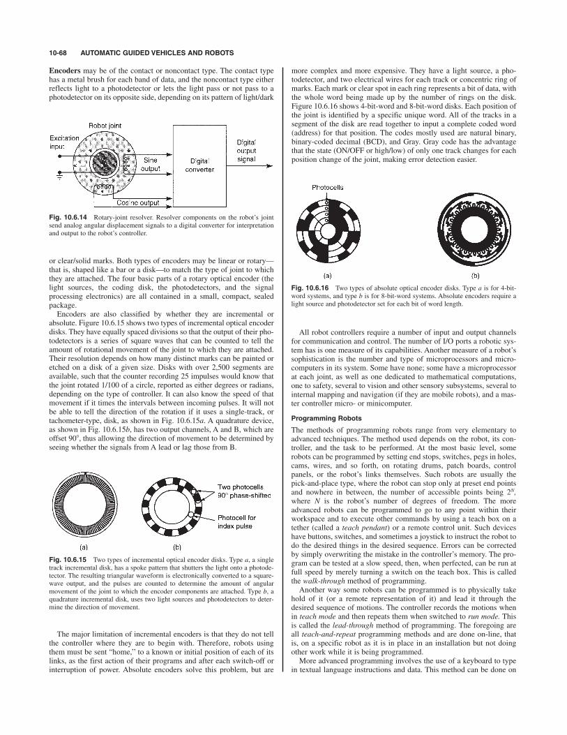
Encoders may be of the contact or noncontact type. The contact typehas a metal brush for each band of data, and the noncontact type eitherreflects light to a photodetector or lets the light pass or not pass to aphotodetector on its opposite side, depending on its pattern of light/dark
more complex and more expensive. They have a light source, a pho-todetector, and two electrical wires for each track or concentric ring ofmarks. Each mark or clear spot in each ring represents a bit of data, withthe whole word being made up by the number of rings on the disk.Figure 10.6.16 shows 4-bit-word and 8-bit-word disks. Each position ofthe joint is identified by a specific unique word. All of the tracks in asegment of the disk are read together to input a complete coded word(address) for that position. The codes mostly used are natural binary,binary-coded decimal (BCD), and Gray. Gray code has the advantagethat the state (ON/OFF or high/low) of only one track changes for eachposition change of the joint, making error detection easier.
10-68 AUTOMATIC GUIDED VEHICLES AND ROBOTS
Fig. 10.6.14 Rotary-joint resolver. Resolver components on the robot’s joint
send analog angular displacement signals to a digital converter for interpretation
and output to the robot’s controller.
or clear/solid marks. Both types of encoders may be linear or rotary—that is, shaped like a bar or a disk—to match the type of joint to whichthey are attached. The four basic parts of a rotary optical encoder (thelight sources, the coding disk, the photodetectors, and the signalprocessing electronics) are all contained in a small, compact, sealedpackage.Encoders are also classified by whether they are incremental or
absolute. Figure 10.6.15 shows two types of incremental optical encoderdisks. They have equally spaced divisions so that the output of their pho-todetectors is a series of square waves that can be counted to tell theamount of rotational movement of the joint to which they are attached.Their resolution depends on how many distinct marks can be painted oretched on a disk of a given size. Disks with over 2,500 segments areavailable, such that the counter recording 25 impulses would know thatthe joint rotated 1/100 of a circle, reported as either degrees or radians,depending on the type of controller. It can also know the speed of thatmovement if it times the intervals between incoming pulses. It will notbe able to tell the direction of the rotation if it uses a single-track, ortachometer-type, disk, as shown in Fig. 10.6.15a. A quadrature device,as shown in Fig. 10.6.15b, has two output channels, A and B, which areoffset 90", thus allowing the direction of movement to be determined byseeing whether the signals from A lead or lag those from B.
Fig. 10.6.15 Two types of incremental optical encoder disks. Type a, a single
track incremental disk, has a spoke pattern that shutters the light onto a photode-
tector. The resulting triangular waveform is electronically converted to a square-
wave output, and the pulses are counted to determine the amount of angular
movement of the joint to which the encoder components are attached. Type b, a
quadrature incremental disk, uses two light sources and photodetectors to deter-
mine the direction of movement.
The major limitation of incremental encoders is that they do not tellthe controller where they are to begin with. Therefore, robots usingthem must be sent “home,’’ to a known or initial position of each of itslinks, as the first action of their programs and after each switch-off orinterruption of power. Absolute encoders solve this problem, but are
Fig. 10.6.16 Two types of absolute optical encoder disks. Type a is for 4-bit-
word systems, and type b is for 8-bit-word systems. Absolute encoders require a
light source and photodetector set for each bit of word length.
All robot controllers require a number of input and output channelsfor communication and control. The number of I/O ports a robotic sys-tem has is one measure of its capabilities. Another measure of a robot’ssophistication is the number and type of microprocessors and micro-computers in its system. Some have none; some have a microprocessorat each joint, as well as one dedicated to mathematical computations,one to safety, several to vision and other sensory subsystems, several tointernal mapping and navigation (if they are mobile robots), and a mas-ter controller micro- or minicomputer.
Programming Robots
The methods of programming robots range from very elementary toadvanced techniques. The method used depends on the robot, its con-troller, and the task to be performed. At the most basic level, somerobots can be programmed by setting end stops, switches, pegs in holes,cams, wires, and so forth, on rotating drums, patch boards, controlpanels, or the robot’s links themselves. Such robots are usually thepick-and-place type, where the robot can stop only at preset end pointsand nowhere in between, the number of accessible points being 2N,where N is the robot’s number of degrees of freedom. The moreadvanced robots can be programmed to go to any point within theirworkspace and to execute other commands by using a teach box on atether (called a teach pendant) or a remote control unit. Such deviceshave buttons, switches, and sometimes a joystick to instruct the robot todo the desired things in the desired sequence. Errors can be correctedby simply overwriting the mistake in the controller’s memory. The pro-gram can be tested at a slow speed, then, when perfected, can be run atfull speed by merely turning a switch on the teach box. This is calledthe walk-through method of programming.Another way some robots can be programmed is to physically take
hold of it (or a remote representation of it) and lead it through thedesired sequence of motions. The controller records the motions whenin teach mode and then repeats them when switched to run mode. Thisis called the lead-through method of programming. The foregoing areall teach-and-repeat programming methods and are done on-line, thatis, on a specific robot as it is in place in an installation but not doingother work while it is being programmed.More advanced programming involves the use of a keyboard to type
in textual language instructions and data. This method can be done on

IDENTIFICATION AND CONTROL OF MATERIALS 10-69
line or off line (away from and detached from the robot, such that it canbe working on another task while the program is being created). Thereare many such programming languages available, but most are limitedto use on one or only a few robots. Most of these languages are explic-it, meaning that each of their instructions gives the robot a specific com-mand to do a small step (e.g., open gripper) as part of a larger task. Themore advanced higher-level implicit languages, however, give instruc-tions at the task level (e.g., assemble 200 of product XYZ), and therobot’s computer knows what sequence of basic steps it must execute todo that. These are also called object-level or world-modeling languagesand model-based systems. Other ways of instructing a robot includespoken commands and feedback from a wide array of sensors, including
vision systems. Telecherics, teleoperators, and other mechanisms underthe continuous control of a remotely located operator are not truerobots, as they are not autonomous.
Using Robots
The successful utilization of robots involves more than selecting andinstalling the right robot and programming it correctly. For an assemblyrobot, for example, care must be taken to design the product so as tofacilitate assembly by a robot, presenting the component piece parts andother material to it in the best way, laying out the workplace (work cell)efficiently, installing all required safety measures, and training pro-gramming, operating, and maintenance employees properly.
10.7 MATERIAL STORAGE AND WAREHOUSINGby Vincent M. Altamuro
The warehouse handling of material is often more expensive thanin-process handling, as it frequently requires large amounts of space,expensive equipment, labor, and computers for control. Warehousingactivities, facilities, equipment, and personnel are needed at both endsof the process—at the beginning as receiving and raw materials andpurchased parts storage, and at the end as finished goods storage, pick-ing, packing, and shipping. These functions are aided by various sub-systems and equipment—some simple and inexpensive, some elaborateand expensive.The rapid and accurate identification of materials is essential. This
can be done using only human senses, humans aided by devices, orentirely automated. Bar codes have become an accepted and reliablemeans of identifying material and inputting that data into an informa-tion and control system.Material can be held, stacked, and transported in simple devices, such
as shelves, racks, bins, boxes, baskets, tote pans, pallets and skids, or incomplex and expensive computer-controlled systems, such as automat-ed storage and retrieval systems.
IDENTIFICATION AND CONTROL OF MATERIALS
Materials must be identified, either by humans or by automated sensingdevices, so as to:1. Measure presence or movement2. Qualify and quantify characteristics of interest3. Monitor ongoing conditions so as to feed back corrective actions4. Trigger proper marking devices5. Actuate sortation or classification mechanisms6. Input computing and control systems, update data bases, and
prepare analyses and summary reportsTo accomplish the above, the material must have, or be given, a unique
code symbol, mark, or special feature that can be sensed and identified.If such a coded symbol is to be added to the material, it must be:1. Easily and economically produced2. Easily and economically read3. Able to have many unique permutations—flexible4. Compact—sized to the package or product5. Error resistant—low chance of misreading, reliable6. Durable7. Digital—compatible with computer data formatsThe codes can be read by contact or noncontact means, by moving or
stationary sensors, and by humans or devices.There are several technologies used in the identification and control
of materials. The most important of these are:1. Bar codes2. Radio-frequency identification (RFID)3. Smart cards
4. Machine vision5. Voice recognition6. Magnetic stripes7. Optical character recognition (OCR)
All can be used for automatic data collection (ADC) purposes and aspart of a larger electronic data interchange (EDI), which is the paper-less, computer-to-computer, intercompany, and international communi-cations and information exchange using a common data language. Thedominant data format standard in the world is Edifact (Electronic DataInterchange for Administration, Commerce, and Transportation).Bar codes are one simple and effective means of identifying and con-
trolling material. Bar codes are machine-readable patterns of alternat-ing, parallel, rectangular bars and spaces of various widths whosecombinations represent numbers, letters, or other information as deter-mined by the particular symbology, or language, employed. Severaltypes of bar codes are available. While multicolor bar codes are possi-ble, simple black-and-white codes dominate because a great number ofpermutations are available by altering their widths, presence, andsequences. Some codes are limited to numeric information, but otherscan encode complete alphanumeric plus special symbols character sets.Most codes are binary digital codes, some with an extra parity bit tocatch errors. In each bar code, there is a unique sequence set of bars andspaces to represent each number, letter, or symbol. One-dimensional, orlinear, codes print all of the bars and spaces in one row. Two-dimensionalstacked codes arrange sections above one another in several rows so asto condense more data into a smaller space. To read stacked codes, thescanner must sweep back and forth so as to read all of the rows. Themost recent development is the two-dimensional matrix codes that con-tain much more information and are read with special scanners or videocameras. Many codes are of the n of m type, i.e., 2 of 5, 3 of 9, etc. Forexample, in the 2-of-5 code, a narrow bar may represent a 0 bit or OFFand a wide bar a 1 or ON bit. For each set of 5 bits, 2 must be ON—hence, 2 of 5. See Table 10.7.1 for the key to this code. A variation tothe basic 2 of 5 is the Interleaved 2-of-5, in which the spaces between thebars also can be either narrow or wide, permitting the reading of a setof bars, a set of spaces, a set of bars, a set of spaces, etc., and yieldingmore information in less space. See Fig. 10.7.1. Both the 2-of-5 and theInterleaved 2-of-5 codes have ten numbers in their character sets.Code 39, another symbology, permits alphanumeric information to be
encoded by allowing each symbol to have 9 modules (locations) alongthe bar, 3 of which must be ON. Each character comprises five bars andfour spaces. Code 39 has 43 characters in its set (1-10, A-Z, six symbols,and one start/stop signal). Each bar or space in a bar code is calledan element. In Code 39, each element is one of two widths, referred toas wide and narrow. As in other bar codes, the narrowest element isreferred to as the X dimension and the ratio of the widest to narrowestelement widths is referred to as the N of the code. For each code, X and

N are constants. These values are used to calculate length of the bar codelabels. The Y dimension of a bar code is the length (or height) of its barsand spaces. It influences the permissible angle at which a label may bescanned without missing any of the pattern. See Table 10.7.2 for theCode 39 key. The patterns for the Code 39 bars and spaces are designedin such a way that changing or misreading a single bit in any of them
10-70 MATERIAL STORAGE AND WAREHOUSING
Table 10.7.1 Bar Code 2-of-5 and I 2/5 Key
Code
Character 1 2 4 7 P
0 0 0 1 1 0
1 1 0 0 0 1
2 0 1 0 0 1
3 1 1 0 0 0
4 0 0 1 0 1
5 1 0 1 0 0
6 0 1 1 0 0
7 0 0 0 1 1
8 1 0 0 1 0
9 0 1 0 1 0
Wide bars and spaces 1Narrow bars and spaces 0
Fig. 10.7.1 A sample of a Uniform Symbology Specification Interleaved 2-
of-5 bar code (also called I 2/5 or ITF).
results in an illegal code word. The bars have only an even number ofwide elements and the spaces have only an odd number of wide ele-ments. The code is called self-checking because that design providesfor the immediate detection of single printing or reading errors. SeeFig. 10.7.2. Code 39 was developed by Intermec (Everett, WA), as wasCode 93, which requires less space by permitting more sizes of bars andspaces. Code 93 has 128 characters in its set (the full ASCII set) andpermits a maximum of about 14 characters per inch, versus Code 39’smaximum of about 9. Code 39 is discrete, meaning that each characteris printed independently of the other characters and is separated fromthe characters on both sides of it by a space (called an intercharactergap) that is not part of the data. Code 93 is a continuous code, meaningthat there are no intercharacter gaps in it and all spaces are parts of thedata symbols.Code 128, a high-density alphanumeric symbology, has 128 charac-
ters and a maximum density of about 18 characters per inch (cpi) fornumeric data and about 9 cpi for alphanumeric data. A Code 128 char-acter comprises six elements: three bars and three spaces, each of fourpossible widths, or modules. Each character consists of eleven 1X widemodules, where X is the width of the narrowest bar or space. The sum ofthe number of bar modules in any character is always even (even parity),while the sum of the space modules is always odd (odd parity), thuspermitting self-checking of the characters. See Table 10.7.3 for the
SOURCE: Uniform Symbology Specification Code 39, Table 2: Code 39 SymbolCharacter Set, © Copyright 1993 Automatic Identification Manufacturers, Inc.
Table 10.7.2 Uniform Symbology Specification Code 39Symbol Character Set
Code 128 key. Code 128 is a continuous, variable-length, bidirectionalcode.The Universal Product Code (U.P.C.) is a 12-digit bar code adopted by
the U.S. grocery industry in 1973. See Figure 10.7.3 for a sample of theU.P.C. standard symbol. Five of the six digits in front of the two long barsin the middle [called the center guard pattern (CGP)] identify the item’smanufacturer and five of the six digits after the CGP identifies the specif-ic product. There are several variations of the U.P.C., all those in theUnited States are controlled by the Uniform Code Council, located inDayton, OH. One variation is an 8-digit code that identifies both the man-ufacturer and the specific product with one number. The U.P.C. uses pre-fix and suffix digits separated from the main number. The prefix digit isthe number system character. See Table 10.7.4 for the key to these prefixnumbers. The suffix is a “modulo-10” check digit. It serves to confirm thatthe prior 11 digits were read correctly. See Figure 10.7.4 for the method by

10-71
Table 10.7.3 Uniform Symbology Specification Code 128 Symbol Character Set
SOURCE: Uniform Symbology Specification Code 128, Table 2: Code 128 Symbol Character Set, © Copyright 1993 Automatic Identification Manufacturers, Inc.

which the check digit is calculated. Each U.P.C. character comprisestwo bars and two spaces, each of which may be one, two, three, or fourmodules wide, such that the entire character consumes a total of sevenmodules of space. See Table 10.7.5 for the key to the code. It will benoted that the codes to the left of the CGP all start with a zero (a space)
10-72 MATERIAL STORAGE AND WAREHOUSING
Fig. 10.7.2 A sample of Uniform Symbology Specification Code 39 bar code.
Fig. 10.7.3 A sample of the Universal Product Code Standard Symbol. (U.P.C.
Symbol Specification Manual, January 1986, Copyright © 1986 Uniform Code
Council, Inc. The Uniform Code Council prohibits the commercial use of their copy-
righted material without prior written permission.)
and end with a one (a bar) while those to the right of the CGP all startwith a one and end with a zero. This permits the code to be scannedfrom either left to right or right to left (that is, it is omnidirectional) andallows the computer to determine the direction and whether it needs tobe reversed before use by the system. The U.P.C. label also has thenumber printed in human-readable form along the bottom. When integrated into a complete system, the U.P.C. can serve as the
input data point for supermarket pricings, checkouts, inventory control,reordering stock, employee productivity checks, cash control, specialpromotions, purchasing habits and history of customers holding store“club” cards, sales analyses, and management reports. Its use increasescheckout speed and reduces errors. In some stores, it is combined with
Table 10.7.4 U.P.C. Prefix Number System Character KeyThe human-readable character identifying the encoded number system will be
shown in the left-hand margin of the symbol as per Fig. 10.7.3.
Number system
character Specified use
0 Regular U.P.C. codes (Versions A and E)
2 Random-weight items, such as meat and produce,
symbol-marked at store level (Version A)
3 National Drug Code and National Health Related
Items Code in current 10-digit code length
(Version A). Note that the symbol is not affected
by the various internal structures possible with the
NDC or HRI codes.
4 For use without code format restriction with check
digit protection for in-store marking of nonfood
items (Version A).
5 For use on coupons (Version A).
6, 7 Regular U.P.C. codes (Version A).
1, 8, 9 Reserved for uses unidentified at this time.
SOURCE: U.P.C. Symbol Specification Manual, January 1986, © Copyright 1986 UniformCode Council, Inc. The Uniform Code Council prohibits the commercial use of theircopyrighted material without prior written permission.
a speech synthesizer that voices the description and price of each itemscanned. It is a vital component in a fully automated store.As with many new technologies, different users use different proto-
cols. New users must choose to use an existing protocol or create one oftheir own better suited to their particular needs. Soon there arise sever-al camps of conflicting “standards,” where one universally acceptedstandard is essential for the full application of the technology in allproducts, systems, companies, and countries. The longer users of eachdifferent design go separate ways, the more difficult it is for them tochange, as their investment in hardware and software increases. Suchwas the case with bar codes. Hence, in January 1, 2005, in order to havetheir bar code compatible with the rest of the world, and as directed bythe Uniform Code Council, the U.S. and Canada added a digit to their12-digit UPC to make a 13-digit pattern that would match the EuropeanArticle Numbering system pattern and become the global standard.
The following example will illustrate the calculation of the check character
for the symbol shown in Fig. 10.7.3. Note that the code shown in Fig. 10.7.3
is in concurrent number system 0.
Step 1: Starting at the left, sum all the characters in the odd positions (that
is, first from the left, third from the left, and so on), starting with the number
system character.
(For the example, 0 $ 2 $ 4 $ 6 $ 8 $ 0 20.)
Step 2: Multiply the sum obtained in Step 1 by 3.
(The product for the example is 60.)
Step 3: Again starting at the left, sum all the characters in the even posi-
tions.
(For the example, 1 $ 3 $ 5 $ 7 $ 9 25.)
Step 4: Add the product of step 2 to the sum of step 3.
(For the example, the sum is 85.)
Step 5: The modulo-10 check character value is the smallest number which
when added to the sum of step 4 produces a multiple of 10.
(In the example, the check character value is 5.)
The human-readable character identifying the encoded check character will
be shown in the right-hand margin of the symbol as in Fig. 10.7.3.
Fig. 10.7.4 U.P.C. check character calculation method. (U.P.C. Symbol
Specification Manual, January 1986, Copyright © 1986 Uniform Code Council,
Inc. The Uniform Code Council prohibits the commercial use of their copyrighted
material without prior written permission.)

IDENTIFICATION AND CONTROL OF MATERIALS 10-73
Also, the Uniform Code Council and EAN International combined toform a global code-controlling organization, called GSI, headquarteredin Brussels.Over the years, nearly 50 different one-dimensional bar code sym-
bologies have been introduced. Around 20 found their way into com-mon use at one time or another, with six or seven being most important.These are the Interleaved 2-of-5, Code 39, Code 93, Code 128,Codabar, Code 11, and the U.P.C. Table 10.7.6 compares some of thecharacteristics of these codes. The choice depends on the use by othersin the same industry, the need for intercompany uniformity, the type andamount of data to be coded, whether mere numeric or alphanumericplus special symbols will be needed, the space available on the item,and intracompany compatibility requirements.Some bar codes are limited to a fixed amount of data. Others can be
extended to accommodate additional data and the length of their labelis variable. Figure 10.7.5 shows a sample calculation of the length of aCode 39 label.
The foregoing one-dimensional, linear bar codes are sometimescalled license plates because all they can do is contain enough infor-mation to identify an item, thereby permitting locating more informa-tion stored in a host computer. Two-dimensional stacked codes containmore information. The stacked codes, such as Code 49, developed byDr. David Allais at Intermec, Code 16K, invented by Ted Williams, ofLaserlight Systems, Inc., Dedham, MA, and others are really one-dimensional codes in which miniaturized linear codes are printed inmultiple rows, or tiers. They are useful on small products, such as elec-tronic components, single-dose medicine packages, and jewelry, wherethere is not enough space for a one-dimensional code. To read them, ascanner must traverse each row in sequence. Code 49 (see Fig. 10.7.6) canarrange all 128 ASCII encoded characters on up to eight stacked rows.Figure 10.7.7 shows a comparison of the space required for the sameamount (30 characters) of alphanumeric information in three bar codesymbologies: Code 39, Code 93, and Code 49. Code 16K (Fig. 10.7.8),which stands for 128 squared, shrinks and stacks linear codes in from 2
Table 10.7.5 U.P.C. Encodation KeyEncodation for U.P.C. characters, number system character, and
modulo check character.
Left characters Right characters
Decimal value (Odd parity—O) (Even parity—E)
0 0001101 1110010
1 0011001 1100110
2 0010011 1101100
3 0111101 1000010
4 0100011 1011100
5 0110001 1001110
6 0101111 1010000
7 0111011 1000100
8 0110111 1001000
9 0001011 1110100
The encodation for the left and right halves of the regular symbol,including UPC characters, number system character and modulo checkcharacter, is given in this following chart, which is applicable to version A.Note that the left-hand characters always use an odd number (3 or 5) ofmodules to make up the dark bars, whereas the right-hand charactersalways use an even number (2 or 4). This provides an “odd” and “even”parity encodation for each character and is important in creating, scanning,and decoding a symbol.SOURCE: U.P.C. Symbol Specification Manual, January 1986, ©
Copyright 1986 Uniform Code Council, Inc. The Uniform Code Councilprohibits the commercial use of their copyrighted material without priorwritten permission. Fig. 10.7.6 Code 49. (Uniform Symbology Specification Code 49, Copyright ©
1993 Automatic Identification Manufacturers, Inc.)
Fig. 10.7.5 Calculation of a bar code label length.
Example used:
Symbology: Code 39
System: Each bar or space one element
Each character 9 elements (5 bars and 4 spaces)
Each character 3 wide and 6 narrow elements
(That is, 3 of 9 elements must be wide)
Width of narrow element X dimension 0.015 in (0.0381 cm)
Wide to narrow ratio N value 3 : 1 3
Length segments per data character 3(3) $ 6 15
Number of data characters in example 6
Length of data section 6 ! 5 90.0 segments of length
Start character 15.0
Stop character 15.0
Intercharacter gaps (at 1 segment per gap):
No. of gaps (data characters ' 1)
$ start $ stop
(6 ' 1) $ 1 $ 1 7 7.0
Quiet zones
(2, each at least 10 segments) 20.0
Total segments 147.0
Times X, length of each segment !0.015
2.205 in (5.6007 cm)
Fig. 10.7.7 A comparison of the space required by three bar codes. Each bar
code contains the same 30 alphanumeric characters.
to 16 rows. It offers high-data-density encoding of the full 128-characterASCII set and double-density encoding of numerical data strings. It canfit 40 characters of data in the same space as eight would take in Code128, and it can be printed and read with standard printing and scanningequipment.
Two-dimensional codes allow extra information regarding an item’sdescription, date and place of manufacture, expiration date, lot number,package size, contents, tax code, price, etc. to be encoded, rather thanmerely its identity. Two-dimensional matrix codes permit the encodingof very large amounts of information. Read by video cameras or speciallaser scanners and decoders, they can contain a complete data file about
Fig. 10.7.8 Code 16K with human-readable interpretation. (Uniform Symbology
Specification Code 16K, Copyright © 1993 Automatic Identification Manufacturers,
Inc.)

the product to which they are affixed. In many cases, this eliminates theneed to access the memory of a host computer. That the data file trav-els with (on) the item is also an advantage. Their complex patterns andinterpretation algorithms permit the reading of complete files evenwhen part of the pattern is damaged or missing. Code PDF417, developed by Symbol Technologies Inc., Bohemia, NY
(and put in the public domain, as are most codes), is a two-dimensionalbar code symbology that can record large amounts of data, as well asdigitized images such a fingerprints and photographs. To read the high-density PDF417 code, Symbol Technologies Inc. has developed a ras-tering laser scanner. This scanner is available in both a hand-held andfixed-mount version. By design, PDF417 is also scannable using a widerange of technologies, as long as specialized decoding algorithms areused. See Fig. 10.7.9 for an illustration of PDF417’s ability to compressAbraham Lincoln’s Gettysburg Address into a small space. The mini-mal unit that can represent data in PDF417 is called a codeword. It com-prises 17 equal-length modules. These are grouped to form 4 bars and4 spaces, each from one to six modules wide, so that they total 17modules. Each unique codeword pattern is given one of 929 values.Further, to utilize different data compression algorithms based on thedata type (i.e., ASCII versus binary) the system is multimodal, so that acodeword value may have different meanings depending on which ofthe various modes is being used. The modes are switched automatically
during the encoding process to create the PDF417 code and then againduring the decoding process. The mode-switching instructions are car-ried in special codewords as part of the total pattern. Thus, the value ofa scanned codeword is first determined (by low-level decoding), then itsmeaning is determined by virtue of which mode is in effect (by high-level decoding). Code PDF417 is able to detect and correct errorsbecause of its sophisticated error-correcting algorithms. Scanning at
10-74 MATERIAL STORAGE AND WAREHOUSING
Table 10.7.6 Comparison of Bar Code Symbologies
Interleaved Code 39 Codabar Code 11 U.P.C./EAN Code 128 Code 93
Date of inception 1972 1974 1972 1977 1973 1981 1982
Industry-standard specification AIM AIM CCBBA AIM UPCC AIM AIM
ANSI ANSI ANSI IAN
UPCC AIAG
AIAG HIBC
Government support DOD
Corporate sponsors Computer Intermec Welch Intermec Computer Intermec
Identics Allyn Identics
Most-prominent application area Industry Industry Medical Industry Retail New New
Variable length Noa Yes Yes Yes No Yes Yes
Alphanumeric No Yes No No No Yes Yes
Discrete No Yes Yes Yes No No No
Self-checking Yes Yes Yes No Yes Yes No
Constant character width Yes Yes Yesb Yes Yes Yes Yes
Simple structure (two element widths) Yes Yes No No No No No
Number of data characters in set 10 43/128 16 11 10 103/128 47/128
Densityc:
Units per character 7–9 13–16 12 8–10 7 11 9
Smaller nominal bar, in 0.0075 0.0075 0.0065 0.0075 0.0104 0.010 0.008
Maximum characters/inch 17.8 9.4 10 15 13.7 9.1 13.9
Specified print tolerance at maximum density, in
Bar width 0.0018 0.0017 0.0015 0.0017 0.0014 0.0010 0.0022
Edge to edge 0.0015 0.0014 0.0013
Pitch 0.0030 0.0029 0.0013
Does print tolerance leave more than half of Yes Yes No Yes No No Yes
the total tolerance for the scanner?
Data securityd High High High High Moderate High High
a Interleaved 2 of 5 is fundamentally a fixed-length code.b Using the standard dimensions Codabar has constant character width. With a variant set of dimensions, width is not constant for all characters.c Density calculations for interleaved 2 of 5, Code 39, and Code 11 are based on a wide-to-narrow ratio of 2.25 : 1. Units per character for these symbols are shown as a range corresponding to
wide/narrow ratios from 2 : 1 to 3 : 1. A unit in Codabar is taken to be the average of narrow bars and narrow spaces, giving about 12 units per character.d High data security corresponds to less than 1 substitution error per several million characters scanned using reasonably good-quality printed symbols. Moderate data security corresponds to
1 substitution error per few hundred thousand characters scanned. These values assume no external check digits other than those specified as part of the symbology and no file-lookup protectionor other system safeguards.
eAIM Automatic Identification Mfrs Inc (Pittsburgh)ANSI American National Standards Institute (New York)AIAG Automative Industry Action Group (Southfield, MI)IAN Intl Article Numbering Assn (Belgium)DOD Dept of DefenseCCBBA Committee for Commonality in Blood Banking (Arlington, VA)UPCC Uniform Product Code Council Inc (Dayton, OH)SOURCE: Intermec—A Litton Company, as published in the March, 1987 issue of American Machinist magazine, Penton Publishing Co., Inc.
Fig. 10.7.9 A sample of PDF417 Encoding: Abraham Lincoln’s Gettysburg
Address. (Symbol Technologies, Inc.)

IDENTIFICATION AND CONTROL OF MATERIALS 10-75
angles is made possible by giving successive rows of the stacked codedifferent identifiers, thereby permitting the electronic “stitching” of theindividual codewords scanned. In addition, representing the data byusing codewords with numerical values that must be interpreted by adecoder permits the mathematical correction of reading errors. At itssimplest level, if two successive codewords have values of, say, 20 and52, another codeword could be made their sum, a 72. If the first code-word were read, but the second missed or damaged, the system wouldsubtract 20 from 72 and get the value of the second codeword. Morecomplex high-order simultaneous polynomial equations and algorithmsare also used. The PDF417 pattern serves as a portable data file thatprovides local access to large amounts of information about an item (orperson) when access to a host computer is not possible or economicallyfeasible. PDF417 provides a low-cost paper-based method of transmit-ting machine-readable data between systems. It also has use in WORM(written once and read many times) applications. The size of the labeland its aspect ratio (the shape, or relationship of height to width) arevariable so as to suit the user’s needs.Data Matrix, a code developed by International Data Matrix Inc.,
Clearwater, FL, is a true matrix code. It may be square or rectangular, andcan be enlarged or shrunk to whatever size [from a 0.001-in (0.254-mm),or smaller, to a 14-in (36-cm), or larger, square] suits the user andapplication. Figure 10.7.10 shows the code in three sizes, but with thesame contents. Its structure is uniform—square cells all the same size fora given pattern. To fit more user data into a matrix of a specific size, allthe internal square cells are reduced to a size that will accommodate the
alternating light and dark cells. This signature serves to have the video[charge-coupled device (CCD)] camera locate and identify the symbol.It also provides for the determination of its angular orientation. Thatcapability permits a robot to rotate the part to which the code is affixedto the proper orientation for assembly, test, or packaging. Further, theinformation it contains can be program instructions to the robot. Thelabels can be printed in any combination of colors, as long as their dif-ference provides a 20 percent or more contrast ratio. For aesthetic orsecurity reasons, it can be printed in invisible ink, visible only whenilluminated with ultraviolet light. The labels can be created by anyprinting method (laser etch, chemical etch, dot matrix, dot peen, ther-mal transfer, ink jet, pad printer, photolithography, and others) and onany type of computer printer through the use of a software interface dri-ver provided by the company. The pattern’s binary code symbology isread with standard CCD video cameras attached to a company-madecontroller linked to the user’s computer system with standard interfacesand a Data Matrix Command Set. The algorithms for error correction
Fig. 10.7.10 Three sizes of Data Matrix patterns, all with the same contents.
(International Data Matrix, Inc.)
amount of data to be encoded. Figure 10.7.11 shows five patterns, allthe same size, containing different amounts of data. As a user selectsadditional data, the density of the matrix naturally increases. A patterncan contain from 1 to 2,000 characters of data. Two adjacent sides arealways solid, while the remaining two sides are always composed of
Fig. 10.7.11 Five Data Matrix patterns, all the same size but containing dif-
ferent amounts of information. (International Data Matrix, Inc.)

that it uses create data values that are cumulative and predictable so thata missing or damaged character can be deduced or verified from thedata values immediately preceding and following it.Code One (see Fig. 10.7.12), invented by Ted Williams, who also cre-
ated Code 128 and Code 16K, is also a two-dimensional checker-boardor matrix type code read by a two-dimensional imaging device, such asa CCD video camera, rather than a conventional scanner. It can be readat any angle. It can encode the full ASCII 256-character set in additionto four function characters and a pad character. It can encode from 6 toover 2,000 characters of data in a very small space. If more data is need-ed, additional patterns can be linked together.
largest version, can encode 3,550 numeric or 2,218 alphanumeric char-acters, while correcting up to 2,240 bit errors. The data is encoded inrectangular tile groups, each composed of 8-bit squares arranged in afour-wide by two-high array. Within each tile, each square encodes onebit of data, with a white square representing a zero and a black squarerepresenting a one. The squares are used to create the 8-bit bytes thatare the symbol’s characters. The most significant bit in the characterpattern is in the top left corner of the rectangle, proceeding left to rightthrough the upper row and then the lower row, to the least significant bitin the bottom right corner of the pattern. The symbol characters areordered left to right and then top to bottom, so that the first character isin the top left corner of the symbol and the last character is in the bot-tom right corner.The fact that the patterns for its characters are arrays of spots whose
images are captured by a camera, rather than the row of bars that one-dimensional and stacked two-dimensional codes have, frees it from theY-dimension scanning angle restraint of those codes and makes it lesssusceptible to misreads and no-reads. The size of each square data bit iscontrolled only by the smallest optically resolvable or printable spot.Bar codes may be printed directly on the item or its packaging or on
a label that is affixed thereon. Some are scribed on with a laser. In manycases, they are printed on the product or package at the same time otherprinting or production operations are being performed, making the costof adding them negligible. Labels may be produced in house or orderedfrom an outside supplier.A recent application (made compulsory in 2006) of bar codes is on
hospital medications to ensure that patients get the correct dose of thecorrect drug at the correct time so as to reduce the thousands of hospi-talized patients and nursing home residents who die annually from drugerrors. Matching the bar code on the patient’s wristband with the drugsprescribed can also catch the administration of drugs which might causean allergic reaction, drugs in conflict with other drugs, and drugs thatshould be given in liquid rather than pill form and vice versa.In addition to the bar code symbology, an automatic identification
system also requires a scanner or a video camera. A scanner is an elec-trooptical sensor which comprises a light source [typically a light-emitting diode (LED), laser diode, or helium-neon-laser tube], a lightdetector [typically a photodiode, photo-integrated circuit (photo-IC),phototransistor, or charge-coupled device (CCD)], an analog signalamplifier, and (for digital scanners) an analog-to-digital converter. Thesystem also needs a microprocessor-based decoder, a data communica-tion link to a computer, and one or more output or actuation devices.See Fig. 10.7.14.The scanner may be hand-held or mounted in a fixed position, but
something must move relative to the other, either the entire scanner, thescanner’s oscillating beam of light, or the package or item containingthe bar code. For moving targets, strobe lights are sometimes used tofreeze the image while it is being read.The four basic categories of scanners are: hand-held fixed beam,
hand-held moving beam, stationary fixed beam, and stationary movingbeam. Some scanners cast crosshatched patterns on the object so as tocatch the bar code regardless of its position. Others create holographiclaser patterns that wrap a field of light beams around irregularly shapedarticles. Some systems require contact between the scanner and the barcode, but most are of the noncontact type. A read-and-beep system emitsa sound when a successful reading has been made. A specialized type ofscanner, a slot scanner, reads bar codes on badges, cards, envelopes, doc-uments, and the like as they are inserted in the slot and swiped.In operation, the spot or aperture of the scanner beam is directed by
optics onto the bar code and reflected back onto a photodetector. Therelative motion of the scanner beam across the bar code results in ananalog response pattern by the photodetector as a function of the rela-tive reflectivities of the dark bars and light spaces. A sufficient contrastbetween the bars, spaces, and background color is required. Some scan-ners see red bars as white. Others see aluminum as black, requiring thespaces against such backgrounds to be made white.The system anticipates an incoming legitimate signal by virtue of
first receiving a zero input from the “quiet zone”—a space of a certain
10-76 MATERIAL STORAGE AND WAREHOUSING
Fig. 10.7.12 Code One. (Laserlight Systems, Inc.)
Figure 10.7.13 shows a comparison of the sizes of four codes—Code128, Code 16K, PDF-417, and Code One—to illustrate how muchsmaller Code One is than the others. Code One can fit 1,000 charactersinto a 1-in (2.54-cm) square of its checkerboard-like pattern. All CodeOne patterns have a finder design at their center. These patterns serveseveral purposes. They permit the video camera to find the label anddetermine its position and angular orientation. They eliminate the needfor space-consuming quiet zones. And, because the internal patterns aredifferent for each of the versions (sizes, capacities, and configurations)of the code, they tell the reader what version it is seeing. There are 10different versions and 14 sizes of the symbol. The smallest contains 40checkerboard-square type bits and the largest has 16,320. Code 1H, the
Fig. 10.7.13 Comparative sizes of four symbols encoding the same data with
the same x dimension. (Laserlight Systems, Inc.)

IDENTIFICATION AND CONTROL OF MATERIALS 10-77
width (generally at least 10 times the code’s X dimension) that is clearof all marks and which precedes the start character and follows the stopcharacter. The first pattern of bars and spaces (a character) that the scan-ner sees is the start/stop code. These not only tell the system that datacodes are coming next and then that the data section has ended, but inbidirectional systems (those that can be scanned from front to back orfrom back to front) they also indicate that direction. In such bidirec-tional systems, the data is read in and then reversed electronically asnecessary before use. The analog signals pass through the scanner’s sig-nal conditioning circuitry, were they are amplified, converted into digi-tal form, tested to see whether they are acceptable, and, if so, passed tothe decoder section microprocessor for algorithmic interpretation.The decoder determines which elements are bars and which are spaces,
determines the width (number of modules) of each element, determineswhether the code has been read frontward or backward and reverses thesignal if needed, makes a parity check, verifies other criteria, converts thesignal into a computer language character—the most common of whichis asynchronous American Standard Code for Information Interchange(ASCII)—and sends it, via a data communication link, to the computer.Virtually all automatic identification systems are computer-based. Thebar codes read become input data to the computer, which then updates itsstored information and/or triggers an output.Other types of automatic identification systems include radio-frequency
identification, smart cards, machine vision, voice recognition, magneticstripes, and optical character recognition.Radio-frequency identification has many advantages over the other
identification, control, and data-collection methods. It is immune to fac-tory noise, heat, cold, and harsh environments. Its tags can be coveredwith dirt, grease, paint, etc. and still operate. It does not require line ofsight from the reader, as do bar codes, machine vision, and OCR. It canbe read from a distance, typically 15 ft (4.6 m). Its tags can both receiveand send signals. Many types have higher data capacities than one-dimensional bar codes, magnetic stripes, and OCR. Some tags canread/write and process data, much like smart cards. However, RFIDalso has some disadvantages, compared to other methods. The tags arenot human-readable and their cost for a given amount of data capacityis higher than that of some other methods. The RFID codes are cur-rently closed—that is, a user’s code is not readable by suppliers or cus-tomers—and there are no uniform data identifiers (specific numeric oralphanumeric codes that precede the data code and that identify thedata’s industry, category, or use) like the U.P.C. has.Since 2004, the U.S. military, faced with frequent separations of
wounded personnel and their medical records, has recorded medical data
on passive RFID chips sewn into wristbands, embedded in dog tags, andotherwise attached to the person, so that the records and the woundedtravel together. The attached RFID chips also serve to identify woundedor killed personnel. The chips, which can hold 2 kbits of information, arealso used by the military to monitor and warn individuals going into andout of chemical, biological, or radioactive “hot” areas and also to keeptrack of the movements, levels, and ages of munitions and supplies.An RFID system consists of a transceiver and a tag, with a host com-
puter and peripheral devices possible. The transceiver has a coil orantenna, a microprocessor, and electronic circuitry, and is called areader or scanner. The tag can also have an antenna coil, a capacitor, anonvolatile type of memory, transponder electronic circuitry, and con-trol logic—all encapsulated for protection.The system’s operations are very simple. The reader transmits an RF
signal to the tag, which is usually on a product, tote bin, person, or otherconvenient carrier and can be made small and concealed. This signaltells the tag that a reader is present and wants a response. The activatedtag responds by broadcasting a coded signal on a different frequency.The reader receives that signal and processes it. Its output may be assimple as emitting a sound for the unauthorized removal of an item con-taining the tag (retail theft, library books, and the like), flashing a greenlight and/or opening a door (employee ID badges), displaying informa-tion on a human-readable display, directing a robot or automatic guid-ed vehicle (AGV), sending a signal to a host computer, etc. The signalsfrom the reader to the tags can also provide energy to power the tag’scircuitry and supply the digital clock pulses for the tag’s logic section.The tags may be passive or active. Passive tags use power contained in
the signal from the reader. The normal range for these is 18 in (0.46 m)or less. Active tags contain a battery for independent power and usual-ly operate in the 3- to 15-ft (0.9- to 4.6-m) range. Tags programmedwhen made are said to be factory programmed and are read-onlydevices. Tags programmed by plugging them into, or placing them verynear, a programmer are called field-programmed devices. Tags whoseprogram or data can be changed while they are in their operating loca-tions are called in-use programmed devices. The simplest tags containonly one bit of code. They are typically used in retail stores to detectshoplifting and are called electronic article surveillance (EAS),presence sensing, or Level I tags. The next level up are the tags that, likebar codes, identify an object and serve as an input code to a database ina host computer. These “electronic license plates” are called Level IItags and typically have a capacity of between 8 and 128 bits. The thirdlevel devices are called Level III, or transaction/routing tags. They holdup to 512 bits so that the item to which they are attached may be
Fig. 10.7.14 Components of a bar code scanner.

described as well as identified. The next level tags, Level IV, are calledportable databases, and, like matrix bar codes, carry large amounts ofinformation in text form, coded in ASCII. The highest current level tagsincorporate microprocessors, making them capable of data processingand decision making, and are the RF equivalent of smart cards. Smart cards, also called chipcards, or memory cards, are the size of
credit cards but twice as thick. They are composed of self-contained cir-cuit boards, stacked memory chips, a microprocessor, a battery, andinput/output means, all laminated between two sheets of plastic whichusually contain identifiers and instructions. They are usually read byinserting them into slots and onto pins of readers. The readers can befree-standing devices or components of production and inventory con-trol systems, computer systems, instruments, machines, products, main-tenance records, calibration instruments, store checkout registers,vending machines, telephones, automatic teller machines, road tollbooths, doors and gates, hospital and patient records, etc. One smartcard can hold the complete data file of a person or thing and that datacan be used as read and/or updated.The cards may be described as being in one of four classifications:
contactless cards, those which contain a tiny antenna, such that energy aswell as data are exchanged via electromagnetic fields rather than directphysical contact and are used mostly for general access, such as trans-portation; intelligent memory cards, those having an EEPROM (electri-cally erasable programmable read-only memory), a logic circuit, andsecurity feature and which are used mainly as telephone, shopping, andhealth cards; microcontroller cards, which have an EEPROM, RAM,ROM, I/O, and a CPU, making them a complete computer system witha security feature and are typically used as network access cards andbanking cards; and cryptocards, which contain microcontrollers plus amathematics coprocessor for cryptographic applications and high-securitysituations.Cards with up to 64-Mbytes of flash memory are available. They are
made by tape-automated bonding of 20 or more blocks of two-layeredmemory chips onto both sides of a printed-circuit board.Machine vision can be used to:1. Detect the presence or absence of an entire object or a feature of
it, and sort, count, and measure.2. Find, identify, and determine the orientation of an object so that
a robot can go to it and pick it up.3. Assure that the robot or any other machine performed the task it
was supposed to do, and inspect the object.4. Track the path of a seam so that a robot can weld it.5. Capture the image of a matrix-type bar code for data input or a
scene for robotic navigation (obstacle avoidance and path finding).In operation, the machine-vision system’s processor digitizes the
image that the camera sees into an array of small square cells (called pic-ture elements, or pixels). It classifies each pixel as light or dark or a rela-tive value between those two extremes. The system’s processor thenemploys methods such as pixel counting, edge detection, and connectiv-ity analysis to get a pattern it can match (a process called windowing andfeature analysis) to a library of images in its memory, triggering a spe-cific output for each particular match. Rather than match the entire imageto a complete stored pattern, some systems use only common featuretests, such as total area, number of holes, perimeter length, minimum andmaximum radii, and centroid position. The resolution of a machine visionsystem is its field of view (the area of the image it captures) divided byits number of pixels (e.g., 256 ! 256 65,536, 600 ! 800 480,000).The system can evaluate each pixel on either a binary or a gray scale.Under the binary method, a threshold of darkness is set such that pixelslighter than it are assigned a value of 1 and those darker than it are givena value of 0 for computer processing. Under the gray scale method, sev-eral intensity levels are established, the number depending on the size ofthe computer’s words. Four bits per pixel permit 16 levels of gray, 6 bitsallow 64 classifications, and 8-bit systems can classify each pixel into anyof 256 values, but at the cost of more computer memory, processing time,and expense. As the cost of vision systems drops, their use in automaticidentification increases. Their value in reading matrix-type bar codes andin robotics can justify their cost.
Voice recognition systems process patterns received and match them toa computer’s library of templates much like machine vision does.Memory maps of sound pattern templates are created either by the sys-tem’s manufacturer or user, or both. A speaker-dependent system rec-ognizes the voice of only one or a few people. It is taught to recognizetheir words by having the people speak them several times while thesystem is in the teach mode. The system creates a speech template foreach word and stores it in memory. The system’s other mode is therecognition mode, during which it matches new input templates to thosein its memory. Speaker-independent systems can recognize almost any-one’s voice, but can handle many fewer words than speaker-dependentsystems because they must be able to recognize many template varia-tions for each word. The number of words that each system can recog-nize is constantly being increased.In operation, a person speaks into a microphone. The sound is ampli-
fied and filtered and fed into an analyzer, thence to a digitizer. Then asynchronizer encodes the sound by separating its pattern into equalslices of time and sends its frequency components to a classifier whereit is compared to the speech templates stored in memory. If there is amatch, the computer produces an output to whatever device is attachedto the system. Some systems can respond with machine-generatedspeech. The combination of voice recognition and machine speech iscalled speech processing or voice technology. Products that can “hear”and “talk” are called conversant products. Actual systems are morecomplicated and sophisticated than the foregoing simplified descrip-tion. The templates, for example, instead of having a series of singledata points define them, have numerical fields based on statistical prob-abilities. This gives the system more tolerant template-to-template vari-ations. Further, and to speed response, neural networks, fuzzy logic, andassociative memory techniques are used.Some software uses expert systems that apply grammatical and con-
text rules to the inputs to anticipate that a word is a verb, noun, number,etc. so as to limit memory search and thereby save time. Some systemsare adaptive, in that they constantly retrain themselves by modifying thetemplates in memory to conform to permanent differences in the speak-ers’ templates. Other systems permit the insertion by each user of anindividual module which loads the memory with that person’s particu-lar speech templates. This increases the capacity, speed, and accuracyof the system and adds a new dimension: security against use by anunauthorized person. Like fingerprints, a person’s voice prints areunique, making voice recognition a security gate to entry to a comput-er, facility, or other entity. Some systems can recognize thousands ofwords with almost perfect accuracy. Some new products, such as theVCP 200 chip, of Voice Control Products, Inc., New York City, arepriced low enough, by eliminating the digital signal processor (DSP)and limiting them to the recognition of only 8 or 10 words (commands),to permit their economic inclusion in products such as toys, cameras,and appliances.A major use of voice recognition equipment is in industry where it
permits assemblers, inspectors, testers, sorters, and packers to workwith both hands while simultaneously inputting data into a computerdirectly from the source. They are particularly useful where keyboardsare not suitable data-entry devices. They can eliminate paperwork,duplication, and copying errors. They can be made to cause the printingof a bar code, shipping label, or the like. They can also be used toinstruct robots—by surgeons describing and directing an operation, forexample—and in many other applications. Magnetic stripes encode data on magnetic material in the form of a
strip or stripe on a card, label, or the item itself. An advantage to themethod is that the encoded data can be changed as required.Optical character recognition uses a video camera to read numbers, let-
ters, words, signs, and symbols on packages, labels, or the item itself. Itis simpler and less expensive than machine vision but more limited.The information collected from the foregoing can be used at the loca-
tion where it is obtained, observed by a human, stored in the sensingdevice for later input to a computerized system, or transmitted in realtime to a central location via either fixed wires or by a wireless means.Users should be aware that wireless signals travel through the air,
10-78 MATERIAL STORAGE AND WAREHOUSING

STORAGE EQUIPMENT 10-79
making them more vulnerable than wired connections to reception byunauthorized persons, unless security features are included. Devicesequipped with Bluetooth components for shorter-range transmissions orWiFi (wireless fidelity) technology for longer ranges can communicatewirelessly with other devices so equipped. WiFi requires the use oflocations called access points or “hot spots” to connect to the Internet,networks of portable computers, or other WLANs (wireless local areanetworks).The industry’s trade group is the Automatic Identification
Manufacturers, Inc. (AIM), located in Pittsburgh.
STORAGE EQUIPMENT
The functions of storage and handling devices are to permit:
The greatest use of the space available, stacking high, using the“cube” of the room, rather than just floor areaMultiple layers of stacked items, regardless of their sizes, shapes,
and fragility“Unit load” handling (the movement of many items of material
each time one container is moved)Protection and control of the material
Shelves and Racks Multilevel, compartmentalized storage is pos-sible by using shelves, racks, and related equipment. These can beeither prefabricated standard size and shape designs or modular units orcomponents that can be assembled to suit the needs and space available.Variations to conventional equipment include units that slide on floorrails (for denser storage until needed), units mounted on carousels togive access to only the material wanted, and units with inclined shelvesin which the material rolls or slides forward to where it is needed.
removed. Figure 10.7.19 shows mobile racks. Here the racks are storednext to one another. When material is required, the racks are separatedand become accessible. Figure 10.7.20 shows racks where the pickerpasses between the racks. The loads are supported by arms attached to
Fig. 10.7.15 Pallet racks. (Modern Materials Handling, Feb. 22, 1980,
p. 85.)
Figure 10.7.15 shows the top view of a typical arrangement of pallet racksproviding access to every load in storage. Storage density is low because ofthe large amount of aisle space. Figure 10.7.16 shows multiple-depth palletracks with proportionally smaller aisle requirement. Figure 10.7.17shows cantilever racks for holding long items. Figure 10.7.18 showsflow-through racks. The racks are loaded on one side and emptied fromthe other. The lanes are pitched so that the loads advance as they are
Fig. 10.7.16 Multiple-depth pallet racks. (Modern Materials Handling, Feb.
22, 1980, p. 85.)
Fig. 10.7.17 Cantilever racks. (Modern Materials Handling, Feb. 22, 1980,
p. 85.)
uprights. Figure 10.7.21 shows block storage requiring no rack. Densityis very high. The product must be self-supporting or in stacking frames.The product should be stored only a short time unless it has a very longshelf life.
Fig. 10.7.18 Flow-through racks. (Modern Materials Handling, Feb. 22,
1980, p. 85.)
Bins, Boxes, Baskets, and Totes Small, bulk, odd-shaped, or frag-ile material is often placed in containers to facilitate unit handling.These bins, boxes, baskets, and tote pans are available in many sizes,strength grades, and configurations. They may be in one piece or withhinged flaps for ease of loading and unloading. They may sit flat on the
Fig. 10.7.19 Mobile racks and shelv-
ing. (Modern Materials Handling,
Feb. 22, 1980, p. 85.)
Fig. 10.7.20 Drive-in drive-through
racks. (Modern Materials Handling,
Feb. 22, 1980, p. 85.)
floor or be raised to permit a forklift or pallet truck to get under them.Most are designed to be stackable in a stable manner, such that they nestor interlock with those stacked above and below them. Many are sizedto fit (in combination) securely and with little wasted space in trucks,ships, between building columns, etc.

Pallets and Skids Pallets are flat, horizontal structures, usuallymade of wood, used as platforms on which material is placed so thatit is unitized, off the ground, stackable, and ready to be picked up andmoved by a forklift truck or the like. They can be single-faced(Fig. 10.7.22), double-faced, nonreversible (Fig. 10.7.23) double-faced,reversible (Fig. 10.7.24), or solid (slip pallets). Pallets with overhang-ing stringers are called wing pallets, single or double (Figs. 10.7.25 and10.7.26).
Skids typically stand higher off the ground than do pallets and standon legs or stringers. They can have metal legs and framing for extrastrength and life (Fig. 10.7.27), be all steel and have boxes, stackingalignment tabs, hoisting eyelets, etc. (Fig. 10.7.28).
10-80 MATERIAL STORAGE AND WAREHOUSING
Fig. 10.7.22 Single-faced pallet.Fig. 10.7.21 Block storage.
(Modern Materials Handling,
Feb. 22, 1980, p. 85.)
Fig. 10.7.26 Double-wing pallet.
Fig. 10.7.23 Double-faced pallet.
Fig. 10.7.24 Double-faced reversible pallet.
Fig. 10.7.25 Single-wing pallet.
Fig. 10.7.28 Steel skid box.Fig. 10.7.27 Wood skid with
metal legs.
AUTOMATED STORAGE/RETRIEVAL SYSTEMS
An automated storage/retrieval system (AS/RS) is a high-rise, high-density material handling system for storing, transferring, and control-ling inventory in raw materials, work-in-process, and finished goodsstages. It comprises:1. Structure2. Aisle stacker cranes or storage-retrieval machines and their asso-
ciated transfer devices3. Controls
Fig. 10.7.29 Schematic diagram of an automated storage and retrieval system
(AS/RS) structure. (Harnischfeger Corp.)
The AS/RS structure (see Fig. 10.7.29) is a network of steel membersassembled to form an array of storage spaces, arranged in bays, rows,and aisles. These structures typically can be 60 to 100 ft (18 to 30 m)high, 40 to 60 ft (12 to 18 m) wide and 300 to 400 ft (91 to 121 m) long.Usually, they are erected before their protective building, which mightbe merely a “skin” and roof wrapped around them.The AS/RS may contain only one aisle stacker crane which is trans-
ferred between aisles or it may have an individual crane for each aisle.The function of the stacker crane storage-retrieval machine is to movedown the proper aisle to the proper bay, then elevate to the proper stor-age space and then, via its shuttle table, move laterally into the space todeposit or fetch a load of material.

LOADING DOCK DESIGN 10-81
AS/RS controls are usually computer-based. Loads to be stored neednot be given a storage address. The computer can find a suitable loca-tion, direct the S/R machine to it, and remember it for retrieving theload from storage.
ORDER PICKING
Material is often processed or manufactured in large lot sizes for moreeconomical production. It is then stored until needed. If the entire batchis not needed out of inventory at one time, order picking is required.Usually, to fill a complete order, a few items or cartons of several dif-ferent materials must be located, picked, packed in one container,address labeled, loaded, and delivered intact and on time.In picking material, a person can go to the material, the material can
be brought to the person doing the packing, or the process can be auto-mated, such that it is released and routed to a central point without ahuman order picker.When the order picking is to be done by a human, it is important to
have the material stored so that it can be located and picked rapidly,safely, accurately, and with the least effort. The most frequently picked
items should be placed in the most readily accessible positions. Gravityracks, with their shelves sloped forward so that as one item is picked,those behind it slide or roll forward into position for ease of the nextpicking, are used when possible.
LOADING DOCK DESIGN
In addition to major systems and equipment such as automatic guidedvehicles and automated storage/retrieval systems, a material handlingcapability also requires many auxiliary or support devices, such as thevarious types of forklift truck attachments, slings, hooks, shippingcartons, and packing equipment and supplies. Dock boards to bridgethe gap between the building and railroad cars or trucks may be one-piece portable plates of steel or mechanically or hydraulically operat-ed leveling mechanisms. Such devices are required because the trucksthat deliver and take away material come in a wide variety of sizes.The shipping-receiving area of the building must be designed andequipped to handle these truck size variations. The docks may beflush, recessed, open, closed, side loading, saw tooth staggered,straight-in, or turn-around.

Section 11Transportation
BY
CHARLES A. AMANN Principal Engineer, KAB EngineeringV. TERREY HAWTHORNE late Senior Engineer, LTK Engineering ServicesKEITH L. HAWTHORNE Vice President–Technology, Transportation Technology Center, Inc.MICHAEL C. TRACY Rear Admiral, U.S. NavyMICHAEL W. M. JENKINS Professor, Aerospace Design, Georgia Institute of TechnologySANFORD FLEETER McAllister Distinguished Professor, School of Mechanical Engineering,Purdue University
WILLIAM C. SCHNEIDER Retired Assistant Director Engineering/Senior Engineer, NASAJohnson Space Center and Visiting Professor, Texas A&M University
G. DAVID BOUNDS Senior Engineer, Duke Energy Corp.
11-1
11.1 AUTOMOTIVE ENGINEERINGby Charles A. Amann
Automotive Vehicles . . . . . . . . . . . . . . . . . . . . . . . . . . . . . . . . . . . . . . . . . . 11-3
Tractive Force . . . . . . . . . . . . . . . . . . . . . . . . . . . . . . . . . . . . . . . . . . . . . . . 11-3
Performance . . . . . . . . . . . . . . . . . . . . . . . . . . . . . . . . . . . . . . . . . . . . . . . . 11-4
Fuel Consumption . . . . . . . . . . . . . . . . . . . . . . . . . . . . . . . . . . . . . . . . . . . . 11-4
Transmissions . . . . . . . . . . . . . . . . . . . . . . . . . . . . . . . . . . . . . . . . . . . . . . . 11-6
Driveline . . . . . . . . . . . . . . . . . . . . . . . . . . . . . . . . . . . . . . . . . . . . . . . . . . . 11-9
Suspensions. . . . . . . . . . . . . . . . . . . . . . . . . . . . . . . . . . . . . . . . . . . . . . . . 11-11
Steering . . . . . . . . . . . . . . . . . . . . . . . . . . . . . . . . . . . . . . . . . . . . . . . . . . . 11-12
Braking Systems . . . . . . . . . . . . . . . . . . . . . . . . . . . . . . . . . . . . . . . . . . . . 11-13
Wheels and Tires . . . . . . . . . . . . . . . . . . . . . . . . . . . . . . . . . . . . . . . . . . . . 11-15
Heating, Ventilating, and Air Conditioning (HVAC). . . . . . . . . . . . . . . . . . 11-16
Automobile construction . . . . . . . . . . . . . . . . . . . . . . . . . . . . . . . . . . . . . . 11-17
11.2 RAILWAY ENGINEERINGby V. Terrey Hawthorne and Keith L. Hawthorne
(in collaboration with E. Thomas Harley, Charles M. Smith,Robert B.Watson, and C. A.Woodbury)
Diesel-Electric Locomotives . . . . . . . . . . . . . . . . . . . . . . . . . . . . . . . . . . . 11-18
Electric Locomotives . . . . . . . . . . . . . . . . . . . . . . . . . . . . . . . . . . . . . . . . . 11-24
Freight Cars. . . . . . . . . . . . . . . . . . . . . . . . . . . . . . . . . . . . . . . . . . . . . . . . 11-25
Passenger Equipment. . . . . . . . . . . . . . . . . . . . . . . . . . . . . . . . . . . . . . . . . 11-32
Track . . . . . . . . . . . . . . . . . . . . . . . . . . . . . . . . . . . . . . . . . . . . . . . . . . . . . 11-36
Vehicle-Track Interaction. . . . . . . . . . . . . . . . . . . . . . . . . . . . . . . . . . . . . . 11-38
11.3 MARINE ENGINEERINGby Michael C. Tracy
The Marine Environment . . . . . . . . . . . . . . . . . . . . . . . . . . . . . . . . . . . . . . 11-40
Marine Vehicles . . . . . . . . . . . . . . . . . . . . . . . . . . . . . . . . . . . . . . . . . . . . . 11-40
Seaworthiness . . . . . . . . . . . . . . . . . . . . . . . . . . . . . . . . . . . . . . . . . . . . . . 11-40
Engineering Constraints. . . . . . . . . . . . . . . . . . . . . . . . . . . . . . . . . . . . . . . 11-46
Propulsion Systems . . . . . . . . . . . . . . . . . . . . . . . . . . . . . . . . . . . . . . . . . . 11-47
Main Propulsion Plants . . . . . . . . . . . . . . . . . . . . . . . . . . . . . . . . . . . . . . . 11-48
Propulsors . . . . . . . . . . . . . . . . . . . . . . . . . . . . . . . . . . . . . . . . . . . . . . . . . 11-52
Propulsion Transmission . . . . . . . . . . . . . . . . . . . . . . . . . . . . . . . . . . . . . . 11-55
High-Performance Ship Systems . . . . . . . . . . . . . . . . . . . . . . . . . . . . . . . . 11-56
Cargo Ships . . . . . . . . . . . . . . . . . . . . . . . . . . . . . . . . . . . . . . . . . . . . . . . . 11-58
11.4 AERONAUTICSby M.W. M. Jenkins
Definitions. . . . . . . . . . . . . . . . . . . . . . . . . . . . . . . . . . . . . . . . . . . . . . . . . 11-59
Standard Atmosphere. . . . . . . . . . . . . . . . . . . . . . . . . . . . . . . . . . . . . . . . . 11-59
Upper Atmosphere. . . . . . . . . . . . . . . . . . . . . . . . . . . . . . . . . . . . . . . . . . . 11-60
Subsonic Aerodynamic Forces . . . . . . . . . . . . . . . . . . . . . . . . . . . . . . . . . . 11-60
Airfoils . . . . . . . . . . . . . . . . . . . . . . . . . . . . . . . . . . . . . . . . . . . . . . . . . . . 11-61
Control, Stability, and Flying Qualities . . . . . . . . . . . . . . . . . . . . . . . . . . . 11-70
Helicopters . . . . . . . . . . . . . . . . . . . . . . . . . . . . . . . . . . . . . . . . . . . . . . . . 11-71
Ground-Effect Machines (GEM) . . . . . . . . . . . . . . . . . . . . . . . . . . . . . . . . 11-72
Supersonic and Hypersonic Aerodynamics. . . . . . . . . . . . . . . . . . . . . . . . . 11-72
Linearized Small-Disturbance Theory . . . . . . . . . . . . . . . . . . . . . . . . . . . . 11-78
11.5 JET PROPULSION AND AIRCRAFT PROPELLERSby Sanford Fleeter
Essential Features of Airbreathing or Thermal-Jet Engines. . . . . . . . . . . . . 11-84
Essential Features of Rocket Engines. . . . . . . . . . . . . . . . . . . . . . . . . . . . . 11-87
Notation . . . . . . . . . . . . . . . . . . . . . . . . . . . . . . . . . . . . . . . . . . . . . . . . . . 11-89
Thrust Equations for Jet-Propulsion Engines . . . . . . . . . . . . . . . . . . . . . . . 11-91
Power and Efficiency Relationships . . . . . . . . . . . . . . . . . . . . . . . . . . . . . . 11-91
Performance Characteristics of Airbreathing Jet Engines . . . . . . . . . . . . . . 11-92
Criteria of Rocket-Motor Performance. . . . . . . . . . . . . . . . . . . . . . . . . . . . 11-97
Aircraft Propellers . . . . . . . . . . . . . . . . . . . . . . . . . . . . . . . . . . . . . . . . . . . 11-98
11.6 ASTRONAUTICSby William C. Schneider
Space Flight (BY AARON COHEN) . . . . . . . . . . . . . . . . . . . . . . . . . . . . . . . 11-104
Shuttle Thermal Protection System Tiles . . . . . . . . . . . . . . . . . . . . . . . . . 11-104
Dynamic Environments (BY MICHAEL B. DUKE) . . . . . . . . . . . . . . . . . . . . 11-108
Space-Vehicle Trajectories, Flight Mechanics, and Performance
(BY O. ELNAN, W. R. PERRY, J. W. RUSSELL, A. G. KROMIS,
AND D. W. FELLENZ) . . . . . . . . . . . . . . . . . . . . . . . . . . . . . . . . . . . . . . 11-109
Orbital Mechanics (BY O. ELNAN ANDW. R. PERRY) . . . . . . . . . . . . . . . . 11-110
Lunar- and Interplanetary-Flight Mechanics (BY J. W. RUSSELL). . . . . . . . 11-111
Atmospheric Entry (BY D. W. FELLENZ) . . . . . . . . . . . . . . . . . . . . . . . . . . 11-112

Attitude Dynamics, Stabilization, and Control of Spacecraft
(BY M. R. M. CRESPO DA SILVA). . . . . . . . . . . . . . . . . . . . . . . . . . . . . . 11-114
Metallic Materials for Aerospace Applications
(BY STEPHEN D. ANTOLOVICH; REVISED BY ROBERT L. JOHNSTON) . . . . . 11-116
Structural Composites (BY TERRY S. CREASY) . . . . . . . . . . . . . . . . . . . . . 11-117
Materials for Use in High-Pressure Oxygen Systems
(BY ROBERT L. JOHNSTON) . . . . . . . . . . . . . . . . . . . . . . . . . . . . . . . . . . 11-118
Meteoroid/Orbital Debris Shielding (BY ERIC L. CHRISTIANSEN) . . . . . . . . 11-119
Space-Vehicle Structures (BY THOMAS L. MOSER AND ORVIS E. PIGG) . . . 11-125
Inflatable Space Structures for Human Habitation
(BYWILLIAM C. SCHNEIDER) . . . . . . . . . . . . . . . . . . . . . . . . . . . . . . . . 11-126
TransHab (BY HORACIO DE LA FUENTE). . . . . . . . . . . . . . . . . . . . . . . . . 11-127
Portable Hyperbaric Chamber (BY CHRISTOPHER P. HANSEN AND
JAMES P. LOCKE) . . . . . . . . . . . . . . . . . . . . . . . . . . . . . . . . . . . . . . . 11-129
Vibration of Structures (BY LAWRENCE H. SOBEL). . . . . . . . . . . . . . . . . . . 11-130
Space Propulsion (BY HENRY O. POHL) . . . . . . . . . . . . . . . . . . . . . . . . . . 11-131
Spacecraft Life Support and Thermal Management
(BYWALTERW. GUY). . . . . . . . . . . . . . . . . . . . . . . . . . . . . . . . . . . . . . 11-133
Docking of Two Free-Flying Spacecraft (BY SIAMAK GHOFRANIAN
AND MATTHEW S. SCHMIDT) . . . . . . . . . . . . . . . . . . . . . . . . . . . . . . . . . 11-138
11.7 PIPELINE TRANSMISSIONby G. David Bounds
Natural Gas . . . . . . . . . . . . . . . . . . . . . . . . . . . . . . . . . . . . . . . . . . . . . . . 11-139
Crude Oil and Oil Products . . . . . . . . . . . . . . . . . . . . . . . . . . . . . . . . . . . 11-145
Solids . . . . . . . . . . . . . . . . . . . . . . . . . . . . . . . . . . . . . . . . . . . . . . . . . . . 11-147
11.8 CONTAINERIZATION(Staff Contribution)
Container Specifications . . . . . . . . . . . . . . . . . . . . . . . . . . . . . . . . . . . . . 11-149
Road Weight Limits . . . . . . . . . . . . . . . . . . . . . . . . . . . . . . . . . . . . . . . . . 11-150
Container Fleets. . . . . . . . . . . . . . . . . . . . . . . . . . . . . . . . . . . . . . . . . . . . 11-150
Container Terminals. . . . . . . . . . . . . . . . . . . . . . . . . . . . . . . . . . . . . . . . . 11-150
Other Uses. . . . . . . . . . . . . . . . . . . . . . . . . . . . . . . . . . . . . . . . . . . . . . . . 11-150
11-2 TRANSPORTATION

REFERENCES: Sovran and Blazer, “A Contribution to Understanding Automotive
Fuel Economy and Its Limits,” SAE Paper 2003–01–2070. Toboldt, Johnson, and
Gauthier, “Automotive Encyclopedia,” Goodheart-Willcox Co., Inc. “Bosch
Automotive Handbook,” Society of Automotive Engineers. Gillespie,
“Fundamentals of Vehicle Dynamics,” Society of Automotive Engineers. Hellman
and Heavenrich, “Light-Duty Automotive Technology Trends: 1975 Through
2003,” Environmental Protection Agency. Davis et al., “Transportation Energy
Book,” U.S. Department of Energy. Various publications of the Society of
Automotive Engineers, Inc. (SAE International).
AUTOMOTIVE VEHICLES
The dominant mode of personal transportation in the United States isthe light-duty automotive vehicle. This category is composed not onlyof passenger cars, but of light-duty trucks as well. Light-duty trucksinclude passenger vans, SUVs (suburban utility vehicles), and pickuptrucks. Among light-duty trucks, the distinction between personal andcommercial vehicles is blurred because they may be used for either pur-pose. Beyond the light-duty truck, medium- and heavy-duty trucks arenormally engaged solely in commercial activities.In 2003, there were 135.7 million passenger cars registered in the
United States, and 87.0 million light trucks. Purchasing preferences ofthe citizenry have caused a gradual shift from passenger cars to lighttrucks in recent decades. In 1970, light trucks comprised a 14.8 percentshare of light-vehicle sales. By 2003, that share had swollen to nearlyhalf of new vehicle sales.Among heavier vehicles, there were 7.9 million heavy trucks (more
than two axles or more than four tires) registered in 2003, of which26 percent were trailer-towing truck tractors. In addition, there were0.7 million buses in use, 90 percent of which were employed in trans-porting school students.U.S. highway vehicles traveled a total of 2.89 trillion miles in 2003. Of
this mileage, 57 percent was accumulated by passenger cars, 34 percentby light trucks, and 8 percent by heavy trucks and buses.In 2000, 34 percent of U.S. households operated one vehicle, 39 percent
had two, and 18 percent had three or more, leaving only 9 percent ofhouseholds without a vehicle. The 2001 National Household TravelSurvey found that the most common use of privately owned vehicleswas in trips to or from work, which accounted for 27 percent of vehiclemiles. Other major uses were for shopping (15 percent), other family orpersonal business (19 percent), visiting friends and relatives (9 percent),and other social or recreational outlets (13 percent).According to a 2002 survey by the U.S. Department of Transportation,
slightly over 11 billion tons of freight were transported in the UnitedStates. Of this, 67 percent was carried by truck, 16 percent by rail, 4 per-cent over water, and 6 percent by pipeline. Much of the balance was trans-ported multimodally, with truck transport often being one of those modes.Trucks are often grouped by gross vehicle weight (GVW) rating into
light duty (0 to 14,000 lb), medium-duty (14,001 to 33,000 lb), andheavy-duty (over 33,000 lb) categories. They are further subdivided intoclasses 1 through 8, as outlined in Table 11.1.1. Examples of Classes6 through 8 are illustrated by the silhouettes of Fig. 11.1.1.
TRACTIVE FORCE
The tractive force (FTR) required to propel an automobile, measured atthe tire-road interface, is composed of four components—the rollingresistance (FR), the aerodynamic drag (FD), the inertia force (FI), and thegrade requirement (FG). That is, FTR FR ! FD ! FI ! FG.The force of rolling resistance is CRW, where CR is the rolling resis-
tance coefficient of the tires and W is vehicle weight. For a given tire,
CR is normally considered constant with speed, although it does riseslowly at very high speeds. In the days of bias-ply tires, it had a typicalvalue of 0.015, but with modern radial tires, coefficients as low as 0.006have been reported. The rolling resistance of cold tires is greater thanthese warmed-up values, however. On a 708F day, it may take 20 min-utes of driving for a tire to reach its equilibrium running temperature.Under-inflated tires also have higher rolling resistance. Figure 11.1.2
11-3
11.1 AUTOMOTIVE ENGINEERINGby Charles A. Amann
Fig. 11.1.1 Medium and heavy-duty truck classification by gross weight and
vehicle usage. (Reprinted from SAE, SP-868, © 1991, Society of Automotive
Engineers, Inc.)
Table 11.1.1 Gross VehicleWeight Classification
Weight
GVW group Class kg (max)
6000 lb or less 1 2722
6001–10,000 lb 2 4536
10,001–14,000 lb 3 6350
14,001–16,000 lb 4 7258
16,001–19,500 lb 5 8845
19,501–26,000 lb 6 11,794
26,001–33,000 lb 7 14,469
33,001 lb and over 8 14,970
Fig. 11.1.2 Dependence of rolling resistance on inflation pressure for FR78-14
tire, 1280-lb load and 60-mi/h speed. (“Tire Rolling Losses,” SAE Proceedings P-74.)

illustrates how the rolling resistance of a particular tire falls off withincreasing inflation pressure.Aerodynamic drag force is given by where CD is the
aerodynamic drag coefficient, A is the projected vehicle frontal area,r is the ambient air density, V is the vehicle velocity, and g is the grav-itational constant. The frontal area of most cars falls within the range of20 to 30 ft2 (1.9 to 2.8 m2). The frontal areas of light trucks generallyrange from 27 to 38 ft2 (2.5 to 3.5 m2). For heavy-duty trucks and truck-trailer combinations, frontal area can range from 50 to 100 ft2 (4.6 to9.3 m2). The drag coefficient of a car is highly dependent on its shape,as illustrated in Fig. 11.1.3. The power required to overcome aerody-namic drag is the product of the aerodynamic component of tractiveforce and vehicle velocity. That power is listed at various speeds inFigure 11.1.3 for a car with a frontal area of 2 m2. For most contempo-rary cars, CD falls between 0.30 and 0.35, although values around 0.20have been reported for certain advanced concepts. For light trucks, CD
generally falls between 0.40 and 0.50. Drag coefficients for heavy-dutytrucks and truck-trailers range from 0.6 to over 1.0, with 0.7 being atypical value for a Class 8 tractor-trailer.
CDA r V 2/2g,
PERFORMANCE
In the United States, a commonly used performance metric is accelera-tion time from a standstill to 60 mi/h. A zero to 60 mi/h acceleration atwide-open throttle is seldom executed. However, a vehicle with inferi-or acceleration to 60 mi/h is likely to do poorly in more important per-formance characteristics, such as the ability to accelerate uphill athighway speeds, to carry a heavy load or pull a trailer, to pass a slow-moving truck, or to merge into freeway traffic.The most important determinant of zero-to-60 mi/h acceleration time
is vehicle weight-to-power ratio. To calculate this acceleration time rig-orously, the appropriate power is the power available from the engine ateach instant, diminished for the inefficiencies of the transmission anddriveline. Furthermore, the actual weight of the vehicle is replaced byits effective weight (Weff), which includes the rotational inertia of thewheels, driveline, transmission, and engine. In the highest (drive) gear,Weff may exceed W by about 10 percent. In lower gears (higherinput/output speed ratios), the engine and parts of the transmissionrotate at higher speeds for a given vehicle velocity. Because rotationalenergy varies as the square of angular velocity, operation in lower gearsincreases the effective mass of the vehicle more significantly.The maximum acceleration capability calculated in this manner may
be limited by loss of traction between the driving wheels and the roadsurface. This is dependent upon the coefficient of friction between tireand road. For a new tire, this coefficient can range from 0.85 on dryconcrete to 0.5 if water is puddled on the road. Under the same condi-tions, the coefficient for a moderately worn tire can range from 1.0down to 0.25. Using special rubber compounds, coefficients as high as1.8 have been attained with special racing tires.To avoid all these variables when estimating the acceleration perfor-
mance of a typical light-duty vehicle under normal driving conditionson a level road, various empirical correlations have been developed byfitting test data from large fleets of production cars. Such correlationsfor the time from zero to 60 mi/h (t60) have generally taken the form,C(P/W)n. In one simple correlation, t60 is approximated in seconds whenP is the rated engine horsepower, W is the test weight in pounds, C 0.07 and n 1.0. According to the U.S. Environmental ProtectionAgency, the fleet-average t60 for new passenger cars has decreasedrather consistently from 14.2 s in 1975 to 10.3 s in 2001. Over that sametime span, it has decreased from 13.6 to 10.6 s for light-duty trucks.
FUEL CONSUMPTION
Automotive fuels are refined from petroleum. In 1950, less than 10 percentof U.S. petroleum consumed was imported, but that fraction has grownto 52.8 percent in 2002. Much of this imported petroleum comes frompolitically unstable parts of the world. Therefore, it is in the nationalinterest to reduce automotive fuel consumption, or conversely, toincrease automotive fuel economy.In the United States, passenger-car fuel-economy standards were
promulgated by Congress in 1975 and took effect in 1978. Standardsfor light-duty trucks took effect in 1982. The fuel economies of new
11-4 AUTOMOTIVE ENGINEERING
Fig. 11.1.3 Drag coefficient and aerodynamic power requirements for various
body shapes. (Bosch, “Automotive Handbook,” SAE.)
The tractive force at the tire patch that is associated with changes invehicle speed is given by FI (W/g) a, where a is vehicle acceleration.If the vehicle is decelerating, then a (hence FI) is negative.If the vehicle is operated on a grade, an additional tractive force must
be supplied. Within the limits of grades normally encountered, thatforce is FG W tan u, where u is the angle of the grade, measured fromthe horizontal.For constant-speed driving over a horizontal roadbed, FI and FG are
both zero, and the tractive force is simply FTR FR ! FD. This istermed the road load force. In Fig. 11.1.4, curve T shows this road-loadforce requirement for a car with a test weight of 4000 lb (1814 kg).Curves A and R represent the aerodynamic and rolling resistance com-ponents of the total resistance, respectively, on a level road with nowind. Curves T" paralleling curve T show the displacement of curve Tfor operation on 5, 10, and 15 percent grades. Curve E shows the trac-tive force delivered from the engine at full throttle. The differencesbetween the E curve and the T curves represent the tractive force avail-able for acceleration. The intersections of the E curve with the T curvesindicate maximum speed capabilities of 98, 87, and 70 mi/h on gradesof 0, 5, and 10 percent. Operation on a 15 percent grade is seen to exceedthe capability of the engine in this transmission gear ratio. Therefore, oper-ation on a 15 percent grade requires a transmission downshift. Tractiveforces on the ordinate of Fig. 11.1.4 can be converted to power by mul-tiplying by the corresponding vehicle velocities on the abscissa.
Fig. 11.1.4 Traction available and traction required for a typical large automobile.

FUEL CONSUMPTION 11-5
vehicles are monitored by the U.S. Environmental Protection Agency(EPA). Each vehicle model is evaluated by running that model over pre-scribed transient driving schedules of velocity versus time on a chassisdynamometer. Those driving schedules are plotted in Figs. 11.1.5and 11.1.6. The urban driving schedule (Fig. 11.1.5) simulates 7.5 mi ofdriving at an average speed of 19.5 mi/h. It is the same schedule usedin measuring emissions compliance. It requires a 12-h soak of the vehi-cle at room temperature, with driving initiated 20 s after the cold start.The 18 start-stop cycles of the schedule are then followed by engine shut-down and a 10-min hot soak, after which the vehicle is restarted andthe first five cycles repeated. The highway driving schedule (Fig. 11.1.6)is free of intermediate stops, covering 10.2 mi at an average speed of48.2 mi/h.The combined fuel economy of each vehicle model is calculated by
assuming that the 55 percent of the distance driven is accumulated inthe urban setting and 45 percent on the highway. Consequently, thecombined value is sometimes known as the 55/45 fuel economy. It isderived from MPG55/45 1/[(0.55 MPGU ! 0.45 MPGH)], whereMPG represents fuel economy in mi/gal, and subscripts U and H signifythe urban and highway schedules, respectively.Each manufacturer’s CAFE (corporate average fuel economy) is the
sales-weighted average of the 55/45 fuel economies for its vehicle sales
in a given year. CAFE standards are set by the U.S. Congress. From1990–2004, the CAFE standard for passenger cars was 27.5 mi/gal. Forlight-duty trucks, it was 20.7 mi/gal from 1976–2004. Manufacturersfailing to meet the CAFE standard in any given year are fined for theirshortfall.The 55/45 fuel economy of a vehicle depends on its tractive-force
requirements, the power consumption of its accessories, the losses in itstransmission and driveline, the vehicle-to-engine speed ratio, and thefuel-consumption characteristics of the engine itself. For a given levelof technology, of all these variables, the most significant factor is theEPA test weight. This is the curb weight of the vehicle plus 300 lb. In agiven model year, test weight correlates with vehicle size, which isloosely related for passenger cars to interior volume. The various EPAclassification of vehicles are listed in Table 11.1.2, along with theirfleet-average test weights and fuel economies, for the 2003 model year.After the CAFE regulation had been put in place, the driving public
complained of its inability to achieve the fuel economy on the road thathad been measured in the laboratory for regulatory purposes. Over-the-road fuel consumption is affected by ambient temperature, wind, hills,and driver behavior. Jack-rabbit starts, prolonged engine idling, shorttrips, excessive highway speed, carrying extra loads, not anticipatingstops at traffic lights and stop signs, tire underinflation and inadequate
Fig. 11.1.5 Urban driving schedule.
Time, s
Speed, mi/h
10
00 200 400 600 800 1000 1200
20
30
40
50
60
70
80
Fig. 11.1.6 Highway driving schedule.
80
70
60
50
40
30
20
10
00 100 200 300 400 500 600 700
Time, s
Speed, mi/h

maintenance all contribute to higher fuel consumption. To compensatefor the difference between the EPA 55/45 fuel economy and the over-the-road fuel economy achieved by the average driver, EPA tested afleet of cars in typical driving. It determined that on average, the publicshould expect to achieve 90 percent of MPGU in city driving and 78 per-cent of MPGH on the highway. Applying these factors to the urban andhighway economies measured in the laboratory results in adjusted fueleconomy for each of the two driving schedules. These can be combinedto derive an adjusted 55/45 fuel economy, as listed for 2003 in Table11.1.2. Typically, the adjusted 55/45 fuel economy is about 15 percentless than the measured laboratory fuel economy on which CAFE regu-lation is based. The historical trend in adjusted 55/45 fuel economy fornew cars, light-duty trucks, and the combined fleet of both are repre-sented for each year in Fig. 11.1.7. The decline in fuel economy for thecombined fleet since 1988 reflects the influence of an increasing con-sumer preference for less fuel-efficient vans, SUVs, and pickups insteadof passenger cars.
TRANSMISSIONS
The torque developed by the engine is fed into a transmission. One func-tion of the transmission is to control the ratio of engine speed to vehi-cle velocity, enabling improved fuel economy and/or performance. Thismay be done either with a manual transmission, which requires the dri-ver to select that ratio with a gear-shift lever, or with automatic trans-
mission, in which the transmission controls select that ratio unlessoverridden by the driver. Another function of the transmission is to pro-vide a means for operating the vehicle in reverse.Because an internal-combustion engine cannot sustain operation at zero
rotational speed, a means must be provided that allows the engine to runat its idle speed while the driving wheels of the vehicle are stationary. Withthe manual transmission, this is accomplished with a dry friction clutch(Fig. 11.1.8). During normal driving, the pressure plate is held tightlyagainst the engine flywheel by compression springs, forcing the flywheeland plate to rotate as one. At idle, depression of the clutch pedal by thedriver counters the force of the springs, freeing the engine to idle while
the pressure plate and driving wheels remain stationary. The transmissiongearbox on the output side of the clutch changes its output/input speedratio, typically in from three to six discrete gear steps. As the driver shiftsthe transmission from one gear ratio to the next, he disengages the clutchand then slips it back into engagement as the shift is completed.With an automatic transmission, such a dry clutch is unnecessary at idle
because a fluid element between the engine and the gearbox accommo-dates the required speed disparity between the engine and the drivingwheels. However, the wet clutch, cooled by transmission fluid, is used inthe gearbox to ease the transition from one gear set to another duringshifting. Typically, the hydraulically operated multiple-disk clutch is used(Fig. 11.1.9). The band clutch is also used in automatic transmissions.The fluid element used between the engine and gearbox in early auto-
matic transmissions was the fluid coupling (Fig. 11.1.10). It assumes theshape of a split torus, filled with transmission fluid. Each semitorus islined with radial blades. As the engine rotates the driving member, fluidis forced outward by centrifugal force. The angular momentum of thisswirling flow leaving the periphery to the driving member is thenremoved by the slower rotating blades of the driven member as the fluidflows inward to reenter the driving member at its inner diameter. Thistransmits the torque on the driving shaft to the driven shaft with aninput/output torque ratio of unity, independent of input/output speedratio. That gives the fluid coupling the torque delivery characteristic ofa slipping clutch. Transmitted torque being proportional to the square ofinput speed, very little output torque is developed when the engine isidling. This minimizes vehicle creep at stoplights. Because torque istransmitted from the fastest to the slowest member in either direction,the engine may be used as a brake during vehicle declaration. This char-acteristic also permits starting the engine by pushing the car.In modern automatic transmissions, the usual fluid element is the
three-component torque converter, equipped with a one-way clutch(Fig. 11.1.11a). As with the fluid coupling, transmission fluid is cen-trifuged outward by the engine-driven pump and returned inward througha turbine connected to the output shaft delivering torque to the gearbox.However, a stator is interposed between the turbine exit and the pumpinlet. The shaft supporting the stator is equipped with sprag clutch.
11-6 AUTOMOTIVE ENGINEERING
Table 11.1.2 Characteristics of U.S. New-Car Fleet (2003 model year)
Passenger Cars
Sales fraction Volume, ft3 Test weight, lb Adj. 55/45 mpg
Two-seater 0.010 — 3444 21.5
Minicompact 0.006 81.5 3527 22.7
Subcompact 0.033 95.5 3379 23.5
Compact 0.198 103.9 3088 27.6
Midsize 0.156 114.4 3582 23.8
Large 0.081 125.1 3857 22.1
Station wagons
Small 0.025 116.0 3296 25.0
Midsize 0.015 133.2 3687 28.2
Large 0.001 170.2 4500 19.9
Light trucks (gross vehicle weight rating # 8500 lb)
Sales fraction Wheel base, in. Test weight, lb Adj. 55/45 mpg
Vans
Small 0.000 #105 — —
Midsize 0.073 105–115 4345 20.3
Large 0.008 %115 5527 15.4
SUVs
Small 0.017 #109 3508 21.6
Midsize 0.128 109–124 4140 19.0
Large 0.089 %124 5383 15.8
Pickups
Small 0.013 #100 3750 20.1
Midsize 0.028 100–110 3966 18.7
Large 0.119 %110 4978 16.1
SOURCE: “Light-Duty Automotive Technology and Fuel Economy Trends, 1975 through 2003,” U.S. EPA, April 2003.

TRANSMISSIONS 11-7
The blading in the torque converter is nonradial, being oriented to pro-vide torque multiplication. When the output shaft is stalled, the spraglocks the stator in place, multiplying the output torque to from 2.0 to2.7 times the input torque (Fig. 11.1.11b). As the vehicle acceleratesand the output/input speed ratio rises, the torque ratio falls toward 1.0.Beyond that speed ratio, known as the coupling point, the direction of theforce imposed on the stator by the fluid reverses, the sprag allows thestator to free wheel, and the torque converter assumes the characteristicof a fluid coupling.
It is clear from Fig. 11.1.11b that multiplication of torque by thetorque converter comes at the expense of efficiency. Therefore, mostmodern torque-converter transmissions incorporate a hydraulicallyoperated lockup clutch capable of eliminating the speed differentialbetween pump and turbine above a preset cruising speed, say 40 mi/hin high gear. In the lower gears, lockup is less likely to be used. Whena significant increase in engine power is requested, the clutch is alsodisengaged to capitalize on the torque multiplication of the torque
Fig. 11.1.7 Historical trends in average adjusted combined fuel economy for new-vehicle fleet. (U.S. Environmental
Protection Agency, April 2003.)
Fig. 11.1.8 Single-plate dry-disk friction clutch. Fig. 11.1.9 Schematic of two hydraulically operated multiple-disk clutches in
an automatic transmission. (Ford Motor Co.)
1970
10
15
20
25
30
1975 1980 1985 1990 1995 2000 2005
Model year
Adjusted 55/45 MPG
Cars
Trucks
Both

converter. During its engagement, the efficiency-enhancing eliminationof torque-converter slip comes with a loss of the torsional dampingquality of the fluid connection. Sometimes the loss of damping is coun-tered by allowing modest slippage in the lockup clutch.A cross section through the gearbox of a three-speed manual trans-
mission is shown in Fig. 11.1.12. The input and output shafts share acommon axis. Below, a parallel countershaft carries several gears of dif-fering diameter, one of which is permanently meshed with a gear on theinput shaft. Additional gears of differing diameter are splined to the out-put shaft. Driver operation of the gear-shift lever positions these splinedgears along the output shaft, determining which pair of gears on the out-put shaft and the countershaft is engaged. In direct drive (high gear), theoutput shaft is coupled directly to the input shaft. Reverse is secured byinterposing an idler gear between gears on the output shaft and thecountershaft. Helical gears are favored to minimize noise production.During gear changes, a synchromesh device, acting as a friction clutch,brings the gears to be meshed approximately to the correct speed justbefore their engagement. Typically, transmission gear ratios follow anapproximately geometric pattern. For example, in a four-speed gearbox,the input/output speed ratios might be 2.67 in first, 1.93 in second, 1.45 inthird, and 1.0 in fourth, or direct, drive.The gearbox for a typical automatic transmission uses planetary gear
sets, any one set of which can supply one or two gear-reduction ratios,and reverse, by actuating multiple-disk or band clutches that lock vari-ous elements of the planetary system in Fig. 11.1.13. These clutches areactuated hydraulically according to a built-in control schedule thatutilizes such input signals as vehicle velocity and engine throttle position.
11-8 AUTOMOTIVE ENGINEERING
Fig. 11.1.10 Fluid coupling.
Fig. 11.1.11 Torque converter coupling: (a) section; (b) characteristics.
Fig. 11.1.12 Three-speed synchromesh transmission. (Buick.)
Fig. 11.1.13 Planetary gear action: (a) Large speed reduction: ratio 1! (internal gear diam.)/(sun gear diam.) 3.33
for example shown. (b) Small speed reduction: ratio 1 ! (sun gear diam.)/(internal gear diam.) 1.428. (c)
Reverse gear ratio (internal gear diam.)/(sun gear diam.) &2.33.

DRIVELINE 11-9
A schematic of such an automatic transmission, combining a torque con-verter and a compound planetary gearbox, is shown in Fig. 11.1.14.Increasingly, electronic transmission control is taking over from totally
hydraulic control. Although hydraulic actuation is retained, electronicmodules control gear selection and modulate hydraulic pressure inaccordance with torque flow, providing smoother shifts.The influence of the transmission on the interaction between a vehicle
and its roadbed is illustrated by Fig. 11.1.15, where the tractive forcerequired to propel the vehicle is plotted against its road speed. Thehyperbolas of constant horsepower superimposed on these coordinatesare independent of engine characteristics. The family of curves risingfrom the left axis at increasing rates trace the traction requirements ofthe vehicles as it travels at constant speed on grades of increasing steep-ness. Two curves representing the engine operating at full throttle inhigh gear are overlaid on this basic representation of vehicle characteri–stics. One is for a manual transmission followed by a differential withan input/output speed ratio of 3.6. The other is for the same engine witha torque-converter transmission using a differential with a speed ratio of3.2. With either transmission, partial closing of the engine throttleallows operation below these two curves, but operation above them isnot possible. The difference in tractive force between the engine curveand the road-load curve indicates the performance potential—theexcess power available for acceleration or for hill climbing on a levelroad. The high-speed intersection of these two curves indicates thatwith either transmission, the vehicle can sustain a speed of 87 mi/h ona grade of nearly 5 percent. From 87 mi/h down to 37 mi/h, the manualtransmission shows slightly greater performance potential. However,at 49 mi/h the torque converter reaches its coupling point, torque
multiplication begins to occur, and below 37 mi/h its performancepotential in high gear exceeds that of the manual transmission by anincreasing margin. This performance disadvantage of the manual trans-mission may be overcome by downshifting. This transmission compar-ison illustrates why the driver is usually satisfied with an automatictransmission that has one fewer forward gear ratio than an equivalentmanual transmission.An evolving transmission development is the continuously variable
transmission (CVT), which changes the engine-to-vehicle speed ratiowithout employing finite steps. This greater flexibility promisesimproved fuel economy. Its most successful implementation in passen-ger cars to date varies transmission input/output speed ratio by using asteel V-belt composed of individual links held together by steel bands.This belt runs between variable-geometry sheaves mounted on parallelinput and output shafts. Each of these two sheaves is split in the planeof rotation such that moving its two halves apart decreased its effectivediameter, and vice versa. The control system uses hydraulic pressure tomove the driving sheaves apart while concurrently moving the drivensheaves together in such a way that the constant length of the steel beltis accommodated. Thus the effective input/output diameter ratio, hencespeed ratio, of the sheaves can be varied over a range of about 6:1. Toaccommodate the infinite speed ratio required when the vehicle isstopped and the engine is idling, and to manage vehicle accelerationfrom a standstill, this type of CVT typically includes a torque converteror a wet multidisk clutch.
DRIVELINE
The driveline delivers power from the transmission output to the drivingwheels of the vehicle, whether they be the rear wheels or the front.An important element of the driveline is the differential, which in itsbasic form delivers equal torque to both left and right driving wheelswhile allowing one wheel to rotate faster than the other, as is essentialduring turning. Fig. 11.1.16 is a cross section through the differential
Fig. 11.1.14 Three-element torque converter and planetary gear. (General Motors Corp.)
Fig. 11.1.15 Comparative traction available in the performance of a fluid
torque-converter coupling and a friction clutch. Fig. 11.1.16 Rear-axle hypoid gearing.
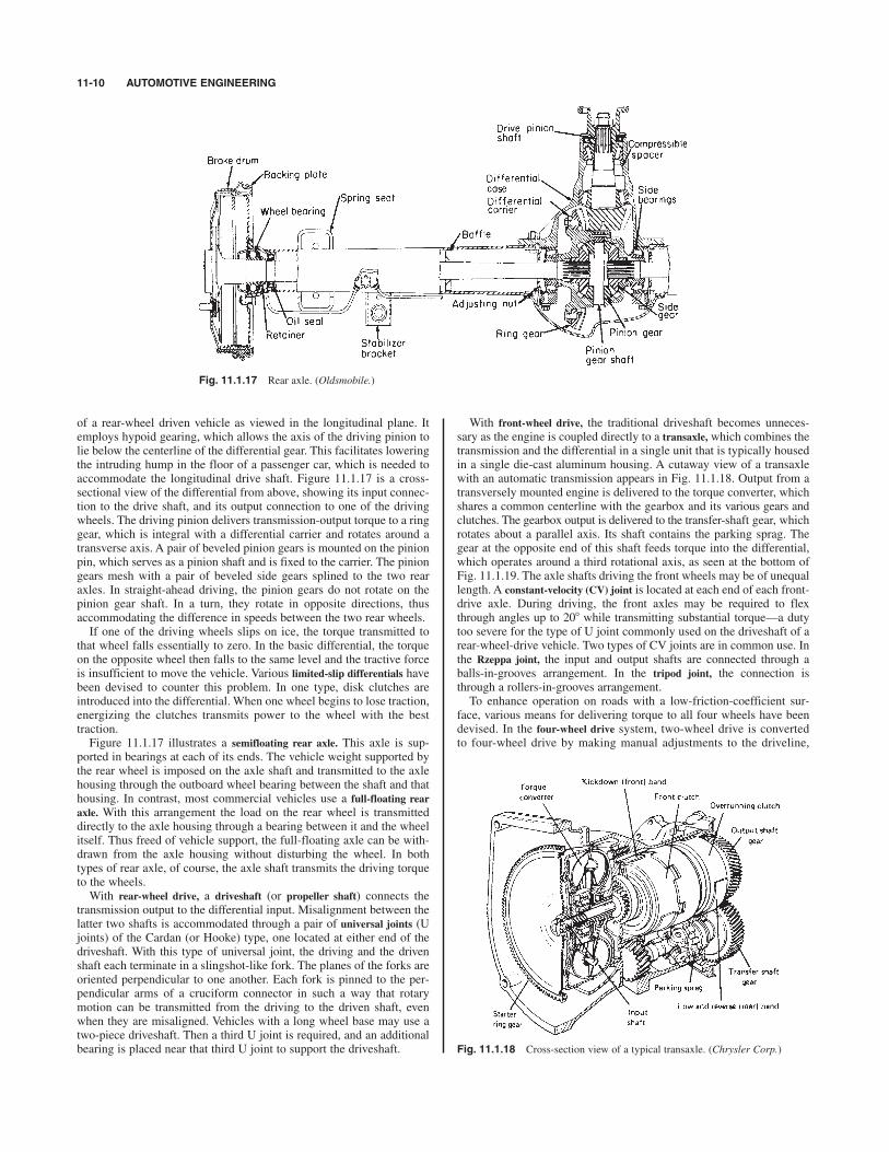
of a rear-wheel driven vehicle as viewed in the longitudinal plane. Itemploys hypoid gearing, which allows the axis of the driving pinion tolie below the centerline of the differential gear. This facilitates loweringthe intruding hump in the floor of a passenger car, which is needed toaccommodate the longitudinal drive shaft. Figure 11.1.17 is a cross-sectional view of the differential from above, showing its input connec-tion to the drive shaft, and its output connection to one of the drivingwheels. The driving pinion delivers transmission-output torque to a ringgear, which is integral with a differential carrier and rotates around atransverse axis. A pair of beveled pinion gears is mounted on the pinionpin, which serves as a pinion shaft and is fixed to the carrier. The piniongears mesh with a pair of beveled side gears splined to the two rearaxles. In straight-ahead driving, the pinion gears do not rotate on thepinion gear shaft. In a turn, they rotate in opposite directions, thusaccommodating the difference in speeds between the two rear wheels.If one of the driving wheels slips on ice, the torque transmitted to
that wheel falls essentially to zero. In the basic differential, the torqueon the opposite wheel then falls to the same level and the tractive forceis insufficient to move the vehicle. Various limited-slip differentials havebeen devised to counter this problem. In one type, disk clutches areintroduced into the differential. When one wheel begins to lose traction,energizing the clutches transmits power to the wheel with the besttraction.Figure 11.1.17 illustrates a semifloating rear axle. This axle is sup-
ported in bearings at each of its ends. The vehicle weight supported bythe rear wheel is imposed on the axle shaft and transmitted to the axlehousing through the outboard wheel bearing between the shaft and thathousing. In contrast, most commercial vehicles use a full-floating rearaxle. With this arrangement the load on the rear wheel is transmitteddirectly to the axle housing through a bearing between it and the wheelitself. Thus freed of vehicle support, the full-floating axle can be with-drawn from the axle housing without disturbing the wheel. In bothtypes of rear axle, of course, the axle shaft transmits the driving torqueto the wheels.With rear-wheel drive, a driveshaft (or propeller shaft) connects the
transmission output to the differential input. Misalignment between thelatter two shafts is accommodated through a pair of universal joints (Ujoints) of the Cardan (or Hooke) type, one located at either end of thedriveshaft. With this type of universal joint, the driving and the drivenshaft each terminate in a slingshot-like fork. The planes of the forks areoriented perpendicular to one another. Each fork is pinned to the per-pendicular arms of a cruciform connector in such a way that rotarymotion can be transmitted from the driving to the driven shaft, evenwhen they are misaligned. Vehicles with a long wheel base may use atwo-piece driveshaft. Then a third U joint is required, and an additionalbearing is placed near that third U joint to support the driveshaft.
With front-wheel drive, the traditional driveshaft becomes unneces-sary as the engine is coupled directly to a transaxle, which combines thetransmission and the differential in a single unit that is typically housedin a single die-cast aluminum housing. A cutaway view of a transaxlewith an automatic transmission appears in Fig. 11.1.18. Output from atransversely mounted engine is delivered to the torque converter, whichshares a common centerline with the gearbox and its various gears andclutches. The gearbox output is delivered to the transfer-shaft gear, whichrotates about a parallel axis. Its shaft contains the parking sprag. Thegear at the opposite end of this shaft feeds torque into the differential,which operates around a third rotational axis, as seen at the bottom ofFig. 11.1.19. The axle shafts driving the front wheels may be of unequallength. A constant-velocity (CV) joint is located at each end of each front-drive axle. During driving, the front axles may be required to flexthrough angles up to 208 while transmitting substantial torque—a dutytoo severe for the type of U joint commonly used on the driveshaft of arear-wheel-drive vehicle. Two types of CV joints are in common use. Inthe Rzeppa joint, the input and output shafts are connected through aballs-in-grooves arrangement. In the tripod joint, the connection isthrough a rollers-in-grooves arrangement.To enhance operation on roads with a low-friction-coefficient sur-
face, various means for delivering torque to all four wheels have beendevised. In the four-wheel drive system, two-wheel drive is convertedto four-wheel drive by making manual adjustments to the driveline,
11-10 AUTOMOTIVE ENGINEERING
Fig. 11.1.17 Rear axle. (Oldsmobile.)
Fig. 11.1.18 Cross-section view of a typical transaxle. (Chrysler Corp.)

SUSPENSIONS 11-11
normally with the vehicle at rest. In all-wheel drive systems, torque isalways delivered to all four wheels, by a system capable of distributingpower to the front and rear wheels at varying optimal ratios accordingto driving conditions and the critical limits of vehicle dynamics. Invehicles capable of driving through all four wheels, a transfer casereceives the transmission output torque and distributes it through driveshafts and differentials to the front and rear axles.
SUSPENSIONS
The suspension system improves ride quality and handling in drivingon irregular roadbeds and during maneuvers like turning and braking.The vehicle body is supported on the front and rear springs, which areimportant elements in the suspension system. Three types used are thecoil spring, the leaf spring, and the torsion bar.Also important are the shock absorbers. These piston-in-tube devices
dampen spring oscillation, road shocks, and vibration. As the hydraulicshock-absorber strut telescopes, it forces fluid through a restrictive orifice,thus damping its response to deflections imposed by the springs.Especially in the front suspension, most vehicles incorporate an
antiroll bar (sway bar, stabilizer). This is a U-shaped bar mounted trans-versely across the vehicle, each end attached to an axle. During high-speed turns, torsion developed in the bar reduces the tendency of thevehicle to lean to one side, thus improving handling.A wide variety of suspension systems have seen service.Front Suspension All passenger cars use independent front-wheel
suspension, which allows one wheel to move vertically without dis-turbing the opposite wheel. Rear-wheel drive cars typically use theshort-and-long-arm (SLA) system illustrated in Fig. 11.1.20. Thesteering knuckle is held between the outboard ends of the upper andlower control arms (wishbones) by spherical joints. The upper controlarm is always shorter than the lower. The load on these control arms isgenerally taken by coil springs acting on the lower arm, or by torsion-bar springs mounted longitudinally.Figure 11.1.21 shows a representative application of the spring strut
(MacPherson) system for the front suspension of front-wheel drive cars.The lower end of the shock absorber (strut) is mounted within the coilspring and connected to the steering knuckle. The upper end isanchored to the body structure.Rear Suspensions The trailing-arm rear suspension illustrated in
Fig. 11.1.22 is used on many passenger cars. Each longitudinal trail-ing arm pivots at its forward end. Motion of its opposite end is con-strained by a coil spring. One or more links may be added to enhancestability.Using leaf springs in place of coil springs is common practice on
trucks. The Hotchkiss drive, used with a solid rear axle, employs longi-tudinal leaf springs. They are connected to the chassis at their front andrear ends, with the rear axle attached near their midpoints.
Active Suspension A variety of improvements to the traditionalpassive suspension system have been introduced. Generally they requiresome form of input energy. The air suspension widely used in heavy-duty trucks, for example, requires an air compressor. To an increasingdegree, advanced systems employ sensors and electronic controls.Some of the improvements available with active suspension areimproved ride quality (adaptation to road roughness), control of vehicleheight (low for reduced aerodynamic drag on highways; high for
Fig. 11.1.19 Automatic transaxle used on a front-wheel-drive car. (Chrysler
Corp.)
Fig. 11.1.20 Front-wheel suspension for rear-wheel-drive car.
Fig. 11.1.21 Typical MacPherson strut, coil spring front suspension for front-
wheel-drive car. (Chrysler Corp.)
Fig. 11.1.22 Trailing-arm type rear suspension with coil springs, used on some
front-wheel-drive cars. (Chrysler Corp.)

off-road driving), and vehicle leveling (to correct change in pitch whenthe trunk is heavily loaded; avoid pitching during braking and heavyaccelerations).
STEERING
When turning a corner, each wheel traces an arc of different radius, asillustrated in Fig. 11.1.23. To avoid tire scrubbing when turning acorner of radius R, the point of intersection M for the projected front-wheel axes must fall in a vertical plane through the center of the rearaxle. This requires each front wheel to turn through a different angle.For small turning angles of the vehicle, a and b can be shown to besimple functions of W, L, and R. A steering geometry conforming toFig. 11.1.23 is known as Ackerman geometry, and L/R defines theAckerman angle. The difference in front-wheel angles, b & a, varieswith turning radius R. Having the a and b corresponding to Ackermangeometry improves handling in low-speed driving, as in parking lots.At higher speeds, dynamic effects become significant. In a turn, the
vehicle may encounter either understeer or oversteer. With understeer,the vehicle fails to turn as sharply as the position of the steering wheelsuggests it should. With oversteer, the vehicle turns more sharply thanintended, and in extreme cases may spin around. These tendencies areamplified by increased speed and are affected by many variables, e.g.,tire pressure, weight distribution, design of the suspension system, andthe application of brakes.
A common motion transformer is the rack and pinion, in which apinion gear attached to the steering column engages a geared bar, or rack,causing it to slide to the left or right as the steering wheel is turned. Theends of the rack are attached to the inner ends of the tie rods. In the vari-ation of the rack-and-pinion illustrated in Fig. 11.1.25a, the rotationof the pinion on the end of the steering shaft causes a rotatable wormgear to control the tie-rod positions as it moves left and right like therack.With the rotatable ball system of Fig. 11.1.25b, a worm is mounted on
the end of the steering column. Its spiral grooves contain ball bearings.The outer surfaces of the balls rotate in spiral grooves lining the insideof a ball nut. The outer surface of the ball nut contains gear teeth thatmesh with a gear sector on the pitman arm. The end of pitman arm isconnected to the tie rods through a series of links.
11-12 AUTOMOTIVE ENGINEERING
Fig. 11.1.23 Ackerman steering geometry.
W
L
M
R
β − α
β α
Fig. 11.1.24 Schematic of front-wheel steering system.
Motion transformer
Tie rod
Kingpin axis
Steering arm
Steering column
Fig. 11.1.25 Two commonly used types of steering gear. (a) Variation of rack-
and-pinion using rotating worm in place of translating rack; (b) recirculating ball.
The physical implementation of a front-wheel steering system isshown schematically from above in Fig. 11.1.24. The front wheels aresteered around the axes of their respective kingpins. For improved han-dling, the axes of the two kingpins are not vertical. In the transverseplane they lean inward, and in the longitudinal plane they lean rearward.The steering arms are the lever arms for turning the front wheels. Eachtie rod is pinned at one end to a steering arm and at its opposite end tosome type of motion transformer, the purpose of which is to convert therotational input of the steering column into translational motion at theinner ends of the tie rods.
With variable-ratio steering, the response of the front wheels to steer-ing-wheel rotation is increased as the steering wheel approaches theextremes of its travel. This is especially helpful in curbside parallelparking. Variable-ratio steering can be achieved by nonuniformly spac-ing the worm grooves in Fig. 11.1.25a, or by varying the lengths of theteeth on the sector of the pitman arm in Fig. 11.1.25b.Most modern U.S. cars have power-assisted steering. A pressurized
hydraulic fluid is used to augment the steering effort input by the dri-ver, but if the engine is off or if there is a failure in the power-steeringsystem, the driver retains steering control, albeit with greater effort.The power-steering circuit contains an engine-driven hydraulic
pump, a fluid reservoir, a hose assembly, return lines, and a controlvalve. One of a variety of pumps that has been used is the rotary-vanepump of Fig. 11.1.26. As the rotor is turned by a belt drive from theengine, the radially slidable vanes are held against the inner surface ofthe eccentric case by centrifugal force, springs, and/or hydraulic pres-sure. Not shown are the inlet and exit ports, and a pressure-reliefvalve.A balanced-spool control valve is represented in Fig. 11.1.27. In
straight-ahead driving, centering springs hold the spool in the neutralposition. In the position illustrated, however, the driver has turned the steer-ing wheel to position the spool valve at the right extremity of its travel.
Fig. 11.1.26 Rotary power-steering pump. (General Motors, Saginaw.)

BRAKING SYSTEMS 11-13
That directs all of the pump discharge flow to the left side of a piston, mov-ing the piston rod to the right. The piston illustrated can, for example, beincorporated into the rack of a rack-and-pinion steering system to add tothe turning effort put into the steering wheel by the driver.Some cars now use electric power steering. Both the need for
hydraulic fluid and the equipment pictured in Fig. 11.1.27 are eliminat-ed. They are replaced by a variable-speed electric motor, and electron-ic sensors that match the appropriate degree of assistance to driverdemand and road resistance. Compared to hydraulic power steering,electric power steering effects a small improvement in fuel economy byreducing the parasitic load on the engine.
BRAKING SYSTEMS
Brakes The moving automobile is stopped with hydraulic servicebrakes on all four wheels. The service brakes are engaged by depress-ing and holding down a self-returning foot pedal. The mechanicalparking brake, used to prevent the vehicle from rolling when parked,acts on the rear wheels. It is engaged with an auxiliary foot pedal or ahand pull and is held by a ratchet until released. Drum brakes, once usedextensively on all four wheels, are now used primarily on rear wheels.Typically, disk brakes are used on the front wheels, but sometimes onthe rear wheels.A Bendix dual-servo drum brake is illustrated in Fig. 11.1.28c. It is
self-energizing because the rotating drum tries to drag the brake liningand shoe counter-clockwise, along with it. Because the anchor pin pre-vents this for the secondary shoe, and the adjusting screw prevents it forthe primary shoe, both are called leading shoes. This causes both shoesto push more strongly against the drum, increasing the friction force.This self-energization is lost when the wheel turns in the reverse direc-tion. With this brake configuration, typically a linkage turns a notched
wheel on the adjusting screw when the brake is applied with the carmoving in reverse. This automatically adjusts for lining wear.In the arrangement of Fig. 11.1.28a, the anchor pin has been
moved 1808. The leading shoe continues to be self-energized, but thatquality is lost on the trailing (following) shoe. In this arrangement theleading shoe provides most of the braking torque and experiences mostof the wear when traveling forward. In reverse, however, the trailingshoe in forward travel becomes the leading shoe and provides most ofthe braking torque. This arrangement is used on the rear wheels of somefront-wheel drive cars.The Caliper disk brake is illustrated in Fig. 11.1.29. The disk rotates
with the wheel. The fixed caliper straddles the disk. Within the caliper,the pistons in opposing hydraulic cylinders press the attached padsagainst opposite sides of the disk when actuated.Fig. 11.1.27 Control valve positioned for full-turn power steering assistance
using maximum pump pressure.
Fig. 11.1.28 Three types of internal-expanding brakes.
Fig. 11.1.29 Schematic of caliper disk brake.
As friction heats the brake lining and the surface on which it rubsduring stopping, the coefficient of friction often falls. This undesirablecharacteristic causes what is known as brake fade. Because brakes arenormally applied only intermittently, the time available for cool downbetween successive brake applications keeps brake fade at a tolerablelevel. However, closely spaced panic stops from high speeds can causeobjectionable fade. The “disk” illustrated in Fig. 11.1.29 often consistsof two parallel disks that are joined together by radial vanes. The abilityof air to access the nonfriction side of each of these disks, and theair pumped between the disks by the vanes when the wheel rotates, helpto avoid brake overheating. Brake fade is more probable with drumbrakes because the more enclosed nature of their construction makesbrake cooling more difficult.Many modern disk brakes use a single-cylinder caliper. One cylinder
and its actuating piston and attached pad are retained on the inboard side.However, the outboard cylinder is eliminated, the pad on that side insteadbeing fastened directly to the inner surface of the caliper. Instead of beingfixed, the caliper is allowed to slide inboard on mounting bolts when thesingle piston is actuated. Transverse movement of the caliper on itsmounting bolts then causes each pad to rub on its adjacent disk surface.Because disk brakes are not self-energizing, and the rubbing area of
the pads is less than the rubbing area of the shoes on an equivalent drum

brake, a higher hydraulic pressure is required with disk brakes than withdrums. If disk brakes are used on the front wheels and drums on therear, then provisions are made in the upstream hydraulic system to pro-vide that difference.Cast iron is the preferred material for the rubbing surface on both
rotors and drums. The brake lining on pad or shoe may contain high-temperature resins, metal powder, solid lubricant, abrasives, and fibersof metal, plastic, and ceramic. Friction coefficients from 0.35 to 0.50are typical with these combination. The asbestos once common in brakelinings has been abandoned because of the adverse health effect ofasbestos wear particles.Hydraulics When the brake pedal is depressed, it moves pistons in
the master cylinder, as illustrated in Fig. 11.1.30. This forces pressur-ized brake fluid through lines to the wheel cylinders for brake applica-tion. The magnitude of the fluid pressure is proportional to themagnitude of the force applied to the brake pedal. As is typical, thisdual master cylinder contains two pistons in tandem (Fig. 11.1.31), pro-viding a split system. One operates the rear brakes and the other thefront brakes, providing the ability to brake the vehicle even if one of thetwo systems should fail. Late model cars often use a diagonal-splitarrangement, where each piston in the dual master cylinder serves diag-onally opposite wheels.
The conventional cast-iron master cylinder with integral reservoir hasbeen largely replaced by the aluminum master cylinder with translucentplastic reservoirs for visual inspection of brake-fluid level. The speciallyformulated brake fluid must be free of petroleum-based oil, whichwould cause swelling of rubber parts in the braking system. Double-walled steel lines are used to distribute the brake fluid. Near the wheels,these rigid lines are replaced by flexible hydraulic hoses to accommo-date wheel movement.Power Brakes Power brakes relieve the driver of much physical
effort in retarding or stopping a car. Several types have been used, buton passenger cars, the vacuum-suspended type illustrated in Fig. 11.1.32is the most common. The power section contains a large diaphragm. Inthe unapplied condition, the chambers on each side of the diaphragmare exposed to intake-manifold vacuum. When the brake pedal isdepressed, first the vacuum passage is closed and then, with furtherdepression, air is admitted to one side of the diaphragm. The pressuredifference across the diaphragm, acting over its area, creates an axialforce that is applied to the piston in the master cylinder. This augmentsthe force provided directly by the driver’s foot. Without requiring anadditional reservoir, the vacuum captured allows at least one stop afterthe engine operation has terminated.
11-14 AUTOMOTIVE ENGINEERING
Fig. 11.1.30 “Split” hydraulic brake system.
Fig. 11.1.31 Typical design of a dual master cylinder for a split brake system.
Fig. 11.1.32 Power-assisted brake installation.
When the brake pedal is released, a spring in the master cylinderreturns the pistons to their original positions. This uncovers ports in themaster cylinder, allowing communication with the brake-fluid reser-voirs on the master cylinder and relieving the pressure in the wheelcylinders. A check valve maintains a minimum pressure in the systemto prevent the entrance of air. Air in the system makes the brakes feelspongy, and, if it gains entrance, must be bled from the system.
A combination valve is usually included in vehicles using disks in thefront and drums in the rear. Among its functions, the proportioning valveregulates pressure individually to the front and rear wheels to compen-sate for the different pressure requirements of disks and drums, and thepressure differential valve checks to ensure that both sides of a diagonal-ly split system experience the same pressures.
Another type of power brake used a hydraulic booster. The accumula-tor, a reservoir of pressurized fluid provided by the power-steeringpump, provides the force that moves the piston in the master cylinder.Heavy-duty tractor-trailer combinations require braking forces far in
excess of what can be supplied from a simple foot pedal. Air brakes arecommon in such applications. Air supplied from an engine-driven aircompressor is stored in a high-pressure tank, from which the air is with-drawn for brake augmentation as needed.Retarders Using traditional wheel brakes to control the road speed
of a heavily laden tractor-trailer rig on long downhill runs promotesbrake fade and accelerates brake-lining wear. Several types of retardersare available that decelerate the vehicle independent of wheel brakes.With the compression-release braking system (often called the Jake
brake), fuel injection in the diesel engine is terminated and engine valvetiming is temporarily changed so that the exhaust valve opens near theend of the compression stroke. This releases the air compressed duringcompression directly into the exhaust system and imposes the negativework of compression on the crankshaft. A disadvantage of this systemis that the sudden intermittent release of high-pressure air from thecylinder creates considerable noise.The hydrodynamic retarder consists essentially of a centrifugal fluid
pump that is run by the driveshaft. The high tangential velocity of thedischarge fluids is removed by stator vanes as the fluid is returned tothe pump inlet. Because such a pump consumes little torque at lowrotational speeds, a booster retarder that is geared to rotate at a higherspeed may be added in parallel. Since the braking energy generatedappears as heat in the recirculating fluid, adequate cooling must beprovided for it.The electrodynamic retarder resembles an eddy-current dynamometer.
Voltage applied from the battery or the alternator to the field coils controls

WHEELS AND TIRES 11-15
braking torque. The electrodynamic retarder offers greater brakingtorque at low speeds than the hydrodynamic retarder. However, its brak-ing ability falls off significantly as it is heated by the energy absorbed,and heat rejection is problematic.Antilock Brakes At a steady forward speed, vehicle velocity equals
product of the rolling radius of the tire and its angular velocity. Whenthe brakes are applied, the vehicle velocity exceeds that product by a difference known as slip. As slip in any wheel increases, its brak-ing force rises to a peak, then slowly decreases until the wheel locks upand the tire merely slides over the road surface. At lockup, the brakeshave not only lost much of their effectiveness, but steering control isalso sacrificed. The antilock braking system (ABS) incorporates wheel-speed sensors, an electronic control unit (ECU), and solenoids torelease and reapply pressure to each brake. When the ECU determinesfrom a wheel-speed signal that lockup is imminent, it signals the corre-sponding solenoid to release hydraulic pressure in that brake line. Oncethat wheel has accelerated again, the solenoid reapplies its brake-linepressure. This sequence is repeated in each wheel at a high frequency,thus avoiding lockup and generally shortening stopping distance duringsevere braking or on slippery roads.Traction Control The traction control system (TCS) helps maintain
traction and directional stability, especially on slippery roads. It usesmany of the same components as ABS. If one driven wheel spins, theECU applies the brake on that wheel until traction is regained. If bothdriven wheels spin, the ECU temporarily overrides the command signalfrom the accelerator pedal to reduce engine output torque.Electronic Stability Control The step beyond ABS and TCS is elec-
tronic stability control, which helps the driver to maintain steering dur-ing severe vehicle maneuvers. By adding sensor measurements ofsteering-wheel angle and vehicle yaw rate to the ECU input, it is possi-ble to reduce the incidence of inadvertent departure of the vehicle fromthe road, or of vehicle rollover. This is accomplished by controlling thewheel brakes as with TCS, and in addition, by temporarily reducingengine torque.Stopping Distance The service brakes are the most important ele-
ment in arresting a moving vehicle, but they derive some help fromother sources. Aerodynamic drag provides a retarding force. Because itvaries with the square of speed, it is most influential at highway speeds.The engine, when it is driven by the inertia of the vehicle during brak-ing, and transmission and driveline losses, all contribute resistance toforward motion. On the other hand, during forward motion the inertiaof these components, as well as that of the wheels, all oppose the actionof the brakes. The braking force from the motoring engine can be espe-cially significant if it is joined to the driven wheels by a manual trans-mission. The force can be amplified by downshifting that transmissionto increase the speed of the crankshaft. With the conventional automatictransmission, however, engine braking is minimal because the torqueconverter is relatively ineffective in transmitting torque in the reversedirection. A small retarding force is also derived from the rolling resis-tance of the tires.In braking, the sequence of events involves, successively, (1) the dri-
ver reaction time tr , during which the driver responds to an external sig-nal by engaging the brake pedal, (2) a response time from pedalengagement to full pedal depression, (3) a buildup time, during whichbrake line pressure increases to develop a substantial braking force, and(4) a prolonged active braking time. In estimating minimum stoppingdistance from initial vehicle velocity V, the vehicle may be assumed tomove at its original speed during the reaction time, response time, andhalf of the buildup time. The sum of the latter two is the delay time td.During the second half of the buildup time and the active braking time,the braking force depends on m, the average coefficient of frictionbetween tire and roadbed. Then the stopping distance is S V(tr ! td)! V2/2mg, where g is the gravitational constant. The reaction time typ-ically consumes 1 ' 0.7 s. For brakes in good condition, the delay timemay range from 0.35 s for passenger cars to 0.55 s for large vehicles.The static friction coefficient depends on speed and the condition of tiresand road. For new tires on dry paved roads, it is in the range of 0.75 to0.85, increasing about 20 percent with wear. On moderately wet pavement
the coefficient for new tires may fall to the 0.55 to 0.65 range. On wetpavement, the coefficient falls even more, especially at high speeds. Thesliding friction coefficient, applicable when the wheels are locked andskid over the roadbed, is less than the static coefficient.
WHEELS AND TIRES
The total weight of a vehicle is the sum of the sprung weight supported bythe tires and suspension system, and the unsprung weight. Wheels andtires are primary contributors to unsprung weight. For a given vehicle,the lower the unsprung weight, the better the acceleration performance,and the ride and handling qualities on rough roads. Because of cost con-siderations, most automotive wheels are fabricated from sheet steel.Special lower weight wheels have been forged or cast in aluminum,however, and even made of magnesium.Maintenance of proper front-wheel alignment is important for opti-
mum vehicle performance and handling. Normally, proper camber, caster,and toe-in are specified by the manufacturer.
Camber is the tilt angle of the wheel plane with respect to the longi-tudinal plane of the vehicle. When the plane of the wheel is perpen-dicular to the ground, the camber angle is 08. During operation, thatangle is affected by the changing geometry of the suspension systemas the vehicle is loaded or traverses a bump in the road, or as the bodyrolls during cornering. Taking such factors into account, the manufac-turer specifies the proper camber angle for each vehicle design whenthe vehicle is at rest. With positive camber, the distance betweenwheels is greater at their tops than between their bottoms, where theycontact the roadbed. Normally, a zero to slightly negative camber isspecified.The caster angle is the angle between the kingpin axis (axis around
which the wheel is steered) and a radial line from the center of thewheel to the ground, when both are projected onto a longitudinal plane.When the caster is positive, that radial line intersects the ground behindthe intersection of the kingpin axis with the ground. Increasing the casterangle increases the tendency of a turned wheel to restore itself to thestraight-ahead position as the vehicle moves forward. This self-restoringtendency can also be influenced somewhat by the inclination of thekingpin in the transverse plane.When viewing an unloaded vehicle at rest from above, the front
wheels may be set either to toe in or toe out slightly to compensate forthe effects of driving forces and kingpin inclination. This adjustmentinfluences the tendency of the wheel to shimmy. Toe-in is typical forrear-wheel-drive cars, while the front wheels of front-wheel-drive carsmay be set to toe out.The automotive pneumatic tire performs four main functions: sup-
porting a moving load; generating steering forces; transmitting drivingand braking forces; and providing isolation from road irregularities byacting as a spring in the total suspension system. A tire made up of twobasic parts: the tread, or road-contacting part, which must provide trac-tion and resist wear and abrasion; and the body, consisting of rubber-ized fabric that gives the tire strength and flexibility.The three principal types of automobile and truck tires are the cross-
ply or bias-ply, the radial-ply, and the bias-belted (Fig. 11.1.33). In thebias-ply design, the cords in each layer of fabric run at an angle from
Fig. 11.1.33 Three types of tire construction.

one bead (rim edge) to the opposite bead. To balance the tire strengthsymmetrically across the tread center, another layer is added at anopposing angle of 30 to 388, producing a two-ply tire. The addition oftwo criss-crossed plies makes a four-ply tire.In the radial tire (used on most automobiles), the cords run straight
across from bead to bead. The second layer of cords runs the same way;the plies do not cross over one another. Reinforcing belts of two or morelayers are laid circumferentially around the tire between the radial bodypiles and the tread. The bias-belted tire construction is similar to that ofthe conventional bias-ply tire, but it has circumferential belts like thosein the radial tire.Of the three types, the radial-ply offers the longest tread life, the
best traction, the coolest running, the highest gasoline mileage, andthe greatest resistance to road hazards. The bias-ply provides a softer,quieter ride and is least expensive. The bias-belted design is interme-diate between the good quality bias-ply and the radial tire. It has alonger tread life, and it gives a smoother low-speed ride than theradial tire.
Tire specifications are molded into the sidewall. Consider, for exam-ple, the specification “P225/60TR16.” The initial P designates “passen-ger car” (LT light truck, ST trailer). Next, 225 is the tire width inmm. Following the slash, 60 is the aspect ratio, i.e., the ratio of sidewallheight, from bead to tread, to tire width, expressed as a percentage. Tindicates a maximum speed rating of 190 km/h. Speed designatorsprogress from S 180 km/h through T (190 km/h), U (200 km/h),H (210 km/h), V (240 km/h) to Z (%240 km/h). On some tires the speedrating is omitted. R indicates radial construction (D bias ply; B bias belted). Finally, 16 indicates a wheel with a 16-in. rim diameter.Alternatively, such a tire could be labeled “P225/60R 89T,” where thespeed rating comes last and is preceded by a numerical load index indi-cating carrying capacity.For passenger cars, the recommended tire pressure is posted on the
rear edge of the driver’s door. Underinflation causes excessive tire flex-ing and heat generation in the tire, more rapid wear, poor handling, andpoor fuel economy. Overinflation causes a rough ride, unusual wear,poor handling, and increased susceptibility to tire damage from roadhazards.As a safety measure, a dashboard signal of tire under-inflation can be
provided for the driver. Early versions of such a system made use of thewheel-speed signal necessary for traction control. Any wheel that con-sistently rotates at a higher speed than the rest suggests a reduced run-ning radius, as would occur with an underinflated tire. Later versionsmeasure the pressure of individual tires with wheel-mounted sensors,electronically transmitting their signals to an on-board receiver fordashboard display.An out-of-balance wheel causes uneven tire wear and adversely
affects ride quality. Wheel-tire assemblies are balanced individuallyby attaching balance weights to the rim of the wheel. For static bal-ance, a proper weight on the outside rim of the wheel suffices. For thedynamic balance required at high speeds, weights are necessary onboth the outside and inside rims. Dynamic balancing necessitatesspinning the wheel to determine correct placement of the balanceweights.The trunk space occupied by a fifth wheel on which a spare tire is
mounted to replace a flat tire has long bothered consumers and man-ufacturers alike. To regain part of that space, some cars have used acollapsible tire that must be inflated when pressed into service, usingeither a compressed-air storage reservoir or an onboard air com-pressor. Alternatively, some cars store a smaller-than-standard compactspare tire that has been preinflated to a high pressure. The run-flattire is another option. It eliminates the need to carry a jack. It mayrely upon an extra stiff sidewall to carry the load if the tire is punc-tured, or upon a plastic donut built into the tire. Such run-flat tireseliminate not only the storage-space requirement for carrying anyspare, but also the need to carry a jack. When used, all of these alter-natives to carrying a fifth wheel/tire combination entail some sacrificein ride quality, and a limitation on allowable travel distance andspeed.
HEATING, VENTILATING, AND AIR CONDITIONING (HVAC)
The heating, ventilation, and air conditioning (HVAC) system is installedto provide a comfortable environment within the passenger compart-ment. Fresh air for HVAC usually enters through an opening in front ofthe windshield and into a plenum that separates rain from the ambientair. The airflow rate is augmented by a variable-speed electrically dri-ven blower.In cold weather, heater air is passed through a finned heat-exchanger
core, where it is heated by the engine coolant. Compartment temper-ature is controlled by (1) mixing ambient air with heated air, (2) mix-ing heated air with recirculated air, or (3) changing blower speed.Provision is made to direct heated air against the interior surface ofthe windshield to prevent the formation of ice or fog. Figure 11.1.34schematically illustrates a system in which a multispeed blower dri-ves fresh air through (1) a radiator core or (2) a bypass. The flow rateand direction of the air entering the passenger compartment are con-trolled with manually operated doors and vanes in the dischargeducts.
11-16 AUTOMOTIVE ENGINEERING
Fig. 11.1.34 Heater airflow diagram.
Fig. 11.1.35 Schematic of air conditioning system using HFC-134a refrigerant.
(Reprinted with permission from SAE, SP-916, © 1992, Society of Automotive
Engineers, Inc.)
For cooling in hot weather, an electric clutch is engaged to operatethe air-conditioning compressor, which is belt-driven from the engine(Fig. 11.1.35). The pressurized, hot gaseous refrigerant exiting the

AUTOMOBILE CONSTRUCTION 11-17
compressor enters the condenser, a heat exchanger typically located infront of the engine radiator. Ambient air passed through this heatexchanger by a fan cools the refrigerant, liquefying it. The high-pressureliquid then passes through a liquid reservoir and on to an expansionvalve that drops the refrigerant pressure as it sprays the refrigerant intothe evaporator. The evaporator is a heat exchanger normally mountedon the firewall. Compartment air circulated through the evaporatorrejects its heat to the colder refrigerant, thus cooling as it vaporizes therefrigerant in preparation for reentry of the refrigerant into the com-pressor. Moisture condensed from the ambient air during cooling isleaked onto the roadbed.Figure 11.1.36 shows schematically a combined air-heating and air-
cooling system. Various dampers control the proportions of fresh andrecirculated air to the heater and evaporator cores. Compartment-airtemperature is controlled electronically by a thermostat that modulatesthe mixing of cooled and heated air, and cycles the compressor on andoff through a magnetic clutch. During defrosting, mixing cooled air inwith heated air helps to remove humidity from the air directed to theinterior of the windshield.
separate frame. Most of the suspension, bumper, and brake loads aretransmitted to the frame. Body-and-frame construction dominates inpickups and SUVs. With unit construction, most common in passen-ger cars, the frame is eliminated. Its function is assumed by a frame-work consisting of stamped sheet-metal sections joined together bywelding. Outer panels are then fastened to this framework, primarily bybolting.A third construction option that has been borrowed from aircraft
practice and used to a limited extent is the space frame andmonocoque combination. The space frame is a skeleton to which thebody panels are attached, but the body assembly is designed in amanner that causes it to contribute significantly to the strength of thevehicle.An important aspect of auto design is passenger protection.
Crumple zones are designed into the structure, front and rear, toabsorb collision impacts. Beams may be built into doors to protectagainst side impact.The 1990s drive for improved passenger-car fuel economy, hence
smaller and lighter cars, and for improved corrosion resistance has ledto a gradual shift in material usage. This trend is evident in Table 11.1.3.The weight percentage of ferrous content has declined consistently, butremains over half the total weight of the average car. The shift fromconventional to high-strength steel is evident. In areas likely to experi-ence rust, the steel may be galvanized. The percentage use of lighteraluminum has doubled. The use of plastics and composites, while stillless than 10 percent of the car weight, has increased by 50 percent on amass basis.The interest in recycling materials from scrapped vehicles has also
increased. In the mid-1990s, 94 percent of scrapped vehicles wereprocessed for recycling. Approximately 75 percent of vehicle contentwas recycled. Table 11.1.4 indicates the disposition of materials fromrecycled vehicles.
Fig. 11.1.36 Combined heater and air conditioner. (Chevrolet.)
For many years the refrigerant in automotive air conditioners wasCFC-12, a chlorinated fluorocarbon also known as F-12. About 1990the depletion of stratospheric ozone, which shields humankind fromharmful solar ultraviolet radiation, became an environmental con-cern. The chlorine in CFC-12 having been identified as a contributorto the problem, the use of CFC-12 was banned worldwide. About thesame time, concern mounted about the threat of global warming fromthe anthropogenic production of greenhouse gases. Carbon dioxidefrom the combustion of fossil fuels is a major contributor. It was esti-mated that on a mass basis, CFC-12 was about 10,000 times as seri-ous a greenhouse gas as carbon dioxide. In the United States, animmediate response to the ozone depletion concern was to requiremechanics to capture spent CFC-12 for recycling, rather than ventingit to the atmosphere, every time an air conditioner was serviced.Beyond that, within a few years, CFC-12 was replaced by chlorine-free HFC-134a, which has a global warming effect about one-eighththat of CFC-12. Because HFC-134a is still 1300 times as serious agreenhouse gas as carbon dioxide, a replacement for HFC-134a isbeing sought.
AUTOMOBILE CONSTRUCTION
Light-duty vehicles include passenger cars and light-duty trucks.Light-duty trucks include passenger vans, sports utility vehicles(SUVs), and pickup trucks. The layout of light-duty vehicles generallyfalls into one of four categories: (1) front engine, rear-wheel drive—used mostly in large cars and light-duty trucks, (2) front engine, front-wheel drive—used mostly in small cars and passenger vans, (3) rear ormidengine, rear-wheel drive—sometimes used in sports cars, and (4)four-wheel drive—used mostly in light-duty trucks and premium largecars.The two most common basic body constructions, illustrated in
Fig. 11.1.37 and Fig. 11.1.38, are body-and-frame and unit con-
struction. The body-and-frame design uses a body that is bolted to a
Fig. 11.1.38 Unit-construction design for automobiles.
Fig. 11.1.37 Separate body and frame design.

REFERENCES: Proceedings, Association of American Railroads (AAR),
Mechanical Division. Proceedings, American Railway Engineering Association
(AREA). Proceedings, American Society of Mechanical Engineers (ASME).
“The Car and Locomotive Cyclopedia,” Simmons-Boardman. J. K. Tuthill, “High
Speed Freight Train Resistance,” University of Illinois Engr. Bull., 376, 1948. A.
I. Totten, “Resistance of Light Weight Passenger Trains,” Railway Age, 103, Jul.
17, 1937. J. H. Armstrong, “The Railroad—What It Is, What It Does,” Simmons-
Boardman, 1978. Publications of the International Government-Industry Research
Program on Track Train Dynamics, Chicago. Publications of AAR Research and
Test Department, Chicago. Max Ephraim, Jr., “The AEM-7—A New High Speed,
Light Weight Electric Passenger Locomotive,” ASME RT Division, 82-RT-7,
1982. W. J. Davis, Jr., General Electric Review, October 1926. R. A. Allen,
Conference on the Economics and Performance of Freight Car Trucks, October
1983. “Engineering and Design of Railway Brake Systems,” The Air Brake
Association, Sept. 1975. Code of Federal Regulations, Title 40, Protection of
Environment. Code of Federal Regulations, Title 49, Transportation. Standards
and Recommended Practices and Proceedings, Association of American
Railroads (AAR) Mechanical Division, www.aar.com. “Standard for the Design
and Construction of Passenger Railroad Rolling Stock,” American Public
Transportation Association (APTA), www.apta.com. “Manual for Railway
Engineering,” American Railway Engineering and Maintenance-of-Way
Association (AREMA), www.arema.com. Proceedings, American Society of
Mechanical Engineers (ASME), www.asme.org. “The Car and Locomotive
Cyclopedia of American Practices,” Simmons-Boardman Books, Inc.,
www.transalert.com. Publications of AAR Research and Test Department,
www.aar.com. Code of Federal Regulations, Title 40, Protection of Environment
and Title 49, Transportation, published by the Office of the Federal Register,
National Archives and Records Administration. “The Official Railway Equipment
Register—Freight Connections and Freight Cars Operated by Railroads and
Private Car Companies of North America,” R.E.R. Publishing Corp., East
Windsor, NJ, www.cbizmedia.com.
DIESEL-ELECTRIC LOCOMOTIVES
Diesel-electric locomotives and electric locomotives are classified bywheel arrangement; letters represent the number of adjacent drivingaxles in a rigid truck (A for one axle, B for two axles, C for three axles,etc.). Idler axles between drivers are designated by numerals. A plussign indicates articulated trucks or motive power units. A minus sign
11-18 RAILWAY ENGINEERING
Table 11.1.3 Average Materials Consumption for a Domestic Automobile
1978 1985 2001
Material Pounds Percent Pounds Percent Pounds Percent
Ferrous materials
Conventional steel 1880.0 53.8% 1481.5 46.5% 1349.0 40.8%
High-strength steel 127.5 3.6 217.5 6.8 351.5 10.6
Stainless steel 25.0 0.7 29.0 0.9 54.5 1.6
Other steels 56.0 1.6 54.5 1.7 25.5 0.8
Iron 503.0 14.4 468.0 14.7 345.0 10.4
Total ferrous 2591.5 74.1% 2250.5 70.6% 2125.5 64.2%
Nonferrous materials
Powdered metal1 16.0 0.5 19.0 0.6 37.5 1.1
Aluminum 112.0 3.2 138.0 4.3 256.5 7.8
Copper 39.5 1.1 44.0 1.4 46.0 1.4
Zinc die castings 28.0 0.8 18.0 0.5 11.0 0.3
Plastics/composites 176.0 5.0 211.5 6.6 253.0 7.6
Rubber 141.5 4.1 136.0 4.3 145.5 4.4
Glass 88.0 2.5 85.0 2.7 98.5 3.0
Fluids & lubricants 189.0 5.4 184.0 5.8 196.0 5.9
Other materials2 112.5 3.2 101.5 3.2 139.5 4.2
Total nonferrous 902.5 25.8% 937.02 29.4% 1183.5 35.7%
Total 3494.0 lb 3187.5 lb 3309.0 lb
1 Powdered metals may include ferrous materials.2 Other materials include sound deadeners, paint and anti-corrosion dip, ceramics, cotton, cardboard, battery lead, magnesium
castings, etc.SOURCE: Reproduced with permission from American Metal Market. Copyright 2004 American Metal Market LLC, a division of
Metal Bulletin plc. All rights reserved.
Table 11.1.4 Materials Disposition from Recycled Vehicles
Recycled materials
Ferrous metals Nonferrous metals Fluids Shredder residue
• Steel • Aluminum • Engine oil • Plastic• Iron • Copper • Coolant • Rubber
• Lead • Refrigerant • Glass• Zinc • Fluids
• Other
11.2 RAILWAY ENGINEERINGby V. Terrey Hawthorne and Keith L. Hawthorne
(in collaboration with E. Thomas Harley, Charles M. Smith, Robert B.Watson, and C. A.Woodbury)

DIESEL-ELECTRIC LOCOMOTIVES 11-19
indicates separate nonarticulated trucks. This nomenclature is fullyexplained in RP-5523, issued by the Association of American Railroads(AAR). Virtually all modern locomotives are of either B-B or C-Cconfiguration.The high efficiency of the diesel engine is an important factor in its
selection as a prime mover for traction. This efficiency at full or partialload makes it ideally suited to the variable service requirements of rou-tine railroad operations. The diesel engine is a constant-torque machinethat cannot be started under load and hence requires a variably coupledtransmission arrangement. The electric transmission system allows it tomake use of its full rated power output at low track speeds for startingas well as for efficient hauling of heavy trains at all speeds. Examplesof the most common diesel-electric locomotive types in service areshown in Table 11.2.1. A typical diesel-electric locomotive is shown inFig. 11.2.1.Diesel-electric locomotives have a dc generator or rectified alternator
coupled directly to the diesel engine crankshaft. The generator/alterna-tor is electrically connected to dc series traction motors having nosesuspension mountings. Many recent locomotives utilize gate turn-offinverters and ac traction motors to obtain the benefits of increased adhe-sion and higher tractive effort. The gear ratio for the axle-mounted bullgears to the motor pinions that they engage is determined by the loco-motive speed range, which is related to the type of service. A high ratiois used for freight service where high tractive effort and low speeds arecommon, whereas high-speed passenger locomotives have a lowerratio.Diesel Engines Most new diesel-electric locomotives are equipped
with either V-type, two strokes per cycle, or V-type, four strokes percycle, engines. Engines range from 8 to 20 cylinders each. Outputpower ranges from 1,000 hp to over 6,000 hp for a single engine appli-cation. These medium-speed diesel engines have displacements from560 to over 1,000 in3 per cylinder. Two-cycle engines are aspirated by either a gear-driven blower or a
turbocharger. Because these engines lack an intake stroke for natural
aspiration, the turbocharger is gear-driven at low engine speeds. Athigher engine speeds, when the exhaust gases contain enough energy todrive the turbocharger, an overriding clutch disengages the gear train.Free-running turbochargers are used on four-cycle engines, as at lowerspeeds the engines are aspirated by the intake stroke.The engine control governor is an electrohydraulic or electronic
device used to regulate the speed and power of the diesel engine.Electrohydraulic governors are self-contained units mounted on the
engine and driven from one of the engine camshafts. They have integraloil supplies and pressure pumps. They utilize four solenoids that areactuated individually or in combination from the 74-V auxiliary generator/battery supply by a series of switches actuated by the engineer’s throttle.There are eight power positions of the throttle, each corresponding to aspecific value of engine speed and horsepower. The governor maintainsthe predetermined engine speed through a mechanical linkage to theengine fuel racks, which control the amount of fuel metered to thecylinders.Computer engine control systems utilize electronic sensors to moni-
tor the engine’s vital functions, providing both electronic engine speedcontrol and fuel management. The locomotive throttle is interfaced withan on-board computer that sends corresponding commands to theengine speed control system. These commands are compared to inputfrom timing and engine speed sensors. The pulse width and timing ofthe engine’s fuel injectors are adjusted to attain the desired engine speedand to optimize engine performance.One or more centrifugal pumps, gear driven from the engine crank-
shaft, force water through passages in the cylinder heads and liners toprovide cooling for the engine. The water temperature is automaticallycontrolled by regulating shutter and fan operation, which in turn con-trols the passage of air through the cooling radiators. The fans are dri-ven by electric motors.The lubricating oil system supplies clean oil at the proper tempera-
ture and pressure to the various bearing surfaces of the engine, such asthe crankshaft, camshaft, wrist pins, and cylinder walls. It also provides
Table 11.2.1 Locomotives in Service in North America
Tractive effort
Starting† for
Locomotive*Weight min./max.
min./max. weight At continuous‡ Number of Horsepower
Builder Model Service Arrangement (1,000 lb) (l,000 lb) speed (mi/h) cylinders rating (r/min)
Bombardier HR-412 General purpose B-B 240/280 60/70 60,400 (10.5) 12 2,700 (1,050)
Bombardier HR-616 General purpose C-C 380/420 95/105 90,600 (10.0) 16 3,450 (1,000)
Bombardier LRC Passenger B-B 252 nominal 63 19,200 (42.5) 16 3,725 (1,050)
EMD SW-1001 Switching B-B 230/240 58/60 41,700 (6.7) 8 1,000 (900)
EMD MP15 Multipurpose B-B 248/278 62/69 46,822 (9.3) 12 1,500 (900)
EMD GP40-2 General purpose B-B 256/278 64/69 54,700 (11.1) 16 3,000 (900)
EMD SD40-2 General purpose C-C 368/420 92/105 82,100 (11.0) 16 3,000 (900)
EMD GP50 General purpose B-B 260/278 65/69 64,200 (9.8) 16 3,500 (950)
EMD SD50 General purpose C-C 368/420 92/105 96,300 (9.8) 16 3,500 (950)
EMD F40PH-2 Passenger B-B 260 nominal 65 38,240 (16.1) 16 3,000 (900)
GE B18-7 General purpose B-B 231/268 58/67 61,000 (8.4) 8 1,800 (1,050)
GE B30-7A General purpose B-B 253/280 63/70 64,600 (12.0) 12 3,000 (1,050)
GE C30-7A General purpose C-C 359/420 90/105 96,900 (8.8) 12 3,000 (1,050)
GE B36-7 General purpose B-B 260/280 65/70 64,600 (12.0) 16 3,600 (1,050)
GE C36-7 General purpose C-C 367/420 92/105 96,900 (11.0) 16 3,600 (1,050)
EMD AEM-7 Passenger B-B 201 nominal 50 33,500 (10.0) NA¶ 7,000 §
EMD GM6C Freight C-C 365 nominal 91 88,000 (11.0) NA 6,000 §
EMD GM10B Freight B-B-B 390 nominal 97 100,000 (5.0) NA 10,000 §
GE E60C General purpose C-C 364 nominal 91 82,000 (22.0) NA 6,000 §
GE E60CP Passenger C-C 366 nominal 91 34,000 (55.0) NA 6,000 §
GE E25B Freight B-B 280 nominal 70 55,000 (15.0) NA 2,500 §
* Engines: Bombardier—model 251, 4-cycle, V-type, 9 10 in cylinders.EMD—model 645E, 2-cycle, V-type, 9 10 in cylinders.GE—model 7FDL, 4-cycle, V-type, 9 10 in cylinders.
† Starting tractive effort at 25% adhesion.‡ Continuous tractive effort for smallest pinion (maximum).§ Electric locomotive horsepower expressed as diesel-electric equivalent (input to generator).¶ Not applicable.
1⁄2
1⁄16
1⁄2

oil internally to the heads of the pistons to remove excess heat. One ormore gear-type pumps driven from the crankshaft are used to move theoil from the crankcase through filters and strainers to the bearings andthe piston cooling passages, after which the oil flows by gravity back tothe crankcase. A heat exchanger is part of the system as all of the oilpasses through it at some time during a complete cycle. The oil iscooled by engine cooling water on the other side of the exchanger.Paper-element cartridge filters in series with the oil flow remove fineimpurities in the oil before it enters the engine.Electric Transmission Equipment A dc main generator or three-
phase ac alternator is directly coupled to the diesel engine crankshaft.Alternator output is rectified through a full-wave bridge to keep rippleto a level acceptable for operation of series field dc motors or for inputto a solid-state inverter system for ac motors.Generator power output is controlled by (1) varying engine speed
through movement of the engineer’s controller and (2) controllingthe flow of current in its battery field or in the field of a separateexciter generator. Shunt and differential fields (if used) are designedto maintain constant generator power output for a given engine speedas the load and voltage vary. The fields do not completely accomplishthis, thus the battery field or separately excited field must be con-trolled by a load regulator to provide the final adjustment in excita-tion to load the engine properly. This field can also be automatically
deenergized to reduce or remove the load to prevent damage to thepower plant or other traction equipment when certain undesirableconditions occur.
The engine main generator or alternator power plant functions at anythrottle setting as a constant-horsepower source of energy. Therefore,the main generator voltage must be controlled to provide constantpower output for each specific throttle position under the varying con-ditions of train speed, train resistance, atmospheric pressure, and qualityof fuel. The load regulator, which is an integral part of the governor,accomplishes this within the maximum safe values of main generatorvoltage and current. For example, when the locomotive experiences anincrease in track gradient with a consequent reduction in speed, tractionmotor counter emf decreases, causing a change in traction motor andmain generator current. Because this alters the load demand on theengine, the speed of the engine tends to change to compensate. As thespeed changes, the governor begins to reposition the fuel racks, but atthe same time a pilot valve in the governor directs hydraulic pressureinto a load regulator vane motor, which changes the resistance value ofthe load regulator rheostat in series with the main generator excitationcircuit. This alters the main generator excitation current and conse-quently, main generator voltage and returns the value of main generatorpower output to normal. Engine fuel racks return to normal, consistentwith constant values of engine speed.
The load regulator is effective within maximum and minimum limitvalues of its rheostat. Beyond these limits the power output of theengine is reduced. However, protective devices in the main generatorexcitation circuit limit its voltage to ensure that values of current andvoltage in the traction motor circuits are within safe limits.Auxiliary Generating Apparatus DC power for battery charging,
lighting, control, and cab heaters is provided by a separate generator,geared to the main engine. Voltage output is regulated within 1 percentof 74 V over the full range of engine speeds. Auxiliary alternators withfull-wave bridge rectifiers are also utilized for this application. Modernlocomotives with on-board computer systems also have power supplies
11-20 RAILWAY ENGINEERING
Fig. 11.2.1 A typical diesel-electric locomotive. (Electro-Motive Division, General Motors Corp.)
Fig. 11.2.2 Axle-hung traction motors for diesel-electric and electric
locomotives.
Horn
Sandbox Electrical
control
cabinet
TC
cabinet
blwr mtr
TC
cabinet
blwr
Inertial
filters
Gen./alt.
blwr
Eng. air
filter
Gen. room
partitionExhaust
silencer
Fuel
pump
16 cylinder
710G3C-ESCooling
fansDyn. brk.
blw mtr
DYN brk
grids & mtr
Dyn. brk.
gridsSandbox
AC
cabinet
Fuel
filtersToilet
Conductor's
desk RefrigeratorTC
cabinet
Engineman's
console
Electrical
control
cabinet
TA22-CABB
generator/
alternator
Main
reservoir
Air
dryerLube oil
cooler
Engine
water tank
4 cyl
air compTraction
mtr blw
TC
cabinet
TM blwr
duct
ITB2830
traction
motors
Heat. vent.
air cond
Draft
gear
IPR
resistorTM blwr
ductTM
blwr.
TA22-CABB
generator/
alternator
Oil
pan
Fule
tank
(5900 gal)
Engine
water
tank
Lube oil
filters
4-cyl
air
compressor
drive motor
Traction
mtr blw
Draft
gear

DIESEL-ELECTRIC LOCOMOTIVES 11-21
to provide “clean” dc for sensors and computer systems. These are typ-ically 24-V systems.Traction motor blowers are mounted above the locomotive under-
frame. Air from the centrifugal blower housings is carried through theunderframe and into the motor housings through flexible ducts. Otherdesigns have been developed to vary the air output with cooling require-ments to conserve parasitic energy demands. The main generator/alter-nators are cooled in a similar manner.Traction motors are nose-suspended from the truck frame and bear-
ing-suspended from the axle (Fig. 11.2.2). The traction motors employseries exciting (main) and commutating field poles. The current in theseries field is reversed to change locomotive direction and may be par-tially shunted through resistors to reduce counter emf as locomotivespeed is increased. Newer locomotives dispense with field shunting toimprove commutation. Early locomotive designs also required motorconnection changes (series, series/parallel, parallel) referred to as tran-sition, to maintain motor current as speed increased.AC traction motors employ a variable-frequency supply derived from
a computer controlled solid-state inverter system, fed from the rectifiedalternator output. Locomotive direction is controlled by reversing thesequence of the three-phase supply.The development of the modern traction alternator with its high out-
put current has resulted in a trend toward dc traction motors that are per-manently connected in parallel. DC motor armature shafts are equippedwith grease-lubricated roller bearings, while ac traction motor shaftshave grease-lubricated roller bearings at the free end and oil-lubricatedbearings at the pinion drive end. Traction motor support bearings areusually of the plain sleeve type with lubricant wells and spring-loadedfelt wicks, which maintain constant contact with the axle surface; how-ever, many new passenger locomotives have roller support bearings.Electrical Controls In the conventional dc propulsion system, elec-
tropneumatic or electromagnetic contactors are employed to make andbreak the circuits between the traction motors and the main generator.They are equipped with interlocks for various control circuit functions.Similar contactors are used for other power and excitation circuits oflower power (current). An electropneumatic or electric motor-operatedcam switch, consisting of a two-position drum with copper segmentsmoving between spring loaded fingers, is generally used to reverse trac-tion motor field current (“reverser”) or to set up the circuits for dynamicbraking. This switch is not designed to operate under load. On some dclocomotives these functions have been accomplished with a system ofcontractors. In the ac propulsion systems, the power control contractorsare totally eliminated since their function is performed by the solid-state switching devices in the inverters.Locomotives with ac traction motors utilize inverters to provide
phase-controlled electrical power to their traction motors. Two basicarrangements of inverter control for ac traction motors have emerged.One arrangement uses an individual inverter for each axle. The otheruses one inverter per truck. Inverters are typically GTO (gate turn-off)or IGBT (insulated-gate bipolar transistor) devices.Cabs In order to promote uniformity and safety, the AAR has
issued standards for many locomotive cab features, RP-5104.Locomotive cab noise standards are prescribed by 49 CFR § 229.121.Propulsion control circuits transmit the engineer’s movements of the
throttle lever, reverse lever, and transition or dynamic brake control leverin the controlling unit to the power-producing equipment of each unitoperating in multiple in the locomotive consist. Before power is applied,all reversers must move to provide the proper motor connections for thedirection of movement desired. Power contractors complete the circuitsbetween generators and traction motors. For dc propulsion systems,excitation circuits then function to provide the proper main generatorfield current while the engine speed increases to correspond to the engi-neer’s throttle position. In ac propulsion systems, all power circuits arecontrolled by computerized switching of the inverter.To provide for multiple unit operation, the control circuits of each loco-
motive unit are connected by jumper cables. The AAR has issued StandardS-512 covering standard dimensions and contact identification for 27-pointcontrol jumpers used between diesel-electric locomotive units.
Wheel slip is detected by sensing equipment connected either electri-cally to the motor circuits or mechanically to the axles. When slippingoccurs on some units, relays automatically reduce main generator exci-tation until slipping ceases, whereupon power is gradually reapplied.On newer units, an electronic system senses small changes in motorcurrent and reduces motor current before a slip occurs. An advancedsystem recently introduced adjusts wheel creep to maximize wheel-to-rail adhesion. Wheel speed is compared to ground speed, which is accu-rately measured by radar. A warning light and/or buzzer in the operatingcab alerts the engineer, who must notch back on the throttle if the slipcondition persists. With ac traction the frequency selected preventswheel slip if the wheel tries to exceed a speed dictated by the inputfrequency.Batteries Lead-acid storage batteries of 280 or 420 ampere-hour
capacity are usually used for starting the diesel engine. Thirty-two cellson each locomotive unit are used to provide 64 V to the system. (Seealso Sec. 15.) The batteries are charged from the 74-V power supply.Air Brake System The “independent” brake valve handle at the
engineer’s position controls air pressure supplied from the locomotivereservoirs to the brake cylinders on only the locomotive itself.The “automatic” brake valve handle controls the air pressure in thebrake pipe to the train (Fig. 11.2.3). On more recent locomotives, pure-ly pneumatic braking systems have been supplanted by electropneu-matic systems. These systems allow for more uniform brakeapplications, enhancing brake pipe pressure control and enabling bettertrain handling. The AAR has issued Standard S-5529, “Multiple UnitPneumatic Brake Equipment for Locomotives.”
Fig. 11.2.3 Automatic-brake valve-handle positions for 26-L brake equipment.
Compressed air for braking and for various pneumatic controls on thelocomotive is usually supplied by a two-stage, three-cylinder compres-sor connected directly or through a clutch to the engine crankshaft, orwith electric motor drive. A compressor control switch is activated tomaintain a pressure of approximately 130 to 140 lb/in2 (896 to 965 kPa)in the main reservoirs.Dynamic Braking On most locomotives, dynamic brakes supple-
ment the air brake system. The traction motors are used as generators toconvert the kinetic energy of the locomotive and train into electricalenergy, which is dissipated through resistance grids located near thelocomotive roof. Motor-driven blowers, designed to utilize some of thisbraking energy, force cooler outside air over the grids and out throughroof hatches. By directing a generous and evenly distributed air streamover the grids, their physical size is reduced, in keeping with the rela-tively small space available in the locomotive. On some locomotives,resistor grid cooling is accomplished by an engine-driven radiator/brakingfan, but energy conservation is causing this arrangement to be replacedby motor-driven fans that can be energized in response to need, using theparasitic power generated by dynamic braking itself.By means of a cam-switch reverser, the traction motors are connected
to the resistance grids. The motor fields are usually connected in seriesacross the main generator to supply the necessary high excitation cur-rent. The magnitude of the braking force is set by controlling the trac-tion motor excitation and the resistance of the grids. Conventional

dynamic braking is not usually effective below 10 mi/h (16 km/h), butit is very useful at 20 to 30 mi/h (32 to 48 km/h). Some locomotives areequipped with “extended range” dynamic braking which enablesdynamic braking to be used at speeds as low as 3 mi/h (5 km/h) byshunting out grid resistance (both conventional and extended range areshown on Fig. 11.2.4). Dynamic braking is now controlled according tothe “tapered” system, although the “flat” system has been used in thepast. Dynamic braking control requirements are specified by AARStandard S-5018. Dynamic braking is especially advantageous on longgrades where accelerated brake shoe wear and the potential for thermaldamage to wheels could otherwise be problems. The other advantagesare smoother control of train speed and less concern for keeping thepneumatic trainline charged. Dynamic brake grids can also be used fora self-contained load-test feature, which permits a standing locomotiveto be tested for power output. On locomotives equipped with ac tractionmotors, a constant dynamic braking (flat-top) force can be achievedfrom the horsepower limit down to 2 mi/h (3 km/h).
circuits) and gearing to develop rail horsepower. Power output of themain generator for traction may be expressed as
(11.2.2)
where Eg is the main-generator voltage and Im is the traction motor cur-rent in amperes, multiplied by the number of parallel paths or the dclink current in the case of an ac traction system.Rail horsepower may be expressed as
(11.2.3)
where V is the velocity, mi/h, and TE is tractive effort at the rail, lb.Thermal Efficiency The thermal efficiency of the diesel engine at
the crankshaft, or the ratio of bhp output to the rate at which energy ofthe fuel is delivered to the engine, is about 33 percent. Thermal effi-ciency at the rail is about 26 percent.Drawbar Horsepower The drawbar horsepower represents power
available at the rear of the locomotive to move the cars and may beexpressed as
(11.2.4)
where V is the speed in mi/h. Train resistance calculations are discussedlater under “Vehicle/Track Interaction.” Theoretically, therefore, draw-bar horsepower available is the power output of the diesel engine lessthe parasitic loads and losses described above.Speed-Tractive Effort At full throttle the losses vary somewhat at
different values of speed and tractive effort, but a curve of tractive effortplotted against speed is nearly hyperbolic. Figure 11.2.5 is a typicalspeed-tractive effort curve for a 3,500-hp (2,600-kW) freight locomotive.The diesel-electric locomotive has full horsepower available over theentire speed range (within the limits of adhesion described below). Thereduction in power as continuous speed is approached is known aspower matching. This allows multiple operation of locomotives of dif-ferent ratings at the same continuous speed.Adhesion In Fig. 11.2.6 the maximum value of tractive effort rep-
resents the level usually achievable just before the wheels slip underaverage rail conditions. Adhesion is usually expressed as a percentageof vehicle weight on drivers, with the nominal level being 25 percent. Thismeans that a force equal to 25 percent of the total locomotive weight ondrivers is available as tractive effort. Actually, adhesion will vary widelywith rail conditions, from as low as 5 percent to as high as 35 percent or
hpdrawbar 5 hprail 2 locomotive running resistance 3V
375
hprail 5 V 3 TE/375
Wattstraction 5 Eg 3 Im
11-22 RAILWAY ENGINEERING
Fig. 11.2.4 Dynamic-braking effort versus speed. (Electro-Motive Division,
General Motors Corp.)
Performance
Engine Indicated Horsepower The power delivered at the diesellocomotive drawbar is the end result of a series of subtractions from theoriginal indicated horsepower of the engine, which takes into accountthe efficiency of transmission equipment and the losses due to thepower requirements of various auxiliaries. The formula for the engine’sindicated horsepower is:
(11.2.1)
where P! mean effective pressure in the cylinder, lb/in2; L! length ofpiston stroke, ft; A ! piston area, in2; and N ! total number of cyclescompleted per min. Factor P is governed by the overall condition of theengine, quality of fuel, rate of fuel injection, completeness of combus-tion, compression ratio, etc. Factors L and A are fixed with design ofengine. Factor N is a function of engine speed, number of workingchambers, and strokes needed to complete a cycle.Engine Brake Horsepower In order to calculate the horsepower
delivered by the crankshaft coupling to the main-generator, frictionallosses in bearings and gears must be subtracted from the indicatedhorsepower (ihp). Some power is also used to drive lubricating oilpumps, governor, water pumps, scavenging blower, and other auxil-iary devices. The resultant horsepower at the coupling is brake horse-power (bhp).Rail Horsepower A portion of the engine bhp is transmitted mechan-
ically via couplings or gears to operate the traction motor blowers, aircompressor, auxiliary generator, and radiator cooling fan generator oralternator. Part of the auxiliary generator electrical output is used to runsome of the auxiliaries. The remainder of the engine bhp transmitted tothe main generator or main alternator for traction purposes must be mul-tiplied by generator efficiency (usually about 91 percent), and the resultagain multiplied by the efficiency of the traction motors (including power
ihp 5PLAN
33,000
Fig. 11.2.5 Tractive effort versus speed.

DIESEL-ELECTRIC LOCOMOTIVES 11-23
the temperature of the motor to its maximum safe limit when coolingair at maximum expected ambient temperature is forced through it atthe prescribed rate by the blowers. Continuous operation at this currentlevel ideally allows the motor to operate at its maximum safe powerlevel, with waste heat generated equal to heat dissipated. The tractiveeffort corresponding to this current is usually somewhat lower than thatallowed by adhesion at very low speeds. Higher current values may bepermitted for short periods of time (as when starting). These ratings arespecified in intervals of time (minutes) and are posted on or near theload meter (ammeter) in the cab.Maximum Speed Traction motors are also rated in terms of their
maximum safe speed in r/min, which in turn limits locomotive speed.The gear ratio and wheel diameter are directly related to speed as wellas the maximum tractive effort and the minimum speed at which fullhorsepower can be developed at the continuous rating of the motors.Maximum locomotive speed may be expressed as follows:
(11.2.5)
where the gear ratio is the number of teeth on the gear mounted on the axledivided by the number of teeth on the pinion mounted on the armatureshaft.Locomotive Compatibility The AAR has developed two standards
in an effort to improve compatibility between locomotives of differentmodel, manufacture, and ownership: a standard 27-point control system(Standard S-512, Table 11.2.2) and a standard control stand (RP-5132).The control stand has been supplanted by a control console in manyroad locomotives (Fig. 11.2.8).Energy Conservation Efforts to improve efficiency and fuel econ-
omy have resulted in major changes in the prime movers, including
smi/hdmax 5wheel diameter sind 3 maximum motor r/min
gear ratio 3 336
Fig. 11.2.6 Typical tractive effort versus speed characteristics. (Electro-Motive
Division, General Motors Corp.)
Fig. 11.2.7 Traction motor characteristics. (Electro-Motive Division, General
Motors Corp.)
more. Adhesion is severely reduced by lubricants which spread as thinfilms in the presence of moisture on running surfaces. Adhesion can beincreased with sand applied to the rails from the locomotive sanding sys-tem. More recent wheel slip systems permit wheel creep (very slow con-trolled slip) to achieve greater levels of tractive effort. Even higheradhesion levels are available from ac traction motors; for example,45 percent at start-up and low speed, with a nominal value of 35 percent.Traction Motor Characteristics Motor torque is a function of
armature current and field flux (which is a function of field cur-rent). Since the traction motors are series-connected, armature andfield current are the same (except when field shunting circuits are intro-duced), and therefore tractive effort is solely a function of motor cur-rent. Figure 11.2.7 presents a group of traction motor characteristiccurves with tractive effort, speed and efficiency plotted against motorcurrent for full field (FF) and at 35 (FS1) and 55 (FS2) percent fieldshunting. Wheel diameter and gear ratio must be specified when plot-ting torque in terms of tractive effort. (See also Sec. 15.)Traction motors are usually rated in terms of their maximum contin-
uous current. This represents the current at which the heating due toelectrical losses in the armature and field windings is sufficient to raise
Table 11.2.2 Standard Dimensions and Contact Identification of 27-Point Control Plug and Receptacle for Diesel-Electric Locomotives
Receptacle Wire size,
point Function Code AWG
1 Power reduction setup, (PRS) 14
if used
2 Alarm signal SG 14
3 Engine speed DV 14
4* Negative N 14 or 10
5 Emergency sanding ES 14
6 Generator field GF 12
7 Engine speed CV 14
8 Forward FO 12
9 Reverse RE 12
10 Wheel slip WS 14
11 Spare 14
12 Engine speed BV 14
13 Positive control PC 12
14 Spare 14
15 Engine speed AV 14
16 Engine run ER 14
17 Dynamic brake B 14
18 Unit selector circuit US 12
19 2d negative, if used (NN) 12
20 Brake warning light BW 14
21 Dynamic brake BG 14
22 Compressor CC 14
23 Sanding SA 14
24 Brake control/power BC/PRC 14
reduction control
25 Headlight HL 12
26 Separator blowdown/ SV/RR 14
remote reset
27 Boiler shutdown BS 14
*Receptacle point 4—AWG wire size 12 is “standard” and AWG wire size 10 is“Alternate standard” at customer’s request. A dab of white paint in the cover latch cavitymust be added for ready identification of a no. 10 wire present in a no. 4 cavity.

more efficient turbocharging, fuel injection, and combustion. The aux-iliary (parasitic) power demands have also been reduced by improve-ments, which include fans and blowers that move only the air requiredby the immediate demand, air compressors that declutch whenunloaded, and a selective low-speed engine idle. Fuel-saver switchespermit dropping trailing locomotive units off the line when less thanmaximum power is required, while allowing the remaining units tooperate at maximum efficiency.
Emissions The U.S. Environmental Protection Agency has pro-mulgated regulations aimed at reducing diesel locomotive emissions,especially oxides of nitrogen (NOx). These standards also include emis-sions reductions for hydrocarbons (HC), carbon monoxide (CO), par-ticulate matter (PM), and smoke. These standards are executed in three“tiers.” Tier 0 going into effect in 2000, Tier 1 in 2002, and Tier 3 in2005. EPA locomotive emissions standards are published under 40 CFR§ 85, § 89, and § 92.
ELECTRIC LOCOMOTIVES
Electric locomotives are presently in very limited use in North America.Freight locomotives are in dedicated service primarily for hauling coalor mineral products. Electric passenger locomotives are used in high-density service in the northeastern United States.Electric locomotives draw power from overhead catenary or third-rail
systems. While earlier systems used either direct current up to 3,000 V orsingle-phase alternating current at 11,000 V, 25 Hz, the newer systems inNorth America use 25,000 or 50,000 V at 60 Hz. The higher voltage lev-els can be used only where clearances permit. A three-phase power sup-ply was tried briefly in this country and overseas many years ago, but wasabandoned because of the complexity of the required double catenary.While the older dc locomotives used resistance control, ac locomo-
tives have used a variety of systems including Scott-connected trans-formers; series ac motors; motor generators and dc motors; ignitronsand dc motors; silicon thyristors and dc motors; and, more recently,chopper control and inverter with ac motors. Examples of the variouselectric locomotives in service are shown in Table 11.2.1.An electric locomotive used in high-speed passenger service is shown
in Fig. 11.2.9. High short-time ratings (Figs. 11.2.10 and 11.2.11)
11-24 RAILWAY ENGINEERING
Fig. 11.2.8 Locomotive control console. (Electro-Motive Division, General
Motors Corp.)
Fig. 11.2.9 Modern electric high-speed locomotive.(Courtesy of Bombardier Transportation.)
Console
top surfaceFront
instrument
panel
Left side
CB/switch panel
Upper
control
console
Lower
control
console

FREIGHT CARS 11-25
render electric locomotives suitable for passenger service where highacceleration rates and high speeds are combined to meet demandingschedules.
The modern electric locomotive in Fig. 11.2.9 obtains power for themain circuit and motor control from the catenary through a pantograph.A motor-operated switch provides for the transformer change fromseries to parallel connection of the primary windings to give a constantsecondary voltage with either 25-kV or 12.5-kV primary supply. Theconverters for armature current consist of two asymmetric-type bridgesfor each motor. The traction-motor fields are each separately fed froma one-way connected field converter.
Identical control modules separate the control of motors on eachtruck. Motor sets are therefore connected to the same transformer wind-ing. Wheel slip correction is also modularized, utilizing one module foreach two-motor truck set. This correction is made with a complementarywheel-slip detection and correction system. A magnetic pickup speedsignal is used for the basic wheel slip. Correction is enhanced by a mag-netoelastic transducer used to measure force swings in the tractionmotor reaction rods. This system provides the final limit correction.
To optimize the utilization of available adhesion, the wheel-slip con-trol modules operate independently to allow the motor modules to
receive different current references, depending on their respective adhe-sion conditions.All auxiliary machines—air compressor, traction motor blower, cool-
ing fans, etc.—are driven by three-phase, 400-V, 60-Hz inductionmotors powered by a static inverter that has a rating of 175 kVA at a 0.8power factor. When cooling requirements are reduced, the controlsystem automatically reduces the voltage and frequency supplied to theblower motors to the required level. As a backup, the system can bepowered by the static converter used for the head-end power require-ments of the passenger cars. This converter has a 500-kW, 480-V, three-phase, 60-Hz output capacity and has a built-in overload capacity of10 percent for half of any 1-hour period.Dynamic brake resistors are roof-mounted and are cooled by ambi-
ent airflow induced by locomotive motion. The dynamic brake capacityrelative to train speed is shown in Fig. 11.2.12. Regenerative brakingcan be utilized with electric locomotives by returning braking energy tothe distribution system.
Fig. 11.2.11 Tractive effort versus speed (half-worn wheels). [Voltage ! 11.0
kV at 25 Hz; gear ratio ! 85/36; wheel diameter ! 50 in (1270 mm).] (Courtesy
of M. Ephraim, ASME, Rail Transportation Division.)
Fig. 11.2.10 Speed-horsepower characteristics (half-worn wheels). [Gear ratio !
85/36; wheel diameter ! 50 in (1270 mm); ambient temperature ! 60"F
(15.5"C).] (Courtesy of M. Ephraim, ASME, Rail Transportation Division.)
Fig. 11.2.12 Dynamic-brake performance. (Courtesy of M. Ephraim, ASME,
Rail Transportation Division.)
Many electric locomotives utilize traction motors identical to thoseused on diesel-electric locomotives. Some, however, use frame-suspended motors with quill-drive systems (Fig. 11.2.13). In these sys-tems, torque is transmitted from the traction motor by a splinedcoupling to a quill shaft and rubber coupling to the gear unit. This trans-mission allows for greater relative movement between the tractionmotor (truck frame) and gear (wheel axle) and reduces unsprungweight.
FREIGHT CARS
Freight Car Types
Freight cars are designed and constructed for either general service orspecific ladings. The Association of American Railroads (AAR) hasestablished design and maintenance criteria to assure the interchange-ability of freight cars on all North American railroads. Freight cars thatdo not conform to AAR standards have been placed in service by
Fig. 11.2.13 Frame-suspended locomotive transmission. (Courtesy of M. Ephraim,
ASME, Rail Transportation Division.)

special agreement with the railroads over which the cars operate. TheAAR “Manual of Standards and Recommended Practices” specifiesdimensional limits, weights, and other design criteria for cars, whichmay be freely interchanged between North American railroads. Thismanual is revised annually by the AAR. Many of the standards arereproduced in the “Car and Locomotive Cyclopedia,” which is revisedperiodically. Safety appliances (such as end ladders, sill steps, anduncoupling levers), braking equipment, and certain car design featuresand maintenance practices must comply with the Safety AppliancesAct, the Power Brake Law, and the Freight Car Safety Standards cov-ered by the Federal Railroad Administration’s (FRA) Code of FederalRegulations (Title 49 CFR). Maintenance practices are set forth in the“Field Manual of the AAR Interchange Rules” and repair pricing infor-mation is provided in the companion “AAR Office Manual.”
The AAR identifies most cars by nominal capacity and type. In somecases there are restrictions as to type of load (i.e., food, automobileparts, coil steel, etc.). Most modern cars have nominal capacities ofeither 70 or 100 tons.*A 100-ton car is limited to a maximum gross railload of 263,000 lb (119.3 t*) with by 12 in (165 by 305 mm) axlejournals, four pairs of 36-in (915-mm) wheels and a 70-in (1,778-mm)rigid truck wheel base. Some 100-ton cars are rated at 286,000 lb andare handled by individual railroads on specific routes or by mutualagreement between the handing railroads. A 70-ton car is limited to amaximum gross rail load of 220,000 lb (99.8 t) with 6- by 11-in (152- by280-mm) axle journals, four pairs of 33-in (838-mm) wheels withtrucks having a 66-in (1,676-mm) rigid wheel base.
On some special cars where height limitations are critical, 28-in(711-mm) wheels are used with 70-ton axles and bearings. In thesecases wheel loads are restricted to 22,400 lb (10.2 t). Some special carsare equipped with two 125-ton two-axle trucks with 38-in (965-mm)wheels in four-wheel trucks having 7 by 14 in (178 by 356 mm) axlejournals and 72-in (1,829-mm) truck wheel base. This application isprevalent in articulated double-stack (two-high) container cars.Interchange of these very heavy cars is by mutual agreement betweenthe operating railroads involved.
The following are the most common car types in service in NorthAmerica. Dimensions given are for typical cars; actual measurementsmay vary.Box cars (Fig. 11.2.14a) come in six popular types:1. Standard box cars may have either sliding or plug doors. Plug doors
provide a tight seal from weather and a smooth interior. Unequipped boxcars are usually of 70-ton capacity. These cars have tongue-and-groove orplywood lining on the interior sides and ends with nailable floors (eitherwood or steel with special grooves for locking nails). The cars carry typ-ical general merchandise lading: packaged, canned, or bottled foodstuffs;finished lumber; bagged or boxed bulk commodities; or, in the past whenequipped with temporary door fillers, bulk commodities such as grain[70-ton: L ! 50 ft 6 in (15.4 m), H ! 11 ft 0 in (3.4 m), W ! 9 ft 6 in(2.9 m), truck centers ! 40 ft 10 in (12.4 m)].2. Specially equipped box cars usually have the same dimensions
as standard cars but include special interior devices to protect ladingfrom impacts and over-the-road vibrations. Specially equipped carsmay have hydraulic cushion units to dampen longitudinal shock at thecouplers.3. Insulated box cars have plug doors and special insulation. These
cars can carry foodstuffs such as unpasteurized beer, produce, and dairyproducts. These cars may be precooled by the shipper and maintain aheat loss rate equivalent to 18F (0.558C) per day. They also can protectloads from freezing when operating at low ambient temperatures.4. Refrigerated box cars are used where transit times are longer.
These cars are equipped with diesel-powered refrigeration units and areprimarily used to carry fresh produce and meat. They are often 100-toncars [L ! 52 ft 6 in (16.0 m), H ! 10 ft 6 in (3.2 m), truck centers !42 ft 11 in (13.1 m)].
5. “All door” box cars have doors which open the full length of the carfor loading package lumber products such as plywood and gypsum board.
61⁄2
11-26 RAILWAY ENGINEERING
6. High cubic capacity box cars with an inside volume of 10,000 ft3
(283 m3) have been designed for light density lading, such as someautomobile parts and low-density paper products.
Box car door widths vary from 6 to 10 ft for single-door cars and 16to 20 ft (4.9 to 6.1 m) for double-door cars. “All door” cars have cleardoorway openings in excess of 25 ft (7.6 m). The floor height above railfor an empty uninsulated box car is approximately 44 in (1,120 mm)and for an empty insulated box car approximately 48 in (1,220 mm).The floor height of a loaded car can be as much as 3 in (76 mm) lowerthan the empty car.Covered hopper cars (Fig. 11.2.14b) are used to haul bulk commodi-
ties that must be protected from the environment. Modern covered hop-per cars are typically 100-ton cars with roof hatches for loading and fromtwo to six bottom outlets for discharge. Cars used for dense commodi-ties, such as fertilizer or cement, have two bottom outlets, round roofhatches, and volumes of 3,000 to 4,000 ft3 (84.9 to 113.2 m3) [100-ton:L ! 39 ft 3 in (12.0 m). H ! 14 ft 10 in (4.5 m), truck centers ! 26 ft2 in (8.0 m)]. Cars used for grain service (corn, wheat, rye, etc.) havethree or four bottom outlets, longitudinal trough roof hatches, and vol-umes of from 4,000 to 5,000 ft3 (113 to 142 m3). Cars used for haulingplastic pellets have four to six bottom outlets (for pneumatic unloadingwith a vacuum system), round roof hatches, and volumes of from 5,000to 6,000 ft3 (142 to 170 m3) [100-ton: L! 65 ft 7 in (20.0 m), H ! 15 ft5 in (4.7 m), truck centers ! 54 ft 0 in (16.5 m)].Open-top hopper cars (Fig. 11.2.14c) are used for hauling bulk com-
modities such as coal, ore, or wood chips. A typical 100-ton coal hoppercar will vary in volume depending on the light weight of the car and den-sity of the coal to be hauled. Volumes range from 3,900 to 4,800 ft3
(110 to 136 m3). Cars may have three or four manually operated hopperdoors or a group of automatically operated doors. Some cars are equippedwith rotating couplers on one end of allow rotary dumping withoutuncoupling [100-ton: L! 53 ft in (16.2 m), H! 12 ft in (3.9 m),truck centers ! 40 ft 6 in (12.3 m)]. Cars intended for aggregate or ore ser-vice have smaller volumes for the more dense commodity. These carstypically have two manual bottom outlets [100-ton: L! 40 ft 8 in (12.4 m),H! 11 ft 10 in (3.6 m), truck centers ! 29 ft 9 in (9.1 m)]. Hopper carsused for wood chip service are configured for low-density loads.Volumes range from 6,500 to 7,500 ft3 (184 to 212 m3).High-side gondola cars (Fig. 11.2.14d) are open-top cars typically used
to haul coal or wood chips. These cars are similar to open-top hoppercars in volume but require a rotary coupler on one end for rotary dump-ing to discharge lading since they do not have bottom outlets. Rotary-dump coal gondolas are usually used in dedicated, unit-train servicebetween a coal mine and an electric power plant. The length over cou-pler pulling faces is approximately 53 ft 1 in (16.2 m) to suit the stan-dard coal dumper [100-ton: L! 50 ft in (15.4 m), H! 11 ft 9 in (3.6m), W ! 10 ft 5 in (3.2 m), truck centers ! 50 ft 4 in (15.3 m)]. Woodchip cars are used to haul chips from sawmills to paper mills or particleboard manufacturers. These high-volume cars are either rotary-dumpedor, when equipped with end doors, end-dumped [100-ton: L ! 62 ft 3in (19.0 m), H ! 12 ft 7 in (3.8 m), W ! 10 ft 5 in (3.2 m), truck cen-ters ! 50 ft 4 in (15.3 m)]. Rotary dump aggregate or ore cars, called“ore jennies,” have smaller volumes for the high-density load.Bulkhead flat cars (Fig. 11.2.14e) are used for hauling such com-
modities as packaged finished lumber, pipe, or, with special inwardcanted floors, pulpwood. Both 70- and 100-ton bulkhead flats are used.Typical deck heights are approximately 45 to 50 in (1,143 to 1,270 mm)[100-ton: L ! 66 ft 2 in (20.2 m), W ! 10 ft 5 in (3,175 m), H ! 14 ft
in (4.3 m), truck centers ! 48 ft 2 in (14.7 m)]. Special “centerbeam” bulkhead flat cars designed for pulpwood and lumber servicehave a full-height, longitudinal beam from bulkhead to bulkhead.Tank cars (Fig 11.2.14f ) are used for liquids, compressed gases, and
other ladings, such as sulfur, which can be loaded and unloaded in amolten state. Nonhazardous liquids such as corn syrup, crude oil, andmineral spring water are carried in nonpressure cars. Cars used to haulhazardous substances such as liquefied petroleum gas (LPG), vinylchloride, and anhydrous ammonia are regulated by the U.S. Departmentof Transportation. Newer and earlier-built retrofitted cars equipped forhazardous commodities have safety features including safety valves;
2 9⁄16
51⁄2
81⁄21⁄2
* 1 ton ! 1 short ton ! 2,000 lb; 1 t ! 1 metric ton ! 1,000 kg ! 2205 lb.

FREIGHT CARS 11-27
especially designed top and bottom “shelf” couplers, which increase theinterlocking effect between couplers and decrease the danger of disen-gagement due to derailment; head shields on the ends of the tank to pre-vent puncturing; bottom outlet protection if bottom outlets are used; andthermal insulation and jackets to reduce the risk of rupturing in a fire.These features resulted from industry-government studies in the RPI-AAR Tank Car Safety Research and Test Program.
Cars for asphalt, sulfur, and other viscous liquid service have heatingcoils on the shell so that steam may be used to liquefy the lading fordischarge [pressure cars, 100-ton: volume ! 20,000 gal (75.7 m3),L ! 59 ft 11 in (18.3 m), truck centers ! 49 ft in (14.9 m)] [non-pressure, 100-ton: volume ! 21,000 gal (79.5 m3), L ! 51 ft 3 in(15.6 m), truck centers ! 38 ft in (11.9 m)].Conventional intermodal cars are 89 ft 4 in (27.2-m) intermodal flat cars
equipped to haul one 45-ft (13.7-m) and one 40-ft (12.2-m) trailer with orwithout end-mounted refrigeration units, two 45-ft (13.7-m) trailers (dryvans), or combinations of containers from 20 to 40 ft (6.1 to 12.2 m) inlength. Hitches to support trailer fifth wheels may be fixed for trailer-onlycars or retractable for conversion to haul containers or to facilitate driving
111⁄4
1⁄4
1⁄43⁄4
trailers onto the cars in the rare event where “circus” loading is stillrequired. In some cars a drawbar connects two units so three 57-ft trail-ers can be loaded, with one trailer over the drawbar. Trailer hauling ser-vice (Fig. 11.2.14g) is called TOFC (trailer on flat car); container service(Fig. 11.2.14h) is called COFC (container on flat car) [70-ton: L ! 89 ft4 in (27.1 m), W! 10 ft 3 in (3.1 m), truck centers ! 64 ft 0 in (19.5 m)].Introduction of larger trailers in highway service has led to the devel-
opment of alternative TOFC and COFC cars. Other techniques involvearticulation of well-type car bodies or skeletonized spine car bodies,assembled into multiunit cars for lift-on loading and lift-off unloading(stand-alone well car, Fig. 11.2.14n and articulated well car, Fig. 11.2.14o).These cars are typically composed of from three to ten units. Well carsconsist of a center well for double-stacked containers [10-unit spine car;L ! 46 ft 6 in (14.2 m) per end unit, L ! 465 ft in (141.8 m)].
In the 1980s another approach was to haul larger trailers on two axlespine cars. These cars, used either singly or in multiple combinations,can haul a single trailer from 40 to 48 ft long (12.2 to 14.6 m) with end-mounted refrigeration unit and 36 or 42-in (914 to 1070 mm) spacingbetween the kingpin and the front of the trailer.
31⁄2
Fig. 11.2.14 Typical freight cars.

Bilevel and trilevel auto rack cars (Fig. 11.2.14i) are used to haul fin-ished automobiles and other vehicles. Most recent designs of these carsfeature fully enclosed racks to provide security against theft and vandal-ism [70-ton: L! 89 ft 4 in (27.2 m), H! 18 ft 11 in (5.8 m), W! 10 ft7 in (3.2 m), truck centers ! 64 ft 0 in (19.5 m)]. Because of increasedclearances provided by some railroads for double-stack cars, auto rackcars with a height of 20 ft 2 in (6.1 m) are now being produced.Mill gondolas (Fig. 11.2.14 j) are 70- or 100-ton open-top cars princi-
pally used to haul pipe, structural steel, scarp metal, and when special-ly equipped, coils of aluminum or tinplate and other steel materials[100-ton: L ! 52 ft 6 in (16.0 m), W ! 9 ft 6 in (2.9 m), H ! 4 ft 6 in(1.4 m), truck centers ! 43 ft 6 in (13.3 m)].General-purpose ormachinery flat cars (Fig. 11.2.14k) are 70- or 100-ton
cars used to haul machinery such as farm equipment and highway trac-tors. These cars usually have wood decks for nailing lading restraintdunnage. Some heavy-duty six-axle cars are used for hauling off high-way vehicles such as army tanks and mining machinery [100-ton, four-axle: L ! 60 ft 0 in (18.3 m), H ! 3 ft 9 in (1.1 m), truck centers !42 ft 6 in (13.0 m)] [200-ton, 8-axle: L ! 44 ft 4 in (13.5 m), H ! 4 ft0 in (1.2 m), truck centers ! 33 ft 9 in (10.3 m)].Depressed-center flat cars (Fig. 11.2.14l) are used for hauling transform-
ers and other heavy, large materials that require special clearance consid-erations. Depressed-center flat cars may have four- or six-axle or dualfour-axle, trucks with span bolsters, depending on weight requirements.Schnabel cars (Fig. 11.2.14m) are special cars for transformers and
power plant components. With these cars the load itself provides the
center section of the car structure during shipment. Some Schnabel carsare equipped with hydraulic controls to lower the load for height restric-tions and shift the load laterally for wayside restrictions [472-ton: L! 22ft 10 in to 37 ft 10 in (7.0 to 11.5 m), truck centers ! 55 ft 6 in to 70 ft6 in (16.9 to 21.5 m)]. Schnabel cars must be operated in special trains.
Freight Car Design
The AAR provides specifications to cover minimum requirements fordesign and construction of new freight cars. Experience has demonstrat-ed that the AAR specifications alone do not ensure an adequate design forall service conditions. The designer must be familiar with the specific ser-vice and increase the design criteria for the particular car above the min-imum criteria provided by the AAR. The AAR requirements includestress calculations for the load-carrying members of the car and physicaltests that may be required at the option of the AAR EquipmentEngineering Committee (EEC) approving the car design. In the applica-tion for approval of a new or untired type of car, the EEC may requireeither additional calculations or tests to assess the design’s ability to meetthe AAR minimum requirements. These tests might consist of a staticcompression test of 1,000,000 lb (4.4 MN), a static vertical test applied atthe coupler, and impact tests simulating yard impact conditions.In some cases, it is advisable to operate an instrumented prototype
car in service to detect problems which might result from unexpectedtrack or train-handling input forces. The car design must comply withwidth and height restrictions shown in AAR clearance plates furnishedin the specifications, Fig. 11.2.15. In addition, there are limitations on
11-28 RAILWAY ENGINEERING
Fig. 11.2.15 AAR Equipment diagrams. (a) Plate B unrestricted interchange service; (b) Plate C limited interchange
service; (c) Plate H controlled interchange service.
15'-6''
7'-0''
10'-0''
10'-8''
UNRESTRICTED ON ALL ROADS EXCEPT ON CERTAIN ROUTES. FOR SPECIFIC
RESTRICTED AREAS ON SUCH ROADS SEE “RAILWAY LINE CLEARANCES”.
LIGHT CAR CONDITIONS
CARS MAY BE CONSTRUCTED TO AN EXTREME WIDTH OF 10'-8"
AND TO THE OTHER LIMITS OF THIS DIAGRAM WHEN TRUCK
CENTERS DO NOT EXCEED 46'-3" AND WHEN, WITH TRUCK
CENTERS OF 46'-3". THE SWINGOUT AT ENDS OF CAR DOES
NOT EXCEED THE SWINGOUT AT CENTER OF CAR ON A 13"
CURVE; A CAR TO THESE DIMENSIONS IS DEFIND AS THE
BASE CAR.
WHEN TRUCK CENTERS EXCEED 46'-3", CAR WIDTH FOR
ENTIRE CLEARANCE OUTLINE SHALL BE REDUCED TO
COMPENSATE FOR THE INCREASED SWINGOUT AT CENTER
AND/OR ENDS OF CAR ON A 13" CURVE SO THAT THE
WIDTH OF CAR SHALL NOT PROJECT BEYOND THE
CENTER OF TRACK MORE THAN THE BASE CAR.
MAXIMUM CAR WIDTHS FOR VARIOUS TRUCK CENTERS, AT
CENTER OF CAR ARE SHOWN ON PLATE C-1. MAXIMUM CAR
WIDTH AT LOCATIONS OTHER THAN CENTER OF CAR ARE SHOWN
ON PLATE D.
10'-8''
(b)
9'-4''
9'-0''
14'-2'' 14'-8''
8'-0''
7'-4''
1'−3''
3'−4''
9''
23''4
CARS WITH RAIL LOADS IN EXCESS OF 65,750 LBS. PER
AXLE CANNOT BE OPERATED IN UNRESTRICTED INTERCHANGE.
HOWEVER, THEY MAY BE PERMITTED UNDER CONTROLLED
CONDITIONS WHERE SPECIAL AGREEMENT HAS BEEN REACHED
BETWEEN PARTICIPATING RAILROADS TO SO HANDLE.

FREIGHT CARS 11-29
the height of the center of gravity of the loaded car and on the verticaland horizontal curving capability allowed by the clearance provided atthe coupler. The AAR provides a method of calculating the minimumradius curve that the car design can negotiate when coupled to anothercar of the same type or to a standard AAR “base” car. In the case of hor-izontal curves, the requirements are based on the length of the car overthe pulling faces of the couplers.
Freight cars are designed to withstand single-end impact or couplingloads on the basis of the type of energy absorption, cushioning, providedin the car design. Conventional friction, elastomer, or combination draftgears or short-travel hydraulic cushion units that provide less than 6 in(152 mm) of travel require a structure capable of withstanding a1,250,000-lb (5.56-MN) impact load. For cars with hydraulic units thatprovide greater than 14 in (356 mm) of travel, the required designimpact load is 600,000 lb (2.7 MN). In all cases, the structural connec-tions to the car must be capable of withstanding a static compressive(squeeze) end load of 1,000,000 lb (4.44 MN) or a dynamic (impact)compressive load of 1,250,000 lb (5.56 MN).
The AAR has adopted requirements for unit trains of high-utilizationcars to be designed for 3,000,000 mi (4.8 Gm) of service based uponfatigue life estimates. General-interchange cars that accumulate lessmileage in their life should be designed for 1,000,000 mi (1.6 Gm) ofservice. Road environment spectra for various locations within the carare being developed for different car designs for use in this analysis. Thefatigue strengths of various welded connections are provided in the AAR“Manual of Standards and Recommended Practices,” Section C, Part II.
Many of the design equations and procedures are available from theAAR. Important information on car design and approval testing is con-tained in the AAR “Manual of Standards and Recommended Practice,”Section C-II M-1001, Chapter XI.
Freight-Car Suspension
Most freight cars are equipped with standard three-piece trucks(Fig. 11.2.16) consisting of two side-frame castings and one bolstercasting. Side-frame and bolster designs are subjected to both static andfatigue test requirements specified by the AAR. The bolster casting isequipped with a female centerplate bowl upon which the car body restsand with side bearings generally located 25 in (635 mm) on each sideof the centerline. In most cases, the side bearings have clearance to thecar body and are equipped with either flat sliding plates or rollers. Insome cases, constant-contact side bearings provide a resilient materialbetween the car body and the truck bolster.
Fig. 11.2.15 (Continued)
Fig. 11.2.16 Three-piece freight car truck. (Courtesy AAR Research and Test
Department.)
The centerplate arrangement may have a variety of styles of wearplates or friction materials and a vertical loose or locked pin betweenthe truck centerplate and the car body.Truck springs nested into the bottom of the side-frame opening sup-
port the end of the truck bolster. Requirements for spring designs andthe grouping of springs are generally specified by the AAR.Historically, the damping provided within the spring group has utilizeda combination of springs and friction wedges. In addition to frictionwedges, in more recent years, some cars have been equipped withhydraulic damping devices that parallel the spring group.A few trucks have a “steering” feature that includes an interconnec-
tion between axles to increase the lateral interaxle stiffness anddecrease the interaxle yaw stiffness. Increased lateral stiffness improvesthe lateral stability and decreased yaw stiffness improves the curvingcharacteristics.
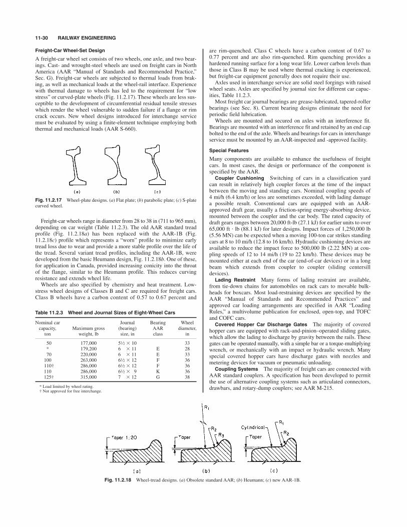
11-30 RAILWAY ENGINEERING
Freight-Car Wheel-Set Design
A freight-car wheel set consists of two wheels, one axle, and two bear-ings. Cast- and wrought-steel wheels are used on freight cars in NorthAmerica (AAR “Manual of Standards and Recommended Practice,”Sec. G). Freight-car wheels are subjected to thermal loads from brak-ing, as well as mechanical loads at the wheel-rail interface. Experiencewith thermal damage to wheels has led to the requirement for “lowstress” or curved-plate wheels (Fig. 11.2.17). These wheels are less sus-ceptible to the development of circumferential residual tensile stresseswhich render the wheel vulnerable to sudden failure if a flange or rimcrack occurs. New wheel designs introduced for interchange servicemust be evaluated by using a finite-element technique employing boththermal and mechanical loads (AAR S-660).
are rim-quenched. Class C wheels have a carbon content of 0.67 to0.77 percent and are also rim-quenched. Rim quenching provides ahardened running surface for a long wear life. Lower carbon levels thanthose in Class B may be used where thermal cracking is experienced,but freight-car equipment generally does not require their use.Axles used in interchange service are solid steel forgings with raised
wheel seats. Axles are specified by journal size for different car capac-ities, Table 11.2.3.Most freight car journal bearings are grease-lubricated, tapered-roller
bearings (see Sec. 8). Current bearing designs eliminate the need forperiodic field lubrication.Wheels are mounted and secured on axles with an interference fit.
Bearings are mounted with an interference fit and retained by an end capbolted to the end of the axle. Wheels and bearings for cars in interchangeservice must be mounted by an AAR-inspected and -approved facility.
Special Features
Many components are available to enhance the usefulness of freightcars. In most cases, the design or performance of the component isspecified by the AAR.Coupler Cushioning Switching of cars in a classification yard
can result in relatively high coupler forces at the time of the impactbetween the moving and standing cars. Nominal coupling speeds of4 mi/h (6.4 km/h) or less are sometimes exceeded, with lading damagea possible result. Conventional cars are equipped with an AAR-approved draft gear, usually a friction-spring energy-absorbing device,mounted between the coupler and the car body. The rated capacity ofdraft gears ranges between 20,000 ft-lb (27.1 kJ) for earlier units to over65,000 ft # lb (88.1 kJ) for later designs. Impact forces of 1,250,000 lb(5.56 MN) can be expected when a moving 100-ton car strikes standingcars at 8 to 10 mi/h (12.8 to 16 km/h). Hydraulic cushioning devices areavailable to reduce the impact force to 500,000 lb (2.22 MN) at cou-pling speeds of 12 to 14 mi/h (19 to 22 km/h). These devices may bemounted either at each end of the car (end-of-car devices) or in a longbeam which extends from coupler to coupler (sliding centersilldevices).Lading Restraint Many forms of lading restraint are available,
from tie-down chains for automobiles on rack cars to movable bulk-heads for boxcars. Most load-restraining devices are specified by theAAR “Manual of Standards and Recommended Practices” andapproved car loading arrangements are specified in AAR “LoadingRules,” a multivolume publication for enclosed, open-top, and TOFCand COFC cars.Covered Hopper Car Discharge Gates The majority of covered
hopper cars are equipped with rack-and-pinion–operated sliding gates,which allow the lading to discharge by gravity between the rails. Thesegates can be operated manually, with a simple bar or a torque-multiplyingwrench, or mechanically with an impact or hydraulic wrench. Manyspecial covered hopper cars have discharge gates with nozzles andmetering devices for vacuum or pneumatic unloading.Coupling Systems The majority of freight cars are connected with
AAR standard couplers. A specification has been developed to permitthe use of alternative coupling systems such as articulated connectors,drawbars, and rotary-dump couplers; see AAR M-215.
Fig. 11.2.17 Wheel-plate designs. (a) Flat plate; (b) parabolic plate; (c) S-plate
curved wheel.
Freight-car wheels range in diameter from 28 to 38 in (711 to 965 mm),depending on car weight (Table 11.2.3). The old AAR standard treadprofile (Fig. 11.2.18a) has been replaced with the AAR-1B (Fig.11.2.18c) profile which represents a “worn” profile to minimize earlytread loss due to wear and provide a more stable profile over the life ofthe tread. Several variant tread profiles, including the AAR-1B, weredeveloped from the basic Heumann design, Fig. 11.2.18b. One of these,for application in Canada, provided increasing conicity into the throatof the flange, similar to the Heumann profile. This reduces curvingresistance and extends wheel life.
Wheels are also specified by chemistry and heat treatment. Low-stress wheel designs of Classes B and C are required for freight cars.Class B wheels have a carbon content of 0.57 to 0.67 percent and
Table 11.2.3 Wheel and Journal Sizes of Eight-Wheel Cars
Nominal car Journal Bearing Wheel
capacity, Maximum gross (bearing) AAR diameter,
ton weight, lb size, in class in
50 177,000 5 10 33
* 179,200 6 11 E 28
70 220,000 6 11 E 33
100 263,000 6 12 F 36
110† 286,000 6 12 F 36
110 286,000 6 9 K 36
125† 315,000 7 12 G 38
* Load limited by wheel rating.† Not approved for free interchange.
1⁄2
1⁄2
1⁄2
1⁄2
Fig. 11.2.18 Wheel-tread designs. (a) Obsolete standard AAR; (b) Heumann; (c) new AAR-1B.

FREIGHT CARS 11-31
Freight-Train Braking
The retarding forces acting on a railway train are rolling and mechani-cal resistance, aerodynamic drag, curvature, and grade, plus that forceresulting from friction of brake shoes rubbing the wheel treads. Onlocomotives so equipped, dynamic or rheostatic brake using the tractionmotors as generators can provide all or a portion of the retarding forceto control train speed.
Quick-action automatic air brakes of the type specified by the AARare the common standard in North America. With the automatic airbrake system, the brake pipe extends through every vehicle in the train,connected by hoses between each locomotive unit and car. The frontand rear end brake pipe angle cocks are closed.
Air pressure is provided by compressors on the locomotive units tothe main reservoirs, usually at 130 to 150 lb/in2 (900 to 965 kPa).(Pressure values are gage pressures.) The engineer’s automatic brakevalve, in “release” position, provides air to the brake pipe on freighttrains at reduced pressure, usually at 75, 80, 85, or 90 lb/in2 (520, 550,585, or 620 kPa), depending on the type of service, train weight, grades,and speeds at which a train will operate. In passenger service, brakepipe pressure is usually 90 or 110 lb/in2 (620 to 836 kPa).When brake pipe pressure is increased, the control valve allows the
reservoir capacity on each car and locomotive to be charged and at thesame time connects the brake cylinders to exhaust. Brake pipe pressureis reduced when the engineer’s brake valve is placed in a “service” posi-tion, and the control valve cuts off the charging function and allows thereservoir air on each car to flow into the brake cylinder. This moves thepiston and, through a system of levers and rods, pushes the brake shoesagainst the wheel treads.When the engineer’s automatic brake valve is placed in the emer-
gency position, the brake pipe pressure (BP) is reduced very rapidly.The control valves on each car move to the emergency-application posi-tion and rapidly open a large vent valve, exhausting brake pipe pressureto atmosphere. This will serially propagate the emergency applicationthrough the train at from 900 to 950 ft/s (280 to 290 m/s.) With the con-trol valve in the emergency position both auxiliary- and emergency-reservoir volumes (pressures) equalize with the brake cylinder, andhigher brake cylinder pressure (BCP) results, building up at a faster ratethan in service applications.The foregoing briefly describes the functions of the fundamental
automatic air brake based on the functions of the control valve. AAR-approved brake equipment is required on all freight cars used in inter-change service. The functions of the control valve have been refinedto permit the handling of longer trains by more uniform brake perfor-mance. Important improvements in this design have been (1) reduc-tion of the time required to apply the brakes on the last car of a train,
(2) more uniform and faster release of the brakes, and (3) availability ofemergency application with brake pipe pressure greater than 40 lb/in2
(275 kPa). Faster brake response has been achieved by a number of rail-roads using “distributed power,” where radio-controlled locomotivesare spaced within the train or placed at both ends of the train.The braking ratio of a car is defined as the ratio of brake shoe (normal)
force to the car’s rated gross weight. Two types of brake shoes, high-friction composition and high-phosphorus cast iron, are used in inter-change service. As these shoes have very different friction characteristics,different braking ratios are required to assure uniform train braking per-formance (Table 11.2.4). Actual or net shoe forces are measured with cal-ibrated devices. The calculated braking ratio R (nominal) is determinedfrom the equation
(11.2.6)
where P ! brake cylinder pressure, 50 lb/in2 gage; L ! mechanicalratio of brake levers; A! brake cylinder area, in2; N! number of brakecylinders; E! brake rigging efficiency and W! carweight, lb.To estimate rigging efficiency consider each pinned joint and hori-
zontal sliding joint as a 0.01 loss of efficiency; i.e., in a system with 20pinned and horizontal sliding joints, Er ! 0.80. For unit-type (hanger-less) brake beams Eb! 0.90 and for the brake cylinder Ec! 0.95, givingan overall efficiency of 0.684 or 68.4 percent.
The total retarding fore in pounds per ton may be taken as:
F ! (PLef/W) ! FgG (11.2.7)
where P ! total brake-cylinder piston force, lbf; L ! multiplying ratioof the leverage between cylinder pistons and wheel treads; ef ! productof the coefficient of brake shoe friction and brake rigging efficiency; W!loaded weight of vehicle, tons; Fg ! force of gravity, 20 lb/ton/percentgrade; G ! ascending grade, percent.Stopping distance can be found by adding the distance covered dur-
ing the time the brakes are fully applied to the distance covered duringthe equivalent instantaneous application time.
(11.2.8)
where S ! stopping distance, ft; V1 ! initial speed when brakeapplied, mi/h; V2 ! speed, mi/h, at time t1; Wn ! weight on which
1 1.467 t1BV1 2 ¢R 1 2000G
91.1≤ t12R
S 50.0334V 2
2
BWnBns pa/pndef
Wa
R 1 ¢ R
2000≤ 6 sGd
5 Er 3 Eb 3 Ec;
R 5 PLANE 3 100/W
Table 11.2.4 Braking Ratios, AAR Standard S-401
With 50 lb/in2 brake
cylinder pressureHand brake*
Percent of grossMinimum
rail loadMaximum percent of
percent of gross rail
Type of brake rigging and shoes Min. Max. light weight load
Conventional body-mounted brake rigging or truck-mounted brake
rigging using levers to transmit brake cylinder force to the
brake shoes
Cars equipped with cast iron brake shoes 13 20 53 13
Cars equipped with high-friction composition brake shoes 6.5 10 30 11
Direct-acting brake cylinders not using levers to transmit brake
cylinder force to the brake shoes
Cars equipped with cast iron brake shoes
Cars equipped with high-friction composition brake shoes 6.5 10 33 11
Cabooses†
Cabooses equipped with cast iron brake shoes 35–45
Cabooses equipped with high-friction composition brake shoes 18–23
* Hand brake force applied at the horizontal hand brake chain with AAR certified or AAR approved hand brake.† Effective for cabooses ordered new after July 1, 1982, hand brake ratios for cabooses to the same as lightweight ratios for cabooses.NOTE: Above braking ratios also apply to cars equipped with empty and load brake equipment.

11-32 RAILWAY ENGINEERING
intraurban service is divided into three major categories: commuter rail,heavy rail rapid transit, and light rail transit, depending upon the char-acteristics of the service. Commuter rail equipment operates on conven-tional railroad rights-of-way, usually intermixed with other long-haulpassenger and freight traffic. Heavy-rail rapid transit (HRT), oftenreferred to as “metro,” operates on a dedicated right-of-way, which iscommonly in subways or on elevated structures. Light-rail transit (LRT)utilizing light rail vehicles (LRV) has evolved from the older trolley orstreetcar concepts and may operate in any combination of surface, sub-way, and elevated dedicated rights-of-way, semireserved surface rights-of-way with grade crossing, and shared rights-of-way with other trafficon surface streets. In a few cases LRT shares the trackage with freightoperations, which are time-separated to comply with FRA regulations.Since mainline and commuter rail equipment operates over conven-
tional railroad rights-of-way, the structural design is heavy to providethe FRA-required “crashworthiness” of vehicles in the event of colli-sions with other trains or at grade crossings with automotive vehicles.Although HRT vehicles are designed to stringent structural criteria, therequirements are somewhat different, since the operation is separatefrom freight equipment and there are usually no highway grade cross-ings. Minimum weight is particularly important for transit vehicles sothat demanding schedules over lines with close station spacing can bemet with minimum energy consumption.Main-Line Passenger Equipment There are four primary passen-
ger train sets in operation across the world: diesel locomotive hauled,diesel multiple unit (DMU), electric locomotive hauled, and electricMU (EMU). In recent years the design of mainline passenger equip-ment has been controlled by specifications provided by APTA and theoperating authority. Most of the newer cars provided for Amtrak havehad stainless steel structural components. These cars have beendesigned to be locomotive-hauled and to use a separate 480-V three-phase power supply for heating, ventilation, air conditioning, foodcar services, and other control and auxiliary power requirements.Figure 11.2.20a shows an Amtrak coach car of the Superliner class;Fig. 11.2.20b shows an intercity high-speed coach.Trucks for passenger equipment are designed to provide a superior
ride to freight-car trucks. As a result, passenger trucks include a form of“primary” suspension to isolate the wheel set from the frame of thetruck. A softer “secondary” suspension is provided to isolate the truckfrom the car body. In most cases, the primary suspension uses eithercoil springs, elliptical springs, or elastomeric components. The sec-ondary suspension generally utilizes either large coil ring springs orpneumatic springs with special leveling valves to control the height ofthe car body. Hydraulic dampers are also applied to improve the verti-cal and lateral ride quality.
Table 11.2.5 Capacity versus Load Limitfor Railroad Freight Cars
Capacity, ton Wn, 1,000 lb
50 177
70 220
100 263
110 286
125 315
empty or ready-to-run weight); Bn ! braking ratio (total brake shoeforce at stated brake cylinder, lb/in2, divided by Wn); Pn ! brake cylin-der pressure on which Bn is based, usually 50 lb/in
2; Pa ! full brakecylinder pressure; e ! overall rigging and cylinder efficiency, decimal;f ! typical friction of brake shoes, see below; R ! total resistance,mechanical plus aerodynamic and curve resistance, lb/ton; G ! gradein decimal, $ upgrade, % downgrade; t1 ! equivalent instantaneousapplication time, s.Equivalent instantaneous application time is that time on a curve of
average brake cylinder buildup versus time for a train or car where thearea above the buildup curve is equal to the area below the curve. Astraight-line buildup curve starting at zero time would have a t1 of halfthe total buildup time.
The friction coefficient f varies with the speed; it is usually lower athigh speed. To a lesser extent, it varies with brake shoe force and withthe material of the wheel and shoe. For stops below 60 mi/h (97 km/h),a conservative figure for a high-friction composition brake shoe on steelwheels is approximately
ef ! 0.30 (11.2.9)
In the case of high-phosphorus iron shoes, this figure must be reducedby approximately 50 percent.Pn is based on 50 lb/in
2 (345 kPa) air pressure in the cylinder; 80lb/in2 is a typical value for the brake pipe pressure of a fully chargedfreight train. This will give a 50 lb/in2 (345 kPa) brake cylinder pressureduring a full service application on AB equipment, and a 60 lb/in2
(415 kPa) brake cylinder pressure with an emergency application.To prevent wheel sliding, FR ' fW, where FR ! retarding force at
wheel rims resisting rotation of any pair of connected wheels, lb; f !coefficient of wheel-rail adhesion or friction (a decimal); and W!weightupon a pair of wheels, lb. Actual or adhesive weight on wheels when thevehicle is in motion is affected by weight transfer (force transmitted to thetrucks and axles by the inertia of the car body through the truck centerplates), center of gravity, and vertical oscillation of body weight upontruck springs. The value of varies with speed as shown in Fig. 11.2.19.The relationship between the required coefficient of wheel-rail
adhesion to prevent wheel sliding and rate of retardation A is miles perhour per second may be expressed by There has been some encouraging work to develop an electric brake
that may eventually obsolete the present pneumatic brake systems.Test Devices Special devices have been developed testing brake
components and cars on a repair track.End-of-Train Devices To eliminate the requirement for a caboose
crew car at the end of the train, special electronic devices have beendeveloped to transmit the end-of-train brake-pipe pressure to the loco-motive operator by telemetry.
PASSENGER EQUIPMENT
During the past two decades most mainline or long-haul passenger ser-vice in North America has become a function of government agencies,i.e., Amtrak in the United States and Via Rail in Canada. Equipment for
A 5 21.95f1.
ff
Fig. 11.2.19 Typical wheel-rail adhesion. Track has jointed rails. (Air Brake
Association.)
braking ratio Bn is based, lb (see Table 11.2.5 for values of Wn forfreight cars; for passenger cars and locomotives: Wn is based on

PASSENGER EQUIPMENT 11-33
Fig. 11.2.20 Mainline passenger cars. (a) Double-deck coach; (b) Single-deck coach. (Courtesy of Bombardier
Transportation.)

Commuter Rail Passenger Equipment Commuter rail equipmentcan be either locomotive-hauled or self-propelled (Fig. 11.2.21). Somelocomotive-hauled equipment is arranged for “push-pull” service. Thisconfiguration permits the train to be operated with the locomotive eitherpushing or pulling the train. For push-pull service, some of the passen-ger cars must be equipped with cabs to allow the engineer to operate thetrain from the end opposite the locomotive during the push operation.All cars must have control trainlines to connect the lead (cab) car tothe trailing locomotive. Locomotive-hauled commuter rail cars use
AAR-type H couplers. Most self-propelled (single- or multiple-unit)cars use other automatic coupler designs, which can be mechanicallycoupled to an AAR coupler with an adaptor.Heavy Rail Rapid Transit Equipment This equipment is used on
traditional subway/elevated properties in such cities as Boston, NewYork, Philadelphia (Fig. 11.2.22), and Chicago in a semiautomaticmode of operation over dedicated rights-of-way which are constrainedby limiting civil features. State-of-the-art subway-elevated propertiesinclude such cities as Washington, Atlanta, Miami, and San Francisco,
11-34 RAILWAY ENGINEERING
Fig. 11.2.21 Commuter rail car. (Courtesy of Bombardier Transportation.)
Fig. 11.2.22 Heavy rail transit car. (Courtesy of Bombardier Transportation.)

PASSENGER EQUIPMENT 11-35
where the equipment provides highly automated modes of operation onrights-of-way with generous civil alignments.
The cars can operate bidirectionally in multiple with as many as 12 ormore cars controlled from the leading cab. They are electrically propelled,usually from a dc third rail, which makes contact with a shoe insulatedfrom and supported by the frame of the truck. Occasionally, roof-mountedpantographs are used. Voltages range from 600 to 1,500 V dc.The cars range from 48 to 75 ft (14.6 to 22.9 m) over the anticlimbers,
the longer cars being used on the newer properties. Passenger seatingvaries from 40 to 80 seats per car, depending upon length and the localpolicy (or preference) regarding seated to standee ratio. Older propertiesrequire negotiation of curves as sharp as 50 ft (15.2 m) minimum radiuswith speeds up to only 50 mi/h (80 km/h) on tangent track, while newerproperties usually have no less than 125 ft (38.1 m) minimum radiuscurves with speeds up to 75 mi/h (120 km/h) on tangent track.
All North American properties operate on standard-gage track with theexception of the 5 ft 6 in (1.7 m) San Francisco Bay Area Rapid Transit(BART), the 4 ft 10 in (1.5 m) Toronto Transit Subways, and the 5 ft in(1.6 m) Philadelphia Southeastern Pennsylvania TransportationAuthority (SEPTA) Market-Frankford line. Grades seldom exceed 3percent, and 1.5 to 2.0 percent is the desired maximum.
Typically, newer properties require maximum acceleration rates ofbetween 2.5 and 3.0 mi/(h # s) [4.0 to 4.8 km/(h # s)] as nearly inde-pendent of passenger loads as possible from 0 to approximately 20 mi/h(32 km/h). Depending upon the selection of motors and gearing, thisrate falls off as speed is increased, but rates can generally be controlledat a variety of levels between zero and maximum.
Deceleration is typically accomplished by a blended dynamic andelectropneumatic friction tread or disk brake, although a few propertiesuse an electrically controlled hydraulic friction brake. In some casesenergy is regenerated and sent back into the power system. All of thesesystems usually provide a maximum braking rate of between 3.0 and3.5 mi/(h # s) [4.8 and 5.6 km/(h # s)] and are made as independent ofpassenger loads as possible by a load-weighing system that adjustsbraking effort to suit passenger loads. Some employ regenerative brak-ing to supplement the other brake systems.
Dynamic braking is generally used as the primary stopping mode andis effective from maximum speed down to 10 mi/h (16 km/h) with fric-tion braking supplementation as the characteristic dynamic fade occurs.The friction brakes provide the final stopping forces. Emergencybraking rates depend upon line constraints, car subsystems, and otherfactors, but generally rely on the maximum retardation force that can be
21⁄2
provided by the dynamic and friction brakes within the limits of avail-able wheel-to-rail adhesion.Acceleration and braking on modern properties are usually con-
trolled by a single master controller handle that has power positions inone direction and a coasting or neutral center position and braking posi-tions in the opposite direction. A few properties use foot-pedal controlwith a “deadman” pedal operated by the left foot, a brake pedal operatedby the right foot, and an accelerator (power) pedal also operated bythe right foot. In either case, the number of positions depends uponproperty policy and control subsystems on the car. Control elementsinclude motor-current sensors and some or all of the following: speedsensors, rate sensors, and load-weighing sensors. Signals from thesesensors are processed by an electronic control unit (ECU), which pro-vides control functions to the propulsion and braking systems. Thepropulsion systems currently include pilot-motor-operated cams whichactuate switches or electronically controlled unit switches to controlresistance steps, or chopper or inverter systems that electronically pro-vide the desired voltages and currents at the motors.In some applications, dynamic braking utilizes the traction motors as
generators to dissipate energy through the onboard resistors also usedin acceleration. It is expected that regenerative braking will becomemore common since energy can be returned to the line for use by othercars. Theoretically, 35 to 50 percent of the energy can be returned, butthe present state-of-the-art is limited to a practical 20 percent on prop-erties with large numbers of cars on close headways.Car bodies are made of welded stainless steel or low-alloy high-
tensile (LAHT) steel of a design that carries structural loads. Earlierproblems with aluminum, primarily electrolytic action among dissimi-lar metals and welding techniques, have been resolved and aluminum isalso used on a significant number of new cars.Trucks may be cast or fabricated steel with frames and journal bear-
ings either inside or outside the wheels. Axles are carried in roller-bear-ing journals connected to the frames so as to be able to move verticallyagainst a variety of types of primary spring restraint. Metal springs or airbags are used as the secondary suspension between the trucks and the carbody. Most wheels are solid cast or wrought steel. Resilient wheels havebeen tested but are not in general service on heavy rail transit equipment.All heavy rail rapid transit systems use high-level loading platforms
to speed passenger flow. This adds to the civil construction costs, but isnecessary to achieve the required level of service.Light Rail Transit Equipment The cars are called light rail vehicles
(Fig. 11.2.23 shows typical LRVs) and are used on a few remaining
Fig. 11.2.23 Light-rail vehicle (LRV). (a) Articulated; (b) nonarticulated

streetcar systems such as those in Boston, Philadelphia, and Toronto oncity streets and on state-of-the-art subway, surface, and elevated sys-tems such as those in Calgary, Edmonton, Los Angeles, San Diego, andPortland (oregon) and in semiautomated modes over partially or whollyreserved rights-of-way.
As a practical matter, the LRV’s track, signal systems, and power sys-tems utilize the same subsystems as heavy rail rapid transit and are not“lighter” in a physical sense.
Most LRVs are designed to operate bidirectionally in multiple, with upto four cars controlled from the leading cab. The LRVs are electrically pro-pelled from an overhead contact wire, often of catenary design, that makescontact with a pantograph or pole on the roof. For reasons of waysidesafety, third-rail pickup is not used. Voltages range from 550 to 750 V dc.The cars range from 60 to 65 ft (18.3 to 19.8 m) over the anticlimbers
for single cars and from 70 to 90 ft (21.3 to 27.4 m) for articulated cars.The choice is determined by passenger volumes and civil constraints.
Articulated cars have been used in railroad and transit applicationssince the 1920s, but have found favor in light rail applications becauseof their ability to increase passenger loads in a longer car that can nego-tiate relatively tight-radius curves. These cars require the additionalmechanical complexity of the articulated connection and a third truckbetween two car-body sections.
Passenger seating varies from 50 to 80 or more seats per car, depend-ing upon length, placement of seats in the articulation, and the policyregarding seated/standee ratio. Older systems require negotiation ofcurves down to 30 ft (9.1 m) minimum radius with speeds up to only40 mi/h (65 km/h) on tangent track, while newer systems usually haveno less than 75 ft (22.9 m) minimum radius curves with speeds up to65 mi/h (104 km/h) on tangent track.
The newer properties all use standard-gage track; however, existingolder systems include 4 ft 10 in (1,495 mm) and 5 ft in (1,587 mm)gages. Grades have reached 12 percent but 6 percent is now consideredthe maximum and 5 percent is preferred.
Typically, newer properties require maximum acceleration rates ofbetween 3.0 to 3.5 mi/(h # s) [4.8 to 5.6 km/(h # s)] as nearly indepen-dent of passenger load as possible from 0 to approximately 20 mi/h(32 km/h). Depending upon the selection of motors and gearing, thisrate falls off as speed is increased, but the rates can generally be con-trolled at a variety of levels.Unlike most heavy rail rapid transit cars, LRVs incorporate three
braking modes: dynamic, friction, and track brake, which typically pro-vide maximum service braking at between 3.0 and 3.5 mi/(h # s) [4.8 to5.6 km/(h # s)] and 6.0 mi/(h # s) [9.6 km/(h # s)] maximum emergencybraking rates. The dynamic and friction brakes are usually blended, buta variety of techniques exist. The track brake is intended to be used pri-marily for emergency conditions and may or may not be controlled withthe other braking systems.The friction brakes are almost exclusively disk brakes, since LRVs
use resilient wheels that can be damaged by tread-brake heat buildup.No single consistent pattern exists for the actuation mechanism. All-electric, all-pneumatic, electropneumatic, electrohydraulic, and electro-pneumatic over hydraulic are in common use.Dynamic braking is generally used as the primary braking mode and
is effective from maximum speed down to about 5 mi/h (8 km/h) withfriction braking supplementation as the characteristic dynamic fadeoccurs.As with heavy rail rapid transit, the emergency braking rates depend
upon line constraints, car-control subsystems selected, and other fac-tors, but the use of track brakes means that higher braking rates can beachieved because the wheel-to-rail adhesion is not the limiting factor.Acceleration and braking on modern properties are usually con-
trolled by a single master controller handle that has power positions inone direction and a coasting or neutral center position and braking posi-tions in the opposite direction. A few properties use foot-pedal controlwith a “deadman” pedal operated by the left foot, a brake pedal operatedby the right foot, and an accelerator (power) pedal also operated by theright foot. In either case, the number of positions depends upon propertypolicy and control subsystems on the car.
21⁄2
Control elements include motor-current sensors and some or all ofthe following: speed sensors, rate sensors, and load-weighing sensors.Signals from these sensors are processed by an electronic control unit(ECU), which provides control functions to the propulsion and brakingsystems.The propulsion systems currently include pilot-motor-operated cams
that actuate switches or electronically controlled unit switches to con-trol resistance steps. Chopper and inverter systems that electronicallyprovide the desired voltages and currents at the motors are also used.Most modern LRVs are equipped with two powered trucks. In two-
section articulated designs (Fig. 11.2.23a), the third (center) truck maybe left unpowered but usually has friction and track brake capability.Some European designs use three powered trucks but the additionalcost and complexity have not been found necessary in North America.Unlike heavy rail rapid transit, there are three major dc-motor con-
figurations in use: the traditional series-wound motors used in bimotortrucks, the European-derived monomotor, and a hybrid monomotorwith a separately excited field—the last in chopper-control versiononly.The bimotor designs are rated between 100 and 125 shaft hp per
motor at between 300 and 750 V dc, depending upon line voltage andseries or series-parallel control schemes (electronic or electromechanicalcontrol). The monomotor designs are rated between 225 and 250 shafthp per motor at between 300 and 750 V dc (electronic or electro-mechanical control).The motors, gear units (right angle or parallel), and axles are joined
variously through flexible couplings. In the case of the monomotor, it issupported in the center of the truck, and right-angle gearboxes aremounted on either end of the motor. Commonly, the axle goes throughthe gearbox and connection is made with a flexible coupling arrange-ment. Electronic inverter control drives with ac motors have beenapplied in recent conversions and new equipment.Dynamic braking is achieved in the same manner as in heavy rail
rapid transit.Unlike heavy rail rapid transit, LRV bodies are usually made only
of welded LAHT steel and are of a load-bearing design. Because ofthe semireserved right-of-way, the risk of collision damage with auto-motive vehicles is greater than with heavy rail rapid transit and theLAHT steel has been found to be easier to repair than stainless steelor aluminum. Although LAHT steel requires painting, this can be anasset since the painting can be performed in a highly decorative man-ner pleasing to the public and appropriate to themes desired by thecities.Trucks may be cast or fabricated steel with either inside or outside
frames. Axles are carried in roller-bearing journals, which are usuallyresiliently coupled to the frames with elastomeric springs as a primarysuspension. Both vertical and a limited amount of horizontal movementoccur. Since tight curve radii are common, the frames are usually con-nected to concentric circular ball-bearing rings, which, in turn, are con-nected to the car body. Air bags, solid elastomeric springs, or metalsprings are used as a secondary suspension. Resilient wheels are usedon virtually all LRVs.Newer LRVs have low-level loading doors and steps, which mini-
mize station platform costs.
TRACK
Gage The gage of railway track is the distance between the innersides of the rail heads measured 0.626 in (15.9 mm) below the top run-ning surface of the rail. North American railways are laid with a nomi-nal gage of 4 ft in (1,435 mm), which is known as standard gage.Rail wear causes an increase in gage. On sharp curves [over 88, see Eq.(11.2.10)], it has been the practice to widen the gage to reduce rail wear.Track Structure In basic track structure is composed of six major
elements: rail, tie plates, fasteners, cross ties, ballast, and subgrade(Fig. 11.2.24).Rail The American Railway Engineering and Maintenance of Way
Association had defined standards for the cross section of rails of
81⁄2
11-36 RAILWAY ENGINEERING

TRACK 11-37
various weights, which are identified by their weight (in pounds) peryard. The AREMA standards provide for rail weights varying from90 to 141 lb/yd. However, recommendations for new rail purchasesare limited to weights of 115 lb/yd and above. Many railroads histor-ically used special sections of their own design; however, the freightindustry is converging on the use of the 115-, 136-, and 141-lb/yd sec-tions. The standard length in use is 80 ft (31.5 m), although some millsare now considering making longer lengths available.
The prevailing weight of rails used in mainline track is from 112 to141 lb/yd. Secondary and branch lines are generally laid with 90- to115-lb/yd or heavier rail that has been previously used and partlyworn in mainline service. In a very limited application, rail weights aslow as 60 lb/yd exist in some tracks having very light usage. In thepast, rail sections were connected by using bolted joint bars. Currentpractice is the use of continuous welded rail (CWR). In general, railsare first welded into lengths averaging 1,440 feet (440 m) or more.After these strings, or “ribbons,” are installed, they are later field weldedto eliminate conventional joints. At one time the gas-fusion weldingprocess was common, but today almost all rail is welded by the elec-tric-flash or aluminothermic processes. CWR requires the use of morerail anchors than jointed rail in order to clamp the base of the rail andposition it on the cross ties to prevent rail movement. This is neces-sary to restrain longitudinal forces that result from thermal expansionand contraction with ambient temperature changes. Failure to ade-quately restrain the rail can result in track buckling in extremely hotweather or in rail “pull aparts” in extremely cold weather. Care mustbe exercised to install the rail at temperatures that do not approachhigh or low extremes.
A variety of heat-treating and alloying processes have been used toproduce rail that is more resistant to wear and less susceptible to fatiguefailure. Comprehensive studies indicate that both gage face and top-of-rail lubrication can dramatically reduce the wear rate of rail in curves(see publications of AAR Research and Test Department). Frictionmodification using top-of-rail lubrication must be carefully managed sothat it does not interfere with traction required to move and brake trains.Reduced wear and higher permissible axle loads have led to fatiguebecoming the dominant cause for rail replacement at extended life.Grinding the running surface of rail has been greatly increased toreduce the damage caused by fatigue.Tie Plates Rail is supported on tie plates that restrain the rail later-
ally, transmit the vehicle loads to the cross tie, and position (cant) therail for optimum vehicle performance. Tie plates cant the rail toward thegage side. Cants vary from 1:14 to 1:40, depending on service condi-tions and operating speeds, with 1:40 being most common.Fasteners Rail and tie plates are fixed to the cross ties by fasteners.
Conventional construction with wood cross ties utilizes steel spikes dri-ven into the tie through holes in the tie plate. In some cases, screw-typefasteners are used to provide more resistance to vertical forces. Elastic,clip-type fasteners are used on concrete and, at times, on wooden crossties to provide a uniform, resilient attachment and longitudinal restraintin lieu of anchors. This type of fastening system also reduces the like-lihood of rail overturns.Cross Ties To retain gage and provide a further distribution of
vehicle loads to the ballast, lateral cross ties are used. The majority ofcross ties used in North America are wood. However, concrete cross tiesare being used more frequently in areas where track surface and lateral
stability are difficult to maintain and in high-speed passenger corridors.Slab track designs are now being given scrutiny for high-utilizationareas.Ballast Ballast serves to further distribute vehicle loads to the sub-
grade, restrain vertical and lateral displacement of the track structure,and provide for drainage. Typical mainline ballast materials are lime-stone, trap rock, granite, or slag. Lightly built secondary lines have usedgravel, cinders, or sand in the past.Subgrade The subgrade serves as the interface between the ballast
and the native soil. Subgrade material is typically compacted or stabi-lized soil. Instability of the subgrade due to groundwater permeation isa concern in some areas. Subgrade instability must be analyzed andtreated on a case-by-case basis.Track Geometry Railroad maintenance practices, state standards,
AREMA standards, and, more recently, FRA safety standards (49 CFRTitle § 113) specify limitations on geometric deviations for track struc-ture. Among the characteristics considered are:
GageAlignment (the lateral position of the rails)Profile (the elevation of the rail)CurvatureEasement (the rate of change from tangent to curve)Superelevation (the elevation of the outer or “high” rail in a curvecompared to the inner or “low” rail)Runoff (the rate of change in superelevation)Cross level (the relative height of opposite rails)Twist (the change in cross level over a specified distance)
FRA standards specify maximum operating speeds by class of trackranging from Class 1 (lowest acceptable) to Class 9. Track geometry isa significant consideration in vehicle suspension design. For operatingspeeds greater than 110 mi/h, FRA has promulgated regulations (trackClasses 6 through 9) that require qualification of locomotives and carsthrough a test program over each operating route. These tests call forcomprehensive measurement of wheel/rail forces and vehicle accelera-tions (49 CFT § 213).Curvature The curvature of track is designated in terms of “degrees
of curvature.” The degree of curve is the number of degrees of centralangle subtended by a chord of 100-ft length (measured on the trackcenterline). Equation (11.2.10) gives the approximate radius R in feetfor ordinary railway curves.
(11.2.10)
On important main lines where trains are operated at relatively highspeed, the curves are ordinarily not sharper than 6 to 88. In mountainousterritory, and in other rare instances, curves as sharp as 188 occur. Mostdiesel and electric locomotives are designed to traverse curves up to 218.Most uncoupled cars will pass considerably sharper curves, the limitingfactor in this case being the clearance of the truck components to carbody structural members or equipment or the flexibility of the brakeconnections to the trucks (AAR “Manual of Standards andRecommended Practices,” Sec. C).Clearances For new construction, the AREMA standard clearance
diagrams provide for a clear height of 23 ft (7.0 m) above the tops ofthe railheads and for a width of 18 ft (5.5 m). Where conditions require,as in tunnels and bridges, these dimensions are reduced at the top andbottom of the diagram. For tracks entering buildings, an opening 16 ft(4.9 m) wide and 18 ft (5.5 m) high is recommended and will ordinarilysuffice to pass the largest locomotives and most freight cars. A standardcar clearance diagram for railway bridges (Fig. 11.2.25) represents theAAR recommendation for new construction. Minimum clearances aredictated by state authorities, and are summarized in Chapter 28, Table 3.3,of the AREMA Manual. Individual railroads have their own standardsfor existing lines and new construction, which are generally more strin-gent than the legal requirements. The actual clearance limitations on aparticular railroad can be found in the official publication “RailwayLine Clearances,” Railway Equipment and Publishing Co.
R 55,730
degrees per 100-ft chord
Fig. 11.2.24 Track structure.

Track Spacing The distance between centers of mainline trackcommonly varies between 12 and 15 ft (3.6 and 4.6 m). Twelve-footspacing exists, however, only on older construction. Most states requirea minimum of 14 ft 0 in (4.3 m) between main tracks; however, manyrailroads have adopted 15 ft 0 in (3.6 m) as their standard. In a fewcases, where space permits, 20 ft (6.1 m) is being used.Turnouts Railway turnouts are defined by frog number. The frog
number is the cotangent of the frog angle, which is the ratio of the lat-eral displacement of the diverging track per unit of longitudinaldistance along the nondiverging track. Typical turnouts in yard andindustry trackage range from number 7 to number 10. For mainlineservice, typical turnouts range from number 10 to number 20. The otherimportant part of a turnout is the switch. The switch has movable pointsthat direct the wheel down the straight or diverging side of the turnout. Thehigher the turnout number, the longer the switch, and the higher the allow-able speed for trains traversing the diverging track. Allowable speeds aregoverned by the curvature of the diverging tack, and the angle of theswitch. As a general rule, the allowable speed (in mi/h) is slightly less thantwice the turnout number. In recent track construction for high-speedservice special turnouts with movable point frogs have been applied.Noise Allowable noise levels from railroad operation are pre-
scribed by 40 CFR § 201.
VEHICLE-TRACK INTERACTION
Train Resistance The resistance to a train in motion along the trackis of prime interest, as it is reflected directly in locomotive energyrequirement. This resistance is expressed in terms of pounds per ton oftrain weight. Gross train resistance is that force that must be overcomeby the locomotives at the driving-wheel–rail interface. Trailing trainresistance must be overcome at the rear drawbar of the locomotive.There are two classes of resistance that must be overcome: inherent and
incidental. Inherent resistance includes the rolling resistance of bearingsand wheels and aerodynamic resistance due to motion through still air. Itmay be considered equal to the force necessary to maintain motion atconstant speed on level tangent track in still air. Incidental resistanceincludes resistance due to grade, curvature, wind, and vehicle dynamics.Inherent Resistance Of the elements of inherent resistance, at low
speeds rolling resistance is dominant, but at high speeds aerodynamicresistance is the predominant factor. Attempts to differentiate and evalu-ate the various elements through the speed range are a continuing part of
industry research programs to reduce train resistance. At very highspeeds, the effect of air resistance can be approximated as an aid tostudies in its reduction by means of cowling and fairing. The resistanceof a car moving in still air on straight, level track increases parabolical-ly with speed. Because the aerodynamic resistance is independent of carweight, the resistance in pounds per ton decreases as the weight of thecar increases. The total resistance in pounds per ton of a 100-ton car ismuch less than twice as great as that of a 50-ton car under similar con-ditions. With known conditions of speed and car weight, inherent resis-tance can be predicted with reasonable accuracy. Knowledge of trackconditions will permit further refining of the estimate, but for very roughtrack or extremely cold ambient temperatures, generous allowances mustbe made. Under such conditions normal resistance may be doubled. Aformula proposed by Davis (General Electric Review, Oct. 1926) andrevised by Tuthill (“High Speed Freight Train Resistance.” Univ. of
Illinois Engr. Bull., 376, 1948) has been used extensively for inherentfreight-train resistances at speeds up to 40 mi/h:
R ! 1.3W $ 29n $ 0.045WV $ 0.0005 AV 2 (11.2.11)
where R! train resistance, lb/car; W!weight per car, tons; V! speed,mi/h; n ! total number of axles; A ! cross-sectional area, ft2.With freight train speeds of 50 to 70 mi/h (80 to 112 km/h), it has
been found that actual resistance values fall considerably below calcu-lations based on the above formula. Several modifications of the Davisequation have been developed for more specific applications. All ofthese equations apply to cars trailing locomotives.
1. Davis equation as modified by I. K. Tuthill (University of IllinoisEngr. Bull, 376, 1948):
R ! 1.3W $ 29n $ 0.045WV $ 0.045V 2 (11.2.12)
Note: In the Totten modification, the equation is augmented by a matrixof coefficients when the velocity exceeds 40 mi/h.
2. Davis equation as modified by the Canadian National Railway:
R ! 0.6W $ 20n $ 0.01WV $ 0.07V 2 (11.2.13)
3. Davis equation as modified by the Canadian National Railway and
former Erie-Lackawanna Railroad for trailers and containers on flat cars:
R ! 0.6W $ 20n $ 0.01WV $ 0.2V 2 (11.2.14)
Other modifications of the Davis equation have been developed forpassenger cars by Totten (“Resistance of Light Weight Passenger Trains,”Railway Age, 103, July 17, 1937). These formulas are for passenger carspulled by a locomotive and do not include head-end air resistance.
1. Davis equations as modified by Totten for streamlined passengercars:
R ! 1.3W $ 29n $ 0.045WV $ [0.00005 $ 0.060725(L /100)0.88]V 2
(11.2.15)
2. Davis equations as modified by Totten for nonstreamlined pas-senger cars
R ! 1.3W $ 29n $ 0.045WV $ [0.00005 $ 0.1085(L /100)0.7]V 2
(11.2.16)
where L ! car length in feet.Aerodynamic and Wind Resistance Wind-tunnel testing has indi-
cated a significant effect on freight train resistance resulting from vehi-cle spacing, open tops of hopper and gondola cars, open boxcar doors,vertical side reinforcements on railway cars and intermodal trailers, andprotruding appurtenances on cars. These effects can cause significantincreases in train resistance at higher speeds. For example, the spacingof intermodal trailers or containers greater than approximately 6 ft canresult in a new frontal area to be considered in determining train resis-tance. Frontal or cornering ambient wind conditions can also have anadverse effect on train resistance, which is increased with discontinu-ities along the length of the train.Curve Resistance Train resistance due to track curvature varies
with speed and degree of curvature. The behavior of rail vehicles incurve negotiation is the subject of several ongoing AAR studies.
11-38 RAILWAY ENGINEERING
Fig. 11.2.25 Wayside clearance diagram. (AREA “Manual for Railway
Engineering—Fixed Properties.”)

VEHICLE-TRACK INTERACTION 11-39
Lubrication of the rail gage face or wheel flanges has become commonpractice for reducing friction and the resulting wheel and rail wear.Recent studies indicate that flange and/or gage face lubrication can sig-nificantly reduce train resistance on tangent track as well (Allen,Conference on the Economics and Performance of Freight Car Trucks,October 1983). In addition, a variety of special trucks (wheel assem-blies) that reduce curve resistance by allowing axles to steer toward aradial position in curves have been developed. For general estimates ofcar resistance and locomotive hauling capacity on dry (unlubricated)rail with conventional trucks, speed and gage relief may be ignored anda figure of 0.8 lb/ton per degree of curvature used.Grade resistance depends only on the angle of ascent or descent and
relates only to the gravitational forces acting on the vehicle. It equatesto 20 lb/ton for each percent of grade, or 0.379 lb/ton for each foot permile rise.Acceleration The force (tractive effort) required to accelerate the
train is the sum of the forces required for linear acceleration and thatrequired for rotational acceleration of the wheels about their axle cen-ters. A linear acceleration of 1 mi/h # s (1.6 km/h # s) is produced by aforce of 91.1 lb/ton. The rotary acceleration requirement adds 6 to 12percent, so that the total is nearly 100 lb/ton (the figure commonly used)for each mile per hour per second. If greater accuracy is required, thefollowing expression is used:
Ra ! A(91.05W $ 36.36n) (11.2.17)
where Ra ! the total accelerating force, lb; A ! acceleration, mi/h # s;W ! weight of train, tons; n ! number of axles.Acceleration and Distance If a distance of S ft the speed of a car
or train changes from V1 to V2 mi/h, the force required to produce accel-eration (or deceleration if the speed is reduced) is
(11.2.18)
The coefficient, 74, corresponds to the use of 100 lb/ton. This formulais useful in the calculation of the energy required to climb a grade withthe assistance of stored energy. In any train-resistance calculation oranalysis, assumptions with regard to acceleration will generally submergeall other variables; e.g., an acceleration of 0.1 mi/h # s (0.16 km/h # s)requires more tractive force than that required to overcome inherentresistance for any car at moderate speeds.Starting Resistance Most railway cars are equipped with roller
bearings requiring a starting force of 5 or 6 lb/ton.Vehicle Suspension Design The primary consideration in the
design of the vehicle suspension system is to isolate track input forcesfrom the vehicle car body and lading. In addition, there are a few spe-cific areas of instability that railway suspension systems must address;see AAR “Manual of Standards and Recommended Practice,” Sec. C-II-M-1001, Chap. XI.Harmonic roll is the tendency of a freight car with a high center of
gravity to rotate about its longitudinal axis (parallel to the track). Thisinstability is excited by passing over staggered low rail joints at a speedthat causes the frequency of the input for each joint to match the naturalroll frequency of the car. Unfortunately, in many car designs, this occursfor loaded cars at 12 to 18 mi/h (19.2 to 28.8 km/h), a common speedfor trains moving in yards or on branch lines where tracks are not wellmaintained. Many freight operations avoid continuous operation in thisspeed range.This adverse behavior is more noticeable in cars with truck centers
approximately the same as the rail length. The effect of harmonic rollcan be mitigated by improved track surface and by damping in the trucksuspension.Pitch and bounce are the tendencies of the vehicle to either translate
vertically up and down (bounce), or rotate (pitch) about a horizontalaxis perpendicular to the centerline of track. This response is also excitedby low track joints and can be relieved by increased truck damping.
Ra 5 74sV 22 2 V 2
1d/S
Yaw is the tendency of the car to rotate about its axis vertical to thecenterline of track. Yaw responses are usually related to truck hunting.Truck hunting is an instability inherent in the design of the truck and
dependent on the stiffness parameters of the truck and on wheel conicity(tread profile). The instability is observed as “parallelogramming” ofthe truck components at a frequency of 2 to 3 Hz, causing the car bodyto yaw or translate laterally. This response is excited by the effect of thenatural frequency of the gravitational stiffness of the wheel set when thespeed of the vehicle approaches the kinematic velocity of the wheel set.This problem is discussed in analytic work available from the AARResearch and Test Department.Superelevation As a train passes around a curve, there is a tenden-
cy for the cars to roll toward the outside of the curve in response to cen-trifugal force acting on the center of gravity of the car body (Fig.11.2.26a). To compensate for this effect, the outside rail is superelevat-ed, or raised, relative to the inside rail (Fig. 11.2.26b). The amount ofsuperelevation for a particular curve is based upon the radius of thecurve and the operating speed of the train. The “balance” or equilibri-um speed for a given curve is that speed at which the weight of the vehi-cle is equally distributed on each rail. The FRA allows a railroad tooperate with 3 in of unbalance, or at the speed at which equilibriumwould exist if the superelevation were 3 in greater than that whichexists. The maximum superelevation is usually 6 in but maybe lower iffreight operation is used exclusively.Longitudinal Train Action Longitudinal train (slack) action is
associated with the dynamic action between individual cars in a train.An example would be the effect of starting a long train in which thecouplers between each car had been compressed (i.e., bunched up). Asthe locomotive begins to pull the train, the slack between the locomo-tive and the first car must be traversed before the first car begins tomove. Next the slack between the first and second car must traversedbefore the second car beings to move, and so on. Before the last carin a long train begins to move, the locomotive and the moving carsmay be traveling at a rate of several miles per hour. This effect canresult in coupler forces sufficient to cause the train to break in two.Longitudinal train (slack) action is also induced by serial braking,
undulating grades, or by braking on varying grades. The AAR TrackTrain Dynamics Program has published guidelines titled “Track TrainDynamics to Improve Freight Train Performance” that explain the causesof undesirable train action and how to minimize its effects. Analysis ofthe forces developed by longitudinal train action requires the applica-tion of the Davis equation to represent the resistance of each vehiclebased upon its velocity and location on a grade or curve. Also, thelongitudinal stiffness of each car and the tractive effort of the locomo-tive must be considered in equations that model the kinematic responseof each vehicle in the train. Computer programs are available from theAAR to assist in the analysis of longitudinal train action.
Fig. 11.2.26 Effect of superelevation on center of gravity of car body.

11-40
11.3 MARINE ENGINEERINGby Michael C. Tracy
REFERENCES: Harrington, “Marine Engineering,” SNAME, 1992. Lewis,
“Principles of Naval Architecture,” SNAME, 1988/89. Myers, “Handbook of
Ocean and Underwater Engineering,” McGraw-Hill, 1969. “Rules for Building
and Classing Steel Vessels,” American Bureau of Shipping. Rawson and Tupper,
“Basic Ship Theory,” Oxford: Butterworth-Heinemann, 2001. Gillmer and
Johnson, “Introduction to Naval Architecture,” Naval Institute, 1982. Barnaby,
“Basic Naval Architecture,” Hutchinson, London, 1967. Jour. Inst. Environ, Sci.
Taggert, “Ship Design and Construction,” SNAME, 1980. Trans. Soc. Naval
Architects and Marine Engrs., SNAME. Naval Engrs. Jour., Am. Soc. of Naval
Engrs., ASNE. Trans. Royal Inst. of Naval Architects, RINA. Figures and exam-
ples herein credited to SNAME have been included by permission of The Society
of Naval Architects and Marine Engineers.
Marine engineering is an integration of many engineering disciplines directed to the development and design of systems oftransport, warfare, exploration, and natural-resource retrieval whichhave one thing in common: operation in or on a body of water.Marine engineers are responsible for the engineering systemsrequired to propel, work, or fight ships. They are responsible for themain propulsion plant; the powering and mechanization aspects ofship functions such as steering, anchoring, cargo handling, heating,ventilation, air conditioning, etc.; and other related requirements.They usually have joint responsibility with naval architects in areasof propulsor design; hull vibration excited by the propeller or mainpropulsion plant; noise reduction and shock hardening, in fact,dynamic response of structures or machinery in general; and envi-ronmental control and habitability. Marine engineering is a distinctmultidiscipline and characteristically a dynamic, continuouslyadvancing technology.
THE MARINE ENVIRONMENT
Marine engineers must be familiar with their environment so that they mayunderstand fuel and power requirements, vibration effects, and propulsion-plant strength considerations. The outstanding characteristic of the openocean is its irregularity in storm winds as well as under relatively calmconditions. The irregular sea can be described by statistical mathematicsbased on the superposition of a large number of regular waves having dif-ferent lengths, directions, and amplitudes. The characteristics of idealizedregular waves are fundamental for the description and understanding ofrealistic, irregular seas. Actual sea states consist of a combination of manysizes of waves often running in different directions, and sometimesmomentarily superimposing into an exceptionally large wave. Air temper-ature and wind also affect ship and machinery operation.
The effects of the marine environment also vary with water depth andtemperature. As a ship passes from deep to shallow water, there is anappreciable change in the potential flow around the hull and a changein the wave pattern produced. Additionally, silt, sea life, and bottomgrowth may affect seawater systems or foul heat exchangers.
MARINE VEHICLES
The platform is additionally a part of marine engineers’ environment.Ships are supported by a buoyant force equal to the weight of the vol-ume of water displaced (Archimedes’ principle). For surface ships, thisweight is equal to the total weight of the structure, machinery, outfit,fuel, stores, crew, and useful load. The principal sources of resistance topropulsion are skin friction and the energy lost to surface waves gener-ated by moving in the interface between air and water. Minimization ofone or both of these sources of resistance has generally been a primaryobjective in the design of marine vehicles.
Displacement Hull Forms
Displacement hull forms are the familiar monohull, the catamaran, andthe submarine. The moderate-to-full-displacement monohull form pro-vides the best possible combinations of high-payload-carrying ability,economical powering characteristics, and good seakeeping qualities. Amore slender hull form achieves a significant reduction in wave-makingresistance, hence increased speed; however, it is limited in its ability tocarry topside weight because of the low transverse stability of itsnarrow beam. Multihull ships provide a solution to the problem of lowtransverse stability. They are increasingly popular in sailing yachts,high-speed passenger ferries, and research and small support ships.Sailing catamarans, with their superior transverse stability permittinglarge sail-plane area, gain a speed advantage over monohull craft ofcomparable size. A powered catamaran has the advantage of increaseddeck space and relatively low roll angles over a monohull ship. Thesubmarine, operating at depths which preclude the formation of sur-face waves, experiences significant reductions in resistance comparedto a well-designed surface ship of equal displacement.
Planing Hull Forms
The planing hull form, although most commonly used for yachts andracing craft, is used increasingly in small, fast commercial craft and incoastal patrol craft. The weight of the planing hull ship is partiallyborne by the dynamic lift of the water streaming against a relatively flator V-shaped bottom. The effective displacement is hence reduced belowthat of a ship supported statically, with significant reduction in wave-making resistance at higher speeds.
High-Performance Ships
In a search for high performance and higher speeds in rougher seas, sev-eral advanced concepts to minimize wave-making resistance have beendeveloped, such as hydrofoil craft, surface-effect vehicles, and small-waterplane-area twin hull (SWATH) forms (Fig. 11.3.1). The hydrofoilcraft has a planing hull that is raised clear of the water through dynamiclift generated by an underwater foil system. The surface-effect vehiclesride on a cushion of compressed air generated and maintained in thespace between the vehicle and the surface over which it hovers ormoves. The most practical vehicles employ a peripheral-jet principle,with flexible skirts for obstacle or wave clearance. A rigid sidewallcraft, achieving some lift from hydrodynamic effects, is more adaptableto marine construction techniques. The SWATH gains the advantages ofthe catamaran, twin displacement hulls, with the further advantage ofminimized wave-making resistance and wave-induced motionsachieved by submarine-shaped hulls beneath the surface and the smallwater-plane area of the supporting struts at the air-water interface.
SEAWORTHINESS
Seaworthiness is the quality of a marine vehicle being fit to accomplishits intended mission. In meeting their responsibilities to produce sea-worthy vehicles, marine engineers must have a basic understanding ofthe effects of the marine environment with regard to the vehicle’s (1)structure, (2) stability (3) seakeeping, and (4) resistance and powering
requirements.
Units and Definitions
The introduction of the International System of units (SI) to the marineengineering field presented somewhat of a revolutionary change.Reference will generally be made to both USCS and SI systems in sub-sequent examples.

SEAWORTHINESS 11-41
The displacement ( is the weight of the water displaced by theimmersed part of the vehicle. It is equal (1) to the buoyant force exertedon the vehicle and (2) to the weight of the vehicle (in equilibrium)and everything on board. Displacement is expressed in long tons(1.01605 metric tons). Since the specific weight of seawater averagesabout 64 lb/ft3, displacement in saltwater is measured by the displacedvolume ) in ft3 divided by 35. In freshwater, divide by 35.9.
The standard maritime industry metric weight unit is the metric ton(tonne) of 1,000 kilograms. Under the SI system, the mass displacementof a ship is commonly represented in metric tons, which under gravity,leads to a force displacement represented in metric tonneforce or newtons.Two measurements of a merchant ship’s earning capacity that are of
significant importance to its design and operation are deadweight andtonnage. The deadweight of a ship is the weight of cargo, stores, fuel,water, personnel, and effects that the ship can carry when loaded to aspecific load draft. Deadweight is the difference between the load dis-placement, at the minimum permitted freeboard, and the light displace-ment, which comprises hull weight and machinery. Deadweight isexpressed in long tons (2,240 lb each) or MN. The volume of a ship isexpressed in tons of 100 ft3 (2.83 m3) each and is referred to as itstonnage. Charges for berthing, docking, passage through canals andlocks, and for many other facilities are based on tonnage. Gross tonnagewas based on cubic capacity below the tonnage deck, generally theuppermost complete deck, plus allowances for certain compartmentsabove, which are used for cargo, passengers, crew, and navigating equip-ment. Deduction of spaces for propulsion machinery, crew quarters, andother prescribed volumes from the gross tonnage leaves the net tonnage.The dimensions of a ship may refer to the molded body (or form
defined by the outside of the frames), to general outside or overall dimen-sions, or to dimensions on which the determination of tonnage or of clas-sification is based. There are thus (1) molded dimensions, (2) overalldimensions, (3) tonnage dimensions, and (4) classification dimensions.The published rules and regulations of the classification societies and theU.S. Coast Guard should be consulted for detailed information.The designed load waterline (DWL) is the waterline at which a ship
would float freely, at rest in still water, in its normally loaded ordesigned condition. The keel line of most ships is parallel to DWL.Some keel lines are designed to slope downward toward the stern,termed designed drag.
A vertical line through the intersection of DWL and the foreside of thestem is called the forward perpendicular, FP. A vertical line through theintersection of DWL with the afterside of the straight portion of the rud-der post, with the afterside of the stern contour, or with the centerlineof the rudder stock (depending upon stern configuration), is called theafter perpendicular, AP.
The length on the designed load waterline, LWL, is the length mea-sured at the DWL, which, because of the stern configuration, may be
equal to the length between perpendiculars, Lpp. This is generally thesame as classification-society-defined length, with certain stipulations.The extreme length of the ship is the length overall, LOA.
The molded beam B is the extreme breadth of the molded form. Theextreme or maximum breadth is generally used, referring to the extremetransverse dimension taken to the outside of the plating.
The draft T (molded) is the distance from the top of the keel plate or barkeel to the load waterline. It may refer to draft amidships, forward, or aft.
Trim is the longitudinal inclination of the ship usually expressed asthe difference between the draft forward, TF, and the draft aft, TA.
Coefficients of Form Assume the following notation: L! length onwaterline; B! beam; T! draft;)! volume of displacement; AWP! areaof water plane; AM! area of midship section, up to draft T; v ! speedin ft/s (m/s); and V ! speed in knots.Block coefficient, CB!)/LBT, may vary from about 0.38, for high-
powered yachts and destroyers, to greater than 0.90 for slow-speedseagoing cargo ships and is a measure of the fullness of the underwaterbody.Midship section coefficient, CM! AM/BT, varies from about 0.75 for
tugs or trawlers to about 0.99 for cargo ships and is a measure of thefullness of the maximum section.Prismatic coefficient, CP!)/LAM!CB/CM, is a measure of the fullness
of the ends of the hull, and is an important parameter in powering esti-mates.Water-plane coefficient, CWP ! AWP/LB, ranges from about 0.67 to
0.95, is a measure of the fullness of the water plane, and may be esti-mated by
Displacement/length ratio, (L is a measure of the slen-derness of the hull, and is used in calculating the power of ships and inrecording the resistance data of models.A similar coefficient is the volumetric coefficient,
which is commonly used as this measure.Table 11.3.1 presents typical values of the coefficients with represen-
tative values for Froude number discussed under “Resistanceand Powering.”
Structure
The structure of a ship is a complex assembly of small pieces of mate-rial. Common hull structural materials for small boats are wood,aluminum, and fiberglass-reinforced plastic. Large ships are nearly alwaysconstructed of steel, with common application of alloyed aluminum insuperstructures of some ship types, particularly for KG-critical designs.The methods for design and analysis of a ship’s structure have under-
gone significant improvement over the years, with research from theocean environment, shipboard instrumentation, model testing, computerprogramming and probabilistic approaches. Early methods consisted of
sv/2gLd,
CV 5 =/sL /10d3,
5 ( /sL/100d3,
CWP < 2⁄3CB 11⁄3.
Fig. 11.3.1 Family of high-performance ships.

standard strength calculations involving still water and quasi-staticanalysis along with conventions and experience from proven designs.These methods were extremely useful and remain the basis, as well asa starting tool, for comparative analysis with the newer applications andrules in use today. For detailed discussion of these methods, see theSNAME publications referenced earlier.
Weight, buoyancy, and load curves (Figs. 11.3.2 and 11.3.3) aredeveloped for the ship for the determination of shear force and bendingmoment. Several extreme conditions of loading may be analyzed. Theweight curves include the weights of the hull, superstructure, rudder,and castings, forgings, masts, booms, all machinery and accessories,solid ballast, anchors, chains, cargo, fuel, supplies, passengers, and bag-gage. Each individual weight is distributed over a length equal to thedistance between frames at the location of that particular weight.
The traditional method of calculating the maximum design bendingmoment involved the determination of weight and buoyancy distribu-tions with the ship poised on a wave of trochoidal form whose lengthLw is equal to the length of the ship, Lpp, and whose height Hw! Lw /20.To more accurately model waves whose lengths exceed 300 ft,
has been widely used. With the wave crest amidships, theship is in a hogging condition (Fig. 11.3.4a); the deck is in tension andthe bottom shell in compression. With the trough amidships, the ship isin a sagging condition (Fig. 11.3.4b); the deck is in compression and the
Hw 5 1.12L
bottom in tension. For cargo ships with the machinery amidships, thehogging condition produces the highest bending moment, whereas fortankers and ore carriers with the machinery aft, the sagging conditiongives the highest bending moment.The limitations of the above approach should be apparent; neverthe-
less, it has been an extremely useful one for many decades, and a greatdeal of ship data have been accumulated upon which to base refine-ments. Many advances have been made in the theoretical prediction ofthe actual loads a ship is likely to experience in a realistic, confused sea-way over its life span. Today it is possible to predict reliably the bend-ing moments and shear forces a ship will experience over a short termin irregular seas. Long-term prediction techniques use a probabilisticapproach which associates load severity and expected periodicity toestablish the design load.The maximum longitudinal bending stress normally occurs in the
deck or bottom plating in vicinity of the midship section. In determin-ing the design section modulus Z which the continuous longitudinal mate-rial in the midship section must meet, an allowable bending stress *allmust be introduced into the bending stress equation. Based on pastexperience, an appropriate choice of such an allowable stress is 1.19 L1/3
tons/in2 (27.31 L1/3 MN/m2) with L in ft (m).For ships under 195 ft (90 m) in length, strength requirements are dic-
tated more on the basis of locally induced stresses than longitudinal bend-ing stresses. This may be accounted for by reducing the allowable stressbased on the above equation or by reducing the K values indicated by thetrend in Table 11.3.2 for the calculation of the ship’s bending moment.For aluminum construction, Z must be twice that obtained for steel con-struction. Minimum statutory values of section modulus are published bythe U.S. Coast Guard in “Load Line Regulations.” Shipbuilding classifi-cation societies such as the American Bureau of Shipping have sectionmodulus standards somewhat greater. Rules for section modulus have apermissible (allowable) bending stress based on the hull material.The maximum bending stress at each section can be computed by the
equation
where s!maximum bending stress, lb/in2 (N/m2) or tons/in2 (MN/ m2);M! maximum bending moment, ft # lb (N # m) or ft # tons; Z! sectionmodulus, in2 # ft (m3); Z ! I/y, where I ! minimum vertical moment
s 5 M/Z
11-42 MARINE ENGINEERING
Table 11.3.1 Coefficients of Form
Type of vessel CB CM CP CWP
Great Lakes ore ships 0.116–0.128 0.85–0.87 0.99–0.995 0.86–0.88 0.89–0.92 70–95
Slow ocean freighters 0.134–0.149 0.77–0.82 0.99–0.995 0.78–0.83 0.85–0.88 180–200
Moderate-speed freighters 0.164–0.223 0.67–0.76 0.98–0.99 0.68–0.78 0.78–0.84 165–195
Fast passenger liners 0.208–0.313 0.56–0.65 0.94–0.985 0.59–0.67 0.71–0.76 75–105
Battleships 0.173–0.380 0.59–0.62 0.99–0.996 0.60–0.62 0.69–0.71 86–144
Destroyer, cruisers 0.536–0.744 0.44–0.53 0.72–0.83 0.62–0.71 0.67–0.73 40–65
Tugs 0.268–0.357 0.45–0.53 0.71–0.83 0.61–0.66 0.71–0.77 200–420
(
sL/100d3v
2gL
Fig. 11.3.4 Hogging (a) and sagging (b) conditions of a vessel. (From “Principles
of Naval Architecture,” SNAME, 1967.)
Fig. 11.3.2 Representative buoyancy and weight curves for a ship in still water.
Fig. 11.3.3 Representative moment and net-load curves for a ship in still water.
Table 11.3.2 Constants for Bending Moment Approximations
( L
Type tons (MN) ft (m) K*
Tankers 35,000–150,000 600–900 35–41
(349–1495) (183–274)
High-speed cargo passenger 20,000–40,000 500–700 29–36
(199–399) (152–213)
Great Lakes ore carrier 28,000–32,000 500–600 54–67
(279–319) (152–183)
Trawlers 180–1,600 100–200 12–18
(1.79–16) (30–61)
Crew boats 65–275 80–130 10–16
(0.65–2.74) (24–40)
*Based on allowable stress of sall. 5 1.19 23 L tons/in2s27.3123 L MN/m2d with L in ft smd.

SEAWORTHINESS 11-43
of inertia of section, in2 # ft2 (m4), and y ! maximum distances fromneutral axis to bottom and strength deck, ft (m).
The maximum shear stress can be computed by the equation
where t ! horizontal shear stress, lb/in2 (N/m2); V ! shear force, lb(N); ac ! moment of area above shear plane under consideration takenabout neutral axis, ft3 (m3); I ! vertical moment of inertia of section,in2 # ft2 (m4); t ! thickness of material at shear plane, ft (m).
For an approximation, the bending moment of a ship may be comput-ed by the equation
where ( ! displacement, tons (MN); L ! length, ft (m); and K is aslisted in Table 11.3.2.The above formulas have been successfully applied in the past as a
convenient tool for the initial assessment of strength requirements forvarious designs. At present, computer programs are routinely used inship structural design. Empirical formulas for the individual calculationof both still water and wave-induced bending moments have beenderived by the classification societies. They are based on ship length,breadth, block coefficient, and effective wave height (for the wave-induced bending moment). Similarly, permissible bending stresses arecalculated from formulas as a function of ship length and its serviceenvironment. Finite element techniques in the form of commerciallyavailable computer software packages combined with statisticalreliability methods are being applied with increasing frequency.For ships, the maximum longitudinal bending stresses occur in the
vicinity of the midship section at the deck edge and in the bottom plat-ing. Maximum shear stresses occur in the shell plating in the vicinity ofthe quarter points at the neutral axis. For long, slender girders, such asships, the maximum shear stress is small compared with the maximumbending stress.The structure of a ship consists of a grillage of stiffened plating
supported by longitudinals, longitudinal girders, transverse beams,transverse frames, and web frames. Since the primary stress system inthe hull arises from longitudinal bending, it follows that the longitudi-nally continuous structural elements are the most effective in carryingand distributing this stress system. The strength deck, particularly at theside, and the keel and turn of bilge are highly stressed regions. The shellplating, particularly deck and bottom plating, carry the major part of thestress. Other key longitudinal elements, as shown in Fig. 11.3.5, are lon-gitudinal deck girders, main deck stringer plate, gunwale angle, sheerstrake, bilge strake, inner bottom margin plate, garboard strake, flatplate keel, center vertical keel, and rider plate.Transverse elements include deck beams and transverse frames and
web frames which serve to support and transmit vertical and transverseloads and resist hydrostatic pressure.Good structural design minimizes the structural weight while pro-
viding adequate strength, minimizes interference with ship function,includes access for maintenance and inspection, provides for effectivecontinuity of the structure, facilitates stress flow around deck openingsand other stress obstacles, and avoids square corner discontinuities inthe plating and other stress concentration “hot spots.”A longitudinally framed ship is one which has closely spaced longi-
tudinal structural elements and widely spaced transverse elements. Atransversely framed ship has closely spaced transverse elements andwidely spaced longitudinal elements. Longitudinal framing systems aregenerally more efficient structurally, but because of the deep web framessupporting the longitudinals, it is less efficient in the use of internalspace than the transverse framing system. Where interruptions of openinternal spaces are unimportant, as in tankers and bulk carriers, longitu-dinal framing is universally used. However, modern practice tendsincreasingly toward longitudinal framing in other types of ships also.
Stability
A ship afloat is in vertical equilibrium when the force of gravity, actingat the ship’s center of gravity G, is equal, opposite, and in the same
ft # tons sMN # mdM 5 ( L/K
t 5 Vac/It
vertical line as the force of buoyancy, acting upward at the center of buoy-ancy B. Figure 11.3.6 shows that an upsetting, transverse couple actingon the ship causes it to rotate about a longitudinal axis, taking a list f.G does not change; however, B moves to B1, the centroid of the newunderwater volume. The resulting couple, created by the transverseseparation of the two forces opposes the upsetting couple, there-by righting the ship. A static stability curve (Fig. 11.3.7), consisting of
sGZd
Fig. 11.3.5 Key structural elements.
Fig. 11.3.6 Ship stability.
Fig. 11.3.7 Static stability curve.

values for the righting arm plotted against angles of inclination (f),gives a graphic representation of the static stability of the ship. The pri-mary indicator for the safety of a ship is the maximum righting arm itdevelops and the angle heel at which this righting arm occurs.
For small angles of inclination (f+ 108), centers of buoyancy followa locus whose instantaneous center of curvature M is known as thetransverse metacenter. When M lies above G the resultinggravity-buoyancy couple will right the ship; the ship has positive sta-bility. When G and M are coincident, the ship has neutral stability.When G is above negative stability results. Hence known as the transverse metacentric height, is an indication of initial sta-bility of a ship.
The transverse metacentric radius and the vertical location of thecenter of buoyancy are determined by the design of the ship and can becalculated. Once the vertical location of the ship’s center of gravity isknown, then can be found. The vertical center of gravity of practi-cally all ships varies with the condition of loading and must be deter-mined either by a careful calculation or by an inclining experiment.
Minimum values of ranging from 1.5 to 3.5 ft (0.46 to 1.07 m),corresponding to small and large seagoing ships, respectively, havebeen accepted in the past. The of passenger ships should be under6 percent of the beam to ensure a reasonable (comfortable) rolling period.This relatively low value is offset by the generally large range of stabil-ity due to the high freeboard of passenger ships.
The question of longitudinal stability affects the trim of a ship. As inthe transverse case, a longitudinal metacenter exists, and a longitudinalmetacentric height can be determined. The moment to alter
trim 1 in, is computed by ft # tons/in and
moment to alter trim 1 m is Displacement
( is in tons and MN, respectively.The location of a ship’s center of gravity changes as small weights are
shifted within the system. The vertical, transverse, or longitudinal com-ponent of movement of the center of gravity is computed by !
w d/(, where w is the small weight, d is the distance the weight isshifted in a component direction, and ( is the displacement of the ship,which includes w.
Vertical changes in the location of G caused by weight addition orremoval can be calculated by
where and is the height of the center of gravity ofw above the keel.
The free surface of the liquid in fuel oil, lubricating oil, and waterstorage and service tanks is deleterious to ship stability. The weight
Kg(1 5 ( 6 w
KG1 5(KG 6 wKg
(1
GG1
MT1 5 106(GML/L,N# m/m.
MT1 5 (GML/12L,MT1,
GML
GM
GM
GM
BM
GM,MsGM , 0d,
sGM . 0d,
GZ shift of the liquid as the ship heels can be represented as a virtual risein G, hence a reduction in and the ship’s initial stability. Thisvirtual rise, called the free surface effect, is calculated by the expression
where gi, gw ! specific gravities of liquid in tank and sea, respectively;i ! moment of inertia of free surface area about its longitudinal cen-troidal axis; and ) ! volume of displacement of ship. The ship designercan minimize this effect by designing long, narrow, deep tanks or byusing baffles.
Seakeeping
Seakeeping is how a ship moves in response to the ocean’s wave motionand determines how successfully the ship will function in a seaway.These motions in turn directly affect the practices of marine engineers.The motion of a floating object has six degrees of freedom. Figure11.3.8 shows the conventional ship coordinate axes and ship motions.Oscillatory movement along the x axis is called surge; along the y axis,sway; and along the z axis, heave. Rotation about x is called roll; abouty, pitch; and about z, yaw.Rolling has a major effect on crew comfort and on the structural and
bearing requirements for machinery and its foundations. The natural
period of roll of a ship is where K is the radius ofgyration of virtual ship mass about a longitudinal axis through G. Kvaries from 0.4 to 0.5 of the beam, depending on the ship depth andtransverse distribution of weights.Angular acceleration of roll, if large, has a very distressing effect on
crew, passengers, machinery, and structure. This can be minimized byincreasing the period or by decreasing the roll amplitude. Maximumangular acceleration of roll is
where is the maximum roll amplitude. The period of the roll can beincreased effectively by decreasing ; hence the lowest value of compatible with all stability criteria should be sought.Pitching is in many respects analogous to rolling. The natural period
of pitching, bow up to bow down, can be found by using the sameexpression used for the rolling period, with the longitudinal radius ofgyration KL substituted for K.A good approximation is KL! L/4, whereL is the length of the ship. The natural period of pitching is usuallybetween one-third and one-half the natural period of roll. A by-productof pitching is slamming, the reentry of bow sections into the sea withheavy force.Heaving and yawing are the other two principal rigid-body motions
caused by the sea. The amplitude of heave associated with head seas,which generate pitching, may be as much as 15 ft (4.57 m); that arising
GMGM
fmax
d2f/dt 2 5 24p2sfmax/T2d
T 5 2pK/2gGM,
GGv 5 gii/gw=
GM
11-44 MARINE ENGINEERING
Fig. 11.3.8 Conventional ship coordinate axes and ship motions.

SEAWORTHINESS 11-45
from beam seas, which induce rolling, can be even greater. Yawing isstarted by unequal forces acting on a ship as it quarters into a sea. Oncea ship begins to yaw, it behaves as it would at the start of a rudder-actuated turn. As the ship travels in a direction oblique to its plane ofsymmetry, forces are generated which force it into heel angles independentof sea-induced rolling.Analysis of ship movements in a seaway is performed by using proba-
bilistic and statistical techniques. The seaway is defined by a mathemat-ically modeled wave energy density spectrum based on data gathered byoceanographers. This wave spectrum is statistically calculated for vari-ous sea routes and weather conditions. One way of determining a shipresponse amplitude operator or transfer function is by linearly superim-posing a ship’s responses to varying regular waves, both experimentallyand theoretically. The wave spectrum multiplied by the ship responsetransfer function yields the ship response spectrum. The ship responsespectrum is an energy density spectrum from which the statistical char-acter of ship motions can be predicted. (See Edward V. Lewis, Motionsin Waves, “Principles of Naval Architecture,” SNAME, 1989.)
Resistance and Powering
Resistance to ship motion through the water is the aggregate of(1) wave-making, (2) frictional, (3) pressure or form, and (4) air resis-tances.Wave-making resistance is primarily a function of Froude number,
where v ! ship speed, ft/s (m/s); g ! acceleration ofgravity, ft/s2 (m/s2); and L ! ship length, ft (m). In many instances, the
dimensional speed-length ratio is used for convenience, where V isgiven in knots. A ship makes at least two distinct wave patterns, onefrom the bow and the other at the stern. There also may be other pat-terns caused by abrupt changes in section. These patterns combine toform the total wave system for the ship. At various speeds there is mutual can-cellation and reinforcement of these patterns. Thus, a plot of total resis-tance of the ship versus Fr or is not smooth but shows humps andhollows corresponding to the wave cancellation or reinforcement.Normal procedure is to design the operating speed of a ship to fall atone of the low points in the resistance curve.Frictional resistance is a function of Reynolds number (see Sec. 3).
Because of the size of a ship, the Reynolds number is large and the flowis always turbulent.Pressure or form resistance is a viscosity effect but is different from
frictional resistance. The principal observed effects are boundary-layerseparation and eddying near the stern.
It is usual practice to combine the wave-making and pressure resis-tances into one term, called the residuary resistance, assumed to be afunction of Froude number. The combination, although not strictlylegitimate, is practical because the pressure resistance is usually only 2to 3 percent of the total resistance. The frictional resistance is then theonly term which is considered to be a function of Reynolds number andcan be calculated. Based on an analysis of the water resistance of flat,smooth planes, Schoenherr gives the formula
where Rf! frictional resistance, lb (N); r ! mass density, lb/s2 # ft4
(kg/m3); S ! wetted surface area, ft2 (m2); v ! velocity, ft/s (m/s); andCf is the frictional coefficient computed from the ITTC formula
and Re ! Reynolds number ! vL/v.Through towing tests of ship models at a series of speeds for which
Froude numbers are equal between the model and the ship, total modelresistance (Rtm) is determined. Residuary resistance (Rrm) for the model isobtained by subtracting the frictional resistance (Rfm). By Froude’s law ofcomparison, the residuary resistance of the ship (Rrs) is equal to Rrm mul-tiplied by the ratio of ship displacement to model displacement. Totalship resistance (Rts) then is equal to the sum of Rrs, the calculated ship
Cf 50.075
slog10 Re 2 2d2
Rf 5 0.5rSv2Cf
V/2L
V/2L
Fr 5 v/2gL,
frictional resistance (Rfs), and a correlation allowance that allows for theroughness of ship’s hull opposed to the smooth hull of a model.
A nominal value of 0.0004 is generally used as the correlationallowance coefficient Ca. Ra! 0.5rSv2Ca.
From Rts, the total effective power PE required to propel the ship canbe determined:
ehp
where Rts! total ship resistance, lb (N); v! velocity, ft/s (m/s); and PE!Ps P.C., where Ps is the shaft power (see Propulsion Systems) and P.C.is the propulsive coefficient, a factor which takes into considerationmechanical losses, propeller efficiency, and the flow interaction with thehull. P.C.! 0.45 to 0.53 for high-speed craft; 0.50 to 0.60, for tugs andtrawlers; 0.55 to 0.65, for destroyers; and 0.63 to 0.72, for merchant ships.Figure 11.3.9 illustrates the specific effective power for various dis-
placement hull forms and planing craft over their appropriate speedregimes. Figure 11.3.10 shows the general trend of specific resistanceversus Froude number and may be used for coarse powering estimates.
kWE≤¢PE 5 Rtsv
1,000PE 5
Rtsv
550
Rts 5 Rrs 1 Rfs 1 Ra
Rrs 5 Rtms(s/(md
Rrm 5 Rtm 2 Rfm
Rtm 5 measured resistance
Fig. 11.3.9 Specific effective power for various speed-length regimes. (From
“Handbook of Ocean and Underwater Engineering,” McGraw-Hill, 1969.)
Fig. 11.3.10 General trends of specific resistance versus Froude number.

In early design stages, the hull form is not yet defined, and modeltesting is not feasible. Reasonably accurate power calculations aremade by using preplotted series model test data of similar hull form,such as from Taylor’s Standard Series and the Series 60. The StandardSeries data were originally compiled by Admiral David W. Taylor andwere based on model tests of a series of uniformly varied twin screw,cruiser hull forms of similar geometry. Revised Taylor’s Series data areavailable in “A Reanalysis of the Original Test Data for the TaylorStandard Series,” Taylor Model Basin, Rept. no. 806.Air Resistance The air resistance of ships in a windless sea is only
a few percent of the water resistance. However, the effect of wind canhave a significant impact on drag. The wind resistance parallel to theship’s axis is roughly 30 percent greater when the wind direction isabout 308 (p/6 rad) off the bow vice dead ahead, since the projectedabove-water area is greater. Wind resistance is approximated by RA!
where B ! ship’s beam, ft (m) and VR !ship speed relative to the wind, in knots (m/s).Powering of Small Craft The American Boat and Yacht Council,
Inc. (ABYC) provides guidance for determining the maximum powerfor propulsion of outboard boats, to evaluate the suitability of powerinstalled in inboard boats, and to determine maneuvering speed. Figures11.3.11 and 11.3.12 demonstrate such data. The latest standard reviewdates are available at www.abycinc.org.
The development of high-power lightweight engines facilitated theevolution of planing hulls, which develop dynamic lift.
Small high-speed craft primarily use gasoline engines for poweringbecause of weight and cost considerations. However, small high-speeddiesel engines are commonly used in pleasure boats.
0.002B2V 2R lb s0.36B2V 2
R Nd,
ENGINEERING CONSTRAINTS
The constraints affecting marine engineering design are too numerous,and some too obvious, to include in this section. Three significant cate-gories, however, are discussed. The geometry of the hull forms immedi-ately suggests physical constraints. The interaction of the vehicle with themarine environment suggests dynamic constraints, particularly vibration,noise, and shock. The broad topic of environmental protection is one ofthe foremost engineering constraints of today, having a very pronouncedeffect on the operating systems of a marine vehicle.
Physical Constraints
Formerly, tonnage laws in effect made it economically desirable for thepropulsion machinery spaces of a merchant ship to exceed 13 percentof the gross tonnage of the ship so that 32 percent of the gross tonnagecould be deducted in computing net tonnage. In most design configura-tions, however, a great effort is made to minimize the space required forthe propulsion plant in order to maximize that available to the missionor the money-making aspects of the ship.Specifically, space is of extreme importance as each component of
support equipment is selected. Each component must fit into the mastercompact arrangement scheme to provide the most efficient operationand maintenance by engineering personnel.Weight constraints for a main propulsion plant vary with the applica-
tion. In a tanker where cargo capacity is limited by draft restrictions, theweight of machinery represents lost cargo. Cargo ships, on the otherhand, rarely operate at full load draft. Additionally, the low weight ofpropulsion machinery somewhat improves inherent cargo ship stabilitydeficiencies. The weight of each component of equipment is con-strained by structural support and shock resistance considerations.Naval shipboard equipment, in general, is carefully analyzed to effectweight reduction.
Dynamic Constraints
Dynamic effects, principally mechanical vibration, noise, shock, andship motions, are considered in determining the dynamic characteristicsof a ship and the dynamic requirements for equipment.Vibration (See Sec. 9.) Vibration analyses are especially important in
the design of the propulsion shafting system and its relation to the exci-tation forces resulting from the propeller. The main propulsion shaftingcan vibrate in longitudinal, torsional, and lateral modes. Modes of hullvibration may be vertical, horizontal, torsional, or longitudinal; mayoccur separately or coupled; may be excited by synchronization withperiodic harmonics of the propeller forces acting either through theshafting, by the propeller force field interacting with the hull afterbody,or both; and may also be set up by unbalanced harmonic forces fromthe main machinery, or, in some cases, by impact excitation from slam-ming or periodic-wave encounter.
It is most important to reduce the excitation forces at the source. Veryobjectionable and serious vibrations may occur when the frequency ofthe exciting force coincides with one of the hull or shafting-system nat-ural frequencies.Vibratory forces generated by the propeller are (1) alternating pressure
forces on the hull due to the alternating hydrodynamic pressure fieldsof the propeller blades; (2) alternating propeller-shaft bearing forces,primarily caused by wake irregularities; and (3) alternating forces trans-mitted throughout the shafting system, also primarily caused by wakeirregularities.
The most effective means to ensure a satisfactory level of vibration isto provide adequate clearance between the propeller and the hull sur-face and to select the propeller revolutions or number of blades to avoidsynchronism. Replacement of a four-blade propeller, for instance, by athree- or five-blade, or vice versa, may bring about a reduction in vibra-tion. Singing propellers are due to the vibration of the propeller bladeedge about the blade body, producing a disagreeable noise or hum.Chamfering the edge is sometimes helpful.
Vibration due to variations in engine torque reaction is hard to over-come. In ships with large diesel engines, the torque reaction tends to
11-46 MARINE ENGINEERING
Fig. 11.3.11 Boat brake power capacity for length-width factor under 52.
(From “Safety Standards for Small Craft,” ABYC, 1974.)
Fig. 11.3.12 Boat brake power capacity for length-width factor over 52. (From
“Safety Standards for Small Craft,” ABYC, 1974.)

PROPULSION SYSTEMS 11-47
produce an athwartship motion of the upper ends of the engines. Themotion is increased if the engine foundation strength is inadequate.Foundationsmust be designed to take both the thrust and torque of the
shaft and be sufficiently rigid to maintain alignment when the ship’shull is working in heavy seas. Engines designed for foundations withthree or four points of support are relatively insensitive to minor work-ing of foundations. Considerations should be given to using flexiblecouplings in cases when alignment cannot be assured.Torsional vibration frequency of the prime mover–shafting-propeller
system should be carefully computed, and necessary steps taken toensure that its natural frequency is clear of the frequency of the main-unit or propeller heavy-torque variations; serious failures haveoccurred. Problems due to resonance of engine torsional vibration(unbalanced forces) and foundations or hull structure are usually foundafter ship trials, and correction consists of local stiffening of the hullstructure. If possible, engines should be located at the nodes of hullvibrations.Although more rare, a longitudinal vibration of the propulsion shaft-
ing has occurred when the natural frequency of the shafting agreed withthat of a pulsating axial force, such as propeller thrust variation.Other forces inducing vibrations may be vertical inertia forces due to
the acceleration of reciprocating parts of an unbalanced reciprocatingengine or pump; longitudinal inertia forces due to reciprocating parts oran unbalanced crankshaft creating unbalanced rocking moments; andhorizontal and vertical components of centrifugal forces developed byunbalanced rotating parts. Rotating parts can be balanced.Noise The noise characteristics of shipboard systems are increas-
ingly important, particularly in naval combatant submarines whereremaining undetected is essential, and also from a human-factors pointof view on all ships. Achieving significant reduction in machinery noiselevel can be costly. Therefore desired noise levels should be analyzed.Each operating system and each piece of rotating or reciprocatingmachinery installed aboard a submarine are subjected to intensive air-borne (noise) and structureborne (mechanical) vibration analyses andtests. Depending on the noise attenuation required, similar tests andanalyses are also conducted for all surface ships, military and merchant.Shock In naval combatant ships, shock loading due to noncontact
underwater explosions is a major design parameter. Methods of qualify-ing equipment as “shock-resistant” might include “static” shock analysis,“dynamic” shock analysis, physical shock tests, or a combination.Motions Marine lubricating systems are specifically distinguished
by the necessity of including list, trim, roll, and pitch as design criteria.The American Bureau of Shipping requires satisfactory functioning oflubricating systems when the vessel is permanently inclined to certainangles athwartship and fore and aft. In addition, electric generatorbearings must not spill oil under momentary roll specifications.Military specifications are similar, but generally add greater require-ments for roll and pitch.Bearing loads are also affected by ship roll and pitch accelerations,
and thus rotating equipment often must be arranged longitudinally.
Environmental Constraints
The Refuse Act of 1899 (33 U.S.C. 407) prohibits discharge of any refusematerial from marine vehicles into navigable waters of the UnitedStates or into their tributaries or onto their banks if the refuse is likelyto wash into navigable waters. The term refuse includes nearly any sub-stance, but the law contains provisions for sewage. The EnvironmentalProtection Agency (EPA) may grant permits for the discharge of refuseinto navigable waters.
The Oil Pollution Act of 1961 (33 U.S.C. 1001-1015) prohibits the dis-charge of oil or oily mixtures (over 100 mg/L) from vehicles generallywithin 50 mi of land; some exclusions, however, are granted. (The OilPollution Act of 1924 was repealed in 1970 because of supersession bysubsequent legislation.)
The Port and Waterways Safety Act of 1972 (PL92-340) grants the U.S.Coast Guard authority to establish and operate mandatory vehicle traf-fic control systems. The control system must consist of a VHF radio forship-to-shore communications, as a minimum. The Act, in effect, also
extends the provisions of the Tank Vessel Act, which protects againsthazards to life and property, to include protection of the marine environ-ment. Regulations stemming from this Act govern standards of tankerdesign, construction, alteration, repair, maintenance, and operation.The most substantive marine environmental protection legislation is
the Federal Water Pollution Control Act (FWPCA), 1948, as amended (33U.S.C. 466 et seq.). The 1972 and 1978 Amendments contain provi-sions which greatly expand federal authority to deal with marine pollu-tion, providing authority for control of pollution by oil and hazardoussubstances other than oil, and for the assessment of penalties. Navigablewaters are now defined as “. . . the waters of the United States, includ-ing territorial seas.”“Hazardous substances other than oil” and harmful quantities of
these substances are defined by the EPA in regulations. The CoastGuard and EPA must ensure removal of such discharges, costs borne bythe responsible vehicle owner or operator if liable. Penalties now may beassessed by the Coast Guard for any discharge. The person in charge ofa vehicle is to notify the appropriate U.S. government agency of anydischarge upon knowledge of it.The Coast Guard regulations establish removal procedures in coastal
areas, contain regulations to prevent discharges from vehicles and trans-fer facilities, and regulations governing the inspection of cargo vessels toprevent hazardous discharges. The EPA regulations govern inland areasand non-transportation-related facilities.
Section 312 of the FWPCA as amended in 1972 deals directly withdischarge of sewage. The EPA must issue standards for marine sanitationdevices, and the Coast Guard must issue regulations for implementingthose standards. In June, 1972, EPA published standards that now pro-hibit discharge of any sewage from vessels, whether it is treated or not.Federal law now prohibits, on all inland waters, operation withmarine sanitation devices which have not been securely sealed orotherwise made visually inoperative so as to prevent overboard dis-charge.
TheMarine Plastic Pollution Control Act of 1987 (PL100-220) prohibitsthe disposal of plastics at sea within U.S. waters.The Oil Pollution Act of 1990 (PL101-380) provides extensive legisla-
tion on liability and includes measures that impact the future use of sin-gle-hull tankers.
PROPULSION SYSTEMS
(See Sec. 9 for component details.)
The basic operating requirement for the main propulsion system is topropel the vehicle at the required sustained speed for the range orendurance required and to provide suitable maneuvering capabilities.In meeting this basic requirement, the marine propulsion system inte-grates the power generator/prime mover, the transmission system, thepropulsor, and other shipboard systems with the ship’s hull or vehi-cle platform. Figure 11.3.13 shows propulsion system alternativeswith the most popular drives for fixed-pitch and controllable-pitchpropellers.
Definitions for Propulsion Systems
Brake power PB, bhp (kWB), is the power delivered by the output cou-pling of a prime mover before passing through speed-reducing andtransmission devices and with all continuously operating engine-drivenauxiliaries in use.Shaft power Ps, shp (kWs), is the net power supplied to the propeller
shafting after passing through all reduction gears or other transmissiondevices and after power for all attached auxiliaries has been taken off.Shaft power is measured in the shafting within the ship by a torsion-meter as close to the propeller or stern tube as possible.Delivered power PD, dhp (kWD), is the power actually delivered to the
propeller, somewhat less than Ps because of the power losses in thestern tube and other bearings between the point of measurement andthe propeller. Sometimes called propeller power, it is also equal to theeffective power PE, ehp (kWE), plus the power losses in the propellerand the losses in the interaction between the propeller and the ship.

Normal shaft power or normal power is the power at which a marinevehicle is designed to run most of its service life.Maximum shaft power is the highest power for which propulsion
machinery is designed to operate continuously.Service speed is the actual speed maintained by a vehicle at load draft
on its normal route and under average weather and sea conditions typi-cal of that route and with average fouling of bottom.Designed service speed is the speed expected on trials in fair weather at
load draft, with clean bottom, when machinery is developing a specifiedfraction of maximum shaft power. This fraction may vary but is of orderof 0.8.
MAIN PROPULSION PLANTS
Steam Plants
The basic steam propulsion plant contains main boilers, steam turbines,a condensate system, a feedwater system, and numerous auxiliary com-ponents necessary for the plant to function. A heat balance calculation,the basic tool for determining the effect of various configurations onplant thermal efficiency, is demonstrated for the basic steam cycle. Bothfossil-fuel and nuclear energy sources are successfully employed formarine applications.
Main Boilers (See Sec. 9.) The pressures and temperaturesachieved in steam-generating equipment have increased steadily overrecent years, permitting either a higher-power installation for a givenspace or a reduction in the size and weight of a given propulsion plant.The trend in steam pressures and temperatures has been an increase
from 600 psig (4.14 MN/m2) and 8508F (4548C) during World War II to1,200 psig (8.27 MN/m2) and 9508F (5108C) for naval combatants inand since the postwar era. For merchant ships, the progression has beenfrom 400 psig (2.76 MN/m2) and 7508F (3998C) gradually up to 850psig (5.86 MN/m2) and 8508F (4548C) in the 1960s, with some boilersat 1,500 psig (10.34 MN/m2) and 1,0008F (5388C) in the 1970s.The quantity of steam produced by a marine boiler ranges from
approximately 1,500 lb/h (680 kg/h) in small auxiliary boilers to over400,000 lb/h (181,500 kg/h) in large main propulsion boilers. Outputsof 750,000 lb/h (340,200 kg/h) or more per boiler are practical for high-power installations.Most marine boilers are oil-fired. Compared with other fuels, oil is
easily loaded aboard ship, stored, and introduced into the furnace, anddoes not require the ash-handling facilities required for coal firing.Gas-fired boilers are used primarily on power or drill barges which are
fixed in location and can be supplied from shore (normally classed inthe Ocean Engineering category). At sea, tankers designed to carry liq-uefied natural gas (LNG) may use the natural boil-off from their cargogas tanks as a supplemental fuel (dual fuel system). The cargo gas boil-off is collected and pumped to the boilers where it is burned in con-junction with oil. The quantity of boil-off available is a function of theambient sea and air temperatures, the ship’s motion, and the cargo load-ing; thus, it may vary from day to day.For economy of space, weight, and cost and for ease of operation, the
trend in boiler installations is for fewer boilers of high capacity ratherthan a large number of boilers of lower capacity. The minimum instal-lation is usually two boilers, to ensure propulsion if one boiler is lost;one boiler per shaft for twin-screw ships. Some large ocean-going shipsoperate on single boilers, requiring exceptional reliability in boilerdesign and operation.Combustion systems include forced-draft fans or blowers, the fuel oil
service system, burners, and combustion controls. Operation and main-tenance of the combustion system are extremely important to the effi-ciency and reliability of the plant. The best combustion with the leastpossible excess air should be attained.Main Turbines (See Sec. 9.) Single-expansion (i.e., single casing)
marine steam turbines are fairly common at lower powers, usually notexceeding 4,000 to 6,000 shp (2,983 to 4,474 kWS). Above that powerrange, the turbines are usually double-expansion (cross-compound)with high- and low-pressure turbines each driving the main reductiongear through its own pinion. The low-pressure turbine normally con-tains the reversing turbine in its exhaust end. The main condenser iseither underslung and supported from the turbine, or the condenser iscarried on the foundations, with the low-pressure turbine supported onthe condenser.The inherent advantages of the steam turbine have favored its use over
the reciprocating steam engine for all large, modern marine steampropulsion plants. Turbines are not size-limited, and their high temper-atures and pressures are accommodated safely. Rotary motion is sim-pler than reciprocating motion; hence unbalanced forces can beeliminated in the turbine. The turbine can efficiently utilize a lowexhaust pressure; it is lightweight and requires minimum space and lowmaintenance.The reheat cycle is the best and most economical means available to
improve turbine efficiencies and fuel rates in marine steam propulsionplants. In the reheat cycle, steam is withdrawn from the turbine afterpartial expansion and is passed through a heat exchanger where its tem-perature is raised; it is then readmitted to the turbine for expansion tocondenser pressure. Marine reheat plants have more modest steam con-ditions than land-based applications because of lower power ratings anda greater reliability requirement for ship safety.The reheat cycle is applied mostly in high-powered units above
25,000 shp (18,642 kWs) and offers the maximum economical thermal
11-48 MARINE ENGINEERING
Fig. 11.3.13 Alternatives in the selection of a main propulsion plant. (From
“Marine Engineering” SNAME, 1992.)

MAIN PROPULSION PLANTS 11-49
efficiency that can be provided by a steam plant. Reheat cycles are notused in naval vessels because the improvement in efficiency does notwarrant the additional complexity; hence a trade-off is made.Turbine foundations must have adequate rigidity to avoid vibration
conditions. This is particularly important with respect to periodic vari-ations in propeller thrust which may excite longitudinal vibrations inthe propulsion system.Condensate System (See Sec. 9.) The condensate system pro-
vides the means by which feedwater for the boilers is recovered andreturned to the feedwater system. The major components of the con-densate system of a marine propulsion plant are the main condenser,the condensate pumps, and the deaerating feed tank or heater. Both sin-glepass and two-pass condenser designs are used; the single-passdesign, however, allows somewhat simpler construction and lowerwater velocities. The single-pass condenser is also adaptable to scoopcirculation, as opposed to pump circulation, which is practical forhigher-speed ships. The deaerating feedwater heater is supplied fromthe condensate pumps, which take suction from the condenser hotwell, together with condensate drains from steam piping and variousheaters.
The deaerating feed heater is normally maintained at about 35 psig(0.241 MN/m2) and 2808F (1388C) by auxiliary exhaust and turbineextraction steam. The condensate is sprayed into the steam atmosphereat the top of the heater, and the heated feedwater is pumped from thebottom by the feed booster or main feed pumps. In addition to remov-ing oxygen or air, the heater also acts as a surge tank to meet varyingdemands during maneuvering conditions. Since the feed pumps takesuction where the water is almost saturated, the heater must be located30 to 50 ft (9.14 to 15.24 m) above the pumps in order to provideenough positive suction head to prevent flashing from pressure fluctua-tions during sudden plant load change.Feedwater System The feedwater system comprises the pumps,
piping, and controls necessary to transport feedwater to the boiler orsteam generator, to raise water pressure above boiler pressure, and tocontrol flow of feedwater to the boiler. Main feed pumps are so vital thatthey are usually installed in duplicate, providing a standby pump capa-ble of feeding the boilers at full load. Auxiliary steam-turbine-drivencentrifugal pumps are usually selected. A typical naval installation con-sists of three main feed booster pumps and three main feed pumps foreach propulsion plant. Two of the booster pumps are turbine-driven andone is electric. Additionally, an electric-motor-driven emergency boost-er pump is usually provided. The total capacity of the main feed pumpsmust be 150 percent of the boiler requirement at full power plus therequired recirculation capacity. Reliable feedwater regulators areimportant.Steam Plant—Nuclear (See Sec. 9.) The compact nature of the
energy source and not requiring air for combustion are the most signif-icant characteristics of nuclear power for marine applications. The fis-sion of one gram of uranium per day produces about one megawatt ofpower. (One pound produces about 600,000 horsepower.) In otherterms, the fission of 1 lb of uranium is equivalent to the combustion ofabout 86 tons (87,380 kg) of 18,500 Btu/lb (43.03 MJ/kg) fuel oil. Thischaracteristic permits utilization of large power plants on board shipwithout the necessity for frequent refueling or large bunker storage.Economic studies, however, show that nuclear power, as presentlydeveloped, is best suited for military purposes, where the advantages ofhigh power and endurance override the pure economic considerations.As the physical size of nuclear propulsion plants is reduced, their eco-nomic attractiveness for commercial marine application will increase.Major differences between the nuclear power and fossil-fuel plants
are: (1) The safety aspect of the nuclear reactor system—operating per-sonnel must be shielded from fission product radiation, hence the sizeand weight of the reactor are increased and maintenance and reliabilitybecome more complicated; (2) the steam produced by a pressurized-water reactor plant is saturated and, because of the high moisture contentin the turbine steam path, the turbine design requires more careful atten-tion; (3) the steam pressure provided by a pressurized-water reactorplant varies with output, the maximum pressure occurring at no load
and decreasing approximately linearly with load to a minimum at fullpower; hence, blade stresses in a nuclear turbine increase more rapidlywith a decrease in power than in a conventional turbine. Special atten-tion must be given to the design of the control stage of a nuclear tur-bine. The N.S. Savannah was designed for 700 psig (4.83 MN/m2) at noload and 400 psig (2.76 MN/m2) at full power.Steam Plant—Heat Balance The heat-balance calculation is the
basic analysis tool for determining the effect of various steam cycles onthe thermal efficiency of the plant and for determining the quantities ofsteam and feedwater flow.
The thermal arrangement of a simple steam cycle, illustrated in Fig.11.3.14, and the following simplified analysis are taken from “MarineEngineering,” SNAME, 1992.
Fig. 11.3.14 Simple steam cycle. (From “Marine Engineering,” SNAME,
1992.)
The unit is assumed to develop 30,000 shp (22,371 kWs). The steam rateof the main propulsion turbines is 5.46 lb/(shp # h) [3.32 kg/ (kWS # h)]with throttle conditions of 850 psig (5.86 MN/m2) and 9508F (5108C)and with the turbine exhausting to the condenser at 1.5 inHg abs (5,065N/m2). To develop 30,000 shp (22,371 kWS), the throttle flow must be163,800 lb/h (74,298 kg/h).The generator load is estimated to be 1,200 kW, and the turbogenera-
tor is thus rated at 1,500 kW with a steam flow of 10,920 lb/h (4,953 kg/h)for steam conditions of 850 psig (5.86 MN/m2) and 9508F (5108C) and a1.5 inHg abs (5,065 N/m2) back pressure. The total steam flow is there-fore 174,720 lb/h (79,251 kg/h).Tracing the steam and water flow through the cycle, the flow
exhausting from the main turbine is 163,800 % 250 ! 163,550 lb/h(74,298 % 113 ! 74,185 kg/h), 250 lb/h (113 kg/h) to the gland con-denser, and from the auxiliary turbine is 10,870 lb/h (4,930 kg/h), 50lb/h (23 kg/h) to the gland condenser. The two gland leak-off flowsreturn from the gland leak-off condenser to the main condenser. Thecondensate flow leaving the main condenser totals 174,720 lb/h(79,251 kg/h).It is customary to allow a 18F (0.5568C) hot-well depression in the
condensate temperature. Thus, at 1.5 inHg abs (5,065 N/m2) the con-denser saturation temperature is 91.78F (33.28C) and the condensate is90.78F (32.68C). Entering the gland condenser there is a total energyflow of 174,720 59.7 ! 10,430,784 Btu/h (11,004,894,349 J/h). Thegland condenser receives gland steam at 1,281 Btu/lb (2,979,561 J/kg)and drains at a 108F (5.68C) terminal difference or 101.78F (38.68C).This adds a total of 300 (1,281% 69.7) or 363,390 Btu/h (383,390,985J/h) to the condensate, making a total of 10,794,174 Btu/h(11,388,285,334 J/h) entering the surge tank. The feed leaves the surgetank at the same enthalpy with which it enters.

The feed pump puts an amount of heat into the feedwater equal to thetotal power of the pump, less any friction in the drive system. This fric-tion work can be neglected but the heat from the power input is a sig-nificant quantity. The power input is the total pump head in feet offeedwater, times the quantity pumped in pounds per hour, divided bythe mechanical equivalent of heat and the efficiency. Thus,
Heat equivalent of feed pump work
Btu/h
where (P ! pressure change, lb/in2 (N/m2); vf ! specific volume offluid, ft3/lb (m3/kg); Q ! mass rate of flow, lb/h (kg/h); and E !efficiency of pump.Assuming the feed pump raises the pressure from 15 to 1,015 lb/in2
abs (103,421 to 6,998,178 N/m2), the specific volume of the water is0.0161 ft3/lb (0.001005 m3/kg), and the pump efficiency is 50 percent,the heat equivalent of the feed pump work is 1,041,313 Btu/h(1,098,626,868 J/h). This addition of heat gives a total of 11,835,487 Btu/h(12,486,912,202 J/h) entering the boiler. Assuming no leakage of steam,the steam leaves the boiler at 1,481.2 Btu/lb (3,445,219 J/kg), with atotal thermal energy flow of 1,481.2 174,720 ! 258,795,264 Btu/h(273,039,355,300 J/h). The difference between this total heat andthat entering [258,795,264 % 11,835,487 ! 246,959,777 Btu/h(260,552,443,098 J/h)] is the net heat added in the boiler by the fuel.With a boiler efficiency of 88 percent and a fuel having a higher heatingvalue of 18,500 Btu/lb (43,030,353 J/kg), the quantity of fuel burned is
or
The specific fuel rate is the fuel flow rate divided by the net shaftpower [15,170/30,000 ! 0.506 lb/(shp # h) or 6881/22,371 ! 0.308 kg/(kWS # h)]. The heat rate is the quantity of heat expended to produce onehorsepower per hour (one kilowatt per hour) and is calculated by divid-ing the net heat added to the plant, per hour, by the power produced.
Heat rate
or
This simple cycle omits many details that must necessarily be includedin an actual steam plant. A continuation of the example, developing thedetails of a complete analysis, is given in “Marine Engineering,”SNAME, 1992. A heat balance is usually carried through several itera-tions until the desired level of accuracy is achieved. The first heat balancemay be done from approximate data given in the SNAME Technical andResearch Publication No. 3-11, “Recommended Practices for PreparingMarine Steam Power Plant Heat Balances,” and then updated as equip-ment data are known.
Diesel Engines
(See Sec. 9.)
While steam plants are custom-designed, diesel engines and gas tur-bines are selected from commercial sources at discrete powers. Dieselengines are referred to as being high, medium, or low speed. Low-speeddiesels are generally categorized as those with engine speeds less thanabout 300 r/min, high-speed in excess of 1,200 r/min. Low-speedmarine diesel engines are directly coupled to the propeller shaft. Unlikesteam turbines and gas turbines, which require special reversing provi-sions, most direct-drive diesel engines are readily reversible.
Slow-speed diesel engines are well-suited to marine propulsion.Although larger, heavier, and initially more expensive than higher-speed engines, they generally have lower fuel, operating, and mainte-nance costs. Slow-speed engine parts take longer to wear to the samepercentage of their original dimension than high-speed engine parts.Largebore, low-speed diesel engines have inherently better combustionperformance with lower-grade diesel fuels. However, a well-designedhigh-speed engine which is not overloaded can give equally good ser-vice as a slow-speed engine.
296,091,858,933/22,371 5 13,235,522 J/skWs# hd
5 s15,170 lb/hds18,500 Btu/lbd/30,000 shp 5 9,335 Btu/sship # hd
260,552,443,098/s43,030,353ds0.88d 5 6,881 kg/hFuel flow rate 5 246,959,777/s18,500ds0.88d 5 15,170 lb/h
J/h≤¢(PvfQE
5
144(PvfQ
778 E
Medium- and High-Speed Diesels The number of medium- andhigh-speed diesel engines used in marine applications is relatively smallcompared to the total number of such engines produced. The medium-and high-speed marine engine of today is almost universally an adaptationof engines built in quantities for service in automotive and stationaryapplications. The automotive field contributes high-speed engine appli-cations in the 400-hp (298-kW) range, with engine speeds commonlyvarying from 1,800 to 3,000 r/min, depending on whether use is con-tinuous or intermittent. Diesels in the 1,200- to 1,800-r/min range aretypical of off-highway equipment engines at powers from 500 toupward of 1,200 hp (373 to 895 kW). Medium-speed diesel engines inunits from 6 to 20 cylinders are available at ratings up to and exceeding8,000 hp (5,966 kW) from both locomotive and stationary engine man-ufacturers. These applications are not all-inclusive, but only examplesof the wide variety of diesel ratings commercially available today.
Some of the engines were designed with marine applications in mind,and others require some modification in external engine hardware. Thechanges are those needed to suit the engine to the marine environment,meaning salt-laden air, high humidity, use of corrosive seawater for cool-ing, and operating from a pitching and rolling platform. It also maymean an installation made in confined spaces. In order to adapt to thisenvironment, the prime requisite of the marine diesel engine is the abil-ity to resist corrosion. Because marine engines may be installed withtheir crankshafts at an angle to the horizontal and because they are sub-jected to more motion than in many other applications, changes are alsonecessary in the lubricating oil system. The air intake to a marine enginemay not be dust-free and dirt-free when operating in harbors, inlandwaters, or close offshore; therefore, it is as important to provide a goodair cleaner as in any automotive or stationary installation.Diesel engines are utilized in all types of marine vehicles, both in the
merchant marine and in the navies of the world. The power range inwhich diesel engines have been used has increased directly with theavailability of higher-power engines. The line of demarcation in horse-power between what is normally assigned to diesel and to steam has con-tinually moved upward, as has the power installed in ships in general.Small boats in use in the Navy are usually powered by diesel engines,
although the gas turbine is being used in special boats where high speedfor short periods of time is the prime requirement. Going a little higherin power, diesels are used in many kinds of workboats such as fishingboats, tugs, ferries, dredges, river towboats and pushers, and smallertypes of cargo ships and tankers. They are used in the naval counterpartsof these ships and, in addition, for military craft such as minesweepers,landing ships, patrol and escort ships, amphibious vehicles, tenders,submarines, and special ships such as salvage and rescue ships and ice-breakers. In the nuclear-powered submarine, the diesel is relegated toemergency generator-set use; however, it is still the best way to powera nonnuclear submarine when not operating on the batteries. This willlikely change, giving way to the new technology of air-independentpropulsion systems for nonnuclear submarines.Diesel engines are used either singly or in multiple to drive propeller
shafts. For all but high-speed boats, the rpm of the modern diesel is toofast to drive the propeller directly with efficiency, and some means ofspeed reduction, either mechanical or electrical, is necessary. If a singleengine of the power required for a given application is available, then adecision must be made whether it or several smaller engines should beused. The decision may be dictated by the available space. The dieselpower plant is flexible in adapting to specific space requirements. Whenmore than one engine is geared to the propeller shaft, the gear serves asboth a speed reducer and combining gear. The same series of enginescould be used in an electric-drive propulsion system, with even greaterflexibility. Each engine drives its own generator and may be locatedindependently of other engines and the propeller shaft.Low-Speed, Direct-Coupled Diesels Of the more usual prime mover
selections, only low-speed diesel engines are directly coupled to the pro-peller shaft. This is due to the low rpm required for efficient propelleroperation and the high rpm inherent with other types of prime movers.A rigid hull foundation, with a high resistance to vertical,
athwartship, and fore-and-aft deflections, is required for the low-speed
11-50 MARINE ENGINEERING

MAIN PROPULSION PLANTS 11-51
diesel. The engine room must be designed with sufficient overhaulspace and with access for large and heavy replacement parts to be liftedby cranes.
Because of the low-frequency noise generated by low-speed engines,the operating platform often can be located at the engine itself. Specialcontrol rooms are often preferred as the noise level in the control roomcan be significantly less than that in the engine room.
Electric power may be produced by a generator mounted directly onthe line shafting. Operation of the entire plant may be automatic andremotely controlled from the bridge. The engine room is often com-pletely unattended for 16 h a day.
Gas Turbines
(See Sec. 9.)
The gas turbine has developed since World War II to join the steam tur-bine and the diesel engine as alternative prime movers for various ship-board applications.
In gas turbines, the efficiency of the components is extremely impor-tant since the compressor power is very high compared with its coun-terpart in competitive thermodynamic cycles. For example, a typicalmarine propulsion gas turbine rated at 20,000 bhp (14,914 kWB) mightrequire a 30,000 hp (22,371 kW) compressor and, therefore, 50,000 hp(37,285 kW) in turbine power to balance the cycle.The basic advantages of the gas turbine for marine applications are its
simplicity, small size, and light weight. As an internal-combustionengine, it is a self-contained power plant in one package with a mini-mum number of large supporting auxiliaries. It has the ability to startand go on line very quickly. Having no large masses that require slowheating, the time required for a gas turbine to reach full speed andaccept the load is limited almost entirely by the rate at which energy canbe supplied to accelerate the rotating components to speed. A furtherfeature of the gas turbine is its low personnel requirement and readyadaptability to automation.The relative simplicity of the gas turbine has enabled it to attain out-
standing records of reliability and maintainability when used for air-craft propulsion and in industrial service. The same level of reliabilityand maintainability is being achieved in marine service if the unit isproperly applied and installed.Marine units derived from aircraft engines usually have the gas gener-
ator section, comprising the compressor and its turbine, arranged to beremoved and replaced as a unit. Maintenance on the power turbine,which usually has the smallest part of the total maintenance require-ments, is performed aboard ship. Because of their light weight, smallgas turbines used for auxiliary power or the propulsion of small boats,can also be readily removed for maintenance.Units designed specifically for marine use and those derived from indus-
trial gas turbines are usually maintained and overhauled in place. Sincethey are somewhat larger and heavier than the aviation-type units,removal and replacement are not as readily accomplished. For this rea-son, they usually have split casings and other provisions for easy accessand maintenance. The work can be performed by the usual ship repairforces.Both single-shaft and split-shaft gas turbines can be used in marine ser-
vice. Single-shaft units are most commonly used for generator drives.When used for main propulsion, where the propeller must operate overa very wide speed range, the single-shaft unit must have a controllable-pitch propeller or some equivalent variable-speed transmission, such asan electric drive, because of its limited speed range and poor accelera-tion characteristics. A multishaft unit is normally used for main propul-sion, with the usual arrangement being a split-shaft unit with anindependent variable-speed power turbine; the power turbine and pro-peller can be stopped, if necessary, and the gas producer kept in opera-tion for rapid load pickup. The use of variable-area nozzles on thepower turbine increases flexibility by enabling the compressor to bemaintained at or near full speed and the airflow at low-power turbinespeeds. Nearly full power is available by adding fuel, without waitingfor the compressor to accelerate and increase the airflow. Wherelow-load economy is of importance, the controls can be arranged to
reduce the compressor speed at low loads and maintain the maximumturbine inlet and/or exhaust temperature for best efficiency. Since a gasturbine inherently has a poor part-load fuel rate performance, thisvariable-area nozzle feature can be very advantageous.The physical arrangement of the various components, i.e., compres-
sors, combustion systems, and turbines, that make up the gas turbine isinfluenced by the thermodynamic factors (i.e., the turbine connected toa compressor must develop enough power to drive it), by mechanicalconsiderations (i.e., shafts must have adequate bearings, seals, etc.), andalso by the necessity to conduct the very high air and gas flows to andfrom the various components with minimum pressure losses.
In marine applications, the gas turbines usually cannot be mountedrigidly to the ship’s structure. Normal movement and distortions of thehull when under way would cause distortions and misalignment inthe turbine and cause internal rubs or bearing and/or structural failure.The turbine components can be mounted on a subbase built up of struc-tural sections of sufficient rigidity to maintain the gas-turbine alignmentwhen properly supported by the ship’s hull.Since the gas turbine is a high-speed machine with output shaft
speeds ranging from about 3,600 r/min for large machines up to100,000 r/min for very small machines (approximately 25,000 r/min isan upper limit for units suitable for the propulsion of small boats), areduction gear is necessary to reduce the speed to the range suitable for apropeller. Smaller units suitable for boats or driving auxiliary units,such as generators in larger vessels, frequently have a reduction gearintegral with the unit. Larger units normally require a separate reduc-tion gear, usually of the double- or triple-reduction type.A gas turbine, in common with all turbine machinery, is not inherent-
ly reversible and must be reversed by external means. Electric drivesoffer ready reversing but are usually ruled out on the basis of weight,cost, and to some extent efficiency. From a practical standpoint thereare two alternatives, a reversing gear or a controllable reversible-pitch(CRP) propeller. Both have been used successfully in gas-turbine-driven ships, with the CRP favored.
Combined Propulsion Plants
In some shipboard applications, diesel engines, gas turbines, and steamturbines can be employed effectively in various combinations. Theprime movers may be combined either mechanically, thermodynami-cally, or both. The leveling out of specific fuel consumption over theoperating speed range is the goal of most combined systems.The gas turbine is a very flexible power plant and consequently fig-
ures in most possible combinations which include combined diesel andgas-turbine plants (CODAG); combined gas- and steam-turbine plants(COGAS); and combined gas-turbine and gas-turbine plants (COGAG).In these cycles, gas turbines and other engines or gas turbines of twodifferent sizes or types are combined in one plant to give optimum per-formance over a very wide range of power and speed. In addition, com-binations of diesel or gas-turbine plants (CODOG), or gas-turbine orgas-turbine plants (COGOG), where one plant is a diesel or small gasturbine for use at low or cruising powers and the other a large gas tur-bine which operates alone at high powers, are also possibilities. Eventhe combination of a small nuclear plant and a gas turbine plant(CONAG) has undergone feasibility studies.COGAS Gas and steam turbines are connected to a common reduc-
tion gear, but thermodynamically are either independent or combined.Both gas- and steam-turbine drives are required to develop full power.In a thermodynamically independent plant, the boost power is furnishedby a lightweight gas turbine. This combination produces a significantreduction in machinery weight.
In the thermodynamically combined cycle, commonly called STAG(steam and gas turbine) or COGES (used with electric-drive systems),energy is recovered from the exhaust of the gas turbine and is used toaugment the main propulsion system through a steam turbine. The prin-cipal advantage gained by the thermodynamic interconnection is thepotential for improved overall efficiency and resulting fuel savings. Inthis arrangement, the gas turbine discharges to a heat-recovery boilerwhere a large quantity of heat in the exhaust gases is used to generate

steam. The boiler supplies the steam turbine that is geared to the pro-peller. The steam turbine may be coupled to provide part of the powerfor the gas-turbine compressor. The gas-turbine may be used to provideadditional propulsion power, or its exhaust may be recovered to supplyheat for various ship’s services (Fig. 11.3.15).
Combined propulsion plants have been used in several applicationsin the past. CODOG plants have serviced some Navy patrol gunboatsand the Coast Guard’s Hamilton class cutters. Both COGOG andCOGAS plants have been used in foreign navies, primarily for destroy-er-type vessels.
PROPULSORS
The force to propel a marine vehicle arises from the rate of change ofmomentum induced in either the water or air. Since the force producedis directly proportional to the mass density of the fluid used, the reason-able choice is to induce the momentum change in water. If air were used,either the cross-sectional area of the jet must be large or the velocitymust be high. A variety of propulsors are used to generate this streamof water aft relative to the vehicle: screw propellers, controllable-pitchpropellers, water jets, vertical-axis propellers, and other thrust devices.Figure 11.3.16 indicates the type of propulsor which provides the bestefficiency for a given vehicle type.
Screw Propellers
The screw propeller may be regarded as part of a helicoidal surfacewhich, as it rotates, appears to “screw” its way through the water, drivingwater aft and the vehicle forward. A propeller is termed “right-handed”if it turns clockwise (viewed from aft) when producing ahead thrust; if
counterclockwise, “left-handed.” In a twin-screw installation, the star-board propeller is normally right-handed and the port propeller left-handed. The surface of the propeller blade facing aft, which experiencesthe increase in pressure, producing thrust, is the face of the blade; the for-ward surface is the back. The face is commonly constructed as a truehelical surface of constant pitch; the back is not a helical surface. A truehelical surface is generated by a line rotated about an axis normal to itselfand advancing in the direction of this axis at constant speed. The dis-tance the line advances in one revolution is the pitch. For simple pro-pellers, the pitch is constant on the face; but in practice, it is common forlarge propellers to have a reduced pitch toward the hub and less usuallytoward the tip. The pitch at 0.7 times the maximum radius is usually arepresentative mean pitch; maximum lift is generated at that approxi-mate point. Pitch may be expressed as a dimensionless ratio, P/D.The shapes of blade outlines and sections vary greatly according to
the type of ship for which the propeller is intended and to the designer’sideas. Figure 11.3.17 shows a typical design and defines many of theterms in common use. The projected area is the area of the projection ofthe propeller contour on a plane normal to the shaft, and the developedarea is the total face area of all the blades. If the variation of helical cordlength is known, then the true blade area, called expanded area, can beobtained graphically or analytically by integration.
11-52 MARINE ENGINEERING
Fig. 11.3.15 COGAS system schematic.
Fig. 11.3.16 Comparison of optimum efficiency values for different types of
propulsors. (From “Marine Engineering,” SNAME, 1992.)
Fig. 11.3.17 Typical propeller drawing. (From “Principles of Naval Architec-
ture,” SNAME, 1988.)
Diameter ! D Pitch ratio ! P/D Pitch ! P
Blade thickness ratio ! t/D No. of blades ! 4
Pitch angle ! f
Disk area ! area of tip circle ! p D2/4 !AODeveloped area of blades, outside hub ! ADDeveloped area ratio ! DAR ! AD/AOProjected area of blades (on transverse plane) outside hub ! APProjected area ratio ! PAR ! AP /AOBlade width ratio ! BWR ! (max. blade width)/D
Mean width ratio ! MWR ! [AD/length of blades (outside hub)]/D
Consider a section of the propeller blade at a radius r with a pitchangle f and pitch P working in an unyielding medium; in one revolu-tion of the propeller it will advance a distance P. Turning n revolutionsin unit time it will advance a distance P n in that time. In a real fluid,there will be a certain amount of yielding when the propeller is devel-oping thrust and the screw will not advance P n, but some smallerdistance. The difference between P n and that smaller distance iscalled the slip velocity. Real slip ratio is defined in Fig. 11.3.18.
A wake or a frictional belt of water accompanies every hull inmotion; its velocity varies as the ship’s speed, hull shape, the distancefrom the ship’s side and from the bow, and the condition of the hull sur-face. For ordinary propeller design the wake velocity is a fraction w ofthe ship’s speed. Wake velocity ! wV. The wake fraction w for a shipmay be obtained from Fig. 11.3.19. The velocity of the ship relative tothe ship’s wake at the stern is VA ! (1 % w)V.
The apparent slip ratio SA is given by
Although real slip ratio, which requires knowledge of the wake frac-tion, is a real guide to ship performance, the apparent slip ratio requires
SA 5 sPn 2 Vd/Pn 5 1 2 V/Pn

PROPULSORS 11-53
only ship speed, revolutions, and pitch to calculate and is thereforeoften recorded in ships’ logs.
For P in ft (m), n in r/min, and V in knots, SA ! (Pn – 101.3 V)/Pn;[SA ! (Pn – 30.9V)/Pn].Propeller Design The design of a marine propeller is usually carried
out by one of two methods. In the first, the design is based upon chartsgiving the results of open-water tests on a series of model propellers.These cover variations in a number of the design parameters such aspitch ratio, blade area, number of blades, and section shapes. A pro-peller which conforms with the characteristics of any particularseries can be rapidly designed and drawn to suit the required shipconditions.The second method is used in cases where a propeller is heavily
loaded and liable to cavitation or has to work in a very uneven wake pat-tern; it is based on purely theoretical calculations. Basically thisinvolves finding the chord width, section shape, pitch, and efficiency ata number of radii to suit the average circumferential wake values andgive optimum efficiency and protection from cavitation. By integrationof the resulting thrust and torque-loading curves over the blades, thethrust, torque, and efficiency for the whole propeller can be found.Using the first method and Taylor’s propeller and advance coefficients
BP and d, a convenient practical design and an initial estimate ofpropeller size can be obtained
where Bp ! Taylor’s propeller coefficient; d ! Taylor’s advance coeffi-cient; n ! r/min; PD ! delivered power, dhp (kWD); VA ! speed of
¢ TVA
1,942.5PDhR≤hO 5
TVA
325.7PDhR
¢ 3.281 nDVA
≤d 5nD
VA
B 1.158nsPDd0.5sVAd
2.5RBP 5
nsPDd0.5
sVAd2.5
advance, knots; D! propeller diameter, ft (m); T! thrust, lb (N); hO!open-water propeller efficiency; hR ! relative rotative efficiency(0.95 + hR+ 1.0, twin-screw; 1.0 + hR+ 1.05, single-screw), a factorwhich corrects hO to the efficiency in the actual flow conditions behindthe ship.Assume a reasonable value for n and, using known values for PD and
VA (for a useful approximation, PD ! 0.98PS), calculate Bp. Then enterFig. 11.3.20, or an appropriate series of Taylor or Troost propellercharts, to determine d, hO, and P/D for optimum efficiency. The chartsand parameters should be varied, and the results plotted to recognize themost suitable propeller.
Fig. 11.3.18 Definition of slip. (From “Principles of Naval Architecture,”
SNAME, 1988.)
Real slip ratio ! SR ! MS/ML ! (Pn % VA)/Pn ! 1 % VA/Pn
tan w 5 Pn/2pnr 5 P/2pr
Fig. 11.3.19 Wake fractions for single- and twin-screw models. (From “Prin-
ciples of Naval Architecture,” SNAME, 1988.)
Fig. 11.3.20 Typical Taylor propeller characteristic curves. (From “Handbook
of Ocean and Underwater Engineering,” McGraw-Hill, 1969.)
Propeller cavitation, when severe, may result in marked increase inrpm, slip, and shaft power with little increase in ship speed or effectivepower. As cavitation develops, noise, vibration, and erosion of the pro-peller blades, struts, and rudders are experienced. It may occur either onthe face or on the back of the propeller. Although cavitation of the facehas little effect on thrust and torque, extensive cavitation of the back canmaterially affect thrust and, in general, requires either an increase inblade area or a decrease in propeller rpm to avoid. The erosion of thebacks is caused by the collapse of cavitation bubbles as they move intohigher pressure regions toward the trailing edge.
Avoidance of cavitation is an important requirement in propellerdesign and selection. The Maritime Research Institute Netherlands(MARIN) suggests the following criterion for the minimum blade arearequired to avoid cavitation:
or
where Ap ! projected area of blades, ft2 (m2); T ! thrust, lb (N); p0 !pressure at screw centerline, due to water head plus atmosphere, lb/in2
(N/m2); pv ! water-vapor pressure, lb/in2 (N/m2); and VA ! speed ofadvance, knots (1 knot ! 0.515 m/s); and
or
where h ! head of water at screw centerline, ft (m).A four-blade propeller of 0.97 times the diameter of the three-blade,
the same pitch ratio, and four-thirds the area will absorb the same powerat the same rpm as the three-blade propeller. Similarly, a two-blade pro-peller of 5 percent greater diameter is approximately equivalent to athree-blade unit. Figure 11.3.20 shows that propeller efficiency increas-es with decrease in value of the propeller coefficient Bp.A low value ofBp in a slow-speed ship calls for a large-diameter (optimum) propeller.It is frequently necessary to limit the diameter of the propeller andaccept the accompanying loss in efficiency.
The number of propeller blades is usually three or four. Four bladesare commonly used with single-screw merchant ships. Recently five, and
N/m2ds p0 2 pv 5 99,629 1 10,179hlb/in2p0 2 pv 5 14.45 1 0.45h
B T 2
5.44s p0 2 pvd1.5VA
RA2P 5
T 2
1,360s p0 2 pvd1.5VA

even seven, blades have been used to reduce vibration. Alternatively,highly skewed blades reduce vibration by creating a smoother interac-tion between the propeller and the ship’s wake. Highly loaded propellersof fast ships and naval vessels call for large blade area, preferably threeto five blades, to reduce blade interference and vibration.Propeller fore-and-aft clearance from the stern frame of large single-
screw ships at 70 percent of propeller radius should be greater than 18in. The stern frame should be streamlined. The clearance from the pro-peller tips to the shell plating of twin-screw vessels ranges from about20 in for low-powered ships to 4 or 5 ft for high-powered ships. U.S.Navy practice generally calls for a propeller tip clearance of 0.25D.Many high-speed motorboats have a tip clearance of only several inches.The immersion of the propeller tips should be sufficient to prevent thedrawing in of air.
EXAMPLE. Consider a three-blade propeller for a single-screw installation
with Ps! 2,950 shp (2,200 kWs), V! 17 knots, and CB! 0.52. Find the propeller
diameter D and efficiency hO for n ! 160 r/min.
From Fig. 11.3.19, the wake fraction w ! 0.165. VA! V(1 % 0.165) ! 14.19
knots. PD ! 0.98Ps ! 2,891 dhp (2,156 kWD). At 160 r/min, BP! 160(2,891)0.5/
(14.19)2.5! 11.34. [1.158 160 (2,156)0.5/(14.19)2.5! 11.34.] From Fig. 11.3.20,
the following is obtained or calculated:
r/min Bp P/d hO d D, ft (m) P, ft (m)
160 11.34 0.95 0.69 139 12.33 (3.76) 11.71 (3.57)
For a screw centerline submergence of 9 ft (2.74 m) and a selected projected
area ratio PAR ! 0.3, investigate the cavitation criterion. Assume hR ! 1.0.
Minimum projected area:
Actual projected area: PAR ! Ap/A0 ! 0.3, Ap ! 0.3A0 ! 0.37p (12.33)2/4 !
35.82 ft2 (3.33 m2).
Since the selected PAR does not meet the minimum cavitation criterion, either
the blade width can be increased or a four-blade propeller can be adopted. To absorb
the same power at the same rpm, a four-blade propeller of about 0.97 (12.33) !
11.96 ft (3.65 m) diameter with the same blade shape would have an Ap! 35.82
4/3 (11.96/12.33)2! 44.94 ft2 (4.17 m2), or about 25 percent increase. The
pitch! 0.95 (11.96) ! 11.36 ft (3.46 m). The real and apparent slip ratios for the
four-blade propeller are:
that is, 20.9 and 5.1 percent (SA calculated using SI values).
Since the projected area in the three-blade propeller of this example is only
slightly under the minimum, a three-blade propeller with increased blade width
would be the more appropriate choice.
Controllable-Pitch Propellers
Controllable-pitch propellers are screw propellers in which the bladesare separately mounted on the hub, each on an axis, and in which thepitch of the blades can be changed, and even reversed, while thepropeller is turning. The pitch is changed by means of an internalmechanism consisting essentially of hydraulic pistons in the hub act-ing on crossheads. Controllable-pitch propellers are most suitable forvehicles which must meet different operating conditions, such as tugs,trawlers, ferries, minesweepers, and landing craft. As the propellerpitch is changed, the engine can still run at its most efficient speed.Maneuvering is more rapid since the pitch can be changed more rapidlythan could the shaft revolutions. By use of controllable-pitch pro-pellers, neither reversing mechanisms are necessary in reciprocatingengines, nor astern turbines in turbine-powered vehicles, especiallyimportant in gas-turbine installations. Except for the larger hub needed
SA 5 1 2 s30.9ds17.0d/s3.46ds160d 5 0.051
SR 5 1 2 s101.3ds14.19d/s11.36ds160d 5 0.209
5 3.43 m2minimum
A2p 5 s203,646d2/5.44s127,519d1.5s14.19d 5 11.79, Ap
5 36.95 ft2 minimum
A2p 5 s45,786d2/1,360s18.5d1.5s14.19d 5 1,365, Ap
s p0 2 pv 5 99,629 1 10,179s2.74 5 127,519 N/m2d
p0 2 pv 5 14.45 1 0.45s9d 5 18.5 lb/in2sT 5 1,942.5 3 0.69 3 2,156/14.19 5 203,646 Nd5 45,786 lb
T 5 325.7 hOhRPD/VA 5 325.7 3 0.69 3 1.0 3 2,891/14.19
to house the pitch-changing mechanism, the controllable-pitch propellercan be made almost as efficient as the solid, fixed-blade propeller. Gasturbines and controllable reversible-pitch propellers (CRPs) are gener-ally used in all recent U.S. Navy surface ship designs (except carriers).
Water Jet
This method usually consists of an impeller or pump inside the hull,which draws water from outside, accelerates it, and discharges it asternas a jet at a higher velocity. It is a reaction device like the propeller butin which the moving parts are contained inside the hull, desirable forshallow-water operating conditions and maneuverability. The overallefficiency is lower than that of the screw propeller of diameter equal tothe jet orifice diameter, principally because of inlet and ducting losses.Other disadvantages include the loss of volume to the ducting andimpeller and the danger of fouling of the impeller. Water jets have beenused in several of the U.S. Navy’s hydrofoil and surface-effect vehicles.
Vertical-Axis Propellers
There are two types of vertical-axis propulsor systems consisting of oneor two vertical-axis rotors located underwater at the stern. Rotor disksare flush with the shell plating and have five to eight streamline, spade-like, vertical impeller blades fitted near the periphery of the disks. Theblades feather during rotation of the disk to produce a maximum thrusteffect in any direction desired. In the Kirsten-Boeing system the bladesare interlocked by gears so that each blade makes a half revolutionabout its axis for each revolution of the disk. The blades of the Voith-Schneider system make a complete revolution about their own axis foreach revolution of the disk. A bevel gear must be used to transmit powerfrom the conventional horizontal drive shaft to the horizontal disk;therefore, limitations exist on the maximum power that can be trans-mitted. Although the propulsor is 30 to 40 percent less efficient than thescrew propeller, it has obvious maneuverability advantages. Propulsorsof this type have also been used at the bow to assist in maneuvering.
Other Thrust Devices
Pump Jet In a pump-jet arrangement, the rotating impeller is externalto the hull with fixed guide vanes either ahead and/or astern of it; thewhole unit is enclosed in a duct or long shroud ring. The duct diameterincreases from the entrance to the impeller so that the velocity falls andthe pressure increases. Thus the impeller diameter is larger, thrust load-ing less, and the efficiency higher; the incidence of cavitation and noiseis delayed. A penalty is paid, however, for the resistance of the duct.Kort Nozzles In the Kort nozzle system, the screw propeller operates
in a ring or nozzle attached to the hull at the top. The longitudinal sec-tions are of airfoil shape, and the length of the nozzle is generally aboutone-half its diameter. Unlike the pump-jet shroud ring, the Kort nozzleentrance is much bigger than the propeller, drawing in more water thanthe open propeller and achieving greater thrust. Because of the accelera-tion of the water into the nozzle, the pressure inside is less; hence a for-ward thrust is exerted on the nozzle and the hull. The greatest advantageis in a tug, pulling at rest. The free-running speed is usually less with thenozzle than without. In some tugs and rivercraft, the whole nozzle is piv-oted and becomes a very efficient steering mechanism.Tandem and Contrarotating Propellers Two or more propellers
arranged on the same shaft are used to divide the increased loading fac-tor when the diameter of a propeller is restricted. Propellers turning inthe same direction are termed tandem, and in opposite directions,contrarotating. In tandem, the rotational energy in the race from the for-ward propeller is augmented by the after one. Contrarotating propellerswork on coaxial, contrary-turning shafts so that the after propeller mayregain the rotational energy from the forward one. The after propelleris of smaller diameter to fit the contracting race and has a pitchdesigned for proper power absorption. Such propellers have been usedfor years on torpedoes to prevent the torpedo body from rotating. Hy-drodynamically, the advantages of contrarotating propellers areincreased propulsive efficiency, improved vibration characteristics, andhigher blade frequency. Disadvantages are the complicated gearing,coaxial shafting, and sealing problems.
11-54 MARINE ENGINEERING

PROPULSION TRANSMISSION 11-55
Supercavitating Propellers When cavitation covers the entire backof a propeller blade, an increase of rpm cannot further reduce the pres-sure at the back but the pressure on the face continues to increase asdoes the total thrust, though at a slower rate than before cavitationbegan. Advantages of such fully cavitating propellers are an absence ofback erosion and less vibration. Although the characteristics of suchpropellers were determined by trial and error, they have long been usedon high-speed racing motor boats. The blade section design must ensureclean separation of flow at the leading and trailing edges and providegood lift-drag ratios for high efficiency. Introducing air to the back ofthe blades (ventilated propeller) will ensure full cavitation and alsoenables use at lower speeds.Partially Submerged Propellers The appendage drag presented by a
propeller supported below high-speed craft, such as planing boats, hydro-foil craft, and surface-effect ships, led to the development of partially sub-merged propellers. Although vibration and strength problems, arising fromthe cyclic loading and unloading of the blades as they enter and emergefrom the air-water interface, remain to be solved, it has been demonstratedthat efficiencies in partially submerged operation, comparable to fully sub-merged noncavitating operation, can be achieved. The performance ofthese propellers must be considered over a wide range of submergences.Outboard Gasoline Engine Outboard gasoline engines of 1 to 300
bhp (0.75 to 225 kWB), combining steering and propulsion, are popularfor small pleasure craft. Maximum speeds of 3,000 to 6,000 r/min aretypical, as driven by the propeller horsepower characteristics (see Sec. 9).
PROPULSION TRANSMISSION
In modern ships, only large-bore, slow-speed diesel engines are directlyconnected to the propeller shaft. Transmission devices such as mechan-ical speed-reducing gears or electric drives (generator/motor transmis-sions) are required to convert the relatively high rpm of a compact,economical prime mover to the relatively low propeller rpm necessaryfor a high propulsive efficiency. In the case of steam turbines, mediumand high-speed diesel engines, and gas turbines, speed reduction gearsare used. Gear ratios vary from relatively low values for medium-speeddiesels up to approximately 50 : 1 for a compact turbine design. Wherethe prime mover is unidirectional, the drive mechanism must alsoinclude a reversing mechanism, unless a CRP is used.
Reduction Gears
Speed reduction is usually obtained with reduction gears. The simplestarrangement of a marine reduction gear is the single-reduction, single-inputtype, i.e., one pinion meshing with a gear (Fig. 11.3.21). This arrangementis used for connecting a propeller to a diesel engine or to an electric motorbut is not used for propelling equipment with a turbine drive.
Electric Drive
Electric propulsion drive is the principal alternative to direct- or geared-drive systems. The prime mover drives a generator or alternator whichin turn drives a propulsion motor which is either coupled directly to thepropeller or drives the propeller through a low-ratio reduction gear.Among its advantages are the ease and convenience by which pro-
peller speed and direction are controllable; the freedom of installationarrangement offered by the electrical connection between the generatorand the propulsion motor; the flexibility of power use when not used forpropulsion; the convenience of coupling several prime movers to thepropeller without mechanical clutches or couplings; the relative sim-plicity of controls required to provide reverse propeller rotation whenthe prime mover is unidirectional; and the speed reduction that can beprovided between the generator and the motor, hence between the primemover and the propeller, without mechanical speed-reducing means.The disadvantages are the inherently higher first cost, increased weight
and space, and the higher transmission losses of the system. The adventof superconductive electrical machinery suitable for ship propulsion, how-ever, has indicated order-of-magnitude savings in weight, greatly reducedvolume, and the distinct possibility of lower costs. Superconductivity, aphenomenon occurring in some materials at low temperatures, is charac-terized by the almost complete disappearance of electrical resistance.Research and development studies have shown that size and weightreductions by factors of 5 or more are possible. With successful develop-ment of superconductive electrical machinery and resolution of associat-ed engineering problems, monohulled craft, such as destroyers, canbenefit greatly from the location flexibility and maneuverability capabil-ities of superconductive electric propulsion, but the advantages of such asystem will be realized to the greatest extent in the new high-performanceships where mechanical-drive arrangement is extremely complex.In general, electric propulsion drives are employed in marine vehi-
cles requiring a high degree of maneuverability such as ferries, ice-breakers, and tugs; in those requiring large amounts of special-purposepower such as fireboats, and large tankers; in those utilizing nonrevers-ing, high-speed, and multiple prime movers; and in deep-submergencevehicles. Diesel-electric drive is ideally adapted to bridge control.
Reversing
Reversing may be accomplished by stopping and reversing a reversibleengine, as in the case of many reciprocating engines, or by addingreversing elements in the prime mover, as in the case of steam turbines.It is impracticable to provide reversing elements in gas turbines; hencea reversing capability must be provided in the transmission system or inthe propulsor itself. Reversing reduction gears for such transmissionsare available up to quite substantial powers, and CRP propellers are alsoused with diesel or gas-turbine drives. Electrical drives provide revers-ing by dynamic braking and energizing the electric motor in the reversedirection. Waterjets reverse inserting reversing thrust buckets into thedischarge stream.
Marine Shafting
A main propulsion shafting system consists of the equipment necessaryto transmit the rotative power from the main propulsion engines to the
Fig. 11.3.21 Single-reduction, single-input gear. (From “Marine Engineering,”
SNAME, 1992.)
The usual arrangement for turbine-driven ships is the double-reduc-tion, double-input, articulated type of reduction gear (Fig. 11.3.22). Thetwo input pinions are driven by the two elements of a cross-compound tur-bine. The term articulated applies because a flexible coupling is gen-erally provided between the first reduction or primary gear wheel and thesecond reduction or secondary pinion.The locked-train type of double-reduction gear has become standard
for high-powered naval ships and, because it minimizes the total weightand size of the assembly, is gaining increased popularity for higher-powered merchant ships (Fig. 11.3.23).
Fig. 11.3.22 Double-reduction,
double-input, articulated gear.
(From “Marine Engineering,”
SNAME, 1992.)
Fig. 11.3.23 Double-reduction,
double-input, locked-train gear.
(From “Marine Engineering,”
SNAME, 1992.)

propulsor; support the propulsor; transmit the thrust developed by thepropulsor to the ship’s hull; safely withstand transient operating loads(e.g., high-speed maneuvers, quick reversals); be free of deleteriousmodes of vibration; and provide reliable operation.
Figure 11.3.24 is a shafting arrangement typical of multishaft shipsand single-shaft ships with transom sterns. The shafting must extendoutboard a sufficient distance for adequate clearance between thepropeller and the hull. Figure 11.3.25 is typical of single-screw merchantships.
The shafting located inside the ship is line shafting. The outboard sec-tion to which the propeller is secured is the propeller shaft or tail shaft. Thesection passing through the stern tube is the stern tube shaft unless thepropeller is supported by it. If there is a section of shafting between thepropeller and stern tube shafts, it is an intermediate shaft.The principal dimensions, kind of material, and material tests are
specified by the classification societies for marine propulsion shafting.The American Bureau of Shipping Rules for Steel Vessels specifies theminimum diameter of propulsion shafting, tail shaft bearing lengths,bearing liner and flange coupling thicknesses, and minimum fitted boltdiameters.
Tail or propeller shafts are of larger diameter than the line or tunnelshafting because of the propeller-weight-induced bending moment;also, inspection during service is possible only when the vessel isdrydocked.Propellers are fitted to shafts over 6 in (0.1524 m) diameter by a taper
fit. Aft of the propeller, the shaft is reduced to 0.58 to 0.68 of its speci-fied diameter under the liner and is fitted with a relatively fine thread,nut, and keeper. Propeller torque is taken by a long flat key, the widthand total depth of which are, respectively, about 0.21 and 0.11 times theshaft diameter under the liner. The forward end of the key slot in theshaft should be tapered off in depth and terminate well aft of the largeend of the taper to avoid a high concentrated stress at the end of the key-way. Every effort is made to keep saltwater out of contact with the steeltail shaft so as to prevent failure from corrosion fatigue.
A cast-iron, cast-steel, or wrought-steel-weldment stern tube is rigid-ly fastened to the hull. In single-screw ships it supports the propellershaft and is normally provided with a packing gland at the forward endas seawater lubricates the stern-tube bearings. The aft stern-tube bear-ing is made four diameters in length; the forward stern-tube bearing is
much shorter. A bronze liner, to 1 in (0.0191 to 0.0254 m) thick, isshrunk on the propeller shaft to protect it from corrosion and to give agood journal surface. Lignum-vitae inserts, epoxy applications, or rub-ber linings have been used for stern-tube bearings; the average bearingpressure is about 30 lb/in2 (206,842 N/m2). Rubber and phenolic com-pound bearings, having longitudinal grooves, are also extensively used.White-metal oil-lubricated bearings and, in Germany, roller-type sternbearings have been fitted in a few installations.
The line or tunnel shafting is laid out, in long equal lengths, so that,in the case of a single-screw ship, withdrawal of the tail shaft inboard forinspection every several years will require only the removal of the nextinboard length of shafting. For large outboard or water-exposed shafts oftwin-screw ships, a bearing spacing up to 30 shaft diameters has beenused. A greater ratio prevails for steel shafts of power boats. Bearingsinside the hull are spaced closer—normally under 15 diameters if theshaft is more than 6 in (0.1524 m) diameter. Usually, only the bottomhalf of the bearing is completely white-metaled; oil-wick lubrication iscommon, but oil-ring lubrication is used in high-class installations.Bearings are used to support the shafting in essentially a straight line
between the main propulsion engine and the desired location of the pro-peller. Bearings inside the ship are most popularly known as lineshaftbearings, steady bearings, or spring bearings. Bearings which supportoutboard sections of shafting are stern-tube bearings if they are locatedin the stern tube and strut bearings when located in struts.
The propeller thrust is transmitted to the hull by means of a mainthrust bearing. The main thrust bearing may be located either forwardor aft of the slow-speed gear.
HIGH-PERFORMANCE SHIP SYSTEMS
High-performance ships have spawned new hull forms and propulsionsystems which were relatively unknown just a generation ago. Becauseof their unique characteristics and requirements, conventional propul-sors are rarely adequate. The prime thrust devices range from thoseusing water, to water-air mixtures, to large air propellers.The total propulsion power required by these vehicles is presented in
general terms in the Gabrielli and Von Karman plot of Fig. 11.3.26.Basically, there are those vehicles obtaining lift by displacement andthose obtaining lift from a wing or foil moving through the fluid. In
3⁄4
11-56 MARINE ENGINEERING
Fig. 11.3.24 Shafting arrangement with strut bearings. (From “Marine Engineering,” SNAME, 1992.)
Fig. 11.3.25 Shafting arrangement without strut bearings. (From “Marine Engineering,” SNAME, 1992.)

HIGH-PERFORMANCE SHIP SYSTEMS 11-57
ventilation of foils have given rise to foil system configurations definedin Fig. 11.3.27.The hydrofoil craft has three modes of operation: hullborne, takeoff,
and foilborne. The thrust and drag forces involved in hydrofoil operationare shown in Fig. 11.3.28. Design must be a compromise betweenthe varied requirements of these operating conditions. This may bedifficult, as with propeller design, where maximum thrust is oftenrequired at takeoff speed (normally about one-half the operating speed).order for marine vehicles to maintain a reasonable lift-to-drag ratio over
a moderate range of speed, the propulsion system must provideincreased thrust at lower speeds to overcome low-speed wave drag. Theweight of any vehicle is converted into total drag and, therefore, totalrequired propulsion and lift power.
Lightweight, compact, and efficient propulsion systems to satisfyextreme weight sensitivity are achieved over a wide range of power bythe marinized aircraft gas-turbine engine. Marinization involves addi-tion of a power turbine unit, incorporation of air inlet filtration to pro-vide salt-free air, addition of silencing equipment on both inlet andexhaust ducts, and modification of some components for resistance tosalt corrosion. The shaft power delivered is then distributed to thepropulsion and lift devices by lightweight shaft and gear power trans-mission systems.
A comparison of high-performance ship propulsion system charac-teristics is given in Table 11.3.3.
Hydrofoil Craft
Under foilborne conditions, the support of the hydrofoil craft is derivedfrom the dynamic lift generated by the foil system, and the craft hull islifted clear of the water. Special problems relating to operation anddirectly related to the conditions presented by waves, high fluid densi-ty, surface piercing of foils and struts, stability, control, cavitation, and
Fig. 11.3.26 Lift-drag ratio versus calm weather speed for various vehicles.
Table 11.3.3 U.S. Navy High-Performance Ship Propulsion System Characteristics
Ship Engine Propulsor/lift
Hydrofoil, PHM, 215 tons (2.1 MN), 50 knots Foilborne: one LM-2500 GT, 22,000 bhp Foilborne: one 2-stage axial-flow waterjet, twin aft
(15,405 kWB), 3,600 r/min strut inlets
Surface-effect ship, SES-200, 195 tons (1.94 MN), Propulsion: two 16V-149TI diesel, 1,600 bhp Two waterjet units
30 $ knots (1,193 kWB)
Lift: two 8V-92TI diesel, 800 bhp (597 kWB) Two double-inlet centrifugal lift fans
Air-cushion vehicle, LCAC, 150 tons (1.49 MN), Propulsion and lift: four TF-40B GT, 3,350 bhp Two ducted-air propellers, 12 ft (3.66 m) dia., 1,250
50 knots (2,498 kWB), 15,400 r/min r/min; four double-entry centrifugal lift fans,
1,900 r/min
SWATH, SSP, 190 tons (1.89 MN), 25 knots Propulsion: two T-64 GT, 3,200 bhp (2,386 kWB), Two subcavitating controllable-pitch propellers, 450
1,000 r/min at output of attached gearbox r/min
Fig. 11.3.27 Some foil arrangements and sections.
Fig. 11.3.28 Thrust and drag forces for a typical hydrofoil.

A propeller designed for maximum efficiency at takeoff will have asmaller efficiency at design speeds, and vice versa. This is complicatedby the need for supercavitating propellers at operating speeds over 50knots. Two sets of propellers may be needed in such a case, one for hull-borne operation and the other for foilborne operation. The selection ofa surface-piercing or a fully submerged foil design is determined fromspecified operating conditions and the permissible degree of complexity.A surface-piercing system is inherently stable, as a deviation from theequilibrium position of the craft results in corrective lift forces. Fullysubmerged foil designs, on the other hand, provide the best lift-drag ratiobut are not stable by themselves and require a depth-control system forsatisfactory operation. Such a control system, however, permits opera-tion of the submerged-foil design in higher waves.
Surface-Effect Vehicles (SEV)
The air-cushion-supported surface-effect ship (SES) and air-cushion vehi-cle (ACV) show great potential for high-speed and amphibious opera-tion. Basically, the SEV rides on a cushion of air generated andmaintained in the space between the vehicle and the surface over whichit moves or hovers. In the SES, the cushion is captured by rigid side-walls and flexible skirts fore and aft. The ACV has a flexible seal orskirt all around. Figure 11.3.29 illustrates two configurations of the surface-effect principle.
strut by a group of three wide-belt chain drives with speed reductionto the propellers. By contrast, the T-AGOS 19 series SWATH vesselsemploy diesel-electric drive, with both motors and propulsors in thelower hull.
CARGO SHIPS
The development of containerization in the 1950s sparked a growth inship size. More efficient cargo-handling methods and the desire toreduce transit time led to the emergence of the high-speed containervessel.
The Container Vessel
Because of low fuel costs in the 1950s and 1960s, early container vesseldesign focused on higher speed and container capacity. Rising fuelcosts shifted emphasis toward ship characteristics which enhancedreduced operating costs, particularly as affected by fuel usage and traderoute capacity. By the early 1980s, ships were generally sized for TEU(twenty-foot-equivalent-unit) capacity less than 2,500 and speeds ofabout 20 knots, lower if fuel was significant in the overall operatingcosts. Largely a function of the scale of trade route capacity, containerships carrying in excess of 5,000 TEUs are common today. The largerthe trade capacity, the larger the containerships operating the route.However, many trade route scales do not support even moderately sizedcontainership service.The on deck and under deck container capacity varies with the type of
vessel, whether a lift on/lift off vessel, a bulk carrier equipped for con-tainers, or a roll on/roll off vessel. Extensive studies have been conduct-ed to optimize the hull form and improve the operating efficiency forthe modern containership.
11-58 AERONAUTICS
Fig. 11.3.29 Two configurations of the surface-effect principle.
Since the ACV must rise above either land or water, the propulsorsuse only air for thrust, requiring a greater portion of the total powerallocated to lift than in the SES design as shown in Fig. 11.3.30.
While SES technology has greatly improved the capability ofamphibious landing vehicles, it is rapidly being developed for high-speed large cargo vessels.
Small Water-Plane Area Twin Hull
The SWATH, configured to be relatively insensitive to seaway motions,gains its buoyant lift from two parallel submerged, submarinelike hullswhich support the main hull platform through relatively small verticalstruts. The small hull area at the waterline lowers the response of thehull to waves. The same small waterplane area makes the SWATH hullform sensitive to changes in weight and load distribution. In this con-figuration, a propulsion arrangement choice must be with regard tothe location of the main engines. In the U.S. Navy’s SSP, power fromtwo independently operated gas turbines is transmitted down each aft
Fig. 11.3.30 Comparison of power requirements: SES versus ACV.
11.4 AERONAUTICSby M.W. M. Jenkins
REFERENCES: National Advisory Committee for Aeronautics, Technical Reports
(designated NACA-TR with number), Technical Notes (NACA-TN with number),
and Technical Memoranda (NACA-TM with number). British Aeronautical
Research Committee Reports and Memoranda (designated Br. ARC-R & M with
number). Ergebnisse der Aerodynamischen Versuchsanstalt zu Göttingen. Diehl,
“Engineering Aerodynamics,” Ronald. Reid, “Applied Wing Theory,” McGraw-Hill.
Durand, “Aerodynamic Theory,” Springer. Prandtl-Tietjens, “Fundamentals of
Hydro- and Aeromechanics,” and “Applied Hydro- and Aeromechanics,”
McGraw-Hill. Goldstein, “Modern Developments in Fluid Dynamics,” Oxford.
Millikan, “Aerodynamics of the Airplane,” Wiley. Von Mises, “Theory of Flight,”
McGraw-Hill. Hoerner, “Aerodynamic Drag,” Hoerner. Glauert, “The Elements of
Airfoil and Airscrew Theory,” Cambridge. Milne-Thompson, “Theoretical

STANDARD ATMOSPHERE 11-59
Hydrodynamics,” Macmillan. Munk, “Fluid Dynamics for Aircraft Designers,”
and “Principles of Aerodynamics,” Ronald. Abraham, “Structural Design of
Missiles and Spacecraft,” McGraw-Hill. “U.S. Standard Atmosphere, 1976,” U.S.
Government Printing Office.
DEFINITIONS
Aeronautics is the science and art of flight and includes the operation ofheavier-than-air aircraft. An aircraft is any weight-carrying devicedesigned to be supported by the air, either by buoyancy or by dynamicaction. An airplane is a mechanically driven fixed-wing aircraft, heavierthan air, which is supported by the dynamic reaction of the air against itswings. An aircraft supported by buoyancy is called an airship, which canbe either a balloon, a hot-air type, or of semirigid or rigid construction.These airships can be free floating or, if of semirigid or rigid design, pro-pelled by fixed or vectoring propeller or jet propulsion. Ascent or descentis achieved primarily through helium gas or hot air, venting, and by the useof disposable ballast. A helicopter is a kind of aircraft lifted and moved bya large propeller mounted horizontally above the fuselage. It differs fromthe autogiro in that this propeller is turned by motor power and there is noauxiliary propeller for forward motion. A ground-effect machine (GEM) is aheavier-than-air surface vehicle which operates in close proximity to theearth’s surface (over land or water), never touching except at rest, beingseparated from the surface by a cushion or film of air, however thin, anddepending entirely upon aerodynamic forces for propulsion and control.Aerodynamics is the branch of aeronautics that treats of the motion of air
and other gaseous fluids and of the forces acting on solids in motion rela-tive to such fluids. Aerodynamics falls into velocity ranges, dependingupon whether the velocity is below or above the local speed of sound in
the fluid. The velocity range below the local speed of sound is called thesubsonic regime. Where the velocity is above the local speed of sound, theflow is said to be supersonic. The term transonic refers to flows in whichboth subsonic and supersonic regions are present. The hypersonic regimeis that speed range usually in excess of five times the speed of sound.
STANDARD ATMOSPHERE
The U.S. Standard Atmosphere, 1976 of Table 11.4.1a is the work of theU.S. Committee on Extension to the Standard Atmosphere (COESA),established in 1953, which led to the 1958, 1962, 1966, and 1976 ver-sions of this standard. It is an idealized, steady-state representation of theatmosphere and extends to approximately 621.4 miles (1000 kilometres)above the surface. It is assumed to rotate with the earth.It is the same as COESA’s “U.S. Standard Atmosphere—1962”
below approximately 32 miles (51 km) but replaces this standard abovethis altitude. Figure 11.4.1 shows the variation of base temperature Kwith altitude Z up to approximately 76 miles (122 km). Above 281,952feet, our distinct altitude zones are identified (Table 11.4.1b) in which
Table 11.4.1a U.S. Standard Atmosphere, 1976
Pressure Speed of
Altitude Temp ratio, Density ratio, sound Vs,
h, ft* T, "F† p/p0 r/r0 (r0/r)0.5 ft/s‡
0 59.00 1.0000 1.0000 1.000 1,116
5,000 41.17 0.8320 0.8617 1.077 1,097
10,000 23.34 0.6877 0.7385 1.164 1,077
15,000 5.51 0.5643 0.6292 1.261 1,057
20,000 %12.62 0.4595 0.5328 1.370 1,036
25,000 %30.15 0.3711 0.4481 1.494 1,015
30,000 %47.99 0.2970 0.3741 1.635 995
35,000 %65.82 0.2353 0.3099 1.796 973
36,089 %69.70 0.2234 0.2971 1.835 968
40,000 %69.70 0.1851 0.2462 2.016 968
45,000 %69.70 0.1455 0.1936 2.273 968
50,000 %69.70 0.1145 0.1522 2.563 968
55,000 %69.70 0.09001 0.1197 2.890 968
60,000 %69.70 0.07078 0.09414 3.259 968
65,000 %69.70 0.05566 0.07403 3.675 968
65,800 %69.70 0.05356 0.07123 3.747 968
70,000 %67.30 0.04380 0.05789 4.156 971
75,000 %64.55 0.03452 0.04532 4.697 974
80,000 %61.81 0.02725 0.03553 5.305 977
85,000 %59.07 0.02155 0.02790 5.986 981
90,000 %56.32 0.01707 0.02195 6.970 984
95,000 %53.58 0.01354 0.01730 7.600 988
100,000 %50.84 0.01076 0.01365 8.559 991
* 0.3048 ! metres.† ("F % 32)/1.8 ! "C.‡ 0.3048 ! m/s.
Table 11.4.1b Reference Levels and Function Designations for Each of Four Zones of the Upper Atmosphere
Base BaseBase temperature
Form of function
Altitude (Z), altitude, relating K to ZBase values
km ft K "F (four zones) r/r0 p/p0
86 281,952 186.9 %123.3 Linear-constant 5.680 10%6 3.685 10%6
91 298,320 186.9 %123.3 Elliptical 2.335 10%6 1.518 10%6
110 361,152 240.0 %27.7 Linear-increasing 0.0793 10%6 0.0701 10%6
120 393,888 360.0 188.3 Exponential 0.0181 10%6 0.0251 10%6
1000 3,280,992 1000.0 1340.3 — 2.907 10%15 7.416 10%14
Fig. 11.4.1 Temperature as a function of altitude. (COESA-1976.)
0
−100 −75 −50
Temperature, °C
−25 0 25
20
40
60
80
100
Altitude, km
120
Temperature, °F

temperature altitude relationships are defined relative to the base alti-tude of each zone. These four zones constitute the current standardatmosphere in terms of base temperature K from 53.4 miles to approx-imately 621.4 miles (1000 km). For further definition of the standardatmosphere in this four-zone region the reader is referred to U.S.Department of Commerce document “U.S. Standard Atmosphere,1976,” ADA035728.
The assumed sea-level conditions are: pressure, p0 ! 29.91 in (760mm Hg) ! 2,116.22 lb/ft2; mass density, r0 ! 0.002378 slugs/ft3
(0.001225 g/cm3); T0! 598F (158C).
UPPER ATMOSPHERE
High-altitude atmospheric data have been obtained directly from bal-loons, sounding rockets, and satellites and indirectly from observationsof meteors, aurora, radio waves, light absorption, and sound effects. Atrelatively low altitudes, the earth’s atmosphere is, for aerodynamic pur-poses, a uniform gas. Above 250,000 ft, day and night standards differbecause of dissociation of oxygen by solar radiation. This difference indensity is as high as 35 percent, but it is usually aerodynamically neg-ligible above 250,000 ft since forces here will become less than 0.05percent of their sea-level value for the same velocity.Temperature profile of the COESA atmosphere is given in Fig. 11.4.1.
From these data, other properties of the atmosphere can be calculated.Speed in aeronautics may be given in knots (now standard for U.S
Armed Forces and FAA), miles per hour, feet per second, or metres persecond. The international nautical mile ! 6,076.1155 ft (1,852 m). Thebasic relations are: 1 knot ! 0.5144 m/s ! 1.6877 ft/s ! 1.1508 mi/h.For additional conversion factors see Sec. 1. Higher speeds are oftengiven as Mach number, or the ratio of the particular speed to the speedof sound in the surrounding air. For additional data see “Supersonic andHypersonic Aerodynamics” below.Axes The forces and moments acting on an airplane (and the resul-
tant velocity components) are referred to a set of three mutually per-pendicular axes having the origin at the airplane center of gravity (cg)and moving with the airplane. Three sets of axes are in use. The basicdifference in these is in the direction taken for the longitudinal, or x,axis, as follows:
Wind axes: The x axis lies in the direction of the relative wind. Thisis the system most commonly used, and the one used in this section. Itis shown on Fig. 11.4.2.Body axes: The x axis is fixed in the body, usually parallel to the
thrust line.Stability axes: The x axis points in the initial direction of flight. This
results in a simplification of the equations of motion.
Absolute Coefficients Aerodynamic force and moment data areusually presented in the form of absolute coefficients. Examples of force
coefficients are: lift CL ! L/qS; drag CD ! D/qS; side force CY ! Y/qS;where q is the dynamic pressure rV 2, r ! air mass-density, and V! air speed. Examples of moment coefficients are Cm ! M/qSc; roll Cl
! L/qSb; and yaw Cn ! N/qSb; where c ! mean wing chord and b !wing span.Section Coefficients Basic test data on wing sections are usually
given in the form of section lift coefficient Cl and section drag coeffi-cient Cd. These apply directly to an infinite aspect ratio or to two-dimensional flow, but aspect-ratio and lift-distribution corrections arenecessary in applying to a finite wing. For a wing having an ellipticallift distribution, CL ! (p/4)Cl, where Cl is the centerline value of thelocal lift coefficient.
SUBSONIC AERODYNAMIC FORCES
When an airfoil is moved through the air, the motion produces a pres-sure at every point of the airfoil which acts normal to the surface. Inaddition, a frictional force tangential to the surface opposes the motion.The sum of these pressure and frictional forces gives the resultant forceR acting on the body. The point at which the resultant force acts isdefined as the center of pressure, c.p. The resultant force R will, in gen-eral, be inclined to the airfoil and the relative wind velocity V. It isresolved (Fig. 11.4.3) either along wind axes into
L ! lift ! component normal to VD ! drag or resistance ! component along V, or along body axes
intoN ! normal force ! component perpendicular to airfoil chordT ! tangential force ! component along airfoil chord
Instead of specifying the center of pressure, it is convenient to specifythe moment of the air forces about the so-called aerodynamic center,a.c. This point lies at a distance a (about a quarter-chord length) backof the leading edge of the airfoil and is defined as the point about whichthe moment of the air forces remains constant when the angle of attacka is changed. Such a point exists for every airfoil. The force R acting atthe c.p. is equivalent to the same force acting at the a.c. plus a momentequal to that force times the distance between the c.p. and the a.c. (seeFig. 11.4.3). The location of the aerodynamic center, in terms of thechord c and the section thickness t, is given for NACA 4- and 5-digitseries airfoils approximately by
a/c 5 0.25 2 0.40st/cd2
1⁄2
11-60 AERONAUTICS
Fig. 11.4.2 Wind axes.
Fig. 11.4.3 Forces acting on an airfoil. (a) Actual forces; (b) equivalent forces
through the aerodynamic center plus a moment.

AIRFOILS 11-61
The distance xc.p. from the leading edge to the center of pressureexpressed as a fraction of the chord is, in terms of the moment Mc/4
about the quarter-chord point,
From dimensional analysis it can be seen that the air force on a body oflength dimension l moving with velocity V through air of density r canbe expressed as
where w is a coefficient that depends upon all the dimensionless factorsof the problem. In the case of a wing these are:1. Angle of attack a, the inclination between the chord line and the
velocity V2. Aspect ratio A ! b/c, where b is the span and c the mean chord of
the wing3. Reynolds number Re ! rVl/m, where m is the coefficient of
dynamic viscosity of air4. Mach number V/Vs, where Vs is the velocity of sound5. Relative surface roughness6. Relative turbulence
The dependence of the force coefficient w upon a and A can be theo-retically determined; the variation of w with the other parameters mustbe established experimentally, i.e., by model tests.
AIRFOILS
Applying Bernoulli’s equation to the flow around a body, if p representsthe static pressure, i.e., the atmospheric pressure in the undisturbed air,and if V is superposed as in Fig. 11.4.4 and if p1, V1 represent the pres-sure and velocity at any point 1 at the surface of the body,
The maximum pressure occurs at a point s on the body at which thevelocity is zero. Such a point is defined as the stagnation point. The max-imum pressure increase occurs at this point and is
This is called the stagnation pressure, or dynamic pressure, and is denot-ed by q. It is customary to express all aerodynamic forces in terms of rV 2, hence
For the case of a wing, the forces and moments are expressed as
where S ! wing area and c ! wing chord.The lift produced can be determined from the intensity of the circu-
latory flow or circulation by the relation Lr! rV,, where Lr is the liftper unit width of wing. In a wing of infinite aspect ratio, the flow is two-dimensional and the lift reaction is at right angles to the line of relativemotion. The lift coefficient is a function of the angle of attack a and bymathematical analysis CL ! 2p sin a, which for small angles becomesCL ! 2pa. Experiments show that CL ! 2ph(a % a0), where a0 is the
Moment 5 M 5 CM 1⁄2rV 2Sc 5 CMqSc
Drag 5 D 5 CD 1⁄2rV 2S 5 CDqS
rV 2S 5 CLqS1⁄2Lift 5 L 5 CL
F 5 1⁄2wrV 2l 2 5 qwl 2
1⁄2
ps 2 p 5 1⁄2rV 2
p 1 1⁄2rV 2 5 p1 11⁄2rV 2
1
F 5 w # rV 2l 2
xc.p. 51
42Mc/4
cN
Mc/4 5 s1⁄4 2 xc.p.d# cN
angle of attack corresponding to zero lift. h < 1 % 0.64(t/c), where t isairfoil thickness.In a wing of finite aspect ratio, the circulation flow around the wing
creates a strong vortex trailing downstream from each wing tip (Fig.11.4.5). The effect of this is that the direction of the resultant velocityat the wing is tilted downward by an induced angle of attack ai ! wi/V(Fig. 11.4.6). If friction is neglected, the resultant force R is now tiltedto the rear by this same angle ai . The lift force L is approximately thesame as R. In addition, there is also a drag component Di, called theinduced drag, given by
For a given geometrical angle of attack a the effective angle of attack hasbeen reduced by ai, and thus
CL ! 2ph(a % a0 % ai)
According to the Lanchester-Prandtl theory, for wings having an ellipticallift distribution
and
where b ! span of wing and A ! b2/S ! aspect ratio of wing. Theseresults also apply fairly well to wings not differing much from the ellip-tical shape. For square tips, correction factors are required:
These formulas are the basis for transforming the characteristics of rec-tangular wings from an aspect ratio A1 to an aspect ratio A2:
For elliptical wings the values of t and s are zero. Most wing-sectiondata are given in terms of aspect ratios 6 and -. For other values, thepreceding formulas must be used.
CD2 5 CD1 1C 2
L
p ¢1 1 s2
A2
21 1 s1
A1
≤deg a2 5 a1 1
57.3CL
p ¢ 1 1 t2
A2
21 1 t1
A1
≤
ai 5CL
pAs1 1 td where t 5 0.05 1 0.02A
CDi 5C 2
L
pAs1 1 sd where s 5 0.01A 2 0.01
s for A , 12
CDi 5 Di/qS 5 C 2L/pADi 5 L2/pb2q
radai 5 wi/V 5 CL/pA
Di 5 L tan ai 5 Lwi/V
Fig. 11.4.4 Fluid flow around an airfoil.
V1, p1
S
p
V
Fig. 11.4.5 Vortex formation at wing tips.
Fig. 11.4.6 Induced angle of attack.

Characteristics of Wings Wings have airfoil sections that can beconstant from wing root to tip, or sections that vary across the wing totailor the aerodynamic properties of the wing. Wing aerodynamic prop-erties are expressed in terms of the dimensionless coefficients CL, CD,and CM. Airfoil coefficients, termed section characteristics, are usuallydenoted as Cl, Cd, and Cm, and refer to wings of infnite aspect ratio.Figure 11.4.10 presents tunnel test results from early NACA studies on6 percent and 12 percent thick two-dimensional sections.The lift coefficient CL is a linear function of the angle of attack up to
a critical angle called the stalling angle (Fig. 11.4.7). The maximum liftcoefficient CLmax which can be reached is one of the important char-acteristics of a wing because it determines the landing speed of theairplane.
11-62 AERONAUTICS
The drag of a wing is made up of three components: the profile drag D0,the induced drag Di, and the wave drag DW, near the speed of sound. Theprofile drag is due principally to surface friction. At aspect ratio - or atzero lift the induced drag is zero, and thus the entire drag is profile drag.In Fig. 11.4.8 the coefficient of induced drag is alsoCDi 5 C 2
L/pA
plotted for a wing. The difference CD% CDi! CD0, the profile-drag coef-ficient. Among the desirable characteristics of a wing is a small value ofthe minimum profile-drag coefficient and a large value of CL/CD (L/D).
The moment characteristics of a wing are obtainable from the curveof the center of pressure as a function of a or by the moment coefficienttaken about the aerodynamic center CMa.c. as a function of CL. A forwardmotion of the c.p. as a is increased corresponds to an unstable wing sec-tion. This instability is undesirable because it requires a large downloadon the tail to counteract it.The characteristics of a wing section (Fig. 11.4.9) are determined
principally by its mean camber line, i.e., the curvature of the median lineof the profile, and secondly by the thickness distribution along thechord. In the NACA system of designation, when a four-digit number isused such as 2412, the significance is always first digit ! maximumcamber in percent of chord, second digit ! location of position of maxi-mum camber in tenths of chord measured from the leading edge (thatis, 4 stands for 40 percent), and the last two figures indicate the maxi-mum thickness in percent of chord. NACA also developed a 5-digit and6-digit series of airfoils, the latter referred to as laminar flow sections.More recently, NASA work has centered on developing low-speed sec-tions for general aviation aircraft. Today most major aerospace compa-nies no longer use the early NACA section data and prefer to developtheir own geometric and aerodynamic section properties, through eithercomputational or experimental means. Extensive reshaping of airfoilleading edge geometries has yielded significant increases in maximumlift coefficients, and high-speed sections, termed “peaky” or “supercrit-ical” sections have permitted cruise Mach numbers to increase signifi-cantly. These high-speed sections retain a large region of high pressurein front of the airfoil crest, resulting in a peak in pressure coefficientthere at high speeds.
Fig. 11.4.7 Stalling angle of an airfoil.
Below stalling angle
Above stalling angle
Fig. 11.4.8 Polar-diagram plot of airfoil data.
Fig. 11.4.9 Characteristics of a wing section.
Selection of Wing Section
In selecting a wing section for a particular airplane the following fac-tors are generally considered:
1. Maximum lift coefficient CLmax
2. Minimum drag coefficient CDmin
3. Moment coefficient at zero lift Cm0
4. Maximum value of the ratio CL/CD
For certain special cases it is necessary to consider one or more fac-tors from the following group:
5. Value of CL for maximum CL/CD
6. Value of CL for minimum profile drag7. Maximum value of
8. Maximum value of 9. Type of lift curve peak (stall characteristics)
10. Drag divergence Mach number MDD
Characteristics of airfoil sections are given in NACA-TR 586, 647,669, 708, and 824. Figure 11.4.10 gives data on two typical sections:0006 is often used for tail surfaces, and NACAI 65-212 is especially suit-able for the wings of subsonic airplanes. For Mach numbers greaterthan 0.6 thin wings must be used.The dimensionless coefficients CL and CD are functions of the
Reynolds number Re ! rVl/m. For wings, the characteristic length l istaken to be the chord. In standard air at sea level
Re 5 6,378Vft/s# lft 5 9,354Vmi/h
# lft
C 1/2L /CD
C 3/2L /CD

AIRFOILS 11-63
For other heights, multiply by the coefficient Valuesof K are as follows:
K 5 sr/md/sr0/m0d.
sharply as the speed of sound is approached. Airfoil sections known astransonic airfoils have been developed which significantly delay this dragrise to Mach numbers of 0.9 or greater (Fig. 11.4.13). Advantage may
Altitude, ft* 0 5,000 10,000 15,000 20,000 25,000 30,000 40,000 50,000 60,000
K 1.000 0.884 0.779 0.683 0.595 0.515 0.443 0.300 0.186 0.116
* 3 0.305 5 m.
The variation of CL and CD with the Reynolds number is known asscale effect. These are shown in Figs. 11.4.11 and 11.4.12 for some typ-ical airfoils. Figure 11.4.12 shows in dashed lines also the theoreticalvariation of the drag coefficient for a smooth flat plate for laminar andturbulent flow, respectively, and also for the transition region.In addition to the Reynolds number, airfoil characteristics also
depend upon the Mach number (see “Supersonic and HypersonicAerodynamics” below).Laminar-flow Wings NACA developed a series of low-drag wings in
which the distribution of thickness along the chord is so selected as tomaintain laminar flow over as much of the wing surface as possible.
The low-drag wing under controlled conditions of surface smooth-ness may have drag coefficients about 30 percent lower than thoseobtained on normal conventional wings. Low-drag airfoils are so sensi-tive to roughness in any form that the full advantage of laminar flow isunobtainable.
Transonic Airfoils At airplane Mach numbers of about M ! 0.75,normal airfoil sections begin to show a greater drag, which increases
Fig. 11.4.10 Properties of two airfoil sections. (Courtesy of NACA.)
0.010
0.012
0.008
0.006
0.004
−20
−1.0
−0.6
−0.8
−0.4
−0.2
0.0
0.2
0.4
0.6
0.8
1.0
−15 −10 −5 0 5 201510
Cd
Cl
Cm (c/4)
Section angle of attack, degrees
Section lift coefficient, Cl
Moment coefficient, Cm(c/4)
Section drag coefficient, Cd
NACA 0006 wing section
0.014
0.016
0.012
0.010
0.008
0.006
0.004
0.002
−15
−1.2
−0.4
−0.8
0.0
0.4
0.8
1.2
1.6
−10 −5 0 5 201510
Cd
Cm(c/4)
Cl
Section angle of attack, degrees
Section lift coefficient, Cl
Moment coefficient, Cm(c/4)
Section drag coefficient, Cd
NACA 65–212 wing section
0
0
30 40
3.001
0.947
1.25 2.5
1.307
50
2.6472.902
5
1.777
60
2.282
70
1.832
2.1
7.5 10
2.341
80
1.312
15
2.673
90
0.724
20
2.869
95
0.403
25
2.971
100
−0.063
x, % c
x, % c
y, % c(+/−)
y, % c(+/−)
L.E. Radius: 0.40c
Fig. 11.4.11 Scale effect on section maximum lift coefficient.
Fig. 11.4.12 Scale effect on minimum profile-drag coefficient.
Fig. 11.4.13 Drag rise delay due to transonic section.

also be taken of these airfoil sections by increasing the thickness of theairfoil at a given Mach number without suffering an increase in drag.Wing sweepback (Fig. 11.4.14) or sweepforward also delays the onset
of the drag rise to higher Mach numbers. The flow component normal tothe wing leading edge, M cos , determines the effective Mach numberfelt by the wing. The parallel component, M sin ,, does not significant-ly influence the drag rise. Therefore for a flight Mach number M, thewing senses it is operating at a lower Mach number given by M cos ,.
try to obtain the lower frictional drag of laminar flow either by provid-ing favorable pressure gradients, as in the NACA “low-drag” wings, orby removing part of the boundary layer. The boundary-layer thicknesscan be partially controlled by the use of suction applied either to span-wise slots or to porous areas. The flow so obtained approximates thelaminar skin-friction drag coefficients (see Fig. 11.4.12). Schemes inthe second category try to delay or improve the stall. Examples are theleading-edge slot, slotted flaps, and various forms of suction or blowingapplied through transverse slots. The slotted flap is a highly effectiveform of boundary-layer control that delays flow separation on the flap.Spanwise Blowing Another technique for increasing the lift from
an aerodynamic surface is spanwise blowing. A high-velocity jet of airis blown out along the wing. The location of the jet may be parallel toand near the leading edge of the wing to prevent or delay leading-edgeflow separation, or it may be slightly behind the juncture of the trailing-edge flap to increase the lift of the flap. Power for spanwise blowing issensitive to vehicle configuration and works most efficiently on sweptwings. Other applications of this technique may include local blowingon ailerons or empennage surfaces (Fig. 11.4.16).
The pressure distributions on a typical airfoil are shown in Fig.11.4.17. In this figure the ratio p/q is given as a function of distancealong the chord. In Fig. 11.4.18 the effect of addition of an external air-foil flap is shown.
Airplane Performance
In horizontal flight the lift of the wings must be equal to the weight ofthe airplane, or L! nW, where W is the weight (lb or kg) of the airplaneand n is 1.00. When the airplane is in a turn or is performing a pull-up, n . 1.00. The following equation determines the minimum or stallspeed of the airplane at the appropriate value of n:
or (11.4.1)Vmin 5 Å 2nW
CL max rSnW 5 CL max
1
2rV 2
minS
11-64 AERONAUTICS
Flaps and Slots
The maximum lift of a wing can be increased by the use of slots,retractable or fixed slats on the leading edge, or flaps on the trailingedge. Fixed slots are formed by rigidly attaching a curved sheet of metalor a small auxiliary airfoil to the leading edge of the wing. The trailing-edge flap is used to give increased lift at moderate angles of attack andto increase CLmax . Theoretical analyses of the effects are given inNACA-TR 938 and Br. ARCR&M 1095. Flight experience indicates thatthe four types shown in Fig. 11.4.15 have special advantages over otherknown types. Values of CLmax for these types are shown in Table 11.4.2.All flaps cause a diving moment (%Cm) which must be trimmed out bya download on the tail, and this download reduces CLmax. The correctionis (CLmax (trim) ! (Cmo(l/c), where l/c is the tail length in meanchords.Boundary-Layer Control (BLC) This includes numerous schemes
for (1) maintaining laminar flow in the boundary layer in the flow overa wing or (2) preventing flow separation. Schemes in the first category
Fig. 11.4.14 Influence of wing sweepback on drag rise Mach number.
Fig. 11.4.15 Trailing-edge flaps: (1) plain flap; (2) split flap; (3) single-slotted
flap; (4) double-slotted flap (retracted); (5) double-slotted flap (extended).
Table 11.4.2 Flaps*
Section Finite wing
CLmax CLmax
Type of flap (approx) (approx) Remarks
Plain 2.4 1.9 Cf/c ! 0.20. Sensitive
to leakage between
flap and wing.
Split 2.6 2.0 Cf /c ! 0.20. Simplest
type of flap.
Single slotted 2.8 2.2 Cf /c ! 0.25. Shape of
3.0 2.4 slot and location of
deflected flap are
critical.
Double slotted 3.0 2.4 Cf /c ! 0.25. Shape of
3.4 2.7 slot and location of
deflected flap are
critical.
* The data is for wing thickness t/c ! 0.12 or 0.15. Lift increment is dependent on theleading-edge radius of the wing.
Fig. 11.4.16 Influence of spanwise blowing.

AIRFOILS 11-65
which the aircraft cannot fly in steady flight. Climb angle becomeszero also and the airplane can fly at one speed only. A practical maxi-mum altitude, termed service ceiling, is assumed to occur when dh/dt !100 ft/min. The absolute ceiling can be determined from the curve ofmaximum rate of climb as a function of altitude when this is approxi-mated by a straight line, usually accurate at the higher altitudes. SeeFig. 11.4.21. For a linear decrease in the rate of climb the followingapproximations hold:
Absolute ceiling H ! (r0 h)/(r0 % r) ft (11.4.4)
where subscript 0 refers to sea level rate of climb and r is the rate ofclimb, in ft/min, at altitude h.
Service ceiling hs ! H (r0 % 100)/r0 ft (11.4.5)
Altitude climbed in t minutes is
h ! H (1 % ek) ft (11.4.6)
where k ! (%r0 t)/H.
This is called the stalling speed and when multiplied by a suitable safetyfactor, such as 1.2, can be termed the minimum safe flight speed.
The interplay of airplane drag D and thrust T dictates the airplaneperformance. Usually graphical means are used to display performancecapability. Here the airplane drag polar and thrust available, at sea level,are superimposed as shown in Fig. 11.4.19. In level flight at constantspeed T! D, where T can be generated either by propeller, rocket, or jetengine. For propeller-driven airplanes, T becomes TV and D becomesDV in performance analyses. Our discussion will center on jet propul-sion with a summary showing significant propeller-induced equationchanges.
Figure 11.4.19 shows that at maximum B and minimum A speeds, T!D. The minimum thrust-dictated speed is usually less than the stallspeed; the latter then dictates the lower performance boundary speed.Between the maximum and minimum speeds T . D, and this excess inT available can be used to climb (dh/dt), or to accelerate in level flight.Similar curves can be constructed for a range of altitudes (a 30,000-footset is shown), resulting in the performance boundaries as shown inFig. 11.4.20. Here are minimum and maximum speeds, best climbspeed, stall speed, and best cruise speed. Maximum and minimumspeeds are equal at the absolute ceiling where dh/dt ! 0.
Rate of climb, or airplane vertical velocity, is given by
ft/s (11.4.2)
where V is in ft/s.Climb angle is given by
deg (11.4.3)
Jet engine thrust reduces with increase in altitude approximately asdensity reduces. At some altitude (T % D) becomes zero (thereforedh/dt ! 0) and the absolute ceiling of the airplane is reached, beyond
u 5 sin21¢T 2 D
W≤
u
dh
dt5 V ¢T 2 D
W≤
Fig. 11.4.18 Pressure distribution on an airfoil-flap combination.
Fig. 11.4.17 Pressure distribution over a typical airfoil.
Fig. 11.4.19 Thrust-drag relationships for airplane performance at sea level
and 30,000 ft.
0
0
2000
1000
3000
4000
5000
200 400 600 800 1000
Aircraft speed, ft/s
Total drag—30,000 ft
Total drag—sea level
Tmax— 30,000 ft
T > D (sea level)
BA
Tmax—sea level
Max. speed—sea level
Min. power-dictated speed —sea level
Thrust and drag, lb
Fig. 11.4.20 Summary of airplane speed variations with altitude.
Best rate of climb speed
Max. speed
Stall speed
Min. speed- thrust dictated
Max. endurance speed
Airplane absolute ceiling
Max. range speed
Airplane speed, ft/s
0
0
10
20
30
50
40
60
200 400 600 800 1000
Altitude, 1000 ft

Time to climb to altitude h is
min (11.4.7)
Power off minimum glide angle g is given by
deg (11.4.8)
The minimum glide angle corresponds to maximum straight line glidedistance measured along the ground, sg, given by
sg ! hg(L/D)max ft (11.4.9)
where hs is the start of glide altitude in feet.For performance purposes, an airplane drag polar is required,
which will vary with Mach number. This polar will also changewhen flaps and landing gears are extended, and is given by thegeneric equation,
(11.4.10)
where CD0 ! profile drag coefficient, [ f(Mach number)] ! CD0(cleanaircraft) $ (flaps) $ (gear). A ! wing aspect ratio, e !
Oswald’s span efficiency factor, , q ! ! wingreference area.A typical clean aircraft drag variation with V, complete with the corre-
sponding L/D is shown in Fig. 11.4.22 which shows that a maximum valueof L/D occurs at a given velocity which is termed the best endurance speed.The best range speed occurs at 0.866 (L/D)max as shown. Table 11.4.3 showstypical values of CD0 for various types of jet aircraft.
The ratio L/D, (CL/CD), is sometimes called the aerodynamic efficien-cy of the airplane. Mission requirements dictate the magnitude for com-petitive values of this ratio which is primarily controlled by the value ofthe wing aspect ratio and CD0. Airliners usually have high aspect ratiovalues and fighter aircraft low values. See Fig. 11.4.23. As seen in thefollowing equations, maximizing L/D will maximize range andendurance. Range, more accurately termed maximum range, is definedas the maximum distance flown on a given quantity of fuel. Maximumendurance is defined as the maximum time spent in the air on a givenquantity of fuel.
Range R at constant altitude is
ft (11.4.11)
where r ! air density in slugs/ft3, c ! specific fuel consumption in lbof fuel/lb thrust # s, V! aircraft velocity in ft/s. Subscript 0 refers to the
R 5 2Å 2
rS
1c
C 1/2L
CD
sW1/20 2 W1/2
1 d
rV 2, S1⁄2p 5 3.14159
(CD0(CD0
CDqS 5 sCD0 1 C 2L/AepdqS
g 5 tan21¢ 1
sL/Ddmax
≤t 5 2.303¢Hr0 ≤ log ¢ H
H 2 h≤
segment weight at start of mission and subscript 1 to segment weight atend of mission.Endurance E, in hours, is given by
h (11.4.12)
In each instance, c and (L /D) correspond to the appropriate altitude andspeed, and (W0 % W1) represents fuel used.
For propeller-powered airplanes, the above equations, starting at Eq.(11.4.2) become
ft/s (11.4.13)
where V is in ft/s. If thrust horsepower available PTa! where Pa!
available engine horsepower, is the propeller efficiency, and Pr! horse-power required, then
ft/s (11.4.14)
Range ln ft (11.4.15)
where the units of c are (lb fuel)/ft # lb/s) # (s).
Endurance E ! h
(11.4.16)
See Table 11.4.4 for dimensions and performance of selected airplanes.
¢hc ≤C 3/2L
CD
s2rSd1/2sW21/21 2 W21/2
0 d¢ 1
3600≤
¢W0
W1
≤R 5h
c ¢ CL
CD
≤dh
dt5 550 ¢PTa 2 Pr
W≤
h
h # Pa,
dh
dt5 ¢TV 2 DV
W≤
E 51c ¢ CL
CD
≤ ln ¢W0
W1
≤
11-66 AERONAUTICS
Fig. 11.4.21 Characteristic rate of climb curves.
Fig. 11.4.22 Aircraft aerodynamic properties: drag polar and L/D ratio.
Max, range speed
Max. endurance speed
D
L/D max
L/D
L/D
Max. range L/D
0
0
1000
3000
2000
4000
5000
200 400 600 800 1000
0
5
10
15
Aircraft speed, ft/sTotal drag D, 1b
Table 11.4.3 Total CD0 Values for
Typical Aircraft Types (Clean Aircraft)
Aircraft type Subsonic CD0
Supersonic twin-jet fighter 0.0237
Narrow-body twin-jet transport 0.0166
Wide-body four-jet transport 0.0170

AIRFOILS 11-67
Power Available The maximum efficiency hm and the diameter of apropeller to absorb a given power at a given speed and rpm are foundfrom a propeller-performance curve. The thrust horsepower at maxi-mum speed PTm is found from PTm ! hm pm. The thrust horsepower atany speed can be approximately determined from the ratios given in thefollowing table:
The brake horsepower of an engine decreases with increase of alti-tude. The variation of PT with altitude depends on engine and propellercharacteristics with average values as follows:
h, ft 0 5,000 10,000 15,000 20,000 25,000
PT /PT0 (fixed pitch) 1.00 0.82 0.66 0.52 0.41 0.30
PT /PT0 (controllable
pitch) 1.00 0.85 0.71 0.59 0.48 0.38
Parasite Drag
The drag of the nonlifting parts of an airplane is called the parasite drag.It consists of two components: the frictional and the eddy-making drag.Frictional drag, or skin friction, is due to the viscosity of the fluid. It is
the force produced by the viscous shear in the layers of fluid immediately
Fig. 11.4.23 Typical aircraft configurations. (Drawings courtesy of Lockeed-Martin.)
V/Vmax 0.20 0.30 0.40 0.50 0.60
PT /PTMFixed-pitch propeller 0.29 0.44 0.57 0.68 0.77
constant-rpm propeller 0.47 0.62 0.74 0.82 0.88
V/Vmax 0.70 0.80 0.90 1.00 1.10
PT /PTmFixed-pitch propeller 0.84 0.90 0.96 1.00 1.03
constant-rpm propeller 0.93 0.97 0.99 1.00 1.00
h
h

11-68
Table 11.4.4
Principle Dimensions and Performance of Typical Air Vehicles
General
Lockheed
Raytheon
Bell Helicopter
Northrop-
Agusta-
Dynam
ics
Martin
Aircraft
Textron
Boeing
Boeing
Airbus
Airbus
Grumman
Westland
Designation
Gulfstream
F-35C
Beech King
Super
model no.
G 500
Air C-90B
427
747–400
737–800
A380–800
A310–200
B-2A
Lynx 300
Type
Executive
General
Utility
Wide-body
Narrow-body
Wide-body
Wide-body
Naval
transport
Fighter
aviation
helicopter
turbofan
turbofan
turbofan
turbofan
Bomber
helicopter
No passengers
14–19
Pilot only
12
6416
162
555
220–280
2 crew
9
Cargo capacity, lb
N.A.
15,000
N.A.
N.A.
6,025 ft3
1,555 ft3
N.A.
N.A.
40,000 payload
N.A.
Span, ft
93.5
35
50.3
37*
211.4
112.6
261.8
144
172
42*
Overall length, ft
96.4
51.4
35.5
42.9
231.8
129.5
239.5
153.1
69
50
Overall height, ft
25.8
15
14.3
11.4
63.7
41.2
79.1
51.1
17
12
Wing area, ft2
1136.5
620
294
N.A.
5,650
1,341
9,095
2,360
5,140
N.A.
Weight em
pty, lb
47,800
30,000
6,810
3,485
398,800
91,660
611,000
174,700
N.A.
N.A.
Weight gross, lb
85,500
60,000
10,100
6,000
875,000
174,200
1,234,600
313,100
336,500
11,750
Power plant
2
RR Tay–
1
PWF 135–
2
PWC–
2
PWC
4
PW4056
2
CFM56-7B
4
RR Trent
2
GE
4
GE-F118
2
LHTEC
BR710
PW-400
PT6A-21
PW–206D
970
CF6
CTS800-4N
High speed, mi/h (Mach)
(0.89)
(1.6$)
283
160
(0.92)
(0.82)
(0.89)
(0.84)
N.A.
173
Cruise speed, mi/h (Mach)
(0.85)
N.A.
283
N.A.
(0.85)
(0.788)
(0.85)
N.A.
N.A.
N.A.
Range, m
i7,200
N.A.
1,640
411
8,356
3,522
9,200
N.A.
N.A.
550
NOTES:*rotor diameter.
N.A.!
not available.
SOURCE:Aviation Week, 2003 Source Book,Copyright 2003 by The McG
raw-H
ill Companies.

AIRFOILS 11-69
adjacent to the body. It is always proportional to the wetted area, i.e.,the total surface exposed to the air.Eddy-making drag, sometimes called form drag, is due to the disturbance
or wake created by the body. It is a function of the shape of the body.The total drag of a body may be composed of the two components in
any proportion, varying from almost pure skin friction for a plate edgewiseor a good streamline form to 100 percent form drag for a flat plate nor-mal to the wind. A steamline form is a shape having very low form drag.Such a form creates little disturbance in moving through a fluid.When air flows past a surface, the layer immediately adjacent to the
surface adheres to it, or the tangential velocity at the surface is zero. Inthe transition region near the surface, which is called the boundary layer,the velocity increases from zero to the velocity of the stream. When theflow in the boundary layer proceeds as if it were made up of laminaesliding smoothly over each other, it is called a laminar boundary layer. Ifthere are also irregular motions in the layers normal to the surface, it isa turbulent boundary layer. Under normal conditions the flow is laminarat low Reynolds numbers and turbulent at high Re with a transition rangeof values of Re extending between 5 105 and 5 107. The profile-dragcoefficients corresponding to these conditions are shown in Fig. 11.4.12.For laminar flow the friction-drag coefficient is practically indepen-
dent of surface roughness and for a flat plate is given by the Blasiusequation,
The turbulent boundary layer is thicker and produces a greater fric-tional drag. For a smooth flat plate with a turbulent boundary layer
CDF 5 0.91/logRe2.58
CDF 5 2.656/2Re
For rough surfaces the drag coefficients are increased. The drag coefficientsas given above are based on projected area of a double-surfaced plane.If wetted area is used, the coefficients must be divided by 2. The fric-tional drag is DF ! CDF qS, where S is the projected area, or DF !
CDF qA, where A is the wetted area.Values of CDF for double-surfaced planes may be estimated from the
following tabulation:Laminar flow (Blasius equation):
Re 10 102 103 104 105 106
CDF 0.838 0.265 0.0838 0.0265 0.0084 0.0265
Turbulent flow:
Re 105 106 107 108 109 1010
CDF 0.0148 0.0089 0.0060 0.0043 0.00315 0.0024
These are double-surface values which facilitate direct comparisonwith wing-drag coefficients based on projected area. For calculationsinvolving wetted area, use one-half of double-surface coefficients.Interpolations in the foregoing tables must allow for the logarithmicfunctions; i.e., the variation in CDF is not linear with Re.
Drag Coefficients of Various Bodies
For bodies with sharp edges the drag coefficients are almost independentof the Reynolds number, for most of the resistance is due to the differ-ence in pressure on the front and rear surfaces. Table 11.4.5 gives CD!
D/qS, where S is the maximum cross section perpendicular to the wind.
1⁄2
Table 11.4.5 Drag Coefficients
Object Proportions Attitude CD
1 1.16
4 1.17
8 1.23
Rectangular plate, 1.34
sides a and b 25 1.57
50 1.76
/ 2.00
1 0.93
Two disks, spaced a 1.5 0.78
distance l apart 1.04
3 1.52
1 0.91
2 0.85
Cylinder 0.87
7 0.99
Circular disk 1.11
Hemispherical cup, 0.41
open back
Hemispherical cup, 1.35
open front,
parachute
a ! 608, 0.51
Cone, closed base a ! 308, 0.34
l
d5 4
l
d5 2
a
b5 12.5

For rounded bodies such as spheres, cylinders, and ellipsoids the dragcoefficient depends markedly upon the Reynolds number, the surfaceroughness, and the degree of turbulence in the airstream. A sphere anda cylinder, for instance, experience a sudden reduction in CD as theReynolds number exceeds a certain critical value. The reason is that at lowspeeds (small Re) the flow in the boundary layer adjacent to the body islaminar and the flow separates at about 838 from the front (Fig. 11.4.24).A wide wake thus gives a large drag. At higher speeds (large Re) theboundary layer becomes turbulent, gets additional energy from the out-side flow, and does not separate on the front side of the sphere. The dragcoefficient is reduced from about 0.47 to about 0.08 at a critical Reynoldsnumber of about 400,000 in free air. Turbulence in the airstream reducesthe value of the critical Reynolds number (Fig. 11.4.25). The Reynoldsnumber at which the sphere drag CD ! 0.3 is taken as a criterion of theamount of turbulence in the airstream of wind tunnels.Cylinders The drag coefficient of a cylinder with its axis normal to
the wind is given as a function of Reynolds number in Fig. 11.4.26.Cylinder drag is sensitive to both Reynolds and Mach number. Figure11.4.26 gives the Reynolds number effect for M ! 0.35. The increasein CD because of Mach number is approximately:
M 0.35 0.4 0.6 0.8 1.0
CD increase, percent 0 2 20 50 70
(See NACA-TN 2960.)
Streamline Forms The drag of a streamline body of revolutiondepends to a very marked extent on the Reynolds number. The differencebetween extreme types at a given Reynolds number is of the same orderas the change in CD for a given form for values of Re from 106 to 107.Tests reported in NACA-TN 614 indicate that the shape for minimum
drag should have a fairly sharp nose and tail. At Re ! 6.6 106 the bestforms for a fineness ratio (ratio of length to diameter) 5 have a drag
where A ! max cross-sectional area and V ! volume. This value isequivalent to about 1.0 lb/ft2 at 100 mi/h. For Re . 5 106, the dragcoefficients vary approximately as Re0.15.
Minimum drag on the basis of cross-sectional or frontal area isobtained with a fineness ratio of the order of 2 to 3. Minimum drag onthe basis of contained volume is obtained with a fineness ratio of theorder of 4 to 6 (see NACA-TR 291).
The following table gives the ordinates for good streamline shapes:the Navy strut, a two-dimensional shape; and the Class C airships, athree-dimensional shape. Streamline shapes for high Mach numbershave a high fineness ratio.
D 5 0.040qA 5 0.0175qV 2/3
11-70 AERONAUTICS
Fig. 11.4.24 Boundary layer of a sphere.
Fig. 11.4.25 Drag coefficients of a sphere as a function of Reynolds number
and of turbulence.
Fig. 11.4.26 Drag coefficients of cylinders and spheres.
Percent length 1.25 2.50 4.00 7.50 10.0 12.50
Percent Navy strut 26 37.1 52.50 63.00 72.0 78.50
of max Class C
ordinate airship 20 33.5 52.60 65.80 75.8 83.50
Percent length 20 40 60 80 90
Percent Navy strut 91.1 99.5 86.1 56.2 33.8
of max Class C
ordinate airship 94.7 99.0 88.5 60.5 49.3
h
hTest data on the RM-10 shape are given in NACA-TR 1160. This shapeis a parabolic-arc type for which the coordinates are given by the equa-tion rx ! X/7.5(1.0 – X/L).
Nonintrusive flow field measurements about airfoils can be made bylaser Doppler velocimeter (LDV) techniques. A typical LDV measure-ment system setup is shown in Fig. 11.4.27a. A seeded airflow generatesthe necessary reflective particles to permit two-dimensional flow direc-tions and velocities to be accurately recorded.
Fig. 11.4.27a Typical laser Doppler velocimeter measurement system.
CONTROL, STABILITY, AND FLYING QUALITIES
Control An airplane is controlled in flight by imposing yawing,pitching, and rolling moments by use of rudders, elevators, andailerons. In some instances special airplane configurations will use mix-tures or combinations of these control methods. It is possible to controlaircraft through the use of two controls by suitable blending of aileronand rudder inputs.Stability An airplane is statically stable if the airframe moments, due
to a disturbance, tend to return the airplane to its original attitude. It isdynamically stable if the oscillations produced by the static stability arerapidly damped out. A statically unstable aircraft will produce upsettingmoments instead of restoring moments. A dynamically unstable aircraftwill generate oscillations increasing in amplitude with time. A statical-ly unstable or a dynamically unstable aircraft can be made stable by theuse of suitable automatic flight control systems.

HELICOPTERS 11-71
Longitudinal static and dynamic stability, and longitudinal trim, arecommonly achieved through the use of a suitable sized horizontal tail.Under these conditions the pitching moment equation, representingforces and moments on the airframe, is conditioned as follows: Cm ! 0for trim, and ( ) + 0 for stability, where Cm is the overall pitchingmoment coefficient about the aircraft center of gravity and is the air-craft angle of attack. When a definitive value is chosen for ( in
the design process (such as %0.03), this is known as the design staticmargin. In a similar manner the vertical tail size is determined from lat-eral/directional stability and lateral trim requirements. The trim require-ment is usually overriding in fixing vertical tail size for multiengineaircraft when critical engine-out design requirements are evaluated.It can be shown that the forces and moments, inertial and aerodynamic,
acting on an aircraft can be represented by six simultaneous, linear,small perturbation differential equations. These are called the equationsof motion of an aircraft, and they represent the three forces and threemoments assumed to act on the aircraft center of gravity (Fig. 11.4.27b).For conventional aircraft configurations, it is common practice to sepa-rate these into two sets of three each: one set representing longitudinalmotions and one set the lateral-directional motions of the aircraft.
'Cm /'ada
'Cm /'a
Small Civil Propeller Aircraft,W ! 2,800 lb, V ! 104 knots,altitude ! sea level
t1/2, s vn, rad/s z
Short period 0.28 3.6 0.69
Phugoid 40.3 0.22 0.08
Rolling (or banking) does not produce any lateral shift in the center ofthe lift, so that there is no restoring moment as in pitch. However, whenbanked, the airplane sideslips toward the low wing. A fin placed above thecenter of gravity gives a lateral restoring moment that can correct the rolland stop the slip. The same effect can be obtained by dihedral, i.e., by rais-ing the wing tips to give a transverse V.An effective dihedral of 1 to 38 oneach side is generally required to obtain stability in roll. In low-wingmonoplanes, 28 effective dihedral may require 88 or more of geometricaldihedral owing to interference between the wing and fuselage.In a yaw or slip the line of action of the lateral force depends on the
size of the effective vertical fin area. Insufficient fin surface aft willallow the skid or slip to increase. Too much fin surface aft will swingthe nose of the plane around into a tight spiral. Sound design demandssufficient vertical tail surface for adequate directional control and thenenough dihedral to provide lateral stability.When moderate positive effective dihedral is present, the airplane
will possess static lateral stability, and a low wing will come up auto-matically with very little yaw. If the dihedral is too great, the airplanemay roll considerably in gusts, but there is little danger of the amplitudeever becoming excessive. Dynamic lateral stability is not assured by sta-tic stability in roll and yaw but requires that these be properly propor-tioned to the damping in roll and yaw.Spiral instability is the result of too much fin surface and insufficient
dihedral.
HELICOPTERS
REFERENCES: Br. ARC-R & M 1111, 1127, 1132, 1157, 1730, and 1859. NACA-TM
827, 836, 858. NACA-TN 626, 835, 1192, 3323, 3236. NACA-TR 434, 515, 905,
1078. NACA Wartime Reports L-97, L-101, L-110. NACA, “Conference on
Helicopters,” May, 1954. Gessow and Myers, “Aerodynamics of the Helicopter,”
Macmillan.
Helicopters derive lift, propulsion force, and control effect from adjust-ments in the blade angles of the rotor system. At least two rotors arerequired, and these may be arranged in any form that permits controlover the reaction torque. The common arrangements are main lift rotor;auxiliary torque-control or tail rotor at 908; two main rotors side byside; two main rotors fore and aft; and two main rotors, coaxial andoppositely rotating.The helicopter rotor is an actuator disk or momentum device that fol-
lows the same general laws as a propeller. In calculating the rotor per-formance, the major variables concerned are diameter D, ft (radius R);tip speed, Vt !0R, ft/s; angular velocity of rotor 0 ! 2pn, rad/s; androtor solidity q (! ratio of blade area/disk area). The rotor performanceis usually stated in terms of coefficients similar to propeller coefficients.The rotor coefficients are:
Hovering The hovering flight condition may be calculated frombasic rotor data given in Fig. 11.4.28. These data are taken from full-scale rotor tests. Surface-contour accuracy can reduce the total torquecoefficient 6 to 7 percent. The power required for hovering flight isgreatly reduced near the ground. Observed flight-test data from varioussources are plotted in Fig. 11.4.29. The ordinates are heights above theground measured in rotor diameters.Effect of Gross Weight on Rate of Climb Figure 11.4.30 from
Talkin (NACA-TN 1192) shows the rate of climb that can be obtained byreducing the load on a helicopter that will just hover. Conversely, given
Torque Q 5 5,250 bhp/rpmTorque coefficient CQ 5 Q/rs0Rd2pR3
Thrust coefficient CT 5 T/rs0Rd2pR2
Fig. 11.4.27b Six equations of motion.
Six equations of motion
Longitudinal set Lateral-directional set
Short period
Dutch roll (oscillatory)
Spiral (aperiodic)
(aperiodic)
Directional Lateral
b
f
f
(oscillatory)
HeightSpeed
(oscillatory)
a
q
y
Long period
In this separation, the assumption is that these motions do notnormally influence each other, therefore they can be solved separatelyto establish the separate dynamic behaviors. The longitudinal set ischaracterized by two distinct oscillations called short period and longperiod. Short period motions usually influence angle of attack and pitchangle , whereas the long period, called “phugoid,” primarily influencesthe height excursions and small speed changes. The lateral-directionalset characterizes the motions in spiral the so-called Dutch roll mode,a mixture of bank angle f and sideslip motions, and in the bankangle response. All response behavior is characterized by the oscillatoryparameters, relative damping ratio and undamped natural frequency
as well as time to one-half amplitude (t1/2), or time to double ampli-tude (t2). It is the magnitudes of these parameters that establish theflying or handling qualities of an aircraft.Flying Qualities Requirements These are for military aircraft and
civil aircraft and are in the form of Federal Aviation Requirements(FARs) and Military Standards (Mil. STD). These imply certain levelsfor the response parameters to ensure that the aircraft will achieve sat-isfactory pilot acceptability in the operation of the aircraft. Theresponse parameter requirements vary with mission segments. Typicallongitudinal response values for two aircraft, in cruise, are:
Large Jet Transport,W ! 630,000 lb, V ! 460 knots, altitude !40,000 ft
t1/2, s vn, rad/s z
Short period 1.86 1.00 0.39
Phugoid 211.00 0.07 0.05
vn,z,
bc,
u

the rate of climb with a given load, the curves determine the increase inload that will reduce the rate of climb to zero; i.e., they determine themaximum load for which hovering is possible.Performance with Forward Speed The performance of a typical
single-main-rotor-type helicopter may be shown by a curve of CTR /CQR
plotted against m ! v/pnD, where v is the speed of the helicopter, as inFig. 11.4.31. This curve includes the parasite-drag effects which areappreciable at the higher values of m. It is only a rough approximation
to the experimentally determined values. CTR may be calculated todetermine CQR, from which Q is obtained.
The performance of rotors at forward speeds involves a number ofvariables. For more complete treatment, see NACA-TN 1192 and NACAWartime Report L-110.
GROUND-EFFECT MACHINES (GEM)
For data on air-cushion vehicles and hydrofoil craft, see Sec. 11.3“Marine Engineering.”
SUPERSONIC AND HYPERSONICAERODYNAMICS
REFERENCES: Liepmann and Roshko, “Elements of Gas Dynamics,” Wiley. “High
Speed Aerodynamics and Jet Propulsion” 12 vols., Princeton. Shapiro, “The
Dynamics and Thermodynamics of Compressible Fluid Flow,” Vols. I, II, Ronald.
Howarth (ed.), “Modern Developments in Fluid Mechanics—High Speed Flow,”
Vols. I, II, Oxford. Kuethe and Schetzer, “Foundations of Aerodynamics,” Wiley.
Ferri, “Elements of Aerodynamics of Supersonic Flows,” Macmillan. Bonney,
“Engineering Supersonic Aerodynamics,” McGraw-Hill.
The effect of the compressibility of a fluid upon its motion is deter-mined primarily by the Mach number M.
(11.4.17)
where V! speed of the fluid and Vs! speed of sound in the fluid which
for air is 49.02 where T is in 8R and Vs in ft/s. The Mach numbervaries with position in the fluid, and the compressibility effect likewisevaries from point to point.
If a body moves through the atmosphere, the overall compressibilityeffects are a function of the Mach number of the body, defined as
Table 11.4.6 lists the useful gas dynamics relations between velocity,Mach number, and various fluid properties for isentropic flow. (See alsoSec. 4, “Heat.”)
(11.4.18)
where h! enthalpy of the fluid, A! stream-tube cross section normal tothe velocity, and the subscript 0 denotes the isentropic stagnation condi-tion reached by the stream when stopped frictionlessly and adiabatically(hence isentropically). Vs0 denotes the speed of sound in that medium.The superscript * denotes the conditions occurring when the speed of
the fluid equals the speed of sound in the fluid. For M ! 1, Eqs. (11.4.18)become
For air p* ! 0.52828p0; r* ! 0.63394r0; T* ! 0.83333T0.
r*
r05 ¢ 2
g 1 1≤ 1/sg21d
p*
p05 ¢ 2
g 1 1≤g/sg21d
T*
T05 ¢V*s
Vs0≤ 2
52
g 1 1
¢ A
A*≤ 2
51
M2B 2
g 1 1¢1 1 g 2 1
2 M2≤ R sg11d/sg21d
1⁄2 rV2
p05
sg/2dM2
¢1 1 g 2 1
2 M2≤g/sg21d
¢ pp0 ≤ sg21d/g
5T
T05 ¢ rr0 ≤g21 5 ¢ Vs
Vs0≤ 2
51
1 1g 2 1
2 M2
V 2
V 2s0
5M2
1 1g 2 1
2 M2
V 2 5 2sh0 2 hd 5 2CPsT0 2 Td
M 5 velocity of body/speed of sound in the atmosphere
M
2T,
M 5 V/Vs
11-72 AERONAUTICS
Fig. 11.4.28 Static thrust performance of NACA 8-H-12 blades.
Fig. 11.4.29 Observed ground effect on Sikorsky-type helicopters.
Fig. 11.4.30 Effect of gross weight on the rate of climb of a helicopter.
Fig. 11.4.31 Performance curve for a single-main-rotor-type helicopter.
(11.4.19)

SUPERSONIC AND HYPERSONIC AERODYNAMICS 11-73
For subsonic regions flow behaves similarly to the familiar hydraulics orincompressible aerodynamics: In particular, an increase of velocity isassociated with a decrease of stream-tube area, and friction causes a pres-sure drop in a tube. There are no regions where the local flow velocityexceeds sonic speed. For supersonic regions, an increase of velocity is asso-ciated with an increase of stream-tube area, and friction causes a pressurerise in a tube. M ! 1 is the dividing line between these two regions. Fortransonic flows, there are regions where the local flow exceeds sonic veloc-ity, and this mixed-flow region requires special analysis. For supersonicflows, the entire flow field, with the exception of the regime near stagna-tion areas, has a velocity higher than the speed of sound.The hypersonic regime is that range of very high supersonic speeds
(usually taken as M . 5) where even a very streamlined body causesdisturbance velocities comparable to the speed of sound, and stagnation
temperatures can become so high that the gas molecules dissociate andbecome ionized.Shock wavesmay occur at locally supersonic speeds. At low velocities
the fluctuations that occur in the motion of a body (at the start of themotion or during flight) propagate away from the body at essentially thespeed of sound. At higher subsonic speeds, fluctuations still propagateat the speed of sound in the fluid away from the body in all directions,but now the waves cannot get so far ahead; therefore, the force coeffi-cients increase with an increase in the Mach number. When the Machnumber of a body exceeds unity, the fluctuations instead of travelingaway from the body in all directions are actually left behind by thebody. These cases are illustrated in Fig. 11.4.32. As the supersonicspeed is increased, the fluctuations are left farther behind and the forcecoefficients again decrease.
Table 11.4.6 Isentropic Gas Dynamics Relations
M
0.00 1.000 0.000 - 0.000 0.000 1.000 1.000 1.000
0.05 0.998 0.050 11.59 0.002 0.050 0.999 0.999 1.000
0.10 0.993 0.100 5.82 0.007 0.099 0.995 0.998 0.999
0.15 0.984 0.150 3.91 0.016 0.148 0.989 0.996 0.998
0.20 0.972 0.199 2.964 0.027 0.195 0.980 0.992 0.996
0.25 0.957 0.248 2.403 0.042 0.241 0.969 0.988 0.994
0.30 0.939 0.297 2.035 0.059 0.284 0.956 0.982 0.991
0.35 0.919 0.346 1.778 0.079 0.325 0.941 0.976 0.988
0.40 0.896 0.394 1.590 0.100 0.364 0.924 0.969 0.984
0.45 0.870 0.441 1.449 0.123 0.399 0.906 0.961 0.980
0.50 0.843 0.488 1.340 0.148 0.432 0.885 0.952 0.976
0.55 0.814 0.534 1.255 0.172 0.461 0.863 0.943 0.971
0.60 0.784 0.580 1.188 0.198 0.487 0.840 0.933 0.966
0.65 0.753 0.624 1.136 0.223 0.510 0.816 0.922 0.960
0.70 0.721 0.668 1.094 0.247 0.529 0.792 0.911 0.954
0.75 0.689 0.711 1.062 0.271 0.545 0.766 0.899 0.948
0.80 0.656 0.753 1.038 0.294 0.557 0.740 0.887 0.942
0.85 0.624 0.795 1.021 0.315 0.567 0.714 0.874 0.935
0.90 0.591 0.835 1.009 0.335 0.574 0.687 0.861 0.928
0.95 0.559 0.874 1.002 0.353 0.577 0.660 0.847 0.920
1.00 0.528 0.913 1.000 0.370 0.579 0.634 0.833 0.913
1.05 0.498 0.950 1.002 0.384 0.578 0.608 0.819 0.905
1.10 0.468 0.987 1.008 0.397 0.574 0.582 0.805 0.897
1.15 0.440 1.023 1.018 0.407 0.569 0.556 0.791 0.889
1.20 0.412 1.057 1.030 0.416 0.562 0.531 0.776 0.881
1.25 0.386 1.091 1.047 0.422 0.553 0.507 0.762 0.873
1.30 0.361 1.124 1.066 0.427 0.543 0.483 0.747 0.865
1.35 0.337 1.156 1.089 0.430 0.531 0.460 0.733 0.856
1.40 0.314 1.187 1.115 0.431 0.519 0.437 0.718 0.848
1.45 0.293 1.217 1.144 0.431 0.506 0.416 0.704 0.839
1.50 0.272 1.246 1.176 0.429 0.492 0.395 0.690 0.830
1.55 0.253 1.274 1.212 0.426 0.478 0.375 0.675 0.822
1.60 0.235 1.301 1.250 0.422 0.463 0.356 0.661 0.813
1.65 0.218 1.328 1.292 0.416 0.443 0.337 0.647 0.805
1.70 0.203 1.353 1.338 0.410 0.433 0.320 0.634 0.796
1.75 0.188 1.378 1.387 0.403 0.417 0.303 0.620 0.788
1.80 0.174 1.402 1.439 0.395 0.402 0.287 0.607 0.779
1.85 1.161 1.425 1.495 0.386 0.387 0.272 0.594 0.770
1.90 0.149 1.448 1.555 0.377 0.372 0.257 0.581 0.762
1.95 0.138 1.470 1.619 0.368 0.357 0.243 0.568 0.754
2.00 0.128 1.491 1.688 0.358 0.343 0.230 0.556 0.745
2.50 0.059 1.667 2.637 0.256 0.219 0.132 0.444 0.667
3.00 0.027 1.793 4.235 0.172 0.137 0.076 0.357 0.598
3.50 0.013 1.884 6.790 0.112 0.085 0.045 0.290 0.538
4.00 0.007 1.952 10.72 0.074 0.054 0.028 0.238 0.488
4.50 0.003 2.003 16.56 0.049 0.035 0.017 0.198 0.445
5.00 0.002 2.041 25.00 0.033 0.023 0.011 0.167 0.408
10.00 0.00002 2.182 536.00 0.002 0.001 0.005 0.048 0.218
SOURCE: Emmons, “Gas Dynamics Tables for Air,” Dover Publications, Inc., 1947.
Vs
Vs0
T
T0
r
r0
rV
r0Vs0
1⁄2 rV2
r0
A
A*
V
Vs0
p
p0

Where, for any reason, waves form an envelope, as at M . 1 in Fig.11.4.32, a wave of finite pressure jump may result.
The speed of sound is higher in a higher-temperature region. For a com-pression wave, disturbances in the compressed (hence high-temperature)fluid will propagate faster than and overtake disturbances in the lower-temperature region. In this way shock waves are formed.
For a stationary normal shock wave the following properties exist,where subscripts 1 and 2 refer to conditions in front of and behind theshock, respectively,
(11.4.20a)
(11.4.20b)
In the following equations, also for a normal shock, the second formshown is for air with
(11.4.20c)
(11.4.20d)
(11.4.20e)
(11.4.20 f )
(11.4.20g)
The subscript 20 refers to the stagnation condition after the shock, andthe subscript 10 refers to the stagnation condition ahead of the shock.
In a normal shock M, V, and p0 decrease; p, r, T, and s increase,whereas T0 remains unchanged. These relations are given numericallyin Table 11.4.7.If the shock is moving, these same relations apply relative to the
shock. In particular, if the shock advances into stationary fluid, it doesso at the speed V1 which is always greater than the speed of sound in thestationary fluid by an amount dependent upon the shock strength.
¢T2T1≤ 5 1 1 ¢g 2 1
2≤ M2
1
1 1 ¢g 2 1
2≤ M2
2
5 ¢1 1 0.2M21
1 1 0.2M22
≤
5 ¢ 6M21
M21 1 5
≤ 3.5
# ¢ 6
7M21 2 1
≤ 2.5
¢ p20p10 ≤ 5 B sg 1 1dM21
sg 2 1dM21 1 2
Rg/sg21d # B g 1 1
2gM21 2 sg 2 1d
R 1/sg21d
M2 5 B sg 2 1dM21 1 2
2gM21 2 sg 2 1d
R 1/2
5 ¢ M21 1 5
7M21 2 1
≤ 1/2
¢r2r1 ≤ 5 sg 1 1dM21
sg 2 1dM21 1 2
5 ¢ 6M21
M21 1 5
≤¢ p2p1 ≤ 5 2gM2
1 2 sg 2 1d
g 1 15 ¢ 7M2
1 2 1
6≤
g 5 1.4.
¢V2V1≤ 5 ¢M2
M1
≤ # ¢ a2a1 ≤¢VS2VS1
≤ 5 Å ¢T2T1≤ 5 ¢ a2a1 ≤
When an air vehicle is traveling at high subsonic, transonic, or super-sonic speeds, shock waves will form on it. A shock wave is a thin regionof air through which air physical properties change. Shock waves canbe normal or oblique to the air vehicle direction of flight. If oblique, itbehaves exactly like a normal shock to the normal component of thestream. The tangential component is left unchanged. Thus the resultantvelocity not only drops abruptly in magnitude but also changes discon-tinuously in direction. Figure 11.4.33 gives the relations between M1,M2, uW, and d.
In supersonic flow past a two-dimensional wedge with semiangle onestrong and one weak oblique shock wave will theoretically formattached to the leading edge. See Fig. 11.4.34a. In practice only theweak one will be present and downstream of this oblique shock theresultant flow will be parallel to the wedge surface. It is possible to useEqs. (11.4.20) to generate the flow characteristics about wedges withvarious wedge angles or more easily with the help of Fig. 11.4.33.The relationship between M1, and is shown in Fig. 11.4.34b.
These are related through the equation
The results of a numerical evaluation of the above equation for1.5 +M1 +20, (for air) are shown graphically in Fig. 11.4.35.The locus of the maximum wedge angle line differentiates betweenweak and strong shocks. For small wedge angles, the shock angle dif-fers only slightly from sin%1 (1/M1), the Mach angle, and the velocitycomponent normal to this wave is the speed of sound. The pressurejump is small and is given approximately by
where is the wedge semiangle.For wedge semiangles that exceed the corresponding Mach number
lines, a detached shock will form at the leading edge (Fig. 11.4.36). Forexample, if and M1 ! 3.00, then a detached bow wave willform in front of the wedge leading edge (see Fig. 11.4.35). Behind thisdetached shock there will be a region of subsonic flow reaching thewedge leading edge.
Exact solutions also exist for supersonic flow past a cone.Above a cer-tain supersonic Mach number, a conical shock wave is attached to theapex of the cone. Figures 11.4.37 and 11.4.38 show these exact rela-tions; they are so accurate that they are often used to determine theMach number of a stream by measuring the shock-wave angle on a coneof known angle. For small cone angles the shock differs only slightlyfrom the Mach cone, i.e., a cone whose semiapex angle is the Machangle; the pressure on the cone is then given approximately by
(11.4.21)
where d is the cone semiangle.
p 2 p1 5 gp1M21d
2sln 2/d2M21 2 1 d
d 5 408
d
p 2 p1 5 B gp1M21
2M21 2 1
R d
g 5 1.4
tan d 5 B 2 cot uW sM21 sin
2 uW 2 1d
M21 sg 1 cos 2uWd 1 2d
RuWd,
d,
11-74 AERONAUTICS
Fig. 11.4.32 Propagation of sound waves in moving streams.

SUPERSONIC AND HYPERSONIC AERODYNAMICS 11-75
falling from unity to zero will produce shock-free flow for all exit Machnumbers from zero to the subsonic Mach number corresponding to itsarea ratio. From this Mach number to the supersonic Mach number corre-sponding to the given area ratio, there will be shock waves in the nozzle.For all smaller pressure ratios, the Mach number at the nozzle exit willnot change, but additional expansion to higher velocities will occur out-side of the nozzle.To obtain a uniform parallel shock-free supersonic stream, the con-
verging section of the nozzle can be designed as for a simple convergingnozzle. The diverging or supersonic portion must be designed to produceand then cancel the expansion waves. These nozzles would perform asdesigned if it were not for the growth of the boundary layer. Experienceindicates that these nozzles give a good first approximation to a uniformparallel supersonic stream but at a somewhat lower Mach number.For rocket nozzles and other thrust devices the gain in thrust obtained
by making the jet uniform and parallel at complete expansion must bebalanced against the loss of thrust caused by the friction on the wall ofthe greater length of nozzle required. A simple conical divergingsection, cut off experimentally for maximum thrust, is generally used(see also Sec. 11.5 “Jet Propulsion and Aircraft Propellers”).
For transonic and supersonic flow, diffusers are used for the recovery ofkinetic energy. They follow the test sections of supersonic wind tunnelsand are used as inlets on high-speed planes and missiles for ram recov-ery. For the first use, the diffuser is fed a nonuniform stream from the testsection (the nonuniformities depending on the particular body under test)and should yield the maximum possible pressure-rise ratio. In missile usethe inlet diffuser is fed by a uniform (but perhaps slightly yawed)airstream. The maximum possible pressure-rise ratio is important butmust provide a sufficiently uniform flow at the exit to assure good per-formance of the compressor or combustion chamber that follows.In simplest form, a subsonic diffuser is a diverging channel, a nozzle
in reverse. Since boundary layers grow rapidly with a pressure rise, sub-sonic diffusers must be diverged slowly, 6 to 88 equivalent cone angle,i.e., the apex angle of a cone with the same length and area ratio.
A nozzle consisting of a single contraction will produce at its exit ajet of any velocity from M ! 0 to M ! 1 by a proper adjustment ofthe pressure ratio. For use as a subsonic wind-tunnel nozzle where auniform parallel gas stream is desired, it is only necessary to connectthe supply section to the parallel-walled or open-jet test section by asmooth gently curving wall. If the radius of curvature of the wall isnowhere less than the largest test-section cross-sectional dimension, noflow separation will occur and a good test gas stream will result.When a converging nozzle connects two chambers with the pressure
drop beyond the critical [(p/p0)+ (p*/p0)], the Mach number at the exitof the nozzle will be 1; the pressure ratio from the supply section to thenozzle exit will be critical; and all additional expansion will take placeoutside the nozzle.A nozzle designed to supply a supersonic jet at its exit must con-
verge to a minimum section and diverge again. The area ratio from theminimum section to the exit is given in the column headed A/A* inTable 11.4.6. A converging-diverging nozzle with a pressure ratiop/p0 ! (gas pressure)/(stagnation pressure), Table 11.4.6, gradually
Table 11.4.7 Normal Shock Relations
M p2/p1 p20/p1 p20/p10 M2 Vs2/Vs1 V2/V1 T2/T1 r2/r1
1.00 1.000 1.893 1.000 1.000 1.000 1.000 1.000 1.000
1.05 1.120 2.008 1.000 0.953 1.016 0.923 1.033 1.084
1.10 1.245 2.133 0.999 0.912 1.032 0.855 1.065 1.169
1.15 1.376 2.266 0.997 0.875 1.047 0.797 1.097 1.255
1.20 1.513 2.408 0.993 0.842 1.062 0.745 1.128 1.342
1.25 1.656 2.557 0.987 0.813 1.077 0.700 1.159 1.429
1.30 1.805 2.714 0.979 0.786 1.091 0.660 1.191 1.516
1.35 1.960 2.878 0.970 0.762 1.106 0.624 1.223 1.603
1.40 2.120 3.049 0.958 0.740 1.120 0.592 1.255 1.690
1.45 2.286 3.228 0.945 0.720 1.135 0.563 1.287 1.776
1.50 2.458 3.413 0.930 0.701 1.149 0.537 1.320 1.862
1.55 2.636 3.607 0.913 0.684 1.164 0.514 1.354 1.947
1.60 2.820 3.805 0.895 0.668 1.178 0.492 1.388 2.032
1.65 3.010 4.011 0.876 0.654 1.193 0.473 1.423 2.115
1.70 3.205 4.224 0.856 0.641 1.208 0.455 1.458 2.198
1.75 3.406 4.443 0.835 0.628 1.223 0.439 1.495 2.279
1.80 3.613 4.670 0.813 0.617 1.238 0.424 1.532 2.359
1.85 3.826 4.902 0.790 0.606 1.253 0.410 1.573 2.438
1.90 4.045 5.142 0.767 0.596 1.268 0.398 1.608 2.516
1.95 4.270 5.389 0.744 0.586 1.284 0.386 1.647 2.592
2.00 4.500 5.640 0.721 0.577 1.299 0.375 1.688 2.667
2.50 7.125 8.526 0.499 0.513 1.462 0.300 2.138 3.333
3.00 10.333 12.061 0.328 0.475 1.637 0.259 2.679 3.857
3.50 14.125 16.242 0.213 0.451 1.821 0.235 3.315 4.261
4.00 18.500 21.068 0.139 0.435 2.012 0.219 4.047 4.571
4.50 23.458 26.539 0.092 0.424 2.208 0.208 4.875 4.812
5.00 29.000 32.653 0.062 0.415 2.408 0.200 5.800 5.000
10.00 116.500 129.220 0.003 0.388 4.515 0.175 20.388 5.714
SOURCE: Emmons, “Gas Dynamics Tables for Air,” Dover Publications, Inc., 1947.
Fig. 11.4.33 Oblique shock wave relations.
Next Page

Similarly, a supersonic diffuser in its simplest form is a supersonic noz-zle in reverse. Both the convergent and divergent portions must changecross section gradually. In principle it is possible to design a shock-freediffuser. In practice shock-free flow is not attained, and the design isbased upon minimizing the shock losses. Oblique shocks should be pro-duced at the inlet and reflected a sufficient number of times to get com-pression nearly to M 1. A short parallel section and a divergentsection can now be added with the expectation that a weak normalshock will be formed near the throat of the diffuser.For a supersonic wind tunnel, the best way to attain the maximum pres-
sure recovery at a wide range of operating conditions is to make the dif-fuser throat variable. The ratio of diffuser-exit static pressure to thediffuser-inlet (test-section outlet) total pressure is given in Table 11.4.8.These pressure recoveries are attained by the proper adjustment of thethroat section of a variable diffuser on a supersonic wind-tunnel nozzle.A supersonic wind tunnel consists of a compressor or compressor sys-
tem including precoolers or aftercoolers, a supply section, a supersonicnozzle, a test section with balance and other measuring equipment, adiffuser, and sufficient ducting to connect the parts. The minimum
pressure ratio required from supply section to diffuser exit is given inTable 11.4.8. Any pressure ratio greater than this is satisfactory. Theextra pressure ratio is automatically wasted by additional shockwaves that appear in the diffuser. The compression ratio required ofthe compressor system must be greater than that of Table 11.4.8 byat least an amount sufficient to take care of the pressure drop in theducting and valves. The latter losses are estimated by the usualhydraulic formulas.After selecting a compressor system capable of supplying the re-
quired maximum pressure ratio, the test section area is computedfrom
(11.4.22)
where Q is the inlet volume capacity of the compressors, ft3/s; Vs0 is thespeed of sound in the supply section, ft/s; A/A* is the area ratio given inTable 11.4.6 as a function of M; pe/p0 is the pressure ratio given in Table11.4.8 as a function of M.
ft2A 5 1.73Q
Vs0
A
A*
pep0
11-76 AERONAUTICS
Fig. 11.4.34 Shock waves on a wedge.
A
Weak shock
θW
Wedge angle
δ
Wedge
M1
Strong shock
(b)
δ
A
Weak shock
θW
Wedge
M1
M1 cos θW
M1 sin θW
(tangential component
to shock wave)
(normal component
to shock wave)
(a)
Previous Page

SUPERSONIC AND HYPERSONIC AERODYNAMICS 11-77
The nozzle itself is designed for uniform parallel airflow in the testsection. Since for each Mach number a different nozzle is required, thenozzle must be flexible or the tunnel so arranged that fixed nozzles canbe readily interchanged.The Mach number of a test is set by the nozzle selection, and the
Reynolds number is set by the inlet conditions and size of model. TheReynolds number is computed from
Re Re0D(p0 /14.7)(540/T0)1.268 (11.4.23)
where Re0 is the Reynolds number per inch of model size for atmos-pheric temperature and pressure, as given by Fig. 11.4.39, D is modeldiam, in; p0 is the stagnation pressure, lb/in2; T0 is the stagnation tem-perature, 8R.
For a closed-circuit tunnel, the Reynolds number can be varied inde-pendently of the Mach number by adjusting the mass of air in the sys-tem, thus changing p0.
Intermittent-wind tunnels for testing at high speeds do not require thelarge and expensive compressors associated with continuous-flow tun-nels. They use either a large vacuum tank or a large pressure tank (oftenin the form of a sphere) to produce a pressure differential across the test
section. Such tunnels may have steady flow for only a few seconds, butby careful instrumentation, sufficient data may be obtained in this time.A shock tube may be used as an intermittent-wind tunnel as well as tostudy shock waves and their interactions; it is essentially a long tube ofconstant or varying cross section separated into two parts by a frangiblediaphragm. High pressure exists on one side; by rupturing thediaphragm, a shock wave moves into the gas with the lower pressure.After the shock wave a region of steady flow exists for a few millisec-onds. Very high stagnation temperatures can be created in a shock tube,which is not the case in a wind tunnel, so that it is useful for studyinghypersonic flow phenomena.
Wind-tunnel force measurements are subject to errors caused by themodel support strut. Wall interference is small at high Mach numbersfor which the reflected model head wave returns well behind the model.Near M 1, the wall interference becomes very large. In fact, the tunnelchokes at Mach numbers given in Table 11.4.6, at
(11.4.24)
There are two choking points: one subsonic and one supersonic.Between these two Mach numbers, it is impossible to test in the tunnel.As these Mach numbers are approached, the tunnel wall interferencebecomes very large.
A
A*5
1
1 2area of model projected on test-section cross section
area of test-section cross section
Fig. 11.4.35 Oblique shock properties for air: strong and weak shock variables.
10
20
40
60
80
0
0
20 30 40 50
M = 1.5
M = 3
M = 20
γ = 1.4
Strong shock
Weak shock
Wedge angle δ, degrees
δmax
Shock angle θW, degrees
Fig. 11.4.36 Detached shock relations on a wedge.
Wedge
Detached shock
M >1
Sonic lineM1
Subsonic region M <1
δ > δmax
Fig. 11.4.37 Wave angles for supersonic flow around cones.
δ
θW
Conicalshock
M1
Conicalshock

For tests in this range of Mach number, specially constructedtransonic wind tunnels with perforated or slotted walls have been built.The object here is to produce a mean flow velocity through the wallsthat comes close to that which would have existed there had the bodybeen moving at that speed in the open. Often auxiliary blowers areneeded to produce the necessary suction on the walls and to reinject thisair into the tunnel circuit in or after the diffuser section.
Drag is difficult to predict precisely from wind-tunnel measure-ments, especially in the transonic regime. Flight tests of rocket-boostedmodels which coast through the range of Mach numbers of interest areused to obtain better drag estimates; from telemetered data and radaror optical sighting the deceleration can be determined, which in turnyields the drag.
11-78 AERONAUTICS
LINEARIZED SMALL-DISTURBANCE THEORY
As the speed of a body is increased from a low subsonic value(Fig. 11.4.40a), the local Mach number becomes unity somewhere inthe fluid along the surface of the body, i.e., the lower critical Machnumber is reached. Above this there is a small range of transonic speedin which a supersonic region exists (Fig. 11.4.40b). Shock waves appearin this region attached to the sides of the body (Fig. 11.4.40c) and growwith increasing speed. At still higher transonic speeds a detached shockwave appears ahead of the body, and the earlier side shocks either dis-appear or move to the rear (Fig. 11.4.40d ). Finally, for a sharp-nosedbody, the head wave moves back and becomes attached (Fig. 11.4.40e).The flow is now generally supersonic everywhere, and the transonicregime is replaced by the supersonic regime. With the appearance ofshock waves there occurs a considerable alteration of the pressure dis-tribution, and the center of pressure on airfoil sections moves from theone-fourth chord point back toward the one-half chord point. There isan associated increase of drag and, often, flow separation at the base ofthe shock.
The redistribution of pressures and the motion of shock waves overthe wing surfaces through the transonic regime demands special con-sideration in the design of control surfaces so that they do not becomeineffective by separation or inoperative by excessive loading.
If a body is slender (i.e., planes tangent to its surface at any pointmake small angles with the flight direction), the disturbance velocitiescaused by this body will be small compared with the flight speed and,excluding the hypersonic regime, small compared with the speed ofsound. This permits the use of linearized small-disturbance theory topredict the approximate flow past the body. This theory relates thesteady flow past the body at subsonic speeds to the incompressible flowpast a distorted version of this body (the “generalized Prandtl-Glauertrule”). For thin airfoil sections at subsonic speeds, this theory predicts
(11.4.25)
where L = CLqS and q = (g/2)p0M2.
An approximation to the subsonic lift curve slope for wings is given by:
per radian
where A aspect ratio, b (1!M2)0.5, "c/2 semichord sweep angle.This can be applied to wings of all aspect ratios, taper ratios, and forquarter chord sweep angles of up to 608.
The corresponding induced drag, or drag due to lift, is given by
where e is the span efficiency factor, which is usually between 0.85 and0.95.
At supersonic speeds, the Prandtl-Glauert rule is also applicable if we
replace b by l . For thin airflow sections (see Fig. 11.4.41)this theory predicts
(11.4.26)
(11.4.27)
where dyu/dx and dyl /dx are the slopes of the upper and lower surfacesof the airfoil, respectively, and CDF is the skin-friction drag coefficient.Note that there is a drag due to thickness and a drag due to lift at super-sonic speeds for an airfoil section where there is none at subsonicspeeds. For symmetric double-wedge airfoil sections, the thicknessdrag coefficient becomes (4/l)(t/c)2, and for symmetric biconvex airfoilsections it is (16/3l)(t/c)2, where t is the maximum thickness.
CD 52
l 31
0
B ¢dyudx
≤ 2
1 ¢ dyldx
≤ 2R d ¢ xc ≤ 14a2
l1 CDF
a” in radiansCL 5 4a/2M2 2 1
5 2M2 2 1
CDi 5C 2
L
pAe
CLa 5 § 2pAB2 1 b ¢A2b2
0.90≤ ¢1 1
tan2"c/2
b2≤ 1 4r 1/2R¥
CL 5 2pa/21 2 M2 a in radians
Fig. 11.4.38 Pressure calculations for supersonic flow around cones.
Table 11.4.8
M 1 1.5 2 3 4
Pe/P0 0.83 0.69 0.50 0.23 0.10
Fig. 11.4.39 Reynolds number–Mach number relation (for a fixed model size
and stagnation condition).
δ
θWp
M1
p1
Curved
Shock

LINEARIZED SMALL-DISTURBANCE THEORY 11-79
Within the small disturbance approximation, a disturbance at a point insupersonic flow can affect only the points in the downstream Mach cone.
Thus a rectangular wing with constant airfoil section has two-dimensionalflow on all parts of the wing except the points within the Mach cones. AtMach numbers near unity these tip Mach cones cover nearly the entirewing, whereas at high Mach numbers they cover only a small part.
Research at NACA (NACA TR 839, NACA TR 900) established thatfor supersonic wings, swept and unswept, the relative location of theMach lines and the wing planform (Fig. 11.4.42) is important in thedetermination of the magnitudes of the wing lift curve slopes andthe drag due to lift. For swept wings, the wing possesses a subsonicleading edge when (Fig. 11.4.43), and a supersonic leading edgewhen . When the leading edge is termed sonic.
For thin airfoil section supersonic delta wings with subsonic leading
edges, lift can be approximated by
b ¢CL
a ≤ 5 ¢ 2p2
p 1 l≤ ¢ tan e
tan m≤
e 5 me . mm . e,
where is given in Fig. 11.4.44 and , and the corre-sponding drag due to lift approximated by
For delta wings with supersonic leading edges, the corresponding firstapproximations are
and
For delta wings with sharp leading edges, research at NASA (NASATN-D 4739) established the presence of a vortex lift component at low
CDi 54a2
2M2 2 1¢CL
a ≤ 54
2M2 2 1 per radian
CDi 5 ¢ C 2L
pA≤ B2 ¢1 1
lp ≤ 2 21 2 b2 tan2eRb 5 sM2 2 1d0.5l
Fig. 11.4.40 Regions of flow about an airfoil (Mach numbers are approximate).
Subsonic
Supersonic
Transonic
Transonic
M < 1.0
M < 1.0
M > 1.0
M > 1.0
M > 1.0
0.8 < M < 1.0
1 < M < 1.2
M > 1.2
M = 0.7
0.7 < M < 0.8
(a)
(b)
(c)
(d)
(e)
Fig. 11.4.41 Supersonic airfoil section.
Fig. 11.4.42 Mach cones and Mach lines for wing with supersonic leading edge.
Mach cones
Mach lines
M <1

11-80 AERONAUTICS
speed. Figure 11.4.45 illustrates the formation of these vortices whichgenerates a total lift coefficient given by
Drag due to this lift is given by
where Kp and Kv are given in Fig. 11.4.46.Rectangular wings in supersonic flight are not amenable to simple
closed form solutions for either lift or drag due to lift and the reader isreferred to NACA TN 2114 for lift and drag estimations.
The lift of a slender axially symmetric body at small angle of attackis nearly independent of Mach number and is given approximately by
(11.4.28)
where the lift coefficient is based on the cross-sectional area of the base.The drag for a 0 at subsonic speeds is made up of skin friction and
CL 5 2a
#CDi 5 Kp sin2 a cos a 1 Kv sin
3 a
CL 5 Kp sin a cos2 a 1 Kv cos a sin2 a
base drag; a dead-air region exists just behind the blunt base, and thepressure here is below ambient, causing a rearward suction which is thebase drag. At supersonic speeds a wave drag is added, which representsthe energy dissipated in shock waves from the nose. Figure 11.4.47shows a typical drag-coefficient curve for a body of revolution wherethe fineness ratio (ratio of length to diameter) is 12.2. The skin-frictiondrag coefficient based on wetted area is the same as that of a flat plate,within experimental error.
Fig. 11.4.43 Wing sweep/Mach line relationship.
M
µ
$
Fig. 11.4.44 Lambda (l) variation with sweep and Mach number.
0.0
0.0
0.2
0.2
0.4
0.4
0.6
0.6
0.8
0.8
1.0
1.2
1.4
1.6
1.8
1.0
tan ε / tan µ
λ
Fig. 11.4.45 Vortex-induced lift.
Fig. 11.4.46 Variations of Kp and Kv with wing aspect ratio.
0
0.0
0.5
1.0
1.5
2.0
2.5
3.0
3.5
1 2 3 4
Kp
Kv
Aspect ratio
Kp and K
v
Fig. 11.4.47 Drag coefficients for parabolic-arc (NACA-RM 10) body (calcula-
tions from experimental data for a 30,000-ft altitude, D = 12 in, from NACA-TR
1160 and 1161, 1954).

LINEARIZED SMALL-DISTURBANCE THEORY 11-81
At transonic and moderate supersonic speeds, the wave drag of a wing
body combination can be effectively reduced by making the cross-sec-tional area distribution (including wings) a smooth curve when plottedversus fuselage station. This is the area rule; its application results in adecided indentation in the fuselage contour at the wing juncture. Lift
interference effects also occur, especially when the body diameter is notsmall compared with the wing span. If the wing is attached to a cylin-drical body, and if the wing-alone lift coefficient would have been CL,then the lift carried on the body is KBCL, and the lift carried on the wingis KWCL. Figure 11.4.48 shows the variation of KB and KW with bodydiameter to wing-span ratio.
The effect of compressibility on skin-friction drag is slight at subsonicspeeds, but at supersonic speeds, a significant reduction in skin-frictioncoefficient occurs. Figure 11.4.49 shows the turbulent-boundary-layermean skin-friction coefficient for a cone as a function of wall tempera-ture and Mach number. An important effect at high speed is aerodynamic
heating.
Figure 11.4.50 illustrates the velocity profile behind the shock waveof a body traveling at hypersonic speed. The shock-wave front representsan area of high-temperature gas which radiates energy to the body, butboundary-layer convective heating is usually the major contributor.Behind this front is shown the velocity gradient in the boundary layer.The decrease in velocity in the boundary layer is brought about by theforces of interaction between fluid particles and the body (viscosity).This change in velocity is accompanied by a change in temperature andis dependent on the characteristics of the boundary layer. For example,heat transfer from a turbulent boundary layer may be of an order ofmagnitude greater than for laminar flow.
If the gas is brought to rest instantaneously, the total energy in theflow is converted to heat and the temperature of the air will rise. The
resulting temperature is known as the stagnation temperature (see stag-nation point, Fig. 11.4.50).
(11.4.29)
T% is the ambient temperature of the gas at infinity, and g is the specific-heat ratio of the gas. For undissociated air, g 1.4.
In general, this simple, one-dimensional relationship between veloc-ity and temperature does not hold for temperature in the boundary layer.The laminae of the boundary layer are not insulated from each other,and there is cross conduction. This is associated with the Prandtl num-
ber Pr, which is defined as
(11.4.30)
where kr thermal conductivity of fluid, Cp specific heat of fluid atconstant pressure, and m absolute viscosity of fluid.
Defining the recovery factor r as the ratio of the rise in the idealisticwall and stagnation temperature over the free-stream temperature,
(11.4.31)
For laminar flow, r (Pr)1/2; and for turbulent flow, r (Pr)1/3.Prandtl number Pr greatly complicates the thermal computations,
but since it varies only over a small range of values, a recovery fac-tor of 0.85 is generally used for laminar flow and 0.90 for turbulentflow.
For a thermally thin wall, the rate of change of the surface tempera-ture is a function of the rate of total heat input and the surface’s abilityto absorb the heat.
(11.4.32)
where t time, qT forced convective heating & radiation heating –heat radiation from the skin, w density of skin material, c specific heat of skin material, b skin thickness, and Tw skintemperature.
The heat balance may then be written
(11.4.33)
where Ap correction factor to account for area normal to radiationsource, gB specific heat ratio of boundary layer, P radiative emis-sivity of surface, s Stefan-Boltzmann constant [17.3 ' 10!10 Btu/(h( ft2 ( 8R4), a surface absorptivity, Gs solar irradiation Btu/ (h(ft2).
1 aGs Ap 2 PsT 4w
wcb ¢dTwdt
≤ 5 kc BT0 ¢1 1 rgB 2 1
2 M2
0≤ 2 TwR
dTw /dt 5 qT /wcb
r 5 sTaw 2 T d/sTs 2 T d 5 sPrdn
Pr 5 Cpm/kr
TS 5 T`¢1 1
g 2 1
2 M2≤
Fig. 11.4.48 Wing-body lift-interface factors.
Fig. 11.4.49 Laminar-skin-friction coefficient for a cone.
Fig. 11.4.50 Velocity profile behind a shock wave.

11-82 AERONAUTICS
For small time increments #t,
Then
(11.4.34)
The local heat-transfer coefficient hc is defined as
(11.4.35)
where Cp specific heat of air; Cf local skin-friction coefficient;r0 density outside of boundary layer; V velocity outside of bound-ary layer; g acceleration of gravity.
For a cone, kr 1,800 (laminar Re ) 2 ' 106) and kr 1,800r4/3
(turbulent).For a flat-plate transition, Reynolds number is 1 ' 106.Figure 11.4.49 gives laminar-skin-friction coefficient for a cone. For
a flat plate, multiply For turbulent skin-friction coefficientfor a cone,
where
For a flat plate, use Re instead of Re/2 in the above equation.Figure 11.4.51 shows data on stagnation and adiabatic wall tempera-
tures.
B 51 1 sg0 2 1⁄2dM2
0
Tw /T0
2 1u 5B
2B2 1 4A2
A2 5sg0 2 1⁄2dM2
0
Tw/T0
c 52A2 2 B
2B2 1 4A2
5 0.41 log Re
2Cf 2 1.26 log
Tw
T0
0.242
2A2CfTw /T0
ssin21c 1 sin21 ud
Cf by 23/2.
hc 5kr
r 4/3CpCf r0Vg
1 aGs Ap 2 T 4wr
Tw2 5 Tw1 1#t
wcbbhc BT0¢1 1
gB 2 1
2 M2
0≤ 2 TwRdTw
dt5
Tw2 2 Tw1
#t
normal, so that the equation for water flow in layer form over horizon-tal tubes (see “Transmission of Heat by Conduction and Convection” inSec. 4) gives the relation of the measured impact pressure to the isen-tropic stagnation pressure.
Force measurements of total lift, drag, side force, pitching moment,yawing moment, and rolling moment on models are made on wind-tunnelbalances just as at low speed. Small internal-strain-gage balances areoften used to minimize strut interference.
An open thermocouple is unreliable for determining stagnation tem-
perature if it is in a stream of high velocity. Figure 11.4.52 shows a sim-ple temperature probe in which the fluid is decelerated adiabaticallybefore its temperature is measured. The recovery factor used in equa-tions, for this probe, accurately aligned to the stream, is 0.98.
Optical measurements in high-speed flow depend on the variation ofindex of refraction with gas density. This variation is given by
n 1 & kr (11.4.36)
where k 0.116 ft3/slug for air. A Mach-Zehnder interferometer
(Fig. 11.4.53a), is capable of giving accurate density information fortwo-dimensional and axially symmetric flows. The Schlieren opticalsystem (Fig. 11.4.53b) is sensitive to density gradients and is the mostcommonly used system to determine location of shock waves andregions of compression or expansion. The shadowgraph optical systemis the simplest system (Fig. 11.4.53c) and is sensitive to the secondspace derivative of the density.
Fig. 11.4.51 Variation of stagnation and adiabatic wall temperature with Mach
number.
The primary measurements in aerodynamics are pressure measure-ments. A well-aligned pitot tube with an impact-pressure hole at itsnose and static-pressure holes 10 diameters or more back from the nosewill accurately measure the impact pressure and the static pressure of auniform gas stream. Up to sonic speed the impact pressure is identicalwith stagnation pressure, but at supersonic speeds, a detached shockwave forms ahead of the probe, through which there is drop in stagna-tion pressure; the portion of the shock wave just ahead of the probe is
Fig. 11.4.53 Optical systems for observing high-speed flow phenomena.
(a) Interferometer; (b) Schlieren (two-mirror) system; (c) shadowgraph.
Fig. 11.4.52 Stagnation-temperature probe (recovery factor 0.98).

JET PROPULSION AND AIRCRAFT PROPELLERS 11-83
FURTHER READING: “Aerospace Source Book 2003,” Aviation Week & Space
Technology, McGraw-Hill, New York. “Air International,” 1989–2001, Vol.
36–60, Key Publishing Ltd, Stamford, Lincolnshire, U.K. Anderson, J. D., Jr.,
1999, “Aircraft Performance and Design,” WCB/McGraw-Hill, Boston.
Jenkinson, D., Simpson, P., and Rhodes, D. “Civil Jet Aircraft Design,” AIAA
Education Series, Washington, DC. Loftin, L. K., Jr., 1980. “Subsonic Aircraft:
Evolution and the Matching of Size to Performance,” NASA, Reference
Publication 1060. Nicolai, L. M., 1984, “Fundamentals of Aircraft Design,” 1st
ed., METS, San Jose, CA. Raymer, D. P., 1989, “Aircraft Design—A
Conceptual Approach,” AIAA Educational Series, Washington, DC. Rolls-
Royce, plc, 1986, “The Jet Engine,” Rolls-Royce, plc, Derby, U.K. Roskam, J.,
1980, “Aircraft Design, Parts I through VIII,” DAR Corporation, Lawrence, KS.
Gessow, A., and Myers, G. C., Jr., 1952, “Aerodynamics of the Helicopter,”
Macmillan, New York. Huenecke, K., 1987, “Modern Combat Aircraft Design,”
Naval Institute Press, Annapolis, MD. Khoury, G. A., and Gilbert, J. D., 1999,
“Airship Technology,” Cambridge Aerospace Series 10, Cambridge University
Press, Cambridge, U.K. Mair, W. A., and Birdshall, D. J., 1992, “Aircraft
Performance,” Cambridge Aerospace Series 5, Cambridge University Press,
Cambridge, U.K. McCormick, B. W., Jr., 1967, “Aerodynamics of V/STOL
Flight,” Academic Press, New York. Schaufele, R., 2000, “The Elements of
Aircraft Preliminary Design,” Aires, Santa Ana, CA. Shapiro, J., 1955,
“Principles of Helicopter Engineering,” McGraw-Hill, New York. Smetana, F.
O., 2001, “Flight Vehicle Performance and Aerodynamic Control,” AIAA
Educational Series, Washington, DC. Stinton, D., 1988, “The Anatomy of the
Airplane,” 2nd ed., Blackwell Science, Oxford, and AIAA, Washington, DC.
Stinton, D., 1983, “The Design of the Airplane,” Van Nostrand, New York,
Stinton, D., 1996, “Flying Qualities and Flight Testing of the Airplane,” AIAA
Educational Series, Washington, DC.
11.5 JET PROPULSION AND AIRCRAFT PROPELLERSby Sanford Fleeter
REFERENCES: Zucrow, “Aircraft and Missile Propulsion,” Vol. 2, Wiley. Hill and
Peterson, “Mechanics and Thermodynamics of Propulsion,” Addison-Wesley.
Sutton, “Rocket Propulsion Elements,” Wiley. Shorr and Zaehringer, “Solid
Propellant Technology,” Wiley. Forestor and Kuskevics, “Ion Propulsion,” AIAA
Selected Reprints. Theodorsen, “Theory of Propellers,” McGraw-Hill. Smith,
“Propellers for High Speed Flight,” Princeton. Zucrow, “Principles of Jet
Propulsion,” Wiley. “Aircraft Propeller Handbook,” Depts. of the Air Force, Navy,
and Commerce, U.S. Government Printing Office, 1956. Kerrebrock, “Aircraft
Engines and Gas Turbines,” MIT Press. Oates, ed., “The Aerothermodynamics of
Aircraft Gas Turbine Engines,” AFAPL-TR-78–52, 1978. Fleeter, “Aeroelasticity
for Turbomachine Applications,” AIAA J. of Aircraft, 16, no. 5, 1979. Bathie,
“Fundamentals of Gas Turbines,” Wiley. “Aeronautical Technologies for the
Twenty-First Century,” National Academy Press. Mattingly, Heiser, and Daley,
“Aircraft Engine Design,” AIAA.
Newton’s reaction principle, based on the second and third laws ofmotion, is the theoretical basis for all methods of propelling a bodyeither in (or on) a fluid medium or in space. Thus, the aircraft propeller,the ships screw, and the jet propulsion of aircraft, missiles, and boats areall examples of the application of the reaction principle to the propul-sion of vehicles. Furthermore, all jet engines belong to that class ofpower plants known as reaction engines.
Newton’s second law states that a change in motion is proportional tothe force applied; i.e. a force proportional to the rate of change of thevelocity results whenever a mass is accelerated: F ma. This can beexpressed in a more convenient form as F d(mv)/dt, which makes itclear that the application of the reaction principle involves the time rateof increase of the momentum (mv) of the body. It should be noted thatthe same force results from either providing a small acceleration to alarge mass or a large acceleration to a small mass.
Newton’s third law defines the fundamental principle underlying allmeans of propulsion. It states that for every force acting on a body thereis an equal and opposite reaction force.
The application of this reaction principle for propulsion involves theindirect effect of increasing the momentum of a mass of fluid in onedirection and then utilizing the reaction force for propulsion of the vehi-cle in the opposite direction. Thus, the reaction to the time rate ofincrease of the momentum of that fluid, called the propulsive fluid, cre-ates a force, termed the thrust, which acts in the direction of motiondesired for the propelled vehicle. The known devices for achieving thepropulsion of bodies differ only in the methods and mechanisms forachieving the time rate of increase in the momentum of the propulsivefluid or matter.
The function of a propeller is to convert the power output of anengine into useful thrust. To do this it accelerates a mass of air in thedirection opposite to the direction of flight, generating thrust via New-ton’s reaction principle. Figure 11.5.1 illustrates schematically, in the
relative coordinate system for steady flow, the operating principle of theideal aircraft propeller. Power is supplied to the propeller, assumed to beequivalent to an actuator disk, which imparts only an axial accelerationto the air flowing through it. The rotation of the actuator disk producesa slipstream composed of the entire mass of air flowing in the axialdirection through the area of the actuator disk, i.e., the circle swept bythe propeller. Atmospheric air enters the slipstream with the flight speedV0 and mass flow rate ma. It leaves the slipstream with the wake velocity w.The thrust is given in Eq. (11.5.5). Propulsion systems utilizing pro-pellers will be termed propeller propulsion. (For detailed discussions ofthe airplane propeller, see the section “Aircraft Propellers.”)
Jet propulsion differs from propeller propulsion in that the propul-sive fluid (or matter), instead of being caused to flow around the pro-pelled body, is ejected from within the propelled body in the form ofone or more high-speed jets of fluid or particles. In fact, the jetpropulsion engine is basically designed to accelerate a large streamof fluid (or matter) and to expel it at a high velocity. There are a num-ber of ways of accomplishing this, but in all instances the resultantreaction or thrust exerted on the engine is proportional to the timerate of increase of the momentum of the fluid. Thus, jet engines pro-duce thrust in an analogous manner to the propeller and engine com-bination. While the propeller gives a small acceleration to a largemass of air, the jet engine gives a larger acceleration to a smallermass of air.
Theoretically, there are no restrictions on either the type of matter,called the propellant, for forming a high-velocity jet or the means forproducing the propulsive jet. The selection of the most suitable propel-lant and the most appropriate jet propulsion engine is dictated by thespecific mission for the propelled vehicle. For example, in the case ofthe jet propulsion of a boat, termed hydraulic jet propulsion, the propul-sive jet is formed from the water on which the boat moves. For the
Fig. 11.5.1 Ideal propeller in the relative coordinate system.

practical propulsion of bodies through either the atmosphere or inspace, however, only two types of propulsive jets are suitable:
1. For propulsion within the atmosphere, there is the jet formed byexpanding a highly heated, compressed gas containing atmospheric airas either a major or a sole constituent. Such an engine is called eitheran airbreathing or a thermal-jet engine. If the heating is accomplished byburning a fuel in the air, the engine is a chemical thermal-jet engine. If theair is heated by direct or indirect heat exchange with a nuclear-energysource, the engine is termed a nuclear thermal-jet engine.
2. For propulsion both within and beyond the atmosphere of earth,there is the exhaust jet containing no atmospheric air. Such an exhaustjet is termed a rocket jet, and any matter used for creating the jet iscalled a propellant. A rocket may consist of a stream of gases, solids,liquids, ions, electrons, or a plasma. The assembly of all the equipmentrequired for producing the rocket jet constitutes a rocket engine.
Modern airbreathing engines may be segregated into two principaltypes: (1) ramjet engines, and (2) turbojet engines. The turbojet enginesare of two types: (1) the simple turbojet engine, and (2) the turbofan, orbypass, engine.
Rocket engines can be classified by the form of energy used forachieving the desired jet velocity. The three principal types of rocketengines are (1) chemical rocket engines, (2) nuclear heat-transfer rocket
engines, and (3) electric rocket engines.The propulsive element of a jet-propulsion engine, irrespective of
type, is the exhaust nozzle or orifice. If the exhaust jet is gaseous, theassembly comprising all the other components of the jet-propulsionengine constitutes a gas generator for supplying highly heated, high-pressure gases to the exhaust nozzle.
These classifications of jet-propulsion engines apply to the basictypes of engines. It is possible to have combinations of the differenttypes of thermal-jet engines and also combinations of thermal-jetengines with rocket engines; only the principal types are discussed here.
ESSENTIAL FEATURES OF AIRBREATHING OR THERMAL-JET ENGINES
In the subsequent discussions a relative coordinate system is employedwherein the atmospheric air flows toward the propulsion system withthe flight speed V0, and the gases leave the propulsion system with thevelocity w, relative to the walls of the propulsion system. Furthermore,steady-state operating conditions are assumed.Ramjet Engine Figure 11.5.2 illustrates schematically the essential
features of the simple ramjet engine. It comprises three major compo-nents: a diffusion or inlet system, (0–2); a combustion chamber (2–7);and an exhaust nozzle (7–9). In this simple ramjet engine, apart fromthe necessary control devices, there are no moving parts. However, foraccelerating the vehicle or for operating at different Mach numbers, avariable geometry diffuser and exhaust may be required.
The operating principle of the ramjet engine is as follows. Thefreestream air flowing toward the engine with a velocity V0 and Machnumber M0 is decelerated by the inlet diffuser system so that it arrivesat the entrance to the combustion chamber with a low Mach number, onthe order of M2 0.2. When the inlet-flow Mach number is supersonic,
this diffuser system consists of a supersonic diffuser followed by a sub-sonic diffuser. The supersonic diffuser decelerates the inlet flow toapproximately unity Mach number at the entrance to the subsonic dif-fuser; this deceleration is accompanied by the formation of shock wavesand by an increase in the pressure of the air (diffusion). In the subson-ic diffuser the air is further diffused so that it arrives at the entrance tothe combustion chamber with the required low Mach number. If P0 isthe total pressure of the free-stream air having the Mach number M0 andP2 that for the air entering the combustion system with the Mach num-ber M2, then it is desirable that P2/P0 be a maximum.
In the combustion chamber a fuel is burned in the air, thereby rais-ing the total temperature of the gases entering the exhaust nozzle (seeSec. 7) to approximately T7 4,2608R (2,366 K). Most generally a liq-uid hydrocarbon fuel is used, but experiments have been conductedwith solid fuels, liquid hydrogen, liquid methane, and “slurries” ofmetallic fuels in a liquid fuel. The combustion process is not quite iso-baric because of the pressure drops in the combustion chamber,because of the increase in the momentum of the working fluid due toheat addition, and because of friction. The hot gases are discharged tothe atmosphere, after expanding in the exhaust nozzle, with the relativevelocity w V9.
Since the ramjet engine can function only if there is a ram pressurerise at the entrance to the combustion chamber, it is not self-operatingat zero flight speed. It must, therefore, be accelerated to a flight speedwhich permits the engine to develop sufficient thrust for acceleratingthe vehicle it propels to the design flight Mach number. Consequently,a ramjet-propelled missile, for example, must either be launched bydropping it from an airplane or be boosted to the required flight speedby means of launching, or bootster, rockets. It appears that the mostappropriate flight regime for the ramjet is at low to moderate superson-ic Mach numbers, between approximately M0 2 and 5. The lowerlimit is associated with the necessary ram pressure rise while the upperlimit is set by the problem of either cooling or protecting the outer skinof the engine body.Scramjet Low-cost access to space is one of the major reasons for
the interest in hypersonic propulsion (speeds above Mach 5). A vehicleto provide access to space must be capable of reaching very high Machnumbers, since orbital velocity (17,000 mi/h) is about Mach 24. Theramjet engine, which must slow the entering air to a low subsonicvelocity, cannot be used much above Mach 5 or 6. The solution is todecelerate the flow in the engine to a supersonic Mach number lowerthan the flight Mach number but greater than the local speed of sound.This propulsion device is the supersonic combustion ramjet, or scramjet,
which is capable, in principle, of operation to Mach 24. As shownschematically in Fig. 11.5.3, in contrast to the ramjet, the scramjetengine requires that fuel be added to the air, mixed, and burned, all atsupersonic velocities, which is a significant technical challenge.
The advantage derived from supersonic combustion of the liquidfuel (usually liquid hydrogen) is that the diffuser of the scramjetengine is required to decelerate the air entering the engine from M0
to only approximately M2 0.35M0 instead of the M2 0.2, whichis essential with subsonic combustion. This elimination of the sub-sonic diffusion increases the diffuser efficiency, reduces the staticpressure in the combustor (and, therefore, the engine weight and heattransfer rate), and increases the velocity in the combustor (therebydecreasing engine frontal area). It is the combination of the aboveeffects that makes ramjet propulsion at high flight Mach numbers(*7) feasible.
Pulsejets may be started and operated at considerably lower speedsthan ramjets. A pulsejet is a ramjet with an air inlet which is providedwith a set of shutters loaded to remain in the closed position. After thepulsejet engine is launched, ram air pressure forces the shutters to open,fuel is injected into the combustion chamber, and is burned. As soon asthe pressure in the combustion chamber equals the ram air pressure, theshutters close. The gases produced by combustion are forced out the jetnozzle by the pressure that has built up within the chamber. When thepressure in the combustion chamber falls off, the shutters open again,admitting more air, and the cycle repeats at a high rate.
11-84 JET PROPULSION AND AIRCRAFT PROPELLERS
Fig. 11.5.2 Ramjet engine.

ESSENTIAL FEATURES OF AIRBREATHING OR THERMAL-JET ENGINES 11-85
Simple Turbojet Engine Figure 11.5.4 illustrates schematically theprincipal features of a simple turbojet engine, which is basically a gas-turbine engine equipped with a propulsive nozzle and diffuser.Atmospheric air enters the engine and is partially compressed in the dif-fusion system, and further compressed to a much higher pressure by theair compressor, which may be of either the axial-flow or centrifugaltype. The highly compressed air then flows to a combustion chamberwherein sufficient fuel is burned to raise the total temperature of thegases entering the turbine to approximately T4 2,1608R (1,200 K) foran uncooled turbine. The maximum allowable value for T4 is limited bymetallurgical and stress considerations; it is desirable, however, that T4
be as high as possible. The combustion process is approximately iso-baric. The highly heated air, containing approximately 25 percent ofcombustion products, expands in the turbine, which is directly connectedto the air compressor, and in so doing furnishes the power for drivingthe air compressor. From the turbine the gases pass through a tailpipewhich may be equipped with an afterburner. The gases are expanded ina suitably shaped exhaust nozzle and ejected to the atmosphere in theform of a high-speed jet.
Like the ramjet engine, the turbojet engine is a continuous-flowengine. It has an advantage over the ramjet engine in that its function-ing does not depend upon the ram pressure of the entering air, althoughthe amount of ram pressure recovered does affect its overall economyand performance. The turbojet is the only airbreathing jet engine thathas been utilized as the sole propulsion means for piloted aircraft. Itappears to be eminently suited for propelling aircraft at speeds above500 mi/h (805 km/h). As the design flight speed is increased, the ram
pressure increases rapidly, and the characteristics of the turbojet enginetend to change over to those of the ramjet engine. Consequently, its topspeed appears to be limited to that flight speed where it becomes moreadvantageous to employ the ramjet engine. It appears that for speedsabove approximately 2,000 mi/h (3,219 km/h) it is advantageous to usesome form of a ramjet engine.
The thrust of the simple turbojet engine increases rapidly with T4,because increasing T4 increases the jet velocity Vj. Actually, Vj increasesfaster than the corresponding increase in T4. It is also an inherent charac-teristic of the gas-turbine engine which produces shaft power, called aturboshaft engine, that its useful power increases proportionally fasterthan a corresponding increase in its turbine inlet temperature T4. Becauseof the decrease in strength of turbine materials with increase in tempera-ture, the turbine blades, stators, and disks require cooling at T4* 2,1608R(1,200 K) approximately. A typical advanced turbine environment has gastemperatures of 3,6008R (2,000 K), with cooling provided to maintain ablade metal temperature of 2,2508R (1,250 K). Note that gas temperaturesare being pushed toward the 4,6008R (2,556 K) stoichioemetric limit ofJP4 fuel. The cooling air is bled from the compressor at the appropriatestage (or stages) and used to cool the stator blades or rotor blades by con-vective, film, or transpiration heat transfer. Up to 10 percent of the com-pressor air may be bled for turbine cooling, and this air is “lost” forturbine work for that blade row where it is used for cooling. Consequently“trade” studies must be made to “weigh” the increased complexity of theengine and the turbine work loss due to air bleed against the increasedengine performance associated with increased T4.
As in the case of any gas-turbine power plant, the efficiencies of thecomponents of the turbojet engine have an influence on its performancecharacteristics, but its performance is not nearly as sensitive to changesin the efficiency of its component machines as is a gas turbine whichdelivers shaft power. (See Sec. 9.)
As noted previously, two types of compressors are currentlyemployed, the axial-flow compressor and the centrifugal compressor.Irrespective of the type, the objectives are similar. The compressor mustbe reliable, compact, easy to manufacture, and have a small frontal area.Because of the limited air induction capacity of the centrifugal com-pressor, also called the radial compressor, engines for developingthrusts above 7,000 lb (31 kN) at static sea level employ axial-flowcompressors (see Sec. 14).
The turbojet engine exhibits a rather flat thrust-versus-speed curve.Because the ratio of the takeoff thrust to thrust in flight is small, certainoperational problems exist at takeoff. Since the exhaust gases from theturbine contain considerable excess air, the jet velocity, and conse-quently the thrust, can be increased by burning additional fuel in thetailpipe upstream from the exhaust nozzle. By employing “tailpipe burn-ing,” or “afterburning,” as it is called, the thrust can be increased by 35percent and at 500 mi/h, in a tactical emergency, by approximately 60percent. With afterburning, the temperature of the gases entering thenozzle T7, is of the order of 3,8008R (2,110 K).Turbofan, or Bypass, Engine For a fixed turbine inlet temperature,
the jet velocity from a simple turbojet engine propelling an airplane atsubsonic speed is relatively constant. The propulsive efficiency dependson the ratio of the flight speed to the jet velocity and increases as theratio increases. On the other hand, the thrust depends on the differencebetween the jet velocity and the flight speed; the larger the difference,the larger the thrust per unit mass of air induced into the engine. Byreducing the jet velocity and simultaneously increasing the mass rate ofairflow through the engine, the propulsive efficiency can be increasedwithout decreasing the thrust. To accomplish this, a turbofan or bypassengine is required.
Figure 11.5.5 illustrates schematically the components of a turbofanengine. There are two turbines, a low-pressure turbine (LPT) and ahigh-pressure turbine (HPT); one drives the air compressor of the hot-gas generator and the other drives the fan. Air enters the fan at the rateof and is ejected through the nozzle of area A7F with the jet velocityVjF) Vj , where Vj is the jet velocity attained by the air flowing throughthe hot-gas generator with the mass flow rate ; the hot-gas generatoris basically a turbojet engine.
m#
a1
m#
aF
Fig. 11.5.3 Ramjet and scramjet flow configurations.
Fig. 11.5.4 Simple turbojet engine.

A key parameter is the bypass ratio, defined as the ratio of the air massflow rate through the fan bypass duct to that through the hot-gas gener-ator Bypass ratios of 5 to 10 are in use, with values of about10 utilized in modern large commercial transport engines, for example,the Trent 800, the GE-90, and the PW-4000. The hot-gas generator isbasically a turbojet engine. The fuel is added to at the rate . The hot-gas stream is discharged to the atmosphere through A7 withthe velocity Vj. Turbofan engines produce an “overall” jet velocity VjTF
which is smaller than that for a turbojet engine operating with the sameP3/P2 and T4. The arrangement shown in Fig. 11.5.5 is for subsonicpropulsion. Fuel can, of course, be burned in the fan air maF for increas-ing the thrusts of the engines. Practically all the newer commercial pas-senger aircraft, including regional jets, are propelled by turbofanengines. The advantage of the lower effective jet velocity VjTF istwofold: (1) It increases the propulsive efficiency hp by reducing v VjTF/V0 and, consequently, raises the value of h0. (2) The reduced jetvelocity reduces the jet noise; the latter increases with approximatelythe eighth power of the jet speed.
The next generation of large transport engines will be conventionalhigh-bypass engines, but will have a larger thrust capability and willoffer further improvements in specific fuel consumption, achieved byusing even higher overall pressure ratios (over 50:1) and turbine inlettemperature (over 1,850 K or 2,8708F) combined with even more effi-cient components (Fig. 11.5.6).
A highly loaded, multiblade swept variable-pitch propeller, thepropfan or advanced turboprop, could be combined with the latest
sm#
a1 1 m#
fdm#
fm#
a1
sm#
a F /m#
a1d.
turbine engine technology. The resulting advanced turboprop wouldoffer a potential fuel saving of 50 percent over an equivalent-technologyturbofan engine operating at competitive speeds and altitudes becauseof the turboprop’s much higher installed efficiency. To eliminate thegearbox development for a 20,000 shaft horsepower engine, thepropfans of the unducted fan (UDF) engine were directly driven withcounterrotating turbine stages, a unique concept (Fig. 11.5.7). The pro-jected specific fuel consumption at cruise for the resulting gearless,counterrotating UDF engine was 30 percent lower than that of the mostmodern turbofan engines, and about 50 percent lower than that ofengines presently in use on 150-passenger airplanes. The fuel-savingpotential of the turboprop has already been demonstrated. If economicconditions change, this concept could replace conventional high-bypass-ratio turbofans on small aircraft and military transports.
11-86 JET PROPULSION AND AIRCRAFT PROPELLERS
Fig. 11.5.5 Schematic arrangement of components of turbofan engines (subsonic
flight).
Fig. 11.5.6 Efficiency trends.
Fig. 11.5.7 UDF counterrotating turbine configuration.
The work of traditional gas turbines is based on the constant-pressureBrayton cycle. However, the Humphrey cycle’s constant-volume detona-tion combustion, or pulse detonation, has potential of increased efficien-cy and fuel consumption as compared to constant-pressure-combustionturbofan and turbojet engines, while having fewer moving parts andbeing able to operate at both subsonic and supersonic speeds. The pulsedetonation engine (PDE) is, thus, a new engine technology currentlybeing developed.
PDEs are essentially tubes with fuel and air admitted into one end,with detonation combustion occurring rather than the deflagration com-bustion utilized in current gas turbines. Note that there are two types ofcombustion: deflagration and detonation. Consider a tube containing afuel-air mixture. The fuel is ignited by a spark at one end and the com-bustion reaction then propagates down the tube. With deflagration, theburning is relatively slow. Detonation combustion, in contrast, results ina high-pressure detonation or shock wave that travels down the tube atsupersonic speeds, resulting in a nearly constant-volume heat additionprocess that produces a high pressure in the combustor and provides thethrust. This wave compresses and ignites the fuel and air in a narrowhigh-pressure zone, thereby resulting in burning at thousands of metresper second. Exhaust gases are expelled at the open end of the tube and,as the exhaust gases clear out, a new cycle begins. A schematic of PDEoperation is shown in Fig. 11.5.8. The operation of multitube configu-rations at high frequencies (100& Hz) produces near-constant thrust.
To generate the critical high-pressure combustion zone, the fuel, air,and the ignition spark must be precisely coordinated, thereby generatingthe deflagration-to-detonation transition (DDT). The DDT process, where-by an ordinary flame suddenly accelerates into a detonation, has fourphases. In the first phase, deflagration is initiated by an electric spark.The second phase is characterized by flame acceleration and shock waveformation. This is followed by the formation and amplification of explo-sion centers from pockets of reactants that create small blast waves.Finally, in the last phase, a strong detonation wave is formed by couplingbetween the amplified blast waves and the reaction zone.

ESSENTIAL FEATURES OF ROCKET ENGINES 11-87
There are three categories of pulse-detonation-based propulsion sys-tems being considered. Pure PDEs are the simplest and comprise anarray of detonation tubes, an inlet, and a nozzle. The upper speed limitof a pure PDE is about Mach 4 with a hydrocarbon fuel, but could behigher with hydrogen. Combined-cycle PDEs consist of a pure PDEcombined with a ramjet/scramjet flow path or other propulsion cycle,where each cycle operates in a different speed range to optimize over-all engine performance. Hybrid PDEs involve pure PDEs in combina-tion with turbomachinery. For example, a hybrid turbofan-PDE wouldcombine a turbofan with a PDE: the turbofan core engine would stillpower the large fan, but the bypass air would flow into a ring of PDEs,thereby producing significantly more thrust.
ESSENTIAL FEATURES OF ROCKET ENGINES
Figure 11.5.9 is a block-type diagram illustrating the essential featuresof a rocket engine, which comprises three main components: (A) a sup-ply of propellant material contained in the rocket-propelled vehicle, (B)a propellant feed and metering system, and (C) a thrust chamber, alsocalled a rocket motor, thrustor, or accelerator. In any rocket engine, energymust be added to the propellant as it flows through the thrustor.In Fig. 11.5.9 propellant material from the supply is metered and fed tothe thrust chamber, where energy is added to it. As a consequence of theenergy addition, the propellant is discharged from the thrustor with thejet velocity Vj. The thrustor F acts in the direction opposite to that forthe jet velocity Vj.
Liquid-Bipropellant Rocket Engine Figure 11.5.10 illustrates theessential features of a liquid-bipropellant rocket engine employingturbopumps for feeding two propellants, an oxidizer and a fuel, to a rock-et motor. The motor comprises (1) an injector, (2) a combustion cham-ber, and (3) a converging-diverging exhaust nozzle. The liquidpropellants are fed under pressure, through the injector, into the com-bustion chamber, where they react chemically to produce large volumesof high-temperature, high-pressure gases. For a given propellant com-bination, the combustion temperature Tc depends primarily on the oxidizer-fuel ratio (by weight), termed the mixture ratio, and to a lesser extentupon the combustion static pressure pc. When the mass rate of flowof the liquid propellants equals that of the exhaust gases, the com-bustion pressure remains constant—the mode of operation that is usu-ally desired.
Fig. 11.5.8 Pulse detonation engine schematic.
Fig. 11.5.9 Essential features of a rocket engine.
Chemical Rocket Engines
All chemical rocket engines have two common characteristics: (1) Theyutilize chemical reactions in a thrust chamber to produce a high-pressure,high-temperature gas at the entrance to a converging-diverging exhaustnozzle; (2) the hot propellant gas expands in flowing through theexhaust nozzle, and the expansion process converts a portion of thethermal energy, released by the chemical reaction, into the kinetic energyassociated with a high-velocity gaseous-exhaust jet. Chemical rocketengines may be grouped into (1) liquid-bipropellant rocket engines, (2)liquid-monopropellant rocket engines, and (3) solid-propellant rocketengines.
Fig. 11.5.10 Essential features of a liquid-bipropellant rocket engine.
If the bipropellants react chemically when their liquid streams comein contact with each other, they are said to be hypergolic. Propellantswhich are not hypergolic are said to be diergolic, and some form of igni-tion system is required to initiate combustion.
Except in those cases where the operating duration of the rocketmotor is very short or where the combustion temperature is low, meansmust be provided for protecting the interior walls of the motor. The twomost common methods are ablative cooling and regenerative cooling.In ablative cooling the inner surfaces of the thrust chamber are coveredwith an ablative material which vaporizes, thereby providing somecooling. Ordinarily, the material leaves a “char” which acts as a high-temperature insulating material. For high-performance engines whichare to operate for relatively long periods, regenerative cooling isemployed. In regenerative cooling, one of the propellants is circulatedaround the walls before injection into the motor. In some engines theregenerative cooling is combined with local liquid film cooling at criti-cal areas of the thrust chamber. See Table 11.5.1 for bipropellant com-binations.
Refer to Figure 11.5.10. By removing the oxidizer tank, the oxi-dizer pump, and the plumbing associated with the liquid oxidizer,one obtains the essential elements of a liquid-monopropellant rocketengine. Such an engine does not require a liquid oxidizer to causethe monopropellant to decompose and release its thermochemicalenergy.
There are basically three groups of monopropellants: (1) liquidswhich contain the fuel and oxidizer in the same molecule, e.g., hydro-gen peroxide (H2O2) or nitromethane (CH3NO2); (2) liquids which con-tain either the oxidizer or the fuel constituent in an unstable moleculararrangement, e.g., hydrazine (N2H4); and (3) synthetic mixtures of liq-uid fuels and oxidizers. The most important liquid monopropellants arehydrazine and hydrogen peroxide (up to 98% H2O2). Hydrazine can bedecomposed by a suitable metal catalyst, which is ordinarily packed ina portion of the thrust chamber at the injector end. The decompositionof hydrazine yields gases at a temperature of 2,2608R (1,265 K); thegases are a mixture of hydrogen and ammonia. Hydrogen peroxide canbe readily decomposed either thermally, chemically, or catalytically.The most favored method is catalytically; a series of silver screens coatedwith samarium oxide is tightly packed in a decomposition chamberlocated at the injector end of the thrust chamber. At Pc 300 psia, the
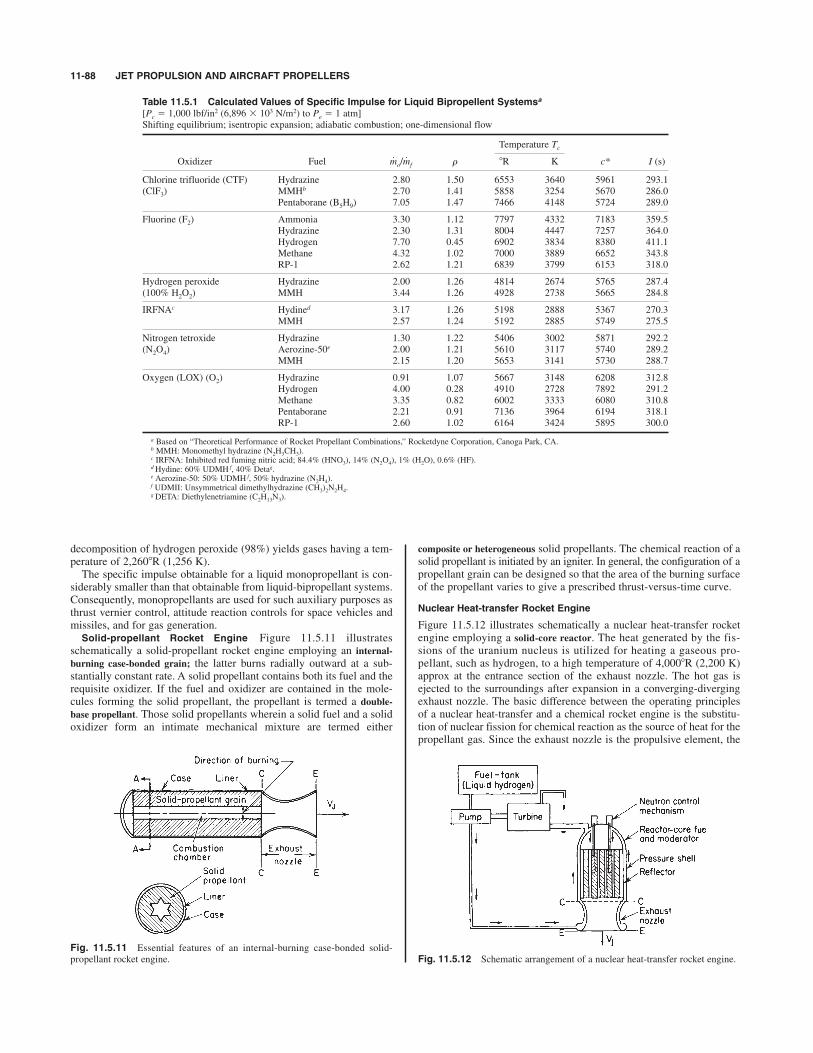
11-88 JET PROPULSION AND AIRCRAFT PROPELLERS
composite or heterogeneous solid propellants. The chemical reaction of asolid propellant is initiated by an igniter. In general, the configuration of apropellant grain can be designed so that the area of the burning surfaceof the propellant varies to give a prescribed thrust-versus-time curve.
Nuclear Heat-transfer Rocket Engine
Figure 11.5.12 illustrates schematically a nuclear heat-transfer rocketengine employing a solid-core reactor. The heat generated by the fis-sions of the uranium nucleus is utilized for heating a gaseous pro-pellant, such as hydrogen, to a high temperature of 4,0008R (2,200 K)approx at the entrance section of the exhaust nozzle. The hot gas isejected to the surroundings after expansion in a converging-divergingexhaust nozzle. The basic difference between the operating principlesof a nuclear heat-transfer and a chemical rocket engine is the substitu-tion of nuclear fission for chemical reaction as the source of heat for thepropellant gas. Since the exhaust nozzle is the propulsive element, the
decomposition of hydrogen peroxide (98%) yields gases having a tem-perature of 2,2608R (1,256 K).
The specific impulse obtainable for a liquid monopropellant is con-siderably smaller than that obtainable from liquid-bipropellant systems.Consequently, monopropellants are used for such auxiliary purposes asthrust vernier control, attitude reaction controls for space vehicles andmissiles, and for gas generation.Solid-propellant Rocket Engine Figure 11.5.11 illustrates
schematically a solid-propellant rocket engine employing an internal-burning case-bonded grain; the latter burns radially outward at a sub-stantially constant rate. A solid propellant contains both its fuel and therequisite oxidizer. If the fuel and oxidizer are contained in the mole-cules forming the solid propellant, the propellant is termed a double-base propellant. Those solid propellants wherein a solid fuel and a solidoxidizer form an intimate mechanical mixture are termed either
Table 11.5.1 Calculated Values of Specific Impulse for Liquid Bipropellent Systemsa
[Pc 1,000 lbf/in2 (6,896 ' 103 N/m2) to Pe 1 atm]
Shifting equilibrium; isentropic expansion; adiabatic combustion; one-dimensional flow
Temperature Tc
Oxidizer Fuel r +R K c* I (s)
Chlorine trifluoride (CTF) Hydrazine 2.80 1.50 6553 3640 5961 293.1
(ClF3) MMHb 2.70 1.41 5858 3254 5670 286.0
Pentaborane (B5H9) 7.05 1.47 7466 4148 5724 289.0
Fluorine (F2) Ammonia 3.30 1.12 7797 4332 7183 359.5
Hydrazine 2.30 1.31 8004 4447 7257 364.0
Hydrogen 7.70 0.45 6902 3834 8380 411.1
Methane 4.32 1.02 7000 3889 6652 343.8
RP-1 2.62 1.21 6839 3799 6153 318.0
Hydrogen peroxide Hydrazine 2.00 1.26 4814 2674 5765 287.4
(100% H2O2) MMH 3.44 1.26 4928 2738 5665 284.8
IRFNAc Hydined 3.17 1.26 5198 2888 5367 270.3
MMH 2.57 1.24 5192 2885 5749 275.5
Nitrogen tetroxide Hydrazine 1.30 1.22 5406 3002 5871 292.2
(N2O4) Aerozine-50e 2.00 1.21 5610 3117 5740 289.2
MMH 2.15 1.20 5653 3141 5730 288.7
Oxygen (LOX) (O2) Hydrazine 0.91 1.07 5667 3148 6208 312.8
Hydrogen 4.00 0.28 4910 2728 7892 291.2
Methane 3.35 0.82 6002 3333 6080 310.8
Pentaborane 2.21 0.91 7136 3964 6194 318.1
RP-1 2.60 1.02 6164 3424 5895 300.0
a Based on “Theoretical Performance of Rocket Propellant Combinations,” Rocketdyne Corporation, Canoga Park, CA.b MMH: Monomethyl hydrazine (N2H3CH3).c IRFNA: Inhibited red fuming nitric acid; 84.4% (HNO3), 14% (N2O4), 1% (H2O), 0.6% (HF).d Hydine: 60% UDMH f, 40% Detag.e Aerozine-50: 50% UDMH f, 50% hydrazine (N2H4).f UDMII: Unsymmetrical dimethylhydrazine (CH3)2N2H4.g DETA: Diethylenetriamine (C2H13N3).
m#
o/m#
f
Fig. 11.5.11 Essential features of an internal-burning case-bonded solid-
propellant rocket engine. Fig. 11.5.12 Schematic arrangement of a nuclear heat-transfer rocket engine.

NOTATION 11-89
remaining components of the nuclear heat-transfer rocket engine con-stitute the hot-gas generator.
The propellant in a nuclear heat-transfer rocket engine functionsbasically as a fluid for cooling the solid-core nuclear reactor. Its reac-tion is not based on energy considerations alone, but on such propertiesas specific heat, latent heat, molecular weight, and liquid density and oncertain practical considerations.
Electric Rocket Engines
Several different types of electric rocket engines have been conceived;the principal types are described below. All of them require some formof power plant for generating electricity. Thus the power plant may benuclear, solar-cell batteries, thermoelectric, or other. The choice of thetype of power plant depends upon the characteristics of both the electricrocket engine and the space-flight mission. Figure 11.5.13 illustratesdiagrammatically an electric rocket engine, comprising (1) a nuclearpower source, (2) an energy-conversion unit for obtaining the desiredform of electric energy, (3) a propellant feed and metering system, (4)an electrically operated thrustor, and (5) the requisite control devices.Electric rocket engines may be classified as (1) electrothermal, (2) elec-tromagnetic, and (3) electrostatic.Electrothermal Rocket Engine Figure 11.5.14a illustrates the type
of engine which uses electric power for heating gaseous propellant to ahigh temperature before ejecting it through a converging-divergingexhaust nozzle. If an electric arc is employed for heating the propellant,the engine is called a thermal arc-jet rocket engine.
Electromagnetic Rocket Engine Figure 11.5.14b illustrates anelectromagnetic, or plasma, rocket engine. There is a wide variety ofsuch engines, but all of them utilize the same operating principle. Aplasma (a neutral ionized conducting gas) is accelerated by means of itsinteraction with either a stationary or a varying magnetic field.Basically, a plasma engine differs from a conventional electric motor bythe substitution of a conducting plasma for a moving armature.Electrostatic Rocket Engine Figure 11.5.14c illustrates schemati-
cally the electrostatic, or ion, rocket engine, comprising (1) an electricpower plant; (2) a propellant supply; (3) ionization apparatus; (4) an ionaccelerator; and (5) an electron emitter for neutralizing the ion beamejected from the accelerator. Its operating principle is based on utilizingelectrostatic fields for accelerating and ejecting electrically chargedparticles with extremely large velocities. The overall objective is totransform thermal energy into the kinetic energy associated with anextremely high-velocity stream of electrically neutral particles ejectedfrom one or more thrustors. Mercury ion engines are currently being tested.The engine provides thrust by a rapid, controlled discharge of ions cre-ated by the ionization of atoms of the mercury fuel supply. Solar cellsconvert sunlight into electricity, which is then used to bombard the mer-cury with free electrons. This causes one electron to be stripped fromeach mercury atom, resulting in ionized mercury atoms. The ions mixwith other electrons to form a plasma. A magnetic field set up betweentwo metal screens at the aft end of the engine draws the positivelycharged ions from the plasma and accelerates them at very high exitspeeds out the back of the engine. This creates a high-velocity exitbeam producing low-level but extremely long-term thrust.
All electric rocket engines are low-thrust devices. The interest insuch engines stems from the fact that chemical-rocket technology, forexample, the space shuttle, is now so advanced that it has become fea-sible to place heavy payloads, such as a satellite equipped with an elec-tric rocket engine, into an earth orbit. An electric rocket engine whichis virtually inoperable terrestrially can be positioned in space and canthen operate effectively because of the absence of aerodynamic dragand strong gravitational fields. Consequently, if a vehicle equipped withan electric rocket engine is placed in an earth orbit, the low-thrust elec-tric rocket engine, under the conditions in space, will accelerate it to alarge vehicle velocity if the operating time for the engine is sufficientlylong.
In a chemical rocket engine, the energy for propulsion, as well as themass ejected through the exhaust nozzle, is provided by the propellants,but the energy which can be added to a unit mass of the propellant gasis a fixed quantity, limited by the nature of the chemical bonds of thereacting materials. For that reason, chemical rocket engines are said tobe energy-limited rocket engines. Although a nuclear heat-transfer rocketengine is also energy-limited, the limitation is imposed by the amountof energy that can be added per unit mass of propellant without exceed-ing the maximum allowable temperature for the materials employed forthe solid-core reactor.
In an electric rocket engine, on the other hand, the energy added tothe propellant is furnished by an electric power plant. The power avail-able for heating the propellant is limited by the maximum power outputof the electric power plant, accordingly, electric rocket engines arepower-limited.
NOTATION
a acoustic speeda0 acoustic speed in free-stream aira2 burning rate constant for solid propellantAe cross-sectional area of exit section of exhaust nozzleAp area of burning surface for solid propellantAt cross-sectional area of throat of exhaust nozzlecp specific heat at constant pressurecv specific heat at constant volumec* characteristic velocity for rocket motorCd discharge coefficient for exhaust nozzleCF thrust coefficient
PcAt /m#
Fig. 11.5.13 Essential features of an electric rocket engine.
Fig. 11.5.14 Electric rocket engine. (a) Electrothermal rocket engine;
(b) electromagnetic rocket engine; (c) electrostatic (ion) engine.

11-90 JET PROPULSION AND AIRCRAFT PROPELLERS
CFg gross-thrust coefficient for ramjet engineCFn net thrust coefficient
D or $ dragDi V0 ram drag for airbreathing or thermal-jet engined diameterdp diameter of propellerEin rate at which energy is supplied to propulsion systemEf calorific value of fuelEp calorific value of rocket propellantsf fuel-air ratio
f r f/hB fuel-air ratio for ideal combustion chamberF force or thrustFi mew ! mi V0 & (pe ! p0)Ae thrust due to internal flowFj meVj jet thrustFp (pe ! p0)Ae pressure thrustFg Fi gross thrust for ramjet engine
FgSFC gross-thrust specific-fuel consumption for ramjet enginegc correction factor defined by Newton’s second law of
motionh static specific enthalpy
#hn enthalpy change for exhaust nozzleH total (stagnation) specific enthalpy
#Hc lower heating value of fuelI specific impulseIa F/gma air specific impulseJ mechanical equivalent of heat; advance ratio, propellerk cp/cv specific heat ratio
L or + liftM massm mass rate of flow mass rate of air consumption for thermal-jet engine
mass rate of flow of gas leaving propulsion system
mass rate of fuel consumption
mass rate of flow of gas into propulsion system
mass rate of oxidizer consumption for rocket engine
mass rate of propellant consumption for rocket
engine molecular weight
Me momentum of gases leaving propulsion system in unit timeMi momentum of gases entering propulsion system in unit timeM0 V0 /a0 Mach number of free-stream air (flight speed)n revolutions per unit timep absolute static pressure; pitch of propeller bladepc absolute static pressure of gases in combustion chamberpe absolute static pressure in exit section of exhaust nozzlep0 absolute static pressure of free-stream ambient airP absolute total (stagnation) pressurePc absolute total pressure at entrance to exhaust nozzle
absolute total pressure of
free-stream air3 propulsion power3L leaving loss3T thrust powerq rV2/2 dynamic pressure
dynamic pressure of free-stream airQ torqueQi heat supplied to actual combustor heat supplied to ideal combustor (no losses)
r0 linear burning rate for solid propellant gas constant
Ru universal gas constant t absolute static temperaturetp temperature of solid propellant prior to ignitionT absolute total (stagnation) temperatureTc absolute total temperature of gas entering exhaust nozzle of
rocket motor
mR
R 5 Ru/ m
Qri
q0 5 r0V20/2 5 k0p0M
20/2
P0 5 p0¢1 1k 2 1
2 M2
0≤ k/sk21d
m
m#
o 1 m#
fm#
p
m#
o
m#
i
m#
f
m#
e
m#
a
m#
f /m#
a
m#
a
T2 absolute total temperature at entrance to air compressor (seeFig. 11.5.4)
T3 absolute total temperature at exit section of air compressor(see Fig. 11.5.4)
absolute total temperature at exit section of ideal compressor(see Fig. 11.5.4) operating between same pressure limits asactual compressor
T4 absolute total temperature at entrance to turbine (see Fig. 11.5.4)
T5 absolute total temperature at exit from turbine (see Fig. 11.5.4)
absolute total temperature at exit from ideal turbineu pndp propeller tip speedV velocityVF forward speed of propellerVj effective jet velocityV0 velocity of free-stream air (flight speed)w velocity of exit gases relative to walls of exhaust nozzle or
velocity of air in ultimate wake of propeller weight rate of flow
weight rate of flow of oxidizer
p weight rate of flow of propellants
Greek
, T4/t0 ada1 cycle temperature ratio; angle of attack,d T2/t0 diffusion temperature ratio,1 T4/T2
b bypass ratio for turbofans; helix angle for propeller bladed P/Pstd corrected pressureh efficiency
hB f r/f efficiency of combustion for thermal-jet enginehc ( – T2)/(T3–T2) isentropic efficiency of compressorhd isentropic efficiency of diffuserhn w2 isentropic efficiency of exhaust nozzleho 3T /Ein overall efficiency of propulsion systemhp 3T /(3T & 3L) ideal propulsive efficiencyht (T4 ! T5)/(T4 ! isentropic efficiency of turbine
hth 3T /Ein thermal efficiency of propulsion engine
thrust parameter for turbojet engine;
cos f divergence coefficient for exhaust nozzle for rocketengines
v V0 /w speed ratior density mean density
v angular velocity of propeller shaftvr rate of rotation of slipstream at propellervs rate of rotation of slipstream in ultimate slipstream- fan velocity coefficient VF/uf semiangle of exhaust-nozzle divergence; effective helix
angle
velocity coefficient for exhaust nozzle
r densitys solidity of propeller
cycle pressure ratio parameter
compressor pressure-ratio parameter
diffuser pressure-ratio parameter
(P7/p9)(k!1)/k nozzle pressure-ratio parameter
turbine pressure-ratio parameter
corrected temperature
Subscripts
(a) numbered0 free stream1 entrance to subsonic diffuser
u 5 T/Tstd
.t 5 sP4/P5dsk21d/k
.n 5 sP7/p0dsk21d/k
.d 5 sP2/p0dsk21d/k
.c 5 sP3/P2dsk21d/k
. 5 sP3/p0dsk21d/k 5 .d.c
w 5 2hn
/ 5 2k ¢ 2
k 1 1≤ sk21ds2k21d
r
1⁄2 1 1⁄2l 5 gIa /22gJcpt0
T r5d
T r3
W#W#
o
W#
T r5
T r3

POWER AND EFFICIENCY RELATIONSHIPS 11-91
2 exit from subsonic diffuser3 entrance to combustion chamber4 entrance to turbine of turbojet engine5 exit from turbine of turbojet engine6 tail-pipe entrance7 entrance to exhaust nozzle8 throat section of exhaust nozzle9 exit section of exhaust nozzle
(b) lettereda airB burner or combustion chamberb bladec compressord diffusere exit section; effectiveF fanf fuelh hydraulicn nozzleo overall or oxidizerp propellantP propulsive
std standardt turbine or throat, as specified in text
Statement on Units The dynamic equations employed in the follow-ing sections are written for consistent sets of units, i.e., for sets in which1 unit of force 1 unit of mass ' 1 unit of acceleration. Consequently,the gravitational correction factor gc in Newton’s equation F (1/gc)ma(see notation) has the numerical value unity and is omitted from thedynamic equations. When the equations are used for calculation purposes,gc should be included and its appropriate value employed.
THRUST EQUATIONS FOR JET-PROPULSION ENGINES
Refer to Fig. 11.5.15, which illustrates schematically a rotationallysymmetrical arbitrary propulsion engine immersed in a uniform flowfield. Because of the reactions between the fluid flowing through theengine, called the internal flow, and the interior surfaces wetted by theinternal flow a resultant axial force is produced, that is, a force collinearwith the longitudinal axis of the engine. If an axial force acts in theforward direction, employing a relative coordinate system, it is called athrust; if it acts in the backward direction it is called a drag. Similarly,the resultant axial force due to the external flow, the flow passing overthe external surfaces of the propulsion system, is a thrust or dragdepending upon whether it acts in the forward direction or the backwarddirection.
Application of the momentum equation of fluid mechanics to thegeneralized propulsion system illustrated in Fig. 11.5.15 gives the fol-lowing equation for the thrust Fi due to the internal flow. Thus, if it isassumed that the external flow is frictionless, there is no change in therate of momentum for the external flow between Si and Se . Hence, thethrust F Fi is due entirely to the internal flow, and
(11.5.1)F 5 Fi 5 mew 2 m#
iV0 1 s pe 2 p0dAe
In Eq. (11.5.1), jet thrust, ram drag, and
( pe ! p0)Ae Fp pressure thrust. Hence,
(11.5.2)
It is convenient to introduce a fictitious effective jet velocity Vj , which isdefined by
(11.5.3)
If the gases are expanded completely, in the exhaust nozzle, then w Vj
and Fp 0. No appreciable error is introduced, in general, if it isassumed that Fp 0. For thermal jet engines, (see notation),
and then
(11.5.4)
In the case of uncooled turbojet engines, is not significantly dif-ferent from the fraction of ma utilized for cooling the bearings and tur-bine disk. Consequently, no significant error is introduced by assuming
that . Hence, for a simple turbojet engine, onemay write
(11.5.5)
Equation (11.5.5) is also the thrust equation for an ideal propeller; inthat case Vj is the wake velocity for the air leaving its slipstream. Thethrust equation for a hydraulic jet propulsion system has the same formas Eq. (11.5.5). Let V0 denote the speed of a boat, and the mass rateof flow of the water entering the hydraulic pump and discharged by theexit nozzle with the velocity w Vj relative to the boat. Hence, forhydraulic jet propulsion
(11.5.6)
where v V0 /Vj .
In the case of rocket engines, since they do not consume atmosphericair, and the flow of gas out of the rocket motor, under steady-state conditions, is equal to (see notation).
The effective jet velocity Vj is larger than Ve exit velocity if pe * p0;that is, if the gases are underexpanded. The effective jet velocity is a use-ful criterion because it can be determined accurately from the measuredvalues of Fi and obtained from a static firing test of the rocket motor.
The ratio is denoted by I and called eitherthe specific thrust or the specific impulse. Hence
(11.5.7)
Although the dimensions of specific impulse are force/(mass)(s), it isconventional to state its units as seconds.
Equation (11.5.5) for the thrust of a turbojet engine, when expressedin terms of the effective jet velocity Vj , becomes
(11.5.8)
POWER AND EFFICIENCY RELATIONSHIPS
In a jet-propulsion engine the propulsion element is the exhaust nozzle,and the rate at which energy is supplied to it is called the propulsionpower, denoted by 3. The rate at which the propulsion system does use-ful work is termed the thrust power 3T and is given by
3T FV0 (11.5.9)
Assume that pe p0, and that the only energy loss in a propulsionsystem is the leaving loss 3L that is, the kinetic energyassociated with the jet gases discharged from the system; then thepropulsive power is given by
3 3L & 3T (11.5.10)
The ideal propulsive efficiency is defined, in general, by
hP 3T /(3T & 3L) thrust power/propulsion power (11.5.11)
m#
sVj 2 V0d2/2,
F 5 m#
asVj 2 V0d
I 5 F/m#
p 5 Vj /gc
Fi /m#
p
m#
p
m#
p 2 m#
o 1 m#
f
m#
a 5 0,
F 5 m#
ssVj 2 V0d 5 m#
wV0s1/v 2 1d
m#
w
Fe 5 m#
asVj 2 V0d 5 m#
V0s1/v 2 1d
m#
e 5 m#
a 1 m#
f < m#
a 5 m#
m#
f
Fi 5 ¢1 1 f
v 2 1≤ m#
aV0 1 s pe 2 p0dAe
m#
e 5 m#
a 1 m#
f ? Let f 5 m#
f /m#
a, v 5 V0 /Vj ;
m#
i 5 m#
a
F 5 m#
eVj 2 m#
iV0 5 m#
ew 2 m#
iV0 1 s pe 2 p0dAe
Fi 5 Fj 2 Di 1 Fp
m#
iV0 5 Di 5m#
ew 5 Fj 5
Fig. 11.5.15 Generalized jet-propulsion system.

11-92 JET PROPULSION AND AIRCRAFT PROPELLERS
For a turbojet engine and hydraulic jet propulsion,
(11.5.12)
For a chemical rocket engine,
(11.5.13)
The propulsive efficiency hP is of more or less academic interest. Ofmore importance is the overall efficiency ho, which for airbreathing androcket engines is defined by
(11.5.14)
where
3 (11.5.15)
and Ein is the rate at which energy is supplied to the propulsion system.The overall efficiency of a hydraulic jet-propulsion system is
given by
(11.5.16)
where hth is the thermal efficiency of the power plant which drives thewater pump, and hh is the hydraulic efficiency of the water pump. Toachieve a reasonable fuel consumption rate, hh must have a larger value.For an airbreathing jet engine, and
(11.5.17)
The ratio is called the thrust specific-fuel consumption (TSFC) andis measured in mass of fuel per hour per unit of thrust. Hence,
(11.5.18)
For a rocket engine, so that
(11.5.19)
PERFORMANCE CHARACTERISTICS OF AIRBREATHING JET ENGINES
The Ramjet Engine In ramjet technology the thrust due to the internalflow Fi is called the gross thrust and denoted by Fg . Refer to Fig. 11.5.2and assume Then
(11.5.20)
In level unaccelerated flight Fg is equal to the external drag of thepropelled vehicle and the ramjet body.
It is customary to express the thrust capabilities of the engine in termsof the gross-thrust coefficient CFg . If Am is the maximum cross-sectionalarea of the ramjet engine, the dynamic
pressure of the free-stream air, then
(11.5.21)
In terms of the Mach numbers M0 and M9,
(11.5.22)
In a fixed-geometry engine, M9 depends upon the total temperatureT7, the total pressure P7, the fuel-air ratio f, the nozzle area ratio Ae /At ,and the efficiency of the nozzle hn. For estimating purposes, k0 1.4and k9 1.28, when the engine burns a liquid-hydrocarbon fuel. Themanner in which CFg varies with altitude M0 and fuel-air ratio f is shownschematically in Fig. 11.5.16.
If a T7/t0 cycle temperature ratio, and kB is the mean value of k forthe combustion gases, the rate at which heat is supplied to the engine is
(11.5.23)Qi 5 Qri /hB 5 m#
acpBt0sa 2 T2d/hB
CFg 52A9 /Am
k0M20
¢P9
p0
1 1 k9M29
P9 /p9
2 1≤ 22A0
Am
CFg 5
Fg
q0Am
5
2Fg
Amk0p0M20
q0 5 r0V20 /2 5 k0 p0M
20 /2
Fg 5 Fi < m#
asVj 2 V0d
m#
0 < m#
9 5 m#
a.
ho 52v
1 1 v2
3
m#
psEp 1 V 20 /2d
Ein 5 m#
psEp 1 V 20 /2d,
TSFC 5 m#
f /F 5 fm#
a /F
m#
f /F
ho 52v
1 1 v 3
m#
fsEf 1 V 20/2d
Ein 5 m#
fsEf 1 V 20 /2d,
ho 5 hthhhhp 5 hhhth[2v/s1 1 vd]
/Ein 5 thermal efficiency of systemhth 5
ho 5 hthhP
hP 5 2v/s2 1 v2d
hP 5 2v/s1 1 vd
It is readily shown that
(11.5.24)
The gross-thrust specific-fuel consumption (FgSFC) is, by definition,
(11.5.25)
The principal sources of loss are aerothermodynamic in nature andcause a decrease in total pressure between stations 0 and 7. For esti-mating purposes, assuming M0 2.0 and T6 3,8008R (2,111 K), thetotal pressures across different sections of the engine may be assumedto be approximately those tabulated below.
FgSFC 5 m#
f /Fg
Qi 5A0p0V0
hBJ
kB
kB 2 1Ba 2 ¢1 1
k0 2 1
2 M2
0≤ R
Fig. 11.5.16 Effect of altitude and fuel-air ratio on the gross-thrust coefficient
of a fixed-geometry ramjet engine. (a) Effect of altitude; (b) effect of fuel-air ratio.
Total pressure
Part of engine ratio
Supersonic diffuser (0–1) P1/P0 0.92
Subsonic diffuser (1–2) P2/P1 0.90
Flameholders (2–7) P7/P2 0.97
Combustion chamber (2–7) P7/P2 0.92
Exhaust nozzle (7–9) P9/P7 0.97
The Simple Turbojet Engine A good insight into the design perfor-mance characteristics of the turbojet engine is obtained conveniently bymaking the following assumptions: (1) The mass rate of flow of work-ing fluid is identical at all stations in the engine; (2) the thermodynam-ic properties of the working fluid are those for air; (3) the air is a perfectgas and its specific heats are constants; (4) there are no pressure lossesdue to friction or heat addition; (5) the exhaust nozzle expands theworking fluid completely so that p9 p0; and (6) the auxiliary powerrequirements can be neglected. Refer to Fig. 11.5.4 and let
In view of the assumptions,
(11.5.26)
and
(11.5.27)
The diffuser pressure-ratio parameter is given by
(11.5.28)
where hd isentropic efficiency of diffuser (0.75 to 0.90 for well-designed systems).
The turbine pressure-ratio parameter is given by
(11.5.29)
where ht the isentropic efficiency of the turbine (0.90 to 0.95).
1/.t 5 1 2 [s.c 2 1d/a1hcht]
.t
.d 5 1 1 hd[sk 2 1d/2]M20
.d
a 5 aaa1
. 5 .d.c 5 .t.n
a1 5 T4/T2ad 5 T2/t0a 5 T4/t0
.t 5 ¢P4
P5
≤ sk21d/k
.n 5 ¢P7
p0≤ sk21d/k
5 ¢P7
p9≤ sk21d/k
. 5 ¢P3
p0≤ sk21d/k
.d 5 ¢P2
p0≤ sk21d/k
.c 5 ¢P3
P2
≤ sk21d/k

PERFORMANCE CHARACTERISTICS OF AIRBREATHING JET ENGINES 11-93
Heat supplied, per unit mass of air, is
or
(11.5.30)
where hc is the isentropic efficiency of the air compressor (0.85 to0.90), and hB is the efficiency of the burner (0.95 to 0.99).
The enthalpy change for the exhaust nozzle #hn is given by
(11.5.31)
The specific thrust, also called the air specific impulse, is
(11.5.32)
The overall efficiency ho is given by
(11.5.33)
where hB ranges from 0.95 to 0.99 and l is the dimensionless turbojetspecific thrust parameter.
The TSFC for a turbojet engine is given by
(11.5.34)
It can be shown by dimensional analysis, if the effects of Reynoldsnumbers are neglected, that the variables entering into the performanceof a given turbojet engine may be grouped as indicated in Table 11.5.2.
Table 11.5.2
Nondimensional group Uncorrected form Corrected form
Flight speed
Rotational speed
Air flow rate
Thrust F/D2P
Fuel flow rate
u T/Tstd T/519 (T/288) corrected temperature (exact value for Tstd is 518.6998R).d P/pstd P/14.7 (P/1.013 ' 105) corrected pressure.
Figure 11.5.17 is a design-point chart presenting l and ho as func-tions of a, P3/P2, and for the subsonic performance of simple turbo-jet engines. The curves apply to propulsion at 30,000 ft (9.14 km)altitude for engines having characteristic data indicated in the figure.Curve A illustrates the effect of pressure ratio P3/P2 or for enginesoperating with a 5.0. It is seen that increasing the compressor pres-sure ratio increases ho but it approaches a maximum value at P3/P2
approximately equal to 19. Curve B applies to the design point ofengines having a fixed compressor pressure ratio of 10 : 1 but having dif-ferent values of a, that is, turbine inlet temperature. It shows thatincreasing a much above a 5 reduces the overall efficiency and con-sequently TSFC. Curve C presents the design-point characteristics forengines operating with a 5 but having different compressor pressureratios. The maximum value of l is obtained at a relatively low pressureratio: approximately P3/P2 5. Curve D presents the design-pointcharacteristics of engines having a fixed compressor pressure ratio of
.c
.c
W#
f /d2uW#
f J#Hc /D2P2T
F/d
W#
a2u/dW#
a2T/D2P
N/2uN/2T
V0/2uV0/2t0
TSFC 5
m#
f
F
5 2hBhc
lM0¢ k 2 1
2≤ 1/2
ahc 2 ¢1 1k 2 1
2 M2
0≤ shc 1 .c 2 1d
ho 5 hthhp 5IaV0
JQi
Ia 5 Fi /m#
ag 5 s22#hn 2 V0d/m#
a
3 b1 2a1hcht
.c[1 1 hdsad 2 1d][a1hcht 2 s.c 2 1d]r
#hncpt0
5hn
hc [ahc 2 ads.c 2 1d]
Qi 5
cpt0hBhc
ad ¢ aadhc 2 hc 2 .c 1 1≤
Q1 5 scp/hBdsT4 2 T3d
10 : 1 but different cycle temperature ratios. Increasing a gives signifi-cant increases in l. Hence, large values of turbine inlet temperature T4
offer the potential for large thrusts per unit of frontal area for such tur-bojet engines.
Figure 11.5.18 presents the design-point characteristics for engineshaving hc 0.85, ht 0.90, hr 0.93, and hB 0.99. Different val-ues of diffuser efficiency are presented for flight Mach numbers M0 0.8 (hd 0.91), M0 1.60 (hd 0.90), and M0 2.4 (hd 0.88). Twodifferent classes of engines are considered, those with P3/P2 4.0 andthose with P3/P2 12.0. The dimensionless thrust l is plotted as afunction of a with M0 as a parameter. It is evident that increasing l, thatis, the turbine inlet temperature T4, offers the advantage of a largeincrease in thrust per unit area of the engine under all the conditionsconsidered in Fig. 11.5.18.
Figure 11.5.19 presents the effect of flight speed on the design-pointperformance, at 30,000 ft (9.14 km) altitude, for engines having hc 0.85,ht 0.90, hB 0.95, T4 2,0008R (1,111 K) and burning a fuel havinga heating value #Hc 18,700 Btu/lbm (10,380 kcal/kgm). The magni-tude of the compressor pressure ratio P3/P2 approaches unity when V0 isapproximately 1,500 mi/h, indicating that at higher speeds the com-pressor and turbine are superfluous; i.e., the propulsion requirementswould be met more adequately by a ramjet engine. Raising T4 tends todelay the aforementioned condition to a high value of V0.
It is a characteristic of turbojet engines, since ho hthhp, that for agiven M0 increasing hth causes #hn to increase, and hence the jetvelocity Vj . As a consequence, hp is decreased. It is this characteristicwhich causes ho f (a), curve B of Fig. 11.5.17, to be rather flat for awide range of values of a T4 /t0.
The curves of Figs. 11.5.17 to 11.5.19 are design-point performancecurves; each point on a curve is the design point for a different turbojetengine. The performance curves for a specific engine are either
Fig. 11.5.17 Dimensionless thrust parameter and overall efficiency as
functions of the compressor pressure ratio (simple turbojet engine).
h0l

11-94 JET PROPULSION AND AIRCRAFT PROPELLERS
The thrust equation for the turbofan engine is
(11.5.35)
where VjF ) Vj. The thrust per unit mass of airflow, or air specificimpulse, is
(11.5.36)
The TSFC is given by
(11.5.37)
One of the most important applications of turbofans is for high-sub-sonic transport aircraft where the fuel consumption in cruise is a majorconsideration. In general, as the bypass ratio increases, the TSFCdecreases but the engine weight and external drag increase. Theoptimum bypass ratio for any particular application is determined by atrade-off between fuel weight, which is reduced by increasing thebypass ratio, and engine weight and external drag, which increase withbypass ratio for a given thrust. In general, the optimum value of b is thatwhich makes the difference (F ! De) a maximum, where De is theexternal drag of the engine. Up to a certain point, the more sophisticatedand efficient the engine, the larger the bypass ratio.
To achieve the maximum potential for the turbofan engine, high val-ues of turbine inlet temperature T4 are essential; i.e., cooled turbine sta-tor and rotor blades must be developed. There is an upper limit to T4;above it the TSFC begins to increase. As T4 is increased, however, theoptimum value of b must also be increased to avoid excessive leavinglosses in the propulsive jet.
Mechanical Design
Blades New technologies being developed to achieve higherthrust-to-weight ratios in advanced gas turbine engines also cause highervibratory blade row responses and stresses that delay engine develop-ment and may adversely affect engine reliability. In particular, thedesign trend toward higher stage loadings and higher specific flow arebeing attained through increased tip speeds, lower radius ratios, loweraspect ratios, and fewer stages. The resultant axial-flow compressorblade designs utilize thin, low-aspect-ratio blading with correspondinghigh steady-state stresses. Also, the mechanical damping is consider-ably reduced in newer rotor designs, particularly those with integralblade-disk configurations (blisks) and in those without shrouds. Theseare similar trends in turbine blading, but they are further complicatedby increased inlet and cooling temperatures that have resulted inthin-walled, complex cooling passage designs. As a result, advancedaxial-flow blade designs, both compressors and turbines, feature low-aspect-ratio blading which affect the structural integrity of the blading.These problems can be classified into two general cateories: (1) flutterand (2) forced response. A fundamental parameter common to both cat-egories is the reduced frequency, k vb/V, where b is the blade semi-chord, v the frequency of vibration, and V the relative free-streamvelocity. For engine applications, the frequency corresponds generallyto one of the lower-blade or coupled-blade disk natural frequencies.
Under certain conditions, a blade row operating in a completely uni-form flow can enter into a self-excited vibrational instability termedflutter. The vibration is sustained by the extraction of energy from theuniform flow during each vibratory cycle. The outstanding feature offlutter is that high stresses exist in the blading, leading to short-term,high-cycle, fatigue failures. Its importance is evidenced by the fact thatif a portion of a single blade fails due to flutter, the result may be instan-taneous and total loss of engine power.
Figure 11.5.20 is a typical compressor map showing schematically themore common types of flutter. At subsonic Mach numbers, up to 0.8 to0.9, either positive or negative stall flutter in the bending or torsion modemay occur. It is caused by operating beyond some critical airfoil angleof attack. A critical reduced frequency value of 0.8 has been cited for stallflutter; i.e., if k ) 0.8 stall flutter is possible. Choking flutter usuallyoccurs at negative incidence angles at a part-speed condition with theblade operating either subsonically or transonically. The physical mech-anism of choke flutter is not fully understood; both high negative
TSFC 5 m#
f /F
Ia 5 F/m#
a1s1 1 bd
F 5 m#
a1s1 1 f dVj 1 bm#
a1VjF 2 m#
a1s1 1 bdV0
computed from experimental data pertaining to its components operat-ing over a wide range of conditions or obtained from testing the com-plete turbojet engine. It is customary to present the data in standardizedform.The Turbofan or the Ducted-Fan Engine Refer to Fig. 11.5.5b.
Assume that the hot-gas flow is ejected through the con-
verging nozzle, area At, with the effective jet velocity Vj , and that theairflow is ejected through the converging annular nozzle, area A7F ,with the jet velocity VjF . Let denote the bypass ratio,approximately 5 to 10 for modern transport engines.
b 5 m#
aF /m#
a1
m#
aF
sm#
a1 1 m#
fd
Fig. 11.5.18 Dimensionless thrust parameter for a simple turbojet engine and
its overall efficiency as functions of the cycle temperature ratio , with the
flight Mach number as a parameter.
ah0
l
Fig. 11.5.19 TSFC and specific thrust Ia functions of the compressor pressure
ratio, with flight speed as a parameter (simple turbojet engine).

PERFORMANCE CHARACTERISTICS OF AIRBREATHING JET ENGINES 11-95
incidence angles and choked flow are viable candidates. Supersonicunstalled flutter is largely associated with thin fan blades operating atsupersonic relative flow velocities at the tip section. It is caused by a lag-ging of the unsteady aerodynamic forces relative to the blade motion andimposes a limit on the high-speed operation of the engine. The stressencountered during this type of flutter can be catastrophically large,decreasing rapidly as a constant speed line is traversed toward higherpressure ratios. High-speed operation near the surge line can lead tosupersonic stall flutter. Because this flutter is associated with high pressureratios, there can be strong shocks present within the blade passages, andin some circumstances, ahead of the blade row.
Destructive aerodynamic forced responses have been noted in allengine blading. These failure-level vibratory responses occur when aperiodic forcing function, with frequency equal to a natural bladeresonant frequency, acts on a blade row. Responses of sufficient magni-tude to fail blades have been generated by a variety of sources includ-ing upstream and downstream blade rows, flow distortion, bleeds, andmechanical sources.
The importance of forced response lies in the multiple sources of exci-tation for any rotating system. The rotor speeds at which forcedresponses occur are predicted with “Campbell” or speed-frequency dia-grams. These display the natural frequency of each blade mode versusrotor speed and, at the same time, the forcing function frequency (orengine order E lines) versus rotor speed, as indicated schematically inFig. 11.5.21. These E lines represent the loci of available excitation energyat any rotational speed for 1, 2, 3, etc. excitations per revolution.
Wherever these curves intersect, a potential source of destructive forcedresponse exists. Not all intersections can be avoided. Design practice isto eliminate the lower-order excitations from the operating range when-ever possible. This is because the sources of most forced response ener-gy usually result from these lower-order resonances, particularly the 2Eline.
High-cycle fatigue (HCF) of turbomachine blading resulting fromflow-induced vibrations is a significant problem throughout the gas tur-bine industry. To address this problem, various approaches have beendeveloped. In these, the response of a tuned airfoil row, i.e., a rotor withall airfoils having the same structural properties and thus identical nat-ural frequencies, is analyzed. In fact, there are small airfoil-to-airfoilstructural property variations that result, for example, from the manu-facturing process or as a consequence of in-service wear. These are col-lectively referred to as mistuning and are known to lead to significantincreases in airfoil resonant response amplitudes as compared to that ofthe tuned airfoil row, with mistuning thus often cited as a source of HCFin gas turbine engines. Hence, the key metric that characterizes the res-onant response of mistuned bladed disks is the amplification factor,
defined as the ratio of a blade’s response amplitude on a mistuned bladeddisk to its response amplitude on a tuned bladed disk.
Turbomachinery rotors typically have been bladed disks, with indi-vidual airfoils inserted into a slotted disk and retained by means of adovetail or fir-tree attachment. However, advances in manufacturingtechniques have resulted in bladed-disk assemblies with increased uni-formity; i.e., the blade-to-blade natural frequency variation, termedmistuning, is small. In addition, new design and manufacturing tech-niques have enabled the development and implementation of integrallybladed rotors (IBRs) wherein the blades and disk are machined from asingle piece of material. IBRs have even less blade-to-blade mistuningthan do bladed disks. Unfortunately, smaller mistuning does not trans-late into smaller amplification factors. On the contrary, as mistuningdecreases, the maximum amplification factor on a disk tends to increaseuntil some threshold is reached, at which point it decreases rapidlytoward 1. Figure 11.5.22 shows this trend; it is based on studies where-in many hundreds of bladed disks are simulated for each percent mis-tuning, with the maximum resulting amplification factor taken. Thedecrease in mistuning due to new manufacturing methods is on the neg-ative slope portion of Fig. 11.5.22, thus rendering the new manufactur-ing methods a strong impetus for improving models which predictmistuned bladed disk response. In contrast to the maximum amplifica-tion factor of Fig. 11.5.22, there is a theoretical maximum amplification
factor that depends only on the number of blades N; specifically,
amplification factor Taking these theoretical maximainto account during design is an important first step in building bladerows resistant to HCF failure.
Environmental Issues
The increasing worldwide concern for the environment has led to twotechnical issues becoming significant: (1) airport noise and (2) theEarth’s ozone layer.
0.5s1 1 2N d.
Fig. 11.5.20 Common types of compressor flutter.
Fig. 11.5.21 Schematic speed-frequency diagram. Fig. 11.5.22 Amplification factor versus mistuning level.

The high-bypass-ratio turbofans introduced in the late 1960s had amajor effect on engine noise reduction. ICAO recognized this when itestablished the Chapter 3 regulations in 1978. Turbofans direct more airthrough the bypass than through the core. As a result, the maximum jetexhaust velocity is substantially reduced and the turbomachinery noise ismore important. The fan, the low-pressure or boost compressor, and thelow-pressure turbine are the primary noise sources for a high-bypassturbofan. Their noise signatures include a broadband noise level with largespikes or tones at multiples of blade passing frequencies (Fig. 11.5.25).
11-96 JET PROPULSION AND AIRCRAFT PROPELLERS
Aeroacoustics is an increasingly important issue in the design ofadvanced gas turbine engines for commercial aircraft. This is becauseengine certification requires meeting prevailing International Civil
Aviation Organization (ICAO) Chapter 3 noise regulations established in1978. Aircraft are certified to a standard that is actually a combinationof three measures: the noise generated as the plane approaches the run-way radiating to the community under its flight path; the noise it gen-erates during takeoff radiating to the areas surrounding the runway; andthe noise under the flight path further out in the community during take-off (Fig. 11.5.23).
Fig. 11.5.23 Aircraft certification noise measurement locations.
The ICAO Chapter 3 regulations specify approach, sideline, and take-off perceived noise levels (EPNL) as a function of the aircraft takeoffgross weight (Fig. 11.5.24). The total or cumulative margin for a givenaircraft defined as the sum of the margin at all three conditions. Note thatall current-technology aircraft meet ICAO Chapter 3 regulations.
Air travel has increased dramatically since 1978. To meet thedemands of community groups for stricter aircraft noise requirements,ICAO has established a new set of limits which are to become effectivein 2006—the Chapter 4 rule. These new limits require aircraft to be 10dB (cumulative) quieter than current Chapter 3 levels. The use of tradesto meet the new rules was also eliminated. With Chapter 3, an aircraftcould exceed the limits on one measure of noise, takeoff, as long as itwas lower than the limits at the other conditions by an offsettingamount. With Chapter 4, an aircraft must operate below the Chapter 3curve at all three conditions: approach, sideline, and takeoff.
Fig. 11.5.24 Chapter 3 regulations specify EPNL at approach, sideline, and
takeoff.
Fan-OGV
interaction
FanInflow distortion
fan interaction
Fan inlet
noise
Subsonic top speed
15 dB
Broadband noise
Frequency (kHZ) Frequency (kHZ)
Harmonic
tune
Blade pass frequency Blade pass frequency
Sound pressure level (dB)
Sound pressure level (dB)
Multiple pure tonesSupersonic speed
Core/jet
noise
Fan jet
mixing
noise
LP turbine
noise
Fan
exhaust
noise
Struts and
pylonOGVs
Booster-fan
interaction
Strut and pylon
pressure field —
fan interaction
Fig. 11.5.25 High-bypass-ratio turbofan noise sources and noise spectrum.
Current noise control and reduction methods for high-bypass turbo-fans are a combination of turbomachinery noise source control and sup-pression. Source control is accomplished by increasing the axial spacingbetween adjacent blade rows and by selecting blade and vane numbercombinations to produce cutoff, whereby the highest-energy acousticmodes decay exponentially with distance along the ducting. Source sup-pression is achieved with acoustic liners in the fan inlet and exhaustducts and the core exhaust duct. As a result, future advanced turbofanswill have much lower levels of turbomachinery noise. Thus, the domi-nant engine sources in these future engines are the fan at takeoff andapproach and the turbulent mixing in the jet exhaust stream at takeoff.
The emissions generated by the combustion of aviation fuel includecarbon dioxide (CO2), carbon monoxide (CO), oxides of nitrogen(NOx), and particulates such as soot and oxides of sulfur (SOx). Theeffect that each has on the atmosphere depends on the altitude at whichit is emitted and its concentration. Most commercial aircraft cruise inthe troposphere, which ranges from an altitude of 11 mi (58,000 ft) atthe equator to 6 mi (33,000 ft) at the poles. In this region, the tempera-ture decreases with increasing altitude, resulting in large air motionsand mixing. Increased NOx concentration results in increased ozoneconcentration through complex photochemical reactions with CO andhydroxyls (HOx). Ozone also acts as a global warming gas in the tro-posphere. Methane is another global warming gas, although NOx
reduces the concentration of methane.It has been projected that, by 2050, aircraft emissions will increase
by a factor of 4 because of an increase in air traffic and that the totalcontribution to global warming by aircraft will be a factor of 2 greaterthan from CO2 alone. In addition, aircraft exhaust plumes contribute toglobal warming. Contrails are formed by water in the exhaust freezingin cold atmospheric conditions, with their formation aided by the par-ticulates present in exhaust plumes. These contrails may turn into cirrusclouds, which lead to a net increase in warming.
In summary, pollutants generated by aircraft engines contribute toglobal warming because of the altitude at which they operate and theprojected growth of the aviation industry. Hence, there is a distinct need

CRITERIA OF ROCKET-MOTOR PERFORMANCE 11-97
to develop ultralow-emission combustor designs for aircraft engines.The two primary approaches to ultralow-emission combustors are richand lean front-end designs. Each has demonstrated the potential toachieve low emissions.
The International Civil Aviation Organization (ICAO) standards limitaircraft engine emissions in the vicinity of an airport, up to 3,000 ftaltitude. A standardized landing-takeoff cycle (LTO) is specified, whichincludes time at each of four engine power settings. Typical levelsof engine emissions as a function of engine thrust are presented inFig. 11.5.26. Emissions of carbon monoxide (CO) and unburned hydro-carbons (UHC) are dominant at low power conditions such as idle, andrapidly decrease to negligible levels as engine power increases. Mostmodern combustor designs result in very low levels of CO and UHC atall cruise power settings through efficient combustion that minimizesfuel burn. Nitrogen oxides (NOx) and soot particle emissions or smokeboth exhibit the opposite trend, increasing with engine power. can be highly nonuniform, resulting in local stoichiometric combustion
with high NOx production rates.The lean-front-end combustor focuses on mixing the air and fuel in the
front end of the combustor exactly to create a combustion zone that is,on average, below the peak stoichiometric equivalence ratio of 1.0. Thelower flame temperature at these lean conditions significantly reducesthe NOx production rate. Lean-front-end combustors require multiplefuel stages to achieve the operability requirements for aircraft applica-tion. Typical modern engine designs require the combustor to operatewith a factor of 3 higher exit fuel-air ratio at maximum power than atminimum power. A lean combustion system must be optimized to amuch narrower range of fuel-air ratios to avoid high CO production, iftoo lean, and high NOx production, if too rich. This issue has beenaddressed by combustors with many small air and fuel injectors andsequentially fueling a subset of these as engine power increases.
CRITERIA OF ROCKET-MOTOR PERFORMANCE
In most applications of rocket motors the objective is to produce a largethrust for a limited period. The criteria of rocket-motor performanceare, therefore, related to thrust-producing capabilities and operatingduration. If denotes the rate at which the rocket motor consumespropellants, Pc the total pressure at the entrance to the exhaust nozzle,and Cw the weight flow coefficient, then
(11.5.38)
Ordinarily, the values of Cw as a function of Pc and mixture ratio
are determined experimentally. If no experimental data are available, thevalues of Cw can be calculated with good accuracy from the calculatedthermodynamic properties of the combustion gases. If Tc is the total tem-perature, and Pc the total pressure of the combustion gases at the entrancesection of the nozzle, then, for steady operating conditions,
(11.5.39)
where
(11.5.40)
An equation similar to Eq. (11.5.38) can be written for the thrustdeveloped by the rocket motor. Thus
(11.5.41)
The values of the thrust coefficient CF for specific propellant combi-nations are determined experimentally as functions of Pc and the ratio
. When no experimental values are available, CF can be calculatedfrom the following equation. Therefore
(11.5.42)
where
Zt 5 1 2 ¢pePc≤ sk21d/k
CF 5 Cdlf/Å 2k
k 2 1Zt 1 ¢ pe
Pc2
p0
Pc≤ Ae
At
W#
o /W#
f
F 5 CFPcAt
/ 5 ¢ 2
k 1 1≤ sk21d/[2sk21d]
2k
W#
g 5 CdAtPc/Äg
RTc
W#
p 5 W#
g,
W#
o /W#
f
W#
p 5 CwPc At
W#
pFig. 11.5.26 Typical aircraft combustor emission characteristics.
Aircraft spend much more time at takeoff, climb, and cruise settingsthan at idle. Thus, NOx is the dominant pollutant by mass in a flight. Infact, the NO
xproduced at cruise is significantly higher than that produced
during the LTO cycle. NOx emissions are a result of the high tempera-tures in the combustor, with the rate of NOx production highly nonlinearwith temperature. This is shown in Fig. 11.5.27, with the NOx produc-tion rate presented as a function of the combustion reaction equivalence
ratio, which is the ratio of fuel to air in the actual mixture divided by thefuel-to-air ratio for stoichiometric conditions. The peak is in the regionof stoichiometric combustion, i.e., an equivalence ratio of 1.0.
Rich-front-end combustors are found in most current engines. Fuel isintroduced at the front and mixed with some of the total combustor air-flow to create a stable rich reaction zone (Fig. 11.5.28), with theremainder of the airflow introduced in a mixing zone. The combinationof rich oxygen-depleted products from the front end quicky react withthe mixing air and are then diluted to exit conditions. This mixing zone
Fig. 11.5.27 NOx production rate versus equivalence ratio.
Leanstability and excessive
Lean Rich
COemissions
Equivalence ratio
Excessive smoke
Log (NOxproduction rate)
High NOxproduction
Fig. 11.5.28 Schematic of rich-front-end combustor.
Hc
CO
NOx
Smoke
0
10
20
30
40
50
60
0 100,00080,00060,00040,00020,000
Thrust, Ib
Emission index or smoke number

11-98 JET PROPULSION AND AIRCRAFT PROPELLERS
Equation (11.5.42) shows that CF is independent of the combustiontemperature Tc and the molecular weight of the combustion gases. Thenozzle area ratio Ae /At is given by the formula
(11.5.43)
Figure 11.5.29 presents CF calculated by means of the precedingequations, as a function of the area ratio Ae /At, with Pc /p0 as a parameter,for gases having k 1.28; the calculations assumed l 0.983 and
The curves do not take into account the separation phe-nomena which occur when Ae /At is larger than that required to expandthe gases to p0.
Cd 5 w 5 1.0d.
Ae
At
5sPc /ped
1/k
¢ k 1 1
2≤ 1/sk21d
2[sk 1 1d/sk 2 1d]Zt
the province of the liquid rocket engine. In military applications, thereis a strong tendency to supplant liquid rocket engines with solid rocketengines. Only in such areas as the large thrust launching rockets forboosting manned vehicles into space have the liquid rocket enginesreigned supreme; the space shuttle is equipped with liquid-bipropellantrocket engines, but it is boosted with auxiliary solid-propellant rocketmotors.
The following considerations are what make solid-propellant rocketmotors attractive: (1) They are simpler in construction than liquid rock-et engines; (2) they are easier to handle in the field; (3) they have instantreadiness for use; (4) they have very good storage properties; (5) theyhave a larger average density than most liquid-propellant combina-tions; (6) they have considerably fewer parts; and (7) their reliability inpractice has been very good. Furthermore, once the performance char-acteristics and physical properties of a solid propellant have been estab-lished, it is a relatively straightforward engineering problem to designand develop solid-propellant rocket motors of widely different thrustlevels and burning times tR .
Rocket motors which burn double-base propellants find the greatestuse in weaponry, e.g., artillery rockets, antitank weapons, etc.
Rocket motors burning heterogeneous, also called composite, solidpropellants are used for propelling all kinds of military missiles and forsounding rockets. Modern composite propellants have three basictypes of ingredients: (1) a fuel which is an organic polymer, called thebinder; (2) a finely powdered oxidizer, ordinarily ammonium perchlo-rate (NH4NO3); and (3) various additives, for catalyzing the combus-tion process, for increasing the propellant density, for increasing thespecific impulse (e.g., powdered aluminum), for improving the physi-cal properties of the propellant, and the like. After the ingredients havebeen thoroughly mixed, the resulting viscous fluid is poured, usuallyunder vacuum to prevent the formation of voids, directly into thechamber of the rocket motor which contains a suitable mandril forproducing the desired configuration for the propellant grain. The pro-pellant is cured by polymerization to form an elastomeric material.Some of the more common binders are butadiene copolymers andpolyurethane.
Modern composite solid propellants have densities ranging from 1.60to 1.70, depending upon the formulation, and specific impulse values ofapproximately 245 s, based on a combustion pressure of 1000 psia andexpansion to 14.7 psia.
In the case of solid-propellant rockets the rate of propellant con-sumption is related to the linear burning rate for the propellant r0, thatis, the rate at which the burning surface of the propellant recedes nor-mal to itself as it burns. For practical purposes it can be assumed thatthe linear burning rate r0 is given by
(11.5.47)
where a2 and n are constants which are determined by experiment.If rp denotes the density of the solid propellant and Ap the area of the
burning surface, then the propellant consumption rate is given by
(11.5.48)
Figure 11.5.30 presents the linear burning rate as a function of thecombustion pressure for several propellants.
The linear burning rate r0 is influenced by the temperature of thesolid propellant tp prior to its ignition. Low values of tp reduce the burn-ing rate, and vice versa. Consequently, the temperature of the propellantmust be given in presenting data on linear burning rates. Figure 11.5.31presents r0 as a function of pc for tp !40, 60, and 1408F for a com-posite propellant manufactured by the Aerojet-General Corp., Azusa,Calif.
AIRCRAFT PROPELLERS
The function of the aircraft propeller (or airscrew) is to convert thetorque delivered to it by an engine into the thrust for propelling an air-plane. If the airplane is in steady, level flight, the propeller thrust and
m#
p 5 Aprpr0 5 a2Aprppnc
m#
p
r0 5 a2 pnc
m#
p
rP
Fig. 11.5.29 Calculated thrust coefficient versus expansion ratio for different
pressure ratios (based on k 1.28, 0.9830, Cd w 1.0).l
The specific impulse I is defined by Eq. (11.5.8) and can be shown tobe given by
(11.5.44)
A criterion which is employed for stating the performance of rocketmotor is the characteristic velocity c*. By definition
(11.5.45)
The values of c* for a given propellant combination are determinedexperimentally. It should be noted that the value of c* is independent ofthe thrust. Basically, c* measures the effectiveness with which the ther-mochemical energy of the propellants is converted into effective jetkinetic energy. When no experimental data are available the value of c*can be estimated quite closely from
(11.5.46)
Table 11.5.1 presents values of specific impulse for some possiblerocket-propellant combinations.
Solid-propellant rocket motors may be segregated into (1) double-basepowders and (2) composite, or heterogeneous, propellants. Double-base pow-ders are gelatinized colloidal mixtures of nitroglycerin and cellulose towhich certain stabilizers have been added. Heterogeneous, or compos-ite, propellants are physical mixtures of a solid oxidizer in powder formand some form of solid fuel, such as a plastic or rubberlike material.
Solid-propellant rocket motor technology has made tremendousstrides. It is possible to produce solid propellants with a wide range oflinear burning rates and with good physical properties. It has beendemonstrated experimentally that large thrust rocket motors with cham-ber diameters of approximately 22 ft (6.7 m) are feasible. As a result,the solid-propellant rocket motor has displaced the liquid rocket enginefrom a large number of applications, which heretofore were considered
c* 5 2RTc //
c* 5 Vj /CF 5 PcAt /m#
5 I/CF
I 5 F/m#
p 5 CF /Cw 5 Vj /gc

AIRCRAFT PROPELLERS 11-99
the airplane drag equal each other. If the airplane is climbing, the thrustmust overcome the drag plus the weight component of the airplane.
The propeller may be the sole thrust-producing element, but it canalso be employed in conjunction with another thrust-producing device,such as the exhaust jet of a turboprop or gas-turbine engine. It may alsobe employed as a windmilling device for producing power.
The conventional propeller consists of two or more equally spacedradial blades, which are rotated at a substantially uniform angularvelocity. At any arbitrary radius, the section of a blade has the shape ofan airfoil, but as the hub is approached, the sections become more nearlycircular because of considerations of strength rather than aerodynamicperformance. The portions of the blades in the vicinity of the hub
contribute, at best, only a small portion of the thrust developed by thepropeller blades.
Each section of the propeller blade experiences the aerodynamicreactions of an airfoil of like shape moving through the air in a similarmanner. Furthermore, at each radius, the section of one blade formswith the corresponding sections on the other blades a series of similarairfoils, which follow one another as the propeller rotates.
The torque of the rotating propeller imparts a rotational motion to theair flowing through it and, furthermore, causes the pressure immediatelybehind the propeller to increase while that in front of it is reduced; i.e.,the air is sucked toward the front of the propeller and pushed awaybehind it. A slipstream is created as illustrated in Fig. 11.5.1. The ratioof the cross-sectional area of the slipstream at any station to that of theactuator disk is termed the slipstream contraction.
The thrust produced by the propeller follows the relationships devel-oped from the momentum theorem of fluid mechanics for jet engines aspresented in Fig. 11.5.15 and Eq. (11.5.5). The thrust equation for theairbreathing engine (simplified) and the propeller is
(11.5.49)
In the case of a propeller the mass flow m is large and the velocityrise across the propeller is small, as compared with a jet engine of thesame thrust. However, the thrust of propellers falls off rapidly as aircompressibility effects on the propeller become large (flight speeds of300 to 500 mi/h).
Propeller efficiency is defined as the useful work divided by the energysupplied to the propeller:
(11.5.50)
where v V0/w.Since w is only slightly larger than V0 , the ideal efficiency is of the
order of 0.95, and actual efficiencies are in the range of 0.5 to 0.9.
Propeller Theory
Axial-Momentum Theory The axial-momentum theory of the pro-peller is basically a special case of the generalized jet-propulsion systempresented in Fig. 11.5.15. It is only a first approximation of the action ofthe propeller and cannot be employed for design purposes. It neglectssuch factors as the drag of the blades, energy losses due to slipstreamrotation, blade interference, and air compressibility effects. Because ofthose losses, an actual propeller requires power to rotate at zero thrust,and at zero thrust its propulsive efficiency is, of course, zero.Blade-Element Theory This theory, called strip theory, takes into
account the profile losses of the blade sections. It is the theory mostcommonly employed in designing a propeller blade and for assessingthe off-design performance characteristics of the propeller.
Each section of the propeller is considered to be a rotating airfoil. Itis assumed that the radial flow of air may be neglected, so that the flowover a blade section is two-dimensional. Figure 11.5.32 illustrates dia-grammatically the velocity vectors pertinent to a blade section of lengthdr, located at an arbitrary radius r. The projection of the axis of rotationis OO0, the plane of rotation is OC, the blade angle is b, the angle ofattack for the air flowing toward the blade (in the relative coordinatesystem) with the velocity V0 is a, the tangential velocity of the blade
hp 5PT
P5
FV0
P5
msv 2 V0dV0
m/2sw2 2 V 20d
52v
1 1 v
F 5 m#
sw 2 V0d 5 rAV0sw 2 V0d
Fig. 11.5.30 (a) Linear burning rate as a function of combustion pressure for
double-base propellants; (b) burning-rate characteristics of several heterogeneous
propellants at 60+F (15.5+C). (Aerojet-General Corp.)
Fig. 11.5.31 Effect of propellant temperature upon the linear burning rate of a
heterogeneous propellant. (Aerojet-General Corp.)
Fig. 11.5.32 Vector diagram for a blade element of a propeller.

11-100 JET PROPULSION AND AIRCRAFT PROPELLERS
element is u 2pnr, and the pitch or advance angle is FromFig. 11.5.32
(11.5.51)
and
(11.5.52)
Figure 11.5.33 illustrates the forces acting on the blade element. If bdenotes the width of the blade under consideration and CL and CD arethe lift and drag coefficients of the blade (airfoil) section, then the thrustforce dF acting on the blade element is given by
(11.5.53)
The corresponding torque force dQ is given by
(11.5.54)
where
tan g d$/d+ CD/CL $/+ (11.5.55)
where $ and + denote drag and lift, respectively.The propulsion efficiency of the blade element, termed the blading
efficiency, is defined by
(11.5.56)
The value of f which makes hb a maximum is termed the optimum
advance angle . Thus
(11.5.57)
The maximum blade efficiency is accordingly
(11.5.58)
A force diagram similar to Fig. 11.5.33 can be constructed for each ele-ment of the propeller blade, taking into account the variation in f withthe radius. The resultant forces acting on the propeller are obtained bysumming (integrating) those forces acting on each blade element.
The integrated lift coefficient is
(11.5.59)
where CLr propeller-blade-section lift coefficient and r/R = fractionof propeller-tip radius.
The integrated lift coefficient is in the range 0.15 to 0.70. There isa dilemma in the design and selection of blade sections since highstatic thrust requires high CLi which gives relatively low hp at cruise.Cruise conditions require low CLi for good hp . Variable camber pro-pellers permit optimization of CLi, but at the expense of weight andcomplexity.
CLi 5 3r/R51.0
rL/R
CLr ¢ r
R≤ 3
d ¢ r
R≤
shbdmax 52g 2 1
2g 1 15
2s+/$d 2 1
2s+/$d 1 1
fopt 5p
42
g
25 458 2
57.3
2s+/$d
fopt
hb 5V0dF
u dQ5
tan f
tansf 1 gd5+/$ 2 tan f
+/$ 1 cot f
dQ 5 1⁄2rV 20b drCL
sinsf 1 gd
cos g sin2f
dF 5 1⁄2rV 20b drCL
cossf 1 gd
cos g sin2f
f 5 tan21sV0 /pndd
a 5 b 2 f
f.
Vortex Theory The simple two-dimensional blade-element theorycan be further improved by taking account of the actual velocity distri-bution in the slipstream and thus determining the actual loading on theblading by the so-called vortex theory. The blades are represented bybound vortex filaments sweeping out vortex sheets to infinity. The vor-tex sheets are distorted both by the slipstream contraction and by theprofile drag of the blades. If such distortions are neglected, the inducedvelocity in the wake can be calculated by assuming the vortex sheets tobe tubular. Thus, in Fig. 11.5.32, the induced axial velocity becomes thearithmetic mean of the axial velocities at far distances upstream anddownstream of the rotor disk; and the induced rotational velocity at thedisk becomes v ! 0.5vr, where vr is the rotation of the slipstream inthe plane of the propeller. Hence, the angle of attack a for a rotor ele-ment is given by
(11.5.60)
where VF is the induced axial velocity in the plane of the propeller.The addition of the vortex effects improves the representation of
the propeller by the blade sections. There are, however, three-dimen-sional flow effects which are not included, and the following coeffi-cients have been suggested to include this effect (which reduces thelift coefficient).
a 5 b 2 tan21[VF/rsv 2 0.5 vrd]
Fig. 11.5.33 Aerodynamic forces acting on a blade element.
Lift Curve Slope Correction Factorsfor Three-Dimensional Airfoils
Radial station (ratio r/R) Correction factor
(0.2)(0.3)(0.45)(0.6)(0.7) 0.85
0.8 0.80
0.9 0.70
0.95 0.65
SOURCE: Departments of the Air Force, Navy, andCommerce, “Propeller Handbook.”
Performance Characteristics
The pitch and the angle f (Fig. 11.5.32) have different values at differ-ent radii along a propeller blade. It is customary, therefore, to refer toall parameters determining the overall characteristics of a propeller totheir values at either 0.7r or 0.75r.
For a given blade angle b, the angle of attack a at any blade sectionis a function of the velocity coefficient V0/u, where u pndp; it is cus-tomary, however, to replace V0 /u by its equivalent, the advance ratio J V0 /ndp.
For given values of b and n, the angle of attack a attains its maxi-mum value when V0 0, with In other words, the propellerthrust F is maximum at takeoff. As V0 increases, a decreases and sodoes the thrust. Finally, a forward speed is reached for which the thrustis zero.
Increasing J V0 /ndp , for a constant blade angle, causes the pro-peller to operate successively as a fan, propeller, brake, and windmill.Most of the operation, however, is conducted in the propeller state. Attakeoff, the propeller is in the fan state. Windmilling must be avoidedbecause it may overspeed the engine and damage it.
The lift coefficient CL is a linear function of a up to the stalling angle,and CD is a quadratic function of a. Furthermore, the lift + is zero at anegative value for a. Figure 11.5.34 presents the +/$ ratios of typicalpropeller sections. Figure 11.5.35 presents the blade (section) efficiencyas a function of the pitch angle f for different values of +/$. Propellersnormally operate at +/$ ratios of 20 or more. Supersonic propellersoperate with +/$ ratios of approximately 10, and from Fig. 11.5.34 it isapparent that they must operate close to the optimum pitch angle f toobtain usable blade efficiencies.Propeller Coefficients It can be shown, neglecting the compress-
ibility of the air, that
(11.5.61)fsV0 ,n ,dp , r, Fd 5 0
f 5 0.

AIRCRAFT PROPELLERS 11-101
By dimensional analysis, the following coefficients are obtained forexpressing the performances of propellers having the same geometry:
3 (11.5.62)
CF, CQ, and CP are termed the thrust, torque, and power coefficients,
respectively. They are independent of the size of the propeller. Conse-quently, tests of small-scale models can be employed for obtaining thevalues of F, Q, and 3 for geometrically similar full-scale propellers.Hence, the ideal propulsive efficiency of a propeller is given by
(11.5.63)
Other useful coefficients are the speed-power coefficient CS and thetorque-speed confficient CQS . Thus,
(11.5.64)
A commonly employed factor related to the geometry of a propeller isthe solidity 1. By definition,
(11.5.65)
The solidity varies from radius to radius; at a given radius, s is propor-tional to the power-absorption capacity of the annulus of blade elements.
The activity factor of a blade AF is an arbitrary measure of the bladesolidity and hence of its ability to absorb power. It takes the form
(11.5.66)
where R dp/2, r radius at any section, and rh spinner radius.
Performance
Static Thrust From the simple axial-momentum theory, the staticthrust F0 of an actuator disk of diameter dp is given by
(at sea level) (11.5.67)F0 5 spr/2d1/3s3dpd2/3 5 10.4bhp 3 d2/3
p
AF 5100,000
16 3r/R51.0
rh /R
c
dp¢ r
R≤ 3
d ¢ r
R≤
s 5 c/p
CQS 5 V02rd3p /QCS 5 V052r/3n2
hp 5FV0
35
CF
Cp
V0
dpn5 J
CF
CP
5 rn3d5pCpQ 5 rn2d5
pCQF 5 rn2d4pCF
The thrust horsepower (thp) is accordingly
(11.5.68)
Equations (11.5.67) and (11.5.68) assume uniform axial velocity, norotation of the air, and no profile losses. Consequently, they may be inerror by as much as 50 percent. Hesse suggests the use of the equations
(11.5.69)
and
(11.5.70)
together with data computed for a specific propeller, as illustrated inFig. 11.5.36. The static thrust for a given power input increases withthe diameter and the number of blades. Controllable pitch propellersselected for good overall performance will develop 3 to 4 lb of thrustper shp.
F 5 10.42[dpshp staticd shp]2/3sr/r0d1/3
hp static 5 Ä 2p
C 3/2F
CP
5 0.798C 3/2
F
Cp
thp 5F0
bhp5 s38,400/Ndpds1/C 1/3
p d
Fig. 11.5.34 Maximum lift-drag ratios for representative sections.
Fig. 11.5.35 Blade-element efficiency versus pitch angle.
Fig. 11.5.36 Static-thrust performance of a propeller; four-bladed, 100 activity-
factor propellers of various integrated design CL’s. (From Hamilton Standard
Division, United Aircraft Corporation.)
Fig. 11.5.37 Propeller performance—efficiency in forward flight; four-bladed,
100 activity factor, 0.500 integrated design CL propeller. (From Hamilton
Standard Division, United Aircraft Corporation.)
At flight conditions the performance may be obtained from general-ized charts presenting CP as a function of the advance ratio J, with thepropeller efficiency and blade pitch angle at 75 percent radius, u3/4, asparameters. Figure 11.5.37 is such a chart.

11-102 JET PROPULSION AND AIRCRAFT PROPELLERS
Reverse Thrust By operating the propeller blades at large negativeangles of attack, reversed thrust can be developed. In that condition, theblades are stalled, and as in the case of static thrust, the forces acting onthe blades cannot be calculated. In practice, the reverse-pitch stop is setby trial and error so that the propeller can absorb the rated power at zerospeed, i.e., at V0 0. With fixed-pitch reversing, the power absorbedwhen there is forward speed will be smaller than the rated value, but thereversed thrust is usually substantially larger than the static forwardthrust corresponding to the rated power. The landing roll of an aircraftwith reversed thrust plus brakes is approximately 45 percent of that withbrakes alone.Compressibility Effects As the relative velocity between an airfoil
and the free-stream air approaches the sonic speed, the lift coefficientCL decreases rapidly, and simultaneously there is a large increase in thedrag coefficient CD . The propeller is subject to those effects. Since theacoustic speed decreases from sea level to the isothermal altitude,the effects appear at lower tip speeds at high altitude. Furthermore, theeffect is more pronounced at higher tip speeds. Shock waves are formedat the leading edge of a propeller blade when its pitch-line velocityapproaches the local sonic velocity of the air. As a consequence, thecoefficient CF is reduced and CP is increased, thereby adversely affect-ing the propulsive efficiency of the propeller.
Because of the high propulsive efficiency of propellers, the applica-tion of advanced technologies may provide turboprop-powered trans-ports with cruise speeds and other desirable characteristics comparableto advanced turbofan-powered transports, but with a 15 to 20 percentreduction in fuel consumption.
Advanced turboprop propeller blades operate at high power loading,are extremely thin, and have swept leading edges to minimize com-pressibility losses. Shaping the spinner and nacelle minimizes chokingand compressibility losses. Efficiencies of about 70 percent at Mach 0.8and design power loadings have been achieved in research propellers.Such propellers may be relatively noisy because the tips may be slightlysupersonic at Mach 0.8 cruise. Attenuating the noise within the cabinwall will likely add airframe weight and reduce the fuel savings.
Mechanical Design
Blades The principal blade loadings are (1) steady tensile, due tocentrifugal forces; (2) steady bending, due to the aerodynamic thrustand torque forces; and (3) vibratory bending, due to cyclic variations inairloads and other excitations originating in the engine. The most seri-ous and limiting stresses usually result from the vibratory loadings. Theprincipal vibratory loading results from the cyclic variation in angle ofattack of the blades when the axis of rotation is pitched or yawed rela-tive to airstream. When the axis is pitched up, such as when the aircraftis in a high-angle-of-attack climb, the blades are at a higher angle ofattack on the downstroke than when on the upstroke. This results in aonce per revolution, 1E, variation in aerodynamic loading on the blades,usually referred to as 1E aerodynamic excitation, and a steady side forceand yawing moment, which are transmitted through the shaft to the air-craft.
The degree of pitch or yaw of the propeller axis is usually measuredin terms of the excitation factor, defined as
(11.5.71)
where c angle of pitch or yaw, deg; Vi indicated flight velocity,mi/h. Another factor sometimes used is Aq, where Aq excitation factor ' 410.
Because of the restoring moment of the centrifugal loads on the bladeelements when the blade deflects in bending, centrifugal forces have theeffect of apparently stiffening the blade in bending. In Fig. 11.5.38, thebending natural frequency increase with rpm. At some rpm, the bend-ing natural frequency will come into resonance with the 1E excitation,at which point small loadings will be greatly magnified (limited only bythe damping present in the blade).
Propellers are designed so that the 1E resonant speed is above anyexpected operating speed. However, there will always be some magni-fication of the vibratory loads (due to proximity to resonant speed),
A 5 co, q 5 12rV 2i ,
Excitation factor 5 csVi /400d2
resulting in disproportionately high vibratory stresses. As indicated inFig. 11.5.38, blades normally pass through a 2E resonance in coming upto speed (usually not critical because it is a transient condition) and maypass through or be close to resonance with other modes.
The natural frequencies of the rotating propeller blade can be com-puted with good accuracy, but since the excitation varies from aircraftto aircraft and is usually not well defined, vibration surveys must bemade of all new installations. These often result in the definition ofranges at which continuous operation should be avoided. Allowable
vibratory stresses are limited by the fatigue strength of the material.Unlike the steady-stress limits, fatigue strength is not a unique functionof the material but is a function of surface finish as well. A sharp notchin the surface reduces the fatigue strength to a very low value. If pro-pellers were designed to hold vibratory stresses below the lowest possi-ble fatigue strength, the blades would be unacceptably heavy. Thuspropellers are designed on the maintenance of a reasonably smooth sur-face finish. Since the blade surfaces are constantly subject to store dam-
age, blades must be regularly inspected to make sure that the finish doesnot deteriorate below design standards.
Propeller blades are stalled when operating at low forward speedsand when reversing (see Performance, above). Under these conditionstorsion-mode stall flutter can occur.
In general, 1E considerations control the design of the inboard por-tions of a blade, and stall flutter the outboard sections.
There are five types of blade construction in common use today: solidaluminum; fabricated steel; one-piece steel; monocoque, fiberglass construc-
tion, supported on a steel shank; and a construction with a hollow steel
central spar and a lightweight fiberglass cover that forms the aerodynamiccontour of the blade. As in any beam designed on the basis of bendingloads, it is desirable to concentrate the structural material at the maxi-mum radii, as in the flanges of a simple I beam, and omit it from thecenter, where it carries no load. This is accomplished, with steel blades,by making them hollow. The structural material is concentrated in theouter fibers, or surface. In general, steel blades weigh about 80 to 85percent of the equivalent solid aluminum blade. The advantage of steelincreases with size. The blades normally constitute from one-third toone-half of the total propeller weight.
The hub retains the blades and contains the pitch-change motor.A pitch-change mechanism is provided so that the blades can be posi-tioned at the proper angle of attack a to absorb the desired power at thedesired rpm, regardless of flight speed. If the pitch is unchanged, as inFig. 11.5.39, the angle of attack is excessive at low speed. This preventsthe engine from reaching rated speed and delivering rated power. Thecentrifugal loads on the blade elements tend to rotate the blades towardflat pitch (see Fig. 11.5.40). The pitch-change motor acts against thismoment by applying a pitch-increasing moment. The addition ofcounterweights, shown dotted in Fig. 11.5.40, reduces the moment and thesize of the pitch-change motor. Counterweights, however, add to the radi-al centrifugal load of the blades, necessitating a heavier retention, andconsequently do not necessarily reduce the net weight of the propeller.
Most pitch-change mechanisms employ a hydraulic piston, mountedon the hub, with feed through the propeller shaft and with rotation of theblades by means of gears or links. Electric motors and direct mechanical
drives have been used successfully. In the past, the weight of all systems,when fully developed, has turned out to be about the same.
Fig. 11.5.38 Relation between blade natural frequency and major excitations.

AIRCRAFT PROPELLERS 11-103
Action of the pitch-change motor is limited by low- and high-pitch
stops. These prevent the blades from assuming negative angles withreverse thrust. On reciprocating engines, the low-pitch stop is set toallow the propeller to absorb approximately rated power at zero forwardspeed. A lower setting results in higher windmilling drags in glidingflight, which could be dangerous if carried too far. In reversing pro-pellers the low-pitch stop is automatically removed when the controlsare set for reverse pitch. The high-pitch stop prevents the propeller fromreversing through the positive range. In feathering propellers it is set atthe angle which gives zero aerodynamic moment about the shaft.
Propeller feathering is provided in order to reduce the drag of a deadengine. To accomplish it, the blade-angle range is extended to 908,approximately. Auxiliary pitch-change power is provided to completethe feathering as the engine slows down and to unfeather when theengine is stationary.
Reversing is provided in order to give propeller braking on the land-ing roll. It is accomplished by removing the flight low-pitch stop anddriving the blades to a high negative reverse-pitch angle. The principalmechanical problem is to provide a mechanism which has the least pos-sible chance of going into reverse inadvertently.
The propeller control is that portion of the system which regulates theblade angle. In light aircraft, this may consist merely of a mechanismwhich sets a given blade angle corresponding to a given position of thecockpit control. In such cases the propeller acts as a fixed-pitch pro-peller except when activated by the pilot. In most cases, the propellercontrol regulates blade angle so as to maintain a preset rotary rpm, irre-spective of flight speed or shaft power. The basic elements of this system
normally consist of a spring-balanced, engine-drive flyweight deliver-ing an error signal which directs the servo, or pitch-change motor, toincrease or decrease blade angle (Fig. 11.5.41). The control loop isclosed by rpm feedback through the main engine. This basic systemmay be embellished with anticipating and delay devices to maintainspeed in rapid throttle movements, synchronizing to coordinate two ormore engines, and with overriding features to activate the reversing andfeathering sequences. (See also Sec. 16.)
Propeller controls are fundamentally the same, with several addedsecondary features. First, because the engine is capable of a very rapidincrease or decrease in torque and because of the high gear ratiobetween the propeller and engine shaft, anticipating features are neces-sary to prevent overspeeds in the propeller from producing large over-speeds and possible failure in the turbine. Second, because of the highidle rpm needed to maintain the pressure ratio in the compressor, thelow-pitch stop of the turboprop engine propeller must be set substan-tially lower than for a piston engine. This is not true of a free-turbinedrive and is only partially true of a split-compressor engine. In theevent of an engine failure, the propeller, sensing the loss in rpm, willgovern down to the low-pitch stop. This may lead to large, oftenuncontrollable, negative thrust. To avoid this possibility, an engine-shaft torque signal is put into the control, a negative torque automati-cally activating the feathering system. This portion of the system isknown as the ENT (emergency negative-thrust) system. Third, because ofthe high idle rpm characteristic of the turboprop engine, and the result-ing low blade angles at low power in the ground-taxi regime, provisionmust be made to cut out the governing system and substitute directblade-angle regulation (known as beta control). This is requiredbecause the propeller will not govern under these conditions as thetorque-to-blade-angle relationship goes to zero. The propeller controlof a turboprop engine is normally mechanically coordinated directly tothe engine throttle, leaving only a single control, with so-called powerlever, in the aircraft.
The shaft on which the propeller is mounted is subjected to thesteady-thrust load, vibratory loads due to the propeller side, andgyroscopic forces (the 1E moment, acting on the blades, is reactionless inpropellers with three or more blades). In large aircraft, the shaft size isusually determined by the propeller side force. In aircraft used for aer-obatics, gyroscopic loads may become limiting. The gyroscopic moment
on the propeller shaft is given by 2v1 ( v2(I1 – I2), where v1 angularvelocity of maneuver, v2 angular velocity of shaft, I1 polarmoment of inertia of propeller about shaft, I2 moment of inertia ofpropeller about diameter in plane of rotation. (See also Sec. 3.)
Fig. 11.5.39 Effect of flight speed on the desired blade angle.
Fig. 11.5.40 Twisting effect of centrifugal loads on blades.
Fig. 11.5.41 Propeller-speed governor.

11-104
REFERENCES: “Progress in Astronautics and Aeronautics,” AIAA series,
Academic Press. “Advances in Astronautical Sciences,” American Astronautical
Society series. “Handbook of the British Astronautical Association.” Koelle,
“Handbook of Astronautical Engineering,” McGraw-Hill. Purser, Faget, and
Smith, “Manned Spacecraft: Engineering Design and Operation,” Fairchild
Publications. Herrick, “Astrodynamics,” Vol. 1, Van Nostrand Reinhold. Cohen,
“Space Shuttle,” Yearbook of Science and Technology, 1979, McGraw-Hill.
SPACE FLIGHT
by Aaron Cohen
The science of astronautics deals with the design, construction, andoperation of craft capable of flight through interplanetary or interstellarspace. In addition to orbits around, and trajectories between, such bod-ies as stars, planets, and planetoids, the ascents from and descents to thesurface of such bodies are considered to be part of the field.
The purposes of such craft are numerous and include the transporta-tion of people and cargo, the transmission or relaying of signals, and thecarrying of instruments for the measurement of the characteristics of (1)the environment through which the craft flies, (2) the surface of thecelestial body over which the craft flies, or (3) astronomical objects orphenomena. The commercial applications of space are now being real-ized. Many communication, weather, and earth-sensing satellites havebeen deployed. The space shuttle which provides a method to go to andfrom low earth orbits offers an expanded use of space.
Processing of materials in a microgravity environment is proving tobe very reliable. In microgravity the effects of thermal convection andgravity are eliminated, hence purer materials can be manufactured.Containerless processing can also be accomplished which will lead toadditional applications in microgravity materials technology. The spaceshuttle allows payloads up to 32,000 lb to be placed in earth orbit at alti-tudes of 150 to 200 nautical miles (nmi) and inclinations of 28.58 to 908.A description of the space shuttle is contained in Table 11.6.1. Usingexpendable launch vehicles or the space shuttle and propulsion-assistance modules, satellites can be placed in various orbits. A polarorbit is one whose orbital plane includes the earth’s axis and permitsline-of-sight contact between the spacecraft and every point on earth ona periodic basis. Synchronous orbits have angular rates equal to therotational rate of the earth about its axis, providing a spacecraft locus ofpositions at nearly constant longitude. Orbital-parameter variation pro-vides a wide variety of other orbits, permitting the selection of character-istics most suitable for the specific flight objective, such as commu-nication relays, meteorological observations, earth surface monitoring,or interplanetary trajectories.
SHUTTLE THERMAL PROTECTION SYSTEM TILES
by William C. Schneider
Texas A & M University
REFERENCES: “National Space Transportation System Reference Document,”
NASA, June 1988. Moser and Schneider, “Strength Integrity of the Space Shuttle
Orbiter Tiles,” AIAA First Flight Testing Conference, Nov. 11–12, 1981, Las
Vegas, paper AIAA-81-2469. Schneider and G. J. Miller, “The Challenging Scales
of the Bird (Shuttle Tile Structural Integrity),” Space Shuttle Technical
Conference, June 28–30, Houston. O’Hearn, “Application of Probabilistic
Analysis to Aerospace Structural Design,” AIAA 81-0231.
The thermal protection system (TPS) consists of various materialsapplied externally to the outer structural skin of the shuttle orbiter topassively maintain the skin within acceptable temperatures, primarilyduring the entry phase of the mission. The orbiter’s outer structural skinis constructed primarily of aluminum and a limited amount of graphite
11.6 ASTRONAUTICSby William C. Schneider
epoxy. During entry, the TPS materials protect the orbiter outer skinfrom exceeding temperatures of 3508F. In addition, they are reusable for100 missions, with refurbishment and maintenance. These materialsperform in temperature ranges from !2508F in the cold soak of spaceto entry temperatures that reach nearly 3,0008F. The TPS also with-stands the forces induced by deflections of the orbiter airframe as itresponds to the various external environments. Because the thermalprotection system is installed on the outside of the orbiter skin, it estab-lishes the aerodynamics over the vehicle. The orbiter interior tempera-tures also are controlled by internal insulation, heaters, and purgingtechniques in the various phases of the mission.
The TPS is a passive thermal insulation system consisting of materi-als selected for stability at high temperatures and weight efficiency.Additionally, the TPS has to be reusable flight after flight. These high-ly constraining requirements drove the design to the highly reliable,passive, lightweight, reusable system that, flight after flight, protectsthe Shuttle Orbiter. However, the TPS was never designed to withstandsignificant impacts of any kind any more than an automobile wind-shield was designed to withstand significant impacts. The region of theorbiter vehicle where each material is used is depicted in Fig. 11.6.1.These materials are as follows:
1. Reinforced carbon-carbon (RCC) protects areas where the surfacetemperatures exceed 2,3008F during entry, such as the wing leadingedges and the nose cap.
2. Black high-temperature reusable surface insulation (HRSI) tiles pro-tect areas where the surface temperatures are below 2,3008F but above1,2008F. These tiles have a black surface coating, necessary for entryemittance. HRSI tiles are used in areas on the upper forward fuselage,including around the forward fuselage windows; the entire underside ofthe vehicle where RCC is not used; portions of the orbital maneuveringsystem and reaction control system pods; the leading and trailing edgesof the vertical stabilizer; wing glove areas; elevon trailing edges; adja-cent to the RCC on the upper wing surface; the base heat shield; theinterface with wing leading edge RCC; and the upper body flap surface.
3. Black tiles, called fibrous refractory composite insulation (FRCI),with higher strength and weight were developed later in the thermalprotection system program. FRCI tiles replace some of the HRSI tilesin selected areas of the orbiter.
4. Low-temperature reusable surface insulation (LRSI) tiles protectareas where surface temperatures are below 1,2008F but above 7008F andhave a white surface coating to provide better thermal characteristics onorbit. These white tiles are used on the upper wing and vertical tail andin selected areas of the forward, mid-, and aft fuselages, etc.
5. After the initial delivery of Columbia to the assembly facility, anadvanced flexible reusable surface insulation (AFRSI) was developed. Thismaterial consists of composite quilted fabric insulation batting sewnbetween two layers of white fabric. AFRSI was used on Discovery andAtlantis to replace the vast majority of the LRSI tiles. Following its sev-enth flight, Columbia also was modified to replace most of the LRSI tileswith portions on the upper wing. The AFRSI blankets provide improvedproducibility and durability, reduced fabrication and installation time andcosts, and a weight reduction over that of the LRSI tiles.
6. White blankets made of coated Nomex felt reusable surface insula-tion (FRSI) protect areas where surface temperatures are below 7008Fand are used on the upper payload bay doors, portions of the mid-fuse-lage and aft fuselage sides.
7. Additional materials are used in other special areas such as thethermal panes for the windows; metal for the forward reaction controlsystem fairings and elevon seal panels on the upper wing-to-elevoninterface; and a combination of white- and black-pigmented silica cloth

SHUTTLE THERMAL PROTECTION SYSTEM TILES 11-105
Table 11.6.1 Specifications of the Space Shuttle System and Its Components
Component Characteristic Specifications
Overall system Length 184.2 ft (56.1 m)
Height 76.6 ft (23.3 m)
System weight
Due-east launch 4,490,800 lbm (2037.0 Mg)
104+ launch azimuth 4,449,000 lbm (2018.0 Mg)
Payload weight
Due-east launch 65,000 lbm (29.5 Mg)
104+ launch azimuth 32,000 lbm (14.5 Mg)
External tank Diameter 27.8 ft (8.5 m)*
Length 154.4 ft (47.1 m)
Weight
Launch 1,648,000 lbm (747.6 Mg)
Inert 70,990 lbm (32.2 Mg)
Solid rocket booster (SRB) Diameter 12.2 ft (3.7 m)
Length 149.1 ft (45.4 m)
Weight (each)
Launch 1,285,100 lbm (582.9 Mg)
Inert 176,300 lbm (80.0 Mg)
Launch thrust (each) 2,700,000 lbf (12.0 MN)
Separation motors (each SRB), four aft, four forward Thrust (each) 22,000 lbf (97.9 kN)
Orbiter Length 121.5 ft (37.0 m)
Wingspan 78.1 ft (23.8 m)
Taxi height 57 ft (17.4 m)
Weight
Inert 161,300 lbm (73.2 Mg)
Landing
With payload 203,000 lbm (92.1 Mg)
Without payload 173,000 lbm (78.5 Mg)
Cross range 1,100 nmi (2037.2 km)
Payload bay Length 60 ft (18.3 m)
Diameter 15 ft (4.6 m)
Main engine (three) Vacuum thrust (each) 470,000 lbf (2090.7 kN)
Orbital maneuvering system engines (two) Vacuum thrust (each) 6,000 lbf (26.7 kN)
Reaction control system engines
38 engines Vacuum thrust (each) 870 lbf (3870 N)
6 vernier rockets Vacuum thrust (each) 24 lbf (111.2 N)
* Includes spray-on foam insulation.
Fig. 11.6.1 Thermal protection system regions.
Reinforced carbon
High-temperature reusable surface insulation tiles and/
or fibrous refractory composite insulation tilesLow-temperature reusable surface
insulation tiles
Nomex felt reussable surface insulation
Metal or glass
Advanced flexibile reusable surface
insulation blankets
Top view
Side view
Orbiter thermal protection system
Bottom view orbiter thermal protection system

11-106 ASTRONAUTICS
for thermal barriers and gap fillers around operable penetrations, suchas main and nose landing gear doors, egress and ingress flight crew sidehatch, umbilical doors, elevon cove, forward RCS, RCS thrusters, mid-fuselage vent doors, payload bay doors, rudder/speed brake, and gapsbetween TPS tiles in high differential pressure areas.
The area of the shuttle orbiter vehicle protected by the TPS tiles isshown in Fig. 11.6.1 and is designated as reusable surface insulation. Ascan be seen in Fig. 11.6.2, the tiles protect the vehicle from surface tem-peratures in the range of 7008F to 2,3008F.
The RSI tiles, shown conceptually in Fig. 11.6.3, are designed to radi-ate 80 to 90 percent of the reentry heat back to space before it can beconducted to the Orbiter’s structure. Since the structure deforms in-planeduring a mission, continuous covering for large areas would be prohibi-tive because of the weak RSI material, therefore the nominal 6-in-squaretile with a 0.05-in gap between was used. To accommodate the flight-induced out-of-plane structural deformation, the individual tiles are indi-vidually mounted on a compliant strain isolation pad (SIP) made ofNomex felt, the same material as FRSI. This design concept of usingindividual tiles on SIP becomes fairly obvious with a limited amount ofstress analysis using the RSI physical properties shown in Table 11.6.2.
As the LI-900 RSI 13-psi ultimate flatwise tension strength allowablewas being established, the strength properties of the tile/SIP system werealso being established. The effective joint allowable of this interface wasapproximately 50 percent that of the LI-900 material. This reduction instrength was caused by stress concentrations in the RSI because of “stiffspots” introduced into the SIP by the needling felting process. The chal-lenge of accommodating these stiff spots for the more highly loaded tiles,as opposed to using the heavier, higher-strength LI-2200, was met bylocally densifying (strengthening) the underside of the tile. A solution ofcolloidal silica particles is applied to the noncoated tile underside andbaked in an oven at 3,5008F for 3 hours. The densified layer produced is
0.1 in thick and increases the weight of a typical 6- by 6-in tile by only0.06 lb. For load distribution, the densified layer serves as a structural platethat distributes the concentrated SIP loads evenly into the weakerunmodified RSI material. As shown in Fig. 11.6.4, this forces the fail-ure surface to occur above the densified layer. This enhancement in itselfoffers somewhat of a fail-safe feature for thermal protection, but the majorenhancement is in the improved tile/SIP system strength shown in Fig. 11.6.5.
There were many tiles that had standard 6- by 6-in square planformsbut the numerous special tiles created a greater structural design chal-lenge. It was necessary to design thousands of unique tiles that hadcompound curves, which interfaced with thermal barriers and hatches,which had penetrations for instrumentation and structural access, etc.The overriding challenge then was to assure the strength integrity of thetiles with a confidence that there was no greater chance than 1/10,000of losing any one of the more than 10,000 more critical tiles (i.e., aprobability of tile failure of no greater than 1/108). The statistical treat-ment of the tile strength integrity is addressed in the first reference.
To accomplish this magnitude of system reliability and still minimizethe weight it was necessary to define the detail loads and environmentson each tile. Each tile experienced stresses induced by the followingcombined sources:
• Substrate or structure out-of-plane displacement• Aerodynamic loads on the tile• Tile accelerations due to vibration and acoustics• Mismatch between tile and structure at installation• Thermal gradients in the tile• Residual stress due to tile manufacture• Substrate in-plane displacementLiterally years of complex structural analysis, hundreds of tile
specimens on high-speed-aircraft flow tests, tens of multitile windtunnel tests, approximately 40 full-scale structural vibroacoustic tests
Fig. 11.6.2 Orbiter isotherms. (From Moser et al.; reprinted by permission of the American Institute of Aeronautics
and Astronautics, Inc.)
1200F600F
600F
1800F
2000F
2300F 2575F
2000F
2300F
2625F
2000F
2300F
800F
1200F
1800F
1200F
1200F
∗1000F∗1750F
∗2200F
∗1000F
∗830F
∗680F.∗760F.∗805F.∗805F
∗760F∗795F∗785F
600F 700F750F
750F830F
850F 900F
∗2150F
∗2100F
800F
1680F 800F
Lower surface view
Upper surface view
∗Denotes ascent temperatures (maximum yaw 8 deg)
Entry/Ascent
700F/750F750F/830F850F/930F
Side surface view
Entry Ascent
2000F1800F
2565F
1200F
800F

SHUTTLE THERMAL PROTECTION SYSTEM TILES 11-107
Fig. 11.6.3 Tile design. (From Moser et al.; reprinted by permission of the American Institute of Aeronautics and
Astronautics, Inc.)
Table 11.6.2 Properties of Reusable Surface Insulation
Low density High density
Material High-purity silica fiber, LI-900 High-purity silica fiber, LI-2200
Density 9 lb/ft3 22 lb/ft3
Strength
Flatwise tension 13 psi 35 psi
In-plane tension 41 psi 100 psi
Modulus of elasticity 6000 psi 36,000 psi
Thermal coefficient of expansion 2.7 ' 10!7 in/in/8F 2.7 ' 10!7 in/in/8F
SOURCE: AIAA Paper 81–2469. From Moser et al., reprinted by permission of the American Institute of Aeronautics andAstronautics, Inc.
Fig. 11.6.4 Salient features of densified tiles. (From Moser et al.; reprinted by permission of the American Institute
of Aeronautics and Astronautics, Inc.)
Gap variable
SIP
Adhesive
Materials
Filler bar
Uncoated
Coatingterminatior
Step
Coated tile
Tile— Pure silica fiber-fired at
Coating—Bord-silicate (glass) for water proof & optical properties
SIP—Nommex felt Filler bar —coated Nomex felt Adhesive—RTV silicome
22 lb/ft3
9 lb/ft3
2300°F
Undensified
Densified
DensifiedUndensified
High strength at SIP interface and better stress distribution
Failure always occurs above SIP interface

(containing hundreds of tiles each), and approximately 10,000 on-the-vehicle structural tile proof tests served in concert to design and verifythe integrity of the TPS tile design.
DYNAMIC ENVIRONMENTS
by Michael B. Duke
NASA
REFERENCES: Harris and Crede, “Shock and Vibration Handbook,” McGrawHill.
Beranek, “Noise Reduction,” McGraw-Hill. Crandall, “Random Vibration,”
Technology Press, MIT. Neugebauer, The Space Environment, Tech. Rep. 34-229,
Jet Propulsion Lab., Pasadena, 1960. Hart, Effects of Outer Space Environment
Important to Simulation of Space Vehicles, AST Tech Rep. 61-201. Cornell
Aeronautical Lab. Barret, Techniques for Predicting Localized Vibratory
Environments of Rocket Vehicles, NASA TN D-1836. Wilhold, Guest, and Jones,
A Technique for Predicting Far Field Acoustic Environments Due to a Moving
Rocket Sound Source, NASA TN D-1832. Eldred, Roberts, and White, Structural
Vibration in Space Vehicles, WADD Tech. Rep. 61-62. Bolt, Beranek, and New-
man, Exterior Sound and Vibration Fields of a Saturn Vehicle during Static Firing
and during Launching, U.S.A. Ord. Rep. 764.
The forces required to propel a space vehicle from the launch pad aretremendous. The dynamic pressures generated in the atmosphere bylarge rocket engines are exceeded only by nuclear blasts. Slow initialascent from the launch pad is followed by rapid acceleration and high gloading, and acoustic and aerodynamic forces drive every point of thevehicle surface. The space-vehicle velocity quickly becomes supersonicand continues to hypersonic velocities. Gradually, as the space vehicleleaves the atmosphere, the aerodynamic forces recede. Then suddenlythe rocket thrust decays and is followed by the ignition of another rocket,which quickly develops thrust and continues to accelerate the spacevehicle. Finally, the space vehicle becomes weightless. In completing amission, a space vehicle is subjected to the additional environmentalextremes of planetary landings, escape, and earth reentry.
These environments represent basic criteria for space-vehicledesign. For operational reliability, the most important are the shock,vibration, and acoustic environments which are present to varyingmagnitudes in all operational phases and which constitute major engi-neering problems.
It is not possible to have original environmental data prior to fabrica-tion and testing of a particular structure. Vibration, shock, and acousticnoise adversely affect structural integrity and vehicle reliability. Theseenvironments must be considered prior to design and fabrication and
then again for design verification through ground testing. Precise vibra-tion and acoustic environmental predictions are complicated because ofstructural nonlinearities, random forcing functions, and multipledegree-of-freedom systems. Current environmental-prediction tech-niques consist mainly of extrapolating measured data obtained fromexisting vehicles. Acoustic environments produced during ground testare important factors in evaluating ground-facility locations and design,personnel safety, and public relations.
A source of sound common to all jet and rocket-engine propulsionsystems is the turbulent exhaust flow. This high-velocity flow producespressure fluctuations, referred to as noise, and has adverse effects on thevehicle and its operations. Also, far-field uncontrolled areas may besubjected to intense acoustic-sound-pressure levels which may requirepersonnel protection or sound-suppression devices. (See also Sec. 12.)
The sound-generation mechanism is presented in empirical and ana-lytical form, utilizing measured sound pressures and the known engineoperational parameters. This combination of empirical terms and ana-lytical reasoning provides a generalized relationship to predict sound-pressure levels for the vehicle structure and also for far-field areas. Ithas been shown by Lighthill (Proc. Royal Soc., 1961) that acoustic-powergeneration of a subsonic jet is proportional to , where r is thedensity of the ambient medium, a0 is the speed of sound in the ambientmedium, V is the jet or rocket exit exhaust velocity, and D is a charac-teristic dimension of the engine. Attempts have been made to extendthis relationship to allow supersonic-jet acoustic-power predictions tobe made, but no one scheme is accepted for broad use.
From acoustic-data-gathering programs utilizing rocket engines, var-ious trends have been noted which facilitate acoustic predictions. Forrocket engines of up to 5 ' 109 W mechanical power, the acoustic effi-ciency shows a nonlinear rate of increase. For greater mechanicalpower, the acoustic efficiency approaches a value slightly higher than0.5 percent (Fig. 11.6.6).
rV 8D2/a30
11-108 ASTRONAUTICS
Turbulent-exhaust-flow sound-source mechanisms also exhibit direc-tional characteristics. Figure 11.6.7 shows data from a Saturn rocketvehicle launch with the microphone flush-mounted on the vehicle skinat approximately 100 ft above the nozzle plane.
During the period between on-pad firing and post-lifting-off or main-stage flight, the exhaust-flow direction changes. The directivity has alsoshifted 908 to retain its inherent relationship to the exhaust stream. Thesound-pressure-level variation during a small time interval—betweenon-pad condition and shortly after liftoff—depends on the changeswhich have occurred in the directivity and the jet-exhaust-velocityvector (Fig. 11.6.7). The change in sound-pressure level is 20 dB
Fig. 11.6.5 Allowable flatwise tension in presence of substrate deflection.
(From Moser et al.; reprinted by permission of the American Institute of
Aeronautics and Astronautics, Inc.)
00 0.02 0.04 0.06
Limit of half amplitude, in
0.08 0.10
4
Limit P/A, psi
8
12
16
Densified LI-900
Undensified LI-900
Fig. 11.6.6 Acoustic-efficiency trends.
Fig. 11.6.7 Vehicle acoustic environment.

SPACE-VEHICLE TRAJECTORIES, FLIGHT MECHANICS, AND PERFORMANCE 11-109
approximately in this case and is indicative of the significance of asound source’s directional properties, which depend on velocity andtemperature of the jet.
The acoustic environments produced by a given conventional enginecan be empirically described by that engine’s flow parameters andgeometry. It is difficult to predict the acoustic environments for non-conventional engines such as the plug-nozzle and expansion-deflectionengines.
The turbulent-boundary-layer problem of high-velocity vehicleflights is difficult to evaluate in all but the simplest cases. Only forattached, homogeneous, subsonic flows can the boundary-layer noisebe estimated with confidence.
The vibratory environment on rocket vehicles consists of total-vehiclebending vibrations, in which the vehicle is considered a nonuniformbeam, with low-frequency responses (0 to 20 Hz) and localized vibra-tions with frequencies up to thousands of hertz. (See also Sec. 5.)
The response of a simple structure to a dynamic forcing function maybe described by the universal equation of motion given as &
and is a complex func-tion containing real and imaginary quantities. In the case of rocket-vehicle vibrations, F(t) is a random forcing phenomenon. Thus, themotion responses must also be random. Random vibration may bedescribed as vibration whose instantaneous magnitudes can be speci-fied only by probability-distribution functions giving the probable frac-tion of the total time that the magnitude, or some sequence ofmagnitudes, lies within a specified range. In this type of vibration,many frequencies are present simultaneously in the waveform (Fig.11.6.8). Power spectral density (PSD; in units of g2/Hz) is defined as thelimiting mean-square value of a random variable, in this case accelera-tion per unit bandwidth; i.e.,
PSD 5 lim#fS0
g 2/#f 5 dg 2/df
Kx 5 FstdorFstdxstd 5 sM 2 Kv2d 2 jsc/vdcx#
Mx#
1
SPACE-VEHICLE TRAJECTORIES, FLIGHTMECHANICS, AND PERFORMANCE
by O. Elnan,W. R. Perry, J.W. Russell,A. G. Kromis, and D.W. Fellenz
University of Cincinnati
REFERENCES: Russell, Dugan, and Stewart, “Astronomy,” Ginn. Sutton, “Rocket
Propulsion Elements,” Wiley. White, “Flight Performance Handbook for Powered
Flight Operations,” Wiley. “U.S. Standard Atmosphere, 1962,” NASA, USAF,
U.S. Weather Bureau. Space Flight Handbooks, NASA SP-33, SP-34, and SP-35.
Gazley, Deceleration and Heating of a Body Entering a Planetary Atmosphere
from Space, “Visits in Astronautics,” Vol. I, Pergamon. Chapman, An
Approximate Analytical Method for Studying Entry into Planetary Atmospheres,
NACA-TN 4276, May 1958. Chapman, An Analysis of the Corridor and Guidance
Requirements for Super-circular Entry into Planetary Atmospheres, NASA-TN
D-136, Sept 1959. Loh, “Dynamics and Thermodynamics of Planetary Entry,”
Prentice-Hall. Grant, Importance of the Variation of Drag with Lift in
Minimization of Satellite Entry Acceleration, NASA-TN D-120, Oct. 1959. Lees,
Hartwig, and Cohen, Use of Aerodynamic Lift during Entry into the Earth’s
Atmosphere, Jour. ARS, 29, Sept 1959. Gervais and Johnson, Abort during
Manned Ascent into Space, AAS, Jan. 1962.
Notation
A reference areaAz launch azimuthB ballistic coefficientCL lift coefficiente eccentricityf stage-mass fraction (WP/WA)H total energyH% hyperbolic excess energy
Fig. 11.6.8 Random-vibration spectrum of a space-vehicle structure.
The sources of vibration excitation are (1) acoustic pressures gener-ated by rocket-engine operation; (2) aerodynamic pressures created byboundary-layer fluctuations; (3) mechanically induced vibration fromrocket-engine pulsation, which is transmitted throughout the vehicle struc-ture; (4) vibration transmitted from adjacent structure; and (5) localizedmachinery. Since the mean square acceleration is proportional to power,the total vibrational power at any point on the vehicle may be expressed as
This is illustrated in Fig. 11.6.9 for an arbitrary vehicle. In manyinstances, the structure is principally excited by only one of thesesources and the remaining can be considered negligible (Fig. 11.6.10).The vibration characteristics of structure B, taken from a skin panel,closely correspond to the trends of the acoustic pressures during flight.However, structure A, taken from a rocket-engine component, exhibitsstationary trends, indicating no susceptibility to the impinging acousticfield. Thus, for this structure, it can be assumed that only Pv(3) is sig-nificant, whereas for structure B, only Pv(1) is the principal excitingsource during the on-pad phase and only Pv(2) is significant during themaximum dynamic-pressure phase. This also holds true for captive fir-ings of the vehicle, in which only Pv(1) is significant for structure B andPv(3) for structure A.
Pv 5#
Pvs1d 1 Pvs2d 1 Pvs3d 1 Pvs4d 1 Pvs5d
Fig. 11.6.9 Sources of vibration excitement.
Fig. 11.6.10 Typical structural responses to a random-vibration environment.

11-110 ASTRONAUTICS
I specific impulse#i plane-change angleL lift forcem massn mean motion (2p/psid)p ambient atmospheric pressureq dynamic pressureR earth’s equatorial radiusS wing areaT transfer time, time, absolute temperaturetpp time after perigee passageVc injection velocityV velocityVg velocity loss to gravityW weightWL payload weightWP propellant weightY distancea/ right ascension of the ascending node
g u ! 908 flight-path angle used in reentry analysisv true anomalyv earth’s rotational velocityc central angle
s r/r0 relative atmospheric density2 vernal equinoxAe nozzle exit areaa semimajor axis
CD drag coefficientD drag forceE eccentric anomalyF thrustg acceleration due to gravity
Hesc escape energyh altitudei inclinationJ2 oblateness coefficient of the earth’s potential
(second-zonal harmonic)M molecular weight, mean anomaly
nm nautical milesP period of revolutionPe nozzle exit pressureqs stagnation-point heat-transfer rater radiuss ranget time
V% hyperbolic excess velocityVid ideal velocity#V impulsive velocityWA stage weight (WO ! WL)WO gross weightX distancea angle of attack, right ascensionb exponent of density-altitude functionl longitudet hour anglev argument of perigee latitude
r atmospheric densityu flight-path angle
Subscripts
a apogeee entryf finalo sea level conditions at 458 latitudes space fixed
vac vacuumcirc circular orbital condition
fr
esc escapei initialp perigeeM meanSL sea levelsid sidereal
ORBITAL MECHANICS
by O. Elnan and W. R. Perry
University of Cincinnati
The motion of the planets about the sun, as well as that of a satellite inits orbit about a planet, is governed by the inverse-square force law forattracting bodies. In those cases where the mass of the orbiting body issmall relative to the central attracting body, it can be neglected. Thissimplifies the analysis of the orbital motion. The shape of the orbit isalways a conic section, i.e., ellipse, parabola, or hyperbola, with thecentral attracting body at one of the foci. Parabolic and hyperbolicorbits are open, terminate at infinity, and represent cases where theorbiting body escapes the central force field of the attracting body.
The laws of Kepler for satellite orbits are (1) the radius vector to thesatellite from the central body sweeps over equal areas in equal times;(2) the orbit is an ellipse, with the central attracting body at one of itsfoci; and (3) the square of the period of the satellite is proportional tothe cube of the semimajor axis of the orbit.
Six orbital elements are required to describe the orbit in the orbit planeand the orientation of the plane in inertial space. The three elements thatdefine the orbit are the semimajor axis a, eccentricity e, and period ofrevolution P. The orientation of the orbit (Fig. 11.6.11) is defined by theright ascension of the ascending node a/, inclination of the orbit planeto the earth’s equatorial plane i, and the argument of perigee v, whichis the central angle measured in the orbit plane from ascending node toperigee. The following equations compute these orbital elements andother orbital parameters.
(for circular orbits, r a)
Vesc 5 s2m/rd0.5
r 5 as1 2 e cos Ed
M 5 ntpp 5 E 2 e sin E
2 e[1 2 sa 2 rd2/saed2]0.56tpp 5 sa3/md0.55cos21[sa 2 rd/ae]
v 5 cos215[2rarp 2 rsra 1 rpd]/rsra 2 rpd6Vp 5 Vas1 1 ed/s1 2 ed 5 [ms1 1 ed/as1 2 ed]0.5
Va 5 Vps1 2 ed/s1 1 ed 5 [ms1 2 ed/as1 1 ed]0.5
P 5 2psa3md0.5
V 5 [ms2/r 2 1/ad]0.5
rp 5 as1 2 ed 5 ras1 2 ed/s1 1 ed
ra 5 as1 1 ed 5 rps1 1 ed/s1 2 ed
r 5 as1 2 e2d/s1 1 e cosvd
e 5 sra/ad 2 1 5 sVp 2 Vad/sVp 1 Vad 5 srpV2p/md 2 1
a 5 sra 1 rpd/2 5 m/VaVp 5 ra/s1 1 ed 5 rp/s1 2 ed
Fig. 11.6.11 Elements of satellite orbit around a planet.

LUNAR- AND INTERPLANETARY-FLIGHT MECHANICS 11-111
equation above, the transfer velocities are #Vi {m[2/ri ! 2/(ri &rf)]}
0.5! (m/ri)0.5 and #Vf (m/rf)
0.5! {m[2/rf! 2/(ri& rf)]}0.5, where
Vi is the orbiting velocity in low orbit and Vf is the orbiting velocity inthe high orbit.Orbital Lifetime The satellite orbit will gradually decay to lower
altitudes because of the drag effects of the atmosphere. This drag forcehas the form D CDArV
2, where values of the drag coefficient CD
may range from 2.0 to 2.5. The atmospheric density, as a function ofaltitude, can be used for computing an estimated orbital lifetime of asatellite (Fig. 11.6.13). (See NASA, “U.S. Standard Atmosphere” and“Space Flight Handbooks.”)Perturbations of Satellite Orbits There are many secular and peri-
odic perturbations of satellite orbits due to the effects of the sun, themoon, and some planets. The most significant perturbation on close-earthsatellite orbits is caused by the oblateness of the earth. Its greatest effectsare the precession of the orbit along the equator (nodal regression) andthe rotation of the orbit in the orbit plane (advance of perigee). Thenodal-regression rate is given to first-order approximation by
The mean motion of the perigee is
LUNAR- AND INTERPLANETARY-FLIGHTMECHANICS
by J.W. Russell
University of Cincinnati
The extension of flight mechanics to the areas of lunar and interplane-tary flight must include the effects of the sun, moon, and planets on thetransfer trajectories. For most preliminary performance calculations,the “sphere-of-influence,” or “patched-conic,” method—whereby themultibody force field is treated as a series of central force fields—provides sufficient accuracy. By this method, the trajectories in the cen-tral force field are calculated to the “sphere of influence” of each bodyas standard Keplerian mechanics, and the velocity and position of theextremals are then matched to give a continuous trajectory. After themissions have been finalized, the precision trajectories are obtained bynumerically integrating the equations of motion which include all theperturbative elements. It is necessary to know the exact positions of thesun, moon, and planets in their respective orbits.
v#
5 J2ns2 2 s5⁄2d sin2 id/a2s1 2 e2d2
a#
/ 5 23⁄2sm/a3d0.5J2[R/as1 2 e2d]2 cos i
1⁄2
The elements may be determined from known injection conditions.For example,
General precession in longitude of vernal equinox:
where T is in Julian centuries of 36,525 mean solar days reckoned from1900 Jan. 0.5 UT.
Measurement of Time
The concept of time is based on the position of celestial bodies withrespect to the observer’s meridian as measured along the geocentriccelestial equator. The mean sun and the vernal equinox (2) are used todefine mean solar time and sidereal time. The mean sun, rather than theapparent (true) sun, is used since the latter’s irregular motion frommonth to month gives a variation in the length of a day. The mean sunmoves with uniform speed along the equator at a rate equal to the aver-age of the true sun’s angular motion during the year.
One sidereal day is the interval between two successive transits of thevernal equinox across the observer’s meridian. A mean solar day is theinterval between two successive transits of the mean sun. Local civiltime (LCT) is defined to be the hour angle of the mean sun plus 12 h.Local sidereal time is the hour angle of the vernal equinox plus 12 h.For an observer at the Greenwich meridian, the local civil time isGreenwich mean time (GMT) or universal time (UT). The earth isdivided into 24 time zones, each 158 of longitude wide. Each zonekeeps the time of the standard meridian in the middle of the zone. (SeeFig. 11.6.12.)
Time T t & 12 hLocal sidereal time LST t2 & 12 hGreenwich sidereal time GST LST & l(w)Local civil time LCT tM & 12 h mean solar timeEquation of time ET t ! tM aM ! aGreenwich mean time GMT UT tM(Greenwich) & 12 h
universal time
GMT 5 ZT 6 l8/15
LCT 5 UT 2 lswd
x 5 50s.2575 1 0s.0222T
e2 5 cos2VisriV2i /m 2 1d2 1 sin2Vi
1/a 5 V 2im 2 2/ri
Fig. 11.6.12 Time-zone geometry.
The “American Ephemeris and Nautical Almanac” gives the equationof time for every day of the year and conversions of mean solar time toand from sidereal time.Hohmann Transfer This is a maneuver between two coplanar orbits
where the elliptical transfer orbit is tangent at its perigee to the lowerorbit and tangent at its apogee to the higher orbit. To transfer from a lowcircular orbit to a higher one, the impulsive velocity required is the dif-ference between the velocities in the circular orbits and the velocities inthe corresponding points on the transfer orbit. Using the general velocity
Fig. 11.6.13 Satellite lifetimes in elliptic orbits. r ARDC, 1959; B CDA/2m 1.0 ft2/slug; e initial eccentricity; --- decay histories.

Lunar-Flight Mechanics The moon moves about the earth in anorbit having an eccentricity of 0.055 and an inclination to the ecliptic ofabout 5.1458. The sun causes a precession of the lunar orbit about theecliptic, making the inclination of the lunar plane to the earth’s equato-rial plane oscillate between 18.5 and 28.58 over a period of 18.5 yearsapprox. To compute precision earth-moon trajectories, it is necessary toknow the precise launch time to be able to include the perturbativeeffects of the sun, moon, and planets. The data presented are based onthe moon being at its mean distance from earth and neglect the pertur-bation of the sun and planets; they are therefore only to be consideredas representative data. The injection velocity (see Gazley) at 100 nmifor earth-moon trajectories and the impulsive velocity for braking intoa 100-nmi orbit about the moon are shown in Fig. 11.6.14 as a functionof transfer time. Additional energy is required to offset losses due togravity and aerodynamic drag as well as to provide plane-change andlaunch-window capabilities.
In many recent planetary missions, use has been made of planetaryflybys to gain velocity and aim the space probe. These “gravity assists”significantly increase the capability of interplanetary flight.
ATMOSPHERIC ENTRY
by D.W. Fellenz
University of Cincinnati
A vehicle approaching a planet possesses a considerable amount ofenergy. The entry vehicle must be designed to dissipate this energywithout exceeding its limits with respect to maximum decelerations orheating.
The trajectory parameters of an entering vehicle are determinedlargely by its initial trajectory conditions (suborbital, orbital, superor-bital), by the ratio of gas-dynamic forces acting upon it, and by its mass(ballistic factor, lift-drag ratio) and the type of atmosphere it is entering.
Planetary atmospheres (Table 11.6.4) can be assumed, as a firstapproximation, to have exponential density-altitude distributions: s r/rSL e!bh, where
For more exacting analyses, empirical atmospheric characteristics(e.g., U.S. Standard Atmosphere) have to be used.
The trajectory of the vehicle in flight-path fixed notation with theassumption of a nonrotating atmosphere is described as dV/dt g sin g!(CDA/m)(r/2)V 2 and (V/cos g)(dg/dt) g – (V2/r) ! (CLA/m)(r/2)(V2/cos 3). Solutions exist for direct (g * 58) ballistic entry and forequilibrium glide-lifting entry for L/D * 1. General solutions of theequations of motion have been obtained for shallow entry of both bal-listic and lifting bodies. For a survey of analytical methods available,see Chapman, Loh, Grant, Lees, and Gervais.
The energy of an earth satellite at 200 mi altitude is about 13,000 Btu/lb, anda vehicle entering at escape velocity possesses twice this energy. Thisenergy is transformed, through the mechanism of gas-dynamic drag,into thermal energy in the air around the vehicle, of which only a frac-tion enters the vehicle surface as heat. This fraction depends on thecharacteristics of the boundary-layer flow, which is determined byshape, surface condition, and Reynolds number. Figure 11.6.16 illus-trates the energy conversion where it is necessary to manage a given
b 5 2s1/rdsdr/dhd 5 Mg/RT
11-112 ASTRONAUTICS
Fig. 11.6.14 Lunar-mission velocity requirements.
Fig. 11.6.15 Stage-velocity for earth departure from a 100-nmi parking orbit
(specific impulse 450 s).
Interplanetary-Flight Mechanics The fact that planetary orbitsabout the sun are not coplanar greatly restricts the number of feasibleinterplanetary trajectories. The plane of the interplanetary trajectorymust include the position of the departure planet at departure, the sun,and the position of the target planet at arrival. The necessary planechange can be prohibitive even though the relative inclinations of theplanetary orbits are small. The impulsive velocity required to effect aplane change for a spacecraft departing earth can be approximated by#V 195,350 sin (#i/2), where #i is the amount of plane changerequired and #V is in ft/s.
For interplanetary flight, the “ideal” total energy that must be impartedto the spacecraft is the energy required to escape the gravitational fieldof the departure planet plus the energy required to change path aboutthe sun so as to arrive at the target planet at the desired position andtime. The energy required to escape the gravitational attraction of aplanet can be determined by Keplerian mechanics to be Hesc m/r,where m is the gaussian gravitational constant and r is the distance fromthe center of the planet. After escaping the departure planet, the veloc-ity must be altered in both magnitude and direction—in order to arriveat the target planet at the chosen time—by supplying additional energy,
For determination of vehicle size necessary to inject the spacecraftinto the interplanetary trajectory, it is convenient to express the totalenergy H Hesc & H% in terms of the required injection velocity
or
Hyperbolic excess velocities V% for earth-to-Mars missions are shownin Table 11.6.3 as a function of date. These velocities are near optimumfor the trip time and year given but do not represent absolute-optimumtrajectories. Mars has a cyclic period with respect to earth of 17 yearsapprox; hence the energy requirements for Mars missions from earthalso follow approximate 17-year cycles.
Figure 11.6.15 shows how the hyperbolic excess velocities ofTable 11.6.3 can be converted to stage characteristic velocities for avehicle leaving a 100-nmi earth parking orbit. These are simple cases.
Vc 5 2s2m/rd 1 V 2`
Vc 5 22sHesc 1 H`d
H`
5 1⁄2V 2`.
Table 11.6.3 Hyperbolic-Excess-Velocity Requirements (ft/s) for Typical Mars Missions
Trip time,Opposition year
days 1982 1984 1986 1988 1990
100 27,241 23,012 18,070 15,569 19,955
150 15,940 13,088 11,437 10,520 13,792
200 12,268 10,021 11,486 9,308 12,463
250 10,510 12,688 13,410 10,480 15,784
SOURCE: Gammal, “Space Flight Handbooks.”

ATMOSPHERIC ENTRY 11-113
amount of energy in a way that minimizes structural and heat-protectionweights, operational restraints, and cost. It would be most desirable ifthis energy could be dissipated at a constant rate, but with constantvehicle parameters, decelerations vary proportionally to rV2 and heat-ing rates proportionally to rV3. The selection of a heat-protectionsystem depends on the type of entry flown. Lifting entry from orbitresults in relatively long flight times (in the order of h) as comparedwith 10 min in the case of a steep ballistic entry. Radiative-heat-transfer
systems favor low heating rates over long time periods. Ablative systems
favor short heat pulses. In fact, longer soaking periods may melt theablation coating without getting the benefit of heat absorption throughmultiple-phase changes. A more uniform dissipation of energy can beachieved by modulation of vehicle parameters.
Determination of an entry-vehicle configuration is a process of itera-tion. The entry-flight profile and the entry and recovery procedures aremainly determined by whether experiments or passengers are carried.The external shape is determined by requirements for hypersonic glidecapability and subsonic handling and landing characteristics and alsoby the relations between aerodynamic shape, heat input, and structural-materials characteristics. Intermediate results are fed back into the eval-uation of performance and operational effectiveness of the totaltransportation system.
If reentry capability from any point of the ascent trajectory isdesired for a manned vehicle, vehicle constraints and trajectoryrequirements must be compatible. Performance-optimized trajectories
encompass combinations of relatively small velocities and largeflight-path angles, which would result in considerable decelerations.In such cases, either reshaping the ascent trajectory or adding veloci-ty at the time of abort, resulting in lower entry-flight-path angles, iseffective (see Fig. 11.6.17). Lower flight-path angles during ascentdepress the trajectory and increase drag losses. Atmospheric entry is
initiated by changing the vehicle-velocity vector so that the virtualperigee of the descent ellipse comes to lie inside the atmosphere. Theretrovelocity requirement for entry from low orbit is between 250 and500 ft/s, depending on the range desired from deorbit to landing. Fornonlifting entry, maximum deceleration and heat input into the vehi-cle are largely a function of entry angle, with the ballistic factor
1⁄2 W/CDA determining the altitude at which the maximum decelerationsand heating rates occur. Deceleration can be readily determinedthrough the approximate relation !(1/g)(dv/dt) < q/(W/CDA).Decelerations and temperatures are drastically reduced with increas-ing lift-drag ratio (Fig. 11.6.18) and decreasing W/CDA (Figs. 11.6.19and 11.6.20). This effect is particularly beneficial at steeper entryangles. The combination of longer flight times with lower heatingrates, however, may actually result in a larger total heat input into thevehicle.
Table 11.6.4 Planetary Atmospheres
Vesc, M, rSL,
Planet ft/s Gases gmol!1 T, K b!1, ft bt lb/ft3
Venus 34,300 2% N2 40 250–350 2 ' 104 1,006 1.0
98% CO2
Earth 36,800 78% N2 29 240 2.35 ' 104 880 0.0765
21% O2
Mars 16,900 95% N2 28 130–300 6 ' 104 132 0.0062
3% CO2
Jupiter 195,000 89% H2 2.2 100–200 6 ' 104 3,600
11% He
Fig. 11.6.16 Energy conversion during reentry. (After Gazley in Knoelle,
“Handbook of Astronautical Engineering.”)
Fig. 11.6.17 Suborbital entry of a lifting vehicle. W/CDA 28 lb/ft; L/D 0.7.
Fig. 11.6.18 Peak decelerations for entry at constant L/D.

The influence of lift on the reduction of decelerations is greatest forthe step up to L/D < 1. The influence of W/CD A on decelerationsdisappears beyond L/D < 0.6. Higher, hypersonic L/D ratios serve to
ATTITUDE DYNAMICS, STABILIZATION, AND CONTROL OF SPACECRAFT
by M. R. M. Crespo da Silva
University of Cincinnati
REFERENCES: Crespo da Silva, Attitude Stability of a Gravity-stabilized Gyrostat
Satellite, Celestial Mech., 2, 1970; Non-linear Resonant Attitude Motions in
Gravity-stabilized Gyrostat Satellites, Int. Jour. Non-linear Mech., 7, 1972; On the
Equivalence Between Two Types of Vehicles with Rotos, Jour. Brit. Int. Soc.,
25,1972. Thomson, Attitude Dynamics of Satellites, in Huang and Johnson (eds.),
“Developments in Mechanics,” Vol. 3, 1965. Kane, Attitude Stability of Earth
11-114 ASTRONAUTICS
Fig. 11.6.19 Glide reentry, dynamic pressure. W/CDA 1 lb/ft2; g 28;
r%V (W/CDA)( r%V2); h h1! 23,500 ln (W/CDA); V V1.
1⁄21⁄2
Fig. 11.6.20 Glide reentry, stagnation-heating rate. W/CDA 1 lb/ft2; g 28;
qs qs1 W/CDA; h h1 ! 23,500 ln (W/CDA); V V1.
Table 11.6.5
L/D Lateral, nmi Longitudinal, nmi
0.5 < 200 < 2,000
1 < 600 < 4,000
1.5 < 1,200 < 6,000
2 < 2,000 < 9,000
* Assumptions: ge 18; be 400,000 ft; Ve 26,000 ft/s.
Fig. 11.6.21 Comparison of decelerations and duration for entry into various
atmospheres from decaying orbits. (After Chapman.)
improve maneuverability. For entry from low orbit, the landing areaselection (footprint) can be increased (see Table 11.6.5).
For entry at parabolic or hyperbolic speeds, it is necessary to dis-sipate sufficient energy so that the planet can capture the vehicle.Vehicle mass and aerodynamic characteristics determine the minimumallowable entry angle, the skip limit. The vehicle must be steeredbetween the skip limit and the angle for maximum tolerable decelera-tion and heating. (See Figs. 11.6.21 and 11.6.22.)
Fig. 11.6.22 Maximum surface temperature for entry into various planets from
decaying orbits. (After Chapman.)

ATTITUDE DYNAMICS, STABILIZATION, AND CONTROL OF SPACECRAFT 11-115
Pointing Satellites, AIAA Jour., 3, 1965. Kane and Mingori, Effect of a Rotor on
the Attitude Stability of a Satellite in a Circular Orbit, AIAA Jour., 3, 1965. Lange,
The Drag-free Satellite, AIAA Jour., 2, 1964. Fleming and DeBra, Stability of
Gravity-stabilized Drag-free Satellites, AIAA Jour., 9, 1971. Kendrick (ed.), TWR
Space Book, 3d ed., 1967. Greensite, “Analysis and Design of Space Vehicle
Flight Control Systems,” Spartan Books, 1970.
A spacecraft is required to maintain a certain angular orientation, orattitude, in space in order to perform its mission adequately. For exam-ple, within a certain tolerance, it may be required to point a face towardthe earth for communications and observation purposes, as well as asolar panel toward the sun for power generation. A vehicle in space issubject to several external forces which produce a moment about itscenter of mass tending to change its attitude. The environmentalmoments that can act on a spacecraft can be due to solar radiation pres-sure, aerodynamic forces, magnetic forces, and the gravity-gradienteffect. The relative importance of each of the above moments dependson the spacecraft design and on how close it is to a central attractingbody. Most often, the effect on the vehicle’s attitude of the first threemoments mentioned above is undesirable, although they have been usedoccasionally for attitude control (e.g., Mariner IV, Tiros, OAO). Microme-teorite impacts can also produce a deleterious effect on the vehicle’sattitude.
The most common ways to stabilize a vehicle’s attitude in space arethe gravity-gradient and the spin-stabilization methods. When a space-craft is subject to the gravitational force of a central attracting body E,its mass element near the center of the gravity field will be subject to agreater force than that acting on the mass elements farther from E. Thiscreates a moment about the center of mass, C, of the spacecraft, whichdepends on the inertia properties of the vehicle and also on the distancer from E to C. This gravity-gradient moment is given by
where I is the inertia dyadic of the spacecraft, referred to its mass cen-ter, and is the unit vector in the direction from E to C. As a specificexample, consider the elongated orbiting spacecraft shown in Fig. 11.6.23.The body-fixed x axis (yaw) departs an angle u3 from the local vertical,and the body-fixed z axis (pitch) remains normal to the orbital plane.The gravitational moment about C is readily found to be as given in theequation below (it is assumed that the maximum dimension of the vehi-cle is much smaller than the distance r).
(Ix and Iy are the spacecraft’s moments of inertia about the x and y axes,respectively.) It is seen that unless the spacecraft’s x axis is vertical orhorizontal, this moment is nonzero, and for Ix ) Iy it tends to force thex axis of the vehicle to oscillate about the local vertical. Thus, the gravity-gradient moment provides a passive, and therefore very reliable, meansfor stabilizing the vehicle’s attitude.
The orientation of a rigid body with respect to a reference frame isdescribed by a set of three Euler angles. Figures 11.6.24 and 11.6.25show a rigid body in orbit around a central attracting point E and thecoordinate systems used to describe its attitude. The unit vectors â1, â2,and â3, with origin at the spacecraft’s center of mass, define the orbitalreference frame. The vector â1 points in the direction of the vector from
M 5 s3GMe/2r3dsIx 2 Iydssin 2u3dz
r
M 5 s3GMe /r3dr 3 sI # rd
E to C; â3 in the direction of the orbital angular velocity (whose magni-tude is denoted by n); and â2 is such that â2 â3' â1. The unit vectorsx, y, and z in Figs. 11.6.24 and 11.6.25 are directed along the three prin-cipal axes of inertia of the spacecraft. The attitude of the vehicle withrespect to the orbiting frame is defined by the three successive rotationsu1 (yaw), u2 (roll), and u3 (pitch) as shown in Fig. 11.6.25.
Using the above Euler angles, the gravity-gradient moment (about C)acting on the vehicle is given as
If the spacecraft is subject to an external (other than the gravitationalattraction of E) torque T Txx& Ty y& Tz z about its center of mass C,and if its attitude deviations u1, u2, and u3 remain small, its linearizedequations of motion are obtained as given in the following equations.
Care must be taken in the design of a gravity-gradient stabilized satel-lite in order to guarantee that Ix/Iz) Iy/Iz) 1 for the attitude motions tobe stable in the presence of the least amount of damping. For augment-ing the gravity-gradient moments, booms are added to the satellite inorder to make its inertia ellipsoid thinly shaped. It is interesting to notethat theoretically stable motions can also be obtained when the axis ofminimum moment of inertia is normal to the orbital plane. However,this orientation is unstable if damping is present, and this is what occursin practice since all actual vehicles have parts that can move relative toeach other, such as an antenna.
It is seen from the equations above that for infinitesimal oscillationsthe pitch motion of the satellite is uncoupled from its coupled roll-yawmotions. The natural frequency vp of the infinitesimal pitch oscillationsis given by
and those of the coupled roll-yaw oscillations are given by the roots ofthe polynomial v4 ! a2n
2v2 ! a0n4 0, where
For noninfinitesimal oscillations the pitch motion is coupled to theroll-yaw motion through nonlinear terms in the equations of motion.This coupling may give rise to an internal undesirable energy inter-change between the modes of the oscillation, causing the roll-yawmotion, if uncontrolled, to oscillate slowly between two bounds. Theupper bound of this nonlinear resonant roll-yaw motion may be muchgreater than (and independent of) the roll-yaw initial condition. Forgiven values of Ix, Iy, and Iz, it can be decreased only by reducing theinitial conditions of the pitch motion. This phenomenon can be excitedif vp< 2v1 or vp < 2v2, where v1 and v2 are the two natural frequen-cies of the roll-yaw oscillations. The same phenomenon can also beexcited if vp < v1 (or vp < v2). However, the observation of this latter
a0 5 4sIz 2 IydsIx 2 1zd/sIx Iyd
a2 5 1 2 [3 1 sIz 2 Iyd/Ix]sIx 2 Izd/Iy
vp 5 n23sIy 2 1xd/Iz
Izu$
3 1 3n2sIy 2 Ixdu3 5 Tz
Iyu$
2 1 nu#
1sIx 2 Iz 1 Iyd 2 4n2u2sIx 2 Izd 5 Ty
Ixu$
1 1 nu#
2sIz 2 Iy 2 Ixd 1 n2u1sIz 2 Iyd 5 Tx
1 ysIx 2 Izd sin 2u2 cos u3 1 zsIx 2 Iyd cos2 u2 sin 2u3]
M 5 3⁄2n2[xsIy 2 Izd sin 2u2 sin u3
Fig. 11.6.23 Dumbell satellite. Fig. 11.6.24 Orbiting satellite. Fig. 11.6.25 Coordinate frames and
Euler angles.

resonance requires a much finer “tuning” between the modes of oscil-lation, and therefore it is of lesser importance.
As the altitude of the orbit increases, the gravity-gradient momentdecreases rapidly. For precise pointing systems, spin stabilization isused. Historically, spin stabilization was the first method used in spaceand is still the most commonly employed today. Simplicity and relia-bility are the advantages of this method when only two-axis stabiliza-tion is needed. By increasing the spin rate, the vehicle can be made verystiff in resisting disturbance moments.
A rigid body spins in a stable manner about either its axis of maxi-mum or of minimum moment of inertia. However, in the presence ofenergy dissipation, even if it is infinitesimal, a spin about the axis ofminimum moment of inertia leads to an unstable roll-yaw motion.Spinning satellites are built in such a way as to achieve symmetry aboutthe spin axis which, in practice, is the axis of maximum moment ofinertia. A spin of a rigid body about its intermediate axis of inertia leadsto an unstable roll-yaw motion. Since damping can destroy roll-yaw sta-bility, an individual analysis of the equations of motion must be per-formed to guarantee the stability of the motions when the spacecrafthouses a specific damper.
For planet-orbiting spinning satellites (for which the gravitationalmoment can now be viewed as a disturbance) the stability of the roll-yaw motion depends not only on the magnitude of the spin rate but alsoon the direction of its angular velocity (relative to the orbital referenceframe) due to spin. Denoting the satellite’s angular velocity due to spinby s s the following inequalities must be satisfied for the roll-yawmotions of a spinning symmetric (Ix Iy) satellite in a circular orbit tobe stable in the presence of an infinitesimal amount of damping:
Very often, a spinning pitch wheel is added to a satellite to provideadditional stiffness for resisting motions out of the orbital plane. Also,the inclusion of such a wheel provides more freedom to the spacecraftdesigner when specifying the range of the inertia ratios to guarantee thatthe attitude motions of the vehicle are stable.
Let us assume that a pitch wheel with axial moment of inertia Iw isconnected to the spacecraft shown in Fig. 11.6.24. It is assumed that thewheel is driven by a motor at a constant angular velocity rela-tive to the main body of the spacecraft. If the attitude deviations of themain body with respect to the orbiting reference frame remain small,the linearized equations for the attitude motion of the vehicle are nowgiven as
In these equations, the parameter b is defined as b Iws/Izn, and Ix,Iy,Iz refer to the principal moments of inertia of the entire vehicle (rotorincluded).
Figure 11.6.26 shows a “stability chart” for this spacecraft when itscenter of mass, C, is describing a circular orbit around the centralattracting point E. In this figure, a cut along the plane b 0 producesthe stability conditions for a gravity-gradient satellite, whereas a cutalong the plane K1 & K2 0 (that is, Ix Iy) gives rise to the inequali-ties for a spin-stabilized vehicle. Note that a rotor’s spin rate with oppo-site sign to the orbital angular speed (s ) 0) may destabilize theroll-yaw motions. Nonlinear resonances, as previously discussed, canalso be excited in this vehicle. However, since the natural frequenciesof the roll-yaw motions now also depend on the magnitude and sign ofthe internal angular momentum due to the rotor, the resonance lines aredisplaced in the region shown in Fig. 11.6.26 when the spin rate s of therotor is changed to a different constant. Therefore, this phenomenon,when excited, can be avoided simply by changing the parameter b.
Izu$
3 1 3n2sIy 2 Ixdu3 5 Tz
Iyu$
2 1 nu#
1sIx 2 Iz 1 Iy 2 bIzd 2 n2u2[4sIx 2 Izd 2 bIz] 5 Ty
Ixu$
1 1 nu2sIz 2 Iy 2 Ix 1 bIzd 1 n2u1sIz 2 Iy 1 bIzd 5 Tx
s 5 sz
¢4 1sn ≤ Iz
Ix2 4 . 0
¢1 1sn ≤ Iz
Ix2 1 . 0
z,
11-116 ASTRONAUTICS
For a spacecraft to perform its mission adequately during a long periodof time, an attitude control system to maintain the vehicle’s attitudewithin specified limits is necessary. Typically, this is done by means ofa set of mass expulsion jets mounted on the vehicle, which are actuatedby the output of a controller that receives information from the attitudesensors.Drag-Free Satellites For scientific applications that require the use
of a satellite that follows a purely gravitational orbit, a translationalcontrol system is incorporated into the vehicle. Typical applicationsinclude satellite geodesy and navigation where accurate ephemeris pre-diction is needed. A drag-free satellite consists of a vehicle that containsa spherical cavity which houses an unsupported spherical proof mass.Sensors in the satellite detect the relative position of the proof massinside the cavity and activate a set of thrustors placed in the vehicle,forcing it to follow the proof mass without touching it. Since the proofmass is shielded by the satellite from nongravitational forces, it followsa purely gravitational orbit.
METALLIC MATERIALS FOR AEROSPACE APPLICATIONS
by Stephen D. AntolovichRevised by Robert L. Johnston
NASA
REFERENCES: MIL-HDBK-5C, “Metallic Materials and Elements for Aerospace
Vehicle Structures,” Sept. 1976. Wolf and Brown (eds.), “Aerospace Structural
Metals Handbook,” 1978, Mechanical Properties Data Center, Traverse City,
Michigan. (This handbook gives information on mechanical, physical, and chem-
ical properties; fabrication; availability; etc. in five published volumes encom-
passing ferrous, nonferrous, light metal alloys, and nonferrous heat-resistant
alloys.) “Damage Tolerant Design Handbook,” MCIC-HB-01, Metals and
Ceramics Information Center, Battelle Columbus Laboratories, 1975, parts 1 and
2. (These two documents provide the most up-to-date and complete compilation
of fracture-mechanics data for alloy steels, stainless steels, aluminum, and titanium
alloys.) “Metals Handbook,” 8th ed., 11 vols., American Society for Metals: Vol.
I, Properties and Selection of Metals, 1961; Vol. II, Heat Treating, Cleaning and
Finishing, 1964; Vol. III, Machinery, 1967; Vol. IV, Forming, 1969; Vol. V,
Forging and Casting, 1970; Vol. VI, Welding and Brazing, 1971; Vol. VII, Atlas of
Microstructures, 1972, Vol. VIII, Metallography, Structure and Phase Diagrams,
1973; Vol. IX, Fractography and Atlas of Fractographs, 1974; Vol. X, Failure
Analysis and Prevention, 1975; Vol. XI, Nondestructive Testing and Quality
Control, 1976. “Metals Handbook,” 9th ed., 5 vols., American Society for Metals:
Vol. I, Properties and Selection: Nonferrous Alloys and Pure Metals, 1979; Vol. III,
Properties and Selection: Stainless Steels, Tool Materials and Special Purpose
Metals, 1980; Vol. IV, Heat Treating; Vol. V, Surface Cleaning, Finishing and
Coating. “Structural Alloys Handbook,” Mechanical Properties Data Center,
Belfour Stulen, Inc., Traverse City, Michigan, 1978. “Titanium Alloys
Handbook,” MCIC-HB-05, Metals and Ceramics Information Center, Battelle
Columbus Laboratories, 1972.
A wide variety of materials are utilized in aerospace applications whereperformance requirements place extreme demands on the materials.
Fig. 11.6.26 Stable region of the vehicle parameter space.
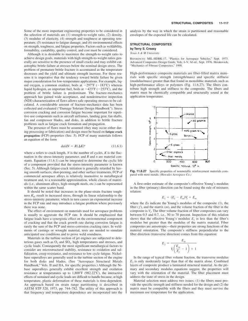
STRUCTURAL COMPOSITES 11-117
Some of the more important engineering properties to be considered inthe selection of materials are (1) strength-to-weight ratio, (2) density,(3) modulus of elasticity, (4) strength and toughness at operating tem-perature, (5) resistance to fatigue damage, and (6) environmental effectson strength, toughness, and fatigue properties. Factors such as weldability,formability, castability, quality control, and cost must be considered.
Although it is desirable to maximize the strength-to-weight ratio toachieve design goals, materials with high strength-to-weight ratios gen-erally are sensitive to the presence of small cracks and may exhibit cat-astrophic brittle failure at stresses below the nominal design stress. Theproblem of premature brittle fracture is accentuated as the temperaturedecreases and the yield and ultimate strength increase. For these rea-sons it is imperative that the tendency toward brittle failure be givenmajor consideration for low-temperature applications. For example, liq-uid oxygen, a common oxidizer, boils at !2978F (!1838C) whereasliquid hydrogen, an important fuel, boils at !4238F (!2538C), and theproblem of brittle failure is predominant. The fracture-mechanicsapproach has gained wide acceptance, and nondestructive inspection(NDI) characterization of flaws allows safe operating stresses to be cal-culated. A considerable amount of fracture-mechanics data has beencollected and evaluated (“Damage Tolerant Design Handbook”). Stresscorrosion cracking and corrosion fatigue become important for repeti-tive-use components such as aircraft airframes, landing gear, fan shafts,fan and compressor blades, and disks, in addition to brittle fractureproblems such as fatigue crack formation and propagation.
The presence of flaws must be assumed (they may occur either dur-ing processing or fabrication) and design must be based on fatigue crackpropagation (FCP) properties (Sec. 5). FCP of many materials followsan equation of the form
(11.6.1)
where a refers to crack length, N is the number of cycles, K is the fluc-tuation in the stress-intensity parameter, and R and n are material con-stants. Equation (11.6.1) can be integrated to determine the cyclic lifeof a component provided that the stress-intensity parameter is known(Sec. 5). Although fatigue-crack initiation is generally retarded by hav-ing smooth surfaces, shot-peening, and other surface treatments, FCP ofcommercial aerospace alloys is relatively insensitive to metallurgicaltreatment and, to a reasonable approximation, whole classes of materi-als (i.e., aluminum alloys, high-strength steels, etc.) can be representedwithin the same scatter band.
It should be noted that increases in the plane-strain fracture tough-ness KIC result in increased stress, through its linear relationship to thestress-intensity parameter, which in turn causes an exponential increasein the FCP rate and may introduce a fatigue problem where previouslythere was none.
The effect of environment on materials used for aerospace problemsis usually to aggravate the FCP rate. It should be emphasized thatfatigue loads have a synergistic effect on the environmental componentof cracking and that the crack growth rate during corrosion fatigue israrely the sum of the FCP and stress-corrosion cracking rates. In weld-ments of castings or wrought material, tests are needed to simulateanticipated use conditions and to prove weld soundness.
Materials in the turbine section of jet engines are subjected to dele-terious gases such as O2 and SO2, high temperatures and stresses, andcyclic loads. Consequently the most significant metallurgical factors toconsider are microstructural stability, resistance to oxidation and sul-fidization, creep resistance, and resistance to low cycle fatigue. Nickel-base superalloys are generally used in the turbine section of the enginefor both disks and blades. (See “Aerospace Structural MetalsHandbook,” Vols. II and IIA, for specific properties.) Although the Ni-base superalloys generally exhibit excellent strength and oxidationresistance at temperatures up to 1,8008F (982.228C), the interactiveeffects of sustained and cyclic loads are difficult to handle because, at hightemperature, plastic deformation of these materials is time-dependent.An approach based on strain range partitioning is described inASTM STP 520, 1973, pp. 744–782. The utility of this approach isthat frequency and temperature dependence are incorporated into the
da/dN 5 Rs#Kdn
analysis by the way in which the strain is partitioned and reasonableenvelopes of the expected life can be calculated.
STRUCTURAL COMPOSITES
by Terry S. Creasy
Texas A & M University
REFERENCES: MIL-HDBK-17, “Plastics for Aerospace Vehicles,” Sept. 1973.
Advanced Composites Design Guide, Vols. I–V, 3d ed., Sept. 1976. Herakovich,
“Mechanics of Fibrous Composites,” 1998.
High-performance composite materials are fiber-filled matrix mate-rials with specific strength (strength/mass) and specific stiffness(modulus/mass) greater than that found in monolithic materials such ashigh-performance alloys or polymers (Fig. 11.6.27). The fibers con-tribute high strength and stiffness to the composite. The fibers andmatrix must be chemically compatible and structurally sound at theapplication temperature.
Fig. 11.6.27 Specific properties of nonmetallic reinforcement materials com-
pared with most metals. (Hercules Aerospace Co.)
A first-order estimate of the composite’s effective Young’s modulusin the fiber (primary) direction can be found using the rule of mixturesrelation:
where the Es indicate the Young’s modulus of the composite (1), thefiber ( f ), and the matrix (m), and the volume fraction of the fiber in thecomposite is Vf. The fiber volume fraction of fiber composites can varybetween 0.5 and 0.7, i.e., 50 to 70 percent. Inspection of this relationshows that the effective Young’s modulus E1 is less than the fiber’smodulus but greater than the modulus of the matrix material. Fibercomposites are anisotropic—their properties are strong functions of thematerial orientation. The composite’s stiffness perpendicular to thefiber direction (transverse direction) comes from this equation:
In the range of typical fiber volume fraction, the transverse modulusE2 is only moderately larger than that of the matrix alone. Combinedlayers of composite produce a laminated structural material. As the pri-mary and secondary modulus equations suggest, the properties willvary with the orientation of the material. The fiber placement mustaddress the state of stress in the design.
Material selection must address two issues: (1) the fibers must pro-vide the specific strength and stiffness needed for the design and (2) thematrix must be compatible with the fibers and they must survive themaximum use temperature for the application.
E2 5Em
Vf ¢Em
Ef
2 1≤ 1 1
E1 5 sEf 2 EmdVf 1 Em

Tables 11.6.6 and 11.6.7 list typical properties of fiber and matrixmaterials.
The fatigue behavior of several fiber/matrix systems appears inFig. 11.6.28. The response of these composites can be compared with2024-T3 aluminum alloy.
MATERIALS FOR USE IN HIGH-PRESSURE OXYGEN SYSTEMS
by Robert L. Johnston
NASA
Oxygen is relatively reactive at ambient conditions and extremely reac-tive at high pressures. The design of high-pressure oxygen systemsrequires special consideration of materials and designs. The types ofpotential ignition sources that could be present in even a simplecomponent are quite varied. Sources of ignition include electrical fail-ures, particle impact in high-flow regions, pneumatic shock, adiabaticcompression, fretting or galling, and Helmholtz resonance in blind pas-sages. Other sources of ignition energy are also possible. A compre-hensive review of potential design problems is available in NASAReference Publication 1113, A.C. Bond et al., “Design Guide for HighPressure Oxygen Systems.”
Materials currently used in high-pressure oxygen systems range fromignition-resistant materials like Monel 400 to materials of widely varyingignitability like butyl rubber and the silicones. The range of ignitabilityof various materials is shown in Figs. 11.6.29 and 11.6.30.
While material selection alone cannot preclude ignition, properchoices can markedly reduce the probability of ignition and limit prop-agation. Selecting materials with small exothermic heats of combustionwill reduce the possibility of propagation. Materials with high heats of
11-118 ASTRONAUTICS
Table 11.6.6 Properties of Fibers Used in Composites
Tensile Tensile
Modulus, strength, failure Specific Density,
Fiber 106 lb/in2 ksi strain, % gravity lb/in3
Boron (4 mil) 60 460 0.8 2.60 0.094
Carbon (Thornel 300) 34 470 1.1 1.74 0.063
Carbon (IM8) 45 750 1.9 1.79 0.065
Carbon (pitch) 120 350 0.4 2.18 0.079
Kevlar 49 19 400 1.8 1.45 0.052
Kevlar 29 12 400 3.8 1.45 0.052
Glass (E) 10.5 250–300 2.4 2.54 0.092
Glass (S) 12.5 450 3.6 2.48 0.090
Table 11.6.7 Properties of Matrix Materials Usedin Composites
Maximum use
Material temperature, 8F
Polyester 250
Polysulfone 250
Epoxy 350
Polyarylsulfone 400
Phenolic 450
Silicone 450
Polyimide 650
Aluminum 700
Magnesium 700
Glass 2,500
Carbon* (W/C) 3,200
* With oxidation resistance.
Fig. 11.6.28 Fatigue behavior of unidirectional composites and aluminum.
(Hercules Aerospace Co.)
Finally, composite materials provide two unique capabilities forastronautic structures. Some carbon fibers have a negative coefficient ofthermal expansion of approximately in/in. With carefuldesign a composite structure can compensate for expansion and con-traction of other components. In addition, carbon fibers provide highthermal conductivity in the fiber direction. Thermal management ofastronautic systems can take advantage of this capability.
20.2 3 1026
Fig. 11.6.29 Ignition variability of current oxygen-system nonmetallic
materials.
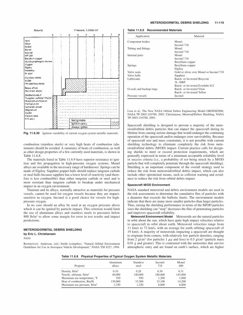
METEROID/ORBITAL DEBRIS SHIELDING 11-119
combustion (stainless steels) or very high heats of combustion (alu-minum) should be avoided. A summary of heats of combustion, as wellas other design properties of a few currently used materials, is shown inTable 11.6.8.
The materials listed in Table 11.6.9 have superior resistance to igni-tion and fire propagation in high-pressure oxygen systems. Monelalloys are available in the necessary range of hardnesses. Springs can bemade of Elgiloy. Sapphire poppet balls should replace tungsten carbideor steel balls because sapphire has a lower level of reactivity (and there-fore is less combustible) than either tungsten carbide or steel and ismore resistant than tungsten carbide to breakup under mechanicalimpact in an oxygen environment.
Titanium and its alloys, normally attractive as materials for pressurevessels, cannot be used for oxygen vessels because they are impact-sensitive in oxygen. Inconel is a good choice for vessels for high-pressure oxygen.
In no case should an alloy be used at an oxygen pressure abovewhich it can be ignited by particle impact. This criterion would limitthe use of aluminum alloys and stainless steels to pressures below800 lb/in2 to allow some margin for error in test results and impactpredictions.
METEROID/ORBITAL DEBRIS SHIELDING
by Eric L. Christiansen
NASA
REFERENCES: Anderson, (ed.) Smith (compiler), “Natural Orbital Environment
Guidelines for Use in Aerospace Vehicle Development,” NASA TM 4527, 1994.
Liou et al., The New NASA Orbital Debris Engineering Model ORDEM2000,
NASA TP-2002-210780, 2002. Christiansen, Meteroid/Debris Shielding, NASA
TP-2003-210788, 2003.
Spacecraft shielding is designed to prevent a majority of the mete-oroid/orbital debris particles that can impact the spacecraft during itslifetime from causing serious damage that would endanger the continuingoperation of the spacecraft and/or endanger crew survivability. Becauseof spacecraft size and mass constraints, it is not possible with currentshielding technology to eliminate completely the risk from mete-oroid/orbital debris (M/OD) impact. Current practice calls for design-ing shields to meet or exceed protection requirements, which aregenerally expressed in terms of a minimum acceptable reliability levelor success criteria (i.e., a probability of not being struck by a M/ODparticle that will completely penetrate through the spacecraft shielding).Shielding is an important component of the overall strategy used toreduce the risk from meteoroid/orbital debris impact, which can alsoinclude other operational means, such as collision warning and avoid-ance to reduce the risk from orbital debris impact.
Spacecraft M/OD Environment
NASA standard meteoroid and debris environment models are used inthe risk assessments to determine the cumulative flux of particles witha diameter that exceeds the ballistic limits. The environment modelsindicate that there are many more smaller particles than larger particles.Thus, raising the shielding performance in terms of the M/OD particlessizes the shielding can “stop” decreases the flux of penetrating particlesand improves spacecraft reliability.Meteoroid Environment Model Meteoroids are the natural particles
in orbit about the sun, which have quite high impact velocities relativeto spacecraft in orbit about earth. Meteoroid velocities range from11 km/s to 72 km/s, with an average for earth orbiting spacecraft of19 km/s. A majority of meteoroids impacting a spacecraft are thoughtto originate from comets, with relatively low particle densities, rangingfrom 2 g/cm3 (for particles 1 and less) to 0.5 g/cm3 (particle mass0.01 g and greater). This is contrasted with the meteorites that surviveatmospheric entry and are found on earth’s surface, which are higher
mg
Fig. 11.6.30 Ignition variability of current oxygen-system metallic materials.
Table 11.6.9 Recommended Materials
Application Material
Component bodies Monel
Inconel 718
Tubing and fittings Monel
Inconel 718
Internal parts Monel
Inconel 718
Beryllium copper
Springs Beryllium copper
Elgiloy
Valve seats Gold or silver over Monel or Inconel 718
Valve balls Sapphire
Lubricants Batch- or lot-tested Braycote
3L-38RP
Batch- or lot-tested Everlube 812
O-seals and backup rings Batch- or lot-tested Viton
Batch- or lot-tested Teflon
Pressure vessels Inconel
Table 11.6.8 Physical Properties of Typical Oxygen System Metallic Materials
Aluminum Stainless Inconel Monel
Property alloys steel 718 400
Density, lb/in3 0.10 0.28 0.30 0.31
Tensile, ultimate, lb/in2 40,000 140,000 180,000 145,000
Maximum use temperature, 8F 350 950 1,200 1,000
Heat of combustion, Btu/lb 130,000 33,500 15,100 14,200
Maximum use pressure, lb/in2 1,250 1,250 8,000 8,000

density and thought to originate mainly from asteroids. The meteoroidenvironment model to be used for shielding design is defined in theNASA documentation.Orbital Debris Environment Model Orbital debris is human-created
pieces of spacecraft that are in orbit about earth (Fig. 11.6.31). Orbitaldebris impact velocities are lower than meteoroids, generally impactingspacecraft in low earth orbit at relative speeds of less than 1 km/s to justover 15 km/s, with an average velocity of about 9 km/s for a 400-kmaltitude. The debris environment threat is composed of metallic frag-ments, paint, aluminum oxide, and other components of spacecraft andsolid-rocket motor exhaust. Typically, for debris risk assessments,orbital debris particle density is assumed to be 2.8 g/cm3, correspond-ing to aluminum metal. Because the orbital debris environment is tiedto human activities in space, it is much more dynamic then the mete-oroid environment, and the orbital debris environment definitions aresubject to periodic updates and revisions as more data is collected onthe amount and evolution of orbital debris in earth orbit. The currentdebris environment model for purposes of shielding design is definedby NASA TP-2002-210780 and referred to as ORDEM2000.
each program defines “critical” penetrations as those that would endan-ger the survivability of the vehicle and/or crew, although requirementsfor mission success and functionality have been applied as well.Space Station Design Requirements The Space Station has mete-
oroid/debris protection requirements consistent with past programs. Assuch, it carries by far the most capable meteoroid/debris shields everflown. This is because ISS is larger and exposed longer than other spacevehicles. It operates at higher altitudes in general than other spacecraftand its operation will extend into the future. These factors increase theexpected number of meteoroid/debris impacts. To meet comparable pro-tection requirements, ISS shielding must be more effective. For instance,most ISS critical hardware exposed to the M/OD flux in the velocity vector(front) or port/starboard (side) directions will be protected by shieldseffective at stopping 1- to 1.3-cm-diameter aluminum debris particle attypical impact velocity and angle (9 km/s, 458). In comparison, the Mirspace station is able to stop 0.3-cm particles, the space shuttle orbiter iscapable of stopping 0.2- to 0.5-cm particles, and Apollo and Skylab wereable to stop 0.15 to 0.2-cm particles under similar impact conditions. ISSwill also have the ability to maneuver from ground-trackable debris par-ticles (typically *10 cm diameter). By virtue of the large internal volumeof ISS, its crews will have time to locate and isolate leaks, if they were tooccur, by closing hatches. Hole repair kits will be available and crews willbe trained to repair a leak in a module if it occurs. Crew escape vehicleswill be docked to ISS in the event of a major event requiring evacuation.
Risk Assessment Process
The approach to evaluating and designing protection systems to meetrequirements is illustrated in Fig. 11.6.32. By using this methodology,the analyst will be able to accurately evaluate spacecraft risks fromM/OD impact, identify zones or areas of the spacecraft that are the “riskdrivers” that control the M/OD risk, and evaluate options to reduce risk.Each major step in the risk assessment process is described in the fol-lowing sections.Space Geometry Spacecraft size is directly proportional to the
number of impacts as given in Eq. (11.6.1). Risk of M/OD impact fail-ure increases as the area and time exposed to the M/OD flux increases.
(11.6.1)
where N is the number of impacts causing failure and is equal to thesum of the impact failures in each region (Ni) over all regions (i 1 to n)of the spacecraft. Ni is found from the product of flux (F, number/m2-year)of meteoroid and debris impacts that exceed the failure ballistic limitsof a region, exposed area (A, m2), and time (t, year). It is important tobreak down the spacecraft geometry into different regions, each with a
N 5 gni51
Ni 5 gni51
sFAtdi
11-120 ASTRONAUTICS
Fig. 11.6.31 Orbital debris “snapshot.”
Table 11.6.10 Historical Meteoroid/Debris ShieldingRequirements
Required probability of
Vehicle Environments no penetration (PNP)
Apollo command Meteoroid 0.996 per 8.3-day
module mission
Skylab module Meteoroid 0.995 for 8-month
mission
Meteoroid 0.95 for 500 missions
(design requirement)
Meteoroid and debris 0.995 per mission
Shuttle orbiter (for critical penetration)
0.984 per missionMeteoroid and debris(for radiator leak—
mission abort)
Spacelab module Meteoroid 0.999 for 7-day mission
Hubble space telescope Meteoroid and debris 0.95 for 2 years
ISS Meteoroid and debris 0.98 to 0.998 per critical
element over 10 years
Design Requirements
Vehicles from the early years of space exploration have used the proba-bilistic approach to design meteoroid shielding. Table 11.6.10 providesa listing of historical M/OD protection design requirements. Generally,

METEROID/ORBITAL DEBRIS SHIELDING 11-121
different exposed area, materials of construction, shielding configura-tions, and thickness. For instance, there are over 400 different shieldsprotecting International Space Station (ISS) habitable modules andexternal critical items (pressure vessels, control moment gyros) whichhave been optimized according to their location and exposure to theM/OD threat to provide the necessary M/OD protection.Impact Directionality The front and sides of a spacecraft are more
exposed to debris impact, while the front, sides, and top (zenith) are moreexposed to meteoroid impact. The Long Duration Exposure Facility(LDEF) had 20 times more craters observed on the forward face com-pared to the aft, and 200 times more craters on the forward than theearth-facing side (Fig. 11.6.33). Heavier shielding is typically placed onfront and sides of spacecraft with fixed orientation relative to the veloc-ity direction to protect from higher impact rates on these surfaces.Spacecraft Failure Criteria A key step in the risk assessment
process is to precisely define what is meant by “failure,” that is, todefine potential damage modes from M/OD impact and, for each, toquantify the minimum amount of damage that can lead to failure ofspacecraft hardware. This definition establishes the failure criterion orcriteria that are assigned to each region of the spacecraft geometrymodel. For instance, M/OD damage modes and failure criteria for ele-ments of the Space Station are given in Table 11.6.11.Hypervelocity Impact Tests Hypervelocity impact (HVI) tests are
an integral part of the analyses conducted to ensure adequate design ofspacecraft M/OD shielding. Two-stage light-gas guns (LGGs) are usedto accelerate projectiles up to 7 km/s (Fig. 11.6.34). LGGs are capable
of launching a variety of different and well-controlled projectile shapes.A disadvantage is that LGGs are capable of velocities that cover only afraction of the orbital debris threat. Since average orbital debris velocityin low-earth orbit is on the order of 9 km/s, LGG can directly simulateonly 40 percent of the orbital debris threat.
Other techniques exist to launch projectiles at speeds over 10 km/s.For instance, an inhibited shaped-charge launcher (ISCL) at SouthwestResearch Institute (SwRI) is capable of launching aluminum projec-tiles, 0.25 g to 2 g mass, in the shape of a cylinder to 11.5 km/s(Fig. 11.6.35). Another high-speed launcher that has provided usefulinformation on shield capabilities in excess of 10 km/s is the three-stagehypervelocity launcher (HVL) developed at Sandia National Laboratories.
Fig. 11.6.32 Meteoroid/orbital debris risk assessment methodology.
Fig. 11.6.33 Long duration exposure facility.
Table 11.6.11 Damage Modes and Failure Criteria for Space Station Elements(Note: Critical failure criteria marked with*.)
Thermal
protection Spall/perforation of
system (TPS) shield exterior of Perforation of Uncontrolled Catastrophic
Critical elements damage pressure shell pressure shell decompression rupture Detonation
Crew modules X* X X
Pressure vessels (liquids and gases) X*1 X*1 X X
Control moment gyros (rotating equipment) X* X
Crew return vehicles X X* X X
1 Failure criterion for Russian PVs is perforation of pressure shell. Failure criterion of other designs is perforation or detached spall of shielding surrounding PV.
Surface Short or open
Functional elements degradation Leak circuit
Radiator panels X X
Radiator flex/hard lines X
Thermal loop lines and exchangers X
Power cables X
Batteries X X
Solar arrays X X
Data lines/cables X
Window outer panes X

This launches thin disks (L/d 0.1 to 0.2, mass 0.2 to 1 g) of alu-minum and titanium from 10 to 15 km/s with some bowing and tiltingof the projectile. Hydrocode simulations are used to assess projectileshape effects on shield response.
Ballistic Limit Equations
Ballistic limit equations (BLEs) or “penetration” equations are based onthe HVI test results, numerical simulations, and analytical assessments(Christiansen, 2003). BLEs describe the particle sizes that are on thefailure threshold of a particular spacecraft component. The ability of aparticular shield to withstand hypervelocity impact is predicted by a BLE.BLEs are a function of the target “failure criteria”; target configuration,materials, and thickness; and projectile parameters such as velocity, angle,shape, and density. M/OD risk assessments require a BLE defined for eachsurface of a spacecraft, for each failure criterion assessed. Shield designequations have also been developed that provide a means to estimateshielding parameters needed to defend against specific projectile threats.
Because of the complexity of spacecraft and their HVI failure modes,many different ballistic limit equations exist for a wide variety ofshielding types, spacecraft components and hardware, and differingdamage/failure modes. A description of ballistic limit equations for oneparticular type of shield, the basic Whipple shield, is provided in thefollowing section. This example illustrates the considerations involvedin developing ballistic limit equations.
Whipple Shield Ballistic Limit Equations
Fred Whipple proposed in the 1940s a meteoroid shield for spacecraftconsisting of a thin “sacrificial” bumper at a distance from a rear wall.
The Whipple shield is shown in Fig. 11.6.36. The function of the firstsheet, or bumper, is to break up the projectile into a cloud of materialcontaining both projectile and bumper debris. This cloud expands whilemoving across the standoff, resulting in the impactor momentum beingdistributed over a wide area of the rear wall (Figs. 11.6.37 to 11.6.39).The back sheet must be thick enough to withstand the blast loadingfrom the debris cloud and any solid fragments that remain. For mostconditions, a Whipple shield results in a significant weight reductionover a single plate, which must contend with deposition of the projec-tile kinetic energy in a very localized area.
Whipple shields were used to provide protection to the Apollo com-mand module and lunar lander. Apollo shields were capable of stopping0.16-cm-diameter aluminum particles at 7 km/s, normal impact angle (08).Whipple Shield Design Equations For design purposes, Eq. (11.6.2)
to (11.6.4) provide bumper and rear wall thickness to defeat a giventhreat particle (assuming km/s).
(11.6.2)
(11.6.3)
where cb 0.25 when S/d ) 30, cb 0.20 when and cw Normalized yield stress (unitless)
The ballistic limit criterion is no perforation or spall of the rear wall.Bumper fragments become the primary source of rear wall damage atimpact angles greater than 658. Therefore, for oblique angles over 658,
ss/70ksid.srh0.79 cm23/4 # s # g1/3 # km21.
S/d $ 30,
tw 5 cwd0.5M1/3srprbd
1/6rw21sV cos udS23/4srh
21/2
tb 5 cbmp/rb 5 cbdrp/rb
Vn $ 7
11-122 ASTRONAUTICS
Fig. 11.6.35 SwRI’s inhibited shaped-charge launcher. Various size charges are available that are capable of launching
0.25 to 2 g aluminum projectiles up to 11.5 km/s (left view). Projectiles are typically in the shape of a hollow cylinder
(right view.)
Fig. 11.6.36 Whipple shield. (a) Whipple shields consist of a bumper, standoff
(gap or spacing), and real wall. (b) Hypervelocity impacts will generate a cloud of
bumper and projectile debris that can contain solid fragments, liquid, and vapor
particles. (c) The rear wall must survive the fragments and debris cloud impulsive
loading. It could fail by perforation from solid fragments, spall, or tear and petal
from the impulsive loading.
Ejecta
Bumper
Standoff
Rear wall Debris cloudCraters and holes
Detached spall
(a) (b)
(c)
Fig. 11.6.34 NASA JSC-WSTF two-stage light-gas gun.

METEROID/ORBITAL DEBRIS SHIELDING 11-123
Whipple Shield Ballistic Limits for All Impact Velocities Typicalballistic limits for a Whipple shield at all impact velocities are illustratedin Fig. 11.6.40 for normal impact by an aluminum sphere. The Whippleshield ballistic limit is compared to a monolithic, single aluminum plateof same mass as the combined Whipple shield’s bumper and rear wall.Protection capabilities are defined for three penetration regimes basedon normal component velocity (Vn) for an aluminum impact on aWhipple shield: ballistic regime (Vn ) 3 km/s), fragmentation regime(3 km/s ) Vn ) 7 km/s), and melt/vaporization regime (Vn * 7 km/s).Important shield physical and material properties that influence ballis-tic limits of the shield vary as a function of impact velocity. Equationsused to quantify ballistic limits for various types of shields are provid-ed in the literature (Christiansen, 2003).
A key factor governing the performance of spaced shields is the“state” of the debris cloud projected from the bumper toward the rearwall. The debris cloud may contain solid, liquid, or vaporized projectileand bumper materials, or a combination of the three states, depending
Fig. 11.6.37 A 0.32-cm projectile impacts bumper at 6.8 km/s, left to right,
with l ms between frames. [High-speed camera film (photograph by Cordin).]
Fig. 11.6.38 Ejecta and debris cloud.
Ajecta
Debriscloud
Fig. 11.6.39 Rear wall after impact.
Fig. 11.6.40 Ballistic limits for equal mass monolithic target and Whipple shield. Failure criterion is threshold perfo-
ration or detached spall from rear wall. Monolithic target is 0.44-cm-thick Al 6061T6. Whipple shield consists of 0.12-
cm-thick A1 6061T6 bumper followed at 10 cm by 0.32-cm-thick A1 6061T6 rear wall.
0.8
0.7
0.6
0.5
0.4
0.3
0.2
0.1
00 2 4 6 8 10 12 14
Ballistic limit improvement due to shield standoff ∆ dcrit
“Failure” occurs above curves
Velocity range: Ballistic regime Fragmentation and partial melt regime
Complete melt regime
Many (increasing with velocity) solid fragments and liquid
droplets
Few solid fragments
Important shield and material properties:
Bumper: strength, density, EOS, thermal
characteristics standoff
rear wall strength
Bumper density, EOS standoff
rear wall strength
Fine droplets, few solid fragments, some vapor
Strength
State of debris cloud: (for Al on Al impacts)
Critical Al diameter, cm
Whipple dcrit@0°
Monolithic dcrit@0°
Velocity, km/s
the calculated rear wall thickness should be constrained to 658.Coefficient cw should be adjusted by the factor [(S/d )/(S/d)0] where(S/d )0 15, when S/d ) 15, as follows.
cw 0.79 [(S/d)/(S/d)0]!0.185 (11.6.4)

on the initial impact pressure. Solid fragments in the debris cloud aregenerally more penetrating when they contact the rear wall than liquidor vapor particles. Blast loading in the rear wall is a function of shieldstandoff, which becomes of increasing importance as impact velocityincreases above about 5 km/s.
Bumper Code
The BUMPER code has been the standard in use by NASA and contrac-tors to perform meteoroid/debris risk assessments since the early 1960s.Over that period of time, it has undergone extensive revisions and updates.NASA has applied BUMPER to risk assessments for space station, shut-tle, Mir, extravehicular mobility units (i.e., “space suits”), and other satel-lites and spacecraft. Significant effort has been expended to validateBUMPER and “benchmark” it to other M/OD risk assessment codes usedby some ISS international partners. Figure 11.6.31 illustrates whereBUMPER fits in the risk assessment process. The BLEs and M/OD envi-ronment models are embedded into BUMPER. A finite-element model(FEM) that describes the spacecraft geometry is created in and input intoBUMPER. BUMPER calculates the number of failures by determiningthe number of M/OD particles that exceed the ballistic limits for eachelement of the FEM, and calculates the total number of failures by sum-ming the individual elements. BUMPER results are used to determine therisk drivers, that is, the areas on the spacecraft that control the risk.Emphasis on risk reduction is placed on lowering the risk for the drivers.
Probability of No Penetration (PNP)
Probability of no penetration (PNP) failure is assessed on the basis ofPoisson statistics [Eq. (11.6.5)], where N is defined by Eq. (11.6.1).This is NASA’s standard approach used to assess meteoroid shieldingsince Apollo. The same probabilistic approach has been extended todesigning spacecraft protection systems for the combined meteoroidand debris environments, assessing risks of functional failure, or calcu-lating risks of impact damage exceeding a user-defined size (diameteror depth). The same statistical approach is used to assess risks of anykind of damage extent that can be expressed in terms of different bal-listic limit equations.
PNP exp (!N) (11.6.5)
The risk of penetration is:
Risk 1 ! PNP (11.6.6)
Analysis Iteration and Design Qualification
Assessed PNP is compared to requirements for M/OD protection. Theshielding design effort is successful when the assessed PNP is greaterthan the required PNP. As illustrated in Fig. 11.6.31, iteration of the riskassessment and risk reduction process is often necessary to meet pro-tection requirements and optimize the design, i.e., meet the require-ments with less weight, lower volume (less standoff), less cost, etc. Thelast step in the process is to conduct final shield verification by analy-sis (supported by HVI test as appropriate), prior to final design certifi-cation and acceptance.
Risk Reduction Practices
Engineering practices to decrease risk, improve shielding performance,and decrease shielding mass are summarized below.Find M/OD Risk Drivers Perform detailed assessment of penetra-
tion risks for the overall vehicle to determine the zones that control therisks. Selectively improve the protection capability in the areas identi-fied as risk drivers.Shielding Enhancement
1. Optimize the shielding weight distribution to account for thedirectional M/OD distribution. Shielding on each critical item is tai-lored for the environment and its location on station. Because M/ODimpact rate is highest on forward and side surfaces, more capableshielding (heavier or with greater standoff) is applied to these surfacesand less on the earth-facing surface. Shielding is also reduced in areas
where shadowing from neighboring structures will reduce impacts. Thegoal of this effort is to equalize the ratio of risk to area for the variousvehicle zones. The risk/area ratio for each zone is assessed and opti-mized by repeated BUMPER code runs.2. Incorporate enhancements such as increasing the spacing between
bumper and rear wall, or using higher-performance alloys and materialsfor the rear wall.3. Implement more-fundamental changes such as incorporating
more efficient, multibumper shielding concepts.4. Incorporate toughening materials, such as ceramic fabric and
high-strength fabric into the multilayer insulation (MLI) thermal blan-ket that is often integral to the M/OD shielding.Impact Reduction
1. Maximize shadowing. Take advantage of shielding/shadowingfrom neighboring items. Locate external critical equipment to trailingor earth-facing surfaces to reduce M/OD impact rates, or put them inareas highly shadowed by other hardware.2. Select low frontal area orientations. It has been shown that the
best orientation for a relatively short cylinder (length/diameter of 1.8)in terms of lowest meteoroid/debris impact risk is with cylindricallength axis oriented perpendicular to the orbital plane. A vertical (gravity-gradient) orientation (with length axis parallel to earth radial) has a30 percent higher M/OD impact risk. An orientation with length axisparallel to velocity vector is in the middle.3. Flight attitude. Selecting the best flight attitude by pointing the
most vulnerable surfaces aft or toward earth is standard procedure forthe shuttle. Other spacecraft can take a similar approach.Insert Stored Energy Equipment After use, stored energy equip-
ment should be made inert if possible. For instance, completely depres-surize any storage tank after it is emptied. The risk of catastrophicrupture is eliminated when stress levels in the pressure wall are madenegligible by depressurizing to a small value. This would require designmodifications to implement for propellant tanks and other fluid storagetanks. Another example is to keep spare flywheels, gyros, and othermomentum storage devices in an inactive state until required. A corol-lary idea for gaseous pressure vessels is to use them in series (not par-allel) and deplete first the pressure vessels in the locations that are mostexposed to M/OD impact (those in the forward or side positions), fol-lowed by less exposed positions.Reduce Hazards if Shield Penetration Occurs Design and opera-
tional options may exist to reduce hazards if a penetration occurs. Forinstance, some hatches to unoccupied modules can be kept closed toprevent a depressurization of an entire station if a penetration occurredto the module. A perforation into an unoccupied module with hatchclosed would not result in loss of crew from the fragments/shrapnel,light flash, acoustic overpressure, or depressurization. Vent linesbetween modules could be left open to allow for some air circulationand to keep pressures equalized to facilitate hatch opening during nor-mal operations.Critical Damage Detection, Repair, and Replacement (R&R)
Inspection and repair of impact damage to critical areas of reentry vehi-cles (such as the crew return vehicle attached to ISS) can be used as asupplement to M/OD shielding for maintaining flight worthiness. Someimpact damage to thermal protection systems (TPS) on earth-returnvehicles is not a hazard while on orbit (and may therefore be undetected)but could become hazardous later during reentry aerodynamic heatingphases. Properly placed instrumentation with correct sensitivity todetect critical TPS damage can help support the inspection/detectionprocess.
Enhanced Shielding
The primary purpose of developing improved shielding is to providehigher levels of spacecraft meteoroid/debris protection with lessweight.To illustrate the issue, consider the shielding required to stop 1-cm-
diameter aluminum projectiles at 7 km/s, 08 impact angle. Four shieldconcepts to meet the requirement are given in Fig. 11.6.41: a con-ventional aluminum Whipple shield with a 10.2-cm standoff, a
11-124 ASTRONAUTICS

SPACE-VEHICLE STRUCTURES 11-125
Nextel/Kevlar stuffed Whipple shield with the same standoff, aWhipple shield with a 30-cm standoff, and a Nextel multishockshield concept. The stuffed Whipple shield incorporates a blanketbetween the outer aluminum bumper and inner pressure wall thatcombines two materials: NextelTM ceramic fabric and KevlarTM high-strength fabric. The shielding mass estimates are made assuming theshielding encloses a cylinder, with 4.2-m inside diameter by 8.5 mlong. Stuffed Whipple and multishock shields are described in moredetail later in this section. But it is clear for this example that thereare significant mass savings by using advanced shielding concepts (i.e.,up to 50 percent reduction).Also, it is possible to trade weight for protection capability (i.e.,
capability and shield PNP are related), so it can be shown that lowerweight and more effective protection in terms of higher PNP are possi-ble by using Nextel/Kevlar stuffed Whipple and multishock shields,compared to conventional Whipple shields.
SPACE-VEHICLE STRUCTURES
by Thomas L. Moser and Orvis E. Pigg
NASA
REFERENCES: MIL-HDBK-5D, “Metallic Materials and Elements for AerospaceVehicle Structures.” Advanced Composites Design Guide, Sept. 1976, LibraryAccession no. AD916679 through AD916683. Ashton, Halpin, Pertit, “Primer onComposite Materials Analysis,” Technomic Pur. Co. Aeronautical StructuresManual (Vols. I–III), NASA TMX-73305. Bruhn, “Analysis and Design of FlightVehicle Structures,” Tri-State Offset Co., Cincinnati. Barton, “Fundamentals ofAircraft Structures,” Prentice-Hall, 1948. Roark, “Formulas for Stress and Strain,”McGraw-Hill. “Nastran Theoretical Manual,” Computer Software Management andInformation Control (COSMIC), University of Georgia. Perry, “Aircraft Structures,”
McGraw-Hill. Gathwood, “Thermal Stress,” McGraw-Hill. Zienkiewicz, “TheFinite Filement,” McGraw-Hill. MIL-STD-810D, “Environmental Test Methodsand Engineering Guidelines.” Chapman, “Heat Transfer,” Macmillan.
Space vehicles include a large variety of vehicle types, like their prede-cessors, earth vehicles. Airplanes were the first generation of spacevehicles, and our definition of space vehicle has changed as the airplaneapproached the limits of the earth’s atmosphere. Space, in this discus-sion, is the region beyond the earth’s atmosphere.Many space vehicles are hybrids since they are required to operate in
the earth’s atmosphere and beyond. The space shuttle orbiter is such ahybrid space vehicle. The Apollo command and service module is alsoa hybrid, but the Apollo lunar module, which primarily functioned out-side the earth’s atmosphere, was a space vehicle.The design procedure for any vehicle structure is basically the
same:1. Establish the design requirements and criteria2. Define the loads and environments3. Perform the design and analysis4. Iterate the previous two steps (as required) because of the interre-
lation between configuration and loads5. Verify the design
There are conditions and requirements which are unique for hybrid andspace-vehicle structures.Minimum weight and high reliability are significant but opposing
requirements for space-vehicle structures which must be balanced toachieve an efficient, reliable structure design. Depending on the missionof the particular space vehicle, the ratio between the weight of the earthlaunch vehicle and the payload (e.g., interplanetary probe) can be ashigh as 400 to 1. The large weight leverages require that the design be
Fig. 11.6.41 Shielding concepts comparison. (Projectile in all cases 1-cm-diameter aluminum, 1.5 g,7 km/s, normal impact.)

as efficient as possible. Structural materials, therefore, must be stressed(or worked) as close to the capabilities as possible. Like aircraft struc-tures, space-vehicle structures should be designed for a zero margin ofsafety (MS):
1. Material ultimate allowable. The stress at which the materialwill fail.2. FS (factor of safety). This factor usually ranges between 1.25
and 1.50, for space structures, depending on the maturity of the design,the behavior of the material, the confidence in the loads, etc.3. Limit stress. The maximum (reasonable) stress that the structural
component would be expected to encounter.Failure can be based on rupture, collapse, or yield as dictated by thefunctional requirements of the component. High reliability is neces-sary for most space vehicle structures since a failure is usually cata-strophic or nonrepairable. Total structural reliability is composed ofmany of the design elements—loads, materials, allowables, loadpaths, factor of safety, analysis techniques, etc. If the reliability isspecified and the statistical parameters are known for each design ele-ment, then the process is straightforward. A total structural reliabilityis seldom specified and good engineering practice is used for the solu-tion of the reliability of each design element. Commonly used toassure structural reliability are (1) material allowables equivalent to Avalues from MIL-Handbook-5A for safe-life structure and B valuesfor fail-safe structures; (2) limit loads which correspond to events andconditions which would not be exceeded more often than 3 times in1,000 occurrences; (3) factor of safety equal to 1.4 for crew-carryingspace vehicles and 1.25 for those without crews; and (4) verificationof the structural design by test demonstration. A good structuraldesign is one which has the correct balance between minimum weightand high reliability.Space vehicles are usually manufactured and assembled on earth
and transported to space. The launch environments of acceleration,vibration, aerodynamic pressure, rapid pressure change, and aerody-namic heating coupled with the space environments of extremely lowpressure, wide ranges in temperature, meteroids, and radiation dictatethat the design engineers accurately define the magnitudes of theseenvironments and the correct time-compatible combinations of theseenvironments if realistic loads are to be determined. Many naturalenvironments have been defined and are documented in the refer-ences. The induced environments, which are a function of the systemand/or structural characteristics (e.g., dynamic pressure, vibration,etc.), must be determined by analysis, test, or extrapolation from sim-ilar space vehicles. Quantifying the induced loads for the structuraldesigners is one of the major consumers of time and money in anyaerospace program and one of the most important. Load determina-tion can be a very complex task. For further guidance the reader isdirected to the references.For a space vehicle which is not exposed to the launch loads, the load
determination is greatly simplified. In the absence of an appreciableatmosphere and gravitational accelerations the predominant externalforce on a space-vehicle structure is that of the propulsion and attitudecontrol systems and the resulting vibration loads. Even though notinduced by an external force, thermal stresses and/or deflections can bea major design driver. Space vehicles commonly experience larger ther-mal gradients because of the time- or attitude-related exposure to solarradiation.The thermal effects of stress and deflections of the structure require
that temperature distributions be defined consistent with the strengthand deflection requirements. From a strength integrity standpoint, tem-perature distribution on a space vehicle can be as important as the pres-sure distribution on an aircraft. The significance and sensitivity ofthermal effects are greatly reduced by the use of composite materialsfor the structure. The materials can be layered to achieve, within limits,
MS 5material ultimate allowable
FS slimit stressd2 1
the desired thermal coefficient of expansion and thereby reduce thethermal effects.Space vehicles which return to the earth must withstand the extremely
high temperatures of atmospheric reentry. This produces dynamictemperature distributions which must be combined with the aerodynamicpressures and vehicle dynamic loads.Innovative, clever, and efficient structural designs minimize the
effects of loads associated with launch for a vehicle which is to remainin space. This is accomplished by attaching the space vehicle to thebooster rocket to minimize scar weight and to reduce the aerodynamicloads by the use of shrouds, fairings, or controlling the attitude duringatmospheric flight.Efficiencies of weight-critical structures have been greatly improved
by more accurately quantifying the loads and stress distributions incomplex structural configurations. Finite element methods (FEM) ofanalysis and large capacity, high-speed digital computers have enabledthe increased fidelity of analyses. In this process, the structure is mod-ified with finite elements (beams, bars, plates, or solids) by breaking thestructure into a group of nodal points and connecting the nodal pointswith the finite elements which best represent the actual structure. Loadsare applied at the nodal points or on the elements which then distributethe loads to the nodal points. Constraints are also applied to the nodalpoints to support or fix the structure being analyzed. The finite elementprogram then assembles all the data into a number of linear simultane-ous equations and solves for the unknown displacements and then forinternal loads and stresses, as required. Many finite element programshave been developed to perform a variety of structural analyses includ-ing static, buckling, vibration, and response.The loads in a structure depend on the characteristics of the structure
and the characteristics of the structure are largely dictated by the loads.This functional dependency between loads and structures requires aniterative design process.Classically, when structures are worked to stresses near the capa-
bility of the materials, e.g., airplane structures, the design is verifiedby test demonstration. This method of verification was commonbefore high-fidelity structural mathematical models were employedand is still used when practical to apply the design loads and environ-ments to a dedicated test article to verify the design. Design deficien-cies are then corrected depending on the importance and themanufacturing schedule.Space-vehicle structures often do not lend themselves to the classical
test approach because of the multitude of loads and environments whichmust be applied, because testing in earth’s gravity precludes realisticloadings, and because of the size and configuration. Verification byanalyses with complementary component tests and tests of selectedload conditions are common.
INFLATABLE SPACE STRUCTURES FOR HUMAN HABITATION
by William C. Schneider
Texas A & M University
Inflatable space structures have been considered for many years andeven some have been put into practice for applications such as largereflecting satellites, shock attenuation, and reentry vehicles. Their clearadvantage over rigid structures from the standpoint of weight, com-pactness, and large volume potential have been recognized for years,but only recently, as a result of the development of very high strengthfabrics, has serious development of inflatable structures for humanapplication taken place. NASA, as well as some private aerospace com-panies, recognize the increasing demand for human-inhabited inflatablespace structures in astronautics. As newer, even higher strength, fabricsare developed, the full utilization of inflatable structures for humanspace will be realized. In the following subsections the TransHab andthe portable hyperbaric chamber are discussed, and they represent onlytwo examples of the emerging inflatable space structure technology forhuman habitation.
11-126 ASTRONAUTICS

INFLATABLE SPACE STRUCTURES FOR HUMAN HABITATION 11-127
TransHab
by Horacio de la Fuente
NASA
One example of the significant advantages derived from the use ofinflatable technology for human space applications was demonstratedby the TransHab inflatable habitation module. Figure 11.6.42 shows aunit developed at the NASA Johnson Space Center. The TransHab is aninflatable human habitation module (30 ft long ft in diameter)originally conceived as an interplanetary module for use in spaceflightmissions beyond low earth orbit. The long transit times required forthese types of missions create several significant design challenges.Because multiple crewmembers will be living in a confined space forlong periods of time, psychological health required the spacecraft tohave a large-volume living space yet be lightweight. The ability ofinflatable structures to be folded and packaged during the launch envi-ronment is a key feature that allows this requirement to be met. Theadvantages of inflatable modules, however, go beyond the obvious vol-umetric packing efficiency. The inflatable TransHab is folded and pack-aged tightly during the launch phase of the mission and is inflated onlyafter it is in the quiescent space environment. Huge weight savings arerealized when compared to a large rigid shell structure, since the rigidshell must be designed to withstand the severe steady-state, transient,and vibration launch loads as a large, rigid shell. There is, however, norequirement for the inflated TransHab to react to the launch loads. Itmust only withstand the differential pressure experienced in space.The TransHab module design was later adapted to serve as a habita-
tion module for the International Space Station. This change primarilyresulted in modifications to some of the inflatable shell layers. Asdescribed later, the shell layers most affected by this change were the
3 25
orbital debris protection layer, the atomic oxygen protection layer, andthe restraint layer, which was strengthened to be compatible with the14.7-lb/in2 internal pressure of the International Space Station.Central Structure Core Turning the large volume into a functional
living environment creates additional challenges. Once inflated, thespace habitation module requires several internal integrated subsystemssuch as environmental control and life support, power distribution,communication, and data handling, as well as crew mobility and trans-lations aids. In addition, to maintain psychological health during thelong stay times, dedicated living spaces for exercise, personal hygiene,food preparation and consumption, and sleeping are required. All of theabove require internal structure as well as a significant amount of prein-tegration. For this reason the TransHab is designed as a preintegratedsystem. The integrated systems approach for TransHab used a hard cen-tral structural core, shown in Fig. 11.6.43, to provide the necessarybackbone structure to allow for the preintegration and checkout of allthe subsystems before launch, to support the subsystems during launch,and to provide the necessary internal structure for the module afterinflation.The inflatable shell of the TransHab is folded and wrapped around
the central structural core during launch, then released and inflated onorbit, leaving a central structural core running down the central axis ofthe inflated module. All of the necessary structural elements needed tosupport the internal distributed systems, crew translation aids, and dedi-cated living spaces are obtained from the central structural core, which isalready inside the module. Many of the structural elements of the centralstructural core are repositioned after inflation to provide a new functionwithin the module. A good example is the use of removable shelf ele-ments in the core. These shelves, which contain preintegrated subsys-tem components, are used to strengthen the core during launch and are
Fig. 11.6.42 TransHab inflatable habitation module.

then repositioned adjacent to the core after inflation. Another exampleis a stretched fabric flooring system that partitions the internal volumeinto three separate “floors” after inflation. These floor system elementswere also used to provide a protective barrier between the central struc-tural core and the inflatable shell during launch.The approach of reusing elements for multiple purposes is a common
feature used throughout the TransHab design.Inflatable Shell The design of the inflatable shell is driven by sev-
eral requirements. These requirements include the need for flexureresistance, high tensile strength, low air permeability, internal punctureresistance, protection from meteoroid and orbital debris, thermal insu-lation, and protection against atomic oxygen. Finding a single materialconstruction that meets all these requirements is difficult. As shown inFig. 11.6.44, the TransHab design uses a multilayer construction tosatisfy all of these requirements. This allows each layer to be optimizedfor its specific function. In addition, the use of separate layers looselyconnected to each other allows the layers to slip relative to each otherduring the folding process. The different layers used in the TransHabdesign are an inner protective liner, a redundant bladder system, a strongrestraint layer, a multilayer meteoroid and orbital debris layers, a multi-layer insulation system, and an atomic oxygen protection layer. Theselayers are described briefly below.
Inner protective liner. The primary function of the inner liner is to pro-tect the bladder layers from internal puncture and from flammability
hazards. It uses a Nomex fabric backed by Kevlar felt. This layer isdirectly attached to the innermost bladder layer.
Bladder system. The primary function of the bladder system is to con-tain the internal gas, in this case air, from escaping. Because this layeris so critical, the TransHab design uses more than one bladder forredundancy in the event of a puncture. The bladder layers are madefrom a polyurethane-based laminated film, which provides extremelylow permeability as well as excellent flexure characteristics at low tem-perature. The bladder system is oversized so that it transfers the entirepressure load to the restraint layer.
Restraint layer. The primary function of the restraint layer is to reactthe shell loads created by internal pressure. The restraint layer is com-posed of interwoven Kevlar straps running in a circumferential and alongitudinal direction.
Orbital debris protection layer. The primary function of the orbital debrisprotection layer is to act as a shield to protect the inboard layers fromspace debris impacts. To shield against hypervelocity impacts, the debrisprotection layer consists of multiple layers of Nextel and KevlarTM clothseparated by foam spacers. While the spacing of the debris protection lay-ers is needed for the shield to function, it also makes the inflatable shelldifficult to fold and package. The use of open cell foam inside individualbags allows the foam spacers to be vacuum packed and collapsed for easyfolding. After deployment of the inflatable shell, the lack of externalatmospheric pressure allows the foam to expand back to its original state.As a result, the debris protection layer contributes approximately16 inches to the overall thickness of the inflatable shell after deployment.
Thermal insulation layer. The primary function of the thermal insula-tion layer is to protect the inboard layers from the extreme on-orbit tem-peratures. The thermal insulation layer for TransHab uses standardmultilayer insulation blankets with some modifications to account forhaving the shell constrained during launch and then released on orbit.
Atomic oxygen layer. The primary function of the atomic oxygen layeris to protect the inboard layers from atomic oxygen degradation in lowearth orbit. The TransHab module uses a standard Beta-cloth layer forthis purpose.Integrity Tests Two of the key TransHab features, the ability to
protect against space debris and the structural integrity of theTransHab restraint layer design, were verified by test. Sample crosssections of the debris protection layer were shot with a hypervelocitygun. The debris protection layer successfully stopped an approxi-mately 2-cm-diameter aluminum projectile traveling at 7 km/s frompenetrating into the bladder layers. A 1-g particle traveling at11.5 km/s was also tested successfully. The structural integrity of the
11-128 ASTRONAUTICS
Fig. 11.6.43 Central structural core.
Fig. 11.6.44 Multilayer inflatable shell.

INFLATABLE SPACE STRUCTURES FOR HUMAN HABITATION 11-129
restraint layer was test-verified through hydrostatic pressure testing.A full-scale-diameter, yet shorter length, test article, shown in Fig.11.6.45, was fabricated and hydrostatically pressurized. While spacehabitation modules are designed to withstand a structural factor ofsafety equal to 2 (2" the operating pressure) and are typically 14 ft indiameter, the TransHab test article was 23 ft in diameter and was test-ed to a factor of safety equal to 4 (4" the operating pressure).Because pressure vessel stresses increase linearly with diameter, thetest showed that the test article had much greater structural capabilitythan its metallic counterpart. Since the structural weight of theTransHab module was comparable to that of existing metallic habita-tion modules, the test showed the significant advantages of inflatablehabitation modules.
Portable Hyperbaric Chamber
by Chris Hansen and Jim Locke
NASA
The assembly and maintenance of the International Space Stationrequires that astronauts perform many extravehicular activities (EVAs),or spacewalks. The interior habitable compartment contains a nitrogen/oxygen atmosphere maintained at sea level atmospheric pressure(14.7 lb/in2 or 760 mm Hg). Current spacesuit designs must be operatedat significantly lower pressures, so that they are flexible enough toallow the performance of meaningful work. The NASA extravehicularmobility unit (EMU) spacesuit operates in space at a pressure of4.3 lb/in2 (220 mm Hg), or an earth altitude equivalent of approxi-mately 30,000 ft. Depressurizing from sea level to 30,000 ft can cause
the nitrogen gas dissolved in body tissues to leave solution and formgas bubbles, which can lead to decompression sickness (DSC), or “thebends.” The risk of such altitude DCS can be mitigated by breathingpure oxygen prior to depressurization. This safely decreases tissuenitrogen content and decreases bubble formation. However, even withthese procedures, the risk of serious, or even fatal, DCS remains. DCScan be effectively treated by using a hyperbaric chamber, a room con-taining air at high pressure (typically equivalent to a depth of 60 ft ofseawater). Breathing pure oxygen under such high atmospheric pres-sure forces the nitrogen bubbles back into solution. In general,patients can be easily cured of even severe DCS if the hyperbaricchamber treatment is initiated quickly. Since it takes more than 24hours to leave the space station, reenter the earth’s atmosphere, land,and reach a terrestrial hyperbaric chamber, placing such a chamber onthe station would be highly desirable. Unfortunately, hyperbaricchambers are typically very large and heavy, making their use on thespace station impractical.However, with the development of lightweight, high-strength
inflatable construction techniques developed for the TransHab project,it was possible to design and build a portable hyperbaric chamber thatwas light enough to put on the space station, and could be stowed awayin a relatively small space. In the late 1990s, a small NASA group wasfunded to develop a prototype for a portable hyperbaric chamber (PHC)that could be tested and eventually used on the space station. In the firstphase of the project, the team concentrated on the structural compo-nents of the chamber, since it was considered to be the most difficulttechnical challenge. While TransHab had revolutionized inflatablespace structures, the PHC had to be greatly scaled down from TransHabwhile still utilizing, as much as possible, the materials research and con-struction techniques previously developed. The PHC had to be just bigenough to accommodate two astronauts: one (a patient) with DCS anda second to tend to the possibly incapacitated patient.The structure of the PHC is shown in Fig. 11.6.46. It is composed of
an inner, airtight polyurethane bladder surrounded by a woven Kevlarrestraint layer. The restraint layer is actually composed of two sets oforthogonal interwoven Kevlar straps. One end of the chamber has ahigh-strength 7050 aluminum interface ring that acts as a doorway tothe chamber and provides the sealing surface for the hatch andfeedthroughs for air, pure oxygen, communication equipment, etc. Thehatch, also high-strength aluminum, is machined in an oval shape,allowing the hatch to be internally sealing, yet allowing it to beremoved by rotating it sideways and sliding it through the oval door-way. By having an internally sealing hatch, the hatch structure isgreatly reduced in size and the need for numerous heavy latches iseliminated. The interface ring has series of steel brackets with Delrinrollers that connect the restraint layer to the interface ring. The Delrinrollers reduce the stress concentration in the straps at the interface ring
Fig. 11.6.45 Structural integrity test article.
Fig. 11.6.46 Portable hyperbaric chamber structure (shown in an exploded view).

enough to allow the full pressure of the chamber to be developed with-out failure of the Kevlar straps. The seal between the hatch and theinterface ring is formed with an O ring. The O-ring interface and theDelrin roller are shown in Fig. 11.6.47.One of the most challenging parts of the structural design was
developing a method of manufacturing the restraint layer. Made from1-in Kevlar straps, the restraint layer had to be woven into the cylin-drical shape of the chamber. Unlike TransHab, the restraint layershape could not be formed into a flat pattern because it did not havean interface ring at each end. The second interface ring was eliminated
to save weight, although it complicated the restraint layer design.However, this decision led to an estimated 30 percent reduction inweight.After completion of the structural prototype, a pressurized hydrosta-
tic test was performed. The working pressure of the chamber is 1.8 atm,and the chamber is designed to withstand 4.0 atm without failure. Thefinal prototype is shown in Fig. 11.6.48 during a low-pressure leak test.All testing of the PHC was successful and demonstrated the flexibilityof the inflatable structure technology developed during the TransHabproject.
VIBRATION OF STRUCTURES
by Lawrence H. Sobel
University of Cincinnati
REFERENCES: Crandall and McCalley, Numerical Methods of Analysis, chap. 28,in Harris and Crede (eds.), “Shock and Vibration Handbook,” Vol. 2, McGraw-Hill. Hurty and Rubinstein, “Dynamics of Structures,” Prentice-Hall. Meirovitch,“Analytical Methods in Vibrations,” Macmillan. Przemieniecki, “Theory ofMatrix Structural Analysis,” McGraw-Hill. Wilkinson, “The Algebraic EigenvalueProblem,” Oxford.
As a result of the vast improvements in large-scale, high-speed digitalcomputers, numerical methods are being used at an exponentiallyincreasing rate to analyze complex structural vibration problems. Thenumerical methods most widely used in structural mechanics are thefinite element method and the finite difference method. In the finite ele-ment method, the actual structure is represented by a finite collection,or assemblage, of structural components whereas, in the finite differ-ence method, spatial derivatives in the differential equations governingthe motion of the structure are approximated by finite difference quo-tients. With either method, the continuous structure with an infinitenumber of degrees of freedom is, in effect, approximated by a discretesystem with a finite number of degrees of freedom (unknowns). The lin-ear, undamped free and forced vibration analysis of such a discrete sys-tem is discussed herein. The analysis is most conveniently carried outwith the aid of matrix algebra, which is well suited for theoretical andcomputational purposes. The following discussion will be brief, and thereader is referred to the cited references for more comprehensive treat-ments and examples.
Equation of Motion
Consider a conservative discrete system undergoing small motion abouta state of equilibrium (neutral or stable). Let q1(t), . . . , qn(t), where tis time, be the minimum number of independent coordinates (linear orrotational) that completely define the general dynamical configurationof the system and that are compatible with any geometrical constraintsimposed on the system. Then the n coordinates q1, . . . , qn are calledgeneralized coordinates, and the system is said to have n degrees offreedom. Let {Q(t)} be the vector of generalized forces, and let {q(t)}be the vector of generalized displacements, {q(t)} {q1(t), . . . , qn(t)}.Corresponding elements of the generalized force and displacementvectors are to be conjugate in the energy sense, which simply meansthat if one of the elements of {q} is a rotation (for instance), then thecorresponding element of {Q} must be a moment, so that their prod-uct represents work or energy. Methods of computing {Q} are dis-cussed in the references (e.g., Meirovitch). The matrix equationgoverning the small undamped motion of the system is given by
[M]{q} # [K ]{q} {Q} (11.6.7)
In this equation a dot denotes single differentiation in time, and [M] and[K] are the mass and stiffness matrices, respectively. [M] and [K] arereal and constant matrices, which are assumed to be symmetric. Suchsymmetry will arise whenever an energy approach (e.g., Lagrange’sequations) is employed to derive the equation of motion. The massmatrix is assumed always to be positive definite (and hence nonsingu-lar, or can be made to be positive definite; see Przemieniecki).
11-130 ASTRONAUTICS
Fig. 11.6.47 Cross section of the hatch, interface ring, and restraint layerinterface.
Fig. 11.6.48 Portable hyperbaric chamber structural prototype during low-pressureleak test.

SPACE PROPULSION 11-131
Free-Vibration Analysis
The following equation governing the free vibration motion of theconservative system is obtained from Eq. (11.6.2) with {Q} {0}:[M]{q} # [K ]{q} {0}. To obtain a solution of this equation,we note that, for a conservative system, periodic motion may be possi-ble. In particular, let us assume a harmonic solution for {q} in the form{q} {A} cos (vt ! a). That is, we inquire whether it is possible forall coordinates to vibrate harmonically with the same angular frequencyv and the same phase angle a.This means that all points of the system willreach their extreme positions at precisely the same instant of time andpass through the equilibrium position at the same time. Substitution of thistrial solution into the free vibration equation yields the eigenvector equa-tion [K]{A} v2[M]{A}. In this equation {A} is called the eigenvectorand v2 is the eigenvalue (the square of a natural frequency). This homo-geneous equation always admits the trivial solution {A} {0}.Nontrivial solutions are possible provided that v2 takes on certain
discrete values, which are obtained from the requirement that the deter-minant of the coefficient matrix of {A} vanishes. This yields the eigen-equation (frequency equation) It is
an nth-degree polynomial in v2, and its n roots are denoted by r
1, . . . , n. The eigenvector {A}r, r 1, . . . , n, corresponding to eacheigenvalue is determined from [K]{A}r, {A}r. However, thehomogeneous nature of this equation precludes the possibility ofobtaining the explicit values of all the elements of {A}r . It is possible todetermine only their relative values or ratios in terms of one of the com-ponents. Thus, we see that for each eigenvalue there is a corre-sponding eigenvector {A}r, which has a unique shape (based on therelative values of its components) but which is determined only to within ascalar multiplicative factor that may be regarded as being the amplitudeof the shape. This unique shape is called the mode shape, and it can bethought of as being the position of the system when it is in its extremeposition, and hence momentarily stationary, as in a static problem. Eachfrequency along with its corresponding mode shape is said to define a so-called natural mode of vibration. Methods of determining these naturalmodes are presented in the references (e.g., Wilkinson). If the initial con-ditions are prescribed in just the right way, it is possible to excite just oneof the natural modes. However, for arbitrary initial conditions all modesof vibration are excited. Thus, the general solution of the free-vibrationproblem is given by a linear combination of the natural modes, i.e.,
The 2n arbitrary constants Cr and $r are determined through specifica-tion of the 2n initial conditions {q(0)}, and { An explicit repre-sentation for {q} in terms of {q(0)} and { is given later.Some of the properties of the natural modes of vibration will now be
listed. Unless stated otherwise, the following properties are all conse-quences of the assumptions that [M] and [K] are real and symmetric andthat [M] is positive definite: (1) the n eigenvalues and eigenvectors arereal. (2) If [K] is positive definite (corresponding to vibration about astable state of equilibrium), all eigenvalues are positive. (3) If [K] ispositive semidefinite (corresponding to vibration about a neutral stateof equilibrium), there is at least one zero eigenvalue. All zero eigenval-ues correspond to rigid-body modes. (4) Eigenvectors {A}r, {A}s corre-sponding to different eigenvalues 1, . . . , n)are orthogonal by pairs with respect to the mass and stiffness matrices(weighting matrices), that is, {A} {A}s 0 and {A} {A}s 0for . . . , n. Since the eigenvectors are orthogonal, andhence independent, they form a basis of the n-dimensional vector space.Thus, any vector in the space, such as the solution vector {q}, can berepresented as a linear combination of the eigenvectors (base vectors).This theorem (expansion theorem) is of vital importance for theresponse problem to be considered next.
Response Analysis
The response of the system due to arbitrary deterministic excitations inthe form of initial displacements {q(0)}, initial velocities (impulses)
r 2 s; r, s 5 1,
Tr [K]
Tr [M]
v2r, v2s sv
2r 2 v2s; r 2 s; r, s
s0d6.q?s0d6.q?
5q6 5 gnr 5 1
Cr5A6r cossvr t 2 ard
v2r
5 v2r[M]
v2r,
% sv2d 5 u [K] 2 v2[M] u 5 0.
, or forcing functions {Q(t)} may be obtained by means ofthe above expansion theorem. That is, the displacement solution of theresponse problem is expanded with respect to the eigenvectors of thecorresponding free-vibration problem. The time-dependent coefficientsin this expansion are the so-called normal coordinates of the system.The equations of motion when expressed in terms of the n normal coor-dinates are uncoupled, and each one of the equations is mathematicallyidentical in form to the equation governing the motion of a simple one-degree-of-freedom spring-mass system. Hence solutions of these equa-tions are readily obtained for the normal coordinates. The normalcoordinates are then inserted into the eigenvector expansion to obtainthe following explicit solution for displacement response {q(t)}(Przemieniecki) for undamped constrained or unconstrained (free)structures:
(11.6.8)
From this equation, it is seen that the displacement response isexpressed directly in terms of the arbitrary excitations and the free-vibration frequencies and eigenvectors. The eigenvectors have beenseparated into two types denoted by {A}ro and {A}re. The “rigid-body”eigenvectors {A}ro correspond to the m rigid-body modes (if there areany) for which vr 0, r 1, . . . , m. The “elastic” eigenvectors {A}recorrespond to the remaining n! m eigenvectors, for which vr2 0, r m # 1, . . . , n. The general solution given by Eq. (11.6.8) is very usefulprovided that the second integral (Duhamel’s integral) can be evaluated.(The first integral is easier to evaluate.) Closed-form solutions of thisintegral for some of the simpler types of elements of {Q(t)}, such asstep functions, ramps, etc., are available (see Przemieniecki). Solutionsof Duhamel’s integral for more complicated forcing functions can beobtained through superposition of solutions for the simpler cases or, ofcourse, from direct numerical integration.The displacement response obtained from Eq. (11.6.8) may be
employed to obtain other response variables of interest, such as velocities,accelerations, stresses, strains, etc. Velocities and accelerations areobtained from successive time differentiations of Eq. (11.6.8). The methodused to evaluate the stresses depends on the type of spatial discretizationemployed to approximate the structural continuum. For example, dif-ference quotients are used in the finite difference approach. Note thatthe rigid-body components do not contribute to the stress or strainresponse and hence the first summation in Eq. (11.6.8) can be omittedfor computation of these responses.
SPACE PROPULSION
by Henry O. Pohl
NASA
The propulsion system provides the maneuverability, speed, andrange of a space vehicle. Modern propulsion systems have diverseforms, however, they all convert an energy source into a controlled highvelocity stream of particles to produce force. Among the many possibleenergy sources, five are considered useful for space-vehicle propulsion:1. Chemical reaction2. Solar energy3. Nuclear energy4. Electrical energy5. Stored energy (cold gas)
11vr 3
t5 t
t50
5Qstd6 sin vrst 2 td dt≤1 gn
r 5 m11
5A6re5A6Tre
5A6Tre[M]5A6re¢ [M]¢ 5qs0d6 cos vrt 1
1vr
5q? s0d6 sin vr t≤
1 3t25 t
t2503t15t2
t150
5Qst1d6 dt1 dt2≤5qstd6 5 gm
r 5 1
5A6ro5A6Tro
5A6Tro[M]5A6ro¢ [M]s5qs0d6 1 t5qs0d6d
5q? s0d6

Accordingly, the various propulsion devices are categorized into chem-ical energy propulsion, nuclear energy propulsion, stored energy propul-sion, solar energy propulsion and electrical energy propulsion.Chemical propulsion can be further categorized into liquid propul-
sion or solid propulsion systems. Many combinations of fuels and oxi-dizers are available. Likewise, electrical energy propulsion can besubdivided into systems using resistive heating, arc heating, plasma, orion propulsion. Nuclear energy and solar energy are external energysources used to heat a gas (usually hydrogen).All space propulsion systems, with the exception of ion propulsion,
use nozzle expansion and acceleration of a heated gas as the mechanismfor imparting momentum to a vehicle. The fundamental relationships ofspace propulsion systems are commonly expressed by a number ofparameters as follows: The basic performance equation can be derivedfrom the classical newtonian equation F MA. It is defined as
where F thrust, lbf; propellant weight flow rate; g gravita-
tional acceleration; Ve exhaust velocity; Ae nozzle exit area; Pe pressure at nozzle exit; and Pa ambient external pressure.The specific impulse is one of the more important parameters used in
rocket design. It is defined as Is F/W, where Is specific impulse inseconds, F thrust, and W propellant weight flow rate per second ofoperation. Is increases in engines using gas expansion in a nozzle as thepressure and temperature increase and/or the molecular weight of thegas decreases. The specific impulse values for representative spacepropulsion systems are shown in Table 11.6.12.The total impulse is useful to determine candidate
rocket firing duration and thrust combinations required to satisfy agiven change in momentum, where F thrust and t time.Mass fraction is the ratio of propellant to total weight of the vehicle
and is defined as g (Wi ! Wf)/Wi, where g mass fraction; Wi
total weight of the vehicle including the propellant, structure, engine,etc., at the start of operation; and Wf total weight of the vehicle lessthe weight of propellant consumed.In the simplified case of a vehicle operating free of atmospheric
drag and gravitational attractions, the velocity increment obtainedfrom a propulsion system is defined as where
%V velocity increment obtained; Wi total weight of vehicle includ-ing propellant, structure, engine, etc., at start of operation; and Wf =
total weight of vehicle less weight of propellant consumed during oper-ations. This equation brings together the mission parameters, vehicleparameters, and rocket-engine parameters.Figure 11.6.49 graphically shows the effect specific impulse and
mass fraction have on the ability of a propulsion system to change thevelocity of a payload in space.
%V 5 Isg lnsWi /Wfd,
It 5 Fstd dt
W#
F 5 ¢W#
g ≤ Ve 1 AesPe 2 Pad
Chemical Propulsion Only chemical energy has found wide accep-tance for use in space propulsion systems. Modern materials and cur-rent technologies have made it possible to operate rockets at relativelyhigh pressures. When these rockets are fitted with very large expansion-ratio nozzles (nozzle exits 40 to 200 times the area of the throat) theforce produced per unit of propellant consumed is greatly increasedwhen operating in the vacuum of space.
Solid-propellant rocket motors are used for moderate total impulserequirements, in spite of their low specific impulse, provided that thetotal impulse requirements can be precisely set before the rocket is built.The low specific impulse for these applications is largely offset by thehigh mass fraction (ratio of propellant weight to total propulsion systemweight including propellant weight). They are simple to start, have goodstorage characteristics and multiple velocity requirements can be accom-modated by staging, i.e., using a separate motor for each burn.
Liquid-propellant systems are generally used for moderate to high totalimpulse requirements, multiple burns, velocity-controlled thrust termi-nations, variable thrust requirements or for applications where the totalimpulse requirement is likely to change after the rocket is built orlaunched.
Bipropellant systems are the most commonly desired systems to satisfymoderate to high total impulse requirements. A fuel and oxidizer areinjected into a combustion chamber where they burn, producing largevolumes of high-temperature gases. Oxygen and hydrogen produce thehighest specific impulse of any in-service chemical rocket (440 to 460 s).These systems also have good mass fractions (0.82 to 0.85). Oxygen andhydrogen, as stored in the rocket propellant tanks, are cryogenic, withboiling points of !296.78F and !4428F, respectively. Storing these pro-pellants for long periods of time requires thermally insulated propellantcontainers and specially designed thermodynamic vents or refrigerationsystems to control boil-off losses. The low density of hydrogen (4.4 lb/ft3)requires the use of bulky containers. Because of these characteristics,oxygen/hydrogen rocket systems can best satisfy moderate to high total-impulse requirements. Where designs are constrained by volume, verylong durations of time between firings, many short burns, or preciseimpulse requirements, nitrogen tetroxide and monomethylhydrazine areoften preferred, if the total impulse requirements are moderate.
Monopropellant systems generally use a single propellant that decom-poses in the presence of a catalyst. These are usually low total-impulse
11-132 ASTRONAUTICS
Table 11.6.12 Specific Impulse for Representative SpacePropulsion Systems
SpecificEngine type Working fluid impulse
Chemical (liquid)Monopropellant Hydrogen peroxide- 110–140
hydrazine 220–245Bipropellant O2-H2 440–480
O2-hydrocarbon 340–380N2O4-Monomethyl 300–340hydrazine
Chemical (solid) Fuel and oxidizer 260–300Nuclear H2 600–1000Solar heating H2 400–800Arc jet H2 400–2000Cold gas N2 50–60Ion Cesium 5000–25,000
Fig. 11.6.49 Performance curves for a range of specific impulse and massfractions.

SPACECRAFT LIFE SUPPORT AND THERMAL MANAGEMENT 11-133
systems used to provide attitude control of a spacecraft or verniervelocity corrections. For attitude control, small thrustors are arrangedin clusters around the perimeter of the vehicle. These small thrustorsmay, in the course of a single mission, produce over 1,000,000 impuls-es, to keep the vehicle oriented or pointed in the desired direction.
Solar-heating propulsion would use a solar collector to heat the work-ing fluid which is exhausted through a conventional nozzle. The con-centrated solar energy heats the rocket propellant directly through theheat exchanger. The heated propellant is then exhausted through thenozzle to produce thrust. Many design problems make the practicaldevelopment of the solar-heating rocket quite difficult. For example, thesolar collector must be pointed toward the sun at all times and the avail-able solar energy varies inversely with the square of the distance fromthe sun. Using hydrogen as a working fluid, this type system wouldhave a specific impulse of 400 to 800 s and could satisfy very high totalimpulse requirements at low thrust levels.
Nuclear propulsion is similar to solar-heating propulsion except that theenergy source is replaced by a nuclear reactor. A propellant is injectedinto the reactor heat exchanger, where the propellant is heated under pres-sure and expanded through the nozzle. Liquid hydrogen is the best choicefor the nuclear rocket’s working fluid because its low molecular weightproduces the highest exhaust velocity for a given nozzle-inlet tempera-ture. For example, for a given entrance nozzle pressure of 43 atm andtemperatures of 1650, 3300, and 4950 K the following specific impulsesare obtainable: 625, 890, and 1,216 s, respectively. The nuclear rocketengine is started by adjusting the reactor neutron-control drums toincrease the neutron population. Propellant flow is initiated at a low reac-tor-power level and is increased in proportion to the increasing neutronpopulation until the design steady-state reactor power output is obtained.For shutdown of the engine, control drums are adjusted to poison the
core and decrease the neutron population. Steady-state reactor thermalpower, in megawatts, is determined by the relation P1 Kw (hout! hin),where w and h are core flow rate and enthalpy, respectively, and K is theappropriate conversion factor to megawatts.The reactor is a high-power-density, self-energizing heat exchanger
which elevates the temperature of the hydrogen propellant to the limitof component materials.
SPACECRAFT LIFE SUPPORT AND THERMALMANAGEMENT
by Walter W. Guy
NASA
REFERENCES: NASA SP-3006, “Bioastronautics Data Book.” Chapman, “HeatTransfer,” Macmillan. Purser, Faget, and Smith, “Manned Spacecraft: Engineer-ing Design and Operation,” Fairchild.
Life Support—General Considerations
To sustain human life in a spacecraft two functions must be provided.The first is to replenish those substances which humans consume andthe second is to control the conditions of the environment at levelsconsistent with human existence. Humans consume oxygen, water, andfood in the metabolism process. As a by-product of this metabolism,they generate CO2 , respired and perspired water, urine, and feces(Table 11.6.13). The provisioning of man’s necessities (and the elimination
of his wastes) is a primary function of life support. However, an equallyimportant function is the maintenance of the environment in whichhe lives.There are three aspects of environmental control—ambient pressure,
atmospheric composition, and thermal condition of the environs. In atypical spacecraft design the ambient pressure is maintained generallyin the range between atm and sea-level pressure, with the oxygenpartial pressure varying in accordance with Fig. 11.6.50 in order toprovide the appropriate partial pressure of oxygen in the lungs forbreathing.
1⁄3
Table 11.6.13 Metabolic Balance for Humans
Consumed Produced
Oxygen 1.84 Carbon dioxide 2.20Drinking water 5.18 Perspiration 2.00Food ( H2O) 3.98 Respiration 2.00
Urine 4.53Feces 0.27
11.00 11.00
NOTE: Metabolic rate 11,200 Btu/human-day and RQ 0.87; RQ(respiratory quotient) vol CO2 produced/vol O2 consumed. All values arein units of lb/human-day.
2⁄3
Fig. 11.6.50 Atmospheric oxygen pressure requirements for humans.
The other constituents of concern in the atmosphere are the diluent,CO2, water vapor, and trace amounts of noxious and toxic gases. Thepercent of the diluent in the atmosphere (or indeed whether a diluent ispresent at all) is selectable after proper consideration of the design para-meters. For instance, short-duration spacecraft can take advantage ofhuman adaptability and use atmospheric pressures and compositionssignificantly different from those at sea level, with the attendant advan-tage of system design simplicity. The Mercury, Gemini, and Apollospacecrafts utilized 5-lb/in2 pure oxygen as the basic cabin atmosphere.Skylab used an oxygen-nitrogen mixture although at a reduced pres-sure, while the shuttle is designed for an essentially sea-level equivalentatmosphere. When selecting the pressure and composition, it is impor-tant to remember that although a two-gas system adds complexity, it caneliminate the concerns of (1) flammability in an oxygen-rich environ-ment, (2) oxygen toxicity of the crew, and (3) decreased atmosphericcooling potential for electronic equipment in a reduced-pressure cabin.In the selection of a diluent, nitrogen should be considered first, sinceits properties and effects on humans and equipment are well under-stood. However, other diluents, such as helium, which have characteris-tics attractive for a special application, are available.The other atmospheric constituents—CO2, water vapor, and trace
gases—must be controlled within acceptable ranges for comfort andwell-being. Although the partial pressure of CO2 is less than half amillimetre of mercury in an ambient earth environment, humans aregenerally insensitive to CO2 levels up to 1 percent of the atmosphere (or7.6 mmHg) unless mission durations increase to more than a month. Asspacecraft missions are further extended, the partial pressure of CO2
should approach the earth ambient level to ensure physiological accep-tance. Atmospheric water vapor (or humidity) should be maintainedhigh enough to prevent drying of the skin, eyes, and mucous mem-branes, but low enough to facilitate evaporation of body perspiration,maximizing crew comfort. The generally accepted range for design is40 to 70 percent relative humidity. In the closed environment of thespacecraft, cabin noxious and toxic gases are of particular concern. Itshould be noted that 8-h/day industrial exposure limits are not appro-priate for the continuous exposure which results from a sealed space-craft cabin. Therefore, materials which can offgas should be screenedand limited in the crew compartment. The small quantities which

cannot be completely eliminated, as well as certain undesirable prod-ucts of metabolism, must be actively removed by the life-support sys-tem to maintain an acceptable atmosphere for the crew.The third of the environmental control aspects—atmospheric thermal
condition—is subject to several design variables, all of which must betaken into account. Thermal comfort is a function of the temperatureand relative humidity of the surrounding atmosphere, the velocity ofany ventilation present, and the temperature and radiant properties ofthe cabin walls and equipment. The interrelationship of these parame-ters is shown in Fig. 11.6.51 for a reasonable range of flight clothingensembles. Because of the effective insulations available to the vehicledesigners, the problem of thermal control in the spacecraft cabin is gen-erally one of heat removal. Utilizing increased ventilation rates toenhance local film coefficients is one means of improving thermal com-fort within the cabin. However, the higher power penalties associatedwith gas circulation blowers, as compared to liquid pumps, should sug-gest using the spacecraft thermal control liquid circuit in reducing thetemperature of the radiant environment as potentially a lower-poweralternative. However, if the walls or equipment are chilled below thedew point, condensation will occur.
this concept is probably optimum. However, even a minor increase inmission duration will result in a sizable weight penalty to the space-craft. By adding a simple chemical absorption bed to the spacecraftventilation loop (with a chemical such as lithium hydroxide as theabsorbent), the expendable penalty for CO2 removal can be reduced tothe weight of the chemical canisters consumed in the absorptionprocess. This concept was used on the Apollo spacecraft. The penaltyfor this type of concept also becomes prohibitive if mission durationsare further extended. For missions such as Skylab, the expendablechemical absorbent can be replaced by a regenerable adsorbent. Thischange eliminates the lithium hydroxide weight penalty but incurs asmall atmospheric ullage loss during the vacuum regeneration of theadsorbent. In addition, the regenerable system is more complex,requiring redundant beds (one for adsorption while the alternate beddesorbs), and mechanical-timing circuits and switching valves. Thisresult is typical in that reducing expendable requirements is generallyat the expense of system complexity.The three CO2 removal concepts discussed above all prevent the sub-
sequent use of the collected CO2 after removal from the atmosphere.Should the CO2 be required for reclaiming the metabolic oxygen (suchas will be the case for a space station design), the regenerable conceptscan be adapted to accommodate retrieval of the CO2 during desorption.However, this enhancement further complicates the subsystem design.There is an alternative CO2 removal concept available which utilizes afuel-cell-type reaction to concentrate the CO2 in the atmospherethrough electrochemical means. This process is mechanically simple(as compared to the adsorption-desorption system) but does requiremore electrical power. However, it has an integration advantage in thatit provides the CO2 collected from the atmosphere mixed with hydro-gen, which makes its effluent a natural feedstock for either one of
11-134 ASTRONAUTICS
Fig. 11.6.51 Thermal comfort envelope for humans. (Note: metabolic rate300–600 Btu/h; air velocity 15–45 ft/min; pressure 14.7 lb/in2.)
As an additional benefit, maintaining an acceptable thermal environ-ment through radiative means reduces the psychological annoyance ofa drafty, noisy environment. Ventilation rates between 15 and 45 ft/minare generally considered comfortable, and exceeding this range shouldbe avoided.
Life Support—Subsystems Selection
In designing the life-support system for a spacecraft, subsystems con-cepts must be selected to accomplish each of the required functions.This process of selection involves many design criteria. Size, weight,power consumption, reliability of operation, process efficiency, serviceand maintenance requirements, logistics dependency, and environmen-tal sensitivity may each be very important or inconsequential depend-ing on the spacecraft application. In general, for life support subsystems,the dominant selection criterion is mission duration. Various subsystemchoices for accomplishing the life support functions are shown inFig. 11.6.52.To illustrate the relationship between mission duration and subsys-
tem selection, the various concepts for removal of CO2 from the atmos-phere shown in Fig. 11.6.52b will be discussed. The simplest methodof controlling the level of CO2 in the spacecraft cabin is merely topurge a small amount of the cabin atmosphere overboard. This conceptis simple and reliable and requires almost no subsystem hardware,although it does incur a fairly significant penalty for atmosphericmakeup. For missions such as Alan Sheppard’s first Mercury flight,
Fig. 11.6.52 Concepts to accomplish the life-support function. (a) Waterrecovery; (b) atmospheric revitalization.

SPACECRAFT LIFE SUPPORT AND THERMAL MANAGEMENT 11-135
several CO2 reduction subsystems (which will be required for oxygenrecovery on a space station). Although Fig. 11.6.52 identifies the vari-ous life-support subsystem choices for candidate spacecraft designs ofdifferent mission durations, this information should be used only as aguide. The crew size as well as other design parameters can skew therange of applicability for each subsystem (e.g., a large crew can renderexpendable dependent subsystems inappropriate even for relativelyshort missions).There is another major aspect of life support system design for
spacecraft (in addition to subsystem selection) and that is processintegration and mass balance. For example, a space-station-class life-support system design must accommodate wastewater with a widerange of contamination levels—from humidity condensate whichincludes only minor airborne contamination to various wash andrinse waters (including personal hygiene, shower, clothes washing,and dish washing) and urine. The degree of contamination generallyinfluences the reclamation process selection; therefore, multiple con-taminated sources tend to result in multiple subsystem processes. Forexample, highly contaminated water, such as urine, is most reliablyreclaimed through a distillation process since evaporation and con-densation can be more effectively utilized to separate dissolved andparticulate material from the water, while less contaminated washwaters can be effectively reclaimed through osmotic and mechanicalfiltration techniques at significantly less power penalties in watts/lbH2O recovered. Regardless of the techniques selected, water must bemade available for drinking, food preparation, and cleaning the crewand the equipment they use, as well as for generating the oxygen theybreathe. In fact, the space station life-support design process can belooked upon, in one respect, as a multifaceted water balance since thedissociation of CO2 and generation of O2 both involve water in therespective processes. Figure 11.6.53 is a typical space stationschematic depicting the interrelationship of the subsystems and theresulting mass balance.
Thermal Management—GeneralConsiderations
Although there is an aspect of life support associated with thermal com-fort, the area of spacecraft thermal management encompasses a much
broader scope. In the context of this section, thermal managementincludes the acquisition and transport of waste heat from the varioussources on the spacecraft, and the disbursing of this thermal energy atvehicle locations requiring it, as well as the final rejection of the netwaste heat to space. Although there are thermal implications to thedesign of most spacecraft hardware, the Life Support and ThermalManagement section only deals with the integration of the residual ther-mal requirements of the various vehicle subsystems to provide an energy-efficient spacecraft design (i.e., one which utilizes waste heat to themaximum and therefore minimizes requirements for the vehicle heatrejection system).Thermal management systems are typically divided into two parts.
The first, associated with the spacecraft cabin, has design require-ments associated with maintaining the crew environment and equip-ment located in the cabin at acceptable temperatures, and in additionhas special requirements imposed on its design because of the loca-tion of the system in the pressurized compartment and its proximityto humans. These additional requirements are usually dominant. Anycooling medium which is used in the crew compartment must haveacceptable toxicological and flammability characteristics in order tonot impose a hazard to the crew in the event of malfunction or leak-age. Although there are thermal control fluids which have low toxic-ity potential, reasonable flammability characteristics and adequatethermal transport properties, none are better than water.The second aspect of the thermal management system involves those
spacecraft systems located outside the cabin. The dominant design cri-teria in thermal control fluid selection for these systems are thermaltransport efficiency and low-temperature characteristics. The thermaltransport efficiency is important since the size, weight, and powerrequirements of the pumping and distribution system depend on thisparameter. However, in the environs of deep space the potential existsfor very low temperatures. Therefore, for maximum system operatingflexibility, the characteristics of the thermal transport fluid must besuch that operation of the system can continue even in a cold environ-ment; thus, low-temperature properties become a fluid selection con-straint. Although the range of acceptable fluids is broader here, severalfluids in the Freon family meet these requirements. For single-phase,pumped-fluid systems, the temperature levels of the heat sources are
Fig. 11.6.53 Life-support systems mass balance. (All values are in pounds per day for an eight-person crew.)

important in determining the optimum sequence for locating equip-ment in the thermal circuit. The equipment with the lowest-tempera-ture heat sink requirements are accommodated by placing themimmediately after the heat rejection devices, while equipment whichcan accept a higher-temperature heat sink are located downstream.Also, those subsystems which require heating must be located at apoint in the circuit which can provide the thermal energy at therequired temperature level.Typically spacecraft heat sources include cabin-atmosphere heat
exchangers, the avionics system as well as other electronic black boxes,power generation and storage equipment, etc., while heat sinks includepropulsion system components, various mechanical equipment requir-ing intermittent operation, dormant fluid systems which have freezingpotential, etc. The ultimate elimination of the net thermal energy (i.e.,sources minus sinks) is by rejection to space. This is accomplishedthrough expendables or radiation.Recent developments in thermal management technology have
resulted in the consideration of a two-phase acquisition, transport, andrejection system. This concept uses the heat of evaporation and con-densation of the transport fluid to acquire and reject thermal energy,reducing by several orders of magnitude the amount of fluid required tobe pumped to the various heat sources and sinks within the spacecraft.This concept has the added advantage of operating nearly isothermally,permitting the idea of a thermal “bus” to be included in future space-craft design, with indiscriminate sequencing of the heat sources andsinks within the vehicle.
Thermal Management Subsystem Selection
The subsystem selection process associated with the thermal manage-ment area depends largely on the magnitude of thermal energy beingmanaged and the duration of the mission. Figure 11.6.54 graphicallydepicts the areas of applicability for various types of heat-rejectiondevices as a function of these parameters.Small heat-rejection requirements can sometimes be met by direct
heat sinking to the structure (or a fluid reservoir). Often, passive heatsinks need to be supplemented with fusible heat sinks (to take advan-tage of the latent heat of fusion) or evaporative heat sinks (to takeadvantage of the latent heat of evaporation). Of the three types of heatsinks, the evaporative heat sink is the only one which has been used asthe primary vehicle heat-rejection device in the manned spaceflightprogram to date. Both the Mercury spacecraft and the lunar moduleutilized a water evaporative heat sink in this manner. However, theApollo spacecraft and the shuttle have also used evaporative heat sinks
and Skylab used a fusible heat sink as supplemental heat rejectiondevices.Since space is the ultimate heat sink for any nonexpendable heat
rejection, devices which allow the thermal energy which has beencollected in spacecraft coolant circuits to be radiated to space becomethe mainstay of the thermal management system. These “radiators” takemany forms. The simplest design involves routing the cooling circuitsto the external skin of the spacecraft so that the thermal energy can beradiated to deep space. Because of spacecraft configuration restrictions,only partial use can be made of the external skin of the spacecraft, andthe amount of thermal energy which can be rejected by this techniqueis thereby limited. Although the Gemini and Apollo spacecraft success-fully used integral skin radiators, the unique characteristics of the outersurface of the orbiter required a different technique be adopted for itsradiator design. Accordingly, the radiators were designed to bedeployed from inside of the payload bay doors. This not only providesgood exposure to space, but also, in the case of the forward panels,allows two-sided exposure of the panels, thereby doubling the activeradiating area.Heat rejected Qrej, according to the Stefan-Boltzmann law, is given
by the following equation:
where g constant, 0.174 " 10!8 Btu/(h & ft2 & ºR4); e emittanceproperty of surface (termed emissivity), A area available for radia-tion; and T radiating temperature. From this equation it is obviousthat a radiator with both sides exposed will reject twice as much heat tospace as one of the same dimensions which is integral with the skin ofthe vehicle. A space radiator can absorb as well as reject thermal energy.The net heat rejected Qnet from a radiator is given by the followingequation:
The energy absorbed by the radiator, Qabs, can come from varioussources (see Fig. 11.6.55).The most common heat sources for an earth-orbiting spacecraft are
direct solar impingement, reflected solar energy from the earth (i.e.,albedo), direct radiation from the earth, radiation from other parts ofthe spacecraft, and radiation from other spacecraft in the immediatevicinity. These energy sources are absorbed on the radiator surface indirect proportion to the absorptance characteristic of the surface,
Qnet 5 Qrej 2 gA51
N
Qabs
Qrej 5 egAT 4
11-136 ASTRONAUTICS
Fig. 11.6.54 Range of application of various heat-rejection methods.

SPACECRAFT LIFE SUPPORT AND THERMAL MANAGEMENT 11-137
termed absorptivity. Emissivity and absorptivity are unique to eachsurface material but are variables directly linked to the temperature ofthe source of the radiation (i.e., wavelength of the radiation).Therefore, since absorptivity and emissivity are characteristics of thesurface, the careful selection of a surface coating can significantlyenhance the effectiveness of the radiator. The coating should have ahigh emissivity in the wavelength of the rejected energy from the radi-ator (for good radiation efficiency) and a low absorptivity in the wave-length of the impinging radiation (for minimal absorbed energy).Since generally the earth and the surrounding spacecraft are produc-ing thermal energy of essentially the same wavelength as the radiator,it is necessary to restrict the view of the radiating surface to theseobjects since absorptivity and emissivity of a surface are equal for thesame wavelength energy. Thus, radiators which can be located so thatthey are not obstructed from viewing deep space by elements of thespacecraft or other spacecraft in the vicinity will be much more effec-tive in rejecting waste heat. The sun, however, emits thermal energyof a dramatically different wavelength and, therefore, coatings can beselected which absorb less than 10 percent of the solar energy whileradiating nearly 90 percent of the energy at the emitting temperatureof the radiator.For applications which require large radiating surface areas as com-
pared to the vehicle’s size, integral skin radiators offer insufficient areaand thus space radiators which use deployment schemes must be con-
sidered. However, as radiators become larger the mechanisms becomevery complicated. To circumvent the mechanical problems of deploy-ment, a new radiator concept has been developed which allows in-orbitconstruction. This concept utilizes a single-tube heat pipe as the primaryelement (see Fig. 11.6.56).There are two distinct advantages of heat pipe radiators. The first is
that assembly of large surface areas in-orbit can be effected withoutbreaking into the thermal control circuit. This is practical since the heatpipe radiator element is completely self-contained. The second advan-tage is that in-orbit damage from accidental collision or meteoroidpuncture affects only that portion of the radiator actually damaged anddoes not drain the entire radiating surface of fluid as it would the radi-ators which have been used on spacecraft to date. Because of thisadvantage, future missions which require either of the three types ofradiators (i.e., integral skin, deployable, or space constructible) will uti-lize the heat pipe concept to transport the thermal energy to the exposedradiating surface.The design of space radiators can take many forms, but the basic
concept is an exposed surface made of a conducting material withregularly spaced fluid tubes to distribute the heat over the surface (seeFig. 11.6.57).The selection of the material and configuration of the radiating sur-
face (i.e., honeycomb, box structure, thin sheet, etc.) determine its ther-mal conductance. This conductance, when coupled with tube spacingand the internal heat transfer characteristics within the tube and fluidsystem, determines the temperature gradient on the radiating surfacebetween adjacent tubes. This so-called “fin effectiveness” represents aloss in radiating potential for any particular radiator design; therefore,these parameters should be selected carefully to optimize the radiatordesign within the constraints of each application. Figure 11.6.58 demon-strates the effect of the configuration parameters of the radiator on panelweight.
Fig. 11.6.55 Space radiator energy balance.
Fig. 11.6.56 Basic heat-pipe operation. Fig. 11.6.57 Typical radiator tube/fin configurations.

DOCKING OF TWO FREE-FLYING SPACECRAFT
by Siamak Ghofranian and Matthew S. Schmidt
Rockwell Aerospace
REFERENCES: Ghofranian, Schmidt, Briscoe, and Shliesing, “Space ShuttleDocking to MIR, Mission-1”; Ghofranian, Schmidt, Briscoe, and Shliesing,“Simulation of Shuttle/MIR Docking”; Ghofranian, Schmidt, Lin, Khalessi, andRazi, “Probabilistic Analysis of Docking Mechanism Induced Loads for MIR/Shuttle Mission”; 35th Structures, Structural Dynamics, and Materials Conf.AIAA/ASME/ASCE/AHS/ASC. Haug, “Computer Aided Kinematics andDynamics of Mechanical Systems,” vol 1: “Basic Methods,” Allyn and Bacon.Greenwood, “Principles of Dynamics,” Prentice-Hall.
The information in this section covers the mechanics of docking twofree-flying unconstrained vehicles in space. Different methods of mat-ing are addressed with the emphasis applied to docking. The contentdoes not encompass all facets of the procedure, but it does bring forththe physics of the operation which make the process an engineeringchallenge.
Types of Mating
The understanding of mating is a precursor to preliminary design.Different techniques of mating free-flying bodies are often discussedwhen planning the rendezvous of two vehicles in space. The mating oftwo structures can be performed in three ways: docking, berthing, or acombination of both. Docking relies on the transfer of vehicle momen-tum to provide the means to force the docking ports into alignment. Ifa significant amount of momentum is required for capture, jet firingscan be used to introduce the impulse into the system as needed. Berthingrelies on a secondary system, such as a robotic arm to enforce the dock-ing ports into alignment. The active vehicle grapples the other with arobot manipulator and guides the structural interfaces together. Ifmanipulator usage is attempted, specific design factors need to be con-sidered: arm configuration, gearbox stiffness, linkage flexibility, andcontrollability.
Mating of two structures in space is by every means considered amultibody dynamic event. Docking involves a significant level of momen-tum transfer, while berthing involves relatively little. The dynamicsresult from the deliberate impact of the two vehicles. As docking occursthe system responds with rigid-body motion and mechanical motion ofthe docking device. Depending on the relative states between the vehi-cles and the mode in which the maneuver is attempted, the response ofthe system and the physics vary considerably.For discussion purposes the two docking vehicles can be considered
as a target vehicle (passive) and a docking vehicle (active). The passivevehicle maintains attitude control as the active vehicle is navigatedalong an approach corridor. The active vehicle holds an attitude controlmode with translational control authority. As the corridor narrows,sighting aids, range, and range-rate feedback on both vehicles are usedto guide the docking ports into contact.As the vehicles approach, a closing velocity exists. From a design
standpoint the operation of a docking system involves various mecha-nism operational phases: mechanism deployment, interface contact andcapture, attenuation of relative motion, mechanism retraction, andstructural lockup. The deployment phase is where the mechanism is dri-ven from its stowed position to its ready-to-dock position. Vehicle inter-face contact and capture are initiated when the docking ports of eachvehicle are maneuvered into contact. Ideally, a positive closing veloci-ty should be maintained from initial contact through capture. Once anopening velocity develops, the probability of a failed capture increases.As the vehicles interact the mechanism interfaces are indexed intoalignment as the system responds to the impact loads. The complianceof the system occurs in two forms: mechanism movement and rigidbody vehicle motion.When the docking interfaces interact, the system responds in six
degrees of freedom and the docking system is stroked as the mechanismabsorbs the relative misalignments. Once the interfaces are fullyaligned, capture latches lock the opposing interfaces together, and thevehicles are “soft-docked.” After capture, residual energy in the systemallows relative motion between the structures to continue. Dependingon the location of the docking system relative to the vehicle center ofmasses, the motion may dissipate due to the inherent hysteresis in thedocking system; otherwise, separate energy-dissipation devices may benecessary. After attenuation the vehicles are likely to be misaligned dueto the new relative equilibrium position of the spacecraft. Separate pro-cedures or devices can be used to bring the structural interfaces intoalignment.The retraction process is where the active mechanism is driven back
to its stowed position. Once they are fully retracted, the structuralinterfaces are latched at hard interfaces, and the vehicles are “hard-docked.”The mass of each vehicle is an essential part of the docking sys-
tem design. The momentum of the docking vehicle is the mediumwhich provides the force required by the docking mechanism to com-ply with the relative misalignments between the vehicles at the dock-ing interface. The operation can be complicated if a vehicle center ofmass is offset from the longitudinal axis of the docking system. As aresult, the vehicle effective mass at the docking interface is reduced.Furthermore, the center-of-mass offset induces relative rotation aftercontact which complicates the capture and attenuation process. Ideallytwo vehicles should dock such that the velocity vector and longitudi-nal axis of the docking system have minimum offset from the center ofmass. The relative rotation of the vehicles after contact is known asjackknifing.
The docking mechanism center-of-mass offset and the vehicle sizesignificantly influence the design of the docking interfaces, attenua-tion components, docking aids, piloting procedures, and capture-assist methods. The relative vehicle misalignments and rates at themoment the docking interfaces first come into contact (initial condi-tions) should be known in order to size the mechanism attenuationcomponents, to establish piloting procedures and training criteria,and to study the mechanics of the system before, during, and afterdocking.
11-138 ASTRONAUTICS
Fig. 11.6.58 Radiator configuration optimization.

NATURAL GAS 11-139
The initial conditions result from vehicle as-built tolerances, ther-mal and dynamic distortions, variation in piloting performance, andcontrol system tolerances. The misalignments are composed of lateralmisalignments in the plane of the docking interface and angularmisalignments about three axes. The rates are composed of transla-tional velocities along three axes and angular velocities about threeaxes.The mass and motion of the system are the basic ingredients for
providing the energy necessary to join the interfaces. Ideally theinterfaces should capture before an opening velocity developsbetween the docking interfaces. Adequate momentum at the dockingport is required to actuate the mechanism. The impulse introduced tothe system during the impact must be less than that required toreduce the relative interface velocity to zero. If the relative interfacevelocity goes to zero before capture, the vehicles will separate. Forlow closing velocities, a small axial impulse due to initial contact canreduce the relative interface velocity to zero and cause a “no capture”condition.A drive system along the longitudinal axis of the docking mechanism
or reaction control jets increases the probability of capture. It extendsthe docking system toward the target vehicle once initial contact ismade and thus improves capture performance for a docking vehiclewith a low closing velocity. However, a drawback of a drive system isthat the reaction has the tendency to push the vehicles apart. The actionof jet thrusting has the opposite effect; it tends to push the vehiclestogether. If the momentum required to provide a low possibility of nocapture becomes operationally prohibitive, thrusting can be used as asubstitute and applied as necessary.As energy introduced into the system increases, whether in the form
of vehicle momentum or jets pulsing, a tradeoff exists between accept-able internal vehicle loads, allowable component stroke limits, vehiclejackknifing, and piloting capability.
Vehicle Mass and Inertia Effects
Concentrated spherical masses colliding in two dimensions can be usedto describe the dynamic effects of an impact. The same class of exam-ples are consistently used in beginning physics textbooks to describethe macroscopic concepts of impulse, momentum, and energy. Thesame theory should be applied to understand the requirements ofmating two vehicles and perform conceptual and preliminary designstudies. A single-degree-of-freedom mechanical equivalent exhibitingsimple harmonic motion is a useful example for understanding themechanics.Consider two spacecraft in a two-dimensional plane on a planned
course of docking without any misalignments and with some closing
velocity. If only the docking-axis degree of freedom is considered, theeffective mass of each body, M1 and M2, can be computed from
where M is the vehicle mass, I is the vehicle mass moment of inertiaabout the center of mass, and L is the mass center offset from the dock-ing axis. In this case the process of capture and attenuation can bethought of as a perfectly plastic impact of two bodies. The masses dockand stick together. After impact the two bodies continue their trajectorywith some final velocity. The combined effective mass of the two bodiesrepresented as a single degree of freedom can be computed from Meff !
M1M2/(M1#M2). Since momentum is conserved during a perfectly plas-tic impact, kinetic energy loss during docking can be computed fromMeffv
2, where v is the capture velocity. Since at capture we know theeffective mass of the system and the capture velocity, the unknown para-meter becomes the work required to bring the system to rest.
Design Parameters
The energy loss during docking is equal to the work done, F" d, by themechanism-attenuation components. If a hysteresis brake is used tobring the system to rest, then a trade can be performed on the force-distance relationship by using
where F represents the force necessary to bring the system to rest overdistance d. Using the hysteresis brake as a starting point provides theaverage about which other devices would oscillate. For an underdampedspring/damper attenuation system, the relative motion and maximumforce can be computed from
and
respectively. In this representation,
and
where z represents the damping factor and K and C represent the atten-uation component characteristics. As can be seen, minimal knowledgeof the basic system characteristics can be used to design the type andarrangement of the attenuation components. During the design of theattenuation components the following components may prove useful:preloaded centering springs, staged springs, ON/OFF dampers, andvariable-level hysteresis brakes. The material in this section is only afirst look at understanding the design of a docking system. As moredetail is developed, the effects of relative vehicle motion, interface con-tact dynamics, mechanism performance, and vehicle flexibility need tobe simulated, which goes beyond the scope of this section. For a com-prehensive background, the reader should refer to the cited references.
v2 5 K/Meffvd 5 vs1 2 z2d1/2
F 5 Kx 1 Cdx/dtx 5 v/vd 3 e2zv sin vd t
Meff v25 Fd1⁄2
1⁄2
M1sorM2d 5 M 2 sMLd2/sI 1 ML2d
11.7 PIPELINE TRANSMISSIONby. G. David Bounds
REFERENCES: AGA publication “2001 Gas Facts.” Huntington, “Natural Gas andGasoline,” McGraw-Hill. Leeston, Crichton, Jacobs, “The Dynamic Natural GasIndustry,” University of Oklahoma Press. Lester, Hydraulics for Pipeliners,Oildom. Bell, “Petroleum Transportation Handbook,” McGraw-Hill. Bureau ofMines, “Mineral Yearbook,” Vol. II, Fuels. “The Transportation of Solids in SteelPipelines,” Colorado School of Mines Research Foundation, Inc. Echterhoff,“Pipeline Economics Revisited,” PCGA, 1981. U.S. Crude Oil, Natural Gas, andNatural Gas Liquids Reserves, 1999 Annual Report, Department of Energy,Energy Information Administration, December, 2000, PLATTS, The McGraw-HillCompanies, Pipeline Project Tracker, WorldWide Web. Federal EnergyRegulatory Commission Forms 2 & 2A, “Annual Report of Major/Minor NaturalGas Companies,” 1999. System Capacity & Mileage: Federal Energy RegulatoryCommission, FERC Annual Capacity Report (18CFR 284.12). Various newssources and natural gas trade press periodicals on the World Wide Web.
NATURAL GAS
General According to AGA Estimates for 2003, approximately73 percent of the U.S. natural gas reserves occur in five states (Texas,Wyoming, New Mexico, Colorado, and Oklahoma) and the Gulf ofMexico Federal Offshore. Within these areas alone, estimated produc-tion in 2003 exceeded 15 trillion ft3 (425 billion m3). Total exports,interstate and international, from these states in 2002 were estimated atapproximately 9.1 trillion ft3 (258 billion m3), while imports wereapproximately 4.6 trillion ft3 (130 billion m3). Offshore production isbecoming increasingly significant. According to an INGAA Foundationreport referenced by PLATTS in May, 2002, the Gulf of Mexico is thestrongest growth area for U.S. gas production through the year 2020.

Citing the growing interest in deepwater resources, current production,averaging 5 trillion ft3 (142 billion m3) per year, is predicted to increaseto 7.2 trillion ft3 (204 billion m3) per year by 2020. In 2003, approxi-mately 12 percent of the total proven U.S. natural gas reserves and22 percent of natural gas production were located in the Gulf of MexicoFederal Offshore Area. U.S. natural gas reserves in the state of Wyomingare second only to those in Texas, due to the approximately 114 trillion ft3
(3.2 trillion m3) of recoverable gas resources in the Appalachian Basin,of which almost 20 trillion ft3 (566 billion m3) is from coal bed methane(CBM). Industry leaders are excited about this supply of gas but are con-cerned that the future of this resource will not be determined by howmuch is produced, but rather by how much pipeline capacity is availableto carry it to market. Actual production from these CBM resources isonly about 50 billion ft3 (1.4 billion m3) per year because of insufficientpipeline capacity, onsite power generation and water handling facilities.Natural gas consumption in the United States increased by 17 percent
in the past decade; from 19.0 trillion ft3 (538 billion m3) in 1991 to 22.3trillion ft3 (631 billion m3) in 2000. This demand is expected to groweven more rapidly over the next 20 years. To meet this increasingdemand, natural gas pipeline transmission companies have transformedthe way they do business. In addition to the extensive growth in the U.S.natural gas pipeline network, the growth of natural gas market centersintegrating underground storage facilities and the consolidation of cor-porations through acquisitions and mergers have been the key factors inthis transformation.In 2002, production in the United States declined by 750 billion ft3
(21.2 billion m3) compared to 2001. In the same year, consumptionincreased by 860 billion ft3 (24.4 billion m3). Hurricanes in the Gulf ofMexico played a role in the reduced production, which was partiallyoffset by increased production of 11.4 billion ft3 (3.2 billion m3) inColorado and Wyoming. The increased demand was primarily met,however, by increased withdrawals from storage. In 2002, natural gasstorage capacity in the United States was approximately 8.2 trillion ft3
(232 billion m3). Over 40 percent of this capacity and 35 percent of allstorage facilities in the nation were located in four sates: Michigan,Illinois, Pennsylvania, and Texas. Ranked by storage capacity, the com-mon types of natural gas storage fields are: depleted fields (82 percent),acquifers (15 percent), and salt formations (3 percent). At the beginningof 2002, natural gas storage inventory was 2.9 trillion ft3 (82 billion m3),the largest volume since 1990. At the end of 2002, natural gas storagevolume was 35 billion ft3 (1 billion m3) less than the previous 5-yearaverage of 2.4 trillion ft3 (68 billion m3).Implementation of FERC Order 636, issued in 1992, has had a sign-
ificant impact on natural gas transmission pipelines. Order 636 man-dated interstate natural gas pipeline companies to transform themselvesfrom natural gas marketers to strictly transporters of natural gas.Pipeline companies that built and operated gathering systems to supportcontractual obligations are now restricted from including costs for theseactivities with the costs of buying, transporting, and selling gas, becauseof the mandate that gathering be provided as a separate service. Open-access marketing has replaced bundled sales services to meet the instan-taneous needs of buyers at competitive prices. When open-accessmarketing was first tried in the early 1980s, competitive bidding resultedin curtailment of gas flow to approximately 18 trillion ft3 (510 billion m3)per year through a national pipeline grid that had moved 24 trillion ft3
(680 billion m3) per year in the 1970s. The swing in market demand andcompliance with FERC Order 637 has magnified the need for pipelinecompanies to provide “parking” and “lending” type services. Underguidance from the Gas Industry Standards Board (GISB), FERC nowrequires all natural gas pipeline companies to have an Internet site pro-viding information on its rates (tariffs), operational capabilities, andavailability. Pipeline companies typically offer interruptible servicesupported by system linepack and storage facilities in both gatheringand market areas to provide the flexibility required to operate efficient-ly in an open access market. Market centers and hubs have evolved toprovide gas shippers the physical and administrative capabilities for-merly provided as “bundled” services by the interstate pipelines. Thetwo primary functions of these hubs are to provide interconnection with
other pipelines and to provide short-term receipt/delivery balancingneeds. Many of the hubs also developed Internet-based access to gastrading platforms and capacity release programs that have improved theefficiency of the entire gas transportation and marketing processes. In2003, there were 37 operational market centers in the United States andCanada (see Table 11.7.1). The collapse of Enron in 2001 precipitatedfinancial difficulties for many gas marketing companies and the shut-down of most major Internet-based energy trading platforms. However,the impact on gas market center activity was short-term. By the middleof 2003, most market centers reported business levels that matched orexceeded previous levels.Increasing competition brought about as a consequence of open-access
marketing has been accompanied by major shifts in pipeline ownershipand changes in the way pipeline companies do business. In addition to alarge number of mergers and acquisitions, many pipeline companies cre-ated affiliated marketing arms, or subsidiaries, and transferred merchantfunctions to these new divisions to comply with FERC Order 636. Manyof these marketing entities engage in marketing other types of energy aswell, and some are much larger now than the pipeline divisions fromwhich they were originally developed. Corporate expansion strategieshave helped pipeline companies to maintain market share and reduceoverhead costs as they search to find more efficient ways to operate. Asnapshot of the major gas pipeline companies in the United States, show-ing shifts in ownership as of the year 2001, is shown in Table 11.7.2.The need to transport natural gas from the producing regions to con-
suming areas throughout the continent has generated a burgeoning net-work of transmission pipelines. In 1950, there were 314,000 miles(505,000 km) of gas pipelines in this country. By 2000, with natural gascontinuing to supply 24 percent of the nation’s energy requirements,this mileage had increased to 1,369,000 miles (2,204,000 km), anincrease of 435 percent in 50 years. Approximately 250,000 miles(402,500 km) of this pipeline is devoted to transmission service. Fieldgathering pipelines amount to about 40,000 miles (64,400 km). Theremaining 1,079,000 miles (1,737,000 km) are in distribution service.In 2002, an additional 3,571 miles (5,750 km) of pipelines was added tothe pipeline grid in the United States, incorporating a record increase of12.8 billion ft3 (362,000 m3) per day to the national pipeline capacity.Modern gas pipelines in the United States consist of diameters rang-
ing from 2 to 48 in (60 to 1,219 mm) and grades of steel with specifiedminimum yield strengths (SMYS) ranging from 35,000 to 80,000 lb/in2
(2,460 to 5,625 kg/cm2). The type of longitudinal seams available areseamless (SMLS) in sizes ranging from 2 to 20 in (60 to 508 mm)diameter, electric resistance weld (ERW) in sizes ranging from 2 to24 in (60 to 610 mm) diameter, and double submerged arc weld(DSAW) in sizes ranging from 16 to 48 in (406 to 1,219 mm) diameter.Higher yield strengths are usually more cost-effective in sizes largerthan 10 in (273 mm) diameter.Although the trend has been toward the use of larger pipe diameters
and pipe steel of greater tensile strength, the economics of pipe pro-duction and coating and the ease of handling, including transportationas well as installation, has led to greater utilization of 36-in-diameter(914-mm) pipe with a specified minimum yield strength of 70,000 lb/in2
(4,922 kg/cm2).In most new construction, mainline valves are usually ball or gate
valves and are of the full-opening variety to allow for the passage ofcleaning pigs and inspection tools. Ball and gate valves are also usedin addition to check and plug valves on piping other than mainlinepiping.Pipe bends are usually made on site by a contractor; however, on short-
distance pipelines, or in cases where a large degree of bend is required,shop-fabricated bends are produced by induction heating.Repairs to a pipeline segment according to current regulations of the
Department of Transportation (DOT) are to either replace the segment,or use alternative methods that have been shown by reliable testing andanalysis to restore pipeline serviceability. The installation of steel repairsleeves over localized pipeline defects has been used extensively toeffect permanent repairs. Repair sleeves may be installed by welding orbolting in place. A newer repair method being used by many pipeline
11-140 PIPELINE TRANSMISSION

NATURAL GAS 11-141
operators is a polymer composite reinforcement warp (Clock Spring®or equivalent) which is wrapped around the repair area. For this type ofrepair, welding is not required.The rapidly growing network of large-diameter pipelines, along with
increasing pressure capabilities, has brought forth a considerable rise inprime mover and compressor requirements. Natural gas pipelines in theUnited States have experienced an increase from about 6 millioninstalled hp (4.5 million kW) in 1960 to 15 million hp (11.2 million kW)by the end of 2003, an increase of 250 percent. More than 1,600 com-pressor stations are now installed on interstate gas pipelines at a spacingof between 50 to 75 miles (80 to 120 km). Natural gas–fueled engines,natural gas–fueled combustion gas turbines, and electric motors areemployed as prime movers on gas pipelines. Approximately 60 percentof the existing 15 million hp is created by 5,700 reciprocating enginesdriving large-bore, slow-speed reciprocating compressors. The greatestpart of the remaining 6 million hp (4.5 million kW) is developed by gasturbines and electric motors driving high-speed centrifugal compressors.Gas-fueled engines range in size from 2,500 to 13,500 hp (1,865 to10,070 kW). Combustion gas turbines range in size from 1,000 to
35,000 hp (745 to 26,110 kW), and electric-motor drivers range in sizefrom 2,500 to 20,000 hp (1,865 to 14,920 kW). Modified aircraft-typejet engines are also employed as prime movers, driving centrifugal com-pressors and range in size from 800 to 45,000 hp (600 to 33,570 kW).Much progress has been made in automated operations of all types of
pipeline facilities. Valves, measuring and regulating stations, and otherfacilities are operated remotely or automatically. Factory-packagedcompressor station assemblies, most of which are highly automated, arenow commonplace. Whole compressor stations with thousands ofhorsepower are operated unattended by coded dispatching systems han-dled by high-speed communications.Automatic supervision and operation of pipeline systems are becom-
ing almost commonplace in today’s climate of microprocessor-basedremote terminal units (RTUs). These ultrahigh-speed data-gatheringsystems can be used to gather operational data, do calculations, provideproportional integral derivative (PID) process control, and undertakeother auxiliary functions. Data may be communicated to a central dis-patch office for real-time control. A system of several hundred locationsmay be scanned and reported out in a few seconds.
Table 11.7.1 Operational Natural Gas Market Centers in the United States and Canada, 2003
State/ Online Yearprovince Market center Administrator service Operation started Associated storage
United States
Colorado Cheyenne Hub Colorado Interstate Gas Co. CIG-Express Market hub 2000 Huntsman/Young/LitigoWyoming Opal Hub Williams Field Services Gaskit Production hub 1999 NoneKansas Mid-Continent Center Oneok Gas Transportation Fax or phone only Market center 1995 Brehm/RichfieldIllinois ANR Joliet Hub ANR Pipeline Co. Gems Market center 2003 System linepack onlyIllinois Chicago Hub Enerchange Inc. “Gas Exchange” Market center 1993 All NICOR sitesNew York Iroquois Center Iroquois Gas Trans. Co. Iroquois Online Market center 1996 System linepackPennsylvania Dominion Hub Dominion Transmission Inc. EScript Market center 1994 All Dominion sitesPennsylvania Ellisburg-Leidy Center National Fuel Gas Supply Co. SBSPRD Market center 1993 NFGS sites/Stagecoach/
Seneca LakeLouisiana Egan Hub Egan Hub Partners LP LINK System Market hub 1995 Egan StorageLouisiana Henry Hub Sabine Hub Services Inc. Yes Market hub 1988 Jefferson Island/SorrentoLouisiana Nautilus Hub Shell Gas Trans. Co. Caminus Production hub 2000 NoneLouisiana Perryville Center Centerpoint Energy Gas ServiceLynx Market center 1994 Ruston/Ada/Childes/
Trans. Co. BistineauNew Mexico Blanco Hub Transwestern Gas Pipeline HotTap Market center 1993 System linepack onlyEast Texas Agua Dulce Hub ConocoPhillips Inc. Fax or phone only Production hub 1990 NoneEast Texas Carthage Hub Duke Energy Field Services AltraWeb Market hub 1990 Indirect onlyEast Texas Katy (DEFS) Hub Duke Energy Field Services Fax or phone only Market hub 1995 NoneEast Texas Katy Storage Center Enstor Inc. Yes Market hub 1993 Katy/Stratton RidgeEast Texas Moss Bluff Hub Moss Bluff Hub Partners LP LINK System Market hub 1994 Moss BluffEast Texas Spindletop Storage Hub Centana Intrastate Pipeline Fax or phone only Market hub 1998 SpindletopWest Texas Waha (EPGT) Texas Hub EI Paso Texas Pipeline LP StarWeb Market hub 1995 Boling SiteWest Texas Waha (DEFS) Hub Duke Energy Field Services Fax or phone only Market hub 1995 NoneWest Texas Waha (Encina) Hub Sid Richardson Gas Co. Fax or phone only Production hub 1995 NoneWest Texas Waha (Lone Star) Hub TXU Lone Star Gas Co. Caminus Market hub 1995 KeystoneCalifornia California Energy Hub Southern California Gas Co. ENVOY Market center 1994 All SoCal fieldsCalifornia Golden Gate Center Pacific Gas & Electric PipeRanger Market center 1996 All PG&E fields
and linepackIdaho Kingsgate Center PG&E Gas Trans.—NW ETran system Market hub services 1994 System linepack onlyOregon Malin Center PG&E Gas Trans.—NW ETran system Market hub services 1994 System linepack onlyOregon Stanfield Center Pacific Gas Transmission Co. ETran system Market hub services 1994 System linepack only
Canada
Alberta AECO-C Hub EnCana Energy Co. AECO-Link Market center 1990 Suffield/Dunvegan/CarbonAlberta Alberta Hub Enstor–PPM Energy Inc. Fax or phone only Market hub 1997 Alberta HubAlberta Alberta Market Centre Atco Gas Services Ltd Fax or phone only Market hub 1998 Carbon FacilityAlberta Crossfield Hub Crossalta Gas Stor. & Srvcs. Fax or phone only Market hub 1995 East CrossfieldAlberta Empress Center Transcanada Gas Pipeline NRGhighway Market hub 1986 LinepackAlberta Intra-Alberta Center Transcanada Gas Pipeline NGX Trading Sys Market center 1994 Indirect onlyBritish Sumas Center Westcoast Pipeline Co. WestFlo Market hub 1994 Aitken CreekColumbiaAlberta TransCanada Center Transcanada Gas Pipeline NRGhighway Market hub 1998 Indirect onlyQuebecOntario Dawn Market Center Union Gas Ltd. UnionOnline Market center 1995 Dawn (20 fields)
SOURCE: Energy Information Administration, Office of Oil and Gas, Natural Gas Division, Natural Gas Hubs Database, as of August 2003.

11-142 PIPELINE TRANSMISSION
Table 11.7.2 Major Interstate Natural Gas Pipeline Companies—Mergers as of 2001
SystemParent Marketer affiliate Merger System capacity,Pipeline name Prior ownership year mileage MMCFD
CMS Energy Corp. CMS–MST
Panhandle Eastern Pipeline Co. PanEnergy Corp. 2000 6,467 2,765Sea Robin Pipeline Co. SONAT Corp. 2000 470 1,241Trunkline Gas Co. PanEnergy Corp. 2000 4,134 1,884
Dominion Resources Corp.
Dominion Gas Transmission Co. Consolidated Natural Gas Co. 2000 9,950 6,257Duke Energy Corp. Duke Energy Trading Co.
Algonquin Gas Transmission Co. PanEnergy Corp. 1999 1,092 1,586East Tennessee Natural Gas Co. Tenneco Energy Corp. 2000 1,100 700Maritimes & Northeast PL Co. Built in 1999 n/a 304 440Texas Eastern Transmission Corp. PanEnergy Corp. 1999 12,100 5,939
El Paso Corp. El Paso Merchant Energy
ANR Pipeline Co. Coastal Corp. 2000 9,553 5,846Colorado Interstate Gas Co. Coastal Corp. 2000 4,123 2,350El Paso Natural Gas Co. El Paso Energy Co. n/a 10,009 5,344Mojave Pipeline Co. Built in 1993 n/a 362 550Portland Gas Transmission Co. Built in 1998 n/a 242 178South Georgia Natural Gas Co. SONAT Corp. 1999 909 129Southern Natural Gas Co. SONAT Corp. 1999 7,612 2,536Tennessee Gas Pipeline Co. Tenneco Energy Corp. 1999 9,270 5,587Wyoming Interstate Gas Co. Coastal Corp. 2000 425 1,175
Enron Corp Enron Online Trading
Florida Gas Transmission Co. (50%) No Change n/a 5,203 1,405Northern Natural Gas Co. No Change n/a 15,637 3,800Transwestern Gas Co. No Change n/a 2,532 2,700
Great Lakes Gas LP
Great Lakes Gas Transmission Co. No Change n/a 2,101 2,483Iroquois Pipeline LP
Iroquois Gas Transmission System Built in 1991 n/a 375 850Kinder-Morgan Corp. KM Gas Services Division
Kinder-Morgan Interstate PL Co. KN Energy Corp. 1999 6,081 1,075Kinder-Morgan Texas PL Co. MidCon Corp. 1998 2,101 naNatural Gas Pipeline Co. of America MidCon Corp. 1998 10,076 5,001Trailblazer Pipeline Co. MidCon Corp. 1998 436 605
Koch Corp. Koch Energy Trading
Gulf South Pipeline Co. United Gas Corp. n/a 7,252 3,476Mobile Bay Pipeline Co. Built in 1993 1998 26 600
Leviathan Gas Pipeline Partners
High Island Offshore System KN Energy Corp. 2000 247 1,800UT Offshore System KN Energy Corp. 2000 30 1,040
NiSource Corp.
Columbia Gas Transmission Corp. Columbia Energy Corp. 2000 11,215 7,276Columbia Gulf Transmission Co. Columbia Energy Corp. 2000 4,200 2,317Crossroads Pipeline Co. Built in 1995 n/a 205 250Granite States Gas Transmission Co. Northern Utilities Inc. 1999 na na
Northern Border Partners
Midwestern Gas Transmission Co. Tenneco Energy Corp. 2001 350 785Northern Border Pipeline Co. No Change n/a 1,214 2,355
Questar Corp.
Overthrust Pipeline Co. No Change n/a 88 227Questar Pipeline Co. No Change n/a 2,000 1,400TransColorado Gas Transmission Co. Built in 1998 n/a 295 300
Reliant Energy Corp. Reliant Energy Wholesale Group
Mississippi River Transmission Co. No Change n/a 1,976 1,670Reliant Energy Gas Transmission Co. No Change n/a 6,228 2,797
Williams Companies, Inc. Williams Energy Services
Cove Point LNG LP Columbia Energy Group 2001 87 585Kern River Transmission Co. Built in 1992 n/a 922 800Northwest Pipeline Co. No Change n/a 3,932 2,900Transcontinental Gas Pipeline Co. Transco Energy Corp. 1997 10,562 7,000Williams Gas Pipeline–Central No Change n/a 5,926 2,800Williams Gas Pipeline–South Central Transco Energy Corp. 1997 5,573 2,000
Xcel Corp.
Viking Gas Transmission Co. Northern States Power Co. 2000 662 516
NOTE: All interstate pipelines operating in the U.S. are not included. MMCFD million cubic feet per day; n/a denotes not applicable and na means not available.SOURCES: Total gas deliveries: Federal Energy Regulatory Commission Forms 2 & 2A, “Annual Report of Major/Minor Natural Gas Companies,” 1999. System capacity and mileage : Federal
Energy Regulatory Commission, FERC Annual Capacity Report (18CFR 284.12). Ownership and affiliations: Complied from various news sources and natural gas trade press periodicals.

NATURAL GAS 11-143
Natural gas measurement stations usually consist of pressure controlvalves and gas measurement devices—either AGA dimensioned orifices,turbine meters, or ultrasonic meters. Flow and pressure control valves, aswell as overpressure protection, may also be required. If a large tempera-ture drop is anticipated across any of the pressure-reducing valves, then aradiant heater or indirect-fired heater may be required. A rough estimate oftemperature drop is 68F per 100 lb/in2 (3.38C per 690 kPa) of pressure drop.Electronic flow measurement has become commonplace, meeting therequirements of current regulations. Microprocessors calculate, remotelymonitor, and control flow in real time using the latest calculation methodsof the AGA and American Petroleum Institute (API) reports. The quality ofthe gas is also measured by one of several means. For small-volume sta-tions, a continuous gas sampler accumulates a small volume for laboratorytesting. Medium- and large-volume stations will use a gas chromatograph.Flow From the thermodynamic energy balance equations for the
flow of compressible fluids (Sec. 4), the general flow formula is derivedand expressed in BuMines Monograph 6 (1935) as
(11.7.1)
whereQ is the rate of flow, ft3/day; T0 is the temperature base, 8R; P0 is thepressure base, psia; P1 is the initial gas pressure, psia; P2 is the final gaspressure, psia; d is the internal pipe diameter, in; G is the specific gravityof the gas, which is dimensionless (for air, G 1.0); Tf is the gas flowingtemperature, 8R; and Lf is the length of the pipeline, mi. The general flowequation for constant-volume (steady-state), isothermal, horizontal flow ofnatural gas is given by U.S. BuMines Monograph 9 (1956) as
(11.7.2)
whereQ rate of flow, ft3/day; Tb temperature base, 8R; Pb pressurebase, psia; P1 inlet pressure, psia; P2 outlet pressure, psia; D inter-nal pipe diameter, in; f friction factor, dimensionless; Z average gascompressibility, dimensionless; G gas gravity (for air, G 1.0); T average flowing temperature, 8R; and L length of pipe, mi. Monograph 9also gives a good discussion of friction factors and elevation corrections.Other flow equations may be derived from the general equation by
substitution of the proper expression for the friction factor. The appliesto the Panhandle A equation, which has the form
(11.7.3)
where E pipeline flow efficiency, a dimensionless decimal fraction(design values of 0.88 to 0.96 are common). In the Panhandle Aequation, the compressibility is included in the pipeline efficiency, andthe other symbols are as previously defined. This formula may besolved graphically as described by C. W. Marvin, Oil and Gas Journal,Sept. 20, 1954.An AGA paper, Steady Flow in Gas Pipelines (1965), gives a good
general review of constant-volume gas flow equations, both with andwithout elevation corrections. Equations and test data are included forboth the partially turbulent (Reynolds number–dependent) flow regimeand the fully turbulent flow regime using effective internal pipe rough-ness. In this reference, the drag factor is introduced to account for pressurelosses for fittings such as bends and valves and is applied in the partiallyturbulent flow regime.When the volume of gas flowing varies with time and position (tran-
sient or unsteady-state flow), the simultaneous momentum and massbalance equations are usually solved by use of numerical methods andthe aid of computers. An AGA computer program, Pipetran, is availablefor this purpose, as are several related texts on transient flow. A paperentitled Gas Transportation System Modeling appears in the 1972 AGAOperating Proceedings. Gas flowing in a pipeline undergoes a numberof transient, or unsteady-state, flow conditions caused by such thingsas prime movers starting and stopping, valves opening and closing, andflows either into or out of the pipeline. DOS-based computer pro-grams, such as WinFlow (Gregg Engineering) and others, allow the
Q 5 435.87¢ TbPb≤ 1.0788¢ P 2
1 2 P 22
G 0.8539TL≤ 0.5394 D2.6182 E
Q 5 38.7744Tb
PbB sP 2
1 2 P 22dD
5
f ZGTLR 0.5
Q 5 KT0
P0B sP 2
1 2 P 22dd
5
GTfLfR 1⁄2
engineer to model simple as well as complex pipeline situations. Theseprograms can be used to test proposed system expansions such as loopsor additional compressor stations, to perform capacity studies, and toevaluate the effects of the transients mentioned above.Compression The theoretical horsepower requirements for a sta-
tion compressing natural gas may be calculated by polytropic com-pression formulas (see Sec. 4). The change of state that takes placein almost all reciprocating compressors is close to polytropic. Heatof compression is taken away by the jacket cooling and by radi-ation, and a small amount of heat is added by piston-ring friction.Compression by centrifugal compressors is even closer to polytropic(see Sec. 14).For general design, the horsepower requirements for a station com-
pressing natural gas with reciprocating compressors can be calculatedas follows:
(11.7.4)
The value of hp can be taken from Fig. 11.7.1, typical manufacturer’scurve; Ts is suction temperature, 8R; and Zs can be taken from Fig. 11.7.2.
Reciprocating station horsepower 5 hpZsTs
520
Fig. 11.7.2 Supercompressibility factor Zs for natural gas. (Natural gas, 1 per-cent N2.)
Fig. 11.7.1 Reciprocating-compressor horsepower (MW) graph. Rc P2/P1 discharge pressure, lb/in2 abs ' suction pressure, lb/in2 abs.

Similarly, the horsepower requirements for a station compressingnatural gas with centrifugal compressors can be calculated as follows:
(11.7.5)
The value for hp can be taken from Fig. 11.7.3, typical centrifugalhorsepower curve; Ec is the centrifugal-compressor shaft efficiency.(Design shaft efficiencies of 80 to 85 percent are common.)Compression ratios across a single machine normally do not exceed
3.0 because of outlet temperature limitations. For greater ratios, com-pressors can be arranged in series operation with an interstage gas coolerplaced between the individual units. Multiple units can also be placedin parallel operation in order to increase flexibility and provide for rou-tine maintenance.Design The pipe and fittings for gas transmission lines are manu-
factured in accordance with the specifications of the API, ANSI,ASTM, and MSS (see also Sec. 8). Interstate pipelines are installed andoperated in conformance with regulations of the U.S. Department ofTransportation (DOT). The ANSI B31.8 Code and the Gas MeasurementCommittee Report 3 (Orifice) and Gas Measurement Committee Report 9(Ultrasonic) of the AGA provide supplemental design guidelines. Theequation for pipeline design pressure, as dictated by the DOT in Part192 of Title 49, Code of Federal Regulations, is
(11.7.6)
where P design pressure, psig; S specified minimum yieldstrength, lb/in2; t nominal wall thickness, in; D nominal outsidediameter, in; F design factor based on population density in the areathrough which the line passes, dimensionless; E longitudinal jointfactor, dimensionless; and T temperature derating factor (appliesabove 2508F only), dimensionless.The selection of the diameter, steel strength, and wall thickness of a
line and the determination of the optimum station spacing and sizing arebased on transportation economics. Figures 11.7.4 through 11.7.6 showschematically methods of analysis commonly used to relate design fac-tors to the cost of transportation. A perspective of various elements ofthe cost of transportation for a long-distance, large-diameter, fullydeveloped pipeline system is presented in Fig. 11.7.7.The cost of installed pipelines varies greatly with the location, the
type of terrain, the design pressure, the total length to be constructed,and many other factors. In general, figures from $32,000 to $90,000 perin (per 2.54 cm) of OD represent the range of approximate costs permile (per 1.61 km) of installed pipeline. Offshore pipeline installedcosts vary with such items as length, water depth, bottom conditions,
P 52St
DFET
Centrifugal station horsepower 5hpZs
Ec
Ts
520
pipeline crossings, depth of bury, and many other factors. These costsrange from $53,000 to $76,000 per inch (per 2.54 cm) of OD per mile(per 1.61 km) for a typical offshore pipeline. Compressor-stationinstalled costs vary widely with the amount and type of horsepower tobe installed and with the location, the type of construction, and weatherconditions. The installed costs of gas turbine stations range from $800 to$3,300 per installed hp ($1,070 to $4,425 per kW); gas engine stations,from $1,700 to $7,800 per hp ($2,280 to $10,455 per kW); andelectric motor stations, from $1,300 to $5,000 per hp ($1,740 to$6,700 per kW).
11-144 PIPELINE TRANSMISSION
Fig. 11.7.3 Centrifugal-compressor horsepower (MW) graph. Rc P2 /P1 discharge pressure, lb/in2 abs ' suction pressure, lb/in2 abs.
Fig. 11.7.5 Schematic relationship of cost of transportation versus pipelinesteel strength and wall thickness.A 36-in dia., 0.385-in wall thickness, 52,000-lb/in2min. yield (800-lb/in2 oper-
ating pressure).B 36-in dia., 0.385-in wall thickness, 60,000-lb/in2min. yield (924-lb/in2 oper-
ating pressure).C 36-in dia., 0.404-in wall thickness, 65,000-lb/in2 min. yield (1,050-lb/in2
operating pressure).D 36-in dia., 0.438-in wall thickness, 70,000-lb/in2 min. yield (1,220-lb/in2
operating pressure).
Fig. 11.7.4 Schematic relationship of cost of transportation versus designcapacity for a given length of line with various pipeline diameters at equal designpressures.
30 in (76.2 cm) OD
36 in (91.4 cm) OD
42 in (106.7 cm) OD
26 in (66.0 cm) OD
24 in (61.0 cm) OD
15.0
16.0
17.0
18.0
19.0
500400300
m3/s
200100540
520
500
480
460
440
420
400400200 600 800 1000 1200 1400 1600 1800
Park day design capacity, million ft3/ day
Cost of transportation, cents/1000 ft3
Cents/m
3
300 400 600500 700 800 900 1000 1100
14.5
15.0
15.5
16.0
16.5
350250200150100470
460
450
440
430
420
410
300
m3/s
B
C
D
Wall and strength A
Peak day design capacity, million ft3/day
Cents/m
3
Cost fo transportation, cents/1000 ft3

CRUDE OIL AND OIL PRODUCTS 11-145
After a pipeline system is constructed and fully utilized, expansion ofdelivery capacity can be accomplished by adding pipeline loops (con-necting segments of line parallel to the original line), by adding addi-tional horsepower at compressor stations, or by a combination of thesetwo methods.
CRUDE OIL AND OIL PRODUCTS
General Approximately 91 percent of the U.S. proven liquidhydrocarbon reserves are situated in the seven states of Texas, Alaska,California, New Mexico, Oklahoma, Wyoming, and Louisiana, or inthe marine areas off their coasts. Offshore production is becomingincreasingly significant. The refinement of multiphase pumpingsystems has enhanced crude oil recovery from formerly marginal off-shore fields. In 2003, approximately 23 percent of the total provencrude oil reserves were located in federal waters offshore of California,Louisiana, and Texas. The major markets in which petroleum productsare consumed are remote from the proven reserves. About 61 percentof all petroleum consumed in the United States is imported and mustbe moved from ports to the centers of consumption. Forty percent ofall movements of petroleum and petroleum products is made bypipeline. The interstate pipelines alone transport over 2 billion barrels(318 million m3) of petroleum a year. There are about 177,000 mi(285,000 km) of operating interstate liquid-petroleum trunk lines in theUnited States.Consumption of refined petroleum products in the United States has
been divided into five Petroleum Administration for Defense Districts,or PADDs, based on historical, demographic, geological, and topo-graphical characteristics, by the Energy Information Administration.The East Coast (PADD 1) is the most heavily populated and has thehighest petroleum consumption. With virtually no local natural petrole-um resources and limited refineries, the Northeast area must cover itsdeficit in refined product supply through pipeline deliveries from theGulf Coast and imports of refined products by tanker. The Midwest(PADD II) has a better balance of supply and demand to meet the needsof its less heavily populated area. Logistics hubs as well as refininghubs in the region, such as the Chicago hub, depend on deliveries frompipelines to provide their services. The Gulf Coast (PADD III) is thenation’s primary oil supply region. The design and sophistication ofrefineries in this region are unrivaled in the world. Production from thisregion alone is greater than all but two members of the Organization ofPetroleum Exporting Countries (OPEC). Low regional demand enablesit to provide for the needs of the other regions. The Rocky MountainStates (PADD IV) are thinly populated and more than 80 percent of theconsumption within the area is low-sulfur diesel fuel for highway
consumption. On a per capita basis, the consumption of diesel fuel isapproximately 60 percent higher than the national average, but its con-sumption per square mile is less than 30 percent of the national average.Pipelines serving this region distribute products from refineries inDenver, CO, Billings, MT, and Casper, WY. The West Coast (PADD V)oil market is separated from the rest of the country geographically aswell as politically. For many years, the Rockies have been a challengeto the transport of oil in and out of the region. More recently,California’s stringent oil product specifications have exacerbated itsisolation from oil supplies. There is high demand in the region, due tothe high population in California. Kinder Morgan is one of the keypipeline companies in the region, redistributing products from refiner-ies in the northwest corner of Washington and from its own system inArizona, which connects to supplies in PADD III.
60 mi (97 km) spacing
40 mi (64 km) spacing
50 mi (80 km) spacing
70 mi (113 km) spacing
80 mi (129 km) spacing
15.0
15.2
15.4
900850800750700650600420
425
430
435
440200 220 240 260 280
m3/s
Peak day design capacity, million ft3/day
Cents/m
3
Cost of transportation, cents/1000 ft3
Fig. 11.7.6 Schematic relationship of cost of transportation versus designcapacity for a given pipeline diameter and length, with various spacings of com-pressor stations.
Fig. 11.7.7 Analysis of (a) investment and (b) cost of transportation.
Annual fixed charges
(23.7% of investment) 79.0%
Fuel loss & company
use17.0%
(Depreciation, ad valorem taxes, in- come taxes, interest on debt, and equity
return)
Administration, supervision & engineering
2.0%
Pipelinemeasurement & regulating
1.0%
Compressor stations (excluding fuel)
1.0%
(b)
(a)
Pipeline79.0%
Compressorstations18.0%
Measuring & regulating1.0%
General plant2.0%

Centrifugal pumps have been used extensively. Generally, these unitsare multistaged, installed in series or parallel, depending on the appli-cation. Many operators install smaller multiple units instead of largersingle units to improve operating efficiency and flexibility.Reciprocating pumps are installed in parallel; i.e., a common suction
and a common discharge header are utilized by all pumps. There areinstances where rotary, gear, and vane-type pumps have been employedto fulfill specific requirements.Electrically driven centrifugal pumps are now widely employed for
the liquid pipeline industry because they are environmentally friendlyand because of their compactness, low initial costs, and ease of control.Centrifugal pumps driven by gas-turbine engines have also come intoroutine use.Positive-displacement and turbine meters are in general use on prod-
ucts systems (see Sec. 16). Totalizers for multimeter installations andremote transmission of readings are an industry standard. Greater appli-cation of meters with crude-oil gathering facilities is being made asautomatic-custody units are installed.Flow The Darcy formula,
(11.7.7)
where hf friction loss, ft; f friction factor (empirical values),dimensionless; L length of pipe, ft; D ID, ft; V velocity flow,ft/s; and g 32.2 ft/s2, is in general use by engineers making crude-oilpipeline calculations. The Darcy formula, when stated in a form utiliz-ing conventional pipeline units, is
(11.7.8)
where P friction pressure drop, lb/(in2 & mi); f friction factor(empirical values), dimensionless; B flow rate, bbl/h (42 gal/bbl);S specific gravity of the oil, dimensionless; and d ID, in.TheWilliams and Hazen formula, which has wide acceptance for prod-
uct pipeline calculations, can be stated in a form employing conven-tional pipeline terms as follows:
(11.7.9)
where P friction pressure drop, lb/in2 per 1,000 ft of pipe length; B flow rate, bbl/h; S specific gravity of the oil product; C frictionfactor, dimensionless; and d ID, in. The friction factor C includes theeffect of viscosity and differs with each product (C for gasoline is 150;for No. 2 furnace oil, 130; for kerosene, 134).The brake horsepower for pumping oil is
(11.7.10a)
or
(11.7.10b)
where R flow rate, gal/min; S specific gravity of the oil; h pumphead, ft; E pump efficiency, decimal fraction; B flow rate, bbl/h;and P pump differential pressure, lb/in2.Design The pipe and fittings for oil transmission lines are manu-
factured in accordance with specifications of the API and are fabricated,installed, and operated in the United States in conformance withFederal Regulations, DOT, Part 195 (see also Sec. 8). Many factorsinfluence the working pressure of an oil line, and the ANSI B31.4 codefor pressure piping is used as a guide in these matters. A study of thehydraulic gradient, land profile, and static-head conditions is made inconjunction with the selection of the mainline pipe (Sec. 3).Oil pipelines typically carry multiple products or grades of product
in the same pipeline. This is accomplished by introducing the differentproducts sequentially at the origin of the pipeline so that a given “batch”of the product occupies a section of the pipeline during the transport.
hp 5BP
2450E
hp 5RSh
3960E
P 52340B1.852S
C 1.852d4.870
P 5 34.87fB2S
d5
hf 5f LV 2
D2g
A 25,000-barrel (4,000-m3) product will occupy nearly 50 miles (80 km)of 10-in-diameter (273-mm) pipeline. Product batches are typicallytransported without any special means or devices to separate them.Turbulent flow minimizes interface mixing, whereas flows that start andstop will generate greater interface contamination. In most pipelines,interface contamination is relatively minor. It is typical for 150 barrels(24 m3) of mixed material to be generated in a 10-in (273-mm) pipelineover a shipment of 100 miles (161 km). The mixed material is not lostor wasted, as it reflects the two materials from which it is generated.The interface mix between batches of different grades of the samematerial is generally blended back into the lower-grade material. Theinterface mix between batches of different products which cannot beblended is segregated and reprocessed in a full-scale refinery or specialfacility built for that purpose.Terminals receiving products typically distinguish between batches
by monitoring the specific gravity of the product. The pipeline operator“swings” batches from one pipeline or storage facility to another basedon this signal of the interface location. This method of separating batch-es of low-sulfur diesel fuel may become inadequate, however, asultralow-sulfur diesel (ULSD) fuel specifications are mandated. TheULSD may be contaminated by the sulfur in the adjacent product by thetime the shift in specific gravity is discernable. This is one of the chal-lenges facing products pipelines as product specifications become morecritical.Oil and refined petroleum products pipelines that are referred to as
trunk lines transport high volumes of product over long distances.Pipelines that transport smaller volumes over shorter distances arecalled delivering pipelines. Both types of pipelines deliver batches ofproduct based on contract deliveries. These delivery contracts also fallinto two modes of operation: batched service and fungible service.Under batched service, a specific volume of refined petroleum productstracked throughout the transportation process. The product delivered isthe same material designated for the contract at the origin of the ship-ment. Under fungible service, the carrier does not deliver the samematerial that is designated for the contract at the origin of the shipment,but instead delivers material that has the same product specifications.Operating and economic efficiency are the bases for which mode ofoperation is used. In general, the fungible mode is most efficient sinceit tends to minimize the generation of interface contamination and per-mits split-stream deliveries to multiple customers from the same batch.Trunk lines in fungible service provide greater flexibility than deliver-ing pipelines operating in batch mode. The chances for operating lock-outs increase as a trunk line reaches its furthest delivery capillaries.Such a lockout could occur if a terminal does not have the capacity toaccept a scheduled shipment and there are no alternative terminalsavailable to accept it. The pipeline would be stalled until the productcan be delivered.Determining the pipe size and station spacing to transport a given oil
or oil product at a specified rate of flow and to provide the lowest cost oftransportation is complex matter. Usually the basic approach is to prepare(1) a series of pipeline cost estimates covering a range of pipe diametersand wall thicknesses and (2) a series of station cost estimates for evalua-tion of the effect of station spacing. By applying capital charges to thesystem cost estimates and estimating the system operating costs, a seriesof transportation-cost curves similar to those in Fig. 11.7.8 can be drawn.Estimates of $30,000 to $120,000 per in (per 2.54 cm) of OD repre-
sent the cost per mile (1.61 km) of installed trunk pipeline. The tabula-tion of pump-station investment costs for automated electric-motor,centrifugal-type installations presented in Table 11.7.3 can be used forpreliminary evaluations.Careful design and good operating practice must be followed to min-
imize contamination due to interface mixing in oil-product pipelines.When the throughput capacity of an oil line becomes fully utilized,additional capacity can be obtained by installing a parallel pipeline or apartial-loop line. A partial loop is a parallel line that runs for only partof the distance between stations. In the case of product lines, carefulattention must be paid to the design of the facilities where the loop lineis tied into the original pipeline to prevent commingling of products.
11-146 PIPELINE TRANSMISSION

SOLIDS 11-147
SOLIDS
General Solids may be transported by pipeline by a number of dif-ferent methods. In capsule pipelining, dry solids are placed in a circu-lar capsule, which is then pumped down the pipeline. This method canhave economic and other advantages in many cases, especially wherewater is scarce, because the water is never contaminated and can bereturned easily in a closed loop.Another method being developed for the transport of coal is by coal
log pipelines (CLPs). Pulverized coal is mixed with a binder (usuallypetroleum-based) to form a solid log, designed to resist water absorption,that can be transported down the pipeline intact. No dewatering isrequired with this method of coal transportation, and because the binderis combustible it enhances burning. Considerable research, funded by theDepartment of Energy (DOE), the National Science Foundation, theMissouri Department of Economic Development and the Electric PowerResearch Institute (EPRI) as well as numerous private companies, isbeing conducted at the Capsule Pipeline Research Center (CPRC),University of Missouri [both the Columbia Campus (UMC) and the RollaCampus (UMR)]. A number of coal companies and electric utilities haveproposed potential demonstration projects to refine this methodology sothat it may be considered commercially viable. In addition to economicadvantages, CLP offers environmental benefits that may improve thechances for state-level eminent domain legislation that restricts the devel-opment of coal slurry pipelines in the United States. These advantagesinclude considerably less water usage (25 percent) than slurry pipelines;reduced water contamination compared to slurry pipelines; reduced airand noise pollution, due to fewer coal trucks and coal trains; reduced traf-fic congestion and accidents; less coal dust; and cleaner power plants. Itis also predicted that commercial development of this methodology willlead to greater use of capsule pipelines for transportation of grain, agri-cultural products, solid wastes, and other solids.The most prevalent method of transporting solids by pipeline is by
slurry. A slurry is formed by mixing the solid in pulverized form witha true liquid, usually water, to a consistency that allows it to be pumpeddown the pipeline as a liquid. Nonvolatile gases, such as carbon diox-ide, may also be used as the carrying fluid. In some instances, the car-rying fluid may also be marketed after separation from the solid.
Slurry Transport Some of the solids being transported in slurry fromconsiderable distances by pipeline are coal, coal refuse, gilsonite, phos-phate rock, tin ore, nickel ore, copper ore, gold ore, kaolin, limestone,clay, borax, sand, and gravel. Solids pipelines differ from pipelines foroil, gas, and other true fluids in that the product to be transported must bedesigned and prepared for pipeline transportation. After much research inthe field of slurry hydrotransportation, methods for predicting the energyrequirements for pipeline systems have vastly improved and slurries aretransported today at much higher concentrations than 20 years ago. In theearly, 1980s, slurry designs ranging from 45 to 58 percent concentration,by weight, were common. Today, ultrafine coal-water mixtures with con-centrations, by weight, ranging up to 75 percent, or more, are used.Dispersants and chemical additives, such as Carbogel and Densecoal areused to reduce drag and facilitate pumping. These additives significantlyreduce the operating costs of slurry pipelines. Additional savings are real-ized by direct burning of these high-concentration coal-water mixturesthrough a nozzle, since dewatering is not required.Current trends in the construction of solids pipelines and those proposed
for construction indicate that future transportation of minerals and othercommodities will bear more consideration. Some of the commercially suc-cessful slurry pipelines throughout the world are listed in Table 11.7.4.Advances in slurry rheology studies and technology related to homoge-
neous and heterogeneous slurry transport have made the potential forslurry pipelining unlimited. Immediate advantages for slurry pipelinesexist where the solids to be transported are remotely located; however,each potential slurry transport project possesses some other advantages.Materials must satisfy the following conditions to be transported bylong-distance pipelines: (1) the largest particle size must be limited tothat which can readily pass through commercially available pumps,pipes, and other equipment; (2) solids must mix and separate easilyfrom the carrying fluids or be consumable in the slurry state; (3) mate-rial degradation must be negligible or beneficial to pipelining and uti-lization; (4) material must not react with the carrying fluid or becomecontaminated in the pipeline; (5) the solids-liquid mixture must not beexcessively corrosive to pipe, pumps, and equipment; (6) solids mustnot be so abrasive as to cause excessive wear at carrying velocities.Coal Slurry Uncleaned coal can be transported by pipeline, but a
more stable and economic long-distance pipeline operation can beachieved with clean coal. The use of clean coal allows a variety of supplysources; produces a slurry with a lower, more uniform friction-head loss;reduces the pipe-wall wear, and increases the system capacity. Cleaningpipeline coal costs considerably less than cleaning coals for other forms oftransportation, since drying can be eliminated after the cleaning operation.Coal-slurry preparation normally consists of a wet grinding process
for reducing clean coal to the proper particle size and size-range distri-bution. The final slurry-water concentration can be adjusted before itenters the pipeline with quality control of the slurry holding tanks. Thecost of slurry preparation is only slightly affected by changes in con-centration or size consist. The normal slurry-preparation-plant practiceis to hold the concentration within 1 percent of design to provide a slurrywith a uniform pressure drop. Continued research has made it possibleto predict accurately the anticipated pressure drop in a pipeline by usinga laboratory and computer correlation.Optimum characteristics for a slurry are (1) maximum concentra-
tion, (2) low rate of settling, and (3) minimum friction-head loss.Variables that can be manipulated to control and optimize slurry designare particle shape, size distribution, concentration, and ash content.Established computer techniques are used to evaluate these variables.Design Because of the many slurry variations, there is no single
formula available by which the friction-head loss can be readily deter-mined for all slurry applications. A general approach is described byWasp, Thompson, and Snoek (The Era of Slurry Pipelines, Chemtech,Sept. 1971, pp. 552–562), and by Wasp, Kenny, and Gandhi in theirbook, “Solid-Liquid Flow Slurry Pipeline Transportation,” giving cal-culation methods that have been developed for predicting slurry pres-sure drops. The described methods are quite accurate and can be usedfor preliminary design. Additional calculation procedures and methodsfor specifying slurry size consist (solid size–range distribution) and
Fig. 11.7.8 Schematic relationship of pipeline capacity to cost of transportation.
0350300250200150
150
300
450
600
750
9000.1 0.2 0.3 0.4 0.5 0.6
50 10000
1000
2000
3000
4000
500010 in (27.3 cm) OD
12 in (32.4 cm) OD
16 in (40.6 cm) OD
20 in (50.8 cm) OD
26 in (66.0 cm) OD
Pipeline design capacity, 1,000 bbl/day
m3/s
Transportation cost, cents/bbl
Cents/m
3
Table 11.7.3 Pump-StationInvestment Costs
Pump-station Cost per installed hpinstalled hp, total (1 hp 0.746 kW)
250–500 $800–1,400500–750 $600–1,050750–1,000 $500–8501,000–2,000 $350–600Above 2,000 $300

velocity have been developed by continuing research and may be foundin the following books: Shook and Roco, “Slurry Flow Principles andPractice,” Butterworth Heinemann, 1991, and Wilson, Addie, and Clift,“Slurry Transport Using Centrifugal Pumps,” Elsevier, 1992. Slurryhydraulics should be verified with bench-scale tests and compared withcommercial operating data reference points or pilot-plant operationsbefore constructing a full-scale long-distance pipeline.Slurry velocities are generally limited to a minimum critical velocity
to prevent solids from settling to the bottom of the pipe and a maximumvelocity to prevent excessive friction-head loss and pipe-wall wear.These velocity limitations and the throughput volume determine thediameter of the mainline pipe. The relationship of volume and velocity
to the pipe diameter is expressed as ID 0.6392 , wherethe ID is in inches, gal/min is the volume rate of slurry flow (gallons perminute), and V is flow velocity, ft/s.Pipe-wall thickness in inches is computed by the modified Barlow
formula as [(PD/2SF) # tc]/tm, where P maximum pressure, lb/in2;D pipe OD, in; S minimum yield strength of the pipe, lb/in2; F safety factor; tm pipe mill tolerance, usually 0.875; and tc internalerosion/corrosion allowances, in, for the life of the system. The internalmetal loss results from the erosion of corrosion products from the pipewall and thus can be limited with chemical inhibitors and velocity con-trol. This metal loss occurs in all pipeline steels and according toCowper, Thompson, et al., Processing Steps: Keys to Successful Slurry-Pipeline Systems, Chem. Eng., Feb. 7, 1972, pp. 58–67, must be evalu-ated on a case-by-case basis. A minimum pipe wall of 0.250 in (0.635 cm)is often used to provide mechanical strength for large lines, even wherepressures and wear permit the use of a thinner wall. Coal pipelinesemploy a graduated wall thickness to meet the demands of the hydraulicgradient, which saves pipe costs.Pump-station hydraulic horsepower is calculated as (Pd ! Ps)(Q)/
1,716, where (Pd ! Ps) pressure across the station, lb/in2; Q max-imum flow rate through the station in gallons per minute, and 1,716 isa constant, gal/(ft in2). Stations usually employ positive-displacement
2sgal/mind/V
reciprocating pumps of the type used for oil-field mud pumps, as theyattain high pressures with low slurry velocities. This allows fewer sta-tions and lower overall costs than with centrifugal pumps. Stations arelocated where the friction-head loss and the effects of terrain havereduced the pressure head to 100 ft (30.48 m). Centrifugal pump usageis advantageous in low-pressure, high-velocity applications such ascoarse coal transportation for short distances.The annual tonnage throughput for any diameter line can be varied
within the velocity limits or by intermittent operation near the lowvelocity limit. The optimum mainline size for high-load-factor systemsis found by comparing the relative cost of transportation for a series ofpipe sizes, as in Fig. 11.7.9.
11-148 PIPELINE TRANSMISSION
Table 11.7.4 Commercial Slurry Pipelines
Capacity,‡Length,* Diameter,† Millions of Concentration,
Location mi in tons/year % by weight
Coal slurryBlack Mesa, Arizona 273 18 4.8 45–50Consolidation, Ohio 108 10 1.3 50Belovo–Novosibirsk, Russia 155 20 3.0 60
Limestone slurryRugby, England 57 10 1.7 50–60Calaveras, California 17 7 1.5 70Gladstone, Australia 18 8 1.8 62–64Trinidad 6 8 0.6 60
Copper concentrate slurryBougainville, New Guinea 17 6 1.0 56–70KBI, Turkey 38 5 1.0 45Pinto Valley, Arizona 11 4 0.4 55–65China 7 5 0.6 60
Iron concentrate slurrySavage River, Tasmania 53 9 2.3 55–60Samarco, Brazil 245 20 12.0 60–70Bailadila, India 166 14/16 6.8 66Kudremukh, India 44 18 7.5 60–70La Perla–Hercules, Mexico 53/183 8/14 4.5 60–68
Phosphate concentrate slurryValep, Brazil 74 9 2.0 60–65Chevron Resources, U.S.A. 95 10 2.9 53–60Goiasfertil, Brazil 9 6 0.9 62–65
Kaolin clay slurryHuber, U.S.A. 21 6 0.7 40Cornwall, England 25 10 2.9 55
* 1 mi = 1.61 km.† 1 in = 25.4 mm.‡ 1 ton = 907 kg.
Fig. 11.7.9 System relative transportation cost for various mainline pipe sizes.
2
76
6
5
5
5
4
4
4
3
3
3
2
2
2
11
1
3
4
5
6
6
Annual tonnage transported, millions of tons per year
Relative cost per metric ton
Relative transportation cost per ton
Mt/a
10 in (27.3 cm) OD
14 in (35.6 cm) OD
18 in (45.7 cm) OD

CONTAINER SPECIFICATIONS 11-149
When a main-line size is selected, the cost of transportation for thatline size at various rates of throughput is weighed against the project-ed system growth and compared with other line sizes to determine thesize which gives the best overall system economics. Coal pipelines
cannot be expanded by line looping because of the velocity limita-tions. Some expansion can be attained by oversizing the line and oper-ating it intermittently near the minimum velocity in the earlier yearsof life.
11.8 CONTAINERIZATION(Staff Contribution)
REFERENCE: Muller, “Intermodal Freight Transportation,” 4th ed., Eno Founda-tion for Transportation. “The Container Handbuch,” Web address: www.contain-erhandbuch.de.
Shipping of freight has always suffered from pilferage and other lossesassociated with the handling of cargo and its repeated exposure toweather conditions and to human access. In addition, the extremelylabor-intensive loading and unloading practices of the past becamemore and more expensive. In the late 1920s and early 1930s the fore-runners of present-day container service were offered. They varied fromcontainers on trucks to services in which railroad cars were loaded ontorubber-tired trailers and delivered to the customer’s door with no inter-mediate handling of the cargo. Starting in 1956, containerization as weknow it today came into being.The immense savings in shipping costs resulted in the rapid growth
of containerization throughout the world in the 1960s and 1970s and ininternational standardization. The time savings obtainable through theuse of containers is particularly noticeable in maritime service. It is esti-mated that a container-handling ship can achieve a 4 : 1 sea-to-port timeratio compared to 1 : 1 for a conventional break-bulk ship.
CONTAINER SPECIFICATIONS
There are many standards which apply to containers, among which areISO, ANSI, the International Container Bureau (BIC), and theAmerican Bureau of Shipping (ABS).In order for a container to be used on a ship or a plane, a CSC plate is
required. CSC stands for the International Convention for SafeContainers. CSC is also defined as standing for Container SafetyConvention. A CSC plate is good for 5 years after construction. Afterthat, the container must be reinspected at least every 2 years.Alternatively, a container may come under an Approved ContinuousExamination Program (ACEP) under which registered owners examine,maintain, and repair their own containers.Every conceivable aspect about containers, their construction, usage,
labeling, biological-pest treatment, marking and numbering, is coveredby detailed international standards. “The Container Handbuch,” whichis in both German and English and has Web address www.container-handbuch.de, describes many of these.Types Ninety percent of containers are dry, nonrefrigerated units
with double doors on one end. Other types include refrigerated and/orinsulated units, ventilated units, tank containers, and frames with fold-ing ends or corner posts for carrying large items such as automobiles.
Condensation can be a problem inside a closed container. While agood unit can protect against outside elements, it cannot protect againstcondensation inside the container unless special steps are taken.Condensation typically arises from the moisture in the product beingshipped; temperature changes during the trip; or moisture from dun-nage, packing, or the container itself.
Construction materials usually consist of a steel, aluminum, or fiber-glass outer cover on an internal steel frame. Containers are designed tobe stacked from six to ten units high. Since containers are designed withoceangoing shipment in mind where the container, and those stacked ontop of it, will be rising and falling with the movement of the ship, the
additional acceleration forces have to be taken into account. This is usu-ally done by rating the maximum stacking load using a g force of 1.8.Figure 11.8.1 shows a typical 20-ft container. At each of the eight
corners there are special fittings which facilitate the lifting, stacking,interconnecting, and tying down of units. These fittings have speciallyshaped slots and holes which enable standard crane and sling hooks andclevises to be used as well as special hooks and twist-locks.
Fig. 11.8.1 Typical 20-ft container.
Sizes The most widely used containers are 20 ft (6.1 m) or 40 ft(12.2 m) long by 8 ft (2.5 m) wide by 8 ft (2.5 m) high. The usual heightof 102 in (2.6 m) includes an 8-in-deep (200-mm) underframe. Thisframe often has two, or sometimes four, transverse slots for forkliftforks. Standard lengths are: 20, 35, 40, 45, and 48 ft (6.1, 10.7, 12.2,13.7, and 14.6 m).
Typical specifications for a 20-ft (6.1-m) container are: maximum grossweight of 52,910 lb (24,000 kg), tare of 5,070 lb (2,300 kg), payload of47,840 lb (21,700 kg), cubic capacity of 1,171 ft3 (33.2 m3), and allow-able stacked weight for a g force of 1.8 of 423,280 lb (192,000 kg).Typical specifications for a 40-ft (12.2-m) container are: maximum
gross weight of 67,200 lb (30,480 kg), tare of 8,223 lb (3,730 kg), pay-load of 58,977 lb (26,750 kg), allowable stacked weight for a g force of1.8 of 304,170 lb (182,880 kg), cubic capacity of 2,300 ft3 (65 m3).Thus a 40-ft (12.2-m) container has roughly the same volume as a 40-ft(12.2-m) highway semitrailer. A typical 40-ft (12.2-m) dry-cargo con-tainer with an aluminum outer skin weighs about 6,000 lb (2,720 kg).Specifications for a typical 40-ft (12.2-m) refrigerated container are:
maximum gross weight of 67,200 lb (30,480 kg), tare of 8,770 lb (3,980kg), payload of 58,430 lb (26,500 kg), allowable stacked weight for a gforce of 1.8 of 423,307 lb (192,000 kg), cubic capacity of 2,076 ft3 (58.8m3). The refrigeration system specifications are: minimum inside tem-perature of 08F (–188C), maximum outside temperature of 1008F(388C). The refrigeration system is powered through cables connectedto the loading site, the ship, or to a generator mounted in the bed of thecontainer chassis or trailer.Some companies have a sufficiently large volume of shipping to have
containers differing from these specifications. For example, the refrig-erated containers used to ship Chiquita bananas are 43 ft (13.1 m) long.Their specifications are: maximum gross weight of 67,200 lb (30,480 kg),tare of 8,270 lb (3,750 kg), payload of 58,930 lb (26,730 kg), allowable

stacked weight for a g force of 1.8 is 335,980 lb (152,400 kg), and acubic capacity of 2,324 ft3 (65.8 m3). The height of the floor above thebottom of the underframe is 11 in (280 mm). The refrigeration rating is16,721 Btu/h (4,214 kcal/h). Electric power supplied is three-phaseat 460 V, 60 Hz (or 380 V, 50 Hz). The overall heat-transfer rate is7,965 Btu/h (2,007 kcal/h).
ROAD WEIGHT LIMITS
The gross weight of a typical 40-ft (12.2-m) dry-cargo container isabout 67,000 lb (30,000 kg). The special-purpose semitrailer for carry-ing containers on the highway is called a container chassis and weighsabout 10,000 lb (4,500 kg). The towing tractor weighs about 16,000 lb(7,256 kg). Many U.S. highways do not allow such heavy loads. Typicalallowable axle loads are 12,000 lb (5,442 kg) on the front wheels,34,000 lb (15,420 kg) on the tractor rear wheels, and 34,000 lb (15,420 kg)on the chassis wheels. So if the container is to be forwarded by truck inthe United States, the load must be limited to 54,000 lb (24,500 kg) and,on many secondary roads, even less. Similar constraints exist elsewherein the world as well. As with any closed shipping space, depending onthe density of the material being shipped, the weight or the volume maybe the controlling factor.
CONTAINER FLEETS
As of 1988 about half of the world’s containers were owned bycontainer-leasing companies. Most of the remainder were owned bycarriers. About 4 percent were owned by shippers. Container shipmentfigures and fleet sizes are usually given in TEUs (20-ft equivalentunits). A TEU is the equivalent of a 20-ft (6.1-m) by 8-ft (2.5-m) by 8-ft(2.5-m) unit.Containers are easy to make. As a result the competition among man-
ufacturers is intense. The low-cost manufacturers are in Japan, Taiwan,the Peoples Republic of China, and South Korea. In 2004, prices fornew standard 20-ft and 40-ft dry-freight containers were in the range of$1,800 to $2,200 and $2,500 to $5,200, respectively. For 20-ft and 40-ftrefrigerated containers, prices were $5,000 to $9,000 and $10,000,respectively.
CONTAINER TERMINALS
A typical marine container terminal may have 50 acres (20 hectares) ofyard space. It can load and unload 150 to 200 ships a year, and in so
doing handle 60,000 to 80,000 containers. Under such circumstancesthe requirements for record keeping and fast, efficient handling are verysevere. Specialized container-handling cranes and carriers have beendeveloped to facilitate safe, fast, damage-free handling.Handling Equipment By its design and purpose, the container is
intended to go from shipper to receiver without any access to the con-tents. The container with its load may, however, travel by truck trailerfrom the shipper to the railroad, by rail to a marine terminal, by shipacross the ocean, and again by rail and by truck trailer to the receiver.While the container is on the truck trailer, rail car, or ship, little or nohandling needs to be done. When a container changes from one modeof transportation to another, at intermodal or transfer points, the con-tainer requires handling.The general transfer tasks of container-handling machinery are: ship
to/from rail, ship to/from truck, and rail to/from truck. Since a ship mayhave a capacity of up to 4,400 20-ft containers, extensive yard storagespace has to be available. A 50-car double-stacked railroad train canhandle up to 200 containers. Container-handling equipment varies froma simple crane with some slings or a large forklift truck at low-volumesites to special-purpose gantry and boom cranes and straddle carriers athigh-volume sites.Terminal designs come in two basic types: decked and wheeled sys-
tems. With a wheeled system, the containers are stored on their highwaytrailers. They are transferred to/from the loading crane by terminal trac-tors, which are also called yardhorses. In a decked system, the contain-ers are removed from their highway trailers, rail cars, or ships andstacked in rows on the paved yard surface. When the containers are tobe loaded, they are picked up at the stacked location, if possible bystraddle carriers or mobile cranes, and loaded onto outgoing highwaytrailers, railcars, or ships. When the full area of the container storageyard is not accessible to the cranes, containers may be loaded onto yardtrailers and transported from their stack location to the cranes. Anequivalent procedure is also used for incoming containers where theymust be transferred by yard trailer from the cranes to their yard storagelocation.
OTHER USES
As containers age and lose their CSC certification, their use as shippingcontainers becomes more restricted. Many businesses are finding thatcontainers no longer acceptable for shipping service make excellentlow-cost storage facilities and construction- and other-site offices. Theyare weather- and rodent-proof.
11-150 CONTAINERIZATION