Inverse Jacobi multipliers and first integrals for nonautonomous differential systems

INVERSE JACOBI MULTIPLIERS AND FIRST INTEGRALSFOR NONAUTONOMOUS DIFFERENTIAL SYSTEMS

ADRIANA BUICA1 & ISAAC A. GARCIA2

Abstract. In this paper we consider nonautonomous differential systems ofarbitrary dimension and first find expressions for their inverse Jacobi multi-pliers and first integrals in some nonautonomous invariant set in terms of thesolutions of the differential system. Given an inverse Jacobi multiplier V , wefind a relation between the Poincare translation map Π at time T that ex-tends to arbitrary dimensions the fundamental relation for scalar equations,V (T,Π(x)) = V (0, x)Π′(x), found in Trans. Amer. Math. Soc. 362 (2010),3591-3612. The main result guarantees the existence of continua of T -periodicsolutions for T -periodic systems in the presence of T -periodic first integralsand inverse Jacobi multipliers.

1. Introduction

We consider a nonautonomous differential system

(1) x = f(t, x) ,

where f : I × U → Rn is a C1 function, I ⊂ R is an open interval, U ⊂ Rn isopen. A solution of (1) is a C1 function φ : J → U that satisfies the equationfor all t in the open interval J ⊂ I. We denote, as usual, the components of thecolumn vectors x = (x1, . . . , xn) and f = (f1, . . . , fn). We associate to system(1) the vector field

X = ∂t +n∑

i=1

fi(t, x)∂xi.

The divergence of X is divX =∑n

i=1 ∂fi/∂xi.

Definition 1. A function V : Ω → R is said to be an inverse Jacobi multiplierfor system (1) in the open set Ω ⊂ I × U if V is of class C1(Ω), it is not locallynull and it satisfies the following linear first order partial differential equation:

(2) XV = V divX .

We remark that in the special cases of autonomous planar systems and, re-spectively nonautonomous scalar equations, instead of the term inverse Jacobi

2010 Mathematics Subject Classification. 34A34, 34C25, 35F10, 70H06, 70H12.Key words and phrases. non-autonomous systems, inverse Jacobi multipliers, Poincare

translation map, periodic solutions.The authors are partially supported by a MCYT/FEDER grant number MTM2008-00694

and by a CIRIT grant number 2014 SGR 1204.1

2 A. BUICA & I. A. GARCIA

multiplier it is commonly used the term inverse integrating factor.

Jacobi introduced his (last) multiplier 1/V for the first time in the work [12]in 1844, for the sole purpose of finding the (last) additional first integral tak-ing into account that equation (2) is equivalent to the divergence free conditiondiv(X/V ) ≡ 0. Since than, inverse Jacobi multipliers (inverse integrating factors)have been used in order to study autonomous planar systems resulting interest-ing and powerful properties (see, for example, the survey [8]). For the use ofinverse Jacobi multipliers in the study of higher dimensional systems (mainlyautonomous) we remind here only the survey [2] and the recent work [3], and weemphasize that the literature is not so rich as in the case of planar systems. Oneof the specific subjects where inverse Jacobi multipliers have been proved to beespecially useful is related to closed orbits of autonomous systems: limit cyclesor continua of periodic solutions.

When studying planar autonomous systems via inverse integrating factors,sometimes the authors need to transform the system and the inverse integratingfactor into a nonautonomous scalar equation and, respectively its correspondingnonautonomous inverse integrating factor. This is the case in [6, 9, 10]. Wewere motivated by these works to study nonautonomous scalar equations andtheir inverse integrating factors, and, in fact, we gave results for nonautonomoussystems of arbitrary dimension.

In Theorem 3 of [9], passing to curvilinear coordinates, a planar autonomoussystem is transformed in a neighborhood of a regular orbit into some scalar(thus with n = 1) nonautonomous equation of the form (1). The authors provea fundamental relation which is a differential equation for the Poincare mapwritten in terms of an inverse integrating factor. This relation proved to beuseful in analyzing the bifurcation of limit cycles from a multiple limit cycle aswell as from a homoclinic orbit in [9]. In this work we find an analogous of thisfundamental relation for nonautonomous systems of arbitrary dimension. Theresult is stated below.

First we introduce some notation used throughout this work. For each (t0, y) ∈I × U we denote by ψ(·; t0, y) the solution of (1) satisfying ψ(t0; t0, y) = y andby I(t0,y) its maximal interval of existence. Moreover, we recall that the Poincare

translation map at time τ > 0 is the map Π : U ⊂ U → U defined by Π(x) =ψ(τ ; 0, x) where U is such that [0, τ ] ⊂ I(0,x) for any x ∈ U .

Theorem 2. Let V : Ω → R be an inverse Jacobi multiplier of (1). If there existssome τ > 0 and some open set U ⊂ U such that [0, τ ] ⊂ I(0,x) and (t, ψ(t; 0, x)) ∈Ω for all t ∈ [0, τ ] and x ∈ U , the following relation holds

(3) V (τ,Π(x)) = V (0, x) detDΠ(x), for all x ∈ U.

A key ingredient in the proof of one of the main results (Theorem 1.2) of [6]uses this fundamental relation (3) when n = 1. In [10] the same relation wasused to study multiple Hopf bifurcation in a neighborhood of certain singularpoint of focus type of a planar autonomous system by means of generalized polar

INVERSE JACOBI MULTIPLIERS 3

coordinates. Moreover, in [4, 14], the above Theorem 2 was used to study mul-tiple Hopf bifurcation in a neighborhood of a Hopf point of systems in arbitrarydimensions. We use this result here in order to prove our main result Theorem3).

Both in [9] and [10] appears in a natural way that the corresponding scalardifferential equation of the form (1) is also periodic and the inverse integrat-ing factor of the planar system is transformed into a nonautonomous inverseintegrating factor which is periodic.

We were motivated by these facts to study periodic inverse Jacobi multipliersfor periodic systems (1) of arbitrary dimension. In this context, it is natural toassume what we will call Hypothesis * in the rest of the paper.

Hypotheses *:

(a) System (1) is well defined for any time, that is, I = R;(b) System (1) is T -periodic for some fixed period T > 0. This means that

the function f(·, x) is T -periodic for each x ∈ U ;(c) There is an open set U ⊂ U such that [0, T ] ⊂ I(0,x) for any x ∈ U .

Our main result is stated below. Our contribution is part (ii) and for com-pleteness we state also (i) which is known by specialists.

Theorem 3. Assume Hypothesis * and that there exists x ∈ U such that ψ(·; 0, x)is a T -periodic solution of (1).

(i) If there exist n independent first integrals in R × U of (1) which are T -periodic, then there exists an open neighborhood U0 of x such that ψ(·; 0, x)is T -periodic for any initial condition x ∈ U0.

(ii) If there exist n − 1 independent first integrals, and an inverse Jacobimultiplier V in R × U which are T -periodic and such that V (0, x) = 0for all x ∈ U , then the T -periodic solution ψ(·; 0, x) is included into a1-parameter family of T -periodic solutions ψ(t; 0, x∗(µ)), where x∗ is a C1

function in some open interval of reals.

The notion of independence for first integrals is the usual one (can be found alsoin Section 2). A key step in the proof of Theorem 3 (ii) is the fundamentalrelation (3). We also prove in the forthcoming Theorem 24 the T -periodicity ofany first integral and any inverse Jacobi multiplier of a system whose solutionsare T -periodic. We note here that in [7] are given sufficient conditions to ensurethe existence of periodic first integrals for Hamiltonian systems of Lie type.

Our paper is organized as follows. In Section 2 we present the proof of Theo-rem 2 and we also find in Proposition 7, using the characteristics method, theexpressions for an inverse Jacobi multiplier and a first integral in some invariantnonautonomous set, as well as a relation between these two objects. Section 3contains the above mentioned Theorems 3 and 24 on T -periodic systems togetherwith some useful examples.

In this paper det denotes the determinant, D is the symbol for the derivative(the Jacobian matrix if applied to a vector function of various variables), Dx is


the symbol for the derivative with respect to x, ∇ is the symbol for the gradientof a real function of various variables.

2. Inverse Jacobi multipliers and first integrals

Let U ⊂ U be open. We fix some t∗ ∈ I, but, for simplicity we write t∗ = 0. Let

(4) Ω∗ =(t, ψ(t; 0, x)) ∈ I × U : x ∈ U, t ∈ I(0,x)

.

This set is an invariant nonautonomous set in the sense of [13] for the differentialequation (1).In the next lemma we state some properties of a process ψ(t; t0, x) and we alsowrite an equivalent definition of the set Ω∗ defined in (4).

Lemma 4. Assume that f ∈ Cm(I × U ,Rn) with m ∈ N∗ ∪ ∞. Then:(i) ψ : D → U is of class Cm on D = (t, t0, y) ∈ I × I × U : t ∈ I(t0,y).

(ii) Ω∗ =(t, y) ∈ I × U : 0 ∈ I(t,y), ψ(0; t, y) ∈ U

and is open.

(iii) ψ(s; t, ψ(t; 0, x)) = ψ(s; 0, x) for all x ∈ U , t ∈ I(0,x), 0 ≤ s ≤ t.

(iv) ψ(t; 0, ψ(0; t, y)) = y for all (t, y) ∈ Ω∗.

Proof. Statement (i) is Theorem 9.5 from [1]. Statement (ii) follows directlyfrom the definition of Ω∗. Statements (iii) and (iv) express the cocycle propertyof a process of a nonautonomous differential equation that is a consequence ofthe fact that the solutions are determined uniquely by their initial values. Forinsight in these topic one can see [11, 13]. Remark 5. Relation (iv) in Lemma 4, which can be written as

y = ψ(t; 0, x) if and only if x = ψ(0; t, y),

is a key ingredient in the proof of many statements in this paper.

Proof of Theorem 2. Let x ∈ U be fixed. We denote φ(t) = V (t, ψ(t; 0, x)) anda(t) = divX (t, ψ(t; 0, x)) for any t ∈ [0, τ ]. Using that V satisfies the linearpartial differential equation (2), i.e. XV = V divX , we obtain

φ(t) = (XV )(t, ψ(t; 0, x)) = divX (t, ψ(t; 0, x))V (t, ψ(t; 0, x)) = a(t)φ(t).

Then φ(t) = φ(0)exp[∫ t

0a(s)ds

]which gives for x ∈ U and t ∈ [0, τ ],

(5) V (t, ψ(t; 0, x)) = V (0, x) exp

[∫ t

0

divX (s, ψ(s; 0, x))ds

].

On the other hand, the matrix function Dxψ(·; 0, x) is the principal fundamentalmatrix solution of the linear variational system u = Dxf(t, ψ(t; 0, x))u. Liouville’sformula (see for example page 152 of [5]) written for this linear system is

(6) det (Dxψ(t; 0, x)) = exp

[∫ t

0


], t ∈ I(0,x), x ∈ U.


Using (5) and (6) we obtain

(7) V (t, ψ(t; 0, x)) = V (0, x) det (Dxψ(t; 0, x)) , t ∈ [0, τ ], x ∈ U.

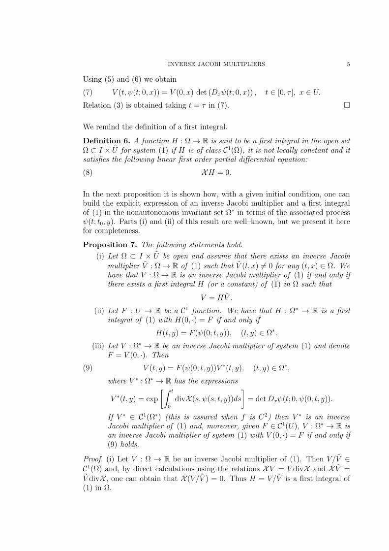
Relation (3) is obtained taking t = τ in (7).

We remind the definition of a first integral.

Definition 6. A function H : Ω → R is said to be a first integral in the open setΩ ⊂ I × U for system (1) if H is of class C1(Ω), it is not locally constant and itsatisfies the following linear first order partial differential equation:

(8) XH = 0.

In the next proposition it is shown how, with a given initial condition, one canbuild the explicit expression of an inverse Jacobi multiplier and a first integralof (1) in the nonautonomous invariant set Ω∗ in terms of the associated processψ(t; t0, y). Parts (i) and (ii) of this result are well–known, but we present it herefor completeness.

Proposition 7. The following statements hold.

(i) Let Ω ⊂ I × U be open and assume that there exists an inverse Jacobimultiplier V : Ω → R of (1) such that V (t, x) = 0 for any (t, x) ∈ Ω. Wehave that V : Ω → R is an inverse Jacobi multiplier of (1) if and only ifthere exists a first integral H (or a constant) of (1) in Ω such that

V = HV .

(ii) Let F : U → R be a C1 function. We have that H : Ω∗ → R is a firstintegral of (1) with H(0, ·) = F if and only if

H(t, y) = F (ψ(0; t, y)), (t, y) ∈ Ω∗.

(iii) Let V : Ω∗ → R be an inverse Jacobi multiplier of system (1) and denoteF = V (0, ·). Then

(9) V (t, y) = F (ψ(0; t, y))V ∗(t, y), (t, y) ∈ Ω∗,

where V ∗ : Ω∗ → R has the expressions

V ∗(t, y) = exp

[∫ t

0

divX (s, ψ(s; t, y))ds

]= detDxψ(t; 0, ψ(0; t, y)).

If V ∗ ∈ C1(Ω∗) (this is assured when f is C2) then V ∗ is an inverseJacobi multiplier of (1) and, moreover, given F ∈ C1(U), V : Ω∗ → R isan inverse Jacobi multiplier of system (1) with V (0, ·) = F if and only if(9) holds.

Proof. (i) Let V : Ω → R be an inverse Jacobi multiplier of (1). Then V/V ∈C1(Ω) and, by direct calculations using the relations XV = V divX and X V =V divX , one can obtain that X (V/V ) = 0. Thus H = V/V is a first integral of(1) in Ω.


Conversely, now let H : Ω → R be a first integral. Then HV ∈ C1(Ω) and,using the relations XH = 0 and X V = V divX , one can obtain that X (HV ) =(HV )divX . Thus V = HV is indeed an inverse Jacobi multiplier of (1) in Ω.

(ii) Let first H : Ω∗ → R be a first integral with H(0, x) = F (x) for any x ∈ U .Using that XH = 0 in Ω∗, one can see that the derivative with respect to t ofH(t, ψ(t; 0, x)) is zero for all t ∈ I(0,x). Hence H(t, ψ(t; 0, x)) = H(0, ψ(0; 0, x)) =H(0, x) = F (x) for all t ∈ I(0,x) and x ∈ U . Taking x = ψ(0; t, y) for (t, y) ∈ Ω∗

and using (iv) of Lemma 4 we obtain the conclusion.Conversely, let now H(t, y) = F (ψ(0; t, y)) for all (t, y) ∈ Ω∗. Using again

Lemma 4 one can see thatH satisfies for any x ∈ U and t ∈ I(0,x),H(t, ψ(t; 0, x)) =F (x). Taking the derivative with respect to t we obtain that H satisfies XH = 0in Ω∗.

(iii) Like in the proof of Theorem 2 one can show that V satisfies (5) for anyx ∈ U and t ∈ I(0,x). In (5) we put F (x) instead of V (0, x), and x = ψ(0; t, y)for (t, y) ∈ Ω∗ such that finally we obtain (9) with V ∗ having the first expressiongiven in the statement. In order to obtain the second expression of V ∗ we replacex = ψ(0; t, y) for (t, y) ∈ Ω∗ in (6).

Finally assume that V ∗ ∈ C1(Ω∗) and note that, taking in its expression y =ψ(t; 0, x), for any x ∈ U and t ∈ I(0,x) we obtain

(10) V ∗(t, ψ(t; 0, x)) = exp

[∫ t

0


].

Taking the derivative with respect to the variable t in (10) one obtains the relationXV ∗ = V ∗divX which holds true in any point of the form (t, ψ(t; 0, x)), hence inany (t, y) ∈ Ω∗. Now let F ∈ C1(U). Since, by (ii), F (ψ(0; t, y)) is a first integral,and V ∗ is an inverse Jacobi multiplier in Ω∗, applying (i) we obtain that V givenby (9) is indeed an inverse Jacobi multiplier.

In the next example we see the expression of V ∗ (given in Proposition 7 (iii)) fora linear system.

Example 8. Let A ∈ C(R,Rn×n) and b ∈ C(R,Rn). For a linear differentialsystem x = A(t)x + b(t) we have that the inverse Jacobi multiplier V ∗ is given

by V ∗(t, x) = exp(∫ t

0Tr(A(s)) ds

), for all (t, x) ∈ R×Rn where Tr(A(s)) is the

trace of A(s). We can choose here U = Rn and find that Ω∗ = R× Rn.

Now, for the simple scalar equation x = x3, we present its family of time-dependent inverse Jacobi multipliers. This is just to see how Proposition 7 works.Anyway, in some problems it is important to know the expression of an inverseJacobi multiplier of some system in order to study perturbations of that system(see [9, 10, 4, 14].

Example 9. We consider the differential equation x = x3 in R2. For any t0, x ∈R we have ψ(t; t0, x) = x/

√1− 2(t− t0)x2, I(t0,x) = (−∞, t0+1/(2x2)) for x = 0


and I(t0,0) = R. Choosing U = R one can find that Ω∗ = (t, x) ∈ R2 : 1+2tx2 >0 and, for an inverse Jacobi multiplier V in Ω∗ with F = V (0, ·) we have

V (t, x) = F (x/√1 + 2tx2)(1 + 2tx2)3/2, (t, x) ∈ Ω∗.

If we take, for example, F1(x) = x or F2(x) = x3 for all x ∈ R we obtain twoinverse Jacobi multipliers V1(t, x) = x+ 2tx3 and V2(x) = x3, respectively. Notethat they are defined in the whole R2 and they satisfy (2) in the whole R2. Here(2) is ∂V /∂t+ x3∂V /∂x = 3x2V.

The following is the usual definition of a set of C1 (functionally) independentreal functions, see for example page 436 of [5]. We consider it for a set of firstintegrals of (1) and we will use it in the next Section.

Definition 10. Let 1 ≤ k ≤ n and Ω ⊂ I × U be open. We say that kfirst integrals H1, . . . , Hk of (1) are independent in Ω if the gradient vectors∇H1(t, y), . . . ,∇Hk(t, y) are linearly independent for each (t, y) ∈ Ω.

In the next proposition we will see that n first integrals H1, . . . , Hn of (1)are independent in Ω∗ if and only if the map F : U → Rn defined by F =(H1(0, ·), . . . , Hn(0, ·)) is a local diffeomorphism. This result must be known, westate and prove it for completeness and also for further use.

Proposition 11. The set of n first integrals H1, . . . , Hn of (1) are independent inΩ∗ if and only if the C1 function F = H(0, ·) : U → Rn, where H = (H1, . . . , Hn),is such that detDF (x) = 0 for all x ∈ U .

Proof. We take n first integrals H1, . . . , Hn which are independent in Ω∗ andconsider F and H like in the statement of this Proposition. Using Proposition 7(ii) we must have

(11) H(t, y) = F (ψ(0; t, y)), (t, y) ∈ Ω∗.

In order to prove that the set of vectors ∇H1(t, y), . . . ,∇Hn(t, y) from Rn+1 arelinearly independent for each (t, y) ∈ Ω∗, it is necessary and sufficient to provethat the n×(n+1) matrix DH(t, y) has constant rank n in Ω∗. Since using (8) weobtain ∂H/∂t = −DyH f , we deduce that DH(t, y) has constant rank n in Ω∗ if

and only if detDyH(t, y) = 0 for all (t, y) ∈ Ω∗. But using the chain rule and (11)

we get DyH(t, y) = DF (ψ(0; t, y))Dyψ(0; t, y). Using Liouville’s formula like

in the proof of Theorem 2, detDyψ(0; t, y) = exp(∫ 0

tdivX (s, ψ(s; t, y)ds) = 0.

Hence detDyH(t, y) = 0 for all (t, y) ∈ Ω∗ if and only if det F (ψ(0; t, y)) = 0 for

all (t, y) ∈ Ω∗, which is equivalent to det F (x) = 0 for all x ∈ U .

For our next result we will need the following stronger notion of independencefor n first integrals of (1). This notion essentially requires that the local dif-feomorphism F : U → F (U) defined in Proposition 11 to be actually a globaldiffeomorphism. This justifies the use of the term globally in the following defi-nition.


Definition 12. We say that n first integrals H1, . . . , Hn of (1) in Ω∗ are globallyindependent if F = H(0, ·) : U → Rn is a diffeomorphism onto its image, whereH = (H1, . . . , Hn).

Corollary 13. Assume that f ∈ Cm(I× U ,Rn) with m ∈ N∗∪∞. Then thereare n first integrals of (1) in Ω∗ of class Cm(Ω∗) which are globally independent.

Proof. Take any diffeomorphism F : U → F (U) of class Cm and define thefunction H : Ω∗ → Rn by H(t, y) = F (ψ(0; t, y)). Then using Lemma 4 (i) we getthat H ∈ Cm(Ω∗,Rn) and by Proposition 7 (ii) we obtain that its components arefirst integrals of (1) in Ω∗. Clearly, these first integrals are globally independentin Ω∗ by construction since F = H(0, ·).

As is well-known, independent first integrals can be used to describe any otherfirst integral or inverse Jacobi multiplier. We state below this idea for the nglobally independent first integrals given by Corollary 13.

Proposition 14. Assume that f ∈ Cm(I × U ,Rn) with m ∈ N∗ ∪ ∞. LetH1, . . . , Hn be Cm first integrals of (1) in Ω∗ which are globally independent.Define the vector function H = (H1, . . . , Hn). Then we have.

(i) H : Ω∗ → R is a Cm first integral of (1) if and only if there exists a Cm

function ϕ which is not locally constant and such that H = ϕ(H) on Ω∗.

(ii) Let m ≥ 2 and V ∗ : Ω∗ → R as given in Proposition 7, i.e.

V ∗(t, y) = exp

[∫ t

0

divX (s, ψ(s; t, y))ds

].

V : Ω∗ → R is a Cm−1 inverse Jacobi multiplier of (1) linearly indepen-dent with V ∗ if and only if there exists a Cm−1 function ϕ which is notlocally constant and such that V = ϕ(H)V ∗ on Ω∗.

Proof. First we recall that the inverse Jacobi multiplier V ∗ defined in Proposition7 (iii) is of class Cm−1 at least and satisfies V ∗(t, y) = 0 for any (t, y) ∈ Ω∗.Second, since H1, . . . , Hn are Cm first integrals of (1) in Ω∗ by hypothesis, wecan define according to Definition 12 the diffeomorphism F : U → F (U) of classCm as F (x) = H(0, x).

(i) Let H : Ω∗ → R be a Cm first integral of (1), take F = H(0, ·) andϕ = F F−1. Then ϕ is Cm and F = ϕ(F ) on U and, further, F (ψ(0; t, y)) =ϕ(F (ψ(0; t, y))) for all (t, y) ∈ Ω∗. But, using Proposition 7, this last relationreads as H = ϕ(H) on Ω∗. The fact that, given some Cm function ϕ, ϕ(H) is aCm first integral follows using Definition 6 of a first integral.

Statement (ii) follows using the previous one and Proposition 7.


3. Periodic inverse Jacobi multipliers and periodic first integrals

In this section we always assume what we call Hypotheses * in the Introduction.Under these hypothesis it is known that a solution ψ(·; 0, x) : [0, T ] → Rn ofsystem (1) satisfying ψ(0; 0, x) = ψ(T ; 0, x) is actually a T -periodic solution, inthe sense that it has an extension to R which is a T -periodic solution. Hencex ∈ U is a fixed point of the Poincare map Π : U → U if and only if ψ(·; 0, x) isa T -periodic solution of (1).

Remark 15. If system (1) has a T -periodic solution ψ(t; 0, x) then there existsan open neighborhood U of x that satisfies statement (c) from Hypotheses *. Inorder to justify this fact, one can use Lemma 6.6 and Theorem 7.6 from [1].

Let U0 ⊂ U be open. We say that an inverse Jacobi multiplier V of system (1) isT -periodic in R× U0 if V (t, x) = V (t+ T, x) for all t ∈ R and x ∈ U0. Similarlywe define the T -periodicity of a first integral H in R× U0.

Theorem 3 stated in the Introduction shows how the existence of sufficientlymany T -periodic and independent first integrals and nonvanishing T -periodic in-verse Jacobi multipliers in R× U assures the existence of continua of T -periodicsolutions.

Proof of Theorem 3. (i) Denote H = (H1, ..., Hn) having as components the nindependent first integrals in R×U that are T -periodic. First consider the set Ω∗

defined by (4) in the case U = U , i.e. Ω∗ = (t, ψ(t; 0, x)) : x ∈ U , t ∈ I(0,x).Since Ω∗ ⊂ R × U , we also have that H1, . . . , Hn are independent in Ω∗. Wemade these considerations in order to apply Proposition 11 and deduce thatF : U → Rn defined by F = H(0, ·) is a local diffeomorphism. We can take

an open set U ⊂ U ⊂ U , where U is from Hypotheses *, such that x ∈ U andF : U → F (U) is a diffeomorphism. We consider now the corresponding set Ω∗

defined by (4) for U , i.e. Ω∗ = (t, ψ(t; 0, x)) : x ∈ U , t ∈ I(0,x) and note that

we have Ω∗ ⊂ Ω∗. From Proposition 7 (ii) we have that H(t, y) = F (ψ(0; t, y))

for all y ∈ ψ(t; 0, U) and t ∈ [0, T ]. We define U0 = U ∩ ψ(T ; 0, U) and notethat U0 is an open neighborhood of x and that both H(0, y) and H(T, y) arewell-defined for any y ∈ U0. Since H(·, x) is T -periodic for any x ∈ U , we must

have F (ψ(0; 0, y)) = F (ψ(0;T, y)) for any y ∈ U0. From here (recalling that

ψ(0; 0, y) = y and that F is a diffeomorphism in U) it follows that y = ψ(0;T, y)for all y ∈ U0, that further gives ψ(T ; 0, x) = x for all x ∈ U0. This assures thatψ(·; 0, x) is T -periodic for any x ∈ U0.

(ii) Denote H1, . . . , Hn−1 the n−1 independent first integrals in R×U that areT -periodic. In particular the gradient vectors ∇xH1(0, x), . . . ,∇xHn−1(0, x) arelinearly independent for all x ∈ U and this implies that we can select a C1 functionFn : U → R to obtain F : U → Rn defined by F = (H1(0, ·), . . . , Hn−1(0, ·), Fn)satisfying detDF (x) = 0 for any x ∈ U (if necessary, U can eventually be


smaller). Like in (i), there is a sufficiently small open set U ⊂ U ⊂ U with

x ∈ U and such that F : U → F (U) is a diffeomorphism. Consider again

Ω∗ = (t, ψ(t; 0, x)) : x ∈ U , t ∈ I(0,x) and Hn(t, y) = Fn(ψ(0; t, y)) for all

(t, y) ∈ Ω∗. Then, if we denote H = (H1, . . . , Hn−1, Hn) we have H(t, y) =

F (ψ(0; t, y)) for any (t, y) ∈ Ω∗. We define as in (i) the open neighborhood of x

given by U0 = U ∩ ψ(T ; 0, U).Since the first n − 1 components of H(·, x) are T -periodic for any x ∈ U , we

have that the first n−1 components of F (y) and of F (ψ(0;T, y)) are the same forany y ∈ U0. Then for each h = (h1, . . . , hn) ∈ F (U0) the first n− 1 componentsof F ψ(0;T, ·) F−1(h) are h1, ..., hn−1. From here we deduce that the inverseof this map shares the same property. Denote now U0 = F (ψ(0;T, U0)) and notethat it is an open neighborhood of F (x). But, using properties of the inverses ofcompositions and recalling that the inverse of ψ(0;T, ·) is ψ(T ; 0, ·), one can seethat the inverse of F ψ(0;T, ·) F−1 : F (U0) → U0 is just F ψ(T ; 0, ·) F−1 :U0 → F (U0).

After all these, taking into account the definition of the Poincare map Π =ψ(T ; 0, ·), we obtain that for each h ∈ U0 the first n− 1 components of F Π F−1(h) are h1, ..., hn−1. We denote the last component of this function by p(h).In this way we obtain p : U0 → R, which is C1, such that

F Π F−1(h) =

h1. . .hn−1

p(h)

with h =

h1. . .hn−1

hn

.

Since ψ(·; 0, x) is T -periodic, we have that Π(x) = x and further, denoting

h = F (x)

we obtain

F Π F−1(h) = h.

This gives p(h) = hn. We define the C1 scalar function p of a scalar variable

µ 7→ p(µ) = p(h1, ..., hn−1, µ)

where the variable µ ranges in an open neighborhood of hn. Hence we have

(12) F Π F−1

h1. . .

hn−1

µ

=

h1. . .

hn−1

p(µ)

.

We observe that

p(hn) = hn.

We claim that p is the identity map in an open neighborhood of hn. For any µin that neighborhood we denote

x∗(µ) = F−1(h1, ..., hn−1, µ).


Then Π(x∗(µ)) = x∗(µ) finishing the proof.

It remains to prove the claim. For this we need to use the existence of an inverseJacobi multiplier. The hypotheses of Theorem 2 are fulfilled for the inverseJacobi multiplier V : R× U → R, hence (3) is satisfied. Using that V (0, x) = 0for all x ∈ U and that, by T -periodicity of V , V (T,Π(x)) = V (0,Π(x)) for anyx ∈ U , (3) gives

(13) detDΠ(x) =V (0,Π(x))

V (0, x)for all x ∈ U.

This is a fully nonlinear first order partial differential equation for the Poincaremap Π, which has as solution the identity map. Of course, when n = 1 thisreduces to a first order scalar ordinary differential equation for Π. In arbitrarydimensions, using (13), we will find that p(µ) satisfies a first order scalar ordi-nary differential equation. For this we compute the determinant of the Jacobianmatrix of F Π F−1 in two ways. First we take into account the structure ofthis map emphasized before, so that

D(F Π F−1

)=

(In−1

∂p∂hn

)where In denotes the identity matrix of order n. Therefore we obtain that

detD(F Π F−1

)=

∂p

∂hn.

Second, we use the chain rule and properties of determinants so that

detD(F Π F−1

)= detDF

(Π F−1

)detDΠ

(F−1

)detDF−1.

Using the two relations above and (13) we obtain that

(14)∂p

∂hn= detDF

(Π F−1

) V (0,Π F−1)

V (0, F−1)detDF−1

holds for every variable h ∈ U0. If we write (14) only for the vectors

hµ =

h1. . .

hn−1

µ

,

using (12), we obtain

(15)dp

dµ(µ) = detDF

(F−1(hp(µ))

) V (0, F−1(hp(µ)))

V (0, F−1(hµ))detDF−1(hµ).

Hence p is the unique solution of the Cauchy problem for the ordinary differentialequation (15) with the initial condition p(hn) = hn. It is not difficult to see that

the identity function p(µ) = µ, with µ in a neighborhood of hn, is the solutionof this initial value problem. The claim is proved.


Remark 16. The assumption that there exists n− 1 independent first integralswhich are T -periodic in Theorem 3 (ii) is essential when n ≥ 2 as the followingexample shows. We consider the linear 2-dimensional system x = A(t)x with thecontinuous T -periodic in R diagonal matrix A(t) = diaga1(t), a2(t) such that∫ T

0ai(s)ds = 0 for i = 1, 2 but

∫ T

0(a1(s) + a2(s))ds = 0. This system has the

T -periodic inverse Jacobi multiplier V ∗(t, x) = exp(∫ t

0[a1(s) + a2(s)]ds

)with

V ∗(0, x) = 1, but the only T -periodic solution is the trivial one ψ(t; 0, (0, 0)) =(0, 0) as can be easily shown using the theory of linear systems under the condi-tions imposed to the coefficients of the system.

Example 17. Let us consider the following family of systems defined in R×R2:

(16) x1 = a1(t)x1 + xk11 F1(t, x2) , x2 = a2(t)x2 + xk22 F2(t, x1) ,

where ki ∈ N, and ai ∈ C(R) are T -periodic functions satisfying∫ T

0ai(s)ds = 0.

The system admits the T -periodic in R× R2 inverse Jacobi multiplier

V (t, x1, x2) = xk11 xk22 exp

(∫ t

0

[(1− k1)a1(s) + (1− k2)a2(s)]ds

).

Hence V (0, x1, x2) = 0 if (x1, x2) ∈ U = (x1, x2) ∈ R2 : x1x2 = 0.Notice that the axis of coordinates are invariant under the process and we have

ψ(t; 0, (x1, 0)) =

(x1 exp

(∫ t

0

a1(s)ds

), 0

),

ψ(t; 0, (0, x2)) =

(0, x2 exp

(∫ t

0

a2(s)ds

)).

In particular the origin is an equilibrium and ψ(t; 0, (x1, 0)) and ψ(t; 0, (0, x2))are (non-isolated) T -periodic solutions for each x1 ∈ R and x2 ∈ R. Now thequestion is: what about the T -periodicity of ψ(t; 0, (x1, x2)) with x1x2 = 0? Canthe system have isolated T -periodic solutions?

To give a partial answer to this question we consider the particular case of (16),

(17) x1 = a1(t)x1 −m2b(t)xk11 x

k2−12 , x2 = a2(t)x2 +m1b(t)x

k1−11 xk22 ,

with mi ∈ N and b ∈ C(R). We found for (17) the T -periodic first integral

H(t, x1, x2) = xm11 xm2

2 exp

(−∫ t

0

[m1a1(s) +m2a2(s)]ds

)in R× R2.

One can see that ∇H(t, x1, x2) = (0, 0, 0) if (t, x1, x2) ∈ R × U . We intend toapply Theorem 3 (ii) in order to deduce that (17) does not have isolated T -periodic solutions. Let ψ(t; 0, (x1, x2)) be a T -periodic solution with x1x2 = 0(when x1x2 = 0 we already know that it is not isolated). Take U an openneighborhood of (x1, x2) with the properties guaranteed in Remark 15. We canassume that U ⊂ U . We conclude now that all the hypotheses of Theorem 3 (ii)are fulfilled with n = 2, the first integral H and the inverse Jacobi multiplier Vgiven above. Hence, indeed the T -periodic solution ψ(t; 0, (x1, x2)) (if it exists)is not isolated in the set of T -periodic solutions of (17).


An interesting particular case of system (1) is when it is divergence free, i.e.divX =

∑ni=1 ∂fi/∂xi = 0 in I × U . In this case the inverse Jacobi multiplier

V ∗ given in Proposition 7 (ii) is simply V ∗ = 1, hence always T -periodic andnon-null. Theorem 3 (ii) becomes in this case.

Corollary 18. Assume Hypothesis * and that there exists x ∈ U such thatψ(·; 0, x) is a T -periodic solution of (1). Assume, in addition, that div X = 0in I × U . If there exist n − 1 independent first integrals in R × U which areT -periodic then the T -periodic solution ψ(·; 0, x) is included into a 1-parameterfamily of T -periodic solutions ψ(t; 0, x∗(µ)), where x∗ is a C1 function in someopen interval of reals.

We restate now Theorem 3 in the particular case n = 1, but introducing the smallimprovement that the conclusion holds globally. The proof does not introduceany new idea.

Theorem 19. Let n = 1. Assume Hypothesis * and that there exists x ∈ U suchthat ψ(·; 0, x) is a T -periodic solution of (1).

(i) If there exists a first integral H in R × U of (1) which is T -periodicand such that H(0, ·) : U → R is a diffeomorphism onto its image, thenψ(·; 0, x) is T -periodic for any initial condition x ∈ U ∩ ψ(T ; 0, U).

(ii) If there exist an inverse Jacobi multiplier V in R× U which is T -periodicand such that V (0, x) = 0 for all x ∈ U , then ψ(·; 0, x) is T -periodic forany x ∈ U .

Proof. Part (i) can be easily seen following the proof of Theorem 3 (i).

(ii) In this particular case we need only relation (13) from the proof of Theorem3 (ii), that gives that the Poincare map Π : U → U is a solution of the ordinarydifferential equation

Π′(x) =V (0,Π(x))

V (0, x), x ∈ U.

In addition, we have that Π(x) = x. We deduce using the uniqueness of thesolution of an ordinary differential equation with C1 right-hand side, that wemust have Π(x) = x for any x ∈ U .

Remark 20. The assumption that there exists a T -periodic solution ψ(·; 0, x)with x ∈ U is essential in Theorem 19 (i) as the following example shows. Weconsider the scalar ordinary differential equation x = x, with I = R, U = (0,∞)and U = (1, 2). One can check that H(t, x) = sin(t− lnx) is a 2π-periodic firstintegral in R× U of x = x. Moreover, H(0, x) = − sin(lnx) is a diffeomorphismfrom U = (1, 2) onto its image. But it is easy to see that none of the solutionsψ(·; 0, x) with x ∈ U is 2π-periodic. In fact here we have that U ∩ ψ(2π; 0, U) =(1, 2) ∩ (e2π, 2e2π) = ∅.


Remark 21. The assumption that there exists a T -periodic solution ψ(·; 0, x)with x ∈ U is essential in Theorem 19 (ii) as the following example shows. Weconsider the scalar linear ordinary differential equation x = a(t)x + b(t), where

a, b are continuous and T -periodic scalar functions. Assume that∫ T

0a(s)ds = 0

and∫ T

0exp

(−∫ t

0a(s)ds

)b(t)dt = 0. In these conditions this linear differential

equation has no T -periodic solution. Take I = U = U = R. One can check that

V (t, x) = V ∗(t, x) = exp(∫ t

0a(s)ds

)is a T -periodic inverse Jacobi multiplier in

R× R that also satisfies V (0, x) = 1 = 0.

Remark 22. The assumption that V (0, x) = 0 for all x ∈ U is essential inTheorem 19 (ii) as the following example shows. We consider again the scalarordinary differential equation x = x, this time with I = U = U = R and T > 0arbitrary fixed. We have that the solution ψ(t; 0, 0) = 0 is T -periodic and theinverse Jacobi multiplier V (t, x) = x is also T -periodic in R× R. But there areno other T -periodic solutions of x = x.

We are interested now to study the reciprocal of Theorem 3 (i). The next Lemmaand Theorem state in what conditions is valid.

Lemma 23. Assume Hypothesis * and suppose that ψ(·; 0, x) is T -periodic forall x ∈ U . Let H : Ω∗ → R and V : Ω∗ → R be a first integral, and, respectively,an inverse Jacobi multiplier of (1). Then

H(t+ T, y) = H(t, y) and V (t+ T, y) = V (t, y) for all (t, y) ∈ Ω∗.

If there exists an open set U0 ⊂ U such that R×U0 ⊂ Ω∗ then both H and V areT -periodic in R× U0.

Proof. Let (t, y) ∈ Ω∗, and denote x = ψ(0; t, y) ∈ U . Then y = ψ(t; 0, x) =ψ(t + T ; 0, x) and, further, x = ψ(0; t + T, y). Thus, using the hypothesis thatψ(·; 0, x) is T -periodic for any x ∈ U , we have proved that

(18) ψ(0; t+ T, y) = ψ(0; t, y) for any (t, y) ∈ Ω∗.

Now, the T -periodicity of ψ(·; 0, x) for any x ∈ U assures also the T -periodicityof Dxψ(·; 0, x) for any x ∈ U . This fact and relation (18) assure that V ∗(t, y) =det (Dxψ(t; 0, ψ(0; t, y))) that appears in Proposition 7 satisfies

(19) V ∗(t+ T, y) = V ∗(t, y) for any (t, y) ∈ Ω∗.

The conclusion follows using the expressions of H and V given in Proposition 7and relations (18) and (19).

Theorem 24. Assume Hypothesis * and suppose that ψ(·; 0, x) is T -periodic forall x ∈ U . Fix x ∈ U and denote φ = ψ(·; 0, x). Let H : Ω∗ → R and V : Ω∗ → Rbe a first integral, and, respectively, an inverse Jacobi multiplier of (1). Thenthere exists an open neighborhood U0 ⊂ U of x such that

H(t+ T, y + φ(t)) = H(t, y + φ(t)) and V (t+ T, y + φ(t)) = V (t, y + φ(t)),


for all t ∈ R and y ∈ U0. In particular, if ψ(t; 0, x) = x for all t ∈ R then H andV are T -periodic in R× U0.

Proof. We consider first the particular case that the fixed solution is the nullsolution, i.e. ψ(t; 0, 0) = 0 for all t ∈ R. In this case, for any t ∈ [0, T ] we havethat ψ(t; 0, U) is an open neighborhood of 0, which implies that

(20) U0 =∩

t∈[0,T ]

ψ(t; 0, U) ⊂ U

is an open neighborhood of 0. Since Ω∗ = (t, ψ(t; 0, x)) : t ∈ R, x ∈ U) andψ(·; 0, x) is T -periodic for all x ∈ U , from the definition of U0 it is clear thatR× U0 ⊂ Ω∗. The conclusion follows by Lemma 23.

Consider now the general case and let H and V like in the hypothesis. Weintroduce the new variable u = x−φ(t) so that equation (1) is transformed intoequation

(21) u = f(t, u+ φ(t))− f(t, φ(t)).

Its process γ satisfies γ(t; 0; u) = ψ(t; 0, u+ x)− φ(t) for all u ∈ U − x, assuringthat γ(·; 0, u) is T -periodic for all u ∈ U − x and that γ(t; 0, 0) = 0 for all t ∈ R.Then equation (21) is in the particular case solved before. It can be easily shownthat H(t, u + φ(t)) and V (t, u + φ(t)) is a first integral, and, respectively, aninverse Jacobi multiplier of (21). Thus they are T -periodic in R×U0. The proofis done.

References

[1] H. Amann, Ordinary Differential Equations. An Introduction to Nonlinear Analysis, deGruyter Studies in Mathematics, 13 Walter de Gruyter & Co., Berlin, 1990.

[2] L.R. Berrone and H. Giacomini, Inverse Jacobi multipliers, Rend. Circ. Mat. Palermo(2) 52 (2003), 77–130.

[3] A. Buica, I. A. Garcıa and S. Maza, Existence of inverse Jacobi multipliers aroundHopf points in R3: emphasis on the center problem, J. Differential Equations 252 (2012),6324–6336.

[4] A. Buica, I. A. Garcıa, S. Maza, Multiple Hopf bifurcation in R3 and inverse Jacobimultipliers , J. Differential Equations 256 (2014), 310–325.

[5] C. Chicone, Ordinary Differential Equations with Applications. (2 ed.), New York:Springer-Verlag, 2006.

[6] A. Enciso and D. Peralta-Salas, Existence and vanishing set of inverse integratingfactors for analytic vector fields, Bull. London Math. Soc. 41 (2009), 1112–1124.

[7] R. Flores-Espinoza, Periodic first integrals for Hamiltonian systems of Lie type, Int.J. Geom. Meth. Mod. Phys. 8 (2011), 1169-1177.

[8] I.A. Garcıa and M. Grau, A survey on the inverse integrating factor, Qual. TheoryDyn. Syst. 9 (2010), 115-166.

[9] I.A. Garcıa, H. Giacomini and M. Grau, The inverse integrating factor and thePoincare map, Trans. Amer. Math. Soc. 362 (2010), 3591–3612.

[10] I.A. Garcıa, H. Giacomini and M. Grau, Generalized Hopf bifurcation for planarvector fields via the inverse integrating factor, J. Dyn. Differ. Equ. 23 (2011), 251–281.

[11] J.K. Hale, Ordinary Differential Equations, 2nd Edition, Robert E. Krieger PublishingCo., Huntington, NY, 1980.


[12] C.G.J. Jacobi, Sul principio dellultimo moltiplicatore, e suo uso come nuovo principiogenerale di meccanica, Giornale Arcadico di Scienze, Lettere ed Arti 99 (1844), 129-146.

[13] P.E. Kloeden and M. Rasmussen, Nonautonomous Dynamical Systems, MathematicalSurveys and Monographs 176, American Mathematical Society, 2011.

[14] X. Zhang, Inverse Jacobian multipliers and Hopf bifurcation on center manifolds, J.Differential Equations 256 (2014), 3552–3567.

1 Department of Mathematics, Babes-Bolyai University, Kogalniceanu 1, 400084Cluj-Napoca, Romania

E-mail address: [email protected]

2 Departament de Matematica, Universitat de Lleida, Avda. Jaume II, 69,25001 Lleida, Spain

E-mail address: [email protected]

Inverse Jacobi multipliers and first integrals for nonautonomous differential systems

Documents

Transcript of Inverse Jacobi multipliers and first integrals for nonautonomous differential systems