Characterization of Passive Intermodulation Distortion in ...
86
IN DEGREE PROJECT INFORMATION AND COMMUNICATION TECHNOLOGY, SECOND CYCLE, 30 CREDITS , STOCKHOLM SWEDEN 2019 Characterization of Passive Intermodulation Distortion in MultiBand FDD Radio Systems TOMÁS SOARES DA COSTA KTH ROYAL INSTITUTE OF TECHNOLOGY SCHOOL OF ELECTRICAL ENGINEERING AND COMPUTER SCIENCE
-
Upload
khangminh22 -
Category
Documents
-
view
5 -
download
0
Transcript of Characterization of Passive Intermodulation Distortion in ...

IN DEGREE PROJECT INFORMATION AND COMMUNICATION TECHNOLOGY,SECOND CYCLE, 30 CREDITS
, STOCKHOLM SWEDEN 2019
Characterization of Passive Intermodulation Distortion in MultiBand FDD Radio Systems
TOMÁS SOARES DA COSTA
KTH ROYAL INSTITUTE OF TECHNOLOGYSCHOOL OF ELECTRICAL ENGINEERING AND COMPUTER SCIENCE


Characterization of Passive Intermodulation
Distortion in MultiBand FDD Radio Systems
TOMAS SOARES DA COSTA
Stockholm September, 2019
Communication Systems
School of Electrical Engineering and Computer Science
Kungliga Tekniska Hogskolan


Supervisors:
Adnan Kiayani, Ph.D.
Department of Algorithm System Design,
Ericsson AB
Stockholm, Sweden
Claes Beckman, Ph.D., Professor
Department of Wireless Communications,
Kungliga Tekniska Hogskolan
Stockholm, Sweden
Examiner:
Slimane Ben, Ph.D., Professor
Department of Wireless Communications,
Kungliga Tekniska Hogskolan
Stockholm, Sweden
Opposition:
Joao Torres,
Information and Communication Technology,
Kungliga Tekniska Hogskolan
Stockholm, Sweden


Abstract
Intermodulation distortion (IMD) is a phenomenon that results in generation of spurious
distortion signals when two or more signals of different frequencies pass through a nonlin-
ear system. In general, IMD occurs in active circuits of a radio system, however, passive
wireless components such as filters, transmission lines, connectors, antennas, attenuators
etc., can also generate IMD particularly when transmit power is very high. The IMD
in the latter case is referred to as passive intermodulation (PIM) distortion. With the
continuing advancement of radio system coupled with the radio spectrum scarcity, PIM
interference is recognized as a potential obstacle to achieving the full capacity of a radio
network.
The assiduous enhancement of radio systems for faster data speeds and higher capacity
further exacerbate the PIM interference problem. Features like carrier aggregation (CA)
and multiple input multiple output (MIMO) make the PIM a more problematic issue. In
modern co-sites, radio systems are often coupled together, operating in multiple bands.
Furthermore, in frequency division duplex (FDD) systems, transmitter (Tx) and receiver
(Rx) operate simultaneously. In such scenarios, PIM is likely to occur in the signal’s
path and may potentially hit multiple Rx bands causing undesired interference.
The PIM sources in the BS radio systems can be divided into two groups, namely
internal and external. Internal sources are the passive components within the radio such
as filters, transmission lines, connectors, antennas, etc. External sources, on the other
hand, are the passive elements beyond the BS antenna but within the RF signal path
such as metallic and rusty objects in antenna near field. For both types of sources,
the high power current flowing through such passive objects can prompt a nonlinear
behavior that in turn generates IMD.
This thesis addresses PIM distortion in multiband BS radio systems by devising a charac-
terization. For this purpose, the research begins by establishing a mathematical model
for IMD and reviewing the physics that prompt nonlinear behavior in these sources.
Afterwards, the enhancements in radio systems that enlarge the bandwidths and ex-
acerbate PIM are discussed. In particular, how IMD is worsen in broadband radios is
iii

Abstract iv
highlighted, and to complement this discussion, a review of PIM mitigation techniques
is also presented. In the final part of this work, extensive lab measurement results are
presented where effects of PIM with external PIM sources are analyzed and discussed.
Overall, this thesis helps to build a better understanding of PIM interference problem
in radio systems by providing useful insights into the nonlinear mechanisms in passive
components causing PIM.

Abstrakt
Harmonisk distorsion eller ”Intermodulationsdistorsion” (IMD) ar ett fenomen som
resulterar i generering av falska signaler nar tva eller flera radiosignaler med olika
frekvenser blandas nar de passerar genom ett olinjart system. I allmanhet forekommer
IMD i aktiva kretsar i ett radiosystem. Emellertid, passiva tradlosa komponenter sasom
filter, transmissionsledningar, kontakter, antenner, dampare etc., kan ocksa generera
IMD, sarskilt nar sandningseffekten ar mycket hog. IMD i det senare fallet kallas ”pas-
siv intermodulationsdistorsion” (PIM). De senaste arens utveckling av mer avancerade
radiosystem, i kombination med radiospektrumbrist, har inneburit att PIM idag ses
som ett av de storsta potentiella hindren for att uppna den fulla kapaciteten i tex 5G
radionatverk.
Den standiga utvecklingen av de cellulara radiosystemen mot hogre datahastigheter och
hogre kapacitet forvarrar ytterligare PIM-storningsproblemet: Funktioner som barvags
aggregering (carrier aggregation, CA) och ”multiple input multiple output” (MIMO)
system gor PIM till ett annu storre problem. I moderna samarbetsplatser, radiosystem
ar ofta kopplade ihop och fungerar i flera band.
I system med frekvensduplex (FDD-system), dar sandare (Tx) och mottagare (Rx) ar-
betar samtidigt men pa skilda frekvenser, kan PIM med hog sannolikhet intraffa i sig-
nalenvagen och dess distortionsprodukter potentiellt traffa flera Rx-band och darmed
orsakar oonskad storning.
PIM-kallorna i Basstationssystemen kan delas in i tva grupper: interna och externa.
Interna kallor ar passiva komponenter inne i radion sasom filter, transmissionslinjer,
kontakter, antenner etc. Externa kallor a andra sidan ar de passiva elementen bortom
Basstations-antennen men inom RF-signalvagen sasom metalliska och rostiga foremal i
antennen narfalt. For bada typerna av kallor ar det den hoga effekttatheten som far
sadana passiva objekt att uppvisa ett elektriskt olinjar beteende som i sin tur genererar
IMD.
v

Abstrakt vi
Denna avhandling behandlar PIM-distorsion i basstationssystem for multipla frekvens-
band genom att utforma en karaktarisering av de genererade signalerna. For detta
andamal borjar studien med att skapa en matematisk modell for IMD och sedan granska
fysiken som skapar det olinjara beteendet i olika PIM-kallor.
Darefter diskuteras hur PIM genereras i bredbandiga radiosystem. I synnerhet diskuteras
hur IMD forvarras i bredbandiga radiosystem samtidigt som en oversikt av metoder att
motverka dess effekter pa prestandan presenteras.
I den forsta delen av denna rapport presenteras resultat fran omfattande laborato-
riematningar, dar effekterna av PIM med externa PIM-kallor analyseras och diskuteras.
Sammantaget bidrar denna avhandling till att bygga en battre forstaelse av PIM-storningsproblem
i radiosystem genom att tillhandahalla anvandbar insikter om passiva icke-linjara mekanis-
mer i komponenter som orsakar PIM.

Acknowledgments
The research work reported in this thesis was carried out during the year 2019 at the
Department of Algorithm System Design, Ericsson AB, Stockhom, and Department of
Wireless Communications, Kungliga Tekniska Hogskolan (KTH), Stockholm, Sweden.
Foremost, I would like to express my sincere gratitude to my two supervisors Dr. Adnan
Kiayani and Prof. Claes Beckman, who guided and helped me during the research of this
thesis. I am deeply grateful to Dr. Adnan Kiayani for giving me the opportunity to work
under his supervision during my time in Ericsson. His guidance and feedback instigated
in me work ethic, perfectionism and professional values that will support the remainder
of my careers. I am also grateful to my supervisor at KTH, Prof. Claes Beckman, for the
assiduous feedback and guidance. His tremendous amount of knowledge on the subject
and positive attitude gave me the curiosity to further investigate the problem and were
crucial during the research.
This thesis was financially supported by Ericsson AB, Sweden. Hence, I would like to
express my appreciation to the company itself, the HR department for handling practical
matters efficiently and everyone at the department of Algorithm System Design for
creating such an inspiring work environment. In particular, I would like to express my
gratitude to this department leader, Spendim Dalipi for giving me the opportunity to
work in Ericsson, and for being a great person to work for.
I would like to thank my beloved friends in Portugal Pedro Croca, Pedro Martins, Ruben,
Carlos, Nuno, Sebastiao, etc. for the experiences in the past five years. Without their
constant support, motivation and company, this achievement would be nothing short
than impossible. Also, I would like to extend the compliments to my peers, namely my
friends Joao Torres and Mariana Filipe, who accompanied me during my time in Sweden
and, with whom I had the pleasure to work throughout the academic year. Lastly, I
would like to thanks the faculties and professors of both IST and KTH and, in particular,
Prof. Jose Santa Rita for being my mentor and teaching me how to think.
vii

Acknowledgments viii
I would like to extend my thanks to my beloved family as I would not be the person
I am if not for them. Thanks my grandparents Rui, Dina, Fernando and Madalena,
my cousins Andre, Teresa and Miguel, and aunt Margarida. Thanks to my dad, Pedro,
thanks for inspiring me to become a engineer as well, for teaching me how to laugh
and play sports, and for attending every event I ever participated, since the first day of
school to the last soccer game. Thanks to my younger brother Martim, thanks for every
fight, argument, game, holiday, birthday, moment I got to share with you, hopefully I
will be able to repay your affection by becoming a great role model for you to follow
and by help you with your endeavors. Lastly my thanks to my wonderful mother, Carla.
You are my inspiration, and everything I ever accomplish or become is because of you.
Finally I would like to dedicate this work to the memory of my late aunt and uncle,
Eugenia and Acacio Barreiros, who, unfortunately, will not be with me when I graduate.
They were truly incredible persons whose memory I will forever cherish.
Stockholm, August 2019
Tomas Soares da Costa

Contents
Abstract iii
Abstrakt v
Acknowledgments vii
Contents ix
Abbreviations xi
1 Introduction 1
1.1 Background and Motivation . . . . . . . . . . . . . . . . . . . . . . . . . . 1
1.2 Scope and Contributions of the Thesis . . . . . . . . . . . . . . . . . . . . 3
1.3 Thesis Outline . . . . . . . . . . . . . . . . . . . . . . . . . . . . . . . . . 4
2 Fundamentals of Passive Intermodulation 5
2.1 Intermodulation Distortion . . . . . . . . . . . . . . . . . . . . . . . . . . 5
2.2 Sources of Intermodulation Distortion . . . . . . . . . . . . . . . . . . . . 8
2.2.1 Classification of PIM Sources . . . . . . . . . . . . . . . . . . . . . 9
2.3 Internal PIM sources . . . . . . . . . . . . . . . . . . . . . . . . . . . . . . 11
2.3.1 Contact Nonlinearities . . . . . . . . . . . . . . . . . . . . . . . . . 11
2.3.1.1 Metal-Insulator-Metal situations in a RF system . . . . . 12
2.3.2 Electro-Thermal PIM Sources . . . . . . . . . . . . . . . . . . . . . 14
2.3.2.1 Electro-Thermal Theory . . . . . . . . . . . . . . . . . . . 15
2.3.2.2 Distributed PIM sources . . . . . . . . . . . . . . . . . . 16
2.4 External PIM Sources . . . . . . . . . . . . . . . . . . . . . . . . . . . . . 17
2.4.1 Reflection on Metal Surfaces . . . . . . . . . . . . . . . . . . . . . 18
2.4.2 Dielectric Coating and Wave Polarization . . . . . . . . . . . . . . 19
2.4.3 External Sources as PIM Antennas . . . . . . . . . . . . . . . . . . 20
2.5 Discussion . . . . . . . . . . . . . . . . . . . . . . . . . . . . . . . . . . . . 21
ix

Contents x
3 PIM Distortion in Radio Systems 23
3.1 Evolution of Wireless Networks . . . . . . . . . . . . . . . . . . . . . . . . 24
3.1.1 Overview of 3GPP Global System for Mobile Communications . . 24
3.1.2 Overview of 3GPP Long Term Evolution . . . . . . . . . . . . . . 25
3.1.2.1 OFDMA and SC-FDMA Principles . . . . . . . . . . . . 26
3.1.3 Overview of 3GPP Long Term Evolution-Advanced . . . . . . . . . 26
3.1.3.1 Carrier Aggregation Fundamentals . . . . . . . . . . . . . 28
3.1.4 Overview of 3GPP New Radio . . . . . . . . . . . . . . . . . . . . 29
3.1.4.1 NR Physical Layer Principles . . . . . . . . . . . . . . . . 30
3.2 Passive Intermodulation Distortion in Radio Systems . . . . . . . . . . . . 31
3.2.1 Passive Intermodulation in Broadband Radio Systems . . . . . . . 32
3.2.2 Passive Intermodulation Impact on Network Performance and Phys-ical Layer . . . . . . . . . . . . . . . . . . . . . . . . . . . . . . . . 35
3.3 Passive Intermodulation Mitigation Techniques . . . . . . . . . . . . . . . 36
3.3.1 Physical Mitigation of Passive Intermodulation Interference . . . . 36
3.3.1.1 Guidelines for Mitigation of Internal Sources . . . . . . . 37
3.3.1.2 Guidelines for Mitigation of External Sources . . . . . . . 37
3.3.2 Radio Integrated Mitigation of Passive Intermodulation Interference 38
3.4 Discussion . . . . . . . . . . . . . . . . . . . . . . . . . . . . . . . . . . . . 39
4 Measurements-based Analysis of External Passive Intermodulation 41
4.1 Radio Setup and Use Cases . . . . . . . . . . . . . . . . . . . . . . . . . . 41
4.2 Power Spectral Density Analysis . . . . . . . . . . . . . . . . . . . . . . . 44
4.3 External PIM Analysis for Case Studies . . . . . . . . . . . . . . . . . . . 46
4.4 Digital Cancellation of PIM . . . . . . . . . . . . . . . . . . . . . . . . . . 51
4.5 Discussion . . . . . . . . . . . . . . . . . . . . . . . . . . . . . . . . . . . . 52
5 Conclusion and Future Work 55
Bibliography 59

Abbreviations
3GPP 3rd Generation Partnership Project
2G second generation
3G third generation
4G fourth generation
5G fifth generation
BS base station
BSS base station subsystem
Bw bandwidth
CA carrier aggregation
CC component carrier
CDMA code division multiple access
CFO carrier frequency offset
CM cubic metric
CP cyclic prefix
DFT discrete Fourier transform
DL downlink
ET electro-thermal
FDD frequency division duplexing
FDMA frequency division multiple access
GPRS general packet radio service
GSM global system for mobile communications
HD harmonic distortion
ICI intercarrier interference
IDFT inverse discrete Fourier transform
IEEE institute of electrical and electronics engineers
IM intermodulation
IMD intermodulation distortion
IM3 third-order intermodulation distortion product
IMT International Mobile Telecommunications
ISI inter symbol interference
xi
Abbreviations xii
ITU-R international telecommunication union radio communication sector
LS least squares
LTE long term evolution
LTE-A long term evolution advanced
eMBB enhanced mobile broadband
mMTC massive machine-type communications
MCS metal clamp attached to small support structure
MM metal-metal junction
MIM metal-insulator-metal
MIMO multiple input multiple output
MSC mobile-services switching center
NTL nonlinear transmission line
NR new radio
NNS network and switching subsystem
OFDM orthogonal frequency division multiplexing
OFDMA orthogonal frequency division multiple access
OSS operation support subsystem
PA power amplifier
PAPR peak-to-average power ratio
PIM passive intermodulation
PIMP passive intermodulation products
PHY physical layer
PO physical optics
PSD power spectral density
PSK phase shift keying
QAM quadrature amplitude modulation
QPSK quadrature phase shift keying
RAN radio access network
RB resource block
RF radio frequency
Rx receiver
RU radio unit
SC-FDMA single carrier frequency division multiple access
SER symbol error rate
SNR signal-to-noise ratio
SINR signal-to-interference plus noise ratio
TDPO temperature coefficients of resistance
TDPO time domain physical approach
TDD time division duplexing

Abbreviations xiii
TDMA time division multiple access
Tx transmitter
UE user equipment
UL uplink
UMTS universal mobile telecommunications system
URLLC ultra-reliable low-latency communications
WLAN wireless local area network
WB wideband


Chapter 1
Introduction
1.1 Background and Motivation
Radio systems have experienced tremendous growth during the last few decades due to
the ever-increasing demands of higher data rates, low latency, and better wireless con-
nectivity. This is due to the growing data usage in mobile devices for modern services
like multimedia contents, and the growing number of devices. Hence, existing wireless
communication systems are specified to support the data rates within the range of 100
Mbps to 1 Gbps for both uplink (UL) and downlink (DL), depending on the mobility
of the device. Currently, the 3rd Generation Partnership Project (3GPP) has defined
standards for operators to accommodate data rates of 10+ Gbps during the radio trans-
mission under various mobility conditions. In order to achieve even higher data rates,
its required wider bandwidths and better flexibility in data transmission. However,
the available bandwidth in radio-frequency (RF) spectrum is limited and, due to the
numerous wireless services available, it is becoming completely saturated.
Given the restrictions of the spectrum and available technologies at the time of release,
different generations of radio system have different operating strategies to provide in-
creased data rates. Second generation (2G) radio systems, commonly referred as Global
System for Mobile Communications (GSM), make use of narrowband Time Division
Multiple Access (TDMA) techniques to transmit (Tx) signals. This technique increased
the capacity of the radio system compared to the previous first generation (1G) tech-
nology, as it allowed more users to be accommodated within the available transmission
bandwidth. This technology uses 200 kHz wide RF channels and enables up to eight
users to access each carrier, which results in data rates around 270 kbps. The next
enhancement, third generation (3G) radio systems or Universal Mobile Telecommunica-
tions System (UMTS), was introduced to increase this data rate. UMTS uses a wideband
1

Introduction 2
Code Division Multiple Access (CDMA) technology occupying a 5 MHz wide channel
to transmit signals. In addition, this technology employs technologies like frequency
division duplex (FDD) or time division duplex (TDD) to transmit data as well as Phase
Shift Keying (PSK) modulation schemes to achieve data rates up to 2048 kbps. The next
enhancement is the fourth generation (4G) also known as Long-Term Evolution which
provides the aforementioned data rates of 100 Mbps to 1 Gbps. To realize such high data
rates, this technology employs advanced techniques including new access schemes like
Orthogonal Frequency Division Multiplexing (OFDM), higher modulation alphabets,
advanced scheduling techniques, Multiple Input Multiple Output (MIMO) antenna con-
figurations and Carrier Aggregation (CA) features to enlarge bandwidth. At the time
of writing, the next radio enhancement, fifth generation (5G) or New Radio (NR) is
on the brink of release. This technology will allow data rates of 20 Gbps in the DL
and 10 Gbps in the UL per base station (BS) using adding techniques like mmW wave
communications, i.e., utilizing available RF spectrum until 100 MHz, massive MIMO
with beam-steering and dense network systems.
In achieving extremely high data rates, a big importance is placed on both user equip-
ment (UE) and BS since they are expected to be multimode and multiband to support
the transmission. However, there are restrictions on power consumption, cost and size,
particularly on the UE side. The quality of the transmission is dependent on the sig-
nal’s quality and elements of the radio system, hence interference problems must be
minimized. Imperfections in the radio system architecture cause interference and arise
due to the technical constraints of the components. This is especially problematic in
BSs, where high amounts of current flow through the structure and affect the linearity
of its components. In these high power systems, signal paths must be kept highly linear,
or else imperfections start to arise given the nonlinear behavior. These nonlinearities
can create imperfections in the system such as intermodulation distortion (IMD).
Intermodulation (IM) is a phenomenon that occurs when one or more transmit (Tx)
signals with both one or more frequencies, or carriers, are input to a nonlinear system.
The output produced are prejudicial spurious frequencies resulting from the combination
of the input tones, i.e., prejudicial in-band and adjacent band frequency components are
generated. These unwanted spectral emissions are called spurious emissions and can
appear at the receiver (Rx) band causing interference to the desired receiver signal. If
the nonlinear system that creates these new frequency components is a passive, linear
element of these high power systems such as transmission lines, connectors, joints, etc.
(internal source) or simply a metallic component in the RF path (external source), the
phenomenon is called Passive Intermodulation distortion (PIM). The general topic of
this thesis is the investigation of PIM in multiband FDD radio system.
Introduction 3
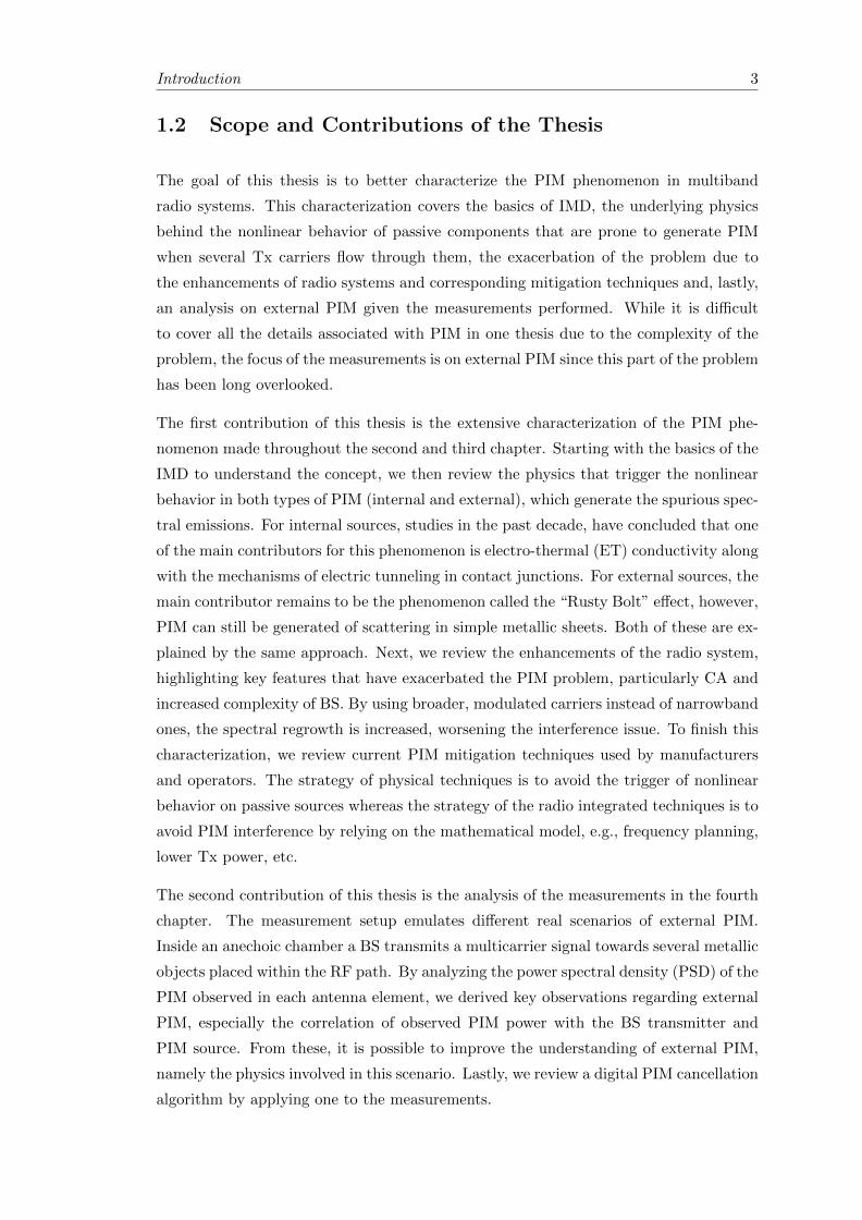
1.2 Scope and Contributions of the Thesis
The goal of this thesis is to better characterize the PIM phenomenon in multiband
radio systems. This characterization covers the basics of IMD, the underlying physics
behind the nonlinear behavior of passive components that are prone to generate PIM
when several Tx carriers flow through them, the exacerbation of the problem due to
the enhancements of radio systems and corresponding mitigation techniques and, lastly,
an analysis on external PIM given the measurements performed. While it is difficult
to cover all the details associated with PIM in one thesis due to the complexity of the
problem, the focus of the measurements is on external PIM since this part of the problem
has been long overlooked.
The first contribution of this thesis is the extensive characterization of the PIM phe-
nomenon made throughout the second and third chapter. Starting with the basics of the
IMD to understand the concept, we then review the physics that trigger the nonlinear
behavior in both types of PIM (internal and external), which generate the spurious spec-
tral emissions. For internal sources, studies in the past decade, have concluded that one
of the main contributors for this phenomenon is electro-thermal (ET) conductivity along
with the mechanisms of electric tunneling in contact junctions. For external sources, the
main contributor remains to be the phenomenon called the “Rusty Bolt” effect, however,
PIM can still be generated of scattering in simple metallic sheets. Both of these are ex-
plained by the same approach. Next, we review the enhancements of the radio system,
highlighting key features that have exacerbated the PIM problem, particularly CA and
increased complexity of BS. By using broader, modulated carriers instead of narrowband
ones, the spectral regrowth is increased, worsening the interference issue. To finish this
characterization, we review current PIM mitigation techniques used by manufacturers
and operators. The strategy of physical techniques is to avoid the trigger of nonlinear
behavior on passive sources whereas the strategy of the radio integrated techniques is to
avoid PIM interference by relying on the mathematical model, e.g., frequency planning,
lower Tx power, etc.
The second contribution of this thesis is the analysis of the measurements in the fourth
chapter. The measurement setup emulates different real scenarios of external PIM.
Inside an anechoic chamber a BS transmits a multicarrier signal towards several metallic
objects placed within the RF path. By analyzing the power spectral density (PSD) of the
PIM observed in each antenna element, we derived key observations regarding external
PIM, especially the correlation of observed PIM power with the BS transmitter and
PIM source. From these, it is possible to improve the understanding of external PIM,
namely the physics involved in this scenario. Lastly, we review a digital PIM cancellation
algorithm by applying one to the measurements.

Introduction 4
1.3 Thesis Outline
Chapter 2 of this thesis gives a literature review of intermodulation distortion, internal
and external PIM sources in radio systems, the physics of the nonlinear triggers behind
PIM, and an understanding on how PIM is generated.
Chapter 3 of this thesis addresses the evolution of radio systems since the time where PIM
first had its effect. In addition, it also accounts with the exacerbation of PIM generation
in these modern radio systems due to the assiduous enhancements for increased data
rates, especially the enlargement of bandwidth by CA and possible PIM sources in the
transmission by the increase in BS complexity. Lastly, this discussion is complemented
with an overview of existing PIM mitigation techniques used by manufacturers and
operators, both physical and radio integrated.
Chapter 4 of this thesis investigates the relation between observed PIM power in the
Rx, possible external PIM sources, and Tx. This is done by assessing PIM power on
the antenna elements, namely by analyzing PIM’s PSD on antenna’s polarization. This
analysis is based on the contents reviewed in the previous chapters. Lastly, a PIM
cancellation algorithm (radio integrated mitigation technique) is implemented in the
results to assess its performance.
Chapter 5 contains a summary of the work performed, the results obtained, and the
significant outcomes from this thesis work.

Chapter 2
Fundamentals of Passive
Intermodulation
In any RF communication system, an ideal behavior is strived for, which translates into
components with linear relation. Unfortunately, it is unavoidable due to the presence
of weak intrinsic nonlinearities. Such nonlinearities result in interference problems, or
intermodulation and harmonic distortion. Intermodulation occurs when an input signal
composed of a sum of frequencies passes through a nonlinear system, generating new
frequency content. The mixing of the fundamental frequencies creates new frequency
components that are integer multiples of the frequencies of the input signal [1, 2, 3]. IM
content appears both above and below the fundamental frequencies in the spectrum, and
occurs in both active and passive “circuits”. An active circuit is driven by a (voltage)
source whereas passive circuit does not require power. For instance, an active circuit
can be the output stage of an amplifier, mixers, etc. A passive circuit on the other hand
could be an RF connector, antenna element, a metal sheet, etc [2, 4, 5, 6]. In this thesis,
the focus is on IMD caused by passive sources, and its implications on radio system per-
formance. However, we first briefly review the fundamental of passive intermodulation
distortion in this chapter. Thus, in the following section, the mathematical formulation
of the IMD is presented, which is followed by a review of the physics behind the most
common PIM sources, e.g., triggering mechanisms.
2.1 Intermodulation Distortion
Intermodulation becomes an interference problem when, in the RF spectrum, the IM
frequencies generated by the circuits fall into the receiver bands near the transmitter
signals. To develop a mathematical model of IMD, consider a simplified case where our
5

Fundamentals of Passive Intermodulation 6
input signal denoted here as Vi , is composed of two tones with frequencies f1 and f2,
with corresponding amplitudes of A1 and A2, which can be written as
Vi(s) = A1 cos(2πf1t) +A2 cos(2πf2t). (2.1)
This signal then passes through a non-ideal and, therefore, nonlinear current-voltage
(I-V) system, whose transfer function is represented by a nth-order power series with
coefficients K1,K2,K3, ... The output signal of the nonlinear system, denoted as Vo, can
be described as
Vo(s) = K1Vi +K2V2i +K3V
3i + .... (2.2)
Note that, in the series (2.2), the larger the K− th coefficient, the more dominant is the
nonlinear term, i.e., the bigger the nonlinear contribution. Upon combining both equa-
tions and expanding the series terms using the trigonometry identity and the Binomial
theorem, additional terms at new frequencies are generated [4, 5, 7]. These spurious fre-
quency components are either harmonics (multiples) of the original signal or the result
of the sum or difference of the original signals frequencies. These additions and subtrac-
tions of the original frequencies f1 and f2 are named IM products, or frequencies, that
follow the relationship,
fIM = nf1 ±mf2, (2.3)
where n and m are integer coefficients. The sum of the absolute value of these coefficients
provides the order of the IM product. For instance, 2f1 ± f2 are 3rd order IM products
(|2| + |±1| = 3), 3f1 ± 2f2 are 5th order IM products and so on. Despite some of the
higher and lower products being easily filtered out, odd order IM frequencies are of
most concern since they are typically located close to the original signals (if the original
frequencies in the original signal are close, which is common for multicarrier signals). An
example of an output spectrum showing the full extent of this phenomenon in frequency
is displayed in Figure 2.1. In general, the proposed concept can be extended to multiple
frequency components, for example, in the case of three frequency components mixing
in a nonlinear system, the corresponding third-order IM products (IM3) would be f1 ±f2 ± f3.
In case the signals are modulated, the bandwidth (Bw) of the IM products created must
be considered, not just the center frequency. The bandwidth of the IM products is wider
than the original signals bandwidth, and scales with the order of IM. For instance, if both

Fundamentals of Passive Intermodulation 7
Non-linear
Function
f1
f2
Tx2Tx1
f1 f2
3f 1
-2f 2
3f 2
-2f 1
4f 2
-3f 1
f 1+
f 2
f 2-f
1
2f 2
-f1
2f 1
-f2
4f 1
-3f 2
DC
2f 1
2f 2
2f 2
-2f 1
3f 1
-f2
3f 2
-f1
f
Fig. 2.1: Intermodulation frequency spectrum
input signals are 1 MHz wide, the third-order product will have a 3 MHz bandwidth,
the fifth-order product will have a 5 MHz bandwidth, and so on [6]. So, it is possible
to conclude that, if both original signals have the same bandwidth then the IM product
bandwidth is the original signal bandwidth multiplied with the IM product order number
[3]. Likewise, for different bandwidth modulated signals, the IM products bandwidth
derives from equation (2.4) [4]
BwIM = |n|Bw1 + |m|Bw2. (2.4)
Another important consideration of the IM products is the respective amplitudes. IM
products have small amplitudes if the input power on the signals is low, however, if the
input power is high (which is the case in radio systems) the amplitudes will also increase.
From mathematical expressions developed in [4, 5, 7], if we increase the input signals
such that the desired output power is increased by 1 dB, the IM3 product amplitude
increases by 3 dB. In theory, the relation between fundamental signal power and the IMD
distortion components power is directly proportional, with the slope being the product
order number. However, in practice, the power level of the measured IM products are
lower than the theory as proved in [7, 8, 9]. Figure 2.2 shows the theoretical and realistic
plots for output IM3 product signal. It also shows intersection of the theoretical line
extension of output IM3 signal and the desired output power ratio, or the third order
intercept (TOI) point. This is the point where the power growth of the intermodulation
product intersects, or is equal to, the output power growth of the fundamental signal
[10, 11, 12]. In general, the output power of the intermodulation intersect point (OIP)
can be calculated according to the equation:
OIPN = Pout + |IMN/(N − 1)| , (2.5)

Fundamentals of Passive Intermodulation 8
Pout (d
B)
Pin (dB)
1:1 3:1 2:1
IP3
IP2
Fig. 2.2: Representation of intersection points (IP) of the 2nd and 3rd order IM prod-ucts with the desired output power, red, green, and blue respectively. The dashed linesrepresent the theoretical slope from the calculation whereas the full line represent the
actual plot.
where Pout is the output power of the fundamental signal, N is the order of the product,
and IMN is the level (in dBc) of the intermodulation product relative to the fundamental.
By solving the previous equation in order to IMN and obtaining the distortion values,
it is possible to determine the amplitudes for each IM product. Higher-order terms have
lines with a sharper slope meaning their amplitude variation will be higher, however,
they are restrained due to a lower OIP and spread over a larger bandwidth. Thus, in
addition with the mathematical expansion previously mentioned, we denote that the
amplitude of each order IM is lower than the order before, i.e., 5th order IM products
have lower amplitude than 3rd order IM products, 7th order IM products have lower
amplitude than 5th, and so on. Nevertheless, the increase in input power leads to higher
IM products which may block desired Rx signals.
In conclusion, IMD is a phenomenon characterized by the transmitted signals that are
mixed in the nonlinear device, e.g., respective carrier frequencies, bandwidth and power.
This new frequency content, or IM products, are characterized by the same parameters.
However, the impact of the distortion is also dependent on the Rx characteristics like
sensitivity level of the radio systems.
2.2 Sources of Intermodulation Distortion
As mentioned in the beginning of the Chapter, IMD is the result of two or more sig-
nals interacting in a nonlinear device to produce unwanted signals. This mainly occurs

Fundamentals of Passive Intermodulation 9
in active circuits (devices) such as amplifiers and mixers. In a radio system, nonlin-
earity of the power amplifier (PA) has the most significant impact on the transmitter
output spectrum. The relative strength of these spurious IMD products can be very
strong. In active components such as the PA, intermodulation can be more predictable.
This is mainly due to existing models based on measurements taken from specific PA
[13, 14, 15]. The nonlinearities from the PA derive from a phenomenon called gain
compression. It occurs when increasing the input power in the amplifier does not result
in the corresponding increase in the output power when operating near the maximum
power. Generally, nonlinearity from active devices can be predicted, and there is already
some extensive research on how to model these type of nonlinearities. [3, 4, 16]
To a lesser extent, IMD can occur in passive circuits, e.g., passive devices or compo-
nents. PIM distortion classifies the effects of the unwanted IM products generated by
the nonlinear properties of a passive component in a radio communication system. As
stated before, these products may lead to interference in the receiver bands of several RF
systems since they can likely obstruct a channel, also leading to a reduction in channel’s
signal to noise ratio [1, 3, 4]. In general, the occurrence of the nonlinearities associated
with the passive components are hard to predict, and the strength of the products de-
pends on the strength of the nonlinear relation. However, there is extensive research on
the mechanisms that generate the nonlinear behavior. Thus, it is possible to distinguish
different types of PIM sources based on the nonlinear triggering mechanisms. In the
following section, we classify the different types of existing PIM sources that are capable
of producing IM products, or PIMP.
2.2.1 Classification of PIM Sources
PIM has been known as a potential interference source in radio communications systems
for a long time, with first studies dating back to 1989-90 [5, 17]. However, due to the
adoption of wideband multicarriers signals and increasing saturation of the frequency
spectrum, PIM problem has started to regain considerable interest in recent years. In
general, PIM distortion can be classified into three distinct types: design PIM, assembly
PIM and rusty bolt PIM, [18]. This characterization is based on different types of
nonlinear trigger mechanisms that generate PIM interference which, in turn, can require
a different solution.
Design PIM refers to the choices taken by designers when choosing the layout members,
in other words, picking components based on trade-offs of size, power, rejection and PIM
performance. Assembly PIM designates the interference created by the degradation of
the installed system over time, based on the quality (materials, robustness, stability,
interface) of the components and surrounding environment. Rusty bolt PIM is associated

Fundamentals of Passive Intermodulation 10
with reflections of the downlink frequencies towards the uplink in metallic objects (rusty
fence, barn, etc.) in the beam’s propagation path. Essentially, any interference signals
that can couple into the radio receiver and has significant power than the desired received
signal can lead to receiver desensitization. [18]
Based on the short description of PIM above, it is beneficial to, from now on, classify
PIM sources into two types, internal and external. Internal PIM couples design and
assembly PIM sources like coaxial cables, connectors, waveguides, antennas, filters, etc.
[5, 6, 17, 19, 20]. External PIM refers to sources beyond the antenna such as support
structures, tower and masts, wire fences and nearby metallic objects that re-radiate the
prejudicial spurious emission towards the Rx. [5, 6, 18]
The signals mixing in a nonlinear passive source normally come from transmitters shar-
ing an antenna structure or nearby towers with conflicting antenna patterns. Some of
the triggers that derive the nonlinear I-V relation in the passive components to generate
the mixing of the frequency are damaged or poorly torqued RF connections, contami-
nation (oxide, dirt, etc.), fatigue breaks, cold solder joints, electro-thermal conductivity,
metallic material and corrosion. These mechanisms are all inherent to components of
the radio system BS, e.g., internal sources. Each component has its own method to
generate PIM. These methods described here are unavoidable, especially PIM due to
ferromagnetic and ferrimagnetic materials since they are widely used in infrastructures
and microwave components like isolators, circulators, resonators, etc. [1, 6, 7, 21, 22]
In addition to these potential sources, nearby metallic objects are prone to generate
PIM as well. Commonly seen in rusty metallic objects, PIM generation in external
sources is commonly associated to the “Rusty Bolt” effect. However, it can still occur
by scattering of the surface of external metallic objects. These sources are located beyond
the antenna, typically in a site. For instance, sheet metal roof vents, loose cable hangers
behind the antenna, overlapping layers of metal flashing are some of the possible existing
objects that can radiate IM products back into the antenna. Also, depending on the
site configuration, there can be multiple external PIM sources radiating simultaneously,
both in front of and behind the antenna. [23, 24, 25]
On the upcoming sections, the physics of the generating mechanisms for the two possible
type of sources, internal and external, are described in Section 2.3 and Section 2.4,
respectively.

Fundamentals of Passive Intermodulation 11
2.3 Internal PIM sources
In this section we discuss the physics of the triggers of the nonlinear behavior account-
able for PIM generation in internal sources. Since most of these processes can arise
from the same source, it is difficult to establish which one is the dominant during the
PIM generation process. This is mainly due to the variety of models that exist to
describe the different triggers, and the impossibility to concretely assess in a real ap-
plication. Currently, it is known that several physical mechanisms are responsible for
generating PIMP, namely, electron tunneling and thin dielectric layers between metallic
contacts, micro discharge between microcrakcs and across voids (multipactor discharge),
nonlinearities associated with dirt and metal particles on metal surfaces, high current
densities, nonlinear resistivity of materials used, nonlinear hysteresis (memory effects)
due to ferromagnetic and ferrimagnetic materials, electro-thermal (ET) conductivity ef-
fects and poor workmanship that causes loose connections, cracks and oxidization at
joints, [1, 5, 17, 21, 26].
Until recent studies, [1, 27, 28, 29, 30, 31], contact mechanisms in RF components were
considered the main source of internal PIM in radio system elements such as filter,
antennas, connectors etc. However, ET research surfaced and classified itself as another
important contributor for PIM generation in internal sources. To a lesser extent, dirt
particles and corrosion (contamination) still remain as a severe source of PIM and it
is a compulsory problem to deal with in radio systems. Since the physics of contact
mechanisms explain why corrosion can also generate PIM, the explanation of the triggers
will focus on contact mechanisms and ET. This explanation will also play an integral
role when assessing the results derived from the measurements in Chapter 4.
2.3.1 Contact Nonlinearities
As stated previously, one of the main mechanisms responsible for PIMP generation are
the nonlinearities involved in metal contacts. Two physical contact situations can oc-
cur, the metal-insulator-metal (MIM) situation and the metal-metal (MM) situation.
Each of these physical structures, MIM and MM contacts, have several of their own
distinct nonlinear mechanisms. MIM structures are more susceptible to electron tunnel-
ing ,thermionic emission and corona discharge. MM structures, on the other hand, can
create diode like junctions due to differences in metal work functions as well as nonlinear
contact resistances due to thermal processes such as expansion and thermal variation
[1, 21]. These two contact types may occur by a multitude of ways, especially since they
are dependent on both ends of the contacts topography and pressure.

Fundamentals of Passive Intermodulation 12
In general, it is impossible to achieve a full smooth surface on the termination of radio
components during their fabrication process. When coupling two radio components, at a
microscopic level, both contact surface topographies possess numerous peaks in random
positions and a native oxide or sulfide layer covering it. The thickness of this layer
depends on the chosen metals, and is usually in the order of couple nanometers [32].
Therefore, contacting two surfaces of this nature is comparable to contacting needle of
various lengths [1, 21]. From this observations, one can assume that the “real” contact
area is merely a fraction of macroscopic contact and, it is only happening in peaks making
contact. Likewise, due to surface imperfections, the MM situations only occur at the
microasperities where the mechanical pressure was strong enough to force the junction
of the peaks. The analogous MIM situation occurs in case that the mechanical pressure
is insufficient to pierce through the thin dielectric layer covering the metal’s surface
[1, 21, 32]. Hence, due to surfaces topology, a contact can be seen as a combination of
both types of structure. However, an increase in pressure translates into an increase in
mechanical deformation, which enhances the size of the “real” area as it is forcing more
microasperities connections, so it can determine whether MM occurs more often. Based
on the factors that define the type of structure, e.g., deterioration, metals used and
cleanliness, different models exist to describe the nonlinearities that appear [21, 32, 33].
Figure 2.3 shows the physical situation described above, where the current is constricted
to flow through the microasperities. The determination of whether it is MM or a MIM
scenario depends on whether there is a thin dielectric layer in between the microasper-
ities, or appearance of corrosion in the void region. Nonetheless, the number of MM
and MIM scenario depends on the amount of pressure applied. The PIM distortion
generated at a junction can comprise of several contributions, either from MIM or MM,
however some contributions are higher [1, 21, 32, 34]. In most radio systems, the applied
pressure connecting two radio components can decrease, it is very likely that the main
source for IMD occurs from MIM regions, especially since a high number of contacting
zones can appear. In the following subsection, MIM situation is further explained.
2.3.1.1 Metal-Insulator-Metal situations in a RF system
The physic phenomenon responsible for the nonlinear behavior presented in MIM sit-
uations is called tunneling theory as mentioned before. The general idea is that the
current, or electrons, flow through a forbidden region between two propagating medi-
ums. In MIM type of structures, the dielectric layer refers to this forbidden region and
introduces a potential barrier that the electrons can not overcome unless the amplitude
of the wave function (or current as called here) can exponentially decay to the other side
of the barrier due to the transmission coefficient. The tunnel current between metals can

Fundamentals of Passive Intermodulation 13
Metal
Metal
Air RegionsAir Regions Air Regions
Fig. 2.3: Constriction of current in the connection between microasperities
be obtained using the Simmon’s model, where the nonlinear I-V relations are portrayed.
Given this nonlinear relation, IM products are generated. [1, 21, 32, 35]v
Besides electron tunneling, thermionic emission and corona discharge are another phe-
nomenons that occur in MIM. In thermionic emissions, electrons jump the aforemen-
tioned potential wall due to thermal energy. By doing so, a nonlinear current is generated
that is dependent on barrier thickness. This current accumulates with the tunneling cur-
rent but is typically weaker, therefore negligible. Although its current contribution is
considerably less than the tunneling current, it is relevant to point that these weak non-
linear currents can be accumulated at the interfaces. Corona discharge is a process that
usually occurs in low pressure cases, i.e., when the junction start to loosen up. In this
process the current flows from a high potential conductor (radio component) towards
a neutral fluid, in our case, air [1, 32, 35]. In summary, one can deduce that the con-
tribution for PIM distortion in contact situations can simultaneously be from multiple
mechanisms.
In [34] and [36], the authors corroborated the relationship between contact mechanisms
and nonlinear I-V equations. After deriving pressure-dependent nonlinear I-V equations
for metallic contact interfaces and PIM models, the consequential PIM’s level can be
obtained. It is dependent on contact resistance, surface current density and the nonlinear
current coefficients. In other words, MIM contact structures can be seen as transmitters
(Tx) of PIM signals, whose total power (in dBm) can be represented as
PPIM = 10 log
(Pint[J(V )]
1× 10⁻³
)(dBm), (2.6)

Fundamentals of Passive Intermodulation 14
where Pint[J(V )] is the total sum of the current generated by the several nonlinearities
(transmitters) mechanisms of the contact. The mathematical approach of obtaining
these currents is described in detail in [32].
There are several key conclusions that can be drawn from the discussion above. First
of, as the mechanical load increases, the PIM level decreases much faster since the area
of contact is dramatically increased. Hence, the thicker the dielectric layer in between
contacts, the higher the PIM level. Secondly, for proper mechanical connections, i.e., no
loose contacts, the cleanliness of the surface determines the PIM level. Based on these
arguments, one can argue that the use of soft metals for contacts as the inherent coating
and oxidation is thinner. Unfortunately, for this type of materials, there is the possibility
that the deformation from the thermal increase of applying mechanical load permanently
changes the surface’s original shape. This leads to a decrease in contact pressure when
the contact temperature unavoidably decreases, which creates a gap between surfaces.
As a consequence, inside the gap, dirt particles can intrude, creating undesired MIM
PIM transmitters. Thus, the emphasis on cleaning and maintaining the radio system
structure is enhanced.
In sum, PIM interference can be originated in contacts, mainly due to the ferromagnetic
materials and dirtiness. These mechanisms are present throughout the RF network,
beyond contacts and junctions, including transmission lines, resonant structures and
antennas. Nonetheless, physical situation embedded in the radio system components
generate PIM signals that can be accumulated throughout the system. These interfer-
ences become more and more pronounced in high power BS radio systems, where the
downlink signals contributing to PIM generation are substantially strong.
2.3.2 Electro-Thermal PIM Sources
In the previous subsection, we review how contact mechanism in BSs components can
induce PIM interference. Additionally, these high power transmit signal can also produce
electro-thermal effects which also induce PIM. The constant change in both thermal
and electrical domain when modulated RF signals travel lead to time variant nonlinear
conductivity, which is responsible for PIMP generation [1, 30]. As stated previously as
well, PIM generation due to ET conductivity are also one of the main contributors to
aggravate the problem in internal sources, so its physics are discussed in the following
subsections.

Fundamentals of Passive Intermodulation 15
2.3.2.1 Electro-Thermal Theory
In general, metals possess disturbing influences that impede the free flows of the electrons
under a electric field, known as electrical resistance. According to the Wiedemann-Franz
Law, metals also exhibit a thermally-based resistance, Rth [37]. Therefore the specific
resistivity of a material can be written according to a function of temperature (T ),
expressed as equation (2.7) [1, 27, 30]
ρe(T ) = ρe0(1 + αT + βT 2 + ...), (2.7)
where ρe0 is the static resistivity constant and α and β are temperature coefficients of
resistance (TCR).
In a resistive element, the heat generated per unit volume, Q, is directly proportional to
the current density, J . Thus, the electrical domain is coupled with the thermal domain
according to equation (2.8)
Q = J2ρe. (2.8)
The time needed to conduct the heat from the element to its surrounding environment
at a given rate is captured by the thermal capacity Cv, and it is propelled by the heat
conduction equation, given by equation (2.9) [1, 27, 30].
O · (OTRth
)− Cv∂T
∂t= Q. (2.9)
Combining equations Equations (2.7) to (2.9), equation (2.10) is originated, which de-
scribes a nonlinear system. This is a crucial result because it means that the electro-
thermal process can be separated into static and dynamic components, with static and
dynamic power signals Ps and Pd, respectively. They are dissipated through the respec-
tive static and dynamic resistance components Rs and Rd, respectively. The total power
dissipated over these resistive components is converted to the heat signal Q(Ps + Pd)
and filtered by the material’s thermal response (baseband lowpass). This is relevant
because, in a situation where two or more signals are applied to a resistive element
(two-tone case), the instantaneous power of the signal varies periodically at the beat
frequency of the two-tone input to the device. If the beat frequency is within the ther-
mal bandwidth of the lowpass filter, periodic heating and cooling of the element occurs
at baseband frequencies due to the oscillation of the instantaneous power. Consequently,

Fundamentals of Passive Intermodulation 16
the resistance of the element varies periodically. This periodic oscillation creates a pas-
sive mixer producing intermodulation distortion through up conversion (heterodyning)
of the envelope frequencies at baseband to RF frequencies [1, 27, 30].
O · (OTRth
)− Cv∂T
∂t= J2ρe0(1 + αT + βT 2 + ...) (2.10)
The process described above is displayed in Figure 2.4. In sum, the electrical and ther-
mal domain couple at RF frequencies due to low frequency variations in the dissipated
electrical power. Note that the filtering property response (lowpass) of the thermal
domain is due to the diffusive nature of heat conduction [1, 30, 31].
ff1 f2
PI (f
,T)
Thermal Response
(a)
f1 f2 f
VO
(f,
T)
IM products
(b)
Fig. 2.4: Passive mixing inherent in electrical and thermal coupling process: (a) inputpower spectrum Pi, resulting from two-tone excitation, interacting with the thermalresponse of the passive component, and (b) corresponding output spectrum voltages Vo
after electro-thermal mixing has occurred
2.3.2.2 Distributed PIM sources
Passive nonlinearities in modern radio systems can be categorized in two main cate-
gories, lumped, where PIM in generated by one main source, typically metal-to-metal
contacts, and distributed, where the sources are scattered throughout the whole infras-
tructure. Similar to the MIM scenario, in modern base stations, weak passive nonlinear-
ities due to ET effects that act like PIM sources are spread throughout the system. The
temperature’s dependence on conductivity produces appreciable electrical distortion in
microwave elements as concluded in [1, 30]. So, due to electro-thermal effects previously
explained in 2.3.2.1, distributed PIM distortion is typically modeled as a nonlinear trans-
mission line (NTL). Note that this model can be used to describe PIM generation due
to ET conductivity in passive components like coaxial cables and microstrips. These

Fundamentals of Passive Intermodulation 17
E1-E3
z
+E3 -E3 +E3 +E3-E3
z
V(t,x)
Δt ΔtΔz Δz
Fig. 2.5: PIM’s signal strength sequential increase due to the generated fields in nonlinear consecutive points in the transmission line
elements, alongside contact terminations (lumped components), play a major role on
generating PIM in a radio system.
In the NTL model, the PIM distortion is generated by singular elements of a nonlinear
transmission line. The sum of all the effect reproduced by the cells generate the total
nth order PIM outage power due to ET effects. For a detailed explanation of how PIM is
generated in each infinitesimal element, the reader is referred to [1, 29, 30]. However, to
briefly summarize it, in a line component, a nonlinear electric field (E) of IM products
is generated through the nonlinear current (J) produced by the varying heat dissipation
(Q). The PIM signal is the sum of the electric fields accumulated throughout the line
via different components. Basically, each line element functions as a nonlinear generator
whose signal power depends on the element’s impedance (varies throughout the line). It
is relevant to note that two electric fields are generated at each point, the forward one
and the reverse. Yet, due to destructive interference after line’s length ∆z = λ/4, the
latter one is negligible. However, PIM can still travel in the reverse way by reflecting
the forward PIM signal at the line’s termination. In Figure 2.5, a representation of
PIM generation from NTL model is displayed. In summary, one can deduce that the
contribution for PIM distortion due to ET conductivity can be from the multiple resistive
elements in which the current flows through.
With this, all main internal PIM sources in radio system components are accounted for.
In the following section, we discuss the physics of external PIM sources to finalize the
theoretical characterization of the phenomenon.
2.4 External PIM Sources
So far, the discussion has been focused on nonlinear triggers of internal PIM sources,
however, the PIM problem goes beyond the internal constituents of a radio system.

Fundamentals of Passive Intermodulation 18
PIM can also derive from unpredictable and uncontrollable external sources. In either
case scenario, indoor or outdoor, solving the problems of site interference unveils the
issues associated with external sources of PIM. In [23], the author performed a study
regarding the challenges in a site. It concluded that potential non-linear objects such
as sheet metal vents, metal flashing, ceiling tile frames, street lamps, etc. that are
typically present in the RF path might generate IM products and re-radiate them into the
system. As mentioned previously in 2.2, this effect is commonly referred to as the “Rusty
Bolt” effect, demonstrated in [25]. Consequently, antenna location and orientation to
remove external sources from the system’s RF path is extremely important. Antenna
polarization also as an effect on how energy couples into the nonlinear object and how it
is received back into the Rx. As shown also in [23], different antenna’s linear polarization
(+45◦ and −45◦ respectively) lead to distinct levels of third order IM products generated
externally by overlaying metal sheets.
In a typical FDD radio system, Tx and Rx functions are coupled into one antenna
and, in a co-site scenario where multiple radios from the same or different operators are
deployed, several antennas and bands act simultaneously. Distortion of the signals by
intermodulation is a severe concern in site integration. PIM interference in the antennas
is usually attributed to internal sources such as contact nonlinearities, explained and
cited in 2.3.1 and 2.3.1.1, material nonlinearities, and electro-thermal nonlinearities [1,
5, 17, 20, 38, 39, 40]. However, as it was previously mentioned in section 2.2, PIM can be
generated externally (beyond the base stations), in simple metallic components. Simple
objects in the RF path like a rusty junctions or metal structures can either generate
or reflect PIM products that are captured by the antenna as noise [5, 41, 42, 43]. The
characterization of physics behind the triggering mechanisms of external PIM sources is
explained in the following subsections.
2.4.1 Reflection on Metal Surfaces
As stated previously, metal flashing in the RF path can generate PIM. Not only this
specific case, but for any finite metallic or dielectric component in the beam’s path.
Although likely, a transient situation will not be considered for simplicity reasons. Con-
sider the simple situation where a radio is transmitting towards a metal sheet, showcased
in Figure 2.6. The incident wave reflects of nonlinear metallic surface. Consequentially,
the scattered electric field by the surface can be calculated by the physical optics (PO)
approach since it is a well-known and efficient method for high frequency diffraction
techniques [44]. The PO approach abides that a local surface current is induced by the
incident wave on the illuminated part of the body’s surface element. Consequently, an-
other scattered field is created by summing the contributions of each lit element of the

Fundamentals of Passive Intermodulation 19
Fig. 2.6: Two incident waves lit an area of the metallic surface (gray) and IM productsare reflected of the nonlinear region generates given the mixing in the nonlinear region
body’s surface by the induced current. For a perfectly conducting body, the postulated
surface-current-density distribution in the frequency domain is given by the following
equation [45, 46, 47, 48]
−→J s =
{2n×
−→H inc(
−→R,ω) in the lit region
−→0 otherwise
(2.11)
where n is the unit vector normal to the surface at point−→R , and
−→H inc(
−→R,ω) is the
incident magnetic field with angular frequency ω.
In order to determine the reflected electric field, equation (2.11) domain needs to change
from frequency to time. Afterwards, the sum of all contributions of the lit regions need
to considered. This process is named Time Domain Physical Optics (TDPO) and is
performed by the author in [46]. An application of this technique toward PIM problems
was researched in [49]. By accounting for the induced nonlinear currents on metal
surfaces, it is possible to calculate resulting scattered electric field. The frequency of
the scattered field is of IM products. The paper also provides some nonlinear functions
to properly simulate the electromagnetic considerations. The results presented in the
publication validate the TDPO model, which explains the generation of PIM products
of reflections on finite metallic surfaces. Yet, the complexity of the problem increases if
it is considered dielectric coating and wave polarization. These variables are considered
in the following subsection.
2.4.2 Dielectric Coating and Wave Polarization
In the previous section, the physics responsible for instigating electric fields of IM tones
on conducting surfaces was developed. However, polarization dependence and dielectric

Fundamentals of Passive Intermodulation 20
coatings were not incorporated into the discussion. Likewise, the purpose of this section
is to deepen the study of PIM generation in external sources by assimilating these two
variables. Scattering of a material coated body is a complex problem yet the physics
approach for studying it remains the same, TDPO.
Even though the example displayed in Figure 2.6 was a simple planar conducting surface,
the TDPO approximation technique remains valid for a convex surface coated with
an absorbent dielectric material [46, 50, 51]. Hence, consider now a convex surface,
coated with an absorbent dielectric material that causes an effect on the high frequency
scattering fields due to the respective intrinsic properties (relative µ and ε). This urges
repercussions in the diffraction phenomenons and surface impedance, Z. Hence, with a
dielectric coating, the impedance of the object, Z, changes. This has an impact on the
nonlinear current, J , produced by equation (2.11), namely the direction of which the
current is produced and the strength of the current. [50, 51, 52]
Consider now the incidence angle, θi, and the incident wave polarization orientation,
which can be either perpendicular (P⊥) or parallel (P‖). These affect the parameters
that characterize optical phenomenons, namely, reflection coefficient, R. This correlation
can be expressed as [51, 52]
R‖ =Z − cos(Θi)
Z + cos(Θi)and R⊥ =
Z − sec(Θi)
Z + sec(Θi). (2.12)
These reflection coefficients have a direct affect on the magnetic field used in equation
(2.11) and prove that, for different wave polarizations, different responses ought to be
expected. Mainly because it directly affects the nonlinear current produced, J , and,
consequently, the strength of the scattered electric field, E. This electric field radiated
from the object has a random polarization, dependent on the current path. Using this
formulation, in [52], the author calculated the reflected electric field of a dielectric surface
for different polarizations.
In summary, both variables, dielectric coating and wave polarization, have an effect on
the induced nonlinear current at the metallic object surface. This effect can be the a
change on the radiated IM products amplitude, or an affect in the current’s direction,
i.e., the polarization with which they are reflected.
2.4.3 External Sources as PIM Antennas
In the previous subsections, we discussed the physics behind IM generated products
of reflections in metallic objects, which is based on the TDPO approach. Basically, it
induces a nonlinear current which radiates an electric field with the frequency of IM

Fundamentals of Passive Intermodulation 21
products back to the BS antenna, which can couple with the receiver chain. In fact,
the TDPO approach is applicable to calculate the scattered EM fields of large reflector
antennas and dielectric bodies. However, in the case of a reflector antenna such as a
parabolic reflector, the main cause for the radiation of spurious signals is the electron
tunneling in the MIM junctions when the parabolic reflector is illuminated by high
power microwave radiation, i.e., the “Rusty Bolt” effect. In this case, nonlinear currents
from two or more transmitters are induced in the reflector surface and flow through the
object. During this process, the local current encounters connectors, slits or cracks that
are seen as MM or MIM junctions. These give rise to nonlinear I-V characteristics that
generate and radiate IM products through tunneling phenomena and corona discharge
of the two or more currents flowing through the junction. The generated IM products
are then radiated back at the transmitting antenna, and potentially overlap with Rx
bands leading to interference [25, 53, 54, 55].
Based on this analysis, external sources can be viewed as antennas of PIM. Even though
the sources are beyond the antenna, e.g., are external to the radio, the physics of PIM
from internal sources, namely MIM junctions, are the main contributors to radiate PIM
towards the Tx antenna. As any antenna, it is characterized by its parameters, how-
ever, these can not be measured. Radiation pattern, polarization, directivity, gain, are
all dependent on the strength of the current induced and how it flows in the surface.
Additionally, one external source can have multiple MIM junctions and reflections con-
tributing to the radiation of IM products. There is also uncontrollable variables that
can affect this generation such as dielectric coating and incident wave polarization. So,
it is feasible to assume that, depending on the external source it is encountered by the
transmitted tones, different PIM antennas ought to be expected.
2.5 Discussion
In this chapter, nonlinear behavior was shown to be a consistent problem in passive com-
ponents of the radio systems. The nonlinearities are prone to cause IMD when signals
containing two or more carriers frequencies flow through these sources. The spurious
spectral content created due to the nonlinear I-V relation in a nonlinear device can in-
terfere with the Rx bands. Heterodyning by passive devices, or PIM, is a concerning
problem due to the several possible sources, for instance, connectors, cables, antennas,
metallic objects, corrosion, etc. and for being unavoidable. Furthermore, two types of
PIM sources were identified and discussed, internal or external, depending on where they
are encountered by the Tx tones in the radio system and which mechanisms generate
the nonlinear behavior. For internal sources, the main triggers of nonlinearity are MIM
junctions and ET conductivity which were discussed in detail. It is concluded that MIM

Fundamentals of Passive Intermodulation 22
junctions cause electron tunneling and ET effects by heat conduction and dissipation,
lead to a nonlinear I-V relation that create IM products when signals interact with the
component. For external sources, an overview of the generation mechanism based on
the TDPO approach is presented. Nonlinear currents are induced on external metal-
lic objects which cause IM products to be radiated back, especially when the current
flows through nonlinear junctions (MIM) of the object. For both types of PIM sources,
each mechanism is seen as individual contributors for the interfering signal, i.e., a PIM
transmitter. Hence, one passive source can have multiple PIM contributors (Txs) which
exacerbate the PIM signal, and each radio system can have multiple passive sources.

Chapter 3
PIM Distortion in Radio Systems
The continuous desire for higher data rates, lower latencies, higher capacity, wider cover-
age and system diversity lead to the unceasing development of improving radio systems.
The mobile communication technologies, often divided into generations, started with the
analog radio systems in 1980, referred to as 1G. Since then, it has been evolving until the
present day, where 5G is on the brink of release for certain services. Notwithstanding,
2G, 3G, and 4G, will still remain as the primary commercial services offered by opera-
tors in the near future. In general, modern radio systems are operating at a very high
power, and support multiple bands simultaneously. This makes spectrum management
tremendously important to ensure a reliable link, free of interfering signals.
Unpredictable nonlinearities of passive components that generate new frequency con-
tents, i.e., PIM interference, presents itself as a major source of interference. The gen-
esis of spurious signals that can potentially block a receiving channel or can severely
reduce the channel to interference ratio, as was explained in 2.2. This type of distortion
is accounted in specifications for different types of mobile networks. For instance, in a
narrowband (NB) network like GSM, intermodulation products level within Rx bands
should not exceed -103 dBm [56]. However, it is in wideband (WB) networks such as
4G and 5G, where PIM interference turns into a more serious issue. Chances of cross
channel and co-channel interference are increased due to the widening of the bandwidth.
This concept is further explained later in this chapter, in section 3.2. First, we address
the evolution of radio networks in this chapter. Then, we characterize the mitigation
techniques that are typically adopted for PIM suppression.
23

PIM in Wireless Networks 24
3.1 Evolution of Wireless Networks
The 3GPP unites telecommunications standard development organizations together with
the International Telecommunication Union, Radio Communication Sector (ITU-R) to
define standards and spectrum efficiency in telecommunication radio access network
(RAN) technologies through technical reports and specifications [3, 57]. In this section,
we present a brief overview on the advances in mobile radio communications systems,
namely, GSM, LTE, LTE-Advanced and NR. The principles supporting these systems
such as transmission schemes, physical layer processing and spectrum allocation are
described.
3.1.1 Overview of 3GPP Global System for Mobile Communications
GSM was the first digital radio service deployed, i.e., the first to specify digital modu-
lation and network level architectures and services. It is a narrowband system, where
channel bandwidth is 200kHz, and is based on TDMA and FDD. Furthermore, it was
the first mobile network that allowed hardware to function on different countries. Even
though there are better radio systems have since been developed and deployed, GSM
hardware is still incorporated into millions of devices and will remain as the most com-
mon cellular standard until 2025.
This radio system utilizes two bands of 25 MHz, 890-915 MHz and 935-960 MHz, for
uplink and downlink, respectively. The Rx band is divided into 128 channels each with
200 kHz, and can be shared by eight users. Taking out 200 kHz as a guard band at
the lower end of each band will leave 124 paired duplex channels with 45 MHz spacing.
Each of the 124 channels operates at different carrier frequency. Most of transmission
time of the slot is reserved for two bursts of 58 bits each. A combination of a time slot
number and a carrier frequency number form a physical channel number that will be
assigned to a user during the call [58, 59].
GSM services are divided into telephone services and data services. To operate, the
system is divided into three subsystems, Network and Switching Subsystem (NNS),
Base Station Subsystem (BSS) and Operation Support Subsystem (OSS). However it is
the BSS that is associated with channel management, transmission functions, and radio
link control [58, 59]. Interference issues are then captured by BSS and expected to be
handled by the OSS.
This technology was then enhanced by implementing a packet-switch domain in addition
to the circuit-switch domain- General Packet Radio Service (GPRS) is one of the packet-
data protocols embedded to the GSM. The combination of both technologies is often
refereed to as 2.5G and provides data rates of 100 kbps. It was also the beginning of the

PIM in Wireless Networks 25
development of the 3G technology since it shares some of the radio network elements.
UMTS has increased data rates and enlarged carrier bandwidth. However, we will not
draft an overview of this wideband technology since, for the context of this thesis, the
PIM interference problem can be studied in the broadband LTE radio.
3.1.2 Overview of 3GPP Long Term Evolution
LTE evolved by focusing on packet-switch data domain, revolutionizing radio-access
technology. The drivers behind this evolution were the new set of performance and ca-
pability targets defined by the 3GPP in the first phase of the project. These requirements
are derived to enhance peak data rates, user system throughput, spectral efficiency, la-
tency and other specifications such as spectrum flexibility and interaction with other
existing technologies (GSM, UMTS). These parameters were essential drivers in the de-
sign of LTE network and were achieved throughout three 3GPP releases, Release 8 -
Release 10.
These releases contain the basic functionalities of LTE, protocol, physical layer, chan-
nels, data flow, etc. In case of the LTE downlink, the transmission scheme is based
on conventional OFDM which provides a high degree of robustness against channel fre-
quency selectivity as well as access to the frequency domain and a flexible broadcast
transmission bandwidth. The LTE uplink is also based on OFDM transmission how-
ever, in data transmission, the OFDM modulator is preceded by a Discrete Fourier
transform (DFT) precoder. This leads to a DFT-spread OFDM (DFTS-OFDM), also
known as SC-FDMA, to reduce the cubic metric (CM) of the uplink transmission. This
enables higher terminal power-amplifier efficiency and orthogonal separation of uplink
transmissions in the frequency domain. [60]
In addition to the radio access schemes employed, LTE also offers a high degree of
spectrum flexibility. The goal of this flexibility is to allow the deployment of LTE
radio access in several frequency bands with diverse characteristics, including different
duplex arrangements and different sizes of the available spectrum. In other words, LTE
supports both TDD and FDD on both downlink and uplink transmissions, respectively.
Consequently, LTE manages to support data rates according to the available spectrum
(wider the band the higher the rate) peaking at 100 Mbps in the downlink and 50 Mbps
in the uplink. In addition to the RF flexibility, MIMO technology was also introduced in
this technology. The main principles of the physical layer are explained in the following
subsection.
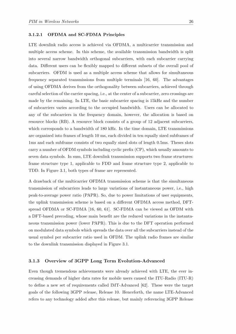
PIM in Wireless Networks 26
3.1.2.1 OFDMA and SC-FDMA Principles
LTE downlink radio access is achieved via OFDMA, a multicarrier transmission and
multiple access scheme. In this scheme, the available transmission bandwidth is split
into several narrow bandwidth orthogonal subcarriers, with each subcarrier carrying
data. Different users can be flexibly mapped to different subsets of the overall pool of
subcarriers. OFDM is used as a multiple access scheme that allows for simultaneous
frequency separated transmissions from multiple terminals [16, 60]. The advantages
of using OFDMA derives from the orthogonality between subcarriers, achieved through
careful selection of the carrier spacing, i.e., at the center of a subcarrier, zero crossings are
made by the remaining. In LTE, the basic subcarrier spacing is 15kHz and the number
of subcarriers varies according to the occupied bandwidth. Users can be allocated to
any of the subcarriers in the frequency domain, however, the allocation is based on
resource blocks (RB). A resource block consists of a group of 12 adjacent subcarriers,
which corresponds to a bandwidth of 180 kHz. In the time domain, LTE transmissions
are organized into frames of length 10 ms, each divided in ten equally sized subframes of
1ms and each subframe consists of two equally sized slots of length 0.5ms. Theses slots
carry a number of OFDM symbols including cyclic prefix (CP), which usually amounts to
seven data symbols. In sum, LTE downlink transmission supports two frame structures:
frame structure type 1, applicable to FDD and frame structure type 2, applicable to
TDD. In Figure 3.1, both types of frame are represented.
A drawback of the multicarrier OFDMA transmission scheme is that the simultaneous
transmission of subcarriers leads to large variations of instantaneous power, i.e., high
peak-to-average power ratio (PAPR). So, due to power limitations of user equipments,
the uplink transmission scheme is based on a different OFDMA access method, DFT-
spread OFDMA or SC-FDMA [16, 60, 61]. SC-FDMA can be viewed as OFDM with
a DFT-based precoding, whose main benefit are the reduced variations in the instanta-
neous transmission power (lower PAPR). This is due to the DFT operation performed
on modulated data symbols which spreads the data over all the subcarriers instead of the
usual symbol per subcarrier ratio used in OFDM. The uplink radio frames are similar
to the downlink transmission displayed in Figure 3.1.
3.1.3 Overview of 3GPP Long Term Evolution-Advanced
Even though tremendous achievements were already achieved with LTE, the ever in-
creasing demands of higher data rates for mobile users caused the ITU-Radio (ITU-R)
to define a new set of requirements called IMT-Advanced [62]. These were the target
goals of the following 3GPP release, Release 10. Henceforth, the name LTE-Advanced
refers to any technology added after this release, but mainly referencing 3GPP Release

PIM in Wireless Networks 27
1 2 3 4 10 1918...... ......
1 Sub-Frame (1 msec) 1 Slot (0.5 msec)
1 Frame (10 msec)
10 2 3 4 5 6
7 OFDM Symbols (short cyclic prefix)
Cyclic Prefixes
LTE Frame Type 1
(a)
1 Frame (10 msec)
1 Half-Frame (5 msec)
Subframe 0 Subframe 1 Subframe 9Subframe 4
DL Pilot
Time SlotGuard
Period
LTE Frame Type 2
UL Pilot
Time Slot
DL Pilot
Time SlotGuard
Period
UL Pilot
Time Slot
(b)
Fig. 3.1: LTE frame structures: (a) Frame structure type 1 applicable to FDD andhalf duplex FDD; (b) Frame structure type 2 applicable only to TDD
10. Overall, LTE-Advanced covers 3GPP Release 10 through Release 14 and, at the
time of writing of this thesis, is the most advanced radio network commercially available
[16, 60]. In terms of features, LTE-Advanced incorporates a multitude of enhancements
that can be grouped in three major categories: 1) Carrier aggregation (CA) that bonds
multiple carriers together to provide extremely high data rates; 2) Advanced antenna
techniques to improve spectral efficiency; 3) Heterogeneous Networks optimizations to
bring more out of small cells. Among these main categories, we only described the CA
principle in more detail as it is particularly relevant in the context of PIM interference
problem.
In the previous section, some general relevant properties of LTE regarding physical
layer were introduced. For LTE-Advanced, most of these properties remain similar yet,
mostly due to CA, some changes in both uplink and downlink are introduced. For
instance, while LTE supports scalable bandwidths with 6 different carrier bandwidths,

PIM in Wireless Networks 28
i.e., 1.4, 3, 5, 10, 15 and 20 MHz, however, CA techniques introduced in LTE-Advanced
enable considerably larger bandwidths and, consequently, higher data rates across the
cell coverage area (over 1 Gbps in the downlink). Together with CA, multi-cluster
transmission was also introduced (although it was not until 3GPP Release 11), which
allows for a more flexible channel-dependent scheduling at the uplink, but at the cost of
increasing PAPR. Other notable features achieved throughout the 3GPP LTE-Advanced
releases include improved spectral efficiency, low latency, multi-antenna transmission,
and backward compatibility with legacy LTE systems. [16, 63]
3.1.3.1 Carrier Aggregation Fundamentals
CA has a crucial role in fulfilling the data rate requirements defined by ITU-R. The
peak data rate requirements are fulfilled by realizing a large transmission bandwidth,
where multiple legacy LTE carriers, each with up to 20 MHz bandwidth and called com-
ponent carriers (CCs), are combined. Hence, CA is an intriguing approach as it allows
operators to deploy a system with extended bandwidth by aggregating several smaller
component carriers (CC) while providing backward compatibility to legacy users [64, 65].
This technique also provides an increase in spectrum flexibility and efficient spectrum
utilization since data traffic is asymmetric, i.e., the number of aggregated CCs of the
uplink and downlink can be different [66, 67, 68]. However, the number of aggregated
CCs in the uplink is always less than or equal to the number of aggregated CCs in the
downlink. There are two possible scenarios of CA are possible: contiguous CA, and
noncontiguous aggregation CA. The noncontiguous CA can be within one frequency
band (intraband) or spread over multiple bands (interband) [64, 65, 66]. In Figure 3.2
it is represented both types of CA. The interband case allows network operators to fully
utilize their spectrum resources, i.e., scattered frequency bands over the RF spectrum.
In early releases of LTE-A, up to five CCs could be aggregated, amounting to 100 MHz
in operation bandwidth, however, currently it can go as high as combinations allow.
The complexity of noncontiguous CA is much higher compared to contiguous CA since
the multi-carrier signal can not be treated as a single signal. Also, given the fact that
the spectrum resources are scarce in low frequency bands (< 4 GHz), it is difficult to
allocate contiguous 100 MHz of bandwidth. However, in UE, it is easier to implement
contiguous CA [3, 66]. In the context of PIM interference, it is preferable to focus on
noncontiguous CA since the intermodulation problem is harder to deal with in this case
as it is explained further ahead in section 3.2.1.

PIM in Wireless Networks 29
Carrier 1 Carrier 2 Carrier 3 Carrier 4 Carrier 5
10 MHz 10 MHz 10 MHz20 MHz 20 MHz
f [MHz]
(a)
Carrier 1 Carrier 2 Carrier 3
10 MHz 10 MHz20 MHz
f [MHz]
(b)
Fig. 3.2: Types of CA: (a) Contiguous CA of several 10 and 20 MHz carriers; (b)Noncontiguous CA of carriers of 10 and 20 MHz carriers
3.1.4 Overview of 3GPP New Radio
Thus far, we have examined some of key principles in existing radio systems, however,
two more 3GPP Releases can be accounted for, Release 15 and Release 16, respectively
. With these releases a new generation of mobile communication is being introduced,
5G, commonly refereed to as NR. This network is capable of enormously expanding the
capabilities of current networks since it is expected to provide extreme data rates, ubiq-
uitous coverage, ultra-reliability, very low latency, high energy efficiency, and a massive
number of heterogeneous connections. Nonetheless, there are three major challenges
that 5G is required to tackle: massive growth in the number of connected devices, mas-
sive growth in traffic volume and a wide range of applications with diverse requirements
and characteristics. [69, 70, 71]
Similar to 4G LTE-A technology, an ITU-R recommendation defines the requirements
for 5G. It is called IMT-2020, and started being developed with 3GPP Release 15 and is
expected to be finished with 3GPP Release 16 [72]. Some key capabilities of IMT-2020
are, peak data rates of 20 Gbit/s, average data rates of 200 Mbit/s, latency of 1 ms, etc.
These requirements induced the main change in 5G technology, previously mentioned,
the use of higher frequencies in the millimeter-wave range. Supporting frequencies below
1 GHz and up to 100 GHz allows for larger bandwidths, in the range of several GHz.
However, the use of millimeter waves brings up several challenges, thus 5G must be
designed for flexible frequency use over the available spectrum. Spectrum flexibility and
operation in both sides of the spectrum provides both reliable coverage and very high
capacity. In total, 5G will provide three types of communications based on their main
features: enhanced mobile broadband (eMBB), massive machine-type communications
(mMTC), and ultra-reliable low-latency communications (URLLC) [69, 70, 71]. For
these three network subsystems, a complex physical layer was split into different layers.
The main properties of the physical layer are explained in the following subsection.

PIM in Wireless Networks 30
3.1.4.1 NR Physical Layer Principles
The NR physical layer handles coding/decoding, modulation/demodulation, multiantenna
processing, and mapping of signals to physical time-frequency resources. As in LTE, it
supports different modulation schemes (different options of QPSK and QAM), that can
be adopted based flexibly. Additionally, NR employs cyclic prefix OFDM in both uplink
and downlink up to at least 52 GHz , with an option to use DFT-spread OFDM (SC-
FDMA) in uplink for coverage limited scenarios. This is different compared with LTE,
where CP-OFDM is only used for downlink transmission and SC-FDMA is used solely
for uplink transmissions. NR also possesses a scalable OFDM numerology to enable
diverse services on a wide range of frequencies and deployments. The subcarrier spacing
is scalable, i.e., 15 kHz, 30 kHz, 60 kHz and 120 kHz, with normal CP included as in
LTE. The number of active subcarriers in Release 15 is 3300, whose combinations with
the different bandwidths, allows for maximum bandwidths of 400 MHz. Finally, carrier
aggregation can also be employed, supporting up to 16 CCs [70, 71, 73].
With OFDM transmission scheme for both downlink and uplink, it is observed that NR
also supports both TDD and FDD transmission. NR also supports dynamic TDD, where
uplink and downlink allocations dynamically change over time [71]. In the time domain,
each radio frame has a duration of 10 ms and consists of 10 subframes with a duration of
1 ms. A subframe is formed by one or multiple slots, each slot with 14 adjacent OFDM
symbols. A mini-slot is restricted to either 2,4 and 7 OFDM symbols, and is used to
support transmissions with a flexible start position. This feature is particularly useful
for low latency transmissions and transmissions in the millimeter wave spectrum. The
time duration of a slot/mini-slot scales with the chosen subcarrier spacing [70, 71, 73].
Figure 3.3 shows an example of an NR radio frame.
Finally, physical time-frequency resources correspond to OFDM symbols and subcarriers
within the OFDM symbols. The smallest physical time-frequency resource consists of
one subcarrier in one OFDM symbol, previously defined as a resource element. Similar to
LTE, the transmissions are scheduled in group(s) of 12 subcarriers, RB. Yet, in contrast
to LTE, the reference signals in NR are only transmitted when necessary, typically at
the beginning of a slot [70, 71, 73]. To support the increase in channel capacity and
operation in the new part of the RF spectrum, multi-user MIMO (or massive MIMO)
and beamforming are introduced in NR. There is a support to increased number of
antennas (over 100) and connectors in the BS.

PIM in Wireless Networks 31
1 Radio Frame (10 msec)
1 Sub-Frame (1 msec)
0 1 2 3 4 5 6 7 8 9
1 2 3 141312......
1 Slot (1 msec) with 14 OFDM symbols (15 kHz subcarrier spacing)
1 2 3 12 13 14......
2 Slot (0.5 msec each) with 14 OFDM symbols each(30 kHz subcarrier spacing)
......13 14 1
4 Slot (0.25 msec each) with 14 OFDM symbols each (60 kHz subcarrier spacing)
1 .................. 1 114 14 14114
Fig. 3.3: NR radio frame transmitted per TDD topology with the flexible subcarrierspacing derived from basic 15 kHz subcarrier spacing
3.2 Passive Intermodulation Distortion in Radio Systems
In section 2.2, PIM was defined as an interference source in radio systems that has the
potential to degrade the efficiency of a cell site, thereby directly affecting the performance
of a radio network. Furthermore PIM interference problem is exacerbated due to the
coexistence of multiple communication systems in the same areas, and is a growing
problem as the network complexity and deployments increase. Therefore, it is a problem
whose impact in networks is growing. Since PIM interference is a problem concerning
RF spectrum, intermodulation issues are aggravated in broadband radio systems where
bandwidth is enlarged to achieve increased data rates, particularly when CA is employed.
Nonetheless, active narrowband systems like GSM are also prone to PIM interference
effects. [4, 74]
Passive intermodulation is often viewed as an installation problem, mostly observed in
high-power cell sites, given the nonlinear generation mechanisms. Yet, this is merely
a superficial consideration, as this interference problems often arise from the saturated
RF spectrum. The assiduous update and growing of the network systems turns PIM
into a volatile problem, whose effects on RF systems will continue to escalate. This is
particularly significant in 5G with the growth of seamless integration of multiple base
station technologies [74]. Based on these considerations, this section focus on explaining
PIM in radio systems, in terms of PIM generation on broadband radios and its impact
on the network.

PIM in Wireless Networks 32
3.2.1 Passive Intermodulation in Broadband Radio Systems
Most literature describe and analyze PIM based on two unmodulated carrier signals. As
it was showed in section 2.1, in this case, the resulting PIM products are also narrow
carriers spurs. However, in broadband radio systems like UMTS and LTE, the signal
is modulated over a wider bandwidth and can be transmitted through several bands of
the RF frequency, especially with the employment of features like CA. Furthermore, the
combined modulated signals can be both narrowband or broadband at the same time.
Hence, consider a general noncontiguous dual-carrier CA FDD transceiver whose Tx
signal is represented as
x[n] = x1ejf1 + x2e
jf2 . (3.1)
This signal is composed of two CCs, denoted by x1 and x2 and respective frequencies f1
and f2 (f1 < f2). When this noncontiguous Tx signal passes through a nonlinear passive
source, mixing occurs and IM components arise. This prejudicial output is expressed as
y[n] =
P∑p=1p odd
x[n] |x[n]|p−1 , (3.2)
where P denotes the polynomial (IM product) order. For simplicity purposes, only
nonlinearity orders up to P = 5 are considered. After substituting (3.1) in (3.2) and
developing the several odd order terms, P = 1, 3 and 5, we obtain two types of frequency
components in addition to the original Tx signals. The first type of components are
classified as spurious terms and correspond to the 3rd and 5th order IM products. As
explained in section 2.1, this spurious IM products appear on both sides of the Tx
signals on the spectrum with the bandwidth of equation (2.4). The 3rd order products
appear at 2f1− f2 and 2f2− f1 whereas the 5th order products appear at 3f1− 2f2 and
3f2− 2f1. However, for P = 5, additional spurious 5th order products appear at the 3rd
order products frequency, e.g., 5th order products appear at frequencies 2f1 − f2 and
2f2− f1 in addition to the 3rd order ones. Thus, the spurious components appearing on
2f1 − f2, IM3−, is the sum of the 3rd and 5th order products expressed as
IM3−3 = x21x∗2e
j(2f2−f1) (3.3)
IM3−5 = IM3−3 (2|x1|2 + 3|x2|2). (3.4)

PIM in Wireless Networks 33
B21 UL B2 DL B21 DL
1710 1755 1930 1990 2110 2155 2320
19402130
3rd
5th
5th
3rd
1900 1920
B15 UL
Fig. 3.4: Spectral regrowth given the spurious and OOB emission due to IM of carriersfrom B2 and B21 that can lead to interference in B15 and B21
The spurious components appearing on 2f2− f1, IM3+, are simply obtained from (3.3)
and (3.4) by interchanging x1 and x2 and substituting 2f2− f1. Regarding IM products
appearing on frequencies 3f1 − 2f2 and 3f2 − 2f1, in this case, are just composed of
5th order products. Assuming an analogous notation, the spurious components on both
sides of the spectrum, IM5− and IM5+, are expressed as
IM5− = x31x∗22ej(3f1−2f2) (3.5)
IM5+ = x32x∗12ej(3f2−2f1). (3.6)
The second type of components show up at the close vicinities of the CCs. Similarly
to the first type, there are 3rd and 5th order IM products, however, these components
appear as a bandwidth extension of CCs, i.e., sub-bands appear on both sides of each
CC. Assuming an analogous notation, the 3rd and 5th order side bands that appear on
the vicinity of the first CC, IM3CC1sub and IM5CC1
sub respectively, are expressed as
IM3CC1sub+ = x1 × (|x1|2 + 2|x2|2)ejf1 (3.7)
IM5CC1sub+ = x1 × (|x1|4 + 6|x1|2|x2|2 + |x2|4)ejf1 . (3.8)
The sideband components appearing at the vicinity of the second CC, IM3CC2sub and
IM5CC2sub , can be obtained from (3.7) and (3.8) by interchanging x1 and x2 and substi-
tuting f1 for f2. Both OOB emissions and spurious emissions are classified as unwanted
spectral emissions, or spectral regrowth [3, 16, 75]. Spectral regrowth can be seen as
spreading of the power spectrum. The unwanted power can appear in Rx bands and
cause interference to the desired receiver signal. In real scenarios, current radio systems
rely on multi-carrier and multi-band technologies, so spectral regrowth due to IM can
affect a wide range of the spectrum, i.e., potentially interfere with several Rx bands.

PIM in Wireless Networks 34
RU1 RU1RU1
External PIM
Source
PIM
Fig. 3.5: Cross-PIM scenario involving three radio units, RU1, RU2 and RU3 and anexternal source close to the BS
As an example, consider a FDD system where signals are transmitted from separate
bands. Consider two channels transmitting from band 2 and band 21, B2 and B21
respectively. Band 2 DL ranges from 1930 MHz to 1990 MHz, and the transmitting
carrier has a center frequency of 1940 MHz with 10 MHz of bandwidth. Band 21 DL
ranges from 2110 MHz to 2155 MHz, and the transmitting carrier has a center frequency
of 2130 MHz with 10 MHz of bandwidth. Due to a nonlinearity on a passive device
during the transmission, PIM products are generated. As a result, one of the generated
spurious 3rd order and fifth order IM products will overlap with the receiver band of
B21, comprised between 1710 MHz and 1765 MHz, since they are centered around which
1750 MHz. In addition, OOB 5th order product overlaps with B15 UL, as the bandwidth
extension of the B2 carrier is wide enough to fall within this Rx band. Both of these
scenarios lead to a potential risk of interference, even though the spurious emission is
more prejudicial. Figure 3.4 portrays the example described above.
In an active broadband base station, it is common to have spectral regrowth where the
carriers combined at the source are from different frequency bands. If the CCs involved
in PIM generation are from multiple bands like the example above, the scenario is titled
as cross-band PIM. Likewise, if the carriers are from one single band, the scenario is
titled in-band PIM [76, 77]. Cross-band PIM is being exacerbated by the refarming of
RF spectrum, e.g., new DL bands and interband CA, and the increase in complexity of
the BS. Furthermore, cross-band PIM is a concurrent scenario in modern radio systems
given that the number of external sources in which the carriers can mix is increasing.
This scenario is depicted in Figure 3.6.

PIM in Wireless Networks 35
3.2.2 Passive Intermodulation Impact on Network Performance and
Physical Layer
The RF spectrum is divided in several bands for different services and operators. Shar-
ing passive infrastructures (co-sites) has become a common strategy adopted by telecom
operators due to key factors such as cost reduction, environmental impact, increased
revenue, etc. [78]. It was previously established that PIM sources are mainly present
in co-sites environments. Therefore, it is denoted that IM interference caused by the
nonlinearities of passive components may impact the radio system performance, partic-
ularly when taking into account frequency relationship between the configured bands.
[4, 7, 74, 79]
In typical co-sites scenarios, standard PIM interference specifications are designed to
meet -150 dBc noise floor level. In state-of-the-art radio infrastructure components,
even low-level PIM may severely degrade system performance. For instance, if a com-
ponent’s PIM characteristics degrade due to uncleanliness then the noise level rises to
-145 dBc, which corresponds to 3 dB power loss in the uplink. In general, a reduction of
1 dB in uplink sensitivity due to PIM interference corresponds to 11% decrease in the
coverage [74, 80]. This indeed translates to severe system degradation and the loss of
income to the operators. In radio networks, PIM’s impact on the uplink transmission
can be categorized in the cell coverage reduction, reduced system capacity and inter-
cell interference. In 4G radio network where CA framework is introduced, nonlinear
IM products due to PIM fall within Rx bands spread throughout the spectrum. The
overall effect is an increase in noise floor and reduced margin in receivers sensitivity [80].
The PIM problem becomes further complicated in 5G networks where nonlinear inter-
band intermodulation have already been identified as the main threat to the network’s
performance should the principles drafted in section 3.1.4 remain, [81].
Moreover, PIM has also become a threat in high power multicarrier transmitting systems
like OFDM [82]. The degradation in the performance in communication systems (in-
crease in noise levels) can be quantified by bit error rate (BER), symbol error rate (SER)
and synchronization probabilities. The PIM effects on the BER of M-PSK modulations
and on digital channels were investigated in [83] and [84] respectively. The results show
that PIM negatively affects the channel since it increases the error probability in mak-
ing a decision in the detection part, however, PIM interference decreases with increasing
PIM order. In the case of frame synchronization, the PIM effect was studied in [85]. The
statistical properties of a time metric function (window that slides in the time domain
to search for the first training symbol) in presence of PIM are the basis for analyzing
the false or missing probability of the OFDM system. The results show that, in case the
PIM interference makes the window function locate the symbol behind the actual start

PIM in Wireless Networks 36
position, i.e., the starting position does not fall into CP, intersymbol interference (ISI) is
introduced, worsening the probabilities of both missing and false detection. In summary,
it can be concluded that PIM has a severe impact on radio systems performance. In the
following sections, we review commonly adopted PIM mitigation techniques.
3.3 Passive Intermodulation Mitigation Techniques
In general, PIM generated spurious signals interfering in the Rx bands are unpredictable.
As previously explained, the spurious signals are dependent on the site’s environment,
RF infrastructure conditions, external and internal sources respectively, as well as con-
figured bands and used frequency channel. The strength of interfering signals typically
depends on the nonlinear properties of the PIM causing source. Furthermore, there is
also the uncontrollable aspect of dielectric coating in external sources discussed in sec-
tion 2.4.2. With this, countering any PIM interference becomes a complex problem. The
complexity of PIM mitigation further increases when assuming continuous enhancement
of radio systems, e.g., higher performing services, smaller cells and radio configuration in
the RF path. Nevertheless, until now, PIM interference has been managed with different
mitigation techniques which are now briefly reviewed below.
PIM mitigation techniques can broadly be split into two categories, physical techniques
and radio integrated techniques. Physical mitigation techniques are procedures or mod-
ifications that can be applied to the RF equipment, infrastructure and surrounding
environment to rectify or reduce the level of PIM interference. Often, these processes
are specific counter measures to the generation mechanisms explained before, and imply
a complete understanding of the physics associated. Digital mitigation techniques are
engineered into the signal’s path and make use of digital signal processing techniques to
reduce the PIM interference.
3.3.1 Physical Mitigation of Passive Intermodulation Interference
This section summarizes the guidelines followed by RF manufacturers to mitigate PIM
when setting up a radio system on a site with PIM issues. For these physical endeavors,
the physics of the mechanisms behind PIM described in Chapter 2 are taken into account.
Since PIM sources can be either internal or external, it is logical to divide this section
into two subsections to account for the physical actions to mitigate both types of sources.

PIM in Wireless Networks 37
3.3.1.1 Guidelines for Mitigation of Internal Sources
To mitigate internal sources of PIM in radio systems, it is needed to counteract the effects
shown in section 2.3. The following guidelines are usually adopted by manufacturers for
the last couple of decades:
• Avoid the use of nonlinear components within or near the infrastructure;
• Keep current densities low in the conduction paths by using larger conductors or
having bigger contact areas, e.g., MM contact;
• Minimize metallic contacts and connectors, ensuring that loose contacts and ro-
tating joints are avoided;
• Keep thermal variations to the minimum in the components of the radio system;
• Have all joints clean and tight, preferably made or coated with materials less
bounded to oxidation;
• Shorten the use of cables to the maximum and use semi-rigid coaxial cables;
• Achieve good isolation between the high power transmit signals and the low level
receive signals (duplexer isolation);
Although no system is completely free from PIM, careful planning, good workmanship
and a high standard of system maintenance are equally important to substantially reduce
its level [4, 5, 17, 27, 29, 80, 86, 87, 88].
These guidelines have been applied to mitigate PIM in radio systems, however, since
electro-thermal effects have been identified as the main internal PIM sources (see e.g.
Section 2.3.2) low electronic conducting materials are now being employed in the man-
ufacturing of radio system components. This pratice ensure that the thermal variations
are kept to a minimum while employing high power currents flowing through the RF
components of the base station [89].
3.3.1.2 Guidelines for Mitigation of External Sources
To mitigate external sources of PIM in radio systems, it is required to counteract the
effects shown in section 2.4. However, unlike internal sources, these are more difficult
to deal with as previously explained. A simple and recurrent guideline used by manu-
facturers when setting up a site is scanning the environment, or RF path, for potential
nonlinear sources that can generate PIM and then removing them. These scanners,
for instance the PIM Hunter by Anritsu, test for primary test tones that generate IM

PIM in Wireless Networks 38
products to locate the source [90]. Yet, objects on the antenna’s radiation path are
unpredictable and uncontrollable which makes their mitigation a complex problem. The
power of the distortion caused by these sources is also dependent on how far the source is
located so, in some cases, may even be the principal PIM source. Since PIM is intrinsic
to every radio system, most manufacturers turn to digital signal processing techniques
to mitigate the inherent PIM. However, with the continuous increase in radio systems,
section 3.1, the complexity of the base stations is also increasing, especially the number
of antennas. As it was mentioned previously, MIMO systems are already implemented
and will soon be upgraded to massive MIMO, with antennas playing a major role in
PIM. Since their sensitivity level is getting lower, every enhancement that increases the
power of the transmission link (dB) matters. It is based on these considerations that the
study of Chapter 4 is performed, with the objective of lowering the complexity of PIM
mitigation algorithms. The study also contributes to existing mitigation techniques of
antenna isolation that will be proceeded to explain.
Antenna isolation are considerations taking in co-site base stations to avoid the excessive
interference (PIM) and improve the link quality. The amount of isolation achieved is
dependent on several factors such as physical horizontal and vertical separation distance
between antennas, antenna polarization, radiation pattern, and surrounding environ-
ment of the antenna [91, 92]. In general, the mitigation of IM interference improves
with increasing separation between the antennas as well as with increasing electrical
down tilt (azimuth) angle.
3.3.2 Radio Integrated Mitigation of Passive Intermodulation Inter-
ference
In general, the PIM interference problem cannot be fully contained through physical
PIM mitigation approaches. Therefore, recently, digital PIM mitigation approaches
have started to receive an interest, see for examples [4, 91, 93, 94] among others.
The digital PIM cancellation approach is normally based on the block diagram shown
in Figure 3.6. This model is based on adaptive filter theory and, the general idea is
to predict PIM-induced IM products based on the transmitting signal to subtract them
from the receiving signal chain (after I/Q conversion and duplexer). However, the main
problem in digital cancellation is that PIM products amplitudes, phases and delays
depend on the used RF components (PA, duplexer, etc.),e.g., they are not constant.
This adds extra complexity in the model used for estimating the IM products since the
parameters have to be adjusted or analyzed when the transreceiver system is offline.
However, the main benefit of this digital cancellation is that it can be used to reduce
the IM products which are generated internally, after the Tx filter.

PIM in Wireless Networks 39
Fig. 3.6: Diagram block for an adaptive cancellation PIM algorithm
Another commonly employed strategy is known as frequency or resource planning. Al-
though this study ([91]) was made in deployments of 2G and 3G networks, the same
principles analogously apply to include 4G and 5G networks in the base stations. In
this process, the distribution of available channels is chosen for every tier following a
channel spacing rule. The choice of the channel allocation is made frantically so as to
achieve minimization of the spurious interference signals. When superimposing the net-
works, this process can be done either by block assignment or frequency banning. The
first assigns blocks of channels to both networks that guarantee that no potentially IM
product affects the transmission inside the cell. The second comprises of three steps:
identify the channel combinations that give harmful IM products in every cell; avoid-
ing the most popular channels in the combinations; compensate of the loss in capacity
(number of channels) by using frequency hopping. Unlike other approaches, frequency
planning completely avoids the PIM problem thereby guaranteeing a PIM-free channel.
However, this approach hinders full exploitation of available resources and can lead to
reduced throughput.
Some uncommon strategies can also be employed but come at a greater cost. For in-
stance, reducing the transmit power can reduce PIM, as PIM power is directly related to
Tx power. But this comes at a cost of reduced coverage. Another example is to improve
Rx sensitivity when PIM is eminent. But this also impacts users on cell-edge which will
be communicating with BS at a low power and their signals may be blocked.
3.4 Discussion
In this chapter, we firstly presented an overview of the evolution of the radio systems.
We reviewed that the development of new features and techniques integrated in cur-
rent radio systems like CA contribute to exacerbate the PIM interference problem. In
particular the enlargement of the bandwidth in broadband radio systems and shared

PIM in Wireless Networks 40
co-sites base stations where PIM is ought to be more likely due to the several frequency
carriers, the spectral regrowth turns into a more serious issue. As we have showed,
the mixing of these carries lead to broadband IM products that, in a highly saturated
RF spectrum, are prone to overlap with Rx bands. This interference has a prejudicial
effect on the network’s performance and in the detection system of the physical layer.
Finally, we discuss different types of PIM mitigation techniques used by manufacturers
and operators, i.e., physical and radio integrated techniques. Concerning physical miti-
gation techniques, due to the extensive research on the physical generation mechanisms,
several countermeasures are already employed. However, it is also due to this extensive
research that we confirm that PIM is an assiduous and uncontrollable problem. Thus,
radio integrated mitigation techniques are very important to assist in dealing with the
unpredictability. So far, the strategy for this type of techniques was centered around
predicting the spurious frequency emissions, however, with the saturation of the spec-
trum, new strategies are asked for. In recent years, digital cancellation algorithms have
surfaced as a viable alternative but, improvements are required for better performance.
Enhancements are obtained through data collection and analysis.

Chapter 4
Measurements-based Analysis of
External Passive Intermodulation
Thus far, throughout this work, a characterization on PIM generation in radio sys-
tems has been drafted. Building on the discussions in the previous chapters, we now
hone external PIM, namely the PIM power induced in different antenna elements. For
this purpose, in this chapter, we emulate and analyze different transmission scenarios
with different external sources to induce PIM. In addition, several measurements were
recorded for the several case studies established. Even though the main intention is to
investigate and characterize the relation between external generated PIM, Tx and Rx
characteristics, it is also investigated the fundamental triggers of external PIM covered
in section 2.4.
Firstly, we present the measurement setup, describing the radio hardware and different
PIM sources that are employed in the measurements. The external PIM sources mimic
a real-world scenario of an object that can be within the RF signal path. Then, we
analyze the PSD of the most likely case and measurement to introduce performance
metrics for PIM measurements. Afterwards, we analyze the different measures obtained
for different sources as well as the PIM changes over time. Finally, we apply a digital
PIM cancellation algorithm developed by Ericsson to see how it works.
4.1 Radio Setup and Use Cases
The radio setup used in the experiments emulates the scenario described in Figure 4.1.
The base station radio consists of a dual-band (B2 and B66) LTE radio connected to
two cross polarized antennas, horizontally separated 90 cm. This implies that there
are, in total, four antenna elements, two with +45◦ polarization and two with −45◦
41

Measurements and Analysis 42
Fig. 4.1: Measurement setup with an external PIM source, Rusty Metal Clamp
polarization, each capable of transmitting and receiving the signals, i.e., serve as Tx and
Rx. Linear cross polarization is generally widely adopted in radio systems, especially
in broadband antenna arrays, since it lowers mutual interference [92, 95]. The antenna
infrastructure is assembled inside an anechoic chamber and is connected the to the ports
of the radio outside the chamber through coaxial cables and diplexers. For evaluation
purposes, we transmit and receive only on Band2, whose downlink band is comprised
of interval 1930 - 1990 MHz while the uplink band is comprised of interval 1850 - 1910
MHz. The duplex gap, in general, is 80 MHz, however, it can drastically reduce down to
only 20 MHz if the carriers are configured for transmission at the edges of the band. This
experimental setup ensures that 3rd order cross-modulation products of the DL carriers
center frequencies can fall within the Rx band, and we may observe PIM interference in
the uplink band.
In the transmission, we adopt a multicarrier Tx signal (dual-carrier DL signals), which
is modulated with a 64-QAM modulation scheme and carriers with bandwidth of 5
MHz. The DL carriers center frequency are 1930 MHz and 1985 MHz which makes
the prejudicial 3rd order PIM product centered around 1875 MHz. In addition, the
data transmitted on each antenna element is uncorrelated. Despite only being observed
the 3rd order product, several higher order PIM products can also be present due to
broadband TX carriers. Consequentially, when mentioning PIM distortion power level
in each measurement, it refers to the power ratio of the 3rd order PIM product signal
relative to the carrier, generated by the external source. The Tx power used to transmit
the DL carriers is 5 W in each antenna element, and the induced external PIM is
observed in the Rx chain. In the antenna’s beam we placed three different types of
objects prompted to generate external PIM given the mechanisms explained in Chapter

Measurements and Analysis 43
(a) (b)
(c)
Fig. 4.2: External PIM sources used for the measurements: (a) Steel Wool; (b) CleanMetal Clamp attached to small support structure (MCS); (c) Rusty Metal Clamp at-
tached to small support structure (Rusty MCS)
2 namely, steel wool; clean metal clamp attached to small support structure; rusty
metal clamp attached to small support structure. Since the goal of the research is
to investigate external PIM, the guidelines of section 3.3.1 were followed to minimize
internal mechanisms of PIM generation. Additionally, external PIM from scattering
on the absorbent material inside the chamber can also contribute towards the PIM
power level. However, the PIM power level without any external source was measured
(calibration), and the value obtained was -160 dB so this contribution can be disregarded.
Figure 4.1 presents the setup inside the anechoic chamber.
Given the radio setup described, nine measurements are drafted for each source. In every
measurement, the PIM distortion is measured on each antenna element, i.e., all four
antenna elements function as receivers (4R). The variation between the measurements
is the number of active transmitters, which can be either one, two, or four, referred to as
1T, 2T, and 4T, respectively. In 1T cases, the transmitter is linearly polarized at +45◦
or −45◦ in one of the antennas (A1 or A2), which amounts to a total of four distinct
combinations. In 2T cases, the transmitters are linearly polarized at +45◦ or −45◦ in
both antennas (A1 and A2), which amounts to a total of four combinations as well.
And, in the 4T case, the transmitters are all four branches linearly polarized at +45◦
and −45◦ in both antennas (A1 and A2).

Measurements and Analysis 44
The first source tested for this research is a piece of steel wool, which was molded into a
block. This emulates the transmission into a rough metal surface, derived from a physical
deformation, or a curled metal fence or wire. The second source tested in this research
was a metal clamp attached to a small support structure. The metal was cleaned and free
of dirt particles to review different generation mechanisms. This emulates the presence
of metallic objects in the RF path. The third and final source tested in this research was
a rusty metal clamp attached to a small antenna structure, similar to second source but
oxidized. This emulates the presence of rusty metal objects in the transmission path.
For the nine cases referenced above, every source was placed at a distance d = 1.32m,
and the PIM distortion observed on each branch for each case was measured. Note that,
whilst comparing both of the metal clamp sources, the image of the rusty source has
additional screws. However, equal ones were incorporated in the clean source despite
not being displayed. In the following sections, the results from these measurements are
displayed and analyzed. Figure 4.2 presents each source just described.
4.2 Power Spectral Density Analysis
The measure that better approximates a real case in radio system is the 4T4R case.
We plotted the observed PIM relative to the noise floor. For each antenna element it
is plotted the PSD of the PIM distortion. Additionally, every case was measured at
least twice to support the validity of the results obtained. In every measure, the PSDs
showed that external PIM exits, generated by the external sources, and it affects all
of the branches (receivers). So, in this transmission, external PIM characterizes the
interference problem in the BS.
In Figure 4.3, it is presented the 4T4R measurements for each source. In each plot,
each line represents the PIM power level in each of the antenna elements. For instance,
the red line and the black line represent the branches linearly polarized −45◦ and +45◦
in A1 respectively, whereas the blue and the pink line represent the branches linearly
polarized −45◦ and +45◦ in A2 respectively. Figure 4.3a plots the PIM distortion with
steel wool as a PIM source, Figure 4.3b plots the distortion with a clean metal clamp as
a PIM source, and Figure 4.3c plots the distortion with a rusty metal clamp as a PIM
source. Based on these plots, it can be confirmed that PIM distortion occurs and is a
problem in the BS as it is received by both antennas. Note as every plot is normalized,
hence the PIM power level can be measured in dBs.
In Figure 4.3a, steel wool case, the PIM power is higher in A2, peaking at 30 dB above
the noise floor for the branch linearly polarized +45◦. In A1, the PIM power is a couple
dB’s lower but its still stronger on the branch linearly polarized +45◦. In Figure 4.3b,

Measurements and Analysis 45
1850 1860 1870 1880 1890 1900 1910
-5
0
5
10
15
20
25
30
35
40
45
50
(a)
1850 1860 1870 1880 1890 1900 1910
-5
0
5
10
15
20
25
30
35
40
45
50
(b)
1850 1860 1870 1880 1890 1900 1910
-5
0
5
10
15
20
25
30
35
40
45
50
(c)
Fig. 4.3: PSD curves of the measured PIM on different antenna elements and withdifferent PIM source in 4T4R configuration: (a) Steel wool as PIM source; (b) Clean
metal clamp as PIM source; (c) Rusty metal clamp as PIM source.
clean metal clamp attached to antenna structure, PIM power is stronger on the branches
linearly polarized −45◦ with 22 dB and 19 dB for A1 and A2 respectively. Between the
branches linearly polarized +45◦, PIM is stronger in A2. In Figure 4.3c, rusty metal
clamp attached to antenna structure, the PIM power is stronger in A1, especially in the
branch linearly polarized +45◦ peaking at 35 dB above the noise floor. In addition, in
A2, PIM is stronger in the branch linearly polarized +45◦. Comparing the three plots,
it can be concluded that there is not a dominant type of polarization where the PIM
power is better or worse. For instance, in the clean metal case, the order from highest
to lowest PIM distortion on each antenna element is −45◦ A2, −45◦ A1, +45◦ A2, and
+45◦ A1, whereas in the rusty metal case the order is +45◦ A1, −45◦ A1, +45◦ A2, and
−45◦ A2. Additionally, comparing the observed PIM power in each antenna element,
of the clean metal and the rusty metal, it is higher in the rusty metal clamp, except
for the branch linearly polarized −45◦ in A2. Note as the only difference between both
sources is oxidization and exposition (more directive towards the antennas) of the rusty

Measurements and Analysis 46
source. These small changes are enough to affect the strength of the interfering signal
(PIM) and to cause an inconsistency in the strength of received PIM distortion in the
same receivers. In the following section this analysis is applied for every measure of each
source and the derived conclusion from the study.
4.3 External PIM Analysis for Case Studies
As it was mentioned in Section 4.1, measurements were made for all the 27 cases. For
each case, a PSD analysis similar to the one described in the previous section is per-
formed. Based on this analysis, a characterization of PIM power from the Tx side is
drafted on Table 4.1. This table contains the total PIM power observed, e.g., sum of
the power received in different antenna elements. Like it was mentioned in the previous
section, the PIM distortion values vary in every branch, for different measurements,
hence the discrepancy of the values. This is mainly due to the inconsistency of the
generation mechanisms explained in Chapter 2. For instance, according to section 2.4.1
and 2.4.2, the PIM product generated of the illuminated part (area where radio beam
incides) of the source is one of the contributors of the interference. This means that the
PIM products generated and reflected are highly directional. However, depending on
the topography of the dielectric coating, both the strength and the scattering of the IM
products are affected. The loss in signal strength and divergence of received values in
each branch is also due to a change in wave polarization, from a linearly polarized one
to a random one, and to the change of the source’s reflection coefficient. This random
wave polarization reflected back is differently coupled by the antenna elements, which
explains the variances in the observed PIM. The reflection coefficient affects how much
of the incident wave is scattered of the medium (in this case the coated source), which
also affects the strength of the PIM product. The main contributor for external PIM
is the gap between metals that behave like contact mechanisms, e.g., the “Rusty Bolt”
effect. As explained in Section 2.4.3, when the incident waves lits part of the external
source, a nonlinear current is formed. This current travels through the surface of the
source and it can encounter small air gaps or thin electric layers between metal extrem-
ities which generate PIM products. These products generated of MIM junctions are
emitted towards the antennas with a random polarization. With an oxidation layer,
other MIM cases can appear beyond gaps in the source, which contribute for the total
PIM observed. Based on this considerations, we can assess that each external source
has its own number of PIM generators, inherent to the source topology.

Measurements and Analysis 47
Table 4.1: Total PIM power observed for the several configurations (dB)
Case Study Tx Ant. ElementTotal PIM Power (dB)
Steel Wool MCS Rusty MCS
1T4R
+45◦ A1 31 35 24
−45◦ A1 35 20 32
+45◦ A2 33 39 22
−45◦ A2 37 36 47
2T4R
+45◦ A1/A2 27 38 24
−45◦ A1/A2 35 24 38
+45◦/−45◦, A1/A2 34 37 30
−45◦/+45◦, A1/A2 32 31 25
4T4R ±45◦, A1/A2 35 25 34
In every measure, we always ensure that the total Tx power remains the same as we
add more DL carriers. However, adding more DL carriers whose signals have different
polarizations does not increase the PIM distortion. For example, with the steel wool
source, the highest PIM distortion power is received is the 1T4R transmission (37 dB)
whereas in 2T and 4T4R cases it is less or equal. The same can be observed if it is
looked at the values for the two other sources. As explained in the previous paragraph,
a possibility to explain this is that, with the extra amount of carriers, a destructive
interference when generating PIM is being created in the source, or the polarization of the
extra signals being reflected or created by the MIM junctions is more randomized. The
inconsistency of the values from the aforementioned table and from the PSDs confirm the
inability to detect a specific pattern common to different kinds of sources. For instance,
the antenna element with the worse level of PIM is not the same for the different sources
even though the configuration is the same. The antenna element with the worst level of
PIM also varies when changing the configuration for the same source. So, external PIM
is an interference that is also derived from the conditions the source is exposed to when
interfering with the transmission. For different sources, different powers of received PIM
signals ought to be expected, as highlighted in Table 4.2.

Measurements and Analysis 48
Table 4.2: Variation on PIM power level for different sources relative to Tx polariza-
tion
PIM SourceObserved PIM power and Ant. Polarization
Min Max
Steel Wool 27/ +45◦ 37/ −45◦
MCS 20/ −45◦ 39/ +45◦
Rusty MCS 22/ +45◦ 47/ −45◦
In Table 4.2, it is also indicated which polarization does the limit correspond to. Looking
at the polarization values it appears the polarization for the branch with the maximum
PIM value is opposite to the one with the lowest. Furthermore, from both tables, its
derived that oxidization, i.e., creation of a dielectric layer, worsens the problem (as
expected).
For the different test cases, several measurements are made to assess the consistency of
the PIM values when measured in different time instants. This helps to characterize PIM
from the Rx side. For comparison reasons, in Figure 4.4, it is presented the 4T4R cases
of the metal clamp sources (clean and rusty) measured in different instants. Figure 4.4a,
plots the total PIM power Rx in each measure for both the clean and the rusty case. Even
though there are some deviations, for the clean source case, it is observed an average of
25 dB of PIM distortion in the Rx, whereas, for the rusty source case, the Rx receives an
average of 34 dB. Figures 4.4b and 4.4c, plot the PIM power received per antenna element
in different measurements. For different measurements, the PIM power values appear to
vary similar for the same polarization, i.e., for different measurements, the branches with
equal polarization, +45◦ and −45◦, show the same amount of increase or decrease despite
belonging to different antennas. Although the values in each iteration may oscillate, the
interval between same polarizations is maintained. Hence, the consistency of a certain
polarization being worst in one antenna is a useful result as it can lead to improvements
in real time optimization. In addition, we also observe that the PIM distortion values
observed in the Rx vary tremendously, especially in the rusty source case. In the rusty
source case, we observe that the PIM distortion values can vary, at most, 15 dB between
different measurements at each antenna element. In the clean source case, we observe
that the PIM distortion values vary, at most, 7 dB between different measurements
at each antenna element. However this variance can be attributed to the adoption of
multicarrier signal with high PAPR values.
Since the measurements are simulated inside an anechoic chamber, to assess the validity
of the analysis from the previous paragraph, we repeat the measurements for the rusty
metal clamp source. Thus, Figure 4.5 shows the total observed PIM distortion values

Measurements and Analysis 49
1 2 3 4 5
Measurement
0
5
10
15
20
25
30
35
40
45
To
tal re
ceiv
ed P
IM p
ow
er
(dB
)
Clean Metal Clamp
Rusty Metal Clamp
(a)
1 2 3 4 5
Measurement
0
5
10
15
20
25
30
35
40
PIM
po
wer
pe
r an
t. e
lem
ent (d
B)
PIM in Band2 UL-A (-45deg,RU-1)
PIM in Band2 UL-B(-45deg,RU-2)
PIM in Band2 UL-C(+45deg,RU-2)
PIM in Band2 UL-D(+45deg,RU-1)
(b)
1 2 3 4 5
Measurement
0
5
10
15
20
25
30
35
40
PIM
po
we
r p
er
ant.
ele
ment (d
B)
PIM in Band2 UL-A (-45deg,RU-1)
PIM in Band2 UL-B(-45deg,RU-2)
PIM in Band2 UL-C(+45deg,RU-2)
PIM in Band2 UL-D(+45deg,RU-1)
(c)
Fig. 4.4: Total observed PIM distortion relative to the noise floor in different instantsfor 4T4R configuration: (a) Steel wool as PIM source; (b) Clean metal clamp as PIM
source; (c) Rusty metal clamp as PIM source.
relative to the noise for different configurations in several measurements. Comparing
the 4T4R plot of Figure 4.5 to the plot of Figure 4.4a we can see that the observed PIM
power has lowered around 10 dB even though the setup is identical. For the 2T4R case
displayed in Figure 4.5, we observe that the total PIM power does not vary besides a
couple of dB. However, for the 1T4R case, the total PIM power observed displays some
variance, to a max of 7 dB. Lastly, again with the 4T4R configuration, we reproduced
the measurements with the rusty metal clamp rotated −45◦ clockwise to see whether it
has an effect in the level of PIM distortion. As it can be seen in Figure 4.5, the total PIM
power observed is lower after the source was rotated. To better interpret the results, the
average of the observed PIM values through the repeated measurements in each antenna
elements are shown in Table 4.3. From this table and the aforementioned figure it is
derived that the external source, e.g., the rusty metal clamp, generates a PIM signal that
has a spatial distribution of gain. Furthermore, we also confirmed that changing small
conditions in the measurements, for instance, rotating the source, changing its height

Measurements and Analysis 50
1 2 3 4 5
Measurement
0
5
10
15
20
25
30
35
40
Tota
l re
ceiv
ed P
IM p
ow
er
rela
tive to the n
ois
e level(dB
)
Fig. 4.5: Total observed PIM distortion relative to the noise floor for several configu-rations with the Rusty metal clamp as external source.
Antenna ElementObserved PIM power relative to the noise floor (dB)
Rusty Metal Clamp Rusty Metal Clamp rotated −45◦
−45◦ A1 17.8 17.5
−45◦ A2 12.23 17.47
+45◦ A2 8.88 8.19
+45◦ A1 17.95 9.9
Table 4.3: Comparing observed PIM power values on antenna elements after rotatingthe external source, Rusty Metal Clamp
relative to the floor, or simply touching the rust of the source affects the current’s path
and consequentially, the polarization of the PIMP products emitted.
In summary, we assess the stability of PIM induced by external sources. Despite main-
taining the measurement setup throughout the testing of the several configurations, the
PIM distortion observed can be very unstable and the values can differ in different days
of experimentation. This variation can be attributed to changing in the conditions of
the setup (only being visually identical) or stress built on by the radio throughout the
measurements. However, we have confirmed that an external PIM source can be viewed
as a reflective PIM antenna, where nonlinear currents produced on the surface generate
the PIMP products. Hence, each source or antenna has its own broad spectrum of direc-
tivity and gain, that is dependent on its conditions and format. In turn, the conditions
that the source is exposed to can affect the PIM distortion captured by the Rx of radio
system. In the following section, we apply digital PIM mitigation algorithm developed
by Ericsson to one of the measurements to review its performance in mitigating the
interference.

Measurements and Analysis 51
4.4 Digital Cancellation of PIM
In Section 3.3.2, digital cancellation of PIM was highlighted as one potential PIM mitiga-
tion approach. In fact, since the saturation of the RF spectrum makes PIM interference
unavoidable, this mitigation technique has become the main research focus of radio inte-
grated mitigation techniques. As it was explained, the idea of PIM’s digital cancellation
is to create an opposite-phase digital replica of true RF PIM interference in the digital
domain, and then add it to the baseband received signal. In general, PIM can be viewed
as a nonlinear filtering on the transmitted signals, which are already known inside the
radio. Therefore, one can exploit the deterministic nature of PIM for building a digital
model and its cancellation.
In a most recent application, [94], the author employed an adaptive filter for the interfer-
ence cancellation. In this technique, the filter (linear combiner) cancels the interference
by adaptively adjusting its coefficients such as the output signal is as close as possi-
ble to the desired signal. To generate the parameters, it is used two popular adaptive
algorithms, LMS and RLS (the better choice depends on how much computational com-
plexity is available). Combining these into a cancellation block alongside some other
digital signal processes, it is feasible to correctly estimate coefficients, compensate for
phase distortion and track PIM in real time. In the scenario when PIM distortion is
present, it was possible to suppress third-order PIM.
The purpose of this section is to see if we can cancel PIM observed on the clean and rusty
MCS sources, while employing a similar cancellation algorithm. The digital cancellation
is for the case of 4T4R, i.e., there are 4 unique downlink Tx data while PIM cancellation
is only pursued on only one uplink branch. The digital cancellation is based on Least
Squares (LS) model fitting principle, and only third-order PIM is modeled and canceled.
Figure 4.6 displays the received signal’s PSD after the algorithm was applied.
By analyzing the Figures 4.6a and 4.6b, we can deduce that PIM of clean and rusty MCS
can be suppressed to a certain extent with digital PIM cancellation. The cancellation
is in the order of 15 dB, with only third-order PIM modeling. The residual PIM is due
to higher-order of PIM, that can potentially be mitigated by modeling them. However,
here the intention is to only demonstrate the digital cancellation capability, and showing
that digital cancellation is indeed an intriguing mitigation approach. Lastly, the obtained
PIM cancellation is more effective for rusty MCS then for clean MCS. This is due to
the rusty source producing a stronger third-order PIM interference that can be more
efficiently suppressed, and due to the clean source having higher than third-order PIM
components that leave more residual PIM.

Measurements and Analysis 52
-30 -20 -10 0 10 20 30
-5
0
5
10
15
20
25
30
35
(a)
-30 -20 -10 0 10 20 30
-5
0
5
10
15
20
25
30
35
(b)
Fig. 4.6: Observed PIM distortion in one uplink branch for 4T case: (a) Clean metalclamp as PIM source; (b) Rusty metal clamp as PIM source.
4.5 Discussion
In this chapter, it is determined that PIM is indeed a significant problem in broadband
radios as evidenced with the different measurements with different external PIM sources.
Based on the previous research concerning external PIM, this chapter ought to produce
more concrete results to contribute for the characterization of PIM generation from
different external sources. The measurements and scenarios replicated emulate real
cases of radio systems where PIM is likely. An analysis of PIM is made from both the
transmitter side and the receiver side. From the transmitter side, the analysis is done
based on the PIM power observed on each antenna element for the same configuration
on the different sources. From the evaluation of the PSDs obtained, the distortion on
one specific antenna element varies for different sources with the same configuration,
e.g., the antenna element with worse or better PIM changes for different sources while
maintaining the same configurations. From the receiver side, the analysis is done based
on the PIM power observed on each antenna element for different configurations on
the same source. From the analysis of the PSDs obtained, for the same source, the
antenna element with worse or better PIM varies with the change in configurations.
From these evaluations, it is derived that each external PIM source exhibits its own
inherent characteristics, similar to an antenna. Furthermore, a conclusion regarding an
optimal antenna polarization to receive less PIM, and an optimal amount of Tx, can
not be made. However, as it was seen from observing the total PIM power varying
over different measurements, this is due to the adoption of multicarrier signals with high
PAPR. Lastly, we confirm that oxidation or corrosion increases the PIM power produced
by the external source.
Regarding the mitigation aspect, we observe how a radio integrated algorithm performs.
The results suggest that these types of algorithms can not fully mitigate the interference

Measurements and Analysis 53
due to contributions from the residual power from the spectral regrowth. However, the
data collected from the measurements can contribute to improve existing radio integrated
mitigation techniques. For instance, it is evident from the measurements that different
RX capture different PIM levels, and that different TXs contribute differently. Based
on this, some algorithm based on supervised learning, e.g., Support Vector Machines
(SVM), can be designed to determine the contributions of PIM from different Tx signals.
Since PIM varies over time, an adaptive digital cancellation solution is called upon to
also integrate existing radio systems.


Chapter 5
Conclusion and Future Work
This thesis addressed the PIM distortion problem in multiband radio systems. More
specifically, characterizing the physics behind the triggering mechanisms that originate
the nonlinear behavior in passive components, reviewing how the enhancement of radio
systems (broadband radios) worsened the PIM problem and devised mitigation tech-
niques, and, lastly, measurements analyzing the relation between external PIM power
observed and BS antenna elements. The main purpose of this work was to complement
the current knowledge on external PIM, hence some of the main findings are summarized
below.
In the first part of this work, Chapter 2, we developed a mathematical approach to
characterize the IMD imperfection and reviewed the nonlinear triggers of the two types
of existing PIM sources, internal and external. More concretely, electron tunneling and
ET conductivity for internal sources, and a PO approach to explain nonlinear current
generation in metallic objects for external sources. Every situation where these mecha-
nisms are prone to occur form a PIM transmitter. The appearance of these situations
in radio systems is diversified as well as unpredictable and unavoidable, especially ag-
ing and corrosion. Each PIM transmitter emits its own signal that gets accumulated
throughout the transmission and can lead to interference in the Rx bands.
Next, in Chapter 3 we reviewed the enhancement of radio systems, particularly tech-
niques embedded in the radios to increase data rates (CA), and enlarge the bandwidth.
The devised broadband radio systems worsen the spectral regrowth, i.e., PIM’s effect
in the network. The known mitigation techniques, physical and radio integrated, main
strategy is either avoiding the nonlinear behavior of the passive components by under-
taking physical endeavors towards so, or avoiding the IM spurious frequencies performing
55

Conclusion 56
frequency planning by relying on the mathematical model. We considered these insuffi-
cient as modulated signals generate broader PIMP which makes PIM interference inex-
orable. Adaptive PIM cancellation algorithms are surfacing as the next logical counter
measure to the problem but they still need improvements for better performance.
In the final part of this work, Chapter 4, we presented the analysis of the measurements
performed. By emulating a real scenario of a broadband radio system transmitting to-
wards different PIM sources inside an anechoic chamber, we ought to investigate the
relation between observed PIM power in the Rx and PIM source. The radio setup uti-
lized comprised of a multicarrier LTE signal from Band2 transmitted from the antenna
elements linearly polarized +45◦ and −45◦ installed on a high power BS. In addition,
we tested three distinct sources that emulated likely cases of external PIM, steel wool,
clean metal clamp support structure and rusty metal clamp support structure. In an
initial observation of the PSDs, we were not able to assess a specific pattern common to
each source, i.e., the PIM power observed in each antenna element would vary tremen-
dously depending on the amount of Tx chosen for each source, hence a specific antenna
polarization could not be said to be better or worse to receive the signal. In addition,
in consecutive measurements, we denoted that the total PIM power observed on the
Rx largely varies within a dynamic range. This can be attributed to the possibility of
generation of constructive or destructive interference in the source due to the use of
multicarrier Tx signals. Lastly, we determined that each external PIM source can be
viewed as a PIM antenna, with an unique radiation pattern depending on the conditions
it is exposed to at the moment of the transmission. The directivity of PIM produced by
each source varies spatially. Disturbances like change of height, direction, time when the
measurement is taken or interaction with the source change the PIM power observed in
each element drastically.
Overall, in this thesis, we have characterized the PIM distortion phenomenon in multi-
band radio systems. The main outcome of this work are the measurements performed as
the analysis provides valuable insight towards optimizing current mitigation techniques
even though better characterization can be obtained through single-tones signals. As a
result, several different research opportunities exist as a direct result of this work in ex-
ternal PIM. For instance, further work would be to implement, in adaptive cancellation
algorithms, features to accommodate the sudden changes in the PIM distortion values as
well as a machine learning feature to optimize the total PIM power received in the BS.
This would be done by selecting the most appropriate receivers, e.g., antenna element
with lower PIM. Additionally, it is important to research how beamforming and massive
MIMO could lower the PIM power received in a BS, i.e., improve the suppression of
PIM. With beamforming, the remaining variables of the external PIM scenario such as,

Conclusion 57
tilting and steering, whereas with massive MIMO, the number of antennas is incorpo-
rated in the study. Finally, it would also be interesting to investigate a scenario where
the source is transient and exposed to other environmental conditions. These form good
topics for future work beyond this thesis.


Bibliography
[1] J. R. Wilkerson, Passive intermodulation distortion in radio frequency communica-
tion systems. North Carolina State University, 2010.
[2] J. C. Pedro and N. B. Carvalho, Intermodulation distortion in microwave and wire-
less circuits. Artech House, 2003.
[3] T. Lahteensuo, “Linearity requirements in lte-advanced mobile transmitter,” Mas-
ter’s thesis, Tampere University of Technology, 2013.
[4] J. Jokinen, “Passive intermodulation in high-power radio transceivers,” Master’s
thesis, Tampere University of Technology, 2016.
[5] P. L. Lui, “Passive intermodulation interference in communication systems,” Elec-
tronics Communication Engineering Journal, vol. 2, no. 3, pp. 109–118, June 1990.
[6] “Passive intermodulation (pim),” https://www.anritsu.com/en-us/
test-measurement/technologies/pim, accessed: 2019-03-18.
[7] 3GPP, “3gpp tr 37.808 v1.0.0 (2013-09),” ARIB, ATIS, CCSA, ETSI, TTA, TTC,
Tech. Rep., 2013.
[8] Kaelus, “Passive intermodulation (pim) testing guidelines,” White paper,
2013. [Online]. Available: https://www.testworld.com/wp-content/uploads/
PIM-Testing-Guidelines.pdf
[9] M. Simon, “Interaction of intermodulation products between dut and spectrum
analyzer, white paper,” Munich, Germany, Rohde & Schwarz, 2012.
[10] M. Microwave, “Theory of intermodulation distortion measurement (imd),”
White Paper, July 1999. [Online]. Available: https://www.maurymw.com/pdf/
datasheets/5C-043.pdf
[11] G. Christian Henn, Burr-Brown International, “Intermodulation distortion (imd),”
Burr-Brown Corporation, April 1994. [Online]. Available: www.ti.com/lit/an/
sboa077/sboa077.pdf
59

Bibliography 60
[12] Anritsu, “Intermodulation distortion (imd) measurements using the 37300 series
vector network analyzer,” White paper, September 2000. [Online]. Available:
https://www.electrotest.co.nz/site/etl/Papers/Intermod Measurements.pdf
[13] M. Bruno, J. Cousseau, A. S. H. Ghadam, and M. Valkama, “On high linear-
ity? high efficiency rf amplifier design,” in 2010 Argentine School of Micro-
Nanoelectronics, Technology and Applications (EAMTA). IEEE, 2010, pp. 97–102.
[14] J. Vuolevi and T. Rahkonen, Distortion in RF power amplifiers. Artech house,
2003.
[15] L. Ding, “Digital predistortion of power amplifiers for wireless applications,” Ph.D.
dissertation, Georgia Institute of Technology, 2004.
[16] A. Q. Kiayani, “Modeling and digital mitigation of transmitter imperfections in
radio communication systems,” Tampereen teknillinen yliopisto. Julkaisu-Tampere
University of Technology. Publication; 1332, 2015.
[17] P. L. Lui and A. D. Rawlins, “Passive non-linearities in antenna systems,” in IEE
Colloquium on Passive Intermodulation Products in Antennas and Related Struc-
tures, June 1989, pp. 6/1–6/7.
[18] F. K. andSteven Chen Download PDF, “Passive intermodulation (pim)
effects in base stations: Understanding the challenges and solutions,” Mar
2017. [Online]. Available: https://www.analog.com/en/analog-dialogue/articles/
passive-intermodulation-effects-in-base-stations-understanding-the-challenges-and-solutions.
html
[19] D. S. Kozlov, A. P. Shitvov, and A. G. Schuchinsky, “Characterisation of passive
intermodulation in passive rf devices with x-parameters,” in 2014 Loughborough
Antennas and Propagation Conference (LAPC), Nov 2014, pp. 64–67.
[20] J. Sanford, “Passive intermodulation considerations in antenna design,” in Proceed-
ings of IEEE Antennas and Propagation Society International Symposium, June
1993, pp. 1651–1654 vol.3.
[21] C. Quiles, Passive Intermodulation and Corona Discharge for Microwave Structures
in Communications Satellites. Technical University Darmstadt, 2005. [Online].
Available: https://books.google.se/books?id=BaRiHAAACAAJ
[22] D. E. Zelenchuk, A. P. Shitvov, and A. G. Schuchinsky, “Effect of laminate prop-
erties on passive intermodulation generation,” in 2007 Loughborough Antennas and
Propagation Conference, April 2007, pp. 169–172.
[23] T. Bell, Mitigating external sources of Passive Intermodulation. IET, 2013.

Bibliography 61
[24] Anritsu, “Identifying sources of external pim,” White paper, 2016. [Online]. Avail-
able: https://dl.cdn-anritsu.com/en-us/test-measurement/files/Technical-Notes/
White-Paper/11410-00992A.pdf
[25] R. F. Elsner, “”rusty bolt” demonstrator,” IEEE Transactions on Electromagnetic
Compatibility, vol. EMC-24, no. 4, pp. 420–421, Nov 1982.
[26] Z. Shi-quan and G. De-biao, “The generation mechanism and analysis 0f passive
intermodulation in metallic contacts,” in The 2006 4th Asia-Pacific Conference on
Environmental Electromagnetics, Aug 2006, pp. 546–549.
[27] J. R. Wilkerson, K. G. Gard, and M. B. Steer, “Electro-thermal passive intermod-
ulation distortion in microwave attenuators,” in 2006 European Microwave Confer-
ence, Sep. 2006, pp. 157–160.
[28] A. Shitvov, A. G. Schuchinsky, M. B. Steer, and J. M. Wetherington, “Characterisa-
tion of nonlinear distortion and intermodulation in passive devices and antennas,”
in The 8th European Conference on Antennas and Propagation (EuCAP 2014),
April 2014, pp. 1454–1458.
[29] J. R. Wilkerson, P. G. Lam, K. G. Gard, and M. B. Steer, “Distributed passive in-
termodulation distortion on transmission lines,” IEEE Transactions on Microwave
Theory and Techniques, vol. 59, no. 5, pp. 1190–1205, May 2011.
[30] J. R. Wilkerson, K. G. Gard, A. G. Schuchinsky, and M. B. Steer, “Electro-thermal
theory of intermodulation distortion in lossy microwave components,” IEEE Trans-
actions on Microwave Theory and Techniques, vol. 56, no. 12, pp. 2717–2725, Dec
2008.
[31] J. R. Wilkerson, K. G. Gard, and M. B. Steer, “Electro-thermal passive intermod-
ulation distortion in microwave attenuators,” in 2006 European Microwave Confer-
ence, Sep. 2006, pp. 157–160.
[32] C. Vicente and H. L. Hartnagel, “Passive-intermodulation analysis between rough
rectangular waveguide flanges,” IEEE Transactions on Microwave Theory and
Techniques, vol. 53, no. 8, pp. 2515–2525, Aug 2005.
[33] Q. Jin, J. Gao, G. T. Flowers, Y. Wu, and G. Xie, “Modeling of passive inter-
modulation with electrical contacts in coaxial connectors,” IEEE Transactions on
Microwave Theory and Techniques, vol. 66, no. 9, pp. 4007–4016, Sep. 2018.
[34] X. Zhao, Y. He, M. Ye, F. Gao, W. Peng, Y. Li, C. Bai, and W. Cui, “Analytic pas-
sive intermodulation model for flange connection based on metallic contact nonlin-
earity approximation,” IEEE Transactions on Microwave Theory and Techniques,
vol. 65, no. 7, pp. 2279–2287, July 2017.

Bibliography 62
[35] J. G. Simmons, “Generalized formula for the electric tunnel effect between similar
electrodes separated by a thin insulating film,” Journal of applied physics, vol. 34,
no. 6, pp. 1793–1803, 1963.
[36] K. Zhang, T. Li, and J. Jiang, “Passive intermodulation of contact nonlinearity
on microwave connectors,” IEEE Transactions on Electromagnetic Compatibility,
vol. 60, no. 2, pp. 513–519, April 2018.
[37] G. Meaden, Electrical Resistance of Metals, ser. The International Cryogenics
Monograph Series. Springer US, 2013. [Online]. Available: https://books.google.
se/books?id=UFv0BwAAQBAJ
[38] P. Ansuinelli, A. G. Schuchinsky, F. Frezza, and M. B. Steer, “Passive intermodula-
tion due to conductor surface roughness,” IEEE Transactions on Microwave Theory
and Techniques, vol. 66, no. 2, pp. 688–699, Feb 2018.
[39] F. Arazm and F. A. Benson, “Nonlinearities in metal contacts at microwave frequen-
cies,” IEEE Transactions on Electromagnetic Compatibility, vol. EMC-22, no. 3, pp.
142–149, Aug 1980.
[40] J. R. Wilkerson, I. M. Kilgore, K. G. Gard, and M. B. Steer, “Passive intermodu-
lation distortion in antennas,” IEEE Transactions on Antennas and Propagation,
vol. 63, no. 2, pp. 474–482, Feb 2015.
[41] D. Pozar, Microwave Engineering, 4th Edition. Wiley, 2011. [Online]. Available:
https://books.google.se/books?id=JegbAAAAQBAJ
[42] J. T. Kim, I.-K. Cho, M. Y. Jeong, and T.-G. Choy, “Effects of external pim sources
on antenna pim measurements,” ETRI journal, vol. 24, no. 6, pp. 435–442, 2002.
[43] W. H. Higa, “Spurious signals generated by electron tunneling on large reflector
antennas,” Proceedings of the IEEE, vol. 63, no. 2, pp. 306–313, Feb 1975.
[44] W. Rusch and P. Potter, Analysis of Reflector Antennas [by] W.V.T. Rusch [and]
P.D. Potter, ser. Electrical science. Academic Press, 1970. [Online]. Available:
https://books.google.se/books?id=WJsRtAEACAAJ
[45] P. Y. Ufimtsev, “Method of edge waves in the physical theory of diffraction,” FOR-
EIGN TECHNOLOGY DIV WRIGHT-PATTERSONAFB OH, Tech. Rep., 1971.
[46] and W. V. T. Rusch, “Time-domain physical-optics,” IEEE Transactions on An-
tennas and Propagation, vol. 42, no. 1, pp. 9–15, Jan 1994.
[47] Shao-zhou Wu, Shi-quan Zhang, Jiang-hu Jiang, Yan Li, and Bing Wei, “Research
on electromagnetic scattering characteristics of electrically large object based on

Bibliography 63
time-domain physical optics,” in Proceedings of 2011 Cross Strait Quad-Regional
Radio Science and Wireless Technology Conference, vol. 1, July 2011, pp. 123–126.
[48] A. Altintas and P. Russer, “Time-domain equivalent edge currents for transient
scattering,” IEEE Transactions on Antennas and Propagation, vol. 49, no. 4, pp.
602–606, April 2001.
[49] P. Bolli, A. Naldini, G. Pelosi, C. Pochini, and S. Selleri, “A time domain physical
optics approach to passive intermodulation scattering problems,” in IEEE Antennas
and Propagation Society International Symposium. 1999 Digest. Held in conjunction
with: USNC/URSI National Radio Science Meeting (Cat. No.99CH37010), vol. 3,
July 1999, pp. 2018–2021 vol.3.
[50] V. Weston, “Theory of absorbers in scattering,” IEEE Transactions on Antennas
and Propagation, vol. 11, no. 5, pp. 578–584, Sep. 1963.
[51] D. W. Hill and C. . Cha, “Physical optics approximation of the rcs of an impedance
surface,” in 1988 IEEE AP-S. International Symposium, Antennas and Propaga-
tion, June 1988, pp. 416–419 vol.1.
[52] H. A. Serim and H. A. Ulku, “Analysis of transient scattering from impedance
surfaces using physical optics approximation,” in 2018 International Applied Com-
putational Electromagnetics Society Symposium (ACES), March 2018, pp. 1–2.
[53] W. H. Higa, “Spurious signals generated by electron tunneling on large reflector
antennas,” Proceedings of the IEEE, vol. 63, no. 2, pp. 306–313, Feb 1975.
[54] E. . Sun and W. V. T. Rusch, “Time-domain physical-optics analysis of large reflec-
tor antennas,” in International Symposium on Antennas and Propagation Society,
Merging Technologies for the 90’s, May 1990, pp. 26–29 vol.1.
[55] T. Topa, A. Noga, and A. Karwowski, “Fdtd/po hybrid method for analysis of
planar antennas radiating near large conducting objects,” in Proceedings of 21st
International Conference Radioelektronika 2011, April 2011, pp. 1–3.
[56] V. Golikov, S. Hienonen, and P. Vainikainen, “Passive intermodulation distortion
measurements in mobile communication antennas,” in IEEE 54th Vehicular Tech-
nology Conference. VTC Fall 2001. Proceedings (Cat. No.01CH37211), vol. 4, Oct
2001, pp. 2623–2625 vol.4.
[57] “The mobilebroadband standard.” [Online]. Available: https://www.3gpp.org/
about-3gpp
[58] M. Mouly, M.-B. Pautet, and T. Foreword By-Haug, The GSM system for mobile
communications. Telecom publishing, 1992.

Bibliography 64
[59] G. Gu and G. Peng, “The survey of gsm wireless communication system,” in 2010
International Conference on Computer and Information Application, Dec 2010, pp.
121–124.
[60] E. Dahlman, S. Parkvall, and J. Skold, 4G: LTE/LTE-advanced for mobile broad-
band. Academic press, 2013.
[61] H. Holma and A. Toskala, LTE for UMTS: OFDMA and SC-FDMA based radio
access. John Wiley & Sons, 2009.
[62] ITU-R, “Requirements related to technical performance for imt-advanced radio in-
terface (s),” International Telecommunications Union, 2008.
[63] 3GPP, “136 211 v10. 0.0 (2011-01) technical specification lte,” Evolved Universal
Terrestrial Radio Access (E-UTRA), Physical channels and modulation (3GPP TS
36.211 version 10.0. 0 Release 10), 2011.
[64] A. Ghosh, R. Ratasuk, B. Mondal, N. Mangalvedhe, and T. Thomas, “Lte-
advanced: next-generation wireless broadband technology [invited paper],” IEEE
Wireless Communications, vol. 17, no. 3, pp. 10–22, June 2010.
[65] Z. Shen, A. Papasakellariou, J. Montojo, D. Gerstenberger, and F. Xu, “Overview
of 3gpp lte-advanced carrier aggregation for 4g wireless communications,” IEEE
Communications Magazine, vol. 50, no. 2, pp. 122–130, February 2012.
[66] G. Yuan, X. Zhang, W. Wang, and Y. Yang, “Carrier aggregation for lte-advanced
mobile communication systems,” IEEE Communications Magazine, vol. 48, no. 2,
pp. 88–93, February 2010.
[67] M. Iwamura, K. Etemad, M. Fong, R. Nory, and R. Love, “Carrier aggregation
framework in 3gpp lte-advanced [wimax/lte update],” IEEE Communications Mag-
azine, vol. 48, no. 8, pp. 60–67, August 2010.
[68] K. I. Pedersen, F. Frederiksen, C. Rosa, H. Nguyen, L. G. U. Garcia, and Y. Wang,
“Carrier aggregation for lte-advanced: functionality and performance aspects,”
IEEE Communications Magazine, vol. 49, no. 6, pp. 89–95, June 2011.
[69] K. Dongwook and M. Zarri, “Road to 5g: Introduc-
tion and migration whitepaper,” Apr 2019. [Online]. Avail-
able: https://www.gsma.com/futurenetworks/wp-content/uploads/2018/04/
Road-to-5G-Introduction-and-Migration FINAL.pdf
[70] A. Osseiran, J. F. Monserrat, and P. Marsch, 5G mobile and wireless communica-
tions technology. Cambridge University Press, 2016.

Bibliography 65
[71] A. Zaidi, F. Athley, J. Medbo, U. Gustavsson, G. Durisi, and X. Chen, 5G Physical
Layer: Principles, Models and Technology Components. Academic Press, 2018.
[72] G. Romano, “The mobilebroadband standard,” Jan 2018. [Online]. Available:
https://www.3gpp.org/NEWS-EVENTS/3GPP-NEWS/1937-5G DESCRIPTION
[73] E. Dahlman, S. Parkvall, and J. Skold, 5G NR: The next generation wireless access
technology. Academic Press, 2018.
[74] F. W. Nigel Chapman, “Pim in mobile broadband networks-measurement and
management,” Apr 2018. [Online]. Available: https://www.mpdigest.com/2018/
04/26/pim-in-mobile-broadband-networks-measurement-and-management/
[75] ETSI, “3gpp ts 36.101 version 14.4.0 release 14,” LTE: Evolved Universal Terrestrial
Radio Access (E-UTRA);User Equipment (UE) radio transmission and reception,
2017.
[76] Kaelus, “Cross-band pim generation in collocated cellu-
lar base stations,” Tech. Rep., Jan 2018. [Online]. Avail-
able: https://www.kaelus.com/getmedia/73337822-6bbf-415a-85ae-d1a61bd4cfc8/
Cross-Band-PIM-in-Collocated-Base-Stations-(Rev3).pdf.aspx?ext=.pdf
[77] Kathrein, “Calculating passive intermodulation for wideband antenna arrays,”
Tech. Rep., July 2018. [Online]. Available: http://www.panosing.com/wp-content/
uploads/2018/07/Calculating PIM 2018.pdf
[78] GSMA, “Mobile infrastructure sharing,” Sep 2012. [Online].
Available: https://www.gsma.com/publicpolicy/wp-content/uploads/2012/09/
Mobile-Infrastructure-sharing.pdf
[79] O. Fratu, A. Vulpe, S. V. Halunga, and R. Craciunescu, “Interference analysis for
inter-band carrier aggregation in lte-advanced,” in 2013 11th International Confer-
ence on Telecommunications in Modern Satellite, Cable and Broadcasting Services
(TELSIKS), vol. 01, Oct 2013, pp. 199–208.
[80] R. Butler, “Pim testing: advanced wireless services emphasize the need for better
pim control,” COMMSCOPE White Paper WP-107482-EN (2/14), pp. 1–10, 2014.
[81] J. Wang, C. Liu, J. Zhang, M. Zhu, M. Xu, F. Lu, L. Cheng, and G. Chang, “Non-
linear inter-band subcarrier intermodulations of multi-rat ofdm wireless services
in 5g heterogeneous mobile fronthaul networks,” Journal of Lightwave Technology,
vol. 34, no. 17, pp. 4089–4103, Sep. 2016.

Bibliography 66
[82] C. Hoeber, D. Pollard, and R. Nicholas, “Passive intermodulation product gener-
ation in high power communications satellites,” in 11th Communications Satellite
Systems Conference, 1986, p. 657.
[83] A. Al-Mudhafar and H. Hartnagel, “Bit error probability in the presence of passive
intermodulation,” IEEE Communications Letters, vol. 16, no. 8, pp. 1145–1148,
August 2012.
[84] K. Y. Eng and O. Yue, “High-order intermodulation effects in digital satellite chan-
nels,” IEEE Transactions on Aerospace and Electronic Systems, vol. AES-17, no. 3,
pp. 438–445, May 1981.
[85] Y. Wang, X. Bu, X. Gao, and L. Tian, “Analysis of passive intermodulation effect
on ofdm frame synchronization,” in International Conference on Machine Learning
and Intelligent Communications. Springer, 2017, pp. 79–86.
[86] D. Kozlov, S. Bulja, R. Lundy, P. Rulikowski, and J. J. Walsh, “Mitigation of pas-
sive intermodulation on planar microstrip circuits with distributed current-driven
nonlinearities,” in 2018 48th European Microwave Conference (EuMC), Sep. 2018,
pp. 1029–1032.
[87] J. Henrie, A. Christianson, and W. J. Chappell, “Cancellation of passive inter-
modulation distortion in microwave networks,” in 2008 38th European Microwave
Conference, Oct 2008, pp. 1153–1156.
[88] D. Weinstein, “Passive intermodulation distortion in connectors, cable and cable
assemblies,” Amphenol application note, 2001.
[89] S. Lee, K. Hippalgaonkar, F. Yang, J. Hong, C. Ko, J. Suh, K. Liu, K. Wang,
J. J. Urban, X. Zhang et al., “Anomalously low electronic thermal conductivity in
metallic vanadium dioxide,” Science, vol. 355, no. 6323, pp. 371–374, 2017.
[90] “Pim hunterTM.” [Online]. Available: https://www.anritsu.com/en-us/
components-accessories/products/2000-1884-r
[91] G. Paschos, S. Kotsopoulos, D. Zogas, and G. Karagiannidis, “The impact of in-
termodulation interference in superimposed 2g and 3g wireless networks and opti-
mization issues of the provided qos,” The impact of intermodulation interference in
superimposed 2G and gr/Archive/Papers, 2003.
[92] N. Okorogu Victor, G. Onoh, D. Onyishi, and N. Utebor, “Mitigation of intermod-
ulation effects due to co-existence of gsm 900 and cdma 2ooo 1x systems using
antenna isolation technique,” International Journal of Scientific and Engineering
Research, June 2013.

Bibliography 67
[93] B. Jang, H. Kim, Y. Seo, S. Im, and S. Hong, “Mitigation of the third-order pas-
sive intermodulation distortion interference on uplink signal,” in 2019 International
Conference on Electronics, Information, and Communication (ICEIC), Jan 2019,
pp. 1–3.
[94] F. Chen, “Passive inter-modulation cancellation in fdd system,” Master’s thesis,
Lund University, 2017.
[95] J. Gavan, “Main effect of mutual interference in radio communication systems using
broad-band transmitters,” IEEE Transactions on Electromagnetic Compatibility,
vol. 28, no. 4, pp. 211–219, Nov 1986.

TRITA-EECS-EX-2019:764
www.kth.se


![Passive design[1]](https://static.fdokumen.com/doc/165x107/63215c9580403fa2920cb59b/passive-design1.jpg)