Clustering and Prediction of Adjective-Noun Pairs for Visual ...
27
MASTER THESIS DISSERTATION, MASTER IN COMPUTER VISION, SEPTEMBER 2016 1 Clustering and Prediction of Adjective-Noun Pairs for Visual Affective Computing D` elia Fern` andez Ca˜ nellas, Universitat Polit` ecnica de Catalunya Supervised by: Xavier Gir´ o, Universitat Polit` ecnica de Catalunya Shih-Fu Chang, Columbia University Brendan Jou, Columbia University Abstract One of the main problems in visual Affective Computing is overcoming the affective gap between low-level visual features and the emotional content of the image. One rising method to capture visual affection is through the use of Adjective-Noun Pairs (ANP), a mid-level affect representation. This thesis addresses two challenges related to ANPs: representing ANPs in a structured ontology and improving ANP detectability. The first part develops two techniques to exploit relations between adjectives and nouns for automatic ANP clustering. The second part introduces and analyzes a novel deep neural network for ANP prediction. Based on the hypothesis of a different contribution of the adjective and the noun depending of the ANP, the novel network fuses the feature representations of adjectives and nouns from two independently trained convolutional neural networks. Index Terms Affective Computing; Sentiment; Emotions; Ontology; Concept Detection; Attribute Learning; Social Multimedia I. I NTRODUCTION Computers are acquiring increasing ability for understanding visual high level content such as objects and actions in images and videos, but often lack an affective comprehension of this content. Technologies have largely obviated emotion from data, while neurology demonstrates how emotions are fundamental to human experience: influencing cognition, perception and everyday tasks as learning, communication and decision-making [31]. Early Artificial Intelligence works focus on achieving goals like winning a game or proving a theorem [38], ignoring affective implications. It was not until 1997 when Picard popularized a new research line on artificial intelligence: she discussed the neurological role of emotions in human cognition and perception and the need for ethical implications on computers to understand and reproduce it, calling it Affective Computing [46]. Affective Computing studies and develops systems capable to recognize, interpret, process, and simulate human affects. First works analyzed affection from physiological signals, trying to recognize the affective state of the user and using it to improve user-computer interaction, e.g. [17], [51] and [50]. Affection has also been largely studied in Natural Language Processing (NLP). Early works studied text from narrative, poetry and literature, as in [34], [28] and [18]. But since 2001 its importance for opinion mining started to rise, opening new perspectives [44]. In Computer Vision, Affective Computing was initially focused on face expression [19] [27] and gesture recognition [7] [11], as its first purpose was detecting and recognizing the affective states of individuals. Early works that studied the affect of visual stimuli began with color-based features and proposed applications for color-based emotion detection, such as image retrieval [56], web-page design [53] and image database organization [47]. Likewise for video, affect understanding has been studied in film clips combining visual and audio stimulus [48] [15]. During the last decade, with the growing availability and popularity of opinion-rich resources such as social networks, the interest on the computational analysis of sentiment has increased. Everyday, Internet users post and share billions of multimedia information in online platforms to express sentiments and opinions about several topics [26]. This affective rich knowledge is embedded in multiple facets, such as comments, tags, titles or in multimedia content. Recently, affective computing has been extended to large-scale multimedia content, as images and videos [8] [25] [22]. The ability of analyzing and understanding this kind of information opens the door to behavior sciences, which leads to several applications such as brand monitoring, advertisement effect, stock market prediction, or political voting forecasts. There are still many unresolved challenges from the visual Affective Computing side. One of the main problems is overcoming the affective gap between low-level visual features and the emotional content of an image. We can find many works in the literature [40] [52] trying to overcome this issue. The most common solution is to use physiological signals to translate human
-
Upload
khangminh22 -
Category
Documents
-
view
5 -
download
0
Transcript of Clustering and Prediction of Adjective-Noun Pairs for Visual ...

MASTER THESIS DISSERTATION, MASTER IN COMPUTER VISION, SEPTEMBER 2016 1
Clustering and Prediction of Adjective-Noun Pairsfor Visual Affective Computing
Delia Fernandez Canellas, Universitat Politecnica de Catalunya
Supervised by: Xavier Giro, Universitat Politecnica de CatalunyaShih-Fu Chang, Columbia University
Brendan Jou, Columbia University
Abstract
One of the main problems in visual Affective Computing is overcoming the affective gap between low-level visual featuresand the emotional content of the image. One rising method to capture visual affection is through the use of Adjective-Noun Pairs(ANP), a mid-level affect representation. This thesis addresses two challenges related to ANPs: representing ANPs in a structuredontology and improving ANP detectability. The first part develops two techniques to exploit relations between adjectives andnouns for automatic ANP clustering. The second part introduces and analyzes a novel deep neural network for ANP prediction.Based on the hypothesis of a different contribution of the adjective and the noun depending of the ANP, the novel network fusesthe feature representations of adjectives and nouns from two independently trained convolutional neural networks.
Index Terms
Affective Computing; Sentiment; Emotions; Ontology; Concept Detection; Attribute Learning; Social Multimedia
I. INTRODUCTION
Computers are acquiring increasing ability for understanding visual high level content such as objects and actions in imagesand videos, but often lack an affective comprehension of this content. Technologies have largely obviated emotion from data,while neurology demonstrates how emotions are fundamental to human experience: influencing cognition, perception andeveryday tasks as learning, communication and decision-making [31].
Early Artificial Intelligence works focus on achieving goals like winning a game or proving a theorem [38], ignoring affectiveimplications. It was not until 1997 when Picard popularized a new research line on artificial intelligence: she discussed theneurological role of emotions in human cognition and perception and the need for ethical implications on computers tounderstand and reproduce it, calling it Affective Computing [46].
Affective Computing studies and develops systems capable to recognize, interpret, process, and simulate human affects. Firstworks analyzed affection from physiological signals, trying to recognize the affective state of the user and using it to improveuser-computer interaction, e.g. [17], [51] and [50]. Affection has also been largely studied in Natural Language Processing(NLP). Early works studied text from narrative, poetry and literature, as in [34], [28] and [18]. But since 2001 its importancefor opinion mining started to rise, opening new perspectives [44].
In Computer Vision, Affective Computing was initially focused on face expression [19] [27] and gesture recognition [7][11], as its first purpose was detecting and recognizing the affective states of individuals. Early works that studied the affectof visual stimuli began with color-based features and proposed applications for color-based emotion detection, such as imageretrieval [56], web-page design [53] and image database organization [47]. Likewise for video, affect understanding has beenstudied in film clips combining visual and audio stimulus [48] [15].
During the last decade, with the growing availability and popularity of opinion-rich resources such as social networks, theinterest on the computational analysis of sentiment has increased. Everyday, Internet users post and share billions of multimediainformation in online platforms to express sentiments and opinions about several topics [26]. This affective rich knowledge isembedded in multiple facets, such as comments, tags, titles or in multimedia content. Recently, affective computing has beenextended to large-scale multimedia content, as images and videos [8] [25] [22]. The ability of analyzing and understandingthis kind of information opens the door to behavior sciences, which leads to several applications such as brand monitoring,advertisement effect, stock market prediction, or political voting forecasts.
There are still many unresolved challenges from the visual Affective Computing side. One of the main problems is overcomingthe affective gap between low-level visual features and the emotional content of an image. We can find many works in theliterature [40] [52] trying to overcome this issue. The most common solution is to use physiological signals to translate human

MASTER THESIS DISSERTATION, MASTER IN COMPUTER VISION, SEPTEMBER 2016 2
affection. Nevertheless, the acquisition of this kind of data requires expensive and complex methodologies and is not applicablefor big data multimedia analysis. Other solutions are purely based on the visual content, and use low-level features to predictemotion. For example, [33] uses HSV color histograms and bag of words on SIFT descriptors, and [20] uses only colorfeatures. Similarly, [54] introduces a high-level representation of emotions, but is limited to low-level features such as colorbased schemes.
One rising method to capture visual affections is through the use of Adjective-Noun Pair (ANP) semantics [8]. ANPs wereintroduced as a mid-level representation to overcome the affective gap by combining nouns, which define the object content,and adjectives, which add a strong emotional bias, yielding concepts such as ”happy dog”, ”misty morning” or ”beautiful girl”.
In this work we focus on the analysis of the ANPs from two prespectives: (1) building an automated frequency-basedontology of the ANPs, and (2) studying the detection of the ANPs based on the hypothesis that the visual contribution betweennouns and adjectives differ between ANPs.
The first part of the work focuses on automatically building an ontology for the ANPs. Ontologies deal with the determinationof relations between concepts and categories. The construction of ontologies has been a recurrent Artificial Intelligence topic,as they facilitate data interpretation, utilization and organization [55]. Here we present an innovative method to constructa large-scale ontology based only on Flickr tag frequencies1. Compared to similar works, our method creates an ontologywithout the use of external hierarchical dictionaries as WordNet [14] or Natural Language Processing (NLP) techniques forWord Embedding, which would depend on an external corpus. A purely semantic-based analysis would cluster semanticallysimilar concepts together, missing word usage differences on a specific domain. On the other hand, a visual-based analysiswould only cluster visually-similar images together without considering concept similarities or popularity.
Our work has explored two clustering approaches for automated ontology construction based on ANP frequency. To do so,we extended the amount of ANP classes from MVSO dataset [25] by retrieving new adjective-noun combinations from Flickrand keep its usability frequency. The first clustering solution was made using a one-stage approach by representing ANPs ina bipartite graph and applying a spectral co-clustering method on the graph. The second clustering solution is based on atwo-stage approach, using agglomerative hierarchical clustering on adjective and noun similarity matrices. Through this workwe also examine several interesting multimedia research questions, such as ”which are the most popular ANPs on Flickr?”,”which adjectives and nouns are more correlated between them?” or ”which nouns and adjectives appear more often together?”.
The second part of the project studies the prediction of ANPs in images. As described before, ANP concepts are basedon the combination of two semantic classes: adjectives and nouns. In this work we hypothesize that the adjectives and nounscontribute differently between ANPs and propose a fusion method of these semantic classes that allows to study adjective andnoun contributions.
We generate a feature-based intermediate representation of adjectives and nouns for ANP prediction using specializedConvolutional Neural Networks (CNN) for adjectives and nouns separately. By fusing a representation from nouns andadjectives, the network learns how much the nouns and adjectives contribute to each ANP, which a single-branch networkdoes not allow. We investigate noun and adjective contributions using semantic and visual oriented features, extracted from afine-tuned CaffeNet architecture [21]. We call semantic features the outputs from the softmax layer: these are class-probabilityvectors, so all dimensions have class-correspondence to adjectives and nouns, allowing us to interpret contributions semantically.As visual features, we take the output from the fc7 layer: these features contain visual information, which allows us to interpretoverall adjective and noun visual relevance in the detection. We later compute a deep Taylor decomposition [5] to estimate thecontributions of each feature in the ANP prediction.
This work is organized into five sections:• In Section II, we start with a review on related work and state of the art techniques for Visual Affective Computing.• In section III we do a brief introduction to the MVSO dataset, which is used on both parts of the project.• Sections IV and V consist on the explanation of the two works being presented in this thesis: the frequency-based ANP
ontology and the study on adjective and noun contributions for ANP prediction:– Section IV explains the work on automated ontology construction. It starts by describing the ANP representation
techniques in IV-A, while the similarity metrics developed to measure adjective and noun relations are presented inIV-B. The one-stage and two-stage clustering methodologies are explained in subsections IV-C and IV-D, respectively.In subsection IV-E we present the corresponding experiment setup, and final results are in subsection IV-F.
1In this work, we refer to frequency as the amount of images retrieved from Flickr, for a given ANP query.

MASTER THESIS DISSERTATION, MASTER IN COMPUTER VISION, SEPTEMBER 2016 3
– Section V explains the study about adjective and noun contributions to ANP prediction. We start this section witha review on deep learning fundamentals and tools used for this part of the project, in V-A. We follow with theexplanation of the intermediate adjective and noun feature extraction method through specialized CNN, in V-B andV-C. In V-D. we describe the two proposed architectures to fuse these representations. In subsection V-F we explainthe experimental setup and we finish presenting the experiment results and analyzing adjective and noun contributionsin V-G.
• Finally, in section VI, we present our conclusions and discussion about the project achievements for both topics andpropose future work and open research lines.
II. RELATED WORK
The concept of Adjective-Noun Pairs (ANP) was introduced for the first time on 2013, together with the first large-scaleVisual Sentiment Ontology (VSO) [8]. Since then many works have addressed ANP detection using different classificationtechniques. The first ANP detector was SentiBank [9], a SVM-based bank detector for 1,200 ANPs. Nevertheless, performanceresults on VSO dataset were soon improved by the introduction of Convolutional Neural Networks (CNNs). During the lastyears, CNNs have proved their efficiency for large-scale image datasets [30] [49]. DeepSentiBank [10] presented the firstapplication of CNNs for ANP prediction.
In 2015, an extension of VSO to a Multilingual Visual Sentiment Ontology (MVSO) [25] was released. In MVSO the datasetis expanded from 3,000 ANPs to more than 4,000 for the English-based partition, and also expands the ANP labels to 11 otherlanguages. This dataset is going to be used as the basis for our experiments.
In the following subsections we will develop on state of the art methods and related work for the two parts of our project:
A. Frequency-Based ANP OntologyIn the original MVSO paper, a more complete ontology-structure than in VSO is proposed. While VSO presents a flat-
ontology structure of ANP concepts, the MVSO ontology consists of a two-level hierarchy of multilingual concepts with nounson the first-level and adjectives on the second-level. Nouns and adjectives are mapped to vectors using Word Embeddings [39],to represent these concepts in a low dimensional vector space. The clustering is generated by using k-means on the noun andadjective concept-vectors.
Recent work on the MVSO dataset released new clustering schemes and evaluation metrics for it [45]. As in the originalMVSO work, they used Word Embeddings to represent words in a semantic space, but trained the skip-gram model on adifferent corpus (Google News, Wikipedia and Flickr metadata, while in the original MVSO work it was just trained onGoogle News. They also presented one-stage and two-stage clustering approaches and evaluation metrics based on semanticand sentiment consistency. Unlike previous MVSO work, two-stage clustering is done by considering both noun-first andadjective-first options. They find out that similar sentiments are clustered together when clustering similar adjectives on thefirst level.
In [8] and [25] Visual Sentiment Ontologies have been created based on psychological foundations and web mining. Butin the past years, other kinds of ontologies have been proposed for other large-scale image datasets, not related to sentiment.The most famous one is ImageNet [12], which consists of a visual dataset for object category classification. The database isorganized according to the WordNet [14] hierarchical structure, in which each node of the hierarchy is depicted by hundredsand thousands of images. Another recent visual large-scale dataset is Visual Genome [29]. Its corresponding ontology modelsthe relation between objects in an image apart from its category-hierarchical structure. Visual Genome was created by usingWordNet synsets, together with human annotations.
Our work focuses on building a new ontology from the MVSO dataset, but with the particularity of only being based on thefrequency of use of ANPs as Flickr tags. Unlike previous described works, we do not use external dictionaries as WordNet orWord Embeddings, which need to be learned on a large external corpus that may not reflect our data usability in the particulardomain.
B. Adjective and Noun Contribution for ANP PredictionRegarding ANP detection in images, current state of the art approaches train visual classifiers on these ANPs through the
use of single CNNs. The latest work on MVSO detector-banks [24] shows performance improvement by using a more modernarchitecture, GoogLeNet [49], which also reduces the amount of parameters of the model.

MASTER THESIS DISSERTATION, MASTER IN COMPUTER VISION, SEPTEMBER 2016 4
In [42], the mapping of images to ANPs is decomposed in a two-concept detection problem. Different architectures areproposed in order to combine adjective and nouns. The most promising one is the Factorized-Net, which combines adjectiveand noun features with a product factorization. The use of this kind of architecture also allows ANP detection on zero-shotlearning problems. Nevertheless, accuracy performance does not reach to improve single-tower ANP-Net results.
Another promising ANP detection approach is the one presented on [23]. In this work the learning of ANPs is understoodas a multitask problem. They present an extension of residual learning [16] that integrates information from related tasks,enabling cross-task representation. These Cross-Residual Networks are applied to a subset of the VSO dataset in order to showhow all noun, adjective and ANP prediction can benefit from the use of cross-residual architectures.
Motivated by these last works, this thesis report proposes a new architecture for ANP detection, based on specializednetworks from adjective and nouns and which allows for an study on adjective and noun contributions. Unlike previous worksour architecture does not only provide comparable or better performance, but also allows adjective and noun contributioninterpretation, shedding some light on the problem of understanding ANP detectability.
III. BRIEF OVERVIEW ON THE MVSO DATASET
The data used for this project experiments is based on the Multilingual Visual Sentiment Ontology (MVSO) dataset. In thissection we will briefly overview the features of this dataset, the way it is constructed and the affective background behind it.
As introduced stated in II, this dataset is an extension and improvement of the previous Visual Sentiment Ontology (VSO).MVSO consists of over 156,000 ANPs, coming from 12 different languages. The ANP candidates are selected following acriterion that ensures the next conditions: (1) reflecting a strong sentiment, (2) being linked to emotions, (3) being frequentlyused in practice, and (4) having a reasonable detection accuracy.
Fig. 1: Plutchnik’s Wheel of Emotions (from [13])
TABLE I: Plutchnik’s Emotions
ecstasy joy serenityadmiration trust acceptance
terror fear apprehensionamazement surprise distraction
grief sadness pensivenessloathing disgust boredrom
range anger annoyancevigilance anticipation interest
In order to ensure a link to emotions, the ontology is based on emotion keywords from a well-known emotion model derivedfrom psychological studies, the Plutchik’s Wheel of Emotions [13]. This psychology model consists of 3 degrees of intensityfor 8 basic emotions, providing a rich set of 24 emotions (Table I). The wheel is inspired by chromatics, and bi-polar emotionsare opposite to each other (Fig.1). This emotion keywords were used to query the Flickr API 2 and retrieve a large corpus ofimages with related tags and other metadata. The ANP candidates discovery was done based on the co-occurrences of ANPsand emotions as tags for the same image. These ANP candidates where filtered in order to ensure semantics correctness,sentiment strength and popular usage on Flickr. ANPs concepts where then used to query the Flickr API to retrieve associatedimages and metadata. This process is schematized in Fig.2
In this work we focused on the data from the English-MVSO subset with small modifications which are reported in thefollowing sections. English-MVSO consists on a total of 4,342 ANPs and 1,082,760 images.
Fig. 2: Construction process of the Multilingual Visual Sentiment Ontology (MVSO). (from [25])
2https://www.flickr.com/services/api

MASTER THESIS DISSERTATION, MASTER IN COMPUTER VISION, SEPTEMBER 2016 5
IV. FREQUENCY-BASED ANP ONTOLOGY
In this section we explain the first part of the project, which consists on building an automated frequency-based ANPontology. We consider two different approaches: one-stage clustering and two-stage clustering. Subsections IV-A and IV-Bdescribe the tools we used to represent frequencies and compute similarities between pairs of concepts3. The methods used tocreate both one-stage and two-stage clustering are described in subsections IV-C and IV-D. The experimental setup is explainedin IV-E, and the final experimental results are presented in IV-F.
A. ANP-Frequency MatrixAs the base to compute ANP usability statistics, we construct an ANP frequency matrix composed by adjectives (rows) and
nouns (columns). Each position of the matrix represents an ANP frequency, i.e. the amount of images retrieved from Flickr fora given ANP query. On Fig.3 we show an example of the matrix structure for a reduced set of 44 randomly selected ANPs.This subset of ANPs is going to be used as example in the following subsections. Notice that the matrix tends to be sparse,as not all adjectives combine with all nouns, in order to correctly visualize the large frequency range we show the matrix inlogarithmic scale.
Fig. 3: Example of ANP frequency matrix for a reduced set of 44 ANPs. Frequencies are expressed on logarithmic scale.
Individual columns and rows from the matrix are histogram representations of the frequencies of occurrence of a specificnoun versus all the adjectives (column-histograms) or a specific adjective versus all the nouns (row-histograms). Depending onif we are studding nouns or adjectives, the frequency-matrix is normalized by rows or columns, such that the frequency valuesfrom each row or column sum up to 1. Two normalized histogram examples are shown on Fig.4: (a) shows the frequency ofcombination of the noun ”dog” with all the adjectives in the matrix, and (b) shows the equivalent relations for the adjective”old” and all the nouns in the matrix.
(a) Normalized frequency histogram from the noun ”dog” (b) Normalized frequency histogram from the adjective ”old”
Fig. 4: Normalized Frequency Histogram examples for (a)Nouns and (b)Adjectives.
3In this work we use ”concept” to refer to noun or adjective classes
MASTER THESIS DISSERTATION, MASTER IN COMPUTER VISION, SEPTEMBER 2016 6
B. Similarity MatricesIn order to measure similarity between noun pairs or adjective pairs we use three different metrics and create the corresponding
square matrices expressing similarity between pairs of concepts. This subsection contains the definitions for such metrics.1) Histogram Intersection: this measure calculates the similarity of two histograms as the amount of overlap between the
two of them. It is represented with a value on the range between 0 and 1, where 0 means no overlap and 1 means identicaldistribution. Being a and b two histograms with n bins each, we define the histogram intersection as:
Hint(a, b) =
n∑i=1
min(ai, bi) (1)
2) Cross-Correlation: being a and b two histograms, cross-correlation measures the similarity between a and shifted copiesof b as a function of the lag. We define the cross-correlation as:
R(a, b) = (a ∗ b)[n] =∞∑
m=−∞a∗[m] ∗ b[m+ n]) (2)
3) Shared-concepts: we introduce a third similarity measure where similarity between noun-pairs is measured by the amountof adjectives two nouns share when creating ANPs. For instance, in the example matrix in Fig.3 the nouns ”cat” and ”dog”have similarity 4, as they share 4 adjectives: ”happy”, ”beautiful”, ”wild” and ”old”. The equivalent measure is applied on theadjective-pairs. We are calling this similarity measure shared-concepts.
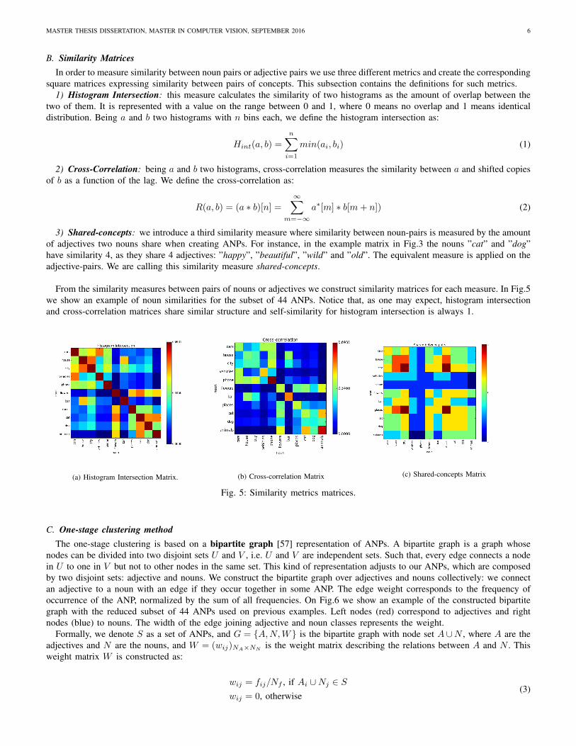
From the similarity measures between pairs of nouns or adjectives we construct similarity matrices for each measure. In Fig.5we show an example of noun similarities for the subset of 44 ANPs. Notice that, as one may expect, histogram intersectionand cross-correlation matrices share similar structure and self-similarity for histogram intersection is always 1.
(a) Histogram Intersection Matrix. (b) Cross-correlation Matrix (c) Shared-concepts Matrix
Fig. 5: Similarity metrics matrices.
C. One-stage clustering methodThe one-stage clustering is based on a bipartite graph [57] representation of ANPs. A bipartite graph is a graph whose
nodes can be divided into two disjoint sets U and V , i.e. U and V are independent sets. Such that, every edge connects a nodein U to one in V but not to other nodes in the same set. This kind of representation adjusts to our ANPs, which are composedby two disjoint sets: adjective and nouns. We construct the bipartite graph over adjectives and nouns collectively: we connectan adjective to a noun with an edge if they occur together in some ANP. The edge weight corresponds to the frequency ofoccurrence of the ANP, normalized by the sum of all frequencies. On Fig.6 we show an example of the constructed bipartitegraph with the reduced subset of 44 ANPs used on previous examples. Left nodes (red) correspond to adjectives and rightnodes (blue) to nouns. The width of the edge joining adjective and noun classes represents the weight.
Formally, we denote S as a set of ANPs, and G = {A,N,W} is the bipartite graph with node set A∪N , where A are theadjectives and N are the nouns, and W = (wij)NA×NN
is the weight matrix describing the relations between A and N . Thisweight matrix W is constructed as:
wij = fij/Nf , if Ai ∪Nj ∈ S
wij = 0, otherwise(3)

MASTER THESIS DISSERTATION, MASTER IN COMPUTER VISION, SEPTEMBER 2016 7
Fig. 6: ANP bipartite graph example with a reduced set of 44 ANPs.
where fij denotes the frequency of occurrence of the ANP composed by Ai∪Nj , and Nf is the sum of all ANP frequencies:
Nf =
NA∑i=1
NN∑j=1
fij (4)
The above described bipartite graph G = {A,N,W}, is partitioned into k groups by using spectral co-clustering. Thistechnique allows simultaneous clustering on the rows and columns of a matrix, generating bi-clusters, a subset of rows whichexhibit similar behavior across a subset of columns, or vice versa [3].
After applying spectral co-clustering independent nouns and adjectives are grouped together in the same cluster, but we stilldo not have ANP clusters. We combine adjectives and nouns in the same cluster creating ANPs. As not all pairs of adjective-noun combinations are correct, we use the ANP-frequency matrix described in subsection IV-A to discard those ANPs withfrequency zero.
As most clustering methods, spectral co-clustering algorithm requires to define the number of clusters, k, that the graph isgoing to be partitioned into. As we do not have any prior knowledge of the total number of clusters, we created a concept-similarity evaluation metric to optimize. Given the premise that nouns and adjectives in the same cluster must be similarbetween them, we are using the similarity metrics described in IV-A to decide the best number of clusters to be used.
The similarity value for a specific number of clusters k is measured as the average similarity between the k clusters, wecall it D[k]. As expressed in Eq.5 we optimize the hyperparameter k in order maximize the similarity metric D[k]:
k = argmax{D[k]} = argmax
{1
k
k−1∑c=0
( ∑i>j Scnoun
[i, j]
ncnoun(ncnoun
− 1)/2+
∑i>j Scadj
[i, j]
ncadj(ncadj
− 1)/2
)}(5)
In Eq.5, Scadjand Scnoun represent the similarity sub-matrix, with only the pairs of adjectives or nouns in a given cluster
c. This similarity sub-matrix may correspond to the measures of Histogram Intersection Matrix, Cross-Correlation Matrix orShared-concepts Matrix between pairs of concepts, while ncadj
and ncnounrepresent the total number of adjectives and nouns
inside a given cluster c.
D. Two-stage clustering methodThe two-stage clustering operates on both noun and adjective category on the first-stage, and then creates sub-clusters of the
other category on the second-stage. We split the first category (nouns or adjectives) into k1 clusters and for each cluster wegenerate k2i sub-clusters. For the second-stage clustering we just consider the subset of nouns/adjectives that can form ANPswith the adjectives/nouns on the first-stage.

MASTER THESIS DISSERTATION, MASTER IN COMPUTER VISION, SEPTEMBER 2016 8
Stage clustering is based on agglomerative hierarchical clustering [36]. This technique builds a bottom-up hierarchy byprogressively merging pairs of clusters. It starts with a cluster for each observation and pairs of clusters are merged togetheras one moves up the hierarchy. In order to decide which clusters should be combined, a measure of dissimilarity between setsof observations is required. In our work, the previously described similarity matrices constructed with histogram intersection(Eq.1) and cross-correlation (Eq.2) are used. In each step of the algorithm, the clusters with smaller distance between themare merged. We can express it mathematically as:
c = a ∪ b if d(a, b) = mina,b{d(ai, bi)} (6)
where a and b are independent clusters and c is their union. Being S(a, b), the similarity measure, the distance betweenclusters is expressed as:
d(a, b) = 1− S(a, b) (7)
Once first-level and second-level stages are clustered, we need to combine the adjectives and nouns from the two levels tocreate ANP clusters. As not all adjective-noun combinations are possible ANPs, we restrict ANP combinations to pairs withfrequency higher than zero, according to the ANP-frequency matrix from IV-A.
As for spectral co-clustering on the one-stage clustering approach, (IV-C), agglomerative hierarchical clustering requires astopping criterion like setting the number of clusters for the partition, k. Equivalently as for the one-stage clustering, basedon the premise that adjectives and nouns in the same cluster must be similar between them, we use the similarity matrix ofshared-concepts to optimize the hyperparameter k. We adapted Eq.5 for this case, where we only have names or adjectivesinside the same cluster. The optimization problem is thus expressed as:
k = argmax{D[k]} = argmax
{1
k
k−1∑c=0
∑i>j Sc[i, j]
nc(nc − 1)/2
}(8)
where Sc is the Shared-Concepts similarity matrix, containing only the subset of concepts in the cluster c, and nc is thetotal number of concepts in the cluster. The similarity function D[k] is maximized in order to optimize the number of clustersk to be used.
E. Experimental SetupAs described in III, MVSO dataset images come from retrieving images from Flickr through a query search of the ANPs
using Flickr-API. During the creation of the MVSO dataset, no more than 1,000 images per ANP query were downloaded.Also, for those ANPs with less than 1,000 images retrieved when using tag-search, the total number of retrieved images wasenlarged to include query search on the image title, description and metadata.
For building our ontology, we need our statistics to be based on the real ANP usage as Flickr image tags. Thus, as the ANPfrequencies from MVSO were modified by its authors, they are not useful for us. In order to get the real ANP frequencies weneeded to repeat the ANP query retrieval from Flickr, following the next procedure:
1) Based on the list of 4,342 ANPs from English-MVSO, we build an extended set of non-filtered ANPs by listing allthe possible combinations between the 686 adjectives and 1,467 nouns. We get a total of 1,006,362 adjective-nouncombinations.
2) We perform a query search on Flickr image tags for all adjective-noun combination and retrieve the number of images.From all the possible combinations we discard those ones with less than 40 images retrieved, getting a total of 35,384ANPs.
Analyzing the ANP-frequencies from Flickr, we notice a huge concentration of images from a little number of ANPs. Weshow the sorted frequency range in Fig.7a, and observe that the first 2, 804 ANPs from the total of 35, 384 concentrate an80% of the total sum of frequencies.
This tag popularity difference is going to produce a bias in our statistics that might affect our results negatively. In orderto mitigate this bias, we propose to apply an upper threshold on the frequencies, so all the frequencies above a thresholdth are set to th. Experiments are going to compare cluster similarity with no thresholding, when th = 100, 000 and whenth = 40, 000. Fig.7 shows ANP frequency distribution with and without thresholding. Observe how the unbalance is mostlyremoved when thresholding, but we still keep the statistic relevance of most popular tags.
The ANP-frequency matrix described in IV-A is constructed using the retrieved ANPs, resulting a sparse matrix of size686× 1, 467 with 35, 384 non-zero elements. This matrix is used as the base to construct both clustering approaches.

MASTER THESIS DISSERTATION, MASTER IN COMPUTER VISION, SEPTEMBER 2016 9
(a) Original ANP Tag Frequency
(b) ANP Tag Frequency with th = 100, 000
(c) ANP Tag Frequency with th = 40, 000
Fig. 7: Frequency distribution with and without.
F. Results and discussion1) Similarity metrics results: Using the three concept-similarity metrics, presented in subsection IV-B, we listed the resulting
top-20 most similar adjective-pairs and noun-pairs in table II, and analyzed the results. Concept-pairs are listed from moresimilar to less similar, according to the three similarity measurements without any thresholding.
We notice that using histogram intersection and cross-correlation provide similar results. While the share-concepts metricfinds other kinds of relations. This is because similarity in histogram intersection and cross-correlation is based on the ANPfrequencies, while shared-concepts considers binary relations between adjectives and nouns. For histogram intersection andcross-correlation we also observe a repeated presence of the same concepts, e.g. the adjective ”old”, ”exotic” and ”classique”appear multiple times in the adjective top-ranking. This is because adjectives with higher popularity have higher values ofhistogram intersection and cross-correlation. Similar relations are found when analyzing results from top noun-pairs similarities.As for adjective similarities, most popular nouns, i.e. nouns with higher frequency, are predominant on the top similaritiesusing histogram intersection and cross-correlation, e.g. ”city”, ”warden”, ”man” and ”woman”.
We observe how our metrics are able to detect usability relations between concepts. For example, the adjectives ”classic”,”antique”, ”modern” and ”contemporary” are all used to describe buildings, while ”beautiful”, ”cute”, ”pretty” and ”sexy” areused to describe people, and also express similar sentiment. We also notice semantic relations between pairs. Like synonymousrelations, e.g. ”beautiful-pretty”, ”hot-sexy” or ”old-antique”; and antonymous or contrasting relations, e.g. ”sunny-rainy” and”big-small”. Equivalently for nouns, semantic similar ones are paired together, e.g. ”woman-men”, ”dog-cat” or ”woman-women”.
2) One-stage clustering: The one-stage clustering method presented in Section IV-C was tested to create clusters includingboth adjectives and nouns, and then we generate ANPs by combining those adjectives and nouns. We first show the results fromusing the spectral co-clustering technique in the bipartite graph from Fig.6 (the 44 ANPs example). In Fig.8 we representedthe same graph but with colored nodes, depending on the cluster they fall in. We optimized the number of clusters usinghistogram intersection as similarity metric, resulting an optimal k = 3. The resulting ANPs from the combination of adjectives

MASTER THESIS DISSERTATION, MASTER IN COMPUTER VISION, SEPTEMBER 2016 10
TABLE II: Top-20 most similar pairs
ADJECTIVE PAIRS NOUN PAIRSHistogram Intersection Cross-correlation Shared-concepts Histogram Intersection Cross-correlation Shared-concepts
classic - exotic classic - exotic big - small city - warden mill - stone dog - catnatural - low natural - low beautiful - cute city - woman mill - tier people - dog
classic - super classic - super great - beautiful warden - woman house - bikes weather - dayexotic - super old - classic beautiful - little city - men stuff - mill people - girlold - classic exotic - super beautiful - pretty woman - men bikes - housekeeping cat - girlold - super old - exotic little - small cars - factory warden - clouds people - catold - exotic classic - antique old - beautiful mill - door bikes - comedy men - women
old - historic old - super wild - beautiful house - architecture warden - schools dog - girlold - antique exotic - antique hot - sexy warden - men warden - days girl - face
classic - antique super - antique beautiful - happy house - road mill - exchange house - architectureexotic - antique old - antique beautiful - sexy lady - cemetery bikes - castle house - dogsuper - antique classic - fast beautiful - amazing truck - lady warden - church cat - boy
beautiful - young classic - historic beautiful - lovely architecture - road street - bikes city - architectureclear - fresh classic - cool outdoor - creative barn - architecture house - street city - day
beautiful - little open - hot old - abandoned woman - market bikes - space house - peoplemodern - contemporary clear - fresh natural - beautiful city - phone warden - wood woman - women
hot - sexy natural - soft big - great house - barn bikes - bones people - flowerssunny - rainy old - windy big - little barn - road bikes - zoo people - man
old - abandoned old - historic beautiful - young cemetery - dominion house - zoo dog - foodbeautiful - pretty exotic - fast old - classic advertising - memories dog - sailing dog - boy
and nouns are shown in Table III. Notice how stronger frequency relations between adjectives and nouns are kept, but theweakest ones are cut during the clustering process. This produces the loss of some possible adjective-noun combinations, asindividual nouns and adjectives can just belong to one cluster. From the 44 ANPs listed initially we just keep 25 after thisclustering.
Fig. 8: Spectral Co-clustering results for the 44 ANP example.
TABLE III: Example of one-stage ANP Clustering Results
Cluster 1 Cluster 2 Cluster 3
wild places old cars open housewild cat old city open barwild dog old vehicles
wild flowers old phonewild animals classic cars
beautiful places classic citybeautiful cat classic vehiclesbeautiful dog classic phone
beautiful flowersbeautiful animals
happy placeshappy cathappy dog
happy flowershappy animals
When we apply the one-stage clustering technique to all the retrieved ANPs, we noticed that we highly reduce the numberof ANPs as we increase the number of clusters k. For example, for the 40,000 threshold configuration and 600 clusters wekeep only 4,912 ANPs from the original 35,384 ANPs.
Analyzing the clusters we find that through the frequencies our method was able to reveal some semantic relations, e.g.a cluster grouping automobile and transport noun concepts as ”cars”, ”transport”, ”automobiles”, ”trucks”, ”mustang”and ”motors”, with the adjectives ”classic”, ”luxury” and ”crushed”, or an other cluster grouping animal noun concepts as”dogs”,”cat” and ”animals”, with the adjectives ”grumpy”, ”fat”, ”stray”, ”wet”, ”adopted” and ”beautiful”.
In Table IV we report the best number of clusters after optimization of the mean similarity D[k]. We compare the use ofdifferent similarity metrics on the optimization, with different maximum frequency thresholds. We observe some consistencybetween metrics. As expected, histogram intersection and cross-correlation tend to give the same optimal k across configurations.For the shared-concepts metric we also find consistency, e.g. for th = 100, 000, it is giving the optimal k at the same point as

MASTER THESIS DISSERTATION, MASTER IN COMPUTER VISION, SEPTEMBER 2016 11
the histogram intersection and in the other configurations we find local minim in the ki where the other metrics are optimal.
We also observe that as a consequence of lowering down the frequency threshold, the optimal number of clusters tends tobe smaller. This can be explained because when lowering the threshold, the frequency range is smaller and thus the distancebetween some concept pairs is shortened, increasing pairs similarity measurement. Because of this, some concept relations thatwere split when no thresholding are kept when th = 100, 000 or th = 40, 000.
TABLE IV: One-Stage Clustering Results
Config. Th Similarity metric D[k] k
1 - Histogram Intersection 2.29× 10⁻⁴ 9402 - Cross-correlation 2.08× 10⁻⁶ 9403 - Shared-concepts 13.16 740
4 100,000 Histogram Intersection 9.98× 10⁻⁵ 5505 100,000 Cross-correlation 1, 59× 10−7 9606 100,000 Shared-concepts 8.28 550
7 40,000 Histogram Intersection 1.81× 10⁻⁴ 6008 40,000 Cross-correlation 1, 64× 10−7 6009 40,000 Shared-concepts 23.27 260
3) Two-stage clustering: The two-stage clustering introduced in Section IV-D was also tested in the same dataset. Followingthe same approach as the the one-stage clustering, we first show results when applying the clustering method to the subsetof 44 ANPs. In Fig.9 we present results using the both considered approaches: noun-first and adjective-first. Clustering hasbeen done by using histogram intersection as distance metric and the number of clusters has been optimized using the meansimilarity measure from Equation 8. Next to each noun or adjective we show the cluster number where it belongs to.
(a) Noun-First Example (b) Adjective-First Example
Fig. 9: Two stage clustering example for the subset of 44 ANPs
In Table V we show mean similarity D[k] results, the best number of clusters in the first level k1 and the final total number ofclusters k. We vary the distance metric, the maximum frequency threshold and we cluster using the two approaches: adjective-first and noun-first. Unlike the one-stage clustering, with this method we keep all the possible adjective-noun combinations.
TABLE V: Two-Stage Clustering Results
Config. Threshold Distance metric D[k] k1 k
Adjective First
1 - Cross-correlation 281.78 105 1,9152 - Hist. Intersection 193.64 230 1,2683 100,000 Cross-Correlation 427.10 180 3,1734 100,000 Hist. Intersection 298.72 230 1,9325 40,000 Cross-Correlation 82.43 100 6466 40,000 Hist. Intersection 207.74 140 1,736
Noun First
7 - Cross-correlation 145.31 180 1,2588 - Hist. Intersection 708.09 335 5,2329 100,000 Cross-correlation 461.23 210 3,252
10 100,000 Hist. Intersection 718.09 295 5,25111 40,000 Cross-correlation 349.83 175 3,00912 40,000 Hist. Intersection 659.62 390 5,159

MASTER THESIS DISSERTATION, MASTER IN COMPUTER VISION, SEPTEMBER 2016 12
From Table V we notice how, in general, the total mean similarity D[k] is higher when clustering noun first, and also thetotal number of clusters (k) tends to be higher. According to our mean similarity metric we are getting better performance whenusing histogram intersection than cross-correlation. We believe histogram intersection is a better distance metric for this kind ofhistograms, as cross-correlation considers shifted copies of our histogram, which does not make sense for our representations.We get the best mean similarity when clustering noun-first and setting frequency th=100,000, using histogram intersection asdistance metric.
This technique is able to detect and cluster together plural and singular forms of the same nouns, as well as synonymousconcepts. For the adjectives we group concepts with similar applicability. See some examples of noun and adjective groupson Fig.10. For the noun-first configuration we group car and automobile related concepts in Cluster 139, animal and natureconcepts in Cluster 68, politics related nouns in Cluster 243, parts of the day or the year in Cluster 136, etc. And for adjective-first we cluster architecture related concepts in Clusters 36 and 47, church related concepts in Cluster 113, adjectives usuallyapplied to women and girls are grouped in Cluster 49, food related concepts in Cluster 15, etc.
Fig. 10: First-level clustering results for nouns (left) and adjectives (right). Noun cluster results are from configuration 10, andadjective cluster results from configuration 4 (table V).
Final (second-level) ANP clusters for noun-first and adjective-first configurations are shown in Fig.11. See how whenclustering noun-first we group ANP concepts as ”primary school”, ”secondary school”, ”elementary school”, ”medical school”,and when clustering adjectives we group concepts as ”delicious food”, ”delicous cake”, ”delicous dinner”, etc. While noun-first clustering brings together concepts that talk about similar entities, like girls/woman/girl/boy or bay/river/pond/beach;adjective-based clustering yields to concepts about similar or closely related emotions, like delicious/spicy/yummy.
Fig. 11: Final ANP clustering results for nouns (left) and adjectives (right). Noun cluster results are from configuration 10,and adjective cluster results from configuration 4 (table V).

MASTER THESIS DISSERTATION, MASTER IN COMPUTER VISION, SEPTEMBER 2016 13
V. ADJECTIVE AND NOUN CONTRIBUTION FOR ANP PREDICTION
In this section we present the proposed architectures for Adjective-Noun Pair (ANP) prediction that allows to study adjectiveand noun contribution on the ANP decision. To do that we construct specialized networks for adjective and nouns independently,which we are calling AdjNet and NounNet respectively. These network architectures are described on subsection V-B. Fromthese networks we extract intermediate feature representations of nouns and adjectives and fuse them with a fully connectedlayer of artificial neurons for ANP classification. Depending on the layer the intermediate features are extracted from, wedistinguish between two kind of ANP networks, which we call Visual-ANPNet and Semantic-ANPNet. The feature extractionmethod and the networks architecture is presented in V-C and V-D. Then, on subsection V-E we explain the method usedto back-propagate classification results in order to analyze adjective and noun contribution for each ANP prediction. Theexperimental setup is described on V-F and finally, results and contribution analysis are presented in subsection V-G.
A. Fundamentals on Deep Learning Tools
Before going deeper on the project methods, we are going to start with an overview on fundamentals on deep learning [6]and the tools we are going to use in this part of the project.
1) Artificial Neural Networks: Artificial Neural Networks are machine learning systems inspired on biological neurons.Biologically, each neuron is responsible for aggregating its inputs and passing them through an activation, that is then fedto subsequent neurons. Equivalently, in Artificial Neural Networks, the output of each neuron is computed by applying anon-linear operation (activation function) to a linear combination of its inputs. In Fig.12a we show an example of an artificialneuron and an activation step function in Fig.12b.
(a) Artificial Neuron (from [2])
(b) Step function or Activation function (from [1])
Fig. 12: Artificial Neuron and and activation function with threshold 1.
In the example Fig.12a the neuron has three inputs x1, x2, x3, which are combined with weights w1, w2, w3. Weights arereal numbers expressing the importance of the respective inputs to the output. The neuron’s output is 0 if non activated, or 1if activated. It is activated if the weighted sum of the neuron inputs (activation value) is greater than a given threshold. Theactivation value for a generic case of n inputs is expressed mathematically as:
a = x1w1 + x2w2 + ...+ xnwn =
i=n∑i=0
wixi (9)
In order to build deeper and more complex structures, neurons are grouped forming layers. See an example of a simpleneural network with three fully connected layers in Fig.13a, notice that two of the layers are considered hidden.
Once the network architecture and the activation functions are defined, the network parameters need to be set. Each neuronhas its own weights, which need to be optimized for an specific task during the learning process. These parameters are chosenby optimizing a certain loss function using backpropagation of the stochastic gradient descent algorithm, taking a minibatchof samples instead of single samples [32]. The use of a minibatch opposed to a single example reduces the variance in theparameter update and can lead to more stable convergence. During the learning process some hyper-parameters need to bedefined, e.g. the batch size of training data, the total amount of iterations or the learning rate.
Convolutional Neural Networks (CNN) are a subset of the described Artificial Neural Nets NN, with some characteristicsthat make them adequate for image and video recognition. Convolutional Neural Networks (CNNs) take advantage of thespatial relationships of the pixels in an image to learn convolutional filters which share parameters when spatially scanning theinput image and intermediate feature maps. The characteristic layers of CNNs have neurons arranged in 3 dimensions: width,height and depth. Contrast examples in Fig.13.

MASTER THESIS DISSERTATION, MASTER IN COMPUTER VISION, SEPTEMBER 2016 14
(a) Example of a regular 3-layer Neural Network
(b) Example of ConvNet
Fig. 13: Examples of NN (left) and ConvNet (right). A ConvNet arranges its neurons in three dimensions (width, height,depth), as visualized in one of the layers. Every layer of a ConvNet transforms the 3D input volume to a 3D output volumeof neuron activations. In this example the red input layer holds the image, so its width and height would be the dimensions ofthe image and the depth would be 3, corresponding to the RGB channels. (from [2])
The main types of layers that are employed when designing CNN are:• Convolutional (CONV): The convolutional layers are the core building block of a CNN. It consists on a set of filters (or
kernels), that are replicated across the whole visual field, sharing the same parametrization. This filters are trained in orderto activate when they see some specific type of feature at some spatial position in the input. Because of the share weights,all the neurons in the same layer detect exactly the same feature. During the forward pass, each filter is convolved acrossthe width and height of the input volume, producing a 2D activation map. It can be modeled as a convolution operation.
• Rectifier Linear Unit (ReLU): applies f = max(0, x) in an element-wise fashion. This leaves the size of the volumeunchanged.
• Normalization (NORM): these layers perform contrast normalization to its input, which has been proven to increaseclassification accuracy [30].
• Pooling (POOL): it performs a non-linear downsampling operation along the spatial dimensions (width, height), thus itcan be understood as a dimensionality reduction operation. The most typical types of pooling operations are max poolingand average pooling. It helps to make the representation become invariant to small translations of the input.
• Fully Connected (FC): all neuron in this layer are connected to all activations in previous layer. The output of each unitis an activation of the linear combination of all inputs and the weights, which can be expressed as dot product. They areusually placed at the end of the architecture.
• Softmax normalization: this layer converts scores from the last layer into probabilities, thus it is usually placed at thetop of the architecture.
2) Deep Taylor Decomposition: Neural Networks (NNs), as the ones just introduced in V-A1, perform impressively welland are state of the art method for solving various challenging machine learning problems. Nevertheless NNs are not fullyunderstood yet [37], limiting the interpretability of the solution and thus the scope of application in practice.
In the original deep Taylor decomposition work [41], Montavon et al. presented a methodology for interpreting genericmultilayer neural networks by decomposing the network classification decision into contributions of its input elements. In thissection we will shortly summarize this technique, as we are going to use it on our project to analyze adjective and noun featurecontributions. We chose this method over other similar methods because of its simplicity and easy applicability for simplefully connected networks, as the ones used in our method, giving very competitive results.
This technique is based on a decomposition approach. Decomposition techniques seek to redistribute the function outputon the input variables in a meaningful way. In particular, the proposed model is an iterative decomposition model based on afirst-order Taylor expansion. Remember that Taylor series consist on a representation of a function as an infinite sum of termsthat are calculated from the values of the function’s derivatives at a single point.
If considering a neural network mapping an input vector (xp)p to an output scalar xf , which are interconnected throughmany ReLU neurons arranged in a directed acyclic graph, Montavon shows the decomposition is applied iterativly as follows:
1) The output neuron xf is first decomposed on its input neurons.2) The redistribution on these neurons is redistributed on their own inputs3) The redistributed process is repeated until the input variables are reached
This back-propagation can be described through messages [[xf ]j ]i, designating how much of xf is redistributed from an

MASTER THESIS DISSERTATION, MASTER IN COMPUTER VISION, SEPTEMBER 2016 15
arbitrary neuron xj to one of its inputs xi. The redistributed terms coming from the neurons (xj)j to which xi contributes aresummed:
[xf ]i =∑j
[[xf ]j ]i (10)
In Fig.14 we show an example of a portion of a simple neural network where we can see how on backward propagation theneuron xj is decomposed on the two previous neurons, and how contributions on neurons xi from all the forward neurons aresummed.
Fig. 14: Portion of a neural network with an example of the Forward computation (left) and Backward computation (right).For the backward computation we show the distribution of contributions in red. (from [5] )
B. AdjNet and NounNet architectureAdjNet and NounNet are based on an AlexNet-styled architecture [30], called CaffeNet [21]. This network consists on five
convolutional layers and three fully-connected layers with pooling and normalization layers swapped. Network architecture isshown on Fig.15, where the purple nodes correspond to input (an RGB image of size 224 224) and output (N class labels),green units correspond to outputs of convolutions, red units correspond to the outputs of max pooling, and blue units correspondto the outputs of rectified linear (ReLU) transform. Convolutional layers 1 and 2 have also a normalization layer after thepooling. Layers 6, 7, and 8 are fully connected layers. Layer 8 is the last fully connected layer, which does the work of asoftmax classifier. Scores from the softmax classifier are translated to probabilities through a softmax normalization layer.
Fig. 15: CaffeNet architecture. In the read squares we highlight the layers from where we extract the visual-fetures (FC7) andthe semantic-features (Softmax). (form [4])
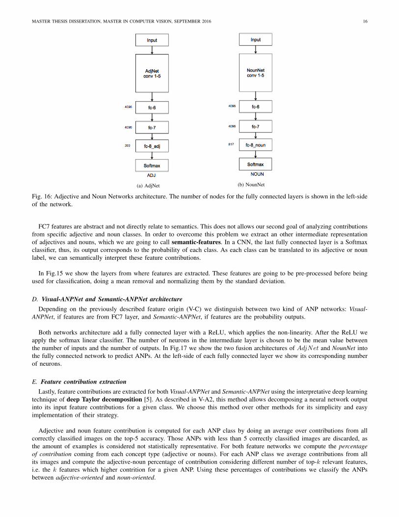
For learning adjectives and nouns the last fully connected layer of CaffeNet is changed for a new layer, its number of outputunits corresponds to the number of classes on each dataset. We show specific architectures for AdjNet and NounNet in Fig.16
C. Feature extractionThe two specialized nets, AdjNet and NounNet, are going to be used to extract an intermediate representation of adjective and
nouns. We propose two kind of ANP-learning architectures, depending on the adjective and noun intermediate representationfeature origin. In this sub-subsection the feature extraction procedure is described.
Recently, many works have shown the potential of deep learning features, using CNN as feature extractors. Layers fromCNN encode different parts and features of the image. While lower levels focus on details and local parts, upper levels containa more global description of the image. For this reason it has been suggested by some authors [43] [35] that the featuresfrom the upper layers of the CNN are the best ones to be used as image descriptors. Following those insights, our systemuses Layer 7 (FC7) of AdjNet and NounNet as intermediate representations of adjectives and nouns. From this features avisual-contribution study of adjectives and nouns is going to be done, that is why we are going to call these representation asvisual-features.
MASTER THESIS DISSERTATION, MASTER IN COMPUTER VISION, SEPTEMBER 2016 16
(a) AdjNet (b) NounNet
Fig. 16: Adjective and Noun Networks architecture. The number of nodes for the fully connected layers is shown in the left-sideof the network.
FC7 features are abstract and not directly relate to semantics. This does not allows our second goal of analyzing contributionsfrom specific adjective and noun classes. In order to overcome this problem we extract an other intermediate representationof adjectives and nouns, which we are going to call semantic-features. In a CNN, the last fully connected layer is a Softmaxclassifier, thus, its output corresponds to the probability of each class. As each class can be translated to its adjective or nounlabel, we can semantically interpret these feature contributions.
In Fig.15 we show the layers from where features are extracted. These features are going to be pre-processed before beingused for classification, doing a mean removal and normalizing them by the standard deviation.
D. Visual-ANPNet and Semantic-ANPNet architectureDepending on the previously described feature origin (V-C) we distinguish between two kind of ANP networks: Visual-
ANPNet, if features are from FC7 layer, and Semantic-ANPNet, if features are the probability outputs.
Both networks architecture add a fully connected layer with a ReLU, which applies the non-linearity. After the ReLU weapply the softmax linear classifier. The number of neurons in the intermediate layer is chosen to be the mean value betweenthe number of inputs and the number of outputs. In Fig.17 we show the two fusion architectures of AdjNet and NounNet intothe fully connected network to predict ANPs. At the left-side of each fully connected layer we show its corresponding numberof neurons.
E. Feature contribution extractionLastly, feature contributions are extracted for both Visual-ANPNet and Semantic-ANPNet using the interpretative deep learning
technique of deep Taylor decomposition [5]. As described in V-A2, this method allows decomposing a neural network outputinto its input feature contributions for a given class. We choose this method over other methods for its simplicity and easyimplementation of their strategy.
Adjective and noun feature contribution is computed for each ANP class by doing an average over contributions from allcorrectly classified images on the top-5 accuracy. Those ANPs with less than 5 correctly classified images are discarded, asthe amount of examples is considered not statistically representative. For both feature networks we compute the percentageof contribution coming from each concept type (adjective or nouns). For each ANP class we average contributions from allits images and compute the adjective-noun percentage of contribution considering different number of top-k relevant features,i.e. the k features which higher contrition for a given ANP. Using these percentages of contributions we classify the ANPsbetween adjective-oriented and noun-oriented.

MASTER THESIS DISSERTATION, MASTER IN COMPUTER VISION, SEPTEMBER 2016 17
(a) ANPNet (baseline)
(b) Semantic-ANPNet
(c) Visual-ANPNet
Fig. 17: The three ANP networks architectures.
For the Semantic-ANPNet we also translate the top-5 contributing adjectives and nouns to its semantic label. This allows usa more extensive analysis, lighting up the network classification process and giving insights about co-occurring elements andattributes on our dataset images.
F. Experimental Setup1) Dataset Construction: in [24] a subset of MVSO images coming from tag-restricted queries on Flickr is released. These
subset is called tag-pool from MVSO images. For our experiments 1,200 ANPs from the 3,911 ANPs in the English-MVSOtag-pool dataset are used. ANPs are selected to have around 1,000 images each. The total number of images in our subset is1,179,365.
From the 1,200 ANPs we list and re-label unique adjectives and nouns, getting a total of 350 adjective classes and 617 nounclasses. Unlike ANP classes, adjective and noun classes are unbalanced. This unbalancing is representative of each adjectiveand noun visual variance in the dataset, i.e. adjectives like ”happy” or ”beautiful” may need a wide range of visual featuresin order to represent the concept, so we may also need a higher amount of images for training these concepts. In Table VIwe show a summary of our dataset characteristics. The 80% of this dataset is assigned to the train set and the 20% to the test set.
TABLE VI: Dataset characteristics
Category #Images #Classes Min class #Images Max class #Images
ANP 1,179,365 1,200 864 1,000Adjective 1,179,365 350 912 51,020
Noun 1,179,365 617 919 19,663

MASTER THESIS DISSERTATION, MASTER IN COMPUTER VISION, SEPTEMBER 2016 18
2) Training AdjNet and NounNet: As described on V-B, these networks are based on CaffeNet architecture. The adoptedarchitecture contains more than 60 million parameters, which is too much to optimize from scratch with the limited amount ofdata. A common method that has already been used and proved good results in previous VSO and MVSO works [8] [25] isfine-tuning an existing model. The advantage of using this technique instead of randomly initializing all parameters is that thegradient descent algorithm starting point is already closer to an optimum, reducing thus the amount of iterations needed for thealgorithm to converge and the likelihood of over-fitting [59] [58]. Fine-tuning consists in initializing parameters in each layerbut the last one with weights and biases from another model. The last fully connected layer is then discarded and replacedby a new one, usually containing the same number of neurons as the number of classes in the dataset: in this case 350 forAdjNet and 617 for NounNet, as shown in the network schemes on Fig.16. This last layer weights are initialized randomly andlearned from scratch.
For fine-tuning AdjNet and NounNet, weight parameters are initialized from the English-MVSO [25] bank detector. Theseweights were already fine-tuned from the CaffeNet model trained using ILSVRC 2012 dataset [12] and are already sentiment-biased, as they were trained to detect the 4,342 ANPs from English-MVSO. Last fully connected layer weights are randomlyinitialized using Gaussian random initialization.
We fine-tune each network during 15 epochs, using mini-batches of 201 randomly sampled images each, i.e. the CNN seeseach training image 15 times. The network is trained using stochastic gradient descent, with momentum of 0.9 and an initialbase learning rate of 0.001. The learning rate for the last fully connected layer is multiplied by a factor of 10 to allow formore aggressive updates on that layer compared to the other layers. The learning rate is decreased gradually by a factor of 10every 20,000 iterations.
3) Training ANPNet (baseline): With identical settings to the adjective and noun networks, an ANP network is trainedend-to-end as the baseline. We are going to refer to this network as ANPNet. We show an scheme of this architecture in Fig.17-a.
4) Training Visual-ANPNet and Semantic-ANPNet: Unlike previous networks, as these architectures are not based in anyprevious model, weights and bias parameters for these two fully connected networks are completely learned from scratch. Weinitialize the weights using random Gaussian initialization, and train each network during 100 epochs, using mini-batches of201 feature vectors. The initial base learning rate is the same for all the layers. We set it to 0.1 to provide faster convergencerate on the first iterations, and we divide it by a factor of 2 every 8 epochs.
G. Results and discussionThis sub-section presents results from the experiments described in V-F, as well as discussion about it.
Networks performance is evaluated and compared using accuracy. Accuracy is a common performance evaluation metricfor this kind of networks, as can be seen in similar works [10] [25] [24].
As the images in the dataset have been automatically download from Flickr and labels correspond to user generated tags,many labels are noisy or ambiguous, i.e. some of the labels are non representative of the image content, or in some casesdifferent labels correspond to visually equivalent concepts, e.g. ”beautiful flower” and ”pretty flower”. Because of the nature ofthese data, evaluation was based on both top-1 and top-5 accuracy results, as we believe top-5 accuracy is more representativeof the real network performance. Top-k Accuracy is defined as:
Top-k Accuracy =number of correctly predicted samples in the top-k
number of samples(11)
1) Adjective vs. Noun vs. ANP Detection: The accuracy results from testing the single tower networks (AdjNet, NounNetand ANPNet) are shown in table VII. Despite these results are not completely comparable due to the different number ofclasses for each concept, they give us an insight on the difficulty of each task. As originally pointed by the deep cross-residuallearning work [23], in terms of problem difficulty ordering, noun prediction is the least challenging visual recognition task,followed by adjective and finally ANP recognition.
Adjective detection is expected to be more difficult than noun detection because of the more abstract concepts and thehighest visual variance, e.g. there may be a wide range of visual features required to describe the concept ”happy”. Also,the fact that the original network weights were trained to detect objects may be biasing performance. However, if comparingadjective versus ANP detection task, ANP seems to be affected for more visual difficulties than the overall visual variance.

MASTER THESIS DISSERTATION, MASTER IN COMPUTER VISION, SEPTEMBER 2016 19
TABLE VII: Single-Tower Networks Classification Accuracy
Network #Classes #Images #Train #Test top-1 top-5
AdjNet 3501,179,365 943,494 234,870
19,85% 42,41%NounNet 617 21,56% 42,16%ANPNet 1,200 18.03% 35.22%
In Fig.18 we show the top-100 adjectives, nouns and ANPs with better classification accuracy. Notice how ANPs withsmaller visual variance are the ones better detected, e.g. ”amazing circles” is the ANP better detected with a 97.23% accuracyand ”circles” is also the noun with better accuracy (97.79%), as the visual variance for both classes is very low, while for theadjective ”amazing” the accuracy is only a 30.39%.
Fig. 18: The top-100 classes with best classification accuracy for nouns (top graphic), adjectives (middle graphic) and ANPs(bottom graphic), considering the top-5 accuracy.
When contrasting class accuracies we notice the different information learned from each classifier. For example, the top-5accuracy for ”cute boy” is only 13.79% with ANPNet, while cute and boy have accuracies of 65.77% and 33.98%, respectively.This results make us belive that there is information from adjectives and nouns that AdjNet and NounNet are learning but

MASTER THESIS DISSERTATION, MASTER IN COMPUTER VISION, SEPTEMBER 2016 20
ANPNet is not. This gives us hope on the fusion of these networks being able to improve accuracy with respect to the baseline.
2) Visual vs. Semantic vs. Baseline architectures for ANP Detection: In table VIII we present the accuracy results fromthe two architectures proposed for ANP detection, compared to the single tower detector, trained as baseline. Notice how, asforeseen from previous networks results, through the fusion of adjective and noun features from the FC7 in Visual-ANPNet weare able to improve over a 2% the ANP detection performance for both top-1 and top-5 accuracy. Despite Semantic-ANPNetis not improving results over the baseline, this network allows for an extensive concept-based contribution analysis with a lowaccuracy decrease cost.
TABLE VIII: ANP Classification Accuracy
Network #Classes #Images #Train #Test Top-1 Top-5
ANPNet (baseline)1,200 1,179,365 943,494 234,870
18.03% 35.22%Semantic-ANPNet 16.44% 32.68%Visual-ANPNet 20.02% 37.88%
We also compared class by class accuracy behavior on the architectures in order to visualize which different information isbeing learned. On Fig.19 we show a graphic with the top-100 classes with the highest improvement increase, in comparison withthe ANP-Net baseline. Notice how all three networks benefit from different information depending on the class. In general,classes with greatest performance when using a singe-tower network tend to decrease performance when using the otherarchitectures. This behavior could be expected, as end-to-end learning performs better for classes with low visual variance.Nevertheless, accuracy tends to improve when fusing networks information for ANPs with higher visual variance.
Fig. 19: The 100 ANPs with higher accuracy improvement for each purposed network (green), compared to ANPNet baseline(blue), sorted in descending order. In the top we show results for the Visual-ANPNet and in the bottom for the Semantic-ANPNet.

MASTER THESIS DISSERTATION, MASTER IN COMPUTER VISION, SEPTEMBER 2016 21
3) Feature Contribution Analysis: Finally, we show some examples of the feature-contribution results for individual classesusing Semantic-Net and Visual-Net. We first present results from the percentage of contribution study on nouns and adjectives.These values are computed for both Visual and Semantic features. Second part focuses on analyzing specific semantic featuresfor each ANP, translated to its original label.
• Percentage of contribution In Table IX we show some result examples, considering different top-k features. We confirmour theory of adjective and nouns contributing different depending on the ANP. Nevertheless we observe a tendency ofbalanced contributions the more features we add in the top-k, with a slightly higher contribution from nouns. This isnot surprising, as we have more nouns than adjectives and, in general, nouns are more visually explicit than adjectives.Moreover NounNet showed better accuracy than AdjNet, so noun features are giving a higher degree of confidence on theprediction. We also noticed that even for adjective-oriented ANPs, the adjective contributions tend to be weaker than nouncontributions, i.e. even for adjective-oriented ANPs the noun still plays an important part. In some ANPs noun-contributioncan reach the 90% when taking less than a top-10 features, while adjective contributions for the Semantic-Net are allbellow the 80%, and bellow 60% for the Visual-ANPnet. This tells us that noun-visual information tends to be moredescriptive of the image content and thus have more influence on the ANP detection. We also observe that the conceptcontribution orientation is in general consistent between the two networks.
Contrasting contributions from visual versus semantic features, we see the percentage contributions differ. It is actuallynot surprising, as the feature representations are very different. Nevertheless, from the examples in the table, we identifya tendency for both kinds of networks to give more relevance to the adjective or the noun, e.g. for the ANPs ”pregnantwoman”, ”frozen water” and ”sparkling water” the predominance is in the adjective, while for ”happy dog”, ”cute kitten”and ”old cars” the predominance is in the noun.
TABLE IX: Percentage of Contribution Examples
Visual-ANPNet Semantic-ANPNet
top-1 top-5 top-10 all features top-1 top-5 top-10 all features
happy dog 31.00% 26.07% 25.70% 41.60% 35.12% 38.58% 42.19% 46.67%pregnant woman 43.47% 49.01% 51.20% 43.91% 58.32% 51.26% 49.10% 47.89%cute kitten 30.78% 33.23% 34.06% 43.43% 42.40% 35.23% 34.43% 48.65%lazy river 39.34% 44.44% 44.47% 43.57% 72.22% 66.65% 63.91% 47.30%sparkling water 47.54% 51.27% 49.76% 43.65% 70.89% 61.98% 57.84% 49.63%frozen water 57.53% 52.27% 51.42% 43.79% 72.00% 54.44% 51.43% 48.13%old cars 36.76% 33.83% 32.47% 42.57% 25.43% 31.18% 33.86% 42.57%bright sun 40.89% 42.41% 42.64% 43.42% 13.49% 25.35% 30.31% 43.42%sunny beach 44.32% 41.04% 39.52% 43.14% 48.67% 41.62% 42.23% 43.14%big city 48.53% 42.55% 42.16% 43.27% 27.22% 30.91% 35.24% 43.27%little kid 39.10% 39.55% 39.34% 43.33% 17.41% 26.67% 30.28% 43.31%
In table X we show a list of ANPs classified between noun-oriented and adjective-oriented. The noun-oriented ANPs arein general object-based concepts, like ”dog”, ”birds” or ”cars”, with abstract adjectives like ”good”, ”funny”, ”beautiful”or ”cute”. In the other hand, the adjective-oriented ANPs are in general scene-based or cases where the noun is moreabstract, and thus the differentiating part is in the adjectives, like ”architecture”, ”morning” or ”music”. Other exampleswhere the noun is not abstract but the ANP is adjective-oriented are ”pregnant belly” or ”sad face”, where the determininginformation to distinguish the concept and limiting the noun visual variance is found on the adjective.
TABLE X: Top-10 ANP Concept-Contribution Clustering
Visual-ANPNet Semantic-ANPNet
Adjective-oriented Noun-oriented Adjective-oriented Noun-oriented
Abandoned Building Good Dog Overcast Sky Dead BodyWarning Sign Wild Pig Sad Face Small mouth
Sparkling Water Old Dog Simple Life Holy CowTropical Garden Beautiful Birds Popular Music Exotic Fruit
Wet Cat Domestic Cat Linear Park Funny HatsMedieval Architecture Happy Dog Grumpy Cat Wild Child
Foggy Morning Cute Kitty Pregnant Belly Lovely CityContemporary Architecture Big Buddha Fat Cat Fast Cars
Teenage Girl Little Dog Lazy River Hidden TreasureModern Building Sweet Food Foggy Morning Long Nose
In table XI we show the complete contribution analyze results for the noun-oriented ANP ”cute cat”, versus the adjective-oriented ANP ”foggy day”. Each ANP table shows the detection accuracy for each network, the percentage of contribution
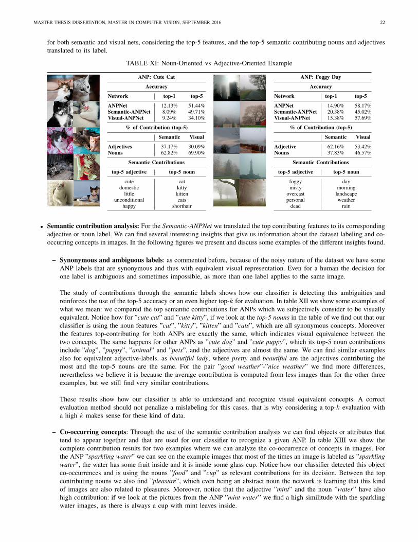
MASTER THESIS DISSERTATION, MASTER IN COMPUTER VISION, SEPTEMBER 2016 22
for both semantic and visual nets, considering the top-5 features, and the top-5 semantic contributing nouns and adjectivestranslated to its label.
TABLE XI: Noun-Oriented vs Adjective-Oriented Example
ANP: Cute Cat ANP: Foggy Day
Accuracy Accuracy
Network top-1 top-5 Network top-1 top-5
ANPNet 12.13% 51.44% ANPNet 14.90% 58.17%Semantic-ANPNet 8.09% 49.71% Semantic-ANPNet 20.38% 45.02%Visual-ANPNet 9.24% 34.10% Visual-ANPNet 15.38% 57.69%
% of Contribution (top-5) % of Contribution (top-5)
Semantic Visual Semantic Visual
Adjectives 37.17% 30.09% Adjective 62.16% 53.42%Nouns 62.82% 69.90% Nouns 37.83% 46.57%
Semantic Contributions Semantic Contributions
top-5 adjective top-5 noun top-5 adjective top-5 noun
cute cat foggy daydomestic kitty misty morning
little kitten overcast landscapeunconditional cats personal weather
happy shorthair dead rain
• Semantic contribution analysis: For the Semantic-ANPNet we translated the top contributing features to its correspondingadjective or noun label. We can find several interesting insights that give us information about the dataset labeling and co-occurring concepts in images. In the following figures we present and discuss some examples of the different insights found.
– Synonymous and ambiguous labels: as commented before, because of the noisy nature of the dataset we have someANP labels that are synonymous and thus with equivalent visual representation. Even for a human the decision forone label is ambiguous and sometimes impossible, as more than one label applies to the same image.
The study of contributions through the semantic labels shows how our classifier is detecting this ambiguities andreinforces the use of the top-5 accuracy or an even higher top-k for evaluation. In table XII we show some examples ofwhat we mean: we compared the top semantic contributions for ANPs which we subjectively consider to be visuallyequivalent. Notice how for ”cute cat” and ”cute kitty”, if we look at the top-5 nouns in the table of we find out that ourclassifier is using the noun features ”cat”, ”kitty”, ”kitten” and ”cats”, which are all synonymous concepts. Moreoverthe features top-contributing for both ANPs are exactly the same, which indicates visual equivalence between thetwo concepts. The same happens for other ANPs as ”cute dog” and ”cute puppy”, which its top-5 noun contributionsinclude ”dog”, ”puppy”, ”animal” and ”pets”, and the adjectives are almost the same. We can find similar examplesalso for equivalent adjective-labels, as beautiful lady, where pretty and beautiful are the adjectives contributing themost and the top-5 nouns are the same. For the pair ”good weather”-”nice weather” we find more differences,nevertheless we believe it is because the average contribution is computed from less images than for the other threeexamples, but we still find very similar contributions.
These results show how our classifier is able to understand and recognize visual equivalent concepts. A correctevaluation method should not penalize a mislabeling for this cases, that is why considering a top-k evaluation witha high k makes sense for these kind of data.
– Co-occurring concepts: Through the use of the semantic contribution analysis we can find objects or attributes thattend to appear together and that are used for our classifier to recognize a given ANP. In table XIII we show thecomplete contribution results for two examples where we can analyze the co-occurrence of concepts in images. Forthe ANP ”sparkling water” we can see on the example images that most of the times an image is labeled as ”sparklingwater”, the water has some fruit inside and it is inside some glass cup. Notice how our classifier detected this objectco-occurrences and is using the nouns ”food” and ”cup” as relevant contributions for its decision. Between the topcontributing nouns we also find ”pleasure”, which even being an abstract noun the network is learning that this kindof images are also related to pleasures. Moreover, notice that the adjective ”mint” and the noun ”water” have alsohigh contribution: if we look at the pictures from the ANP ”mint water” we find a high similitude with the sparklingwater images, as there is always a cup with mint leaves inside.

MASTER THESIS DISSERTATION, MASTER IN COMPUTER VISION, SEPTEMBER 2016 23
TABLE XII: Semantic Contribution Comparison of Visually Equivalent ANPs
Cute Cat Cute Kitty Cute Dog Cute Puppy
top-5 adjectives top-5 nouns top-5 adjectives top-5 nouns top-5 adjectives top-5 nouns top-5 adjectives top-5 nouns
cute cat cute cat cute dog cute puppydomestic kitty domestic kitty unconditional puppy unconditional dog
little kitten little kitten happy breed sad breedunconditional cats unconditional cats sad animal little pets
happy shorthair happy shorthair little boy mixed animals
Pretty Lady Beautiful Lady Good Weather Nice Weather
top-5 adjectives top-5 nouns top-5 adjectives top-5 nouns top-5 adjectives top-5 nouns top-5 adjectives top-5 nouns
pretty lady pretty lady hot air hot airbeautifu women beautifu women final approach nice distanceyoung model young model mad weather cold parksexy woman sexy woman special livery personal weather
happy girl teen girl fluffy sun long day
Using the semantic contributions we also understand which concepts are the ones defining abstract scenes like ”happyHalloween” or ”special day”. In table XIII we show an example of contributions for the ANP ”happy Halloween”.Notice how the network learned differentiating concepts for a Halloween scene, as ”blood”, ”cat”, ”haunted” and”dark”. Probably if we had the noun ”pumpkin” we would found it too in the top-5 contributions. In the other hand,for the ANP ”special day” (table XIV) the contribution study shows that when people tag images using this ANP itusually refers to a wedding, so we find ”wedding”, ”couple”, ”bride” and ”occasion” as the most contributing nouns,and positive descriptive adjectives as ”young”, ”happy”, ”beautiful” and ”outdoor”. We verify this correspondencewith the images in the dataset for this label. More examples of contribution results are shown in table XIV
TABLE XIII: Co-occurring concepts Examples
ANP: Sparkling Water ANP: Happy Halloween
Accuracy Accuracy
Network top-1 top-5 Network top-1 top-5
ANPNet 25.13% 38.50% ANPNet 11.11% 22.70%Semantic-ANPNet 24.06% 35.83% Semantic-ANPNet 12.08% 19.32%Visual-ANPNet 24.59% 39.03% Visual-ANPNet 13.59% 27.66%
% of Contribution (top-5) % of Contribution (top-5)
Semantic Visual Semantic Visual
Adjectives 61.98% 51.25% Adjective 21.63% 37.51%Nouns 38.01% 48.72% Nouns 78.36% 62.48%
Semantic Contributions Semantic Contributions
top-5 adjective top-5 noun top-5 adjective top-5 noun
sparkling water happy halloweenmint food haunted blood
happy tea stuffed stuffhot pleasures dark commentsraw cup little cat

MASTER THESIS DISSERTATION, MASTER IN COMPUTER VISION, SEPTEMBER 2016 24
TABLE XIV: More ANP Contribution Examples
ANP: Special Day ANP: Happy Birthday
Accuracy Accuracy
Network top-1 top-5 Network top-1 top-5
ANPNet 3.91% 22.90% ANPNet 7.07% 17.67%Semantic-ANPNet 1.68% 22.91% Semantic-ANPNet 6.57% 13.13%Visual-ANPNet 12.84% 25.69% Visual-ANPNet 8.08% 21.71%
% of Contribution (top-5) % of Contribution (top-5)
Semantic Visual Semantic Visual
Adjectives 24.61% 42.93% Adjective 23.53% 40.58%Nouns 75.38% 57.06% Nouns 76.46% 59.41%
Semantic Contributions Semantic Contributions
top-5 adjective top-5 noun top-5 adjective top-5 noun
young wedding happy birthdayhappy couple traditional causespecial bride little sweater
beautiful day young kidsoutdoor occasion sweet times
ANP: Traditional Architecture ANP: Medieval City
Accuracy Accuracy
Network top-1 top-5 Network top-1 top-5
ANPNet 2.87% 18.39% ANPNet 8.05% 27.01%Semantic-ANPNet 5.17% 18.97% Semantic-ANPNet 5.69% 33.18%Visual-ANPNet 9.77% 27.01% Visual-ANPNet 9.04% 34.76%
% of Contribution (top-5) % of Contribution (top-5)
Semantic Visual Semantic Visual
Adjectives 47.27% 45.86% Adjective 52.34% 51.58%Nouns 52.72% 54.13% Nouns 47.65% 48.41%
Semantic Contributions Semantic Contributions
top-5 adjective top-5 noun top-5 adjective top-5 noun
traditional architecture medieval cityimperial palace narrow villagehistoric city historic townancient house old architecture
old village gothic street
ANP: Cute Guy ANP: Modern Dance
Accuracy Accuracy
Network top-1 top-5 Network top-1 top-5
ANPNet 5.82% 21.69% ANPNet 29.60% 54.74%Semantic-ANPNet 6.88% 26.46% Semantic-ANPNet 22.91% 44.69%Visual-ANPNet 6.41% 27.27% Visual-ANPNet 28.65% 50.56%
% of Contribution (top-5) % of Contribution (top-5)
Semantic Visual Semantic Visual
Adjectives 31.32% 39.86% Adjective 36.35% 41.74%Nouns 68.37% 60.13% Nouns 63.64% 58.25%
Semantic Contributions Semantic Contributions
top-5 adjective top-5 noun top-5 adjective top-5 noun
cute guy modern dancesexy man contemporary news
young guys young dancinghot boy long music
happy chest senior light

MASTER THESIS DISSERTATION, MASTER IN COMPUTER VISION, SEPTEMBER 2016 25
VI. CONCLUSIONS
In this work we addressed two main challenges of the Visual Affective Computing field. In the first part of the projectwe proposed two data-driven clustering methods to construct an structured ANP ontology, based on adjective and nounfrequency relations. In the second part we presented a novel deep neural network for ANP prediction, that allows foradjective and noun contribution analyzes. In this section we discuss the degree of achievement for each part and wepropose future work and comment on open research lines.
A. Frequency-Based ANP OntologyIn this first part of the project we presented different tools to represent ANPs and three metrics to evaluate similaritybetween adjective and noun pairs, based exclusively on ANP-frequency. Using these tools, we developed two automaticANP clustering methods.
The first ANP clustering method is based on a bipartite graph representation of the ANPs. This kind of ANP representationhelps visualizing adjective-noun relations and is a useful way to help understand adjective and nouns visual variances.On this ANP representation we applied spectral co-clustering in order to group adjectives and nouns to generate ANPclusters. Nevertheless the applied clustering method does not allow for adjective and nouns to be on more than one cluster,thus we miss ANPs of those adjective-noun combinations that fall on different clusters. Soft clustering techniques, thatallow for data points to belong to more than one partition, should be explored in order to explode the bipartite graph ANPrepresentation. The second clustering method is based on a two-stage clustering, that allows us to represent adjective andnoun relations in a tree-structure. Unlike previous method, this clustering keeps all possible ANP combinations. Whenclustering nouns on the first level we tend to group similar objects, creating more semantic related clusters, while whenclustering adjective first adjectives with similar descriptive applications are clustered together, grouping emotional-relatedANPs. For both clustering methods we developed an optimization method in order to select the best number of clustersand measure consistence inside a cluster.
Future work should focus on creating objective evaluation metrics for the clustering methods. A way to evaluate similaritymetrics is comparing more similar adjective and noun pairs results with the results that an external dictionary as WordNetgives. A way of evaluating clustering, proposed on [45], is measuring sentiment-consistency and semantic-consistency.The metrics should be adapted to be used for our data representation. To evaluate sentiment consistency it would also benecessary to extend ANP-sentiment annotations to the new combinations of adjectives and nouns that do not belong tothe original MVSO dataset.
B. Adjective and Noun Contribution for ANP PredictionIn the second part of the project we proposed two new architectures for ANP prediction, in order to prove the hypothesisof adjective and nouns contributing different depending on the ANP class. The two architectures base the ANP predictionon the fusion of intermediate feature representations of adjectives and nouns, which are extracted from specializedconvolutional neural networks. Depending on the layer from which features are extracted and the kind of contributionsthese features allow us to study, we differentiated between two kind of features: visual and semantic. Through the use ofthe visual features we were able to improve accuracy results for both top-1 and top-5 accuracy, compared to the traditionalmethod.
Moreover, using the interpretable deep learning technique of deep Taylor decomposition we shed some light into theblack box that neural networks usually are. Through this technique we decomposed the network classification decisionfor each class into contributions for its input elements. This allowed us to compute adjective and noun feature relevancefor each ANP class decision, proving our hypothesis that contributions are different depending on the ANP and thatclassification benefits from decomposing the network into specialized sub-networks. By decomposing the results from theSemantic-ANPNet, we were also able to translate input elements to its corresponding adjective or noun semantic label.This allowed for a more extended contribution analysis study, that allowed us to understand our network learning processwhile getting insights about our dataset. For example, detecting visually equivalent ANPs or concept co-occurrences inimages, i.e. nouns or adjectives that appear together in images for a given ANP.
The information from the top-contributing labels can be used for many applications. For example, for an automatic imagecontent annotation, or to improve our networks accuracy by modifying the loss function so it does not penalize as muchthose equivalent ANPs. Future work should consider a human-evaluation based study in order to measure the quality ofour concept-contribution labels.

MASTER THESIS DISSERTATION, MASTER IN COMPUTER VISION, SEPTEMBER 2016 26
We believe accuracy in the prediction of ANPs could be improved by combining ANP frequency information extractedin the first part of this project, with the deep learning architectures from the second part. Fusing the specialized adjectiveand noun networks with the ANP frequency-matrix would open a new research line of combining deep learning withprobability models for ANP prediction. This kind of architecture also allows to explore zero-shot detection of ANPs.
In conclusion, in this work we contributed on representing and understanding better ANP relations, on the specific Flickrdomain, and we opened new research lines for ANP detection, by constructing specialized networks for adjectives andnouns.
ACKNOWLEDGMENT
First of all, I would like to thank Shih-Fu Chang for hosting me on his team and giving me the opportunity of coming toColumbia University to take part in such interesting project. Thanks a lot to my advisor back in Barcelona, Xavier Giro, forall his support, guidance, and dedication during all the thesis. Thanks too to Brendan Jou, as my third advisor, for his advice,patience and being always ready to help despite his busy working schedule. This project would not have been possible eitherwithout Vıctor Campos, who I want to thank for his dedication, support, help and great ideas.
Moreover, I am very grateful to Albert Gil and Josep Pujal for their technical support, and the students in the ImageProcessing Group from UPC, who have also been helpful when dealing with technical problems.
Also thanks to all the new friends in New York, who made this experience richer and unforgivable, and also to all the friendsback in Barcelona with who I know I can always count.
Finally, and most important, I would like to thank the support from my parents, Artur and Mariantonia, in all my decisions,not only during the past months, but also during my whole life.
REFERENCES
[1] Ai-Junkie cnn tutorial. http://cs231n.github.io/convolutional-networks/. Accessed: 2016-09-01.[2] Neural Networs and Deep Learning tutorial. http://neuralnetworksanddeeplearning.com/chap1.html. Accessed: 2016-09-01.[3] C. C. Aggarwal and C. K. Reddy. Data clustering: algorithms and applications. CRC Press, 2013.[4] A. Babenko, A. Slesarev, A. Chigorin, and V. Lempitsky. Neural codes for image retrieval. In ECCV, 2014.[5] S. Bach, H. FRAUNHOFER, A. Binder, and W. Samek. Deep taylor decomposition of neural networks.[6] I. G. Y. Bengio and A. Courville. Deep learning. Book in preparation for MIT Press, 2016.[7] N. Bianchi-Berthouze and A. Kleinsmith. A categorical approach to affective gesture recognition. Connection science, 2003.[8] D. Borth, T. Chen, R. Ji, and S.-F. Chang. Sentibank: large-scale ontology and classifiers for detecting sentiment and emotions in visual content. In
ACMM, 2013.[9] D. Borth, T. Chen, R. Ji, and S.-F. Chang. Sentibank: large-scale ontology and classifiers for detecting sentiment and emotions in visual content. In
ACMM, 2013.[10] T. Chen, D. Borth, T. Darrell, and S.-F. Chang. Deepsentibank: Visual sentiment concept classification with deep convolutional neural networks. 2014.[11] P. R. De Silva, M. Osano, A. Marasinghe, and A. P. Madurapperuma. Towards recognizing emotion with affective dimensions through body gestures.
In FGR, 2006.[12] J. Deng, W. Dong, R. Socher, L.-J. Li, K. Li, and L. Fei-Fei. Imagenet: A large-scale hierarchical image database. In CVPR, 2009.[13] S. d’Osgood. Tannenbaum, the measurement of meaning. Urbano, University of Illinois Press, 1957.[14] C. Fellbaum. WordNet. Wiley Online Library, 1998.[15] A. Hanjalic and L.-Q. Xu. Affective video content representation and modeling. IEEE transactions on multimedia, 2005.[16] K. He, X. Zhang, S. Ren, and J. Sun. Deep residual learning for image recognition. CVPR, 2015.[17] J. Healey and R. Picard. Digital processing of affective signals. In ASSP, 1998.[18] M. Hearst. Direction-based text interpretation as an information access refinement. Text-based intelligent systems: Current research and practice in
information extraction and retrieval, 1992.[19] J. Hornak, E. Rolls, and D. Wade. Face and voice expression identification in patients with emotional and behavioural changes following ventral frontal
lobe damage. Neuropsychologia, 1996.[20] J. Jia, S. Wu, X. Wang, P. Hu, L. Cai, and J. Tang. Can we understand van gogh’s mood?: learning to infer affects from images in social networks. In
ACMM, 2012.[21] Y. Jia, E. Shelhamer, J. Donahue, S. Karayev, J. Long, R. Girshick, S. Guadarrama, and T. Darrell. Caffe: Convolutional architecture for fast feature
embedding. In ACMM, 2014.[22] Y.-G. Jiang, B. Xu, and X. Xue. Predicting emotions in user-generated videos. In AAAI, 2014.[23] B. Jou and S.-F. Chang. Deep cross residual learning for multitask visual recognition. 2016.[24] B. Jou and S.-F. Chang. Going deeper for multilingual visual sentiment detection. 2016.[25] B. Jou, T. Chen, N. Pappas, M. Redi, M. Topkara, and S.-F. Chang. Visual affect around the world: A large-scale multilingual visual sentiment ontology.
In ACMM, 2015.[26] B. W. Jou. Large-scale affective computing for visual multimedia. 2016.[27] T. Kanade, J. F. Cohn, and Y. Tian. Comprehensive database for facial expression analysis. In FGR, 2000.[28] M. Kantrowitz. Method and apparatus for analyzing affect and emotion in text, 2003.[29] R. Krishna, Y. Zhu, O. Groth, J. Johnson, K. Hata, J. Kravitz, S. Chen, Y. Kalantidis, L.-J. Li, D. A. Shamma, et al. Visual genome: Connecting language
and vision using crowdsourced dense image annotations. 2016.[30] A. Krizhevsky, I. Sutskever, and G. E. Hinton. Imagenet classification with deep convolutional neural networks. In NIPS, 2012.[31] R. D. Lane and L. Nadel. Cognitive neuroscience of emotion. Oxford University Press, USA, 2002.

MASTER THESIS DISSERTATION, MASTER IN COMPUTER VISION, SEPTEMBER 2016 27
[32] Y. LeCun, L. Bottou, Y. Bengio, and P. Haffner. Gradient-based learning applied to document recognition. Proceedings of the IEEE, 86(11):2278–2324,1998.
[33] B. Li, S. Feng, W. Xiong, and W. Hu. Scaring or pleasing: exploit emotional impact of an image. In ACMM, 2012.[34] H. Liu, T. Selker, and H. Lieberman. Visualizing the affective structure of a text document. In ACMM, 2003.[35] M. Long and J. Wang. Learning transferable features with deep adaptation networks. CoRR, abs/1502.02791, 1:2, 2015.[36] O. Maimon and L. Rokach. Data mining and knowledge discovery handbook. 2005.[37] S. Mallat. Understanding deep convolutional networks. Phil. Trans. R. Soc. A, 374(2065):20150203, 2016.[38] P. McCorduck, M. Minsky, O. G. Selfridge, and H. A. Simon. History of artificial intelligence. In IJCAI, pages 951–954, 1977.[39] T. Mikolov and J. Dean. Distributed representations of words and phrases and their compositionality. NIPS, 2013.[40] F. F. Montalvo. Bridging the affective gap. Affective Education: Methods and Techniques, 1989.[41] G. e. a. Montavon. Explaining nonlinear classification decisions with deep taylor decomposition. 2015.[42] T. Narihira, D. Borth, S. X. Yu, K. Ni, and T. Darrell. Mapping images to sentiment adjective noun pairs with factorized neural nets. 2015.[43] M. Oquab, L. Bottou, I. Laptev, and J. Sivic. Learning and transferring mid-level image representations using convolutional neural networks. In
Proceedings of the IEEE conference on computer vision and pattern recognition.[44] B. Pang and L. Lee. Opinion mining and sentiment analysis. Foundations and trends in information retrieval, 2008.[45] N. Pappas, M. Redi, M. Topkara, B. Jou, H. Liu, T. Chen, and S.-F. Chang. Multilingual visual sentiment concept matching. ICMR, 2016.[46] R. W. Picard and R. Picard. Affective computing. MIT press Cambridge, 1997.[47] Y. Shin and E. Y. Kim. Affective prediction in photographic images using probabilistic affective model. In Proceedings of the ACM International
Conference on Image and Video Retrieval. ACMM, 2010.[48] P. Sidiropoulos, V. Mezaris, I. Kompatsiaris, H. Meinedo, M. Bugalho, and I. Trancoso. Temporal video segmentation to scenes using high-level
audiovisual features. TCSVT, 2011.[49] C. Szegedy, W. Liu, Y. Jia, P. Sermanet, S. Reed, D. Anguelov, D. Erhan, V. Vanhoucke, and A. Rabinovich. Going deeper with convolutions. In CVPR,
2015.[50] E. Vyzas. Recognition of emotional and cognitive states using physiological data. PhD thesis, MIT, 1999.[51] E. Vyzas and R. W. Picard. Affective pattern classification. In AAAI, 1998.[52] H. L. Wang and L.-F. Cheong. Affective understanding in film. IEEE, 2006.[53] W. Wang and Q. He. A survey on emotional semantic image retrieval. In ICIP, 2008.[54] X. Wang, J. Jia, P. Hu, S. Wu, J. Tang, and L. Cai. Understanding the emotional impact of images. In ACMM, 2012.[55] Y. Wang, J. Volker, and P. Haase. Towards semi-automatic ontology building supported by large-scale knowledge acquisition. In AAAI Fall Symposium
On Semantic Web for Collaborative Knowledge Acquisition, 2006.[56] W. Wei-ning, Y. Ying-lin, and J. Sheng-ming. Image retrieval by emotional semantics: A study of emotional space and feature extraction. In 2006 IEEE
International Conference on Systems, Man and Cybernetics, 2006.[57] D. B. West et al. Introduction to graph theory. Prentice hall Upper Saddle River, 2001.[58] J. Yosinski, J. Clune, Y. Bengio, and H. Lipson. How transferable are features in deep neural networks? In NIPS, 2014.[59] M. D. Zeiler and R. Fergus. Visualizing and understanding convolutional networks. In ECCV, 2014.