sustainability

Article

Machine Learning and Algorithmic Pairs Trading inFutures Markets

Seungho Baek 1, Mina Glambosky 1 , Seok Hee Oh 2,* and Jeong Lee 3

1 Department of Finance, Brooklyn College, City University of New York, 2900 Bedford Ave,Brooklyn, NY 11210, USA; Seungho.Baek@brooklyn.cuny.edu (S.B.);mglambosky@brooklyn.cuny.edu (M.G.)

2 Department of Computer Engineering, Gachon University, 1342 Seongnam-daero, Sujeong-gu, Seongnam-si,Gyeonggi-do 461-701, Korea

3 Department of Economics and Finance, University of North Dakota, Gamble Hall Room 110,293 Centennial Dr Stop 8098, Grand Forks, ND 58202, USA; jeong.lee@ndus.edu

* Correspondence: seokhee5@gachon.ac.kr

Received: 22 July 2020; Accepted: 20 August 2020; Published: 21 August 2020�����������������

Abstract: This study applies machine learning methods to develop a sustainable pairs tradingmarket-neutral investment strategy across multiple futures markets. Cointegrated pairs with similarprice trends are identified, and a hedge ratio is determined using an Error Correction Model (ECM)framework and support vector machine algorithm based upon the two-step Engle–Granger method.The study shows that normal backwardation and contango do not consistently characterize futuresmarkets, and an algorithmic pairs trading strategy is effective, given the unique predominantprice trends of each futures market. Across multiple futures markets, the pairs trading strategyresults in larger risk-adjusted returns and lower exposure to market risk, relative to an appropriatebenchmark. Backtesting is employed and results show that the pairs trading strategy may hedgeagainst unexpected negative systemic events, specifically the COVID-19 pandemic, remainingprofitable over the period examined.

Keywords: futures markets; backwardation; contango; futures prices; machine learning; cointegrationpairs trading; statistical arbitrage; support vector machine

1. Introduction

The classic rationale for futures prices is that the current futures contract price reflects the marketconsensus of the spot price at maturity. Since investors’ demand is conveyed in futures markets,the changes in futures prices and spot prices are strongly correlated [1–4]. Further, Tilton et al. [2]suggest that spot and futures prices exhibit a high correlation in strong contango, while they are lessrelated during periods of backwardation. It is well documented that returns to futures investors arehighly associated with market conditions [5–7]. In futures markets, there are two important marketconditions: contango and backwardation, which are terms used to explain the structure of the forwardcurve. A futures market in a contango condition exhibits a futures contract forward price that is higherthan the spot price. In contrast, a futures market in a backwardation condition exhibits a futurescontract forward price below the spot price.

Various papers have studied investor’s ability to forecast futures prices [6–8], but the evidence isinconclusive. The absence of consistent results regarding forecasting ability may be due to a focus oncertain futures markets over relatively short intervals, the impact of changes in market conditions,and the heterogeneous assumption that the rate of returns on futures contracts is normally distributed.In order to provide a more rigorous output, we hypothesize that hypothetical naïve speculators do not

Sustainability 2020, 12, 6791; doi:10.3390/su12176791 www.mdpi.com/journal/sustainability

Sustainability 2020, 12, 6791 2 of 21

demonstrate persistent performance in futures markets using a nonparametric method, as suggestedby Henriksson and Merton [9], and Chang [1]. Since the hypothetical speculators do not commandany forecasting ability, a rejection of the hypothesis means speculators make positive gains fromexpected risk premiums. Conditional probabilities result in a rejection of the hypothesis, evidenceof the effectiveness of speculator forecasting ability of a price trend. This suggests that investors canexploit a price trend over time in both contango and backwardation market conditions.

Previously, studies have identified that trend-following strategies (or momentum strategies)create significant abnormal returns in futures markets [10–14]. For example, Miffre and Rallis [12]show that trend-following strategies in commodity futures produce sizable returns after transactioncosts. Clare et al. [15] identify that trend-following strategies offer appealing risk-adjusted returns.Hurst et al. [14] find that time-series momentum was achieved even during past crisis periods.Previous studies have had a common view on the performance of trend-following strategies—theoutperformance of the strategy is not attributed to cross-sectional differences in expected returns acrossmarkets, but due to time-series dependence in realized returns [13].

However, there is very little research that has applied machine learning methods to futuresinvestments, as Creamer [15] summarizes. Few studies employ Neural Network [16], GeneticAlgorithm [17,18], Support Vector Machine [19], or Reinforcement Learning [20]. Most previous studieslimited the application of these methods to index futures trading using technical indicators. Moreover,trend following strategies typically see reversals when futures contracts that previously signaled anupward trend unexpectedly reverse (e.g., COVID-19 market crash). To mitigate this risk, we use apairs trading market neutral strategy, which involves long and short positions in two different futurescontracts with similar time-series price trends. As Rad et al. [21] suggest, the presence of a cointegrationrelation between two securities indicates a long-term relationship between the two; helping investorsaccurately implement a pairs trading strategy. Thus, we choose cointegrated pairs that have a similarpredominant price trend (e.g., contango and backwardation) and use Support Vector Machine (SVM)to determine a hedge ratio in an Error Correction Model (ECM) framework based upon the two-stepEngle–Granger method [22].

From the empirical analysis of the U.S. futures markets, we find that normal backwardationand forecasting theory may not be mutually exclusive, although they can be contrasting. This studyshows that normal backwardation and contango do not consistently characterize futures markets,but each futures market presents unique predominant price trends. This finding supports our approachof constructing pairs of futures contracts in the same futures markets as appropriate in developingalgorithmic pairs trading strategies. We find that our pairs trading strategy makes notable risk-adjustedreturns in various futures markets. Interestingly, our backtesting results show that our strategies canhedge against an unexpected decline in futures prices and importantly remain profitable through theCOVID-19 pandemic.

The remainder of the paper is organized as follows. Section 2 presents the development ofa measure of futures market conditions, details the model architecture, and a description of themethodology. Results and conclusions are presented in Sections 3 and 4, respectively.

2. Methodology

2.1. Measurement for Backwardation and Contango

Normal backwardation includes the following assumptions regarding speculators: (i) they take netlong positions, (ii) want positive profits, and (iii) do not have the skill to forecast prices. The implicationof normal backwardation is that, on average, futures prices rise approaching maturity. Conversely,under the contango market condition, hedgers are net short, and the futures price lies above theexpected future spot price; the price of the futures contract falls as the contract approaches maturity.

Assuming speculators are not equipped to forecast prices, the profits they generate can becategorized as a reward for bearing risk rather than for accurate forecasting. To examine this, we define

Sustainability 2020, 12, 6791 3 of 21

the values and returns of long and short trading positions following Rockwell [23]. Let VLm and VS

m bethe total value of the trading group’s long and short positions, in a specific market m, aggregated overthe selected period. Let Rm be the rate of return on the long open position in that market. The netreturn of a trading group credited to basic forecasting skill is defined as in Equation (1).

RBm =

Rm(VL

m −VSm

)VL

m + VSm

(1)

RAm denotes the actual return for the group; the measure of the special forecasting skill is then

obtained, defined as the residual.RF

m = RAm −RB

m. (2)

Hence, the aggregate return on any set of markets is defined as

RB =

∑m Rm

(VL

m −VSm

)∑

m VLm + VS

m(3)

and its corresponding forecasting skill is computed by

RF = RA−RB (4)

When, on average, the group takes a net long position (VLm −VS

m > 0), and Rm is positive, the RBm

measure will be positive. Conversely, the group is roughly net short (VLm − VS

m < 0) when Rm isnegative. From this relationship, we can define the basic skill as (i) the capacity to take a net longposition in markets with rising prices, and (ii) the capacity to take a net short position in markets withfalling prices.

The definition of the basic skill reflects the long-run skills of a trading group to generate profitsin the futures market. Furthermore, forecasting skill reflects the facility of a trading group to alterits position over time in order to take advantage of short-run price trends. In markets where nostrong evidence of backwardation or contango appears, forecasting skills will be crucial to makepositive returns. For example, both contango and backwardation reflect the term structure of futuresprices. Backwardation refers to prices that decline with maturity (downward sloping term structure),and contango is the opposite, with an upward slope. The future spot price is expected to remain similarto the current value so that in backwardation, low futures prices for distant maturities are expected torise over time. This would provide an expected profit to the speculators who, in aggregate, took on theprice risk from hedgers who were holding inventories in the spot market and selling futures to protectagainst a price drop. A similar argument when hedgers are net-long leads to a contango pattern andexpected profits to speculators who are net short.

By analyzing the number of price increase periods over the total number periods (i.e., PIP/TP),we are able to understand price behaviors in futures markets. In terms of PIP/TP, we classify fourpatterns of futures prices over time: (i) normal backwardation (i.e., prices in the futures markets rise)if PIP/TP > 51%, (ii) contango (i.e., prices in the futures markets decline) if PIT/TP < 49%, (iii) weakbackwardation if PIP/TP is between 50% and 51%, and (iv) weak contango if PIP/TP is between 49%and 50%.

2.2. Nonparametric Statistical Procedure

To evaluate forecasting ability, we use a nonparametric statistical procedure, as suggested byHenriksson and Merton [9] and Chang [1]. Originally, Henriksson and Merton [9] present thisprocedure to identify market-timing forecasting skills. As the test suggested by Henriksson andMerton [9] evaluates forecasting skills between any two assets, even though their test procedure is ofmarket timing, Chang [1] altered their procedure to fit the test of forecasting ability. Following their

Sustainability 2020, 12, 6791 4 of 21

procedure, we describe (i) the rational behavior of speculators in futures markets is to take a longposition when futures contract prices are below prices projected for the point of liquidation; (ii) theywill take a short position in futures contracts priced above those projected for the offset point. Let F(t)represent the futures contracts price at t, and R(t) represent the change in futures prices during theperiod t, given as

R(t) ≡ F(t) − F(t− 1) (5)

Thus, speculators forecast either R(t) > 0 or R(t) ≤ 0 before they liquidate or change theirinvestment positions. γ(t) represents the speculator’s forecast variable. We consider two forecastingevents. The first event is γ(t) = 1, indicating that the forecast at t–1 for period t is R(t) > 0. The secondevent is γ(t) = 0, indicating that the forecast at t − 1 is R(t) ≤ 0. Following Chang, we suggest conditionalprobabilities for γ(t) as in Equations (6) and (7).

Ps1(t) ≡ prob[γ(t) = 0

∣∣∣ R(t) ≤ 0] (6)

Ps2(t) ≡ prob[γ(t) = 1

∣∣∣ R(t) > 0] (7)

Ps1(t) represents the conditional probability of a correct forecast at t − 1 given that R(t) ≤ 0.

Ps2(t) represents the probability of an accurate forecast at t − 1 given that R(t) > 0.

When an investor incorrectly predicts the futures market, it implies there is zero value in forecasting.Our research hypothesis suggests that speculators do not have positive gains. H0 : PS

1(t) + PS2(t) = 1,

Ps1(t) and Ps

2(t) are unknown. Henriksson and Merton [9] and Chang [1] show this null hypothesis isdefined and tested by the hypergeometric distribution.

Utilizing the hypergeometric distribution does not require the estimation of conditionalprobabilities. Distribution is independent for Ps

1(t) and Ps2(t) and forecasts are known [1]. For large

samples, the hypergeometric distribution is approximately equal to the normal distribution under thecentral limit theorem. We use parameters in the hypergeometric distribution for this approximation,as in Equations (8) and (9).

E(n1) =nN1

N(8)

σ2(n1) =nN1(N −N1)(N − n)

N2(N − 1)(9)

2.3. Cointegration and Pairs Trading

The pairs trading strategy is developed based on Geometric Brownian Motion (GMB), S(t),which is given by:

S(t) = S0eX(t) (10)

where X(t) = µt + σB(t) is the Brownian Motion (BM) with drift and S(0) = S0 > 0 is the inceptionvalue. Taking the logarithm provides:

ln(S(t)) − ln(S0) = X(t) X(t) ∼ N(µ∆t, σ

√

∆t)

(11)

where S(t) is log-normally distributed for each t, ∆S(t) = ln(S(t)) − ln(S(0)), and Et(∆S(t)) = µ.Consider S1(t) and S2(t), which are non-stationary I(1) variables, we can expect any form of a linearcombination of S1(t) and S2(t) to be I(1) as well. However, we can conclude that S1(t) and S2(t) arecointegrated and have similar stochastic trends if the following linear form is a stationary I(0) process:

S2(t) − βS1(t) = νt (12)

Sustainability 2020, 12, 6791 5 of 21

where νt is a stationary residual, or spread, and β is the cointegration efficient. As Rad et al. [21]summarize, the Error Correction Model describes the cointegration relationship between two timeseries variable S1(t) and S2(t) as in the following forms:

S2(t) − S2(t− 1) = γ[S2(t− 1) − βS1(t− 1)] + ε(t) (13)

where ε(t) is white noise, γ represents a rate of correction, S2(t− 1)− βS1(t− 1) is the cointegration term,and γ[S2(t− 1) − βS1(t− 1)] represents an error correction term associated with the mean-reversionproperty of cointegrated time series. A cointegrated time series demonstrates long-term equilibrium.The error correction term rectifies any short term deviations from equilibrium that may occur in somecases. Hence, the change of spread between time t and t − 1 is given by

∆νt = νt − νt−1 = ∆S2(t) − β∆S1(t) (14)

Let denote Et(∆S1(t)) = µ1 as the expected value of ∆S1(t), and Et(∆S2(t)) = µ2 as the expectedvalue of ∆S2(t). Then, the expected value of the spread, ∆νt, is specified as

Et(∆νt) = Et(∆S2(t)) − Et(β∆S1(t)) = µ2 − βµ1 (15)

Setting µ2 − βµ1 = 0 gives β = µ2µ1

. Replacing β to µ2µ1

yields the following form:

Et(∆νt) = Et(∆S2(t)) − Et(β∆S1(t)) = 0 (16)

The change of the spread for the time period, ∆t, is associated with the profit of buying S2(t) andselling the quantity of β for that period.

A two-step Engle–Granger method is utilized to identify the presence of any cointegration betweenpairs. We first estimate the cointegration coefficient of β, and we estimate the ECM in the next step.In the first step, we use the SVM regression method, which is a machine learning tool suggestedby Vapnik [24]. SVM regression is considered a nonparametric method in that it depends on kernelfunctions (e.g., polynomial kernel, gaussian kernel, radial basis kernel, sigmoid kernels, etc.). As Caoand Tay [25] summarize, given a set of data points (x1, y1), (x1, y1), . . . , (xN, yN), which are randomlyand independently generated, where xi ∈ X ⊆ Rn, yi ∈ Y ⊆ R, and N is the total number of the trainingsample, SVM approximates the linear function using the form:

f (x) = x′ · β+ b (17)

where x represents the high-dimensional feature spaces. We find β that minimizes the followingoptimal function

J(β) = 12β′β+ C

N∑i=1

(ξi + ξ∗i

)Lε(yi, f (xi)) =

{ ∣∣∣yi − f (xi)∣∣∣− ε

0,,

∣∣∣yi − f (xi)∣∣∣ ≥ ε

otherwise

(18)

subject toyi −

(x′iβ+ b

)≤ ε+ ξi(

x′iβ+ b)− yi ≤ ε+ ξ∗i , i = 1, . . . , N

ξ∗i ≥ 0ξi ≥ 0

(19)

Sustainability 2020, 12, 6791 6 of 21

where Lε represents the linear ε the insensitive loss function, xi′ represents a vector of N input variablesx with observed response values yi, ξi and ξ∗i are slack variables for each point, C is constant, and ε isthe tube size. By using Lagrange multipliers, we reach the following form:

N∑i=1

(ai − a∗i

)= 0

0 ≤ a∗i ≤ C, i = 1, . . . , N0 ≤ ai ≤ C

(20)

where ai and a∗i are non-negative Lagrange multipliers. The β parameter can be obtained using a linearcombination of the variables, given by

β =∑N

i=1

(ai − a∗i

)(x′i x

)+ b (21)

Employing the mean reverting properties and a hedge ratio of β, a systemic pairs trading strategyis designed. The strategy utilizes the cointegrated pairs deviations from long-term equilibrium todetermine the long and short positions.

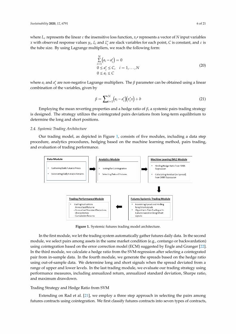
2.4. Systemic Trading Architecture

Our trading model, as depicted in Figure 1, consists of five modules, including a data stepprocedure, analytics procedures, hedging based on the machine learning method, pairs trading,and evaluation of trading performance.

Sustainability 2020, 12, x FOR PEER REVIEW  6 of 24 

 

where 𝐿  represents  the  linear 𝜀  the  insensitive  loss  function, 𝑥 ′  represents  a  vector  of N  input variables 𝑥  with  observed  response  values 𝑦 , 𝜉  and 𝜉∗  are  slack  variables  for  each  point,  C  is 

constant, and 𝜀 is the tube size. By using Lagrange multipliers, we reach the following form: 

𝑎 𝑎∗ 0 

0 𝑎∗ 𝐶,                                                   𝑖 1, … , 𝑁 

0 𝑎 𝐶 

(20) 

where 𝑎  and 𝑎∗ are non‐negative Lagrange multipliers. The β parameter can be obtained using a 

linear combination of the variables, given by 

𝛽 ∑ 𝑎 𝑎∗ 𝑥 𝑥 𝑏   (21) 

Employing  the mean  reverting  properties  and  a  hedge  ratio  of  β,  a  systemic  pairs  trading 

strategy  is  designed.  The  strategy  utilizes  the  cointegrated  pairs  deviations  from  long‐term 

equilibrium to determine the long and short positions.   

2.4. Systemic Trading Architecture 

Our  trading model,  as depicted  in Figure  1,  consists of  five modules,  including  a data  step 

procedure, analytics procedures, hedging based on the machine learning method, pairs trading, and 

evaluation of trading performance.   

 

Figure 1. Systemic futures trading model architecture. 

In  the  first module, we  let  the  trading system automatically gather  futures daily data.  In  the 

second module, we  select  pairs  among  assets  in  the  same market  condition  (e.g.,  contango  or 

backwardation) using cointegration based on the error correction model (ECM) suggested by Engle 

and Granger  [22].  In  the  third module, we calculate a hedge  ratio  from  the SVM‐regression after 

selecting a cointegrated pair  from  in‐sample data.  In  the  fourth module, we generate  the spreads 

based on the hedge ratio using out‐of‐sample data. We determine long and short signals when the 

spread deviated from a range of upper and lower levels. In the last trading module, we evaluate our 

trading  strategy using performance measures,  including  annualized  return,  annualized  standard 

deviation, Sharpe ratio, and maximum drawdown. 

Figure 1. Systemic futures trading model architecture.

In the first module, we let the trading system automatically gather futures daily data. In the secondmodule, we select pairs among assets in the same market condition (e.g., contango or backwardation)using cointegration based on the error correction model (ECM) suggested by Engle and Granger [22].In the third module, we calculate a hedge ratio from the SVM-regression after selecting a cointegratedpair from in-sample data. In the fourth module, we generate the spreads based on the hedge ratiousing out-of-sample data. We determine long and short signals when the spread deviated from arange of upper and lower levels. In the last trading module, we evaluate our trading strategy usingperformance measures, including annualized return, annualized standard deviation, Sharpe ratio,and maximum drawdown.

Trading Strategy and Hedge Ratio from SVM

Extending on Rad et al. [21], we employ a three step approach in selecting the pairs amongfutures contracts using cointegration. We first classify futures contracts into seven types of contracts,

Sustainability 2020, 12, 6791 7 of 21

including grain oil seeds, live stocks, soft, lumber, metal, energy, and financial futures. Secondly,we sort combinations of pairs within each type of futures contract based upon the sum of squaredresiduals using standardized futures prices. Last, we test cointegration for each selected pair andchoose pairs that are statistically significant in the framework of the error correction model.

The Engle–Granger two-step approach [22] is used to test whether the selected pairs arecointegrated. The first step utilizes the SVM to estimate the cointegration regression. The second stepis to estimate the error correction model (ECM). The SVM regression method in the first step providesthe estimation of the cointegration coefficient β. Upon calculation of the spread, the long and shortpositions are simultaneously opened and closed. Specifically, if the spread at time t is greater than the15-day rolling moving average plus the 15-day rolling standard deviation, we take a short position.In contrast, if the spread at t is less than the 15-day rolling moving average plus the 15-day rollingstandard deviation, we take a long position. When the spread reverts toward the mean, we exit bothpositions as that is indicative of reverting to long-term equilibrium.

2.5. Research Data

Our data include futures settlement prices from January 1998 through December 2018 (the lasttrading day of each month) published in the Wall Street Journal (WSJ) Futures section and Investor’sBusiness Daily (IBD). The prices are used to create semi-monthly data points, from the first to the 15thday of the month and from the 16th to the end of the month. If the 15th day falls on a non-tradingday, the next closest day which results in two equal, or as close to equal, semi-monthly data points isused. Subsequently, there are 504 data points for the futures contracts included in the study. The firstdata point included is on 15 January 1998 (settlement price on 15 January 1998 minus settlement priceon 31 December 1997), and the last data point is obtained on 31 December 2018 (settlement price on31 December 2018 minus settlement price on 15 December 2018). We then count the number of priceincreases and decreases in a semi-monthly period over the entire study period.

The price at the start and end point of the period is reported in each futures market, and thechange in price over the period is calculated. Price changes are estimated for the most active tradingmonths, an average annual percentage price change of the contract during the period is defined as:

Annual Percentage Price Change (APPC) =(Pend − Pstart)/Pstart

Number o f Years× 100 (22)

The fraction of semi-annual periods where prices increase relative to the total number of periodsis calculated.

In order to examine the progression of the pricing mechanisms in futures markets, the sample isdivided into two sub-periods 1998–2007 and 2008–2018. The resulting data points for the sub-periodsare 240 for the first and 264 for the second. The purpose of this division is to determine if one pricingmechanism is dominant in each futures market and if the dominant mechanism is stable and sustainedover the entire sample period.

3. Empirical Results and Discussions

Table 1 reports descriptive price changes across 28 futures markets over the period 1998 to 2018.The Annual Percentage Price Change (APPC) for most futures contracts, excluding the coffee andBritish Pound markets, shows a positive price increase, with a rising price trend in futures markets over504 semi-monthly periods. The key reason for the negative APPC in coffee futures stems from Brazil,which represents 40% of global coffee production and has overproduced. Additionally, its currency(REAL) has substantially depreciated—approximately 60% since 2006. The negative APPC in GBPfutures can be attributed to market participants’ concern regarding the currency market’s deeperdecline due to Brexit uncertainty. The t-statistic for the difference between the starting and ending priceacross each futures market is shown in column (4) and indicates almost total support for rejecting thenull hypothesis of zero equivalence. Most of the futures contracts experience price increases, excluding

Sustainability 2020, 12, 6791 8 of 21

coffee and sterling, and the differences are statistically significant at the 1% level. In addition, based onPIP/TP, we observe that 11 futures markets are either contango or weak contango, while the remaining17 markets are either normal backwardation or weak normal backwardation. APPC in column (5)shows that futures prices in metal and energy markets have sharply increased relative to other futuresprices, with an APPC for energy and metal futures ranging from 9.74 to 16.43.

Table 1. Futures Prices over 480 semi-months from Jan. 1998 to Dec. 2018.

Futures Markets Price (01/98) Price (12/18) Diff. (t-Stat) APPC # of PriceIncreases (%)

AGRICULTUREGrain and Oilseeds

Com, CBOT 283.25 350.75 67.5 (9.39) *** +1.18 239 (49.8%)Beans, CBOT 670.25 961.25 291.0 (5.61) *** +2.17 251 (52.3%)Meal, CBOT 194.4 316.8 122.4 (4.18) *** +3.14 245 (51.0%)S-Oil, CBOT 25.18 33.08 7.9 (7.37) *** +1.56 234 (48.8%)

LivestockWheat, CBOT 351.0 427.0 76.0 (10.24) *** +0.54 221 (46.0%)F-Cattle, CME 78.02 142.67 64.7 (3.41) *** +4.14 255 (53.1%)L-Cattle, CME 67.97 122.52 54.6 (3.49) *** +4.02 244 (50.8%)

Hogs, CME 55.75 75.65 19.9 (6.60) *** +1.78 241 (50.2%)Soft

Cocoa, CSCE 1574 1892 318 (10.90) *** +1.01 246 (51.3%)Coffee, CSCE 168.2 126.20 −42.0 (7.01) *** −1.24 219 (45.6%)Sugar, CSCE 11.17 15.16 4.0 (6.60) *** +1.78 236 (49.2%)Cotton, ICE 65.97 78.63 12.7 (11.42) *** +0.95 225 (46.9%)

Frozen Orange JuiceOrange Juice, ICE 97.10 136.85 39.8 (5.89) *** +2.04 246 (51.3%)

LumberRandom Lumber, CME 274.5 441.9 167.4 (4.28) *** +3.05 228 (47.5%)

METALBase

Copper, CMX 78.00 330.05 252.1 (5.61) *** +16.15 247 (51.5%)Precious

Gold, CMX 287.7 1309.3 1021.6 (5.42) *** +17.75 237 (49.4%)Platinum, NYM 388.6 938.3 549.7 (8.36) *** +7.07 251 (52.3%)

Silver, CMX 513.6 1714.5 1200.9 (6.43) *** +9.74 245 (51.0%)

ENERGYCrude Oil, NYM 16.72 60.44 43.7 (6.11) *** +13.07 265 (55.2%)

Heating Oil, NYM 0.4697 2.0136 1.5 (5.57) *** +16.43 263 (54.8%)Unleaded Gasoline 1, NYM 0.5356 1.9919 1.5 (6.01) *** +13.59 276 (57.5%)

CURRENCYJapanese Yen, CME 0.7774 0.8914 0.1 (14.64) *** +0.73 229 (47.7%)

Canadian Dollar, CME 0.6979 0.7990 0.1 (14.81) *** +0.72 255 (53.1%)British Pound, CME 1.6246 1.3559 −0.3 (11.09) *** −0.88 237 (49.4%)Swiss Franc, CME 0.6712 1.0327 0.4 (4.71) *** +2.69 232 (48.3%)

FINANCIALEurodollar, CME 94.53 98.24 3.7 (51.96) *** +0.19 250 (52.1%)T-Bonds, CBOT 123.01 153.00 30.0 (9.20) *** +1.22 251 (52.3%)S & P 500, CME 955.1 2676.0 1720.9 (2.11) *** +9.00 254 (52.9%)

1 NY Harbor Gas Blend was used after November 2006. *** denote significance at the 1% level.

To investigate whether the impact of market mechanisms changes over time, we conduct a splitsample analysis, dividing the futures price movement into two sub-periods. Table 2 summarizesprice changes in futures markets over 240 semi-monthly periods from 1998 to 2007. The prices for thefutures contracts have increased in APPC, excluding coffee, lumber, and T-bonds futures. The lastcolumn of Table 2 shows that 21 futures markets exhibit price increases of over 50% of the total periods.Noticeably, energy and metal futures are backwardation oriented markets over the sub-sample period.The APPCs of metal and energy futures are approximately nine times greater than that of other futures(32.26 for metal and energy vs. 9.34 for others).

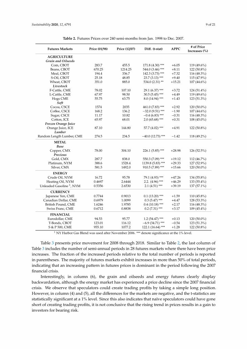
Sustainability 2020, 12, 6791 9 of 21

Table 2. Futures Prices over 240 semi-months from Jan. 1998 to Dec. 2007.

Futures Markets Price (01/98) Price (12/07) Diff. (t-stat) APPC # of PriceIncreases (%)

AGRICULTUREGrain and Oilseeds

Com, CBOT 283.7 455.5 171.8 (4.30) *** +6.05 119 (49.6%)Beans, CBOT 670.25 1214.25 544.0 (3.46) *** +8.11 122 (50.8%)Meal, CBOT 194.4 336.7 142.3 (3.73) *** +7.32 116 (48.3%)S-Oil, CBOT 25.18 48.85 23.7 (3.13) *** +9.40 115 (47.9%)

Wheat, CBOT 351.0 885.0 534.0 (2.31) ** +15.21 107 (44.6%)Livestock

F-Cattle, CME 78.02 107.10 29.1 (6.37) *** +3.72 124 (51.4%)L-Cattle, CME 67.97 98.50 30.5 (5.45) *** +4.49 119 (49.6%)

Hogs CME 55.75 63.75 8.0 (14.94) *** +1.43 123 (51.3%)Soft

Cocoa, CSCE 1574 2035 461.0 (7.83) *** +2.92 120 (50.0%)Coffee, CSCE 168.2 136.2 −32.0 (9.51) *** −1.90 107 (44.6%)Sugar, CSCE 11.17 10.82 −0.4 (6.83) *** −0.31 116 (48.3%)Cotton, ICE 65.97 68.01 2.0 (65.68) *** +0.31 108 (45.0%)

Frozen Orange JuiceOrange Juice, ICE 87.10 144.80 57.7 (4.02) *** +4.91 122 (50.8%)

LumberRandom Length Lumber, CME 274.5 234.5 −40.0 (12.73) *** −1.42 118 (49.2%)

METALBase

Copper, CMX 78.00 304.10 226.1 (5.85) *** +28.98 126 (52.5%)Precious

Gold, CMX 287.7 838.0 550.3 (7.09) *** +19.12 112 (46.7%)Platinum, NYM 388.6 1528.4 1139.8 (5.83) *** +29.33 127 (52.9%)

Silver, CMX 581.5 1492.0 910.5 (7.89) *** +15.66 120 (50.0%)

ENERGYCrude Oil, NYM 16.72 95.78 79.1 (4.93) *** +47.26 134 (55.8%)

Heating Oil, NYM 0.4697 2.6444 2.2. (4.96) *** +46.29 133 (55.4%)Unleaded Gasoline 1, NYM 0.5356 2.6530 2.1 (4.51) *** +39.19 137 (57.1%)

CURRENCYJapanese Yen, CME 0.7744 0.9013 0.1 (13.20) *** +1.59 110 (45.8%)

Canadian Dollar, CME 0.6979 1.0099 0.3 (5.47) *** +4.47 128 (53.3%)British Pound, CME 1.6246 1.9785 0.4 (10.18) *** +2.17 116 (48.3%)Swiss Franc, CME 0.6712 0.8838 0.2 (7.31) *** +3.17 109 (45.4%)

FINANCIALEurodollar, CME 94.53 95.77 1.2 (54.47) *** +0.13 120 (50.0%)T-Bonds, CBOT 123.01 116.12 −6.9 (34.71) *** −0.54 123 (51.3%)S & P 500, CME 955.10 1077.2 122.1 (16.64) *** +1.28 122 (50.8%)

1 NY Harbor Gas Blend was used after November 2006. *** denote significance at the 1% level.

Table 3 presents price movement for 2008 through 2018. Similar to Table 2, the last column ofTable 3 includes the number of semi-annual periods in 28 futures markets where there have been priceincreases. The fraction of the increased periods relative to the total number of periods is reportedin parentheses. The majority of futures markets exhibit increases in more than 50% of total periods,indicating that an increasing pattern in futures prices is dominant in the period following the 2007financial crisis.

Interestingly, in column (6), the grain and oilseeds and energy futures clearly displaybackwardation, although the energy market has experienced a price decline since the 2007 financialcrisis. We observe that speculators could create trading profits by taking a simple long position.However, in column (4) and (5), all the differences for the markets are negative, and the t-statistics arestatistically significant at a 1% level. Since this also indicates that naïve speculators could have goneshort of creating trading profits, it is not conclusive that the rising trend in prices results in a gain toinvestors for bearing risk.

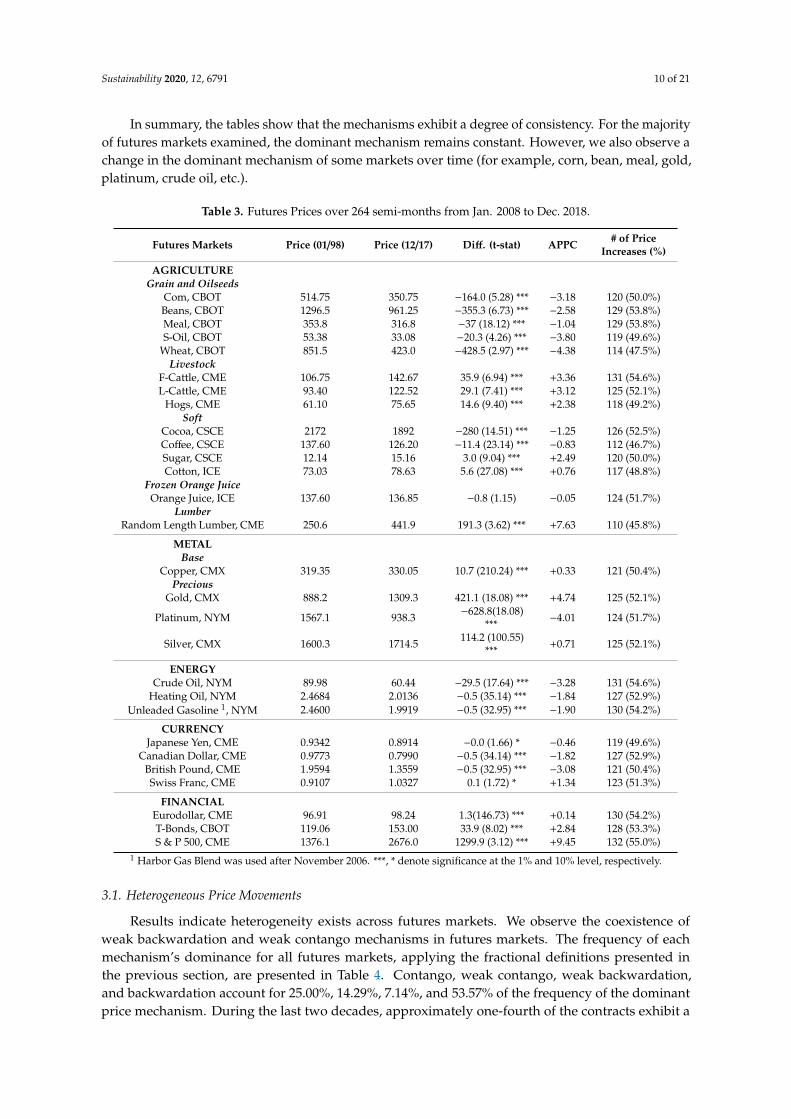
Sustainability 2020, 12, 6791 10 of 21

In summary, the tables show that the mechanisms exhibit a degree of consistency. For the majorityof futures markets examined, the dominant mechanism remains constant. However, we also observe achange in the dominant mechanism of some markets over time (for example, corn, bean, meal, gold,platinum, crude oil, etc.).

Table 3. Futures Prices over 264 semi-months from Jan. 2008 to Dec. 2018.

Futures Markets Price (01/98) Price (12/17) Diff. (t-stat) APPC # of PriceIncreases (%)

AGRICULTUREGrain and Oilseeds

Com, CBOT 514.75 350.75 −164.0 (5.28) *** −3.18 120 (50.0%)Beans, CBOT 1296.5 961.25 −355.3 (6.73) *** −2.58 129 (53.8%)Meal, CBOT 353.8 316.8 −37 (18.12) *** −1.04 129 (53.8%)S-Oil, CBOT 53.38 33.08 −20.3 (4.26) *** −3.80 119 (49.6%)

Wheat, CBOT 851.5 423.0 −428.5 (2.97) *** −4.38 114 (47.5%)Livestock

F-Cattle, CME 106.75 142.67 35.9 (6.94) *** +3.36 131 (54.6%)L-Cattle, CME 93.40 122.52 29.1 (7.41) *** +3.12 125 (52.1%)

Hogs, CME 61.10 75.65 14.6 (9.40) *** +2.38 118 (49.2%)Soft

Cocoa, CSCE 2172 1892 −280 (14.51) *** −1.25 126 (52.5%)Coffee, CSCE 137.60 126.20 −11.4 (23.14) *** −0.83 112 (46.7%)Sugar, CSCE 12.14 15.16 3.0 (9.04) *** +2.49 120 (50.0%)Cotton, ICE 73.03 78.63 5.6 (27.08) *** +0.76 117 (48.8%)

Frozen Orange JuiceOrange Juice, ICE 137.60 136.85 −0.8 (1.15) −0.05 124 (51.7%)

LumberRandom Length Lumber, CME 250.6 441.9 191.3 (3.62) *** +7.63 110 (45.8%)

METALBase

Copper, CMX 319.35 330.05 10.7 (210.24) *** +0.33 121 (50.4%)Precious

Gold, CMX 888.2 1309.3 421.1 (18.08) *** +4.74 125 (52.1%)

Platinum, NYM 1567.1 938.3 −628.8(18.08)*** −4.01 124 (51.7%)

Silver, CMX 1600.3 1714.5 114.2 (100.55)*** +0.71 125 (52.1%)

ENERGYCrude Oil, NYM 89.98 60.44 −29.5 (17.64) *** −3.28 131 (54.6%)

Heating Oil, NYM 2.4684 2.0136 −0.5 (35.14) *** −1.84 127 (52.9%)Unleaded Gasoline 1, NYM 2.4600 1.9919 −0.5 (32.95) *** −1.90 130 (54.2%)

CURRENCYJapanese Yen, CME 0.9342 0.8914 −0.0 (1.66) * −0.46 119 (49.6%)

Canadian Dollar, CME 0.9773 0.7990 −0.5 (34.14) *** −1.82 127 (52.9%)British Pound, CME 1.9594 1.3559 −0.5 (32.95) *** −3.08 121 (50.4%)Swiss Franc, CME 0.9107 1.0327 0.1 (1.72) * +1.34 123 (51.3%)

FINANCIALEurodollar, CME 96.91 98.24 1.3(146.73) *** +0.14 130 (54.2%)T-Bonds, CBOT 119.06 153.00 33.9 (8.02) *** +2.84 128 (53.3%)S & P 500, CME 1376.1 2676.0 1299.9 (3.12) *** +9.45 132 (55.0%)

1 Harbor Gas Blend was used after November 2006. ***, * denote significance at the 1% and 10% level, respectively.

3.1. Heterogeneous Price Movements

Results indicate heterogeneity exists across futures markets. We observe the coexistence ofweak backwardation and weak contango mechanisms in futures markets. The frequency of eachmechanism’s dominance for all futures markets, applying the fractional definitions presented inthe previous section, are presented in Table 4. Contango, weak contango, weak backwardation,and backwardation account for 25.00%, 14.29%, 7.14%, and 53.57% of the frequency of the dominantprice mechanism. During the last two decades, approximately one-fourth of the contracts exhibit a

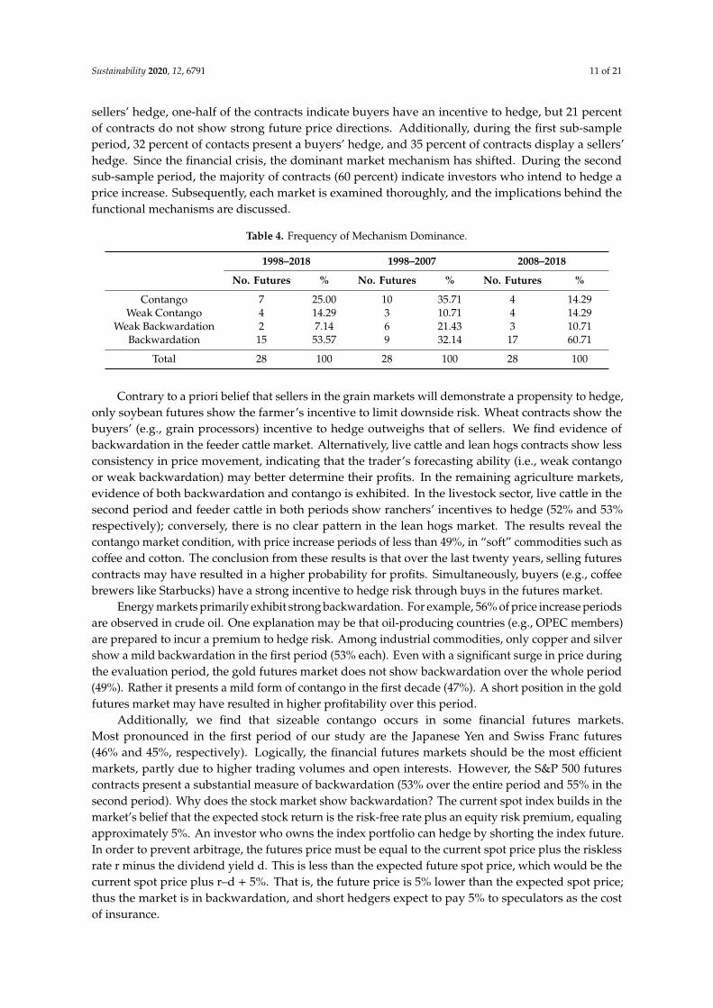
Sustainability 2020, 12, 6791 11 of 21

sellers’ hedge, one-half of the contracts indicate buyers have an incentive to hedge, but 21 percentof contracts do not show strong future price directions. Additionally, during the first sub-sampleperiod, 32 percent of contacts present a buyers’ hedge, and 35 percent of contracts display a sellers’hedge. Since the financial crisis, the dominant market mechanism has shifted. During the secondsub-sample period, the majority of contracts (60 percent) indicate investors who intend to hedge aprice increase. Subsequently, each market is examined thoroughly, and the implications behind thefunctional mechanisms are discussed.

Table 4. Frequency of Mechanism Dominance.

1998–2018 1998–2007 2008–2018

No. Futures % No. Futures % No. Futures %

Contango 7 25.00 10 35.71 4 14.29Weak Contango 4 14.29 3 10.71 4 14.29

Weak Backwardation 2 7.14 6 21.43 3 10.71Backwardation 15 53.57 9 32.14 17 60.71

Total 28 100 28 100 28 100

Contrary to a priori belief that sellers in the grain markets will demonstrate a propensity to hedge,only soybean futures show the farmer’s incentive to limit downside risk. Wheat contracts show thebuyers’ (e.g., grain processors) incentive to hedge outweighs that of sellers. We find evidence ofbackwardation in the feeder cattle market. Alternatively, live cattle and lean hogs contracts show lessconsistency in price movement, indicating that the trader’s forecasting ability (i.e., weak contangoor weak backwardation) may better determine their profits. In the remaining agriculture markets,evidence of both backwardation and contango is exhibited. In the livestock sector, live cattle in thesecond period and feeder cattle in both periods show ranchers’ incentives to hedge (52% and 53%respectively); conversely, there is no clear pattern in the lean hogs market. The results reveal thecontango market condition, with price increase periods of less than 49%, in “soft” commodities such ascoffee and cotton. The conclusion from these results is that over the last twenty years, selling futurescontracts may have resulted in a higher probability for profits. Simultaneously, buyers (e.g., coffeebrewers like Starbucks) have a strong incentive to hedge risk through buys in the futures market.

Energy markets primarily exhibit strong backwardation. For example, 56% of price increase periodsare observed in crude oil. One explanation may be that oil-producing countries (e.g., OPEC members)are prepared to incur a premium to hedge risk. Among industrial commodities, only copper and silvershow a mild backwardation in the first period (53% each). Even with a significant surge in price duringthe evaluation period, the gold futures market does not show backwardation over the whole period(49%). Rather it presents a mild form of contango in the first decade (47%). A short position in the goldfutures market may have resulted in higher profitability over this period.

Additionally, we find that sizeable contango occurs in some financial futures markets.Most pronounced in the first period of our study are the Japanese Yen and Swiss Franc futures(46% and 45%, respectively). Logically, the financial futures markets should be the most efficientmarkets, partly due to higher trading volumes and open interests. However, the S&P 500 futurescontracts present a substantial measure of backwardation (53% over the entire period and 55% in thesecond period). Why does the stock market show backwardation? The current spot index builds in themarket’s belief that the expected stock return is the risk-free rate plus an equity risk premium, equalingapproximately 5%. An investor who owns the index portfolio can hedge by shorting the index future.In order to prevent arbitrage, the futures price must be equal to the current spot price plus the risklessrate r minus the dividend yield d. This is less than the expected future spot price, which would be thecurrent spot price plus r–d + 5%. That is, the future price is 5% lower than the expected spot price;thus the market is in backwardation, and short hedgers expect to pay 5% to speculators as the costof insurance.

Sustainability 2020, 12, 6791 12 of 21

The backwardation indicates a high premium conferred from buyers to sellers in interest futuresmarkets, Eurodollars and T-bonds. For example, the U.S. Treasury is strongly incentivized to pay aninsurance premium to establish the sale price of government securities. One factor potentially drivingthis pattern is that over the observation period, the general interest rate levels have fallen. Decreasinginterest rates and resulting in rising bonds prices, appear linked through normal backwardation.

3.2. Normal Backwardation and Contango: Price Patterns Over Time

Sub-periods are examined to determine the time-series consistency of functional mechanismsfor each market, as shown in Table 5. The results in Table 5 indicate that the mechanisms exhibit atendency toward backwardation (60.7%), as observed in Table 4, most pronounced is the continuationfrom backwardation to backwardation (25.0%). Another distinct trend is that over the observationperiod, the contango mechanism seems to lose intensity (14.3%). We observe zero transitions from thebackwardation to contango. The implication of the change in the pattern of futures contract prices isan increase in the sellers’ needs to hedge. Only coffee and wheat begin and remain contango in bothdecades. Some markets, such as gold, change from contango to backwardation. In these markets, buyerdominance, driven by large and small speculators, transforms into seller dominance, driven by largehedgers such as mining companies. In the currency market, Swiss Franc, British Pound, and JapaneseYen all convert from the contango to weak contango or weak backwardation mechanism. While theremay be many explanations for these price pattern changes, conclusions should be interpreted withcaution as multiple factors may drive the change.

Table 5. Cross Tabulated Patterns from Sub-period 1 to Sub-period 2.

Sub-Period(1998–2007)

Sub-Period (2008—2018)TotalContango Weak Contango Weak Backwardation Backwardation

Contango 3 (1.4) 3 (1.4) 1 (1.1) 3 (6.1) 10Weak Contango 1 (0.4) 0 (0.4) 1 (0.3) 1 (1.8) 3

Weak Backwardation 0 (0.9) 0 (0.9) 0 (0.6) 6 (3.6) 6Backwardation 0 (1.3) 1 (1.3) 1 (1.0) 7 (5.5) 9

Total 4 4 3 17 28

χ2 = 13.67, p-value = 0.000

Note: values in parentheses indicate expected frequencies from distribution.

Additionally, we run a nonparametric χ2 test of independence in order to examine whether thereis an association between market dominance over the first and the second sub-sample periods. The χ2

of 13.67 rejects the null hypothesis that the past market mechanism is independent of the currentmarket mechanism. This is consistent with our findings and supporting evidence that speculatorsgenerate positive expected risk premiums based on superior forecasting ability.

In summary, presented in Tables 4 and 5, the prevailing trend across futures markets isbackwardation, although there are cross-sectional differences. This implies that futures pricesincorporate the insurance premiums of sellers seeking to shed risk. In addition, it indicates thatfutures prices reflect less of the buyer’s needs and more of the seller’s needs, as futures markets wereoriginally intended.

3.3. Nonparametric Statistical Test

In addition to analyzing forecasting ability, nonparametric procedures are applied to futurescontract price changes for each semi-monthly period. Following Chang (1985), “up-futures” are definedas positive price changes, and “down-futures” are defined as all negative price change intervals. Table 6summarizes the null hypothesis H0 : PS

1(t) + PS2(t) = 1 and the estimated conditional probabilities

of speculators in 28 up and down futures contracts. The results show that traders may not be asconsistent in their ability to forecast down-futures contracts as they are in forecasting up-futures. Forexample, the forecasting ability of the agricultural speculators in down-futures outperforms relative to

Sustainability 2020, 12, 6791 13 of 21

that of other market traders. The average conditional probability in down-futures for agricultural,mineral, currency, and financial futures are 44.0%, 37.5%, 43.3%, 3.25%, respectively. Comparingconditional probabilities of down-futures in column 3 and those of up-futures in column 4, we findthat, generally, speculators tend to have better forecasting ability in up-futures than in down-futures.Speculator positions are impactful across agricultural, mineral, currency, and financial futures markets.These findings are consistent with those of Chang [1] and Schwarz [26].

Table 6. Sum of Conditional Probabilities of a Correct Market Position of Speculation Given thatR(t) ≤ 0 and R(t) > 0 for H0 : Ps

1(t) + Ps2(t) = 1 and H1 : Ps

1(t) + Ps2(t) > 1.

Futures MarketsDown Futures Markets

Ps1(t)

Up Futures MarketsPs

2(t)All Futures Markets

Ps1(t) + Ps

2(t)

AGRICULTUREGrain and Oilseeds

Corn, CBOT 0.472 0.619 1.091 **Beans, CBOT 0.442 0.652 1.094 **Meal, CBOT 0.315 0.892 1.207 ***S-Oil, CBOT 0.439 0.607 1.046

Wheat, CBOT 0.461 0.587 1.048Livestock

F-Cattle, CME 0.417 0.636 1.053L-Cattle, CME 0.494 0.551 1.045

Hogs, CME 0.452 0.609 1.061 *Soft

Cocoa, CSCE 0.461 0.779 1.240 ***Coffee, CSCE 0.482 0.612 1.094 **Sugar, CSCE 0.332 0.793 1.125 ***Cotton, ICE 0.484 0.625 1.109 **

Frozen Orange JuiceOrange Juice, ICE 0.477 0.610 1.087 **

LumberRandom Length Lumber, CME 0.429 0.656 1.085 ***

MINERALBase

Copper, CMX 0.331 0.721 1.092 **Precious

Gold, CMX 0.287 0.896 1.183 ***Platinum, NYM 0.411 0.764 1.175 ***

Silver, CMX 0.485 0.795 1.280 ***

ENERGYCrude Oil, NYM 0.389 0.812 1.201 ***

Heating Oil, NYM 0.310 0.858 1.168 ***Unleaded Gasoline 1, NYM 0.354 0.789 1.143 ***

CURRENCYJapanese Yen CME 0.370 0.698 1.068

Canada Dollar CME 0.451 0.598 1.079 *British Pound CME 0.418 0.662 1.090 **Swiss Franc CME 0.473 0.582 1.035

FINANCIALEurodollar CME 0.364 0.717 1.081 *T-Bonds CBOT 0.369 0.861 1.230 ***S & P 500 CME 0.273 0.886 1.159 ***

1 NY Harbor Gas Blend was used after November 2006. ***, **, * denote significance at the 1%, 5%, and 10%level, respectively.

In column 5, the conditional probabilities for all markets are greater than zero. However, tests forS-Oil, Wheat, F-Cattle, L-Cattle, Japanese Yen, Swiss Franc, and Euro-dollar futures fail to reject the nullhypothesis that speculators do not make positive gains at the 5% level of significance. Interestingly,tests of mineral futures result in a rejection of the null hypothesis providing evidence that speculatorsin metal markets are informed with superior forecasting ability.

Sustainability 2020, 12, 6791 14 of 21

3.4. Systemic Pairs Trading

To evaluate our pairs trading strategy, daily futures data are collected using Bloomberg over thesample period 2 January2015 to 9 July 2020. The dataset is divided into two sub-samples: in-sampledata (2 January 2015–31 December 2017); out-of-sample data (2 January 2018–9 July 2020). The tradingstrategy is developed using in-sample-data, and backtesting is performed using the out-of-sampledataset. By using in-sample-data, we examine combinations of pairs in the same futures markets.Pairs that can be constructed across futures markets are not considered, as our previous findings suggestthat each market has its own unique price trend. Regressions are run using various combinations ofpairs constructed within the same markets. Next, the sum of squared residuals is calculated, and thepairs are ranked by the sum of squared residuals. Five pairs of futures remain after excluding pairsthat are not statistically cointegrated: CME E-Mini S&P 500 and CME NASDAQ100 futures; COMEXGold and COMEX Silver futures; COMEX Copper and NYMEX Platinum futures; CBOT Oats andCBOT Corn futures; CME Feeder cattle and CME Live cattle futures. The SVM regression analysis isperformed with a tuning process using in-sample-data to estimate the best hedge ratios for the fiveselected pairs. Table 7 summarizes the hedge ratios for the pairs, ranging from 0.02 (Oats and Corn) to0.72 (S&P500 and NASDAQ 100). By utilizing the hedge ratios, we calculate spreads, and determinethe size of hedging for backtesting. For example, we buy 1 dollar of E-mini S&P500 futures and sell0.72 dollars of NASDAQ 100 when the spread between the two futures is below a specified lowerbound. Conversely, when the spread is above a specified upper bound, 1/0.72 dollars of E-Mini S&P500futures is shorted, and 1 dollar of NASDAQ 100 is purchased. The lower and upper bounds at time t aredynamically calculated based on the 15-day rolling average and standard deviation of the past spread.

Table 7. Spread, ∆νt = ∆S2(t)− β∆S1(t1), and Hedge ratios for the Selected Pairs from In-Sample-Data(2 January 2015–31 December 2017).

∆S2(t) ∆S1(t1) Hedge Ratio (β)

CME E-Mini S&P 500 CME Nasdaq 100 0.72COMEX Gold COMEX Silver 0.24CMEX Copper NYMEX Platinum 0.02

CBOT Oats CBOT Corn 0.04CME Feeder Cattle CME Live Cattle 0.49

Figure 2 illustrates cumulative returns for the five pairs traded over the out-of-sample period.In order to examine each pair’s performance, we compare our pairs trading approach and abuy-and-hold investment strategy. In each panel, a solid black line represents a time series of cumulativereturns for pairs trading and a solid red line represents cumulative returns for a correspondingbenchmark. In panel (a), the cumulative returns for the pair between E-mini S&P500 and NASDAQ 100futures steadily grow over the out-of-sample period, while the cumulative returns for the S&P 500 indexfutures buy-and-hold strategy show wide fluctuation. Notably, when the number of deaths due to theCOVID-19 pandemic steeply increased after 24 February 2020, the cumulative return for the benchmarkplummeted, and the slope of the time series line reverted to negative. In contrast, the cumulativereturn for pairs trading still shows an upward trend. Pairs trading two index futures appears tohedge against unexpected systemic risk during the backtesting period. In panel (b), the cumulativereturns for the gold and silver futures pair and for gold futures both show an upward trend, but thecumulative returns for pairs trading outperform the benchmark. In panel (c), pairs trading utilizingcopper and platinum futures achieves an exceptional outcome. The time series line for pairs tradingshows relatively little fluctuation and stays above the benchmark (i.e., a buy-and-hold copper trading)over the trading period. Additionally, the graph shows that pairs trading was not markedly affectedby COVID-19, unlike the benchmark. The backtesting result for oats and corn futures in panel (d)shows the return from pairs trading is stable relative to the movement in the cumulative return ofthe oat futures benchmark. Similarly, in panel (e), pairs trading with feeder and live cattle futures is

Sustainability 2020, 12, 6791 15 of 21

less risky than the feeder cattle benchmark. The slope of the cumulative return for the benchmarkconverted to negative with the onset of COVID-19, while the trend of the cumulative returns in thepairs trading was positive. This result also suggests that pairs trading can hedge against an adversedecline in futures prices stemming from a systemic event.

Sustainability 2020, 12, x FOR PEER REVIEW  17 of 24 

 

 

(a)  Pairs  (E‐Mini  S&P  500  and Nasdaq  100  Futures)  vs.  E‐Mini 

S&P500 Index Futures. 

 

(b) Pair (Gold and Silver Futures) vs. Gold Futures 

 

(c) Pair (Copper and Platinum Futures) vs. Copper Futures 

Figure 2. Cont.

Sustainability 2020, 12, 6791 16 of 21Sustainability 2020, 12, x FOR PEER REVIEW  18 of 24 

 

 

(d) Pair (Oats and Corn Futures) vs. Oats Futures 

 

(e) Pair (Feeder Cattle and Live Cattle Futures) vs. Feeder Cattle Futures 

Figure 2. Cumulative returns for the pairs and the respective benchmarks. 

To examine whether the application of SVM to estimate cointegration coefficients can improve 

pairs trading performance in futures markets, we further estimate cointegration coefficients using the 

ordinary linear square (OLS) estimation method. Figure 3 exhibits the comparison of the cumulative 

returns  of  pairs  trading  between  the  SVM method  and  the OLS  approach. Each  panel  provides 

evidence that SVM improves the pairs trading strategy. The pairs trading algorithm implemented by 

the SVM coefficient outperforms the OLS pairs trading strategy. Notably, the performance of SVM 

consistently outperforms prior to COVID‐19 and through the pandemic compared to the performance 

of OLS. SVM can add considerable value in pairs trading with futures contacts. 

Figure 2. Cumulative returns for the pairs and the respective benchmarks.

To examine whether the application of SVM to estimate cointegration coefficients can improvepairs trading performance in futures markets, we further estimate cointegration coefficients using theordinary linear square (OLS) estimation method. Figure 3 exhibits the comparison of the cumulativereturns of pairs trading between the SVM method and the OLS approach. Each panel provides evidencethat SVM improves the pairs trading strategy. The pairs trading algorithm implemented by the SVMcoefficient outperforms the OLS pairs trading strategy. Notably, the performance of SVM consistentlyoutperforms prior to COVID-19 and through the pandemic compared to the performance of OLS.SVM can add considerable value in pairs trading with futures contacts.

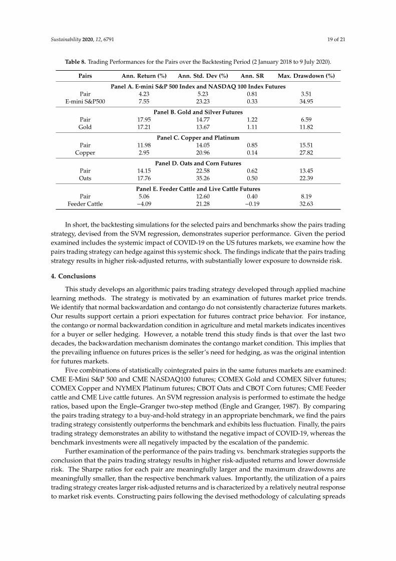
In addition to the cumulative returns, performance measures are examined to evaluate thepairs trading system. Table 8 reports the pairs trading performance for the five pairs. Panel Apresents the performance of the pairs trading strategy for the E-mini S&P 500 and NASDAQ 100index futures. The annualized return for the pairs trading is 4.23 percent, which is 3.32 percentagepoints less than that of the benchmark. However, the Sharpe Ratio (SR) of the pairs trading is higher,as the standard deviation of the benchmark is approximately four times greater than that of the pairstrading. The maximum drawdowns and the maximum observed loss from peak to trough during thetrading period, are 3.51 percent for the pairs trading and 34.95 percent for the benchmark, respectively.This suggests that the pairs trading strategy is not considerably riskier than the E-mini S&P 500 indexfutures benchmark. In panel B, the gold and silver futures pair and gold futures benchmark arepresented. They display similarities in annualized return and standard deviation. The pairs tradingstrategy has slightly higher SR than the benchmark (1.22 vs. 1.11) and has a lower maximum drawdown(6.59 vs. 11.82), which indicates that the pairs trading between gold and silver futures exhibits arelatively neutral performance to market risk events. Panel C reports that the pairs trading strategy forcopper and platinum futures outperforms the benchmark. The annualized return for the pairs trading

Sustainability 2020, 12, 6791 17 of 21

is approximately ten percentage points higher than that of the buy-and-hold copper futures benchmark.The SR of the pairs trading is around six times higher than that of the benchmark (0.85 vs. 0.14).The risk measurements (annualized standard deviation, and maximum drawdown) show the pairstrading strategy is less sensitive to market risk (Ann. Std. Deviation: 14.05 vs. 20.96; Max. Drawdown:15.51 vs. 27.82). Panel D presents the performance of the oats and corn futures pair. The annualizedreturns are similar for the pairs trading and oats futures benchmark. The SR for the pairs trading isgreater than the benchmark, indicating a larger risk-adjusted return from the pairs trading than thebenchmark. The maximum drawdown also shows that the pairs trading is less exposed to downsiderisk than the oats futures benchmark (13.45 vs. 22.39). Similarly, the feeder and live cattle futures pair isexamined in panel E, the annualized return for the pairs trading is 9.15 percentage points greater thanthat of the feeder cattle benchmark. The annualized standard deviation for the pairs trading is lowerthan the benchmark, with a higher SR for the pairs trading. During the trading period, the pairs tradingstrategy had a considerably lower maximum drawdown compared to the benchmark (8.19 vs. 32.63).

Sustainability 2020, 12, x FOR PEER REVIEW  19 of 24 

 

 

(a) Pair (E‐Mini S&P 500 and Nasdaq 100 Futures): SVM and OLS 

 

(b) Pair (Gold and Silver Futures): SVM vs. OLS 

Figure 3. Cont.

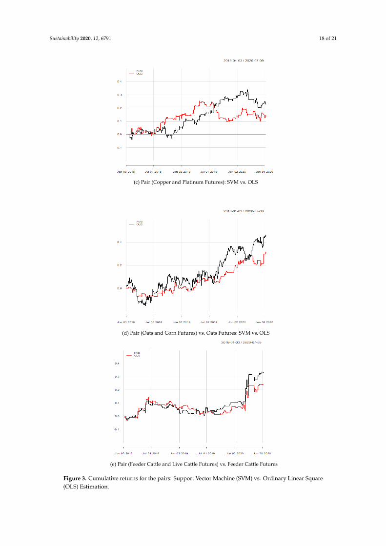
Sustainability 2020, 12, 6791 18 of 21Sustainability 2020, 12, x FOR PEER REVIEW  20 of 24 

 

 

(c) Pair (Copper and Platinum Futures): SVM vs. OLS 

 

(d) Pair (Oats and Corn Futures) vs. Oats Futures: SVM vs. OLS 

Sustainability 2020, 12, x FOR PEER REVIEW  21 of 24 

 

 

(e) Pair (Feeder Cattle and Live Cattle Futures) vs. Feeder Cattle Futures 

Figure 3. Cumulative returns for the pairs: Support Vector Machine (SVM) vs. Ordinary Linear Square 

(OLS) Estimation. 

In addition to the cumulative returns, performance measures are examined to evaluate the pairs 

trading system. Table 8 reports the pairs trading performance for the five pairs. Panel A presents the 

performance of the pairs trading strategy for the E‐mini S&P 500 and NASDAQ 100 index futures. 

The annualized return for the pairs trading is 4.23 percent, which is 3.32 percentage points less than 

that of the benchmark. However, the Sharpe Ratio (SR) of the pairs trading is higher, as the standard 

deviation of the benchmark is approximately four times greater than that of the pairs trading. The 

maximum drawdowns and  the maximum observed  loss  from peak  to  trough during  the  trading 

period, are 3.51 percent for the pairs trading and 34.95 percent for the benchmark, respectively. This 

suggests  that  the pairs  trading strategy  is not considerably riskier  than  the E‐mini S&P 500  index 

futures benchmark.  In panel B,  the gold and  silver  futures pair and gold  futures benchmark are 

presented. They display similarities in annualized return and standard deviation. The pairs trading 

strategy  has  slightly  higher  SR  than  the  benchmark  (1.22  vs.  1.11)  and  has  a  lower maximum 

drawdown (6.59 vs. 11.82), which  indicates that the pairs trading between gold and silver futures 

exhibits a relatively neutral performance to market risk events. Panel C reports that the pairs trading 

strategy for copper and platinum futures outperforms the benchmark. The annualized return for the 

pairs trading  is approximately ten percentage points higher than that of the buy‐and‐hold copper 

futures benchmark. The SR of the pairs trading is around six times higher than that of the benchmark 

(0.85 vs. 0.14). The risk measurements (annualized standard deviation, and maximum drawdown) 

show the pairs trading strategy is less sensitive to market risk (Ann. Std. Deviation: 14.05 vs. 20.96; 

Max. Drawdown: 15.51 vs. 27.82). Panel D presents the performance of the oats and corn futures pair. 

The annualized returns are similar for the pairs trading and oats futures benchmark. The SR for the 

pairs trading is greater than the benchmark, indicating a larger risk‐adjusted return from the pairs 

trading  than  the benchmark. The maximum drawdown  also  shows  that  the pairs  trading  is  less 

exposed to downside risk than the oats futures benchmark (13.45 vs. 22.39). Similarly, the feeder and 

live cattle  futures pair  is examined  in panel E,  the annualized  return  for  the pairs  trading  is 9.15 

percentage  points  greater  than  that  of  the  feeder  cattle  benchmark.  The  annualized  standard 

deviation for the pairs trading is lower than the benchmark, with a higher SR for the pairs trading. 

During the trading period, the pairs trading strategy had a considerably lower maximum drawdown 

compared to the benchmark (8.19 vs. 32.63). 

Figure 3. Cumulative returns for the pairs: Support Vector Machine (SVM) vs. Ordinary Linear Square(OLS) Estimation.

Sustainability 2020, 12, 6791 19 of 21

Table 8. Trading Performances for the Pairs over the Backtesting Period (2 January 2018 to 9 July 2020).

Pairs Ann. Return (%) Ann. Std. Dev (%) Ann. SR Max. Drawdown (%)

Panel A. E-mini S&P 500 Index and NASDAQ 100 Index FuturesPair 4.23 5.23 0.81 3.51

E-mini S&P500 7.55 23.23 0.33 34.95

Panel B. Gold and Silver FuturesPair 17.95 14.77 1.22 6.59Gold 17.21 13.67 1.11 11.82

Panel C. Copper and PlatinumPair 11.98 14.05 0.85 15.51

Copper 2.95 20.96 0.14 27.82

Panel D. Oats and Corn FuturesPair 14.15 22.58 0.62 13.45Oats 17.76 35.26 0.50 22.39

Panel E. Feeder Cattle and Live Cattle FuturesPair 5.06 12.60 0.40 8.19

Feeder Cattle −4.09 21.28 −0.19 32.63

In short, the backtesting simulations for the selected pairs and benchmarks show the pairs tradingstrategy, devised from the SVM regression, demonstrates superior performance. Given the periodexamined includes the systemic impact of COVID-19 on the US futures markets, we examine how thepairs trading strategy can hedge against this systemic shock. The findings indicate that the pairs tradingstrategy results in higher risk-adjusted returns, with substantially lower exposure to downside risk.

4. Conclusions

This study develops an algorithmic pairs trading strategy developed through applied machinelearning methods. The strategy is motivated by an examination of futures market price trends.We identify that normal backwardation and contango do not consistently characterize futures markets.Our results support certain a priori expectation for futures contract price behavior. For instance,the contango or normal backwardation condition in agriculture and metal markets indicates incentivesfor a buyer or seller hedging. However, a notable trend this study finds is that over the last twodecades, the backwardation mechanism dominates the contango market condition. This implies thatthe prevailing influence on futures prices is the seller’s need for hedging, as was the original intentionfor futures markets.

Five combinations of statistically cointegrated pairs in the same futures markets are examined:CME E-Mini S&P 500 and CME NASDAQ100 futures; COMEX Gold and COMEX Silver futures;COMEX Copper and NYMEX Platinum futures; CBOT Oats and CBOT Corn futures; CME Feedercattle and CME Live cattle futures. An SVM regression analysis is performed to estimate the hedgeratios, based upon the Engle–Granger two-step method (Engle and Granger, 1987). By comparingthe pairs trading strategy to a buy-and-hold strategy in an appropriate benchmark, we find the pairstrading strategy consistently outperforms the benchmark and exhibits less fluctuation. Finally, the pairstrading strategy demonstrates an ability to withstand the negative impact of COVID-19, whereas thebenchmark investments were all negatively impacted by the escalation of the pandemic.

Further examination of the performance of the pairs trading vs. benchmark strategies supports theconclusion that the pairs trading strategy results in higher risk-adjusted returns and lower downsiderisk. The Sharpe ratios for each pair are meaningfully larger and the maximum drawdowns aremeaningfully smaller, than the respective benchmark values. Importantly, the utilization of a pairstrading strategy creates larger risk-adjusted returns and is characterized by a relatively neutral responseto market risk events. Constructing pairs following the devised methodology of calculating spreads

Sustainability 2020, 12, 6791 20 of 21

and hedge ratios based on the SVM machine learning algorithm can generate a more sustainablemarket neutral trading strategy.

However, our trading approach is limited to a theoretical price. The proposed method assumesthat an asset can be bought and sold at the target price without any restriction. Expanding on ourstudy, future research could make contributions to the literature by considering the actual order bookdynamics and a scenario where stock trades might be queued.

Author Contributions: S.B. contributed to Data curation, Formal analysis, Methodology, Supervision,Writing—original draft, and Writing—review and editing. M.G. contributed to Formal analysis, Investigation,Methodology, Writing—original draft, and Writing—review and editing. S.H.O. contributed to Data curation,Investigation, Methodology, Project administration, Software, Writing—original draft, and Writing—review andediting. J.L. contributed to Conceptualization, Methodology, Resources, and Writing—original draft. All authorshave read and agreed to the published version of the manuscript.

Funding: This research received no external funding.

Conflicts of Interest: The authors declare no conflict of interest.

References

1. Chang, E.C. Returns to speculators and the theory of normal backwardation. J. Financ. 1985, 40, 193–208.[CrossRef]

2. Tilton, J.E.; Humphreys, D.; Radetzki, M. Investor demand and spot commodity prices. Resour. Policy 2011,36, 187–195. [CrossRef]

3. Gulley, A.; Tilton, J.E. The relationship between spot and futures prices: An empirical analysis. Resour. Policy2014, 41, 109–112. [CrossRef]

4. Fernandez, V. Spot and futures markets linkages: Does contango differ from backwardation? J. Futures Mark.2016, 36, 375–396. [CrossRef]

5. Park, H.Y.; Chen, A.H. Differences between futures and forward prices: A further investigation of theMarking-to-Market effects. J. Futures Mark. 1985, 5, 77–88. [CrossRef]

6. Krehbiel, T.; Collier, R. Normal backwardation in Short-Term interest rate futures markets. J. Futures Mark.1996, 16, 899–913. [CrossRef]

7. Movassagh, N.; Modjtahedi, B. Bias and backwardation in natural gas futures prices. J. Futures Mark. 2005,25, 281–308. [CrossRef]

8. Miffre, J. Normal backwardation is normal. J. Futures Mark. 2000, 20, 803–821. [CrossRef]9. Henriksson, R.D.; Merton, R.C. On market timing and investment performance. II. Statistical procedures for

evaluating forecasting skills. J. Bus. 1981, 54, 513–533.10. Gorton, G.; Rouwenhorst, K.G. Facts and fantasies about commodity futures. Financ. Anal. J. 2006, 62, 47–68.

[CrossRef]11. Erb, C.B.; Harvey, C.R. The strategic and tactical value of commodity futures. Financ. Anal. J. 2006, 62, 69–97.

[CrossRef]12. Miffre, J.; Rallis, G. Momentum strategies in commodity futures markets. J. Bank. Financ. 2007, 31, 1863–1886.

[CrossRef]13. Szakmary, A.C.; Shen, Q.; Sharma, S.C. Trend-Following trading strategies in commodity futures:

A Re-Examination. J. Bank. Financ. 2010, 34, 409–426. [CrossRef]14. Hurst, B.; Ooi, Y.H.; Pedersen, L.H. A century of evidence on Trend-Following investing. J. Portf. Manag.

2017, 44, 15–29. [CrossRef]15. Creamer, G. Model calibration and automated trading agent for euro futures. Quant. Financ. 2012, 12,

531–545. [CrossRef]16. Shin, K.; Kim, K.; Han, I. In financial data mining using genetic algorithms technique: Application to KOSPI

200. Korea Intell. Inf. Syst. Soc. 1998, 113–122.17. Hamid, S.A.; Iqbal, Z. Using neural networks for forecasting volatility of S&P 500 index futures prices.

J. Bus. Res. 2004, 57, 1116–1125. [CrossRef]18. Tsaih, R.; Hsu, Y.; Lai, C.C. Forecasting S&P 500 stock index futures with a hybrid AI system. Decis. Support

Syst. 1998, 23, 161–174. [CrossRef]

Sustainability 2020, 12, 6791 21 of 21

19. Tay, F.E.H.; Cao, L. Application of support vector machines in financial time series forecasting. Omega 2001,29, 309–317. [CrossRef]

20. Moriyama, K.; Matsumoto, M.; Fukui, K.; Kurihara, S.; Numao, M. Reinforcement learning on a futuresmarket simulator. KES Int. Symp. Agent Multi-Agent Syst. Technol. Appl. 2007, 42–52. [CrossRef]

21. Rad, H.; Low, R.K.Y.; Faff, R. The profitability of pairs trading strategies: Distance, cointegration and copulamethods. Quant. Financ. 2016, 16, 1541–1558. [CrossRef]

22. Engle, R.F.; Granger, C.W.J. Co-Integration and error correction: Representation, Estimation, and Testing.Econometrica 1987, 55, 251–276. [CrossRef]

23. Rockwell, C.S. Normal backwardation, forecasting, and the return to commodity futures traders. Food Res.Inst. Stud. 1967, 7, 1–24.

24. Vapnik, V. The Nature of Statistical Learning Theory; Springer Science & Business Media: Berlin/Heidelberg,Germany, 1995.

25. Cao, L.J.; Tay, F.E.H. Support vector machine with adaptive parameters in financial time series forecasting.IEEE Trans. Neural Netw. 2003, 14, 1506–1518. [CrossRef] [PubMed]

26. Schwarz, K. Are speculators informed? J. Futures Mark. 2012, 32, 1–23. [CrossRef]

© 2020 by the authors. Licensee MDPI, Basel, Switzerland. This article is an open accessarticle distributed under the terms and conditions of the Creative Commons Attribution(CC BY) license (http://creativecommons.org/licenses/by/4.0/).