arX

iv:1

112.

3352

v1 [

hep-

th]

14

Dec

201

1

Algorithmic deformation

of matrix factorisations

Nils Carqueville1 Laura Dowdy Andreas Recknagel2

1LMU Munchen Theresienstraße 37, D-80333 Munchen,

Universe Cluster, Boltzmannstraße 2, D-85748 Garching

2King’s College London, Department of Mathematics,

Strand, London WC2R2LS, UK

Branes and defects in topological Landau-Ginzburg models are de-scribed by matrix factorisations. We revisit the problem of deformingthem and discuss various deformation methods as well as their re-lations. We have implemented these algorithms and apply them toseveral examples. Apart from explicit results in concrete cases, thisleads to a novel way to generate new matrix factorisations via nilpo-tent substitutions, and to criteria whether boundary obstructions canbe lifted by bulk deformations.

nils.carqueville@physik.uni-muenchen.de, dowdy.laura@googlemail.com,

andreas.recknagel@kcl.ac.uk

1

Contents

1 Introduction 2

2 Deformation methods 4

2.1 The direct method . . . . . . . . . . . . . . . . . . . . . . . . . . 52.2 A∞-products . . . . . . . . . . . . . . . . . . . . . . . . . . . . . . 82.3 The Massey product algorithm . . . . . . . . . . . . . . . . . . . . 12

3 Some examples 17

3.1 Minimal models . . . . . . . . . . . . . . . . . . . . . . . . . . . . 173.2 Tensor products of minimal models . . . . . . . . . . . . . . . . . 19

4 Some general observations 23

4.1 Nilpotent substitutions . . . . . . . . . . . . . . . . . . . . . . . . 234.2 Lifting boundary obstructions by bulk deformations . . . . . . . . 26

1 Introduction

Perturbative superstring theory at microscopic length scales involves the study of(deformations of) two-dimensional N = 2 superconformal field theories (CFTs)on the worldsheet of the strings. These CFTs describe string vacua, and ampli-tudes in string theory are computed as integrals over CFT correlators.The more exhaustive our knowledge of CFTs is, the better our understanding of

string theory will be. Highly symmetric, so-called rational CFTs are under goodcontrol, both conceptually and computationally. But for theories with lowersymmetry or in the case of, say, boundary conditions in rational CFTs thatdo not preserve the full extended symmetry algebra, the situation is much lesssatisfactory. Hence in order to get to grips with a wider class of string vacua,additional insight is needed.One source of such ideas is the correspondence between CFTs and Landau-

Ginzburg models. The latter are non-conformal N = 2 supersymmetric fieldtheories, and many interesting CFTs can be described as infrared fixed pointsof the renormalisation group flow of Landau-Ginzburg models. There is alreadyoverwhelming evidence for the CFT/LG correspondence at the level of full quan-tum field theories, and the picture becomes even clearer when one restricts tothe topologically twisted sectors, which on the CFT side describes chiral primaryfields and BPS branes. The practical value of the CFT/LG correspondence liesin the fact that several quantities of interest are protected under renormalisationgroup flow, thus they may be studied on the Landau-Ginzburg side, which ismuch less sensitive to loss of symmetry as may result from deformations.

A central topic in many parts of mathematical physics and in string theory

2

in particular is that of moduli spaces. In the present paper we will discuss,interrelate and implement several algorithmic methods to study moduli spacesof boundary conditions in topologically twisted Landau-Ginzburg models, corre-sponding to deformations of BPS branes in N = 2 superconformal field theories.Twisted Landau-Ginzburg models are fairly well-understood examples of two-

dimensional topological field theories [28, 34], and all their structure is encodedin the superpotential W ∈ C[x1, . . . , xn] ≡ C[x], where n is the number of chiralsuperfields. In particular, the bulk sector (corresponding to bulk chiral primariesin the associated CFT) is given by the Jacobi ring Jac(W ) = C[x]/(∂W ) [37],and boundary conditions (corresponding to half-BPS branes) are described bymatrix factorisations Q of W [7, 23, 30]. This means that Q = ( 0 q1

q0 0 ) is an oddsupermatrix with polynomial entries such that Q2 = W ·1. Open strings startingon Q and ending on Q′ are described by elements in the cohomology of the asso-ciated boundary BRST operator. It acts on homogeneous supermatrices ψ of theappropriate size as ψ 7−→ Q′ψ−(−1)|ψ|ψQ, and we denote its even and odd coho-mologies (describing “bosonic” and “fermionic” open strings) by Ext2(Q,Q′) andExt1(Q,Q′), respectively. Matrix factorisations together with these cohomologiesas morphisms form the Z2-graded D-brane category MF(W ).

It is easily explained what it means to deform a given boundary conditionQ = Q(x): we want to find matrix factorisations Qdef(x; u) such that

Qdef(x; 0) = Q(x) and Qdef(x; u)2 =W (x) · 1 (1.1)

in the presence of the boundary moduli u. (Later on, we will also allow simulta-neous bulk deformations.) A perturbative treatment of this deformation problemimmediately shows that first-order deformations are given by fermionic strings,i. e. one adds representatives of elements in Ext1(Q,Q) to Q, but in general therewill be (higher order) obstructions. These obstructions have an interpretationas the F-term equations of the effective low-energy field theory associated to thebrane Q. The F-terms are the physically interesting information that can beextracted from the effective superpotential Weff as ∂Weff = 0. By solving the de-formation problem (1.1) we can obtain the F-terms without having to constructWeff first.There are at least three different algorithmic methods to tackle the deforma-

tion problem (1.1). For example, one may choose not to rely on any additionalmachinery and try for a direct construction of Qdef and the obstructions, bysolving the perturbative deformation equations order by order. For cases whereobstructions do not arise this was already explained in [19]. With a little extrainput from commutative algebra, one can also treat obstructions in this directapproach and obtain a computer-implementable algorithm.A more conceptual approach rests on the observation that deformations are also

at the heart of topological string theory. Indeed, as explained e. g. in [18] stringamplitudes are deformations of field theory correlators. On the other hand, any

3

topological string theory can be completely described in terms of certain A∞-algebras [13, 18], see [9, 11] for the case of Landau-Ginzburg models. Thus itcomes as no surprise that the deformation problem (1.1) can be phrased andsolved in the language and with the methods of A∞-algebras.Finally, any deformation problem can be dealt with using the general machinery

of deformation functors [35]. Luckily, at least in the case of matrix factorisations,this approach is also very explicit [27, 36], and (given enough computing power)it is guaranteed to produce all solutions to (1.1).

In this paper we will set up and review all these methods in detail, and we shallelucidate and expand on the connections between them. In a tiny nutshell, theseconnections are as follows: the condition Q2

def =W ·1 is the same as the Maurer-Cartan equation of the A∞-structure underlying topological string theory, andthe Massey products featuring in the deformation functor approach are to bethought of as special kinds of A∞-products or amplitudes.We have also implemented from scratch (two versions of) the direct defor-

mation algorithm mentioned above, as well as the algorithm building on thedeformation functor approach. These implementations were carried out in thecomputer algebra system Singular and are available along with documentationand detailed examples at [10]. This allows to study deformations of branes inarbitrary (orbifolds of) Landau-Ginzburg models. Since matrix factorisations arethe sole input, our code may also be of interest for problems in singularity theory,where matrix factorisations play an important role as well.

The rest of the present paper is organised as follows. In section 2 we discussin detail the three deformation methods mentioned above, explain their connec-tions, and put them in a slightly wider context of general deformation theory.We also briefly indicate the important points for our implementation [10] of thealgorithms. These were applied to numerous examples, some of which (includinga family (3.1) of defects in a Landau-Ginzburg model corresponding to a rationalCFT) we collect in section 3 for illustration. Playing with examples has alsohelped us to uncover some more general patterns. These are the subject of sec-tion 4, where we discuss a construction of new matrix factorisations via “nilpotentsubstitutions”, as well as criteria for when and how boundary obstructions canbe lifted by bulk deformations. Some interesting open problems will be pointedout along the way.

2 Deformation methods

In this section we spell out the details of the three approaches to our deformationproblem mentioned in the introduction: trying to solve it with “bare hands”,using A∞-algebras, and using the general theory of deformation functors andMassey products. Along the way it will also become clearer how these approaches

4

are related, and we shall point out how we implemented two of the deformationalgorithms in [10].

2.1 The direct method

We begin by formulating the problem of constructing deformations of matrixfactorisations in more detail. We will see how the fermionic and bosonic coho-mologies control deformations and obstructions, respectively, and we will alsoshow that a rather naive approach can be made into a fast algorithm which oftenallows to find families of deformations even if it may not yield the most generalone.

Given a matrix factorisation Q of a Landau-Ginzburg potential W , i. e.Q(x)2 =W (x) ·12M for some integerM , one would like to find a family Qdef(x; u)of matrix factorisations of W (x) with Qdef(x; 0) = Q and such that the extrafermionic terms are polynomials or power series in the deformation parametersu = (u1, u2, . . .). We write

Qdef(x; u) =∑

n>0

Q(n)(x; u)

where Q(0) = Q and where the term Q(n) consists of all order-n monomials inthe ui. One now tries to solve Q2

def = W order by order.To first order in the ui, one obtains the condition

Qdef(x; u)2 = Q2 + {Q,Q(1)}+O(u2)

!= W · 1

which is satisfied iff Q(1) is an odd element in the kernel of the BRST operator,which we denote dQ.The most straightforward, and most simple-minded “solution” to the deforma-

tion problem would now be to stick to Q + Q(1) with Q(1) ∈ ker dQ, to treat theterm Q2

(1) as an obstruction and to read off (quadratic) equations on the ui fromeach entry. This simplistic Qdef would indeed provide a matrix factorisation ofW (x) as soon as the parameters are restricted to the zero locus of the obstructionequations. However, this typically leads to unnecessarily stringent conditions onthe deformation parameters, which often only admit the trivial solution ui = 0.(Mapping cones are an exception.)One therefore aims at keeping the obstructions as “small” as possible by incor-

porating suitable higher order terms Q(2), Q(3), . . . into Qdef . Consider the secondorder term of Q2

def = W , namely

{Q,Q(2)}+Q2(1) = 0 .

Once Q(1) has been chosen in the previous step, this is an equation for Q(2); itcan be solved only if Q2

(1) ∈ im dQ – which is usually not the case. Let πB denote

5

the projection of matrices to im dQ; then one can find Q(2) such that

{Q,Q(2)} = −πB Q2(1)

and is left with a second order obstruction

ob(2) := (id− πB)Q2(1)

which cannot be removed by clever choices in Qdef .A simple computation shows that any component in Q(1) of the form {Q,α}

can be absorbed into a redefinition of Q(2) – thus the first order deformationsare parametrised by the fermionic cohomology H1

Q = Ext1(Q,Q), and we haveu = (u1, . . . , ud) with d = dimH1

Q. This fits with the physical intuition thatboundary deformations of branes arise from turning on boundary fields.Likewise, it is easy to see that the second order obstruction ob(2) is a bosonic

element in H0Q = Ext2(Q,Q). This is in keeping with the standard pattern that

deformations are controlled by Ext1, obstructions by Ext2.Proceeding to n-th order in the ui, one arrives at the Maurer-Cartan type

equation

{Q,Q(n)}+n−1∑

k=1

Q(k)Q(n−k) = 0 ,

and one “solves” this as before by choosing a Q(n) such that

{Q,Q(n)} = −πBn−1∑

k=1

Q(k)Q(n−k) (2.1)

and adding the n-th order obstruction

ob(n) := (id− πB)

n−1∑

k=1

Q(k)Q(n−k) (2.2)

to the list collected so far. This obstruction need not be in Ext2(Q,Q) a priori(though it often happens to be in concrete examples, and this is always the casewith the method of section 2.3). One has the pretty relation

[Q, ob(n) ] = −n−1∑

k=2

[Q(n−k), ob(k) ] ,

but for the left-hand side to vanish, one needs to choose the Q(k) such that thefollowing additional condition is satisfied:

n−1∑

k=1

{Q(k), Q(n−k)} ∈ ker dQ . (2.3)

6

At any rate, the algorithm allows to build up the deformed matrix factorisationand the total obstruction ob =

∑n>2 ob(n) in

Qdef(x; u)2 = W (x) · 1+ ob(x; u) (2.4)

step by step. For many (but not all) cases of interest, the algorithm will terminateat finite order, and one is left with a polynomial Qdef and polynomial obstructions

ob(x; u) =∑

j

fj(u)φj . (2.5)

If the obstructions are in Ext2(Q,Q), then the φj can be chosen as bosons repre-senting a basis of H0

Q; otherwise they are a basis of the complement of im dQ.Note that no matter how elementary or impenetrable the deformation algo-

rithm, it is always straightforward to check correctness and whether one hasreached a termination point, simply by squaring Q+Q(1) + . . .+Q(n) and com-paring to W + ob(2) + . . .+ ob(n).

Various comments are in order: The simple method described above is more orless the standard one given in [19], except that obstructions terms are computedexplicitly.Assuming that the algorithm terminates, one will obtain new matrix factori-

sations Qdef(x; u) of W (x), valid for

u ∈ Lf := { u ∈ Cd | fj(u) = 0 } , (2.6)

the common zero locus of the fj(u) (which also has a physical interpretation asthe flat directions of the effective superpotential Weff(u) on the topological branedescribed by Q – see section 2.2 for further remarks). By analysing these newbranes, one can make statements about renormalisation group flow patterns.What is not guaranteed, however, is that the most general (“miniversal”) de-

formation is found: at each step, the obstruction terms are listed, but not solved,thus none of the abstract theorems describing liftings and the associated obstruc-tion theory (see section 2.3) are applicable, because after the first obstruction hasoccurred, we are no longer dealing with a matrix factorisation ofW . These issuesare taken care of e. g. by Laudal’s Massey product algorithm, which is accordinglyfar more intricate.The main advantage of the above direct method to compute deformations com-

pared to the Massey product algorithm of section 2.3 is speed, making it possibleto tackle a much wider class of topological branes than before. In examples whichcan be just about dealt with by the latter, the simpler algorithm from above istypically faster by a factor 105. It should also be noted that in these cases, thezero loci obtained from the two algorithms happen to coincide.

Note that at every step, the algorithm respects the grading by R-charges, there-fore it applies to orbifolds of Landau-Ginzburg models without change. Moreover,

7

one can incorporate bulk deformations of the potential W (x), by solving

Qdef(x; u, t)2 =

(W (x) +

∑

k

tk ϕBk

)· 1 (2.7)

where ϕBk ∈ Jac(W ) are bulk fields from the Jacobi ring of the Landau-Ginzburg

potential. Mapping any such ϕBk to ϕB

k · 1 produces a bosonic element of ker dQ.In case it is non-zero in the cohomology H0

Q, one can find (certain) solutionsto (2.7) by proceeding exactly as before if one imposes the equation tk = fk(u)that relates the bulk and boundary parameters; in this case Qdef(x; u, t) dependsonly implicitly on tk. If, on the other hand, ϕB

k · 1 = {Q,αk} for some fermionicmatrix αk, then the only way to introduce a tk-dependence into the deformedmatrix factorisation is to add tk αk to the first order term Q(1). The algorithmcan be carried out as before, except that (to our knowledge) it is no longer guar-anteed that the higher order terms Q(n−1) can always be chosen such that (2.3)is satisfied, i. e. such that the obstructions are always in Ext2(Q,Q). In the caseof pure boundary deformations, the Massey product algorithm proves that suchchoices exist in principle.

The procedure described above can be implemented on a computer in astraightforward way. The main steps at each order are first to compute theobstruction (2.2) and then to solve the linear equation (2.1) for Q(n). Both stepsboil down to a Grobner basis computation; in the algebra package Singular onecan basically use the functions reduce and lift to take these two steps, respec-tively. We have implemented this deformation algorithm as the function deform

in our library MFdeform.lib available at [10]. This comparably fast procedureis not guaranteed to make choices such that all obstructions are in Ext2(Q,Q)(though often this is the case). One may also try to insist that such choices aremade in the framework of the simple approach described above (as opposed tothe setting of section 2.3 where we always have ob ∈ Ext2(Q,Q)). This leads to amore involved construction implemented as the function deformForceExt2 (seethe documentation of [10] for details). It manages to satisfy the conditions (2.3)more often than deform, but if it does not one has to resort to another deforma-tion method.

2.2 A∞-products

Another method to study deformations is using A∞-algebras. There are tworelated ways such algebras show up in our setting: on the one hand, given anappropriate A∞-structure one can immediately write down solutions to the defor-mation problem (1.1), and on the other hand A∞-products are intimately relatedto Massey products which play a central role in the deformation algorithm dis-cussed in section 2.3. We shall now review these links after recalling the basicnotions from A∞-theory.

8

An A∞-algebra is a graded vector space A =⊕

iAi with linear maps rn :A[1]⊗n −→ A[1] of degree +1 for all n ∈ Z+, where A[1] is the same vectorspace A but with components A[1]i = Ai+1. The A∞-products rn have to satisfythe quadratic constraints

n∑

k=1

rkrkn = 0 (2.8)

where we use the notation rkn =∑k−1

j=0 1⊗j ⊗ rn−k+1 ⊗ 1⊗(k−j+1). A∞-products

describe amplitudes in open topological string theory [13, 18] where the con-straints (2.8) arise from Ward identities.Note that for n = 1 and n = 2 the A∞-relations (2.8) tell us that d = r1 is

a differential: it squares to zero, d2 = 0, and satisfies the Leibniz rule d(a · b) =d(a) · b+(−1)|a|a · d(b) with respect to the product a · b = (−1)|a|+1r2(a⊗ b). Thecase n = 3 in (2.8) says that this product is associative up to a homotopy givenby r3. Thus we find that an A∞-algebra with rn = 0 for all n > 3 is precisely thesame as a differential graded (DG) algebra.Given two A∞-algebras (A, rn) and (A′, r′n) an A∞-morphism F is a family of

linear maps Fn : A[1]⊗n −→ A′[1] of degree 0 for all n ∈ Z+ compatible with theA∞-structures in the sense that

n∑

k=1

r′kFkn =

n∑

k=1

Fkrkn (2.9)

where F kn =

∑j1+...+jk=n

Fj1 ⊗ . . . ⊗ Fjk . We call F an A∞-isomorphism if F1

is an isomorphism, and F is called an A∞-quasi-isomorphism if F1 induces anisomorphism between the cohomologies Hr1(A) and Hr′1

(A′).The most fundamental result [21, 32] in A∞-theory is the minimal model

theorem. The variant that we will use is as follows: for any DG algebra(A, rn) its cohomology H = Hr1(A) can be endowed with A∞-products rn(unique up to A∞-isomorphisms) such that there is an A∞-quasi-isomorphismF : (H, rn) −→ (A, rn).It will be useful to know some details of the construction. Let us decompose

A ∼= H ⊕ B ⊕ L where B = im(r1) and L is the complement of ker r1. Itfollows that r1|L : L −→ B is an isomorphism, and we can define the propagator

G = (r1|L)−1πB where here and below we denote the projection to a subspace Vby πV . Note that G2 = 0. Next we set λ2 = r2 and then recursively

λn = −r2(Gλn−1 ⊗ id)− r2(id⊗Gλn−1)−∑

i,j>2,i+j=n

r2(Gλi ⊗Gλj) .

Finally, the new A∞-products on H are given by rn = πHλn, and the A∞-quasi-isomorphism F has components F1 : H −→ A and Fn = GλnF

⊗n1 for n > 2. We

remark that different decompositions A ∼= H ⊕B ⊕ L may lead to different (butA∞-isomorphic) A∞-structures (H, rn).

9

We should keep in mind that for our purposes DG algebras (A, rn) are givenby the off-shell open string space of cubic string field theory with its BRST dif-ferential r1 and operator product expansion r2. In this setting the above minimalmodel construction of the on-shell A∞-algebra (H, rn) encoding the amplitudesof open topological string theory arises by computing Feynman diagrams in thestring field theory (A, rn), see [29].

We now turn to the relation between A∞-algebras and deformation theory.(For a more complete study in the framework of topological string theory werefer to [11].) Recall that we want to deform a matrix factorisation Q of W ,i. e. we want to find all odd matrices δQ such that (Q + δQ)

2 = W · 1. Since Qalready squares to W · 1 this condition is equivalent to

[Q, δQ ] + δ2Q = 0 . (2.10)

If we write δQ =∑

n>1Q(n) and introduce parameters ui by setting Q(1) =∑

i uiψiwhere the ψi are the “directions” into which we deform, then (2.10) becomes

[Q,Q(n) ] +

n−1∑

j=1

Q(j)Q(n−j) = 0 (2.11)

for all n > 2.Now we remember that the off-shell open string space A of all matrices of the

same size as Q together with the graded commutator r1 = [Q, · ] as differentialand matrix multiplication r2 is a DG algebra. For any DG algebra, the equationr1(δ) + r2(δ ⊗ δ) = 0 with |δ| = 1 is called its Maurer-Cartan equation. Thus wefind that our deformation problem (2.11) is precisely the problem of solving theMaurer-Cartan equation of the off-shell open string algebra.This is more than just introducing new vocabulary because we can relate the

off-shell Maurer-Cartan equation to another physical condition coming from theon-shell open string space. To do this we first recall that for any A∞-algebra(A, rn) its Maurer-Cartan equation takes the form

∑n>1 rn(δ

⊗n) = 0. An impor-tant result of [26, 33] is that A∞-quasi-isomorphic A∞-algebras have isomorphicspaces of solutions to their Maurer-Cartan equations modulo gauge transforma-tions.As a special case it follows that in this sense our deformation problem (2.10)

is equivalent to that of solving the Maurer-Cartan equation

∑

n>2

rn(δ⊗n) = 0 (2.12)

of the on-shell A∞-algebra (H, rn). If the latter has a Calabi-Yau propertywhich in particular means that the A∞-products rn are cyclic with respect to thetopological two-point correlator 〈 · , · 〉 of the boundary Landau-Ginzburg model

10

(see [9, 18] for a detailed discussion), then (2.12) can be rewritten as the F-term

equation

∂Weff = 0

for the effective D-brane superpotential

Weff(u) =∑

n>2

1

n + 1

⟨ψi0 , rn(ψi1 ⊗ . . .⊗ ψin)

⟩ui0ui1 . . . uin .

We have thus found that solving Q2def = W is the same as solving ∂Weff = 0.

With the minimal model construction in hand one can also write down explicitsolutions and obstruction constraints to (2.11). For this we start by settingQ(n) = Fn(Q

⊗n(1) ) where F : (H, rn) −→ (A, rn) is our minimal model A∞-quasi-

isomorphism. To see whether this solves (2.11) we note that this equation canbe written as

r1(Q⊗n(1) ) = −r2(F 2

n(Q⊗n(1) )) , (2.13)

where r1 = [Q, · ] and F 2n(ψ

⊗n) =∑n−1

j=1 Fj(ψ⊗j) ⊗ Fn−j(ψ

⊗(n−j)) as introducedafter equation (2.9).If the right-hand side of (2.13) lies in the image B of r1,

((id− πB)r2F

2n

)(Q⊗n

(1) ) = 0 , (2.14)

then we can apply the propagator G and integrate (2.13) to obtain the next order

Q(n) = −(Gr2F2n)(Q

⊗n(1) ) = Fn(Q

⊗n(1) ) ,

where the second step follows from equation (2.9). Thus we arrive at the factthat computing the on-shell A∞-structure (encoded in the minimal model A∞-map F ) provides a solution to the deformation problem (2.11): the deformedmatrix factorisation Q+

∑n>1Q(n) is given in terms of Q(n) = Fn(Q

⊗n(1) ), and the

obstructions are given by (2.14).We saw that the problem of computing deformations is solved as soon as we

know the A∞-structure on the on-shell open string space. We also saw thatcomputing the latter essentially boils down to explicitly computing the propaga-tor G, i. e. the inverse of the BRST operator. In practise this can become ratherinvolved, hence the more pedestrian deformation method of section 2.1 can bevery useful.

As reviewed in the next subsection, another general algorithmic method toobtain all deformations of a given matrix factorisation features Massey products.Roughly, whenever these products are defined they are given by A∞-products.To make the statement precise we will first recall what Massey products are inthe context of DG algebras, following [31].Let A be a DG algebra with differential d. For a d-closed element a in A we

denote by [a] its cohomology class in H = Hd(A). If a is homogeneous we set

11

a = (−1)|a|+1a. Given two classes [a1], [a2] ∈ H , their length-2 Massey product

〈[a1], [a2]〉 is defined to be the set {[a1a2]} with only one element given by theusual product.The length-n Massey products 〈[a1], . . . , [an]〉 for n > 3 are also sets that are

defined recursively, but only if the lower-order Massey products 〈[ai], . . . , [aj]〉exist for i < j and j − i < n− 1, and if they contain the zero element [0]. Underthese assumptions one can show that there is a set {ai,j}(i,j)∈In ⊂ A, indexed byIn = {(i, j) | 0 < i < j < n, j − i + 1 > n}, whose elements satisfy [ai−1,i] = [ai]and d(ai,j) =

∑j−1k=i+1 ai,kak,j whenever i < j − 1. Such a set {ai,j} is called a

defining system for [a1], . . . , [an], and one sets

〈[a1], . . . , [an]〉 ={[ n−1∑

i=1

a0,iai,n

] ∣∣∣ {ai,j} is a defining system for [a1], . . . , [an]

}.

One relation between Massey products and A∞-products is as follows. Earlierwe saw that for any DG algebra (A, rn) one can construct A∞-structures (H, rn)on cohomology H = Hr1(A). Now the result of [31, Thm. 3.1 & Cor. A.5] is thatif the Massey product exists for [a1], . . . , [an] ∈ H , then

(−1)1+∑

0<i<(n+1)/2 |an+1−2i| rn([a1]⊗ . . .⊗ [an]) ∈ 〈[a1], . . . , [an]〉

for all A∞-structures on H .

2.3 The Massey product algorithm

Of the methods discussed so far, the second is relatively abstract, but conceptu-ally interesting as A∞-algebras are the structure governing all of open topologicalstring theory. The method described in section 2.1 gives a very pedestrian yetfast algorithm to produce some deformations of a given matrix factorisation, butit is not all clear in which cases it detects all possible deformations.In contrast, the algorithm described in this section allows to construct the most

general deformation. It is based on very general and far-reaching theorems ondeformation functors by Schlessinger [35] and a concrete method for computingliftings and obstructions developed by Laudal [27]. Massey products appear as aby-product in the latter construction and lend their name to the algorithm eventhough their definition is not required to understand the procedure.In this section, we first very briefly sketch Schlessinger’s concept of deformation

functors (narrowed down to our situation and with many details suppressed).This is done mainly so as to put the relatively technical Massey product algorithminto a wider context. After that, we present the concrete steps of this algorithm,including some details that are not spelt out explicitly in the literature.

In [35], Schlessinger studies functors of Artin rings and gives necessary andsufficient conditions for such a functor to admit a “hull”. In our present context,

12

the relevant Artin rings are S/mN or quotients thereof, with S = C[[u1, . . . , ud]]and m = (u1, . . . , ud) the maximal ideal of the power series ring S. (Divisionby m

N was already used in section 2.1, when we considered deformations up toorder N − 1 in the parameters ui, and this “finite-dimensionality” is indeed theproperty of Artin rings which is relevant here.)The covariant functors considered in [35] assign, to an Artin ring A, a set F (A)

– which can e. g. be an isomorphism class of modules over C[x]⊗A. (Recall thata matrix factorisation Q = ( 0 q1

q0 0 ) determines a module coker q1 over C[x]/(W ),from which we can recover q0 and q1 via a free resolution.) The set F (C) con-tains just one element ξ0, corresponding to the undeformed structure (the matrixfactorisation Q in our case), and the first order deformations F (S/m2) actuallyform a finite-dimensional vector space (called the tangent space of F ), which inour case corresponds to the d boundary fermions in H1

Q = Ext1(Q,Q) that canbe turned on. The elements ξ ∈ F (A) are called (infinitesimal) deformations ofξ0 over A – and correspond to our Qdef(u), truncated at certain orders.One natural question about such functors is when they are easily manageable

in the following sense: ideally, one would like to a have a complete local algebraS∞ such that F ∼= hS∞

where hS∞( · ) = Hom(S∞, · ); in this (rare) situation F is

called pro-representable. Suboptimally (but more common in cases of interest),one would like to find a so-called hull (or miniversal deformation) for F , which isa ring S∞ such that the tangent spaces F (S/m2) and hS∞

(S/m2) are isomorphicand such that for any surjection A′ −→ A of Artin rings, there is a surjective maphS∞

(A′) −→ hS∞(A) ×F (A) F (A

′); then S∞ still contains complete informationabout the deformation functor F . (We refer to [35] or appendix C of [17] for thedefinition of this canonical map.)More precisely, a miniversal deformation consists of the local algebra S∞ (which

may not be an Artin ring) together with an element ξ∞ in F (S∞), where Fdenotes the functor extended to complete local algebras in a straightforward wayby taking projective limits. In our case, the hull is given by S∞ = S/I∞ whereI∞ denotes the ideal spanned by the obstructions (F-terms) of the deformation,and ξ∞ corresponds to the deformed matrix factorisation Qdef(u) with all ordersincluded.Schlessinger’s main theorem gives conditions which guarantee the existence of

a hull, see [35], and the proof contains a “semi-constructive” procedure how toascend along a chain of Artin rings Sk ⊂ Sk+1, where each Sn is determinedby an ideal Ik as Sk = S/Ik; we will use pk+1 : Sk+1 −→ Sk to denote thenatural projection. One needs to lift an F (Sk)-element ξk (say, a deformed matrixfactorisation Qdef(x; u) that squares to W (x) up to terms of order k+1 in the ui)to an element ξk+1 ∈ F (Sk+1). The main step in the process is: given Sk = S/Ikand ξk, find the smallest ideal Ik+1 ⊂ S such that m Ik ⊂ Ik+1 ⊂ Ik and such thatthere is a pre-image ξk+1 of ξk under F (pk+1).The first condition on Ik+1 means that pk+1 is a small extension, i. e. a surjective

ring homomorphism such that mSk+1· ker pk+1 = 0, where mSk+1

denotes the

13

maximal ideal of Sk+1. Small extensions are relatively easy to handle in practise(the canonical surjections S/mN+1 −→ S/mN are special examples, others willappear in the Massey product algorithm at each lifting step), but they suffice todetermine the behaviour of F under arbitrary extensions, see [35]. The secondcondition on Ik+1 has to be imposed because in the lifting of ξk to the next stepone may encounter obstructions, which need to be absorbed into Ik+1.

Laudal’s algorithm [27] allows to construct the deformation functor as wellas the obstruction ideals Ik (and thus the Artin rings Sk = S/Ik) explicitly,and it yields the hull S∞ in the limit k → ∞. We provide some details of thealgorithm, adapted to deformations of matrix factorisations (Laudal’s theoremshave a somewhat wider scope). Apart from Laudal’s work, the papers [36] and[24] may be useful.To obtain explicit formulas, one works in a monomial basis un := un1

1 · · ·undd

with n ∈ (Z+)d. We can use this to expand the obstruction ob ∈ Ext2(Q,Q)⊗S∞

in two ways,

ob =∑

j

f(∞)j (u)φj =

∑

n

y(n) un

where the boundary bosons φj are representatives of a basis of H0Q = Ext2(Q,Q),

and where the bosonic matrices y(n) will be computed by Laudal’s algorithm.Along the way, one also computes coefficients βn,r such that there is a fermionicmatrix αr with

{Q,αr} =∑

n

βn,r y(n) .

These pre-images then contribute the term ur αr to Qdef(u). In the languageof the preceding section, the linear combination on the right-hand side is theprojection πB of y(n) onto the image of r1.The process starts out as in section 2.1: lift Q(0) = Q over C to Q(0) + Q(1)

over S1 = S/m2, which is unobstructed. At second order, obstructions ob(2)

may appear, which can be brought into the form ob(2) ∈ Ext2(Q,Q) ⊗ I2 andthus define an ideal I2 ⊂ S and also the next Artin ring S2 = S/(m3 + I2) inour chain of liftings. One can expand ob(2) into monomials to obtain y(n) for|n| := n1 + . . . + nd 6 2, or into the Ext2-basis φj with coefficients f (2)(u). Asecond order term Q(2) of the deformed matrix factorisation is found as a (non-unique) pre-image {Q,Q(2)} = (Q + Q(1))

2 − ob(2) + O(u3), and this pre-imagefixes coefficients βn,r for length-2 multi-indices.Suppose y(n) and βn,r have been constructed up to order k, which means that

the rings Sl, as well as Q(l) and ob(l) are known for 1 6 l 6 k. The ring Skhas a finite basis (over C) consisting of monomials un , n ∈ Bk for some setBk ⊂ (Z+)

d; these monomials satisfy |n| 6 k. The ideal Ik is generated by

polynomials f(k)j , which consist of the first k orders of the full F-terms, with

j = 1, . . . , dimExt2(Q,Q).

14

In order to find the obstruction ideal and deformed matrix factorisation at thenext step k + 1, consider the equation

Q2def −W · 1 =

∑

j

f(k+1)j φj +O(uk+2)

=∑

|m|6k+1

∑

m1,m2∈Bk,

m1+m2=m

αm1αm2 um +

{Q, α

}+O(uk+2) . (2.15)

The expression in the first line contains obstructions, the one in the second lineis obtained from squaring the first k terms of the deformed matrix factorisation.The precise form of the α-term is of no interest for the following, as we will passto the Q-cohomology directly; the resulting equation holds in Ext2(Q,Q)⊗ S.It still involves higher order terms O(uk+2), but we can project down to any Sl

or any other Artin ring: a useful choice is S#k+1 = S/Jk+1 with Jk+1 := m

k+2+m Ik;

we denote the projection by p#k+1 : S#k+1 −→ Sk+1.

Computing in this auxiliary ring includes the next order in the ui while stilltaking the F-term equations from the previous order into account. A monomialbasis un for S#

l can then be labelled by n ∈ B#l := B#

l ∪Bl−1, where the n ∈ B#l

all have length |n| = l. Using this basis and the generators f(k)j of the ideal Ik,

any monomial um with |m| 6 k + 1 has an expansion

um =∑

n∈B#k+1

β#(k+1)m,n un +

∑

j

β#(k+1)m,j f

(k)j

in the ring S#k+1 with unique complex coefficients β#(k+1).

This is already sufficient to determine the next order of the obstruction polyno-mials. To see this, project equation (2.15) to cohomology classes [ · ], then applyidExt2 ⊗p#k+1. The higher order terms disappear, and we can use the basis of S#

k+1

to express the um using the β#(k+1)n,m . This gives

[∑

j

f(k+1)j φj

]=[ ∑

n∈B#k+1

∑

m1,m2∈Bk,

m1+m2=m

β#(k+1)m,n αm1αm2 u

n]+O(uk+2) .

We have also split up the summation over n ∈ B#

k+1 = B#

k+1 ∪ Bk into the newterms at order k+1 and lower order terms with n ∈ Bk; the latter are all hiddenin the “remainder” and contribute precisely the obstruction ob(k) =

∑j f

(k)j φj

already computed in the previous steps of the algorithm. One can now read offthe new

y(n) :=∑

m1,m2∈Bk,

m1+m2=m

β#(k+1)m,n αm1αm2

15

and one arrives at the following expression for a representative of the obstructionup to order k + 1:

∑

j

f(k+1)j φj =

∑

n∈B#2 ∪...∪B#

k ∪B#k+1

y(n) un . (2.16)

In particular, the f(k+1)j determine the new ideal Ik+1 and the next Artin ring

Sk+1 = S/Ik+1 in our sequence of liftings.It remains to find the terms of order k+1 for the deformed matrix factorisation

Qdef(u). First note that Sk+1 has a monomial basis un with n ∈ Bk+1 = Bk∪Bk+1

where Bk+1 ⊂ B#k+1, and one has a unique expansion

un =∑

m∈Bk+1

β(k+1)n,m um

for any monomial un with |n| 6 k+1 in Sk+1. (One can show that β(k+1)m,n = β

(k)m,n

as long as |m|, |n| 6 k, so the coefficients computed at lower orders carry over.)Next, we project (2.16) to the Q-cohomology and apply idExt2 ⊗ pk+1. This

annihilates the left-hand side, and using the β(k+1) we obtain, for each r ∈ Bk+1,a relation [ ∑

n∈B′

2∪B′

3∪...∪B′

k+1

β(k+1)n,r y(n)

]= 0 .

Since the expression in brackets is zero in cohomology, it can be written as {Q,αr}for some fermionic matrix αr. These form a defining system for the Masseyproducts at order k + 1 (see [27]) and, more importantly for us, make up thedeformed matrix factorisation Qdef(u) up to this order.

The main difference between this algorithm and the pedestrian computationfrom section 2.1 is that at each step, the obstructions are carefully quotiented outby restricting to the rings Sk – so the deformed matrix factorisation actually existsover this ring. Lifting this to small extensions Sk+1 −→ Sk (or S#

k+1 −→ Sk) isthen possible if and only if the obstruction ob(k+1) vanishes. (This is more or lessobvious, but see [27], [36] or [17] for details of the proof.) Again, any non-trivialobstruction arising in this step is then removed by dividing by Ik+1.Therefore, the Massey product algorithm guarantees that no obstruction is

overlooked, and the end result is a deformation functor as introduced by Sch-lessinger, yielding Qdef(u), together with a hull that describes all possible de-formations of the original matrix factorisation and captures the F-terms of theassociated topological brane.

Our implementation of the above algorithm relies on the same basic Singularfunctions used also for the procedure described in section 2.1. However, thevarious auxiliary rings and their relations make the Massey product algorithmmuch more intricate. This subtle bookkeeping was carried out in programmingthe function MFcohom def in our library MFMassey.lib available at [10].

16

3 Some examples

We have applied the algorithms of the preceding section to numerous examplesand will discuss a few in the following. We will focus on deformed matrix factori-sations and obstructions (F-terms), not on effective superpotentials. Not only is ita tedious task to find Weff , but the result depends very much on the moduli spacecoordinates one chooses. (Note that any transformation ui 7−→ ui =Mijuj+pi(u)with an invertible complex matrix Mij is allowed, with arbitrary polynomialspi ∈ m

2. Imposing R-charge conservation is in general insufficient to prevent wildmixings in higher order terms of Weff .)Information that is invariant under transformations of the ui is given by the RG

flow pattern: what are (up to equivalence) the matrix factorisations Qdef(x; u)with u ∈ Lf that the initial Q can be deformed into? For the examples discussedbelow, we give that information where known, but so far we have to resort tocase by case checks for equivalence (apart from an inequivalence criterion usingFitting ideals, see section 3.2). It would be very useful to find tools that are bothgeneral and easy to implement to tackle questions of (in-)equivalence of Qdef(x; u)for different u.We start with minimal model examples; unsurprisingly, the zero loci of the

obstructions and the RG flow patterns are not very rich, still we uncover someflows that were not given in the literature. Also, the examples show that thesimple method from section 2.1 allows to treat cases in practise that were wayout of reach for present implementations of the Massey product algorithm.In section 3.2, we consider branes for tensor products of minimal models. Here

richer flow patterns emerge, and in particular we find a one-parameter family ofinequivalent matrix factorisations in a Landau-Ginzburg model corresponding toa CFT which is rational with respect to its maximal symmetry algebra. Theseare to be interpreted as symmetry-breaking branes – objects that are notoriouslydifficult to construct in CFT. We also add some very brief remarks on deforma-tions of topological branes in c = 9 Gepner models. Here, one often encountersthe problem that deformation algorithms need not terminate, and one would needadditional structural insights to uncover the full moduli space. Still, the methodfrom section 2.1 at least allows to compute F-terms to rather high order.Readers are invited to try out the programs made available at [10] at home.

3.1 Minimal models

Minimal N = 2 CFTs have an ADE classification, and so do the correspondingLandau-Ginzburg models. There is not much to say about deformations of ma-trix factorisations of A-type potentials WAn = xn+1. For small values of n, thealgorithms of section 2.1 and 2.3 both produce only trivial deformations whenapplied to indecomposable objects in MF(WAn): ui = 0 is the only solution to the

17

obstruction equations. The method of section 2.1 can also easily treat n & 100,with the same result.The situation is similarly uninteresting for potentials WA′

n= xn+1 + z2 corre-

sponding to A-type CFTs with the opposite GSO projection. Here the obstruc-tion equations do admit non-trivial solutions, but the associated deformed matrixfactorisations themselves are trivial.

Minimal models with D-type modular invariant correspond to Landau-Ginzburg models with potentials WDn+2 = xn+1

1 − x1x22. Their matrix factori-

sations have e. g. been studied in [22] and [6]. We will use the notations of thelatter paper, where the indecomposable matrix factorisations were labelled asfollows: For n odd, there is a single rank M = 1 matrix factorisation R0, and foreven n two additional ones R± exist; none of these allow for fermions, so theyhave no deformations (unless one considers direct sums). There are two sequencesof rank 2 factorisations, called Sl and Tl in [6].In contrast to A-type minimal model, deformations often admit non-trivial

zero loci for the obstructions, along with non-trivial RG flow patterns. We willsketch the results for two simple examples; in both of these, Qdef(x; u) can becomputed with our direct algorithm as well as the Massey product algorithm,and the results coincide. Using the direct method of section 2.1, it takes no morethan minutes to compute deformations of indecomposable objects in MF(WDn)for n . 30.For n = 3, consider the matrix factorisation Q = S1 in the notation of [6].

Deforming by the two fermions leads to Qdef(x; u) = ( 0 q1q0 0 ) with

q1 =

(x1 + u1 x1x2 − u1u2−x2 + u2 −x31 + x21u1 − x1u

21 + x2u2 + u31

),

q0 =

(x31 − x21u1 + x1u

21 − x2u2 − u31 x1x2 − u1u2

−x2 + u2 −x1 − u1

),

and the obstruction can be read off from Qdef(x; u)2 = (WD5(x)− (u41+u1u

22)) ·1.

The zero locus isLf = {(0, u2)} ∪ {(u1,±u

321 )} ⊂ C

2

which can be reproduced as the flat directions of the effective superpotentialWeff(u) = (u41u1 +

13u1u

32)

2 − 10499u111 . One can now evaluate Qdef(x; u) at selected

points in Lf and check whether the resulting matrix factorisation of WD5(x)is equivalent to one from the list of fundamental matrix factorisations. In thepresent example, we found that Qdef(x; u) is trivial for all points we looked at: thebrane S1 is not stable, but decays completely under any non-trivial perturbation.The case n = 4 with Q = T2 displays a richer pattern of RG flows. This

brane has four fermions and six bosons, and the Massey product algorithm yields

18

Qdef(x; u) built from the blocks

q1 =

(x21 + x1u2 + u4 x2 + x1u1 + u3−x2 + x1u1 + u3 −x21 + x1u2 + u21 − u22 + u4

),

q0 =

(x31 − x21u2 − x1u

21 + x1u

22 − x1u4 x1x2 + x21u1 + x1u3

−x1x2 + x21u1 + x1u3 −x31 − x21u2 − x1u4

).

The obstruction polynomials are

f1(u) = u21u2 − u32 − 2u1u3 + 2u2u4 ,

f2(u) = −1

2u21u

22 + 4u1u2u3 − u21u4 + u22u4 + u23 − u4

and lead to a rather complicated zero locus Lf with several intersecting branches.Selecting special points from Lf and testing for equivalence with known D-typematrix factorisations, one finds that T2 can under perturbations flow to T1 withfour bosons and two fermions (this happens e. g. for u1 = u2 = 1, u3 = u4 = 0),or to T0 with two bosons and no fermions (e. g. for u1 = u2 = 0, u3 = u4 = 1).These results complement the general statements on mapping cones establishedin [6].

Deformed matrix factorisations for the three exceptional singularities WE6 =x31 + x42 − x23, WE7 = x31 + x1x

32 − x23, WE8 = x31 + x52 − x23 are much harder to

construct. The Massey product algorithm can so far only tackle the two simplestE6 matrix factorisations and the simplest one for E7. The pedestrian algorithmfrom section 2.1, on the other hand, produces results (summarised in table 1) forall the indecomposable matrix factorisations listed in [22] except for the biggest E8

matrix factorisation Q5, where the algorithm does not terminate on the ordinarydesktop computers we have access to.

3.2 Tensor products of minimal models

A family of defects

We now turn to matrix factorisations of xd − yd. These may either be viewed asbranes in the tensor product theory of two A-type models, or as defects betweentwo such theories.Let us start with the simplest non-trivial case where d = 3. The ADE classifi-

cation of simply-laced complex semisimple Lie algebras and isolated singularitiestogether with the isomorphism su(2)⊕ su(2) ∼= so(4) suggests that MF(x3 − y3)should be equivalent to MF(x2y−y3). The latter category describes branes in B-twisted Landau-Ginzburg models of type D4, and all its objects are known to beisomorphic to direct sums of a finite set of indecomposable objects, see e. g. [38].One says that MF(x2y − y3) is of finite type.

19

matrix factorisation size terminates at order time taken

E6: Q1 8× 8 15 secondsQ2 12× 12 15 secondsQ3 8× 8 12 secondsQ4 8× 8 12 secondsQ5 4× 4 12 secondsQ6 4× 4 12 seconds

E7: Q1 8× 8 23 secondsQ2 12× 12 25 secondsQ3 16× 16 24 minutesQ4 8× 8 23 secondsQ5 12× 12 23 secondsQ6 8× 8 22 secondsQ7 4× 4 18 seconds

E8: Q1 8× 8 44 secondsQ2 12× 12 43 secondsQ3 16× 16 40 1 hourQ4 20× 20 41 3 daysQ5 24× 24 ?? ??Q6 12× 12 35 minutesQ7 16× 16 37 4 hoursQ8 8× 8 38 seconds

Table 1: Deformations of indecomposable matrix factorisations for minimal mod-els of type E, using the same numbering as in [22].

MF(x3 − y3) is also of finite type, and we can obtain its indecomposables fromthose of MF(x2y − y3) via the equivalence f∗ : MF(x2y − y3) −→ MF(x3 − y3).Note that this means that defects in the A2-model are the “same” as branes in theD4-model. The functor f∗ is induced by the isomorphism f : C[x, y] −→ C[x, y]given by

x 7−→ (−1)1/6√3

21/3x+

(−1)1/6√3

21/3y , y 7−→ −

(−1

2

)2/3

x+

(−1

2

)2/3

y

such that f(x2y − y3) = x3 − y3. In this way we find indecomposables ( 0 xx2 0 ) ⊗

(0 −yy2 0 ) and

Pj =

(0 x− ηjy

xd−yd

x−ηjy0

), η = e2πij/d , j ∈ {0, . . . , d− 1}

for d = 3. These are all indecomposables of MF(x3 − y3). We shall not discusstheir deformations.

20

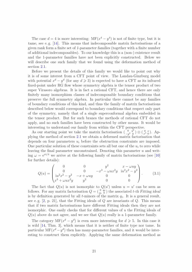
The case d = 4 is more interesting: MF(x4 − y4) is not of finite type, but it istame, see e. g. [14]. This means that indecomposable matrix factorisations of agiven rank form a finite set of 1-parameter families (together with a finite numberof additional indecomposables). To our knowledge this is a (non-) existence resultand the 1-parameter families have not been explicitly constructed. Below wewill describe one such family that we found using the deformation method ofsection 2.1.Before we present the details of this family we would like to point out why

it is of some interest from a CFT point of view. The Landau-Ginzburg modelwith potential xd − yd (for any d > 3) is expected to have a CFT as its infraredfixed-point under RG flow whose symmetry algebra is the tensor product of twosuper Virasoro algebras. It is in fact a rational CFT, and hence there are onlyfinitely many isomorphism classes of indecomposable boundary conditions thatpreserve the full symmetry algebra. In particular there cannot be any familiesof boundary conditions of this kind, and thus the family of matrix factorisationsdescribed below would correspond to boundary conditions that respect only partof the symmetry, namely that of a single superconformal algebra embedded inthe tensor product. But for such branes the methods of rational CFT do notapply, and no such families have been constructed by other means. It would beinteresting to understand our family from within the CFT perspective.As our starting point we take the matrix factorisation ( 0 y2

−y2 0) ⊗ ( 0 x

x3 0 ). Ap-plying the method of section 2.1 we obtain a deformed matrix factorisation thatdepends on four parameters ui before the obstruction constraints are imposed.One particular solution of these constraints sets all but one of the ui to zero whileleaving the final parameter unconstrained. Denoting this parameter u and writ-ing ω = eπi/4 we arrive at the following family of matrix factorisations (see [10]for further details):

Q(u) =

0 0 y2 x− ωuy0 0 −x3 − ωux2y iu2x2 − y2

iu2x2 − y2 −x+ ωuy 0 0x3 + ωux2y y2 0 0

. (3.1)

The fact that Q(u) is not isomorphic to Q(u′) unless u = u′ can be seen asfollows. For any matrix factorisation Q = ( 0 q0

q1 0 ) the associated t-th Fitting ideal

is by definition generated by all t-minors of the matrix q1. It is a general result,see e. g. [2, p. 21], that the Fitting ideals of Q are invariants of Q. This meansthat if two matrix factorisations have different Fitting ideals then they are notisomorphic. One easily checks that for different values of u the Fitting ideals ofQ(u) above do not agree, and we see that Q(u) really is a 1-parameter family.

The category MF(xd − yd) is even more interesting for d > 5. In this case itis wild [14, Thm. 3], which means that it is neither of finite type nor tame. Inparticular MF(xd− yd) then has many-parameter families, and it would be inter-esting to construct them explicitly. Applying the same deformation method as

21

before leads to obstruction constraints with many solutions. Those few solutionsthat we studied in detail did however not give rise to families in the above strictsense.

Generalised permutation branes

One may also study tensor products of distinct minimal models, i. e. Landau-Ginzburg models with potential W = xd + yd

′

. If the exponents d and d′ have acommon factor there is a class of matrix factorisations ofW known as generalisedpermutation branes [12, 16]. We will only consider the case W = x3 + y6 wherethese branes are given by

Gω =

(0 x− ωy2

x3+y6

x−ωy20

), ω3 = −1 ,

and their anti-branes. Every matrix factorisation of W that has been consideredso far is a direct sum of generalised permutation branes and tensor product branes

( 0 xa

x3−a 0 )⊗ ( 0 y2b

y2(3−b) 0).

Since the fermionic self-spectra of generalised permutation branes are trivial(one easily computes dimExt1(Gω, Gω) = 4 and dimExt1(Gω, Gω) = 0), thereare no directions into which Gω can be deformed. Instead we deform the super-position

Q = Geπi/3 ⊕G−1

which has 8 bosons and 4 fermions.Both deformation algorithms from sections 2.1 and 2.3 terminate at order 4

when applied to Q. Most of the solutions of the associated quartic obstructionequations lead to matrix factorisations which are of type Gω. Hence a directsum of two generalised permutation branes can be deformed to a single suchbrane. However, one finds that there is one particular solution that gives rise toa deformation of Q which is not a direct sum of generalised permutation branesand tensor product branes. It has 6 bosons and 2 fermions and turns out to beisomorphic to the cone of the open string state

(y 00 xy − 1

1−e−πi/3y3

): Qeπi/3 −→ Q−1 .

Simple branes on Calabi-Yau hypersurfaces

Our final two examples of tensor product matrix factorisations are branes inCalabi-Yau hypersurfaces. These two examples have already been consideredin [25] to which we refer for the explicit representatives of the boundary fields bywhich we deform below.

22

First we look at Q = (0 x61x61 0

) ⊗ (0 x62x62 0

) ⊗ (0 x33x33 0

) ⊗ (0 x34x34 0

) ⊗ ( 0 x5x5 0 ). In [25,

sect. 4.3.1] deformations (with non-zero obstructions) of this brane by the twobulk fields x61x

62 and x1x2x3x4x5 as well as four boundary fields were computed

up to fourth order. Using our implementation, we can go to order 50 in lessthan 40 minutes; in both cases the algorithm does not terminate at the givenorder. However, if only two particular boundary fermions are turned on, ouralgorithm terminates at order 4 without any obstructions, in agreement with [25,sect. 4.3.3].

The second example is Q = (0 x71x71 0

) ⊗ (0 x32x42 0

) ⊗ (0 x33x43 0

) ⊗ (0 x34x44 0

) ⊗ ( 0 x5x5 0 ).

We consider deformations by the bulk fields x71x5 and x1x2x3x4x5, and againfour boundary fields. Then our algorithm finds non-vanishing obstructions andterminates at order 7 after two minutes, consistent with [25, sect. 6.3.1].

Other examples

We have applied our code to an extensive list of further (mostly geometric) ex-amples, including linear matrix factorisations [15], D0-branes on the quintic (seee. g. [20]) and various D2-branes on Calabi-Yau hypersurfaces studied in [3, 4].We managed to compute deformations and obstructions to high orders, alwaysconsistent with known results and expectations, but to keep our presentation rea-sonably short we refrain from listing any details. From the point of view of studieslike [3, 4] only the binary information of whether deforming in a certain directionis obstructed or not is relevant; it should be interesting to include knowledge ofthe precise form of obstructions into such analyses.

4 Some general observations

We conclude the paper with some general observations on how to generate newmatrix factorisations and on how to deal with obstructions. While these remarksmay seem obvious in hindsight, studying deformation algorithms and producinga large pool of concrete examples definitely helped recognise the patterns.

4.1 Nilpotent substitutions

The ui in the deformed matrix factorisation Qdef(x; u) are of course intended ascomplex parameters, but all the computations performed in any of the algorithmsfrom section 2 remain correct as long as the ui commute among themselves andwith the variables xl of the Landau-Ginzburg potential W (x). This observationopens up an interesting playground: we can e. g. replace the ui by (commuting)matrices ui which solve the obstructions fj(u) = 0.An especially simple choice is to use nilpotent matrices of size N ,

ui 7−→ ui := viM[N ] , vi ∈ C , M[N ] ∈ MatN(C) such that MN[N ] = 0, (4.1)

23

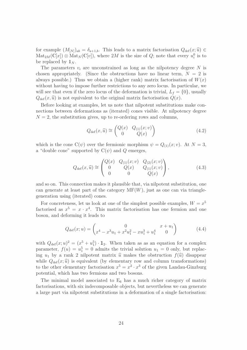
for example (M[N ])ab = δa+1,b. This leads to a matrix factorisation Qdef(x; u) ∈Mat2M(C[x]) ⊗MatN(C[v]), where 2M is the size of Q; note that every u0i is tobe replaced by 1N .The parameters vi are unconstrained as long as the nilpotency degree N is

chosen appropriately. (Since the obstructions have no linear term, N = 2 isalways possible.) Thus we obtain a (higher rank) matrix factorisation of W (x)without having to impose further restrictions to any zero locus. In particular, wewill see that even if the zero locus of the deformation is trivial, Lf = {0}, usuallyQdef(x, u) is not equivalent to the original matrix factorisation Q(x).

Before looking at examples, let us note that nilpotent substitutions make con-nections between deformations as (iterated) cones visible. At nilpotency degreeN = 2, the substitution gives, up to re-ordering rows and columns,

Qdef(x, u) ∼=(Q(x) Q(1)(x; v)0 Q(x)

)(4.2)

which is the cone C(ψ) over the fermionic morphism ψ = Q(1)(x; v). At N = 3,a “double cone” supported by C(ψ) and Q emerges,

Qdef(x, u) ∼=

Q(x) Q(1)(x; v) Q(2)(x; v)0 Q(x) Q(1)(x; v)0 0 Q(x)

, (4.3)

and so on. This connection makes it plausible that, via nilpotent substitution, onecan generate at least part of the category MF(W ), just as one can via triangle-generation using (iterated) cones.

For concreteness, let us look at one of the simplest possible examples, W = x5

factorised as x5 = x · x4. This matrix factorisation has one fermion and oneboson, and deforming it leads to

Qdef(x; u) =

(0 x+ u1

x4 − x3u1 + x2u21 − xu31 + u41 0

)(4.4)

with Qdef(x; u)2 = (x5 + u51) · 12. When taken as as an equation for a complex

parameter, f(u) = u51 = 0 admits the trivial solution u1 = 0 only, but replac-ing u1 by a rank 2 nilpotent matrix u makes the obstruction f(u) disappearwhile Qdef(x; u) is equivalent (by elementary row and column transformations)to the other elementary factorisation x5 = x2 · x3 of the given Landau-Ginzburgpotential, which has two fermions and two bosons.

The minimal model associated to E6 has a much richer category of matrixfactorisations, with six indecomposable objects, but nevertheless we can generatea large part via nilpotent substitutions in a deformation of a single factorisation:

24

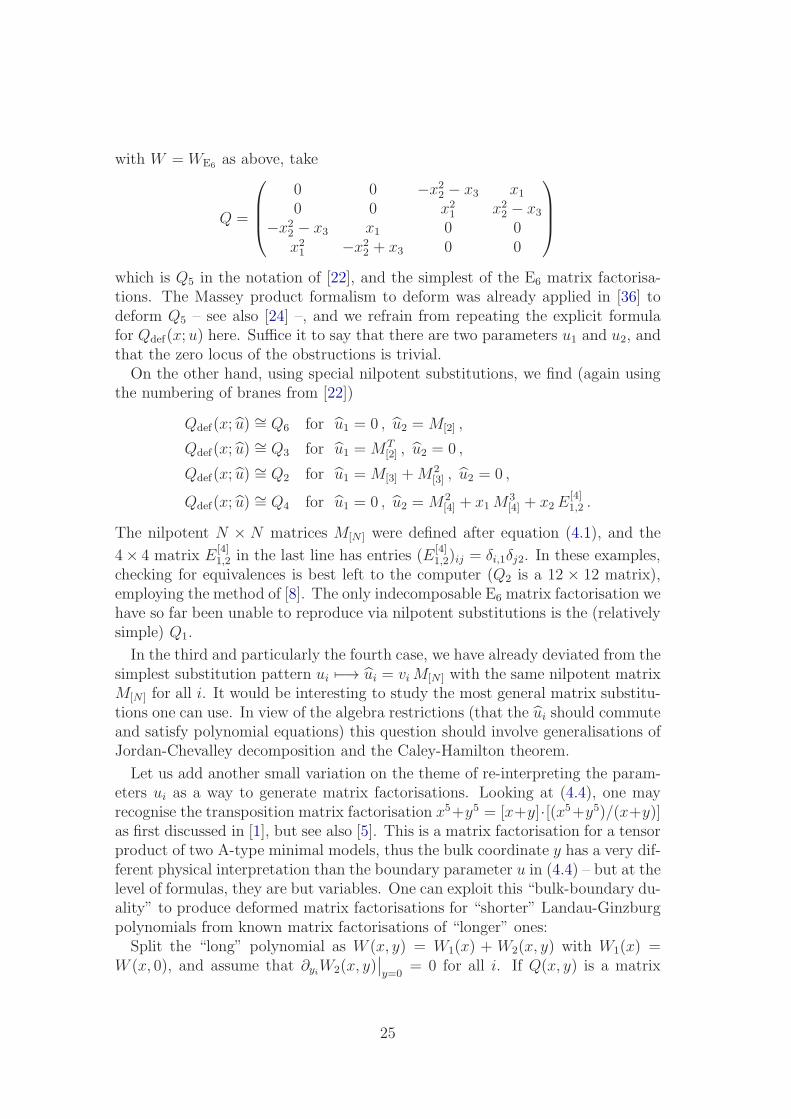
with W =WE6 as above, take

Q =

0 0 −x22 − x3 x10 0 x21 x22 − x3

−x22 − x3 x1 0 0x21 −x22 + x3 0 0

which is Q5 in the notation of [22], and the simplest of the E6 matrix factorisa-tions. The Massey product formalism to deform was already applied in [36] todeform Q5 – see also [24] –, and we refrain from repeating the explicit formulafor Qdef(x; u) here. Suffice it to say that there are two parameters u1 and u2, andthat the zero locus of the obstructions is trivial.On the other hand, using special nilpotent substitutions, we find (again using

the numbering of branes from [22])

Qdef(x; u) ∼= Q6 for u1 = 0 , u2 =M[2] ,

Qdef(x; u) ∼= Q3 for u1 =MT[2] , u2 = 0 ,

Qdef(x; u) ∼= Q2 for u1 =M[3] +M2[3] , u2 = 0 ,

Qdef(x; u) ∼= Q4 for u1 = 0 , u2 =M2[4] + x1M

3[4] + x2E

[4]1,2 .

The nilpotent N × N matrices M[N ] were defined after equation (4.1), and the

4× 4 matrix E[4]1,2 in the last line has entries (E

[4]1,2)ij = δi,1δj2. In these examples,

checking for equivalences is best left to the computer (Q2 is a 12 × 12 matrix),employing the method of [8]. The only indecomposable E6 matrix factorisation wehave so far been unable to reproduce via nilpotent substitutions is the (relativelysimple) Q1.

In the third and particularly the fourth case, we have already deviated from thesimplest substitution pattern ui 7−→ ui = viM[N ] with the same nilpotent matrixM[N ] for all i. It would be interesting to study the most general matrix substitu-tions one can use. In view of the algebra restrictions (that the ui should commuteand satisfy polynomial equations) this question should involve generalisations ofJordan-Chevalley decomposition and the Caley-Hamilton theorem.

Let us add another small variation on the theme of re-interpreting the param-eters ui as a way to generate matrix factorisations. Looking at (4.4), one mayrecognise the transposition matrix factorisation x5+y5 = [x+y]·[(x5+y5)/(x+y)]as first discussed in [1], but see also [5]. This is a matrix factorisation for a tensorproduct of two A-type minimal models, thus the bulk coordinate y has a very dif-ferent physical interpretation than the boundary parameter u in (4.4) – but at thelevel of formulas, they are but variables. One can exploit this “bulk-boundary du-ality” to produce deformed matrix factorisations for “shorter” Landau-Ginzburgpolynomials from known matrix factorisations of “longer” ones:Split the “long” polynomial as W (x, y) = W1(x) + W2(x, y) with W1(x) =

W (x, 0), and assume that ∂yiW2(x, y)∣∣y=0

= 0 for all i. If Q(x, y) is a matrix

25

factorisation of W (x, y), we can set

Q := Q(x, 0) and Qi := ∂yiQ(x, y)∣∣y=0

and we automatically have Q2 = W1 ·1 and {Q,Qi} = 0. If Qi happens to be non-trivial in the fermionic cohomology of Q, it is a bona fide first order deformationwith associated parameter yi, and one obtains a deformed matrix factorisation ofW1(x) for free: Qdef(x; u) = Q(x, u). The term W2 in the original potential Wplays the role of the total obstruction – seemingly of a rather special form, butsee the next section for further observations on this point.It should be interesting to explore connections between branes for different

Landau-Ginzburg models further, in particular in view of the intriguing relationbetween bulk and boundary quantities.

4.2 Lifting boundary obstructions by bulk deformations

There is one very surprising, and almost universal feature exhibited by the ex-amples we have studied so far: the total obstructions ob to deforming a matrixfactorisation Q of W are of the form

ob = f(x; u) · 1 , f ∈ Jac(W )[u] . (4.5)

In words, the obstruction is proportional to the unit matrix, and the total obstruc-tion polynomial f(x; u) is a linear combination (with u-dependent coefficients) ofelements in the Jacobi ring Jac(W ) of the Landau-Ginzburg potential.In many of the cases where this is true, the chosen representatives for a basis

of Ext2(Q,Q) do have off-diagonal entries, thus some “miraculous” cancellationmust be happening.

The physical interpretation of this is as follows. On the one hand, since Jac(W )is the space of bulk states, whenever (4.5) holds true, the obstructions againstboundary deformations can be lifted by an appropriate perturbation f(x; u) ofthe closed string background. On the other hand, since we have an explicitexpression for Qdef(x; u), we may read (4.5) in the opposite direction: it showshow a brane Q in the background theory with potential W needs to change if itis to remain a brane under the perturbation of the background to W + f(x; u).Whether the brane can “survive” arbitrary bulk perturbations, i. e. whether

the latter can be compensated by suitable boundary deformations, depends onwhether all bulk fields occur in the obstruction and on the details of the u-dependent coefficients.

Clearly it is desirable to have an easily verifiable criterion on Q = ( 0 q1q0 0 )

which guarantees that the obstruction satisfies property (4.5), with the resultinginterplay of bulk and boundary deformations. One can show that under certainassumptions, including that det(q1) = W and that W is irreducible, the bosonic

26

cohomology Ext2(Q,Q) is isomorphic to the Jacobi ring modulo some ideal, whichin particular implies that every bosonic state in Ext2(Q,Q) can be represented bya matrix of the form f(x, u) ·1. However, in the majority of examples considered,the identity (4.5) holds even if det(q1) does not divideW , or if the very restrictivecondition of W being irreducible is not met.A more general observation is that (4.5) is always true if the bulk-boundary

mapJac(W ) = C[x1, . . . , xn]/(∂W ) −→ Ext2(Q,Q) (4.6)

is surjective. The bulk-boundary map is part of the structure of open/closedtopological field theory for Landau-Ginzburg models, and it simply maps ϕ toϕ · 1. Indeed, a general discussion of the possible surjectivity of bulk-boundarymaps in topological field theories has already been initiated in [28], but to checkwhether (4.6) is surjective for a concrete Landau-Ginzburg boundary conditionis relatively easy to do in practise: We choose bases ϕi of Jac(W ) and φj ofExt2(Q,Q), then by reducing and lifting we can find a matrix C with polynomialentries such that

ϕi · 1 =∑

j

Cijφj .

If the rank of C equals the dimension of Ext2(Q,Q) then (4.6) is surjective andthe obstruction condition (4.5) will hold. We have implemented this procedure asthe function Ext2check in the library MFdeform.lib of [10]. It is independent ofany deformation algorithm, and can be easily applied to branes with geometricmeaning, where our deformation procedures may not terminate. For example,the bulk-boundary map is surjective in the case of the D2 branes on the quinticstudied e. g. in [3], and it is not surjective for the D0 brane given in [20].

Acknowledgements

We would like to thank C. Baciu, Ch. Barheine, I. Burban, I. Brunner, M. Gab-erdiel, B. Hovinen, D. Murfet, D. Plencner, D. Roggenkamp, E. Scheidegger,M. Soroush and in particular R.-O. Buchweitz and M. Kay for valuable discus-sions. This work was supported by STFC grant ST/G000395/1.

References

[1] S. K. Ashok, E. Dell’Aquila and D. E. Diaconescu, Fractional branes

in Landau-Ginzburg orbifolds, Adv. Theor. Math. Phys. 8 (2004), 461,[hep-th/0401135].

[2] W. Bruns and J. Herzog, Cohen-Macaulay rings, Cambridge studies in ad-vanced mathematics, Cambridge University Press, Cambridge U.K. (1998).

27

[3] M. Baumgartl, I. Brunner, and M. R. Gaberdiel, D-brane superpotentials

and RG flows on the quintic, JHEP 0707 (2007), 061, [arXiv:0704.2666].

[4] M. Baumgartl, I. Brunner, and D. Plencner, D-brane Moduli Spaces and

Superpotentials in a Two-Parameter Model, to appear.

[5] I. Brunner and M. R. Gaberdiel, Matrix factorisations and permutation

branes, JHEP 0507 (2005) 012 [hep-th/0503207].

[6] I. Brunner and M. R. Gaberdiel, The matrix factorisations of the D-model,J. Phys. A 38 (2005), 7901, [hep-th/0506208].

[7] I. Brunner, M. Herbst, W. Lerche, and B. Scheuner, Landau-Ginzburg Re-

alization of Open String TFT, JHEP 0611 (2003), 043, [hep-th/0305133].

[8] N. Carqueville, Triangle-generation in topological D-brane categories, JHEP04 (2008), 031, [arXiv:0802.1624].

[9] N. Carqueville, Matrix factorisations and open topological string theory,JHEP 0907 (2009), 005, [arXiv:0904.0862].

[10] N. Carqueville, L. Dowdy, and A. Recknagel, Code to compute deformations

of matrix factorisations, http://nils.carqueville.net/MFdeform.

[11] N. Carqueville and M. M. Kay, Bulk deformations of open topological string

theory, [arXiv:1104.5438].

[12] C. Caviezel, S. Fredenhagen, and M. R. Gaberdiel, The RR charges of A-type

Gepner models, JHEP 0601 (2006), 111, [hep-th/0511078].

[13] K. J. Costello, Topological conformal field theories and Calabi-Yau cate-

gories, Adv. in Math. 210 (2007), [math.QA/0412149].

[14] Y. A. Drozd and M.-G. Greuel, Cohen-Macaulay module type, CompositioMathematica 89 (1993), 315–338.

[15] H. Enger, A. Recknagel, and D. Roggenkamp, Permutation branes and linear

matrix factorisations, JHEP 0601 (2006), 087, [hep-th/0508053].

[16] S. Fredenhagen and M. R. Gaberdiel, Generalised N = 2 permutation

branes, JHEP 0601 (2006), 041, [hep-th/0607095].

[17] G.-M. Greuel, C. Lossen, and E. Shustin, Introduction to Singularities and

Deformations, Springer 2007.

[18] M. Herbst, C. I. Lazaroiu, and W. Lerche, Superpotentials, A∞ Relations

and WDVV Equations for Open Topological Strings, JHEP 0502 (2005),071, [hep-th/0402110].

28

[19] K. Hori and J. Walcher, F-term equations near Gepner points, JHEP 0501

(2005), 008, [hep-th/0404196].

[20] H. Jockers, D-brane monodromies from a matrix-factorization perspective,JHEP 0702 (2007), 006, [hep-th/0612095].

[21] T. Kadeishvili, On the homology theory of fibre spaces, Uspekhi Mat. Nauk35:3 (1980), 183–188, English translation in Russian Math. Surveys, 35:3(1980), 231–238, [math.AT/0504437].

[22] H. Kajiura, K. Saito, and A. Takahashi, Matrix Factorizations and Repre-

sentations of Quivers II: type ADE case, Adv. in Math. 211 (2007), 327–362,[math.AG/0511155].

[23] A. Kapustin and Y. Li, D-branes in Landau-Ginzburg Models and Algebraic

Geometry, JHEP 0312 (2003), 005, [hep-th/0210296].

[24] J. Knapp and H. Omer, Matrix factorizations, minimal models and Massey

products, JHEP 0605 (2006), 064, [hep-th/hep-th/0604189].

[25] J. Knapp and E. Scheidegger, Matrix Factorizations, Massey Products and

F-Terms for Two-Parameter Calabi-Yau Hypersurfaces, Adv. Theor. Math.Phys. 14 (2010), 225–308, [arXiv:0812.2429].

[26] M. Kontsevich, Deformation quantization of Poisson manifolds, Lett. Math.Phys. 66 (2003), 157–216, [math.QA/9709040].

[27] O. A. Laudal, Matric Massey products and formal moduli I, Lecture Notesin Mathematics 1183 (1983), 218–240.

[28] C. I. Lazaroiu, On the structure of open-closed topological field theory in

two dimensions, Nucl. Phys. B 603 (2001), 497–530, [hep-th/0010269].

[29] C. I. Lazaroiu, String field theory and brane superpotentials, JHEP 0110

(2001), 018, [hep-th/0107162].

[30] C. I. Lazaroiu, On the boundary coupling of topological Landau-Ginzburg

models, JHEP 0505 (2005), 037, [hep-th/0312286].

[31] D.-M. Lu, J. H. Palmieri, Q.-S. Wu, and J. J. Zhang, A-infinity struc-

ture on Ext-algebras, J. Pure Appl. Alg. 213 (2009), no. 11, 2017–2037,[math.KT/0606144].

[32] S. A. Merkulov, Strongly homotopy algebras of a Kahler manifold, Internat.Math. Res. Notices 3 (1999), 153–164, [math.AG/9809172].

[33] S. A. Merkulov, Frobenius∞ invariants of homotopy Gerstenhaber algebras,

I, Duke Math. J. 105 (2000), 411–461, [math.AG/0001007].

29

[34] G. W. Moore and G. Segal, D-branes and K-theory in 2D topological field

theory, [hep-th/0609042].

[35] M. Schlessinger, Functors of Artin rings, Transactions Amer. Math. Soc. 130(1968), 208–222, JSTOR/1994967

[36] A. Siqveland, The method of computing formal moduli, J. of Algebra 241

(2001), 291–327

[37] C. Vafa, Topological Landau-Ginzburg Models, Mod. Phys. Lett. A 6 (1991),337–346.

[38] Y. Yoshino, Cohen-Macaulay modules over Cohen-Macaulay rings, Lon-don Mathematical Society Lecture Note Series, Cambridge University Press,Cambridge U.K. (1990).

30