Преглед НЦД 12 (2008), 17–31 Vesna Vučković (Faculty of Mathematics, Belgrade)

IMAGE AND ITS MATRIX, MATRIX AND ITS IMAGE Abstract: The need for matrix presentation by image is clear to all who in their work use high dimension matrices. Particular problem here make matrices that could not normally be presented by images – those whose elements are arbitrary real, or even complex numbers. Here we propose a solution for visualization of arbitrary, high dimension matrix. This is illustrated by several examples, with matrices used in two-dimensional discrete linear transforms, in image processing.

Keywords: digital image, matrix, visualization, discrete cosine transform, discrete Fourier transform, JPEG compression

1. Introduction

There is a relation between matrices and digital images. A digital image in a computer is presented by pixels matrix. On the other hand, there is a need (especially with high dimensions matrices) to present matrix with an image. The motive of this work is to perceive matrix elements nature and arrangement: to recognize matrix parts – positive from negative, real from complex, bigger from smaller (by magnitude).

1.1. Image and its matrix. A digital grayscale image is presented in the computer by pixels matrix. Each pixel of such image is presented by one matrix element – integer from the set

. The numeric values in pixel presentation are uniformly changed from zero (black pixels) to 255 (white pixels). { 255210 ,...,, }

For example, the image 1or, magnified:

is presented with the matrix 0 16 32 48 64 80 96 112 128 144 160 176 192 208 224 240 1 17 33 49 65 81 97 113 129 145 161 177 193 209 225 241 2 18 34 50 66 82 98 114 130 146 162 178 194 210 226 242 3 19 35 51 67 83 99 115 131 147 163 179 195 211 227 243 4 20 36 52 68 84 100 116 132 148 164 180 196 212 228 244 5 21 37 53 69 85 101 117 133 149 165 181 197 213 229 245 6 22 38 54 70 86 102 118 134 150 166 182 198 214 230 246 7 23 39 55 71 87 103 119 135 151 167 183 199 215 231 247 8 24 40 56 72 88 104 120 136 152 168 184 200 216 232 248 9 25 41 57 73 89 105 121 137 153 169 185 201 217 233 249 10 26 42 58 74 90 106 122 138 154 170 186 202 218 234 250 11 27 43 59 75 91 107 123 139 155 171 187 203 219 235 251 12 28 44 60 76 92 108 124 140 156 172 188 204 220 236 252 13 29 45 61 77 93 109 125 141 157 173 189 205 221 237 253 14 30 46 62 78 94 110 126 142 158 174 190 206 222 238 254 15 31 47 63 79 95 111 127 143 159 175 191 207 223 239 255

Color images (with RGB color model) in a computer are presented with three grayscale images matrices (one for each – red, green and blue – color components). 1.2. Matrix and its image. Each image processing operation in a computer may be observed as an operation on image matrix. Usually, the result of such operation is matrix of original image 1 If it is necessary, images will have borders, which will visually demarcate them from the background.

Vesna Vučković 18

dimension ( ), whose elements need not be from the set , but also they may be arbitrary real, or even complex numbers. Matrices we use here, are of very high dimensions (several tens, or hundreds of thousands, or even over million of elements). In order to get visualization about such matrix overall, the need to present it with an image arises naturally.

nm × },...,,{ 25510

This idea, certainly, is not new. In programs dedicated for work with matrices, there exists a possibility to present matrix by image. However, this presentation is mainly inadequate. It does not take into consideration values out of the set . },...,,,{ 255210

Matlab-like programs do this in the following steps: – First, imaginary part is discarded (if matrix is complex) – Then, all elements are rounded to the nearest integer – Finally, values less than 0 become 0 – Values greater than 255 become 255

Clearly, such presentation does not show information about the contents for majority of matrices.

Good matrix presentation needs to represent nature and mutual relation between elements values. It has to show whether the matrix elements are positive or negative, real or complex numbers, and which is mutual relation between elements magnitudes.

Here we propose a different solution – hopefully better. The following text consists of two parts (sections 2 and 3). In section 2 ("Matrices

coloring") an algorithm for visualization of arbitrary matrices will be proposed. In section 3 ("Visualization of matrices used in image processing") several interesting examples of presenting high dimension matrices (real and complex) ") will be given. All these examples are related with linear transforms, which have use in image processing. The proposed algorithm of matrices visualization will hopefully be useful for linear transforms understanding.

2. Matrices coloring 2.1. Presentation of real matrices. In a matrix, in which all elements are positive or equal to zero, we may present value 0 with black, and maximum positive value with white color; in this way, all positive matrix values will be presented as grayscale nuances (from black for zero, to white for maximum positive value).

Example 2.1: A matrix and its image:

0 50 100 150 200 250 300 350 50 100 150 200 250 300 350 400 100 150 200 250 300 350 400 450 150 200 250 300 350 400 450 500 200 250 300 350 400 450 500 550 250 300 350 400 450 500 550 600 300 350 400 450 500 550 600 650 350 400 450 500 550 600 650 700

In this solution, matrix element values are scaled in order to be squeezed into interval [0, 255] – all matrix values are multiplied by factor (255/max. value) (in our example, this is 255/700). A matrix with all elements non-positive may be presented similarly, in nuances from black to yellow.

Vesna Vučković 19

Example 2.2: The matrix

0 -50 -100 -150 -200 -250 -300 -350 -50 -100 -150 -200 -250 -300 -350 -400 -100 -150 -200 -250 -300 -350 -400 -450 -150 -200 -250 -300 -350 -400 -450 -500 -200 -250 -300 -350 -400 -450 -500 -550 -250 -300 -350 -400 -450 -500 -550 -600 -300 -350 -400 -450 -500 -550 -600 -650 -350 -400 -450 -500 -550 -600 -650 -700

A matrix with positive and negative values will be presented with an image, in which positive values will be given in nuances from black to white, and negative – from black to yellow. Scaling may be done according to the biggest matrix elements magnitude.

Example 2.3: The matrix

-1 1 0 -1 1 0 -1 1 1 0 -1 1 0 -1 1 0 0 -1 1 0 -1 1 0 -1 -1 1 0 -1 1 0 -1 1 1 0 -1 1 0 -1 1 0 0 -1 1 0 -1 1 0 -1 -1 1 0 -1 1 0 -1 1 1 0 -1 1 0 -1 1 0

Example 2.4: In the next figure, two white Gaussian noise matrices2 may be seen. Matrix on the left is of considerably lower dimension comparing with that on the right, and its elements are presented "zoomed".

2.2. Complex matrix presentation. Pure imaginary matrices may be presented similarly. Negative imaginary values we present with nuances from black to green, and positive – from black to red color.

Example 2.5: In the next three images real and imaginary matrix, and their sum – complex matrix are presented. 2 Matrices whose elements have values from normal distribution with zero mean

Vesna Vučković 20

-4 -3 -2 -1 0 1 2 3 4 -4 -3 -2 -1 0 1 2 3 4 -4 -3 -2 -1 0 1 2 3 4 -4 -3 -2 -1 0 1 2 3 4 -4 -3 -2 -1 0 1 2 3 4 -4 -3 -2 -1 0 1 2 3 4 -4 -3 -2 -1 0 1 2 3 4 -4 -3 -2 -1 0 1 2 3 4 -4 -3 -2 -1 0 1 2 3 4

+4i +4i +4i +4i +4i +4i +4i +4i +4i +3i +3i +3i +3i +3i +3i +3i +3i +3i +2i +2i +2i +2i +2i +2i +2i +2i +2i +1i +1i +1i +1i +1i +1i +1i +1i +1i 0 0 0 0 0 0 0 0 0 -1i -1i -1i -1i -1i -1i -1i -1i -1i -2i -2i -2i -2i -2i -2i -2i -2i -2i -3i -3i -3i -3i -3i -3i -3i -3i -3i -4i -4i -4i -4i -4i -4i -4i -4i -4i

-4+4i -3+4i -2+4i -1+4i +4i 1+4i 2+4i 3+4i 4+4i -4+3i -3+3i -2+3i -1+3i +3i 1+3i 2+3i 3+3i 4+3i -4+2i -3+2i -2+2i -1+2i +2i 1+2i 2+2i 3+2i 4+2i -4+1i -3+1i -2+1i -1+1i +1i 1+1i 2+1i 3+1i 4+1i -4 -3 -2 -1 0 1 2 3 4 -4-1i -3-1i -2-1i -1-1i -1i 1-1i 2-1i 3-1i 4-1i -4-2i -3-2i -2-2i -1-2i -2i 1-2i 2-2i 3-2i 4-2i -4-3i -3-3i -2-3i -1-3i -3i 1-3i 2-3i 3-3i 4-3i -4-4i -3-4i -2-4i -1-4i -4i 1-4i 2-4i 3-4i 4-4i

Of course, the proposed colors combination is not the only possible. However, it is not also completely arbitrary. In colors choice it is very important that every two distant points in the complex plane would be presented with different colors.

Let us explain the notion of "distant points". This demand means that between any two points in the complex plane presented with the same color must not be any point of different color. (Clearly, two close points, due to infinite number of complex plane points, and finite number of different colors, may be colored by the same color).

The suggested color combination (yellow–white& green–red) is correct in this sense. Used colors intensity increases with moving away of origin, and therefore, in none of the four complex plane quadrants two distant points colored with the same color exist.

In addition, in quadrants, colors appearance in complex numbers presentation is : ),( 0≥yx

I quadrant: rybgrx ⋅+++ )( mostly red, and some amount of blue color II quadrant: mostly red, and without blue color rygrx ⋅++ )(III quadrant: mostly green, and without blue color gygrx ⋅++ )(IV quadrant: gybgrx ⋅+++ )( mostly green, and some amount of blue color

Therefore two points in different quadrants presented with the same color, do not exist. If, instead of green, we use blue color, it will be (combination yellow–white& blue–red):

Vesna Vučković 21

III quadrant: bxybgrxbygrx )()()( −+++=⋅++ IV quadrant: bybgrx ⋅+++ 1)(

Hence, in the third and in the fourth quadrant, two points presented with the same color (combination of white and blue) exist. Therefore, the combination yellow–white& blue–red is not a good one.

In the next two figures are presented these two colors combinations. In the left figure is the "good" combination (yellow–white& green–red). In the right one is the "bed" combination (yellow–white& blue–red). Here, there are marked several pairs of distant points, presented by the same color.

3. Visualization of matrices used in image processing In this section several interesting examples will be mentioned, in which, owing to very high dimensions, it is necessary to present matrix with an image,. Examples are chosen with the goal of making easier understanding of (in image processing often used) linear transforms of matrices. Subsection 3.1 is dedicated to discrete cosine transform (DCT) of image of arbitrary dimensions. Subsection 3.2 presents blocked DCT, used in JPEG compression. Subsection 3.3 illustrates one way for image dimensions (including aspect ratio) changing. Subsection 3.4 presents Fourier transform (FT), which, in contrast to other transforms, uses complex matrices. 3.1. Discrete cosine transform of image. We get discrete cosine transform (DCT) of matrix

of dimension , using formula , where is an image matrix in spatial domain (original image matrix), S nm × nm MSMD ⋅⋅= −1 S

D is image matrix in transform domain; both matrices ( and S D ) have dimensions . and are square matrices of dimensions nm× mM nM mm× and respectively, and may be calculated with the code (here written for matrix of dimension , labeled with

nn×mm× M ):

c=ones(m)*sqrt(2/m); c(1)=sqrt(1/m); for i=1:m for j=1:m M(i,j)=c(j)*cos((2*i-1)*(j-1)*pi/(2*m)); end end

Vesna Vučković 22

These matrices are constant – they do not depend on image content, but only on its dimension.

S

In the several next figures are images for matrices , , , and , for discrete cosine transform.

2M 3M 4M 8M 128M

2M

0.707 0.707 0.707 -0.707

3M

0.577 0.707 0.408 0.577 0.000 -0.816 0.577 -0.707 0.408

4M

0.500 0.653 0.500 0.271 0.500 0.271 -0.500 -0.653 0.500 -0.271 -0.500 0.653 0.500 -0.653 0.500 -0.271

8M

0.35 0.49 0.46 0.42 0.35 0.28 0.19 0.10 0.35 0.42 0.19 -0.10 -0.35 -0.49 -0.46 -0.28 0.35 0.28 -0.19 -0.49 -0.35 0.10 0.46 0.42 0.35 0.10 -0.46 -0.28 0.35 0.42 -0.19 -0.49 0.35 -0.10 -0.46 0.28 0.35 -0.42 -0.19 0.49 0.35 -0.28 -0.19 0.49 -0.35 -0.10 0.46 -0.42 0.35 -0.42 0.19 0.10 -0.35 0.49 -0.46 0.28 0.35 -0.49 0.46 -0.42 0.35 -0.28 0.19 -0.10

128M

We may observe matrices and S D as presentations of the same image in two different bases.

Example 3.1: If the image is in the spatial domain presented with matrix , then

(since

⎥⎦

⎤⎢⎣

⎡=

200100500

S

⎥⎦

⎤⎢⎣

⎡−

⋅== −

1111

211

22 MM ),

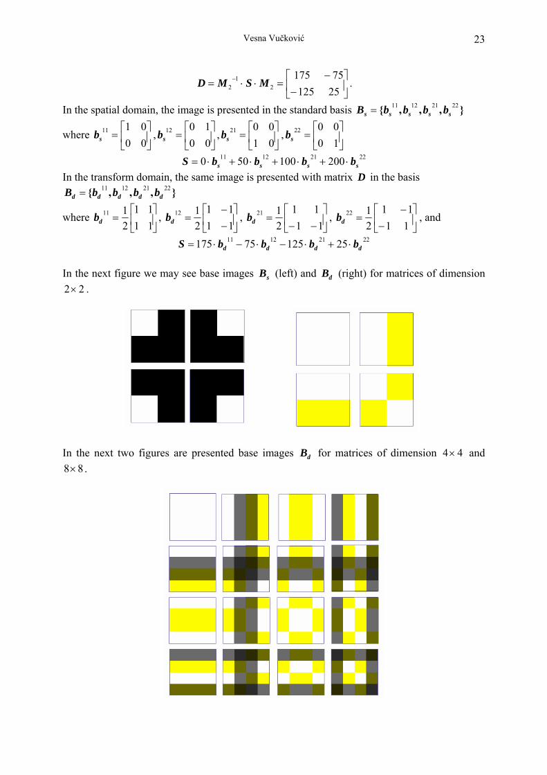
Vesna Vučković 23

⎥⎦

⎤⎢⎣

⎡−

−=⋅⋅= −

2512575175

21

2 MSMD .

In the spatial domain, the image is presented in the standard basis },,,{ 22211211sssss bbbbB =

where , , , ⎥⎦

⎤⎢⎣

⎡=

000111

sb ⎥⎦

⎤⎢⎣

⎡=

001012

sb ⎥⎦

⎤⎢⎣

⎡=

010021

sb ⎥⎦

⎤⎢⎣

⎡=

100022

sb

22211211 200100500 ssss bbbbS ⋅+⋅+⋅+⋅= In the transform domain, the same image is presented with matrix D in the basis

},,,{ 22211211ddddd bbbbB =

where ⎥⎦

⎤⎢⎣

⎡=

1111

2111

db , ⎥⎦

⎤⎢⎣

⎡−−

=1111

2112

db , ⎥⎦

⎤⎢⎣

⎡−−

=11

112121

db , ⎥⎦

⎤⎢⎣

⎡−

−=

1111

2122

db , and

22211211 2512575175 dddd bbbbS ⋅+⋅−⋅−⋅= In the next figure we may see base images (left) and (right) for matrices of dimension

. sB dB

22×

In the next two figures are presented base images for matrices of dimension and

. dB 44×

88×

Vesna Vučković 24

Example 3.2: Several first steps in presentation of crest image of Faculty of Mathematics, Belgrade:

Original image

Vesna Vučković 25

Original image has dimension , and it is presented in base with linear combination of 896 base images (each of them is multiplied by corresponding element in matrix

2832× dBD ). Here

first 18 steps in deriving original image from base images, are showed. Each step is presented by pair (base image, result image). Steps are arranged in compliance with decreasing order of coefficients magnitudes in matrix D . 3.2. Blocked DCT and JPEG compression. JPEG compression of grayscale image is based on blocked DCT:

cS

– Image is divided in image blocks of dimensions cS 88× pixels – DCT is applied on each image block. Result is matrix , produced with joining all cD 88× blocks in the transform domain. – Each element of each block is subjected to quantization – is divided by a number, determined in advance, and the quotient is rounded to the nearest integer. The divisor for each block element is determined by quantization table

88×

3, i.e. by position of the element in the block. This is a "lossy" step in compression – it enables that the image data may be recorded in a less memory space, with respect to the original image data.

Example 3.3: In the next figure we may see images for matrices (dimension S 88× ), and 8M D .

Block D – result of discrete cosine transform (also of dimension 88× ), in contrast with block in spatial domain, has prominent differences between values in different block parts. Its elements near top-left corner (so-called DC element) are with far bigger magnitudes values comparing with block remaining part. These values decline with going to bottom-right corner.

The same result we obtain with matrix multiplication of (here, "Cameraman", dimension of ) and (presented in the middle) – result is again matrix (right)

cS128128× cM 8 cD

cccc MSMD 81

8 ⋅⋅= − .

3 Quantization table is in advanced determined matrix of dimension 88× , which contains divisors for all block elements.

Vesna Vučković 26

Matrix is almost diagonal. On its diagonal, it has matrices , and beyond it, all elements have values zero.

cM 8 8M

In each matrix block, the block elements near the DC element have bigger magnitudes comparing with the rest of the block; on the other hand, they have smaller quantization coefficients in relation to remote elements. Thus, quantization is more intensive (more data will be lost) in block elements remote from DC element.

88× cD

Therefore, in JPEG compression, data in bottom-right corner of each DCT block are lost much more, than in top-left corner.

Three next examples show data nullifying impact4 in bottom–right image block parts on matrix (Nullifying effect for the small part of each cD 88× block; a half of each image block; the most part of each image block in transform domain). Each of the showed three examples is presented with three images:

– designation of block part that will be nullified; – matrix arisen by nullifying of coefficients part in all matrix blocks; 'cD– matrix arisen from by applying inverse DCT. 'cS 'cD

Inverse DCT (multiplication by inverse of matrix ) returns us into the spatial domain with some extent distorted image. If we have not gone too far, these changes need not be visible to human eyes.

cM 8

3.3. One way for image dimension changing. Image dimension changing may also be done by applying transform (for example discrete cosine) on the whole image:

4 In these examples, in order to illustrate, more complicate (and not much different) quantization we replace with data nullifying in bottom-right corner of each block.

Vesna Vučković 27

– We perform DCT overall on the whole image (here presented, as example, image "Cameraman", of dimension – top left). Result of this operation (matrix

S128128× D ) we may

see on the right (showed on top–right image). Matrix D is the same dimension ( ). 128128×– We add 30 columns to the right side of matrix D (elements values in these appended columns are 0). Then, we crop 30 rows in the bottom of it. The result matrix D ', of dimension

we may see on the bottom–left image15898× 5. On matrix 'D we apply inverse DCT. Result is image of dimension 'S 15898×

showed bottom right. After inverse DCT, we have original image with aspect ratio changed.

3.4. Fourier transform. Fourier transform (FT) of matrix of dimension we get with formula

S nm ×

nm MSMF ⋅⋅= −1 Matrix is an original image matrix, matrix S F is FT for this image; both of them have dimension . Square matrices and have dimensions , and nm × mM nM mm× nn× , respectively, and they may be calculated by Matlab code (here, this matrix is labeled with , and of dimension ):

Mmm ×

for i1=1:m for j1=1:m M(i1,j1)=exp(-2*pi*i/m)*(i1-1)*(j1-1); end end

5 When DCT is applied on the whole image, elements magnitudes near DC element in resultant matrix are much bigger, comparing with the rest of the matrix. So, matrix D (and 'D ) would be presented with totally black rectangle, with little white point in top–left corner. In order to have better matrix presentation, top–right ( D ) and bottom–left ( 'D ) images are presented with logarithmed magnitudes.

Vesna Vučković 28

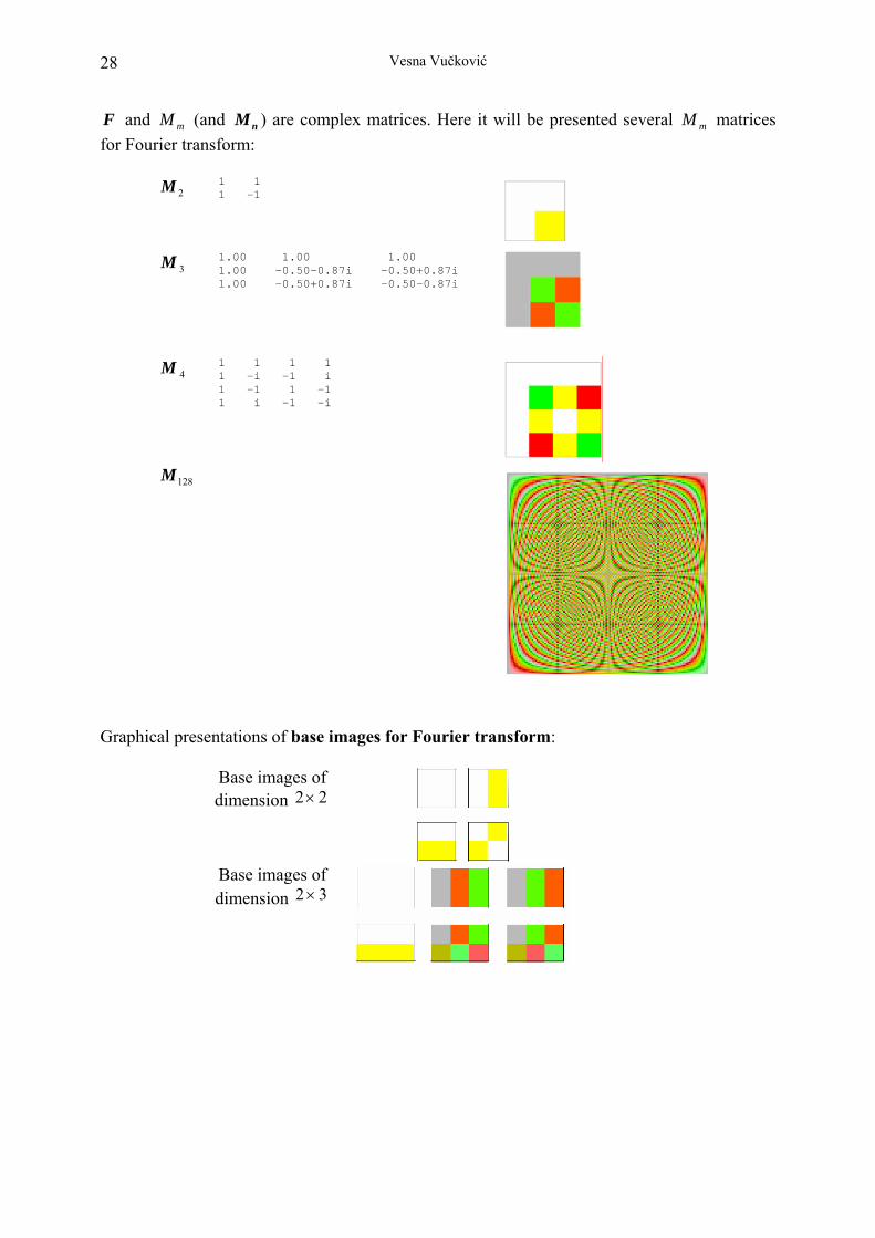
F and (and ) are complex matrices. Here it will be presented several matrices for Fourier transform:

mM nM mM

2M

1 1 1 -1

3M

1.00 1.00 1.00 1.00 -0.50-0.87i -0.50+0.87i 1.00 -0.50+0.87i -0.50-0.87i

4M 1 1 1 1 1 -i -1 i 1 -1 1 -1 1 i -1 -i

128M

Graphical presentations of base images for Fourier transform:

Base images of dimension 22×

Base images of dimension 32×

Vesna Vučković 29

Base images of dimension 33×

Base images of dimension 44×

Base images of dimension 88×

For matrices and S F applies

∑∑∑∑= == =

⋅=⋅=m

i

n

j

ijfij

m

i

n

j

ijsij bfbsS

1 11 1

, where [ ]nmijsS

×= , [ ]

nmijfF×

= , and

ijsb is base image in spatial domain that correspond with matrix coefficient , S ijs

ijfb is base image in transform domain that corresponds with matrix F coefficient . ijf

Vesna Vučković 30

Example 3.5: Image presentation in new basis. In the next figure, we may see several first steps in presentation of image by FT base images. S

Original image of dimension 88× pixels

In this example matrix is of dimension S 88× , and it is presented in base with linear combination of 64 base images of dimension

dB88× (each of them is multiplied by

corresponding element of matrix F ). Here, first 18 steps in deriving original image from matrix F and base images are showed. Each step is presented by pair (base image, result image). Steps are arranged in compliance with decreasing order of coefficients magnitudes in matrix F .

4. Conclusion Here the proposed solution enables visualization of arbitrary matrices. The presented examples are mainly related with linear transforms – DCT and Fourier, and blocked DCT (which is used in JPEG compression). This examples choice is made for the reader to understand better high dimension matrices, used in image processing. This solution may be helpful, not only to people that are engaged in image processing, but also to all engaged in (real or complex) high dimension matrices.

Vesna Vučković 31

Bibliography

[1] MATLAB – The Language of Technical Computing (Matlab 6.5/13, Disc 2, \help\pdf_doc\matlab\using_ml.pdf )

[2] Image Processing Toolbox – For Use with MATLAB (Matlab 6.5/13, Disc 2, \help\pdf_doc\images\images_tb.pdf)

[3] Y.Q.Shi, H.Sun: Image and Video Compression for Multimedia Engineering: Fundamentals, Algorithms, and Standards, CRC Press, 1999

[4] William K. Pratt: Digital Image Processing: PIKS Inside, John Wiley &Sons, Inc, 2001

[5] John C. Russ: The Image Processing Handbook, CRC Press, 2002

[6] Mark D. Schroeder: JPEG Compression Algorithm and Associated Data Structures, 1997, http://akbar.marlboro.edu/~mahoney/courses/Fall01/computation/compression/jpeg/jpeg.html

[7] I.T. Young, J.J. Gerbrands, L.J. van Vliet: Image Processing Fundamentals, http://www.ph.tn.tudelft.nl/Courses/FIP/noframes/fip.html

Весна Вучковић (Математички факултет, Београд)

СЛИКА И ЊЕНА МАТРИЦА. МАТРИЦА И ЊЕНА СЛИКА Сажетак: Предлажмо решење за визуелизацију матрица – како реалних, тако и комплексних. Потреба за приказом матрице у облику слике јасна је свима који се баве матрицама великих димензија. Посебан проблем ту стварају матрице које не могу бити нормално приказане сликом – оне чији су елементи произвољни реални, па чак и комплексни бројеви. Дато решење илустровано је са неколико примера, матрицама коришћеним у дводимензионим дискретним линеарним трансформацијама, у обради слика.

Кључне речи: дигитална слика, матрица, визуелизација, дискретна косинусна трансформација, дискретна Фуријеова трансформација, ЈПЕГ компресија

vesnav@matf.bg.ac.yu