Algorithmic construction of optimal symmetricLatin hypercube designsKenny Q. Ye William Li Agus SudjiantoDepartment of Applied Department of Operations Reliability Methods DepartmentMathematics and Statistics and Management ScienceSUNY at Stony Brook University of Minnesota Ford Motor CompanyStony Brook, NY 10021 Minneapolis, MN 55455 Dearborn, MI 48121AbstractWe propose symmetric Latin hypercubes for designs of computer exepriment.The goal is to o�er a compromise between computing e�ort and design opti-mality. The proposed class of designs has some advantages over the regularLatin hypercube design with respect to criteria such as entropy and the min-imum intersite distance. An exchange algorithm is proposed for constructingoptimal symmetric Latin hypercube designs. This algorithm is compared1

with two existing algorithms by Park (1994) and Morris and Mitchell (1995).Some examples, including a real case study in the automotive industry, areused to illustrate the performance of the new designs and the algorithms.Key Words: Computer experiment; Maximum Entropy Design; Maximindesign1 IntroductionOne of our recent projects is concerned with the thermal analysis of multi-layer electrical traces at a major automotive company. As more and moreelectronic devices are installed in vehicles, the peak temperature of electricaltraces becomes a major concern in designing the instrument panels. Thetemperature of an electrical trace is largely determined by its width, itspassing current strength, and its position in a stack of traces. The goal ofthis project is to provide guidelines for design engineers for width and passingcurrent strength of multi-layer electrical traces. Physical experiments areinevitably very expensive and time consuming since a set of electrical traceshas to be assembled in certain con�gurations for each test and measuringthe temperature of each trace is di�cult. Therefore, �nite element analysis2

(FEA) models have been developed to simulate the thermal dynamics ofelectrical traces.Using the computer model, the study starts from a simple case, in whichthere are two layers with three traces on each layer. One primary interestis the interaction between a center trace and an edge trace on two di�erentlayers since the heat coming o� the center trace spreads out and a�ects thetemperature at the edge. A center trace on layer 1 and an edge trace on layer2 are selected in the study. The goal is to predict their peak temperatures(y1 and y2) based on four predictors: the width of the center trace (x1), theapplied current of the center trace (x2), the width of the edge trace (x3),and the applied current of the edge trace (x4). Given a set of xi-values, thecomputer model generates a deterministic peak temperature for each trace.Though computer experiments are much cheaper and faster than physicalexperiments, each run is still time consuming and expensive. Thus, only asmall number of combinations of the xi can be tested. In this case, the exper-iment is to be conducted by another company which specializes in thermaldynamic computer models, and the budget only allows for 25 runs. A feasibleapproach is to establish a statistical model from the results of the 25 runsand then use it to predict peak temperatures for any given combinations of3

the xi. An optimal Latin hypercube design was chosen for this experiment.A Latin hypercube design (LHD) is an n � l matrix in which each col-umn is a random permutation of f1; : : : ; ng which can be mapped onto theactual range of the variables. It has good projection properties on any singledimension. Latin hypercube designs have been applied in many computerexperiments since they were proposed by McKay et al. (1979). In practice,a LHD can be randomly generated, but a randomly selected LHD may havebad properties and act poorly in estimation and prediction. Another ap-proach is to use optimal designs according to some criteria such as entropy(Shewry and Wynn 1987), Integrated Mean Squared Error (IMSE) (Sackset al. 1989), and minimum intersite distance (Johnson et al. 1990). Thesedesigns have been shown to be e�cient for certain models. However, thecomputational cost of obtaining these designs is high. In an attempt to o�era compromise between good projective properties of LHDs and a criterion,Park (1994) and Morris and Mitchell (1995) proposed optimal Latin hyper-cube designs. For an excellent review of design and analysis of computerexperiments, see Koehler and Owen (1996).One of the criteria considered in this paper is the entropy criterion,�rst proposed by Shewry and Wynn (1987) and then adopted by Currin4

et al. (1991). The response of a computer model is modeled by Y (x) =Pkj=1 �jfj(x) + Z(x), in which Z(x) is a Gaussian process with mean zeroand covarianceR(s; t) = �2 exp8<:�� lXj=1 jsj � tjjq9=; ; 0 < q � 2 (1)between two l-dimensional inputs s and t. The entropy criterion is equiva-lent to the minimization of �logjRj; where R is the covariance matrix of thedesign. The parameters � and q determine the properties of Z(x). Through-out this paper, we set q = 2 so that the correlation between two sites is afunction of their L2 distance.The construction of an optimal LHD can still be time consuming. Forexample, to generate a maximum entropy 25� 4 LHD using a columnwise-pairwise (CP) algorithm (discussed in Section 3), the whole procedure takes3.3 hours on a Sun SPARC 20 workstation, which appears to be quite longas the size of the design is moderate. The search for a larger design wouldtake even longer, and may be computationally prohibitive. This situationmotivated us to look for alternatives that require less computing time. Theeasiest method is to generate a large number of random LHDs and thenchoose the best one according to the criterion. For example, the generationof 1000 random LHDs takes only 14.7 seconds on the same machine. However,5

the best design obtained from these random designs is usually signi�cantlyinferior to that produced by the algorithmic search. In our example, theentropy value at � = 2 of the former is 25.26, compared with the latter's20.48. To reduce the searching time and still generate competitive designs,our approach is to restrict the search within a subset of the general LHD. Ifthis subset of designs has some desirable properties with respect to a criterion,then selecting a design from this group of designs may be more e�cient.In Section 2, we introduce a new class of LHD, the symmetric Latin hyper-cube design, whose geometric property enables us to �nd optimal LHDs moree�ciently. Section 3 considers a simple exchange algorithm for constructingoptimal symmetric LHDs. Its performance is compared with the existingalgorithmic approaches of Park (1994), and Morris and Mitchell (1995). Sec-tion 4 demonstrates the performance of the new design with an example. Asummary is given in Section 5.2 Symmetric Latin hypercubesOur goal is to �nd a special type of LHD that has some good \built-in"properties with respect to the optimality of a design. In our de�nition, a6

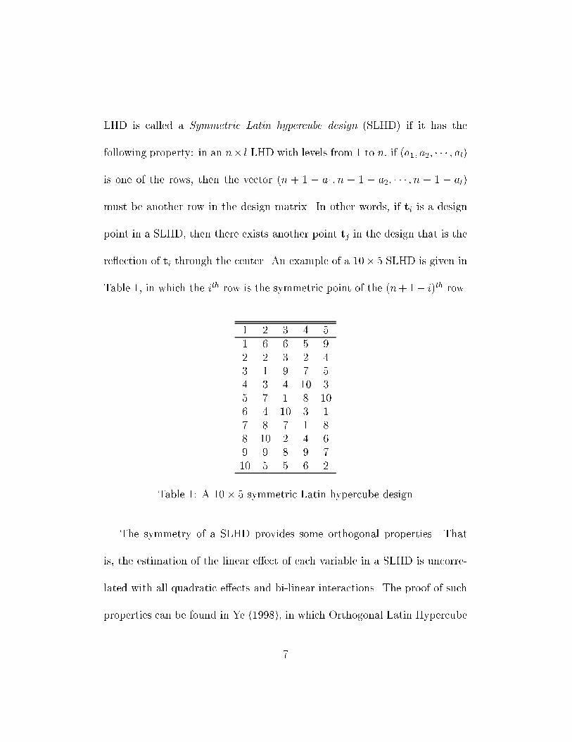
LHD is called a Symmetric Latin hypercube design (SLHD) if it has thefollowing property: in an n� l LHD with levels from 1 to n, if (a1; a2; � � � ; al)is one of the rows, then the vector (n + 1 � a1; n + 1 � a2; � � � ; n + 1 � al)must be another row in the design matrix. In other words, if ti is a designpoint in a SLHD, then there exists another point tj in the design that is there ection of ti through the center. An example of a 10� 5 SLHD is given inTable 1, in which the ith row is the symmetric point of the (n+ 1� i)th row.1 2 3 4 51 6 6 5 92 2 3 2 43 1 9 7 54 3 4 10 35 7 1 8 106 4 10 3 17 8 7 1 88 10 2 4 69 9 8 9 710 5 5 6 2Table 1: A 10� 5 symmetric Latin hypercube designThe symmetry of a SLHD provides some orthogonal properties. Thatis, the estimation of the linear e�ect of each variable in a SLHD is uncorre-lated with all quadratic e�ects and bi-linear interactions. The proof of suchproperties can be found in Ye (1998), in which Orthogonal Latin Hypercube7

Designs (OLHD) are constructed and proposed. OLHDs have the same sym-metric properties but also process additional orthogonality which insures thezero correlation among estimation of linear e�ects. Therefore, one can viewthe SLHD as a generalization of the OLHD. However, the number of runsin an OLHD has to be a power of two, which increases dramatically as thenumber of factors increases. In the cases that an appropriate OLHD cannot be found under the constraint of run size, one can consider using SLHDswhich have the exibility of the run size, yet retain some of the orthogonalityof an OLHD.Are SLHDs better than regular LHDs with respect to design criteria?Many optimal LHDs reported by Park (1994) and Morris and Mitchell (1995)have some symmetric properties. In particular, Morris and Mitchell (1995)noticed that a large number of the optimal LHDs they obtained are SLHDsand referred them as \foldover designs". This is the �rst time the SLHDis mentioned in the literature. They called for a thorough investigation onthis phenomenon. Intuitively, the optimal designs are considered to havegood space �lling properties, and a good space �lling design probably hassome degree of symmetry. To verify this, we undertook a simulation study tocompare random SLHDs to random LHDs with respect to both entropy and8

minimum intersite distance criteria. Table 2 compares the best design amongthe 1000 random SLHDs of size 25 with that of the 1000 random regularLHDs. The former has a smaller entropy criterion value of 23.60 at � = 2,compared with the latter's 25.26. In the table, we also list the minimumdistances of three designs, a criterion �rst proposed by Johnson et al. (1990)and then used by Morris and Mitchell (1995) in constructing optimal LHDs.For a design S, the minimum distance d�(S) = mins;t2S d(s; t), where sand t are two design points (i.e., two rows in the design). Both the L1(rectangular) distance L1(s; t) = Plj=1 jsj � tjj and L2 (Euclidean) distanceL2(s; t) = [Plj=1(sj � tj)2] 12 of three designs are listed in Table 2. A designS1 is said to be better than design S2 if d�(S1) > d�(S2). The numberof pairs separated by this distance, denoted J , is shown in parentheses inthe table. If two designs have the same d� values, then the design withsmaller J value is better. Throughout this paper, entropy and distances arecomputed after LHDs are scaled into [0; 1]l. The levels of scaled LHDs aref0; 1n�1 ; 2n�1 ; � � � ; 1g, which are the same used by Morris and Mitchell (1995).Note that Park (1994) used a di�erent scale, f 1n ; 2n ; � � � ; 1g.Tables 3 and 4 provide more comparisons between regular LHDs andSLHDs. We study Latin hypercubes with six di�erent sizes, 25� 4, 20� 6,9

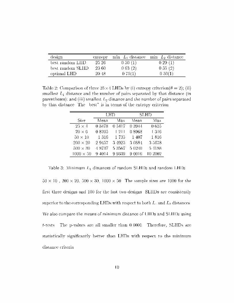
design entropy min. L1 distance min. L2 distancebest random LHD 25.26 0.50 (1) 0.29 (1)best random SLHD 23.60 0.63 (2) 0.35 (2)optimal LHD 20.48 0.75(1) 0.50(1)Table 2: Comparison of three 25�4 LHDs by (i) entropy criterion(� = 2); (ii)smallest L1 distance and the number of pairs separated by that distance (inparentheses); and (iii) smallest L2 distance and the number of pairs separatedby that distance. The \best" is in terms of the entropy criterion.LHD SLHDSize Mean Max Mean Max25� 4 0.3478 0.5417 0.3944 0.62520� 6 0.8205 1.211 0.8968 1.31650� 10 1.316 1.735 1.407 1.816200� 20 2.9457 3.4925 3.0884 3.5678500� 30 4.8737 5.3567 5.0240 5.41881000� 50 9.4014 9.9339 9.6016 10.2002Table 3: Minimum L1 distances of random SLHDs and random LHDs50 � 10 , 200 � 20, 500 � 30, 1000 � 50. The sample sizes are 1000 for the�rst three designs and 100 for the last two designs. SLHDs are consistentlysuperior to the corresponding LHDs with respect to both L1 and L2 distances.We also compare the means of minimum distance of LHDs and SLHDs usingt-tests. The p-values are all smaller than 0.0001. Therefore, SLHDs arestatistically signi�cantly better than LHDs with respect to the minimumdistance criteria. 10

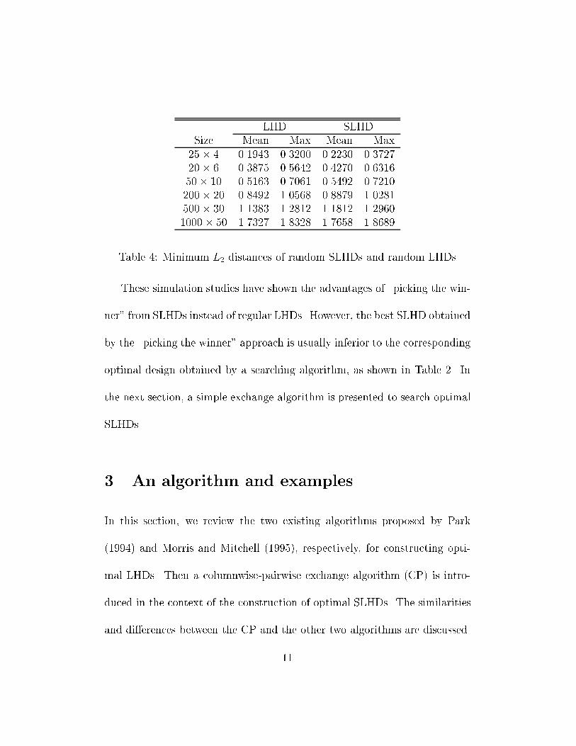
LHD SLHDSize Mean Max Mean Max25� 4 0.1943 0.3200 0.2230 0.372720� 6 0.3875 0.5642 0.4270 0.631650� 10 0.5163 0.7061 0.5492 0.7210200� 20 0.8492 1.0568 0.8879 1.0281500� 30 1.1383 1.2812 1.1812 1.29601000� 50 1.7327 1.8328 1.7658 1.8689Table 4: Minimum L2 distances of random SLHDs and random LHDsThese simulation studies have shown the advantages of \picking the win-ner" from SLHDs instead of regular LHDs. However, the best SLHD obtainedby the \picking the winner" approach is usually inferior to the correspondingoptimal design obtained by a searching algorithm, as shown in Table 2. Inthe next section, a simple exchange algorithm is presented to search optimalSLHDs.3 An algorithm and examplesIn this section, we review the two existing algorithms proposed by Park(1994) and Morris and Mitchell (1995), respectively, for constructing opti-mal LHDs. Then a columnwise-pairwise exchange algorithm (CP) is intro-duced in the context of the construction of optimal SLHDs. The similaritiesand di�erences between the CP and the other two algorithms are discussed.11

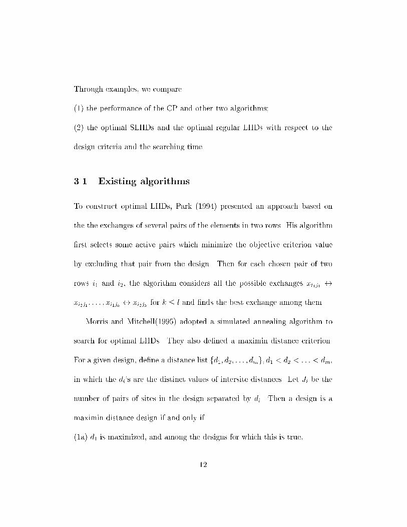
Through examples, we compare(1) the performance of the CP and other two algorithms;(2) the optimal SLHDs and the optimal regular LHDs with respect to thedesign criteria and the searching time.3.1 Existing algorithmsTo construct optimal LHDs, Park (1994) presented an approach based onthe the exchanges of several pairs of the elements in two rows. His algorithm�rst selects some active pairs which minimize the objective criterion valueby excluding that pair from the design. Then for each chosen pair of tworows i1 and i2, the algorithm considers all the possible exchanges xi1j1 $xi2j1; : : : ; xi1jk $ xi2jk for k � l and �nds the best exchange among them.Morris and Mitchell(1995) adopted a simulated annealing algorithm tosearch for optimal LHDs. They also de�ned a maximin distance criterion.For a given design, de�ne a distance list fd1; d2; : : : ; dmg; d1 < d2 < : : : < dm,in which the di's are the distinct values of intersite distances. Let Ji be thenumber of pairs of sites in the design separated by di. Then a design is amaximin distance design if and only if(1a) d1 is maximized, and among the designs for which this is true,12

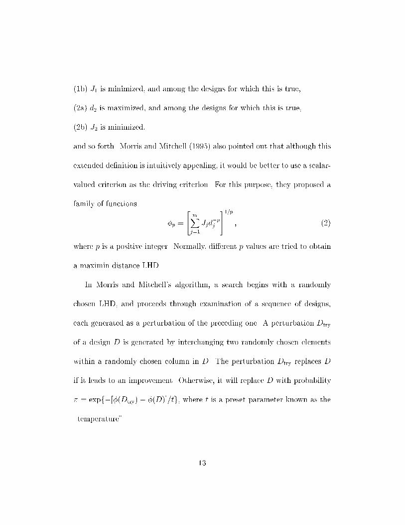
(1b) J1 is minimized, and among the designs for which this is true,(2a) d2 is maximized, and among the designs for which this is true,(2b) J2 is minimized,and so forth. Morris and Mitchell (1995) also pointed out that although thisextended de�nition is intuitively appealing, it would be better to use a scalar-valued criterion as the driving criterion. For this purpose, they proposed afamily of functions �p = 24 mXj=1Jjd�pj 351=p ; (2)where p is a positive integer. Normally, di�erent p values are tried to obtaina maximin distance LHD.In Morris and Mitchell's algorithm, a search begins with a randomlychosen LHD, and proceeds through examination of a sequence of designs,each generated as a perturbation of the preceding one. A perturbation Dtryof a design D is generated by interchanging two randomly chosen elementswithin a randomly chosen column in D. The perturbation Dtry replaces Dif it leads to an improvement. Otherwise, it will replace D with probability� = expf�[�(Dtry)� �(D)]=tg, where t is a preset parameter known as the\temperature".13

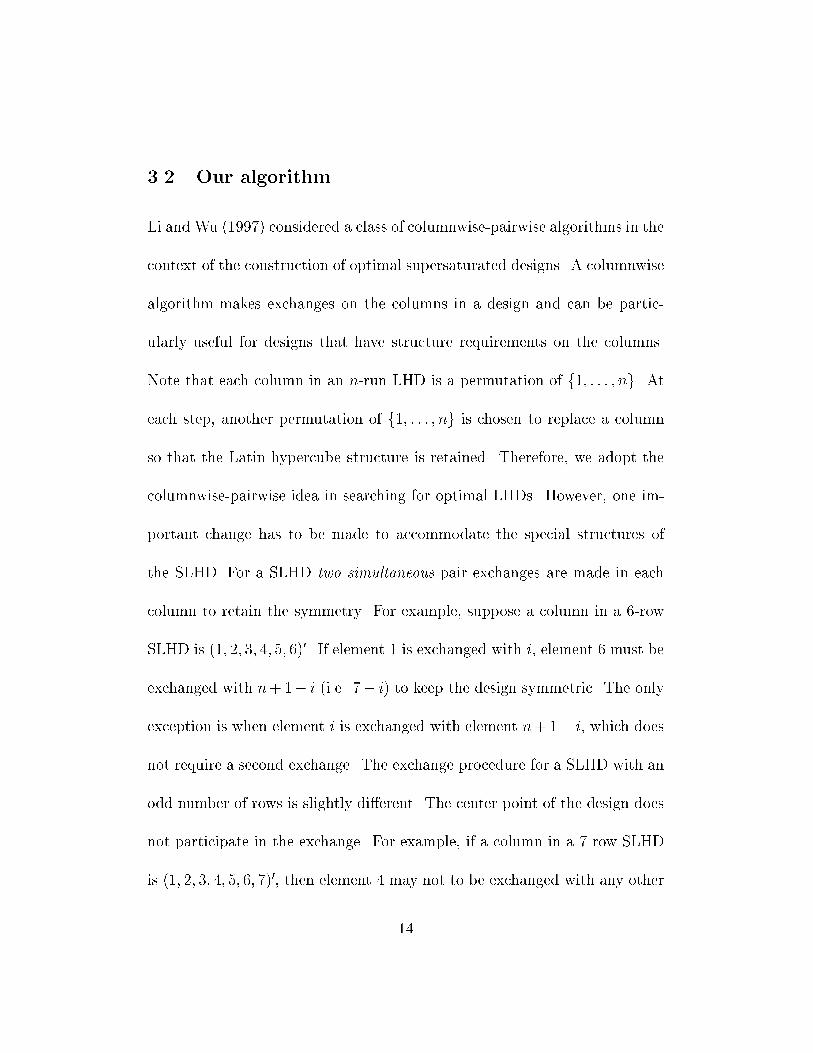
3.2 Our algorithmLi and Wu (1997) considered a class of columnwise-pairwise algorithms in thecontext of the construction of optimal supersaturated designs. A columnwisealgorithm makes exchanges on the columns in a design and can be partic-ularly useful for designs that have structure requirements on the columns.Note that each column in an n-run LHD is a permutation of f1; : : : ; ng. Ateach step, another permutation of f1; : : : ; ng is chosen to replace a columnso that the Latin hypercube structure is retained. Therefore, we adopt thecolumnwise-pairwise idea in searching for optimal LHDs. However, one im-portant change has to be made to accommodate the special structures ofthe SLHD. For a SLHD two simultaneous pair exchanges are made in eachcolumn to retain the symmetry. For example, suppose a column in a 6-rowSLHD is (1; 2; 3; 4; 5; 6)0. If element 1 is exchanged with i, element 6 must beexchanged with n+1� i (i.e. 7� i) to keep the design symmetric. The onlyexception is when element i is exchanged with element n+1� i, which doesnot require a second exchange. The exchange procedure for a SLHD with anodd number of rows is slightly di�erent. The center point of the design doesnot participate in the exchange. For example, if a column in a 7-row SLHDis (1; 2; 3; 4; 5; 6; 7)0, then element 4 may not to be exchanged with any other14

element.The algorithm for searching optimal SLHD is summarized as follows:1. Start with a random SLHD.2. Each iteration has l steps. At the ith step, the best two simultaneousexchanges within column i are found. The design matrix is updatedaccordingly.3. If the resulting design is better with respect to the criterion, repeatStep 2. Otherwise, it is considered to be an \optimal design", and thesearch is terminated.The resulting optimal designs depend largely on the starting designs used inthe algorithm. Hence, one should repeat the algorithm with several di�er-ent random starting designs. The best design among the generated optimaldesigns is chosen to be the �nal design.3.3 ExamplesExample 1 CP vs. Simulated AnnealingThe simulated annealing algorithm proposed by Morris and Mitchell (1995)aims at constructing optimal regular LHDs. We modify their algorithm to15

search for SLHDs. Similarly, the CP algorithm discussed in the previoussection is modi�ed to construct optimal regular LHDs. Both algorithms arecolumnwise-pairwise procedures. The simulated annealing algorithm oper-ates on a (randomly chosen) column and then considers a (randomly chosen)pair in each column. Our proposed CP algorithm resembles the former witha very low starting temperature (so that switches to inferior designs are nevermade). An important di�erence is that the simulated annealing algorithmperturbs the design in a random manner, and our CP algorithm perturbs thedesign in a deterministic manner.To compare their performances, we use both algorithms to construct opti-mal regular LHDs and optimal SLHDs. Two examples are considered. Table5 lists the 12 � 2 maximin distance LHDs and SLHDs generated by bothalgorithms. The simulated annealing algorithm uses 10 starting designs andthe CP uses 100 starting designs. The driving criterion is �p with p = 50.To compare the e�ciency of the algorithms, the number of searched LHSs isalso recorded. Both algorithms obtain equally good optimal designs. But theCP algorithm searches far fewer LHDs than the simulated annealing algo-rithm does. When both algorithms are used to construct 25� 4 designs, thesimulated annealing algorithm produces better optimal designs than the CP.16

design algorithm min. dist. # of searched LHDsLHD Simulated Annealing .4545 (16) 269520LHD CP .4545 (16) 44220SLHD Simulated Annealing .4545 (16) 240416SLHD CP .4545 (16) 14652Table 5: Comparison of optimal 12 � 2 LHDs and SLHDs using two al-gorithms, CP (100 starting designs) and simulated annealing (10 startingdesigns). The search criterion is �p with p = 50 and L2 distance. Note:using the simulated annealing search in LHD, only two out of 10 startingdesigns result in 0.4545 (16), compared to all 10 in the SLHD case.design algorithm min. L1 dist. # of searched LHDsLHD Simulated Annealing .9177 (19) 1537663LHD CP .8750 (6) 2241900SLHD Simulated Annealing .9583 (36) 1426985SLHD CP .9177 (6) 546480Table 6: Comparison of optimal 25 � 4 LHDs and SLHDs using two al-gorithms, CP (100 starting designs) and simulated annealing (10 startingdesigns). The search criterion is �p with p = 50 and L1 distance.Therefore, we may conclude that the systematic search algorithm is betterfor small designs and the simulated annealing algorithm is better for largerdesigns.Example 2 CP vs. ParkPark's algorithm (1994) cannot be easily modi�ed to accommodate theproperty of symmetry. Thus, its comparison with the CP is done through17

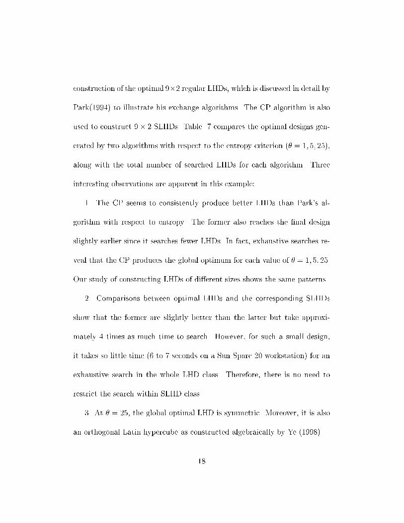
construction of the optimal 9�2 regular LHDs, which is discussed in detail byPark(1994) to illustrate his exchange algorithms. The CP algorithm is alsoused to construct 9� 2 SLHDs. Table 7 compares the optimal designs gen-erated by two algorithms with respect to the entropy criterion (� = 1; 5; 25),along with the total number of searched LHDs for each algorithm. Threeinteresting observations are apparent in this example:1. The CP seems to consistently produce better LHDs than Park's al-gorithm with respect to entropy. The former also reaches the �nal designslightly earlier since it searches fewer LHDs. In fact, exhaustive searches re-veal that the CP produces the global optimum for each value of � = 1; 5; 25.Our study of constructing LHDs of di�erent sizes shows the same patterns.2. Comparisons between optimal LHDs and the corresponding SLHDsshow that the former are slightly better than the latter but take approxi-mately 4 times as much time to search. However, for such a small design,it takes so little time (6 to 7 seconds on a Sun Sparc 20 workstation) for anexhaustive search in the whole LHD class. Therefore, there is no need torestrict the search within SLHD class.3. At � = 25, the global optimal LHD is symmetric. Moreover, it is alsoan orthogonal Latin hypercube as constructed algebraically by Ye (1998).18

� design algorithm optimal average # of searched LHDs1 SLHD CP 20.38 22.16 5488LHD CP 19.16 19.29 20592LHD Park 20.01 20.79 241325 SLHD CP 3.09 4.35 4768LHD CP 2.95 3.06 20052LHD Park 3.42 3.79 2397025 SLHD CP 0.49 �10�2 0.83 �10�2 4784LHD CP 0.49 � 10�2 1.11 �10�2 19080LHD Park 1.03 �10�2 4.67 �10�2 23580Table 7: Comparison of three algorithms for generating 9 � 2 optimal LHDswith 100 random starting designsExample 3 LHD vs. SLHDWe now revisit the case study at the beginning of this paper: the con-struction of a 25 � 4 LHD for the thermal analysis of electrical traces. Aprimary motivation of using the SLHD is to reduce the searching time. Sincethe number of possible exchanges of each column in a SLHD is much lessthan that for a regular LHD, it is expected that the exchange algorithm forthe SLHD will use much less CPU time. This is con�rmed when the algo-rithm is applied to the construction of the optimal 25 � 4 SLHD. Withoutthe restriction to SLHD, it takes 13.3 hours and 10.6 hours for the algorithmto terminate using the entropy and �p criteria, respectively. Using the samenumber of starting designs (100), the optimal SLHDs are found only after 1.619

hours and 1.3 hours. The results are summarized in Table 8. Theoretically,the global optimal SLHD cannot be better than the global optimal LHDsince the SLHD is a subset of the LHD. It is seen in our Example 2 that theobtained optimal LHDs are globally optimal veri�ed by exhaustive search,but they do not always have the symmetrical structure. Morris and Mitchell(1995) use an exhaustive search to �nd maximin distance LHDs for manysmall designs. Not all those global optimal designs are symmetric. In prac-tice, a globally optimal design is rarely obtained when the exhaustive search isnot feasible. In our case, with much less searching time, the optimal SLHDsfound are actually better than the two optimal LHDs obtained previouslywith respect to both entropy and minimum distance criteria. The maximumentropy SLHD has the criterion value of 18.53 compared with 20.48 for thepreviously obtained optimal LHD. The former also has the better (i.e. larger)minimum distance of 0.83, with six pairs separated by this distance. Using�p as the driving criterion, a SLHD was obtained with four pairs separatedby the minimum intersite distance of 0.92, which is considerably better thanthe optimal maximin distance LHD previously found (six pairs separated by0.83).Now we revisit Table 6 and focus on the di�erence between SLHD and20

design criterion entropy min. L1 dist. CPU time(hrs)LHD entropy 20.48 .75 (1) 13.34LHD �p 23.52 .83 (6) 10.63SLHD entropy 18.53 .83 (6) 1.6SLHD �p 19.48 .92 (4) 1.28Table 8: Comparison of optimal 25 � 4 LHDs vs. SLHDs with respect toentropy and �p. The entropy is calculated for � = 2.regular LHD. For the simulated annealing algorithm, restricting the searchwithin the SLHD did not save much searching time, but the obtained designis signi�cantly better with respect to the minimum distance criterion. For theCP algorithm, there is a dramatic reduction in searching time after we restrictthe search within the SLHDs, yet the obtained design is much better. It is alsointeresting to observe that in far less time the CP found a better design withinthe SLHDs than the simulated annealing algorithm found within generalLHDs.4 A robust design simulation exampleOne of the goals in computer experiments is prediction. The Kriging methodwas developed in geostatistics and brought into computer experiment bySacks et al. (1989) and Currin et al. (1991) to predict untested sites in the21

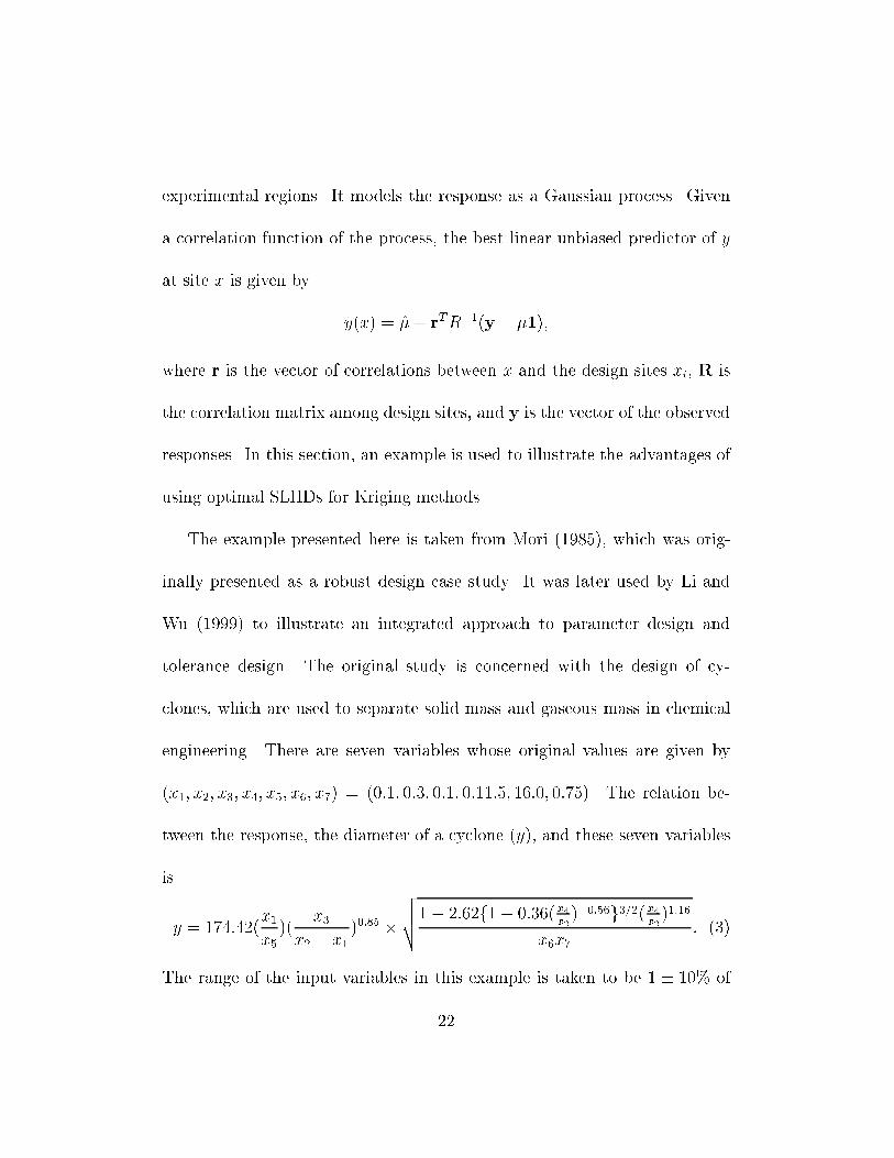
experimental regions. It models the response as a Gaussian process. Givena correlation function of the process, the best linear unbiased predictor of yat site x is given by y(x) = �+ rTR�1(y � �1);where r is the vector of correlations between x and the design sites xi, R isthe correlation matrix among design sites, and y is the vector of the observedresponses. In this section, an example is used to illustrate the advantages ofusing optimal SLHDs for Kriging methods.The example presented here is taken from Mori (1985), which was orig-inally presented as a robust design case study. It was later used by Li andWu (1999) to illustrate an integrated approach to parameter design andtolerance design. The original study is concerned with the design of cy-clones, which are used to separate solid mass and gaseous mass in chemicalengineering. There are seven variables whose original values are given by(x1; x2; x3; x4; x5; x6; x7) = (0:1; 0:3; 0:1; 0:11:5; 16:0; 0:75). The relation be-tween the response, the diameter of a cyclone (y), and these seven variablesisy = 174:42(x1x5 )( x3x2 � x1 )0:85 �vuut1� 2:62f1� 0:36(x4x2 )�0:56g3=2(x4x2 )1:16x6x7 : (3)The range of the input variables in this example is taken to be 1 � 10% of22

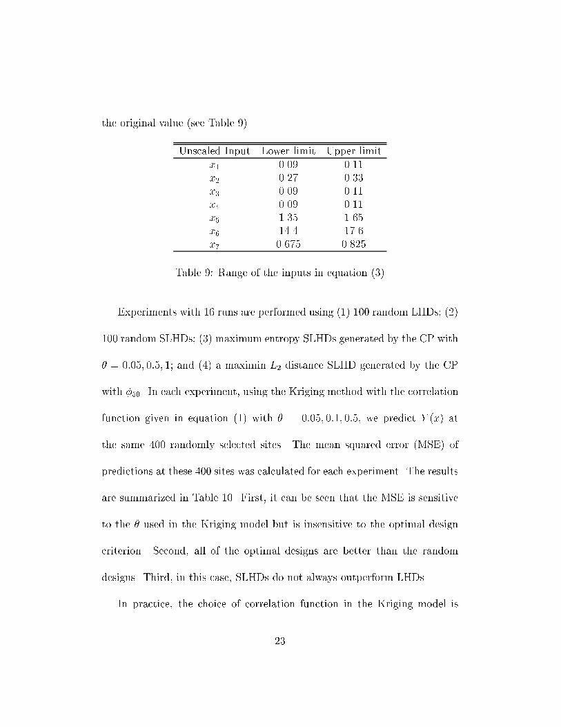
the original value (see Table 9).Unscaled Input Lower limit Upper limitx1 0.09 0.11x2 0.27 0.33x3 0.09 0.11x4 0.09 0.11x5 1.35 1.65x6 14.4 17.6x7 0.675 0.825Table 9: Range of the inputs in equation (3)Experiments with 16 runs are performed using (1) 100 random LHDs; (2)100 random SLHDs; (3) maximum entropy SLHDs generated by the CP with� = 0:05; 0:5; 1; and (4) a maximin L2 distance SLHD generated by the CPwith �50. In each experiment, using the Kriging method with the correlationfunction given in equation (1) with � = 0:05; 0:1; 0:5, we predict Y (x) atthe same 400 randomly selected sites. The mean squared error (MSE) ofpredictions at these 400 sites was calculated for each experiment. The resultsare summarized in Table 10. First, it can be seen that the MSE is sensitiveto the � used in the Kriging model but is insensitive to the optimal designcriterion. Second, all of the optimal designs are better than the randomdesigns. Third, in this case, SLHDs do not always outperform LHDs.In practice, the choice of correlation function in the Kriging model is23

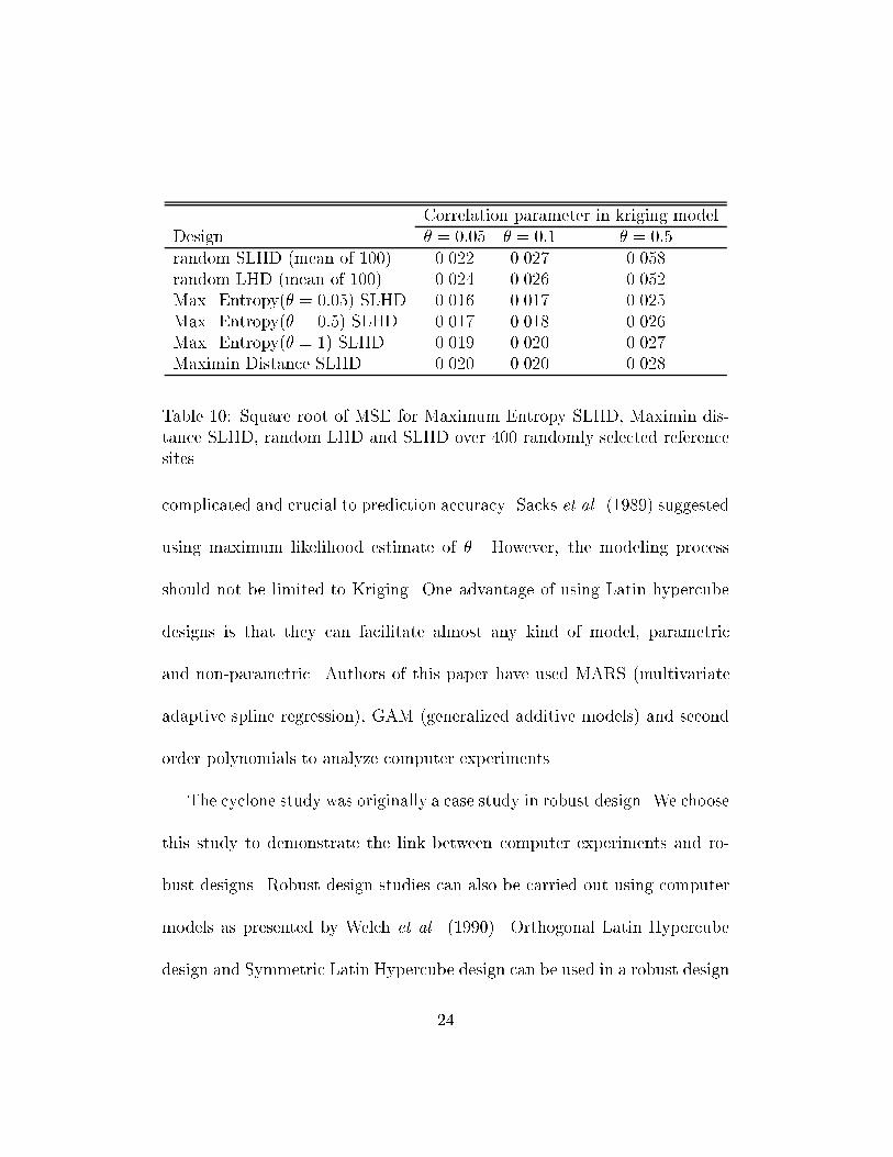
Correlation parameter in kriging modelDesign � = 0:05 � = 0:1 � = 0:5random SLHD (mean of 100) 0.022 0.027 0.058random LHD (mean of 100) 0.024 0.026 0.052Max. Entropy(� = 0:05) SLHD 0.016 0.017 0.025Max. Entropy(� = 0:5) SLHD 0.017 0.018 0.026Max. Entropy(� = 1) SLHD 0.019 0.020 0.027Maximin Distance SLHD 0.020 0.020 0.028Table 10: Square root of MSE for Maximum Entropy SLHD, Maximin dis-tance SLHD, random LHD and SLHD over 400 randomly selected referencesitescomplicated and crucial to prediction accuracy. Sacks et al. (1989) suggestedusing maximum likelihood estimate of �. However, the modeling processshould not be limited to Kriging. One advantage of using Latin hypercubedesigns is that they can facilitate almost any kind of model, parametricand non-parametric. Authors of this paper have used MARS (multivariateadaptive spline regression), GAM (generalized additive models) and secondorder polynomials to analyze computer experiments.The cyclone study was originally a case study in robust design. We choosethis study to demonstrate the link between computer experiments and ro-bust designs. Robust design studies can also be carried out using computermodels as presented by Welch et al. (1990). Orthogonal Latin Hypercubedesign and Symmetric Latin Hypercube design can be used in a robust design24

study as well. One can follow the response model approach of robust designsas proposed in Welch et al. (1990) and Shoemaker, Tsui and Wu (1991).First, establish a prediction model for both control and noise factors. Then,given the distribution of noise variables, estimate the variation of Y for eachcombination of control variables using the model obtained at the �rst stage.If a computer experiment is not expensive, one can skip the �rst step and es-timate the variation caused by the noise variable directly using the computermodel. In that case, Latin hypercubes can serve as a sampling mechanismto obtain samples from noise variable, as it was �rst proposed by McKay etal. (1979).5 Summary and DiscussionThis paper proposes a class of symmetric Latin hypercube designs (SLHDs),referred previously by Morris and Mitchell(1995) as \foldover designs", and anew columnwise-pairwise (CP) algorithm for searching optimal design withinthe SLHD class as well as within the regular LHD.We summarize the properties of SLHDs as follows.1. They are a good subset of LHDs with respect to both entropy and25

maximin distance criteria (see Tables 2-4).2. As a generalization of Orthogonal Latin hypercube designs, SLHDsretain some orthogonality. The estimation of quadratic e�ects and bi-linear interactions is uncorrelated with the estimation of linear e�ects.3. The searching time of the CP algorithm is greatly reduced by restrictingthe search within the SLHDs (see Tables 5-8). The restriction doesnot signi�cantly reduce the searching time of the simulated annealingalgorithm, but it often leads to better designs (See Table 8).4. The global optimal LHD is not always a SLHD. Morris and Mitchell(1995) did an exhaustive search to �nd the optimal LHDs of small sizes.Not all of the true optimal designs they found are symmetric.Despite the fact that the true optimal LHDs do not necessarily fall into thesymmetric class. We recommend using the SLHD in computer experimentsfor two reasons. First, users will bene�t from the orthogonal properties ofSLHD as summarized above when they try to �t the data with a polynomialmodel. A non-symmetric LHD does not have such orthogonality. Second,as shown in Tables 6 and 8, by restricting the search within SLHDs, onecould obtain approximately optimal designs in a more e�cient manner for26

moderate to large-size designs. In fact, in these cases, an exhaustive search isusually prohibitive and one should be less concerned about whether a searchmethod has the potential to reach the global optimum and more about howit can obtain a good design with reasonable computing e�ort. Especially forcomputer experiments, extra computing power could be spent on additionalruns rather than obtaining a slightly better design.The performances of the three algorithms for searching optimal LHDs aresummarized as follows:1. The CP algorithm consistently outperforms the algorithm of Park (1994).2. For smaller designs, the CP algorithm is more e�cient than the simu-lated annealing algorithm of Morris and Mitchell (1995). However, thelatter can generate better large designs.One of the referees suggested that we brie y comment on the performanceof optimal LHDs compare to other types of designs proposed for computerexperiments in recent literature, such as orthogonal arrays, OA based Latinhypercubes and quasi-Monte Carlo lattices. The comparison of di�erent kindof designs is one of the most important problems and deserves a thoroughinvestigation that is beyond the scope of this paper. However, we would27

be glad to share some of our opinions. Unlike traditional designs for whichthe models are in known forms, the computer experimenter often has littleidea which model in his/her statistical toolbox will best describe his/hercomplex computer model before an experiment is done and several kind ofmodels are tried. Most of the proposed designs for computer experimentsallow users to try many di�erent models, linear or nonlinear, parametric ornon-parametric. Among those, orthogonal arrays may not be appropriate forcomputer experiments since they do not take the advantage of exibility ofcomputer experiment in terms of changing levels. Their projections to lowdimensions are only a few points so that they are not good for non-parametricregression methods. However, they are good for �tting low-order polynomialmodels.An optimal SLHD actually takes three criteria into consideration: thediscrepancy of one-dimension projection optimized by the Latin hypercubestructure, desired orthogonality inherited from the symmetric structure, anda third criterion (entropy or minimum distance) optimized through an algo-rithmic search. Therefore, we expect that optimal SLHD should perform verywell with many modeling methods. Quasi-Monte Carlo lattice designs (Fangand Wang, 1994) are generated by some sequence which are asymptotically28

optimal in discrepancy measure. Since it spreads the design point evenly inthe design space, it should have robust performance with di�erent modelingmethods. In particular, a glp (good lattice point) set is a Latin Hypercube.Bates et. al (1996) compared Latin hypercubes designs with lattice designsand found the quasi-Monte Carlo lattice design performed surprisingly well.Tang(1993) and Owen(1993) proposed a special type of Latin Hypercubeswhich are constructed based on orthogonal arrays. Such Latin hypercubesspread points evenly on t-dimensional projections. The actual dimensiont depends on the strength of the original orthogonal array. However, thisapproach only provides LHD at the sizes of which orthogonal arrays exist.In Table 11, we compare three LHDs. The �rst one is the fourth optimalSLHD listed in Table 6. The second one is a glp set of generating vector(25;11,29,6,13). The third one is a LHD constructed based on OA(25; 54�2)using the procedure described in Tang (1993). It can be seen that in termsof entropy and minimum intersite distance, the optimal SLH is better thanthe glp and OA-based LH. The glp, however, is surprisingly good given thefact that it is easy to generate. Therefore, it could be a good choice if quicksolutions to design problems in computer experiments are needed. On theother hand, the OA-based LH is far inferior to the other two designs. Since29

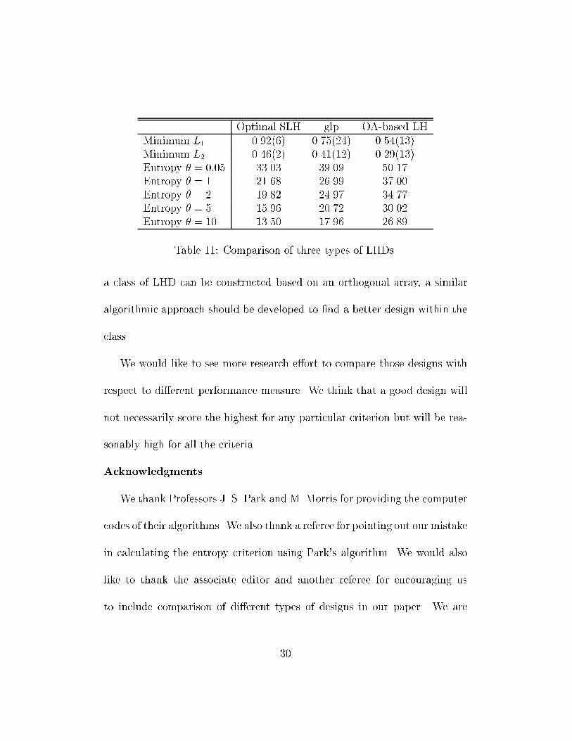
Optimal SLH glp OA-based LHMinimum L1 0.92(6) 0.75(24) 0.54(13)Minimum L2 0.46(2) 0.41(12) 0.29(13)Entropy � = 0:05 33.03 39.09 50.17Entropy � = 1 21.68 26.99 37.00Entropy � = 2 19.82 24.97 34.77Entropy � = 5 15.96 20.72 30.02Entropy � = 10 13.50 17.96 26.89Table 11: Comparison of three types of LHDs.a class of LHD can be constructed based on an orthogonal array, a similaralgorithmic approach should be developed to �nd a better design within theclass.We would like to see more research e�ort to compare those designs withrespect to di�erent performance measure. We think that a good design willnot necessarily score the highest for any particular criterion but will be rea-sonably high for all the criteria.AcknowledgmentsWe thank Professors J. S. Park and M. Morris for providing the computercodes of their algorithms. We also thank a referee for pointing out our mistakein calculating the entropy criterion using Park's algorithm. We would alsolike to thank the associate editor and another referee for encouraging usto include comparison of di�erent types of designs in our paper. We are30

also indebted to Professor Morris for his valuable comments on our relatedresearch work.ReferencesBates, R.A., Buck, R.J., Riccomagno, E., Wynn, H.P. (1996). ExperimentalDesign and Observation for Large Systems, Journal of Royal StatisticalSociety, Series B. 58, 77-94Currin, C., Mitchell, T., Morris, D. and Ylvisaker, D. (1991). Bayesian pre-diction of deterministic functions, with applications to the design andanalysis of computer experiments. Journal of the American StatisticalAssociation 86, 953-963.Fang, K.-T., Wang, Y. (1994) Number-theoretic Methods in Statistics, Chap-man & Hall, London.Johnson, M. and Moore, L. and Ylvisaker, D. (1990). Minimax and maximindistance designs. Journal of Statistical Planning and Inference 26, 131-148.Koehler J. and Owen, A. (1996). Computer experiments. In S. Ghosh andC.R. Rao, editor, Handbook of Statistics, 13: Design and Analysis ofExperiments, 261-308, 1996, North-Holland.31

Li, W. and Wu, C. F. J., (1997). Columnwise-pairwise algorithms with ap-plications to the construction of supersaturated designs. Technometrics39, 171-179.Li, W. and Wu, C. F. J., (1999) An intergrated method of parameter designand tolerance design. Quality Engineering 11, 417-425McKay, M., Beckman, R. and Conover, W. (1979). A comparison of threemethods for selecting values of input variables in the analysis of outputfrom a computer code. Technometrics 21, 239-246.Mori, T. (1985), Case studies in experimental design, (in Japanese).Morris, M. and Mitchell, T. (1995). Exploratory design for computer ex-periments. Journal of Statistical Planing and Inference 43, 381-402.Owen, A.(1992), Orthogonal Arrays for Computer Experiments, Integra-tion, and Visualization, Statistica Sinica, 2, 439-452.Park, J.-S. (1994). Optimal Latin-hypercube designs for computer experi-ments. Journal of Statistical Planning Inference 39, 95-111.Sachs, J., Schiller, S. B. and Welch, W. J. (1989). Designs for computerexperiments. Technometrics 34, 15-25.32

Shewry, M. and Wynn, H. (1987). Maximum entropy design. Journal ofApplied Statistics 14, 2, 165-170.Shoemaker, A. C., Tsui, L. L., and Wu, C. F. J. (1991). Economical exper-imentation methods for robust design. Technometrics, 33, 415-427.Tang, B (1993). Orthogonal Array-Based Latin Hypercubes, Journal ofAmerican Statistical Association, 88, 1392-1397.Welch, W. J., Yu, T. K., Kang, S. M. and Sacks, J. (1990). Computerexperiments for quality control by parameter design. Journal of QualityTechnology, 22, 15-22.Ye, K. Q.(1998), Column Orthogonal Latin hypercubes and their applica-tion in computer experiments. Journal of American Statistical Associ-ation, 93 1430-1439.

33