Analysis of Various Algorithmic approaches to Software ...

Analysis of Various Algorithmic approaches to Software-Based 1200 Baud

Audio Frequency Shift Keying Demodulation for APRS

A Thesis

Presented to

the Faculty of California Polytechnic State University,

San Luis Obispo

In Partial Fulfillment

of the Requirements for the Degree

Master of Science in Computer Science

by

Robert F. Campbell

June 2016

c© 2016

Robert F. Campbell

ALL RIGHTS RESERVED

ii

COMMITTEE MEMBERSHIP

TITLE: Analysis of Various Algorithmic approaches toSoftware-Based 1200 Baud Audio FrequencyShift Keying Demodulation for APRS

AUTHOR: Robert F. Campbell

DATE SUBMITTED: June 2016

COMMITTEE CHAIR: John Bellardo, Ph.D.Associate Professor, Computer Science

COMMITTEE MEMBER: Bridget Benson, Ph.D.Assistant Professor, Electrical Engineering

COMMITTEE MEMBER: Dennis Derickson, Ph.D.Department Chair, Electrical Engineering

iii

ABSTRACT

Analysis of Various Algorithmic approaches to Software-Based 1200 Baud Audio

Frequency Shift Keying Demodulation for APRS

Robert F. Campbell

Digital communications continues to be a relevant field of study as new technologies appear

and old methodologies get revisited or renovated. The goal of this research is to look into

the old digital communication scheme of Bell 202 [67] used by APRS and improve soft-

ware based demodulation performance. Improved performance is defined by being able to

correctly decode more packets in an efficient, real time, manner. Most APRS demodula-

tion is currently done using specialized hardware since that yields the best performance.

This research shows that through using Sivan Toledo’s javAX25 [72] software package, new

demodulation algorithms can be implemented that decode more Bell 202 encoded AX.25

packets than the existing software could. These improvements may help drive the adoption

of software demodulation since it is a low cost alternative to specialized hardware.

iv

TABLE OF CONTENTSLIST OF TABLES . . . . . . . . . . . . . . . . . . . . . . . . . . . . . . . . . . . . . viiLIST OF FIGURES . . . . . . . . . . . . . . . . . . . . . . . . . . . . . . . . . . . . viii

CHAPTER1 Introduction . . . . . . . . . . . . . . . . . . . . . . . . . . . . . . . . . . . . . . . 12 APRS Background and Definitions . . . . . . . . . . . . . . . . . . . . . . . . . . 4

2.1 Layer 3 - AX.25 . . . . . . . . . . . . . . . . . . . . . . . . . . . . . . . . . . 52.1.1 X.25 . . . . . . . . . . . . . . . . . . . . . . . . . . . . . . . . . . . . 52.1.2 AX.25 . . . . . . . . . . . . . . . . . . . . . . . . . . . . . . . . . . . 6

2.2 Layer 2 - High-Level Data Link Control . . . . . . . . . . . . . . . . . . . . 62.3 Layer 1 - Bell 202 Modulation and the Radio . . . . . . . . . . . . . . . . . 7

2.3.1 Frequency Shift Keying . . . . . . . . . . . . . . . . . . . . . . . . . 82.3.2 Bell 202 . . . . . . . . . . . . . . . . . . . . . . . . . . . . . . . . . . 8

3 Approaches to Accessing the APRS Network . . . . . . . . . . . . . . . . . . . . 103.1 Terminal Node Controllers . . . . . . . . . . . . . . . . . . . . . . . . . . . . 103.2 Specialized APRS Hardware . . . . . . . . . . . . . . . . . . . . . . . . . . . 123.3 Software Based Demodulation . . . . . . . . . . . . . . . . . . . . . . . . . . 13

3.3.1 javAX25 . . . . . . . . . . . . . . . . . . . . . . . . . . . . . . . . . . 144 Bell 202 Demodulation Techniques . . . . . . . . . . . . . . . . . . . . . . . . . . 16

4.1 Edge Detection . . . . . . . . . . . . . . . . . . . . . . . . . . . . . . . . . . 184.2 Correlation . . . . . . . . . . . . . . . . . . . . . . . . . . . . . . . . . . . . 184.3 Filtering . . . . . . . . . . . . . . . . . . . . . . . . . . . . . . . . . . . . . . 19

4.3.1 Discrete Fourier Transform . . . . . . . . . . . . . . . . . . . . . . . 204.3.2 Goertzel Algorithm . . . . . . . . . . . . . . . . . . . . . . . . . . . . 20

4.4 Phase Locked Loop . . . . . . . . . . . . . . . . . . . . . . . . . . . . . . . . 214.5 Additional Benefits of Software Based Decoding . . . . . . . . . . . . . . . . 21

4.5.1 Exhaustive Search of Incoming Signal . . . . . . . . . . . . . . . . . 234.5.2 Taking Advantage of Parallel Demodulation . . . . . . . . . . . . . . 23

5 Demodulation Challenges . . . . . . . . . . . . . . . . . . . . . . . . . . . . . . . 245.1 Challenge: DC Offset . . . . . . . . . . . . . . . . . . . . . . . . . . . . . . . 245.2 Challenge: Noise . . . . . . . . . . . . . . . . . . . . . . . . . . . . . . . . . 255.3 Challenge: Emphasis . . . . . . . . . . . . . . . . . . . . . . . . . . . . . . . 26

6 Demodulator Benchmarking . . . . . . . . . . . . . . . . . . . . . . . . . . . . . . 286.1 Plain, Straight, and Clean Packets . . . . . . . . . . . . . . . . . . . . . . . 286.2 White Noise Testing . . . . . . . . . . . . . . . . . . . . . . . . . . . . . . . 296.3 Los Angeles APRS Test Recordings . . . . . . . . . . . . . . . . . . . . . . . 30

7 Testing . . . . . . . . . . . . . . . . . . . . . . . . . . . . . . . . . . . . . . . . . 327.1 Hardware Testing Setup . . . . . . . . . . . . . . . . . . . . . . . . . . . . . 32

7.1.1 Setting TNC Audio Levels . . . . . . . . . . . . . . . . . . . . . . . . 327.2 Software Testing Setup . . . . . . . . . . . . . . . . . . . . . . . . . . . . . . 34

8 Implementation . . . . . . . . . . . . . . . . . . . . . . . . . . . . . . . . . . . . . 358.1 Strict Zero Crossing Demodulator . . . . . . . . . . . . . . . . . . . . . . . 358.2 Floating Ground Zero Crossing Demodulator . . . . . . . . . . . . . . . . . 358.3 Windowed Zero Crossing Counting Demodulator . . . . . . . . . . . . . . . 36

v

8.4 Peak Detection Demodulator . . . . . . . . . . . . . . . . . . . . . . . . . . 368.5 Derivative Zero Crossing Demodulator . . . . . . . . . . . . . . . . . . . . . 378.6 Goertzel Filter Demodulator . . . . . . . . . . . . . . . . . . . . . . . . . . 378.7 Phase Locked Loop Demodulator . . . . . . . . . . . . . . . . . . . . . . . . 388.8 Mixed Preclocking Demodulator . . . . . . . . . . . . . . . . . . . . . . . . 388.9 Goertzel Preclocking Demodulator . . . . . . . . . . . . . . . . . . . . . . . 398.10 Goertzel Exhaustive Preclocking Demodulator . . . . . . . . . . . . . . . . 39

9 Results . . . . . . . . . . . . . . . . . . . . . . . . . . . . . . . . . . . . . . . . . 419.1 Dedicated Hardware Results . . . . . . . . . . . . . . . . . . . . . . . . . . . 419.2 Software Results . . . . . . . . . . . . . . . . . . . . . . . . . . . . . . . . . 43

9.2.1 Hardware and Software Comparisons . . . . . . . . . . . . . . . . . . 4910 Future Work . . . . . . . . . . . . . . . . . . . . . . . . . . . . . . . . . . . . . . 56

10.1 The Discrete Short-Time Fourier Transform . . . . . . . . . . . . . . . . . . 5610.2 Use the CRC for FEC . . . . . . . . . . . . . . . . . . . . . . . . . . . . . . 5610.3 Integrations with a Radio . . . . . . . . . . . . . . . . . . . . . . . . . . . . 57

11 Conclusion . . . . . . . . . . . . . . . . . . . . . . . . . . . . . . . . . . . . . . . 58BIBLIOGRAPHY . . . . . . . . . . . . . . . . . . . . . . . . . . . . . . . . . . . . . 59

vi

LIST OF TABLESTable Page

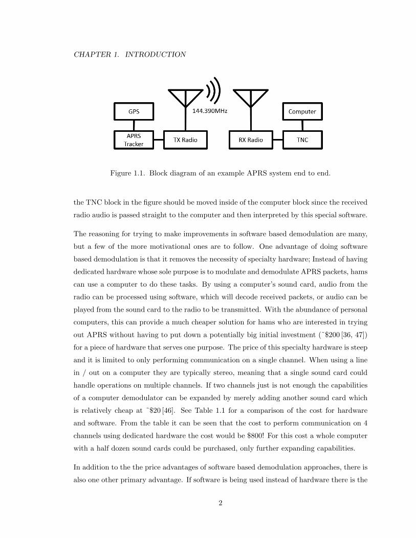
1.1 Cost comparison of conducting APRS communications on 1 through 4 chan-nels for hardware versus software. . . . . . . . . . . . . . . . . . . . . . . . . 3

2.1 Example packet showing the results of bit stuffing and framing with leadingand trailing flags. . . . . . . . . . . . . . . . . . . . . . . . . . . . . . . . . . 7

4.1 Hardware Demodulation Techniques [31, 18, 16, 33, 43, 2]. . . . . . . . . . . 167.1 Minimum Optimal TNC Input Audio Levels [35, 43, 2, 31]. . . . . . . . . . 34

vii

LIST OF FIGURESFigure Page

1.1 Block diagram of an example APRS system end to end. . . . . . . . . . . . 22.1 Example Bell 202 signal encoding the bit stream ’0000’. The bit is determined

at the bit period boundary with a change in frequency representing a ’0’ andno change in frequency representing a ’1’. Since a frequency transition occursat every visible boundary in this plot (at samples 40, 80, 120, and 160) theunderlying data is ’0000’. Without knowing the frequency before sample 0or after sample 200 no other bits can be determined. . . . . . . . . . . . . . 9

3.1 Image of the Kantronics KAM Plus TNC [37]. . . . . . . . . . . . . . . . . . 113.2 Image of Argent Data’s OpenTracker 3 [15]. . . . . . . . . . . . . . . . . . . 123.3 Image of the Yaesu FTM-350 Radio which has APRS integrated [83]. . . . . 134.1 Example of a coherent FSK signal. . . . . . . . . . . . . . . . . . . . . . . . 174.2 Example of a non-coherent FSK signal. . . . . . . . . . . . . . . . . . . . . 174.3 Block diagrams for (a) A Correlation Receiver and (b) A Matched Filter

Receiver [14]. . . . . . . . . . . . . . . . . . . . . . . . . . . . . . . . . . . . 194.4 Block Diagram of a time delay correlator [58]. . . . . . . . . . . . . . . . . . 204.5 Block diagram of a PLL demodulator [51]. . . . . . . . . . . . . . . . . . . . 224.6 Circuit connection for FSK Decoding of Bell 202 Format using an Exar XR-

2211A [18]. . . . . . . . . . . . . . . . . . . . . . . . . . . . . . . . . . . . . . 225.1 An example Bell 202 signal with DC offset problems. . . . . . . . . . . . . . 255.2 An example Bell 202 signal with white noise added. The additional zero

crossings at sample 9 in the first bit period and sample 169 in the last bitperiod will make these 1200Hz bit periods look more like 2200Hz signals. . . 26

5.3 An example signal that was not preemphasized, but was deemphasized. . . 276.1 Example of the AFSK signal present in the 200 packet generated file. . . . . 296.2 Example of a generated AFSK signal with artificial white noise added. . . . 306.3 Example of the AFSK signal in Track 1 of the Los Angeles Recording Test

File. . . . . . . . . . . . . . . . . . . . . . . . . . . . . . . . . . . . . . . . . 317.1 Example Radio Port pin out for Kantronics, also consistent with others in-

cluding OpenTrackers [41]. . . . . . . . . . . . . . . . . . . . . . . . . . . . . 337.2 Break-out board fabricated for hardware testing. . . . . . . . . . . . . . . . 337.3 Block diagram of the test setup used for testing APRS hardware. . . . . . . 339.1 Number of packets successfully decoded for all tested hardware on the Open-

Tracker 3 test file with noise. . . . . . . . . . . . . . . . . . . . . . . . . . . 429.2 Number of packets successfully decoded for all tested hardware on the Track

1 test file. . . . . . . . . . . . . . . . . . . . . . . . . . . . . . . . . . . . . . 439.3 Number of packets successfully decoded for all tested hardware on the Track

2 test file. . . . . . . . . . . . . . . . . . . . . . . . . . . . . . . . . . . . . . 449.4 Performance of software on the raw signal from OpenTracker 3 Test. . . . . 459.5 Performance of software on OpenTracker 3 Test with a flat bandpass filter. 469.6 Performance of software on OpenTracker 3 Test with an emphasis filter. . . 469.7 Performance of Software on the raw signal from Generated 200. . . . . . . . 479.8 Performance of software on Generated 200 with a flat bandpass filter. . . . 47

viii

9.9 Performance of Software on Generated 200 with an emphasis filter. . . . . . 489.10 Performance of software on the raw signal from OpenTracker Test with noise

added. . . . . . . . . . . . . . . . . . . . . . . . . . . . . . . . . . . . . . . . 499.11 Performance of software on OpenTracker Test with noise added with a flat

bandpass filter. . . . . . . . . . . . . . . . . . . . . . . . . . . . . . . . . . . 509.12 Performance of Software on OpenTracker Test with noise added with an

emphasis filter. . . . . . . . . . . . . . . . . . . . . . . . . . . . . . . . . . . 519.13 Performance of software on the raw signal from Track 1. . . . . . . . . . . . 519.14 Performance of software on Track 1 with a flat bandpass filter. . . . . . . . 529.15 Performance of software on Track 1 with an emphasis filter. . . . . . . . . . 529.16 Performance of software on the raw signal from Track 2. . . . . . . . . . . . 539.17 Performance of software on Track 2 with a flat bandpass filter. . . . . . . . 539.18 Performance of software on Track 2 with an emphasis filter. . . . . . . . . . 549.19 Performance of software versus hardware on Track 1. . . . . . . . . . . . . . 54

ix

1 Introduction

Amateur Radio Operators, commonly referred to as ”hams,” make the best of resources

available to them. However, once something is working a ”don’t touch it if it ain’t broke”

approach is often taken. Between these two mentalities some interesting phenomenon have

occurred within the ham community. For example, some radio systems that are in active

service today have only seen very minimal attention since the 1980’s when they were origi-

nally installed. The implementation and development of the Automated Packet Reporting

System (APRS) is no exception to the way hams approach things [6]. Much of this system

is based off older hardware and protocols - from the 1980s - that were readily available

and few improvements have been made. Unfortunately, although the specification has been

relatively stable there are inconsistencies. These inconsistencies include varying implemen-

tations from vendor to vendor as well as portions of the specification that are not clearly

defined resulting in vastly inconsistent performance [19, 20].

So, what is APRS, and why does it matter? A brief introduction to APRS is that it is a

digital communication scheme used by hams where a packet (whose content is varied, but

is usually a GPS position - which is what gave APRS it’s original name ”Automated Posi-

tion Reporting System”[76]) is sent out over radio and then interpreted by other receiving

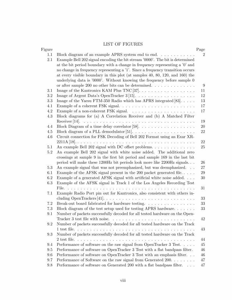
stations. Figure 1.1 shows one example of an end to end APRS system which starts with

The GPS communicating information using NEMA to the APRS tracker, the tracker then

takes this information and the preferences in its configuration to formulate APRS packets.

The APRS packets are encoded by the tracker and the resulting audio passed to a transmit

radio which sends the data. Typically this is done on frequency 144.390MHz in the United

States. Receiving radios tuned to the same frequency pass the received audio to a TNC

which decodes the packet and passes it to a computer using RS-232.

A major challenge to this protocol and many other methods of digital communication is

the fact that it uses radio. Transmitting the signal wirelessly over radio means that it

is susceptible to interference, weak signals as the distance from the transmitting station

increases, as well as a myriad of other items. This research focuses specifically on the

receiving end of these signals in order to see what improvements can be made to software

based approaches to demodulating (decoding) these packets, which is represented by the

TNC block in Figure 1.1. However, to more accurately portray software based demodulation

1

CHAPTER 1. INTRODUCTION

Figure 1.1. Block diagram of an example APRS system end to end.

the TNC block in the figure should be moved inside of the computer block since the received

radio audio is passed straight to the computer and then interpreted by this special software.

The reasoning for trying to make improvements in software based demodulation are many,

but a few of the more motivational ones are to follow. One advantage of doing software

based demodulation is that it removes the necessity of specialty hardware; Instead of having

dedicated hardware whose sole purpose is to modulate and demodulate APRS packets, hams

can use a computer to do these tasks. By using a computer’s sound card, audio from the

radio can be processed using software, which will decode received packets, or audio can be

played from the sound card to the radio to be transmitted. With the abundance of personal

computers, this can provide a much cheaper solution for hams who are interested in trying

out APRS without having to put down a potentially big initial investment (˜$200 [36, 47])

for a piece of hardware that serves one purpose. The price of this specialty hardware is steep

and it is limited to only performing communication on a single channel. When using a line

in / out on a computer they are typically stereo, meaning that a single sound card could

handle operations on multiple channels. If two channels just is not enough the capabilities

of a computer demodulator can be expanded by merely adding another sound card which

is relatively cheap at ˜$20 [46]. See Table 1.1 for a comparison of the cost for hardware

and software. From the table it can be seen that the cost to perform communication on 4

channels using dedicated hardware the cost would be $800! For this cost a whole computer

with a half dozen sound cards could be purchased, only further expanding capabilities.

In addition to the the price advantages of software based demodulation approaches, there is

also one other primary advantage. If software is being used instead of hardware there is the

2

CHAPTER 1. INTRODUCTION

Table 1.1: Cost comparison of conducting APRS communications on 1 through 4 channels

for hardware versus software.

Cost for: 1 Channel 2 Channels 3 Channels 4 Channels

Software $0 $0 $20 $20

Hardware $200 $400 $600 $800

potential for a lot more capabilities since processing power and available memory increase

drastically. For instance, one of the dedicated hardware solutions, the Kantronics KPC-3

Plus, has a mere 512KB of memory compared to that of any computer which is over 4GB

as of 2014 - and that is just the ram, not hard drive space [36, 25]. Additionally, instead

of just being able to handle live events and process each data point in the best manner

possible as soon as it comes in, post processing becomes an option.

With the cost and versatility of a software demodulation solution now introduced, the pa-

per addresses the following: Chapter 2 goes into background information, with a deeper

introduction to APRS and a presentation of the aspects important to understanding this

research. In Chapter 3, some of the current methods for interfacing with APRS, both hard-

ware and software, are explained. Demodulation techniques are discussed in Chapter 4.

Chapter 5 talks about the challenges of demodulating APRS packets. Chapter 6 discusses

the methods used for benchmarking and comparing the demodulators. In Chapter 7, infor-

mation on how the demodulators and algorithms are tested is presented. Chapter 8 goes

into more detail about the software implementations in this project. Chapter 9 discusses

the results of both the newly implemented algorithms and compares them to other demod-

ulators. Areas of additional research and future work are discussed in Chapter 10. Chapter

11 is concluding remarks.

3

2 APRS Background and Definitions

Thus far APRS has been introduced as a method of digital communication used by hams in

order to inform other hams of their location. In addition to supporting sending positions,

APRS can be used to send messages, bulletins, weather, and other information. Since these

packets are transmitted via radio - which has limited coverage - APRS should be viewed as

a local area awareness network. This gives hams who are listening for and decoding APRS

packets information about nearby transmitting stations. These previous few sentences give

a brief overview of what APRS is from a user’s perspective, but the rest of the section will

focus more on what is going on behind-the-scenes to explain how APRS works in terms

of the protocols, data transmission, modulation, etc. The full specification (version 1.0.1)

published in 2000 can be found at reference [27] and the 1.1 and proposed 1.2 addendum

at [7, 8], for those interested. Although the APRS specification was published in 2000,

APRS over VHF has the 1980s technology of Bell 202 at its heart. It is worth pointing

out that depending on where one looks, APRS may be an acronym for either Automatic

Packet Reporting Service [6], Automatic Position Reporting Service [64], Amateur Packet

Reporting Service [29], or others.

This discussion of the different components of APRS will be handled by breaking down

APRS into the layers of the Open Systems Interconnection (OSI) model. However, before

fitting APRS into the OSI model it is important to keep in mind the relevant layers that

are going to be discussed: Layer 1 of the OSI model is the physical layer, which consists of

everything that is used to transport one bit of information from one location to another. The

second layer is the data link layer. Within the data link layer bits from the physical layer are

passed up to the network layer, and information from the network layer is framed and handed

off to the physical layer. Layer 3 is the Networking layer, which is responsible for determining

the path that packets will take and for providing flow control to prevent flooding. Above

these are layers four through seven which are the transport, session, presentation, and

application layers respectively [66]. For APRS, these upper layers get too inter-tangled to

be able to cleanly separate them. For instance, within the AX.25 2.2 specification a TNC

is mentioned that only implements layers 1, 2, and 7 of the OSI model [4].

The best division of APRS into the OSI model is as follows, with a more detailed and

individualized discussion after this introduction. Layer 3 of the OSI model for APRS is the

4

CHAPTER 2. APRS BACKGROUND AND DEFINITIONS

the AX.25 Protocol; High-Level Data Link Control (HDLC) protocol composes layer 2. All

the way at the bottom, layer 1 for APRS consists of the Terminal Node Controller (TNC),

utilizing a variation of Bell 202 modulation, and a Radio [60]. A brief note on why the

discussion begins with Layer 3, and does not address Layers 4-7, is because this is how the

data is transferred. The interest in terms of this research stops here and does not continue

to the layers above layer three, because those are all application specific and do not have

a direct influence on decoding the data from the raw bit stream. Starting with AX.25 the

background information will be given down to Layer 1 which is where this research actually

aims to make a contribution.

2.1 Layer 3 - AX.25

Layer 3, the network layer, is responsible for routing frames between individual nodes in

the network. A frame of data is more traditionally called a packet since AX.25 is a packet

switched network protocol [49]. AX.25 is the amateur X.25 protocol, hence the prefixed

letter ’A’. As such, the AX.25 protocol is the ham’s interpretation of the X.25 protocol.

Since the origins of AX.25 lie within X.25, the discussion will begin with X.25.

2.1.1 X.25

Developed in the 1970’s, the packet switching protocol X.25 was deployed on telephone

networks where it was used until it began to be displaced by the IP protocol. The X.25

protocol suite provides OSI layers 1-3, although it does have standards that support each of

those layers [66]. For instance the X.21 standard was commonly used for layer 1 of X.25 and

ISO 7776 specifies a Link Access Procedure Balanced (LAPB) to assist with layer 2 (the data

link layer) [22]. The data link layer of LAPB, a bit oriented protocol derived from HDLC,

manages packet framing and ensures that frames are error-free and properly sequenced.

When used on telephone networks there are five distinct modes that the protocol operates

in: call setup for establishing the connection, data transfer, idle where the connection is

established but no data is being transferred, call clearing for terminating the connection,

and restart for resynchronizing the host and client [34]. Some of the features of the Layer 2

and Layer 3 operations of X.25 can be found in a similar fashion in AX.25.

5


2.1.2 AX.25

In this section, the AX.25 protocol will be discussed through comparison and contrast

with X.25. One of the main differences between the X.25 and AX.25 is that when the

specification is read, in addition to specifying the behavior of Layer 3, the behavior of

Layer 2 is specified. Although this is somewhat implied for X.25, there are still separate

documents for the specifications for each one of the layers. The specification for AX.25 very

clearly defines the framing with starting and terminating flags as well as the networking

and routing [4]. This means that one specification and protocol defines two layers in the

OSI model. Both X.25 and AX.25 use HDLC derivative for layer two, while AX.25 uses

Bell 202 for layer one instead of the X.21 specification used by X.25.

2.2 Layer 2 - High-Level Data Link Control

Layer 2 of the OSI model which is responsible for framing the bits, or packets, from layer

3 is taken on by High-Level Data Link Control (HDLC) for APRS. The goal of HDLC is

to make sure that when the data is received and passed up to Layer 3, it is error free,

without loss, and in the correct order [34]. There are a few ways that HDLC accomplishes

this, two of which are framing and the Frame Check Sequence (FCS). The framing occurs

through the use of flags around the data. A flag is one byte and is hex 0x7E. For AX.25,

common practice is to send multiple flags consecutively to give the transmitting radio time

to key up and settle and to give receiving radios time for their squelch (an item that stops

radio output when the desired signal strength is too low) to open. Since HDLC is an non-

return to zero inverted (NRZI) encoding, no change in frequency corresponds to a 1 and

a change in frequency corresponds to a 0. As such multiple 1s in a row make it hard to

keep timing, since consecutive 1s are encoded as the same frequency and the timing can

only be determined when a frequency change is detected, which is why bit stuffing is used.

With the exception of the flag containing six consecutive 1s (0x7E = 01111110), if there

are six or more consecutive 1s in the data packet, a zero will be stuffed after the fifth 1

to increase the clocking energy by forcing a frequency transition in the transmitted signal.

In addition to increasing the clocking energy, bit stuffing also serves the more important

purpose of making sure that there is nothing that can be confused with a flag in the data

6


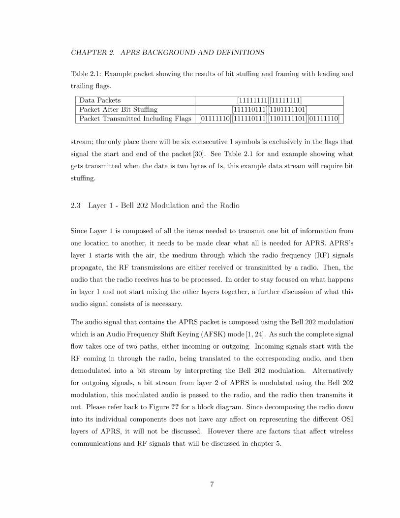
Table 2.1: Example packet showing the results of bit stuffing and framing with leading and

trailing flags.

Data Packets [11111111][11111111]

Packet After Bit Stuffing [111110111][1101111101]

Packet Transmitted Including Flags [01111110][111110111][1101111101][01111110]

stream; the only place there will be six consecutive 1 symbols is exclusively in the flags that

signal the start and end of the packet [30]. See Table 2.1 for and example showing what

gets transmitted when the data is two bytes of 1s, this example data stream will require bit

stuffing.

2.3 Layer 1 - Bell 202 Modulation and the Radio

Since Layer 1 is composed of all the items needed to transmit one bit of information from

one location to another, it needs to be made clear what all is needed for APRS. APRS’s

layer 1 starts with the air, the medium through which the radio frequency (RF) signals

propagate, the RF transmissions are either received or transmitted by a radio. Then, the

audio that the radio receives has to be processed. In order to stay focused on what happens

in layer 1 and not start mixing the other layers together, a further discussion of what this

audio signal consists of is necessary.

The audio signal that contains the APRS packet is composed using the Bell 202 modulation

which is an Audio Frequency Shift Keying (AFSK) mode [1, 24]. As such the complete signal

flow takes one of two paths, either incoming or outgoing. Incoming signals start with the

RF coming in through the radio, being translated to the corresponding audio, and then

demodulated into a bit stream by interpreting the Bell 202 modulation. Alternatively

for outgoing signals, a bit stream from layer 2 of APRS is modulated using the Bell 202

modulation, this modulated audio is passed to the radio, and the radio then transmits it

out. Please refer back to Figure ?? for a block diagram. Since decomposing the radio down

into its individual components does not have any affect on representing the different OSI

layers of APRS, it will not be discussed. However there are factors that affect wireless

communications and RF signals that will be discussed in chapter 5.

7


2.3.1 Frequency Shift Keying

There are multiple ways to encode information into a sinusoidal signal. Among these are

amplitude modulation (AM), phase modulation (PM), and frequency modulation (FM) [24].

As each one of the names implies, the underlying data is encoded by modifying that cor-

responding part of the sinusoidal signal - either the amplitude, phase, or frequency [32]. In

order to understand the Bell 202 modulation scheme, the communication mode of AFSK

needs to be introduced which derives from a FM modulation scheme. AFSK is a form of

frequency shift keying (FSK) that occurs by modulating frequencies in the audible range.

FSK uses multiple frequencies in order to represent the different symbols such as 1 and 0

or mark and space. If the frequency of the data carrying signal can be determined, then

the symbol is known for that bit period. One example of FSK, as opposed to AFSK, is

9600 baud (bits per second) packet radio on Ultra High Frequencies (UHF). In this mode,

the actual RF carrier in the 440MHz band is modulated between one frequency and an-

other nearby frequency in order to represent the two different symbols. In contrast, AFSK

switches between two different audio tones, which for APRS on Very High Frequencies

(VHF) is then modulated onto the RF carrier using FM.

2.3.2 Bell 202

With FSK and AFSK now introduced the AFSK used within Bell 202 can be described.

Bell 202 is an older technology with the Bell 202 integrated circuit filter patented in 1984

using 1200Hz and 2200Hz tones, although the patent was originally filed in 1981 [67]. After

the patent was filed it took the International Telecommunication Union (ITU) another 7

years to publish a standard for this modulation in 1988 that was used in telephone networks.

In the standard, however they use 1300Hz tone for a mark symbol and 2100Hz tone for a

space symbol [1]. The convention in FSK is for the higher frequency to correspond to the

mark and the lower one be the space [74]. An example Bell 202 AFSK signal can be seen

in Figure 2.1. In Figure 2.1 and others to follow, the horizontal axis is a relative sample

number from the audio file. Since all audio was captured at 48000Hz and the Bell 202 signal

is 1200 baud this works out to each baud being 40 samples.

8


Figure 2.1. Example Bell 202 signal encoding the bit stream ’0000’. The bit is determined

at the bit period boundary with a change in frequency representing a ’0’ and no change in

frequency representing a ’1’. Since a frequency transition occurs at every visible boundary

in this plot (at samples 40, 80, 120, and 160) the underlying data is ’0000’. Without knowing

the frequency before sample 0 or after sample 200 no other bits can be determined.

9

3 Approaches to Accessing the APRS Network

In the world of APRS, there are many solutions that hams take advantage of in order to

utilize the network. Some they find and make work, some they purchase to use exclusively

for APRS, and some go through the trouble of building their own solutions. This chapter

explains some of the common systems used on the APRS network, primarily those that can

be used for receiving, starting with terminal node controllers and progressing to software

based demodulation.

3.1 Terminal Node Controllers

Currently there are many systems that will demodulate Bell 202 encoded APRS packets.

The original hardware used for this communication style was dedicated modems similar to

dial-up 56k modems that did the encoding and decoding. These modems were connected

directly to the radio and would decode the signal that the radio received as well as sending

audio to the radio to transmit [82]. These modems are more commonly referred to as

terminal node controllers (TNCs), which are specialized modems used in APRS operation.

A reminder of the age of the technologies that are being used for the data transport of

APRS, packet radio originated in the 1980s as TNCs became affordable [28]. This means

that this technology is over 30 years old at the time of writing in the year 2016.

With a radio and a TNC, amateur packet stations and digipeaters (digital packet repeaters)

are possible [26, 75]. Digipeaters are an essential part of APRS, but many users wish to

report their GPS position onto the network instead of just relaying traffic for other stations.

In order to accomplish this, a GPS receiver is required. Now, stations can take the data

from their GPS receiver and put it in the payload of the APRS packet and transmit the

GPS position onto the network. One other common use of a TNC is an Internet attached

digipeater, usually though the use of a computer, that would allow the data to be posted to

the APRS-IS servers [12]. To give an example of some of the TNCs available, those within

the testing scope of this project will be listed. There are a total of eight TNCs - six unique

models - whose decoding results are compared to the software approaches. This includes

two Kantronics KAM Plus, a Kantronics KAM, an MFJ-1278, two AEA PK-88, a PK-232,

and a PK-232MBX. An example image of what a TNC looks like can be seen in Figure 3.1.

10

CHAPTER 3. APPROACHES TO ACCESSING THE APRS NETWORK

Figure 3.1. Image of the Kantronics KAM Plus TNC [37].

11


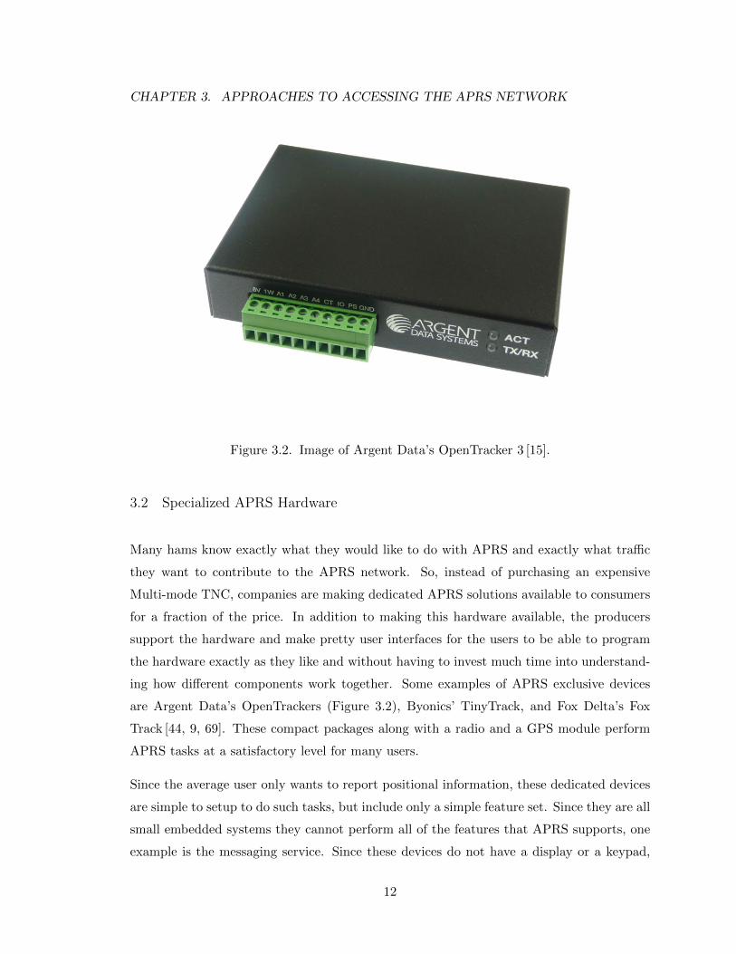
Figure 3.2. Image of Argent Data’s OpenTracker 3 [15].

3.2 Specialized APRS Hardware

Many hams know exactly what they would like to do with APRS and exactly what traffic

they want to contribute to the APRS network. So, instead of purchasing an expensive

Multi-mode TNC, companies are making dedicated APRS solutions available to consumers

for a fraction of the price. In addition to making this hardware available, the producers

support the hardware and make pretty user interfaces for the users to be able to program

the hardware exactly as they like and without having to invest much time into understand-

ing how different components work together. Some examples of APRS exclusive devices

are Argent Data’s OpenTrackers (Figure 3.2), Byonics’ TinyTrack, and Fox Delta’s Fox

Track [44, 9, 69]. These compact packages along with a radio and a GPS module perform

APRS tasks at a satisfactory level for many users.

Since the average user only wants to report positional information, these dedicated devices

are simple to setup to do such tasks, but include only a simple feature set. Since they are all

small embedded systems they cannot perform all of the features that APRS supports, one

example is the messaging service. Since these devices do not have a display or a keypad,

12


Figure 3.3. Image of the Yaesu FTM-350 Radio which has APRS integrated [83].

there is no way to input or display a message. Certain radio manufacturers have begun

integrating the TNCs into the radios themselves to utilize the radio’s screen. The Kenwood

TM-D700 series and Yaesu FTM-350 (Figure 3.3) are examples [13, 73].

However, both the options in this section and the one previous on TNCs require going

out and buying special hardware in order to utilize APRS. This can be expensive and cost

prohibitive for some hams to be able to begin APRS operations.

3.3 Software Based Demodulation

It’s fair to assume that before a ham operator becomes interested in the APRS network

and sending APRS packets that they will already have a radio. So, if they already have a

radio all they have to do is buy a piece of hardware that will do the modulation in order

to send a packet. However, hardware costs money and before diving right in, some users

might appreciate being able to try APRS out first. A good, cheap alternative to dedicated

13


hardware is to use hardware that hams already have. A good choice that will fit the needs

is a computer, which most hams are likely to already own. If they don’t happen to own

a computer, much of this argument is null and void since a computer is required to use

both TNCs and to program the specialty hardware. On the computer, amateurs can use

software to do the modulation and demodulation, and build or buy a cheap interface to a

radio, around $15 instead of roughly $200 for a piece of dedicated hardware.

This seems to be a route that some are taking and a demodulation scheme that this project

explores in detail, but before exploring this in more detail, more information on current

systems that operate in this software realm is necessary. Some examples of the software

that can be used are George Rossopoylos’s Packet Engine [52], Thomas Sailer’s Linux Sound

Modem [55, 56], and Sivan Toledo’s javAX25 [72, 70]. On a computer, even one with minimal

resources, there are algorithms that are being used to demodulate the APRS packets. Again,

what this project aims to investigate is what improvements can be made to the algorithms of

software-based demodulation approaches in order to achieve performance similar to TNCs

and dedicated hardware. Improved performance for the software is defined by being able to

correctly decode more packets in an efficient, real time, manner. Based on observations in

initial analyses where software was unable to decode packets, the hypothesis is made that

improvements can be made to software based demodulation.

3.3.1 javAX25

Sivan Toledo’s javAX25 is very comprehensive software package that handles the encoding,

decoding, radio control, and interfacing with sound cards to allow for full use of APRS.

However, in addition to just being able to utilize APRS, there is also a test application

inside of this package that allows for quick and easy testing of everything in the suite - of

the most interest, however, is the ability to test demodulators. Although all of these features

were included, the three primarily used in this project were the modulation, demodulation,

and demodulator testing. Due to its comprehensiveness and ease of access online through

Github, javAX25 was chosen to be the basis for this project [72]. For a complete list of

features, the manual can be found in the following reference, and even from the beginning

the mission statement the author outlines coincides with that of this research [70].

14


Toledo did some benchmarking of his software and found that running two demodulators

in parallel provided the best results. The demodulators were exactly the same; the only

difference was that one was processing data after a bandpass filter that was centered around

the two frequencies of interest, and the other had a bandpass filter that additionally applied

6dB of attenuation at 1200Hz [71]. Being published in 2012, this is the newest reference

in this paper on the subject of AX.25 (aside from the papers published by Finnegan [19,

20]), which provided additional incentive to use this project for this research. As added

verification of making the correct decision of what software to use, a very popular Android

APRS application written by Georg Lukas uses javAX25 by a direct import [38].

15

4 Bell 202 Demodulation Techniques

There are a few primary approaches to demodulating 1200 baud 1200Hz/2200Hz AFSK

signals in hardware. However, before talking about the techniques for doing AFSK demod-

ulation, it is worth specifying what type of FSK Bell 202 is. There are two features that

are relevant for taking into consideration when demodulating the signal. First is that it is

asynchronous, meaning that there is no separate clocking signal as the clocking is embedded

within the data signal. Hence the conversation on bit stuffing and clocking energy in the

APRS Background chapter. If it were synchronous, there would be two different signal in-

puts coming into the demodulator; the actual data and the clock. The second characteristic

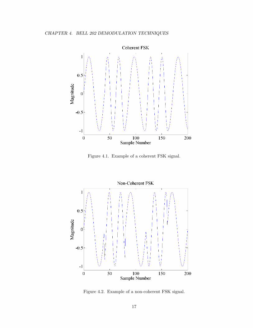
is that the FSK is coherent or continuous. This means that there is a continuous signal at

bit boundaries and there are no jumps as the signal changes from one frequency to another

as seen in Figure 4.1 as opposed to non-coherent Figure 4.2 which does have these jumps.

Another name sometime applied to this method of FSK, coherent FSK, is continuous-phase

frequency shift keying or CPFSK [77].

Among the demodulation techniques for coherent FSK are edge detection, correlation, fil-

tering, and phase-locked-loops (PLLs). Each of these will be explained in more detail in the

corresponding sections below; however with Correlation and Filtering being very popular

and mentioned in many books and applications, there is a lot of overlap so more detailed

information can be found in the following references [61, 62, 14, 50, 58, 59]. The following

sections in this chapter explain how the demodulation approach works with the software

implementation details being saved for the Implementation chapter. However, there will be

an additional section at the end of this chapter to discuss some of the potential advantages

of using software over hardware. Before talking about all of the techniques a little context

as to which onces are being used in the various pieces of hardware can be found in Table 4.1.

Table 4.1: Hardware Demodulation Techniques [31, 18, 16, 33, 43, 2].

Device Demodulation Technique

OpenTracker 2 PLL using XR-2211

OpenTracker 3 Software time delay correlation

Kantronics Kam Edge detection using TCM3105 Chip

MFJ-1278 PLL using XR-2211

PK-88 Digital filters using AMD 7910 chip

PK-232 Analog filters

16

CHAPTER 4. BELL 202 DEMODULATION TECHNIQUES

Figure 4.1. Example of a coherent FSK signal.

Figure 4.2. Example of a non-coherent FSK signal.

17


4.1 Edge Detection

An edge detection, or zero-crossing, demodulator identifies rising and falling edges in the

signal to determine the frequency present. In the TCM3105 chip, which is an FSK modem,

rising and falling edges trigger pulses that are at a frequency that is double the input

frequency [33]. Although this is how it is done in hardware, it may be easier to understand

through the more simple discussion of zero-crossings. The idea is that based off of the time

elapsed between zero crossings (rising and falling edges or vice versa) of the signal, one-half

the period of the waveform can be measured. Once the period has been measured the

frequency can then be easily calculated using the inverse relationship between period and

frequency, f = 1 /T where f is the frequency and T is the period [58]. Just to reiterate, two

consecutive zero crossings is only half of the period do to the nature of sinusoidal signals,

which is also why the TCM3105 chip outputs pulses at twice the input frequency. As the

TCM3105 is an older chip, a replacement is now commonly used in 1200 baud modem

projects, and that is the MX614 made by MX-COM [45].

4.2 Correlation

A correlation demodulator works through correlating - comparing - an FSK signal with the

possible options based off the modulation scheme. In this instance we expect the signal to

be either a 1200Hz or 2200Hz signal and hence the signal will be compared to two internal

oscillators, one at each frequency [53]. In practice, the input signal is mixed with each one

of the two reference signals and then integrated over the bit period. The results from each

of these correlations is then fed into a decision unit. The output of the decision unit is

whichever of the frequencies has more power and hence was more prominent in the signal.

The basic block diagram can be seen in Figure 4.3. Correlation is the current method used

in Toledo’s javAX25. An alternative implementation of a correlator is to have a delay line

instead of an internal oscillator. This delay line can delay the input by the time for one

period of an expected frequency (i.e. 1/2200Hz) to elapse and then this delayed signal can

be multiplied by the original signal [58]. Essentially, the delayed signal becomes the internal

oscillator in this example (see Figure 4.4). Side note, this would work better for higher

frequencies than those here since the delay line would be about 145 miles long if using

18


Figure 4.3. Block diagrams for (a) A Correlation Receiver and (b) A Matched Filter Re-

ceiver [14].

copper wire for the 1200Hz tone [40]. However, this is possible in software since buffers can

be used.

4.3 Filtering

Much like the correlation demodulation approach, a filter based demodulator operates on

knowing the expected frequencies in the FSK signal. For our case of 1200Hz and 2200Hz

frequencies, a filter will be set and centered about each one of these frequencies. The input

signal is passed to each one of these narrow band pass filters and then the power of each of

the signals out of the filters is fed to a comparator. The stronger of the two frequencies is the

one that must have been present in the original signal [74]. One example of a filter that can

be used is a Finite Impulse Response (FIR) Filter. The block diagram for this approach can

19


Figure 4.4. Block Diagram of a time delay correlator [58].

be seen in Figure 4.3, and the general structure is very similar to correlation. This method

seems to be prevalent in both hardware and software based approaches. For instance,

if one examines the schematic for the PK-232 MBX, two parallel filters can be seen [31].

Rossopoulos’s Packet Engine measures the energy on the two modem frequencies using filters

to do the demodulation. Sailer’s Sound Modem also uses a matched filter demodulation [54]

whose algorithm was then reused on a micro controller by Holder [29]. Additionally, AMD

produced an FSK Modem chip that used digital filtering for demodulation [16]. All of these

independent uses make this look like the most prominent approach for demodulation.

4.3.1 Discrete Fourier Transform

One example of a digital filter is a Discrete Fourier Transform (DFT). A discrete Fourier

Transform is one implementation of Fourier Transform that is executed on discrete samples

similar to what is present in a digital audio file. Once a Fourier transform has been applied

on a signal the output is a relative power versus frequency. With this data, whichever

frequency (either 1200Hz or 2200Hz) is more prominent is the symbol which must be present

in the bit period, and hence can be used for the demodulation; however, Fourier Transforms

are computationally intensive.

4.3.2 Goertzel Algorithm

Computing a discrete Fourier transform is more reasonable computationally than a full

Fourier transform, which is a continuous integral as opposed to having discrete terms [80].

However, even the results from the DFT have more data than is needed to do the demodula-

20


tion since the results will be a spectrum of powers over a range of frequencies [78, 79]. A more

simplified and specific approach can be used. The Goertzel Algorithm evaluates the coeffi-

cients and corresponding powers of the individual frequencies of 1200Hz and 2200Hz [81, 17].

This approach, sometimes called a Goertzel Filter, means that no additional computation

is wasted on computing frequency power data that is not relevant, making it faster and a

vast simplification to the DFT [57].

4.4 Phase Locked Loop

Another option for determining the frequencies present in the original data carrying signal,

and hence the actual data in the signal, is to use a Phase-Locked Loop (PLL) [3, 48, 39].

There are a few different approaches for utilizing a phase locked loop. The basic idea is that

there is an internal oscillator and the input (the received signal) is used to influence this

oscillator [21] . The input signal and the reference oscillator signal are integrated and this

output is used for feedback to the internal oscillator (hence the loop portion of PLL) [51].

The convenient thing about monitoring the phase of the signal so closely and being able

to stay locked onto it is that the frequency must also be known and this is the portion

that is really of interest. A block diagram of a phase locked loop can be seen in Figure

4.5. There is a chip produced by Exar that does FSK demodulation and tone detection

using a PLL, for which the model number is XR-2211A [18]. A circuit diagram of using

the XR-2211A for Bell 202 can be seen in Figure 4.6 which also shows some of the primary

items needed for a PLL including the phase detection (integrator) and the VCO (Voltage

Controlled Oscillator).

4.5 Additional Benefits of Software Based Decoding

Software is flexible. As Bergquist mentioned, it was only a matter of time before hams

developed a bond between computers and radios using TNCs and it is time to take it a step

further and leverage the capabilities of a computer even more [5]. Any one of the afore-

mentioned algorithms can be used on the same hardware without having to add additional

discrete components, new Integrated Circuits (ICs), or make modifications to a Printed

Circuit Board (PCB). There are two benefits of using software instead of dedicated hard-

21


Figure 4.5. Block diagram of a PLL demodulator [51].

Figure 4.6. Circuit connection for FSK Decoding of Bell 202 Format using an Exar XR-

2211A [18].

22


ware that this research will investigate; first exhaustive search of a signal through the use of

buffers, and second, the ability to be able to run multiple of these demodulation approaches

in parallel.

4.5.1 Exhaustive Search of Incoming Signal

Using software the input signal can be buffered in the program and then searched for a

signal. Since there is not a separate data and clock signal, there could be a case when the

clocking is improperly selected. Using an approach of buffering data that may contain a

valid packet, the software can step through the data trying every possible clocking option.

4.5.2 Taking Advantage of Parallel Demodulation

Another advantage of using software for decoding these AFSK signals is being able to apply

multiple demodulation techniques. Once the data is collected and converted to a digital

form there is no reason, other than computation limitations of the host computer, not to

run multiple algorithms in parallel in order to be able to demodulate the maximum number

of packets possible. Although there are packets that every algorithm is able to decode,

there are also packets that some approaches can decode while others can not. Through

using multiple demodulators in parallel and de-duplicating the results, even more packets

can be correctly decoded.

23

5 Demodulation Challenges

While analyzing different demodulation algorithms and trying to improve their performance,

there were a few phenomena that were observed that made correct demodulation more

challenging. The following items created difficulty and can all be attributed to the fact that

APRS uses RF and hence is susceptible to all the items relating to an RF transmission.

The main challenge in decoding the APRS data was the fact that the digital stream is

converted to an audio signal and then transmitted over RF. The addition of RF adds

a whole plethora of obstacles which can include Path Loss, Multi-path, Fading, Doppler

effects, Co-channel interference, Interference and Noise, and Foliage [24]. A few items which

are important to note, due to the fact that some of the algorithms had to be coded to

tolerate them are: DC Offset, Noise, and Emphasis.

5.1 Challenge: DC Offset

An audio signal can be characterized by a sine wave. In order to get different sounds the

frequency of the sine wave is changed and in the context here, the two frequencies are

1200Hz and 2200Hz. Since an audio signal is a sine wave, the average value should be

zero. The zero value is commonly referred to as the ground of the audio signal, and as the

definition would imply the signal should spend the same amount of time above ground as

it does below ground. As the performance of zero crossing algorithms were investigated it

was evident that this was a challenge. If one assumes that the signal is centered about zero,

and it is not, the logical decisions made with this incorrect assumption will hence not hold

true. Figure 5.1 shows that the signal is not centered around zero. This lack of the signal

being centered around 0 (or ground) is why it is said to have a DC offset. It can be noticed

in this figure that near the center there are time periods that would be both much longer

and much shorter than those expected from subsequent zero crossings during demodulation

due to this DC offset effect.

24

CHAPTER 5. DEMODULATION CHALLENGES

Figure 5.1. An example Bell 202 signal with DC offset problems.

5.2 Challenge: Noise

First, a definition of noise in the context of this research: noise refers to unwanted electrical

signals present in electrical systems [62]. Since the data is an AFSK signal that is then

frequency modulated, there are two distinct steps where noise can be introduced, but must

be kept to a minimum to increase the chances of the data being properly transferred. Hence,

a large signal to noise ratio (SNR) is preferred. This is not the case for only APRS but

with all wireless technologies. One cause of having an increased effect from noise and hence

a lower SNR is increased distance between the transmitter and receiver. An example that

many are probably familiar with is as a client gets farther away from a wireless access point

the bandwidth decreases. This happens because the signal strength drops off at 1 / distance

cubed [65]. What was noticed when some of the algorithms were being debugged was the

random noise embedded in the signal caused significant problems.

One such example of this is if the noise happened to also take on the form of a sine wave and

the algorithm locked onto that frequency instead of the 1200Hz or 2200Hz signal that was

wanted to be decoded. Alternatively, if the noise was just random and jostled the signal in

25


Figure 5.2. An example Bell 202 signal with white noise added. The additional zero

crossings at sample 9 in the first bit period and sample 169 in the last bit period will make

these 1200Hz bit periods look more like 2200Hz signals.

the correct spot 1200Hz tones might look like 2200Hz (this ended up being fairly common)

or vice versa. An example of what noise may look like on the original signal can be seen in

Figure 5.2.

5.3 Challenge: Emphasis

Due to the fact that this is AFSK data being transmitted over a voice channel, emphasis be-

comes a concern. Preemphasis is when the the higher audio tones in a Frequency Modulated

(FM) signal are intentionally increased and deemphasis is when that process is reversed on

the receiving end to return the audio to a flat level. Why emphasize the audio signal?

This process of emphasis is not necessary, but the effects are desirable since it increases the

signal to noise ratio in the RF signal by having the higher audio tones preemphasized [23].

The reason this is a concern is because the adoption of emphasizing and deemphasizing

APRS signals is inconsistent. Some radios have data ports which bypass the emphasis step

26


Figure 5.3. An example signal that was not preemphasized, but was deemphasized.

while other APRS users utilize the microphone and speaker ports of a radio which would

utilize emphasis. This would mean that a signal transmitted out of a radio with a data

port may not be emphasized, but then when received through the speaker out of another

radio would be deemphasized. The effects of a non-emphasized signal being deemphasized

can be seen in Figure 5.3. This causes problems with the demodulation because it can not

be assumed that the relative powers of each frequency will be equal since they will have

different magnitudes in this case.

27

6 Demodulator Benchmarking

In order to compare the results of the different demodulators a method of benchmarking

must be instituted. Each one of the demodulators was tested using multiple audio files that

have different characteristics. These different files as well as the advantage of using them in

the benchmarking are explained in their corresponding section. The winner of each of the

benchmark files is determined by which demodulator could demodulate the most packets

out of the file. It is worth noting that for each test audio file a sample rate of 48000Hz was

standardized on since it works out nicely to 40 samples per bit period for 1200 baud digital

communications which made conceptualizing the data easier.

6.1 Plain, Straight, and Clean Packets

These audio files were just what the title implies - straight packets. What is meant by

straight packets is that they are pure ”perfect” 1200Hz and 2200Hz tone audio samples.

There is no noise introduced through artificial or natural means such as that introduced

through the intrinsics of using RF. Although these files do not provide meaningful results

for hardware or already implemented software solutions (since these devices should be able

to decode every packet in the audio file) it still provides a good starting point for getting

new algorithms up and running. Two of these clean files were generated. One was generated

from an OpenTracker creating packets with a counter and the text ”The quick brown fox

jumps over the lazy dog”. This audio file contained a total of 40 packets each separated

by 30ms and proved to be short enough to allow for quick cross checking as modifications

were made. The second file was generated in software using Toledo’s javAX25 package. All

that is relevant at this point is that it has perfect levels (1200Hz and 2200Hz tones are at

the exact same level) and contains 200 packets each separated by 300ms (this was chosen

so that the space between packets was sufficient to be heard) making the file quite a bit

longer. A sample from the 200 packet audio file can be seen in Figure 6.1.

28

CHAPTER 6. DEMODULATOR BENCHMARKING

Figure 6.1. Example of the AFSK signal present in the 200 packet generated file.

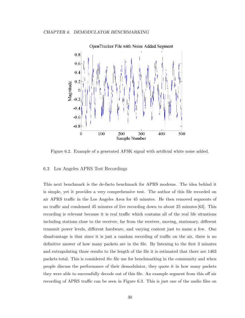
6.2 White Noise Testing

The second test file that was used on the demodulators was the 40 packet OpenTracker

file mentioned in the previous section with added artificial white noise. An advantage of

this file is that its contents are known, it contains 40 packets, while still being a reasonable

benchmarking file because the later packets in the file are buried in noise. No demodulator

could demodulate all the packets out of the file as the noise was increased all the way up

to a signal to noise ratio (SNR) of 0.5, making the magnitude of the white noise twice

that of the original signal. There were total of 10 steps of increasing noise meaning that

at each noise level there were approximately 4 packets. Using this information on how the

test file was created, the total number of packets decoded from this file in addition to the

calculated SNR will be presented in the results section. This noise was added to the original

audio file using the audio editing program Audacity [42]. Although this file does not directly

characterize what is introduced by RF, it provides a reasonable test simulating the effects

of a decreased SNR on the audio signal. An example segment from this white noise added

file can be seen in Figure 6.2.

29


Figure 6.2. Example of a generated AFSK signal with artificial white noise added.

6.3 Los Angeles APRS Test Recordings

This next benchmark is the de-facto benchmark for APRS modems. The idea behind it

is simple, yet it provides a very comprehensive test. The author of this file recorded on

air APRS traffic in the Los Angeles Area for 45 minutes. He then removed segments of

no traffic and condensed 45 minutes of live recording down to about 25 minutes [63]. This

recording is relevant because it is real traffic which contains all of the real life situations

including stations close to the receiver, far from the receiver, moving, stationary, different

transmit power levels, different hardware, and varying content just to name a few. One

disadvantage is that since it is just a random recording of traffic on the air, there is no

definitive answer of how many packets are in the file. By listening to the first 3 minutes

and extrapolating those results to the length of the file it is estimated that there are 1463

packets total. This is considered the file use for benchmarking in the community and when

people discuss the performance of their demodulator, they quote it in how many packets

they were able to successfully decode out of this file. An example segment from this off air

recording of APRS traffic can be seen in Figure 6.3. This is just one of the audio files on

30


Figure 6.3. Example of the AFSK signal in Track 1 of the Los Angeles Recording Test File.

this author’s test CD and is in fact the first one on the CD, so it will be referred to as Track

1. This was the the file that was most important to the testing, but the author also has a

second version of this file in Track 2. The only difference between Track 1 and Track 2 is

that an audio filter was used to create Track 2 which had the result of being a deemphasized

version of Track 1. A quick note about Track 2 is that the processing performed to create

it had other undesirable side effects including the white noise between packets being at a

much higher magnitude than the packets themselves.

31

7 Testing

In order to be able to evaluate the results from this research, each demodulation technique

considered needs to be tested and the number of packets that each technique was able to

successfully decode needs to be compared. From this analysis, it will be seen which tech-

niques are effective and are able to decode relatively more packets as opposed to those that

decode fewer. In order to validate the software techniques, results for dedicated hardware

will also be collected for comparison. The testing for both the dedicated hardware and the

software algorithms will be described in the corresponding sections below.

7.1 Hardware Testing Setup

The testing setup for the hardware is fairly simple since they are basically black boxes that

just need to be supplied with the correct inputs. Each piece of hardware has two connections;

one is the radio port, and the other is the serial connection. As the name implies, the radio

port is used to be able to interface with the radio. This port has connections such as transmit

audio, receive audio, push-to-talk (PTT), supply voltage (VCC), and ground. A digram of

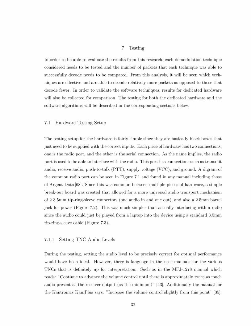
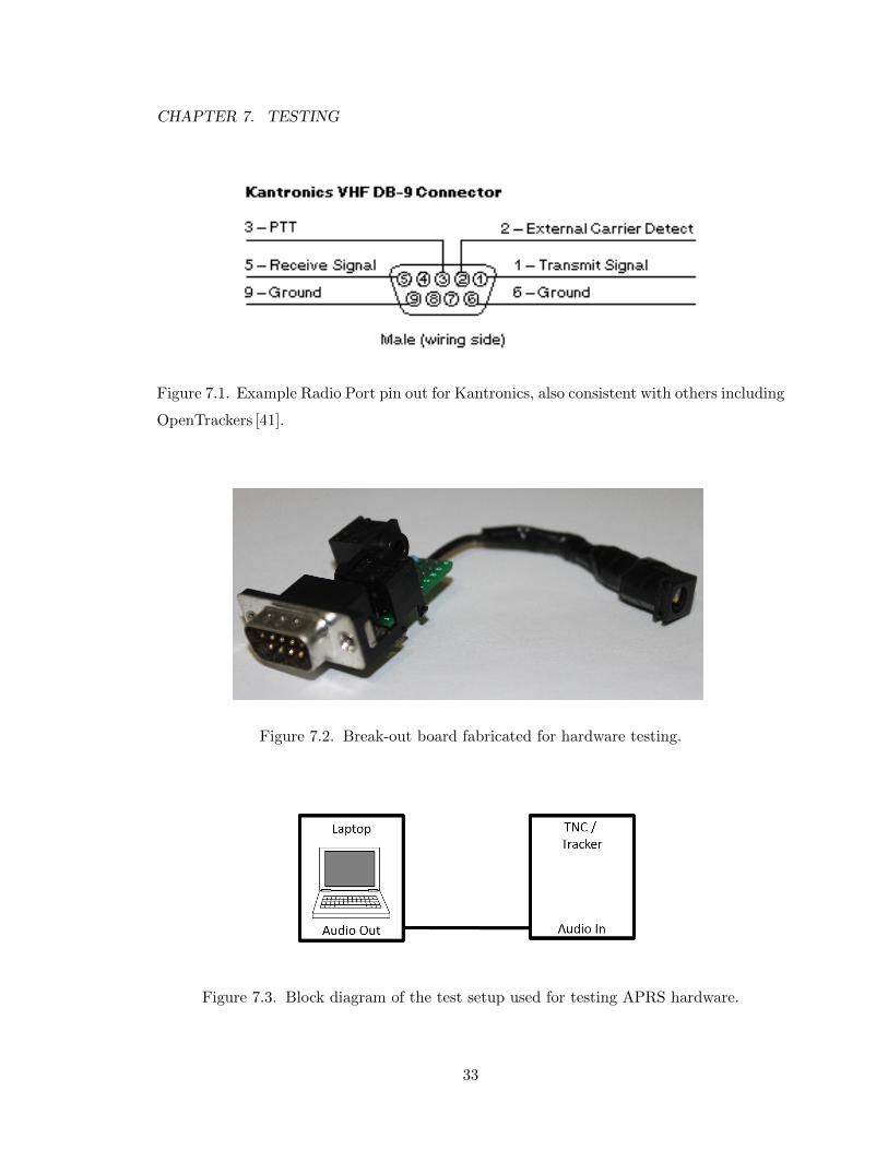
the common radio port can be seen in Figure 7.1 and found in any manual including those

of Argent Data [68]. Since this was common between multiple pieces of hardware, a simple

break-out board was created that allowed for a more universal audio transport mechanism

of 2 3.5mm tip-ring-sleeve connectors (one audio in and one out), and also a 2.5mm barrel

jack for power (Figure 7.2). This was much simpler than actually interfacing with a radio

since the audio could just be played from a laptop into the device using a standard 3.5mm

tip-ring-sleeve cable (Figure 7.3).

7.1.1 Setting TNC Audio Levels

During the testing, setting the audio level to be precisely correct for optimal performance

would have been ideal. However, there is language in the user manuals for the various

TNCs that is definitely up for interpretation. Such as in the MFJ-1278 manual which

reads: ”Continue to advance the volume control until there is approximately twice as much

audio present at the receiver output 〈as the minimum〉” [43]. Additionally the manual for

the Kantronics KamPlus says: ”Increase the volume control slightly from this point” [35].

32

CHAPTER 7. TESTING

Figure 7.1. Example Radio Port pin out for Kantronics, also consistent with others including

OpenTrackers [41].

Figure 7.2. Break-out board fabricated for hardware testing.

Figure 7.3. Block diagram of the test setup used for testing APRS hardware.

33

CHAPTER 7. TESTING

Table 7.1: Minimum Optimal TNC Input Audio Levels [35, 43, 2, 31].

TNC KamPlus MFJ-1278 PK-88 PK-232

Level (Vpp) 0.5 0.25 0.15 0.35

The volume level that was used for the audio provided to the TNCs was setting the laptop

system volume to 50% which worked out to about 1.1V peak-to-peak (Vpp). After doing

some deeper reading of the individual TNC user manuals and verifying the expected results

that were outlined, the approximate minimum optimal audio levels can be seen in Table

7.1.

7.2 Software Testing Setup

Included within the javAX25 suite was a testing application that could both generate and

decode packets. However, it was limited to only being able to specify one audio file and

one demodulation algorithm. Using this test file as a basis, a new testing application was

created that allowed for the multiple demodulators to be compared side by side against

multiple audio files with a single run of the application. In addition to the output being

printed to the console, it was saved to a file. Having these features in the testing application

allowed for a much more streamlined analysis of all the algorithms collectively and tuning

individual algorithms. One very convenient aspect of programmatically testing is that it is

very easy to add a loop to try a range of tuning parameters and then look at the results to

decide what is the best option. All of the results listed in the following chapter are from

the testing application and mechanism described here.

34

8 Implementation

This chapter will go through all of the implementation details of each demodulator im-

plemented. They will be presented in order of complexity, with the more intricate ones

presented last. This also will introduce them mostly chronologically since naive approaches

allowed for more insight to be gained into the javAX25 software package, as well as APRS

packet demodulation, before implementing more complicated algorithms. In addition to

giving a brief overview of each implementation some performance data will be provided,

but all of the data will be presented in the Results chapter. As mentioned in the Demod-

ulation Techniques chapter, javAX25 was selected because of its availability and as such

all of these implementations can be found in this author’s Fork of the javAX25 GitHub

repository in the following reference [10].

8.1 Strict Zero Crossing Demodulator

This approach used the technique of finding zero crossings and then using those to determine

the period; and frequency. For 1200Hz and 2200Hz tones, zero crossings are expected every

833us and 455us respectively. If the resulting frequency after calculations was above 1700Hz

it was assumed that a mark was present in the signal and if lower than 1700Hz a space must

be present. Each zero crossing was found by determining if the signal was negative and

changed to positive or if it was positive and changed to negative. Although this algorithm

was only able to decode a little over half of the packets as some of the other algorithms, it

proved to be an important stepping stone into javAX25 and allowed for preparation into

restructuring the project for added modularity of the filtering.

8.2 Floating Ground Zero Crossing Demodulator

Building on the strict zero crossing algorithm the next zero crossing demodulator tried to

use some more intelligence in finding the zero crossings through additional processing. One

reason that the strict zero crossing approach was thought to have relatively poor results was

due to the previously introduced challenge of DC offset. If the signal does not actually cross

zero then it will be very hard to find the zero crossings. This new zero crossing method

35

CHAPTER 8. IMPLEMENTATION

keeps a window of history (it was arbitrarily chosen to be one bit period) and from this

collection of samples the average is taken to use this as the ground - or zero value. Instead

of checking to see if the signal crosses zero, the signal is analyzed for going from either above

to below or below to above this average value. This ended up having worse results than

the strict zero crossing demodulator. This was due in part to the fact that 2200Hz signals

- even when properly centered around zero - will not have an average of zero since it can

not complete two full periods within one bit period, which tainted the average. Referring

back to Figure 2.1 it can be seen that the second bit (samples 40-80) would have a positive

average, not zero, since at the end of the bit period (sample 80), this 2200Hz tone still has

60 degrees to go to finish its current cycle.

8.3 Windowed Zero Crossing Counting Demodulator

With a good handle on utilizing zero crossing, a new approach was taken to keeping history.

Instead of using the history to calculate where ”zero” is, a new question was asked, ”What

if how many zero crossings within one period is observed?” If a window slightly shorter

than one bit period is selected, then if there are only two crossings within the window that

will correspond to a 1200Hz symbol being present. More crossings than two means that a

2200Hz symbol must be present. The thought behind taking this approach is that it would

give some additional resiliency to noise by finding the average during that bit period through

utilizing multiple zero crossings instead of individually analyzing every zero crossing.

8.4 Peak Detection Demodulator

After making a simple zero crossing overly complicated, it was decided that maybe a different

approach should be taken, specifically to look at a different part of the signal. It was

considered that perhaps better performance could be achieved by looking at the peaks in

the signal instead of the noisy zero crossing around ground, or not around ground if there

are DC offset problems. Conveniently, the difference between two consecutive peaks will be

equal to the period of the underlying signal. Although the methodology is the same as the

zero crossing for converting the period to the actual frequency, it was perceived that this

would give better results. It turns out that this method did not work as well as hoped due

36


to the fact that local peaks were commonly discovered from the noise instead of the actual

peak in the transmitted signal. More analysis into selecting a proper filter may give this

approach better results.

8.5 Derivative Zero Crossing Demodulator

After a failure with the peak detection demodulator, a new approach was taken to finding

”peaks.” Instead of actually looking for the peaks, the zero crossing demodulator was re-

visited with a new spin. Instead of using the raw samples for determining the frequency

using zero crossings, the derivative was to be used. The derivative was calculated by doing

the same averaging as in the strict zero crossing approach and then subtracting the current

average from the average two samples prior. It was thought that this would solve the DC

offset problem for sure, but it turns out that this was not the larger problem. The problem

was with using the zero crossing approach and this derivative implementation ended up

having very similar results to the strict zero crossing with which of these two was better

changing based off of pre-filtering. This can be attributed to the change in emphasis caused

by taking the derivative.

8.6 Goertzel Filter Demodulator

Finally moving away from approaches utilizing zero crossing methodologies, an approach

using Goertzel filters was implemented. The implementation was very simple and corre-

sponds with that outlined in the Demodulation Techniques chapter. Since it has to be

applied onto a set of data, a window size that was equal to one bit period was originally

selected so as to make sure that the data being processed was only that of one frequency,

but after analyzing the effect of the window size on performance, a window size of slightly

longer than a bit period ended up being better. The optimal size was tested to be 135

percent of a bit period, and the reason why this worked better is because it gave more

signal in the window for the filter to lock to. Essentially, the window was only extended 18

percent on each side of a bit period. This over-extension of the window is what led to being

able to exceed the performance of the original correlator on unfiltered data.

37


8.7 Phase Locked Loop Demodulator

Next, the PLL demodulator was implemented. Using Lutus’s python based software PLL

initial testing was performed to see how it would work for tracking AX.25 signals [39]. Once

the parameters were tuned sufficiently that it seemed to be staying locked onto the signal,

it was ported over to java and actually run as a demodulator. Once inside of the javAX25

framework additional tuning was done programmatically instead of manually to further fine

tune the performance. The final results were that it was not the winner, but comparable

to the other top contenders.

8.8 Mixed Preclocking Demodulator

Finally, with numerous simple algorithms implemented, it was time to try something much

more complicated and also only possible in software. This approach and the name preclock-

ing comes from an abbreviation for predetermined clocking where packets are analyzed a

whole packet at a time. The start and end are found and then the clocking, and hence bit

boundaries, are predetermined before the actual demodulation takes place on a baud by

baud basis as opposed to a sample by sample basis. Each one of the preceding algorithms

was on a sample by sample basis, meaning they had to make their best determination of

bits elapsed using a little bit of history.

There are five steps to the demodulation in the Mixed Preclocking Demodulator. It was

speculated that processing one packet at a time with the correct clocking to demodulate

bit by bit would allow for very accurate demodulation.

1. Flags are found in the signal so that the demodulation can happen one packet at a

time instead of just blindly trudging forward through the packet sample by sample.

2. The derivative of the whole packet is taken to determine the zero crossings.

3. Frequency transitions are extrapolated from the derivative data.

4. The frequency transitions found in the packet are used to determine the clocking (bit

boundaries).

38


5. The tone demodulation is done on a baud by baud basis.

Although it was hoped that the results would be phenomenal, there were so many different

methodologies being used that this preclocking demodulator was very difficult to tune.

For instance, the flags were found using the correlation approach, the transitions using a

derivative, and the final demodulation using the zero crossings. What were thought to be

advantages ended up being the challenges, but as predicted it did well enough to still be

considered one of the successful implementations. The intricate nature of this demodulator

made it delicate, which was noticed during the testing through the fact that it would not

decode any packets unless a bandpass filter was used on the incoming data.

8.9 Goertzel Preclocking Demodulator

After the first attempt at a preclocking approach, it was thought that perhaps using only

one methodology to perform all the different steps of demodulation would be at the very

least simpler, and hopefully better. The perception that it might be better came from the

fact that there was only one item to tune, the Goertzel Filter which had already shown

good performance. Instead of having to worry about noise affecting zero crossings and

the derivative potentially adding emphasis problems, only the filter had to be considered.

Unfortunately, the number of packets that this method decoded was not as many as the

first Goertzel approach or the previous preclocking. This was due to the fact that even

though there was one underlying algorithm it was used in three separate instances, and

each needed slightly different tuning. The three instances were for flag detection, frequency

transition detection, and the the final bit by bit demodulation.

8.10 Goertzel Exhaustive Preclocking Demodulator

The final algorithm implemented was just a matter of verification, and another one that

could be performed only in software. Instead of analyzing packets one at a time using flags

as the start and end points, a whole array of data that had a length equal to the number of

samples that a packet of the maximum length would have. Every time a few more samples

came in, every single clocking was attempted on the large array of data just to see what

39


packets could be decoded by exhaustively searching through the data. In terms of run time,

this algorithm took much longer. For instance, the mixed preclocking and original Goertzel

preclocking took 3 minutes and 5 seconds and 2:36 respectively to run, while this exhaustive

search took 26:48 on the 25:49 Track 1 of the test suite. This means that a 2.1Ghz Intel i7

(i7-3612QM) could not process the audio file in less time than elapses during the content of

the audio file. With that being the case, the result is that with live data this approach would

not work since it would continuously fall behind. Gratefully, this approach only decoded an

additional 15 packets that the Correlation, original Goertzel (non-preclocking), and PLL

did not decode. This result could be used to make the argument that the few more packets

decoded is not worth the vast number more CPU cycles it takes to achieve it.

40

9 Results

This results chapter is meant as a mechanism to present all of the data that was collected

on the performance of different demodulators. All of the demodulators that were tested in

the course of this research will be shown, whether it be dedicated hardware or software.

The first results that will be shown are those of the dedicated hardware, being TNCs and

Argent Data’s OpenTrackers. Following the hardware will be the software implementations.

Following these two categories will be some general comparison between them.

9.1 Dedicated Hardware Results

In the scope of this research a total of 12 pieces of hardware were tested. They include

Argent Data’s OpenTracker 2, OpenTracker 3, OpenTracker USB, OpenTracker 3 Micro,

Kantronics KAM, two Kantronics KAM Plus, two AEA PK-88, a PK-232, a PK-232MBX,

and an MFJ-1278. Hardware models for which more than one was tested will be differen-

tiated by a number in parentheses following the model number. Please note that on the

figures OpenTracker will be abbreviated OT.

The first two tests consisting of clean packets - 40 generated from the OpenTracker and

200 using Toledo’s suite - was relatively uninteresting. Essentially every piece of hardware

decoded all 40 and all 200 packets. The only anomalies to this were that the OpenTracker

USB was only able to decode 39 and 193 out of the 40 and 200 packet files respectively.

Additionally the OpenTracker 3 Micro missed one packet in the 200 packet file to only

decode 199. Since there is no real way to debug and see the cause of decoding relatively

fewer or more packets, just the data for these hardware items is presented as it was measured

to allow for comparison to the software. This will continue to be the case for the remainder

of this hardware section.

Following the two easy files the next file is same content as the file with 40 packets in it, with

the only difference being that noise was progressively added. In Figure 9.1, the two PK-88s

stand out for being able to decode 25 of the 40 packets in this file, which is a calculated

SNR of 0.8. Just a reminder that in this figure and future figures that present results for

this test file the number above each bar represents the caluclated SNR.

41

CHAPTER 9. RESULTS

Figure 9.1. Number of packets successfully decoded for all tested hardware on the Open-

Tracker 3 test file with noise.

The next two files are the ones that were used most extensively in the testing for comparison

and tuning. Primarily the first, which is just a recording of traffic off the air. They are Track

1 and 2 from the APRS CD mentioned in the Demodulator Benchmarking Chapter. The

results from Track 1 are in Figure 9.2 and Track 2 in Figure 9.3. The top three performances

of the hardware on Track 1 were the PK-88 (2) with 1007 packets decoded, the KAM with

988 Packets, and the KAM Plus (2) with 985 Packets. For Track 2 the top hardware was

the KAM Plus (2) with 998, the KAM Plus (1) with 967, and the KAM with 938.

Using these results the best numbers for the hardware were 40 packets decoded from the

Open Track 3 test, 200 from the javAX25 generated file, 25 from the Open Tracer 3 test

with added noise, 1007 from Track 1 of the LA test suite, and 998 from Track 2. These

best results can be used as a comparison for the software.

42

CHAPTER 9. RESULTS

Figure 9.2. Number of packets successfully decoded for all tested hardware on the Track 1

test file.

9.2 Software Results

In this section, the number of packets that each of the demodulators in the javAX25 package

was able to decode will be presented, highlighting those that were newly implemented in

the course of this research. This will include the correlation approach that was already

implemented before the start of this research as well as all of the new algorithms that were

outlined in the previous chapter on Implementation. However, before getting the results

from javAX25 there is one more data set to be introduced which is the results from another

software based demodulation from AGW Packet Engine. Using this software, 40 packets

were decoded from the OpenTracker 3 test, 200 from the javAX25 generated file, 21 from

the OpenTracker 3 test with added noise (SNR of 1.1), 967 from Track 1 of the LA test

suite, and 497 from Track 2. The results from javAX25 end up being on par with these

results as well as those of the hardware.

With a total of 13 algorithms implemented, some did well and others not at all, so as in

the section on hardware results, all of the data will be presented followed by a focus on

43

CHAPTER 9. RESULTS

Figure 9.3. Number of packets successfully decoded for all tested hardware on the Track 2

test file.

those that performed the best. In the new javAX25 software implementation the filtering

was moved from its original location of being on a per demodulator level basis to a central

location that allowed each of the algorithms to utilize it. Some of the algorithms ended

up relying on it after tuning and others could remain independent. As such, in order to

present all of the data, each algorithm will not only have a result for each of the 5 test files,

but also for each of the three filters used on the data. The three filters used are no filter, a

900-2500Hz bandpass filter, and the same bandpass with a 6dB attenuation of 1200Hz tones

to combat the signals that were not emphasized when transmitted but were deemphasized

when received. For instance, for the Zero Crossing demodulator there will be three values

for the OpenTracker 3 Test file, one at each filtering, and so on for the remaining 4 test

files.

As correlation was the original implementation and already present in the javAX25 package

its performance should be considered the baseline. Since this is the baseline it will be on

the far left of the plots for reference. The performance of no filter on the OpenTracker 3

Test can be seen in Figure 9.4, Figure 9.5 shows data with the bandpass filter, and the

44

CHAPTER 9. RESULTS

Figure 9.4. Performance of software on the raw signal from OpenTracker 3 Test.

emphasizing filter results in Figure 9.6. It can be observed that zero crossing did not favor

the filters, others were resilient, and preclocking thrived. The Generated 200 Test file is the

only file that the peak demodulator performed comparably to the other techniques. The

good performance of the peak demodulator on only this file was due to the fact that it was

tuned using this file. As it was attempted to optimize it for other files, it was found that

the peak demodulation was too delicate which has a lot to do with its poor performance on

the other files. The unfiltered data from Generated 200 test is in Figure 9.7, the bandpass

data in Figure 9.8, and the results of emphasizing the signal in Figure 9.9. Although the

generated 200 packet file and the OpenTracker test file had similar results, the results for

the generated 200 were better. This can be attributed to the fact that this file has only

ever existed in the digital realm, it was made and consumed there, as opposed to being

produced in the physical world and then recording and digitizing it.

Again, moving on from the ”easy” files the performance of the software demodulators on

the OpenTracker 3 Test with the noise added can be seen. Figure 9.10 shows the data for

the unfiltered file, Figure 9.11 shows bandpass filter data, and Figure 9.12 shows data from

the emphasis filter. Two algorithms really start to shine as being comparable, and in some

45

CHAPTER 9. RESULTS

Figure 9.5. Performance of software on OpenTracker 3 Test with a flat bandpass filter.

Figure 9.6. Performance of software on OpenTracker 3 Test with an emphasis filter.

46

CHAPTER 9. RESULTS

Figure 9.7. Performance of Software on the raw signal from Generated 200.

Figure 9.8. Performance of software on Generated 200 with a flat bandpass filter.

47

CHAPTER 9. RESULTS

Figure 9.9. Performance of Software on Generated 200 with an emphasis filter.

cases better, than the correlation demodulator. Those are the Goertzel Filter Demodulator

and the PLL Demodulator. Although this is not data that was actually transmitted or

received, these two start to show promise. Even the Strict Zero crossing can be seen doing

well once the audio file is emphasized, but it doesn’t stand up to the competition in the

next two test files containing off air data.

As mentioned earlier, these next two test files were those that were thought the be most

important to succeed at. As such, Track 1 was used to tune the algorithms since this would

represent the closest real-world simulation possible. The Track 2 results are also presented

for comparison. However in Track 2, in addition to being deemphasized the process of this

filtering also reduced the magnitude of the signal in the audio file as mentioned earlier. As

such, this file shows two things: One, the ability to pick up lower level signal and second,

the algorithms tolerance to signals that were not emphasized when transmitted, but were

deemphasized when received. The results of no filtering, bandpass filtering, and emphasis

filtering can be seen in their respective Figure 9.13, 9.14, and 9.15 for Track 1. The data

from demodulating Track 2 can be seen in Figure 9.16, 9.17, and 9.18. As was caught

during the OpenTracker 3 Test with noise it can be noticed that the Goertzel and PLL

48

CHAPTER 9. RESULTS

Figure 9.10. Performance of software on the raw signal from OpenTracker Test with noise

added.

algorithms are still doing well on Track 1, and also the Mixed preclocking is doing fairly

well. With the filter that is applied on Track 1 to create Track 2 it is basically the opposite

effect of Toledo’s emphasis filter and hence they cancel each other out. This can be seen

by looking at the performance of the Goertzel Demodulator which does poorly with both

other filterings on Track 2. However, its ability to detect low level signals and this reversal

of the emphasis filtering applied makes it end of having comparable results to just the band

pass filter on Track 1 - 956 versus 965.

9.2.1 Hardware and Software Comparisons

It is now time to actually compare the new software implementations to the old ones as well

as to the hardware. The first thing to notice is that the Goertzel Filter did very well, and

in some cases better than the original correlation. Secondly, the complicated preclocking

algorithm was also able to hold its own and still be a top contender. In fact the top three

software algorithms were Correlation, Goertzel, and Mixed Preclocking with 964, 965, and

49

CHAPTER 9. RESULTS

Figure 9.11. Performance of software on OpenTracker Test with noise added with a flat

bandpass filter.

939 packets decoded from Track 1 with the bandpass filter, the results of these top three

algorithms versus the top three pieces of hardware can be seen in Figure 9.19. In addition

to having the top 3 of each Figure 9.19 includes the results of AGWPE and running the top

3 software algorithms in parallel. Even though each algorithm decodes different numbers

of packets they each still have their expertise with being able to exclusively decode packets

that others could not. For instance when the three are run together there is a total of 975

packets decoded due to the fact that Goertzel gets 12 packets that the other two do not,

Correlation gets 7 that the others do not, and Preclocking decoded 3 that these other two

missed. This could still be a good argument for the use of software over hardware since it is

very easy to run multiple demodulators in parallel. Especially since the cost of this is only

5 minutes and 2 seconds on a file that is 25:49 long.

The question is, is the software better than the hardware? Looking at the highest numbers,

no, but looking at the bigger picture, maybe. One thing about the hardware is that it is

prone to variations and in need of periodic tuning. So, if instead of looking at the best of

the breed for the hardware, if the average values are compared under the presumption that

50

CHAPTER 9. RESULTS

Figure 9.12. Performance of Software on OpenTracker Test with noise added with an

emphasis filter.

Figure 9.13. Performance of software on the raw signal from Track 1.

51

CHAPTER 9. RESULTS

Figure 9.14. Performance of software on Track 1 with a flat bandpass filter.

Figure 9.15. Performance of software on Track 1 with an emphasis filter.

52

CHAPTER 9. RESULTS

Figure 9.16. Performance of software on the raw signal from Track 2.

Figure 9.17. Performance of software on Track 2 with a flat bandpass filter.

53

CHAPTER 9. RESULTS

Figure 9.18. Performance of software on Track 2 with an emphasis filter.

Figure 9.19. Performance of software versus hardware on Track 1.

54

CHAPTER 9. RESULTS

this would correspond to the average ham’s decoding capabilities, then the software does

decode more packets. Additionally, the software does not have any capacitors that will dry

up or solder joints that may become brittle and affect the performance. The performance

of the software today will be exactly the same in 5, 10, many years. The average number

of packets decoded by the hardware on Track 1 was 935. Looking at this value any one of

the three algorithms that are the top performers would be considered better.

55

10 Future Work

The sections in this chapter will explain some aspects that this project uncovered that have

the potential for future research. There are three main items that the author thinks should

be explored in more depth as future work in this area of AX.25 software based demodulation,

including the Discrete Short-Time Fourier Transform, the use of the checksum for forward

error correction, and to actually integrate these demodulators with live traffic from a radio.

10.1 The Discrete Short-Time Fourier Transform

In a paper by Zhonghui-Chen et. al., methods are outlined to use the discrete short-time

Fourier transform (DSTFT) to demodulate a binary frequency shift keyed (BFSK) signal.

After a discussion of the DSTFT they go into their specific implementation, but this appears

to show promise because of their results section. Granted, this was for a simulation but

they showed that the error rate was lower using the DSTFT than traditional coherent

demodulation even for lower signal to noise ratios [11].

10.2 Use the CRC for FEC

Each AX.25 packet contains a checksum that is generated by using a cyclic redundancy

check (CRC). This is used by all demodulators in order to determine if the packet that the

demodulator thinks it decoded was actually a legitimate packet or just noise that happened

to look like a packet. Although the CRC was not intended for forward error correction

(FEC), it would be interesting to see the effects of using it as such. With algorithms such

as the preclocking algorithms, the power of each symbol is determined and this power could

be used to assign a level of confidence on that demodulated bit. If a packet fails the CRC

check, and all except for one of the bits has a confidence greater than 80 percent, would the

CRC pass if that one bit was flipped to the other symbol? This is a very good argument

for the use of software since this meta data about the decoding of the packets can be kept

in memory, something that most hardware does not have much of.

56

CHAPTER 10. FUTURE WORK

10.3 Integrations with a Radio

Finally another area for future work would be to integrate the new algorithms with a radio

and use them to decode live data. Although the data used in the testing was a recording of

live data, it would be very gratifying to be able to see these algorithms decode audio straight

from the radio. Inside of javAX25, the packages should already support it, so it should be a

matter of just setting it up and letting it run. This analysis would allow for verification of

the implementations’ functionalities as well as to be able to see how the different algorithms

perform side by side in real time.

57

11 Conclusion

This research set out to try and prove that software could do APRS demodulation better

than the hardware. Depending on perspective, it may have done so. However, at the very

least the research shows that there are many ways to approach the challenge of demodulating

these packets and presents the relative performance of over 10 software based approaches

and 12 dedicated hardware approaches, whether that hardware is an OpenTracker or TNC.

In the end, the software did do better than the average result using hardware, but in the

primary benchmarking file, software was only able to decode 975 packets as opposed to the

1007 that the best piece of hardware detected. The software’s improved performance coupled

with its low cost, continues to make it an attractive approach over dedicated hardware.

Exploring some of the items in the future work section such as using the checksum for

forward error correction may be able to get software to outperform hardware.

58

BIBLIOGRAPHY

[1] 600/1200-baud modem standarized for use in the general switched telephone network.

https://www.itu.int/rec/T-REC-V.23-198811-I/en, November 1988. V.23.

[2] Inc. Advanced Electronic Applications. Model pk-88 packet conroller operating man-

ual. http://www.repeater-builder.com/aea/pdf/aea-pk-88-user-manual.

pdf, 1990.

[3] Salam Akoum and Behrouz Farhang-Boroujeny. A phase locked lopp with arbitrarily

wide lock range for software defined radios. http://www.ece.utah.edu/~akoum/

PLL_Paper.pdf.

[4] William A. Beech. Ax.25 link access protocol for amateur packet radio. https://www.

tapr.org/pdf/AX25.2.2.pdf, July 1998.

[5] Carl Bergquist. Ham Radio Operator’s Guide. PROMPT Publications, second edition

edition, 2001.

[6] Bob Bruninga. Automated packet reporting system. http://aprs.org/.

[7] Bob Bruninga. Aprs spec addendum 1.1. http://www.aprs.org/aprs11.html, July

2004.

[8] Bob Bruninga. Aprs spec addendum 1.2 proposals. http://www.aprs.org/aprs12.

html, July 2013.

[9] Byonics. Byonics tinytrak. http://www.byonics.com/tinytrak/.

[10] Robert Campbell. javax25 (github). https://github.com/robbieford/javAX25,

2015.

[11] Zhonghui Chen, Haibin Lin, Xin Chen, and Huiqun Hong. Fsk signal demodulation

method based on dstft. In Wireless Communications, Networking and Mobile

Computing, 2008. WiCOM ’08. 4th International Conference on, pages 1–3, Oct

2008.

[12] APRS Community. Aprs-is. http://www.aprs-is.net/, 2015.

59

https://www.itu.int/rec/T-REC-V.23-198811-I/en

http://www.repeater-builder.com/aea/pdf/aea-pk-88-user-manual.pdf

http://www.repeater-builder.com/aea/pdf/aea-pk-88-user-manual.pdf

http://www.ece.utah.edu/~akoum/PLL_Paper.pdf

http://www.ece.utah.edu/~akoum/PLL_Paper.pdf

https://www.tapr.org/pdf/AX25.2.2.pdf

https://www.tapr.org/pdf/AX25.2.2.pdf

http://aprs.org/

http://www.aprs.org/aprs11.html



http://www.byonics.com/tinytrak/

https://github.com/robbieford/javAX25

http://www.aprs-is.net/

BIBLIOGRAPHY

[13] Kenwood U.S.A Corporation. Tm-d700a owner manual. http://www.

kenwoodusa.com/UserFiles/File/UnitedStates/Communications/AMA/

Manuals/TM-D700-Owner-Manual.PDF.

[14] J. Das, S. K. Mullick, and P. K. Chatterjee. Principles Of Digital Communication.

John Wiley & Sons, 1986.

[15] Argent Data. Ot3m case front. http://www.argentdata.com/catalog/images/

Ot3m-termblk.jpg.

[16] Advanced Micro Devices. Am7910/11 fsk modem datasheet. http://pdf1.

alldatasheet.com/datasheet-pdf/view/124524/AMD/AM7910.html, June 1989.

[17] Wilfried Elmenreich. Emodulation detecting a frequency using a goertzel filter. http:

//netwerkt.wordpress.com/2011/08/25/goertzel-filter/, August 2011.

[18] EXAR. Xr-2211a data sheet. https://www.exar.com/common/content/document.

ashx?id=170, June 1997.

[19] Kenneth W. Finnegan. Examing ambiguities in tthe automated packet reporting sys-

tem. Master’s thesis, California Polytechnic State University San Luis Obispo,

2014.

[20] Kenneth W. Finnegan and Bridget Benson. Clarifying the amateur bell 202 modem.

33rd ARRL and TAPR Digital Communications Conference, 2014.

[21] Joseph D. Gaeddert. Wrloops a phase-locked loop in straight c. http://liquidsdr.

org/blog/pll-howto/, November 2013.

[22] Michaek D. Gallagher and Randall A. Snyder. Mobile Telecommunications Networking

With IS-41. McGraw-Hill, 1997.

[23] Stan Gibilisco, editor. Amateur Radio Encyclopedia. TAB Books, 1994.

[24] Lillian Goleniewski. Telecommunications Essentials. Addison-Wesley, second edition

edition, 2006.

[25] Darien Graham-Smith. How to: How much ram do you re-

60

http://www.kenwoodusa.com/UserFiles/File/UnitedStates/Communications/AMA/Manuals/TM-D700-Owner-Manual.PDF



http://www.argentdata.com/catalog/images/Ot3m-termblk.jpg

http://www.argentdata.com/catalog/images/Ot3m-termblk.jpg

http://pdf1.alldatasheet.com/datasheet-pdf/view/124524/AMD/AM7910.html

http://pdf1.alldatasheet.com/datasheet-pdf/view/124524/AMD/AM7910.html

http://netwerkt.wordpress.com/2011/08/25/goertzel-filter/

http://netwerkt.wordpress.com/2011/08/25/goertzel-filter/

https://www.exar.com/common/content/document.ashx?id=170

https://www.exar.com/common/content/document.ashx?id=170

http://liquidsdr.org/blog/pll-howto/

http://liquidsdr.org/blog/pll-howto/

BIBLIOGRAPHY

ally need? http://www.pcauthority.com.au/Feature/375815,

how-to-how-much-ram-do--you-really-need.aspx, March 2014.

[26] GTA-West Regional Packet Group. Introduction to packet radio for ares. http://

barc.ca/wordpress/wp-content/uploads/2014/07/Packet_Basics_GTAW.pdf,

2012.

[27] The APRS Working Group. Automatic position reporting system: Aprs protocol ref-

erence. http://www.aprs.org/doc/APRS101.PDF, August 2000.

[28] Harry Helms. All About Ham Radio. HighText Publications, 1992.

[29] Wayne Holder. Wayne’s tinkering page: Bell 202, 1200 baud de-

modulator in an attiny10. https://sites.google.com/site/

wayneholder/attiny-4-5-9-10-assembly-ide-and-programmer/

bell-202-1200-baud-demodulator-in-an-attiny10, July 2012.

[30] Stan Horzepa. Your Gateway to Packet Radio. The American Radio Relay League,

1992.

[31] Timewave Technology Inc. Pk-232 mbx operating manual. http://www.

repeater-builder.com/aea/pk232/pk232mbx-operating-manual.pdf, 2001.

[32] National Instruments. Keying and digital modulation. http://www.ni.com/

white-paper/3013/en/, November 2014.

[33] Texas Instruments. Tcm 3105 fsk modem datasheet. http://www.netti.fi/~ryydis/

tcm3105.pdf, May 1994.

[34] Javvin. Network Protocols Handbook. Javvin Technologies, Inc., third edition edition,

2006.

[35] Kantronics. Kam plus getting started. http://www.ocrg.org/documents/Kam%

20Plus%20Getting%20Started.pdf, 1993.

[36] Kantronics. Kpc-3+ packet communicator. http://www.kantronics.com/products/

kpc3.html, 2014.

61

http://www.pcauthority.com.au/Feature/375815,how-to-how-much-ram-do--you-really-need.aspx

http://www.pcauthority.com.au/Feature/375815,how-to-how-much-ram-do--you-really-need.aspx

http://barc.ca/wordpress/wp-content/uploads/2014/07/Packet_Basics_GTAW.pdf

http://barc.ca/wordpress/wp-content/uploads/2014/07/Packet_Basics_GTAW.pdf

http://www.aprs.org/doc/APRS101.PDF

https://sites.google.com/site/wayneholder/attiny-4-5-9-10-assembly-ide-and-programmer/bell-202-1200-baud-demodulator-in-an-attiny10



http://www.repeater-builder.com/aea/pk232/pk232mbx-operating-manual.pdf

http://www.repeater-builder.com/aea/pk232/pk232mbx-operating-manual.pdf

http://www.ni.com/white-paper/3013/en/

http://www.ni.com/white-paper/3013/en/

http://www.netti.fi/~ryydis/tcm3105.pdf

http://www.netti.fi/~ryydis/tcm3105.pdf

http://www.ocrg.org/documents/Kam%20Plus%20Getting%20Started.pdf

http://www.ocrg.org/documents/Kam%20Plus%20Getting%20Started.pdf

http://www.kantronics.com/products/kpc3.html

http://www.kantronics.com/products/kpc3.html

BIBLIOGRAPHY

[37] KK6RF. Kantronics kam plus v8.2 firmware and 512kb. http://forums.qrz.com/

attachment.php?attachmentid=192170&d=1406602474&thumb=1.

[38] Georg Lukas. Aprsdroid (github). https://github.com/ge0rg/aprsdroid, December

2013.

[39] Paul Lutus. Understanding phase-locked loops. http://arachnoid.com/phase_

locked_loop/, 2011.

[40] Edward Claro Mader. What is the speed of electricity and why? https://www.quora.

com/What-is-the-speed-of-electricity-and-why, July 2014.

[41] Bruce W. Martin. Radio, tnc & gps pinouts. http://www.bwm.us/Resource/radio_

pinout.html, June 2014.

[42] Dominic Mazzoni. Audacity. http://audacity.sourceforge.net/.

[43] MFJ. Model mfj-1278/mfj-1278t instruction namual. http://www.radiomanual.

info/schemi/ACC_packet/MFJ-1278_MFJ-1278T_user.pdf, 1990.

[44] Scott Miller. Aprs and packet radio products. http://www.argentdata.com/

products/aprs.html.

[45] James A. Mitrenga. An mx614 packet modem. http://www.cmlmicro.com/assets/

614_TCM3105.pdf, January 2000.

[46] Newegg. Rosewill rc-701 5.1 channels pci interface sound card. http://www.newegg.

com/Product/Product.aspx?Item=N82E16829265001, 2014.

[47] Ham Radio Outlet. Kantronics kpc-3 plus. http://www.hamradio.com/detail.cfm?

pid=H0-000229, 2014.

[48] Michael H. Perrott. Tutradio on digital phase-locked loops. http://www.cppsim.com/

PLL_Lectures/digital_pll_cicc_tutorial_perrott.pdf, September 2009.

[49] Larry L. Peterson and Bruce S. Davie. Computer Networks: A Systems Approach.

Elsevier, fifth edition edition, 2011.

[50] John G. Proakis. Digital Communications. McGraw-Hill Book Company, 1983.

62

http://forums.qrz.com/attachment.php?attachmentid=192170&d=1406602474&thumb=1

http://forums.qrz.com/attachment.php?attachmentid=192170&d=1406602474&thumb=1

https://github.com/ge0rg/aprsdroid

http://arachnoid.com/phase_locked_loop/

http://arachnoid.com/phase_locked_loop/

https://www.quora.com/What-is-the-speed-of-electricity-and-why

https://www.quora.com/What-is-the-speed-of-electricity-and-why

http://www.bwm.us/Resource/radio_pinout.html

http://www.bwm.us/Resource/radio_pinout.html

http://audacity.sourceforge.net/

http://www.radiomanual.info/schemi/ACC_packet/MFJ-1278_MFJ-1278T_user.pdf

http://www.radiomanual.info/schemi/ACC_packet/MFJ-1278_MFJ-1278T_user.pdf

http://www.argentdata.com/products/aprs.html

http://www.argentdata.com/products/aprs.html

http://www.cmlmicro.com/assets/614_TCM3105.pdf

http://www.cmlmicro.com/assets/614_TCM3105.pdf

http://www.newegg.com/Product/Product.aspx?Item=N82E16829265001

http://www.newegg.com/Product/Product.aspx?Item=N82E16829265001

http://www.hamradio.com/detail.cfm?pid=H0-000229

http://www.hamradio.com/detail.cfm?pid=H0-000229

http://www.cppsim.com/PLL_Lectures/digital_pll_cicc_tutorial_perrott.pdf

http://www.cppsim.com/PLL_Lectures/digital_pll_cicc_tutorial_perrott.pdf

BIBLIOGRAPHY

[51] Thaddeus A. Roppel. Fsk-frequency shift keying. http://www.eng.auburn.

edu/~troppel/courses/TIMS-manuals-r5/TIMS%20Experiment%20Manuals/

Student_Text/Vol-D1/D1-07.pdf.

[52] George Rossopoylos. Agw packet engine. http://www.sv2agw.com/ham/agwpe.htm.

[53] David Rowe. Fsk over fm. http://www.rowetel.com/blog/?p=3799, December 2014.

[54] Thomas Sailer. Internationale packet-radio tagung darmastadt: Dsp modems.

http://web.archive.org/web/*/http://www.baycom.org/~tom/ham/da95/d_

dspmod.pdf, 1995.

[55] Thomas Sailer. Using a pc and a soundcard for popular amateur digital modes. http:

//www.tapr.org/pdf/DCC1997-Soundcard4Digital-HB9JNX.pdf, 1997.

[56] Thomas Sailer. Soundmodem on modern operating systems. https://www.tapr.org/

pdf/DCC2000-SOUNDMODEMonOS-HB9JNX-AE4WA.pdf, August 2000.

[57] Mitra Sanjit K and James F. Kaiser, editors. Handbook For Digital Signal Processing.

John Wiley & Sons, 1993.

[58] Dennis Seguine. Simplified fsk signal detection. http://dx.eng.uiowa.edu/

eedesign/fskcorr.pdf, September 2006.

[59] Cypress Semiconductor. Modulation and demodulation. http://www.cypress.com/

?docID=43670.

[60] H. Ward Silver, editor. The ARRL Handbook for Radio Communications 2014. The

Amatuer Radio Relay League, Inc., 91 edition, 2013.

[61] Marvin K. Simon, Sami M. Hinedi, and William C. Lindsey. Digital Communication

Techniques. PTR Prentice Hall, 1995.

[62] Bernard Sklar. Digital Communications Fundamentals and Applications. Prentice Hall,

1988.

[63] Stephen H. Smith. Tnc test cd. http://www.wa8lmf.net/TNCtest/, August 2009.

63

http://www.eng.auburn.edu/~troppel/courses/TIMS-manuals-r5/TIMS%20Experiment%20Manuals/Student_Text/Vol-D1/D1-07.pdf



http://www.sv2agw.com/ham/agwpe.htm

http://www.rowetel.com/blog/?p=3799

http://web.archive.org/web/*/http://www.baycom.org/~tom/ham/da95/d_dspmod.pdf

http://web.archive.org/web/*/http://www.baycom.org/~tom/ham/da95/d_dspmod.pdf

http://www.tapr.org/pdf/DCC1997-Soundcard4Digital-HB9JNX.pdf

http://www.tapr.org/pdf/DCC1997-Soundcard4Digital-HB9JNX.pdf

https://www.tapr.org/pdf/DCC2000-SOUNDMODEMonOS-HB9JNX-AE4WA.pdf

https://www.tapr.org/pdf/DCC2000-SOUNDMODEMonOS-HB9JNX-AE4WA.pdf

http://dx.eng.uiowa.edu/eedesign/fskcorr.pdf

http://dx.eng.uiowa.edu/eedesign/fskcorr.pdf

http://www.cypress.com/?docID=43670

http://www.cypress.com/?docID=43670

http://www.wa8lmf.net/TNCtest/

BIBLIOGRAPHY

[64] Stephen H. Smith. Automatic position reporting system. http://wa8lmf.net/aprs/,

January 2012.

[65] 4Gon Solutions. Factors affecting wireless networking performance. http:

//www.4gon.co.uk/solutions/technical_factors_affecting_wireless_

performance.php#range.

[66] Barrie Sosinsky. Networking Bible. Wiley Publishing, Inc., 2009.

[67] M.K. Stauffer. Fsk voiceband modem using digital filters. http://www.google.com/

patents/US4425665, January 1984. US Patent 4,425,665.

[68] Argent Data Systems. Argent data systems opentracker usb users manual. https:

//www.argentdata.com/support/OpenTrackerUSB_manual.pdf, February 2013.

[69] Fox Delta Project Team. Foxtrak :: Aprs viewers, trackers & gps encoder. http:

//www.foxdelta.com/products/foxtrak.htm.

[70] Sivan Toledo. Ax25 java soundcard modem. https://github.com/sivantoledo/

javAX25/blob/master/manual.doc, February 2012.

[71] Sivan Toledo. A high-performance sound-card ax.25 modem. QEX, July / August

2012:19–25, 2012.

[72] Sivan Toledo. javax25 (github). https://github.com/sivantoledo/javAX25, April

2012.

[73] Yaesu USA. Ftm-350 series aprs manual. http://www.yaesu.com/

indexVS.cfm?cmd=DisplayProducts&ProdCatID=106&encProdID=

33C814E3D04C92310507ECDE68CC3C01&DivisionID.

[74] Bob Watson. Fsk: Signal and demodulation. WJ Communication, 7, 1980.

[75] APRS Wiki. Digipeater. http://info.aprs.net/index.php?title=Digipeater,

November 2012.

[76] Wikipedia. Automated packet reporting system. https://en.wikipedia.org/wiki/

Automatic_Packet_Reporting_System.

64

http://wa8lmf.net/aprs/

http://www.4gon.co.uk/solutions/technical_factors_affecting_wireless_performance.php#range



http://www.google.com/patents/US4425665

http://www.google.com/patents/US4425665

https://www.argentdata.com/support/OpenTrackerUSB_manual.pdf

https://www.argentdata.com/support/OpenTrackerUSB_manual.pdf

http://www.foxdelta.com/products/foxtrak.htm

http://www.foxdelta.com/products/foxtrak.htm

https://github.com/sivantoledo/javAX25/blob/master/manual.doc

https://github.com/sivantoledo/javAX25/blob/master/manual.doc

https://github.com/sivantoledo/javAX25

http://www.yaesu.com/indexVS.cfm?cmd=DisplayProducts&ProdCatID=106&encProdID=33C814E3D04C92310507ECDE68CC3C01&DivisionID



http://info.aprs.net/index.php?title=Digipeater

https://en.wikipedia.org/wiki/Automatic_Packet_Reporting_System

https://en.wikipedia.org/wiki/Automatic_Packet_Reporting_System

BIBLIOGRAPHY

[77] Wikipedia. Continuous-phase frequency shift keying. http://en.wikipedia.org/

wiki/Continuous_phase_modulation#Continuous-phase_frequency-shift_

keying, March 2014.

[78] Wikipedia. Discrete forier transform. http://en.wikipedia.org/wiki/Discrete_

Fourier_transform, November 2014.

[79] Wikipedia. Fast forier transform. http://en.wikipedia.org/wiki/Fast_Fourier_

transform, November 2014.

[80] Wikipedia. Fourier transform. http://en.wikipedia.org/wiki/Fourier_

transform, November 2014.

[81] Wikipedia. Goertzel algorithm. http://en.wikipedia.org/wiki/Goertzel_

algorithm, November 2014.

[82] Larry D. Wolfgang, editor. Now You’re Talking! All you Need for Your First Amateur

Radio License. The Amatuer Radio Relay League, Inc., 5th edition edition, 2005.

[83] Yaesu. Ftm-350 high res. http://www.yaesu.com/downloadFile.cfm?FileID=5183&

FileCatID=171&FileName=FTM%2D350US%5FF.jpg&FileContentType=image%

2Fpjpeg.

65

http://en.wikipedia.org/wiki/Continuous_phase_modulation#Continuous-phase_frequency-shift_keying



http://en.wikipedia.org/wiki/Discrete_Fourier_transform

http://en.wikipedia.org/wiki/Discrete_Fourier_transform

http://en.wikipedia.org/wiki/Fast_Fourier_transform

http://en.wikipedia.org/wiki/Fast_Fourier_transform

http://en.wikipedia.org/wiki/Fourier_transform

http://en.wikipedia.org/wiki/Fourier_transform

http://en.wikipedia.org/wiki/Goertzel_algorithm

http://en.wikipedia.org/wiki/Goertzel_algorithm

http://www.yaesu.com/downloadFile.cfm?FileID=5183&FileCatID=171&FileName=FTM%2D350US%5FF.jpg&FileContentType=image%2Fpjpeg



Analysis of Various Algorithmic approaches to Software ...

Documents

Transcript of Analysis of Various Algorithmic approaches to Software ...