Computer Science and Artificial Intelligence Laboratory

Technical Report

m a s s a c h u s e t t s i n s t i t u t e o f t e c h n o l o g y, c a m b r i d g e , m a 0 213 9 u s a — w w w. c s a i l . m i t . e d u

MIT-CSAIL-TR-2014-014 June 23, 2014

Autotuning Algorithmic Choice for Input SensitivityYufei Ding, Jason Ansel, Kalyan Veeramachaneni, Xipeng Shen, Una-May O�Reilly, and Saman Amarasinghe

Autotuning Algorithmic Choice for Input Sensitivity

Yufei Ding, Jason Ansel∗, Kalyan Veeramachaneni∗

Xipeng Shen, Una-May O’Reilly∗, Saman Amarasinghe∗

The College of William and Mary∗Massachusetts Institute of Technology

{yding,xshen}@cs.wm.edu∗{jansel,kalyan,unamay,saman}@csail.mit.edu

AbstractEmpirical autotuning is increasingly being used in many do-mains to achieve optimized performance in a variety of dif-ferent execution environments. A daunting challenge facedby such autotuners is input sensitivity, where the best auto-tuned configuration may vary with different input sets.

In this paper, we propose a two level solution that: first,clusters to find input sets that are similar in input featurespace; then, uses an evolutionary autotuner to build an opti-mized program for each of these clusters; and, finally, buildsan adaptive overhead aware classifier which assigns each in-put to a specific input optimized program. Our approach ad-dresses the complex trade-off between using expensive fea-tures, to accurately characterize an input, and cheaper fea-tures, which can be computed with less overhead. Experi-mental results show that by adapting to different inputs onecan obtain up to a 3x speedup over using a single configura-tion for all inputs.

1. IntroductionThe developers of languages and tools have invested a greatdeal of collective effort into extending the lifetime of soft-ware. To a large degree, this effort has succeeded. Mil-lions of lines of code written decades ago are still beingused in new programs. A typical example of this can befound in the C++ Standard Template Library (STL) routinestd::stable sort, distributed with the current version ofGCC and whose implementation dates back to at least the2001 SGI release of the STL. This legacy code contains ahard coded optimization, a cutoff constant of 15 betweenmerge and insertion sort, that was designed for machines ofthe time, having 1/100th the memory of modern machines.Our tests have shown that higher cutoffs (60 to 150) performmuch better on current architectures. While this paradigm ofwrite once and run it everywhere is great for productivity, amajor sacrifice of these efforts is performance. Write onceuse everywhere often becomes write once slow everywhere.We need programs with performance portability, where pro-

grams can re-optimize themselves to achieve the best perfor-mance on widely different execution targets.

One of the most promising techniques to achieve perfor-mance portability is program autotuning. Rather than hard-coding optimizations, that only work for a single microar-chitecture, or using fragile heuristics, program autotuningexposes a search space of program optimizations that canbe explored automatically. Autotuning is used to search thisoptimization space to find the best configuration to use foreach platform.

A fundamental problem faced by programs and librariesis input sensitivity. For a large class of problems, the best op-timization to use depends on the input data being processed.For example, sorting an almost-sorted list can be done mostefficiently with a different algorithm than one optimized forsorting random data. This problem is worse in autotuningsystems, because there is a danger that the auotuner will cre-ate an algorithm specifically optimized for the inputs it isprovided during training. Some existing solutions search forthe preferable optimization on every training input, and thenapply statistical learning algorithms to these data to build apredictive model, which maps input features to the best con-figurations [14, 20, 22, 27, 30].

But such solutions are not applicable to an important classof autotuning, namely algorithmic autotuning. The goal ofalgorithmic autotuning is to determine the best ways to con-figure an algorithm or assemble multiple algorithms togetherfor solving a class of problems effectively. Its special chal-lenges for addressing input sensitivity come from its fourprimary properties.

First, algorithmic autotuning is often sensitive to many in-put features that are domain-specific and require deep, pos-sibly expensive, analysis to extract. For example, our singu-lar value decomposition benchmark is sensitive to the num-ber of eigenvalues in the input matrix. This is not reflectedin a generic feature such as input size. A complete solutionto this problem must address the fundamental trade-off be-tween extracting a series of more expensive input featuresin order to be able to select a better algorithm and the costof extracting such features overwhelming any performance

1 2014/6/19

gains achieved by the better algorithm. Prior work has notaddressed this problem in a systematic way.

Second, algorithmic autotuning often features a large ir-regular configuration space. In the benchmarks we consider,the autotuner uses algorithmic choices embedded in the pro-gram to construct polyalgorithms which process a single in-put through a hybrid of many different individual techniques.This results in enormous search spaces, ranging from 10312

to 101016 possible configurations of a program. For suchcomplex search spaces, techniques based statistical modelsbreak down because relations between input features and op-timal configurations are not continuous. Even for a singleinput, modeling based techniques have been shown to be in-effective for these search space [3].

Finally, the case of algorithmic autotuning we considerfeatures multiple optimization objectives. Many algorithmsproduce outputs of different quality, and the algorithmic au-totuner is required to produce configurations that will meeta target quality of service level. For example, our Pois-son’s equation solver benchmark must produce an outputthat matches the output of a direct solver to seven digitsof precision with at least 90% confidence. Meeting such arequirement is especially difficult, because the difficulty ofmeeting accuracy requirements can vary with each inputs.For a class of inputs, a very fast poly-algorithm may sufficeto achieve seven digits of accuracy, while for different inputsthat same solver may not meet the accuracy target. Prior so-lutions of input-adaptive autotuning have not carefully con-sidered such a complexity.

This work presents a general means of automatically de-termining what algorithmic optimizations to use for eachspecific inputs, using selected subset of input features thatmust be extracted inputs. This work demonstrates that thisproblem can be solved through a simple self-refining ap-proach.

At the center of this approach is a simple idea: In mostcases, inputs to a program have some kind of affinity, mean-ing that many inputs share the same best configuration. Soinstead of finding the best configuration for every traininginput—which is impractical in many cases, we only need tofind one best configuration for each affine class of traininginputs. The difficulty is in how to find out such classes with-out requiring the best configuration on each input.

Our self-refining approach resolves the difficulty by let-ting the classes refine themselves in two levels. In the firstlevel, it uses raw input features to cluster training inputsinto some primitive classes. It then finds one configurationthat fits the centroid of each class. We call these landmarkconfigurations. In the second level, it refines the primitiveclasses by taking the performance of all training inputs onthese landmark configurations as the clue—the rationale isthat if two inputs are actually affine, they are likely to favorthe same configuration. Based on the refined input classes, itcan then use supervised statistical learning to distill the input

feature sets and build up an input classifier, which makes analgorithmic choice that is sensitive to input variation whilemanaging the input space and search space complexity.

This self-refining design leverages the observation thatrunning a program is usually much faster than finding outthe best configuration on an input (which requires a tech-nique like autotuning). That observation makes it possible toavoid finding the best configuration for every input by fur-nishing evidence of how example inputs and different land-mark configurations affect program performance. The de-sign reconciles the stress between accuracy and performanceby introducing a programmer-centric scheme and a coherenttreatment to the dual objectives at both levels of learning. Itseamlessly integrates consideration of the feature extractionoverhead into the construction of input classifiers. In addi-tion, we propose a new language keyword that allows theprogrammer to specify arbitrary domain-specific input fea-tures with variable sampling levels.

1.1 ContributionsThis paper makes the following contributions:

• Our system is, to the best our knowledge, the first tosimultaneously address the interdependent problems ofvariable accuracy algorithms and input sensitivity.• Our novel self-refining approach solves the problem

of input sensitivity for much larger algorithmic searchspaces than would be tractable using prior techniques.• We offer a principled understanding of the influence of

program inputs on algorithmic autotuning, and the rela-tions among the spaces of inputs, algorithmic configura-tions, performance, and accuracy. We identify a key dis-parity between input properties, configuration, and exe-cution behavior which makes it impractical to producea direct mapping from input properties to configurationsand motivates our two level approach.• We show through an experimentally tested model that for

many types of search spaces there are rapidly diminishingreturns to adding more and more input adaption to aprogram. A little bit of input adaptation goes a long way,while a large amount is often unnecessary.• Experimental results show that by dynamically selecting

between different optimized configurations for each inputone can obtain up to a 3x speedup over using a singleconfiguration for all inputs.

2. Language and UsageThis work is an extension to the PetaBricks language, com-piler, and autotuner [3]. This section will briefly describesome of the key features of PetaBricks, and then discuss ourextensions to it to support the input sensitive autotuning ofalgorithms.

2 2014/6/19

1 f u n c t i o n S o r t2 to o u t [ n ]3 from i n [ n ]4 i n p u t f e a t u r e S o r t e d n e s s , D u p l i c a t i o n5 {6 e i t h e r {7 I n s e r t i o n S o r t ( out , i n ) ;8 } or {9 Q u i c k S o r t ( out , i n ) ;

10 } or {11 MergeSor t ( out , i n ) ;12 } or {13 R a d i x S o r t ( out , i n ) ;14 } or {15 B i t o n i c S o r t ( out , i n ) ;16 }17 }1819 f u n c t i o n S o r t e d n e s s20 from i n [ n ]21 to s o r t e d n e s s22 tunab le double l e v e l ( 0 . 0 , 1 . 0 )23 {24 i n t s o r t e d c o u n t = 0 ;25 i n t c o u n t = 0 ;26 i n t s t e p = ( i n t ) ( l e v e l ∗n ) ;27 f o r ( i n t i =0 ; i + s t e p <n ; i += s t e p ) {28 i f ( i n [ i ] <= i n [ i + s t e p ] ) {29 / / i n c r e m e n t f o r c o r r e c t l y o r d e r e d30 / / p a i r s o f e l e m e n t s31 s o r t e d c o u n t += 1 ;32 }33 c o u n t += 1 ;34 }35 i f ( c o u n t > 0)36 s o r t e d n e s s = s o r t e d c o u n t / ( double ) c o u n t ;37 e l s e38 s o r t e d n e s s = 0 . 0 ;39 }4041 f u n c t i o n D u p l i c a t i o n42 from i n [ n ]43 to d u p l i c a t i o n44 . . .

Figure 1. PetaBricks pseudocode for Sort with input fea-tures

Figure 1 shows a fragment of the PetaBricks Sort bench-mark extended for input sensitivity. We will use this as arunning example throughout this section.

2.1 Algorithmic ChoiceThe most distinctive feature of the PetaBricks language isalgorithmic choice. Using algorithmic choice, a programmercan define a space of possible polyalgorithms rather than justa single algorithm from a set. There are a number of ways tospecify algorithmic choices, but the most simple is the ei-ther...or statement shown at lines 6 through 16 of Figure 1.The semantics are that when the ether...or statement is ex-ecuted, exactly one of the sub blocks will be executed, andthe choice of which sub block to execute is left up to theautotuner.

The either...or primitive implies a space of possiblepolyalgorithms. In our example, many of the sorting routines(QuickSort, MergeSort, and RadixSort) will recursively callSort again, thus, the either...or statement will be executedmany times dynamically when sorting a single list. The au-totuner uses evolutionary search to construct polyalgorithmswhich make one decision at some calls to the either...or state-ment, then different decisions in the recursive calls [4].

These polyalgorithms are realized through selectors (some-times called decision trees) which efficiently select which al-gorithm to use at each recursive invocation of the either...orstatement. As an example, a selector could create a polyal-gorthm that first uses MergeSort to decompose a probleminto lists of less than 1420 elements, then uses QuickSort todecompose those lists into lists of less than 600 elements,and finally these lists are sorted with InsertionSort.

2.2 Input FeaturesIn this work, we have extended the PetaBricks languageto support input sensitivity by adding the keyword in-put feature, shown on lines 4 and 5 of Figure 1. The in-put feature keyword specifies a programmer-defined func-tion, a feature extractor, that will measure some domainspecific property of the input to the function. A feature ex-tractor must have no side effects, take the same inputs as thefunction, and output a single scalar value. The autotuner willcall this function as necessary.

Feature extractors may have tunable parameters whichcontrol their behavior. For example, the level tunable online 23 of Figure 1, is a value that controls the sampling rateof the sortedness feature extractor. Higher values will resultin a faster, but less accurate measure of sortedness. Tunableis a general language keyword that specifies a variable to beset by the autotuner and two values indicating the allowablerange of the tunable (in this example between 0.0 and 1.0).

Section 3 describes how input features are used by theauotuner.

3 2014/6/19

2.3 Variable AccuracyOne of the key features of the PetaBricks programming lan-guage is support for variable accuracy algorithms, which cantrade output accuracy for computational performance (andvice versa) depending on the needs of the programmer. Ap-proximating ideal program outputs is a common techniqueused for solving computationally difficult problems, adher-ing to processing or timing constraints, or optimizing perfor-mance in situations where perfect precision is not necessary.Algorithmic methods for producing variable accuracy out-puts include approximation algorithms, iterative methods,data resampling, and other heuristics.

At a high level, PetaBricks extends the idea of algorithmicchoice to include choices between different accuracies. Theprogrammer specifies a programmer defined accuracy met-ric, to measure the quality of the output and set an accuracytarget. The autotuner must then consider a two dimensionalobjective space, where its first objective is to meet the accu-racy target (with a given level of confidence) and the secondobjective is to maximize performance. A detailed descrip-tion of the variable accuracy features of PetaBricks is givenin [5].

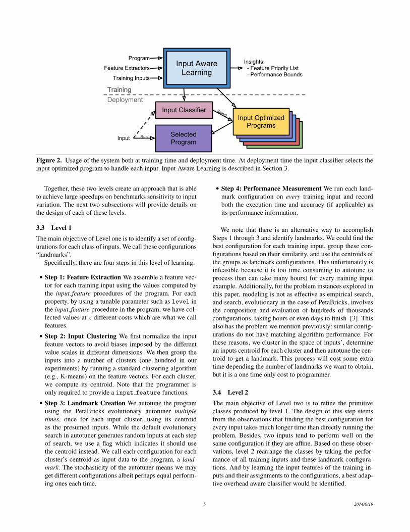
2.4 UsageFigure 2 describes the usage of our system for input sen-sitive algorithm design. At the first level, there is inputaware learning which takes the user’s program (containingalgorithmic choices), the feature extractors specified by theinput feature language keyword and input exemplars asinput. Input aware learning is described in Section 3. Theoutput of the learning is an input classifier and a set of inputoptimized programs, each of which has been optimized forspecific class of inputs.

When an arbitrary input is encountered in deployment,the classifier created by learning is used to select an inputoptimized program which is expected to perform the best onthis input. The classifier will use some (possibly variable)subset of the feature extractors available to it to probe theinput. Finally, the selected input optimized program willprocess the input and return the output to the user.

3. Input Aware LearningTo help motivate our self-refining approach, we will firstexplore existing solutions and their issues. The section willcontinue to explain the design and implementation of ourtechnique.

3.1 Existing Solutions and Their IssuesA straightforward way to construct an input classifier is viainput-based clustering. First, construct feature vectors forevery example input set with the input feature extractionprocedures encoded by the programmer. Then, cluster ex-amples based on the feature vectors. Next, find a good algo-rithmic configuration for each cluster’s centroid. For a new

input, the classifier first invokes the feature extraction proce-dures to compute its feature vector, based on which, it findsout what input cluster the new input belongs, and then runsthe configuration of that cluster on that new input. This de-sign has been used for addressing input sensitivity in pro-gram specialization and others [30]. However, applying it toalgorithmic autotuning raises three issues.

First, it fails to acknowledge that two input sets thatare similar may not have correspondingly similar configura-tions. As well, while there may be more than one configura-tion that suits an input set, but some will perform well on aninput set similar to it, while others will not. In other words,there is no direct correspondence between similar input fea-tures, similar configurations and/or similar algorithm perfor-mance (measured in execution speed and accuracy). Insteadthe relationships among input properties, configurations andprogram behavior are non-linear and complex. We call thisphenomena a mapping disparity. It implies that by assigningconfigurations based on the differences in input features, thesimple design is likely to assign an inferior configuration fornew input.

The second issue with the simple design is that it does notconsider the overhead in feature extraction on the new input.Due to the complexity in algorithmic choice, some featuresmay take a substantial time to extract. As the feature extrac-tion occurs on the critical path of the program execution, thesimple design may end up with a significant slowdown forthe introduced extra work.

The third issue is that even if the configuration found bythe simple classifier happens to provide the highest perfor-mance on that new input, its calculation accuracy may notmeet the requirement. It is unclear how the simple designcan handle accuracy-performance conflicts, a special com-plexity in algorithmic autotuning.

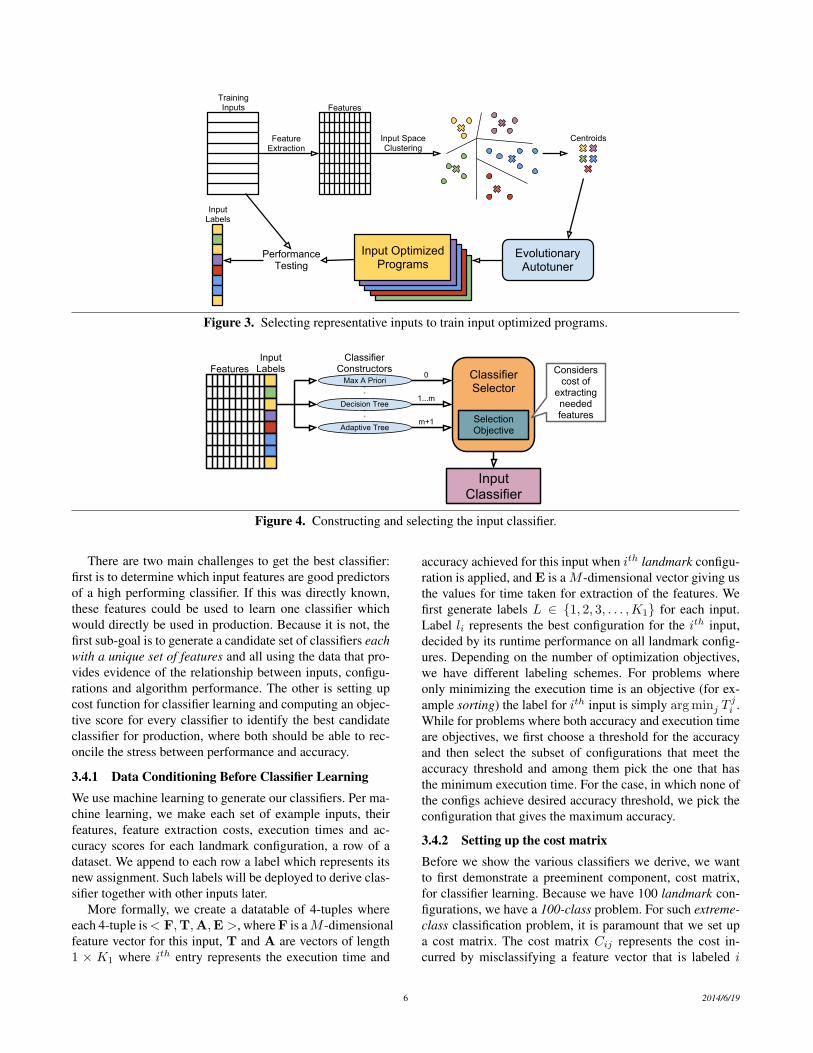
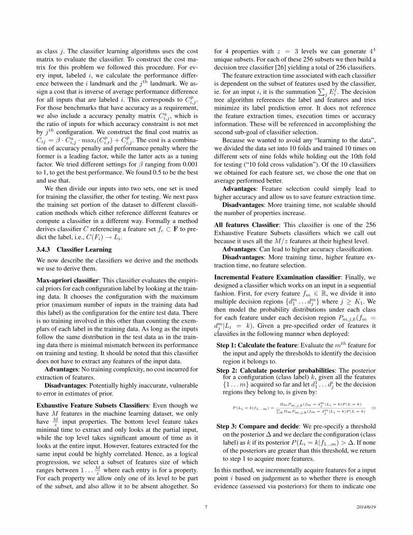
3.2 Self-Refining ApproachOur self-refining approach is divided into two levels. Thefirst level is shown in Figure 3. In its first step it clusters andgroups the input space into a finite number of input classesand then uses the autotuner to identify a optimized algorith-mic configuration for each cluster’s centroid. We call theseautotuned configurations landmarks. Next, it executes everytraining input using every landmark configuration. This isorder of magnitude faster than autotuning for every traininginput. These results will be used at the next level.

The second level is shown in Figure 4. It refines the primi-tive classes by interpreting the mapping evidence previouslycollected on the inputs and their performance on a small setof landmark configurations. It builds a large number of clas-sifiers each different by which input features it referencesand/or different by the algorithm used to derive the classifier.It then computes an objective score, incorporating both fea-ture extraction costs and predicted algorithm execution time,for every classifier and selects the best one as the productionclassifier.

4 2014/6/19

TrainingDeployment

Input Classifier

Input Aware Learning

Program

Training Inputs

Feature ExtractorsInsights: - Feature Priority List - Performance Bounds

Input

Select Input Optimized Programs

Training

Selected Program

Run

Figure 2. Usage of the system both at training time and deployment time. At deployment time the input classifier selects theinput optimized program to handle each input. Input Aware Learning is described in Section 3.

Together, these two levels create an approach that is ableto achieve large speedups on benchmarks sensitivity to inputvariation. The next two subsections will provide details onthe design of each of these levels.

3.3 Level 1The main objective of Level one is to identify a set of config-urations for each class of inputs. We call these configurations“landmarks”.

Specifically, there are four steps in this level of learning.

• Step 1: Feature Extraction We assemble a feature vec-tor for each training input using the values computed bythe input feature procedures of the program. For eachproperty, by using a tunable parameter such as level inthe input feature procedure in the program, we have col-lected values at z different costs which are what we callfeatures.• Step 2: Input Clustering We first normalize the input

feature vectors to avoid biases imposed by the differentvalue scales in different dimensions. We then group theinputs into a number of clusters (one hundred in ourexperiments) by running a standard clustering algorithm(e.g., K-means) on the feature vectors. For each cluster,we compute its centroid. Note that the programmer isonly required to provide a input feature functions.• Step 3: Landmark Creation We autotune the program

using the PetaBricks evolutionary autotuner multipletimes, once for each input cluster, using its centroidas the presumed inputs. While the default evolutionarysearch in autotuner generates random inputs at each stepof search, we use a flag which indicates it should usethe centroid instead. We call each configuration for eachcluster’s centroid as input data to the program, a land-mark. The stochasticity of the autotuner means we mayget different configurations albeit perhaps equal perform-ing ones each time.

• Step 4: Performance Measurement We run each land-mark configuration on every training input and recordboth the execution time and accuracy (if applicable) asits performance information.

We note that there is an alternative way to accomplishSteps 1 through 3 and identify landmarks. We could find thebest configuration for each training input, group these con-figurations based on their similarity, and use the centroids ofthe groups as landmark configurations. This unfortunately isinfeasible because it is too time consuming to autotune (aprocess than can take many hours) for every training inputexample. Additionally, for the problem instances explored inthis paper, modeling is not as effective as empirical search,and search, evolutionary in the case of PetaBricks, involvesthe composition and evaluation of hundreds of thousandsconfigurations, taking hours or even days to finish [3]. Thisalso has the problem we mention previously: similar config-urations do not have matching algorithm performance. Forthese reasons, we cluster in the space of inputs’, determinean inputs centroid for each cluster and then autotune the cen-troid to get a landmark. This process will cost some extratime depending the number of landmarks we want to obtain,but it is a one time only cost to programmer.

3.4 Level 2The main objective of Level two is to refine the primitiveclasses produced by level 1. The design of this step stemsfrom the observations that finding the best configuration forevery input takes much longer time than directly running theproblem. Besides, two inputs tend to perform well on thesame configuration if they are affine. Based on these obser-vations, level 2 rearrange the classes by taking the perfor-mance of all training inputs and these landmark configura-tions. And by learning the input features of the training in-puts and their assignments to the configurations, a best adap-tive overhead aware classifier would be identified.

5 2014/6/19

Feature Extraction

Input Space Clustering

Evolutionary Autotuner

Features

Input Optimized Programs

Centroids

Performance Testing

Training Inputs

Input Labels

Figure 3. Selecting representative inputs to train input optimized programs.

FeaturesInput

Labels

Decision Tree

Max A Priori

Adaptive Tree

Classifier Constructors

1...m

0

m+1

Classifier Selector

Selection Objective

Considers cost of

extracting needed features

Input Classifier

Figure 4. Constructing and selecting the input classifier.

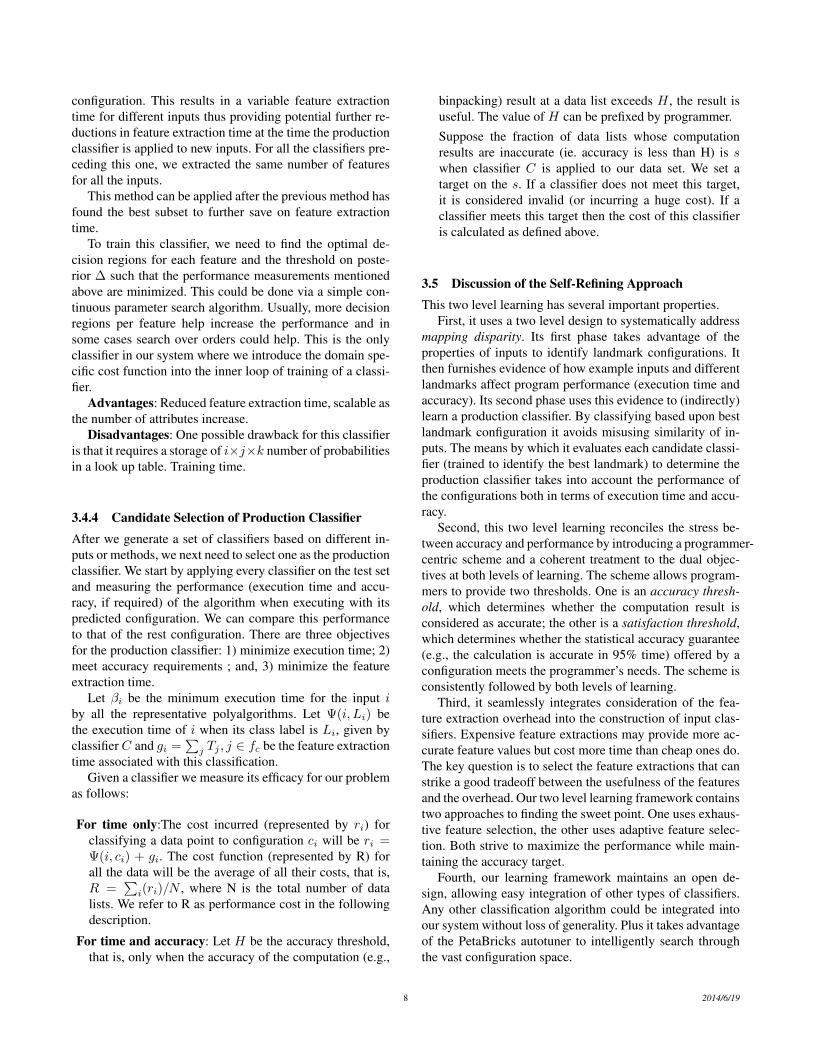
There are two main challenges to get the best classifier:first is to determine which input features are good predictorsof a high performing classifier. If this was directly known,these features could be used to learn one classifier whichwould directly be used in production. Because it is not, thefirst sub-goal is to generate a candidate set of classifiers eachwith a unique set of features and all using the data that pro-vides evidence of the relationship between inputs, configu-rations and algorithm performance. The other is setting upcost function for classifier learning and computing an objec-tive score for every classifier to identify the best candidateclassifier for production, where both should be able to rec-oncile the stress between performance and accuracy.

3.4.1 Data Conditioning Before Classifier LearningWe use machine learning to generate our classifiers. Per ma-chine learning, we make each set of example inputs, theirfeatures, feature extraction costs, execution times and ac-curacy scores for each landmark configuration, a row of adataset. We append to each row a label which represents itsnew assignment. Such labels will be deployed to derive clas-sifier together with other inputs later.

More formally, we create a datatable of 4-tuples whereeach 4-tuple is< F,T,A,E >, where F is aM -dimensionalfeature vector for this input, T and A are vectors of length1 × K1 where ith entry represents the execution time and

accuracy achieved for this input when ith landmark configu-ration is applied, and E is a M -dimensional vector giving usthe values for time taken for extraction of the features. Wefirst generate labels L ∈ {1, 2, 3, . . . ,K1} for each input.Label li represents the best configuration for the ith input,decided by its runtime performance on all landmark config-ures. Depending on the number of optimization objectives,we have different labeling schemes. For problems whereonly minimizing the execution time is an objective (for ex-ample sorting) the label for ith input is simply arg minj T

ji .

While for problems where both accuracy and execution timeare objectives, we first choose a threshold for the accuracyand then select the subset of configurations that meet theaccuracy threshold and among them pick the one that hasthe minimum execution time. For the case, in which none ofthe configs achieve desired accuracy threshold, we pick theconfiguration that gives the maximum accuracy.

3.4.2 Setting up the cost matrixBefore we show the various classifiers we derive, we wantto first demonstrate a preeminent component, cost matrix,for classifier learning. Because we have 100 landmark con-figurations, we have a 100-class problem. For such extreme-class classification problem, it is paramount that we set upa cost matrix. The cost matrix Cij represents the cost in-curred by misclassifying a feature vector that is labeled i

6 2014/6/19

as class j. The classifier learning algorithms uses the costmatrix to evaluate the classifier. To construct the cost ma-trix for this problem we followed this procedure. For ev-ery input, labeled i, we calculate the performance differ-ence between the i landmark and the jth landmark. We as-sign a cost that is inverse of average performance differencefor all inputs that are labeled i. This corresponds to Cp

i,j .For those benchmarks that have accuracy as a requirement,we also include a accuracy penalty matrix Ca

i,j , which isthe ratio of inputs for which accuracy constraint is not metby jth configuration. We construct the final cost matrix asCij = β · Ca

i,j · maxt(Cpi,t) + Cp

i,j . The cost is a combina-tion of accuracy penalty and performance penalty where theformer is a leading factor, while the latter acts as a tuningfactor. We tried different settings for β ranging from 0.001to 1, to get the best performance. We found 0.5 to be the bestand use that.

We then divide our inputs into two sets, one set is usedfor training the classifier, the other for testing. We next passthe training set portion of the dataset to different classifi-cation methods which either reference different features orcompute a classifier in a different way. Formally a methodderives classifier C referencing a feature set fc ⊂ F to pre-dict the label, i.e., C(Fi)→ Li.

3.4.3 Classifier LearningWe now describe the classifiers we derive and the methodswe use to derive them.

Max-apriori classifier: This classifier evaluates the empiri-cal priors for each configuration label by looking at the train-ing data. It chooses the configuration with the maximumprior (maximum number of inputs in the training data hadthis label) as the configuration for the entire test data. Thereis no training involved in this other than counting the exem-plars of each label in the training data. As long as the inputsfollow the same distribution in the test data as in the train-ing data there is minimal mismatch between its performanceon training and testing. It should be noted that this classifierdoes not have to extract any features of the input data.

Advantages: No training complexity, no cost incurred forextraction of features.

Disadvantages: Potentially highly inaccurate, vulnerableto error in estimates of prior.

Exhaustive Feature Subsets Classifiers: Even though wehave M features in the machine learning dataset, we onlyhave M

z input properties. The bottom level feature takesminimal time to extract and only looks at the partial input,while the top level takes significant amount of time as itlooks at the entire input. However, features extracted for thesame input could be highly correlated. Hence, as a logicalprogression, we select a subset of features size of whichranges between 1 . . . M

z where each entry is for a property.For each property we allow only one of its level to be partof the subset, and also allow it to be absent altogether. So

for 4 properties with z = 3 levels we can generate 44

unique subsets. For each of these 256 subsets we then build adecision tree classifier [26] yielding a total of 256 classifiers.

The feature extraction time associated with each classifieris dependent on the subset of features used by the classifier,ie. for an input i, it is the summation

∑j E

ji . The decision

tree algorithm references the label and features and triesminimize its label prediction error. It does not referencethe feature extraction times, execution times or accuracyinformation. These will be referenced in accomplishing thesecond sub-goal of classifier selection.

Because we wanted to avoid any “learning to the data”,we divided the data set into 10 folds and trained 10 times ondifferent sets of nine folds while holding out the 10th foldfor testing (“10 fold cross validation”). Of the 10 classifierswe obtained for each feature set, we chose the one that onaverage performed better.

Advantages: Feature selection could simply lead tohigher accuracy and allow us to save feature extraction time.

Disadvantages: More training time, not scalable shouldthe number of properties increase.

All features Classifier: This classifier is one of the 256Exhaustive Feature Subsets classifiers which we call outbecause it uses all the M/z features at their highest level.

Advantages: Can lead to higher accuracy classification.Disadvantages: More training time, higher feature ex-

traction time, no feature selection.

Incremental Feature Examination classifier: Finally, wedesigned a classifier which works on an input in a sequentialfashion. First, for every feature fm ∈ R, we divide it intomultiple decision regions {dm

1 . . . dmj } where j ≥ K1. We

then model the probability distributions under each classfor each feature under each decision region Pm,j,k(fm =dm

j |Li = k). Given a pre-specified order of features itclassifies in the following manner when deployed:

Step 1: Calculate the feature: Evaluate themth feature forthe input and apply the thresholds to identify the decisionregion it belongs to.

Step 2: Calculate posterior probabilities: The posteriorfor a configuration (class label) k, given all the features{1 . . .m} acquired so far and let d1

1 . . . dij be the decision

regions they belong to, is given by:

P (Li = k|f1...m) =ΠmPm,j,k(fm = dm

j |Li = k)P (L = k)∑k ΠmPm,j,k(fm = dm

j|Li = k)P (L = k)

(1)

Step 3: Compare and decide: We pre-specify a thresholdon the posterior ∆ and we declare the configuration (classlabel) as k if its posterior P (Li = k|f1...m) > ∆. If noneof the posteriors are greater than this threshold, we returnto step 1 to acquire more features.

In this method, we incrementally acquire features for a inputpoint i based on judgement as to whether there is enoughevidence (assessed via posteriors) for them to indicate one

7 2014/6/19

configuration. This results in a variable feature extractiontime for different inputs thus providing potential further re-ductions in feature extraction time at the time the productionclassifier is applied to new inputs. For all the classifiers pre-ceding this one, we extracted the same number of featuresfor all the inputs.

This method can be applied after the previous method hasfound the best subset to further save on feature extractiontime.

To train this classifier, we need to find the optimal de-cision regions for each feature and the threshold on poste-rior ∆ such that the performance measurements mentionedabove are minimized. This could be done via a simple con-tinuous parameter search algorithm. Usually, more decisionregions per feature help increase the performance and insome cases search over orders could help. This is the onlyclassifier in our system where we introduce the domain spe-cific cost function into the inner loop of training of a classi-fier.

Advantages: Reduced feature extraction time, scalable asthe number of attributes increase.

Disadvantages: One possible drawback for this classifieris that it requires a storage of i×j×k number of probabilitiesin a look up table. Training time.

3.4.4 Candidate Selection of Production ClassifierAfter we generate a set of classifiers based on different in-puts or methods, we next need to select one as the productionclassifier. We start by applying every classifier on the test setand measuring the performance (execution time and accu-racy, if required) of the algorithm when executing with itspredicted configuration. We can compare this performanceto that of the rest configuration. There are three objectivesfor the production classifier: 1) minimize execution time; 2)meet accuracy requirements ; and, 3) minimize the featureextraction time.

Let βi be the minimum execution time for the input iby all the representative polyalgorithms. Let Ψ(i, Li) bethe execution time of i when its class label is Li, given byclassifierC and gi =

∑j Tj , j ∈ fc be the feature extraction

time associated with this classification.Given a classifier we measure its efficacy for our problem

as follows:

For time only:The cost incurred (represented by ri) forclassifying a data point to configuration ci will be ri =Ψ(i, ci) + gi. The cost function (represented by R) forall the data will be the average of all their costs, that is,R =

∑i(ri)/N , where N is the total number of data

lists. We refer to R as performance cost in the followingdescription.

For time and accuracy: Let H be the accuracy threshold,that is, only when the accuracy of the computation (e.g.,

binpacking) result at a data list exceeds H , the result isuseful. The value of H can be prefixed by programmer.Suppose the fraction of data lists whose computationresults are inaccurate (ie. accuracy is less than H) is swhen classifier C is applied to our data set. We set atarget on the s. If a classifier does not meet this target,it is considered invalid (or incurring a huge cost). If aclassifier meets this target then the cost of this classifieris calculated as defined above.

3.5 Discussion of the Self-Refining ApproachThis two level learning has several important properties.

First, it uses a two level design to systematically addressmapping disparity. Its first phase takes advantage of theproperties of inputs to identify landmark configurations. Itthen furnishes evidence of how example inputs and differentlandmarks affect program performance (execution time andaccuracy). Its second phase uses this evidence to (indirectly)learn a production classifier. By classifying based upon bestlandmark configuration it avoids misusing similarity of in-puts. The means by which it evaluates each candidate classi-fier (trained to identify the best landmark) to determine theproduction classifier takes into account the performance ofthe configurations both in terms of execution time and accu-racy.

Second, this two level learning reconciles the stress be-tween accuracy and performance by introducing a programmer-centric scheme and a coherent treatment to the dual objec-tives at both levels of learning. The scheme allows program-mers to provide two thresholds. One is an accuracy thresh-old, which determines whether the computation result isconsidered as accurate; the other is a satisfaction threshold,which determines whether the statistical accuracy guarantee(e.g., the calculation is accurate in 95% time) offered by aconfiguration meets the programmer’s needs. The scheme isconsistently followed by both levels of learning.

Third, it seamlessly integrates consideration of the fea-ture extraction overhead into the construction of input clas-sifiers. Expensive feature extractions may provide more ac-curate feature values but cost more time than cheap ones do.The key question is to select the feature extractions that canstrike a good tradeoff between the usefulness of the featuresand the overhead. Our two level learning framework containstwo approaches to finding the sweet point. One uses exhaus-tive feature selection, the other uses adaptive feature selec-tion. Both strive to maximize the performance while main-taining the accuracy target.

Fourth, our learning framework maintains an open de-sign, allowing easy integration of other types of classifiers.Any other classification algorithm could be integrated intoour system without loss of generality. Plus it takes advantageof the PetaBricks autotuner to intelligently search throughthe vast configuration space.

8 2014/6/19

4. EvaluationTo measure the efficacy of our system we tested it on a suiteof 6 parallel PetaBricks benchmarks [5]. Of these bench-marks 1 requires fixed accuracy and 5 require variable accu-racy. Each of these benchmarks was modified to add featureextractors for their inputs and a richer set of input generatorsto exercise these features. Each feature extractor was set to 3different sampling levels providing more accurate measure-ments at increasing costs. Tests were conducted on a 32-core(8 × 4-sockets) Xeon X7550 system running GNU/Linux(Debian 6.0.6).

We use two primary baselines to provide both a lowerbound of performance without input adaptation and an up-per bound of the limits of input adaption. Neither baselineincludes (or requires) any feature extraction costs.

• Static oracle uses a single configuration for all inputs.This configuration is selected by trying each input opti-mized program configuration and picking the one withthe best performance. The static oracle is the perfor-mance that would be obtained by not using our systemand instead using an autotuner without input adaptation.In practice the static oracle may be better than some of-fline autotuners, because such autotuners may train onnon-representative sets of inputs.• Dynamic oracle uses the best configuration for each in-

put. It is the lower bound of the best possible performancethat can be obtained by our input classifier. It is equiva-lent to a classifier that always picks the best optimizedprogram and requires no features to do so. We allow thedynamic oracle to miss the accuracy target on up to 10%of the inputs, to match the selection criteria of the inputclassifier.

4.1 BenchmarksWe use the following 6 benchmarks to evaluate our results.

Sort The sort benchmark sorts a list of doubles using eitherInsertionSort, QuickSort, MergeSort, or BitonicSort. Themerge sort has a variable number of ways and has choicesto construct a parallel merge sort polyalgorithm. Sort is theonly non-variable accuracy benchmark shown. Input vari-ability comes from different algorithms having fast and slowinputs, for example QuickSort has pathological input casesand InsertionSort is good on mostly-sorted lists. For inputfeatures we use standard deviation, duplication, sortedness,and the performance of a test sort on a subsequence of thelist.

Sort1 results are sorting real-world inputs taken from theCentral Contractor Registration (CCR) FOIA Extract, whichlists all government contractors available under FOIA fromdata.gov. Sort2 results are sorting synthetic inputs generatedfrom a collection of input generators meant to span the spaceof features.

Clustering The clustering benchmark assigns points in 2Dcoordinate space to clusters. It uses a variant of the kmeansalgorithm with choices of either random, prefix, or center-plus initial conditions. The number of clusters (k) and thenumber of iterations of the kmeans algorithm are both setby the autotuner. The accuracy metric compares the sum ofdistances squared to cluster centers to a canonical clusteringalgorithm. Clustering uses input the features: radius, centers,density, and range.

Clustering1 results are clustering real-world inputs takenfrom the Poker Hand Data Set from UCI machine learningrepository. Clustering2 results are clustering synthetic inputsgenerated from a collection of input generators meant tospan the space of features.

Bin Packing Bin packing is a classic NP-hard problemwhere the goal of the algorithm is to find an assignmentof items to unit sized bins such that the number of binsused is minimized, no bin is above capacity, and all itemsare assigned to a bin. The bin packing benchmark con-tains choices for 13 individual approximation algorithms:AlmostWorstFit, AlmostWorstFitDecreasing, BestFit, Best-FitDecreasing, FirstFit, FirstFitDecreasing, LastFit, LastFit-Decreasing, ModifiedFirstFitDecreasing, NextFit, NextFit-Decreasing, WorstFit, and WorstFitDecreasing. Bin packingcontains 4 input feature extractors: average, standard devia-tion, value range, and sortedness.

Singular Value Decomposition The SVD benchmark at-tempts to approximate a matrix using less space through Sin-gular Value Decomposition (SVD). For any m× n real ma-trix A with m ≥ n, the SVD of A is A = UΣV T . Thecolumns ui of the matrix U , the columns vi of V , and thediagonal values σi of Σ (singular values) form the best rank-k approximation of A, given by Ak =

∑ki=1 σiuiv

Ti . Only

the first k columns of U and V and the first k singular valuesσi need to be stored to reconstruct the matrix approximately.The choices for the benchmark include varying the numberof eigenvalues used and changing the techniques used to findthese eigenvalues. The accuracy metric used is the ratio be-tween the RMS error of the initial guess (the zero matrix) tothe RMS error of the output compared with the input matrixA, converted to log-scale. For input features we used range,the standard deviation of the input, and a count of zeros inthe input.

Poisson 2D The 2D Poisson’s equation is an elliptic par-tial differential equation that describes heat transfer, electro-statics, fluid dynamics, and various other engineering disci-plines. The choices in this benchmark are multigrid, wherecycle shapes are determined by the autotuner, and a num-ber of iterative and direct solvers. As an accuracy metric, weused the ratio between the root mean squared (RMS) error ofthe initial guess fed into the algorithm and the RMS error ofthe guess afterwards. For input features we used the residual

9 2014/6/19

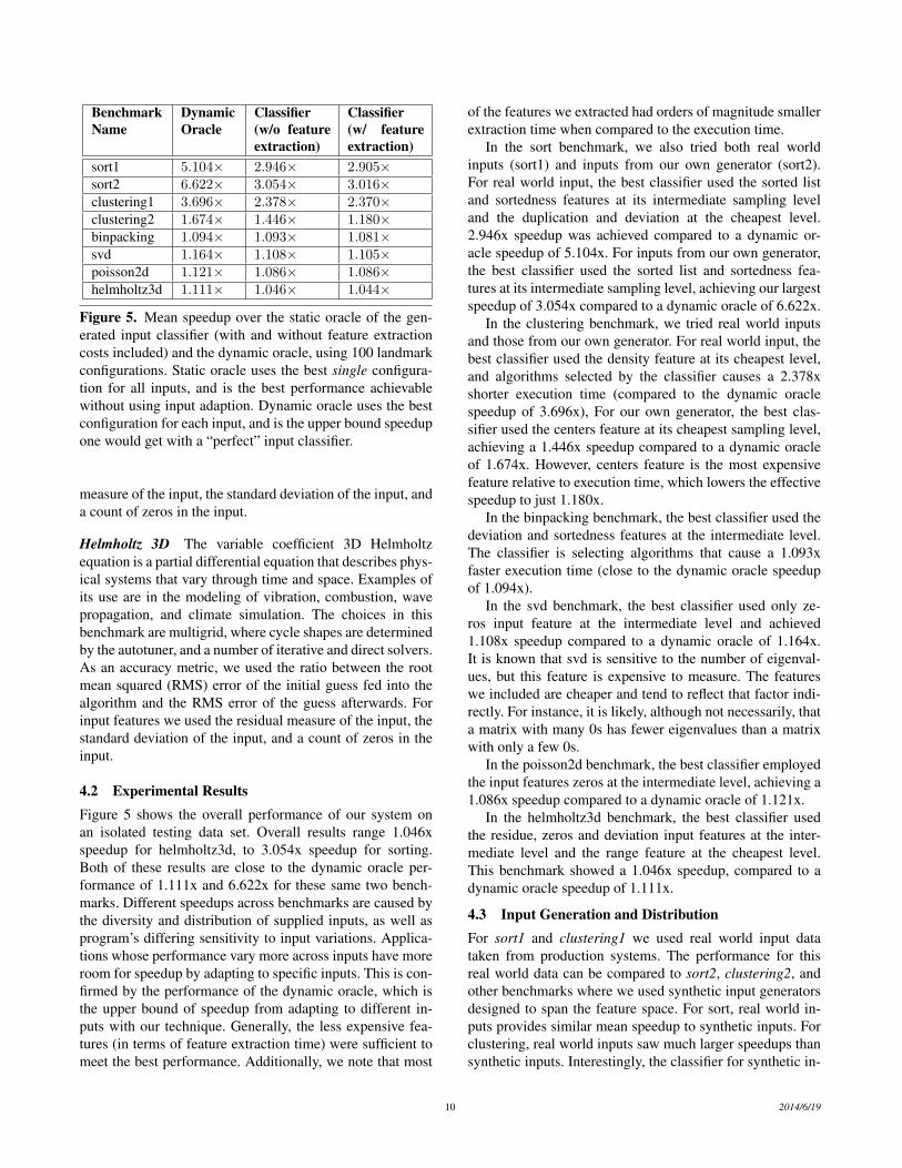
BenchmarkName

DynamicOracle

Classifier(w/o featureextraction)

Classifier(w/ featureextraction)

sort1 5.104× 2.946× 2.905×sort2 6.622× 3.054× 3.016×clustering1 3.696× 2.378× 2.370×clustering2 1.674× 1.446× 1.180×binpacking 1.094× 1.093× 1.081×svd 1.164× 1.108× 1.105×poisson2d 1.121× 1.086× 1.086×helmholtz3d 1.111× 1.046× 1.044×

Figure 5. Mean speedup over the static oracle of the gen-erated input classifier (with and without feature extractioncosts included) and the dynamic oracle, using 100 landmarkconfigurations. Static oracle uses the best single configura-tion for all inputs, and is the best performance achievablewithout using input adaption. Dynamic oracle uses the bestconfiguration for each input, and is the upper bound speedupone would get with a “perfect” input classifier.

measure of the input, the standard deviation of the input, anda count of zeros in the input.

Helmholtz 3D The variable coefficient 3D Helmholtzequation is a partial differential equation that describes phys-ical systems that vary through time and space. Examples ofits use are in the modeling of vibration, combustion, wavepropagation, and climate simulation. The choices in thisbenchmark are multigrid, where cycle shapes are determinedby the autotuner, and a number of iterative and direct solvers.As an accuracy metric, we used the ratio between the rootmean squared (RMS) error of the initial guess fed into thealgorithm and the RMS error of the guess afterwards. Forinput features we used the residual measure of the input, thestandard deviation of the input, and a count of zeros in theinput.

4.2 Experimental ResultsFigure 5 shows the overall performance of our system onan isolated testing data set. Overall results range 1.046xspeedup for helmholtz3d, to 3.054x speedup for sorting.Both of these results are close to the dynamic oracle per-formance of 1.111x and 6.622x for these same two bench-marks. Different speedups across benchmarks are caused bythe diversity and distribution of supplied inputs, as well asprogram’s differing sensitivity to input variations. Applica-tions whose performance vary more across inputs have moreroom for speedup by adapting to specific inputs. This is con-firmed by the performance of the dynamic oracle, which isthe upper bound of speedup from adapting to different in-puts with our technique. Generally, the less expensive fea-tures (in terms of feature extraction time) were sufficient tomeet the best performance. Additionally, we note that most

of the features we extracted had orders of magnitude smallerextraction time when compared to the execution time.

In the sort benchmark, we also tried both real worldinputs (sort1) and inputs from our own generator (sort2).For real world input, the best classifier used the sorted listand sortedness features at its intermediate sampling leveland the duplication and deviation at the cheapest level.2.946x speedup was achieved compared to a dynamic or-acle speedup of 5.104x. For inputs from our own generator,the best classifier used the sorted list and sortedness fea-tures at its intermediate sampling level, achieving our largestspeedup of 3.054x compared to a dynamic oracle of 6.622x.

In the clustering benchmark, we tried real world inputsand those from our own generator. For real world input, thebest classifier used the density feature at its cheapest level,and algorithms selected by the classifier causes a 2.378xshorter execution time (compared to the dynamic oraclespeedup of 3.696x), For our own generator, the best clas-sifier used the centers feature at its cheapest sampling level,achieving a 1.446x speedup compared to a dynamic oracleof 1.674x. However, centers feature is the most expensivefeature relative to execution time, which lowers the effectivespeedup to just 1.180x.

In the binpacking benchmark, the best classifier used thedeviation and sortedness features at the intermediate level.The classifier is selecting algorithms that cause a 1.093xfaster execution time (close to the dynamic oracle speedupof 1.094x).

In the svd benchmark, the best classifier used only ze-ros input feature at the intermediate level and achieved1.108x speedup compared to a dynamic oracle of 1.164x.It is known that svd is sensitive to the number of eigenval-ues, but this feature is expensive to measure. The featureswe included are cheaper and tend to reflect that factor indi-rectly. For instance, it is likely, although not necessarily, thata matrix with many 0s has fewer eigenvalues than a matrixwith only a few 0s.

In the poisson2d benchmark, the best classifier employedthe input features zeros at the intermediate level, achieving a1.086x speedup compared to a dynamic oracle of 1.121x.

In the helmholtz3d benchmark, the best classifier usedthe residue, zeros and deviation input features at the inter-mediate level and the range feature at the cheapest level.This benchmark showed a 1.046x speedup, compared to adynamic oracle speedup of 1.111x.

4.3 Input Generation and DistributionFor sort1 and clustering1 we used real world input datataken from production systems. The performance for thisreal world data can be compared to sort2, clustering2, andother benchmarks where we used synthetic input generatorsdesigned to span the feature space. For sort, real world in-puts provides similar mean speedup to synthetic inputs. Forclustering, real world inputs saw much larger speedups thansynthetic inputs. Interestingly, the classifier for synthetic in-

10 2014/6/19

1 500001

10

20

Inputs

Spe

edup

(a) sort1

1 500001

50

100

Inputs

Spe

edup

(b) sort2

1 500001

50

100

Inputs

Spe

edup

(c) clustering1

1 500001

4

7

Inputs

Spe

edup

(d) clustering2

1 500001

2

3

4

Inputs

Spe

edup

(e) binpacking

1 500001

2

3

Inputs

Spe

edup

(f) svd

1 500001

2

Inputs

Spe

edup

(g) poisson2d

1 500001

2

5

Inputs

Spe

edup

(h) helmholtz3d

Figure 6. Distribution of speedups over static oracle for each individual input. For each problem, some individual inputs getmuch larger speedups than the mean.

1 100

1

3

5

Landmarks

Spe

edup

(a) sort1

1 100

1

3

5

Landmarks

Spe

edup

(b) sort2

1 100

2

3

Landmarks

Spe

edup

(c) clustering1

1 100

0.5

1.5

Landmarks

Spe

edup

(d) clustering2

1 100

1

1.05

Landmarks

Spe

edup

(e) binpacking

1 100

0.9

1.1

Landmarks

Spe

edup

(f) svd

1 100

0.9

1.2

Landmarks

Spe

edup

(g) poisson2d

1 100

0.8

1.0

Landmarks

Spe

edup

(h) helmholtz3d

Figure 8. Measured speedup over static oracle as the number of landmark configurations changes, using 1000 random subsetsof the 100 landmarks used in other results. Error bars show median, first quartiles, third quartiles, min, and max.

puts in clustering needs to use a much more expensive setof input features because the classes of inputs are harder todistinguish.

To have a better idea of the origin of different speedup,not only among benchmarks, but also for the same bench-mark, but different input sources. We further investigate thedistribution of speedups for individual inputs to each pro-gram, sorted such that the largest speedup is on the right,showed in Figure 6. What is interesting here is the speedupsare not uniform. For each benchmark there exist small setsof inputs with very large speedups, in some cases up to 90x.

This shows that way inputs are chosen can have a large ef-fect on mean speedup observed. If one had a real world in-put distribution that favored these types of inputs the over-all speedup of this technique would be much larger. In otherwords, the relative benefits of using of input adaptation tech-niques can vary drastically depending on your input data dis-tribution.

11 2014/6/19

0 0.2 0.4 0.6 0.8 1

Lost

spe

edup

(L)

Size of region (pi)

2 configs3 configs4 configs5 configs6 configs7 configs8 configs9 configs

(a) Predicted loss in speedup contributed by input space regionsof different sizes.

10 20 30 40 50 60 70 80 90 100

Spe

edup

Landmarks

(b) Predicted speedup with a worst-case region size with differentnumbers of sampled landmark configurations.

Figure 7. Model predicted speedup compared to samplingall input points as the number of landmarks are increated. Y-axis units are omitted because the problem-specific scalingterm in the model is unknown.

4.4 Theoretical Model Showing Diminishing Returnswith More Landmark Configurations

In addition to the evaluation of our classifier performanceit is important to evaluate if our methodology of clusteringand using 100 landmark configurations is sufficient. To helpgain insight into this question we created a theoretical modelwhere we consider the input search space of a programwhere some finite number of optimal program configurationsdominate different subsets of the input space. For each ofthese dominate configurations, we define the values pi andsi, where pi is fraction of the inputs in the search spacewhere this configuration dominates and si is the speedup onthese configurations obtained by training a configuration forany of the inputs where this configuration dominates. Themodel assumes that no speedup is obtained if one of thesepoints is not sampled. We also assume that all inputs haveequal cost before the speedups are applied, to avoid the needfor weighting terms.

If we assume the k landmark configurations are sampleduniform randomly (which is likely a worse technique thanour actual clustering) the total expected loss in speedup, L,compared to a perfect method that sampled all points would

be:L =

∑i

(1− pi)kpisi

Where (1 − pi)k represents the chance of “missing” theregion of the search space where configuration i is optimaland pisi represents the cost of missing that region of thesearch space in terms of speedup.

Figure 7(a) shows the value of this function for a sin-gle region as pi changes. One can see that on the extremespi = 0 and pi = 1 there is no loss in speedup, because eitherthe region is so small a speedup in that region does not mat-ter or the region is so large that random sampling is likely tofind it. For each number of configs, there exists a worst-caseregion size where the expected loss in speedup is maximized.We can find this worst-case region size by solving for pi indLdpi

= 0 which results in a worst-case pi = 1k+1 . Using this

worst-case region size, Figure 7(b) shows the diminishingreturns predicted by our model as more landmark configura-tions are sampled. Figure 8 validates this theoretical modelby running each benchmark with varying numbers of land-mark configurations. This experiment takes random subsetsof the 100 landmarks used in other results and measures thatspeedup over the static oracle. Real benchmarks show a sim-ilar trend of diminishing returns with more landmarks that ispredicted by our model. We believe that this is strong evi-dence that using a fixed number of landmark configurations(e.g., 10 to 30 for the benchmarks we tested) suffices in prac-tice, however correct number of landmarks needed may varybetween benchmarks.

5. Related WorkA number of studies have considered program inputs in li-brary constructions [9, 12, 19, 24, 29, 35]. They concentrateon some specific library functions (e.g., FFT, sorting) whilethe algorithmic choices in these studies are limited. Tianand others have proposed an input-centric framework [30]for dynamic program optimizations and showed the bene-fits in enhancing Just-In-Time compilation. Jung and othershave considered inputs when selecting the appropriate datastructures to use [20]. Several recent studies have exploredthe influence of program inputs on GPU program optimiza-tions [22, 27].

This current study is unique in focusing on input sensitiv-ity to complex algorithmic autotuning, which features vastalgorithmic configuration spaces, sensitivity to deep inputfeatures, variable accuracy, and complex relations betweeninputs and configurations. These special challenges promptthe development of the novel solutions described in this pa-per.

A number of offline empirical autotuning frameworkshave been developed for building efficient, portable librariesin specific domains. ATLAS [34] utilizes empirical autotun-ing to produce a cache-contained matrix multiply, which isthen used in larger matrix computations in BLAS and LA-

12 2014/6/19

PACK. FFTW [13] uses empirical autotuning to combinesolvers for FFTs. Other autotuning systems include SPAR-SITY [18] for sparse matrix computations, SPIRAL [25] fordigital signal processing, and OSKI [33] for sparse matrixkernels.

The area of iterative compilation contains many projectsthat use different machine learning techniques to optimizelower level compiler optimizations [1, 2, 14, 23]. Theseprojects change both the order that compiler passes are ap-plied and the types of passes that are applied. PetaBricks [3]offers a language support to better leverage the power of au-totuning for complex algorithmic choices. However, none ofthese projects have systematically explored the influence ofprogram inputs beyond data size or dimension.

In the dynamic autotuning space, there have been a num-ber of systems developed [7, 8, 10, 16, 17, 21, 28] thatfocus on creating applications that can monitor and auto-matically tune themselves to optimize a particular objective.Many of these systems employ a control systems based auto-tuner that operates on a linear model of the application beingtuned. For example, PowerDial [17] converts static configu-ration parameters that already exist in a program into dy-namic knobs that can be tuned at runtime, with the goal oftrading QoS guarantees for meeting performance and powerusage goals. The system uses an offline learning stage toconstruct a linear model of the choice configuration spacewhich can be subsequently tuned using a linear control sys-tem. The system employs the heartbeat framework [15] toprovide feedback to the control system. A similar techniqueis employed in [16], where a simpler heuristic-based con-troller dynamically adjusts the degree of loop perforationperformed on a target application to trade QoS for perfor-mance. The principle theme of these studies is to react todynamic changes in the system behavior rather than proac-tively adapt algorithm configurations based on the character-istics of program inputs.

Additionally, there has been a large amount of work [6,11, 31, 32] in the dynamic optimization space, where in-formation available at runtime is used combined with staticcompilation techniques to generate higher performing code.Such dynamic optimizations differ from dynamic autotuningbecause each of the optimizations is hand crafted in a waythat makes it likely lead to an improvement of performancewhen applied. Conversely, autotuning searches the space ofmany available program variations without a priori knowl-edge of which configurations will perform better.

6. ConclusionsWe have shown a self-refining solution to the problem ofinput sensitivity in autotuning that, first, clusters to find in-put sets that are similar in the multi-dimensional propertyspace and uses an evolutionary autotuner to build an opti-mized program each of these clusters, and then builds anadaptive overhead aware classifier which assigns each in-

put to a specific input optimized program. This provides ageneral means of automatically determining what algorith-mic optimization to use when different optimization strate-gies suit different inputs. Though this work, we are able toextract principles for understanding the performance and ac-curacy space of a program across a variety of inputs, andachieve speedups of up to 3x.

While at first input sensitivity seems to be excessivelycomplicated issue where one must deal with large optimiza-tion spaces and complex input spaces, we show that inputsensitivity can be handled with simple extensions to an exist-ing autotuning system. We also showed that there are funda-mental diminishing returns as more and more input adapta-tion is added to a system and that a little bit of input adaptioncan go a long way.

References[1] F. Agakov, E. Bonilla, J. Cavazos, B. Franke, G. Fursin,

M. F. P. O’boyle, J. Thomson, M. Toussaint, and C. K. I.Williams. Using machine learning to focus iterative optimiza-tion. In International Symposium on Code Generation andOptimization, pages 295–305, 2006.

[2] L. Almagor, K. D. Cooper, A. Grosul, T. J. Harvey, S. W.Reeves, D. Subramanian, L. Torczon, and T. Waterman. Find-ing effective compilation sequences. In LCTES’04, pages231–239, 2004.

[3] J. Ansel, C. Chan, Y. L. Wong, M. Olszewski, Q. Zhao,A. Edelman, and S. Amarasinghe. PetaBricks: A languageand compiler for algorithmic choice. In PLDI, Dublin, Ire-land, Jun 2009.

[4] J. Ansel, M. Pacula, S. Amarasinghe, and U.-M. O’Reilly.An efficient evolutionary algorithm for solving bottom upproblems. In Annual Conference on Genetic and EvolutionaryComputation, Dublin, Ireland, July 2011.

[5] J. Ansel, Y. L. Wong, C. Chan, M. Olszewski, A. Edelman,and S. Amarasinghe. Language and compiler support for auto-tuning variable-accuracy algorithms. In CGO, Chamonix,France, Apr 2011.

[6] J. Auslander, M. Philipose, C. Chambers, S. J. Eggers, andB. N. Bershad. Fast, effective dynamic compilation. In PLDI,1996.

[7] W. Baek and T. Chilimbi. Green: A framework for supportingenergy-conscious programming using controlled approxima-tion. In PLDI, June 2010.

[8] V. Bhat, M. Parashar, . Hua Liu, M. Khandekar, N. Kan-dasamy, and S. Abdelwahed. Enabling self-managing appli-cations using model-based online control strategies. In Inter-national Conference on Autonomic Computing, Washington,DC, 2006.

[9] J. Bilmes, K. Asanovic, C.-W. Chin, and J. Demmel. Op-timizing matrix multiply using PHiPAC: A portable, high-performance, ANSI C coding methodology. In Proceedings ofthe ACM International Conference on Supercomputing, pages340–347, 1997.

13 2014/6/19

[10] F. Chang and V. Karamcheti. A framework for automaticadaptation of tunable distributed applications. Cluster Com-puting, 4, March 2001.

[11] P. C. Diniz and M. C. Rinard. Dynamic feedback: an effectivetechnique for adaptive computing. In PLDI, New York, NY,1997.

[12] M. Frigo and S. G. Johnson. The design and implementationof FFTW3. Proceedings of the IEEE, 93(2):216–231, 2005.

[13] M. Frigo and S. G. Johnson. The design and implementationof FFTW3. IEEE, 93(2), February 2005. Invited paper, specialissue on “Program Generation, Optimization, and PlatformAdaptation”.

[14] G. Fursin, C. Miranda, O. Temam, M. Namolaru, E. Yom-Tov,A. Zaks, B. Mendelson, E. Bonilla, J. Thomson, H. Leather,C. Williams, M. O’Boyle, P. Barnard, E. Ashton, E. Courtois,and F. Bodin. MILEPOST GCC: machine learning basedresearch compiler. In Proceedings of the GCC Developers’Summit, Jul 2008.

[15] H. Hoffmann, J. Eastep, M. D. Santambrogio, J. E. Miller,and A. Agarwal. Application heartbeats: a generic interfacefor specifying program performance and goals in autonomouscomputing environments. In ICAC, New York, NY, 2010.

[16] H. Hoffmann, S. Misailovic, S. Sidiroglou, A. Agarwal, andM. Rinard. Using code perforation to improve performance,reduce energy consumption, and respond to failures. Tech-nical Report MIT-CSAIL-TR-2209-042, Massachusetts Insti-tute of Technology, Sep 2009.

[17] H. Hoffmann, S. Sidiroglou, M. Carbin, S. Misailovic,A. Agarwal, and M. Rinard. Power-aware computing withdynamic knobs. In ASPLOS, 2011.

[18] E. Im and K. Yelick. Optimizing sparse matrix computationsfor register reuse in SPARSITY. In International Conferenceon Computational Science, 2001.

[19] E.-J. Im, K. Yelick, and R. Vuduc. Sparsity: Optimizationframework for sparse matrix kernels. Int. J. High Perform.Comput. Appl., 18(1):135–158, 2004.

[20] C. Jung, S. Rus, B. P. Railing, N. Clark, and S. Pande. Brainy:effective selection of data structures. In Proceedings of the32nd ACM SIGPLAN conference on Programming languagedesign and implementation, PLDI ’11, pages 86–97, NewYork, NY, USA, 2011. ACM.

[21] G. Karsai, A. Ledeczi, J. Sztipanovits, G. Peceli, G. Simon,and T. Kovacshazy. An approach to self-adaptive softwarebased on supervisory control. In International Workshop inSelf-adaptive software, 2001.

[22] Y. Liu, E. Z. Zhang, and X. Shen. A cross-input adaptiveframework for gpu programs optimization. In Proceedings ofInternational Parallel and Distribute Processing Symposium(IPDPS), pages 1–10, 2009.

[23] E. Park, L.-N. Pouche, J. Cavazos, A. Cohen, and P. Sadayap-pan. Predictive modeling in a polyhedral optimization space.In IEEE/ACM International Symposium on Code Generationand Optimization, pages 119 –129, April 2011.

[24] M. Puschel, J. Moura, J. Johnson, D. Padua, M. Veloso,B. Singer, J. Xiong, F. Franchetti, A. Gacic, Y. Voronenko,K. Chen, R. Johnson, and N. Rizzolo. SPIRAL: code genera-

tion for DSP transforms. Proceedings of the IEEE, 93(2):232–275, 2005.

[25] M. Puschel, J. M. F. Moura, B. Singer, J. Xiong, J. R. Johnson,D. A. Padua, M. M. Veloso, and R. W. Johnson. Spiral: Agenerator for platform-adapted libraries of signal processingalogorithms. IJHPCA, 18(1), 2004.

[26] J. Quinlan. Induction of decision trees. Machine learning,1(1):81–106, 1986.

[27] M. Samadi, A. Hormati, M. Mehrara, J. Lee, and S. Mahlke.Adaptive input-aware compilation for graphics engines. InProceedings of ACM SIGPLAN 2012 Conference on Program-ming Language Design and Implementation, 2012.

[28] C. Tapus, I.-H. Chung, and J. K. Hollingsworth. Active har-mony: Towards automated performance tuning. In In Proceed-ings from the Conference on High Performance Networkingand Computing, pages 1–11, 2003.

[29] N. Thomas, G. Tanase, O. Tkachyshyn, J. Perdue, N. M. Am-ato, and L. Rauchwerger. A framework for adaptive algorithmselection in STAPL. In Proceedings of the Tenth ACM SIG-PLAN Symposium on Principles and Practice of Parallel Pro-gramming, pages 277–288, 2005.

[30] K. Tian, Y. Jiang, E. Zhang, and X. Shen. An input-centricparadigm for program dynamic optimizations. In the Confer-ence on Object-Oriented Programming, Systems, Languages,and Applications (OOPSLA), 2010.

[31] M. Voss and R. Eigenmann. Adapt: Automated de-coupledadaptive program transformation. In International Conferenceon Parallel Processing, 2000.

[32] M. Voss and R. Eigenmann. High-level adaptive program op-timization with adapt. ACM SIGPLAN Notices, 36(7), 2001.

[33] R. Vuduc, J. W. Demmel, and K. A. Yelick. OSKI: A libraryof automatically tuned sparse matrix kernels. In ScientificDiscovery through Advanced Computing Conference, Journalof Physics: Conference Series, San Francisco, CA, June 2005.

[34] R. C. Whaley and J. J. Dongarra. Automatically tuned linearalgebra software. In Supercomputing, Washington, DC, 1998.

[35] R. C. Whaley, A. Petitet, and J. Dongarra. Automated empiri-cal optimizations of software and the ATLAS project. ParallelComputing, 27(1-2):3–35, 2001.

14 2014/6/19