This content has been downloaded from IOPscience. Please scroll down to see the full text.

Download details:

IP Address: 93.180.53.211

This content was downloaded on 02/01/2014 at 13:54

Please note that terms and conditions apply.

Sensitivity map generation in electrical capacitance tomography using mixed normalization

models

View the table of contents for this issue, or go to the journal homepage for more

2007 Meas. Sci. Technol. 18 2092

(http://iopscience.iop.org/0957-0233/18/7/040)

Home Search Collections Journals About Contact us My IOPscience

IOP PUBLISHING MEASUREMENT SCIENCE AND TECHNOLOGY

Meas. Sci. Technol. 18 (2007) 2092–2102 doi:10.1088/0957-0233/18/7/040

Sensitivity map generation in electricalcapacitance tomography using mixednormalization modelsYong Song Kim1, Seong Hun Lee2, Umer Zeeshan Ijaz3,Kyung Youn Kim3 and Bong Yeol Choi1

1 Department of Electronics, Kyungpook National University, Daegu 702-701, Korea2 Daegu Gyeongbuk Institute of Science and Technology, Daegu 704-230, Korea3 Department of Electronic Engineering, Cheju National University, Cheju 690-756, Korea

E-mail: kyungyk@cheju.ac.kr

Received 14 December 2006, in final form 19 April 2007Published 12 June 2007Online at stacks.iop.org/MST/18/2092

AbstractThis work is concerned with the generation of sensitivity maps in electricalcapacitance tomography based on the concepts of electrical field centrelines. Electrical capacitance tomography systems are normalized at theupper and lower permittivity values for image reconstruction. Conventionalnormalization assumes the distribution of materials in parallel and results innormalized capacitance as a linear function of measured capacitance. Arecent approach is the usage of a series sensor model which results innormalized capacitance as a nonlinear function of measured capacitance. Inthis study different forms of normalizations are combined with sensitivitymaps based on electrical field centre lines and it is shown that a mix of twonormalization models improves the reconstruction performance.

Keywords: sensitivity map, electrical capacitance tomography, thresholdingmodel, adaptive model

(Some figures in this article are in colour only in the electronic version)

1. Introduction

Electrical capacitance tomography (ECT) is a non-intrusiveand non-destructive image reconstruction technique inindustrial processes for obtaining information about thecontents of closed pipes or vessels by measuring variationsin the dielectric property of material inside the vessel.This technique determines the permittivity distribution usingcapacitance measurements obtained by applied voltagesthrough the electrodes mounted on the periphery of the domainof interest. One can also obtain information about volumefraction and velocities of the contents of pipes for a two-phase system. With the aid of ECT, it is possible to imagematerials such as oils, plastics, dry powders, image flames andcombustion (Yang and Peng 2003). Most of these have lowelectrical conductivity.

ECT is a soft-field technique, implying that thesensing field (electric potential) is spread over the entire

volume and the path is ill-defined. Because of thenonlinear relationship between capacitance measurementsand permittivity distribution, distortion of electric fielddue to soft-field characteristics, under-determined solutionas the number of unknowns (permittivity distribution) ismore than knowns (capacitance measurements), ill-posedand ill-conditioned inverse problem, the image reconstructionbecomes a challenging task. An ECT image shows the cross-sectional distribution of the vessel contents averaged overthe length of the sensor electrodes. The spatial resolutionachievable depends on the size and radial position of thetarget object, together with its permittivity difference relativeto that of the other material in the pipe. Typically, targetobjects (or local changes in permittivity) with a diameter5% of that of the pipe or vessel can be detected, providedthere is sufficient contrast between the permittivity of thetarget and the surrounding media. Also, the accuracy of theimage depends on the method used to construct the image

0957-0233/07/072092+11$30.00 © 2007 IOP Publishing Ltd Printed in the UK 2092

Sensitivity map generation in electrical capacitance tomography using mixed normalization models

from the inter-electrode capacitance measurements. Thesereasons make ECT a good candidate for its applicabilityto industrial processes in comparison to medical imagingwhere the foremost requirement is high resolution. Anotheradvantage is that ECT has a simple hardware architecture andhas a fast processing time (Beck et al 1997).

Since the governing equations in ECT are nonlinear so it isdifficult to solve them analytically. Recently, there have beenmany attempts at nonlinear reconstruction in ECT (Marashdehet al 2006, Kortschak et al 2007), and spatial imaging with3D capacitance measurements are also considered as mostprocesses take place in 3D space (Wajman et al 2006).However, linearization and normalization remain a popularchoice, and linear algorithms are used in 2D. Linearizationrequires the generation of a system matrix that contains theproperties of the targeted system. The most simple and popularway in ECT is to use sensitivity maps (Loser et al 2001) as asubstitute for a system matrix.

Furthermore, to take full advantage of soft-fieldcharacteristics, a recent approach is to consider electric fieldcentre lines (EFCL) in the development of directed algebraicreconstruction technique (DART) and a new concept ofweighting matrices is introduced (Kim et al 2006). In DART,the weighting matrices are generated based on the distanceof the pixel from the EFCL. Pixels that lie on or near theEFCLs are more sensitive and have more contribution in thereconstruction process.

Concerning the normalization process, the previousnormalization approach mainly considers a parallel sensormodel (Xie et al 1992, Peng et al 2000, Kim et al 2006), and inanother approach a series sensor model (Yang and Byars 1999)was considered which makes up for the shortcomings of theparallel sensor model. The results obtained through the linearback-projection (LBP) algorithm suggest an improvementin image quality, sensitivity and concentration measurementaccuracy. However, the series model is correct only for aparallel-plate capacitance sensor. For an ECT sensor withnon-parallel and curved electrodes, the model is approximatelycorrect only.

In this paper, we propose two novel sensitivity maps usinga distance based normalization concept, which incorporatesthe normalization based on the distance between EFCL ofeach electrode pairs and perturbed element. The proposedsensitivity matrices improve the sensitivity near the EFCLand have a small condition number resulting in the improvedminimum-norm solution and more robustness against noiseas compared to the conventional sensitivity maps in whichthe sensitivity is high closer to the electrodes and ratherlow in the centre of the sensor (Yang et al 1997). Weevaluated the performance of the sensitivity matrices usingthe iterative Landweber method (ILM), and the results showthat the convergence rate and image quality were improvedespecially near the centre of the sensor and even in the noise-contaminated environment.

2. Electrical capacitance tomography

2.1. The capacitance measurement and forward solver

The image reconstruction in ECT is to determine thepermittivity distribution from measured capacitances. An ECT

system can be categorized into two parts: an ECT sensorfor the measurement of capacitances between electrodes,and a computer system for the image reconstruction usingreconstruction algorithms. The capacitance measurementsin ECT are obtained by a multiplexing unit and a numberof capacitance detectors. For a 16-electrode sensor,electrodes 1–15 are used as source electrodes, one at atime. Electrode 1 is first excited with a voltage signal, thecapacitance detectors 2–16, i.e., the detector electrodes, arethen used to measure the capacitance between electrode 1and all other electrodes. Next electrodes 2–15 are excited insequence, so that the capacitances for all electrode pairs aremeasured. There are generally M = L(L − 1)/2 independentmeasurements for an L-electrode sensor, and hence the totalnumber of independent measurements is 120 for a 16-electrodesensor.

Theoretically, the capacitance between the electrodes canbe obtained through a Poisson equation, which is given by

∇ · [ε(x, y)∇φ(x, y)] = −ρ(x, y), (1)

where ε(x, y) is the permittivity distribution in the sensingfield, φ(x, y) is the potential distribution and ρ(x, y) is thecharge distribution, which is the source of the electrical field.Since there are no sources, i.e. no charge inside the sensor, (1)can be rewritten as

∇2φ(x, y) +1

ε(x, y)∇ε(x, y)∇φ(x, y) = 0, (2)

where the electric field E(x, y) = −∇φ(x, y). In general, itis impossible to solve (2) for an inhomogeneous permittivitydistribution. The potential φ(x, y) can be calculatednumerically by applying the finite element method (FEM).If the potential φ(x, y) is known, the charge Q of an electrodecan be calculated using Gauss’ law:

Q = −∮

�

ε(x, y)∇φ(x, y) d�, (3)

where � is the electrode surface. Using the charge Q ateach detector electrode, the electrical capacitance C can becalculated as

C = Q

V= − 1

V

∮�

ε(x, y)∇φ(x, y) d�, (4)

where V is the potential difference between the source anddetector electrode.

2.2. Linearization based on sensitivity map

To apply various iterative and non-iterative methods, a linearrelationship between capacitance and permittivity distributionis approximated by a linear function although the relationshipis inherently nonlinear (Yang and Peng 2003):

λ = Sg, (5)

where S ∈ RM×N is the normalized sensitivity map, λ ∈ R

M

is the normalized capacitance vector, g ∈ RN is the normalized

permittivity vector, M is the number of independentmeasurements and N is the number of elements defined byFEM. The sensitivity of the electrode pair i–j with respect tothe kth element in FEM mesh, a component of S is defined as(Xie et al 1992, Peng et al 2000)

Si j (k) = Cmi j (k) − Cl

i j

Chi j − Cl

i j

1

εh − εl

, (6)

2093

Y S Kim et al

where Cmi j (k) is the measured capacitance between electrode

pair i–j when the kth element has high permittivity and otherelements have low permittivity. εh and εl represent highand low permittivity values, respectively. Ch

i j and Cli j for

electrode pair i–j are the electrical capacitances when thesensor is filled with εh and εl , respectively. In general, (6)also considers an area weighting term but, in the context of thecurrent study, we are not considering it. Lastly the sensitivitymap for a certain electrode pair is normalized as

S∗i j = Si j∑N

k=1 Si j (k). (7)

In this paper the normalized sensitivity matrix is expressed as Sinstead of S∗ for convenience. This kind of linearization basedon the sensitivity matrix S makes it possible to use a simplereconstruction method such as the linear back-propagation(LBP) algorithm (Xie et al 1992) and various other iterativemethods as well.

2.3. Normalization approaches

Currently most ECT systems are calibrated using a lowerpermittivity material and a higher permittivity material, sothat the high permittivity material can be imaged in the lowpermittivity material background. It is general practice toconsider the normalized version of linear equations beforeapplying reconstruction algorithms. McKeen and Pugsley(2002) considered three types of normalization models: theseries, parallel and Maxwell models. Among these, the seriesand parallel models are of notable interest in the currentcontext. The conventional normalization approach assumesthat the distribution of the materials is in parallel and thenormalized capacitance is a linear function of capacitance(Yang and Byars 1999). Here we express normalizedcapacitance λ as a linear function of Cm defined betweenelectrode pair i–j as

λi j = Cmi j − Cl

i j

Chi j − Cl

i j

. (8)

Yang and Byars (1999), on the other hand, proposed analternative normalization method in which the distribution ofthe materials is in series. The new normalized capacitance ζ

is expressed as a nonlinear function of Cm defined betweenelectrode pair i–j as

ζi j = 1/Cm

i j − 1/Cl

i j

1/Ch

i j − 1/Cl

i j

. (9)

They verified the improvement of the series model over theparallel model through the LBP algorithm. The visualizationof the two models is provided in figure 1 in which the measuredcapacitances that exist between 1 and 2 are normalizedbetween 0 and 1.

3. Sensitivity maps based on EFCL

The concept of EFCL has its origin in x-ray CT which hashard-field characteristics. In x-ray CT, a ray path is definedbetween the source and detector which is in a straight line.The algebraic reconstruction technique (ART) is commonly

1 1.1 1.2 1.3 1.4 1.5 1.6 1.7 1.8 1.9 20

0.1

0.2

0.3

0.4

0.5

0.6

0.7

0.8

0.9

1

measured capacitance

norm

aliz

ed c

apac

itanc

e

parallel modelseries model

Figure 1. Comparison between parallel model normalization andseries model normalization.

used as a reconstruction technique. Since ECT has soft-field characteristics, the shape of the ray path depends onthe permittivity distribution inside the sensor. For ECT, theconcept of EFCL was introduced by Kim et al (2006) in whichthe ray path is represented by a curve between the sourceand detector electrodes when the permittivity distributionis homogeneous and a concept of directional EFCL wasintroduced. Based on EFCL, DART was derived whichwas based on new weighting matrices that considered thesensitivity of elements dependent on the distance from EFCL.The same concept is considered, however, in the present study;the sensitivity maps are considered for iterative methods suchas ILM. Furthermore, in DART, multiple EFCL were groupedtogether and considered in a single direction (the total numberof directions being the number of electrodes) and weightingmatrices were introduced for each direction, whereas, in thecurrent study, only one EFCL is considered between the sourceand detector electrodes and the sensitivity map is derivedaccordingly.

Until now, only the parallel model based sensitivitymap (PSM) has been considered. In the current study, acombination of two normalization models is desired. For thatpurpose, some assumptions are made. In view of figure 2,we consider two cases: an element that is located close toEFCL (figure 3(a)) and an element that is located far fromEFCL (figure 3(b)). It is assumed that if the element is closeto EFCL, series normalization can be used and if it lies far fromEFCL then parallel normalization can be used.

3.1. Thresholding model

In a simple thresholding model, the threshold is selected to bea certain percentage of the phantom’s diameter from EFCL.Figure 3 illustrates selection of mesh elements according tothe different thresholds taken by corresponding percentages.When the perturbed element exists within the threshold fromEFCL, the measured capacitance is normalized based on theseries model and when the elements are located outside thethreshold, the normalization is based on the parallel model.Consequently, the thresholding model based sensitivity map

2094

Sensitivity map generation in electrical capacitance tomography using mixed normalization models

(a) (b)

Figure 2. Location of the marked element: (a) located on or near EFCL and (b) located far from EFCL.

(a) 10% (b) 15%

(c) 20% (d ) 30%

Figure 3. Selection of mesh elements based on thresholding.

(TSM) is formulated as

Si j (k) =

λki j

1

εh − εl

, dki j � dth

ζ ki j

1

εh − εl

, dki j < dth,

(10)

where dki j is the distance of the kth element from EFCL

between electrode pair i–j and dth is the threshold. Byusing the thresholding model, the sensitivity matrix has areduced condition number as compared to the conventionalsensitivity matrix; however, there is no concrete methodto find the best threshold and so it should be chosenempirically.

3.2. Adaptive model

In this section, we propose an adaptive model to make up forthe shortcomings of the threshold model in which the selectionof threshold is subjective. Here, also a mix of both serialand parallel models is desired; therefore, instead of using aconcrete threshold to make the distinction, series-to-parallelnormalization is proposed as a function of distance from EFCL.As a result, the adaptive model based sensitivity map (ASM)is formulated as

Si j (k) = f(λk

i j

) 1

εh − εl

, (11)

2095

Y S Kim et al

1 1.1 1.2 1.3 1.4 1.5 1.6 1.7 1.8 1.9 20

0.1

0.2

0.3

0.4

0.5

0.6

0.7

0.8

0.9

1

measured capacitance

no

rma

lize

d c

ap

aci

tan

ce

parallel modelseries modelapproximated series model

1 1.1 1.2 1.3 1.4 1.5 1.6 1.7 1.8 1.9 20

0.1

0.2

0.3

0.4

0.5

0.6

0.7

0.8

0.9

1

measured capacitance

no

rma

lize

d c

ap

aci

tan

ce

adaptive modelparallel model

(a) (b)

less convex

more convex

Figure 4. Normalization functions plot: (a) approximated series model and (b) variation of β from 1 to 1.56.

(a) scenario 1 (b) scenario 2

Figure 5. True profile: (a) one target located in the centre and (b) three scattered targets.

(a) PSM 1st iteration (b) TSM 1st iteration (c) ASM 1st iteration

(d ) PSM 20th iteration (e) TSM 20th iteration ( f ) ASM 20th iteration

(g) PSM 200th iteration (h) TSM 200th iteration ( i) ASM 200th iteration

Figure 6. Reconstructed images for scenario 1.

2096

Sensitivity map generation in electrical capacitance tomography using mixed normalization models

0 20 40 60 80 100 120 140 160 180 20010

20

30

40

50

60

70

80

90

100

iteration

rela

tive

imag

e er

ror (

%)

PSMTSMASM

0 20 40 60 80 100 120 140 160 180 2000.4

0.5

0.6

0.7

0.8

0.9

1

iteration

corr

elat

ion

coef

ficie

nt

PSMTSMASM

(a) (b)

Figure 7. Numerical results: (a) RE for scenario 1 and (b) CC for scenario 1.

(a) PSM 1st iteration (b) TSM 1st iteration (c) ASM 1st iteration

(d ) PSM 20th iteration (e) TSM 20th iteration ( f ) ASM 20th iteration

(g) PSM 200th iteration (h) TSM 200th iteration (i) ASM 200th iteration

Figure 8. Reconstructed images for scenario 2.

f(λk

i j

) = (λk

i j

)1/β, (12)

where f is a weighting function and β is a factor to controlthe convexity, i.e., by varying β from 1 to the upper bound,the normalization should become more and more convex. Soin (12) if β = 1, f

(λk

i j

)becomes λk

i j which is the parallelmodel. To find the upper bound that will approximate theseries model, β is chosen to minimize ‖λ1/β − ζ‖. The bestapproximation to the series model is plotted in figure 4(a) andis found to be

arg minβ

‖λ1/β − ζ‖ = 1.56. (13)

Figure 4(b) shows f(λk

i j

)when β is varied from 1 to 1.56.

Next, we express β as a function of dki j varying between 1

and 1.56 as

β = 1 + 0.56

(1 − dk

i j

dmax

), (14)

where dki j is the distance between the kth element and EFCL

of the electrode pair i–j, and dmax is the maximum distance.As with the thresholding model, the sensitivity matrix builtby the adaptive model also has a small condition number ascompared to the conventional system matrix.

2097

Y S Kim et al

0 20 40 60 80 100 120 140 160 180 20010

20

30

40

50

60

70

80

90

100

iteration

rela

tive

imag

e er

ror

(%)

PSMTSMASM

0 20 40 60 80 100 120 140 160 180 2000.4

0.5

0.6

0.7

0.8

0.9

1

iteration

corr

elat

ion

coef

ficie

nt

PSMTSMASM

(a) (b)

Figure 9. Numerical results: (a) RE for scenario 2 and (b) CC for scenario 2.

(a) PSM 1st path (electrode pair 1-2) (b) PSM 3rd path (electrode pair 1-4)

(c) TSM 1st path (electrode pair 1-2) (d ) TSM 3rd path (electrode pair 1-4)

(e) ASM 1st path (electrode pair 1-2) ( f ) ASM 3rd path (electrode pair 1-4)

Figure 10. Sensitivity distribution for electrode pairs 1–2 and 1–4.

2098

Sensitivity map generation in electrical capacitance tomography using mixed normalization models

(a) PSM 5th path (electrode pair 1-6) (b) PSM 7th path (electrode pair 1-8)

(c) TSM 5th path (electrode pair 1-6) (d) TSM 7th path (electrode pair 1-8)

(e) ASM 5th path (electrode pair 1-6) ( f ) ASM 7th path (electrode pair 1-8)

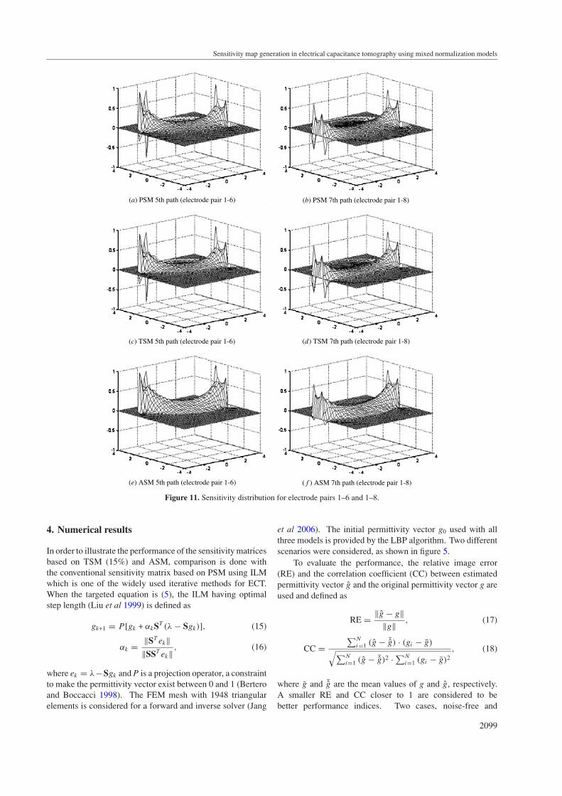
Figure 11. Sensitivity distribution for electrode pairs 1–6 and 1–8.

4. Numerical results

In order to illustrate the performance of the sensitivity matricesbased on TSM (15%) and ASM, comparison is done withthe conventional sensitivity matrix based on PSM using ILMwhich is one of the widely used iterative methods for ECT.When the targeted equation is (5), the ILM having optimalstep length (Liu et al 1999) is defined as

gk+1 = P [gk + αkST (λ − Sgk)], (15)

αk = ‖ST ek‖‖SST ek‖

, (16)

where ek = λ−Sgk and P is a projection operator, a constraintto make the permittivity vector exist between 0 and 1 (Berteroand Boccacci 1998). The FEM mesh with 1948 triangularelements is considered for a forward and inverse solver (Jang

et al 2006). The initial permittivity vector g0 used with allthree models is provided by the LBP algorithm. Two differentscenarios were considered, as shown in figure 5.

To evaluate the performance, the relative image error(RE) and the correlation coefficient (CC) between estimatedpermittivity vector g and the original permittivity vector g areused and defined as

RE = ‖g − g‖‖g‖ , (17)

CC =∑N

i=1 (g − ¯g) · (gi − g)√∑Ni=1 (g − ¯g)2 · ∑N

i=1 (gi − g)2, (18)

where g and ¯g are the mean values of g and g, respectively.A smaller RE and CC closer to 1 are considered to bebetter performance indices. Two cases, noise-free and

2099

Y S Kim et al

0 20 40 60 80 100 12010

-5

10-4

10-3

10-2

10-1

100

singular value index

mag

nitu

de

PSMTSMASM

Figure 12. Magnitude distribution of normalized singular values for each sensitivity matrix.

(a) scenario 1 PSM (b) scenario 1 TSM (c) scenario 1 ASM

(d ) scenario 2 PSM (e) scenario 2 TSM ( f ) scenario 2 ASM

Figure 13. Reconstructed images using ILM after 200th iteration with 5% noise.

noise-contaminated, are considered to assess the merit of theproposed sensitivity maps.

4.1. Noise-free case

The reconstruction results are shown in figures 6 and 8 afterthe 1st, 20th, and 200th iteration for the considered scenarios.From the reconstructed images, it can be seen that the imagequality with TSM and ASM is far better than that with PSM,especially when the target is located at the centre. In addition,the convergence rate is fast and similar performance can beachieved by ASM and TSM in only 20 iterations that isachieved with PSM after 200 iterations.

Figures 7 and 9 show the behaviour of RE and CC until the200th iteration for the considered cases which also ascertainsthat the ILM using the two new sensitivity matrices not onlyconverges faster than by using the conventional one, but alsohas improved the minimum-norm solution. However, in thecase of ILM with ASM for the scattered targets, RE decreasesto the minimum value till the 60th iteration and then increasesagain and for the same instance the CC is similar to the CCobtained with PSM. This behaviour is only exhibited by ILMwith ASM and can be regarded as a limiting factor.

To see why the new sensitivity matrices have improvedperformance, we compare the sensitivity distribution betweenall three models by considering the sensitivity distributionbetween electrode pairs 1–2, 1–4, 1–6 and 1–8. The resultsare presented in figures 10 and 11. As can be seen, the PSMmodel is more sensitive near electrodes, whereas TSM andASM are more sensitive near the EFCL and in the centre.

Even though the performances of the proposed systemmatrices are similar, if the images are analysed carefully, itcan be noticed that when TSM is employed, there is somedistortion near the electrodes which in the case of ASM iseither absent or significantly small.

4.2. Noise-contaminated case

To see the effectiveness of TSM and ASM in the presence ofnoise, we considered the worst case scenario by considering5% relative white Gaussian noise where noise seed isuniformly distributed on the interval [–1, 1]. The results areshown in figures 13 and 14.

In the noise-contaminated case, RE has risen by 10% to20% from the noise-free case and CC has decreased by 0.3to 0.5. However, as can be seen in figure 13, the resulting

2100

Sensitivity map generation in electrical capacitance tomography using mixed normalization models

0 20 40 60 80 100 120 140 160 180 20010

20

30

40

50

60

70

80

90

100

iteration

rela

tive

imag

e er

ror

(%)

PSMTSMASM

0 20 40 60 80 100 120 140 160 180 2000.4

0.5

0.6

0.7

0.8

0.9

1

iteration

corr

elat

ion

coef

ficie

nt

PSMTSMASM

(a) (b)

(c) (d )

0 20 40 60 80 100 120 140 160 180 20010

20

30

40

50

60

70

80

90

100

iteration

rela

tive

imag

e er

ror

(%)

PSMTSMASM

0 20 40 60 80 100 120 140 160 180 2000.4

0.5

0.6

0.7

0.8

0.9

1

iteration

corr

elat

ion

coef

ficie

nt

PSMTSMASM

Figure 14. Numerical results using ILM with 5% noise: (a) RE for scenario 1, (b) CC for scenario 1, (c) RE for scenario 2 and (d) CC forscenario 2.

Table 1. The condition number of each sensitivity matrix.

Sensitivity Sensitivity Sensitivitymatrix based matrix based matrix basedon PSM on TSM on ASM

Condition number 1.2676 × 105 3.9895 × 102 4.1647 × 102

images obtained through ILM based on PSM are significantlydistorted, whereas with TSM and ASM the background andtargets are distinguished well.

This robustness against noise is associated with theimproved condition number. Table 1 shows the conditionnumber of the three sensitivity matrices. As seen in table 1,the two newly proposed sensitivity matrices have a roughly1/300 times smaller condition number as compared to theconventional one. Hence we can easily attribute the robustnessagainst noise to the reduced condition number. In addition,a detailed analysis can be done by considering singularvalue decomposition (SVD). Figure 12 shows the magnitudeof normalized singular values when they are arranged asσ1 � σ2 � · · · � σrank(S) > 0. In figure 12 the magnitude is ona log-scale. As can be seen, the magnitude distribution of eachsensitivity matrix is more or less similar in the initial values;however, there are significant differences in the last 40 singularvalues. Furthermore, it can also be observed that in the last40 singular values, the sensitivity matrix based on PSM hasa relatively smaller magnitude than those based on TSM andASM. Such smaller singular values account for the solutionbeing error-prone. From this fact, it can be established that

the sensitivity matrices built by TSM and ASM can deal withrelatively higher noise levels than the conventional one.

5. Conclusions

This paper has presented two novel sensitivity maps usingmixed normalization models: a sensitivity map using athreshold model; a sensitivity map using an adaptive model.A mix of series and parallel models was introduced. It wasshown that the two newly proposed sensitivity matrices havea faster convergence rate and superior image quality than theconventional one and are robust against noise. It was shownthat the new sensitivity matrices result in better sensitivitynear the electric field centre lines and have a small conditionnumber that contributed to these enhancements.

The two novel sensitivity matrices are similar in behaviourand performance, but the sensitivity map based on thresholdhas an intrinsic weakness, i.e., the optimum threshold valueshould be selected empirically and should be based on thechoice of the applied reconstruction algorithm, the permittivityof dielectric materials and FEM mesh used. On the otherhand, the adaptive model showed comparable results withoutconsidering these factors. From this point of view, we canconclude that the sensitivity map based on the adaptive modelis more suitable for practical purposes and allows ease ofimplementation.

2101

Y S Kim et al

References

Bertero M and Boccacci P 1998 Introduction to Inverse Problem inImaging (Bristol: Institute of Physics Publishing) pp 137–67

Beck M S, Byars M, Dyakowski T, Waterfall R, He R, Wang S Mand Yang W Q 1997 Principles and industrial applications ofelectrical capacitance tomography Meas. Control 30 197–200

Jang J D, Lee S H, Kim K Y and Choi B Y 2006 Modified iterativeLandweber method in electrical capacitance tomography Meas.Sci. Technol. 17 1909–17

Kim J H, Choi B Y and Kim K Y 2006 Novel iterative imagereconstruction algorithm for electrical capacitancetomography: directional algebraic reconstruction techniqueIEICE Trans. Fundamentals E89-A 1578–84

Kortschak B, Wegleiter H and Brandstatter B 2007 Formulation ofcost functionals for different measurement principles innonlinear capacitance tomography Meas. Sci. Technol.18 71–8

Liu S, Fu S and Yang W Q 1999 Optimization of an iterative imagereconstruction algorithm for electrical capacitance tomographyMeas. Sci. Technol. 10 L37–9

Loser T, Wajman R and Mewes D 2001 Electrical capacitancetomography: image reconstruction along electrical field linesMeas. Sci. Technol. 12 1083–91

Marashdeh Q, Warsito W, Fan L-S and Teixeira F L 2006 Anonlinear image reconstruction technique for ECT using a

combined neural network approach Meas. Sci. Technol.17 2097–13

McKeen T R and Pugsley T S 2002 The influence of permittivitymodels on phantom images from electrical capacitancetomography Meas. Sci. Technol. 13 1822–30

Peng L, Merkus H and Scarlett B 2000 Using regularizationmethods for image reconstruction of electrical capacitancetomography Part. Part. Syst. Charact. 17 96–104

Wajman R, Banasiak R, Mazurkiewicz L, Dyakowski T andSankowski D 2006 Spatial imaging with 3D capacitancemeasurements Meas. Sci. Technol. 17 2113–8

Xie C G, Huang S M, Hoyle B S, Thorn R, Lenn C, Snowden D andBeck M S 1992 Electrical capacitance tomography for flowimaging: system model for development of imagereconstruction algorithms and design of primary sensors IEEProc. G 139 89–98

Yang W Q and Byars M 1999 An improved normalizationapproach for electrical capacitance tomography Proc. 1stWorld Congr. on Industrial Process Tomography (Buxton, UK)pp 215–8

Yang W Q and Peng L 2003 Image reconstruction algorithms forelectrical capacitance tomography Meas. Sci. Technol.14 R1–3

Yang W Q, Spink D M, Gamio J C and Beck M S 1997 Sensitivitydistributions of capacitance tomography sensor with parallelfield excitation Meas. Sci. Technol. 8 562–9

2102