arX

iv:1

110.

0586

v1 [

nlin

.SI]

4 O

ct 2

011

October 5, 2011 0:35 Applicable Analysis Hickmanetal-Applicable-Analysis-2011

Applicable AnalysisVol. 00, No. 00, January 2009, 1–20

Dedicated to the memory of Alan Jeffrey

Scaling invariant Lax pairs of nonlinear evolution equations

Mark Hickmana∗, Willy Heremanb, Jennifer Larueb and Unal Goktasc

aDepartment of Mathematics and Statistics,

University of Canterbury, Christchurch, New Zealand;bDepartment of Applied Mathematics and Statistics,

Colorado School of Mines, Golden, CO, USA;cDepartment of Computer Engineering,

Turgut Ozal University, Kecioren, Ankara, Turkey(Received 00 Month 200x; in final form 00 Month 200x)

A completely integrable nonlinear partial differential equation (PDE) can be associated witha system of linear PDEs in an auxiliary function whose compatibility requires that the originalPDE is satisfied. This associated system is called a Lax pair. Two equivalent representationsare presented. The first uses a pair of differential operators which leads to a higher orderlinear system for the auxiliary function. The second uses a pair of matrices which leads to afirst-order linear system. In this paper we present a method, which is easily implemented inMaple or Mathematica, to compute an operator Lax pair for a set of PDEs.

In the operator representation, the determining equations for the Lax pair split into a set ofkinematic constraints which are independent of the original equation and a set of dynamicalequations which do depend on it. The kinematic constraints can be solved generically. Weassume that the operators have a scaling symmetry. The dynamical equations are then reducedto a set of nonlinear algebraic equations.

This approach is illustrated with well-known examples from soliton theory. In particular, itis applied to a three parameter class of fifth-order KdV-like evolution equations which includesthe Lax fifth-order KdV, Sawada-Kotera and Kaup-Kuperschmidt equations. A second Laxpair was found for the Sawada–Kotera equation.

Keywords: Lax pair, Lax operator, scaling symmetry, complete integrability, fifth-orderKdV-type equations

AMS Subject Classification: Primary: 37J35, 37K40, 35Q51; Secondary: 68W30, 47J35,70H06.

1. Introduction

The complete integrability of a system of partial differential equations has beena topic of active research over the last forty or so years. Even today there is noone generally accepted definition of integrability. Many approaches have been ad-vocated (see [32] for a recent review), all of which have their merits but none seemto encapsulate the essence of integrability. However one concept has appeared inmany different approaches; the Lax pair. This is a reformulation of the originalsystem of nonlinear equations as the compatibility condition for a system of linearequations.The story of Lax pairs begins with the discovery by Lax [31] of such a linear

system for the ubiquitous KdV equation. This equation [6, 28] models a variety

∗Corresponding author. Email: mark.hickman@canterbury.ac.nz

ISSN: 0003-6811 print/ISSN 1563-504X onlinec© 2009 Taylor & FrancisDOI: 10.1080/0003681YYxxxxxxxxhttp://www.informaworld.com

October 5, 2011 0:35 Applicable Analysis Hickmanetal-Applicable-Analysis-2011

2 M. Hickman et al.

of nonlinear wave phenomena, including shallow water waves [20] and ion-acousticwaves in plasmas [1, 4, 11]. Lax’s discovery shed light on the then newly discoveredinverse scattering transform method [16] to solve the KdV equation. It allowedthis method to be extended to a variety of integrable equations. In 1979 it wasrealised that the Lax pair could be interpreted as a zero curvature condition onan appropriate connection [44]. This led to generalisations of the method of in-verse scattering transforms. In the 1980s, the algebraic structure of Lax pairs waselucidated. The connection between Lax pairs and Kac-Moody algebras was givenin [13]. Subsequent applications for Lax pairs include Backlund-Darboux transfor-mations [35], recursion operators [19] and generating integrable hierarchies via theroot method [17, 25, 34]. However there was a problem; finding the Lax pair in thefirst place.A Lax pair is associated with an infinite hierarchy of local conservation laws; a

harbinger of complete integrability (though not all equations with a Lax pair havean infinite set of conservation laws). Exploiting this connection, Wahlquist andEstabrook [14, 40] proposed a method based on pseudopotentials that, in certaincircumstances, leads to Lax pairs. However their method leads to a nontrivialproblem of finding a representation of a Lie algebra when only a subset of thecommutation relations are known.Another approach to the construction of a Lax pair is provided by singularity

analysis. In 1977 it was noted [3] that all symmetry reductions of the classical com-pletely integrable equations result in equations that can be transformed to Painleveequations. This observation subsequently gave rise to the so-called Painleve test[41]. In this approach Lax pairs are generated from truncated Painleve expansions[33]. However the complexity of Painleve expansion depends critically on the choiceof expansion variable.Computer algebra packages have also been employed to symbolically verify Lax

pairs [24, 30]. Of course this requires prior knowledge (or a good guess) of the Laxpair.In this paper we address the issue of finding Lax pairs, in operator form, for a

given system of differential equations by an approach that is amenable to computeralgebra. The determining equations for the Lax pair is split into two sets. The firstset, the kinematic constraints, are solved generically. The second set, the dynamicalequations, depend on the system under consideration. We make the assumptionthat the system has a scaling symmetry and that this symmetry is inherited by theLax pair. This allows us to reduce the dynamical equations to an overdeterminedsystem of algebraic equations (nonlinear, naturally). Such systems may then besolved by Grobner basis techniques.In the next section, Lax pairs are introduced in their operator representation. In

Section 3 the matrix representation of Lax pairs is discussed. The relationship be-tween these two representations is also examined. Section 4 introduces the conceptof scaling symmetries. The algorithm to compute Lax pairs based upon scalingsymmetries is outlined in the next section. Examples of the algorithm applied tosome well-known equations are given in Section 6. Finally the algorithm is usedto classify the integrable subcases of a fifth–order KdV-like equation with threeparameters. A second Lax pair was found for the Sawada–Kotera equation.

October 5, 2011 0:35 Applicable Analysis Hickmanetal-Applicable-Analysis-2011

Applicable Analysis 3

2. Lax Pairs in Operator Form

In this paper we consider nonlinear systems of evolution equations in (1 + 1) di-mensions,

ut = F(u,ux,u2x, . . . ), (1)

where x and t are the space and time variables, respectively. The vector u(x, t) hasN components ui and F is a nonlinear function of its arguments. In the exampleswe denote the components of u by u, v, w, . . .. Throughout the paper we use thesubscript notation for partial derivatives. If parameters are present in (1), they willbe denoted by lower-case Greek letters.In his seminal paper [31], Lax showed that completely integrable nonlinear PDEs

have an associated system of linear PDEs in an auxiliary function ψ(x, t),

Lψ = λψ,(2)

ψt = Mψ

where L and M are linear differential operators (expressed in powers of the totalderivative operator Dx for the space variable x). ψ is an eigenfunction of L corre-sponding to eigenvalue λ. The operators (L, M) are now known as a Lax pair for(1). The property that (1) is completely integrable is reflected in the fact that theeigenvalues do not change with time which makes the problem isospectral.Let G be a differential function (functional); that is, a function of x, t, u and

partial derivatives of u and let up,q = ∂px ∂

qt u. The total derivatives of G is given by

DxG =∂G

∂x+∑

p,q

∂G

∂up,qup+1,q,

(3)

DtG =∂G

∂t+∑

p,q

∂G

∂up,qup,q+1.

The sums are finite since we will assume that G depends only on finitely manyderivatives.

Example 2.1 The KdV equation [1] for u(x, t) can be recast in dimensionlessvariables as

ut + αuux + u3x = 0. (4)

The parameter α can be scaled to any real number. Commonly used values areα = ±1 or α = ±6. A Lax pair for (4) is given by [31]

L = D2x +

16αu I,

(5)M = −4D3

x − αuDx − 12αux I

where Dnx denotes repeated application of Dx (n times) and I is the identity oper-

ator. Substituting L and M into (2) yields

D2xψ =

(

λ− 16αu

)

ψ, (6)

Dtψ = −4D3xψ − αuDxψ − 1

2αuxψ. (7)

October 5, 2011 0:35 Applicable Analysis Hickmanetal-Applicable-Analysis-2011

4 M. Hickman et al.

The first equation is a Schrodinger equation for the eigenfunction ψ with eigenvalueλ and potential u(x, t). The second equation governs the time evolution of theeigenfunction.The compatibility condition for the above system is

DtD2xψ − D

2xDtψ = 1

6α (ut + αuux + u3x)ψ = 0 (8)

where (6) and (7) are used to eliminate Dtψ, D2xψ, D3

xψ and D5xψ. Obviously, (6)

and (7) will only be compatible on solutions of (4).

The compatibility of (2) may be expressed directly in terms of the operators L andM. Indeed

Dt (Lψ) = Ltψ + LDtψ = λDtψ

where Ltψ ≡ Dt (Lψ)− LDtψ. Using (2) we have

Ltψ + LMψ = λMψ = Mλψ = MLψ;

that is,

(Lt + LM−ML)ψ = 0.

If this operator does not vanish then (2) is not involutive and so would have ad-ditional (nonlinear) constraints; that is, one cannot freely specify the initial datafor (2). However, if this operator vanishes identically then Lax pair will not encodethe original differential equation. Therefore, for a non-trivial Lax pair for (1), thisoperator must vanish only on solutions of (1). Hence

Lt + [L,M].= O, (9)

where.= denotes that this equality holds only on solutions to the original PDE (1).

Here [L,M] ≡ LM −ML is the commutator of the operators and O is the zerooperator. Equation (9) is called the Lax equation. Note that Lt = [Dt,L] and sothe Lax equation takes the form

[Dt −M,L] .= O. (10)

Example 2.2 Returning to (5) for the KdV equation, we have

Lt = [Dt,L] = 16αut I,

LM = − 4D5x − α

(

53uD

3x +

52uxD

2x +

(

16αu

2 + 2uxx)

Dx +(

112αuux +

12u3x

)

I

)

,

ML = − 4D5x − α

(

53uD

3x +

52uxD

2x +

(

16αu

2 + 2uxx)

Dx +(

14αuux +

23u3x

)

I

)

.

Therefore,

Lt + [L,M] = 16α (ut + αuux + u3x) I,

which is equivalent to (8).

October 5, 2011 0:35 Applicable Analysis Hickmanetal-Applicable-Analysis-2011

Applicable Analysis 5

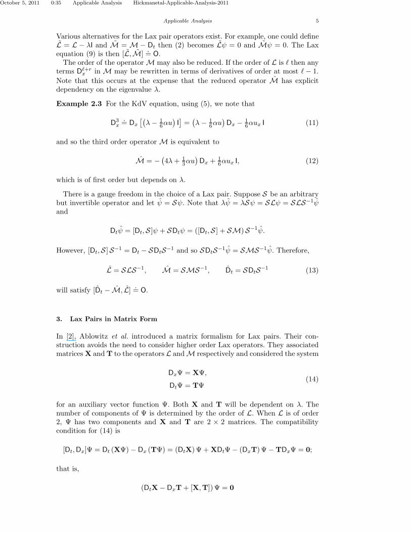
Various alternatives for the Lax pair operators exist. For example, one could defineL = L − λI and M = M− Dt then (2) becomes Lψ = 0 and Mψ = 0. The Laxequation (9) is then [L,M]

.= O.

The order of the operator M may also be reduced. If the order of L is ℓ then anyterms Dℓ+r

x in M may be rewritten in terms of derivatives of order at most ℓ− 1.

Note that this occurs at the expense that the reduced operator M has explicitdependency on the eigenvalue λ.

Example 2.3 For the KdV equation, using (5), we note that

D3x.= Dx

[(

λ− 16αu

)

I]

=(

λ− 16αu

)

Dx − 16αux I (11)

and so the third order operator M is equivalent to

M = −(

4λ+ 13αu

)

Dx +16αux I, (12)

which is of first order but depends on λ.

There is a gauge freedom in the choice of a Lax pair. Suppose S be an arbitrarybut invertible operator and let ψ = Sψ. Note that λψ = λSψ = SLψ = SLS−1ψ

and

Dtψ = [Dt,S ]ψ + SDtψ = ([Dt,S ] + SM)S−1ψ.

However, [Dt,S ]S−1 = Dt − SDtS−1 and so SDtS−1ψ = SMS−1ψ. Therefore,

L = SLS−1, M = SMS−1, Dt = SDtS−1 (13)

will satisfy [Dt − M, L] .= O.

3. Lax Pairs in Matrix Form

In [2], Ablowitz et al. introduced a matrix formalism for Lax pairs. Their con-struction avoids the need to consider higher order Lax operators. They associatedmatrices X andT to the operators L andM respectively and considered the system

DxΨ = XΨ,(14)

DtΨ = TΨ

for an auxiliary vector function Ψ. Both X and T will be dependent on λ. Thenumber of components of Ψ is determined by the order of L. When L is of order2, Ψ has two components and X and T are 2 × 2 matrices. The compatibilitycondition for (14) is

[Dt,Dx]Ψ = Dt (XΨ)− Dx (TΨ) = (DtX)Ψ +XDtΨ− (DxT)Ψ−TDxΨ = 0;

that is,

(DtX− DxT+ [X,T])Ψ = 0

October 5, 2011 0:35 Applicable Analysis Hickmanetal-Applicable-Analysis-2011

6 M. Hickman et al.

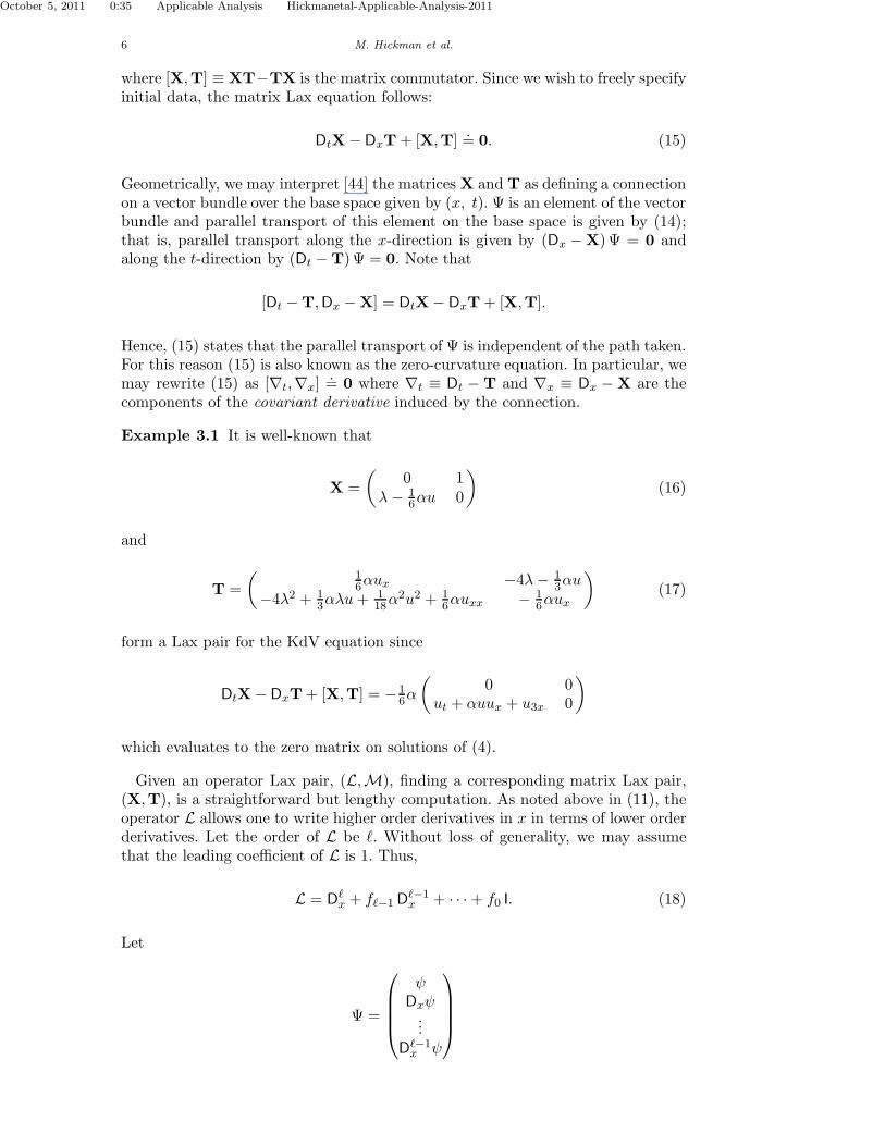
where [X,T] ≡ XT−TX is the matrix commutator. Since we wish to freely specifyinitial data, the matrix Lax equation follows:

DtX− DxT+ [X,T].= 0. (15)

Geometrically, we may interpret [44] the matrices X and T as defining a connectionon a vector bundle over the base space given by (x, t). Ψ is an element of the vectorbundle and parallel transport of this element on the base space is given by (14);that is, parallel transport along the x-direction is given by (Dx −X)Ψ = 0 andalong the t-direction by (Dt −T)Ψ = 0. Note that

[Dt −T,Dx −X] = DtX− DxT+ [X,T].

Hence, (15) states that the parallel transport of Ψ is independent of the path taken.For this reason (15) is also known as the zero-curvature equation. In particular, wemay rewrite (15) as [∇t,∇x]

.= 0 where ∇t ≡ Dt − T and ∇x ≡ Dx − X are the

components of the covariant derivative induced by the connection.

Example 3.1 It is well-known that

X =

(

0 1λ− 1

6αu 0

)

(16)

and

T =

(

16αux −4λ− 1

3αu

−4λ2 + 13αλu+ 1

18α2u2 + 1

6αuxx − 16αux

)

(17)

form a Lax pair for the KdV equation since

DtX− DxT+ [X,T] = −16α

(

0 0ut + αuux + u3x 0

)

which evaluates to the zero matrix on solutions of (4).

Given an operator Lax pair, (L,M), finding a corresponding matrix Lax pair,(X,T), is a straightforward but lengthy computation. As noted above in (11), theoperator L allows one to write higher order derivatives in x in terms of lower orderderivatives. Let the order of L be ℓ. Without loss of generality, we may assumethat the leading coefficient of L is 1. Thus,

L = Dℓx + fℓ−1D

ℓ−1x + · · ·+ f0 I. (18)

Let

Ψ =

ψ

Dxψ...

Dℓ−1x ψ

October 5, 2011 0:35 Applicable Analysis Hickmanetal-Applicable-Analysis-2011

Applicable Analysis 7

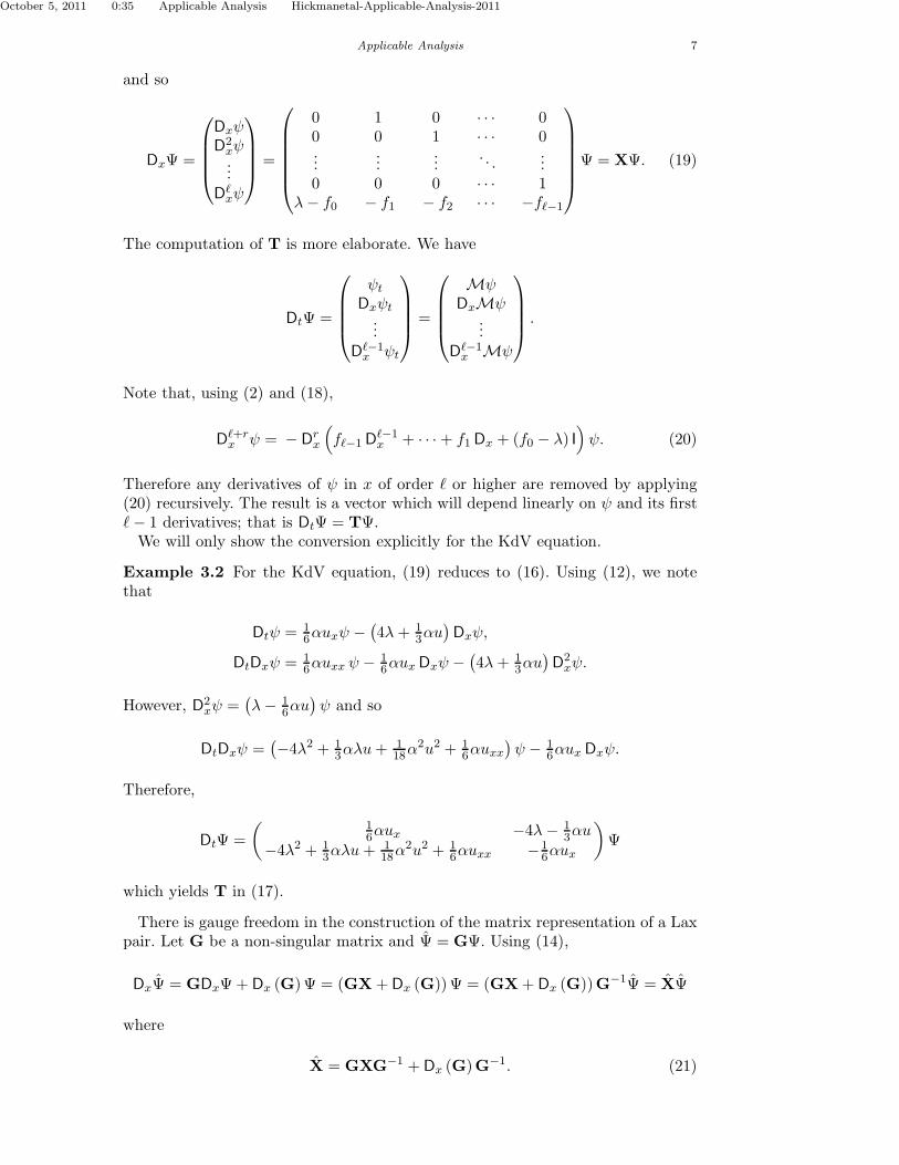
and so

DxΨ =

Dxψ

D2xψ...

Dℓxψ

=

0 1 0 · · · 00 0 1 · · · 0...

......

. . ....

0 0 0 · · · 1λ− f0 − f1 − f2 · · · −fℓ−1

Ψ = XΨ. (19)

The computation of T is more elaborate. We have

DtΨ =

ψt

Dxψt

...Dℓ−1x ψt

=

Mψ

DxMψ...

Dℓ−1x Mψ

.

Note that, using (2) and (18),

Dℓ+rx ψ = − D

rx

(

fℓ−1Dℓ−1x + · · ·+ f1Dx + (f0 − λ) I

)

ψ. (20)

Therefore any derivatives of ψ in x of order ℓ or higher are removed by applying(20) recursively. The result is a vector which will depend linearly on ψ and its firstℓ− 1 derivatives; that is DtΨ = TΨ.We will only show the conversion explicitly for the KdV equation.

Example 3.2 For the KdV equation, (19) reduces to (16). Using (12), we notethat

Dtψ = 16αuxψ −

(

4λ+ 13αu

)

Dxψ,

DtDxψ = 16αuxx ψ − 1

6αuxDxψ −(

4λ+ 13αu

)

D2xψ.

However, D2xψ =

(

λ− 16αu

)

ψ and so

DtDxψ =(

−4λ2 + 13αλu+ 1

18α2u2 + 1

6αuxx)

ψ − 16αux Dxψ.

Therefore,

DtΨ =

(

16αux −4λ− 1

3αu

−4λ2 + 13αλu+ 1

18α2u2 + 1

6αuxx −16αux

)

Ψ

which yields T in (17).

There is gauge freedom in the construction of the matrix representation of a Laxpair. Let G be a non-singular matrix and Ψ = GΨ. Using (14),

DxΨ = GDxΨ+ Dx (G)Ψ = (GX+Dx (G))Ψ = (GX+ Dx (G))G−1Ψ = XΨ

where

X = GXG−1 + Dx (G)G−1. (21)

October 5, 2011 0:35 Applicable Analysis Hickmanetal-Applicable-Analysis-2011

8 M. Hickman et al.

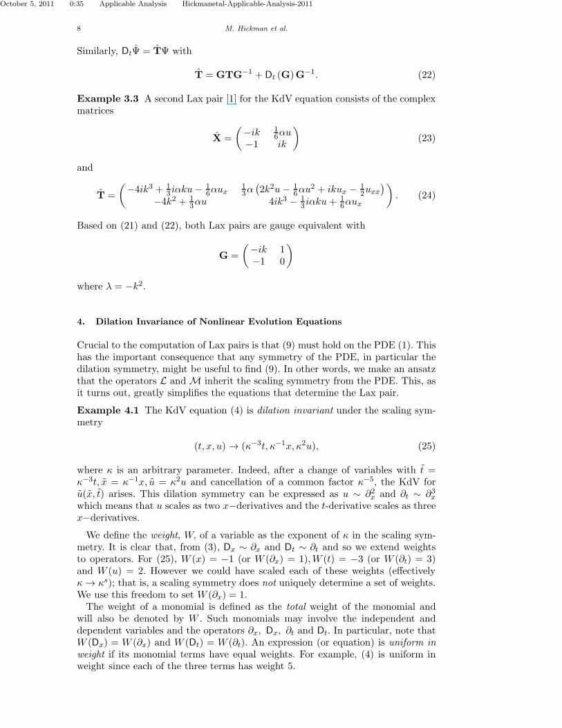
Similarly, DtΨ = TΨ with

T = GTG−1 + Dt (G)G−1. (22)

Example 3.3 A second Lax pair [1] for the KdV equation consists of the complexmatrices

X =

(

−ik 16αu

−1 ik

)

(23)

and

T =

(

−4ik3 + 13 iαku− 1

6αux13α

(

2k2u− 16αu

2 + ikux − 12uxx

)

−4k2 + 13αu 4ik3 − 1

3 iαku+ 16αux

)

. (24)

Based on (21) and (22), both Lax pairs are gauge equivalent with

G =

(

−ik 1−1 0

)

where λ = −k2.

4. Dilation Invariance of Nonlinear Evolution Equations

Crucial to the computation of Lax pairs is that (9) must hold on the PDE (1). Thishas the important consequence that any symmetry of the PDE, in particular thedilation symmetry, might be useful to find (9). In other words, we make an ansatzthat the operators L and M inherit the scaling symmetry from the PDE. This, asit turns out, greatly simplifies the equations that determine the Lax pair.

Example 4.1 The KdV equation (4) is dilation invariant under the scaling sym-metry

(t, x, u) → (κ−3t, κ−1x, κ2u), (25)

where κ is an arbitrary parameter. Indeed, after a change of variables with t =κ−3t, x = κ−1x, u = κ2u and cancellation of a common factor κ−5, the KdV foru(x, t) arises. This dilation symmetry can be expressed as u ∼ ∂2x and ∂t ∼ ∂3xwhich means that u scales as two x−derivatives and the t-derivative scales as threex−derivatives.

We define the weight, W, of a variable as the exponent of κ in the scaling sym-metry. It is clear that, from (3), Dx ∼ ∂x and Dt ∼ ∂t and so we extend weightsto operators. For (25), W (x) = −1 (or W (∂x) = 1),W (t) = −3 (or W (∂t) = 3)and W (u) = 2. However we could have scaled each of these weights (effectivelyκ→ κs); that is, a scaling symmetry does not uniquely determine a set of weights.We use this freedom to set W (∂x) = 1.The weight of a monomial is defined as the total weight of the monomial and

will also be denoted by W . Such monomials may involve the independent anddependent variables and the operators ∂x, Dx, ∂t and Dt. In particular, note thatW (Dx) = W (∂x) and W (Dt) = W (∂t). An expression (or equation) is uniform in

weight if its monomial terms have equal weights. For example, (4) is uniform inweight since each of the three terms has weight 5.

October 5, 2011 0:35 Applicable Analysis Hickmanetal-Applicable-Analysis-2011

Applicable Analysis 9

The importance of uniformity of weight is demonstrated by the KdV equation(4). From (5), it is clear that L has weight 2 and M has weight 3 since W (I) = 0.Therefore this Lax pair inherits the scaling symmetry. Also note that we mustassign W (λ) = 2. The elements of the matrices X and T in (16) and (17) are alsouniform in weight, albeit of different weights. This is also true for the matrices in(23) and (24).

5. An algorithm for Computing Lax Pairs in Operator Form

First, one computes the dilation symmetry of the nonlinear PDE and assignsweights such thatW (∂x) = 1. Next, one selects the weight ℓ of the operator L. Sincewe have chosen W (∂x) = 1, ℓ will also be the order of L. The minimal weight for Lis the maximum weight of the dependent variables since we want the Lax equationto depend non-trivially on the PDE. It is only through Lt that the t-derivativesof the dependent variables appear. Since Lt = [Dt,L], W (Lt) = W (L) +W (∂t)and, from (9), W (Lt) = W (L) +W (M). Thus W (M) = W (∂t). Since we requirethat M to be a differential operator, we must choose a system of weights such thatW (∂t) is a non-negative integer.Thus the candidate Lax pair has the form

L = Dℓx + fℓ−1D

ℓ−1x + · · ·+ f0 I,

M = cmDmx + gm−1 D

m−1x + · · · + g0 I

where m =W (∂t). Now

[L,M] = (ℓDxcm)Dm+ℓ−1x + · · · . (26)

Recall that we require that (9) only holds on solutions of the PDE. Thus theoperator Dm+ℓ−1

x could be reduced to an operator that depends on derivatives oforder strictly less than ℓ. However this would introduce the eigenvalue λ and, inthis case, there would be a term ℓλm−1Dxcm. This would be the only term in λm−1.Under the assumption that the operator L has a complete (and therefore infinite)set of eigenvalues, we conclude Dxcm = 0; that is, cm is a constant. Therefore (26)becomes

[L,M] = (ℓDxgm−1 −mcmDxfℓ−1)Dm+ℓ−2x + · · · .

After reduction, the coefficient of λm−2 must vanish and so

ℓDxgm−1 −mcmDxfℓ−1 = 0. (27)

In this way, we obtain m− 1 equations for the unknown coefficient functions fi, gjthat do not depend on the PDE. We call these equations kinematic constraints.The remaining ℓ components of (9) may involve terms from Lt. When t-

derivatives do appear, we must use the PDE to remove them. We call these equa-tions dynamical equations.The kinematic constraints are easily solved. All have the form (27) and so may

be solved in terms of the leading gj . Specifically, (27) yields

gm−1 =mℓcmfl−1.

October 5, 2011 0:35 Applicable Analysis Hickmanetal-Applicable-Analysis-2011

10 M. Hickman et al.

In this way, gj , j = 1, . . . , m− 1, may be written in terms of g0 and fi. Note thatthis process does not depend on the PDE and so this rewrite is canonical.After the elimination of the gj , the dynamical equations are a set of ODEs for

the remaining coefficient functions g0 and fi. We now make the ansatz that theterms in the operators L and M have uniform weight; that is, fi has weight ℓ− i

and g0 has weight m. Thus, for example, g0 is assumed to be a linear combination(with unknown coefficients) of monomials of weight m. If, in addition, the weightsof the dependent variables are positive and the monomials do not depend explicitlyon x and t, the dynamical equations reduce to an finite system of algebraic equa-tions for the unknown coefficients. This algebraic system (which will also have anyparameters that are present in the PDE) is then solved by Grobner basis methods.We now illustrate the steps of the algorithm for the KdV equation.

5.1. Step 1: Computing the scaling symmetry

The dilation symmetry of (4) can be readily computed by the requirement that (4)is uniform in weight. Indeed, setting W (∂x) = 1, we have

W (u) +W (∂t) = 2W (u) + 1 =W (u) + 3,

which yields W (u) = 2 and W (∂t) = 3. This confirms (25). So, the requirement ofuniformity in weight of a PDE allows one to compute the weights of the variables(and thus the scaling symmetry) with linear algebra.Dilation symmetries, which are special Lie-point symmetries, are common to

many nonlinear PDEs. Needless to say, not every PDE is dilation invariant. How-ever non-uniform PDEs can be made uniform by extending the set of dependentvariables with auxiliary parameters with appropriate weights. Upon completion ofthe computations one can set these parameters to 1.

5.2. Step 2: Building a candidate Lax pair

Since W (u) = 2, the minimal weight for L is 2. We therefore choose ℓ = 2. Note,that there is no monomial of weight 1 (any monomial that involves u must haveweight at least 2). Therefore we could set f1 = 0. However the kinematic constraintsand dynamical equations only depend on the choice of weight for L andW (∂t). So,by not setting f1 = 0 at this stage, we will derive the dynamical equations for allLax pairs with L of second order and W (∂t) = 3. Our candidate Lax pair is

L = D2x + f1Dx + f0 I,

(28)M = c3 D

3x + g2 D

2x + g1 Dx + g0 I.

The kinematic constraints (that is, the coefficients of D3x and D4

x in [L,M]) give

g2 =32c3f1, g1 =

38c3

(

2Dxf1 + f21 + 4f0)

.

Therefore, (28) must have the form

L = D2x + f1Dx + f0 I,

(29)M = c3 D

3x +

32c3f1D

2x +

38c3

(

2Dxf1 + f21 + 4f0)

Dx + g0 I.

October 5, 2011 0:35 Applicable Analysis Hickmanetal-Applicable-Analysis-2011

Applicable Analysis 11

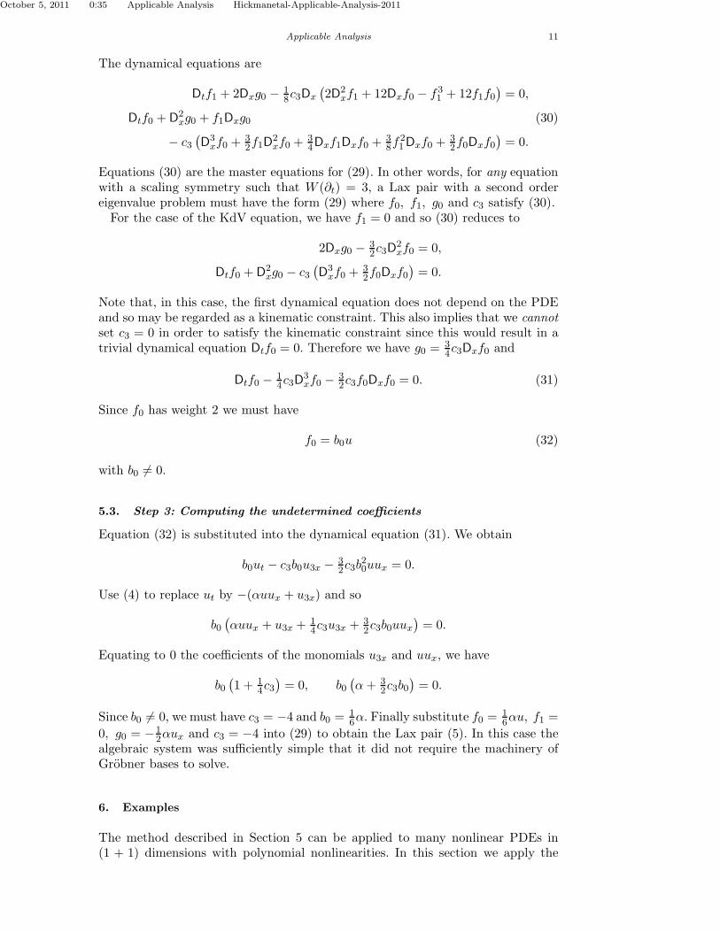
The dynamical equations are

Dtf1 + 2Dxg0 − 18c3Dx

(

2D2xf1 + 12Dxf0 − f31 + 12f1f0

)

= 0,

Dtf0 + D2xg0 + f1Dxg0 (30)

− c3(

D3xf0 +

32f1D

2xf0 +

34Dxf1Dxf0 +

38f

21Dxf0 +

32f0Dxf0

)

= 0.

Equations (30) are the master equations for (29). In other words, for any equationwith a scaling symmetry such that W (∂t) = 3, a Lax pair with a second ordereigenvalue problem must have the form (29) where f0, f1, g0 and c3 satisfy (30).For the case of the KdV equation, we have f1 = 0 and so (30) reduces to

2Dxg0 − 32c3D

2xf0 = 0,

Dtf0 + D2xg0 − c3

(

D3xf0 +

32f0Dxf0

)

= 0.

Note that, in this case, the first dynamical equation does not depend on the PDEand so may be regarded as a kinematic constraint. This also implies that we cannotset c3 = 0 in order to satisfy the kinematic constraint since this would result in atrivial dynamical equation Dtf0 = 0. Therefore we have g0 =

34c3Dxf0 and

Dtf0 − 14c3D

3xf0 − 3

2c3f0Dxf0 = 0. (31)

Since f0 has weight 2 we must have

f0 = b0u (32)

with b0 6= 0.

5.3. Step 3: Computing the undetermined coefficients

Equation (32) is substituted into the dynamical equation (31). We obtain

b0ut − c3b0u3x − 32c3b

20uux = 0.

Use (4) to replace ut by −(αuux + u3x) and so

b0(

αuux + u3x +14c3u3x +

32c3b0uux

)

= 0.

Equating to 0 the coefficients of the monomials u3x and uux, we have

b0(

1 + 14c3

)

= 0, b0(

α+ 32c3b0

)

= 0.

Since b0 6= 0, we must have c3 = −4 and b0 =16α. Finally substitute f0 =

16αu, f1 =

0, g0 = −12αux and c3 = −4 into (29) to obtain the Lax pair (5). In this case the

algebraic system was sufficiently simple that it did not require the machinery ofGrobner bases to solve.

6. Examples

The method described in Section 5 can be applied to many nonlinear PDEs in(1 + 1) dimensions with polynomial nonlinearities. In this section we apply the

October 5, 2011 0:35 Applicable Analysis Hickmanetal-Applicable-Analysis-2011

12 M. Hickman et al.

method to scalar equations as well as systems. The featured scalar examples arethe modified KdV and Boussinesq equations. The method is also illustrated forsystems, including a coupled system of KdV equations due to Hirota & Satsumaand the Drinfel’d-Sokolov-Wilson system.

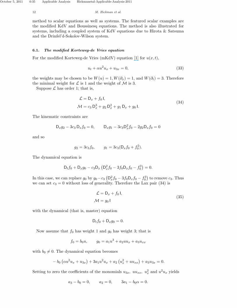
6.1. The modified Korteweg-de Vries equation

For the modified Korteweg-de Vries (mKdV) equation [1] for u(x, t),

ut + αu2ux + u3x = 0, (33)

the weights may be chosen to be W (u) = 1,W (∂x) = 1, and W (∂t) = 3. Thereforethe minimal weight for L is 1 and the weight of M is 3.Suppose L has order 1; that is,

L = Dx + f0 I,(34)

M = c3 D3x + g2 D

2x + g1 Dx + g0 I.

The kinematic constraints are

Dxg2 − 3c3 Dxf0 = 0, Dxg1 − 3c3D2xf0 − 2g2Dxf0 = 0

and so

g2 = 3c3f0, g1 = 3c3(Dxf0 + f20 ).

The dynamical equation is

Dtf0 + Dxg0 − c3Dx

(

D2xf0 − 3f0Dxf0 − f30

)

= 0.

In this case, we can replace g0 by g0−c3(

D2xf0 − 3f0Dxf0 − f30

)

to remove c3. Thuswe can set c3 = 0 without loss of generality. Therefore the Lax pair (34) is

L = Dx + f0 I,(35)

M = g0 I

with the dynamical (that is, master) equation

Dtf0 + Dxg0 = 0.

Now assume that f0 has weight 1 and g0 has weight 3; that is

f0 = b0u, g0 = a1u3 + a2uux + a3uxx

with b0 6= 0. The dynamical equation becomes

− b0(

αu2ux + u3x)

+ 3a1u2ux + a2

(

u2x + uuxx)

+ a3u3x = 0.

Setting to zero the coefficients of the monomials u3x, uuxx, u2x and u2ux yields

a3 − b0 = 0, a2 = 0, 3a1 − b0α = 0.

October 5, 2011 0:35 Applicable Analysis Hickmanetal-Applicable-Analysis-2011

Applicable Analysis 13

Since b0 is free, we can set b0 = 1 and (35) becomes

L1 = Dx + u I,(36)

M1 =(

13αu

3 + uxx)

I.

The Lax equation for (36) is the conservation law form of (33).If we assume that L has weight 2, then, since W (∂t) = 3, the Lax pair is given

by (29) and the dynamical equations are given by (30). In this case, a gauge on g0will not remove c3 from the dynamical equations. The ansatz of uniform weightsdetermines

f1 = b0u, f0 = b1u2 + b2ux, g0 = a1u

3 + a2uux + a3uxx.

The solution to resultant algebraic system has two branches;

Case I: L = D2x + 2uDx +

(

u2 + ux)

I,

M =(

13αu

3 + uxx)

I.

Case II: L = D2x + 2ǫuDx +

16

(

6ǫ2u2 + 6ǫux + αu2 ±√−6αux

)

I,

M = − 4D3x − 12ǫuD2

x −(

12ǫ2u2 + 12ǫux + αu2 ±√−6αux

)

Dx

−(

4ǫ3u3 + 23ǫαu

3 + 12ǫ2uux ± ǫ√−6αuux + 3ǫuxx

+ αuux ± 12

√−6αuxx

)

I.

The second case is a 1-parameter family (with parameter ǫ) of Lax pairs. Thisfamily has the property M → − 4D3

x for solutions of (33) such that u → 0 as|x| → ∞. Wadati [38, 39] used this property to construct soliton solutions for (33)via the inverse scattering transform from Case II with ǫ = 0.There is one Lax pair with L of order 3 which is

L = D3x + 3uD2

x + 3(

u2 + ux)

Dx +(

u3 + 3uux + uxx)

I,

M =(

13αu

3 + uxx)

I.

However

L = (Dx + uI)3 = L31, M = M1

where L1 and M1 are given by (36).

6.2. The Boussinesq equation

The wave equation,

utt − uxx + 3u2x + 3uuxx + αu4x = 0, (37)

for u(x, t) with real parameter α, was proposed by Boussinesq [5] to describe surfacewaves in shallow water [1]. This equation may be rewritten as a system

ut − vx = 0, vt − ux + 3uux + αu3x = 0, (38)

October 5, 2011 0:35 Applicable Analysis Hickmanetal-Applicable-Analysis-2011

14 M. Hickman et al.

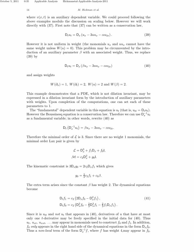
where v(x, t) is an auxiliary dependent variable. We could proceed following theabove examples modulo the discussion on scaling below. However we will workdirectly with (37). First note that (37) can be written as a conservation law,

Dtut = Dx (ux − 3uux − αu3x) . (39)

However it is not uniform in weight (the monomials ux and uux cannot have thesame weight unless W (u) = 0). This problem may be circumvented by the intro-duction of an auxiliary parameter β with an associated weight. Thus, we replace(39) by

Dtut = Dx (βux − 3uux − αu3x) (40)

and assign weights

W (∂x) = 1, W (∂t) = 2, W (u) = 2 and W (β) = 2.

This example demonstrates that a PDE, which is not dilation invariant, may beexpressed in a dilation invariant form by the introduction of auxiliary parameterswith weights. Upon completion of the computations, one can set each of theseparameters to 1.The “fundamental” dependent variable in this equation is ut (that is, utt = Dtut).

However the Boussinesq equation is a conservation law. Therefore we can use D−1x ut

as a fundamental variable; in other words, rewrite (40) as

Dt

(

D−1x ut

)

= βux − 3uux − αu3x.

Therefore the minimal order of L is 3. Since there are no weight 1 monomials, theminimal order Lax pair is given by

L = D3x + f1Dx + f0I,

M = c2D2x + g0I.

The kinematic constraint is 3Dxg0 = 2c2Dxf1 which gives

g0 =23c2f1 + c0β.

The extra term arises since the constant β has weight 2. The dynamical equationsbecome

Dtf1 = c2(

2Dxf0 − D2xf1

)

, (41)

Dtf0 = c2(

D2xf0 − 2

3D3xf1 − 2

3f1Dxf1)

.

Since it is utt and not ut that appears in (40), derivatives of u that have at mostonly one t-derivative may be freely specified in the initial data for (40). Thusut, uxt, uxxt, . . .may appear in monomials used to construct f0 and f1. In addition,f0 only appears in the right hand side of the dynamical equations in the form Dxf0.Thus a non-local term of the form D−1

x f , where f has weight 4,may appear in f0.

October 5, 2011 0:35 Applicable Analysis Hickmanetal-Applicable-Analysis-2011

Applicable Analysis 15

Consequently, the weight ansatz implies

f1 = a1u+ a2β,

f0 = a3ux + D−1x

(

a4u2 + a5βu+ a6ut + a7β

2)

.

Under this ansatz, the dynamical equation (41) becomes the kinematic constraint

a1ut = 2c2(

a3uxx + a4u2 + a5βu+ a6ut + a7β

2 − 12a1uxx

)

. (42)

For a non-trivial solution, we require a1 6= 0 and so c2 6= 0. Thus a4 = a5 = a7 = 0,a1 = 2c2a6 and a3 = c2a6. Hence,

Dtf0 = a3uxt + a6D−1x utt

.= a6 (c2uxt + βux − 3uux − αu3x)

on solutions of (40). Therefore the remaining dynamical equation is

a6 (c2uxt + βux − 3uux − αu3x) = c2a6(

uxt − 13c2u3x − 4

3c2ux(2c2a6u+ a2β))

.

The solution of this equation gives the Lax pair

L = D3x +

1

4α(3u− β)Dx +

3

8α2

(

αux ± 13

√3αD

−1x ut

)

I,

M = ±√3αD

2x ±

√3α

2αu I.

The subcase β = 1 is a Lax pair for (37) [43]. Note that the auxiliary variable vthat was introduced to obtain the system (38) is, in fact, D−1

x ut. A Lax pair forthe system is obtained by replacing D−1

x ut by v.

6.3. The coupled Korteweg-de Vries equations

The coupled Korteweg-de Vries (cKdV) equations [21],

ut − 6βuux + 6vvx − βu3x = 0, vt + 3uvx + v3x = 0 (43)

where β is a nonzero parameter, describes interactions of two waves with differentdispersion relations. System (43) is known in the literature as the Hirota-Satsumasystem. It is completely integrable [1, 21] when β = 1

2 .

We assign the weights W (∂x) = 1, W (∂t) = 3, W (u) = 2 and W (v) = 2. SinceW (∂t) = 3 and there are no weight 1 monomials, the dynamical equations areprecisely those of the KdV equation (4). The minimal weight for L is 2 and so thedynamical equation is (31) with

f0 = b0u+ b1v.

The resultant equations have only a trivial solution. Likewise, there are also noLax pairs with L of third order.For the case W (L) = 4, the candidate Lax pair, after the kinematic constraints

October 5, 2011 0:35 Applicable Analysis Hickmanetal-Applicable-Analysis-2011

16 M. Hickman et al.

have been solved, is

L = D4x + f2D

2x + f1Dx + f0 I,

M = c3 D3x +

34c3f2Dx +

38c3 (2f1 − Dxf2) I

with dynamical equations

Dtf2 +14c3

(

6D2xf1 − D

3xf2 + 3f2Dxf2 − 12Dxf0

)

= 0,

Dtf1 +14c3

(

8D3xf1 − 3D4

xf2 + 3f2Dxf1 + 3f1Dxf2 − 12D2xf0

)

= 0,

Dtf0 +18c3

(

6D4xf1 − 3D5

xf2 + 6f2D2xf1 − 3f2D

3xf2

+ 6f1Dxf1 − 3f1D2xf1 − 8D3

xf0 − 6f2Dxf0)

= 0.

A non-trivial solution exists only when β = 12 . In this case the solution is

L = D4x + 2uD2

x + 2 (ux − vx)Dx +(

u2 − v2 + u2x − v2x)

I,

M = 2D3x + 3uDx +

32 (ux − 2vx) I.

Note that this Lax pair is given in [9, 42].

6.4. The Drinfel’d-Sokolov-Wilson equations

We consider a one-parameter family of the Drinfel’d-Sokolov-Wilson (DSW) equa-tions

ut + 3vvx = 0, vt + 2uvx + αuxv + 2v3x = 0, (44)

where α is a nonzero parameter. The system with α = 1 was first proposed byDrinfel’d and Sokolov [12, 13] and Wilson [42]. It can be obtained [26] as a reductionof the Kadomtsev-Petviashvili equation (a two-dimensional version of the KdVequation).We may assign weights W (∂t) = 3, W (u) = 2 and W (v) = 2. Thus we have the

same weight system as the KdV equation and the coupled system above. There areno Lax pairs for this system with L of order 2, 3, 4 or 5 which inherit this scalingsymmetry.There are no solutions for W (L) = 6 except for α = 1. In that case

L = D6x + 2uD4

x + (4ux − 3vx)D3x +

(

92 (u2x − v2x) + u2 − v2

)

D2x

+(

52 (u3x − v3x) + 2 (uux − vvx) + uxv − uvx

)

Dx

+ 14

(

2 (u4x − v4x) + 2 (u+ v) (u2x − v2x) + u2x − v2x)

I,

M = D3x + uDx − 1

2 (3vx − ux) I.

The DSW system (44) is known to have infinitely many conservation laws whenα = 1 and is completely integrable [12, 42]. This is the Lax pair given in [42].

October 5, 2011 0:35 Applicable Analysis Hickmanetal-Applicable-Analysis-2011

Applicable Analysis 17

Parameterratios

(α

γ2,β

γ)

Commonlyused values

(α, β, γ)

Equation name Lax pairreferences

( 310 , 2) (30, 20, 10), (120, 40, 20), Lax [31]

(270, 60, 30)

(15 , 1) (5, 5, 5), (180, 30, 30), Sawada-Kotera [10, 15](45, 15, 15) [27, 36]

(15 ,52) (20, 25, 10) Kaup-Kupershmidt [15, 27]

(29 , 2) (2, 6, 3), (72, 36, 18) Ito –

Special cases of the fifth-order family (45) of KdV-type equations.

7. Classification of fifth-order KdV-like equations

For an equation or system with parameters, the algorithm described in Section 5can be used to find the necessary conditions on the parameters so that the PDEhas a Lax pair and therefore may be completely integrable.Consider the family of fifth-order KdV-type equations with three parameters

ut + αu2ux + βuxuxx + γuu3x + u5x = 0. (45)

This family includes several well-known completely integrable equations.Replacing u by u

γ, it is clear that only the ratios α2

γand β

γmatter. We continue

with (45) for an easier comparison with the results in the literature. The specialcases of (45) shown in the table are extensively discussed in the literature [18, 22,29, 36]. Only the first three equations are completely integrable. Ito’s equation isnot completely integrable but has an unusual set of conservation laws [18, 23].

We wish to determine which members, if any, have a Lax pair, with L of secondorder, which may then be amenable to a (standard) inverse scattering transformbased on a quadratic eigenvalue problem. Kaup [27] has considered this family withrespect to a cubic eigenvalue problem (that is L is a third order operator).Uniformity of weights implies that W (∂t) = 5. The first kinematic constraint is

2Dxg4 − 5c5Dxf1 = 0.

In this situation we may need or wish to give the parameters weight. If this is thecase, there may be a weight 1 constant. Therefore the solution to this constraint is

g4 =52c5f1 + c4

where c4 is a constant of integration of weight 1. After all four kinematic constraints

October 5, 2011 0:35 Applicable Analysis Hickmanetal-Applicable-Analysis-2011

18 M. Hickman et al.

are solved, we have

L = D2x + f1Dx + f0 I,

M = c5 D5x +

(

52f1 + c4

)

D4x +

(

58c5(6Dxf1 + 3f21 + 4f0) + 2c4f1 + c3

)

D3x

+(

516c5(12D

2xf1 + 10Dxf

21 + 12Dxf0 + f31 + 12f1f0) + c4(2Dxf1 + f21 + 2f0)

+ 32c3f1 + c2

)

D2x +

(

5128c5(48f0Dxf1 + 96f1Dxf0 + 4Dxf

31 + 24f21 f0

+ 20(Dxf1)2 + 40f1D

2xf1 + 24D3

xf1 + 80D2xf0 + 48f20 − f41 )

+ c4(2Dxf0 + f1Dxf1 + D2xf1 + 2f1f0) +

38c3(4f0 + f21 + 2Dxf1)

+ c2f1 + c1

)

Dx + g0 I.

For brevity, we omit the two dynamical equations.We now need to make a choice for the remaining weights. The obvious choice

is W (u) = 2. With this choice, α, β and γ all have weight zero. Therefore theconstants of integration, c1, . . . , c4, are all zero which simplifies the Lax pair dra-matically. The only non-trivial solution occurs when α = 3

10γ2, β = 2γ which

corresponds to the fifth-order KdV equation due to Lax [31]. The Lax pair is

L = D2x +

110γu I,

M = − 16D5x − 4γuD3

x − 6γux D2x − γ

(

5uxx +310γu

2)

Dx − γ(

32u3x +

310γuux

)

I.

In [7], it is shown that all scalar evolution equations, which have the form of aconservation law, have a Lax pair with a second order L. Such Lax pairs can befound if we choose the weights W (u) = 1, W (α) = 2, W (β) = 1 and W (γ) = 1.In this case, the constants of integration may not be zero.For weight 3, we obtain non-trivial solutions for the Sawada-Kotera and Kaup-

Kupershmidt equations. For the Sawada-Kotera equation (α = 15γ

2,

beta = γ) [8, 37] there are two solutions:

Case I: L = D3x +

15γuDx,

M = 9D5x + 3γuD3

x + 3γux D2x + γ

(

15γu

2 + 2u2x)

Dx

Case II: L = D3x +

15γuDx +

15γux I,

M = 9D5x + 3γuD3

x + 6γux D2x + γ

(

15γu

2 + 5u2x)

Dx

+ 2γ(

15γuux + u3x

)

I.

The first Lax pair is given in [10, 15].The Kaup-Kupershmidt equation (α = 1

5γ2, β = 5

2γ) [27] has a single Lax pair

L = D3x +

15γuDx +

110γux I,

M = 9D5x + 3γuD3

x +92γux D

2x + γ

(

15γu

2 + 72u2x

)

Dx + γ(

15γuux + u3x

)

I

which is given in [15]. We cannot find any reference to the second Lax pair in theliterature.

October 5, 2011 0:35 Applicable Analysis Hickmanetal-Applicable-Analysis-2011

REFERENCES 19

8. Conclusions

The algorithm described in this paper can be easily implemented inMathematica

or Maple. Therein lies its value; it gives a quick method to “test the waters” witha new system of equations. If the equations do not have a scaling symmetry, orthe scaling symmetry does not yield a Lax pair, then weighted parameters may beintroduced. A new assignment of weights may lead to a Lax pair. The “focus on theequation” of our approach is a marked contrast to existing work where integrablesystems have, by and large, been developed from geometric considerations (forexample, the use of the Drinfel’d–Sokolov construction [12, 13]).The question of an appropriate system of weights is non-trivial. As noted above,

all members of the three parameter family of fifth–order KdV–like equations havea Lax pair with a second order L. The question naturally arises as to which ofthese Lax pairs are useful. Can, for example, a criteria be developed that wouldguarantee an infinite family of local conservations laws?

Dedication

This paper is dedicated to the memory of Alan Jeffrey. As a Ph.D. student, oneof us (WH) was first introduced to the mathematics of nonlinear waves throughAlan’s seminal paper on Nonlinear Wave Propagation published in Zeitschrift furAngewandte Mechanik und Mathematik 58, T38-56 (1978). With Alan’s passingwe loose a researcher, educator, and expositor par excellence.

Acknowledgements

This material is based in part upon research supported by the National ScienceFoundation (NSF) under Grant No. CCF-0830783. Any opinions, findings, andconclusions or recommendations expressed in this material are those of the authorsand do not necessarily reflect the views of NSF.WH is grateful for the hospitality and support of the Department of Computer

Engineering at Turgut Ozal University (Kecioren, Ankara, Turkey) where code forLax pair computations was further developed.MH would like the thank the Department of Applied Mathematics and Statistics,

Colorado School of Mines for their hospitality while this work was completed.Undergraduate students Oscar Aguilar, Sara Clifton, William “Tony” McCollom,

and graduate student Jacob Rezac are thanked for their help with this project.

References

[1] M. J. Ablowitz and P. A. Clarkson, Solitons, Nonlinear Evolution Equations and Inverse Scattering,London Mathematical Society Lecture Note Series 149, Cambridge University Press, Cambridge,1991.

[2] M. J. Ablowitz, D. J. Kaup, A. C. Newell, and H. Segur, The inverse scattering transform – Fourieranalysis for nonlinear problems, Stud. Appl. Math. 53 (1974) 249–315.

[3] M. J. Ablowitz and H. Segur, Exact linearisation of a Painleve transcendent, Phys. Rev. Lett. 38(1977) 1103–1106.

[4] M. J. Ablowitz and H. Segur, Solitons and The Inverse Scattering, SIAM Stud. Appl. Math. 4, SIAM,Philadelphia, 1981.

[5] J. Boussinesq, Theorie des ondes et des remous qui se propagent le long d’un canal rectangulairehorizontal, en communiquant au liquide contenu dans ce canal des vitesses sensiblement pareilles dela surface au ford, J. Math. Pure Appl., 2eme Series, 17 (1872) 55–108.

[6] J. Boussinesq, Essai sur la theorie des eaux courantes. Memoires presentes par divers savants. L’Acad.des Sci. Inst. Nat. France XXIII (1877), p 360.

October 5, 2011 0:35 Applicable Analysis Hickmanetal-Applicable-Analysis-2011

20 REFERENCES

[7] F. Calogero and M. C. Nucci, Lax pairs galore, J. Math. Phys. 32 (1991) 72–74.[8] P. J. Caudrey, R. K. Dodd, and J. D. Gibbon, A new hierarchy of Korteweg-de Vries equations, Proc.

R. Soc. Lond. A 351 (1976) 407–422.[9] R. K. Dodd and A. Fordy, On the integrability of a system of coupled KdV equations, Phys. Lett. A

89 (1982) 168–170.[10] R. K. Dodd and J. D. Gibbon, The prolongation structure of a higher order Korteweg-de Vries

equation, Proc. R. Soc. Lond. A 358 (1978) 287–296.[11] P. G. Drazin and R. S. Johnson, Solitons: an Introduction, Cambridge University Press, Cambridge,

1989.[12] V. G. Drinfel’d and V. V. Sokolov, Equations of Korteweg-de Vries type and simple Lie algebras, Sov.

Math. Dokl. 23 (1981) 457–462.[13] V. G. Drinfel’d and V. V. Sokolov, Lie algebras and equations of Korteweg-de Vries type, J. Sov.

Math. 30 (1985) 1975–2036.[14] F. B. Estabrook and H. D. Wahlquist, Prolongation structures of non-linear evolutions equations, II.

The non-linear Schrodinger equation, J. Math. Phys. 17 (1976) 1293–1297.[15] A. Fordy and J. Gibbons, Factorization of operators I. Miura transformations, J. Math. Phys. (1980)

21, 2508–2510.[16] C. S. Gardner, J. M. Greene, M. D. Kruskal, and R. M. Miura, Method for solving the Korteweg-de

Vries equation, Phys. Rev. Lett. 19 (1967) 1095–1097.[17] I. M. Gel’fand and L. A. Dikii, Fractional powers of operators and Hamiltonian systems, Funct. Anal.

Appl. 10 (1976) 259–273.

[18] U. Goktas and W. Hereman, Symbolic computation of conserved densities for systems of nonlinearevolution equations, J. Symb. Comp. 24 (1997) 591–621.

[19] M. Gurses, A. Karasu, and V. V. Sokolov, On construction of recursion operators from Lax represen-tation, J. Math. Phys. 40 (1999) 6473–6490.

[20] W. Hereman, Shallow water waves and solitary waves, in: Encyclopedia of Complexity and SystemsScience, Ed.: R. A. Meyers, Springer Verlag, Berlin, Germany, 2009, pp. 8112–8125.

[21] R. Hirota and J. Satsuma, Soliton solutions of a coupled Korteweg-de Vries equation, Phys. Lett. A85 (1981) 407–408.

[22] R. Hirota and M. Ito, Resonance of solitons in one dimension, J. Phys. Soc. Jpn. 52 (1983) 744–748.[23] M. Ito, An extension of nonlinear evolution equations of the K-dV (mK-dV) type to higher orders, J.

Phys. Soc. Jpn. 49 (1980) 771–778.[24] M. Ito, A Reduce program for evaluationg a Lax form, Comp. Phys. Commun. 34 (1985) 325–331.[25] Y.-F. Jia and Y.-F. Chen, Pseudo-differential operators and generalized Lax equations in symbolic

computation, Commun. Theor. Phys. 49 (2008) 1139–1144.[26] M. Jimbo and T. Miwa, Solitons and infinite dimensional Lie algebras, Publ. RIMS, Kyoto Univ. 19

(1983) 943–1001.[27] D. J. Kaup, On the inverse scattering problem for cubic eigenvalue problems of the class Ψxxx +

6QΨx + 6RΨ = λΨ. Stud. Appl. Math. 62 (1980) 189–216.[28] D. J. Korteweg and G. de Vries, On the change of form of long waves advancing in a rectangular canal,

and on a new type of long stationary waves, Philosophical Magazine 39 (1895) 422-433. Reprinted inPhilosophical Magazine 91 (2011) 1007–1028.

[29] B. A. Kupershmidt and G. Wilson, Modifying Lax equations and the second Hamiltonian structure,Invent. Math. 62 (1981) 403–436.

[30] J. Larue, Symbolic verification of operator and matrix lax pairs for completeley integrable nonlinearpartial differential equations. M. S. Thesis, Colorado School of Mines, 2011.

[31] P. D. Lax, Integrals of nonlinear equations of evolution and solitary waves, Commun. Pure Appl.Math. 21 (1968) 467–490.

[32] A. V. Mikhailov, Introduction, in: Integrability, Lect. Notes Phys., 767, Ed. A. V. Mikhailov, Springer-Verlag, Berlin Heidelberg, 2009, pp. 1–18.

[33] M. Musette and R. Conte, Algorithmic method for deriving Lax pairs from the invariant Painleveanalysis of nonlinear partial differential equations, J. Math. Phys. 32 (1991) 1450–1457.

[34] Y. Ohta, J. Satsuma, D. Takahashi and T. Tokihiro, An elementary introducton to Sato theory, Prog.Theor. Phys. Supp. 94 (1988) 210–241.

[35] C. Rogers and W, K. Schief, Backlund and Darboux Transformations Geometry and Modern Appli-cations in Soliton Theory, Cambridge Texts in Applied Mathematics, Cambridge University Press,Cambridge, 2002.

[36] J. Satsuma and D. J. Kaup, A Backlund transformation for a higher order Korteweg-de Vries equation,J. Phys. Soc. Jpn. 43 (1977) 692–697.

[37] K. Sawada and T. Kotera, A method for finding N-Soliton solutions of the K.d.V. equation andK.d.V.-like equation, Prog. Theor. Phys. 51 (1974) 1355–1367.

[38] M. Wadati, The exact solution of the modified Korteweg-de Vries equation, J. Phys. Soc. Jpn. 32(1972) 1681.

[39] M. Wadati, The modified Korteweg-de Vries equation, J. Phys. Soc. Jpn. 34 (1973) 1289–1296.[40] H. D. Wahlquist and F. B. Estabrook, Prolongation structures of non-linear evolutions equations, I.

The KdV equation, J. Math. Phys. 16 (1975) 1–7.[41] J. Weiss, M. Tabor, and G. Carnevale, The Painleve property for partial differential equations, J.

Math. Phys. 24 (1983) 522–526.

[42] G. Wilson, The affine Lie algebra C(1)2 and an equation of Hirota and Satsuma, Phys. Lett. A 89

(1982) 332–334.[43] V. E. Zakharov, On stocastization of one-dimensional chains of nonlinear oscillators, Sov. Phys. JETP

38 (1974) 108–110.[44] V. E. Zakharov and A. B. Shabat, Integration of nonlinear equations of mathematical physics by the

method of inverse scattering, Funct. Anal. Appl. 13 (1979) 166–174.