mathematics

Article

The Finite Volume WENO with Lax–WendroffScheme for Nonlinear System of Euler Equations

Haoyu Dong 1, Changna Lu 2 and Hongwei Yang 1,*1 College of Mathematics and Systems Science, Shandong University of Science and Technology,

Qingdao 266590, China; dongdong971122@163.com2 School of Mathematics and Statistics, Nanjing University of Information Science and Technology,

Nanjing 210044, China; luchangna@nuist.edu.cn* Correspondence: hwyang1979@163.com

Received: 27 September 2018; Accepted: 14 October 2018; Published: 18 October 2018�����������������

Abstract: We develop a Lax–Wendroff scheme on time discretization procedure for finite volumeweighted essentially non-oscillatory schemes, which is used to simulate hyperbolic conservationlaw. We put more focus on the implementation of one-dimensional and two-dimensional nonlinearsystems of Euler functions. The scheme can keep avoiding the local characteristic decompositionsfor higher derivative terms in Taylor expansion, even omit partly procedure of the nonlinearweights. Extensive simulations are performed, which show that the fifth order finite volume WENO(Weighted Essentially Non-oscillatory) schemes based on Lax–Wendroff-type time discretizationprovide a higher accuracy order, non-oscillatory properties and more cost efficiency than WENOscheme based on Runge–Kutta time discretization for certain problems. Those conclusions almostagree with that of finite difference WENO schemes based on Lax–Wendroff time discretizationfor Euler system, while finite volume scheme has more flexible mesh structure, especially forunstructured meshes.

Keywords: Lax–Wendroff-type time discretization; WENO schemes; finite volume method; nonlinearEuler system; high order accuracy

1. Introduction

1.1. Background

In this paper, a new scheme is proposed using Lax–Wendroff scheme to discretize the timederivative and finite volume WENO (Weighted Essentially Non-oscillatory) scheme to discretizethe spatial derivative of PDEs (partial differential equations). The scheme is adopted to simulateone-dimensional and two-dimensional nonlinear Euler systems of compressible gas dynamics; in fact,the scheme and results can be generalized to other hyperbolic conservation laws easily.

1.2. Formulation of the Problem of Interest for This Investigation

It has been an important work to study nonlinear PDE [1] due to their rich mathematical structuresand features [2–5] as well as important applications in fluid dynamics and plasma physics [6–12].Although many theories and methods were proposed to discuss the PDE [13–20], however, mostnonlinear PDE have no analytic solutions; numerical methods are necessary to study hydrodynamiccharacteristics of PDEs [21–24]. For the discretization of time derivative in time-dependent PDEsfor numerical methods, the well-known ways is the ODE solver, such as multi-step method andRunge–Kutta method. These approaches are popular for their simplicity in concept and in coding, andbetter stability properties. Mostly, a total variation diminishing (TVD) time discretization is preferred.

Mathematics 2018, 6, 211; doi:10.3390/math6100211 www.mdpi.com/journal/mathematics

Mathematics 2018, 6, 211 2 of 17

Of course, there also exist disadvantages, the main disadvantage being that total variation diminishing(TVD) Runge–Kutta methods with positive coefficients cannot reach fifth order accuracy or a higherorder. In many practical schemes, a third TVD Runge–Kutta method has also been used, even fora very high order in spatial. This combination gives satisfactory results as spatial accuracy is morecrucial than temporal accuracy for many problems.

For the discretization of spatial derivative in PDEs for numerical methods, especially forhyperbolic conservation law, traditional finite difference methods and finite volume methods arenot fit to simulate Riemann solutions. In recent years, even many numerical methods have beendeveloped and applied in recent years, many studies have more interest on WENO scheme. WENO isone of the very important high accuracy numerical methods, as WENO provides a procedure ofspatial discretization for PDE. WENO schemes are shown to be very robust, especially at those regionswhere solutions are discontinuities, or have sharp gradient and other complicated solution structures.The WENO schemes have been developed as a class of high order finite difference or finite volumemethods for hyperbolic conservation laws [25,26] in recent years. Finite difference methods are easilyprogrammed and are convenient for high dimensional cases, while weakness is only fit for structuredmesh with regular computational domain. In fact, the areas of inshore coastal waters and rivers haveirregularly shaped areas.

1.3. Literature Survey

WENO [27,28] is a numerical method [29] used to approximate the spatial derivative terms to solvePDEs. WENO schemes have been very important high accuracy numerical methods, since the firstWENO scheme was constructed for the third order finite volume version based on ENO (EssentiallyNon-oscillatory) scheme [30]. The main idea of WENO schemes is a non-linear-weighted combinationof several local reconstructions based on different stencils and the usage of it as a final WENOreconstruction. Now, many improved WENO scheme are developed, such as Hermite-WENO [31],hybrid-WENO [32], positivity-preserving WENO [33], ADER-WENO [34], CWENO [35] and so on.The finite difference and the finite volume WENO schemes are widely used in many areas [36–41].Lu and Qiu [42] investigated the performance of finite volume WENO methods for shallow waterequations on unstructured meshes and simulated the tidal bore on Qiantang River.

Another way to approximate the time derivative is Lax–Wendroff-type time discretizationprocedure [43]. The method is based on traditional Lax–Wendroff method [44], which is an alternativemethod for time discretization, referring to a Taylor expansion in time, also called Taylor type.Qiu and Shu [43] developed Lax–Wendroff time discretization procedure with finite difference WENOscheme to solve Euler system of compressible gas dynamics, which obtained an interesting conclusionof exploring a balance between reducing the cost and maintaining the non-oscillatory properties.Lu and Qiu [45] also developed Lax–Wendroff with finite difference WENO scheme for shallow waterequations, and similar results were obtained.

1.4. Scope and Contribution of This Study

The Lax–Wendroff time discretization method is via the classical Lax–Wendroff procedure,which relies on the conversion that makes all the time derivatives into spatial derivatives in a temporalTaylor expansion, and by using the PDE, discrete spatial derivatives. When the two ways obtain thesame high order accuracy, the Lax–Wendroff time discretization needs a smaller effective stencil thanthe ODE solver, and it makes full use of the original PDE. However, the formulation and coding of thismethod can be quite complex to understand. The Lax–Wendroff time discretization formula basedon finite volume is easier than that of the finite difference, but the computation is little more complexthan that of finite difference method, as cell averages have to be calculated for finite volume method,while finite difference method only needs to calculate the point value.

Mathematics 2018, 6, 211 3 of 17

Thus, in this paper, we mainly discuss finite volume WENO scheme in space as it is more flexiblethan finite difference scheme. We follow the same ideas of the previous papers [46,47] about finitevolume WENO schemes.

1.5. Organization of the Paper

We develop the fifth order WENO finite volume schemes based on the third order Lax–Wendroff-type time discretization in this paper, which is used to solve the one-dimensional andtwo-dimensional nonlinear systems of Euler equations to see if similar conclusions still hold. The mainwork of this paper is organized as follows, in Section 2, we describe details of the discretizationfor Euler system with finite volume WENO schemes and Lax–Wendroff-type time discretization.Numerical examples are given in Section 3. The results demonstrate the accuracy, resolution andefficiency of the constructed schemes. Concluding remarks are included in Section 4.

2. Description of Numerical Model

2.1. The Nonlinear Euler System

We introduce the nonlinear Euler system in two dimensions; it has the following form

Ut + F(U)x + G(U)y = 0, (1)

withU = (ρ, ρu, ρv, E)T ;

F(U) =(

ρu, ρu2 + p, ρuv, u(E + p))T

;

G(U) =(

ρv, ρuv, ρv2, v(E + p))T

;

(2)

where ρ stands for the density, E is the total energy, u, v are the velocity in x, y directions, p is thepressure, and p is related to E = p

γ−1 + 12 ρ(u2 + v2), with γ related to specific heat ratio, for ideal gas

γ = 1.4. Euler system is important and typical hyperbolic conservation laws. In the Euler system(Equation (1)), U is the conserved vector, F(U), G(U) are the flux terms. We rewrite the Euler systemin a quasi-linear form as follows

Ut + A(U)Ux + B(U)Uy = 0, (3)

where A, B are Jacobian matrices,

A(U) =∂F∂U

=

0 1 0 0

12 (u

2(γ− 3) + v2(γ− 1)) −u(γ− 3) −v(γ− 1) γ− 1−uv v u 0

u((u2 + v2)(γ− 1)− γ E

ρ

)12

(2γ E

ρ − (3u2 + v2)(γ− 1))−uv(γ− 1) uγ

,

and

B(U) =∂G∂U

=

0 0 1 0−uv v u 0

12

(v2(γ− 3) + u2(γ− 1)

)−u(γ− 1) −v(γ− 3) γ− 1

v((u2 + v2)(γ− 1)− γ E

ρ

)−uv(γ− 1) 1

2

(2γ E

ρ − (u2 + 3v2)(γ− 1))

vγ

.

Mathematics 2018, 6, 211 4 of 17

The eigenvalues of Jacobian matrices A and B are

λ(A) = u− c, u, u, u + c; λ(B) = v− c, v, v, v + c,

respectively, where c =√

γpρ is the sound speed of the polytropic gas. The corresponding right and

left eigenvectors of Jacobian matrices A and B as follows:

RA =

1 0 1 1

u− C 0 u u + Cv 1 v v

H − uC v q H + uC

, LA =

12 (

qH−q +

uC ) −

12 (

uH−q +

1C ) −

v2(H−q)

12(H−q)

−v 0 1 01− q

H−qu

H−qv

H−q − 1H−q

12 (

qH−q −

uC ) −

12 (

uH−q −

1C ) −

v2(H−q)

12(H−q)

; (4)

RB =

1 0 1 1u 1 u u

v− C 0 v v + CH − vC u q H + vC

, LB =

12 (

qH−q +

vC ) −

u2(H−q) − 1

2 (v

H−q +1C )

12(H−q)

−u 1 0 01− q

H−qu

H−qv

H−q − 1H−q

12 (

qH−q −

vC ) −

u2(H−q) − 1

2 (v

H−q −1C )

12(H−q)

; (5)

where H = E+pρ and q = 1

2 (u2 + v2), C =

√(γ− 1)(H − q). RALA = I and RBLB = I hold for

hyperbolic conservation law, where I is unit matrix.Neglecting all the variables in y direction of the above formula, we can easily get the characteristic

of one-dimensional Euler system (Equation (6)), thus the following procedure is done:

Ut + F(U)x = 0, (6)

with

UT = (ρ, ρv, E)T ,

F(U) =(

ρv, ρv2 + p, v(E + p))T

.(7)

2.2. Overview of the Fifth Order Finite Volume WENO Schemes

We use the finite volume WENO scheme to solve the spatial derivative of Euler equations. We takea brief look at WENO scheme [28] for the typical scalar one-dimensional hyperbolic conservation lawEquation (8)

ut + f (u)x = 0. (8)

Denote Ii = [xi− 12, xi+ 1

2] the ith cell; the center is xi. We assume that the meshes are uniform and

∆x = ∆xi = xi+ 12− xi− 1

2. For a finite volume scheme, we define the approximate average value ui

of u(xi, t) = 1∆x∫

Iiu(x, t)dx at mesh cell Ii in time. We construct the discrete finite volume scheme of

Equation (8) asddt

u(xi, t) = − 1∆x

(f (u(xi+ 1

2, t))− f (u(xi− 1

2, t))

).

where f(

u(xi+ 12, t))

is approximated by numerical flux fi+ 12= f (uL

i+ 12, uR

i+ 12); here, the simplest and

monotone Lax–Friedrich flux is employed, which has the form

f (uLi+ 1

2, uR

i+ 12) =

12

(f (uL

i+ 12) + f (uR

i+ 12)− α(uR

i+ 12− uL

i+ 12))

,

where α = maxu| f ′(u)| and uL,Ri+ 1

2are the high order point approximations to u(xi+ 1

2, t) of left

side and right side at interface xi+ 12, which are obtained from the cell averages by a WENO

reconstruction procedure.

Mathematics 2018, 6, 211 5 of 17

For a (2k− 1)th WENO scheme, the point values of uL,Ri+ 1

2are computed through k neighboring

mean values uj, based on stencil with r cells to the left on the order of accuracy k. Thus, there existconstants ckj and ckj, such that

uLi+ 1

2=

k−1

∑j=0

crjui−r+j, uRi− 1

2=

k−1

∑j=0

crjui−r+j.

The constants crj are obtained by the unique k− 1 degree polynomial pr(x), which is

pr(x) =k

∑m=0

m−1

∑j=0

ui−r+j∆xr−r+j

(∑kl=0,l 6=m ∏k

q=0,q 6=m,l(x− xi−r+q− 12)

∏kl=0,l 6=m(xi−r+m− 1

2− xi−r+l− 1

2)

), (9)

so the approximate point value is uLi+ 1

2= pr(xi+ 1

2), uR

i− 12= pr(xi− 1

2).

For example, for the fifth order WENO scheme (k = 3), the r(r = 0, 1, 2) approximated pointvalues of uL

i+ 12

are given by

uL(0)i+ 1

2=

13

ui +56

ui+1 −16

ui+2;

uL(1)i+ 1

2= −1

6ui−1 +

56

ui +13

ui+1;

uL(2)i+ 1

2=

13

ui−2 −76

ui−1 +116

ui.

(10)

The following part describes the computation of the smoothness indicators βs and the nonlinearweights ωm. The (2k− 1)th order WENO reconstruction is a convex combination based on all these kpoint values

uLi+ 1

2=

k−1

∑m=0

ωmuL(m)

i+ 12

.

The nonlinear weights ωm have the following new definitions:

ωm =αm

∑k−1s=0 αs

, αs =ds

(ε + βs)2 ,

where ε is a small positive constant to avoid zero denominator; usually, we take it as 10−6. ds arelinear weights which yield (2k− 1)th order accuracy on area of smooth solution, βs are the so-called“smoothness indicators", which are usually used to measure the smoothness of the polynomials andthey have the form:

βr =k−1

∑l=1

∫ xi+ 1

2

xi− 1

2

∆x2l−1i

(∂l pr(x)∂l x

)2dx. (11)

For the fifth order WENO scheme on uniform mesh, the linear weights ds have the form:

d0 =310

, d1 =35

, d2 =1

10,

Mathematics 2018, 6, 211 6 of 17

and the smoothness indicators βs are given by

β0 =1312

(ui − 2ui+1 + ui+2)2 +

14(3ui − 4ui+1 + ui+2)

2;

β1 =1312

(ui−1 − 2ui + ui+1)2 +

14(ui−1 − ui+1)

2;

β2 =1312

(ui−2 − 2ui−1 + ui)2 +

14(ui−2 − 4ui−1 + 3ui)

2.

(12)

On uniform meshes, we do not have to calculate crj. The reconstruction of uRi+ 1

2is mirror

symmetry to that of uLi+ 1

2. For the Euler system, the reconstruction is performed in eigenspace,

so local characteristic decompositions should be used. The reconstruction in eigenspace is more robustthan a component by component method. We need to calculate the right eigenvectors and the lefteigenvectors of the Jacobian matrices A, B and Roe’s average in the local characteristic decomposition.

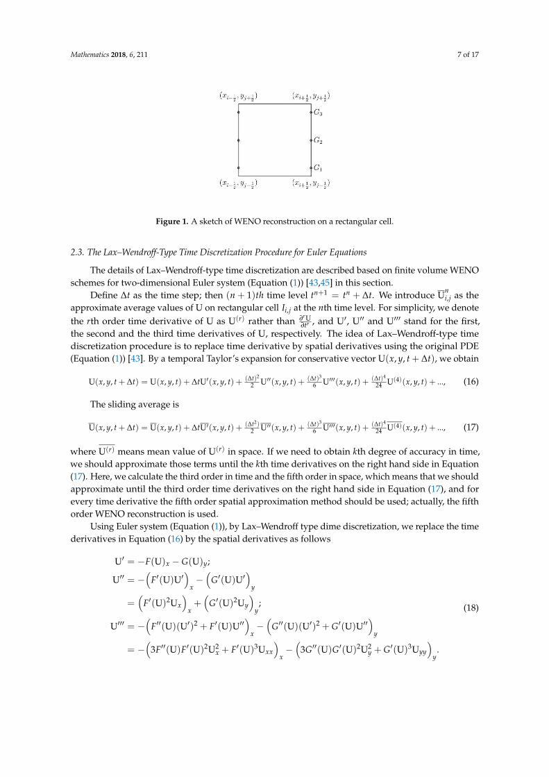
For two-dimensional finite volume case, we cannot simply procede in a dimension-by-dimensionfashion as in finite difference method. The spatial surface integration on rectangular cell Ii,j =

[xi− 12, xi+ 1

2]× [yj− 1

2, yj+ 1

2] can be converted to line integration by Gauss theorem. To obtain the fifth

order, we can use three-point Gaussian quadrature for line integration of every rectangular cell asin Figure 1. For example, to calculate numerical flux in x direction, three Gaussian point values onevery vertical lines should be reconstructed from cell average values in y direction first; then left andright Gaussian point values should be reconstructed by the WENO scheme; next is the numerical flux;and finally the cell average value can be approximate on next time level. When dissipation does notexist, we first suppose

r = ρ cos θ − ct, (13)

where c is a constant and denote the phase speed of the wave. Equation (8) implies that

∂

∂t=

∂

∂r∂r∂t

= −c∂

∂r,

∂

∂ρ=

∂

∂r∂r∂ρ

= cos θ∂

∂r,

∂

∂θ=

∂

∂r∂r∂θ

= −ρ sin θ∂

∂r.

Based on the above transform, Equation (7) becomes

− c∂

∂r

[∂2φ

∂r2 +cos θ

ρ

∂φ

∂r− β

cφ

]= 0. (14)

where

∇2 =∂2

∂ρ2 +1ρ

∂

∂ρ+

1ρ2

∂2

∂θ2 ,

J(a, b) =(cos θ∂a∂ρ− sin θ

ρ

∂a∂θ

)(sin θ∂b∂ρ

+cos θ

ρ

∂b∂θ

)

− (sin θ∂a∂ρ

+cos θ

ρ

∂a∂ρ

)(cos θ∂b∂ρ− sin θ

ρ

∂b∂θ

).

When∂2u∂r2 +

cos θ

ρ

∂u∂r− β

cu = 0,

we can easy infer that the relative vorticity ∇2u is a function of stream function u only. Thus, we get

∂2u∂ρ2 +

1ρ

∂u∂ρ

+1ρ2

∂2u∂θ2 =

β

cu. (15)

Mathematics 2018, 6, 211 7 of 17

Figure 1. A sketch of WENO reconstruction on a rectangular cell.

2.3. The Lax–Wendroff-Type Time Discretization Procedure for Euler Equations

The details of Lax–Wendroff-type time discretization are described based on finite volume WENOschemes for two-dimensional Euler system (Equation (1)) [43,45] in this section.

Define ∆t as the time step; then (n + 1)th time level tn+1 = tn + ∆t. We introduce Uni,j as the

approximate average values of U on rectangular cell Ii,j at the nth time level. For simplicity, we denotethe rth order time derivative of U as U(r) rather than ∂rU

∂tr , and U′, U′′ and U′′′ stand for the first,the second and the third time derivatives of U, respectively. The idea of Lax–Wendroff-type timediscretization procedure is to replace time derivative by spatial derivatives using the original PDE(Equation (1)) [43]. By a temporal Taylor’s expansion for conservative vector U(x, y, t + ∆t), we obtain

U(x, y, t + ∆t) = U(x, y, t) + ∆tU′(x, y, t) + (∆t)2

2 U′′(x, y, t) + (∆t)3

6 U′′′(x, y, t) + (∆t)4

24 U(4)(x, y, t) + ..., (16)

The sliding average is

U(x, y, t + ∆t) = U(x, y, t) + ∆tU′(x, y, t) + (∆t2)2 U′′(x, y, t) + (∆t)3

6 U′′′(x, y, t) + (∆t)4

24 U(4)(x, y, t) + ..., (17)

where U(r) means mean value of U(r) in space. If we need to obtain kth degree of accuracy in time,we should approximate those terms until the kth time derivatives on the right hand side in Equation(17). Here, we calculate the third order in time and the fifth order in space, which means that we shouldapproximate until the third order time derivatives on the right hand side in Equation (17), and forevery time derivative the fifth order spatial approximation method should be used; actually, the fifthorder WENO reconstruction is used.

Using Euler system (Equation (1)), by Lax–Wendroff type dime discretization, we replace the timederivatives in Equation (16) by the spatial derivatives as follows

U′ = −F(U)x − G(U)y;

U′′ = −(

F′(U)U′)

x−(

G′(U)U′)

y

=(

F′(U)2Ux

)x+(

G′(U)2Uy

)y;

U′′′ = −(

F′′(U)(U′)2 + F′(U)U′′)

x−(

G′′(U)(U′)2 + G′(U)U′′)

y

= −(

3F′′(U)F′(U)2U2x + F′(U)3Uxx

)x−(

3G′′(U)G′(U)2U2y + G′(U)3Uyy

)y.

(18)

Mathematics 2018, 6, 211 8 of 17

where brief notes are used, such as F′(U)2 = F′(U)F′(U), the details are given below. Thus, Equation (16)can be written as

U(x, y, t + ∆t) = U(x, y, t)− ∆t(

F(U)− ∆t2

F′(U)2Ux +∆t2

6(3F′′(U)F′(U)2U2

x + F′(U)3Uxx))

x

− ∆t(

G(U)− ∆t2

G′(U)2Uy +∆t2

6(3G′′(U)G′(U)2U2

y + G′(U)3Uyy))

y+ ...

(19)

Then, the sliding average (Equation (17)) with third order in time on a rectangular cell Iij isapproximated as

Un+1i,j = Un

i,j −∆t

∆x∆y

∫ yj+ 1

2

yj− 1

2

(F(Ui+ 1

2 ,∗)− F(U(xi− 12 ,∗))

dy

− ∆t∆x∆y

∫ xi+ 1

2

xi− 1

2

(G(U∗,j+ 1

2)− G(U∗,j− 1

2))

dx,(20)

with

F(U) = F(U)− ∆t2

F′(U)2Ux +∆t2

6(3F′′(U)F′(U)2U2

x + F′(U)3Uxx);

G(U) = G(U)− ∆t2

G′(U)2Uy +∆t2

6(3G′′(U)G′(U)2U2

y + G′(U)3Uyy),(21)

where F(U) and G(U) are approximated by numerical flux ˆF and ˆG, such as F(Ui+ 12 ,∗) ≈

ˆFi+ 12 ,∗ =

ˆF(ULi+ 1

2 ,∗, URi+ 1

2 ,∗).

For example, the first term in F(U) and G(U) are for the approximation of the first time derivativeU′, where U′ = −F(U)x − G(U)y. In the fifth order finite volume WENO scheme, on rectangle controlvolume Ii,j,

U′ i,j = −1

∆x∆y

∫ yj+ 1

2

yj− 1

2

(Fi+ 1

2 , ∗ − Fi− 12 , ∗

)dy− 1

∆x∆y

∫ xi+ 1

2

xi− 1

2

(G∗ ,j+ 1

2− G∗ ,j− 1

2

)dx,

three point Gaussian quadrature formulae are used for the above line integration. The integrand,that is numerical flux vector F(UL

i± 12 ,G

, URi± 1

2 ,G) and G(UL

G,j± 12, UR

G,j± 12), at every Gaussian point

(xG, yj± 12), (xi± 1

2, yG), is obtained by the regular fifth order WENO finite volume reconstruction and the

Lax–Friedrich numerical flux, as described in Section 2.2, where xG = {xi −√

35

∆x2 , xi, xi +

√35

∆x2 }

are the three Gaussian points. Meanwhile, the reconstruction of Ux, Uxx and Uy, Uyy in the second andthird term (Equation (21)) on Gaussian points of cell interface are calculated in this procession of WENOreconstruction. That is, in this procession, we calculate UL,R

G,j+ 12, (Ux)

L,RG,j+ 1

2, (Uxx)

L,RG,j+ 1

2, in subroutine of

WENO reconstruction. Notice that the extra ∆t factor multiplying by U′′ in Equation (21) leads to aone order lower flux approximation than that of the first time derivative U′. In x-direction, the linearpolynomial p′r(x) and constant p′′r (x) are the approximations to Ux and Uxx. According to polynomialpr(x) (Equation (9)), on r(r = 0, 1, 2) small stencil, we have

p′r(x) =k

∑m=0

m−1

∑j=0

ui−r+j∆xr−r+j

(∑kl=0,l 6=m ∑k

q=0,q 6=m,l ∏ks=0,s 6=m,l,q(x− xi−r+s− 1

2)

∏kl=0,l 6=m(xi−r+m− 1

2− xi−r+l− 1

2)

),

p′′r (x) = 2kk

∑m=0

( ∑m−1j=0 ui−r+j∆xr−r+j

∏kl=0,l 6=m(xi−r+m− 1

2− xi−r+l− 1

2)

).

(22)

Mathematics 2018, 6, 211 9 of 17

The same linear weights of U are used for Ux, Uxx. According to the definition of smooth,Equation (11) indicates constant β′r and zero β′′r are used for Ux and Uxx, as

β′r =∫ x

i+ 12

xi− 1

2

∆xi(p′′r (x))2dx +∫ x

i+ 12

xi− 1

2

(∆xi)3(p′′′r (x))2dx.

Similar formulae can be written for Uy and Uyy in y-direction in WENO reconstruction.In Equation (21), the Jacobian matrices are F′(U) = A(U), G′(U) = B(U), which have been

mentioned above. F′(U)2Ux, G′(U)2Uy are 4× 1 vectors. If we denote

F′′(U) = A′(U) = (A21|A22|A23|A24), (23)

where A21, A22, A23, A24 are 4× 4 matrices,

F′′(U)F′(U)2(Ux)2 =

(A21(F′(U)2Ux), A22(F′(U)2Ux), A23(F′(U)2Ux), A24(F′(U)2Ux)

)Ux,

which is also a 4× 1 vector and have been calculated in a previous step, in which we known F′(U)2(Ux)

is a 4× 1 vector, with

A21 =1ρ

0 0 0 0

−(γ− 3)u2 − (γ− 1)v2 u(γ− 3) v(γ− 1) 02uv −v −u 0

u(

2Eγρ − 3(γ− 1)(u2 + v2)

)(γ− 1)(3u2 + v2)− Eγ

ρ 2uv(γ− 1) −uγ

,

A22 =1ρ

0 0 0 0

(γ− 3)u −(γ− 3) 0 0−v 0 1 0

− Eγρ + (γ− 1)(3u2 + v2) −3(γ− 1)u −v(γ− 1) γ

,

A23 =1ρ

0 0 0 0

(γ− 1)v 0 −(γ− 1) 0−u 1 0 0

2uv(γ− 1) −v(γ− 1) −u(γ− 1) 0

,

A24 =1ρ

0 0 0 00 0 0 00 0 0 0−uγ γ 0 0

.

(24)

If we denoteG′′(U) = B′(U) = (B21|B22|B23|B24), (25)

Mathematics 2018, 6, 211 10 of 17

where B21, B22, B23, B24 are 4× 4 matrices, and

B21 =1ρ

0 0 0 0

2uv −v −u 0−(γ− 1)u2 − (γ− 3)v2 u(γ− 1) v(γ− 3) 0

v(

2Eγρ − 3(γ− 1)(u2 + v2)

)(γ− 1)2uv − Eγ

ρ + (γ− 1)(u2 + 3v2) −vγ

,

B22 =1ρ

0 0 0 0−v 0 1 0

(γ− 1)u −(γ− 1) 0 0(γ− 1)2uv −(γ− 1)v −(γ− 1)u 0

,

B23 =1ρ

0 0 0 0−u 1 0 0

(γ− 3)v 0 −(γ− 3) 0− Eγ

ρ + (γ− 1)(u2 + 3v2) −(γ− 1)u −3(γ− 1)v γ

,

B24 =1ρ

0 0 0 00 0 0 00 0 0 0−vγ 0 γ 0

.

(26)

If a higher accuracy order in time is required, the procedure needs to be continued untilthe corresponding derivatives in a similar fashion. For convenience, in the following parts,WENO5-LW3 denotes a scheme coupling the fifth order finite volume WENO scheme in space and thethird order Lax–Wendroff-type method in time and WENO5-RK3 denotes a scheme coupling the fifthorder finite volume WENO schemes and the third order Runge–Kutta methods.

3. Numerical Results

In this section, extensive numerical examples are used for performance testing for the new finitevolume WENO5-LW3 schemes. We compare the results of WENO5-LW3 for one- and two-dimensionalEuler equations and that of the WENO5-RK3 schemes, focusing on the important issue of CPU timecost, non-oscillatory and efficiency. For comparison of CPU time cost, all computations are performedon a personal computer, Core (TM) i5-3470 CPU @ 3.20 GHz with 4 GB RAM. In these numericalsimulations, we use CFL number 0.4 and 0.6 for WENO5-LW3 and WENO-RK3 schemes, respectively.The small positive constant ε = 10−6 is used to avoid denominator zero in the nonlinear weightformula. All of these simulations are based on uniform meshes.

Example 1 (One-Dimensional Accuracy Test). To check the order accuracy of the finite volume WENO5-LW3schemes based on one-dimensional Euler system with a smooth solution (Equation (6)), for comparison, we usethe same test as in [43]. In the computational domain [−1, 1], the initial condition is given below:

ρ(x, 0) = 1 + 0.2sin(πx),

v(x, 0) = 1.0, p(x, 0) = 1.0.

Two-periodic boundary conditions are used; we simulate until the ending time t = 2, when the solutionsare continuous and there are no shocks. The exact solution is

ρ(x, t) = 1 + 0.2sin(π(x− t)),

v(x, t) = 1.0, p(x, t) = 1.0.

Mathematics 2018, 6, 211 11 of 17

The numerical errors and orders of accuracy based on L1 and L∞ norm metric for density ρ byWENO5-LW3 are shown in Table 1. N stands for the number of mesh grids; adjusted adaptive time stepsize should be used to get the fifth order as mesh refining. For comparison, the L1 and L∞ numericalerrors and accuracy orders by WENO5-RK3 schemes are displayed in Table 1. In Table 1, we canfind that the designed accuracy order are attained for both WENO5-LW3 and WENO5-RK3, and theygenerate similar numerical errors.

Table 1. L1 and L∞ errors and numerical orders of accuracy for density of one-dimensional order test,WENO5-LW3 and WENO5-RK3 using N space mesh points.

NWENO5-LW3 WENO5-RK3

L1 error order L∞ error order L1 error order L∞ error order

10 6.38 × 10−3 1.02 × 10−2 6.37 × 10−3 1.01 × 10−2

20 3.14 × 10−4 4.34 5.45 × 10−4 4.23 3.15 × 10−4 4.34 5.45 × 10−4 4.2140 9.80 × 10−6 5.00 1.88 × 10−5 4.86 9.85 × 10−6 5.00 1.89 × 10−5 4.8580 3.06 × 10−7 5.00 6.14 × 10−7 4.94 3.07 × 10−7 5.00 6.15 × 10−7 4.94

160 9.59 × 10−9 5.00 1.85 × 10−8 5.05 9.58 × 10−9 5.00 1.85 × 10−8 5.05320 2.97 × 10−10 5.01 5.40 × 10−10 5.10 2.98 × 10−10 5.01 5.42 × 10−10 5.10640 9.71 × 10−12 4.93 1.82 × 10−11 4.89 9.20 × 10−12 5.02 1.91 × 10−11 4.82

In Figure 2, we give the numerical errors and CPU time cost for density ρ based on L1 and L∞ normmetric with cell numbers are 10× 2k−1, k = 1, 2, ..., 7, and Log scale is used for numerical errors in y axis.In this figure, the line of WENO5-LW3 always underneath the line of WENO5-RK3, which implies that,with the same CPU time cost, WENO5-LW3 obtains a higher accuracy than WENO5-RK3. From thetrend of the line, it seems that the phenomenon will be more serious when the test has more meshpoints.

CPU time

Err

or o

f Den

sity

0 50 100

10-11

10-10

10-9

10-8

10-7

10-6

10-5

10-4

10-3

10-2

WENO5-LW3WENO5-RK3

CPU time

Err

or o

f Den

sity

0 50 100

10-11

10-10

10-9

10-8

10-7

10-6

10-5

10-4

10-3

10-2

WENO5-LW3WENO5-RK3

Figure 2. Numerical errors of density and CPU time for the one-dimensional order test in Example 1:(Left) L1 error; and (Right) L∞ error.

Example 2 (One-Dimensional Test with Shocks). This problem is commonly applied to test the ability ofshock capturing for schemes in one-dimensional Euler system [43]. In this case, we considertwo different initial

Mathematics 2018, 6, 211 12 of 17

conditions in the domain [−0.5, 0.5], with continuation boundary condition for two boundary; the first test isLax Problem,

(ρ, v, p) =

{(0.445, 0.698, 3.528) x ≤ 0(0.5, 0, 0.571) x > 0

. (27)

and the second test is Sod Problem,

(ρ, v, p) =

{(1.0, 0, 1.0) x ≤ 0(0.25, 0, 0.1) x > 0

, (28)

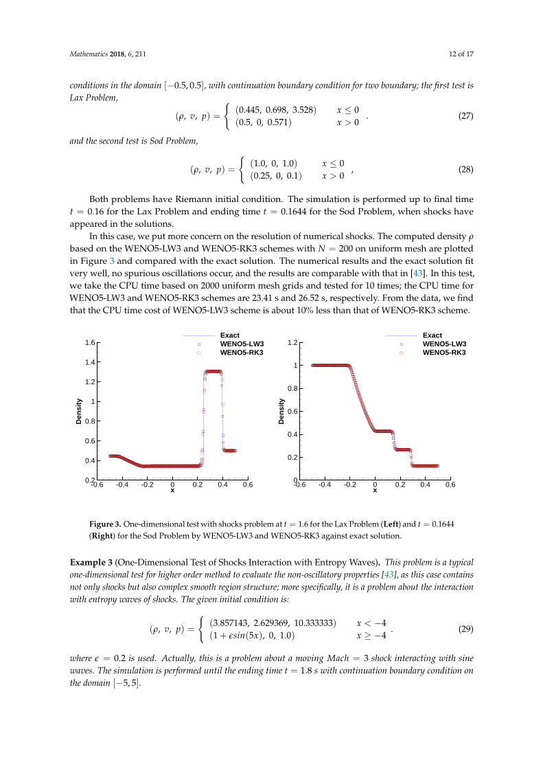
Both problems have Riemann initial condition. The simulation is performed up to final timet = 0.16 for the Lax Problem and ending time t = 0.1644 for the Sod Problem, when shocks haveappeared in the solutions.

In this case, we put more concern on the resolution of numerical shocks. The computed density ρ

based on the WENO5-LW3 and WENO5-RK3 schemes with N = 200 on uniform mesh are plottedin Figure 3 and compared with the exact solution. The numerical results and the exact solution fitvery well, no spurious oscillations occur, and the results are comparable with that in [43]. In this test,we take the CPU time based on 2000 uniform mesh grids and tested for 10 times; the CPU time forWENO5-LW3 and WENO5-RK3 schemes are 23.41 s and 26.52 s, respectively. From the data, we findthat the CPU time cost of WENO5-LW3 scheme is about 10% less than that of WENO5-RK3 scheme.

x

Den

sity

-0.6 -0.4 -0.2 0 0.2 0.4 0.60.2

0.4

0.6

0.8

1

1.2

1.4

1.6ExactWENO5-LW3WENO5-RK3

x

Den

sity

-0.6 -0.4 -0.2 0 0.2 0.4 0.60

0.2

0.4

0.6

0.8

1

1.2ExactWENO5-LW3WENO5-RK3

Figure 3. One-dimensional test with shocks problem at t = 1.6 for the Lax Problem (Left) and t = 0.1644(Right) for the Sod Problem by WENO5-LW3 and WENO5-RK3 against exact solution.

Example 3 (One-Dimensional Test of Shocks Interaction with Entropy Waves). This problem is a typicalone-dimensional test for higher order method to evaluate the non-oscillatory properties [43], as this case containsnot only shocks but also complex smooth region structure; more specifically, it is a problem about the interactionwith entropy waves of shocks. The given initial condition is:

(ρ, v, p) =

{(3.857143, 2.629369, 10.333333) x < −4(1 + εsin(5x), 0, 1.0) x ≥ −4

. (29)

where ε = 0.2 is used. Actually, this is a problem about a moving Mach = 3 shock interacting with sinewaves. The simulation is performed until the ending time t = 1.8 s with continuation boundary condition onthe domain [−5, 5].

Mathematics 2018, 6, 211 13 of 17

The computed density ρ based on the WENO5-LW3 schemes and WENO5-RK3 schemes with themesh points N = 200 and N = 400 and zoomed in pictures are plotted in Figure 4 against a referenceexact solution by 2000 mesh points, which show that the computed solution converges to the referenceexact solution, and no spurious oscillations occur. The WENO5-LF3 scheme could get much betterresolution than that of WENO5-RK3 scheme. The results are better confirmed with reference solutionon N = 400 than that on N = 200, which also shows a converged solution computed by WENO5-LW3.All results agree with that in [43]. The time cost to run 10 times based on uniform mesh with N = 2000is taken as the CPU time for every problem. The CPU time is 59.94 s for WENO5-LW3 and 66.24 sfor WENO5-RK3, respectively, so the CPU time cost of WENO5-RK3 is around 8.5% more than thatof WENO5-LW3.

(a)

x

Den

sity

-6 -4 -2 0 2 4 60.5

1

1.5

2

2.5

3

3.5

4

4.5

5

ExactWENO5-LW3WENO5-RK3

(b)

x

Den

sity

0 0.5 1 1.5 2 2.5 3 3.5 43

3.5

4

4.5ExactWENO5-LW3WENO5-RK3

(c)

x

Den

sity

-6 -4 -2 0 2 4 60.5

1

1.5

2

2.5

3

3.5

4

4.5

5

ExactWENO5-LW3WENO5-RK3

(d)

x

Den

sity

0 0.5 1 1.5 2 2.5 3 3.5

Figure 4. The shock density wave interaction problem at t = 1.8 by WENO5-LW3 and WENO5-RK3with N = 200 and N = 400. (a) N = 200 for density; (b) N = 200 density zoomed in; (c) N = 400 fordensity; (d) N = 400 density zoomed in.

Example 4 (Two-Dimensional Accuracy Order Test). To check the order accuracy of the schemes fortwo-dimensional Euler system with a smooth solution, for comparison, we use the test in [43]. In thecomputational domain [0, 2]× [0, 2], we take the following initial conditions:

ρ(x, y, 0) = 1 + 0.2sin(

π(x + y))

,

Mathematics 2018, 6, 211 14 of 17

u(x, y, 0) = 0.7, v(x, y, 0) = 0.3, p(x, y, 0) = 1.

Four-periodic boundary conditions are used; the final time t = 2 is when no shocks appear in the solution.The exact solution for the problem is

ρ(x, y, t) = 1 + 0.2sin(

π(x + y− (u + v)t))

,

u(x, y, t) = 0.7, v(x, y, t) = 0.3, p(x, y, t) = 1.

In Table 2, the numerical errors and accuracy orders for ρ by WENO5-LW3 based on L∞ andL1 norm metric are shown, while N is the number of mesh cells. The rectangle cell is used to avoidcancelations of some special error due to the symmetry axis being in the diagonals of cells. L∞ andL1 numerical errors and accuracy orders by WENO5-RK3 schemes are also displayed in Table 2 tocompare with the results of WENO5-LW3. The two schemes have achieved the fifth order accuracy atthe final time and generate similar numerical errors.

Table 2. L1 and L∞ errors and numerical orders of accuracy for density of two-dimensional accuracytest, WENO5-LW3 and WENO5-RK3 with N cells.

NWENO5-LW3 WENO5-RK3

L1 error order L∞ error order L1 error order L∞ error order

8× 12 4.46×10−2 0.00 1.73×10−2 0.00 4.46×10−2 0.00 1.74×10−2 0.0016× 24 2.70×10−3 4.05 1.15×10−3 3.91 2.72×10−3 4.03 1.16×10−3 3.9032× 48 8.79×10−5 4.94 4.32×10−5 4.73 8.85×10−5 4.94 4.35×10−5 4.7464× 96 2.75×10−6 5.00 1.38×10−6 4.97 2.77×10−6 5.00 1.40×10−6 4.96

128× 192 8.62×10−8 5.00 4.24×10−8 5.02 8.65×10−8 5.00 4.27×10−8 5.03

On mesh 64× 96, the corresponding CPU time costs for WENO5-LW3 and WENO5-RK3 are986.73 s and 1103.93 s. We can see that WENO5-RK3 cost about 10% more CPU time than WENO5-LW3.

Example 5 (Two-Dimensional Double Mach Reflection). This problem is a two-dimensional double machreflection test; complex boundary conditions are implemented. For the example, multiple shocks with complexself-similar structure are emergent, and the initial geometry is very simple [43].

In this test, the wedge of the oblique shock is set as a partially reflecting horizontal lower boundary.The computational domain is [0, 4]× [0, 1], the x axis is 4.0 units long. At the first 1/6 units, the outflowis free and the remaining units reflect the rest of the boundary. At the upper boundary, the flow valuesare used to describe the exact motion of a shock at Mach = 10. The left boundary is constant withthe post oblique shock values, and there is no limit for the right boundary. In the whole calculation,the final time is t = 0.2.

At the ending time, we plot the computed density contours by the WENO5-LW3 scheme with1920× 480 meshes in Figure 5, which is almost the same as the results by WENO5-RK3, and comparablewith previous results in [43]. When the CPU time is considered, we can find that WENO5-RK3 alsocosts a little more time than WENO5-LW3.

Mathematics 2018, 6, 211 15 of 17

X

Y

0 0.5 1 1.5 2 2.5 30

0.2

0.4

0.6

0.8

1

Figure 5. The two-dimensional double mach reflection problem at t = 0.2 by WENO5-LW3.

4. Concluding Remarks

In this paper, we take advantage of Lax–Wendroff-type time discretizations and high resolutionfinite volume WENO schemes to simulate one-dimensional and two-dimensional Euler equations.By comparing the addressing on CPU time, non-oscillatory, resolution and relevant efficiency of finitevolume WENO schemes using time discetizations, the numerical results show that the WENO5-LW3schemes takes smaller CPU costs than WENO5-RK3 schemes, while WENO5-LW3 schemes got thesame order of accuracy with Runge–Kutta time discretization on the same mesh grids number.These conclusions agree with the theory of the finite difference WENO with Lax–Wendroff-typeand Runge–Kutta time discretizations for Euler system of compressible gas dynamics.

Author Contributions: These authors contributed equally to this work.

Acknowledgments: The work was partially supported by the China Postdoctoral Science Foundation fundedproject (2017M610436); Nature Science Foundation of Shandong Province of China (No.ZR2018MA017);Natural Science Foundation of China (11801280); Natural Science Foundation of Jiangsu Province (BK20180780);and Natural Science Foundation of the Jiangsu Higher Education Institutions (18KJB110020).

Conflicts of Interest: The authors declare that they have no competing interests.

References

1. Guo, M.; Zhang, Y.; Wang, M.; Chen, Y.D.; Yang, H.W. A new ZK-ILW equation for algebraic gravitysolitary waves in finite depth stratified atmosphere and the research of squall lines formation mechanism.Comput. Math. Appl. 2018, 75, 3589–3603. [CrossRef]

2. Lu, C.N.; Fu, C.; Yang, H.W. Time-fractional generalized Boussinesq Equation for Rossby solitary waves withdissipation effect in stratified fluid and conservation laws as well as exact solutions. Appl. Math. Comput.2018, 327, 104–116. [CrossRef]

3. Zhang, Y.; Dong, H.H.; Zhang, X.E.; Yang, H.W. Rational solutions and lump solutions to the generalized(3 + 1)-dimensional Shallow Water-like equation. Comput. Math. Appl. 2017, 73, 246–252. [CrossRef]

4. Li, X.Y.; Zhao, Q.L.; Li, Y.X. Binary Bargmann symmetry constraint associated with 3× 3 discrete matrixspectral problem. J. Nonlinear Sci. Appl. 2015, 8, 496–506. [CrossRef]

5. Barnett, M.P.; Capitani, J.F.; Joachim, V.Z. Symbolic calculation in chemistry: Selected examples. Int. J.Quantum Chem. 2004, 100, 80–104. [CrossRef]

6. Yang, H.W.; Chen, X.; Guo, M.; Chen, Y.D. A new ZK-BO equation for three-dimensional algebraic Rossbysolitary waves and its solution as well as fission property. Nonlinear Dyn. 2018, 91, 2019–2032. [CrossRef]

7. Yang, H.W.; Xu, Z.H.; Yang, D.Z. ZK-Burgers equation for three-dimensional Rossby solitary waves and itssolutions as well as chirp effect. Adv. Differ. Equ. 2016, 2016, 167. [CrossRef]

8. Saleh, M.F.; Chang, W.; Travers, J.C. Plasma-induced asymmetric self-phase modulation and modulationalinstability in gas-filled hollow-core photonic crystal fibers. Phys. Rev. Lett. 2012, 109, 1–5. [CrossRef][PubMed]

Mathematics 2018, 6, 211 16 of 17

9. Gorza, S.P.; Deconinck, B.; Emplit, P. Experimental demonstration of the oscillatory snake instability of thebright soliton of the (2 + 1)D hyperbolic nonlinear Schrödinger equation. Phys. Rev. Lett. 2011, 106, 094101.[CrossRef] [PubMed]

10. Shi, Y.; Yin, B.; Yang, H. Dissipative nonlinear Schrödinger equation for envelope solitary Rossby waveswith dissipation effect in stratified fluids and its solution. Abstr. Appl. Anal. 2014, 2014, 643652. [CrossRef]

11. Guo, M.; Fu, C.; Zhang, Y.; Liu, J.X.; Yang, H.W. Study of ion-acoustic solitary waves in a magnetized plasmausing the three-dimensional time-space fractional Schamel-KdV equation. Complexity 2018, 2018, 6852548.[CrossRef]

12. Yang, H.W.; Yin, B.; Wang, Q. Forced ILW-Burgers Equation As A Model For Rossby Solitary WavesGenerated By Topography In Finite Depth Fluids. J. Appl. Math. 2012, 2012, 491343. [CrossRef]

13. Bekir, A. Painlevé test for some (2 + 1)-dimensional nonlinear equations. Chaos Solitons Fractals 2007, 32,449–455. [CrossRef]

14. Xu, X.X.; Sun, Y.P. An integrable coupling hierarchy of Dirac integrable hierarchy, its Liouville integrabilityand Darboux transformation. J. Nonlinear Sci. Appl. 2017, 10, 3328–3343. [CrossRef]

15. Li, X.Y.; Zhang, Y.Q.; Zhao, Q.L. Positive and negative integrable hierarchies, associated conservation lawsand darboux transformation. J. Comput. Appl. Math. 2009, 233, 1096–1107. [CrossRef]

16. Guo, X.R. On bilinear representations and infinite conservation laws of a nonlinear variable-coefficientequation. Appl. Math. Comput. 2014, 248, 531–535. [CrossRef]

17. Ma, W.X.; Zhou, Y. Lump solutions to nonlinear partial differential equations via hirota bilinear forms.J. Differ. Equ. 2018, 264, 2639–2659. [CrossRef]

18. Dong, H.H.; Chen, T.; Chen, L.; Zhang, Y. A new integrable symplectic map and the lie point symmetryassociated with nonlinear lattice equations. J. Nonlinear Sci. Appl. 2016, 9, 5107–5118. [CrossRef]

19. Fu, C.; Lu, C.N.; Yang, H.W. Time-space fractional (2 + 1) dimensional nonlinear Schrédinger equationfor envelope gravity waves in baroclinic atmosphere and conservation laws as well as exact solutions.Adv. Differ. Equ. 2018, 2018, 56. [CrossRef]

20. Tang, J.; He, G.P.; Fang, L. A new non-interior continuation method for second-order cone programming.J. Numer. Math. 2013, 21, 301–323. [CrossRef]

21. Wang, Z. A numerical method for delayed fractional-order differential equations. J. Appl. Math. 2013,2013, 256071. [CrossRef]

22. Zhang, S.Q.; Meng, X.Z.; Zhang, T.H. Dynamics analysis and numerical simulations of a stochasticnon-autonomous predator-prey system with impulsive effects. Nonlinear Anal. Hybrid Syst. 2017, 26,19–37. [CrossRef]

23. Liu, X.K.; Li, Y.; Zhang, W.H. Stochastic linear quadratic optimal control with constraint for discrete-timesystems. Appl. Math. Comput. 2014, 228, 264–270. [CrossRef]

24. Zhou, S.W.; Zhang, W.H. Discrete-time indefinite stochastic Lq control via sdp and Lmi methods.J. Appl. Math. 2012, 2012, 638762. [CrossRef]

25. Liu, X.D.; Osher, S.; Chan, T. Weighted essentially non-oscillatory schemes. J. Comput. Phys. 1994, 115,200–212. [CrossRef]

26. Jiang, G.S.; Shu, C.W. Effecient implementation of weighted ENO schemes. J. Comput. Phys. 1996, 126,202–228. [CrossRef]

27. Balsara, D.S.; Shu, C.W. Monotonicity preserving weithted essentially non-oscillatory schemes withincreasingly high order of accuracy. J. Comput. Phys. 2000, 160, 405–452. [CrossRef]

28. Shu, C.W. Essential non-oscillatory and weighted essentially non-oscillatory schemes for hyperbolicconservation laws. In Advanced Numerical Approximation of Nonlinear Hyperbolic Equations; Springer: Berlin,Gemany, 1998; pp. 325–432.

29. Wang, Z.; Huang, X.; Zhou, J.P. A numerical method for delayed fractional-order differential equations:Based on G-L definition. Appl. Math. Inf. Sci. 2013, 7, 525–529. [CrossRef]

30. Harten, A.; Engguist, B.; Osher, S.; Chakravarthy, S. Uniformly high order essentially non-oscillatoryschemes.J. Comput. Phys. 1987, 71, 231–303. [CrossRef]

31. Zhu, J.; Qiu, J.X. Finite volume Hermite WENO schemes for solving the Hamilton-Jacobi equations II:Unstructured meshes. Comput. Math. Appl. 2014, 68, 1137–1150. [CrossRef]

32. Li, G.; Qiu, J.X. Hybrid weighted essentially non-oscillatory schemes with different indicators.J. Comput. Phys. 2010, 229, 8105–8129. [CrossRef]

Mathematics 2018, 6, 211 17 of 17

33. Christlieb, A.J.; Liu, Y.; Tang, Q.; Xu, Z.F. High order parametrized maximum-principle-preserving andpositivity-preserving WENO schemes on unstructured meshes. J. Comput. Phys. 2015, 281, 334–351.[CrossRef]

34. Dumbser, M. Arbitrary-Lagrangian-Eulerian ADER-WENO finite volume schemes with time-accurate localtime stepping for hyperbolic conservation laws. Comput. Methods Appl. Mech. Eng. 2014, 280, 57–83.[CrossRef]

35. Huang, C.S.; Arbogast, T.; Hung, C.H. A re-averaged WENO reconstruction and a third order CWENOscheme for hyperbolic conservation laws. J. Comput. Phys. 2014, 262, 291–312. [CrossRef]

36. Arándiga, F.; Belda, A.M.; Mulet, P. Point-Value WENO Multiresolution Applications to Stable ImageCompression. J. Sci. Comput. 2009, 43, 158–182. [CrossRef]

37. Balsara, D.S. Divergence-free reconstruction of magnetic fields and WENO schemes formagnetohydrodynamics. J. Comput. Phys. 2009, 228, 5040–5054. [CrossRef]

38. Vukovic, S.; Sopta, L. ENO and WENO schemes with the exact conservation property for one-dimensionalshallow water equations. J. Comput. Phys. 2002, 179, 593–621. [CrossRef]

39. Zhao, S.; Lardjane, N.; Fedioun, I. Comparison of improved finite-difference WENO schemes for the implicitlarge eddy simulation of turbulent non-reacting and reacting high-speed shear flows. Comput. Fluid 2014, 99,74–87. [CrossRef]

40. Vecil, F.; Mestre, P.M.; Labrunie, S. WENO schemes applied to the quasi-relativistic Vlasov-Maxwell modelfor laser-plasma interaction. C. R. Mecanique 2014, 342, 583–594. [CrossRef]

41. Zhu, H.; Qiu, J.; Qiu, J.M. An h-adaptive RKDG method for the two-dimensional incompressible Eulerequations and the guiding center vlasov model. J. Sci. Comput. 2017, 73, 1316–1337. [CrossRef]

42. Lu, C.N.; Qiu, J.X.; Wang, R.Y. Weighted Essential Non-oscillatory Schemes for Tidal Bore on UnstructuredMeshes. Int. J. Numer. Method Fluid 2009, 59, 611–630. [CrossRef]

43. Qiu, J.X.; Shu, C.W. Finite difference WENO schemes with Lax-wendroff-type time discretizations. SIAM J.Sci. Comput. 2003, 24, 2185–2198. [CrossRef]

44. Lax, P.D.; Wendroff, B. Systems of conservation law. Commun. Pure Appl. Math. 1960, 13, 217–237. [CrossRef]45. Lu, C.N.; Qiu, J.X. Simulation of shallow water equations with finite difference Lax–Wendroff weighted

essential non-oscillatory schemes. J. Sci. Comput. 2011, 47, 281–302. [CrossRef]46. Lu, C.N.; Qiu, J.X.; Wang, R.Y. A numerical study for the performance of the WENO schemes based on

different numerical fluxes for the shallow water equations. J. Comput. Math. 2010, 28, 807–825. [CrossRef]47. Lu, C.N.; Xie, L.Y.; Yang, H.W. The Simple Finite Volume Lax-Wendroff Weighted Essentially Nonoscillatory

Schemes for Shallow Water Equations with Bottom Topography. Math. Probl. Eng. 2018, 2018, 2652367.[CrossRef]

c© 2018 by the authors. Licensee MDPI, Basel, Switzerland. This article is an open accessarticle distributed under the terms and conditions of the Creative Commons Attribution(CC BY) license (http://creativecommons.org/licenses/by/4.0/).