4th Twente Workshop onCooperative Game Theory

joint with 3rd Dutch–Russian Symposium

WCGT2005, June 28–30, 2005

edited by

T.S.H. Driessen, A.B. Khmelnitskaya, J.B. Timmer

University of Twente

Enschede, The Netherlands

www.math.utwente.nl/∼driessentsh

Foreword

This workshop volume contains the program, in its global and detailed version,as well as the contributions by the invited speakers as well as the extendedabstracts by the Russian participants.

We thank Dini Heres for her excellent computer assistance and webmasterMichel ten Bulte.We gratefully acknowledge the financial support from the following sources:

• College van Bestuur, Beleidsbureau CvB van de Universiteit Twente (UT)

• Stichting Universiteitsfonds Twente, University of Twente(www.utwente.nl/ufonds)

• Faculty of Electrical Engineering, Mathematics, and Computer Science(EEMCS), UT (www.ewi.utwente.nl)

• Chair “Discrete Mathematics and Mathematical Programming” (DMMP),UT (www.math.utwente.nl/dos/dwmp)

• Mathematical Research Institute (MRI), Utrecht (www.mri.math.uu.nl)

• Center for Telematics and Information Technology (CTIT), UT, Enschede(www.ctit.utwente.nl)

• Netherlands Organization for Scientific Research (NWO),(www.nwo.nl) in the framework of the ongoing research-cooperation be-tween the Russian Federation and The Netherlands, as approved by NWOwith reference to the research project entitled “Axiomatic Approach tothe Elaboration of Cooperative Games” (dos.nr. 047-008-010)

Sponsors

Theo Driessen,Judith Timmer,Anna Khmelnitskaya Enschede, June 2005

i

ii

Contents

Workshop Program 1

Contributions by invited speakers

J.M. Bilbao, J.R. Fernandez, N. Jimenez, J.J. Lopez 5A survey of bicooperative games

I. Dragan 17On the computation of semivalues for TU games via Shapley value

V. Fragnelli 27Game Theoretic Analysis of Transportation Problems

Y. Funaki, T. Yamato 39Sequentially stable coalition structures

G. Kassay, J.B.G. Frenk 61On noncooperative games and minimax theory

S. Muto, N. Watanabe 71Stable profit sharing in patent licensing: general bargaining outcomes

B. Peleg, P. Sudholter 89On Bargaining Sets and Voting Games

C. Rafels, M. Nunez 105Core-based solutions for assignment markets

J. Rosenmuller 117Convex Geometry and Bargaining

S. Tijs, R. Branzei 141Games and Geometry

Extended abstracts by Russian participants

P. Chebotarev, V. Borzenko, Z. Lezina, A. Loginov, J. Tsodikova 151Comparing selfishness and versions of cooperationas the voting strategies in a stochastic environment

A. Gan’kova, M. Dementieva, P. Neittaanmaki, V. Zakharov 153Cooperative models of joint implementation

V. Domansky 159Repeated games with lack of information on one side and multistage auctions

V. Gurvich 161War and peace in veto voting

iii

A. B. Khmelnitskaya, E.B. Yanovskaya 169Owen coalitional value without additivity axiom

G. Koshevoy 175Pareto choice functions and elimination of dominated strategies

N. Naumova 177Generalized kernels and bargaining sets for coalition systems

V. Vasil’ev 181Information equilibrium: existence and core equivalence

E. Yanovskaya 187Values for TU games with linear cooperation structures

List of participants 193

Postal addresses of Russian participants 197

iv

Workshop Program3rd Dutch–Russian symposium

Scientific program, Tuesday, June 28Cubicus building, room C-238

Session I: Invited speakers

09:00 Registration/co!ee Payment fee upon arrival

09:30 Invited speaker 1: Bezalel PelegOn Bargaining Sets and Voting Games

10:30 Co!ee break

11:00 Invited speaker 2: Gabor KassayOn noncooperative games and minimax theory

12:00 Lunch break, Cubicus Cafetaria

Session II: 30 minutes talks by Russian partners

13:30 Anna Khmelnitskaya:Owen coalitional value without additivity axiom

14:00 Elena Yanovskaya:Values for TU games with linear cooperation structures

14:30 Natalia Naumova:Generalized kernels and bargaining sets for coalition systems

15:00 Vladimir Gurvich:Perfect graphs, kernels, and cores of cooperative games

15:30 Co!ee break

16:00 Valery Vasil’ev:Information equilibrium: existence and core equivalence

16:30 Gleb Koshevoy:Pareto choice functions and elimination of dominated strategies

17:00 Victor Domansky:Repeated games with lack of information on one side and multistage auctions

Evening program

19:00 Piano concert, Faculty Club, UT

20.00 Workshop dinner, Faculty Club, UT

1

Workshop Program4th Twente Workshop on Cooperative Game Theory

Scientific program, Wednesday, June 29Cubicus building, room C-238

Session I: Invited speakers

09:30 Invited speaker 3: Joachim RosenmullerConvex geometry and bargaining

10:30 Co!ee break

11:00 Invited speaker 4: Stef TijsGames and geometry

12:00 Lunch break, Cubicus Cafetaria

Session II: 30 minutes talks by Russian partners

13:30 Pavel Chebotarev:Comparing selfishness and versions of cooperation as thevoting strategies in a stochastic environment

14:00 Maria Dementieva:Cooperative models of joint implementation (Kyoto protocol)

14:30 Co!ee break

Session III: Invited speakers

15:00 Invited speaker 5: Shigeo MutoStable profit sharing in patent licensing: general bargaining outcomes

16:00 Co!ee break

16:30 Invited speaker 6: Yukihiko FunakiSequentially stable coalition structures

Evening program

19:00 Joint dinner, Hotel de Broeierd (close to UT)

2

Workshop Program4th Twente Workshop on Cooperative Game Theory

Scientific program, Thursday, June 30Cubicus building, room C-238

Session I: Invited speakers

09:30 Invited speaker 7: Irinel DraganOn the computation of semivalues via the Shapley value

10:30 Co!ee break

11:00 Invited speaker 8: Mario BilbaoA survey of bicooperative games

12:00 Lunch break, Cubicus Cafetaria

Session II: Poster session by seven participants

13:30 Encarna Algabe:The Banzhof index in the European Constitution Game

Yusuke Kamishiro:Ex ante alpha-core with incentive constraints

Marcin Malawski:Sharing marginal contribitions in TU games

Miklos Pinter:A Bayesian cooperative game

Tadeusz Radzik:Simple Nash equilibria in convex non-cooperative games

David Ramsey:Selection of correlated equilibria in stopping games

Tamas Solymosi:Pairwise monotonicity of the nucleolus in assignment games

14:30 Co!ee break

Session III: Invited speakers

15:00 Invited speaker 9: Carles RafelsUniform-price assignment markets

16:00 Co!ee break

16:30 Invited speaker 10: Vito FragnelliGame theoretic analysis of transportation problems

Evening program

19.00 Joint dinner, City of Enschede

3

4

A SURVEY OF BICOOPERATIVE GAMES

J.M. Bilbao∗, , J.R. Fernandez, N. Jimenez, J.J. Lopez

Matematica Aplicada II, Escuela Superior de IngenierosCamino de los Descubrimientos s/n, 41092 Sevilla, Spain.

Abstract. The aim of the present paper is to study several solutionconcepts for bicooperative games. For these games introduced by Bilbao [1],we define a one-point solution called the Shapley value, since this value can beinterpreted in a similar way to the classical Shapley value for cooperative games.The firs result of the paper is an axiomatic characterization of this value. Next,we define the core and the Weber set and prove that the core of a bicooperativegame is always contained in its Weber set. Finally, we introduce an special classof bicooperative games, the so-called bisupermodular games, and show that thesegames are the only ones in which their core and the Weber set coincide.

Keywords Bicooperative games, Bisupermodular games, Shapley value, Core,Weber set

1. Introduction

The theory of cooperative games studies situations where a group of people/agentsare associated to obtain a profit as a result of their cooperation. Thus, a cooperativegame is defined as a pair (N, v) , where N is a finite set of players and v : 2N → Ris a function verifying that v (∅) = 0. For each S ∈ 2N

, the worth v (S) can beinterpreted as the maximal gain or minimal cost that the players which form coalitionS can achieve themselves against the best offensive threat by the complementarycoalition N \S. Classical market games for economies with private goods are examplesof cooperative games. Hence, we can say that a cooperative game has orthogonalcoalitions (see Myerson [10]).

Games with non-orthogonal coalitions are games in which the worth of coalitionS are not independent of the actions of coalition N \ S. Clearly, social situationsinvolving externalities and public goods are such cases. For instance, we consider agroup of agents with a common good which is causing them expenses or costs. In aexternal or internal way, a modification (sale, buying, etc.) of this good is proposedto them. This action will suppose a greater profit to them in case they all agreewith the change proposed about the actual situation of the good. Moreover, eventhough the patrimonial good can be divisible, we suppose that the greatest value ofthe selling operation is reached if we consider all the common good.

A possibility of modeling these situations may be the following. We consider pairs(S, T ), with S, T ⊆ N and S∩T = ∅. Thus, (S, T ) is a partition of N in three groups.Players in S are defenders of modifying the statu quo and they want to accept aproposal; players in T do not agree with modifying the situation and they will takeaction against any change. Finally, the members of N \ (S ∪ T ) are not convinced ofthe profits derived from the proposal and they vote abstention.

∗E-mail: mbilbao@us.es

5

Thus, in our model we consider the set of all ordered pairs of disjoint coalitions3N = (S, T ) : S, T ⊆ N, S ∩ T = ∅ , and define a function b : 3N → R. For each(S, T ) ∈ 3N

, the worth b (S, T ) can be interpreted as the maximal gain (wheneverb (S, T ) > 0) or minimal loss (whenever b (S, T ) < 0) that the players of the coalitionS can achieve when they decide to play together against the players of T and theplayers of N \(S ∪ T ) not taking part. This leads us in a natural way into the conceptof bicooperative game introduced by Bilbao [1].

Definition 1. A bicooperative game is a pair (N, b) with N a finite set and b is afunction b : 3N → R with b (∅, ∅) = 0.

An especial kind of bicooperative games has been studied by Felsenthal and Ma-chover [5] who consider ternary voting games. This concept is a generalization ofvoting games which recognizes abstention as an option alongside yes and no votes.These games are given by mappings u : 3N → −1, 1 satisfying the following threeconditions: u (N, ∅) = 1, u (∅, N) = −1, and 1(S,T ) (i) ≤ 1(S,T ) (i) for all i ∈ N,

implies u (S, T ) ≤ u (S, T ) . A negative outcome, −1, is interpreted as defeat and apositive outcome, 1, as passage of a bill.

In Chua and Huang [3] the Shapley-Shubik index for ternary voting games isconsidered. More recently, several works by Freixas [6, 7] and Freixas and Zwicker[8] have been devoted to the study of voting systems with several ordered levels ofapproval in the input and in the output. In their model, the abstention is a level ofinput approval intermediate between yes and no votes.

A one-point solution concept for cooperative games is a function which assignsto every cooperative game a n-dimensional real vector which represents a payoffdistribution over the players. The study of solution concepts is central in cooperativegame theory. The most important solution concept is the Shapley value as proposedby Shapley [12]. A solution concept for cooperative games is a function which assignsto every cooperative game (N, v) with |N | = n, a subset of n-dimensional real vectorswhich represent the payoff distribution over the players. The core is one of the moststudied solution concepts. Weber [14] proposed as a solution concept for a cooperativegame, a set that contains the core, is always nonempty and easier to compute. Itsdefinition is based in the marginal worth vectors. Each permutation of the elementsof N, π = (i1, i2, . . . , in), can be interpreted as a sequential process of formation of thegrand coalition N. Beginning from the emptyset, first the player i1 is incorporated,next the player i2 and so sucessively until the incorporation of the player in giverise to the coalition N . In each one of these processes, the corresponding marginalworth vector, a

π (v) ∈ Rn, evaluates the marginal contribution of every player to the

coalition formed by his predecessors, that is,

aπi (v) = v

π

i ∪ i− v

π

i

for all i ∈ N,

where πi is the set of the predecessors of player i in the order π. The Weber set of

game v is the convex hull of all marginal worth vectors, that is,

W (N, v) = conv aπ (v) : π ∈ Πn .

6

Let us outline the contents of our work. In the next section, we study someproperties and characteristics of the lattice 3N . The aim of the third section is tointroduce the Shapley value for a bicooperative game. We obtain an axiomatizationof the Shapley value in this context as well as a nice formula to compute it. Thisvalue is the only one that satisfies our five axioms. Four of them are extensions of theclassical axioms for the Shapley value: linearity, symmetry, dummy and efficiency.The fifth axiom is refereed to the structure of the family of signed coalitions. In thefourth section we define the above solutions concepts for bicooperative games andprove that the core is always contained in the Weber set. In the relation betweenthe Weber set and the core, the bisupermodular games, which are defined in the fifthsection, play an important role. We see that the bisupermodular games are the onlyones for which their Weber set and the core coincide, establishing a characterizationof these games. Throughout this paper, we will write S∪ i and S \ i instead of S∪iand S \ i respectively.

2. The lattice 3N

Let N = 1, . . . , n be a finite set and let 3N = (A,B) : A,B ⊆ N, A ∩B = ∅ .

Grabisch and Labreuche [9] proposed a relation in 3N given by

(A,B) (C,D) ⇐⇒ A ⊆ C, B ⊇ D.

The set3N

,

is a partially ordered set (or poset) with the following properties:1. (∅, N) is the first element: (∅, N) (A,B) for all (A,B) ∈ 3N

.

2. (N, ∅) is the last element: (A,B) (N, ∅) for all (A,B) ∈ 3N.

3. Every pair of elements of 3N has a join

(A,B) ∨ (C,D) = (A ∪ C,B ∩D)

and a meet(A,B) ∧ (C,D) = (A ∩ C,B ∪D) .

Moreover,3N

,

is a finite distributive lattice. Two pairs (A,B) and (C,D) arecomparable if (A,B) (C,D) or (C,D) (A,B) ; otherwise, (A,B) and (C,D) areincomparable. A chain of 3N is an induced subposet of 3N in which any two elementsare comparable. In

3N

,, all maximal chains have the same number of elements

and this number is 2n + 1. Thus, we can consider the rank function

ρ : 3N → 0, 1, . . . , 2n

such that ρ [(∅, N)] = 0 and ρ [(S, T )] = ρ [(A,B)]+1 if (S, T ) covers (A,B) , that is, if(A,B) (S, T ) and there no exists (H,J) ∈ 3N such that (A,B) (H,J) (S, T ) .

For the distributive lattice 3N , let P denote the set of all nonzero ∨-irreducibleelements. Then P is the disjoint union C1 + C2 + · · · + Cn of the chains

Ci = (∅, N \ i), (i, N \ i), 1 ≤ i ≤ n = |N |.

An order ideal of P is a subset I of P such that if x ∈ I and y ≤ x, then y ∈ I.The set of all order ideals of P , ordered by inclusion, is the distributive lattice J(P ),where the lattice operations ∨ and ∧ are just ordinary union and intersection. The

7

fundamental theorem for finite distributive lattices (see [13, Theorem 3.4.1]) statesthat the map ϕ : 3N → J(P ) given by (A,B) → (X, Y ) ∈ P : (X, Y ) (A,B) isan isomorphism (see Figure 1).

Example. Let N = 1, 2. Then P = (∅, 1), (∅, 2), (2, 1), (1, 2) is thedisjoint union of the chains (∅, 1) (2, 1) and (∅, 2) (1, 2). We willdenote a = (∅, 1), b = (2, 1), c = (∅, 2), d = (1, 2), and hence

J(P ) = ∅, a, c, a, c, a, b, c, d, a, b, c, a, c, d, a, b, c, d

•

• •

• • •

• •

•

a, b, c, d

a, b, c a, c, d

a, ba, c

c, d

a c

∅

•

• •

• • •

• •

•

(1, 2, ∅)

(2, ∅) (1, ∅)

(2, 1)(∅, ∅)

(1, 2)

(∅, 1) (∅, 2)

(∅, 1, 2)

Figure 1.

In the following, we will denote by c3N

the number of maximal chains in 3N and

by c ([(A,B) , (C,D)]) the number of maximal chains in the sublattice [(A,B) , (C,D)] .

Proposition 1. The number of maximal chains of 3N is (2n)!/2n, where n = |N |.

Proposition 2. For all (A,B) ∈ 3N, the number of maximal chains of the sublattice

[(∅, N) , (A,B)] is (n + a− b)!/2a, where a = |A| and b = |B| .

Proposition 3. Let (A,B) , (C,D) ∈ 3N with (A,B) (C,D) . The number ofmaximal chains of the sublattice [(A,B) , (C,D)] is equal to the number of maximalchains of the sublattice [(D,C) , (B,A)] .

3. The Shapley value for bicooperative games

We denote by BGN the real vector space of all bicooperative games on N. A valueon BGN is a function Φ : BGN → Rn

, which associates to each bicooperative gameb a vector (Φ1 (b) , . . . ,Φn (b)) which represents the ‘a priori’ value that every playerhas in the game b. In order to define a reasonable value for a bicooperative game andfollowing the same issue and interpretation of the Shapley value in the cooperativecase, we consider that a player i estimates his participation in game b, evaluatinghis marginal contributions b(S ∪ i, T ) − b(S, T ) in those signed coalitions (S ∪ i, T )that are formed from others (S, T ) when i is incorporated to S and his marginalcontributions b(S, T ) − b(S, T ∪ i) in those (S, T ) that are formed when i leaves thecoalition T ∪ i. Thus, a value for player i can be written as

Φi(b) =

(S,T )∈3N\i

p

i(S,T ) (b(S ∪ i, T )− b(S, T )) + p

i(S,T )

(b(S, T )− b (S, T ∪ i)),

8

where for every (S, T ), the coefficient pi(S,T ) can be interpreted as the subjective

probability that the player i has of joining the coalition S and pi(S,T )

as the subjectiveprobability that the player i has of leaving the coalition T ∪i. Thus, Φi (b) is the valuethat the player i can expect in the game b.

If we assume that all sequential orders or chains have the same probability, wecan deduce formulas for these probabilities p

i(S,T ) and p

i(S,T )

in terms of the numberof chains which contain to these coalitions. Applying Propositions 2 and 3, we obtain

pi(S,T ) =

(n + s− t)! (n + t− s− 1)!(2n)!

2n−s−t,

pi(S,T )

=(n + t− s)! (n + s− t− 1)!

(2n)!2n−s−t

.

Taking into account that pi(S,T ) and p

i(S,T )

are independent of player i, and onlydepend of s = |S| and t = |T | , we can establish the following definition.

Definition 2. The Shapley value for the bicooperative game b ∈ BGN is given, foreach i ∈ N, by

Φi(b) =

(S,T )∈3N\i

ps,t (b(S ∪ i, T )− b(S, T )) + p

s,t(b(S, T )− b (S, T ∪ i))

where, for all (S, T ) ∈ 3N\i,

ps,t =(n + s− t)! (n + t− s− 1)!

(2n)!2n−s−t

and

ps,t

=(n + t− s)! (n + s− t− 1)!

(2n)!2n−s−t

.

With the aim to characterize the Shapley value for bicooperative games, we con-sider a set of reasonable axioms and we prove that the Shapley value is the uniquevalue on BGN which satisfies these axioms.

Linearity axiom. For all α, β ∈ R, and b, w ∈ BGN,

Φi(αb + βw) = αΦi(b) + βΦi(w).

We now introduce the dummy axiom, understanding that a player is a dummyplayer when his contributions to signed coalitions (S ∪ i, T ) formed with his incorpo-ration to S and his contributions to signed coalitions (S, T ) formed with his desertionof T ∪ i coincide exactly with his individual contributions, that is, a player i ∈ N isa dummy in b ∈ BGN if, for every (S, T ) ∈ 3N\i

, it holds

b(S ∪ i, T )− b(S, T )) = b (i , ∅) , b(S, T )− b (S, T ∪ i) = −b (∅, i) .

Note that if i ∈ N is a dummy in b ∈ BGN then, for all (S, T ) ∈ 3N\i,

b(S ∪ i, T )− b (S, T ∪ i) = b(i , ∅)− b (∅, i) .

9

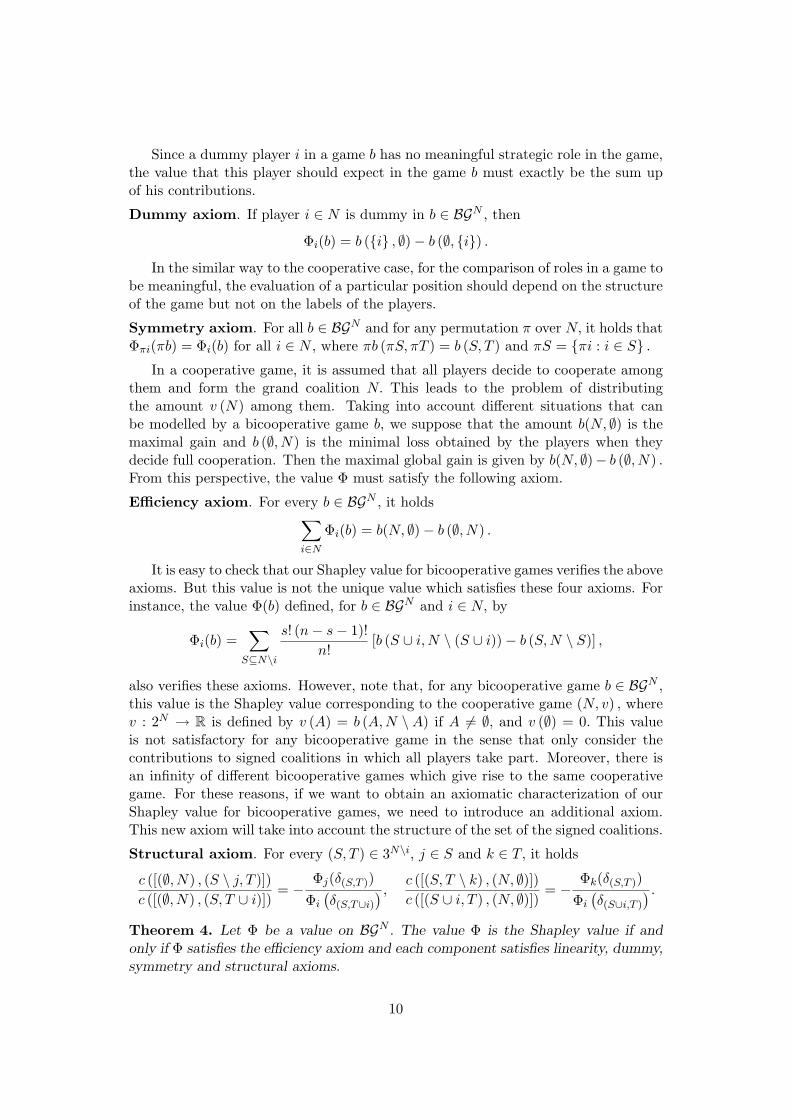
Since a dummy player i in a game b has no meaningful strategic role in the game,the value that this player should expect in the game b must exactly be the sum upof his contributions.

Dummy axiom. If player i ∈ N is dummy in b ∈ BGN , then

Φi(b) = b (i , ∅)− b (∅, i) .

In the similar way to the cooperative case, for the comparison of roles in a game tobe meaningful, the evaluation of a particular position should depend on the structureof the game but not on the labels of the players.

Symmetry axiom. For all b ∈ BGN and for any permutation π over N, it holds thatΦπi(πb) = Φi(b) for all i ∈ N , where πb (πS, πT ) = b (S, T ) and πS = πi : i ∈ S .

In a cooperative game, it is assumed that all players decide to cooperate amongthem and form the grand coalition N. This leads to the problem of distributingthe amount v (N) among them. Taking into account different situations that canbe modelled by a bicooperative game b, we suppose that the amount b(N, ∅) is themaximal gain and b (∅, N) is the minimal loss obtained by the players when theydecide full cooperation. Then the maximal global gain is given by b(N, ∅)− b (∅, N) .

From this perspective, the value Φ must satisfy the following axiom.

Efficiency axiom. For every b ∈ BGN, it holds

i∈N

Φi(b) = b(N, ∅)− b (∅, N) .

It is easy to check that our Shapley value for bicooperative games verifies the aboveaxioms. But this value is not the unique value which satisfies these four axioms. Forinstance, the value Φ(b) defined, for b ∈ BGN and i ∈ N, by

Φi(b) =

S⊆N\i

s! (n− s− 1)!n!

[b (S ∪ i,N \ (S ∪ i))− b (S, N \ S)] ,

also verifies these axioms. However, note that, for any bicooperative game b ∈ BGN ,this value is the Shapley value corresponding to the cooperative game (N, v) , wherev : 2N → R is defined by v (A) = b (A,N \ A) if A = ∅, and v (∅) = 0. This valueis not satisfactory for any bicooperative game in the sense that only consider thecontributions to signed coalitions in which all players take part. Moreover, there isan infinity of different bicooperative games which give rise to the same cooperativegame. For these reasons, if we want to obtain an axiomatic characterization of ourShapley value for bicooperative games, we need to introduce an additional axiom.This new axiom will take into account the structure of the set of the signed coalitions.

Structural axiom. For every (S, T ) ∈ 3N\i, j ∈ S and k ∈ T, it holds

c ([(∅, N) , (S \ j, T )])c ([(∅, N) , (S, T ∪ i)])

= −Φj(δ(S,T ))

Φiδ(S,T∪i)

,c ([(S, T \ k) , (N, ∅)])c ([(S ∪ i, T ) , (N, ∅)]) = −

Φk(δ(S,T ))Φi

δ(S∪i,T )

.

Theorem 4. Let Φ be a value on BGN. The value Φ is the Shapley value if and

only if Φ satisfies the efficiency axiom and each component satisfies linearity, dummy,symmetry and structural axioms.

10

4. The core and the Weber set

Now, some solution concepts for bicooperative games are introduced, understandingas a solution concept any subset of vectors in Rn that provide an equitable distributionof the total saving among the players. A vector x ∈ Rn which satisfies

i∈N xi =

b (N, ∅)− b (∅, N) is called efficient vector and the set of all efficient vectors is calledpreimputation set which is defined by

I∗(N, b) =

x ∈ Rn :

i∈N

xi = b (N, ∅)− b (∅, N)

.

The imputations for game b are the preimputations that satisfy the individualrationality principle for all players, that is, each player gets at least the differencebetween the amount that he can attain for himself taking the rest of players againstand the value of the signed coalition (∅, N) ,

I(N, b) = x ∈ I∗(N, b) : xi ≥ b(i,N \ i)− b (∅, N) for all i ∈ N .

A satisfactory distribution criterium could be that every signed coalition (S, T ) ∈3N receives at least the amount it can contribute to the coalition (∅, N) , that is, theamount b(S, T )− b (∅, N) . It leads us to define the notion of the core of the game b

as the set

C(N, b) =

x ∈ I∗(N, b) : x = y + z with

y (S) + z (N \ T ) ≥ b(S, T )− b (∅, N) ∀ (S, T ) ∈ 3N

.

This definition can be interpreted in the following manner. For each (S, T ) ∈ 3N , theplayers who are not in the coalition T have contributed to the formation of (S, T )since they will not act against the player of the coalition S and for this, they must bereceived a payoff given by the vector z. Moreover, those players of N \ T who are inthe coalition S must get a different payoff to the rest of players, given by the vectory since these players have contributed to the formation of (S, T ) in a different way.

In order to extend the idea of the Weber set to a bicooperative game (N, b) , itis assumed that all players estimate that (N, ∅) is formed as a sequential processwhere in each step a different player is incorporated to the defender coalition or adifferent player leaves the detractor coalition. These sequential processes are obtainedconsidering the different chains from (∅, N) to (N, ∅) . In each one of these processes,a player can evaluate his contribution when is incorporated to the defenders or hiscontribution when leaves the detractors. This can be reflected in the vectors of Rn

denominated superior marginal worth vectors and inferior marginal worth vectors.With the aim to formalize this idea, we introduce the following notation.

Given N = 1, . . . , n , let N = −n, . . . ,−1, 1, . . . , n . We can define an isophor-fim Λ : 3N −→ 2N as follows: For each (S, T ) ∈ 3N

, Λ (S, T ) = S∪−i : i ∈ N \ T ∈2N

. For instance, Λ (∅, N) = ∅ and Λ (N, ∅) = N. Since S ∩ T = ∅ ⇔ S ⊆ N \ T wesee that i ∈ Λ (S, T ) and i > 0 imply −i ∈ Λ (S, T ) .

In the lattice3N

,, we consider the set of all maximal chains which going from

(∅, N) to (N, ∅) and denote this set by Θ3N

. If θ ∈ Θ

3N

is the maximal chain

(∅, N) (S1, T1) · · · (Sj , Tj) · · · (S2n−1, T2n−1) (N, ∅) ,

11

we can write the associated chain of sets in 2N

∅ ⊂ i1 ⊂ · · · ⊂ i1, . . . , ij ⊂ · · · ⊂ i1, . . . , i2n−1 ⊂ N.

where i1, . . . , ij = Λ (Sj , Tj) for j = 1, . . . , 2n. We define the vector θ (ij) =(i1, . . . , ij) , where the last component ij ∈ N satisfies the following property: ifij > 0 then the player ij ∈ Sj and ij /∈ Sj−1, that is, ij is the last player whojoins Sj and if ij < 0, then the player −ij /∈ Tj and −ij ∈ Tj−1, that is, −ij isthe last player who leaves Tj−1. Equivalently, the elements in θ (ij) = (i1, . . . , ij)are written following the order of incorporation in the defenders coalitions or de-sertion of the detractors coalition (depending on the sign of each ik) in the signedcoalitions in chain θ . Moreover, we write θ (ij) \ ij = (i1, i2, . . . , ij−1) = θ (ij−1)and ik ∈ θ (ij) when ik is one component of the vector θ (ij) , that is 1 ≤ k ≤ j.

Note that an equivalence between maximal chains and vectors θ = (i1, . . . , i2n) isobtained. Fix an order θ = (i1, . . . , i2n) , we also define α [θ (ij)] = (Sj , Tj) suchthat Λ (Sj , Tj) = i1, . . . , ij. Moreover, α [θ (ij) \ ij ] = α [θ (ij−1)] = (Sj−1, Tj−1) .

In particular, α [θ (i2n)] = (N, ∅) and α [θ (i1) \ i1] = (∅, N) .

For example, let N = 1, 2, 3 and θ ∈ Θ3N

given by

(∅, N) (∅, 1, 3) (2 , 1, 3) (2 , 1) (2 , ∅) (2, 3 , ∅) (N, ∅) .

Its associated chain of sets in 2N is given by

∅ ⊂ −2 ⊂ −2, 2 ⊂ −2, 2,−3 ⊂ −2, 2,−3,−1 ⊂ −2, 2,−3,−1, 3 ⊂ N.

and the maximal chain can be also represented by the order θ = (−2, 2,−3,−1, 3, 1) .

One signed coalition, for example (2 , ∅) , can be also represented by α [θ (−1)] andby Λ−1 (−2, 2,−3,−1)

Definition 3. Let θ ∈ Θ3N

and b ∈ BGN . We call inferior and superior marginal

worth vectors with respect to θ to the vectors mθ (b) , M

θ (b) ∈ Rn respectively where

mθi (b) = b (α [θ (−i)])− b (α [θ (−i) \−i]) ,

Mθi (b) = b (α [θ (i)])− b (α [θ (i) \ i]) ,

for all i ∈ N. We call marginal worth vector respect to θ, aθ (b) ∈ Rn

, to the vectorobtained as the sum of inferior and superior marginal worth vectors, that is,

aθi (b) = m

θi (b) + M

θi (b) , for i ∈ N.

The following result show that the marginal worth vectors are efficients.

Proposition 5. For any b ∈ BGN and θ ∈ Θ3N

we have

i∈N

aθi (b) = b (N, ∅)− b (∅, N) .

12

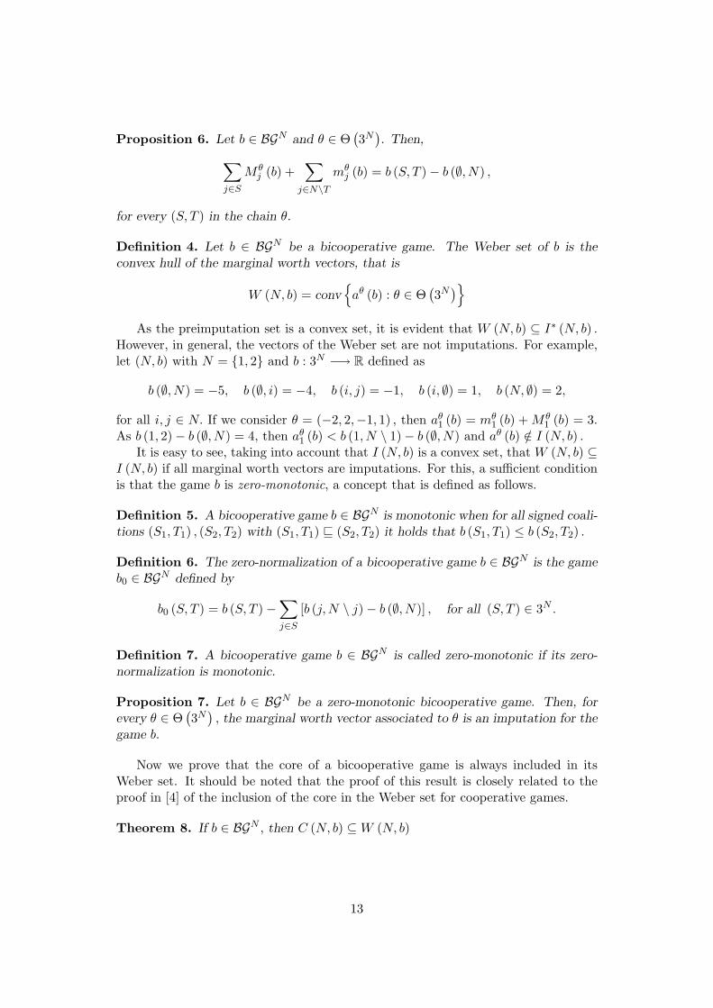
Proposition 6. Let b ∈ BGN and θ ∈ Θ3N

. Then,

j∈S

Mθj (b) +

j∈N\T

mθj (b) = b (S, T )− b (∅, N) ,

for every (S, T ) in the chain θ.

Definition 4. Let b ∈ BGN be a bicooperative game. The Weber set of b is theconvex hull of the marginal worth vectors, that is

W (N, b) = conv

aθ (b) : θ ∈ Θ

3N

As the preimputation set is a convex set, it is evident that W (N, b) ⊆ I∗ (N, b) .

However, in general, the vectors of the Weber set are not imputations. For example,let (N, b) with N = 1, 2 and b : 3N −→ R defined as

b (∅, N) = −5, b (∅, i) = −4, b (i, j) = −1, b (i, ∅) = 1, b (N, ∅) = 2,

for all i, j ∈ N. If we consider θ = (−2, 2,−1, 1) , then aθ1 (b) = m

θ1 (b) + M

θ1 (b) = 3.

As b (1, 2)− b (∅, N) = 4, then aθ1 (b) < b (1, N \ 1)− b (∅, N) and a

θ (b) /∈ I (N, b) .

It is easy to see, taking into account that I (N, b) is a convex set, that W (N, b) ⊆I (N, b) if all marginal worth vectors are imputations. For this, a sufficient conditionis that the game b is zero-monotonic, a concept that is defined as follows.

Definition 5. A bicooperative game b ∈ BGN is monotonic when for all signed coali-tions (S1, T1) , (S2, T2) with (S1, T1) (S2, T2) it holds that b (S1, T1) ≤ b (S2, T2) .

Definition 6. The zero-normalization of a bicooperative game b ∈ BGN is the gameb0 ∈ BGN defined by

b0 (S, T ) = b (S, T )−

j∈S

[b (j, N \ j)− b (∅, N)] , for all (S, T ) ∈ 3N.

Definition 7. A bicooperative game b ∈ BGN is called zero-monotonic if its zero-normalization is monotonic.

Proposition 7. Let b ∈ BGN be a zero-monotonic bicooperative game. Then, forevery θ ∈ Θ

3N

, the marginal worth vector associated to θ is an imputation for the

game b.

Now we prove that the core of a bicooperative game is always included in itsWeber set. It should be noted that the proof of this result is closely related to theproof in [4] of the inclusion of the core in the Weber set for cooperative games.

Theorem 8. If b ∈ BGN, then C (N, b) ⊆ W (N, b)

13

5. Bisupermodular games

Now we introduce a special class of bicooperative games.

Definition 8. A bicooperative game b ∈ BGN is called bisupermodular if, for all(S1, T1) and (S2, T2) it holds

b((S1, T1) ∨ (S2, T2)) + b ((S1, T1) ∧ (S2, T2)) ≥ b (S1, T1) + b (S2, T2) ,

or equivalently

b(S1 ∪ S2, T1 ∩ T2) + b (S1 ∩ S2, T1 ∪ T2) ≥ b (S1, T1) + b (S2, T2) .

The next proposition characterizes the bisupermodular games as those bicooper-ative games for which the marginal contributions of a player to one signed coalitionis never less that the marginal contribution of this player to any signed coalitioncontained in it. This characterization will be used in the proves of the followingresults.

Proposition 9. Let b ∈ BGN . The bicooperative game b is bisupermodular if andonly if for all i ∈ N and (S1, T1), (S2, T2) ∈ 3N\i such that (S1, T1) (S2, T2) , itholds

b (S2 ∪ i, T2)− b (S2, T2) ≥ b (S1 ∪ i, T1)− b (S1, T1)

andb (S2, T2)− b (S2, T2 ∪ i) ≥ b (S1, T1)− b (S1, T1 ∪ i)

The following result permits the identification of the games for which the marginalworth vectors are distributions of the core.

Theorem 10. A necessary and sufficient condition so that all marginal worth vectorsof a bicooperative game b ∈ BGN are vectors of the core is that the game b isbisupermodular

As the core of a bicooperative game b ∈ BGN is a convex set, an immediateconsequence of this theorem is the following result.

Corollary 11. Let b ∈ BGN. A necessary and sufficient condition so that W (N, b) =

C (N, b) is that the bicooperative game b is bisupermodular.

Note that the Shapley value of a bicooperative game b is given by

Φi (N, b) =1

c(3N )

θ∈Θ(3N )

m

θi (b) + M

θi (b)

,

for all i ∈ N. Then the Shapley value of a bisupermodular game b is in C (N, b) andhence, the core of a bisupermodular game is non-empty.

Acknowledgements

This research has been partially supported by the Spanish Ministry of Science andTechnology, under grant SEC2003–00573, and the Center of Andalusian Studies ofthe Andalusia Government.

14

References

[1] J.M. Bilbao (2000). Cooperative Games on Combinatorial Structures. Boston,Kluwer Academic Publishers.

[2] J.M. Bilbao, J.R. Fernandez, N. Jimenez, and J.J. Lopez (2004). Probabilisticvalues for bicooperative games. Working paper, University of Seville.

[3] V.C.H. Chua and H.C. Huang (2003). The Shapley-Shubik index, the donationparadox and ternary games. Social Choice and Welfare 20, 387–403.

[4] J. Derks (1992). A Short Proof of the Inclusion of the Core in the Weber set.International Journal of Game Theory 21, 149–150.

[5] D. Felsenthal, and M. Machover (1997). Ternary Voting Games. InternationalJournal of Game Theory 26, 335–351.

[6] J. Freixas (2005). The Shapley-Shubik power index for games with several levelsof approval in the input and output. Decision Support Systems 39, 185–195.

[7] J. Freixas (2005). Banzhaf measures for games with several levels of approval inthe input and output. Forthcoming in Annals of Operations Research.

[8] J. Freixas and W.S. Zwicker (2003). Weighted voting, abstention, and multiplelevels of approval. Social Choice and Welfare 21, 399–431.

[9] M. Grabisch, and Ch. Labreuche (2002). Bi-capacities. Working paper, Univer-sity of Paris VI.

[10] R.B. Myerson (1991). Game Theory: analysis of conflict. Harvard UniversityPress, Cambridge.

[11] R.T. Rockafellar (1970). Convex Analysis. Princeton University Press, Princeton.

[12] L.S. Shapley (1953). A value for n-person games. In Contributions to the Theoryof Games II, Ann. of Math. Stud. 28. Princeton: Princeton University Press, pp.307–317.

[13] R.P. Stanley (1986). Enumerative Combinatorics I. Monterey, Wadsworth.

[14] R.J. Weber (1988). Probabilistic values for games. In The Shapley Value: Essaysin Honor of Lloyd S. Shapley. Cambridge: Cambridge University Press, pp. 101–119.

15

16

On the computation of Semivalues for TU games

via Shapley value

Irinel Dragan, University of Texas, Mathematics, Arlington, Texas,E-mail:dragan@uta.edu

In an earlier paper (I.Dragan,2004) we proved that every Least SquareValue is the Shapley value of a game obtained by rescaling from the givengame. In the paper where the Least Square Values were introduced (L.Ruiz,F.Valenciano and J.M. Zarzuelo,1998), the authors have shown that theefficient normalization of a Semivalue is a Least Square Value, (briefly LS-value).

In the present paper, we developed the idea suggested by these tworesults and we obtained a direct relationship between the efficient normal-ization of a Semivalue and the Shapley value. The main tools for proofswere the so-called the Average per capita formulas we proved earlier for theShapley value (I.Dragan,1992) and for the Semivalues (1999), as well as theformula for the Power game of a given game relative to Semivalues (I.Draganand J.E.Martinez-Legaz,2001). The last one was needed to compute the effi-ciency term and to derive an algorithm for computing any Semivalue via theShapley value. The present paper is containing results from various sources,so that in order to make this paper self contained, we shall be proving belowour previous results together with the new results, which appear here for thefirst time. All proofs are algebraic, in opposition to the RVZ proofs whichare axiomatic. The direct connection between a Semivalue and the Shapleyvalue does not need any reference to LS-values, which may well be unknownto the reader of the present paper.

In the first section, we prove the Average per capita formula for Semival-ues, (Theorem 1), from which we derive our formula for the Shapley value,(Corollary 2), to be used later. In the second section, we give the formula forthe efficiency term in the efficient normalization of a Semivalue ,(Theorem3), as well as the main results showing the connection between the efficientnormalization of a Semivalue and the Shapley value, (Theorems 4 and 5). Inthe last section we discuss the algorithm for computing a Semivalue via theShapley value, after noticing that the Average per capita formula for Semi-values proposed as a basic tool in computing a Semivalue, is doubling thenumber of weighting operations. A small game is used for illustrating howthis algorithm works (Example 1). The motivation for the present work wasthe fact that in Mathematica there is a program for computing the Shapley

17

value and there is some experience in computing the Shapley value, whilewe do not know of any computational work relative to the Semivalues. Fur-ther, we consider the inverse problem for Semivalues which was solved in anearlier paper, (I.Dragan,2002), by extending to Semivalues our procedureused for the Shapley value (I.Dragan,1991). It is interesting to note thathere the solution set of the inverse problem depends on a unique basis, thebasis for the inverse problem of the Shapley value, (Theorem 6), in opposi-tion to what has happened in the previous paper on the inverse problem forSemivalues, where there was an infinite set of bases, each one being singledout by the dependence of the weight vector of the Semivalue. An exampleis also shown here, (Example 2).

Keywords: Shapley value, Semivalues, Average per capita formulas, Efficientnormalization, Banzhaf value, the inverse problem.

1 Average per capita formula for Semivalues

Let GN denote the space of cooperative TU games with a fixed set of players

N . The Semivalues associated with a weight vector pn ∈ R

n satisfying thenormalization condition

n

s=1

n− 1s− 1

pns = 1, (1)

have been introduced axiomatically by P.Dubey, A.Neyman and R.J.Weber(1981), as values on G

N , and even on more general structures. For GN they

proved that a Semivalue associated with a weight vector pn is given by

SEi(N, ν) =

S:i∈S⊆N

pns [ν(S)− ν(S − i)], ∀i ∈ N. (2)

where s = |S|, and pns is the common weight of all coalitions of size

s. We take this formula as the definition of Semivalues on GN . To define

the Semivalues on the union of all spaces GN , when N is arbitrary, we

need a sequence of weight vectors p1, p

2, ..., p

n, ..., all satisfying the above

normalization condition, that is p11 = 1, p

21 + p

22 = 1, p

31 + p

32 + p

33 = 1, ...

and so on. The definition of Semivalues on GT is given by the same formula

as above, where N is replaced by T , nbyt, and pn by p

t. However, thesequence of weight vectors are supposed to satisfy what we call the inversePascal triangle relations

pt−1s = p

ts + p

ts+1, s = 1, 2, ..., t− 1. (3)

It is easy to see that if the normalization condition for GN holds, then

from the inverse Pascal triangle relations we get the normalization conditionsatisfied for G

T , and all coalitionsT ⊆ N

18

Note the important fact that among the Semivalues we get the Shapleyvalue for p

ns = /frac(s− 1)!(n− s)!n!, the Banzhaf value for p

ns = 21−n

, s =1, 2, ..., n, and many other well known values. Therefore, if we prove whatwe call the Average per capita formula for Semivalues, (I.Dragan,1999, andI.Dragan and J.E.Martinez-Legaz,2001), we get also the formula for theShapley value (I.Dragan,1992), by taking these particular weights (see alsoI.Dragan,T.Driessen and Y.Funaki,1996). This will be used later.

We call an Average per capita formula any formula in which occur onlythe average worth of various coalitions defined as follows:

νs =

n

s

−1

|S|=s

ν(s), νis =

n− 1

s

−1

|S|=s,i/∈S

ν(s), s = 1, 2, ...n−1,∀i ∈ N.

(4)Clearly, νs is the average worth of coalitions of size s , while ν

is is the

average worth of coalitions of size s which do not contain player i. If wedenote νn = ν(N), then there are n averages νs, and n(n − 1) averagesν

is, hence n

2 averages all together. Let us introduce also the new weights,defined for all t by

qis =

pts

γts, s = 1, 2, ..., t, (5)

where γts = (t!)−1(s−1)!(t−s)!, that is the weights for the Shapley value

on GT .

Theorem 1 (I.Dragan,1999): Let SE be a Semivalue associated with anon- negative weight vector p

n satisfying the normalization condition. Letqn be the nonnegative weight vector defined above. Then, SE is given by

the formula

SE(N, ν) = qnnνn

n+

s=1

nqns νs − q

n−1s ν

is

s, ∀i ∈ N. (6)

For qns = 1, s = 1, 2, ..., n, that is p

ns = γ

ns , s = 1, 2, ..., n, we obtain:

Corollary 2 (I.Dragan,1992): The Shapley value of the game (N, ν) isgiven by

SHi(N, ν) =νn

n+

s=1

nνs − ν

is

s, ∀i ∈ N. (7)

Proof of Theorem 1: For i ∈ N fixed, rewrite (2) as

SEi(N, ν) = pnnν(N) +

S:i∈S⊂N

pns ν(S)−

S:i∈S⊆N

pns ν(S − i); (8)

19

now, write the two sums separately as

S:i∈S⊂N

pns ν(S) =

n−1

s=1

pns

|S|=s,i∈S

ν(S)

=n−1

s=1

pns

|S|=s

ν(S)−

|S|=s,i/∈S

ν(S)

,

(9)and

S:i∈S⊆N

pns ν(S − i) =

n−1

s=1

pns+1

|S|=s

ν(S)

. (10)

From (8), (9), and (10), with notations (4), we obtain

SEi(N, ν) = pnnνn +

s=1

n− 1[pns

n

s

νs − pn−1s

n− 1

s

], (11)

where we have also used (3) for t = n. If in (11) we introduce the new

weights by noticing that pns

n

s

= s−1

qns , s− 1, 2, ..., n− 1 , we get (6).

Note that the weights qns should satisfy the normalization condition

n

s=1

qns = n, (12)

derived from (1) and (5), and the Pascal triangle conditions (3) become

qi−1s = (1− st

−1)qts + st

−1qts+t, s = 1, 2, ..., t− 1. (13)

In the next section, we shall derive a new Average per capita formulafor the term which should be added to the Semivalue, to get the efficientnormalization. This formula will be needed later in the computation ofSemivalues via Shapley value.

2 Average per capita formula for the efficiencyterm

In the paper where the Least Square Values (briefly LS-values) were in-troduced by L.Ruiz, F.Valenciano and J.M.Zarzuelo, (1998), the authorsdefined what they called the Efficient normalization of a Semivalue SE as-sociated with a nonnegative weight vector p

n = (pns ). This is the value

ESE : GN → R

n written componentwise as

ESEi(N, ν) = SEi(N, ν) + α, ∀i ∈ N, (14)

with α such that ESE is efficient, that is

20

α =1n

[ν(N)−

j∈N

SEj(N, ν)]. (15)

We call α the efficiency term and we intend to derive an Average percapita formula for α . This can be derived from our formula for a PowerGame relative to a Semivalue by introducing the averages (4) and our newweights (5), (I.Dragan and J.E.Martinez- Legaz,2001). However, we cutsomehow the work by using (6). From the last formula, we obtain

j∈N

SEj(N, ν) = qnnνn+

n−1

s=1

nqns νs − q

n−1s

j∈N ν

js

s= q

nnνn+n

n−1

s=1

(qns − q

n−1s )νs

s,

(16)where we have used the equality

j∈N ν

js = nνs, holding for all s = 1, 2, ..., n−

1. In this way, from (15) and (16), we proved:Theorem 3: The efficiency term for the additive normalization of a Semi-

value is given by the Average per capita formula

α =νn

n− [

qnnνn

n+

n−1

s=1

(qns − q

n−1s )

s]. (17)

Putting together the Average per capita formulas (6) and (17) of the The-orems 1 and 3, we prove algebraically for the efficient normalization of aSemivalue the main result:

Theorem 4: The Efficient normalization of a Semivalue associated witha non- negative weight vector p

n = (pns ) is given by

ESEi(N, ν) =νn

n+

n−1

s=1

qn−1s

νs − νis

s, ∀i ∈ N, (18)

where qn−1s are expressed in terms of p

n as

qn−1s =

pns + p

ns+1

γns + γ

ns+1

, s = 1, 2, ...n− 1, (19)

with γns and γ

ns+1 denoting the corresponding Shapley weights.

Note that (19) is derived from (5) for t = n− 1 and (3) for t = n, takinginto account that the weights for the Shapley value satisfy also (3). Notealso that for the Banzhaf value (19) becomes

qn−1s =

12n−2γ

n−1s

, s = 1, 2, ...n− 1, (20)

Note that Theorem 4 could be derived from the relationship axiomati-cally proved by Ruiz, Valenciano and Zarzuelo (1998) between the efficient

21

normalization of a Semi- value and the LS-values, together with our rela-tionship between the LS-values and the Shapley value (I.Dragan,2004). Inthe present paper, as it was shown, there is no need of LS-values, and thiswas the reason why we have chosen the above proof.

Consider a game (N, ν) and rescale it by introducing the new game(N,w) :

w(N) = ν(N), w(S) = qn−1s ν(S), ∀S ⊂ N. (21)

By (4) we have

ws = qn−1s νs, w

is = q

n−1s ν

is, ∀i ∈ N, s = 1, 2, ..., n− 1. (22)

Therefore, from (18) and (22), we get the right hand side in (7), for thenew game (N,w). We proved:

Theorem 5. The Efficient normalization of the Semivalue of a game(N, ν), associated to the weight vector p

n ∈ Rn, is the Shapley value of a

new game (N,w) obtained by rescaling of (N, ν) with factors qn−1s , for the

worth of coalitions of size s, s = 1, 2, ..., n − 1, derived from the weightvector p

n and the Shapley weights by means of (19).This last result is helpful in computing the Semivalues of the TU games

via the Shapley value, as it will be discussed in the next section, where weshall also discuss an application of Theorem 5 to the Inverse problem forSemivalues.

3 Applications to the computation of Semivaluesand to the Inverse problem

In an earlier paper (I.Dragan,1999), we have shown that a Semivalue for aTU game may be computed by means of the Average per capita formulain the same way as the Shapley value was shown to be computable fromits Average per capita formula, (I.Dragan,1992). The difference is that theaverages should be weighted, as could be seen in (6). Based upon Theo-rem 5, we may modify first the game, then use the algorithm for computingthe Shapley value. However, as shown in Theorem 4, we may better com-pute the usual terms which appear in the Shapley value formula, then goon and rescale the term by q

n−1s , as seen in formula (18), to get the Effi-

cient normalization. Now, we have also two alternatives: if we rescale thegame, then we may still modify it by subtracting an additive game (N,α),in which α(S) = sα for all S ⊂ N , and α(N) = Nα, where α is the ef-ficiency term. Due to the linearity of the Shapley value, and to Theorem5, we get the game for which the Shapley value is exactly the Semivalueto be computed. However, this entails to subtract from each value of thecharacteristic function the corresponding value of α(S) so that the numberof operations needed is increasing dramatically. Therefore, we prefer the

22

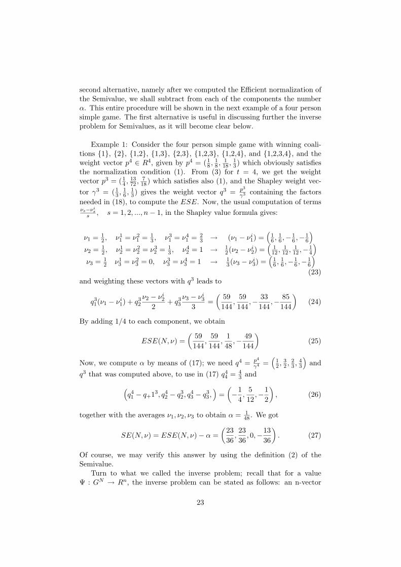
second alternative, namely after we computed the Efficient normalization ofthe Semivalue, we shall subtract from each of the components the numberα. This entire procedure will be shown in the next example of a four personsimple game. The first alternative is useful in discussing further the inverseproblem for Semivalues, as it will become clear below.

Example 1: Consider the four person simple game with winning coali-tions 1, 2, 1,2, 1,3, 2,3, 1,2,3, 1,2,4, and 1,2,3,4, and theweight vector p

4 ∈ R4, given by p

4 = (18 ,

18 ,

118 ,

13) which obviously satisfies

the normalization condition (1). From (3) for t = 4, we get the weightvector p

3 = (14 ,

1372 ,

718) which satisfies also (1), and the Shapley weight vec-

tor γ3 = (1

3 ,16 ,

13) gives the weight vector q

3 = p3

γ3 containing the factorsneeded in (18), to compute the ESE. Now, the usual computation of termsνs−νi

ss , s = 1, 2, ..., n− 1, in the Shapley value formula gives:

ν1 = 12 , ν

11 = ν

21 = 1

3 , ν31 = ν

41 = 2

3 → (ν1 − νi1) =

16 ,

16 ,−1

6 ,−16

ν2 = 12 , ν

12 = ν

22 = ν

32 = 1

3 , ν42 = 1 → 1

2(ν2 − νi2) =

112 ,

112 ,

112 ,−1

4

ν3 = 12 ν

13 = ν

23 = 0, ν

33 = ν

43 = 1 → 1

3(ν3 − νi3) =

16 ,

16 ,−1

6 ,−16

(23)and weighting these vectors with q

3 leads to

q31(ν1 − ν

i1) + q

32ν2 − ν

i2

2+ q

33ν3 − ν

i3

3=

59144

,59144

,− 33144

,− 85144

(24)

By adding 1/4 to each component, we obtain

ESE(N, ν) = 59

144,

59144

,148

,− 49144

(25)

Now, we compute α by means of (17); we need q4 = p4

γ4 =

12 ,

32 ,

23 ,

43

and

q3 that was computed above, to use in (17) q

44 = 4

3 and

q41 − q+13

, q42 − q

32, q

43 − q

33,

=

−1

4,

512

,−12

, (26)

together with the averages ν1, ν2, ν3 to obtain α = 148 . We got

SE(N, ν) = ESE(N, ν)− α =23

36,2336

, 0,−1336

. (27)

Of course, we may verify this answer by using the definition (2) of theSemivalue.

Turn to what we called the inverse problem; recall that for a valueΨ : G

N → Rn, the inverse problem can be stated as follows: an n-vector

23

L being given, find out all games in GN such that Ψ(N, ν) =L. This prob-

lem has been solved for the Shapley value and the weighted Shapley value(I.Dragan,1991). Recently, the problem was also solved for Semivalues(I.Dragan,2002), extending the procedure used for the Shapley value toSemivalues. Here we have an alternative solution based upon the remarkmade at the beginning of this section, precisely

SE(N, ν) = SH(N,w − α). (28)

Let us state the result which solves the inverse problem for the Shapley value.Consider the following basis for G

N : B =Bs ∈ G

N : S ⊆ N,S = ∅,

where for S ⊂ N we have Bs(T ) = |S|, if T = S, and Bs(T ) = −1, ifT = S∪j, j /∈ S, and Bs(T ) = 0, otherwise; BN (N) = n, and BN (T ) = 0,otherwise.

Theorem 6 (I.Dragan,1991): For any L ∈ Rn, the set of games in G

N

with the Shapley value SH(N, ν) = L is given by the formula:

ν =

|S|≤n−2

βSBS + βN (BN +

j∈N

BN−j)−

j∈N

LjBN−j, (29)

where βN and βS , |S| ≤ n− 2, are any real numbers.Taking into account (28), the solution of the inverse problem for a Semi-

value can be obtained from (29), where in the left hand side we should takeν = w − α, with the game (N,α) defined at the beginning of this section,and (N,w) defined in (21), then the equation should be solved for w. The2n − 1 dimensional games (N,w) and (N,α) should be expressed in termsof the original game and L, by using (21); the last game is via (15) given by

α(S) =s

n[ν(N)−

j∈N

Lj ], ∀S ⊆ N. (30)

(see below).Example 2: Consider the given vector L =

2336 ,

2336 , 0,−13

36

, and find

out all games for which the Semivalue associated with the weight vectorp4 =

18 ,

18 ,

118 ,

13

equals L. For our four person game, from (29) we obtain:

w = α +

|S|=1,2

βSBS + βN (BN +

j∈N

BN−j)−

j∈N

LjBN−j, (31)

This is a vector-equation, in which the left hand side is providing the coali-tional form of all the games we are trying to find (each ν(S) is multipliedby γ

3s , s = 1, 2, 3) and in the right hand side appear linear combinations

of the 12 parameters defining the set of the solution games, precisely, the 10

24

parameters βS with |S| = 1, 2, then βN and α. For

β1 = 3548 ,β2 = 35

48 ,β3 = − 148 ,β4 = − 1

48 .

β12 = 54 ,β13 = 7

8 ,β14 = 13 ,β23 = 7

8 ,β24 = 13 ,β34 = − 1

24β1234 = 71

72 ,α = 148 ,

(32)

we obtain our game considered in Example 1. It is interesting to notice thatthe basis does not depend on the weight vector, which appear only in theleft hand side, as was explained above. Hence, in fact the entire set of gamessolving the inverse problem is depending on 15 parameters, namely besidethe 12 parameters mentioned above, we have also γ

31 , γ

32 , γ

33 . In the paper

where we solved the inverse problem relative to the Semivalues, we had aninfinite set of bases depending on the chosen weight vector p

4 .Returning to the general case, the similar procedure is providing the

characteristic function of all solution games as functions of 2n − n − 1parameters βN and βS for |S| ≤ n − 2, and α. The other parametersγ

n−1s , s = 1, 2, ...n− 1, appear in the left hand sides.

Aknowledgement. This is a survey on the research of the author on theSemivalues, to be presented at The 4th Twente Workshop on CooperativeGame Theory, Enschede, The Netherlands, June 28-30,2005.

References

[1] J.F.Banzhaf, (1965), Weighted voting doesn’t work; a mathemat-ical analysis, Rutgers Law Review,19,317-343.

[2] I.Dragan, (1991), The potential basis and the weighted Shapleyvalue, Libertas Math, XI,139-150.

[3] I.Dragan, (1992),The Average per capita formula for the Shapleyvalue, Libertas Math. XII,139-146.

[4] I.Dragan, T.S.H.Driessen and Y.Funaki, (1996), Collinearity be-tween the Shapley value and the egalitarian division rules forcooperative games, O.R.Spektrum,18, 97-105.

[5] I.Dragan, (1999), Potential, Balanced contributions, Recursionformula, Shapley blue-print, properties for values of cooperativeTU games, in Proceedings of LGS’99, Harrie DeSwart, (ed.),Tilburg University Press, 57-67.

[6] I.Dragan and J.E.Martinez-Legaz, (2001), On the Semivalues andthe Power Core of cooperative TU games, IGTR,3,2&3,127-139.

25

[7] I.Dragan, (2002), On the inverse problem for Semivalues of coop-erative TU games, Technical Report # 348, University of Texasat Arlington, U.S.A.

[8] I.Dragan, (2004), The Least Square Values and the Shapley valuefor cooperative TU Games, Top, (to appear).

[9] P.Dubey, A.Neyman and R.J.Weber, (1981), Value theory with-out efficiency, Math. O.R.,6,122-128.

[10] L.Ruiz, F.Valenciano and J.M.Zarzuelo, (1998), The fam-ily of Least Square Values For T.U. games, GEB,27,109-130. 11. L.S.Shapley, (1953), A value for n-person games,Ann.Math.Studies,28,307-317

26

Game Theoretic Analysis of Transportation

Problems

Vito FRAGNELLIDipartimento di Scienze e Tecnologie Avanzate

Universita del Piemonte Orientalevito.fragnelli@mfn.unipmn.it

AbstractThis paper presents some game theoretical approaches to railway problems.The main topic is the definition of a fair access fee to the European railwaynetwork, which matches the directives of the European Union.

1 Introduction

In the last fifteen years game theory found many applications to railwaysector in Europe, after the European Community directives 440/91, 18/95and 19/95, later confirmed and/or modified as European Union directives12/01, 13/01 and 14/01. These directives deal with the reorganization of theEuropean railway system; in particular they state the separation betweeninfrastructure management and transport operations and allow the accessto the infrastructure also to private railway undertakers.

Since the railway industry traditionally has been organized as verticallyintegrated firms, the allocation of scarce resources (track capacity) mayresults in inefficiencies arising from differential information, inappropriateincentives and the existence of priority groups. The EC/EU directives in-creased the importance of an efficient capacity allocation, jointly with thenecessity of a fair tariff system that guarantees a non discriminatory ac-cess to the infrastructure, minimizing the government subsidizations to therailway system.

The EU directive 14/01 explicitly refers to the cooperation between theinfrastructure managers and railway undertakers in order to enhance the ex-ploitation of the track capacity, maximizing the number of requests satisfiedas best as possible.

More precisely, the directive 14/01/UE gives some useful suggestions andguidelines. A tariff system should favor transparency and non-discriminatoryaccess, impose equivalent tariffs for equivalent services, averaging the costs,encourage an optimal use of the network, reduce the scarcity of the capacityof the network, coordinating the requests of railway undertakers, enhancethe available infrastructure capacity, incentivating the investments by theinfrastructure managers. Moreover it is possible to charge the transportoperators for infrastructure maintenance.

27

The issue of track allocation has been treated, for instance, in Brewerand Plott (1996), Bassanini and Nastasi (1997) and Nilsson (1999).

Brewer and Plott (1996) proposed a decentralized allocation processbased on a binary conflict ascending price (BICAP) mechanisms in whicheach agent submits bids for trains in a continuous time auction. The highestbid on a train prevails as the potential winner and cancels all lower bids forthe train. Since the potential allocation is of higher value than any alloca-tion possible from the excluded trains, the final allocation must necessarilybe efficient if the excluded agents are fully revealing their willingness to pay.Experiments indicate that the mechanism operates at near 100% efficiency.

Bassanini and Nastasi (1997) presented a three-stage model: in the firststage the railway undertaker ask for their preferred tracks, specifying a mon-etary evaluation; in the second stage the infrastructure manager assigns theavailable capacity of the network, maximizing the total assigned value in anon-discriminatory mechanism, based on a non cooperative market game;the third stage deals with the service prices for the users.

Nilsson (1999) suggested a Vickrey-type mechanism to handle incentiveaspects of this technically complex optimization task. Here, the price foroperating a train will correspond to the bids foregone by other operators whoare pushed off their preferred routes. The main advantage of a second priceauction is that bidders can confine their attention to appraising the value ofan item in their own hands rather than deliberating over value or biddingstrategy by others. Consequently, more bidders are induced to participate inthe process, resulting in a better allocation of resources and a higher sellingprice. Experimental solutions capture 90-100% of the potential benefits.

Here we are interested in the second issue, the design of a tariff system.A fair infrastructure access fee, i.e. the amount paid by the railway

undertakers to the firm in charge of the infrastructure management for aparticular journey, should take into account several aspects such as the apriori profitability and social utility of the journey, congestion issues, thenumber of passengers and/or goods transported, the services required bythe operator, infrastructure costs, etc. The tariff is conceived in an additiveway, i.e. as the sum of various tariffs corresponding to the different aspectsto be considered.

The problem can be informally described as follows. A given railwaypath is used by different types of trains belonging to several operators, andthe infrastructure costs have to be divided among these trains. Clearly it isa problem of joint cost allocation (see Tijs and Driessen, 1986 and Young,1994).

The infrastructure can be considered as consisting of some kinds of “fa-cilities” (track, signaling system, stations, etc.). Different groups of trainsneed these facilities at different levels: for example, fast trains need a moresophisticated track and signaling system, compared to local trains, for whichinstead station services are more important (particularly in small stations).

28

So the infrastructure can be viewed as the “sum” of different facilities,each of them required by the trains at a different level of cost.

Furthermore, for each facility, infrastructure costs can be seen as the sumof “building” costs and “maintenance” costs. The first can be seen as a fixedpart, because they depend on the level of the facility, but are independentfrom the number of trains; the latter represent a variable part, because theyare proportional to the number of trains (and depend on the level of thefacility).

In a game theoretical setting Fragnelli et al. (2000) proposed as a so-lution for this problem the Shapley value (see Shapley, 1953) that resultsespecially appropriate because of the following two reasons:

1. It is well-known that the Shapley value is an additive solution. Thisfeature fits well with the “additive nature” of the access tariff, ascommented above.

2. The infrastructure access tariff based on the Shapley value can becomputed very easily (using, once more, the additivity of the Shapleyvalue). As a very big amount of fees will have to be computed bythe infrastructure manager every new season, computational issuesbecome highly relevant.

Similar considerations extend to other problems: for example the costsfor a bridge, to be used by small and big cars. There are building costs, whichare different in the case of a bridge for small or big cars, and maintenancecosts, which can be assumed to be proportional to the number of vehiclesusing the bridge and to the kind of bridge needed.

Another situation (see Remark 1) refers to the allocation of the oper-ating costs for a consortium for urban solid wastes collection and disposal(Fragnelli and Iandolino, 2004). This application fully exploits the struc-ture of fixed and variable costs; in fact operating costs apparently refer onlyto “maintenance interventions”, but those costs that depend only on thetype of users, e.g. environmental monitoring, can be classified as “building”costs, while the costs that take into account also the number of users, e.g.Raw materials, can be classified as “maintenance” costs.

Maintenance and building cost games were used also in Garcia andGarcia-Jurado (2000) in queue management and in Gonzalez and Herrero(2004) for sharing the costs related to the operating-theatre in a hospital.

In Section 2 we introduce the infrastructure cost games for one facilityand provide a simple expression of the Shapley value for this class of games.In Section 3 we briefly study the balancedness of the infrastructure costgames and give a simple expression for the nucleolus. Section 4 deals withinfrastructure cost games for more than one facility. In Section 5 we presenta simple case-study. Section 6 concludes.

29

2 One Facility Infrastructure Cost Games

For simplicity, we concentrate first on infrastructure cost games when we aredealing with the building and maintenance costs of one facility. To beginwith, we recall the definition of an “airport game” (see Littlechild and Owen,1973).

Definition 1 Suppose we are given k groups of players g1, ..., gk with n1,...,nk

players respectively and k non-negative numbers b1, ..., bk. The airport gamecorresponding to g1, ..., gk and b1, ..., bk is the cooperative (cost) game (N, c)with N = ∪i=1,...,kgi and cost function c defined by

c(S) = b1 + · · · + bj(S)

for every S ⊆ N , where j(S) = maxj : S ∩ gj = ∅.

Airport games match the characteristics of building cost games for onefacility, where the groups of players represent the trains requiring a certainlevel of the facility and bi represents the extra cost in order that a facilitythat can be used by players in groups g1, ...gi−1 can also be used by the moresophisticated players in group gi; consequently, the cost of a facility of leveli is given by b1 + · · · + bi.

The Shapley value of a building cost game (N, cb) for a player in the

group gi, i = 1, ..., k is given by:

φi(cb) =

j=1,...,i

bj

Gjk

where Gjk = |∪h=j,...,k gh|.Now we consider the maintenance cost games (see Fragnelli et al., 2000)

for one facility, starting from the basic assumptions that maintenance costsare proportional to the number of users and increasing with the level of thefacility.

Definition 2 Suppose we are given k groups of players g1,...,gk with n1,...,nk

players respectively and k(k+1)/2 non-negative numbers αiji,j∈1,...,k,j≥i.The maintenance cost game corresponding to g1,...,gk and αiji,j∈1,...,k,j≥i

is the cooperative (cost) game (N, cm) with N = ∪i=1,...,k gi and cost function

cm defined by:

cm(S) =

j(S)

i=1

|S ∩ gi|Aij(S)

for every S ⊆ N , where Aij = αii + ...+αij for all i, j ∈ 1, ..., k with j ≥ i.

The interpretation of the numbers αij and Aij is the following. Suppose thatone player in gi has used the facility. In order to restore the facility up to

30

level i the maintenance costs are Aii = αii. If, however, the facility is goingto be restored up to level i + 1, then extra maintenance costs αi,i+1 will bemade. So, in order to restore the facility up to level j ≥ i the maintenancecosts are Aij = αii + .... + αij .

Note that, for every i ≤ j, the more sophisticated the facility is, i.e. thelarger j is, the higher the maintenance costs produced by a player in gi are.

A maintenance cost game (N, cm) can be decomposed as:

cm(S) =

i=1,...,k

j=i,...,k

αijcij(S), S ⊆ N

where

cij(S) =

|S ∩ gi| if j ≤ j(S)

0 if j > j(S)

for all i, j ∈ 1, ..., k with j ≥ i.The previous decomposition allows us stating the following theorem (see

Theorem 3.1 in Fragnelli et al., 2000) that provides a simple expression ofthe Shapley value for a maintenance cost game.

Theorem 1 Let (N, cm) be the maintenance cost game corresponding to

the groups g1,...,gk, with n1,...,nk players respectively and to non-negativenumbers αlml,m∈1,...,k,m≥l. Then the Shapley value for a player in thegroup gi, i = 1, ..., k is:

φi(cm) = αii +

l=i+1,...,k

αil

Glk

Glk + 1+

l=2,...,i

j=1,...,l−1

αjl

|gj |(Glk)(Glk + 1)

The following graphical example may make clearer the previous formulasfor the Shapley value.

Example 1 Let N = g1 ∪ g2 ∪ g3 where g1 = 1; g2 = 2, 3; g3 = 4 andlet the building cost game represented as in the figure on the left; the Shapleyvalue divides the cost as in the figure on the right:

b1 b2 b3

1234

234

4

φ1(cb) = 14b1

φ2(cb) = φ3(cb) = 14b1 + 1

3b2

φ4(cb) = 14b1 + 1

3b2 + b3

Analogously, let the maintenance cost game represented as in the figure onthe left; the Shapley value divides the cost as in the figure on the right:

31

α1,1 α1,2 α1,3

α2,2 α2,3

α2,2 α2,3

α3,3

1 1 1 4

2 2 4

3 3 4

4

234

φ1(cm) = α1,1 + 34α1,2 + 1

2α1,3

φ2(cm) = φ3(cm) = α2,2 + 12α2,3 + 1

3 · 14α1,2

φ4(cm) = α3,3 + 13 · 1

4α1,2 + 12α1,3 + 2 · 1

2α2,3

Remark 1 Applying the infrastructure cost games to a different kind of fa-cility, namely a consortium for collection and disposal of urban solid wastes(see Fragnelli and Iandolino, 2004), an undesired behavior of the Shapleyvalue showed up (see also the discussion on the monotonicity of the Shapleyvalue in Young, 1994). When the number of players in each group increasesproportionally (for example the population in each group doubles) the Shap-ley value of the maintenance cost game smooths the differences among theamount charged to the different groups (in the case analyzed in Fragnelliand Iandolino (2004) they converge to a unique value for all the players).This characteristic may be avoided using the Owen value (Owen, 1977), forwhich a simple expression exists, as stated in the following theorem (seeProposition 1 in Fragnelli and Iandolino, 2004).

Theorem 2 Let (N, cm) be the maintenance cost game corresponding to the

groups g1,...,gk, with n1,...,nk players respectively and to the non-negativenumbers αlml,m∈1,...,k,m≥l. If the groups g1,...,gk correspond to the apriori unions, then the Owen value for a player in the group gi, i = 1, ..., k

is:

Ωi(cm) =

H⊂Gi−1

h!(k − h− 1)!k!

1|gi|

β(H) + αii

+

H ⊂Gi−1

h!(k − h− 1)!k!

Ai,j(H)

where h = |H|, Gi−1 = g1, ..., gi−1, β(H) is the cost for ”upgrading” theplayers in H, i.e. β(H) = Aj(H),i

j|gj∈H

|gj | and j(H) = maxj|gj ∈ H.

Analogously, for a building cost game (N, cb) corresponding to the groups

g1,...,gk, with n1,...,nk players respectively and to the non-negative numbersb1,...,bk, with a priori unions g1,...,gk, then the Owen value for a player inthe group gi, i = 1, ..., k is:

Ωi(cb) =

H⊂Gi−1

h!(k − h− 1)!k!

bi − bj(H)

|gi|

32

3 Balancedness of One Facility Infrastructure Cost

Games

In this section we provide a characterization of the balancedness for onefacility infrastructure cost games and a formula for computing the nucleolus.

The balancedness conditions may be stated by the following proposition(see Proposition 3.1 in Norde et al., 2002)

Proposition 1 Let (N, c) be a one facility infrastructure cost game withgroups g1,...,gk, with n1,...,nk players respectively and non-negative numbersb1,...,bk and αiji,j∈1,...,k,j≥i. Then (N, c) is balanced iff:

i=1,...,j

ni (Aik −Aij) ≤

i=1,...,j

bi

for every j = 1, ..., k − 1.

The balancedness conditions are obtained by considering minimal balancedcollections which correspond to “splits” of N into two groups of the followingkind: g1 ∪ · · ·∪ gj and gj+1 ∪ · · ·∪ gk. The interpretation of these conditionsis the following: the maintenance costs that the players in g1 ∪ · · ·∪ gj haveto pay for the level of the “needs” of the other players should be less thanor equal to the building costs for the facility at the level needed by thesegroups themselves.

Remark 2 The computation of the Shapley values and the check of the bal-ancedness conditions may be done using the package ShRInC (Sharing Rail-ways Infrastructure Costs), created with the collaboration of Luisa Carpenteand Claudia Viale.

The nucleolus of a one facility infrastructure game (see Schmeidler, 1969)can be computed according to the following definition and proposition (seeDefinition 3.4 and Proposition 3.5 in Norde et al., 2002).

Definition 3 Let (N, c) be a balanced one facility infrastructure cost gamewith groups g1,...,gk, with n1,...,nk players respectively and non-negativenumbers b1,...,bk and αiji,j∈1,...,k,j≥i. Let the numbers b1,...,bk be definedby the linear system:

b1 = b1 − n1 (A1k −A11)b1 + b2 =

i=1,2

bi −

i=1,2

ni (Aik −Ai2)

... ...

b1 + b2 + ... + bk−1 =

i=1,...,k−1

bi −

i=1,...,k−1

ni (Aik −Ai,k−1)

b1 + b2 + ... + bk−1 + bk =

i=1,...,k

bi

33

Let the vector (z1, ..., zk) be defined recursively by:

z1 = min1≤j≤k

l=1,...,j

bl

Wj

zi = mini≤j≤k

l=1,...,j

bl − (n1z1 + ... + ni−1zi−1)Wj −

l=1,...,i−1 nl

, i = 2, ..., k

where Wj =

l=1,...,j

nl + 1 for j = 1, ..., k − 1 and Wk =

l=1,...,k

nl.

Define the allocation Φ(c) = (Φ1(c), ...,Φk(c)) by:

Φi(c) = Aik + zi, i = 1, ..., k

Proposition 2 Let (N, c) be a balanced one facility infrastructure cost gamewith groups g1,...,gk, with n1,...,nk players respectively and non-negativenumbers b1,...,bk and αiji,j∈1,...,k,j≥i. Then Φ(c) is the nucleolus of(N, c).

4 Infrastructure cost games

In this section we consider infrastructure cost games with an arbitrary num-ber m of facilities, where no special requirements upon the ordering of thewishes of the coalitions for the several facilities will be made, but the groupsare the same for each facility.

Suppose we are given an infrastructure cost game (N, c) with groups ofplayers g1,...,gk, with n1,...,nk players respectively. Let c = c

1 + ... + cm be

such that, for every l ∈ M := 1, ...,m, (N, cl) is a one facility infrastructure

cost game with groups of players gπl(1),...,gπl(k), where πl is a permutation

of the set K = 1, ..., k. Let (bl

i)i∈K and αl

iji,j∈K,j≥i be the non-negative

numbers which define the one facility infrastructure game (N, cl) and let

nl

i:= nπl(i) be the number of players in the group ranked at the i-th place

for facility l.If an infrastructure cost game is the sum of balanced one facility in-

frastructure cost games then clearly this game is balanced. The followingexample (see Example 4.2 in Norde et al., 2002) shows that the conversestatement is not true.

Example 2 Consider the infrastructure cost game (N, c), dealing with thebuilding and maintenance costs of two facilities, where the ordering of thewishes of the three groups involved for the facilities are given by:

facility 1 g1 g2 g3

facility 2 g2 g1 g3

34

Suppose that every group has precisely one player, say g1 = 1, g2 = 2,and g3 = 3. The one facility infrastructure cost games < N, c

1> and

< N, c2

> are defined by the numbers

b11 = b

21 = 1 b

12 = b

22 = 9 b

13 = b

23 = 1

α11,1 = α

21,1 = 1 α

11,2 = α

21,2 = 1 α

11,3 = α

21,3 = 1

α12,2 = α

22,2 = 2 α

12,3 = α

22,3 = 1

α13,3 = α

23,3 = 3

One easily verifies that c1(1) = 2, c

1(2) = 12, c1(3) = c

1(12) = 14, c1(13) =

c1(23) = 17, and c

1(123) = 20. Since c1(123) > c

1(1) + c1(23) we conclude

that (N, c1) is not balanced. Moreover, we have c

2(1) = 12, c2(2) = 2,

c2(3) = c

2(12) = 14, c2(13) = c

2(23) = 17, and c2(123) = 20. From

c2(123) > c

2(2) + c2(13) we infer that (N, c

2) is not balanced. The game(N, c) is specified by the data c(1) = 14, c(2) = 14, c(3) = c(12) = 28,c(13) = c(23) = 34, and c(123) = 40. One easily verifies that (6, 6, 28) is acore element of (N, c), so it is balanced.

Remark 3 The different ordering of the groups of players for the variousfacilities makes the monotonicity condition for the costs associated to thedifferent groups no longer valid. This leads to the definition of generalizedairport games (Norde et al. 2002). Generalized airport games have beenapplied to deterministic auction situations for computing the Shapley valuein an easy way (see Branzei et al. 2005).

5 An Example

In this section we compute the Shapley value for a case study elaboratedon data taken from Baumgartner (1997). The example (see Fragnelli etal. 2000) concentrates on a single element (the track), even if Baumgartnerprovides data also for other elements (line, catenary, signaling and securitysystem, etc.), that can be analyzed in a similar fashion. Consider one kilo-meter of track, we get two kinds of costs1, that depend on the type of train(slow or fast) and on the number of trains running. More precisely, we haveboth renewal costs and repairing costs and accordingly we divide the trackinto two facilities: “track renewal” and “track repairing”.

Renewal costs can be approximated by the following formula:

RWC = 0.001125X + 11, 250

where RWC are the renewal costs per kilometer and per year (expressed inSwiss Francs) and X measures the “number” of trains, expressed in yearlyTGCK (Tons Gross and Complete per Kilometer).

1We assumed the weight of 50Kg for a meter of rail and made a linear approximationof the costs given in table 2 of Baumgartner (1997).

35

Assuming for simplicity that all of the trains running are of the sameweight, the facility “track renewal” has a fixed component (building costs)and a part proportional to the number of trains running (maintenance costs).If the assumption of equal weight cannot be sustained, it suffices to dividethe trains into groups of similar weight. In such a case each group will havedifferent unitary maintenance costs.

Similarly, for the facility “track repairing”, costs can be given by analo-gous formulas:

RPCs = 0.001X + 10, 000

RPCf = 0.00125X + 12, 500.

RPCs denotes the repairing costs (in Swiss Francs) per kilometer and peryear of a track prepared only for slow trains, whereas RPCf denotes the re-pairing costs (in Swiss Francs) per kilometer and per year of a track preparedfor all trains. X denotes the same as before.

So, consider one kilometer of line, which will be used this year by a totalweight of 107 TGCK (corresponding to 20,000 trains, assuming a weight pertrain of approximately 500 tons). Assume that 5,000 trains are fast and15,000 are slow. The infrastructure cost game that can be used to allocatethe costs is (N, c) given by:

• N = g1∪g2, g1 being the set of slow trains (n1 = 15, 000) and g2 beingthe set of fast trains (n2 = 5, 000).

• c = c1 + c

2, c1 and c

2 being one facility infrastructure cost games bothhaving the same groups of players and ordered in the same way: g1,g2.

Now, c1 and c

2 are characterized by the following parameters.

• c1 : b

11 = 11, 250; b

12 = 0; α

11,1 = 0.5625; α

11,2 = 0; α

12,2 = 0.5625.

• c2 : b

21 = 10, 000; b

22 = 2, 500; α

21,1 = 0.5; α

21,2 = 0.125; α

22,2 = 0.625.

Denoting the Shapley value of a slow and a fast train by φs(c) and φf (c)respectively, then:

• φs(c) = b11

n1+n2+ α

11,1 + b

21

n1+n2+ α

21,1 + α

21,2

n2n2+1 = 2.25

• φf (c) = b11

n1+n2+ α

12,2 + b

21

n1+n2+ b

22

n2+ α

22,2 + α

21,2

n1n2(n2+1) = 2.75.

These are the fees, in Swiss Francs, that every slow and fast train (respec-tively) should pay per kilometer of track used, according to our solution.Clearly, in front of a specific allocation problem regarding a specific line,with specific transport operators and trains, appropriate data should becollected.

36

6 Concluding Remarks

The interactions among railways cost allocation and game theory continuewith the analysis of the problem of a tariff system for the freight trains.Again, the directive 14/01/UE suggests that a tariff system that favors sus-tainable mobility, a better balance of transport between modes, efficient useof international freight corridors, discounts for efficient use of the under-utilized lines, direct charge of direct costs; moreover appropriate chargesfor paths allocated but not used are suggested and, similarly, incentives forreducing scarcity and limiting environmental impact, mainly acoustic pol-lution. The aim of the present researches is to develop a unified formula forall European infrastructure managers, in order to simplify the proceduresfor the railway undertakers.

Other possibilities are offered by the railway scheduling where the coop-eration among the different agents may improve the gains and the timetable.In this last case the concept of homotachicity may improve the exploitationof the capacity of a line, with higher regularity of trains.

References

Bassanini A, Nastasi A (1997) A Market Based Model for Railroad Capacity Allo-cation. Proceedings of Tristan III Conference, San Juan, Portorico, USA.

Baumgartner JP (1997) Ordine di grandezza di alcuni costi nelle ferrovie. Ingeg-neria Ferroviaria 7:459-469.

Branzei R, Fragnelli V, Meca A, Tijs S (2005) On Cooperative Games Arising fromDeterministic Auction Situations. Meeting AIRO2005. Camerino, Italy.

Brewer PJ, Plott CR (1996) A Binary Conflict Ascending Price (BICAP) Mecha-nism for the Decentralized Allocation of the Right to Use Railroad Tracks. Interna-tional Journal of Industrial Organization 14:857-886

Fragnelli V, Garcıa-Jurado I, Norde H, Patrone F, Tijs S (2000) How to Share Rail-way Infrastructure Costs?, in Game Practice: Contributions from Applied GameTheory (Garcıa-Jurado I, Patrone F, Tijs S eds.). Kluwer, Amsterdam:91-101.

Fragnelli V, Iandolino A (2004) A Cost Allocation Problem in Urban Solid WastesCollection and Disposal. Mathematical Methods of Operations Research 59:447-464.

Garcia MD, Garcıa-Jurado I (2000) Cooperation in Queuing Models. Fourth Span-ish Meeting on Game Theory. Valencia, Spain.

Gonzalez P, Herrero C (2004) Optimal Sharing of Surgical Costs in the Presence ofQueues. Mathematical Methods of Operations Research 59:435-446.

37

Littlechild S, Owen G (1973) A Simple Expression for the Shapley Value in a SpecialCase. Management Science 20:370-372

Nilsson JE (1999) Allocation of track capacity: Experimental evidence on the useof priority auctioning in the railway industry. International Journal of IndustrialOrganization 17:1139-1162

Norde H, Fragnelli V, Garcıa-Jurado I, Patrone F, Tijs S (2002) Balancedness ofInfrastructure Cost Games. European Journal of Operational Research 136:635-654.

Owen G (1977) Values of Games with a Priori Unions, in Mathematical Economicsand Game Theory (Henn R, Moeschlin O eds.). Springer Verlag, Berlin:76-87.

Schmeidler D (1969) The Nucleolus of a Characteristic Function Game. SIAMJournal of Applied Mathematics 17:1163-1170.

Shapley LS (1953) A Value for n-Person Games, in Contributions to the Theory ofGames, Vol. II (Annals of Mathematics Studies, 28) (Kuhn HW, Tucker AW eds.).Princeton University Press, Princeton, USA.

Tijs SH, Driessen TSH (1986) Game Theory and Cost Allocation Problems. Man-agement Science 32:1015-1028

Young HP (1994) Cost Allocation, in Handbook of Game Theory, Vol. II (AumannRJ, Hart S eds.). North Holland, Amsterdam:1193-1235

38

Sequentially Stable Coalition Structures ∗

Yukihiko FunakiSchool of Political Science and Economics

Waseda University, 1-6-1 Nishi-Waseda, Shinjuku-kuTokyo 169-8050, Japan.E-mail: funaki@waseda.jp

Takehiko YamatoDepartment of Value and Decision Science

Graduate School of Decision Science and TechnologyTokyo Institute of Technology, 2-12-1 Ookayama

Meguro-ku, Tokyo 152-8552, Japan.E-mail: yamato@valdes.titech.ac.jp

AbstractIn this paper, we examine the questions of which coalition structure is

formed and how payoff is distributed among players in cooperative gameswith externalities. We introduce a stability concept called a sequentially sta-ble coalition structure in a game with coalition structures by extending theconcept of the equilibrium binding agreements by Ray and Vohra (1997). Intheir definition, only breaking up is allowed for coalitions. However, in ourstability concept, coalitions can both break up and merge into. A sequen-tially stable payoff configuration is defined as a payoff configuration whichsequentially dominates all other payoff configurations. Diamantaudi and Xue(2002) also extend the concept of the Ray and Vohra, but the domination isvery different. As an application of our stability notion, we study a commonpool resource game. We show that if the number of players is between 4and 48, then for some concave production function, the payoff configurationrelated to the grand coalition structure is sequentially stable in the commonpool resource game.

1 IntroductionIn this paper, we examine the questions of which coalition structure is formed andhow payoff is distributed among players in cooperative games with externalities.We introduce a stability concept called a sequentially stable coalition structure ina game with coalition structures by extending the concept of the equilibrium bind-ing agreements(EBA) by Ray and Vohra (1997). Ray and Vohra capture explicitly

∗Preliminaries

39

the credibility of blocking coalitions, and then induce a recursive definition of thestable coalition structures in a game with externalities. However, in their defini-tion, only breaking up is allowed for coalitions. This means that for example thecoalition structure containing only singletons is always EBA.

Diamantoudi and Xue (2002) extend this notion and it is called EEBA. In theirstability concept, both breaking up and merging into are allowed for coalitions.However in their definition, both breaking and merging occur at the same time,and this implies a lot of possibilities of changes in coalition structures at one stepand makes its analysis complicated.

We extend the notion of EBA by a different way. In our definition, a domina-tion between two coalition structures is defined by a sequence in which only twocoalitions can merge into one coalition or one coalition can break into two coali-tions. This gives a restriction to changes in coalition structures. Our definition ofthe domination is given as follows. The coalition structure z is said to sequentiallydominate the coalition structure z if there is a sequence of coalition structuresstarting from z to z such that(1) in each step, two coalitions may merge or one coalition may break into twocoalitions, and(2) in each step, the members in the merging coalitions or the breaking coalitionprefer the payoffs of the final configuration z to the present payoff.

A sequentially stable coalition structure is defined as a coalition structure whichsequentially dominates all other coalition structures.

We compare these three notions and we show that these are characterized byvNM stable sets with respect to different domination relations.

Next we apply our stability concept to a common pool resource game, whereeach coalition structure corresponds to one coalition structure. We show that if thenumber of players is between 4 and 48, then for some concave production function,the coalition structure containing only the grand coalition is sequentially stable inthe common pool resource game.

On the other hand, it is difficult to eliminate the stability of coalition structurescontaining singleton and n − 1 person coalition because the singleton player getsthe maximal payoff among the payoffs for all coalition structures. However wecould show that the coalition structures containing singleton and n − 1 personcoalition are not sequentially stable under some concave production function forgames with any number of players.

2 Dominations and Some Basic ConceptsLet N = 1, 2, ..., n be a set of players. A subset S of N is called a coalition.First we define a set of feasible payoff vectors under a coalition structure. Weuse the concept of a coalition structure how players form coalitions. Here a coali-tion structure P is a partition S1, S2, ..., Sk of N , where S1, S2, ..., Sk in P aredisjoint and ∪k

j=1Sj = N. The set of partitions of N is denoted by Π(N).

40

We assume that given any coalition structure P ∈Π(N), the feasible payoffvector under P , u(P) = (u1(P), u2(P), ..., un(P))∈IRn, is uniquely determined.

We give an example of a feasible payoff vector.

Example 1. A game in partition function form (N, v) is defined by a pair of a setof players N and a partition function v which assigns to each pair of a partitionP ∈ Π(N) and a coalition S ∈ P , a real value v(S|P). Given a game in partitionfunction form, the feasible payoff vector under P is given by ui(P) = v(S|P)

|S| ∀i ∈S,∀S ∈ P .

We introduce two special types of coalition structures. PN = N is called agrand coalition structure, and PI = 1, 2, ..., n is called a singleton coali-tion structure or individual coalition structure. We also say that P is a finer coali-tion structure of P (P is a coarser coalition structure of P ), if the coalition struc-ture P is given by re-dividing the coalition structure P , that is, ∀S ∈ P ,∃S ∈ Psuch that S ⊆ S and |P | > |P|.

We introduce several stability concepts for a set of coalition structures. This isan alternative way to define a core of a game with externalities. For this purpose,we define two simple concepts of dominations between two coalition structures.

Definition 1. Let P,P ∈ Π(N). We say that P is dominated by P if(1) P is a finer coalition structure of P , and(2) there exists T ∈ P such that T ∈/ P and ui(P ) > ui(P) ∀i ∈ T .

Definition 2. Let P,P ∈ Π(N). We say that P is directly dominated by P underP if

(1) P is a finer coalition structure of P , and |P | = |P| + 1,(2) there exists T ∈ P such that T ∈/ P and ui(P ) > ui(P) ∀i ∈ T .

We can define stable coalition structures by these definitions of dominations.The following definition is a natural extension of the credible core by Ray(1989)

to games with externalities.

Definition 3. A credible coalition structure is given as follows:(1) PI = 1, 2, ..., n is credible.(2) For k (k = n − 1, n − 2, ..., 1), P with |P| = k is credible if P is not

directly dominated by any coalition structure P where P is credible and |P | =k + 1.

We call this P a credible coalition structure. Moreover, the set of all crediblecoalition structures is called a credible core, and is denoted by CC.

This is a recursive definition. First, according to (1), PI is credible. Second,we can check whether or not each of a coalition structure of (n − 1) coalitions iscredible by using the fact PI is credible. Third, we can check whether or not eachof a coalition structure of (n − 2) coalitions is credible by using the fact obtainedin the second step, and so on.

41

Ray and Vohra (1997) extends the credible core concept by a different way.Their concept is called “equilibrium binding agreement (EBA)”. The followingdefinition of an EBA coalition structure is the same as their concept properly, butit is expressed by a simpler way using a recursive definition.

Definition 4. An EBA coalition structure is given as follows:(1) PI = 1, 2, ..., n is an EBA.(2’) For k (k = n − 1, n − 2, ..., 1), P with |P| = k is an EBA if P is not

dominated by any coalition structure P where P is an EBA and |P | > k.The set of all EBA coalition structures is called an EBA core.

The difference between the two definitions is as follows: In a credible coali-tion structure, only the direct domination is considered, but in an EBA coalitionstructure, every any domination is considered.

We consider the stability concepts of coalition structures with respect to onlydeviation of coalitions but not for merge of coalitions in both Definitions 3 and 4.

3 Credible Cores in Common Pool Resource Games

Here we apply the above two cores to an economy with externalities. Considerthe following game of an economy with a common pool resource. For any playeri ∈ N , let xi ≥ 0 represent the amount of labor input of i. Clearly, the over-all amount of labor is given by

j∈N xj . The technology that determines the

amount of product is considered to be a joint production function of the overallamount of labor f : IR+ → IR+ satisfying f(0) = 0, limx→∞ f (x) = 0, f (x) >0 and f (x) < 0 for x > 0. The distribution of the product is supposed to be pro-portional to the amount of labor expended by players. In other words, the amountof the product assigned to player i is given by xi

j∈N xj· f(

j∈N xj). The price of

the product is normalized to be one unit of money and let q be a cost of labor perunit, and we suppose 0 < q < f (0).

Then individual i’s income is denoted by

mi(x1, x2, ..., xn) =xi

xNf(xN )− qxi.

The total income of coalition S is denoted by

mS ≡

i∈S

mi =xS

xNf(xN )− qxS ,

where xS ≡

i∈S xi. We consider a game where each coalition is a player. Itchooses its total labor input and its payoff is given by the sum of the income overits members. Naturally we can define a Nash equilibrium of that game.

Definition 5. (x∗S1, x∗S2

, ..., x∗Sk) is an equilibrium under P ⇐⇒

mSj (x∗Sj

, x∗S−j) ≥ mSj (xSj , x

∗S−j

), ∀j, ∀xSj ∈ IR+.

42

Proposition 1 (Funaki and Yamato(1999)). For any P = S1, S2, ..., Sk, thereexists a unique equilibrium (x∗S1

, x∗S2, ..., x∗Sn

) under P which satisfies

f (x∗N ) +(k − 1)f(x∗N )

x∗N= kq, x∗Sj

=x∗Nk

∀j, x∗Sj> 0 ∀j,

where x∗N =k

j=1 x∗Sj.

Given a coalition structure P = S1, ..., Sk, let (x∗S1(P), ..., x∗Sk

(P)) be aunique equilibrium underP and let x∗N (P) =

ki=1 x∗Si

(P). Moreover, letm∗Si

(P) =mSi(x∗S1

(P), ..., x∗Sk(P)) be the equilibrium income of coalition Si for i = 1, .., k

and thereforem∗

N (P) =k

i=1 mSi(x∗S1(P), ..., x∗Sk

(P)). The following result is given by Fu-naki and Yamato (1999).

Proposition 2 (Funaki and Yamato(1999)). For two coalition structuresPk = S1, S2, ..., Sk and P k = S1, S2, ..., Sk with k < k,

x∗N (Pk) < x∗N (P k),m∗

N (Pk)n

>m∗

N (P k)n

,

S ∈ Pk and S ∈ P k =⇒ m∗S(Pk) > m∗

S(P k).

We assume that for a common pool resource game, the feasible payoff vector is

given by ui(P) =m∗

Sj(P)

|Sj | ∀i ∈ Sj ,∀Sj ∈ P . It is natural to consider this becauseof the symmetry of players.

The following is an important lemma to obtain Theorems 1 and 2.

Lemma 1. In a common pool resource game, let a coalition structure P =PI be given. Without loss of generality, denote the coalition structure by P =S1, S2, ..., Sk, where S1 = 1, 2, ..., r, 2 ≤ r ≤ n, and 1 ≤ k ≤ n−r+1. Sup-pose that the coalition S1 is divided into two subcoalitions, S1≡1, .., and S1 ≡ + 1, .., r, where 1 ≤ ≤ r/2. All other players do not change their behaviorin coalition formation. Denote this coalition structure P = S1, S1 , S2, ..., Sk.Let m∗

1(P) ≡ m∗S1

(P)/r and m∗1(P ) ≡ m∗

S1(P )/. Then m∗

1(P ) > m∗1(P) if

k2/(k + 1)2 ≥ /r, in particular, if (i) r = n and n/ ≥ 4, (ii) 3 ≤ r ≤ n− 1 and/r ≤ 4/9, or (iii) r = 2 and k ≥ 3.

Proof. By Proposition 1,

m∗1(P) = m∗

S1(P)/r =

f(x∗N (P))− qx∗N (P)rk

=f(x∗N (P))− f (x∗N (P))x∗N (P)

rk2,

m∗1(P ) = m∗

S1(P )/ =

f(x∗N (P ))− qx∗N (P )(k + 1)

=f(x∗N (P))− f (x∗N (P))x∗N (P)

(k + 1)2.

43

Therefore,

m∗1(P )−m∗

1(P) =

rk2f(x∗N (P ))− f (x∗N (P ))x∗N (P )− (k + 1)2f(x∗N (P))− f (x∗N (P))x∗N (P)rk2(k + 1)2

.

Here, 0 < f(x∗N (P))−x∗N (P)f (x∗N (P)) < f(x∗N (P ))−x∗N (P )f (x∗N (P ))holds because f(x) − xf (x) is increasing for x > 0, and x∗N (P) < x∗N (P ) byProposition 2. Therefore, m∗

1(P ) > m∗1(P) if A ≡ rk2 − (k + 1)2 ≥ 0, that is,

k2/(k + 1)2 ≥ /r. This condition is satisfied in the following cases.Case 1. r = n and n/ ≥ 4 Note that r = n if and only if k = 1. Hence,

A = n− 4 ≥ 0 if n/ ≥ 4.Case 2. 3 ≤ r ≤ n−1 and 4/9 ≥ /r: Since r = n, k ≥ 2. Also, k2/(k+1)2

is increasing for k > 0. Therefore, k2/(k+1)2 ≥ 4/9. Accordingly, if 4/9 ≥ /r,then A ≥ 0.

Case 3. r = 2 and k ≥ 3: Since r = 2, = 1. ThusA = (k−1)2−2 ≥ 2 > 0.Q.E.D.

We apply the stability concepts to this common pool resource game.

Example 2. In a common pool resource game, suppose a production function f(x)is given by f(x) =

√x.

(1)When n = 4, the singleton coalition structurePI and all coalition structuresconsisting of two coalitions are both credible and EBA coalition structures.

(2) When n = 5, all coalition structures consisting of odd number of coalitionsare credible. All coalition structures consisting of odd number of coalitions exceptfor i, j, T (|T | = 3) are EBA coalition structures.

(3) When n = 6, all coalition structures containing even number of coalitionsare credible. Only the grand coalition structure PN , the singleton coalition struc-ture PI , Q,R (|Q| = |R| = 3) and i, j, T, U (|T | = |U | = 2) areEBA coalition structures.

The following theorem shows that if the number of players is odd, then coali-tion structures consisting of odd numbers of coalitions are credible, in particular,the grand coalition structure is credible and a credible core allocation exists. If thenumber of players is even, then coalition structures consisting of even numbers ofcoalitions are credible. In this case, although the grand coalition structure is notcredible, coalition structures consisting of (n-1) -person coalition and one-personcoalition are credible. This result is rather simple, but for the EBA coalition struc-tures, it is not easy to get a general result.Theorem 1. In a common pool resource game, let n ≥ 4 . If n is odd, P con-sisting of odd number of coalitions is credible, and CC(PN ) = ∅. If n is even,P consisting of even number of coalitions is credible, and CC(PN\i) = ∅. HerePN\i = N \ i, i

44

Proof. Consider the case n ≥ 5 first. According to the proof of Theorem 1, forthe payoff vector z in F(P) with P = PI , P is directly blocked by some T undersome P’. Consider any coalition structure P such that |P| − 1 = |PI | and PI isfiner than P . Since PI is credible by definition, the above result implies that P isdirectly blocked by finer credible coalition structure PI . This means that P is notcredible.. The set of such P is denoted by P2. That is,

P2 = P||P|− 1 = |PI | and PI is finer than P.

By a simple consideration, we have P2 = P||P| = n − 1. The above resultdirectly implies that any P ∈ P3 is credible because any P ∈ P2 is not credible,where

P3 = P ||P |− 1 = |P| for some P ∈ P2 and P is finer than P

= P ||P | = n− 2.

This consideration implies that any P ∈ Pm is credible if m = n − 2k(k =0, 1, 2, ...), and not credible ifm = n−2k−1(k = 0, 1, 2, ..., ). Sincem = n−2kis odd if n is odd, P consisting of odd number of coalitions is credible, and PN ∈Pn is credible, that is, CC(PN ) = ∅. Since m = n − 2k is even if n is even, Pconsisting of even number of coalitions is credible, and PN\i ∈ P(n−1) is credible,that is, CC(PN\i) = ∅.

For the case n = 4, put r = 2 and k = 3 in Lemma 1. This implies P ∈ P2 isnot credible because PI is credible. Then P ∈ P3 is credible. Put r = 3 and = 1in Lemma 1. This implies P ∈ P4 is not credible because P ∈ P3 is credible.

Q.E.D.

Unfortunately we cannot find a general property of an EBA core of a commonpool resource game as the following example illustrates.

Example 3. In a common pool resource game, let f(x) = xα, and let n = 8.When α = 0.2, 0.5, 0.8, the grand coalition structure PN is both credible and is anEBA. When α = 0.001, 0.9, 0.995, the grand coalition structure PN is not an EBAbut credible.

In both definitions of credible cores and EBA cores, only breaking up is al-lowed for coalitions. In the next section, we propose another new stability conceptof coalition structures such that coalitions can both break up and merge into.

4 Sequentially Stable Coalition Structures

In this section, we give our main stability concept called a “Sequentially Stablecoalition structure”. First we give a definition of sequential domination, and afterthat we give a definition of a sequentially stable coalition structure.

45

Definition 6. Let P,P ∈ Π(N). We say that P sequentially dominates P if thereis a sequence of coalition structures PtT

t=0 such that(1) PT = P and P0 = P ,(2) for all t (0 ≤ t ≤ T − 1), either Pt+1 is a finer coalition structure of

Pt with |Pt+1| = |Pt| + 1, or Pt+1 is a coarser coalition structure of Pt with|Pt+1| = |Pt|− 1, and

(3) for all t (0 ≤ t ≤ T − 1), for some S ∈ Pt+1 with S ∈/ Pt,

ui(Pt) < ui(PT ) ∀i ∈ S.

We use the following notation for this sequence of coalition structures:

P0 → P1 → P2 → ... → PT .

The condition (3) shows that if Pt+1 is a finer coalition structure of Pt, for anymember i in one of the divided two coalitions S and T such that S, T ∈ Pt+1 andS ∪ T ∈ Pt, his payoff ui(Pt) is smaller than his terminal payoff ui(PT ); andif Pt+1 is a coarser coalition structure of Pt, for any member i in two combiningcoalitions S and T such that S, T ∈ Pt and S ∪ T ∈ Pt+1, his payoff ui(Pt) issmaller than his terminal payoff ui(PT ).

Definition 7. We say that P∗ ∈ Π(N) is a sequentially stable coalition structureif for all other coalition structures P = P∗, P∗ sequentially dominates P .

We will compare our domination notion with those of Ray and Vohra(1997) andDiamantoudi and Xue (2002). We have the domination due to Ray and Vohra calledRV-domination by changing the condition (2) in Definition 6 into the followingcondition (2’).

Definition 8. Let P,P ∈ Π(N). We say that P RV-dominates P if there is asequence of coalition structures PtT

t=0 such that(1) PT = P and P0 = P ,(2’) for all t (0 ≤ t ≤ T − 1), Pt+1 is a finer coalition structure of Pt with

|Pt+1| = |Pt| + 1.(3) for all t (0 ≤ t ≤ T − 1), for some S ∈ Pt+1 with S ∈/ Pt,

ui(Pt) < ui(PT ) ∀i ∈ S.

Note in condition (2’), only refinement of coalition structures is allowed. Theset of EBA coalition structures is defined by the following set E of coalition struc-tures such that

(a) PI ∈ E and

46

(b) for any coalition structure P ∈/ E, there exists P ∈ E such that P RV-dominates P , and

(c) for any coalition structure P ∈ E, there is no P ∈ E such that P RV-dominates P .

Indeed the set E is the vNM-stable set via RV- domination (Diamantoudi andXue (2002)) because condition (b) corresponds to the external stability of the vNM-stable set, and condition (c) corresponds to the internal stability of the vNM-stableset. For our notion of sequential domination, the singleton set consisting of any se-quentially stable coalition structure is also the vNM-stable set via that domination.

If we change the conditions (2) and (3) in Definition 6 into the following con-ditions (2”) and (3’), then we have a domination concept of Diamantoudi and Xue(2002) called DX-domination.

Definition 9. Let P,P ∈ Π(N). We say that P DX-dominates P if there is asequence of coalition structures PtT

t=0 such that

(1) PT = P , P0 = P , and

(2”) for all t (0 ≤ t ≤ T − 1), Pt+1 and Pt ≡ S1, S2, ..., Sk satisfy thefollowing condition; there exists a coalition Q(t) ⊆ N such that

(i) Q(t) = Q1 ∪Q2 ∪ ... ∪Ql, Qj ∈ Pt+1 ∀j = 1, 2, .., l and Qjs are disjoint,

(ii) ∀j = 1, 2, ..., k, Sj ∩Q(t) = ∅ ⇒ Sj \ Q(t) ∈ Pt+1,

(iii) ∀j = 1, 2, ..., k, Sj ∩Q(t) = ∅ ⇒ Sj ∈ Pt+1.

(3’) for all t (0 ≤ t ≤ T − 1),

ui(Pt) < ui(PT ) ∀i ∈ Q(t).

In condition (2”), many possibility of refining and merging are allowed. Theirdefinition and our definition of domination are both farsighted and coalition struc-tures other than breaking or merging coalitions do not change. However the break-ing or merging is step by step in our definition, but a jump is allowed in theirdefinition. The vNM-stable set of the coalition structures using DX-dominationis called the set of Extended EBA (EEBA) coalition structures. For two coalitionstructures P and P , P DX-dominates P if P sequentially dominates P because(2) in Definition 6 implies (2”) in Definition 9. Hence the sequentially stable coali-tion structure is an EEBA structure.

The properties of EEBA coalition structures are examined in Diamantoudi andXue (2002). In their paper, they give the following proposition:

47

Definition 10. The coalition structure P ∈ Π(N) is Pareto efficient if there doesnot exist P ∈ Π(N) such that ui(P ) > ui(P) for any i ∈ N.

Proposition 3 (Diamantoudi and Xue (2002)). Let P∗ ∈ Π(N) be Pareto effi-cient. P∗ is an EEBA if

(a) ui(P∗) > ui(PI) ∀i ∈ N , and

(b) for all P ∈ Π(N) such that P = P∗ and P = PI , there is a coalitionS ∈ P such that |S| > 1 and ui(P∗) > ui(P) for some i ∈ S.

The similar proposition holds for our notion of a sequential domination.

Proposition 4. Let P∗ ∈ Π(N) be Pareto efficient. P∗ is sequentially stable if

(a) P∗ sequentially dominates PI , and

(b) for all P ∈ Π such that P = P∗ and P = PI , there is a coalition S ∈ Psuch that |S| > 1 and for some member i ∈ S, ui(P∗) > ui(P).

Proof. Take any P such that P = P∗. We have to find a sequence of coalitionstructures from any P to P∗ satisfying (1)(2)(3) in Definition 6. First we constructa sequence PkR

k=0 of coalition structures from P to PI , where P0 = P to PR =PI (R ≤ n). In the sequence PkR

k=0, for any Pk such that Pk = PI , one persondeviates from one of the largest coalition in Pk. In this step, the deviated personprefers P∗ to P because of (b). Second, (a) implies that the existence of a sequenceof coalition structures from PI to P∗. Combining these sequences, we obtain thedesired sequence of coalition structures. This implies P∗ sequentially dominatesP .

Q.E.D.

5 Sequentially Stable Coalition Structures in Common PoolResource Game

We apply our stability concept, sequentially stable coalition structure, to a commonpool resource game.

The following lemma gives a necessary and sufficient condition that the payoffconfiguration in the grand coalition structure is preferable to the coalition structurein another coalition structure for all players.

Lemma 2. In a common pool resource game, let a coalition structure P be given.Without loss of generality, denote the coalition structure byP = S1, S2, S3, ..., Sk,where |S1| = r1 ≤ |S2| = r2 ≤ |S3| = r3 ≤ ... ≤ |Sk| = rk. Let

B(k) ≡ f(x∗N (P))− f (x∗N (P))x∗N (P)/[k2f(x∗N (PN ))−

48

−f (x∗N (PN ))x∗N (PN )], (1)

where PN = 1, 2, .., n is the grand coalition structure. Then for each i ∈ N ,m∗

i (P) m∗i (PN ) if and only if B(k) r1/n.

Proof. By Proposition 1,

m∗i (P) = m∗

Sj(P)/rj = [f(x∗N (P))− qx∗N (P)] /(rjk) =

=f(x∗N (P))− f (x∗N (P))x∗N (P)

/(rjk

2),

for i ∈ Sj and j = 1, ..., k. Notice that for the grand coalition structure PN , k = 1and r1 = n, so that m∗

i (PN ) =f(x∗N (PN ))− f (x∗N (PN ))x∗N (PN )

/n for

i ∈ N.We also remark that a player belonging to the smallest coalition, S1, obtainsthe highest payoff among all players, that is, the payoff of each player i,m∗

i (P), isless than or equal tom∗

S1(P)/r1. Therefore, each i ∈ N ,m∗

i (P) m∗i (PN ) if and

only if B(k) = f(x∗N (P)) − f (x∗N (P))x∗N (P)/[k2f(x∗N (PN ))−f (x∗N (PN ))x∗N (PN )] r1/n.

Q.E.D.

We check the sequential stability of the grand coalition structure. First considera case n = 2m (m ≥ 2). We say P is a k-th stage coalition structure if |P| = k.

Theorem 2. If B(k) < 1/2k−1 for all k(k = 2, ...,m, m + 1), the grand coalitionstructure is sequentially stable.

Proof. We have to show that every coalition structure other than the grand coali-tion structure PN is sequentially dominated by PN . In the following, we denotea coalition structure P = S1, S2, S3, ..., Sk, where |S1| = r1 ≤ |S2| = r2 ≤|S3| = r3 ≤ ... ≤ |Sk| = rk, by r1; r2; r3; ...; rk, because the payoff is deter-mined by the sizes of all cotillions in a coalition structure.

Consider a coalition structureP∗ consisting of the following (m+1) coalitions:two 1-person coalitions, one 2-person coalition, one 4-person coalition, one 8-person coalition, ..., and one 2m−1-person coalition. This coalition structure isdenoted by 1; 1; 2; 4; 8; ....; 2m−1.

The proof consists of four steps.(Step 1) P∗ is sequentially dominated by PN :

Consider a sequence of coalition structures Ptmt=0 such that P0 = P∗,Pm =

PN , and the two coalitions of the smallest size in Pt merge in Pt+1 for t =0, 1, 2, ...,m− 1. This sequence is expressed by

P0 = P∗ = 1; 1; 2; 4; 8; ...; 2m−2; 2m−1→ P1 = 2; 2; 4; 8; ...; 2m−2; 2m−1

→ P2 = 4; 4; 8; ...; 2m−2; 2m−1→

.... → .... → Pm−2 = 2m−2; 2m−2; 2m−1→

49

Pm−1 = 2m−1; 2m−1→ Pm = PN = 2m

First, it follows from Lemma 2 that the 2nd stage coalition structure Pm−1 =2m−1; 2m−1 is dominated by PN , since r1/n = 2m−1/2m = 1/2 > B(2) bythe hypothesis.

Next, it follows from Lemma 1 that the 3rd stage coalition structure Pm−2 =2m−2; 2m−2; 2m−1 is dominated by PN , since r1/n = 2m−2/2m = 1/4 >B(3) by the hypothesis.

In general, for k = 2, ...,m, m+1, it follows from Lemma 2 that the k-th stagecoalition structure Pm−k+1 = 2m−k+1; 2m−k+1; 2m−k+2; 2m−k+3; ...; 2m−1 issequentially dominated by PN , since r1/n = 2m−k+1/2m = 1/2k−1 > B(k) bythe hypothesis.

Therefore, the (m + 1)-th stage coalition structure P0 = P∗ = 1; 1; 2; 4; ...;2m−1 is sequentially dominated by PN .(Step 2) Every (m + 1)-th stage coalition structure is sequentially dominated byPN :

Take any (m + 1)-stage coalition structure P .First we consider a sequence PtT

t=0 such that1) P0 = P = r1; r2; r3; ...; rm−1; rm; rm+12) PT = 1; 1; 1; ...; 1; 2m −m, where |PT | = m + 1.3) If t is zero or even, then the largest and the second largest coalitions in Pt

merge in Pt+1.4) If t is odd, then one person belonging to the largest coalition in Pt deviates

and forms one person coalition in Pt+1.Then the sequence PtT

t=0 of coalition structures is given by:

P0 = r1; r2; r3; ..., rm−1; rm; rm+1 ((m + 1)-th stage)

→ P1 = r1; r2; r3; ...; rm−1; rm + rm+1 (m-th stage)

→ P2 = 1; r1; r2; r3; ...; rm−1; rm + rm+1− 1 ((m + 1)-th stage)

→ ... → ...

→ PT−2 = 1; 1; 1; ...; 1; r1;m+1

k=2

rk −m + 1 ((m + 1)-th stage)

→ PT−1 = 1; 1; 1; ...; 1;m+1

k=1

rk −m + 1 (mth-stage)

→ PT = 1; 1; 1; 1; ...; 1;m+1

k=1

rk−m = 1; 1; 1; ...; 1; 2m−m ((m+1)th-stage)

Next consider PtT+T

t=T such that1) PT = 1; 1; 1; ...; 1; 2m −m,2) PT+T = P∗ = 1; 1; 2; 4; 8; ...; 2m−2; 2m−1,

50

3) If t = T + λ and λ is zero or even (λ ≤ T − 2), then the smallest coalitionof more than one members and a 1-person coalition in PT+λ merge in PT+λ+1.

4) If t = T + λ and λ is odd (λ ≤ T − 2), then 2m−λ+12 persons in the

coalition of 2m−λ+12 +1− (m− λ+1

2 ) persons in PT+λ deviate and form a coalitionin PT+λ+1. Note that 2m−λ+1

2 +1 − (m− λ+12 ) ≥ 1.

5) If t = T + T − 1, then two one-person coalitions in PT+T −1 merge inPT+T .

This sequence PtT+T

t=T of coalition structures is given by:

PT = 1; 1; 1; 1; ...; 1; 1; 1; 1; 2m −m ((m + 1)-th stage)

→ PT+1 = 1; 1; 1; 1; ...; 1; 1; 1; 2m −m + 1 (m-th stage)

→ PT+2 = 1; 1; 1; 1; ...; 1; 1; 1; 2m −m + 1− 2m−1; 2m−1

= 1; 1; 1; 1; ...; 1; 1; 1; 2m−1 −m + 1; 2m−1 ((m + 1)-th stage)

→ PT+3 = 1; 1; 1; 1; ...; 1; 1; 2m−1 −m + 2; 2m−1 (m-th stage)

→ PT+4 = 1; 1; 1; 1; ...; 1; 1; 2m−1 −m + 2− 2m−2; 2m−2; 2m−1

= 1; 1; 1; 1; ...; 1; 1; 2m−2−m+2; 2m−2; 2m−1 ((m+1)-th stage)

→ PT+5 = 1; 1; 1; 1; ...; 1; 2m−2 −m + 3; 2m−2; 2m−1 (m-th stage)

→ ... → ...

→ PT+T −1 = 1; 1; 1; 1; 4; 8; ...; 2m−3; 2m−2; 2m−1 ((m + 1)-th stage)

→ PT+T = 1; 1; 2; 4; 8; ...; 2m−3; 2m−2; 2m−1 (m-th stage)

This sequence ends at the coalition structure PT = P∗.Hence if we combine two sequences PtT

t=0 and PtT+T

t=T , we can get a se-quence PtT+T

t=0 from any (m+1)-th stage coalition structure P to P∗. Note thatonly (m + 1)-th stage andm-th stage coalition structures appear in this sequence.

Each member of any coalition in (m+1)-th stage coalition structure prefers thepayoff under the grand coalition structure PN to the payoff under the (m + 1)-thstage coalition structure because of B(m + 1) < 1/2m. Moreover any deviatingcoalition in the process from m-th stage coalition structure to (m + 1)-th stagecoalition structure consists of at least two players. Each member of such a deviatingcoalition prefers the payoff in the grand coalition structure PN to the payoff in them-th stage coalition structure, because of B(m) < 2/2m = 1/2m−1 by Lemma 1.

Therefore if we combine this sequence PtT t=0 and a sequence from PT+T =

P∗ to PN , every coalition structure in the sequence PtT+T

t=0 is sequentially dom-inated by PN . And so is the (m+1)-th stage coalition structure P . This completesthe proof of Step 2.(Step 3) Every coalition structure P of less than m + 1 coalitions other than thegrand coalition structure PN is sequentially dominated by PN .

51

First, we show that each member of a coalition of the maximal size in anycoalition structure P prefers her payoff under PN to her payoff under P . DenoteP by P = S1, S2, S3, ..., Sk, where |S1| = r1 ≤ |S2| = r2 ≤ |S3| = r3 ≤ ... ≤|Sk| = rk. Because rk ≥ ri for all ri, krk ≥

ki=1 ri = n, that is, rk/n ≥ 1/k.

Since B(k) < 1/2k−1, it follows that rk/n ≥ 1/k ≥ 1/2k−1 > B(k). By Lemma1, we have the desired result.

Take any coalition structure P of less than m + 1 coalitions other than PN .Consider the following sequence Pt starting from P to some (m + 1)-stagecoalition structure P : one person in a coalition of the maximal size in Pt deviatesand forms a 1-person coalition in Pt+1. Notice that such a person in Pt prefers herpayoff under PN to her payoff under Pt, as shown above. Moreover, it is easy toconstruct a sequence of coalition structures from P to PN by combining the abovesequence from P to P and the sequence from P to PN in Step 2. These implythat P is sequentially dominated by PN .(Step 4) Every coalition structure P of more thanm + 1 coalitions is sequentiallydominated by PN .

Take any k-th stage coalition structure P of more thanm + 1 coalitions. SinceB(k) is a decreasing function by Lemma 2, B(k) < B(m + 1) < 1/2m = 1/n ≤ri/n holds for any ri ≥ 1. This together with Lemma 1 imply that each memberof any coalition in P prefers her payoff under the grand coalition structure PN toher payoff under P .

Consider a sequence Pt starting from P to some (m + 1)-stage coalitionstructure P such that two coalitions in Pt merge and form one coalition in Pt+1.Notice that each member in these two coalitions in Pt prefers her payoff under PN

to her payoff underPt, as shown above. Moreover, it is easy to construct a sequenceof coalition structures from P to PN by combining the above sequence from P toP and the sequence from P to PN in Step 2. These imply that P is sequentiallydominated by PN . Q.E.D.

Next consider a case that n = 2m + l (m ≥ 2, 1 ≤ l ≤ 2m − 1).

Theorem 3. IfB(k) < 2m−k+1

n (k = 2, ...,m, m+1),the grand coalition structureis sequentially stable.

Proof. The basic idea of the proof is the same as that of the proof of Theorem 3.Consider a coalition structure P∗ = 1; 1; 2; 4; 8; ....; 2m−2; 2m−1 + l consistingof (m + 1) coalitions.(Step 1) P∗ is sequentially dominated by PN .

Consider a sequence of coalition structures Ptmt=0 such that P0 = P∗,Pm =

PN , and the two coalitions of the smallest size in Pt merge in Pt+1 for t =0, 1, 2, ...,m− 1. This sequence is expressed by

P∗ = 1; 1; 2; 4; 8; ...; 2m−2; 2m−1 + l→ 2; 2; 4; 8; ...; 2m−2; 2m−1 + l

52

→ 4; 4; 8; ...; 2m−2; 2m−1 + l→ ....

→ 2m−2; 2m−2; 2m−1+l→ 2m−1; 2m−1+l→ 2m+l = PN

First, it follows from Lemma 1 that the 2nd stage coalition structure Pm−1 =2m−1; 2m−1 + l is dominated by PN , since r1/n = 2m−1/n > B(2) by thehypothesis.

Next, it follows from Lemma 1 that the 3rd stage coalition structure Pm−2 =2m−2; 2m−2; 2m−1 + l is dominated by PN , since r1/n = 2m−2/n > B(3) bythe hypothesis.

In general, for k = 2, ...,m, m+1, it follows from Lemma 1 that the k-th stagecoalition structure Pm−k+1 = 2m−k+1; 2m−k+1; 2m−k+2; 2m−k+3; ...; 2m−1 + lis sequentially dominated byPN , since r1/n = 2m−k+1/n > B(k) by the hypoth-esis. Therefore the (m + 1)-th stage coalition structure P0 = P∗ = 1; 1; 2; 4; ...;2m−1 + l is sequentially dominated by PN .

We omit the rest of the proof that is similar to that of Proposition 3. Q.E.D.

Theorem 4. IfB(k) < 2m−k+1

n (k = 2, ...,m),B(m+1) ≥ 1n andB(m+2) < 1

nthe grand coalition structure is sequentially stable.

Proof. The important difference from Theorem 4 is that one person coalition in(m + 1)-th stage coalition structure does not like to move to PN , but membersin coalitions with two or more players like to move to the destination coalitionstructure PN . We follow the procedures of the proof of Theorems 3 and 4.

Consider a coalition structure P∗∗ = 1; 1; 2; 2; 2; 8; ....; 2m−2; 2m−1 + l con-sisting of (m + 2) coalitions instead of P∗ = 1; 1; 2; 4; 8; ...; 2m−1 + l in Theo-rems 3 and 4.(Step 1) P∗∗ is sequentially dominated by PN . Consider a sequence of coalitionstructures Ptm+1

t=0 such that P0 = P∗∗,Pm+1 = PN ,

P∗∗ = 1; 1; 2; 2; 2; 8; ...; 2m−2; 2m−1 + l

→ P1 = 2; 2; 2; 2; 8; ...; 2m−2; 2m−1 + l ((m + 1)-th stage)

→ P2 = 2; 2; 4; 8; ...; 2m−2; 2m−1 + l (m-th stage)

→ P3 = 4; 4; 8; ...; 2m−2; 2m−1 + l ((m− 1)-th stage)

→ .... → ....

→ Pm−1 = 2m−2; 2m−2; 2m−1 + l

→ Pm = 2m−1; 2m−1 + l→ Pm+1 = 2m + l = PN

We can prove that Pm = 2m−1; 2m−1+ l, Pm−1 = 2m−2; 2m−2; 2m−1+ l,..., and P2 = 2; 2; 4; 8; ...; 2m−2; 2m−1 + l are sequentially dominated by PN

by the same argument as Step 1 in the proof of Theorem 4.

53

Also, it follows from Lemma 1 that P1 = 2; 2; 2; 2; 8; ...; 2m−2; 2m−1 + lis dominated by PN , since r1/n = 2/n > B(m + 1) which is obtained from2/n > B(m) by the hypothesis and B(m) > B(m + 1).Moreover, it follows from Lemma 1 that P0 = P∗∗ = 1; 1; 2; 2; 2; 8; ...; 2m−2;2m−1 + l is dominated by PN , since r1/n = 1/n > B(m+2) by the hypothesis.Therefore P∗∗ = 1; 1; 2; 2; 2; 8; ...; 2m−1 + l is sequentially dominated by PN .(Step 2) Every (m + 1)-th stage coalition structure is sequentially dominated byPN :

Take any (m + 1)-stage coalition structure P .First we consider a sequence PtT

t=0 such that1) P0 = P = r1; r2; r3; ...; rm−1; rm; rm+12) PT = 1; 1; 1; ...; 1; 2m + l −m, where |PT | = m + 1.3) If t is zero or even, then one person belonging to the largest coalition in Pt

deviates and forms one person coalition in Pt+1.4) If t is odd, then the largest and the second largest coalitions in Pt merge in

Pt+1.Then the sequence PtT

t=0 of coalition structures is given by:

P0 = r1; r2; r3; ..., rm−1; rm; rm+1 ((m + 1)-th stage)

→ P1 = 1; r1; r2; r3; ...; rm−1; rm; rm+1 − 1 ((m + 2)-th stage)

→ P2 = 1; r1; r2; r3; ...; rm−1; rm + rm+1− 1 ((m + 1)-th stage)

→ P3 = 1; 1; r1; r2; r3; ...; rm−1; rm+rm+1−2 ((m+2)-th stage)

→ ... → ...

→ PT−2 = 1; 1; 1; ...; 1; r1;m+1

k=2

rk −m + 1 ((m + 1)-th stage)

→ PT−1 = 1; 1; 1; 1; ...; 1; r1;m+1

k=2

rk −m ((m + 2)th-stage)

→ PT = 1; 1; 1; 1; ...; 1;m+1

k=1

rk −m = 1; 1; 1; 1; ...; 1; 2m + l −m

((m+1)th-stage)

Next consider PtT+T

t=T such that1) PT = 1; 1; 1; ...; 1; 2m + l −m,2) PT+T = P∗∗ = 1; 1; 2; 2; 2; 8; ...; 2m−2; 2m−1 + l.3) If t = 0, 2m−1 −m persons in the coalition of 2m + l −m persons in P0

deviate and form a coalition in P1.4) If t = T + λ and λ is odd (λ ≤ T − 3), then the smallest coalition of more

than one members and a 1-person coalition in PT+λ merge in PT+λ+1.

54

5) If t = T + λ and λ is even (λ ≤ T − 3), then 2m−λ2−1 persons in the

coalition of 2m−λ2 − (m − λ

2 ) persons in PT+λ deviate and form a coalition inPT+λ+1. Note that 2m−λ

2 − (m− λ2 ) ≥ 1.

6) If t = T +T −2, two one person coalitions in PT+T −2 merge in PT+T −1.7) If t = T + T − 1, one 4 person coalition in PT+T −1 is divided into two 2

person coalitions in PT+T .This sequence PtT+T

t=T of coalition structures is given by:

PT = 1; 1; 1; 1; ...; 1; 1; 1; 2m + l −m ((m + 1)-th stage)

→ PT+1 = 1; 1; 1; 1; ...; 1; 1; 1; 2m−1 −m; 2m−1 + l ((m + 2)-th stage)

→ PT+2 = 1; 1; 1; 1; ...; 1; 1; 2m−1 −m + 1; 2m−1 + l ((m + 1)-th stage)

→ PT+3 = 1; 1; 1; 1; ...; 1; 1; 2m−2−m+1; 2m−2; 2m−1+l ((m+2)-th stage)

→ PT+4 = 1; 1; 1; 1; ...; 1; 2m−2−m+2; 2m−2; 2m−1 + l ((m+1)-th stage)

→ PT+5 = 1; 1; 1; 1; ...; 1; 2m−3−m+2; 2m−3; 2m−2; 2m−1+l ((m+2)-th stage)

→ ... → ...

→ PT+T −3 = 1; 1; 1; 1; 12; ...; 2m−3; 2m−2; 2m−1 + l ((m + 1)-th stage)

→ PT+T −2 = 1; 1; 1; 1; 4; 8; ...; 2m−3; 2m−2; 2m−1 (m + 2)-th stage)

→ PT+T −1 = 1; 1; 2; 4; 8; ...; 2m−3; 2m−2; 2m−1 ((m + 1)-th stage)

→ PT+T = 1; 1; 2; 2; 2; 8; ...; 2m−3; 2m−2; 2m−1 + l (m + 2)-th stage) = P∗∗

Hence if we combine two sequences PtTt=0 and PtT+T

t=T , we can get asequence PtT+T

t=0 from any (m + 1)-th stage coalition structure P to P∗∗. Notethat only deviation of a coalition with 2 or more members appears for all (m+1)-thcoalition structures in this sequence.

The rest part of the proof is the same as the proof of Theorem 4. Q.E.D.

We now apply the above theorems when the production function is give byf(x) = xα (0 < α < 1). First of all, by Proposition 1, it is easy to check that forany P,

x∗N (P) = (α + k − 1)(x∗N (P))α−1/(kq) =

α− 1 + k

kq

1/(1−α)

,

m∗1(P) = m∗

S1(P)/r1 = [f(x∗N (P))− qx∗N (P)] /(r1k)

=f(x∗N (P))− f (x∗N (P))x∗N (P)

/(r1k

2) = (1− α)(x∗N (P))α/(r1k2).

55

Notice that if P = PN , then k = 1 and r1 = n, so that

x∗N (PN ) = α(x∗N (PN ))α−1/q =

α

q

1/(1−α)

.

f(x∗N (PN ))− f (x∗N (PN ))x∗N (PN ) = (1− α)(x∗N (PN ))α.

This implies

B(k) = f(x∗N (P))−f (x∗N (P))x∗N (P)/[k2f(x∗N (PN ))−f (x∗N (PN ))x∗N (PN )]

=1k2

α− 1 + k

αk

α/(1−α)

. (∗)

Corollary 1. If f(x) = xα and 4 ≤ n ≤ 48, then for some α, the grand coalitionstructure PN is sequentially stable in the common pool game.

Proof. Note that B(k) is an increasing function of α, and limα→0 B(k) = 1/k2

for any k. Hence for sufficiently small α > 0, B(k) is very close to 1/k2.First, consider the case of n = 2m. In this case, it follows from Theorem

2 that for m ≤ 5, that is, for n = 4, 8, 16, 32, PN is sequentially stable for asufficiently small α, since limα→0 B(k) = 1/k2 < 1/2k−1 for k = 2, 3, 4, 5, 6:limα→0 B(2) = 1/4 < 1/2, limα→0 B(3) = 1/9 < 1/22 = 1/4, limα→0 B(4) =1/16 < 1/23 = 1/8, limα→0 B(5) = 1/25 < 1/24 = 1/16, and limα→0 B(6) =1/36 < 1/25 = 1/32.

Next consider the case of n = 2m + l (1 ≤ l ≤ 2m − 1). There are foursubcases to examine:

1)m = 2. In this case, n ∈ 5, 6, 7. Since limα→0 B(2) = 1/4 < 2m−k+1

n =2/n and limα→0 B(3) = 1/9 < 2m−k+1

n = 1/n, it follows from Theorem 3 thatPN is sequentially stable for a sufficiently small α.

2) m = 3. In this case, n ∈ 9, 10, ..., 14, 15. Since limα→0 B(2) = 1/4 <2m−k+1

n = 4/n, limα→0 B(3) = 1/9 < 2m−k+1

n = 2/n, and limα→0 B(4) =1/16 < 2m−k+1

n = 1/n, it follows from Theorem 3 that PN is sequentially stablefor a sufficiently small α.

3) m = 4. In this case, n ∈ 17, 18, ..., 30, 31. Suppose that n ≤ 24. Sincelimα→0 B(2) = 1/4 < 2m−k+1

n = 8/n, limα→0 B(3) = 1/9 < 2m−k+1

n = 4/n,limα→0 B(4) = 1/16 < 2m−k+1

n = 2/n, and limα→0 B(5) = 1/25 < 2m−k+1

n =1/n, it follows from Theorem 3 that PN is sequentially stable for a sufficientlysmall α if 17 ≤ n ≤ 24.

On the other hand, when limα→0 B(5) > 1/n, that is, n ∈ 25, 26, ..., 31,limα→0 B(6) = 1/36 < 1/n. It follows from Theorem 4 that PN is sequentiallystable for a sufficiently small α if 25 ≤ n ≤ 31.

4) m = 5. In this case, n ∈ 32, 33, ..., 62, 63. Suppose that n ≤ 35. Sincelimα→0 B(2) = 1/4 < 2m−k+1

n = 16/n, limα→0 B(3) = 1/9 < 2m−k+1

n = 8/n,

56

limα→0 B(4) = 1/16 < 2m−k+1

n = 4/n, limα→0 B(5) = 1/25 < 2m−k+1

n = 2/n,and limα→0 B(6) = 1/36 < 2m−k+1

n = 1/n, it follows from Theorem 3 that PN

is sequentially stable for a sufficiently small α if 32 ≤ n ≤ 35.On the other hand, when limα→0 B(6) > 1/n, if limα→0 B(7) = 1/49 < 1/n,

that is, n ∈ 36, 37, ..., 48, it follows from Theorem 4 that PN is sequentially sta-ble for a sufficiently smallα if 32 ≤ n ≤ 48. Q.E.D.

This corollary says that if we apply our stability concept to a common poolresource game, the grand coalition structure is sequentially stable in the commonpool resource game with between 4 and 48 players, for some concave productionfunction. For more than 48 players, it might be possible to prove the similar the-orem, but the proof needs much more steps and it will be very complicated. Theimportant thing is if we succeed to prove the similar theorem for more players byfollowing this proof, we also face an upper limit. Thus we need a very differentproof to extend the corollary essentially.

Let PN\i = i, N \i, (i ∈ N) and for P such that#P = k, C(k) ≡f(x∗N (P))−f (x∗N (P))x∗N (P)/f(x∗N (PN\i))−f (x∗N (PN\i))x∗N (PN\i).

Theorem 5. Let n ≥ 5. If C(3) ≥ 98 , then the coalition structures P

N\i =i, N \i, (i ∈ N) are not sequentially stable in the common pool resourcegame.

Proof.It suffices to show that there is a coalition structure which is not sequentially

dominated by the coalition structure PN\i.We will show that any coalition structure containing three coalitions is not

sequentially dominated by PN\i if C(3) ≥ 98 .

Consider a coalition structure containing 3 coalitions P = S1, S2, S3 where|S1| ≤ |S2| ≤ |S3|. We will show that every coalition structure with 3 coalitionsis not sequentially dominated by PN\i. Since in this sequential domination, wehave to consider a merging of two coalitions, it is enough to show that the payoffof the player in one of two coalitions of the coalition structure with 3 coalitionsis smaller than the payoff in the coalition N \ i of coalition structure PN\i.Hence if the largest payoff of a player in S2 out of several coalition structures with3 coalitions is smaller than the payoff of a player in N \ i, we can attain ourpurpose.

Then we have to compare the payoffm∗j (P) of player j in a coalition S2 of the

smallest size with the payoffm∗j (PN\i).

Remark that such a coalition structure is given by |S1| = 1, |S2| = |S3| = n−12

if n is odd, and |S1| = 1, |S2| = n−22 , |S3| = n+2

2 . if n is even.By Proposition 1,

m∗j (P) =

f(x∗N (P))− f (x∗N (P))x∗N (P)

/(9r2),

57

for j ∈ S2, and

m∗j (PN\i) =

f(x∗N (PN\i))− f (x∗N (PN\i))x∗N (PN\i)

/(4(n− 1)),

for j ∈ N\i.Note that for j ∈ S2, m∗

j (P) ≥ m∗j (PN\i) iff [4(n − 1)/(9r2)] f(x∗N (P)) −

f (x∗N (P))x∗N (P)/f(x∗N (PN\i))− f (x∗N (PN\i))x∗N (PN\i)] = [4(n−1)/(9r2)]C(3) ≥ 1. There are two cases to examine. First, if n is even, consider acoalition structure P with r2 = (n− 2)/2. In this case, 4(n− 1)/(9r2) = 8(n−1)

9(n−2) ,so that if C(3) ≥ 9

8 , then m∗j (P) > m∗

j (PN\i). Second, if n is odd, consider acoalition structure P with r2 = (n−1)/2. In this case, 4(n−1)/(9r2) = 8

9 , so thatifC(3) ≥ 9

8 , thenm∗j (P) ≥ m∗

j (PN\i). Q.E.D.

By applying this theorem to the case in which the production function is giveby f(x) = xα (0 < α < 1), we have the following:

Corollary 2. Let n ≥ 5. If f(x) = xα and α ≥ 0.583804, then the coalitionstructures PN\i = i, N \ i, (i ∈ N) are not sequentially stable in thecommon pool resource game.

Proof. It is easy to see that

C(3) =

3(α + 1)2(α + 2)

−α/(1−α)

.

Therefore, C(3) > 98 iff 1/C(3) =

3(α+1)2(α+2)

α/(1−α)< 8

9 . Figure 1 illustratesthe function 1/C(3) − 8

9 . It is not hard to check that if 1/C(3) < 89 if α ≥

0.5083804. Q.E.D.

It is difficult to eliminate the stability of coalition structures containing single-ton and n−1 person coalition because the singleton player gets the maximal payoffamong the payoffs for all coalition structures. (See Diamantoudi and Xue (2002).)However we could show that the coalition structures containing singleton and n−1person coalition are not sequentially stable under some concave production func-tion for games with any number of players.

It is not true that all the coalition structures other than the grand coalitionstructure are not sequentially stable for the common pool resource game withf(x) = xα for some α and 3 ≤ n ≤ 48. In a 6-person game, we have an examplethat shows some coalition structure including two coalitions is also sequentiallystable. It can be proved that, in these games, coalition structures with two or morecoalitions are sequentially stable.

58

ReferencesDiamantoudi, E. and L. Xue (2002) Coalitions, Agreements and Efficiency. University ofAarhus, Economics Working Paper 2002-9.Funaki, Y. and T. Yamato (1999). The Core of an Economy with a Common Pool Resource:A Partition Function Form Approach. International Journal of Game Theory, 78, 157-171.1999Ray, D. (1989). Credible Coalitions and the Core. International Journal of Game Theory,18, 185-187, 1989.Ray, D. and R. Vohra (1997). Equilibrium Binding Aggrement. Journal Economic Theory,73, 30-78, 1997.Romer, J. (1989). Public Ownership Resolution of the Tragedy of the Commons. SocialPhilosophy and Policy, 6, 74-92, 1989.

59

60

On noncooperative games and minimax theory

J.B.G.Frenk∗G.Kassay†

Abstract

In this note we review some known minimax theorems with applicationsin game theory and show that these results form an equivalent chain whichincludes the strong separation result in finite dimensional spaces betweentwo disjoint closed convex sets of which one is compact. By simplifyingthe proofs we intend to make the results more accessible to researchers notfamiliar with minimax or noncooperative game theory.

1 Introduction.In a two person noncooperative zero sum game one faces the following problem.LetX be the set of actions of player 1 and Y the set of actions of player 2. If player1 chooses action x ∈ X and player 2 chooses action y ∈ Y , then player 2 has topay to player 1 an amount f(x, y) with f : X × Y → R a given function. Thisfunction is called the payoff function of player 1. Since player 1 likes to gain asmuch profit as possible, but at the moment he does not know how to achieve this,he first decides to compute a lower bound on his profit. To do this, player 1 arguesas follows : if he chooses action x ∈ X, then he wins at least infy∈Y f(x, y)irrespective of the action of player 2. Therefore a lower bound on the profit forplayer 1 is given by

r∗ := supx∈X infy∈Y f(x, y). (1)

Similarly player 2 likes to minimize his losses. Therefore, he also decides to com-pute first an upper bound on his losses. If he decides to choose action y ∈ Y itfollows that he loses at most supx∈X f(x, y) and this is independent of the actionof player 1. Therefore an upper bound on his losses is given by

r∗ := infy∈Y supx∈X f(x, y). (2)

Since the profit of player 1 is at least r∗ and the losses of player 2 is at most r∗

and the losses of player 2 are the profits of player 1, it follows that r∗ ≤ r∗. If

∗Econometric Institute, Erasmus University, PO Box 1738, 3000DR Rotterdam, The Netherlands.E-mail: frenk@few.eur.nl

†G.Kassay, Faculty of Mathematics and Computer Science, Babes-Bolyai University, 400084Cluj, Romania. E-mail kassay@math.ubbcluj.ro

61

r∗ = r∗, then this equality is called a minimax result. If additionally inf and

sup are attained, an optimal action for both players can then be easily derived.However, in general r∗ < r

∗, as the following example shows.

Example 1 Let f : [0, 1] × [0, 1] → R given by f(x, y) = (x − y)2. For thisfunction it holds 0 = r∗ < r

∗ = 14 . For this example it is not obvious which

actions should be selected by the two players.

By extending the sets of actions of each player, it is possible to show undercertain conditions that the extended game satisfies a minimax result. In the nextdefinition we introduce the set of mixed strategies.

Definition 2 For a nonempty set D of actions and d ∈ D let d denote the one-point probability measure concentrated on the set d and denote by F(D) the setof all probability measures on D with a finite support.

Introducing the unit simplex ∆k := α :

k

i=1 αi = 1,αi ≥ 0, 1 ≤ i ≤ k,it follows by Definition 2 that λ belongs to the set F(D) if and only if there existsome k ∈ N and a set d1, ..., dk ⊆ D such that

λ =k

i=1λidi , (λ1, ...,λk) ∈ ∆k and λi ≥ 0.

A game theoretic interpretation of a mixed strategy λ ∈ F(D) is now givenby the following. If a player with action set D selects the mixed strategy λ =

k

i=1 λidi ∈ F(D), then with probability λi, 1 ≤ i ≤ k this player will use ac-tion di ∈ D. By the above definition it is clear that the action set D of any playercan be identified with the set of one-point probability measures; therefore the setD is often called the set of pure strategies for that player. Assume that player 1uses the set F(X) of mixed strategies and the same holds for player 2 using theset F(Y ). This means that the payoff function f should be extended to a functionfe : F(X)× F(Y ) → R given by

fe(λ, µ) :=m

i=1

n

j=1λiµjf(xi, yj) (3)

with λ =

m

i=1 λixi ∈ F(X) and µ =

n

j=1 µjyj ∈ F(Y ). This extensionrepresents the expected profit for player 1 or expected loss of player 2. In [3]the authors showed that several well known minimax theorems form an equiva-lent chain and this chain includes the strong separation result in finite dimensionalspaces between two disjoint convex sets of which one is closed and the other com-pact. By reducing the number of results in this equivalent chain and by giving moretransparent and simpler proofs, we intend to make the results more accessible toresearchers not familiar with minimax or noncooperative game theory. The firstminimax result was proved in a famous paper by von Neumann (cf.[6]) in 1928 forX and Y unit simplices in finite dimensional vector spaces and f affine in both

62

variables. Later on, the conditions on the function f were weakened and moregeneral sets X and Y were considered. These results turned out to be useful alsoin optimization theory (see for instance [2]) and were derived by means of short orlong proofs using a version of the Hahn Banach theorem in either finite or infinitedimensional vector spaces. With von Neumann’s result as a starting point, we willshow that several of these so-called generalizations published in the literature canbe derived from each other using only elementary observations. Before introduc-ing this chain of equivalent minimax results we need the following notations. Theset F2(X) ⊆ F(X) denotes the set of two-point probability measures on X. Thismeans that λ belongs to F2(X) if and only if

λ = λ1x1 + (1− λ1)x2 (4)

with xi, 1 ≤ i ≤ 2 different elements of X and 0 < λ1 < 1 arbitrarily chosen.Also, for each 0 < α < 1 the set F2,α(X) represents the set of two point probabil-ity measures with λ1 = α in relation (4). On the set Y similar spaces of probabilitymeasures with finite support are introduced.

2 Equivalent minimax resultsTo start in a chronological order we first mention the famous von Neumann’s min-imax result (cf.[6]).

Theorem 3 (von Neumann, 1928). If X and Y are finite sets, then it follows that

maxλ∈F(X) minµ∈F(Y ) fe(λ, µ) = minµ∈F(Y ) maxλ∈F(X) fe(λ, µ).

A generalization of Theorem 3 due to Wald [7]) and published in 1945 is givenby the next result. This result plays a fundamental role in the theory of statisticaldecision functions. While in case of Theorem 3 the action sets of players 1 and2 are finite, this condition is relaxed in Wald’s theorem claiming that only one setshould be finite.

Theorem 4 (Wald, 1945). If X is an arbitrary nonempty set and Y is a finite set,then it follows that

supλ∈F(X) minµ∈F(Y ) fe(λ, µ) = minµ∈F(Y ) supλ∈F(X) fe(λ, µ).

In order to prove Wald’s theorem by von Neumann’s theorem, we first need thefollowing elementary lemma. For its proof, see for instance [3]. Recall a functionis upper semicontinuous if all its upper level sets are closed. For every set D let< D > be the set of all finite subsets of D.

Lemma 5 If the set X is compact and the function h : X × Y → R is uppersemicontinuous onX for every y ∈ Y , thenmaxx∈X infy∈Y h(x, y) is well definedand

maxx∈X infy∈Y h(x, y) = infY0∈<Y > maxx∈X miny∈Y0 h(x, y).

63

Since for every µ ∈ F(Y ) and J ⊆ X it is easy to see that

supλ∈F(J) fe(λ, µ) = supx∈J fe(x, µ), (5)

we are now ready to derive Wald’s minimax result from von Neumann’s minimaxresult. Observe Wald (cf.[7]) uses in his paper von Neumann’s minimax result andthe Lebesgue dominated convergence theorem.

Theorem 6 von Neumann’s minimax result⇒Wald’s minimax result.

Proof. If α := supλ∈F(X) minµ∈F(Y ) fe(λ, µ) then clearly

α = supJ∈<X> maxλ∈F(J) minµ∈F(Y ) fe(λ, µ). (6)

Since the set Y is finite we may apply von Neumann’s minimax result in relation(6) and this implies in combination with relation (5) that

α = supJ∈<X> minµ∈F(Y ) maxλ∈F(J) fe(λ, µ) (7)= supJ∈<X> minµ∈F(Y ) maxx∈J fe(x, µ)

= − infJ∈<X> maxµ∈F(Y ) minx∈J(−fe(x, µ)).

The finiteness of the set Y also implies that the set F(Y ) is compact and the func-tion µ → fe(x, µ) is continuous on F(Y ) for every x ∈ X. This shows in relation(7) that we may apply Lemma 5 with the set X replaced by F(Y ), Y by X andh(x, y) by −fe(x, µ) and so it follows that

α = minµ∈F(Y ) supx∈X fe(x, µ). (8)

Finally by relation (5) with J replaced byX the desired result follows from relation(8).

In 1996 Kassay and Kolumban (cf.[4]) introduced the following class of func-tions.

Definition 7 The function f : X × Y → R is called weakly concavelike on X iffor every I belonging to < Y > it follows that

supλ∈F(X) miny∈I fe(λ, y) ≤ supx∈X miny∈I f(x, y).

Since x belongs to F(X) it is easy to see that f is weakly concavelike on X

if and only if for every I ∈ < Y > it follows that

supλ∈F(X) miny∈I fe(λ, y) = supx∈X miny∈I f(x, y)

and this equality also has an obvious interpretation within game theory. The mainresult of Kassay and Kolumban is given by the following theorem (cf.[4]).

64

Theorem 8 (Kassay-Kolumban, 1996). If X is a compact subset of a topologi-cal space and the function f : X × Y → R is weakly concavelike and uppersemicontinuous on X for every y ∈ Y , then it follows that

infµ∈F(Y ) maxx∈X fe(x, µ) = maxx∈X infy∈Y fe(x, y).

At first sight this result might not be recognized as a minimax result. However,it is easy to verify for every x ∈ X that

infy∈Y f(x, y) = infµ∈F(Y ) fe(x, µ). (9)

By relation (9) an equivalent formulation of Theorem 8 is now given by

infµ∈F(Y ) maxx∈X fe(x, µ) = maxx∈X infµ∈F(Y ) fe(x, µ),

and so the result of Kassay and Kolumban is actually a minimax result. We nowgive an elementary proof of Theorem 8 using Wald’s minimax theorem.

Proof. Let α = infµ∈F(Y ) maxx∈X fe(x, µ), β = maxx∈X infµ∈F(Y ) fe(x, µ)and suppose by contradiction that α > β. (The inequality β ≤ α always holds.)Let γ so that α > γ > β. Then by relation (9) and Lemma 5 we have

γ > β = maxx∈X infy∈Y f(x, y) = infY0∈<Y > maxx∈X miny∈Y0 f(x, y).

Therefore, there exists a finite subset Y0 ∈< Y > such that

maxx∈X miny∈Y0 f(x, y) < γ

and this implies using f is weakly concavelike on X that

supλ∈F(X) miny∈Y0 fe(λ, y) < γ. (10)

Similarly to relation (9), it is easy to see that for every λ ∈ F(X) and everyµ ∈ F(Y ) the relations

infµ∈F(Y0) fe(λ, µ) = miny∈Y0 fe(λ, y)

andsupλ∈F(X) fe(λ, µ) = maxx∈X fe(x, µ)

hold, and these together with (10) and Wald’s theorem imply

α > γ > supλ∈F(X) infµ∈F(Y0) fe(λ, µ) = infµ∈F(Y0) supλ∈F(X) fe(λ, µ)

≥ infµ∈F(Y ) supλ∈F(X) fe(λ, µ) = infµ∈F(Y ) maxx∈X fe(x, µ) = α.

This is clearly a contradiction and we have completed the proof.

In 1952 Kneser (cf.[5]) proved a general minimax result useful in game theory.Its proof is ingenious and very elementary and uses only some simple computa-tions and the well-known result that any upper semicontinuous function attains itsmaximum on a compact set.

65

Theorem 9 (Kneser, 1952). If X is a nonempty convex compact subset of a topo-logical vector space and Y is a nonempty convex subset of a vector space and thefunction f : X × Y → R is affine in both variables and upper semicontinuous onX for every y ∈ Y , then it follows that

maxx∈X infy∈Y f(x, y) = infy∈Y maxx∈X f(x, y). (11)

One year later, generalizing the proof and result of Kneser, Ky Fan (cf.[1])published his celebrated minimax result. To show his result Ky Fan introducedthe following class of functions which we call Ky Fan convex (Ky Fan concave)functions.

Definition 10 The function f : X × Y → R is called Ky Fan concave on X if forevery λ ∈ F2(X) there exists some x0 ∈ X satisfying

fe(λ, y) ≤ f(x0, y)

for every y ∈ Y. The function f : X × Y → R is called Ky Fan convex on Y if forevery µ ∈ F2(Y ) there exists some y0 ∈ Y satisfying

fe(x, µ) ≥ f(x, y0)

for every x ∈ X. Finally, the function f : X × Y → R is called Ky Fan concave-convex on X × Y if f is Ky Fan concave on X and Ky Fan convex on Y.

By induction it is easy to show that one can replace in the above definitionF2(X) and F2(Y ) by F(X) and F(Y ). Although rather technical, the above con-cept has a clear interpretation in game theory. It means that the payoff functionf has the property that any arbitrary mixed strategy is dominated by a pure strat-egy. Eliminating the linear structure in Kneser’s proof Ky Fan (cf.[1]) showed thefollowing result.

Theorem 11 (Ky Fan, 1953). If X is a compact subset of a topological space andthe function f : X × Y → R is Ky Fan concave-convex on X × Y and uppersemicontinuous on X for every y ∈ Y , then it follows that

maxx∈X infy∈Y f(x, y) = infy∈Y maxx∈X f(x, y).

Proof. In what follows we show that Ky Fan’s minimax theorem can easily beproved by Kassay-Kolumban’s result. Indeed, it is easy to see that every Ky Fanconcave function onX is also weakly concavelike onX . By Theorem 8 it followsthat

maxx∈X infy∈Y f(x, y) = infµ∈F(Y ) maxx∈X fe(x, µ). (12)

Also, since f is Ky Fan convex on Y , there exists for every µ ∈ F(Y ) some y0 ∈ Y

such that fe(x, µ) ≥ f(x, y0) for every x ∈ X . Thus,

maxx∈X fe(x, µ) ≥ maxx∈X f(x, y0) ≥ infy∈Y maxx∈X f(x, y)

66

implying that

infµ∈F(Y ) maxx∈X fe(x, µ) ≥ infy∈Y maxx∈X f(x, y)

and this, together with (12) leads to

maxx∈X infy∈Y f(x, y) ≥ infy∈Y maxx∈X f(x, y).

Since the reverse inequality always holds, we have equality in the last relation andthe proof is complete.

We show now that the following well-known strong separation result in convexanalysis can easily be proved by Kneser’s minimax theorem.

Theorem 12 If X ⊆ Rn is a closed convex set and Y ⊆ Rn a compact convex setand the intersection ofX and Y is empty, then there exists some s0 ∈ Rn satisfying

sups0 x : x ∈ X < infs0 y : y ∈ Y .

Proof. Since X ⊆ Rn is a closed convex set and Y ⊆ Rn is a compact convexset we obtain that H := X − Y is a closed convex set. It is now easy to seethat the strong separation result as given in Theorem 12 holds if and only if thereexists some s0 ∈ Rn satisfying σH(s0) := sups0 x : x ∈ H < 0. To verifythis, we assume by contradiction that σH(s) ≥ 0 for every s ∈ Rn

. This clearlyimplies σH(s) ≥ 0 for every s belonging to the compact Euclidean unit ball E andapplying Kneser’s minimax result we obtain

suph∈H infs∈E sh = infs∈E suph∈H s

h ≥ 0. (13)

Since by assumption the intersection ofX and Y is nonempty, we obtain that 0 doesnot belong toH := X−Y and this implies usingH is closed that infh∈H h > 0.

By this observation we obtain for every h ∈ H that −hh−1 belongs to E and sofor every h ∈ H it follows that infs∈E s

h ≤ −h. This implies that

suph∈H infs∈E sh ≤ suph∈H −h = − infh∈H h < 0

and we obtain a contradiction with relation (13). Hence there must exist somes0 ∈ Rn satisfying σH(s0) < 0 and we are done.

Observe that without loss of generality one may suppose that the vector s0 inTheorem 12 belongs to ∆n (the unit simplex in Rn). An easy consequence ofTheorem 12 is the following result.

Lemma 13 If C ⊆ Rn is a convex compact set, then it follows that

infu∈C maxα∈∆n αu = maxα∈∆n infu∈C α

u.

67

Proof. It is obvious that

infu∈C maxα∈∆n αu ≥ maxα∈∆n infu∈C α

u. (14)

To show the reverse inequality, we assume by contradiction that

infu∈C maxα∈∆n αu > maxα∈∆n infu∈C α

u := γ. (15)

Let e be the vector (1, ...., 1) in Rn and introduce the mappingH : C → Rn givenby H(u) := u− βe with β satisfying

infu∈C maxα∈∆n αu > β > γ (16)

If we assume thatH(C)∩Rn− is nonempty, then there exists some u0 ∈ C satisfy-

ing u0 − βe ≤ 0. This impliesmaxα∈∆n αu0 ≤ β and we obtain a contradiction

with relation (16). Therefore H(C) ∩ Rn− is empty. Since H(C) is convex and

compact and Rn− is closed and convex, we may apply Theorem 12. Hence one can

find some α0 ∈ ∆n satisfying α0 u − β ≥ 0 for every u ∈ C and using also the

definition of γ listed in relation (15) this implies that

γ ≥ infu∈C α0 u ≥ β.

Hence we obtain a contradiction with relation (16) and the desired result is proved.

Finally we show that von Neumann’s minimax theorem (Theorem 3) is an easyconsequence of Lemma 13. In this way we close the equivalent chain of resultsconsidered in this note.

Proof. Indeed, let m := card(X) and introduce the mapping L : F(Y ) → Rm

given byL(µ) := (fe(x, µ))x∈X .

It is easy to see that the range L(F(Y )) ⊆ Rm is a convex compact set. Applyingnow Lemma 13 yields

infµ∈F(Y ) maxλ∈F(X) fe(λ, µ) = infu∈L(F(Y )) maxα∈∆m αu

= maxα∈∆m infu∈L(F(Y )) αu

= maxλ∈F(X) infµ∈F(Y ) fe(λ, µ),

which completes the proof.

As we have seen, the equivalent minimax results presented here corresponds todifferent zero-sum games with different action sets. From our technique it followsthat finite pure action sets and compact pure action sets are not really ”far apart”.

68

References[1] Fan, K. Minimax theorems. Proc.Nat.Acad.Sci.U.S.A., 39:42–47, 1953.

[2] Frenk, J.B.G., Kas, P. and Kassay, G. On linear programming duality andnecessary and sufficient conditions in minimax theory. To appear in Journalof Optimization Theory and Applications.

[3] Frenk, J.B.G., Kassay, G. and Kolumban, J. Equivalent results in minimaxtheory. European Journal of Operational Research, 157:46–58, 2004.

[4] Kassay, G. and Kolumban, J. On a generalized sup-inf problem. Journal ofOptimization Theory and Applications, 91:651–670, 1996.

[5] Kneser, H. Sur un theoreme fondamental de la theorie des jeux. ComptesRendus Acad.Sci.Paris, 234:2418–2420, 1952.

[6] von Neumann, J. Zur theorie der gessellschaftsspiele. Math.Ann, 100:295–320, 1928.

[7] Wald, A. Generalization of a theorem by von Neumann concerning zero-sumtwo-person games. Annals of Mathematics, 46(2):281–286, 1945.

69

70

Stable Profit Sharing in Patent Licensing:

General Bargaining Outcomes

Naoki Watanabe∗

Institute of Economic Research, Kyoto University

Yoshida-Honmachi, Sakyo, Kyoto 606-8501, Japan

and

Shigeo Muto†

VALDES Department, Tokyo Institute of Technology

2-12-1 Oh-Okayama, Meguro, Tokyo 152-8552, Japan

Abstract

In a generalized framework of oligopolistic markets, we study howmany potential licensees an external licensor of a patented innovationshould negotiate with on the license issue and how much profit sharingthe licensor can gain through the negotiation, from a viewpoint of thestability of coalition structures. The core with coalition structure isempty, unless the grand coalition forms under some condition. Thebargaining set with coalition structure is a singleton, if the number oflicensees optimal for the licensor is larger than that of non-licensees.The bargaining set coincides with the core, if the core is nonempty.

Keywords : licensing, oligopolistic markets, stable profit sharing,bargaining set with coalition structure, core

JEL Classification Numbers : D45, D43, C71

∗E-mail: watanabe@kier.kyoto-u.ac.jp. The first author is partially supported by

the Ministry of Education, Culture, Sports, Science and Technology (MEXT), Grant-in-

Aid for 21 Century COE Program.

†E-mail: muto@valdes.titech.ac.jp

71

1 Introduction

Patent licensing problems in oligopolistic markets have been studied

only with noncooperative licensing policies; fixed fees or royalty in Kamien

and Tauman (1984, 1986), and auction in Katz and Shapiro (1985, 1986).

Kamien, Oren and Tauman (1992) compared those three policies for general

demand functions: in the Cournot competition, it is never optimal for an

external patent holder to license a cost-reducing innovation by means of the

royalty. Muto (1993) studied the optimal licensing in the Bertrand duopoly

with differentiated commodities: there is a case where it is optimal for an

external patent holder to license by means of the royalty.

On the other hand, licensing through negotiations are also observed in

reality. If there are many potential licensees, it may be best for the licensor to

adopt simpler noncooperative policies in order to reduce large “transaction

costs” due to persistent negotiations. However, such costs will not be so

large if the licensor negotiate with a limited number of potential licensees.

Hence, we study bargaining outcomes in the patent licensing problems,

applying cooperative solutions with coalition structures considered by Thrall

and Lucas (1963), Aumann and Maschler (1964), and Aumann and Dreze

(1974). Our questions are: (1) how many potential licensees should an

external licensor of a patented innovation negotiate with? (2) how much

profit sharing can the licensor gain through the negotiation?

A key problem with us is how to define the worth of each coalition of

players. Driessen, Muto and Nakayama (1992) applied a classical definition

to an information trading: the information is shared in a most efficient way

among the seller and the potential buyers. However, not all the potential

buyers are provided with the information, although they can share their

total profits. We define the worth of each coalition in a more natural way.

Watanabe and Tauman (2003) proposed an alternative definition that

reflects a sophisticated nature of events under a subtle mixture of conflict

and cooperation: licensees can form a cartel S to enhance their oligopolistic

power, whereas non-licensees may react also by forming some cartels. Then,

the licensees in S might not merge into a single entity, but gather as smaller

subcartels in S forming the headquarter-subsidiaries relationship.

72

In this paper, we assume that any forms of cooperations among firms

are prohibited (by law) for the sake of a fair comparison of our results

with noncooperative ones in the literature. A group of the licensor and

the potential licensees forms only for the negotiation on the license issue.

However, such a group formation appears also in Watanabe and Tauman’s

setting under some conditions as described in section 3; even if firms are

allowed to cooperate in the market, firms in any groups will decide not to

do so by themselves.

Another key point in this paper is to study the bargaining outcomes

in a generalized framework of patent licensing models that have ever been

studied. In the classical literature, functional forms, market structures, and

characteristics of the innovation are specified, e.g., linear demand and cost

functions, Cournot oligopoly, a non-drastic cost-reducing innovation under

the “perfect” patent protection, and so there is no possibility of relicensing

and spillover of the innovation to non-licensees. However, the stable profit

sharing of the licensor can be characterized in a much less specified model.

Our main results are: (1) the core with coalition structure is empty, if

the grand coalition does not form under some condition. it is always empty

in the classical linear model followed by the Cournot competition. (2) the

upper and lower bounds of the bargaining set with coalition structure is

characterized. it is a singleton, if the number of licensees optimal for the

licensor is larger than that of non-licensees. (3) the bargaining set coincides

with the core, if the core is nonempty. even in a linear model, it can be

nonempty, if commodities are differentiated.

We hereafter refer to the “stable profit sharing” as the set of the licensor’s

payoffs that belong to the bargaining set with coalition structure, since the

core is empty under almost every coalition structure as stated above.

The outline of this paper is as follows. For better understanding our

generalization, Section 2 gives a classical linear model of patent licensing.

Section 3 formalizes our general cooperative licensing game. The core and

the bargaining set with coalition structure are the solution concepts we

study. Section 4 and 5 provide the results. Some discussions and remarks

on related literature are stated in the last section.

73

2 A Linear Model

There are n firms operating in the market, where 2 ≤ n <∞. Each firm

i produces qi(≥ 0) units of an identical commodity with the same unit cost

c(> 0) of production. The market price p of the commodity is determined by

p = max(a−

i∈Nqi, 0), where a ∈ (c,∞) is a constant. An external licensor

has a patent of an innovation which reduces the unit cost of production from

c to c− , where c− > 0.

The profit of firm i is ui(q) = pqi − C(qi). C(qi) = (c − )qi if i is a

licensee of the patented innovation, and C(qi) = cqi otherwise. Without any

production facilities, the licensor takes no action in the market but shares

some of the profits of licensees in return for licensing his innovation.

Below is the game where the licensor sells the license to firms by means

of fixed fees only. (1) The licensor first shows the prices of the patented

innovation to firms. (2) Each firm next decides whether or not to purchase

it at each price shown by the licensor simultaneously and independently

of the other firms. (3) Finally they compete a la Cournot in the market,

knowing that which firms are licensed or not. (The game with licensing

by means of royalties only or auctions is played in a similar manner. See

Kamien and Tauman (1984, 1986) and Katz and Shapiro (1985, 1986).)

The game is analyzed backwardly in the spirit of the subgame perfection.

Given that s firms are licensed, let W (s) and L(s) denote the equilibrium

profit of each licensee and that of each non-licensee, respectively. Let s :=

(a− c)/. If a− c− ≥ 0 (non-drastic innovation), then

W (s) =

((a− c + (n− s + 1))/(n + 1))2 if s ≤ s

((a− c + )/(s + 1))2 if s > s

L(s) =

((a− c− s)/(n + 1))2 if s ≤ s

0 if s > s

Regardless of the innovation being non-drastic or drastic (a − c < ), the

equilibrium profits of licensees and non-licensees are summarized as

W (1) > · · · > W (s) > · · · > W (n) > L(0) > · · · > L(s) > · · · > L(s− 1)

≥ L(s) = · · · = L(n− 1) = 0.

74

3 A Licensing Game with Coalition Structures

We generalize the linear model described in section 2. There are n firms

with the same cost functions and an external licensor of a patented innova-

tion. N = 1, . . . , n is the set of all the firms and the external licensor is

denoted as player 0. The market can be either the Cournot or the Bertrand

oligopoly for homogeneous or differentiated commodities. The innovation

can be a quality-improving technology as well as a drastic or non-drastic

cost-reducing one. Let 0 ∪ S (S ⊆ N) denote the set of the licensor and

all the potential licensees. No firm outside 0 ∪ S is licensed.

The game has two stages. It starts with negotiations among the licensor

and the firms in S. The patented innovation is licensed to the firms in S,

while how much each firm pays to the licensor is determined in negotiations.

Next, firms compete in the market, knowing that which firms are licensed

or not. No cooperation among firms is allowed in the market for a fair

comparison of our results with noncooperative ones.

The equilibrium profit of each firm i ∈ N in the market is determined

for general (symmetric) demand and cost functions. Given that s firms hold

the license, W (s) and L(s) denote the equilibrium profit of each licensee and

that of each non-licensee, respectively. We require only the following:

W (s) > L(0) > L(s) ∀s.

W (1) < W (2) can happen in the Bertrand duopoly with substitutive

commodities at a sufficiently small rate. Muto and Watanabe (2004) showed

that the prices raised by two licensees may cover the decreased demand for

the commodity of the formerly single licensee. Our model contains this case.

The “spillover” of the patented innovation to non-licensees is also included in

this model, since the magnitudes of equilibrium profits are not concerned.

Suppose that non-licensees can also utilize the patented innovation with

some probability due to the spillover. Then, W (s) and L(s) are interpreted

as the expected equilibrium profits when s firms are officially licensed.

We hereafter formalize this situation as a cooperative game with sidepay-

ments. Denote by s∗ the number of licensees such that s∗(W (s∗)− L(0)) ≥s(W (s)− L(0)) for any s.

75

Let s = |S|. The worth of each set of players is then characterized by

v(0) = v(∅) = 0 v(0 ∪ S) = sW (s)

v(S) = sL(n− s).

The licensor 0 can gain nothing without selling the innovation, since he or

she has no production facilities. v(0∪S) = sW (s) is the total equilibrium

profits of licensees in S. v(S) is the total equilibrium profits that the firms

in S can guarantee for themselves even in the worst anticipation that all

the other n − s firms are licensed when firms in S jointly break off the

negotiations. In the linear model described in section 2, our v-function is

the same as in Watanabe and Tauman (2003), if s ≤ (n + 1)/2 and s ≤ s.

That implies that even if firms are allowed to cooperate in the market,

firms in any coalitions will decide not to do so by themselves. Any firms

can equally be a member of S, since every firm is identical before licensed.

Hence, we can apply v(S) to a group S of non-licensees.

Given a set S ⊆ N of firms, negotiations are done only within 0 ∪ S,

and so the permissible coalition structure is PS = (0 ∪ S, ii∈N\S).

Since no cooperation is allowed in the market, coalition 0 ∪ S forms only

for negotiations.

The set of imputations under a coalition structure PS is then defined as

XS = x = (x0, x1, · · · , xn) ∈ Rn+1|x0 +

i∈Sxi = sW (s),

x0 ≥ 0, xi ≥ L(n− 1) ∀i ∈ S, xi = L(s) ∀i ∈ N \ S.

The core with coalition structure PS is defined as

CS = x ∈ XS |

i∈T

xi ≥ v(T ) ∀T ⊆ 0 ∪N, T ∩ (0 ∪ S) = ∅.

It can be shown that CS = x ∈ XS |

i∈Txi ≥ v(T ) ∀T ⊆ 0 ∪N.

Let i, j ∈ 0 ∪ S and x ∈ XS . We say that i has an objection (y, T )

against j in x if i ∈ T , j /∈ T , T ⊆ 0 ∪ N , yk > xk∀k ∈ T , and

k∈T

yk ≤ v(T ), and that j has a counter objection (z, R) to i’s objection

(y, T ) if j ∈ R, i /∈ R, R ⊆ 0 ∪N , zk ≥ xk∀k ∈ R, zk ≥ yk

∀k ∈ R ∩ T ,

and

k∈Rzk ≤ v(R). We say that i has a valid objection (y, T ) against j

in x if (y, T ) is not countered.

76

The bargaining set with coalition structure PS is defined as

MS = x ∈ XS |no player in 0 ∪ S has a valid objection in x.

The bargaining set contains other several cooperative solutions. It is clear

that CS ⊂MS under any coalition structure PS by the definitions.

Let i, j ∈ N . We say that i and j are substitutes in game v if

v(S ∪ i) = v(S ∪ j) ∀S ⊂ (N \ i, j).

Since all the firms in S are substitutes in game v, the following symmetric

sets facilitate our analysis:

XS = x ∈ XS |xi = xj∀i, j ∈ S

CS = CS ∩ XS , MS = MS ∩ XS

4 The Core with P S

Lemma 1 If CS = ∅, then there exists an x ∈ CS such that xi = x ∀i ∈ S.

Proof : Let y = (y0, y1, . . . , yn) ∈ CS . Define x = (x0, x1, . . . , xn) ∈ XS by

xj = yj if j /∈ S and xi = x = (1/s)

i∈Syi = (1/s)y(S) if i ∈ S. Fix

a coalition T ⊆ 0 ∪ N such that T ∩ S = ∅. Let l = |T ∩ S|. Then

minU⊂S, |U |=l y(U) ≤ (l/s)y(S) = x(T ∩ S). Hence,

x(T ) = x(T \ S) + x(T ∩ S) ≥ y(T \ S) + minU⊂S, |U |=l y(U)

≥ minU⊂S, |U |=l y((T \ S) ∪ U) ≥ v((T \ S) ∪ U) = v(T ),

since y((T \S)∪U) ≥ v((T \S)∪U) and v((T \S)∪U) = v(T ) by the fact

that all the firms in S are substitutes. Q.E.D.

Proposition 1 CS = ∅ if S = N

Proof : We first show that CS = ∅ if S = N . Suppose CS = ∅ and take

x ∈ CS . Let xi = x ∀i ∈ S. Then, we have x > L(0). Otherwise, we would

have sx + (n − s)L(s) < nL(0) since L(s) < L(0), which would imply that

coalition N could block x.

77

Take a coalition 0∪T with |T | = |S| where T ⊆ N \S if |S| ≤ n/2 and

T ⊇ N \S if |S| > n/2. Let t = |T |. Then, we have x0+

i∈Txi < sW (s) =

tW (t), since x0+sx = sW (s) and x > L(0) > L(s)(= xi∀i ∈ N \S). Hence,

CS = ∅ if S = N .

Now we know CS = ∅, which implies that CS = ∅ because of Lemma 1.

Q.E.D.

Proposition 2 CN = ∅ if and only if s∗ = n.

Proof : (⇒) Suppose s∗ < n. If x ∈ CN = ∅, then we have

x ≥ L(0) (1)

x0 + sx ≥ sW (s), s = 0, 1, · · · , n− 1, (2)

where xi = x ∀i ∈ S and x0 = nW (n)−nx. Letting s = s∗ in (2), we obtain

nW (n)−nx + s∗x ≥ s∗W (s∗) or (n− s∗)x ≤ nW (n)− s∗W (s∗). By (1), we

get (n− s∗)L(0) ≤ nW (n)− s∗W (s∗) or

s∗(W (s∗)− L(0)) ≤ n(W (n)− L(0)),

contradicting the uniqueness of s∗.

(⇐) Take x such that

xi =

n(W (n)− L(0)) if i = 0

L(0) if i ∈ N.

Since s∗ = n, it is easily shown that x ∈ CN . Q.E.D.

Remark 1: It is easily confirmed that s∗ < n in the linear model described

in section 2. Watanabe and Tauman (2003) showed that the core of the

linear model is empty as the number of licensees tends to infinity. We could

show the same result even in the case of a finite number of players, although

our v-function is slightly different from theirs.

We could know that CS = ∅ unless s = s∗ = n by Proposition 1 and 2.

Let us next consider the bargainig set with PS .

78

5 The Symmetric Bargaining Set with P S

It suffices to examine objections and counter objections of the licensor 0

and a licensee i ∈ S, because of the licensees’ symmetric payoffs x.

Lemma 2 Suppose n/2 ≤ s < n. If x ∈ MS, then x ≤ L(0).

Proof : Suppose x > L(0) and take the licensor 0’s objection (y, 0 ∪ T )

against firm i ∈ S such that |T | = s, T ⊇ N \ S and

yk =

x0 + if k = 0

x + if k ∈ T ∩ S

L(0) + if k ∈ T ∩ (N \ S),

where = (n− s)(x− L(0))/(s + 1) > 0.

Note that

y0 +

k∈Tyk = x0 + (2s− n)x + (n− s)L(0) + (s + 1)

= x0 + (2s− n)x + (n− s)L(0) + (n− s)(x− L(0))

= x0 + sx = sW (s).

Since yk > L(0) ∀k ∈ T and xk = x > L(0) ∀k ∈ N \ T , any firm i ∈ S has

no counter objection against (y, 0 ∪ T ). Contradiction. Q.E.D.

Lemma 3 Suppose 1 ≤ s ≤ n/2. If x ∈ MS and if s(W (s) − L(0)) ≤(n− s)(W (n− s)− L(0)), then x ≤ L(0).

Proof : Suppose x > L(0). Then x0 < s(W (s)−L(0)). Take the licensor 0’s

objection (y, 0 ∪ (N \ S)) against firm i ∈ S with

yk =

(n− s)(W (n− s)− L(0)) if k = 0

L(0) if k ∈ N \ S,

Since yk > L(0) ∀k ∈ N \ S and xk = x > L(0) ∀k ∈ S, any firm i ∈ S has

no counter objection against (y, 0 ∪ (N \ S)). Contradiction. Q.E.D.

Lemma 4 Suppose 1 ≤ s ≤ n/2. If x ∈ MS and if 0 < s(W (s)−W (t)) ≤(n− s)(W (n− s)− L(0)), then x ≤W (t).

Proof : Suppose x > W (t). Then x0 < s(W (s)−W (t)). Since W (t) > L(0),

the same argument as in the proof of Lemma 2 applies. Q.E.D.

79

Lemma 5 If x ∈ MS, then x0 ≤ s∗(W (s∗)− L(0)).

Proof : Suppose x0 > s∗(W (s∗) − L(0)). Then, x = (sW (s) − x0)/s <

(sW (s) − s∗(W (s∗) − L(0)))/s ≤ L(0) by s∗. Take an objection (y, N) of

i ∈ S against 0 such that yk = L(0) ∀k ∈ N . If 0 had a counter objection

(z, 0 ∪ T ), then we would have z0 ≥ x0 > s∗(W (s∗) − L(0)) and zk ≥yk = L(0) ∀k ∈ T , and thus we would reach a contradiction z0 +

k∈T

zk >

s∗(W (s∗)− L(0)) + tL(0) ≥ tW (t). Q.E.D.

Proposition 3 Let x ∈MS. Then, we have the following.

(a) If 1 ≤ s ≤ n/2 and s(W (s)−W (t)) ≤ (n− s)(W (n− s)− L(0)), then

s(W (s)−W (t)) ≤ x0 ≤ s∗(W (s∗)− L(0)),

where W (t) is the lowest one satisfying the above condition.

(b) If n/2 ≤ s < n or s(W (s)− L(0)) ≤ (n− s)(W (n− s)− L(0)), then

s(W (s)− L(0)) ≤ x0 ≤ s∗(W (s∗)− L(0)).

(c) If s∗ < s = n, then n(W (n)− L(0)) ≤ x0 ≤ s∗(W (s∗)− L(0)).

Proof : Lemma 2 to Lemma 5 jointly implies (a) and (b). Consider the

case (c). Let x = L(0) + z where z > 0. If x0 = n(W (n) − x), then 0

can make an objection (y, 0 ∪ S∗) where yi > xi for any i ∈ 0 ∪ S∗,

since n(W (n) − x) = n(W (n) − L(0)) − nz < s∗(W (s∗) − L(0)) − s∗z =

s∗(W (s∗)− x). Any counter objection cannot be made by i ∈ N \ S∗, since

x > L(0). Lemma 5 completes (c). Q.E.D.

Let S∗ be a set S ⊆ N with |S| = s∗. Proposition 3 (b) directly implies

the next corollary.

Corollary 1 If n/2 ≤ s∗ < n, then MS∗ = x∗ where

xi =

s∗(W (s∗)− L(0)) if i = 0

L(0) if i ∈ S∗

L(s∗) if i ∈ N \ S∗.

80

In the linear model described in section 2, it is easily shown that there

exists a threshold of the cost reduction such that n/2 ≤ s∗ if ≤ .

Note: The bargaining set merely suggests the set of payoffs reachable by

a series of objections and counter objections in a real negotiation. In that

sense, it has no criterion for the value judgement on a payoff distribution.

On the other hand, it generally comtains the “nucleolus” that is uniquely

determined in any game v by repeatedly applying the principle of minimizing

the maximum complaint on a payoff distribution. Corollary 1 implies that

the bargaining set coincides with the nucleolus under a coalition structure

PS∗ with n/2 ≤ |S∗| < n and then reflects a “fairness” notion that the

nucleolus has.

Proposition 4 Let x∗ be such that

x∗i =

s∗(W (s∗)− L(0)) if i = 0

L(0) if i ∈ S∗

L(s∗) if i ∈ N \ S∗,

where 1 ≤ s∗ ≤ n. Then x∗ ∈ MS∗.

Proof : Take any objection (y, 0 ∪ T ) of 0 against i ∈ S∗ in x∗. Then, we

have

k∈Tyk < tL(0). Otherwise, we would obtain tW (t) ≥ y0+

y∈T

yk >

s∗(W (s∗)− L(0)) + tL(0), contradicting the definition of s∗. Hence, i has a

counter objection (z,N) against (y, 0 ∪ T ) with

zi =

L(0) if k ∈ S∗ \ T

yk + if k ∈ T

L(0) if k ∈ (N \ S∗) \ T .

where = (tL(0)−

k∈Tyk)/t > 0. In fact,

k∈N

zk = nL(0), zk ≥ xk∀k ∈

N and zk > yk∀k ∈ T .

Next take any objection (u, R) of i ∈ S∗ against 0 in x∗. Let

uk

=

uk if k ∈ R

xk if k ∈ N \ R.

81

Order all the n firms according to their payoffs in the non-decreasing

order, and take the first s∗ firms. Then, we have

k∈Qu

k< s∗L(0) where

Q is the set of the first s∗ firms. Hence 0 has a counter objection against

(u, R). Q.E.D.

Lemma 6 If x ∈ MS∗, then x ≥ L(0).

Proof : Suppose x < L(0). Then, a licensee i ∈ S∗ has an objection (y, N)

against the licensor 0 in x, where yk = L(0) ∀k ∈ N . Suppose that 0 had a

counter objection (z, 0 ∪R) to i’s objection (y, N). Then we would have

rW (r) ≥ z0 +

k∈Rzk

z0 ≥ x0, and zk ≥ yk = L(0) ∀k ∈ R

Since x < L(0), it must be that x0 = s∗W (s∗) − s∗x > s∗W (s∗) − s∗L(0).

We would then obtain

rW (r) ≥ z0 +

k∈R

zk > s∗W (s∗)− s∗L(0) + rL(0),

contradicting the definition of s∗. Thus, i’s objection (y, N) could not be

countered by 0. Contradiction. Q.E.D.

Proposition 5 If s∗ = n, then MN = CN . x ∈ CN is characterized as

x0 = n(W (n)− x) and L(0) ≤ x ≤ mins =n(nW (n)− sW (s))/(n− s).

Proof: (⊇) It is clear by the definitions of CN and MN .

(⊆) Suppose that there exists x ∈ MN with x /∈ CN . Since x ∈ MN , we

must have x ≥ L(0) by Lemma 6. Since x /∈ CN , there must exist 0 ∪ T

such that

x0 +

i∈T

xi < tW (t), where t < n.

Let (y, 0 ∪ T ) be 0’s objection against any i ∈ N \ T in x, where

yk = xk + ∀k ∈ 0 ∪ T and (t + 1) = tW (t)− (x0 +

i∈Txi) > 0. Since

x ≥ L(0), i has no counter objection, contradicting that x ∈ MS .

The system of inequalities to characterize CN yields L(n − s) ≤ x ≤(nW (n)− sW (s))/(n− s) for any s. By Lemma 6, x ≥ L(0). Q.E.D.

Even with the linear demand and cost functions, it can be that CN = ∅if the commodities are differentiated. See Muto and Watanabe (2004).

82

Remark 2: Proposition 3, 4 and 5 jointly imply that s∗(W (s∗)−L(0)) is the

“stable profit sharing” always, but that he or she cannnot gain more than

that amount and may not obtain it unless s = s∗ and n/2 ≤ s∗ < n. Hence,

the licensor should invite s∗(< n) firms to the negotiation if n/2 ≤ s∗ < n,

which is the most favorable coalition size for him. When s∗ = n, there are

some cases where it is better for him not to invite all the n firms to the

negotiation, if (collective) bargaining power of the firms is quite large. For

example, it is better for the licensor to invite n− 1 firms to the negotiations

if (n− 1)(W (n− 1)− L(0)) ≥ n(W (n)− x) where x ≥ L(0).

6 Concluding Remarks

Negotiations versus Fees

Recall the linear model in section 2. Kamien and Tauman (1986) showed

that it is better for the licensor to license the innovation by means of fixed

fees only than by means of royalties only. In the same model, we can find

some cases where negotiations are superior to fixed fees.

Let denote the magnitude of the cost reduction, and let π∗PH

denote the

profit of the patent holder who licenses using the fixed fees only. In the case

of moderate cost reduction such that 2(a− c)/(3n− 2) ≤ ≤ 1 + (a− c)/n,

the stable profit sharing s∗(W (s∗)− L(0)) is lower than π∗PH

, regardless of

any s∗. On the other hand, if ≤ 2(a− c)/(3n− 2) or if 1 + (a− c)/n ≤ ,

it can then be that s∗(W (s∗)− L(0)) > π∗PH

.

When ≤ 2(a − c)/(3n − 2) (or 1 + (a − c)/n ≤ ), n (or s) firms are

licensed by means of fixed fees to obtain π∗PH

. In the former case, we know

that s∗ < n by Remark 1, and obviously s∗ ≤ s by the definition of s in the

latter case. Negotiations could be superior to fixed fees in such cases that

the innovation is trivial or very nice.

Muto and Watanabe (2004) showed that it can be optimal for the licensor

to sell the innovation by means of negotiations in the Bertrand duopoly with

differentiated commodities. The interpretation of such cases is not so easy,

since it depends also on the rate of substitution (complementarity) between

the commodities.

83

Let Sh0(v) denote the Shapley value of the licensor1 and let x ∈ MS .

Lemma 5 shows that x0 ≤ s∗(W (s∗)− L(0)) if x0 is a stable profit sharing.

Watanabe and Tauman (2003) also showed in the linear model that Sh0(v) >

s∗(W (s∗)−L(0)) as the number of licensees tends to infinity. It happens in

our model if

(1/n + 1)

n−s

s=1 sL(0)) + (1/n + 1)

n−1s=n−s+1 s(L(0)− L(n− s))

> s∗(W (s∗)− L(0))− (1/n + 1)

n

s=1 s(W (s)− L(0)).

It is well known that the Shapley value is not necessarily in the core,

but its relationship to the bargaining set has not been studied comprehen-

sively. In this paper, s did not play any important role. With more specified

assumptions on it, we could have proceed further on that topic.

Limitation of Sidepayments

We could have studied an alternative model where no sidepayments are

allowed except payments of fees to the licensor: in 0 ∪ S, each i ∈ S pays

pi to the licensor 0, ∀S ⊆ N , and there is no money transfer in S. Assume

the uniform pricing scheme: pi = p ∀i ∈ S. We can regain almost the same

results even in this setup. Hence, the assumption on the sidepayments does

not play any important role for our propositions. Below is the addendum to

extend our model.

The permissible coalition structure is

PS = (0 ∪ S, ii∈N\S), ∀S ⊆ N,

and so the characteristic function is given by

V (0 ∪ S) = (xi)i∈0∪S |x0 ≤ sp, xi ≤W (s)− p, 0 ≤ p ≤W (s)V (0) = 0, V (S) = (xi)i∈S |xi ≤ L(n− s).

The imputations under a coalition structure PS is defined by

XS = x = (x0, x1, · · · , xn) ∈ Rn+1|x0 = sp, xi = W (s)− p, ∀i ∈ S

0 ≤ p ≤W (s)− L(n− 1), xi ≥ L(n− s), ∀i ∈ N \ S.

The core CS is defined by

CS = x ∈ XS | for any T ⊆ 0 ∪N with T ∩ (0 ∪ S) = ∅,there exists no y ∈ V (T ) such that yk > xk, ∀k ∈ T.

84

Let i, j ∈ 0 ∪ S and x ∈ XS . i has an objection (y, T ) against j in

x if i ∈ T , j /∈ T , T ⊆ 0 ∪ N , yk > xk∀k ∈ T , and y ∈ V (T ). j has a

counter objection (z,R) to i’s objection (y, T ) if j ∈ R, i /∈ R, R ⊆ 0∪N ,

zk ≥ xk∀k ∈ R, zk ≥ yk

∀k ∈ R ∩ T , and z ∈ V (R). i has a valid objection

(y, T ) against j in x if (y, T ) is not countered. The bargaining set MS is

defined by

MS = x ∈ XS |no player in 0 ∪ S has a valid objection in x.

Final Remarks

Similar results are obtained with other solution concepts such as the

strong equilibrium and the coalition-proof Nash equilibrium. We will show

them precisely in another paper. For reference, see Muto (1987, 1990) and

Nakayama and Quintas (1991).

Since our primary purpose was to show the general bargaining outcomes,

it was difficult to analyze the welfare issues, especially in the consumer’s

surplus. The welfare analysis with more specified models are left for our

future research.

In this paper, we assumed that no cooperation is allowed in the market.

However, cooperative actions are observed in reality. Watanabe and Tauman

(2003) defined the worth of each coalition under a subtle mixture of conflict

and cooperation. Their main result is an asymptotic equivalence: with

many small firms in the Cournot oligopolistic market, the Shapley value of

the licensor of a patented cost-reducing innovation approximates the payoff

he or she obtains in the linear non-cooperative licensing games (described

in section 2) traditionally studied in the literature. Extending their idea,

Watanabe (2004) argues how to represent strategic-form games in coalitional

form without sidepayments.

85

Footnotes

(1) Let R(s + 1) be an ordering of n + 1 players where the licensor 0 is

at the (s+1)-st place. jR(s+1)0 means that firm j precedes the licensor 0

in the ordering R(s + 1). Denote by PR(s+1)0 = j ∈ N |jR(s + 1)0 the set

of firms that precedes the licensor in R(s + 1). Since every firm is identical

before licensed, there are n! such orderings that have the same marginal

contribution v(PR(s+1)0 ∪ 0)− v(PR(s+1)

0 ) of the licensor to coalition S0 =

PR(s+1)0 ∪ 0. The Shapley value of the licensor in our licensing game is

Sh0(v) = (1/(n + 1)!)

s=1,···,n+1 n!v(PR(s+1)0 ∪ 0)− v(PR(s+1)

0 )= (1/n + 1)

n

s=1 s(W (s)− L(n− s)).

86

References

[1] Aumann, R. J., and Dreze, M. (1974). “Cooperative Games with Coali-

tion Structures,” Int. J. of Game Theory, 3, 217-237

[2] Aumann, R. J., and Maschler, M. (1964). “The Bargaining Set for Co-

operative Games,” in Advances in Game Theory, Dresher, M., Shapley,

L. S., and Tucker, A. W. (Eds.), Princeton University Press, 443-476

[3] Driessen, T., Muto, S., and Nakayama M. (1992). “A Cooperative Game

of Information Trading: The Core, the Nucleolus and the Kernel,”

ZOR-Methods and Models of Operations Research, 36, 55-72

[4] Kamien, M. I. (1992). “Patent Licensing,” in Handbook of Game Theory

vol. 1, Aumann, R. J., and Hart, S. (Eds.), North-Holland, 332-354

[5] Kamien, M. I., Oren, S. S., and Tauman, Y. (1992). “Optimal Licensing

of Cost-reducing Innovation,” J. Math. Econ. 21, 483-508

[6] Kamien, M. I., and Tauman, T. (1984). “The Private Value of a Patent:

A Game Theoretic Analysis,” J. of Econ. Suppl. 4, 93-118

[7] Kamien, M. I., and Tauman, T. (1986). “Fees versus Royalties and the

Private Value of a Patent,” Quart. J. Econ. 101, 471-491

[8] Katz, M. L., and Shapiro, C. (1985). “On the Licensing of Innovation,”

Rand J. Econ. 16, 504-520

[9] Katz, M. L., and Shapiro, C. (1986). “How to license Intangible Prop-

erty,” Quart. J. Econ. 101, 567-589

[10] Muto, S. (1987). “Possibility of Relicensing and Patent Protection,”

Europ. Econ. Rev. 31, 927-945

[11] Muto, S. (1990). “Resale-proofness and coalition-proof Nash equilibria,”

Games Econ. Behav. 2, 337-361

[12] Muto, S. (1993). “On Licensing Policies in Bertrand Competition,”

Games Econ. Behav. 5, 257-267

87

[13] Muto, S., and Watanabe, N. (2004). “Patent Licensing through Nego-

tiations in the Bertrand Duopoly with Differentiated Commodities,”

working paper, KIER, Kyoto University

[14] Nakayama M., and Quintas, L. (1991). “Stable Payoffs in Resale-proof

Trades of Information,” Games Econ. Behav 3, 339-349

[15] Thrall, R. M., and Lucas, W. F.(1963). “n-person Games in Partition

Function Form,” Naval Res. Ligist. Quart. 10, 281-298

[16] Watanabe, N. (2004). “On the Shapley NTU Values of Games in Strate-

gic Form,” discussion paper no.30, Center for Advanced Economic

Analysis, Kyoto University

[17] Watanabe, N., and Tauman, Y. (2003). “Asymptotic Properties of the

Shapley Value of Patent Licensing Games,” working paper, Department

of Economics, SUNY at Stony Brook (revised, 2004) discussion paper

no.27, Center for Advanced Economic Analysis, Kyoto University

88

On Bargaining Sets and Voting Games∗

Bezalel Peleg† Peter Sudholter‡

Abstract

Using α-effectiveness we define the NTU games corresponding tosimple majority voting, plurality voting, and approval voting. TheAumann-Davis-Maschler bargaining set of a simple majority votinggame is nonempty if there are at most three alternatives and it may beempty for four or more alternatives, whereas the Mas-Colell bargainingset may be empty only for more than five alternatives. However, if thenumber of players tends to infinity, then the bargaining sets of simplemajority voting games are likely to be nonempty. The emptiness of anupper hemicontinuous extension of the Mas-Colell bargaining set fora simple majority voting game with four persons is used to concludethat the Mas-Colell bargaining set of a non-levelled superadditive NTUgame may be empty.

Journal of Economic Literature Classification: C71, D71

1 Introduction

The Voting Paradox prevents us from applying the majority voting rule

to choice problems with more than two alternatives. The standard way

to avoid the paradox is to assume that the preferences of the voters are∗The second author was supported by the Edmund Landau Center for Research in

Mathematical Analysis and Related Areas and by the Center for the Study of Rationalityat the Hebrew University of Jerusalem.

†Institute of Mathematics and Center for the Study of Rationality, The Hebrew Uni-versity of Jerusalem, Feldman Building, Givat Ram, 91904 Jerusalem, Israel. E-mail:pelegba@math.huji.ac.il

‡Department of Economics, University of Southern Denmark, Campusvej 55, 5230Odense M, Denmark. E-mail: psu@sam.sdu.dk

89

restricted so that the method of decision by majority yields no cycles (see

Gaertner (2001) for a recent comprehensive survey). In this paper we follow

a different path. It is well-known that the Voting Paradox is equivalent to

the emptiness of the core of the corresponding cooperative majority voting

game. We have chosen to investigate two bargaining sets which include

the core: The Aumann-Davis-Maschler bargaining set and the Mas-Colell

bargaining set. While it is well-known that the Aumann-Davis-Maschler

bargaining set may be empty for superadditive NTU games, the problem

of the non-emptiness of the Mas-Colell bargaining set (for the same class

of games) was open when we started our investigation. Indeed, Example

4.5 provides for the first time a superadditive NTU game with an empty

Mas-Colell bargaining set. Although the foregoing two bargaining sets may

be empty, they perform much better than the core; for example, both are

nonempty for the Voting Paradox and satisfy interesting asymptotic results.

We shall now review our results. At the end of the review we shall present

our main conclusions.

In Section 2 we derive the exact form of the cooperative NTU games which

correspond to simple majority voting, plurality voting, and approval voting

(see Brams and Fishburn (1983)). We also recall the definitions of the

Aumann-Davis-Maschler and Mas-Colell bargaining sets of cooperative NTU

games. Throughout our study we focus, almost exclusively, on the foregoing

two bargaining sets of simple majority voting games.

Section 3 deals with the Aumann-Davis-Maschler bargaining set. We report

that it is nonempty for three alternatives. We show by means of an example

that it may be empty (for a simple majority voting game), when there are

four or more alternatives. Nevertheless, in a simple probabilistic model, if

the number of alternatives is fixed, then the probability that the Aumann-

Davis-Maschler bargaining set is nonempty tends to one as the number of

voters tends to infinity.

Our main existence theorem is presented in Section 4: The Mas-Colell bar-

gaining set of a simple majority voting game is nonempty for five (or less)

90

alternatives. For six alternatives Example 4.5 shows that the Mas-Colell

bargaining set (of a simple majority voting game) may be empty. Finally,

we report in Section 4 the following result: If RN is a profile of preferences

of the n members of the set N of voters and if k ≥ n+2, then the Mas-Colell

bargaining set of any simple majority voting game that is derived from the

k-th replication of RN is nonempty.

In Section 5 we introduce an extension of the Mas-Colell bargaining set

which is upper hemicontinuous. The emptiness of this extension for a four-

person simple majority voting game with ten alternatives can be used to

show the existence of a four-person non-levelled superadditive NTU game

with an empty Mas-Colell bargaining set. This result solves an open problem

of Vohra (1991).

Now we present our conclusions. Let (N,V ) be a simple majority voting

game and let x be an individually rational payoff vector. Then x is in a

bargaining set if: (i) x is (weakly) Pareto optimal; and (ii) for every objection

(in the sense of the bargaining set) there is a counter objection. Our study

proves that the tension between (i) and (ii) is so strong that for six or more

alternatives all bargaining sets may be empty. This is our first conclusion.

Our second conclusion is more vague: If the number of players tends to

infinity and the number of alternatives is held fixed, then the bargaining

sets of (simple majority) voting games are likely to be non-empty.

Proofs of the results are contained in Peleg and Sudholter (2004, 2005).

2 Preliminaries

Let N = 1, . . . , n, n ≥ 3, be a set of voters, also called players, and

let A = a1, . . . , am, m ≥ 3, be a set of m alternatives. For S ⊆ N we

denote by RS the set of all real functions on S. So RS is the |S|-dimensional

Euclidean space. (Here and in the sequel, if D is a finite set, then |D|denotes the cardinality of D.) If x, y ∈ RS , then we write x ≥ y if xi ≥ yi

for all i ∈ S. Moreover, we write x > y if x ≥ y and x = y and we write

91

x y if xi > yi for all i ∈ S. Denote RS+ = x ∈ RS | x ≥ 0. A set

C ⊆ RS is comprehensive if x ∈ C, y ∈ RS , and y ≤ x imply that y ∈ C.

An NTU game with the player set N is a pair (N,V ) where V is a function

which associates with every coalition S (that is, S ⊆ N and S = ∅) a set

V (S) ⊆ RS , V (S) = ∅, such that V (S) is closed and comprehensive and

V (S) ∩ (x + RS+) is bounded for every x ∈ RS .

We shall focus on choice by simple majority voting, by plurality voting, and

by approval voting. The corresponding three strategic game forms leading to

three kinds of NTU voting games may be described as follows. The first game

form consists of the voters selecting an element of A. If a strict majority of

voters agrees on α ∈ A, then the outcome is α; otherwise no alternative is

selected. The second game form is a multi-valued game form which differs

from the first game form only inasmuch as the set of all alternatives that

are announced by a maximal number of voters is selected. In the third

game form each voter has to announce a nonempty subset – a ballot – of

alternatives. The outcome is the set of alternatives that are members of a

maximal number of ballots.

We shall now assume that each i ∈ N has a linear preference Ri on A.

Thus, for every i ∈ N , Ri is a complete, transitive, and antisymmetric

binary relation on A. Moreover, let ui, i ∈ N , be a utility function that

represents Ri. With the exception of Section 5 we shall always assume that

minα∈A

ui(α) = 0 for all i ∈ N. (2.1)

As we are going to break ties by even-chance lotteries, we shall further

assume that the utilities are weakly cardinal, that is, they satisfy the ex-

pected utility hypothesis for even-chance lotteries (see Fishburn (1972)).

For each of the three strategic game forms any utility profile uN = (ui)i∈N

that satisfies the foregoing assumptions determines its corresponding strate-

gic game. These considerations motivate us to define the cooperative NTU

voting games that are associated (via α-effectiveness) with our strategic

games. Indeed, let uN be a utility profile that satisfies (2.1). The NTU

game (N,VuN ) associated with choice by simple majority voting and called

92

simple majority voting game (see Aumann (1967)) is defined by

VuN (S) = x ∈ RS | x ≤ 0 if S ⊆ N, 1 ≤ |S| ≤ n

2; (2.2)

VuN (S) = x ∈ RS | ∃α ∈ A such that x ≤ uS(α) if S ⊆ N, |S| > n

2.

(2.3)

The coalition function of the plurality voting game, that is, the NTU game

associated with choice by plurality voting, is denoted by V pluN and it may

differ from VuN only for coalitions S ⊆ N such that |S| = n/2 and for the

grand coalition N . Indeed, we define

V pluN (S) =

x ∈ RS

∃ α ∈ A such that x ≤ 12uS(α)

for all S ⊆ N, |S| = n

2,

(2.4)

and

V pluN (N) =

x ∈ RN

∃ B ⊆ A such that 1 ≤ |B| ≤ n,

n|B|

− 1

|A|+ |B| ≥ n, and x ≤

β∈B uN (β)

|B|

,

(2.5)

where [r] denotes the largest integer less than or equal to r. Indeed, if

|S| = n/2 and all members of S select the same alternative α, then a player

i ∈ S cannot be prevented from the utility ui(α)/2 even if all members

of N \ S select i’s worst alternative (see (2.1)). Moreover, if B is the set

of alternatives that are announced by a maximal number t of voters, then

0 ≤ n− t|B| ≤ (t− 1)(|A|− |B|) and, hence, t ≤ [n/|B|] and

n− |B| ≤ ([n/|B|]− 1)|A|. (2.6)

If B ⊆ A satisfies (2.6), then there exists a profile of strategies that results

in the outcome B.

Now, if approval voting is employed, if S ⊆ N satisfies |S| = n/2, and if

each member j of S selects a ballot Bj , then the strategies of the players in

N \S may induce the following sets of outcomes: (1) Any subset of

j∈S Bj

and (2) any superset of

j∈S Bj . Hence, if i ∈ S, then N \ S may prevent i

from receiving more than the utility

min

minβ∈

j∈S Bj

ui(β), minC⊇

j∈S Bj

γ∈C

ui(γ)|C|

≤

93

≤ min

minβ∈Bj

ui(β), minC⊇Bj

γ∈C

ui(γ)|C|

∀j ∈ S.

Also, if all members of the grand coalition select B⊆A, then the resulting

utility profile is

β∈BuN (β)/|B|. Hence, the NTU game associated with

choice by approval voting, (N,V apuN ), called approval voting game, differs

from (N,VuN ) only inasmuch as for any S ⊆ N, |S| = n2 ,

V apuN (S) =

x ∈ RS

∃ ∅ = B A such that

xi ≤ min

minβ∈B

ui(β), min∅=C⊆A\B

β∈B∪C ui(β)|B|+ |C|

∀ i ∈ S

, (2.7)

and

V apuN (N) =

x ∈ RN

∃ ∅ = B ⊆ A such that x ≤

β∈B uN (β)|B|

. (2.8)

Hence, for each coalition S, VuN (S) (or V pluN (S), V ap

uN (S), respectively) con-

sists of all vectors x ∈ RS that S can get, regardless of the strategies chosen

by the members of N\S, with respect to choice by simple majority voting (or

plurality voting, approval voting, respectively). Note that the selection of

no alternative in the context of choice by simple majority voting is assumed

to result in the utility 0 for each voter.

Notation 2.1 In the sequel let L = L(A) denote the set of linear prefer-

ences on A. If RN ∈ LN , then denote

URN= (ui)i∈N | ui is a representation of Ri satisfying (2.1) ∀i ∈ N.

Remark 2.2 Let RN ∈ LN . Then the associated simple majority voting

games are derived from each other by ordinal transformations. The associ-

ated plurality voting games and the associated approval voting games may

not be derived from each other by an ordinal transformation, because weakly

cardinal utilities may not be covariant under monotone transformations.

94

Let (N,V ) be an NTU game. The pair (N,V ) is zero-normalized if V (i) =

−Ri+ (= x ∈ Ri | x ≤ 0) for all i ∈ N . Also, (N,V ) is superadditive if for

every pair of disjoint coalitions S, T , V (S) × V (T ) ⊆ V (S ∪ T ). It should

be remarked that the three foregoing NTU games are zero-normalized and

superadditive.

Now we shall recall the definitions of two bargaining sets introduced by

Davis and Maschler (1967) and by Mas-Colell (1989). Let (N,V ) be a zero-

normalized NTU game and x ∈ RN . We say that x is

• individually rational if x ≥ 0;

• Pareto optimal (in V (N)) if x ∈ V (N) and if y ∈ V (N) and y ≥ x

imply x = y;

• weakly Pareto optimal (in V (N)) if x ∈ V (N) and if for every y ∈V (N) there exists i ∈ N such that xi ≥ yi;

• a preimputation if x is weakly Pareto optimal in V (N);

• an imputation if x is an individually rational preimputation.

A pair (P, y) is an objection at x if ∅ = P ⊆ N , y is Pareto optimal in

V (P ), and y > xP . An objection (P, y) is strong if y xP . The pair (Q, z)

is a weak counter objection to the objection (P, y) if Q ⊆ N , Q = ∅, P , if

z ∈ V (Q), and if z ≥ (yP∩Q, xQ\P ). A weak counter objection (Q, z) is

a counter objection to the objection (P, y) if z > (yP∩Q, xQ\P ). A strong

objection (P, y) is justified in the sense of the bargaining set if there exist

players k ∈ P and ∈ N \P such that there does not exist any weak counter

objection (Q, z) to (P, y) satisfying ∈ Q and k /∈ Q. The bargaining

set of (N,V ), M(N,V ), is the set of all imputations x that do not have

strong justified objections at x in the sense of the bargaining set (see Davis

and Maschler (1967)). An objection (P, y) is justified in the sense of the

Mas-Colell bargaining set if there does not exist any counter objection to

(P, y). The Mas-Colell bargaining set of (N,V ), MB(N,V ), is the set of all

imputations x that do not have a justified objection at x in the sense of the

Mas-Colell bargaining set (see Mas-Colell (1989)).

95

Notation 2.3 If RN ∈ LN and α, β ∈ A, α = β, then α dominates β

(abbreviated α RN β) if |i ∈ N | α Ri β| > n2 . For R ∈ L and for

k ∈ 1, . . . ,m, let tk(R) denote the k-th alternative in the order R. Also,

for B ⊆ A let R|B denote the restriction of R to B.

Remark 2.4 Let uN ∈ URN , let B A, let i ∈ N , and let

(t1(Ri|A\B), . . . , tm−|B|(Ri

|A\B)) = (α1, . . . ,αm−|B|)

be the vector of alternatives in A \B ordered by Ri. For j = 1, . . . ,m− |B|,define

zj =1

m− j + 1

β∈B

ui(β) +m−|B|

k=j

ui(αk)

.

It can be deduced that the sequence (zj)m−|B|j=1 is unimodal, i.e., there exists

t ∈ 1, . . . ,m− |B| such that zk > zk+1 for k ≤ t− 1, zk < zk+1 for k > t,

and zt ≤ zt+1 if t < m− |B|. We conclude that

min∅=C⊆A\B

β∈B∪C

ui(β)|B|+ |C| = min

j=1,...,m−|B|zj = zt.

This remark enables us to easily compute (2.7), taking (2.1) into account,

that is,

tm(Ri) ∈ B ⇒ minβ∈B

ui(β) = 0 ≤ zt, (2.9)

tm(Ri) /∈ B ⇒ ui(αm−|B|) = ui(tm(Ri)) = 0. (2.10)

We shall say that an alternative α ∈ A is a weak Condorcet winner (with

respect to RN ) if β RN α for all β ∈ A.

3 The Aumann-Davis-Maschler Bargaining Set

Throughout this section and Section 4 let RN ∈ L(A)N , uN ∈ URN (see

Notation 2.1), V = VuN (see (2.2) and (2.3)) and let = RN (see

Notation 2.3).

96

Theorem 3.1 If |A| = 3, then M(N,VuN ) = ∅.

In order to partially characterize the bargaining set, for α, β ∈ A, α = β, let

Dαβ(RN ) = Dαβ = i ∈ N | α Ri β.

Theorem 3.2 Let A = a, b, c. Assume that a b, b c, c a, and that

|Dαβ | >n

2+ 1 for all (α, β) ∈ (a, b), (b, c), (c, a).

If x ∈ RN satisfies

0 ≤ x ≤ uN (α) for some α ∈ A (3.1)

and

xi ≤ ui(t2(Ri)) for all i ∈ N, (3.2)

then x ∈M(N,V ).

Remark 3.3 In fact |Dca| > n2 + 1 is not used when x ≤ uN (a). Thus, the

following stronger result may be deduced.

Corollary 3.4 Let A = a, b, c. Assume that x ∈ RN satisfies 0 ≤ x ≤(ui(t2(Ri)))i∈N and assume that a b, b c, and c a. Then x ∈M(N,V ) in each of the following three cases:

x ≤ uN (a) and |Dab|, |Dbc| > n

2 + 1, or

x ≤ uN (b) and |Dbc|, |Dca| > n

2 + 1, or

x ≤ uN (c) and |Dca|, |Dab| > n

2 + 1.

By means of an example we shall show that M (N,VuN ) may be empty for

any uN ∈ URN , provided |A| ≥ 4.

Example 3.5 Let A = a, b, c, d, let n = 3, let RN be given by Table

3.1, let uN ∈ URN , and let V = VuN . Then M(N,V ) = ∅. Example 3.5

shows that the tension between (weak) Pareto optimality and stability (a la

Aumann and Maschler (1964)) may result in an empty bargaining set.

97

Table 3.1: Preference Profile of a 4-Alternative Voting Problem

R1 R2 R3

a c b

b a c

d d d

c b a

Example 3.5 may be generalized to any number m ≥ 4 of alternatives.

Indeed, let A = a, b, c, d1, . . . , dk, where k = m− 3, and define RN by

R1 = (a, b, d1, . . . , dk, c),

R2 = (c, a, d1, . . . , dk, b),

R3 = (b, c, d1, . . . , dk, a),

and note that M (N,VuN ) = ∅ for any uN ∈ URN . More interestingly,

Example 3.5 can be generalized to yield an empty bargaining set for simple

majority voting games on four alternatives with infinitely many numbers of

voters.

Example 3.6 (Example 3.5 generalized) Let

R1 = (a, b, d, c), R2 = (a, c, d, b), R3 = (b, a, d, c),

R4 = (b, c, d, a), R5 = (c, a, d, b), R6 = (c, b, d, a),

and let k ∈ N. Let N = 1, . . . , 6k − 3 and let RN ∈ LN satisfy

|j ∈ N | Rj = Ri| =

k , if i = 1, 4, 5,

k − 1 , if i = 2, 3, 6.

Then M (N,VuN ) = ∅ for any uN ∈ URN. Indeed, k = 1 coincides with

Example 3.5.

Notwithstanding Example 3.5, there is a simple probabilistic model in which

most preference profiles lead to a nonempty bargaining set M as the num-

ber of players becomes large. Let |A| = m ≥ 4 and let L(A) = L. Assume

98

that each R ∈ L appears with positive probability pR > 0 in the pop-

ulation of potential voters, where

R∈L pR = 1. Now let (Ri)i∈N be a

sequence of independent and identically distributed random variables such

that Pr(Ri = R) = pR for all i ∈ N, R ∈ L. Call RN ∈ LN good if for

all α ∈ A there exists i ∈ N such that α = tm(Ri). If RN is good, thenui(tm(Ri))

i∈N

∈M(N,VuN ) for any uN ∈ URN . By the law of large num-

bers, limn→∞ PrRN is good

= 1, where RN =

R1, . . . ,Rn

. Hence,

limn→∞ PrM

N,V

RN

= ∅

= 1, where

N,V

RN

is a random

NTU game which is a simple majority voting game VuN , uN ∈ URN , for any

realization RN of RN .

4 The Mas-Colell Bargaining Set

Remark 4.1 If there exists a weak Condorcet winner with respect to RN ,

then MB(N,VuN ) contains the set of the utility profiles of all weak Con-

dorcet winners.

In the case of three alternatives we may deduce the following results.

Theorem 4.2 If |A| = 3 and if there is no weak Condorcet winner with

respect to RN and if x ∈ RN satisfies

0 ≤ xi ≤ ui(t2(Ri)) for all i ∈ N ; (4.1)

there exists α ∈ A such that x ≤ uN (α), (4.2)

then x ∈MB(N,V ).

Corollary 4.3 If |A| = 3 and there is no weak Condorcet winner with re-

spect to RN , then M(N,V ) ⊆MB(N,V ).

Examples show that the inclusion in the foregoing corollary may be strict.

Theorem 4.4 If m ≤ 5, then MB (N,VuN ) = ∅ for all uN ∈ URN .

99

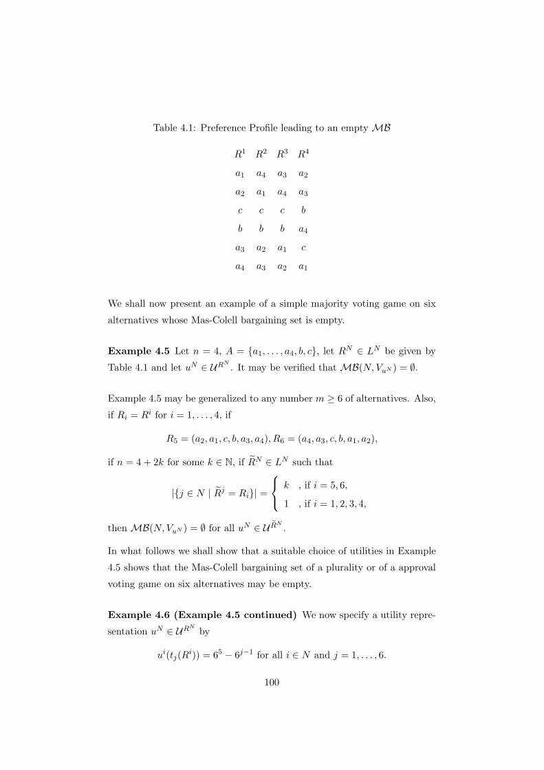
Table 4.1: Preference Profile leading to an empty MB

R1 R2 R3 R4

a1 a4 a3 a2

a2 a1 a4 a3

c c c b

b b b a4

a3 a2 a1 c

a4 a3 a2 a1

We shall now present an example of a simple majority voting game on six

alternatives whose Mas-Colell bargaining set is empty.

Example 4.5 Let n = 4, A = a1, . . . , a4, b, c, let RN ∈ LN be given by

Table 4.1 and let uN ∈ URN . It may be verified that MB(N,VuN ) = ∅.

Example 4.5 may be generalized to any number m ≥ 6 of alternatives. Also,

if Ri = Ri for i = 1, . . . , 4, if

R5 = (a2, a1, c, b, a3, a4), R6 = (a4, a3, c, b, a1, a2),

if n = 4 + 2k for some k ∈ N, if RN ∈ LN such that

|j ∈ N | Rj = Ri| =

k , if i = 5, 6,

1 , if i = 1, 2, 3, 4,

then MB(N,VuN ) = ∅ for all uN ∈ U RN .

In what follows we shall show that a suitable choice of utilities in Example

4.5 shows that the Mas-Colell bargaining set of a plurality or of a approval

voting game on six alternatives may be empty.

Example 4.6 (Example 4.5 continued) We now specify a utility repre-

sentation uN ∈ URN by

ui(tj(Ri)) = 65 − 6j−1 for all i ∈ N and j = 1, . . . , 6.

100

Let (N,V ) the corresponding plurality or approval voting game, that is,

V ∈ V pluN , V ap

uN .

Then MB(N,V ) = ∅.

Remark 4.7 It is possible to modify the utility profile uN of the foregoing

example in such a way that the Mas-Colell bargaining sets of the approval

or the plurality voting game are nonempty. Indeed, if we just replace ui,

i = 1, 2, by ui which differs from ui only inasmuch as ui(tj(Ri)) = 12 − 2j

for j = 4, 5, then

x =

u1(a3) + u1(a4)2

,u2(a1)

2, u3,4(a4)

= (1, 3885, 7770, 7560) ∈MB(N,V ).

In order to replicate the simple majority voting game (N,VuN ), let k ∈ Nand denote

kN = (j, i) | i ∈ N, j = 1, . . . , k.

Furthermore, let R(j,i) = Ri and u(j,i) = ui for all i ∈ N and j = 1, . . . , k.

Then (kN, VukN ) is the k-fold replication of (N,VuN ).

Remark 4.8 If α is a weak Condorcet winner with respect to RN , then

ukN (α)∈MB(kN, VukN ).

Theorem 4.9 If k ≥

n + 2 , if n is odd,n2 + 2 , if n is even,

then MB(kN, VukN ) = ∅.

It should be remarked that the foregoing theorem remains valid for any

ukN ∈ URkN .

5 A Non-Levelled Superadditive Game with anEmpty MB

In this section we show that there exists a non-levelled1 superadditive NTU

game whose Mas-Colell bargaining set is empty. Note that simple majority1A zero-normalized NTU game (N, V ) is non-levelled if for every coalition S every

weakly Pareto optimal element of V (S) ∩ RS+ is Pareto optimal.

101

voting games are levelled. We shall now extend MB and modify the game

of Example 4.5 suitably. Let (N,V ) be a zero-normalized superadditive

NTU game and let x be an imputation. A strong objection at x is strongly

justified if it has no weak counter objection. The extended bargaining set

MB∗(N,V ) is the set of all imputations that do not have strongly justified

strong objections. Clearly, MB(N,V ) ⊆MB∗(N,V ).

If (N,V ) is the game of Example 4.5, then (u1,2,3(b), u4(a4)) ∈MB∗(N,V ).

However, the following example presents a game whose extended bargaining

set is empty.

Example 5.1 Let n = 4, A = a1, . . . , a4, a∗1, . . . , a∗4, b, c, let RN ∈ LN be

given by Table 5.1, let uN represent RN such that minα∈A ui(α) > 0 for all

Figure 5.1: A Preference Profile

R1 R2 R3 R4

a1 a4 a3 a2

a2 a1 a4 a3

a∗2 a∗1 a∗4 a∗3

a∗1 c a∗3 a∗2

c a∗4 c b

b b b a∗4

a∗3 a∗2 a∗1 a4

a3 a2 a1 c

a∗4 a∗3 a∗2 a∗1

a4 a3 a2 a1

i ∈ N , and let V = VuN . It may be verified that MB∗(N,V ) = ∅.

Let N be a finite nonempty set and let Γ denote the set of all superadditive

zero-normalized NTU games (N,V ).

102

The following lemma may be shown directly.

Lemma 5.2 MB∗ is an upper hemicontinuous correspondence2 on Γ.

With the help of Theorem 4 of Wooders (1983) it is possible to deduce the

following desired result.

Theorem 5.3 There exists a superadditive and non-levelled four-person game

U such that MB(U) = ∅.

References

Aumann, R. J. (1967): “A survey of cooperative games without side pay-ments”, in Shubik (1967), pp. 3 – 27.

Aumann, R. J., and M. Maschler (1964): “The bargaining set for co-operative games”, in Advances in Game Theory, ed. by M. Dresher, L. S.Shapley, and A. W. Tucker, Vol. 52 of Annals of Mathematical Studies,pp. 443 – 476, Princeton, N.J. Princeton University Press.

Brams, S. J., and P. C. Fishburn (1983): Approval Voting. Birkhauser,Boston.

Davis, M., and M. Maschler (1967): “Existence of stable payoff config-urations for cooperative games”, in Shubik (1967), pp. 39 – 52.

Fishburn, P. C. (1972): “Even-chance lotteries in social choice theory”,Theory and Decision, 3, 18 – 40.

Gaertner, W. (2001): Domain Conditions in Social Choice Theory. Cam-bridge University Press, Cambridge.

Mas-Colell, A. (1989): “An equivalence theorem for a bargaining set”,Journal of Mathematical Economics, 18, 129 – 139.

Peleg, B., and P. Sudholter (2004): “Bargaining sets of voting games”,Discussion paper, 376, Center for the Study of Rationality, The HebrewUniversity of Jerusalem.2Here we identify any game (N, V ) ∈ Γ with V +, defined by V +(S) = V (S)∩RS

+ for allS ⊆ N , S = ∅. The distance between two games V +

1 and V +2 is the number δ(V +

1 , V +2 ) =

max∅=S⊆N dS(V +1 (S), V +

2 (S)), where dS(·, ·) is the Hausdorff distance between nonemptycompact subsets of RS .

103

(2005): “On the non-emptiness of the Mas-Colell bargaining set”,Journal of Mathematical Economics, forthcoming.

Shubik, M. (ed.) (1967): Essays in Mathematical Economics in Honor ofOskar Morgenstern, Princeton, NJ. Princeton University Press.

Vohra, R. (1991): “An existence theorem for a bargaining set”, Journalof Mathematical Economics, 20, 19 – 34.

Wooders, M. (1983): “The epsilon core of a large replica game”, Journalof Mathematical Economics, 11, 277 – 300.

104

Core-based solutions for assignmentmarkets

Marina Nunez and Carles Rafels ∗

Department of Actuarial, Financialand Economic Mathematics, CREB and CREA

University of Barcelona, Av.Diagonal, 690, E-08034 Barcelona, Spaine-mail: mnunez@ub.edu; crafels@ub.edu

Abstract

This survey reviews some contributions to the literature that showthat most cooperative solutions to the assignment market are deter-mined by the core of the game. Different assignment markets withthe same core have the same τ -value, the same kernel and the samenucleolus.Key words: Assignment games, core, τ -value, kernel, nucleolus.

1 Introduction

In an assignment market, two disjoint sets of agents exist, let us say buyersand sellers, and one good is present in indivisible units. Each seller owns aunit of the indivisible good and each buyers needs exactly one unit. Differ-entiation in the units is allowed and therefore a buyer might place differentvaluations on the units of different sellers. When the difference betweenwhat an object on sale is worth to the buyer and the minimum that wouldbe accepted by the seller is nonnegative, the trading between this pair ofagents is possible and this difference is the joint profit that this mixed-pairwill obtain if they trade. If the reservation price of a seller exceeds the worththat a buyer places in the object, no profit can be made by this mixed-pairof agents. In this way, a nonnegative assignment matrix is obtained withthe profits of all pairings.

The assignment problem is then an operations research problem whichlooks for a matching from buyers to sellers that maximizes the total profit.

Under the assumption that side payments among agents are allowed,and identifying utility with money, Shapley and Shubik (1972) introduce a

∗Institutional support from Ministerio de Ciencia y Tecnologıa and FEDER undergrant BEC 2002-00642 and from Generalitat de Catalunya under grant SGR2001-0029 isacknowledged

105

cooperative model for this two–sided market. A coalitional game is then de-fined where the characteristic function assigns to each coalition of agents theprofit of an optimal matching in the corresponding submarket. They provethat the core of the assignment game is nonempty and, since it consists ofthe set of solutions to the dual assignment problem, it can be described justin terms of the assignment matrix. As a consequence of the lattice structureof the core of the assignment game, for each side of the market there is anextreme core allocation where all agents on this side simultaneously maxi-mize their core payoff. Demange (1982) and Leonard (1983) show that, foran assignment market, the maximum core payoff of an agent is his or hermarginal contribution to the grand coalition.

Several papers analyze the core of the assignment market. Balinsky andGale (1987) give upper and lower bounds for the number of extreme coreallocations, Hamers et al. (2002) show that every extreme core allocation isa marginal worth vector, although these are nonconvex games, and Nunezand Rafels (2003) characterize the set of extreme core allocations by meansof the reduced marginal worth vectors.

Other works relate the core of the assignment game with other coopera-tive solutions such as the stable sets, the bargaining set, the kernel and thenucleolus. Solymosi and Raghavan (2001) determine when the core of anassignment game is a stable set, that is to say, a von Neumann and Morgen-stern (1944) solution. To be more precise, the core is proved to be stable ifand only if the minimum core payoff for each agent in the market is zero.Moreover, in Solymosi (1999) the core of the assignment game is proved tocoincide with the bargaining set defined by Aumann and Maschler (1964).This implies the coincidence of the bargaining sets of any two assignmentmarkets with the same core.

In Rochford (1984) some core allocations are selected by means of classi-cal cooperative bargaining theory: if the optimal matching is assumed to begiven exogenously, matched pairs engage in a pairwise bargaining process a

la Nash which is solved symmetrically, after defining threats based on theoutside opportunities given the current payoff to other pairs. In this way, aset of equilibria is defined (the symmetrically pairwise-bargained allocationsor SPB allocations) which are stable under rebargaining. This set is provedto coincide with the intersection of the kernel (a well-known set solution fortransferable utility cooperative games defined by Davis and Maschler, 1965)and the core of the assignment game. After Driessen (1998), we know thatthe kernel of an assignment game is a subset of the core and thus the set ofSPB allocations coincides with the kernel of the assignment game. Moreover,Granot and Granot (1992) characterize those assignment markets where thekernel coincides with the whole core.

A well known single-valued core selection is the nucleolus (Schmeidler,1969), and Solymosi and Raghavan (1994) provide an algorithm to computethe nucleolus of an assignment game. Another single-valued solution is the

106

τ -value (Tijs, 1981). For arbitrary cooperative games this solution may lieoutside the core but in the case of the assignment game it turns out to bealso a core selection (Nunez and Rafels, 2002a).

In this survey paper we review some of our contributions to this litera-ture to emphasize the fact that most of the aforementioned solutions to theassignment game are determined by its core. This means that, as it hap-pens with the bargaining set, different assignment markets with the samecore also have the same τ -value, the same kernel and the same nucleolus.

The starting point is the characterization of the core of the assignmentgame given in Quint (1991): any “45o lattice” can be associated with thecore of an appropriately defined assignment game. However this assignmentgame might not be unique, and Quint asks for an assignment matrix withthe entries “as high as possible”. After presenting the assignment modelin Section 2, in Section 3 we will define a representative matrix with theentries as high as possible among those defining games with the same core. InSection 4 and Section 5 we show that the τ -value, the kernel or the nucleolusof an assignment market ar those of the aformentioned representative.

2 The assignment model

Let M = 1, 2, . . . ,m be a set of buyers, M = 1, 2, . . . ,m a set of sellersand let A = (aij)(i,j)∈M×M be a nonnegative matrix where aij representsthe profit obtained by the mixed–pair (i, j) if they trade. Let n = m + m

denote the cardinality of M ∪ M . The assignment problem (M,M , A)consists in looking for an optimal matching between the two sides of themarket. A matching for A is a subset µ of M ×M such that each k ∈M ∪ M belongs at most to one pair in µ . We will denote the set ofmatchings of A by M(A) or M(M,M ) . We say a matching µ is optimalif for all µ ∈ M(M,M ) ,

(i,j)∈µ aij ≥

(i,j)∈µ aij , and will denote

the set of optimal matchings by M∗(A) .Assignment games were introduced by Shapley and Shubik (1972) as a

cooperative model for a two–sided market with transferable utility. Given anassignment problem (M,M , A) , the player set is M ∪M , and the matrixA determines the characteristic function wA . Given S ⊆ M and T ⊆ M ,wA(S ∪ T ) = max

(i,j)∈µ aij | µ ∈M(S, T ) , M(S, T ) being the set of

matchings between S and T . It will be assumed as usual that a coalitionformed only by sellers or only by buyers has worth zero. For all i ∈ Moptimally matched by µ , we will denote by µ(i) the agent j ∈ M suchthat (i, j) ∈ µ . Similarly, i could be denoted by µ−1(j) . Moreover, wesay a buyer i ∈ M is not assigned by µ if (i, j) ∈ µ for all j ∈ M (andsimilarly for sellers).

Shapley and Shubik proved that the core of the assignment game (M ∪M , wA) is nonempty and can be represented in terms of any optimal match-

107

ing µ of M ∪M by

C(wA) =

ui ≥ 0, for all i ∈ M ; vj ≥ 0, for all j ∈ M

ui + vj = aij if (i, j) ∈ µ(u, v) ∈ RM × RM

ui + vj ≥ aij if (i, j) ∈ µui = 0 if i not assigned by µvj = 0 if j not assigned by µ .

(1)Moreover, the core has a lattice structure with two special extreme points:the buyers–optimal core allocation, (u, v) , where each buyer attains hismaximum core payoff, and the sellers–optimal core allocation, (u, v) , whereeach seller does.

¿From Demange (1982) and Leonard (1983) we know that the maximumcore payoff of any player coincides with his marginal contribution:

ui = wA(M∪M )−wA((M∪M )\i) and vj = wA(M∪M )−wA((M∪M )\j) .(2)

From (2) and the description of the core (1) the minimum core payoff ofbuyer i is

ui = aiµ(i)−wA(M ∪M )+wA((M ∪M )\µ(i)) for all µ ∈M∗(A) , (3)

while the minimum core payoff of seller j is

vj = aµ−1(j)j−wA(M ∪M )+wA((M ∪M )\µ−1(j)) for all µ ∈M∗(A) .(4)

Example 1 (Shapley and Shubik, 1972) Let M = 1, 2, 3 be the set

of buyers, M = 1, 2, 3 be the set of sellers and let the assignment matrix

A be

1’ 2’ 3’

1 5 8 2

2 7 9 63 2 3 0

Notice there exists only one optimal matching µ = (1, 2), (2, 3), (3, 1) .Following Shapley and Shubik, to describe the core of the assignment gameyou do not need to compute the complete characteristic function since onlythe mixed-pair coalitions are relevant. Thus, the core of this game is:

C(wA) =

(u, v) ∈ R6+

u1 + v1 ≥ 5, u1 + v2 = 8, u1 + v3 ≥ 2,u2 + v1 ≥ 7, u2 + v2 ≥ 9, u2 + v3 = 6,u3 + v1 = 2, u3 + v2 ≥ 3, u3 + v3 ≥ 0 .

This set is the convex hull of its extreme points: (3,5,0;2,5,1), (3,6,0;2,5,0),(4,6,1;1,4,0), (5,6,1;1,3,0), (5,6,0;2,3,0) and (4,5,0;2,4,1). Although this core

108

is a subset of R6 , taking into account the equality constraints u1 + v2 = 8,u2+v3 = 6, u3+v1 = 2 , the core is completely determined by its projectionto the space of payoffs to the buyers and this projection is depicted in figure1.

(5, 6, 0; 2, 3, 0)

(5, 6, 1; 1, 3, 0)

(4, 5, 0; 2, 4, 1)

(4, 6, 1; 1, 4, 0)

(3, 6, 0; 2, 5, 0)

(3, 5, 0; 2, 5, 1)

Figure 1: The core of the assignment game in Example 1

Among these extreme points we point out the buyers-optimal core al-location, (u, v) = (5, 6, 1; 1, 3, 0) , and the sellers-optimal core allocation,(u, v) = (3, 5, 0; 2, 5, 1) , which are the two more distant extreme points.

3 Buyer-seller exactness

Notice that in the above example u1 + v3 ≥ 3 > 2 = a13 for all (u, v) ∈C(wA) . As a consequence, if we raise a13 in one unit, the resulting assign-ment game will have the same core. In fact, all matrices

A(α) =

5 8 α7 9 62 3 0

with 0 ≤ α ≤ 3 define assignment games with the same core as (M ∪M , wA) .

In Nunez and Rafels (2002b) an assignment game is defined to be buyer-seller exact if no matrix entry can be raised without modifying the core ofthe game.

Definition 2 An assignment game (M ∪M , wA) is buyer-seller exactif and only if for all i ∈ M and all j ∈ M there exists (u, v) ∈ C(wA)such that ui + vj = aij .

109

It is then proved that for all assignment game (M ∪M , wA) there existsa unique buyer-seller assignment game with its same core. This is denoted by(M∪M , wAr) and is the buyer-seller exact representative of the initialgame. Notice that Ar is maximal among all matrices defining assignmentgames with the same core as (M ∪M , wA) . Moreover, both matrices haveat least one optimal matching in common.

Of course, given the core of the game, the buyer-seller exact representa-tive is easily computed, as we have done in our example. But, how to obtainAr directly from the assignment problem?

To answer this question we analyze how the payoff to a mixed-pair coali-tion is bounded in the core. From now on, without loss of generality wewill assume that A is square by adding null rows or columns, and wewill denote the j-th seller by j to distinguish it from the j-th buyer.Then, an optimal matching can be assumed to be placed in the diagonal:µ = (i, i) | i ∈ M ∈M∗(A).

We define, for all (i, j) ∈ M × M , Kij to be the upper core boundfor the mixed-pair coalition i, j , Kij = max(u,v)∈C(wA) ui + vj , and kij

the lower core bound for the same coalition, kij = min(u,v)∈C(wA) ui + vj .These bounds can be expressed in terms of the characteristic function.

Proposition 3 Let (M ∪M , wA) be an assignment game. Then, Kij =wA(M ∪M ) − wA(M ∪M \ i, j) and kij = aii + ajj + wA(M ∪M \j, i)− wA(M ∪M ).

This shows that, as it happens with the marginal contributions of one-player coalitions, all marginal contributions of mixed pair coalitions are at-tained in the core of the assignment game.

Then (M ∪M , wA) is buyer–seller exact if and only if kij = aij for all(i, j) ∈ M ×M .

All the same, we would like to be able to determine, just in terms ofthe matrix entries, whether an assignment game (M ∪ M , wA) is buyer-seller exact and, if it is not, to compute the buyer-seller exact representative(M ∪M , wAr) .

To this end, we recall a definition due to Solymosi and Raghavan (2001).An assignment game is doubly dominant diagonal if and only if aij +akk ≥ aik+akj for all i, j, k ∈ M and different. This property characterizesthose matrices with the property of buyer-seller exactness.

Theorem 4 (Nunez and Rafels, 2002b) An assignment game (M∪M , wA)is buyer–seller exact if and only if A is doubly dominant diagonal.

Moreover, the representative matrix Ar can be computed from matrixA in the following way: ar

ij = maxaij , aij , where, for all (i, j) ∈ M ×M ,

aij = maxk1,k2,...,kr∈M\i,j

different

aik1+ ak1k2

+ · · ·+ akrj − (ak1k1+ · · ·+ akrkr) . (5)

110

To conclude this section, notice that, from the definition of the buyer-seller representative matrix Ar , two assignment games with the same corehave the same buyer–seller exact representative. In some sense, the coinci-dence of the cores provides a classification of assignment games. This factmakes us question how the main cooperative solutions behave with respectto this classification.

4 The kernel and the τ-value

In the case of the assignment game, it is quite straightforward to realizethat these two cooperative solutions are completely determined by the coreof the game.

The τ -value is a single-valued solution for coalitional games that wasintroduced by Tijs (1981) as a compromise value between a utopia vectorand a minimal rights vector. In some games the τ -value does not lie in thecore. This is not the case for the assignment game, since in Nunez and Rafels(2002a) its τ -value is proved to coincide with the midpoint of the segmentdetermined by the buyers-optimal and the sellers-optimal core allocations:

τ(wA) =12(u, v) +

12(u, v) ∈ C(wA) .

Thus, two assignment games with the same core have the same τ -value. InExample 1, τ(wA(α)) = (4, 5.5, 0.5; 1.5, 4, 0.5) for all 0 ≤ α ≤ 3 .

The case of the kernel is similar. Let us denote by I(v) the set ofimputations (efficient allocations that are individually rational) of a game(N, v) . For zero–monotonic games ( v(S) ≥ v(T ) +

i∈S\T v(i) , for all

T ⊆ S ), as it is the case of assignment games, the kernel is given by

K(v) = z ∈ I(v) | svij(z) = sv

ji(z), ∀i, j ∈ N, i = j,

where the maximum surplus svij(z) of player i over another player j with

respect to the allocation z ∈ RN is defined by

svij(z) = maxv(S)− z(S) | S ⊆ N , i ∈ S , j ∈ S .

It is known from Maschler, Peleg and Shapley (1979) that given twocoalitional games with the same core, the intersections of the kernel and thecore also coincide. As a consequence, if (M∪M , wA) and (M∪M , wB) aretwo assignment games with the same core, then K(wA)∩C(wA) = K(wB)∩C(wB) . Since the kernel of an assignment game is always included in thecore (Driessen, 1998), the above equality is equivalent to K(wA) = K(wB) .

As it is shown in Nunez (2004), the kernel of Example 1 reduces to onlyone point, thus being the nucleolus.

111

5 All assignment games with the same core havethe same nucleolus

The nucleolus is a single-valued solution for coalitional games that wasintroduced by Schmeidler (1969) as the imputation that lexicographicallyminimizes the vector formed by the excesses of all nontrivial coalitions innon-increasing order. This minimum always exists and reduces to only onepoint. Moreover, if the core is nonempty, the nucleolus lies in the core.

It is known from Huberman (1980) that only essential coalitions are to beconsidered in the computation of the nucleolus of a coalitional game. Fromhis definition, it is easy to check that, for assignment games, only one-playercoalitions and mixed-pair coalitions are essential.

Given an assignment game (M ∪ M , wA) , for all x ∈ I(wA) and allS ⊆ M ∪M , the excess of coalition S at x is

e(S, x) = v(S)−

i∈S

xi = v(S)− x(S).

Then, for all x ∈ I(wA) define the vector θ(x) ∈ Rm×m+m+mof excesses

of all non-trivial essential coalitions at x in non-increasing order: θ(x)k =e(Sk, x) , where e(Sk, x) ≥ e(Sk+1, x) and Sk is either a one-player coalitionor a mixed-pair coalition.

The nucleolus of (M∪M , wA) is the imputation ν(wA) that minimizesθ(x) , with respect to the lexicographic order, over the set of imputations:

θ(ν(v)) ≤Lex θ(x) , for all x ∈ I(wA) .

Solymosi and Raghavan (1994) adapt the definition of lexicographic cen-ter due to Maschler, Peleg and Shapley (1979) to the case of the assignmentgame. With some small changes, their definition of lexicographic center ofan assignment game is used in Nunez (2004).

Given (M ∪M , wA) , we take an optimal matching µ ∈ M∗(A) , andconsider the set of coalitions

P = k | k ∈ M ∪M ∪ i, j | i ∈ M , j ∈ M .

We iteratively construct• Σ0 ⊇ Σ1 ⊇ · · · ⊇ Σs+1 and ∆0 ⊆ ∆1 ⊆ · · · ⊆ ∆s+1 sets of coalitions inP such that for all 0 ≤ r ≤ s + 1 , (∆r,Σr) is a partition of P , and• X0 ⊇ X1 ⊇ · · · ⊇ Xs+1 a sequence of payoff sets, such that:

Initially ∆0 = i, j | (i, j) ∈ µ∪k | k ∈ M∪M not matched by µ ,Σ0 = P \∆0 , and X0 = C(wA) .

For r ∈ 0, 1, . . . , s define recursively

1. αr+1 = min(u,v)∈Xr maxS∈Σr e(S, (u, v))

112

2. Xr+1 = (u, v) ∈ Xr | maxS∈Σr e(S, (u, v)) = αr+1

3. Σr+1 = S ∈ Σr | e(S, (u, v)) is constant on Xr+1

4. Σr+1 = Σr \ Σr+1, ∆r+1 = ∆r ∪ Σr+1

where s is the last index for which Σr = ∅ . The set Xs+1 is the lexico-graphic center of (M ∪M , wA) .

It is then proved that the lexicographic center is well defined and itreduces to only one point which coincides with the nucleolus.

In our Example 1, the process begins with a linear program with 6 vari-ables and 15 constraints, and you obtain:

ν(wA) = (4, 5.667, 0.333; 1.667, 4, 0.333) .

In Maschler, Peleg and Shapley (1979) an example is given of two co-operative games with the same core but different nucleoli. Next theoremshows that this cannot happen with two assignment games.

Theorem 5 (Nunez, 2004) Let (M ∪ M , wA) be an assignment game

with the same number of agents on each side of the market and (M ∪M , wAr) its buyer-seller exact representative. Then,

ν(wA) = ν(wAr) .

To prove that, take (∆0,Σ0), . . . , (∆s+1,Σs+1) and X0, . . . , Xs+1 thepartitions and payoff sets in the definition of lexicographic center of (M ∪M , wA) , and consider also (∆0, Σ0), . . . , (∆s+1, Σs+1) and X0, . . . , Xs+1

the partitions and payoff sets in the definition of lexicographic center of(M ∪ M , wAr) . Then it can be proved (by induction on r) that for all0 ≤ r ≤ s + 1 , ∆r = ∆r , Σr = Σr and Xr = Xr , and consequentlyν(wA) = ν(wAr) .

As a consequence of the above theorem, if (M ∪ M , wA) and (M ∪M , wB) are two assignment games with the same core and the same numberof agents on each side of the market, then ν(wA) = ν(wAr) = ν(wBr) =ν(wB) . The result is easily extended to assignment games where one sideof the market has more agents than the opposite side.

Thus, all the markets (M ∪M , wAα) , with α ∈ [0, 3] , in our previousexample have the same nucleolus:

ν(wA(α)) = (4, 5.667, 0.333; 1.667, 4, 0.333) .

References

[1] Aumann, R.J., Maschler, M. (1964) The bargaining set for cooperativegames. In: Advances in Game Theory, M. Dresher, L.S. Shapley and A.W.Tucker, eds. Princeton University Press, Princeton, New Jersey, 443–476.

113

[2] Balinski, M.L., Gale, D. (1987) On the core of the assignment game. In:Functional Analysis, Optimization and Matematical Economics. OxfordUniversity Press, New York, 274–289.

[3] Bohm–Bawerk, E. von (1923) Positive theory of capital (translated byW. Smart). G.E. Steckert, New York, (original publication 1891).

[4] Demange, G. (1982) Strategyproofness in the Assignment Market Game.Laboratorie d’Econometrie de l’Ecole Politechnique, Paris. Mimeo.

[5] Davis, M., Maschler, M. (1965) The kernel of a cooperative game, NavalResearch Logistics Quarterly, 12, 223–259.

[6] Driessen, T.S.H. (1998) A note on the inclusion of the kernel in the coreof the bilateral assignment game. International Journal of Game Theory,27, 301–303.

[7] Granot, D., Granot, F. (1992) On some network flow games. Mathemat-ics of Operations Research, 17, 792–841.

[8] Hamers, H., Klijn, F., Solymosi, T., Tijs, S., Villar, J.P.(2002) Assign-ment games satisfy the CoMa-property. Games and Economic Behavior,38, 231–239.

[9] Huberman, G. (1980) The nucleolus and the essential coalitions. In:Analysis and Optimization of Systems, Lecture Notes in Control and In-formation Science 28, 417–422.

[10] Leonard, H.B. (1983) Elicitation of Honest Preferences for the Assign-ment of Individuals to Positions. Journal of Political Economy, 91, 461–479.

[11] Maschler, M., Peleg, B., Shapley, S. (1979) Geometric properties of thekernel, nucleolus, and related solution concepts. Mathematics of Opera-tions Research, 4, 303–338.

[12] Neumann, J. von, Morgenstern, O. (1944) Theory of games and eco-

nomic behavior. Princeton University Press, Princeton, New Jersey.

[13] Nunez, M. (2004) A note on the nucleolus and the kernel of the assign-ment game. International Journal of Game Theory, 33, 55–65.

[14] Nunez, M., Rafels, C. (2002a) The assignment game: the τ–value.International Journal of Game Theory 31, 411-422.

[15] Nunez, M., Rafels, C. (2002b) Buyer–seller exactness in the assignmentgame. International Journal of Game Theory, 31, 423–436.

114

[16] Nunez, M., Rafels, C. (2003) Characterization of the extreme core al-locations of the assignment game. Games and Economic Behavior 44,311–331.

[17] Quint, T. (1991) Characterization of cores of assignment games. Inter-national Journal of Game Theory, 19, 413–420.

[18] Rochford, S.C. (1984) Symmetrically pairwise–bargained allocations inan assignment market. Journal of Economic Theory, 34, 262–281.

[19] Schmeidler, D. (1969) The nucleolus of a characteristic function game.SIAM Journal of Applied Mathematics, 17, 1163–1170

[20] Shapley, L.S., Shubik, M. (1972) The Assignment Game I: The Core.International Journal of Game Theory, 1, 111–130.

[21] Solymosi, T. (1999) On the bargaining set, kernel and core of superad-ditive games. International Journal of Game Theory, 28, 229–240.

[22] Solymosi, T., Raghavan, T.E.S. (1994) An algorithm for finding thenucleolus of assignment games. International Journal of Game Theory,23, 119–143.

[23] Solymosi, T., Raghavan, T.E.S. (2001) Assignment games with stablecore. International Journal of Game Theory, 30, 177–185.

[24] Tijs, S.H. (1981) Bounds for the core and the τ–value. In Game Theory

and Mathematical Economics, O. Moeschlin and D. Pallaschke, eds. NorthHolland Publishing Company, 123–132.

115

116

Convex Geometry and Bargaining

Joachim Rosenmüller12

1Institute of Mathematical EconomicsIMW

University of BielefeldD-33615 Bielefeld

Germany

2This survey describes the contents of a series of papersthat originated from a project conducted

jointly withDiethard Pallaschke, Karlsruhe

Abstract

We discuss the construction of a superadditive bargaining solu-tion in the spirit of Maschler–Perles. The family of poly-hedra admitting such a solution is provided by the “cephoids”,i.e., finite sums of “prisms”. The geometrical shape of these poly-hedra, the partially ordered set of their maximal faces, and thecombinatorial structure describing this poset provide the foun-dation for the construction of a bargaining solution.

1 Superadditivity of Solutions

The Shapley value ([15]) is a mapping defined on TU games (on realvalued set functions) with values in Euclidean space (distributions of wealth)respecting anonymity, Pareto e!ciency, and a dummy property. The solutionconcept is uniquely defined by the additional requirement that it should beadditive. More precisely, if I is a finite set and P = P(I) the power set (theset of coalitions), then a function v : P ! satisfaying v(") = 0 is agame . A mapping ! : v v is a game ! I is additive if, for any twogames v,w it satisfies

!(v) + !(w) = !(v + w) .

117

The Shapley value for a game v is given by

!i(v) :=!

S!P

(s # 1)!(n # s)!

n!(v(S) # v(S \ i)).

It can be computed in various other ways and enjoys a host of nice properties;the amount of work dealing with this concept is huge.

Additivity of a solution concept is traditionally justified by risk neutrality.Players facing a lottery of two games do not distinguish between the valueof the expected game and the expected value of the games. Yet, one can aswell think that players act independently in two remote games and evaluatethe expectations either in both games independently or else by establishinga package deal.

If side payments are not permitted, than additivity of a solution conceptcannot be obtained. Yet, the sum of two games (or in particular of twobargaining problems) is well defined. This is the algebraic sum which isobtained by summing all pairs of utility vectors available to a coalition inthe two games.

One can at best hope for superadditivity. This means that by striking apackage deal both players improve their situation with regard to the solutionconcept. Or else, when facing a lottery of two games, it is an advantage forboth players to contract ex ante and evaluate the expected game accordingto the solution concept.

We shall first of all necessarily restrict the discussion on bargaining problems.The Nash bargaining solution [8] is not superadditive as is seen by simpleexamples for two persons. The Maschler–Perles solution [7] on the otherhand is uniquely defined by superadditivity – given that one takes the usualrequirements regarding symmetry etc. for granted. The serious problem isthat the Maschler–Perles solution exists for two person games only. Infact, Perles [12] proved in 1982 that a superadditive solution generally doesnot exist for three and more persons.

Yet, when generalizing the Shapley value to the NTU context the gen-eral approach assumes coincidence with the Nash solution for the n personbargaining problem (see Shapley [16] Aumann [1], Harshanyi [4], [5],Kern [6]). This idea is justified on the overwhelming acceptance of theNash–solution. It may also recognize the fact that there is no superadditivesolution in higher dimensions and a fortiori there will be no superadditiveShapley value. Yet, one might argue that this is not a particulaly consis-tent approach.

118

We establish a solution concept that is superadditive on a certain sub–classof games. As it turns out to establish this class requires quite an e"ort. Thenature of sums of convex polyhedra is discussed within the framework ofconvex geometry,this task may, depending on the context, in itself be quiteinvolved. The particular class we will exhibit is the family of “cephoids”which are sums of hyperplane games (bargaining situations) with variingnormal vector.

Let us recall some basic facts. The Maschler–Perles bargaining solution(Maschler–Perles [7], see also [13] for a textbook presentation) is a map-ping defined on 2–dimensional bargaining problems respecting anonymity,Pareto e!ciency, and a!ne transformations of utility. Moreover, this map-ping is superadditive by which property it is uniquely characterized. Wewant to be more precise.

A bargaining problem is a pair (0, U) with a compact, convex, and com-prehensive subset " $= U % 2

+. 0 & U is the status quo point and U thefeasible set . Players may reach agreement on some feasible utility vector.Or else end up at the status quo point, which we assume to be 0. It su!cesto mention U .

A solution is a mapping ! that, based on some axiomatic justification,assignes to each bargaining problem U a Pareto e!cient vector !(U).

Suppose two players are engaged in two “remote” problems U and U " simul-taneously. In the beginning, they considered these to be di"erent a"airs,thus wanted to settle for !(U) and !(U ") separately. Later on they real-ized that one should consider giving in with respect to one contract in favorof receiving concessions with respect to the other one. That is, they de-cided to consider this to be one problem. The utilities available are nowx + x"|x & U, x" & U " =: U + U ". If a solution is superadditive, i.e.,satisfies !(U + U ") ' !(U) + !(U "), it turnes out that both players profitfrom a quid quo pro.

Od course the interpretation that players face a lottery involving two bar-gaining problems applies as well. Superaddivity is then seen to consistentlyfavor contracting ex ante, thereby increasing expected utility (see [7] or [13],p.562, for a detailed discussion).

We focus on polyhedral bargaining problems. A bargaining problem (in 2)is polyhedral if the Pareto surface consists of line segments only. TheMaschler–Perles solution µ is based on the observation that every poly-hedral bargaining solution in 2 is an sum of “elementary” bargaining prob-lems that are generated by a line segment (thus reflect constant transfer ofutility). More precisely, let a = (a1, a2) > 0 & n. We introduce the unit

119

vectors ei, the vectors ai := aiei (i & I), and associate with a the triangle

(1.1) "a := convH"#

0,a1,a2,$%

.

The Pareto curve of this triangle is the line segment #a which is given by

(1.2) #a := convH"#

a1,a2$%

.

Now, a bargaining problem is seen to be polyhedral if and only if the feasibleset is given by

(1.3) " =!

k!K

"a(k)

with a suitable family of (positive) vectors&a(k)

'

k!K, K := 1, . . . ,K

To any triangle "a we associate the volume V (a) := 12a1a2 = area ("a).

Consider the case that all triangles involved in a representation (1.3) haveequal volume. The bargaining problems having this property form a densesubset of the set of all bargaining problems (employing the Hausdor" metric).Similarly, whenever we deal with the sum of two bargaining problems, wemay assume that the summands as well as the sum are dyadic with the samebasis.

Each triangle equal area

r22T

s22T

s12T

r12T

"

Figure 1.1: A standard dyadic bargaining problem

Definition 1.1. A bargaining problem standard dyadic if the feasible set isa polyhedron represented as in (1.3) with dyadic vectors all generating equalvolume.

120

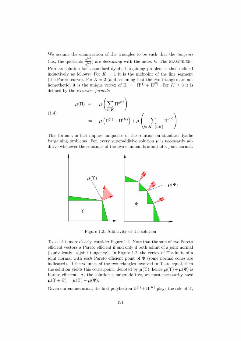
We assume the enumeration of the triangles to be such that the tangents

(i.e., the quotientsa(k)2

a(k)1

) are decreasing with the index k. The Maschler–

Perles solution for a standard dyadic bargaining problem is then definedinductively as follows: For K = 1 it is the midpoint of the line segment(the Pareto curve). For K = 2 (and assuming that the two triangles are nothomothetic) it is the unique vertex of " = "(1) + "(2). For K ' 3 it isdefined by the recursive formula

(1.4)

µ(") = µ

(!

k!K

"a(k)

)

:= µ&"(1) + "(K)

'+ µ

*

+!

k!K#1,K

"a(k)

,

- .

This formula in fact implies uniquenes of the solution on standard dyadicbargaining problems. For, every superadditive solution µ is necessarily ad-ditive whenever the solutions of the two summands admit of a joint normal.

µ($)

µ(%)

$

%

Figure 1.2: Additivity of the solution

To see this more clearly, consider Figure 1.2. Note that the sum of two Paretoe!cient vectors is Pareto e!cient if and only if both admit of a joint normal(equivalently: a joint tangency). In Figure 1.2, the vertex of $ admits of ajoint normal with each Pareto e!cient point of % (some normal cones areindicated). If the volumes of the two triangles involved in $ are equal, thenthe solution yields this cornerpoint, denoted by µ($), hence µ($)+µ(%) isPareto e!cient. As the solution is superadditive, we must necessarily haveµ($ + %) = µ($) + µ(%).

Given our enumeration, the first polyhedron "(1) +"(K) plays the role of $,

121

hence its solution admits of a joint normal with every Pareto e!cient pointof the second polyhedron.

We present two stories concerning the supperadditive solution. The first oneis due to Maschler–Perles: two travelers (it may help to think of donkeycarts) move along the Pareto curve in a way that the product of the speedcomponents in axis directions is equal at any moment.When they start outat the extremal points of the Pareto surface, then they meet eventually atthe solution point.

The second story is a reframed version of the above one: instead of travelingalong the Pareto surface with a certain speed, we may define a surface mea-sure on it such the density (w.r. to the local Lebesgue mesure) correpondsto the travelling speed as mentioned above.

To every line segment #(k) (and every translate of such line segment) weassign a length measure "! (i.e. a dilated version of Lebesgue measure) bysetting

(1.5) "!(#(k)) =

.a(k)

1 a(k)2 := !k.

Then, for every k & K we take a corresponding multiple of the unit simplex,i.e., we put

(1.6) /"(k) :=(

!k"e

such that the surface has length "(/#(k)) = !k. Summing these we obtaina multiple of the unit simplex /" =

0k!K

/"(k) the surface /# of which haslength

(1.7) "(/#) =!

k!K

!k ,

which is the same as the total length of the Pareto curve of " in terms ofthe surface measure.

Therefore, we now construct a bijective and “locally” a!ne linear mapping,say # : # ! /# by mapping the translates of the various #(k) on copies of

the /#(k) in the order dictated by the slopes |a(k)2

a(k)1

|. That is, if #(1) has the

smallest slope |a(1)2

a(2)1

|, then a copy of #(1) is the line segment in the uppermost

left corner of # and this is mapped on a line segment of length !1 in theuppermost left corner of /# etc. Figure 1.3 indicates the procedure. Now, ifx is the midpoint of /#, then the Maschler–Perles solution is given by

(1.8) µ(") = ##1(x).

122

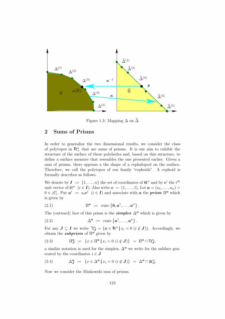
replacemen

#(1)

#(2)

#(3)

#(4)

#(5)

/#(1)

/#(2)

/#(3)

/#(4)

/#(5)

#

##1

xµ(")

"/"

Figure 1.3: Mapping # on /#

2 Sums of Prisms

In order to generalize the two dimensional results, we consider the classof polytopes in n

+ that are sums of prisms. It is our aim to exhibit thestructure of the surface of these polyhedra and, based on this structure, todefine a surface measure that resembles the one presented earlier. Given asum of prisms, there appears a the shape of a cephalopod on the surface.Therefore, we call the polytopes of our family “cephoids”. A cephoid isformally describes as follows.

We denote by I := 1, . . . , n the set of coordinates of n and by ei the ith

unit vector of n (i & I). Also write e = (1, . . . , 1). Let a = (a1, . . . , an) >0 & n

+. Put ai := aiei (i & I) and associate with a the prism "a which

is given by

(2.1) "a := conv#0,a1, . . . ,an

$.

The (outward) face of this prism is the simplex #a which is given by

(2.2) #a := conv#a1, . . . ,an

$.

For any J % I we write nJ

= x & n xi = 0 (i /& J). Accordingly, weobtain the subprism of "a given by

(2.3) "aJ := x & "a xi = 0 (i /& J) = "a ) n

J ,

a similar notation is used for the simplex, #a we write for the subface gen-erated by the coordinates i & J

(2.4) #aJ := x & #a xi = 0 (i /& J) = #a ) n

J .

Now we consider the Minkowski sum of prisms.

123

Definition 2.1. Let a• := (a(k))Kk=1 denote a family of positive vectors andlet

(2.5) " =K!

k=1

"a(k)

be the (algebraic) sum. Then " is called a cephoid.

Note that the representation of a cephoid by a family of prisms is in generalnot unique. Some few examples may serve to motivate a condition thatensures uniqueness.

Example 2.2. A prism may be represented as a cephoid in various ways.E.g., let " = "e be the unit prism and let " be represented as the sum" = "!e + ""e with !,# ' 0, ! + # = 1. The outer surface, i.e., theunit simplex # = #e = #!e + #"e is the union of the two translates!e1 + #"e, #e2 + #!e and a “diamond” #!e

13 + #"e

23 . (cf. Figure 2.1)

#

!e1 + #"e

#e2 + #!e

#!e13 + #"e

23

Figure 2.1: The unit simplex as a cephoid

However, the representation is not unique. As all prisms involved are homo-thetic, the vector used to translate a prism is rather arbitrary. Now considertwo nonhomothetic prisms. The sum is indicated in Figure 2.2. Again thereare the translates of the two prisms involved, i.e. #a + b1 and #b + a1. The“diamond” is the sum #a

23 + #b13.

124

Figure 2.2: Adding two non–homothetic prisms

Figure 2.3: A sum of four prisms

125

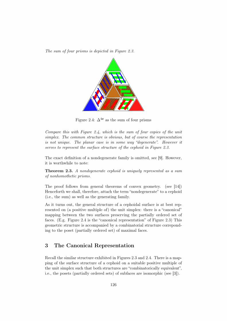
The sum of four prisms is depicted in Figure 2.3.

Figure 2.4: #4e as the sum of four prisms

Compare this with Figure 2.4, which is the sum of four copies of the unitsimplex. The common structure is obvious, but of course the representationis not unique. The planar case is in some way “degenerate”. However itserves to represent the surface structure of the cephoid in Figure 2.3.

The exact definition of a nondegenerate family is omitted, see [9]. However,it is worthwhile to note:

Theorem 2.3. A nondegenerate cephoid is uniquely represented as a sumof nonhomothetic prisms.

The proof follows from general theorems of convex geometry. (see [14])Henceforth we shall, therefore, attach the term “nondegenerate” to a cephoid(i.e., the sum) as well as the generating family.

As it turns out, the general structure of a cephoidal surface is at best rep-resented on (a positive multiple of) the unit simplex: there is a “canonical”mapping between the two surfaces preserving the partially ordered set offaces. (E.g. Figure 2.4 is the “canonical representation” of Figure 2.3) Thisgeometric structure is accompanied by a combinatorial structure correpond-ing to the poset (partially ordered set) of maximal faces.

3 The Canonical Representation

Recall the similar structure exhibited in Figures 2.3 and 2.4. There is a map-ping of the surface structure of a cephoid on a suitable positive multiple ofthe unit simplex such that both structures are “combinatorically equivalent”,i.e., the posets (partially ordered sets) of subfaces are isomorphic (see [3]).

126

In order to simplify the notation, we use K := 1, . . . ,K for the index setof a family of prisms. We consider a family (a(k))k!K of vectors in generalposition; the prism " :=

0k!K

"(k) and its surface # :=0

k!K#(k)

are defined as previously.

We take K copies of e which we denote by a0(1), . . . ,a0(K). As in Section

2 we write a0(k)i := a0(k)i ei, where a0(k)

i denotes the i"th coordinate of a0(k).

For every k & K let "0(k) := "e and #0(k) := #e be a copy of the unit prismand simplex respectively. The (homothetic) sums generated are denoted by

"0 :=!

k!K

"0(k) = "Ke = K"e

and#0 :=

!

k!K

#0(k) = #Ke = K#e

respectively. As all prisms involved are homothetic, the simplex #0 has the(trivial) face poset of the unit simplex.

a

b

c1

2

3

4

Figure 3.1: A sum of 3 prisms in 4 dimensions.

The canonical representation of # is the suitable projection of the outersurface # of a cephoid " on #0 in a way which preserves the poset offaces. For example, the canonical representation of the cephoid representedin Figure 2.3 is indicated by Figure 2.4. Here, both # and #0 are twodimensional while the prisms "(k) = "(a(k)) as well as the resulting cephoid" are three dimensional.

127

Figure 3.2: A sum of 3 prisms – not all prisms at a vertex

Analogously, for n = 4 dimensions and K = 3 prisms, we represent the sumof the prisms canononically on a suitable multiple of the unit simplex of 4,which is a three dimensional tetrahedron. It turns out, that there are threetranslates of simplices on #. Each of these generates ’tentacles’ consistingof 2 cylinders. Thus, we find immediately nine maximal faces that involvea vertex. However, in addition to these nine faces, there is exactly 1 block,i.e., a maximal face that is the sum of three edges, each one taken from. oneof the prisms involved.

The canonical representation of a sum of three prisms in 4 has a surface #which is presented in Figure 3.1.

The translates of the simplices are located at the vertices of #. Each simplexgenerates two cylinders which together form a “tentacle” issued from thatsimplex. Finally, there is the “block”, which is the representation of a partof # which can be written

(3.1) #(a)12 + #(b)

23 + #(c)34 .

In Figure 3.2 we perceive a variant – not all translates of the three prismainvolved are licated at some ertex.

Given nondegeneracy, the number of maximal faces of a cephoid is actuallydepending on the dimension n and the number of prisms involved K only.

E.g., four prisms in 4 yield a cephoid with 20 maximal faces; a canonical

128

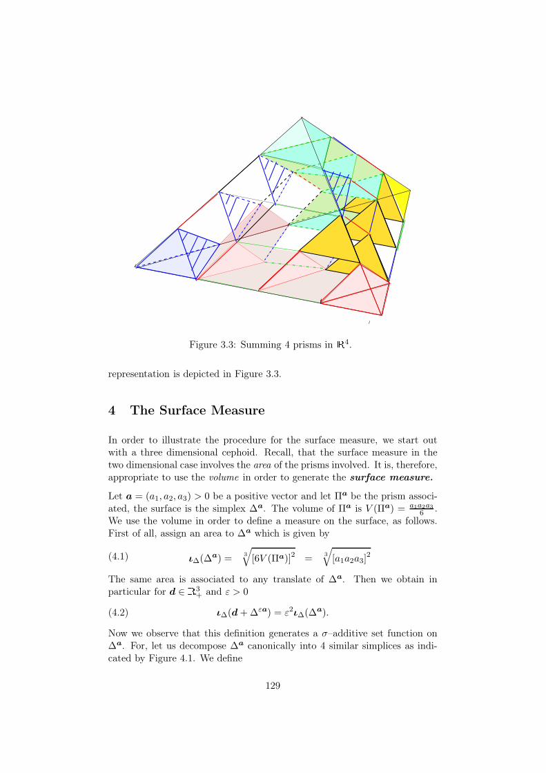
Figure 3.3: Summing 4 prisms in 4.

representation is depicted in Figure 3.3.

4 The Surface Measure

In order to illustrate the procedure for the surface measure, we start outwith a three dimensional cephoid. Recall, that the surface measure in thetwo dimensional case involves the area of the prisms involved. It is, therefore,appropriate to use the volume in order to generate the surface measure.

Let a = (a1, a2, a3) > 0 be a positive vector and let "a be the prism associ-ated, the surface is the simplex #a. The volume of "a is V ("a) = a1a2a3

6 .We use the volume in order to define a measure on the surface, as follows.First of all, assign an area to #a which is given by

(4.1) "!(#a) =3

.[6V ("a)]2 =

3

.[a1a2a3]

2

The same area is associated to any translate of #a. Then we obtain inparticular for d & 3

+ and $ > 0

(4.2) "!(d + ##a) = $2"!(#a).

Now we observe that this definition generates a %–additive set function on#a. For, let us decompose #a canonically into 4 similar simplices as indi-cated by Figure 4.1. We define

129

Figure 4.1: Canonical Decomposition of a Simplex

(4.3) #a$ := convH

12a1 + a2

2,a1 + a2

3,a2 + a3

3,

34

in order to obtain

(4.4) #a =35

i=1

11

2ei +

1

2#a

4*

111

2,1

2,1

2

4+

1

2#a$

4.

Each of the 4 triangles involved has measure "!(12d + 1

2#a) and because of(4.2) we have

(4.5) 4"!(1

2d +

1

2#a) = "!(#a).

The decomposition of a simplex into 4 equal subsimplices may be contin-ued and we obtain an additive set function on the field generated by thesesimplices on #a. By the usual extension theorems, we obtain the surfacemeasure "! on the surface d + #a of every translate d + "a of some prism"a (the %–algebra is generated by the relative topology).

Now we turn to the sum of two prisms. Let a, b > 0 and consider thepolyhedron "ab := "a + "b. Figure 4.2 shows the situation in which weassume

(4.6)a2 > a2 > a1 ; b3 < b1 < b2;

a2 > b2, b3 > a3, b1 > a1.

130

The two vectors are nondegenerate.

Figure 4.2: The sum of two prisms

The surface consists of the translates b1 + "a and a2 + "b and the diamond

(4.7) &ab = &ab23 13 = #a

23 + #b13

which is the sum of the subsimplices of #a and #b indicated.

Now we define a measure on the surface &ab consistently to the one on thesurface of the simplices. There is a marked di"erence to the two dimensionalcase,as the diamond is the first new type of a maximal face that appearsin three dimensions. (The next new type is the block in four dimensions).&ab

23 13 now receives a measure that depends on the volumes of the two prismsinvoved (consider Figure 4.2). We define

(4.8) "!(&ab) := 2 3

.6V ("a)6V ("b) .

The generalization to several dimensions is now at hand. Again, we use thevolume in order to define a measure on the surface of a cephoid. We startout with a prism. Let a = (a1, . . . , an) > 0 be a positive vector and let "a

be the prism associated, the surface is the simplex #a.

The volume of "a is

V ("a) =

6i!I

ai

n!.

131

We associate a surface measure of

(4.9) n7

(n!)n#1(V ("a))n#1 =: n7

vn(V ("a))n#1

to any translate of the surface #a. In particular, the simplex #e (the surfaceof the unit prism "e) receives surface measure 1. Next we we turn to moregeneral types of maximal faces of a cephoid (diamonds, blocks,...).

Such a maximal face is given by a system of index sets J = (J (1), . . . ,J (K))which is called the reference system . A maximal face is the sum of certainsubfaces of the prisms involved. That is, such a face may be written

(4.10) F = #(1)

J(1) + . . . + #(K)

J(K)

The numbers jl := |J (l)| satisfy

(4.11) (j1 # 1) + . . . + (jK # 1) = n # 1 , j1 + . . . + jK = n + K # 1 .

This is a consequence of the nondegeneracy assumption (see [9]). Considerthe Minkowski sum

(4.12) #e

J(1) + . . . + #e

J(K) .

The (Lebesgue) surface measure of this convex compact polyhedron is amultiple of the surface of the unit simplex, this multiple is denoted by cJ .Of course the number depends on j1, . . . , jK only and not on the ordering ofthese indices. Thus we write

(4.13) cJ = cj1,...,jK:=

$(#e

J(1) + . . . + #e

J(K))

$(#e),

where $ denotes the Lebesgue measure. E.g., for n = 3 two triangles willfit into a diamond, hence c13 = 1, c22 = 2. For n = 4 three tetrahedra justfill a cylinder and two cylinders fill a cube, hence c114 = c141 = c411 = 1,c123 = ... = 3, and c222 = 6, etc.

Having obtained the above defined “normalizing coe!cients” we can nowproceed by defining a surface measure on any face of a cephoid.

Definition 4.1. Let a• be a positive family of vectors and let F be a maxi-male face represented via a family of index sets J by

(4.14) F = #(1)

J(1) + . . . + #(K)

J(K) .

Then the surface measure associated with F is given by

(4.15) "!(F ) = cJn

.(vn)

8V ("(1))

9j1#1 · . . . ·8V ("(K))

9jK#1.

132

Within the following lemma we list some obvious properties of the surfacemeasure. This shows that the surface measure exhibits the “appropriatebehaviour”.

Lemma 4.2.

1. For t = (t1, . . . , tK) > 0 and ta(•) = (tka(k))k!K let tF denote theface corresponding to a face F . Then

(4.16) "!(tF ) = tj1#11 · . . . · tjK#1

K "!(F ).

2. In particular, for t = ($, . . . , $), we obtain from (4.11)

(4.17) "!($F ) = $n#1"!(F ).

Equations (4.16) and (4.17) show that "!(•) behaves like the Lebesguemeasure of the surface.

3. If, for some family a•, we have a(1) = . . . = a(K), then it follows thata face F represented by (4.10) satisfies

(4.18) "!(F ) = cJ"!(#a(1)) .

4. More generally, if for some family a• the volumes satisfy

V ("a(1)) = . . . = V ("a(K)

) ,

then it follows that a face F represented by (4.10) satisfies

(4.19) "!(F ) = cJ"!(#a(1)).

Corollary 4.3. Let a• be a family of vectors and let ",# be the cephoidgenerated and its surface. Let F be a maximal face of # represented by J asin (4.10). Then there is a measure "! defined on F which satisfies (4.15),has the properties stated in Lemma 4.2, and is continuous as a function onfamilies a•.

Definition 4.4. As was the case for 3 dimensions, we call the measure "!

the surface measure.

Remark 4.5. 1. Let e := (1, . . . , 1) The measure "! on #e is theLebesgue measure $ normalized to "!(#e) = 1.

2. A sum of homothetic prism is a multiple of one of those prisms. Whilethe surface structure is not unique, the surface measure is seen to be amultiple of Lebesgue measure – independently on a homothetic decom-position and the surface structure. The measure "! behaves consistentlywith any surface structure.

133

Now we create a second mapping (apart from the canonical one) which carriesthe surface of a cephoid onto the one of a suitable multiple of the unitsimplex such that the surface measure is carried into Lebesgue measure. Theprocedure is quite similar. We arrange the surface structure of /# in a waysuch that the surface structure (the poset of maximal faces) of # is preserved.This is achieved by mapping the extremals of the faces of # bijectivelyonto certain corresponding vectors of /# such that the surface measure istransported into the Lebesgue measure.

In a well defined sense, the mapping # defined this way constitutes a piece-wise linear isomorphism between # and /#.

Geometrically, the di"erence between the canonical representation and themeasure preserving representation consists just in a di"erent size/volume/surfaceof the images of the various faces.

E.g. Figure 4.3 is a relative of Figure 3.1 inasmuch as it represents the sumof three cephoids in 4. The location of the cylinders is however slightlydi"erent (observe the cylinders generated by prism b in 3.1). And the sur-face measure of the various maximal faces (or rather their representations)(which is the volume of the polyhedra in Figure 4.3 as our surface is threedimensional), is not normalized but varies depending on the surface measure.

Figure 4.3: The measure preserving representation of a cephoid

134

5 The Superadditive Solution

Finally we describe an n–dimensional version of the Maschler–Perles

superadditive solution ([7]). It is well known that we cannot expect sucha solution to behave superadditively for all bargaining problems (see Per-

les([12]). Yet, there is a class of bargaining solutions on which a superad-ditive solutions exist.

The appropriate definition generalizing the two–dimensional version makesuse of the measure preserving representation.

Definition 5.1. Let " be a cephoid. Let /# = #/!e be the appropriate multi-ple of the unit simplex of n to carry the measure preserving representationof " . That is, there is the bijective and locally a!ne linear mapping

# : " ! /#

that preserves the poset of maximal faces and carries the surface measureinto the Lebesgue measure. Let

µ(#/!e) :=/!n

e

denote the barycenter of #/!e. Then

(5.1) µ(") := ##1(/!e)

is the solution of ".

µ(")µ(/")

##1

Figure 5.1: The mapping ##1 for a two person problem

In two dimension a polyhedral bargaining problem is bijectively mapped ona suitable multiple of the two dimensional unit simplex and Maschler–Perles

135

solution is the inverse of the barycenter under the mesure preserving mapping#. Obviously we imitate this procedure for the general case of n dimensions.Figure 5.1 indicates the geometrical setup and figures 5.2 and 5.3 show theanalogous geometrical setup for a 3 dimensional bargaining problem.

The inverse image of the barycenter of the measure preserving representationdefines the generalizes Maschler–Perles solution.

"

µ(")

#a

#b

#c

Figure 5.2: A 3–dimensional bargaining problem

1

4

9

µ(/")

Figure 5.3: The measure preserving representation of 5.2

136

Now there should be a short discussion concerning the family of bargainingproblems admitting the solution to be superadditive. In two dimensions, apolyhedral bargaining problem is bounded by a Pareto curve which consistsof line segments. The slopes of these line segments can be ordered. Theessential requirement for the general case is that some kind of ordering canbe imposed on the normals of the prisms involved in a general cephoid.

Example 5.2. For n = 3, Concider a cyclic case in which the coordinatesof the vectors are ordered as follows:

(5.2)

a(1)1 ' . . . ' a(K)

1

a(K

3 +1)2 ' . . . ' a(K)

2 ' a(1)2 ' . . . ' a

(K

3 )2

a( 2K

3 +1)3 ' . . . ' a(K)

3 ' a(1)3 ' . . . ' a

( 2K

3 )3

E.g.t Figure 5.4 represents a cyclic polyhedron (assuming that the volume ofthe prisms is equal). However, the orientation in the setup suggested by thisfigure is clockwise, i.e., mathematically negative. The orientation above ismathematically positive. Yet, both versions are, in a sense, well ordered.

Figure 5.4: a cyclic bargaining problem

The above example requires that the total number K of prisms involved isa multiple of the dimension n. This condition is actually not too restrictive.It can be achieved by replacing each prism by a sum of three homothetic1n–copies of itself. Also, the requirement that all the prisms involved haveequal volume is not as strong as it might appear on a first glance. The detailsof the discussion can be found in [9] and [10].

Thus, we come up with

137

Definition 5.3. A family a• of positive vectors as well as the cephoid "generated is called well ordered if the following conditions are satisfied.

1. a• is weakly nondegenerate in the sense that it is obtained by a nonde-generate family via a possible repetition of some of its members, thusadmitting of homothetic prisms.

2. The K prisms involved have equal volume.

3. n is a divisor of K.

4. There is a decomposition of K into n disjoint subsets Ki (i & I) such

that a(k)i ' a(l)

i (k & Ki, l /& Ki) holds true.

We are now in the position to state the version of superadditivity that holdstrue for our solution.

Theorem 5.4 (see [10]). µ behaves superadditively along decompositions ofa well ordered polyhedron. More precisely, if " is a well ordered polyhedronand " is the sum of two bargaining problems, say " = $ + %, then

1. $,% are cephoids.

2. µ is superadditive, i.e.,

(5.3) µ(") ' µ($) + µ(%)

holds true.

References

[1] R. J. Aumann, An axiomatization of the non–transferable utility value,Econometrica 53 (1985), 599 – 612.

[2] Calvo E. and E. Gutiérrez, Extension of the Perles–Maschler solution ton-person bargaining games, International Journal of Game Theory 23(1994), 325–346.

[3] G. Ewald, Combinatorial convexity and algebraic geometry, GraduateTexts in Mathematics, vol. 168, Springer Verlag, New York, Berlin,Heidelberg, 1996.

[4] J.C. Harsanyi, A bargaining model for the cooperative n-person game,Contributions to the Theory of Games IV (A.W.Tucker and R.D. Luce,eds.), Princeton University Press, Princeton, 1959, pp. 325 – 355.

138

[5] , A simplified bargaining model for the n-person cooperativegame, International Economic Review 4 (1963), 194 – 220.

[6] R. Kern, The Shapley transfer value without zero weights, InternationalJournal of Game Theory 14 (1985), 73 – 92.

[7] M. Maschler and M. A. Perles, The present status of the superadditivesolution, Essays in Game Theory and Mathematical Economics, Bibli-ographisches Institut, Mannheim, 1981.

[8] J. F. Nash, The bargaining problem, Econometrica 18 (1950), 155–162.

[9] D. Pallaschke and J. Rosenmüller, Cephoids: Minkowski sums of prisms,Working Papers, IMW, No. 360 (2004), 40 pp.

[10] , A superadditive solution, Working Papers, IMW 361 (2004),28.

[11] D Pallaschke and R. Urba#ski, Pairs of compact convex sets — frac-tional arithmetic with convex sets, Mathematics and its Applications,vol. 548, Kluwer Academic Publishers, Dordrecht, The Netherlands,2002.

[12] M. A. Perles, Non–existence of superadditive solutions for 3–persongames, International Journal of Game Theory 11 (1982), 151–161.

[13] J. Rosenmüller, Game theory: Stochastics, information, strategies andcooperation, Theory and Decision Library, C, vol. 25, Kluwer AcademicPublishers Boston, Dordrecht, London, 2000.

[14] R. Schneider, Convex bodies: The Brunn–Minkowski theory, Encyclope-dia of Mathematics and its Applications, vol. 44, Cambridge UniversityPress, Cambridge, UK, 1993.

[15] L.S. Shapley, A value for n-person games, Ann. Math. Studies 28 (1953),307 – 318.

[16] , Utility comparisons and the theory of games, La Decision: Ag-gregation et Dynamique des Ordres de Preference (Paris), Editions duCentre National de la Recherche Scientifique, 1969, pp. 251 – 263.

[17] G.M. Ziegler, Lectures on polytopes, Graduate Texts in Mathematics,vol. 152, Springer Verlag, Heidelberg, Berlin, New York, 1995.

139

140

Games and Geometry

S. Tijs and R. Branzei

1 Introduction

The main aim of this paper is to look with a geometric eye to the theoryof cooperative games with transferable utility. We observe that several con-cepts from Euclidean and convex geometry such as hyperplanes, hypercubes,simplices, (polyhedral) cones, extreme points and directions, generating sets,polytopes, halfspaces, orthants, centers of gravity or barycenters have beenused in cooperative game theory to obtain insight in the structure of gamesand in the description of solution concepts.

The outline of the paper is as follows. Section 2 recalls basic cooperativegame theoretic notions and game properties which are used throughout thepaper. In Section 3 we briefly present three geometric representations ofcooperative games with transferable utility that have been extensively usedin the analysis of such games. Section 4 deals with polyhedral cones ofcooperative games and Section 5 is devoted to the geometry of solutionconcepts for such games. We conclude the paper in Section 6 with someremarks on geometry in non-cooperative game theory.

2 Preliminaries

A cooperative n-person game is a pair < N, v > where N is the set ofplayers, usually of the form 1, 2, . . . , n, and v : 2N → R with v(φ) = 0is the characteristic function with domain the family 2N of subsets of N.For each coalition S, v(S) indicates the worth generated by cooperation ofplayers in S. Normally a game is identified with its characteristic function.

The subgame of a game v relative to a non-empty coalition S is thegame < S, v|S > where v|S is defined to be the restriction of v to 2S . Theunanimity game uS based on φ = S ⊂ N is defined by uS(T ) = 1 if T ⊃ Sand uS(T ) = 0 otherwise. The dual game v∗ of v is defined by v∗(S) =v(N)− v(N\S) for each φ = S ⊂ N.

The value v(k) is called the individual value of player k, and i(v) =(v(1), v(2), . . . , v(n) is the individual rational point of v. The realnumber v∗(k) = v(N) − v(N\k) is the marginal contribution of k

141

to the grand coalition N, called also the utopia payoff for player k, andu(v) = (v∗(1), v∗(2), . . . , v∗(n)) is the utopia point of v. The maximalremainder point a(v) of v, called also the minimum right vector, is definedby ak(v) = max

S:Sk(v(S)−

i∈S\k

ui(v)) for each k ∈ N.

A game v is called quasi-balanced ifn

i=1ai(v) ≤ v(N) ≤

ni=1

ui(v) and

ai(v) ≤ ui(v) for all i ∈ N. A game v is said to be monotonic if v(S) ≤ v(T )for all S, T ∈ 2N with S ⊂ T.

Given an ordering σ = (σ(1),σ(2), . . . ,σ(n)) of players in N, the σ-marginal vector mσ(v) ∈ Rn of v is the vector which has for each k ∈ N asits σ(k)-th coordinate the real numberv(σ(1),σ(2), . . . ,σ(k))− v(σ(1),σ(2), . . . ,σ(k − 1)).

For a coalition S ∈ 2N , eS denotes the characteristic vector of S with(eS)i = 1 if i ∈ S and (eS)i = 0 otherwise. For S ∈ 2N\φ, the per capitavalue of S is v(S)/|S|, where |S| denotes the number of elements of S.

To solve the problem of how to divide v(N) among the players in Nwhen all of them agree to cooperate, several solution concepts have beenproposed. Sometimes subsets of payoff distributions of v(N) are assigned togames as solutions. The following three such subsets will play a role in thispaper:

• the imputation set I(v) of v defined by

I(v) = x ∈ Rn|n

i=1xi = v(N), xi ≥ v(i) for each i ∈ N;

• the dual imputation set I∗(v) of v defined by

I∗(v) = x ∈ Rn|n

i=1xi = v(N), xi ≤ v∗(i) for each i ∈ N;

• the core C(v) of v introduced by Gillies (1953) is defined by

C(v) = x ∈ Rn|n

i=1xi = v(N),

i∈S

xi ≥ v(S) for all S ∈ 2N.

A game with a non-empty core is called balanced. A balanced gamewhose subgames are also balanced is called totally balanced. A game is calledexact if for each S ∈ 2N\φ there exists x ∈ C(v) such that x(S) = v(S).

Of the one-point solution concepts for cooperative games we mentionhere only the Shapley value (Shapley, 1953), the nucleolus (Schmeidler,1969) and the τ -value (Tijs, 1981).

142

• The Shapley value φ(v) of v is equal to the average 1n!

σ∈Π(N)

mσ(v) of

marginal vectors; here we denote by Π(N) the set of n! orderings ofN.

• The nucleolus N(v,X) of a game v w.r.t. a non-empty closed setX ⊂ Rn is defined by N(v,X) := x ∈ X|θ(x) θ(y) for all y ∈X, where θ(x) is a (2n − 1)-dimensional vector of the excesses ofcoalitions S ∈ 2N\φ w.r.t. x in decreasing order and denotes thelexicographical order.

• The τ -value τ(v) of a quasi-balanced game v is defined as the feasiblecompromise between u(v) and a(v); in formula τ(v) = αu(v) + (1 −α)a(v), where α is the unique real number such that

ni=1

τi(v) = v(N).

It turns out that for various classes of games the nucleolus and the τ -valuecoincide and then τ(v) has a computational advantage over the nucleolus.

A game v is called superadditive if

v(S ∪ T ) ≥ v(S) + v(T ) for all S, T ∈ 2N , S ∩ T = φ

An interesting and important class of cooperative games is the class of con-vex games introduced by Shapley (1971). A game v is called convex if

v(S ∪ T ) + v(S ∩ T ) ≥ v(S) + v(T ) for all S, T ∈ 2N .

A game v is called a big boss game with n as big boss if the followingproperties hold:

(i) v(S) = 0 if n /∈ S (big boss property);

(ii) v is monotonic;

(iii) v(N)− v(N\S) ≥i∈S

Mi(v) for each S ∈ 2N\n (union property).

For an introduction to cooperative game theory the reader is referred toDriessen (1988), Tijs (2003) and Branzei, Dimitrov and Tijs (2005).

3 Geometric representations of cooperative games

A first geometric representation identifies a game with a vector in R2n−1.This can be done by ordering in some way all non-empty coalitions(S1, S2, . . . , S2n−1) and identifying the game v with the (2n−1)-dimensionalvector whose i-th coordinate is v(Si). The game space GN is treated as aEuclidean vector space with dimension 2n − 1 in which many of the con-sidered classes of games may be seen as polyhedral cones, i.e. as a finite

143

intersection of closed halfspaces. It is possible to find a set of simple games,for example the unanimity games, that form a basis for the linear space GN .

The second geometric approach is to represent any n-person game vas a real-valued function w defined on the set of extreme points of theunit hypercube in Rn by w(eS) = v(S) for each S ∈ 2N . This geometricrepresentation is based on the idea that there is a one-to-one correspondencebetween 2N and ext[0, 1]N which associates with each coalition S ∈ 2N itscharacteristic vector eS . The multi-linear extension of v, introduced by Owen(1972), extends the function w to the entire hypercube. Further, Aubin(1974, 1981) introduces the notion of fuzzy game, specifically a cooperativegame with fuzzy coalitions, as a function from [0, 1]N to N. In Muto et al.(2005) generalized cores of fuzzy games are introduced based on looking witha geometrical eye to the (Aubin) core.

The third geometric representation of an n-person game v is to convert

it to a real-valued function u :

eS

|S| |S ∈ 2N\φ∪ 0 → R defined by

u

eS

|S|

= v(S)

|S| for each S ∈ 2N\φ, and u(0) = 0. With each subsim-

plex’s barycentereS

|S| the function u associates the per capita value of S.

Such representation is used by Branzei and Tijs (2001a) to reformulate theBondareva-Shapley result in geometric terms. Azrieli and Lehrer (2004)consider the concavification of u, denoted cav u, which is a function definedon the entire simplex as the minimum of all concave functions that are largerthan or equal to u. They show that cav u induces a game which is the totallybalanced cover of v and use cav u to characterize well-known classes of co-operative games like balanced, totally balanced, exact and convex games. Asimilar approach is developed by Tijs et al. (2005) for games with restrictedcooperation and fuzzy games.

4 Polyhedral cones of cooperative games

A primary task of cooperative game theory is to obtain insight in the struc-ture of several types of games considered as subsets in the game space GN .Most of the corresponding classes of games may be seen as polyhedral cones.

A cone K in GN is a set of games with the property that αv + βw ∈ Kif v, w ∈ K and α, β are non-negative real numbers. Note that IN = v ∈GN |I(v) = φ and IN

∗ = v ∈ GN |I∗(v) = φ are cones of games as wellas the related classes of games with a simplicial core SIN = v ∈ GN |φ =C(v) = I(v) and SIN

∗ = v ∈ GN |φ = C(v) = I∗(v) which are called sim-plex games and dual simplex games, respectively (Branzei and Tijs (2001b)).A cone K is said to be polyhedral if it is the intersection of a finite familyof closed halfspaces. Examples of polyhedral cones of cooperative games are

144

the cones of: superadditive games, convex games, (totally) balanced games,big boss games, quasi-balanced games, information market games (Muto,Potters and Tijs (1989); Branzei, Tijs and Timmer (2000)).

A polyhedral cone is characterized by the existence of a finite generatingset, which is a finite subset of the cone with the property that each ele-ment in the cone can be described as a non-negative weighted sum of theelements of this set. Each polyhedral cone can be described by its extremedirections. For a systematic study of polyhedral cones of cooperative gameswe refer to Derks (1991). See also Tijs and Branzei (2002) for perfect conesof cooperative games.

The characterization of the extreme directions of a cone of games andthe construction of a (finite) generating set are also useful for describing thebehavior of solution concepts defined on the underlying cone. An exhaustivestudy of the cone of superadditive games and the cone of convex games isdone by Rosenmuller (1977) from the viewpoint that the extremality of agame in the geometrical sense should correspond to a notion of extremalityin the social behavior sense.

5 Geometry and solution concepts for cooperativegames

We start this section by looking from a geometric point of view to theimputation set I(v) and the dual imputation set I∗(v) of a game v ∈ GN .

The imputation set I(v) of v is equal to the intersection of the efficiency

hyperplane x ∈ Rn|n

i=1xi = v(N) and the orthant x ∈ Rn|x ≥ i(v) of in-

dividual rational vectors. I(v) is non-empty iff v(N) ≥n

i=1v(i). If v(N) >

ni=1

v(i), i.e. the game v is N -essential, I(v) is an (n− 1)-dimensional sim-

plex with extreme points f1(v), f2(v), . . . , fn(v), where (f i(v))k = v(k) ifk = i, and (f i(v))i = v(N)−

k∈N\i

v(k).

The dual imputation set I∗(v) of v is equal to the intersection of the effi-ciency hyperplane and the orthant x ∈ Rn|x ≤ u(v) of subutopic vectors.

I∗(v) is non-empty iffn

i=1v∗i ≥ v(N). In case of strict inequality I∗(v) is

an (n− 1)-dimensional simplex with extreme points g1(v), g2(v), . . . , gn(v),where (gi(v))k = v∗(k) if k = i, and (gi(v))i = v(N)−

k∈N\i

v∗(k).

The core C(v) of v is a subset of I(v) ∩ I∗(v). The core C(v) is thebounded solution set of a set of linear inequalities, which means that thecore is a polytope, i.e. the convex hull of a finite set of vectors in Rn.

145

The core C(v) is non-empty iff v(N) ≥

S∈2N\φλSv(S) in case λS ≥ 0 for

all S ∈ 2N\φ, and

S∈2N\φλSeS = eN . These balancedness conditions

(Bondareva (1963) and Shapley (1967)) have been reformulated by Branzeiand Tijs (2001a) in geometric terms: C(v) is non-empty iff for each way ofwriting the barycenter of the imputation set I(v) as a convex combinationof barycenters of subsimplices of I(v), the per capita value of N is at leastas large as the corresponding convex combination of per capita values of thecoalitions S ∈ 2N\φ.

The core of a convex game and the core of a big boss game are specialpolytopes with a beautiful geometric structure. The paper by Shapley (1971)basically describes the shape of the core of an convex game. The paper byMuto et al. (1989) describes the shape of the core of a big boss game.

The core is a useful solution concept and it is extensively studied. How-ever, as we already noted, not all games possess a non-empty core. Moreover,in case C(v) = φ, often the core is large and then the problem to single out aunique allocation in the core arises. From a geometric viewpoint the “centerof gravity” of the core could be a candidate.

Now we briefly discuss three well-known single-valued (or one-point) so-lution concepts for cooperative games focusing on their geometric facet.

The Shapley value of v is the average of marginal vectors and eachmarginal vector mσ(v), σ ∈ Π(N), corresponds to a walk according to theordering σ along the edges of the unit hypercube [0, 1]N starting from thevertex 0 and ending at the vertex eN . For a convex game the Shapley valueis essentially the center of gravity of the core. However, there are gameswith a non-empty core whose Shapley value does not lie in the core.

In this respect, the nucleolus has an advantage over the Shapley value.The nice properties that the nucleolus possesses and its geometric construc-tion motivate its choice as a unique outcome in the core. In the paper byMaschler, Peleg and Shapley (1979) a sequence of geometric constructionsleading to the nucleolus point is given, which is based on “pushing” at equalspeed hyperplanes of the form x(S) = v(S) + k, where k is a constant.

The τ -value of a quasi-balanced game v is the intersection pointbetween the efficiency hyperplane and the line segment with endpoints theutopia point u(v) and the maximal remainder point a(v) of v. This corre-sponds to the situation for quasi-balanced games where the utopia point andthe minimum right vector are at different sides of the efficiency hyperplane.For a big boss game the τ -value is the center of the core and coincides withthe nucleolus (see Muto et al. (1988)). Two single-valued solution conceptsdiscussed by Branzei and Tijs (2001b), namely CIS (the center of the impu-tation set) and ENSR (the equal split of the non-separable rewards solution)have the property CIS(v) = ENSR(v) = τ(v) for each superadditive simplexgame v and ENSR(v) = τ(v) for each dual simplex game v. Recall that

146

CIS : IN → Rn is defined by CIS(v) = 1n

ni=1

f i(v) for each v ∈ IN , and

ENSR : IN∗ → R∗ is defined by ENSR(v) = 1

n

ni=1

gi(v) for each v ∈ IN∗ . For

the geometry of the τ -value for games on matroids we refer to the paper ofBilbao et al. (2002).

For additional information on the geometry of solution concepts for n-person cooperative games the reader is referred to Spinetto (1971, 1974).

For (super)additivity properties of solution concepts for cooperative gameshave been sudied on different cones of games; we refer here to Dragan, Pot-ters and Tijs (1989), Branzei and Tijs (2001b) and Tijs and Branzei (2002).

6 Final remarks

In the foregoing sections we have concentrated on geometric issues in co-operative game theory. The next few sentences deal with geometry andnon-cooperative game theory. The interesting proof of the minimax theo-rem of J. von Neumann (1928) by Ville (1938) uses a separation theoremof two disjoint convex sets. For a finite matrix game the sets of optimalmixed strategies are polytopes in the simplices of mixed strategies for whichinteresting dimension relations exist (cf. Bohnenblust, Karlin and Shapley(1950) and Gale and Sherman (1950)). The extreme points of these opti-mal strategy spaces correspond to submatrices (Shapley and Snow (1950)).Geometric methods to solve 2× n- and m× 2-matrix games are well-known(see Tijs (2003), chapter 3). For each finite bimatrix game (Nash (1950))the set of Nash equilibria is a finite union of polytopes (cf. Jansen, Jurgand Vermeulen (2002)). For m×∞-matrix games (Tijs (1975)) the strategyspaces of the players are convex sets but not necessarily polytopes. In factfor each compact convex subset C of the mixed strategy space ∆m of player1 there exists an m ×∞-matrix such that C is the optimal strategy spaceof player 1.

References

Aubin, J.P. (1974), Coeur and valeur des jeux flous a paiement lateraux. C.R. Acad. Sci. Paris 279 A, 891-894.Aubin, J.P. (1981), Cooperative fuzzy games. Mathematics of OperationsResearch 6, 1-13.Azrieli, Y. and E. Lehrer (2004), Concavification and convex games. Work-ing Paper.Bilbao, J.M., E. Lebron, A. Jimenez-Losada and S. Tijs (2002), The τ -valuefor games on matroids. TOP 10, 67-81.

147

Bohnenblust, H.F., S. Karlin and L.S. Shapley (1950), Solutions of discrete,two-person games. Annals of Mathematics Studies 24, 51-72.Bondareva, O.N. (1963), Some applications of linear programming methodsto the theory of cooperative games (in Russian). Problemy Kibernetiky 10,119-139.Branzei, R., S. Tijs and J. Timmer (2000), Cones of games arising frommarket entry problems. Libertas Mathematica 20, 113-119.Branzei, R. and S. Tijs (2001a), Cooperative games with a simplicial core.Balkan Journal of Geometry and Applications 6, 7-15.Branzei, R. and S. Tijs (2001b), Additivity regions for solutions in cooper-ative game theory. Libertas Mathematica 21, 155-167.Branzei, R., D. Dimitrov and S. Tijs, Models in Cooperative Game Theory:Crisp, Fuzzy and Multichoice Games, Springer-Verlag (forthcoming), 2005.Derks, J. (1991), On Polyhedral Cones of Cooperative Games. Ph.D. Dis-sertation, University of Limburg, Maastricht, The Netherlands.Dragan, I., J. Potters and S. Tijs (1989), Superadditivity for solutions ofcoalitional games. Libertas Mathematica 9, 101-110.Driessen, T.S.H., Cooperative Games, Solutions and Applications. Theoryand Decision Library, Series C: Game Theory, Mathematical Programmingand Operations Research, Boston, Kluwer Academic Publishers, 1988.Gale, D. and S. Sherman (1950), Solutions of finite two-person games. An-nals of Mathematics Studies 24, 37-49.Gillies, D.B. (1953), Some theorems on n-person games. PhD Dissertation,Princeton, New Jersey.Jansen, M., P. Jurg and D. Vermeulen (2002), On the set of equilibria of abimatrix game: a survey. In: P. Borm and H.J. Peters (Eds.), Chapters inGame Theory, in Honor of Stef Tijs, Theory and Decision Library C: vol.31, Kluwer Academic Publishers, Boston.Maschler, M., B. Peleg and L.S. Shapley (1979), Geometric properties of thekernel, nucleolus and related solution concepts. Mathematics of OperationsResearch 4, 303-338.Muto, S., M. Nakayama, J. Potters and S.H. Tijs (1988), On big boss games.The Economic Studies Quarterly 39, 303-321.Muto, S., J. Potters and S. Tijs (1989), Information market games. Inter-national Journal of Game Theory 18, 209-226.Muto, S., S. Ishihara, E. Fukuda, S.H. Tijs and R. Branzei (2005), Gen-eralized cores and stable sets. (to appear in) International Game TheoryReview.Nash, J.F.(1950), Equilibrium points in n-person games. Proc. Nat. Acad.Sci. U.S.A. 36, 48-49.von Neumann, J. (1928), Zur Theorie der Gessellschaftsspiele. Math. Ann.100, 295-320.Owen, G. (1972), Multilinear extensions of games. Management Science 18,64-79.

148

Rosenmuller, J., Extreme Games and Their Solutions. Lecture Notes in Eco-nomics and Mathematical Systems 145 (Managing Editors: M. Beckmannand H. P. Kunzi), Springer-Verlag, Berlin, 1977.Schmeidler, D. (1969), The nucleolus of a characteristic function game.SIAM Journal of Applied Mathematics 217, 1163-1170.Shapley, L.S. (1953), A value for n-person games, in: H.W. Kuhn, A.W.Tucker (Eds.), Contributions to the Theory of Games, Vol. II. PrincetonUniversity Press, Princeton, NJ (Annals of Mathematical Studies 28), 307-317.Shapley, L.S. (1967), On balanced sets and cores. Naval Research LogisticsQuarterly 14, 453-460.Shapley, L.S. (1971), Cores of convex games. International Journal of GameTheory 1, 11-26.Shapley, L.S. and R.N. Snow (1950), Basic solutions of discrete games. An-nals of Mathematics Studies 24, 27-35.Spinetto, R.D. (1971), Solution Concepts of n-Person Cooperative Gamesas Points in the Game Space. Ph.D. Dissertation, technical report, No. 138,Department of Operations Research, Cornell University Ithaca, New York.Spinetto, R.D. (1974), The geometry of solution concepts for n-person co-operative games. Management Science C, 20, 1292-1299.Tijs, S.H. (1975), Semi-Infinite and Infinite Matrix Games and BimatrixGames. Ph.D. Dissertation, Nijmegen University, Nijmegen, The Nether-lands.Tijs, S.H. (1981), Bounds for the core and the τ -value, in: O. Moeschlin andD. Pallaschke (Eds.), Game Theory and Mathematical Economics, 123-132,North Holland, Amsterdam.Tijs, S. and R. Branzei (2002), Additive stable solutions on perfect cones ofcooperative games. International Journal of Game Theory 31, 469-474.Tijs, S., Introduction to Game Theory, Hindustan Book Agency, 2003.Tijs, S., E. Fukuda, R. Branzei and S. Muto (2005), Simplicial representa-tions of cooperative restricted games and of fuzzy games. Working Paper.Ville, J.A. (1938), Sur la theorie generale des jeux ou intervient l’habilitedes joueurs. Traite du calcul des probabilites et de ses applications IV parEmile Borel, 105-113.

149

150

Comparing selfishness and versions of cooperationas the voting strategies in a stochastic environment

Pavel Chebotarev∗, Vladimir Borzenko, Zoya Lezina, Anton Loginov, and Jana TsodikovaInstitute of Control Sciences of the Russian Academy of Sciences, 65 Profsoyuznaya Str., Moscow 117997, Russia

Sociologists have been discussing for a long time the matter of whether altruistic behavior is socially advanta-

geous or not. Evidently, a single “altruist” can hardly expect any advantage among “egoists” except moral gain;

most probably he/she will be “swallowed up”. The initial idea of this work was as follows. A certain version

of altruism can be approximated by “group egoism” with respect to a very large group. Suppose that, in some

community, a group consisting of group egoists competes with individual egoists. In case the group wins and it is

possible to freely join it (and leave it as well), the inflow of new members will expand the group (possibly, even

all people will enter it), and as a result, the group-egoistic behavior will become more and more altruistic. This

idea reminds the idea of competition between the capitalist and radical socialist development trends, but some

very important peculiarities distinguish it from the well-known historical implementations.

The present paper investigates the dynamics of communities that consecutively vote for external motions

distributed in accordance with a stochastic law. More specifically, the current state of the system is characterized

by the vector of actors’ welfare. At every stage, the body of voters can preserve status quo or accept a new

external motion. The motion is a vector of algebraic increments (d1, . . . , dn) of actors’ welfare, where n is the

number of voters and (d1, . . . , dn) a sample from a normal distribution N(µ, σ2). Each actor votes for a motion

or against it, being guided by his/her own selfish or cooperative voting principle. A selfish person i votes for a

motion if and only if di > 0. The number of selfish persons (=egoists) is ; n − = g is the number of group

members. We consider a variety of group voting principles. The simplest ones are as follows:

Principle A1. The group, G, votes for a motion (d1, . . . , dn) if and only if #i ∈ G | di > 0 > g/2.Principle B. The group, G, votes for a motion (d1, . . . , dn) if and only if

i∈G di > 0.

Thus, all members of G vote similarly. The collective decisions are made by means of threshold majority voting

with some threshold α ∈ [0, 1]: a motion passes if and only if the number of voters that support it exceeds αn.

In this case, then (d1, . . . , dn) is added to the vector of actors’ welfare; otherwise this vector remains the same.

One more natural principle of group voting is as follows:

Principle A2. The group, G, votes for a motion (d1, . . . , dn) if and only if #i ∈ G | di > 0 > αg.

Let 2β = /n. The following diverse examples of social dynamics are typical of the corresponding parameters.

In all of them, n = 200, σ = 10, and the group follows the utilitarian principle B.

a. µ = 0, 2β = 0.5, α = 0.5 b. µ = −1, 2β = 0.08, α = 0.07 c. µ = −1, 2β = 0.08, α = 0.04 d. µ = 0.5, 2β = 0.08, α = 0.97

Figure 1: Examples of social dynamics: the average welfare of egoists and group members vs step number.

∗Corresponding author. E-mail addresses: chv@lpi.ru, pchv@rambler.ru

151

These figures have been obtained by simulation, as well as the following plots which represent the average

welfare of egoists and group members after 500 steps versus the decision threshold α.

Figure 2: Average welfare in one simulated implementation with n = 450, σ = 10, principle B, and s = 500.

The first author has found the mathematical expectations of actors’ one-step welfare increments: M(dE) for

egoists and M(dG) for group members. Their approximations in the matrix notation are as follows:

M(dAE ) ≈ [PA

G QAG]

µ

Fγ

Fα

+

σf√pq

fγ

fα

, M(dA

G ) ≈ [Fγ Fα]

µ

PA

G

QAG

+

σffAG√

pqg

1

−1

, (1)

M(dBE ) ≈ [PB

G QBG]

µ

Fγ

Fα

+

σf√pq

fγ

fα

, M(dB

G ) ≈ [Fγ Fα]

µ

PB

G

QBG

+

σfBG√g

1

−1

, (2)

where

PAG ≈ F

pg − 0.5− [αg]

√pqg

, QA

G ≈ 1− F

pg − 0.5− [αg]

√pqg

, fA

G = f

pg − 0.5− [αg]

√pqg

(3)

with α = g/2 in the case of principle A1 and α = α in the case of principle A2, [αg] the integer part of αg,

PBG = F

µ√

g

σ

, QB

G = 1− PBG , fB

G = f

µ√

g

σ

, (4)

Fθ = F

p− 0.5− [θn]√

pq

, fθ = f

p− 0.5− [θn]√

pq

, γ = α− (1− 2β), (5)

p = Fµ

σ

, q = 1− p, f = f

µ

σ

, the superscripts A and B denote the voting principles, (6)

F (·) and f(·) being the cumulative distribution function and the density of the standard normal distribution.

Three examples of the expected welfare dynamics obtained with the above expressions are given in Fig. 3.

a. n = 300, µ = −0.3, 2β = 0.92 b. n = 450, µ = −0.3, 2β = 0.14 c. n = 300, µ = 0.03, 2β = 0.8

Figure 3: Expected welfare after a series of s = 1000 steps with σ = 10 and principles A1, A2 and B.

Owing to the preferable welfare dynamics of the group, the prospects of group expansion through the entry

of egoists are quite natural. As another conclusion, the group is challenged by the tradeoff between maximizing

the absolute values of its welfare and relative advantages over egoists.

152

Cooperative models of Joint Implementation

Anna Gan’kova a, Maria Dementieva a,b,∗,Pekka Neittaanmaki b, Victor Zakharov a

aFaculty of Applied Mathematics–Control Processes,

St. Petersburg State University,

Universitetskii prospekt 35, Petergof,

Saint-Petersburg, Russia 198504

bDepartment of Mathematical Information Technology,

University of Jyvaskyla, P.O. Box 35 (Agora), 40014, Finland

In this work we construct multistage cooperative model of the Kyoto Protocolrealization and suggest time-consistent solutions to numerical examples withthree country groups.

Without a doubt, climate change is the first among the global environmentalthreats to civilization at the beginning of the XXI Century. The importance ofthis problem is demonstrated by the adaptation costs the global communitypays to protect itself from a growing number of natural disasters. The UnitedNations Framework Convention on Climate Change was signed at the WorldSummit on the Environment and Development in Rio de Janeiro in 1992,and the Kyoto Protocol to the Convention was adopted in 1997 [20]. TheKyoto Protocol proposes six innovative “mechanisms:” joint implementation,clean development, emission trading, joint fulfilment, banking, and sinks. Themechanisms aim to reduce the costs of curbing emissions by allowing Parties(Party is a term of Kyoto Protocol and means a country, or group of countries,that has ratified the Kyoto Protocol) to pursue opportunities to cut emissionsmore cheaply abroad than at home. The cost of curbing emissions varies con-siderably from region as a result of differences in, for example, energy sources,energy efficiency and waste management. It makes economic sense to cut emis-sions where it is cheapest to do so, given that the impact on the atmosphereis the same.

This work was partly supported by RFBR, program University of Russia, andCOMAS graduate school∗ Corresponding author

Email addresses: anforyou@yandex.ru (Anna Gan’kova), madement@cc.jyu.fi(Maria Dementieva), pn@mit.jyu.fi (Pekka Neittaanmaki),mcvictor@icape.nw.ru (Victor Zakharov).

153

The Kyoto protocol defines six flexibility mechanisms and three of them havethe following sense: “joint implementation” provides for Annex B Parties(mostly highly developed industry countries) to implement projects that re-duce emission, or remove carbon from the air, in other Annex B Parties, in re-turn for emission reduction units (ERUs); the “clean development” mechanismprovides for Annex B Parties to implement projects that reduce emissions innon-Annex B Parties, in return for certified emission reductions (CERs), andassist the host Parties in achieving sustainable development and contributingto the ultimate objective of the Convention; “emission trading” provides forAnnex B Parties to acquire units from other Annex B Parties. The emissionreduction units and certified emission reductions generated by the flexibil-ity mechanisms can be used by Annex B Parties to help meet their emissiontargets.

That flexibility mechanisms are the base of the co-operation behavior becausejoint implementation, clean development, and emission trading comprehendthat Parties work together and receive common “benefit” (emission reductionand economy of total cost). which should be allocated fairly. Joint implementa-tion projects demand to develop distribution principles to allocate the benefit.Cooperative games with transferable utility (TU-games) are the mathematicalmodels of such conflicts. Cooperative theory takes into account only incomeof cooperation but does not consider various coalitional attitudes towards ex-tra payoffs due to common actions. In the problem of extra payoff allocationanalyst should pay attention to desires and ambitions of individual playersand coalitions to propose realizability of a solution. Cooperative game theorytreats many optimality concepts (core, Shapley value, nucleolus, etc.) It is pos-sible to choose an appropriate solution by a number of axioms [12]. We offer atool to compare different solutions via their attraction for every coalition. Themain idea of the proposed method is based on multicriteria methodology andthe ASPID technique [10]. Vector Shapley and nucleolus are compared underdifferent available information about excess preferences.

It is natural to use the dynamic cooperative theory to model the Kyoto Pro-tocol realization [8]. An important problem in a dynamic cooperative theoryis the time-consistency of a solution [13]. As in the theory of non zero-sumdifferential games [1,3,9], the use of optimality principles from the static the-ory in dynamic TU-games leads to contradictions arising from loss of time-consistency. Time-consistency of the optimality principle means that any seg-ment of an optimal trajectory determines the optimal motion with respect torelevant initial states of the process. This property holds for the overwhelmingmajority of classical optimal control problems and follows from the Bellmanoptimality principle [2].

The absence of time-consistency in the optimality principle involves the pos-sibility that the previous “optimal” decision are abandoned at some current

154

moment of time, thereby making meaningless the problem of seeking an op-timal control as such. This is why particular emphasis is placed on the con-struction of time-consistent optimality principles. This problem has attractedmuch attention [4,5,11,14–19].

The problem of time-consistency of a solution in a differential TU-cooperativegame was investigated for the first time in [13]. It is directly relevant to reg-ularization methods of cooperative games [13,21,22]. We suggest constructingtime-consistent optimality principles for multistage cooperative games on thebasis of “regularization” of optimality principles from the differential cooper-ative game theory. The idea of regularization is based on constructing delaysof the payoffs to the players along optimal trajectory of the game.

We study time-consistency of the subcore selectors and propose two imputa-tion distribution procedures that provide non-negative payoffs at every mo-ment of the game. Both algorithms are based on delays of total payoff ata current moment of the game to avoid debtors at the following steps. Weformulate necessary and sufficient conditions for the time-consistency of animputation from the subcore in a multistage cooperative game. The results ofthis part were partially presented in [23,24].

Then we formulate a new problem of minimal reduction, and apply it to theregularization of dynamic TU-games. We apply a reduced game due to Davisand Maschler [6] and a modified Davis-Maschler reduced game to get theappropriate IDPs. This approach we can use even in the case of no time-consistent imputation in the core of a balanced game [7] .

References

[1] T. Basar, G.J. Olsder (1995). Dynamic noncooperative game theory. AcademicPress, London, 519 pp.

[2] R. Bellman (2003). Dynamic programming. Reprint of the sixth (1972) edition.Dover Publications, Inc., Mineola, NY, 340 pp.

[3] L.D. Berkovitz (1967). A survey of differential games. In: Mathematical Theoryof Control (A.V. Balakrishnan and L.W. Neustadt, Eds.) Academic Press, NewYork.

[4] S. Chistiakov (1992). About construction strong time consistent solutions of

cooperative differential games. Vestnik St. Petersburg State University. 1, no.1. (Russian)

[5] N.N. Danilov (1986). A connection between a dynamic programming and time

consistency in cooperative games. Multistage, hierarchical, differential andcooperative games: Sbornik Nauchnyh Trudov, Kalinin. (Russian)

155

[6] M. Davis, M. Maschler (1965). The kernel of a cooperative game. Naval ResearchLogistics Quarterly 12, pp. 223–259.

[7] M. Dementieva, P. Neittaanmaki, V. Zakharov (2003). Minimal reduction

and time-consistency. Report of the Department of Mathematical InformationTechnology, Series B: Scientific Computing, University of Jyvaskyla, B 11 (toappear in Game Theory and Applications 10).

[8] M. Dementieva, P. Neittaanmaki, V. Zakharov (2004). Time-consistent decision

making in models of co-operation. Proceedings of the 4th European Congresson Computational Methods in Applied Sciences and Engineering (ECCOMAS2004), Jyvaskyla, Finland. Vol. 2, pp. 435.

[9] E.J. Dockner, S. Jørgensen, N.V. Long, G. Sorger (2000). Differential games in

economics and management science. Cambridge University Press, Cambridge,382 pp.

[10] N.V. Hovanov (1996). Analysis and synthesis of parameters under informational

deficit. St. Petersburg State University Press, St. Petersburg.

[11] D. Kuzutin (1996). One approach to the construction of time consistent

optimality principles in n-person differential games. Game Theory andApplications (L. Petrosjan and V. Mazalov, Eds.). NY: Nova Science Publishers.pp. 113–120.

[12] H. Moulin (1988). Axioms of cooperative decision making. Cambridge UniversityPress, Cambridge. 332 pp.

[13] L. Petrosjan (1977). Stability of solutions in n-person differential games.Bulletin of Leningrad University, no. 19, pp. 46–52. (Russian)

[14] L.A. Petrosjan, N.N. Danilov (1979). Stability of

the solutions in nonantagonistic differential games with transferable payoffs.Vestnik Leningradskogo Universiteta. Matematika, Mekhanika, Astronomiya.no. 1, pp. 52–59, 134.

[15] L.A. Petrosjan, N.N. Danilov (1985). Cooperative differential games and

applications. Tomsk. (Russian)

[16] L.A. Petrosjan, D. Kuzutin. (2000). The games in extensive form. Published inSt. Petersburg State University. (Russian)

[17] L. Petrosjan and V. Zakharov (1997). Mathematical models in environmental

policy analysis. Nova Science Publishers, NY. 246 pp.

[18] M. Simaan and J.B.Cruz (1973). On the Stackelberg strategy in non-zero sum

games. Journal of Optimization Theory and Applications 11, 533-535.

[19] B. Tolwinski (1983). A Stackelberg solution of dynamic games. Institute ofElectrical and Electronics Engineers. Transactions on Automatic Control 28,pp. 85–93.

[20] http://unfccc.int/resource/docs/convkp/kpeng.pdf

156

[21] V. Zakharov (1988). On regularization and time consistency of the solutions

in hierarchical differential games. Vestnic Leningradskogo Universiteta, no. 4,pp. 27-31. (Russian)

[22] V. Zakharov (1993). Stackelberg differential games and problem of time

consistency. Game Theory and Applications, Vol. I. Nauka, Novosibirsk.

[23] V. Zakharov, M. Dementieva (2002). Time-Consistent Impiutations in Subcore

of Dynamic Cooperative Games. Proceedings of the 10th InternationalSymposium on Dynamic Games and Applications, 2002 (St. Petersburg,Russia).

[24] V. Zakharov, M. Dementieva (2002). Time-consistent imputation distribution

procedure for multistage game. Proceedings of the International ConferenceICM-GTA 2002 (Qingdao, China).

157

158

Repeated games with lack of information on oneside and multistage auctions

Domansky Victor (Saint-Petersburg)

Models of multistage counter-auctions with asymmetric information, as

introduced by De Meyer and Saley (2002), are considered. At such auctions

two stockbrokers carry on repeated bidding with risky assets (shares). Before

the bidding chance move determines the final value of one share once for all.

This value is 1 with probability p and 0 with probability 1− p. Player 1 is

informed on the final value, Player 2 is not. Both players know p. At each

subsequent step t = 1, 2, ..., n both players propose simultaneously their

prices. The maximal bid wins and one share is transacted at this price.

Each player aims to maximize the value of his final portfolio (money plus

shares).

At each step both players are supposed to remind all previous bids in-

cluding these of their opponent. This allows uninformed player to draw

conclusions on the proper final value of risky asset from the opponent’s ac-

tions. The informed player should take it into account and try to reveal as

few as possible information.

In game theory this kind of problems is modelled with repeated games

with lack of information at one side (Aumann, Maschler (1995)). In such

games players have to play a matrix game n times. Payoffs depend on the

state of nature s, chosen at the beginning of the game from the finite set S by

a chance move. Player 1 is informed on the result of the chance move while

Player 2 knows only its prior probability distribution. During the game both

players learn the opponent’s choice of actions and make statistical inference

based on these observations. At the end of the game Player 2 pays to Player

1 the average of intermediate payoffs. Such game may be regarded as a

stochastic game with a set of probability distributions over S as a state

space.

At each stage of the game Player 2 should reestimate his prior informa-

tion on the base of Player 1’s actions. Player 1 should take into account

the opportunity of such reestimation and try to reveal as less as possible

information to the opponent.

De Meyer and Saley constructed a class of zero-sum repeated games

Gn(p) with lack of information at one side modelling multistage counter-

auctions. The sets of strategies (the sets of bids) are intervals [0,1]. Two

payoffs are defined over the unit square according to two possible outcomes

159

of chance move. One step gain of player buying the asset (and the opponent’s

loss) is equal to the difference between the final value of asset and his bid.

Before the start of the game chance move determines the payoff function

with probabilities p and 1 − p. Players play this game n times. Player 1 is

informed on the outcome of chance move. Both players know p. After each

step players learn opponent’s move. At the end of the game player 2 pays

player 1 the sum of one step gains.

They obtain solutions for these n-step games and their asymptotics. The

values Vn(p) of n-step games infinitely grow up as√

n. Vn(p)/√

n converges

to a limit expressed through normal distribution. Thus the asymptotics of

values for these games turns to be similar to the asymptotics of values for

the games studied in the works Mertens, Zamir (1995), while the structure

of games essentially differs.

It seems more realistic to assume that players may assign only thresh-

old auction bids. We consider games Gmn (p) modelling auctions with the

admissible bids being multiples of 1/m.

The game Gmn (p) is an ”eventually revealing” game. It means that in

the long run the information advantage of Player 1 annihilates and the loss

of Player 2 becomes equal to his loss in the case if he knows the state of

nature a priori.

The asymptotics of values for these games essentially differs from such

asymptotics for the games studied by De Meyer and Saley. We show that

as the number of steps n infinitely increase the values of the games Gmn (p)

converge to a piecewize-linear function of p. For p ∈ [k/m, (k + 1)/m], k =

0, . . . ,m− 1

limn→∞

valGmn (p) = p(m− 2k − 1)/2 + k(k + 1)/2m.

For p from this interval the optimal first move of player 2 converges to the

bid k/m.

Thus, in the game with m admissible bids player 2 in the long run learns

almost for sure the final value of risky asset. On the other hand, optimal

behavior of player 1 requires permanent randomization. To determine his

bids he employs lotteries depending on his private information. Therefore,

in this model it is just the randomized behavior of player 1 that generates

stochastic fluctuations of stock prices.

REFERENCES

Aumann R.J., Maschler M. Repeated Games with Incomplete Information.

The MIT Press Cambridge, Massachusetts - London, England, 1995.

Mertens J.F., Zamir S. Incomplete Information Games and the Normal

Distribution. CORE Discussion Paper 9520, 1995.

De Meyer B., Saley H. On the strategic origin of Brownian motion in finance.

– Int. Journal of Game Theory, 2002, v.31, p.285-319.

160

War and Peace in Veto Voting ∗

Vladimir Gurvich †

Abstract

Let I = i1, . . . , in be a set of voters (players) and A = a1, . . . , apbe a set of candidates (outcomes). Each voter i ∈ I has a preferencePi over the candidates. We assume that Pi is a complete order on A.The preference profile P = Pi, i ∈ I is called a situation. A situationis called war if the set of all voters I is partitioned in two coalitions K1

and K2 such that all voters of Ki have the same preference, i = 1, 2,and these two preferences are opposite. For a simple class of veto vot-ing schemes we prove that the results of elections in all war situationsuniquely define the results for all other (peace) situations.Key words: veto, voting scheme, voting by veto, veto power, veto re-sistance, voter, candidate, player, outcome, coalition, block, effectivityfunction, veto function, social choice function, social choice correspon-dence

1 Main Theorem

We follow standard concepts and notation of veto voting theory; see e.g.[1, 2]. Let I = i1, . . . , in be a set of voters (players) and A = a1, . . . , apbe a set of candidates (outcomes). Each voter i ∈ I has a preference (acomplete order) Pi over all candidates. The set of all preferences P =Pi, i ∈ I is called a preference profile or a situation. A situation is calledwar if the set of voters I is partitioned in two coalitions K1 and K2 such thatall voters of Ki have the same preference, i = 1, 2, and these two preferencesare opposite.

Further, each voter i ∈ I has µi veto cards and each candidate a ∈ Ahas λa counter-veto cards. Positive integers µi and λa are called the veto

power of i ∈ I and veto resistance of a ∈ A, respectively. The correspondingintegral-valued functions. µ : I → ZZ+ and λ : I → ZZ+ are called vetopower and veto resistance distributions.

∗The research was supported by the National Science Foundation, Grant IIS-0118635,

and by DIMACS, the NSF Center for Discrete Mathematics and Theoretical Computer

Science†RUTCOR, Rutgers University, 640 Bartholomew Road, Piscataway NJ 08854-8003;

gurvich@rutcor.rutgers.edu.

161

Let us define the veto order σµ as a word in the alphabet I = i1, . . . , inin which every letter i ∈ I appears exactly µi times and hence each wordσµ has the same length

i∈I µi. The triplet (λ, µ, σµ) is called veto voting

scheme (VVS). It is realized as follows. In the given order σµ the voters puttheir veto cards against the candidates until all veto cards are finished. Thevoters have perfect information. It is forbidden to over-veto, that is as soonas a candidate a has got λa veto cards he is eliminated and no more vetocards can be used against him. All non-eliminated candidates are elected.Obviously, this set will be empty unless total veto power is strictly less thantotal veto resistance, that is

i∈I

µi <

a∈A

λa (1.1)

If we assume further that

a∈A

λa −

i∈I

µi = 1. (1.2)

then exactly one candidate is elected in each situation. However, unlike(1.1), this assumption is not mandatory.

The voters may behave in many different, sometimes rather sophisti-cated, ways, see [1, 2]. In this paper we consider only the simplest conceptof their so-called sincere behavior. This means that each voter i ∈ I al-ways put each veto card against the worst (with respect to the preferencePi) not yet eliminated candidate. Hence, given a VVS (λ, µ, σµ), a set ofelected candidates B = B(P ) ⊆ A is uniquely defined for every situationP = Pi, i ∈ I.

In general, a mapping S : P → 2A which assigns a set of candidates toevery preference profile is called a social choice correspondence (SCC), andit is called a social choice function (SCF) if only one candidate is elected,that is |S(P )| = 1 for each situation P . Thus, every veto voting scheme(λ, µ, σµ) defines a SCC Sλ,µ,σµ which is an SCF whenever (1.2) holds. TheSCC or SCF generated by a veto voting scheme are called veto SCC and

SCF, respectively.A veto order σµ is called simple if the voters do not alternate, or more

precisely, if there exists a permutation τ of I such that first the voter τ−1(i1)put all veto cards, followed by τ−1(i2), etc. Obviously, a simple veto order σµ

is uniquely determined by µ and τ . The corresponding veto voting schemeand SCC we will call simple and denote by (λ, µ, τ) and Sλ,µ,τ , respectively.

In this paper we prove that each simple veto SCC is uniquely definedby the values it takes in the war situations. More precisely, the followingstatement holds.

162

Theorem 1 Given two simple veto voting schemes V V S = (λ, µ, τ) and

V V S = (λ, µ, τ) which generate social choice correspondences S = Sλ,µ,τ (P )and S = Sλ,µ,τ (P ), respectively, if S(P ) = S(P ) for each war situation

P then S(P ) = S(P ) for all P .

Note, however, that Theorem 1 can not be promoted to the rank ofa ”general law of diplomacy”. For example, it is not general enough justbecause it only holds when the two involved veto orders coincide, moreover,it must be a simple order; see Example 1 below.

Further, let us remark that in a war situation the veto order (simple ornot) does not matter at all. In this case all candidates are uniquely orderedand all voters are split in two coalitions which veto candidates ”from twoopposite ends of this order”. Some ”moderate centrist” candidates will beelected and the set of these candidates does not depend on the order inwhich the voters act. More accurately these arguments are summarized asfollows.

Lemma 1 Given distributions λ, µ and two veto orders σµ,σµ, the equality

Sλ,µ,σµ(P ) = Sλ,µ,σ

µ(P ) holds for each war situation P .

Yet, for other (peace) situations the result can depend on the veto order.

Example 1 Let us consider two voters of veto power 3 and 1 and three

candidates of veto resistance 1,2, and 2, that is I = i1, i2, A = a1, a2, a3,µ1 = 3, µ2 = 1, λ1 = 1,λ2 = λ3 = 2. Note that (1.2) holds and hence this

voting scheme generates an SCF. Let the preferences be a1 > a2 > a3 and

a2 > a1 > a3 for i1 and i2 respectively. This profile defines a peace situation

P .

First, let us consider two simple veto orders. If i1 votes first then i1eliminates a3 and puts one remaining veto card against a2. Still a2 is not

eliminated, yet. Moreover, a2 will be elected, since i2 vetoes a1. If i2 votes

first i2 puts the veto card against a3. This allows i1 to eliminate both a3 and

a2. Hence. in this case a1 is elected.

Now let us consider two veto orders i1, i1, i2, i1 and i1, i2, i1, i1. These

orders are not simple and they have similar pattern: first i1, then i2, and

then i1 again. Yet, these two orders result in electing different candidates.

In the first case i1 eliminates a3, then i2 eliminates a1, and a2 is elected. In

the second case i1 puts just one veto card against a3, then i2 eliminates a3,

and now i1 can eliminate a2 by the two remaining veto cards, hence, a1 is

elected.

Finally, let us remark that, according to Lemma 1, all four veto orders

considered above would give the same result in each war situation.

163

2 An equivalent statement

The theorem can be equivalently reformulated in a less emotional way.The veto function is defined as a mapping V : 2I × 2A → 0, 1, that is

V has two arguments: a coalition of voters K ⊆ I and a block of candidatesB ⊆ A. The equalities V (K, B) = 1 and V (K, B) = 0 mean that K can,and respectively can not, veto B. The complementary function E(K, B) =V (K, A \ B) is called effectivity function; see [1, 2].

Each pair of distributions µ : I → ZZ+ and λ : I → ZZ+, generates aveto function V = Vµ,λ

V (K, B) = 1 iff

i∈K

µi ≥

a∈B

λa. (2.3)

In other words, K can veto B if the voters from K has sufficiently many veto-cards to eliminate all candidates from B. In these terms we can reformulateTheorem 1 as follows.

Theorem 2 Let V V S = (λ, µ, τ) and V V S = (λ, µ, τ) be two sim-

ple veto voting schemes such that they have the same simple veto order τand their veto functions V = Vµ,λ and V = Vµ,λ are equal, that is

V (K, B) = V (K, B) for all K ⊆ I, B ⊆ A. Then the SCCs S = Sµ,λ,τ

and S = Sµ,λ,τ are equal, too, that is S(P ) = S(P ) for every situation

P .

To prove that Theorems 1 and 2 are equivalent we only need to showthat Theorem 2 becomes trivial if we restrict ourselves by the war situationsonly. In other words, given a veto function, the results of elections in allwar situations are uniquely defined, and vice versa. Due to Lemma 1, thisis true for all (not only simple) veto orders.

Lemma 2 Given two veto voting schemes V V S = (λ, µ,σµ) and V V S =(λ, µ,σµ) which generate veto functions V = Vλ,µ,σ

µ, V = Vλ,µ,σ

µ

and SCCs S = Sλ,µ,σµ

, S = Sλ,µ,σµ

, the following claims are equiva-

lent:

(i) V = V , that is V (K, B) = V (K, B) for all K ⊆ I, B ⊆ A,

(ii) S(P ) = S(P ) for every war situation P .

Proof . Suppose that V = V , say 1 = V (K, B) = V (K, B) = 0 for someK ⊆ I, B ⊆ A, that is in V V S coalition K can veto block B but in V V S

it can not. Consider a complete order P0 over A such that each candidatefrom B precedes each candidate from A \ B. Let a0 be the last candidatefrom B in this order. Define a war situation P as follows. All voters fromK prefer candidates according to P0, (that is for them A \ B is better thanB) and all voters from I \ K have the opposite preference. Then obviously,

164

a0 ∈ S(P ), since V (K, B) = 1 and in V V S coalition K can veto the wholeblock B including a0. Yet a0 ∈ S(P ) since V (K, B) = 0, that is in V V S

coalition K has not enough veto power to eliminate B and hence a0 willremain unvetoed. Thus S(P ) = S(P ).

Vice versa, suppose that S(P ) = S(P ) for a war situation P definedby a complete order P0 over A and a partition K, I \ K. Without loss ofgenerality, we can assume that a0 ∈ S(P ) \ S(P ), that is a0 ∈ S(P ) anda0 ∈ S(P ). Let B consists of a0 and all candidates preceding a0 in orderP0. Then obviously, V (K, B) = 1, otherwise a0 would be elected in V V S,and V (K, B) = 0, otherwise a0 would be vetoed in V V S.

Let us underline again that all above arguments are based on Lemma 1.

3 Proof of Theorems 2

Now without loss of generality we can assume that permutation τ is identical,that is i1 distributes all veto cards first, followed by i2, etc. In this case theargument τ becomes irrelevant and we will omit it in all formulas.

Given a voting scheme (λ, µ), let us fix a voter i ∈ I and a candidatea ∈ A. We say that i kills a if a is eliminated and the last veto card againsthim is put by i. We say that i wounds a if i puts at least one veto cardagainst a but does not eliminate a, that is either a is elected or eliminated(killed) later by some other voter. Finally, we say that i ignores a if i putsno veto card against a.

Lemma 3 A voter can ignore and/or kill several candidates but wound at

most one.

Proof . Indeed, if i wounds a then i can not switch to another candidatea before a is killed. This follows from our two basic assumptions: (i) theveto order is simple and (ii) the voting is sincere. Let us remark that bothassumptions are important.

Given a veto voting scheme (λ, µ), we will divide the voting procedure in|I| = n steps. The m-th one begins after m− 1 voters are finished. In otherwords, we will consider voting schemes V V Sm = (λ, µ, m) with a truncatedset of voters Im = i1, . . . , im, where m = 1, . . . , n.

Given m and a candidate a ∈ A, let sm(a) be the sequence of thosevoters from Im who put at least one veto card against a. The length ofthis sequence is a non-decreasing function of m. We will also add a specialsymbol 0 at the end of sm(a) if after m steps a is eliminated. This symbol0 will remain the last one, since it is not allowed to over-veto.

Now let us compare two veto voting schemes V V S = (λ, µ, τ) = (λ, µ)and V V S = (λ, µ, τ) = (λ, µ). Theorem 2 claims that if two veto

165

functions are equal V (K, B) = V (K, B) for all K ⊆ I and B ⊆ A thenthe result of elections is always the same, that is S(P ) = S(P ) for everysituation P .

We would like to prove (by induction on m) a stronger claim: sm(a) =sm(a) for each m and a ∈ A. Unfortunately, this is not true. Yet, itbecomes true if we slightly modify the voting procedure. Let us introduceone additional rule: the last veto card of a voter must wound, not kill. Wewill refer to this rule as the DNK-rule. Suppose that a voter i ∈ I runs outof the veto cards exactly after killing a candidate a ∈ A. In this case we willgive one extra veto card to i and one extra anti-veto card to the candidatea who follows a in the order Pi. Anyway, these two cards will immediatelyannihilate each other since i will put the extra card against a by the next(and the last) move. Hence, this modification preserves the SCC S(P ) inevery situation P . Though the veto function V (K, B) changes, we will seethat this does not create a problem.

We will prove by induction on m that sm(a) = sm(a) for all a ∈ A. Letm = 1 and suppose that s1(a) = s1(a). There are two possibilities.

Case 1. The candidate a is eliminated in one voting scheme, say V V S,but not in the other, that is µ(i1) ≥ λ(B) =

b∈B λ(b), µ(i1) <

λ(B) =

b∈B λ(b), where block B consists of a and all candidates worsethan a with respect to Pi1 . In other words, i1 has enough veto power toeliminate B in V V S but not in V V S. Indeed, in this case s1(a) = s1(a),more precisely, s1(a) = (s1(a), 0). Then it is clear that veto functions V

and V are not equal either, because 1 = V (i1, B) = V (i1, B) = 0,and we get a contradiction.

Case 2. In V V S and V V S voter i1 eliminates the same set of can-didates. Yet, in V V S i1 runs out of the veto cards exactly after killing acandidate, while in V V S i1 still have some extra veto cards to wound anew candidate a but not enough for killing a. Though in this case s1(a) ands1(a) differ, yet, we must apply the DNK-rule and they become equal.

Analogous (just a little more sophisticated) arguments work for the gen-eral inductive step from m − 1 to m. We assume that sm−1(a) = sm−1(a)for all a ∈ A and will prove indirectly that sm(a) = sm(a) for all a ∈ A.Assume that sm(a) = sm(a) for some a ∈ A and consider again the sametwo cases. In case 2 our arguments do not change, except we substitute imfor i1.

Case 2. In V V S and V V S voter im eliminates the same set of can-didates. Yet, in V V S im runs out of the veto cards exactly after killing acandidate a, while in V V S im still have some extra veto cards to wounda new candidate a, though not enough to kill a. In this case sm(a) = sm(a)but we apply the DNK-rule and they become equal.

Case 1. Candidate a is killed by im in one voting scheme, say in V V S,but not in the other. Perhaps, in V V S voter im did not even wound a.Yet obviously, there is a candidate a0 wounded but not killed by im. By

166

induction hypothesis, in V V S the voter im kills a0 before a. In this cases1(a0) = s1(a0) (more precisely, (sm(a0), 0) = sm(a0)) and we will prove thatV = V . Consider V V S, set B1 = a0, and denote by K1 the coalition ofall voters who wound a0. In particular, im ∈ K1. By Lemma 3, the votersof K1 wound no other candidate but perhaps they kill some other. Denoteby B2 the set of all candidates killed by K1 (if any) and by K2 the set of allvoters who wound a candidate from B2. By construction, K1 ∩K2 = ∅ andB1 ∩ B2 = ∅. By Lemma 3, the voters of K2 wound no other candidates,except the candidates from B2, but perhaps they kill some other. Denoteby B3 the set of all candidates killed by K2 (if any) and by K3 the set ofall voters who wound a candidate from B3, etc. Obviously, this process willfinish and we get a family of coalitions K1, . . . ,Kp and blocks B1, . . . , Bq

such that(i) p = q or p = q + 1;(ii) the obtained coalitions and blocks are pairwise disjoint;(iii) the voters from Kj wound only candidates from Bj and kill only

candidates from Bj+1, and vice versa, the candidates from Bj are woundedonly by the voters from Kj and are killed only by the candidates from Kj−1.

Let K = ∪pj=1Kj and B = ∪q

j=1Bj . By (iii), K put all veto cardsonly against B and vice versa, each veto card put against B belongs toK. Yet, K can not eliminate B in V V S, hence V (K, B) = 0. Now let usconsider V V S and the same pair (K, B). By induction hypothesis, (iii)“almost holds” again, except the voter im after eliminating a0 can (andmust, according to the DNK-rule) spend the remaining veto cards out of B.Hence, V (K, B) = 1, since in V V S, unlike V V S, a0 is killed by im. Thus1 = V (K, B) = V (K, B) = 0.

Finally, we have to recall that in m steps the original distributionsλ, µ,λ, µ can change. Yet, S(P ) and S(P ) can not. Let us show thatV (K, B) and V (K, B) (for the considered pair (K, B)) can not change ei-ther. Indeed, in both V V S and V V S, the voters from K\im put all vetocards only against B and the candidates from B receive all veto cards onlyfrom the voters of K. Hence, the numbers of extra cards given to K andto B are equal. Thus the modified veto functions take in (K, B) the samevalues as the original ones. In particular, 1 = V (K, B) = V (K, B) = 0and we get a contradiction.

Acknowledgments. The author is thankful to E.Boros and L.Khachiyanfor helpful comments.

167

References

[1] H. Moulin, The Strategy of Social Choice, Advanced Textbooks inEconomics, vol. 18, North Holland Publishing Company, Amsterdam,New York, Oxford, 1983.

[2] B. Peleg, Game Theoretic Analysis of Voting in Committees. Econo-metric Society Publication, vol. 7, Cambridge Univ. Press, Cambridge,London, New York, New Rochelle, Melburn, Sydney, 1984.

168

Owen coalitional value without additivity axiom∗

Anna B. Khmelnitskaya, Elena B.YanovskayaSPb Institute for Economics and

Mathematics Russian Academy of Sciences,1 Tchaikovsky St., 191187 St.Petersburg, Russia,

e-mail: anna@AK3141.spb.edu, eyanov@iatp20.spb.org

Abstract

We show that the Owen value for TU games with coalition structurecan be characterized without additivity axiom similarly as it was doneby Young for the Shapley value for general TU games. Our axiom-atization via four axioms of efficiency, marginality, symmetry acrosscoalitions, and symmetry within coalitions is obtained from the origi-nal Owen’s one by replacement of the additivity and null-player axiomsvia marginality. We show that the alike axiomatization for the gener-alization of the Owen value suggested by Winter for games with levelstructure is valid as well.

Keywords: cooperative TU game, coalitional structure, Owenvalue, axiomatic characterization, marginality.Mathematics Subject Classification 2000: 91A12

1 Introduction

We consider the Owen value for TU games with coalition structure that canbe regarded as an expansion of the Shapley value for the situation whena coalition structure is involved. The Owen value was introduced in [2]via a set of axioms it determining. These axioms were vastly inspired byoriginal Shapley’s axiomatization that in turn exploits the additivity axiom.However, the additivity axiom that being a very beautiful mathematicalstatement does not express any fairness property. Another axiomatizationof the Shapley value proposed by Young [5] via marginality, efficiency, andsymmetry appears to be more attractive since all the axioms present dif-ferent reasonable properties of fair division. The goal of this paper is toevolve the Young’s approach to the case of the Owen value for games withcoalition structure. We provide a new axiomatization for the Owen value

∗The research was supported by NWO (The Netherlands Organization for Scientific

Research) grant NL-RF 047.017.017.

169

without additivity axiom that is obtained from the original Owen’s one bythe replacement of additivity and null-player via marginality. We show thatthe similar axiomatization can be also obtained for the generalization of theOwen value suggested by Winter in [4] for games with level structure.

Sect. 2 introduces basic definitions and notation. In Sect. 3, we presentan axiomatization for the Owen value for games with coalition structure andfor the Winter’s generalization for games with level structure on the basisof marginality axiom.

2 Definitions and notation

First recall some definitions and notation. A cooperative game with trans-

ferable utility (TU game) is a pair N, v, where N = 1, . . . , n is a finiteset of n ≥ 2 players and v : 2N → R is a characteristic function, defined onthe power set of N , satisfying v(∅) = 0. A subset S ⊆ N (or S ∈ 2N ) ofs players is called a coalition, and the associated real number v(S) presentsthe worth of the coalition S. For simplicity of notation and if no ambiguityappears, we write v instead of N, v when refer to a game, and also omit thebraces when writing one-player coalitions such as i. The set of all gameswith a fixed player set N we denote GN . For any set of games G ⊆ GN , avalue on G is a mapping ψ : G → Rn that associates with each game v ∈ G avector ψ(v) ∈ Rn, where the real number ψi(v) represents the payoff to theplayer i in the game v.

We consider games with coalition structure. A coalition structureB = B1, ..., Bm on a player set N is a partition of the player set N ,i.e., B1 ∪ ...∪Bm = N and Bi ∩Bj = ∅ for i = j. Denote by BN a set of allcoalition structures on N . In this context a value is an operator that assignsa vector of payoffs to any pair (v,B) of a game and a coalitional structureon N . More precisely, for any set of games G ⊆ GN and any set of coalitionstructures B ⊆ BN , a coalitional value on G with a coalition structure from

B is a mapping ξ : G × B → Rn that associates with each pair v,B of agame v ∈ G and a coalition structure B ∈ B a vector ξ(v,B) ∈ Rn, wherethe real number ξi(v,B) represents the payoff to the player i in the game v

with the coalition structure B.We say players i, j ∈ N are symmetric with respect to the game v ∈ G

if they make the same marginal contribution to any coalition, i.e., for anyS ⊆ N\i, j, v(S ∪ i) = v(S ∪ j). A player i is a null-player in thegame v ∈ G if he adds nothing to any coalition non-containing him, i.e.,v(S ∪ i) = v(S), for every S ⊆ N\i.

In what follows we denote the cardinality of any set A by |A|.A coalitional value ξ is efficient if, for all v ∈ G and all B ∈ B,

i∈N

ξi(v,B) = v(N).

170

A coalitional value ξ is marginalist if, for all v ∈ G and all B ∈ B,for every i ∈ N , ξi(v,B) depends only upon the ith marginal utility vectorv(S ∪ i)− v(S)S⊆N\i, i.e.,

ξi(v,B) = φi(v(S ∪ i)− v(S)S⊆N\i),

where φi : R2n−1 → R1.A coalitional value ξ possesses the null-player property if, for all v ∈ G

and all B ∈ B, every null-player i in game v gets nothing, i.e., ξi(v,B) = 0.A coalitional value ξ is additive if, for any two v, w ∈ G and all B ∈ B,

ξi(v + w,B) = ξi(v,B) + ξi(w,B),

where (v + w)(S) = v(S) + w(S), for all S ⊆ N .We consider two symmetry axioms. First note that for a given game

v ∈ G and coalition structure B = B1, ..., Bm ∈ B, we can define agame between coalitions or in other terms a quotient game M,vB withM = 1, . . . ,m in which each coalition Bi acts as a player. We define thequotient game vB as:

vB(Q) = v(

i∈Q

Bi), for all Q ⊆ M.

A coalitional value ξ is symmetric across coalitions if, for all v ∈ G and allB ∈ B, for any two symmetric in vB players i, j ∈ M , the total payoffs forcoalitions Bi, Bj are equal, i.e.,

k∈Bi

ξk(v,B) =

k∈Bj

ξk(v,B).

A coalitional value ξ is symmetric within coalitions if, for all v ∈ G and allB ∈ B, any two players who are symmetric in v and belong to the samecoalition in B get the same payoffs, i.e., for any i, j ∈ Bk ∈ B that aresymmetric in v,

ξi(v,B) = ξj(v,B).The Owen value was introduced in Owen [2] as the unique efficient, addi-tive, symmetric across coalitions, and symmetric within coalitions coalitionalvalue that possesses the null-player property.1 In the sequel the Owen valuein a game v with a coalition structure B we denote Ow(v,B). For any v ∈ GN

and any B ∈ BN , for all i ∈ N , Owi(v,B) can be given by the followingformula

Owi(v,B) =

Q⊆MQ k

S⊆BkS i

q! (m− q − 1)! s! (bk − s− 1)!m! bk!

· (1)

(v(

j∈Q

Bj ∪ S ∪ i)− v(

j∈Q

Bj ∪ S)),

1We present above the original Owen’s axioms in the formulation of Winter [4].

171

where k is such that i ∈ Bk ∈ B.

3 Axiomatization of the Owen

value via marginality

We prove below that the Owen value defined on entire set of games GN

with any possible coalition structure from BN can be characterized by fouraxioms of efficiency, marginality, symmetry across coalitions, and symmetrywithin coalitions. Our proof strategy by induction is similar to that in Young[5].

Theorem 1 The only efficient, marginalist, symmetric across coalitions,

and symmetric within coalitions coalitional value defined on GN ×BN is the

Owen value.

Remark 2 Notice that similar as in Young for the Shapley value everyefficient, marginalist, symmetric across coalitions, and symmetric withincoalitions coalitional value defined on GN × BN possesses the null-playerproperty.

Remark 3 It is reasonable to note that for some subclasses of games G ⊂GN , for example for the subclass Gsa

N of superadditive games or for the sub-class Gc

N of constant-sum games, if it is desired to stay entirely within oneof these subclasses and not in the entire set of games GN , the same axiom-atization for the Owen value via efficiency, marginality, symmetry acrosscoalitions, and symmetry within coalitions is still valid. It can be provedsimilarly to the case of the Shapley value (see [5], [1]) adapting the ideasapplied in the proof of Theorem 1.

Winter [4] introduced a generalization of the Owen value for games withlevel structure. A level structure is a finite sequence of partitions L =(B1, ...,Bp) such that every Bi is a refinement of Bi+1. Denote by LN the setof all level structures on N . In this context, for any set of games G ⊆ GN

and any set of level structures L ⊆ LN , a level structure value on G with a

level structure from L is an operator defined on G×L that assigns a vector ofpayoffs to any pair (v,L) of a game v ∈ G and a level structure L ∈ L. It isnot difficult to see that the Winter’s extension of the Owen value for gameswith level structure admits the similar axiomatization with the replacementof two above mentioned symmetry axioms by the following two capturedfrom [4].

A level structure value ξ is coalitionally symmetric if, for all v ∈ G andany level structure L = (B1, ...,Bp), for each level 1 ≤ k ≤ p for any twosymmetric in vBk players i, j ∈ Mk such that Bi, Bj ∈ Bk are subsets of the

172

same component in Bt for all t > k, the total payoffs for coalitions Bi, Bj

are equal, i.e.,

r∈Bi

ξr(v,L) =

r∈Bj

ξr(v,L).

A level structure value ξ is symmetric within coalitions if, for all v ∈ Gand any level structure L = (B1, ...,Bp), any two players i, j who aresymmetric in v and for every level 1 ≤ k ≤ p simultaneously belong ornot to the same non-singleton coalition in Bk, get the same payoffs, i.e.,ξi(v,L) = ξj(v,L).

Theorem 4 The only efficient, marginalist, coalitionally symmetric, and

symmetric within coalitions level structure value defined on GN × LN is the

Winter value for games with level structure.

References

[1] Khmelnitskaya AB (2003) Shapley value for constant-sum games. Int JGame Theory 32: 223–227

[2] Owen G (1977) Values of games with a priori unions. In: Henn R,Moeschlin O (eds.) Essays in mathematical economics and game theory.Springer-Verlag, Berlin, pp. 76–88

[3] Shapley LS (1953) A value for n-person games. In: Tucker AW,Kuhn HW (eds.) Contributions to the theory of games II. PrincetonUniversity Press, Princeton, NJ, pp. 307–317

[4] Winter E (1989) A value for games with level structures. Int J GameTheory 18: 227–242

[5] Young HP (1985) Monotonic solutions of cooperative games. Int J GameTheory 14: 65–72

173

174

Pareto choice functions and elimination ofdominated strategies

Cleb KoshevoyCentral Institute of Economics and Mathematics (CEMI)

Russian Academy of SciencesNahimovskii Prosp. 47117418 Moscow,Russia

Abstract

Regarded demand functions as a special case of choice functions, Uzawaand Arrow referred analysis of rational demand behavior to an abstractframework of studying rational choice functions. The foundation for therationalizability results in tradition choice theory is formed by propertiesof the Weak Axiom of Revealed Preference for a binary choice and PathIndependence for a general choice. Plott considered the concept of “pathindependence“ of a choice function C (i.e. for all A, B ⊂ P, C(A ∪ B) =C(C(A) ∪C(B))) as a means of weakening the condition of rationality in amanner which preserves one of the key properties of rational choice, namelythat choice over any subset should be independent of the way the alternativeswere initially divided up to consideration.

The aim of the talk is to apply theory of choice functions to analyzerationality of strategic behavior in noncooperative game theory. The idea isas follows. Let U be a set of n-persons games in the normal form. Given agame G = (S1, . . . , Sn;u1, . . . , un), Si denotes the set of strategies of the i-thagent and ui : ×i∈NSi → R denotes its payoff function, a solution conceptSol(G) = (Sol(G)i ⊂ Si, i ∈ N) is a tuple of strategies of each players whichare used in the solution.

Given a solution concept Sol, define a choice function for each player,say the first, of the form

CSol(A) := Sol(G|A)1 ⊂ A,

where we denote by G|A := (A,S2, . . . , Sn;u1, . . . , un) a sub-game of G undershrinking the strategy set of the first player from S1 to A. So that, we callthe strategic behavior of the first player rational under the solution conceptSol if the corresponding choice function is rational.

175

We demonstrate that a solution concept of the form elimination of purelydominated strategies lead to rational choice function being ordinally ratio-nalizable and, moreover, any ordinally rationalizable choice function is ofsuch a form. Elimination of weakly dominated strategies as the solutionconcept leads to path independent choice functions, and Plott choice func-tion might be implemented of this form. The Nash equilibrium as a solutionconcept does not reveal a rationale strategic behavior in the framework ofour approach.

176

Generalized kernels and bargaining sets for coalitionsystems.

Natalia NaumovaSt.Petersburg State University, Russia

We consider a generalization of the theory of bargaining sets for coop-erative TU–games (see [1], [4], [8]). Objections and counter-objections arepermited only between elements of a fixed collection A of subsets of theplayer set. For A, we define a generalization of the kernel KA, containedin the corresponding bargaining set Mi

A. We give sufficient condition on Afor existence of KA. This condition is also necessary for existence of KA forall games but is not necessary for existence of the corresponding bargainingset. For a set of coalitions A we also define a generalization of the nucleolusNA but we have an example when it does not belong to nonempty KA.

Let (N, v) be a cooperative TU-game, K, L ⊂ N , x be an imputationfor (N, v). A vector-objection of K against L in x is a vector yC = yii∈C

such that K ⊂ C ⊂ N , L ∩ C = ∅,

i∈C yi = v(C), yi > xi for all i ∈ K,and yi ≥ xi for all i ∈ C. A vector counter–objection of L against Kto the objection yC in x is a vector zD such that L ⊂ D ⊂ N , K ⊂ D,

i∈D zi = v(D), zi ≥ xi for all i ∈ D, zi ≥ yi for all i ∈ C ∩D. A vectorobjection is justified if there is no vector counter–objection to it.

For superadditive v, K has a justified vector objection against L in x iffK has a justified objection against L in x (w.r.t. the definitions in [1]).

Let A be a set of subsets of N . An individually rational imputation x of(N, v) belongs to the bargaining set Mi

A(N, v) if for all K, L ∈ A there areno justified objections of K against L in x.

For a set A of subsets of N consider the following generalization of thekernel. Let K, L ⊂ N and x be an imputation of (N, v). K overweights Lin x if K ∩ L = ∅,

i∈L xi > v(L), and sK,L(x) > sL,K(x), where

sP,Q(x) = maxv(S)−

i∈S

xi : S ⊂ N,P ⊂ S, Q ⊂ S.

The set KA(N, v) is a set of all individually rational imputations x of (N, v)such that no K ∈ A overweights any L ∈ A.

It was proved in [5] that KA(N, v) ⊂MiA(N, v).

In what follows we suppose that v(S) ≥

i∈S v(i) for all S ⊂ N . Thenwe can assume without loss of generality that v(i) = 0 for all i ∈ N andv(S) ≥ 0 for all S ⊂ N .

If A is a set of all singletons, then MiA = Mi

1, KA is the kernel andthe existence theorems for these sets are well known (see [2], [3], [7], [4]).Here we describe conditions on A that ensure the existence of Mi

A(N, v)and KA(N, v) for all v.

A set of coalitions A generates the undirected graph G = G(A), whereA is the set of vertices and K, L ∈ A are adjacent iff K ∩ L = ∅.

177

Theorem 1. Let A be a set of subsets of N satisfying the followingcondition : if a single vertex is taken in each connected component of G(A),then the union of the remaining elements of A does not contain N . ThenKA(N, v) = ∅ for all (N, v).

The proof is based on Peleg’s lemma [7].

If A is a collection of subsets of N , then a player i ∈ S is called a fanaticfor A if it belongs to precisely one element of A.

Corollary. If each element of A contains a fanatic of A, then KA(N, v) =∅ for all (N, v).

Let us consider the collections of subsets A that satisfy the condition ofTheorem 1. If N is not covered by the elements of A, then this conditionis obviously fulfilled. Let A0 be the set of isolated vertices of graph G(A),A = A\A0. Then the collections of coalitions A and A satisfy the conditionof Theorem 1 simultaneously.

Let us describe for some n all collections of coalitions A that cover N .If n = 3 then either A = 1, 2, 3 or A = i, j, k.If n = 4 then either each element of A contains a fanatic of A or A =

i, j, k, l, i, k, j, l.If n = 5 then either each element of A contains a fanatic of A or

A = i, j, k, l,m, i, k, j, l orA = i, j, k, l,m, i, k, j, l,m.

Note that for A satisfying the condition of Theorem 1 the case |A| > nis possible.

Example 1. n = 11, A = S ∪ 11, (1, 2, 3, 4 \ S) ∪ i(S) :|S| = 2, S ⊂ 1, 2, 3, 4, i(S) ∈ 5, 6, 7, 8, 9, 10, i(S) = i(T ) for S = T.Here A = A and |A| = 12.

Theorem 2. If a collection A of subsets of N does not satisfy thecondition of Theorem 1, then there exits (N, v) such that KA(N, v) = ∅.

For nonemptyness of MiA the condition of Theorem 1 is not necessary.

Example 2. Let A = K, L, M, where K ⊂ L, K = L, M ∩ L = ∅,M ∪L = N . Then A does not satisfy the condition of Theorem 1 but it canbe proved (as in Theorem 1) that Mi

A(N, v) = ∅.

An open problem is to find selectors of the set KA. A generalizationof the nucleolus is the set NA(N, v), where we consider only excesses ofcoalitions containing elements of A. Differently from the case when A is thecollection of singletons, it is possible that NA(N, v) ∩ KA(N, v) = ∅ and Asatisfies the condition of Theorem 1.

Example 3. Let N = 1, 2, 3, 4, A = 1, 2, 3, 4, v(i) = 0 forall i ∈ N , v(N) = v(S) = 1 for |S| = 3, v(1, 2) = v(3, 4) = 0, v(1, 3) =v(2, 3) = 1, 2/3 < v(1, 4) = v(2, 4) < 1.

178

Here NA = z, where z1 = z2 = z3 = 1/2− v(2, 4)/4, z4 = 3v(2, 4)/4−1/2. But z /∈ KA(N, v) because s1,3,4(z) = v(2, 4)/2 > s3,4,1(z) =1/2− v(2, 4)/4.

References

[1] Aumann R.J., Maschler M., The bargaining set for cooperative games,Annals of Math. Studies 52, Princeton Univ. Press, Princeton, N.J.,1964, 443-476.

[2] Davis M., Maschler M., Existence of stable payoff configurations forcooperative games, Bull. Amer. Math. Soc. 69, 1963, 106-108.

[3] Davis M., Maschler M., Existence of stable payoff configurations forcooperative games, in: Essays in Mathematical Economics in Honor ofOskar Morgenstern, M. Shubic ed., Princeton Univ. Press, Princeton,1967, 39-52.

[4] Maschler M., Peleg B., A characterization, existence proof and dimen-sion bounds of the kernel of a game, Pacific J. of Math. 18, 1966, 289-328.

[5] Naumova N.I., The existence of certain stable sets for games with adescrete set of players, Vestnik Leningrad. Univ. N 7 (Ser. Math. Mech.Astr. vyp. 2), 1976, 47-54; English transl. in Vestnik Leningrad. Univ.Math. 9, 1981.

[6] Naumova N.I., M-systems of relations and their application in coop-erative games, Vestnik Leningrad. Univ. N 1 (Ser. Math. Mech. Astr.), 1978, 60-66; English transl. in Vestnik Leningrad. Univ. Math. 11,1983, 67-73.

[7] Peleg B., Existence theorem for the bargaining set M i1, in: Essays in

Mathematical Economics in Honor of Oskar Morgenstern, M. Shubiced., Princeton Univ. Press, Princeton, 1967, 53-56.

[8] Schmeidler D., The nucleolus of a characteristic function game, SIAMJ. of Appl. Math. 17, 1969, 1163-1170.

179

180

Information equilibrium: Existence and coreequivalence∗

Valeri Vasil’ev†

The paper deals with the existence and fuzzy core equivalence problems for so-called information equilibrium and its modifications in pure exchange economy withexternalities. Some existence results similar to that obtained for the classic Wal-rasian equilibrium are established, and coalitional stability with respect to severaltypes of fuzzy blocking is investigated. In particular, the concept of representativefuzzy core is introduced, and the coincidence of this core and the set of modified(dual) information equilibria is demonstrated under rather general assumptions. Anotion of replica for the exchange economy with externalities is elaborated, and ageneralization of the famous Debreu-Scarf Theorem on the shrinkability of the coresis proposed. Besides the existence and core equivalence problems, some Pareto-optimality and individual rationality properties of equilibrium in the models withnonautonomous preferences are discussed. The main tool we apply to investigatethe Lindahlian type equilibria proposed in the paper is the information extension ofthe original market with externalities, introduced by V.L.Makarov (1982), Modern

Problems of Mathematics, v.19, 23 - 59, Moscow: VINITI (in Russian).Key words: Information equilibrium, representative fuzzy core, information ex-

tension.

§1. Modified information equilibrium

It is common knowledge (see, e.g., [1], [2]), that the Pareto-optimalityof Walrasian equilibria in the models of economic exchange is guaranteedonly in the case of autonomous preferences when the utility function ofeach agent depends only on the agent’s own consumption. At the sametime, many important problems of equilibrium analysis do not fit within theframework of the classical autonomy requirement. The most typical exampleis the problem of choosing the production level of public goods which is to beone and the same for the whole economic system and various modificationsof the problem (see, e.g., [7], [8], [9] and references therein). Possible ways toeliminate the inefficiency of the standard market mechanism in the modelswith externalities (nonautonomous preferences) might consist in some kind

∗Financial support from the Russian Leading Scientific Schools Fund (grant 80.2003.6)

and Russian Humanitarian Scientific Fund (grant 02-02-00189a) is gratefully acknowl-

edged.†V.A. Vasil’ev, Sobolev Institute of Mathematics, Prosp. Koptyuga 4, 630090 Novosi-

birsk, Russia, email: vasilev@math.nsc.ru

181

of extension of the original market. Such an extension is obtained, for ex-ample, at the expense of introducing additional commodities for exchangingthe information on the consumption structure of the economic system as awhole which would be appropriate for the agents.

In this section we introduce a rather general concept of equilibriumunder the presence of externality, based on the information extension thatwas first proposed in [2] and in more general setting in [3]. First, remindthat a model of economic exchange with externalities (nonautonomous pref-erences) is an economy of the form

E =< N, L, Xi, wi, ui, i∈N >,

where N = 1, . . . , n is the set of agents and Xi ⊆ Rl, wi ∈ Rl, and ui :j∈N Xj → R are respectively the consumption set, the initial endowments,

and the utility function of an agent i ∈ N.The distinction of the model E from the standard exchange model

is that, in the first case, the values of the utility function of each agentare defined not only by the agent’s individual consumption but also by theconsumption of the other economic agents.

As it was already mentioned, the traditional Walrasian equilibria are,typically, not Pareto optimal in the presence of externalities. The general-ized information equilibria presented in the paper not only retains the mostimportant features of the classical equilibrium but also (according to theresults concerning the fuzzy core, given in the paper) are localized in asufficiently narrow section of the Pareto boundary of the model under con-sideration.

To give the main definitions we start with some technical notations.Put A = (Rl)N , A0 = (p1, . . . , pn) ∈ (Rl

+)N | p1 = . . . = pn and denoteby P the set of individual prices of the model E , defined by the formula

P = (p1, . . . , pn) ∈ AN \ 0 | ∃p0 ∈ A0[

i∈N

pi = p0].

From the definition of P it follows, that for any p = (p1, . . . , pn) ∈ P thereexists the vector p0 = p0(p) ∈ Rl such that

i∈N pi = (p0, . . . , p0). This

vector p0(p) is said to be the public prices, corresponding to the individualprices p = (p1, . . . , pn). To introduce the income functions we deal withdenote by A the set of n-tuples α = (α1, . . . ,αn) of functions αi : P →R, i ∈ N, satisfying requirement similar to the Walras law for the standardexchange models

i∈N

αi(p) = p0 ·

i∈N

wi, p ∈ P. (1)

Further, put X =

i∈N Xi and denote by X(N) the set of attainable allo-cations

X(N) = x = (xi)i∈N ∈ X |

i∈N

xi ≤

i∈N

wi.

182

Finally, as usual, for any x ∈ X we put

Pi(x) = z ∈ X | ui(z) > ui(x), i ∈ N.

Let α = (α1, . . . ,αn) be any n-tuple of income functions from A.

Definition 1.1 An allocation x ∈ X(N) is said to be an α-informationequilibrium for the model E if there exist individual prices p = (p1, . . . , pn) ∈P such that for any i ∈ N it holds

pi · x = αi(p), and pi · x > αi(p) for any x ∈ Pi(x). (2)

Denote by WαI (E) the set of the α-information equilibria for the model E .

From (1) and directly from the definition of α-information equilibria it fol-lows that any allocation x belonging to Wα

I (E) is weakly Pareto-optimal.Namely, for any economy E with nonautonomous preferences it holds

WαI (E) ⊆ P (E), (3)

where P (E) is the set of weak Pareto-optimal allocations of the economy E .The most interesting concrete forms of the income functions αi seem to

be two polar ones. Historically, the first one was introduced in the seminalwork by Makarov V.L. [2] (see, also, [3]) as follows

αi(p) = p0(p) · wi, i ∈ N.

Some results, concerning the existence and fuzzy core equivalence problemsfor this type of income function can be found in [3], [4], [5] and [8]. Here wepay more attention to the polar case

αi(p) = pi · w, i ∈ N,

with w to be equal to the allocation of initial endowments of the agents:w = (w1, . . . , wn). It should be noted that α-information corresponding tothis type of income functions are individually rational (which may not bethe case for the first type mentioned above).

In the paper, we discuss rather natural (and typical in some cases for themodels with externalities only) conditions providing quite general equilib-rium existence results for several types of income functions, including thoseindicated above.

§2. Information fuzzy core

One of the main results of the paper is the core equivalence theoremthat demonstrates the coincidence of the properly defined fuzzy core andthe equilibrium set Wα

I (E) of the exchange model with externalities. As in

183

[3] and [8], the equivalence theorem is heavily relied upon a characterizationof equilibrium allocations in terms of an appropriate, rather subtle fuzzydomination relation.

To show this fuzzy domination in case αi(p) = pi · w, i ∈ N, denoteby TN the set of so-called representative fuzzy coalitions, defined as follows

TN = (τ1, . . . , τn) ∈ Rn | τi ∈ (0, 1], i ∈ N.

Definition 2.1 A fuzzy coalition τ = (τ1, . . . , τn) ∈ TN dominates (blocks)an x ∈ X(N) if there exist an allocations x0 = (x1

0, . . . , xn0 ) ∈ X and

zi = (z1i , . . . , zn

i ) ∈ X, i ∈ N, such that(CI1) zi ∈ Pi(x), for any i ∈ N,(CI2) τi(zi − w) = (τ1(x1

0 − w1), . . . , τn(xn0 − wn)) for any i ∈ N,

(CI3)

i∈N τixi0 ≤

i∈N τiwi.

The set of allocations x ∈ X(N) which are not blocked by any fuzzy coalitionτ ∈ TN is denoted by ICw

F (E) and called the representative fuzzy w-core (w-core, shortly) for the model E .It is not very hard to prove the following amplification of the inclusion (3).

Proposition 2.1 For any economy E with αi(p) = pi ·w, i ∈ N, it holds

WαI (E) ⊆ ICw

F (E).

In the paper, some rather general core equivalence results are given whichdemonstrate that the equality

WαI (E) = ICw

F (E)

holds, provided that quite standard continuity and convexity assumptionson the parameters of the model E are fulfilled. In addition, the notions ofreplica and blocking in replica of the exchange model with externalities areproposed. It turns out, that one of the most interesting feature of domina-tion in replicas is the dependence of utility levels obtained by the members ofa blocking coalition M on the structure of the coalition: when evaluating theutility of an allocation suggested by this coalition, each economic agent con-sider both the average consumption of the agent’s partners and the numberof members of M which are identical to the agent. For more details on thisfeature of domination relations in replicas in case αi(p) = p0(p) · wi, i ∈ N,see [3] and [8].

§3. Information extension of the model EIt should be stressed that the key tool we use to investigate the models

with externalities is the so-called information extension of the original econ-omy E . More or less detailed description of this extension can be found in [2],

184

[3], [5], and [8]. Here we restrict ourselves to the case αi(p) = pi · w, i ∈ N.To give a brief account on the standard model E without any externalitieswhich is associated with the original model E =< N,L, Xi, wi, ui, i∈N >,put D = (i, j) | i, j ∈ N, i = j, D0 = D ∪ 0 and define linear operatorsΓi : (Rl)N → (Rl)D0 , i ∈ N, by the formulas

Γi(x1, · · · , xn)d =

xi, d = 0;−xi, d = (k, i), k ∈ N \ i;xk, d = (i, k), k ∈ N \ i;0 otherwise.

Put N = N, L = L× D0, and denote by wi and X

i the ”informationextensions” of the initial endowments and consumption sets of the originaleconomy E , defined by

wi = Γi(w), X

i = Γi(X), i ∈ N. (4)

Further, for any i ∈ N denote by ui the function, defined on Xi by the

formula

ui (Γi(x)) = ui(x), x ∈ X. (5)

Finally, denote by Y the aggregated production set of the economy E,defined as follows

Y = y = (yd)d∈D0 ∈ (−Rl+)× (Rl)D | y(i,j) = 0, (i, j) ∈ D. (6)

Now we are in position to give a formal description of so-called informationextension in terms of a standard exchange model with aggregated productionset.

Definition 3.1 The standard exchange model (with aggregated produc-tion set), defined by

E =< N,L, Xi , wi

, ui i∈N , Y >,

with consumption sets, initial endowments, utility functions, and aggregatedproduction set given by the formulas (4) - (6) is said to be the informationextension (or information market) of the exchange model E with externali-ties.

185

References

[1] Laffont J.J. Effets Externes et Theorie Economique - Paris: CNRS -CEPREMAP, 1977.

[2] Makarov V.L. Economic equilibrium: Existence and extreme property.

- In: Modern Problems of Mathematics, v.19 (1982), 23-59, Moscow:VINITI (in Russian).

[3] Makarov V.L. and Vasil’ev V.A. Information equilibrium and the core

in generalized exchange models. - Soviet Math. Dokl, v. 29 (1984), 264-268.

[4] Makarov V.L., Vasil’ev V.A., et al. Equilibria, rationing and stability. -Matekon, v. 25 (1989), N4, 4-95.

[5] Vasil’ev V.A. The existence of information equilibria in a pure exchange

economy. - Optimizacija, Vyp. 33 (1983), 79-94 (in Russian).

[6] Vasil’ev V.A. Models of Economic Exchange and Cooperative Games. -Novosibirsk: Novosibirsk State Univ., 1984 (in Russian).

[7] Vasil’ev V.A. Asymptotics of cores in models of Lindahlian type. - Op-timizacija, Vyp. 41 (1987), 15-35 (in Russian).

[8] Vasil’ev V.A. On Edgeworth equilibria for some types of nonclassic mar-

kets. - Siberian Adv. Math., v. 6 (1996), N3, 96-150.

[9] Vasil’ev V.A., Weber S., and Wiesmeth H. Core equivalence with con-

gested public goods - Econom. Theory, v. 6 (1995), 373-387.

186

Values for TU games with linear cooperationstructures

Elena Yanovskaya

The study of cooperative TU games with coalitional structures, givenexogenously, are dated from the analysis of games in partition function form(Thrall, Lucas (1963)). The authors considered TU games generated by thevectors of coalitional values defined for each partition of the player set.

Later TU games with a coalitional strtucture, i.e. a partition of theplayer set have been studied. Auman and Dreze (1975) were the first tointroduce such a structure into a study of value. Their outcomes were thepayoff vectors whose sums of components for each coalition of the partitionwas equal to the corresponding characteristic function value. Thus, thevalues for such games, in general, were not efficient.

Owen (1977) extended the Shapley value (1953) to games with a coali-tional structure by a modification of symmetry: in such games the symmetryis admitted between players from the same coalition and between the wholecoalitions. Winter (1991) extended this approach to the games with an hi-erarchy of a finite sequence of partitions. Both values are expressed by thesimilar formulas: for each player the value is the expectation of its marginalcontributions w.r.t. equally probable random orders of players consistentwith the coalitional or level structure respectively.

Myerson (1977) defined an extension of the Shapley value to the case ofa more general cooperation structure. This structure is defined by a graphwhose vertices are players and a link between two vertices means the pos-sibility of communication. Thus, the complete graph corresponds to thedefinition of the usual cooperative game, and the Myerson value coincidewith the Shapley value. For cooperation graphs that are not connected theMyerson value is, in general, not efficient. Moreover, the definition of coop-eration structure by graphs, i.e. by bilateral links between the players is notgeneral, because the complete subgraph for a coalition S can express bothpairwise communications and the complete communication of the playersfrom S.

In this paper we extend the Owen and the Winter values to TU gameswith cooperation structures whose coalitions may intersect.

Let N be a finite set of players. A linear cooperation structure (LCS) onN is a collection B = (B1, . . . , Bk) of coalitions Bl ⊂ N, l = 1, . . . , k such

187

that there is an ordering of N such that for each l = 1, . . . , k, i, j ∈ Bl

the relations i m j imply m ∈ Bl.Evidently, each partition of N is a linear cooperation structure. If N =

1, 2, 3, then besides the partitions the linear cooperation structures con-sists of the following collections: (1, 2), (2, 3), (1, 3), (2, 3), (1, 2), (1, 3).The ordering , participating in the definition of LCS, is in some sense sim-ilar to the ordering defining single-peakened profiles of preferences: if twoplayers are permitted to cooperate, all intermediate players w.r.t. the or-dering may adjoin to them.

Therefore, the class of TU games N, v,B with linear cooperation struc-tures is an extenstion of the class of TU games with coalitional structures(CS) being partitions of the player sets.

In the sequel the notation B will be used for the LCSs, and the partitionswill be denoted by P.

Definition 1 Given a LCS B on a set N we call a permutation π : N → Nconsistent with the LCP B if πB is also a LCS.

Note that consistent permutations always exist. For example, let (1, 2, . . . , n)be an ordering defining a LCS B. Then the opposite ordering (n, n−1, . . . , 1)defines the LCS πB for π : (1, 2, . . . , n) → (n, n−1, . . . , 1). It is easy to checkthat this definition extends permutations consistent with partitions. In fact,if B is a partition then any permutation consistent with B in the sense ofHart–Kurz (1984) is consistent with B in the sense of Definition 1 and viceversa.

Consider the class GlcsN of TU games with linear cooperation structures

and a finite player set N. Let Φ be a value for this class. First, we are goingto reformulate the Owen axioms for games with LCS. For this purpose weshould define more precisely linear cooperative structures.

We call a linear cooperation structure B decomposable, if there is a par-tition P = (P1, . . . , Pl) l > 1 of N such that

B ∈ B =⇒ B ⊂ Ph for some h = 1, . . . , l

and for each h = 1, . . . , l the restriction Bh of B on Ph :

Bh = B ∈ B, B ⊂ Ph (1)

is a LCS on Ph. Otherwise, a LCS is called non decomposable.Thus, if a LCS B is decomposable, then there is a partition P = (P1, . . . , Pl)

of the set N such that for each h = 1, . . . , l the collection Bh defined in (1)is a LCS which may be decomposable or not. In particular, a partition isa decomposable LCS. An hierarchical level structure due to Winter (1991),i.e. a finite sequence of partitions P = (P1,P2, . . . ,Pm) such that Pi is arefinement of Pi+1, is also a decomposable LCS.

188

The general LCS B on N can be represented by the following way:

B = (B1,B2, . . . ,Bp), (2)

where Bk, k = 1, . . . , p is a non decomposable LCS defined on the correspond-ing coalition Pk of the partition P = (P1, . . . , Pp) of N, and an hierarchiallevel structure (P1,P2, . . . ,Pm) can be given on the partition P such thatP = P1, Pk is a partition of N for all k = 1, . . . , p, and

T ∈ Pk+1 =⇒ T =

j∈J(T ) Sj , Sj ∈ Pk for some index setJ(T ) ⊂ 1, 2, . . . , , |Pk| and k = 1, . . . ,m− 1.

(3)

In this case we call the partition Pk a refinement of Pk+1. If all LCSBk, k = 1, . . . , p consist of a single coalition Pk, then such a decomposableLCS B is a (hierarchical) level structure considered by Winter (1991).

We begin with games with non decomposable LCS. Let GndN be the class

of TU games Γ = N, v,B, with the player set N, where B is either a nondecomposable LCS, or a partition of N. Let Φ be a value for this class.Before giving modifications of Owen’s axioms for the value Φ let us notethat the restriction BS of non decomposable LCS B on a subset S ⊂ Nis a LCS which can be decomposable or not. Thus, the Carrier axiom isformulated for the class Gnd

N as follows:

Carrier. If R ⊂ N is the carrier of v, and the restriction BR of B onR is a non decomposable LCS or a partition of R, then

Φj(N, v,B) = v(j) for all j ∈ N \ R,

i∈R Φ(N, v,B) = v(R),BR = BR, R− the carrier of B =⇒ Φ(N, v,B) = Φ(N, v,B).

Additivity. If N, v,B, N, v,B ∈ GndN , then

Φ(N, v,B) + Φ(N, v,B) = Φ(N, v + v,B).

Anonymity. Let N, v,B be a game with a nondecomposable LCSB, π be a permutation of N, consistent with B. Then

Φ(N,πv,πB) = πΦ(N, v,B). (4)

If N, v,P is a game with coalitional structure P, then equality (4)holds for every permutation π : N → N.

Anonymity of the value for games with LCS states invariance of the valuew.r.t. permutations consistent with the LCS. Indeed, other permutationstransform a LCS into cooperation structures which are not linear.

Associate with each game N, v,P with a coalitional structure P =(P1, . . . , Pm) a TU game M,v between coalitions, where M = 1, 2, . . . ,m,v(S) = v

j∈S Pj

for each S ⊂ M.

189

Inessential game. If the game M,v between coalitions is inessen-tial, then

i∈Pj

φi(N, v,P) = v(Pj) for each j = 1, . . . ,m.

Let B be an arbitrary non decomposable LCS on the set N, be theordering of N, corresponding to B. If for some coalitions S, T ⊂ N it holdsi j for all i ∈ S, j ∈ T, then we write S T.

The LCS B generates an ordered partition S = S1, . . . , Sl of N suchthat Sp Sq for p > q onto coalitions of players belonging to the samecoalitions from B :

i, j ∈ Sk, k = 1, . . . , l, ⇐⇒ i ∈ B ∈ B ←→ j ∈ B. (5)

For every coalition S from partition S (5) denote by N1(S), N2(S) thecoalitions of all predecessors and followers w.r.t. the ordering , definingthe LCS B respectively.

For LCS differing from partitions we should state one more axiom statingdependence of the value Φ only on characteristic function values of coalitions,”consistent” with the LCS:

Independence of coalitions not supporting the LCS. Let Sk ∈ Sbe an arbitrary coalition from the partition S (5). Then Φi(N, v,B), i ∈Sk, k = 1, . . . , l(i ∈ Sk, k = 1, . . . , l does not depend on v(T ), for allT ⊂ N such that

Sk ⊂ T, T ∩N1(Sk) = ∅, T ∩N2(Sk) = ∅,

and not equal to the carrier of v.

This means that the values Φi(N, v,B) for players belonging to someSk, do not depend on the characteristic function values of coalitions having”holes” on the coalition Sk.

Now we are ready to characterize the values of games for the whole classGnd

N .

Theorem 1 The unique value Φ for the class GndN satisfying axioms Carrier,

Additivity, Anonymity, Inessential games, and Independence of coalitions

not supporting the LCS, is defined by

Φ(N, v,B) = E[v(P i ∪ i)− v(P i)], (6)

where the expectation E is over all equally probable random orders on a

carrier of v consistent with B. Here B is either a partition, or a non decom-

posable LCS.

A decomposable LCS differs from a level structure by the highest levelwhere each of coalition of the partition P1 (in the level structure) is re-placed by a non decomposable LCS. Therefore, it is not difficult to unify

190

the axioms given in this and the previous section to the class of games withdecomposable LCS and to characterize the value for this class.

Assume as earlier that the orderings defining the LCS Bk, k = 1, . . . , tcoincides with the natural ordering of the numbers. Denote by Π the setof all permutations consistent with the level structure P, and by Sk =(Sk

1 , . . . , Skqk

) – the partition of P 1k , k = 1, . . . , |Mk| defined as in (5). Then

we have

Sk1j > Sk2

l for all k1 > k2 and all j, l,Sk

j1 > Skj2 for all j1 > j2 and all k = 1, . . . , |M |.

We call a permutation π consistent with the LCS B, if π ∈ Π, and

i, j ∈ πSkl , i ππ j =⇒ (π)−1r ∈ Sk

l for all k = 1, . . . , |M |, l = 1, . . . , qk,

where the ordering π corresponds to the LCS πB. Thus, this definitionis the composition of those of permutations consistent with level structuresand with non decomposable LCS.

Let GdN be the class of TU games with decomposable LCS and the player

set N. Give generalizations of the axioms given above for the characterizationof the value for games from the class Gd

N . The axioms Carrier and Additivityare immediately reformulated for this class of games.

Anonymity. Let N, v,B ∈ GdN . Then for each permutation π con-

sistent with BπΦ(N, v,B) = Φ(N,πv,πB).

In the same way as for games from the class GlsN , with any game N, v,B ∈

GdN we can associate m games M1, v1, . . . , Mm, vm between coalitions,

one for each hierarchy level (partition). The number of players |Mk| isequal to the number of coalitions on the partition Pk, and the characteristicfunction vj is defined by

vj(S) = v

i∈S

P ji

,

where Pj = (P j1 , . . . , P j

|Mj |), j = 1, . . . ,m. The next axioms are the straight-forward generalizations of the same axioms for games with level structuresand non decomposable LCS respectively:

Inessential game. If for some k = 1, . . . ,m the game Mk, vk isinessential, then

i∈P kj

Φi(N, v,B) = v(P jk ) for each k = 1, . . . ,M j .

191

Independence of coalitions not supporting the LCS. Let Skj ∈ S

be an arbitrary coalition from the partition S. Then Φi(N, v,B), i ∈Sk

j , j = 1, . . . ,Mk, k = 1, . . . ,m does not depend on v(T ), for allT ⊂ N such that

Skj ⊂ T, T ∩N1(Sk

j ) = ∅, T ∩N2(Skj ) = ∅,

and not equal to the carrier of v.

The next theorem is the generalization of Theorem 1 and the WinterTheorem:

Theorem 2 If a value Φ for the class GdN of games with decomposable LCS

satisfies axioms Carrier, Additivity, Anonymity, Inessential games, and In-

dependence of coalitions not supporting the LCS, then for each N, v,B ∈Gd

NΦ(N, v,B) = E(v(P i ∪ i)− v(P i)),

where the expectation is over all equally probable random orders consistent

with the decomposable LCS B.

192

List of participants

Name E-mail addressEncarna Algaba Duran ealgaba@us.esSevilla, SpainRoman Babenko r.babenko@uvt.nlTilburg, The NetherlandsMario Bilbao Arrese mbilbao@us.esSevilla, SpainRodica Branzei branzeir@infoiasi.roIasi, RomaniaRene van den Brink jrbrink@feweb.vu.nlAmsterdam, The NetherlandsPavel Chebotarev chv@com2com.ru, chv@lpi.ruMoscow, RussiaPedro Calleja Cortes calleja@ub.eduBarcelona, SpainJean Derks jean.derks@math.unimaas.nlMaastricht, The NetherlandsMaria Dementieva m!dement@rambler.ruSt. Petersburg, RussiaVictor Domansky kreps@emi.spb.suSt. Petersburg, RussiaIrinel Dragan dragan@uta.eduArlington, USA (Texas)Theo Driessen t.s.h.driessen@math.utwente.nlEnschede, The NetherlandsVito Fragnelli fragnell@mfn.unipmn.itAlessandria, ItalyYukihiko Funaki funaki@waseda.jpTokyo, JapanVladimir Gurvich gurvich@rutcor.rutgers.eduNew Jersey, USA (New York)Ruud Hendrickx ruud.hendrickx@gmail.comTilburg, The NetherlandsJosep Maria Izquierdo jizquierdoa@ub.eduBarcelona, Spain

193

Name E-mail addressReinoud Joosten r.a.m.g.joosten@utwente.nlEnschede, The NetherlandsYusuke Kamishiro yusuke@valdes.titech.ac.jpTokyo, JapanGabor Kassay kassay@math.ubbcluj.roCluj, RomaniaWalter Kern w.kern@math.utwente.nlEnschede, The NetherlandsAnna Khmelnitskaya a.khmelnitskaya@math.utwente.nlSt. Petersburg, Russia anna@AK3141.spb.eduAlexander Konovalov konovalo@few.eur.nlRotterdam, The NetherlandsGleb Koshevoy koshevoy@cemi.rssi.ruMoscow, RussiaJeroen Kuipers kuipers@math.unimaas.nlMaastricht, The NetherlandsGerard van der Laan glaan@feweb.vu.nlAmsterdam, The NetherlandsFrancesc Llerena Garres francesc.llerena@urv.netReus (Barcelona), SpainMarcin Malawski malawski@ipipan.waw.plWarsaw, PolandMaria Marina marina@mbox.economia.unige.itGenova, ItalyJavier Martınez de Albeniz javier.martinezdealbeniz@ub.eduBarcelona, SpainHolger Meinhardt hme@vwl3.wiwi.uni-karlsruhe.deKarlsruhe, GermanyShigeo Muto muto@valdes.titech.ac.jpTokyo, JapanNatalia Naumova natalia.naumova@pobox.spbu.ruSt. Petersburg, RussiaMarina Nunez mnunez@ub.eduBarcelona, SpainGabriel Okyere goasare@yahoo.co.ukKumasi, GhanaBezalel Peleg pelegba@math.huji.ac.ilJerusalem, IsraelMiklos Pinter miklos.pinter@uni-corvinus.huBoedapest, Hungary

194

Name E-mail addressTadeusz Radzik t!radzik@dami.plWroclaw, PolandCarles Rafels crafels@ub.eduBarcelona, SpainDavid Ramsey david.ramsey@pwr.wroc.plWroclaw, PolandHans Reijnierse j.h.reijnierse@uvt.nlTilburg, The NetherlandsJoachim Rosenmuller imw@wiwi.uni-bielefeld.deBielefeld, GermanyTamas Solymosi tamas.solymosi@uni-corvinus.huBoedapest, HungaryDolf Talman talman@uvt.nlTilburg, The NetherlandsMartijn Tennekes martijn.tennekes@math.unimaas.nlMaastricht, The NetherlandsJudith Timmer j.b.timmer@math.utwente.nlEnschede, The NetherlandsStef Tijs s.h.tijs@uvt.nlTilburg, The NetherlandsValery Vasilev vasilev@math.nsc.ruNovosibirsk, RussiaElena Yanovskaya eyanov@iatp20.spb.orgSt. Petersburg, Russia

195

196

Postal addresses of Russian participants

Dr. Pavel Chebotarev Maria DementievaInstitute of Control Sciences Dept. of Mathematical Information TechnologyRussian Academy of Sciences University of Jyvaskyla65 Profsoyuznaya Str. P.O. Box 35 (Agora)117997 Moscow 40014 University of JyvaskylaRussia Finland

Prof. Victor Domansky Dr. Vladimir GurvichSaint-Petersburg Institute for RUTCOR, RutgersEconomics and Mathematics The State University of New JerseyRussian Academy of Sciences 640 Bartholomew RdTchaikovsky Str. 1 Piscataway, NJ 08854-8003191187 Saint-Petersburg U.S.A.Russia

Dr. Anna Khmelnitskaya Dr. Alexander KonovalovSaint-Petersburg Institute for Econmetric InstituteEconomics and Mathematics Faculty of EconomicsRussian Academy of Sciences Erasmus University RotterdamTchaikovsky Str. 1 P.O. Box 1738191187 Saint-Petersburg 3000 DR RotterdamRussia The Netherlands

Prof. Gleb Koshevoy Prof. Natalia NaumovaCentral Institute of Economics Dept. of Mathematics and Mechanicsand Mathematics (CEMI) St. Petersburg State UniversityRussian Academy of Sciences Bibliotechnaya Pl. 2, PetrodvoretzNahimovskii Prosp. 47 198904 Saint-Petersburg117418 Moscow RussiaRussia

Prof. Valery A. Vasilev Prof. Elena YanovskayaSobolev Institute of Mathematics Saint-Petersburg Institute forRussian Academy of Sciences Economics and MathematicsSiberian Branch Russian Academy of SciencesProsp. Acad. Koptyuga 4 Tchaikovsky Str. 1630090 Novosibirsk 91187 Saint-PetersburgRussia Russia

197