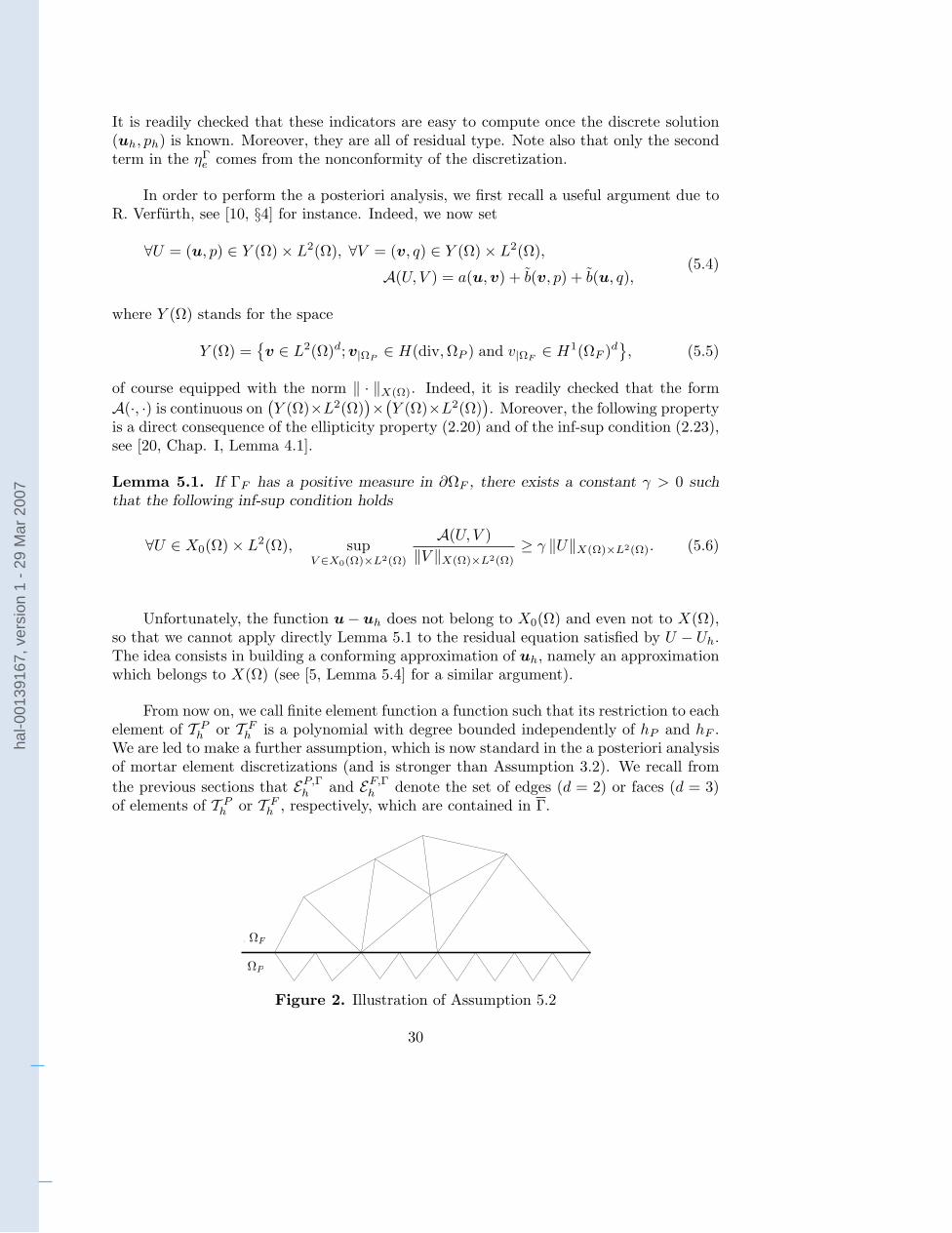
Mortar finite element discretization of a model coupling Darcy and Stokes equations

Mortar finite element discretization

of a model coupling Darcy and Stokes equations

by C. Bernardi1, T. Chacon Rebollo1,2, F. Hecht1 and Z. Mghazli3

Abstract: As a first draft of a model for a river flowing on a homogeneous porous ground,we consider a system where the Darcy and Stokes equations are coupled via appropriatematching conditions on the interface. We propose a discretization of this problem whichcombines the mortar method with standard finite elements, in order to handle separatelythe flow inside and outside the porous medium. We prove a priori and a posteriori errorestimates for the resulting discrete problem. Some numerical experiments confirm theinterest of the discretization.

Resume: Comme premiere esquisse d’un modele de riviere coulant sur un sol poreux ho-mogene, nous considerons un systeme ou les equations de Darcy et de Stokes sont coupleespar des conditions de raccord appropriees sur l’interface. Nous proposons une discretisationde ce probleme qui combine la methode de joints avec des elements finis usuels de facon atraiter separement l’ecoulement a l’interieur et a l’exterieur du milieu poreux. Nous prou-vons des estimations a priori et a posteriori de l’erreur. Quelques experiences numeriquesconfirment l’interet de la discretisation.

1Laboratoire Jacques-Louis Lions, C.N.R.S. & Universite Pierre et Marie Curie,

B.C. 187, 4 place Jussieu, 75252 Paris Cedex 05, France.

e-mail addresses: [email protected], [email protected]

Departamento de Ecuaciones Diferenciales y Analisis Numerico, Universidad de Sevilla,

Tarfia s/n, 41012 Sevilla, Spain.

e-mail address: [email protected]

Equipe d’Ingenierie Mathematique, Departement de Mathematiques et d’Informatique,

Faculte des sciences, Universite Ibn Tofail, B.P. 133, Kenitra, Maroc.

e-mail address: mghazli−[email protected]

hal-0

0139

167,

ver

sion

1 -

29 M

ar 2

007

http://hal.archives-ouvertes.fr/hal-00139167/fr/

http://hal.archives-ouvertes.fr

hal-0

0139

167,

ver

sion

1 -

29 M

ar 2

007

1. Introduction.

We first describe the model we intend to work with. Let Ω be a rectangle in dimensiond = 2 or a rectangular parallelepiped in dimension d = 3. We assume that it is divided(without overlap) into two connected open sets ΩP and ΩF with Lipschitz–continuousboundaries, where the indices P and F stand for porous and fluid, respectively. The fluidthat we consider is viscous and incompressible. So in the porous medium, which is assumedto be rigid and saturated with the fluid, we consider the following equations, due to Darcy,

αu + grad p = f in ΩP ,

div u = 0 in ΩP .(1.1)

In ΩF , the flow of this same fluid is governed by the Stokes equations−ν∆u + grad p = f in ΩF ,

div u = 0 in ΩF .(1.2)

The unknowns both in (1.1) and (1.2) are the velocity u and the pressure p of the fluid. Theparameters ν and α are positive constants, representing the viscosity of the fluid and theratio of this viscosity to the permeability of the medium, respectively. The porous mediumis supposed to be homogeneous, so that we take α constant on the whole subdomain ΩP

(we refer to [1] and [5] for handling the somewhat more realistic case where α is piecewiseconstant in a different framework).

1. Introduction.

We first describe the model we intend to work with. Let ! be a rectangle in dimensiond = 2 or a rectangular parallelepiped in dimension d = 3. We assume that it is divided(without overlap) into two connected open sets !P and !F with Lipschitz–continuousboundaries, where the indices P and F stand for porous and fluid, respectively. The fluidthat we consider is viscous and incompressible. So in the porous medium, which is assumedto be rigid and saturated with the fluid, we consider the following equations, due to Darcy,

!! u + grad p = f in !P ,

div u = 0 in !P .(1.1)

In !F , the flow of this same fluid is governed by the Stokes equations

!!" "u + grad p = f in !F ,

div u = 0 in !F .(1.2)

The unknowns both in (1.1) and (1.2) are the velocity u and the pressure p of the fluid. Theparameters " and ! are positive constants, representing the viscosity of the fluid and theratio of this viscosity to the permeability of the medium, respectively. The porous mediumis supposed to be homogeneous, so that we take ! constant on the whole subdomain !P

(we refer to [1] and [5] for handling the somewhat more realistic case where ! is piecewiseconstant in a di#erent framework).

Figure 1. Basic examples of domain !

Concerning the boundary conditions, as illustrated in Figure 1, we denote by $a theupper edge (d = 2) or face (d = 3) of !, where the index a means in contact with theatmosphere. Let $aP be the intersection $a " #!P and $aF the intersection $a " #!F

(note that $aP can be empty in some practical situations). We set:

$P = (#! " #!P ) \ $aP and $F = (#! " #!F ) \ $aF .

Let n stand for the unit outward normal vector to ! on #! and also to !P on #!P . Weprovide the previous partial di#erential equations (1.1) and (1.2) with the conditions

u · n = k on $P and p = pa on $aP , (1.3)

1

1. Introduction.



div u = 0 in !P .(1.1)


!!" "u + grad p = f in !F ,

div u = 0 in !F .(1.2)






$P = (#! " #!P ) \ $aP and $F = (#! " #!F ) \ $aF .



1

1. Introduction.



div u = 0 in !P .(1.1)


!!" "u + grad p = f in !F ,

div u = 0 in !F .(1.2)






$P = (#! " #!P ) \ $aP and $F = (#! " #!F ) \ $aF .



1

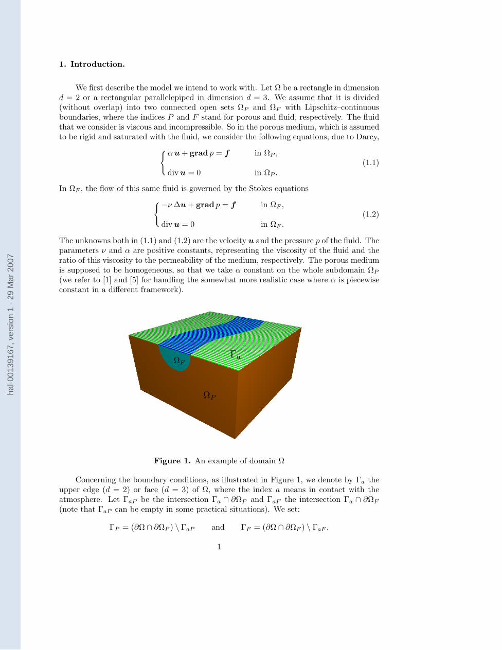
Figure 1. An example of domain Ω

Concerning the boundary conditions, as illustrated in Figure 1, we denote by Γa theupper edge (d = 2) or face (d = 3) of Ω, where the index a means in contact with theatmosphere. Let ΓaP be the intersection Γa ∩ ∂ΩP and ΓaF the intersection Γa ∩ ∂ΩF

(note that ΓaP can be empty in some practical situations). We set:

ΓP = (∂Ω ∩ ∂ΩP ) \ ΓaP and ΓF = (∂Ω ∩ ∂ΩF ) \ ΓaF .

1

hal-0

0139

167,

ver

sion

1 -

29 M

ar 2

007

Let n stand for the unit outward normal vector to Ω on ∂Ω and also to ΩP on ∂ΩP . Weprovide the previous partial differential equations (1.1) and (1.2) with the conditions

u · n = k on ΓP and p = pa on ΓaP , (1.3)

andu = g on ΓF and ν ∂nu− pn = ta on ΓaF . (1.4)

Note that these conditions are of Dirichlet type on ∂Ω \ Γa, while the condition on ΓaP

only means that the pressure, here equal to pa, depends on the atmospheric pressure. Thecondition on ΓaF means that the variations of the free surface at the top of the flow areneglected in the model. Thus ta mainly depends on the atmospheric pressure and thewind on the river. This is standard in geophysics, see e.g. [24, §1.4]; note however that,when the flux

∫ΓF

(g · n)(τ ) dτ +∫ΓPk(τ ) dτ is too large, this boundary condition is not

compatible with the physics of the problem.

To conclude, let Γ denote the interface ∂ΩP ∩ ∂ΩF . On Γ we consider the matchingconditions

u|ΩP· n = u|ΩF

· n and − p|ΩPn = ν ∂nu|ΩF

− p|ΩFn on Γ. (1.5)

Indeed, from a physical point of view, conservation of mass enforces continuity of the nor-mal velocities at the interface. Similarly, conservation of momentum enforces conservationof the normal stresses. Such interface conditions are studied for instance in [23], [17] and[15, §4.5].

System (1.1) − (1.5) is only a first draft of a model for the laminar flow of a riverover a porous rock such as limestone, however it seems that its discretization has notbeen considered before. Of course, in more realistic models, the Stokes equations must bereplaced by the Navier-Stokes equations (for instance when the river meets obstacles) andthe Darcy equations must be replaced by more complex models as proposed in [29] (seealso [4] or [26]). However we are interested with this system. We first write an equivalentvariational formulation of it and prove that it admits a unique solution.

The discretization that we propose relies on the mortar element method, a domaindecomposition technique introduced in [7] (see also [9] for the new trends). Indeed itseems convenient to use a subdomain for the fluid and another one for the porous medium.Moreover, owing to the flexibility of the mortar method, independent meshes can be usedon the different parts of the domain. On each subdomain, we consider a finite elementdiscretization, relying on standard finite elements both for the Stokes problem (the elementfirst introduced in [18] and analyzed in [11]) and the Darcy equations (the Raviart–Thomaselement [30]). Combining these two choices, we construct a discrete problem and we checkthat it has a unique solution. We then prove optimal a priori and a posteriori upper boundsfor the error, despite the lack of conformity of the mortar method.

Thanks to the error indicators issued from the a posteriori analysis, we are in a positionto perform mesh adaptivity independently in the porous and fluid domain. We describethe adaptivity strategy that we use. Next we present numerical experiments. The resultsare in good agreement with the error estimates, so they justify our choice of discretization.

2

hal-0

0139

167,

ver

sion

1 -

29 M

ar 2

007

https://www.researchgate.net/publication/2377462_Coupling_Fluid_Flow_with_Porous_Media_Flow?el=1_x_8&enrichId=rgreq-8582cec155a6e0058d418ce45c9fd6c0-XXX&enrichSource=Y292ZXJQYWdlOzQzMjkzODE5O0FTOjEwMjEyMDQxODE4NTIyNEAxNDAxMzU4ODEzODAy

https://www.researchgate.net/publication/229643218_Old_and_New_Finite_Elements_for_Incompressible_Flows?el=1_x_8&enrichId=rgreq-8582cec155a6e0058d418ce45c9fd6c0-XXX&enrichSource=Y292ZXJQYWdlOzQzMjkzODE5O0FTOjEwMjEyMDQxODE4NTIyNEAxNDAxMzU4ODEzODAy

https://www.researchgate.net/publication/243119752_Analysis_of_Some_Finite_Elements_for_the_Stokes_Problem?el=1_x_8&enrichId=rgreq-8582cec155a6e0058d418ce45c9fd6c0-XXX&enrichSource=Y292ZXJQYWdlOzQzMjkzODE5O0FTOjEwMjEyMDQxODE4NTIyNEAxNDAxMzU4ODEzODAy

https://www.researchgate.net/publication/238555778_Basics_and_some_applications_of_the_mortar_element_method?el=1_x_8&enrichId=rgreq-8582cec155a6e0058d418ce45c9fd6c0-XXX&enrichSource=Y292ZXJQYWdlOzQzMjkzODE5O0FTOjEwMjEyMDQxODE4NTIyNEAxNDAxMzU4ODEzODAy

https://www.researchgate.net/publication/237129496_Boundary_Value_Problems_in_Mechanics_of_Non-Homogeneous_Fluids?el=1_x_8&enrichId=rgreq-8582cec155a6e0058d418ce45c9fd6c0-XXX&enrichSource=Y292ZXJQYWdlOzQzMjkzODE5O0FTOjEwMjEyMDQxODE4NTIyNEAxNDAxMzU4ODEzODAy

https://www.researchgate.net/publication/226715991_A_Mixed_Finite_Element_Method_for_Second_Order_Elliptic_Problems?el=1_x_8&enrichId=rgreq-8582cec155a6e0058d418ce45c9fd6c0-XXX&enrichSource=Y292ZXJQYWdlOzQzMjkzODE5O0FTOjEwMjEyMDQxODE4NTIyNEAxNDAxMzU4ODEzODAy

https://www.researchgate.net/publication/51991990_A_New_Nonconforming_Approach_to_Domain_Decomposition_The_Mortar_Element_Method?el=1_x_8&enrichId=rgreq-8582cec155a6e0058d418ce45c9fd6c0-XXX&enrichSource=Y292ZXJQYWdlOzQzMjkzODE5O0FTOjEwMjEyMDQxODE4NTIyNEAxNDAxMzU4ODEzODAy

The outline of the paper is as follows.• In Section 2, we write the variational formulation of the problem and prove its well-posedness.• Section 3 is devoted to the description of the discrete problem and to the proof of itswell-posedness.• We prove the a priori and a posteriori estimates in Sections 4 and 5, respectively.• The adaptivity strategy and numerical experiments are presented in Section 6.

3

hal-0

0139

167,

ver

sion

1 -

29 M

ar 2

007

2. Analysis of the model.

We first intend to write a variational formulation of system (1.1) − (1.5). From nowon, for each domain O in Rd with a Lipschitz-continuous boundary, we use the full scale ofSobolev spaces Hs(O) and Hs

0(O), s ≥ 0, their trace spaces on ∂O and their dual spaces.We denote by C∞(O) the space of restrictions to O of indefinitely differentiable functionson Rd and by D(O) its subspace made of functions with a compact support in O.

Let also H(div,Ω) denote the space of functions v in L2(Ω)d such that div v belongsto L2(Ω), equipped with the norm

‖v‖H(div,Ω) =(‖v‖2

L2(Ω)d + ‖div v‖2L2(Ω)

) 12. (2.1)

We recall the Stokes formula, valid for smooth enough functions v and q,∫Ω

(div v)(x) q(x) dx +∫

Ω

v(x) · (grad q)(x) dx =∫

∂Ω

(v · n)(τ )q(τ ) dτ .

Since C∞(Ω)d is dense in H(div,Ω) [20, Chap I, Thm 2.4], we derive from this formulathat the normal trace operator: v 7→ v · n is defined and continuous from H(div,Ω) intoH− 1

2 (∂Ω). This leads to define

H0(div,Ω) =

v ∈ H(div; ,Ω); v · n = 0 on ∂Ω. (2.2)

Then D(Ω)d is dense in H0(div,Ω) [20, Chap. I, Thm 2.6], and both H(div,Ω) andH0(div,Ω) are Hilbert spaces for the scalar product associated with the norm defined in(2.1).

Remark 2.1. Let Γ∗ be any part of ∂Ω with positive measure. We refer to [25, Chap. 1,

§11] for the definition of H1200(Γ

∗) as the space of functions in H12 (Γ∗) such that their

extension by zero belongs to H12 (∂Ω). The normal trace on Γ∗ of a function v in H(div,Ω)

makes sense in H1200(Γ

∗)′, owing to the following formula

∀q ∈ H1200(Γ

∗),∫

Γ∗(v · n)(τ )q(τ ) dτ =

∫Ω

(div v)(x) q(x) dx +∫

Ω

v(x) · (grad q)(x) dx,

where q is any lifting in H1(Ω) of the extension by zero of q to ∂Ω (clearly the integralin the left-hand side of the previous equality represents a duality pairing). Note moreover

that H− 12 (Γ∗) is imbedded in H

1200(Γ

∗)′.

We now introduce the variational spaces

X(Ω) =

v ∈ H(div,Ω); v|ΩF∈ H1(ΩF )d

,

X0(Ω) =

v ∈ X(Ω); v · n = 0 on ΓP and v = 0 on ΓF

.

(2.3)

4

hal-0

0139

167,

ver

sion

1 -

29 M

ar 2

007

Both of them are equipped with the norm

‖v‖X(Ω) =(‖v‖2

H(div,ΩP ) + ‖v‖2H1(ΩF )

) 12, (2.4)

and are Hilbert spaces for the corresponding scalar product. We also consider the bilinearforms

a(u,v) = aP (u,v) + aF (u,v),

with aP (u,v) = α

∫ΩP

u(x) · v(x) dx,

aF (u,v) = ν

∫ΩF

(gradu)(x) : (gradv)(x) dx,

b(v, q) = −∫

Ω

(div v)(x)q(x) dx.

(2.5)

It is readily checked that the first three forms are continuous on X(Ω)×X(Ω), while thelast one is continuous on X(Ω)× L2(Ω).

The variational problem that we consider now reads

Find (u, p) in X(Ω)× L2(Ω) such that

u · n = k on ΓP and u = g on ΓF , (2.6)

and that∀v ∈ X0(Ω), a(u,v) + b(v, p) = L(v),

∀q ∈ L2(Ω), b(u, q) = 0,(2.7)

where the linear form L(·) is defined by

L(v) =∫

Ω

f(x) · v(x) dx−∫

ΓaP

(v · n)(τ )pa(τ ) dτ +∫

ΓaF

v(τ ) · ta(τ ) dτ . (2.8)

Note that, in this definition, we have used integrals for the sake of clarity, however theyare most often replaced by duality pairings. Indeed, from now on, we make the followingassumption on the five data

k ∈ H− 12 (ΓP ), g ∈ H 1

2 (ΓF )d, f ∈ X0(Ω)′, pa ∈ H1200(ΓaP ), ta ∈ H− 1

2 (ΓaF )d,(2.9)

where H− 12 (ΓP ) and H− 1

2 (ΓaF ) stand for the dual spaces of H12 (ΓP ) and H

12 (ΓaF ), re-

spectively. With this choice, the boundary conditions (2.6) makes sense (see Remark 2.1)and the form L(·) is continuous on X0(Ω).

Standard arguments lead to the equivalence of problems (1.1)−(1.5) and (2.6)−(2.7).

Proposition 2.2. Any smooth enough pair of functions (u, p) is a solution of problem(2.6)− (2.7) if and only if it is a solution of problem (1.1)− (1.5).

5

hal-0

0139

167,

ver

sion

1 -

29 M

ar 2

007

To prove the well-posedness of problem (2.6)− (2.7), we first construct a lifting of theboundary conditions (2.6).

Lemma 2.3. There exists a divergence-free function ub in X(Ω) which satisfies

ub · n = k on ΓP and ub = g on ΓF , (2.10)

and‖ub‖X(Ω) ≤ c

(‖k‖

H− 12 (ΓP )

+ ‖g‖H

12 (ΓF )d

). (2.11)

Proof: It is performed in three steps.1) Let g be an extension of g into H

12 (∂ΩF ). We introduce a fixed smooth function ϕ

with support in Γ and set

g∗ = g −∫

∂ΩF(g · n)(τ ) dτ∫

Γ(ϕ · n)(τ ) dτ

ϕ.

So the function g∗ belongs to H12 (∂ΩF ) and satisfies∫

∂ΩF

(g∗ · n)(τ ) dτ = 0 and ‖g∗‖H

12 (∂ΩF )d

≤ c ‖g‖H

12 (ΓF )d

.

Thus, the Stokes problem−ν∆ubF + grad pbF = 0 in ΩF ,div ubF = 0 in ΩF ,ubF = g∗ on ∂ΩF ,

(2.12)

has a solution in H1(ΩF ) × L2(ΩF ), which is unique up to an additive constant on thepressure [20, Chap. I, Thm 5.1]. Moreover, thanks to the previous inequality, this solutionsatisfies

‖ubF ‖H1(ΩF )d ≤ c ‖g‖H

12 (ΓF )d

. (2.13)

2) We now denote by Y (ΩP ) the space

Y (ΩP ) =µ ∈ H1(ΩP ); µ = 0 on ΓaP

,

When ΓaP has a positive measure, we consider the problem: Find λ in Y (ΩP ) such that

∀µ ∈ Y (ΩP ),∫

ΩP

(gradλ)(x) · (gradµ)(x)

=∫

ΓP

k(τ )µ(τ ) dτ +∫

Γ

(ubF · n)(τ )µ(τ ) dτ .(2.14)

This problem has a unique solution. Moreover the function ubP = gradλ is divergence-freeon ΩP (as follows by taking µ in D(Ω) in the previous problem) and satisfies

ubP · n = k on ΓP and ubP · n = ubF · n on Γ, (2.15)

6

hal-0

0139

167,

ver

sion

1 -

29 M

ar 2

007

and‖ubP ‖H(div,ΩP ) ≤ c

(‖k‖

H− 12 (ΓP )

+ ‖g‖H

12 (ΓF )d

). (2.16)

3) When ΓaP has a zero measure, it follows from the definition of ΓaP and ΓaF that ΓaF

has a positive measure. Thus, we introduce a further function g∗ in H12 (Γ)d such that∫

Γ

(g∗ · n)(τ ) dτ = −∫

ΓP

k(τ ) dτ ,

and there exists a function g in H12 (∂ΩF ) equal to g on ΓF and to g∗ on Γ (note that this

requires some compatibility conditions between g and g∗ on ΓF ∩ Γ when this last set isnot empty). By adding to g a constant times a fixed smooth function now with supportin ΓaF , we construct a function g∗ in H

12 (∂ΩF ) which satisfies∫

∂ΩF

(g∗ · n)(τ ) dτ = 0.

Then the Stokes problem (2.12) with this modified function g∗ still admits a solution, andthis solution satisfies

‖ubF ‖H1(ΩF )d ≤ c(‖k‖

H− 12 (ΓP )

+ ‖g‖H

12 (ΓF )d

). (2.17)

Next, since the function equal to k on ΓP and to ubF · n = g∗ · n on Γ has a null integralon ∂ΩP , problem (2.14) admits a solution λ, unique up to an additive constant (note thatY (ΩP ) now coincides with H1(ΩP )). The function ubP = gradλ is divergence-free on ΩP

and still satisfies (2.15) and (2.16).To conclude, we observe from either (2.13) or (2.17) and (2.16) that the function ub equalto ubP on ΩP and to ubF on ΩF satisfies all the desired properties.

Remark 2.4. Note that the first assumption in (2.9) could be replaced by the weaker one

k ∈ H1200(ΓP )′,

see Remark 2.1. However, the previous proof does not work with only this assumptionwhen, for instance, ΓP ∩ Γ is not empty, see (2.14). So we do not handle this modifiedassumption since we have no direct application for it.

To go further, we set: u0 = u−ub, where ub is the function exhibited in Lemma 2.3.We observe that problem (2.6)− (2.7) admits a solution if the following problem has one:

Find (u0, p) in X0(Ω)× L2(Ω) such that

∀v ∈ X0(Ω), a(u0,v) + b(v, p) = −a(ub,v) + L(v),

∀q ∈ L2(Ω), b(u0, q) = 0.(2.18)

It is readily checked that the kernel

V (Ω) =v ∈ X0(Ω); ∀q ∈ L2(Ω), b(v, q) = 0

, (2.19)

7

hal-0

0139

167,

ver

sion

1 -

29 M

ar 2

007

coincides with the space of functions in X0(Ω) which are divergence-free on Ω. We firstcheck the ellipticity of the form a(·, ·) on V (Ω).

Lemma 2.5. Assume that(i) either ΓF has a positive measure in ∂ΩF ,(ii) or the normal vector n(x) runs through a basis of Rd when x runs through Γ.There exists a constant α > 0 such that the following ellipticity property holds

∀v ∈ V (Ω), a(v,v) ≥ α ‖v‖2X(Ω). (2.20)

Proof: Let us observe that, for all v in V (Ω),

a(v,v) ≥ minα, ν(‖v‖2

L2(ΩP )d + |v|2H1(ΩF )d

), (2.21)

and‖v‖X(Ω) =

(‖v‖2

L2(ΩP )d + |v|2H1(ΩF )d + ‖v‖2L2(ΩF )d

) 12 . (2.22)

Let now v be a function in V (Ω) such that ‖v‖L2(ΩP )d and |v|H1(ΩF )d are equal to zero.Thus, v is zero on ΩP and is equal to a constant c on ΩF . When assumption (i) holds,it follows from the definition of X0(Ω) that this constant is zero. When assumption (ii)holds, since v is zero on ΩP , c · n is zero on Γ and, since n runs through a basis of Rd, cis zero. Then v is zero on Ω. Thanks to the Peetre–Tartar Lemma [20, Chap. I, Thm 2.1],it follows from this property, (2.22) and the compactness of the imbedding of H1(ΩF ) intoL2(ΩF ) that

∀v ∈ V (Ω),(‖v‖2

L2(ΩP )d + |v|2H1(ΩF )d

) 12 ≥ c ‖v‖X(Ω).

This, combined with (2.21), gives the desired ellipticity property.

Lemma 2.6. There exists a constant β > 0 such that the following inf-sup condition holds

∀q ∈ L2(Ω), supv∈X0(Ω)

b(v, q)‖v‖X(Ω)

≥ β ‖q‖L2(Ω). (2.23)

Proof: Let Ω+ be a rectangle (d = 2) or a rectangular parallelepiped (d = 3) such thatΓ+ = Γa ∩ ∂Ω+ is contained in the interior of Γa and has a positive measure. Then, thefunction q+ defined by

q+ =q on Ω,− 1

meas(Ω+)

∫Ωq(x) dx on Ω+,

belongs to L2(Ω ∪ Ω+) and has a null integral on this domain. It thus follows from thestandard inf-sup condition, see [20, Chap. I, Cor. 2.4], that there exists a function v+ inH1

0 (Ω ∪ Γ+ ∪ Ω+)d such that

div v+ = −q+ and ‖v+‖H1(Ω∪Γ+∪Ω+)d ≤ c ‖q+‖L2(Ω∪Γ+∪Ω+).

8

hal-0

0139

167,

ver

sion

1 -

29 M

ar 2

007

Taking v equal to the restriction of v+ to Ω (which obviously belongs to X0(Ω)) leads tothe desired inf-sup condition.

We are now in a position to prove the main result of this section. Note that, due tothe mixed boundary conditions, no further assumption on the flux of the data is neededfor the existence of a solution.

Theorem 2.7. If the assumptions of Lemma 2.5 hold, for any data (k, g,f , pa, ta) satis-fying (2.9), problem (2.6)− (2.7) has a unique solution (u, p) in X(Ω)×L2(Ω). Moreoverthis solution satisfies

‖u‖X(Ω) + ‖p‖L2(Ω)

≤ c(‖k‖

H− 12 (ΓP )

+ ‖g‖H

12 (ΓF )d

+ ‖f‖X0(Ω)′ + ‖pa‖H

1200(ΓaP )

+ ‖ta‖H− 1

2 (ΓaF )d

).

(2.24)

Proof: It follows from Lemmas 2.5 and 2.6, see [20, Chap. I, Thm 4.1], that problem(2.18) has a unique solution (u0, p) in X0(Ω)× L2(Ω) and that this solution satisfies

‖u0‖X(Ω) +‖p‖L2(Ω) ≤ c(‖ub‖X(Ω) +‖f‖X0(Ω)′ +‖pa‖

H1200(ΓaP )

+‖ta‖H− 1

2 (ΓaF )d

). (2.25)

Then, the pair (u = u0 + ub, p) is a solution of problem (2.6)− (2.7), and estimate (2.24)is a consequence of (2.25) and (2.11). On the other hand, let (u1, p1) and (u2, p2) be twosolutions of problem (2.6)− (2.7). Then, the difference (u1 − u2, p1 − p2) is a solution ofproblem (2.18) with data ub, f , pa and ta equal to zero. Thus, it follows from (2.25) thatit is zero. So the solution of problem (2.6)− (2.7) is unique.

From now on, we assume that the non restrictive assumptions of Lemma 2.5 hold. Weconclude with some regularity properties of the solution (u, p).

Proposition 2.8. Let us assume that the five data satisfy

k ∈ H 12 (ΓP ), g ∈ H 3

2 (ΓF )d, f ∈ H1(Ω)d, pa ∈ H32 (ΓaP ), ta ∈ H

12 (ΓaF )d. (2.26)

Then, the restriction (u|ΩP, p|ΩP

) of the solution (u, p) of problem (2.6) − (2.7) to ΩP

belongs to the space HsP (ΩP )d ×HsP +1(ΩP ) for a real number sP > 0 given by• sP = 1/4 if ΩP is a polygon (d = 2),• sP = 1/2 if ΓaP is empty or if ΩP is a polygon or a polyhedron and there exists a convexneighbourhood in ΩP of (ΓP ∪ Γ) ∩ ΓaP ,• sP < 1 if ΓaP is empty and ΩP is a convex polygon or polyhedron or has a C 1,1-boundary.The restriction (u|ΩF

, p|ΩF) of the solution (u, p) of problem (2.6) − (2.7) to ΩF belongs

to the space HsF +1(ΩF )d ×HsF (ΩF ) for a real number sF > 0 given by• sF = 1/4 if ΩF is a polygon (d = 2),• sF = 1/2 if ΓF is empty or if ΩF is a polygon (d = 2) and there exists a convexneighbourhood in ΩF of (ΓaF ∪ Γ) ∩ ΓF ,• sF < 1 if ΓF is empty and ΩF is a convex polygon or polyhedron or has a C 1,1-boundary.

9

hal-0

0139

167,

ver

sion

1 -

29 M

ar 2

007

Proof: We check successively the two assertions.1) The function p|ΩP

is a solution of the Poisson equation with mixed boundary conditions

−∆p = −div f in ΩP ,p = pa on ΓaP ,∂np = f · n− αk on ΓP ,∂np = f · n− αu|ΩF

· n on Γ.

Moreover, since u|ΩFbelongs to H1(Ω)d, its normal trace u|ΩF

· n belongs to H12 (Γ).

The desired regularity of p|ΩPis easily derived from [21, Thms 2.2.2.3 & 3.2.1.2] or [16,

§3] thanks to appropriate Sobolev imbeddings. The regularity of u|ΩPthen follows from

the first line in (1.1).2) The pair (u|ΩF

, p|ΩF) is a solution of the Stokes problem with mixed boundary conditions

−ν∆u + grad p = f in ΩF ,div u = 0 in ΩF ,u = g on ΓF ,ν ∂nu− pn = ta on ΓaF ,ν ∂nu− pn = −p|ΩP

n on Γ.

It can also be noted from part 1) of the proof that p|ΩPn belongs at least to H

12 (Γ)d. So

the desired results follow from [28].

Assumption (2.26) is too strong for most results of Proposition 2.8, and we only makeit for simplicity. Moreover the norms of (u|ΩP

, p|ΩP) in HsP (ΩP )d × HsP +1(ΩP ) and of

(u|ΩF, p|ΩF

) in HsF +1(ΩF )d×HsF (ΩF ) are bounded as a function of weaker norms of thedata. Note also that compatibility conditions on the data at the intersections of differentparts of the boundaries should be made to obtain higher regularity, i.e. to break therestrictions sP < 1 and sF < 1. Similar results hold in other situations that we do notconsider in this work (for instance, when ΓaF is empty).

10

hal-0

0139

167,

ver

sion

1 -

29 M

ar 2

007

3. The discrete problem and its well-posedness.

The mortar finite element discretization relies on the partition of Ω into ΩP andΩF . Indeed, even if some further partitions could be introduced to handle anisotropicdomains for instance, we do not consider them in this work. Let (T P

h )hPand (T F

h )hFbe

regular families of triangulations of ΩP and ΩF , respectively, by closed triangles (d = 2)or tetrahedra (d = 3), in the usual sense that:• For each hP , ΩP is the union of all elements of T P

h and, for each hF , ΩF is the union ofall elements of T F

h ;• The intersection of two different elements of T P

h , if not empty, is a vertex or a wholeedge or a whole face of both of them, and the same property holds for the intersection oftwo different elements of T F

h ;• The ratio of the diameter hK of any element K of T P

h or of T Fh to the diameter of its

inscribed circle or sphere is smaller than a constant σ independent of hP and hF .As usual, hP stands for the maximum of the diameters of the elements of T P

h and hF forthe maximum of the diameters of the elements of T F

h . From now on, c, c′, . . . stand forgeneric constants that may vary from one line to the next but are always independent ofhP and hF . We make the further standard and non restrictive assumptions.

Assumption 3.1. The intersection of each element K of T Ph with either ΓaP or ΓP or Γ,

if not empty, is a vertex or a whole edge or a whole face of K. The intersection of eachelement K of T F

h with either ΓaF or ΓF or Γ, if not empty, is a vertex or a whole edge ora whole face of K.

It must be noted that, up to now, no assumption is made on the intersection of theelements of T P

h and T Fh . So the K ∩ Γ, K ∈ T P

h , and the K ∩ Γ, K ∈ T Fh , form two

independent triangulations of Γ, that we denote by EP,Γh and EF,Γ

h , respectively. However,we are led to make a third assumption.

Assumption 3.2. For any element K of T Fh , the number of elements K ′ of T P

h such that∂K ∩ ∂K ′ has a positive (d− 1)-measure is bounded independently of K, hP and hF .

We now define the local discrete spaces. As already explained in the introduction, thespace of discrete velocities in ΩP is contructed from the Raviart–Thomas finite element[30], which leads to the following definition

XPh =

vh ∈ H(div,ΩP ); ∀K ∈ T P

h , vh|K ∈ PRT (K), (3.1)

where PRT (K) stands for the space of restrictions to K of polynomials of the form a+ bx,a ∈ Rd and b ∈ R. We also introduce the space

XP0h =

vh ∈ XP

h ; vh · n = 0 on ΓP

. (3.2)

Similarly, on ΩF , we consider the space related to the Bernardi–Raugel element [11], i.e.

XFh =

vh ∈ H1(ΩF )d; ∀K ∈ T F

h , vh|K ∈ PBR(K), (3.3)

where PBR(K) stands for the space spanned by the restrictions to K of affine functions onRd with values in Rd and the d+ 1 normal bubble functions ψe ne (for each edge (d = 2)

11

hal-0

0139

167,

ver

sion

1 -

29 M

ar 2

007



or face (d = 3) e of K, ψe denotes the bubble function on e equal to the product of thebarycentric coordinates associated with the endpoints or vertices of e and ne stands forthe unit outward normal vector on e). We also need the space

XF0h =

vh ∈ XF

h ; vh = 0 on ΓF

. (3.4)

Let now h denote the discretization parameter, here equal to the pair (hP , hF ), andlet Th stand for the union of T P

h and T Fh . We define the discrete space of pressures as

Mh =qh ∈ L2(Ω); ∀K ∈ Th, qh|K ∈ P0(K)

, (3.5)

where P0(K) is the space of constant functions on K.

Remark 3.3. Other choices of finite elements are possible. However, the Raviart-Thomaselement is the simplest div-conforming element and is necessarily associated with piecewiseconstant pressures. So we must keep the same type of pressure finite elements for the Stokespart, and the Bernardi-Raugel element is the less expensive H1-conforming finite elementfor this type of pressures. In dimension d = 2, piecewise quadratic velocities can also beused on ΩF and in dimension d = 3, PBR(K) can be replaced by the space spanned byaffine functions and the ψe, up to the power d.

The skeleton of the decomposition is now the interface Γ. As standard for the mortarelement method, see [7] and [9], the construction of the global space of velocities relieson the fact that the matching conditions are enforced via the orthogonality to functionsdefined on T P

h or T Fh . Since these matching conditions only deal with the normal trace

of the velocity, we have decided to make the choice proposed in [5, §3], which is morenaturally associated with functions defined on T P

h , i.e. we define the space

Wh =ϕh ∈ L2(Γ); ∀e ∈ EP,Γ

h , ϕh|e ∈ P0(e), (3.6)

with obvious definition for P0(e).

The global spaces of velocities are then the spaces Xh and X0h of functions vh suchthat• their restrictions vh|ΩP

to ΩP belong to XPh and XP

0h, respectively,• their restrictions vh|ΩF

to ΩF belong to XFh and XF

0h, respectively,• the following matching conditions hold on Γ

∀ϕh ∈ Wh,

∫Γ

((vh|ΩP

− vh|ΩF) · n

)(τ )ϕh(τ ) dτ = 0, (3.7)

where τ stands for the tangential coordinate(s) on Γ. Note that these conditions arenot sufficient to enforce the continuity of vh · n through Γ, so that the discretization isnonconforming: For instance, Xh is not contained in H(div,Ω). However, the spaces Xh

and X0h are still equipped with the norm ‖ · ‖X(Ω).

To discretize the essential boundary conditions that appear in (2.6), we now definethe approximations of the data k and g that we use in this work. We denote by kh thepiecewise constant approximation of k defined by

∀K ∈ T Ph /meas(K ∩ ΓP ) > 0, kh|K∩ΓP

=1

meas(K ∩ ΓP )

∫K∩ΓP

k(τ ) dτ . (3.8)

12

hal-0

0139

167,

ver

sion

1 -

29 M

ar 2

007



Note that this choice requires that k belongs to H−σ(Ω), σ < 12 . We also introduce an

approximation of g: When assuming that g is continuous on ΓF (which is slightly strongerthan the hypothesis made in (2.9)), the function gh

• belongs to the trace space of XFh ,

• for each K in T Fh , is equal to g(a) at each endpoint or vertex a of K ∩ ΓF ,

• and satisfies ∫K∩ΓF

(gh · n)(τ ) dτ =∫

K∩ΓF

(g · n)(τ ) dτ .

Indeed, these conditions define kh and gh in a unique way, as follows from [30, Remark 3]and [11, Lemma II.1].

We are now in a position to write the discrete problem, which is constructed by theGalerkin method from (2.7). It reads

Find (uh, ph) in Xh ×Mh such that

uh · n = kh on ΓP and uh = gh on ΓF , (3.9)

and that∀vh ∈ X0h, a(uh,vh) + b(vh, ph) = L(vh),

∀qh ∈ Mh, b(uh, qh) = 0,(3.10)

where the bilinear form b(·, ·) is defined by

b(v, q) = −∫

ΩP

(div v|ΩP)(x)q(x) dx−

∫ΩF

(div v|ΩF)(x)q(x) dx. (3.11)

The introduction of this modified form is due to the nonconformity of the discretization,and it is readily checked that it coincides with b(·, ·) on H(div,Ω)× L2(Ω).

As in the continuous case, to prove the well-posedness of problem (3.9) − (3.10), wefirst construct a lifting of the boundary conditions (3.9). It requires the Raviart-Thomasoperator ΠRT

h , see [30, §3] and also [27, §1.3] for its three-dimensional analogue: For anysmooth enough function v on ΩP , ΠRT

h v belongs to XPh and satisfies on all edges (d = 2)

or faces (d = 3) e of elements of T Ph ,∫

e

(ΠRT

h v · n)(τ ) dτ =∫

e

(v · n)(τ ) dτ . (3.12)

The fact that these equations define the operator ΠRT

h in a unique way and its mainproperties are proved in [30, Thm 3] in the two-dimensional case. Moreover, this operatorpreserves the nullity of the normal trace on ΓP (this requires Assumption 3.1). Similarly,we introduce another operator that we call Bernardi–Raugel operator and denote by ΠBR

h :For any continuous function v on ΩF , ΠBR

h v belongs to XFh , is equal to v(a) at any vertex

a of the elements of T Fh and satisfies on all edges (d = 2) or faces (d = 3) e of elements of

T Fh , ∫

e

(ΠBR

h v · n)(τ ) dτ =∫

e

(v · n)(τ ) dτ . (3.13)

13

hal-0

0139

167,

ver

sion

1 -

29 M

ar 2

007

This defines the operator ΠBR

h in a unique way, see [11, Lemma II.1].

We now establish some properties of the operator ΠRT

h . We refer to [19, Appendix]for their proof in the two-dimensional case and for quadrilateral finite elements and to[14, §III.3] for additional results. It requires the Piola transform AK , defined as follows,see [20, Chap. III, form. (4.63)]: For any element K of T P

h , denoting by FK one of theaffine mappings which maps the reference triangle or tetrahedron K onto K and by BK

the Jacobian matrix of FK , we associate with any vector field v defined on K the vectorfield v = AK v defined on K by the formula

(AK v) FK =1

|detBK |BK v. (3.14)

We recall two properties of this transform, valid for all smooth enough functions v and ϕ

(div v) FK =1

|detBK |div (A−1

K v), (3.15)

∫∂K

(v · n)(τ )ϕ(τ ) dτ =∫

∂K

(A−1K v · n)(τ )(ϕ FK)(τ ) dτ , (3.16)

where n and n stand for the unit outward normal vectors to K and K, respectively. Wealso introduce the basis functions associated with the space XP

h : If EPh denotes the set of

edges (d = 2) or faces (d = 3) of elements of T Ph , with each e in EP

h , we associate thefunction ϕe in XP

h such that∫e

(ϕe · n)(τ ) dτ = 1 and ∀e′ ∈ EPh , e

′ 6= e,

∫e′

(ϕe · n)(τ ) dτ = 0. (3.17)

The ϕe, e ∈ EPh , form a basis of XP

h . Moreover, it is readily checked that each ϕe · n ispiecewise constant, equal to 1

meas(e) on e and to zero on all e′ 6= e.

Lemma 3.4. The following property holds for any K in T Ph and any v in H(div,ΩP ),

‖div ΠRT

h v‖L2(K) ≤ ‖div v‖L2(K). (3.18)

The following property holds for any K in T Ph and any v in H(div,ΩP ) ∩ Hs(ΩP )d,

0 < s < 12 ,

‖ΠRT

h v‖L2(K)d ≤ c(‖v‖L2(K)d + hs

K |v|Hs(K)d + hK ‖div v‖L2(K)

). (3.19)

Proof: We check successively the two assertions of the lemma.1) Since the divergence of all functions in XP

h is constant on each element K of T Ph , we

have

‖div ΠRT

h v‖2L2(K) = (div ΠRT

h v)|K∫

K

(div ΠRT

h v)(x) dx

= (div ΠRT

h v)|K∫

∂K

(ΠRT

h v · n)(τ ) dτ .

14

hal-0

0139

167,

ver

sion

1 -

29 M

ar 2

007

It follows from the definition (3.12) of ΠRT

h that

‖div ΠRT

h v‖2L2(K) = (div ΠRT

h v)|K∫

∂K

(v · n)(τ ) dτ =∫

K

(div ΠRT

h v) (div v)(x) dx,

so that using a Cauchy–Schwarz inequality yields (3.18).2) Denoting by EK the set of edges (d = 2) or faces (d = 3) of K, we have from (3.12)

(ΠRT

h v)|K =∑

e∈EK

(∫e

(v · n)(τ ) dτ)ϕe,

so that‖ΠRT

h v‖L2(K)d ≤∑

e∈EK

∣∣ ∫e

(v · n)(τ ) dτ∣∣ ‖ϕe‖L2(K)d . (3.20)

When setting e = F−1K (e), it follows from (3.16) and (3.17) that the function ϕe = A−1

K ϕe

is such that∫e

(ϕe · n)(τ ) dτ = 1 and ∀e′ ∈ EK , e′ 6= e,

∫e′

(ϕe · n)(τ ) dτ = 0,

so that ‖ϕe‖L2(K)d is bounded independently of K. Thus, standard arguments relying on(3.14) give

‖ϕe‖L2(K)d ≤ c h1− d

2K . (3.21)

On the other hand, denoting by χe the function equal to 1 on e and to 0 on ∂K \ e, by χe

the function χe FK and by χe a lifting of χe to K, we have from (3.16)∫e

(v · n)(τ ) dτ =∫

∂K

(A−1K v · n)(τ )χe(τ ) dτ

=∫

K

(A−1K v)(x) · (grad χe)(x) dx +

∫K

(div (A−1

K v))(x) χe(x) dx.

Note however that, since χe only belongs to Hr(∂K) for all r < 12 , (grad χe)(x) only

belongs to Hr− 12 (K) and that the first integral in the second line of the previous equation

must be replaced by a duality pairing. Then, choosing r such that 12 − r = s yields

∣∣ ∫e

(v · n)(τ ) dτ∣∣ ≤ c

(‖A−1

K v‖Hs(K)d + ‖div (A−1K v)‖L2(K)

).

Standard arguments relying on (3.14), (3.15) and the use of intrinsic norm and seminormon Hs(K), see for instance [3, §7.43], give

∣∣ ∫e

(v · n)(τ ) dτ∣∣ ≤ c

(h

d2−1

K ‖v‖L2(K)d + hd2 +s−1

K ‖v‖Hs(K)d + hd2K ‖div v‖L2(K)

). (3.22)

Inserting (3.21) and (3.22) into (3.20) leads to (3.19).

We now briefly prove analogous results for the operator ΠBR

h .

15

hal-0

0139

167,

ver

sion

1 -

29 M

ar 2

007

Lemma 3.5. The following property holds for any real number s0, 0 ≤ s0 ≤ 1, for any Kin T F

h and any v in Hs(ΩF )d, d2 < s ≤ 2,

‖v −ΠBR

h v‖Hs0 (K)d ≤ c hs−s0K ‖v‖Hs(K)d . (3.23)

Proof: Let Ih denote the Lagrange interpolation operator with values in piecewise affinefunctions. It follows from the definition of ΠBR

h that, if EK denotes the set of edges (d = 2)or faces (d = 3) of K,

(ΠBR

h v)|K = (Ihv)|K +∑

e∈EK

∫e

((v − Ihv) · ne

)(τ ) dτ∫

eψe(τ ) dτ

ψe ne.

We recall the usual estimate, for 0 ≤ r0 ≤ 1 and d2 < r ≤ 2,

‖v − Ihv‖Hr0 (K)d ≤ c hr−r0 ‖v‖Hr(K)d . (3.24)

Applying this estimate with r0 = s0 yields

‖v − Ihv‖Hs0 (K)d ≤ c hs−s0K ‖v‖Hs(K)d . (3.25)

On the other hand, we derive from standard arguments that

‖ψe ne‖Hs0 (K)d ≤ c hd2−s0

K ,∣∣ ∫

e

ψe(τ ) dτ∣∣ ≥ c′ hd−1

K .

Combining this with (3.22) and three applications of (3.24) gives for each e in EK∣∣∣∫e

((v − Ihv) · ne

)(τ ) dτ∫

eψe(τ ) dτ

∣∣∣ ‖ψe ne‖Hs0 (K)d ≤ c hs−s0K ‖v‖Hs(K)d .

This inequality and (3.25) yield the desired estimate.

To go further, we need the following result which is a consequence of Assumption 3.2.

Lemma 3.6. For each h, let λh denote the maximal ratio hK/hK′ , where K runs throughT F

h , K ′ runs through T Ph and ∂K ∩ ∂K ′ has a positive (d− 1)-measure. Then, all λh are

smaller that a constant λ independent of h.

Proof: Let K be any element of T Fh which has an edge (d = 2) or a face (d = 3) e

contained in Γ. Assumption 3.2 yields that e is contained in the union of edges or facesei, 1 ≤ i ≤ I, of elements Ki of T P

h , where I is bounded independently of K and h. So,we have

meas(e) ≤I∑

i=1

meas(ei).

On the other hand,• meas(e) is equivalent to hd−1

K and each meas(ei) is equivalent to hd−1Ki

, with equivalenceconstants only depending on the regularity parameter σ,

16

hal-0

0139

167,

ver

sion

1 -

29 M

ar 2

007

• when ei and ej are adjacent, i.e. share a vertex in dimension d = 2 or an edge indimension d = 3, the ratio hKi/hKj is bounded by constants only depending on σ,• for all ei and ej , there exists a path linking ei to ej , only going from an e to an adjacente′ and crossing at most c elements e, where c is bounded as a function of I.Combining all this yields the desired result.

Lemma 3.7. If the data (k, g) belong to HσP (ΓP )×HσF (ΓF )d, σP > − 12 and σF > d−1

2 ,there exists a function ubh in Xh which satisfies

ubh · n = kh on ΓP and ubh = gh on ΓF , (3.26)

and‖ubh‖X(Ω) ≤ c

(‖k‖HσP (ΓP ) + ‖g‖HσF (ΓF )d

). (3.27)

Proof: We use once more the function ub exhibited in Lemma 2.3 and, since it is con-structed from the solutions of problems (2.12) and (2.14), we observe from [21, §7.3.3] or[16, Cor. 3.7], that, since ΩP and ΩF are polygons or polyhedra, there exist real numberssP , 0 < sP < σP + 1

2 , and sF , d2 < sF < σF + 1

2 , such that the pair (ub|ΩP,ub|ΩF

) belongsto HsP (ΩP )d ×HsF (ΩF )d and satisfies

‖ub‖HsP (ΩP )d + ‖ub‖HsF (ΩF )d ≤ c(‖k‖HσP (ΓP ) + ‖g‖HσF (ΓF )d

). (3.28)

The construction of the function ubh is now performed in two steps.1) We first introduce the function w1

h such that

w1h|ΩP

= ΠRT

h ub|ΩP, w1

h|ΩF= ΠBR

h ub|ΩF.

It follows from Lemmas 3.4 and 3.5 that, since ub is divergence-free on ΩP ,

‖w1h‖H(div,ΩP ) + ‖w1

h‖H1(ΩF )d ≤ c(‖ub‖HsP (ΩP )d + ‖ub‖HsF (ΩF )d

). (3.29)

Moreover, owing to the definitions of ΠRT

h and ΠBR

h , the function w1h satisfies the boundary

conditions (3.26).2) Recalling that EP,Γ

h denotes the set of edges (d = 2) or faces (d = 3) of elements of T Ph

which are contained in Γ, we consider the function w2h defined by

w2h|ΩP

=∑

e∈EP,Γh

(∫e

((w1

h|ΩF−w1

h|ΩP) · n

)(τ ) dτ

)ϕe, w2

h|ΩF= 0.

where the functions ϕe are defined in (3.17). We observe from the choice of w2h that the

function ubh = w1h + w2

h satisfies the matching conditions (3.7), hence belongs to Xh.Owing to the properties of the functions ϕe, w2

h · n vanishes on ΓP , so that ubh satisfies(3.26). Moreover, it follows from (3.15) and (3.21) that, if K denotes the triangle of T P

h

that contains e,‖ϕe‖H(div,K) ≤ c h

− d2

K . (3.30)

Next, owing to the definition of w1h, we have∫

e

((w1

h|ΩF−w1

h|ΩP) · n

)(τ ) dτ = −

∫e

((ub −w1

h|ΩF) · n

)(τ ) dτ .

17

hal-0

0139

167,

ver

sion

1 -

29 M

ar 2

007

Applying (3.22) yields

∣∣ ∫e

((ub −w1

h|ΩF) · n

)(τ ) dτ |

≤ c∑

κ

(h

d2−1κ ‖ub −ΠBR

h ub‖L2(κ)d + hd2 +s−1κ ‖ub −ΠBR

h ub‖Hs(κ)d

+ hd2κ ‖ub −ΠBR

h ub‖H1(κ)d

),

where the previous summation is taken on all the κ in T Fh such that e ∩ ∂κ has a positive

measure. We use Lemma 3.5 to bound the norms on the κ. Combining all this with (3.30)yields∣∣ ∫

e

((w1

h|ΩF−w1

h|ΩP) · n

)(τ ) dτ | ‖ϕe‖H(div,K) ≤ c h

− d2

K

∑κ

hd2 +sF−1κ ‖ub‖HsF (κ)d .

Note also that the ratio hd2κ /h

d2K is bounded by λ

d2h , hence by a constant independent of h,

see Lemma 3.6. This gives

‖w2h‖H(div,ΩP ) ≤ c hsF−1

F ‖ub‖HsF (ΩF )d . (3.31)

Finally, estimate (3.27) is derived from (3.28), (3.29) and (3.31).

We prove a further result which is needed in Section 4. It requires the followingparameters.

Notation 3.8. The parameters λP and λF are defined as follows:(i) λP is positive in the general case, equal to 1/4 if ΩP is a polygon (d = 2), equal to 1/2if ΓaP is empty or if there exists a convex neighbourhood in ΩP of (ΓP ∪Γ)∩ΓaP and < 1if ΓaP is empty and ΩP is a convex polygon or polyhedron,(ii) λF is equal to 1

2 in the general case and to 1 if ΩF is convex.

Corollary 3.9. If the assumptions of Lemma 3.7 are satisfied, the following estimateshold between the function ub introduced in Lemma 2.3 and the function ubh introducedin Lemma 3.7

‖ub − ubh‖X(Ω) ≤ c(h

minσP + 12 ,λP

P + hminσF− 1

2 ,λF F

) (‖k‖HσP (ΓP ) + ‖g‖HσF (ΓF )d

),

(3.32)and

supqh∈Mh

b(ubh, qh)‖qh‖L2(Ω)

≤ c hminσF− 1

2 ,λF F

(‖k‖HσP (ΓP ) + ‖g‖HσF (ΓF )d

). (3.33)

Proof: Owing to the regularity properties of problems (2.12) and (2.14), see [21, §7.3.3] or[16, Cor. 3.7], estimate (3.28) holds with sP = minσP + 1

2 , λP and sF = minσF + 12 , λF +

1. With the notation of the previous proof, since both ub and ΠRT

h ub are divergence-freeon ΩP , we have the inequality

‖ub −ubh‖X(Ω) ≤ ‖ub −ΠRT

h ub‖L2(ΩP )d + ‖ub −ΠBR

h ub‖H1(ΩF )d + ‖w2h‖H(div,ΩP ). (3.34)

18

hal-0

0139

167,

ver

sion

1 -

29 M

ar 2

007

The approximation properties of the operator ΠRT

h are easily derived from the fact that itpreserves the constants on each K in T P

h , by applying (3.19) to the function v−cK for anappropriate constant cK and using the approximation properties of this constant. Theyread, for 0 < r ≤ 1,

‖v −ΠRT

h v‖L2(K)d ≤ c hr ‖v‖Hr(K)d . (3.35)

So, using (3.35) to bound the first term in the right-hand side of (3.34), (3.23) to boundthe second term and (3.31) to bound the third term yields (3.32). We also derive from theproperties (3.12) and (3.13) of the operators ΠRT

h and ΠBR

h that, since ub is divergence-freeon Ω, we have for all qh in Mh,

b(w1h, qh) =

∑K∈T P

h∪T F

h

qh|K

∫∂K

(w1h · n)(τ ) dτ =

∑K∈T P

h∪T F

h

qh|K

∫∂K

(ub · n)(τ ) dτ = 0,

so thatb(ubh, qh) = b(w2

h, qh) ≤ ‖w2h‖H(div,ΩP )‖qh‖L2(Ω),

and we derive (3.33) from (3.31).

In analogy with Section 2, we now set: u0h = uh − ubh, where ubh is the functionexhibited in Lemma 3.7. This leads to consider the problem

Find (u0h, ph) in X0h ×Mh such that

∀vh ∈ X0h, a(u0h,vh) + b(vh, ph) = −a(ubh,vh) + L(vh),

∀qh ∈ Mh, b(u0h, qh) = −b(ubh, qh).(3.36)

We also introduce the discrete kernel

Vh =vh ∈ X0h; ∀q ∈ Mh, b(vh, qh) = 0

. (3.37)

It must be noted that the functions in Vh are divergence-free only on ΩP . We now studythe properties of the forms a(·, ·) and b(·, ·) on the discrete spaces.

Lemma 3.10. If ΓF has a positive measure in ∂ΩF , there exists a constant α > 0 suchthat the following ellipticity property holds

∀vh ∈ Vh, a(vh,vh) ≥ α ‖vh‖2X(Ω). (3.38)

Proof: Since functions in Vh are divergence–free on ΩP , properties (2.21) and (2.22) stillhold for all functions vh in Vh. So, we now wish to check that

∀vh ∈ Vh, ‖vh‖L2(ΩF )d ≤ c |vh|H1(ΩF )d .

When ΓF has a positive measure, this inequality is a simple consequence of the Poincare–Friedrichs inequality and of the imbedding of XF

0h into the space of functions in H1(ΩF )vanishing on ΓF .

19

hal-0

0139

167,

ver

sion

1 -

29 M

ar 2

007

Remark 3.11. When ΓF has a zero measure but the normal vector n(x) when x runsthrough Γ runs through a basis of Rd (this is the second possible assumption of Lemma2.5), it is readily checked that any element of Vh such that a(vh,vh) = 0 is equal to zero.Thus, using the equivalence of norms on the finite-dimensional space Vh yields that thereexists a constant αh positive but depending on the triangulations T P

h and T Fh such that

∀vh ∈ Vh, a(vh,vh) ≥ αh ‖vh‖2X(Ω). (3.39)

However the standard arguments to evaluate the dependence of αh with respect to hP andhF seem to fail here. Fortunately, the assumption that ΓF has a positive measure in ∂ΩF

is not restrictive for the applications that we wish to consider.

We now prove the inf-sup condition on b(·, ·). It requires the modified Bernardi-Raugeloperator ΠBR

h defined as follows: if Rh denotes a Clement type regularization operator withvalues in the space of piecewise affine functions which vanish on ΓF (see for instance [8,§IX.3] for a detailed definition of such an operator),

(ΠBR

h v)|K = (Rhv)|K +∑

e∈EK

∫e

((v −Rhv) · ne

)(τ ) dτ∫

eψe(τ ) dτ

ψe ne. (3.40)

Lemma 3.12. There exist two constants h0 > 0 and β > 0 such that, either when bothΓaP and ΓaF have a positive measure or for all h ≤ h0, the following inf-sup conditionholds

∀qh ∈ Mh, supvh∈X0h

b(vh, qh)‖vh‖X(Ω)

≥ β ‖qh‖L2(Ω). (3.41)

We must prove this lemma in the three next situations: When both ΓaP and ΓaF

have a positive measure, when ΓaP has a zero measure and when ΓaF has a zero measure.However, we skip the proof in the third situation since it is less realistic than the secondone (see Figure 1) and the arguments are exactly the same.

Proof: Case where ΓaP and ΓaF have a positive measureIn this situation, it follows from exactly the same arguments as in the proof of Lemma 2.6that, for any function qh in Mh, there exists a function vP in H1(ΩP )d, vanishing on ΓP

and also on Γ such that

div vP = −qh on ΩP and ‖vP ‖H1(ΩP )d ≤ c ‖qh‖L2(ΩP ), (3.42)

and also a function vF in H1(ΩF )d, vanishing on ΓF ∪ Γ such that

div vF = −qh on ΩF and ‖vF ‖H1(ΩF )d ≤ c ‖qh‖L2(ΩF ). (3.43)

We now definevh|ΩP

= ΠRT

h vP , vh|ΩF= ΠBR

h vF .

Only for this proof, we make the further assumption that the operator Rh takes its valuesin the space of piecewise affine functions which also vanish on Γ, so that ΠBR

h vF vanishes

20

hal-0

0139

167,

ver

sion

1 -

29 M

ar 2

007

on ΓF ∪ Γ. On the other hand, it is readily checked that all functions vK in PRT (K) aresuch that vK · n is constant on each edge (d = 2) or face (d = 3) of K, so that ΠRT

h vP · nvanishes on ΓP ∪Γ. These two properties yield that the function vh satisfies that matchingconditions (3.7), hence belongs to X0h. We also have

b(vh, qh) = −∑

K∈T Ph

qh|K∫

∂K

(vh · n)(τ ) dτ −∑

K∈T Fh

qh|K∫

∂K

(vh · n)(τ ) dτ .

So it follows from the definition of the operators ΠRT

h and ΠBR

h that

b(vh, qh) = −∑

K∈T Ph

qh|K∫

∂K

(vP · n)(τ ) dτ −∑

K∈T Fh

qh|K∫

∂K

(vF · n)(τ ) dτ

= −∫

ΩP

(div vP )(x)qh(x) dx−∫

ΩF

(div vF )(x)qh(x) dx.

Combining this with (3.42) and (3.43) yields

b(vh, qh) = ‖qh‖2L2(Ω). (3.44)

We also deduce from Lemma 3.4 that

‖vh‖H(div,ΩP ) ≤ c ‖vP ‖H1(ΩP )d ,

whence, from (3.42),‖vh‖H(div,ΩP ) ≤ c ‖qh‖L2(ΩP ). (3.45)

The same arguments as in the proof of Lemma 3.5, with (3.24) replaced by (see [8, Chap.IX, Th. 3.11])

‖v −Rhv‖Hs0 (K)d ≤ c h1−s0K ‖v‖H1(∆K)d ,

where ∆K is the union of elements κ of T Fh such that K ∩ κ is not empty, lead to

‖vh‖H1(ΩF )d ≤ c ‖vF ‖H1(ΩF )d ,

whence, owing to (3.43),‖vh‖H1(ΩF )d ≤ c ‖qh‖L2(ΩF ). (3.46)

The desired inf-sup condition now follows from (3.44), (3.45) and (3.46).

Proof: Case where ΓaP has a zero measure.Let ϕΓ be a smooth vector field with support contained in the interior of Γ such that∫

Γ

(ϕΓ · n)(τ ) dτ = 1.

We define ϕΓh in the following way: On ΩF , ϕΓh is affine on all elements K of T Fh and is

equal to ϕΓ(a) at all vertices a of these elements that belong to Γ and to zero at all othervertices; on ΩP , we set

ϕΓh|ΩP=

∑e∈EP,Γ

h

(∫e

(ϕΓh|ΩF· n)(τ ) dτ

)ϕe.

21

hal-0

0139

167,

ver

sion

1 -

29 M

ar 2

007

Thus, it is readily checked that ϕΓh belongs to X0h and moreover that, when h is small

enough, ∫Γ

(ϕΓh · n)(τ ) dτ ≥ 12. (3.47)

For a while, we set

bP (v, q) = −∫

ΩP

(div v|ΩP)(x)q(x) dx, bF (v, q)−

∫ΩF

(div v|ΩF)(x)q(x) dx.

Next, we proceed in two steps.1) On ΩP , we use the decomposition

qh|ΩP= qh + qh, with qh =

1meas(ΩP )

∫ΩP

qh(x) dx.

Indeed, there exists a stable function v in H10 (ΩP )d such that −div v = qh; then, the

function vh = ΠRT

h v belongs to XPh ∩H0(div,ΩP ) and satisfies

bP (vh, qh) = ‖qh‖2L2(ΩP ) and ‖vh‖H(div,ΩP ) ≤ c ‖qh‖L2(ΩP ). (3.48)

On the other hand, it is readily checked by integration by parts and also from (3.47) thatthe function

vh = −qh

meas(ΩP )∫Γ(ϕΓh · n)(τ ) dτ

ϕΓh,

satisfiesbP (vh, qh) = ‖qh‖2

L2(ΩP ) and ‖vh‖X(Ω) ≤ c ‖qh‖L2(ΩP ). (3.49)

Thus, applying the Boland and Nicolaides argument, see [12], which relies on the orthog-onality properties

bP (vh, qh) = 0,∫

ΩP

qh(x)qh(x) dx = 0,

gives the existence of a constant µ independent of h such that the function vh|ΩP= vh+µvh

satisfiesbP (vh, qh) ≥ c ‖qh‖2

L2(ΩP ) and ‖vh‖H(div,ΩP ) ≤ c′ ‖qh‖L2(ΩP ). (3.50)

2) It follows from the definition of ϕΓh that (div vh)|ΩFis constant on each element of T F

h .Thus, Lemma 2.6 yields the existence of a function v in H1(ΩF )d, vanishing on ΓF ∪ Γ,such that −div v is equal to qh + div (µvh) and applying the modified Bernardi-Raugeloperator ΠBR

h defined in (3.40) to it yields that the function vh|ΩF= ΠBR

h v +µvh satisfies

bF (vh, qh) = ‖qh‖2L2(ΩF ) and ‖vh‖H1(ΩF )d ≤ c

(‖qh‖L2(ΩF ) + ‖vh‖X(Ω)

). (3.51)

To conclude, we observe that the function vh belongs to X0h. The desired inf-sup conditionis then derived from (3.50), (3.51) and (3.49).

From now on, we assume that h is small enough for the inf-sup condition (3.41) tohold. Indeed, this condition which is only needed when ΓaP or ΓaF has a zero measure is

22

hal-0

0139

167,

ver

sion

1 -

29 M

ar 2

007

https://www.researchgate.net/publication/253178890_Stability_of_Finite_Elements_under_Divergence_Constraints?el=1_x_8&enrichId=rgreq-8582cec155a6e0058d418ce45c9fd6c0-XXX&enrichSource=Y292ZXJQYWdlOzQzMjkzODE5O0FTOjEwMjEyMDQxODE4NTIyNEAxNDAxMzU4ODEzODAy

not at all restrictive. Owing to the previous lemmas, we are now in a position to provethe main result of this section.

Theorem 3.13. Assume that ΓF has a positive measure in ∂ΩF . Then, for any data(k, g,f , pa, ta) satisfying

k ∈ HσP (ΓP ), g ∈ HσF (ΓF )d, f ∈ L2(Ω)d, pa ∈ H1200(ΓaP ), ta ∈ H− 1

2 (ΓaF )d,(3.52)

for some real numbers σP > − 12 and σF > d−1

2 , problem (3.9) − (3.10) has a uniquesolution (uh, ph) in Xh ×Mh. Moreover this solution satisfies

‖uh‖X(Ω) + ‖ph‖L2(Ω) ≤ c(‖k‖HσP (ΓP ) + ‖g‖HσF (ΓF )d + ‖f‖L2(Ω)d

+ ‖pa‖H

1200(ΓaP )

+ ‖ta‖H− 1

2 (ΓaF )d

).

(3.53)

Proof: We check separately the existence and the uniqueness.1) Let ubh denote the function exhibited in Lemma 3.7. It follows from the ellipticityproperty (3.38) and the inf-sup condition (3.41), see [20, Chap. I, Thm 4.1], that problem(3.36) has a unique solution (u0h, ph) in X0h ×Mh which moreover satisfies

‖u0h‖X(Ω) + ‖ph‖L2(Ω) ≤ c(‖ubh‖X(Ω) + ‖f‖L2(Ω)d + ‖pa‖

H1200(ΓaP )

+ ‖ta‖H− 1

2 (ΓaF )d

).

(3.54)Then, the pair (uh = u0h + ubh, ph) is a solution of problem (3.9)− (3.10), and estimate(3.53) is a direct consequence of (3.27) and (3.54).2) If all data (k, g,f , pa, ta) are equal to zero, (uh, ph) is a solution of problem (3.36) withthe right-hand sides of the two equations equal to zero. Thus, it follows from (3.38) and(3.41) that it is equal to zero. So, the solution of problem (3.9)− (3.10) is unique.

Remark 3.14. The regularity assumptions that are made on the data f in Theorem3.13 can easily be weakened: It suffices to enforce that f|ΩP

belongs to the dual space offunctions on H(div,ΩP ) with zero normal traces on ΓP and f|ΩF

belongs to the dual spaceof functions on H1(ΩF )d vanishing on ΓF . However we have no direct application for thisweaker regularity.

23

hal-0

0139

167,

ver

sion

1 -

29 M

ar 2

007

4. A priori error estimates.

We intend to prove an error estimate between the solution (u, p) of problem (2.6) −(2.7) and the solution (uh, ph) of problem (3.9)− (3.10). The main difficulty here is thatapplying the interpolation operator Ih or the operator ΠBR

h to the solution u|ΩF(in order

to recover the boundary condition gh of the discrete problem) would require that u|ΩFis

continuous on ΩF . In view of Proposition 2.8, this assumption is not likely, at least indimension d = 3. So we prefer to follow another approach, based on the triangle inequality

‖u− uh‖X(Ω) ≤ ‖ub − ubh‖X(Ω) + ‖u0 − u0h‖X(Ω), (4.1)

where the functions ub and ubh are introduced in Lemmas 2.3 and 3.7, respectively.

An estimate for the quantity ‖ub−ubh‖X(Ω) is established in Corollary 3.9. So we arenow interested in proving the following version of the second Strang’s lemma for problems(2.18) and (3.36), the main difficulty being due to the nonconformity of the mortar elementdiscretization.

Lemma 4.1. Assume that ΓF has a positive measure in ∂ΩF . The following estimateholds between the solution (u0, p) of problem (2.18) and the solution (u0h, ph) of problem(3.36)

‖u0 − u0h‖X(Ω) ≤ c(

infwh∈Vh

‖u0 −wh‖X(Ω) + infrh∈Mh

‖p− rh‖L2(Ω)

+ ‖ub − ubh‖X(Ω) + supqh∈Mh


+ supvh∈X0h

∫Γ

((vh|ΩP

− vh|ΩF) · n

)(τ ) p|ΩP

(τ ) dτ‖vh‖X(Ω)

).

(4.2)

Proof: It is divided in three steps.1) Owing to the inf-sup condition (3.41), there exists [20, Chap. I, Lemma 4.1] a functionuh in X0h such that

∀qh ∈ Mh, b(uh, qh) = b(u0h, qh),

and, by using the second line of (3.36),

‖uh‖X(Ω) ≤ β−1 supqh∈Mh


. (4.3)

Then, the function u0h = u0h − uh belongs to Vh and satisfies

∀vh ∈ Vh, a(u0h,vh) = −a(ubh,vh)− a(uh,vh) + L(vh). (4.4)

2) When multiplying the first lines of (1.1) and (1.2) by a function vh of Vh, integratingby parts and summing the two resulting equations, we obtain

a(u,vh) + b(vh, p) = L(vh)−∫

Γ

((vh|ΩP

− vh|ΩF) · n

)(τ ) p|ΩP

(τ ) dτ .

24

hal-0

0139

167,

ver

sion

1 -

29 M

ar 2

007

This last equation can be written equivalently as

∀vh ∈ Vh, a(u0,vh) + b(vh, p) = −a(ub,vh) + L(vh)

−∫

Γ

((vh|ΩP

− vh|ΩF) · n

)(τ ) p|ΩP

(τ ) dτ .(4.5)

3) Let now wh and rh be any elements of Vh and Mh, respectively. It follows from (4.4)and (4.5) that

∀vh ∈ Vh, a(u0h −wh,vh) = a(u0 −wh,vh) + a(ub − ubh,vh)− a(uh,vh)

+ b(vh, p− rh) +∫

Γ

((vh|ΩP

− vh|ΩF) · n

)(τ ) p|ΩP

(τ ) dτ .

Since u0h−wh belongs to Vh, we now use the ellipticity property (3.38) of the form a(·, ·)on Vh. When combined with several Cauchy–Schwarz inequalities, this yields

‖u0h −wh‖X(Ω) ≤ c(‖u0 −wh‖X(Ω) + ‖ub − ubh‖X(Ω) + ‖uh‖X(Ω)

+ ‖p− rh‖L2(Ω) + supvh∈X0h

∫Γ

((vh|ΩP

− vh|ΩF) · n

)(τ ) p|ΩP


).

Combining this with (4.3) and using a further triangle inequality lead to (4.2).

In the right-hand side of (4.2), the first two terms represent the approximation error.The next two ones are issued from the treatment of the Dirichlet boundary conditions.The last term represents the consistency error and is due to the nonconformity of thediscretization.

Lemma 4.2. If the assumptions of Lemma 4.1 are satisfied, the following estimate holdsbetween the solution (u0, p) of problem (2.18) and the solution (u0h, ph) of problem (3.36)

‖p− ph‖L2(Ω) ≤ c(

infwh∈Vh

‖u0 −wh‖X(Ω) + infrh∈Mh

‖p− rh‖L2(Ω)

+ ‖ub − ubh‖X(Ω) + supqh∈Mh


+ supvh∈X0h

∫Γ

((vh|ΩP

− vh|ΩF) · n

)(τ ) p|ΩP


).

(4.6)

Proof: The same arguments as in the previous proof yield, for any function rh in Mh,

∀vh ∈ X0h, b(vh, ph − rh) = a(u0 − u0h,vh) + a(ub − ubh,vh)

+ b(vh, p− rh) +∫

Γ

((vh|ΩP

− vh|ΩF) · n

)(τ ) p|ΩP

(τ ) dτ .

So the desired estimate follows from the inf-sup condition (3.41) combined with severalCauchy–Schwarz inequalities, estimate (4.2) and a further triangle inequality.

25

hal-0

0139

167,

ver

sion

1 -

29 M

ar 2

007

We now evaluate the approximation errors. The distance of the pressure to the spaceMh is bounded in a completely standard way, see [8, Chap. IX, Th. 2.1] for instance: Ifp|ΩP

belongs to H1(ΩP ) (which is always true, see Proposition 2.8) and p|ΩFbelongs to

HsF (ΩF ), 0 ≤ sF ≤ 1,

infrh∈Mh

‖p− rh‖L2(Ω) ≤ c(hP ‖p‖H1(ΩP ) + hsF

F ‖p‖HsF (ΩF )

). (4.7)

To estimate the distance of u to Vh, we first use an argument due to [20, Chap. II,form. (1.16)]: Since u0 belongs to V (Ω), it follows from the inf-sup condition (3.41) that

infwh∈Vh

‖u0 −wh‖X(Ω) ≤ c infwh∈X0h

‖u0 −wh‖X(Ω). (4.8)

Lemma 4.3. The following estimate holds for any function u0 in V (Ω) such that u0|ΩP

belongs to HsP (ΩP )d, 0 < sP ≤ 1, and u0|ΩFbelongs to HsF +1(ΩF )d, 0 ≤ sF ≤ 1,

infwh∈X0h

‖u0 −wh‖X(Ω) ≤ c(hsP

P ‖u0‖HsP (ΩP )d + hsF

F ‖u0‖HsF +1(ΩF )d

). (4.9)

.

Proof: The construction of the function wh is performed in two steps.1) We first set

w]h|ΩP

= ΠRT

h u0, w]h|ΩF

= Rhu0,

where the Clement regularization operator Rh is introduced in Section 3, see (3.40). Sinceboth u0 and w]

h are divergence-free on ΩP , we have

‖u0 −w]h‖H(div,ΩP ) = ‖u0 −w]

h‖L2(ΩP )d .

Then, relying on the fact that ΠRT

h preserves the constants on each K in T Ph and combining

(3.19) with the approximation properties of this constant leads to

‖u0 −w]h‖H(div,ΩP ) ≤ c hsP

P ‖u0‖HsP (ΩP )d . (4.10)

On the other hand, we derive from the approximation properties of the operator Rh, see[8, Chap. IX, Th. 3.11], that

‖u0 −w]h‖H1(ΩF )d ≤ c hsF

F ‖u0‖HsF +1(ΩF )d . (4.11)

2) For the functions ϕe introduced in (3.17), we now set

w[h|ΩP

=∑

e∈EP,Γh

(∫e

((w]

h|ΩF−w]

h|ΩP) · n

)(τ ) dτ

)ϕe, w[

h|ΩF= 0.

The arguments for evaluating ‖w[h‖X(Ω) are nearly the same as in the proof of Lemma 3.7:

Combining (3.30) with (3.12) and a Cauchy-Schwarz inequality yields

‖w[h‖X(Ω) ≤ c

( ∑e∈EP,Γ

h

h−1e ‖u0 −w]

h|ΩF‖2

L2(e)

) 12 .

26

hal-0

0139

167,

ver

sion

1 -

29 M

ar 2

007

We refer to [8, Chap. IX, Cor. 3.12] for the following result: on each element e′ of EF,Γh ,

‖u0 −Rhu0‖L2(e′) ≤ c hsF + 1

2e′ ‖u0‖HsF +1(∆e′ )

d ,

where ∆e′ is the union of elements κ of T Fh such that e′ ∩ κ is not empty. Using this

estimate for all e′ such that e ∩ e′ has a positive measure leads to, owing to Lemma 3.6,

‖w[h‖X(Ω) ≤ c hsF

F ‖u0‖HsF +1(ΩF )d . (4.12)

To conclude, we note that the function wh = w]h + w[

h belongs to X0h. Estimate (4.9) isthen derived from (4.10), (4.11) and (4.12).

Estimating the consistency error requires the orthogonal projection operator fromL2(Γ) onto Wh, that we denote by πΓ

h .

Lemma 4.4. The following estimate holds for any function p in L2(Ω) such that p|ΩP

belongs to HsP +1(ΩP ), 0 ≤ sP ≤ 12 ,

supvh∈X0h

∫Γ

((vh|ΩP

− vh|ΩF) · n

)(τ ) p|ΩP


≤ c hsP +1P ‖p‖HsP +1(ΩP ). (4.13)

.

Proof: It follows from the matching conditions (3.7) that, for each e in EP,Γh ,∫

Γ

((vh|ΩP

−vh|ΩF) · n

)(τ ) p|ΩP

(τ ) dτ =∫

Γ

((vh|ΩP

−vh|ΩF) · n

)(τ ) (p|ΩP

−πΓhp|ΩP

)(τ ) dτ .

Moreover, since the normal trace of vh|ΩPon Γ belongs to Wh for any vh in X0h, this gives∫

Γ

((vh|ΩP

− vh|ΩF) · n

)(τ ) p|ΩP

(τ ) dτ = −∫

Γ

(vh|ΩF

· n)(τ ) (p|ΩP

− πΓhp|ΩP

)(τ ) dτ .

This yields

∫Γ

((vh|ΩP

− vh|ΩF) · n

)(τ ) p|ΩP


≤‖vh|ΩF

‖H

12 (Γ)d

‖p|ΩP− πΓ

hp|ΩP‖

H− 12 (Γ)

‖vh‖X(Ω),

whence, by applying the trace theorem on Γ,∫Γ

((vh|ΩP

− vh|ΩF) · n

)(τ ) p|ΩP


≤ c ‖p|ΩP− πΓ

hp|ΩP‖

H− 12 (Γ)

.

The standard duality argument

‖p|ΩP− πΓ

hp|ΩP‖

H− 12 (Γ)

= supϕ∈H

12 (Γ)

∫Γ(p|ΩP

− πΓhp|ΩP

)(τ )(ϕ− πΓhϕ)(τ ) dτ

‖ϕ‖H

12 (Γ)

,

27

hal-0

0139

167,

ver

sion

1 -

29 M

ar 2

007

combined with the approximation properties of the operator πΓh , see [8, Chap. IX, Th.

2.1], leads to‖p|ΩP

− πΓhp|ΩP

‖H− 1

2 (Γ)≤ c hsP +1

P ‖p|ΩP‖

HsP + 12 (Γ)

,

whence the desired result.

The five terms in the right-hand side of (4.2) and (4.6) are bounded in (4.8) andLemma 4.3, (4.7), Corollary 3.9 and Lemma 4.4, respectively. When combining this with(4.1) and using once more Corollary 3.9, we derive the a priori error estimate. We recallthat the parameters λP and λF have been introduced in Notation 3.8.

Theorem 4.5. Assume that ΓF has a positive measure in ∂ΩF and moreover that(i) the data (k, g) belong to HσP (ΓP )×HσF (ΓF )d, σP > − 1

2 and σF > d−12 ,

(ii) the solution (u0, , p) of problem (2.18) is such that (u0|ΩP, p|ΩP

) belongs toHsP (ΩP )d×H1(ΩP ), 0 < sP ≤ 1, and (u0|ΩF

, p|ΩF) belongs to HsF +1(ΩF )d ×HsF (ΩF ), 0 ≤ sF ≤ 1.

Then the following a priori error estimate holds between the solution (u, p) of problem(2.6)− (2.7) and the solution (uh, ph) of problem (3.9)− (3.10)

‖u− uh‖X(Ω) + ‖p− ph‖L2(Ω)

≤ c(hsP

P

(‖u0‖HsP (ΩP )d + ‖p‖H1(ΩP )

)+ hsF

F

(‖u0‖HsF +1(ΩF )d + ‖p‖HsF (ΩF )

)+

(h

minσP + 12 ,λP

P + hminσF− 1

2 ,λF F

) (‖k‖HσP (ΓP ) + ‖g‖HσF (ΓF )d

)).

(4.14)

The statement of Theorem 4.5 is rather complex. Note anyhow that:• In the case of zero boundary conditions k and g, estimate (4.14) can be written moresimply as

‖u− uh‖X(Ω) + ‖p− ph‖L2(Ω)

≤ c(hsP

P

(‖u‖HsP (ΩP )d + ‖p‖H1(ΩP )

)+ hsF

F

(‖u‖HsF +1(ΩF )d + ‖p‖HsF (ΩF )

)).

(4.15)

This last estimate is fully optimal: Indeed, for a smooth solution (u, p), the error behaveslike hP + hF .• In the general case, the order of convergence depends on the parameters λP and λF . Sothe order 1 is only obtained when ΓaP is empty and both ΩP and ΩF are convex, for smoothdata and solutions. When the regularity of (u, p) is unknown, the order of convergence isgiven by Proposition 2.8 and, for instance, is always larger than 1/4 in dimension d = 2.Moreover, a different analysis (relying on the construction of an approximation of u in Xh

satisfiying the boundary conditions (3.9), which requires the continuity of u|ΩF), yields

that, there also, for a smooth solution (u, p), the error behaves like hP + hF .

To conclude, it can be observed that, in all cases and for smooth enough data (k, g),the convergence of the discretization results from Theorem 4.5.

28

hal-0

0139

167,

ver

sion

1 -

29 M

ar 2

007

5. A posteriori error estimates.

Some further notation are needed to define the error indicators. For each K in T Ph ,

we denote• by EK the set of edges (d = 2) or faces (d = 3) of K which are not contained in ∂ΩP ,• by EaP

K the set of edges (d = 2) or faces (d = 3) of K which are contained in ΓaP .For each K in T F

h , we denote• by EK the set of edges (d = 2) or faces (d = 3) of K which are not contained in ∂ΩF ,• by EaF

K the set of edges (d = 2) or faces (d = 3) of K which are contained in ΓaF .For each e in any of the EK and also in EP,Γ

h , we agree to denote by [·]e the jump throughe (making its sign precise is not necessary). We also denote by he the length (d = 2) ordiameter (d = 3) of e.

We need a further notation for some global sets:• EaP

h is the set of edges or faces of elements of T Ph which are contained in ΓaP ,

• EPh is the set of all other edges or faces of elements of T P

h .

With each element K of T Fh and each edge e of K, we associate the quantities γK and

γe equal to 1 if K or e, respectively, intersects Γ \ ΓF and to zero otherwise.

We introduce the space Zh of functions in L2(Ω)d such that their restrictions to eachK in T P

h or in T Fh is constant. Similarly, we denote by ZF

h the space of functions inL2(ΓaF )d such that their restriction to each e in EaF

K , K ∈ T Fh , is constant. Indeed, we

consider an approximation fh of f in Zh and an approximation tah of ta in ZFh . Finally,

assuming that the datum pa is continuous on ΓaP , we define pah as the function which isaffine on each e in EaP

K , K ∈ T Ph , and equal to pa(a) at all endpoints (d = 2) or vertices

(d = 3) a of these e.

We consider three families of error indicators, related to the error on ΩP , ΩF and Γ,respectively.• For each K in T P

h , the error indicator ηPK is defined by

ηPK = ‖fh − αuh‖L2(K)d +

∑e∈EK

h− 1

2e ‖[ph]e‖L2(e) +

∑e∈EaP

K

h− 1

2e ‖pah − ph‖L2(e). (5.1)

• For each K in T Fh , the error indicator ηF

K is defined by

ηFK = h1−γK

K ‖fh + ν∆uh‖L2(K)d +∑

e∈EK

h12−γee ‖[ν ∂nuh − ph n]e‖L2(e)d

+∑

e∈EaFK

h12−γee ‖tah − ν ∂nuh + ph n‖L2(e)d + ‖div uh‖L2(K).

(5.2)

• For each e in EP,Γh , the error indicator ηΓ

e is defined by

ηΓe = ‖(ph n)|ΩP

+ (ν ∂nuh − ph n)|ΩF‖L2(e)d + h

− 12

e ‖[uh · n]e‖L2(e). (5.3)

29

hal-0

0139

167,

ver

sion

1 -

29 M

ar 2

007

It is readily checked that these indicators are easy to compute once the discrete solution(uh, ph) is known. Moreover, they are all of residual type. Note also that only the secondterm in the ηΓ

e comes from the nonconformity of the discretization.

In order to perform the a posteriori analysis, we first recall a useful argument due toR. Verfurth, see [10, §4] for instance. Indeed, we now set

∀U = (u, p) ∈ Y (Ω)× L2(Ω), ∀V = (v, q) ∈ Y (Ω)× L2(Ω),

A(U, V ) = a(u,v) + b(v, p) + b(u, q),(5.4)

where Y (Ω) stands for the space

Y (Ω) =v ∈ L2(Ω)d;v|ΩP

∈ H(div,ΩP ) and v|ΩF∈ H1(ΩF )d

, (5.5)

of course equipped with the norm ‖ · ‖X(Ω). Indeed, it is readily checked that the formA(·, ·) is continuous on

(Y (Ω)×L2(Ω)

)×

(Y (Ω)×L2(Ω)

). Moreover, the following property

is a direct consequence of the ellipticity property (2.20) and of the inf-sup condition (2.23),see [20, Chap. I, Lemma 4.1].

Lemma 5.1. If ΓF has a positive measure in ∂ΩF , there exists a constant γ > 0 suchthat the following inf-sup condition holds

∀U ∈ X0(Ω)× L2(Ω), supV ∈X0(Ω)×L2(Ω)

A(U, V )‖V ‖X(Ω)×L2(Ω)

≥ γ ‖U‖X(Ω)×L2(Ω). (5.6)

Unfortunately, the function u− uh does not belong to X0(Ω) and even not to X(Ω),so that we cannot apply directly Lemma 5.1 to the residual equation satisfied by U − Uh.The idea consists in building a conforming approximation of uh, namely an approximationwhich belongs to X(Ω) (see [5, Lemma 5.4] for a similar argument).

From now on, we call finite element function a function such that its restriction to eachelement of T P

h or T Fh is a polynomial with degree bounded independently of hP and hF .

We are led to make a further assumption, which is now standard in the a posteriori analysisof mortar element discretizations (and is stronger than Assumption 3.2). We recall fromthe previous sections that EP,Γ

h and EF,Γh denote the set of edges (d = 2) or faces (d = 3)

of elements of T Ph or T F

h , respectively, which are contained in Γ.

1. Introduction.



div u = 0 in !P .(1.1)


!!" "u + grad p = f in !F ,

div u = 0 in !F .(1.2)






$P = (#! " #!P ) \ $aP and $F = (#! " #!F ) \ $aF .



1

1. Introduction.



div u = 0 in !P .(1.1)


!!" "u + grad p = f in !F ,

div u = 0 in !F .(1.2)






$P = (#! " #!P ) \ $aP and $F = (#! " #!F ) \ $aF .



1

Figure 2. Illustration of Assumption 5.2

30

hal-0

0139

167,

ver

sion

1 -

29 M

ar 2

007

https://www.researchgate.net/publication/250693064_Mortar_finite_element_discretization_for_the_flow_in_a_nonhomogeneous_porous_medium?el=1_x_8&enrichId=rgreq-8582cec155a6e0058d418ce45c9fd6c0-XXX&enrichSource=Y292ZXJQYWdlOzQzMjkzODE5O0FTOjEwMjEyMDQxODE4NTIyNEAxNDAxMzU4ODEzODAy


Assumption 5.2. Each element e of EF,Γh is the union of a finite number of elements of

EP,Γh , where “finite” means bounded independently of hP and hF .

Lemma 5.3. If Assumption 5.2 holds, there exists a finite element function u∗h in X(Ω),still satisfying the boundary conditions (3.9), such that

‖uh − u∗h‖X(Ω) ≤ c( ∑e∈EP,Γ

h

h−1e ‖[uh · n]e‖2

L2(e)

) 12 . (5.7)

Proof: It follows from Assumption 5.2 that each e in EF,Γh is the union of edges ei of EP,Γ

h

1 ≤ i ≤ Ie, where Ie is bounded independently of hP and hF (see Figure 2). We denoteby ne the unit normal vector on e, directed from ΩP to ΩF . Let Ki be the element of T P

h

such that ei is an edge of Ki, let bi denote the vertex of Ki which does not belong to ei.Thus, it can be checked that the function ϕei

introduced in (3.17) (with obvious notation)is equal to x−bi

d meas(Ki)on Ki and to zero elsewhere. Its normal trace on ei is constant, equal

to 1meas(ei)

. On the other hand, it must be observed that• on each e in EF.Γ

h which is an edge or a face of K, uh|e is the trace of a function inPBR(K), which we denote by ue

h for a while,• on each edge ei, uh|ΩP

is equal to αi ϕeifor a constant αi.

Next, we setwei = Rei(u

eh · ne) meas(ei)− αi,

where Reiis a lifting operator from polynomials on ei onto polynomials on Ki, constructed

by affine transformation from a fixed lifting operator on a reference triangle, and we define

u∗h = uh +∑

e∈EF,Γh

Ie∑i=1

weiϕei

.

Since u∗h coincides with uh in ΩF , the function u∗h−uh has its support contained in ΩP ∪Γ.Moreover, since the normal trace of ϕei

vanishes on all edges of triangles or all faces oftetrahedra Ki that are not contained in Γ, u∗h−uh belongs to H(div,ΩP ) and u∗h satisfiesthe boundary conditions (3.9). Finally, the jump of u∗h · ne on each e in EP,Γ

h is equal tozero, so that u∗h belongs to X(Ω).In order to prove a bound for ‖uh − u∗h‖H(div,ΩP ), we write

‖weiϕei

‖H(div,Ki) ≤ ‖wei‖H1(Ki)‖ϕei

‖L∞(Ki)d + ‖wei‖L2(Ki)‖div ϕei

‖L∞(Ki).

Next, we use the estimates

‖ϕei‖L∞(Ki)d ≤ c h1−dei

, ‖div ϕei‖L∞(Ki) ≤ c h−dei,

and, noting that its trace of weion ei is equal to [uh · n]e meas(ei), we obtain by switching

to the reference triangle

‖wei‖H1(Ki) + h−1

ei‖wei

‖L2(Ki) ≤ hd−1− 1

2ei ‖[uh · n]e‖L2(ei).

31

hal-0

0139

167,

ver

sion

1 -

29 M

ar 2

007

Combining all this yields

‖weiϕei

‖H(div,Ki) ≤ c h− 1

2ei ‖[uh · n]e‖L2(ei).

Summing the square of this estimate on the Ki gives (5.7).

For a different reason, mainly due to the lack of regularity of the normal trace of func-tions in H(div,ΩP ), we also need an approximation p∗h of ph in H1(ΩP ). The constructionof such a function is standard, see [2, Thm 4.7]. Therefore, we only give an abridged proofof the following lemma.

Lemma 5.4. There exists a finite element function p∗h equal to ph on ΩF and to pah onΓaP , such that p∗h|ΩP

belongs to H1(ΩP ) and satisfies

‖ph − p∗h‖L2(ΩP ) ≤ c( ∑e∈EP

h

he ‖[ph]e‖2L2(e) +

∑e∈EaP

h

he ‖ph − pah‖2L2(e)

) 12 ,

|p∗h|H1(ΩP ) ≤ c( ∑e∈EP

h

h−1e ‖[ph]e‖2

L2(e) +∑

e∈EaPh

h−1e ‖ph − pah‖2

L2(e)

) 12 ,

(5.8)

and

‖ph − p∗h‖L2(Γ) ≤ c( ∑e∈EP

h

‖[ph]e‖2L2(e) +

∑e∈EaP

h

‖ph − pah‖2L2(e)

) 12 . (5.9)

Proof: Let VPh denote the set of all vertices of the elements of T P

h . We define p∗h|ΩPas

the function which is affine on each element K of T Ph , equal to

• to pah(a) at all vertices a in VPh which belong to ΓaP ,

• and, at all other vertices a in VPh , to the mean value of the ph|K(a) on all elements K

of T Ph which contain a.

This leads to the construction p∗h satisfying the properties stated in the lemma. Estimates(5.8) and (5.9) are derived by exactly the same arguments as in [2, Thm 4.7], see also [5,Lemma 5.4].

Finally, with any function v in X0(Ω), we associate the function vh equal to Rhv onΩF and to zero on ΩP , where Rh stands for the modified Clement operator with values inpiecewise affine functions which vanish on ΓF ∪ Γ. The main interest of this vh is that itbelongs to X0(Ω). The next lemma is derived by using the local approximation propertiesof the operator Rh see [8, Chap. IX, §3].

Lemma 5.5. For any function v in X0(Ω), there exists a funtion vh in X0h ∩X0(Ω), withsupport in ΩF , such that, for all K in T F

h and all edges or faces e of K,

h−(1−γK)K ‖v − vh‖L2(K)d + h

−( 12−γe)

e ‖v − vh‖L2(e)d ≤ c ‖v‖H1(∆K), (5.10)

where ∆K is the union of the elements of T Fh that intersects K.

32

hal-0

0139

167,

ver

sion

1 -

29 M

ar 2

007

Setting U = (u, p), Uh = (uh, ph) and U∗h = (u∗h, p

∗h), we observe that the function

U − U∗h now belongs to X(Ω)× L2(Ω). Moreover, it satisfies

(u− u∗h) · n = k − kh on ΓP and uh − u∗h = g − gh on ΓF .

Thus, applying Lemma 2.3 yields the existence of a divergence-free function eb in X(Ω)such that u− u∗h − eb belongs to X0(Ω) and which satisfies

‖eb‖X(Ω) ≤ c(‖k − kh‖

H− 12 (ΓP )

+ ‖g − gh‖H

12 (ΓF )d

). (5.11)

When setting Eb = (eb, 0), we observe that the function U − U∗h − Eb now belongs tp

X0(Ω)× L2(Ω).

Next, we write, for any V = (v, q) in X0(Ω)× L2(Ω),

A(U − U∗h − Eb, V ) = a(uh − u∗h − eb,v) + b(uh − u∗h, q)

+ a(u− uh,v) + b(v, p− p∗h) + b(u− uh, q).

Denoting by vh the approximation of v exhibited in Lemma 5.5 and setting Vh = (vh, 0),we observe from problems (2.6)− (2.7) and (3.9)− (3.10) (note that b(vh, ph − p∗h) is zerosince the intersection of the supports of vh and ph − p∗h is empty) that we can subtract Vh

from the second line in this equation. Thus, we derive by integration by parts the followingresidual equation

A(U − U∗h − Eb, V ) = a(uh − u∗h − eb,v) + b(uh − u∗h, q)

+ 〈RP , V − Vh〉+ 〈RF , V − Vh〉+ 〈RΓ, V − Vh〉+ 〈F , V − Vh〉,(5.12)

where the four quantities RP , RF , RΓ and F are given by

〈RP , V 〉 =∑

K∈T Ph

(∫K

(fh − αuh)(x) · v(x) dx−∫

K

v(x) · (grad p∗h)(x) dx), (5.13)

〈RF , V 〉 =∑

K∈T Ph

(∫K

(fh + ν∆uh)(x) · v(x) dx

+12

∑e∈EK

∫e

v(τ ) · [ν ∂nuh − ph n]e(τ ) dτ

+∑

e∈EaFK

∫e

v(τ ) · (tah − ν ∂nuh + ph n)(τ ) dτ +∫

K

(div uh)(x)q(x) dx),

(5.14)

〈RΓ, V 〉 =∑

e∈EP,ΓK

(∫e

v(τ ) ·((ph n)|ΩP

+ (ν ∂nuh − ph n)|ΩF

)(τ ) dτ

+∫

Γ

(v · n)(τ )(p∗h|ΩP

− ph|ΩP

)(τ ) dτ

),

(5.15)

33

hal-0

0139

167,

ver

sion

1 -

29 M

ar 2

007

〈F , V 〉 =∫

Ω

(f − fh)(x) · v(x) dx−∫

ΓaP

(v · n)(τ )(pa − pah)(τ ) dτ

+∫

ΓaF

v(τ ) · (ta − tah)(τ ) dτ .(5.16)

We can now apply Lemma 5.1 to the function U −U∗h −Eb, which leads to the main result

of this section.

Finally, we denote by EaFh the set of edges or faces of elements of T F

h which arecontained in ΓaF .

Theorem 5.6. Assume that ΓF has a positive measure in ∂ΩF , that Assumption 5.2 issatisfied and that the datum pa is continuous on ΓaP . Then the following a posteriorierror estimate holds between the solution (u, p) of problem (2.6)− (2.7) and the solution(uh, ph) of problem (3.9)− (3.10)

‖u− uh‖X(Ω) + ‖p− ph‖L2(Ω) ≤ c( ∑

K∈T Ph

(ηPK)2 +

∑K∈T F

h

(ηFK)2 +

∑e∈EP,Γ

h

(ηΓe )2

) 12

+ c′(‖k − kh‖

H− 12 (ΓP )

+ ‖g − gh‖H

12 (ΓF )d

+ ‖f − fh‖L2(ΩP )d +( ∑K∈T F

h

h2K ‖f − fh‖2

L2(K)

) 12

+ ‖pa − pah‖H

1200(ΓaP )

+( ∑e∈EaF

h

h1−2γee ‖ta − tah‖2

L2(e)d

) 12).

(5.17)

Proof: Applying Lemma 5.1 to U − U∗h − Eb and using equation (5.12) with a further

triangle inequality, we are led to bound the quantities

‖uh − u∗h‖X(Ω), ‖ph − p∗h‖L2(Ω), ‖eb‖X(Ω),

which follows from (5.7), the first part of (5.8) and (5.11), and the sum

supV ∈X0(Ω)×L2(Ω)

〈RP , V − Vh〉+ 〈RF , V − Vh〉+ 〈RΓ, V − Vh〉+ 〈F , V − Vh〉‖V ‖X(Ω)×L2(Ω)

.

This is obtained by combining Cauchy-Schwarz inequalities with Lemmas 5.4 and 5.5.

To go further, we intend to prove an upper bound for each indicator ηPK , ηF

K and ηΓe .

To do this, we write the residual equation (5.12) in a simpler (and more usual) form: Fora smooth enough pair V = (v, q),

A(U − Uh, V ) = 〈R∗P , V 〉+ 〈RF , V 〉+ 〈R∗

Γ, V 〉+ 〈F , V 〉, (5.18)

where the new quantities R∗P and R∗

Γ are defined by

〈R∗P , V 〉 =

∑K∈T P

h

(∫K

(fh − αuh)(x) · v(x) dx +12

∑e∈EK

∫e

v(τ ) · n [ph]e(τ ) dτ

+∑

e∈EaPK

∫e

v(τ ) · n (ph − pah)(τ ) dτ),

(5.19)

34

hal-0

0139

167,

ver

sion

1 -

29 M

ar 2

007

〈R∗Γ, V 〉 =

∑e∈EP,Γ

K

∫e

v(τ ) ·((ph n)|ΩP


)(τ ) dτ . (5.20)

However the quantity 〈R∗P , V 〉 is not defined for all V in X0(Ω) since it requires a little

more regularity.

Proving the upper bounds for the ηPK is rather standard, it relies on the following

choices of the function V = (v, 0) in (5.18):• Taking v equal to (fh − αuh)ψK on K and to zero elsewhere, where ψK denotes thebubble function on K equal to the product of the barycentric coordinates associated withthe vertices of K;• If the edge e in EK belongs to another triangle K ′, taking v equal to Re([ph]e)ψe onK∪K ′ and to zero elsewhere. Here ψe denotes the bubble function on e and Re is the liftingoperator introduced in the proof of Lemma 5.3 and constructed by affine transformationfrom a fixed lifting operator on a reference triangle;• Finally, for each e in EaP

K , taking v equal to Re(ph−pah)ψe on K and to zero elsewhere.Note that the next estimate is not optimal. However this seems due to the choice of thediscretization: Indeed, the same lack of optimality appears in [13] for the Darcy’s equationsonly and in [6, Prop. 5.4] for another type of coupling Darcy and Stokes problems.

Proposition 5.7. The following estimate holds for each error indicator ηPK defined in

(5.1), K ∈ T Ph ,

ηPK ≤ c

(‖u− uh‖H(div,ωK) + h−1

K ‖p− ph‖L2(ωK)

+ ‖f − fh‖L2(ωK)d + h− 1

2K ‖pa − pah‖L2(K∩ΓaP )

),

(5.21)

where ωK denotes the union of the elements of T Ph that share at least an edge (d = 2) or

a face (d = 3) with K.

Bounding the ηFK relies again on the residual equation (5.18). The arguments are

exactly the same as in [10, Prop. 6] for instance, up to the multiplication by h−γK

K andh−γe

e . So we skip the proof.

Proposition 5.8. The following estimate holds for each error indicator ηFK defined in

(5.2), K ∈ T Fh ,

ηFK ≤ c h−γK

K

(‖u− uh‖H1(ωK)d + ‖p− ph‖L2(ωK)

+ hK ‖f − fh‖L2(ωK)d + h12K‖ta − tah‖L2(K∩ΓaF )d

),

(5.22)

where ωK denotes the union of the elements of T Fh that share at least an edge (d = 2) or

a face (d = 3) with K.

Proving upper bounds for the ηΓe requires a further argument.

Proposition 5.9. The following estimate holds for each error indicator ηΓe defined in

(5.3), e ∈ EP,Γh ,

ηΓe ≤ c

(h−1

e ‖u− uh‖X(ωe) + h− 1

2e ‖p− ph‖L2(ωe) + h

12e ‖f − fh‖L2(ωe)d

), (5.23)

35

hal-0

0139

167,

ver

sion

1 -

29 M

ar 2

007

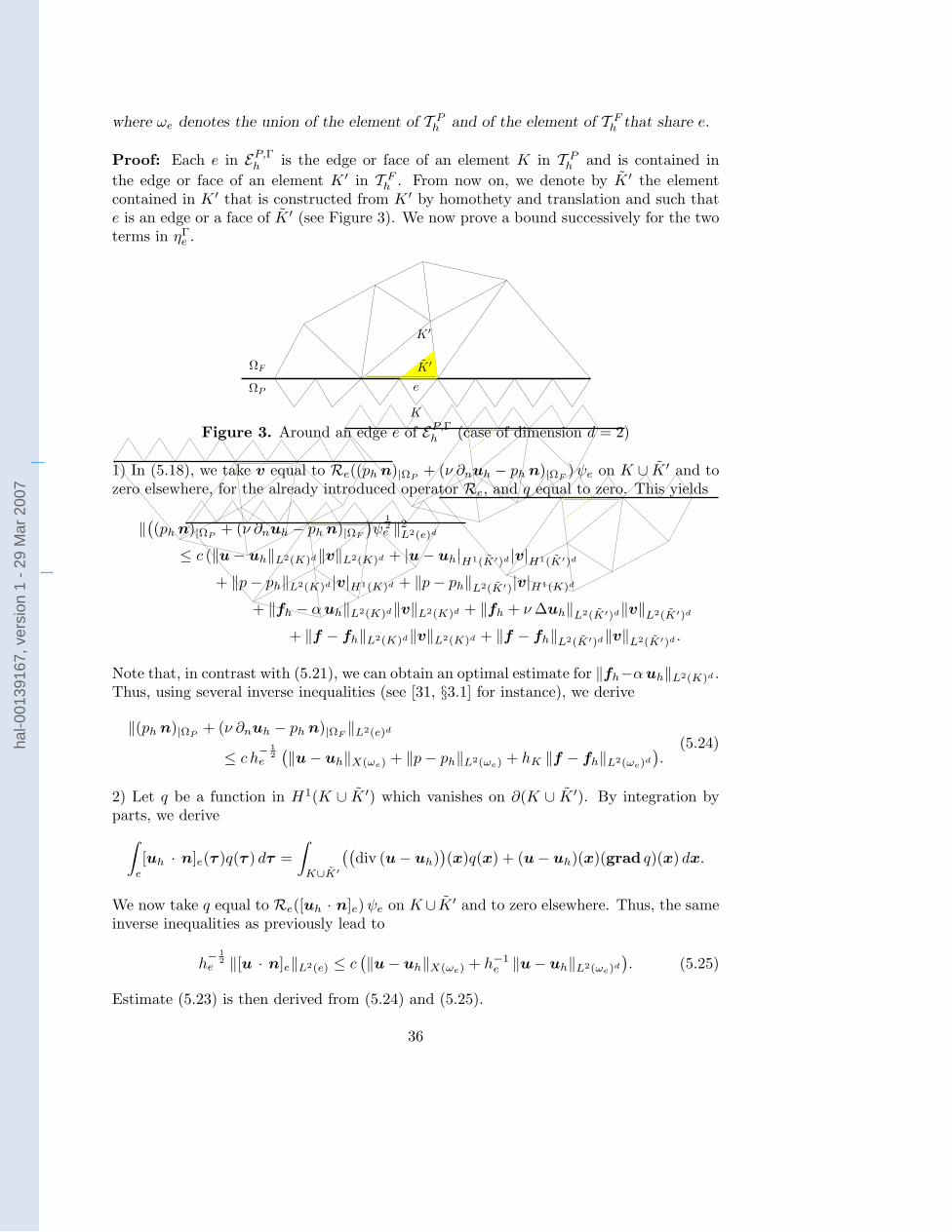
https://www.researchgate.net/publication/266977010_A_Posteriori_Error_Estimators_for_the_Raviart-Thomas_Element?el=1_x_8&enrichId=rgreq-8582cec155a6e0058d418ce45c9fd6c0-XXX&enrichSource=Y292ZXJQYWdlOzQzMjkzODE5O0FTOjEwMjEyMDQxODE4NTIyNEAxNDAxMzU4ODEzODAy

where ωe denotes the union of the element of T Ph and of the element of T F

h that share e.

Proof: Each e in EP,Γh is the edge or face of an element K in T P

h and is contained inthe edge or face of an element K ′ in T F

h . From now on, we denote by K ′ the elementcontained in K ′ that is constructed from K ′ by homothety and translation and such thate is an edge or a face of K ′ (see Figure 3). We now prove a bound successively for the twoterms in ηΓ

e .1. Introduction.



div u = 0 in !P .(1.1)


!!" "u + grad p = f in !F ,

div u = 0 in !F .(1.2)






$P = (#! " #!P ) \ $aP and $F = (#! " #!F ) \ $aF .



1

1. Introduction.



div u = 0 in !P .(1.1)


!!" "u + grad p = f in !F ,

div u = 0 in !F .(1.2)






$P = (#! " #!P ) \ $aP and $F = (#! " #!F ) \ $aF .



1

where !e denotes the union of the element of T Ph and of the element of T F

h that share e.

Proof: Each e in EP,!h is the edge or face of an element K in T P

h and is contained inthe edge or face of an element K ! in T F

h . From now on, we denote by K ! the elementcontained in K ! that is constructed from K ! by homothety and translation and such thate is an edge or a face of K ! (see Figure 3). We now prove a bound successively for the twoterms in "!

e .

K

K !

K ! e!e !+

m

!+m

1

Figure 3. Around an edge e of EP,!h (case of dimension d = 2)

1) In (5.18), we take v equal to Re((ph n)|"P+ (# $nuh ! ph n)|"F

) %e on K " K ! and tozero elsewhere, for the already introduced operator Re, and q equal to zero. This yields

#!(ph n)|"P

+ (# $nuh ! ph n)|"F

"%

12e #2L2(e)d

$ c (#u! uh#L2(K)d#v#L2(K)d + |u! uh|H1(K!)d |v|H1(K!)d

+ #p! ph#L2(K)d |v|H1(K)d + #p! ph#L2(K!)|v|H1(K)d

+ #fh ! & uh#L2(K)d#v#L2(K)d + #fh + # !uh#L2(K!)d#v#L2(K!)d

+ #f ! fh#L2(K)d#v#L2(K)d + #f ! fh#L2(K!)d#v#L2(K!)d .

Note that, in contrast with (5.21), we can obtain an optimal estimate for #fh!& uh#L2(K)d .Thus, using several inverse inequalities (see [30, §3.1] for instance, we derive

#(ph n)|"P+ (# $nuh ! ph n)|"F

#L2(e)d

$ c h" 1

2e

!#u! uh#X(!e) + #p! ph#L2(!e) + hK #f ! fh#L2(!e)d

".

(5.24)

2) Let q be a function in H1(K " K !) which vanishes on $(K " K !). By integration byparts, we derive

#

e[uh · n]e(! )q(! ) d! =

#

K#K!

!!div (u! uh)

"(x)q(x) + (u! uh)(x)(grad q)(x) dx.

We now take q equal to Re([uh · n]e) %e on K " K ! and to zero elsewhere. Thus, the sameinverse inequalities as previously lead to

h" 1

2e #[u · n]e#L2(e) $ c

!#u! uh#X(!e) + h"1

e #u! uh#L2(!e)d

". (5.25)

Estimate (5.23) is then derived from (5.24) and (5.25).

35


h that share e.




e .

K

K !

K ! e!e !+

m

!+m

1




#!(ph n)|"P

+ (# $nuh ! ph n)|"F

"%

12e #2L2(e)d






#(ph n)|"P+ (# $nuh ! ph n)|"F

#L2(e)d

$ c h" 1

2e


".

(5.24)


#

e[uh · n]e(! )q(! ) d! =

#

K#K!

!!div (u! uh)



h" 1

2e #[u · n]e#L2(e) $ c

!#u! uh#X(!e) + h"1

e #u! uh#L2(!e)d

". (5.25)


35


h that share e.




e .

K

K !

K ! e!e !+

m

!+m

1




#!(ph n)|"P

+ (# $nuh ! ph n)|"F

"%

12e #2L2(e)d






#(ph n)|"P+ (# $nuh ! ph n)|"F

#L2(e)d

$ c h" 1

2e


".

(5.24)


#

e[uh · n]e(! )q(! ) d! =

#

K#K!

!!div (u! uh)



h" 1

2e #[u · n]e#L2(e) $ c

!#u! uh#X(!e) + h"1

e #u! uh#L2(!e)d

". (5.25)


35


h that share e.




e .

K

K !

K ! e!e !+

m

!+m

1




#!(ph n)|"P

+ (# $nuh ! ph n)|"F

"%

12e #2L2(e)d






#(ph n)|"P+ (# $nuh ! ph n)|"F

#L2(e)d

$ c h" 1

2e


".

(5.24)


#

e[uh · n]e(! )q(! ) d! =

#

K#K!

!!div (u! uh)



h" 1

2e #[u · n]e#L2(e) $ c

!#u! uh#X(!e) + h"1

e #u! uh#L2(!e)d

". (5.25)


35

Figure 3. Around an edge e of EP,Γh (case of dimension d = 2)

1) In (5.18), we take v equal to Re((ph n)|ΩP+ (ν ∂nuh − ph n)|ΩF

)ψe on K ∪ K ′ and tozero elsewhere, for the already introduced operator Re, and q equal to zero. This yields

‖((ph n)|ΩP


)ψ

12e ‖2

L2(e)d

≤ c (‖u− uh‖L2(K)d‖v‖L2(K)d + |u− uh|H1(K′)d |v|H1(K′)d

+ ‖p− ph‖L2(K)d |v|H1(K)d + ‖p− ph‖L2(K′)|v|H1(K)d

+ ‖fh − αuh‖L2(K)d‖v‖L2(K)d + ‖fh + ν∆uh‖L2(K′)d‖v‖L2(K′)d

+ ‖f − fh‖L2(K)d‖v‖L2(K)d + ‖f − fh‖L2(K′)d‖v‖L2(K′)d .

Note that, in contrast with (5.21), we can obtain an optimal estimate for ‖fh−αuh‖L2(K)d .Thus, using several inverse inequalities (see [31, §3.1] for instance), we derive

‖(ph n)|ΩP+ (ν ∂nuh − ph n)|ΩF

‖L2(e)d

≤ c h− 1

2e

(‖u− uh‖X(ωe) + ‖p− ph‖L2(ωe) + hK ‖f − fh‖L2(ωe)d

).

(5.24)

2) Let q be a function in H1(K ∪ K ′) which vanishes on ∂(K ∪ K ′). By integration byparts, we derive∫

e

[uh · n]e(τ )q(τ ) dτ =∫

K∪K′

((div (u− uh)

)(x)q(x) + (u− uh)(x)(grad q)(x) dx.

We now take q equal to Re([uh · n]e)ψe on K ∪ K ′ and to zero elsewhere. Thus, the sameinverse inequalities as previously lead to

h− 1

2e ‖[u · n]e‖L2(e) ≤ c

(‖u− uh‖X(ωe) + h−1

e ‖u− uh‖L2(ωe)d

). (5.25)


36

hal-0

0139

167,

ver

sion

1 -

29 M

ar 2

007



There also, estimate (5.23) is not optimal. This seems due to the lack of homogeneitywhen coupling Darcy and Stokes equations. Indeed, the jump [u · n] on Γ is the sum of a

function in H1200(Γ)′ and of a function in H

12 (Γ).

To conclude, we observe that estimate (5.17) is optimal: Up to the terms involvingthe data, the full error is bounded by a constant times the Hilbertian sum of all indicators.Estimates (5.21), (5.22) and (5.23) are local, i.e., only involve the error in a neighbourhoodof K or e, and estimate (5.22) is optimal for all elements K that does not intersect Γ. Soit can be hoped that the error indicators ηP

K , ηFK and ηΓ

e provide a good tool for meshadaptivity.

37

hal-0

0139

167,

ver

sion

1 -

29 M

ar 2

007

6. The adaptivity strategy and some numerical experiments.

As standard, the adaptivity strategy that we use combines two steps, an initializationstep and an adaptation step. We fix a positive tolerance η∗ and present it in dimensiond = 2 for simplicity.

Initialization step. We fix a triangulation T P (0)h of ΩP and a triangulation T F (0)

h ofΩF which satisfy Assumptions 3.1 and 5.2 and such that the sum of the errors on the fivedata which appear in Theorem 5.6, namely

‖k − kh‖H− 1

2 (ΓP )+ ‖g − gh‖

H12 (ΓF )d

+ ‖f − fh‖L2(ΩP )d +( ∑K∈T F

h

h2K ‖f − fh‖2

L2(K)

) 12

+ ‖pa − pah‖H

1200(ΓaP )

+( ∑e∈EaF

h

h1−2γee ‖ta − tah‖2

L2(e)d

) 12 ,

is smaller than η∗. This last condition is possible for smooth data thanks to the approxi-mation properties of the finite element spaces involved in the discretization, and we haveno applications for non smooth data.

Adaptation step. Assuming that the triangulations T P (n)h and T F (n)

h are known, wecompute the discrete solution of problem (3.9) − (3.10) corresponding to these triangula-tions, and the error indicators ηP

K , ηFK and ηΓ

e defined in (5.1), (5.2) and (5.3). We denoteby ηP , ηF and ηΓ the mean values of the ηP

K , ηFK and ηΓ

e , respectively, times 0.9. Next, weperform adaptivity in three substeps, of course taking into account Assumption 3.1 in allof them:• All e in EP,Γ(n)

h (wih obvious notation) such that ηΓe is larger than maxη∗, ηΓ are di-

vided into N equal segments, where N is proportional to the ratio ηΓe /maxη∗, ηΓ. This

gives rise to a new set EP,Γ(n+1)h .

• The triangulation T F (n)h is refined and coarsened according to the next criterion: The

diameter of a new element contained in K or containing K is proportional to hK timesthe ratio ηF /ηF

K . This gives rise to the new triangulation T F (n+1)h .

• First, the elements of EP,Γ(n+1)h are divided where needed in order that Assumption 5.2

holds (this can be omitted when Assumption 5.2 does not seem necessary). Second, a newtriangulation on ΩP is constructed such that these new edges are edges of the elements ofthe new triangulation. Next, adaptivity is performed exactly as in the previous substep,now depending on the ratios ηP /ηP

K . This gives rise to the new triangulation T P (n+1)h .

Of course, the adaptation step is iterated either a finite number of times or until theHilbertian sum of all error indicators, namely( ∑

K∈T Ph

(ηPK)2 +

∑K∈T F

h

(ηFK)2 +

∑e∈EP,Γ

h

(ηΓe )2

) 12,

become smaller than η∗ (this is not always possible).

38

hal-0

0139

167,

ver

sion

1 -

29 M

ar 2

007

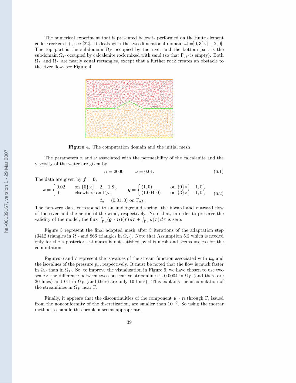
The numerical experiment that is presented below is performed on the finite elementcode FreeFem++, see [22]. It deals with the two-dimensional domain Ω =]0, 3[×] − 2, 0[.The top part is the subdomain ΩF occupied by the river and the bottom part is thesubdomain ΩP occupied by calcalenite rock mixed with sand (so that ΓaP is empty). BothΩP and ΩF are nearly equal rectangles, except that a further rock creates an obstacle tothe river flow, see Figure 4.

Figure 4. The computation domain and the initial mesh

The parameters α and ν associated with the permeability of the calcalenite and theviscosity of the water are given by

α = 2000, ν = 0.01. (6.1)

The data are given by f = 0,

k =

0.02 on 0×]− 2,−1.8[,0 elsewhere on ΓP ,

g =

(1, 0) on 0×]− 1, 0[,(1.004, 0) on 3×]− 1, 0[,

ta = (0.01, 0) on ΓaF .

(6.2)

The non-zero data correspond to an underground spring, the inward and outward flowof the river and the action of the wind, respectively. Note that, in order to preserve thevalidity of the model, the flux

∫ΓF

(g · n)(τ ) dτ +∫ΓPk(τ ) dτ is zero.

Figure 5 represent the final adapted mesh after 5 iterations of the adaptation step(3412 triangles in ΩP and 866 triangles in ΩF ). Note that Assumption 5.2 which is neededonly for the a posteriori estimates is not satisfied by this mesh and seems useless for thecomputation.

Figures 6 and 7 represent the isovalues of the stream function associated with uh andthe isovalues of the pressure ph, respectively. It must be noted that the flow is much fasterin ΩF than in ΩP . So, to improve the visualization in Figure 6, we have chosen to use twoscales: the difference between two consecutive streamlines is 0.0004 in ΩP (and there are20 lines) and 0.1 in ΩF (and there are only 10 lines). This explains the accumulation ofthe streamlines in ΩP near Γ.

Finally, it appears that the discontinuities of the component u · n through Γ, issuedfrom the nonconformity of the discretization, are smaller than 10−6. So using the mortarmethod to handle this problem seems appropriate.

39

hal-0

0139

167,

ver

sion

1 -

29 M

ar 2

007

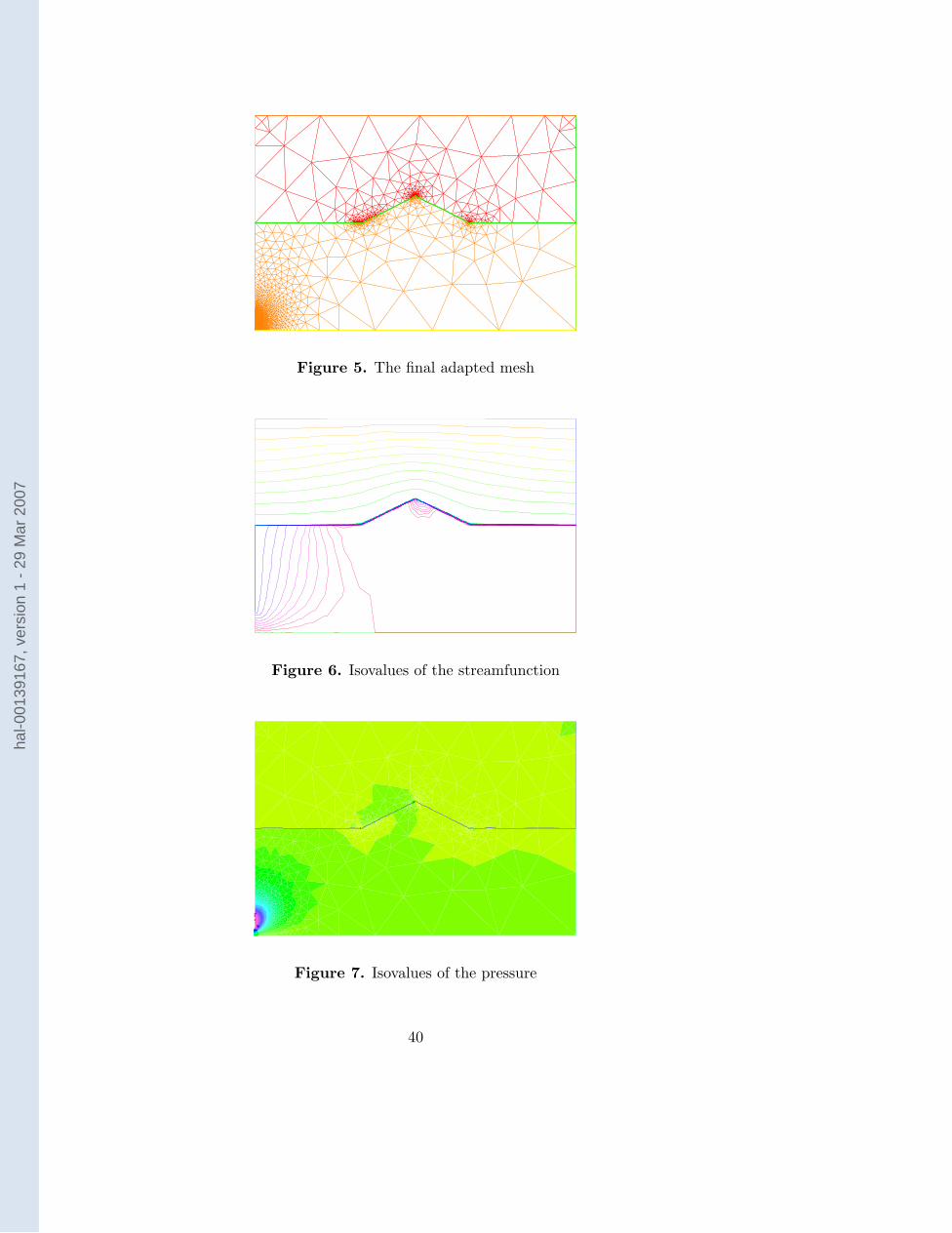
Figure 5. The final adapted mesh

Figure 6. Isovalues of the streamfunction

Figure 7. Isovalues of the pressure

40

hal-0

0139

167,

ver

sion

1 -

29 M

ar 2

007

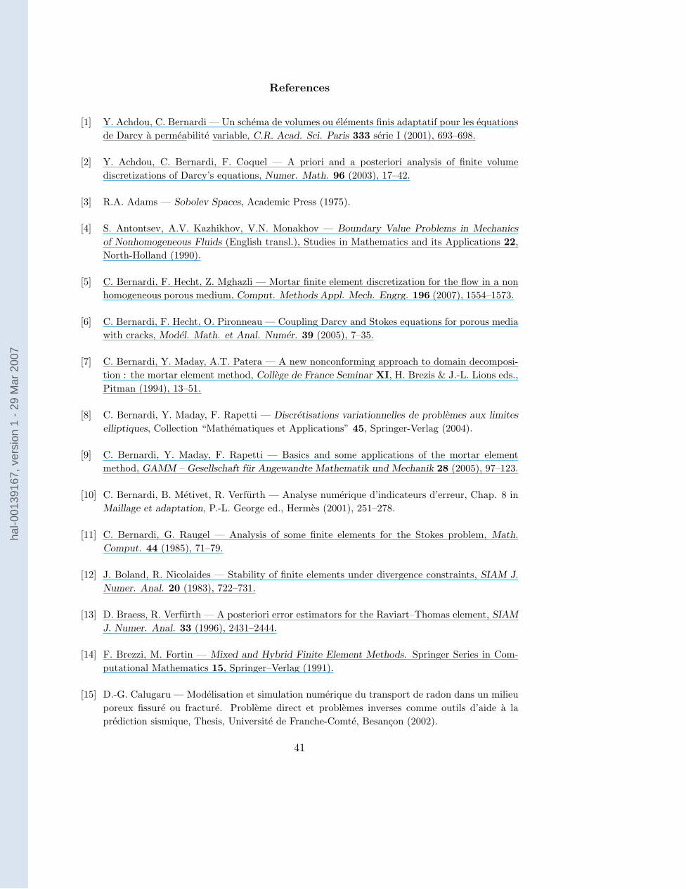
References

[1] Y. Achdou, C. Bernardi — Un schema de volumes ou elements finis adaptatif pour les equationsde Darcy a permeabilite variable, C.R. Acad. Sci. Paris 333 serie I (2001), 693–698.

[2] Y. Achdou, C. Bernardi, F. Coquel — A priori and a posteriori analysis of finite volumediscretizations of Darcy’s equations, Numer. Math. 96 (2003), 17–42.

[3] R.A. Adams — Sobolev Spaces, Academic Press (1975).

[4] S. Antontsev, A.V. Kazhikhov, V.N. Monakhov — Boundary Value Problems in Mechanics

of Nonhomogeneous Fluids (English transl.), Studies in Mathematics and its Applications 22,North-Holland (1990).

[5] C. Bernardi, F. Hecht, Z. Mghazli — Mortar finite element discretization for the flow in a nonhomogeneous porous medium, Comput. Methods Appl. Mech. Engrg. 196 (2007), 1554–1573.

[6] C. Bernardi, F. Hecht, O. Pironneau — Coupling Darcy and Stokes equations for porous mediawith cracks, Model. Math. et Anal. Numer. 39 (2005), 7–35.

[7] C. Bernardi, Y. Maday, A.T. Patera — A new nonconforming approach to domain decomposi-tion : the mortar element method, College de France Seminar XI, H. Brezis & J.-L. Lions eds.,Pitman (1994), 13–51.

[8] C. Bernardi, Y. Maday, F. Rapetti — Discretisations variationnelles de problemes aux limites

elliptiques, Collection “Mathematiques et Applications” 45, Springer-Verlag (2004).

[9] C. Bernardi, Y. Maday, F. Rapetti — Basics and some applications of the mortar elementmethod, GAMM – Gesellschaft fur Angewandte Mathematik und Mechanik 28 (2005), 97–123.

[10] C. Bernardi, B. Metivet, R. Verfurth — Analyse numerique d’indicateurs d’erreur, Chap. 8 inMaillage et adaptation, P.-L. George ed., Hermes (2001), 251–278.

[11] C. Bernardi, G. Raugel — Analysis of some finite elements for the Stokes problem, Math.

Comput. 44 (1985), 71–79.

[12] J. Boland, R. Nicolaides — Stability of finite elements under divergence constraints, SIAM J.

Numer. Anal. 20 (1983), 722–731.

[13] D. Braess, R. Verfurth — A posteriori error estimators for the Raviart–Thomas element, SIAM

J. Numer. Anal. 33 (1996), 2431–2444.

[14] F. Brezzi, M. Fortin — Mixed and Hybrid Finite Element Methods. Springer Series in Com-putational Mathematics 15, Springer–Verlag (1991).

[15] D.-G. Calugaru — Modelisation et simulation numerique du transport de radon dans un milieuporeux fissure ou fracture. Probleme direct et problemes inverses comme outils d’aide a laprediction sismique, Thesis, Universite de Franche-Comte, Besancon (2002).

41

hal-0

0139

167,

ver

sion

1 -

29 M

ar 2

007



https://www.researchgate.net/publication/41717218_Coupling_Darcy_and_Stokes_equations_for_porous_media_with_cracks?el=1_x_8&enrichId=rgreq-8582cec155a6e0058d418ce45c9fd6c0-XXX&enrichSource=Y292ZXJQYWdlOzQzMjkzODE5O0FTOjEwMjEyMDQxODE4NTIyNEAxNDAxMzU4ODEzODAy

https://www.researchgate.net/publication/41717218_Coupling_Darcy_and_Stokes_equations_for_porous_media_with_cracks?el=1_x_8&enrichId=rgreq-8582cec155a6e0058d418ce45c9fd6c0-XXX&enrichSource=Y292ZXJQYWdlOzQzMjkzODE5O0FTOjEwMjEyMDQxODE4NTIyNEAxNDAxMzU4ODEzODAy



https://www.researchgate.net/publication/226109599_A_priori_and_a_posteriori_analysis_of_finite_volume_discretizations_of_Darcy's_equations?el=1_x_8&enrichId=rgreq-8582cec155a6e0058d418ce45c9fd6c0-XXX&enrichSource=Y292ZXJQYWdlOzQzMjkzODE5O0FTOjEwMjEyMDQxODE4NTIyNEAxNDAxMzU4ODEzODAy

https://www.researchgate.net/publication/226109599_A_priori_and_a_posteriori_analysis_of_finite_volume_discretizations_of_Darcy's_equations?el=1_x_8&enrichId=rgreq-8582cec155a6e0058d418ce45c9fd6c0-XXX&enrichSource=Y292ZXJQYWdlOzQzMjkzODE5O0FTOjEwMjEyMDQxODE4NTIyNEAxNDAxMzU4ODEzODAy










https://www.researchgate.net/publication/229356398_Un_schema_de_volumes_ou_elements_finis_adaptatif_pour_les_equations_de_Darcy_a_permeabilite_variable?el=1_x_8&enrichId=rgreq-8582cec155a6e0058d418ce45c9fd6c0-XXX&enrichSource=Y292ZXJQYWdlOzQzMjkzODE5O0FTOjEwMjEyMDQxODE4NTIyNEAxNDAxMzU4ODEzODAy






https://www.researchgate.net/publication/51992242_Mixed_and_Hybrid_Finite_Element_Method?el=1_x_8&enrichId=rgreq-8582cec155a6e0058d418ce45c9fd6c0-XXX&enrichSource=Y292ZXJQYWdlOzQzMjkzODE5O0FTOjEwMjEyMDQxODE4NTIyNEAxNDAxMzU4ODEzODAy

https://www.researchgate.net/publication/51992242_Mixed_and_Hybrid_Finite_Element_Method?el=1_x_8&enrichId=rgreq-8582cec155a6e0058d418ce45c9fd6c0-XXX&enrichSource=Y292ZXJQYWdlOzQzMjkzODE5O0FTOjEwMjEyMDQxODE4NTIyNEAxNDAxMzU4ODEzODAy

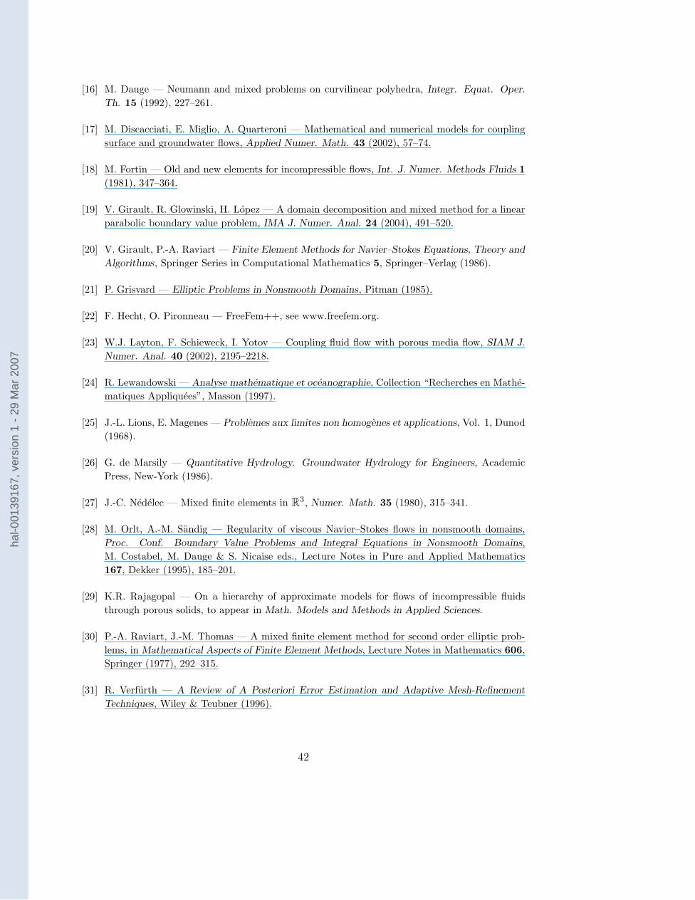
[16] M. Dauge — Neumann and mixed problems on curvilinear polyhedra, Integr. Equat. Oper.

Th. 15 (1992), 227–261.

[17] M. Discacciati, E. Miglio, A. Quarteroni — Mathematical and numerical models for couplingsurface and groundwater flows, Applied Numer. Math. 43 (2002), 57–74.

[18] M. Fortin — Old and new elements for incompressible flows, Int. J. Numer. Methods Fluids 1(1981), 347–364.

[19] V. Girault, R. Glowinski, H. Lopez — A domain decomposition and mixed method for a linearparabolic boundary value problem, IMA J. Numer. Anal. 24 (2004), 491–520.

[20] V. Girault, P.-A. Raviart — Finite Element Methods for Navier–Stokes Equations, Theory and

Algorithms, Springer Series in Computational Mathematics 5, Springer–Verlag (1986).

[21] P. Grisvard — Elliptic Problems in Nonsmooth Domains, Pitman (1985).

[22] F. Hecht, O. Pironneau — FreeFem++, see www.freefem.org.

[23] W.J. Layton, F. Schieweck, I. Yotov — Coupling fluid flow with porous media flow, SIAM J.

Numer. Anal. 40 (2002), 2195–2218.

[24] R. Lewandowski — Analyse mathematique et oceanographie, Collection “Recherches en Mathe-matiques Appliquees”, Masson (1997).

[25] J.-L. Lions, E. Magenes — Problemes aux limites non homogenes et applications, Vol. 1, Dunod(1968).

[26] G. de Marsily — Quantitative Hydrology. Groundwater Hydrology for Engineers, AcademicPress, New-York (1986).

[27] J.-C. Nedelec — Mixed finite elements in R3, Numer. Math. 35 (1980), 315–341.

[28] M. Orlt, A.-M. Sandig — Regularity of viscous Navier–Stokes flows in nonsmooth domains,Proc. Conf. Boundary Value Problems and Integral Equations in Nonsmooth Domains,M. Costabel, M. Dauge & S. Nicaise eds., Lecture Notes in Pure and Applied Mathematics167, Dekker (1995), 185–201.

[29] K.R. Rajagopal — On a hierarchy of approximate models for flows of incompressible fluidsthrough porous solids, to appear in Math. Models and Methods in Applied Sciences.

[30] P.-A. Raviart, J.-M. Thomas — A mixed finite element method for second order elliptic prob-lems, in Mathematical Aspects of Finite Element Methods, Lecture Notes in Mathematics 606,Springer (1977), 292–315.

[31] R. Verfurth — A Review of A Posteriori Error Estimation and Adaptive Mesh-Refinement

Techniques, Wiley & Teubner (1996).

42

hal-0

0139

167,

ver

sion

1 -

29 M

ar 2

007





https://www.researchgate.net/publication/37445417_Mathematical_and_numerical_models_for_coupling_surface_and_groundwater_flows?el=1_x_8&enrichId=rgreq-8582cec155a6e0058d418ce45c9fd6c0-XXX&enrichSource=Y292ZXJQYWdlOzQzMjkzODE5O0FTOjEwMjEyMDQxODE4NTIyNEAxNDAxMzU4ODEzODAy

https://www.researchgate.net/publication/37445417_Mathematical_and_numerical_models_for_coupling_surface_and_groundwater_flows?el=1_x_8&enrichId=rgreq-8582cec155a6e0058d418ce45c9fd6c0-XXX&enrichSource=Y292ZXJQYWdlOzQzMjkzODE5O0FTOjEwMjEyMDQxODE4NTIyNEAxNDAxMzU4ODEzODAy

https://www.researchgate.net/publication/51992117_Elliptic_Problems_in_Non_Smooth_Domains?el=1_x_8&enrichId=rgreq-8582cec155a6e0058d418ce45c9fd6c0-XXX&enrichSource=Y292ZXJQYWdlOzQzMjkzODE5O0FTOjEwMjEyMDQxODE4NTIyNEAxNDAxMzU4ODEzODAy

https://www.researchgate.net/publication/266214630_A_domain_decomposition_and_mixed_method_for_a_linear_parabolic_boundary_value_problem?el=1_x_8&enrichId=rgreq-8582cec155a6e0058d418ce45c9fd6c0-XXX&enrichSource=Y292ZXJQYWdlOzQzMjkzODE5O0FTOjEwMjEyMDQxODE4NTIyNEAxNDAxMzU4ODEzODAy

https://www.researchgate.net/publication/266214630_A_domain_decomposition_and_mixed_method_for_a_linear_parabolic_boundary_value_problem?el=1_x_8&enrichId=rgreq-8582cec155a6e0058d418ce45c9fd6c0-XXX&enrichSource=Y292ZXJQYWdlOzQzMjkzODE5O0FTOjEwMjEyMDQxODE4NTIyNEAxNDAxMzU4ODEzODAy




https://www.researchgate.net/publication/265834153_Regularity_of_viscous_Navier-Stokes_flows_in_nonsmooth_domains?el=1_x_8&enrichId=rgreq-8582cec155a6e0058d418ce45c9fd6c0-XXX&enrichSource=Y292ZXJQYWdlOzQzMjkzODE5O0FTOjEwMjEyMDQxODE4NTIyNEAxNDAxMzU4ODEzODAy




https://www.researchgate.net/publication/299497483_Analyse_mathematiques_et_oceanographie?el=1_x_8&enrichId=rgreq-8582cec155a6e0058d418ce45c9fd6c0-XXX&enrichSource=Y292ZXJQYWdlOzQzMjkzODE5O0FTOjEwMjEyMDQxODE4NTIyNEAxNDAxMzU4ODEzODAy

https://www.researchgate.net/publication/299497483_Analyse_mathematiques_et_oceanographie?el=1_x_8&enrichId=rgreq-8582cec155a6e0058d418ce45c9fd6c0-XXX&enrichSource=Y292ZXJQYWdlOzQzMjkzODE5O0FTOjEwMjEyMDQxODE4NTIyNEAxNDAxMzU4ODEzODAy

https://www.researchgate.net/publication/222360998_A_Review_of_A_Posteriori_Error_Estimation_Adaptive_Mesh-Refinement_Techniques?el=1_x_8&enrichId=rgreq-8582cec155a6e0058d418ce45c9fd6c0-XXX&enrichSource=Y292ZXJQYWdlOzQzMjkzODE5O0FTOjEwMjEyMDQxODE4NTIyNEAxNDAxMzU4ODEzODAy

https://www.researchgate.net/publication/222360998_A_Review_of_A_Posteriori_Error_Estimation_Adaptive_Mesh-Refinement_Techniques?el=1_x_8&enrichId=rgreq-8582cec155a6e0058d418ce45c9fd6c0-XXX&enrichSource=Y292ZXJQYWdlOzQzMjkzODE5O0FTOjEwMjEyMDQxODE4NTIyNEAxNDAxMzU4ODEzODAy

Mortar finite element discretization of a model coupling Darcy and Stokes equations

Documents

Transcript of Mortar finite element discretization of a model coupling Darcy and Stokes equations