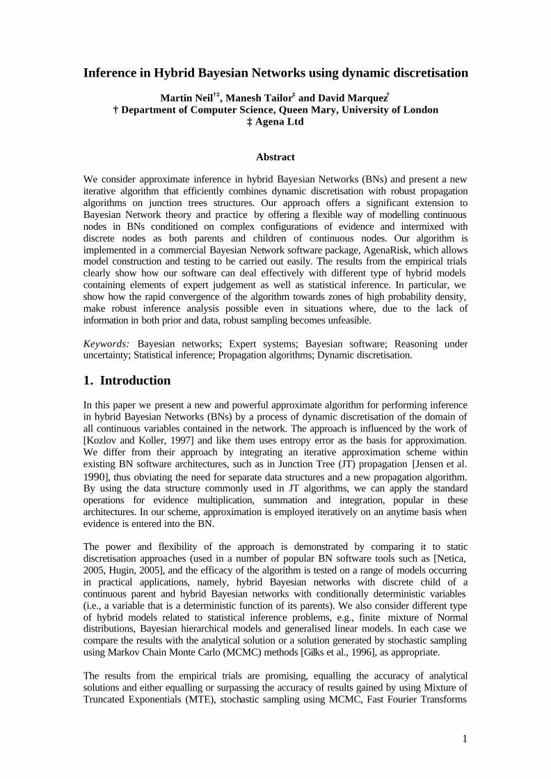
1

Inference in Hybrid Bayesian Networks using dynamic discretisation

Martin Neil†‡, Manesh Tailor‡ and David Marquez† † Department of Computer Science, Queen Mary, University of London

‡ Agena Ltd

Abstract We consider approximate inference in hybrid Bayesian Networks (BNs) and present a new iterative algorithm that efficiently combines dynamic discretisation with robust propagation algorithms on junction trees structures. Our approach offers a significant extension to Bayesian Network theory and practice by offering a flexible way of modelling continuous nodes in BNs conditioned on complex configurations of evidence and intermixed with discrete nodes as both parents and children of continuous nodes. Our algorithm is implemented in a commercial Bayesian Network software package, AgenaRisk, which allows model construction and testing to be carried out easily. The results from the empirical trials clearly show how our software can deal effectively with different type of hybrid models containing elements of expert judgement as well as statistical inference. In particular, we show how the rapid convergence of the algorithm towards zones of high probability density, make robust inference analysis possible even in situations where, due to the lack of information in both prior and data, robust sampling becomes unfeasible. Keywords: Bayesian networks; Expert systems; Bayesian software; Reasoning under uncertainty; Statistical inference; Propagation algorithms; Dynamic discretisation. 1. Introduction In this paper we present a new and powerful approximate algorithm for performing inference in hybrid Bayesian Networks (BNs) by a process of dynamic discretisation of the domain of all continuous variables contained in the network. The approach is influenced by the work of [Kozlov and Koller, 1997] and like them uses entropy error as the basis for approximation. We differ from their approach by integrating an iterative approximation scheme within existing BN software architectures, such as in Junction Tree (JT) propagation [Jensen et al. 1990], thus obviating the need for separate data structures and a new propagation algorithm. By using the data structure commonly used in JT algorithms, we can apply the standard operations for evidence multiplication, summation and integration, popular in these architectures. In our scheme, approximation is employed iteratively on an anytime basis when evidence is entered into the BN. The power and flexibility of the approach is demonstrated by comparing it to static discretisation approaches (used in a number of popular BN software tools such as [Netica, 2005, Hugin, 2005], and the efficacy of the algorithm is tested on a range of models occurring in practical applications, namely, hybrid Bayesian networks with discrete child of a continuous parent and hybrid Bayesian networks with conditionally deterministic variables (i.e., a variable that is a deterministic function of its parents). We also consider different type of hybrid models related to statistical inference problems, e.g., finite mixture of Normal distributions, Bayesian hierarchical models and generalised linear models. In each case we compare the results with the analytical solution or a solution generated by stochastic sampling using Markov Chain Monte Carlo (MCMC) methods [Gilks et al., 1996], as appropriate. The results from the empirical trials are promising, equalling the accuracy of analytical solutions and either equalling or surpassing the accuracy of results gained by using Mixture of Truncated Exponentials (MTE), stochastic sampling using MCMC, Fast Fourier Transforms

2

(FFT) and analytical solutions. In addition to the models presented here the approach has been applied to a wide variety of real-world modelling problems requiring hybrid Bayesian models containing elements of expert judgement as well as statistical inference [Neil et al., 2001, Neil et al. 2003a, Neil et al. 2003b, Fenton et al. 2002, Fenton et al. 2004]. However for brevity these results cannot be presented here. Our dynamic discretisation algorithm is implemented in the commercial general-purpose Bayesian Network software tool AgenaRisk [Agena 2005]. Likewise, the example models are built and executed using this software as is the graphical output (marginals and BN graphs) presented here. A brief description of the paper is as follows. In Section 2 we describe the problem and relevant background research. In Section 3 we give a detailed presentation of our algorithm. Then, in Section 4, we test the efficacy of the algorithm by conducting a series of analyses on a set of models. Finally Section 5 contains concluding remarks. 2. Background Hybrid Bayesian networks (BNs) have been widely used to represent full probability models in a compact and intuitive way. In the Bayesian network framework the independence structure (if any) in a joint distribution is characterised by a directed acyclic graph, with nodes representing random variables, which can be discrete or continuous, and may or may not be observable, and directed arcs representing causal or influential relationship between variables [Pearl, 1993]. The conditional independence assertions about the variables, represented by the lack of arcs, reduce significantly the complexity of inference and allow to decompose the underlying joint probability distribution as a product of local conditional probability distributions (CPDs) associated to each node and its respective parents. [Speigelhalter D.J., and Lauritzen S.L. 1990, Lauritzen, 1996]. If the variables are discrete, the CPDs can be represented as Node Probability Table (NPTs), which list the probability that the child node takes on each of its different values for each combination of values of its parents. Since a Bayesian network encodes all relevant qualitative and quantitative information contained in a full probability model, it provides an excellent tool to perform many types of probabilistic inference tasks [Whittaker, 1990, Heckerman et al., 1995], consisting mainly in computing the posterior probability distribution of some variables of interest (unknown parameters and unobserved data) conditioned on some other variables that have been observed. A range of robust and efficient propagation algorithms has been developed for exact inference on Bayesian networks with discrete variables [Pearl, 1988, Lauritzen and Spiegelhalter, 1988, Shenoy and Shafer, 1990, Jensen et al, 1990]. The common feature of these algorithms is that the exact computation of posterior marginals is performed through a series of local computations over a secondary structure, a tree of clusters, which allows calculating the marginal without computing the joint distribution. See also [Huang, 1996]. In hybrid Bayesian networks, local exact computations can be performed only under the assumption of Conditional Gaussian (CG) distributions [Lauritzen and Jensen, 2001]. The advantages and drawbacks of using Conditional Gaussian distributions are well known. They are useful to model mixtures of Gaussian variables conditioned on discrete and weighted combinations of CG parents but they are much too inflexible to support general-purpose inference over hybrid models containing mixtures of discrete labelled, integer and continuous types and non-Gaussian distributions. Most real applications demand non-standard high dimensional statistical models with intermixed continuous and discrete variables, where exact inference becomes computationally intractable.

3

The present generation of BN software tools attempt to model continuous nodes by numerical approximations using static discretisation as implemented in a number of software tools [Hugin, 2005, Netica, 2005]. Although disctretisation allows approximate inference in a hybrid BN without limitations on relationships among continuous and discrete variables, current software implementations requires users to define a uniform discretisation of the states of any numeric node (whether it is continuous or discrete) as a sequence of pre-defined intervals, which remain static throughout all subsequent stages of Bayesian inference regardless of any new conditioning evidence. The more intervals you define, the more accuracy you can achieve, but at a heavy cost of computational complexity. This is made worse by the fact that you do not necessarily know in advance where the posterior marginal distribution will lie on the continuum for all nodes and which ranges require the finer intervals. It follows that where a model contains numerical nodes having a potentially large range, results are necessarily only crude approximations. Alternatives to discretisation have been suggested by [Moral et al, 2001, Cobb and Shenoy, 2005a], who describe potential approximations using mixtures of truncated exponential (MTE) distributions, [Koller at al., 1999] who combine MTE approximations with direct sampling (Monte Carlo) methods, and [Murphy, 1999] who uses variational methods. There have also been some attempts for approximate inference on hybrid BNs using Markov Chain Monte Carlo (MCMC) approaches [Shachter and Peot, 1989], however, constructing dependent samples that mixed well (i.e., that move rapidly throughout the support of the target distribution) remains a complex task. 3. Dynamic Discretisation Let X be a continuous random node in the BN. The range of X is denoted by ΩX , and the

probability density function (PDF) of X , with support ΩX , is denoted by Xf . The idea of

discretisation is to approximate Xf by, first, partitioning ΩX into a set of interval

X jwΨ = , and second, defining a locally constant function Xf% on the partitioning intervals.

The task consists in finding an optimal discretisation set X iωΨ = and optimal values for

the discretised probability density function Xf% . Discretisation operates in much the same way when X takes integer values but in this paper we will focus on the case where X is continuous. The approach to dynamic discretisation described here searches ΩX for the most accurate specification of the high-density regions (HDR), given the model and the evidence, calculating a sequence of discretisation intervals in ΩX iteratively. At each stage in the iterative process a candidate discretisation, XΨ , is tested to determine whether the resulting

discretised probability density Xf% has converged to the true probability density Xf within an

acceptable degree of precision. At convergence, Xf is then approximated by Xf% . By dynamically discretising the model we achieve more accuracy in the regions that matter and incur less storage space over static discretisations. Moreover, we can adjust the discretisation anytime in response to new evidence to achieve greater accuracy. The approach to dynamic discretisation presented here is influenced by work of Kozlov and Koller on using non-uniform discretisation in hybrid BNs [Kozlov and Koller, 1997]. A number of features are introduced in their approach:

4

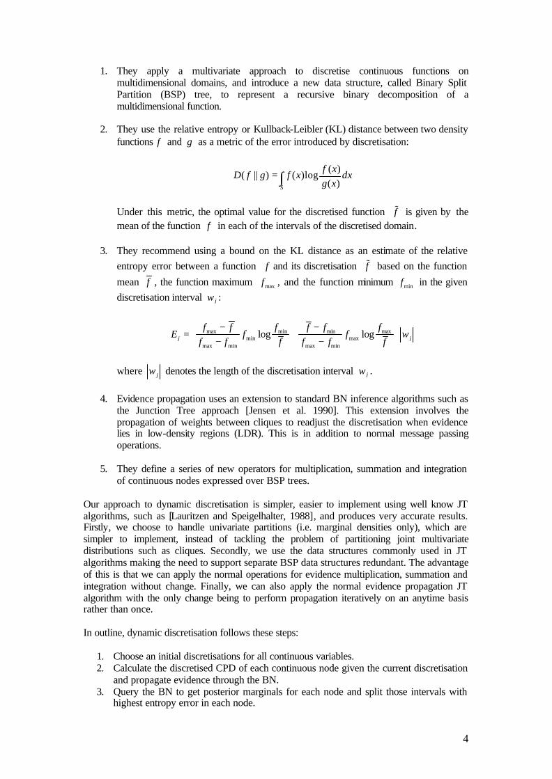
1. They apply a multivariate approach to discretise continuous functions on multidimensional domains, and introduce a new data structure, called Binary Split Partition (BSP) tree, to represent a recursive binary decomposition of a multidimensional function.

2. They use the relative entropy or Kullback-Leibler (KL) distance between two density

functions f and g as a metric of the error introduced by discretisation:

( )( || ) ( )log

( )= ∫

S

f xD f g f x dx

g x

Under this metric, the optimal value for the discretised function f% is given by the mean of the function f in each of the intervals of the discretised domain.

3. They recommend using a bound on the KL distance as an estimate of the relative entropy error between a function f and its discretisation f% based on the function

mean f , the function maximum maxf , and the function minimum minf in the given discretisation interval jw :

max maxmin minmin max

max min max min

log log − −

= + − − j j

f f ff f fE f f w

f f f f f f

where jw denotes the length of the discretisation interval jw .

4. Evidence propagation uses an extension to standard BN inference algorithms such as

the Junction Tree approach [Jensen et al. 1990]. This extension involves the propagation of weights between cliques to readjust the discretisation when evidence lies in low-density regions (LDR). This is in addition to normal message passing operations.

5. They define a series of new operators for multiplication, summation and integration

of continuous nodes expressed over BSP trees. Our approach to dynamic discretisation is simpler, easier to implement using well know JT algorithms, such as [Lauritzen and Speigelhalter, 1988], and produces very accurate results. Firstly, we choose to handle univariate partitions (i.e. marginal densities only), which are simpler to implement, instead of tackling the problem of partitioning joint multivariate distributions such as cliques. Secondly, we use the data structures commonly used in JT algorithms making the need to support separate BSP data structures redundant. The advantage of this is that we can apply the normal operations for evidence multiplication, summation and integration without change. Finally, we can also apply the normal evidence propagation JT algorithm with the only change being to perform propagation iteratively on an anytime basis rather than once. In outline, dynamic discretisation follows these steps:

1. Choose an initial discretisations for all continuous variables. 2. Calculate the discretised CPD of each continuous node given the current discretisation

and propagate evidence through the BN. 3. Query the BN to get posterior marginals for each node and split those intervals with

highest entropy error in each node.

5

4. Continue to iterate the process, by recalculating the conditional probability densities and propagating the BN, and then querying to get the marginals and then split intervals with highest entropy error, until the model converges to an acceptable level of accuracy.

In order to control the growth of the resulting discretisation sets, Ψ X , after each iteration, we merge those consecutive intervals in Ψ X with the lowest entropy error or that have zero mass and zero entropy error. Merging intervals is difficult in practice because of a number of factors. Firstly we do not necessarily want to merge intervals because they have a zero relative entropy error, as is the case with uniform distributions, since we want those intervals to help generate finer grained discretisations in any connected child nodes. Also, we wish to ensure that we only merge zero mass intervals with zero relative entropy error if they belong to sequences of zero mass intervals because some zero mass intervals might separate out local maxima in multimodal distributions. To resolve these issues we therefore apply a number of heuristics whilst merging. A key challenge in our approach to dynamic discretisation occurs when some evidence, =X x , lies in a region of ΩX where temporarily there is no probability mass. This can occur simply because the model as a whole is far from convergence to an acceptable solution and occurs when the sampling has not generated probability mass in the intervals of interest. This is a dangerous situation unremarked by [Kozlov and Koller, 1997]. We solve this problem by postponing the instantiation of evidence to the interval of interest and in the meantime assign it to the closest neighbouring interval with the aim of maximising the probability mass in the region closest to the actual HDR. Similarly, to enter point values evidence into a continuous node X , we assign a tolerance bound around the evidence, namely ( )xδ , and instantiate X on the interval

( ) ( )( ),x x x xδ δ− + . We consider here a Bayesian network for a set of random variables, X , and partition X into the sets, andQ EX X , consisting of the set of query variables and the set of observed variables, respectively. 3.1. The dynamic discretisation algorithm Our approach to simulation using dynamic discretisation is based on the following algorithm:

1: Initialise the discretisation, ( )0XΨ , for each continuous variable X ∈X .

2: Build a junction tree structure to determine the cliques,F , and sepsets.

3: for 1 to max_num_itel =

4: Compute the NPTs, ( ) ( | )lP X pa X , on ( )1lX

−Ψ for all nodes QX ∈ X that have new

discretisation or that are children of parent nodes that have a new discretisation

5: Initialise the junction tree by multiplying the NPTs for all nodes into the relevant

members of F

6: Enter evidence, E =X e , into the junction tree

7: Perform global propagation on the junction tree

6

8: for all nodes QX ∈ X

9: Marginalize/normalise to get the discretised posterior marginals ( ) ( )lEP X =X e

10: Compute the approximate relative entropy error ( )

j

lX j

w

S E= ∑ , for ( ) ( )lEP X =X e

over all intervals jw in ( )1lX

−Ψ

11: If

( )

( )11 1 for 1,2,3l k

Xl k

X

Sk

Sα α

−

− +

− ≤ ≤ + =

# Stable-entropy-error stopping rule #

or

XiS β< # Low-entropy-error stopping rule #

12: then stop discretisation for node X

13: else create a new discretisation ( )lXΨ for node X :

14: Split into two halves the interval jw in ( )1lX

−Ψ with the highest entropy error, jE .

15: Merge those consecutive intervals in ( )1lX

−Ψ with the lowest entropy error or that

have zero mass and zero entropy error

16: end if

17: end for

18: end for

3.2. Estimating deterministic functions using mixtures of Uniform distributions Once a discretisation has been defined at each step in the algorithm we need to calculate the marginal probability for all X in the model, by marginalisation from the conditional distribution of X given its parents, ( | )p X pa X . For standard continuous and discrete density functions this does not represent a problem but for more complex conditional distributions approximation techniques need to be used. Consider, for instance, the case in which the conditional distributions ( | )p X pa X involve

a deterministic function of random variables, e.g. ( )X f pa X= . For differentiable functions of discrete parents, is easy to obtain a closed expression for the marginal probability of X as a function of the joint probability of the parents. In a more general framework, a simple method for generating the local conditional probability table ( | )p X pa X commonly used under the static discretisation approach proceeds by first sampling values from each parent interval in Ωpa X for all parents of X and calculating the result ( )X f pa X= , then counting the frequencies with which the results fall within the static bins predefined for X , and finally normalising the NPT.

7

Although simple this procedure is flawed. On the one hand, there is no guarantee that every bin in XΩ will contain a probability density if the parents’ node values are under sampled. The implication of this is that some regions of XΩ might be void; they should have probability mass but do not. Any subsequent inference in the BN then will return an inconsistency when it encounters either a valid observation in a zero mass interval in X or attempts inference involving X . The only way to counter this under static discretisation is to generate a large number of samples, which is expensive and made more difficult by the fact that the sampling configuration settings in tools that use the static approach are inaccessible. On the other hand, samples from each parent interval in Ωpa X are usually taken uniformly

such that at least two samples are taken for each interval in Ωpa X . As the number of parent

nodes increases, and the states in XΩ and Ωpa X increases, the number of cells in the NPT, ( | )p X pa X , increases exponentially.

Consider, for example, = +Z X Y with , (10,100)∼X Y N . Here

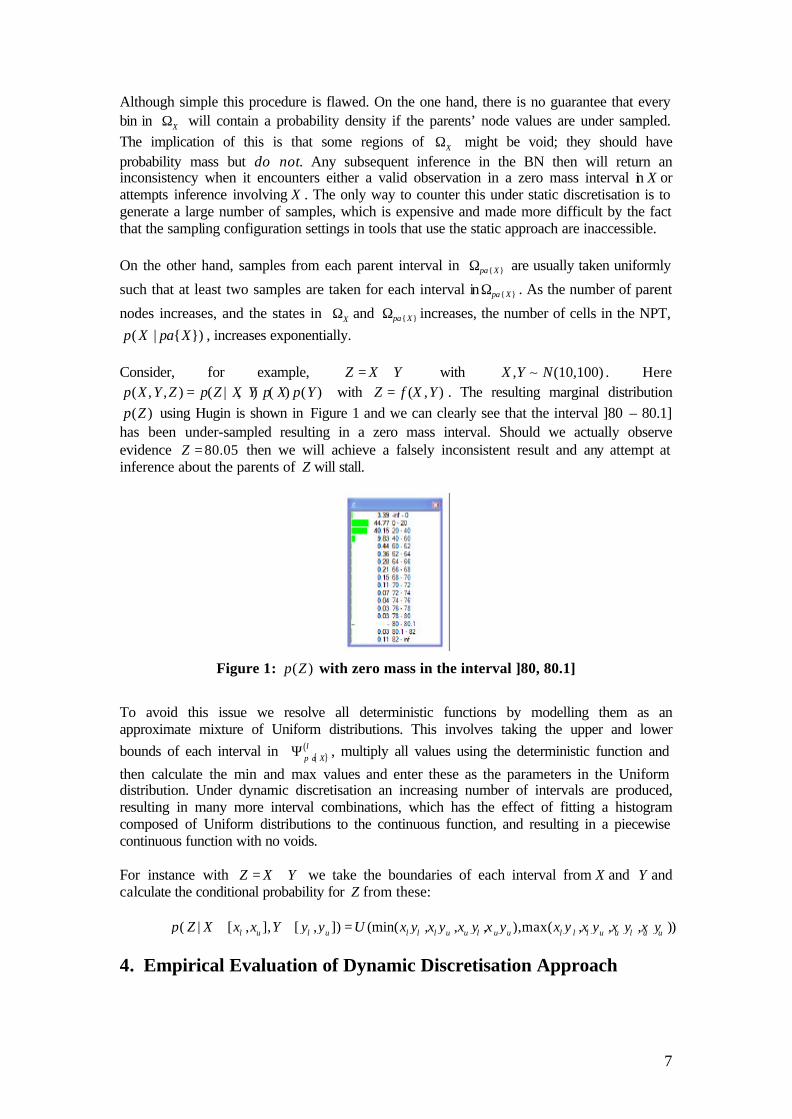
( , , ) ( | , ) ( ) ( )=p X Y Z p Z X Y p X p Y with ( , )=Z f X Y . The resulting marginal distribution ( )p Z using Hugin is shown in Figure 1 and we can clearly see that the interval ]80 – 80.1]

has been under-sampled resulting in a zero mass interval. Should we actually observe evidence 80.05Z = then we will achieve a falsely inconsistent result and any attempt at inference about the parents of Z will stall.

Figure 1: ( )p Z with zero mass in the interval ]80, 80.1]

To avoid this issue we resolve all deterministic functions by modelling them as an approximate mixture of Uniform distributions. This involves taking the upper and lower bounds of each interval in

( )lp a XΨ , multiply all values using the deterministic function and

then calculate the min and max values and enter these as the parameters in the Uniform distribution. Under dynamic discretisation an increasing number of intervals are produced, resulting in many more interval combinations, which has the effect of fitting a histogram composed of Uniform distributions to the continuous function, and resulting in a piecewise continuous function with no voids. For instance with = +Z X Y we take the boundaries of each interval from X and Y and calculate the conditional probability for Z from these:

( | [ , ], [ , ]) (min( , , , ),max( , , , ))l u l u l l l u u l u u l l l u u l u up Z X x x Y y y U x y x y x y x y x y x y x y x y∈ ∈ =

4. Empirical Evaluation of Dynamic Discretisation Approach

8

In this section we study the efficacy of the dynamic discretisation approach in practice by resolving the following models:

• Normal mixture model • Hybrid model • Conditionally deterministic variables • Statistical inference using a hierarchical normal model • Statistical inference using a logistic regression model

The first example, Normal mixture distribution, illustrates how the approach can produce estimates for continuous nodes that have discrete nodes as parents and also illustrates how multi-modal posterior distributions can be recovered. Here we also illustrate how the iterative approximation works and illustrate convergence properties of the algorithm. The second example is a simple hybrid BN consisting of a Conditional Linear Gaussian model of continuous parents with a discrete child. In the third example we show dynamic discretisation generating a probability distribution for hybrid BNs with variables that are deterministic function of its parents. It is important to point out that our approach can be used to solve statistical inference problems on general Bayesian hierarchical models, using both, conjugate and non-conjugate standard prior distributions. To this end the third and fourth examples focus on Bayesian statistical inference using a hierarchical normal and a logistic regression model respectively. In each case we compare the solutions under dynamic discretisation with the analytical equivalent solution, or where this is not possible approximate answers using Monte Carlo Markov Chains (MCMC). In addition to the examples covered here a very large number of examples covering a wide variety of predictive and diagnostic problems have been successfully modelled and are available with the AgenaRisk software. 4.1. Normal Mixture Model The Normal mixture distribution is an example of statistical models of continuous nodes that have discrete nodes as parents. Consider a mixture model with distributions

( ) ( ) 0.5p X false p X true= = = = 2

1 12

2 2

( , )( | )

( , )Normal X false

p Y XNormal X true

µ σµ σ

==

=

The marginal distribution of Y is a mixture of Normal distributions

( ) ( )2 21 1 2 2

1 1( ) | , | ,

2 2P Y N Y N Yµ σ µ σ= +

with mean and variance given by

[ ] ( )

[ ] ( ) ( ) ( )

1 2

22 2 2 21 1 2 2 1 2

121 12 4

E Y

Var Y

µ µ

σ µ σ µ µ µ

= +

= + + + − +

9

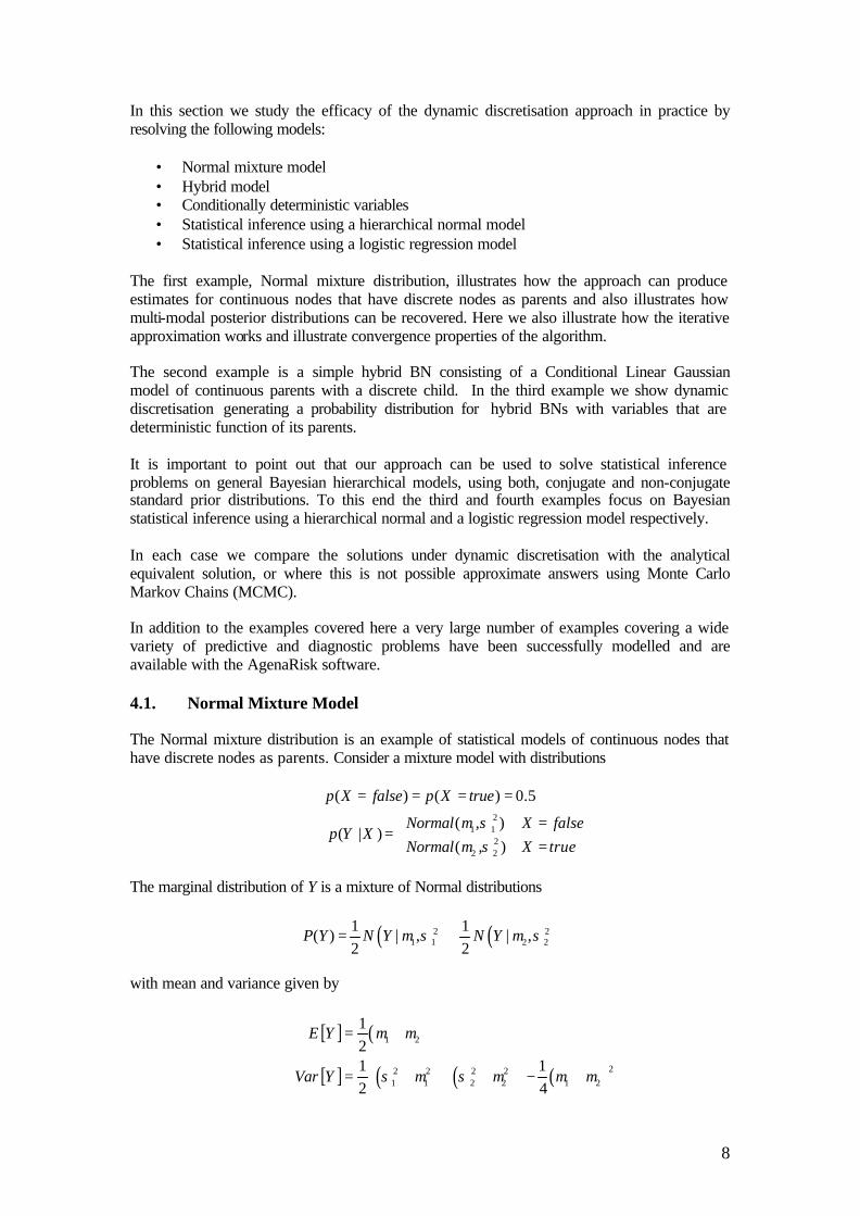
Figure 2 shows the resulting marginal distribution ( )p Y after 25 iterations, for the mixture of

( )|10,100N Y and ( )|50,10N Y , calculated under the static and the dynamic discretisation approaches. While using the later approach we are able to recover the exact values for the mean and variance, ( ) 30=E Y , ( ) 455Var Y = , the static case produces the approximated

values 82.8Yµ = and 2 12518Yσ = , showing clearly just how badly the static discretisation performs.

Figure 2 Comparison of static and dynamic discretisations of the marginal distribution

( )p Y for the Normal mixture model

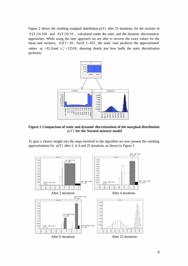
To give a clearer insight into the steps involved in the algorithm we now present the resulting approximations for ( )p Y after 2, 4, 6 and 25 iterations, as shown in Figure 3

After 2 iterations After 4 iterations

After 6 iterations After 25 iterations

10

Figure 3 Approximation of ( )p Y for Normal mixture problem over 2, 4, 6 and 25 iterations (Graphs show 99.8 percentile range around the median)

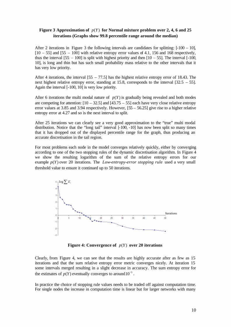
After 2 iterations in Figure 3 the following intervals are candidates for splitting: [-100 – 10], [10 – 55] and [55 – 100] with relative entropy error values of 4.1, 156 and 168 respectively, thus the interval [55 – 100] is split with highest priority and then [10 – 55]. The interval [-100, 10], is long and thin but has such small probability mass relative to the other intervals that it has very low priority. After 4 iterations, the interval [55 – 77.5] has the highest relative entropy error of 18.43. The next highest relative entropy error, standing at 15.8, corresponds to the interval [32.5 – 55]. Again the interval [-100, 10] is very low priority. After 6 iterations the multi modal nature of ( )p Y is gradually being revealed and both modes are competing for attention: [10 – 32.5] and [43.75 – 55] each have very close relative entropy error values at 3.85 and 3.94 respectively. However, [55 – 56.25] give rise to a higher relative entropy error at 4.27 and so is the next interval to split. After 25 iterations we can clearly see a very good approximation to the “true” multi modal distribution. Notice that the “long tail” interval [-100, -10] has now been split so many times that it has dropped out of the displayed percentile range for the graph, thus producing an accurate discretisation in the tail region. For most problems each node in the model converges relatively quickly, either by converging according to one of the two stopping rules of the dynamic discretisation algorithm. In Figure 4 we show the resulting logarithm of the sum of the relative entropy errors for our example ( )p Y over 20 iterations. The Low-entropy-error stopping rule used a very small threshold value to ensure it continued up to 50 iterations.

Figure 4: Convergence of ( )p Y over 20 iterations

Clearly, from Figure 4, we can see that the results are highly accurate after as few as 15 iterations and that the sum relative entropy error metric converges nicely. At iteration 15 some intervals merged resulting in a slight decrease in accuracy. The sum entropy error for the estimates of ( )p Y eventually converges to around 310− . In practice the choice of stopping rule values needs to be traded off against computation time. For single nodes the increase in computation time is linear but for larger networks with many

11

parent nodes the increase is exponential. In this example, using a 3.2Ghz Pentium 4 computer with 1Gb RAM, 10 iterations took 0.485 and 50 iterations took 2.094s. Computation times can be significantly improved by refactoring the network to ensure that no continuous nodes have more than two parent nodes thus ensuring the maximum size of NPTs are only 3n rather than mn for m continuous nodes withn states. 4.2. A simple hybrid Bayesian Network We will use the robot example of [Kozlov and Koller, 1997] to present an application of the dynamic discretisation algorithm to inference in a hybrid network, in this case a Conditional Linear Gaussian (CLG) model, where one of the discrete nodes has a continuous parent. We also illustrate here how the approach can produce accurate estimates in statistical models of continuous variables whose posterior marginal distributions can vary widely when unlikely evidence is provided. Let us assume that a robot can walk randomly on the interval [0,1]. The position x of the robot is unknown but we can record it on a number of sensors. We are interested in the posterior probability of the robot coordinate after reading observations on three sensors,

( )3 1, 2, 3p x o o o . The BN for the model is shown in Figure 5

Figure 5 BN for the one -dimensional robot

The unknown coordinates of the robot’s position, x , are modelled as a CLG network with two variables: ( ) ( )3 | 2 ~ 2,0.01p x x N x and ( ) ( )2 | 1 ~ 1,0.01p x x N x . A non-informative

prior belief is assigned to the first position, ( ) [ ]1 ~ 0,1p x Unif . The first two readings, 1o and

2o , are noisy observations of the robot’s position, so ( ) ( )| ~ ,0.01p o x N x . The third observation is a binary, discrete random variable indicating whether or not the robot is in the

left halfspace 0.5x < and is modelled with a sigmoid function ( ) ( ) 11 exp 40 0.5x

−+ − .

As pointed out by [Kozlov and Koller, 1997, Cobb and Shenoy, 2005], a weakness of the static discretisation is that, as the evidence entered in this type of model becomes more a more unlikely, the static discrete approximation of the posterior marginal degenerate and the estimators are very different from the exact answer The Figure 6 shows how we can obtain good estimators of the posterior marginals with our algorithm, even if unlikely evidence is given to the model. As we can see, the results from AgenaRisk for both, likely and unlikely scenarios compare very well to the exact answer. Here we run three scenarios, each containing different sets of evidence, and compare the posterior marginal for 3x under each. Scenario 1 corresponds to evidence 1 0.2o = and

2 0.2o = , scenario 2 corresponds to evidence 1 0.2o = and 2 0.65o = and scenario 3 to

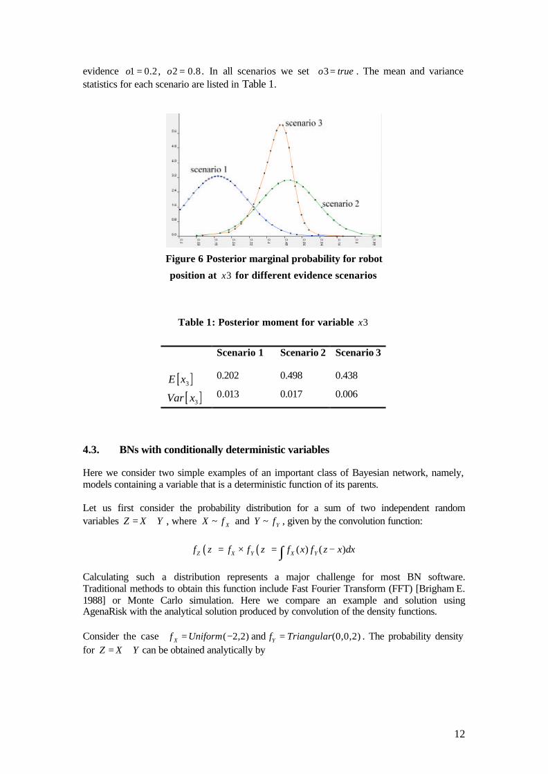
12

evidence 1 0.2o = , 2 0.8o = . In all scenarios we set 3o true= . The mean and variance statistics for each scenario are listed in Table 1.

Figure 6 Posterior marginal probability for robot

position at 3x for different evidence scenarios

Table 1: Posterior moment for variable 3x

Scenario 1 Scenario 2 Scenario 3

[ ]3E x 0.202 0.498 0.438

[ ]3Var x 0.013 0.017 0.006

4.3. BNs with conditionally deterministic variables Here we consider two simple examples of an important class of Bayesian network, namely, models containing a variable that is a deterministic function of its parents. Let us first consider the probability distribution for a sum of two independent random variables Z X Y= + , where ~ XX f and ~ YY f , given by the convolution function:

( ) ( ) ( ) ( )Z X Y X Yf z f f z f x f z x dx= × = −∫

Calculating such a distribution represents a major challenge for most BN software. Traditional methods to obtain this function include Fast Fourier Transform (FFT) [Brigham E. 1988] or Monte Carlo simulation. Here we compare an example and solution using AgenaRisk with the analytical solution produced by convolution of the density functions. Consider the case ( 2,2)Xf Uniform= − and (0,0,2)Yf Triangular= . The probability density for Z X Y= + can be obtained analytically by

13

( )2 2 0

0 0 2

(1/4 /8) (1/4 /8) (1/4 /8)z

Zz

f z x dx x dx x dx+

−

= + + + + +∫ ∫ ∫

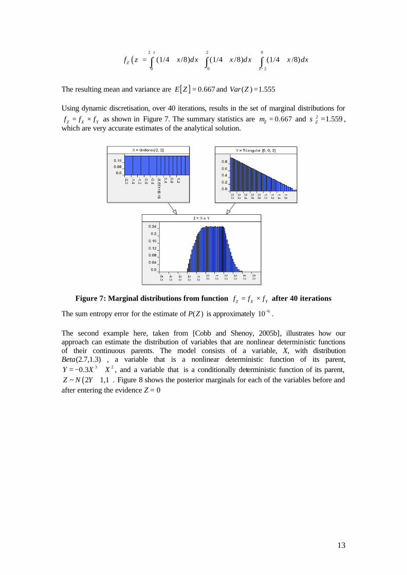
The resulting mean and variance are [ ] 0.667E Z = and ( ) 1.555Var Z = Using dynamic discretisation, over 40 iterations, results in the set of marginal distributions for

Z X Yf f f= × as shown in Figure 7. The summary statistics are 0.667Zµ = and 2 1.559Zσ = , which are very accurate estimates of the analytical solution.

Figure 7: Marginal distributions from function Z X Yf f f= × after 40 iterations

The sum entropy error for the estimate of ( )P Z is approximately 610− . The second example here, taken from [Cobb and Shenoy, 2005b], illustrates how our approach can estimate the distribution of variables that are nonlinear deterministic functions of their continuous parents. The model consists of a variable, X, with distribution Beta(2.7,1.3) , a variable that is a nonlinear deterministic function of its parent,

3 20.3Y X X= − + , and a variable that is a conditionally deterministic function of its parent, ( )~ 2 1,1Z N Y + . Figure 8 shows the posterior marginals for each of the variables before and

after entering the evidence Z = 0

14

Figure 8 Marginal distributions for X, Y, and Z after 25 iterations. a) Before entering the

evidence; b) after entering the evidence Z = 0

Running the model for 25 iterations results in the summary posterior values given in Table 2 and are compared with the estimates produced by [Cobb and Shenoy, 2005b] using MTE approximations to the potentials.

Table 2: Summary posterior values

(Estimates produced using MTE in brackets)

Mean Variance X 0.6747(0.6750) 0.0440(0.4380) Y 0.3037 (0.3042) 0.0165 (0.0159) Z 1.6070 (1.6084) 1.0892 (1.0455)

After observing Z = 0

X 0.5890 (0.5942) 0.0481 (0.0480) Y 0.2511 (0.2560) 0.0174 (0.0167)

As can be observed the results obtained using dynamic discretisation and AgenaRisk compare very favourably with those achieved using MTE approximations. 4.4. Hierarchical Normal Model We now present the analysis of hierarchical model based on the normal distribution. Formally the model for the hierarchical normal model is described by

( )2

1,j

iidn

ij jiy N µ σ

=∼ ,

with conjugate prior distribution for the group means µ j ’s given by ( )2

0 0,µ σN and Inv-

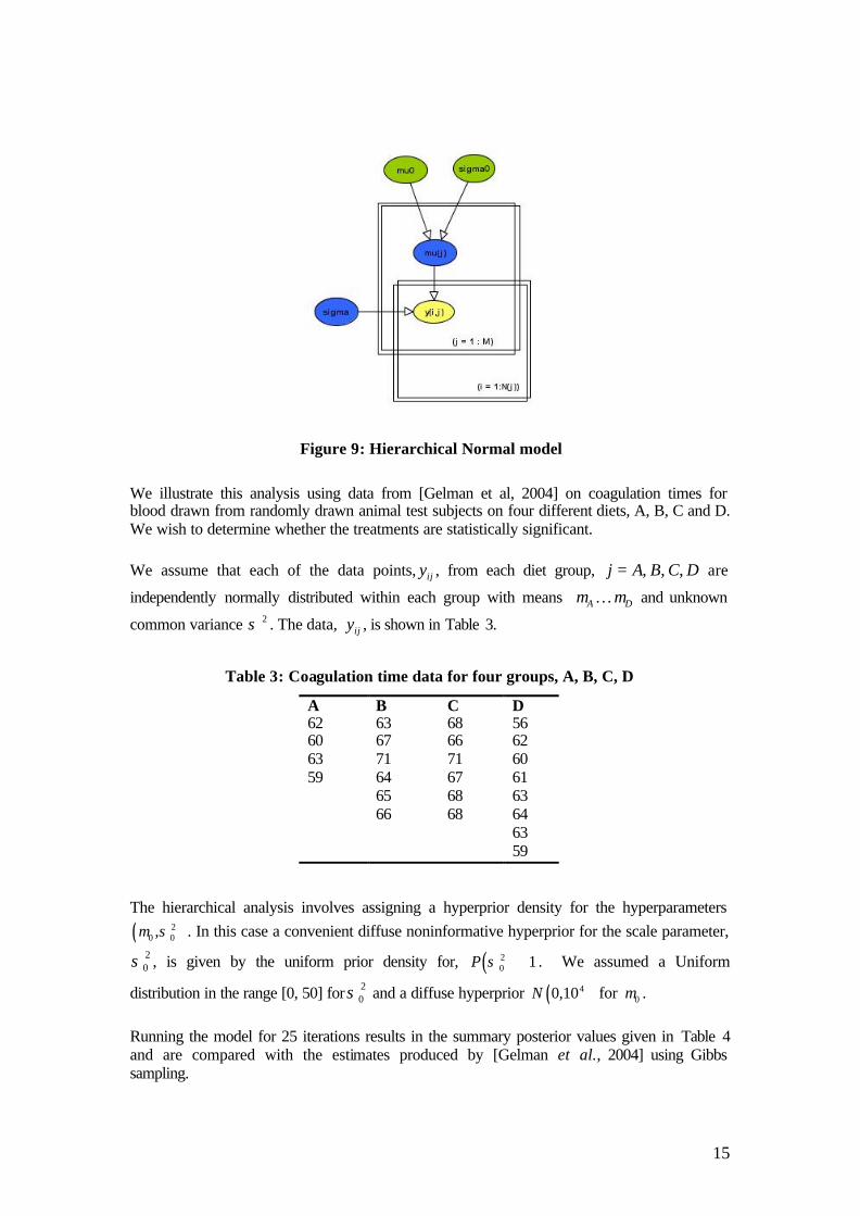
Gamma distribution with hyperparameters , ~ 0α β for the common unknown variance 2σ . Figure 9 shows the corresponding graphical model using plates’ notation [Buntine, 1994].

15

Figure 9: Hierarchical Normal model

We illustrate this analysis using data from [Gelman et al, 2004] on coagulation times for blood drawn from randomly drawn animal test subjects on four different diets, A, B, C and D. We wish to determine whether the treatments are statistically significant. We assume that each of the data points, ijy , from each diet group, , , ,=j A B C D are

independently normally distributed within each group with means µ µ…A D and unknown

common variance 2σ . The data, ijy , is shown in Table 3.

Table 3: Coagulation time data for four groups, A, B, C, D

A B C D 62 63 68 56 60 67 66 62 63 71 71 60 59 64 67 61 65 68 63 66 68 64 63 59

The hierarchical analysis involves assigning a hyperprior density for the hyperparameters

( )20 0,µ σ . In this case a convenient diffuse noninformative hyperprior for the scale parameter,

20σ , is given by the uniform prior density for, ( )2

0 1P σ ∝ . We assumed a Uniform

distribution in the range [0, 50] for 20σ and a diffuse hyperprior ( )40,10N for 0µ .

Running the model for 25 iterations results in the summary posterior values given in Table 4 and are compared with the estimates produced by [Gelman et al., 2004] using Gibbs sampling.

16

Table 4: Summary posterior values

(Estimates produced using Gibbs sampling in brackets)

25% Median 75% µA 60.5 (60.6) 61.3 (61.3) 62.0 (62.1)

µB 65.2 (65.3) 65.8 (65.9) 65.6 (66.6)

µC 67.1 (67.1)) 67.8 (67.8) 68.4 (68.5)

µD 60.7 (60.6) 61.2 (61.1) 61.8 (61.7) µ 62.5 (62.2) 64.0 (63.9) 65.6 (65.5)

2σ 4.2 (4.84) 5.3 (5.76) 6.8 (7.76) 20σ 12.2 (12.96) 20.9 (24.0) 32.6 (57.7)

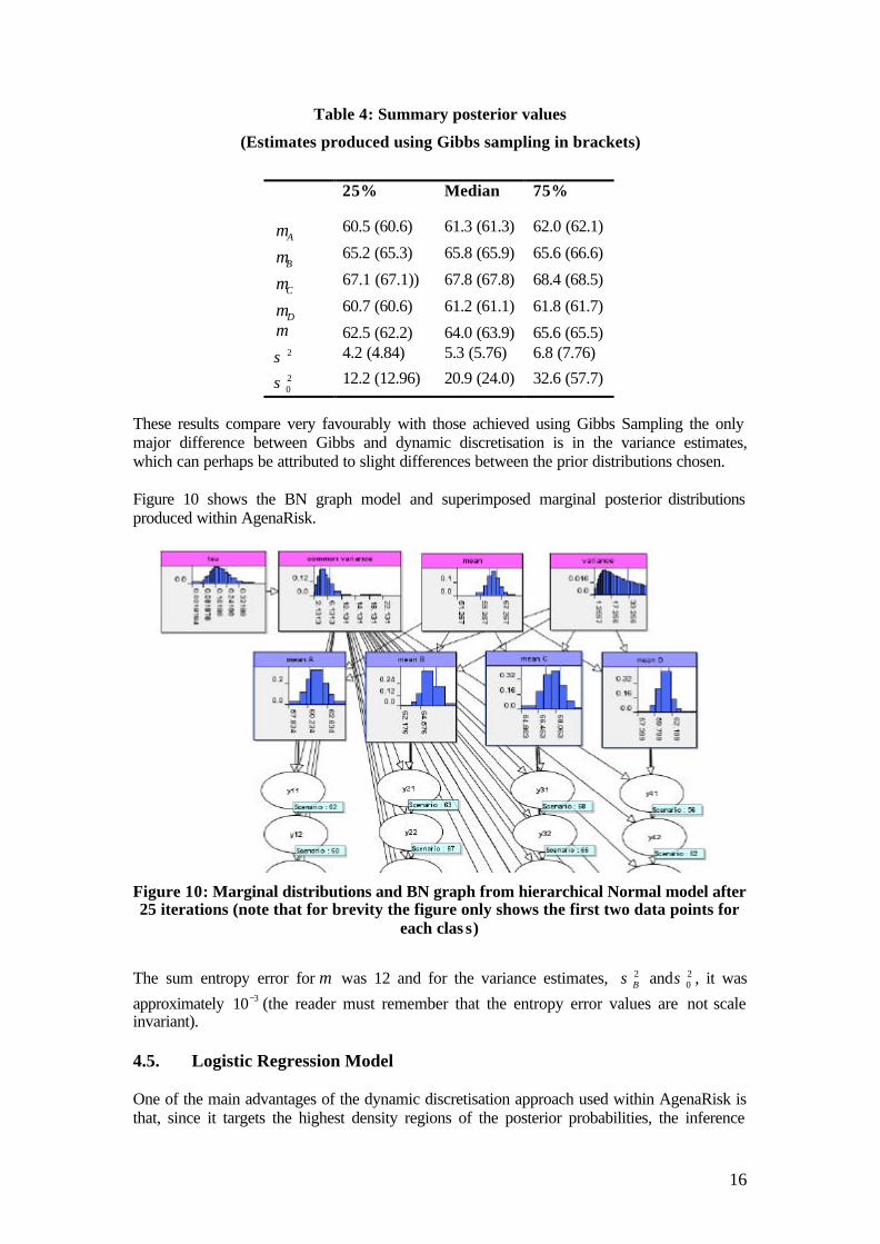
These results compare very favourably with those achieved using Gibbs Sampling the only major difference between Gibbs and dynamic discretisation is in the variance estimates, which can perhaps be attributed to slight differences between the prior distributions chosen. Figure 10 shows the BN graph model and superimposed marginal posterior distributions produced within AgenaRisk.

Figure 10: Marginal distributions and BN graph from hierarchical Normal model after 25 iterations (note that for brevity the figure only shows the first two data points for

each clas s)

The sum entropy error for µ was 12 and for the variance estimates, 2σ B and 2

0σ , it was

approximately 310− (the reader must remember that the entropy error values are not scale invariant). 4.5. Logistic Regression Model One of the main advantages of the dynamic discretisation approach used within AgenaRisk is that, since it targets the highest density regions of the posterior probabilities, the inference

17

analysis is possible even in situations where there is too little information concerning a parameter. We illustrate this using the bioassay example analysed in [Gelman et al. 2004]. It consists of a nonconjugate logistic regression model for the data shown in Table 5.

Table 5: Drug Trial Data

Dose, ix (log) -0.86 -0.3 -0.05 0.73

Number of deaths, iy 0 1 3 5

Number of animals, in 5 5 5 5

The logistic regression model is a particular case of the generalized linear model for binary or

binomial data ( )1 ,N

i i iiy Bin n p= ∼ , with link function given by the logit transformations of the

probability of success, ( )logit log1

ii

i

pp

p

= − . Such a model is commonly used in acute

toxicity tests or bioassay experiments for the development of chemical compounds, to analyse the subject’s responses to various doses of the compound. The model of the dose-response relation is given by the linear equation

( )logit log1

α β

= = + − i

i ii

pp x

p.

where ip is the probability of a ‘positive’ outcome for subjects exposed to a dose level ix . The likelihood function for the regression parameters ( ),α β is given by:

( )

exp 1,1 exp 1 exp

i i iy n y

i

i i

xL

x x

α βα β

α β α β

− +

∝ + + + + ∏ .

In the absence of any prior knowledge about the regression parameters ( ),α β , the use of a noninformative prior leads to the classical maximum likelihood estimates for α and β , which can be obtained using iterative computational procedures, such as the Newton-Raphson and Fisher-Scoring (or iterative re-weighted least squares) methods [Dobson, 1990]. Gelman et al, use a simple simulation approach, computing the posterior distribution of α and β on a grid of points. In order to get an idea of the effective range for the grid, a rough

estimate of the regression parameters is obtained first, by a linear regression of logit i

i

yn

on

ix for the four data points given in Table 5. Further analysis leads to approximate the

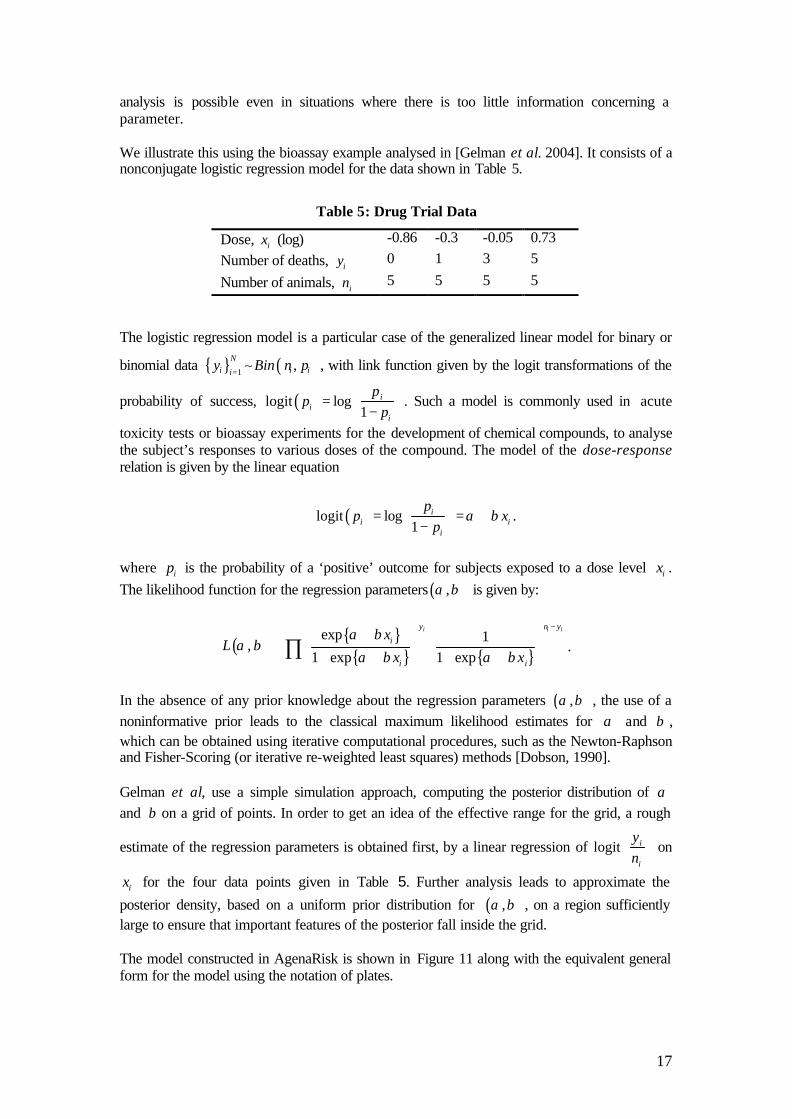
posterior density, based on a uniform prior distribution for ( ),α β , on a region sufficiently large to ensure that important features of the posterior fall inside the grid. The model constructed in AgenaRisk is shown in Figure 11 along with the equivalent general form for the model using the notation of plates.

18

Figure 11: BN graph from Logistic Regression model. The equivalent plate model is

shown alongside

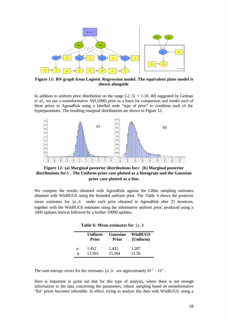
In addition to uniform prior distribution on the range [-2, 5] × [-10, 40] suggested by Gelman et al., we use a noninformative N(0,1000) prior as a basis for comparison and model each of these priors in AgenaRisk using a labelled node “type of prior” to condition each of the hyperparameter. The resulting marginal distributions are shown in Figure 12.

Figure 12: (a) Marginal posterior distributions forα (b) Marginal posterior

distributions for β . The Uniform prior case plotted as a histogram and the Gaussian prior case plotted as a line.

We compare the results obtained with AgenaRisk against the Gibbs sampling estimates obtained with WinBUGS using the bounded uniform prior. The Table 6 shows the posterior mean estimates for ( ),α β under each prior obtained in AgenaRisk after 25 iterations, together with the WinBUGS estimates using the informative uniform prior, produced using a 1000 updates burn-in followed by a further 10000 updates.

Table 6: Mean estimates for ( ),α β

Uniform Prior

Gaussian Prior

WinBUGS (Uniform)

α 1.452 1.432 1.287 β 13.593 15.584 11.56

The sum entropy errors for the estimates ( ),α β are approximately 2 110 10− −− . Here is important to point out that for this type of analysis, where there is not enough information in the data concerning the parameters, robust sampling based on noninformative ‘flat’ priors becomes infeasible. In effect, trying to analyse this data with WinBUGS, using a

19

noninformative N(0,1000) prior, or a uniform on a wider range, makes the sampling algorithm to fail so WinBUGS crashes. As we mentioned before with AgenaRisk is it possible to obtain reasonable good estimators of the regression parameters using a "vague" prior, even if there is too little information in the data concerning a parameter. As we can see the results from AgenaRisk for both cases compare very well to those produced by WinBUGS in the case of the informative uniform prior. 5. Concluding Remarks In this paper we have presented a new approximate inference algorithm for a general class of hybrid Bayesian Networks. Our algorithm is inspired by the dynamic discretisation approach suggested by Kozlov and Koller (1997), and like them uses relative entropy to iteratively adjust the discretisation in response to new evidence, and so achieve more accuracy in the zones of high posterior density. Our approach though is implemented using the data structures commonly used in JT algorithms, making it possible to use the natural operations on the cliques’ potentials, as well as performing propagation iteratively on the junction tree using standard algorithms. We have highlighted how our new dynamic discretisation approach overcome most of the problems inherent to the static or uniform discretisation approaches adopted by a number of popular BN software tools. In particular, problems related to computational inefficiency caused by supporting too many states to represent the domain, high level of inaccuracy in posterior estimates for continuous variables, problems in instantiating evidence in areas of the domain that are grossly under sampled that lead to inconsistency and error. Further technical improvements in our algorithm include coping effectively with situations in which evidence lies in a region where temporarily there is no probability mass, the introduction of tolerance bounds to enter point values evidence into continuous nodes, and finally the approximation of function of random variables using mixtures of uniform distributions. The results from the empirical trials clearly show how our software can produce accurate estimates on different classes of hybrid Bayesian networks appearing in practical applications. In particular Bayesian networks with discrete children of continuous parents and hybrid Bayesian networks with variables that are deterministic (linear and non-linear) functions of their parents are easily modelled. We have shown how our approach can cope with multi-modal posterior distributions, as well as models of continuous variables whose posterior marginal distributions vary widely when unlikely evidence is provided. We have also shown empirical results that illustrate how our software can deal effectively with different type of hybrid models related to statistical inference problems, making it a potential alternative tool for fitting Bayesian statistical models on complex problems in a powerful and user friendly way. In particular, we shown how the rapid convergence of the algorithm towards zones of high probability density, make robust inference analysis possible even in situations where, due to the lack of information in both prior and data, robust sampling becomes unfeasible In spite of the significant potential to address inferential tasks on complex hybrid models, there are some limitations in our algorithm related to the choice of the Hugin architecture as a platform to compute the marginal distributions. As is well known, the efficiency of the Hugin architecture depends on the size of the cliques in the associated junction tree. Although this

20

algorithm is intended to produce junction trees with minimum cliques size, for some statistical models, with d-converging dependency structures, on many unobserved and observed variables, the cliques in the corresponding junction tree can grow exponentially making the computation of the marginal distributions very costly or even impossible. Although we have successfully addressed inferential task on complex (hierarchical) statistical models with a large number of parameters with the current implementation we are unable to solve multiple regression and structural equation modelling problems. This means, we need to look at faster and more efficient approaches to propagation. An extension of our work will include Shenoy-Shafer architecture on binary join trees [Shenoy, 1997, Shenoy and Shafer, 1990], designed to reduce the computation involved in the multiplication and marginalisation of the local conditional distributions and other methods involving clique factorisation. Another useful extension that would optimise the use of Bayesian Networks to solve statistical inference problem is the introduction of plates to represent and manipulate ‘replicated nodes’ [Buntine, 1994]. Repeated node structures might appear in statistical models either in the representation of homogeneous data or in the modelling of unobserved subpopulation parameters (as in the hierarchical models). With the plate’s representation, a single indexed node replaces repeated nodes, and a box, called plate, indicates that the enclosed subgraph is duplicated. This not only should give a more compact representation of the inference model, but also, because of the indexed representation of the nodes, would allow a more efficient input-output data management. We can see potential benefits in extending AgenaRisk’s object-based modelling framework to support this approach. References Agena Ltd. 2005. AgenaRisk Software Package, www.agenarisk.com Bernardo J., and Smith A. 1994. Bayesian Theory. John Wiley and Sons, New York. Brigham E. 1988. Fast Fourier Transform and Its Applications. Prentice Hall; 1st edition. Buntine W. 1996. A guide to the literature on learning graphical models, IEEE Transactions on Knowledge and Data Engineering. 8:195-210. Buntine W. 1994. Operations for Learning with Graphical Models, J. AI Research, 159-225. Casella G., and George E. I. 1992. Explaining the Gibbs sampler, Am. Stat. 46: 167–174. Cobb B., and Shenoy P. 2005a. Inference in Hybrid Bayesian Networks with Mixtures of Truncated Exponentials, University of Kansas School of Business, working paper 294. Cobb B., and Shenoy P. 2005b. Nonlinear Deterministic Relationships in Bayesian Networks, In L. Godo (Ed.) ECSQARU, Springer-Verlag Berlin Heidelberg , pp. 27–38, Dobson A. J. 1990. An introduction to generalized linear models, New York: Chapman & Hall. Fenton N., Krause P., and Neil M. 2002. Probabilistic Modelling for Software Quality Control, Journal of Applied Non-Classical Logics 12(2), pp. 173-188

21

Fenton N., Marsh W., Neil M., Cates P., Forey S., and Tailor T. 2004. Making Resource Decisions for Software Projects, 26th International Conference on Software Engineering, Edinburgh, United Kingdom. Gelman A., Carlin J. B., Stern H. S., and Rubin D. B. 2004. Bayesian Data Analysis (2nd Edition), Chapman and Hall, pp. 209 – 302. Gelfand A., and A. Smith F.M. 1990. Sampling-based approaches to calculating marginal densities, J. Am. Stat. Asso. 85: 398–409. Geman S., and Geman D. 1984. Stochastic relaxation, Gibbs distribution and Bayesian restoration of images, IEEE Transactions on Pattern Analysis and Machine Intelligence 6: 721–741. Gilks W. R., Richardson S., and Spiegelhalter D. J., 1996. Markov chain Monte Carlo in Practice, Chapman and Hall, London, UK Heckerman D. 1999. A Tutorial on Learning with Bayesian Networks, Learning in Graphical Models, M. Jordan, ed. MIT Press, Cambridge, MA. Heckerman D., Mamdani A., and Wellman M.P. 1995. Real- world applications' of Bayesian networks, Comm. of the ACM, vol. 38, no. 3, pp. 24-68 Huang C., and Darwiche A. 1996. Inference in belief networks: A procedural guide. Int. J. Approx. Reasoning 15(3): 225-263 Hugin. 2005. www.hugin.com Jensen F. 1996. An Introduction to Bayesian Networks, Springer. Jensen F., Lauritzen S.L., and Olesen K. 1990. Bayesian updating in recursive graphical models by local computations, Computational Statistics Quarterly, 4: 260-282 Koller D., Lerner U., and Angelov D. 1999. A general algorithm for approximate inference and its applications to Hybrid Bayes Nets, in K.B Laskey and H. Prade (eds.), Proceedings of the 15th Conference on Uncertainty in Artificial Intelligence, pp. 324–333. Kozlov A.V., and Koller D. 1997. Nonuniform dynamic discretization in hybrid networks, in D. Geiger and P.P. Shenoy (eds.), Uncertainty in Artificial Intelligence, 13: 314–325. Lauritzen S.L. 1996. Graphical Models, Oxford. Lauritzen S.L., and Jensen F. 2001. Stable local computation with conditional Gaussian Distributions, Statistics and Computing, 11, 191–203.

Lauritzen S.L., and Speigelhalter D.J. 1988. Local Computations with Probabilities on Graphical Structures and their Application to Expert Systems (with discussion), Journal of the Royal Statistical Society Series B, Vol. 50, No 2, pp.157-224. Moral S., Rumi R., and Salmeron A. 2001. Mixtures of truncated exponentials in hybrid Bayesian networks, in P. Besnard and S. Benferhart (eds.), Symbolic and Quantitative Approaches to Reasoning under Uncertainty, Lecture Notes in Artificial Intelligence, 2143, 156–167.

22

Murphy K. P. 2001. A Brief Introduction to Graphical Models and Bayesian Networks. Berkeley, CA: Department of Computer Science, University of California - Berkeley. Murphy, K. 1999. A variational approximation for Bayesian networks with discrete and continuous latent variables, in K.B. Laskey and H. Prade (eds.), Uncertainty in Artificial Intelligence, 15, 467-475. Netica. 2005. www.norsys.com Neil M., Fenton N., Forey S., and Harris R. 2001. Using Bayesian Belief Networks to Predict the Reliability of Military Vehicles, IEE Computing and Control Engineering J 12(1), 11-20 Neil M., Malcolm B., and Shaw R. 2003a. Modelling an Air Traffic Control Environment Using Bayesian Belief Networks, 21st International System Safety Conference, Ottawa, Ontario, Canada. Neil M., Krause P., and Fenton N. 2003b. Software Quality Prediction Using Bayesian

Networks in Software Engineering with Computational Intelligence, (edited by Khoshgoftaar

T. M). The Kluwer International Series in Engineering and Computer Science, Volume 73

Pearl J. 1993. Graphical models, causality, and intervention, Statistical Science, vol 8, no. 3, pp. 266-273 Speigelhalter D.J., Thomas A., Best N.G., and Gilks W.R. 1995. BUGS: Bayesian inference Using Gibbs Sampling, Version 0.50. MRC Biostatistics Unit, Cambridge.

Speigelhalter D.J., and Lauritzen S.L. 1990. Sequential updating of conditional probabilities on directed graphical structures, Networks, 20, pp. 579-605. Shacter R., and Peot M. 1989. Simulation approaches to general probabilistic inference on belief networks. In Proceedings of the 5th Annual Conference on Uncertainty in AI (UAI), pages 221-230. Shenoy P. 1997. Binary join trees for computing marginals in the Shenoy-Shafer architecture, International Journal of Approximate Reasoning, 17(1), 1–25. Shenoy P., and Shafer G. 1990. Axioms for probability and belief-function propagation, Readings in uncertain reasoning, Morgan Kaufmann Publishers Inc, p.p. 575 - 610 Whittaker J. 1990. Graphical Models in Applied Multivariate Statistics, Wiley.