A Tutorial on Bayesian Inference for the A/B Test with R ... - OSF

A Tutorial on Bayesian Inference for the A/B Test with R andJASP

Tabea Hoffmann, Abe Hofman, & Eric-Jan Wagenmakers

University of Amsterdam

Author Note

The data, all preregistration materials, and an online Appendix are available on the

OSF repository at https://osf.io/anvg2/. Correspondence may be send to Tabea Hoffmann

(mail: [email protected], phone: +4916090535458).

https://osf.io/anvg2/

BAYESIAN A/B TESTING 2

Abstract

Popular in business, psychology, and the analysis of clinical trial data, the A/B test refers

to a comparison between two proportions. Here we discuss two Bayesian A/B tests that

allow users to monitor the uncertainty about a difference in two proportions as data

accumulate over time. We emphasize the advantage of assigning a dependent prior

distribution to the proportions (i.e., assigning a prior to the log odds ratio). This

dependent-prior approach has been implemented in the open-source statistical software

programs R and JASP. Several examples demonstrate how JASP can be used to apply this

Bayesian test and interpret the results.

Keywords: Bayes factor, Bayesian estimation, contingency tables, log odds ratio


A Tutorial on Bayesian Inference for the A/B Test with R andJASP

The A/B test is concerned with the comparison of two sample proportions (Little,

1989). The statistical framework requires that there are two groups and that the data for

each participant are dichotomous (e.g., “correct – incorrect”, “infected – not infected”, or

“watched the commercial” – “did not watch the commercial”).

The A/B test is standard operating procedure for the analysis of clinical trial data:

study participants are randomly allocated to one of two experimental conditions (which are

often called group A and group B). One of the conditions is usually the control condition

(e.g., a placebo), while the other condition introduces an intervention (e.g., a new

pharmacological drug). In each condition, participants are evaluated on a dichotomous

measure such as “dead – alive”, “side effect – no side effect”, etc. The goal of the

experiment is to examine the treatment success of the intervention. Because of its general

nature, the A/B test is also common in fields such as biology and psychology.

Another field that has recently adopted A/B testing – for so-called “conversion rate

optimization” – is online marketing. A conversion rate optimization experiment proceeds

analogously to the classical experiment: two versions of the same website are shown to

different selections of website visitors and the number of visitors who take a desired action

(e.g., clicking on a specific button) is monitored.

Whenever the A/B test is applied, practitioners eventually wish to know whether

and to what extent the experimental condition has a higher success rate than the control

condition. This judgment requires that the observed sample difference in proportions is

translated to the population – that is, the judgment requires statistical inference.

In general, practitioners can choose between the frequentist and the Bayesian

frameworks for their statistical analysis. We subscribe to the three general desiderata for

inference in the A/B test as outlined in Gronau et al. (in press): ideally, (1) evidence can

be obtained in favor of the null hypothesis; (2) evidence can be monitored continually, as


the data accumulate; and (3) expert knowledge can be taken into account. Below we

briefly explain why these desiderata are incompatible with the framework of frequentist

statistics; next we turn to the Bayesian framework and examine two different Bayesian

instantiations of the A/B test.

Frequentist Statistics

Practitioners predominantly use p-value null-hypothesis significance testing (NHST)

to analyze A/B test data. However, the NHST approach does not satisfy the three

desiderata mentioned above. Firstly, the NHST results cannot distinguish between absence

of evidence and evidence of absence (Keysers et al., 2020; Robinson, 2019). Evidence of

absence means that the data support the hypothesis that there is no effect (i.e., the two

conditions do not differ); absence of evidence, however, means that the data are

inconclusive (Altman & Bland, 1995). Secondly, in NHST the data cannot be tested

sequentially without necessitating a correction for multiple comparisons that depends on

the sampling plan (see for instance Berger & Wolpert, 1988; Wagenmakers, 2007;

Wagenmakers et al., 2018). Especially in clinical trials but also for online marketing is it

efficient to act as soon as the data provide evidence that is sufficiently compelling. To

achieve such efficiency many A/B test practitioners repeatedly peek at interim results and

stop data collection as soon as the p-value is smaller than some predefined α-level

(Goodson, 2014). However, this practice inflates the Type I error rate and hence

invalidates an NHST analysis (Jennison, Turnbull, et al., 1990; Wagenmakers, 2007).

Thirdly, NHST does not allow users to incorporate detailed expert knowledge. For

example, among conversion rate optimization professionals it is widely known that online

advertising campaigns often yield minuscule increases in conversion rates (cf. G. Johnson

et al., 2017; Patel, 2018). Such knowledge may affect NHST planning (i.e., knowledge that

the effect is minuscule would necessitate the use of very large sample sizes), but it is


unclear how it would affect inference.1 As we will see below, in the Bayesian framework is

it conceptually straightforward to enrich statistical models with expert background

knowledge, thereby resulting in more informed statistical analyses (Lindley, 1993).

Bayesian Statistics

The limitations of frequentist statistics can be overcome by adopting a Bayesian

data analysis approach (e.g., Deng, 2015; Kamalbasha & Eugster, 2021; Stucchio, 2015). In

Bayesian statistics, probability expresses a degree of knowledge or reasonable belief

(Jeffreys, 1961) and in principle Bayesian statistics fulfills all three desiderata listed above

(e.g., Wagenmakers et al., 2018). In the next sections we introduce two approaches to

Bayesian A/B testing. The two approaches make different assumptions, ask different

questions, and therefore provide different answers (cf. Dablander et al., 2021).

1. The ‘Independent Beta Estimation (IBE) Approach’

Let nA denote the total number of observations and yA denote the number of

successes for group A. Let nB denote the total number of observations and yB denote the

number of successes for group B. The commonly used Bayesian A/B testing model is

specified as follows:

yA ∼ Binomial(nA, θA)

yB ∼ Binomial(nB, θB)

This model assumes that yA and yB follow independent binomial distributions with success

probabilities θA and θB. These success probabilities are assigned independent beta(α, β)

1 For example, with the data in hand one may find that p = .15, and that the power to detect a minuscule

effect was only .20. However, power is a pre-data concept and consequently it remains unclear to what

extent the observed data affect our knowledge (Wagenmakers et al., 2015). Moreover, the selection of the

minuscule effect is often motivated by Bayesian considerations (i.e., it is a value that appears plausible,

based on substantive domain knowledge).


distributions that encode the relative prior plausibility of the values for θA and θB. In a

beta distribution, the α values can be interpreted as counts of hypothetical ‘prior successes’

and the β values can be interpreted as counts of hypothetical ‘prior failures’ (Lee &

Wagenmakers, 2013):

θA ∼ Beta(αA, βA)

θB ∼ Beta(αB, βB)

Data from the A/B testing experiment update the two independent prior

distributions to two independent posterior distributions as dictated by Bayes’ rule:

p(θA | yA, nA) = p(θA) × p(yA, nA | θA)p(yA, nA)

p(θB | yB, nB) = p(θB) × p(yB, nB | θB)p(yB, nB)

where p(θA) and p(θB) are the prior distributions and p(yA, nA | θA) and p(yB, nB | θB) are

the likelihoods of the data given the respective parameters. Hence, the reallocation of

probability from prior to posterior is brought about by the data: the probability increases

for parameter values that predict the data well and decreases for parameter values that

predict the data poorly (Kruschke, 2013; van Doorn et al., 2020; Wagenmakers et al.,

2016). Note that whenever a beta prior is used and the observed data are binomially

distributed, the resulting posterior distribution is also a beta distribution. Specifically, if

the data consist of s successes and f failures, the resulting posterior beta distribution

equals beta(α + s, β + f) (Gelman et al., 2013; van Doorn et al., 2020).2 Ultimately,

practitioners are most often interested in the difference δ = θA − θB between the success

rates of the two experimental groups, as this difference indicates whether the experimental

condition shows the desired effect.

2 When the prior and the posterior belong to the same family of distributions they are said to be conjugate.


R Implementation of the IBE Approach: The bayesAB Package

The IBE approach is implemented for instance in the bayesAB (Portman, 2017)

package in R (R Core Team, 2020). Consider the following fictitious example from ethology,

inspired by the classic work of von Frisch (1914). A researcher wishes to test whether honey

bees have color vision by comparing the behavior of two groups of bees. The experiment

involves a training and a testing phase. In the training phase, the bees in the experimental

condition are presented with a blue and a green disc. Only the blue disc is covered with a

sugar lotion that bees crave. The control group receives no training. In the testing phase,

the sugar lotion is removed from the blue disc, and the behavior of both groups is being

observed. If the bees in the experimental condition have learned that only the blue disc

contains the appetising sugar lotion, and if they can discriminate between blue and green,

they should preferentially explore the blue instead of the green disc during the testing

phase. The researcher finds that in 65 out of 100 times, the bees in the experimental group

continued to approach the blue disc after the sugar lotion was removed. The bees that were

not trained approached the blue disc 50 out of 100 times. In the remainder of this section,

we will refer to the bees in the control condition as group A and to the bees in the

experimental condition as group B. The R file for this fictitious example can be found in

the OSF repository associated with this manuscript (https://osf.io/anvg2/).

Before setting up this A/B test and collecting the data, the prior distribution has to

be specified so that it represents the relative plausibility of the parameter values. For the

present example the researcher specifies two uninformative (uniform) beta(1,1) priors.

After running the A/B test procedure, the priors are updated with the obtained data.

With bayesAB the calculation of the posterior distributions is done by feeding both the

priors and the data to the bayesTest function:

R> library(bayesAB)

R> bees1 <- read.csv2("bees_data1.csv")



R> AB1 <- bayesTest(bees1$y1, bees1$y2, priors = c(‘alpha’ = 1, ‘beta’ = 1),

+ n_samples = 1e5, distribution = ‘bernoulli’)

The results can be obtained and visualized by executing:

R> summary(AB1)

R> plot(AB1)

Figure 1

Independent posterior beta distributions of the success probabilities for group A and B. The

plot is produced by the bayesAB package with the fictitious bee data (i.e., A = 50/100

versus B = 65/100) described in the main text. The analysis used two independent

beta(1, 1) priors.

Figure 1 shows the two independent posterior distributions that plot(AB1) returns.

To plot these posterior distributions, bayesTest makes use of the rbeta function that


draws random numbers from a given beta distribution. To obtain each posterior

distribution the package first exploits conjugacy: the number of successes s are added to

the α values of either version’s prior distribution and the number of failures f are added to

the respective β values. Thus, the posterior distribution for θA is beta(αA + sA, βA + fA)

and that for θB is beta(αB + sB, βB + fB). The rbeta function draws random samples from

each posterior distribution and the density of these values is shown in Figure 1.3 We can

see that group B’s posterior distribution for the success probability assigns more mass to

higher values of θ. This suggests that the success probability of the trained bees is higher,

which in turn implies that bees have color vision.

The bayesAB package also returns a posterior distribution which indicates the

“conversion rate uplift” (θB−θA)θA

, that is, the difference between the success rates expressed

as a proportion of θA. This posterior distribution is computed from the random samples

obtained for the two beta posteriors shown in Figure 1. As shown in Figure 2, the posterior

distribution for the uplift peaks at around 0.4, indicating that the most likely increase of

bee approaches on the blue disc equals 40%. Also, most posterior mass (i.e., 98.4% of the

samples) is above zero, indicating that we can be 98.4% certain that group B approaches

the blue disc more often than group A. Note that this statement assumes that it is a priori

equally likely that the training in the experimental condition B had a positive or negative

effect on the rate at which the bees approach the blue disc, and that the possibility that

both groups have the same approach rate is deemed impossible from the outset – this is an

important point to which we will return later.

The posterior probability that θB > θA can also be obtained analytically (Schmidt

& Mørup, 2019). The formula is not implemented in the bayesAB package; our R

implementation can be found in the OSF repository. For the above example,

3 The posterior distributions are available analytically, so at this point the rbeta function is not needed; it

will become relevant once we start to investigate the posterior distribution for the difference between θA

and θB .


Figure 2

Histogram of the conversion rate uplift from version A (i.e., 50/100) to version B (i.e.,

65/100) for the fictitious bee data set. The uplift is calculated by dividing the difference in

conversion by the conversion in A. The plot is produced by the bayesAB package.

p(θB > θA | data) = 0.984. In fact the entire posterior distribution for the difference

between the two independent beta distributions is available analytically (Pham-Gia et al.,

1993). Figure 3a shows the posterior distribution of the difference between the two

independent beta posteriors from the bee example. Unfortunately, the analytic calculation

fails for values of α and β above ∼ 50, which occur with strong advance knowledge or high

sample sizes. In this case, one can instead employ a normal approximation, the result of

which is shown in the right panel of Figure 3.4

One advantage of the Bayesian approach is that the data can also be added to the

analysis in a sequential manner. This means that the evidence can be assessed continually

4 The appendix contains the formulas from Schmidt and Mørup (2019) and Pham-Gia et al. (1993), as well

as the formulas for the normal approximation.


Figure 3

Posterior distributions of the difference δ = θB − θA for the fictitious bee data (i.e., A =

50/100 versus B = 65/100).

(a) Analytic distribution of the difference

between two independent beta distributions

(Pham-Gia et al., 1993).

(b) Normal approximation of the difference

between two independent beta distributions.

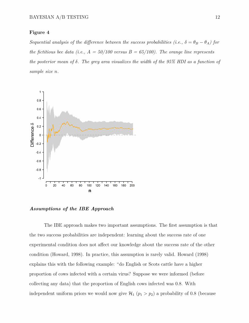
as the data arrives and the analyses can be stopped as soon as the evidence is judged to be

compelling (Deng et al., 2016). As a demonstration, Figure 4 plots the posterior mean of

the difference between θA and θB as well as the 95% highest density interval (HDI) of the

difference in a sequential manner. The HDI narrows with increasing sample size, indicating

that the range of likely values for δ gradually becomes smaller. After some initial

fluctuation, the posterior mean difference between θA and θB (i.e., the orange line) settles

between 0.1 and 0.2. The R code for the sequential computation can be found in the OSF

repository.

In sum, the IBE approach allows practitioners to judge the size and direction of an

effect, that is, the difference between the two success probabilities. It is important,

however, to recognize the assumptions that come with this approach. In the next section,

we will elaborate on these assumptions and their consequences.


Figure 4

Sequential analysis of the difference between the success probabilities (i.e., δ = θB − θA) for

the fictitious bee data (i.e., A = 50/100 versus B = 65/100). The orange line represents

the posterior mean of δ. The grey area visualizes the width of the 95% HDI as a function of

sample size n.

Assumptions of the IBE Approach

The IBE approach makes two important assumptions. The first assumption is that

the two success probabilities are independent: learning about the success rate of one

experimental condition does not affect our knowledge about the success rate of the other

condition (Howard, 1998). In practice, this assumption is rarely valid. Howard (1998)

explains this with the following example: “do English or Scots cattle have a higher

proportion of cows infected with a certain virus? Suppose we were informed (before

collecting any data) that the proportion of English cows infected was 0.8. With

independent uniform priors we would now give H1 (p1 > p2) a probability of 0.8 (because


the chance that p2 < 0.8 is still 0.2). In very many cases this would not be appropriate.

Often we will believe (for example) that if p1 is 80%, p2 will be near 80% as well and will

be almost equally likely to be larger or smaller. (We are still assuming it will never be

exactly the same.)” (p. 363).

The second assumption of the IBE approach is that an effect is always present; that

is, training the bees to prefer a certain color may increase approach rates or decrease

approach rates; it is never the case that the training is completely ineffective. This

assumption follows from the fact that a continuous prior does not assign any probability to

a specific point value such as δ = 0 (Jeffreys, 1939; Williams et al., 2017; Wrinch &

Jeffreys, 1921). Thus, using the IBE approach practitioners can only test whether the

alterations in the experimental group yield a positive or a negative effect. Obtaining

evidence in favor of the null hypothesis – which was one of the desiderata listed by Gronau

et al. (in press) – is not possible with this approach. Hence, the IBE approach does not

represent a testing effort, but rather an estimation effort (Jeffreys, 1939). To allow for both

hypothesis testing and parameter estimation a Bayesian A/B testing model has to be able

to assign prior mass to the possibility that the difference between the two conditions is

exactly zero. It should be acknowledged that this can be achieved when the success

probabilities are assigned beta priors (e.g., Gunel & Dickey, 1974; Jamil et al., 2017;

Jeffreys, 1961); however, here we follow the recent recommendation by Dablander et al.

(2021) and adopt an alternative statistical approach.

2. The Logit Transformation Testing (LTT) Approach

An A/B test model that assigns prior mass to the null hypothesis of no effect was

introduced by Kass and Vaidyanathan (1992) and implemented by Gronau et al. (in press).

In contrast to the IBE approach, this model assigns a prior distribution to the log odds

ratio, thereby accounting for the dependency between the success probabilities of the two


experimental groups. The LTT approach is specified as follows:

yA ∼ Binomial(nA, θA)

yB ∼ Binomial(nB, θB)

log(

θA1 − θA

)= γ − ψ/2

log(

θB1 − θB

)= γ + ψ/2

As before, this model assumes that yA and yB follow binomial distributions with success

probabilities θA and θB. However, the success probabilities are a function of two

parameters, γ and ψ. Parameter γ indicates the grand mean of the log odds, while ψ

denotes the distance between the two conditions (i.e., the log odds ratio). The hypothesis

that there is no difference between the two groups can be formulated as a null hypothesis:

H0 : ψ = 0. Under the alternative hypothesis H1, ψ is assumed to be nonzero. By default,

both parameters are assigned normal priors:

γ ∼ N(µγ, σ2γ)

ψ ∼ N(µψ, σ2ψ)

While the choice of a prior for γ is relatively inconsequential for the comparison between

H0 and H1, the choice of a prior for ψ is far-reaching: it determines the predictions of H1

concerning the difference between versions A and B. In other words, ψ is the test-relevant

parameter.5

We consider four hypotheses that may be of interest in practice:

H0 : θA = θB; The success probabilities θA and θB are identical.

H1 : θA ̸= θB; The success probabilities θA and θB are not identical.

H+ : θB > θA; The success probability θB is larger than the success probability θA.

5 Note that the overall prior distribution for ψ can be considered a mixture between a ‘spike’ at 0 coming

from H0 and a Normal ‘slab’ coming from H1 (e.g., van den Bergh et al., 2021).


H− : θA > θB; The success probability θA is larger than the success probability θB.

By comparing these hypotheses, practitioners may obtain answers to the following

questions: (1) Is there a difference between the success probabilities, or are they the same?

This requires a comparison between H1 and H0; (2) Does group B have a higher success

probability than group A, or are the probabilities the same? This requires a comparison

between H+ and H0; (3) Does group A have a higher success probability than group B, or

are the probabilities the same? This requires a comparison between H− and H0; (4) Does

group B have a higher success probability than group A, or does group A have a higher

success probability than group B? This is the question that is also addressed by the IBE

approach discussed earlier, and it requires a comparison between H+ and H−.

To quantify the evidence that the observed data provide for and against the

hypotheses we compare the models’ predictive performance.6 For two models, say H0 and

H+, the ratio of their average likelihoods for the observed data is known as the Bayes

factor (Jeffreys, 1939; Kass & Raftery, 1995; Wagenmakers et al., 2018):

BF+0 = p(data | H+)p(data | H0)

,

where BF+0 indicates the extent to which H+ outpredicts H0.

The evidence from the data is expressed in the Bayes factor, but to compare two

hypotheses in their entirety, the a priori plausibility of the hypotheses needs to be

considered as well. Bayes’ rule describes how we can use the Bayes factor to update the

relative plausibility of the two competing models after having seen the data (Kass &

Raftery, 1995; Wrinch & Jeffreys, 1921):

p(H+ | data)p(H0 | data)︸︷︷︸posterior odds

= p(H+)p(H0)︸︷︷︸

prior odds

× p(data | H+)p(data | H0)︸︷︷︸

BF+0

.

The prior odds quantify the plausibility of the hypotheses before seeing the data,

while the posterior odds quantify the plausibility of the two hypotheses after taking the

6 We use the terms ‘model’ and ‘hypothesis’ interchangeably.


data into account (Wagenmakers et al., 2018). The Bayes factor is the evidence – the

change from prior to posterior plausibility brought about by the data.

Implementation of the LTT Approach in R and JASP

To demonstrate the analyses with the LTT approach we can use the abtest

package (Gronau, 2019) in R (R Core Team, 2020). The functionality of this package has

also been implemented in JASP (JASP Team, 2020). Below we first discuss the R code and

then turn to the JASP implementation.

It is recommended that a hypothesis is specified before setting up the A/B test

(McFarland, 2012). For the previous example, it can be assumed that the researcher

hypothesized that bees may indeed have color vision and that the bees in group B will

therefore approach the blue disc relatively frequently during the testing phase. Hence, from

a Bayesian perspective, we may want to compare the directional hypothesis H+ (i.e., that

bees in group B approach the blue disc more often than bees in group A) against the null

hypothesis H0 (i.e., there is no difference in the approach rate between groups A and B).

To prevent the undesirable impact of hindsight bias it is likewise recommended to specify

the prior distribution for the log odds ratio ψ under H+ before having inspected the data.

For illustrative purposes we assume that in the present example there is little prior

knowledge, which motivates the specification of an uninformed standard normal prior

distribution: H1 : ψ ∼ N(0, 1), which is also the default in the abtest package. With the

hypotheses of interest specified and the prior distributions assigned to the test-relevant

parameter, we are almost ready to execute the Bayesian hypothesis test using the ab_test

function. This function requires the data, parameter priors, and prior model probabilities.

For the present example, we set the prior probabilities of H+ and H0 equal to 0.5 and we

assign the grand mean parameter γ a relatively uninformative standard normal prior

distribution:

R> library(abtest)


R> bees2 <- as.list(read.csv2("bees_data2.csv")[-1,-1])

R> AB2 <- ab_test(data = bees2, prior_par = list(mu_psi = 0,

+ sigma_psi = 1, mu_beta = 0, sigma_beta = 1),

+ prior_prob = c(0, 0.5, 0, 0.5))

As shown in the code above, the standard normal prior on ψ is specified by assigning

values for mu_psi and sigma_psi to the prior_par argument of the ab_test function.

The ab_test function then returns the Bayes factors and the prior and posterior

probabilities of the hypotheses. For the bee example the Bayes factor BF+0 equals 4.7,

meaning that the data are approximately 5 times more likely under the alternative

hypothesis H+ than under the null hypothesis H0. A Bayes factor of ∼ 5 is generally

considered moderate evidence (e.g., Jeffreys, 1939; Lee & Wagenmakers, 2013).

Figure 5 visualizes the posterior probabilities of the hypotheses as a probability

wheel. The probability of H+ has increased from 0.5 to 0.826 while the posterior

plausibility of H0 has correspondingly decreased from 0.5 to 0.174. The probability wheel

can be obtained as follows:

R> prob_wheel(AB2)

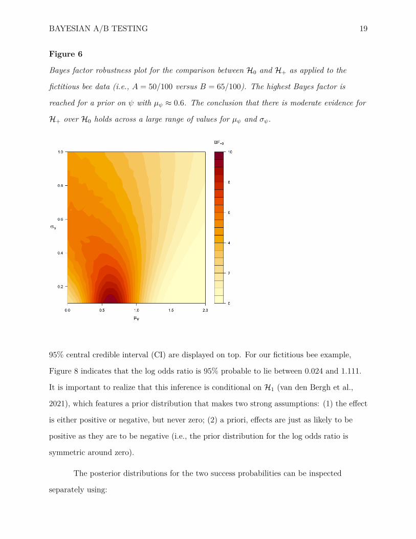
The robustness of this conclusion can be explored by changing the prior distribution

on ψ (i.e., by varying the mean and standard deviation of the normal prior distribution)

and observing the effect on the Bayes factor. Figure 6 visualizes the robustness of the

Bayes factor for changes across a range of values for µψ and σψ. The Bayes factor is highest

for low σψ values and µψ ≈ 0.6. The heatmap shows that our conclusion regarding the

evidence for H+ over H0 is relatively robust. The plot can be produced with:

R> plot_robustness(AB2, mu_range = c(0, 2), sigma_range = c(0.1, 1),

+ bftype = "BF+0")


Figure 5

Posterior probabilities of two rival hypotheses, H0 and H+, as applied to the fictitious bee

data (i.e., A = 50/100 versus B = 65/100). The grey and green areas visualize the

posterior probability of H0 and H+, respectively. Both hypotheses were assigned a

probability of 0.5 before testing.

A sequential analysis tracks the evidence in chronological order. Figure 7 shows how

the posterior probability of either hypothesis unfolds as the observations accumulate. The

figure indicates that after some initial fluctuations, and a tie after about 90 observations,

the last 110 observations cause the probability for the alternative hypothesis to increase

steadily until it reaches its final value of 0.826. Because we consider only two hypotheses,

the probability for H+ is the complement of that for H0. The sequential analysis can be

obtained as follows:

R> plot_sequential(AB2)

Having collected evidence for the hypothesis that trained bees prefer the blue disc

more than do untrained bees, one might then wish to quantify the size of this difference in

preference. To do so, we switch from a testing framework to an estimation framework. For

this purpose we adopt the two-sided model H1 and use Bayes’ rule to obtain the posterior

distribution for the log odds ratio. Figure 8 shows the result as produced via the

plot_posterior function:

R> plot_posterior(AB2, what = ‘logor’)

The dotted line in Figure 8 displays the prior distribution, the solid line displays the

posterior distribution (with a 95% central credible interval), and the posterior median and


Figure 6

Bayes factor robustness plot for the comparison between H0 and H+ as applied to the

fictitious bee data (i.e., A = 50/100 versus B = 65/100). The highest Bayes factor is

reached for a prior on ψ with µψ ≈ 0.6. The conclusion that there is moderate evidence for

H+ over H0 holds across a large range of values for µψ and σψ.

95% central credible interval (CI) are displayed on top. For our fictitious bee example,

Figure 8 indicates that the log odds ratio is 95% probable to lie between 0.024 and 1.111.

It is important to realize that this inference is conditional on H1 (van den Bergh et al.,

2021), which features a prior distribution that makes two strong assumptions: (1) the effect

is either positive or negative, but never zero; (2) a priori, effects are just as likely to be

positive as they are to be negative (i.e., the prior distribution for the log odds ratio is

symmetric around zero).

The posterior distributions for the two success probabilities can be inspected

separately using:


Figure 7

The flow of posterior probability for H0 and H+ as a function of the accumulating number

of observations for the fictitious bee data (i.e., A = 50/100 versus B = 65/100).

0 50 100 150 200

0.0

0.2

0.4

0.6

0.8

1.0

Pos

terio

r P

roba

bilit

y

n

P(H+) = 0.50P(H0) = 0.50

Prior Probabilities

P(H+ | data) = 0.826P(H0 | data) = 0.174

Posterior Probabilities

R> plot_posterior(AB2, what = ‘p1p2’)

The abtest R package has also been implemented in JASP, allowing teachers,

students, and researchers to obtain the above results with a graphical user interface. A

screenshot is provided in Figure 9. There are two ways in which the abtest functionality

can be activated in JASP. The first method, shown in Figure 9, is to activate the Summary

Statistics module using the blue ‘+’ sign in the top right corner. Clicking the Summary

Statistics icon on the ribbon and selecting Frequencies → Bayesian A/B Test brings up

the interface shown in Figure 9.

Using the Summary Statistics module, users only need to enter the total number of

successes and sample sizes in the two groups. As shown in Figure 9, the input panel offers

the similar functionality to the abtest R package. The slight difference in outcomes is due

to the fact that the results for the directional hypotheses H+ and H− involve importance

sampling (Gronau et al., in press).

The second method to activate the abtest functionality in JASP is to store the


Figure 8

Prior and posterior distribution of the log odds ratio under H1 as applied to the fictitious

bee data (i.e., A = 50/100 versus B = 65/100). The posterior median and the 95% credible

interval are shown in the top right corner.

results in a data file, open it in JASP, click the Frequencies icon on the ribbon and then

select Bayesian → A/B Test. When the data file contains the intermediate results, this

second method allows users to conduct a sequential analysis such as the one shown in

Figure 7.

To showcase the different approaches to Bayesian A/B testing we now apply the

methodology to two example data sets. The first example data set features real data

collected on the ‘Rekentuin’ online learning platform, and the second example data set

features fictitious data constructed to be representative of online webshop experiments

(i.e., relatively small effect sizes and relatively high sample sizes).


Figure 9

JASP screenshot of the Summary Statistics implementation of the abtest R package

featuring the comparison between H0 and H+ as applied to the fictitious bee data (i.e.,

A = 50/100 versus B = 65/100). The left panel shows the input options and the right panel

shows the associated analysis output.

Example I: The Rekentuin

The Rekentuin A/B Experiment

Rekentuin (Dutch for ‘math garden’) is a tutoring website where children can

improve their arithmetic skills by playing adaptive online games. The Rekentuin website is

visited by Dutch elementary school children between the ages of 4 and 12. During the

testing interval from the 22nd of January 2019 to the 5th of February 2019, a total of 15,322

children were active on Rekentuin.

The top panel of Figure 10a shows a screenshot of a Rekentuin landing page. In


Rekentuin, children earn coins by quickly solving simple arithmetic problems that are

organized into different classes (e.g., addition, subtraction, division, etc.). An example of

an addition problem is shown in the bottom panel of Figure 10b, with the coins at stake

shown in the bottom right corner. The children can use the coins that are gained to buy

virtual trophies (not shown). The better a given child performs, the more trophies they are

able to add to their trophy cabinet. The prospect of earning trophies motivates the

children to participate and perform well (for details see Brinkhuis et al., 2018; Klinkenberg

et al., 2011). On the Rekentuin landing page, the plant growth near each class of

arithmetic problem indicates the extent to which that class was recently practiced; practice

makes the plants grow, whereas periods of inactivity makes the plants wither away.

In 2019, the developers of Rekentuin faced the challenge that many children would

preferentially engage with the class of arithmetic problems that they had already mastered

(e.g., addition) – a sensible strategy if the goal is to maximize the number of coins gained.

To incentivize the children to practice other classes of arithmetic problems (e.g.,

subtraction) the developers implemented a ‘crown’ for the type of games that the children

had already mastered (see Figure 10a). Children could gain up to three crowns for each

type of game. Thus, in order to obtain more crowns, children had to engage more

frequently with the types of games they had played less often. However, the crowns did not

have the desired effect – instead of decreasing the playtime on crown games, the playtime

on crown games actually increased.

To induce the children to play other games, the Rekentuin developers constructed a

less subtle manipulation: they removed the virtual reward (i.e., the coins) from the crown

games. To test the effectiveness of this manipulation the Rekentuin developers designed an

A/B test. Half of the children continued playing on an unchanged website (version A),

whereas the other half could no longer earn coins for crown games (version B). The

children playing version B were not notified of the change but had to discover the changes

for themselves.


Figure 10

Screenshots from the Rekentuin web environment.

(a) Screenshot of a Rekentuin landing page. The page shows that the child

has earned three crowns for the category ‘optellen’ (Dutch for ‘addition’).

(b) Screenshot of an addition problem in the Rekentuin web environment.

The coins at stake are displayed on the bottom right corner.

The question of interest is whether changing the incentive structure for crown games

(i.e., removing the coins) had the desired effect. To address this question we analyzed the

Rekentuin data set using the two Bayesian A/B testing approaches outlined earlier.


Method

Preregistration

The data were collected by Abe Hofman and colleagues on the Rekentuin website in

2019. All intended analyses were applied to synthetic data and the associated analysis

scripts were stored on a repository at the Open Science Framework (OSF). We did not

inspect the data before the preregistration was finalized. All preregistration materials as

well as the real data are available on the OSF repository at https://osf.io/anvg2/.

Data Preprocessing

Our analysis concerns the last game that each child played during the testing

interval: was it a crown game or not? By examining only the last game we obtain a binary

variable (required for the present A/B test) and also allow children the maximum

opportunity to experience that crown games no longer yield coins.

We excluded children from the analyses according to two criteria. Firstly, we

excluded 8573 children who did not play any crown game during the time of testing

because they could not have experienced the experimental manipulation in version B.

Secondly, we excluded 350 children who only played one crown game and it was their last

game, because for these children we cannot observe the potential influence of the

manipulation on their playing behavior. In total we therefore excluded 8923 children.

Results

Descriptives

The Rekentuin data are summarized in Table 1. The table indicates the number of

children who played a crown game or a non-crown game as their last game. In the control

condition, 2272 out of 3178 children (≈ 71.5%) played a non-crown game as their last

game; in the treatment condition, with the coins for crown games removed, this was the



Table 1

Descriptives of the Rekentuin data. Children in version B (no coins available in crown

games) played more non-crown games.

Game Type

Coins Non-Crown Crown Total

Yes 2272 906 3178

No 2596 625 3221

Total 4868 1531 6399

case for 2596 out of 3221 children (≈ 80.6 %). It appears the manipulation had a large

effect. We now quantify the statistical evidence using the Bayesian A/B tests.

Rekentuin A/B Test: The IBE Approach

As before, in the IBE approach we assigned two uninformed beta(1,1) distributions

to the success probabilities of versions A and B. Figure 11 displays the resulting two

independent posterior distributions. Consistent with the intuitive impression from Table 1,

virtually all of the posterior mass in version B is on higher values of θnon-crown than that in

version A. This suggests that the success probability of the modified Rekentuin version is

higher and that removing the coins from the crown games had a positive impact on the

number of non-crown games played.

Figure 12 shows the conversion rate uplift. The distribution peaks at around 0.12,

indicating that the most likely conversion increase equals 12%. Also, all posterior mass

(i.e., 100% of the samples) is above zero. In other words, we can be relatively certain that

version B is better than version A. Note that this statement assumes that it is equally

likely that the alterations in version B had a positive or negative effect on the rate at which

the children played non-crown games.

In addition to the bayesAB package output, we computed the posterior probability


Figure 11

Independent posterior beta distributions of the success probabilities of playing a non-crown

game. Version A corresponds to the unchanged Rekentuin website. Version B denotes the

Rekentuin version where the children could not earn coins for crown games. The plot is

produced by the bayesAB package. The analysis used two independent beta(1, 1) priors.

of the event θnon-crownB > θnon-crown

A using the formula reported by Schmidt and Mørup

(2019). For the Rekentuin data, p(θB > θA) ≈ 1. The analytic calculation of the posterior

distribution for the difference δ = θnon-crownB − θnon-crown

A between the two independent beta

distributions fails because the data set is too large. Figure 13 plots the entire probability

distribution of the difference δ calculated using the normal approximation. The

distribution is very narrow and peaks at around 0.09.

Figure 14 plots the sequential analysis of the posterior mean of the difference

between θnon-crownA and θnon-crown

B as well as the 95% highest density interval (HDI) of the

difference. After some initial fluctuation, the posterior mean difference between θnon-crownA


Figure 12

Histogram of the conversion rate uplift from version A (i.e., 2272/3178) to version B (i.e.,

2596/3221) for the Rekentuin data. The conversion rate indicates the proportion of

children that played a non-crown game. The uplift is calculated by dividing the difference in

conversion by the conversion in A. The plot is produced by the bayesAB package.

and θnon-crownB settles at ∼ 0.09 while the HDI becomes more narrow with increasing sample

size. The range of likely values for δ eventually ranges from approximately 0.071 to 0.112.

Rekentuin A/B Test: The LTT Approach

For the LTT approach, we compare the directional hypothesis H+ (i.e., children in

version B play more non-crown games then children in version A) against the null

hypothesis H0 (i.e., the proportion of non-crown games played does not differ between

versions A and B). We employed a truncated normal distribution with µ = 0 and σ2 = 1

under the alternative hypothesis as there is a range of parameter values that seem plausible

(see, for example, Cameron et al., 2001; Tang & Hall, 1995). In particular, it is plausible

that removing the coins from the crown games results in a marked change.


Figure 13

Posterior distribution of the difference δ = θnon-crownB − θnon-crown

A for the proportion of

non-crown games between the two Rekentuin website versions. Children in version B – the

modified website version – played more non-crown games compared to children playing on

the website version A.

The observed sample proportions of 0.806 for version B and 0.715 for version A

suggest that the children in version B played more non-crown games as compared to

version A. The Bayes factor BF+0 that assesses the evidence in favor of our hypothesis that

the children in version B played more non-crown games equals 7.944e+14. This means that

the data are about 800 trillion times more likely to occur under the alternative hypothesis

H+ than under the null hypothesis H0. In sum, the Bayes factor indicates overwhelming

evidence for the alternative hypothesis (e.g., Jeffreys, 1939; Lee & Wagenmakers, 2013).

Figure 15 visualizes the dependency of the Bayes factor on the prior distribution for ψ by

varying the mean µψ and standard deviation σψ of the normal prior distribution. From


Figure 14

Sequential analysis of the difference between the success probabilities (i.e.,

θnon-crownB − θnon-crown

A ) of the two Rekentuin versions. The orange line plots the posterior

mean of the difference. The grey area visualizes the width of the highest density interval as

a function of sample size n.

looking at the heatmap we can conclude that the Bayes factor is robust. The data indicate

extreme evidence across a range of different values for the prior distribution on ψ.

Figure 16 tracks the evidence for either hypothesis in chronological order. After

about 800 observations, the evidence for H+ is overwhelming. The posterior probabilities

of the hypotheses are also shown as a probability wheel on the top of Figure 16. The green

area visualizes the posterior probability of the alternative hypothesis and the grey area

visualizes the posterior probability of the null hypothesis. The data have increased the

plausibility of H+ from 0.5 to almost 1 while the posterior plausibility of the null

hypothesis H0 has correspondingly decreased from 0.5 to almost 0.


Figure 15

Bayes factor robustness plot for the Rekentuin data.

In sum, the evidence in favor of the alternative hypothesis is overwhelming. To

complete the picture, we quantified the difference between the two Rekentuin versions by

estimating the size of the log odds ratio. Figure 17 shows the prior and posterior

distribution for the log odds ratio under the two-sided model H1. The dotted line displays

the prior distribution and the solid line displays the posterior distribution (with 95%

central credible interval). The plot indicates that, given that the log odds ratio is not

exactly zero, it is 95% probable to lie between 0.386 and 0.622, where the posterior median

is 0.504. In R and in JASP, this prior and posterior plot may also be shown on a different

scale: as an odds ratio, relative risk, absolute risk, and individual proportions.

Example II: The Fictional Webshop

The Rekentuin manipulation directly targeted children’s motivation to play the

games. Common A/B tests for web development purposes implement more subtle

manipulations that result in much smaller effect sizes. In this section we analyze such a

scenario.


Figure 16

The flow of posterior probability for H0 and H+ as a function of the number of

observations across both Rekentuin versions. The prior and posterior probabilities of the

hypotheses are displayed on top.

Consider the following fictitious scenario: an online marketing team seeks to improve

the click rate on a call-to-action button on their website’s landing page. Therefore, they

devise an A/B test. Half of the website visitors read “Try our new product!” (version A),

and the other half reads “Test our new product!” (version B).7 The success of the website

versions is measured by the rate at which website visitors click on the call-to-action button.

To demonstrate the analyses we use synthetic data. The corresponding R code can

be found at https://osf.io/anvg2/. Table 2 provides the number of clicks in each group.

The conversion rate equals 1131/10000 = 0.1131 in version A and 1275/10000 = 0.1275 in

version B. The company now wishes to determine whether and to what extent the observed

sample difference in proportions translates to the population.

7 This example was inspired by a real conversion rate optimization project at

https://blog.optimizely.com/2011/06/08/optimizely-increases-homepage-conversion-rate-by-29/


https://blog.optimizely.com/2011/06/08/optimizely-increases-homepage-conversion-rate-by-29/


Figure 17

Prior and posterior distribution of the log odds ratio under H1 for the Rekentuin data set.

The median and the 95% credible interval of the posterior density for the Rekentuin data

are shown in the top right corner.

The IBE Approach

We again use the bayesAB package in R to analyze the data according to the IBE

approach using the default independent beta(1, 1) distributions on θA and θB (Portman,

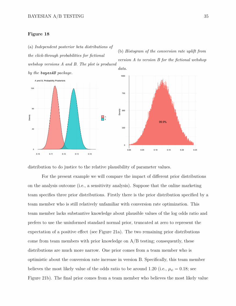
2017; R Core Team, 2020). Figure 18a illustrates the two independent posterior

distributions. We can see that version B’s posterior distribution for the success probability

assigns more mass to higher values of θ. This suggests that the click-through rate for

version B’s message “Test our new product!” is higher than that for version A’s message

“Try our new product!”.

Figure 18b depicts the conversion rate uplift. The posterior distribution for the

uplift peaks at around 0.125, indicating that the most likely conversion increase equals

12.5%. Also, most posterior mass (i.e., 99.9% of the samples) is above zero, indicating that

we can be 99.9% certain that version B is better than version A instead of the other way

around.


Table 2

Descriptives of the fictional webshop data. Visitors confronted with version B clicked the

call-to-action button more often than those confronted with version A.

Click on Button

Condition Yes No Total

A 1131 8869 10000

B 1275 8725 10000

Total 2406 17594 20000

The analytically calculated posterior probability of the event θB > θA equals 0.999

(Schmidt & Mørup, 2019). Figure 19 shows the posterior difference distribution δ. The

distribution peaks at 0.014. A difference of this size is quite large for a conversion rate

optimization endeavor. We calculated δ for this data set with the normal approximation.

Figure 20 plots the posterior mean of the difference between θA and θB as well as

the 95% highest density interval (HDI) of the difference in a sequential manner. With

increasing sample size, the HDI becomes more narrow. This indicates that the range of

likely values for δ becomes smaller. After some initial fluctuation, the posterior mean

difference between the two success probabilities θA and θB settles at ∼ 0.014.

The LTT Approach

Before the data can be analyzed according to the LTT approach, a prior

distribution for the log odds ratio has to be specified. For this purpose it is important to

note that the subtle manipulations of common A/B tests generally result in very small

effect sizes. The effect size of website changes (i.e., the difference in conversion rates

between the baseline version and its modification) is typically as small as 0.5% or less

(Berman et al., 2018). This means that the analysis of such data requires an exceptionally

narrow prior distribution that peaks at a value close to 0 in order for the shape of the prior


Figure 18

(a) Independent posterior beta distributions of

the click-through probabilities for fictional

webshop versions A and B. The plot is produced

by the bayesAB package.

(b) Histogram of the conversion rate uplift from

version A to version B for the fictional webshop

data.

distribution to do justice to the relative plausibility of parameter values.

For the present example we will compare the impact of different prior distributions

on the analysis outcome (i.e., a sensitivity analysis). Suppose that the online marketing

team specifies three prior distributions. Firstly there is the prior distribution specified by a

team member who is still relatively unfamiliar with conversion rate optimization. This

team member lacks substantive knowledge about plausible values of the log odds ratio and

prefers to use the uninformed standard normal prior, truncated at zero to represent the

expectation of a positive effect (see Figure 21a). The two remaining prior distributions

come from team members with prior knowledge on A/B testing; consequently, these

distributions are much more narrow. One prior comes from a team member who is

optimistic about the conversion rate increase in version B. Specifically, this team member

believes the most likely value of the odds ratio to be around 1.20 (i.e., µψ = 0.18; see

Figure 21b). The final prior comes from a team member who believes the most likely value


Figure 19

Posterior distribution of the difference δ = θB − θA for the click-through proportion between

the two fictitious website versions. Visitors confronted with version B clicked more often on

the call-to-action button than visitors confronted with version A.

of the odds ratio to be around 1.05 (i.e., µψ = 0.05; see Figure 21c). All three prior

distributions are truncated at zero to specify a positive effect.

In sum, the data will be analyzed with three priors: the uninformed prior with

µψ = 0 and σψ = 1, the optimistic prior with µψ = 0.18 and σψ = 0.005, and the

conservative prior with µψ = 0.05 and σψ = 0.03.

We used the abtest package (Gronau, 2019) in R (R Core Team, 2020) and JASP

for the present analysis. Before estimating the size of the effect, we first evaluate the

evidence that there is indeed a difference between version A and B. Overall the data

support the hypothesis that visitors confronted with version B click on the call-to-action

button more often than those confronted with version A. Specifically, compared to the null


Figure 20

Sequential analysis of the difference between the click-through probabilities (i.e., θB − θA) of

the two fictitious webshop versions. The orange line plots the posterior mean of the

difference. The grey area visualizes the width of the highest density interval as a function of

sample size n.

(a) Sequential analysis of the difference, with

the y-axis ranging from −1 to 1.

(b) Sequential analysis of the difference, with

the y-axis ranging from −0.1 to 0.1.

hypothesis H0, the data are about 11 times more likely under the uninformed alternative

hypothesis Hu+, about 80 times more likely under the optimistic alternative hypothesis Ho

+,

and about 27 times more likely under the conservative alternative hypothesis Hc+.8

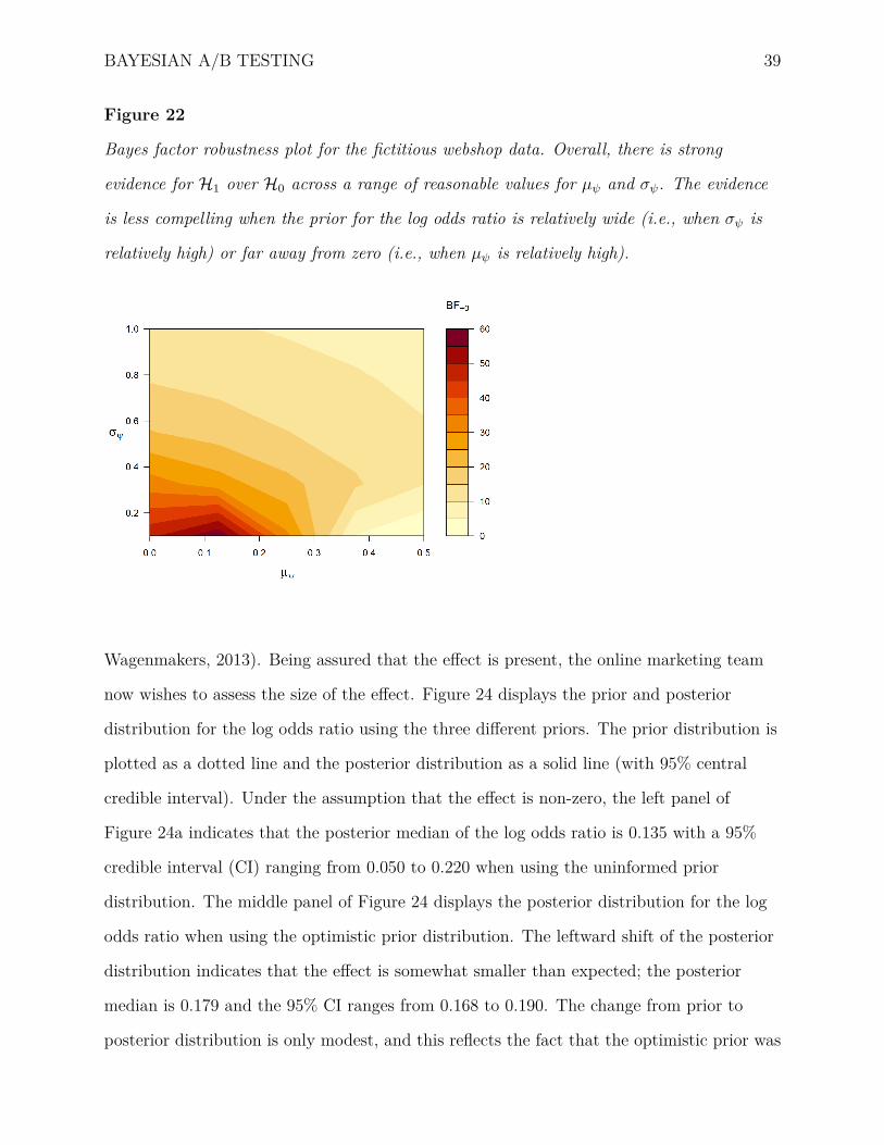
The influence of the prior distribution on the Bayes factor can be explored more

systematically with the Bayes factor robustness plot, shown in Figure 22. Varying both the

mean µψ and the standard deviation σψ of the prior distribution on ψ shows that the BF+0

mostly ranges from about 10 to about 60. The evidence is generally less compelling for

prior distributions that are relatively wide (i.e., high σψ) or relatively peaked but away

from zero (i.e, low σψ and high µψ). In both scenarios, substantial predictive mass is

8 It follows from transitivity that the optimistic colleague outpredicted the pessimistic colleague by a factor

of 80/27 ≈ 2.96.


wasted on effect sizes that are unreasonably large, and were unlikely to manifest themselves

in the context of the present webshop A/B experiment.

The prior and posterior probabilities of the hypotheses are displayed on top of

Figure 23. For the uninformed prior, the optimistic prior, and the conservative prior, the

posterior probabilities for H+ are approximately equal to 0.921, 0.988, and 0.965,

respectively. This illustrates that even though the three priors provide different levels of

evidence as measured by the Bayes factor, the overall interpretation is approximately the

same.

Figure 23 also shows the flow of posterior probability for each of the three prior

distributions as a function of the fictitious incoming observations. For all distributions, a

clear and consistent pattern of preference starts to emerge only after 10, 000 observations,

which is when the posterior probability of H+ gradually rises while that of H0 decreases

accordingly.

In sum, the fictional webshop data present strong to very strong evidence for the

claim that the conversion rate is higher in version B than in version A (Lee &

Figure 21

(a) The uninformed prior,

Hu+ : ψ ∼ N+(0, 1).

(b) The optimistic prior,

Ho+ : ψ ∼ N+(0.18, 0.0052).

(c) The conservative prior,

Hc+ : ψ ∼ N+(0.05, 0.032)


Figure 22

Bayes factor robustness plot for the fictitious webshop data. Overall, there is strong

evidence for H1 over H0 across a range of reasonable values for µψ and σψ. The evidence

is less compelling when the prior for the log odds ratio is relatively wide (i.e., when σψ is

relatively high) or far away from zero (i.e., when µψ is relatively high).

Wagenmakers, 2013). Being assured that the effect is present, the online marketing team

now wishes to assess the size of the effect. Figure 24 displays the prior and posterior

distribution for the log odds ratio using the three different priors. The prior distribution is

plotted as a dotted line and the posterior distribution as a solid line (with 95% central

credible interval). Under the assumption that the effect is non-zero, the left panel of

Figure 24a indicates that the posterior median of the log odds ratio is 0.135 with a 95%

credible interval (CI) ranging from 0.050 to 0.220 when using the uninformed prior

distribution. The middle panel of Figure 24 displays the posterior distribution for the log

odds ratio when using the optimistic prior distribution. The leftward shift of the posterior

distribution indicates that the effect is somewhat smaller than expected; the posterior

median is 0.179 and the 95% CI ranges from 0.168 to 0.190. The change from prior to

posterior distribution is only modest, and this reflects the fact that the optimistic prior was


also relatively peaked, meaning that the prior belief in the relative plausibility of the

different parameter values was very strong. Finally, the right panel of Figure 24 displays

the posterior distribution when using the conservative prior distribution. The rightward

shift of the posterior distribution indicates that the effect is somewhat larger than

expected; the posterior median is 0.072 and the 95% CI ranges from 0.029 to 0.116. The

general pattern in Figure 24 is that the change from prior to posterior is more pronounced

when prior knowledge is weak.

Concluding Comments

The A/B test concerns a comparison between two proportions and it is ubiquitous

in medicine, psychology, biology, and online marketing. Here we outlined two Bayesian

A/B tests: the ‘Independent Beta Estimation’ or IBE approach that assigns independent

beta priors to the two proportion parameters, and the ‘Logit Transformation Testing’ or

LTT approach that assigns a normal prior to the log odds ratio parameter. These

approaches are based on different assumptions and hence ask different questions. We

Figure 23

The flow of posterior probability for H0 and H+ as a function of the number of

observations across both fictitious website versions.

(a) Sequential analysis with the

uninformed prior.

0 5000 10000 15000 20000

0.0

0.2

0.4

0.6

0.8

1.0

Pos

terio

r P

roba

bilit

y

n

P(H+) = 0.50P(H0) = 0.50

Prior Probabilities

P(H+ | data) = 0.920P(H0 | data) = 0.080


(b) Sequential analysis with the

optimistic prior.

0 5000 10000 15000 20000

0.0

0.2

0.4

0.6

0.8

1.0

Pos

terio

r P

roba

bilit

y

n

P(H+) = 0.50P(H0) = 0.50

Prior Probabilities

P(H+ | data) = 0.988P(H0 | data) = 0.012


(c) Sequential analysis with the

conservative prior.

0 5000 10000 15000 20000

0.0

0.2

0.4

0.6

0.8

1.0

Pos

terio

r P

roba

bilit

y

n

P(H+) = 0.50P(H0) = 0.50

Prior Probabilities

P(H+ | data) = 0.965P(H0 | data) = 0.035



Figure 24

Prior and posterior distribution of the log odds ratio under H1 for the fictitious webshop

data set. The median and the 95% credible interval of the posterior density for the fictitious

webshop data are shown in the top right corner.

(a) The uninformed prior and

the posterior distribution of the

log odds ratio under H1.

(b) The optimistic prior and



(c) The conservative prior and



believe that the LTT approach deserves more attention: in many situations, the

assumption of independence for the proportion parameters is not realistic. Moreover, only

with the LTT approach is it possible for practitioners to obtain evidence in favor of or

against the null hypothesis.9 Both approaches allow practitioners to monitor the evidence

as the data accumulate, and to take prior/expert knowledge into account.

The LTT approach could be extended to include the possibility of an interval-null or

peri-null hypothesis to replace the traditional point-null hypothesis (Ly & Wagenmakers,

2021; Morey & Rouder, 2011). If the interval is wide, and if H1 is defined to be

non-overlapping (such that the parameter values inside the null-interval are excluded from

9 It is possible to expand the IBE approach and add a null hypothesis that both success probabilities are

exactly equal (e.g., Jeffreys, 1961), yielding an Independent Beta Testing (IBT) approach. A discussion of

the IBT is beyond the scope of this paper (but see Dablander et al., 2021).


H1) then the evidence in favor of the interval-null hypothesis may increase at a much faster

rate than that in favor of the point-null (see also Jeffreys, 1939, pp. 196-197; V. E. Johnson

and Rossell, 2010). Interval-null hypotheses are particularly attractive in fields such as

medicine and online marketing, where the purpose of the experiment concerns a practical

question regarding the effectiveness of a particular treatment or intervention. An effect size

that is so small as to be practically irrelevant will, with a large enough sample, still give

rise to a compelling Bayes factor against the point-null hypothesis. This concern can to

some extent be mitigated by considering not only the Bayes factor, but also the posterior

distribution. In the above scenario, the conclusion would be that an effect is present, but

that it is very small.

Despite its theoretical advantages, the Bayesian LTT approach has been applied to

empirical data only sporadically. This issue is arguably due to the fact that many

researchers are not familiar with this procedure and the practical advantages that it

entails. The fact that the LTT approach had, until recently, not been implemented in

easy-to-use software is another plausible reason for its widespread neglect. In this

manuscript we outlined the Bayesian LTT approach and showed how implementations in R

and JASP make it easy to execute. In addition, we demonstrated with several examples

how the LTT approach yields informative inferences that may usefully supplement or

supplant those from a traditional analysis.

Declarations

Funding

This research was supported by the Netherlands Organisation for Scientific Research

(NWO; grant #016.Vici.170.083).


Conflicts of Interest

E.J.W. declares that he coordinates the development of the open-source software

package JASP (https://jasp-stats.org), a non-commercial, publicly-funded effort to make

Bayesian and non-Bayesian statistics accessible to a broader group of researchers and

students.

Availability of data and material

Data sets and materials are available in an OSF repository at https://osf.io/anvg2/.

Code availability

The code is available on the OSF repository at https://osf.io/anvg2/.

Consent for Publication

The use and publication of the anonymized Rekentuin data has been coordinated

with and permitted by Oefenweb.

Ethics Approval, Consent to Participate

Not applicable, as we did not collect any data.

Acknowledgments

We are grateful to Oefenweb for allowing us to analyze the anonymized data and

make them publicly available.




References

Altman, D. G., & Bland, J. M. (1995). Statistics notes: Absence of evidence is not evidence

of absence. BMJ, 311 (7003), 485.

Berger, J. O., & Wolpert, R. L. (1988). The likelihood principle (2nd ed.) Institute of

Mathematical Statistics.

Berman, R., Pekelis, L., Scott, A., & Van den Bulte, C. (2018). P-hacking and false

discovery in A/B testing. https://ssrn.com/abstract=3204791

Brinkhuis, M. J., Savi, A. O., Hofman, A. D., Coomans, F., van Der Maas, H. L., &

Maris, G. (2018). Learning as it happens: A decade of analyzing and shaping a

large-scale online learning system. Journal of Learning Analytics, 5 (2), 29–46.

Cameron, J., Banko, K. M., & Pierce, W. D. (2001). Pervasive negative effects of rewards

on intrinsic motivation: The myth continues. The Behavior Analyst, 24 (1), 1–44.

Dablander, F., Huth, K., Gronau, Q. F., Etz, A., & Wagenmakers, E.-J. (2021). A puzzle

of proportions: Two popular Bayesian tests can yield dramatically different

conclusions. Manuscript submitted for publication. https://arxiv.org/pdf/2108.04909

Deng, A. (2015). Objective Bayesian two sample hypothesis testing for online controlled

experiments. WWW’15 Companion: Proceedings of the 24th International

Conference on World Wide Web, 923–928.

Deng, A., Lu, J., & Chen, S. (2016). Continuous monitoring of A/B tests without pain:

Optional stopping in Bayesian testing. 2016 IEEE International Conference on

Data Science and Advanced Analytics (DSAA), 243–252.

Gelman, A., Carlin, J. B., Stern, H. S., Dunson, D. B., Vehtari, A., & Rubin, D. B. (2013).

Bayesian data analysis. CRC press.

Goodson, M. (2014). Most winning A/B test results are illusory. Whitepaper Qubit,

https://tinyurl.com/y9g3m9bq.

Gronau, Q. F., Raj, A., & Wagenmakers, E.-J. (in press). Informed Bayesian inference for

the A/B test. Journal of Statistical Software. https://arxiv.org/abs/1905.02068

https://ssrn.com/abstract=3204791

https://arxiv.org/pdf/2108.04909

https://tinyurl.com/y9g3m9bq.

https://arxiv.org/abs/1905.02068


Gronau, Q. F. (2019). Abtest: Bayesian A/B testing.

https://CRAN.R-project.org/package=abtest

Gunel, E., & Dickey, J. (1974). Bayes factors for independence in contingency tables.

Biometrika, 61, 545–557.

Howard, J. V. (1998). The 2 × 2 table: A discussion from a Bayesian viewpoint. Statistical

Science, 13, 351–367.

Jamil, T., Ly, A., Morey, R. D., Love, J., Marsman, M., & Wagenmakers, E.-.-J. (2017).

Default “Gunel and Dickey” Bayes factors for contingency tables. Behavior Research

Methods, 49, 638–652.

JASP Team. (2020). JASP (Version 0.13)[Computer software]. https://jasp-stats.org/

Jeffreys, H. (1939). Theory of probability (1st ed.). Oxford University Press.

Jeffreys, H. (1961). Theory of probability (3rd ed.). Oxford University Press.

Jennison, C., Turnbull, B. W. et al. (1990). Statistical approaches to interim monitoring of

medical trials: A review and commentary. Statistical Science, 5 (3), 299–317.

Johnson, G., Lewis, R. A., & Nubbemeyer, E. (2017). The online display ad effectiveness

funnel & carryover: Lessons from 432 field experiments.

https://papers.ssrn.com/sol3/papers.cfm?abstract_id=2701578

Johnson, V. E., & Rossell, D. (2010). On the use of non-local prior densities in bayesian

hypothesis tests. Journal of the Royal Statistical Society: Series B, 72 (2), 143–170.

Kamalbasha, S., & Eugster, M. J. (2021). Bayesian A/B testing for business decisions.

Data science–analytics and applications (pp. 50–57). Springer.

Kass, R. E., & Raftery, A. E. (1995). Bayes factors. Journal of the American Statistical

Association, 90, 773–795.

Kass, R. E., & Vaidyanathan, S. K. (1992). Approximate Bayes factors and orthogonal

parameters, with application to testing equality of two binomial proportions.

Journal of the Royal Statistical Society, Series B, 54, 129–144.

https://CRAN.R-project.org/package=abtest

https://jasp-stats.org/

https://papers.ssrn.com/sol3/papers.cfm?abstract_id=2701578


Keysers, C., Gazzola, V., & Wagenmakers, E.-J. (2020). Using Bayes factor hypothesis

testing in neuroscience to establish evidence of absence. Nature Neuroscience, 23,

788–799.

Klinkenberg, S., Straatemeier, M., & van der Maas, H. L. (2011). Computer adaptive

practice of maths ability using a new item response model for on the fly ability and

difficulty estimation. Computers & Education, 57 (2), 1813–1824.

Kruschke, J. K. (2013). Bayesian estimation supersedes the t test. Journal of Experimental

Psychology: General, 142 (2), 573–603.

Lee, M. D., & Wagenmakers, E.-J. (2013). Bayesian cognitive modeling: A practical course.

Cambridge University Press.

Lindley, D. V. (1993). The analysis of experimental data: The appreciation of tea and wine.

Teaching statistics, 15 (1), 22–25.

Little, R. J. (1989). Testing the equality of two independent binomial proportions. The

American Statistician, 43 (4), 283–288.

Ly, A., & Wagenmakers, E.-J. (2021). Bayes factors for peri-null hypotheses. Manuscript

submitted for publication. https://arxiv.org/abs/2102.07162

McFarland, C. (2012). Experiment!: Website conversion rate optimization with A/B and

multivariate testing. New Riders.

Morey, R. D., & Rouder, J. N. (2011). Bayes factor approaches for testing interval null

hypotheses. Psychological Methods, 16, 406–419.

Patel, N. (2018). What is a good conversion rate? The answer might surprise you.

https://www.crazyegg.com/blog/what-is-good-conversion-rate/

Pham-Gia, T., Turkkan, N., & Eng, P. (1993). Bayesian analysis of the difference of two

proportions. Communications in Statistics-Theory and Methods, 22 (6), 1755–1771.

Portman, F. (2017). bayesAB: Fast Bayesian methods for A/B testing.

https://cran.r-project.org/web/packages/bayesAB/index.html

https://arxiv.org/abs/2102.07162

https://www.crazyegg.com/blog/what-is-good-conversion-rate/

https://cran.r-project.org/web/packages/bayesAB/index.html


R Core Team. (2020). R: A language and environment for statistical computing. R

Foundation for Statistical Computing. Vienna, Austria. https://www.R-project.org/

Robinson, G. K. (2019). What properties might statistical inferences reasonably be

expected to have?—crisis and resolution in statistical inference. The American

Statistician, 73, 243–252.

Schmidt, M. N., & Mørup, M. (2019). Efficient computation for Bayesian comparison of

two proportions. Statistics & Probability Letters, 145, 57–62.

Stucchio, C. (2015). Bayesian A/B testing at VWO. Whitepaper, Visual Website Optimizer.

Tang, S.-H., & Hall, V. C. (1995). The overjustification effect: A meta-analysis. Applied

Cognitive Psychology, 9 (5), 365–404.

van den Bergh, D., Haaf, J. M., Ly, A., Rouder, J. N., & Wagenmakers, E.-J. (2021). A

cautionary note on estimating effect size. Advances in Methods and Practices in

Psychological Science, 4 (1), 1–8.

van Doorn, J., Matzke, D., & Wagenmakers, E.-J. (2020). An in-class demonstration of

Bayesian inference. Psychology Learning & Teaching, 19 (1), 36–45.

von Frisch, K. (1914). Der Farbensinn und Formensinn der Biene. Gustav Fischer.

Wagenmakers, E.-J. (2007). A practical solution to the pervasive problems of p values.

Psychonomic Bulletin & Review, 14, 779–804.

Wagenmakers, E.-J., Marsman, M., Jamil, T., Ly, A., Verhagen, J., Love, J., Selker, R.,

Gronau, Q. F., Šmıra, M., Epskamp, S., et al. (2018). Bayesian inference for

psychology. Part I: Theoretical advantages and practical ramifications. Psychonomic

Bulletin & Review, 25 (1), 35–57.

Wagenmakers, E.-J., Morey, R. D., & Lee, M. D. (2016). Bayesian benefits for the

pragmatic researcher. Current Directions in Psychological Science, 25 (3), 169–176.

Wagenmakers, E.-J., Verhagen, A. J., Ly, A., Bakker, M., Lee, M. D., Matzke, D.,

Rouder, J. N., & Morey, R. D. (2015). A power fallacy. Behavior Research Methods,

47, 913–917.

https://www.R-project.org/


Williams, M. N., Bååth, R. A., & Philipp, M. C. (2017). Using Bayes factors to test

hypotheses in developmental research. Research in Human Development, 14 (4),

321–337.

Wrinch, D., & Jeffreys, H. (1921). On certain fundamental principles of scientific inquiry.

Philosophical Magazine, 42, 369–390.


Appendix

Key Statistical Results for the IBE Approach

Below we summarize three key results concerning the IBE approach to the Bayesian A/B

test where the interest centers on the difference between two binomial chance parameters

θ1 and θ2 that are assigned independent beta priors. Thus, we have

θi ∼ Beta(αi, βi), i = 1, 2 with the interest on δ = θ1 − θ2. As described in the main text,

observing y1 successes and n1 − y1 failures results in beta posterior distribution with

parameters α1 + y1 and β1 + n1 − y1. To keep notation simple we assume that the updates

have already been integrated into the parameters of the beta distribution.

The first result below gives an expression for the probability that θ1 > θ2 (Schmidt

& Mørup, 2019); the second result gives an expression of the distribution for θ1 − θ2

(Pham-Gia et al., 1993); the third result shows how this beta difference distribution can be

approximated by a normal distribution.

The Probability of θ1 > θ2 (Schmidt & Mørup, 2019)

The posterior probability that θ1 > θ2 is given by

Pr(θ1 > θ2) = Z(α1, β1, α2, β2)B(α1, β1)B(α2, β2)

,

where B(α, β) is the Beta function and the normalizing constant Z is given by

Z(α1, β1, α2, β2) = Γ(α1 + α2)Γ(β1 + β2)β1α2Γ(α1 + β1 + α2 + β2 − 1) 3F2

[1, 1 − α1, 1 − β2

β1 + 1, α2 + 1 ; 1],

where 3F2 is the generalized hypergeometric function.

The Distribution of δ = θ1 − θ2 (Pham-Gia et al., 1993)

The distribution of δ = θ1 − θ2 has the following density:

For 0 < δ ≤ 1,

f(δ) = B(α2, β1)δβ1+β2−1(1 − δ)α2+β1−1

× F1(β1, α1 + β1 + α2 + β2 − 2, 1 − α1; β1 + α2; (1 − δ), 1 − δ2)/A,


and for −1 ≤ δ < 0

f(δ) = B(α1, β2)(−δ)β1+β2−1(1 + δ)α1+β2−1

× F1(β2, 1 − α2, α1 + α2 + β1 + β2 − 2;α1 + β2; 1 − δ2, 1 + δ)/A,

where A = B(α1, β1)B(α2, β2) and F1 is Appell’s first hypergeometric function.

Moreover, if α1 + α2 > 1 and β1 + β2 > 1 we have:

f(δ = 0) = B(α1 + α2 − 1, β1 + β2 − 1)/A

.

The Normal Approximation to the Difference Between Two Beta Distributions

The Beta(α, β) distribution can be approximated by the Normal distribution when α and β

are sufficiently large:

Beta(α, β) ∼.. Normal(µ = α

α + β, σ2 = αβ

(α + β)2(α + β + 1)

).

Also, the distribution of the difference between two normally distributed variables

X ∼ N(µX , σ2X) and Y ∼ N(µY , σ2

Y ) is given by another Normal distribution as

X − Y ∼ N(µX − µY , σ2X + σ2

Y ). When the parameters of the composite beta distributions

are sufficiently large, the difference between a Beta(α2, β2) and a Beta(α1, β1) distribution

is therefore approximated as follows:

Beta(α2, β2) − Beta(α1, β1) ∼..

Normal(µ = α2

α2 + β2− α1

α1 + β1, σ2 = α2β2

(α2 + β2)2(α2 + β2 + 1) + α1β1

(α1 + β1)2(α1 + β1 + 1)

).

A Tutorial on Bayesian Inference for the A/B Test with R ... - OSF

Documents

Transcript of A Tutorial on Bayesian Inference for the A/B Test with R ... - OSF