2014Pages 1–8

An Efficient Bayesian Inference Framework forCoalescent-Based Nonparametric PhylodynamicsShiwei Lan 1∗, Julia A. Palacios 2,3, Michael Karcher 4, Vladimir N. Minin 4,5

and Babak Shahbaba 6∗

1Department of Statistics, University of Warwick, Coventry CV4 7AL.2Department of Ecology and Evolutionary Biology, Brown University.3Department of Organismic and Evolutionary Biology, Harvard University.4Department of Statistics, University of Washington.5Department of Biology, University of Washington.6Department of Statistics, University of California, Irvine.

ABSTRACTPhylodynamics focuses on the problem of reconstructing past

population size dynamics from current genetic samples taken fromthe population of interest. This technique has been extensively usedin many areas of biology, but is particularly useful for studyingthe spread of quickly evolving infectious diseases agents, e.g.,influenza virus. Phylodynamics inference uses a coalescent modelthat defines a probability density for the genealogy of randomlysampled individuals from the population. When we assume thatsuch a genealogy is known, the coalescent model, equipped witha Gaussian process prior on population size trajectory, allows fornonparametric Bayesian estimation of population size dynamics.While this approach is quite powerful, large data sets collectedduring infectious disease surveillance challenge the state-of-the-art of Bayesian phylodynamics and demand computationally moreefficient inference framework. To satisfy this demand, we providea computationally efficient Bayesian inference framework based onHamiltonian Monte Carlo for coalescent process models. Moreover,we show that by splitting the Hamiltonian function we can furtherimprove the efficiency of this approach. Using several simulated andreal datasets, we show that our method provides accurate estimatesof population size dynamics and is substantially faster than alternativemethods based on elliptical slice sampler and Metropolis-adjustedLangevin algorithm.

1 INTRODUCTIONPopulation genetics theory states that changes in population sizeaffect genetic diversity, leaving a trace of these changes inindividuals’ genomes. The field of phylodynamics relies on thistheory to reconstruct past population size dynamics from currentgenetic data. In recent years, phylodynamic inference has becomean essential tool in areas like ecology and epidemiology. Forexample, a study of human influenza A virus from sequencessampled in both hemispheres pointed to a source-sink dynamics ofthe influenza evolution [Rambaut et al., 2008].

∗to whom correspondence should be addressed

Phylodynamics connects population dynamics and genetic datausing coalescent-based methods [Griffiths and Tavare, 1994, Kuhneret al., 1998, Drummond et al., 2002, Strimmer and Pybus,2001, Drummond et al., 2005, Opgen-Rhein et al., 2005, Heledand Drummond, 2008, Minin et al., 2008, Palacios and Minin,2013]. Typically, phylodynamics relies on Kingman’s coalescentmodel, which is a probability model that describes formationof genealogical relationships of a random sample of molecularsequences. The coalescent model is parameterized in terms of theeffective population size, an indicator of genetic diversity [Kingman,1982].

While recent studies have shown promising results in alleviatingcomputational difficulties of phylodynamic inference [Palaciosand Minin, 2012, 2013], existing methods still lack the levelof computational efficiency required to realize the full potentialof phylodynamics: developing surveillance programs that canoperate similarly to weather monitoring stations allowing publichealth workers to predict disease dynamics in order to optimallyallocate limited resources in time and space. To achieve this goal,we present an accurate and computationally efficient inferencemethod for modeling population dynamics given a genealogy. Morespecifically, we concentrate on a class of Bayesian nonparametricmethods based on Gaussian processes [Minin et al., 2008, Gillet al., 2013, Palacios and Minin, 2013]. Following Palacios andMinin [2012] and Gill et al. [2013], we assume a log-Gaussianprocess prior on the effective population size. As a result, theestimation of effective population size trajectory becomes similar tothe estimation of intensity of a log-Gaussian Cox process [LGCP;Møller et al., 1998], which is extremely challenging since thelikelihood evaluation becomes intractable: it involves integrationover an infinite-dimensional random function. We resolve theintractability in likelihood evaluation by discretizing the integrationinterval with a regular grid to approximate the likelihood and thecorresponding score function.

For phylodynamic inference, we propose a computationallyefficient Markov chain Monte Carlo (MCMC) algorithm usingHamiltonian Monte Carlo [HMC; Duane et al., 1987, Neal, 2010]and one of its variation, called Split HMC [Leimkuhler andReich, 2004, Neal, 2010, Shahbaba et al., 2013], which speeds

c© 2014. 1

arX

iv:1

412.

0158

v1 [

stat

.CO

] 2

9 N

ov 2

014

Shiwei Lan et al

up standard HMC’s convergence. Our proposed algorithm hasseveral advantages. First, it updates all model parameters jointlyto avoid poor MCMC convergence and slow mixing rates whenthere are strong dependencies among model parameters [Knorr-Held and Rue, 2002]. Second, unlike a recently proposed IntegratedNested Laplace Approximation [INLA Rue et al., 2009, Palaciosand Minin, 2012] method, our approach can be extended to amore realistic setting where instead of a genealogy of the sampledindividuals, we observe their genetic data that indirectly inform usabout genealogical relationships. Third, we show that our method isup to an order of magnitude more efficient than MCMC algorithms,such as Metropolis-Adjusted Langevin algorithm [MALA; Robertsand Tweedie, 1996], adaptive MALA [aMALA; Knorr-Held andRue, 2002], and Elliptical Slice Sampler [ES2; Murray et al., 2010],frequently used in phylodynamics. Finally, although in this paperwe focus on phylodynamic studies, our proposed methodology canbe easily applied to more general point process models.

The remainder of the paper is organized as follows. In Section2, we provide a brief overview of the coalescent model and HMCalgorithms. Section 3 presents the details of our proposed samplingmethods. Experimental results based on simulated and real data areprovided in Section 4. Section 5 is devoted to discussion and futuredirections.

2 PRELIMINARIES2.1 CoalescentAssume that a genealogy with time measured in units of generationsis available. The coalescent model allows us to trace the ancestry ofa random sample of n genomic sequences as tree: two sequencesor lineages merge into a common ancestor as we go back in time.Those “merging” times are called coalescent times. The coalescentwith variable population size can be viewed as an inhomogeneousMarkov death process that starts with n lineages at present time,tn = 0, and decreases by one at each of the consequent coalescenttimes, tn−1 < · · · < t1, until reaching their most recent commonancestor [Griffiths and Tavare, 1994].

Suppose we observe a genealogy of n individuals sampled attime 0. Under the standard (isochronous) coalescent model, thecoalescent times tn = 0 < tn−1 < · · · < t1, conditioned onthe effective population size trajectory, Ne(t), have the density

P [t1, . . . , tn | Ne(t)] =

n∏k=2

P [tk−1 | tk, Ne(t)]

=n∏k=2

CkNe(tk−1)

exp

{−∫Ik

CkNe(t)

dt

},

(1)

where Ck =(k2

)and Ik = (tk, tk−1]. Note that the larger the

population size, the longer it takes for two lineages to coalesce.Further, the larger the number of lineages, the faster two of themmeet their common ancestor [Palacios and Minin, 2012, 2013].

For rapidly evolving organisms, we may have different samplingtimes. When this is the case, the standard coalescent model can begeneralized to account for such heterochronous sampling [Rodrigoand Felsenstein, 1999]. Under the heterochronous coalescent thenumber of lineages change at both coalescent times and samplingtimes. Let {tk}nk=1 denote the coalescent times as before, but now

Observed data 6t4

t5

t3

t2

32 43354433

x 1

t1

x 4

x 3

x 2

x 5

1,60,2 0,6

I

0,3

I I I I I I

Number of lineages

s3

s2

s1

Grid of Points

Time (Present to Past)

0,4 0,5 1,5

t =

Fig. 1. A genealogy with coalescent times and sampling times. Bluedashed lines indicate the observed times: coalescent times {t1, · · · , t6} andsampling times {s1, s2, s3}. The intervals where the number of lineageschange are denoted by Ii,k . The superimposed grid {x1, · · · , x5} is markedby gray dashed lines. We count the number of lineages in each intervaldefined by grid points, coalescent times and sampling times.

let sm = 0 < sm−1 < · · · < s1 denote sampling times ofnm, . . . , n1 sequences respectively, where

∑mj=1 nj = n. Further,

let s and n denote the vectors of sampling times {sj}mj=1 andnumbers of sequences {nj}mj=1 sampled at these times, respectively.Then the coalescent likelihood of a single genealogy becomes

P [t1, . . . , tn | s,n, Ne(t)] =

n∏k=2

C0,k exp{−∫I0,k

C0,k

Ne(t)dt−

∑i≥1

∫Ii,k

Ci,kNe(t)

dt}

Ne(tk−1),

(2)

where the coalescent factor Ci,k =(li,k2

)depends on the number

of lineages li,k in the interval Ii,k defined by coalescent times andsampling times. For k = 2, . . . , n, we denote half-open intervalsthat end with a coalescent event by

I0,k = (max{tk, sj}, tk−1 ] , (3)

for sj < tk−1, and half-open intervals that end with a samplingevent by (i > 0)

Ii,k = (max{tk, sj+i}, sj+i−1 ] , (4)

for tk < sj+i−1 ≤ sj < tk−1. In density (2), there are n − 1intervals {Ii,k}i=0 and m − 1 intervals {Ii,k}i>0 for all i, k. Notethat only those intervals satisfying Ii,k ⊂ (tk, tk−1] are non-empty.See Figure 1 for more details.

We can think of isochronous coalescence as a special case ofheterochronous coalescence when m = 1, C0,k = Ck, I0,k =Ik, Ii,k = ∅ for i > 0. Therefore, in what follows, we refer toEquation (2) as the general case.

2

Efficient Bayesian Phylodynamics

We assume the following log-Gaussian Process prior on theeffective population size, Ne(t):

Ne(t) = exp[f(t)], f(t) ∼ GP(0,C(θ)), (5)

where GP(0,C(θ)) denotes a Gaussian process with mean function0 and covariance function C(θ). A priori, Ne(t) is a log-GaussianProcess.

For computational convenience, we use Brownian motion, whichis a special case of GP, as our prior for f(t). We define thecovariance function as C(κ) = 1

κCBM , where the precision

parameter κ has a Gamma(α, β) prior. For ascending times 0 =x0 < x1 < x2 < · · · < xD−1, the (i, j)-th element of CBM

is set to min{xi, xj}. This way, we reduce the computationalcomplexity of inverting the covariance matrix from O(n3) to O(n)since the inverse covariance matrix is tri-diagonal [Rue and Held,2005, Palacios and Minin, 2013] with elements

C−1BM (i, j) =

1{i+1≤D−1}

xi+1 − xi+

1

xi − xi−1, if i = j,

− 1

|xi − xj |, if |i− j| = 1,

0, otherwise.

In practice we modify the (1, 1) element, 1/(x2 − x1) + 1/x1, tobe 1/(x2 − x1) and denote the resulting precision matrix as C−1

in

to indicate that it comes from an intrinsic autoregression [Besag andKooperberg, 1995, Knorr-Held and Rue, 2002]. Note that C−1

in isdegenerate in 1 eigen direction so we add a small number, e, to thediagonal elements of C−1

in to make it invertible when Cin is needed.

2.2 HMCHamiltonian Monte Carlo [Duane et al., 1987, Neal, 2010] is aMetropolis sampling algorithm that suppresses the random walkbehavior by proposing states that are distant from the current state,but nevertheless accepts new proposals with high probability. Thesedistant proposals are found by numerically simulating Hamiltondynamics, whose state space consists of position, denoted by thevector θ, and momentum, denoted by the vector p. The objectiveis to sample from the continuous probability distribution with thedensity function π(θ). It is common to assume p ∼ N (0,M),where M is a symmetric, positive-definite matrix known as the massmatrix, often set to the identity matrix I for convenience.

In this simulation of Hamiltonian dynamics, the potential energy,U(θ), is defined as the negative log density of θ (plus any constant);the kinetic energy, K(p) for momentum variable p, is set to bethe negative log density of p (plus any constant). Then the totalenergy of the system, the Hamiltonian function, is defined as theirsum: H(θ,p) = U(θ) +K(p). Then the system of (θ,p) evolvesaccording to the following set of Hamilton’s equations:

θ = ∇pH(θ,p) = M−1p,

p = −∇θH(θ,p) = −∇θU(θ).(6)

In practice, we use a numerical method called leapfrog toapproximate the Hamilton’s equations [Neal, 2010] when theanalytical solution is not available. We numerically solve the systemfor L steps, with some step size, ε, to propose a new state in

the Metropolis algorithm, and accept or reject it according tothe Metropolis acceptance probability. [See Neal, 2010, for morediscussions].

3 METHOD3.1 DiscretizationAs discussed above, the likelihood function (2) is intractablein general. We can, however, approximate the likelihood usingdiscretization. To this end, we use a fine regular grid, x ={xd}Dd=1, over the observation window and approximate Ne(t) bya piece-wise constant function as follows:

Ne(t) ≈D−1∑d=1

exp[f(x∗d)]1t∈(xd,xd+1], x∗d =xd + xd+1

2. (7)

Note that the regular grid x does not coincide with the samplingcoalescent times, except for the first sampling time sm = x1and the last coalescent time t1 = xD . To rewrite (2) using theapproximation (7), we sort all the time points {t, s,x} to create newD+m+n−4 half-open intervals {I∗α} with either coalescent timepoints, sampling time points, or grid time points as the end points(See Figure 1).

For each α ∈ {1, · · · , D + m + n − 4}, there exists some i, kand d such that I∗α = Ii,k ∩ (xd, xd+1]. Each integral in density (2)can be approximated as a sum:∫

Ii,k

Ci,kNe(t)

dt ≈∑

I∗α⊂Ii,k

Ci,k exp[−f(x∗d)]∆d,

where ∆d := xd+1 − xd. This way, the likelihood of coalescenttimes (2) can be rewritten as a product of the following terms:{

Ci,kexp[f(x∗d)]

}yαexp

{− Ci,k∆d

exp[f(x∗d)]

}, (8)

where yα is set to 1 if I∗α ends with a coalescent time, and to0 otherwise. This happens to be proportional to the probabilitymass of a Poisson random variable yα with intensity λα :=Ci,k∆d exp[−f(x∗d)]. Therefore, the likelihood of coalescent times(2) can be approximated as follows:

P [t1, . . . , tn | Ne(t)] ≈D+m+n−4∏

α=1

P [yα | Ne(t)]

=

D−1∏d=1

∏I∗α⊂(xd,xd+1]

{Ci,k

exp[f(x∗d)]

}yαexp

{− Ci,k∆d

exp[f(x∗d)]

},

(9)

where the coalescent factor Ci,k on each interval I∗α is determinedby the number of lineages li,k in I∗α.

3.2 Sampling methodsDenote f := {f(x∗d)}D−1

d=1 . Our model can be summarized as

yα|f ∼ Poisson[λα(f)],

f |κ ∼ N(

0,1

κCin

),

κ ∼ Gamma(α, β).

(10)

3

Shiwei Lan et al

Transforming the coalescent times, sampling times and grid pointsinto {yα, Ci,k,∆d}, we condition on these data to generateposterior samples for f = logNe(x

∗) and κ, where x∗ = {x∗d}is the set of the middle points in (7). We use these posterior samplesto make inference about Ne(t).

For sampling f using HMC, we use (9) to compute the discretizedlog-likelihood

l = −D−1∑d=1

∑I∗α⊂(xd,xd+1]

{yαf(x∗d) + Ci,k∆d exp[−f(x∗d)]}

and the corresponding gradient (score function)

sd = −∑

I∗α⊂(xd,xd+1]

{yα − Ci,k∆d exp[−f(x∗d)]} .

Because the prior on κ is conditionally conjugate, we coulddirectly sample from its full conditional posterior distribution,

κ|· ∼ Gamma(α+ (D − 1)/2, β + fTC−1in f/2). (11)

However, updating f and κ separately is not recommended ingeneral because of their strong interdependency [Knorr-Held andRue, 2002]: large value of precision κ strictly confines the variationof f , rendering slow movement in the space occupied by f .Therefore, we update (f , κ) jointly in MCMC sampling algorithms.In practice, it is better to sample θ := (f , τ), where τ = log(κ) isin the same scale as f = logNe(x

∗). Note that the log-likelihoodof θ is the same as that of f because equation (2) does not involveτ . The log-density prior on θ is defined as follows:

logP (θ) ∝ ((D − 1)/2 + α− 1)τ − (fTC−1in f/2 + β)eτ . (12)

3.3 Speed up by splitting HamiltonianSplitting the Hamiltonian is a technique used to speed up HMC[Leimkuhler and Reich, 2004, Neal, 2010, Shahbaba et al., 2013].The underlying idea is to divide the total Hamiltonian into severalterms, such that the dynamics associated with some of these termscan be solved analytically. For these parts, typically quadratic forms,the simulation of the dynamics does not introduce a discretizationerror, allowing for faster movements in the parameter space.

We split the Hamiltonian H(θ,p) = U(θ) +K(p) as follows:

H(θ,p) =−l − [(D − 1)/2 + α− 1]τ + βeτ

2+

fTC−1in feτ + pTp

2+−l − [(D − 1)/2 + α− 1]τ + βeτ

2.

(13)

We further split the middle part (which is the dominantpart) into two dynamics involving f |τ and τ |f respectively,{

f |τ = p−D,

p−D = −C−1in feτ .

(14a){τ |f = pD,

pD = −fTC−1in feτ/2.

(14b)

Using the spectral decomposition C−1in = QΛQ−1 and denoting

f∗ :=√

Λeτ/2Q−1f and p∗−D := Q−1p−D , we can analyticallysolve the dynamics (14a) as follows [Lan, 2013] (more details are inthe appendix):[

f∗(t)p∗−D(t)

]=

[cos(√

Λeτ/2t) sin(√

Λeτ/2t)

− sin(√

Λeτ/2t) cos(√

Λeτ/2t)

] [f∗(0)

p∗−D(0)

].

We then use the standard leapfrog method to solve the dynamics(14b) and the residual dynamics in (13) in a symmetric way. Note

that we only need to diagonalize C−1in once before the sampling, and

calculate fTC−1in feτ = f∗Tf∗; therefore, the overall computational

complexity of the integrator is O(D2).

4 EXPERIMENTSWe illustrate the advantages of our HMC-based methods using threesimulation studies and apply these methods to analysis of a realdataset. We evaluate our methods by comparing them to INLAin terms of accuracy and to several sampling algorithms, MALA,aMALA, and ES2, in terms of sampling efficiency. We definesampling efficiency as time-normalized effective sample size (ESS).Given B MCMC samples for each parameter, we calculate thecorresponding ESS = B[1 + 2ΣK

k=1γ(k)]−1, where ΣKk=1γ(k) is

the sum of K monotone sample autocorrelations [Geyer, 1992]. Weuse the minimum ESS normalized by the CPU time, s (in seconds),as the overall measure of efficiency: min(ESS)/s.

We tune the stepsize and number of leapfrog steps for our HMC-based algorithm such that their overall acceptance probabilitiesare in a reasonable range (close to 0.70). Since MALA [Robertsand Tweedie, 1996] and aMALA [Knorr-Held and Rue, 2002]can be viewed as HMC with one leap frog step for numericallysolving Hamiltonian dynamics, we implement MALA and aMALAproposals using our HMC framework. MALA, aMALA, andHMC-based methods update f and τ jointly. aMALA uses ajoint block-update method designed for GMRF models: it firstgenerates a proposal κ∗|κ from some symmetric distributionindependently of f , and then updates f∗|f , κ∗ based on a localLaplace approximation. Finally, (f∗, κ∗) is either accepted orrejected. It can be shown that aMALA is equivalent to a formof Riemannian MALA [Roberts and Stramer, 2002, Girolami andCalderhead, 2011, also see Appendix B]. In addition, aMALAclosely resembles the most frequently used MCMC algorithm inGaussian process-based phylodynamics [Minin et al., 2008, Gillet al., 2013].

ES2 [Murray et al., 2010] is a commonly used sampling algorithmdesigned for models with Gaussian process priors. It was alsoadopted by Palacios and Minin [2013] for phylodynamic inference.ES2 implementation relies on the assumption that the targetdistribution is approximately normal. This, of course, is not asuitable assumption for the joint distribution of (f , τ). Therefore,we alternate the updates f |κ and κ|f when using ES2.

4.1 SimulationsWe simulate three genealogies relating n = 50 individuals with thefollowing true trajectories:

1. logistic trajectory:

Ne(t) =

{10 + 90

1+exp(2(3−(t mod 12))), t mod 12 ≤ 6,

10 + 901+exp(2(−9+(t mod 12)))

, t mod 12 > 6;

2. exponential growth: Ne(t) = 1000 exp(−t);

3. boombust:

Ne(t) =

{1000 exp(t− 2), t ≤ 2,

1000 exp(−t+ 2), t > 2.

4

Efficient Bayesian Phylodynamics

20 15 10 5 0

0.5

2.0

5.0

20.0

50.0

200.

0

Time (past to present)

Sca

led

N[e

](t)

logistic

TruthINLAHMCsplitHMC

MALAaMALAES2

8 6 4 2 0

5e−

015e

+00

5e+

015e

+02

Time (past to present)

Sca

led

N[e

](t)

exponential growth

8 6 4 2 0

5e−

015e

+00

5e+

015e

+02

Time (past to present)

Sca

led

N[e

](t)

boombust

Fig. 2. INLA vs MCMC: simulated data under logistic (top), exponentialgrowth (middle) and boombust (bottom) population size trajectories. Dottedblue lines show 95% credible intervals given by INLA and shaded regionsshow 95% credible interval estimated with MCMC samples given bysplitHMC.

Method AP s/iter minESS(f )/s spdup(f ) ESS(τ )/s spdup(τ )ES2 1.00 1.56E-03 0.22 1.00 0.25 1.00MALA 0.84 1.81E-03 0.41 1.90 1.47 5.89

I aMALA 0.53 4.60E-03 0.08 0.38 0.13 0.53HMC 0.80 9.51E-03 1.78 8.23 1.81 7.25splitHMC 0.75 7.30E-03 2.19 10.13 2.51 10.04ES2 1.00 1.57E-03 0.21 1.00 0.23 1.00MALA 0.78 1.82E-03 0.32 1.53 1.14 5.03

II aMALA 0.53 4.61E-03 0.09 0.41 0.18 0.79HMC 0.76 1.19E-02 2.73 12.99 1.34 5.91splitHMC 0.76 7.84E-03 4.31 20.50 2.35 10.40ES2 1.00 1.56E-03 0.20 1.00 0.20 1.00MALA 0.83 1.82E-03 0.37 1.87 1.05 5.18

III aMALA 0.53 4.61E-03 0.08 0.40 0.14 0.67HMC 0.81 1.18E-02 2.22 11.24 1.17 5.75splitHMC 0.72 7.41E-03 2.87 14.53 1.90 9.33

Table 1. Sampling efficiency in modeling simulated population trajectories.The true population trajectories are: I) logistic, II) exponential growth,and III) boombust respectively. AP is the acceptance probability. s/iter isthe seconds per sampling iteration. “spdup” is the speedup of efficiencymeasurement minESS/s using ES2 as baseline.

We use D = 100 equally spaced grid points in the approximationof likelihood when applying INLA and MCMC algorithms (HMC,splitHMC, MALA, aMALA and ES2).

Figure 2 compares the estimates of Ne(t) using INLA andMCMC algorithms in for the three simulations. In general, theresults of MCMC algorithms match closely with those of INLA.It is worth noting that MALA and ES2 are occasionally slow toconverge. Also, INLA fails when the number of grid points is large,e.g. 10000, while MCMC algorithms can still perform reliably.

For each experiment we run 15000 iterations with the first 5000samples discarded. We repeat each experiment 10 times. The resultsprovided in Table 1 are averaged over 10 repetitions. As we can see,our methods substantially improve over MALA, aMALA and ES2.Note that although aMALA has higher ESS compared to MALA,its time-normalized ESS is worse than that of MALA because of itshigh computational cost of calculating the Fisher information.

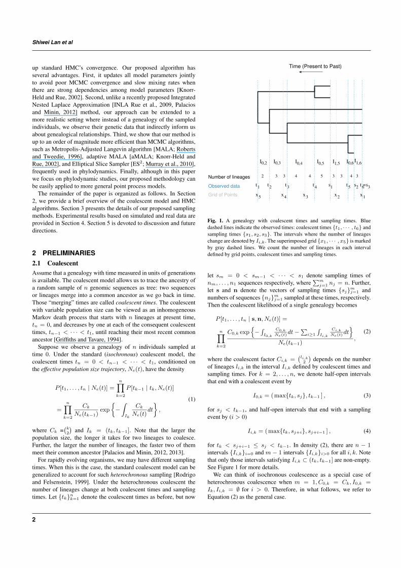
Figure 3 compares different sampling methods in terms of theirconvergence to the stationary distribution when we increase the sizeof grid points to D = 1000. As we can see in this more challengingsetting, Split HMC has the fastest convergence rate. Neither MALAnor aMALA, on the other hand, has converged within the given time.aMALA is not even getting close to the stationarity, making it muchworse than MALA.

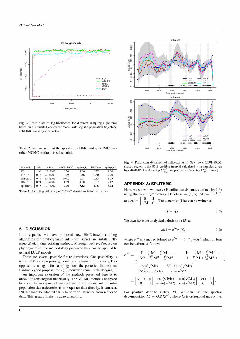
4.2 Human Influenza A in New YorkNext, we analyze real data based on a genealogy estimated from 288H3N2 sequences sampled in New York state from January 2001 toMarch 2005 in order to estimate population size dynamics of humaninfluenza A in New York [Palacios and Minin, 2012, 2013]. Thekey feature of the influenza A virus epidemic in temperate regionslike New York are the epidemic peaks during winters followed bystrong bottlenecks at the end of the winter season. We use 120 gridpoints in the likelihood approximation. Figure 4 shows that withC−1BM , MCMC algorithms identify such peak-bottleneck pattern

more clearly than INLA. However, their results based on intrinsicprecision matrix, C−1

in , are quite comparable to that of INLA. In

5

Shiwei Lan et al

0 500 1000 1500 2000

−50

0−

400

−30

0−

200

time (seconds)

log−

likel

ihoo

d

HMCsplitHMCMALAaMALAES2

Convergence rate

Fig. 3. Trace plots of log-likelihoods for different sampling algorithmsbased on a simulated coalescent model with logistic population trajectory.splitHMC converges the fastest.

Table 2, we can see that the speedup by HMC and splitHMC overother MCMC methods is substantial.

Method AP s/Iter minESS(f )/s spdup(f ) ESS(τ )/s spdup(τ )ES2 1.00 1.92E-03 0.34 1.00 0.27 1.00MALA 0.78 2.12E-03 0.29 0.86 0.60 2.20aMALA 0.77 8.48E-03 0.002 0.01 0.33 1.23HMC 0.71 1.74E-02 1.69 4.98 0.57 2.12splitHMC 0.75 1.11E-02 2.90 8.53 1.06 3.92

Table 2. Sampling efficiency of MCMC algorithms in influenza data.

5 DISCUSSIONIn this paper, we have proposed new HMC-based samplingalgorithms for phylodynamic inference, which are substantiallymore efficient than existing methods. Although we have focused onphylodynamics, the methodology presented here can be applied togeneral LGCP models.

There are several possible future directions. One possibility isto use ES2 as a proposal generating mechanism in updating f asopposed to using it for sampling from the posterior distribution.Finding a good proposal for κ(τ), however, remains challenging.

An important extension of the methods presented here is toallow for genealogical uncertainty. The MCMC methods analyzedhere can be incorporated into a hierarchical framework to inferpopulation size trajectories from sequence data directly. In contrast,INLA cannot be adapted easily to perform inference from sequencedata. This greatly limits its generalizability.

25

1020

5020

050

020

00

Time (past to present)

Sca

led

N[e

](t)

++++++++++++++++++++++++++++++++++++++++++++++++++++++++++++++++++++++++++++++++++++++++++++++++++++++++++++++++++++++++++++++++++++++++++++++++++++++++++++++++++++++++++++++++++++++++++++++++++++++++++++++++++++++++++++++++++++++++++++++++++++++++++++++++++++++++++++++++++++++++++++++++

2000 2001 2002 2003 2004 2005

influenza

INLAHMCsplitHMC

MALAaMALAES2

1020

5010

020

050

0

Time (past to present)

Sca

led

N[e

](t)

++++++++++++++++++++++++++++++++++++++++++++++++++++++++++++++++++++++++++++++++++++++++++++++++++++++++++++++++++++++++++++++++++++++++++++++++++++++++++++++++++++++++++++++++++++++++++++++++++++++++++++++++++++++++++++++++++++++++++++++++++++++++++++++++++++++++++++++++++++++++++++++++

2000 2001 2002 2003 2004 2005

influenza

INLAHMCsplitHMC

MALAaMALAES2

Fig. 4. Population dynamics of influenza A in New York (2001-2005):shaded region is the 95% credible interval calculated with samples givenby splitHMC. Results using C−1

BM (upper) vs results using C−1in (lower).

APPENDIX A: SPLITHMCHere, we show how to solve Hamiltonian dynamics defined by (13)using the “splitting” strategy. Denote z := (f ,p), M := C−1

in eτ ,

and A :=

[0 I−M 0

]. The dynamics (14a) can be written as

z = Az. (15)

We then have the analytical solution to (15) as

z(t) = eAtz(0), (16)

where eAt is a matrix defined as eAt :=∑∞i=0

ti

i!Ai, which in turn

can be written as follows:

eAt =

[I− t2

2!M + t4

4!M2 + · · · It− t3

3!M + t5

5!M2 + · · ·

−Mt+ t3

3!M2 − t5

5!M3 + · · · I− t2

2!M + t4

4!M2 + · · ·

]

=

[cos(√

Mt) M− 12 sin(

√Mt)

−M12 sin(

√Mt) cos(

√Mt)

]

=

[M− 1

2 00 I

] [cos(√

Mt) sin(√

Mt)

− sin(√

Mt) cos(√

Mt)

] [M

12 0

0 I

].

For positive definite matrix M, we can use the spectraldecomposition M = QDQ−1, where Q is orthogonal matrix, i.e.

6

Efficient Bayesian Phylodynamics

Q−1 = QT. Therefore we have

eAt =

[Q 00 Q

] [D−

12 0

0 I

] [cos(√

Dt) sin(√

Dt)

− sin(√

Dt) cos(√

Dt)

]

·[D

12 0

0 I

] [Q−1 0

0 Q−1

].

(17)

In practice, we only need to diagonalize C−1in once: C−1

in =QΛQ−1, then D = Λeτ . If we let f∗ :=

√Λeτ/2Q−1f , p∗−D :=

Q−1p−D , we have the following solution (16):

[f∗(t)

p∗−D(t)

]=

[cos(√

Λeτ/2t) sin(√

Λeτ/2t)

− sin(√

Λeτ/2t) cos(√

Λeτ/2t)

] [f∗(0)

p∗−D(0)

].

We then apply leapfrog method to the remaining dynamics.Algorithm 1 summarizes these steps.

Algorithm 1 splitHMC for the coalescent model (splitHMC)Initialize θ(1) at current θ = (f , τ)

Sample a new momentum value p(1) ∼ N (0, I)

CalculateH(θ(1),p(1)) = U(θ(1)) +K(p(1)) according to (13)for ` = 1 to L do

p(`+1/2)

= p(`)

+ ε/2

[s(`)

((D − 1)/2 + α− 1)− β exp(τ(`))

]

p(`+1/2)D = p

(`)D − ε/2f

∗(`)Tf∗(`)

/2

τ(`+1/2)

= τ(`)

+ ε/2p(`+1/2)D[

f∗(`+1)

p∗(`+1/2)−D

]←

cos(√

Λe12τ(`+1/2)

ε) sin(√

Λe12τ(`+1/2)

ε)

− sin(√

Λe12τ(`+1/2)

ε) cos(√

Λe12τ(`+1/2)

ε)

·[

f∗(`)

p∗(`+1/2)−D

]

τ(`+1)

= τ(`+1/2)

+ ε/2p(`+1/2)D

p(`+1)D = p

(`+1/2)D − ε/2f∗(`+1)T

f∗(`+1)

/2

p(`+1)

= p(`+1/2)

+ ε/2

[s(`+1)

((D − 1)/2 + α− 1)− β exp(τ(`+1))

]

end forCalculateH(θ(+1),p(L+1)) = U(θ(L+1)) +K(p(L+1)) according to (13)Calculate the acceptance probability α = min{1, exp[−H(θ(+1),p(L+1)) +

H(θ(1),p(1))]}Accept or reject the proposal according to α for the next state θ′

APPENDIX B: ADAPTIVE MALAWe now show that the joint block updating in Knorr-Held and Rue[2002] can be recognized as an adaptive MALA algorithm. First,we sample κ∗|κ ∼ p(κ∗|κ) ∝ κ∗+κ

κ∗κ on [κ/c, κc] for some c > 1

controlling the step size of κ. Denote w := {Ci,k∆d}D+m+n−41

Algorithm 2 Adaptive MALA (aMALA)Given current state θ = (f , κ) calculate potential energy U(θ)repeatz ∼ Unif[1/c, c], u ∼ Unif[0, 1]

until u < z+1/zc+1/c

update precision parameter κ∗ = κzSample momentum p ∼ N (0,G(f , κ∗)−1)Calculate log of proposal density log p(f∗|f , κ∗) =− 1

2pTG(f , κ∗)p + 1

2log det G(f , κ∗)

update momentum p← p− ε/2G(f , κ∗)−1∇U(f , κ∗)update latent variables f∗ = f + εpupdate momentum p← p− ε/2G(f∗, κ)−1∇U(f∗, κ)Calculate log of reverse proposal density log p(f |f∗, κ) =− 1

2pTG(f∗, κ)p + 1

2log det G(f∗, κ)

Calculate new potential energy U(θ∗)Accept/reject the proposal according to logα = −U(θ∗) +U(θ)− log p(f∗|f , κ) + log p(f |f∗, κ) for the next state θ′

and use the following Taylor expansion for log p(f |κ) about f :

log p(f |κ) = −yTf −wT exp(−f)− 1

2fTκC−1

in f

≈ −yTf − (w exp(−f))T[1− (f − f) + (f − f)2/2]− 1

2fTκC−1

in f

= (−y + w exp(−f)(1 + f))Tf +

1

2fT[κC−1

in + diag(w exp(−f))]f

=: bTf − 1

2fTGf ,

where b(f) := −y + w exp(−f)(1 + f), G(f , κ) := κC−1in +

diag(w exp(−f)). Setting f to the current state, f , and proposef∗|f , κ∗ from the following Gaussian distribution:

f∗|f , κ∗ ∼ N (µ,Σ),

with

µ = G(f , κ∗)−1b(f) = f + G(f , κ∗)−1∇f log p(f |κ∗) and

Σ = G(f , κ∗)−1,

which has the same form as Langevin dynamical proposals.Interestingly, G(f , κ) is exactly the (observed) Fisher information.That is, this approach is equivalent to Riemannian MALA [Girolamiand Calderhead, 2011].

Finally, θ∗ = (f∗, κ∗) is jointly accepted with the followingprobability:

α = min

{1,p(θ∗|D)

p(θ|D)

p(κ|κ∗)p(f |f∗, κ)

p(κ∗|κ)p(f∗|f , κ∗)

}= min

{1,p(θ∗|D)

p(θ|D)

p(f |f∗, κ)

p(f∗|f , κ∗)

},

where p(κ∗|κ) is a symmetric proposal. Algorithm 2 summarizesthe steps for adaptive MALA.

7

Shiwei Lan et al

REFERENCESJulian Besag and Charles Kooperberg. On conditional and intrinsic autoregressions. Biometrika, 82(4):733–746, 1995.A. J. Drummond, A. Rambaut, B. Shapiro, and O. G. Pybus. Bayesian coalescent inference of past population dynamics from molecular

sequences. Molecular Biology and Evolution, 22(5):1185–1192, 2005. doi: 10.1093/molbev/msi103.Alexei J. Drummond, Geoff K. Nicholls, Allen G. Rodrigo, and Wiremu Solomon. Estimating mutation parameters, population history and

genealogy simultaneously from temporally spaced sequence data. Genetics, 161(3):1307–1320, 2002.S. Duane, A. D. Kennedy, B J. Pendleton, and D. Roweth. Hybrid Monte Carlo. Physics Letters B, 195(2):216 – 222, 1987.C. J. Geyer. Practical Markov Chain Monte Carlo. Statistical Science, 7(4):473–483, 1992.Mandev S Gill, Philippe Lemey, Nuno R Faria, Andrew Rambaut, Beth Shapiro, and Marc A Suchard. Improving bayesian population

dynamics inference: a coalescent-based model for multiple loci. Molecular biology and evolution, 30(3):713–724, 2013.M. Girolami and B. Calderhead. Riemann manifold Langevin and Hamiltonian Monte Carlo methods. Journal of the Royal Statistical

Society, Series B, (with discussion) 73(2):123–214, 2011.R. C. Griffiths and Simon Tavare. Sampling theory for neutral alleles in a varying environment. Philosophical Transactions of the Royal

Society of London. Series B: Biological Sciences, 344(1310):403–410, 1994. doi: 10.1098/rstb.1994.0079.Joseph Heled and Alexei Drummond. Bayesian inference of population size history from multiple loci. BMC Evolutionary Biology, 8(1):

289, 2008. ISSN 1471-2148. doi: 10.1186/1471-2148-8-289.J.F.C. Kingman. The coalescent. Stochastic Processes and their Applications, 13(3):235 – 248, 1982. ISSN 0304-4149. doi: http:

//dx.doi.org/10.1016/0304-4149(82)90011-4.Leonhard Knorr-Held and Havard Rue. On Block Updating in Markov Random Field Models for Disease Mapping. Scandinavian Journal

of Statistics, 29(4):597–614, 2002.Mary K. Kuhner, Jon Yamato, and Joseph Felsenstein. Maximum likelihood estimation of population growth rates based on the coalescent.

Genetics, 149(1):429–434, 1998.Shiwei Lan. Advanced bayesian computational methods through geometric techniques, 2013. Copyright - Copyright ProQuest, UMI

Dissertations Publishing 2013; Last updated - 2014-02-13; First page - n/a; M3: Ph.D.B. Leimkuhler and S. Reich. Simulating Hamiltonian Dynamics. Cambridge University Press, 2004.Vladimir N. Minin, Erik W. Bloomquist, and Marc A. Suchard. Smooth skyride through a rough skyline: Bayesian coalescent-based inference

of population dynamics. Molecular Biology and Evolution, 25(7):1459–1471, 2008. doi: 10.1093/molbev/msn090.Jesper Møller, Anne Randi Syversveen, and Rasmus Plenge Waagepetersen. Log gaussian cox processes. Scandinavian Journal of Statistics,

25(3):pp. 451–482, 1998. ISSN 03036898.Iain Murray, Ryan Prescott Adams, and David J.C. MacKay. Elliptical slice sampling. JMLR: W&CP, 9:541–548, 2010.R. M. Neal. MCMC using Hamiltonian dynamics. In S. Brooks, A. Gelman, G. Jones, and X. L. Meng, editors, Handbook of Markov Chain

Monte Carlo. Chapman and Hall/CRC, 2010.Rainer Opgen-Rhein, Ludwig Fahrmeir, and Korbinian Strimmer. Inference of demographic history from genealogical trees using reversible

jump markov chain monte carlo. BMC Evolutionary Biology, 5(1):6, 2005. ISSN 1471-2148. doi: 10.1186/1471-2148-5-6.Julia A. Palacios and Vladimir N. Minin. Integrated nested laplace approximation for bayesian nonparametric phylodynamics. In Nando

de Freitas and Kevin P. Murphy, editors, UAI, pages 726–735. AUAI Press, 2012.Julia A. Palacios and Vladimir N. Minin. Gaussian process-based bayesian nonparametric inference of population size trajectories from gene

genealogies. Biometrics, 69(1):8–18, 2013. ISSN 1541-0420. doi: 10.1111/biom.12003.Andrew Rambaut, Oliver G Pybus, Martha I Nelson, Cecile Viboud, Jeffery K Taubenberger, and Edward C Holmes. The genomic and

epidemiological dynamics of human influenza A virus. Nature, 453(7195):615–619, 2008.Gareth O Roberts and Osnat Stramer. Langevin diffusions and metropolis-hastings algorithms. Methodology and computing in applied

probability, 4(4):337–357, 2002.Gareth O. Roberts and Richard L. Tweedie. Exponential convergence of langevin distributions and their discrete approximations. Bernoulli,

2(4):pp. 341–363, 1996. ISSN 13507265.Allen G Rodrigo and Joseph Felsenstein. Coalescent approaches to hiv population genetics. The evolution of HIV, pages 233–272, 1999.H. Rue and L. Held. Gaussian Markov Random Fields: Theory and Applications, volume 104 of Monographs on Statistics and Applied

Probability. Chapman & Hall, London, 2005.Havard Rue, Sara Martino, and Nicolas Chopin. Approximate bayesian inference for latent gaussian models by using integrated nested laplace

approximations. Journal of the Royal Statistical Society: Series B (Statistical Methodology), 71(2):319–392, 2009. ISSN 1467-9868. doi:10.1111/j.1467-9868.2008.00700.x.

Babak Shahbaba, Shiwei Lan, Wesley O. Johnson, and RadfordM. Neal. Split hamiltonian monte carlo. Statistics and Computing, pages1–11, 2013. ISSN 0960-3174. doi: 10.1007/s11222-012-9373-1.

Korbinian Strimmer and Oliver G Pybus. Exploring the demographic history of dna sequences using the generalized skyline plot. MolecularBiology & Evolution, 18(12):2298–2305, January 2001 2001.

8