Bayesian inference in mixtures-of-experts and hierarchical mixtures-of-experts models with an...

Bayesian Inference in Mixtures-of-Experts and Hierarchical Mixtures-of-Experts Models Withan Application to Speech RecognitionAuthor(s): Fengchun Peng, Robert A. Jacobs and Martin A. TannerSource: Journal of the American Statistical Association, Vol. 91, No. 435 (Sep., 1996), pp. 953-960Published by: American Statistical AssociationStable URL: http://www.jstor.org/stable/2291714 .

Accessed: 03/10/2013 12:38

Your use of the JSTOR archive indicates your acceptance of the Terms & Conditions of Use, available at .http://www.jstor.org/page/info/about/policies/terms.jsp

.JSTOR is a not-for-profit service that helps scholars, researchers, and students discover, use, and build upon a wide range ofcontent in a trusted digital archive. We use information technology and tools to increase productivity and facilitate new formsof scholarship. For more information about JSTOR, please contact [email protected].

.

American Statistical Association is collaborating with JSTOR to digitize, preserve and extend access to Journalof the American Statistical Association.

http://www.jstor.org

This content downloaded from 128.151.80.181 on Thu, 3 Oct 2013 12:38:41 PMAll use subject to JSTOR Terms and Conditions

http://www.jstor.org/action/showPublisher?publisherCode=astata

http://www.jstor.org/stable/2291714?origin=JSTOR-pdf

http://www.jstor.org/page/info/about/policies/terms.jsp


Bayesian Inference in Mixtures-of-Experts and Hierarchical Mixtures-of-Experts Models With an

Application to Speech Recognition Fengchun PENG, Robert A. JACOBS, and Martin A. TANNER

Machine classification of acoustic waveforms as speech events is often difficult due to context dependencies. Here a vowel recognition task with multiple speakers is studied via the use of a class of modular and hierarchical systems referred to as mixtures-of-experts and hierarchical mixtures-of-experts models. The statistical model underlying the systems is a mixture model in which both the mixture coefficients and the mixture components are generalized linear models. A full Bayesian approach is used as a basis of inference and prediction. Computations are performed using Markov chain Monte Carlo methods. A key benefit of this approach is the ability to obtain a sample from the posterior distribution of any functional of the parameters of the given model. In this way, more information is obtained than can be provided by a point estimate. Also avoided is the need to rely on a normal approximation to the posterior as the basis of inference. This is particularly important in cases where the posterior is skewed or multimodal. Comparisons between a hierarchical mixtures-of-experts model and other pattern classification systems on the vowel recognition task are reported. The results indicate that this model showed good classification performance and also gave the additional benefit of providing for the opportunity to assess the degree of certainty of the model in its classification predictions.

1. INTRODUCTION

Psychological studies of human speech perception have documented people's extraordinary abilities to categorize acoustic waveforms as speech events. These abilities seem all the more impressive when we consider that people can accurately perceive speech while listening to unfamiliar voices in noisy surroundings with widely varying rates of speech production. How we do this, and how we can pro- gram computers to do it, are topics of much recent research.

Advances in our understanding of speech perception have been achieved through the use of various complementary research programs. Psychoacousticians, perceptual and cognitive psychologists, and psycholinguists study the perceptual, cognitive, and linguistic mechanisms that allow people to process speech in an efficient and seemingly effortless man- ner (O'Shaughnessy 1987). Related research is pursued by statisticians and computer scientists, who attempt to build machines that can recognize speech in a wide range of en- vironments (Rabiner and Juang 1993). These research paths have converged in pinpointing the factors that make speech perception a challenging task. Several of these factors stem from the fact that speech production is highly context dependent (O'Shaughnessy 1987). For example, it is often difficult to partition a speech waveform into the acoustic segments that correspond to distinct phonetic segments. This is primarily due to coarticulation; the vocal articulatory move- ments for successive sounds overlap in time such that the motions used to produce a particular phonetic segment are dependent on the preceding and succeeding phonetic segments. As a second example, identical phonemes are spoken

Fengchun Peng is Visiting Assistant Professor, Department of Mathe- matics and Statistics, University of Nebraska, Lincoln, NE 68588. Robert A. Jacobs is Assistant Professor, Department of Brain and Cognitive Sci- ences, University of Rochester, NY 14627. Martin Tanner is Professor, Department of Statistics, Northwestern University, Evanston, IL 60208. This work was supported by National Institutes of Health Research Grants RO1-CA35464, R29-MH54770, and T32-CA09667. This work was also supported by National Science Foundation Grant DMS-9505799 and by a grant from Sun Microsystems. The authors thank J. Kolassa, R. Neal, B. Yakir, two anonymous referees, and the associate editor for their insightful comments, and V. de Sa for providing the speech data set.

differently by different speakers, and by the same speaker at different points in time, yet must be classified as equivalent events. Differences in speakers' speech are often correlated with speakers' gender, age, and dialect.

There are at least three common approaches to overcom- ing the problems associated with context dependency (Ra- biner and Juang 1993). One approach is to detect invariant features. For example, though some features of the acoustic waveform corresponding to a phonetic segment may vary with a speaker's speech characteristics, other acoustic features may be common to all speakers. A related approach is to normalize the acoustic waveform for the context. For example, there may exist a transformation that removes the features that arise due to the speaker's characteristics. A third approach is to use knowledge of context to aid in the classification of speech events. For example, different classifiers may be used depending on the speaker's gender. In addition to classifying the speech events, this approach must also classify the context.

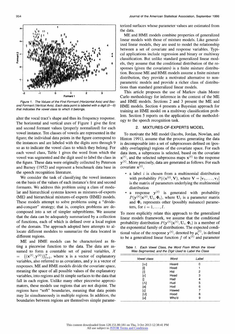
This article considers the application of a class of statistical models to a speech recognition task. The models classify speech events by detecting features that are invariant to speakers' speech characteristics. The data in Figure 1 represent instances of vowels spoken by a large number of speakers. The instances were taken from utterances of 10 words, each of which began with an "h," contained a vowel in the middle, and ended with a "d." These data are from 75 speakers (32 male adults, 28 female adults, and 15 children) who uttered each word twice, with the words in different random orders for each presentation. A spectral analysis was performed on each utterance; the portion of the spectrogram corresponding to the vowel was hand segmented, and the first two formants were extracted from the middle portion of the segmented region. Formants are the vocal tract's resonant frequencies. Different placements of the speech articulators, corresponding to different vowels,

? 1996 American Statistical Association Journal of the American Statistical Association

September 1996, Vol. 91, No. 435, Applications & Case Studies

953



954 Journal of the American Statistical Association, September 1996

N 12

-2 -1 0 1 2 2233

3 4 ~4 4 (U ~~ ~~~~~~~4 4

LL4 4 44 4

0 ~~06& 66

9 ~ ~ ~~66 6

9 7 ~~~~~~~~~~~~6

Formant 1

Figure 1. The Values of the First Formant (Horizontal Axis) and Sec- ond Formant (Vertical Axis). Each data point is labeled with a digit (0-9) that indicates the vowel class to which it belongs.

alter the vocal tract's shape and thus its frequency response. The horizontal and vertical axes of Figure 1 give the first and second formant values (properly normalized) for each vowel instance. Ten classes of vowels are represented in the figure; the individual data points in the figure correspond to the instances and are labeled with the digits zero through 9 so as to indicate the vowel class to which they belong. For each vowel class, Table 1 gives the word from which the vowel was segmented and the digit used to label the class in the figure. These data were originally collected by Peterson and Barney (1952) and represent a benchmark data base in the speech recognition literature.

We consider the task of classifying the vowel instances on the basis of the values of each instance's first and second formants. We address this problem using a class of modular and hierarchical systems known as mixtures-of-experts (ME) and hierarchical mixtures-of-experts (HME) models. These models attempt to solve problems using a "divide- and-conquer" strategy; that is, complex problems are de- composed into a set of simpler subproblems. We assume that the data can be adequately summarized by a collection of functions, each of which is defined over a local region of the domain. The approach adopted here attempts to al- locate different modules to summarize the data located in different regions.

ME and HME models can be characterized as fit- ting a piecewise function to the data. The data are assumed to form a countable set of paired variables, X - {(x(t),y(t))}fT , where x is a vector of explanatory variables, also referred to as covariates, and y is a vector of responses. ME and HME models divide the covariate space, meaning the space of all possible values of the explanatory variables, into regions and fit simple surfaces to the data that fall in each region. Unlike many other piecewise approxi- mators, these models use regions that are not disjoint. The regions have "soft" boundaries, meaning that data points may lie simultaneously in multiple regions. In addition, the boundaries between regions are themselves simple parame-

terized surfaces whose parameter values are estimated from the data.

ME and HME models combine properties of generalized linear models with those of mixture models. Like generalized linear models, they are used to model the relationship between a set of covariate and response variables. Typi- cal applications include regression and binary or multiway classification. But unlike standard generalized linear models, they assume that the conditional distribution of the responses (given the covariates) is a finite mixture distribution. Because ME and HME models assume a finite mixture distribution, they provide a motivated alternative to nonparametric models and provide a richer class of distributions than standard generalized linear models.

This article proposes the use of Markov chain Monte Carlo methodology for inference in the context of the ME and HME models. Sections 2 and 3 present the ME and HME models. Section 4 presents a Bayesian approach for training an HME model on a multiway classification problem. Section 5 reports on the application of the methodology to the speech recognition task.

2. MIXTURES-OF-EXPERTS MODEL

To motivate the ME model (Jacobs, Jordan, Nowlan, and Hinton 1991), assume that the process generating the data is decomposable into a set of subprocesses defined on (possibly overlapping) regions of the covariate space. For each data item, a subprocess is selected, based on the covariate x(t), and the selected subprocess maps x(t) to the response y(t). More precisely, data are generated as follows. For each covariate x(t),

* a label i is chosen from a multinomial distribution with probability P(ilx(t), V), where V = [vi, . ., vjI] is the matrix of parameters underlying the multinomial distribution

* a response y(t) is generated with probability P(y(t)lx(t), Ui Ij), where Ui is a parameter matrix and 'j, represents other (possibly nuisance) parameters, for i = 1,... ,I.

To more explicitly relate this approach to the generalized linear models framework, we assume that the conditional probability distribution P(y(t) lx(t), Ui, 4iJ) is a member of the exponential family of distributions. The expected conditional value of the response y(t), denoted by ttt), is defined to be a generalized linear function f of x(t) and parameter

Table 1. Each Vowel Class, the Word From Which the Vowel Was Segmented, and the Digit Used to Label the Class

Vowel class Word Label

[wI] Heard 0 [i] Heed 1 [I] Hid 2 [E] Head 3 [] Had 4 [A] Hud 5 [a] Hod 6 [sv] Hawed 7 [U] Hood 8 [u] Who'd 9



Peng, Jacobs, and Tanner: Speech Recognition 955

Gating 9

Network

x

1.111.

Expert Expert Network Network

x x

Figure 2. A Mixtures-of-Experts Model.

matrix Ui. The quantities 7ji = f- (pi) and (]Pi are the natural parameter and dispersion parameter of the response's conditional distribution p(y(t) lx(t), Ui, ,i). The total probability of generating y(t) from x(t) is given by the mixture density

p(y(t) IX(t), O)=E P(ilx(t), V)P(y(t) Ix(t), Uijj i), (1)

where e = [vi,..., vI,Ui, ..., Ui, ib, 4.... ]T is the matrix of all parameters. Assuming independently dis- tributed data, the total probability of the data set X is the product of T such densities, with the likelihood given by

L(OIX) fJ E P(ijx(t), V)P(y(t) lx(t), Ui, 4i). (2) t i

Thus the ME model can be viewed as a mixture model in which the mixing weights and the mixed distributions are dependent on the covariate x.

Figure 2 presents a graphical representation of the ME model. The model consists of I modules referred to as expert networks. These networks approximate the data within each region of the covariate space: expert network i maps its input, the covariate vector x, to an output vector pi. It is assumed that different expert networks are appropriate in different regions of the covariate space. Consequently, the model requires a module, referred to as a gating network, that identifies for any covariate x the expert or blend of experts whose output is most likely to approximate the corresponding response vector y. The gating network outputs are a set of scalar coefficients gi that weight the contri- butions of the various experts. For each covariate x, these coefficients are constrained to be nonnegative and to sum to 1. The total output of the model, given by

n

i=l1

is a convex combination of the expert outputs for each x. From the perspective of statistical mixture modeling, we

identify the gating network with the selection of a particular subprocess. That is, the gating outputs gi are interpreted as the covariate-dependent, multinomial probabilities of se- lecting subprocess i. Different expert networks are identified with different subprocesses; each expert models the covariate-dependent distributions associated with its corresponding subprocess.

The expert networks map their inputs to their outputs in a two-stage process. During the first stage, each expert multiplies the covariate vector x by a matrix of parameters. (The vector x is assumed to include a fixed component of 1 to allow for an intercept term.) For expert i, the matrix is denoted as Ui and the resulting vector is denoted as 71i:

71i = Uix. (4)

During the second stage, Tli is mapped to the expert output pi by a monotonic, continuous nonlinear function f.

Selection of the nonlinear function f is based on the na- ture of the problem. For regression problems, f may be taken as the identity function (i.e., the experts are linear). Moreover, the probabilistic component of the model may be Gaussian. In this case the likelihood is a mixture of Gaussians:

L(F9 l ) = H gi(t) Si l 1/2-1 / 2 [y(t) _ Ht(t)]TE-1 [y (t) _tt(t)]

t i

(5)

The expert output pit) and expert dispersion parameter Ei are interpreted as the mean and covariance matrix of expert i's Gaussian distribution for response y(t) given covariate x(t). The output of the entire model 8(t) is, therefore, interpreted as the expected value of y(t) given x(t).

For binary classification problems, f may be the logistic function:

AHi et (6)

In this case rTi may be interpreted as the log-odds of "success" under a Bernoulli probability model. The probabilistic component of the model is assumed to be the Bernoulli distribution. The likelihood is a mixture of Bernoulli densities:

L(@lX) H E g() )[/Z( )]8 [1p(t)]-y(t) (7 t i

The quantity /uz(t) is expert i's conditional probability of classifying the covariate x(t) as success, and ,u is the expected success of x(t). Other problems (e.g., multiway classification, counting, rate estimation, survival estimation) may suggest other choices for f. In all cases we take the inverse of f to be the canonical link function for the appropriate probability model (McCullagh and Nelder 1989).




Gating Network

g2

x

i gg 922 Gating

Network Network * 211/ \/8112-

x 4'1 A fX12l 21 x P-, ,i -~2 ,P .. 2. Expert Expert Expert Expert

Figure 3. A Hierarchical Mixtures-of-Experts Model.

The gating network also forms its outputs in two stages. During the linear stage, it computes the intermediate variables (i as the inner product of the covariate vector x and the vector of parameters vi:

(i = v[x. (8)

During the nonlinear stage, the (i are mapped to the gating outputs gi. This mapping is performed by using a general- ization of the logistic function:

gi= E (9)

Note that the inverse of this function is the canonical link function for a multinomial response model (McCullagh and Nelder 1989).

In this article, Bayesian inference regarding the gating and expert networks' parameters is performed using Markov chain Monte Carlo methods. In particular, we make use of the fact that the problem is greatly simplified by augmenting the observed data with the unobserved indicator variables indicating the expert in the model. This idea of using data augmentation (Tanner and Wong 1987) in mixture problems, where the mixing parameters are unknown scalars, has been discussed in detail by Diebolt and Robert (1994). Jordan and Jacobs (1994) showed how the parameters of the ME (as well as the HME) model can be estimated using this augmentation idea in the context of the Expectation Maximization (EM) algorithm. Jordan and Xu (1993) presented an analysis of the convergence properties of the EM algorithm as applied to ME and HME models. A discussion of the relationship between ME models and neural networks was presented by Peng, Jacobs, and Tan- ner (1995), who also presented an ME model for regression and illustrated Bayesian learning in a nonlinear regression context.

3. HIERARCHICAL MIXTURES-OF-EXPERTS MODEL

The philosophy underlying the ME model is to solve complex modeling problems by dividing the covariate space

into restricted regions, and then use different generalized linear models to fit the data in each region. If this "divide- and-conquer" approach is useful, then it seems desirable to pursue this strategy to its logical extreme. In particular, it seems sensible to divide the covariate space into restricted regions, and then to recursively divide each region into sub- regions. The hierarchical extension of the ME model, referred to as the HME model, is a tree-structured model that implements this strategy (Jordan and Jacobs 1994). In contrast to the single-level ME model, the HME model can summarize the data at multiple scales of resolution due to its use of nested covariate regions. Jordan and Jacobs (1994) have empirically found that models with a nested structure often outperform single-level models with an equivalent number of free parameters.

The HME model, unlike the ME model, contains multiple gating networks. These gating networks, located at the nonterminals of the tree, implement the recursive splitting of the covariate space. The expert networks are at the ter- minals of the tree. Because they are defined over relatively small regions of the covariate space, the experts can fit simple functions to the data (e.g., generalized linear models).

Figure 3 illustrates an HME model. For explanatory rea- sons, we limit our presentation to a two-level tree; the extension to trees of arbitrary depth and width is straightfor- ward. The bottom-level of the tree contains a number of clusters, each one itself an ME model. (The tree in the figure contains two clusters, each enclosed in a box.) The top level of the tree contains an additional gating network that combines the outputs of each cluster. As a matter of nota- tion, we use the letter i to index branches at the top level and the letter j to index branches at the bottom level. The expert networks map the covariate x to the output vectors

ij. The output of the ith cluster is given by

Pi = E9jliAij, (10) j

where the scalar Yjli is the output of the gating network in the ith cluster corresponding to the jth expert. The output of the model as a whole is given by

IL = E gi-Li, (11)

where the scalar gi is the output of the top-level gating network corresponding to the ith cluster.

The probabilistic interpretation of the HME model is a simple extension of that given to the ME model. In short, we assume that the process that generates the data involves a nested sequence of decisions, based on the covariate x(t). The outcome of this sequence is the selection of a subprocess that maps x(t) to the response y(t). In a two-level tree, for example, we assume that a label i is chosen from a multinomial distribution with probability P(ijx(t),V), where V is the matrix of parameters underlying this distribution. Next, a label j is chosen from another multinomial distribution with probability P(j x(t), Vi), where the parameters Vi underlying this distribution are dependent on the value of label i. Subprocess (i, j) generates a re-



Peng, Jacobs, and Tanner; Speech Recognition 957

sponse y(t) by sampling from a distribution with probability P(y(t)[lpij bij)v where rij = f-l(pij) is the natural parameter of this distribution and 4Ji3 is its dispersion parameter. This latter probability may also be written as p(y(t) x(t),Uij,ij). The total probability of generating y(t) from x(t) is given by the hierarchical mixture density

P(y(t) IX(t), E) = P(i IX(t) I V) EP(j Ix(t), Vi) i j

X P(y(0) x(), Uij, 44ij), (12)

where 9 is the matrix of all parameters. To model this process with the HME model, we identify

the top-level gating network with the selection of the label i and the bottom-level gating networks with the selection of the label j. Different expert networks are identified with different subprocesses. To give just one example, the resulting likelihood function for a binary classification problem is a hierarchical mixture of Bernoulli densities:

L(@lX)= t Eg" E 9(t) [A()] [1 _ 4()]l-yt (13) t i j

The quantity pij is expert (i, j)'s conditional probability of classifying the covariate x(t) as success, and ,u is the expected success of x(t).

The HME model has some similarities to classification and regression tree models that have previously been pro- posed in the statistics literature. Like Classification and Regression Trees (CART) (Breiman, Friedman, Olshen, and Stone 1984) and Multi-Adaptive Regression Splines (MARS) (Friedman 1991), the HME model is a tree- structured approach to piecewise function approximation. A major difference between the HME model and CART or MARS is in the way that the covariate space is segmented into regions. Both CART and MARS use "hard" boundaries between regions; each data item lies in exactly one region. In contrast, the HME model allows regions to overlap, so that data items may reside in multiple regions. Thus the boundaries between the regions are said to be "soft." MARS is restricted to forming region boundaries that are perpendicular to one of the covariate space axes. Thus MARS is coordinate dependent; that is, it is sensitive to the particular choice of covariate variables used to en- code the data. The HME model is not coordinate dependent; boundaries between regions are formed along hyperplanes at arbitrary orientations in the covariate space. In addition, CART and MARS are nonparametric techniques, whereas the HME model is a parametric model. Jordan and Jacobs (1994) compared the performance of the HME model with that of CART and MARS on a robot dynamics task and found that the HME model (using the EM algorithm to estimate the parameters) yielded a modest improvement.

4. HME MODEL FOR MULTIWAY CLASSIFICATION

A basic simplification is obtained by augmenting the observed data with the unobserved indicator variables indicating the expert in the model. If we define Z}t) = 1 with

probability

h(t) P(ilx(t), V) E, P(jlx(t) x Vr)P(y(t) IX(t), U', x4)

ZEi P(ilx(t), V) Ej P(j Ix(t), VX)P(y(t) IX(t), UJ3, xij) '

(14)

and z(t) 1 with probability

(t) P(jxt Vi)P(Y(t) iX(t) I uij, 4!ij) h =t .1 (5 iji Ej P(jX(t), Vi)P(y(t)jX(t), Uij, ij) (5

then z (t) = Zi(t) X Z(t) will take value 1 with probability 3ii

h(t) - P(ilx(t), V)P(jIX(t) I Vi)P(y(t) Ix(t), U31 )

Z.3 P(ilX(t) V) E P(jIx(t), IVi)P(y(t) Ix(t), TUiJ, 4i)'

(16) where Uij is the matrix of parameters associated with the (i, j)th expert network, V is the matrix of parameters associated with the gating network at the top level of the model, and Vi is the matrix of parameters associated with the gating network in the ith cluster at the bottom level. Let X' {(X(t),y(t),Z(t))} IT , where z(t) is the vector of indicator variables. Then the augmented likelihood for the HME model is

L(OIX') = 1 J P(ijx(t), V)P(jlx(t), Vi) t i j

(t) X p(y(t) |x(t), UjX ij )}z%i (1 7)

= ]J H17 {gIt)g(l)p(y(t) x(t) U t i j

(18)

where gi is the same as defined in (9) and

vT (t vx(t) gj ii E eVT X(t) (19)

Restricting our attention to multiway classification problems, suppose that y = (y1, y,Y) is the outcome from the n classes, taking the values either zero or 1; Ui

(Uij ,.... , Uijn)T is the n x p matrix of parameters associated with the (i, j)th expert network; and ?ij = 1 for all i and j. In this case the conditional probability model for y can be written as

n

fJIhtk' (20) P(yjx, Uij, (Iij)I ij.k '(0

k=1

If we express this probability model in the density form of the exponential family, then the natural parameters are defined as

rlijk = log ijk (21)

= UijkX, (22)

and hence entak




Table 2. Classification Performances of Four Systems on the Data From the Prediction Set

Total in Gibbs EM CART CART11 Category category # correct #correct #correct #correct

0 127 123.3 123.3 114 124 1 132 96.3 97.9 94 112 2 139 95.9 92.0 30 60 3 137 84.1 79.2 90 109 4 133 104.6 100.9 73 117 5 136 109.1 106.3 102 109 6 128 88.5 84.4 90 96 7 132 74.5 78.0 72 71 8 140 80.7 77.1 49 38 9 141 58.0 50.2 87 60

0-9 1,345 915.0 889.3 801 896

NOTE: The first two systems are the HME model trained with the Gibbs sampler algorithm and with the EM algorithm; the last two systems are two versions of CART.

As noted earlier, the inverse of (23) is the canonical link function for a multinomial response model (McCullagh and Nelder 1989). It follows from (9), (19), and (23) that the augmented likelihood (18) can be rewritten as

L(E)JX') ]J ]J fH (t) (t) (t)}k (24) t i j k

T vTx(t) T ) (t)

tl fl kl l Z- vTx(t) J evTx(t)

(t) (t) Z1

(

eU%jkx(t) )~

(25)

Because this equation with independent normal priors (mean zero, variance A-) on E does not yield standard densities for the full conditionals, we apply the approach of Muller (1991) to draw the posterior sample for the top-level gating network parameter matrix V, the bottom-level gating network parameter matrices Vi, and the bottom-level expert network parameter matrices Uij. In particular, to draw a deviate from a full conditional, we use the Metropo- lis algorithm. As an example, consider the top-level gating network parameters. A candidate value for the next point in the Metropolis chain (V(k+l)) is drawn from the multivariate normal distribution with the current sample values as its mean and a diagonal variance-covariance matrix to allow for variation around the current sample values; that is, V(k+l) + N(V(k), y2l). This candidate value is accepted or rejected according to the standard Metropolis scheme (Tanner 1993). This Metropolis algorithm is iterated, and the final value in this chain is treated as a deviate from the full conditional distribution.

5. THE SPEECH RECOGNITION PROBLEM

The HME model was applied to the speech recognition task described earlier. The data set consists of 1,494 data items (75 speakers x 10 vowel classes x 2 presentations of each vowel; note that three speakers' data for the vowel [W]

us

IN

C4

0.0 02 0:4 0.6 0.8 1.0 Class Probability

Figure 4. The Estimated Posterior Distribution for the Probability that the Data Item Belongs to the Correct Vowel Class 1. Note that the mass is concentrated at unity thus indicating that the model is confident in its prediction. This graph gives the result of one chain of the Gibbs sampler; the other nine chains produced nearly identical results. The Gelman and Rubin R value was equal to 1.0.

are missing from the data set). From this collection, 149 items were randomly selected and assigned to a training set; the remaining 1,345 were assigned to a prediction set. The HME model consisted of 3 gating networks and 10 expert networks arranged in a two-level tree structure. The bottom level had two clusters, each with 1 gating network and 5 expert networks. The outputs of these two clusters were combined by a gating network located at the top level.

The model was trained via the Gibbs sampler algorithm described previously and also via the EM algorithm. For the Gibbs sampler, 10 chains of length 7,500 were created. It is known that posterior distributions based on mixture models can be highly multimodal. We used two approaches in the context of the Gibbs sampler to address this aspect of the problem. In one approach we allowed for mode jumping as the chain moved through the parameter space-hopefully avoiding oversampling in the neighborhoods of isolated mi- nor modes. To facilitate this, after every 100 iterations of the Gibbs sampler, the parameter vector e was selected at random from the modes defined by 20 independent and randomly initialized runs of the EM algorithm. This candidate value was compared to the current point in the Gibbs sampler chain using a Metropolis test based on the observed posterior. The data in Table 2 and Figures 4, 5, and 6 are based on the final 500 iterations of each chain. The Metropolis algorithm used to sample from the full conditional distributions was run for 40 iterations, with the variance on the normal distribution equal to 1.0. The variance of each of the normal priors on the components of the expert and gating networks parameters was equal to 50,000.

It is noted that this mode jumping approach introduces a possible approximation due to the fact that the transition kernel of the Metropolis test is discrete, whereas the posterior distribution is continuous. The expectation is that this algorithm will quickly converge to a good approximation. As a check, we adopted a second approach based on work of Gelman and Rubin (1992). In particular, we formed a



Peng, Jacobs, and Tanner: Speech Recognition 959

________________] 'I 0.0 0.2 0.4 0.6 0.8 1.0 0.0 0.2 0.4 0.6 0.8 1.0

Clan Pmrbabity Cla PrdbNt

d o - .0 0.2 Q04 0.6 0.6 1.0 00.0 0.2 0.4 0.6 0.8 1.0

Can Probabil CIO PWWmf

0.0 0.2 0.4 0.6 Q. 1.0 0.0 Q2 0.4 Q. Q. 1.0 Clas ProbabiGty Ckl Pobabity

no0 0.2 0.4 0.6. 0.8 1.0 Q.0 0.2 0.4 0.6 0.8 1.0 Cla ProbabUIb Clo Pmbbf

Q0 0 0.4 Q 0.8 t.0 Q0 02 0 0.6 08 1. ClI PbUl aa O P abf

Figure 5. Ten Estimated Posterior Distributions for the Probability that the Data Item Belongs to the Correct Vowel Class 8. The "v" along the horizontal axis of each graph indicates the expected value of the distribution. Note that the mass is concentrated in the middle of the probability range, thus indicating that the model is not confident in its prediction. The Gelman and Rubin R value was equal to 1.024.

mixture of normals to approximate the observed posterior. We then drew a sample of size 1,000 from this approximation. We then used importance sampling to obtain 10 starting points for 10 Gibbs sampler chains, which we ran without mode jumping. This second approach confirmed the results of the first approach; that is, the two approaches yielded qualitatively similar outcomes. An alternative technique for sampling from multimodal posteriors was presented by Neal (1994).

The convergence of the 10 chains was evaluated using the technique of Gelman and Rubin (1992). Intuitively, this Gelman and Rubin technique for assessing convergence compares the between-chain variation to the within- chain variation; an algorithm is said to converge when the between-chain and within-chain variations are comparable in size. To assess convergence of our Gibbs sampler algorithm, we used as input to the Gelman and Rubin technique the conditional predictive probability that a data item belongs to a particular vowel class. (For vowel class j, this is p(ya = I Wx, t).) Use of the conditional predictive probability when assessing convergence was also discussed by Neal

the9rsult Fof the fivrsate vapprach that isexmie, the twGppoces-

sentend Rby n Nea (1994). o eced11,mannta therwa cnveruggetdeience of thl0cains was eovalaedrusngefo

the trechniqu oft Gelmand ande Rbn(99)lnuiiey

Table 2 shows the classification performances of four systems on the data from the prediction set. The first two systems are the HME model trained with the Gibbs sampler algorithm and with the EM algorithm. The number of correct classifications is an average over the 10 chains for the first system and over 20 instances of the second system, where the instances differ due to the random ini- tial settings of the system's parameter values. In both cases the vowel class corresponding to the response variable with the largest expected value was used as the model's classification. The third and fourth systems are two versions of CART (Breiman et al. 1984). In the first version, the splits of the covariate space were restricted to be perpendicular to one of the covariate axes; in the second version, the splits were allowed to be linear combinations of the covariate variables. The HME model trained with the Gibbs sampler algorithm showed the best performance. Similar performance levels were achieved by the HME model trained with the EM algorithm and the second version of CART. The first version of CART showed the worst performance.

A major benefit of the sampling-based approach to inference for HME models is the ability to assess the degree of certainty of the model in its classification. This is illustrated in Figures 4, 5, and 6. The graphs in these figures show estimated posterior distributions of the probability that a data item belongs to a particular vowel class given the values

C~~~~~~~~~~~~~~~~~C

0.0 02 0.4 0.6 0.8 1.0 0.0 02

0A 0.6

1

*.0 Clssb PebWt Qor P

('a Iv E a /\

0.0 0.2 0.4 0.6 0.8 1.0 0.0 02 0.4 0.6 08 1.0 Cba5 Probability Ca Probabuty

a

0.0 0.2 0.4 0.6 Me 1.0 0.0 0.2 0.4 0.6

0.8 IA Class PrdsbUt a"PMO

0. 8 1 0100 02 0.4 Q 0.8 1 Clan ProbabWty Cl* Pmbily

0.0 0.2 0.4 0.6 0.8 1.0 0.0 0.2 0.4 0.6 0.8 1. Clan Probabt Cu ProbwblMy

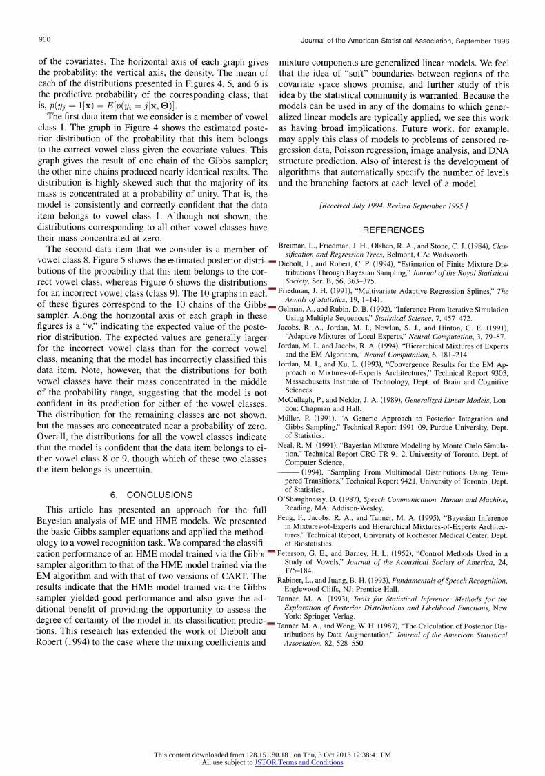
Figure 6. Ten Estimated Posterior Distributions for the Probability that the Data Item Belongs to the Incorrect Value Class 9. The "v" along the horizontal axis of each graph indicates the expected value of the distribution. Note that the mass is concentrated in the middle of the probability range, thus indicating that the model is not confident in its prediction. The Gelman and Rubin R value was equal to 1.021.




of the covariates. The horizontal axis of each graph gives the probability; the vertical axis, the density. The mean of each of the distributions presented in Figures 4, 5, and 6 is the predictive probability of the corresponding class; that is, p(yj = I Ix) = Ep(yi = ijlx, EQ.

The first data item that we consider is a member of vowel class 1. The graph in Figure 4 shows the estimated posterior distribution of the probability that this item belongs to the correct vowel class given the covariate values. This graph gives the result of one chain of the Gibbs sampler; the other nine chains produced nearly identical results. The distribution is highly skewed such that the majority of its mass is concentrated at a probability of unity. That is, the model is consistently and correctly confident that the data item belongs to vowel class 1. Although not shown, the distributions corresponding to all other vowel classes have their mass concentrated at zero.

The second data item that we consider is a member of vowel class 8. Figure 5 shows the estimated posterior distributions of the probability that this item belongs to the correct vowel class, whereas Figure 6 shows the distributions for an incorrect vowel class (class 9). The 10 graphs in each of these figures correspond to the 10 chains of the Gibbs sampler. Along the horizontal axis of each graph in these figures is a "v," indicating the expected value of the posterior distribution. The expected values are generally larger for the incorrect vowel class than for the correct vowel class, meaning that the model has incorrectly classified this data item. Note, however, that the distributions for both vowel classes have their mass concentrated in the middle of the probability range, suggesting that the model is not confident in its prediction for either of the vowel classes. The distribution for the remaining classes are not shown, but the masses are concentrated near a probability of zero. Overall, the distributions for all the vowel classes indicate that the model is confident that the data item belongs to either vowel class 8 or 9, though which of these two classes the item belongs is uncertain.

6. CONCLUSIONS

This article has presented an approach for the full Bayesian analysis of ME and HME models. We presented the basic Gibbs sampler equations and applied the methodology to a vowel recognition task. We compared the classification performance of an HME model trained via the Gibbs sampler algorithm to that of the HME model trained via the EM algorithm and with that of two versions of CART. The results indicate that the HME model trained via the Gibbs sampler yielded good performance and also gave the additional benefit of providing the opportunity to assess the degree of certainty of the model in its classification predictions. This research has extended the work of Diebolt and Robert (1994) to the case where the mixing coefficients and

mixture components are generalized linear models. We feel that the idea of "soft" boundaries between regions of the covariate space shows promise, and further study of this idea by the statistical community is warranted. Because the models can be used in any of the domains to which generalized linear models are typically applied, we see this work as having broad implications. Future work, for example, may apply this class of models to problems of censored regression data, Poisson regression, image analysis, and DNA structure prediction. Also of interest is the development of algorithms that automatically specify the number of levels and the branching factors at each level of a model.

[Received July 1994. Revised September 1995.]

REFERENCES

Breiman, L., Friedman, J. H., Olshen, R. A., and Stone, C. J. (1984), Clas- sification and Regression Trees, Belmont, CA: Wadsworth.

Diebolt, J., and Robert, C. P. (1994), "Estimation of Finite Mixture Dis- tributions Through Bayesian Sampling," Journal of the Royal Statistical Society, Ser. B, 56, 363-375.

Friedman, J. H. (1991), "Multivariate Adaptive Regression Splines," The Annals of Statistics, 19, 1-141.

Gelman, A., and Rubin, D. B. (1 992), "Inference From Iterative Simulation Using Multiple Sequences," Statistical Science, 7, 457-472.

Jacobs, R. A., Jordan, M. I., Nowlan, S. J., and Hinton, G. E. (1991), "Adaptive Mixtures of Local Experts," Neural Computation, 3, 79-87.

Jordan, M. I., and Jacobs, R. A. (1994), "Hierarchical Mixtures of Experts and the EM Algorithm," Neural Computation, 6, 181-214.

Jordan, M. I., and Xu, L. (1993), "Convergence Results for the EM Ap- proach to Mixtures-of-Experts Architectures," Technical Report 9303, Massachusetts Institute of Technology, Dept. of Brain and Cognitive Sciences.

McCullagh, P., and Nelder, J. A. (1989), Generalized Linear Models, Lon- don: Chapman and Hall.

Muller, P. (1991), "A Generic Approach to Posterior Integration and Gibbs Sampling," Technical Report 1991-09, Purdue University, Dept. of Statistics.

Neal, R. M. (1991), "Bayesian Mixture Modeling by Monte Carlo Simula- tion," Technical Report CRG-TR-91-2, University of Toronto, Dept. of Computer Science.

(1994), "Sampling From Multimodal Distributions Using Tem- pered Transitions," Technical Report 9421, University of Toronto, Dept. of Statistics.

O'Shaughnessy, D. (1987), Speech Communication: Human and Machine, Reading, MA: Addison-Wesley.

Peng, F., Jacobs, R. A., and Tanner, M. A. (1995), "Bayesian Inference in Mixtures-of-Experts and Hierarchical Mixtures-of-Experts Architec- tures," Technical Report, University of Rochester Medical Center, Dept. of Biostatistics.

Peterson, G. E., and Barney, H. L. (1952), "Control Methods Used in a Study of Vowels," Journal of the Acoustical Society of America, 24, 175-184.

Rabiner, L., and Juang, B.-H. (1993), Fundamentals of Speech Recognition, Englewood Cliffs, NJ: Prentice-Hall.

Tanner, M. A. (1993), Tools for Statistical Inference: Methods for the Exploration of Posterior Distributions and Likelihood Functions, New York: Springer-Verlag.

Tanner, M. A., and Wong, W. H. (1987), "The Calculation of Posterior Dis- tributions by Data Augmentation," Journal of the American Statistical Association, 82, 528-550.



Bayesian inference in mixtures-of-experts and hierarchical mixtures-of-experts models with an...

Documents

Transcript of Bayesian inference in mixtures-of-experts and hierarchical mixtures-of-experts models with an...