
Probabilistic Models for Inference about Identity
14
Probabilistic Models for Inference about Identity Peng Li, Member, IEEE, Yun Fu, Member, IEEE, Umar Mohammed, Member, IEEE, James H. Elder, Member, IEEE, and Simon J.D. Prince, Member, IEEE Abstract—Many face recognition algorithms use “distance-based” methods: Feature vectors are extracted from each face and distances in feature space are compared to determine matches. In this paper, we argue for a fundamentally different approach. We consider each image as having been generated from several underlying causes, some of which are due to identity (latent identity variables, or LIVs) and some of which are not. In recognition, we evaluate the probability that two faces have the same underlying identity cause. We make these ideas concrete by developing a series of novel generative models which incorporate both within- individual and between-individual variation. We consider both the linear case, where signal and noise are represented by a subspace, and the nonlinear case, where an arbitrary face manifold can be described and noise is position-dependent. We also develop a “tied” version of the algorithm that allows explicit comparison of faces across quite different viewing conditions. We demonstrate that our model produces results that are comparable to or better than the state of the art for both frontal face recognition and face recognition under varying pose. Index Terms—Computing methodologies, pattern recognition, applications, face and gesture recognition. Ç 1 INTRODUCTION G ENERATIVE probabilistic formulations have proven suc- cessful in many areas of computer vision including object recognition [12], image segmentation [36], and tracking [3]. These algorithms assume that the measure- ments are indirectly created from a set of underlying variables in noisy conditions. Vision problems are formu- lated as inverting this process: We attempt to estimate the variables from the measurements. This is not different from nonprobabilistic approaches, but Bayesian generative for- mulations have three desirable characteristics. First, they encourage careful modeling of the measurement noise. Second, they allow us to ignore variables that we are not interested in by marginalizing over them. Third, they provide a coherent way to compare models of different sizes using Bayesian model comparison. In this paper, we describe a probabilistic approach to face recognition that exploits all of these characteristics. 1.1 Distance-Based Face Recognition Most contemporary face recognition methods are based on the distance-based approach (see Fig. 1). A low-dimensional feature vector is extracted from each face image. The distances between these vectors are used to identify faces of the same person. For example, in closed set identification we choose the gallery feature vector with minimum distance from the probe feature vector. In face verification, two face images are ascribed to the same individual if the distance in feature space between them is less than some threshold. The logic of this approach is that for a judicious choice of feature space, the signal-to-noise ratio will be improved relative to that in the original space. Within the class of distance-based methods, the domi- nant paradigm is the “appearance-based” approach, which uses weighted sums of pixel values as features for the recognition decision. Turk and Pentland [38] transformed the image data to a feature space based on the principal components of the pixel covariance. Other work has variously investigated using different linear weighted pixel sums, [1], [2], [17], nonlinear techniques [44], and different distance measures [32]. A notable subcategory of these methods consists of approaches based on linear discriminant analysis (LDA). The Fisherfaces algorithm [2] projected face data to a space where the ratio of between-individual variation to within- individual variation was maximized. Fisherfaces is limited to directions in which at least some within-individual variance has been observed (the small-sample problem). The null-space LDA approach [8] exploited the signal in the remaining subspace. The Dual-Space LDA approach [39] combined these two approaches. These models perform excellently for frontal face recognition (e.g., see [39]). However, they perform poorly when the probe face is viewed with a very different pose, expression, or illumination from the corresponding gallery image [45]. Distance-based methods fail because the extracted feature vector changes with these variables, making the measured distances between vectors unreliable. Indeed, the variation attributable to these factors may dwarf the variation due to differences in identity, rendering the nearest-neighbor decision meaningless. Even LDA-based approaches such as [2], [39] fail as the signal lies in part of the subspace where the noise is also great and is hence down-weighted or discarded. 144 IEEE TRANSACTIONS ON PATTERN ANALYSIS AND MACHINE INTELLIGENCE, VOL. 34, NO. 1, JANUARY 2012 . P. Li, Y. Fu, U. Mohammed and S.J.D. Prince are with the Department of Computer Science, University College London, Gower Street, London WC1E 6BT, United Kingdom. E-mail: {p.li, y.fu, u.mohammed, s.prince}@cs.ucl.ac.uk. . J. Elder is with the Center for Vision Research, York University, Room 0003G, Computer Science Building, 4700 Keele Street, North York, Ontario M3J 1P3, Canada. E-mail: [email protected]. Manuscript received 14 May 2010; revised 21 Dec. 2010; accepted 3 Mar. 2011; published online 13 May 2011. Recommended for acceptance by T. Jebara. For information on obtaining reprints of this article, please send e-mail to: [email protected], and reference IEEECS Log Number TPAMI-2010-05-0378. Digital Object Identifier no. 10.1109/TPAMI.2011.104. 0162-8828/12/$31.00 ß 2012 IEEE Published by the IEEE Computer Society
-
Upload
independent -
Category
Documents
-
view
5 -
download
0
Transcript of Probabilistic Models for Inference about Identity
Probabilistic Models for Inference about IdentityPeng Li, Member, IEEE, Yun Fu, Member, IEEE, Umar Mohammed, Member, IEEE,
James H. Elder, Member, IEEE, and Simon J.D. Prince, Member, IEEE
Abstract—Many face recognition algorithms use “distance-based” methods: Feature vectors are extracted from each face and
distances in feature space are compared to determine matches. In this paper, we argue for a fundamentally different approach. We
consider each image as having been generated from several underlying causes, some of which are due to identity (latent identity
variables, or LIVs) and some of which are not. In recognition, we evaluate the probability that two faces have the same underlying
identity cause. We make these ideas concrete by developing a series of novel generative models which incorporate both within-
individual and between-individual variation. We consider both the linear case, where signal and noise are represented by a subspace,
and the nonlinear case, where an arbitrary face manifold can be described and noise is position-dependent. We also develop a “tied”
version of the algorithm that allows explicit comparison of faces across quite different viewing conditions. We demonstrate that our
model produces results that are comparable to or better than the state of the art for both frontal face recognition and face recognition
under varying pose.
Index Terms—Computing methodologies, pattern recognition, applications, face and gesture recognition.
Ç
1 INTRODUCTION
GENERATIVE probabilistic formulations have proven suc-cessful in many areas of computer vision including
object recognition [12], image segmentation [36], andtracking [3]. These algorithms assume that the measure-ments are indirectly created from a set of underlyingvariables in noisy conditions. Vision problems are formu-lated as inverting this process: We attempt to estimate thevariables from the measurements. This is not different fromnonprobabilistic approaches, but Bayesian generative for-mulations have three desirable characteristics. First, theyencourage careful modeling of the measurement noise.Second, they allow us to ignore variables that we are notinterested in by marginalizing over them. Third, theyprovide a coherent way to compare models of differentsizes using Bayesian model comparison. In this paper, wedescribe a probabilistic approach to face recognition thatexploits all of these characteristics.
1.1 Distance-Based Face Recognition
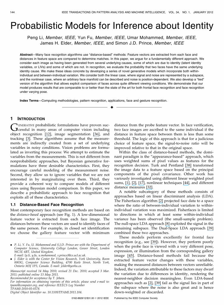
Most contemporary face recognition methods are based onthe distance-based approach (see Fig. 1). A low-dimensionalfeature vector is extracted from each face image. Thedistances between these vectors are used to identify faces ofthe same person. For example, in closed set identificationwe choose the gallery feature vector with minimum
distance from the probe feature vector. In face verification,two face images are ascribed to the same individual if thedistance in feature space between them is less than somethreshold. The logic of this approach is that for a judiciouschoice of feature space, the signal-to-noise ratio will beimproved relative to that in the original space.
Within the class of distance-based methods, the domi-nant paradigm is the “appearance-based” approach, whichuses weighted sums of pixel values as features for therecognition decision. Turk and Pentland [38] transformedthe image data to a feature space based on the principalcomponents of the pixel covariance. Other work hasvariously investigated using different linear weighted pixelsums, [1], [2], [17], nonlinear techniques [44], and differentdistance measures [32].
A notable subcategory of these methods consists ofapproaches based on linear discriminant analysis (LDA).The Fisherfaces algorithm [2] projected face data to a spacewhere the ratio of between-individual variation to within-individual variation was maximized. Fisherfaces is limitedto directions in which at least some within-individualvariance has been observed (the small-sample problem).The null-space LDA approach [8] exploited the signal in theremaining subspace. The Dual-Space LDA approach [39]combined these two approaches.
These models perform excellently for frontal facerecognition (e.g., see [39]). However, they perform poorlywhen the probe face is viewed with a very different pose,expression, or illumination from the corresponding galleryimage [45]. Distance-based methods fail because theextracted feature vector changes with these variables,making the measured distances between vectors unreliable.Indeed, the variation attributable to these factors may dwarfthe variation due to differences in identity, rendering thenearest-neighbor decision meaningless. Even LDA-basedapproaches such as [2], [39] fail as the signal lies in part ofthe subspace where the noise is also great and is hencedown-weighted or discarded.
144 IEEE TRANSACTIONS ON PATTERN ANALYSIS AND MACHINE INTELLIGENCE, VOL. 34, NO. 1, JANUARY 2012
. P. Li, Y. Fu, U. Mohammed and S.J.D. Prince are with the Department ofComputer Science, University College London, Gower Street, LondonWC1E 6BT, United Kingdom.E-mail: {p.li, y.fu, u.mohammed, s.prince}@cs.ucl.ac.uk.
. J. Elder is with the Center for Vision Research, York University, Room0003G, Computer Science Building, 4700 Keele Street, North York,Ontario M3J 1P3, Canada. E-mail: [email protected].
Manuscript received 14 May 2010; revised 21 Dec. 2010; accepted 3 Mar.2011; published online 13 May 2011.Recommended for acceptance by T. Jebara.For information on obtaining reprints of this article, please send e-mail to:[email protected], and reference IEEECS Log NumberTPAMI-2010-05-0378.Digital Object Identifier no. 10.1109/TPAMI.2011.104.
0162-8828/12/$31.00 � 2012 IEEE Published by the IEEE Computer Society
Many other approaches have been proposed to cope withvariable pose and illumination. Important categories in-clude algorithms which 1) require more than one inputimage of each face [14], 2) create a 3D model from the 2Dimage and estimate pose and lighting explicitly [4], [5], and3) learn a statistical relation between faces viewed underdifferent conditions [16], [27], [34].
1.2 Probabilistic Face Recognition
The aforementioned distance-based models provide a hardmatching decision—however, it would be better to assign aposterior probability to each explanation of the data. In apractical system (e.g., access control), we could defer thefinal decision and collect more data if the uncertainty is toogreat. Moreover, a probabilistic solution means that we caneasily combine information from different measurementmodalities and apply priors over the possible matchingconfigurations.
Generative probabilistic approaches have yielded con-siderable progress in the closely related problem of objectrecognition (e.g., [12]). Nonetheless, there have been fewattempts to construct probabilistic algorithms for facerecognition. One of the reasons for the paucity of probabil-istic approaches is the diversity of tasks in face recognition.These include:
1. Closed set recognition: Choose one of N galleryfaces that matches a probe face.
2. Open set recognition: Choose one of N gallery facesthat matches a probe or identify that there is nomatch.
3. Verification: Given two face images, indicatewhether they belong to the same person or not.
4. Clustering: Given N faces, find how many differentpeople are present and which person is in whichimage.
Until recently, recognition algorithms could not provideposterior probabilities over different hypotheses for all ofthese tasks. Liu and Wechsler [26] described a probabilisticmethod in which they model the data for each individual(after projection to a subspace) as a Gaussian with identicaland diagonal variance. However, this method is onlysuitable for closed set recognition and is not a fullprobabilistic model as it only describes the data afterprojection. The scheme of Moghaddam et al. [28] consideredpixel-wise difference between probe and gallery images.
They modeled distributions of “within-individual” and“between-individual” differences. For two new images, theyfind the posterior probability that the difference belongs toeach. This is well suited to face verification, but does notprovide a posterior over possible matches for other tasks.Moreover, performance in uncontrolled conditions is poor[27]. There is no obvious way to remedy these problems.
Recently, probabilistic recognition algorithms have beenproposed which can address all the above tasks [19], [35],[34]. The key idea is to construct a model describing howthe data were generated from identity. Prince et al. [34]developed a probabilistic “tied factor analysis” model forface recognition. This was specialized to the case of largepose changes and is a special case of one of the modelspresented in this paper. Ioffe [19] presented a probabilisticLDA model for face recognition that is also closely relatedto one of the models presented in this paper.
In this paper, we develop a model in which identity isrepresented as a hidden variable in a generative descriptionof the image data. Any remaining variation that is notattributed to identity is described as noise. The model islearned with the expectation-maximization (EM) algorithm[9] and face recognition is framed as a model comparisontask. An earlier version of this work was published in [35].Code is available via http://pvl.cs.ucl.ac.uk.
In Section 2, we introduce a probabilistic framework tosolve face recognition problems. In Section 3, we introducea probabilistic version of Fisherfaces [2], which we termprobabilistic LDA (or PLDA). We show that this approachsidesteps the small sample problem and produces goodresults for frontal faces. In Section 4, we introduce anonlinear generalization of this approach. In Section 5, weintroduce “Tied PLDA,” which allows us to compare facescaptured in very different poses. In Section 7, we discuss therelationship between these models and other work.
2 GENERATIVE MODELS FOR FACE DATA
Our approach is founded on the following four premises.
1. Faces images depend on several interacting factors:These include the person’s identity (signal) and thepose, illumination, etc. (nuisance variables).
2. Image generation is noisy: Even in matchingconditions, images of the same person differ. Thisremaining variation comprises unmodeled factorsand sensor noise.
3. Identity cannot be known exactly: Since generationis noisy, there will always be uncertainty on anyestimate of identity, regardless of how we form thisestimate.
4. Recognition tasks do not require identity esti-mates: In face recognition, we can ask whether twofaces have the same identity, regardless of what thisidentity is.
2.1 Latent Identity Variables
At the core of our approach is the notion that there exists amultidimensional variable h that represents the identity ofthe individual. We term this a latent identity variable (LIV) andthe space that it resides in identity space. Latent identity
LI ET AL.: PROBABILISTIC MODELS FOR INFERENCE ABOUT IDENTITY 145
Fig. 1. Conventional distance-based approach. Observed probe xp andgallery x1...3 images are deterministically transformed from pixel space(left) to a lower dimensional feature space (right). Distance in featurespace between the probe image f p and each of the gallery images f 1...3
is calculated (arrows). The probe vector f p is associated with the nearestneighbor gallery vector (here, f 2).
variables have this key property: If two variables haveidentical values, they describe the same individual. If twovariables differ, they describe different people. Crucially, theidentity variable is constant for an individual, regardless ofpose, illumination, or any other factors that effect the image.
We never observe identity variables directly, but weconsider the observed faces to have been generated from thelatent identity variable by a noisy process (see Fig. 2). Ourgoal is not necessarily to describe the true generativeprocess, but to obtain a model that describes the image data,within which we can obtain accurate predictions and validuncertainty estimates. In this paper, we consider models ofthe form
xij ¼ fðhi;wij; �Þ þ �ij; ð1Þ
where xij is the vectorized data from the jth image of theith person. The term hi is the LIV and is constant for everyimage of that person (i.e., it is not indexed by j). The termwij is another latent variable representing the viewingconditions (pose, illumination, expression, etc.) for thejth image of the ith person. The term �ij is an axis orientedGaussian noise term and is used to explain any remainingvariation. The term � is a vector of model parameters whichare learned during a training phase and remain constantduring recognition.
Assuming that we know the model parameters, �, howcan we then identify if a gallery and probe face match? Inthe next two sections, we consider two alternative strategiesbased on 1) evaluating the joint probability of probe andgallery images and 2) forming class-conditional predictivedistributions.
2.2 Recognition: Joint Perspective
Our framework infers whether two observed images x1 andx2 were generated from the same identity variable h andhence belong to the same individual. Unfortunately, thispresents a problem: The data x was generated in noisyconditions, so we can never be certain of the underlyingvalue of h or w. To resolve this, we consider all possiblevalues of h and w.
More formally, the recognition process compares thelikelihood of the data under different models M. Eachmodel assigns identity variables h to explain the observedfaces x in a different way. If the current model ascribes twoface images to belong to the same person, then they willhave the same identity variable. If not, then they will eachhave their own identity variables.
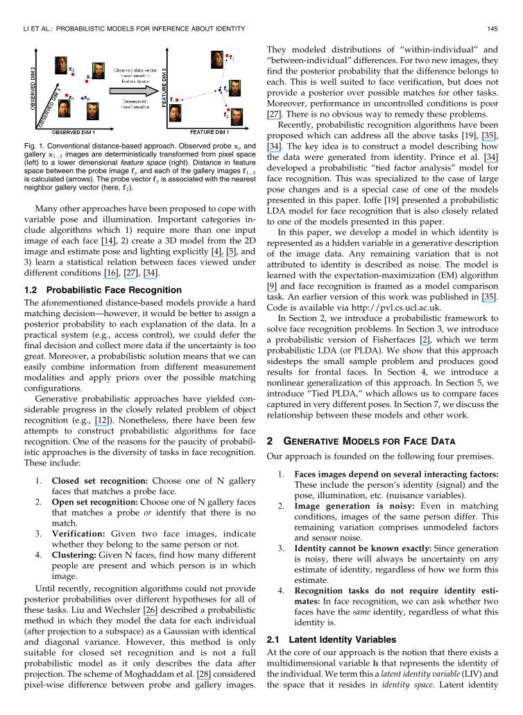
Fig. 3a shows the model construction for closed setidentification. We are given a probe face xp and theN gallery faces (here, N ¼ 2), each representing a differentperson, x1...N . In modelMn the nth gallery face is forced toshare its latent identity variable hn with the probe indicatingthat these faces belong to the same person. Fig. 3c shows themodels for face verification. Here, ModelM0 represents thecase where the two faces do not match (each image has aseparate identity). ModelM1 represents the case where theydo match (they share an identity). In fact, all fourrecognition tasks from Section 1.2 can be expressed in termsof model comparison: For open set identification (Fig. 3b),we start with the closed set case and add a model M0
representing the situation where the probe has its ownunique identity. In face clustering (Fig. 3d), we are givenN faces and there may be N different people (N identityvariables), just one person (1 identity variable), or anythingin between. In this paper, we concentrate on closed setidentification, verification, and clustering.
We combine the likelihoods of these models with suitablepriors PrðMÞ (always uniform in this paper) and find aposterior probability for the match using Bayes’ rule.However, the question remains as to how to calculate themodel likelihoods. Noise in the generation process meansthat we can never exactly know either the identity variables h
or the noise variables w in these models. Hence, wemarginalize (integrate out) these variables:
Prðx1...N;pjM0Þ ¼YNn¼1
PrðxnÞPrðxpÞ; ð2Þ
Prðx1...N;pjMmÞ ¼YN
n¼1;n 6¼mPrðxnÞPrðxp;xmÞ; ð3Þ
where
PrðxnÞ ¼Z Z
Prðxn;hn;wnÞdhndwn; ð4Þ
146 IEEE TRANSACTIONS ON PATTERN ANALYSIS AND MACHINE INTELLIGENCE, VOL. 34, NO. 1, JANUARY 2012
Fig. 2. Latent Identity Variable approach. Observed face data vectors x(left) are generated from the underlying identity space h (right). Themodel, x ¼ fðhÞ þ �, explains the face data x as generated by adeterministic transformation fðÞ of the identity variable h followed by theaddition of a stochastic noise term �. In this case, the faces x2 and xp aredeemed to match as they were generated from the same underlyingidentity variable h2.
Fig. 3. Inference by comparing data likelihood under different models.Each model represents a different relationship between the LIVs h andobservations x. (a) Closed set identification with gallery of two faces. InModel M1, the probe xp matches gallery face x1. In model M2, theprobe xp matches x2. (b) Open set identification. We add the possibilityM0 that the probe face xp matches neither gallery face x1 nor x2.Verification (c) and face clustering (d) can also be expressed as modelcomparison. Note that there is also a noise variable w associated witheach datum x which is not shown.

PrðxpÞ ¼Z Z
Prðxp;hp;wpÞdhpdwp; ð5Þ
Prðxp;xmÞ ¼Z Z Z
Prðxp;xm;hm;wp;wmÞdhmdwpdwm:
ð6Þ
An important aspect of this formulation is that the finallikelihood expression does not explicitly depend on the latentidentity variables h. This makes it valid to compare modelswith different numbers of latent identity variables. Forexample, in face verification we compare a model with twounderlying latent variables (no match) to one (match). This isan example of Bayesian model selection in which we comparethe evidence for the different explanations of the data.
2.3 Recognition: Class Conditional Perspective
In the previous treatment, we evaluate the joint likelihoodof the probe and gallery images under different models ((2)and (3)). An alternative perspective is to consider thepredictive distribution for the probe image xp induced bythe matching gallery data xg in each of the models. To makeface recognition decisions, we evaluate the likelihood of theprobe image under each of these class conditional densityfunctions and combine with priors. Now we write
Prðx1...N;pjM0Þ ¼ Prðxpjx1...N;M0ÞPrðx1...NÞ
¼ PrðxpÞYNn¼1
PrðxnÞ;ð7Þ
Prðx1...N;pjMmÞ ¼ Prðxpjx1...N;MmÞPrðx1...NÞ
¼ PrðxpjxmÞYNn¼1
PrðxnÞ;ð8Þ
where PrðxpjxnÞ is found by taking the conditional of (6).This approach is closely related to object recognition:Generative models such as [12] create a separate probabilitydensity for each class. However, in object recognition thereare usually numerous training examples of each class (e.g.,cars). For face recognition, we often only have a singleexample of each class (individual). Hence, face recognitionmodels necessarily deal with the situation of “one shot”learning [23].
2.4 Tractability of Integrals
We are assuming that the integrals in (4)-(6) can be computed.This is true for all models in this paper. When they cannot becomputed, one approach is to approximate the distributionsover the hidden variables h and/or w by point estimates hand w. The choice of the joint or class-conditional methodsnow becomes important: In the joint method, the pointestimate of the identity will be based on both the gallery andprobe images, whereas in the class-conditional method, theidentity will be based on the gallery alone.
3 MODEL 1: PROBABILISTIC LDA
To make these ideas concrete, we investigate a probabil-istic model that is closely related to LDA. LDA is atechnique that models intraclass and interclass variance as
multidimensional Gaussians. It seeks directions in spacethat have maximum discriminability and are hence mostsuitable for supporting class recognition. We refer to ourversion of this algorithm as probabilistic linear discriminantanalysis. The relationship between PLDA and standardLDA is similar to that between factor analysis and principalcomponents analysis.
We assume that the training data consist of J imageseach of I individuals. We denote the jth image of theith individual by xij. We model the data generation as
xij ¼ �þ Fhi þGwij þ �ij; ð9Þ
where � is the mean of the data, F is a factor matrix with thebasis vectors of the between individual subspace in itscolumns, and hi is the latent identity variable that isconstant for all images xi1 . . . xiJ of person i. Just as thematrix F contains a matrix determining the between-individual subspace, the matrix G contains a basis for thewithin-individual subspace. The term wij represents theposition in this subspace. The term �ij is a stochastic noiseterm, with diagonal covariance �.
The term �þ Fhi is the signal and accounts for between-individual variance. For a given individual, this term isconstant. The term Gwij þ �ij consists of the noise orwithin-individual variance. It explains why two images ofthe same individual do not look identical.
More formally, we can describe the model in (9) in termsof conditional probabilities
Prðxijjhi;wij; �Þ ¼ Gx½�þ Fhi þGwij;��; ð10Þ
PrðhiÞ ¼ Gh½0; I�; ð11Þ
PrðwijÞ ¼ Gw½0; I�; ð12Þ
where Ga½b;C� denotes a Gaussian in a with mean b andcovariance C. In (11) and (12), we have defined simplepriors on the latent variables hi and wij. The relationshipbetween the variables is indicated in Fig. 4A. It is importantto note that (10), (11), and (12) implicitly define the jointprobability distribution required for (4)-(6). The Gaussianforms for this model have been chosen because they provideclean closed form solutions to these integrals, rather thanbecause they represent the true generative process.
LI ET AL.: PROBABILISTIC MODELS FOR INFERENCE ABOUT IDENTITY 147
Fig. 4. PLDA Model. (A) Graphical model relating data x to identities h,noise variables w, and parameters � ¼ f�;F;G;�g. (B) Predictivedistribution for subspace model with one identity factor F (dotted line)and one noise factor G (not shown). The gray region representsassociated Gaussian face manifold. New gallery images (red and greendots) induce Gaussian predictive distributions (red and green ellipses).

3.1 Learning
In the learning stage, we aim to learn the parameters � ¼f�;F;G;�g given data xij. It would be easy to estimate theseparameters if we knew the hidden identity variables hi andhidden noise variables wij. Likewise, it would be easy toinfer the identity variables hi and noise variables wij if weknew the parameters �. This type of “chicken and egg”problem is well suited to the EM algorithm [9]. Details ofthis process are given in Appendix A, which can be foundin the Computer Society Digital Library at http://doi.ieeecomputersociety.org/10.1109/TPAMI.2011.104.
Fig. 5 shows the results of 10 iterations of learning fromthe first 195 individuals from the XM2VTS database withminimal preprocessing. We show several positions in thebetween-individual subspace (samples where h varies butw is constant) and these look like different people. We alsoshow positions in the within-individual subspace (sampleswhere h is constant and w varies). These look like the sameperson under slightly different illuminations and poses.
Fig. 6 shows a visualization of the model for four faces.In each case, we decompose the image into signal Fhi andnoise components Gwij and �ij using the final MAPestimate of the hidden variables from the E-Step in training.
3.2 Recognition with Joint Method
In recognition, we must evaluate the integrals in (4)-(6). Thegeneral problem is to evaluate the likelihood that N imagesx1...N share the same identity variable, h, regardless of thenoise variables w1 . . . wN . Our approach is to rewrite theequations in the form of a factor analyzer and use astandard result for the integral. To this end, we combine thegenerative equations for all N images:
x1
x2
..
.
xN
26664
37775 ¼
��
..
.
�
26664
37775þ
F G 0 . . . 0F 0 G . . . 0... ..
. ... . .
. ...
F 0 0 . . . G
2664
3775
hw1
w2
..
.
wN
2666664
3777775þ
�1
�2
..
.
�N
26664
37775;
ð13Þ
or, giving names to these composite matrices,
x0 ¼ �0 þAyþ �0: ð14Þ
We can rewrite this compound model in terms ofprobabilities to give
Prðx0jyÞ ¼ Gx0 ½�0 þAy;�0�; ð15Þ
PrðyÞ ¼ Gy 0; I½ �; ð16Þ
where
�0 ¼
� 0 . . . 00 � . . . 0... ..
. . .. ..
.
0 0 . . . �
2664
3775: ð17Þ
This now has the form of a factor analyzer. From (14), it is
easy to see that the first two moments of the distribution of
the compound vector x0 are given by
E x0½ � ¼ �0;E½ðx0 � �0Þðx0 � �0ÞT � ¼ E½ðAyþ �0ÞðAyþ �0ÞT �
¼ AAT þ �0;
ð18Þ
and it can be shown that when we marginalize over thehidden variable y, the form of the resulting distribution is
Gaussian with these moments:
Prðx1...NÞ ¼ Prðx0Þ ¼ Gx0 ½�0;AAT þ �0�: ð19Þ
3.3 Recognition with Predictive Distribution
Instead of calculating the expressions in (2)-(6), we couldequivalently have performed this experiment by calculating
the predictive distributions Prðxpjx1Þ . . .PrðxpjxnÞ. We then
assess the likelihood of the probe image under each of these
distributions.The predictive distributions can be calculated by taking
the joint distribution in (19) and finding the conditional
distribution of xp given all the other variables. If the mean
and information matrix of the joint distribution in (19) are
partitioned so that
�0 ¼ mp
mg
� �; ðAAT þ �0Þ�1 ¼ �pp �gp
�pg �gg
� �; ð20Þ
148 IEEE TRANSACTIONS ON PATTERN ANALYSIS AND MACHINE INTELLIGENCE, VOL. 34, NO. 1, JANUARY 2012
Fig. 5. PLDA Model. (A) Mean face. (B) Three directions in between-individual subspace. Each image looks like a different person. (C) Per-pixel noise covariance. (D) Three directions in within-individual sub-space. Each image looks like the same person under minor pose andlighting changes.
Fig. 6. PLDA. The first column shows the original images xij. These arebroken down into a signal subspace component Fhi which is the samefor each identity, a noise subspace component Gwij, and a per pixelnoise �ij.

then the conditional distribution is also Gaussian (see [6])with mean and covariance
PrðxpjxgÞ ¼ Gxp
�mp � ��1
pp �pgðxg �mpÞ;��1pp
�: ð21Þ
It is possible to evaluate this Gaussian probability efficiently(Appendix B, which can be found in the Computer SocietyDigital Library at http://doi.ieeecomputersociety.org/10.1109/TPAMI.2011.104), making the complexity of thisalgorithm similar to that of the original LDA method.
Example predictive distributions for the case where thesubspaces F and G are 1D are shown in Fig. 4B. Thelearned face manifold (indicated in gray) is given byPrðxÞ ¼ Gx½�;FFT þGGT þ ��. A new gallery image in-duces a Gaussian predictive distribution, with a mean thatis projected onto the subspace spanned by the factor in F(dotted line). The projection direction depends on the noiseparameters � and the noise subspace G. To perform facerecognition, we would compare the likelihood of a newprobe point under each of the predictive distributions. Thelikelihood for not matching either gallery image is found byevaluating the probe point under the whole manifolddistribution (gray area).
3.4 Experiment 1: Frontal Face Identification
To explore the properties of the algorithm, we trained thealgorithm with all of the data from the first 195 individuals inthe XM2VTS database. We tested with the last 100 indivi-duals, using the one image from the first capture session asthe gallery set and the one image from the last for the probeset. Hence, the model must generalize from the training setto new individuals.
To ensure that the experiments are easy to replicate, weused minimal preprocessing. Each image was segmentedwith an iterative graph-cuts procedure. Three points weremarked by hand. Faces were normalized to a standardtemplate using an affine transform. Final size was70� 70� 3. Raw pixel values form the input vector. Therewas no photometric normalization. For each probe, wecompute the likelihood that it matches each face in the galleryusing (3). We calculate a posterior for the match, assuminguniform priors. We take the MAP solution as the match.
In Fig. 7a, we plot percent correct first match results as afunction of the subspace dimensions. For each line of thegraph, the dimension of the signal Dim(F) is constant, butthe dimension of the noise Dim(G) varies. Increasing thesignal dimension improves performance. Increasing the
dimension of the noise subspace has a more complex effect:Performance is always worst when Dim(G) is zero and isbest when Dim(G) is roughly the same as Dim(F). Hence,we set the signal and noise subspace size to be identical inall remaining experiments.
In Fig. 7b, we decompose the model into constituentparts. We force the noise � to be a multiple of the identityrather than diagonal (dashed versus solid lines). Thisreduces performance: The full algorithm learns which partsof the image are most variable and downweights them inthe decision. We also remove the noise subspace by settingDim(G) to zero (blue lines versus red lines), whichdecreases performance even further.
These restrictions can be easily related to other models.When the covariance � is uniform and there is no noisesubspace, the model takes the form of probabilistic PCA andthe results are very similar to those for eigenfaces. In fact, thePPCA model has very slightly superior performance due toregularization induced by the prior over h. When we allow �to have independent diagonal terms, the model takes theform of a factor analyzer. When we allow the noise subspacedimension Dim(G) to be nonzero and restrict � to be diagonal,our model is similar to that of Ioffe [19].
3.4.1 Comparison to Other Algorithms
In Fig. 8, we compare the performance of PLDA to otheralgorithms. We emphasize here that the preprocessing ofthe data is exactly the same in each case, so this is a pure testof recognition ability when the remaining parts of thepipeline are held constant.
Fig. 8a shows that PLDA outperforms our implementa-tions of five other algorithms on the XM2VTS database. Theclosest competing methods are dual-space LDA [39] and theprobabilistic approach of Ioffe [19].
LI ET AL.: PROBABILISTIC MODELS FOR INFERENCE ABOUT IDENTITY 149
Fig. 7. (a) Identification performance as with minimal preprocessing as afunction of signal and noise subspace size. (b) Identification perfor-mance for progressive simplifications of the model.
Fig. 8. (a) Comparison of algorithms for the XM2VTS database. PLDAoutperforms PCA [38], LDA [2], the Bayesian approach [28], Dual-Space(DS) LDA [39], and the probabilistic approach of Ioffe [19](b) Performance comparison for the XM2VTS lighting subset.(c) Comparison for the YALE database as a function of gallery images(nearest neighbor approach) to RLDA [7], SLDA [7], LDA [2], and PCA[38]. (d) Comparison for the ORL database.
In Fig. 8b, we investigate performance for the samealgorithms on the lighting subset of the XM2VTS database.The training set consisted of seven images each of the first195 individuals and contained two lighting conditions. Foreach individual, there were five images under frontallighting and two under side-lighting. The test set consistedof 100 different individuals, where the gallery images weretaken from the first recording session and were underfrontal lighting and the probe images were taken from thefourth session and were lit from the side. All otherpreprocessing was the same as for the original XM2VTSdata. Once more, the PLDA algorithm outperforms the fivecompeting algorithms.
In Fig. 8c, we present results from the Yale database,which also contains lighting variation which was prepro-cessed as in [7]. We compare to published data from [7] andshow that performance is superior to the RLDA, SLDA,LDA, and PCA algorithms. Finally, in Fig. 8d we compareresults to the same algorithms on the ORL database (also aspreprocessed by [7]), which contains both pose and lightingvariation. Here the PLDA algorithm provides performancethat is comparable to SLDA and superior to RLDA, LDA,and PCA.
These experiments make a strong case for PLDA: Overfour different databases and seven algorithms it producesreliably better performance when all other parts of the facerecognition pipeline are held constant.
Our technique outperforms other LDA methods for threereasons. First, the per-pixel noise term � means we have amore sophisticated model of within-individual variation(see Fig. 7b). Second, our method does not suffer from thesmall sample problem: The signal subspace F and noisesubspace G may be completely parallel or entirelyorthogonal. There is no need for two separate proceduresas in the dual-space LDA algorithm [39]. Third, a slightbenefit results from the regularizing effect of the prior overthe identity and noise variables.
We also investigated identification performance for thePLDA algorithm for the XM2VTS with more elaboratepreprocessing. Eight keypoints on each face were identifiedby hand or automatically using the method described in[34], depending on the condition. The images wereregistered using a piecewise triangular warp. The finalimage size was 400� 400. We extracted feature vectors
consisting of image gradients at eight orientations and threescales at points in a 6� 6 grid around each keypoint. Aseparate recognition model was built for each and thesewere treated as independent.
Here, the training data consisted of images from the firstthree capture sessions from all 295 individuals in thedatabase. We use images from 1) capture session 1 or2) capture sessions 1-3 to form the gallery. We use imagesfrom capture session 4 to form the probe set. This protocolwas chosen to facilitate comparison with [25].
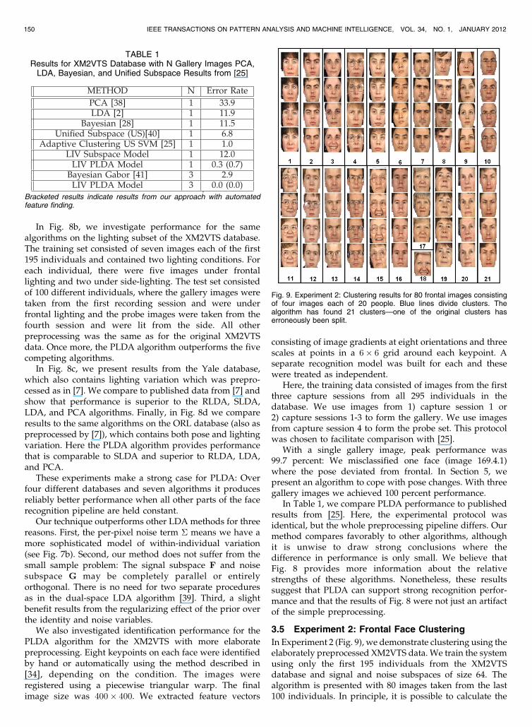
With a single gallery image, peak performance was99.7 percent: We misclassified one face (image 169.4.1)where the pose deviated from frontal. In Section 5, wepresent an algorithm to cope with pose changes. With threegallery images we achieved 100 percent performance.
In Table 1, we compare PLDA performance to publishedresults from [25]. Here, the experimental protocol wasidentical, but the whole preprocessing pipeline differs. Ourmethod compares favorably to other algorithms, althoughit is unwise to draw strong conclusions where thedifference in performance is only small. We believe thatFig. 8 provides more information about the relativestrengths of these algorithms. Nonetheless, these resultssuggest that PLDA can support strong recognition perfor-mance and that the results of Fig. 8 were not just an artifactof the simple preprocessing.
3.5 Experiment 2: Frontal Face Clustering
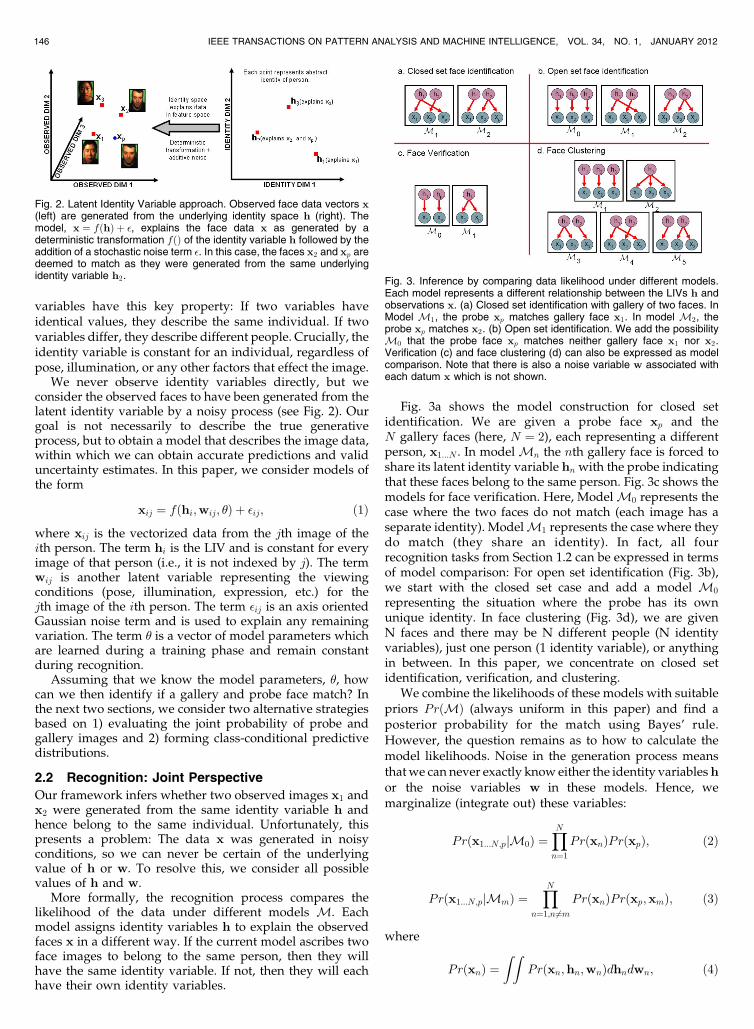
In Experiment 2 (Fig. 9), we demonstrate clustering using theelaborately preprocessed XM2VTS data. We train the systemusing only the first 195 individuals from the XM2VTSdatabase and signal and noise subspaces of size 64. Thealgorithm is presented with 80 images taken from the last100 individuals. In principle, it is possible to calculate the
150 IEEE TRANSACTIONS ON PATTERN ANALYSIS AND MACHINE INTELLIGENCE, VOL. 34, NO. 1, JANUARY 2012
TABLE 1Results for XM2VTS Database with N Gallery Images PCA,
LDA, Bayesian, and Unified Subspace Results from [25]
Bracketed results indicate results from our approach with automatedfeature finding.
Fig. 9. Experiment 2: Clustering results for 80 frontal images consistingof four images each of 20 people. Blue lines divide clusters. Thealgorithm has found 21 clusters—one of the original clusters haserroneously been split.
likelihood for each possible clustering of the data using (19):For example, we can calculate the likelihood that there are80 different individuals or that the 80 images are all of thesame individual.
Unfortunately, in practice there are far too many possibleconfigurations. Hence, we adopt a greedy agglomerativestrategy. We start with the hypothesis that there are80 different individuals. We then consider merging all pairsof individuals and choose the combination that increasesthe likelihood the most. We continue this process until thelikelihood cannot be improved. In order to test theclustering performance, we randomly select four imageseach from 20 individuals and apply our algorithm. We canquantify performance by counting the number of splits andmerges required to change our estimated clustering to theground truth. Averaged over 100 data sets, the meannumber of split/merges was 1.60.
Typical results are shown in Fig. 9 (here the number ofsplit/merges required is 1). The algorithm slightly over-partitions the data but does not erroneously associateimages from different individuals. We conclude that ourmodel can cope with complex compound decisions aboutidentity and can select model size without the need forextra parameters.
3.6 Experiment 3: Face Verification
In Experiment 3, we investigate face verification using theLabeled Faces in the Wild [18] database which containslarge variations in pose, expression, and lighting. Imageswere grayscale and were prepared in two ways: 1) alignedusing commercial face alignment software by Taigmanet al. [37] and 2) funneled, which is available on the LFWwebsite [18]. There are a total of 13,233 images and 5,749people in the database. The number of images varies fromone to 530 images.
The images are divided into 10 groups where the subjectidentities are mutually exclusive. In each group, there are300 pairs of images from the same identity and 300 pairsfrom different identities. There are two possible trainingconfigurations. In the “restricted configuration,” only thesame/not-same labels are used no information about theactual identities is used. Most previous work has restricted
protocol (e.g., [43] and [22]). In the “unrestricted configura-tion,” all available information, including the identities, canbe used for training. The studies of [13], [37] used thisconfiguration.
The aligned images were cropped to 80� 150 pixelsfollowing Nguyen and Bai [29]. Each image was normalizedby passing it through a log function (logðxþ 1Þ) to suppressthe effect of shadows and lighting. In addition, we localizefour keypoints following [10], [24] and estimate the facialpose by projecting the keypoint positions to the firstprincipal component following [37]. The images of largeright profile faces are swapped to left profile faces so that allthe images are left profile or near frontal. We investigatedtwo types of descriptors on the aligned images: local binarypatterns (LBP) [31] and three-patch local binary patterns(TPLBP) [43]. We used the same parameters as [29], [37]. Inaddition, we also investigated the SIFT descriptors com-puted at the nine facial keypoints on the funneled images.The SIFT data are available from [13]. The originaldimensionality of the features was quite high (7,080 forLBP and TPLBP and 3,456 for SIFT), so we reduced thedimension to 200 using PCA.
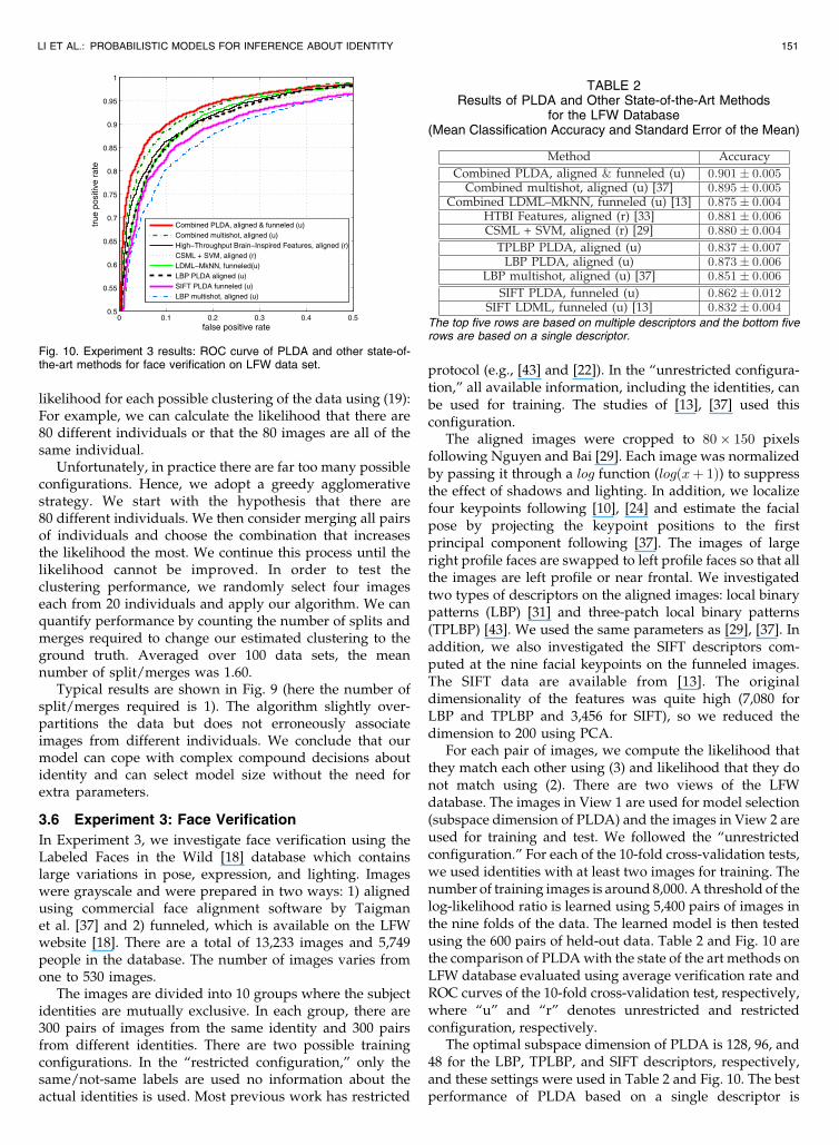
For each pair of images, we compute the likelihood thatthey match each other using (3) and likelihood that they donot match using (2). There are two views of the LFWdatabase. The images in View 1 are used for model selection(subspace dimension of PLDA) and the images in View 2 areused for training and test. We followed the “unrestrictedconfiguration.” For each of the 10-fold cross-validation tests,we used identities with at least two images for training. Thenumber of training images is around 8,000. A threshold of thelog-likelihood ratio is learned using 5,400 pairs of images inthe nine folds of the data. The learned model is then testedusing the 600 pairs of held-out data. Table 2 and Fig. 10 arethe comparison of PLDA with the state of the art methods onLFW database evaluated using average verification rate andROC curves of the 10-fold cross-validation test, respectively,where “u” and “r” denotes unrestricted and restrictedconfiguration, respectively.
The optimal subspace dimension of PLDA is 128, 96, and48 for the LBP, TPLBP, and SIFT descriptors, respectively,and these settings were used in Table 2 and Fig. 10. The bestperformance of PLDA based on a single descriptor is
LI ET AL.: PROBABILISTIC MODELS FOR INFERENCE ABOUT IDENTITY 151
Fig. 10. Experiment 3 results: ROC curve of PLDA and other state-of-the-art methods for face verification on LFW data set.
TABLE 2Results of PLDA and Other State-of-the-Art Methods
for the LFW Database(Mean Classification Accuracy and Standard Error of the Mean)
The top five rows are based on multiple descriptors and the bottom fiverows are based on a single descriptor.
87.3 percent using the LBP descriptor, which is 2.2 percentbetter than the result of multishot learning (also using LBP)in [37]. In addition, PLDA outperforms LDML using asingle SIFT descriptor [13] (3.0 percent higher in terms ofverification rate). Note that we have used the same SIFTdata as [13] and a similar LBP descriptor (but differentimage size) as [37]. Therefore, the performance of our PLDAmodel outperforms the current best model based on singledescriptor [37] that is reported on the result page of LFWdatabase [18].
The combination of different descriptors is straightfor-ward for PLDA. We treat these descriptors independentlyand the likelihoods of match and not-match are just theproduct of those calculated on each descriptor. So it isunnecessary to train another classifier such as SVM to do thefinal decision as in [43], [13], and [37]. The performance ofPLDA by combining LBP, TPLBP, and SIFT descriptors(combined PLDA in Table 2 and Fig. 10) is 90.1 percent,which was consistently better than that using each individualdescriptor alone, agreeing with [43], [13], [37]. Furthermore,this is better than the state of the art result: multishot [37](89.5 percent) and LDML-MkNN [13] (87.5 percent) in theunrestricted setting and High-Throughput Brain-Inspired(HTBI) Features [33] and CSML + SVM [29] in the restrictedsetting. Note that the current top two methods in unrest-ricted setting are based on four types of descriptors and it ispossible that PLDA’s performance might increase further ifwe also introduced more discriminative descriptors.
We also note that multishot learning [37] needs to traintwo classifiers during testing and the marginalized knearest neighbors (MkNN) [13] needs to find a set ofnearest neighbors. Compared to these methods, the PLDAalgorithm is relatively efficient (see Appendix B, which canbe found in the Computer Society Digital Library at http://doi.ieeecomputersociety.org/10.1109/TPAMI.2011.104).
We encourage caution in comparing these results whichcompare pipeline to pipeline rather than algorithm toalgorithm: The remaining differences may be due topreprocessing or the recognition algorithm. We can con-clude that the PLDA algorithm can produce verificationresults that are at least comparable to the state of the artusing this challenging real-world database.
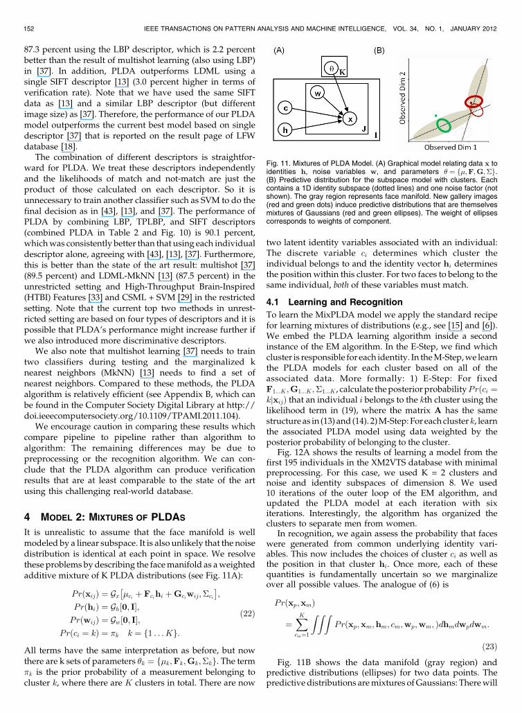
4 MODEL 2: MIXTURES OF PLDAS
It is unrealistic to assume that the face manifold is wellmodeled by a linear subspace. It is also unlikely that the noisedistribution is identical at each point in space. We resolvethese problems by describing the face manifold as a weightedadditive mixture of K PLDA distributions (see Fig. 11A):
PrðxijÞ ¼ Gx �ci þ Fcihi þGciwij;�ci
� �;
PrðhiÞ ¼ Gh 0; I½ �;PrðwijÞ ¼ Gw 0; I½ �;
Prðci ¼ kÞ ¼ �k k ¼ f1 . . .Kg:
ð22Þ
All terms have the same interpretation as before, but nowthere are k sets of parameters �k ¼ f�k;Fk;Gk;�kg. The term�k is the prior probability of a measurement belonging tocluster k, where there are K clusters in total. There are now
two latent identity variables associated with an individual:The discrete variable ci determines which cluster theindividual belongs to and the identity vector hi determinesthe position within this cluster. For two faces to belong to thesame individual, both of these variables must match.
4.1 Learning and Recognition
To learn the MixPLDA model we apply the standard recipefor learning mixtures of distributions (e.g., see [15] and [6]).We embed the PLDA learning algorithm inside a secondinstance of the EM algorithm. In the E-Step, we find whichcluster is responsible for each identity. In the M-Step, we learnthe PLDA models for each cluster based on all of theassociated data. More formally: 1) E-Step: For fixedF1...K;G1...K;�1...K , calculate the posterior probabilityPrðci ¼kjxijÞ that an individual i belongs to the kth cluster using thelikelihood term in (19), where the matrix A has the samestructure as in (13) and (14). 2) M-Step: For each clusterk, learnthe associated PLDA model using data weighted by theposterior probability of belonging to the cluster.
Fig. 12A shows the results of learning a model from thefirst 195 individuals in the XM2VTS database with minimalpreprocessing. For this case, we used K = 2 clusters andnoise and identity subspaces of dimension 8. We used10 iterations of the outer loop of the EM algorithm, andupdated the PLDA model at each iteration with sixiterations. Interestingly, the algorithm has organized theclusters to separate men from women.
In recognition, we again assess the probability that faceswere generated from common underlying identity vari-ables. This now includes the choices of cluster ci as well asthe position in that cluster hi. Once more, each of thesequantities is fundamentally uncertain so we marginalizeover all possible values. The analogue of (6) is
Prðxp;xmÞ
¼XKcm¼1
Z Z ZPrðxp;xm;hm; cm;wp;wm; Þdhmdwpdwm:
ð23Þ
Fig. 11B shows the data manifold (gray region) andpredictive distributions (ellipses) for two data points. Thepredictive distributions are mixtures of Gaussians: There will
152 IEEE TRANSACTIONS ON PATTERN ANALYSIS AND MACHINE INTELLIGENCE, VOL. 34, NO. 1, JANUARY 2012
Fig. 11. Mixtures of PLDA Model. (A) Graphical model relating data x toidentities h, noise variables w, and parameters � ¼ f�;F;G;�g.(B) Predictive distribution for the subspace model with clusters. Eachcontains a 1D identity subspace (dotted lines) and one noise factor (notshown). The gray region represents face manifold. New gallery images(red and green dots) induce predictive distributions that are themselvesmixtures of Gaussians (red and green ellipses). The weight of ellipsescorresponds to weights of component.

be one contribution from each mixture component of themodel. However, many data points (e.g., green point) will bealmost entirely associated with the nearest mixture compo-nent and will effectively have a Gaussian predictive distribu-tion. Notice that this is quite a sophisticated model. The datamanifold is nonlinear. The shape of the predictive distribu-tion is complex and varies depending on the gallery data.
4.2 Experiment 4
In Experiment 4, we repeat the XM2VTS experiment (Fig. 8a)for the mixture model. Percent correct performance improvesas we move from 1 to 2 clusters (Fig. 12B), but adding a thirddoes not make much difference. However, these resultsshould be treated with some caution: The two clustermixPLDA model has twice as many parameters as theoriginal PLDA model. In principle, it is possible for the twoclusters with N/2 dimensions to approximate the samesolution as the PLDA model with N dimensions. However,the clusters found in Fig. 12A suggest that this did nothappen.
The case would be clearer if we could investigate higherdimensional subspaces and demonstrate a clear perfor-mance benefit from the mixture model. Unfortunately, ourability to construct the between individual subspace F islimited by the number of individuals in the database (195).With three clusters of 64 dimensions, this only leaves1.01 people per dimension per cluster. Despite theseconcerns, we believe that the MixPLDA model is apromising method. It is fundamentally more expressivethan linear methods, and retains the advantages of theprobabilistic approach.
It would not have been easy to construct this model witha conventional distance-based approach. The representationof identity consists of one discrete variable ci and onecontinuous variable hi and hence measurements of distanceare no longer straightforward.
5 MODEL 3: TIED PLDA
Although the above methods can cope with a considerableamount of image variation, there are some cases, such aslarge pose changes, where viewing conditions are sodisparate that a more powerful technique must be applied.
In “tied” models [34], two or more viewing conditions arecompared by assuming that they have a common under-lying variable hi, but different generation processes. Forexample, consider viewing J images each of I individuals, at
K different poses. Here, we will assume that the pose k isknown for each observed datum xijk, although this is notnecessary. The generative model for this data is
Prðxijkjhi;wijkÞ ¼ Gx½�k þ Fkhi þGkwijk;�k�;PrðhiÞ ¼ Gh½0; I�;
PrðwijkÞ ¼ Gw½0; I�:ð24Þ
The graphical model for Tied PLDA is given inFig. 13A. Note that this model is quite different from theMixPLDA model. Both models describe the training dataas a mixture of factor analyzers. However, in themixPLDA model, the representation of identity includesthe choice of cluster ci. In the Tied PLDA model, therepresentation of identity hi is constant (tied) regardless ofthe cluster (viewing condition). Another way to thinkabout this is that the data are described as k clusters, butcertain positions in each cluster are “identity-equivalent.”
5.1 Learning and Recognition
Learning is very similar to the original PLDA model, withone major difference. In the E-Step, we calculate theposterior distribution over the latent variables giventhe observed data as before. However, there is now aseparate M-Step for each cluster k in which the terms�k;Fk;Gk;�k are updated using only the data known tocome from these clusters. A more detailed description of theprinciples behind tied models can be found in [34].
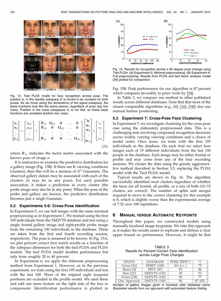
We train using 195 individuals from the XM2VTSdatabase, with four frontal and four profile faces of eachindividual. Fig. 14 shows the results of training the modelwith two clusters using four frontal and four profile imageseach from the first 195 individuals from the XM2VTSdatabase with minimal preprocessing. The “tied” structureis reflected in the fact that the columns of F1 and F2 looklike images of the same people.
Recognition proceeds exactly as in the PLDA model, butnow likelihood terms are calculated by marginalizing the
joint likelihood implicitly defined by (24). The analogue of(13) is
LI ET AL.: PROBABILISTIC MODELS FOR INFERENCE ABOUT IDENTITY 153
Fig. 12. (A) Mixtures of the PLDA model. The top two rows showelements of mixture component 1. The bottom two rows showcomponent 2. Interestingly, the two clusters correspond to the twosexes. The mean of cluster 1 and images representing directions in thesignal subspace all look like women (top row). For cluster 2 (row three),images all look like men. As before, different positions in the within-individual subspace (second and fourth row) look like different images ofthe same person. (B) Identification results from MixPLDA model as afunction of subspace dimension.
Fig. 13. Tied PLDA Model. (A) Graphical model relating data x toidentities h, noise variables w, and parameters � ¼ f�;F;G;�g.(B) Predictive distribution for Tied model with two clusters. Eachcontains a 1D identity subspace (dotted lines) and one noise factor (notshown). Gray region represents face manifold. A new gallery image (reddot) induces a predictive distribution that is a mixture of four Gaussians.Ellipse weight indicates weight of component in predictive distribution.
x1
x2
..
.
xN
26664
37775¼
�k1
�k2
..
.
�kn
26664
37775þ
Fk1 Gk1 0 . . . 0Fk2 0 Gk2 . . . 0
..
. ... ..
. . .. ..
.
Fkn 0 0 . . . Gkn
26664
37775
hw1
w2
..
.
wN
2666664
3777775þ
�1�2...
�N
26664
37775;
ð25Þ
where Fkn indicates the factor matrix associated with theknown pose of image n.
It is instructive to examine the predictive distribution fora gallery image (Fig. 13B). If there are K viewing conditions(clusters), then this will be a mixture of K2 Gaussians. Theobserved gallery datum may be associated with each of theclusters (it may be in any pose). For each possibleassociation, it makes a prediction in every cluster (theprobe image may also be in any pose). When the pose of theprobe and gallery are known, the predictive distributionbecomes just a single Gaussian.
5.2 Experiments 5-6: Cross-Pose Identification
In Experiment 5, we use full images with the same minimalpreprocessing as in Experiment 1. We trained using the first195 individuals from the XM2VTS database and test using asingle frontal gallery image and right-profile probe imagefrom the remaining 100 individuals in the database. Theseare taken from the first and fourth recording session,respectively. The pose is assumed to be known. In Fig. 15A,we plot percent correct first match results as a function ofthe subspace dimension for both the tied PLDA and PLDAmodels. The tied PLDA model doubles performance butonly from roughly 20 to 40 percent.
In Experiment 6, we apply the elaborate preprocessingmethod from Experiment 1. However, as in the previousexperiment, we train using the first 195 individuals and testwith the last 100. Three of the original eight keypointpositions are occluded in the profile model. We omit theseand add one more feature on the right side of the face tocompensate. Identification performance is plotted in
Fig. 15B. Peak performance for our algorithm is 87 percentwhich compares favorably to prior work by [34].
In Table 3, we compare our method to other publishedresults across different databases. Note that that most of theclosest comparable algorithms (e.g., [4], [16], [34]) also usemanual feature positioning.
5.3 Experiment 7: Cross-Pose Face Clustering
In Experiment 7, we investigate clustering for the cross-posecase using the elaborately preprocessed data. This is achallenging task involving compound recognition decisionsacross widely varying viewing conditions and a choice ofmodel order. Once more, we train with the first 195individuals in the database. On each trial we select fourimages each of 15 different individuals from the last 100people in the database. Each image may be either frontal orprofile and may come from any of the four recordingsessions. We cluster the data using the greedy agglomera-tive method described in Section 3.5, replacing the PLDAmodel with the Tied PLDA model.
Typical results are shown in Fig. 16. The algorithmsuccessfully identified most clusters regardless of whetherthe faces are all frontal, all profile, or a mix of both (10/15clusters are correct). The number of splits and mergesrequired to move to the correct clustering for this exampleis 8, which is slightly worse than the experimental averageof 7.32 over 100 repetitions.
6 MANUAL VERSUS AUTOMATIC KEYPOINTS
Throughout this paper, we constructed models usingmanually localized image keypoints. We take this approachas it makes the results easier to replicate and defines a clearupper bound on performance. However, it might be that
154 IEEE TRANSACTIONS ON PATTERN ANALYSIS AND MACHINE INTELLIGENCE, VOL. 34, NO. 1, JANUARY 2012
Fig. 14. Tied PLDA model for face recognition across pose. Theposition hi in the identity subspace F is forced to be constant for bothposes: As we move along the dimensions of the signal subspace, thebasis functions look like the same person, regardless of pose (top tworows). Position in the noise subspaces G is not tied, so these basisfunctions are unrelated (bottom two rows).
Fig. 15. Results for recognition across a 90 degree pose change usingTied PLDA. (A) Experiment 5: Minimal preprocessing. (B) Experiment 6:Full preprocessing. Results from PLDA and tied factor analysis model[34] plotted for comparison.
TABLE 3Results for Percent Correct Face Identification
across Large Pose Changes
Number of gallery images given in brackets after database name.Bracketed results from our approach with automated feature finding.
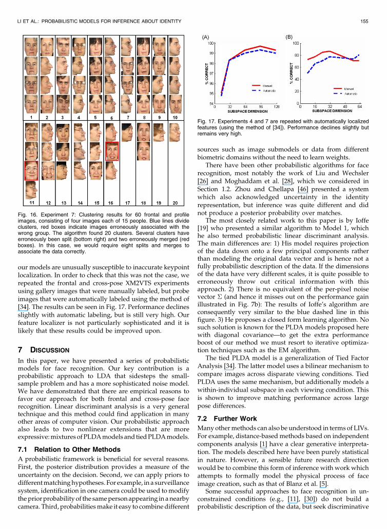
our models are unusually susceptible to inaccurate keypointlocalization. In order to check that this was not the case, werepeated the frontal and cross-pose XM2VTS experimentsusing gallery images that were manually labeled, but probeimages that were automatically labeled using the method of[34]. The results can be seen in Fig. 17. Performance declinesslightly with automatic labeling, but is still very high. Ourfeature localizer is not particularly sophisticated and it islikely that these results could be improved upon.
7 DISCUSSION
In this paper, we have presented a series of probabilisticmodels for face recognition. Our key contribution is aprobabilistic approach to LDA that sidesteps the small-sample problem and has a more sophisticated noise model.We have demonstrated that there are empirical reasons tofavor our approach for both frontal and cross-pose facerecognition. Linear discriminant analysis is a very generaltechnique and this method could find application in manyother areas of computer vision. Our probabilistic approachalso leads to two nonlinear extensions that are moreexpressive: mixtures of PLDA models and tied PLDA models.
7.1 Relation to Other Methods
A probabilistic framework is beneficial for several reasons.First, the posterior distribution provides a measure of theuncertainty on the decision. Second, we can apply priors todifferent matching hypotheses. For example, in a surveillancesystem, identification in one camera could be used to modifythe prior probability of the same person appearing in a nearbycamera. Third, probabilities make it easy to combine different
sources such as image submodels or data from differentbiometric domains without the need to learn weights.
There have been other probabilistic algorithms for facerecognition, most notably the work of Liu and Wechsler[26] and Moghaddam et al. [28], which we considered inSection 1.2. Zhou and Chellapa [46] presented a systemwhich also acknowledged uncertainty in the identityrepresentation, but inference was quite different and didnot produce a posterior probability over matches.
The most closely related work to this paper is by Ioffe[19] who presented a similar algorithm to Model 1, whichhe also termed probabilistic linear discriminant analysis.The main differences are: 1) His model requires projectionof the data down onto a few principal components ratherthan modeling the original data vector and is hence not afully probabilistic description of the data. If the dimensionsof the data have very different scales, it is quite possible toerroneously throw out critical information with thisapproach. 2) There is no equivalent of the per-pixel noisevector � (and hence it misses out on the performance gainillustrated in Fig. 7b): The results of Ioffe’s algorithm areconsequently very similar to the blue dashed line in thisfigure. 3) He proposes a closed form learning algorithm. Nosuch solution is known for the PLDA models proposed herewith diagonal covariance—to get the extra performanceboost of our method we must resort to iterative optimiza-tion techniques such as the EM algorithm.
The tied PLDA model is a generalization of Tied FactorAnalysis [34]. The latter model uses a bilinear mechanism tocompare images across disparate viewing conditions. TiedPLDA uses the same mechanism, but additionally models awithin-individual subspace in each viewing condition. Thisis shown to improve matching performance across largepose differences.
7.2 Further Work
Many other methods can also be understood in terms of LIVs.For example, distance-based methods based on independentcomponents analysis [1] have a clear generative interpreta-tion. The models described here have been purely statisticalin nature. However, a sensible future research directionwould be to combine this form of inference with work whichattempts to formally model the physical process of faceimage creation, such as that of Blanz et al. [5].
Some successful approaches to face recognition in un-constrained conditions (e.g., [11], [30]) do not build aprobabilistic description of the data, but seek discriminative
LI ET AL.: PROBABILISTIC MODELS FOR INFERENCE ABOUT IDENTITY 155
Fig. 16. Experiment 7: Clustering results for 60 frontal and profileimages, consisting of four images each of 15 people. Blue lines divideclusters, red boxes indicate images erroneously associated with thewrong group. The algorithm found 20 clusters. Several clusters haveerroneously been split (bottom right) and two erroneously merged (redboxes). In this case, we would require eight splits and merges toassociate the data correctly.
Fig. 17. Experiments 4 and 7 are repeated with automatically localizedfeatures (using the method of [34]). Performance declines slightly butremains very high.

patch-based features which classify pairs of faces into“same” or “different.” These methods have complementaryproperties to our system: They are specialized to faceverification and cannot easily be adapted for other taskssuch as clustering. They may also struggle with extremevariations such as 90 degree pose differences as featureextraction is based on cross-correlation between images. Aninteresting direction for future work would be to construct aLIV model based on similar features which retains thestrengths of both approaches.
REFERENCES
[1] M.S. Bartlett, H.M. Lades, and T.J. Sejnowski, “IndependentComponent Representations for Face Recognition,” Proc. SPIE,vol. 3299, pp. 528-539, 1998.
[2] P.N. Belhumeur, J. Hespanha, and D.J. Kriegman, “Eigenfacesversus Fisherfaces: Recognition Using Class Specific LinearProjection,” IEEE Trans. Pattern Analysis and Machine Intelligence,vol. 19, no. 7, pp. 711-720, July 1997.
[3] M. Isard and A. Blake, “CONDENSATION—Conditional DensityPropagation for Visual Tracking,” Int’l J. Computer Vision, vol. 29,pp. 5-28, 1998.
[4] V. Blanz, P. Grother, P.J. Phillips, and T. Vetter, “Face RecognitionBased on Frontal Views Generated from Non-Frontal Images,”Proc. IEEE CS Conf. Vision and Pattern Recognition, pp. 454-461,2005.
[5] V. Blanz, S. Romdhani, and T. Vetter, “Face Identificationacross Different Poses and Illumination with a 3D MorphableModel,” Proc. Int’l Conf. Face and Gesture Recognition, pp. 202-207, 2002.
[6] C.M. Bishop, Pattern Recognition and Machine Learning. Springer,2007.
[7] D. Cai, X.F. He, Y.X. Hu, J.W. Han, “Learning a Spatially SmoothSubspace for Face Recognition,” Proc. IEEE Conf. Vision and PatternRecognition, pp. 1-7, 2007.
[8] L.F. Chen, H.Y.M. Liao, J.C. Lin, M.T. Ko, and G.J. Yu, “A NewLDA-Based Face Recognition System which Can Solve the SmallSample Size Problem,” Pattern Recognition, vol. 33, pp. 1713-1726,2000.
[9] A.P. Dempster, N.M. Laird, and D.B. Rubin, “Maximum Like-lihood for Incomplete Data via the EM Algorithm,” J. RoyalStatistical Soc. B, vol. 39, pp. 1-38, 1977.
[10] M. Everingham, J. Sivic, and A. Zisserman, ““Hello! My Name Is..Buffy” C Automatic Naming of Characters in TV Video,” Proc.British Machine Vision Conf., 2006.
[11] A. Ferencz, E. Learned-Miller, and J. Malik, “Learning to LocateInformative Features for Visual Identification,” Int’l J. ComputerVision, vol. 77, pp. 3-24, 2008.
[12] R. Fergus, P. Perona, and A. Zisserman, “Object Class Recognitionby Unsupervised Scale Invariant Learning,” Proc. IEEE CS Conf.Computer Vision and Pattern Recognition, pp. 264-271, 2003.
[13] M. Guillaumin, J. Verbeek, and C. Schmid, “Is that You? MetricLearning Approaches for Face Identification,” Proc. Int’l Conf.Computer Vision, 2009.
[14] A.S. Georghiades, P.N. Belhumeur, and D.J. Kriegman, “FromFew to Many: Illumination Cone Models for Face Recognitionunder Variable Lighting and Pose,” IEEE Trans. PatternAnalysis and Machine Intelligence, vol. 23, no. 6, pp. 643-660,June 2001.
[15] Z. Gharamani and G.E. Hinton, “The EM Algorithm for Mixturesof Factor Analyzers,” Technical Report CRG-TR-96-1, Dept. ofComputer Science, Univ. of Toronto, 1996.
[16] R. Gross, I. Matthews, and S. Baker, “Eigen Light-Fields and FaceRecognition across Pose,” Proc. IEEE Fifth Int’l Conf. Automatic Faceand Gesture Recognition, pp. 1-7, 2002.
[17] X. He, S. Yan, Y. Hu, P. Nihogi, and H. Zhang, “Face RecognitionUsing Laplacian Faces,” IEEE Trans. Pattern Analysis and MachineIntelligence, vol. 27, no. 3, pp. 328-340, Mar. 2005.
[18] G.B. Huang, M. Ramesh, T. Berg, and E. Learned-Miller, “LabeledFaces in the Wild: A Database for Studying Face Recognition inUnconstrained Environments,” Technical Report 07-49, Univ. ofMassachusetts, Oct. 2007.
[19] S. Ioffe, “Probabilistic Linear Discriminant Analysis,” Proc.European Conf. Computer Vision, pp. 531-542, 2006.
[20] E. Jones and S. Soatto, “Layered Active Appearance Models,”Proc. IEEE 10th Int’l Conf. Computer Vision, pp. 1097-1102, 2005.
[21] T. Kim and J. Kittler, “Locally Linear Discriminant Analysis forMultimodally Distributed Classes for Face Recognition with aSingle Model Image,” IEEE Trans. Pattern Analysis and MachineIntelligence, vol. 27, no. 3, pp. 318-327, Mar. 2005.
[22] N. Kumar, A.C. Berg, P.N. Belhumeur, and S.K. Nayar, “Attributeand Simile Classifiers for Face Verification,” Proc. IEEE 12th Int’lConf. Computer Vision, 2009.
[23] L. Fei-Fei, R. Fergus, and P. Perona, “A Bayesian Approach toUnsupervised One-Shot Learning of Object Categories,” Proc.IEEE Ninth Int’l Conf. Computer Vision, pp. 1134-1141, 2003.
[24] P. Li, J. Warrell, J. Aghajanian, and S.J.D. Prince, “Context BasedAdditive Logistic Model for Facial Keypoint Localization,” Proc.British Machine Vision Conf., 2010.
[25] Z. Li and X. Tang, “Bayesian Face Recognition Using SupportVector Machine and Face Clustering,” Proc. IEEE Conf. ComputerVision and Pattern Recognition, pp. 259-265, 2004.
[26] C. Liu and H. Wechsler, “Probabilistic Reasoning Models for FaceRecognition,” Proc. IEEE CS Conf. Computer Vision and PatternRecognition, pp. 827-832, 1998.
[27] S. Lucey and T. Chen, “Learning Patch Dependencies forImproved Pose Mismatched Face Verification,” Proc. IEEE CSConf. Computer Vision and Pattern Recognition, vol. 1, pp. 909-915,2006.
[28] B. Moghaddam, T. Jebara, and A. Pentland, “Bayesian FaceRecognition,” Pattern Recognition, vol. 33, pp. 1771-1782, 2000.
[29] H.V. Nguyen and L. Bai, “Cosine Similarity Metric Learningfor Face Verification,” Proc. 10th Asian Conf. Computer Vision,2010.
[30] E. Nowak and F. Jurie, “Learning Visual Similarity Measures forComparing Never Seen Objects,” Proc. IEEE Conf. Computer Visionand Pattern Recognition, pp. 1-8, 2007.
[31] T. Ojala, M. Pietikainen, and T. Maenpaa, “Multiresolution Gray-Scale and Rotation Invariant Texture Classification with LocalBinary Patterns,” IEEE Trans. Pattern Analysis and MachineIntelligence, vol. 24, no. 7, pp. 971-987, July 2002.
[32] V. Perlibakas, “Distance Measures for PCA-Based Face Recogni-tion,” Pattern Recognition Letters, vol. 25, pp. 711-724, 2004.
[33] N. Pinto and D. Cox, “Beyond Simple Features: A Large-ScaleFeature Search Approach to Unconstrained Face Recognition,”Proc. Int’l Conf. Automatic Face and Gesture Recognition, 2011.
[34] S.J.D. Prince, J. Warrell, J.H. Elder, and F.M. Felisberti, “TiedFactor Analysis for Face Recognition Across Large Pose Differ-ences,” IEEE Trans. Pattern Analysis and Machine Intelligence,vol. 30, no. 6, pp. 970-984, June 2008.
[35] S.J.D. Prince and J.H. Elder, “Probabilistic Linear DiscriminantAnalysis for Inferences about Identity,” Proc. IEEE 11th Int’l Conf.Computer Vision, 2007.
[36] C. Rother, V. Kolmogorov, and A. Blake, “GrabCut: InteractiveForeground Extraction Using Iterated Graph Cuts,” Proc. ACMSIGGRAPH, pp. 309-314, 2004.
[37] Y. Taigman, L. Wolf, and T. Hassner, “Multiple One-Shots forUtilizing Class Label Information,” Proc. British Machine VisionConf., 2009.
[38] M. Turk and A.P. Pentland, “Face Recognition Using Eigenfaces,”Proc. IEEE CS Conf. Vision and Pattern Recognition, pp. 586-591,1991.
[39] X. Wang and X. Tang, “Dual-Space Linear Discriminant Analysisfor Face Recognition,” Proc. IEEE CS Conf. Computer Vision andPattern Recognition, vol. 2, pp. 564-569, 2004.
[40] X. Wang and X. Tang, “Unified Framework for Subspace FaceRecognition,” IEEE Trans. Pattern Analysis and Machine Intelligence,vol. 26, no. 9, pp. 1222-1228, Sept. 2004.
[41] X. Wang and X. Tang, “Bayesian Face Recognition Using GaborFeatures,” Proc. ACM SIGMM Workshop Biometrics Methods andApplications, pp. 70-73, 2003.
[42] X. Wang and X. Tang, “Random Sampling for Subspace FaceRecognition,” Int’l J. Computer Vision, vol. 70, pp. 91-104, 2006.
[43] L. Wolf, T. Hassner, and Y. Taigman, “Descriptor Based Methodsin the Wild,” Proc. European Conf. Computer Vision, 2008.
[44] M.H. Yang, “Kernel Eigenfaces versus Kernel Fisherfaces: FaceRecognition Using Kernel Methods,” Proc. IEEE Fifth Int’l Conf.Automatic Face and Gesture Recognition, pp. 215-220, 2002.
[45] W. Zhao, R. Chellappa, A. Rosenfeld, and J. Phillips, “FaceRecognition: A Literature Survey,” J. ACM Computing Surveys,vol. 35, pp. 399-458, 2003.
156 IEEE TRANSACTIONS ON PATTERN ANALYSIS AND MACHINE INTELLIGENCE, VOL. 34, NO. 1, JANUARY 2012
[46] S.K. Zhou and R. Chellappa, “Probabilistic Identity Characteriza-tion for Face Recognition,” Proc. IEEE CS Conf. Computer Vision andPattern Recognition, vol. 2, pp. 805-812, 2004.
[47] http://www.ee.surrey.ac.uk/Research/VSSP/xm2vtsdb/, 2011.
Peng Li received the BEng and MEng degrees inautomation from North China Electric PowerUniversity in 1993 and 1998, and the PhD degreein electrical and electronic engineering fromNanyang Technological University in 2006. Hewas a lecturer at North China Electric PowerUniversity from 1998 to 2002. From 2005 to2007, he was a computer vision engineer inStratech Systems Ltd., Singapore. He was aresearch associate at the University of Bristol in
2007. From 2008 to 2010, he was a research fellow in the Department ofComputer Science, University College London. He is now a researchassociate at the University of Bristol. His research interests includecomputer vision, machine learning, and bioinformatics, particularly in facerecognition and Bayesian methods, etc. He is a member of the IEEE.
Yun Fu received the BSc degree in computerscience from Xi’an University of Science andTechnology and the MSc degree in vision,image, and virtual environments from UniversityCollege London. He is currently working towardthe PhD degree in the Department of ComputerScience at University College London. Hisresearch interest is in face recognition. He is amember of the IEEE.
Umar Mohammed received the BSc degree inmathematics from City University and the MScdegree in vision, imaging, and virtual environ-ments from University College London. He iscurrently working toward the PhD degree atUniversity College London in the Department ofComputer Science. His research interests in-clude face recognition and image-based render-ing. He is a member of the IEEE.
James H. Elder received the BASc degree inelectrical engineering from the University ofBritish Columbia in 1987 and the PhD degreein electrical engineering from McGill University in1995. From 1995 to 1996, he was with NECResearch Institute in Princeton, New Jersey. Hejoined the faculty of York University, Canada, in1996, where he is presently an associateprofessor. His research interests include com-puter and human vision. Recent work has
focused on natural scene statistics, perceptual organization, contourprocessing, attentive vision systems, and face detection. He is amember of the IEEE.
Simon J.D. Prince received the PhD degree in1999 from the University of Oxford for workconcerning human stereo vision. He has adiverse background in biological and computingsciences and has published papers across thefields of biometrics, psychology, physiology,medical imaging, computer vision, computergraphics, and HCI. He has worked as a researchscientist in Oxford, Singapore, and Toronto. Heis currently a reader in computer science at
University College London. He is a member of the IEEE.
. For more information on this or any other computing topic,please visit our Digital Library at www.computer.org/publications/dlib.
LI ET AL.: PROBABILISTIC MODELS FOR INFERENCE ABOUT IDENTITY 157