SUBSAMPLING APPROACH FOR STATISTICAL INFERENCE WITHIN STOCHASTIC DEA MODELS
Upload
independentCategory
view
7download
0
J Exp Criminol (2007) 3:247–270DOI 10.1007/s11292-007-9036-y
Statistical inference and meta-analysis
Richard Berk
Published online: 31 July 2007© Springer Science + Business Media B.V. 2007
Abstract Statistical inference is a common feature of meta-analysis. Statisticalinference depends on a formal model that accurately characterizes certain keyfeatures of how the studies to be summarized were generated. The implicationsof this requirement are discussed and questions are raised about the credibilityof confidence intervals and hypothesis tests routinely reported.
Keywords Confidence intervals · Hypothesis tests · Meta-analysis ·Statistical inference
Introduction
Statistical inference is an important feature of meta-analysis. Estimation isoften a central goal. Hypothesis tests and confidence intervals are used toaddress uncertainty. Indeed, a significant motivation for meta-analysis canbe improving the precision of the estimates produced and increasing thepower of any hypothesis tests. It follows that expositions of meta-analysismake statistical inference a major theme (Hedges and Olkin 1985; Hunterand Schmidt 1990; Hedges 1994; Raudenbush 1994; Lipsey 1992, 1997; Fleisset al. 2003: Chapter 10).
In the pages ahead, the use of statistical inference in meta-analysis will beexamined. The intent is to consider the statistical models employed and thedata with which they are used. Building on some previous work (Wachter 1988;Berk and Freedman 2003; Briggs 2005), a key issue will be whether the datawere produced by the mechanisms that the models require.
R. Berk (B)Department of Criminology, Department of Statistics,University of Pennsylvania, PA, USAe-mail: [email protected]
248 R. Berk
The paper begins by describing some popular meta-analysis models. Anassessment of their use follows. The conclusions can be simply stated, at leastto a first approximation. All statistical inference, including statistical inferenceused in meta-analysis, depends on a model accurately characterizing certainkey features of how the data were generated. The data for meta-analysisare the results from a set of studies. Therefore, meta-analysis depends on amodel accurately characterizing certain key features of how the set of studieswas produced. If by this criterion the model is found lacking, any statisticalinference that follows will be a fiction. Fictional statistical inference seems tobe common in criminal justice and related applications of meta-analysis.
The basic meta-analysis model
A substantial number of meta-analysis statistical models have been developedto date (Hedges 1994; Raudenbush 1994; Glaser and Olkin 1994). As will beapparent in the pages ahead, the various models have common roots in earlierstatistical and econometric formulations. For purposes of this paper, therefore,the similarities across meta-analysis models are far more important than theirdifferences. The fundamental points to be made apply to all, and for ease ofexposition, the simpler approaches will be emphasized. We begin with the basicmeta-analysis model, branching out only as needed.
Statistical inference is a process by which information contained in a dataset is used to drawn conclusions about unobservables. For meta-analysis, thereis a model, often only implicit, representing how the studies to be summarizedcame to be. This model has unobservable parameters. Investigators use infor-mation from the studies on hand to estimate the values of these parameters.
Consider the basic meta-analysis model (Hedges and Olkin 1985: 76).There are a set of studies to be summarized. Within each study, there is atreatment group and a control group. The treatment group is exposed to someintervention. The control group gets an alternative, often just the status quo.Although the language of treatment and control is often used, meta-analysis isfrequently undertaken with observational studies in which “interventions” canbe almost any variable.
Building blocks
Let the observed response for the treated subjects be represented by YTmi,
where m = 1, 2, . . . M studies, and i=1, 2,. . .nTm treatment subjects for study m.
The observed response for the control subjects is represented by YCmj, where
m = 1, 2, . . . M studies, and j = 1, 2, . . . nCm control subjects for study m.
Under the basic model, the process by which YTmi and YC
mj are generatedleads to
YTmi ∼ N(μT
m, σ 2m), (1)

Statistical inference and meta-analysis 249
and
YCmj ∼ N(μC
m, σ 2m), (2)
where μTm and μC
m are population means for study m, and σ 2m is a common
population variance of the response across all subjects for study m.What sense are we to make of Eqs. 1 and 2? An interpretation that follows
cleanly has treatment group members for study m drawn at random from apopulation of treatment group members with a mean of μT
m and variance σ 2m,
and control group members for study m drawn at random from a populationof control group members with a mean of μC
m, and variance σ 2m.
Alternatively, an account with more causal content may be constructed. Thetwo populations can be thought of as a single population in which the μC
m isshifted up or down to μT
m for those individuals exposed to the treatment. Then,a random sample of treatment group members and control group membersfrom that population is taken. These and other interpretations work insofar asthey are consistent with three assumptions built into Eqs. 1 and 2 (Hedges andOlkin 1985).
1. YTmi is independent and identically distributed for the i = 1, 2, . . . nT
mtreatment subjects for study m;
2. YCmj is independent and identically distributed for the j = 1, 2, . . . nC
mcontrol subjects for study m; and
3. YTmi is independent of the YC
mj for all i = 1, 2, . . . nTm and all j = 1, 2, . . . nC
m.1
Assumptions 1 and 2 define within-group independence for study m.Assumption 3 adds between-group independence for study m. As discussedat some length in Berk and Freedman (2003), all three assumptions can besubstantially violated unless the treatment and control study subjects are reallysampled at random from populations that are large relative to the size ofthe samples or if somehow, natural processes bring about the equivalent.Substantial violations can mean that statistical inference is in trouble even foreach study alone, and substantial violations are common. How the data foreach study are generated really matters, and assumptions 1 through 3 will beexamined in more detail later when several specific meta-analysis statisticalmodels are discussed.
We now denote the mean response for the treatment group in study m byYT
m and the mean response of the control group in study m by YCm. It is then
approximately true that for each of the M studies,
YTm ∼ N(μT
m, σ 2m/nT
m), (3)
and
YCm ∼ N(μC
m, σ 2m/nC
m). (4)
1The normality assumptions are not critical especially when the number of observations in eachstudy is as least modest.

250 R. Berk
This study means for the experimentals and controls are a key summarystatistics in much of what follows.
Meta-analysis is an attempt to combine study effects, which leads to afourth assumption: independence across studies. For the study results beingsummarized, the observed outcome from any one study must be unrelated tothe observed outcome of any other study. Some details will follow shortly.
The assumption of independence across studies is widely acknowledged.Shadish and Haddock (1994: 264), for example, begin their exposition offixed effects models saying, “Suppose that the data to be combined arisefrom k independent studies...”. Hedges (1994: 286) launches his discussionof the one-factor fixed effects model saying, “In the discussion of the one-factor model, we will employ a notation emphasizing that the independenteffect size estimates fall into p groups...”. Fleiss and his colleagues, drawingupon a biostatistical perspective dating back to the 1950s, discuss “combiningevidence across several independent studies...” (2003: 265). Lipsey and Wilson(2001: 106) begin an overview of how to work with a set of study resultsby saying, “Once a set of statistically independent effects sizes is assembled,appropriate weights for each effect size are computed, and any other necessaryadjustments are made (more on this later), the analysis of effect size datagenerally proceeds in several stages.”
Putting the building blocks together
For each study, interest centers on the difference between the two popu-lation means: μT
m − μCm. Often, the scales with which the response variable
is measured will vary from study to study. If one assumes that all of thescales are linear transformations of one another, it is common work withthe standardized difference between the means: (μT
m − μCm)/σm. This is the
population difference between the means in standard deviation units, andis often called the “effect size,” which will be denoted here by αm. For thebasic fixed effects model, the standardized difference between the means isperhaps most commonly what one would like to know. More will be said aboutstandardization later.2
For the basic meta-analysis model, one assumes that for each of the studies,the effect size is the same: α1 = α2 = · · · = αM = α. It can now be instructiveto think about a population consisting of experimental subjects and controlsubjects for which the effect size is equal to α. The data for each of the Mstudies to be summarized is a random sample of experimentals and controlsfrom this population. Because of the random sampling, and only because ofthe random sampling, the observed effect sizes will vary from study to study.
2Glass et al. (1981) define effect size as the difference between the two μ’s, divided by the standarddeviation of the control group. As addressed shortly, this can be reasonable when the interventionaffects the variance of the response as well as the mean.

Statistical inference and meta-analysis 251
Consistent with this framework, Eqs. 1 and 2 can be rewritten to representthe basic “fixed effects model.” With α the common effect size one wants toknow, and εm the random error associated with the mth study, one can write
Dm = α + εm, (5)
where Dm is the observed effect size for study m.In Eq. 5, the unit of analysis is no longer subjects within studies. The unit
of analysis is now a study. This is well understood. What sometimes gets lost isthat the properties of Eq. 5 depend heavily upon what one assumes when thesubjects in each study are the focus. The four assumptions just considered arestill crucial; they do not go away when study subjects are collected into studies.
Equation 5 is drawn from the classical Gaussian linear model is statistics(Bickel and Doksum 2001: 366). The four earlier assumptions imply thatE(εm) = 0 and that the disturbances represented by εm are independent ofone another. One imagines a collection of hypothetical studies in which thevalue of α is shifted up or down by an additive, chance perturbation to produceDm. These chance perturbations are independent across studies, which makesthe Dm independent across studies as well. The assumption that E(εm) = 0implies that α alone is responsible for any systematic difference between theexperimentals and controls. Finally, εm sometimes is assumed to behave as ifdrawn from a normal distribution, but with even a modest number studies,the normality assumption is not essential and in any case, does not figureimportantly in the concerns to be raised later.
It is important to keep in mind that researchers never get to see α or εm. Allthey get to see over studies is Dm. Thus, the model represented by Eq. 5 is atheory about how the results of each study are produced. All that follows canonly make scientific sense if this theory is a good approximation of what reallyhappened.
Equation 5 can be elaborated in many ways. Very commonly, a set ofcovariates is included, so that Eq. 5 applies conditional on these covariates.This too is drawn from the classical Gaussian linear model is statistics (Bickeland Doksum 2001: 366–367; Hedges and Olkin, 168–171). With a total ofp predictors, one just replaces α with β0 + β1x1 + β2x2 · · · + βpxp, where x1
through xp are a set of p regressors.3 The p predictors imply that there is notone α but many, a topic to which we will return. Other elaborations of the basicmodel will be considered later as well.
Using the basic model
Data to estimate α and its standard error must include for all study subjectsin each study a response measure and an indicator for membership in theexperimental or control group. The data will often include covariates aswell. After that, things can get complicated. There are a number of different
3Analysis of variance is just a special case in which the regressor matrix is composed of indicatorvariables. (Hedges 1994: 295).
252 R. Berk
estimators of α and an appropriate standard error (Rosenthal 1994). Whena meta-analysis is done on a large number of studies, the differences be-tween these estimators is often not very important (Hedges and Olkin 1985:82–85) or at least is not the most vulnerable part of the analysis. Moreover, thetechnical properties of these different estimators are essentially irrelevant tothe question of whether Eq. 5 is likely to apply or not. So, we will continueto keep relatively straightforward, following the exposition of Shadish andHaddock (1994).
At the risk of stating the obvious, there is no point in combining studieswhose reported effects are not credible, and an initial and challenging taskis to determine which studies are worth summarizing (Wortman 1994). Butinsofar as there are a sufficient number of studies exceeding the minimumquality threshold, it often seems natural to estimate α from information in eachstudy by
αm = YTm − YC
m
Sm, (6)
where YTm is the observed mean response for the treatment group, YC
m themean observed response for the control group, and Sm is the observed standarddeviation of the response in study m.4
The pooled standard deviation of any given study is computed as
Sm =√
VTm(nT
m − 1) + VCm(nC
m − 1)
nTm + nC
m − 2, (7)
where VTm and VC
m stand for the observed variance of the response variablefor the treatment group and the control group, respectively, and nT
m and nCm
are the corresponding sample sizes. Equation 7 can be justified by assumingthat variances of the treatment group and control group are the same in thepopulation.
Because the goal is to summarize the findings across studies, an averageeffect (over studies) is computed as an estimate of α. It is a weighed average,with weights the inverse of the variance of each study’s standardized treatmenteffect. Studies with larger chance variation are given less weight when theweighted average is computed.5
More formally, the computed variance of αm is
Vαm = nTm + nC
m
nTm nC
m+ α2
m
2(nTm + nC
m). (8)
4Using αm to represent the estimate of α from information in study m, could lead to someconfusion later when αm is the population effect size for study m. To remedy this potentialconfusion would have substantially complicated the notational system. It should be clear in contextwhat is the estimator and what is being estimated. Formally, there is no problem because underthe basic model, αm = α.5It is also possible to weight additionally by a measure of study quality.

Statistical inference and meta-analysis 253
Table 1 Summary statisticsfor three studies nT
m,nCm YT
m − YCm Sm αm Vαm Wm
50,50 30 17.0 1.76 0.06 16.6740,40 20 11.0 1.81 0.07 14.2960,60 40 21.0 1.90 0.05 20.00
Then, the weight for each study is the inverse of each study’s variance:
Wm = 1
Vαm
. (9)
To compute for M studies, the weighted average standardized effect, oneuses,
α =∑M
m=1(Wm × αm)∑Mm=1 Wm
. (10)
Finally, the standard error of the weighted average is computed as
SEα =√
1∑Mm=1 Wm
. (11)
With the weighted average and its standard error in hand, confidenceintervals and hypothesis tests can be produced as usual.
A simple illustration
To help make the preceding discussion more concrete, consider a very simpleexample. Table 1 shows some summary statistics from three hypotheticalstudies. There is an experimental and control group in each. For each study, thetable reports in the first three columns from left to right the sample sizes, thedifference between the mean of the experimental group and the mean ofthe control group (in their original units), and the pooled standard deviationof the response variable. For simplicity, the samples are evenly dividedbetween the treatment and control groups.
The observed standardized effects, computed using Eqs. 6 and 8, are foundin the fourth column. Using Eq. 11, the variance of each αm is shown in thefifth column. In the sixth column are the weights, computed using Eq. 9. FromEq. 10, the weighted average is then 1.82. This is α.
The standard error of the weighted average (SEα), computed using Eq. 11,is .14. The 95% confidence interval is then 1.54 to 2.1. A test of the nullhypothesis that the treatment effect is 0, leads to a t-value of well over 10.Because the p-value is smaller than .05, the null hypothesis is rejected.
Interpreting the basic model
The basic meta-analysis model is simple, and the computations that followare simple as well. Simplicity is good. However, because the model connects
254 R. Berk
statistical inference to how the studies were produced, simplicity by itself isinsufficient. One needs to ask whether that connection performs as advertised.A useful place to begin is with a discussion of the common treatment effect α.What is the nature of the key parameter meta-analysts are trying to estimate?
Causality
Meta-analysis is commonly used to estimate the impact of an intervention.Interventions are manipulable within the real world in which the summarizedstudies have been done. Thus, effect sizes are causal effects and in this context,α is the population effect of a cause.
Some researchers apply meta-analysis to draw causal inferences when the“intervention” is a fixed attribute of an individual, such as sex (Archer 2000)or race (Mitchell 2005). Regardless of the statistical procedure used, it makeslittle sense to ask, for instance, whether a prison sentence would change if theoffender’s race were different, when it could not have been different (Holland1986; Rubin 1986; Berk 2003).
But, there is nothing in Eq. 5 that requires cause and effect. One may treatα as a description of a difference between the mean of one group and the meanof the other. It is possible to conduct a meta-analysis of the association betweenrace and the length of prison sentence as long as no causal interpretations areimposed.
In short, meta-analysis is usually motivated by a desire to estimate a causaleffect; α is a causal effect. This means that all of the issues surrounding causalinference raised in the recent statistics literature (Freedman 2004) are in play,and researchers doing meta-analysis to need to engage. However, descriptioncan suffice as useful research goal. Problems arise when variables that cannotbe manipulated are analyzed as causes. Further confusion can result if thelanguage of experiments is used when it does not apply. We will proceed fromhere onward within a causal framework because cause and effect are usuallykey concerns in a meta-analysis. Still, description is not precluded.
Standardization
Because α is commonly standardized, it is important to briefly address the needfor and consequences of this approach. There is a long history of concernsabout standard scores in regression, and these concerns spill over into meta-analysis (Duncan 1975, Chapter 4; Berk 2003: 28–30, 117–119, 198–199; Berkand Freedman 2003, Section 7.4; Bond et al. 2003).6 What follows in a briefsummary.
6For example, Duncan observes (1975: 51), “... it would probably be salutary if research work-ers relinquished the habit of expressing variables in standard form. The main reason for thisrecommendation is that standardization tends to obscure the distinction between the structuralcoefficients of the model and the several variances and covariances that describe the jointdistribution of the variables in a certain population.” These concerns can apply to meta-analysis.
Statistical inference and meta-analysis 255
If all of the studies to be summarized have outcomes in common andinterpretable units, estimates of α are in those units as well. There is no need tostandardize the units across studies; α is the single, common treatment effect innatural units. Suppose, for example, that α is three fewer burglaries committedby individuals in a certain kind of drug treatment program compared toindividuals under conventional parole supervision. Then there will be exactlythree fewer burglaries for each such drug-treatment program studied, exceptfor random error associated with how each study was conducted.
In a wide variety of social science and criminal justice investigations, theunits in which the response is measured vary fundamentally. For example, theoutcome may be the homicide rate in one study and the number of homicidesin another study. Then, standardization is undertaken so that the treatmenteffects can be more appropriately compared. Under this scenario, the basicmeta-analysis model requires the intervention has the same effect in each studyin standard deviation units (e.g., −1.2), except for each study’s random error.The only systematic difference across studies is a difference in scale.
However, standardization depends on two assumptions about how the real-world functions. Recall that the basic model requires that in each study, thevariance of the experimentals is the same as the variance of the controls. Thisis the first assumption, and it depends on a theory of how the treatment affectsthe response.
For example, when the response to the treatment is proportional to theresponse to the control condition, both the mean and the variance will differbetween the experimentals and controls. The population variance of thetreatment groups will differ from the population variance of the control groupby some multiplicative constant. However, with an additive increase in themean of the treatment group, which is the usual assumption, the equal varianceassumption may be credible. Credibility will depend on the precise nature ofthe study, what is being measured, and the composition of the experimentaland control groups.7
The equal variance assumption is not a mere technicality, and there tech-nical work-arounds in any case. If the effect is really additive, computing astandardized difference between means is may not be misrepresenting impactof the treatment. But if the effect is multiplicative, the treatment impact isbeing misrepresented from the start. Therefore, a strong rationale must beprovided in subject-matter terms for why an additive effect (or some othereffect) is being assumed. Why does the phenomenon being studied workthat way?
The second assumption is that the intervention has exactly the same effect,in standard deviation units, in the different studies. This is a very strong
7An alternative approach is that the variance of the experimental group’s response is the sameas the variance of the control group’s response under the null hypothesis that α = 0. Then thevariance of the control group’s response can be used as the “common” variance. This is essentiallythe position taken by Glass and his colleagues (1981). But if the null hypothesis is rejected, thenwhat? One may need a new model that can be justified in which the variances are not the same.
256 R. Berk
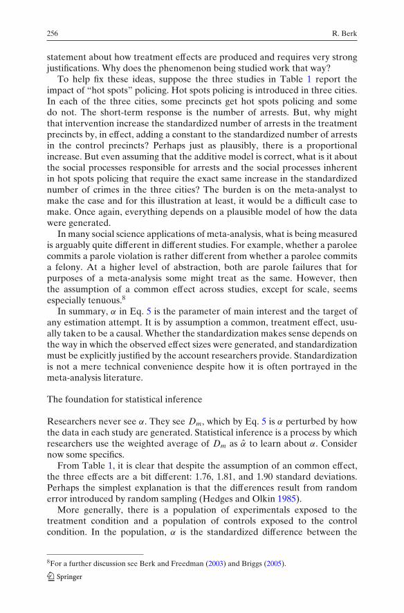
statement about how treatment effects are produced and requires very strongjustifications. Why does the phenomenon being studied work that way?
To help fix these ideas, suppose the three studies in Table 1 report theimpact of “hot spots” policing. Hot spots policing is introduced in three cities.In each of the three cities, some precincts get hot spots policing and somedo not. The short-term response is the number of arrests. But, why mightthat intervention increase the standardized number of arrests in the treatmentprecincts by, in effect, adding a constant to the standardized number of arrestsin the control precincts? Perhaps just as plausibly, there is a proportionalincrease. But even assuming that the additive model is correct, what is it aboutthe social processes responsible for arrests and the social processes inherentin hot spots policing that require the exact same increase in the standardizednumber of crimes in the three cities? The burden is on the meta-analyst tomake the case and for this illustration at least, it would be a difficult case tomake. Once again, everything depends on a plausible model of how the datawere generated.
In many social science applications of meta-analysis, what is being measuredis arguably quite different in different studies. For example, whether a paroleecommits a parole violation is rather different from whether a parolee commitsa felony. At a higher level of abstraction, both are parole failures that forpurposes of a meta-analysis some might treat as the same. However, thenthe assumption of a common effect across studies, except for scale, seemsespecially tenuous.8
In summary, α in Eq. 5 is the parameter of main interest and the target ofany estimation attempt. It is by assumption a common, treatment effect, usu-ally taken to be a causal. Whether the standardization makes sense depends onthe way in which the observed effect sizes were generated, and standardizationmust be explicitly justified by the account researchers provide. Standardizationis not a mere technical convenience despite how it is often portrayed in themeta-analysis literature.
The foundation for statistical inference
Researchers never see α. They see Dm, which by Eq. 5 is α perturbed by howthe data in each study are generated. Statistical inference is a process by whichresearchers use the weighted average of Dm as α to learn about α. Considernow some specifics.
From Table 1, it is clear that despite the assumption of an common effect,the three effects are a bit different: 1.76, 1.81, and 1.90 standard deviations.Perhaps the simplest explanation is that the differences result from randomerror introduced by random sampling (Hedges and Olkin 1985).
More generally, there is a population of experimentals exposed to thetreatment condition and a population of controls exposed to the controlcondition. In the population, α is the standardized difference between the
8For a further discussion see Berk and Freedman (2003) and Briggs (2005).
Statistical inference and meta-analysis 257
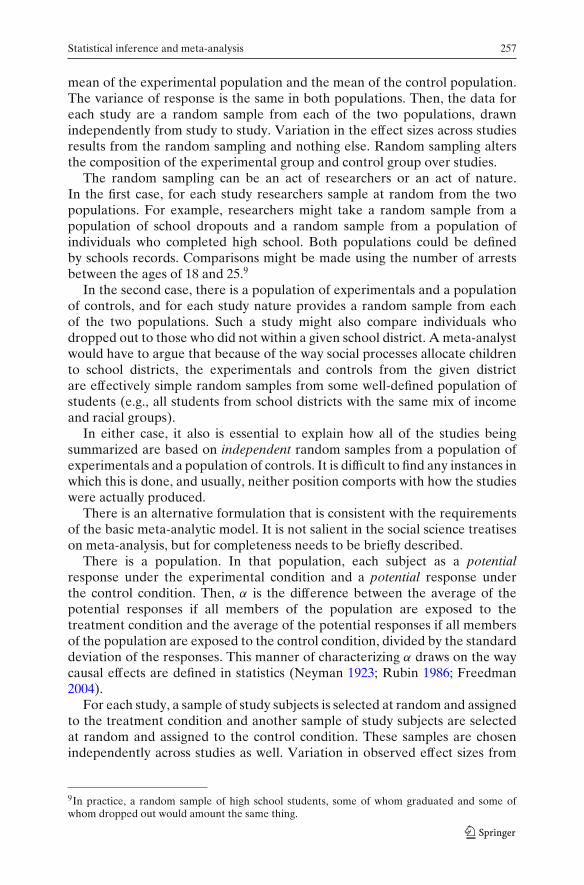
mean of the experimental population and the mean of the control population.The variance of response is the same in both populations. Then, the data foreach study are a random sample from each of the two populations, drawnindependently from study to study. Variation in the effect sizes across studiesresults from the random sampling and nothing else. Random sampling altersthe composition of the experimental group and control group over studies.
The random sampling can be an act of researchers or an act of nature.In the first case, for each study researchers sample at random from the twopopulations. For example, researchers might take a random sample from apopulation of school dropouts and a random sample from a population ofindividuals who completed high school. Both populations could be definedby schools records. Comparisons might be made using the number of arrestsbetween the ages of 18 and 25.9
In the second case, there is a population of experimentals and a populationof controls, and for each study nature provides a random sample from eachof the two populations. Such a study might also compare individuals whodropped out to those who did not within a given school district. A meta-analystwould have to argue that because of the way social processes allocate childrento school districts, the experimentals and controls from the given districtare effectively simple random samples from some well-defined population ofstudents (e.g., all students from school districts with the same mix of incomeand racial groups).
In either case, it also is essential to explain how all of the studies beingsummarized are based on independent random samples from a population ofexperimentals and a population of controls. It is difficult to find any instances inwhich this is done, and usually, neither position comports with how the studieswere actually produced.
There is an alternative formulation that is consistent with the requirementsof the basic meta-analytic model. It is not salient in the social science treatiseson meta-analysis, but for completeness needs to be briefly described.
There is a population. In that population, each subject as a potentialresponse under the experimental condition and a potential response underthe control condition. Then, α is the difference between the average of thepotential responses if all members of the population are exposed to thetreatment condition and the average of the potential responses if all membersof the population are exposed to the control condition, divided by the standarddeviation of the responses. This manner of characterizing α draws on the waycausal effects are defined in statistics (Neyman 1923; Rubin 1986; Freedman2004).
For each study, a sample of study subjects is selected at random and assignedto the treatment condition and another sample of study subjects are selectedat random and assigned to the control condition. These samples are chosenindependently across studies as well. Variation in observed effect sizes from
9In practice, a random sample of high school students, some of whom graduated and some ofwhom dropped out would amount the same thing.

258 R. Berk
study to study is solely a function of within-study random assignment. Were it ispossible to go back in time and randomly assign two samples a second time, theresults would be a little different, even if nothing else had changed. By the luckof the draw, the composition of the experimental and control groups wouldlikely be altered, which would likely alter the observed difference betweenthe mean of the treatment group and the mean of the control group. The factthat there is only one effect size is obscured by an assignment process thatshuffles the composition of the experimental and control groups from studyto study. In one study, for example, higher-crime neighborhoods may be abit over-represented in the experimental group, and in another study, higher-crime neighborhoods may be a bit over-represented in the control group.
If the studies are observational, the same basic formulation can apply. Inthe population, α is defined as before. Then, after conditioning on the set ofcovariates thought to be related to the response and the intervention, natureundertakes the equivalent of random assignment (Rosenbaum 2002). Thereare sets of similarly situated subjects in the population. For each set in turn,nature draws one random sample and exposes them to the treatment condition,and another random sample and exposed them to the control condition.10 Eachset of similarly situated experimentals and controls provides its own estimateof α. The estimate of α for the study as a whole is a weighted average of theseestimates, with the weights determined by the relative number of subjects ineach set.
So, the basic point is this: for statistical inference, the mathematics of thebasic meta-analysis model depend on studies that are generated by the kindsof random sampling or random assignment just described. In the Appendix, aneffort is made to provide a more intuitive explanation of why this is so.
Extensions and elaborations of the basic model
The basic model can be made more elaborate by allowing for many treatmenteffects. On its face, this seems reasonable. It is difficult in practice argueconvincingly for a single treatment effect, even if standardized.
Random effects model
In one formulation, the unobserved treatment effects differ because of randomvariation in the “true” treatment effect. One has a “random effects model”
10This is analogous to a randomized block design, but implemented by nature, not by aninvestigator

Statistical inference and meta-analysis 259
(Raudenbush 1994), basically borrowed from much earlier work in statisticsand econometrics (Koch 1967; Froehlich 1973; Amemiya 1978).11 Thus,
Dm = αm + εm. (12)
The random effects model requires that the αm are independent of oneanother, and that αm is independent of εm. All of the original assumptionsfor εm continue to apply. The usual goal of the meta-analysis is to estimatethe overall mean of the many standardized treatment effects, taking theirrandom variability into account when confidence intervals and statistical testsare undertaken.
Statistical tools for the analysis of random effects models can come inseveral forms drawing on statistical procedures have been available for wellover a generation. In the most simple case, the primary difference between howthe basic model is analyzed and how the random effects model is analyzed isthat for the latter, the standard error for the estimated overall mean has to taketwo chance processes into account, one represented by εm and one representedby αm (Maddala 1977: Chapter 17). Empirical Bayes methods, originallydeveloped in statistics during the 1950s (Robbins 1956) and broadened in laterdecades, (Efron and Morris 1971, 1972, 1973; Maritz and Lwin 1989) go severalsteps farther and also allow one to capitalize on information in the overallmean to obtain better estimates of the effects in each of the individual studies.Under either method, it is usually possible to partition the overall variance intoa component due to between studies variability and a component due to withinstudies variability, a “components of variance” approach.
Translating Eq. 12 into something real takes some serious thought, and itis possible to construct more than one account. Under the basic model, thereis an unobserved, common treatment effect. What researchers see is randomvariation over studies because of how the data for each study were generated(e.g., by random sampling). By one random effects account, the populationnow consists of sets of experimentals and controls, each set associated with adifferent study and each study with a different effect size. A random sample ofstudies taken from which an average effect size is computed. There is randomvariation in the observed effects size because (as before) of how each studywas conducted (e.g., random sampling of study subjects) and because with arandom sample of studies comes a random sample of different αm values.
The obvious question for practitioners is what does it mean to have arandom sample of studies; what’s the population? How can one know whichstudies are included in the population and which are not? An answer such as“all possible studies” is not responsive unless “all” and “possible” are defined.Without such clarity, the population is not real, and inferences to populationsthat are not real are of no practical use. No less important is defending theclaim that the studies were selected independently and at random. By whom?How? If some social process is responsible, one must explain how that process
11Hsiao (2003) provides excellent coverage of recent developments that go way beyond anythingthat has to date been introduced into meta-analysis.
260 R. Berk
works, because on its face, contending that the scientific enterprise producesstudies that are independently realized contradicts all understandings of howscience works (Porter and Ross 2003).
A somewhat more complicated random effects formulation has the effectsizes in the population varying randomly from study to study. This overlayonly makes things more difficult because the nature of that randomness needsto be specified. A claim of “random variation” in effect sizes is akin to “allpossible” studies unless an account can be constructed, consistent with therequisite assumptions about αm, that is more than hand waving. For example,the model requires that the αm vary at random around the overall mean effectsize so that the effect sizes above the mean exactly cancel out the effect sizesbelow the mean. How does the scientific community manage to do that? It ishard enough to get competent peer reviews done in a timely manner.
Systematic fixed effects models
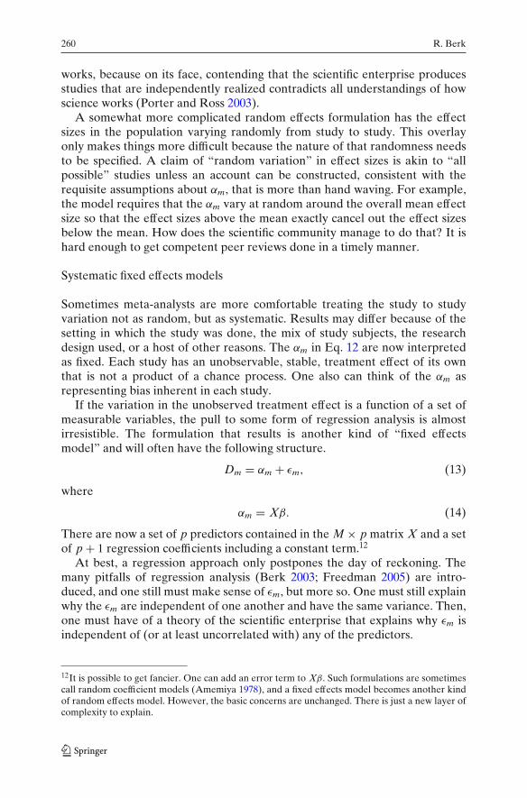
Sometimes meta-analysts are more comfortable treating the study to studyvariation not as random, but as systematic. Results may differ because of thesetting in which the study was done, the mix of study subjects, the researchdesign used, or a host of other reasons. The αm in Eq. 12 are now interpretedas fixed. Each study has an unobservable, stable, treatment effect of its ownthat is not a product of a chance process. One also can think of the αm asrepresenting bias inherent in each study.
If the variation in the unobserved treatment effect is a function of a set ofmeasurable variables, the pull to some form of regression analysis is almostirresistible. The formulation that results is another kind of “fixed effectsmodel” and will often have the following structure.
Dm = αm + εm, (13)
where
αm = Xβ. (14)
There are now a set of p predictors contained in the M × p matrix X and a setof p + 1 regression coefficients including a constant term.12
At best, a regression approach only postpones the day of reckoning. Themany pitfalls of regression analysis (Berk 2003; Freedman 2005) are intro-duced, and one still must make sense of εm, but more so. One must still explainwhy the εm are independent of one another and have the same variance. Then,one must have of a theory of the scientific enterprise that explains why εm isindependent of (or at least uncorrelated with) any of the predictors.
12It is possible to get fancier. One can add an error term to Xβ. Such formulations are sometimescall random coefficient models (Amemiya 1978), and a fixed effects model becomes another kindof random effects model. However, the basic concerns are unchanged. There is just a new layer ofcomplexity to explain.
Statistical inference and meta-analysis 261
Models for dependence between studies
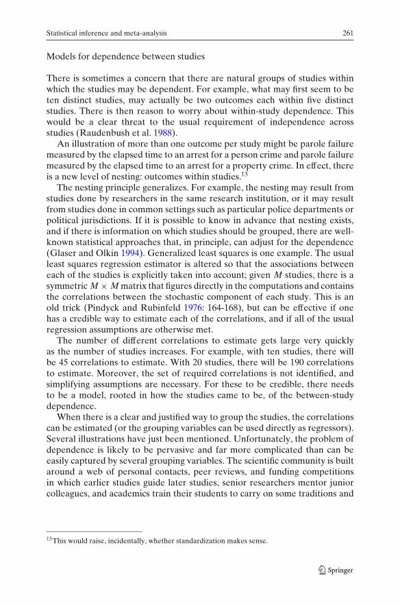
There is sometimes a concern that there are natural groups of studies withinwhich the studies may be dependent. For example, what may first seem to beten distinct studies, may actually be two outcomes each within five distinctstudies. There is then reason to worry about within-study dependence. Thiswould be a clear threat to the usual requirement of independence acrossstudies (Raudenbush et al. 1988).
An illustration of more than one outcome per study might be parole failuremeasured by the elapsed time to an arrest for a person crime and parole failuremeasured by the elapsed time to an arrest for a property crime. In effect, thereis a new level of nesting: outcomes within studies.13
The nesting principle generalizes. For example, the nesting may result fromstudies done by researchers in the same research institution, or it may resultfrom studies done in common settings such as particular police departments orpolitical jurisdictions. If it is possible to know in advance that nesting exists,and if there is information on which studies should be grouped, there are well-known statistical approaches that, in principle, can adjust for the dependence(Glaser and Olkin 1994). Generalized least squares is one example. The usualleast squares regression estimator is altered so that the associations betweeneach of the studies is explicitly taken into account; given M studies, there is asymmetric M × M matrix that figures directly in the computations and containsthe correlations between the stochastic component of each study. This is anold trick (Pindyck and Rubinfeld 1976: 164-168), but can be effective if onehas a credible way to estimate each of the correlations, and if all of the usualregression assumptions are otherwise met.
The number of different correlations to estimate gets large very quicklyas the number of studies increases. For example, with ten studies, there willbe 45 correlations to estimate. With 20 studies, there will be 190 correlationsto estimate. Moreover, the set of required correlations is not identified, andsimplifying assumptions are necessary. For these to be credible, there needsto be a model, rooted in how the studies came to be, of the between-studydependence.
When there is a clear and justified way to group the studies, the correlationscan be estimated (or the grouping variables can be used directly as regressors).Several illustrations have just been mentioned. Unfortunately, the problem ofdependence is likely to be pervasive and far more complicated than can beeasily captured by several grouping variables. The scientific community is builtaround a web of personal contacts, peer reviews, and funding competitionsin which earlier studies guide later studies, senior researchers mentor juniorcolleagues, and academics train their students to carry on some traditions and
13This would raise, incidentally, whether standardization makes sense.

262 R. Berk
challenge others. Complex dependence between studies is the norm, not theexception.
Glaser and Olkin (1994: 340) stress that “... the existence of possiblecorrelations among the estimated effect sizes needs to be accounted for in theanalysis.” At the same time, the fact that the correlations are not identified andthat some simplifying assumptions are needed, is not a blank check. Unlessa credible justification for those assumptions can be constructed, the properresponse is to abandon the model.
The special case of randomized experiments
There is one situation in which statistical inference can be easily justified ina meta-analysis. Assume there is a common effect size α.14 Each study to besummarized is a true randomized experiment. Then, one can obtain reasonablyunbiased estimates of α, sensible estimates of the standard errors, and credibleconfidence intervals and hypothesis tests.
If there is more than one effect size, there is also a happy story under theusual null hypothesis.15 When one assumes that α1 = α2 = · · · = αM = 0, the Meffect sizes are assumed, for testing purposes, to be the same. There is a singleeffect size of 0, and one is left with Dm = εm. Consequently, an instructivetest of the null hypothesis of no effect can be undertaken. However, if thenull hypothesis is rejected, the earlier problems surface again. A model isneeded. Fixed effects? Random effects? What role will any predictor play?It might seem that “all” one need do is compute some summary statistic likethe average effect size. But without a model, it is not clear what parameter ofthe population is being estimated nor how proper standard errors are to beconstructed.
Other variations
Meta-analyses can take a large number of other twists and turns. Perhaps mostimportantly, summaries of the outcomes for the experimentals and controlsare not limited to means. One can use proportions, risk ratios, odds ratios,and other calculations (Fleiss et al. 2003). All of the models discussed abovecan be altered to take these variations into account. But for purposes of thisdiscussion, nothing significant changes. The problems raised are only alteredaround the edges.16
14Across studies, this may well require a common experimental protocol, the same measurementprocedures for the response, the same setting, and the same mix of subjects.15Thanks go to David Freedman for pointing this out to me.16But, a number of quite daunting technical problems sometimes surface (Berk and Freedman2003).
Statistical inference and meta-analysis 263
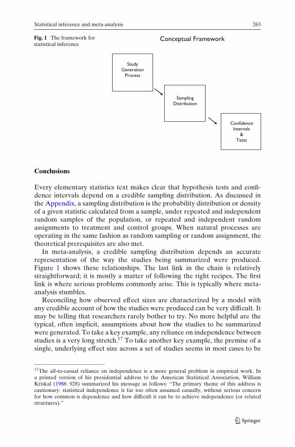
Fig. 1 The framework forstatistical inference
Conclusions
Every elementary statistics text makes clear that hypothesis tests and confi-dence intervals depend on a credible sampling distribution. As discussed inthe Appendix, a sampling distribution is the probability distribution or densityof a given statistic calculated from a sample, under repeated and independentrandom samples of the population, or repeated and independent randomassignments to treatment and control groups. When natural processes areoperating in the same fashion as random sampling or random assignment, thetheoretical prerequisites are also met.
In meta-analysis, a credible sampling distribution depends an accuraterepresentation of the way the studies being summarized were produced.Figure 1 shows these relationships. The last link in the chain is relativelystraightforward; it is mostly a matter of following the right recipes. The firstlink is where serious problems commonly arise. This is typically where meta-analysis stumbles.
Reconciling how observed effect sizes are characterized by a model withany credible account of how the studies were produced can be very difficult. Itmay be telling that researchers rarely bother to try. No more helpful are thetypical, often implicit, assumptions about how the studies to be summarizedwere generated. To take a key example, any reliance on independence betweenstudies is a very long stretch.17 To take another key example, the premise of asingle, underlying effect size across a set of studies seems in most cases to be
17The all-to-casual reliance on independence is a more general problem in empirical work. Ina printed version of his presidential address to the American Statistical Association, WilliamKriskal (1988: 928) summarized his message as follows: “The primary theme of this address iscautionary: statistical independence is far too often assumed casually, without serious concernfor how common is dependence and how difficult it can be to achieve independence (or relatedstructures).”
264 R. Berk
an unreasonable simplification. Yet, models for different effect sizes requirealternative assumptions that are likely to be no more credible.
If the meta-analysis model does not accurately represent how the stud-ies were actually generated, a credible sampling distribution cannot beconstructed. Indeed, the very idea of a sampling distribution may not apply.18
The problem is not with the meta-analysis model itself. The problem is that themodel has little or no correspondence to how the set of studies were actuallydone. And if the model does not apply, the statistical inference that follows isnot likely to help.
There appear to be three common responses to the mismatch betweena meta-analysis model and anything real. In some cases, the problems arenot mentioned. Even if recognized as the meta-analysis was done, they gomissing when the results are written. In other cases, the requisite assumptionsare listed, but not defended. A list of the assumptions by itself apparentlyinoculates the meta-analysis against modelling errors. In yet other cases, themodelling assumptions are specified and discussed, but the account is notconvincing. In perhaps the most obvious illustration, the population to whichgeneralizations are being made is “all possible studies.”
It is also possible to dismiss the issues raised in this paper as statisticalpurity that should not be taken seriously in real research. But that positionis to fundamentally misunderstand the message. This paper is not a call forperfection. It is a call for rigor. At some point, moreover, the correspondencebetween what the formal mathematics require and the way the studies weregenerated is so out of kilter that the mathematical results do not usefully apply.The conclusions reported are just plain wrong.
How should researchers proceed? First, there is always the option of aconventional literature review. These are certainly not flawless, but they haveserved science well for a very long time. Also, readers do not have to cutthrough pages of statistical razzle-dazzle to understand what is really beingsaid.19 Second, a meta-analysis can stop short of statistical inference. Gooddescription alone can make a contribution. Third, one can reconsider the un-certainty that statistical inference is supposed to address, and seek alternativeapproaches. For example, if a concern is the stability of the results had theset of studies summarized been a bit different, a “drop-one” analysis can behelpful. If there are, for instance, ten studies, ten meta-analyses can be doneusing nine of the studies each time. Each study is dropped in turn. If the effect
18The concept of a sampling distribution can apply in principle to any statistic computed froma given data set. However, the definition of a sampling distribution requires that the data weregenerated by random sampling, random assignment, or their equivalent produced by natural/socialprocesses. If the data were not generated by such means, the concept of a sampling distributiondoes not apply. If the study were repeated a number of times, the results might well vary. But theresults would not likely vary in a manner consistent with a specifiable sampling distribution.19Although it is true that thanks to modern computing, doing the calculations has become trivial,choosing which calculation to do and then interpreting them properly has proved to be difficult.The history of meta-analysis is one instance. The problem is actually far more general (Box 1976;Leamer 1978; Lieberson 1985; Duncan 1984; Oakes 1986; Holland 1986; Rubin 1986; Freedman1987, 2005; Kriskal 1988; Manski 1990; de Leeuw 1994; Berk 2003).
Statistical inference and meta-analysis 265
sizes vary dramatically over the ten meta-analyses, there are ample groundsfor caution.20 This and some other possibilities are considered by Greenhouseand Iyengar (1994), but there is a lot more that could be done. That discussionis saved for another time.
Appendix: A primer on sampling distributions for meta-analysis
All statistical inference depends on the concept of a sampling distribution.21
For meta-analysis, the nature of the sampling distribution depends on howthe studies to be summarized came to be. If the correspondence between thestudy generation process and the sampling distribution is poor, any confidenceintervals and statistical tests will likely be misleading.
To appreciate why this is true, we consider a very simple illustration basedon a random effects model consistent with Eq. 12. In the population is thereare different αm contributing to the different values of Dm. The average of theαm, denoted by ν, is what is to be estimated.
Suppose the population consists of five studies with ν = 2.0. A simplerandom sample of three studies is chosen. For the three studies, a weightedaverage of the observed effect sizes is computed by the methods discussedearlier. It is desirable that the weighted mean computed from the sample ofthree studies be an unbiased estimate of ν. What does unbiasedness require?
In the population of five studies, each study has a probability of 1/5 ofbeing selected in the first draw. With one study chosen, each of the remainingstudies has a probability of 1/4 of being selected. Finally, with two studieschosen, the remaining studies each have a probability of 1/3 of being selected.The sampling is, therefore, without replacement and at each draw, all of theremaining studies have the same probability of selection. Because for eachdraw all studies have the same probability of selection, all studies have thesame probability of appearing in the sample.
Whether simple random sampling leads to an unbiased estimate dependsnot on the result from a single sample, but what happens over all possiblesamples from the population. Table 2 contains all possible samples of sizethree from a population of five. The first column shows the studies chosen;the studies are indexed as 1, 2, . . . , 5. In the population, five observable effectsizes are: 3, 1, 0, 1, 5.22 The first value comes from the first study, the second
20This is the start of a resampling procedure called the “jackknife.”21In meta-analysis, occasional reference is made to Bayesian statistical inference in which samplingdistributions play no role. But real applications are difficult to find, and the inferential goals arevery different (Lewis and Zelterman 1994). Moreover, one still has to specify a credible likelihoodfunction, which can raise the same kinds of issues discussed in this paper. Suffice it say, thealternative of Bayesian inference has some real strengths (Leamer 1978; Berk et al. 1995; Gelmanet al. 2003), but in the end trades one set of complications for another (Barnett 1999).22If one had access to the entire population, these are the standardized effect sizes for each studythat would be seen.
266 R. Berk
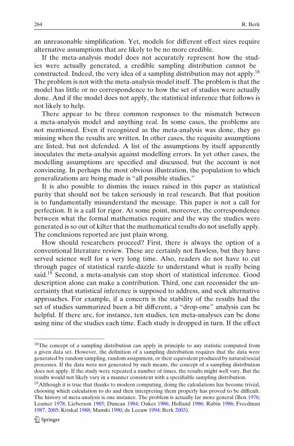
Table 2 Illustrative samplingdistribution for the basic fixedeffects model: ν = 2.0
Study index Dm ν
1,2,3 3,1,0 1.331,2,4 3,1,1 1.671,2,5 3,1,5 3.001,3,4 3,0,1 1.331,3,5 3,0,5 2.671,4,5 3,1,5 3.002,3,4 1,0,1 0.672,3,5 1,0,5 2.002,4,5 1,1,5 2.333,4,5 0,1,5 2.00
value comes from the second study, and so on. The second column shows theDm for each of the three studies sampled. In each case, M = 3.
The third column shows for each sample of three studies the estimate of ν.For ease of exposition and with no impact on the points to be made, all of thestudies are given equal weight.
There are ten possible samples that result from choosing three studies bysimple random sampling from a population of five studies. Because of simplerandom sampling, each sample has the same probability of being selected.That probability here is 1/10. It follows that each ν also has a probability of1/10. The values of ν and their associated probabilities constitute a samplingdistribution. This is the key to all that follows.
If one multiplies each sample’s weighted average by 1/10 and sums them,the result is 2.0, which is the value of ν. By definition, therefore, a ν from anyone of the ten possible samples is an unbiased estimate of the population mean.
There are several points to be taken from this illustration.
1. The five studies constituted a real population; all of the studies in thepopulation were identified and all could have been reviewed, at least inprinciple. In the population, the (unknown) value of ν is 2.0.
2. A single sample of three studies was chosen by probability sampling, here,simple random sampling, leading to a set of three Dm values.
3. The three Dm values are used to compute ν.4. The thought experiment all possible samples, derived from simple random
sampling, then followed directly and led to the theoretical construct of asampling distribution for ν.
5. From this theoretical sampling distribution, it was possible to illustrate howthe weighted average from any sample of the three studies was an unbiasedestimate of ν.
This is the sort of reasoning that should lie behind statistical inference in ameta-analysis. More generally, a properly weighted mean computed from a setof studies is an unbiased estimate of the population mean when coupled withsimple random sampling. Building on Thompson’s exposition (2002, Section2.6), there is a population of N studies, a sample size of n studies is chosen bysimple random sampling. The probability that any given sample of studies will
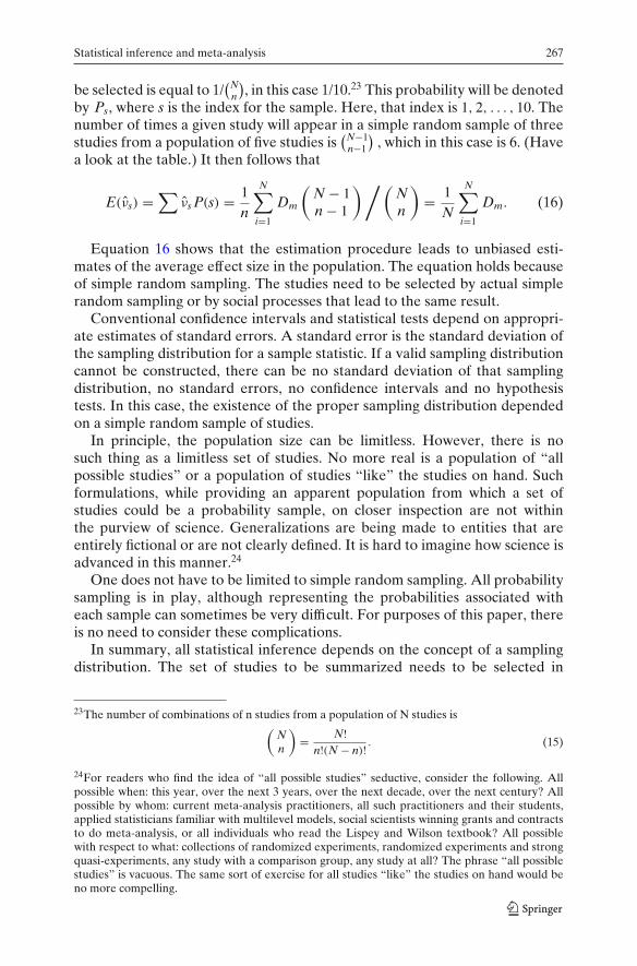
Statistical inference and meta-analysis 267
be selected is equal to 1/(N
n
), in this case 1/10.23 This probability will be denoted
by Ps, where s is the index for the sample. Here, that index is 1, 2, . . . , 10. Thenumber of times a given study will appear in a simple random sample of threestudies from a population of five studies is
(N−1n−1
), which in this case is 6. (Have
a look at the table.) It then follows that
E(νs) =∑
νs P(s) = 1
n
N∑i=1
Dm
(N − 1n − 1
)/(Nn
)= 1
N
N∑i=1
Dm. (16)
Equation 16 shows that the estimation procedure leads to unbiased esti-mates of the average effect size in the population. The equation holds becauseof simple random sampling. The studies need to be selected by actual simplerandom sampling or by social processes that lead to the same result.
Conventional confidence intervals and statistical tests depend on appropri-ate estimates of standard errors. A standard error is the standard deviation ofthe sampling distribution for a sample statistic. If a valid sampling distributioncannot be constructed, there can be no standard deviation of that samplingdistribution, no standard errors, no confidence intervals and no hypothesistests. In this case, the existence of the proper sampling distribution dependedon a simple random sample of studies.
In principle, the population size can be limitless. However, there is nosuch thing as a limitless set of studies. No more real is a population of “allpossible studies” or a population of studies “like” the studies on hand. Suchformulations, while providing an apparent population from which a set ofstudies could be a probability sample, on closer inspection are not withinthe purview of science. Generalizations are being made to entities that areentirely fictional or are not clearly defined. It is hard to imagine how science isadvanced in this manner.24
One does not have to be limited to simple random sampling. All probabilitysampling is in play, although representing the probabilities associated witheach sample can sometimes be very difficult. For purposes of this paper, thereis no need to consider these complications.
In summary, all statistical inference depends on the concept of a samplingdistribution. The set of studies to be summarized needs to be selected in
23The number of combinations of n studies from a population of N studies is(Nn
)= N!
n!(N − n)! . (15)
24For readers who find the idea of “all possible studies” seductive, consider the following. Allpossible when: this year, over the next 3 years, over the next decade, over the next century? Allpossible by whom: current meta-analysis practitioners, all such practitioners and their students,applied statisticians familiar with multilevel models, social scientists winning grants and contractsto do meta-analysis, or all individuals who read the Lispey and Wilson textbook? All possiblewith respect to what: collections of randomized experiments, randomized experiments and strongquasi-experiments, any study with a comparison group, any study at all? The phrase “all possiblestudies” is vacuous. The same sort of exercise for all studies “like” the studies on hand would beno more compelling.
268 R. Berk
a manner that is consistent with what an appropriate sampling distributionrequires. If the studies are not selected in this fashion, any statistical inferencethat is attempted will not convey any useful information.
References
Amemiya, T. (1978). A note on a random coefficients model. International Economics Review,19(3), 793–796.
Archer, J. (2000). Sex differences in aggression between heterosexual partners: A meta-analyticreview. Psychological Bulletin, 126(5), 651–680.
Barnett, V. (1999). Comparative statistical inference (3rd ed.). New York: John Wiley and Sons.Berk, R. A. (2003). Regression analysis: A constructive critique. Newbury Park, Sage Publications.Berk, R. A., Western, B., & Weiss, R. (1995). Statistical Inference for Apparent Populations (with
commentary) Sociological methodology (vol. 25). Cambridge, UK: Blackwell Publishing.Berk, R. A., & Freedman, D. A. (2003). Statistical assumptions as empirical commitments. In
T. G. Blomberg & S. Cohen (Eds.), Punishment and social control: Essays in honor of SheldonMessinger (2nd ed., pp. 235–254). New York: Aldine de Gruyter.
Bickel, P. J., & Doksum, K. A. (2001). Mathematical statistics: Basic ideas and selected topics,volume 1 (2nd ed.). Upper Saddle River: Prentice Hall.
Bond, C. F., Wiitala, W. L., & Richard, F. D. (2003). Meta-analysis of raw mean differences.Psychological Methods, 8(4), 406–418.
Box, G. E. P. (1976). Science and statistics. Journal of the American Statistical Association, 71,791–799.
Briggs, D. C. (2005). Meta-analysis: A case study. Evaluation Review, 29, 87–127.Cameron, A. C., & Trivedi, P. K. (2005). Microeconomics: Methods and applications. Cambridge:
Cambridge University Press.de Leeuw, J. (1994). Statistics and the Sciences. In I. Borg & P. P. Mohler (Eds.), Trends and
perspectives in empirical social science. New York: Walter de Gruyter.Duncan, O. D. (1975). Introduction to structural equation modeling. New York: Russell Sage
Foundation.Duncan, O. D. (1984). Notes on social measurement: Historical and critical. New York: Academic
Press.Efron, B., & Morris, C. (1971). Limiting the risk of Bayes and empirical Bayes estimators. Part I:
The Bayes case. Journal of the American Statistical Association, 66, 807–815.Efron, B., & Morris, C. (1972). Limiting the risk of Bayes and empirical Bayes estimators. Part II:
The empirical Bayes case. Journal of the American Statistical Association, 67, 130–139.Efron, B., & Morris, C. (1973). Combining possibly related estimation problems. Journal of the
Royal Statistical Society, Series B, 35, 379–421. (with discussion)Fleiss, J. L., Levin, B., & Paik, M. C. (2003). Statistical methods for rates and proportions.
New York: John Wiley and Sons.Freedman, D. A. (1987). As others see us: A case study in path analysis. Journal of Educational
Statistics, 12, 101–223. (with discussion)Freedman, D. A. (2004). Graphical models for causation and the identification problem. Evalua-
tion Review, 28, 267–293.Freedman, D. A. (2005). Statistical models: Theory and practice. Cambridge: Cambridge University
Press.Froehlich, B. R. (1973). Some estimators for random coefficient regression models. Journal of the
American Statistical Association, 68(342), 329–335.Glass, G. V., McGraw, B., & Smith, M. L. (1981). Meta-analysis in social research. Newbury Park:
Sage Publications.Gelman, A., Carlin, J. B., Stern, H. S., & Rubin, D. B. (2003). Bayesian data analysis (2nd ed.).
New York: Chapman & Hall.Glaser, L. J., & Olkin, I. (1994). Statistically dependent effects. In H. Cooper & L. V. Hedges
(Eds.), The handbook of research synthesis. New York: Russell Sage Foundation.

Statistical inference and meta-analysis 269
Greenhouse, J. B., & Iyengar, S. (1994). Sensitivity analysis and diagnostics. In H. Cooper & L. V.Hedges (Eds.), The Handbook of research synthesis. New York: Russell Sage Foundation.
Hedges L. V., & Olkin, I. (1985). Statistical methods for meta-analysis. New York: Academic Press.Hedges, L. V. (1994). Fixed effects models. In H. Cooper & L. V. Hedges (Eds.), The handbook
of research synthesis. New York: Russell Sage Foundation.Holland, P. W. (1986). Statistics and causal inference. Journal of the American Statistical Associa-
tion, 81, 945–960.Hunter, J. E., & Schmidt, F. L. (1990). Methods of meta-analysis: Correcting error and bias in
research findings. Newbury Park: Sage Publications.Hsiao, C. (2003). Analysis of panel data (2nd ed.). Cambridge: Cambridge University Press.Koch, G. G. (1967). A procedure to estimate the population mean in random effects models.
Technometrics, 9(4), 577–585.Kriskal, W. (1988). Miracles and statistics: The casual assumption of independence. Journal of the
American Statistical Association, 63(404), 929–940.Leamer, E. E. (1978). Specification searches: Ad Hoc inference with non-experimental data.
New York: John Wiley.Lewis, T. A., & Zelterman, D. (1994). Bayesian approaches to research synthesis. In
H. Cooper & L. V. Hedges (Eds.), The Handbook of research synthesis. New York: RussellSage Foundation.
Lieberson, S. (1985). Making it count: The improvement of social research and theory. Berkeley:University of California Press.
Lipsey, M. W., & Wilson, D. (2001). Practical meta-analysis. Newbury Park, CA: Sage Publications.Lipsey, M. W. (1997). What can you build with thousands of bricks? musings on the cumulation of
knowledge in program evaluation. New Directions for Evaluation, 76(Winter), 7–24.Lipsey, M. W. (1992). Juvenile delinquency treatment: A meta-analysis inquiry into the variability
of effects. In T. C. Cook, D. S. Cooper, H. Hartmann, L. V. Hedges, R. I. Light, T. A.Loomis & F. M. Mosteller (Eds.), Meta-analysis for explanation (pp. 83–127). New York:Russell Sage.
Maddala, G. S. (1977). Econometrics. New York: McGraw Hill.Manski, C. F. (1990). Nonparametric bounds on treatment effects. American Economics Review
Papers and Proceedings, 80, 319–323.Maritz, J. S., & Lwin, T. (1989). Empirical Bayes methods (2nd ed.). New York: Chapman & Hall.Mitchell, O. (2005). A meta-analysis of race and sentencing research: Explaining the inconsisten-
cies. Journal of Quantitative Criminology, 21(4), 439–466.Neyman, J. [1923] (1990). On the application of probability theory to agricultural experiments.
Essay on principles. Section 9. Translated and edited by D. M. Dabrowska & T.P. Speed,Statistical Science, 5, 465–471.
Oakes, M. (1986). Statistical inference: A commentary for the social and behavioral sciences.New York: John Wiley.
Pindyck, R., & Rubinfeld, D. L. (1976). Econometric models and economic forecasts. New York:McGraw Hill.
Porter, T., & Ross, D. (2003). The Cambridge history of science, volume 7: The modern socialsciences. Cambridge: Cambridge University Press.
Raudenbush, S. W., Becker, B. J., & Kalaian, H. (1988). Modeling multivariate effect sizes.Psychological Bulletin, 103(1), 1110–120.
Raudenbush, S. W. (1994). Random effects models. In H. Cooper & L. V. Hedges (Eds.), Thehandbook of research synthesis. New York: Russell Sage Foundation.
Robbins, H. (1956). An empirical Bayes approach to statistics. Proceedings of the Third BerkeleySymposium on Mathematical Statistics and Probability (pp. 157-163). University of CaliforniaPress.
Rosenbaum, P. R. (2002). Observational studies (2nd ed.). New York: Springer-Verlag.Rosenthal, R. (1994). Parametric measures of effect size. In H. Cooper & L. V. Hedges (Eds.),
The handbook of research synthesis. New York: Russell Sage Foundation. Sage Foundation.Rubin, D. B. (1986). Which ifs have causal answers. Journal of the American Statistical Association,
81, 961–962.Shadish, W. R., & Haddock, C. K. (1994). Combining estimates of effect size. In H. Cooper &
L. V. Hedges (Eds.), The handbook of research synthesis. New York: Russell Sage Foundation.Thompson, S. (2002). Sampling (2nd ed.). New York: John Wiley and Sons.

270 R. Berk
Wachter, K. W. (1988). Disturbed about meta-analysis? Science, 241, 1407–1408.Wortman, P. M. (1994). Judging research quality. In H. Cooper & L. V. Hedges (Eds.), The
handbook of research synthesis. New York: Russell Sage Foundation.
Richard Berk is a professor in the Departments of Criminology and Statistics at the Universityof Pennsylvania. He is an elected fellow of the American Statistical Association, the AmericanAssociation for the Advancement of Science, and the Academy of Experimental Criminology.His research interests include statistical learning procedures and applied statistics more generally.He has published extensively in program evaluation, criminal justice, environmental research,and applied statistics. Professor Berk’s most recent book is Regression Analysis: A ConstructiveCritique (Sage Publications, 2003).
Copyright © 2022 FDOKUMEN