A generalized divergence for statistical inference - Project Euclid
38
Bernoulli 23(4A), 2017, 2746–2783 DOI: 10.3150/16-BEJ826 A generalized divergence for statistical inference ABHIK GHOSH 1 , IAN R. HARRIS 2 , AVIJIT MAJI 3 , AYANENDRANATH BASU 1,* and LEANDRO PARDO 4 1 Indian Statistical Institute, Kolkata, India. E-mail: * [email protected] 2 Southern Methodist University, Dallas, USA 3 Indian Statistical Institute, Kolkata, India and Reserve Bank of India, Mumbai, India 4 Complutense University, Madrid, Spain The power divergence (PD) and the density power divergence (DPD) families have proven to be useful tools in the area of robust inference. In this paper, we consider a superfamily of divergences which contains both of these families as special cases. The role of this superfamily is studied in several statistical appli- cations, and desirable properties are identified and discussed. In many cases, it is observed that the most preferred minimum divergence estimator within the above collection lies outside the class of minimum PD or minimum DPD estimators, indicating that this superfamily has real utility, rather than just being a rou- tine generalization. The limitation of the usual first order influence function as an effective descriptor of the robustness of the estimator is also demonstrated in this connection. Keywords: breakdown point; divergence measure; influence function; robust estimation; S -divergence 1. Introduction A density-based minimum divergence approach is a technique in parametric inference where the closeness of the data and the model is quantified by a suitable divergence measure between the data density and the model density. Inference methods based on this approach are useful because of the strong robustness properties that they inherently possess. The use of minimum divergence procedures in robust statistical inference possibly originated with Beran’s 1977 paper [8]. Since then, the literature has grown substantially, with monographs by Vajda [47], Pardo [36] and Basu et al. [7] serving as useful resources for the description of the research and developments in this field. Several density-based minimum divergence estimators have very high asymptotic efficiency. The class of minimum disparity estimators [33] or minimum φ -divergence estimators [14], for example, have full asymptotic efficiency under the assumed parametric model. The power di- vergence (PD) family [13], a prominent subclass of disparities, produces robust and efficient parameter estimators. However, its application in continuous models is not so easy as it requires the use of a non-parametric density estimator such as the kernel density estimator that entails associated complications such as bandwidth selection. Basu et al. [2] developed an alternative family of density based divergences, namely the density power divergences (DPD), which avoids any non-parametric smoothing even under continuous models and generates robust estimators with only a slight loss in efficiency. Patra et al. [37] proved some interesting connections be- tween these two divergence families. 1350-7265 © 2017 ISI/BS
-
Upload
khangminh22 -
Category
Documents
-
view
2 -
download
0
Transcript of A generalized divergence for statistical inference - Project Euclid
Bernoulli 23(4A), 2017, 2746–2783DOI: 10.3150/16-BEJ826
A generalized divergence for statisticalinferenceABHIK GHOSH1, IAN R. HARRIS2, AVIJIT MAJI3,AYANENDRANATH BASU1,* and LEANDRO PARDO4
1Indian Statistical Institute, Kolkata, India. E-mail: *[email protected] Methodist University, Dallas, USA3Indian Statistical Institute, Kolkata, India and Reserve Bank of India, Mumbai, India4Complutense University, Madrid, Spain
The power divergence (PD) and the density power divergence (DPD) families have proven to be usefultools in the area of robust inference. In this paper, we consider a superfamily of divergences which containsboth of these families as special cases. The role of this superfamily is studied in several statistical appli-cations, and desirable properties are identified and discussed. In many cases, it is observed that the mostpreferred minimum divergence estimator within the above collection lies outside the class of minimum PDor minimum DPD estimators, indicating that this superfamily has real utility, rather than just being a rou-tine generalization. The limitation of the usual first order influence function as an effective descriptor of therobustness of the estimator is also demonstrated in this connection.
Keywords: breakdown point; divergence measure; influence function; robust estimation; S-divergence
1. Introduction
A density-based minimum divergence approach is a technique in parametric inference where thecloseness of the data and the model is quantified by a suitable divergence measure between thedata density and the model density. Inference methods based on this approach are useful becauseof the strong robustness properties that they inherently possess.
The use of minimum divergence procedures in robust statistical inference possibly originatedwith Beran’s 1977 paper [8]. Since then, the literature has grown substantially, with monographsby Vajda [47], Pardo [36] and Basu et al. [7] serving as useful resources for the description ofthe research and developments in this field.
Several density-based minimum divergence estimators have very high asymptotic efficiency.The class of minimum disparity estimators [33] or minimum φ-divergence estimators [14], forexample, have full asymptotic efficiency under the assumed parametric model. The power di-vergence (PD) family [13], a prominent subclass of disparities, produces robust and efficientparameter estimators. However, its application in continuous models is not so easy as it requiresthe use of a non-parametric density estimator such as the kernel density estimator that entailsassociated complications such as bandwidth selection. Basu et al. [2] developed an alternativefamily of density based divergences, namely the density power divergences (DPD), which avoidsany non-parametric smoothing even under continuous models and generates robust estimatorswith only a slight loss in efficiency. Patra et al. [37] proved some interesting connections be-tween these two divergence families.
1350-7265 © 2017 ISI/BS
A generalized divergence 2747
In this paper, we describe the power divergence and density power divergence families as spe-cial cases of a superfamily of divergences which we term as the “S-divergence” family. The mainaim of the current paper is, along with the description of the S-divergence family, to illustrate thewide scope of potential applications of this superfamily in case of parametric statistical inferencewith special focus on the robustness issues.
While we describe the development of the S-divergence in this paper and elaborate on themain statistical features of the divergence with special reference to the robustness of the corre-sponding procedures, many other research extensions involving this divergence are also beingcurrently considered (or has been considered) by the authors which consist of applications ortheoretical properties of this divergence. Ghosh [21] and Ghosh and Basu [22] have consideredthe asymptotic properties of the minimum S-divergence estimators under discrete and continuousmodels respectively. Possible applications of the S-divergence family in developing robust testsof hypothesis have been considered by [24,25]. A 2013 technical report [26] provides an exten-sive review of the PD and DPD families and their interconnection in the general framework ofS-divergence. A similar discussion is also provided in a review article by [28], which also illus-trates the use of the DPD measure in the context of robust reliability analysis. We will also pointout several other interesting and potential areas of future research based on the S-divergences inthe present paper.
Here we summarize the main achievements of the paper. These issues will be further elabo-rated upon when we discuss them in the main body of the paper.
1. We describe the development of a new family of divergences which is a superfamily con-taining the well known and well studied PD and DPD families. We explore the use of thecorresponding minimum divergence estimators in statistical inference.
2. Many of these minimum divergence estimators generated by this class of divergences pro-vide a high degree of stability under data contamination while attaining reasonable effi-ciency at the model.
3. Our analysis shows that in many cases involving data contamination, the most preferredminimum divergence estimator often lies outside the class of the union of minimum PD andminimum DPD estimators, demonstrating that the class of S-divergences has real utility,and the development of the class of S-divergences is not just for the sake of generalization.
4. We consider a data-driven method for the selection of “optimal” tuning parameters basedon modifications of existing rules. This is also useful in establishing the issue discussed inthe previous item.
5. Although we do not pursue it in any great length in this paper, we demonstrate that thedevelopment of the S-divergence also generates a generalized class of cross-entropies in-cluding the Boltzmann–Gibbs–Shannon entropy as a special case.
6. We provide a second order influence analysis which is more accurate than the first orderinfluence analysis in predicting the bias of our estimators under contamination. We alsodemonstrate that the first order influence function may be deficient in predicting the biasirrespective of the truth; it may fail to indicate the robustness of highly stable estimators,and can also label highly unstable estimators as being strongly robust.
7. At least in the examples we have studied, the instability of the estimators under contamina-tion is very accurately predicted by the violation of the conditions needed for the breakdownpoint results to hold.

2748 A. Ghosh et al.
The rest of the paper is organized as follows. In Section 2, we describe the PD and DPDfamilies and study their interconnection; extensive discussions and examples about these diver-gences can be found in [7,26,38]. Section 3 ties in these families through the super-family ofS-divergences. In Section 4, we discuss various properties of the minimum S-divergence esti-mators including the classical influence function and the asymptotic properties under both dis-crete and continuous models. A numerical analysis is presented in Section 5 to describe theperformance of the proposed minimum S-Divergence estimators (MSDEs). Here we also discussthe limitation of the classical first order influence function analysis in describing the robust-ness of these estimators. As a remedy, we consider higher order influence function analysis andbreakdown point analysis of the proposed minimum divergence estimators in Section 6 and Sec-tion 8.1, respectively. Combining the robustness perspectives and efficiency of the proposed esti-mators, some suggestions are made in Section 7 for data driven optimal choice of estimators to beused in specific situation. In Section 8.2, we discuss robust equivariant estimation of multivariatelocation and covariances using a particular subfamily of S-divergences. Brief comments aboutthe testing of hypothesis based on the S-divergence family are provided in Section 9. Finally,Section 10 has some concluding remarks. For brevity of presentation, the assumptions requiredto prove the asymptotic distributions of the proposed minimum divergence estimators and someof the proofs are moved to the on-line supplement [27]. Some additional issues/examples are alsoincluded in the supplementary part.
Throughout the paper, we will use the term “density function” for both discrete and continuousmodels. We also use the term “distance” loosely, to refer to any divergence which is non-negativeand is equal to zero if and only if its arguments are identically equal.
2. The PD and the DPD families
2.1. Minimum disparity estimation and the PD family
Let us consider a parametric model of discrete probability distributions F = {Fθ : θ ∈ � ⊆ Rp}.
Let X1, . . . ,Xn denote n independent and identically distributed (i.i.d.) observations from a dis-crete distribution G. Further, assume that both the true distribution G and the model family Fhave the support X = {0,1,2, . . .}, without loss of generality, and both belong to G, the class ofall distributions having densities with respect to some appropriate dominating measure. Let g andfθ be the corresponding true and model density functions respectively. Suppose dn(x) representsthe relative frequency of the value x in the above sample. We wish to estimate the parameter θ byminimizing the discrepancy between the data and the model quantified by the class of disparitiesbetween the probability vectors dn = (dn(0), dn(1), . . .)T and fθ = (fθ (0), fθ (1), . . .)T .
Definition 2.1 (Definition 2.1, [7]). Let C be a thrice differentiable, strictly convex function on[−1,∞), with C(0) = 0. Let the Pearson residual at the value x be defined by δ(x) = δn(x) =dn(x)fθ (x)
− 1. Then the disparity between dn and fθ generated by C is defined by
ρC(dn, fθ ) =∞∑
x=0
C(δ(x)
)fθ (x). (1)

A generalized divergence 2749
The PD family [13] is a special case of this class and is defined in terms of a real parameter λ
as
PDλ(dn, fθ ) = 1
λ(λ + 1)
∑dn
[(dn
fθ
)λ
− 1
](2)
=∑{
1
λ(λ + 1)dn
[(dn
fθ
)λ
− 1
]+ fθ − dn
λ + 1
}. (3)
The second formulation makes all the terms in the summand non-negative. The C(·) function forthe PD under this formulation is given by
Cλ(δ) = (δ + 1)λ+1 − (δ + 1)
λ(λ + 1)− δ
λ + 1.
For particular choices of λ = 1,0,−1/2,−1, the PD family generates the Pearson’s chi-square(PCS), the likelihood disparity (LD), the (twice, squared) Hellinger distance (HD) and theKullback–Leibler divergence (KLD) respectively. Note that, the expressions for the PD corre-sponding to λ = 0,−1 can only be defined in terms of the continuous limit of the expression onthe right-hand side of (2) as λ → 0,−1. These cases result in the likelihood disparity (LD) andthe Kullback–Leibler divergence (KLD), respectively.
Provided such a minimum exists, the minimum disparity estimator (MDE) θ of θ based on thedisparity ρC is defined by the relation
ρC(dn, fθ) = min
θ∈�ρC(dn, fθ ). (4)
The maximum likelihood estimator (MLE) belongs to the class of MDEs as it is the minimizerof the likelihood disparity.
Under differentiability of the model, the MDE solves the estimating equation
−∇ρC(dn, fθ ) =∞∑
x=0
(C′(δ)(δ + 1) − C(δ)
)∇fθ =∞∑
x=0
A(δ)∇fθ = 0, (5)
where ∇ represents the gradient with respect to θ and A(δ) = C′(δ)(δ+1)−C(δ). One can easilycheck that the above estimating equation (5) is an unbiased estimating equation at the assumedmodel. We can standardize the function A(δ), without changing the estimating properties of thedisparity, so that A(0) = 0 and A′(0) = 1. This standardized function A(δ) is called the residualadjustment function (RAF) of the disparity and largely controls the robustness properties of theMDEs. For the PD family, the RAF is given by
Aλ(δ) = (δ + 1)λ+1 − 1
λ + 1. (6)
In particular, the RAF for likelihood disparity is linear, given by A0(δ) = ALD(δ) = δ.An observation x in the sample space with a large (�0) Pearson residual δ may be considered
a “probabilistic outlier” in the sense that the observed proportion dn(x) is significantly higher

2750 A. Ghosh et al.
than what is predicted by the model. An MDE will effectively control such a probabilistic outlierif the corresponding RAF A(δ) exhibits a strongly dampened response to increasing (positive) δ.In particular, the MDEs with negative values of the quantity A2 = A′′(0), known as the estimationcurvature of the disparity [33], are seen to be locally robust. For the PD family, this quantityequals the tuning parameter λ and all members of the PD family with λ < 0 are expected tobe robust. However, the robustness of the MDEs is not adequately reflected by the first orderinfluence function analysis which indicates that all MDEs have the same influence function asthe MLE at the model.
However, the equivalence of the influence functions also indicates the asymptotic efficiency ofthe MDEs. See Lindsay [33] and Morales et al. [35] for the formal results in this context as wellas for a more in depth discussion of the statements of the robustness properties of the MDE. AllMDEs have the same asymptotic distribution as that of the MLE at the model.
The set-up and procedure as described above can also be generalized to the case of continuousmodels. However, here it is necessary to construct a continuous density estimate of the true den-sity using appropriate non-parametric smoothing techniques which involves bandwidth selectionand other problems. This is avoided by the density power divergence family described in the nextsubsection.
2.2. The density power divergence (DPD) family
We assume that the parametric set-up of Section 2.1 holds. Let uθ (x) = ∇ logfθ (x) be the like-lihood score function where ∇ represents the gradient with respect to θ . Consider the estimatingequations
n∑i=1
uθ (Xi) = 0 andn∑
i=1
uθ (Xi)fαθ (Xi) = 0 (7)
in the location model case, where α ∈ [0,1]. The first one is the likelihood score equation whichcorresponds to α = 0. Clearly the second equation involves a density power downweighting com-pared to the likelihood equation, which indicates the robustness of the estimators resulting fromthis process. The degree of downweighting increases with α; α = 0 indicates no downweighting.For more general models, the corresponding unbiased estimating equation at the model is
1
n
n∑i=1
uθ (Xi)fαθ (Xi) −
∫uθ (x)f 1+α
θ (x) dx = 0, α ∈ [0,1]. (8)
Basu et al. [2] used this form to construct the DPD family. Given densities g,f for distributionsG and F in G, the DPD with tuning parameter α is defined as
DPDα(g,f ) =∫ [
f 1+α −(
1 + 1
α
)f αg + 1
αg1+α
]for α ≥ 0. (9)
When α = 0, the divergence is defined as the continuous limit as α ↓ 0; this divergence equals∫g log(g/f ) which is the likelihood disparity and is also the PD measure at λ = 0. For α = 1,
the corresponding divergence is the squared L2-distance.
A generalized divergence 2751
Now, consider again the parametric set up of Section 2.1 and define the minimum DPD func-tional Tα(G) at G by the relation
DPDα(g,fTα(G)) = minθ∈�
DPDα(g,fθ ).
The functional is Fisher consistent by definition of the DPD. As∫
g1+α is independent of θ and∫f α
θ g can be empirically estimated as 1n
∑ni=1 f α
θ (Xi), the objective function to be minimized
for the estimation of the minimum DPD estimator (MDPDE) θα with tuning parameter α turnsout to be
Hn(θ) = 1
n
n∑i=1
Vθ(Xi), (10)
where Vθ(x) = ∫f 1+α
θ − (1 + 1α)f α
θ (x). Thus, the minimization of (10) does not require the useof a non-parametric density estimate for any α. In addition, expression (10) also shows that theMDPDE is in fact an M-estimator. Under differentiability of the model family, the minimizationof Hn(θ) in (10) leads to the estimating equation (8).
Unlike the MDEs, however, all MDPDEs have bounded influence functions for α > 0. Alsothe DPD family allows a clear trade-off between robustness and efficiency, with larger values ofα leading to greater robustness and smaller values of α providing greater asymptotic efficiency.Generally, the estimators corresponding to α > 1 are considered too inefficient to be practicallyuseful. See Basu et al. [2] for more details. Also see Dawid and Musio [15] and Dawid et al. [16].
2.3. Interconnection between the PD and the DPD families
The PD measures between the densities g and fθ may be expressed as
PDλ(g,fθ ) =∫ {
1
λ(1 + λ)
[(g
fθ
)1+λ
−(
g
fθ
)]+ 1 − g/fθ
1 + λ
}fθ . (11)
As the expression within the parentheses is non-negative and equals zero only if g = fθ , the outerfθ term in (11) can be replaced by f 1+λ
θ and one still gets a valid divergence that simplifies to
∫ { [g1+λ − gf λθ ]
λ(1 + λ)+ f 1+λ
θ − gf λθ
1 + λ
}
= 1
1 + λ
∫ {1
λ
[g1+λ − gf λ
θ
] + f 1+λθ − gf λ
θ
}(12)
= 1
1 + λ
∫ {f 1+λ
θ −(
1 + 1
λ
)gf λ
θ + 1
λg1+λ
}.
The right-hand side of the above equation is just a scaled version of the DPD measure given inequation (9) for λ = α. This modification, originally employed by Patra et al. [37] to reduce thedivergence to an empirically estimable quantity, ends up generating the DPD.
The process can also be reversed to obtain the PD family starting from the DPD family.
2752 A. Ghosh et al.
3. A generalized divergence
We have seen in the previous section that the DPD measure at α = 1 equals the squared L2distance while the limit α → 0 generates the likelihood disparity. Thus, the DPD family smoothlyconnects the likelihood disparity, a prominent member of the PD family, with the L2 distance.A natural question is whether it is possible to construct a family of divergences which connect,in a similar way, other members of the PD family with the L2 distance. In the following, wepropose such a density-based divergence, indexed by two parameters α and λ, that connect eachmember of the PD family (having parameter λ) at α = 0 to the L2 distance at α = 1. We denotethis family as the S-divergence family; it is defined by
S(α,λ)(g, f ) = 1
A
∫f 1+α − 1 + α
AB
∫f BgA + 1
B
∫g1+α, α ∈ [0,1], λ ∈ R, (13)
with A = 1 + λ(1 − α) and B = α − λ(1 − α). Clearly, A + B = 1 + α. Also the above form isdefined only when A �= 0 and B �= 0. If A = 0, then the corresponding S-divergence measure isdefined by the continuous limit of (13) as A → 0 which turns out to be
S(α,λ:A=0)(g, f ) = limA→0
S(α,λ)(g, f ) =∫
f 1+α log
(f
g
)−
∫(f 1+α − g1+α)
1 + α. (14)
Similarly, for B = 0 the S-divergence measure is defined by
S(α,λ:B=0)(g, f ) = limB→0
S(α,λ)(g, f ) =∫
g1+α log
(g
f
)−
∫(g1+α − f 1+α)
1 + α. (15)
For α = 0, the S-divergence family reduces to the PD family with parameter λ; for α = 1, it givesthe squared L2 distance irrespective of the value of λ. For λ = 0, the S-divergence generates theDPD measure with parameter α.
Theorem 3.1. Given two densities g and f , the function S(α,λ)(g, f ) represents a genuine sta-tistical divergence for all α ≥ 0 and λ ∈R.
The proof, which proceeds by showing that the integrand in the definition of the S-divergenceitself is non-negative and equals zero if and only if the arguments are identical, is elementary andhence omitted. The S-divergence is not a proper distance metric for all values of the parametersα and λ as they are not symmetric in general. It is easy to see that S(α,λ)(g, f ) = S(α,λ)(f, g) ifand only if A = B; this happens either if α = 1 (which generates the L2 squared divergence), orλ = − 1
2 . The latter case represents an interesting subclass of divergence measures which indeedcorresponds to a proper distance and is defined by
S(α,λ=−1/2)(g, f ) = 2
1 + α
∫ (g(1+α)/2 − f (1+α)/2)2
.
This is a generalized family of Hellinger type distances, which generates the (twice, squared)Hellinger distance at α = 0. We will refer to this particular subfamily as the S-Hellinger Distance(SHD) family and study it further in Section 8.2.

A generalized divergence 2753
Many other special cases are possible for particular values of λ. For example, the subfamilycorresponding to λ = 1 gives the Pearson chi-square at α = 0 and the subfamily corresponding toλ = −2 gives the Neyman chi-square divergence at α = 0. However, they both give the (squared)L2 divergence at α = 1. Thus, these two subfamilies of S-divergence can be considered to begeneralizations of the Pearson and Neyman chi-square divergences respectively; the robustnessof corresponding minimum distance estimator increases with increasing α. These families aredefined by the following expressions:
S(α,1)(g, f ) = 1
(2 − α)
∫ [f 1+α − (1 + α)
(2α − 1)g2−αf 2α−1 + (2 − α)
(2α − 1)g1+α
](α �= 1/2),
S(α,−2)(g, f ) = 1
(2α − 1)
∫ [f 1+α − (1 + α)
(2 − α)g2α−1f 2−α + (2α − 1)
(2 − α)g1+α
](α �= 1/2),
and the corresponding divergences at α = 1/2 are obtained as their continuous limits.The S-divergence family has another interpretation from the information theory point of view.
We can define a suitable cross-entropy function so that the divergence generated from that en-tropy is the S-divergence. The result is presented in the following remark.
Remark 3.1. Define the cross-entropy by
e(g,f ) = −1 + α
AB
∫gAf B + 1
A
∫f 1+α.
Then the divergence induced by this cross entropy is obtained as
S(g,f ) = −e(g, g) + e(g,f ),
which is exactly the S-Divergence.
We will refer the cross-entropy e(g,f ) as the S-cross entropy. Interestingly, at λ = α = 0, theS-cross entropy reduces to the Boltzmann–Gibbs–Shannon entropy; thus, we also get a general-ized family of cross entropy measures as a by-product of the current work on S-divergence. Itwould be an interesting future work to explore the application of this general S-cross entropy ininformation theory.
4. Minimum S-divergence estimators (MSDEs)
Under the parametric set-up of Section 2, we are interested in the estimation of the parameter θ .The minimum S-divergence functional Tα,λ(G) at G is defined by the relation
S(α,λ)
(g,fTα,λ(G)
) = minθ∈�
S(α,λ)(g, fθ ), (16)
provided the minimum exists. From its definition, the functional Tα,λ(G) is Fisher Consistentunder the assumption that the model is identifiable. When G is outside the model, θg
α,λ = Tα,λ(G)
2754 A. Ghosh et al.
represents the best fitting parameter, and fθg is the model element closest to g in the S-divergencesense. For simplicity, we suppress the subscript α,λ for θ
gα,λ.
Given the observed data, we estimate the parameter θ by minimizing the divergenceS(α,λ)(g, fθ ) over θ ∈ �, where g is some non-parametric estimate of g based on the sam-ple. When the model is discrete, a simple choice for g is given by the relative frequencies; forcontinuous models there is no such simple choice and we need something like a non-parametricestimator g for g. The estimating equation for the minimum S-divergence estimator (MSDE) isgiven by
∫f 1+α
θ uθ −∫
f Bθ gAuθ = 0, or
(17)∫K
(δ(x)
)f 1+α
θ (x)uθ (x) = 0,
where δ(x) = δn(x) = g(x)fθ (x)
− 1 and K(δ) = [(δ+1)A−1]A
. For α = 0 one gets A = 1 + λ, and thefunction K(·) coincides with the RAF of the PD family in equation (6). For any fixed α, theestimating equation of the MSDEs differ only in the form of the function K(·), so that the ro-bustness properties of the estimators may at least be partially explained in terms of this function;this parallels the role of the RAF in minimum disparity estimation.
To perform minimum distance estimation using the family of S-divergences without any non-parametric smoothing, we need to choose α and λ so that the parameter A in equation (13) equals1. This requires either λ = 0 or α = 1. Thus the DPD family (corresponding to λ = 0) is the onlysubclass of S-divergences that allows parameter estimation without non-parametric smoothing.In fact, as shown by Patra et al. [37], the DPD family is the only family of divergences havingthis property over a larger class divergences. This property of the S-divergence measures can alsobe verified using the concept of decomposability introduced by Broniatowski, Toma and Vajda[10] for pseudo-distances, that is, for statistical divergences that do not satisfy the informationprocessing property (e.g., PD, DPD families). The decomposability of a divergence allows defin-ing the corresponding minimum divergence estimators without using any non-parametric densityestimator. This is one of the fundamental difference between the PD and DPD families – theDPDs are decomposable but PDs are not; as a consequence the minimum divergence estima-tors based on DPDs do not use non-parametric smoothing, while those based on PDs inevitablyrequire this. The family of S-divergence measures also satisfies the divergence properties butdo not satisfy the information processing property and so they are indeed a family of pseudo-distances. Therefore, we can apply the results of Broniatowski, Toma and Vajda [10] to showthat the S-divergences are decomposable only if A = 1, that is, only if λ = 0 or α = 1. Therefore,the minimum S-divergence estimators avoiding the use of non-parametric density estimators arethose based on the DPDs and the L2-distance only, as noted earlier. Further, these decomposablemembers of the S-divergence family are the only divergences for which equation (17) defines anM-estimators as we can then rewrite the estimating equation in terms of sum of i.i.d. terms.
However, all members of the S-divergence family generate affine invariant estimators as pre-sented in the following proposition. The proof is elementary and hence omitted.
A generalized divergence 2755
Proposition 4.1. Consider the transformation Y = UX+v for some non-singular matrix U andvector v of the same dimension as that of the variable X. Then it easy to see that
S(α,λ)(gY , fY ) = kS(α,λ)(gX,fX),
where k = |Det(U)|1+α > 0. Thus although the divergence S(α,λ)(g, f ) is not affine invariant theestimator that is obtained by minimizing this divergence is affine equivariant.
Considering the entropy interpretation as discussed in Remark 3.1, we can provide an alterna-tive view for the proposed MSDEs. The minimization of the S-divergence measure S(α,λ)(g, fθ )
between the data g and model fθ is equivalent to the minimization of the S-cross entropy be-tween the corresponding uncertainty variables. The MSDEs are also the minimum S-cross en-tropy estimators and provide a generalized approach of the works of Shore and Johnson [40],Boer et al. [17], Wittenberg [49] and others. This may have potential application in informationtheory from the robustness perspective.
4.1. Influence functions
The influence function of an estimator is a common and useful indicator of its first-order ro-bustness and efficiency. The influence function of a robust estimator should be bounded; non-boundedness of the influence function implies that the first order asymptotic bias of the estima-tors may diverge to infinity under contamination. In this section, we will examine the (first-order)robustness of the MSDEs in terms of its influence function.
Consider the minimum S-divergence functional Tα,λ(·) as defined in (16). A straightforwarddifferentiation of the estimating equation yields the following theorem.
Theorem 4.2. Under above mentioned set-up, the influence function of the minimum S-diver-gence functional Tα,λ is given by
IF(y;Tα,λ,G) = J−1[Auθg (y)f Bθg (y)gA−1(y) − ξ
], (18)
where ξ = ξ(θg), J = J (θg) with ξ(θ) = A∫
uθfBθ gA and
J (θ) = A
∫u2
θf1+αθ +
∫ (iθ − Bu2
θ
)(gA − f A
θ
)f B
θ ,
and iθ (x) = −∇[uθ (x)].
Further, if the true distribution G belongs to the model family F with g = fθ , then the influ-ence function of the minimum S-divergence functional simplifies to
IF(y;Fθ ,Tα,λ) = uθ (y)f αθ (y) − ∫
uθf1+αθ∫
u2θf
1+αθ
. (19)

2756 A. Ghosh et al.
Figure 1. Influence function for the minimum S-divergence estimator of θ under the Poisson(θ) model atthe Poisson(5) distribution (first panel) and the normal N(μ,1) model at the N(0,1) distribution (secondpanel).
The remarkable observation here is that the above influence function of the MSDE at the modeldepends only on the parameter α and not on λ. Thus, the influence function analysis will predictsimilar behavior (in terms of first order robustness and efficiency) for all minimum S-divergenceestimators with the same value of α irrespective of λ. In addition, this influence function is thesame as that of the minimum DPD estimators for a fixed value of α; thus it has a bounded re-descending nature except in the case where α = 0. Figure 1 shows the nature of the influencefunctions for the Poisson-mean (discrete case) and Normal-mean (continuous case). This equiv-alence of the influence functions also indicates that the asymptotic variance of the minimumS-divergence estimators corresponding to any given (α,λ) pair should be the same as that of thecorresponding minimum DPD estimator with the same value of α (irrespective of the value of λ).
4.2. Asymptotic properties: Discrete models
As noted earlier, our main aim in this paper is to propose a new family of divergences andindicate its potential uses in robust parametric inference. However, for the sake of completeness,we briefly mention the asymptotic properties of the proposed MSDEs – for the discrete modelsin this subsection and for the continuous models in the next subsection. Detailed proofs anddiscussions can be found in [21] and [22], respectively.
Consider the set-up and notations of discrete models as in Section 2.1. Consider the MSDEobtained by minimizing S(α,λ)(dn, fθ ) over θ ∈ �, where dn is the relative frequency. Define
Jg = Eg
[uθg (X)uT
θg (X)K ′(δgg (X)
)f α
θg (X)] −
∞∑x=0
K(δgg (X)
)∇2fθg (x)
and Vg = Vg[K ′(δgg (X))f α
θg (X)uθg (X)], where Eg and Vg represents the expectation and vari-ance under g respectively, K ′(·) denotes the first derivative of K(·) and θg is the best fittingparameter corresponding to the density g. Under the conditions (SA1)–(SA7) of [21] given inthe on-line supplement, the MSDEs have the following asymptotic properties.
A generalized divergence 2757
Theorem 4.3. Under the above mentioned set-up and conditions (SA1)–(SA7) of [21], the fol-lowing results hold:
(a) There exists a consistent sequence θn of roots to the minimum S-divergence estimatingequation (17).
(b) The asymptotic distribution of n1/2(θn − θg) is p-dimensional normal with vector mean 0and covariance matrix J−1
g VgJ−1g .
Corollary 4.4. If the true distribution G = Fθ belongs to the model, n1/2(θn − θ) has anasymptotic Np(0, J−1V J−1) distribution, where J = Jα(θ) = ∫
uθuTθ f 1+α
θ , V = Vα(θ) =∫uθu
Tθ f 1+2α
θ − ξξT , and ξ = ξα(θ) = ∫uθf
1+αθ . This asymptotic distribution is the same as
that of the DPD, and is independent of the parameter λ.
4.3. Asymptotic properties: Continuous models
Now, let us consider the case of continuous models. In this case, we cannot simply use the relativefrequency to estimate the data density g; instead we use the kernel estimator of the density givenby
g∗n(x) = 1
n
n∑i=1
W(x,Xi,hn) =∫
W(x,y,hn) dGn(y), (20)
where W(x,y,hn) is a smooth kernel function with bandwidth hn and Gn is the empirical dis-tribution function as obtained from the data. We estimate θ by minimizing the S-divergencemeasure between the kernel estimator g∗
n and the model density fθ . Under suitable differentia-bility assumptions, the corresponding estimating equation is then given by (17) with g replacedby g∗
n . The rest of the procedure is similar to the discrete case; however the theoretical derivationof the asymptotic normality of the MSDEs and the description of their other asymptotic proper-ties become far more complex due to the inclusion of the kernel density estimator. In particular,the choice of the sequence of kernel bandwidths hn becomes critical.
In order to avoid such complications, Ghosh and Basu [22] derived the asymptotic propertiesof the MSDEs under the continuous model following an alternative smoothed model approachof [3]. They have considered the kernel integrated “smoothed” version of the model densitydefined as
f ∗θ (x) =
∫W(x,y,hn) dFθ (y), (21)
and have estimated θ by minimizing the S-divergence measure between g∗n and f ∗
θ over � takinghn = h, independent of sample size. The resulting estimator, which they have referred to asthe minimum S∗-divergence estimator (MSDE∗) is, in general, not the same as the estimatorobtained by minimizing S(α,λ)(g
∗n, fθ ). Ghosh and Basu have shown the n1/2-consistency and
asymptotic normality of the MSDE∗ under the conditions (SB1)–(SB7) of [22], which appear tobe substantially simpler than what would be necessary to prove the corresponding properties forthe MSDE itself.

2758 A. Ghosh et al.
Theorem 4.5. Under the above mentioned set-up and conditions (SB1)–(SB7) of [22], the fol-lowing results hold:
(a) There exists a consistent sequence θ∗n of roots to the minimum S∗-divergence estimating
equation obtained by replacing g and fθ by g∗n and f ∗
θ , respectively in (17).(b) The asymptotic distribution of n1/2(θ∗
n −θg) is p-dimensional normal with mean 0 and co-variance matrix [J ∗
g ]−1V ∗g [J ∗
g ]−1, where θg is now the best fitting parameter with respectto the S-divergence between g∗ = ∫
W(·, y,h) dG(y) and f ∗θ ,
J ∗g = J ∗
(α,λ)(g)(22)
= A
∫ (f ∗
θg
)1+αuθg uθg
T +∫ (
iθg − Buθg uθgT)[(
g∗)A − (f ∗
θg
)A](f ∗
θg
)B,
and
V ∗g = V ∗
(α,λ)(g) = Var
[∫W(x,X,h)K ′(δg∗
g (x))(
f ∗θg (x)
)αuθg (x) dx
](23)
with uθ (x) = ∇ logf ∗θ (x) and iθ (x) = −∇[uθ (x)].
In particular, at the model distribution, the above asymptotic distribution is independent ofthe parameter λ as in the discrete cases. Further, one can find suitable conditions on the kernelfunction so that the asymptotic variance (and all other first order asymptotic and robustnessproperties) of MSDE∗ have the same form as that of the MSDE under discrete models. See [22]for detailed proofs and discussions.
In this context, an interesting alternative solution to the above problem of kernel smoothingcould be to transform the S-divergence measures and the defining equation of the correspondingminimum S-divergence estimator (MSDE) in such a way that the transformed problem avoidsthe use of non-parametric kernel density estimators yet yields robust estimators with similarproperties as that of the MSDEs. Broniatowski and Keziou [9] and Toma and Broniatowski [45]proposed one such approach in the context of φ-divergence families (including the power di-vergence family) based on the dual form of the divergences. Their proposed dual φ-divergenceestimators and minimum dual φ-divergence estimators are seen to be highly robust like the min-imum φ-divergence estimators with no significant loss in asymptotic efficiency. It would be aninteresting future work to study the properties of the dual form of the S-divergence measures andcorresponding estimators in order to avoid the complications of kernel smoothing under contin-uous models.
5. Numerical studies: Limitations of the influence function
The classical first order influence function is generally a useful descriptor of the robustness ofthe estimator. However, the fact that the influence function of the MSDEs are independent ofλ raises several questions. In actual practice the behavior of the MSDEs vary greatly over λ,and in this section we will give several numerical illustrations of this differential behavior. This

A generalized divergence 2759
Table 1. The Empirical bias of the MSDEs under pure data from Poisson Model
λ α = 0 α = 0.1 α = 0.25 α = 0.4 α = 0.5 α = 0.6 α = 0.8 α = 1
−1.0 – −0.321 −0.122 −0.053 −0.029 −0.014 0.001 0.006−0.7 −0.172 −0.111 −0.057 −0.027 −0.015 −0.007 0.003 0.006−0.5 −0.093 −0.062 −0.033 −0.015 −0.008 −0.002 0.004 0.006−0.3 −0.045 −0.030 −0.014 −0.005 −0.001 0.002 0.005 0.006
0.0 0.006 0.007 0.008 0.007 0.007 0.007 0.006 0.0060.5 0.073 0.059 0.040 0.026 0.020 0.015 0.009 0.0061.0 0.124 0.103 0.072 0.045 −0.024 0.022 0.011 0.0061.5 0.161 0.139 0.102 0.065 0.045 0.032 0.014 0.0062.0 0.189 0.167 0.129 0.087 0.060 0.039 0.016 0.006
also indicates that the influence function provides an inadequate description of the robustnessof the minimum distance estimators within the S-divergence family. In the next section, we willdemonstrate that a second order bias approximation (rather than the first order) gives a moreaccurate picture of reality, further highlighting the limitations of the first order influence functionin this context.
5.1. A simple discrete model: Poisson model
For simplicity of presentation, we will first restrict our attention to the discrete case; in particularwe will concentrate on the Poisson model. The numbers reported by [21,22] demonstrate thatsimilar results are often obtained for other discrete or continuous models.
We consider a sample size of n = 50 and simulate data from a Poisson(θ = 3) distribution. Wecompute the MSDEs of θ for several combinations of α and λ and calculate the empirical biasand the MSE of each such estimator over 1000 replications. Our findings are reported in Tables1 and 2.
Table 2. The Empirical MSE of the MSDEs under pure data from Poisson Model
λ α = 0 α = 0.1 α = 0.25 α = 0.4 α = 0.5 α = 0.6 α = 0.8 α = 1
−1.0 – 0.203 0.086 0.071 0.071 0.073 0.079 0.086−0.7 0.098 0.078 0.068 0.068 0.070 0.072 0.079 0.086−0.5 0.070 0.065 0.064 0.067 0.069 0.072 0.079 0.086−0.3 0.062 0.061 0.063 0.066 0.069 0.072 0.079 0.086
0.0 0.060 0.060 0.062 0.066 0.069 0.072 0.079 0.0860.5 0.074 0.068 0.064 0.066 0.069 0.072 0.078 0.0861.0 0.100 0.086 0.072 0.068 0.069 0.071 0.078 0.0861.5 0.125 0.108 0.085 0.072 0.070 0.072 0.078 0.0862.0 0.146 0.128 0.101 0.080 0.073 0.072 0.078 0.086
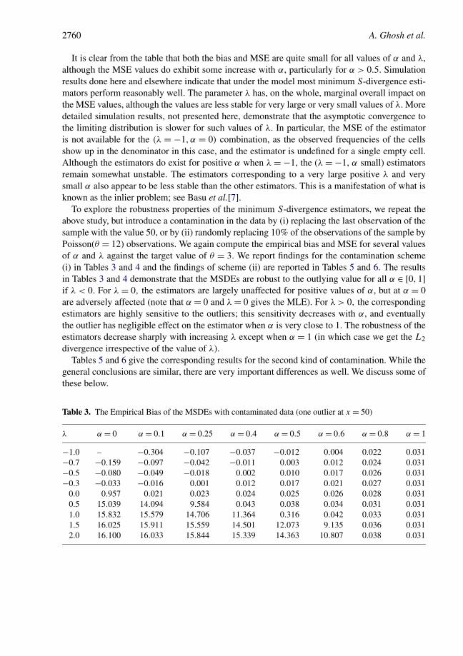
2760 A. Ghosh et al.
It is clear from the table that both the bias and MSE are quite small for all values of α and λ,although the MSE values do exhibit some increase with α, particularly for α > 0.5. Simulationresults done here and elsewhere indicate that under the model most minimum S-divergence esti-mators perform reasonably well. The parameter λ has, on the whole, marginal overall impact onthe MSE values, although the values are less stable for very large or very small values of λ. Moredetailed simulation results, not presented here, demonstrate that the asymptotic convergence tothe limiting distribution is slower for such values of λ. In particular, the MSE of the estimatoris not available for the (λ = −1, α = 0) combination, as the observed frequencies of the cellsshow up in the denominator in this case, and the estimator is undefined for a single empty cell.Although the estimators do exist for positive α when λ = −1, the (λ = −1, α small) estimatorsremain somewhat unstable. The estimators corresponding to a very large positive λ and verysmall α also appear to be less stable than the other estimators. This is a manifestation of what isknown as the inlier problem; see Basu et al.[7].
To explore the robustness properties of the minimum S-divergence estimators, we repeat theabove study, but introduce a contamination in the data by (i) replacing the last observation of thesample with the value 50, or by (ii) randomly replacing 10% of the observations of the sample byPoisson(θ = 12) observations. We again compute the empirical bias and MSE for several valuesof α and λ against the target value of θ = 3. We report findings for the contamination scheme(i) in Tables 3 and 4 and the findings of scheme (ii) are reported in Tables 5 and 6. The resultsin Tables 3 and 4 demonstrate that the MSDEs are robust to the outlying value for all α ∈ [0,1]if λ < 0. For λ = 0, the estimators are largely unaffected for positive values of α, but at α = 0are adversely affected (note that α = 0 and λ = 0 gives the MLE). For λ > 0, the correspondingestimators are highly sensitive to the outliers; this sensitivity decreases with α, and eventuallythe outlier has negligible effect on the estimator when α is very close to 1. The robustness of theestimators decrease sharply with increasing λ except when α = 1 (in which case we get the L2
divergence irrespective of the value of λ).Tables 5 and 6 give the corresponding results for the second kind of contamination. While the
general conclusions are similar, there are very important differences as well. We discuss some ofthese below.
Table 3. The Empirical Bias of the MSDEs with contaminated data (one outlier at x = 50)
λ α = 0 α = 0.1 α = 0.25 α = 0.4 α = 0.5 α = 0.6 α = 0.8 α = 1
−1.0 – −0.304 −0.107 −0.037 −0.012 0.004 0.022 0.031−0.7 −0.159 −0.097 −0.042 −0.011 0.003 0.012 0.024 0.031−0.5 −0.080 −0.049 −0.018 0.002 0.010 0.017 0.026 0.031−0.3 −0.033 −0.016 0.001 0.012 0.017 0.021 0.027 0.031
0.0 0.957 0.021 0.023 0.024 0.025 0.026 0.028 0.0310.5 15.039 14.094 9.584 0.043 0.038 0.034 0.031 0.0311.0 15.832 15.579 14.706 11.364 0.316 0.042 0.033 0.0311.5 16.025 15.911 15.559 14.501 12.073 9.135 0.036 0.0312.0 16.100 16.033 15.844 15.339 14.363 10.807 0.038 0.031
A generalized divergence 2761
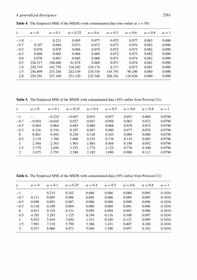
Table 4. The Empirical MSE of the MSDEs with contaminated data (one outlier at x = 50)
λ α = 0 α = 0.1 α = 0.25 α = 0.4 α = 0.5 α = 0.6 α = 0.8 α = 1
−1.0 – 0.221 0.095 0.077 0.075 0.077 0.083 0.090−0.7 0.107 0.084 0.073 0.072 0.073 0.076 0.082 0.090−0.5 0.076 0.070 0.068 0.070 0.072 0.075 0.082 0.090−0.3 0.066 0.065 0.066 0.069 0.072 0.075 0.082 0.090
0.0 0.976 0.063 0.065 0.068 0.071 0.074 0.082 0.0900.5 226.217 198.686 91.878 0.068 0.071 0.074 0.081 0.0901.0 250.719 242.759 216.292 129.174 0.171 0.073 0.081 0.0901.5 256.899 253.246 242.149 210.318 145.791 90.100 0.080 0.0902.0 259.291 257.160 251.120 235.340 206.341 116.826 0.080 0.090
Table 5. The Empirical MSE of the MSDE with contaminated data (10% outlier from Poisson(12))
λ α = 0 α = 0.1 α = 0.25 α = 0.4 α = 0.5 α = 0.6 α = 0.8 α = 1
−1 – −0.224 −0.047 0.015 0.037 0.051 0.069 0.0796−0.7 −0.054 −0.010 0.027 0.047 0.056 0.063 0.072 0.0796−0.5 0.064 0.064 0.065 0.066 0.068 0.070 0.074 0.0796−0.3 0.216 0.154 0.107 0.087 0.080 0.077 0.076 0.0796
0 0.861 0.492 0.220 0.128 0.103 0.089 0.080 0.07960.5 2.119 1.760 1.008 0.335 0.176 0.119 0.085 0.07961 2.584 2.383 1.903 1.081 0.404 0.186 0.092 0.07961.5 2.779 2.656 2.352 1.774 1.125 0.776 0.100 0.07962 2.875 2.793 2.588 2.185 1.690 0.900 0.111 0.0796
Table 6. The Empirical MSE of the MSDE with contaminated data (10% outlier from Poisson(12))
λ α = 0 α = 0.1 α = 0.25 α = 0.4 α = 0.5 α = 0.6 α = 0.8 α = 1
−1 – 0.215 0.102 0.086 0.086 0.088 0.095 0.1034−0.7 0.111 0.095 0.086 0.085 0.086 0.089 0.095 0.1034−0.5 0.098 0.091 0.087 0.086 0.088 0.090 0.096 0.1034−0.3 0.136 0.109 0.094 0.089 0.089 0.091 0.096 0.1034
0 0.812 0.318 0.131 0.099 0.094 0.093 0.096 0.10340.5 4.703 3.283 1.125 0.194 0.116 0.100 0.097 0.10341 6.932 5.934 3.850 1.311 0.249 0.122 0.099 0.10341.5 7.983 7.318 5.798 3.386 1.431 0.807 0.100 0.10342 8.527 8.066 6.971 5.048 3.100 0.957 0.103 0.1034

2762 A. Ghosh et al.
The contamination in case (i) represents an absolutely extreme outlier, which normally wouldbe identified and discounted by most robust estimation methods. This is essentially what is ob-served in Tables 3 and 4. That is why, even the weakly robust estimators generated by the S-divergences, such as the one corresponding to α = 0.1, λ = 0 perform admirably in this case.There is, in fact, little reason to venture outside the fold of DPD generated estimators in thiscase.
The contamination in case (ii), on the other hand, will generate observations of which somemay be legitimately confused with the observations coming from the major Poisson(3) compo-nent. Some others represent mild outliers, while some would be moderate to extreme outliers. Insuch a situation, it is clear from Tables 5 and 6 that the minimum divergence estimators withinthe PD and DPD classes no longer contain the divergence which minimizes the mean squareerror. In fact, the best performance in Table 6 (α = 0.4, λ = −0.7) is well separated from boththe PD and DPD family boundaries. Roughly, the zone of best performance is an elliptical (orcircular) subset of the tuning parameter space, with one axis extending roughly from α = 0.1 toα = 0.6 and the other roughly from λ = −0.3 to λ = −1.
The above study shows that there are many useful divergences in the S-divergence class whichlie outside the PD–DPD families. The above study also clearly illustrates that the robustnessproperties of the MSDEs are critically dependent on the value of λ for each given value of α.Yet, as we have seen, the canonical (first order) influence functions of the MSDE are independentof λ, and this index would fail to make any distinction between the different estimators for a fixedvalue of α; this property severely limits the usefulness of the influence function in assessing therobustness credentials of these estimators. In practice, estimators with α = 0 and negative λ
appear to have excellent outlier resistant properties, while those corresponding to small positivevalues of α and large positive λ perform poorly at the model in terms of robustness; in either casethe these behaviors are contrary to what would be expected from the usual influence functionapproach.
5.2. Mixture normal models
We now consider the more complex example of normal mixture models, where we assume thatthe number of mixing components is known. In particular, we will focus on a two-componentmixture of normal distributions with density
fθ = πφ(·,μ1, σ
21
) + (1 − π)φ(·,μ2, σ
22
), θ = (μ1,μ2, σ1, σ2,π)T , (24)
where φ(·,μ,σ 2) denotes a normal density with mean μ and variance σ 2 and π is the mixingproportion. We are interested in the estimation of the parameter vector θ . The approach can beeasily extended to the mixture of more than two distributions.
A robust solution to this problem can be easily obtained using the minimum S-divergenceestimators. However, since we have a continuous model in this case we will follow the Basu–Lindsay approach of smoothed model as discussed in Section 4.3. Following [22], the Gaussiankernel with W(x,y,h) being the N(y,h2) density at x gives a reasonable choice under thenormal model while using the Basu–Lindsay approach. Note that, the smoothed model with

A generalized divergence 2763
respect to the Gaussian kernel is then given by
f ∗θ = πφ
(·,μ1, σ21 + h2) + (1 − π)φ
(·,μ2, σ22 + h2).
Then we can easily derive the proposed MSDE∗ of θ under this mixture normal model by mini-mizing the S-divergence between the smoothed model f ∗
θ and the kernel density estimate of thetrue density with respect to the same Gaussian kernel.
Here we will present some simulation results to illustrate the performance of our proposedMSDE∗ under this relatively complex model situation. As in the previous example, we willtake the sample size n = 50 and generate 1000 samples from the assumed model (24) with thetrue parameter value θ = (0,10,3,3,0.5). Here, for simplicity, we have taken σ1 = σ2 = 3 asknown and numerically compute the MSDE∗ of the parameters (μ1,μ2,π). For the computationpurpose, we have taken the bandwidth h = hn as per the normal reference rule [39] yielding
hn = 1.06σn−1/5,
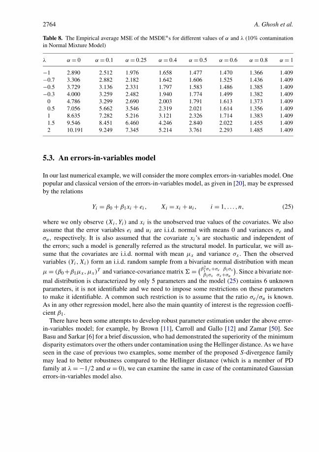
with σ being the common standard deviation (which is assumed to be known and equals 3).Next, for examining the robustness, we contaminate 100ε% of the sample by observations froma N(20,3) distribution which are potential outliers with respect to the assumed two-componentmixture model. Based on the 1000 such Monte-Carlo samples (each of size n = 50), we havecomputed the bias and MSE of the MSDE∗ of the three parameters for different choices of thecontamination proportion ε. For simplicity of presentation, we have presented only the averageabsolute bias and the average MSE of the three parameter estimates under the 10% contaminationscenario in Tables 7 and 8, respectively.
We notice that the general pattern of the performance of the estimators remains the same. Inthis case, the system requires larger values of α for the estimators to achieve reasonable degreesof robustness. Notice that the model is substantially more complicated than the Poisson model,involving three parameters, an additional tuning parameter (the bandwidth) and a measure whichis the combination of the three absolute biases or the MSEs. However in this case also the bestsolution lies well outside the PD–DPD families.
Table 7. The Empirical average absolute bias of the MSDE∗s for different values of α and λ (10% con-tamination in Normal Mixture Model)
λ α = 0 α = 0.1 α = 0.25 α = 0.4 α = 0.5 α = 0.6 α = 0.8 α = 1
−1.0 0.756 0.611 0.492 0.420 0.391 0.353 0.309 0.308−0.7 0.872 0.739 0.534 0.451 0.409 0.381 0.299 0.308−0.5 0.975 0.800 0.567 0.470 0.430 0.365 0.322 0.308−0.3 1.037 0.868 0.624 0.503 0.443 0.395 0.325 0.308
0 1.207 0.889 0.690 0.527 0.466 0.416 0.338 0.3080.5 1.612 1.395 0.937 0.563 0.516 0.443 0.348 0.3081 1.844 1.669 1.329 0.862 0.584 0.480 0.349 0.3081.5 1.953 1.829 1.571 1.134 0.786 0.526 0.361 0.3082 2.038 1.940 1.691 1.342 1.031 0.616 0.374 0.308
2764 A. Ghosh et al.
Table 8. The Empirical average MSE of the MSDE∗s for different values of α and λ (10% contaminationin Normal Mixture Model)
λ α = 0 α = 0.1 α = 0.25 α = 0.4 α = 0.5 α = 0.6 α = 0.8 α = 1
−1 2.890 2.512 1.976 1.658 1.477 1.470 1.366 1.409−0.7 3.306 2.882 2.182 1.642 1.606 1.525 1.436 1.409−0.5 3.729 3.136 2.331 1.797 1.583 1.486 1.385 1.409−0.3 4.000 3.259 2.482 1.940 1.774 1.499 1.382 1.409
0 4.786 3.299 2.690 2.003 1.791 1.613 1.373 1.4090.5 7.056 5.662 3.546 2.319 2.021 1.614 1.356 1.4091 8.635 7.282 5.216 3.121 2.326 1.714 1.383 1.4091.5 9.546 8.451 6.460 4.246 2.840 2.022 1.455 1.4092 10.191 9.249 7.345 5.214 3.761 2.293 1.485 1.409
5.3. An errors-in-variables model
In our last numerical example, we will consider the more complex errors-in-variables model. Onepopular and classical version of the errors-in-variables model, as given in [20], may be expressedby the relations
Yi = β0 + β1xi + ei, Xi = xi + ui, i = 1, . . . , n, (25)
where we only observe (Xi, Yi) and xi is the unobserved true values of the covariates. We alsoassume that the error variables ei and ui are i.i.d. normal with means 0 and variances σe andσu, respectively. It is also assumed that the covariate xi ’s are stochastic and independent ofthe errors; such a model is generally referred as the structural model. In particular, we will as-sume that the covariates are i.i.d. normal with mean μx and variance σx . Then the observedvariables (Yi,Xi) form an i.i.d. random sample from a bivariate normal distribution with mean
μ = (β0 +β1μx,μx)T and variance-covariance matrix � = (β2
1 σx+σe β1σx
β1σx σx+σu
). Since a bivariate nor-
mal distribution is characterized by only 5 parameters and the model (25) contains 6 unknownparameters, it is not identifiable and we need to impose some restrictions on these parametersto make it identifiable. A common such restriction is to assume that the ratio σe/σu is known.As in any other regression model, here also the main quantity of interest is the regression coeffi-cient β1.
There have been some attempts to develop robust parameter estimation under the above error-in-variables model; for example, by Brown [11], Carroll and Gallo [12] and Zamar [50]. SeeBasu and Sarkar [6] for a brief discussion, who had demonstrated the superiority of the minimumdisparity estimators over the others under contamination using the Hellinger distance. As we haveseen in the case of previous two examples, some member of the proposed S-divergence familymay lead to better robustness compared to the Hellinger distance (which is a member of PDfamily at λ = −1/2 and α = 0), we can examine the same in case of the contaminated Gaussianerrors-in-variables model also.

A generalized divergence 2765
In this spirit, we have conducted a simulation study similar to that presented in [6]. In particularwe generate 100 samples each of size n = 20 from the model (25) with true parameter valuesμx = 0, σx = 1, σu = σe = 0.25, β0 = 0 and β1 ∼ Uniform[−5,5]. The values of β1 has beenchosen randomly for each sample following [50], which takes into account that the robustnessof the resulting estimator might depend on the true value of β1. The 5% contamination has beenintroduced into both the error variables ui and ei by observations from N(0, σ 2) and N(0, τ 2)
respectively. Also, for model identifiability, we assume that σe/σu = 1 is known.For each sample, we compute the MSDE∗ of the 5 unknown parameters following the
smoothed model approach. As in [6], we also use the bivariate Gaussian kernel N2(0, h2I ) withthe value of bandwidth h = 0.5. Since our model is bivariate normal with mean μ and vari-ance matrix �, the resulting smoothed model is also a bivariate normal distribution with meanμ and variance matrix (� + h2I ). In particular, we consider the estimator β1j of β1 obtainedfrom j th sample (j = 1, . . . ,100) and derive the following performance measure of the estima-tor [50]
m =100∑j=1
(1 − |1 + β1j β1j |
(1 + β21j )
1/2(1 + β21j )
1/2
),
where β1j is the true value of β1 in the j th sample. Clearly, smaller values of m indicate greaterrobustness of the estimator. We have considered several choices of the (σ, τ ) combinations asin Zamar [50] and compute the above performance measure m for the MSDE∗ with differentvalues of α and λ. However, for brevity in presentation, we only present the results for the choice(σ, τ ) = (2,2) in Table 9; the results for all other choices of (σ, τ ) are generally similar exceptfor changes in magnitude.
It is once again clear that the estimators with moderately large positive values of α and moder-ately large negative values of λ perform better or competitively in terms of robustness comparedto the other estimators.
Table 9. The Empirical performance measure m for estimating β1 under the error-in-variable model with(σ, τ ) = (2,2)
λ α = 0 α = 0.1 α = 0.25 α = 0.4 α = 0.5 α = 0.6 α = 0.8 α = 1
−1 0.136 0.133 0.106 0.089 0.086 0.088 0.080 0.080−0.7 0.129 0.137 0.096 0.082 0.081 0.082 0.077 0.080−0.5 0.147 0.128 0.091 0.088 0.084 0.090 0.081 0.080−0.3 0.197 0.127 0.120 0.102 0.080 0.086 0.083 0.080
0 0.647 0.368 0.165 0.106 0.088 0.081 0.089 0.0800.5 0.526 0.577 0.599 0.177 0.110 0.089 0.082 0.0801 0.471 0.513 0.544 0.578 0.306 0.116 0.075 0.0801.5 0.496 0.439 0.490 0.574 0.586 0.268 0.080 0.0802 0.433 0.514 0.504 0.556 0.629 0.625 0.082 0.080
2766 A. Ghosh et al.
6. Higher order influence analysis
Lindsay [33] had observed that the usual first order influence function failed to capture the ro-bustness of the minimum disparity estimators with large negative values of λ. The descriptionof the previous section has demonstrated that this phenomenon can be a more general one, andis not restricted to estimators which have unbounded influence functions. It may fail to predictthe strength of robustness of highly robust estimators, and it may also declare extremely unstableestimators as having good stability. As in [33], we consider a second order influence functionanalysis of the MSDEs and show that this provides a significantly improved prediction of the ro-bustness of these estimators. See [33] and [7] for a general description of second order influenceanalysis in minimum disparity estimation.
Let G and Gε = (1 − ε)G + ε∧y represent the true distribution and the contaminated dis-tribution respectively, where ε is the contaminating proportion, y is the contaminating point,and ∧y is a degenerate distribution with all its mass on the point y; let T (Gε) be the valueof the functional T evaluated at Gε . The influence function of the functional T (·) is given byT ′(y) = ∂T (Gε)
∂ε|ε=0. Viewed as a function of ε, �T (ε) = T (Gε) − T (G) quantifies the amount
of bias under contamination; under the first-order Taylor expansion the bias may be approximatedas �T (ε) = T (Gε)−T (G) ≈ εT ′(y). From this approximation, it follows that the predicted biasup to the first order will be the same for all functionals having the same influence function. Thusfor the minimum S-divergence estimators, the first order bias approximation is not sufficient forpredicting the true bias under contamination and hence not sufficient for describing the robust-ness of such estimators.
We consider the second order Taylor series expansion to get a second-order prediction of the
bias curve as �T (ε) = εT ′(y) + ε2
2 T ′′(y). The ratio of the second-order (quadratic) approxima-tion to the first (linear) approximation, given by
quadratic approximation
linear approximation= 1 + [T ′′(y)/T ′(y)]ε
2
can serve as a simple measure of adequacy of the first-order approximation. Often when thefirst order approximation is inadequate, the second order approximation can give a more accu-rate prediction. If ε is larger than εcrit = | T ′(y)
T ′′(y)|, the second-order approximation may differ by
more than 50% compared to the first-order approximation. When the first order approximationis inadequate, such discrepancies will occur for fairly small values of ε.
In the following theorem, we will present the expression of our second order approximationT ′′(y); for simplicity we will deal with the case of a scalar parameter. The next straightforwardcorollary gives the special case of the one parameter exponential family having unknown meanparameter.
Theorem 6.1. Let Fθ ∈ F with θ being a scalar parameter. Assume that the true distri-bution belongs to the model F . For the minimum divergence estimator defined by the esti-mating equation (17) where the function K(δ) satisfies K(0) = 0 and K ′(0) = 1, we have

A generalized divergence 2767
T ′′(y) = T ′(y)(∫
u2θf
1+αθ )−1[m1(y) + K ′′(0)m2(y)], where
m1(y) = 2∇uθ (y)f αθ (y) + 2αu2
θ (y)f αθ − 2
∫∇uθf
1+αθ − 2α
∫u2
θf1+αθ
− T ′(y)
[(1 + 2α)
∫u3
θf1+αθ + 3
∫uθ∇uθf
1+αθ
],
m2(y) = T ′(y)
∫u3
θf1+αθ − 2u2
θ (y)f αθ (y) + uθ (y)f α−1
θ (y) − ∫uθf
1+αθ
uθ (y)f αθ (y) − ∫
uθf1+αθ
.
In particular for the minimum S-divergence estimator, we have K ′′(0) = A − 1.
Corollary 6.2. For the one parameter exponential family with mean θ , the above theorem sim-plifies to T ′′(y) = T ′(y)[K ′′(0)Q(y) + P(y)] with
Q(y) =(
uθ (y)f α−1θ (y) − ∫
uθf1+αθ
uθ (y)f αθ (y) − ∫
uθf1+αθ
)+ f α
θ
[(y − θ)c3
c22
− 2(y − θ)2
c2
],
P (y) =(
2c0
c2− 2α
)− f α
θ
[2
c2+ 2α(y − θ)c3
c22
− 2α(y − θ)2
c2
],
where ci = ∫ui
θf1+αθ for i = 0,1,2,3. If y represents an extreme observation with a small
probability, the leading term of Q(y) is dominant.
Example 6.1 (Poisson mean). For a numerical illustration of the second order influence anal-ysis, we consider the Poisson model with mean θ . This is a one-parameter exponential familyso that we can compute the exact values of the second order bias approximation by using theabove corollary. Also we can compute the first order approximation of bias by the expression ofinfluence function from equation (18). For all our simulation results explained below, we haveconsidered the true value of θ to be 4 and put a contamination at the point y = 10 which lies atthe boundary of the 3σ limit for the mean parameter θ = 4.
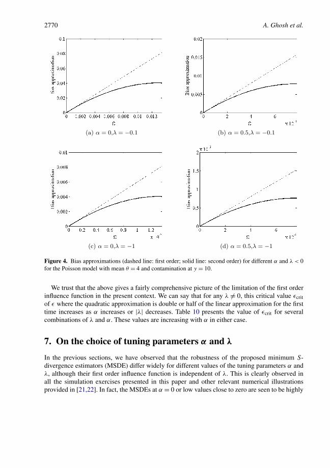
We have examined the relation between these two bias approximations for several differentvalues of α and λ. In the following, we present some of our crucial findings through some graph-ical representations of the predicted biases. Figures 2, 3 and 4 contain the approximate bias plotsfor different α and λ = 0, λ > 0, λ < 0 respectively. In all the plots, the ε-axis runs from 0 tomin(0.1, εcrit), where εcrit is the smallest value of ε where the second order approximation isdouble or half of the quantity predicted by the first order influence function for the first time. Asthis depends on the particular situation, all the plots in this section have different axis ranges.
Comments on Figure 2 (λ = 0): Clearly the two approximations coincide when α = 0 and λ =0 which generates the maximum likelihood estimator. This is expected from the theory of theMLE. However the difference between the predicted biases increase as α increases up to 0.5and then the difference falls again and almost vanishes at α = 1. In addition, the actual bias

2768 A. Ghosh et al.
Figure 2. Bias approximations (dashed line: first order; solid line: second order) for different α and λ = 0for the Poisson mean θ = 4 and contamination at y = 10.
approximation generally drops with increasing α for both the approximations which should alsobe expected.
Comments on Figure 3 (λ > 0): For positive λ, the bias approximations are very differenteven for small values of α. As α increases the difference between the two bias approximationsdecreases. Here, ε = εcrit is the value of ε where the quadratic approximation is exactly doubleof the linear approximation for the first time. These estimators have weak stability properties inthe presence of outliers, but the first order influence function approximation gives a false, con-servative picture. We also note that this critical value of ε (εcrit) also increases as α increases orλ decreases.
Comments on Figure 4 (λ < 0): Here also the plots are shown up to ε = εcrit; in this case εcritis the value where the quadratic approximation drops to half of that of the linear approximation

A generalized divergence 2769
Figure 3. Bias approximations (dashed line: first order; solid line: second order) for different α and λ > 0for the Poisson model with mean θ = 4 and contamination at y = 10.
for the first time. Here the estimators have strong robustness properties, but the influence func-tion gives a distorted negative view. Contrary to the positive λ case, here this critical value εcrit
increases as both α or λ increases.
While the three figures are drawn for zero, positive and negative values of λ, comparing ofspecific panels over the three different figures may show the predicted behavior of the procedureover different λ for the same value of α. For example, consider Figures 2(c), 3(b) and 4(b). As thefirst order influence function is independent of λ, the corresponding predicted behavior in thesethree panels are identical with α fixed at 0.5. As we have seen in Tables 3–6, the actual behaviorsof these estimators are widely different. This is recognized to a large extent in the second orderinfluence curves, which shrinks the first order prediction for λ < 0 and inflates it for λ ≥ 0 (moreso for λ > 0). The first order prediction, however, makes no such distinction.
2770 A. Ghosh et al.
Figure 4. Bias approximations (dashed line: first order; solid line: second order) for different α and λ < 0for the Poisson model with mean θ = 4 and contamination at y = 10.
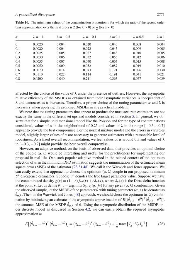
We trust that the above gives a fairly comprehensive picture of the limitation of the first orderinfluence function in the present context. We can say that for any λ �= 0, this critical value εcritof ε where the quadratic approximation is double or half of the linear approximation for the firsttime increases as α increases or |λ| decreases. Table 10 presents the value of εcrit for severalcombinations of λ and α. These values are increasing with α in either case.
7. On the choice of tuning parameters α and λ
In the previous sections, we have observed that the robustness of the proposed minimum S-divergence estimators (MSDE) differ widely for different values of the tuning parameters α andλ, although their first order influence function is independent of λ. This is clearly observed inall the simulation exercises presented in this paper and other relevant numerical illustrationsprovided in [21,22]. In fact, the MSDEs at α = 0 or low values close to zero are seen to be highly
A generalized divergence 2771
Table 10. The minimum values of the contamination proportion ε for which the ratio of the second orderbias approximation over the first order is 2 (for λ > 0) or 1
2 (for λ < 0)
α λ = −1 λ = −0.5 λ = −0.1 λ = 0.1 λ = 0.5 λ = 1
0 0.0020 0.004 0.020 0.040 0.008 0.0040.1 0.0020 0.004 0.023 0.043 0.009 0.0050.2 0.0025 0.005 0.027 0.048 0.010 0.0050.3 0.0030 0.006 0.032 0.056 0.012 0.0060.4 0.0035 0.007 0.040 0.067 0.015 0.0080.5 0.0050 0.009 0.052 0.087 0.019 0.0100.6 0.0070 0.014 0.073 0.121 0.026 0.1300.7 0.0110 0.022 0.114 0.191 0.041 0.0210.8 0.0200 0.040 0.211 0.363 0.077 0.039
affected by the choice of the value of λ under the presence of outliers. However, the asymptoticrelative efficiency of the MSDEs as obtained from their asymptotic variances is independent ofλ and decreases as α increases. Therefore, a proper choice of the tuning parameters α and λ isnecessary when applying the proposed MSDEs in any practical problem.
We note that the tuning parameters that appear to produce the most accurate estimators are notexactly the same in the different set ups and models considered in Section 5. In general, we ob-serve that for a simple unidimensional model like the Poisson and for the type of contaminationsconsidered, values of α in the neighborhood of 0.25 and values of λ in the range [−0.3,−0.7]appear to provide the best compromise. For the normal mixture model and the errors in variablesmodel, slightly larger values of α are necessary to generate estimators with a reasonable level ofrobustness. As a fixed overall recommendation, we feel values of α around 0.5 and values of λ
in [−0.3,−0.7] might provide the best overall compromise.However, an adaptive method, on the basis of observed data, that provides an optimal choice
of the couple (α,λ) would be interesting and useful for the practitioners for implementing ourproposal in real life. One such popular adaptive method in the related context of the optimumselection of α in the minimum DPD estimation suggests the minimization of the estimated meansquare error (MSE) of the estimator [23,31,48]. We call it the Warwick and Jones approach. Wecan easily extend that approach to choose the optimum (α,λ) couple in our proposed minimumS∗ divergence estimators. Suppose θ0 denotes the true target parameter value. Suppose we havethe contaminated density g(x) = (1 − ε)fθ0(x)+ εδy(x), where δy(x) is the Dirac delta functionat the point y. Let us define θα,λ = arg minθ S(α,λ)(g, fθ ) for any given (α,λ) combination. Giventhe observed sample, let the MSDE of the parameter θ with tuning parameter (α,λ) be denoted asθα,λ. Then, in the Warwick and Jones [48] approach, we should chose the optimum (α,λ) combi-nation by minimizing an estimate of the asymptotic approximation of E[(θα,λ −θ0)T (θα,λ −θ0)],the summed MSE of the MSDE θα,λ of θ . Using the asymptotic distribution of the MSDE un-der discrete model as discussed in Section 4.2, we can easily obtain the required asymptoticapproximation as
E[(
θα,λ − θ0)T (θα,λ − θ0)] = (
θα,λ − θ0)T (θα,λ − θ0) + 1
ntrace
{J−1
g VgJ−1g
}, (26)
2772 A. Ghosh et al.
where Jg and Vg are the matrices as defined in Section 4.2. In case of continuous models, weshould use J ∗
g and V ∗g defined in Section 4.3 in place of Jg and Vg respectively, which was also
indicated briefly in [22]. Note that, if we ignore the first bias term in the above approximation(26), the procedure of selecting the optimum tuning parameter coincide with the proposal ofHong and Kim [31].
Clearly, one can easily estimate the second component in the approximation (26) by puttingθα,λ for θα,λ and the empirical estimates of the true density g from the observed data (throughthe relative frequency or the kernel density estimator for discrete and continuous models respec-tively). For the first component in (26), one can again estimate θα,λ by the observed MSDE θα,λ;but there is clearly no direct estimate for θ0. Warwick and Jones [48] took various possible es-timators θ0 which they referred to as the “pilot estimators” and compared these choices throughan extensive simulation study for the MDPDE. They recommended the choice of the “pilot es-timator” which is the MSDE (or the MDPDE) corresponding to α = 1, that is, the minimumL2-divergence estimator. We have followed the Warwick and Jones proposal in this paper. Inrepeated simulations involving the Poisson model, we have observed the following:
(a) When the data come from the pure distributions (as used in Section 5) we have foundthat a large proportion of cases choose α = 0, λ = 0 as the optimal parameter set. Ghoshand Basu [22] reported similar simulation findings in case of the choice of optimal tuningparameters for the use of the S-divergence in continuous models.
(b) When the data are chosen from contaminated Poisson mixtures, very often the optimaltuning parameter set has a moderately large values of α and a moderately large negativevalue of λ. This again indicates the usefulness of minimum S-divergence estimators out-side the PD–DPD class.
It is also worthwhile to note that for Short’s data and Newcomb’s data, two famous data setspresented in [43] which contain moderate to large outliers, the optimal (α, λ) combinations turnout to be (0.8, −0.3) and (0.6, −0.4), as reported by in [22] for the normal model. In either case,the optimal set is far off from the PD–DPD class.
For the set ups in Sections 5.2 and 5.3, we believe we will need more research to make moreclear cut and pinpointed recommendations about the choice of the tuning parameter. Apart fromthe complicated nature of the models, this is also due to the presence of a third tuning parameter,the bandwidth. The actual choice of the bandwidth in an optimal manner will probably require asubstantial amount of additional research. However, we are able to confirm that larger values ofthe bandwidth appear to generate more efficient estimators, while smaller values produce morerobust ones.
8. Two interesting special cases
8.1. Asymptotic breakdown point of the MSDEs under the location model
Now we will establish the breakdown point of the minimum S-divergence functional Tα,λ(G)
under the location family of densities FL = {fθ (x) = f (x − θ) : θ ∈ �}. Note that∫
f 1+α(x −θ) dx = ∫
f 1+α(x) dx = Mαf , say, which is independent of the parameter θ . Recall that we can

A generalized divergence 2773
write the S-divergence as S(α,λ)(g, f ) = ∫f 1+αC(α,λ)(δ) where δ = g
f− 1 and C(α,λ)(δ) =
1AB
[B − (1 + α)(δ + 1)A + A(δ + 1)1+α]. Now C(α,λ)(−1) = 1A
which is clearly bounded for allA �= 0. Define D(α,λ)(g, f ) = f 1+αC(α,λ)(
gf
− 1). Then note that whenever A > 0 and B > 0,
we have D(α,λ)(g,0) = limf →0 D(α,λ)(g, f ) = 1B
g1+α . Our subsequent results will be based onthe next lemma which follows from Holder’s inequality.
Lemma 8.1. Assume that the two parameters α and λ are such that both A and B are posi-tive. Then for any two densities g, h in the location family FL and any 0 < ε < 1, the integral∫
D(α,λ)(εg,h) is minimized when g = h.
Consider the contamination model Hε,n = (1 − ε)G + εKn, where {Kn} is a sequence ofcontaminating distributions. Let hε,n, g and kn be the corresponding densities. We say thatthere is breakdown in Tα,λ for ε level contamination if there exists a sequence Kn such that|Tα,λ(Hε,n)− T (G)| → ∞ as n → ∞. We write below θn = Tα,λ(Hε,n) and assume that the truedistribution belongs to the model family, i.e., g = fθg . We make the following assumptions:
(BP1)∫
min{fθ (x), kn(x)} → 0 as n → ∞ uniformly for |θ | ≤ c for any fixed c. That is,the contamination distribution is asymptotically singular to the true distribution and tospecified models within the parametric family.
(BP2)∫
min{fθg (x), fθn(x)} → 0 as n → ∞ if |θn| → ∞ as n → ∞, that is, large values ofθ give distributions which become asymptotically singular to the true distribution.
(BP3) The contaminating sequence {kn} is such that
S(α,λ)(εkn, fθ ) ≥ S(α,λ)(εfθ , fθ ) = C(α,λ)(ε − 1)Mαf
for any θ ∈ � and 0 < ε < 1 and lim supn→∞∫
k1+αn ≤ Mα
f .
Theorem 8.2. Assume that the two parameters α and λ are such that both A and B are posi-tive. Then under the assumptions (BP1)–(BP3) above, the asymptotic breakdown point ε∗ of theminimum S-divergence functional Tα,λ is at least 1
2 at the (location) model.
Corollary 8.3 (Density power divergence). The well-known Density Power divergence (DPD)belongs to the S-divergence family (for λ = 0) for which A = 1 > 0 and B = α > 0 for all α > 0.Thus under the assumptions (BP1)–(BP3), the MDPDE for α > 0 has breakdown point of 1
2 atthe location model of densities.
Remark 8.1. Whenever the contaminating densities {kn} belong to the location model underconsideration then one can easily check that Assumption (BP3) holds; its second part holdstrivially whereas the first part holds by Lemma 8.1.
Further, if kn = fθn with |θm| → ∞ as n → ∞, then Assumption (BP2) implies assumption(BP1). In particular, for the normal location model, Assumption (BP2) holds trivially and sounder model contamination Assumption (BP1) also holds.
Our breakdown results of this section provide a remarkable match with the empirical findingsabout the performance of the minimum S-divergence estimators as observed in Section 5. Notice

2774 A. Ghosh et al.
Figure 5. The region of positive A and B in the (α,λ)-plane.
that the breakdown result of Theorem 8.8 requires that both A and B should be strictly greaterthan zero. In Figure 5, we have represented the rectangular span of the combination of tuningparameters α and λ given by [0,1] × [−1,2]. This has been the region of our interest in thesimulations of Section 5. The subregion of this rectangle where A > 0, B > 0 condition is vio-lated is given in the lower left hand corner of this region. What is striking is that this subregionmatches exactly with the region of instability observed under data contamination in Tables 3–6in Section 5.
8.2. The S-hellinger distance: Estimating multivariate location andcovariance
Beran [8] considered minimum Hellinger distance estimation for univariate parametric modelsand established the efficiency and demonstrated the robustness of the corresponding minimumdistance estimator. Tamura and Boos [44] extended his work on minimum Hellinger distanceestimation to the case of multivariate location and covariance estimation under the class of ellip-tically symmetric models. In the subsequent literature, there has been many attempts to general-ize the Hellinger distance suitably to extract some more desirable properties along with greaterrobustness; see, for example, [1,41]. However, most, if not all, such generalizations are in thecase of univariate models.
The S-divergence family developed here provides us one such generalization of the Hellingerdistance, namely the S-Hellinger family, briefly described in Section 3; it is the subfamily of S-divergences corresponding to the parameter λ = − 1
2 that connects the ordinary Hellinger distanceto the L2-divergence smoothly through the parameter α.
Here we explore the properties of the S-Hellinger distance family described briefly in Sec-tion 3, to generate a class of robust estimators of multivariate location and covariances. Thus, ourwork will generalize the work of Tamura and Boos [44] from the Hellinger distance to the case
A generalized divergence 2775
of the general family of S-Hellinger distances. Note that just as the ordinary Hellinger distancerepresents the self adjoint member of the PD family in the sense of [32], any other cross sectionof the class of S-divergences for a fixed value α also has a self adjoint member in the S-Hellingerfamily S(α,−1/2).
8.2.1. The S-hellinger distance (SHD) family
The S-Hellinger Distance (SHD) family between two generic probability density functions f
and g is defined in terms of the tuning parameter α as
SHDα(g,f ) = S(α,−1/2) = 2
1 + α
[∫f 1+α − 2
∫f
1+α2 g
1+α2 +
∫g1+α
](27)
= 2
1 + α
∫ (g
1+α2 − f
1+α2
θ
)2 = 2
1 + α
∥∥g1+α
2 − f1+α
2θ
∥∥22,
where ‖ · ‖2 represents the using the L2-norm. Although SHDα(g,f ) in (27) is not itself a
distance, it corresponds to the distance [ 1+α2 SHDα(g,f )] 1
2 . Note that, for α = 0 the measurereduces to the ordinary (twice squared) Hellinger distance.
We will use the S-Hellinger distance for doing multivariate location and covariance estimationbecause it is easily amenable to this unlike other members of S-divergence. These propertiesmainly come from the fact that it corresponds to a distance metric.
Lemma 8.4. Let f1, f2, f3 be three densities with respect to some common dominating measure.Then for any 0 ≤ s ≤ 1, we have
SHDα
((1 − s)f1 + sf2, f3
) ≤ (1 − s)SHDα(f1, f3) + sSHDα(f2, f3).
Lemma 8.5. Let f1, f2, f3 be three densities with respect to some common dominating measure.Then we have
SHDα(f1, f2) ≤ 2[SHDα(f1, f3) + SHDα(f2, f3)
].
8.2.2. The minimum SHD estimator (MSHDE) of multivariate location and covariance
Now let us consider the usual (multivariate) set-up of parametric estimation; we have n indepen-dent and identically distributed observations X1,X2, . . . ,Xn from a (multivariate) distributionG, having density g with respect to a dominating measure ν. We will model the true density bya parametric (multivariate) model Fd = {fθ : θ ∈ �0 ⊆ R
p}; our interest here is to estimate theparameter θ based on the observed data. We will define the measure of discrepancy between thesample data and the model family by the S-Hellinger distance measure between the model den-sity fθ and a non-parametric density estimator gn. Thus the Minimum SHD Estimator (MSHDE)is given by
θn = T (Gn) = arg minθ∈�
2
1 + α
∥∥g1+α
2n − f
1+α2
θ
∥∥22
(28)
= arg minθ∈�
∥∥g1+α
2n − f
1+α2
θ
∥∥2,

2776 A. Ghosh et al.
where gn is the kernel density estimator given by
gn(x) = 1
nhpn
n∑i=1
w
(x − Xi
hn
), (29)
with w(·) being a p-variate density function and {hn} being a suitable sequence of bandwidths;Gn is the distribution function corresponding to the density gn.
In this section, we will consider only the minimum SHD estimator of multivariate locationand covariance under suitable assumptions and describe some important properties of it. Wewill restrict ourselves only to parametric families having elliptically symmetric distribution withdensity function given by
fθ (x) ∝ |�|−1/2ψ{(x − μ)T �−1(x − μ)
}, (30)
where ψ is an univariate density symmetric around zero, θ = (μ,�), � =Rp ×S , with S being
the set of all p × p positive definite matrices.The influence function of the minimum SHD functional can be derived directly from the results
of Section 4.1. As a particular example, we will consider the case of The elliptically symmetricdensity of p-variate normal with mean vector μ and covariance matrix �. The influence functionof the MSHDE of θ = (μ,�) can be written in terms of that of the individual parameters, namelyT
μα (Fθ ) and T �
α (Fθ ) of μ and �, as IF(y;Tα,Fθ ) = (IF(y;T μα ,Fθ ), IF(y;T �
α ,Fθ )). Also, it iseasily seen that the influence function of the MSHDE of location μ is given by
IF(y;T μ
α ,Fθ
) = (1 + α)p2 +1(y − μ)e− α
2 (y−μ)T �−1(y−μ),
and that of the covariance � is given by
IF(y;T �
α ,Fθ
)= ζα,p
[(1 + α)
p2 +1{(y − μ)(y − μ)T �−1 − p
}e− α
2 (y−μ)T �−1(y−μ) − (1 − p(1 + α)
)]�,
with ζα,p = 2(1 + α)[3 − 2p(1 + α) + p2(1 + α)2]−1.
8.2.3. Equivariance
An estimator of (multivariate) location and covariance can potentially be used to infer about theorientation and shape of data-points in a multi-dimensional space. Since there is no single uni-versal way of measuring data, a minimal requirement for these estimators is that they should beindependent of the coordinate system. So for the estimation of multivariate location and covari-ance, we prefer estimators that are affine equivariant and affine covariant respectively; see [44]for relevant definitions. We can derive some sufficient conditions, under which the MinimumSHD estimator of multivariate location and covariance satisfies the requirement of equivariance.
Lemma 8.6. Suppose that:
1. the model family is chosen to be elliptical having density of the form (30) and2. the kernel density estimator satisfies the condition gAX+b,n(x) = gX,n(A
−1(x − b))/|A|.

A generalized divergence 2777
Then the minimum SHD estimator of multivariate location and covariance are affine equivariantand affine covariant, respectively.
The proof is straightforward and is omitted. In a practical situation, it is necessary to choose akernel density estimator satisfying condition (8.6). We can construct a density estimate of the ra-dial type satisfying (8.6), whenever we have an initial affine covariant estimate �0 of covariancebased on the observed data; this will be of the form
gn(x) = 1
nhpn |�0|1/2
n∑i=1
w(h−1
n ‖x − Xi‖�0
), (31)
where ‖x‖2� = xT �−1x. Then the MSHDE of the location and covariance using this kernel den-
sity estimate will be both affine equivariant and affine covariant within the multivariate ellipticalfamily (30).
8.2.4. Consistency
Suppose the observed sample data X1,X2, . . . ,Xn come from the true common density g. Thenthe minimum SHD estimator can be shown to be consistent under suitable conditions on theKernel density estimator gn and the model family fθ , θ ∈ �.
Theorem 8.7. Suppose that, with probability one, the minimum SHD estimator T (Gn) exists forall sufficiently large n and as n → ∞,
∥∥g1+α
2n − f
1+α2
θ
∥∥2 → 0 and (32)
∥∥fθn
1+α2 − f
1+α2
θ
∥∥2 → 0 ⇒ θn → θ, (33)
for any sequence {θn : θn ∈ �}. Then we have, with probability one,
T (Gn) → θ as n → ∞. (34)
Note that condition (32) needed for the consistency of the minimum SHD estimator, simplysays that the kernel density estimator gn converges to the true density g in the metric correspond-ing to the SHD. This is a very intuitive assumption for the consistency and other asymptotic prop-erties of the any minimum distance estimator. However, in this case, it can be proved using theuniform convergence or by L1 convergence of the kernel estimator under some mild assumptionson the corresponding bandwidth sequence. Condition (33) needed for the consistency of the min-imum SHD estimator, is a model specific condition. It is expected to hold for many ellipticallysymmetric densities. We have checked that this holds for the multivariate normal model.
Deriving the complete asymptotic results for the minimum S-Hellinger distance estimator incase of multivariate location and covariance could pose some challenges as it would involve theconvergence properties of a kernel in a multivariate setting. We will take up the actual asymp-totic distribution of these estimators in our future work. In case of the DPD, the corresponding

2778 A. Ghosh et al.
minimum divergence estimators are multivariate M-estimators of location and covariance whichshould be relatively easier to handle. Some relevant results in this connection are presented in[29]. Toma and Leoni-Aubin [46] present some divergence based estimators of multivariate lo-cation and covariance. Note, however, that the DPD and the S-Hellinger distance families haveno overlap except at the L2 distance.
Using robust data reduction techniques prior to the analysis of multivariate location and co-variance could be another approach to tackle this problem. See the recent monograph on robustdimension reduction by [19] for a general discussion of this area.
A small simulation example illustrating the robustness of the minimum S-Hellinger distanceestimators has been provided in the Supplementary Material [27].
8.2.5. Breakdown point
We now consider the breakdown point of the minimum S-Hellinger distance functional in thecase of the estimation of multivariate location and covariance as a measure of its robustness. LetX represent the original data set of a given size n and Y be a contaminating data set of size m
(m ≤ n). The estimator θn will be said to break down if, through proper choice of the elementsof the data set Y , the difference θm+n(X ∪ Y) − θn(X) can be made arbitrarily large. If m∗ isthe smallest number of the contaminating values for which the estimator breaks down, then thebreakdown point of the corresponding estimator at X is m∗
(m+n). In the case of multivariate location
and covariance, the breakdown point of the joint estimation of location and covariance has beendefined by [18] through the following measure of discrepancy
B(θ1, θ2) = tr(�1�
−12 + �−1
1 �2) + ‖μ1 − μ2‖2 (35)
between parameter values θ1 = (μ1,�1) and θ2 = (μ2,�2), where tr represents the trace ofa matrix and ‖ · ‖ represents the Euclidean norm. The joint estimate of multivariate locationand covariance will break down when the supremum of the discrepancy, as given in the aboveequation, between the pure data estimate at X and the contaminated data estimate at X ∪ Y , isinfinite.
We will derive the breakdown point of the minimum SHD estimators under specific assump-tions on the true and model densities. Let G∗ denote a subclass of all probability densities satis-fying
SHDα(g,f ) ≤ κ(α), for all g,f ∈ G∗, (36)
where κ(α) is a finite positive bound depending only on α. Then, we will assume that the modelfamily Fd and true density g both belong to the family G∗. Also let gn(cn) = gn(cn, x) be thekernel density having bandwidth cn and fθn(cn) denotes the model density nearest to the abovekernel estimator in terms of the S-Hellinger distance. We assume that such a model density exists.Define
an,m = SHDα
(gn(cn+m),fθn(cn)
), and
(37)v∗ = lim inf
θ1,θ2SHDα(fθ1, fθ2), where the limit is taken as B(θ1, θ2) → ∞.
A generalized divergence 2779
Theorem 8.8. Assume that the model family Fd and true density g both belong to G∗. Then, theminimum SHD estimator θn(cn) has the breakdown point ε∗(θn(cn)) satisfying
ε∗(θn(cn)) ≥
[ v∗4 − an,m
κ(α) − an,m
]. (38)
Corollary 8.9. Let g be the true density. If SHDα(g,fθn(cn)) → a and gn+m(cn+m) → g(x),for each x, we have aa,m → a almost surely. Then, by the theorem,
lim infn→∞ ε∗(θn(cn)
) ≥[ v∗
4 − a
κ(α) − a
]. (39)
Further, if the true distribution belongs to the model family, that is, g = fθ for some θ ∈ �, weget a = 0 and then
lim infn→∞ ε∗(θn(cn)
) ≥ v∗
4κ(α). (40)
Remark. Whenever v∗ = κ(α) and the true distribution belongs to the model family, the corol-lary yields
lim infn→∞ ε∗(θn(cn)
) ≥ 1
4.
That is, breakdown cannot occur for the minimum SHD estimator in this case for ε < 14 . The
result is remarkable since the breakdown bound is independent of the dimension of the dataunlike the shrinking bounds offered by the M-estimator.
9. Role of the S-divergence in robust hypothesis testing
The S-divergence measure and the minimum S-divergence estimators can also be applied toconstruct robust tests for statistical hypothesis. Such divergence based tests have been attemptedin case of the power divergences [42] and the density power divergences [4,5], which can befurther extended to generate a larger class of test statistics using the family of S-divergences.
As a brief introduction, let us consider the set-up of Section 4 with an i.i.d. sample of size n.Fix θ0 ∈ �. Consider the problem of testing the simple null hypothesis given by
H0 : θ = θ0 against H1 : θ �= θ0. (41)
Under H0, if the model is correctly specified, fθ0 is the true data generating density. Therefore, aclass of test statistics for testing (41) can be constructed by using the S-divergence measure be-tween fθ0 and f
θfor any estimator θ of θ based on the observed sample. And, an ideal choice for
θ in this case should be a minimum S-divergence estimator so that the test statistics has the form
T(1)γ,λ(θβ,τ , θ0) = 2nS(γ,λ)(fθβ,τ
, fθ0),
where θβ,τ is the minimum S-divergence estimator (MDPDE) of θ with tuning parameter β andτ and S(γ,λ)(·, ·) is the S-divergence measure with parameter γ and λ.

2780 A. Ghosh et al.
Ghosh, Basu and Pardo [25] proved several asymptotic and robustness properties of the aboveS-divergence based test statistics with τ = 0. The main advantage of taking τ = 0 is that the MD-PDE θβ,0 does not require the consideration of kernel density estimator and hence avoids all theassociated complications in asymptotic derivations. However, they have argued that, even if thegeneral MSDE θβ,τ were used, under the set-up of discrete models the asymptotic null distribu-tion would remain the same. See [25] for more detailed derivations and examples. Interestingly,the robustness properties of the proposed test procedure have been observed to depend directlyon the robustness of the minimum S-divergence estimator used.
Similar classes of S-divergence based test statistics can also be constructed for testing com-posite hypothesis problems or for testing the two sample problems extending the ideas of [4,5].This problem has also been considered by the first author in his doctoral dissertation and areavailable in [24].
The robustness properties of similar test statistics derived from robust M-estimators have beenpointed out in [30]. The works of [15], [16] and [34] related to scoring rules also suggest someother robust tests of parametric statistical hypothesis which are similar in spirit to our work.
10. Concluding remarks
In this paper, we have described the development of a large family of density based divergenceswhich includes both the classes of power divergences and density power divergences as specialcases. The family gives the data analyst a large number of choices of possible divergences toapply in the minimum distance estimation context. Several members of the family are distin-guished by their strong robustness properties, and many of them generate estimators with highasymptotic efficiency. The best performer within the minimum divergence class induced by theS-divergences is often outside the PD–DPD class, underscoring the utility of the family. The per-formance of the method is demonstrated on very simple everyday use models like the Poisson, aswell as more complicated and sophisticated models like the normal mixture model and normalerrors-in-variables model. The family is indexed by two parameters, only one of which shows upin the influence function and the asymptotic efficiency expressions. Yet both the tuning parame-ters have important roles in actual finite sample efficiencies and the robustness of the estimators.The behavior of the estimators within this family clearly show the limitation of the influencefunction as a measure of robustness; we demonstrate that a second order influence analysis couldbe a much more accurate predictor of the robustness of these estimators (or lack of it). The in-stability of the estimators under contamination also appears to be linked closely to the violationof the breakdown conditions. A particular subfamily of this class can be used to construct robusthigh breakdown equivariant estimators of multivariate location and covariances.
Acknowledgements
This research forms a part of the doctoral dissertation of the first author. The authors thank thethree anonymous referees as well as the members of the editorial board for useful suggestionswhich led to an improved version of the paper.
A generalized divergence 2781
Supplementary Material
Supplement to “A generalized divergence for statistical inference” (DOI: 10.3150/16-BEJ826SUPP; .pdf). Supplement contains all the assumptions required for the asymptotic deriva-tions and proofs of all the technical results presented in the paper. It also contains some remarkson the computation of MSDE and a simulation study illustrating the performance of the MSHDEunder the bivariate normal model.
References
[1] Basu, A., Basu, S. and Chaudhuri, G. (1997). Robust minimum divergence procedures for count datamodels. Sankhya Ser. B 59 11–27. MR1733377
[2] Basu, A., Harris, I.R., Hjort, N.L. and Jones, M.C. (1998). Robust and efficient estimation by min-imising a density power divergence. Biometrika 85 549–559. MR1665873
[3] Basu, A. and Lindsay, B.G. (1994). Minimum disparity estimation for continuous models: Efficiency,distributions and robustness. Ann. Inst. Statist. Math. 46 683–705. MR1325990
[4] Basu, A., Mandal, A., Martin, N. and Pardo, L. (2013). Testing statistical hypotheses based on thedensity power divergence. Ann. Inst. Statist. Math. 65 319–348. MR3011625
[5] Basu, A., Mandal, A., Martin, N. and Pardo, L. (2013). Density power divergence tests for compositenull hypotheses. Preprint. Available at arXiv:1403.0330.
[6] Basu, A. and Sarkar, S. (1994). Minimum disparity estimation in the errors-in-variables model. Statist.Probab. Lett. 20 69–73. MR1294806
[7] Basu, A., Shioya, H. and Park, C. (2011). Statistical Inference: The Minimum Distance Approach.Monographs on Statistics and Applied Probability 120. Boca Raton, FL: CRC Press. MR2830561
[8] Beran, R. (1977). Minimum Hellinger distance estimates for parametric models. Ann. Statist. 5 445–463. MR0448700
[9] Broniatowski, M. and Keziou, A. (2009). Parametric estimation and tests through divergences and theduality technique. J. Multivariate Anal. 100 16–36. MR2460474
[10] Broniatowski, M., Toma, A. and Vajda, I. (2012). Decomposable pseudodistances and applications instatistical estimation. J. Statist. Plann. Inference 142 2574–2585. MR2922007
[11] Brown, M. (1982). Robust line estimation with errors in both variables. J. Amer. Statist. Assoc. 7771–79.
[12] Carroll, R.J. and Gallo, P.P. (1982). Some aspects of robustness in the functional errors-in-variablesregression model. Comm. Statist. Theory Methods 11 2573–2585. MR0681779
[13] Cressie, N. and Read, T.R.C. (1984). Multinomial goodness-of-fit tests. J. Roy. Statist. Soc. Ser. B 46440–464. MR0790631
[14] Csiszár, I. (1963). Eine informationstheoretische Ungleichung und ihre Anwendung auf den Beweisder Ergodizität von Markoffschen Ketten. Publications of the Mathematical Institute of the HungarianAcademy of Sciences 3 85–107.
[15] Dawid, A.P. and Musio, M. (2014). Theory and applications of proper scoring rules. Metron 72 169–183. MR3233147
[16] Dawid, A.P., Musio, M. and Ventura, L. (2016). Minimum scoring rule inference. Scand. J. Stat. 43123–138.
[17] de Boer, P.-T., Kroese, D.P., Mannor, S. and Rubinstein, R.Y. (2005). A tutorial on the cross-entropymethod. Ann. Oper. Res. 134 19–67. MR2136658
2782 A. Ghosh et al.
[18] Donoho, D. and Huber, P.J. (1983). The notion of breakdown point. In A Festschrift for Erich L.Lehmann (P. Bickel, K. Doksum and J. Hodges, Jr., eds.). Wadsworth Statist./Probab. Ser. 157–184.Belmont, CA: Wadsworth. MR0689745
[19] Farcomeni, A. and Greco, L. (2015). Robust Methods for Data Reduction. Londom: Chapman & Hall.[20] Fuller, W.A. (1987). Measurement Error Models. New York: Wiley. MR0898653[21] Ghosh, A. (2015). Asymptotic properties of minimum S-divergence estimator for discrete models.
Sankhya A 77 380–407. MR3400120[22] Ghosh, A. and Basu, A. (2015). The minimum S-divergence estimator under continuous models: The
Basu–Lindsay approach. Statist. Papers. To appear. DOI:10.1007/s00362-015-0701-3.[23] Ghosh, A. and Basu, A. (2015). Robust estimation for non-homogeneous data and the selection of
the optimal tuning parameter: The density power divergence approach. J. Appl. Stat. 42 2056–2072.MR3371040
[24] Ghosh, A. and Basu, A. (2016). Testing composite null hypotheses based on S-divergences. Statist.Probab. Lett. 114 38–47.
[25] Ghosh, A., Basu, A. and Pardo, L. (2016). On the robustness of a divergence based test of simplestatistical hypotheses. J. Statist. Plann. Inference 161 91–108. MR3316553
[26] Ghosh, A., Harris, I.R., Maji, A., Basu, A. and Pardo, L. (2013). A Generalized Divergence for Statisti-cal Inference. Technical Report, BIRU/2013/3, Bayesian and Interdisiplinary Research Unit. Kolkata,India: Indian Statistical Institute.
[27] Ghosh, A., Harris, I.R., Maji, A., Basu, A. and Pardo, L. (2016). Supplement to “A generalized diver-gence for statistical inference.” DOI:10.3150/16-BEJ826SUPP.
[28] Ghosh, A., Maji, A. and Basu, A. (2013). Robust Inference Based on Divergences in Reliability Sys-tems. In Applied Reliability Engineering and Risk Analysis. Probabilistic Models and Statistical In-ference (I. Frenkel, A. Karagrigoriou, A. Lisnianski and A. Kleyner, eds.). New York: Wiley.
[29] Hampel, F.R., Ronchetti, E.M., Rousseeuw, P.J. and Stahel, W.A. (1986). Robust Statistics: The Ap-proach Based on Influence Functions. Wiley Series in Probability and Mathematical Statistics: Prob-ability and Mathematical Statistics. New York: Wiley. MR0829458
[30] Heritier, S. and Ronchetti, E. (1994). Robust bounded-influence tests in general parametric models.J. Amer. Statist. Assoc. 89 897–904. MR1294733
[31] Hong, C. and Kim, Y. (2001). Automatic selection of the tuning parameter in the minimum densitypower divergence estimation. J. Korean Statist. Soc. 30 453–465. MR1895987
[32] Jiménez, R. and Shao, Y. (2001). On robustness and efficiency of minimum divergence estimators.TEST 10 241–248. MR1881138
[33] Lindsay, B.G. (1994). Efficiency versus robustness: The case for minimum Hellinger distance andrelated methods. Ann. Statist. 22 1081–1114. MR1292557
[34] Mameli, V. and Ventura, L. (2015). Higher-order asymptotics for scoring rules. J. Statist. Plann. In-ference 165 13–26.
[35] Morales, D., Pardo, L. and Vajda, I. (1995). Asymptotic divergence of estimates of discrete distribu-tions. J. Statist. Plann. Inference 48 347–369. MR1368984
[36] Pardo, L. (2006). Statistical Inference Based on Divergence Measures. Statistics: Textbooks and Mono-graphs 185. Boca Raton, FL: Chapman & Hall/CRC. MR2183173
[37] Patra, S., Maji, A., Basu, A. and Pardo, L. (2013). The power divergence and the density powerdivergence families: The mathematical connection. Sankhya B 75 16–28. MR3082808
[38] Read, T.R.C. and Cressie, N.A.C. (1988). Goodness-of-Fit Statistics for Discrete Multivariate Data.New York: Springer. MR0955054
[39] Scott, D.W. (2001). Parametric statistical modeling by minimum integrated square error. Technomet-rics 43 274–285. MR1943184
A generalized divergence 2783
[40] Shore, J.E. and Johnson, R.W. (1980). Axiomatic derivation of the principle of maximum entropy andthe principle of minimum cross-entropy. IEEE Trans. Inform. Theory 26 26–37. MR0560389
[41] Simpson, D.G. (1987). Minimum Hellinger distance estimation for the analysis of count data. J. Amer.Statist. Assoc. 82 802–807. MR0909985
[42] Simpson, D.G. (1989). Hellinger deviance tests: Efficiency, breakdown points, and examples. J. Amer.Statist. Assoc. 84 107–113. MR0999667
[43] Stigler, S.M. (1977). Do robust estimators work with real data? Ann. Statist. 5 1055–1098.MR0455205
[44] Tamura, R.N. and Boos, D.D. (1986). Minimum Hellinger distance estimation for multivariate loca-tion and covariance. J. Amer. Statist. Assoc. 81 223–229. MR0830585
[45] Toma, A. and Broniatowski, M. (2011). Dual divergence estimators and tests: Robustness results.J. Multivariate Anal. 102 20–36. MR2729417
[46] Toma, A. and Leoni-Aubin, S. (2015). Robust portfolio optimization using pseudodistances. PLoSONE 10 e0140546. DOI:10.1371/journal.pone.0140546.
[47] Vajda, I. (1989). Theory of Statistical Inference and Information. Dordrecht: Kluwer Academic.[48] Warwick, J. and Jones, M.C. (2005). Choosing a robustness tuning parameter. J. Stat. Comput. Simul.
75 581–588. MR2162547[49] Wittenberg, M. (1962). An introduction to maximum entropy and minimum cross-entropy estimation
using stata. Stata J. 10 315–330.[50] Zamar, R.H. (1989). Robust estimation in the errors-in-variables model. Biometrika 76 149–160.
MR0991433
Received December 2014 and revised February 2016