BIOLOGICAL SYSTEMS - Project Euclid

INTEGRAL EQUATION DESCRIPTIONOF TRANSPORT PHENOMENA IN

BIOLOGICAL SYSTEMSJOHN L. STEPHENSONNATIONAL HEART INSTITUTE

1. Introduction

In considering transport phenomena in biological systems, usually the purposeis to gain some information about the structure of the system from the analysisof flux and concentration data. In a typical experiment radioactively labeledmolecules of some kind are introduced into an animal; subsequently radioactivityof various components of the system is measured, and from this information anattempt is made to characterize the transfer of molecules from one part of thesystem to another and the chemical conversion of one species to another. Mostcommonly this characterization has been in terms of a number of compartmentsor "pools" and "turnover" coefficients between the different pools. A recentreview article by Robertson [1] and a forthcoming book by Sheppard [2] surveythe literature in this area. Mathematically [3] this approach can be shown torepresent an approximation to the basic transport equation

(1.1) -div Jk(r, t) + sk(r, t) =aCk(r, t),at

where Jk(r, t) is the total vector flux of particles of the kth species at position rand time t, sk(r, t) is the net production per unit volume from chemical reactions,and ck(r, t) is the concentration. Here and subsequently we always refer to thelabeled particles unless specifically stated otherwise. Physically this approach canbe justified by the existence of various more or less discrete anatomical andphysiological compartments and pools in biological systems. It also has thepractical justification that frequently flux data take the form of the sum ofseveral exponential terms, which is the form of solution obtained for thecompartmental model.The main difficulty with this approach is that it quite clearly is not a good

approximation for certain problems, for example problems in which transportvia the circulatory system is important. Such systems can of course be describedby the partial differential equation (1.1), but this is essentially vacuous becausethe equation can rarely be solved for biological geometries. An attempt has beenmade therefore to find mathematical descriptions more general than the compart-

335

336 FOURTH BERKELEY SYMPOSIUM: STEPHENSON

mental approximation and yet not completely useless from a manipulative pointof view. One such is to describe the system by an integral equation or system ofintegral equations in which the kernel is regarded as characteristic of the system.This approach has been applied to a variety of problems. (See [3] for references.)Historically the method was applied by Volterra to a variety of hereditaryphenomena including biological problems [4], [5]. In earlier papers [3], [6] wehave discussed in detail the formulation of these equations for certain types ofbiological systems. In this paper we will consider the formulation from a moregeneral point of view and will discuss the problem of determining the kernelfrom experimental data. To illustrate the theory we will briefly discuss a partic-ular problem in lipid metabolism.

2. Formulation of equations

We will assume that the primary experimental variables in a system are aset of fluxes, finite in number, denoted by 71(t), 72(t), * * * , -y.(t). For the momentwe will consider these to be isotopically labeled molecular fluxes, although thetheory we develop is obviously not so restricted. We make the fundamentalassumption that each flux in this set at time t is given by a linear functional onall previous flux in the set plus an additive term accounting for material beingnewly introduced into the system. Specifically, we assume

(2.1) yi(t) = ft wq,(t, w)y,(w) dw + mi(t).If we give the fluxes the vector representation(2.2) Fr = [Yl(t), y2(t), .,(t)]and the additive term the representation,(2.3) MT = [ml(t), m2(t), * * ,m(the system (2.1) can be written as the operator equation(2.4) r1=Wr+M.In (2.4) we define Wr to be a column vector with ith entry

(2.5) wri(t) = | wij(t, w),yj(w) d@.

Equation (2.4) has the formal solution

(2.6) r= (I - W)-'M

and(2.7) r= (I+W+W2+ ... +W + ...)M.Either (2.6) or (2.7) gives a formal solution as can be seen by direct substi-tution in (2.4). However, the series in (2.7) must be computable and convergentto have any real meaning. This problem will be discussed below. One can regard

BIOLOGICAL TRANSPORT PHENOMENA 337

equations (2.6) and (2.7) from two points of view, depending on the situation.One is that the operator W is known or assumed and that the problem is tocompute the response of the system to an arbitrary input M. This, for example,is the problem the engineer faces in computing the response of an electricalnetwork composed of known circuit elements. This is primarily the point ofview taken in earlier papers [3], [6]. The other point of view is to regard W asunknown, and from measurement of the fluxes after known input to determine W.As can be seen from (2.6), what can actually be determined experimentally is(I - W)-', from which (I - W) and hence W can be found, at least in principle,by some appropriate inversion process. It is this problem we will now consider.Before going on to it, however, some additional remarks can be made about theabove equations. The first is that in equation (2.1) the summation can be replacedby integration over one or more parameters, say over space or momentum. Inactuality fluxes usually are more or less continuously distributed in space andmomentum, but in biological systems this problem is too difficult to solve; henceit must be replaced by some approximation in a finite number of fluxes. Also,fluxes integrated over some range of space and momentum usually constitutethe actual experimental data. The second remark is that if the continuous dis-tributions in time are replaced by discrete terms, the vector notation and theoperator formalism remain unchanged, although the operator instead of beingof the integral type is an ordinary matrix. This fact is highly useful in numericalcomputations, particularly machine computations, and also frequently is ofconsiderable heuristic value in more general considerations. A final comment isthat the integrations in (2.1) are ordinarily taken from some initial zero time,marking the original perturbation of the system by the introduction of labeledmaterial.

3. Determination of the operator W from experimental data

3.1. Finite matric representations. We will first consider the case in which thecontinuous time distributuion is approximated by a finite number of discreteterms. Specifically we will suppose that in (2.1) each yi(t) is replaced by a finitenumber of discrete numbers, each number representing the total flux during atime interval Ati, the time interval of integration being divided into m suchperiods, it being assumed there is some finite lower limit, say zero, to the inte-gration. Each -yi(t) is then represented by a column vector with m entries, whosetranspose is

(3.1 1) 'YI =- [Yil, Yi2) ..* XYim]-

Equation (2.1) then becomes the linear system

(3.1.2) aYil E WijlkYPjk + mil,w k

where Wijlk is the probability that a particle which contributes to the jth flux


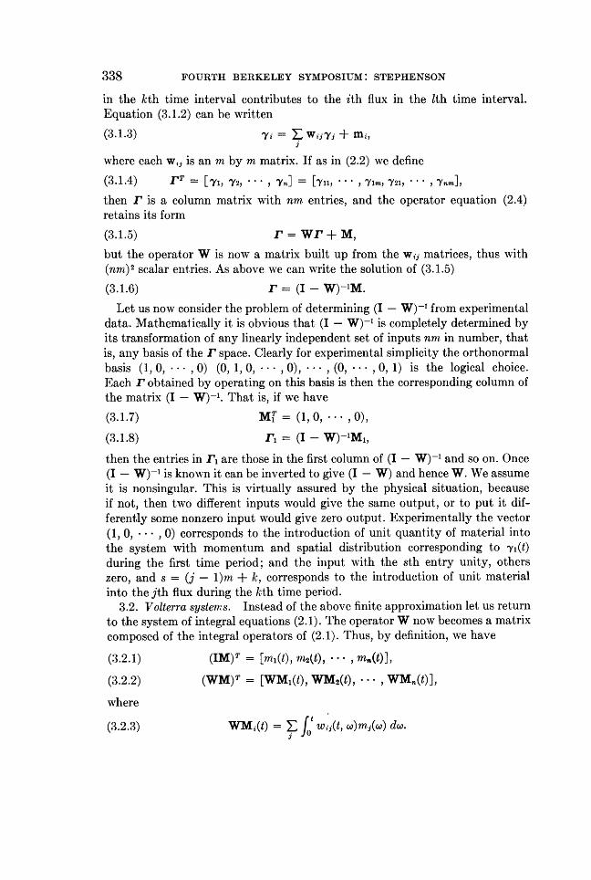
in the kth time interval contributes to the ith flux in the lth time interval.Equation (3.1.2) can be written

(3.1.3) =i wij,j + Mi,j

where each w,j is an m by m matrix. If as in (2.2) we define

(3.1.4) rT = [Lyl, 'Y2, ... , 'Y.] = ['Yll, * **Y1m, Y21, . * 'Ynm] Y

then 1 is a column matrix with nm entries, and the operator equation (2.4)retains its form(3.1.5) I,=Wr+M,but the operator W is now a matrix built up from the wij matrices, thus with(nm)2 scalar entries. As above we can write the solution of (3.1.5)(3.1.6) r = (I - W)-1M.Let us now consider the problem of determining (I - W)-f from experimental

data. Mathematically it is obvious that (I - W)-f is completely determined byits transformation of any linearly independent set of inputs nm in number, thatis, any basis of the r space. Clearly for experimental simplicity the orthonormalbasis (1, 0, * * *, 0) (0, 1, 0, * * *, 0), * * *, (0, - * *, 0, 1) is the logical choice.Each F obtained by operating on this basis is then the corresponding column ofthe matrix (I - W)-1. That is, if we have(3.1.7) MT = (1, 0, * , 0),

(3.1.8) rF = (I - W)-1M1,then the entries in F1 are those in the first column of (I - W)-1 and so on. Once(I - W)-1 is known it can be inverted to give (I - W) and hence W. We assumeit is nonsingular. This is virtually assured by the physical situation, becauseif not, then two different inputs would give the same output, or to put it dif-ferently some nonzero input would give zero output. Experimentally the vector(1, 0, * * *, 0) corresponds to the introduction of unit quantity of material intothe system with momentum and spatial distribution corresponding to yi(t)during the first time period; and the input with the sth entry unity, otherszero, and s = (j - 1)m + k, corresponds to the introduction of unit materialinto the jth flux during the kth time period.

3.2. Volterra systemrs. Instead of the above finite approximation let us returnto the system of integral equations (2.1). The operator W now becomes a matrixcomposed of the integral operators of (2.1). Thus, by definition, we have

(3.2.1) (IM)T = [ml(t), m2(t), ...* *,m-(0(3.2.2) (WM)T = [WM1(t), WM2(t), ,WM(t)]where

(3.2.3) WMi(t) = ff0 wij(t, co)mj(w) dw.


As indicated by (3.2.3) WM is a single column matrix with n entries, each afunction of time. Successive iterates, which appear in the expansion of(I - W)-'M, are defined in the usual way, that is,(3.2.4) W2M = W(WM),(3.2.5) W-M = W(W-lM).Denoting the transpose of W-lM by(3.2.6) (Ws-IM)T = [W8-lM1(t), ** *,W"-M(we obtain for the ith entry in WsM from the operator definitions

(3.2.7) WSMi = wij(t, w)W8-lMj(w) dw.

The resolvent transformation which we will denote by K is then defined by(3.2.8) (I +K)(I-W) = 1.Formally we clearly have for K the expansion(3.2.9) K = W + W2 + ... +W +.with the corresponding kernel matrix(3.2.10) K(t, w) = W(t, W) + W2(t, W) + ... + Wn(t, W) +The entries in W(t, w) are the wxj(t, w) and the entries in Wn(t, W) are given by

(3.2.11) w8(t, W) = f| w.k(t, T)wU`1(T,rw) dT.k

The convergence of the series(3.2.12) KM = [W + WI + + Wn + * ]Mis assured by the fact that the entries in W(t, w) are Volterra kernels, that is,W(t, cw) = 0 if w > t. The argument remains essentially the same for the matrixas for a single function (see [7], p. 147). Briefly, if Wmax is the upper bound of theentries in W(t, w) and A is the upper bound of the integrals j7 mj(w) dw, it iseasily shown that the entries in WM are maximized by nWWmaxA and the entriesin WAM by (nWm..)8A t-l/(s - 1)!. It follows that the series forKM is uniformlyconvergent for any finite upper bound of t.Let us now consider the problem of determining the operator K from experi-

mental data. We have the general operator equation(3.2.13) '-M = KM.

We will suppose that at some time w unit quantity of trace material is suddenly(that is, as rapidly as experimentally possible) introduced into the jth flux, allother inputs remaining zero throughout the experiment. Mathematically thiscorresponds approximately to the condition

(3.2.14) mj(t) = b(t -c).If subsequently the fluxes are all measured, we will determine the entries in


r - M for this injection function. The ith entry in the column matrix r - Mwill then determine an entry K2j(t, co) in the K(t, w) matrix. In other words,with this isolated experiment we can determine one column of the K(t, w) matrixfor one value of c and all subsequent values of t. This is essentially all the infor-mation which can be obtained from a single experiment. In order to gain addi-tional information further separate experiments must be performed. Thisobviously requires the assumption that the characteristic matrix for the systemW(t, w) remains the same in the separate experiments. In other words, it mustbe possible to repeat the experiment either with the same system or with anothernearly identical system. Let us assume that this can be done. If the above ex-periment is repeated, with the injection function for each of the n fluxes beingb(t-Ci) sequentially, each experiment will determine a column of K(t, w,), andthe set will determine the matrix K(t, w,). If these experiments are repeated fora set of values of w, say 0, w1, . .. , C,n, the corresponding set of matrices K(t, 0),K(t, C1), * **, K(t, ,w) will be obtained. From this sequence a continuous approxi-mation of K(t, w) which will be designated by K'(t, w) can be constructed by somesuitable interpolation scheme. Then from K'(t, w) the characteristic matrix ofthe system W(t, w) can be computed approximately. For some purposes thismay be superfluous, the entries in K'(t, c) giving the desired information, butusually the inversion will give additional information. Basically, the inversionutilizes the general operator equation,(3.2.15) (I + K)(I - W) = I,from which we obtain the reciprocal expansion(3.2.16) W = K-K2 +K3- . . . (- l)-K-whose convergence is assured by the fact that K(t, c) is again a Volterra kernel.If we now denote K - K' by e, substitution gives(3.2.17) W = (K' + e)-(K' + e)2 +

Since the series expansion of W given by (3.2.16) yields a uniformly and abso-lutely convergent series when operating on any vector for which the integrals,

Jot ai(w) dw, are bounded, equation (3.2.17) can be rearranged to give(3.2.18) W = K' - K1'2 + . . . - (-)nK'n- . . . + (terms in e).Here, we will pass over a discussion of the terms in f, that is, the error terms, andsimply assume they are small. We then have

(3.2.19) W(t, w) -- K(t, w) - K'2(t, w) + * - (- n)'lK"(t, c)where the iterations have the same definition as above.

3.3. Convolution kernels. It can be seen that an enormous amount of ex-perimental data is necessary to determine a general Volterra kernel of the typeW(t, w). Suppose for example, that one has a modest 4 by 4 matrix, and takes sixtime values woo,wl,xC2, CW3, W04, w5. This requires 24 separate experiments for one com-plete set of values. To test for significant statistical variation in the entries, sev-


eral complete sets would be required. In systems in which the kernel is of theconvolution type, K(t - co), the amount of experimental data necessary for ananalysis is enormously reduced, because each column need be determined for onlyone value of co. Thus, for a 4 by 4 matrix, four separate experiments would giveone complete set of data. The particular time w, chosen for injection clearly isnot important. Experimentally systems with convolution kernels are so-called"steady-state" systems. Once K(t - c) is determined it can be inverted as aboveIf K(t -w) can be given an analytical representation the mathematical machin-ery of the Laplace transform is available for carrying out the manipulations.A detailed analysis of systems of the convolution type has been given in earlierpapers [3], [6] and will not be repeated here. It is worth noting, however, thatformally the analysis of these systems carries over to systems of the more generaltype. Hence, the operator equations developed previously for these systemsremain valid, although any numerical or analytical representation becomesmore involved.

3.4. Systems with incomrplete informaticn. So far in our analysis we have as-sumed that all fluxes are available for injection and subsequent measurement.This may not be the case. Let us suppose that s are available for injection, t formeasurement. This will permit the experimental determination of st entries inthe K(t, co) matrix. Possibly from other information additional entries of W(t, c)or of K(t, w) are known. In addition some of the unknown entries may have otherrestraints on them. The problem is to utilize all the available information torestrict the range of the W(t, w) matrix. The prototype of this problem has beenconsidered by Berman and Schoenfeld for compartmental systems. In our dis-cussion here, we will do little more than state the general problem.The problem appears in its most elementary form in a system in which the

operator is represented by a finite n by n matrix. As before we have the generaloperator equation

(3.4.1) (I + K)(I - W) = I,

where the K and W are matrices. If the multiplications indicated by (3.4.1) arecarried out, we will obtain n2 scalar equations in the 2n2 entries in (I + K) and(I - W). Thus, in general, n2 of the entries can be expressed as functions of theother n2. If these are all known, a determinate solution is obtained; if only r ofthem are known, a solution with n2- r arbitrary parameters is obtained. Restric-tions on the values which can be taken by these parameters and the solutionsmay yield useful information.

Another way of looking at the problem is to consider all transformationsP(I + K) with corresponding transformation of the inverse (I - W)P-', whichwill preserve the known restraints on K and W. All such mappings will thengenerate the space within which admissible solutions must lie. This is the ap-proach taken by Berman and Schoenfeld in their paper on compartmentalsystems [8].The problem can quite clearly be extended to integral operators of the Volterra


type, or for that matter to linear operators in general. As yet the only case wehave investigated at all systematically is that in which the integral operatorsare of the convolution type. Here, instead of (3.4.1) we have

(3.4.2) [I + K(p)][I - W(p)] = I,where K(p) and W(p) are matrices composed of the Laplace transforms of theentries in K(t) and W(t). The remarks made above apply except that the numeri-cal entries in the K andW matrices are replaced by the corresponding functionsin the transform parameter p. Hence, we will have n' relations, involving 2n2functions. From these equations n' of the functions can be expressed (at leasttheoretically) in terms of the remaining n . If r of these are known, we willobtain a solution in terms of n2 - r arbitrary functions of p. As before rathergeneral restraints may restrict the range of possible solutions and lead to usefulinformation.

4. Application to a kinetic problem

4.1. Analysis of fatty acid transpcrt. For obvious reasons, steady-state sys-tems, that is, systems with a kernel of the convolution type, have received morepractical attention, and the above theory will be illustrated with a rather simpleapplication of this type. Nevertheless, conceptually the analysis of a much morecomplicated system would be much the same.Our illustrative application arose in the experimental studies of Dr. D. S.

Fredrickson and colleagues on lipid transport and metabolism. Basically thequestion is whether unesterified fatty acid (denoted by UFA) and fatty acidderived from the splitting of triglyceride (TGFA) follow the same metabolicpathway-more exactly whether the fatty acid derived from splitting triglyc-eride all or nearly all passes through the plasma pool of unesterified fatty acidbefore it is metabolized. The experimental details of the work have been de-scribed previously [9] and here we give only an outline of the mathematicalanalysis, the details of which will be published elsewhere.Two sets of experiments were performed. In one set, C'4 labeled UFA was

injected directly into the blood plasma of dogs. Subsequently the specific activityof UFA in the plasma, and the specific activity of C'4 labeled carbon dioxidein the respiratory output were measured. In the other set C'4 labeled TGFA wasinjected into the plasma as chylomicra. Subsequently the specific activities ofplasma UFA and of respired CO2 were measured. In terms of these experimentsthe problem was to determine whether in the second set, the flux of labeledUFA out of the plasma was sufficient to account for the total output of labeledCO2 or whether a significant fraction of TGFA was metabolized without passingthrough the plasma UFA pool. To decide this question it is clearly necessary tocompute the output of labeled CO2 from the labeled UFA which passes throughthe plasma pool. This can be done utilizing the above mathematical theory andinformation from the first set of experiments.


To set up our model we will suppose that we have two compartments, plasmaand tissue. The plasma is considered to be uniformly mixed, but the tissue isnot. A labeled UFA molecule leaving the plasma has three possible fates:(1) after a certain interim it returns to the plasma as an UFA molecule, (2) it ismetabolized and its C14 appears in the respired C02, (3) it is deposited in sometissue depot where for practical purposes it remains indefinitely (of the order ofmonths or years). It must be recognized, of course, that en route to these fatesthe UFA molecules may follow complicated and devious pathways throughother lipid compartments located in both tissues and plasma. Let us designatethe flux of UFA molecules leaving the plasma by yl(t), the returning flux by72(t), and the flux of labeled C02 by y3(t). We assume that these fluxes arerelated by integral operators of the Volterra type, and the experiments wereperformed so that the dogs were in as near a physiological steady state aspossible. Hence, it is reasonable to assume that these operators are of the con-volution type. Thus, we obtain the equations for the system

(4.1.1) Y2(t) = f0 w21(t - w),y(w) dco,

(4.1.2) aYs (t) = f0o w31(t - w)>y,(c) dw.

In the first set of experiments the fluxes, -yi(t), -Y2(t), and y3(t), are known fromthe experimental data: a3(t) is measured directly and -yi(t) and -Y2(t) are deter-mined from measurements of plasma UFA activity, denoted by cl(t), in a waywe will now briefly outline. If V is the plasma volume, we have for the totalquantity of labeled UFA in the plasma

(4.1.3) ql(t) = cl(t)V.The rate of change of the total quantity of labeled UFA in the plasma poolobviously equals the difference between the ingoing and outgoing fluxes, or

(4.1.4) dq1= 72(t) - yi(t).

During the initial phase of the experiment, UFA radioactivity in the plasmafalls very rapidly and nearly exponentially. It is reasonable to assume that duringthis initial period y2(t) = 0. With this assumption and the assumption that theplasma is well mixed, we have

(4.1.5) y1(0) = kci(O)V = kql(O) = dq1(O)dt

where k is a turnover coefficient, which can be computed from (4.1.5). Subse-quently we assume that k remains constant, that is, that a fraction k of labeledUFA molecules present in the plasma UFA pool leave it per unit time, so that

(4.1.6) 71(t) = kql(t) = kci(t)V,in which k, cl(t) and V are known directly from the experimental data [V =m/q1(0), where m is the total quantity of labeled UFA introduced initially]. The


flux of UFA entering the plasma, -y2(t), can then be computed from (4.1.4).Knowing the fluxes, 71(t), -Y2(t) and -3(t), we can determine w21(t - w) andw31(t- w) by solving equations (4.1.1) and (4.1.2). We have done this analyti-cally by approximating yi(t) and 'y2(t) and 73(t) by sums of exponentials andusing Laplace transforms. We have also carried out numerical solutions on anIBM 650. Both w21(t - w) and w31(t - w) have physiological significance, butit is the latter we want for our computation of the labeled CO2 due to plasmaUFA in the second set of experiments.

In the second set of experiments, the chylomicra are removed from the plasmaand enter the tissue. Here, they are at least partially split into fatty acids andglycerol; at least a fraction of the fatty acid returns to the plasma and entersthe plasma UFA pool. Subsequently this labeled UFA leaves the plasma withthe possible fates given above. If we assume that the turnover constant k is thesame as in the first set of experiments, a condition which is reasonably assured bythe equivalent total UFA concentration in the two sets of experiments [10], -yi(t)can be computed from the plasma level of labeled UFA as in the earlier experi-ments, that is, by means of (4.1.6); and if the transport function w31(t - W) is as-sumed to remain the same, the production of labeled CO2 from yi(t) can becomputed by equation (4.1.2). The total production of labeled CO2 is measureddirectly. The excess of the total production of CO2 over that computed to arisefrom -yi(t), gives the production from TGFA whose fatty acids do not cyclethrough the plasma pool of UFA. We have not yet completed our analysis ofthese experiments, but it turns out that a considerable fraction of TGFA isoxidized without passing through the plasma UFA pool.

5. Concluding remarks

In essence in the theory presented in this paper we represent the state of abiological system by a vector in an abstract space and consider the basic char-acterization of the system to be a linear operator in the space. We have outlinedhow the structure of the operator can be obtained from experimental data. Itis clear that this representation is primarily a data reduction scheme. Until themethod has been applied to a larger number of biological problems, it is difficultto assess its ultimate usefulness. One of the greatest assets of this approach isthat it provides a precise mathematical language in which a large number ofsystems can be described and in terms of which experiments can be formulated.This we have tried to illustrate with the example from fatty acid transport andmetabolism. Another great advantage of the method is that both stationary andnonstationary problems can be handled by it, utilizing the same formal language.The method does not yield any direct information about the microscopic struc-ture of a system, but any microscopic theory must yield an operator whichagrees with that derived directly from the experimental data, in much the sameway that thermodynamic coefficients computed by statistical theory must agreewith those experimentally measured.


It is apparent that we have raised a number of unanswered problems in thispaper. There are statistical sampling problems relative to the construction ofthe operator from experimental data. We have just touched on the question ofthe analysis of systems with incomplete information. We hope that these andother problems will be solved by further investigation along the directions wehave outlined.The author thanks Mr. Arnold Jones for his great help in preparing this paper.

REFERENCES

[1] J. S. ROBERTSON, "Theory and use of tracers in determining transfer rates in biologicalsystems," Physiol. Rev., Vol. 37 (1957), pp. 133-154.

[2] C. W. SHEPPARD, Basic Principles of the Tracer Method, New York, Wiley, 1961.[3] J. L. STEPHENSON, "Theory of transport in linear biological systems: I. Fundamental

integral equation," Bull. Math. Biophysics, Vol. 22 (1960), pp. 1-17.[4] V. VOLTERRA, Theory of Functionals and of Integral and Integrodifferential Equations,

New York, Dover, 1959.[5] , Legons sur la Theorie Mathgmatique de la Lutte pour la Vie, Paris, Gauthier,

Villars, 1931.[6] J. L. STEPHENSON, "Theory of transport in linear biological systems: II. Miltiflux

problems," Bull. Math. Biophysics, Vol. 22 (1960), pp. 113-138.[7] F. RIEsz and B. SZ.-NAGY, Functional Analysis, New York, Frederick Ungar, 1955.,[8] M. BERMAN and R. SCHOENFELD, "Invariants in experimental data on linear kinetics

and the formulation of models," J. Appl. Physics, Vol. 27 (1956), pp. 1361-1370.[9] D. S. FREDRICKSON, D. L. MCCOLLESTER, and K. ONO, "The role of unesterified fatty

acid transport in chylomicron metabolism," J. Clin. Invest., Vol. 37 (1958), pp. 1333-1341.[10] D. S. FREDRICKSON and R. S. GORDON, "The metabolism of albumin-bound Cl4-labeled

unesterified fatty acids in normal human subjects," J. Clin. Invest., Vol. 37 (1958)pp. 1504-1515.

BIOLOGICAL SYSTEMS - Project Euclid

Documents

Transcript of BIOLOGICAL SYSTEMS - Project Euclid