Project Euclid - Physics
12
Communications in Commun. Math. Phys. 110, 467 478 (1987) MathΘITiatiCβl Physics © Springer Verlag 1987 Time Decay of Solutions to the Cauchy Problem for Time Dependent Schrδdinger Hartree Equations Nakao Hayashi 1 and Tohru Ozawa 2 1 Department of Applied Physics, Waseda University, Tokyo 160, Japan 2 Research Institute for Mathematical Sciences, Kyoto University, Kyoto 606, Japan Abstract. We consider the time dependent Schrόdinger Hartree equation ίu t + Δu = ( *\u\ 2 \u + λ , (ί,x)eRx (R 3 , (1) (2) where λ^O and Σ 2 > 2 = {geL 2 ; \\g\\ 2 Σ2 , 2 = Σ \\D a g\\l+ Σ l l * ' 0 l l i < <*>}. We show that there exists a unique global solution u of (1) and (2) such that ueC(U;H U2 )nL™(M;H 2 > 2 )nL£ c {U;Σ 2 > 2 ) with U t GLι [W, LJ ). Furthermore, we show that u has the following estimates: I|w(ί)lk2^c, a e and 2 , a.e. teU. 1. Introduction and Main Results We consider the time decay of solutions to the Cauchy problem for the equation inL 2 =L 2 (lR 3 ) iu t + Δu = f(\u\ 2 )u + λVu, teU, (1.1) «(0) = φ, (1.2) where u t = d t u,f(\u\ 2 ) = \xΓ 1 *\u\ 2 =$\u(t,y)\ 2 /\x y \dy,λ^0,V=l/\x\ andφ
-
Upload
khangminh22 -
Category
Documents
-
view
0 -
download
0
Transcript of Project Euclid - Physics

Communications inCommun. Math. Phys. 110, 467-478 (1987) MathΘITiatiCβl
Physics© Springer-Verlag 1987
Time Decay of Solutions to the Cauchy Problem forTime-Dependent Schrδdinger-Hartree Equations
Nakao Hayashi1 and Tohru Ozawa2
1 Department of Applied Physics, Waseda University, Tokyo 160, Japan2 Research Institute for Mathematical Sciences, Kyoto University, Kyoto 606, Japan
Abstract. We consider the time-dependent Schrόdinger-Hartree equation
ίut + Δu = (-*\u\2 \u + λ-, (ί,x)eRx (R3, (1)
(2)
w h e r e λ ^ O a n d Σ2>2 = {geL2; \\g\\2
Σ2,2= Σ \\Dag\\l+ Σ l l * ' 0 l l i < <*>}.
We show that there exists a unique global solution u of (1) and (2) such that
ueC(U;HU2)nL™(M;H2>2)nL£c{U;Σ2>2)
with
UtGLι [W, LJ ) .
Furthermore, we show that u has the following estimates:
I |w(ί)lk2^c, a e
and
2, a.e. teU.
1. Introduction and Main Results
We consider the time decay of solutions to the Cauchy problem for the equationi n L 2 = L2(lR3)
iut + Δu = f(\u\2)u + λVu, teU, (1.1)
«(0) = φ, (1.2)
where ut = dtu,f(\u\2) = \xΓ1*\u\2=$\u(t,y)\2/\x-y\dy,λ^0,V=l/\x\ and φ

468 N. Hayashi and T. Ozawa
is a given initial data. Let Σlm be the Hubert space defined by
Σι>m = {geL2;\\g\\2
Σl,rn=Σ \\D*g\\2
2 + Σ 11*^111 <*>}
with the inner product
where
{f9g)=Sf-gdx9 Da = dγdfdf and xβ = x{'xβ
2
2xβ
3"
( | α | = α 1 + α 2 + α 3 , \β\= β,+β2+β3).
We shall prove the following:
Theorem 1. We assume that λ ^ 0 and φeΣ2'2. Then there exists a unique globalsolution u of (1.1) and (1.2) such that
with
uteLw(U;L2). (1.3)
Furthermore, there exist positive constants C1 depending only on | |0| |£2,i and C2
depending only on \\ φ \\ Σi,i such that
.2UCu a.e. teU, (1.4)
and
^ C 2 ( l + | ί | ) - 1 / 2 , a.e. teR. (1.5)
In what follows positive constants will be denoted by C and will change fromline to line. If necessary, by C(*,...,*) we denote positive constants dependingonly on the quantities appearing in parentheses.
It has been shown in [9] that any solution ueC(M;Σ2'2) of (1.1) and (1.2) withλ = 0 satisfies
(1.6)
and
(1.7)
Therefore, one of our results (1.4) is an improvement of (1.6).When λ > 0, Chadam and Glassey [1] showed that there exists a unique global
solution u of (1.1) and (1.2) such that
with
uteL?oc(U;L2). (1.8)

Time-Dependent Schrodinger Equations 469
Furthermore, they showed that
H"(ί)l l2.2^C(| |φ | | 2 > 2 )exp[C(| |φ | | 2 f 2 ) | ί | ] , a.e. teU. (1.9)
In [3] Dias and Figueira (see also Dias [2]) considered the time decay ofsolutions of (1.1) and (1.2) satisfying (1.8). They showed the following 1/(2 <p^6)decay estimate:
Hence our results (1.3) and (1.4) are improvements of (1.8) and (1.9), and our result(1.5) is a new estimate in the case of 6 < p 5Ξ oo. Finally we put J = x + 2/ίV =UxU~1 = S2itVS~\ where U = U(t) = exp(ίtΔ) and S = S(t) = exp(i\x\2/4ή.
2. Proof of Theorem 1
We start with stating some useful lemmas.
Lemma2.1. (The Gagliardo-Nirenberg Inequality) Let 1 5Ξ q, r ^ oo, and let 7, meN u {0} satisfy 0 ^ j < m. T/zen we
^ C(mJ,q,r,a) Σ ll^flfli i l^ l l ίΛ
for any geHm'rnU and 1/p = j/3 + (1/r — m/3)a + (1 — a)/q, for all a in the intervalj/m g a S 1? wiίΛ the following exception', if m — j — (3/r) is a nonnegative integer,then the above inequality is asserted for a = j/m.
For Lemma 2.1 see, e.g., Friedman [4].
Lemma 2.2. (a) Let 1 < p < q < 00, 0 < δ < 3 and 1/q = 1/p - <5/3. T/zen we Ziαi e
\\Iό{g)\\qύC(δ9p9q)\\g\\p9 for any geU,
where Iδ(g)(x)= I g(y)/\x-y\3-δdy.
(b) j\g(x)\2/\x\2dx^4\\Vg\\l for any geH1-2.[R3
(c) j \u(t,x)\2/\x\2dxS\\Mή\\2
2/t2, foranyJu(ήeC(U;L2).u3
Proof (a) and (b) are well known results (see, e.g., Stein [10]). We only prove (c).We have by (b)
= \\2itVS~1u(t)\\l/t2 =
This completes the proof.We consider the auxiliary equation
KuH\ + Δun = f{\uH\2)uβ + λVHuH, (t,x)eUxU\ (2.1)
Mπ(0,x) = </>„(*), xeU\ (2.2)

470 N. Hayashi and T. Ozawa
where 2 ^ 0 , neN9 Vn = l/(\x\ + (l/n)) for λ > 0 , Vn = 0 for i = 0 and {<£„} is asequence in the space ^(IR3) of rapidly decreasing infinitely differentiable functionssuch that φn~>φ strongly in X 2 ' 2 as n-> oo. For the sake of brevity we suppressthe subscript n of un for the moment.
Proposition 2.1. For any neN, the Cauchy problem (2.1) and (2.2) has a unique globalsolution u such that
). (2.3)
Furthermore, u satisfies
(2.4)
• λ{Vnu{t),u{t))
Φn\ (2.5)
(2.6)
and
Proof. In the same way as in the proof of Lemmas 3.1-3.3 in [1], we have (2.4)-(2.7).(For details see Chadam and Glassey [1].) We prove (2.3). M. Tsutsumi [11]showed that there exists a positive number T* such that the Cauchy problem (2.1)and (2.2) has a unique solution weC°°([- T*9 T*];^([R3)) for each φn. By theproof of Corollary 3.2 in [11], (2.3) is obtained if a priori estimates of || u(t) | | s 2 (s >(3/2)) are shown. Therefore, (2.7) gives (2.3). This completes the proof.
Proposition 2.2. Let u be the solution constructed in Proposition 2.1. Then we have
\u\2)u(t),u(t)) + λ(Vnu(t),u(
= \\xφn\\l + 4\s(Uf(\u\2)u(s),u(s))0
+ (4λ/nψ
IΛWI3
2\\Ju{s)\\2ds
\\Vnu(s)U
sail*.
ύC{\\φn
ds,
1*.
Ml
.),
+ 1.1)
for
for
I>I2
n>4λ,
I and n>4λ.
(2.8)
(2.9)
(2.10)
and
Proof. When 1 = 0, (2.8) was shown by Ginibre and Velo [6,7]. When λ > 0, (2.8)was shown by Dias and Figueira [3], Therefore, we prove (2.9) and (2.10). Weassume that t S; 0. The case ί ̂ 0 can be treated similarly. Differentiating (2.8) withrespect to t, we have
jt(\\ Ju{t)\\l + 4t2(Uf(\u\2)u(t),u(t)) + λ(Vnu(t),u(t))))
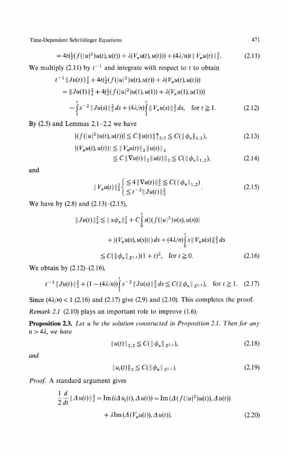
Time-Dependent Schrόdinger Equations 471
= 4ί(!(/(|M |2)M(ί),w(ί)) + λ(Vnu(t),u(t))) + (4A/n)ί || Vnu(t)\\l (2.11)
We multiply (2.11) by f"1 and integrate with respect to £ to obtain
\ ] d s , forί^l. (2.12)1 1
By (2.5) and Lemmas 2.1-2.2 we have
|(/( l« l 2 )«( ί ) ,«( t ) ) l ^ C | | M ( ί ) | | ί 2 / 3 ^ C ( | | φ n | | l j 2 ) , (2.13)
I ( ^ ( ί X u(ί))I g II KBtι(ί) II2II «(ί) II2
^ CII VM(t) II2IIi*(t) II2 ^ C( II φ n II l i 2 χ (2.14)
and
We have by (2.8) and (2.13)-(2.15),
n)\s\\ Vnu{s)\\2ds0
2, forί^O. (2.16)
We obtain by (2.12)-(2.16),
r1\\Ju(t)\\2
2 + (ί-(4λ/ή))\s-2\\Ju(s)\\2ds^C(\\φn\\Σl,1), f o r ί ^ l . (2.17)1
Since {4λ/n) < 1 (2.16) and (2.17) give (2.9) and (2.10). This completes the proof.
Remark 2.1 (2.10) plays an important role to improve (1.6).
Proposition 2.3. Let u be the solution constructed in Proposition 2.1. Then for anyn > 4λ, we have
|| «(t) II 2 , 2 ^C( WφJ^), (2.18)
and
\\ut{t)\\2^C{\\φn\\ΣiΛ (2.19)
Proof. A standard argument gives
λlm(Δ(Vnu(t)),Δu(t)). (2.20)

472 N. Hayashi and T. Ozawa
We consider the second term of the right-hand side of (2.20),
lm(Δ(Vnu{t)),Δu{t)) = 1m{{Δ Vn)u(t),Δu(t)) + 2\mφVn-Vu{t\Δu{t))
= ϊm((Δ Vn)u{t\ - iut(t) + / ( M X O + λVnu(t))
- 2Im (VnΔ u(t\ Δ u(t)) - 2Im {¥„ Vw(f), V4 u(t))
= \lt{{Δ v«Mt)Mt))-2lm(VnVu(t),S7Δu(ή). (2.21)
W e d e n o t e t h e s e c o n d t e r m of t h e r i g h t - h a n d side of (2.21) b y Iγ. W e h a v e
h=- 2lm{Vn V«(ί), V( - iut(t) + f(\u\2)u{t) + λVnu(t)))
= -jt(VnVu(t), Vu(ή) - 2lm(VnWu(tUVf(\u\2))u(ή)
- λIm(VV2
n Vu(t),u(t)Y
Similarly we have
- Im (VV2 Vtί(ί), «(ί)) = Im (V2Δ u(t), u(ή)
= lm(V2( - ίut(t) + f(\u\2)u(t) + Vnu{t))Λt))
=-\jt\\Vnu(t)\\2.
Collecting everything, we obtain
~ ( | | Δ u(t) || I + λ(λ || Vnu(t) III ~ ((Δ Vn)u(t), u(t)) + 21| V\12Vu(t) || \))
(2.22)
By Appendix and Proposition 2.1 (2.6) we have
\121 ύ Ct~2\\Ju(t)||11| Vtί(ί)II2 \\Δu{t)\\2
^ C ( | | ^ | | l f 2 ) r 2 | | J M ( i ) | | | M « ( i ) | | 2 f o r t ^ l . (2.23)
We get by (2.4) and Lemma 2.2
^ CII V « ( ί ) II6II « ( ί ) II6II M(ί) 1 2 1 K B u ( ί ) II2
2)ί" 2 | |Λ(ί) | | 2 | |/lM(ί) | | 2 f o r ί ^ l . (2.24)
Since λ ̂ 0 and Δ Vn S 0, we obtain by (2.22)-(2.24)
|| Δu(t) || I g \\Δ «(1) | | 2 + A(A || Fn«(l) || \ - ((4 FΠ)M(1), H(1)) + 21| F ^ 2 VM(1) || | )
j J 5 . (2.25)

Time-Dependent Schrδdinger Equations 473
We have by Lemmas 2.1-2.2 and Proposition 2.1,
|| Vnu(X)\\\ ύC\\Vu{\)\\l ίί C(\\φJu2), (2.26)
| |^ 1 / 2V«(l) | | i^CM«(l) | | 2 | |V«(l) | | 2^C(| |0J | 2, 2), (2.27)
and
= -2Re(VnΔu(l),u(l))-2(VnVu(l),Vu(ί))^C(\\φJ2t2). (2.28)
We have by (2.25)-(2.28),
\\Au(t)\\l^C(\\φJ2a)h+μ-2\\Ju(s)\\2
2\\Δu(s)\\2dsj.
This and the Schwarz inequality give
\\Δu(t)\\2<C(\\φn\\2Λ)\ l + ^s-2\\Ju(s)\\2ds + ls-2\\Ju(s)\\2\\Δu(s)\\2ds\.
(2.29)
We obtain by (2.29), Proposition 2.2 (2.10) and Gronwall's inequality,
\\Δu(t)\\2^C(\\φJΣ2>ί). (2.30)
Proposition 2.1 and (2.30) yield (2.18). From (2.1), Lemma 2.2, Proposition 2.1 and(2.3) we have
\\ut(t)\\2^\\Au(tn2+\\f(\u\2)u(t)\\2 + l\\vnu(t)\\2
| |2 + C||V«(ί)||2
Ml χ1.I) + C| |M(ί) | | | | |V«(ί) | | 2 gC(| |^ l l 11^..).
Here we have used
\l/2
rdy) \\ψ\\2
(2.31)
This completes the proof.
Proposition 2.4. Let u be the solution constructed in Proposition 2.1. Then for any
n > 4λ, we have
where
J2= f (xj
Proof. We put v(t) = S~1u(t) for ίe[R\{0}. It is easily verified that

474 N. Hayashi and T. Ozawa
t t
where A — (l/2i)(x V + V x). Therefore, v satisfies
ivt= -Δv + ~Av + f(\v\2)υ + λVnv, ίeR\{0}. (2.32)
Since J2 commutes with i(d/dt) + Δ, J2u(t) satisfies
i(J2u(t))t =-ΔJ2u + J2(f(\u\2)u(t)) + λJ2(Vnu(t)),
from which it follows that
i ί II J2u(t) || i = Im (J2 (/(Iu \2)u{t)\ J2u(t)) + Aim (J2(Vnu(t)), J2u(t)\ (2.33)2 at
We consider the second term of the right-hand side of (2.33). Since J 2 =-4t2SΔS~\
lm(J2(Vnu(t)),J2u(t))
= l6tΠm(Δ(Vnv(t)),Δv(ή)
= 16ί4lm (((Δ VMt), Δ v(t)) - 2(VnVυ(t), VΔ v(t)))
= 16ί4lm((Δ Vn)v(t), ~ ίvt(t) + -tAv(ΐ) + f(\v\2)v(t) + λVHυ(t))
- 32ί4Im(FnVD(t), V( - ivt(t) + ̂ Av(t) +f(\v\2)v{t) + λVav(t)))
8t4jt((ΔVn)υ(t)Xt)) + l6t3lm((ΔVn)v(t),Av(t))
-l6t4jt(VnVv(t),Vv(t))-32tΠm(VnVv(t),V(Aυ(t)))
~32t4lm(VnVv(t),V(f(\v\2)υ(t)))-32t4λ\m(VnVv(t),(VVn)v(t))
~ptA{(Δ Vn)v{t), v(ή) - 16t4(VnVυ(ή,
- 32ί3((4 Vn)υ(t)Λt)) + 64t3(VnVv(t),Vv(t))
Vn-]v{t),v(t)) ~ l6t3lm(lA,Vn-]Vv(t),Vv{t))
~ί6t4λlm(Vv{t),{VV2)v{t)).

Time-Dependent Schrόdinger Equations 475
We note that
[V,/l]=-iV, ίΛ,VJ=-ί(x'V)Vn and IA,ΔVJ=-i(x-V)ΔVn.
Therefore, we have
lm(J2(Vnu(t)),J2u(t))
p F>(ί), v(t)) - 16ί4(Fπ Vι (ί),
16ί3((2Fn + (x-V)Vn)Vv(t), Vυ(t)) - 8ί3((4zlFn
(t))) - 16ί4ΛIm(Vι;(t),(VF>(ί)).
We finally note that
,(VF>(ί)) = -Im(Jt>(ί), F^(t)) = - I m ( - ί»t(t) + ̂ t (t), V2
nv(t))
= \jt\\ Vnv{t)II1 + ̂ Im(LA, VlMtlv(ή)
= ~\\Vβυ(t)\\22-γt
Collecting everything, we obtain
jfiII J2u(t) II1 + 8ί4A(2(FπVt (t), V»(ί)) - ((4 Vn)v(t), »(t)) + A || Fnt;(ί) || f)]
= 8ί3l[2((2Fn + (x-V)Vn)Vv(t),
+ ((4λFπ
2 + A(x V)Fn
2 - 4Δ Vn - (x V)Δ Vn)υ(t), »(
-32t4lIm(FnVt;(ί),(V/(|t;|2)) !;(t))+16ί4Im(Zl(/(| ί;|2) l;(ί),4 i ;(ί))
= / 4 + / 5 + / 6 . (2.34)
We assume that ί ̂ 0. The case t ̂ 0 can be proved similarly. In view of the factthat (x V)Fπ ^ 0, (x V)F2 ^ 0, - (x-V)ΔVn S 0 and λ ̂ 0, we have
= 32t3λ[ - (FnV»(t), Vϋ(f)) + λ || Fπu(ί) || \ - 2Re(Fκzl ϋ(ί), ϋ
^ Cί3 [ || Fnt;(ί) || \ - 2Re (FB/1 υ(t), »
^ Cί || Jtt(t)| |2 + C|| JM(t)| |21| J2u(t)\\2. (2.35)
Here we have used Lemma 2.2. We obtain by Lemma 2.2, Proposition 2.2
(2.36)

476 N. Hayashi and T. Ozawa
In the same way as in the proof of (2.31) we have
II f(\vVvI)IIoo ^ 2II Vt;II2. (2.37)
This and (2.36) yield
I h I S Ct41| Vv(t) || 2 ^ C || Ju(t) | |\, (2.38)
By Appendix we have
Now we put
α(ί) = i | | J2u(t)III + St4λ(2(VnVv(t), V»(ί)) - ((Δ FJϋ(ί),»(ί)) + λ|| K.»(ί)111).
We note that £|| J 2 M(£) | | 1 ^α(ί) . We obtain from (2.34), (2.35), (2.38), (2.39) andProposition 2.2,
^αίO^Cdl^ll^.Oίίl + ί)2
This gives
from which we get the desired result.
Proof of Theorem 1. A simple calculation gives
| | x 2 ^ ( ί ) | | 2 ^ C | | W / J ( ί ) l | 2 , 2 ( l + ί2) + C| | J 2
W M ( ί ) | | 2 . (2.40)
By Proposition 2.1-2.3, (2.40) and a standard argument we conclude that thereexists a unique function u satisfying (1.3) and (1.4) such that as n-» oo,
un -> u weakly star in U° (M;H2>2)n L£C(R; Σ 2 ' 2 ) ,
un-+u strongly in C(U;Hia),
and
(un)t -> ut weakly star in L00 (R; L2).
It is easily seen that u solves the Cauchy problem (1.1), (1.2) in the distributionsense. Next we show that u satisfies (1.5). From Proposition 2.3 we see that u satisfies
^ ) , a.e. ίeR. (2.41)
Proposition 2.2 and Proposition 2.4 give
| | Λ ( ί ) | | 2 ^ C(| |φ 11*1.0(1 + Iί | ) 1 / 2
? a.e. ίeR, (2.42)
and
+ | ί | ) 3 / 2
? a.e. ίeR. (2.43)

Time-Dependent Schrodinger Equations 477
We have by using Lemma 2.1 and (2.41)-(2.43)
.2)(l + | ί | Γ 1 / 2 , a.e. teU.
This completes the proof.
Remark 2.2. We can apply our method used in this paper to the following system:
N
i(uj)t + Δuj= X (ujvktk - ukvjtk) + λuj/r, teU,fc=l
uJ(0) = φ J e i ; 2 2,
w h e r e j=ί,2,...,N, υjik = r~ί*Ujΰk, a n d A > 0 .Especially the equality (2.34) in the proof of Proposition 2.4 is useful to
investigate the decay properties of solutions for the linear Schrodinger equations,
iut + A u = Vu, ί G R, w(0) = φ,
where V = V(x) is real-valued function satisfying some additional conditions.
Appendix
Lemma A. Let f(φ)(x) = J φ(y)\x — y\~1dy. Then we have
\lm(Δ(f(\φ\2)φ),Aφ)\
^CΓ2\\Jφ\\2
2\\Vφ\\2\\Δφ\\2, forφeΣ2'1 and teU\{0}. (A.I)
2*2 and teU\{0} [ ]
ίA simple calculation gives
t*Im(Δ(f(\φ(t)\2)φ(t)),Δφ(t))= -2ί 4 lm £ (fj(Rf>φ(f)djΦ(t))Φ(t),Δφ(t))
'ύC\t\-'\\Jφ\\l\\J2φ\\2
| | | J 2 ( / ) | | 2 5 forφeΣ2*2 and teU\{0}.
Proof. (See also [9]). We put φ(t) = S~ιφ and
= ί (χ3 - yj)Ψ{y)/\χ-y\* dy9 1 ύ j ^ 3.3
We have by Holder's inequality and Lemmas 2.1-2.2
\\fj(Rcφ(t)δjφ(t))φ(t)\\2
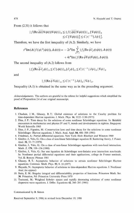
478 N. Hayashi and T. Ozawa
From (2.31) it follows that
|| /(Re φWφ(t))Vφ(t) || 2 S II /(I ΦWφ(t) DILI Vφ(t) || 2
Therefore, we have the first inequality of (A.2). Similarly, we have
t*Im(Δ(f(\φ\2)φ(t)\Δφ(t))= -2 ί 4 lm £ (fj(Reφdjφ)φ(t),Δφ(t))
+ 4ί4lm (/(Re φWφ)Wφ(t\ A φ{t)\
The second inequality of (A.2) follows from
and
ll/CReφV^IL^ Clip11
Inequality (A.I) is obtained in the same way as in the preceding argument.
Acknowledgements. The authors are grateful to the referee for helpful suggestions which simplified the
proof of Proposition 2.4 of our original manuscript.
References
1. Chadam, J. M., Glassey, R. T.: Global existence of solutions to the Cauchy problem for
time-dependent Hartree equations. J. Math. Phys. 16, 1122-1130 (1975)
2. Dias, J. P.: Time decay for the solutions of some nonlinear Schrodinger equations. In: Bielefeld
encounters in mathematics and physics IV and V, trends and developments in eighties. Singapore:
World Scientific 1985
3. Dias, J. P., Figueira, M.: Conservation laws and time decay for the solutions to some nonlinear
Schrodinger-Hartree equations. J. Math. Anal. Appl. 84, 486-508 (1981)
4. Friedman, A.: Partial differential equations. New York: Holt-Rinehart and Winston 1969
5. Ginibre. J., Velo, G.: On a class of non-linear Schrodinger equation II. Scattering theory. J. Funct.
Anal. 32, 33-71 (1979)
6. Ginibre, J., Velo, G.: On a class of non-linear Schrodinger equations with non-local interaction.
Math. Z. 170, 109-136 (1980)
7. Ginibre, J., Velo, G.: Sur une equation de Schrodinger non-lineaire avec interaction non-locale.
In: Nonlinear partial differential equations and their applications, college de France seminair,
Vol. II. Boston: Pitman 1981
8. Glassey, R. T.: Asymptotic behavior of solutions to certain nonlinear Schrodinger-Hartree
equations. Commun. Math. Phys. 53, 9-18 (1977)
9. Hayashi, N.: Asymptotic behavior of solutions to time-dependent Hartree equations. J. Nonlinear
Anal, (to appear)
10. Stein, E. M.: Singular integral and differentiability properties of functions. Princeton Math. Ser.
30. Princeton, NJ: Princeton University Press 1970
11. Tsutsumi, M.: Weighted Sobolev spaces and rapidly decreasing solutions of some nonlinear
dispersive wave equations. J. Differ. Equations 42, 260-281 (1981)
Communicated by B. Simon
Received September 9, 1986; in revised form December 19, 1986