ROCKY MOUNTAIN JOURNAL OF MATHEMATICS Volume 18, Number 1, Winter 1988

SINGLE-LAYER SOLUTIONS FOR THE DIRICHLET PROBLEM FOR A QUASILINEAR

SINGULARLY PERTURBED SECOND ORDER SYSTEM

DONALD R. SMITH

A B S T R A C T . A constructive existence proof is given for solu­tions of boundary layer type for the Dirichlet problem for the singularly perturbed quasilinear second order system of dif­ferential equations ed2x/dt2 = F(t,x,e)dx/dt + g(t,x,e) on a compact interval in the case that a boundary layer occurs at only one endpoint of that interval, subject to a general­ized Coddington/Levinson condition and (in the general case of large boundary-layer jump) subject to the assumption that the matrix-valued function F(t, 2,0) is given in terms of a vector potential / as F(t, x, 0) = Vxf{t,x). A proposed ap­proximate solution, as provided by the O'Malley construction, is readily available throughout the entire compact interval. A direct construction is given for the Green function for the lin­earization of the problem about this proposed approximate solution. The resulting Green function representation for the linearization is used to prove the existence of an exact solution that is well-approximated by the given approximate solution, yielding precise and detailed information on the behavior of the resulting solution throughout the given compact interval. The construction of the Green function is patterned after that of Smith [29] for the scalar case and employs certain Riccati transformations so as to provide convenient representations for certain fundamental solutions and for their inverses. The quasilinear second order system studied here occurs in math­ematical models for certain chemical reactors.

1. Introduction. Consider the second-order system

d x dx (1.1) e-^ = F{t,x,e)— + g(t,x,e) for 0 < t < 1,

for small positive values of e(e —» 0-f), subject to the Dirichlet bound­ary conditions

(1.2) x(0, e) = a{e) at t = 0, and x(l, e) = ß(e) at t = 1,

Received by the editors on July 10, 1985, and in revised form on November 26, 1985.

Copyright ©1988 Rocky Mountain Mathematics Consortium

67

68 D.R. SMITH

for a real n-dimensional (column) vector-valued solution function x = £(£,£), where the given function F is an n x n matrix-valued function, and the given functions g, a and ß are n-vector-valued functions. These data functions are assumed to be sufficiently smooth; the precise smoothness required will be specified below. For simplicity (and clarity of exposition) we generally assume slightly more regularity on the data than required. Systems such as (1.1) occur in mathematical models for chemical reactors; see Chen and O'Malley [8] for references.

The reduced equation obtained by putting e = 0 in (1.1) is

(1.3) F ^ ^ X ^ ) ^ - + 0<°>(t,X«») = 0 for 0 < * < 1,

where F and g are assumed to be continuous at e = 0, with F^ (t, x) := F(t, x, 0) and gW (*, x) := g(t, x, 0), and where X^ will be the leading term in a suitable outer expansion for a corresponding solution x of (1.1)-(1.2). We assume that the first-order system (1.3) has a solution X(°î = X(°) (t) satisfying the boundary condition

(1.4) X ^ ( l ) = / ? ( 0 ) :=/?(0),

along with the outer stability condition

(1.5) Re\{t) < 0 for all eigenvalues X(t) of F^(*,X^(*)),

for 0 < t < 1, and the boundary-layer stability condition

(1.6) (z, + sx)ds\x) < -i/o\\x\\2

forali | | x | | < | | a ^ - X ^ ( 0 ) | | ,

for some fixed positive constant I/Q > 0, where x = (x\, £2 , . . . , xn)T €

R n , where (.,.) denotes the Euclidean inner product in R n , ||.|| denotes the Euclidean norm, and a^ := a(0). Finally, we assume that the matrix-valued function F^0^ (t, x) can be given in terms of a vector potential as

(1.7) F^(tìx):=F(tìxì0) = Vf(t1x)ì

for some suitable, given n-vector-valued function / = f{t,x). In this case (1.6) can be rewritten as (Howes and O'Malley [20]) (x, [f(0,X^ (0) + x)- / (0,X(°)(0))]) < -70IMI2 forali | |z|| < ||a<°> -X<°>(0)||.

DIRICHLET PROBLEM 69

In the scalar case n = 1 (with x(t,e) : [0,1] x (0,ei] —• R) , solutions of (1.1)-(1.2) possessing a single boundary layer have been studied by many authors including von Mises [22], Coddington and Levinson [10], Brish [1], Wasow [34], Cochran [9], VasiPeva [32], Willett [35], Erdelyi [12, 13], O'Malley [23, 24, 26], Chang [3], Yarmish [36], Rosenblat [28], Howes [18, 19], and van Harten [17], In particular, Willet [35], Erdélyi [12] and Chang [3] used a linearization about a suitable approximate solution (with a boundary layer at only one endpoint) to study the scalar equation

(1.8) ex" = /(*,x,x',6:).

With a few exceptions, these works generally use the assumption either that the boundary layer jump is sufficiently small, or that the function F (or in the case of (1.8), the function fx> evaluated at the assumed approximate solution) is uniformly nonzero on a suitable domain. These assumptions are unnecessarily restrictive, as discussed by Coddington and Levinson [10], van Harten [17], and Howes [19], where an assumption of the type (1.6) suffices. This assumption (1.6) of Coddington and Levinson, which is mentioned also in O'Malley [26], cannot be significantly weakened for solutions of the type considered here because this assumption coincides with the condition required for the existence of the proposed approximate solution of boundary layer type, as provided by the O'Malley construction. Note in the scalar case that (1.6) does not require the function F to be of one sign inside a boundary layer, so that turning-point behavior is permitted inside the boundary layer; see Smith [29, Example 3], [30, Example 10.4.3].

There is only a small literature for (1.1)-(1.2) in the vector case n > 1. The vector problem was considered by Chang [4,5,6] and Habets [15] subject to the assumption that the boundary layer jump a^ —X^ (0) is sufficiently small, for a given solution X^ of the reduced system (1.3) satisfying (1.4)-(1.5). Chang and Habets both used a Riccati transformation applied (essentially) to the linearization of (1.1)-(1.2) about X(°), along with a fixed-point theorem, to prove that (1.1)-(1.2) has a solution x = x(t, e) satisfying

(1.9) x(t, e) = X<°> (t) + 0(s) + 0(exp[-i/ii/e])

uniformly for

(1.10) ( i , £ ) e [ 0 , l ] x ( 0 , e i ]

70 D.R. SMITH

for certain fixed positive constants v\ > 0 and E\ > 0. The result of Chang and Habets is reformulated and proved using differential inequal­ity techniques in Chang and Howes [7], subject to a strong assumption on F that requires the matrix F(t, x{t,e),e) to be nonsingular every­where along the corresponding solution x (£,£), including throughout the boundary layer. In this case Chang and Howes obtain a sharp­ened version of (1.9) with no requirement on the size of the boundary layer jump (see Theorem 7.4 of Chang and Howes [7]). An assump­tion related to (1.6) is used in Howes and O'Malley [20] in the formal construction of a proposed approximate solution for (1.1)-(1.2), but no proof of asymptotic validity is given there.

We show here that certain refinements and extensions of the ap­proaches of Willett, Chang, and Habets, coupled with the assumptions (1.3)-(1.7) along with the O'Malley construction and a direct Green function approach, suffice to yield detailed quantitative information on an appropriate solution x throughout 0 < t < 1, without the re­quirement that the boundary layer jump be "sufficiently small". In particular we supply the missing proof that the proposed approximate solution of Howes and O'Malley [20] actually provides a uniformly valid approximation to a corresponding exact solution. The condition (1.7), which is mentioned but not used in Howes and O'Malley [20], is used here in obtaining the fine details of the solution inside the boundary layer in the general case (3.5) of a substantial boundary-layer jump (but (1.7) is not required if the boundary-layer jump is small). Note that (1.7) always holds in the scalar case n = 1,

The conditions (1.4), (1.5) and (1.6) can be replaced respectively with

(1.11) X<o>(0) = a<°\

(1.12) Re X(t) > 0 for all eigenvalues X(t) of F<°> (*,X^(*)),

for 0 < t < 1, and

(1.13) (x[j F^(liX^(l)^sx)ds]x)>iy0\\x\\2

forali ||x|| < H/?W - ^ ° ) ( 1 ) | | ,

in which case the boundary layer occurs at the right endpoint t = 1. It is well-known in the scalar case that the reduced equation (1.3)

DIRICHLET PROBLEM 71

( L 1 4 ) I '„(e\ 1 = 1 „(0) + a (!) ' | e + order (e2)

can in some cases have a solution satisfying (1.4)-(1.6) along with yet a different solution satisfying (1.11)-(1.13), leading to two distinct solutions of boundary-layer type for (1.1)-(1.2), and indeed yet other solutions of interior-layer type are also possible for the same problem; cf. Howes [20] and Smith [30].

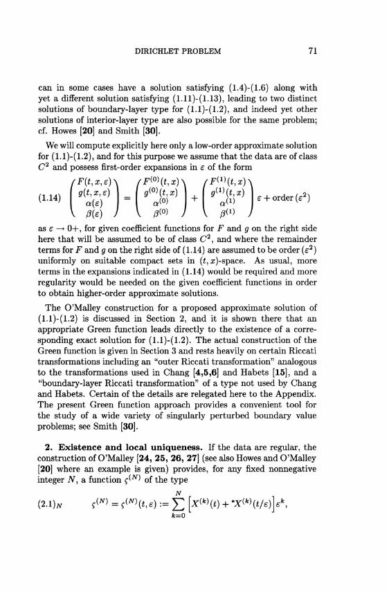
We will compute explicitly here only a low-order approximate solution for (1.1)-(1.2), and for this purpose we assume that the data are of class C2 and possess first-order expansions in e of the form

' F ( t , s , e ) \ /FW(t,x)\ (FWfrxY g(t,x,e) _ gW(t,x)

a{e) ~ a( ß{e) J V ßW J

as e —+ 0-f, for given coefficient functions for F and g on the right side here that will be assumed to be of class C2 , and where the remainder terms for F and g on the right side of (1.14) are assumed to be order (e2) uniformly on suitable compact sets in (£, x)-space. As usual, more terms in the expansions indicated in (1.14) would be required and more regularity would be needed on the given coefficient functions in order to obtain higher-order approximate solutions.

The O'Malley construction for a proposed approximate solution of (1.1)-(1.2) is discussed in Section 2, and it is shown there that an appropriate Green function leads directly to the existence of a corre­sponding exact solution for (1.1)-(1.2). The actual construction of the Green function is given in Section 3 and rests heavily on certain Riccati transformations including an "outer Riccati transformation" analogous to the transformations used in Chang [4,5,6] and Habets [15], and a "boundary-layer Riccati transformation" of a type not used by Chang and Habets. Certain of the details are relegated here to the Appendix. The present Green function approach provides a convenient tool for the study of a wide variety of singularly perturbed boundary value problems; see Smith [30].

2. Existence and local uniqueness. If the data are regular, the construction of O'Malley [24, 25, 26, 27] (see also Howes and O'Malley [20] where an example is given) provides, for any fixed nonnegative integer JV, a function ç(N) of the type

(2.1)* ?<"> = Ç{N)(t,e) := £ [xW(t) + *XW (t/e)] e\ N

c k=0

72 D.R. SMITH

where the leading outer term X^ is taken here to be a fixed, given function satisfying the reduced equation (1.3) along with the conditions of (1.4)-(1.6), and where the remaining outer coefficients X^ and the boundary-layer correction coefficients *X^ are constructed suitably so that the resulting function ç(N) satisfies the problem (1.1)-(1.2) approzetamately, in the sense that there hold

(2.2)* e^^=F(tì^N\e)^ + g(tì^

N\e)-pN(tìe)

for 0 < t < 1, and

(2.3)* C(iV)(0,e) = a(e) - <ßN(e) and Ç{N)(hs) = ß(e) - ^N{e),

for suitable residuals PNI</>N and ipx that are small, with

/ ||pN(*,e)||A <CNeN+\ and Jo (2.4)*

IhMOII, IhMOH < CNeN+1 as s - 0+,

for a suitable constant C*. The residual p * actually satisfies a suitable uniform estimate for | |/9*(£,Ê:)| |, but the integral estimate for PN included in (2.4) suffices for our purpose. For simplicity we consider here mainly the case N = 1.

For later reference we list here several properties of the boundary-layer correction terms *X^ = *X^fc^(r), where the boundary-layer variable r is taken as r = t/e in (2.1). First, *X^ satisfies the generally nonlinear boundary value problem,

m fï^M - ,<».,o,x<»>(o) + -xm^^m for r > „, *X<°>(0) = a'°) - X(°)(0), and *X<°>(oo) = 0,

where the assumptions (1.6) and (1.7) yield the estimates (see Appendix Al)

irx(°)(r) | | < ||a(°> - A-(o)(0)||e-"oT and

\fX(^T)\\ < const. H««» -X(°)(0) | |e-"o T for r > 0, UT

DIRICHLET PROBLEM 73

where i/o is the positive constant appearing in (1.6). The higher-order boundary-layer terms *X^ (for k > 1) satisfy linear systems given in component form as (2.7)*

^ ^ ^ a ( 0 , X ( o ) ( 0 ) + ^ ) ( r ) ) ( ^ ) ( r ) ) ^ ^

+ if} (0, X<°> (0) + **(0) (r ) ) ^ - ^

+ * ^ * ) ( r ) f o r r > 0 ,

for t = 1,2,. . . , n , where F$m{t,x) = {dldxm)F^\t,x), where the summation convention is employed for repeated indices on the right side of (2.7), and where *g(k) = V f cH r) is a certain given vector-valued function that is determined by the O'Malley construction in terms of previous coefficients *X^m\ for m < fc—1. Along with (2.7) one imposes a homogeneous boundary condition (matching condition) at r = oo and an appropriate boundary condition at r = 0. The given assumptions (1.6) and (1.7) can be used to prove that the higher-order terms here also decay exponentially, with (see Appendix Al)

(2.8)* irX ( fc )(r)| | , | | d * X ^ ) ( r ) | | < Cke-^ for r > 0

and for k = 1,2,... , for suitable constants Ck that are not the same here as in (2.4), and for any fixed positive constant v\ less than the constant v0 of (1.6), 0 < vx < v^ The outer functions XW = X^(t) are smooth for 0 < t < 1, always assuming sufficient regularity on the data.

The problem (1.1)-(1.2) is recast as a linearization about the proposed approzetamate solution ç^oi (2.1). If x denotes a solution of (1.1)-(1.2), then the function x defined as

(2.9) x(t) = x{t,e) := z(t,e) - £ ( JV)(^)>

satisfies the boundary conditions

(2.10) £(0,e) = 0jv(e) and x(l,e) = ißN{e)

along with the following differential equation (2.11) 2

£ê =F{t ' 'w {t>£)'e) § + [(â • v*)F(t' <(N) {t>£)'£)] ^ r + [ v , j(«, ?(JV)(*, £),£)] x + pjv(*, s) + ft(*. x, - | , s)

74 D.R. SMITH

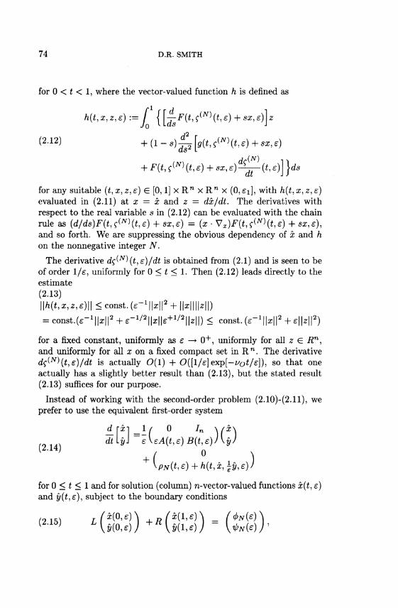
for 0 < t < 1, where the vector-valued function h is defined as

h(t, x, z, e):=J { [—F(i, <T(iV) (*, e) + ss, ej\ z

(2-12) +(l-*)^[^,fw(*,e) + »ie)

+ F(t, f W (t, e) + **, e) ^ (t, e)] }ds

for any suitable (£,x, z,e) G [0,1] x R n x R n x (0,£i], with h(t,x,z,e) evaluated in (2.11) at x = x and z = dx/dt. The derivatives with respect to the real variable s in (2.12) can be evaluated with the chain rule as (d/ds)F(t,ç(N){t,e) + sx,e) = (x • Vx)F{t,^N\t,e) + «a?,e), and so forth. We are suppressing the obvious dependency of x and h on the nonnegative integer N.

The derivative dç(N\t,e)/dt is obtained from (2.1) and is seen to be of order 1/e, uniformly for 0 < t < 1. Then (2.12) leads directly to the estimate (2.13) \\h{t,x,z,e)\\ < const. ( e ^ l N I 2 + | |z | | |H|)

= const . (e-1 | |x | |2+^-1 /2 | | a : | |e+ 1 /2 | |^ | | )< const. O r 1 ^ 2 + e||*||2)

for a fixed constant, uniformly as e —• 0 + , uniformly for all z G Rn, and uniformly for all 2 on a fixed compact set in R n . The derivative d^N\t,e)/dt is actually O(l) + O([l/e]exp[-i/0*/e]), so that one actually has a slightly better result than (2.13), but the stated result (2.13) suffices for our purpose.

Instead of working with the second-order problem (2.10)-(2.11), we prefer to use the equivalent first-order system

dtlyl e\eA{t,e)B{t,e))\y)

for 0 < t < 1 and for solution (column) n-vector-valued functions x(t,e) and y{t,e), subject to the boundary conditions

<-> '(SS:ä)+*(äi::D-($:0-

DIRICHLET PROBLEM 75

where the n x n matrix-valued function A = A(t, e)

(BH:(t,e)) i

= \Aij(t,e)J

and B = B{t,e) = ( B y ( t , e ) ) in (2.14) are defined in terms of their

components as (2.16)

Ai,it,e) := 9iJ(t,f <">(t,e),e) + Fim^f ( " > ( t , e ) , e ) d Ç m ^ £ )

where Qij = dg%/dxp where dÇm \t, e)/dt denotes the mth component of the n-vector dç(N' /dt, and summation is indicated over the repeated index m in (2.16), and

(2 17) Bij(t>e)'- = Fi3&SiN)&e),e) (that is, B(t,e) = F{tiçlNHtie),e))

for i.j = 1,2,... ,n where both (2.16) and (2.17) hold on a region of the type

(2.18) 0 < t < 1, 0 < e < e0,

for a suitably small, fixed eo > 0, and where the given boundary matrices L and R in (2.15) are defined as

2n x 2n 2n x 2n

The obvious dependence of A and £ on N is suppressed to lighten the notation.

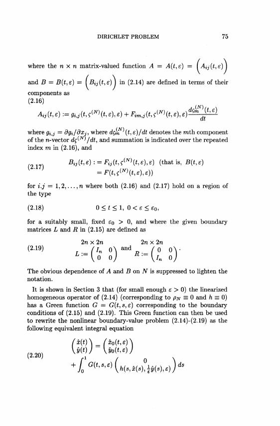
It is shown in Section 3 that (for small enough e > 0) the linearized homogeneous operator of (2.14) (corresponding to PN = 0 and h = 0) has a Green function G = G(£, s,e) corresponding to the boundary conditions of (2.15) and (2.19). This Green function can then be used to rewrite the nonlinear boundary-value problem (2.14)-(2.19) as the following equivalent integral equation

(&{t)\ (x0{t,e)\

[ ' f1 ( 0 \

^J0G{t^6){h(sMs)^y(s)^)ds

76 D.R. SMITH

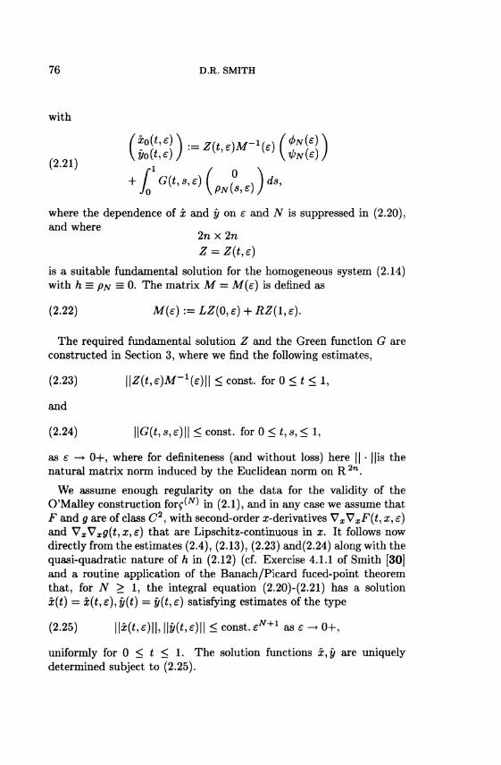
with

(2.21)

+ f G(t,8,e)( ,° x )ds,

where the dependence of x and y on e and N is suppressed in (2.20), and where

2n x 2n

is a suitable fundamental solution for the homogeneous system (2.14) with h = pN = 0. The matrix M = M (e) is defined as

(2.22) M(e) := LZ{0, e) + ÄZ(l, e).

The required fundamental solution Z and the Green function G are constructed in Section 3, where we find the following estimates,

(2.23) \\Z(t,e)M'1(e)\\ < const, for 0 < t < 1,

and

(2.24) ||G(*,*,e)|| < const, for 0 < *,«,< 1,

as e —• OH-, where for definiteness (and without loss) here || • ||is the natural matrix norm induced by the Euclidean norm on R 2 n .

We assume enough regularity on the data for the validity of the O'Malley construction f o r ^ ^ in (2.1), and in any case we assume that F and g are of class C2 , with second-order x-derivatives VxVxF{t, x, e) and VxVxg(t, x, e) that are Lipschitz-continuous in x. It follows now directly from the estimates (2.4), (2.13), (2.23) and(2.24) along with the quasi-quadratic nature of h in (2.12) (cf. Exercise 4.1.1 of Smith [30] and a routine application of the Banach/Picard fuced-point theorem that, for N > 1, the integral equation (2.20)-(2.21) has a solution x(t) = x(t,e),y(t) = y(t,e) satisfying estimates of the type

(2.25) ||x(i,e)||, | |y(e,s)|| < const. £r^+1 as e - • 0+,

uniformly for 0 < t < 1. The solution functions x,y are uniquely determined subject to (2.25).

DIRICHLET PROBLEM 77

The corresponding result for the original boundary-value problem (1.1)-(1.2) is given in the following theorem in the special case N = 1.

THEOREM 2.1. Let the data F,g,a,ß o/(l.l)-(1.2) possess first-order expansions in e as in (1.14), and assume that F,g and the coefficient functions F^k\g^ in (1.14) are of class C2 with Lipschitz-continuous second derivatives in x. Let X^ = X^(t) be a fixed given solution of the reduced equation (1.3) satisfying the boundary condition (1.4) and satisfying the stability conditions (1.5) and (1.6). Assume that F^ can be given in terms of a vector potential as in (1.7) if the boundary-layer jump is order unity, with a^ — X^(0) i=- 0. Then there is a fixed number SQ > 0 such that the function çW = ^(t^e) of (2.1)i is well-defined by the O'Malley construction (in the case N = 1) on the region (2.18), and the resulting boundary-layer terms satisfy (2.6) and (2.8)i. Moreover the problem (1.1)-(1.2) has an exact solution x = x(t,e) close to çW on the region (2.18), and there holds

\\x(t, e) - c(1){t, e)\\ < const.e2

(2-26) Xldz, , dçM, , „ l lÄ ( ' ' e )""A ( ' , e ) l | - c a n f l t ' e

uniformly on (2.18). The particular exact solution so constructed is unique subject to (2.26). (The assumed smoothness for F and g need only hold on a suitable domain containing the graph of ^x\ and the requirement of Lipschitz-continuity can be weakened.)

PROOF. The stated results follow directly from the above discussion. In the special case of a small boundary-layer jump with a^ = X(°)(0), one has *X^(r) ~ 0 in (2.1) and then one sees directly that (1.7) is not required.

From (2.26) along with (2.1)i on has in particular the result

(2.27) x(t, e) = X ( 0 ) (*) + *X<°> (t/e) + 0(e)

uniformly on the region (2.18), along with a related result for dx(t, e)/dt. Hence one obtains useful and detailed information on a corresponding solution x of the second-order problem (l.l)-(1.2)from the solutions X(°) and *X(°) obtained respectively from the first-order problem (1.3)-(1.4) for X(°) and the following first-order problem for *X(°i (see Ap-

78 D.R. SMITH

pendix Al) (2.28)

-^*X (0 )(r) = { I' F<°>(0, Jr<°>(0) + s*xM(T))ds}*xM(r) dr J0

= /(0,X ( 0)(0) + TyW(r)) - /(0,X(o)(0)) for r > 0,

*X^(0) = a ^ - X ^ ( 0 ) a t r = 0,

if the conditions (1.5), (1.6) and (1.7) hold, where / is the vector potential of (1.7).

A corresponding theorem remains true with the obvious modifications if the conditions of (1.4)-(1.6) are replaced by the use of (1.11)-(1.13).

3. The Green function. We consider here the linearized homoge­neous version of the system (2.14),

(3-D j H = - ( ° ' - ) n * * o < t < i , -v ; dtlyi e\eA(t,e)B(ti£)J\yJ

where the circumflexes have been dropped here from x and y in (2.14). The nxn matrix-valued functions A and B are defined by (2.16) and (2.17), and we assume that the conditions of (1.3)-(1.7) hold. We construct the Green function for (3.1) subject to boundary conditions of the type (see (2.15) and (2.19))

<s-2> K ä o ; ' ) ) + Ä ( y ( t 1 ) = given2n-vector' with the boundary matrices L and R given as

/o «x 2n x 2n 2n x 2n (3-3) / / „ o \ a n d _ / 0 oV

• \o oj ~\in o) The required Green function is given by the well-known formula (cf. Exercise 0.1.2 of Smith [30])

Ci 4) C(t s P) - i Z(t,e)M-1(£)LZ(0,e)Z-1(s,e) for s < t 1 ' uV'a>e> - \ -Z{t,e)M-1(e)RZ(l,s)Z-1{s,£) for s > t,

provided that the matrix M — M (e) of (2.22) is nonsingular, where Z denotes a fundamental solution for (3.1).

DIRICHLET PROBLEM 79

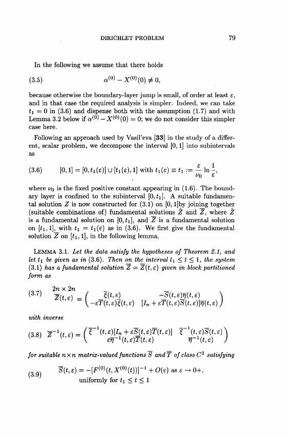
In the following we assume that there holds

(3.5) o l ° ) - X ( ° ) ( 0 ) / 0 ,

because otherwise the boundary-layer jump is small, of order at least £, and in that case the required analysis is simpler. Indeed, we can take h = 0 in (3.6) and dispense both with the assumption (1.7) and with Lemma 3.2 below if a^ — X^(0) = 0; we do not consider this simpler case here.

Following an approach used by Vasil'eva [33] in the study of a differ­ent, scalar problem, we decompose the interval [0,1] into subintervals as

(3.6) [0,1] = [0, hie)} U fate), 1] with hie) = h:=— In -,

where VQ is the fixed positive constant appearing in (1.6). The bound­ary layer is confined to the subinterval [0, h]. A suitable fundamen­tal solution Z is now constructed for (3.1) on [0, l]by joining together (suitable combinations of) fundamental solutions Z and Z, where Z is a fundamental solution on [0, £i], and Z is a fundamental solution on [$i,l], with t\ = tiie) as in (3.6). We first give the fundamental solution Z on fa, 1], in the following lemma.

LEMMA 3.1. Let the data satisfy the hypotheses of Theorem 2.1, and let t\ be given as in (3.6). Then on the interval t\ < t < 1, the system (3.1) has a fundamental solution Z = Zit,e) given in block partitioned form as

In x 2n (3>7) Z(te)-( J(t>el -J(t,e)j(t,e) \

' V -e T ( '> e)t& e) [!n + £T(t, e)S(t, e)}r}(t, e) )

with inverse

for suitable nxn matrix-valued functions S and T of class C1 satisfying

( 3 9 ) S(t,e) = - [ ^ ( a ^ ' W i r ' + O f e ) as e -+ 0+, uniformly for t\ < t < 1

80 D.R. SMITH

and (3.10)

T(t,e) = [F^{t,X^(t))]-1Ao{t) + 0(eVl/V0)

+ 0(e~v{t~tl)/e) as £ -> 0+, uniformly for h < t < 1, with

A0(t): = VxgW(t,XM(t))

- { [ ( F ^ f a ^ W ) ) - 1 ^ ^ . ^ ' « ) ! • Vs}F(°>(t,X«»(t))

/or an / /ïxec? 0 < Fi < o> w/iere i/o is the constant appearing in (1.6), and /or suitable n x n invertible matrix-valued functions £ and rj of class C1 satisfying

J{h,e) = Inirj(t1,e) = Jn;

(3.11) ||ë(*,e)||, Në" 1 ^^)! ! < const, forti < * < 1 ;

\\v{t^)fT1(s^)\\ ^ const. e"F (*- s ) / £ for tx < s < t < 1,

uniformly as s —• 0+, for some positive number V, where F^°\'g^ and are the functions appearing in (1.3)-(1.6). The function £ also

satisfies

(3.12) £(t,e) = f0)(t) + O{eVl/u0) for tx < t < 1, as e -+ 0+,

aoain /or ant/ fixed 0 < Fi < ^o, u^d wÄere £ = £ (£) 25 the nx n matrix-valued function characterized as

,?(o)

(3.13) ^ r = -[^^(^^wr^owf for o < t < i, ê(0) = /n at t = 0,

independent of e, where AQ is understood to be defined for 0 < t < 1 by the formula given in (3.10).

A proof of Lemma 3.1 including the construction of the functions S,T, £ and rj is given below in Appendix A2. Note that the second column-block on the right side of (3.7) represents solutions of (3.1) that decay rapidly away from the boundary layer, while the first column-block in (3.7) represents bounded nondecaying solutions.

A fundamental solution Z is given for (3.1) now on the boundary-layer subinterval [0, t\] in the next lemma, which is needed only if (3.5) holds (boundary-layer jump of order unity).

DIRICHLET PROBLEM 81

LEMMA 3.2. Let (3.5) hold. Then with the same assumptions as in Lemma 8.1 and with t\ given as in (3.6), the system (3.1) has for 0 < t < ti a fundamental solution Z = Z{t, e) given in block partitioned form as

In x In ( 3 - 1 4 ) Z(t e) = ( S(t,e)Ut,e) f,{t,s) \

\[In + f(t,e)S(t,eM(t,£) f(t,e)r,(t,e)J

with inverse (3.15)

{h ' \f)-Ht,e)[In+ 8(1,6)^,6)] -v-1(t,e)S(t,e)J

for suitable n x nmatrix-valued functions S and T of class C1 satisfying

(3.16) f{ti £) = F ( 0 ) ( 0 ' X ( 0 ) ( 0 ) + *X ( 0 ) ( i / £ ) ) + ° ( £ l n ^ uniformly for 0 < t < ti as e —• 0+,

rt/e

(3.17)

r/£ l S(t, e)= r}{t/e, s, e)ds + 0(e ln - ) ,

Jo £

uniformly for 0 < t < t\ S(tue) = - [ F ^ ( 0 , I ( 0 ) ( 0 ) ) ] - 1 + 0 ( 6 I / 1 / I / ° ) ,

as e —• 0+, and

(3.18) S(0,e) = 0,T(*i,e) = - [ S ^ e ) ] " 1 - eT{tue),

where S and T are the functions of Lemma 8.1, and where 77 in (3.17) is a suitable function of class C1 satisfying

\\ri{T,cr,e)\\ < cons t . e "" 1 ^-^ , and

(3.19) f?(r,(j,£) = ?)(o)(r,cT) + 0(£ ln- )

for 0<cr<T < -tu

as e —» 0-f, /or any fixed v\ satisfying 0 < v\ < UQ [see (1.6)], w/iere T)(°) es determined by (3.21) independent of e, and for suitable n x n

82 D.R. SMITH

invertible matrix-valued functions £ and fj of class C1 in (3.14) satisfying (3.20)

^ i , e ) = / n , ^ , e ) = / n + 0 (£( ln i ) 2 )

fj(0,e) = InMt,e) = r){0)(t/£,ti) + O(eln-) for0<t<tu

\\ri{tie)fi-1{sie)\\ < const .e-^ l ( t- 5) / £ for 0 < s < t < tu

as e —• 0+, where fj^ = ^^°)(T,(T) is the fundamental solution for the problem

(3.21)

dfl(0)M = [F(0) ( 0 ) X(0) ( 0 ) + *xW(T)W0HT,a) or

for r / ( 7 ,

7^°) (r, a) = 7n at r = (j, for r, <7 > 0,

independent ofe. This latter fundamental solution satisfies (see Lemma Al.l and Lemma Al.2 in Appendix Al) (3.22)

| |*? ( 0 )(^)ll < const. e-"i(r-<T) for r > cr > 0, and

I* fiW(T,<r)d<T = - [ ^ ( O J ^ f O j + ^ M r ^ O ^ 1 7 ) ./o

as T —• oo, for any fixed positive constant v\ satisfying 0 < v\ <VQ.

A proof of Lemma 3.2 is given in Appendix A3. As in Lemma 3.1, here also the second column-block in (3.14) represents decaying solutions of boundary-layer type, while the first column-block represents bounded nondecaying solutions.

An important feature of Lemma 3.1 and Lemma 3.2 is the fact that we have convenient representations not only for the fundamental solutions (3.7) and (3.14) but also for their inverses (3.8) and (3.15), as a consequence of the Riccati transformations employed in the proofs of the lemmas. It is also noteworthy that the Riccati transformations allow enough flezetability so as to permit the imposition of conditions such as (3.18) which greatly simplify the analysis of the Green function.

We now use the solution Z of (3.14) on the boundary-layer interval [0,£i], along with the solution Z of (3.7) on the outer interval [£i,l] so as to form a suitable composite fundamental solution Z on[0,1].

DIRICHLET PROBLEM 83

Specifically, take Z as

(3.23) Z(^):=(5^L_1 . farO<*<tlf {Z(t,e)Z (tue)Z(tue) for tx < t < 1,

where this Z is of class C 1 for £ € [0,1], for each fixed, sufficiently small e>0.

At t = £i, one finds with Lemma 3.1 and Lemma 3.2 the results

(3.24) Z-\tl,s) = (In + % [ £ ^ £ ) * ( £ e ) ) ,

(3.*>j z ^ 1 ' ^ - ^ J „ + r ( < 1 , e ) 5 ( < 1 , e ) TitueMtue))'

and

(3.26)

•77-1/ , ? , , x IS(tue) Ox \

(_ In 0 \ V S ( t i , e ) - S ( t i , e ) -fifa,e) J'

These results along with (2.22), (3.3) and the above lemmas now yield for the matrix M(e) the result

(3.27) M ( e ) = ( [ / n + A l(£)]ê(l ,£)S(<1 ,£) A 2 ( e ) j

as e —* 0+, where Ai(e) and A2(£) are defined as (3.28)

Aj(e) : = ~'S(lte)i!(l,e)'S~1(tue)\S{ti,e) - S{tueW1(tuë)rx{he)

Aa(e) : = S(l,e)J7(l,e)S_1(fi,e)»?(ti,e),

and where (3.18) has been used here to eliminate some terms and simplify others in (3.26)-(3.28). Note that the matrix-valued quantities ?(l,e) and S(ti,e) are nonsingular, uniformly as e —* 0+, with (see (3.6), (3.9) and(3.12))

(3.29) i Sfa,e) = - [ ^ ( O j C ' t O ) ) ] - 1 + 0 ( £ l n - ) ,

84 D.R. SMITH

where we used also the result F<0)(*i,X(°)(*i)) = F^{0,X^(0)) + 0(eln^). It is seen now that the quantities on the left side of (3.29) tend to fixed invertible matrices independent of £, as e —• 0+. Note also with (3.28) that Ai and A2 are small, with (see Lemma 3.1 and Lemma 3.2)

(3.30) Ai(e), A2(e) = Oi?*lv*fTvl*) as e — OH-,

for some fixed positive constant V > 0 and any fixed v\ with 0 < v\ < VQ, and where we used the result exp(—vit\/è) = e"1/"0 along with various other results listed above in the statements of Lemma 3.1 and Lemma 3.2. It follows now directly from (3.27)-(3.30) that the matrix M(e)is invertible for all small enough e > 0, with inverse given as

(3.31) M-1(e)=(PQ

fiMase->0+,

(3.31)

where P = -S 1{t1,e)Ç 1{l,e)[In + A1(e)]-1A2{e) as e - • 0+,

8^dQ = S'1(tlìs)r1(he)[In + A1(s)}-10

as e —• 0-h. This proves the ezetastence of the Green function G for all sufficiently small e > 0, given by (3.4).

An easy, routine calculation using Lemma 3.1, Lemma 3.2, and (3.23)-(3.31) yields now the result (see (A4.1) and (A4.4) in Appendix A4)

(3.32) \\Z(tis)M-1{e)\\ < const, for 0 < t < 1,

as e —• OH-. Similarly, the above results on Z and M yield for G the result (see Appendix A4)

(3.33) | |G(M,£) | | < const, for 0 < t,s < 1,

a s e - > 0-h. This completes the proof of the results (2.23) and (2.24) required in the earlier proof of Theorem 2.1, thereby completing the proof of that theorem, providing that we are given the validities of Lemma 3.1 and Lemma 3.2. These lemmas are established respectively in Appendix A2 and Appendix A3. A proof of the bound (3.33) is given in Appendix A4.

DIRICHLET PROBLEM 85

Appendix A l . Derivation of the Boundary-Layer Properties (2.6), (2.8), and (3.22).

One sees directly that (2.28) provides a first integral of (2.5) if F^is given in terms of a potential as in (1.7). The inner-product of the first equation of (2.28) can be taken with *AT^(r), and then the boundary-layer stability condition (1.6) or (1.8) yields

( A l l ) j L | r X ( 0 ) ( r ) | | 2 < _ 2 „ 0 | r X ( 0 ) ( T ) | | 2

This differential inequality along with a suitable initial condition from (2.28) can be integrated by Gronwall's inequality, and one obtains the a priori estimate given by the first ineqaulity of (2.6). This a priori estimate and a standard continuation result prove that the solution of the initial-value problem (2.28) ezetasts for all r > 0, and the given estimate holds for all such r. The second inequality of (2.6) then follows from the first inequality and the differential equation of (2.28). This completes the proof that (2.5) has a (unique) solution satisfying (2.6), if (1.7) holds.

We turn now to a proof of (2.8). For this purpose we require initially the first result of (3.22) which is proved in the following lemma.

LEMMA A.l.l Let the data satisfy the hypotheses of Theorem 2.1, and let r)^ — r)(°)(r,<j) be the n x n matrix-valued fundamental solution characterized by (3.21). Then, for any given fixed v\ satisfying 0 < v\ < i/o, there is a corresponding positive number K\ such that there holds

{A1.2) \\fl{0)(T,G)\\ <>ciexp[-i/ i(r-(7)] for 0 < a < r.

PROOF. A routine argument using (2.6) and (3.21) shows that 7)(°)(T, cr) is bounded on any fixed compact set of the form 0 < a < T < f, for any fixed f > 0. Hence we need only prove (Al.2) for large r > f, for some fixed f depending on v\.

In (1.6)let x —• 0 along any fixed direction in R n and find

(ill.3) (x,F(°)(0,X^(0))x) < -^olkl l2

for any fixed unit vector x, from which it follows that (Al.3) holds for all x € R n . The earlier argument leading to (Al.l) can be repeated

86 D.R. SMITH

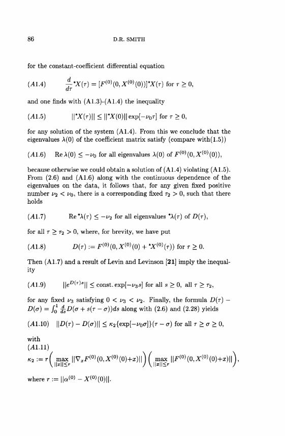
for the constant-coefficient differential equation

(AIA) 4-*X(T) = [^(O)(0,X(o)(0))]*X(r) for r > 0,

and one finds with (A1.3)-(A1.4) the inequality

(41.5) ||*X(r)|| < |pX(0)||exp[-^or] for r > 0,

for any solution of the system (Al.4). From this we conclude that the eigenvalues A(0) of the coefficient matrix satisfy (compare with(1.5))

(41.6) Re A(0) < -v0 for all eigenvalues A(0) of F^(0 ,X( o ) (0 ) ) ,

because otherwise we could obtain a solution of (Al.4) violating (Al.5). From (2.6) and (Al.6) along with the continuous dependence of the eigenvalues on the data, it follows that, for any given fixed positive number v<i < I/Q, there is a corresponding fixed r2 > 0, such that there holds

(41.7) Re *A(r) < - i / 2 for all eigenvalues *A(r) of £>(r),

for all r > T2 > 0, where, for brevity, we have put

(41.8) D(T) := F(°) (0, X^ (0) + *X^ (r)) for r > 0.

Then (A 1.7) and a result of Levin and Levinson [21] imply the inequal­ity

(41.9) H e ^ ^ l l < const.exp[-i/3s] for all s > 0, all r > r2,

for any fixed v^ satisfying 0 < v-$ < v2. Finally, the formula D(r) — D(a) = JQ £D(a + S(T - a))ds along with (2.6) and (2.28) yields

(41.10) \\D{T) - D{a)\\ < K,2{exp[-iy0(7]}{T - a) for all r > a > 0,

with (4 i . l i )

K2:=T( max ||VxF<°>(0,X<°>(0)+z)||) ( max ||F<°>(0,X<0>(0)+a:)|| \INI<»- / VIMI^»-

where r:= ||a(°>-A-(°)(0)||.

DIRICHLET PROBLEM 87

Following Flato and Levinson [14] (cf. Exercise 6.1.5 of Smith [30]), the solution i^0) of (3.21) can be represented as (A1.12)

f)(0)(T,<r) = e ^ H ' - " ) + f eD^T-a^[D(s) - I?(r)]»)^(s,a)rfs.

We introduce the function <\> as (Al.13)

0(T,<T) := \\fi{0)[T,a)\\eVA{T-'<T), any fixed i/4 with 0 < 1/4 < i / 3 ,

and then (Al.12) along with (A1.9)-(A1.10) and (A1.13) yields

(Al.14) 0(r,<r) < /c3 + K4 / e~Xs(j){s,a)ds for 0 < a < r , r > r2,

with A := i o — ^3 +1^4 > ^4 > 0, for suitable fixed positive constants Ks and /C4, where we used the boundedness of (r — s) exp[—(i/3 — 1/4)7] for r > s > 0. In the following we handle separately the two cases f < a < T and 0 < a < f < r, where f is taken now to be the fixed number

(A1.15) f := max{r2, A""1 ln(2A-1/c4)}, so that e x p ( ~ A r ) < J _ .

In the case f < a < r, we lengthen the interval of integration on the right side of (Al. 14) and find

/ e~Xs<f)(s,a)ds (Al.16) 0(r,a) < AC3 + /c4 / e~Xs(j)(s,(j)ds for f < a < r,

which leads directly to the bound (multiply (Al.16) on both sides by e~Ar, integrate with respect to r from f to r, interchange an order of integration, and use (Al. 15) and (Al. 16))

(A1.17) <£(r, a) < 2/C3 for f < <r < r.

In the other case 0 < a < f < r, we rewrite (Al.14) as

(Al.18) </>(r, <r) < KS + /c4 / e~Xs(t){s, a)ds + K4 e"As</>(s, cr)ds

88 D.R. SMITH

for 0 < a < f < r, where the first integral on the right side here involves 0(s,<j) on the compact set 0 < a < s < f, and is easily seen to be bounded because fj^ is known to be bounded on compact sets. Hence from (Al. 18) we have a result of the type (compare with (Al. 16))

•i; (Al.19) 0(r, a)<k3 + K4 e~Xs<j)(s, a)ds for 0 < a < f < r,

where £3 is an upper bound on the first two terms on the right side of (A 1.18). Just as before (cf. (A 1.17)), this last result leads directly to the bound

(A1.20) 0(r, a) < 2/c3 for 0 < a < f < r.

Hence the function <j) is bounded in both cases, and then (Al.13) yields H^H7»*7)!! ^ const. exp[—v±{r — a)] for 0 < o < T,T > f. Since ^ 2 Î ^ 3 Î ^ 4 are arbitrary subject only to the restrictions 0 < v± < v% < "2 < vo, it follows that we can arrange to take v± = v\ as in the statement of the lemma, and this completes the proof.

Turning now to a proof of (2.8)/c, one sees directly that a first integral of (2.7) i vanishing at infinity is given as (41.21)

£*XM(T) = [F<0>(0,Jr<0>(0) + * ^ ° ) ( r ) ) ] ^ 1 ) ( r ) - / *gW(a)da

if (1.7) holds, where the function V1^ is given by the O'Malley con­struction and satisfies

(A1.22) \\*gW(r)\\ < const. exp[--(i/ i + i/0)r] for r > 0,

for any fixed constant v\ satisfying 0 < v\ < VQ.

The linear equation (Al.21) can be integrated with the integrating factor r)(°) = f}(0\r,(j) from (3.21), and one finds (41.23)

PT /«OO

*xM(T) = fìW(Tì0yxM(0)- / r)(0)(r,<r) / *gM{s)dsd(j, JO Jo

where the initial value *X^ (0)is provided by the O'Malley construction but need not be given here. The bound on *XW(T) of (2.8)i follows directly from (Al.2), (Al.22) and (Al.23) by a routine calculation,

DIRICHLET PROBLEM 89

and then the result for d*X^/dr follows also by (Al.21). Details are omitted. One can similarly obtain the bounds of (2.8)& for larger k, but we need not do so here.

The next lemma completes the proof of (3.22).

LEMMA A 1.2. The function fj^ of Lemma Al. 1 satisfies (A1.24)

fT fi^(r,a)da = -[F<o>(0,X(°>(0) + ^ ( r ) ) ] " 1 + 0(e~^T) Jo

as T —• oo, for any fixed positive constant v\ satisfying 0 < v\ <VQ.

PROOF. For any fixed r2 > 0, it follows from Lemma Al . l that there holds

(41.25) H T) (0 ) (r, a)da = 0(e~^T) Jo

as T —* oo. Since there holds

(A1.26) r ^ ^ ( r , a ) ^ = H f)<0>(r,a)dcr + [*rjW(T,v)da, Jo Jo JT2

it follows with (Al.25) that we need only prove the following result (see (A1.24)) (41.27)

fV0)(r,<r)dt7 = -[F<o>(0,X<°>(0) + " X ^ r ) ) ] " 1 + 0 ( e " I / i r ) J T2

as T —• oo, for any fixed T<I > 0.

To this end we take T<I as in (A 1.7), so that the matrix-valued function D — D(T) of (A1.8) is nonsingular for r > T2. The product rule of differentiation gives

(A1.28) 2-W®(Tt&)D-l{a)) = -$(°)(T ,a) + $ ( ° > ( r , a ) ^ i r 1 ( f f )

because of the well-known result dr)(°\T,a)/da = — r/^(r,a)D((T) (see (3.21) and (A1.8)). From (Al.28) we have upon integration with respect to a between T*Z and r, (41.29)

f ri{0) (r, o)da = - [F<°> (0, X'0> (0) + * I ( 0 ) (r))]"1

•/T2

+ f,M(T,T2)D-1(T2) + f fi^M^D-H^do,

90 D.R. SMITH

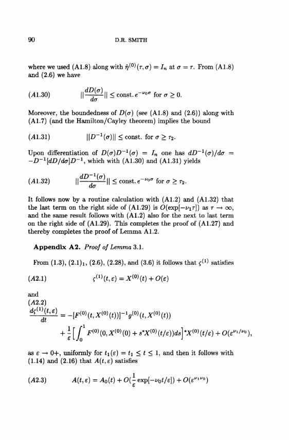
where we used (Al.8) along with fj(°) (r, a) = In at a = r. From (Al.8) and (2.6) we have

{ALSO) H ^ r ^ H < const.e""0* for a > 0. der

Moreover, the boundedness of D{<J) (see (Al.8) and (2.6)) along with (Al.7) (and the Hamilton/Cayley theorem) implies the bound

{AIM) \\D-l{a)\\ < const, for a > r2.

Upon differentiation of D(a)D~1(a) = In one has dD~1(er)/dcr = -D^ldD/dalD-1, which with (A1.30) and (A1.31) yields

(A1.S2) | | ^ L _ M || < const.e~v»a for a > r2. da

It follows now by a routine calculation with (Al.2) and (A1.32) that the last term on the right side of (Al.29) is 0(exp[—V\T\) as r —• oo, and the same result follows with (Al.2) also for the next to last term on the right side of (Al.29). This completes the proof of (Al.27) and thereby completes the proof of Lemma A 1.2.

Appendix A2. Proof of Lemma 3.1.

Prom (1.3), (2.1)i, (2.6), (2.28), and (3.6) it follows that ^ satisfies

(A2.1) ?(1)(*,e) = X<°>(t) + 0(e)

and (A2.2)

^ M = -[F(o){tiXm m-ig(o){ifXm W) dt

- [ / F<°> (0, XW (0) + s*X^ {t/e))ds\ *X^ (t/e) + 0{e"1

as e —• 0+, uniformly for ti(e) = t\ < t < 1, and then it follows with (1.14) and (2.16) that Afae) satisfies

(,42.3) A{t, e) = A0(t) + 0(- exp[-VQt/e]) + Ofc"1"0)

DIRICHLET PROBLEM 91

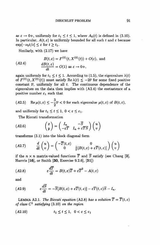
as e —• OH-, uniformly for t\ < t < 1, where Ao(t) is defined in (3.10). In particular, A(t, e) is uniformly bounded for all such t and e because exp[—vot/e) < e for t>ti.

Similarly, with (2.17) we have

ß(t ,£) = F ( ° » ( a ( 0 ) W ) + O(e), and 0*2.4) dB{t,e)

dt = O(l) as e - • 0+,

again uniformly for t\ < t < 1. According to (1.5), the eigenvalues \{i) of F(°)(*,X(°)(£)) must satisfy ReA(i) < - 2 F for some fixed positive constant F, uniformly for all t. The continuous dependence of the eigenvalues on the data then implies with (A2.4) the ezetastence of a positive number £\ such that

3 (A2.5) Re /i(£, e) < — -V < 0 for each eigenvalue //(£, e) of B(t, £),

J*

and uniformly for £i < t < 1, 0 < e < S\.

The Riccati transformation

<™ (;)-(-!a- 7.;^r)(:) transforms (3.1) into the block diagonal form

( ^ 2 > 7 ) * W = ( o ' £ ±{B(t,e) + eT(t, e)}){l)

if the n x n matrix-valued functions T and S satisfy (see Chang [2], Harms [16], or Smith [30, Exercise 9.2.6], [31])

dT — —9 (A2.8) e— = B{tie)T + eT - A{t,e)

and

(A2.9) e^ = -S[£(*, e) + eT(*, e)] - eT{t, e)S - / n .

LEMMA A2.1. 77ie Riccati equation (A2.8) has a solution T = T(t,e) of class C1 satisfying (3.10) on the region

(A2.10) h<t<l, 0 < e < £!

92 D.R. SMITH

for some fixed £\ > 0.

PROOF. Let r}(t,e) be a fundamental solution for e(drj/dt) = B(t,e)rj for ti < t < 1. A well-known result of Flatto and Levinson [14] implies with (A2.4)-(A2.5) the result

(A2.11) l l r ç ^ r r 1 ^ ) ! ! < const. e _ ï 7 ( t - s / £ for h < s < t < 1,

as e - • 0+. Put W = T in the identity (A2.12)

W(t)=rì(t,e)r1-1(ti,e)W(t1)+J rì{t,e)rì-\s,e)(^--eBw\s)ds

and find with (A2.8) the integral equation

T(t,e) = / v^e^is.e^is.efds

(^2.13) +rì(tìe)rì-1{t1,e)B-1(tue)A0(t1)

I rt - - / r?(^,e)r/ 1{s,£)A(s,e)ds,

€ Jt1

where we have imposed the initial condition T(ti,e) = JB~1(^I,Ê:)

Ao{ti). The terms not involving T on the right side of (A2.13) are uniformly bounded because of (A2.3), (A2.4) and (A2.11), so that a routine application of the Banach/Picard fixed-point theorem using (A2.11) shows that (A2.13) has a bounded solution T on the region (A2.10), for some sufficiently small S\ > 0. Now take W(t) = B-1{tie)A0{t) in (A2.12), and subtract the result from (A2.13) and find (A2.14) - 1 (x

T(t,e)-B-1{t,e)A0{t) = — / vfoefr-^eftAfae) - A0(s)]ds

J ri&e^-'&eXT&e)2 - j-(B-1(s,e)A0(s))}ds. f*

Upon differentiation of BB~X = In one has dlB'^/dt = -B'^dB/dt) £ - \ which with (A2.4)-(A2.5) yields dlB'^/dt = O(l) on the region (A2.10). Hence the quantity in square brackets in the last integrand on the right side of (A2.14) is uniformly bounded on (A2.10), and

DIRICHLET PROBLEM 93

routine calculation with (A2.11) then shows that the last integral on the right side of (A2.14) is order (e), uniformly on the region (A2.10). Similarly, a routine calculation using (A2.3), (A2.11) and the result exp(—voti/e) = e shows that the first term on the right side of (A2.14) is O{e^'uo) + 0(exp[-F(* - h)/e]) on (A2.10). The stated result of (3.10) follows directly now from these estimates along with (A2.4) and (A2.14), and this completes the proof of Lemma A2.1. [This proof uses certain refinements of the corresponding arguments in Chang [2] and Harris [16] where the simpler case is considered with the data functions B and A independent of e. The identity (A2.12) used here in obtaining (A2.14) differs from that used by Harris.]

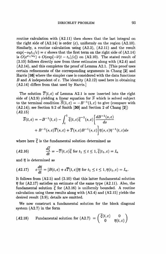
The solution T(t,e) of Lemma A2.1 is now inserted into the right side of (A2.9) yielding a linear equation for 5 which is solved subject to the terminal condition 5(1, e) = — £? - 1(l ,£) to give (compare with (A2.14); see Section 9.2 of Smith [30] and Section 2 of Chang [2]) (42.15)

'dB-^s.e) S(t,e) = -B~1(tie)-J t(t,e)t \s,e)

+ B-1 («, e)T{s, e) + T(s, e)B-1(s, e)

ds

fj(sie)rj~1(t,e)ds

where here £ is the fundamental solution determined as

(42.16) ^ = -T(t,e)ì for h<t< l,?(*i,e) = In

and rj is determined as

(42.17) e~t = [B{t,e) + eT{t,e)]rj for h<t< l , r /(^,e) = In.

It follows from (A2.5) and (3.10) that this latter fundamental solution rj for (A2.17) satisfies an estimate of the same type (A2.11). Also, the fundamental solution £ for (A2.16) is uniformly bounded. A routine calculation using these results along with (A2.4) and (A2.15) yields the desired result (3.9); details are omitted.

We now construct a fundamental solution for the block diagonal system (A2.7) in the form

(42.18) Fundamental solution for (A2.7) = ( ^ ^ ° * J

94 D.R. SMITH

with f and rj determined by (A2.16) and (A2.17). The results of (3.11) are well known (see (A2.5) and Lemma A2.1), so that only (3.12)-(3.13) remains to be proved.

For this purpose consider the following comparison problem for a

function £ {t,e),

Mi)

(A2.19) ^ T = " ' F ( 0 ) ( a ( 0 ) W ) ] - ^ o W ? ( 1 ) for 0 < t < 1,

f1){tlie)=Inatt = t1.

The solution £ is easily seen to be uniformly bounded for 0 < t <

1,£ —• 0+. Let 7 denote the difference between £ and £ 57(^^) :=

Î(t,e)-Î{1)(t,e), and find from (A2.16) and (A2.19),

20) d~dt =-T(t>eh + p(tie) for h<t< l^{tue) = 0,

with p{t,e) := { - f + I f f 0 ) ] - 1 ^ .

The boundedness of T and a routine argument from (A2.20) lead to an estimate of the type

(A2.21) ||7(*,0II < const, f ||p(*,e)||cfc

for ii < t < 1. The function £ is uniformly bounded, and then (3.10) (see Lemma A2.1) implies that the residual p of (A2.20) satisfies

(A2.22) p{t,e) = 0 ( ^ ) + 0(exp[-F(*-*i)/e]) on the region (A2.10),

with /i := VI/VQ. From (A2.21)-(A2.22) there follows by a routine argument the estimate ~i(t,e) = 0(eM), or equivalently, £(£,£) =

ltl\t,e) + O(eFl/ I / 0), uniformly on the region of (A2.10). This same

result follows also with £ (t,e) replaced on the right side here by

£ (t) as characterized by (3.13) because one easily proves with (3.13)

and (A2.19) the result £(1) (*, e) = £(0) (t)+0(e ln[l/e]). This completes the proof of (3.12)-(3.13).

DIRICHLET PROBLEM 95

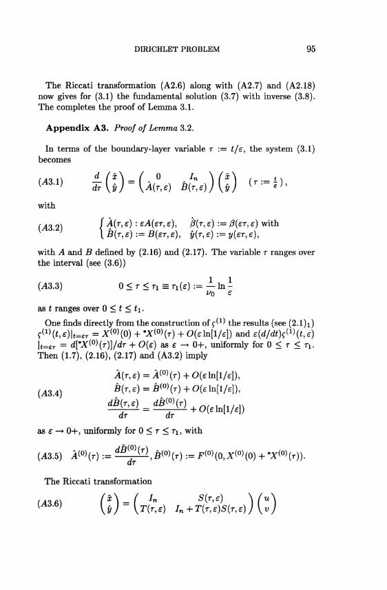
The Riccati transformation (A2.6) along with (A2.7) and (A2.18) now gives for (3.1) the fundamental solution (3.7) with inverse (3.8). The completes the proof of Lemma 3.1.

Appendix A3. Proof of Lemma 3.2.

In terms of the boundary-layer variable r := t/e, the system (3.1) becomes

( i 4 5 U ) &{l)-\A{T,e) B(T,e)){y) ( ' : = ! ) ,

with

(A3 2) / 4 ( r ' £ ) : eAißT, e), ß(r, e) := ß{er, e) with \ B(r, e) := JB(er, e), y{r, e) := y(er, e),

with A and J5 defined by (2.16) and (2.17). The variable r ranges over the interval (see (3.6))

(A3.3) 0 < r < n = n(e) := — In -

as £ ranges over 0 < t < t±.

One finds directly from the construction of f (*) the results (see (2.1)i) C (1 )(^)lt=*r = X(°)(0) + *X<°)(r) + 0(eln[l/e]) and e(d/dt)^(t,e) \t=er = d[*X(°){T)]/dr + 0{e) as e -» 04-, uniformly for 0 < r < n . Then (1.7), (2.16), (2.17) and (A3.2) imply

A(r,e) = A&HT) + 0(e\n[l/e]),

(AS4) ß ( r , e )= f l ( 0 ) ( r ) + O(eIn[l/e]),

as e —• 0+, uniformly for 0 < r < ri , with

043.5) A(°)(r) := ^ ^ , £ ? ( ° ) ( r ) := F«»(0,X<°>(0) + *X<°)(r)). ar

The Riccati transformation

(A3.6) {l) = {T(T,e) /n+T(r?/)S(r,e))(")

96 D.R. SMITH

transforms (A3.1) into the block diagonal form

{M-7) dï\v) = { 0 e è(T,e)-T(T,e))\Uv)

if the n x n matrix-valued functions T and S satisfy (see Smith [30, Exercise 9.2.6; 31])

(A3.8) Ç = - T 2 + B(T, e)T + A(r, e) ar

and

(A3.9) ^ = T(r, e)5 + S[T(T, e) - B(r, e)] + Jn .

LEMMA A3.1. Tne system (A3.8)-(A3.9)has solution functions T and S satisfying

(A3 10) T ( r i ' £ ) = - 5 _ 1 ^ i , e ) - eT( t ! , £ ) , T(r,e) = B(r,e) + 0(eln[l/e]) for 0 < r < n ,

as e —• 0+, and

S(0,e) = 0, (A3.11)

S ( r , e ) = / ^(r,a,e)df7 + 0(eln[l/e]) Jo

as e —• OH-, uniformly for 0 < r < r i , /or a suitable function fj of class C1 satisfying the estimates of (3.19), w/iere S(£i,£) and T(£i,£) are determined as in Appendix A2.

PROOF. T(T, e) is a solution of (A3.8) if and only if the function Ti denned as

(A3.12) Tl(T,e):=T(T,e)-B(r,e)

satisfies the equation

(43.13) - ^ + TiS(r, e) = -if + A(r,e) -(XT dr

DIRICHLET PROBLEM 97

We solve this latter equation for 0 < r < T\ subject to the terminal condition

(A3.14) T1(T1,e) = -{è(T1,e) + S-1(t1,e)+eT(t1,£)].

For this purpose introduce the fundamental solution r/ = r/(r,<j, s) characterized as

(A3.15) drl{T><r,£) = ^ ^ torT±a^ = in f o r T = (7i UT

with

(A3.16) 3 * ? ( w ) = _ ^ ^ g ) è ^ g )

Then the equation (A3.13) subject to the terminal condition (A3.14) is equivalent to the integral equation

T1(a,£)2ri{a,T,e)da with

(A3.17) Ti0)(T,e): = -[B(T1,£) + S~1(t1,s) + eT(t1,e)}

The method of proof of Lemma Al . l can be applied to the present fundamental solution rj with (A3.4), (A3.5) and (A3.15), and one has then

(.43.18) ||r/(r,er,£)|| < const. exp[-^i(r - a)] for 0 < a < r < r^e)

uniformly for e —» 0+, for any fixed 0 < v\ < VQ. One also has from (A3.4)-(A3.5) the result

(A3.19) dB{cr,e) _ ^ = Q^^J^ for 0 < * < n , da

as e -+ 0+. From (2.6), (3.6), (3.9)-(3.10), (A3.4)-(A3.5) and (A3.17)-(A3.19) it follows that the given function T1

(0) satisfies T[°\T,S) = Ò(s:ln[l/£:]) uniformly for 0 < r < r i ,£ —*• 0-f-, and then a routine application of the Banach/Picard fixed-point theorem with (A3.18)

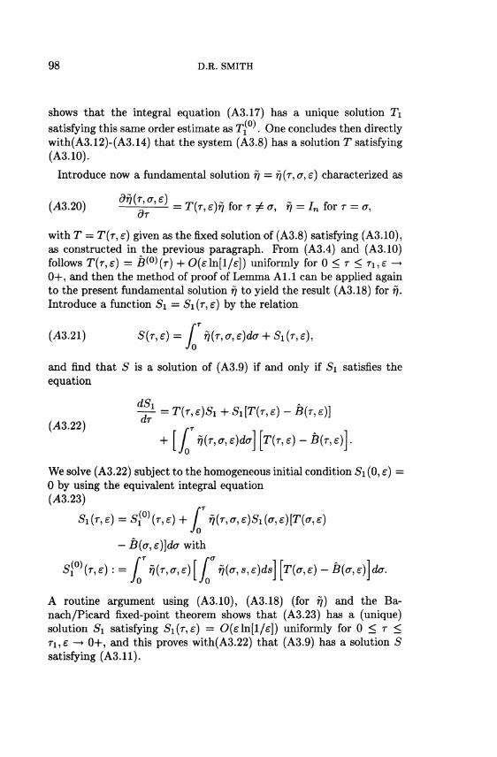
98 D.R. SMITH

shows that the integral equation (A3.17) has a unique solution Ti satisfying this same order estimate as Tj . One concludes then directly with(A3.12)-(A3.14) that the system (A3.8) has a solution T satisfying (A3.10).

Introduce now a fundamental solution rj = r)(r,(j, e) characterized as

(A3.20) d^Y'£) = T(T, e)r, for r ? <J, r) = In for T = a, or

with T = T(T, e) given as the fixed solution of (A3.8) satisfying (A3.10), as constructed in the previous paragraph. From (A3.4) and (A3.10) follows T{r,e) = È^(r) + 0(£Ìn[l/e]) uniformly for 0 < r < rue - • 0+, and then the method of proof of Lemma A 1.1 can be applied again to the present fundamental solution r\ to yield the result (A3.18) for fj. Introduce a function Si = Si (r, e) by the relation

(A3.21) S(r,e) = [Tfl(r^ìe)da^Si(rì6)ì Jo

and find that S is a solution of (A3.9) if and only if Si satisfies the equation

^ = T(r, s)S1 + Si [T{T, e) - B{T, e)) (43.22) aT

+ [ j rKr, a, e)da\ [T(T, e) - B(r, e)].

We solve (A3.22) subject to the homogeneous initial condition Si (0, e) = 0 by using the equivalent integral equation (A3.23)

Si (r, e) = S[0) (r, e) + f *?(r, <r, é)S1 (<r, e)[T(tr, e) Jo

— Ê(a, e)]da with

S[0){T,e): = J fi{T,a,e)[j fjfasrfds^Tfae)-B(v,ej\da.

A routine argument using (A3.10), (A3.18) (for 77) and the Ba-nach/Picard fixed-point theorem shows that (A3.23) has a (unique) solution Si satisfying Si(r, e) = 0(£ln[l/£]) uniformly for 0 < r < Ti,e —> 0+, and this proves with(A3.22) that (A3.9) has a solution S satisfying (A3.11).

DIRICHLET PROBLEM 99

There remains to be proved only the second result of (3.19) for r\. To this end introduce the function h = h(r,<j,e) as

(A3.24) fc(r, a, e) := ^{r, a, e) - fi(0)(r, <r),

and find with (3.21), (A3.5), (A3.20) and (A3.24) the relations (A3.25)

ft(r, <7, s) = 0 at T = cr, and

* * ( y g ) = T(r, e)h(r, a, e ) + [T(r, e) - È™ (r)] • $<°> (r, a)

for T j^ cr.

The method used earlier in the study of (A3.22) can be applied now to (A3.25), and we find directly the result ft(r,cr,£) = 0(ein[l/e]) uniformly for 0 < cr < r < n , e —• (M-, which with (A3.24) provides the stated result for rj. This completes the proof of Lemma A3.1.

We now construct a fundamental solution for the block diagonal system (A3.7) in the form

(A3.26) Fundamental solution for (A3.7) = ( ~ ° ^T\Q°' ^ \

with f/(r, 0, e) given by the solution of (A3.20) evaluated at a = 0, and with \ determined as

(A3.27) % ^ = t ^ r ' e ) * T ^ £^T> *) ** 0 < r < n ,

£(r,e) = Jn for r = r i .

A routine argument with (A3.10) and (A3.27) shows that ç satisfies

(A3.28) £(r, e) = J„ + 0(e[ln(l/e)]2)

uniformly for 0 < r < r i ,£ —• 0+. The Riccati transformation (A3.6) along with (A3.7) and (A3.27) now gives for (A3.1) the fundamental solution 0*3.29) Fundamental solution __ / S(r,e)£(r,£:) 77(7-, 0,e) \

for(A3.1) " \{In + T(T,e)S(T,e)}UT,e) T(r,e)q(r,0,e) /

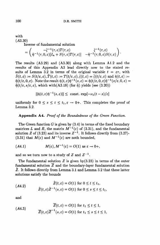
100 D.R. SMITH

with (.43.30)

Inverse of fundamental solution _ / - ? - i ( r , e ) T ( r , £ ) ç- i (T > e ) \

yrj-HTMlIn+SiT^Tfae)] -fi-1{r^e)S{r,e)) '

The results (A3.29) and (A3.30) along with Lemma Al.2 and the results of this Appendix A3 lead directly now to the stated re­sults of Lemma 3.2 in terms of the original variable t = er, with S(t, e) := S(t/e, e), T(i, e) := T(*A, e), ?(t, e) = ?(t/e, e) and r/(t, e) := r/^/e, 0, s). Note the result ?)(£, £)r)_1 (s, e) = f/(t/e, 0, s)rj 1 (s/e, 0, s) = rì\t/£,s/e,e), which with(A3.18) (for rj) yields (see (3.20))

||r)(^6:)r)"1(5,£')|| < const. exp[—i/i(t - s)/e]

uniformly for 0 < s < t < £i,e —• 0+. This completes the proof of Lemma 3.2.

Appendix A4. Proof of the Boundedness of the Green Function.

The Green function G is given by (3.4) in terms of the fixed boundary matrices L and Ä, the matrix M~1(e) of (3.31), and the fundamental solution Z of (3.23) and its inverse Z~x. It follows directly from (3.27)-(3.31) that M{e) and M~1{e) are noth bounded,

{AAA) M{e),M~1{e) = O(l) as e — 0+,

and so we turn now to a study of Z and Z~x.

The fundamental solution Z is given by(3.23) in terms of the outer fundamental solution Z and the boundary-layer fundamental solution Z. It follows directly from Lemma 3.1 and Lemma 3.2 that these latter solutions satisfy the bounds

(-44.2)

and

(A4.3)

Z{t,e) = 0(l) f o r 0 < * < * i ,

Z(tie)Z-1{sie) = 0(l) for 0 < « < * < * i ,

Z{t,e) = 0(1) forii < * < 1,

Z ^ e J Z " 1 ^ , ^ ) = O(l) for tx < s < t < 1,

DIRICHLET PROBLEM 101

all as e —> 0+. A direct calculation using (3.23) and (A4.2)-(A4.3) shows now that Z satisfies the analogous bounds

Z ( M ) = O(l) fi*r 0 < i < 1, Z(t,e)Z~1(sie) = 0(1) for 0 < s < * < l , e - + 0 + .

On the other hand, Z~~l{t,e) is generally not bounded as e —> 0-f, and similarly Z(i,e:)Z~1(3,£:) is generally not bounded for s > t as e —> +. Even so, the Green function G(t, s, e) is bounded as e —• OH-, uniformly for all £, s € [0,1], as we now show. The Green function is piecewise smooth with a single jump discontinuity at t = s, so we need only consider all £, s with t^s.

From (3.4), (A4.1) and (A4.4) follows directly the bound

(Ä4.5) G{t,s,e) = 0 ( 1 ) f o r O < * < * < l , e - > 0 + .

For the other case s < t we use (2.22) and the invertibihty of M(e) to write

(A4.6) A f - ^ e J L Z ^ e ) = J - A f - ^ ^ Ä Z ^ e ) ,

which with (3.4) gives for G, (A4.7) G(t,8,e) = Z(t,e)Z-1(s,e)-Z(tìe)M-1(e)RZ(l,e)Z-1(sìe) for s < t.

The boundedness of G follows in this case directly with (A4.1), (A4.4) and (A4.7),

(A4.8) G(M,e) = 0 ( 1 ) f o r 0 < 5 < * < l , e - > 0 + .

The stated boundedness of the Green function as in (3.33) follows now from(A4.5) and (A4.8). The organization of this proof of bound­edness of G given here follows a suggestion of John Jeffries and replaces at this point an earlier, lengthier proof of the author.

REFERENCES

1. N.I. Brish, Onbmnfary vdueprobkms for the equation e-d2 y/dx2 = f{x,y,dy/dx) for small e, Dokl. Akad. Nauk. 95 (1954), 429-32.

2. K.W. Chang, Singular perturbations of a general boundary value problem, SIAM J. Math. Anal. 3 (1972), 520-526.

102 D.R. SMITH

3. , Approzetamate solutions of nonlinear boundary value problems involving a small parameter, SIAM J. Appi. Math. 26 (1974), 554-567.

4. , Diagonalization method for a vector boundary problem of singular perturbation type, J. Math. Anal. Applications 48 (1974), 652-665.

5. , Diagonalization method in singular perturbations, International Conference on Differential Equations, ed. H.A. Antosiewicz, Academic Press, New York, 1975, 164-184.

6. , Singular perturbations of a boundary value problem for a vector second order differential equations, SIAM J. Appi. Math. 30 (1976), 42-54.

7. , and Howes, F.A., Nonlinear Singular Perturbation Phenomena: Theory and Application, Springer-Verlag, New York-Berlin-Heidelberg-Tokyo, 1984.

8. J. Chen and R.E. O'Malley Jr., On the asymptotic solution of a two-parameter boundary value problem of chemical reactor theory, SIAM J. Appi. Math. 26(1974), 717-729.

9. J.A. Cochran, Problems in singular perturbation theory, Stanford University doctoral dissertation, (1962).

10. E.A. Coddington and N. Levinson, A boundary value problem for a nonlinear differential equation with a small parameter, Proc. Amer. Math. Soc. 3 (1952), 73-81.

11. W.A. Coppel, Stability and Asymptotic Behavior of Differential Equations, D.C. Health and Company, Boston, 1965.

12. A. Erdélyi, Approzetamate solutions of a nonlinear boundary value problem. Arch. Rational Mech. Anal. 29 (1968), 1-17.

13. , A case history in singular perturbations, International Conference on Differential Equations, ed. H.A. Antosieqicz, Academic Press, New York, 1975, 268-286.

14. L. Flatto and N. Levinson, Periodic solutions of singularly perturbed systems, J. Rational Mech. Anal. 4 (1955), 943-950 (currently J. Math. Mech. 4).

15. P. Habets, Singular perturbations of a vector boundary value problem, Lecture Notes in Mathematics 415, Springer-Verlag, (1974) 149-154.

16. W.A. Harris, Jr. Singularly perturbed boundary value problems revisited, Lecture Notes in Math. 312 (1973), Springer-Verlag, Berlin, 54-64.

17. A. van Harten, Nonlinear singular perturbation problems: proofs of correctness of a formal approzetamation based on a contraction principle in a Banach space, J. Math. Anal. Applications 65 (1978), 126-168.

18. F.A. Howes, Effective chamcterization of the asymptotic behavior of solutions of singularly perturbed boundary value problems, SIAM J. Appi. Math. 30 (1976), 296-306.

19. , Boundary-interior layer interactions in nonlinear singular perturbation theory, Memoirs Amer. Soc. 203 (1978), 1-108.

20. , and O'Malley, R.E., Jr. Singular perturbations of semilinear second order systems, Lecture Notes in Mathematics 827 (1980), Springer-Verlag, Berlin, 130-150.

21. J.J. Levin and N. Levinson, Singular perturbations of non-linear systems of differential equations and an associated boundary layer equation, J. Math. Mech. (J. Rational Mech. Anal.) 3 (1954), 247-70.

22. R. von Mises, Die Grenzschichte in der Theorie der gewöhnlichen Differentialgle­ichungen, Acta Scient. Math. Szeged. 12 (1950), 29-34.

23. R.E. O'Malley Jr., A boundary value problem for certain nonlinear second order

DIRICHLET PROBLEM 103

differential equations with a small parameter, Arch. Rational Mech. Anal. 29 (1968), 66-74.

24. 1 On a boundary value problem for a nonlinear differential equation with a small parameter, SIAM J. Appi. Math. 17 (1969), 569-581.

25. , Singular perturbations of a boundary value problem for a system of nonlinear

differential equations, J. Diff. Equations 8 (1970), 431-447.

26. , Introduction to Singular Perturbations, Academic Press, New York, 1974.

27. , On multiple solutions of singularly perturbed systems in the conditionally stable case, Singular Perturbations and Asymptotics (proceedings of a 1980 seminar held in Madison, Wisconsin), ed. R.E. Meyer and S. Parter, Academic Press, New York, 1975, 87-108.

28. S. Rosenblat, Asymptotically equivalent singular perturbation problems, Studies in Applied Math. 55 (formerly J. Math, and Physics) (1976), 249-280.

29. D.R. Smith, A Green Junction for a singularly perturbed DiricMet problem, unpub­lished report (March 7, 1984), Department of Mathematics, University of California, San Diego.

30. , Singular Perturbation Theory, Cambridge University Press, Cambridge, 1985.

31 . , Decoupling and order reduction via the Riccati transformation, SIAM Review 29 (1987), 91-113.

32. A.B. Vasil'eva, Asymptotic behavior of solutions to certain problems involving non­linear differential equations containing a small parameter multiplying the highest derivatives, Russian Math. Surveys 18 (1963), 13-84.

33. ? j % e influence of local perturbations on the solution of a boundary value problem, Differential Equations 8 (4) (1972), 437-443.

34. W. Wasow, Singular perturbations of boundary value problems for nonlinear differ­ential equations of the second order, Comm. Pure Appi. Math. 9 (1956), 93-113.

35. D. Willett, On a nonlinear boundary value problem with a small parameter multiplying the highest derivative, Arch. Rational Mech. Anal. 23 (1966), 276-287.

36. J. Yarmish, Newton's method techniques for singular perturbations, SIAM J. Math. Anal. 6 (1975), 661-680.

U N I V E R S I T Y O F C A L I F O R N I A , SAN D I E G O