CHI-SQUARE ORACLE INEQUALITIES - Project Euclid
20
CHI SQUARE ORACLE INEQUALITIES IAIN M. JOHNSTONE 1 Stanford University We study soft threshold estimates of the non centrality parameter ξ of a non central Xd(ξ) distribution, of interest, for example, in estimation of the squared length of the mean of a Gaussian vector. Mean squared error and oracle bounds, both upper and lower, are derived for all degrees of freedom d. These bounds are remarkably similar to those in the limiting Gaussian shift case. In nonparametric estimation of / / 2 , a dyadic block implementation of these ideas leads to an alternate proof of the optimal adaptivity result of Efromovich and Low. AMS subject classifications: 62E17, 62F11, 62G07, 62G05. Keywords and phrases: Quadratic Punctionals, Adaptive Estimation, Gaussian sequence model, Efficient estimation, non central chi square. 1 Introduction The aim of this paper is to develop thresholding tools for estimation of cer tain quadratic functionals. We begin in a finite dimensional setting, with the estimation of the squared length of the mean of a Gaussian vector with spherical covariance. The transition from linear to quadratic functionals of the data entails a shift from Gaussian to (non central) chi squared distri butions χ^(ξ) and it is the non centrality parameter ξ that we now seek to estimate. It turns out that (soft) threshold estimators of the noncentral ity parameter have mean squared error properties which, after appropriate scaling, very closely match those of the Gaussian shift model. This might be expected for large d, but this is not solely an asymptotic phenomenon the detailed structure of the chi squared distribution family allows relatively sharp bounds to be established for the full range of degrees of freedom d. We develop oracle inequalities which show that thresholding of the nat ural unbiased estimator of ξ at y/2 log d standard deviations (according to central χ^) leads to an estimator of the non centrality parameter that is within a multiplicative factor 2 log d + βd of an 'ideal' estimator that can use knowledge of ξ to choose between an unbiased rule or simply estimating zero. These results are outlined in Section 2. Section 3 shows that the multiplicative 2 log d penalty is sharp for large degrees of freedom d, essentially by reduction to a limiting Gaussian shift problem. lr Γhis research was supported by NSF DMS 9505151 and ANU.
-
Upload
khangminh22 -
Category
Documents
-
view
2 -
download
0
Transcript of CHI-SQUARE ORACLE INEQUALITIES - Project Euclid
CHI-SQUARE ORACLE INEQUALITIES
IAIN M. JOHNSTONE1
Stanford University
We study soft threshold estimates of the non-centrality parameter ξ of a non-central Xd(ξ)distribution, of interest, for example, in estimation of the squared length of the mean of aGaussian vector. Mean squared error and oracle bounds, both upper and lower, are derivedfor all degrees of freedom d. These bounds are remarkably similar to those in the limitingGaussian shift case. In nonparametric estimation of / / 2 , a dyadic block implementationof these ideas leads to an alternate proof of the optimal adaptivity result of Efromovichand Low.
AMS subject classifications: 62E17, 62F11, 62G07, 62G05.Keywords and phrases: Quadratic Punctionals, Adaptive Estimation, Gaussian sequencemodel, Efficient estimation, non-central chi-square.
1 Introduction
The aim of this paper is to develop thresholding tools for estimation of cer-tain quadratic functionals. We begin in a finite dimensional setting, withthe estimation of the squared length of the mean of a Gaussian vector withspherical covariance. The transition from linear to quadratic functionals ofthe data entails a shift from Gaussian to (non-central) chi-squared distri-butions χ^(ξ) and it is the non-centrality parameter ξ that we now seek toestimate. It turns out that (soft) threshold estimators of the noncentral-ity parameter have mean squared error properties which, after appropriatescaling, very closely match those of the Gaussian shift model. This mightbe expected for large d, but this is not solely an asymptotic phenomenon -the detailed structure of the chi-squared distribution family allows relativelysharp bounds to be established for the full range of degrees of freedom d.
We develop oracle inequalities which show that thresholding of the nat-ural unbiased estimator of ξ at y/2 log d standard deviations (according tocentral χ^) leads to an estimator of the non-centrality parameter that iswithin a multiplicative factor 2 log d + βd of an 'ideal' estimator that canuse knowledge of ξ to choose between an unbiased rule or simply estimatingzero. These results are outlined in Section 2.
Section 3 shows that the multiplicative 2 log d penalty is sharp for largedegrees of freedom d, essentially by reduction to a limiting Gaussian shiftproblem.
lrΓhis research was supported by NSF DMS 9505151 and ANU.
400 Iain M. Johnstone
Section 4 illustrates thresholding in a well-studied nonparametric set-ting, namely estimation of / / 2 , which figures in the asymptotic properties(variance, efficiency) of rank based tests and estimates. We apply the oracleinequalities in the now classical model in which a signal / is observed inGaussian white noise of scale e. When this model is expressed in a Haarwavelet basis, the sum of squares of the empirical coefficients at a resolutionlevel j has a €2χlj(pj/e2) distribution with parameter pj equal to the sumof squares of the corresponding theoretical coefficients. Thus / f2 = ]Γ pjand this leads to use of the oracle inequalities on each separate level j .
Section 5 contains some remarks on the extension of our thresholdingresults to weighted combinations of chi-squared variates. In addition to proofdetails, the final section collects some useful identities for central and non-central χ2, as well as a moderate deviations bound for central χ2, Lemma6.1, in the style of the Mill's ratio bound for Gaussian variates.
2 Estimating the norm of a Gaussian Vector
Suppose we observe y = (yi) £ Rd, where y ~ Nd(θ, e2/). We wish to estimatep = ||0||2 A natural unbiased estimate is U = \y\2 — de2 — Σ{y2 — e2). Wepropose to study the shrunken estimate
(1) pt = p(U;t) = (U-te2)+.
This estimate is always non-negative, and like similar shrunken estimatorswe have studied elsewhere, enjoys risk benefits over U when p is zero ornear zero. We will be particularly interested in t = td = σ^\/2 log d, whereσd = \pΐd is the variance of χ^, the distribution of |y|2/e2 when θ = 0. [Thepositive part estimator, corresponding to t = 0, has already been studied,for example by Saxena and Alam (1982); Chow (1987).]
The estimator pt may be motivated as follows. Let
(2) σ2 (p) = Var (U) =2e*d + 4e2p.
An "ideal" but non-measurable estimate of p would estimate by 0 if p < σ(p)and by U if p > σ(p). This rule improves on U when the parameter p isso small that the bias incurred by estimating 0 is less than the varianceincurred by using estimator U. Hence, this ideal strategy would have riskmin{p2,σ2(p)}.
Of course, no statistic can be found which achieves this ideal, becausethe data cannot tell us whether p < σ(p) for certain. However, we show thatβt comes as close to this ideal as can be hoped for.
To formulate the main results, it is convenient to rescale to noise level6 = 1, and to change notation to avoid confusion.
Chi-square Oracle Inequalities 401
Thus, let Wd ~ χl(ξ) - we seek to estimate ξ using a threshold estimator
it{w) = (w-d-t)+.
Write σ2(ξ) = 2d + 4ξ for the variance of Wd, and Fd(w) = P{χ2
d > w) forthe survivor function of the corresponding central χ2 distribution. Introducetwo auxiliary constants (which are small for d large and t = o(d) large):
(3) 771 = 2Fd+2(d + ί), 7/2 = ηι + t/d, t > 2.
Let Dζ and Z)| denote partial derivatives with respect to ξ.
Theorem 2.1 With these definitions, the mean squared error r(ξ,t) =E(ξt(Wd) - ξ)2 satisfies, for all d> l,ξ > 0 and t > 2,
(4) r(ξ,t)<σ2(ξ)+t2,
(5) r(ξ,t)< 2
(6) r ( 0 , ί ) <
(7) D2r(ξ,t)< 2(1+t/d).
Bound (4) has a "variance" character and is useful for large ξ, while(5) has a "bias" flavour and is effective for small ξ. Bound (6) shows thatthe larger the threshold t, the smaller is the risk at 0, while (7) is a globalcurvature estimate.
Remark. These inequalities are valid for all degrees of freedom d > 1.
However, since Wd is asymptotically Gaussian for d large, it is also informa-
tive to rescale these by defining
and
p(θ, λ) = E(θx(Xd) - θf = r(ξ, t)/2d.
Thus X is approximately distributed as N(θ, 1 + θy/%fd) for large d. If we
also introduce Φd(z) = P{Xd > z}, eγ = ηι/2d and e2 = η2 then inequalities
(4) - (7) become
, λ) < 2λ" 2 ( l + Xy/2β)2Φd(λ),
D%p(θ, λ) < 2 + λy/8/d

402 Iain M. Johnstone
Aside from terms that are O(d~1/2) or smaller, these inequalities are essen-tially identical to those for the Gaussian shift problem in which soft thresh-olding at λ is applied to X ~ JV(0,1) (compare Donoho and Johnstone (1994,Appendix 2)).
Proof Missing details and basic facts about (non-) central χ2 are collectedin the Appendix. First define t\ = t+d and write f^d for the density function°f Xrf(0 The "variance" bound (4) is easy: since ξ > 0,
r(ί, t) = E[(Wd - hU - ξ? < E[Wd - ii - ξ}2 = Var Wd + t\
Partial integration and formula (49) lead to useful expressions for the riskfunction and its derivatives (details in Appendix): Let p\(x) = e~λ\x/Γ(x +1) denote the Poisson p.d.f. with mean λ: pχ{x) is also well defined forhalf-integer x.
rt\ poo
(8) r(ξ, t) = ξ2 fa + (w-h- ξ)2fa(w)dw,JO Jti
(9) r(0, ί) = (ί2 + 2d)Fd(d +1) - d(t - 2)ptl/2(d/2),
(10) Dςr(ξ, t) = 2ξ f1 fa+2 + 4 Γ fa+2,Jθ Jti
(11) D2
ξr(ξ,t) = 2 f1 fa+2 + (4 - 2ξ)fa+i(h).Jo
Some fairly crude bounds in (11) (see Appendix) then yield (7).For (5), substitute (10) and (7) into the Taylor expansion
r(ξ,t) = r(O,ί)+ξI>fr(O,t)+ / ds duDJr(u,t)Jo Jo
Replacing 2ξ < 1 + ξ2 leads to (5). Finally, formula (6) is derived from (8)in the Appendix. •
2.1 Numerical Illustration
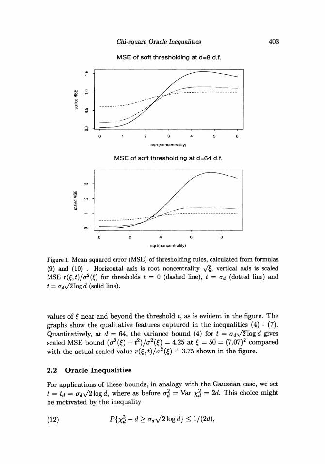
Formulas (9) and (10) enable a straightforward numerical evalution of therisk of thresholding. Figure 1 compares the mean squared error (MSE) ofthresholding at t = 0,1 or \/2 log d standard deviations σd for d = 8 and16. [Numerical integration in r(ξ, ί) = r(0, ί) + f£ Dςr(u, t)du was performedusing the routine integrate in S-PLUS.] The positive part rule (REFER TOTHIS) (ί = 0), namely (w - d)+ yields up to 50% MSE savings at ξ =0. However, to obtain smaller risks at 0 necessarily entails larger MSE at
Chi-square Oracle Inequalities
MSE of soft thresholding at d=8 d.f.
403
MSE of soft thresholding at d=64 d.f.
4 6
sqrt(noncentrality)
Figure 1. Mean squared error (MSE) of thresholding rules, calculated from formulas
(9) and (10) . Horizontal axis is root noncentrality y/ξ, vertical axis is scaled
MSE r(ξ,t)/σ2(ξ) for thresholds t = 0 (dashed line), t = σd (dotted line) and
t = σd\/2ϊogd (solid line).
values of £ near and beyond the threshold ί, as is evident in the figure. The
graphs show the qualitative features captured in the inequalities (4) - (7).
Quantitatively, at d — 64, the variance bound (4) for t = σd\/2 log d gives
scaled MSE bound (σ2(ξ) + t2)/σ2(ξ) = 4.25 at ξ = 50 = (7.07)2 compared
with the actual scaled value r(£,ί)/σ 2(ξ) = 3.75 shown in the figure.
2.2 Oracle Inequalities
For applications of these bounds, in analogy with the Gaussian case, we set
t = td = σd\f2 log cf, where as before σ\ = Var χ2
d = 2d. This choice might
be motivated by the inequality
(12) P{Xd ~d>
404 Iain M. Johnstone
which shows that if ξ = 0, then ξtd = 0 with probability approaching 1 asd —> oo. Thus, there is a vanishing chance that ξtd will spuriously assertthe presence of structure when ξ is actually 0. Formula (12) follows fromLemma 6.1 for large d (d > 72 will do), while for smaller d, (12) may beverified numerically.
We give two inequalities - the first relates MSE to ideal risk, while thelatter is slightly more convenient for the application to adaptive estimationof J f2 in Section 4. The proof is given in the appendix.
Corollary 2.1 Let td = σdλ/2 log d. Then
(13) r(ξ,td) < (21ogd+l){ l + min(ξ2,σ2(ξ))} d > 3,
and
(14) r(ξ,td) <2/logd + mm{2ξ2,σ2{ξ) + t2
d}, d > 18.
We record the arbitrary noise level version of (14) for use in Section 4.
Corollary 2.2 Suppose that Y ~ Nd{θ,e2I) and that one seeks to estimatep — \θ\2 using \Y\2 ~ e 2 χ 2 (p/e 2 ). Suppose that the estimator βtd and variancefunction σ2(p) are defined by (1) and (2) respectively. Then
(15) E(ptd - p)2 < ^ + min{2p2, σ2(p) + eH\}.
3 Lower Bounds
This section argues that the bounds (13) and (14) are sharp for d large,in the sense that no other estimator can asymptotically satisfy a uniformlybetter bound.
We use a standard Bayesian two point prior method, but with non-standard loss function. The resulting bound in the Gaussian case, Proposi-tion 3.1, is then carried over to the chi-square setting via asymptotic nor-mality, to give Proposition 3.2.
Let {PΘ} be a family of probability measures on R, indexed by θ G Θ C M.Denote point mass at θ by VQ and consider two point prior distributions π =πo^0o +
7 Γi I /0i To use weighted squared error measure L(a,θ) = l(θ)(a — θ)2,we will need loss-weighted versions of these priors. With U = /(0i), these are
π = ι-ψ vθo + ι-ψ vθl, L =
Denote the corresponding posterior probabilities for π by
η(x) = P*({θo}\x), η(x) = P*{{θi}\*) = 1 "
L e m m a 3.1 With the previous definitions and for ΘQ = 0,
(16) R := inf sup l(θ)Eθ[θ(X) - θ]2 > lλΈλθ\ Eθlη2(X).
θ θ
Chi-square Oracle Inequalities 405
Proof The minimax risk R is bounded below by the Bayes risk £(τr), usingprior distribution π and loss function Z(α, 0) :
R > B(π) = inf [ π(dθ) Eθl(θ)[θ(X) - θ]2.θ J
At least to aid intuition, it helps to convert this into a Bayes risk for squarederror loss with modified prior π given above, so that
B(π) = L inf f π(dθ) EΘ[Θ(X) - θ}2 =: B(π).θ J
For squared error loss, now, the Bayes estimator 0^ that attains the minimumJB(τf) is given by the posterior mean, which in the two point case with 0o = 0takes the simple form
0#(s) = ^n[θ\x] = 0iP({0i}|x) = θiη{x),
which implies the desired formula (16):
B(π) = L f π(dθ)Eθ[θ*(X) - θ]2 > Lπ({θι})EOl[θιη(X) - 0i]2.
Proposition 3.1 Suppose X ~ N(θ, 1). Then as d -> cx>,
Proof In Lemma 3.1, let PQ correspond to X ~ N(θ, 1) and take l(θ) —
[dΓι + {θ2 A I ) ] " 1 . Choose θ0 = 0 and θι = θd » 1 (to be specified below),
so that lo = d and k = (1 + d " 1 ) " 1 .
Set TΓO = 1/ log d and TΓI = 1 — τro so that L = KQIO + π\l\ ~ dj log d and
the loss weighted prior π = (1 — e)i/o + e^ d with e = π\l\jL ~ logd/d small.
The idea is that with e small, we choose θd so that even for x near 0^,
η[x) = P^({0}|x) « 1. Thus, with probability essentially e we estimate
θjt w 0 even though θ = θd and so incur an error of about 0^.
Now the details. Write g{x; θ) for the JV(0,1) density and, since we will
recenter at 0 , put x = θd + z. Then the likelihood ratio
406 Iain M. Johnstone
Of course, the posterior probability η(x) can be written in terms of thelikelihood ratio as
(19) η{βd + z) = [1 + ί ZooCz; θd)]-\
Put αd = log log d and specify θd as the solution to η(θd + α<f) = 1/2? so that
(20) θdαd + θj/2 = log ί ^ = log d - log log d + o(l),
and hence θd ~ \/2 log d, and also
for all fixed 2:. Consequently
= Jη2(θd
by the dominated convergence theorem. Since hπ\ ~ 1 and θ\ ~ 21ogd, theresult now follows from Lemma 3.1. •
With the Gaussian bound as template, we turn to the correspondingresult for the non-central chi-squared distributions.
Proposition 3.2 Suppose that Wd ~ X^(0 As d -> 00,
Proof The rescaled variable X = (W - d)/y/2d has mean θ = ξ/y/2d,variance σ\(θ) = 1 + θy/8/d and is εtsymptotically Gaussian as d —> 00.Let <7d(£#? ) denote its density function. As in the proof of Proposition 3.1,we recenter at θd ~ \/2 log d (to be defined precisely below) and form thelikelihood ratio
/ 9 9 N j ,.n \ 9d{θd + Z\ θd)
9d\βd + z',ϋ)
With Zoo(y ^d) the corresponding Gaussian likelihood ratio defined at (18),
(23) ud(y) = l^f ^ 1 , a d -4 oo
uniformly in |y| < logd, say (see Appendix.)
Chi-square Oracle Inequalities 407
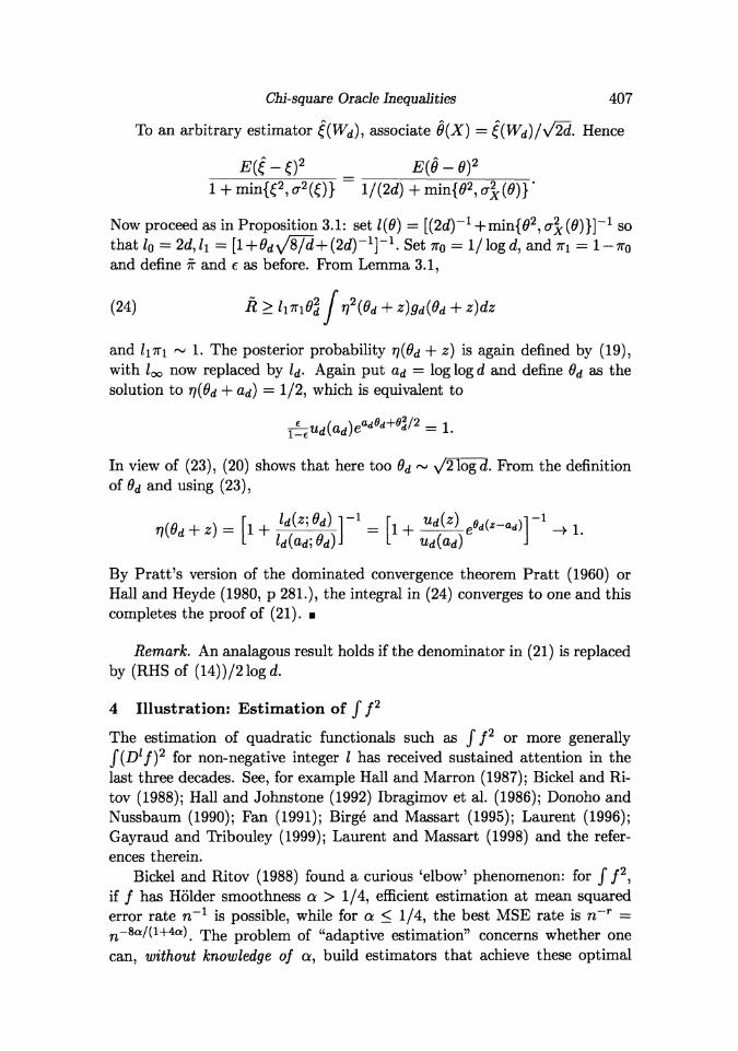
To an arbitrary estimator f (W^), associate Θ(X) = ξ(Wd)/y/2d. Hence
Q 2
= E(θ - θ)2
Now proceed as in Proposition 3.1: set l(θ) = [(2d)~1 + min{02, σ2
x{θ)}}~1 sothat Zo = 2d,/i = [l + v ^ + ί 2 ^ ) " 1 ] " 1 - S e t πo = 1/logd, andπi = l - π 0
and define π and e as before. Prom Lemma 3.1,
(24) R > hπtfl Jη2(θd + z)gd(θd + z)dz
and ZiTΓi ^ l. The posterior probability η(θd + 2:) is again defined by (19),with ZQO now replaced by ld. Again put αd = log log d and define θd as thesolution to η(θd + αd) = 1/2, which is equivalent to
In view of (23), (20) shows that here too θd ~ \/2 log d. Prom the definitionof θd and using (23),
By Pratt's version of the dominated convergence theorem Pratt (1960) orHall and Heyde (1980, p 281.), the integral in (24) converges to one and thiscompletes the proof of (21). •
Remark. An analagous result holds if the denominator in (21) is replacedby (RHSof (14))/21ogd.
4 Illustration: Estimation of f f2
The estimation of quadratic functionals such as J f2 or more generallyJ(Dιf)2 for non-negative integer / has received sustained attention in thelast three decades. See, for example Hall and Marron (1987); Bickel and Ri-tov (1988); Hall and Johnstone (1992) Ibragimov et al. (1986); Donoho andNussbaum (1990); Fan (1991); Birge and Massart (1995); Laurent (1996);Gayraud and Tribouley (1999); Laurent and Massart (1998) and the refer-ences therein.
Bickel and Ritov (1988) found a curious 'elbow' phenomenon: for / / 2 ,if / has Holder smoothness a > 1/4, efficient estimation at mean squarederror rate n~ι is possible, while for a < 1/4, the best MSE rate is n~ r =
n-8α/(i+4α) rp^ p r o b i e r n of "adaptive estimation" concerns whether onecan, without knowledge of α, build estimators that achieve these optimal
408 Iain M. Johnstone
rates for every α in a suitable range. Alas, Efromovich and Low (1996α,6)showed that this is not possible as soon as 0 < α < 1/4. They go on toadapt version of Lepskii's general purpose step-down adaptivity construction(Lepskii, 1991) to build an estimator that is efficient for α > 1/4 and attainsthe best rate (logarithmically worse than n~r) that is possible simultaneouslyfor 0 < α < 1/4.
The treatment here is simply an illustration of chi-square thresholdingto obtain the Efromovich-Low result. Two recent works (received after thefirst draft was completed) go much further with the f f2 problem. Gayraudand Tribouley (1999) use hard thresholding to derive Efromovich-Low, andgo on to provide limiting Gaussian distribution results and even confidenceintervals. Laurent and Massart (1998) derive non-asymptotic risk boundsvia penalized least squares model selection and consider a wide family offunctional classes including ip and Besov bodies.
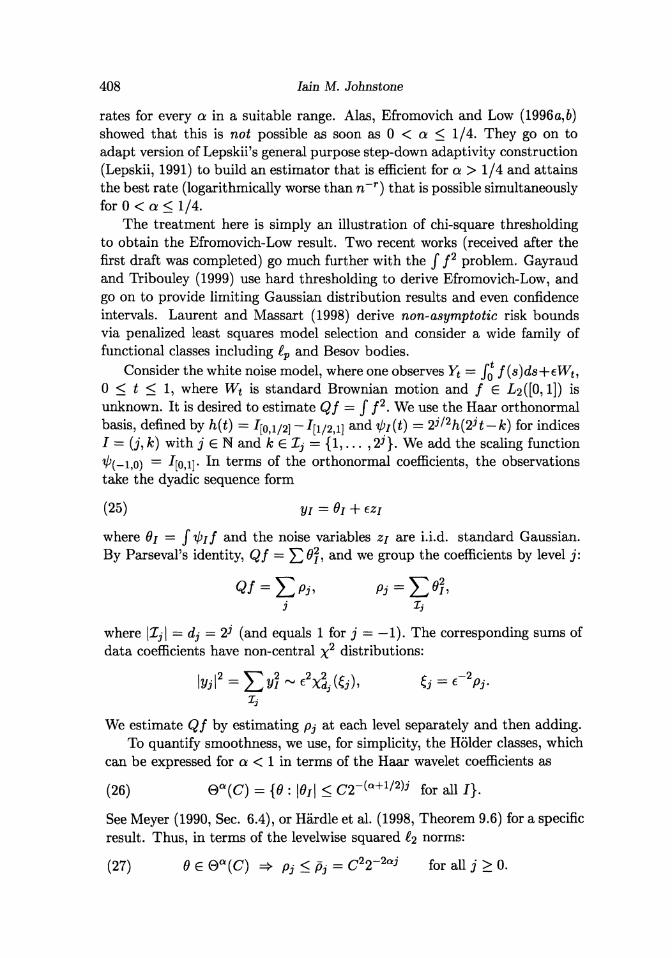
Consider the white noise model, where one observes Yt = f£ f(s)ds+eWt,0 < t < 1, where W% is standard Brownian motion and / G I/2([0,1]) isunknown. It is desired to estimate Qf = J f2. We use the Haar orthonormalbasis, defined by h(t) = i"[o,i/2] ~ J[i/2,i] a n d ψi(t) = 2^2h(2H — k) for indices/ = (j, A;) with j G N and k e lj = {1,... , 2j}. We add the scaling function^(-i,o) = [0,1] ^ n t e r m s of Λe orthonormal coefficients, the observationstake the dyadic sequence form
(25) yi = θt + ezi
where θj = Jφif and the noise variables zι are i.i.d. standard Gaussian.By Parseval's identity, Qf — £)0j, and we group the coefficients by level j:
where \lj\ = dj = 2J (and equals 1 for j = — 1). The corresponding sums ofdata coefficients have non-central χ2 distributions:
We estimate Qf by estimating pj at each level separately and then adding.
To quantify smoothness, we use, for simplicity, the Holder classes, which
can be expressed for a < 1 in terms of the Haar wavelet coefficients as
(26) θa(C) = {θ : \θi\ < C 2 " ( Q + 1 / 2 ^ for all J}.
See Meyer (1990, Sec. 6.4), or Hardle et al. (1998, Theorem 9.6) for a specific
result. Thus, in terms of the levelwise squared l<ι norms:
(27) θ <Ξ Θ α (C) => Pj < pj = C22~2aj for all j > 0.
Chi-square Oracle Inequalities 409
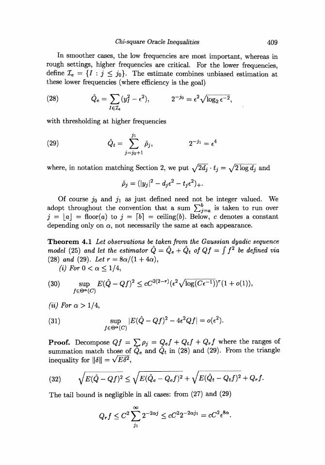
In smoother cases, the low frequencies are most important, whereas inrough settings, higher frequencies are critical. For the lower frequencies,define l e — {I : j < j0}. The estimate combines unbiased estimation atthese lower frequencies (where efficiency is the goal)
(28) Qe = £ (y? - e2),ieXe
with thresholding at higher frequencies
(29) Qt=j
where, in notation matching Section 2, we put y/2dj tj = y/2 log dj and
Of course jo &nd jι as just defined need not be integer valued. Weadopt throughout the convention that a sum Σbj=α is taken to run overj = [α\ = floor(α) to j = [b] = ceiling(6). Below, c denotes a constantdepending only on α, not necessarily the same at each appearance.
Theorem 4.1 Let observations be taken from the Gaussian dyadic sequencemodel (25) and let the estimator Q = Qe + Qt of Qf = J f2 be defined via(28) and (29). Let r = 8α/(l + 4α),
(i) For 0 < α < 1/4,
(30) sup E(Q - Qf)2 < cC2^2-r\e2y/\og(Ce-^)r{l + o(l)),/Gθ«(C)
^ For α > 1/4,
(31) sup \E(Q-Qf)2-4e2Qf\ = o()
Proof. Decompose Qf = Σ,Pj = Qef + Qtf + Qrf where the ranges ofsummation match those of Qe and Qt in (28) and (29). From the triangleinequality for \\δ\\ =
(32) y/E{Q - Qf)2 < \]E{Qe - Qef)2 + sjE{Qt - Qtf)
2 + QJ
The tail bound is negligible in all cases: from (27) and (29)
oo
rj < o > z s cu Δ — co e .
Jl
410 Iain M. Johnstone
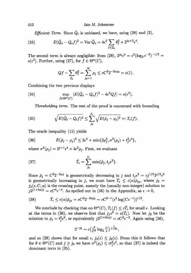
Efficient Term. Since Qt is unbiased, we have, using (28) and (2),
(33) E(Qe - Qef)2 = Var Qe = 4e2 ] Γ θj + 2 J 0 + 2 e 4 .
The second term is always negligible: from (28), 2 7 0 e 4 = e2(log2e~2)~1/2
o(e2). Further, using (27), for / G Θ α (C),
Xe iθ + 1
Combining the two previous displays
(34) sup \E(Qe - QJ)2 - 4ε 2 Q/| = o(e2).feeσ{c)
Thresholding term. The rest of the proof is concerned with bounding
(35) yjE(Qt - Qtf? < Σ \lE{pj - Pj)2 =: Te(/).JO
The oracle inequality (15) yields
(36) ^(p,- - P j ) 2 < 2e4 + min{2p2, σ2(Pj) + ί^e4},
where σ2(pj) = 2 J + 1 e 4 + 4e2pj. First, we evaluate
jl
(37) f^^minίp^ί . e2}.
30
Since pj = C22~2αi is geometrically decreasing in j and tjβ2 = cj1/22 J/2e2
is geometrically increasing in j , we must have Te < c(α)pj2, where j2 =j2(c; C, &) is the crossing point, namely the (usually non-integer) solution to
j 2(i+4a)j = c c 4
e - 4 . As spelled out in (56) in the Appendix, as e -> 0,
(38) fe < c(α)p j 2 = cC 2 2- 2 ^ ' 2 - c C 2 " r ( e 2 logίCe"1))7*/2.
We conclude by checking that on Θ α (C), Te(f) < cTe for small e. Lookingat the terms in (36), we observe first that j\e2 = o(T€). Now let j% be thesolution to pj = ί 2e 2, or equivalently j 2 ( 1 + 2 a ) J = cC2e~2. Again using (56),
and so (28) shows that for small e, js(e) < jo(e) From this it follows thatfor θ E θα(C) and j > j 0 we have σ2(pj) < cήeA, so that (37) is indeed thedominant term in (35).
Chi-square Oracle Inequalities 411
In the efficient case, (38) is negligible, so that (31) follows from (32)and (35). In the nonparametric zone 0 < α < 1/4, (38) shows that (34) isnegligible relative to (35), from which we obtain (30). •
Remark. Haar wavelets have been ingeniously used by Kerkyacharianand Picard (1996) in the context of estimating f f2 and especially J / 3 .However, thresholding is not used there, nor is adaptivity considered.
5 Remarks on weighted chi-square
Suppose, as before, that yk ~ ΛΓ(0fc,e2),fc = l , . . . d are independent, but
that now we desire to estimate pa = 5 ^ OL\ZΘ\ with α^ > 0. Such a scenario
emerges in estimation of f(Dιf)2, for example. Then the natural unbiased
estimator pu^a = Σ i ak{Vk ~~ e 2 ) ι s n 0 l ° n g e r a shift of a chi-square variate.
If the weights are comparable, say 1 < otk < ot for all fc, then an extension
of the risk bounds of Theorem 2.1 is possible. We cite here only the extension
of Corollary 2.2, referring to Johnstone (2000) for further results and details.
Proposition 5.1 With the above notations, set td = σ^\/2 log d. There ex-
ists an absolute constant 7 such that
E[p{Ua; Std) - Pa? < Ίa2 [ ^ + min{2p2, σ
2(Pa) + eH2}}.
6 Appendix
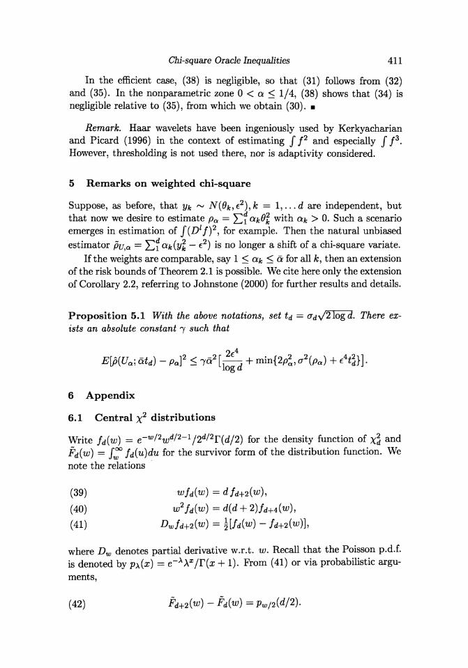
6.1 Central χ2 distributions
Write fd{w) = e~wl2
w
dl2-1 /2d/2Γ(d/2) for the density function of χ2
d and
Fd(w) = J°° fdiu)du for the survivor form of the distribution function. We
note the relations
(39) wfdM=
(40) w2fd{w) =
(41) Dwfd+2(w) = \[fd{w)
where Dw denotes partial derivative w.r.t. w. Recall that the Poisson p.d.f.
is denoted by pχ(x) = e~xXx/Γ(x + 1). Prom (41) or via probabilistic argu-
ments,
(42) Fd+2(w) - Fd(w) = pw/2(d/2).
412 Iain M. Johnstone
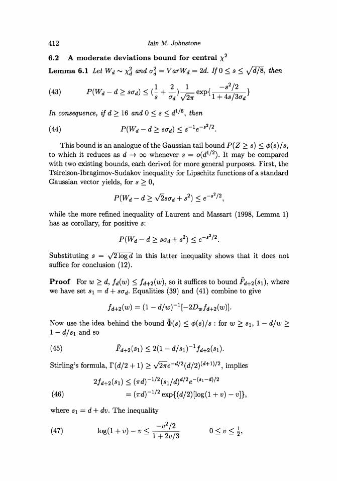
6.2 A moderate deviations bound for central χ2
Lemma 6.1 Let Wd ~ χ2
d and σ\ = VarWd = 2d.IfO<s< y/dβ, then
(43) P(Wd - d > sσd) < (- + - ^ ~f/2
s σd
In consequence, if d > 16 and 0 < s < d1/6, then
(44) P{Wd -d> sσd) < s-ιe~s2/2.
This bound is an analogue of the Gaussian tail bound P(Z > s) < φ(s)/s,to which it reduces as d -ϊ oo whenever s = o(dιl2). It may be comparedwith two existing bounds, each derived for more general purposes. First, theTsirelson-Ibragimov-Sudakov inequality for Lipschitz functions of a standardGaussian vector yields, for 5 > 0,
P(Wd -d> V2sσd + s2) < e~s2l2,
while the more refined inequality of Laurent and Massart (1998, Lemma 1)has as corollary, for positive s:
Substituting 5 = y/2 log d in this latter inequality shows that it does notsuffice for conclusion (12).
Proof For w > d, fd(w) < ^+2(^)5 so it suffices to bound Fd+2(si), wherewe have set s\ = d + sσd. Equalities (39) and (41) combine to give
Now use the idea behind the bound Φ(s) < φ(s)/s : for w > si, 1 — d/w >1 — d/s\ and so
(45) Fd+2(Sl) < 2(1 - d / s i ) " 1 / ^ ^ ! ) .
Stirling's formula, Γ(d/2 + 1) > λ/2^e- ί i/2(ίί/2)(<i+1)/2, implies
(46) = ( π d ) - 1 ' 2 e x p { ( d / 2 ) p o g ( l + v ) - v}},
where si — d + dv. The inequality
(47) losiί + v ) - v < - ^ - „ < . < } ,
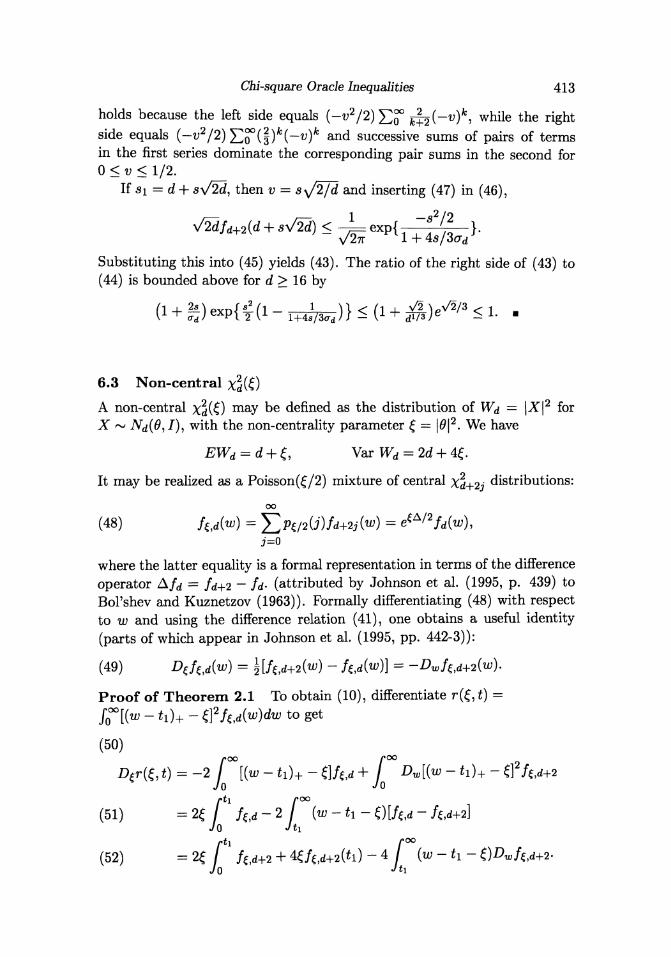
Chi-square Oracle Inequalities 413
holds because the left side equals (-v2/2) Σ™ ^ ( - i ; ) * , while the rightside equals (-v2/2) Σ5°(§)fc(-v)fe a n d successive sums of pairs of termsin the first series dominate the corresponding pair sums in the second for0 < v < 1/2.
If si = d + sVϊd, then υ = Sy/2β and inserting (47) in (46),
< - * exp{y/2π 1
Substituting this into (45) yields (43). The ratio of the right side of (43) to(44) is bounded above for d > 16 by
6.3 Non-central χ2
d(ξ)
A non-central χ^(ξ) may be defined as the distribution of Wd = \X\2 forX ~ Nd(θ,I), with the non-centrality parameter ξ — |0|2. We have
It may be realized as a Poisson(ξ/2) mixture of central χ^+ 2 j distributions:
(48) fcd(w)i=o
where the latter equality is a formal representation in terms of the differenceoperator Afd = fd+2 ~ fd (attributed by Johnson et al. (1995, p. 439) toBoΓshev and Kuznetzov (1963)). Formally differentiating (48) with respectto w and using the difference relation (41), one obtains a useful identity(parts of which appear in Johnson et al. (1995, pp. 442-3)):
(49)
Proof of Theorem 2.1 To obtain (10), differentiate r(ξ,t) =
(50)
Dξr{ξ, t) = -2 Γ[{w - ti)+ - ξ]fζtd + ί Dw[(w -Jo Jo
(51) =2ξ f1 fζ4 ~ 2 Γ(w - ίi - ξ)[fζ,d ~ Λ,Jo Jti
rti
(52) = 2ξ / /e,d+2 + 4ξ/C ld+2(ti) - 4Jo
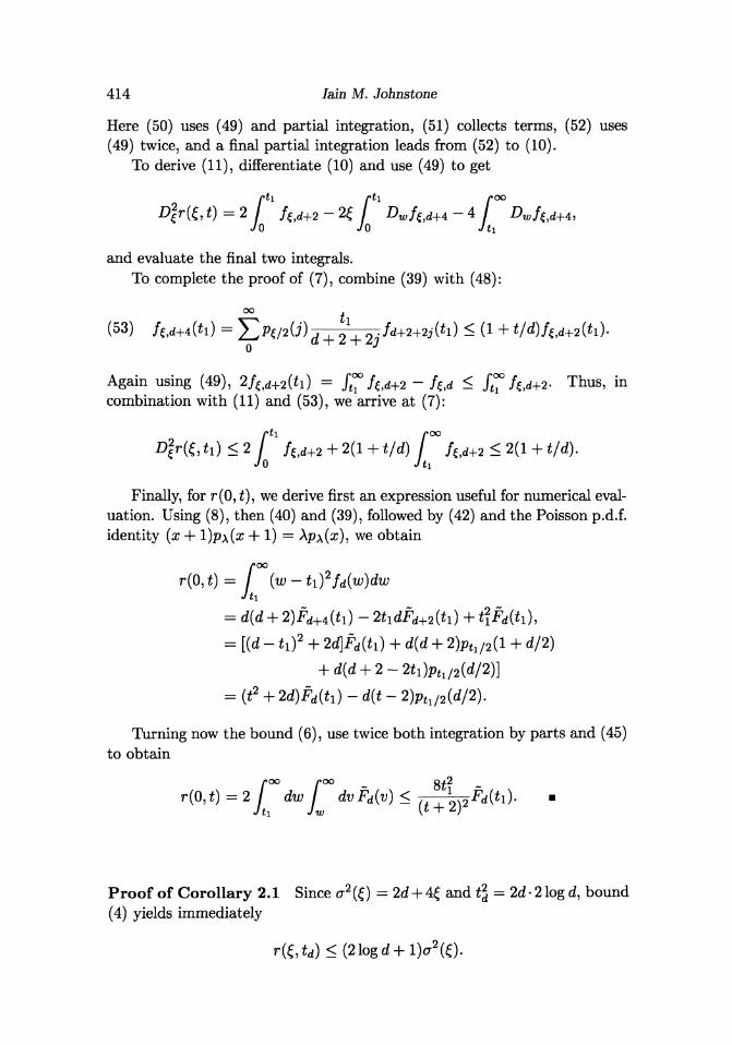
414 Iain M. Johnstone
Here (50) uses (49) and partial integration, (51) collects terms, (52) uses(49) twice, and a final partial integration leads from (52) to (10).
To derive (11), differentiate (10) and use (49) to get
£>f r(£, i) = 2 / * fξM2 -2ξΓ DwfξM4 - 4 fJO Jo Jti
and evaluate the final two integrals.
To complete the proof of (7), combine (39) with (48):
°° t(53) /€ld+4(fi) = ΣPφWd + 2 + 2j
fd+2+2j{tl) " ( 1 +
Again using (49), 2 / w + 2 ( ί i ) = /~/ξ,d+2 - fξ,d < f™ fζW Thus, incombination with (11) and (53), we arrive at (7):
D2r(ξ, h)<2 f1 fζM2 + 2(1 + t/d) Γ fζM2 < 2(1 + t/d).Jθ Jti
Finally, for r(0, ί), we derive first an expression useful for numerical eval-uation. Using (8), then (40) and (39), followed by (42) and the Poisson p.d.f.identity (x + l)pχ(x + 1) = λp\(x), we obtain
r(0, t) = / (w— tχ)2fd{w)dwJti
= [(d - h)2 + 2d\Fd(h) + d(d + 2 ) f t l / 2 ( l + d/2)
2-2ti)ptι,2(d/2)]
- d(t - 2)Ptl/2(d/2).
Turning now the bound (6), use twice both integration by parts and (45)
to obtain
roo roo oj.2
(0,t) = 2 / dw / dvFd(v) < _ - i.2
Proof of Corollary 2.1 Since cr2(ξ) = 2d + 4ξ and t2
d = 2d 2 log d, bound(4) yields immediately
r(£,td) <(21ogd+l)σ 2 (0 .
Chi-square Oracle Inequalities 415
For (13) it remains to check that r(ξ,td) < (21ogd + 1) + (21ogd + 1)£2. Inview of (5), this will follow from
(54) η2 < 2 log d, r(0, td) + ηλ < 2 log d + 1.
Bearing in mind (3) and bound (6), it can be verified numerically that theinequalities (54) are valid for d > 3 and d > 2 respectively.
For (14) we need only verify that r(ξ, td) < 2(log d)" 1 + 2ξ2 and this willfollow from more stringent versions of (54):
(55) % < 1 , r(0,*d) + 7/i<2/log<I
These can be verified numerically for d > 14 and d > 18 respectively. Forcompleteness, we show that (55) (and hence (54)) follow, for large d, from(44). Indeed, some algebra shows
2Fd(d + td) < 2Fd+2{d + td) =m< ?a log a
Using bound (6), we then have
Taking d large in these last two displays implies (55).
Proof of (23) Let N ~ Poisson(ξ/2). Prom (48)
fξ,d(w) _ P fd+2N(w) _} T(d/2 +
The likelihood ratios (22) involve the transformed variable X = (W —d)l\ί2d. Thus with θ = ξ/\/2d, we have gd(x; θ) = V2dfζ,d(d + x\/2d).Using Stirling's formula Γ(s) = V^e-^/ ' s*- 1 / 2 , with \η\ < 1/12, andsetting m = d/2 and x = θj, + z, we obtain the representation
and
Lm = N - (m + N - \) log(l + ^) + ΛΠog(l + ^ ) - θ2mz - Θ2
2J2.
Write the Poisson variable in the form N = θdy/m + Zmy/Θ^m1/4, so that
Zm 4 Z as m -> oo. Expanding the logarithms in Taylor series and collecting
416 Iain M. Johnstone
terms shows that Lm = op(l) uniformly in \z\ < logd, and along with Rm =
op(l), this completes the proof of (23). •
Details for Theorem 4.1. Fix 7 > 0. Let x(z) be the solution of xTx = z.
The approximate solution xo = %o(z) given by
(56) 27 X o (* )
log2
as z —> 00. More precisely, for large z,
(57) 2™W e [c(z), 1]2^W, c(z) > 1 -
To verify (57), set w = log2 z, so that log2x{z) = w — jx(z). Then
w w ~ w
Acknowledgements. Many thanks to David Donoho for his ideas andcollaboration in the first iteration of this project some years back, in a versionbased solely on Gaussian approximation. Thanks also to the AustralianNational University for hospitality and support when the first draft of thismanuscript was written and to the referees for their careful reading andcomments.
REFERENCES
Bickel, P. and Ritov, Y. (1988), 'Estimating integrated squared densityderivatives: sharp best order of convergence estimates.', Sαnkhyα, SeriesA 50, 381-393.
Birge, L. and Massart, P. (1995), 'Estimation of integral functionals of a
density', Annals of Statistics 23, 11-29.
Bol'shev, L. and Kuznetzov, P. (1963), O n computing the integral p(x,y) =...', Shurnal Vychislitelnoj Matematiki i Matematicheskoi Fiziki 3, 419-430. In Russian.
Chow, M. S. (1987), 4A complete class theorem for estimating a noncentrality
parameter', Annals of Statistics 15, 800-804.
Chi-square Oracle Inequalities 417
Donoho, D. L. and Johnstone, I. M. (1994), Ίdeal spatial adaptation viawavelet shrinkage', Biometrikα 81, 425-455.
Donoho, D. L. and Nussbaum, M. (1990), 'Minimax quadratic estimation ofa quadratic functional', Journal of Complexity 6, 290-323.
Efromovich, S. and Low, M. (1996α), O n Bickel and Ritov's conjecture aboutadaptive estimation of the integral of the square of density derivative',Annals of Statistics 24, 682-686.
Efromovich, S. and Low, M. (19966), O n optimal adaptive estimation of aquadratic functional', Annals of Statistics 24, 1106-1125.
Fan, J. (1991), O n estimation of quadratic functional', Annals of Statistics19, 1273-1294.
Gayraud, G. and Tribouley, K. (1999), 'Wavelet methods to estimate an in-tegrated quadratic functional: Adaptivity and asymptotic law', Statisticsand Probability Letters 44, 109-122.
Hall, P. G. and Marron, J. S. (1987), 'Estimation of integrated squareddensity derivatives', Statistics and Probability Letters 6, 109-115.
Hall, P. and Heyde, C. (1980), Martingale Limit Theory and Its Application,Academic Press.
Hall, P. and Johnstone, I. (1992), 'Empirical functional and efficientsmoothing parameter selection', Journal of the Royal Statistical Society,Series B 54, 475-530. with discussion.
Hardle, W., Kerkyacharian, G., Picard, D. and Tsybakov, A. (1998),
Wavelets, Approximation and Statistical Applications, Springer.
Ibragimov, I. A., Nemirovskii, A. S. and Khas'minskii, R. Z. (1986), 'Some
problems on nonparametric estimation in gaussian white noise', Theory of
Probability and its Applications 31, 391- 406.
Johnson, N. L., Kotz, S. and Balakrishnan, N. (1995), Continuous Univariate
Distributions, Volume 2, Second edition, John Wiley and Sons.
Johnstone, I. M. (2000), Thresholding and oracle inequalities for weighted
χ2, To appear, Statistica Sinica.
Kerkyacharian, G. and Picard, D. (1996), 'Estimating nonquadratic func-
tionals of a density using haar wavelets', Annals of Statistics 24, 485-507.
Laurent, B. (1996), 'Efficient estimation of integral functionals of a density',
Annals of Statistics 24, 659-681.
418 Iain M. Johnstone
Laurent, B. and Massart, P. (1998), Adaptive estimation of a quadraticfunctional by model selection, Technical report, Universite de Paris-Sud,Mathematiques.
Lepskii, O. (1991), On a problem of adaptive estimation in gaussian whitenoise', Theory of Probability and its Applications 35, 454-466.
Meyer, Y. (1990), Ondelettes et Operateurs, I: Ondelettes, II: Operateursde Calderόn-Zygmund, III: (with R. Coifman), Operateurs multilineaires,Hermann, Paris. English translation of first volume is published by Cam-bridge University Press.
Pratt, J. W. (1960), On interchanging limits and integrals', Annals of Math-ematical Statistics 31, 74-77.
Saxena, K. M. L. and Alam, K. (1982), 'Estimation of the non-centralityparameter of a chi-squared distribution', Annals of Statistics 10, 1012-1016.
DEPARTMENT OF STATISTICS
SEQUOIA HALL
STANFORD UNIVERSITY
STANFORD CA 94305U.S.A.imj@stat. Stanford, edu