A probabilistic analysis of some tree algorithms - Project Euclid
27
The Annals of Applied Probability 2005, Vol. 15, No. 4, 2445–2471 DOI: 10.1214/105051605000000494 © Institute of Mathematical Statistics, 2005 A PROBABILISTIC ANALYSIS OF SOME TREE ALGORITHMS BY HANÈNE MOHAMED AND PHILIPPE ROBERT INRIA In this paper a general class of tree algorithms is analyzed. It is shown that, by using an appropriate probabilistic representation of the quantities of interest, the asymptotic behavior of these algorithms can be obtained quite easily without resorting to the usual complex analysis techniques. This ap- proach gives a unified probabilistic treatment of these questions. It simplifies and extends some of the results known in this domain. 1. Introduction. A splitting algorithm is a procedure that divides recursively into subsets an initial set of n items until each of the subsets obtained has a cardi- nality strictly less than some fixed number D. These algorithms have a wide range of applications: (a) Data structures. These are algorithms on data structures used to sort and search. They are sometimes referred to as divide and conquer algorithms. See [6] and [23] for a general presentation and [28, 39, 40] for their analysis with analytical methods. (b) Communication networks. These algorithms are used to give a distributed access to a common communication channel that can transmit only one message per time unit. See [3, 10, 41]. (c) Distributed systems. Some algorithms use a splitting technique to select a subset of a set of identical communicating components. See [18, 36]. (d) Statistical tests. A test, performed on a set of individuals, indicates if at least one of these individuals has some characteristics (like a disease if this is blood testing). The purpose is to minimize the number of tests to identify individuals with the specified characteristic as quickly as possible. See [43]. Formally, a splitting algorithm can be described as follows: SPLITTING ALGORITHM S (n) —TERMINATION CONDITION. If n<D −→ STOP. —TREE STRUCTURE. If n ≥ D, randomly divide n into n 1 ,...,n G , with n 1 +···+ n G = n where G is a random variable with some fixed distribution. −→ APPLY S (n 1 ), S (n 2 ),..., S (n G ). Received November 2004; revised March 2005. AMS 2000 subject classifications. Primary 68W40, 60K20; secondary 90B15. Key words and phrases. Splitting algorithms, divide and conquer algorithms, unusual laws of large numbers, asymptotic oscillating behavior, data structures, tries, renewal theorem. 2445
-
Upload
khangminh22 -
Category
Documents
-
view
0 -
download
0
Transcript of A probabilistic analysis of some tree algorithms - Project Euclid

The Annals of Applied Probability2005, Vol. 15, No. 4, 2445–2471DOI: 10.1214/105051605000000494© Institute of Mathematical Statistics, 2005
A PROBABILISTIC ANALYSIS OF SOME TREE ALGORITHMS
BY HANÈNE MOHAMED AND PHILIPPE ROBERT
INRIA
In this paper a general class of tree algorithms is analyzed. It is shownthat, by using an appropriate probabilistic representation of the quantities ofinterest, the asymptotic behavior of these algorithms can be obtained quiteeasily without resorting to the usual complex analysis techniques. This ap-proach gives a unified probabilistic treatment of these questions. It simplifiesand extends some of the results known in this domain.
1. Introduction. A splitting algorithm is a procedure that divides recursivelyinto subsets an initial set of n items until each of the subsets obtained has a cardi-nality strictly less than some fixed number D. These algorithms have a wide rangeof applications:
(a) Data structures. These are algorithms on data structures used to sort andsearch. They are sometimes referred to as divide and conquer algorithms. See [6]and [23] for a general presentation and [28, 39, 40] for their analysis with analyticalmethods.
(b) Communication networks. These algorithms are used to give a distributedaccess to a common communication channel that can transmit only one messageper time unit. See [3, 10, 41].
(c) Distributed systems. Some algorithms use a splitting technique to select asubset of a set of identical communicating components. See [18, 36].
(d) Statistical tests. A test, performed on a set of individuals, indicates if at leastone of these individuals has some characteristics (like a disease if this is bloodtesting). The purpose is to minimize the number of tests to identify individualswith the specified characteristic as quickly as possible. See [43].
Formally, a splitting algorithm can be described as follows:
SPLITTING ALGORITHM S(n)
— TERMINATION CONDITION.If n < D −→ STOP.
— TREE STRUCTURE.If n ≥ D, randomly divide n into n1, . . . , nG, with n1 + · · · + nG = n
where G is a random variable with some fixed distribution.−→ APPLY S(n1), S(n2), . . . , S(nG).
Received November 2004; revised March 2005.AMS 2000 subject classifications. Primary 68W40, 60K20; secondary 90B15.Key words and phrases. Splitting algorithms, divide and conquer algorithms, unusual laws of
large numbers, asymptotic oscillating behavior, data structures, tries, renewal theorem.
2445

2446 H. MOHAMED AND P. ROBERT
1.1. Description. The algorithm starts with a set of n items. This set is ran-domly split into G subsets, the distribution of G is given by P(G = �) = p�, where(p�) is a probability distribution on {2,3, . . . }. Now, conditionally on the event{G = �}, for 1 ≤ i ≤ �, an item is sent into the ith subset with probability Vi,�,where V� = (Vi,�;1 ≤ i ≤ �) is a random probability vector on {1, . . . , �}. It canalso be seen as a vector of random weights on the � arcs of the branching procedureon which each of the n items perform a random walk.
If Ni is the cardinality of the ith subset, then, conditionally on the event {G =�} and on the random variables V1,�, V2,�, . . . , V�,�, the distribution of the vector(N1, . . . ,N�) is multinomial with parameter n and (V1,�, V2,�, . . . , V�,�),
P((N1, . . . ,N�) = (m1, . . . ,m�)
) = n!m1!m2! · · ·m�!
�∏k=1
(Vk,�)mk ,
for (mi) ∈ Nn such that m1 + · · · + m� = n. If the ith subset, 1 ≤ i ≤ n, is such
that Ni < D, the algorithm stops for this subset. Otherwise, it is applied to the ithsubset: a variable Gi , with the same distribution as G, is drawn and this ith subsetis split into Gi subsets, and so on.
Such a random splitting has been introduced by Devroye [7] where the asymp-totic expansion of the depth of the associated tree is investigated.
EXAMPLES. (i) Knuth’s algorithm. When P(G = 2) = 1, D = 2 and V1,2 ≡V2,2 ≡ 1/2, this is one of the oldest algorithms of this kind. It was analyzed byKnuth in 1973.
(ii) Symmetrical splitting algorithm. This is the case where Vi,n ≡ 1/n for anyn ≥ 2 and 1 ≤ i ≤ n.
(iii) Q-ary algorithm. If P(G = Q) = 1 and D = 2, this is the Q-ary resolutionalgorithm with blocked arrivals analyzed by Mathys and Flajolet [30].
See also [7] for other examples. Quite naturally, such an algorithm can be graph-ically represented with a tree as shown by Figure 1.
Splitting measure. As it will be seen in the following, the key characteristicof this splitting algorithm is a probability distribution W on [0,1] defined withthe branching distribution (the variable G) and the weights on each arc [the vector(V1,G, . . . , VG,G)]. The asymptotic behavior of the algorithm is expressed natu-rally in terms of the distribution W .
DEFINITION 1. The splitting measure is the probability distribution Won [0,1] defined by, for a nonnegative Borelian function f ,
∫f (x)W(dx) = E
(G∑
i=1
Vi,Gf (Vi,G)
)=
+∞∑�=2
�∑i=1
P(G = �)E(Vi,�f (Vi,�)
).(1)

PROBABILISTIC ANALYSIS OF TREE ALGORITHMS 2447
FIG. 1. Splitting algorithm with D = 2, two sets of random weights (V1,2,V2,2) and(V1,3,V2,3,V1,3), G a random variable with values in {2,3} and the initial items A, B , C, D,E and F .
ASSUMPTION (A). Throughout the paper, it is assumed that, almost surelyG ≥ 2, and that there exists some δ > 0 such that the relation
sup�≥2
sup1≤i≤�
Vi,� ≤ δ < 1(A)
holds almost surely, in particular W([0, δ]) = 1. These conditions imply in partic-ular the nondegeneracy of the splitting mechanism.
DEFINITION 2. A splitting measure W is exponentially arithmetic if thereexists some λ > 0 such that
W({e−nλ :n ≥ 1}) = 1,
and the largest λ satisfying this relation is defined as the exponential span of W .
If A is some random variable with distribution W , then W is exponentiallyarithmetic with exponential span λ if and only if the distribution of − log(A) isarithmetic with span λ. See [14].
EXAMPLES. (i) Knuth’s algorithm, P(G = 2) = 1, D = 2 and V1,2 ≡V2,2 ≡ 1/2.
In this case
W(dx) = δ1/2,
where δx is the Dirac distribution at x and W is exponentially arithmetic withexponential span log 2.

2448 H. MOHAMED AND P. ROBERT
(ii) Symmetrical splitting algorithm.
W(dx) = ∑n≥2
P(G = n)δ1/n,
the exponential span is logD where D is the largest integer p such that the supportof the random variable G is contained in pN.
(iii) Q-ary algorithm, P(G = Q) = 1, D = 2, V1,Q = p1, . . . , VQ,Q = pQ:
W(dx) = p1δp1 + p2δp2 + · · · + pQδpQ,
the distribution W is exponentially arithmetic if and only if all the real numberslogpi/ logpj , 1 ≤ i < j ≤ Q, are rational.
The cost of a splitting algorithm. For such an algorithm, an important quantityis the number of operations required until the algorithm stops, that is, when all thesubsets have a cardinality less than or equal to D. Denote by Rn this quantity whenthe number of initial items is n; then clearly:
(a) Rn = 1 when n < D;(b) for n ≥ D,
Rndist.= 1 + R1,Nn
1+ · · · + RG,Nn
G,(2)
where conditionally on the event {G = �} and the random variables V1,�, V2,�,
. . . , V�,�,
(1) the vector (Nn1 , . . . ,Nn
� ) has a multinomial distribution with parameter n and(V1,�, V2,�, . . . , V�,�);
(2) for (pi) ∈ N�, the variables R1,p1, . . . ,R�,p�
are independent;(3) for 1 ≤ i ≤ �, the variable Ri,pi
has the same distribution as Rpi.
The variable Rn is simply the number of nodes of the associated tree; see Figure 1.
1.2. Unusual laws of large numbers. Note that, since the splitting procedureis random, the variable Rn is a random variable. With the language of commu-nication networks, this quantity can be thought of as the total time to transmit n
initial messages. If E(Rn) is its expected value, E(Rn)/n is the average transmis-sion time of one message among n. From a probabilistic point of view, it is naturalto expect that the sequence (Rn) satisfies a kind of law of large numbers, that is,that (E(Rn)/n) converges to some quantity α. The constant α is, in some sense,the asymptotic average transmission time of a message. Curiously, this law of largenumbers does not always hold. In some situations, the sequence (E(Rn)/n) doesnot converge at all and, moreover, exhibits an oscillating behavior.
When the splitting degree is constant and equal to 2 and V1,2 ≡ V2,2 ≡ 1/2(the items are equally divided among the two subsets), these phenomena are quitewell known. They have been analyzed using complex analysis techniques, func-

PROBABILISTIC ANALYSIS OF TREE ALGORITHMS 2449
tional transforms (and their associated inversion procedures) by Knuth [23], Fla-jolet, Gourdon and Dumas [13], Louchard and Prodinger [27] and many others.See [16, 28, 39] for a comprehensive treatment of this approach. See also [8] fora survey of the domain. Robert [38] proposed an alternative, elementary methodto get the asymptotic behavior of some related oscillating sequences without usingcomplex analysis.
When the splitting degree is constant and equal to Q but the items are notequally divided among the subsets, studies are quite rare. Using complex analy-sis techniques, Fayolle, Flajolet and Hofri [12] obtained the asymptotic behaviorof the associated sequence (E(Rn)). Mathys and Flajolet [30] presented a sketchof a generalization of this study when Q is arbitrary.
Some alternative approaches. (i) Some laws of large numbers have beenproved by Devroye [8] in a quite general framework for various functionals of theassociated trees. Talagrand’s concentration inequalities are the main tools in thisstudy. In our case, it would consist in proving that the distribution of the randomvariable Rn/E(Rn) is sharply (with an exponential decay) concentrated around 1.Results on limiting distributions such as central limit theorems do not seem to beaccessible with this method.
(ii) Clement, Flajolet and Vallée [5] analyzed related algorithms in the moregeneral context of dynamical systems. By using a Hilbertian setting, they showedthat the first-order behavior of the algorithms is expressed in terms of the spectrumof a functional operator, the transfer operator. Getting explicit results in this wayrequires therefore a good knowledge of some eigenvalues of the transfer operator.
A dynamic version of this class of algorithms is investigated in [33]. The split-ting procedure is the same but, in the language of branching processes, an immi-gration occurs at every leaf of the associated tree, that is, new items arrive everytime unit. This dynamic feature complicates the problem. In this case, an additionalprobabilistic tool has to be used: an autoregressive process with moving averageplays an important role.
1.3. Related problems.
Fragmentation processes. A continuous version of a splitting algorithm couldbe defined as follows: an initial mass of size x is randomly split into several piecesand, at their turn, each of the pieces is randomly split. . . . A class of such modelshas been recently investigated. The fragmentation of each mass occurs after someindependent exponential time with a parameter depending, possibly, on its mass.See [2, 32] and references therein. The problems considered are somewhat differ-ent: regularity properties of associated Markov processes, duality, rate of decayof individual masses, loss of mass, asymptotic distributions, and so on. A split-ting algorithm is just a recursive fragmentation of an integer into integer piecesuntil each of the components has a size less than D. In a continuous setting, ananalogue of the algorithms considered here would consist in stopping the frag-

2450 H. MOHAMED AND P. ROBERT
mentation process of a mass as soon as its value is below some threshold ε > 0.
Random recursive decompositions. As it will be (easily) seen, a splitting algo-rithm can also be described as a random recursive splitting of the interval [0,1].For example, in the case of a dyadic splitting, starting from the interval [0,1], twosubintervals I1, I2 are created and each of them is split at its turn and so on.
These random recursive decompositions have been considered from the pointof view of the geometry of the boundary points by various authors, to express theHausdorff dimension of this set of points in particular. Mauldin and Williams [31]and Waymire and Williams [42] considered decompositions of the interval [0,1]which are not necessarily conservative, that is, when |I1| + |I2| < 1 holds withpositive probability in the dyadic case.
Hambly and Lapidus [15] and Falconer [11] considered decompositions of theinterval [0,1] from the point of view of the lengths of the associated subinter-vals. The interval [0,1] is represented by a nonincreasing sequence (Ln) whosesum is 1. For n ≥ 1, Ln is the length of the nth largest interval of the decompo-sition. This description is similar to the classical representation of fragmentationprocesses. See [34].
In this setting, multiplicative cascades and martingales introduced by Mandel-brot [29] and Kahane and Peyrière [19] show up quite naturally. They have beenanalyzed quite extensively; see [1, 25] and references therein.
1.4. An overview. The purpose of this paper is twofold. First, it considers split-ting algorithms with a random (and possibly unbounded) degree of splitting gen-eralizing the previous studies in this domain. Second, and this is in fact the mainpoint of the paper, it proposes a probabilistic approach that simplifies greatly theanalysis of these algorithms. Moreover, as a by-product, a new direct representa-tion of the asymptotic oscillating behavior is established.
The analysis proposed in this paper also starts from (2), but its treatment is sig-nificantly different from the analytic approach. After some transformation, (2) isinterpreted as a probabilistic equation which is iterated by using appropriate inde-pendent random variables. Following the method of Robert [38], the next step isto perform a probabilistic de-Poissonnization and, by using Fubini’s theorem con-veniently, to represent the quantity E(Rn) by using a Poisson point process on thereal line. The final, crucial step which differs from [38], consists in using the keyrenewal theorem to get the asymptotic behavior of the sequence (E(Rn)).
The approach is elementary; its main advantage over the analytic treatment liescertainly in the use of the renewal theorem which gives directly the asymptoticbehavior.
Results of the paper. Section 2 gives a useful representation for the averagecost of the algorithm. The main result of the paper for the asymptotic cost is thefollowing theorem in Section 3. This is a summary of Propositions 9 and 11.

PROBABILISTIC ANALYSIS OF TREE ALGORITHMS 2451
THEOREM 3 (Asymptotics of the average cost). For a splitting algorithm, un-der the condition ∫ 1
0
| log(y)|y
W(dy) < +∞,(3)
— if the splitting measure W is not exponentially arithmetic, then
limn→+∞
E(Rn)
n= E(G)
(D − 1)∫ 1
0 | log(y)|W(dy).(4)
— If the splitting measure W is exponentially arithmetic with exponential spanλ > 0, as n gets large, the equivalence
E(Rn)
n∼ F
(logn
λ
)(5)
holds, where F is the periodic function with period 1 defined by, for x ≥ 0,
F(x) = E(G)∫ 10 | log(y)|W(dy)
λ
1 − e−λ
×∫ +∞
0exp
(−λ
{x − logy
λ
})yD−2
(D − 1)!e−y dy
and {z} = z − �z is the fractional part of z ∈ R.
Condition (3) is not really restrictive since the variable G is bounded in practice.This theorem covers and extends some of the results in this domain: for Knuth’salgorithm [23] and for Q-ary algorithms with blocked arrivals [30], see Corollaries10 and 12.
Furthermore, when there are asymptotic periodic oscillations, the periodic func-tion F involved is expressed directly and not in terms of its Fourier coefficients asis usually the case. The expression of F generalizes the representation of [38]obtained for Knuth’s algorithm.
The distribution of the sequence (Rn) (and not only its average) is investigatedin Section 4. For simplicity, only the case where the variable G is constant andthe variables V·,G are equal to 1/G is considered. The purpose of this section isto show that the distribution of the Poisson transform of the sequence and, moregenerally, the distribution of most of the functionals of the associated tree, can beexpressed quite simply in terms of Poisson processes and uniformly distributedrandom variables.
Two representations of the distribution of the Poisson transform as a functionalof Poisson processes are derived. As a consequence, a law of large numbers isproved when the number of initial items has a Poisson distribution (Poisson trans-form). Moreover, the asymptotic oscillating behavior of the algorithm is proved as

2452 H. MOHAMED AND P. ROBERT
a consequence of a standard law of large numbers. These unusual laws of largenumbers are, in the end, in the realm of classical laws of large numbers.
The central limit theorem is also proved with a similar method in this case. Thisis a classical result (see [28]); it is usually proved with complex analysis methodsvia quite technical estimations. It is proved here as a consequence of the standardcentral limit theorem for independent random variables. At the same time, a newrepresentation of the asymptotic variance is obtained.
2. General properties. Throughout this paper, (N ([0, x])) denotes a Poissonprocess with intensity 1; equivalently it can also be described as a nondecreasingsequence (tn) such that (tn+1 − tn) is a sequence of i.i.d. random variables expo-nentially distributed with parameter 1. For x ≥ 0, the variable N ([0, x]) is sim-ply the number of tn’s in the interval [0, x]. See [20] for basic results on Poissonprocesses.
Equation (2) and the boundary conditions for the sequence (Rn) are summarizedin the following relation, for n ≥ 0:
Rndist.= 1 + R1,Nn
1+ · · · + RG,Nn
G− G1{n<D},
therefore,
Rn − 1 dist.=G∑
i=1
(Ri,Nn
i− 1
) + G1{n≥D}.(6)
DEFINITION 4. The Poisson transform of a nonnegative sequence (an) is de-fined as
∑n≥0
an
xn
n! e−x = E
(aN ([0,x])
).(7)
The following proposition gives useful representations of the Poisson transformof the sequence of (E(Rn)).
PROPOSITION 5 [Poisson transform of the sequence (Rn)]. For x > 0,
E(RN ([0,x])
) = 1 + E(G)E
(+∞∑i=0
1∏ik=1 Wk
1{tD≤x∏i
k=1 Wk}
),(8)
where (Wi) is an i.i.d. sequence of random variables with distribution W .
PROOF. If n is a Poisson random variable with parameter x, the splitting prop-erty of Poisson variables (see [20], e.g.) shows that, conditionally on the event

PROBABILISTIC ANALYSIS OF TREE ALGORITHMS 2453
{G = �} and on the variables V1,�, . . . , V�,�, the variables Nni , 1 ≤ i ≤ �, are inde-
pendent and Nni has a Poisson distribution with parameter xVi,l . Consequently, for
x > 0, if
�(x)def.= E(RN ([0,x])) − 1
xE(G),(9)
it is easily checked that E(G)�(x) → R1 − R0 = 0 as x ↘ 0.Since {N ([0, x]) ≥ D} = {tD ≤ x}, (6) gives the relation
�(x) =+∞∑�=2
P(G = �)E
(�∑
i=1
Vi,��(xVi,�)
)+ 1
xP(tD ≤ x).(10)
Equation (10) can then be rewritten as
�(x) = E(�(xW1)) + E
(1
x1{tD≤x}
).(11)
The iteration of (11) shows that, for n ≥ 1,
�(x) = E
(�
(x
n∏k=1
Wk
))+ E
(n−1∑i=0
1
x∏i
k=1 Wk
1{tD≤x∏i
k=1 Wk}
).
The assumption on the variable G and the sequence of vectors (Vn) implies that,almost surely, the sequence (
∏nk=1 Wk) converges to 0. The function � can thus
be represented as
�(x) = E
(+∞∑i=0
1
x∏i
k=1 Wk
1{tD≤x∏i
k=1 Wk}
).
The proposition has been proved. �
From now on, throughout the paper, (Wi) will denote an i.i.d. sequence of ran-dom variables on [0,1] with distribution W .
PROPOSITION 6 (Probabilistic de-Poissonnization). For n ≥ D, then
E(Rn) = 1 + E(G)E
(T (UD(n))−1∑
i=0
1∏ik=1 Wk
),(12)
where, for 0 < y < 1,
T (y) = inf
{i ≥ 1 :
i∏k=1
Wk < y
}
and UD(n) is the Dth smallest variable of n independent, uniformly distributed ran-
dom variables on [0,1] independent of (Wi).

2454 H. MOHAMED AND P. ROBERT
PROOF. For x > 0, by decomposing with respect to the number of points ofthe Poisson process (N (t)) in the interval [0, x], one gets, for 0 < α ≤ 1,
P(tD ≤ xα) =+∞∑n=D
P(tD ≤ xα,N ([0, x]) = n
)
=+∞∑n=D
P(tD ≤ xα|N ([0, x]) = n
)P
(N ([0, x]) = n
).
For n ≥ D, conditionally on the event {N ([0, x]) = n}, the variable tD has thesame distribution as the D smallest random variable of n uniformly distributedrandom variables on [0, x]. When x = 1, denote by UD
(n) a variable with this con-ditional distribution. Clearly, by homogeneity, the variable (tD|N ([0, x]) = n) hasthe same distribution as xUD
(n). Finally, one gets the identity
P(tD ≤ xα) =+∞∑n=D
P(UD
(n) ≤ α)xn
n! e−x
= E
( +∞∑n=D
1{UD(n)≤α}
xn
n! e−x
).
By using the independence of the sequence (Wi) and tD in (8), the last identitygives the relation
E(RN ([0,x])
) = 1 + E(G)E
(+∞∑i=0
1∏ik=1 Wk
+∞∑n=D
1{UD(n)≤
∏ik=1 Wk}
xn
n! e−x
).
By Fubini’s theorem and writing 1 = exp(x) exp(−x), this expression can berewritten as
D−1∑n=0
xn
n! e−x +
+∞∑n=D
(1 + E(G)E
(+∞∑i=0
1∏ik=1 Wk
1{UD(n)≤
∏ik=1 Wk}
))xn
n! e−x.
The identification of (7) of E(RN ([0,x])) and the last identity gives (12). �
COROLLARY 7 (Symmetrical Q-ary algorithm). When P(G = Q) = 1 holdsand Vi,Q ≡ 1/Q, for i = 1, . . . ,Q, then for n ≥ D,
E(Rn) = 1 + Q
Q − 1
(E
(Q
�− logQ UD(n)�) − 1
)(13)
with, for 0 ≤ x ≤ 1,
P(UD
(n) > x) =
D−1∑k=0
(n
k
)xk(1 − x)n−k.

PROBABILISTIC ANALYSIS OF TREE ALGORITHMS 2455
From (13), by using the fact that nUD(n) converges in distribution as n tends to
infinity, it is not difficult to get the asymptotic behavior of E(Rn). The generalcase, (12), is slightly more complicated. One has to study the asymptotics of theseries inside the expectation.
2.1. A functional integral equation. If R(x) = E(RN (]0,x])) denotes the ex-pected value of the Poisson transform of the sequence (Rn), then (6) gives therelation
R(x) = 1 ++∞∑�=2
P(G = �)E
(�∑
i=1
R(xVi,�)
)− E(G)P(tD ≥ x);
by denoting
h(x) = 1 − E(G)
∫ +∞x
uD−1
(D − 1)! du,
it is easy to see that the above identity can be written as the following integralequation:
R(x) =∫ +∞
0R(xu)
W(du)
u+ h(x).(14)
Recall that W is some probability distribution on the interval [0,1]. For the Q-aryprotocol considered by Mathys and Flajolet [30], this equation is
R(x) =Q∑
i=1
R(xpi) + h(x).
It is analyzed by considering the Mellin transform R∗(s) of R(x) on some verticalstrip S of C,
R∗(s) =∫ +∞
0R(u)us−1 du, s ∈ S,
which, in this case, is given by
R∗(s) = h∗(s)/(
1 −Q∑
i=1
1
psi
).
The analytical approach consists in analyzing the poles of R∗(s) on the right-handside of S, basically the solutions with positive real part of the equation
p−s1 + p−s
2 + · · · + p−sQ = 1.
Then, by inverting the Mellin transform and using complex analysis techniques,the asymptotic behavior of (R(x)) at infinity is described in terms of these poles.

2456 H. MOHAMED AND P. ROBERT
The final step, an analytic inversion of the Poisson transform together with techni-cal estimates, establishes a relation between the asymptotic behaviors of the func-tion x → R(x) and of the sequence (Rn).
In the general case considered here, (14) gives the following expression for theMellin transform of (R(x)):
R∗(s) = h∗(s)/(
1 −∫ +∞
0
1
us+1 W(du)
).
An analogue of the analytic approach would start with the study of the roots s ∈ C,�(s) ≥ 0, of the equation ∫ +∞
0
1
us+1 W(du) = 1,(15)
and, if possible, proceed with successive inversions of Mellin transform and Pois-son transform.
As it will be seen, our direct approach reduces to the minimum the technicalapparatus required for such an analysis. The Poisson transform of (Rn) is alsoused in our method, but it is conveniently represented [see (8)] so that it can beright away inverted to give an explicit expression (12) for E(Rn) which will givedirectly the asymptotic behavior of the sequence (E(Rn)).
Interestingly, (Ln) denotes the nonincreasing sequence of the lengths of thesubintervals of [0,1] associated to the splitting procedure (see Section 1.3). Thezeta function of the string (Ln) is defined as the meromorphic function
ζ(s) = ∑n≥1
Lsn, s ∈ C,
see [15] and [24]. It is not difficult to see that the relation
E(ζ(s)) =∫ +∞
0usW(du)
/(1 −
∫ +∞0
usW(du)
)
holds. In particular, the poles of the zeta function of the associated random recur-sive string can be expressed in terms of the solutions of (15).
3. Analysis of the asymptotic average cost.
An associated random walk. If (Wi) is an i.i.d. sequence with common distri-bution W defined by (1), the sequence (Bi) = (− log(Wi)) is an i.i.d. sequence ofnonnegative random variables. The random walk (Sn) is associated to (Bi),
Sn = B1 + B2 + · · · + Bn, n ≥ 0.
As it will be seen, the asymptotic behavior of the splitting algorithm depends agreat deal on the distribution of (Bi). For x > 0, the crossing time νx of level x
by (Sn) is defined as
νx = inf{n :Sn > x}.

PROBABILISTIC ANALYSIS OF TREE ALGORITHMS 2457
For 0 < y < 1, the variable T (y) of Proposition 6 is simply ν− log(y). See [9, 14]for the main results concerning renewal theory used in the following.
If is defined as
(x) = E
(νx−1∑i=0
exp
(i∑
k=1
Bk
)), x > 0,
then by (12),
E(Rn) = 1 + E(G)E[
(− log(UD
(n)
))].(16)
It is clear that − log(UD(n)) converges in distribution to +∞ as n goes to infinity.
The asymptotic behavior of at infinity is first analyzed; this function can berewritten as
(x)e−x = E
(νx−1∑i=0
eSi−x
)= E
(νx∑
i=1
eSνx−i−x
).(17)
3.1. The nonarithmetical case. In this part, it is assumed that the distributionof W1 is not exponentially arithmetic. See Definition 2.
LEMMA 8. Under the condition
E
( | log(W1)|W1
)=
∫ 1
0
| log(x)|x
W(dx) < +∞,
the relation
supx≥0
E(eSνx −x) < +∞
holds.
PROOF. Lorden’s inequalities (see [4, 26]) show that, for any p ≥ 0,
supx≥0
E((
Sνx − x)p) ≤ p + 2
(p + 1)E(B1)E(B
p+11 );
thus, one gets the relation
supx≥0
E(eSνx −x) ≤ 1
E(B1)
∫ +∞0
(u + 2)euP(B1 ≥ u)du
= E((B1 + 1)eB1
) − 1
= E
(− log(W1) + 1
W1
)− 1 < +∞. �
For i > 1, the renewal theorem shows that, when x goes to infinity, the variableSνx−i − x converges in distribution to −(τ ∗ + τ1 + τ2 + · · · + τi−1), where the

2458 H. MOHAMED AND P. ROBERT
variables (τn) are i.i.d. distributed as B1 and independent of τ ∗ whose distributionis given by
E(f (τ ∗)) = 1
E(B1)
∫ +∞0
f (u)P(B1 ≥ u)du,
for any nonnegative Borelian function on R. By Assumption (A), the incrementsof the random walk (Sn) are bounded below by − log(δ), therefore one gets therelation, for 1 < K ≤ νx ,
νx∑i=K
eSνx−i−x = eSνx −xνx∑
i=K
eSνx−i−Sνx ≤ eSνx −x δK
1 − δ.
From Lemma 8 and (17), one deduces then
limx→+∞(x)e−x = E
(+∞∑i=1
exp(−τ ∗ − τ1 − τ2 − · · · − τi−1)
)
= 1 − E(exp(−τ1))
E(τ1)× 1
1 − E(exp(−τ1))(18)
= 1
−E(log(W1)),
since the density of τ ∗ on R+ is given by
P(τ1 ≥ x)/E(τ1), x ≥ 0.
PROPOSITION 9 (Convergence of averages). If the distribution of W1 is notexponentially arithmetic and such that
E
( | log(W1)|W1
)< +∞,
then the following convergence holds:
limn→+∞
E(Rn)
n= E(G)
(D − 1)E(− logW1).
PROOF. Equation (16) gives that, for n ≥ 1,
E(Rn)
n= 1
n+ E(G)E
(
[− log(UD
(n)
)]exp
(log
(UD
(n)
)) 1
nUD(n)
).
As n goes to infinity the variable nUD(n) converges in distribution to a random vari-
able tD which is a sum of D i.i.d. exponential random variables with parameter 1;furthermore,
limn→+∞E
(1
nUD(n)
)= E
(1
tD
)= 1
D − 1.

PROBABILISTIC ANALYSIS OF TREE ALGORITHMS 2459
For ε > 0, there exists K such that, for x > K , |(x) exp(−x)+1/E(logW1)| < ε;if C denotes the supremum of x → (x) exp(−x) on R+, then∣∣∣∣E
(
[− log(UD
(n)
)]exp
(log
(UD
(n)
)) 1
nUD(n)
)− 1
(D − 1)E(− logW1)
∣∣∣∣≤ εE
(1
nUD(n)
)+
(C + 1
E(− logW1)
)E
(1{UD
(n)>exp(−K)}1
nUD(n)
)(19)
+ 1
E(− logW1)
∣∣∣∣E(
1
nUD(n)
)− 1
D − 1
∣∣∣∣.For K2 > 0,
lim supn→+∞
E
(1{UD
(n)>exp(−K)}1
nUD(n)
)≤ lim sup
n→+∞E
(1{nUD
(n)>K2 exp(−K)}1
nUD(n)
)
= E
(1{tD>K2 exp(−K)}
1
tD
),
and this term goes to 0 as K2 tends to infinity. One concludes that the right-handside of (19) is arbitrarily small as n goes to infinity. The proposition is proved. �
COROLLARY 10. (1) Q-ary protocol with blocked arrivals. When D = 2,G ≡ Q and Vi,Q = pi for 1 ≤ i ≤ Q, then, if at least one of the real numberslogpi/ logp1, 2 ≤ i ≤ Q, is not rational, the convergence
limn→+∞
E(Rn)
n= Q∑Q
i=1 −pi logpi
holds.(2) Symmetrical case. If G is not a degenerated random variable such that
E(logG) < +∞ and, for � ≥ 2 and 1 ≤ i ≤ �, Vi,� = 1/�, then
limn→+∞
E(Rn)
n= E(G)
(D − 1)E(logG).
3.2. The arithmetical case. It is assumed that the distribution of W1 is expo-nentially arithmetic with exponential span λ > 0. The law of − log(W1)/λ is aprobability distribution on N. For i ≥ 1, one defines Ci = Bi/λ = − log(Wi)/λ. Inthe arithmetic case, the integer-valued random walk associated to (Ci) plays thekey role, much in the same way as for (Sn) in the nonarithmetic case. By denoting
τn = inf
{k ≥ 1 :
k∑i=1
Ci ≥ n
},
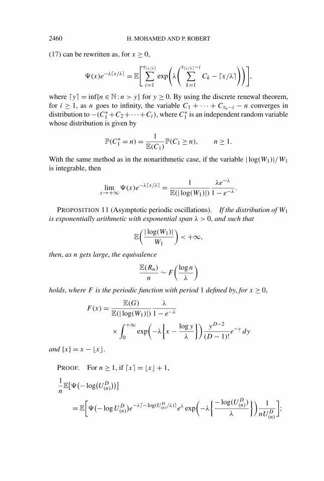
2460 H. MOHAMED AND P. ROBERT
(17) can be rewritten as, for x ≥ 0,
(x)e−λ�x/λ� = E
[τ�x/λ�∑i=1
exp
(λ
(τ�x/λ�−i∑k=1
Ck − �x/λ�))]
,
where �y� = inf{n ∈ N :n > y} for y ≥ 0. By using the discrete renewal theorem,for i ≥ 1, as n goes to infinity, the variable C1 + · · · + Cτn−i − n converges indistribution to −(C∗
1 +C2 +· · ·+Ci), where C∗1 is an independent random variable
whose distribution is given by
P(C∗1 = n) = 1
E(C1)P(C1 ≥ n), n ≥ 1.
With the same method as in the nonarithmetic case, if the variable | log(W1)|/W1is integrable, then
limx→+∞(x)e−λ�x/λ� = 1
E(| log(W1)|)λe−λ
1 − e−λ.
PROPOSITION 11 (Asymptotic periodic oscillations). If the distribution of W1is exponentially arithmetic with exponential span λ > 0, and such that
E
( | log(W1)|W1
)< +∞,
then, as n gets large, the equivalence
E(Rn)
n∼ F
(logn
λ
)
holds, where F is the periodic function with period 1 defined by, for x ≥ 0,
F(x) = E(G)
E(| log(W1)|)λ
1 − e−λ
×∫ +∞
0exp
(−λ
{x − logy
λ
})yD−2
(D − 1)!e−y dy
and {x} = x − �x.
PROOF. For n ≥ 1, if �x� = �x + 1,
1
nE
[
(− log(UD
(n)
))]
= E
[
(− logUD(n)
)e−λ�− log(UD
(n)/λ)�eλ exp
(−λ
{− log(UD(n))
λ
})1
nUD(n)
];

PROBABILISTIC ANALYSIS OF TREE ALGORITHMS 2461
since nUD(n) converges in distribution to tD as n goes to infinity, with the same
method as in the proof of Proposition 9, one gets the equivalences
1
nE
[
(− log(UD
(n)
))] × E(| log(W1)|)1 − e−λ
λ
∼ E
[exp
(−λ
{log(n)
λ− log(nUD
(n))
λ
})1
nUD(n)
]
= E
[exp
(−λ
{log(n)
λ− log tD
λ
})1
tD
].
One concludes by using (16). �
COROLLARY 12 (Q-ary protocol with blocked arrivals). When D = 2, G ≡ Q
and Vi,Q = pi for 1 ≤ i ≤ Q, then, if all the real numbers logpi/ logp1,2 ≤ i ≤ Q, are rational, the equivalence
E(Rn)
n∼ F
(logn
λ
)
holds, where F is the periodic function with period 1 defined by, for x ≥ 0,
F(x) = Q
−∑Qi=1 pi logpi
λ
1 − e−λ
∫ +∞0
exp(−λ
{x − logy
λ
})e−y dy,
where {x} = x − �x and λ = sup{y > 0 :∀ i ∈ {1, . . . ,Q}, logpi ∈ yZ}.
4. The distributions of the symmetrical Q-ary algorithm. From now on, itis assumed that the branching degree of the splitting algorithm is constant, that is,P(G = Q) = 1, and uniform, Vi,Q ≡ 1/Q for 1 ≤ i ≤ Q. A set of n ≥ D items israndomly, equally divided into Q subsets. From Proposition 11, it is known that
E(Rn)/n ∼ F1(logQ n)
as n goes to infinity, with
F1(x) = Q2
Q − 1
∫ +∞0
Q−{x−logQ y} yD−2
(D − 1)!e−y dy.(20)
This is a typical case where a regular law of large numbers does not hold.The purpose of this section is to strengthen the above convergence. The distri-
bution of the Poisson transform of the sequence (Rn), that is, the random variableRN (]0,x]), is investigated and not only its average as before. In particular it is shownthat, for the Poisson transform, a standard law of large numbers can be used toprove the oscillating behavior of the algorithm. In other words, these uncommonlaws of large numbers can be, in the end, expressed in a classical probabilisticsetting.

2462 H. MOHAMED AND P. ROBERT
NOTATION. Throughout the rest of the paper it is assumed that:
(1) N is a Poisson process with intensity 1 on R+. Another Poisson process willbe used but in the two-dimensional space [0,1] × R+.
(2) The variable M denotes a Poisson process on [0,1]×R+ with intensity 1; thisis a distribution of random points on [0,1]×R+ with the following properties:if M(H) denotes the number of points that “fall” into the set H ⊂ [0,1]×R+,
(i) For x ∈ [0,1] × R+, M({x}) ∈ {0,1}.(ii) If G and H are disjoint subsets of [0,1] × R+, the variables M(G)
and M(H) are independent.(iii) The distribution of the variable M([a, b] × [y, z]) is Poisson with pa-
rameter (b − a)(z − y) for 0 ≤ a ≤ b ≤ 1 and 0 ≤ y ≤ z.
Note that the random variables N ([0, x]) and M([0,1] × [0, x]) have a Pois-son distribution with parameter x.
(3) The Poisson transform of the sequence (Rn) is denoted by R(x), x ≥ 0,
R(x)dist.= RN ([0,x])
dist.= RM([0,1]×[0,x]).Its expectation is given by (8). This section is devoted to the study of the asymptoticbehavior of the distribution of R(x).
4.1. Laws of large numbers. In this section it is proved that the Poisson trans-form of the sequence (Rn) satisfies a strong law of large numbers. A nice repre-sentation of this transform as a functional of Poisson processes is first proved inthe following proposition.
PROPOSITION 13. The distribution of the Poisson transform R(x) of the se-quence (Rn) satisfies the following relations:
R(x)dist.= R1(x)
def .= 1 + Q∑p≥0
Qp−1∑k=0
φN(xk/Qp,x(k + 1)/Qp)
,(21)
where, for 0 ≤ a ≤ b, φN (a, b) = 1 if N (]a, b]) ≥ D and 0 otherwise,
R(x)dist.= R2(x)
def .= 1 + Q∑p≥0
Qp−1∑k=0
1{M(]k/Qp,(k+1)/Qp]×[0,x])≥D}.(22)
Note that the function x → R2(x) is clearly nondecreasing. In particular, if f issome nondecreasing function on R+, the same property holds for
x → E[f (R(x))].Representation (21) will be useful to get a strong law of large numbers on subse-quences and also will be used to get the full convergence in distribution of R(x)/x
as x tends to infinity.

PROBABILISTIC ANALYSIS OF TREE ALGORITHMS 2463
PROOF OF PROPOSITION 13. By the splitting property of Poisson randomvariables, the recurrence relation (2) for the sequence (Rn) can be expressed as
RN (]0,x])dist.= 1 +
Q∑i=1
Ri,N (]x(i−1)/Q,xi/Q]) − Q1{N (]0,x])<D},
for x ≥ 0. If, for 0 ≤ a < b,
�(a,b) = 1
Q
(RN (]a,b]) − 1
),(23)
the last equation can be rewritten as
�(0, x) =Q∑
i=1
�i
(i − 1
Qx,
i
Qx
)+ φN (0, x),(24)
with an obvious notation with the subscripts i for �. By iterating this relation, onegets that, almost surely, the expansion
�(0, x) = ∑p≥0
Qp−1∑k=0
φN
(k
Qpx,
k + 1
Qpx
)(25)
holds. The function �(0, x) is just the sum of the function φN on the Q-adicintervals of [0, x].
Equation (22) is proved in the same way. �
Representation of some of the functionals of the associated tree. WhenN ([0, x]) items are at the root of the associated tree, the total number of nodesof the tree RN ([0,x]) is not the only quantity that can be represented, by (21) interms of the Poisson process N .
The maximal depth M(x) of the associated tree when there are N ([0, x]) itemsat the top of the tree can be expressed as a functional of the Poisson process
M(x) = max{p ≥ 1 :∃ k,0 ≤ k < Qp−1 − 1,N
(]k/Qp−1, (k + 1)/Qp−1]) ≥ D}.
The quantity
F(x) = max{p ≥ 1 :∀ k,0 ≤ k < Qp−1 − 1,N
(]k/Qp−1, (k + 1)/Qp−1]) ≥ D}
is the number of full levels of the tree. See [22]. Note that these quantities aredirectly related to classical occupancy problems. The number of nodes at levelp ≥ 1 is given by
Q
Qp−1−1∑k=0
1{N (]k/Qp−1,(k+1)/Qp−1])≥D}.
This is not, of course, an exhaustive list of the possible representations in terms ofthe Poisson process.

2464 H. MOHAMED AND P. ROBERT
It is quite useful to think of splitting algorithms either in terms of trees or interms of Q-adic subintervals of [0,1]. In a more general case, that is, when thesplitting algorithm is not symmetrical, a representation similar to (21) can be ob-tained by using the associated random decomposition of the interval [0,1] insteadof the Q-adic decomposition. See [11].
A strong law of large numbers. Equation (24) shows that, if N > 0, the quan-tity �(0, yQN) is the sum of the � on the intervals [yp,yp + y], 0 ≤ p < QN ,and of φN on the intervals [ykQn, y(k + 1)Qn] contained in [0, yQN ], that is,
�(0, yQN) =QN−1∑p=0
�(yp,yp + y) +N∑
n=1
QN−n−1∑k=0
φN(ykQn, y(k + 1)Qn)
.(26)
By the independence properties of the Poisson process, the classical strong law oflarge numbers shows that, almost surely,
limN→+∞
1
QN
QN−1∑p=0
�(yp,yp + y) = E(�(0, y)
) = ∑p≥0
QpE
(φN (0, y/Qp)
)
= ∑p≥0
QpP
(N (]0, y/Qp]) ≥ D
),
by using (25), and for n > 0,
limN→+∞
1
QN
QN−n−1∑k=0
φN(ykQn, y(k + 1)Qn) = 1
QnE
(φN (0, yQn)
).
Note that, for 0 < K < N ,
N∑n=K
1
QN
QN−n−1∑k=0
φN(ykQn, y(k + 1)Qn) ≤
N∑n=K
1
QNQN−n ≤ 1
QK−1 .
The three last identities and decomposition (26) give that, almost surely,
limN→+∞
1
yQN�(0, yQN) = ∑
n∈Z
1
yQnP
(N (]0, yQn]) ≥ D
).
PROPOSITION 14 (Strong law of large numbers). With the same notation asin Proposition 13, for 0 < y ≤ Q, almost surely,
limN→+∞
R1(yQN)
yQN= Q
∑n∈Z
1
yQnP
(N (]0, yQn]) ≥ D
)
= Q∑n∈Z
1
yQn
∫ yQn
0
uD−1
(D − 1)!e−u du(27)
= F1(logQ y),

PROBABILISTIC ANALYSIS OF TREE ALGORITHMS 2465
where F1 is the periodic function defined by (20).
As a by-product, the proposition establishes the intuitive (and classical) fact thatthe sequence (E(Rn)/n) and the function x → E(RN ([0,x]))/x have the same as-ymptotic behavior at infinity. Note that if G(y) is defined as the second termof (27), then the function x → G(Qx) is clearly periodic with period 1.
PROOF OF PROPOSITION 14. Clearly, only the relation F1(logQ y) = G(y)
has to be proved. For n ∈ Z, if tD is the Dth point of the Poisson process N , then
P(N (]0, yQn]) ≥ D
) = P(tD ≤ yQn) =∫ +∞
01{u≤yQn}
uD−1
(D − 1)!e−u du.
By summing up these terms, with Fubini’s theorem one gets
G(y) = Q
∫ +∞0
∑n∈Z
1
yQn1{u≤yQn}
uD−1
(D − 1)!e−u du
= Q2
Q − 1
∫ +∞0
1
yQ�logQ(u/y)�uD−1
(D − 1)!e−u du
= Q2
Q − 1
∫ +∞0
1
Q−{logQ(u/y)}uD−2
(D − 1)!e−u du
= F1(logQ y).
The proposition is proved. �
The following proposition establishes a weak law of large numbers for the Pois-son transform of the sequence (Rn). Devroye [8] obtained related results in a moregeneral framework by using Talagrand’s concentration inequalities.
THEOREM 15 (Law of large numbers). The following convergence in distrib-ution holds, for any ε > 0:
limx→+∞P
(∣∣∣∣ R(x)
xF1(logQ x)− 1
∣∣∣∣ ≥ ε
)= 0,
where F1 is the function defined by (20).
PROOF. For x > 0, one defines Nx = �logQ x, ux = x/QNx and, for p ≥1, zx = �uxpQNx/p. Note that supx≥1 |x/zx − 1| converges to 0 as p tends toinfinity, hence by continuity of F1,
limp→+∞ sup
x≥1
∣∣∣∣ xF1(logQ x)
zxF1(logQ zx)− 1
∣∣∣∣ = 0.
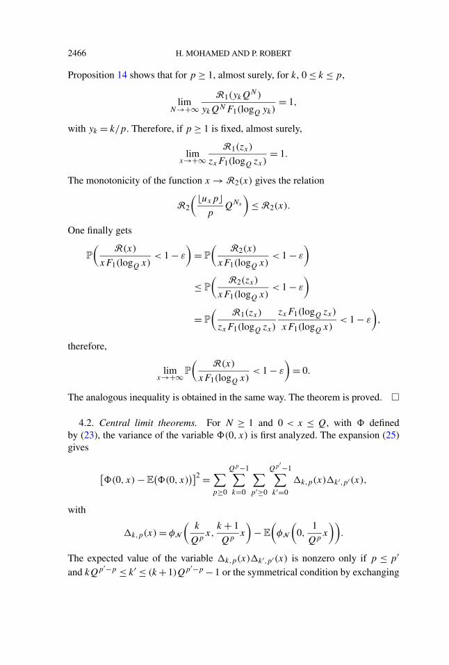
2466 H. MOHAMED AND P. ROBERT
Proposition 14 shows that for p ≥ 1, almost surely, for k, 0 ≤ k ≤ p,
limN→+∞
R1(ykQN)
ykQNF1(logQ yk)= 1,
with yk = k/p. Therefore, if p ≥ 1 is fixed, almost surely,
limx→+∞
R1(zx)
zxF1(logQ zx)= 1.
The monotonicity of the function x → R2(x) gives the relation
R2
(�uxpp
QNx
)≤ R2(x).
One finally gets
P
(R(x)
xF1(logQ x)< 1 − ε
)= P
(R2(x)
xF1(logQ x)< 1 − ε
)
≤ P
(R2(zx)
xF1(logQ x)< 1 − ε
)
= P
(R1(zx)
zxF1(logQ zx)
zxF1(logQ zx)
xF1(logQ x)< 1 − ε
),
therefore,
limx→+∞P
(R(x)
xF1(logQ x)< 1 − ε
)= 0.
The analogous inequality is obtained in the same way. The theorem is proved. �
4.2. Central limit theorems. For N ≥ 1 and 0 < x ≤ Q, with � definedby (23), the variance of the variable �(0, x) is first analyzed. The expansion (25)gives
[�(0, x) − E
(�(0, x)
)]2 = ∑p≥0
Qp−1∑k=0
∑p′≥0
Qp′−1∑k′=0
�k,p(x)�k′,p′(x),
with
�k,p(x) = φN
(k
Qpx,
k + 1
Qpx
)− E
(φN
(0,
1
Qpx
)).
The expected value of the variable �k,p(x)�k′,p′(x) is nonzero only if p ≤ p′and kQp′−p ≤ k′ ≤ (k +1)Qp′−p −1 or the symmetrical condition by exchanging

PROBABILISTIC ANALYSIS OF TREE ALGORITHMS 2467
(p, k) and (p′, k′):
E[(
�(0, x) − E(�(0, x)
))2]
= ∑p≥0
Qp−1∑k=0
E[�k,p(x)2]
+ 2∑p≥0
Qp−1∑k=0
∑p′>p
(k+1)Qp′−p−1∑k′=kQp′−p
E[�k,p(x)�k′,p′(x)].
By using the elementary identities
E[�k,p(x)2] = E[φN (0, x/Qp)](1 − E[φN (0, x/Qp)])= P(tD ≤ x/Qp)P(sD ≥ x/Qp),
E[�k,p(x)�k′,p′(x)] = E[φN (0, x/Qp′)](1 − E[φN (0, x/Qp)])
= P(tD ≤ x/Qp′)P(sD ≥ x/Qp),
where tD and sD are independent random variables with the same distribution asthe Dth point of the Poisson process N , one gets the relation
E[(
�(0, x) − E(�(0, x)
))2] = ∑p≥0
QpP(tD ≤ x/Qp ≤ sD)
+ 2∑
p′>p≥0
Qp′P
(tD ≤ x/Qp′
, x/Qp ≤ sD).
By switching again the series and the expected values, one finally obtains
(Q − 1)E[(
�(0, x) − E(�(0, x)
))2]= QE
((Q�logQ(x/tD) − Q�logQ(x/sD))1{�logQ(x/tD)>�logQ(x/sD)}
)(28)
+ 2QE((�logQ(x/tD) − �logQ(x/sD) − 1
)+Q�logQ(x/tD))
− 2Q
Q − 1E
((Q�logQ(x/tD) − Q�logQ(x/sD)+1)+)
,
where a+ = max(a,0) for a ∈ R. This identity gives the following proposition.A similar proposition has been proved by Jacquet and Régnier [17] and Régnierand Jacquet [37] in the case where Q = D = 2 but without symmetry conditionsas is the case here. See also [28], Chapter 5.
PROPOSITION 16 (Asymptotic variance). The variance of the Poisson trans-form of the sequence (Rn) satisfies the following equivalence, as x goes to infinity:
1
xVar(R(x)) ∼ F2(logQ(x)),

2468 H. MOHAMED AND P. ROBERT
where F2 is the continuous periodic function with period 1 defined by, for y ≥ 0,
F2(y) =∫
R2+
f2({y − logQ(u)}, {y − logQ(v)}, u, v
)(29)
× uD−1
(D − 1)!vD−1
(D − 1)!e−(u+v) dudv,
with {z} = z − �z for z ∈ R and for u > 0, v > 0 and y ∈ R,
f2(a, b,u, v) = Q
Q − 1
(Qa
u− Qb
v
)1{logQ(v/u)+b>a}
+ 2Q
Q − 1
(logQ(v/u) − a + b − 1
)+
− 2Q
(Q − 1)2
(Qa
u− Qb+1
v
)+
where z+ = max(z,0).
Note that a more detailed expansion of the variance could be obtained with (28).
PROPOSITION 17 (Central limit theorem for Poisson transform). For0 < y < Q, as N tends to infinity, the variable
1√QN
(R(yQN) − E(R(yQN))
)converges in distribution to a Gaussian centered random variable with varianceyF2(logQ y), where F2 is defined by (29).
PROOF. It is enough to prove the proposition for the variable �(0, x) definedby
�(0, x) = 1
Q
(RN (]0,x]) − 1
).
Equation (26) gives, for K ≥ 1,
�(0, yQN) − E(�(0, yQN)
)
=QN−1∑p=0
[�(yp,yp + y) − E
(�(0, y)
)]
+K∑
n=1
QN−n−1∑k=0
[φN
(ykQn, y(k + 1)Qn) − E
(φN (0, yQn)
)] + �K,

PROBABILISTIC ANALYSIS OF TREE ALGORITHMS 2469
where �K is the residual term of the series. By using the method to compute thevariance, it is not difficult to establish that, for any ε > 0 there exists some K > 0such that the expected value of (�K/QN)2 is less than ε, for N sufficiently large.
By regrouping the terms of the above equation according to the Q-adic intervals[yk/QK,y(k + 1)/QK ] for 0 ≤ k < QN−K and by using the independence prop-erties of the Poisson process N , the quantity �(0, yQN) − E(�(0, yQN)) − �K
can be written as a sum of QN−K independent identically distributed random vari-ables. Therefore, the classical central limit theorem can be applied. The proposi-tion is proved. �
4.3. The distribution of the sequence (Rn). The following proposition de-scribes the distribution of the variable Rn in terms of n i.i.d. uniformly distributedrandom variables on the interval [0,1]. This characterization is generally implic-itly used to get various asymptotics describing the depth of the associated tree. See[28] and [35].
PROPOSITION 18. For n ≥ 0, the random variable Rn has the same distribu-tion as
Rndist.= 1 + Q
∑p≥0
Qp−1∑k=0
φUn
(]k/Qp, (k + 1)/Qp]),(30)
where, for 0 ≤ a ≤ b ≤ 1, φUn(]a, b]) = 1 if Un(]a, b]) ≥ D and 0 otherwise. Thevariable Un is the point measure on [0,1] defined by
Un = δU1 + δU2 + · · · + δUn,
(U1, . . . ,Un) are i.i.d. random variables uniformly distributed on [0,1], in partic-ular, Un(]a, b]) is the number of Ui ’s in the interval ]a, b].
PROOF. Assume that N is a Poisson process with parameter 1; by definition(RN (]0,x])|N (]0, x]) = n
) dist.= Rn.
Due to Proposition 13, the distribution of the Poisson transform RN (]0,x]) is ex-pressed as a functional of the points of the Poisson process on the interval [0, x].But, as in the proof of Proposition 6, conditionally on the event {N (]0, x]) = n},these points can be expressed as xUi , 1 ≤ i ≤ n, where (Ui) are i.i.d. uniformlydistributed random variables on the interval [0,1]. Equation (30) is thus a directconsequence of (21). �
REFERENCES
[1] BARRAL, J. (1999). Moments, continuité et analyse multifractale des martingales de Mandel-brot. Probab. Theory Related Fields 113 582–597.

2470 H. MOHAMED AND P. ROBERT
[2] BERTOIN, J. (2001). Homogeneous fragmentation processes. Probab. Theory Related Fields121 301–318. MR1867425
[3] CAPETANAKIS, J. I. (1979). Tree algorithms for packet broadcast channels. IEEE Trans. In-form. Theory 25 505–515. MR545006
[4] CHANG, J. T. (1994). Inequalities for the overshoot. Ann. Appl. Probab. 4 1223–1233.MR1304783
[5] CLÉMENT, J., FLAJOLET, P. and VALLÉE, B. (2001). Dynamical sources in information the-ory: A general analysis of trie structures. Algorithmica 29 307–369.
[6] CORMEN, T. H., LEISERSON, C. E. and RIVEST, R. L. (1990). Algorithms. MIT Press.MR1066870
[7] DEVROYE, L. (1999). Universal limit laws for depths in random trees. SIAM J. Comput. 28409–432 (electronic). MR1634354
[8] DEVROYE, L. (2004). Universal asymptotics for random tries and Patricia trees. Preprint.[9] DURRETT, R. (1996). Probability: Theory and Examples, 2nd ed. Duxbury Press, Belmont,
CA. MR1609153[10] EPHREMIDES, A. and HAJEK, B. (1998). Information theory and communication networks: An
unconsummated union. IEEE Trans. Inform. Theory 44 1–20. MR1658779[11] FALCONER, K. (1997). Techniques in Fractal Geometry. Wiley, New York. MR1449135[12] FAYOLLE, G., FLAJOLET, P. and HOFRI, M. (1986). On a functional equation arising in the
analysis of a protocol for a multi-access broadcast channel. Adv. in Appl. Probab. 18441–472. MR840103
[13] FLAJOLET, P., GOURDON, X. and DUMAS, P. (1995). Mellin transforms and asymptotics:Harmonic sums. Theoret. Comput. Sci. 144 3–58. MR1337752
[14] GRIMMETT, G. R. and STIRZAKER, D. R. (1992). Probability and Random Processes, 2nd ed.Oxford Univ. Press. MR1199812
[15] HAMBLY, B. M. and LAPIDUS, M. L. (2005). Random fractal strings: Their zeta functions,complex dimensions and spectral asymptotics. Trans. Amer. Math. Soc. To appear.
[16] HOFRI, M. (1995). Analysis of Algorithms. Oxford Univ. Press. MR1367735[17] JACQUET, P. and RÉGNIER, M. (1986). Trie partitioning process: Limiting distributions. Lec-
ture Notes in Comput. Sci. 214 196–210. Springer, New York.[18] JANSON, S. and SZPANKOWSKI, W. (1997). Analysis of an asymmetric leader election algo-
rithm. Electron. J. Combin. 4 research paper 17. MR1464071[19] KAHANE, J. P. and PEYRIÈRE, J. (1976). Sur certaines martingales de Benoît Mandelbrot.
Adv. Math. 22 131–145.[20] KINGMAN, J. F. C. (1993). Poisson Processes. Oxford Univ. Press. MR1207584[21] KIRSCHENHOFER, P., PRODINGER, H. and SZPANKOWSKI, W. (1996). Analysis of a splitting
process arising in probabilistic counting and other related algorithms. Random StructuresAlgorithms 9 379–401. MR1605403
[22] KNESSL, C. and SZPANKOWSKI, W. (2002). Limit laws for the height in PATRICIA tries.J. Algorithms 44 63–97. MR1932678
[23] KNUTH, D. E. (1973). The Art of Computer Programming 3. Addison–Wesley, Reading, MA.MR378456
[24] LAPIDUS, M. L. and VAN FRANKENHUYSEN, M. (2000). Fractal Geometry and Number The-ory. Birkhäuser, Boston.
[25] LIU, Q. (2000). On generalized multiplicative cascades. Stochastic Process. Appl. 86 263–286.MR1741808
[26] LORDEN, G. (1970). On excess over the boundary. Ann. Math. Statist. 41 520–527. MR254981[27] LOUCHARD, G. and PRODINGER, H. (2004). The moments problem of extreme-value related
distribution functions. Preprint. MR2019639[28] MAHMOUD, H. M. (1992). Evolution of Random Search Trees. Wiley, New York. MR1140708

PROBABILISTIC ANALYSIS OF TREE ALGORITHMS 2471
[29] MANDELBROT, B. (1974). Multiplications aléatoires et distributions invariantes par moyennespondérées. C. R. Acad. Sci. Paris Sér. I Math. 278 289–292 and 355–358.
[30] MATHYS, P. and FLAJOLET, P. (1985). Q-ary collision resolution algorithms in random accesssystems with free or blocked channel access. IEEE Trans. Inform. Theory 31 244–254.MR793094
[31] MAULDIN, R. D. and WILLIAMS, S. C. (1986). Random recursive constructions: Asymptoticgeometric and topological properties. Trans. Amer. Math. Soc. 295 325–346. MR831202
[32] MIERMONT, G. (2003). Coalescence et fragmentation stochastique, arbres aléatoires et proces-sus de Lévy. Ph.D. thesis, Univ. Paris VI.
[33] MOHAMED, H. and ROBERT, P. (2004). Analysis of dynamic tree algorithms. In preparation.[34] PITMAN, J. (1995). Exchangeable and partially exchangeable random partitions. Probab. The-
ory Related Fields 102 145–158. MR1337249[35] PITTEL, B. (1985). Asymptotical growth of a class of random trees. Ann. Probab. 13 414–427.
MR781414[36] RAZ, D., SHAVITT, Y. and ZHANG, L. (2004). Distributed council election. IEEE/ACM Trans.
Networking 12 483–492.[37] RÉGNIER, M. and JACQUET, P. (1989). New results on the size of tries. IEEE Trans. Inform.
Theory 35 203–205.[38] ROBERT, P. (2005). On the asymptotic behavior of some algorithms. Random Structures Algo-
rithms 27 235–250.[39] SEDGEWICK, R. and FLAJOLET, P. (1995). Introduction to the Analysis of Algorithms.
Addison–Wesley, Reading, MA.[40] SZPANKOWSKI, W. (2001). Average Case Analysis of Algorithms on Sequences. Wiley,
New York. MR1816272[41] TSYBAKOV, B. S. and MIKHAILOV, V. A. (1978). Free synchronous packet access in a broad-
cast channel with feedback. Probl. Inf. Transm. 14 32–59. MR538901[42] WAYMIRE, E. C. and WILLIAMS, S. C. (1994). A general decomposition theory for random
cascades. Bull. Amer. Math. Soc. 31 216–222. MR1260522[43] WOLF, J. K. (1985). Born again group testing: Multiaccess communications. IEEE Trans. In-
form. Theory 31 185–191. MR793089
INRIADOMAINE DE VOLUCEAU
B.P. 10578153 LE CHESNAY CEDEX
FRANCE
E-MAIL: [email protected]@inria.fr
URL: www-rocq.inria.fr/~robert