
Statistical Inference in Stochastic Processes - Taylor & Francis Group
55
STATISTICAL INFERENCE in STOCHASTIC PROCESSES
-
Upload
khangminh22 -
Category
Documents
-
view
0 -
download
0
Transcript of Statistical Inference in Stochastic Processes - Taylor & Francis Group

STATISTICAL INFERENCEin STOCHASTIC PROCESSES
PROBABILITY PURE AND APPLIEDA Series of Textbooks and Reference Books
Editor
MARCEL F NEUTSUniversity of Arizona
Tucson Arizona
1 Introductory Probability Theory by Janos Galambos2 Point Processes and Their Statistical Inference by Alan F Kan3 Advanced Probability Theory by Janos Galambos4 Statistical Reliability Theory by I B Gertsbakh5 Structured Stochastic Matrices of MG1 Type and Their Applications
by Marcel F Neuts6 Statistical Inference in Stochastic Processes edited by N U Prabhu and
I V Basawa
Other Volumes in Preparation
Point Processes and Their Statistical Inference Second Edition Revisedand Expanded by Alan F KarrNumerical Solution of Markov Chains by William J Stewart
STATISTICAL INFERENCEIN STOCHASTIC PROCESSES
EDITED BY
MUPRABHUCornell UniversityIthaca New York
IV BASAWAUniversity of GeorgiaAthens Georgia
CRC PressTaylor amp Francis GroupBoca Raton London New York
CRC Press is an imprint of theTaylor amp Francis Group an Informa business
CRC PressTaylor amp Francis Group6000 Broken Sound Parkway NW Suite 300Boca Raton FL 33487-2742
First issued in paperback 2019
copy 1991 by Taylor amp Francis Group LLCCRC Press is an imprint of Taylor amp Francis Group an Informa business
No claim to original US Government works
ISBN-13 978-0-8247-8417-1 (hbk)ISBN-13 978-0-367-40307-2 (pbk)
This book contains information obtained from authentic and highly regarded sources Reasonableefforts have been made to publish reliable data and information but the author and publisher cannotassume responsibility for the validity of all materials or the consequences of their use The authorsand publishers have attempted to trace the copyright holders of all material reproduced in thispublication and apologize to copyright holders if permission to publish in this form has not beenobtained If any copyright material has not been acknowledged please write and let us know so wemay rectify in any future reprint
Except as permitted under US Copyright Law no part of this book may be reprinted reproducedtransmitted or utilized in any form by any electronic mechanical or other means now known orhereafter invented including photocopying microfilming and recording or in any informationstorage or retrieval system without written permission from the publishers
For permission to photocopy or use material electronically from this work please access wwwcopyrightcom (httpwwwcopyrightcom) or contact the Copyright Clearance Center Inc(CCC)222 Rosewood Drive Danvers MA 01923 978-750-8400 CCC is a not-for-profit organization thatprovides licenses and registration for a variety of users For organizations that have been granted aphotocopy license by the CCC a separate system of payment has been arranged
Trademark Notice Product or corporate names may be trademarks or registered trademarks andare used only for identification and explanation without intent to infringe
Library of Congress Cataloging-in-Publication Data
Statistical inference in stochastic processes edited by N U PrabhuI V Basawa
p cm mdash (Probability pure and applied 6)Includes bibliographical references and indexISBN 0-8247-8417-01 Stochastic processes 2 Mathematical statistics I Prabhu
N U (Narahari Umanath) II Basawa Ishwar VIII SeriesQA2743S73 19905192--dc20 90-20939
CIP
Visit the Taylor amp Francis Web site athttpwww taylorandfranciscom
and the CRC Press Web site athttp wwwcrcpresscom
Preface
Currently research papers in the area of statistical inference fromstochastic processes (stochastic inference for short) are published ina variety of international journals such as Annals of Statistics Biome-trika Journal of the American Statistical Association Journal of theRoyal Statistical Society B Sankhya A Stochastic Processes and TheirApplications and Theory of Probability and Its Applications Someimportant papers have also appeared with limited visibility in nationaljournals such as Australian Statistical Association Journal Journal ofthe Institute of Statistical Mathematics (Japan) and the ScandinavianStatistical Journal These journals are mostly interested in papers thatemphasize statistical or probability modeling aspects They seem to viewstochastic inference as peripheral to their domains and consequentlyprovide only limited scope for publication of ongoing research in thisimportant area
The area of stochastic inference is an interface between probabil-ity modeling and statistical analysis An important special topic withinthis broad area is time series analysis where historically modeling andanalysis have gone hand in hand this topic is now well established as anarea of research with an identity of its own with periodic conferences
Hi
iv Preface
publication of proceedings and its own international journal A secondtopic that has been successful in this regard is econometrics Howeverthis balanced development of modeling and inference has not takenplace in other areas such as population growth epidemiology ecologygenetics the social sciences and operations research
The great advances that have taken place in recent years in stochasticprocesses such as Markov processes point processes martingales andspatial processes have provided new powerful techniques for extendingthe classical inference techniques It is thus possible to open up linesof communication between probabilists and statisticians
Researchers in the area of stochastic inference keenly feel the needfor some kind of distinct visibility This fact is evident from recentnational and international conferences at which separate sessions wereorganized on this topic A mini-conference on stochastic inferencewas held at the University of Kentucky Lexington during Spring 1984A major international conference on inference from stochastic processeswas held in Summer 1987 at Cornell University Ithaca New York
Although the need for distinct visibility for research on stochasticinference is strong enough the market conditions do not fully justifythe starting of a new journal on this topic at the present time Ratherwe felt that a series of occasional volumes on current research wouldmeet the current needs in this area and also provide an opportunity forspeedy publication of quality research on a continuing basis In thispublication program we plan to invite established authors to submitsurvey or research papers on their areas of interest within the broaddomain of inference from stochastic processes We also plan to encour-age younger researchers to submit papers on their current research Allpapers will be refereed
The present volume is the first in this series under our joint editor-ship (The proceedings of the Cornell Conference edited by Prabhuhave appeared as Contemporary Mathematics Volume 80 publishedby the American Mathematical Society) We take this opportunity tothank the authors for responding to our invitation to contribute to thisvolume and gratefully acknowledge the referees services
N U PrabhuI V Basawa
Contributors
I V BASAWA Department of Statistics University of GeorgiaAthens GeorgiaP J BROCKWELL Department of Statistics Colorado State Uni-versity Fort Collins ColoradoD J DALEY Department of Statistics (IAS) Australian NationalUniversity Canberra AustraliaMICHAEL DAVIDSEN Copenhagen County Hospital HerlevDenmarkR A DAVIS Department of Statistics Colorado State UniversityFort Collins ColoradoJ M GANI Department of Statistics University of California atSanta Barbara Santa Barbara CaliforniaCOLIN R GOOD ALL School of Engineering and Applied SciencePrinceton University Princeton New JerseyP E GREENWOOD Department of Mathematics University ofBritish Columbia Vancouver British Columbia CanadaMARTIN JACOBSEN Institute of Mathematical Statistics Univer-sity of Copenhagen Copenhagen Denmark
v
vi Contributors
ALAN F KARR Department of Mathematical Sciences The JohnsHopkins University Baltimore MarylandYOUNG-WON KIM Department of Statistics University of GeorgiaAtlanta GeorgiaIAN W McKEAGUE Department of Statistics Florida State Univer-sity Tallahassee FloridaDAVID M NICKERSON Department of Statistics University ofGeorgia Athens GeorgiaMICHAEL J PHELAN School of Engineering and Applied SciencePrinceton University Princeton New JerseyB L S PRAKASA RAO Indian Statistical Institute New DelhiIndiaD A RATKOWSKY Program in Statistics Washington State Uni-versity Pullman WashingtonH SALEHI Department of Statistics Michigan State UniversityEast Lansing MichiganMICHAEL S0RENSEN Department of Theoretical Statistics Insti-tute of Mathematics Aarhus University Aarhus DenmarkTIZIANO TOFONI Postgraduate School of TelecommunicationsLAquila ItalyW WEFELMEYER Mathematical Institute University of CologneCologne Federal Republic of GermanyLIONEL WEISS School of Operations Research and Industrial En-gineering Cornell University Ithaca New York
Contents
Preface Hi
1 Statistical Models and Methods in Image Analysis ASurvey 1
Alan F Karr
2 Edge-Preserving Smoothing and the Assessment of PointProcess Models for GATE Rainfall Fields 35
Colin R Goodall and Michael J Phelan
3 Likelihood Methods for Diffusions with Jumps 67
Michael S0rensen
4 Efficient Estimating Equations for Nonparametric FilteredModels 107
P E Greenwood and W Wefelmeyer
vii
viii Contents
5 Nonparametric Estimation of Trends in Linear StochasticSystems 143
Ian W McKeague and Tiziano Tofoni
6 Weak Convergence of Two-Sided Stochastic Integralswith an Application to Models for Left TruncatedSurvival Data 167
Michael Davidsen and Martin Jacobsen
1 Asymptotic Theory of Weighted Maximum LikelihoodEstimation for Growth Models 183
B L S Prakasa Rao
8 Markov Chain Models for Type-Token Relationships 209
D J Daley J M Gani and D A Ratkowsky
9 A State-Space Approach to Transfer-Function Modeling 233
P J Brockwell R A Davis and H Salehi
10 Shrinkage Estimation for a Dynamic Input-Output LinearModel 249
Young-Won Kim David M Nickerson and I V Basawa
11 Maximum Probability Estimation for an AutoregressiveProcess 267
Lionel Weiss
Index 271
STATISTICAL INFERENCEIN STOCHASTIC PROCESSES
1Statistical Models and Methods in ImageAnalysis A Survey
Alan F KarrThe Johns Hopkins University Baltimore Maryland
This paper is a selective survey of the role of probabilistic modelsand statistical techniques in the burgeoning field of image analysis andprocessing We introduce several areas of application that engenderimaging problems the principal imaging modalities and key conceptsand terminology The role of stochastics in imaging is discussed gen-erally then illustrated by means of three specific examples a Poissonprocess model of positron emission tomography Markov random fieldimage models and a Poisson process model of laser radar We emphas-ize mathematical formulations and the role of imaging within the con-text of inference for stochastic processes
1 INTRODUCTION
Image analysis and processing is a field concerned with the modelingcomputer manipulation and investigation and display of two-dimen-sional pictorial data Like many nascent fields it is a combination ofrigorous mathematics sound engineering and black magic Our objec-
Research supported in part by the National Science Foundation under grantMIP-8722463 and by the Army Research Office
1
2 Karr
tive in this paper is to present some key concepts and issues in imageanalysis and to describe some probabilisticstatistical methods appli-cable to imaging problems Our emphasis is on mathematical formula-tions and issues rather than either theoretical details or empiricaltechniques
In the broadest sense an image is a function whose two-dimensionaldomain the image plane is a (compact) subset of R2 The values ofrepresent brightness and may be one-dimensional in which case theimage is called monochromatic and its values gray levels or multidimen-sional corresponding to brightnesses in several spectral bands so thatthe image is colored For simplicity we deal only with monochromaticimages
The ultimate objective of image analysis is generally mdash albeit notalways mdashto display an image for viewing examination and interpret-ation by humans Thus perceptual issues are important for exampleone must be careful not to confuse colored images with false colormethods for display of monochromatic images The latter map difficult-to-perceive gray levels onto colors which are more easily distinguishedby human viewers for the purpose of displaying the image more in-formatively We do not deal with perception here though The readershould be cautioned moreover not to adhere too dogmatically to thevisual metaphor since there are contexts for example optical characterrecognition and robotics in which it is not apparent that this is the bestway to think
In most realistic situations images are realizations of random pro-cesses leading to the following basic definitions
Definition 11 (a) A continuous image is the realization of a randomfield X(xy)Qltxyltl
(b) A digital image is the realization of a discrete-valued randomfield X ( i j ) 0 lt lt n The X(ij) are referred to as pixels (pictureelements)
2 SOME GENERALITIES ABOUT IMAGING
Some key forms of imaging areCAT computerized axial tomographyMRI magnetic resonance imagingPET positron emission tomographyOCR optical character recognitionradar
Statistical Models in Image Analysis 3
ladar laser radarremote sensing (for example from satellites)ultrasoundcomputer vision and graphicsphotography
Common characteristics of imaging problems are as follows
Digitization This is necessary in order to analyze and manipulateimages by computer and takes two primary forms Given an underlyingcontinuous image X(x y) 0 lt x y lt 1 an approximating digitalimage X ( i j ) 0 lt lt n] is constructed by
Spatial sampling The pixels X(ij) correspond in location to discretespatial sampling of X In most instances the sampling is regular sothat in the absence of quantization X(ij) = X(inJn)
Quantization In a digital system only finitely many pixel values arepossible these result from quantizing the values of X That is werethere is no spatial sampling and assuming that 0 lt Xlt c for someconstant c one would have a quantized image X(x y) = Q(X(x y))where Q is a function from [0 c] to some finite set say g0 bull bull bull gk-An example is the function
laquodeg-if-lk[_c Jwhere [t] is the integer part of t which yields k + 1 equally spacedquantization levels 0 elk 2clk c
The final result of both forms of digitization is the digitized image
X(ii) = Q(X(injn)) (21)Data Transformation Often in imaging problems the data comprisea mathematical transform of the object of interest For example inCAT and MRI two principal forms of medical imaging the object isan unknown function( y representing anatomical structure and theobserved data are (finitely many) line integrals of
gt(pound)= f(xy)dsJL
Recovery of from line integrals is known as the Radon inversionproblem In the case of positron emission tomography (see Section 4)a similar yet different transformation is involved
Noise Usually modeled as random noise may be either inherent to
4 Karr
the imaging process or introduced during transmission or storage ofdata
Randomness Randomness enters image analysis in two quite distinctforms as models ofobjects in the imageimaging processes
One objective of this chapter is to argue that the former in manyways the more important is rather poorly understood and modeledwhereas the latter is generally well understood and modeled
Principal issues in image analysis include a number that arise as wellin classical one-dimensional signal processing such as those that fol-low Many of these are frequency domain methods in spirit
Digitization In order to be processed by computer a continuous sig-nal must be reduced to digital form using for example the samplingand quantization techniques previously described
Data Compression Efficient storage and transmission of image datarequire that it be represented as parsimoniously as possible For exam-ple the Karhunen-Loeve expansion expresses a stationary randomfield without loss of information in terms of a fixed set of orthonormalfunctions and a set of uncorrelated random variables Other techniquesfor data compression include interpolation and predictive methods aswell as classical concepts from coding theory
Enhancement Many signals are subject to known (or estimated)degradation processes which may be either exogenous such as non-linear transmission distortion and noise or endogeneous such as thenoise introduced by quantization Enhancement is intended to re-move these effects For example bursty or speckle noise may beremoved by smoothing the signal in other words subjecting it to alow-pass filter typically an integral operator Smoothing removes iso-lated noise but at the expense of introducing undesirable blurring Onthe other hand identification of more detailed features may require ahigh-pass filter (differentiation) for images this can be interpreted assharpening that removes blur Smoothing and sharpening techniquesare ordinarily implemented in the frequency domain via multiplicationof Fourier transforms Enhancement may also deal simply with graylevels for example in an image degraded by loss of contrast
Statistical Models in Image Analysis 5
Deconvolution A linear time-invariant system has the form
g(i) = hf(t) = th(t-s)f(s)ds (22)
whereis the input g the output and h the transfer function Recoveryoffrom g requires deconvolution effected computationally by meansof Fourier transforms
Filtering Depending on the nature of the filter either large scale orfine scale structure of the signal may be emphasized
But beyond these are issues truly intrinsic to the two-dimensionaland pictorial nature of images
Restoration For images this constitutes removal of specific kinds ofdegradations for example point degradations of the form
g(xy) = lh(xyxy)f(xy)dxdy (23)
whereis the undegraded image g is the degraded image and h is thepoint spread function That is a point source (a unit intensity sourceconcentrated at a single point and represented mathematically by theDirac measure eooo) appears in the degraded image as the measurewith density function h(- bull x y ) The form of the point spread func-tion depends on the physical process under study Recovery offromg in this case typically reduces to a two-dimensional deconvolutionproblem Other techniques for restoration include least squares andmaximum entropy
Feature Identification Images often contain geometric features thatif not actually defining them are their most salient attributes Themost important of these are edges which comprise boundaries betweendifferent objects in an image and are characterized by differing pixelvalues on opposite sides Edges are high frequency phenomena andhence techniques to identify them include spatial high-pass filters moresophisticated means for edge modeling and detection also exist how-ever one of which is described in Section 5
Reconstruction In CAT and MRI as noted above the measured dataare line integrals (see (21)) of an unknown function of interest thatone must then reconstruct A set of such integrals along lines that are
6 Karr
either parallel or emanate in a fan-beam from a single point is termeda projection the measurements are a set of projections Most recon-struction procedures are based on the filtered-backprojection algorithmsee (Kak and Rosenfeld 1982 Chapter 8) for a description
Matching Often images of the same object produced at differenttimes or by different imaging modalities must be compared or registeredin order to extract as much information from them as possible
Segmentation Many images are comprised of large structuredregions within which pixel values are relatively homogeneous Suchregions can be delineated by locating their boundaries (edge identi-fication) but there are also techniques (some based on statistical class-ification procedures) that account explicitly for regional structurebut deal only implicitly with the boundaries between regions (The dualviewpoint of region boundaries as both defining characteristics andderived properties of an image is a sometimes frustrating but alsopowerful aspect of image analysis)
Texture Analysis Texture may be regarded as homogeneous localinhomogeneity in images More broadly textures are complex visualpatterns composed of subpatterns characterized by brightness colorsshapes and sizes Modeling of texture often entails tools such as fractals(Mandelbrot 1983) while textures play a fundamental role in imagesegmentation Mathematical morphology (Serra 1982) is another keytool
3 STOCHASTICS IN IMAGING
The role of probability and statistics in imaging is to formulate andanalyze models of images and imaging processes
These include on the one hand classical degradation models suchas
Y(xy) = lh(x-xy-y)X(xy)dxdy + Z(xy) (31)
where X is a random field representing the undegraded image Y is thedegraded image h is the (spatially homogeneous) point spread functionand Z is a noise process whose effect in the simplest case as aboveis additive The one-dimensional analog of (31) is the time-invariantlinear system of (22)
Statistical Models in Image Analysis 7
On the other hand a number of modern classes of stochasticprocesses play roles in image analysisstationary random fieldsMarkov random fieldspoint processes
Image models based on the latter two are treated in the sequelIn most imaging problems the basic issue is to produce either a literal
image (displayed on a computer screen) or a representation suitablefor manipulation and analysis Mathematically this amounts to esti-mation of a two-dimensional function which may be either deterministicand unknown so that the statistical problem is one of nonparametricestimation or random and unobservable in which case the objective isestimation of the realization-dependent value of an unobservable ran-dom process (referred to in Karr (1986) as state estimation)
Thus from the stochastic viewpoint image analysis falls within thepurview of inference for stochastic processes in which there is rapidlyincreasing activity by probabilists engineers and statisticians In theremaining sections of this paper we attempt using three rather diverseexamples to elucidate the connections between imaging and appli-cations computation probability and statistics
The literature on statistical models and methods for image analysisis growing steadily two useful and fairly general sources are Ripley(1988) and WegmanDePriest (1986)
4 POSITRON EMISSION TOMOGRAPHY
In this section we treat positron emission tomography one of severalcomplementary methods for medical imaging We formulate a stochas-tic model for the process that produces the images and analyze severalstatistical issues associated with the model In the process the statisticalissues are related to some key inference problems for point processesThe material in this section is based on Karr et al (1990) to which thereader is referred for proofs and additional details See also Vardi etal (1985) for an analogous discrete model many of the key ideasemanate from this paper
41 The Physical ProcessPositron emission tomography (PET) is a form of medical imaging usedto discern anatomical structure and characteristics without resorting to
8 Karr
invasive surgical procedures In PET metabolism is measured fromwhich anatomical structure is inferred
In summary the physics of PET are as follows (refer to Figure 11)
1 Based on the organ to be imaged mdashfor concreteness the heart(Figure 11 represents a transverse planar section) a protein isselected that is known to be metabolized there and not elsewhere
2 The protein is synthesized in a manner that tags it with a radioac-tive material often C14 or F18 this material when it decays emitspositrons which are anti-electrons
3 The tagged protein is injected into the circulatory system whichtransports it to the heart where it is absorbed because of its rolein cardiac metabolism
4 When a positron is emitted it is mdash after traveling a short but nonne-gligible distance mdash annihilated by combining with an electron
5 The result of a positronelectron annihilation is two photons (y-rays) that travel in opposite directions (by conservation of momen-tum) along a randomly oriented straight line
6 The object being imaged is surrounded by a planar ring of photondetectors each registers counts of individual photons impinging onit which are recorded for analysis of the image
Detectors
Photon path
Y - unobservable1 annihilation
X a observabledetection pair
Figure 11 Positron emission tomography (PET)
Statistical Models in Image Analysis 9
A typical image is based on approximately 106 photon-pair detectionsobtained over a period of several minutes Often a series of imagesoffset in the third coordinate from one another is produced by shiftingbodily the ring of detectors the various two-dimensional images maybe analyzed individually or in concert or combined to form a three-dimensional image
Returning to a single image each annihilation occurs within theanatomical structure at a random two-dimensional location Y whichcannot be observed directly Instead one observes a two-dimensionalrandom vector Xf corresponding to the two locations on the ring ofdetectors at which photons produced by the annihilation are registeredOne then knows that Y lies along the line segments with endpointsXi9 but nothing more
Physical issues associated with PET includeClassification Photon detections at the various detectors must be
paired correctly In practice misclassification is believed to occur in30 or more of annihilations
Noise Stray photons not resulting from annihilations may be regis-tered by the detectors
Travel distance Positrons are annihilated near but not at the point ofemission
Reabsorption As many as 50 of the photons created by annihilationsmay be absorbed in the body and hence not detected
Time-of-flight Currently available equipment is not sufficiently sophis-ticated to measure the time differential (it is on the order of 10~10
seconds) between the arrivals of the two photons created by a singleannihilation (Were this possible even within a noise level thenYt would be known at least approximately)
Movement Because the data are collected over a period of severalminutes movement of the subject either intrinsic as in the case ofthe heart or spurious may occurDespite the errors introduced by these phenomena they are ignored
in the simple model we present below
42 The Stochastic ModelThere is abundant physical and mathematical basis for assuming as wedo that the two-dimensional point process
N = euroYl (41)
of positronelectron annihilations is a Poisson process (on the unit disk
10 Karr
D = x E R2 |jc| 1) whose unknown intensity function a representsindirectly via metabolic activity the anatomical structure of interestin our example the heart
We further assume also with sound basis that
The Xt are conditionally independent given TV The conditional distribution of Xi9 given TV depends only on Y via
a point spread function kPXi EdxN = k(x | Yf) dx (42)
That is k(- y) is the conditional density of the observed detectionlocation corresponding to an annihilation at y the randomness itintroduces represents the random orientation of the photons engen-dered by the annihilation and to some extent travel distancesIt follows that the marked point process
N=IeltYiM (43)
which is obtained from N by independent marking (Karr 1986 Sec-tion 15) is a Poisson process with intensity function
r1(yx) = a(y)k(xy) (44)
In consequence the point process
N=IeXi (45)
of observed detections is also Poisson with intensity function
A() = ln(yx)dy = l k(x y)a (y) dy (46)
The goal is to estimate the intensity function a of the positronelec-tron annihilation process However before discussing this in detailwe consider some generalities associated with inference for Poissonprocesses
43 Estimation of Intensity Functions of Poisson ProcessesConsider the problem of estimating the intensity function of a Poissonprocess N on R^ from observation of iid copies A^ Nn Denotingby PA the probability law of the observations Nt when the unknownintensity function is A the relevant log-likelihood function is (Karr1986 Proposition 611) given by
L(A) = log(^r) = f (Ao - A) dx + f log(AA0) dNn (47)Varo J J
Statistical Models in Image Analysis 11
where P0 is the probability law corresponding to a fixed function A0and Nn = 2=i Ni9 which is a sufficient statistic for A given the dataNl9Nn
This log-likelihood function of (47) is unbounded above (exceptin the uninteresting case that Nn(Rd) = 0) and maximum likelihoodestimators do not exist We next introduce a technique that circumventsthis difficulty in an especially elegant manner
44 The Method of SievesThe method of sieves of U Grenander and collaborators is one meansfor rescuing the principle of maximum likelihood in situations whereit cannot be applied directly typically because the underlying parameterspace is infinite-dimensional We begin with a brief general description
Suppose that we are given a statistical model P pound E indexedby an infinite-dimensional metric space and iid data XiX2 Then in the absence of special structure we assume the n-sample log-likelihood functions Ln(g) are unbounded above in pound
Grenanders idea is to restrict the index space but let the restrictionbecome weaker as sample size increases all in such a manner thatmaximum likelihood estimators not only exist within the sample-size-dependent restricted index spaces but also fulfill the desirable propertyof consistency More precisely the paradigm (Grenander 1981) is asfollows
1 For each h gt 0 define a compact subset I(h) of such that foreach n and h there exists an n-sample maximum likelihood esti-mator (laquo h) relative to I(h)
Ln(l(nh))gtLn(ft fe (A) (48)
2 Construct the I(h) in such a manner that as h decreases to 0 I(h)increases to a dense subset of
3 Choose sieve mesh hn to depend on the sample size n in such amanner that (laquo hn) -gt pound under Peuro in the sense of the metric on
In most applications is a function space and h has the physicalinterpretation of a constraint on the roughness of functions in I(h)As h decreases rougher and rougher functions are allowed in I(h)See Karr (1986 1987) as well as Section 45 below for additionaldiscussion
Figure 12 provides a pictorial interpretation of the method of sievesThere the squares denote the elements of I(h) and the squares andcircles the elements of I(h) where h lt h pound is the true value of theunknown parameter
12 Karr
a o aLegend
a = i(h)o a = ()( lt )
o 0-61 o
bull -laquo
a o a~-ampFigure 12 The method of sieves
The reasoning that underlies the method of sieves is as follows1 For each z there exists within I(h) a regularization h of pound that
if not a best approximation to pound from 7(z) is at least a sufficientlygood approximation
2 Maximum likelihood estimators for a fixed sieve mesh h shouldsatisfy standard asymptotics so that under the probability P^pound(n h) mdashraquo ih as n -raquoltraquo (with we emphasize i held fixed)
3 Assuming that h = hn is chosen to depend on n in such a mannerthat hn -raquo 0 as n mdashgt odeg then ^^n -gt ^ by construction of the sieve
4 Hence provided that hn-Q slowly enough it should be truethat pound(n hn] - f under Feuro
The fundamental tradeoff involved in determining the hn is esssenti-ally bias against variance as h becomes smaller
The regularization poundh is a better approximation to pound and hence lessbiased
but
poundh is also rougher and hence more difficult to estimate because esti-mators have higher variance
In order that estimators (n hn) be consistent the hn must be chosento balance the competing goals of eliminating both variance (in orderthat estimators converge) and bias (so that they converge to the rightthing)
Statistical Models in Image Analysis 13
We now apply the method of sieves to the problem of estimatingthe intensity function of a Poisson process
45 Application to Inference for Poisson ProcessesOur setting is again the following NiN2 are iid Poisson pro-cesses on R^ with unknown intensity function A satisfying
tfX(x)dx=lsupp(A) is compact (albeit perhaps unknown)
Provided that A lt odeg the former assumption entails no loss of gen-erality since given the data JVl9 NW A admits the maximumlikelihood estimator Nn(Rdln these estimators are strongly consistentand even asymptotically normal The latter does involve some restric-tion mathematically but none in terms of applications
The goal is to estimate A consistentlyThe log-likelihood function (omitting terms not depending on A) is
Ln(A) = |(logA)dAr (49)
which remains unbounded above in AWe invoke the method of sieves using the Gaussian kernel sieve
For each h gt 0 define
Mi -1Wplusmn lV l^ (2irh)dl2 P|_ 2h J
that is kh(x y) = f(x - y) where is a circularly symmetric Gaussiandensity with mean zero and covariance matrix hi The sieve I(h) consistsof all intensity functions A having the form
X(x) = lkh(xy)F(dy) (410)
where F is a probability measure on R^ Elements of I(h) are inparticular smooth densities on R^ See Geman and Hwang (1982) foran application of the same sieve to estimation of probability densityfunctions
Restricted to (i) viewed as indexed by the family 2P of probabilitieson Rd the log-likelihood function Ln of (49) becomes
Ln(F) = | [log J kh(x | y)F(dy)] N(dx) (411)
14 Karr
The inference issues now becomeexistence of maximum likelihood estimators in I(h)computation of maximum likelihood estimators in I(h)consistency of the sieve maximum likelihood estimators
We shall discuss these in turnExistence of maximum likelihood estimators in the I(h) requires only
that k(x | y) -raquo 0 as ||jt|| or y -raquo oo
Proposition 41 For each n and h there exists F(n h) E I(h) suchthat
Lraquo(F(nh))gtLn(F) (412)
for all FEl(h) Moreover P is supported by the convex hull of thepoints of Nn
From (412) one defines an estimator of the intensity function bysubstitution
A(n K)(x) = J kh(x | y)F(n h)(dy) (413)
Computation of maximum likelihood estimators is a more delicateissue We have sought to use the EM algorithm (Dempster et al1977 Wu 1983) but the space amp is infinite-dimensional and someconvergence issues remain unresolved Nevertheless we relate what isknown regarding our problem
The EM algorithm is an iterative method for calculating maximumlikelihood estimators whose direct computation is difficult We presenta brief general description
Consider a random vector (YX) governed by a statistical modelPe 0 E copy in which X is observable but Y is not Define the log-likelihood functions
L(0) = logP = A(0y) = logPY = 3
The goal is to calculate from the observations X a maximum likelihoodestimator 0 of 6 Of course since only L(- X) can be calculated fromthe observations 6 must maximize it
In a variety of situations for example mixture models (Lindsay1983a 1983b) maximization of A(- Y) is easy either numerically orperhaps even in closed form but maximization of L(-X) is much
Statistical Models in Image Analysis 15
more difficult The EM algorithm seeks to ameliorate this situation byiteration Given a previous estimated value 00id the new estimatedvalue is given by
0new = arg max E$JiA(8 Y) X] (414)
There is no guarantee of course that this problem is more amenableto a solution than that for L but the hope is that the functionpoundeold[A(- Y) | AT] inherits the computational tractability of A In manyspecific cases this turns out to be so Note that since it is a conditionalexpectation given X this function is computable from the observations
Thus given an initial estimate 0init the EM algorithm generates asequence ((ampgt) of estimated values The iteration (414) increases thevalue of L
L(0new) L(0old)
and the inequality is strict unless 0new = $oid- Moreover provided thatcertain regularity conditions be fulfilled in particular that be finite-dimensional then 0(pound) mdashraquo 0 the maximizer of L(- X) See Dempster etal (1977) and Wu (1983) for details
Returning to computation of sieve maximum likelihood estimatorsfor Poisson intensity functions we have the following result
Proposition 42 (a) The iteration
~lt4x) = U40 (h(^l^N(^ (4-15)J Jkh(x z)Fold(di) N(R)
corresponds to an EM algorithm for maximizing Ln(F)(b) Provided that the support of F-m-lt is Rd the sequence (F(ampgt) of
iterates produced by (415) is tight
As yet however we have not shown that the EM sequence (())converges nor (even assuming that it does) that the limit maximizesLn
An alternative approach to computation of the maximum likelihoodestimators P(n h) relies on showing that these estimators have finitesupport Suppose that Nn = 211 eXr
Theorem 43 For each n and h the sieve maximum likelihood esti-mators P - P(n h) satisfy
-^ 2 kh(Xi ~V =1 vEsuppf (416)Mi-ifkh(Xt - w)F(dw)
16 Karr
J_ pound kh(Xt - v) ^M-=i(bull-
Consequently the support of P is finite
The conditions (416)-(417) correspond respectively to the firstand second Kuhn-Tucker conditions for the problem of maximizingthe log-likelihood function (411)
The characterization in Theorem 43 engenders a finite-dimensionalEM algorithm for computation of P Denote by tyq the set of probabilitydistributions on R^ whose support consists of at most q points (so thatevery FEampq admits a representation F= SyL=ip()ev())
Theorem 44 For qgtM within ampq the iteration that convertsFold = 2=i()ev() into Fnew = 2=ip()eV() where
M
p()=X)^y^v())rm (418)Mi=i X=ip(l)kh(Xt - v())
vn = ZF-MkAX - v())S=1p()c(^ - v())2^ poundbdquo( - v(j))IIJlp(l)kh(Xi - v())
is an EM algorithm
Known convergence theory for finite-dimensional EM algorithms(Wu 1983) applies to the algorithm of Theorem 44
Finally consistency of maximum likelihood estimators A of (413)with respect to the L1-norm is established in the following theorem
Theorem 45 Suppose that(a) A is continuous with compact support(b) |A()logA()ltfc|ltoo
Then for hn = rc~18+e where e gt 0
||A(laquoO-A||i^O (420)
almost surely
46 Application to PETThe connection between PET and our discussion of inference for Pois-son processes is that estimation within a sieve set I(h) is the sameproblem mathematically as computation of the maximizer of the likeli-hood function for the PET problem given (compare (47)) by
Statistical Models in Image Analysis 17
L(a) = | (AO() - J k(x | y)a(y) dy) dx
+ fiog(^f^W)J V AO(JC)
More succinctly for PET the intensity function has the form
Aa()= [k(xy)a(y)dy
whereas in connection with the method of sieves
AF() = kh(xy)F(dy)
In both cases the point spread function k is knownProposition 42 and an analog of Theorem 43 apply to the PET
problem
5 MARKOV RANDOM FIELD IMAGE MODELS
The image models described in this section differ substantially from thePoisson process model of the preceding section they are based onrandom fields (stochastic processes with multidimensional parametersets) they are inherently discrete they incorporate dependence amongpixel values by means of auxiliary stochatic processes and they admitalmost unlimited modeling flexibility Of course all this does not comeunfettered and applicability in any specific situation must still be deter-mined by resort to physical principles
The principal source for the material in this section is Geman andGeman (1984) to which the reader is referred for details See alsoBesag (1974 1986) Cross and Jain (1983) contains an application ofMarkov random fields to the modeling and analysis of texture
51 The ModelThe image is modeled as a random field X= Ypp pound 5 Z pound LwhereY is an observable pixel process indexed by a set S of sitesZ is an unobservable line process indexed by a set L of lines
The random variables Yp and Z take their values in a finite state spaceE
18 Karr
As illustrated in examples below the role of lines is to introduceadditional dependence into the pixel process in a controlled mannerThus on the one hand the line process is a modeling tool of enormouspower On the other hand however it is artificial in that the linesneed not (and generally do not) represent objects that exist physicallybut are instead artifacts of the model In a sense this dilemma is merelyone manifestation of the somewhat schizophrenic view of edges thatseems to prevail throughout image analysis are edges defined by theimage or do they define it
Returning to the model the crucial mathematical assumption is thatX is a Markov random field That is let G = S U L and assume thatthere is defined on G a symmetric neighborhood structure for each athere is a set Na C G of neighbors of a with 3 E Na if and only ifa E Np Then X is a Markov random field if
(a) PX = x gt 0 for each configuration x E O = EG(b) For each a and s
PXa = sXftpa = PXa = sXppENa (51)
That is once the values of Xat the neighbors of a are known additionalknowledge of X at other sites is of no further use in predicting thevalue at a
An equivalent statement is that the probability PX E (bull) is a Gibbsdistribution in the sense that
PX = x = expf- ^E Vc(x) (52)Z L T c J
where T is a positive parameter with the physical interpretation oftemperature the summation is over all cliques C of the graph G andfor each C the function Vc(x) depends on x only through xa a E C(A subset C of G is a clique if each pair of distinct elements of C areneighbors of one another Note that this definition is satisfied vacuouslyby singleton subsets of C) The Vc and the function
U(x) = I Vc(x) (53)c
particularly the latter are termed energy functionsInterpretations are as follows
The energy function determines probabilities that the system assumesvarious configurations the lower the energy of the configuration jcthe higher the probability PX = x
Statistical Models in Image Analysis 19
The temperature modulates the peakedness of the probability distri-bution PX = (bull) the lower T the more this distribution concen-trates its mass on low energy configurations
The function of T defined by
ZT = Ie-u^T (54)X
which plays the role of a normalizing constant in (52) is known onthe basis of analogies to statistical mechanics as the partition functionIts computation is notoriously difficult
That (51) and (52) are equivalent is an important and nontrivialproperty see Kindermann and Snell (1980) for a proof
One observes only the degraded image a random field Y =Yp p E 5 indexed solely by pixels and having the form
p = ltKH(Y)p) + pp (55)where
H is a known blurring function which operates on the entire unde-graded pixel process Y
ltgt is a known possibly nonlinear transformation applied pixel-by-pixel
v is (typically white Gaussian) noise Though the noise in (55) isshown as additive it need not be In essentially all cases it is indepen-dent of X
Note that the line process Z does not appear in (55)Although in principle the value of the blurred image H( Y) at a given
pixel can depend on the values of Y at every pixel typically H is localin nature For example one may model blur as local averaging aphenomenon well-known in image analysis (it may even be introduceddeliberately in order to remove certain forms of noise) in which eachpixel value is replaced by a weighted average of its value and those ofneighboring pixels
H(Y)p=yYp + (l-y)-plusmn- I YqNp qltENp
where y E (01) and Np is the set of pixel neighbors ofThe goal of the analysis is to recover the original image X although
usually only the pixel process Y is of interest Note that the unknownfunction X is random in this case rather than as in Sections 4 and 6a statistical parameter Thus our context is state estimation the realiza-tion-dependent reconstruction of an unobservable random process This
20 Karr
is effected via Bayesian techniques the reconstructed image X is themaximum a priori probability or MAP estimator that value whichmaximizes the conditional probability PX= (bull) | Y where Y is thedegraded image of (55) Thus the reconstructed image is given by
X = arg max PX = x Y (56)
The central issues are
Model specification that is choice ofthe pixel index (site) set Sthe line set Lthe neighborhood structure on G = 5 U Lthe (prior) distribution PX G (bull) or equivalently the energy functionCof (53)
Computation of conditional probabilitiesSolution of a difficult unstructured discrete optimization problem in
order to calculate the MAP estimator X
The scale of the problem can be massive in realistic situations theimage is 256 x 256 = 65536 pixels there are 16 grey levels and hencethe pixel process alone admits 1665536 configurations In particularsolution of the MAP estimation problem by nonclever means is out ofthe question
52 An ExampleWe now illustrate with perhaps the simplest example Suppose thatS = Z2 the two-dimensional integer latticeL = D2 the dual graph of 5 as depicted in Figure 13Neighbors in S and L are defined as follows
Within S pixels p = () and r = (h k) are neighbors if they arephysical neighbors that is if i - h + | - k = 1Within L lines and m are neighbors if they share a commonendpoint (which is not a site of the pixel process) thus each ofthe four lines in Figure 14 is a neighbor of the others
o o o T Legend
Q = elements of 5
Q I Q Q = elements of L
Figure 13 The sets S and L
Statistical Models in Image Analysis 21
Figure 14 Neighboring lines
Between S and L a pixel p and line are neigbhbors if they arephysically adjacent
The Yp and Z take values in mdash11
The cliques and (typical) energy functions for this example are asfollows
Pixels The only cliques composed solely of pixels are singletons andadjacent pairs The pixel-pair energy function given by
where b is a constant corresponds to the classical Ising model Ifb gt 0 configurations in which adjacent pixels differ have lower en-ergy while if b lt 0 configurations having like adjacent pixels aremore likely
Lines Within rotations and reflections cliques composed only of linesare of the five varieties in Figure 15 The energy function thereillustrates the role of the line process in image modeling it favors(via lower energy hence higher probability) long lines as opposedto corners and short or intersecting lines
Mixed Up to rotation the cliques containing both pixels and lines areall of the form shown in Figure 16 The energy function
Vc(ypyrzi) = 0 zi=-l= 1 zi=lyp = yr
=-1 zt=yp^yr
for the clique C = iypyrZi9 demonstrates as well the role of the
Clique | | mdash mdash
Energy 3 2 1 2 3
Figure 15 Energies of line cliques
22 Karr
yp zt yrO OFigure 16 The only mixed clique
line process Lines are either present or not and if present representedges that is boundaries between different regions of the imageThus if z = -1 there is no edge at and the energy of C isindependent of the values of yp and yr On the other hand if z =1 there is an edge at and the energy of C is 1 or -1 accordinglyas yp = yr or yp ^ yr so that the lower energy mdash and hence higherprobability mdashcorresponds to the case that pixel values differ across
53 Characterization of the Degraded ImageWe return to the model presented in Section 51
Theorem 51 If the blurring function H is local and the noise iswhite Gaussian with parameters IJL cr2 then for each y PX = ( - ) Y =y is a Gibbs distribution with respect to a particular neighborhoodstructure on G and with energy function
U(x) = U(x) + l l u - (y - ltK00))||22a2 (57)
Hence the MAP estimator is the minimizer of the energy functiont7 so that solution of the MAP estimation problem entails minimizationof the energy function of a Markov random field
54 Energy Function MinimizationLet X be a Markov random field on a finite graph (with vertex set) Gwhose energy function [is given by (53) The goal is to find a configur-ation x minimizing U
U(x) lt U(x) (58)for all x That this problem admits a (not necessarily unique) solutionis not at issue the space ft albeit possibly of immense cardinality isfinite The difficulty is numerical computation of
Given the energy function [ for each temperature T gt 0 define the
Statistical Models in Image Analysis 23
probability distribution
Trto-j-e-W (59)poundT
where ZT = Ix e~u(xVT is the partition functionMinimization of U is based on two key observations the first stated
as a proposition
Proposition 52 As TWO TTT converges to the uniform distribution7r0 on the set of global minima of U
Moreover for fixed T TTT can be computed by simulation whichrequires only particular conditional probabilties and does not entailcomputation of the partition function ZT
To make this more precise we introduce the local characteristics ofa Gibbs distribution TT with enegy function C7 Let X be a Markovrandom field satisfying PX = x = TT(X) and for a G G x E fl and5 E E (the state space of X) define r(a x s) E fl by
r(a x S)Q = 5 )8 = a= Jtp ]8 7^ a
That is r(o 5) coincides with x except (possibly) at a where it takesthe value s
Definition The local characteristics of TT are the conditional probabilit-ies
Lw(a s) = PXa = s Xp = Xppair(r(ajcj)) = e-wraquoT
2v7r(r(a jcv)) 2^-^^))r ^ ^Note that the partition function cancels from the ratios that define
the local characteristicsThe next step is to construct an inhomogeneous Markov chain whose
limit distribution is TT Let (yk) be a sequence of elements of G andlet (A (amp)) be a stochastic process with state space (1 and satisfying
PA(k + 1) = r(yk+l x s) | A(k) =x = Lv(yk+l9 x s) (511)This process evolves as follows from time k to k + 1 only the valueof A at yk+i changes and does so according to the local characteristicsof TT That A is a Markov process is evident from (511) less apparentis the following result which states that its limit distribution is TT
24 Karr
Theorem 53 If for each j8 E G yk = 3 for infinitely many values ofk then regardless of A(Q)
lim PA(A) = = TT() E O (512)
Simulation of the process A as described in detail in Geman andGeman (1984) is simple and straightforward In particularOnly the local characteristics of rr are involved and hence computation
of the partition function is not requiredThe local characteristics simplify since the conditional probability in
(510) is equal to PXa = s Xp = Xp j8 E NaOnly one component of A is updated at each timeImplementation of the updating scheme can be realized on a parallel
computer in which each processor communicates only with its neigh-bors in the graph G
Returning to the problem of minimizing the energy function C7 foreach temperature T define TTT via (59) The method of simulatedannealing effects minimization of U by carrying out the processes ofProposition 52 and Theorem 53 simultaneously as we explain shortlyThe analogy is to the physical process of annealing whereby a warmobject cooled sufficiently slowly retains properties that would be lost ifthe cooling occurred too rapidly An alternative interpretation is thatsimulated annealing permits the process A constructed below to escapefrom the local minima of U that are not global minima for details ofthis interpretation and additional theoretical analysis see Hajek (1988)
The key idea is to let the temperature depend on time and toconverge to zero as fc^oo More precisely let (yk) be an updatingsequence as above let T(k) be positive numbers decreasing to zeroand now let A be a process satisfying
PA(k + 1) = r(y+1 s) | A(k) = x = Lv(yk+l s) (513)1 (K)
In words the transition of A at time k is driven by the Gibbs distribu-tion TTT(k
The crucial theoretical property is that mdash provided the updatingscheme is sufficiently regular and the temperature does not convergeto zero too quickly mdashthe limit distribution of A is 7T0
Theorem 54 Assume that there exists ^ |G| such that for all kG C y r+i yt+i and denote by A the difference between the maxi-mum and minimum values of U Then provided that (T(k) mdashgt0 and)
Statistical Models in Image Analysis 25
T(k)fplusmn (514)na k
we have
lim PA(k) =x= TToO) (515)amp-raquo=c
for each x
In practice not surprisingly the rate entailed by (514) thoughsharp is much too slow successful empirical results have been reportedfor much more rapid cooling schedules
6 THE GEOMETRY OF POISSON INTENSITY FUNCTIONS
In this section we discuss a model of laser radar or ladar proposed inKarr (1988) As the name suggests ladar is a form of ranging anddetection based on reflection but the incident energy is provided by alaser rather than a radio transmitter This variant of classical radar isless subject to certain forms of interference and has been suggestedfor use in a variety of contexts one of which is identification of targetsin a scene with a complicated background (for example a battlefield)Our model constitutes a very simple approach to this complicated prob-lem
61 The ModelConsider an image composed of relatively bright objects arrayed againsta dark background The objects have known geometric characteristics mdashsize and shape mdash belonging to a finite catalog of object types The imageis to be analyzed with the objective of determining
the kinds and numbers of objects presentthe locations of the objects
In this section we present a simplified probabilistic model of theimage and imaging process and some empirical investigations of itsstatistical properties
Specifically we suppose that the imaging process (as is ladar) iselectromagnetic or optical so that differing brightnesses correspond todiffering spatial densities of photon counts Let E = [01] x [01]representing the image itself rather than the scene being imaged Intarget or character recognition problems the image consists of
26 Karr
a set S of objects of interest (targets)a background ESThe objects are brighter than the background
The set of targets has the form
s= u (A + tons (61)i=i where A is a nonnegative integer the Af are elements of a finite set 2of subsets of E (2 is the object catalog) and the tt are elements ofE (For A C E and t E E A + t = y + f y E A) (In principle fc theA and the tt are random but here we take them as deterministic0There is no assumption that the objects Af + tf are disjoint so thatpartial or even total occlusion of one object by others is possible Alsovarying orientations of the objects are not permitted except insofar asthey are incorporated in the object catalog SL
Based on Poisson approximation theorems for point processes it isreasonable to suppose the image is a Poisson process whose intensityfunction A assumes one value on the target set S and a smaller valueon the background ES
A(JC) = b + a xlt=S= b x E ES
where b the base rate and a the added rate are positive con-stants possibly unknown
Analysis of the image requires that one address the following statist-ical issues
estimation of fc the Af and the r the statistical parameters of themodel
tests of hypotheses regarding A the Af and the ttestimation of the intensity values a and b
In this section we consider the following sample cases
1 S consists of a single square with sides of length 01 and parallelto the x- and y-axes whose center is at a fixed but unknown location(within the set [05 95] x [05 95])
2 S consists of two (not necessarily disjoint) squares with sides oflength 01 parallel to the axes and with centers at fixed but un-known locations
3 S consists with probability 12 of one square with sides of length01 and parallel to the axes and with center at a fixed but unknown
Statistical Models in Image Analysis 27
location and with probability 12 of one disk of radius 00564with center at a fixed but unknown location (in[0564 9436] x [0564 9436])
(The restrictions on the centers are in order that S lie entirely withinE) We derive maximum likelihood estimators and likelihood ratio testsand use simulation results to assess their behavior
In all cases a and b are taken to be known Although our results todate are incomplete we have tried also to address the effects of theabsolute and relative values of a and b on our statistical procedures
62 Squares with Unknown LocationsWe consider first the case where the target consists of a single squareS with sides of length 01 parallel to the axes and whose center hasfixed but unknown location in [05 95] x [05 95] The observed dataare the points random in number and location of the point processN
The likelihood function associated with this problem is given by
L(S) = - (a + b)S - bES+ N(S) log(a + b) + N(ES) log b (63)
where A denotes the area of the set A Since S is fixed at 001 it isevident that L is maximized at the value S that maximizes N(S) thatis for that square containing the largest number of points of the processN In particular sect is not unique since N(S) does not vary underminor perturbations of 5 however computation of a maximizer S canperformed via the algorithm implicit in the following theorem
Theorem 61 With probability one there is a maximizer S of L thatcontains two points of N on adjacent sides of its boundary
The complexity of the algorithm is O(W(pound)3) since O(N(E)2) candi-date squares 5 must be checked and N(S) must be determined for each
We have performed rather extensive numerical simulations of theprocess and computational algorithm corresponding primarily to differ-ent values of the relative brightness r = (a + amp)amp with the base levelb held constant at 200 The following table summarizes our results Init the target square is considered to have been located correctly if bothcoordinates of the center of the maximum likelihood estimator arewithin 005 of those of its center
28 Karr
a r Cases No correct correct
1000 60 22 20 909500 35 50 19 380250 225 50 9 180125 1625 55 5 9150 125 50 1 20
The centers of the true squares varied case-by-case and were gen-erated by Monte Carlo methods
The following are the key features of the data
1 The accuracy with which the square target is located variesdramatically as a function of the additional brightness a
When a = 1000 the accuracy is very high in only two of the 22 casesis there an error
Even when a = 500 accuracy degenerates substantially with gross er-rors in 31 of 50 cases
For a = 250 let alone the lower values of 125 and 50 there is effectivelyno capability to locate the target In only 9 of the 50 cases when a =250 is the estimated location near to the actual the correspondingnumbers are 555 for a = 125 and 150 for a = 502 From realization to realization the accuracy varies depending
on the (random) number of added points in the square When a = 1000the mean number of added points is 10 whereas when a = 50 it is 05For the case that a = 1000 both of the gross errors correspond torelatively low numbers of added points Similar associations may beobserved in the other tables as well By the time that a = 50 in only16 of the 50 cases are there even added points at all
3 We have also investigated other values of a our simulationresults indicate that the effectiveness of the algorithm depends on bothb and r
We next consider though less completely the case where the targetconsists of two squares each with sides of length 01 parallel to thecoordinate axes whose centers are at fixed but unknown locations
This case differs in several respects from that of one square Mostimportant there is no characterization of the maximum likelihood esti-mator comparable to Theorem 61 and we have been unable to derivea finite algorithm for computation of it
Numerical results for the case a = 1000 b = 250 are presented inTable 11 which contains for fifty simulated realizations the values of
Statistical Models in Image Analysis 29
Table 11 Simulation Results for Two Squares
Base rate (6) = 250 Added rate(a) = 1000
Bas I Add I 1 I 2 I 1amp2 I LL I MLE 1 I MLE 2 I Act Loc 1 I Act Loc 2253 21 8 13 0 1291163 (9008100) (63008100) (5378264) (63118137)237 20 7 13 0 1177985 (27008100) ( 9000900) (42618574) (87511068)235 19 9 10 0 1166249 ( 000 5400) ( 7200 4500) (76664298) ( 030 5253)228 19 10 9 0 1117943 (2700900) (27002700) (1144 1365) ( 2533 2808)245 20 8 12 0 1223157 ( 900 7200) ( 1800 7200) (2149 7377) ( 1038 7064)246 24 10 14 0 1256202 (3600 4500) ( 63008100) (61028439) ( 38954619)242 17 5 12 0 1185200 (45001800) (45002700) (27818112) (50522153)285 15 8 7 0 1410580 (000 7200) ( 900000) (71093154) ( 4755228)302 19 7 12 0 1541016 (2700 6300) ( 7200900) (6747 857) ( 2908 6300)230 18 8 10 0 1131511 (8100 900) ( 9000 9000) (7535456) ( 88708860)221 15 7 8 0 1055940 (81003600) ( 8100 3600) (76313343) ( 61732296)235 22 12 10 0 1182814 (900 5400) ( 45003600) (45723486) ( 7489 165)243 16 7 9 0 1187419 (6300 8100) ( 8100 5400) (4903 5866) ( 80345683)259 17 12 5 0 1273580 (900 3600) ( 900 3600) (32168791) ( 80362854)250 13 8 5 0 1212724 (8100 4500) ( 9000 1800) (8534 1899) ( 89656502)257 18 9 9 0 1275762 (000 7200) ( 3600 3600) (4277 765) ( 0087380)254 22 10 12 0 1284503 (6300 900) ( 63006300) (43524654) ( 58256457)254 21 10 11 0 1277372 (18004500) (18008100) (67322714) (33255702)224 25 11 10 4 1144470 (8100 5400) ( 9000 5400) (80595730) ( 88935675)265 22 14 8 0 1343629 (6300 2700) ( 63004500) (64072427) ( 3050592)274 13 6 7 0 1342363 (900 900) ( 900900) (3914314) ( 521853)232 15 10 5 0 1116333 (6300 5400) ( 7200900) (69085664) ( 6652 1315)233 22 13 9 0 1171771 (9001800) (54005400) (55675332) (20514995)264 Hr~4T~ 10 0 1293936 (000 4500) (3600900) (5864364) (6554784)270 18 I 8 10 0 1357198 (1800 6300) ( 8100 5400) (8242 5177) ( 15585820)237 I 16 I 8 I 8 IO I 1159118 I (2700 900) I ( 7200 9000) (6319 8996) I ( 2957 1091)246 24 10 14 0 1265859 (3600 2700) ( 7200 7200) (7326 7191) ( 35992802)228 14 5 9 0 1086507 (7200 900) (8100900) (28932520) (7727917)249 23 15 8 _0_ 1265636 (000 7200) ( 6300 2700) (6214 3294) ( 036 7029)248 16 9 7 0 1216636 (45001800) (54005400) (43581487) (71022059)238 16 9 7 0 1164640 (9004500) ( 5400 1800) (861 4915) ( 5953 5004)267 21 7 14 0 1358807 (6300 2700) ( 9000 6300) (8416 6083) ( 6508 2614)248 28 17 11 0 1286112 (3600 3600) ( 4500 1800) (4359 1714) ( 31312939)207 18 9 9 0 1001299 (000 5400) ( 90005400) (9635909) ( 89915589)277 17 9 8 0 1377451 (1800 3600) ( 1800 5400) (2284 3719) ( 5684 4783)239 15 5 10 0 1156593 (3600 3600) ( 3600 9000) (6016 2215) ( 36084071)246 24 12 12 0 1254593 (36003600) (36006300) (30073112) (35946469)248 19 11 8 0 1229981 (0004500) (54003600) (3904702) (51774048)242 24 13 11 0 1234116 (1800 1800)~ ( 90003600) (89854197) (17872052)236 9 4 5 0 1118166 (9002700) ( 1800000) (894 2825) ( 1824070)240 20 8 12 0 1204206 (18002700) (8100000) (59612757) (18942588)258 22 12 10 0^ 1314636 (000 2700) ( 7200 2700) (533 2238) ( 71772867)249 21 9 12 1255593 (9008100) (9009000) (13916723) (6748296)259 16 12 4 0 1270934 (000000) ( 0005400) (2975899) ( 47192732)261 21 9 12 0 1319241 (9005400) (36001800) (7485508) (21138217)257 15 8 7 0 1257588 (9003600) (54004500) (10073094) (31632811)258 27 8 19 0 1338415 (3600000) (3600900) (65663828) (3944515)244 11 4 7 0 1162114 (0009000) (27007200) (2568642) (28557314)253 23 10 13 0 1287112 (36005400) (45005400) (46608746) (38875509)250 I 11 I 8 I 3 | 0 I 1201071 | (7200 1800) | ( 7200 2700) | (7354 2635) | ( 5497 4629)
30 Karr
the number of base pointsthe numbers of added points in each of the two squares and their
intersection as wellthe maximum value of the log-likelihood function and associated ap-
proximate maximum likelihood estimators over a grid of candidatesquare pairs computed by considering as candidates squares cent-ered at 09 18 27 36 45 54 63 72 81 and 90 and perform-ing an exhaustive search
the actual locations of the two squaresThe relative brightness r = (a + b)lb is 5 in this case and despite it
being only approximate the algorithm performs reasonably well of the50 cases
In 16 both squares are located with reasonable accuracyIn 28 one square (but not the other) is locatedIn only 6 is neither square located and these correspond in general to
low numbers of added points
63 Square or DiskFinally we consider the case that the target is with probability 5 asquare with sides of length 01 parallel to the axes and center withfixed but unknown location in [05 95] x [05 95] and also withprobability 5 a disk of radius 00564 and center having fixed butunknown location in [0564 9436] x [0564 9436] The radius of thedisks is chosen so that they and the squares have the same area (001)
The objective is to determine the type (square or disk) and locationof the target Our analysis consists of
1 Calculation of maximum likelihood estimators under the hypoth-eses that the target is a square and a disk respectively Theseare effected using the algorithm described in Theorem 61 and acorresponding version for disks
2 Calculation of the associated maximum values of the log-likelihoodwhich we denote by Ms and Md for the square and disk respec-tively
3 Resolution of the object type by means of a likelihood ratio testthe object is deemed a square if Ms gt Md and a disk if Md gt MsThe type is undetermined if Ms = Md
The following table summarizes numerical properties of data ob-tained via Monte Carlo simulations In this table correct means thateither the shape is identified correctly as a square or disk by the likeli-
Statistical Models in Image Analysis 31
hood ratio test described above or that the likelihood ratio test isindeterminate in the sense that Ms = Md and that the shape is locatedwithin 005
b r Cases No correct correct1000 60 50 33 667500 350 100 38 380250 225 100 13 130125 1625 100 8 8050 125 100 2 20
Key qualitative features of the data are
1 The accuracy of the procedure degenerates rapidly as either therelative brightness r or the number of added points in the targetdecreases For r = 6 the accuracy is quite good whereas once r =225 or less there is effectively no accuracy
2 The locations of the two maximum likelihood estimators are highlycorrelated particularly for larger values of r but even for valuesas small as 125 We have performed no formal statistical analysishowever the following table shows the numbers of cases in whichthe locations of the two estimators differ by less than 005
r No of coincident estimators600 4450 = 88350 79100225 671001625 54100125 55100
3 In a number of cases at least for higher values of r in which thetarget type is determined incorrectly nevertheless either the corrector the incorrect maximum likelihood estimator (or both) locatesthe target relatively accurately as the following table shows
r Shape errors Correct locations600 10 8350 17 6225 15 11625 10 0125 11 0
32 Karr
4 Of shape errors more are incorrect identifications of squares asdisks than vice versa We have no explanation of this
For additional discussion of this model see Karr (1988)
REFERENCES
Besag J (1974) Spatial interaction and the statistical analysis of lattice systems Royal Statist Soc B 36 192-236
Besag J (1986) On the statistical analysis of dirty pictures Royal StatistSoc B 36 259-302
Cross G R and Jain A K (1983) Markov random field texture modelsIEEE Trans Patt Anal and Mach Intell 5 25-39
Dempster A P Laird N M and Rubin D B (1977) Maximum likelihoodfrom incomplete data via the EM algorithm Roy Statist Soc B 39 1-38
Geman D and Geman S (1984) Stochastic relaxation Gibbs distributionsand the Bayesian restoration of images IEEE Trans Patt Anal and MachIntell 6 721-741
Geman S and Hwang C R (1982) Nonparametric maximum likelihoodestimation by the method of sieves Ann Statist 10 401-414
Grenander U (1981) Abstract Inference Wiley New York
Hajek B (1988) Cooling schedules for optimal annealing Math OperationsRes 13 311-329
Kak A C and Rosenfeld A (1982) Digital Picture Processing I (2nd ed)Academic Press New York
Karr A F (1986) Point Processes and their Statistical Inference MarcelDekker Inc New York
Karr A F (1987) Maximum likelihood estimation for the multiplicative inten-sity model via sieves Ann Statist 15 473-490
Karr A F (1988) Detection and identification of geometric features in thesupport of two-dimensional Poisson and Cox processes Technical reportThe Johns Hopkins University Baltimore
Karr A F Snyder D L Miller M L and Appel M J (1990) Estimationof the intensity functions of Poisson processes with application to positronemission tomography (To appear)
Kindermann R and Snell J L (1980) Markov Random Fields AmericanMathematical Society Providence
Statistical Models in Image Analysis 33
Lindsay B G (1983a) The geometry of mixture likelihoods I A general theory Ann Statist 11 86-94
Lindsay B G (1983b) The geometry of mixture likelihoods II The exponen-tial family Ann Statist 11 783-792
Mandelbrot B (1983) The Fractal Geometry of Nature W H Freeman New York
Matheron G (1975) Random Sets and Integral Geometry Wiley New York
Ripley B (1988) Statistical Inference for Spatial Processes Cambridge U niver-sity Press Cambridge
Serra J (1982) Image Analysis and Mathematical Morphology Academic Press London
Shepp L A and Kruskal J B (1978) Computerized tomography the new medical x-ray technology Amer Math Monthly 85 420-439
Snyder D L Lewis T J and Ter-Pogossian M M (1981) A mathematical model for positron-emission tomography having time-of-flight measure-ments IEEE Trans Nuclear Sci 28 3575-3583
Snyder D L and Miller M I (1985) The use of sieves to stabilize images produced by the EM algorithm for emission tomography IEEE Trans Nuclear Sci 32 3864-3872
Vardi Y Shepp L A and Kaufman L (1985) A statistical model for positron emission tomography J Amer Statist Assoc 80 8-20
Wegman E J and DePriest D J eds (1986) Statistical Image Processing and Graphics Marcel Dekker Inc New York
Wu C F J (1983) On the convergence properties of the EM algorithm Ann Statist 11 95-103
Akima H (1978) A method of bivariate interpolation and smooth surface fitting for irregularly distributed data points ACM Transactions on Mathe-matical Software 4 148-159
Cox D R and Isham V (1988) A simple spatial-temporal model of rainfall Proc R Soc Land A915 317-328
Eagleson P S Fennessey N M Qinliang W and Rodriguez-Iturbe I (1987) Application of spatial poisson models to air mass thunderstorm rainfall J Geophys Res 92 9661-9678
Goodall C R (1989) Nonlinear filters for ATRlaser radar image enhance-ment Report for US Army Center for Night Vision and Electro-Optics 152pp
Goodall C R and Hansen K (1988) Resistant smoothing of high-dimen-sional data Proceedings of the Statistical Graphics Section American Statist-ical Association
Gupta V K and Waymire E (1987) On Taylors hypothesis and dissipation in rainfall J Geophys Res 92 9657-9660
Hansen K (1989) PhD Thesis Princeton University Princeton New Jersey
Houze R A (1981) Structure of atmospheric precipitation systems a global survey Radio Science 16 671-689
Houze R A and Betts A K (1981) Convection in GATE Rev Geophys Space Phys 19 541-576
Houze R A and Hobbs P V (1982) Organization and structure of precipit-ating cloud systems Adv Geophys 24 225-315
Hudlow M D and Paterson P (1979) GATE Radar Rainfall Atlas NOAA Special Report
Hudlow M D Patterson P Pytlowany P Richards F and Geotis S (1980) Calibration and intercomparison of the GATE C-band weather rad-ars Technical Report EDIS 31 98 pp Natl Oceanic and Atmos Admin Rockville Maryland
Islam S Bras R L and Rodriguez-Iturbe I (1988) Multidimensional modeling of cumulative rainfall parameter estimation and model adequacy through a continuum of scales Water Resource Res 24 985-992
Le Cam L M (1961) A stochastic description of precipitation in Proceeding of the Fourth Berkeley Symposium on Mathematical Statistics and Probability J Neyman (ed) 3 165-186 Berkeley California
Rodriguez-Iturbe I Cox DR and Eagleson P S (1986) Spatial modelling of total storm rainfall Proc R Soc Land A 403 27-50
Rodriguez-Iturbe I Cox D R and Isham V (1987) Some models for rainfall based on stochastic point processes Proc R Soc Land A 410 269-288
Rodriguez-Iturbe I Cox DR and Isham V (1988) A point process model for rainfall further developments Proc R Soc Land A 417 283-298
Smith J A and Karr A F (1983) A point model of summer season rainfall occurrences Water Resource Res 19 95-103
Smith J A and Karr A F (1985) Parameter estimation for a model of space-time rainfall Water Resource Res 21 1251-1257
Tukey J W (1977) Exploratory Data Analysis Addison-Wesley Reading MA
Waymire E Gupta V K and Rodriguez-Iturbe I (1984) Spectral theory of rainfall intensity at the meso-$beta$ scale Water Resource Res 20 1453-1465
Zawadzki I I (1973) Statistical properties of precipitation patterns J Appl Meteorol 12 459-472
Aase K K (1986a) New option pricing formulas when the stock model is a combined continuouspoint process Technical Report No 60 CCREMS MIT Cambridge MA
Aase K K (1986b ) Probabilistic solutions of option pricing and corporate security valuation Technical Report No 63 CCREMS MIT Cambridge MA
Aase K K and Guttorp P (1987) Estimation in models for security prices Scand Actuarial J 3-4 211-224
Aldous D J and Eagleson G K (1978) On mixing and stability of limit theorems Ann Probability 6 325-331
Barndorff-Nielsen 0 E (1978) Information and Exponential Families Wiley Chichester
Barndorff-Nielsen 0 E and Slrensen M (1989) Asymptotic likelihood theory for stochastic processes A review Research Report No 162 Depart-ment of Theoretical Statistics Aarhus University To appear in Int Statist Rev
Basawa I V and Prakasa Rao B L S (1980) Statistical Inference for Stochastic Processes Academic Press London
Bodo B A Thompson M E and Unny T E (1987) A review on stochastic differential equations for applications in hydrology Stochastic Hydro Hy-draul 1 81-100
Feigin P (1985) Stable convergence of semimartingales Stoc Proc Appl 19 125-134
Godambe V P and Heyde C C (1987) Quasi-likelihood and optimal estimation Int Statist Rev 55 231-244
Guttorp P and Kulperger R (1984) Statistical inference for some Volterra population processes in a random environment Can J Statist 12 289-302
Hall P and Heyde C C (1980) Martingale Limit Theory and Its Application Academic Press New York
Hanson F B and Tuckwell H C (1981) Logistic growth with random density independent disasters Theor Pop Biol 19 1-18
Hutton JE and Nelson P I (1984a) Interchanging the order of differenti-ation and stochastic integration Stoc Proc Appl 18 371-377
Hutton J E and Nelson P I (1984b) A mixing and stable cental limit theorem for continuous time martingales Technical Report No 42 Kansas State University
Hutton J E and Nelson P I (1986) Quasi-likelihood estimation for semi-martingales Stoc Proc Appl 22 245-257
Jacod J (1979) Calcul Stochastique et Problemes de Martingales Lecture Notes in Mathematics Vol 714 Springer Berlin-Heidelberg-New York
Jacod J and Mernin J (1976) Caracteristiques locales et conditions de continuite absolue pour Jes semi-martingales Z Wahrscheinlichkeitstheorie verw Gebiete 35 1-37
Jacod J and Shiryaev A N (1987) Limit Theorems for Stochastic Processes Springer New York
Karandikar R L (1983) Interchanging the order of stochastic integration and ordinary differentiation Sankhya Ser A 45 120-124
Kuchler U and S0rensen M (1989) Exponential families of stochastic pro-cesses A unifying semimartingale approach Int Statist Rev 57 123-144
Lepingle D (1978) Sur le comportement asymptotique des martingales lo-cales In Dellacherie C Meyer P A and Weil M (eds) Seminaire de Probabilites XII Lecture Notes in Mathematics 649 Springer Berlin-Heidelberg-New York
Linkov Ju N (1982) Asymptotic properties of statistical estimators and tests for Markov processes Theor Probability and Math Statist 25 83-98
Linkov Ju N (1983) Asymptotic normality of locally square-integrable mar-tingales in a series scheme Theor Probability and Math Statist 27 95-103
Liptser R S and Shiryaev A N (1977) Statistics of Random Processes Springer New York
Mtundu N D and Koch R W (1987) A stochastic differential equation approach to soil moisture Stochastic Hydro[ Hydraul 1 101-116
Renyi A (1958) On mixing sequences of sets Acta Math Acad Sci Hung 9 215-228
Renyi A (1963) On stable sequences of events Sankhya Ser A 25 293-302
Skokan V (1984) A contribution to maximum likelihood estimation in pro-cesses given by certain types of stochastic differential equations In P Mandi and M Huskova (eds) Asymptotic Statistics Vol 2 Elsevier Amsterdam-New York-Oxford
S0rensen M (1983) On maximum likelihood estimation in randomly stopped diffusion-type processes Int Statist Rev 51 93-110
S0rensen M (1989a) A note on the existence of a consistent maximum likelihood estimator for diffusions with jumps In Langer H and Nollau
V (eds) Markov Processes and Control Theory pp 229-234 Akademie-Verlag Berlin
S0rensen M (1989b ) Some asymptotic properties of quasi likelihood esti-mators for semimartingales In Mandel P and Huskova M (eds) Pro-ceedings of the Fourth Prague Symposium on Asymptotic Statistics pp 469-479 Charles University Prague
Sl)rensen M (1990) On quasi likelihood for semimartingales Stach Processes Appl 35 331-346
Stroock D W (1975) Diffusion processes associated with Levy generators Z Wahrscheinlichkeitstheorie verw Gebiete 32 209-244
Aalen 0 0 (1975) Statistical Inference for a Family of Counting Processes PhD dissertation University of California Berkeley
Aalen 0 0 (1978) Nonparametric inference for a family of counting pro-cesses Ann Statist 6 701-725
Aalen 0 0 (1980) A model for nonparametric regression analysis of counting processes In Mathematical Statistics and Probability Theory (W Klonecki A Kozek and J Rosinski eds) 1-25 Springer-Verlag New York
Andersen P K and Gill R D (1982) Coxs regression model for counting processes a large sample study Ann Statist 10 1100-1120
Arjas E and Haara P (1984) A marked point process approach to censored failure data with complicated covariates Scand J Statist 11 193-209
Bailey K R (1984) Asymptotic equivalence between the Cox estimator and the general ML estimators of regression and survival parameters in the Cox model Ann Statist 12 730-736
Basawa I V and Kou H L (1988) Large sample statistics based on quadratic dispersion Int Statist Rev 56 199-219
Begun J M Hall W J Huang W-M and Wellner J A (1983) Infor-mation and asymptotic efficiency in parametric-nonparametric models Ann Statist 11 432-452
Bickel P J (1982) On adaptive estimation Ann Statist 10 647-671
Cox D R (1972) Regression models and life tables (with discussion) J Roy Statist Soc Ser B 34 187-220
Dzhaparidze K (1985) On asymptotic inference about intensity parameters of a counting process Bull Int Statist Inst 51 Vol 4 232-1-233-15
Gill R D (1985) Notes on product integration likelihood and partial likeli-hood for counting processes noninformative and independent censoring Unpublished manuscript
Gill R D (1987) Non- and semiparametric maximum likelihood estimators and the von Mises method (Part 2) Unpublished manuscript
Gill R D (1989) Non- and semiparametric maximum likelihood estimators and the von Mises method (Part 1) Scand J Statist 16 97-128
Greenwood P E (1988) Partially specified semimartingale experiments In Statistical Inference from Stochastic Processes (N U Prabhu ed) 1-17 Contemporary Math 80 Amer Math Soc
Greenwood P E and Shiryaev A N (1990) Sequential estimation for first order autoregressive models To appear in Stochastics
Greenwood P E and Wefelmeyer W (1990a) Efficiency of estimators for partially specified filtered models To appear in Stach Proc Appl
Greenwood P E and Wefelmeyer W (1990b) Efficient estimation in a nonlinear counting process regression model To appear in Canad J Statist
Huffer F W and McKeague I W (1990) Survival analysis using additive risk models To appear in J Amer Statist Assoc
Jacobsen M (1984) Maximum likelihood estimation in the multiplicative intensity model a survey Int Statist Rev 52 193-207
Jacod J (1975) Multivariate point processes predictable projection Radon-Nikodym derivatives representation of martingales Z Wahrscheinlichkeits-theorie verw Gebiete 31 235-253
Jacod J (1987) Partial likelihood process and asymptotic normality Stach Proc Appl 26 47-71
Jacod J (1989) Une application de la topologie dEmery le processus infor-mation dune modele statistique filtre In Seminaire de Probabilites XXIII (J Azema PA Meyer M Yor eds) 448-474 Lecture Notes in Mathe-matics 1372 Springer-Verlag Berlin
Jacod J (1990) Sur le processus de vraisemblance partielle Ann Inst Henri Poincare Probab Statist 26 299-329
Jacod J and Shiryaev A N (1987) Limit Theorems for Stochastic Processes Grundlehren der mathematischen Wissenschaften 288 Springer-Verlag Berlin
Johansen S (1983) An extension of Coxs regression model Int Statist Rev 51 165-174
Klaassen C A J (1987) Consistent estimation of the influence function of locally asymptotically linear estimators Ann Statist 15 1548-1562
Le Cam L (1986) Asymptotic Methods in Statistical Decision Theory Springer Series in Statistics Springer-Verlag New York
McKeague I W (1988) Asymptotic theory for weighted least squares esti-mators in Aalens additive risk model In Statistical Inference from Stochastic Processes (N U Prabhu ed ) 139-152 Contemporary Math 80 Amer Math Soc
McKeague I W and Utikal K J (1990) Stochastic calculus as a tool in survival analysis To appear in Appl Math Comput
Ramlau-Hansen H (1983) Smoothing counting process intensities by means of kernel functions Ann Statist 11 453-466
Schick A (1987) A note on the construction of asymptotically linear esti-mators J Statist Plann Inference 16 89-105 Correction 22 (1989) 269-270
Slud E (1986) Martingale Methods in Statistics Book manuscript
Tsiatis A A (1981) A large sample study of Coxs regression model Ann Statist 9 93-108
Aihara S and Bagchi A (1989) Infinite dimensional parameter identification for stochastic parabolic systems Statist Prob Letters 8 279-287
Andersen P K Borgan 0 Gill R D and Keiding N (1988) Censoring truncation and filtering in statistical models based on counting processes Contemporary Math 80 19-59
Arjas E and Haara P (1984) A marked point process approach to censored failure data with complicated covariates Scand J Statist 11 193-209
Bagchi A and Borkar V (1984) Parameter identification on infinite dimen-sional linear systems Stochastics 12 201-213
Balakrishnan A V (1973) Stochastic Differential Systems Lecture notes in economics and mathematical systems Springer-Verlag Berlin
Beder J H (1987) A sieve estimator for the mean of a Gaussian process Ann Statist 15 59-78
Bittanti S Colaneri P and Guardabassi G (1984) Periodic solutions of periodic Riccati equations IEEE Trans Automatic Control AC-29 665-667
Bittanti S and Guardabassi G (1986) Optimal periodic control and periodic systems analysis An overview In Proc 25th Con[ Decision Control IFAC Athens Greece 1986 pp 1417-1423
Davis M H A (1977) Linear Estimation and Control Chapman and Hall London
Davis M H A and Vinter R B (1985) Stochastic Modelling and Control Chapman and Hall London
Geman S and Hwang C R (1982) Nonparametric maximum likelihood estimation by the method of sieves Ann Statist 10 401-414
Greenwood P E (1988) Partially specified semimartingale experiments Con-temporary Math 80 1-17
Grenander U (1981) Abstract Inference Wiley New York
Ibragimov I A and Khasminski R Z (1980) Estimates of the signal its derivatives and point of maximum for Gaussian distributions Theory Prob Appl 25 703-719
Ibragimov I A and Khasminski R Z (1981) Statistical Estimation Spring-er-Verlag New York
Jazwinski A H (1970) Stochastic processes and filtering theory Academic Press New York
Kallianpur G (1980) Stochastic Filtering Theory Springer-Verlag New York
Kalman R E and Bucy R S (1961) New results in linear filtering and prediction theory Trans ASME Ser D J Basic Eng 83 95-108
Kumar PR and Varaiya P (1986) Stochastic Systems Estimation Identific-ation and Adaptive Control Prentice-Hall Englewood Cliffs NJ
Leskow J (1989) Maximum likelihood estimator for almost periodic stochastic process models Tech Report Center for Stochastic Processes Dept of Statistics University of North Carolina at Chapel Hill
Linz P (1985) Analytical and Numerical Methods for Volterra Equations SIAM Philadelphia
Liptser R S and Shiryayev A N (1977) Statistics of Random Processes I General Theory Springer-Verlag New York
Liptser R S and Shiryayev A N (1978) Statistics of Random Processes Applications Springer-Verlag New York
McKeague I W (1986) Estimation for a semimartingale regression model using the method of sieves Ann Statist 14 579-589
McKeague I W (1988) A counting process approach to the regression analysis of grouped survival data Stach Process Appl 28 221-239
Nguyen P A and Pham T D (1982) Identification of nonstationary dif-fusion model by the method of sieves SIAM J Control Optim 20 603-611
Pons 0 and de Turckheim E (1988) Coxs periodic regression model Ann Statist 678-693
Ramlau-Hansen H (1983) Smoothing counting process intensities by means of kernel functions Ann Statist 11 452-466
Roitenberg I (1974) Theorie du Controle Automatique Mir Moscow
Rubio J E (1971) The Theory of Linear Systems Academic Press New York
Tugnait J K (1980) Identification and model approximation for continuous-time systems on finite parameter sets IEEE Trans Automatic Control AC-25 1202-1206
Billingsley P (1968) Convergence of Probability Measures Wiley New York
Gill R D (1984) A Note on two Papers in Central Limit Theory Proc 44th Session ISi Madrid Bull Inst Internat Statist 50 Vol L Book 3 239-243
Keiding N and Gill R D (1990) Random Truncation Models and Markov Processes Ann Statist 18 582-602
Lindvall T (1973) Weak Convergence of Probability Measures and Random Functions in the Function Space D[O oo) J Appl Probab 10 109-121
Skorohod A V (1956) Limit Theorems for Stochastic Processes Theory Probab Appl 1 261-290
Whitt W (1980) Some Useful Functions for Functional Limit Theroems MathOper Res 5 67-85
Woodroofe M (1985) Estimating a Distribution Function with Truncated Data Ann Statist 13 163-177
Basawa I V and Prakasa Rao B L S (1980) Statistical Inference for Stochastic Processes Academic Press London
Basawa I V and Scott D J (1983) Asymptotic optimal inference for non-ergodic models Lecture Notes in Statistics 17 Springer-Verlag New York
Hall P and Heyde C (1980) Martingale Limit Theory and Its Application Academic Press New York
Pasternak B S and Shohoji T (1976) Filling a Gompertz curve to adolescent standing height growth data Essays in Probability and Statistics in Honor of Professor Junjiro Ogawa 559-577
Shohoji T (1982) On the asymptotic properties of the maximum likelihood estimates in a growth curve Technical Report No 63 Hiroshima University
Allen R F (1984) A Stylo-statistical Study ofAdolphe Slatkine-Champion Geneve et Paris
Bernet C (1983) Le Vocabulaire des Tragedies de Jean Racine Slatkine-Champion Geneve et Paris
Brainerd B (1972) On the relation between types and tokens in literary text J Appl Probab 9 507-518
Brunet E (1978) Le Vocabulaire de Jean Giraudoux Structure et Evolution Slatkine-Champion Geneve et Paris
Brunet E (1983) Le Vocabulaire de Proust Slatkine-Champion Geneve et Paris
Brunet E (1985) Le Vocabulaire de Zola Slatkine-Champion Geneve et Paris
Brunet E (1985) Le Vocabulaire de Zola Slatkine-Champion Geneve et Paris
Dugast D (1979) Vocabulaire et Stylistique 1 Theatre et Dialogue Slatkine-Champion Geneve et Paris
Gani J (1975) Stochastic models for type counts in a literary text In J Gani (ed) Perspectives in Probability and Statistics Applied Probability Trust Sheffield 313-323
Gani J (1985) Literature and statistics In N L Johnson and S Kotz (eds) Encyclopedia of Statistical Sciences Wiley New York 5 90-95
Gani J and Saunders I (1976) Some vocabulary studies of literary texts Sankhya Ser B 38 101-111
Guiraud P (1959) Problemes et Methodes de la Statistique Linguistique D Reidel DordrechtHolland
Herdan G (1960) Type-token Mathematics A Textbook of Mathematical Linguistics Mouton The Hague
Herdan G (1964) Quantitative Linguistics Butterworth London
Ogden C K (1968) Basic English International Second Language Harcourt Brace and World Inc New York
Ratkowsky D A (1988) The Travaux de Linguistique Quantitative Comp Humanities 22 77-85
Sichel H A (1986) Word frequency distributions and type-token character-istics Math Scientist 11 45-72
The Bible in Basic English (1982) Cambridge University Press Cambridge
Yule G U (1944) The Statistical Study of Literary Vocabulary Cambridge University Press London
Aoki M (1987) State Space Modeling of Time Series Springer-Verlag Berlin
Box G E P and Jenkins G M (1976) Time Series Analysis Forecasting and Control 2nd edition Holden Day San Francisco
Brockwell P J and Davis R A (1987) Time Series Theory and Methods Spinger-Verlag New York
Priestley M B (1981) Spectral Analysis and Time Series Vols 1 and 2 Academic Press New York
Schweppe F C (1965) Evaluation oflikelihood functions for Gaussian signals IEEE Transactions on Information Theory IT-11 61-70
Anderson T W (1971) Statistical Analysis of Time Series Wiley New York
Baranchik A J (1970) A family of minimax estimators of the mean of a multivariate normal distribution Ann Math Statist 41 642-645
Berger J 0 (1976) Admissible minimax estimation of a multivariate normal mean with arbitrary quadratic loss The Annals of Statistics 4 223-226
Berger J 0 and Bock M E (1976a) Combining independent normal mean estimation problems with unknown variances The Annals of Statistics 4 642-648
Berger J 0 and Bock M E (1976b) Improved minimax estimators of normal mean vectors for certain types of covariance matrices Proceedings of the 2nd Conference on Statistical Decision Theory and Related Topics 19-36 Academic Press New York
Berger J Bock M E Brown L D Casella G and Gieser L (1977) Minimax estimation of a normal mean vector for arbitrary quadratic loss and unknown covariance matrix The Annals of Statistics 5 763-771
Berger J and Haff L R (1983) A class of minimax estimators of a normal mean vector for arbitrary quadratic loss and unknown covariance matrix Statistics and Decisions 1 105-129
Efron B and Morris C (1976) Families of minimax estimators of the mean of a multivariate normal distribution The Annals of Statistics 4 11-21
Fuller W A (1976) Introduction to Statistical Time Series Wiley New York
James W and Stein C (1961) Estimation with quadratic loss Proc 4th Berkeley Symp Math Statist Probab 1 361-379 Univ of Calif Press
Rao C R (1973) Linear Statistical Inference Wiley New York
Sclove S L (1968) Improved estimators for coefficients in linear regression J Amer Statist Assoc 63 596-606
Strawderman W E (1971) Proper Bayes minimax estimators of the multivari-ate normal mean Ann Math Statist 42 385-388
L Weiss (1973) Asymptotic properties of maximum likelihood estimators in some nonstandard cases Part II J Amer Statist Assoc 68 728-730
L Weiss (1983) Small-sample properties of maximum probability estimators Stochastic Processes and their Applications 14 267-277
L Weiss and J Wolfowitz (1967) Maximum probability estimators Ann Inst Stat Math 19 193-206
L Weiss and J Wolfowitz (1968) Generalized maximum likelihood esti-mators Teoriya Vyeroyatnostey 13 68-97
L Weiss and J Wolfowitz (1970) Maximum probability estimators and asymp-totic sufficiency Ann Inst Stat Math 22 225-244
L Weiss and J Wolfowitz (1974) Maximum Probability Estimators and Re-lated Topics Springer Berlin
- Half Title
- Series Page
- Title Page
- Copyright Page
- Preface
- Contributors
- Table of Contents
- 1 Statistical Models and Methods in Image Analysis A Survey
- References
-
STATISTICAL INFERENCEIN STOCHASTIC PROCESSES
EDITED BY
MUPRABHUCornell UniversityIthaca New York
IV BASAWAUniversity of GeorgiaAthens Georgia
CRC PressTaylor amp Francis GroupBoca Raton London New York
CRC Press is an imprint of theTaylor amp Francis Group an Informa business
CRC PressTaylor amp Francis Group6000 Broken Sound Parkway NW Suite 300Boca Raton FL 33487-2742
First issued in paperback 2019
copy 1991 by Taylor amp Francis Group LLCCRC Press is an imprint of Taylor amp Francis Group an Informa business
No claim to original US Government works
ISBN-13 978-0-8247-8417-1 (hbk)ISBN-13 978-0-367-40307-2 (pbk)
This book contains information obtained from authentic and highly regarded sources Reasonableefforts have been made to publish reliable data and information but the author and publisher cannotassume responsibility for the validity of all materials or the consequences of their use The authorsand publishers have attempted to trace the copyright holders of all material reproduced in thispublication and apologize to copyright holders if permission to publish in this form has not beenobtained If any copyright material has not been acknowledged please write and let us know so wemay rectify in any future reprint
Except as permitted under US Copyright Law no part of this book may be reprinted reproducedtransmitted or utilized in any form by any electronic mechanical or other means now known orhereafter invented including photocopying microfilming and recording or in any informationstorage or retrieval system without written permission from the publishers
For permission to photocopy or use material electronically from this work please access wwwcopyrightcom (httpwwwcopyrightcom) or contact the Copyright Clearance Center Inc(CCC)222 Rosewood Drive Danvers MA 01923 978-750-8400 CCC is a not-for-profit organization thatprovides licenses and registration for a variety of users For organizations that have been granted aphotocopy license by the CCC a separate system of payment has been arranged
Trademark Notice Product or corporate names may be trademarks or registered trademarks andare used only for identification and explanation without intent to infringe
Library of Congress Cataloging-in-Publication Data
Statistical inference in stochastic processes edited by N U PrabhuI V Basawa
p cm mdash (Probability pure and applied 6)Includes bibliographical references and indexISBN 0-8247-8417-01 Stochastic processes 2 Mathematical statistics I Prabhu
N U (Narahari Umanath) II Basawa Ishwar VIII SeriesQA2743S73 19905192--dc20 90-20939
CIP
Visit the Taylor amp Francis Web site athttpwww taylorandfranciscom
and the CRC Press Web site athttp wwwcrcpresscom
Preface
Currently research papers in the area of statistical inference fromstochastic processes (stochastic inference for short) are published ina variety of international journals such as Annals of Statistics Biome-trika Journal of the American Statistical Association Journal of theRoyal Statistical Society B Sankhya A Stochastic Processes and TheirApplications and Theory of Probability and Its Applications Someimportant papers have also appeared with limited visibility in nationaljournals such as Australian Statistical Association Journal Journal ofthe Institute of Statistical Mathematics (Japan) and the ScandinavianStatistical Journal These journals are mostly interested in papers thatemphasize statistical or probability modeling aspects They seem to viewstochastic inference as peripheral to their domains and consequentlyprovide only limited scope for publication of ongoing research in thisimportant area
The area of stochastic inference is an interface between probabil-ity modeling and statistical analysis An important special topic withinthis broad area is time series analysis where historically modeling andanalysis have gone hand in hand this topic is now well established as anarea of research with an identity of its own with periodic conferences
Hi
iv Preface
publication of proceedings and its own international journal A secondtopic that has been successful in this regard is econometrics Howeverthis balanced development of modeling and inference has not takenplace in other areas such as population growth epidemiology ecologygenetics the social sciences and operations research
The great advances that have taken place in recent years in stochasticprocesses such as Markov processes point processes martingales andspatial processes have provided new powerful techniques for extendingthe classical inference techniques It is thus possible to open up linesof communication between probabilists and statisticians
Researchers in the area of stochastic inference keenly feel the needfor some kind of distinct visibility This fact is evident from recentnational and international conferences at which separate sessions wereorganized on this topic A mini-conference on stochastic inferencewas held at the University of Kentucky Lexington during Spring 1984A major international conference on inference from stochastic processeswas held in Summer 1987 at Cornell University Ithaca New York
Although the need for distinct visibility for research on stochasticinference is strong enough the market conditions do not fully justifythe starting of a new journal on this topic at the present time Ratherwe felt that a series of occasional volumes on current research wouldmeet the current needs in this area and also provide an opportunity forspeedy publication of quality research on a continuing basis In thispublication program we plan to invite established authors to submitsurvey or research papers on their areas of interest within the broaddomain of inference from stochastic processes We also plan to encour-age younger researchers to submit papers on their current research Allpapers will be refereed
The present volume is the first in this series under our joint editor-ship (The proceedings of the Cornell Conference edited by Prabhuhave appeared as Contemporary Mathematics Volume 80 publishedby the American Mathematical Society) We take this opportunity tothank the authors for responding to our invitation to contribute to thisvolume and gratefully acknowledge the referees services
N U PrabhuI V Basawa
Contributors
I V BASAWA Department of Statistics University of GeorgiaAthens GeorgiaP J BROCKWELL Department of Statistics Colorado State Uni-versity Fort Collins ColoradoD J DALEY Department of Statistics (IAS) Australian NationalUniversity Canberra AustraliaMICHAEL DAVIDSEN Copenhagen County Hospital HerlevDenmarkR A DAVIS Department of Statistics Colorado State UniversityFort Collins ColoradoJ M GANI Department of Statistics University of California atSanta Barbara Santa Barbara CaliforniaCOLIN R GOOD ALL School of Engineering and Applied SciencePrinceton University Princeton New JerseyP E GREENWOOD Department of Mathematics University ofBritish Columbia Vancouver British Columbia CanadaMARTIN JACOBSEN Institute of Mathematical Statistics Univer-sity of Copenhagen Copenhagen Denmark
v
vi Contributors
ALAN F KARR Department of Mathematical Sciences The JohnsHopkins University Baltimore MarylandYOUNG-WON KIM Department of Statistics University of GeorgiaAtlanta GeorgiaIAN W McKEAGUE Department of Statistics Florida State Univer-sity Tallahassee FloridaDAVID M NICKERSON Department of Statistics University ofGeorgia Athens GeorgiaMICHAEL J PHELAN School of Engineering and Applied SciencePrinceton University Princeton New JerseyB L S PRAKASA RAO Indian Statistical Institute New DelhiIndiaD A RATKOWSKY Program in Statistics Washington State Uni-versity Pullman WashingtonH SALEHI Department of Statistics Michigan State UniversityEast Lansing MichiganMICHAEL S0RENSEN Department of Theoretical Statistics Insti-tute of Mathematics Aarhus University Aarhus DenmarkTIZIANO TOFONI Postgraduate School of TelecommunicationsLAquila ItalyW WEFELMEYER Mathematical Institute University of CologneCologne Federal Republic of GermanyLIONEL WEISS School of Operations Research and Industrial En-gineering Cornell University Ithaca New York
Contents
Preface Hi
1 Statistical Models and Methods in Image Analysis ASurvey 1
Alan F Karr
2 Edge-Preserving Smoothing and the Assessment of PointProcess Models for GATE Rainfall Fields 35
Colin R Goodall and Michael J Phelan
3 Likelihood Methods for Diffusions with Jumps 67
Michael S0rensen
4 Efficient Estimating Equations for Nonparametric FilteredModels 107
P E Greenwood and W Wefelmeyer
vii
viii Contents
5 Nonparametric Estimation of Trends in Linear StochasticSystems 143
Ian W McKeague and Tiziano Tofoni
6 Weak Convergence of Two-Sided Stochastic Integralswith an Application to Models for Left TruncatedSurvival Data 167
Michael Davidsen and Martin Jacobsen
1 Asymptotic Theory of Weighted Maximum LikelihoodEstimation for Growth Models 183
B L S Prakasa Rao
8 Markov Chain Models for Type-Token Relationships 209
D J Daley J M Gani and D A Ratkowsky
9 A State-Space Approach to Transfer-Function Modeling 233
P J Brockwell R A Davis and H Salehi
10 Shrinkage Estimation for a Dynamic Input-Output LinearModel 249
Young-Won Kim David M Nickerson and I V Basawa
11 Maximum Probability Estimation for an AutoregressiveProcess 267
Lionel Weiss
Index 271
STATISTICAL INFERENCEIN STOCHASTIC PROCESSES
1Statistical Models and Methods in ImageAnalysis A Survey
Alan F KarrThe Johns Hopkins University Baltimore Maryland
This paper is a selective survey of the role of probabilistic modelsand statistical techniques in the burgeoning field of image analysis andprocessing We introduce several areas of application that engenderimaging problems the principal imaging modalities and key conceptsand terminology The role of stochastics in imaging is discussed gen-erally then illustrated by means of three specific examples a Poissonprocess model of positron emission tomography Markov random fieldimage models and a Poisson process model of laser radar We emphas-ize mathematical formulations and the role of imaging within the con-text of inference for stochastic processes
1 INTRODUCTION
Image analysis and processing is a field concerned with the modelingcomputer manipulation and investigation and display of two-dimen-sional pictorial data Like many nascent fields it is a combination ofrigorous mathematics sound engineering and black magic Our objec-
Research supported in part by the National Science Foundation under grantMIP-8722463 and by the Army Research Office
1
2 Karr
tive in this paper is to present some key concepts and issues in imageanalysis and to describe some probabilisticstatistical methods appli-cable to imaging problems Our emphasis is on mathematical formula-tions and issues rather than either theoretical details or empiricaltechniques
In the broadest sense an image is a function whose two-dimensionaldomain the image plane is a (compact) subset of R2 The values ofrepresent brightness and may be one-dimensional in which case theimage is called monochromatic and its values gray levels or multidimen-sional corresponding to brightnesses in several spectral bands so thatthe image is colored For simplicity we deal only with monochromaticimages
The ultimate objective of image analysis is generally mdash albeit notalways mdashto display an image for viewing examination and interpret-ation by humans Thus perceptual issues are important for exampleone must be careful not to confuse colored images with false colormethods for display of monochromatic images The latter map difficult-to-perceive gray levels onto colors which are more easily distinguishedby human viewers for the purpose of displaying the image more in-formatively We do not deal with perception here though The readershould be cautioned moreover not to adhere too dogmatically to thevisual metaphor since there are contexts for example optical characterrecognition and robotics in which it is not apparent that this is the bestway to think
In most realistic situations images are realizations of random pro-cesses leading to the following basic definitions
Definition 11 (a) A continuous image is the realization of a randomfield X(xy)Qltxyltl
(b) A digital image is the realization of a discrete-valued randomfield X ( i j ) 0 lt lt n The X(ij) are referred to as pixels (pictureelements)
2 SOME GENERALITIES ABOUT IMAGING
Some key forms of imaging areCAT computerized axial tomographyMRI magnetic resonance imagingPET positron emission tomographyOCR optical character recognitionradar
Statistical Models in Image Analysis 3
ladar laser radarremote sensing (for example from satellites)ultrasoundcomputer vision and graphicsphotography
Common characteristics of imaging problems are as follows
Digitization This is necessary in order to analyze and manipulateimages by computer and takes two primary forms Given an underlyingcontinuous image X(x y) 0 lt x y lt 1 an approximating digitalimage X ( i j ) 0 lt lt n] is constructed by
Spatial sampling The pixels X(ij) correspond in location to discretespatial sampling of X In most instances the sampling is regular sothat in the absence of quantization X(ij) = X(inJn)
Quantization In a digital system only finitely many pixel values arepossible these result from quantizing the values of X That is werethere is no spatial sampling and assuming that 0 lt Xlt c for someconstant c one would have a quantized image X(x y) = Q(X(x y))where Q is a function from [0 c] to some finite set say g0 bull bull bull gk-An example is the function
laquodeg-if-lk[_c Jwhere [t] is the integer part of t which yields k + 1 equally spacedquantization levels 0 elk 2clk c
The final result of both forms of digitization is the digitized image
X(ii) = Q(X(injn)) (21)Data Transformation Often in imaging problems the data comprisea mathematical transform of the object of interest For example inCAT and MRI two principal forms of medical imaging the object isan unknown function( y representing anatomical structure and theobserved data are (finitely many) line integrals of
gt(pound)= f(xy)dsJL
Recovery of from line integrals is known as the Radon inversionproblem In the case of positron emission tomography (see Section 4)a similar yet different transformation is involved
Noise Usually modeled as random noise may be either inherent to
4 Karr
the imaging process or introduced during transmission or storage ofdata
Randomness Randomness enters image analysis in two quite distinctforms as models ofobjects in the imageimaging processes
One objective of this chapter is to argue that the former in manyways the more important is rather poorly understood and modeledwhereas the latter is generally well understood and modeled
Principal issues in image analysis include a number that arise as wellin classical one-dimensional signal processing such as those that fol-low Many of these are frequency domain methods in spirit
Digitization In order to be processed by computer a continuous sig-nal must be reduced to digital form using for example the samplingand quantization techniques previously described
Data Compression Efficient storage and transmission of image datarequire that it be represented as parsimoniously as possible For exam-ple the Karhunen-Loeve expansion expresses a stationary randomfield without loss of information in terms of a fixed set of orthonormalfunctions and a set of uncorrelated random variables Other techniquesfor data compression include interpolation and predictive methods aswell as classical concepts from coding theory
Enhancement Many signals are subject to known (or estimated)degradation processes which may be either exogenous such as non-linear transmission distortion and noise or endogeneous such as thenoise introduced by quantization Enhancement is intended to re-move these effects For example bursty or speckle noise may beremoved by smoothing the signal in other words subjecting it to alow-pass filter typically an integral operator Smoothing removes iso-lated noise but at the expense of introducing undesirable blurring Onthe other hand identification of more detailed features may require ahigh-pass filter (differentiation) for images this can be interpreted assharpening that removes blur Smoothing and sharpening techniquesare ordinarily implemented in the frequency domain via multiplicationof Fourier transforms Enhancement may also deal simply with graylevels for example in an image degraded by loss of contrast
Statistical Models in Image Analysis 5
Deconvolution A linear time-invariant system has the form
g(i) = hf(t) = th(t-s)f(s)ds (22)
whereis the input g the output and h the transfer function Recoveryoffrom g requires deconvolution effected computationally by meansof Fourier transforms
Filtering Depending on the nature of the filter either large scale orfine scale structure of the signal may be emphasized
But beyond these are issues truly intrinsic to the two-dimensionaland pictorial nature of images
Restoration For images this constitutes removal of specific kinds ofdegradations for example point degradations of the form
g(xy) = lh(xyxy)f(xy)dxdy (23)
whereis the undegraded image g is the degraded image and h is thepoint spread function That is a point source (a unit intensity sourceconcentrated at a single point and represented mathematically by theDirac measure eooo) appears in the degraded image as the measurewith density function h(- bull x y ) The form of the point spread func-tion depends on the physical process under study Recovery offromg in this case typically reduces to a two-dimensional deconvolutionproblem Other techniques for restoration include least squares andmaximum entropy
Feature Identification Images often contain geometric features thatif not actually defining them are their most salient attributes Themost important of these are edges which comprise boundaries betweendifferent objects in an image and are characterized by differing pixelvalues on opposite sides Edges are high frequency phenomena andhence techniques to identify them include spatial high-pass filters moresophisticated means for edge modeling and detection also exist how-ever one of which is described in Section 5
Reconstruction In CAT and MRI as noted above the measured dataare line integrals (see (21)) of an unknown function of interest thatone must then reconstruct A set of such integrals along lines that are
6 Karr
either parallel or emanate in a fan-beam from a single point is termeda projection the measurements are a set of projections Most recon-struction procedures are based on the filtered-backprojection algorithmsee (Kak and Rosenfeld 1982 Chapter 8) for a description
Matching Often images of the same object produced at differenttimes or by different imaging modalities must be compared or registeredin order to extract as much information from them as possible
Segmentation Many images are comprised of large structuredregions within which pixel values are relatively homogeneous Suchregions can be delineated by locating their boundaries (edge identi-fication) but there are also techniques (some based on statistical class-ification procedures) that account explicitly for regional structurebut deal only implicitly with the boundaries between regions (The dualviewpoint of region boundaries as both defining characteristics andderived properties of an image is a sometimes frustrating but alsopowerful aspect of image analysis)
Texture Analysis Texture may be regarded as homogeneous localinhomogeneity in images More broadly textures are complex visualpatterns composed of subpatterns characterized by brightness colorsshapes and sizes Modeling of texture often entails tools such as fractals(Mandelbrot 1983) while textures play a fundamental role in imagesegmentation Mathematical morphology (Serra 1982) is another keytool
3 STOCHASTICS IN IMAGING
The role of probability and statistics in imaging is to formulate andanalyze models of images and imaging processes
These include on the one hand classical degradation models suchas
Y(xy) = lh(x-xy-y)X(xy)dxdy + Z(xy) (31)
where X is a random field representing the undegraded image Y is thedegraded image h is the (spatially homogeneous) point spread functionand Z is a noise process whose effect in the simplest case as aboveis additive The one-dimensional analog of (31) is the time-invariantlinear system of (22)
Statistical Models in Image Analysis 7
On the other hand a number of modern classes of stochasticprocesses play roles in image analysisstationary random fieldsMarkov random fieldspoint processes
Image models based on the latter two are treated in the sequelIn most imaging problems the basic issue is to produce either a literal
image (displayed on a computer screen) or a representation suitablefor manipulation and analysis Mathematically this amounts to esti-mation of a two-dimensional function which may be either deterministicand unknown so that the statistical problem is one of nonparametricestimation or random and unobservable in which case the objective isestimation of the realization-dependent value of an unobservable ran-dom process (referred to in Karr (1986) as state estimation)
Thus from the stochastic viewpoint image analysis falls within thepurview of inference for stochastic processes in which there is rapidlyincreasing activity by probabilists engineers and statisticians In theremaining sections of this paper we attempt using three rather diverseexamples to elucidate the connections between imaging and appli-cations computation probability and statistics
The literature on statistical models and methods for image analysisis growing steadily two useful and fairly general sources are Ripley(1988) and WegmanDePriest (1986)
4 POSITRON EMISSION TOMOGRAPHY
In this section we treat positron emission tomography one of severalcomplementary methods for medical imaging We formulate a stochas-tic model for the process that produces the images and analyze severalstatistical issues associated with the model In the process the statisticalissues are related to some key inference problems for point processesThe material in this section is based on Karr et al (1990) to which thereader is referred for proofs and additional details See also Vardi etal (1985) for an analogous discrete model many of the key ideasemanate from this paper
41 The Physical ProcessPositron emission tomography (PET) is a form of medical imaging usedto discern anatomical structure and characteristics without resorting to
8 Karr
invasive surgical procedures In PET metabolism is measured fromwhich anatomical structure is inferred
In summary the physics of PET are as follows (refer to Figure 11)
1 Based on the organ to be imaged mdashfor concreteness the heart(Figure 11 represents a transverse planar section) a protein isselected that is known to be metabolized there and not elsewhere
2 The protein is synthesized in a manner that tags it with a radioac-tive material often C14 or F18 this material when it decays emitspositrons which are anti-electrons
3 The tagged protein is injected into the circulatory system whichtransports it to the heart where it is absorbed because of its rolein cardiac metabolism
4 When a positron is emitted it is mdash after traveling a short but nonne-gligible distance mdash annihilated by combining with an electron
5 The result of a positronelectron annihilation is two photons (y-rays) that travel in opposite directions (by conservation of momen-tum) along a randomly oriented straight line
6 The object being imaged is surrounded by a planar ring of photondetectors each registers counts of individual photons impinging onit which are recorded for analysis of the image
Detectors
Photon path
Y - unobservable1 annihilation
X a observabledetection pair
Figure 11 Positron emission tomography (PET)
Statistical Models in Image Analysis 9
A typical image is based on approximately 106 photon-pair detectionsobtained over a period of several minutes Often a series of imagesoffset in the third coordinate from one another is produced by shiftingbodily the ring of detectors the various two-dimensional images maybe analyzed individually or in concert or combined to form a three-dimensional image
Returning to a single image each annihilation occurs within theanatomical structure at a random two-dimensional location Y whichcannot be observed directly Instead one observes a two-dimensionalrandom vector Xf corresponding to the two locations on the ring ofdetectors at which photons produced by the annihilation are registeredOne then knows that Y lies along the line segments with endpointsXi9 but nothing more
Physical issues associated with PET includeClassification Photon detections at the various detectors must be
paired correctly In practice misclassification is believed to occur in30 or more of annihilations
Noise Stray photons not resulting from annihilations may be regis-tered by the detectors
Travel distance Positrons are annihilated near but not at the point ofemission
Reabsorption As many as 50 of the photons created by annihilationsmay be absorbed in the body and hence not detected
Time-of-flight Currently available equipment is not sufficiently sophis-ticated to measure the time differential (it is on the order of 10~10
seconds) between the arrivals of the two photons created by a singleannihilation (Were this possible even within a noise level thenYt would be known at least approximately)
Movement Because the data are collected over a period of severalminutes movement of the subject either intrinsic as in the case ofthe heart or spurious may occurDespite the errors introduced by these phenomena they are ignored
in the simple model we present below
42 The Stochastic ModelThere is abundant physical and mathematical basis for assuming as wedo that the two-dimensional point process
N = euroYl (41)
of positronelectron annihilations is a Poisson process (on the unit disk
10 Karr
D = x E R2 |jc| 1) whose unknown intensity function a representsindirectly via metabolic activity the anatomical structure of interestin our example the heart
We further assume also with sound basis that
The Xt are conditionally independent given TV The conditional distribution of Xi9 given TV depends only on Y via
a point spread function kPXi EdxN = k(x | Yf) dx (42)
That is k(- y) is the conditional density of the observed detectionlocation corresponding to an annihilation at y the randomness itintroduces represents the random orientation of the photons engen-dered by the annihilation and to some extent travel distancesIt follows that the marked point process
N=IeltYiM (43)
which is obtained from N by independent marking (Karr 1986 Sec-tion 15) is a Poisson process with intensity function
r1(yx) = a(y)k(xy) (44)
In consequence the point process
N=IeXi (45)
of observed detections is also Poisson with intensity function
A() = ln(yx)dy = l k(x y)a (y) dy (46)
The goal is to estimate the intensity function a of the positronelec-tron annihilation process However before discussing this in detailwe consider some generalities associated with inference for Poissonprocesses
43 Estimation of Intensity Functions of Poisson ProcessesConsider the problem of estimating the intensity function of a Poissonprocess N on R^ from observation of iid copies A^ Nn Denotingby PA the probability law of the observations Nt when the unknownintensity function is A the relevant log-likelihood function is (Karr1986 Proposition 611) given by
L(A) = log(^r) = f (Ao - A) dx + f log(AA0) dNn (47)Varo J J
Statistical Models in Image Analysis 11
where P0 is the probability law corresponding to a fixed function A0and Nn = 2=i Ni9 which is a sufficient statistic for A given the dataNl9Nn
This log-likelihood function of (47) is unbounded above (exceptin the uninteresting case that Nn(Rd) = 0) and maximum likelihoodestimators do not exist We next introduce a technique that circumventsthis difficulty in an especially elegant manner
44 The Method of SievesThe method of sieves of U Grenander and collaborators is one meansfor rescuing the principle of maximum likelihood in situations whereit cannot be applied directly typically because the underlying parameterspace is infinite-dimensional We begin with a brief general description
Suppose that we are given a statistical model P pound E indexedby an infinite-dimensional metric space and iid data XiX2 Then in the absence of special structure we assume the n-sample log-likelihood functions Ln(g) are unbounded above in pound
Grenanders idea is to restrict the index space but let the restrictionbecome weaker as sample size increases all in such a manner thatmaximum likelihood estimators not only exist within the sample-size-dependent restricted index spaces but also fulfill the desirable propertyof consistency More precisely the paradigm (Grenander 1981) is asfollows
1 For each h gt 0 define a compact subset I(h) of such that foreach n and h there exists an n-sample maximum likelihood esti-mator (laquo h) relative to I(h)
Ln(l(nh))gtLn(ft fe (A) (48)
2 Construct the I(h) in such a manner that as h decreases to 0 I(h)increases to a dense subset of
3 Choose sieve mesh hn to depend on the sample size n in such amanner that (laquo hn) -gt pound under Peuro in the sense of the metric on
In most applications is a function space and h has the physicalinterpretation of a constraint on the roughness of functions in I(h)As h decreases rougher and rougher functions are allowed in I(h)See Karr (1986 1987) as well as Section 45 below for additionaldiscussion
Figure 12 provides a pictorial interpretation of the method of sievesThere the squares denote the elements of I(h) and the squares andcircles the elements of I(h) where h lt h pound is the true value of theunknown parameter
12 Karr
a o aLegend
a = i(h)o a = ()( lt )
o 0-61 o
bull -laquo
a o a~-ampFigure 12 The method of sieves
The reasoning that underlies the method of sieves is as follows1 For each z there exists within I(h) a regularization h of pound that
if not a best approximation to pound from 7(z) is at least a sufficientlygood approximation
2 Maximum likelihood estimators for a fixed sieve mesh h shouldsatisfy standard asymptotics so that under the probability P^pound(n h) mdashraquo ih as n -raquoltraquo (with we emphasize i held fixed)
3 Assuming that h = hn is chosen to depend on n in such a mannerthat hn -raquo 0 as n mdashgt odeg then ^^n -gt ^ by construction of the sieve
4 Hence provided that hn-Q slowly enough it should be truethat pound(n hn] - f under Feuro
The fundamental tradeoff involved in determining the hn is esssenti-ally bias against variance as h becomes smaller
The regularization poundh is a better approximation to pound and hence lessbiased
but
poundh is also rougher and hence more difficult to estimate because esti-mators have higher variance
In order that estimators (n hn) be consistent the hn must be chosento balance the competing goals of eliminating both variance (in orderthat estimators converge) and bias (so that they converge to the rightthing)
Statistical Models in Image Analysis 13
We now apply the method of sieves to the problem of estimatingthe intensity function of a Poisson process
45 Application to Inference for Poisson ProcessesOur setting is again the following NiN2 are iid Poisson pro-cesses on R^ with unknown intensity function A satisfying
tfX(x)dx=lsupp(A) is compact (albeit perhaps unknown)
Provided that A lt odeg the former assumption entails no loss of gen-erality since given the data JVl9 NW A admits the maximumlikelihood estimator Nn(Rdln these estimators are strongly consistentand even asymptotically normal The latter does involve some restric-tion mathematically but none in terms of applications
The goal is to estimate A consistentlyThe log-likelihood function (omitting terms not depending on A) is
Ln(A) = |(logA)dAr (49)
which remains unbounded above in AWe invoke the method of sieves using the Gaussian kernel sieve
For each h gt 0 define
Mi -1Wplusmn lV l^ (2irh)dl2 P|_ 2h J
that is kh(x y) = f(x - y) where is a circularly symmetric Gaussiandensity with mean zero and covariance matrix hi The sieve I(h) consistsof all intensity functions A having the form
X(x) = lkh(xy)F(dy) (410)
where F is a probability measure on R^ Elements of I(h) are inparticular smooth densities on R^ See Geman and Hwang (1982) foran application of the same sieve to estimation of probability densityfunctions
Restricted to (i) viewed as indexed by the family 2P of probabilitieson Rd the log-likelihood function Ln of (49) becomes
Ln(F) = | [log J kh(x | y)F(dy)] N(dx) (411)
14 Karr
The inference issues now becomeexistence of maximum likelihood estimators in I(h)computation of maximum likelihood estimators in I(h)consistency of the sieve maximum likelihood estimators
We shall discuss these in turnExistence of maximum likelihood estimators in the I(h) requires only
that k(x | y) -raquo 0 as ||jt|| or y -raquo oo
Proposition 41 For each n and h there exists F(n h) E I(h) suchthat
Lraquo(F(nh))gtLn(F) (412)
for all FEl(h) Moreover P is supported by the convex hull of thepoints of Nn
From (412) one defines an estimator of the intensity function bysubstitution
A(n K)(x) = J kh(x | y)F(n h)(dy) (413)
Computation of maximum likelihood estimators is a more delicateissue We have sought to use the EM algorithm (Dempster et al1977 Wu 1983) but the space amp is infinite-dimensional and someconvergence issues remain unresolved Nevertheless we relate what isknown regarding our problem
The EM algorithm is an iterative method for calculating maximumlikelihood estimators whose direct computation is difficult We presenta brief general description
Consider a random vector (YX) governed by a statistical modelPe 0 E copy in which X is observable but Y is not Define the log-likelihood functions
L(0) = logP = A(0y) = logPY = 3
The goal is to calculate from the observations X a maximum likelihoodestimator 0 of 6 Of course since only L(- X) can be calculated fromthe observations 6 must maximize it
In a variety of situations for example mixture models (Lindsay1983a 1983b) maximization of A(- Y) is easy either numerically orperhaps even in closed form but maximization of L(-X) is much
Statistical Models in Image Analysis 15
more difficult The EM algorithm seeks to ameliorate this situation byiteration Given a previous estimated value 00id the new estimatedvalue is given by
0new = arg max E$JiA(8 Y) X] (414)
There is no guarantee of course that this problem is more amenableto a solution than that for L but the hope is that the functionpoundeold[A(- Y) | AT] inherits the computational tractability of A In manyspecific cases this turns out to be so Note that since it is a conditionalexpectation given X this function is computable from the observations
Thus given an initial estimate 0init the EM algorithm generates asequence ((ampgt) of estimated values The iteration (414) increases thevalue of L
L(0new) L(0old)
and the inequality is strict unless 0new = $oid- Moreover provided thatcertain regularity conditions be fulfilled in particular that be finite-dimensional then 0(pound) mdashraquo 0 the maximizer of L(- X) See Dempster etal (1977) and Wu (1983) for details
Returning to computation of sieve maximum likelihood estimatorsfor Poisson intensity functions we have the following result
Proposition 42 (a) The iteration
~lt4x) = U40 (h(^l^N(^ (4-15)J Jkh(x z)Fold(di) N(R)
corresponds to an EM algorithm for maximizing Ln(F)(b) Provided that the support of F-m-lt is Rd the sequence (F(ampgt) of
iterates produced by (415) is tight
As yet however we have not shown that the EM sequence (())converges nor (even assuming that it does) that the limit maximizesLn
An alternative approach to computation of the maximum likelihoodestimators P(n h) relies on showing that these estimators have finitesupport Suppose that Nn = 211 eXr
Theorem 43 For each n and h the sieve maximum likelihood esti-mators P - P(n h) satisfy
-^ 2 kh(Xi ~V =1 vEsuppf (416)Mi-ifkh(Xt - w)F(dw)
16 Karr
J_ pound kh(Xt - v) ^M-=i(bull-
Consequently the support of P is finite
The conditions (416)-(417) correspond respectively to the firstand second Kuhn-Tucker conditions for the problem of maximizingthe log-likelihood function (411)
The characterization in Theorem 43 engenders a finite-dimensionalEM algorithm for computation of P Denote by tyq the set of probabilitydistributions on R^ whose support consists of at most q points (so thatevery FEampq admits a representation F= SyL=ip()ev())
Theorem 44 For qgtM within ampq the iteration that convertsFold = 2=i()ev() into Fnew = 2=ip()eV() where
M
p()=X)^y^v())rm (418)Mi=i X=ip(l)kh(Xt - v())
vn = ZF-MkAX - v())S=1p()c(^ - v())2^ poundbdquo( - v(j))IIJlp(l)kh(Xi - v())
is an EM algorithm
Known convergence theory for finite-dimensional EM algorithms(Wu 1983) applies to the algorithm of Theorem 44
Finally consistency of maximum likelihood estimators A of (413)with respect to the L1-norm is established in the following theorem
Theorem 45 Suppose that(a) A is continuous with compact support(b) |A()logA()ltfc|ltoo
Then for hn = rc~18+e where e gt 0
||A(laquoO-A||i^O (420)
almost surely
46 Application to PETThe connection between PET and our discussion of inference for Pois-son processes is that estimation within a sieve set I(h) is the sameproblem mathematically as computation of the maximizer of the likeli-hood function for the PET problem given (compare (47)) by
Statistical Models in Image Analysis 17
L(a) = | (AO() - J k(x | y)a(y) dy) dx
+ fiog(^f^W)J V AO(JC)
More succinctly for PET the intensity function has the form
Aa()= [k(xy)a(y)dy
whereas in connection with the method of sieves
AF() = kh(xy)F(dy)
In both cases the point spread function k is knownProposition 42 and an analog of Theorem 43 apply to the PET
problem
5 MARKOV RANDOM FIELD IMAGE MODELS
The image models described in this section differ substantially from thePoisson process model of the preceding section they are based onrandom fields (stochastic processes with multidimensional parametersets) they are inherently discrete they incorporate dependence amongpixel values by means of auxiliary stochatic processes and they admitalmost unlimited modeling flexibility Of course all this does not comeunfettered and applicability in any specific situation must still be deter-mined by resort to physical principles
The principal source for the material in this section is Geman andGeman (1984) to which the reader is referred for details See alsoBesag (1974 1986) Cross and Jain (1983) contains an application ofMarkov random fields to the modeling and analysis of texture
51 The ModelThe image is modeled as a random field X= Ypp pound 5 Z pound LwhereY is an observable pixel process indexed by a set S of sitesZ is an unobservable line process indexed by a set L of lines
The random variables Yp and Z take their values in a finite state spaceE
18 Karr
As illustrated in examples below the role of lines is to introduceadditional dependence into the pixel process in a controlled mannerThus on the one hand the line process is a modeling tool of enormouspower On the other hand however it is artificial in that the linesneed not (and generally do not) represent objects that exist physicallybut are instead artifacts of the model In a sense this dilemma is merelyone manifestation of the somewhat schizophrenic view of edges thatseems to prevail throughout image analysis are edges defined by theimage or do they define it
Returning to the model the crucial mathematical assumption is thatX is a Markov random field That is let G = S U L and assume thatthere is defined on G a symmetric neighborhood structure for each athere is a set Na C G of neighbors of a with 3 E Na if and only ifa E Np Then X is a Markov random field if
(a) PX = x gt 0 for each configuration x E O = EG(b) For each a and s
PXa = sXftpa = PXa = sXppENa (51)
That is once the values of Xat the neighbors of a are known additionalknowledge of X at other sites is of no further use in predicting thevalue at a
An equivalent statement is that the probability PX E (bull) is a Gibbsdistribution in the sense that
PX = x = expf- ^E Vc(x) (52)Z L T c J
where T is a positive parameter with the physical interpretation oftemperature the summation is over all cliques C of the graph G andfor each C the function Vc(x) depends on x only through xa a E C(A subset C of G is a clique if each pair of distinct elements of C areneighbors of one another Note that this definition is satisfied vacuouslyby singleton subsets of C) The Vc and the function
U(x) = I Vc(x) (53)c
particularly the latter are termed energy functionsInterpretations are as follows
The energy function determines probabilities that the system assumesvarious configurations the lower the energy of the configuration jcthe higher the probability PX = x
Statistical Models in Image Analysis 19
The temperature modulates the peakedness of the probability distri-bution PX = (bull) the lower T the more this distribution concen-trates its mass on low energy configurations
The function of T defined by
ZT = Ie-u^T (54)X
which plays the role of a normalizing constant in (52) is known onthe basis of analogies to statistical mechanics as the partition functionIts computation is notoriously difficult
That (51) and (52) are equivalent is an important and nontrivialproperty see Kindermann and Snell (1980) for a proof
One observes only the degraded image a random field Y =Yp p E 5 indexed solely by pixels and having the form
p = ltKH(Y)p) + pp (55)where
H is a known blurring function which operates on the entire unde-graded pixel process Y
ltgt is a known possibly nonlinear transformation applied pixel-by-pixel
v is (typically white Gaussian) noise Though the noise in (55) isshown as additive it need not be In essentially all cases it is indepen-dent of X
Note that the line process Z does not appear in (55)Although in principle the value of the blurred image H( Y) at a given
pixel can depend on the values of Y at every pixel typically H is localin nature For example one may model blur as local averaging aphenomenon well-known in image analysis (it may even be introduceddeliberately in order to remove certain forms of noise) in which eachpixel value is replaced by a weighted average of its value and those ofneighboring pixels
H(Y)p=yYp + (l-y)-plusmn- I YqNp qltENp
where y E (01) and Np is the set of pixel neighbors ofThe goal of the analysis is to recover the original image X although
usually only the pixel process Y is of interest Note that the unknownfunction X is random in this case rather than as in Sections 4 and 6a statistical parameter Thus our context is state estimation the realiza-tion-dependent reconstruction of an unobservable random process This
20 Karr
is effected via Bayesian techniques the reconstructed image X is themaximum a priori probability or MAP estimator that value whichmaximizes the conditional probability PX= (bull) | Y where Y is thedegraded image of (55) Thus the reconstructed image is given by
X = arg max PX = x Y (56)
The central issues are
Model specification that is choice ofthe pixel index (site) set Sthe line set Lthe neighborhood structure on G = 5 U Lthe (prior) distribution PX G (bull) or equivalently the energy functionCof (53)
Computation of conditional probabilitiesSolution of a difficult unstructured discrete optimization problem in
order to calculate the MAP estimator X
The scale of the problem can be massive in realistic situations theimage is 256 x 256 = 65536 pixels there are 16 grey levels and hencethe pixel process alone admits 1665536 configurations In particularsolution of the MAP estimation problem by nonclever means is out ofthe question
52 An ExampleWe now illustrate with perhaps the simplest example Suppose thatS = Z2 the two-dimensional integer latticeL = D2 the dual graph of 5 as depicted in Figure 13Neighbors in S and L are defined as follows
Within S pixels p = () and r = (h k) are neighbors if they arephysical neighbors that is if i - h + | - k = 1Within L lines and m are neighbors if they share a commonendpoint (which is not a site of the pixel process) thus each ofthe four lines in Figure 14 is a neighbor of the others
o o o T Legend
Q = elements of 5
Q I Q Q = elements of L
Figure 13 The sets S and L
Statistical Models in Image Analysis 21
Figure 14 Neighboring lines
Between S and L a pixel p and line are neigbhbors if they arephysically adjacent
The Yp and Z take values in mdash11
The cliques and (typical) energy functions for this example are asfollows
Pixels The only cliques composed solely of pixels are singletons andadjacent pairs The pixel-pair energy function given by
where b is a constant corresponds to the classical Ising model Ifb gt 0 configurations in which adjacent pixels differ have lower en-ergy while if b lt 0 configurations having like adjacent pixels aremore likely
Lines Within rotations and reflections cliques composed only of linesare of the five varieties in Figure 15 The energy function thereillustrates the role of the line process in image modeling it favors(via lower energy hence higher probability) long lines as opposedto corners and short or intersecting lines
Mixed Up to rotation the cliques containing both pixels and lines areall of the form shown in Figure 16 The energy function
Vc(ypyrzi) = 0 zi=-l= 1 zi=lyp = yr
=-1 zt=yp^yr
for the clique C = iypyrZi9 demonstrates as well the role of the
Clique | | mdash mdash
Energy 3 2 1 2 3
Figure 15 Energies of line cliques
22 Karr
yp zt yrO OFigure 16 The only mixed clique
line process Lines are either present or not and if present representedges that is boundaries between different regions of the imageThus if z = -1 there is no edge at and the energy of C isindependent of the values of yp and yr On the other hand if z =1 there is an edge at and the energy of C is 1 or -1 accordinglyas yp = yr or yp ^ yr so that the lower energy mdash and hence higherprobability mdashcorresponds to the case that pixel values differ across
53 Characterization of the Degraded ImageWe return to the model presented in Section 51
Theorem 51 If the blurring function H is local and the noise iswhite Gaussian with parameters IJL cr2 then for each y PX = ( - ) Y =y is a Gibbs distribution with respect to a particular neighborhoodstructure on G and with energy function
U(x) = U(x) + l l u - (y - ltK00))||22a2 (57)
Hence the MAP estimator is the minimizer of the energy functiont7 so that solution of the MAP estimation problem entails minimizationof the energy function of a Markov random field
54 Energy Function MinimizationLet X be a Markov random field on a finite graph (with vertex set) Gwhose energy function [is given by (53) The goal is to find a configur-ation x minimizing U
U(x) lt U(x) (58)for all x That this problem admits a (not necessarily unique) solutionis not at issue the space ft albeit possibly of immense cardinality isfinite The difficulty is numerical computation of
Given the energy function [ for each temperature T gt 0 define the
Statistical Models in Image Analysis 23
probability distribution
Trto-j-e-W (59)poundT
where ZT = Ix e~u(xVT is the partition functionMinimization of U is based on two key observations the first stated
as a proposition
Proposition 52 As TWO TTT converges to the uniform distribution7r0 on the set of global minima of U
Moreover for fixed T TTT can be computed by simulation whichrequires only particular conditional probabilties and does not entailcomputation of the partition function ZT
To make this more precise we introduce the local characteristics ofa Gibbs distribution TT with enegy function C7 Let X be a Markovrandom field satisfying PX = x = TT(X) and for a G G x E fl and5 E E (the state space of X) define r(a x s) E fl by
r(a x S)Q = 5 )8 = a= Jtp ]8 7^ a
That is r(o 5) coincides with x except (possibly) at a where it takesthe value s
Definition The local characteristics of TT are the conditional probabilit-ies
Lw(a s) = PXa = s Xp = Xppair(r(ajcj)) = e-wraquoT
2v7r(r(a jcv)) 2^-^^))r ^ ^Note that the partition function cancels from the ratios that define
the local characteristicsThe next step is to construct an inhomogeneous Markov chain whose
limit distribution is TT Let (yk) be a sequence of elements of G andlet (A (amp)) be a stochastic process with state space (1 and satisfying
PA(k + 1) = r(yk+l x s) | A(k) =x = Lv(yk+l9 x s) (511)This process evolves as follows from time k to k + 1 only the valueof A at yk+i changes and does so according to the local characteristicsof TT That A is a Markov process is evident from (511) less apparentis the following result which states that its limit distribution is TT
24 Karr
Theorem 53 If for each j8 E G yk = 3 for infinitely many values ofk then regardless of A(Q)
lim PA(A) = = TT() E O (512)
Simulation of the process A as described in detail in Geman andGeman (1984) is simple and straightforward In particularOnly the local characteristics of rr are involved and hence computation
of the partition function is not requiredThe local characteristics simplify since the conditional probability in
(510) is equal to PXa = s Xp = Xp j8 E NaOnly one component of A is updated at each timeImplementation of the updating scheme can be realized on a parallel
computer in which each processor communicates only with its neigh-bors in the graph G
Returning to the problem of minimizing the energy function C7 foreach temperature T define TTT via (59) The method of simulatedannealing effects minimization of U by carrying out the processes ofProposition 52 and Theorem 53 simultaneously as we explain shortlyThe analogy is to the physical process of annealing whereby a warmobject cooled sufficiently slowly retains properties that would be lost ifthe cooling occurred too rapidly An alternative interpretation is thatsimulated annealing permits the process A constructed below to escapefrom the local minima of U that are not global minima for details ofthis interpretation and additional theoretical analysis see Hajek (1988)
The key idea is to let the temperature depend on time and toconverge to zero as fc^oo More precisely let (yk) be an updatingsequence as above let T(k) be positive numbers decreasing to zeroand now let A be a process satisfying
PA(k + 1) = r(y+1 s) | A(k) = x = Lv(yk+l s) (513)1 (K)
In words the transition of A at time k is driven by the Gibbs distribu-tion TTT(k
The crucial theoretical property is that mdash provided the updatingscheme is sufficiently regular and the temperature does not convergeto zero too quickly mdashthe limit distribution of A is 7T0
Theorem 54 Assume that there exists ^ |G| such that for all kG C y r+i yt+i and denote by A the difference between the maxi-mum and minimum values of U Then provided that (T(k) mdashgt0 and)
Statistical Models in Image Analysis 25
T(k)fplusmn (514)na k
we have
lim PA(k) =x= TToO) (515)amp-raquo=c
for each x
In practice not surprisingly the rate entailed by (514) thoughsharp is much too slow successful empirical results have been reportedfor much more rapid cooling schedules
6 THE GEOMETRY OF POISSON INTENSITY FUNCTIONS
In this section we discuss a model of laser radar or ladar proposed inKarr (1988) As the name suggests ladar is a form of ranging anddetection based on reflection but the incident energy is provided by alaser rather than a radio transmitter This variant of classical radar isless subject to certain forms of interference and has been suggestedfor use in a variety of contexts one of which is identification of targetsin a scene with a complicated background (for example a battlefield)Our model constitutes a very simple approach to this complicated prob-lem
61 The ModelConsider an image composed of relatively bright objects arrayed againsta dark background The objects have known geometric characteristics mdashsize and shape mdash belonging to a finite catalog of object types The imageis to be analyzed with the objective of determining
the kinds and numbers of objects presentthe locations of the objects
In this section we present a simplified probabilistic model of theimage and imaging process and some empirical investigations of itsstatistical properties
Specifically we suppose that the imaging process (as is ladar) iselectromagnetic or optical so that differing brightnesses correspond todiffering spatial densities of photon counts Let E = [01] x [01]representing the image itself rather than the scene being imaged Intarget or character recognition problems the image consists of
26 Karr
a set S of objects of interest (targets)a background ESThe objects are brighter than the background
The set of targets has the form
s= u (A + tons (61)i=i where A is a nonnegative integer the Af are elements of a finite set 2of subsets of E (2 is the object catalog) and the tt are elements ofE (For A C E and t E E A + t = y + f y E A) (In principle fc theA and the tt are random but here we take them as deterministic0There is no assumption that the objects Af + tf are disjoint so thatpartial or even total occlusion of one object by others is possible Alsovarying orientations of the objects are not permitted except insofar asthey are incorporated in the object catalog SL
Based on Poisson approximation theorems for point processes it isreasonable to suppose the image is a Poisson process whose intensityfunction A assumes one value on the target set S and a smaller valueon the background ES
A(JC) = b + a xlt=S= b x E ES
where b the base rate and a the added rate are positive con-stants possibly unknown
Analysis of the image requires that one address the following statist-ical issues
estimation of fc the Af and the r the statistical parameters of themodel
tests of hypotheses regarding A the Af and the ttestimation of the intensity values a and b
In this section we consider the following sample cases
1 S consists of a single square with sides of length 01 and parallelto the x- and y-axes whose center is at a fixed but unknown location(within the set [05 95] x [05 95])
2 S consists of two (not necessarily disjoint) squares with sides oflength 01 parallel to the axes and with centers at fixed but un-known locations
3 S consists with probability 12 of one square with sides of length01 and parallel to the axes and with center at a fixed but unknown
Statistical Models in Image Analysis 27
location and with probability 12 of one disk of radius 00564with center at a fixed but unknown location (in[0564 9436] x [0564 9436])
(The restrictions on the centers are in order that S lie entirely withinE) We derive maximum likelihood estimators and likelihood ratio testsand use simulation results to assess their behavior
In all cases a and b are taken to be known Although our results todate are incomplete we have tried also to address the effects of theabsolute and relative values of a and b on our statistical procedures
62 Squares with Unknown LocationsWe consider first the case where the target consists of a single squareS with sides of length 01 parallel to the axes and whose center hasfixed but unknown location in [05 95] x [05 95] The observed dataare the points random in number and location of the point processN
The likelihood function associated with this problem is given by
L(S) = - (a + b)S - bES+ N(S) log(a + b) + N(ES) log b (63)
where A denotes the area of the set A Since S is fixed at 001 it isevident that L is maximized at the value S that maximizes N(S) thatis for that square containing the largest number of points of the processN In particular sect is not unique since N(S) does not vary underminor perturbations of 5 however computation of a maximizer S canperformed via the algorithm implicit in the following theorem
Theorem 61 With probability one there is a maximizer S of L thatcontains two points of N on adjacent sides of its boundary
The complexity of the algorithm is O(W(pound)3) since O(N(E)2) candi-date squares 5 must be checked and N(S) must be determined for each
We have performed rather extensive numerical simulations of theprocess and computational algorithm corresponding primarily to differ-ent values of the relative brightness r = (a + amp)amp with the base levelb held constant at 200 The following table summarizes our results Init the target square is considered to have been located correctly if bothcoordinates of the center of the maximum likelihood estimator arewithin 005 of those of its center
28 Karr
a r Cases No correct correct
1000 60 22 20 909500 35 50 19 380250 225 50 9 180125 1625 55 5 9150 125 50 1 20
The centers of the true squares varied case-by-case and were gen-erated by Monte Carlo methods
The following are the key features of the data
1 The accuracy with which the square target is located variesdramatically as a function of the additional brightness a
When a = 1000 the accuracy is very high in only two of the 22 casesis there an error
Even when a = 500 accuracy degenerates substantially with gross er-rors in 31 of 50 cases
For a = 250 let alone the lower values of 125 and 50 there is effectivelyno capability to locate the target In only 9 of the 50 cases when a =250 is the estimated location near to the actual the correspondingnumbers are 555 for a = 125 and 150 for a = 502 From realization to realization the accuracy varies depending
on the (random) number of added points in the square When a = 1000the mean number of added points is 10 whereas when a = 50 it is 05For the case that a = 1000 both of the gross errors correspond torelatively low numbers of added points Similar associations may beobserved in the other tables as well By the time that a = 50 in only16 of the 50 cases are there even added points at all
3 We have also investigated other values of a our simulationresults indicate that the effectiveness of the algorithm depends on bothb and r
We next consider though less completely the case where the targetconsists of two squares each with sides of length 01 parallel to thecoordinate axes whose centers are at fixed but unknown locations
This case differs in several respects from that of one square Mostimportant there is no characterization of the maximum likelihood esti-mator comparable to Theorem 61 and we have been unable to derivea finite algorithm for computation of it
Numerical results for the case a = 1000 b = 250 are presented inTable 11 which contains for fifty simulated realizations the values of
Statistical Models in Image Analysis 29
Table 11 Simulation Results for Two Squares
Base rate (6) = 250 Added rate(a) = 1000
Bas I Add I 1 I 2 I 1amp2 I LL I MLE 1 I MLE 2 I Act Loc 1 I Act Loc 2253 21 8 13 0 1291163 (9008100) (63008100) (5378264) (63118137)237 20 7 13 0 1177985 (27008100) ( 9000900) (42618574) (87511068)235 19 9 10 0 1166249 ( 000 5400) ( 7200 4500) (76664298) ( 030 5253)228 19 10 9 0 1117943 (2700900) (27002700) (1144 1365) ( 2533 2808)245 20 8 12 0 1223157 ( 900 7200) ( 1800 7200) (2149 7377) ( 1038 7064)246 24 10 14 0 1256202 (3600 4500) ( 63008100) (61028439) ( 38954619)242 17 5 12 0 1185200 (45001800) (45002700) (27818112) (50522153)285 15 8 7 0 1410580 (000 7200) ( 900000) (71093154) ( 4755228)302 19 7 12 0 1541016 (2700 6300) ( 7200900) (6747 857) ( 2908 6300)230 18 8 10 0 1131511 (8100 900) ( 9000 9000) (7535456) ( 88708860)221 15 7 8 0 1055940 (81003600) ( 8100 3600) (76313343) ( 61732296)235 22 12 10 0 1182814 (900 5400) ( 45003600) (45723486) ( 7489 165)243 16 7 9 0 1187419 (6300 8100) ( 8100 5400) (4903 5866) ( 80345683)259 17 12 5 0 1273580 (900 3600) ( 900 3600) (32168791) ( 80362854)250 13 8 5 0 1212724 (8100 4500) ( 9000 1800) (8534 1899) ( 89656502)257 18 9 9 0 1275762 (000 7200) ( 3600 3600) (4277 765) ( 0087380)254 22 10 12 0 1284503 (6300 900) ( 63006300) (43524654) ( 58256457)254 21 10 11 0 1277372 (18004500) (18008100) (67322714) (33255702)224 25 11 10 4 1144470 (8100 5400) ( 9000 5400) (80595730) ( 88935675)265 22 14 8 0 1343629 (6300 2700) ( 63004500) (64072427) ( 3050592)274 13 6 7 0 1342363 (900 900) ( 900900) (3914314) ( 521853)232 15 10 5 0 1116333 (6300 5400) ( 7200900) (69085664) ( 6652 1315)233 22 13 9 0 1171771 (9001800) (54005400) (55675332) (20514995)264 Hr~4T~ 10 0 1293936 (000 4500) (3600900) (5864364) (6554784)270 18 I 8 10 0 1357198 (1800 6300) ( 8100 5400) (8242 5177) ( 15585820)237 I 16 I 8 I 8 IO I 1159118 I (2700 900) I ( 7200 9000) (6319 8996) I ( 2957 1091)246 24 10 14 0 1265859 (3600 2700) ( 7200 7200) (7326 7191) ( 35992802)228 14 5 9 0 1086507 (7200 900) (8100900) (28932520) (7727917)249 23 15 8 _0_ 1265636 (000 7200) ( 6300 2700) (6214 3294) ( 036 7029)248 16 9 7 0 1216636 (45001800) (54005400) (43581487) (71022059)238 16 9 7 0 1164640 (9004500) ( 5400 1800) (861 4915) ( 5953 5004)267 21 7 14 0 1358807 (6300 2700) ( 9000 6300) (8416 6083) ( 6508 2614)248 28 17 11 0 1286112 (3600 3600) ( 4500 1800) (4359 1714) ( 31312939)207 18 9 9 0 1001299 (000 5400) ( 90005400) (9635909) ( 89915589)277 17 9 8 0 1377451 (1800 3600) ( 1800 5400) (2284 3719) ( 5684 4783)239 15 5 10 0 1156593 (3600 3600) ( 3600 9000) (6016 2215) ( 36084071)246 24 12 12 0 1254593 (36003600) (36006300) (30073112) (35946469)248 19 11 8 0 1229981 (0004500) (54003600) (3904702) (51774048)242 24 13 11 0 1234116 (1800 1800)~ ( 90003600) (89854197) (17872052)236 9 4 5 0 1118166 (9002700) ( 1800000) (894 2825) ( 1824070)240 20 8 12 0 1204206 (18002700) (8100000) (59612757) (18942588)258 22 12 10 0^ 1314636 (000 2700) ( 7200 2700) (533 2238) ( 71772867)249 21 9 12 1255593 (9008100) (9009000) (13916723) (6748296)259 16 12 4 0 1270934 (000000) ( 0005400) (2975899) ( 47192732)261 21 9 12 0 1319241 (9005400) (36001800) (7485508) (21138217)257 15 8 7 0 1257588 (9003600) (54004500) (10073094) (31632811)258 27 8 19 0 1338415 (3600000) (3600900) (65663828) (3944515)244 11 4 7 0 1162114 (0009000) (27007200) (2568642) (28557314)253 23 10 13 0 1287112 (36005400) (45005400) (46608746) (38875509)250 I 11 I 8 I 3 | 0 I 1201071 | (7200 1800) | ( 7200 2700) | (7354 2635) | ( 5497 4629)
30 Karr
the number of base pointsthe numbers of added points in each of the two squares and their
intersection as wellthe maximum value of the log-likelihood function and associated ap-
proximate maximum likelihood estimators over a grid of candidatesquare pairs computed by considering as candidates squares cent-ered at 09 18 27 36 45 54 63 72 81 and 90 and perform-ing an exhaustive search
the actual locations of the two squaresThe relative brightness r = (a + b)lb is 5 in this case and despite it
being only approximate the algorithm performs reasonably well of the50 cases
In 16 both squares are located with reasonable accuracyIn 28 one square (but not the other) is locatedIn only 6 is neither square located and these correspond in general to
low numbers of added points
63 Square or DiskFinally we consider the case that the target is with probability 5 asquare with sides of length 01 parallel to the axes and center withfixed but unknown location in [05 95] x [05 95] and also withprobability 5 a disk of radius 00564 and center having fixed butunknown location in [0564 9436] x [0564 9436] The radius of thedisks is chosen so that they and the squares have the same area (001)
The objective is to determine the type (square or disk) and locationof the target Our analysis consists of
1 Calculation of maximum likelihood estimators under the hypoth-eses that the target is a square and a disk respectively Theseare effected using the algorithm described in Theorem 61 and acorresponding version for disks
2 Calculation of the associated maximum values of the log-likelihoodwhich we denote by Ms and Md for the square and disk respec-tively
3 Resolution of the object type by means of a likelihood ratio testthe object is deemed a square if Ms gt Md and a disk if Md gt MsThe type is undetermined if Ms = Md
The following table summarizes numerical properties of data ob-tained via Monte Carlo simulations In this table correct means thateither the shape is identified correctly as a square or disk by the likeli-
Statistical Models in Image Analysis 31
hood ratio test described above or that the likelihood ratio test isindeterminate in the sense that Ms = Md and that the shape is locatedwithin 005
b r Cases No correct correct1000 60 50 33 667500 350 100 38 380250 225 100 13 130125 1625 100 8 8050 125 100 2 20
Key qualitative features of the data are
1 The accuracy of the procedure degenerates rapidly as either therelative brightness r or the number of added points in the targetdecreases For r = 6 the accuracy is quite good whereas once r =225 or less there is effectively no accuracy
2 The locations of the two maximum likelihood estimators are highlycorrelated particularly for larger values of r but even for valuesas small as 125 We have performed no formal statistical analysishowever the following table shows the numbers of cases in whichthe locations of the two estimators differ by less than 005
r No of coincident estimators600 4450 = 88350 79100225 671001625 54100125 55100
3 In a number of cases at least for higher values of r in which thetarget type is determined incorrectly nevertheless either the corrector the incorrect maximum likelihood estimator (or both) locatesthe target relatively accurately as the following table shows
r Shape errors Correct locations600 10 8350 17 6225 15 11625 10 0125 11 0
32 Karr
4 Of shape errors more are incorrect identifications of squares asdisks than vice versa We have no explanation of this
For additional discussion of this model see Karr (1988)
REFERENCES
Besag J (1974) Spatial interaction and the statistical analysis of lattice systems Royal Statist Soc B 36 192-236
Besag J (1986) On the statistical analysis of dirty pictures Royal StatistSoc B 36 259-302
Cross G R and Jain A K (1983) Markov random field texture modelsIEEE Trans Patt Anal and Mach Intell 5 25-39
Dempster A P Laird N M and Rubin D B (1977) Maximum likelihoodfrom incomplete data via the EM algorithm Roy Statist Soc B 39 1-38
Geman D and Geman S (1984) Stochastic relaxation Gibbs distributionsand the Bayesian restoration of images IEEE Trans Patt Anal and MachIntell 6 721-741
Geman S and Hwang C R (1982) Nonparametric maximum likelihoodestimation by the method of sieves Ann Statist 10 401-414
Grenander U (1981) Abstract Inference Wiley New York
Hajek B (1988) Cooling schedules for optimal annealing Math OperationsRes 13 311-329
Kak A C and Rosenfeld A (1982) Digital Picture Processing I (2nd ed)Academic Press New York
Karr A F (1986) Point Processes and their Statistical Inference MarcelDekker Inc New York
Karr A F (1987) Maximum likelihood estimation for the multiplicative inten-sity model via sieves Ann Statist 15 473-490
Karr A F (1988) Detection and identification of geometric features in thesupport of two-dimensional Poisson and Cox processes Technical reportThe Johns Hopkins University Baltimore
Karr A F Snyder D L Miller M L and Appel M J (1990) Estimationof the intensity functions of Poisson processes with application to positronemission tomography (To appear)
Kindermann R and Snell J L (1980) Markov Random Fields AmericanMathematical Society Providence
Statistical Models in Image Analysis 33
Lindsay B G (1983a) The geometry of mixture likelihoods I A general theory Ann Statist 11 86-94
Lindsay B G (1983b) The geometry of mixture likelihoods II The exponen-tial family Ann Statist 11 783-792
Mandelbrot B (1983) The Fractal Geometry of Nature W H Freeman New York
Matheron G (1975) Random Sets and Integral Geometry Wiley New York
Ripley B (1988) Statistical Inference for Spatial Processes Cambridge U niver-sity Press Cambridge
Serra J (1982) Image Analysis and Mathematical Morphology Academic Press London
Shepp L A and Kruskal J B (1978) Computerized tomography the new medical x-ray technology Amer Math Monthly 85 420-439
Snyder D L Lewis T J and Ter-Pogossian M M (1981) A mathematical model for positron-emission tomography having time-of-flight measure-ments IEEE Trans Nuclear Sci 28 3575-3583
Snyder D L and Miller M I (1985) The use of sieves to stabilize images produced by the EM algorithm for emission tomography IEEE Trans Nuclear Sci 32 3864-3872
Vardi Y Shepp L A and Kaufman L (1985) A statistical model for positron emission tomography J Amer Statist Assoc 80 8-20
Wegman E J and DePriest D J eds (1986) Statistical Image Processing and Graphics Marcel Dekker Inc New York
Wu C F J (1983) On the convergence properties of the EM algorithm Ann Statist 11 95-103
Akima H (1978) A method of bivariate interpolation and smooth surface fitting for irregularly distributed data points ACM Transactions on Mathe-matical Software 4 148-159
Cox D R and Isham V (1988) A simple spatial-temporal model of rainfall Proc R Soc Land A915 317-328
Eagleson P S Fennessey N M Qinliang W and Rodriguez-Iturbe I (1987) Application of spatial poisson models to air mass thunderstorm rainfall J Geophys Res 92 9661-9678
Goodall C R (1989) Nonlinear filters for ATRlaser radar image enhance-ment Report for US Army Center for Night Vision and Electro-Optics 152pp
Goodall C R and Hansen K (1988) Resistant smoothing of high-dimen-sional data Proceedings of the Statistical Graphics Section American Statist-ical Association
Gupta V K and Waymire E (1987) On Taylors hypothesis and dissipation in rainfall J Geophys Res 92 9657-9660
Hansen K (1989) PhD Thesis Princeton University Princeton New Jersey
Houze R A (1981) Structure of atmospheric precipitation systems a global survey Radio Science 16 671-689
Houze R A and Betts A K (1981) Convection in GATE Rev Geophys Space Phys 19 541-576
Houze R A and Hobbs P V (1982) Organization and structure of precipit-ating cloud systems Adv Geophys 24 225-315
Hudlow M D and Paterson P (1979) GATE Radar Rainfall Atlas NOAA Special Report
Hudlow M D Patterson P Pytlowany P Richards F and Geotis S (1980) Calibration and intercomparison of the GATE C-band weather rad-ars Technical Report EDIS 31 98 pp Natl Oceanic and Atmos Admin Rockville Maryland
Islam S Bras R L and Rodriguez-Iturbe I (1988) Multidimensional modeling of cumulative rainfall parameter estimation and model adequacy through a continuum of scales Water Resource Res 24 985-992
Le Cam L M (1961) A stochastic description of precipitation in Proceeding of the Fourth Berkeley Symposium on Mathematical Statistics and Probability J Neyman (ed) 3 165-186 Berkeley California
Rodriguez-Iturbe I Cox DR and Eagleson P S (1986) Spatial modelling of total storm rainfall Proc R Soc Land A 403 27-50
Rodriguez-Iturbe I Cox D R and Isham V (1987) Some models for rainfall based on stochastic point processes Proc R Soc Land A 410 269-288
Rodriguez-Iturbe I Cox DR and Isham V (1988) A point process model for rainfall further developments Proc R Soc Land A 417 283-298
Smith J A and Karr A F (1983) A point model of summer season rainfall occurrences Water Resource Res 19 95-103
Smith J A and Karr A F (1985) Parameter estimation for a model of space-time rainfall Water Resource Res 21 1251-1257
Tukey J W (1977) Exploratory Data Analysis Addison-Wesley Reading MA
Waymire E Gupta V K and Rodriguez-Iturbe I (1984) Spectral theory of rainfall intensity at the meso-$beta$ scale Water Resource Res 20 1453-1465
Zawadzki I I (1973) Statistical properties of precipitation patterns J Appl Meteorol 12 459-472
Aase K K (1986a) New option pricing formulas when the stock model is a combined continuouspoint process Technical Report No 60 CCREMS MIT Cambridge MA
Aase K K (1986b ) Probabilistic solutions of option pricing and corporate security valuation Technical Report No 63 CCREMS MIT Cambridge MA
Aase K K and Guttorp P (1987) Estimation in models for security prices Scand Actuarial J 3-4 211-224
Aldous D J and Eagleson G K (1978) On mixing and stability of limit theorems Ann Probability 6 325-331
Barndorff-Nielsen 0 E (1978) Information and Exponential Families Wiley Chichester
Barndorff-Nielsen 0 E and Slrensen M (1989) Asymptotic likelihood theory for stochastic processes A review Research Report No 162 Depart-ment of Theoretical Statistics Aarhus University To appear in Int Statist Rev
Basawa I V and Prakasa Rao B L S (1980) Statistical Inference for Stochastic Processes Academic Press London
Bodo B A Thompson M E and Unny T E (1987) A review on stochastic differential equations for applications in hydrology Stochastic Hydro Hy-draul 1 81-100
Feigin P (1985) Stable convergence of semimartingales Stoc Proc Appl 19 125-134
Godambe V P and Heyde C C (1987) Quasi-likelihood and optimal estimation Int Statist Rev 55 231-244
Guttorp P and Kulperger R (1984) Statistical inference for some Volterra population processes in a random environment Can J Statist 12 289-302
Hall P and Heyde C C (1980) Martingale Limit Theory and Its Application Academic Press New York
Hanson F B and Tuckwell H C (1981) Logistic growth with random density independent disasters Theor Pop Biol 19 1-18
Hutton JE and Nelson P I (1984a) Interchanging the order of differenti-ation and stochastic integration Stoc Proc Appl 18 371-377
Hutton J E and Nelson P I (1984b) A mixing and stable cental limit theorem for continuous time martingales Technical Report No 42 Kansas State University
Hutton J E and Nelson P I (1986) Quasi-likelihood estimation for semi-martingales Stoc Proc Appl 22 245-257
Jacod J (1979) Calcul Stochastique et Problemes de Martingales Lecture Notes in Mathematics Vol 714 Springer Berlin-Heidelberg-New York
Jacod J and Mernin J (1976) Caracteristiques locales et conditions de continuite absolue pour Jes semi-martingales Z Wahrscheinlichkeitstheorie verw Gebiete 35 1-37
Jacod J and Shiryaev A N (1987) Limit Theorems for Stochastic Processes Springer New York
Karandikar R L (1983) Interchanging the order of stochastic integration and ordinary differentiation Sankhya Ser A 45 120-124
Kuchler U and S0rensen M (1989) Exponential families of stochastic pro-cesses A unifying semimartingale approach Int Statist Rev 57 123-144
Lepingle D (1978) Sur le comportement asymptotique des martingales lo-cales In Dellacherie C Meyer P A and Weil M (eds) Seminaire de Probabilites XII Lecture Notes in Mathematics 649 Springer Berlin-Heidelberg-New York
Linkov Ju N (1982) Asymptotic properties of statistical estimators and tests for Markov processes Theor Probability and Math Statist 25 83-98
Linkov Ju N (1983) Asymptotic normality of locally square-integrable mar-tingales in a series scheme Theor Probability and Math Statist 27 95-103
Liptser R S and Shiryaev A N (1977) Statistics of Random Processes Springer New York
Mtundu N D and Koch R W (1987) A stochastic differential equation approach to soil moisture Stochastic Hydro[ Hydraul 1 101-116
Renyi A (1958) On mixing sequences of sets Acta Math Acad Sci Hung 9 215-228
Renyi A (1963) On stable sequences of events Sankhya Ser A 25 293-302
Skokan V (1984) A contribution to maximum likelihood estimation in pro-cesses given by certain types of stochastic differential equations In P Mandi and M Huskova (eds) Asymptotic Statistics Vol 2 Elsevier Amsterdam-New York-Oxford
S0rensen M (1983) On maximum likelihood estimation in randomly stopped diffusion-type processes Int Statist Rev 51 93-110
S0rensen M (1989a) A note on the existence of a consistent maximum likelihood estimator for diffusions with jumps In Langer H and Nollau
V (eds) Markov Processes and Control Theory pp 229-234 Akademie-Verlag Berlin
S0rensen M (1989b ) Some asymptotic properties of quasi likelihood esti-mators for semimartingales In Mandel P and Huskova M (eds) Pro-ceedings of the Fourth Prague Symposium on Asymptotic Statistics pp 469-479 Charles University Prague
Sl)rensen M (1990) On quasi likelihood for semimartingales Stach Processes Appl 35 331-346
Stroock D W (1975) Diffusion processes associated with Levy generators Z Wahrscheinlichkeitstheorie verw Gebiete 32 209-244
Aalen 0 0 (1975) Statistical Inference for a Family of Counting Processes PhD dissertation University of California Berkeley
Aalen 0 0 (1978) Nonparametric inference for a family of counting pro-cesses Ann Statist 6 701-725
Aalen 0 0 (1980) A model for nonparametric regression analysis of counting processes In Mathematical Statistics and Probability Theory (W Klonecki A Kozek and J Rosinski eds) 1-25 Springer-Verlag New York
Andersen P K and Gill R D (1982) Coxs regression model for counting processes a large sample study Ann Statist 10 1100-1120
Arjas E and Haara P (1984) A marked point process approach to censored failure data with complicated covariates Scand J Statist 11 193-209
Bailey K R (1984) Asymptotic equivalence between the Cox estimator and the general ML estimators of regression and survival parameters in the Cox model Ann Statist 12 730-736
Basawa I V and Kou H L (1988) Large sample statistics based on quadratic dispersion Int Statist Rev 56 199-219
Begun J M Hall W J Huang W-M and Wellner J A (1983) Infor-mation and asymptotic efficiency in parametric-nonparametric models Ann Statist 11 432-452
Bickel P J (1982) On adaptive estimation Ann Statist 10 647-671
Cox D R (1972) Regression models and life tables (with discussion) J Roy Statist Soc Ser B 34 187-220
Dzhaparidze K (1985) On asymptotic inference about intensity parameters of a counting process Bull Int Statist Inst 51 Vol 4 232-1-233-15
Gill R D (1985) Notes on product integration likelihood and partial likeli-hood for counting processes noninformative and independent censoring Unpublished manuscript
Gill R D (1987) Non- and semiparametric maximum likelihood estimators and the von Mises method (Part 2) Unpublished manuscript
Gill R D (1989) Non- and semiparametric maximum likelihood estimators and the von Mises method (Part 1) Scand J Statist 16 97-128
Greenwood P E (1988) Partially specified semimartingale experiments In Statistical Inference from Stochastic Processes (N U Prabhu ed) 1-17 Contemporary Math 80 Amer Math Soc
Greenwood P E and Shiryaev A N (1990) Sequential estimation for first order autoregressive models To appear in Stochastics
Greenwood P E and Wefelmeyer W (1990a) Efficiency of estimators for partially specified filtered models To appear in Stach Proc Appl
Greenwood P E and Wefelmeyer W (1990b) Efficient estimation in a nonlinear counting process regression model To appear in Canad J Statist
Huffer F W and McKeague I W (1990) Survival analysis using additive risk models To appear in J Amer Statist Assoc
Jacobsen M (1984) Maximum likelihood estimation in the multiplicative intensity model a survey Int Statist Rev 52 193-207
Jacod J (1975) Multivariate point processes predictable projection Radon-Nikodym derivatives representation of martingales Z Wahrscheinlichkeits-theorie verw Gebiete 31 235-253
Jacod J (1987) Partial likelihood process and asymptotic normality Stach Proc Appl 26 47-71
Jacod J (1989) Une application de la topologie dEmery le processus infor-mation dune modele statistique filtre In Seminaire de Probabilites XXIII (J Azema PA Meyer M Yor eds) 448-474 Lecture Notes in Mathe-matics 1372 Springer-Verlag Berlin
Jacod J (1990) Sur le processus de vraisemblance partielle Ann Inst Henri Poincare Probab Statist 26 299-329
Jacod J and Shiryaev A N (1987) Limit Theorems for Stochastic Processes Grundlehren der mathematischen Wissenschaften 288 Springer-Verlag Berlin
Johansen S (1983) An extension of Coxs regression model Int Statist Rev 51 165-174
Klaassen C A J (1987) Consistent estimation of the influence function of locally asymptotically linear estimators Ann Statist 15 1548-1562
Le Cam L (1986) Asymptotic Methods in Statistical Decision Theory Springer Series in Statistics Springer-Verlag New York
McKeague I W (1988) Asymptotic theory for weighted least squares esti-mators in Aalens additive risk model In Statistical Inference from Stochastic Processes (N U Prabhu ed ) 139-152 Contemporary Math 80 Amer Math Soc
McKeague I W and Utikal K J (1990) Stochastic calculus as a tool in survival analysis To appear in Appl Math Comput
Ramlau-Hansen H (1983) Smoothing counting process intensities by means of kernel functions Ann Statist 11 453-466
Schick A (1987) A note on the construction of asymptotically linear esti-mators J Statist Plann Inference 16 89-105 Correction 22 (1989) 269-270
Slud E (1986) Martingale Methods in Statistics Book manuscript
Tsiatis A A (1981) A large sample study of Coxs regression model Ann Statist 9 93-108
Aihara S and Bagchi A (1989) Infinite dimensional parameter identification for stochastic parabolic systems Statist Prob Letters 8 279-287
Andersen P K Borgan 0 Gill R D and Keiding N (1988) Censoring truncation and filtering in statistical models based on counting processes Contemporary Math 80 19-59
Arjas E and Haara P (1984) A marked point process approach to censored failure data with complicated covariates Scand J Statist 11 193-209
Bagchi A and Borkar V (1984) Parameter identification on infinite dimen-sional linear systems Stochastics 12 201-213
Balakrishnan A V (1973) Stochastic Differential Systems Lecture notes in economics and mathematical systems Springer-Verlag Berlin
Beder J H (1987) A sieve estimator for the mean of a Gaussian process Ann Statist 15 59-78
Bittanti S Colaneri P and Guardabassi G (1984) Periodic solutions of periodic Riccati equations IEEE Trans Automatic Control AC-29 665-667
Bittanti S and Guardabassi G (1986) Optimal periodic control and periodic systems analysis An overview In Proc 25th Con[ Decision Control IFAC Athens Greece 1986 pp 1417-1423
Davis M H A (1977) Linear Estimation and Control Chapman and Hall London
Davis M H A and Vinter R B (1985) Stochastic Modelling and Control Chapman and Hall London
Geman S and Hwang C R (1982) Nonparametric maximum likelihood estimation by the method of sieves Ann Statist 10 401-414
Greenwood P E (1988) Partially specified semimartingale experiments Con-temporary Math 80 1-17
Grenander U (1981) Abstract Inference Wiley New York
Ibragimov I A and Khasminski R Z (1980) Estimates of the signal its derivatives and point of maximum for Gaussian distributions Theory Prob Appl 25 703-719
Ibragimov I A and Khasminski R Z (1981) Statistical Estimation Spring-er-Verlag New York
Jazwinski A H (1970) Stochastic processes and filtering theory Academic Press New York
Kallianpur G (1980) Stochastic Filtering Theory Springer-Verlag New York
Kalman R E and Bucy R S (1961) New results in linear filtering and prediction theory Trans ASME Ser D J Basic Eng 83 95-108
Kumar PR and Varaiya P (1986) Stochastic Systems Estimation Identific-ation and Adaptive Control Prentice-Hall Englewood Cliffs NJ
Leskow J (1989) Maximum likelihood estimator for almost periodic stochastic process models Tech Report Center for Stochastic Processes Dept of Statistics University of North Carolina at Chapel Hill
Linz P (1985) Analytical and Numerical Methods for Volterra Equations SIAM Philadelphia
Liptser R S and Shiryayev A N (1977) Statistics of Random Processes I General Theory Springer-Verlag New York
Liptser R S and Shiryayev A N (1978) Statistics of Random Processes Applications Springer-Verlag New York
McKeague I W (1986) Estimation for a semimartingale regression model using the method of sieves Ann Statist 14 579-589
McKeague I W (1988) A counting process approach to the regression analysis of grouped survival data Stach Process Appl 28 221-239
Nguyen P A and Pham T D (1982) Identification of nonstationary dif-fusion model by the method of sieves SIAM J Control Optim 20 603-611
Pons 0 and de Turckheim E (1988) Coxs periodic regression model Ann Statist 678-693
Ramlau-Hansen H (1983) Smoothing counting process intensities by means of kernel functions Ann Statist 11 452-466
Roitenberg I (1974) Theorie du Controle Automatique Mir Moscow
Rubio J E (1971) The Theory of Linear Systems Academic Press New York
Tugnait J K (1980) Identification and model approximation for continuous-time systems on finite parameter sets IEEE Trans Automatic Control AC-25 1202-1206
Billingsley P (1968) Convergence of Probability Measures Wiley New York
Gill R D (1984) A Note on two Papers in Central Limit Theory Proc 44th Session ISi Madrid Bull Inst Internat Statist 50 Vol L Book 3 239-243
Keiding N and Gill R D (1990) Random Truncation Models and Markov Processes Ann Statist 18 582-602
Lindvall T (1973) Weak Convergence of Probability Measures and Random Functions in the Function Space D[O oo) J Appl Probab 10 109-121
Skorohod A V (1956) Limit Theorems for Stochastic Processes Theory Probab Appl 1 261-290
Whitt W (1980) Some Useful Functions for Functional Limit Theroems MathOper Res 5 67-85
Woodroofe M (1985) Estimating a Distribution Function with Truncated Data Ann Statist 13 163-177
Basawa I V and Prakasa Rao B L S (1980) Statistical Inference for Stochastic Processes Academic Press London
Basawa I V and Scott D J (1983) Asymptotic optimal inference for non-ergodic models Lecture Notes in Statistics 17 Springer-Verlag New York
Hall P and Heyde C (1980) Martingale Limit Theory and Its Application Academic Press New York
Pasternak B S and Shohoji T (1976) Filling a Gompertz curve to adolescent standing height growth data Essays in Probability and Statistics in Honor of Professor Junjiro Ogawa 559-577
Shohoji T (1982) On the asymptotic properties of the maximum likelihood estimates in a growth curve Technical Report No 63 Hiroshima University
Allen R F (1984) A Stylo-statistical Study ofAdolphe Slatkine-Champion Geneve et Paris
Bernet C (1983) Le Vocabulaire des Tragedies de Jean Racine Slatkine-Champion Geneve et Paris
Brainerd B (1972) On the relation between types and tokens in literary text J Appl Probab 9 507-518
Brunet E (1978) Le Vocabulaire de Jean Giraudoux Structure et Evolution Slatkine-Champion Geneve et Paris
Brunet E (1983) Le Vocabulaire de Proust Slatkine-Champion Geneve et Paris
Brunet E (1985) Le Vocabulaire de Zola Slatkine-Champion Geneve et Paris
Brunet E (1985) Le Vocabulaire de Zola Slatkine-Champion Geneve et Paris
Dugast D (1979) Vocabulaire et Stylistique 1 Theatre et Dialogue Slatkine-Champion Geneve et Paris
Gani J (1975) Stochastic models for type counts in a literary text In J Gani (ed) Perspectives in Probability and Statistics Applied Probability Trust Sheffield 313-323
Gani J (1985) Literature and statistics In N L Johnson and S Kotz (eds) Encyclopedia of Statistical Sciences Wiley New York 5 90-95
Gani J and Saunders I (1976) Some vocabulary studies of literary texts Sankhya Ser B 38 101-111
Guiraud P (1959) Problemes et Methodes de la Statistique Linguistique D Reidel DordrechtHolland
Herdan G (1960) Type-token Mathematics A Textbook of Mathematical Linguistics Mouton The Hague
Herdan G (1964) Quantitative Linguistics Butterworth London
Ogden C K (1968) Basic English International Second Language Harcourt Brace and World Inc New York
Ratkowsky D A (1988) The Travaux de Linguistique Quantitative Comp Humanities 22 77-85
Sichel H A (1986) Word frequency distributions and type-token character-istics Math Scientist 11 45-72
The Bible in Basic English (1982) Cambridge University Press Cambridge
Yule G U (1944) The Statistical Study of Literary Vocabulary Cambridge University Press London
Aoki M (1987) State Space Modeling of Time Series Springer-Verlag Berlin
Box G E P and Jenkins G M (1976) Time Series Analysis Forecasting and Control 2nd edition Holden Day San Francisco
Brockwell P J and Davis R A (1987) Time Series Theory and Methods Spinger-Verlag New York
Priestley M B (1981) Spectral Analysis and Time Series Vols 1 and 2 Academic Press New York
Schweppe F C (1965) Evaluation oflikelihood functions for Gaussian signals IEEE Transactions on Information Theory IT-11 61-70
Anderson T W (1971) Statistical Analysis of Time Series Wiley New York
Baranchik A J (1970) A family of minimax estimators of the mean of a multivariate normal distribution Ann Math Statist 41 642-645
Berger J 0 (1976) Admissible minimax estimation of a multivariate normal mean with arbitrary quadratic loss The Annals of Statistics 4 223-226
Berger J 0 and Bock M E (1976a) Combining independent normal mean estimation problems with unknown variances The Annals of Statistics 4 642-648
Berger J 0 and Bock M E (1976b) Improved minimax estimators of normal mean vectors for certain types of covariance matrices Proceedings of the 2nd Conference on Statistical Decision Theory and Related Topics 19-36 Academic Press New York
Berger J Bock M E Brown L D Casella G and Gieser L (1977) Minimax estimation of a normal mean vector for arbitrary quadratic loss and unknown covariance matrix The Annals of Statistics 5 763-771
Berger J and Haff L R (1983) A class of minimax estimators of a normal mean vector for arbitrary quadratic loss and unknown covariance matrix Statistics and Decisions 1 105-129
Efron B and Morris C (1976) Families of minimax estimators of the mean of a multivariate normal distribution The Annals of Statistics 4 11-21
Fuller W A (1976) Introduction to Statistical Time Series Wiley New York
James W and Stein C (1961) Estimation with quadratic loss Proc 4th Berkeley Symp Math Statist Probab 1 361-379 Univ of Calif Press
Rao C R (1973) Linear Statistical Inference Wiley New York
Sclove S L (1968) Improved estimators for coefficients in linear regression J Amer Statist Assoc 63 596-606
Strawderman W E (1971) Proper Bayes minimax estimators of the multivari-ate normal mean Ann Math Statist 42 385-388
L Weiss (1973) Asymptotic properties of maximum likelihood estimators in some nonstandard cases Part II J Amer Statist Assoc 68 728-730
L Weiss (1983) Small-sample properties of maximum probability estimators Stochastic Processes and their Applications 14 267-277
L Weiss and J Wolfowitz (1967) Maximum probability estimators Ann Inst Stat Math 19 193-206
L Weiss and J Wolfowitz (1968) Generalized maximum likelihood esti-mators Teoriya Vyeroyatnostey 13 68-97
L Weiss and J Wolfowitz (1970) Maximum probability estimators and asymp-totic sufficiency Ann Inst Stat Math 22 225-244
L Weiss and J Wolfowitz (1974) Maximum Probability Estimators and Re-lated Topics Springer Berlin
- Half Title
- Series Page
- Title Page
- Copyright Page
- Preface
- Contributors
- Table of Contents
- 1 Statistical Models and Methods in Image Analysis A Survey
- References
-
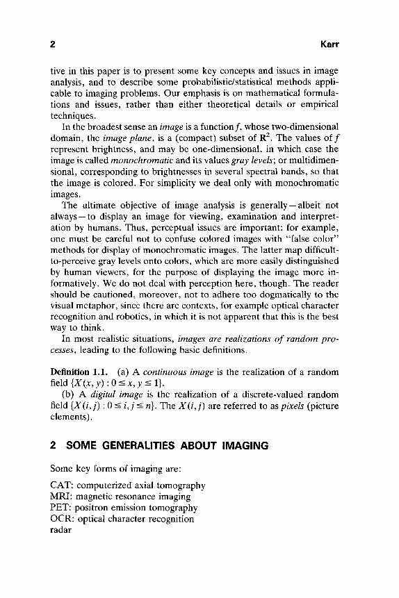
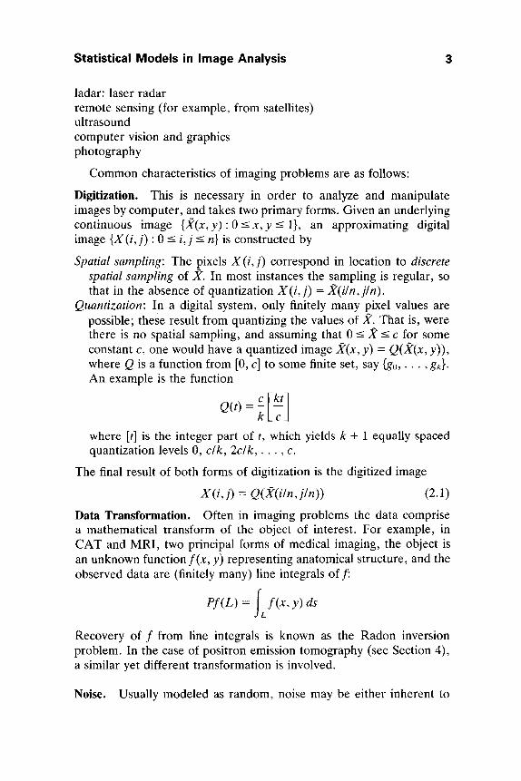
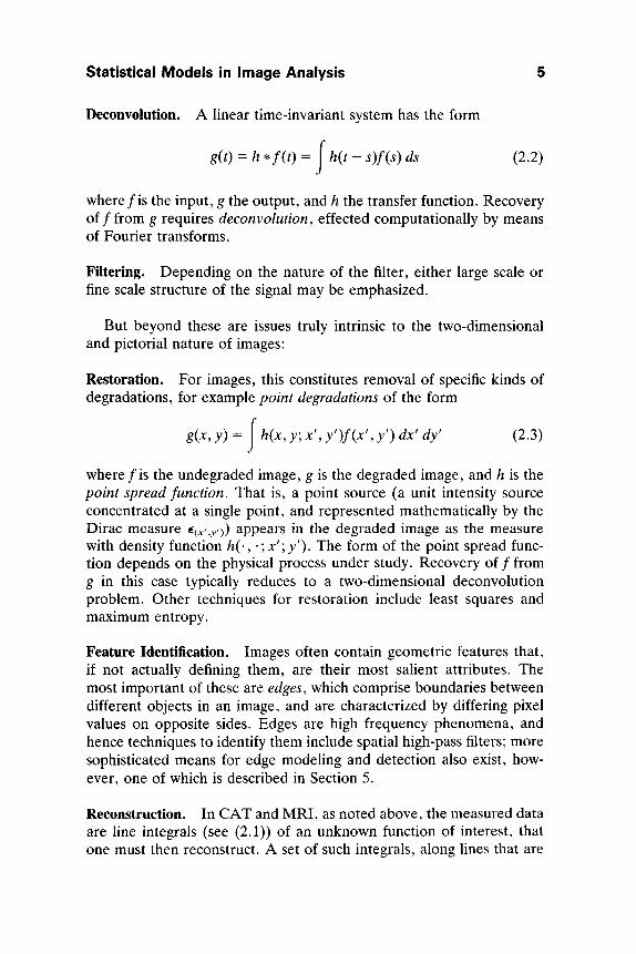
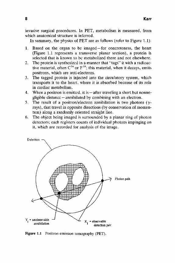
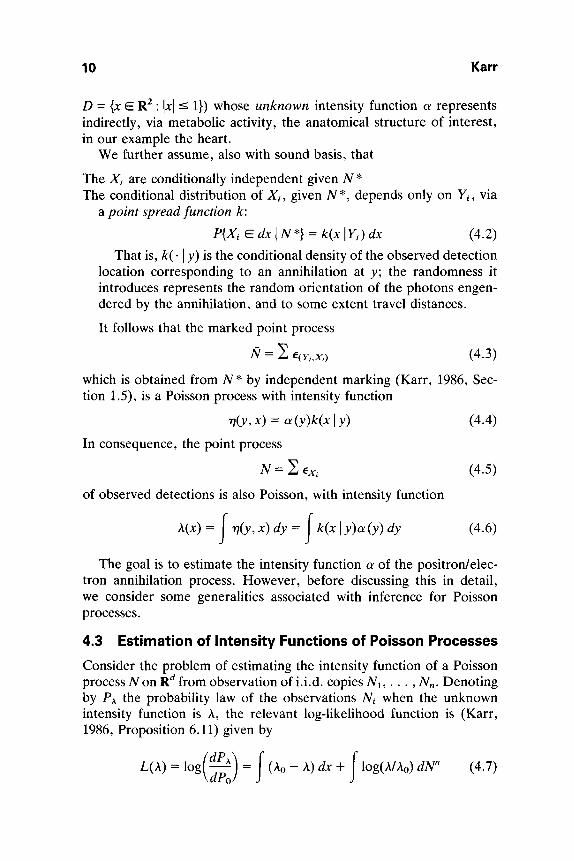
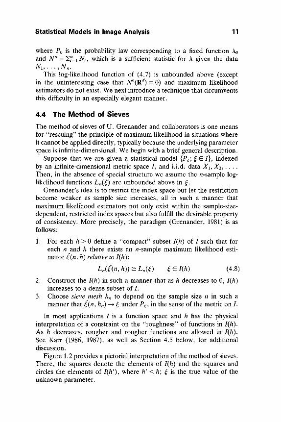
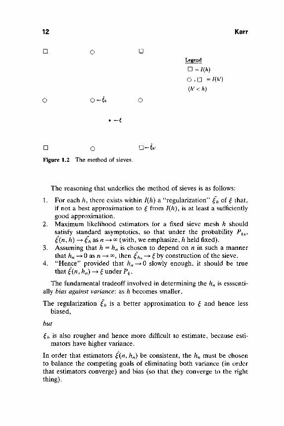
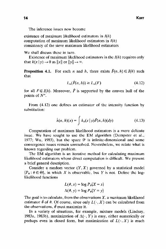
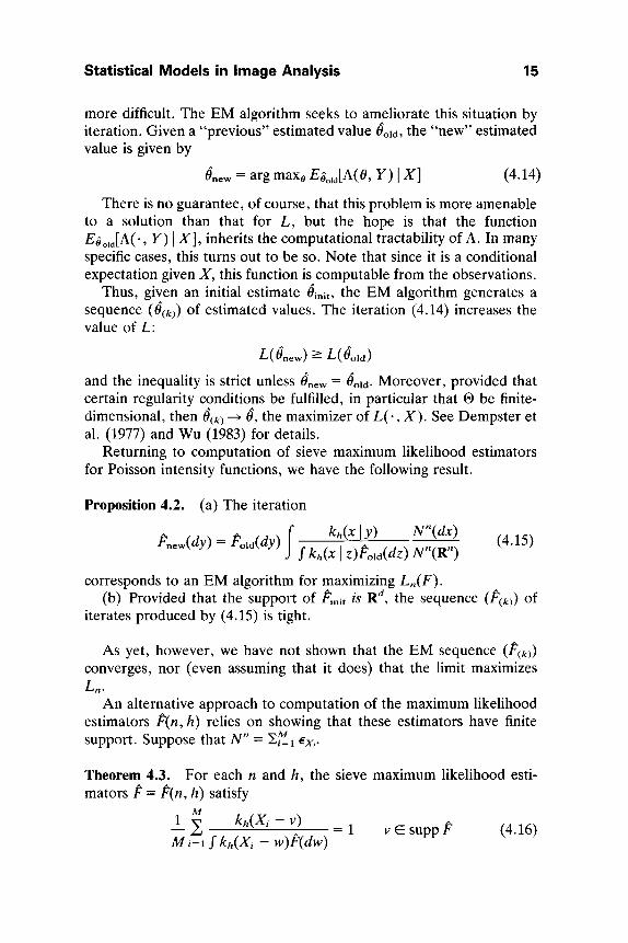
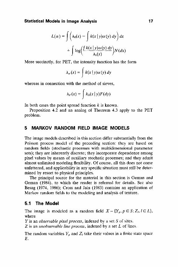
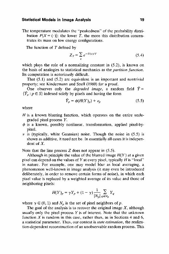
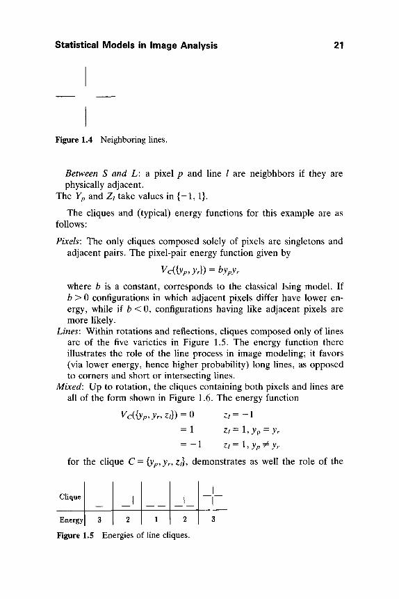
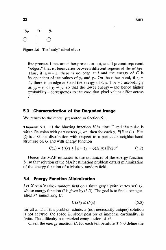
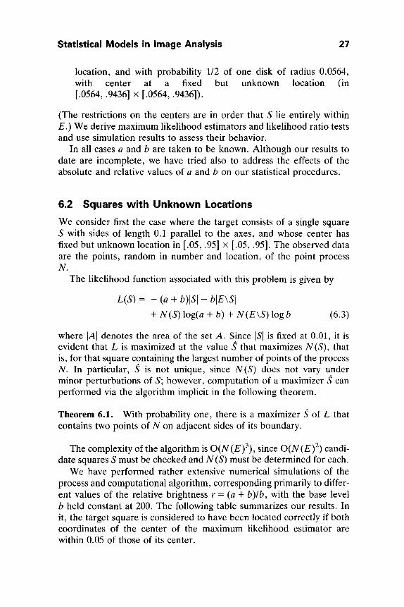
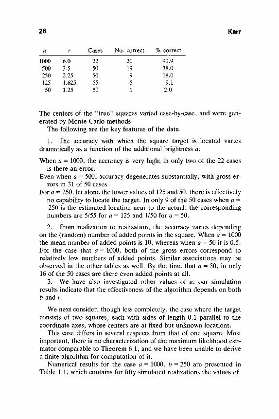
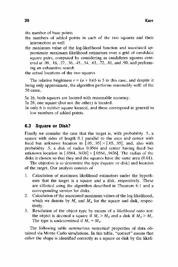
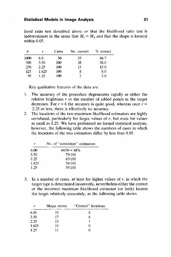