STRUCTURED FACTOR COPULAS AND TAIL INFERENCE
172
STRUCTURED FACTOR COPULAS AND TAIL INFERENCE by Pavel Krupskii B.Sc., Moscow State University, Moscow, Russia, 2006 M.Sc., New Economic School, Moscow, Russia, 2009 A THESIS SUBMITTED IN PARTIAL FULFILLMENT OF THE REQUIREMENTS FOR THE DEGREE OF DOCTOR OF PHILOSOPHY in The Faculty of Graduate and Postdoctoral Studies (Statistics) THE UNIVERSITY OF BRITISH COLUMBIA (Vancouver) July 2014 c Pavel Krupskii 2014
-
Upload
khangminh22 -
Category
Documents
-
view
2 -
download
0
Transcript of STRUCTURED FACTOR COPULAS AND TAIL INFERENCE
STRUCTURED FACTOR COPULAS
AND TAIL INFERENCE
by
Pavel Krupskii
B.Sc., Moscow State University, Moscow, Russia, 2006M.Sc., New Economic School, Moscow, Russia, 2009
A THESIS SUBMITTED IN PARTIAL FULFILLMENT OFTHE REQUIREMENTS FOR THE DEGREE OF
DOCTOR OF PHILOSOPHY
in
The Faculty of Graduate and Postdoctoral Studies
(Statistics)
THE UNIVERSITY OF BRITISH COLUMBIA
(Vancouver)
July 2014
c© Pavel Krupskii 2014
Abstract
In this dissertation we propose factor copula models where dependence ismodeled via one or several common factors. These are general conditionalindependence models for d observed variables, in terms of p latent variablesand the classical multivariate normal model with a correlation matrix hav-ing a factor structure is a special case. We also propose and investigatedependence properties of the extended models that we call structured fac-tor copula models. The extended models are suitable for modeling largedata sets when variables can be split into non-overlapping groups such thatthere is homogeneous dependence within each group. The models allowfor different types of dependence structure including tail dependence andasymmetry. With appropriate numerical methods, efficient estimation ofdependence parameters is possible for data sets with over 100 variables.
The choice of copula is essential in the models to get correct inferencesin the tails. We propose lower and upper tail-weighted bivariate measuresof dependence as additional scalar measures to distinguish bivariate copulaswith roughly the same overall monotone dependence. These measures allowthe efficient estimation of strength of dependence in the joint tails and canbe used as a guide for selection of bivariate linking copulas in factor copulamodels as well as for assessing the adequacy of fit of multivariate copulamodels.
We apply the structured factor copula models to analyze financial datasets, and compare with other copula models for tail inference. Using model-based interval estimates, we find that some commonly used risk measuresmay not be well discriminated by copula models, but tail-weighted depen-dence measures can discriminate copula models with different dependenceand tail properties.
ii
Preface
This dissertation was prepared under the supervision of professor Harry Joeand it is mainly based on three papers coauthored with Harry Joe. One ofthe papers has been published and the other two are currently under review.
Chapter 2 is based on the submitted paper Krupskii and Joe (2014b),Tail-weighted measures of dependence. The idea of using a weighting func-tion to get a measure of dependence in the tails that can perform bettercomparing to semicorrelations of normal scores came from the supervisor.Some good choices of the weighting function were proposed by the author ofthis dissertation. The author also proved asymptotic results and wrote thefirst version of the manuscript followed by the revisions proposed by HarryJoe.
Chapter 3 contains material which is not published or submitted any-where yet. The author of the dissertation uses the concept of tail weightingthat was originally motivated by the supervisor and construct some measuresof asymmetry. Asymptotic results and empirical study was conducted by theauthor. Harry Joe made some useful suggestions on improving the presenta-tion of material in this Chapter and using the 1-factor gamma convolutionmodel to compare the performance of different measures of asymmetry.
Chapter 4 is mostly based on the published paper Krupskii and Joe(2013), Factor copula models for multivariate data, published in Journalof Multivariate Analysis. The idea of using factor copula models came fromthe supervisor. The author completed most of the proofs in this Chapterand implemented fast algorithm based on a modified Newton-Raphson al-gorithm with an adjustment to a positive definite Hessian for estimatingparameters in the model. Some parts of the code were written in Fortran90 to speed up computational process and the author used templates forderivatives of the log-likelihoods that were proposed by the supervisor. Theauthor also provided details on estimating the multivariate Student modelwith a factor correlation structure, including simple formulas for the inverseand determinant of the correlation matrix; this part of research is not in-cluded in the paper. The first version of the manuscript was written by theauthor followed by the revisions proposed by Harry Joe.
iii
Preface
Chapter 5 is mostly based on the submitted paper Krupskii and Joe(2014a), Structural factor copula models: theory, inference and computa-tion. The supervisor proposed to use the bi-factor copula model, which isan extension of the factor copula model, to handle data with a group struc-ture. The author of this dissertation proposed an alternative model, thenested copula model, and completed most of the proofs in this Chapter. Healso adjusted the modified Newton-Raphson algorithm from the previousChapter to estimate parameters in the models proposed in this Chapter.The author also provided details on estimating the multivariate Studentmodel with a bi-factor correlation structure, including simple formulas forthe inverse and determinant of the correlation matrix; this part of researchis not included in the paper. The first version of the manuscript was writtenby the author followed by the revisions proposed by Harry Joe.
In addition to the aforementioned contributions of the supervisor, profes-sor Harry Joe made lots of suggestions regarding the presentation of materialin this dissertation, relevant literature and motivation of the research. Healso checked all the proofs and made some changes in the writing to improvethe flow of ideas in the dissertation and papers.
iv
Table of Contents
Abstract . . . . . . . . . . . . . . . . . . . . . . . . . . . . . . . . . ii
Preface . . . . . . . . . . . . . . . . . . . . . . . . . . . . . . . . . . iii
Table of Contents . . . . . . . . . . . . . . . . . . . . . . . . . . . . v
List of Tables . . . . . . . . . . . . . . . . . . . . . . . . . . . . . . viii
List of Figures . . . . . . . . . . . . . . . . . . . . . . . . . . . . . . xi
Acknowledgements . . . . . . . . . . . . . . . . . . . . . . . . . . . xii
Dedication . . . . . . . . . . . . . . . . . . . . . . . . . . . . . . . . xiii
1 Introduction . . . . . . . . . . . . . . . . . . . . . . . . . . . . . 11.1 Copula notation . . . . . . . . . . . . . . . . . . . . . . . . . 51.2 Some commonly used parametric copula families and their
properties . . . . . . . . . . . . . . . . . . . . . . . . . . . . . 6
2 Tail-weighted measures of dependence . . . . . . . . . . . . 112.1 Tail-weighted measures of dependence: definition and prop-
erties . . . . . . . . . . . . . . . . . . . . . . . . . . . . . . . 122.2 Empirical versions of tail-weighted measures and the choice
of the weighting function . . . . . . . . . . . . . . . . . . . . 152.3 Normal scores plots and tail-weighted measures of dependence 22
3 Measures of asymmetry based on the empirical copula pro-cess . . . . . . . . . . . . . . . . . . . . . . . . . . . . . . . . . . . 263.1 Measures of reflection asymmetry . . . . . . . . . . . . . . . 273.2 Measures of bivariate permutation asymmetry . . . . . . . . 303.3 The power of tests based on the measures of asymmetry . . . 333.4 Preliminary diagnostics using measures of asymmetry . . . . 36
v
Table of Contents
4 Factor copula models for multivariate data . . . . . . . . . 394.1 Factor copula models . . . . . . . . . . . . . . . . . . . . . . 40
4.1.1 One and two-factor copula models . . . . . . . . . . . 414.1.2 Models with p > 2 factors . . . . . . . . . . . . . . . . 44
4.2 p-factor structure in LT-Archimedean copulas . . . . . . . . 474.3 Properties of 1- and 2-factor copula models . . . . . . . . . . 49
4.3.1 Dependence properties . . . . . . . . . . . . . . . . . 504.3.2 Tail properties . . . . . . . . . . . . . . . . . . . . . . 53
4.4 Computational details . . . . . . . . . . . . . . . . . . . . . . 584.4.1 Numerical integration and likelihood optimization . . 584.4.2 Multivariate Student model with a p-factor correlation
structure . . . . . . . . . . . . . . . . . . . . . . . . . 604.5 Empirical results for simulated and financial data sets . . . . 65
4.5.1 Choice of bivariate linking copulas . . . . . . . . . . . 654.5.2 Dependence measures . . . . . . . . . . . . . . . . . . 654.5.3 Simulation results . . . . . . . . . . . . . . . . . . . . 664.5.4 Financial return data . . . . . . . . . . . . . . . . . . 68
5 Structured factor copula models . . . . . . . . . . . . . . . . 755.1 Two extensions of factor copula models for data clustered in
groups . . . . . . . . . . . . . . . . . . . . . . . . . . . . . . 775.1.1 Bi-factor copula model . . . . . . . . . . . . . . . . . 785.1.2 Nested copula model . . . . . . . . . . . . . . . . . . 805.1.3 Special case of Gaussian copulas . . . . . . . . . . . . 81
5.2 Tail and dependence properties of the structured factor cop-ula model . . . . . . . . . . . . . . . . . . . . . . . . . . . . . 86
5.3 Computational details for factor copula models . . . . . . . . 935.3.1 Log-likelihood maximization in factor copula models . 935.3.2 Multivariate Student model with bi-factor correlation
structure . . . . . . . . . . . . . . . . . . . . . . . . . 965.3.3 Multivariate Student model with tri-factor correlation
structure . . . . . . . . . . . . . . . . . . . . . . . . . 985.3.4 Asymptotic covariance matrix of 2-stage copula-GARCH
parameter estimates . . . . . . . . . . . . . . . . . . . 995.4 Interval estimation of VaR, CTE for copula-GARCH model . 1005.5 Empirical study . . . . . . . . . . . . . . . . . . . . . . . . . 103
5.5.1 Assessing the strength of dependence in the tails . . . 1055.5.2 VaR and CTE for different models . . . . . . . . . . . 1075.5.3 Comparing performance of nested copula models . . . 109
vi
Table of Contents
6 Concluding remarks . . . . . . . . . . . . . . . . . . . . . . . . 118
Bibliography . . . . . . . . . . . . . . . . . . . . . . . . . . . . . . . 121
Appendices
A Proof of Proposition 2.1, Section 2.2 . . . . . . . . . . . . . . 127
B Proof of Proposition 2.2, Section 2.2 . . . . . . . . . . . . . . 131
C Proof of Proposition 4.5, Section 4.3.2 . . . . . . . . . . . . 133
D Proof of Proposition 4.6, Section 4.3.2 . . . . . . . . . . . . 134
E Proof of Proposition 4.7, Section 4.3.2 . . . . . . . . . . . . 136
F Parameter estimation in factor copula models . . . . . . . 139F.1 Newton-Raphson algorithm and 1-factor copula model . . . . 139F.2 Newton-Raphson algorithm and 2-factor copula model . . . . 141F.3 First and second order analytical derivatives for different cop-
ula families . . . . . . . . . . . . . . . . . . . . . . . . . . . . 143F.4 Notes on the differentiation under the integral sign . . . . . . 151
G Bivariate copulas satisfying assumptions of Proposition 5.3 153
H Derivatives of bivariate linking copulas . . . . . . . . . . . . 155
I Correlation matrix inverse and determinant in the struc-tured factor Gaussian model . . . . . . . . . . . . . . . . . . . 156
vii
List of Tables
1.1 Some copula notation used throughout this dissertation . . . 61.2 The values λL, λU , κL and κU for some bivariate copulas; ql = −
√(ν+1)(1−ρ)
(1+ρ). 9
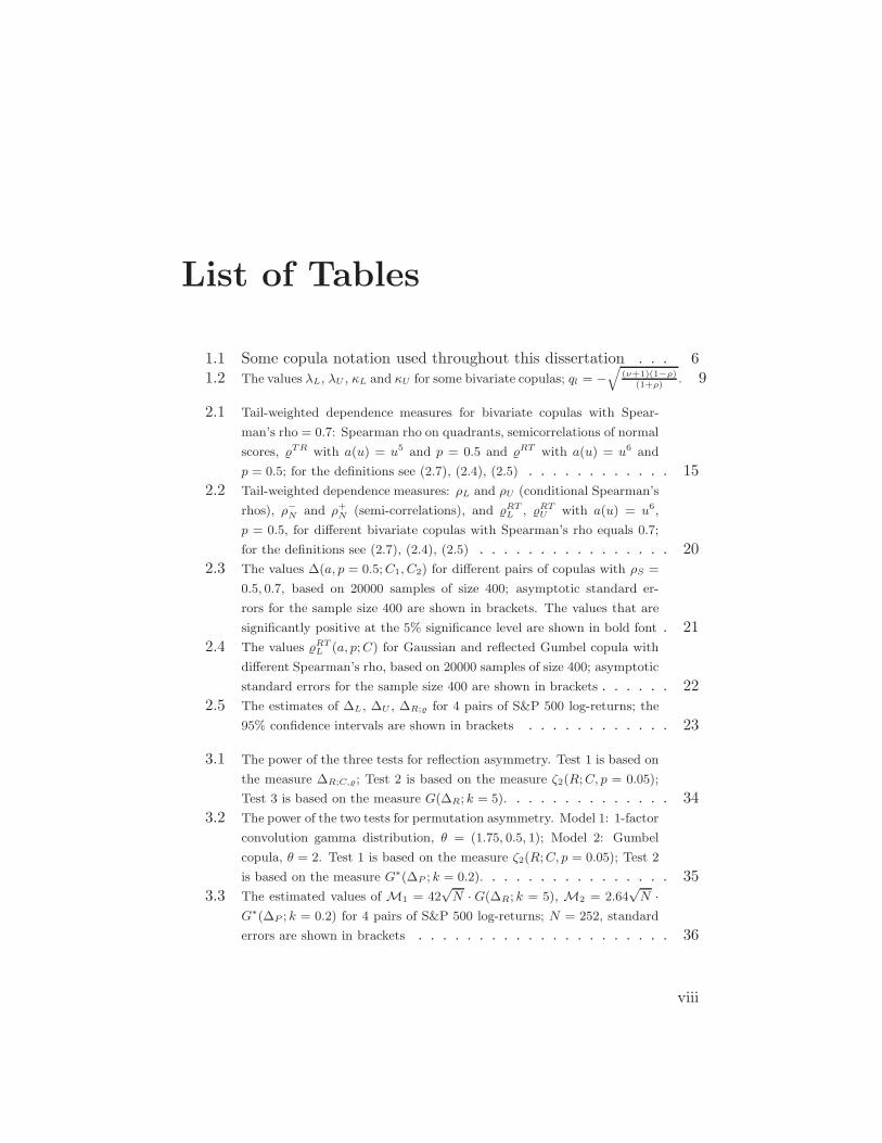
2.1 Tail-weighted dependence measures for bivariate copulas with Spear-
man’s rho = 0.7: Spearman rho on quadrants, semicorrelations of normal
scores, TR with a(u) = u5 and p = 0.5 and RT with a(u) = u6 and
p = 0.5; for the definitions see (2.7), (2.4), (2.5) . . . . . . . . . . . . 152.2 Tail-weighted dependence measures: ρL and ρU (conditional Spearman’s
rhos), ρ−N and ρ+N (semi-correlations), and RTL , RT
U with a(u) = u6,
p = 0.5, for different bivariate copulas with Spearman’s rho equals 0.7;
for the definitions see (2.7), (2.4), (2.5) . . . . . . . . . . . . . . . . 202.3 The values ∆(a, p = 0.5;C1, C2) for different pairs of copulas with ρS =
0.5, 0.7, based on 20000 samples of size 400; asymptotic standard er-
rors for the sample size 400 are shown in brackets. The values that are
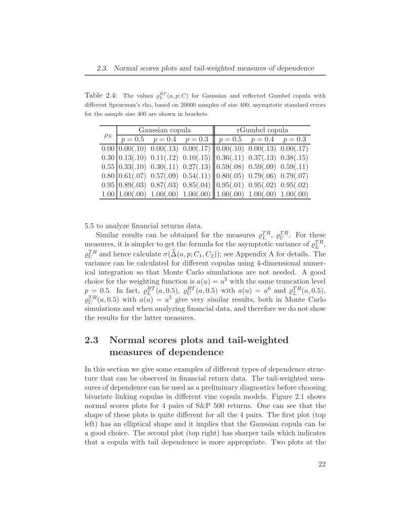
significantly positive at the 5% significance level are shown in bold font . 212.4 The values RT
L (a, p;C) for Gaussian and reflected Gumbel copula with
different Spearman’s rho, based on 20000 samples of size 400; asymptotic
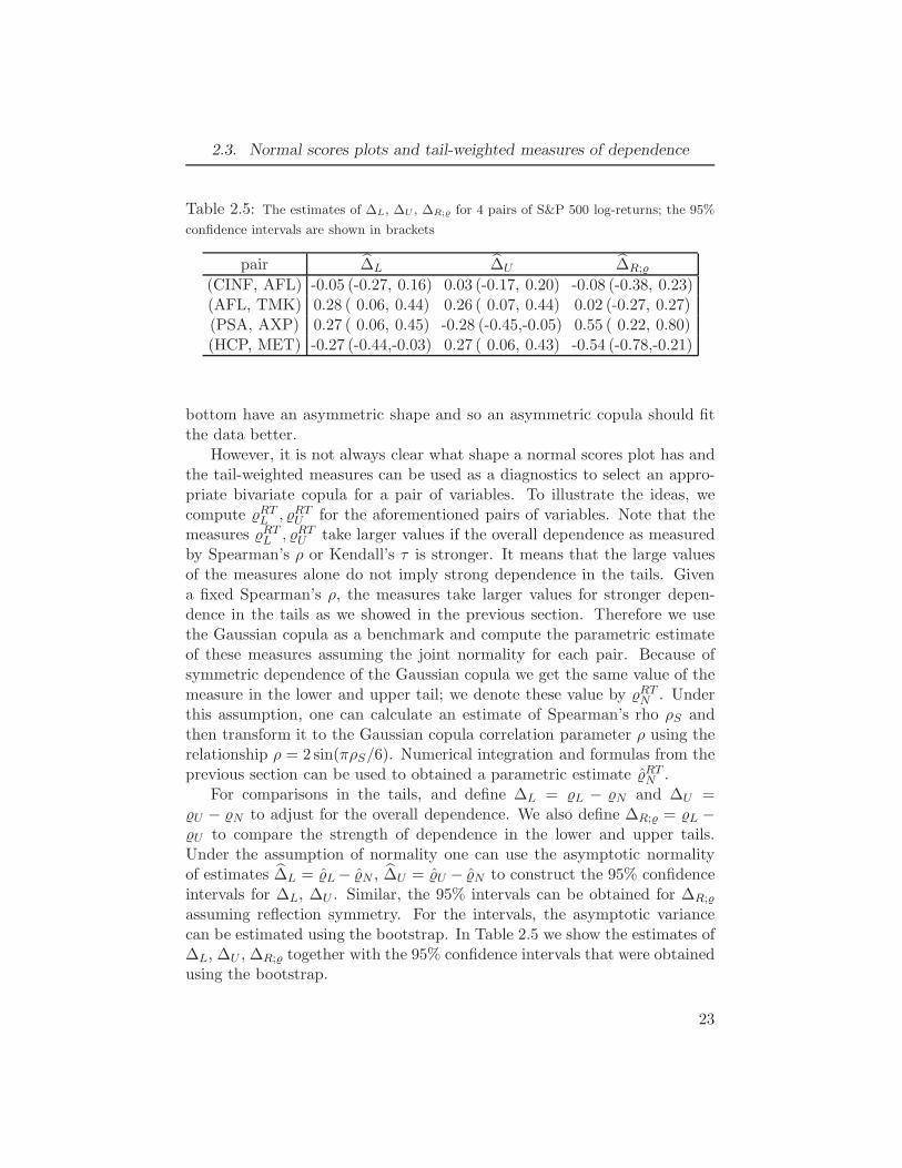
standard errors for the sample size 400 are shown in brackets . . . . . . 222.5 The estimates of ∆L, ∆U , ∆R; for 4 pairs of S&P 500 log-returns; the
95% confidence intervals are shown in brackets . . . . . . . . . . . . 23
3.1 The power of the three tests for reflection asymmetry. Test 1 is based on
the measure ∆R;C,; Test 2 is based on the measure ζ2(R;C, p = 0.05);
Test 3 is based on the measure G(∆R; k = 5). . . . . . . . . . . . . . 343.2 The power of the two tests for permutation asymmetry. Model 1: 1-factor
convolution gamma distribution, θ = (1.75, 0.5, 1); Model 2: Gumbel
copula, θ = 2. Test 1 is based on the measure ζ2(R;C, p = 0.05); Test 2
is based on the measure G∗(∆P ; k = 0.2). . . . . . . . . . . . . . . . 353.3 The estimated values of M1 = 42
√N · G(∆R; k = 5), M2 = 2.64
√N ·
G∗(∆P ; k = 0.2) for 4 pairs of S&P 500 log-returns; N = 252, standard
errors are shown in brackets . . . . . . . . . . . . . . . . . . . . . 36
viii
List of Tables
4.1 [S diffρ ], [S diff
ρ ]max, [ ˆdiffL ], [ ˆdiff
L ]max, [ ˆdiffU ], [ ˆdiff
U ]max (averages and max-
ima over(d2
)bivariate margins; for the definitions see (4.26)) and the
maximum log-likelihood value for different copulas in 1- and 2-factor
models; simulated data set with sample size N = 500 and dimension
d = 30 . . . . . . . . . . . . . . . . . . . . . . . . . . . . . . . . 674.2 [S diff
ρ ], [S diffρ ]max, [ ˆdiff
L ], [ ˆdiffL ]max, [ ˆdiff
U ], [ ˆdiffU ]max (averages or maxima
over(82
)= 28 bivariate margins; for the definitions see (4.26)) and the
maximum log-likelihood value for different copulas in 1- and 2-factor
models and for MVt distribution; US stock data, year 2001 . . . . . . 714.3 MLEs for parameters of linking copula families in 1-factor models, US IT
stock data, year 2001; variables 1=INTC, 2=CSCO, 3=NOVL, 4=MOT,
5=AAPL, 6=MSFT, 7=DELL, 8=ADBE. . . . . . . . . . . . . . . . 724.4 MLEs for parameters of linking copula families in 2-factor models, US IT
stock data, year 2001; variables 1=INTC, 2=CSCO, 3=NOVL, 4=MOT,
5=AAPL, 6=MSFT, 7=DELL, 8=ADBE. . . . . . . . . . . . . . . . 734.5 Log-likelihoods for different models, US data, year 2001; number of de-
pendence parameters for each model is shown in parentheses . . . . . 744.6 Log-likelihoods for truncated R-vine models: US data, year 2001. . . . . 74
5.1 Overall and group averages of ˆL, ˆU , ρS; GARCH-filtered log-returns
from S&P500 index, health care sector, years 2010–2011. . . . . . . . . 1075.2 Overall and group averages of δL, δU , |δL|, |δU |, and the maximum log-
likelihood value for different models; GARCH-filtered log-returns from
S&P500 index, health care sector, years 2010–2011. . . . . . . . . . . 1085.3 Overall and group estimated averages of L, U , ρS and the model-based
95% confidence intervals (intervals that don’t contain the empirical
value are shown in bold font); GARCH-filtered log-returns of stocks
in the health care sector of the S&P500 index, years 2010-2011. . . . . 1105.4 Empirical estimates of VaRα for α = 0.01, 0.05, 0.95, 0.99 and the model-
based 95% confidence intervals; GARCH-filtered log-returns for stocks
from health care sector of the S&P500 index, years 2010–2011. . . . . . 1115.5 Empirical estimates of CTE−(r∗), for r∗ = −0.03,−0.02, and CTE+(r∗),
for r∗ = 0.02, 0.03, and the model-based 95% confidence intervals for the
6 models; model 1: bi-factor Gaussian, model 2: bi-factor Student t,
model 3: bi-factor Frank, model 4: 1-factor reflected BB1, model 5:
nested rGumble/rBB1, model 6: bi-factor BB1/Frank. GARCH-filtered
log-returns for stocks from the health care sector in the S&P500 index,
years 2010–2011. . . . . . . . . . . . . . . . . . . . . . . . . . . . 1115.6 Empirical Spearman’s ρS for GARCH-filtered log return data . . . . . 112
ix
List of Tables
5.7 Lower (upper) tail-weighted dependence measures L (U ) for GARCH-
filtered log returns in lower (upper) triangle . . . . . . . . . . . . . . 1135.8 Overall, tobacco group and soft drinks group averages of ρS, L, U and
N ; GARCH-filtered log-returns from S&P500 index, consumer staples
sector, years 2011–2012 . . . . . . . . . . . . . . . . . . . . . . . 1135.9 Negative log-likelihood and AIC values for copula models applied to
GARCH-filtered log returns; AIC is 2 times the negative log-likelihood
+ 2 times #parameters . . . . . . . . . . . . . . . . . . . . . . . 1155.10 Empirical estimates and the model-based 95% confidence intervals for
VaRα with α = 0.01, 0.05, 0.95, 0.99, CTE−(r∗) with r∗ = −0.026,−0.015
and CTE+(r∗) with r∗ = 0.016, 0.028; GARCH-filtered log-returns from
S&P500 index, consumer staples sector, years 2011–2012 . . . . . . . 1165.11 Estimated averages (overall, tobacco group and soft drinks group) of
ρS, L, U and the model-based 95% confidence intervals (intervals
that don’t contain the empirical value are shown in bold font);
GARCH-filtered log-returns from S&P500 index, consumer staples sec-
tor, years 2011–2012 . . . . . . . . . . . . . . . . . . . . . . . . . 117
x
List of Figures
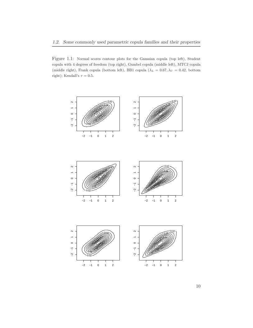
1.1 Normal scores contour plots for the Gaussian copula (top left), Student
copula with 4 degrees of freedom (top right), Gumbel copula (middle
left), MTCJ copula (middle right), Frank copula (bottom left), BB1
copula (λL = 0.67, λU = 0.42, bottom right); Kendall’s τ = 0.5. . . . . 10
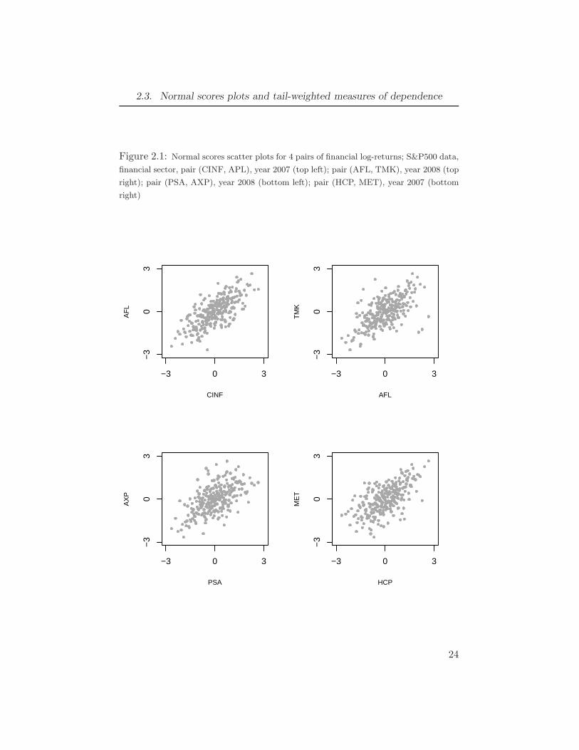
2.1 Normal scores scatter plots for 4 pairs of financial log-returns; S&P500
data, financial sector, pair (CINF, APL), year 2007 (top left); pair (AFL,
TMK), year 2008 (top right); pair (PSA, AXP), year 2008 (bottom left);
pair (HCP, MET), year 2007 (bottom right) . . . . . . . . . . . . . 24
3.1 Uniform scores scatter plots for data generated from the 1-factor convo-
lution gamma distribution with Kendall’s τ = 0.5: no asymmetry (right,
θ0 = 2.2, θ1 = θ2 = 1); moderate asymmetry (middle, θ0 = 1.75, θ1 =
0.5, θ2 = 1); strong asymmetry (left, θ0 = 1.3, θ1 = 0.2, θ2 = 1) . . . . . 333.2 Normal scores scatter plots for 4 pairs of financial returns; S&P500 data,
financial sector, pair (HCP, PSA), year 2007 (top left); pair (AVB, ACE),
year 2007 (top right); pair (WY, AIG), year 2008 (bottom left); pair
(AMT, LNC), year 2008 (bottom right) . . . . . . . . . . . . . . . 37
5.1 Bi-factor model with G groups, dg variables in the g-th group . . . . . 845.2 Nested model with G groups, dg variables in the g-th group . . . . . . 84
xi

Acknowledgements
This research has been supported by an NSERC Discovery Grant. I wouldlike to thank my supervisor, professor Harry Joe, for his help and sup-port during my graduate work. I am grateful to the supervisory committeemembers, Natalia Nolde and Haijun Li, and external examiner AlexanderMcNeil for the valuable comments and suggestions that helped to improvepresentation in this dissertation.
xii

TO MY PARENTS
xiii
Chapter 1
Introduction
The multivariate normality assumption is widely used to model the joint dis-tribution of high-dimensional data. The univariate margins are transformedto normality and then the multivariate normal distribution is fitted to thetransformed data. In this case, the dependence structure is completely de-fined by the correlation matrix and different models on the correlation struc-ture can be used to reduce the number of dependence parameters from O(d2)to O(d), where d is the multivariate dimension or number of variables. TheseGaussian models, however, may not be appropriate for modeling data thathave very strong dependence in the tails. In many applications, variablesin a multidimensional data set tend to take very large negative or positivevalues simultaneously much more often than it is predicted by the Gaussianmodel. Typical examples include financial return data or insurance claimsdata. In addition to strong dependence in the tails, asymmetric dependencecan not be handled by the Gaussian models.
To overcome these difficulties, different models that use a copula functionto model the joint distribution become more popular in different applica-tions. The copula is a function linking univariate margins into the jointdistribution. Let X = (X1, . . . ,Xd) be a random d-dimensional vector withthe joint cumulative distribution function (cdf) FX. Let FXj be the marginalcdf of Xj for j = 1, . . . , d. The copula CX, corresponding to FX, is a multi-variate uniform cdf such that FX(x1, . . . , xd) = CX(FX1(x1), . . . , FXd
(xd)).By Sklar (1959), there exists a unique copula CX if FX is continuous. Cop-ulas are suitable for modeling non-Gaussian data such as financial asset re-turns or insurance data; see Patton (2006), McNeil et al. (2005) and others.The superiority of non-normal copulas over the normal copula in modelingfinancial and insurance data has been discussed in Embrechts (2009).
In a copula model, univariate data are fitted first and the variables arethen transformed to uniform data to obtain estimates of the copula de-pendence parameters. This approach allows modeling in two steps withestimation of parameters for univariate marginals and then for the copulacdf. This greatly simplifies the estimation procedure for high-dimensionaldata. Simple multivariate copula families, such as Archimedean, however,
1
Chapter 1. Introduction
do not have flexible dependence structure. To get flexibility, a popularapproach is to use a sequence of algebraically independent bivariate copu-las applied to either marginal or univariate conditional distributions. Ap-proaches that use a sequence of bivariate copulas include vine pair-copulaconstructions (Kurowicka and Joe (2011)). These classes of copulas havebeen used for finance and other applications because they can cover a widerange of dependence and tail behavior; see for example, Aas et al. (2009),Nikoloulopoulos et al. (2012), Brechmann et al. (2012). More papers onvine copulas can be found at the web site http://vine-copula.org.
In many multivariate applications, the dependence in observed vari-ables can be explained through latent variables; in multivariate item re-sponse in psychology applications, latent variables are related to the ab-stract variable being measured through items, and in finance applications,latent variables are related to economic factors. Classical factor analysis as-sumes (after transforms) that all observed and latent random variables arejointly multivariate normal. Books on multivariate analysis (see for example,Johnson and Wichern (2002)) often have examples with factor analysis andfinancial returns. In this dissertation we propose and study the propertiesof the copula version of multivariate Gaussian models with a factor corre-lation structure. The models, which we will call factor copula models, arespecial cases of vine models with latent variables. The factor copula mod-els keep the interpretability of the Gaussian factor models while allowingfor different types of dependence structure including strong tail dependenceand dependence asymmetry.
A special case of factor copula models is models with conditionally in-dependent and identically distributed random variables. Due to de Finettitheorem (see Loeve (1963)) these models are equivalent to exchangeable ran-dom variables. The latter class of models is not flexible enough for appli-cations; it includes Archimedean copulas. In the general case, factor copulamodels proposed in this dissertation have different conditional margins andexchangeability does not hold.
These common factor copula models implicitly require a homogeneousdependence structure with the assumption of conditional independence givenseveral common factors. In data sets with a large number of variables, datacan come from different sources or be clustered in different groups, for ex-ample, stock returns from different sectors or grouped item response datain psychometrics; thus dependence within each group and among differentgroups can be different. In psychometrics, sometimes a bi-factor correlationstructure is used when variables or items can be split into non-overlappinggroups; see for example Gibbons and Hedeker (1992) and
2
Chapter 1. Introduction
Holzinger and Swineford (1937). In a Gaussian bi-factor model, there is onecommon Gaussian factor which defines dependence among different groups,and one or several independent group-specific Gaussian factors which definedependence within each group. An alternative way to model dependencefor grouped data is a nested model where the dependence in groups is mod-eled via dependent group-specific factors and the observed variables are as-sumed to be conditionally independent given these group-specific factors.The nested model is similar to Gaussian models with multilevel covariancestructure; see Muthen (1994). In this dissertation, we propose copula ex-tensions for the bi-factor and nested Gaussian models. We will call theseextensions as structured factor copula models. The proposed models con-tain 1- and 2-factor copula models as special cases, while allowing flexibledependence structure both for within group and between group dependence.As a result, the models can be suitable for modeling high-dimensional datasets consisting of several groups of variables with homogeneous dependencein each group.
The main advantage of factor copula models is that they can be nicelyinterpreted when used in some applications. In finance applications, for ex-ample, the group latent factors may represent the current state of a financesector and the common latent factor may represent the current state of thewhole economy. In vine copula models the structure of the joint distributioncan be quite complicated and is usually chosen to maximize the likelihoodvalue and a simple interpretation of the model is thus quite difficult. Themain disadvantage of the factor models is that numerical integration is re-quired to compute the likelihood whereas in vine models the joint copuladensity is given in a simple form. It implies the computation can takelonger compared to vine models. However, factor models are closed underthe marginalization, and data can be divided into smaller subsets and pa-rameters can be estimated for each subset independently. This significantlyreduces computational time and the estimates obtained in this way can thenbe used as starting points when all parameters in the model are estimatedsimultaneously. With good starting points, estimation becomes much fasteras quite a small number of iterations is usually required for convergence.
Appropriate choices of bivariate copulas used in the vine and factor cop-ula models are very important. Inappropriate choices can cause the modelto provide incorrect inference on joint tail probabilities. This is crucial inmany applications such as quantitative risk analysis in finance and insur-ance where good estimates of joint tail probabilities are essential. We pro-pose tail-weighted measures of dependence which can be used to distinguishdifferent bivariate copula families through their strength of dependence in
3
Chapter 1. Introduction
the joint tails. The tail-weighted measures provide additional informationto commonly used monotone dependence measures such as Kendall’s τ andSpearman’s ρS , because a single dependence measure, which is dominated bythe copula density in the center part of the unit square, cannot summarizeall of the important dependence and tail properties of the copula.
Bivariate tail-weighted measures of dependence that we propose are de-fined as correlations of transformed variables; they have easily-computedsample versions. The measures can be applied to each pair of variables in amultidimensional data set. These measures put more weight in the tails andthus can efficiently estimate the strength of dependence in the tail even if thesample size is not very large. We also propose some tail-weighted measuresof asymmetry and introduce diagnostic procedures. These procedures canbe used to detect possible departures from normality and help to select moresuitable copula for the data set. What is more important, the measures andprocedures can be used for assessing the adequacy of the chosen model inthe tails. Therefore these measures can be employed in factor copula modelsand in vine models (and other copula models), and we use empirical studiesto illustrate these ideas.
Note that the purpose of these tail-weighted measures of dependenceto assess models is quite different in aim than copula goodness-of-fit proce-dures; Huang and Prokhorov (2014) and Schepsmeier (2014) have developedlikelihood-based copula goodness-of-fit tests and Genest et al. (2009) havean overview of bivariate goodness-of-fit tests for copulas. However these pre-viously proposed goodness-of-fit procedures are not diagnostic in suggestingimproved models when the P-values are small. For preliminary data anal-ysis, the tail-weighted measures of dependence can provide a guide to thechoice of bivariate copulas to use in vine and factor models. After fittingcompeting copula models, the comparison of empirical and model-based es-timates is a method to assess whether the best-fitting copula models basedon AIC or BIC are adequate for tail inference or whether alternative modelsshould be considered. Different copula models with a similar dependencestructure can typically perform similarly in the comparison of empirical ver-sus model-based measure of monotone association such Spearman’s rho, butthey can differ more for tail inference. This is because while the dependencestructure, which is based mostly on the middle of the data, dominates thelog-likelihood of parametric copula models, a secondary contribution to thelog-likelihood is based on the quality of fit in the tails. Most parametriccopula families, including Gaussian, have densities that asymptote to infin-ity at one or more corners of the hypercube, and hence parametric copulafamilies with different strength of dependence in the tails (or different rates
4
1.1. Copula notation
of asymptotes to infinity) can perform quite differently when assessed bytail-weighted dependence measures.
The rest of the dissertation is organized as follows. We define somebasic copula notation and dependence properties in Sections 1.1, 1.2. Thetail-weighted measures of dependence and their properties are presented inChapter 2. We also propose some measures of asymmetry based on theempirical copula function in Chapter 3. The measures perform better com-paring to some other dependence measures that are used in applications.Factor copula models, their dependence and tail properties, and details onparameter estimation are presented in Chapter 4. Extensions of the fac-tor models, structured copula models, are defined in Chapter 5. We derivedependence and tail properties for the structured models and show thatdifferent types of dependence structure can be obtained depending on thechoice of bivariate linking copulas. We apply the models to estimate depen-dence structure of some data sets of financial returns and find that with agood choice of linking copulas the structured copula models fit data quitewell. We find that, unlike the tail-weighted measures of dependence, somerisk measures used in applications in finance are not very sensitive to modelswith different tail behavior. More details are provided for a special case ofthe Gaussian linking copulas. The estimation is much faster in this case asthe log-likelihood function can be obtained in a simple form. Concludingremarks and topics for the future research are presented in Chapter 6 whilethe proofs for some results and more details on numerical computation ofparameters are given in the Appendix.
1.1 Copula notation
We define some general notation that we will use throughout this disserta-tion. Let θ be a dependence parameter (the parameter can be a scalar ora vector). If this parameter is not important it can be suppressed in somenotation. We summarized the copula notation in Table 1.1.
In addition, we will be using the concept of the reflected C copula, or thesurvival copula. If (U1, U2) ∼ C, it follows that (1−U1, 1−U2) ∼ CR, whereCR(u1, u2) := −1+u1 +u2 +C(1−u1, 1− u2). The copula CR is called thereflected C copula. It also implies that C(u1, u2) := 1− u1 − u2 +C(u1, u2)is the survival function for the pair (U1, U2). The function C(1− u1, 1−u2)is usually called the survival copula.
5
1.2. Some commonly used parametric copula families and their properties
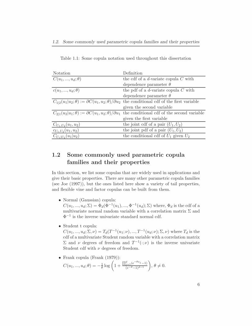
Table 1.1: Some copula notation used throughout this dissertation
Notation Definition
C(u1, ..., ud; θ) the cdf of a d-variate copula C withdependence parameter θ
c(u1, ..., ud; θ) the pdf of a d-variate copula C withdependence parameter θ
C1|2(u1|u2; θ) := ∂C(u1, u2; θ)/∂u2 the conditional cdf of the first variable
given the second variable
C2|1(u2|u1; θ) := ∂C(u1, u2; θ)/∂u1 the conditional cdf of the second variable
given the first variable
CU1,U2(u1, u2) the joint cdf of a pair (U1, U2)
cU1,U2(u1, u2) the joint pdf of a pair (U1, U2)
CU1|U2(u1|u2) the conditional cdf of U1 given U2
1.2 Some commonly used parametric copula
families and their properties
In this section, we list some copulas that are widely used in applications andgive their basic properties. There are many other parametric copula families(see Joe (1997)), but the ones listed here show a variety of tail properties,and flexible vine and factor copulas can be built from them.
• Normal (Gaussian) copula:C(u1, ..., ud; Σ) = Φd(Φ
−1(u1), ...,Φ−1(ud); Σ) where, Φd is the cdf of a
multivariate normal random variable with a correlation matrix Σ andΦ−1 is the inverse univariate standard normal cdf.
• Student t copula:C(u1, ..., ud; Σ, ν) = Td(T
−1(u1; ν), ..., T−1(ud; ν); Σ, ν) where Td is the
cdf of a multivariate Student random variable with a correlation matrixΣ and ν degrees of freedom and T−1(·; ν) is the inverse univariateStudent cdf with ν degrees of freedom.
• Frank copula (Frank (1979)):
C(u1, ..., ud; θ) = −1θ log
(1 +
∏dj=1(e
−θuj−1)
(e−θ−1)d−1
), θ 6= 0.
6
1.2. Some commonly used parametric copula families and their properties
• Gumbel copula (Gumbel (1960)):C(u1, ..., ud; θ) = exp{−(uθ1+...+u
θd)
1/θ}, where θ > 1 and ui = − lnui,i = 1, ..., d.
• MTCJ copula (Mardia (1962), Takahashi (1965), Cook and Johnson(1981)):C(u1, ..., ud; θ) = (u−θ1 + ...+u−θd −d+1)−1/θ, θ > 0. For the bivariatecase, this is also known as the Clayton copula (Clayton (1978)).
• BB1 copula (Joe and Hu (1996), Joe (1997)):C(u1, u2; θ, δ) = {1 + [(u−θ1 − 1)δ + (u−θ2 − 1)δ ]1/δ}−1/θ, θ > 0, δ > 1.
In this dissertation, we will be mainly using bivariate versions of theabove copulas. The densities and conditional cdfs for this copulas for d = 2can be found in Section F.3. Below we define some basic properties forbivariate copulas.
Symmetric copulas
A bivariate copula C is said to be permutation symmetric ifC(u1, u2) = C(u2, u1) for any u1, u2 ∈ (0, 1). If (U1, U2) ∼ C, the permu-tation symmetry implies (U2, U1) ∼ C. It is easy to see that all copulaspresented above are permutation symmetric copulas.
A bivariate copula C is said to be reflection symmetric if C(u1, u2) =CR(u1, u2) for any u1, u2 ∈ (0, 1). If (U1, U2) ∼ C, the reflection symmetryimplies (1 − U1, 1 − U2) ∼ C. The normal, Student and Frank copulas arereflection symmetric copulas and the Gumbel, MTCJ and BB1 copulas arenot.
Dependence properties
A bivariate copula C is said to have positive quadrant dependence(PQD) if C(u1, u2) ≥ u1u2 for any u1, u2 ∈ (0, 1). The normal and Studentcopula with ρ > 0, Frank copula with θ > 0, Gumbel, MTCJ and BB1copula are copulas with positive quadrant dependence. For these copulasdependence is stronger in the first and third quadrants of a unit square.
A bivariate copula C is said to have negative quadrant dependence(NQD) if C(u1, u2) ≤ u1u2 for any u1, u2 ∈ (0, 1). The normal and Studentcopula with ρ < 0, Frank copula with θ < 0 are copulas with negativedependence. For these copulas dependence is stronger in the second andfourth quadrants of a unit square.
The conditional cdf C1|2 of the copula C is stochastically increasing,SI (decreasing) if C1|2(u1|u2) is a decreasing (increasing) function of u2. It
7
1.2. Some commonly used parametric copula families and their properties
implies that the second variable is more likely to take larger (smaller) valueas the first variable increases. The Normal copula with ρ > 0, Frank copulawith θ > 0, Gumbel, MTCJ and BB1 copulas are stochastically increasingcopulas and the Normal copula with ρ < 0, Frank copula with θ < 0 arestochastically decreasing copulas.
The copula C increases (decreases) in concordance ordering ifC(u1, u2; θ) is an increasing (decreasing) function of θ with any fixed 0 <u1, u2 < 1. All copulas that are listed above increase in concordance order-ing. In other words, dependence becomes stronger as dependence parameterincreases. The Student copula does not increase in concordance orderingwith respect to the number of degrees of freedom parameter.
The detailed overview of these dependence concepts are given in Chapter2 of Joe (1997).
Tail properties
Standard measures of tail dependence used in the literature are tail de-pendence coefficients. Assuming the limits exist, the coefficients are definedas follows:
λL = limu↓0
C(u, u)
u, λU = lim
u↓0C(1− u, 1− u)
u. (1.1)
The copula C is said to be lower (upper) tail dependent if the lower(upper) tail dependence coefficient λL (λU ) is positive.
Hua and Joe (2011) assess tail dependence and asymmetry based on therates with which C(u, u) and C(1− u, 1− u) go to 0 as u→ 0. They definethe tail order as the reciprocal of a quantity used in Ledford and Tawn(1996) and Heffernan (2000). It measures the strength of dependence inthe joint lower and upper tails. If C(u, u) ∼ ℓL(u)u
κL as u → 0, whereℓL(u) is a slowly varying function, then we say that the lower tail order isκL. Similarly if C(1 − u, 1 − u) ∼ ℓU (u)u
κU as u → 0, where ℓU (u) is aslowly varying function, then the upper tail order is κU . If 1 < κL < 2or 1 < κU < 2 then λL = 0 (λU = 0 respectively), and this is termedintermediate tail dependence in Hua and Joe (2011). A smaller value ofthe tail order corresponds to more tail dependence (more probability in thecorner). Then, the strongest dependence in the tail corresponds to κL = 1or κU = 1. The tail order can be used to assess tail dependence strength iftail dependence coefficient is zero.
In Table 1.2 the values λL, λU together with κL and κU are presented forbivariate versions of copulas listed in the beginning of this section. It is seenthat the normal copula has intermediate lower and upper tail dependenceand the Student copula is a tail dependent copula. At the same time the
8
1.2. Some commonly used parametric copula families and their properties
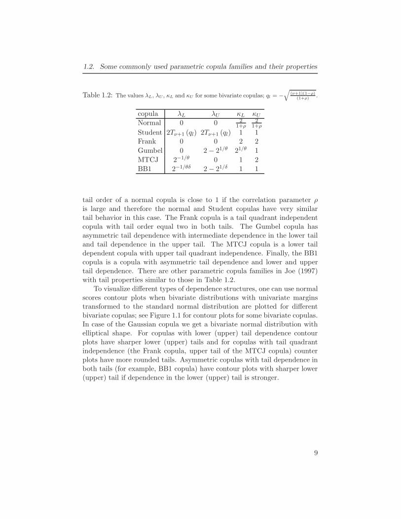
Table 1.2: The values λL, λU , κL and κU for some bivariate copulas; ql = −√
(ν+1)(1−ρ)(1+ρ)
.
copula λL λU κL κUNormal 0 0 2
1+ρ2
1+ρ
Student 2Tν+1 (ql) 2Tν+1 (ql) 1 1Frank 0 0 2 2
Gumbel 0 2− 21/θ 21/θ 1
MTCJ 2−1/θ 0 1 2
BB1 2−1/θδ 2− 21/δ 1 1
tail order of a normal copula is close to 1 if the correlation parameter ρis large and therefore the normal and Student copulas have very similartail behavior in this case. The Frank copula is a tail quadrant independentcopula with tail order equal two in both tails. The Gumbel copula hasasymmetric tail dependence with intermediate dependence in the lower tailand tail dependence in the upper tail. The MTCJ copula is a lower taildependent copula with upper tail quadrant independence. Finally, the BB1copula is a copula with asymmetric tail dependence and lower and uppertail dependence. There are other parametric copula families in Joe (1997)with tail properties similar to those in Table 1.2.
To visualize different types of dependence structures, one can use normalscores contour plots when bivariate distributions with univariate marginstransformed to the standard normal distribution are plotted for differentbivariate copulas; see Figure 1.1 for contour plots for some bivariate copulas.In case of the Gaussian copula we get a bivariate normal distribution withelliptical shape. For copulas with lower (upper) tail dependence contourplots have sharper lower (upper) tails and for copulas with tail quadrantindependence (the Frank copula, upper tail of the MTCJ copula) counterplots have more rounded tails. Asymmetric copulas with tail dependence inboth tails (for example, BB1 copula) have contour plots with sharper lower(upper) tail if dependence in the lower (upper) tail is stronger.
9
1.2. Some commonly used parametric copula families and their properties
Figure 1.1: Normal scores contour plots for the Gaussian copula (top left), Student
copula with 4 degrees of freedom (top right), Gumbel copula (middle left), MTCJ copula
(middle right), Frank copula (bottom left), BB1 copula (λL = 0.67, λU = 0.42, bottom
right); Kendall’s τ = 0.5.
0.02
0.04
0.06
0.08
0.1
0.12 0.14
−2 −1 0 1 2
−2
−1
01
2 0.02
0.04
0.06
0.08
0.1
0.12 0.14
−2 −1 0 1 2−
2−
10
12
0.02
0.04
0.06
0.08
0.1
0.12 0.14
0.1
6
−2 −1 0 1 2
−2
−1
01
2 0.02
0.04 0.06
0.08
0.1
0.12 0.14
0.1
6
−2 −1 0 1 2
−2
−1
01
2
0.02
0.04
0.06 0.08
0.1
0.12
0.14
−2 −1 0 1 2
−2
−1
01
2 0.02 0.04
0.06 0.08 0.1
0.12
0.14
−2 −1 0 1 2
−2
−1
01
2
10
Chapter 2
Tail-weighted measures of
dependence
In this chapter we define some measures of dependence for bivariate copulasthat put more weight in the tails and thus allow to estimate dependence inthe tails more efficiently. The measures are defined for continuous variablesand they are not applicable for discrete variables. These types of measuresare important because there are no exact counterparts to the tail dependencecoefficients and tail orders which are defined through limits. The measurescan be used as a diagnostic tool to detect possible departures from the nor-mal copula, such as stronger dependence in the tails or tail asymmetry. Fora bivariate copula C, we denote theoretical values of dependence measuresin the lower (upper) tail by L(C) (U (C), respectively). There will be twoclasses of such measures. Then we consider
L(C)− U (C) (2.1)
as a tail-weighted measure of asymmetry,
L(C)− L(CN (·; ρ)) (2.2)
as a lower tail-weighted measure of departure from the bivariate normalcopula CN (·; ρ) with ρ chosen as the correlation of normal scores (see (2.6)below) based on C, and
U (C)− U (CN (·; ρ)) (2.3)
as an upper tail-weighted measure of departure from the bivariate normalcopula. For data which are assumed to be realizations of a random sample,we use the sample version of these measures, where C is replaced by anempirical copula and ρ by the sample correlation of normal scores.
We will define tail-weighted measures that depend on a weighting func-tion and a truncation level. We expect a good tail-weighted measure of de-pendence to discriminate data from the normal and Student t copulas. The
11
2.1. Tail-weighted measures of dependence: definition and properties
sample versions of the measures L, U are then the correlation of rankeddata transformed using a weighting function. In other words, the originaldata are converted to uniform ranks and the ranks are then transformed us-ing a monotone function. Since we define our measures for truncated data,there are two versions of L, U . The first version is obtained when theoriginal data truncated in the lower (upper) tail first and then the trun-cated data converted to uniform ranks. For the second version, the originaldata are converted to uniform ranks and the ranks are then truncated in thelower (upper) tail.
Details are given in Section 2.1 for the probabilistic version and Section2.2 for the sample version. Included is a demonstration of how tail-weighteddependence measures can distinguish different copula families with the sameoverall dependence measures such as Kendall’s tau or Spearman’s rho.
2.1 Tail-weighted measures of dependence:
definition and properties
Let a(·) : [0, 1] → (0,∞) be a continuous and strictly increasing functionand let p be a truncation level satisfying 0 < p ≤ 0.5. For a bivariatecopula C, let (U1, U2) ∼ C and let (V1, V2) be distributed with the copulaCp corresponding to conditional distribution of (U1, U2|U1 < p,U2 < p). Forthe lower tail, define
TRL (C, a, p) = cor(a(1− V1), a(1 − V2))
=E[a(1 − V1) a(1− V2)]− E[a(1− V1)]E[a(1 − V2)]
{Var[a(1 − V1)] ·Var[a(1− V2)]}1/2,
RTL (C, a, p) = cor(a(1− U1/p), a(1 − U2/p) | U1 < p,U2 < p)
=Cov[a(1− U1/p), a(1 − U2/p)|U1 < p,U2 < p]
{Var[a(1− U1)|U1 < p,U2 < p] · Var[a(1 − U2/p)|U1 < p,U2 < p]}1/2 .
(2.4)
The notation TRL = TRL (C, a, p) and RTL = RTL (C, a, p) indicates the mea-sure depends on the bivariate copula C, weighting function a(·) and trun-cation level p. The superscript TR (RT) means that truncation is donebefore ranking (after ranking, respectively). For the brevity of notation wewill write TRL and RTL unless we want to indicate a particular copula C,weighting function a(·) or truncation level p.
12
2.1. Tail-weighted measures of dependence: definition and properties
The measure TRU (RTU ) is defined as TRL (RTL , respectively) with thesame weighting function a(·) and truncation level p, applied to univariatemargins of the negative of the variable. Equivalently, the measures areapplied to CR, where the copula CR(u1, u2) = −1+u1+u2+C(1−u1, 1−u2)is the distribution of (U1, U2) = (1 − U1, 1 − U2) when (U1, U2) ∼ C. Let(W1,W2) be a bivariate vector distributed with copula CRp corresponding
to the conditional distribution of (U1, U2|U1 < p, U2 < p), then
TRU (C, a, p) = cor(a(1−W1), a(1 −W2)),
RTU (C, a, p) = cor(a(1− U1/p), a(1 − U2/p) | U1 < p, U2 < p). (2.5)
Special cases of the measures defined above have been proposed previ-ously. Schmid and Schmidt (2007) define a conditional Spearman rho thatcorresponds to TRL and TRU with a(u) = u and 0 < p ≤ 0.5. Letting Φbe the standard normal cdf, if we take a(u) = Φ−1(0.5(1 + u)) and p = 0.5for RTL , we get the semicorrelation of normal scores, that is, the correlationof data in the lower tail, transformed using inverse normal cdf. Semicor-relations were employed in some publications to study the comovementsof financial assets; see for example Ang and Chen (2002) and Gabbi (2005).These semicorrelations of normal scores naturally follow as a diagnostic fromNikoloulopoulos et al (2012), where it is advocated to plot pairs of variablesafter a normal score transform in order to check for deviations from theelliptical shape scatterplot expected for the bivariate normal copula.
When a(u) = Φ−1(0.5(1 + u)), we use the following notation for RTL .If (Z1, Z2) ∼ C(Φ,Φ) and (U1, U2) ∼ C, we define the correlation of thenormal scores as
ρN (C) = cor[Φ−1(U1),Φ−1(U2)] = cor(Z1, Z2), (2.6)
and the upper and lower semi-correlations (of normal scores) are defined as
ρ+N (C) = cor[Z1, Z2|Z1 > 0, Z2 > 0],
ρ−N (C) = cor[Z1, Z2|Z1 < 0, Z2 < 0]. (2.7)
When C = CN (·; ρ) is the bivariate normal copula with parameter ρ, thenρN = ρ and using results in Shah and Parikh (1964),
+N (CN ) = −N (CN ) =v1,1(ρ)− v21,0(ρ)
v2,0(ρ)− v21,0(ρ),
where v1,0(ρ) = (1+ ρ)/[2β0√2π ], v2,0(ρ) = 1+ ρ
√1− ρ2 /[2πβ0], v1,1(ρ) =
ρ+√
1− ρ2 /[2πβ0], β0(ρ) =1
4+ (2π)−1 arcsin(ρ).
13
2.1. Tail-weighted measures of dependence: definition and properties
However, ρ−N , ρ+N and the conditional Spearman rho might not be suffi-
ciently sensitive to the dependence in the tail. We aim to find better choicesof the combination of a transformation function a(·) and truncation levelp. We expect a good measure of dependence in the lower tail based on theweighting function a(·) should have the following properties:
i a(·) is an increasing function: a(1− u) is larger if u is closer to zero.
ii∫ 10 a
4(u)du < ∞: the existence of the fourth moment ensures asymp-totic normality of the sample versions of TRL , RTL .
The following properties follow from i, ii:
iii V1 = V2 (given that U1 < p, U2 < p) or U1 = U2 if and only if TRL = 1or RTL = 1 respectively (comonotonic in the tail).
iv V1 = 1 − V2 (given that U1 < p, U2 < p) or U1 = p − U2 if and onlyif TRL = −1 or RTL = −1 respectively (countermonotonic in the tail).
v If V1, V2 or U1, U2 are independent, then TRL = 0 or RTL = 0 respec-tively (independence in the tail).
Monotonicity of the weighting function is important to guarantee thatthe maximum (minimum) value of the measure can only be achieved whenthere is perfect comonotonic (countermonotonic, respectively) dependencein the tail (properties iii and iv). Then we expect large (small) positive val-ues of L(a, p) and U (a, p) to indicate that dependence in the tails of C isstrong (weak, respectively). However these tail-weighted dependence mea-sures (and likewise the tail dependence parameters) do not satisfy some prop-erties of positive dependence measures as given in Kimeldorf and Sampson(1989); for example, they are not defined for some copulas such as the coun-termonotonic copula that has zero probability on the set U1 < p,U2 < p for0 < p < 0.5. The criterion of tail weighting is to provide information notavailable from the commonly used positive dependence measures.
We next show that the tail-weighted measures of dependence can distin-guish members of common parametric copula families that have the sameSpearman’s rho. We will use 6 copula families to make comparisons in thisdissertation: Gaussian, Student, Gumbel, Frank, MTCJ and BB1 copulas.
In Section 2.2, we provide some theory and computations that suggestgood choices are a(u) = u5 with p = 0.5 for TRL , TRU , and a(u) = u6 withp = 0.5 for RTL , RTU . To demonstrate that these measures can discriminatethe tails of different common bivariate copula families, we show some valuesof ρ−S (C), ρ+S (C) (conditional Spearman rho in lower and upper quadrants),ρ−N (C), ρ−N (C), TRL (C), TRU (C), RTL (C), RTU (C) for some copulas C with
14
2.2. Empirical versions of tail-weighted measures and the choice of the weighting function
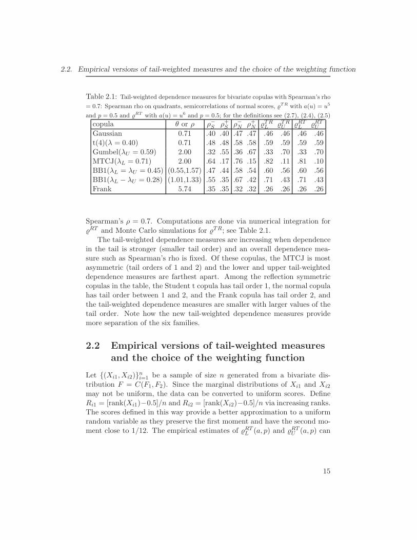
Table 2.1: Tail-weighted dependence measures for bivariate copulas with Spearman’s rho
= 0.7: Spearman rho on quadrants, semicorrelations of normal scores, TR with a(u) = u5
and p = 0.5 and RT with a(u) = u6 and p = 0.5; for the definitions see (2.7), (2.4), (2.5)
copula θ or ρ ρ−S ρ+S ρ−N ρ+N TRL TRU RTL RTUGaussian 0.71 .40 .40 .47 .47 .46 .46 .46 .46t(4)(λ = 0.40) 0.71 .48 .48 .58 .58 .59 .59 .59 .59Gumbel(λU = 0.59) 2.00 .32 .55 .36 .67 .33 .70 .33 .70MTCJ(λL = 0.71) 2.00 .64 .17 .76 .15 .82 .11 .81 .10BB1(λL = λU = 0.45) (0.55,1.57) .47 .44 .58 .54 .60 .56 .60 .56BB1(λL − λU = 0.28) (1.01,1.33) .55 .35 .67 .42 .71 .43 .71 .43Frank 5.74 .35 .35 .32 .32 .26 .26 .26 .26
Spearman’s ρ = 0.7. Computations are done via numerical integration forRT and Monte Carlo simulations for TR; see Table 2.1.
The tail-weighted dependence measures are increasing when dependencein the tail is stronger (smaller tail order) and an overall dependence mea-sure such as Spearman’s rho is fixed. Of these copulas, the MTCJ is mostasymmetric (tail orders of 1 and 2) and the lower and upper tail-weighteddependence measures are farthest apart. Among the reflection symmetriccopulas in the table, the Student t copula has tail order 1, the normal copulahas tail order between 1 and 2, and the Frank copula has tail order 2, andthe tail-weighted dependence measures are smaller with larger values of thetail order. Note how the new tail-weighted dependence measures providemore separation of the six families.
2.2 Empirical versions of tail-weighted measures
and the choice of the weighting function
Let {(Xi1,Xi2)}ni=1 be a sample of size n generated from a bivariate dis-tribution F = C(F1, F2). Since the marginal distributions of Xi1 and Xi2
may not be uniform, the data can be converted to uniform scores. DefineRi1 = [rank(Xi1)−0.5]/n and Ri2 = [rank(Xi2)−0.5]/n via increasing ranks.The scores defined in this way provide a better approximation to a uniformrandom variable as they preserve the first moment and have the second mo-ment close to 1/12. The empirical estimates of RTL (a, p) and RTU (a, p) can
15
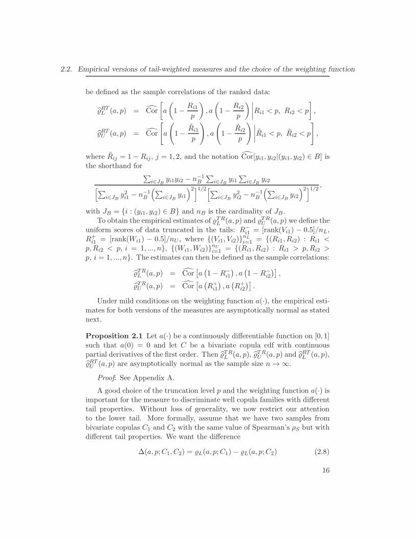
2.2. Empirical versions of tail-weighted measures and the choice of the weighting function
be defined as the sample correlations of the ranked data:
RTL (a, p) = Cor
[a
(1− Ri1
p
), a
(1− Ri2
p
) ∣∣∣∣Ri1 < p, Ri2 < p
],
RTU (a, p) = Cor
[a
(1− Ri1
p
), a
(1− Ri2
p
) ∣∣∣∣Ri1 < p, Ri2 < p
],
where Rij = 1−Rij, j = 1, 2, and the notation Cor[yi1, yi2|(yi1, yi2) ∈ B] isthe shorthand for
∑i∈JB yi1yi2 − n−1
B
∑i∈JB yi1
∑i∈JB yi2[∑
i∈JB y2i1 − n−1
B
(∑i∈JB yi1
)2]1/2[∑i∈JB y
2i2 − n−1
B
(∑i∈JB yi2
)2]1/2 ,
with JB = {i : (yi1, yi2) ∈ B} and nB is the cardinality of JB .To obtain the empirical estimates of TRL (a, p) and TRU (a, p) we define the
uniform scores of data truncated in the tails: R−i1 = [rank(Vi1) − 0.5]/nL,
R+i1 = [rank(Wi1) − 0.5]/nU , where {(Vi1, Vi2)}nL
i=1 = {(Ri1, Ri2) : Ri1 <p,Ri2 < p, i = 1, ..., n}, {(Wi1,Wi2)}nU
i=1 = {(Ri1, Ri2) : Ri1 > p,Ri2 >p, i = 1, ..., n}. The estimates can then be defined as the sample correlations:
TRL (a, p) = Cor[a(1−R−
i1
), a(1−R−
i2
)],
TRU (a, p) = Cor[a(R+i1
), a(R+i2
)].
Under mild conditions on the weighting function a(·), the empirical esti-mates for both versions of the measures are asymptotically normal as statednext.
Proposition 2.1 Let a(·) be a continuously differentiable function on [0, 1]such that a(0) = 0 and let C be a bivariate copula cdf with continuouspartial derivatives of the first order. Then TRL (a, p), TRU (a, p) and RTL (a, p),RTU (a, p) are asymptotically normal as the sample size n→ ∞.
Proof: See Appendix A.
A good choice of the truncation level p and the weighting function a(·) isimportant for the measure to discriminate well copula families with differenttail properties. Without loss of generality, we now restrict our attentionto the lower tail. More formally, assume that we have two samples frombivariate copulas C1 and C2 with the same value of Spearman’s ρS but withdifferent tail properties. We want the difference
∆(a, p;C1, C2) = L(a, p;C1)− L(a, p;C2) (2.8)
16
2.2. Empirical versions of tail-weighted measures and the choice of the weighting function
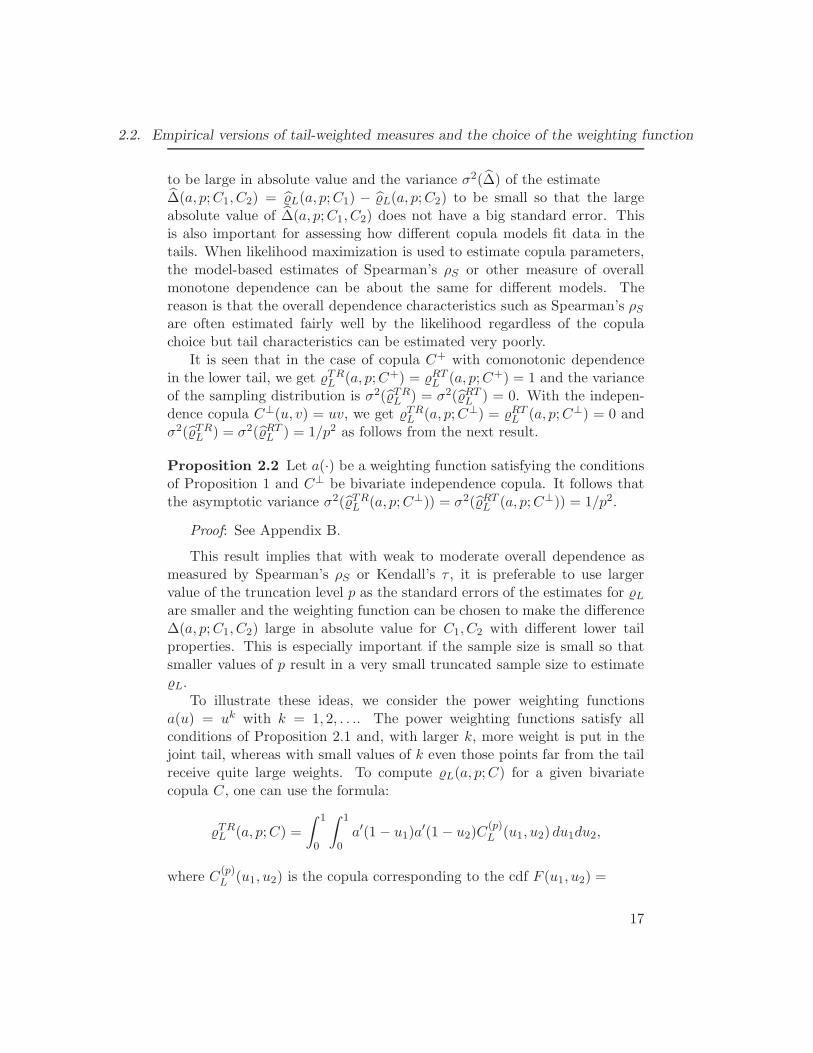
to be large in absolute value and the variance σ2(∆) of the estimate∆(a, p;C1, C2) = L(a, p;C1) − L(a, p;C2) to be small so that the largeabsolute value of ∆(a, p;C1, C2) does not have a big standard error. Thisis also important for assessing how different copula models fit data in thetails. When likelihood maximization is used to estimate copula parameters,the model-based estimates of Spearman’s ρS or other measure of overallmonotone dependence can be about the same for different models. Thereason is that the overall dependence characteristics such as Spearman’s ρSare often estimated fairly well by the likelihood regardless of the copulachoice but tail characteristics can be estimated very poorly.
It is seen that in the case of copula C+ with comonotonic dependencein the lower tail, we get TRL (a, p;C+) = RTL (a, p;C+) = 1 and the varianceof the sampling distribution is σ2(TRL ) = σ2(RTL ) = 0. With the indepen-dence copula C⊥(u, v) = uv, we get TRL (a, p;C⊥) = RTL (a, p;C⊥) = 0 andσ2(TRL ) = σ2(RTL ) = 1/p2 as follows from the next result.
Proposition 2.2 Let a(·) be a weighting function satisfying the conditionsof Proposition 1 and C⊥ be bivariate independence copula. It follows thatthe asymptotic variance σ2(TRL (a, p;C⊥)) = σ2(RTL (a, p;C⊥)) = 1/p2.
Proof: See Appendix B.
This result implies that with weak to moderate overall dependence asmeasured by Spearman’s ρS or Kendall’s τ , it is preferable to use largervalue of the truncation level p as the standard errors of the estimates for Lare smaller and the weighting function can be chosen to make the difference∆(a, p;C1, C2) large in absolute value for C1, C2 with different lower tailproperties. This is especially important if the sample size is small so thatsmaller values of p result in a very small truncated sample size to estimateL.
To illustrate these ideas, we consider the power weighting functionsa(u) = uk with k = 1, 2, . . .. The power weighting functions satisfy allconditions of Proposition 2.1 and, with larger k, more weight is put in thejoint tail, whereas with small values of k even those points far from the tailreceive quite large weights. To compute L(a, p;C) for a given bivariatecopula C, one can use the formula:
TRL (a, p;C) =
∫ 1
0
∫ 1
0a′(1− u1)a
′(1− u2)C(p)L (u1, u2) du1du2,
where C(p)L (u1, u2) is the copula corresponding to the cdf F (u1, u2) =
17
2.2. Empirical versions of tail-weighted measures and the choice of the weighting function
C(u1, u2)/C(p, p), u1 < p, u2 < p of data truncated in the lower tail, and
RTL (a, p;C) =C(p, p)m12 −m1m2
[{C(p, p)m11 −m21}{C(p, p)m22 −m2
2}]1/2,
where
m12 =1
p2
∫ p
0
∫ p
0a′(1− u1/p) a
′(1− u2/p)C(u1, u2) du1du2,
m1 =1
p
∫ p
0a′(1−u1/p)C(u1, p) du1, m2 =
1
p
∫ p
0a′(1−u2/p)C(p, u2) du2,
m11 =1
p
∫ p
02a(1− u1/p) a
′(1− u1/p)C(u1, p) du1,
m22 =1
p
∫ p
02a(1− u2/p) a
′(1− u2/p)C(p, u2) du2;
see the proof of Proposition 2.1 for details. All integrands here are boundedfunctions so that numerical integration should be fast and stable for RTL . To
compute the measure TRL , the copula C(p)L (u1, u2) is needed and therefore
the inverse functions for C(u1, p)/C(p, p) and C(p, u2)/C(p, p) are required.Computation of these inverse functions can be time-consuming and there-fore computation of the measure RTL is faster. With some other weightingfunctions, such as the semi-correlations of normal scores, the integrands areunbounded so that numerical integration can be slower for both measures.This is especially important if one wants to compute the model-based esti-mates of the measures for each pair of variables in a multidimensional dataset.
In practice using copulas with intermediate dependence (tail order 1 <κ < 2 based on Hua and Joe (2011)) or tail quadrant independence (κ = 2and the slowly varying function is a constant) can lead to incorrect inferencesin the tails if the true copula is tail dependent. It means that a good mea-sure of tail-weighted dependence should discriminate well copulas with taildependence and copulas that are not tail dependent. We use the followingbivariate parametric copula families for comparisons in the tails.
• Student t copula with 4 degrees of freedom: This is a reflection sym-metric tail dependent copula.
• Gaussian copula: This is a reflection symmetric copula with interme-diate dependence for 0 < ρ < 1. The tail order is κL = 2/(1 + ρ) andit gets closer to 1 as ρ increases. Therefore it is harder to discriminatethe Student t and Gaussian copulas if the overall dependence is strong.
18
2.2. Empirical versions of tail-weighted measures and the choice of the weighting function
• Gumbel copula: This is a tail asymmetric copula with intermediatelower tail dependence; the tail order is κL = 21/θ where θ > 1 is thecopula dependence parameter.
• Reflected Gumbel (rGumbel) copula: This is a tail asymmetric copulawith lower tail dependence.
• Frank copula: This is a reflection symmetric copula with tail quadrantindependence.
• BB1 copula: This is a tail asymmetric and tail dependent copula.
More details on these copulas can be found in Joe (1997) and Nelsen(2006). Results on how tail properties of the bivariate linking copulas af-fect the tail properties of the bivariate margins of vine models are given inJoe et al. (2010). The various tail-weighted dependence measures can dis-criminate strength of dependence in the tail somewhat like the (limiting)tail order, since the t4 and BB1 copulas have lower and upper tail order of1, the Gaussian copula has lower and upper tail order in (1, 2) for 0 < ρ < 1,the Gumbel copula has κU = 1 and κL ∈ (1, 2) and the Frank copula hasκL = κU = 2; see Table 2.2. Note that the conditional Spearman’s rhos andthe normal scores semi-correlations are less sensitive (especially the former,as seen in Table 2.2) to stronger dependence in the tails and tail asymmetry.
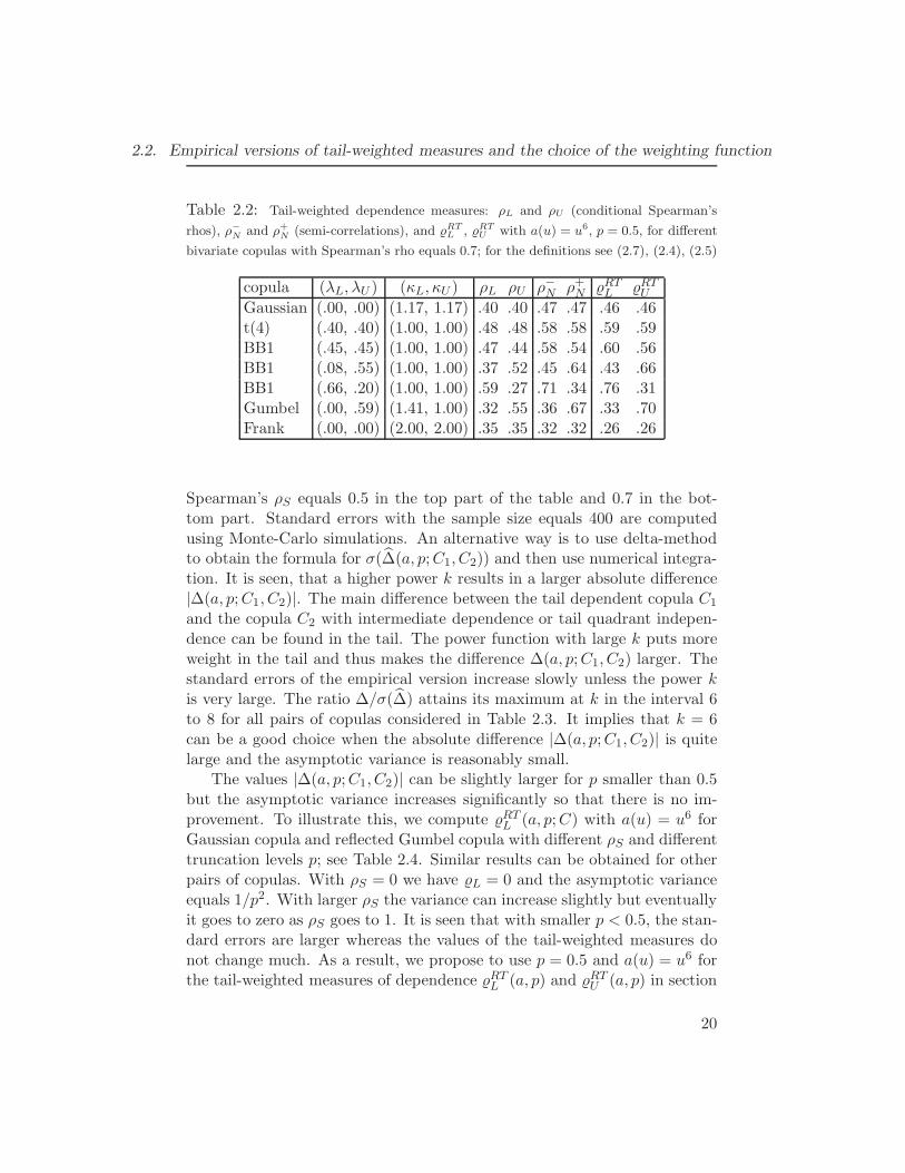
Assuming the Spearman’s ρ is constant, the tail-weighted measures takelarger values for copulas with stronger dependence in the tails. Comparingto copulas with intermediate dependence, the values RTL , RTU are largerfor copulas with tail dependence (the Student, BB1 copulas) and smallerfor copulas with tail quadrant independence (the Frank copula). For taildependent copulas the values RTL , RTU are larger for copulas with larger taildependence coefficients λL and λU . For example, for the tail dependent BB1copula, the tail-weighted dependence measures L and U discriminate wellthree different cases when dependence in the lower tail is about equal (withquite close values of the tail-weighted measures), weaker (with RTL < RTU )or stronger (with RTL > RTU ) than dependence in the upper tail.
The next step is a comparison of a(·) functions that can be used for thetail-weighted dependence measures; we use power functions for a(·) as theresulting measures are fast to compute. We start with the measures RTL ,RTU .
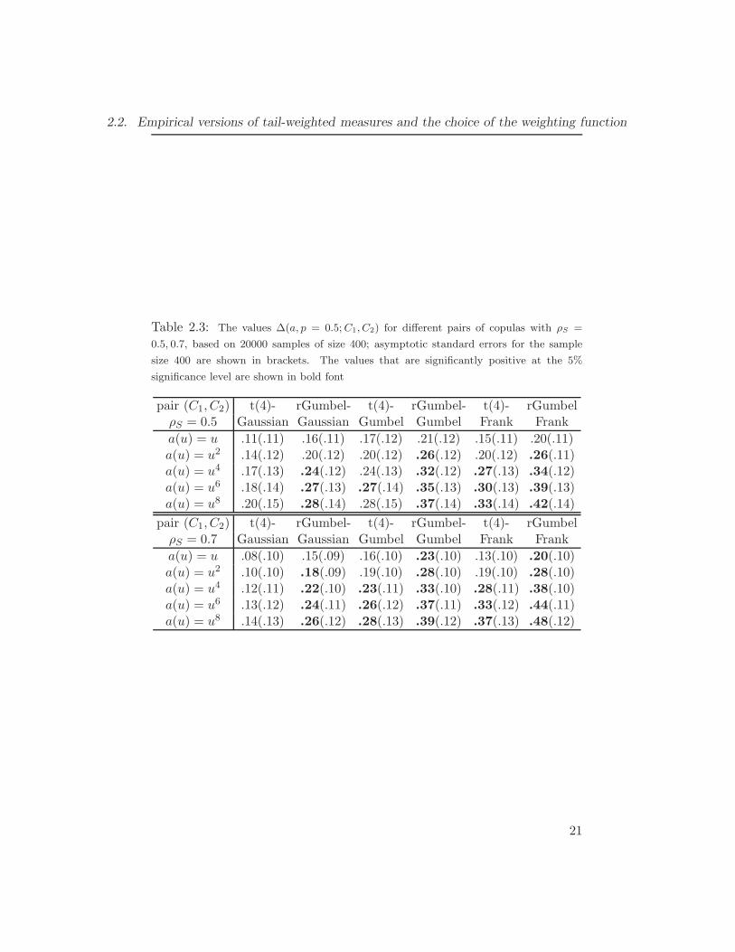
In Table 2.3, we compute ∆(a, p = 0.5;C1, C2) in (2.8) for two copulasC1, C2 with the same value of Spearman’s ρS such that C1 is a tail depen-dent copula and C2 is not; also asymptotic standard errors are included.
19
2.2. Empirical versions of tail-weighted measures and the choice of the weighting function
Table 2.2: Tail-weighted dependence measures: ρL and ρU (conditional Spearman’s
rhos), ρ−N and ρ+N (semi-correlations), and RTL , RT
U with a(u) = u6, p = 0.5, for different
bivariate copulas with Spearman’s rho equals 0.7; for the definitions see (2.7), (2.4), (2.5)
copula (λL, λU ) (κL, κU ) ρL ρU ρ−N ρ+N RTL RTUGaussian (.00, .00) (1.17, 1.17) .40 .40 .47 .47 .46 .46t(4) (.40, .40) (1.00, 1.00) .48 .48 .58 .58 .59 .59BB1 (.45, .45) (1.00, 1.00) .47 .44 .58 .54 .60 .56BB1 (.08, .55) (1.00, 1.00) .37 .52 .45 .64 .43 .66BB1 (.66, .20) (1.00, 1.00) .59 .27 .71 .34 .76 .31Gumbel (.00, .59) (1.41, 1.00) .32 .55 .36 .67 .33 .70Frank (.00, .00) (2.00, 2.00) .35 .35 .32 .32 .26 .26
Spearman’s ρS equals 0.5 in the top part of the table and 0.7 in the bot-tom part. Standard errors with the sample size equals 400 are computedusing Monte-Carlo simulations. An alternative way is to use delta-methodto obtain the formula for σ(∆(a, p;C1, C2)) and then use numerical integra-tion. It is seen, that a higher power k results in a larger absolute difference|∆(a, p;C1, C2)|. The main difference between the tail dependent copula C1
and the copula C2 with intermediate dependence or tail quadrant indepen-dence can be found in the tail. The power function with large k puts moreweight in the tail and thus makes the difference ∆(a, p;C1, C2) larger. Thestandard errors of the empirical version increase slowly unless the power kis very large. The ratio ∆/σ(∆) attains its maximum at k in the interval 6to 8 for all pairs of copulas considered in Table 2.3. It implies that k = 6can be a good choice when the absolute difference |∆(a, p;C1, C2)| is quitelarge and the asymptotic variance is reasonably small.
The values |∆(a, p;C1, C2)| can be slightly larger for p smaller than 0.5but the asymptotic variance increases significantly so that there is no im-provement. To illustrate this, we compute RTL (a, p;C) with a(u) = u6 forGaussian copula and reflected Gumbel copula with different ρS and differenttruncation levels p; see Table 2.4. Similar results can be obtained for otherpairs of copulas. With ρS = 0 we have L = 0 and the asymptotic varianceequals 1/p2. With larger ρS the variance can increase slightly but eventuallyit goes to zero as ρS goes to 1. It is seen that with smaller p < 0.5, the stan-dard errors are larger whereas the values of the tail-weighted measures donot change much. As a result, we propose to use p = 0.5 and a(u) = u6 forthe tail-weighted measures of dependence RTL (a, p) and RTU (a, p) in section
20
2.2. Empirical versions of tail-weighted measures and the choice of the weighting function
Table 2.3: The values ∆(a, p = 0.5;C1, C2) for different pairs of copulas with ρS =
0.5, 0.7, based on 20000 samples of size 400; asymptotic standard errors for the sample
size 400 are shown in brackets. The values that are significantly positive at the 5%
significance level are shown in bold font
pair (C1, C2) t(4)- rGumbel- t(4)- rGumbel- t(4)- rGumbelρS = 0.5 Gaussian Gaussian Gumbel Gumbel Frank Frank
a(u) = u .11(.11) .16(.11) .17(.12) .21(.12) .15(.11) .20(.11)a(u) = u2 .14(.12) .20(.12) .20(.12) .26(.12) .20(.12) .26(.11)a(u) = u4 .17(.13) .24(.12) .24(.13) .32(.12) .27(.13) .34(.12)a(u) = u6 .18(.14) .27(.13) .27(.14) .35(.13) .30(.13) .39(.13)a(u) = u8 .20(.15) .28(.14) .28(.15) .37(.14) .33(.14) .42(.14)
pair (C1, C2) t(4)- rGumbel- t(4)- rGumbel- t(4)- rGumbelρS = 0.7 Gaussian Gaussian Gumbel Gumbel Frank Frank
a(u) = u .08(.10) .15(.09) .16(.10) .23(.10) .13(.10) .20(.10)a(u) = u2 .10(.10) .18(.09) .19(.10) .28(.10) .19(.10) .28(.10)a(u) = u4 .12(.11) .22(.10) .23(.11) .33(.10) .28(.11) .38(.10)a(u) = u6 .13(.12) .24(.11) .26(.12) .37(.11) .33(.12) .44(.11)a(u) = u8 .14(.13) .26(.12) .28(.13) .39(.12) .37(.13) .48(.12)
21
2.3. Normal scores plots and tail-weighted measures of dependence
Table 2.4: The values RTL (a, p;C) for Gaussian and reflected Gumbel copula with
different Spearman’s rho, based on 20000 samples of size 400; asymptotic standard errors
for the sample size 400 are shown in brackets
ρSGaussian copula rGumbel copula
p = 0.5 p = 0.4 p = 0.3 p = 0.5 p = 0.4 p = 0.3
0.00 0.00(.10) 0.00(.13) 0.00(.17) 0.00(.10) 0.00(.13) 0.00(.17)0.30 0.13(.10) 0.11(.12) 0.10(.15) 0.36(.11) 0.37(.13) 0.38(.15)0.55 0.33(.10) 0.30(.11) 0.27(.13) 0.59(.08) 0.59(.09) 0.59(.11)0.80 0.61(.07) 0.57(.09) 0.54(.11) 0.80(.05) 0.79(.06) 0.79(.07)0.95 0.89(.03) 0.87(.03) 0.85(.04) 0.95(.01) 0.95(.02) 0.95(.02)1.00 1.00(.00) 1.00(.00) 1.00(.00) 1.00(.00) 1.00(.00) 1.00(.00)
5.5 to analyze financial returns data.Similar results can be obtained for the measures TRL , TRU . For these
measures, it is simpler to get the formula for the asymptotic variance of TRL ,
TRU and hence calculate σ(∆(a, p;C1, C2)); see Appendix A for details. Thevariance can be calculated for different copulas using 4-dimensional numer-ical integration so that Monte Carlo simulations are not needed. A goodchoice for the weighting function is a(u) = u5 with the same truncation levelp = 0.5. In fact, RTL (a, 0.5), RTU (a, 0.5) with a(u) = u6 and TRL (a, 0.5),TRU (a, 0.5) with a(u) = u5 give very similar results, both in Monte Carlosimulations and when analyzing financial data, and therefore we do not showthe results for the latter measures.
2.3 Normal scores plots and tail-weighted
measures of dependence
In this section we give some examples of different types of dependence struc-ture that can be observed in financial return data. The tail-weighted mea-sures of dependence can be used as a preliminary diagnostics before choosingbivariate linking copulas in different vine copula models. Figure 2.1 showsnormal scores plots for 4 pairs of S&P 500 returns. One can see that theshape of these plots is quite different for all the 4 pairs. The first plot (topleft) has an elliptical shape and it implies that the Gaussian copula can bea good choice. The second plot (top right) has sharper tails which indicatesthat a copula with tail dependence is more appropriate. Two plots at the
22
2.3. Normal scores plots and tail-weighted measures of dependence
Table 2.5: The estimates of ∆L, ∆U , ∆R; for 4 pairs of S&P 500 log-returns; the 95%
confidence intervals are shown in brackets
pair ∆L ∆U ∆R;
(CINF, AFL) -0.05 (-0.27, 0.16) 0.03 (-0.17, 0.20) -0.08 (-0.38, 0.23)(AFL, TMK) 0.28 ( 0.06, 0.44) 0.26 ( 0.07, 0.44) 0.02 (-0.27, 0.27)(PSA, AXP) 0.27 ( 0.06, 0.45) -0.28 (-0.45,-0.05) 0.55 ( 0.22, 0.80)(HCP, MET) -0.27 (-0.44,-0.03) 0.27 ( 0.06, 0.43) -0.54 (-0.78,-0.21)
bottom have an asymmetric shape and so an asymmetric copula should fitthe data better.
However, it is not always clear what shape a normal scores plot has andthe tail-weighted measures can be used as a diagnostics to select an appro-priate bivariate copula for a pair of variables. To illustrate the ideas, wecompute RTL , RTU for the aforementioned pairs of variables. Note that themeasures RTL , RTU take larger values if the overall dependence as measuredby Spearman’s ρ or Kendall’s τ is stronger. It means that the large valuesof the measures alone do not imply strong dependence in the tails. Givena fixed Spearman’s ρ, the measures take larger values for stronger depen-dence in the tails as we showed in the previous section. Therefore we usethe Gaussian copula as a benchmark and compute the parametric estimateof these measures assuming the joint normality for each pair. Because ofsymmetric dependence of the Gaussian copula we get the same value of themeasure in the lower and upper tail; we denote these value by RTN . Underthis assumption, one can calculate an estimate of Spearman’s rho ρS andthen transform it to the Gaussian copula correlation parameter ρ using therelationship ρ = 2 sin(πρS/6). Numerical integration and formulas from theprevious section can be used to obtained a parametric estimate ˆRTN .
For comparisons in the tails, and define ∆L = L − N and ∆U =U − N to adjust for the overall dependence. We also define ∆R; = L −U to compare the strength of dependence in the lower and upper tails.Under the assumption of normality one can use the asymptotic normalityof estimates ∆L = ˆL− ˆN , ∆U = ˆU − ˆN to construct the 95% confidenceintervals for ∆L, ∆U . Similar, the 95% intervals can be obtained for ∆R;
assuming reflection symmetry. For the intervals, the asymptotic variancecan be estimated using the bootstrap. In Table 2.5 we show the estimates of∆L, ∆U , ∆R; together with the 95% confidence intervals that were obtainedusing the bootstrap.
23
2.3. Normal scores plots and tail-weighted measures of dependence
Figure 2.1: Normal scores scatter plots for 4 pairs of financial log-returns; S&P500 data,
financial sector, pair (CINF, APL), year 2007 (top left); pair (AFL, TMK), year 2008 (top
right); pair (PSA, AXP), year 2008 (bottom left); pair (HCP, MET), year 2007 (bottom
right)
−3 0 3
−30
3
CINF
AF
L
−3 0 3
−30
3
AFL
TM
K
−3 0 3
−30
3
PSA
AX
P
−3 0 3
−30
3
HCP
ME
T
24
2.3. Normal scores plots and tail-weighted measures of dependence
For the pair (CINF, AFL) all the three confidence intervals contain zeroso that there are no significant departures from normality. For the pair(AFL, TMK), the lower bound of the first two confidence intervals is greaterthan zero and this indicates that dependence in both tails is significantlystronger comparing to the Gaussian copula. At the same time, there is noevidence of tail asymmetry. It means a symmetric copula with tail depen-dence is a better choice for this pair. The last two pairs, (PSA, AXP) and(HCP, MET), has an asymmetric dependence as the third confidence intervaldoes not contain zero. The first of these two pairs has stronger dependencein the lower tail and weaker dependence in the upper tail, comparing to theGaussian copula. And the second pair has stronger dependence in the uppertail and weaker dependence in the lower tail. It implies that an asymmetriccopula with tail dependence in one tail is needed for these pairs.
Note that because of a large variability, especially if the sample size isnot very large, the 95% confidence intervals can be quite wide and containthe estimates ∆L, ∆U , ∆R; despite the large values for these estimates. Wesuggest using non-Gaussian copula if the estimates are close to the lower orupper boundaries of the confidence intervals. The choice of the copula willthen depend on the sign of these estimates. The primary goal of the mea-sures is not testing against normality but rather providing some guidancein choosing more appropriate bivariate copula depending on the estimatedstrength of dependence in the tails, especially if consistent tail asymmetry orstronger dependence than that for bivariate Gaussian tails is seen in manypairs of variables.
25
Chapter 3
Measures of asymmetry
based on the empirical
copula process
In this chapter we introduce some other measures of dependence asymmetryfor two variables for multivariate data, these can be applied to each pair.Two types of asymmetry will be considered: reflection asymmetry and per-mutation asymmetry. For each of these types of asymmetry, we proposemeasures that are based on the empirical copula process. This approachuse all data unlike the measures proposed in Section 2.2 where only datatruncated in the tails are used. Unlike the measures L, U , the measuresproposed in this chapter use data from the middle of the distribution aswell and this allows to detect possible asymmetric dependence structurein the middle of the distribution and not in the tails (especially for per-mutation asymmetry). When combined with the tail-weighted measures ofdependence, the measures of asymmetry can provide useful summaries ofthe dependence structure. This can help to select suitable bivariate linkingcopulas at the first level of vine or factor copula models.
Assume that (U1, U2) ∼ C where C is a bivariate copula. Throughoutthis section, we will assume that C satisfies the regularity conditions ofProposition 2.1 in Section 2.2. If C is a reflection symmetric copula then∆R := C(u1, u2) − CR(u1, u2) = 0 for all u1, u2 ∈ [0, 1]. Similarly, if C isa permutation symmetric copula, we get ∆P := C(u1, u2) − C(u2, u1) = 0for all u1, u2 ∈ [0, 1]. The idea is to find a functional G(∆) : R2 → R for∆ = ∆R (∆ = ∆P ) such that G(∆) = 0 if and only if the copula C is areflection (respectively, permutation) symmetric copula.
Typical choices for G include the integral of ∆2 or supremum of |∆| overthe unit square: G(∆) =
∫ ∫[0,1]2 ∆
2(u1, u2)du1du2, G(∆) =
sup[0,1]2 |∆(u1, u2)|. Tests of permutation symmetry based on these twofunctionals are proposed in Genest et al. (2012). However the exact distri-bution of the corresponding test statistic under the null hypothesis: H0 :
26
3.1. Measures of reflection asymmetry
∆P ≡ 0 is unknown and depends on the copula C so the authors designa method to get bootstrap replicates of the test statistic and compute P-values. It makes this method of testing relatively slow especially when oneneeds to measure asymmetry for each pair of multidimensional data set. Alsothis functional does not provide information on the direction of asymmetry.The power of the proposed tests may not be very high unless permutationasymmetry is quite strong.
At the same time, any non-degenerate linear transformation of ∆ resultsin a statistic with asymptotic normal distribution. In other words, if wedefine the functional G as follows:
G(∆) =
∫ 1
0
∫ 1
0w(u1, u2)∆(u1, u2)du1du2, (3.1)
the asymptotic distribution of G(∆) = G(∆) will be normal where ∆ is anestimate of ∆ obtained from a sample and w(u1, u2) is a weighting function.It is important that this function does not depend on data and hence thecopula C. The simplest choice w(u1, u2) = 1 results in the degeneratetransformation ∆(G) ≡ 0 since ∆P (u1, u2) = −∆P (u1, u2) and ∆R(u1, u2) =−∆R(1 − u1, 1 − u2) so that the resulting integral equals zero. Thereforemore careful choice of the weighting function w is required. Below we providesome choices for w that work well for ∆R and ∆P .
3.1 Measures of reflection asymmetry
Since ∆R(u1, u2) = −∆R(1−u1, 1−u2) we can use the integral over the lowertriangle {(u1, u2) : u1, u2 ≥ 0 and u1 + u2 ≤ 1}. The resulting weightingfunction w(u1, u2) should be zero if u1 + u2 > 1. Similarly to the tail-weighted measures of dependence proposed in Section 2.1 one can put moreweight in the tail as for many reflection asymmetric bivariate copulas thedifference in dependence between the left lower corner and the right uppercorner of the unit square becomes larger in the tails. That is, w(u1, u2)should take larger values in the neighborhood of (0, 0) and smaller values ifthe point (u1, u2) is close to the u1+u2 = 1 line. It is seen that the functionw(u1, u2) = I{u1 + u2 ≤ 1}(1 − u1 − u2)
k, k > 0 can be a good choice.The function is a constant if u1 + u2 = u• is fixed and it is exponentiallydecreasing from 1 to 0 when u• goes from 0 to 1.
Now we define the empirical version of the measure. Let {(U1i, U2i)}ni=1
27
3.1. Measures of reflection asymmetry
be a sample of size n generated from the copula C. Let
Cn(u1, u2) =1
n
n∑
i=1
I{U1i < u1, U2i < u2},
and
(CR)n(u1, u2) =1
n
n∑
i=1
I{U1i ≥ 1− u1, U2i ≥ 1− u2}
be the corresponding empirical copula processes. Under some mild regularityconditions, empirical copula process gives a consistent estimate of the copulacdf; see Gaenssler and Stute (1987), van der Vaart and Wellner (1996) formore details on convergence and asymptotic theory for the empirical copulaprocesses. Define (∆R)n(u1, u2) = Cn(u1, u2)− (CR)n(u1, u2) and
Gn(∆R) = G((∆R)n) =
∫ ∫
u1+u2≤1(1− u1 − u2)
k(∆R)n(u1, u2)du1du2.
Using the result of Fermanian et al. (2004) and assuming the partialderivatives ∂C(u1, u2)/∂uj , j = 1, 2 are continuous functions on (0, 1)2 we
find that√n (Cn − C) →d GC and
√n ((CR)n − CR) →d GCR
where GC isa Gaussian process with zero mean defined for a copula C. Under the nullhypothesis H0 : ∆R ≡ 0 we get:
√n (∆R)n =
√n (Cn − C) −√
n ((CR)n −CR) →d δR = GC − GCR
and therefore
√n Gn(∆R) →d
∫ ∫
u1+u2≤1(1− u1 − u2)
k[GC(u1, u2)− GCR(u1, u2)]du1du2.
It follows that Gn(∆R) has asymptotic normal distribution with some vari-ance σ2∆R
and the variance can be estimated using the jackknife or boot-strap. The null hypothesis of reflection symmetry should be rejected at the5% significance level if |Gn(∆R)| > 1.96σ∆R
/√n where σ∆R
is an estimateof σ∆R
.Note that
∫ ∫
u1+u2≤1(1− u1 − u2)
kI{U1i < u1, U2i < u2}du1du2
=
∫ 1
U1i
∫ 1−u1
U2i
(1− u1 − u2)kI{U1i + U2i < 1}du2du1
=(1− U1i − U2i)
k+2I{U1i + U2i < 1}(k + 1)(k + 2)
,
28
3.1. Measures of reflection asymmetry
∫ ∫
u1+u2≤1(1− u1 − u2)
kI{U1i ≥ 1− u1, U2i ≥ 1− u2}du1du2
=
∫ 1
1−U1i
∫ 1−u1
1−U2i
(1− u1 − u2)kI{U1i + U2i > 1}du2du1
=(U1i + U2i − 1)k+2I{U1i + U2i > 1}
(k + 1)(k + 2).
It implies that
Gn(∆R) = Gn(∆R; k) =
∑ni=1[|1 − U1i − U2i|k+2sign(1− U1i − U2i)]
n(k + 1)(k + 2)
and
G(∆R) = G(∆R; k) =E[|1− U1 − U2|k+2sign(1− U1 − U2)]
(k + 1)(k + 2).
The measure is defined as the mean of the variable |1 − U1 − U2|k+2
adjusted for the sign of (1 − U1 − U2). Note that this functional gives anindication of the direction of reflection asymmetry. In case of a reflectionasymmetric dependence, the measure takes positive (negative) values if theconditional mean of data truncated in the lower (upper) tail is larger thanthat of data truncated in the upper (lower) tail. Data that are closer to thetails have bigger contribution to the mean because of the weighting functionw and therefore one can expect G(∆R) > 0 if dependence in the lower tailis stronger.
Similar to the tail-weighted measures of dependence, a large power kresults in a large variability of the empirical estimate G(∆R) and we choosek = 5 based on Monte Carlo simulations for different copulas with tail asym-metry that are widely used to model asymmetric dependence in differentapplications.
Rosco and Joe (2013) propose two families of measures of reflection sym-metry:
ζ1(R;C, ℓ) = E[|U1 + U2 − 1|ℓsign(U1 + U2 − 1)],
ζ2(R;C, p) = [QR(1− p)− 2QR(0.5) +QR(p)]/[QR(1− p)−QR(p)], (3.2)
where QR(p) is the p-quantile of (U1 + U2 − 1). Note that ζ1(R;C, ℓ) =ℓ(ℓ− 1)G(∆R; ℓ− 2), and therefore G(∆R) is the same measure of reflectionasymmetry as the first family of measures ζ1(R;C, ℓ), up to a constant. The
29
3.2. Measures of bivariate permutation asymmetry
authors use ℓ = 3 and p = 0.05, however the choice of ℓ = 7 for ζ1(R;C, ℓ)(or k = 5 for G(∆R; k)) may be better as we mentioned before.
Rosco and Joe (2013) showed that the maximum absolute value ofζ1(R;C, k + 2) = (k + 1)(k + 2)G(∆R; k) with k = 5 equals 0.062, and themaximum is attained for a singular copula. For absolutely continuous cop-ulas the maximum is lower. For the BB2 copula (see Joe (1997) for details),the maximum is 0.032 when the copula parameter θ = (0.4, 1.07). Thiscopula is a copula with very strong asymmetric dependence. In practicalapplications, an asymmetric dependence is not very strong, and the BB1or Gumbel copulas are commonly used in applications to model an asym-metric dependence. For these copula families the maximum (minimum) of(k+1)(k+2)G(∆R; k) with k = 5 is equal to 0.025 for the BB1 copula withparameter θ = (1.98, 1.00) (it implies we get MTCJ copula with very stronglower tail dependence and upper tail quadrant independence); -0.013 for theGumbel copula with parameter θ = 1.72 (note that the sign is negative,unlike the BB1 copula, pointing to a stronger dependence in the upper tail).
3.2 Measures of bivariate permutation
asymmetry
Similar to the measure of reflection asymmetry we can use the integral overthe lower triangle {(u1, u2) : u1, u2 ≥ 0 and u1 ≥ u2} and the weightingfunction w(u1, u2) = (u1 − u2)
kI{u1 ≥ u2} so that data in the right lowerand left upper corners get more weight. For the empirical version, one candefine (∆P )n = Cn(u1, u2)− Cn(u2, u1) and
Gn(∆P ) = G((∆P )n) =
∫ ∫
u1≥u2(u1 − u2)
k(∆P )n(u1, u2)du1du2.
We again use the result of Fermanian et al. (2004) to get:√n (Cn(u1, u2)−
C(u1, u2)) →d GC(u1, u2) and√n (Cn(u2, u1) − C(u2, u1)) →d GC(u2, u1)
where GC is again a Gaussian process with zero mean defined for a cop-ula C. Under the null hypothesis H0 : ∆P ≡ 0 we get:
√n (∆P )n =√
n (Cn(u1, u2)−C(u1, u2))−√n (Cn(u2, u1)−C(u2, u1)) →d δp = GC(u1, u2)−
GC(u2, u1) and therefore
√n Gn(∆P ) →d
∫ ∫
u1≥u2(u1 > u2)
k[GC(u1, u2)− GC(u2, u1)]du1du2.
It follows that Gn(∆P ) has asymptotic normal distribution with some vari-ance σ2∆P
and the variance can be estimated using the jackknife or bootstrap.
30
3.2. Measures of bivariate permutation asymmetry
The null hypothesis of permutation symmetry should be rejected at the 5%significance level if |Gn(∆P )| > 1.96σ∆P
/√n where σ∆P
is an estimate ofσ∆P
.Similar to the measure of reflection asymmetry, we have:
∫ ∫
u1≥u2(u1 − u2)
kI{U1i < u1, U2i < u2}du1du2
=
∫ 1
max{U1i,U2i}
∫ u1
U2i
(u1 − u2)kdu2du1
=(1− U2i)
k+2
(k + 1)(k + 2)− (U1i − U2i)
k+2I{U1i > U2i}(k + 1)(k + 2)
,
∫ ∫
u1≥u2(u1 − u2)
kI{U1i < u2, U2i < u1}du1du2
=
∫ 1
max{U1i,U2i}
∫ u1
U1i
(u1 − u2)kdu2du1
=(1− U1i)
k+2
(k + 1)(k + 2)− (U2i − U1i)
k+2I{U2i > U1i}(k + 1)(k + 2)
,
It implies that
Gn(∆P ) = Gn(∆P ; k) = −∑n
i=1[|Ui1 − Ui2|k+2sign(Ui1 − Ui2)]
n(k + 1)(k + 2)+ δ∗P , (3.3)
where δ∗P =∑n
i=1(1−Ui2)k+2
n(k+1)(k+2) −∑n
i=1(1−Ui1)k+2
n(k+1)(k+2) = OP (1n), and the limit is
G(∆P ) = G(∆P ; k) = −E[|U1 − U2|k+2sign(U1 − U2)]
(k + 1)(k + 2). (3.4)
The measure is defined as the mean of the variable |U1 − U2|k+2 adjustedfor the sign of (U1 − U2). Hence this measure gives an indication of thedirection of permutation asymmetry. In case of a permutation asymmetricdependence, the measure takes positive (negative) values if the conditionalmean of data truncated in the right lower (left upper) corner is larger thanthat of data truncated in the left upper (right lower) corner. Data thatare closer to the tails have bigger contribution to the mean because of theweighting function w and therefore one can expect G(∆P ) > 0 if dependencein the right lower tail is stronger.
31
3.2. Measures of bivariate permutation asymmetry
In applications, however, this measure might be not very sensitive toa permutation asymmetry. By construction, Gn(∆P ) applied to the dataset {(U1i, U2i)}ni=1 gives the same result as Gn(∆R) applied to the partiallyreflected data set {(1 − U1i, U2i)}ni=1 assuming the power k is the same forboth measures. Usually, data have positive dependence, so that there arenot much data in the right lower and left upper corners. Consequently, therotated data have negative dependence with no much data points in thelower and upper tails and therefore the measure G(∆P ) will not work well.
For bivariate permutation asymmetric U(0, 1) transformed data with apositive dependence we therefore suggest using a weighting function w thatputs more weight for points that close to the main diagonal of the unitsquare and less weight for points in the tails. Consequently, we propose theweighting function w(u1, u2) =
[1− (u1 − u2)
k]I{u1 ≥ u2} where k is a
small positive number. Define the new measure and its empirical estimateby G∗(∆P ) and G
∗n(∆P ). By construction, we have:
G∗(∆P ; k) = G(∆P ; 0)−G(∆P ; k), G∗n(∆P ; k) = Gn(∆P ; 0)−Gn(∆P ; k),
where Gn(∆P ; k) and G(∆P ; k) are given by (3.3) and (3.4), respectively.Monte Carlo simulations show that the value k = 0.2 can be a good choicefor many permutation asymmetric copulas with positive dependence.
It is seen that G∗n(∆P ; k) has asymptotically normal distribution so that
one can propose a test for testing the null hypothesis of permutation symme-try as in the case of Gn(∆P ; k). These tests for reflection and permutationasymmetry can be used as diagnostic tools when applied to each pair ofvariables in a multidimensional data set. If a large fraction of data havesignificant departures from a symmetric dependence structure, it may beappropriate to select copula families that can handle reflection and/or per-mutation asymmetry, depending on the diagnostic results.
To compute some values of the proposed measure for an asymmetric dis-tribution, we use the 1-factor convolution gamma distribution. To the bivari-ate margin, assuming W0,W1,W2 are independent variables with exponen-tial distribution with parameters θ0, θ1, θ2 respectively, define Z1 =W0+W1,Z2 =W0+W2. The copula corresponding to the joint distribution of (Z1, Z2)will be a permutation asymmetric copula with positive dependence. In themodel, positive dependence with weak to very strong permutation asymme-try can obtained depending on the choice of the parameters; see Figure 3.1for the uniform scores scatter plots of data generated from the model.
We compute (k + 1)(k + 2)G∗n(∆P ; k) with k = 0.2 for the three cases
which are shown in Figure 3.1. For this distribution and θ0 = 2.2, θ1 = θ2 =
32
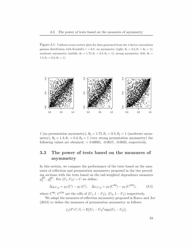
3.3. The power of tests based on the measures of asymmetry
Figure 3.1: Uniform scores scatter plots for data generated from the 1-factor convolution
gamma distribution with Kendall’s τ = 0.5: no asymmetry (right, θ0 = 2.2, θ1 = θ2 = 1);
moderate asymmetry (middle, θ0 = 1.75, θ1 = 0.5, θ2 = 1); strong asymmetry (left, θ0 =
1.3, θ1 = 0.2, θ2 = 1)
0.0 0.5 1.0
0.0
0.5
1.0
0.0 0.5 1.0
0.0
0.5
1.0
0.0 0.5 1.0
0.0
0.5
1.0
1 (no permutation asymmetry), θ0 = 1.75, θ1 = 0.5, θ2 = 1 (moderate asym-metry), θ0 = 1.3, θ1 = 0.2, θ2 = 1 (very strong permutation asymmetry) thefollowing values are obtained: < 0.00001, -0.0017, -0.0035, respectively.
3.3 The power of tests based on the measures of
asymmetry
In this section, we compare the performance of the tests based on the mea-sures of reflection and permutation asymmetry proposed in the two preced-ing sections with the tests based on the tail-weighted dependence measuresRTL , RTU . For (U1, U2) ∼ C we define:
∆R;C, = L(C)− U (C), ∆P ;C, = L(C90)− L(C
270), (3.5)
where C90, C270 are the cdfs of (U1, 1− U2), (U2, 1− U1) respectively.We adapt the measures of reflection asymmetry proposed in Rosco and Joe
(2013) to define the measures of permutation asymmetry as follows:
ζ1(P ;C, ℓ) = E[|U1 − U2|ℓsign(U1 − U2)],
33
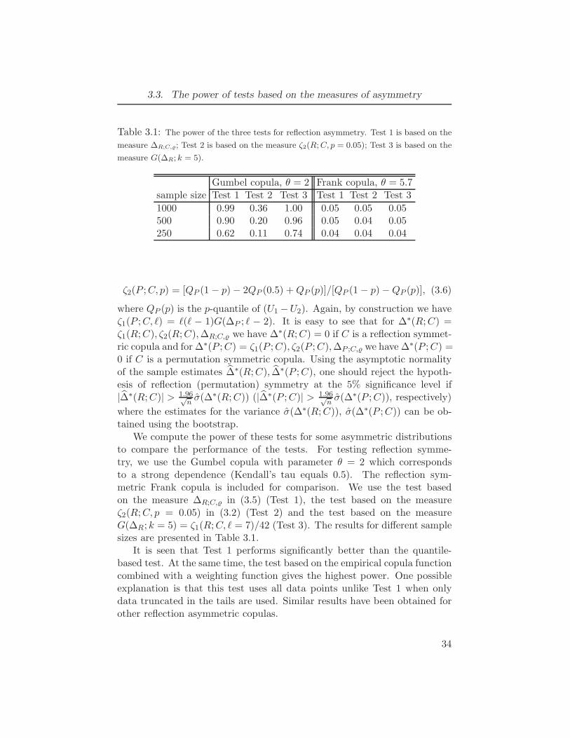
3.3. The power of tests based on the measures of asymmetry
Table 3.1: The power of the three tests for reflection asymmetry. Test 1 is based on the
measure ∆R;C,; Test 2 is based on the measure ζ2(R;C, p = 0.05); Test 3 is based on the
measure G(∆R; k = 5).
Gumbel copula, θ = 2 Frank copula, θ = 5.7sample size Test 1 Test 2 Test 3 Test 1 Test 2 Test 3
1000 0.99 0.36 1.00 0.05 0.05 0.05500 0.90 0.20 0.96 0.05 0.04 0.05250 0.62 0.11 0.74 0.04 0.04 0.04
ζ2(P ;C, p) = [QP (1− p)− 2QP (0.5) +QP (p)]/[QP (1− p)−QP (p)], (3.6)
where QP (p) is the p-quantile of (U1 −U2). Again, by construction we haveζ1(P ;C, ℓ) = ℓ(ℓ − 1)G(∆P ; ℓ − 2). It is easy to see that for ∆∗(R;C) =ζ1(R;C), ζ2(R;C),∆R;C, we have ∆
∗(R;C) = 0 if C is a reflection symmet-ric copula and for ∆∗(P ;C) = ζ1(P ;C), ζ2(P ;C),∆P ;C, we have ∆
∗(P ;C) =0 if C is a permutation symmetric copula. Using the asymptotic normalityof the sample estimates ∆∗(R;C), ∆∗(P ;C), one should reject the hypoth-esis of reflection (permutation) symmetry at the 5% significance level if|∆∗(R;C)| > 1.96√
nσ(∆∗(R;C)) (|∆∗(P ;C)| > 1.96√
nσ(∆∗(P ;C)), respectively)
where the estimates for the variance σ(∆∗(R;C)), σ(∆∗(P ;C)) can be ob-tained using the bootstrap.
We compute the power of these tests for some asymmetric distributionsto compare the performance of the tests. For testing reflection symme-try, we use the Gumbel copula with parameter θ = 2 which correspondsto a strong dependence (Kendall’s tau equals 0.5). The reflection sym-metric Frank copula is included for comparison. We use the test basedon the measure ∆R;C, in (3.5) (Test 1), the test based on the measureζ2(R;C, p = 0.05) in (3.2) (Test 2) and the test based on the measureG(∆R; k = 5) = ζ1(R;C, ℓ = 7)/42 (Test 3). The results for different samplesizes are presented in Table 3.1.
It is seen that Test 1 performs significantly better than the quantile-based test. At the same time, the test based on the empirical copula functioncombined with a weighting function gives the highest power. One possibleexplanation is that this test uses all data points unlike Test 1 when onlydata truncated in the tails are used. Similar results have been obtained forother reflection asymmetric copulas.
34
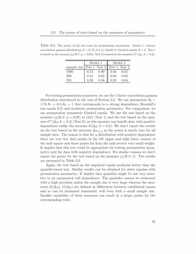
3.3. The power of tests based on the measures of asymmetry
Table 3.2: The power of the two tests for permutation asymmetry. Model 1: 1-factor
convolution gamma distribution, θ = (1.75, 0.5, 1); Model 2: Gumbel copula, θ = 2. Test 1
is based on the measure ζ2(R;C, p = 0.05); Test 2 is based on the measureG∗(∆P ; k = 0.2).
Model 1 Model 2sample size Test 1 Test 2 Test 1 Test 2
1000 0.73 0.90 0.04 0.05500 0.41 0.62 0.04 0.05250 0.20 0.36 0.03 0.04
For testing permutation symmetry, we use the 1-factor convolution gammadistribution introduced in the end of Section 3.2. We use parameters θ0 =1.75, θ1 = 0.5, θ2 = 1 that corresponds to a strong dependence (Kendall’stau equals 0.5) and moderate permutation asymmetry. For comparison, weuse permutation symmetric Gumbel copula. We use the test based on themeasure ζ2(R;C, p = 0.05) in (3.6) (Test 1) and the test based on the mea-sure G∗(∆P ; k = 0.2) (Test 2), as this measure can handle data with positivedependence unlike the measure G(∆P ; k = 0.2). We don’t report the resultson the test based on the measure ∆P ;C, as the power is nearly zero for allsample sizes. The reason is that for a distribution with positive dependencethere are very few data points in the left upper and right lower corners ofthe unit square and those points far from the tails receive very small weight.It implies that this test could be appropriate for testing permutation asym-metry only for data with negative dependence. For similar reasons we don’treport the power for the test based on the measure ζ1(R;C, ℓ). The resultsare presented in Table 3.2.
Again, the test based on the empirical copula performs better than thequantile-based test. Similar results can be obtained for other copulas withpermutation asymmetry. It implies that quantiles might be not very sensi-tive to an asymmetric tail dependence. The quantiles cannot be estimatedwith a high precision unless the sample size is very large whereas the mea-sures G(∆R), G(∆P ) are defined as differences between conditional meansand so can be estimated reasonably well even with a small sample size.Smaller variability of these measures can result in a larger power for thecorresponding tests.
35
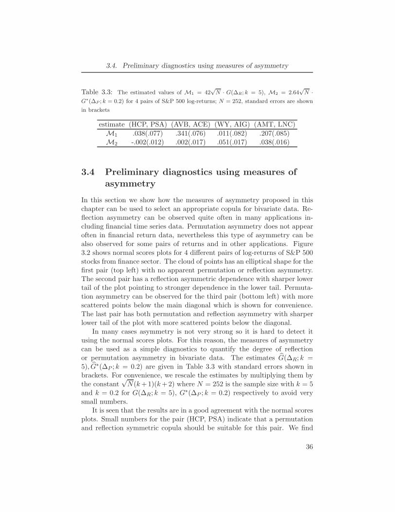
3.4. Preliminary diagnostics using measures of asymmetry
Table 3.3: The estimated values of M1 = 42√N · G(∆R; k = 5), M2 = 2.64
√N ·
G∗(∆P ; k = 0.2) for 4 pairs of S&P 500 log-returns; N = 252, standard errors are shown
in brackets
estimate (HCP, PSA) (AVB, ACE) (WY, AIG) (AMT, LNC)
M1 .038(.077) .341(.076) .011(.082) .207(.085)M2 -.002(.012) .002(.017) .051(.017) .038(.016)
3.4 Preliminary diagnostics using measures of
asymmetry
In this section we show how the measures of asymmetry proposed in thischapter can be used to select an appropriate copula for bivariate data. Re-flection asymmetry can be observed quite often in many applications in-cluding financial time series data. Permutation asymmetry does not appearoften in financial return data, nevertheless this type of asymmetry can bealso observed for some pairs of returns and in other applications. Figure3.2 shows normal scores plots for 4 different pairs of log-returns of S&P 500stocks from finance sector. The cloud of points has an elliptical shape for thefirst pair (top left) with no apparent permutation or reflection asymmetry.The second pair has a reflection asymmetric dependence with sharper lowertail of the plot pointing to stronger dependence in the lower tail. Permuta-tion asymmetry can be observed for the third pair (bottom left) with morescattered points below the main diagonal which is shown for convenience.The last pair has both permutation and reflection asymmetry with sharperlower tail of the plot with more scattered points below the diagonal.
In many cases asymmetry is not very strong so it is hard to detect itusing the normal scores plots. For this reason, the measures of asymmetrycan be used as a simple diagnostics to quantify the degree of reflectionor permutation asymmetry in bivariate data. The estimates G(∆R; k =5), G∗(∆P ; k = 0.2) are given in Table 3.3 with standard errors shown inbrackets. For convenience, we rescale the estimates by multiplying them bythe constant
√N(k+1)(k+2) where N = 252 is the sample size with k = 5
and k = 0.2 for G(∆R; k = 5), G∗(∆P ; k = 0.2) respectively to avoid verysmall numbers.
It is seen that the results are in a good agreement with the normal scoresplots. Small numbers for the pair (HCP, PSA) indicate that a permutationand reflection symmetric copula should be suitable for this pair. We find
36
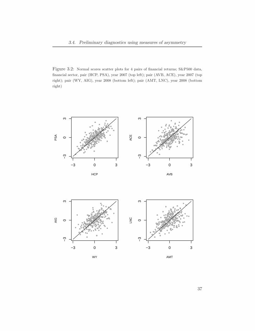
3.4. Preliminary diagnostics using measures of asymmetry
Figure 3.2: Normal scores scatter plots for 4 pairs of financial returns; S&P500 data,
financial sector, pair (HCP, PSA), year 2007 (top left); pair (AVB, ACE), year 2007 (top
right); pair (WY, AIG), year 2008 (bottom left); pair (AMT, LNC), year 2008 (bottom
right)
−3 0 3
−30
3
HCP
PS
A
−3 0 3
−30
3
AVB
AC
E
−3 0 3
−30
3
WY
AIG
−3 0 3
−30
3
AMT
LNC
37
3.4. Preliminary diagnostics using measures of asymmetry
that G(∆R; k = 5) is significantly larger zero for the pair (AVB, ACE). Atthe same time the value of the second measure is nearly zero. It impliesa reflection asymmetric copula with stronger dependence in the lower tailand with no permutation asymmetry can be a good choice. The pair (WY,AIG) has a large positive value of G∗(∆P ; k = 0.2) so that a permutationasymmetric copula would be more appropriate for this pair. And for thelast pair both estimates are quite large comparing to the standard errors sothat a permutation and reflection asymmetric copula is more suitable.
Similar to the tail-weighted measures proposed in Chapter 2, the mainpurpose of the measures of asymmetry is to provide some guidance in se-lecting a more appropriate copula for bivariate data, e.g. tree 1 of a vinecopula. Therefore we recommend using a copula with tail asymmetry evenif the measures G(∆R; k), G
∗(∆P ; k) are estimated to be positive or nega-tive at the 10% significance level only and not at the 5% significance level.Unlike the tail-weighted measures, the measures of asymmetry based on theempirical copula process use all the data and thus allow reduction of vari-ability of the estimates. When used together with the measures L, U ,the measures of asymmetry provide a useful summary on the dependencestructure of the data set. Based on the estimated values of these measuresone can decide on a copula that can handle strong tail dependence and/orpermutation or reflection asymmetry that are found in the data.
38
Chapter 4
Factor copula models for
multivariate data
The multivariate normality assumption is widely used to model the jointdistribution of high-dimensional data. The univariate margins are trans-formed to normality and then the multivariate normal distribution is fittedto the transformed data. In this case, the dependence structure is completelydefined by the correlation matrix and different models on the correlationstructure can be used to reduce the number of dependence parameters fromO(d2) to O(d), where d is the multivariate dimension or number of variables.When dependence in the observed variables is thought to be explained by afew latent variables, the Gaussian or normal factor model assumes a linearrelation on a few unobserved normally distributed factors.
We propose and study the copula version of the multivariate normaldistribution with a correlation matrix that has a factor structure. We namethe extension as the factor copula model. The classical factor model is aspecial case but within our framework, the parametrization is different asit involves partial correlations. The factor copula model is useful when thedependence in observed variables is based on a few unobserved variables,and there exists tail asymmetry or tail dependence in the data, so that themultivariate normality assumption is not valid.
In many multivariate applications, the dependence in observed vari-ables can be explained through latent variables; in multivariate item re-sponse in psychology applications, latent variables are related to the ab-stract variable being measured through items, and in finance applications,latent variables are related to economic factors. Classical factor analysis as-sumes (after transforms) that all observed and latent random variables arejointly multivariate normal. Books on multivariate analysis (see for example,Johnson and Wichern (2002)) often have examples with factor analysis andfinancial returns. We show for some financial return data that, in terms ofthe Akaike or Bayesian information criteria, the factor copula model can bea better fit than truncated vines (because of a simpler dependence structure)and the classical factor model (because of tail dependence).
39
4.1. Factor copula models
An important advantage of factor models is that they can be nicelyinterpreted. In case of stocks in a common sector, the current state ofthis sector can affect all of their change of prices, but the sector index, ifmeasured, might not contain all of the latent information that explains thedependence. Similarly for market data, the state of economy as a wholecan determine the latent dependence structure. The “state variables” areaggregated from many exogenous variables (such as interest rate, refinancingrate, political instabilities, etc.) and can not be easily measured, thereforefactor copula models based on latent variables might be a good choice.
In Section 4.1 we define the factor copula model and give more details forthe one-factor and two-factor models. Some dependence and tail propertiesof bivariate margins of the factor copula models are given in Section 4.3.The results imply that different types of dependence and tail asymmetrycan be modeled with appropriate choices of bivariate linking copulas. Com-putational details for maximum likelihood estimation of the factor copulamodel are given in Section 4.4.1. Section 4.5 discusses diagnostics for choicesof bivariate linking copulas, reports on some simulation results, and showsapplications of the factor copula modelto US stock returns.
4.1 Factor copula models
In multivariate models with copulas, a copula or multivariate uniform dis-tribution is combined with a set of univariate margins. This is equivalentto assuming that variables X1, . . . ,Xd have been transformed to uniformrandom variables. So we assume that U = (U1, . . . , Ud) is a random vec-tor with Ui ∼ U(0, 1). The joint cdf of the vector U is then given byC(u1, . . . , ud) where C is a d-dimensional copula. In the p-factor copulamodel, U1, . . . , Ud are assumed to be conditionally independent given p la-tent variables V1, . . . , Vp. Without loss of generality, we can assume Vi areindependent and identically distributed (i.i.d.) U(0, 1). Let the conditionalcdf of Uj given V1, . . . , Vp be denoted by Fj|V1,...,Vp . Then,
C(u1, . . . , ud) =
∫
[0,1]p
d∏
j=1
Fj|V1,...,Vp(uj |v1, . . . , vp) dv1 · · · dvp. (4.1)
Any conditional independence model, based on p independent latent vari-ables, can be put in this form after transforms to U(0, 1) random variables.Hence, the dependence structure of U is then defined through conditionaldistributions F1|V1,...,Vp , . . ., Fd|V1,...,Vp . We will call (4.1) a factor copula
40
4.1. Factor copula models
model, with Fj|V1,...,Vp expressed appropriately in terms of a sequence of bi-variate copulas that link the observed variables Uj to the latent variablesVk. Some of the bivariate copulas are applied to conditional distributions.Details are given in Sections 4.1.1 and 4.1.2.
In the finance literature there are several factor copula models (e.g., Sec-tion 9.7.2 of McNeil et al. (2005), Hull and White (2004) and Oh and Patton(2012)); these all have a linear latent structure and are not as general asour model. With the conditional independence model with 2 or more latentvariables, there could be alternative ways to specify a model for Fj|V1,...,Vpthan we have.
4.1.1 One and two-factor copula models
We first study the case of p = 1 latent variable in (4.1). For j = 1, . . . , d,denote the joint cdf and density of (Uj , V1) by Cj,V1 and cj,V1 respectively.Since U1, Vj are U(0, 1) random variables, then Fj|V1 is just a partial deriva-tive of the the copula Cj,V1 with respect to the second argument. That is,Fj|V1(uj |v1) = Cj|V1(uj |v1) = ∂Cj,V1(uj , v1)/∂v1. With p = 1, equation (4.1)becomes:
C(u1, . . . , ud) =
∫ 1
0
d∏
j=1
Fj|V1(uj |v1) dv1 =
∫ 1
0
d∏
j=1
Cj|V1(uj |v1) dv1. (4.2)
We will call the copula in (4.2) 1-factor copula. Note that ∂∂uCj|V1(u|v1) =
∂2
∂u∂v1Cj,V1(u, v1) = cj,V1(u, v1). Then (4.2) implies by differentiation that
the density of the 1-factor copula is
c(u1, . . . , ud) =∂dC(u1, . . . , ud)
∂u1 . . . ∂ud=
∫ 1
0
d∏
j=1
cj,V1(uj , v1) dv1. (4.3)
In the model, dependence is defined by d bivariate linking copulas C1,V1 , . . . ,Cd,V1 ; there are no constraints amongst these bivariate copulas. Note thatany conditional independence model for absolutely continuous random vari-ables, conditioned on one latent variable, can be written in this form. Belowwe show that when Cj,V1 are all bivariate normal copulas, then (4.3) becomesthe copula of the multivariate normal distribution with a 1-factor correlationmatrix.
A main advantage of the model is that it allows for different types of taildependence structure. As it was shown in Joe et al. (2010) and Joe (2011),if all bivariate linking copulas are lower (upper) tail dependent then all
41
4.1. Factor copula models
bivariate margins of U are also lower (upper) tail dependent respectively.Thus, with appropriately chosen linking copulas asymmetric dependencestructure as well as tail dependence can be easily modeled.
For the special case of bivariate normal linking copulas, let Cj,V1 be thebivariate normal copula with correlation αj1, j = 1, . . . , d. Let Φ, φ denotethe standard normal cdf and density function, and let Φ2(·; ρ) be bivariatenormal cdf with correlation ρ. Then Cj,V1(u, v) = Φ2(Φ
−1(u),Φ−1(v);αj1)and
Fj|V1(u|v) = Φ([
Φ−1(u)− αj1Φ−1(v)
] / √1− α2
j1
).
For equation (4.2), let uj = Φ(zj) to get a multivariate distribution withN(0, 1) margins. Then
F (z1, . . . , zd) := C(Φ(z1), . . . ,Φ(zd))
=
∫ 1
0
d∏
j=1
{Φ([zj − αj1Φ
−1(v1)] / √
1− α2j1
)}dv1
=
∫ ∞
−∞
d∏
j=1
{Φ([zj − αj1w
] / √1− α2
j1
)}φ(w) dw. (4.4)
Hence this model is the same as a multivariate normal model with a 1-factor correlation structure because this multivariate cdf comes from therepresentation:
Zj = αj1W +√
1− α2j1 ǫj , j = 1, . . . , d,
where W, ǫ1, . . . , ǫd are i.i.d. N(0, 1) random variables.If Cj,V1 is the Student t copula with correlation αj1, and νj degrees of
freedom, j = 1, . . . , d, c(u1, . . . , ud) is no longer the multivariate Student tcopula density. When the Cj,V1 are chosen from the Student t copula oranother copula families, then the simplest representation is a 1-dimensionalintegral, but this is not a problem for likelihood inference, as shown inSection 4.4.1.
We next show details for p = 2. Let Cj,V1 be the copula of (Uj , V1) asbefore. Also let Cj,V2;V1 be the copula for Fj|V1 = FUj |V1 and FV2|V1 , andlet cj,V2;V1 be its density. We make the simplifying assumption that thecopula for FUj |V1(·|v1) and FV2|V1(·|v1) does not depend on v1; this is thesame assumption used in vine copulas or the pair-copula construction. Forboth theory and applications, it is a first step in understanding factor copulamodels with more than 1 latent factor. Note that FV2|V1 is the U(0, 1) cdf
42
4.1. Factor copula models
since we assume that V2 is independent of V1. Then the independence ofV1, V2 implies
Fj|V1,V2(u|v1, v2) = Pr(Uj ≤ u|V1 = v1, V2 = v2) =
=∂
∂v2Pr(Uj ≤ u, V2 ≤ v2|V1 = v1) =
∂
∂v2CjV2;V1
(Cj|V1(u|v1), v2
)
= Cj|V2;V1(Cj|V1(u|v1)|v2
), (4.5)
where Cj|V2;V1(x|v) = ∂Cj,V2;V1(x, v)/∂v. The equation (4.1) becomes:
C(u1, . . . , ud) =
∫ 1
0
∫ 1
0
d∏
j=1
Fj|V1,V2(uj |v1, v2) dv1dv2
=
∫ 1
0
∫ 1
0
d∏
j=1
Cj|V2;V1(Cj|V1(uj |v1)|v2) dv1dv2. (4.6)
We will call the copula in (4.6) 2-factor copula. By differentiation withrespect to u1, . . . , ud, (4.6) implies that the 2-factor copula density is
c(u1, . . . , ud) =
∫ 1
0
∫ 1
0
d∏
j=1
{cj,V2;V1(Cj|V1(uj |v1), v2) · cj,V1(uj , v1)
}dv1dv2.
(4.7)The dependence structure is defined through 2d linking copulas C1,V1 , . . . ,Cd,V1 , C1,V2;V1 , . . . , Cd,V2;V1 ; there are no constraints amongst these 2d bi-variate copulas. Clearly, this is an extension of the 1-factor copula modeland different types of dependence can be modeled. More details on theproperties of bivariate margins are provided in Section 4.3.
This model includes the 2-factor multivariate normal model as a specialcase. Suppose Cj,V1 and Cj,V2;V1 are the bivariate copulas with correlationsαj1 and γj = αj2/(1 − α2
j1)1/2 respectively, j = 1, . . . , d. Here αj2 is a
correlation of Zj = Φ(Uj) andW2 = Φ(V2) so that the independence of V1, V2implies that γj is the partial correlation of Zj and W2 given W1 = Φ(V1) (ingeneral ρZW2;W1 = [ρZW2 −ρZW1ρW2W1 ]/[(1−ρ2ZW1
)(1−ρ2W2W1)]1/2). Then,
43
4.1. Factor copula models
using the above conditional distribution of the bivariate normal copula,
Cj|V2;V1(Cj|V1(u|v1)|v2) =
= Φ
([Φ−1(u)− αj1Φ
−1(v1)
(1− α2j1)
1/2− γjΦ
−1(v2)
] / √1− γ2j
)
= Φ
Φ−1(u)− αj1Φ
−1(v1)− γj(1− α2j1)
1/2Φ−1(v2)√(1− α2
j1)(1− γ2j )
. (4.8)
With zj = Φ(uj), j = 1, . . . , d, the cdf for the 2-factor model becomes
F (z1, . . . , zd) := C(Φ(z1), . . . ,Φ(zd))
=
∫ ∞
−∞
∫ ∞
−∞
d∏
j=1
Φ
(zj − αj1w1 − γj(1− α2
j1)1/2w2√
(1− α2j1)(1− γ2j )
)×
× φ(w1)φ(w2) dw1dw2. (4.9)
Hence this model is the same as a multivariate normal model with a 2-factor correlation structure because this multivariate cdf comes from therepresentation:
Zj = αj1W1 + αj2W2 +√
(1− α2j1)(1− γ2j ) ǫj , j = 1, . . . , d,
where W1,W2, ǫ1, . . . , ǫd are i.i.d. N(0, 1) random variables.
4.1.2 Models with p > 2 factors
The factor copula model can be straightforwardly extended to p > 2 factorsand it becomes an extension of the p-factor multivariate normal distributionwith a correlation matrix Σ that has the p-factor structure, that is, Σ =AAT +Ψ, where A is a d× p matrix of loadings and Ψ is a diagonal matrix.The main difference is that for the factor copula model, the parameters forthe second to p-th factors are partial correlations ρZjWk;W1···Wk−1
(the jthobserved variable and kth latent variable given latent variables 1, . . . , k−1).The advantage of this parametrization is that all of these partial correlationsand ρZjW1 are algebraically independent in the interval (−1, 1), and thepartial correlation parametrization is the one that can extend to the factorcopula, by replacing each correlation with factor 1 by a bivariate copula, andeach partial correlation for factors 2 to p with a bivariate copula applied toconditional distributions.
44
4.1. Factor copula models
We now provide some details on how the parameters of bivariate normallinking copulas are related to the matrix of loadings A in the classical factormodel with p factors. In the model,
Zj =
p∑
i=1
αjiWi +
(1−
p∑
i=1
α2ji
)1/2
ǫj, (4.10)
whereW1, . . . ,Wp, ǫ1, . . . , ǫd are i.i.d. N(0,1) random variables. Let the ma-trix of loadings be A = (Aij); one possibility has Aij = αji, i = 1, . . . , p,j = 1, . . . d. This matrix is unique up to orthogonal transformations. Theunconditional distribution of Zj and W1 is given by a bivariate normaldistribution with correlation αj1 as it follows from (4.10). Similarly, fork = 2, . . . , p the conditional distribution FZj ,Wk;W1,...,Wk−1
is a bivariate nor-mal distribution with correlation
ρZj ,Wk;W1,...,Wk−1=
Cov(Zj ,Wk|W1, . . . ,Wk−1)
[Var(Zj |W1, . . . ,Wk−1)Var(Wk|W1, . . . ,Wk−1)]1/2
=αjk
(1− α2j1 − . . . − α2
j,k−1)1/2
. (4.11)
As a result, CZj ,W1 is a bivariate copula with correlation αj1 andCZj ,Wk;W1,...,Wk−1
is a bivariate normal copula with correlationρZj ,Wk;W1,...,Wk−1
as given in (4.11).The density for a general 2 ≤ p < d can be obtained if we note that due
to independence V1, . . . , Vp
Fj|V1,...,Vp(u|v1, . . . , vp) =∂ Pr(Uj ≤ u, Vp ≤ vp|V1 = v1, . . . , Vp−1 = vp−1)
∂vp
=∂Cj,Vp;V1,...,Vp−1(Fj|V1,...,Vp−1
(u|v1, . . . , vp−1), vp)
∂vp
= Cj|Vp;V1,...,Vp−1(Fj|V1,...,Vp−1
(u|v1, . . . , vp−1)|vp).
This recursion formula for Fj|V1,...,Vp(u|v1, . . . , vp) can be further expandedto express this conditional probability in terms of bivariate linking copulasCj|Vk;V1,...,Vk−1
, k ≤ p and then used in (4.1) to get the joint cdf C(u1, . . . , ud).This cdf, expressed in terms of bivariate linking copulas and conditionalcdfs, will be called p-factor copula. The density can be then obtained bydifferentiating the cdf and applying the chain rule.
p-factor copula models and C-vines
45
4.1. Factor copula models
Let U = (U1, ..., Um) is a random vector with Ui ∼ U(0, 1) with cdfC(u1, ..., um) as before. As in case of factor copula models the idea of vinecopula models is to express the joint cdf C(u1, ..., um) in terms of simple bi-variate conditional copulas. In truncated vine copula model the conditionalindependence at high levels is assumed to reduce the number of depen-dence parameters. A detailed review of a vine copula structure is given inKurowicka and Cooke (2006).
The joint distribution of U can be decomposed using bivariate linkingcopulas in many different ways. Copula vine models have computational ad-vantage as the joint density of U is available in closed form, so no numericalintegration is required. The formula for the density in general case can befound in Aas et al. (2009).
A special case of vine copula models is the C-vine model. In C-vinecopula model the dependence structure of the vector U is modeled usingconditional distributions of (Uj , Ul) given U1, ..., Ul−1, j = l + 1, ...,m, l =1, ...,m− 1. That is why m− l bivariate conditional copulas are required atlevel l and m(m− 1)/2 linking copulas are needed in total as in the case ofthe C-vine copula model. Usually, the conditional independence of Uj andUl is assumed at higher levels l to reduce the number of parameters in themodel. We now consider two cases of C-vine truncated after the first andthe second levels.
C-vine truncated after 1 level
Denote the copula corresponding to (Uj , U1) by Cj1, j = 2, ...,m. As-suming Uj and Ul are conditionally independent given U1, ..., Ul−1 for l > 1we can write the joint density as
c(u1, ..., um) =m∏
j=2
cj1(uj , u1). (4.12)
In this case m− 1 bivariate copulas Cj1, j = 2, ...,m are required.
C-vine truncated after 2 levels
Denote the conditional copula of (Uj , U2) given U1 by Cj2, j = 3, ...,m.Assume now Uj and Ul are conditionally independent given U1, ..., Ul−1 forl > 2. The joint density c(u1, ..., um) is
c(u1, ..., um) =
m∏
j=2
cj1(uj , u1)×m∏
j=3
cj2(Cj|1(uj |u1), C2|1(u2|u1)). (4.13)
46
4.2. p-factor structure in LT-Archimedean copulas
For the C-vine truncated after 2 levels m−1 linking copulas Cj1, j = 2, ...,mare required at the first level and m−2 conditional copulas Cj2, j = 3, ...,mare required at the second level, 2m− 3 copulas are needed in total.
In the preceding sections, we have derived details of the factor copulamodels with one and two factors as conditional independence models to showthat they are very general latent variable models. At the same time, factorcopula models are equivalent to truncated C-vines rooted at the latent vari-ables; the view as C-vines means that one can obtain the joint density of theobserved and unobserved variables through the copula density representa-tion of Bedford and Cooke (2001) and then integrate the latent variables toget the density of the observed variables. In a special case of C-vine mod-els truncated after the first and second levels and d observed variables, thedensity of the 1-factor (2-factor) copula is given in (4.12), m = d + 1, and(4.13), m = d+ 2, after integrating over the first one (first two) variable(s)u1 (u1, u2), respectively. In general case, the factor copula model with platent variables V1, . . . , Vp can be represented as a C-vine copula model for(V1, . . . , Vp, U1, . . . , Ud) rooted at the latent variables and truncated at thep-th level (all copulas at higher levels are independence copulas). By inte-grating over latent variables, note that the p-factor copula density involvesa p-dimensional integral in general when the bivariate linking copulas arenot all normal.
4.2 p-factor structure in LT-Archimedean copulas
In this section we give some details on Laplace transform (LT) Archimedeancopulas with a p-factor structure; see Chapter 9.7.2 in McNeil et al. (2005).Let V1, . . . , Vp be independent random variables and let GVj be the Laplace-Stieltjes transform of the variable Vj , j = 1, . . . , p. Let A be a d by p matrixwith strictly positive elements aij > 0. Then a LT-Archimedean copula witha p-factor structure can be defined as follows:
Cp(u1, . . . , ud) =
p∏
j=1
E
(exp
{−Vj
d∑
i=1
aijG−1i (ui)
})
=
p∏
j=1
GVj
(d∑
i=1
aijG−1i (ui)
), (4.14)
where Gi(t) =∏pj=1 GVj (aijt) is the Laplace-Stieltjes transform of Vi =∑p
j=1 aijVj. LT-Archimedean copulas with the p-factor structure is an al-
47
4.2. p-factor structure in LT-Archimedean copulas
ternative way to incorporate latent factors through the Laplace-Stieltjestransform. Assume hj is the pdf of the random variable Vj, j = 1, ..., p. Thecdf of the LT-Archimedean copula can then be written in the form:
Cp(u1, . . . , ud) =
∫
[0,∞)p
d∏
i=1
exp
−
p∑
j=1
vjaijG−1i (ui)
×
h(v1)...h(vp)dv1...dvp.
It is seen that the variables (U1, ..., Ud) ∼ Cp are conditionally inde-pendent given V1, ..., Vp. After transforming the cdfs of V1, ..., Vp to U(0, 1)variables we can get the formal definition of a factor copula. It impliesthat LT-Archimedean copulas with a p-factor structure is a special case ofp−factor copula models. However, unlike factor copula models, the joint cdfcannot be obtained in a closed form except for some special cases that weconsider below.
The case p = 1 corresponds to the standard definition of an Archimedeancopula based on a Laplace transform. If p = 1, we have Gi(t) = GV1(ai1t)and G−1
i (ui) = G−1V1
(ui)/ai1 so that
C1(u1, . . . , ud) = E
(exp
{−V1
d∑
i=1
ai1G−1i (ui)
})
= E
(exp
{−V1
d∑
i=1
G−1V1
(ui)
}). (4.15)
Next, consider the case of p = 2. It implies that Gi(t) = GV1(ai1t)××GV2(ai2t) for i = 1, ..., d, and the inverse transform G−1
i (ui) is not alwaysavailable in a closed form so that numerical methods are needed to find theLT inverse; see Hofert (2008). Now we consider some cases when a simpleexpression for G−1
i (ui) can be obtained and the joint cdf C2(u1, . . . , ud) isavailable in a closed form.
1. Let Vj ∼ St(1/θ, 1, γ, 0) with γ = (cos(π/(2θ)))θ , θ > 1, j = 1, 2. We
get GVj (t) = exp{−t1/θ
}and Gi(t) = exp
{−ξit1/θ
}where ξi = a
1/θi1 + a
1/θi2 .
It follows that G−1i (t) =
(t/ξi
)θ, t = − ln t, and
C2(u1, . . . , ud) = exp
−
(d∑
i=1
ai1 (ui/ξi)θ
)1/θ
−(
d∑
i=1
ai2 (ui/ξi)θ
)1/θ
48
4.3. Properties of 1- and 2-factor copula models
= exp
−
(d∑
i=1
(a∗i ui)θ
)1/θ
−(
d∑
i=1
((1− a∗i )ui)θ
)1/θ , a∗i = a
1/θi1 /ξi.
Note that C2(u1, . . . , ud) = CG(ua∗11 , . . . , u
a∗dd )·CG(u1−a
∗1
1 , . . . , u1−a∗dd ) where
CG is a d-dimensional Gumbel copula and 0 < a∗i < 1. One can see thatthis case can be readily extended to any value p > 2.
2. Let Vj ∼ Gamma(1/θj , 1), θj > 0. Assume that aij = ai for j = 1, 2.
We get GVj (t) = (1 + t)−1/θj and Gi(t) = (1 + ait)−1/θ1 with 1/θ = 1/θ1 +
1/θ2. It follows that G−1i (t) = (t−θ − 1)/ai, and
C2(u1, . . . , ud) =
(1 +
d∑
i=1
[u−θi − 1]
)−1/θ
=
(d∑
i=1
u−θi − d+ 1
)−1/θ
.
In this case the standard d-dimensional MTCJ copula is obtained. For d > 2if ai1 = . . . = aid = ai, we get
Cp(u1, . . . , ud) = G1
(d∑
i=1
(ai/a1)G−1i (ui)
)= G1
(d∑
i=1
G−11 (ui)
),
which is the standard definition of the LT-Archimedean copula based on arandom variable with the Laplace-Stieltjes transform G1.
In a general case, if ai1 6= ai2 the inverse function G−1i (ui) is not available
in a simple form because the Gamma distribution (unlike a positive stabledistribution) is not closed under positive linear combinations. As a result,this class of copulas may not be appropriate for modeling high-dimensionaldata.
4.3 Properties of 1- and 2-factor copula models
In a later section, we show that the 1-factor and 2-factor copula models aregood fits to some multivariate data sets compared with vine copulas. Henceit is important to know more properties about them to help in the choice ofthe bivariate linking copulas.
In this section we investigate different types of tail behavior and depen-dence properties of bivariate marginal copulas that can be obtained in factorcopula models. Without loss of generality we restrict our attention to thecopula C1,2 corresponding to the joint distribution of U1 and U2.
49
4.3. Properties of 1- and 2-factor copula models
4.3.1 Dependence properties
In the factor copula model some positive dependence properties of the link-ing copulas extend to the bivariate margins under some mild conditions.These properties include positive quadrant dependence (PQD), increasingin the concordance ordering and stochastic increasing (SI); see Section 1.2for details.
For all results in this section we will assume that all bivariate linkingcopulas are twice continuously differentiable functions on (0, 1)2. It followsthat in the factor copula model the three properties — PQD, increasing inconcordance ordering and SI — hold under some mild conditions on bivariatelinking copulas. Basically, SI linking (conditional) copulas imply all theseproperties for bivariate margins in 1-factor copula model as it is shown inPrepositions 1 and 2 below.
Proposition 4.1 For j = 1, 2, supposeCj|V1 = CUj |V1 is SI, that is, Pr(Uj >u|V1 = v) = 1−Cj|V1(u|v) is increasing (or non-decreasing) in v ∈ (0, 1) forany 0 < u < 1. Let (U1, U2) ∼ C1,2, where C1,2 is a bivariate marginof the 1-factor copula (4.2). Then Cov(U1, U2) ≥ 0 and C1,2 is PQD orC1,2(u1, u2) ≥ u1u2 for any 0 < u1 < 1 and 0 < u2 < 1.
Proof : We have
Cov(U1, U2) = E[Cov(U1, U2|V1)] + Cov(E(U1|V1),E(U2|V1))= Cov(E(U1|V1),E(U2|V1)) ≥ 0
since E(U1|V1 = v) and E(U2|V1 = v) are increasing in v from the SI as-sumption, and the covariance of two increasing functions is non-negativefrom Chebyshev’s inequality for similarly ordered functions (see Hardy et al.(1952)). Similarly, for any 0 < u1 < 1 and 0 < u2 < 1,
Pr{U1 ≥ u1, U2 ≥ u2} − (1− u1)(1− u2) = Cov(I{U1 ≥ u1}, I{U2 ≥ u2})= Cov(E[I{U1 ≥ u1}|V1],E[I{U2 ≥ u2}|V1]) ≥ 0,
because E[I{Uj ≥ uj}|V1 = v] = Pr{Uj ≥ uj|V1 = v} for j = 1, 2 areincreasing functions of v from the SI assumption. We have C(u1, u2) ≥(1− u1)(1− u2) which is the same thing as C(u1, u2) ≥ u1u2. �
The result in Proposition 4.1 is a special case of a multivariate resultin Theorem 5.3.1 of Tong (1980), in which case the conclusion is positiveorthant dependence.
50
4.3. Properties of 1- and 2-factor copula models
Proposition 4.2 Consider the bivariate margin C1,2 of (4.2). Assume thatC2,V1 is fixed and that C2|V1 is stochastically increasing (respectively decreas-ing). (a) Assume that C1,V1 increases in the concordance ordering. ThenC1,2 is increasing (respectively decreasing) in concordance. (b) Assume thatCV1|1 is SI. Then C2|1 is stochastically increasing (respectively decreasing).
Proof : Suppose C1,V1 is parameterized by a parameter θ and C2,V1 isfixed. The increasing in concordance assumption implies that C1,V1(·; θ2)−C1,V1(·; θ1) ≥ 0 for θ1 < θ2. Using the integration by parts formula we get:
C1,2(u1, u2; θ) =
∫ 1
0C1|V1(u1|v; θ)C2|V1(u2|v)dv
= u1C2|V1(u2|1) −∫ 1
0C1,V1(u1, v; θ)
∂C2|V1(u2|v)∂v
dv. (4.16)
With the assumption of twice continuous differentiability, ∂C2|V1(u2|v)/∂vis a continuous function of v for v ∈ (0, 1) but can be unbounded at 0 or 1.Nevertheless, the integrand is an integrable function since
∫ 1
0
∣∣∣∣C1,V1(u1, v; θ)∂C2|V1(u2|v)
∂v
∣∣∣∣ dv ≤∣∣∣∣∫ 1
0
∂C2|V1(u2|v)∂v
dv
∣∣∣∣=∣∣C2|V1(u2|0)− C2|V1(u2|1)
∣∣ .
Therefore the formula (4.16) is valid. For θ2 > θ1 we have:
C1,2(u1, u2; θ2)− C1,2(u1, u2; θ1) =
∫ 1
0[C1,V1(u1, v; θ1)− C1,V1(u1, v; θ2)]×
×∂C2|V1(u2|v)
∂vdv. (4.17)
Since C1,V1(u1, v; θ2) ≥ C1,V1(u1, v; θ1) and ∂C2|V1(u2|v)/∂v ≤ (≥) 0 by theassumption of stochastic increasing (decreasing), we get C1,2(u1, u2; θ2) ≥(≤) C1,2(u1, u2; θ1) respectively, that is C1,2 is increasing (decreasing) inconcordance.
Similarly, one can show that for u1 ∈ (0, 1) both parts of (4.16) can bedifferentiated with respect to u1 twice to get
∂2C1,2(u1, u2; θ)
∂u21=∂C2|1(u2|u1; θ)
∂u1= −
∫ 1
0
∂CV1|1(v|u1; θ)∂u1
·∂C2|V1(u2|v)
∂vdv.
Assuming CV1|1 is SI we get ∂CV1|1(v|u1; θ)/∂u1 ≤ 0; since also∂C2|V1(u2|v; θ)/∂v ≤ (≥) 0 by the assumption of stochastically increasing
51
4.3. Properties of 1- and 2-factor copula models
(decreasing), then ∂C2|1(u2|u1; θ)/∂u1 ≤ (≥, respectively) 0, that is, C2|1 isstochastically increasing (decreasing). �
While the result on SI can not be readily extended for 2-factor model,the results for PQD and increasing in the concordance ordering hold in thismodel under similar assumptions.
Proposition 4.3 For the 2-factor copula model in (4.6), suppose thatCj|V1(·|v1) and Cj|V2;V1(·|v2) are SI for j = 1, 2. Then the margin C1,2 of(4.6) is PQD.
Proof: One can see that FU |V1,V2(u|v1, v2) = CU |V2;V1(CU |V1(u|v1)|v2) isa decreasing function of v1 and v2 since CU |V1(u|v1) decreases in v1 andCU |V2;V1(u|v2) decreases in v2 by the SI assumption. Let (U1, U2) ∼ C1,2.Define aj(v1, v2) = P{Uj > uj |V1 = v1, V2 = v2} = E[I{Uj > uj}|V1 =v1, V2 = v2], j = 1, 2. From the SI assumption, aj(v1, v2) is an increas-ing function of v1 and v2. By Chebyshev’s inequality for similarly orderedfunctions, for every v1 we have
b12(v1) = E[a1(v1, V2)a2(v1, V2)|V1 = v1]
≥ E[a1(v1, V2)|V1 = v1]E[a2(v1, V2)|V1 = v1] = b1(v1)b2(v1).
Because V2 is independent of v1 and a1, a2 are increasing in v1, b1, b2 areincreasing in v1. Next, with another application of Cehbyshev’s inequality,
E[b12(V1)] = E[a1(V1, V2)a2(V1, V2)] ≥ E[b1(V1)b2(V1)]
≥ E[b1(V1)]E[b2(V1)] = E[a1(V1, V2)]E[a2(V1, V2)]
and this implies
P{U1 ≥ u1, U2 ≥ u2} − (1− u1)(1− u2) = Cov(I{U1 ≥ u1}, I{U2 ≥ u2})= Cov(E[I{U1 ≥ u1}|V1, V2],E[I{U2 ≥ u2}|V1, V2]) ≥ 0. �
This result also follows from Theorem 5.3.1 and Lemma 2.2.1 of Tong(1980).
Proposition 4.4 Consider the bivariate margin C1,2 of (4.6). Assume thatC1,V2;V1 increases in the concordance ordering and C2|V2;V1 is stochasticallyincreasing (decreasing). Then C1,2 is increasing (decreasing, respectively) inconcordance.
52
4.3. Properties of 1- and 2-factor copula models
Proof: Suppose that C1,V2;V1 is parameterized by a parameter θ andC1,V2;V1 , Cj,V1 , j = 1, 2 are fixed. Using the integration by parts formula weget:
C1,2(u1, u2; θ) =
∫ 1
0
∫ 1
0C1|V2;V1(C1|V1(u1|v1)|v2; θ)×
× C2|V2;V1(C2|V1(u2|v1)|v2)dv1dv2
=
∫ 1
0C1|V1(u1|v1)C2|V2;V1(C2|V1(u2|v1)|1)dv1−
−∫ 1
0
∫ 1
0C1,V2;V1(C1|V1(u1|v1), v2; θ) ·
∂C2|V2;V1(C2|V1(u2|v1)|v2)∂v2
dv1dv2
and therefore for θ2 > θ1 we have:
C1,2(u1, u2; θ2)− C1,2(u1, u2; θ1) =
=
∫ 1
0
∫ 1
0[C1,V2;V1(C1|V1(u1|v1), v2; θ1)−C1,V2;V1(C1|V1(u1|v1), v2; θ2)]×
×∂C2|V2;V1(C2|V1(u2|v1)|v2)
∂v2dv1dv2 ≥ 0 (≤ 0)
since C1,V2;V1(C1|V1(u1|v1), v2; θ2) ≥ C1,V2;V1(C1|V1(u1|v1), v2; θ1) and∂C2|V2;V1(C2|V1(u2|v1)|v2)/∂v2 ≤ 0 (≥ 0) by the assumption. As in Propo-sition 4.2, the derivative ∂C2|V2;V1(C2|V1(u2|v1)|v2)/∂v2 can be unboundedat v2 = 0 or v2 = 1 but one can similarly show that the integrand is anintegrable function and the integration by parts formula is applicable in thiscase. �
4.3.2 Tail properties
In this section, we prove some tail properties of the 1-factor and 2-factorcopula models. We consider the properties of C1,2 in the lower tail, asthe properties in the upper tail can be obtained by reflections Uj → 1 −Uj . In Hua and Joe (2011), the concept of tail order is introduced in amultivariate context to study a range of tail behavior. The lower tail orderof a bivariate copula C1,2 is κL if C1,2(u, u) ∼ ℓL(u)u
κL as u → 0 whereℓL(u) is a slowly varying function (such as a constant or a power of − log u).If C1,2(u, u) = 0 for all 0 < u < u0 for some positive u0, then define κL =∞. Similarly the upper tail order κU is such that C1,2;R(u, u) ∼ ℓU (u)u
κU
53
4.3. Properties of 1- and 2-factor copula models
as u → 0, where C1,2;R(u1, u2) = u1 + u2 − 1 + C1,2(1 − u1, 1 − u2) isthe survival or reflection copula. A property is that κL ≥ 1 and κU ≥ 1with a smaller value corresponding to more dependence in the tail (moreprobability in the corner). Thus, the strongest tail dependence correspondsto κL = 1 or κU = 1. For comonotonic (perfect positive dependence) tail,κL = κU = 1 and ℓL(u) = ℓU (u) = 1 for strongest tail dependence. Forcountermonotonic (perfect negative dependence) tail, κL = κU = ∞ becausethere is no probability in the upper and lower corners. These tail ordersalso provide a simple condition to establish the direction of tail asymmetry,namely: if κL > κU (κL < κU ) then C1,2 has tail asymmetry skewed tothe upper (lower) tail; and if C1,2(u, u) ∼ λLu
κ and C12,R(u, u) ∼ λUuκ as
u → 0 with λU > λL > 0 (λL > λU > 0), then C1,2 has tail asymmetryskewed to the upper (lower) tail.
Below we consider three types of tail behavior for the bivariate copulaC1,2 for κ being κL or κU : tail dependence (κ = 1), intermediate tail depen-dence (1 < κ < 2) and tail quadrant independence (κ = 2). The proofs aremore technical, so are deferred to the Appendix.
Tail dependence
It is shown in Joe (2011) that in the 1-factor model, C1,2 has lower(upper) tail dependence if both C1,V1 and C2,V1 have lower (upper) taildependence. Under mild assumptions, tail dependence is inherited by C1,2
in the 2-factor model. More formally, the next proposition holds.
Proposition 4.5 Let limu→0Cj|V1(u|hu) = tj(h) and assume Cj|V2;V1(u|v)and Cj|V1(u|v) are continuous functions of u and v, j = 1, 2. Assumelimh→0 tj(h) = tj0 > 0, and Cj|V2;V1(tj0|0) ≥ k0 > 0, j = 1, 2. Then thebivariate margin C1,2 of the copula in (4.7) is lower tail dependent. A par-allel result holds for upper tail dependence.
Proof : See Appendix C.
The condition for Cj|V1 is implied by Cj,V1 having lower tail dependence— see Joe (2011). Hence, lower (upper) tail dependence for the observedvariables can be modeled by choosing lower (upper) tail dependent linkingcopulas for the first factor.
Intermediate tail dependence
Intermediate tail dependence can be inherited by C1,2 in many cases.One example of copula with intermediate dependence is a bivariate normalcopula with positive correlation 0 < ρ < 1, for which κ = 2/(1 + ρ). If the
54
4.3. Properties of 1- and 2-factor copula models
bivariate linking copulas are normal, with correlations αjV1 for Cj,V1 andγj = αjV2/(1− α2
jV1)1/2 for Cj,V2;V1 respectively, j = 1, 2, then the marginal
copula C1,2 is again a normal copula with parameter ρ12 = α1V1α2V1 +α1V2α2V2 , Therefore it has intermediate tail dependence if all of the αjV1 , αjV2parameters are positive.
Intermediate lower tail dependence can also be obtained if bivariate link-ing copulas are extreme value copulas, which have upper tail dependence andintermediate lower tail dependence. Because of the structure of extremevalue copulas, this case is amenable to mathematical proofs of tail proper-ties; we expect the behavior to be similar in general for linking copulas withintermediate tail dependence.
We consider 1-factor model first. Let Ci,V1(u1, u2) be a bivariate ex-treme value copula. From Chapter 6 of Joe (1997), there is the followingrepresentation:
Ci,V1(u1, u2) = exp{−(w1+w2)Ai(w2/[w1+w2])} = (u1u2)Ai(lnu2/ ln(u1u2)),
wj = − lnuj , j = 1, 2, (4.18)
where Ai(·) : [0, 1] 7→ [0.5, 1] is a convex function such that Ai(t) ≥ max{t,1− t}, i = 1, 2.
Proposition 4.6 Assume Ai(t) in (4.18) is a continuously differentiablefunction and A′
i(t) > −1 for 0 < t < 0.5, i = 1, 2. The lower tail order of thebivariate marginal copula C1,2 in (4.2) is equal to ξ∗ = min
0<s<∞{ξ(s)} ∈ [1, 2],
where
ξ(s) = (s+ 1)
[A1
(s
s+ 1
)+A2
(s
s+ 1
)]− s. (4.19)
Proof : See Appendix D.
Under the assumptions of Proposition 4.6, the marginal copula C1,2 of(4.2) has intermediate lower tail dependence if 1 < ξ∗ < 2. Note that
ξ(s) ≥ (s + 1)(
ss+1 +
1s+1
)− s = 1 and ξ(s) = 1 only if Ai
(s∗
s∗+1
)= s∗
s∗+1
and A2−i(
s∗
s∗+1
)= 1
s∗+1 for some s∗. Since Ai(t) ≥ max{t, 1− t} it implies
s∗ = 1 and Ai(1/2) = 1/2 which is possible only if both C1,V1 and C2,V1 arecomonotonic copulas. Otherwise, the lower tail order is always larger than1. Let us consider some examples.
Example 1: Gumbel copula: Ai(t) = [tθi + (1 − t)θi ]1/θi , θi > 1, fori = 1, 2. It is seen that ξ(s) = (1 + sθ1)1/θ1 + (1 + sθ2)1/θ2 − s. If θ1 = θ2 =
55
4.3. Properties of 1- and 2-factor copula models
θ0, s∗ =
(2
θ0θ0−1 − 1
)−1/θ0
and ξ∗ =
(2
θ0θ0−1 − 1
)(θ0−1)/θ0
. It follows that
1 < ξ∗ < 2 for any θ1 > 1, θ2 > 1. Hence, C1,2 has intermediate lower tailindependence. The Gumbel copula has upper tail dependence and thereforeC1,2 also has upper tail dependence. As a result, C1,2 has tail asymmetryskewed to the upper tail.
If θ1 = θ2 = θ0 > 1, the tail orders of Gumbel linking copulas are 21/θ0
and this is less than ξ∗. This demonstrates the general pattern that theconditional independence in the 1-factor model “dampens” the strength ofdependence in the tail (or tail order increases). Tail quadrant independence(tail order 2) is possible when the linking copulas with V1 have intermediatetail dependence, as shown in the next example.
Example 2: Let Ai(t) = 1− t(1− t)/θi, θi ≥ 1. Then ξ(s) = 2 + s(1−α0/(s+1)) where α0 = 1/θ1 +1/θ2. If α0 ≤ 1 we have ξ(s) ≥ 2+ s2/(s+1)therefore ξ∗ = 2. However, the lower tail order of Ci,V1 is equal to 2Ai(1/2) =2 − 1/(2θi) < 2. This example shows that intermediate tail dependence ofCi,V1 does not necessarily imply intermediate tail dependence of C1,2.
Now consider 2-factor copula models. Suppose that copulas at the firstlevel C1,V1(u1, u2), C2,V1(u1, u2) are extreme value copulas as above, and inaddition copulas at the second level are also extreme value copulas:
Ci,V2;V1(u1, u2) = (u1u2)Ai;1(lnu2/ ln(u1u2)), (4.20)
where Ai;1(·) : [0, 1] 7→ [0.5, 1] is a convex function such that Ai;1(t) ≥max{t, 1− t}, i = 1, 2.
Proposition 4.7 Assume Ai(t), Ai;1(t) in (4.18) and (4.20) are continu-ously differentiable functions and A′
i(t) > −1, A′i;1(t) > −1 for 0 < t < 0.5.
The lower tail order of the bivariate marginal copula C1,2 in (4.6) is equalto ξ∗2 = min
0<s1,s2<∞{ξ2(s1, s2)} ∈ [1, 2], where
ξ2(s1, s2) = (s1 + m1(s2))A1;1
(s1
s1 + m1(s2)
)
+ (s1 + m2(s2))A2;1
(s1
s1 + m2(s2)
)− s1 + s2, (4.21)
mi(s2) = (s2 + 1)Ai
(s2
s2 + 1
)− s2, i = 1, 2.
56
4.3. Properties of 1- and 2-factor copula models
Proof : See Appendix E.
Note that ξ2(0, s2) = ξ(s2) as given in (4.19) and (4.21), and thereforeξ∗2 ≤ ξ∗. That is, the lower tail order of C1,2 in 2-factor model is lowerthan that in 1-factor model when the same linking copulas Ci,V1 are usedat the first level. It means the intermediate tail dependence is stronger ifthe second factor is added to the model. For example, if all linking copulasare Gumbel copulas, the lower tail order of C1,2 is always smaller than 2.According to Proposition 4.5, C1,2 is an upper tail dependent copula. So allGumbel or survival Gumbel linking copulas imply C1,2 has tail asymmetryas in 1-factor model.
This behavior of the tail order is not the same for the 2-factor modelas with normal copulas. If Ci,V1 and Ci,V2;V1 are all normal copulas withpositive correlation ρ, then C1,2 is a normal copula with correlation ρ12 =ρ2 + (1 − ρ2)ρ2. Hence the tail order 2/(1 + ρ12) is smaller than 2/(1 + ρ)only if (
√5− 1)/2 < ρ < 1.
Also, ξ2(s1, s2) ≥ m1(s2) + s2 ≥ 1 and the equality is possible if and
only if A1
(s2
1+s2
)= 1
1+s2, A1;1
(s1
s1+m1(s2)
)= m1(s2)
s1+m1(s2), A2;1
(s1
s1+m2(s2)
)=
s1s1+m2(s2)
. Since Ai;1(t) ≥ max{t, 1−t}, Ai(t) ≥ max{t, 1−t}, it implies s1 ≤m1(s2) = 1− s2 ≤ m2(s2) ≤ s1. Hence m1(s2) = m2(s2) = s1 = 1− s2 andAi;1(1/2) = 1/2, that is linking copulas at the second level C1,V2;V1 , C2,V2;V1
should be comonotonic copulas.
Tail quadrant independence
Many bivariate copulas C(u, v) with (lower) tail order 2 satisfy the con-dition: CU |V (u|v) ≤ v0u if u > 0 is small enough, where v0 > 0 is a constant.If the bivariate linking copulas Cj,V1 are positive quadrant dependent andsatisfy this condition with positive constants v0j , then C1,2 has tail quadrantindependence with κ = 2. For example, in 1-factor model we have
C1,2(u, u) =
∫ 1
0C1|V1(u|v1)C2|V1(u|v1) dv1 ≤
∫ 1
0v01uv02udv1 = v01v02u
2
and the tail order is not more than 2 with positive dependence for C1,2. Onecan show tail quadrant independence of C1,2 in a similar way. Hence, tailquadrant independence can be obtained by choosing such linking copulaswith tail order 2. Copula families for which the above condition is satisfiedinclude the independence, Frank and Plackett copulas.
In summary, the choice of linking copulas affects the types of dependenceboth in the lower tail and the upper tail of C1,2, and more generally, themargin Cj,k of (4.2) or (4.6). Asymmetric tail dependence can be achievedwith reflection asymmetric linking copulas.
57
4.4. Computational details
4.4 Computational details
In this section, we discuss some computational details of numerical integra-tion and optimization for maximum likelihood.
4.4.1 Numerical integration and likelihood optimization
We consider the estimation of parameters in the factor copula models basedon the set of i.i.d. data vectors with margins transformed to U(0, 1) randomvariables and the joint distribution given by the copula C(u1, . . . , ud;θ),where θ is a vector of dependence parameters. For parametric versions of(4.3) and (4.7), a parametric copula family is used for each linking cop-ula, and θ is the vector of all of the dependence parameters. Similar toNikoloulopoulos et al. (2012) for vine copulas, appropriate choices of the bi-variate linking copulas can be made based on bivariate normal scores plotsfor the data and the properties in Section 4.3.
With parameters of univariate margins estimated first follow by con-version to U(0, 1) data {(ui1, . . . , uid)}ni=1, the parameter vector θ of thejoint density c(·;θ) can then be estimated using maximum likelihood. Thelikelihood can be written as
L(u1, . . . , ud;θ) =
n∏
i=1
c(ui1, . . . , uid;θ).
That is, the parameters of uniform margins are estimated at the firststep and dependence parameters at the second step with parameters of theunivariate margins fixed at the estimates obtained from the first step. Thetwo-step estimation procedure significantly simplifies the computation pro-cess. The second stage optimization of the log-likelihood of the copula modelis done via a quasi-Newton or modified Newton-Raphson numerical methodand this outputs a Hessian matrix from which standard errors (conditionalon the first step) are obtained. To obtain standard errors for the two-stepmethod, appropriate resampling methods can be used. More details on thelog-likelihood optimization are given in Appendix F and Section 5.3.1 formore general structured copula models.
In the p-factor copula model numerical integration is required to evaluatethe p-dimensional integral. This is a minor issue for p = 1. Based on theformula (4.3), with parameter θj for copula Cj,V1 , and θ = (θj)1≤j≤d,
c(ui1, . . . , uid;θ) =
∫ 1
0
d∏
j=1
cj,V1(uij , v1; θj)dv1.
58
4.4. Computational details
For many commonly used parametric copula families, the densitycj,V1(uij, v1; θ) approaches infinity as (uij , v1) → (0, 0) or (uij , v1) → (1, 1)therefore the integrand could be unbounded.
One can transform the variable of integration with v1 7→ Φ(t1), where Φ isthe standard normal cdf and then use Gauss-Hermite quadrature. Howeverwe find that Gauss-Legendre quadrature (Stroud and Secrest (1966)) worksfine; this approach approximates the integral as a weighted combination ofintegrands evaluated at quadrature points:
c(ui1, . . . , uid;θ) ≈nq∑
k=1
wk
d∏
j=1
cj,V1(uij , xk; θj)
where {xk} are the nodes and {wk} are the quadrature weights, and nqis the number of quadrature points. nq between 21 and 25 tends to give agood approximation of these integrals. The nice property of Gauss-Legendrequadrature is that the same nodes {xk} and weights {wk} are used fordifferent functions to compute integral quickly and with a high precision.The same nodes also help in smooth numerical derivatives for numericaloptimization.
The same methods can be used to compute two-dimensional integrals ifp = 2. Approximation using Gauss-Legendre quadrature is now a doublesum. Assuming the parameters are θj1 for Cj,V1 and θj2 for Cj,V2|V1 , from(4.7) we get
c(ui1, . . . , uid;θ) ≈nq∑
k1=1
nq∑
k2=1
wk1wk2×
×d∏
j=1
{cj,V2;V1(Cj|V1(uij |xk1 ; θj1), xk2 ; θj2)× cj,V1(uij , xk1 ; θj1)
}. (4.22)
Usually nq between 15 and 21 per dimension is enough to compute theintegrals with a good precision. One should try using different startingpoints in the algorithms to compute maximum likelihood estimates to ensurethat a global optimum is obtained.
The fastest implementation that we have is through a modified Newton-Raphson algorithm, with log-likelihood functions in Fortran90 code linkedto optimization in R. The analytical derivatives of the integrand function in(4.3) and (4.7) can be computed to get the formula for the first and secondorder derivatives of the log-likelihood function. The step size is controlled
59
4.4. Computational details
to ensure the value of the likelihood increases at each iteration. Again, weprovide more details in Section 5.3.1.
Note that in the Gaussian 2-factor models (with bivariate normal link-ing copulas) and a multivariate normal distribution with correlation matrixhaving factor structure, the number of independent correlation parametersis 2d − 1, because the loading matrix is non-unique and can be rotated sothat one correlation for the second factor is 0. But, as a rough guideline,the multivariate normal model can be used to choose an appropriate numberof factors p in the factor copula model. Different number of factors can beused to get likelihoods for different choices of p; the number of factors can bechosen so that there is not much improvement in terms of the likelihood orAkaike information criterion when adding an additional factor to the model.
However, the two-factor copula model, not based on all bivariate normalcopulas, is identifiable if 2d bivariate linking copulas are used. To indicatethe more general situation, we use the Morgenstern copula: uv[1 + θ(1 −u)(1 − v)], −1 ≤ θ ≤ 1, because the integrals simplify in this case (we arenot recommending that this copula to be used with factor copulas becauseit has limited dependence). If Cj,V1 , Cj,V2;V1 , j = 1, .., d, are Morgensterncopulas with respective parameters θ1,j, θ2,j , then one can show that
c(ui1, ..., uid;θ) = 1+1
3
∑
j1<j2
(θ1,j1θ1,j2+θ2,j1θ2,j2)(1−2uj1)(1−2uj2)+R(θ),
where R(θ) is a higher-order polynomial of θ1,1, . . . , θ1,d, θ2,1, . . . , θ2,d. Thesecond order term depends on θ1,j1θ1,j2 + θ2,j1θ2,j2 and as in the case of nor-mal copula the number of such independent parameters is 2d− 1. However,with higher-order terms in R(θ) the total number of independent parametersin this model is 2d.
In cases where the log-likelihood is quite flat (near non-identifiable), wecan set one of the Cj,V2;V1 to be an independence copula (this can be donewithout loss of generality in the case of normal copulas).
4.4.2 Multivariate Student model with a p-factor
correlation structure
In this section we give more details on estimating parameters for a spe-cial class of models where data are assumed to have multivariate Studentdistribution with a p-factor correlation structure. This class of models isconsidered in Kluppelberg and Kuhn (2009). Let Z = (Z1, ..., Zd) be a vec-tor with standard normal random variables that have multivariate normal
60
4.4. Computational details
distribution. More specifically, let
Zj =
p∑
i=1
αjiWi +
(1−
p∑
i=1
α2ji
)1/2
ǫj, (4.23)
where Wi, ǫj , i = 1, ..., p, j = 1, ..., d are i.i.d. N(0, 1) random variables.Define X = Z/
√Y/ν where Y is a chi-squared random variable with ν
degrees of freedom, independent of Z1, ..., Zd. It follows that X has mul-tivariate Student distribution with a correlation matrix Σ where Σj1,j2 =Cor(Zj1 , Zj2) =
∑pi=1 αj1iαj2i.
As we showed in Section 4.1.1 for p = 1 and p = 2, the multivariatenormal distribution with a p-factor correlation structure is a special case offactor copula models with normal linking copulas. However, the distributionof X for ν < ∞ is not the same as one that can be obtained in a p-factorcopula model by choosing all Student linking copulas. Nevertheless, thesetwo distributions are quite close in terms of the KullbackLeibler divergence.For example, consider the 1-factor Student copula model with d = 2 andthe linking copula parameters ρ1 = ρ2 = 0.7, ν1 = ν2 = 4. We compare thecorresponding 1-factor copula density with the Student copula density withρ = ρ1ρ2 = 0.49 and ν = 4. The KullbackLeibler sample size, that is thesample size which is required to discriminate these two models with 95%probability (see Joe (2014), Section 5.7), is about 1400. It indicates thesetwo models are quite close as a large sample size is required to discriminatethem. With ν1 = ν2 = 8 and ρ1 = ρ2 = 0.7 the corresponding sample size isover 3000.
In applications, the estimate of ν is around 10—15 in many cases there-fore p-factor copula model with Student linking copulas and multivariateStudent distribution with a p-factor correlation matrix are very close, andthe former is preferable since the joint pdf can be obtained in a closed formthus allowing much faster computation of the correlation parameters in Σ.In addition, the multivariate Student distribution with a common numberof degrees of freedom has less dependence parameters and is preferable interms of AIC.
Likelihood maximization
For the log-likelihood maximization, the inverse matrix Σ−1 and thedeterminant det(Σ) are needed. We now show how Σ−1 and det(Σ) can becalculated quickly for a large dimension d. Define a d× p matrix of loadingsA: Aji = αji. Denote ψj = 1 −∑p
i=1 α2ji and Dψ = diag(ψ1, . . . , ψd) and
61
4.4. Computational details
let D−1ψ be its inverse. Ii is easy to see that
Σ = AAT +Dψ.
Now we show that
Σ−1 = D−1ψ −D−1
ψ A(ATD−1ψ A+ Ip)
−1ATD−1ψ ,
det(Σ) =
d∏
j=1
ψj
det(ATD−1
ψ A+ Ip).
We have:
ΣΣ−1 = AATD−1ψ + Id −AATD−1
ψ A(ATD−1ψ A+ Ip)
−1ATD−1ψ
−A(ATD−1ψ A+ Ip)
−1ATD−1ψ
= AATD−1ψ + Id −A(ATD−1
ψ A+ Ip − Ip)(ATD−1
ψ A+ Ip)−1ATD−1
ψ
−A(ATD−1ψ A+ Ip)
−1ATD−1ψ
= AATD−1ψ + Id −AATD−1
ψ +A(ATD−1ψ A+ Ip)
−1ATD−1ψ
−A(ATD−1ψ A+ Ip)
−1ATD−1ψ = Id.
Similarly, one can show that Σ−1Σ = Id. Finally, using the matrix deter-minant lemma (see Theorem 18.1.1 in Harville (1997)), we get:
det(Σ) = det(AAT +Dψ) = det(Dψ) det(ATD−1
ψ A+ Ip)
=
d∏
j=1
ψj
det(ATD−1
ψ A+ Ip).
Therefore to find the inverse and determinant of a d × d matrix Σ it isenough to find the inverse and determinant of a p×p matrix ATD−1
ψ A+ Ip.In applications, d can be larger 50 whereas p ≤ 5 factors are usually usedin the model so the formulas above allow much faster computations of amultivariate Student density with a p-factor correlation structure.
Let XkT = (X1k, ...,Xdk), k = 1, ..., n and assume that we have a sample
X1, ...,Xn of size n from the multivariate Student distribution with ν degrees
62
4.4. Computational details
of freedom and the correlation matrix Σ that is defined above. The negativelog-likelihood in the model is given by the formula:
l(X1, ...,Xn;α) = −nMν + 0.5n log[det(Σ)] + 0.5(d + ν)×
×n∑
k=1
log
(1 +
XkTΣ−1Xk
ν
)− 0.5(1 + ν)
n∑
k=1
log
(1 +
XkTXk
ν
), (4.24)
where Mν = lnΓ(0.5(d + ν)) + (d− 1) ln Γ(0.5ν) − d ln Γ(0.5(1 + ν)) and α
is a vector of correlation parameters.Similar to factor copula models, the Newton-Raphson algorithm can be
applied to minimize the value of l(X1, ...,Xn;α) with respect to the dp-vector of loading parameters α. Note that the numerical derivatives are notrequired as analytical derivatives can be obtained in a closed form. Frommatrix calculus (see Harville (1997)) we know that
∂Σ−1
∂αji= Σ−1 · ∂Σ
∂αji·Σ−1 and
∂ det(Σ)
∂αji= det(Σ) · tr
(Σ−1 ∂Σ
∂αji
).
Denote Bk = Σ−1Xk. From (4.24) we get:
∂l(X1, ...,Xn;α)
∂αji= 0.5n · tr
(Σ−1 ∂Σ
∂αji
)+ 0.5
(d
ν+ 1
)×
×n∑
k=1
(1 +
XkTBk
ν
)−1
BTk · ∂Σ
∂αji·Bk. (4.25)
Note that the matrix D(i, j) = ∂Σ∂αji
has many zeros and the only nonzero
elements are D(i, j)j,k = D(i, j)k,j = αki for k 6= j. That is, for i = 1, ..., pthe matrix ∂Σ
∂αjiis only nonzero in the j-th row and j-th column except for
the (j, j) entry. It means that for a vector S = (s1, ..., sd) we have:
ST ·D(i, j) · S = 2sj∑
m6=jαmism,
so that computational complexity can be further reduced as multiple com-putations of quadratic forms in (4.25) can be avoided.
The parameters αji, j = 1, ..., d, i = 1, ..., n are unconditional correlationparameters with latent variables and therefore when minimizing the negativelog-likelihood one should make sure that
∑pi=1 α
2ji ≤ 1 for j = 1, ..., d. In
other words, constrained optimization should be used if p > 1. To avoidthis, one can use different parametrization in terms of conditional correlation
63
4.4. Computational details
parameters (given latent variables). For p = 2 we have: αj2 = γj1(1−α2j1)
1/2
where γj1 is the conditional correlation between Zj and W2 given W1 in(4.23). Let αi = (α1i, ..., αdi) and γ1 = (γ11, ..., γd1). Using the chain rule,with l∗(X1, ...,Xn;α1,γ1) := l(X1, ...,Xn;α), we get:
∂l∗(X1, ...,Xn;α1,γ1)
∂αj1=
∂l(X1, ...,Xn;α)
∂αj1
− ∂l(X1, ...,Xn;α)
∂αj2· αj1γj1
(1− α2j1)
1/2,
∂l∗(X1, ...,Xn;α1,γ1)
∂γj1=
∂l(X1, ...,Xn;α)
∂αj2· (1− α2
j1)1/2.
If p = 3, we have: αj2 = γj1(1 − α2j1)
1/2 and αj3 = γj2(1 − α2j1)
1/2(1 −γ2j1)
1/2, where γj2 is the conditional correlation between Zj and W3 givenW1 and W2. With γ2 = (γ12, ..., γd2) and l∗(X1, ...,Xn;α1,γ1,γ2) :=:= l(X1, ...,Xn;α) we get:
∂l∗(X1, ...,Xn;α1,γ1,γ2)
∂αj1=
∂l(X1, ...,Xn;α)
∂αj1
− ∂l(X1, ...,Xn;α)
∂αj2· αj1γj1
(1− α2j1)
1/2
− ∂l(X1, ...,Xn;α)
∂αj3·αj1γj2(1− γ2j1)
1/2
(1− α2j1)
1/2,
∂l∗(X1, ...,Xn;α1,γ1,γ2)
∂γj1=
∂l(X1, ...,Xn;α)
∂αj2· (1− α2
j1)1/2
− ∂l(X1, ...,Xn;α)
∂αj3·γj1γj2(1− α2
j1)1/2
(1− γ2j1)1/2
,
∂l∗(X1, ...,Xn;α1,γ1,γ2)
∂γj2=
∂l(X1, ...,Xn;α)
∂αj3· (1− α2
j1)1/2(1− γ2j1)
1/2.
The gradient with respect to conditional correlation parameters for p > 3can be obtained in a similar way. Second order derivatives for the Hessiancan either be computed numerically, using the exact formula (4.25) for thegradient, or obtained in a closed form similar to the gradient. In both casesestimation is very fast even for a very large dimension d.
64
4.5. Empirical results for simulated and financial data sets
4.5 Empirical results for simulated and financial
data sets
The main aims of this section are to report on the accuracy of the MLEsin factor copula models for simulated data sets in Section 4.5.3 and applythe proposed models to financial data sets of asset returns in Section 4.5.4.To assess how well different copulas fit the data we use several measures ofdependence for bivariate margins, some of which put more weight on one ofthe joint tails; see Section 4.5.2. For each margin, we compute empirical es-timate of a dependence measure and compare it to the model-based estimateobtained using MLEs for the linking copula parameters. Before these topics,we discuss choices of suitable bivariate linking copulas in Section 4.5.1.
4.5.1 Choice of bivariate linking copulas
The factor copula models are completely defined by the bivariate linkingcopulas. However, there are many options available for the choice of bivari-ate parametric copula families, therefore some preliminary analysis of datamight be required. For each pair of variables (Uj1 , Uj2), diagnostic methodsusing bivariate normal scores plots and tail-weighted measures of depen-dence can be applied to better assess the dependence structure of bivariatemargins. If there are some evidence of dependence in the lower (upper)tail, the corresponding linking copulas with lower (upper) tail dependenceshould be used. The reflected Gumbel copula is a good choice at the firstlevel (both for the factor and vine models) in the case of only lower taildependence. In the case of tail dependence and approximate tail symmetry,the Student t copula might be a better option for linking copulas.
With a copula family chosen at the first level the same copula family canbe used at the second level. One may also try different copula families andchoose the best one based on Akaike information criterion (AIC) when thenumber of parameters differ for different choices.
4.5.2 Dependence measures
We use Spearman’s correlation as a measure of bivariate dependence in themiddle. To estimate dependence in the tails, small-sample (around n = 220for one year of US stock data) empirical estimates of tail dependence coeffi-cients can be estimated quite poorly. Instead, we use tail-weighted measuresof dependence RTL (a(u) = u6, p = 0.5), RTU (a(u) = u6, p = 0.5) proposed inSection 2.1. Unlike tail dependence coefficients, the tail-weighted measures
65
4.5. Empirical results for simulated and financial data sets
of dependence are defined as correlations and not as limiting values. Hence,these measures can estimate dependence in the tails efficiently even if thesample size is not large.
For a given copula and a bivariate margin (j1, j2), 1 ≤ j1 < j2 ≤ d, we es-timate Spearman’s correlation [S emp
ρ ]j1,j2 , [Smodelρ ]j1,j2 , the lower and upper
tail-weighted measure of dependence [ empL ]j1,j2 , [
modelL ]j1,j2 and [ emp
U ]j1,j2 ,[modelU ]j1,j2 (empirical and the model-based estimates). For M being one of
Sρ, L, U , we define:
[M diff]max = maxj1<j2
∣∣[M emp]j1,j2 − [M model]j1,j2∣∣;
[M diff] =2
d(d− 1)
∑
j1<j2
∣∣[M emp]j1,j2 − [M model]j1,j2∣∣.
(4.26)
These are averages and maxima over d(d − 1)/2 bivariate margins. Wecompute these quantities for different choices of bivariate linking copulasboth in 1- and 2-factor copula models.
4.5.3 Simulation results
In this section, the accuracy of the maximum likelihood estimates (MLEs)is given in details for one simulated data set, but the pattern is similarfor other choices of copulas and parameters. We use 2-factor model withGumbel linking copulas at both levels with d = 30 and sample size n =500. The resulting multivariate copula has upper tail dependence and lowerintermediate tail dependence. The parameters for the linking copulas for thefirst and second factors, θ1 and θ2 respectively, have been chosen as follows:
10θ1 = (20, 22, 24, 26, 28, 30[4], 30 : 40, 40, 39, 38, 37, 36, 35[5])
10θ2 = (15 : 20, 20, 22, 24, 26, 28, 30[7], 28, 26, 24, 22, 20, 18, 16, 15[5]),
where in the above, colons indicate consecutive sequences of integers and30[7] means seven 30s in a row.
To estimate the simulated data we use 1- and 2-factor copula modelwith normal, Frank, Gumbel, and reflected Gumbel linking copulas. Thisis for comparison with misspecification, so we didn’t completely follow theguidelines in the preceding sections. The values of [S diff
ρ ]mean, [S diffρ ]max,
[ ˆdiffL ]mean, [ ˆdiffL ]max, [ ˆ
diffU ]mean, [ ˆ
diffU ]max are summarized in Table 4.1.
It is seen the model with the reflected Gumbel copula is the worst one,both in terms of likelihood and the accuracy of tail-weighted dependence es-timates. The model heavily overestimates dependence in the lower tail and
66
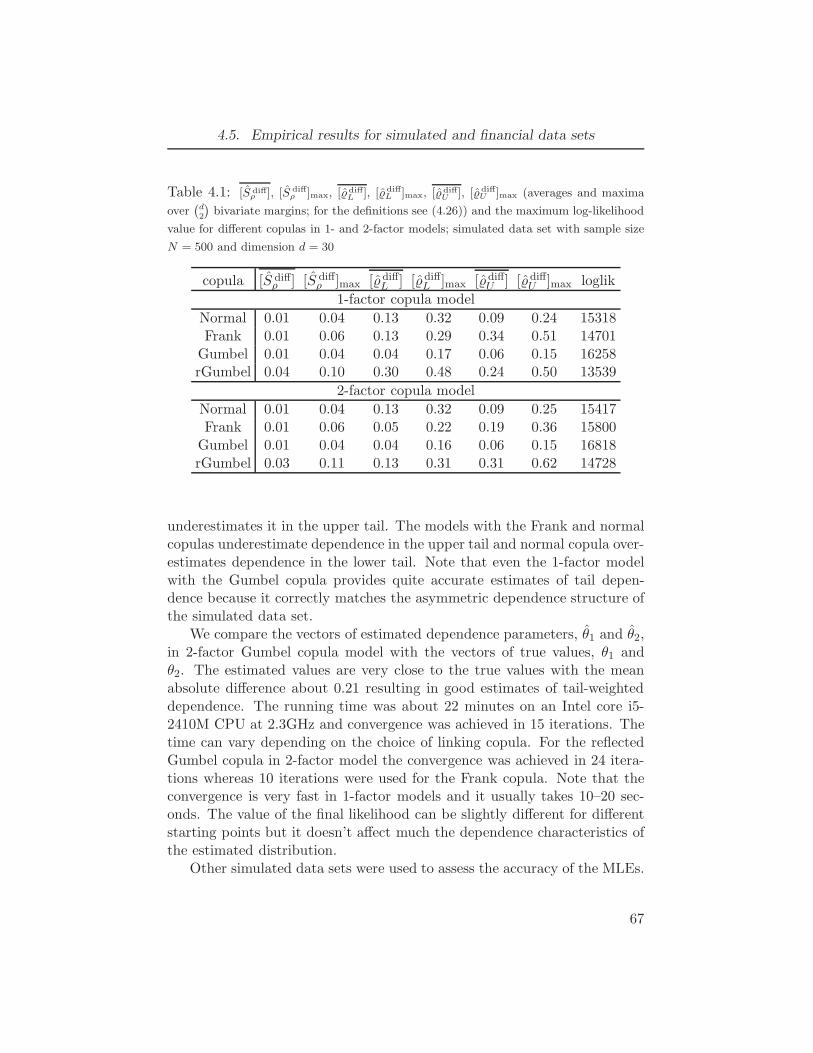
4.5. Empirical results for simulated and financial data sets
Table 4.1: [S diffρ ], [S diff
ρ ]max, [ ˆdiffL ], [ ˆdiff
L ]max, [ ˆdiffU ], [ ˆdiff
U ]max (averages and maxima
over(d2
)bivariate margins; for the definitions see (4.26)) and the maximum log-likelihood
value for different copulas in 1- and 2-factor models; simulated data set with sample size
N = 500 and dimension d = 30
copula [S diffρ ] [S diff
ρ ]max [ ˆdiffL ] [ ˆdiffL ]max [ ˆdiffU ] [ ˆdiffU ]max loglik
1-factor copula model
Normal 0.01 0.04 0.13 0.32 0.09 0.24 15318Frank 0.01 0.06 0.13 0.29 0.34 0.51 14701Gumbel 0.01 0.04 0.04 0.17 0.06 0.15 16258rGumbel 0.04 0.10 0.30 0.48 0.24 0.50 13539
2-factor copula model
Normal 0.01 0.04 0.13 0.32 0.09 0.25 15417Frank 0.01 0.06 0.05 0.22 0.19 0.36 15800Gumbel 0.01 0.04 0.04 0.16 0.06 0.15 16818rGumbel 0.03 0.11 0.13 0.31 0.31 0.62 14728
underestimates it in the upper tail. The models with the Frank and normalcopulas underestimate dependence in the upper tail and normal copula over-estimates dependence in the lower tail. Note that even the 1-factor modelwith the Gumbel copula provides quite accurate estimates of tail depen-dence because it correctly matches the asymmetric dependence structure ofthe simulated data set.
We compare the vectors of estimated dependence parameters, θ1 and θ2,in 2-factor Gumbel copula model with the vectors of true values, θ1 andθ2. The estimated values are very close to the true values with the meanabsolute difference about 0.21 resulting in good estimates of tail-weighteddependence. The running time was about 22 minutes on an Intel core i5-2410M CPU at 2.3GHz and convergence was achieved in 15 iterations. Thetime can vary depending on the choice of linking copula. For the reflectedGumbel copula in 2-factor model the convergence was achieved in 24 itera-tions whereas 10 iterations were used for the Frank copula. Note that theconvergence is very fast in 1-factor models and it usually takes 10–20 sec-onds. The value of the final likelihood can be slightly different for differentstarting points but it doesn’t affect much the dependence characteristics ofthe estimated distribution.
Other simulated data sets were used to assess the accuracy of the MLEs.
67
4.5. Empirical results for simulated and financial data sets
With larger sample size, such as n = 1000, usually fewer iterations arerequired for convergence and the running time doesn’t increase significantly.At the same time the accuracy of the estimates increases.
4.5.4 Financial return data
We have fitted the 1-factor and 2-factor copula models (as well as variousvine copula models) to different financial data sets including returns overseveral stocks in the same sector and European index returns. The resultswere similar (except factor copula models have bigger improvements overtruncated vine models for stock returns than for market index returns), sowe provide details for only one data set in this section.
Vine copula models
Vine copulas have quite flexible dependence and are good approximationsto many multivariate copulas, so they are a baseline to compare our factorcopula models. We briefly recall the concept of vine pair-copula construc-tion. Let U = (U1, ..., Ud) is a random vector with Ui ∼ U(0, 1) with thecdf C(u1, ..., ud). As in the case of factor models the idea of vine copulamodels is to express the joint cdf C(u1, ..., ud) in terms of simple bivariateconditional copulas. In a truncated vine copula model the conditional in-dependence at high levels is assumed to reduce the number of dependenceparameters; see Brechmann et al. (2012).
In particular, we consider two special cases of truncated vine copulamodels, C-vines and D-vines; see Aas et al. (2009) for details. In C-vinecopula model the dependence structure of the vector U is modeled usingconditional distributions of (Uj , Ul) given U1, ..., Ul−1, j = l + 1, ..., d, l =1, ..., d − 1. That is why d − l bivariate conditional copulas are required atlevel l and d(d − 1)/2 linking copulas are needed in total as in the case ofthe C-vine copula model. Usually, the conditional independence of Uj andUl is assumed at higher levels l to reduce the number of parameters in themodel.
The D-vine structure is another way to define the dependence structureof U using bivariate linking copulas. At level l, conditional distributions of(Uj , Uj+l) given Uj+1, ..., Uj+l−1 are used, j = 1, ..., d − l, l = 1, ..., d − 1.Therefore d−l bivariate conditional copulas are required at level l and henced(d− 1)/2 linking copulas are needed in total. Conditional independence ofUj and Uj+l at higher levels l is assumed to reduce the number of parametersin the model. Again, we consider three cases of D-vine truncated after the
68
4.5. Empirical results for simulated and financial data sets
first, second and third levels.
Copula-GARCH model for financial return data
The example shown this section are GARCH-filtered financial return dataconverted to uniform scores. We consider 8 US stocks in the IT sector: Apple(AAPL), Adobe Systems (ADBE), Cisco Systems (CSCO), Dell (DELL), In-tel (INTC), Motorola Solutions (MOT), Microsoft (MSFT), Novell (NOVL)in the year 2001. AR(1)-GARCH(1,1) model with symmetric Student tinnovations was used to fit univariate margins in each set.
Consider d financial assets and let the price of j-th asset at time t bePjt. The copula-GARCH model in Jondeau and Rockinger (2006) and manyother subsequent papers is the following. Let
rjt = µj + ρjrj,t−1 + σjtǫjt, σ2jt = ωj + αjr
2j,t−1 + βjσ
2j,t−1,
j = 1, . . . , d, t = 1, . . . , T,
where rjt = log(Pjt/Pj,t−1) and ǫt = (ǫ1t, . . . , ǫdt) are i.i.d. vectors withdistribution
F (z1, . . . , zd) = C(Fν1(z1), . . . , Fνd(zd);θ).
Fν denotes the cdf of Student t distribution, with ν degrees of freedom andstandardized to have variance 1, used to model innovations in the GARCHmodel.
Parameters µj, ρj , ωj , αj , βj , νj , j = 1, . . . , d were estimated at the firststep. Then different models (truncated vines and factor copula models)for the d-variate copula C(u1, . . . , ud;θ) were applied to the GARCH fil-tered data transformed to uniform scores to get estimates for the vectorof dependence parameters θ. The maximum likelihood at the second stepwas computed for 8 different copula models (1- and 2-factor copula models,D-vine and C-vine copula models truncated after 1, 2 and 3 levels), withvarious choices for the parametric bivariate linking copulas.
In each model, we use 5 different linking copula families: normal, Gum-bel, reflected Gumbel, Frank, BB1 copula to cover different types of depen-dence structure. The Gumbel (reflected Gumbel) copula is an example ofcopula with asymmetric dependence and upper (lower) tail dependence re-spectively. The Frank copula is reflection symmetric and has tail order of 2.The dependence in the tails is weaker than the normal copula in the case ofpositive dependence. Finally, the BB1 copula is reflection asymmetric withlower and upper tail dependence.
69
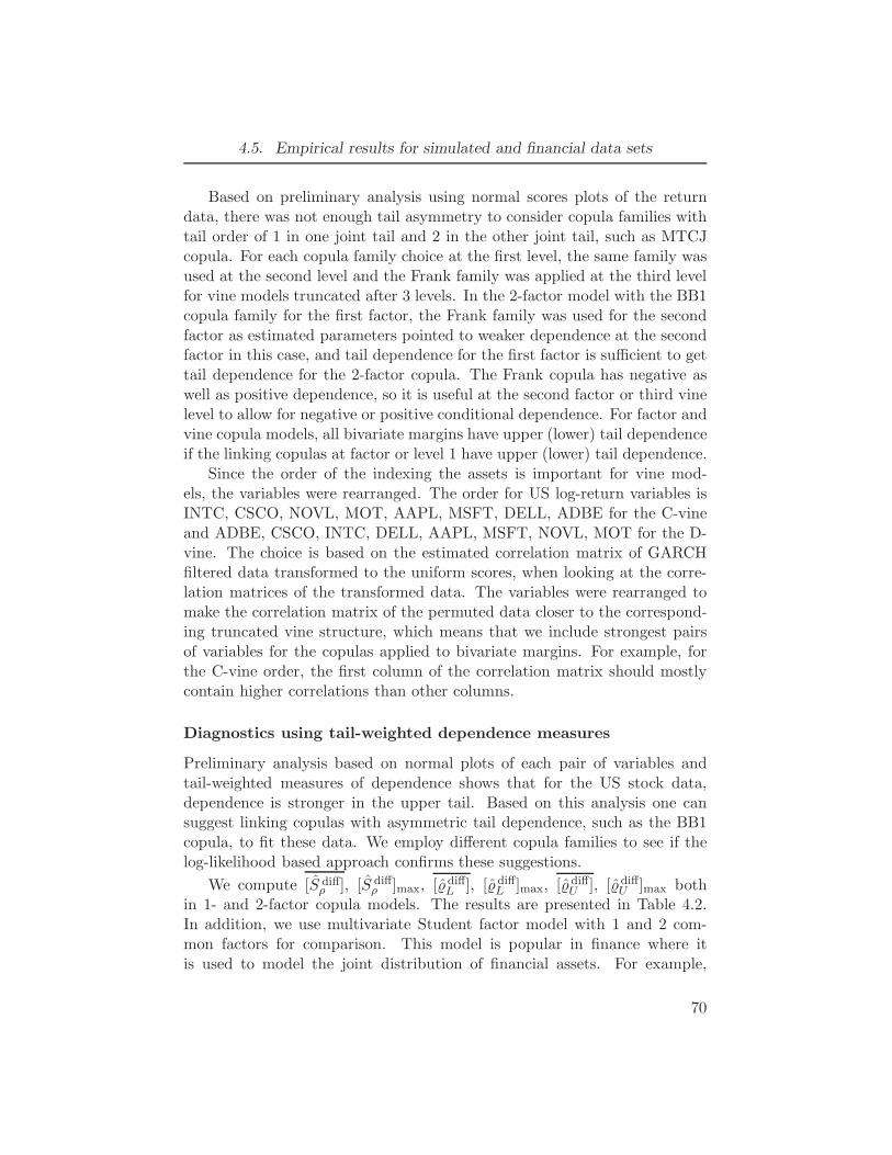
4.5. Empirical results for simulated and financial data sets
Based on preliminary analysis using normal scores plots of the returndata, there was not enough tail asymmetry to consider copula families withtail order of 1 in one joint tail and 2 in the other joint tail, such as MTCJcopula. For each copula family choice at the first level, the same family wasused at the second level and the Frank family was applied at the third levelfor vine models truncated after 3 levels. In the 2-factor model with the BB1copula family for the first factor, the Frank family was used for the secondfactor as estimated parameters pointed to weaker dependence at the secondfactor in this case, and tail dependence for the first factor is sufficient to gettail dependence for the 2-factor copula. The Frank copula has negative aswell as positive dependence, so it is useful at the second factor or third vinelevel to allow for negative or positive conditional dependence. For factor andvine copula models, all bivariate margins have upper (lower) tail dependenceif the linking copulas at factor or level 1 have upper (lower) tail dependence.
Since the order of the indexing the assets is important for vine mod-els, the variables were rearranged. The order for US log-return variables isINTC, CSCO, NOVL, MOT, AAPL, MSFT, DELL, ADBE for the C-vineand ADBE, CSCO, INTC, DELL, AAPL, MSFT, NOVL, MOT for the D-vine. The choice is based on the estimated correlation matrix of GARCHfiltered data transformed to the uniform scores, when looking at the corre-lation matrices of the transformed data. The variables were rearranged tomake the correlation matrix of the permuted data closer to the correspond-ing truncated vine structure, which means that we include strongest pairsof variables for the copulas applied to bivariate margins. For example, forthe C-vine order, the first column of the correlation matrix should mostlycontain higher correlations than other columns.
Diagnostics using tail-weighted dependence measures
Preliminary analysis based on normal plots of each pair of variables andtail-weighted measures of dependence shows that for the US stock data,dependence is stronger in the upper tail. Based on this analysis one cansuggest linking copulas with asymmetric tail dependence, such as the BB1copula, to fit these data. We employ different copula families to see if thelog-likelihood based approach confirms these suggestions.
We compute [S diffρ ], [S diff
ρ ]max, [ ˆdiffL ], [ ˆdiffL ]max, [ ˆdiffU ], [ ˆdiffU ]max bothin 1- and 2-factor copula models. The results are presented in Table 4.2.In addition, we use multivariate Student factor model with 1 and 2 com-mon factors for comparison. This model is popular in finance where itis used to model the joint distribution of financial assets. For example,
70
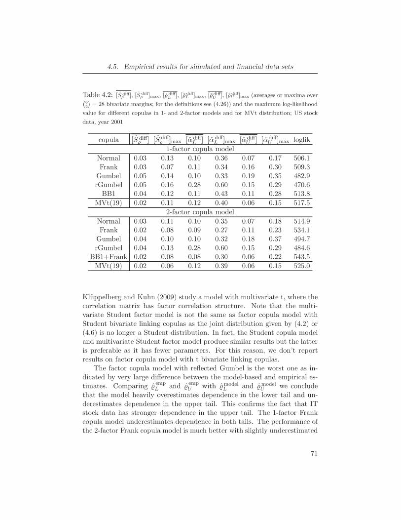
4.5. Empirical results for simulated and financial data sets
Table 4.2: [S diffρ ], [S diff
ρ ]max, [ ˆdiffL ], [ ˆdiff
L ]max, [ ˆdiffU ], [ ˆdiff
U ]max (averages or maxima over(82
)= 28 bivariate margins; for the definitions see (4.26)) and the maximum log-likelihood
value for different copulas in 1- and 2-factor models and for MVt distribution; US stock
data, year 2001
copula [S diffρ ] [S diff
ρ ]max [α diffL ] [α diff
L ]max [α diffU ] [α diff
U ]max loglik
1-factor copula model
Normal 0.03 0.13 0.10 0.36 0.07 0.17 506.1Frank 0.03 0.07 0.11 0.34 0.16 0.30 509.3Gumbel 0.05 0.14 0.10 0.33 0.19 0.35 482.9rGumbel 0.05 0.16 0.28 0.60 0.15 0.29 470.6BB1 0.04 0.12 0.11 0.43 0.11 0.28 513.8
MVt(19) 0.02 0.11 0.12 0.40 0.06 0.15 517.5
2-factor copula model
Normal 0.03 0.11 0.10 0.35 0.07 0.18 514.9Frank 0.02 0.08 0.09 0.27 0.11 0.23 534.1Gumbel 0.04 0.10 0.10 0.32 0.18 0.37 494.7rGumbel 0.04 0.13 0.28 0.60 0.15 0.29 484.6
BB1+Frank 0.02 0.08 0.08 0.30 0.06 0.22 543.5
MVt(19) 0.02 0.06 0.12 0.39 0.06 0.15 525.0
Kluppelberg and Kuhn (2009) study a model with multivariate t, where thecorrelation matrix has factor correlation structure. Note that the multi-variate Student factor model is not the same as factor copula model withStudent bivariate linking copulas as the joint distribution given by (4.2) or(4.6) is no longer a Student distribution. In fact, the Student copula modeland multivariate Student factor model produce similar results but the latteris preferable as it has fewer parameters. For this reason, we don’t reportresults on factor copula model with t bivariate linking copulas.
The factor copula model with reflected Gumbel is the worst one as in-dicated by very large difference between the model-based and empirical es-timates. Comparing ˆemp
L and ˆempU with ˆmodel
L and ˆmodelU we conclude
that the model heavily overestimates dependence in the lower tail and un-derestimates dependence in the upper tail. This confirms the fact that ITstock data has stronger dependence in the upper tail. The 1-factor Frankcopula model underestimates dependence in both tails. The performance ofthe 2-factor Frank copula model is much better with slightly underestimated
71
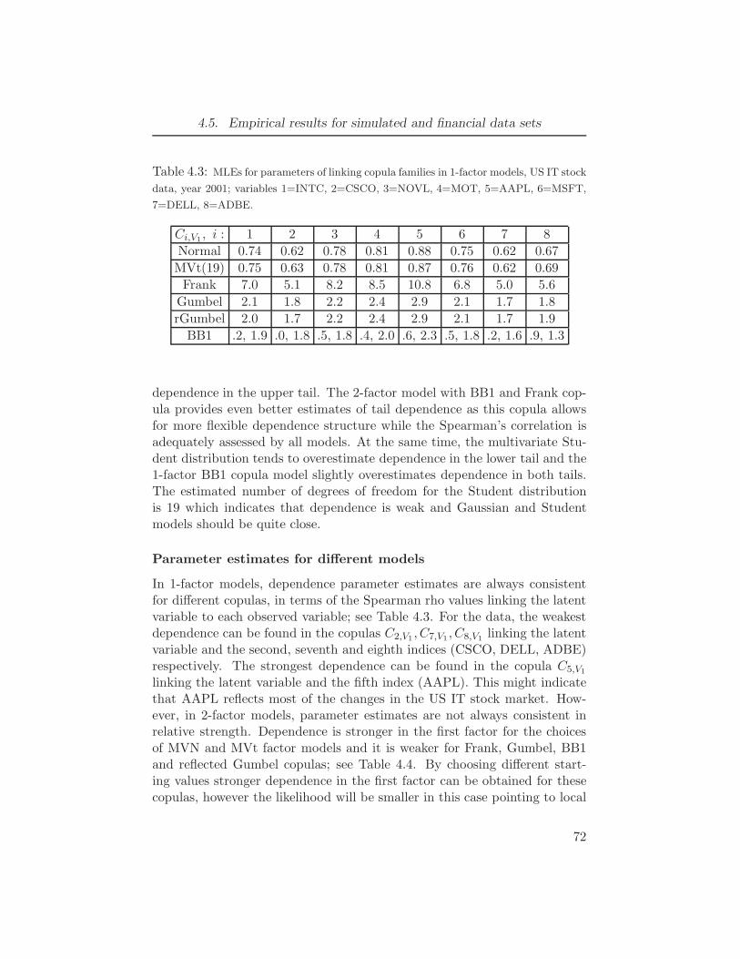
4.5. Empirical results for simulated and financial data sets
Table 4.3: MLEs for parameters of linking copula families in 1-factor models, US IT stock
data, year 2001; variables 1=INTC, 2=CSCO, 3=NOVL, 4=MOT, 5=AAPL, 6=MSFT,
7=DELL, 8=ADBE.
Ci,V1 , i : 1 2 3 4 5 6 7 8
Normal 0.74 0.62 0.78 0.81 0.88 0.75 0.62 0.67
MVt(19) 0.75 0.63 0.78 0.81 0.87 0.76 0.62 0.69
Frank 7.0 5.1 8.2 8.5 10.8 6.8 5.0 5.6
Gumbel 2.1 1.8 2.2 2.4 2.9 2.1 1.7 1.8
rGumbel 2.0 1.7 2.2 2.4 2.9 2.1 1.7 1.9
BB1 .2, 1.9 .0, 1.8 .5, 1.8 .4, 2.0 .6, 2.3 .5, 1.8 .2, 1.6 .9, 1.3
dependence in the upper tail. The 2-factor model with BB1 and Frank cop-ula provides even better estimates of tail dependence as this copula allowsfor more flexible dependence structure while the Spearman’s correlation isadequately assessed by all models. At the same time, the multivariate Stu-dent distribution tends to overestimate dependence in the lower tail and the1-factor BB1 copula model slightly overestimates dependence in both tails.The estimated number of degrees of freedom for the Student distributionis 19 which indicates that dependence is weak and Gaussian and Studentmodels should be quite close.
Parameter estimates for different models
In 1-factor models, dependence parameter estimates are always consistentfor different copulas, in terms of the Spearman rho values linking the latentvariable to each observed variable; see Table 4.3. For the data, the weakestdependence can be found in the copulas C2,V1 , C7,V1 , C8,V1 linking the latentvariable and the second, seventh and eighth indices (CSCO, DELL, ADBE)respectively. The strongest dependence can be found in the copula C5,V1
linking the latent variable and the fifth index (AAPL). This might indicatethat AAPL reflects most of the changes in the US IT stock market. How-ever, in 2-factor models, parameter estimates are not always consistent inrelative strength. Dependence is stronger in the first factor for the choicesof MVN and MVt factor models and it is weaker for Frank, Gumbel, BB1and reflected Gumbel copulas; see Table 4.4. By choosing different start-ing values stronger dependence in the first factor can be obtained for thesecopulas, however the likelihood will be smaller in this case pointing to local
72
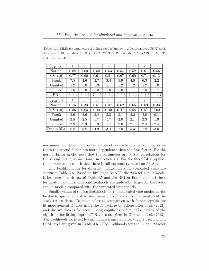
4.5. Empirical results for simulated and financial data sets
Table 4.4: MLEs for parameters of linking copula families in 2-factor models, US IT stock
data, year 2001; variables 1=INTC, 2=CSCO, 3=NOVL, 4=MOT, 5=AAPL, 6=MSFT,
7=DELL, 8=ADBE.
Ci,V1 , i : 1 2 3 4 5 6 7 8
Normal 0.68 1.00 0.50 0.53 0.54 0.52 0.61 0.56
MVt(19) 0.77 0.60 0.61 0.51 0.67 0.60 0.71 0.13
Frank 7.5 4.6 3.7 3.4 5.9 4.0 6.3 2.2
Gumbel 1.2 1.0 1.3 1.1 1.2 1.2 1.2 1.0
rGumbel 1.0 1.0 1.0 1.0 1.0 1.1 1.0 1.7
BB1 .3, 1.4 .6, 1.3 .7, 1.0 .0, 1.4 .0, 1.3 .2, 1.4 .0, 1.3 .0, 1.7
Ci,V2|V1 , i : 1 2 3 4 5 6 7 8
Normal 0.75 0.33 0.51 0.37 0.62 0.66 0.69 0.33
MVt(19) 0.66 0.63 0.40 0.40 0.47 0.58 0.57 1.00
Frank 5.6 5.6 3.4 3.3 3.1 5.2 4.0 6.1
Gumbel 2.8 2.5 1.7 1.7 2.0 2.1 2.3 1.9
rGumbel 2.9 2.3 1.9 1.7 2.0 2.1 2.4 2.4
Frank/BB1 8.8 5.8 4.9 3.4 7.0 5.3 7.8 3.0
maximum. So depending on the choice of bivariate linking copulas, some-times the second factor has more dependence than the first factor. For thenormal factor model, note that the parameters are partial correlations forthe second factor, as mentioned in Section 4.1. For the fitted BB1 copulas,the parameters are such that there is tail asymmetry based on λL, λU .
The log-likelihoods for different models including truncated vines areshown in Table 4.5. Based on likelihood or AIC, the 2-factor copula modelis best one in each row of Table 4.5 and the BB1 or Frank copula is bestfor most of columns. The log-likelihoods are quite a bit larger for the factorcopula models compared with the truncated vine models.
Smaller values of the log-likelihoods for the truncated vine models mightbe due to special vine structure (namely, D-vine and C-vine) used to fit thestock return data. To make a better comparison with factor copulas, wefit more general R-vines using the R package by Schepsmeier et al. (2012),and the six choices for each linking copula as before. The details of thealgorithm for fitting “optimal” R-vines are given in Dißmann et al. (2013).The likelihoods for fitted R-vine models truncated after the first, second andthird level are given in Table 4.6. The likelihoods for the 1- and 2-factor
73
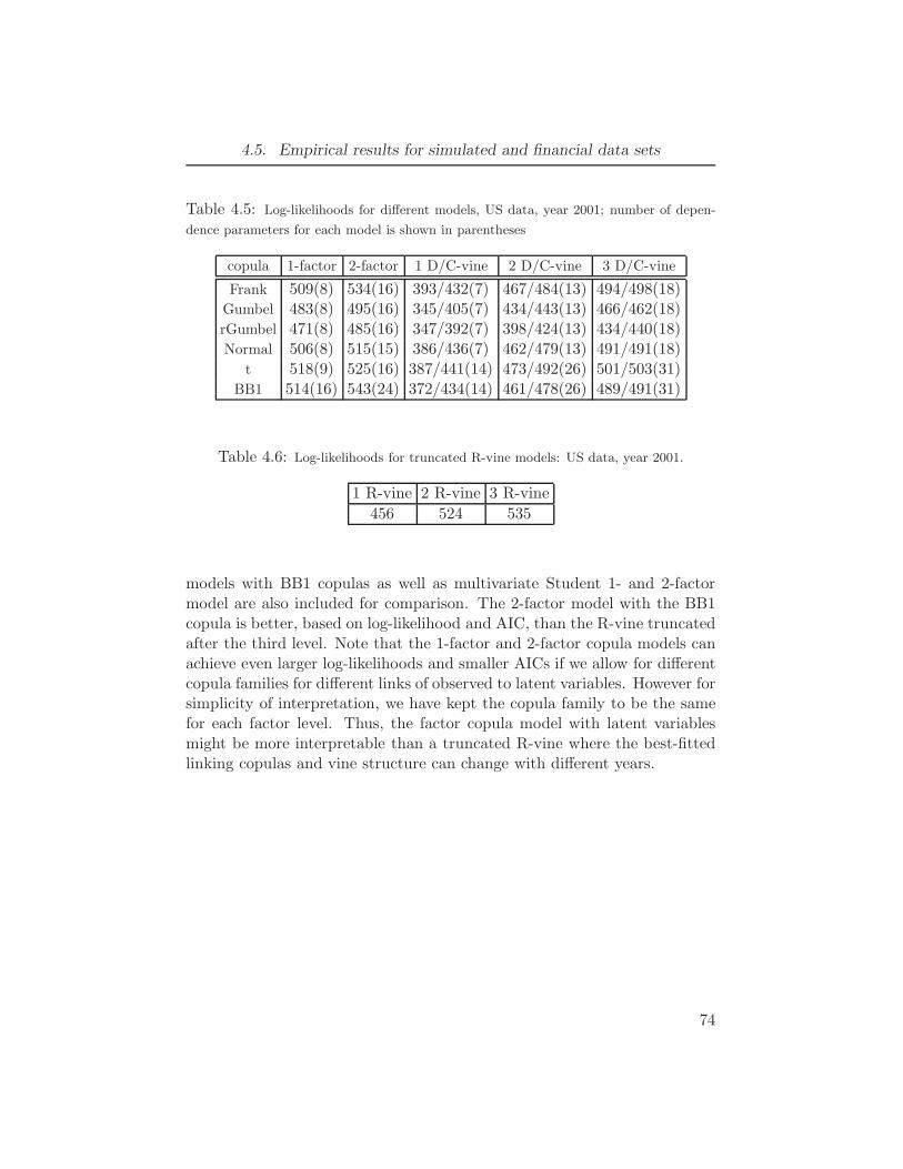
4.5. Empirical results for simulated and financial data sets
Table 4.5: Log-likelihoods for different models, US data, year 2001; number of depen-
dence parameters for each model is shown in parentheses
copula 1-factor 2-factor 1 D/C-vine 2 D/C-vine 3 D/C-vine
Frank 509(8) 534(16) 393/432(7) 467/484(13) 494/498(18)Gumbel 483(8) 495(16) 345/405(7) 434/443(13) 466/462(18)rGumbel 471(8) 485(16) 347/392(7) 398/424(13) 434/440(18)Normal 506(8) 515(15) 386/436(7) 462/479(13) 491/491(18)
t 518(9) 525(16) 387/441(14) 473/492(26) 501/503(31)BB1 514(16) 543(24) 372/434(14) 461/478(26) 489/491(31)
Table 4.6: Log-likelihoods for truncated R-vine models: US data, year 2001.
1 R-vine 2 R-vine 3 R-vine
456 524 535
models with BB1 copulas as well as multivariate Student 1- and 2-factormodel are also included for comparison. The 2-factor model with the BB1copula is better, based on log-likelihood and AIC, than the R-vine truncatedafter the third level. Note that the 1-factor and 2-factor copula models canachieve even larger log-likelihoods and smaller AICs if we allow for differentcopula families for different links of observed to latent variables. However forsimplicity of interpretation, we have kept the copula family to be the samefor each factor level. Thus, the factor copula model with latent variablesmight be more interpretable than a truncated R-vine where the best-fittedlinking copulas and vine structure can change with different years.
74
Chapter 5
Structured factor copula
models
The common factor copula models introduced in the previous chapter im-plicitly require a homogeneous dependence structure with the assumption ofconditional independence given several common factors. In data sets with alarge number of variables, data can come from different sources or be clus-tered in different groups, for example stock returns from different sectorsor item response data in psychometrics; thus dependence within each groupand among different groups can be different.
In psychometrics, sometimes a bi-factor correlation structure is usedwhen variables or items can be split into non-overlapping groups; see forexample Gibbons and Hedeker (1992) and Holzinger and Swineford (1937).In a Gaussian bi-factor model, there is one common Gaussian factor whichdefines dependence between different groups, and one or several independentgroup-specific Gaussian factors which define dependence within each group.An alternative way to model dependence for grouped data is a nested modelwhere the dependence in groups is modeled via dependent group-specific fac-tors and the observed variables are assumed to be conditionally independentgiven these group-specific factors. The nested model is similar to Gaussianmodels with multilevel covariance structure; see Muthen (1994). Despitethe simplicity, these two models have the same drawbacks as a commonGaussian factor model — they do not account for tail asymmetry and taildependence.
In this chapter, we propose copula extensions for bi-factor and nestedGaussian models. The extensions are called structured factor copula mod-
els. The proposed models contain 1- and 2-factor copula models as specialcases, while allowing flexible dependence structure both for within groupand between group dependence. As a result, the models can be suitable formodeling high-dimensional data sets consisting of several groups of variableswith homogeneous dependence in each group.
The proposed multivariate copula models are built from a sequence of bi-variate copulas in a similar way to vine copulas (Kurowicka and Joe (2011)).
75
Chapter 5. Structured factor copula models
Let FX be the multivariate cumulative distribution function (cdf) of a ran-dom d-dimensional vector X = (X1, . . . ,Xd), and let FXj be the cdf of Xj
for j = 1, . . . , d. The copula CX, corresponding to FX, is a multivariate uni-form cdf such that FX(x1, . . . , xd) = CX(FX1(x1), . . . , FXd
(xd)). By Sklar(1959), CX is unique if FX is continuous. Copula functions allow for differenttypes of dependence structure and are popular for modeling non-Gaussiandependence, including stock returns, insurance and hydrology data; see forexample see Patton (2006), McNeil et al. (2005), Salvadori et al. (2007) andothers.
The proposed structured copula models are special cases of truncated-vine copula models with latent variables. In a vine model, bivariate linkingcopulas and conditional cdfs are used to sequentially construct multivari-ate distribution. The resulting vine model or pair-copula construction al-lows great flexibility in modeling different types of dependence structureby choosing appropriate linking copulas; see Kurowicka and Joe (2011) andBrechmann and Czado (2013) for more details. We show that dependingon the choice of bivariate copulas in the structured copula models, differ-ent types of strength of dependence in the tails can be modeled, similar tocommon factor copula models.
All of the details in this chapter are for continuous response variables,but the structured copula models can also be developed for discrete ordinalvariables or mixed discrete/continuous variables. Factor copula models foritem response are studied in Nikoloulopoulos and Joe (2014), and if theitems can be classified into non-overlapping groups, then the bi-factor ornested factor copula models are candidates when there is tail asymmetry ortail dependence.
In Section 5.1 we define bi-factor and nested copula models including aspecial case of Gaussian copulas, and compare the properties of these modelswith those of 1- and 2-factor copula models in Section 5.2. Section 5.3 hasdetails on numerical maximum likelihood with a modified Newton-Raphsonalgorithm. Section 5.4 has a resampling method to obtain model-based inter-val estimates of the portfolio risk measures of Value-at-Risk and conditionaltail expectation. In Section 5.5, we apply different copula-GARCH models toa financial data set and compare estimates of the Value-at-Risk, conditionaltail expectations as well as some other tail-based quantities. The resultsshow that structured factor copula models can parsimoniously estimate thedependence structure of the data. Value-at-Risk and other risk measuresthat are widely used in financial applications cannot efficiently differentiatemodels with different tail properties, but tail-weighted dependence measuresare a better match to the fit of copula models based on Akaike information
76
5.1. Two extensions of factor copula models for data clustered in groups
criterion.
5.1 Two extensions of factor copula models for
data clustered in groups
Common factor models assume that d observed variables are conditionallyindependent given 1 ≤ p≪ d latent variables that affect each observed vari-ables; for identifiability, the latent variables are assumed to be independentor orthogonal. Structured factor models assume that there is structure tothe observed variables and each latent variable is linked to a subset of theobserved variables. For Gaussian structured factor models, this correspondsto many structured zeros in the matrix of loadings; in this case, with fewerparameters in the loading matrix compared with the common factor model,and the p latent variables could be dependent, as in the oblique factor modelof Harris and Kaiser (1964) and McDonald (1985). With a large d, struc-tured Gaussian factor models are also parsimonious models to parameterizethe correlation matrix in O(d) parameters (instead of d(d − 1)/2 param-eters). The main goal of this section is to present the copula version oftwo Gaussian structured factor models; for the extension, the parameters ofthe Gaussian structured factor models are converted to a set of correlationsand partial correlations that are algebraically independent and that have atruncated vine structure, and then the correlations and partial correlationsare replaced by bivariate copulas. Similar copula extensions exist for otherstructured factor models.
A specific case of structured factor models occurs when variables canbe divided into non-overlapping groups. Assume that we have G groupsof variables and there are dg variables in the g-th group, g = 1, . . . , G. LetUij ∼ U(0, 1), i = 1, . . . , dg and suppose variables U1g, . . . , Udgg belong to theg-th group. Denote the joint cdf of U = (U11, . . . , Ud11, · · · , U1G, . . . , UdGG)
by CU . Let d =∑G
g=1 dg be the total number of variables.We consider two classes of structured factor copula models. The first
model is an extension of the bi-factor model and we call it the bi-factorcopula model. The second model is an extension of the oblique factor modelwith a blocked loading matrix where the dependent latent variables satisfya 1-factor structure.
77
5.1. Two extensions of factor copula models for data clustered in groups
5.1.1 Bi-factor copula model
Consider a model with one common (global) factor and G group-specificfactors, such that the G + 1 factors or latent variables are mutually inde-pendent. Assume that within the g-th group, U1g, . . . , Udgg are condition-ally independent given V0 and Vg, where V0, V1, . . . , VG are independent andidentically distributed (i.i.d.) U(0, 1) random variables. We also assumethat Uig in group g does not depend on Vg′ for g′ 6= g. Let CUig,V0 bethe copula cdf of (Uig, V0) and let CUig|V0 be one of its conditional distribu-tions. Let CUig,Vg;V0 be the copula for the conditional univariate distributionsCUig|V0(·|v0) and CVg|V0(·|v0); with V0, V1, . . . , Vg being independent, CVg |V0is the U(0, 1) cdf. By Sklar’s theorem, in general, the copula CUig,Vg;V0 de-pends on v0. However, like in factor copula models and in the vine copulaliterature (Kurowicka and Joe (2011)), we make the simplifying (modeling)assumption that CUig,Vg;V0 does not depend on v0. This is not a strong as-sumption as we are dealing with latent variables, and in a special case ofthe Gaussian model, copulas for conditional distributions do not depend onthe values of the conditioning variables. For further notation, let CUig|Vg;V0be one of the conditional distributions of CUig,Vg;V0 .
The bivariate copulas CUig,V0 (for common factor) and CUig,Vg;V0 (forgroup specific factor) are assumed to be absolutely continuous with respec-tive copula densities cUig,V0 and cUig,Vg;V0 .
With a vector u = (u11, . . . , ud11, · · · , u1G, . . . , udG G), due to the aboveconditional independence assumptions, we get:
Pr(Uig ≤ uig, i = 1, . . . , dg, g = 1, . . . G) =
=
∫
[0,1]G+1
G∏
g=1
dg∏
i=1
Pr(Uig ≤ uig|V0 = v0, Vg = vg) dv1 · · · dvGdv0
and
Pr(Uig ≤ uig|V0 = v0, Vg = vg) =∂
∂vgPr(Uig ≤ uig, Vg ≤ vg|V0 = v0)
=∂
∂vgCUig,Vg;V0(CUig |V0(uig|v0), vg) =: CUig|Vg;V0(CUig |V0(uig|v0)|vg).
78
5.1. Two extensions of factor copula models for data clustered in groups
Hence
CU (u) =
∫ 1
0
∫
[0,1]G
G∏
g=1
dg∏
i=1
CUig|Vg;V0(CUig |V0(uig|v0)|vg) dv1 . . . dvG dv0
=
∫ 1
0
G∏
g=1
∫ 1
0
dg∏
i=1
CUig|Vg;V0(CUig |V0(uig|v0)|vg)
dvg
dv0;
(5.1)
cU (u) =
∫ 1
0
G∏
g=1
{dg∏
i=1
cUig ,V0(uig, v0)
×
×∫ 1
0
dg∏
i=1
cUig ,Vg;V0(CUig |V0(uig|v0), vg)
dvg
}dv0. (5.2)
It is seen that the joint density is represented as a one-dimensional inte-gral of a function which in turn is a product of G one-dimensional integrals.As a result, (G+1)-dimensional numerical integration can be avoided. Themodel has d = d1 + . . .+ dG bivariate linking copulas both for the first andsecond factors, or 2d linking copulas in total. The marginal distribution of(5.2) for a single group g of variables is a 2-factor copula model.
For the parametric version of this model, there is a parameter θi,g forCUig,V0 and a parameter γi,g for CUig|Vg;V0 ; θi,g and γi,g could be vectors. Theparameter vector for the (5.2) is θ = (θi,g, γi,g : i = 1, . . . , dg, g = 1, . . . , G).
The bi-factor copula model can be further extended to a tri-factor cop-ula model with three factors. In this model, the g-th group has mg ≥ 1subgroups and in addition to the common factor V0 and the group factorVg there are mg i.i.d. U(0, 1) subgroup factors that are independent of V0,V1, ..., VG. It follows that in the g-th group dependence is modeled usinga bi-factor copula model. The tri-factor model can be used when data areclustered in groups and each group, in turn, can be subdivided into smallersubgroups. This allows greater flexibility of the model, however estimationprocedure becomes computationally demanding so that we only provide de-tails for a special case when all copulas are Gaussian when the joint pdf isavailable in a closed form and parameters in the model can be estimatedrelatively fast; see section 5.1.3.
79
5.1. Two extensions of factor copula models for data clustered in groups
5.1.2 Nested copula model
Consider the case of d dependent factors without a common factor. Assumethat for a fixed g = 1, . . . , G, U1g, . . . , Udgg are conditionally independentgiven Vg ∼ U(0, 1), and the joint cdf of V = (V1, . . . , VG) is given by thecopula CV . We also assume that Uig in group g does not depend on Vg′
for g′ 6= g. That is, we have G groups of variables and G latent factorswhere the g-th latent factor defines dependence structure in the g-th group.Let CUig,Vg be the copula cdf of (Uig, Vg) and CUig|Vg be the correspondingconditional distribution.
With a vector u = (u11, . . . , ud11, · · · , u1G, . . . , udG G) we get:
CU (u) =
∫
[0,1]G
G∏
g=1
dg∏
i=1
CUig|Vg(uig|vg)
cV (v1, . . . , vG) dv1 . . . dvG (5.3)
where CUig,Vg is the copula linking Uig and Vg. This is a copula version of theoblique Gaussian factor model where each observed variable loads exactlyone latent variable.
We additionally assume that V1, . . . , VG are conditionally independentgiven another latent variable V0, that is the joint distribution of V hasone-factor copula structure. Then we get:
cV (v1, . . . , vG) =
∫ 1
0
G∏
g=1
cVg,V0(vg, v0)
dv0
where CVg,V0 is the copula linking Vg and V0. It implies that
CU (u) =
∫ 1
0
∫
[0,1]G
G∏
g=1
dg∏
i=1
CUig|Vg(uig|vg)
G∏
g=1
cVg,V0(vg, v0)
×
× dv1 . . . dvG dv0
=
∫ 1
0
G∏
g=1
∫ 1
0
cVg ,V0(vg, v0)
dg∏
i=1
CUig|Vg(uig|vg)
dvg
dv0;
cU (u) =
∫ 1
0
G∏
g=1
∫ 1
0
cVg ,V0(vg, v0)
dg∏
i=1
cUig ,Vg(uig, vg)
dvg
dv0.(5.4)
The total number of bivariate linking copulas in the model (5.4) is d1+ . . .+dG + G = d + G (d copulas CUig,Vg and G copulas CVg,V0). The marginal
80
5.1. Two extensions of factor copula models for data clustered in groups
distribution of (5.4) for a single group g of variables is a 1-factor copulamodel.
In this setting, there exist a common factor V0, say the current state ofeconomy, which drives some other factors V1, . . . , VG, say some unobservableparameters reflecting the situation in different stock sectors. Each factor, inturn, defines a dependence structure of a group of variables (such as stocks ina common sector). Besides a good economic interpretation, the model (5.4)can be used in likelihood computations with a multidimensional numericalintegration, similar to the likelihood for a bi-factor copula model.
For the parametric version of this model, there is a parameter θg forCVg ,V0 and a parameter γi,g for CUig,Vg . The parameter vector for (5.4) isθ = (θg, ηi,g : i = 1, . . . , dg, g = 1, . . . , G).
Similar to a bi-factor model, the nested copula model can be furtherextended to a nested copula model with a subgroup structure. In additionto G groups and G group factors V1, ..., VG that are independent given V0,one can assume that there are mg ≥ 1 subgroups in the g-th group and,correspondingly, mg subgroup latent factors that are independent given Vg.Variables inside themg-th group are conditionally independent given themg-th group factor. This is a more flexible model and it has d+m1+...+mG+Gbivariate linking copulas. If the number of subgroups is large, fast estimationof parameters in the model is not possible as in a tri-factor model. Otherwise,the nested model with a subgroup structure should be preferred since the tri-factor copula model has 3d linking copulas and hence much more parametersto estimate. In this dissertation we consider a special case of the nestedmodel with a subgroup structure with all Gaussian linking copulas whenthe joint pdf is available in a closed form and correlation parameters in themodel can be estimated fast; see section 5.1.3.
5.1.3 Special case of Gaussian copulas
In this section, we consider a subset of the Gaussian bi-factor model toshow that if all the bivariate linking copulas for Gaussian, then the nestedfactor model is a special case of the bi-factor model. We also consider amore general tri-factor model with one common factor, G group factors andm1 + ...+mG subgroup factors. Similar to a bi-factor model, nested modelwith a subgroup structure is a special case of a tri-factor model as we showbelow.
Bi-factor model
Let Φ, φ be the standard normal cdf and density respectively. Suppose
81
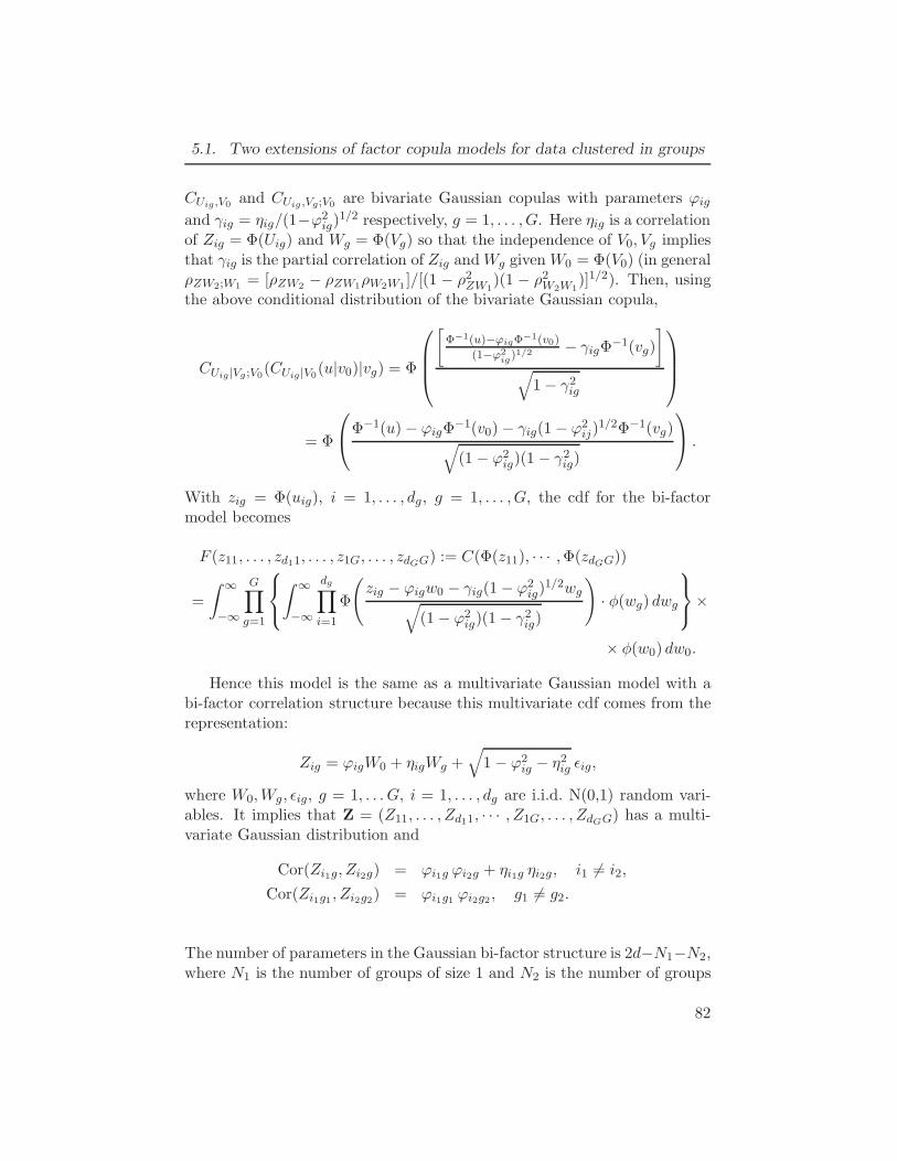
5.1. Two extensions of factor copula models for data clustered in groups
CUig,V0 and CUig ,Vg;V0 are bivariate Gaussian copulas with parameters ϕigand γig = ηig/(1−ϕ2
ig)1/2 respectively, g = 1, . . . , G. Here ηig is a correlation
of Zig = Φ(Uig) and Wg = Φ(Vg) so that the independence of V0, Vg impliesthat γig is the partial correlation of Zig andWg givenW0 = Φ(V0) (in generalρZW2;W1 = [ρZW2 − ρZW1ρW2W1 ]/[(1 − ρ2ZW1
)(1 − ρ2W2W1)]1/2). Then, using
the above conditional distribution of the bivariate Gaussian copula,
CUig|Vg;V0(CUig|V0(u|v0)|vg) = Φ
[Φ−1(u)−ϕigΦ
−1(v0)
(1−ϕ2ig)
1/2 − γigΦ−1(vg)
]
√1− γ2ig
= Φ
Φ−1(u)− ϕigΦ
−1(v0)− γig(1− ϕ2ij)
1/2Φ−1(vg)√(1− ϕ2
ig)(1− γ2ig)
.
With zig = Φ(uig), i = 1, . . . , dg, g = 1, . . . , G, the cdf for the bi-factormodel becomes
F (z11, . . . , zd11, . . . , z1G, . . . , zdGG) := C(Φ(z11), · · · ,Φ(zdGG))
=
∫ ∞
−∞
G∏
g=1
∫ ∞
−∞
dg∏
i=1
Φ
(zig − ϕigw0 − γig(1− ϕ2
ig)1/2wg√
(1− ϕ2ig)(1− γ2ig)
)· φ(wg) dwg
×
× φ(w0) dw0.
Hence this model is the same as a multivariate Gaussian model with abi-factor correlation structure because this multivariate cdf comes from therepresentation:
Zig = ϕigW0 + ηigWg +√
1− ϕ2ig − η2ig ǫig,
where W0,Wg, ǫig, g = 1, . . . G, i = 1, . . . , dg are i.i.d. N(0,1) random vari-ables. It implies that Z = (Z11, . . . , Zd11, · · · , Z1G, . . . , ZdGG) has a multi-variate Gaussian distribution and
Cor(Zi1g, Zi2g) = ϕi1g ϕi2g + ηi1g ηi2g, i1 6= i2,
Cor(Zi1g1 , Zi2g2) = ϕi1g1 ϕi2g2 , g1 6= g2.
The number of parameters in the Gaussian bi-factor structure is 2d−N1−N2,where N1 is the number of groups of size 1 and N2 is the number of groups
82
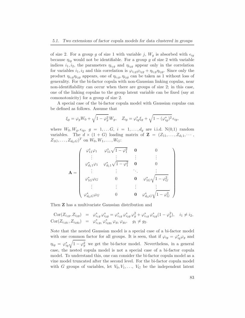
5.1. Two extensions of factor copula models for data clustered in groups
of size 2. For a group g of size 1 with variable j, Wg is absorbed with ǫigbecause ηig would not be identifiable. For a group g of size 2 with variableindices i1, i2, the parameters ηi1g and ηi2g appear only in the correlationfor variables i1, i2 and this correlation is ϕi1gϕi2g + ηi1gηi2g. Since only theproduct ηi1gηi2g appears, one of ηi1g, ηi2g can be taken as 1 without loss ofgenerality. For the bi-factor copula with non-Gaussian linking copulas, nearnon-identifiability can occur when there are groups of size 2; in this case,one of the linking copulas to the group latent variable can be fixed (say atcomonotonicity) for a group of size 2.
A special case of the bi-factor copula model with Gaussian copulas canbe defined as follows. Assume that
ξg = ϕgW0 +√
1− ϕ2gWg, Zig = ϕ∗
igξg +√
1− (ϕ∗ig)
2 ǫig,
where W0,Wg, ǫig, g = 1, . . . G, i = 1, . . . , dg are i.i.d. N(0,1) randomvariables. The d × (1 + G) loading matrix of Z = (Z11, . . . , Zd11, · · · ,Z1G, . . . , ZdGG)
T on W0,W1, . . . ,WG:
A =
ϕ∗11ϕ1 ϕ∗
11
√1− ϕ2
1 0 0...
......
...
ϕ∗d11ϕ1 ϕ∗
d11
√1− ϕ2
1 0 0...
.... . .
...
ϕ∗1GϕG 0 0 ϕ∗
1G
√1− ϕ2
G
......
......
ϕ∗dGG
ϕG 0 0 ϕ∗dGG
√1− ϕ2
G
Then Z has a multivariate Gaussian distribution and
Cor(Zi1g, Zi2g) = ϕ∗i1g ϕ
∗i2g = ϕ∗
i1g ϕ∗i2g ϕ
2g + ϕ∗
i1g ϕ∗i2g(1− ϕ2
g), i1 6= i2,
Cor(Zi1g1 , Zi2g2) = ϕ∗i1g1 ϕ
∗i2g2 ϕg1 ϕg2 , g1 6= g2.
Note that the nested Gaussian model is a special case of a bi-factor modelwith one common factor for all groups. It is seen, that if ϕig = ϕ∗
igϕg and
ηig = ϕ∗ig
√1− ϕ2
g we get the bi-factor model. Nevertheless, in a general
case, the nested copula model is not a special case of a bi-factor copulamodel. To understand this, one can consider the bi-factor copula model as avine model truncated after the second level. For the bi-factor copula modelwith G groups of variables, let V0, V1, . . ., VG be the independent latent
83
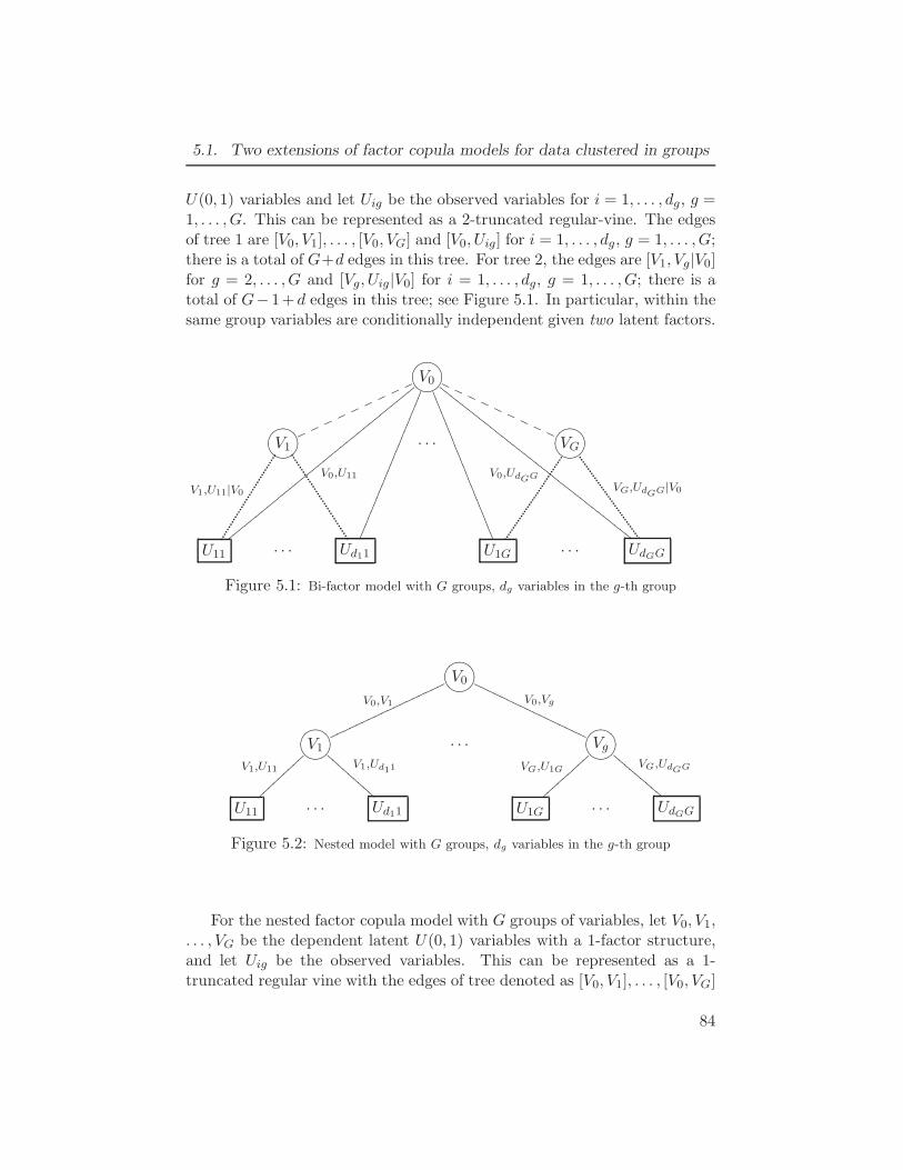
5.1. Two extensions of factor copula models for data clustered in groups
U(0, 1) variables and let Uig be the observed variables for i = 1, . . . , dg, g =1, . . . , G. This can be represented as a 2-truncated regular-vine. The edgesof tree 1 are [V0, V1], . . . , [V0, VG] and [V0, Uig] for i = 1, . . . , dg, g = 1, . . . , G;there is a total of G+d edges in this tree. For tree 2, the edges are [V1, Vg|V0]for g = 2, . . . , G and [Vg, Uig|V0] for i = 1, . . . , dg, g = 1, . . . , G; there is atotal of G− 1+ d edges in this tree; see Figure 5.1. In particular, within thesame group variables are conditionally independent given two latent factors.
GFED@ABCV0
♥ ♥ ♥ ♥ ♥ ♥ ♥ ♥ ♥
V0,U11
②②②②②②②②②②②②②②②②②②②②②②②②②②②②②②②②②
✒✒✒✒✒✒✒✒✒✒✒✒✒✒✒✒✒✒✒✒✒✒
PPPPPPPPP
✱✱✱✱✱✱✱✱✱✱✱✱✱✱✱✱✱✱✱✱✱✱
V0,UdGG
❋❋❋❋
❋❋❋❋
❋❋❋❋
❋❋❋❋
❋❋❋❋
❋❋❋❋
❋❋❋❋
❋❋❋❋
❋❋
GFED@ABCV1
V1,U11|V0
· · · GFED@ABCVG
VG,UdGG|V0
U11 · · · Ud11 U1G · · · UdGG
Figure 5.1: Bi-factor model with G groups, dg variables in the g-th group
GFED@ABCV0
V0,V1
♥♥♥♥♥♥
♥♥♥♥♥♥
♥♥♥♥♥♥
V0,Vg
PPPPPP
PPPPPP
PPPPP
GFED@ABCV1V1,U11
⑥⑥⑥⑥⑥⑥⑥⑥⑥
V1,Ud11
❇❇❇❇
❇❇❇❇
❇ · · · GFED@ABCVgVG,U1G
⑤⑤⑤⑤⑤⑤⑤⑤⑤
VG,UdGG
❉❉❉❉
❉❉❉❉
❉
U11 · · · Ud11 U1G · · · UdGG
Figure 5.2: Nested model with G groups, dg variables in the g-th group
For the nested factor copula model with G groups of variables, let V0, V1,. . . , VG be the dependent latent U(0, 1) variables with a 1-factor structure,and let Uig be the observed variables. This can be represented as a 1-truncated regular vine with the edges of tree denoted as [V0, V1], . . . , [V0, VG]
84
5.1. Two extensions of factor copula models for data clustered in groups
and [Vg, Uig] for i = 1, . . . , dg, g = 1, . . . , G; there is a total of G+d edges; seeFigure 5.2. It is seen that within the same group variables are conditionallyindependent given one latent factor.
Tri-factor model
In the model, there are G groups as in a bi-factor model and the g-th group has mg ≥ 1 subgroups. Assume that there are lk,g i.i.d. N(0, 1)variables Z1kg, ..., Zlk,gkg in the k-th subgroup, k = 1, ...,mg , g = 1, ..., G.These variables are assumed to be independent given the subgroup factorWk,g, group factor Wg and common factor W0, whereW0,Wg,Wk,g are i.i.d.N(0, 1). One can write
Zikg = ϕikgW0 + ηikgWg + ψikgWk,g +√
1− ϕ2ikg − η2ikg − ψ2
ikgǫikg, (5.5)
where ϕikg, ηikg, ψikg are unconditional correlations: ϕikg = Cor(Zikg,W0),ηikg = Cor(Zikg,Wg), ψikg = Cor(Zikg,Wk,g). It implies that the variablesZikg, i = 1, ..., lk,g, k = 1, ...,mg , g = 1, ..., G are jointly normal and
Cor(Zi1kg, Zi2kg) = ϕi1kgϕi2kg + ηi1kgηi2kg + ψi1kgψi2kg, i1 6= i2,
Cor(Zi1k1g, Zi2k2g) = ϕi1k1gϕi2k2g + ηi1k1gηi2k2g, k1 6= k2,
Cor(Zi1k1g1 , Zi2k2g2) = ϕi1k1g1ϕi2k2g2 , g1 6= g2.
Similar to a bi-factor model, one can show that the number of independentparameters in a tri-factor model is 3d−#{groups with 1 or 2 subgroups}−#{subgroups of size 1 or 2}.
The loading matrix in the model is formed by a vector of correlationsϕikg, i = 1, ..., lk,g, k = 1, ...,mg , g = 1, ..., G (first column) and a d× (G+m1 + ...+mg) block diagonal matrix with G blocks. In turn, the g-th blockis formed by a vector of correlations ηikg, i = 1, ..., lk,g , k = 1, ...,mg (firstcolumn of the block) and a (l1,g+ ...+ lmg ,g)×mg block diagonal matrix withmg blocks with the k-th block be a vector of correlations ψikg, i = 1, ..., lk,g .
A special case of the tri-factor model is a nested model with subgroupstructure. In the nested model we have:
ξg = ϕgW0 +√
1− ϕ2gǫg, ζkg = ηkgξg +
√1− η2kgǫkg,
Zikg = ψ∗ikgζkg +
√1− (ψ∗
ikg)2ǫikg,
where ξg is the g-th group factor and ηkg is the k-th subgroup factor inthe g-th group, W0, ξg, ǫg, ǫkg, ǫikg are i.i.d. N(0, 1) random variables, g =
85
5.2. Tail and dependence properties of the structured factor copula model
1, ..., G, k = 1, ...,mg , i = 1, ..., lk,g . It is easy to see that the nestedmodel is a special case of the model (5.5) with ϕikg = ψ∗
ikgηkgϕg, ηikg =
ψ∗ikgηkg
√1− ϕ2
g, ψikg = ψ∗ikg
√1− η2gk.
5.2 Tail and dependence properties of the
structured factor copula model
In this section, we summarize some results on positive dependence and tailorder of bivariate margins of the structured factor copulas in Section 5.1.The lower and upper tail order from Hua and Joe (2011) is can be used tosummarize the strength of dependence in the joint lower and upper tail re-spectively, and the difference of the two tail orders can indicate the directionof tail asymmetry.
From now on we will assume that all bivariate linking copulas are twicecontinuously differentiable functions on (0, 1)2. Note that, for the model(5.2), within each group, variables are independent given the group-specificfactor and the common factor V0. In other words, the dependence structureis a two-factor copula model. At the same time, two variables from differentgroups are independent given the common factor V0 and so the dependenceis the same as a one-factor copula model. For the model (5.4), propertiesderived for bivariate margins in unstructured factor copula models dependon the choice of copula CV . If we choose two variables from the same group,we get the same marginal distribution as in 1-factor copula model. However,the case when the variables are selected from different groups requires specialattention. Without loss of generality, consider the pair (U11, U12) with U11
from group 1 and U12 from group 2. Let C1V1 and C2V2 be shorthand forCU11V1 and CU12V2 respectively. Denote the cdf of (U11, U12) by C12 and thecdf of (V1, V2) by CV1,V2 . Let κL be the lower tail order of C12. It followsfrom (5.3), with two groups of size 1, that
C12(u1, u2) =
∫ 1
0
∫ 1
0C1|V1(u1|v1)C2|V2(u2|v2) cV1,V2(v1, v2) dv1dv2. (5.6)
The conclusions about the tail order depend on some positive dependenceconditions for pairs (V1, V2), (U11, V1), (U12, V2). The conditions includePQD and SI property for a conditional copula; see Section 1.2 for details ondependence properties of bivariate copulas.
The first result is useful to show positive dependence for the nestedcopula model.
86
5.2. Tail and dependence properties of the structured factor copula model
Proposition 5.1 Let both C1|V1 and C2|V2 be stochastically increasing orstochastically decreasing conditional cdfs, and CV1,V2 is a copula with posi-tive quadrant dependence. Then C12 is a PQD copula.
Proof : Using the integration by parts formula (three times), we get:
C12(u1, u2) =
∫ 1
0C1|V1(u1|v1)C2|V2(u2|1)dv1
−∫ 1
0C1|V1(u1|v1) ·
∂C2|V2(u2|v2)∂v2
· CV2|V1(v2|v1)dv2dv1
= u1C2|V2(u2|1)−∫ 1
0
∂C2|V2(u2|v2)∂v2
· v2C1|V1(u1|1)dv2
−∫ 1
0
∂C2|V2(u2|v2)∂v2
·∂C1|V1(u1|v1)
∂v1· CV1,V2(v1, v2)dv1dv2
= u1C2|V2(u2|1) + u2C1|V1(u1|1)− C1|V1(u1|1)C2|V2(u2|1) + I12
where
I12 :=
∫ 1
0
∫ 1
0
∂C1|V1(u1|v1)∂v1
·∂C2|V2(u2|v2)
∂v2· CV1,V2(v1, v2)dv1dv2.
Using the PQD assumption for CV1V2 , and the stochastic monotonicity as-
sumption for∂C1|V1
(u1|v1)∂v1
and∂C2|V2
(u2|v2)∂v2
,
I12 ≥∫ 1
0v1∂C1|V1(u1|v1)
∂v1dv1
∫ 1
0v2∂C2|V2(u2|v2)
∂v2dv2
= [C1|V1(u1|1) − u1][C2|V2(u2|1)− u2].
Therefore,
C12(u1, u2) ≥ u1C2|V2(u2|1) + u2C1|V1(u1|1)− C1|V1(u1|1)C2|V2(u2|1)+ [C1|V1(u1|1) − u1][C2|V2(u2|1)− u2] = u1u2. �
We next indicate how the above result is used for the nested copulamodel. Suppose in (5.4) that all of the bivariate linking copulas CVg|V0 andCUig|Vg satisfy the positive dependence conditioning of stochastic increasing.By Proposition 4.1, CVg1 ,Vg2 is PQD for any g1 6= g2 because of the 1-factorcopula structure for V0, V1, . . . , VG. From the above proposition of Uig1 , Ui′g2are random variables in two different groups, then they are PQD.
87
5.2. Tail and dependence properties of the structured factor copula model
If C12 is PQD and cV1,V2(v1, v2) ≤ K for v1, v2 ∈ [0, 1] for K > 0, thenC12(u1, u2) ≤ Ku1u2 and C12(u, u)/u
2 ≤ K which implies κL = 2; similarly,the upper tail order equals two in this case. Hence, positive dependence ofU11, U12, V1, V2 and a bounded density for cV1,V2 means that (U11, U12) hastail quadrant independence. The next results apply with stronger depen-dence in the tails.
Proposition 5.2 Let limu→0
Cj|Vj(u|hu) = tj(h) and assume that Cj|Vj(u|v) isa continuous function of u and v on (0, 1)2, j = 1, 2. Assume lim
h→0tj(h) =
tj0 > 0, j = 1, 2. In addition, assume that the density cV1,V2(v1, v2) is acontinuous function of v1 and v2, and that cV1,V2(w1u,w2u) ≥ k(w1, w2)/u
α
for small enough u > 0, where α ∈ [0, 1] and k is a positive continuousfunction of w1, w2. Then the tail order κL of C12 in (5.6) is at most 2 − α.A similar result holds for the upper tail dependence.
Proof : It follows from (5.6) that:
C12(u, u) = u2∫ 1/u
0
∫ 1/u
0C1|V1(u|h1u)C2|V2(u|h2u) cV1,V2(h1u, h2u) dh1dh2.
For any ǫ > 0 we can find hj(ǫ) > 0 such that |tj(hj)−tj0| < ǫ for hj ≤ hj(ǫ),j = 1, 2. Denote h∗(ǫ) = min{h1(ǫ), h2(ǫ)}. By the assumption, thereexists u(ǫ) > 0 such that |Cj|Vj(u|h∗(ǫ)u) − tj(h
∗(ǫ))| < ǫ for 0 < u ≤u(ǫ). It implies that |Cj|Vj(u|h∗(ǫ)u) − tj0)| < 2ǫ for u ≤ u(ǫ). Due to
uniform continuity of Cj|Vj on [0, 1] × [0, 1] we can find u0j > 0, h−j , h+j
such that h−j < h∗(ǫ) < h+j and |Cj|Vj(u|h∗(ǫ)u) − Cj|Vj(u|hju))| < ǫ for
0 < u ≤ u0j and h−j ≤ hj ≤ h+j . Therefore |Cj|Vj(u|hju) − tj0| < 3ǫ for
u < u = min{u01, u02, u∗(ǫ)} and h = max{h−1 , h−2 } < hj < h∗(ǫ). Letǫ = min{t10, t20}/6.
Due to the continuity of k(w1, w2), there are constants KV > 0 andh∗ > h such that cV1,V2(h1u, h2u) ≥ KV /u
α for h < hj < h∗, j = 1, 2. Then
C12(u, u) ≥ u2∫ h∗
h
∫ h∗
hC1|V1(u|h1u)C2|V2(u|h2u)cV1,V2(h1u, h2u) dh1dh2
≥ u2∫ h∗
h
∫ h∗
h
t106
t026
KV
uαdh1dh2 ≥ u2−α · KV (h
∗ − h)2t10t2036
and hence the lower tail order of C12 is less or equal than 2− α. �
Remark 1. The condition on the limit limu→0Cj|Vj(u|hu) implies thatCj,Vj is a copula with the lower tail dependence, such as the Student, re-flected Gumbel or BB1 copula.
88
5.2. Tail and dependence properties of the structured factor copula model
Remark 2. Suppose the lower tail order of CV1,V2 is κ with a slowlyvarying function ℓ(u), and there is a tail order function bκ(w1, w2) such thatCV1,V2(w1u,w2u) ∼ uκℓ(u)bκ(w1, w2) as u→ 0. Hua and Joe (2011) showed,under the condition of continuity and ultimate monotonicity in the lowertail, that this implies cV1,V2(w1u,w2u) ∼ uκ−2ℓ(u)∂2bκ(w1, w2)/∂w1∂w2 asu→ 0. Hence the assumption on cV1,V2 in the above proposition is essentiallythat the tail order of CV1,V2 is at most 2 − α. In other words, CV1,V2 is acopula with intermediate tail dependence if 0 < α < 1.
The condition on cV1,V2 with α = 1 implies CV1,V2 is a lower tail depen-dent copula. It follows from the proposition, with tail dependent copulasCV1,V2 , C1,V1 , C2,V2 we get tail dependence for C12; this result also followsfrom a main theorem in Joe et al. (2010) because the pairs (U11, V1), (V1, V2),(V2, U22) are the edges of the first tree of a vine (the vine representations ofthe bi-factor and nested factor copulas are shown in Figures 5.1 and 5.2).
Also, if Cj|Vj(uj |vj) ≤ ujv0j for some v0j > 0 if uj is small enough (thatis, the tail order of Cj|Vj equals two), then we get
C12(u, u) ≤ u2v01v02
∫ 1
0
∫ 1
0cV1,V2(v1, v2) dv1dv2 = u2v01v02.
If in addition C12 is PQD (conditions of Proposition 5.1 are satisfied), thenC12 is a copula with tail quadrant independence. Hence, tail quadrant inde-pendence can be obtained by choosing linking copulas with tail order equalto two.
Proposition 5.3 Assume that Cj,Vj is such that Cj|Vj is stochastically in-creasing for j = 1, 2. Then the tail order κL of C12 in (5.6) is not less thanthe lower tail order of C∗
12(u1, u2) =∫ 10 C1|V1(u1|v)C2|V2(u2|v) dv. Denote
the lower tail order of the latter copula by κ∗L. In addition, if for smallenough v > 0 and some m ≥ 0,Kc > 0 the inequality vcV1,V2(v, vq) ≥ Kc q
m
holds for any q ∈ (0, 1), then κL = κ∗L.
Proof : Write C12(u, u) = C−12(u, u) + C+
12(u, u), where the double inte-gral over [0, 1]2 for C12 is split into an integral over v1 ≤ v2 and v1 > v2
89
5.2. Tail and dependence properties of the structured factor copula model
respectively for C−12 and C+
12. Then, with C2|V2 stochastically increasing,
C−12(u, u) =
∫ ∫
v1≤v2C1|V1(u|v1)C2|V2(u|v2) cV1,V2(v1, v2) dv1dv2
≤∫ 1
0
∫ v2
0C1|V1(u|v1)C2|V2(u|v1) cV1,V2(v1, v2) dv1dv2
≤∫ 1
0
∫ 1
0C1|V1(u|v1)C2|V2(u|v1) cV1,V2(v1, v2) dv1dv2
=
∫ 1
0C1|V1(u|v1)C2|V2(u|v1)
{∫ 1
0cV1,V2(v1, v2)dv2
}dv1
=
∫ 1
0C1|V1(u|v1)C2|V2(u|v1) dv1 = C∗
12(u, u).
Similarly, with C1|V1 stochastically increasing,
C+12(u, u) =
∫ ∫
v1>v2
C1|V1(u|v1)C2|V2(u|v2)cV1,V2(v1, v2)dv1dv2 ≤ C∗12(u, u)
and therefore C12(u, u) = C−12(u, u)+C
+12(u, u) ≤ 2C∗
12(u, u). It implies thatκL ≥ κ∗L.
Now we prove the opposite inequality κL ≤ κ∗L using the second assump-tion. Denote u = lnu. For any ǫ > 0 we have:
C12(u, u) = u2∫ ∞
0
∫ ∞
0C1|V1(u|us1)C2|V2(u|us2) cV1,V2(us1 , us2)×
× us1+s2ds1ds2
≥ u2∫ ∞
0
∫ s1+ǫ
s1
C1|V1(u|us1)C2|V2(u|us2) cV1,V2(us1 , us2)×
× us1+s2ds1ds2
≥ Kcu2
∫ ∞
0
∫ s1+ǫ
s1
C1|V1(u|us1)C2|V2(u|us2)us2um(s2−s1)ds1ds2
≥ Kcu2
∫ ∞
0
∫ s1+ǫ
s1
C1|V1(u|us1)C2|V2(u|us2)us1+ǫumǫds1ds2
≥ Kc ǫu2uǫ(m+1)
∫ ∞
0C1|V1(u|us1)C2|V2(u|us1)us1ds1
= Kc ǫuuǫ(m+1)C∗
12(u, u). (5.7)
It implies that κL ≤ κ∗L + (m+ 1)ǫ for any ǫ > 0 and hence κL ≤ κ∗L. As aresult, κL = κ∗L. �
90
5.2. Tail and dependence properties of the structured factor copula model
The condition on the density in Proposition 5.3 implies CV1,V2 is a lowertail dependent copula. In Appendix G, we show, that the reflected Gumbel,BB1 and Student tν copula satisfy this condition; that is, it is somethingthat can be readily checked and is not the most sufficient condition. Underthis condition, the nested copula model with a tail dependent copula CV1,V2has the same tail order as the corresponding copula C∗
1,2 in a 1-factor copulamodel if C1,V1 and C2,V2 are stochastically increasing copulas. In particular,if Cj,Vj is a Gumbel copula for j = 1, 2, then we get intermediate lower taildependence in the model.
In the next proposition we show that the increasing in concordance andstochastic increasing property can be obtained in a nested copula model un-der assumptions similar to factor copula models. If C1, C2 are two bivariatecopulas, then C2 is larger than C1 in the concordance ordering if C2 ≥ C1
pointwise.
Proposition 5.4 Consider C12 in (5.6). Assume that C2,V2 is fixed, CV2|V1is stochastically increasing and that C2|V2 is stochastically increasing (re-spectively decreasing). (a) As C1,V1 increases in the concordance ordering,then C12 is increasing (respectively decreasing) in concordance. (b) If CV1|1is stochastically increasing. then C2|1 is stochastically increasing (respec-tively decreasing).
Proof : Suppose C1,V1 is parameterized by a parameter θ and C2,V1 isfixed. The increasing in concordance assumption implies that C1,V1(·; θ2)−C1,V1(·; θ1) ≥ 0 for θ1 < θ2. Using the integration by parts formula we get:
C12(u1, u2; θ) = u1
∫ 1
0C2|V2(u2|v2)cV1,V2(1, v2)dv2
−∫ 1
0
∫ 1
0C1,V1(u1, v1; θ)C2|V2(u2|v2)
∂cV1,V2(v1, v2)
∂v1dv1dv2
= u1
∫ 1
0C2|V2(u2|v2)cV1,V2(1, v2)dv2
+
∫ 1
0
∫ 1
0C1,V1(u1, v1; θ)
∂C2|V2(u2|v2)∂v2
∂CV2|V1(v2|v1)∂v1
dv1dv2. (5.8)
With the assumption of twice continuous differentiability, the derivatives∂C2|V2(u2|v2)/∂v2 and ∂CV2|V1(v2|v1)/∂v1 are continuous functions of v1 and
91
5.2. Tail and dependence properties of the structured factor copula model
v2 for v1, v2 ∈ (0, 1) but can be unbounded at 0 or 1. Nevertheless, theintegrand is an integrable function since
∫ 1
0
∫ 1
0
∣∣∣∣C1,V1(u1, v1; θ)∂C2|V2(u2|v2)
∂v2
∂CV2|V1(v2|v1)∂v1
∣∣∣∣ dv1dv2
≤∣∣∣∣∫ 1
0
∫ 1
0
∂C2|V2(u2|v2)∂v2
∂CV2|V1(v2|v1)∂v1
dv1dv2
∣∣∣∣
≤∣∣∣∣∫ 1
0
∂C2|V2(u2|v2)∂v2
dv2
∣∣∣∣ =∣∣C2|V1(u2|0)− C2|V1(u2|1)
∣∣ .
Therefore the formula (5.8) is valid.To complete the proof of (a), for θ2 > θ1 we have:
C1,2(u1, u2; θ2)− C1,2(u1, u2; θ1) =
=
∫ 1
0
∫ 1
0[C1,V1(u1, v; θ2)− C1,V1(u1, v; θ1)] ·
∂C2|V2(u2|v2)∂v2
∂CV2|V1(v2|v1)∂v1
×
× dv1dv2.
Since C1,V1(u1, v; θ2) ≥ C1,V1(u1, v; θ1), ∂CV2|V1(v2|v1)/∂v1 ≤ 0 and∂C2|V1(u2|v)/∂v ≤ (≥) 0 by the assumption of stochastic increasing (de-creasing), we get C1,2(u1, u2; θ2) ≥ (≤) C1,2(u1, u2; θ1) respectively, that isC1,2 is increasing (decreasing) in concordance.
Similarly, for (b), one can show that for u1 ∈ (0, 1) both parts of (5.8)can be differentiated with respect to u1 twice to get
∂2C1,2(u1, u2; θ)
∂u21=∂C2|1(u2|u1; θ)
∂u1=
∫ 1
0
∫ 1
0
∂CV1|1(v|u1; θ)∂u1
×
×∂C2|V1(u2|v2)
∂v2·∂CV2|V1(v2|v1)
∂v1dv1dv2.
Assuming CV1|1 and CV2|V1 are stochastically increasing we get∂CV1|1(v1|u1; θ)/∂u1 ≤ 0 and ∂CV2|V1(v2|v1; θ)/∂u1 ≤ 0. In addition,∂C2|V1(u2|v2; θ)/∂v ≤ (≥) 0 by the assumption of stochastically increasing(decreasing), then ∂C2|1(u2|u1; θ)/∂u1 ≤ (≥, respectively) 0, that is, C2|1 isstochastically increasing (decreasing). �
To summarize dependence properties for the bi-factor copula model, onecan say that the copulas {CUig ,Vg;V0} control the strength of dependence inthe tails within the g-th group and the copulas {CUig,V0} control the strengthof dependence between different groups. To get a model with upper (lower)
92
5.3. Computational details for factor copula models
tail dependence for all pairs within the g-th group (between different groups),a sufficient condition is that copulas CUig,Vg;V0 (CUig ,V0 , respectively) allhave upper (lower) tail dependence. For intermediate lower tail dependence(1 < κL < 2) within the g-th group (between different groups) one can useall Gaussian or all Gumbel copulas, and for tail orthant independence thecopulas CUig,Vg;V0 and CUig,V0 can be chosen to be tail quadrant independent.
Similarly, in the nested copula model, to get upper (lower) tail depen-dence for all pairs within the g-th group (between different groups), a suffi-cient condition is that copulas CUig,V0 (both CVg,V0 and CUig,V0 , respectively)have upper (lower) tail dependence for all i, g. For intermediate lower taildependence within the g-th group (between different groups) all Gaussianor all Gumbel copulas can be used. Finally, for tail orthant independence,the copula CUig,V0 can be chosen to be tail quadrant independent.
5.3 Computational details for factor copula
models
In this section we provide more details on the log-likelihood and maximumlikelihood estimation of parameters in different factor copula models, includ-ing structured factor copula models.
5.3.1 Log-likelihood maximization in factor copula models
Suppose each bivariate linking copula in (5.2) or (5.4) has a parameter andθ is the vector of all dependence parameters in the 2d or d + G bivariatelinking copulas. For multivariate data (ui1, . . . , uid), i = 1, . . . , n, that havebeen converted to have U(0, 1) margins, the log-likelihood is:
ℓn =n∑
i=1
log cU(ui1, . . . , uid;θ). (5.9)
When θ is fixed, each term of the form (5.2) or (5.4) in the log-likelihoodcan be evaluated via Gauss-Legendre quadrature. With a relabeled vectorof data u = (u11, . . . , ud11, · · · , u1G, . . . , udGG), the copula density for thebi-factor copula model is evaluated as:
cU(u;θ) ≈nq∑
i1=1
wi1
G∏
g=1
dg∏
j=1
cUjg ,V0(ujg, xi1)
Ig(u, xi1)
,
93
5.3. Computational details for factor copula models
where
Ig(u, xi1) ≈nq∑
i2=1
wi2
dg∏
j=1
cUjg ,Vg;V0
(CUjg|V0(ujg|xi1), xi2
)
and {xk} are the quadrature nodes, {wk} are the quadrature weights, andnq is the number of quadrature points. Similarly, the copula density for thenested copula model is evaluated as:
cU(u;θ) ≈nq∑
i1=1
wi1
G∏
g=1
I∗g (u, xi1),
where
I∗g (u, xi1) ≈nq∑
i2=1
wi2cVg,V0(xi2 , xi1)
dg∏
j=1
cUjg ,Vg(ujg, xi2).
It is seen, that multidimensional summation is not required for the ap-proximation, so that computational complexity is reduced. The number ofquadrature points nq between 25 and 30 tends to give a good approximationof these integrals and the resulting maximum likelihood estimates.
Maximizing the log-likelihood is the same as minimizing the negativelog-likelihood and the latter is typically the numerical approach so that theHessian of the negative log-likelihood at the global minimum is the inverse ofthe observed Fisher information matrix. For numerical minimization, quasi-Newton or Newton-Raphson algorithms can be used. For this purpose, onerequires the first and second order partial derivatives of the density cU (u;θ)with respect to the dependence parameter vector θ.
The partial derivatives can be evaluated numerically by computing differ-ence quotients of the log-likelihood function. The Hessian is obtained numer-ically through an updating method, such as the Broyden, Fletcher, Gold-farb and Shanno (BFGS) method. The algorithm with numerical deriva-tives is usually referred as a quasi-Newton method (Nash (1990)). However,when d and dimension of θ become larger, multiple computations of thelog-likelihood are needed and the algorithm becomes very slow to convergebecause of the steps needed for evaluating a numerical Hessian.
To overcome this difficulty for arbitrarily large d, we obtain analyti-cal expressions for the gradient and Hessian. Then the Newton-Raphsonmethod can be used, and the numerical minimization of the log-likelihoodcan work for large d and large dimension of θ, with a quadratic rate of con-vergence after iterations get close to a local or global minimum. Using the
94
5.3. Computational details for factor copula models
differentiation under the integral sign, one can see that the first and secondorder derivatives of the bivariate linking copulas with respect to their de-pendence parameters and arguments are required to find the gradient andhessian of the likelihood. See Appendix H, for the required (analytical) par-tial derivatives of the density and conditional distribution of the bivariatelinking copulas. The derivatives of (5.2) or (5.4) with respect to the param-eters are evaluated at the same time with Gauss-Legendre quadrature.
It is important to make sure that the value of the likelihood increases ateach iteration. This is one of the modification steps for the modified Newton-Raphson method. However, when minimizing the nonlinear negative log-likelihood function of many parameters, the function value can decrease andthe algorithm can fail to converge especially if starting points are not closeto the global maximum point. This happens if the Hessian is not a positivedefinite matrix so that there are some negative eigenvalues. To modifythe algorithm, an eigenvalue decomposition of the Hessian matrix can beobtained and negative eigenvalues in the decomposition can be replaced bysmall positive numbers. With the adjusted positive definite Hessian matrix,the iterations will move to a local minimum of the negative log-likelihoodand not a local maximum. The step size of the modified algorithm should becontrolled so that parameters do not exceed lower and/or upper boundariesand it is not too large in any iteration.
Note that for each group of size 1 in a bi-factor model there is no grouplatent variable. Assume the g-th group consists of a single variable U1g
only. To avoid overparametrization, dependence parameter for the copulaCU1g ,Vg;V0 can be set to independence. In addition, if the g-th group has twovariables U1g, U2g in a bi-factor normal model, the correlation parameter ofthe copula CU1g,Vg;V0 or CU2g ,Vg;V0 can be set to 1 as the number of correlationparameters is redundant in this model as well. In a bi-factor model withother copulas the likelihood can be flat if there are some groups of size2 so that dependence parameter for the copula CU1g,Vg;V0 can be set tocomonotone dependence similar to a normal model.
For the algorithm, some good starting points may be required to obtainthe global minimum of the negative log-likelihood. These starting points canbe obtained from a stepwise optimization when dependence parameters areestimated in steps. For a nested copula model, parameters for the copulasCi,Vg , i = 1, . . . , dj can be estimated using data from the g-th group. Withinthe group, data are modeled using a 1-factor copula model so that estimationis fast and stable. The parameters of the copulas CVg,V0 are estimated at thesecond step with the other parameters set equal to their estimates obtainedat the first step. For a bi-factor copula model, the estimation can be done
95
5.3. Computational details for factor copula models
for each group separately. For each group we have a 2-factor copula modelbut with a smaller number of dependence parameters so that the estimationis much faster.
Alternatively, good starting points can be obtained from nested or bi-factor Gaussian model estimates, after conversion to parameter values tomatch Spearman’s rho or Kendall’s tau. Then for both models, stepwiseestimates can be used as starting points when all dependence parametersare estimated simultaneously with the modified Newton-Raphson algorithm.The convergence of the algorithm is fast when good starting points are usedand the sample size is large enough so that the log-likelihood is not as flatwith many local maxima/minima.
In the bi-factor copula model, if bivariate Student tν copulas are usedto link to the global latent variable, then the conditional distributions areunivariate tν+1 and this is needed in the copula CjVg;V0 for linking variablej in group g given the common latent variable V0. The speed of the log-likelihood evaluation is much faster when monotone interpolation is usedfor the univariate tν+1 cdf based on its values on a fixed grid, say, at thequantiles in the set
{0.0001, 0.0002, 0.0005, 0.001, 0.002, 0.005, 0.01(0.01)0.99,0.995, 0.998, 0.999, 0.9995, 0.9998, 0.9999};
references for monotone interpolation are Fritsch and Carlson (1980) andKahaner et al. (1989).
5.3.2 Multivariate Student model with bi-factor correlation
structure
In this section we give more details on estimating parameters for multi-variate Student distribution with bi-factor correlation structure. Let Z =(Z1, ..., Zd) be a vector with standard normal random variables that havemultivariate normal distribution. Assume that we have G groups of datawith variables (Z1g, ..., Zdgg) in the g-th group, d1 + ...+ dG = d, and
Zig = ϕigW0 + ηigWg + (1− ϕ2ig − η2ig)
1/2ǫig,
where W0,Wg, ǫig, g = 1, ..., G, i = 1, ..., dg are i.i.d. N(0, 1) random vari-ables. Now define X = Z/
√Y/ν where Y is a chi-squared random variable
with ν degrees of freedom, independent of Z1, ..., Zd. It follows that X hasmultivariate Student distribution with ν degrees of freedom and a correla-tion matrix Σ, where Σj1,j2 = ϕi1gϕi2g+ηi1gηi2g if Zj1 , Zj2 are the i1-th and
96
5.3. Computational details for factor copula models
i2-th variables from the g-th group and Σj1,j2 = ϕi1g1ϕi2g2 if Zj1 , Zj2 are thei1-th and i2-th variables from the g1-th and g2-th groups, respectively, withg1 6= g2.
As we showed in Section 5.1.3, the Gaussian bi-factor model that corre-sponds to ν = ∞ is a special case of bi-factor copula model with all normallinking copulas. As in the case of p-factor models, the multivariate Studentdistribution with a bi-factor correlation structure can not be obtained bychoosing all Student linking copulas in a bi-factor copula model. However,this distribution is very close to one in a bi-factor Student copula model andso it is preferable as the joint pdf can be expressed in the closed form andnumerical integration is not needed. The derivatives of the likelihood canalso be obtained in a closed form and Newton-Raphson method can appliedto estimate correlation parameters in the model similar to multivariate Stu-dent distribution with a p-factor correlation structure; see section 4.4.2 fordetails.
To speed up the likelihood optimization, the inverse and determinant ofthe correlation matrix Σ can be computed fast as we show below. Define ad× (G+1) matrix of loadings A as follows. The first column of this matrixis formed by correlations ϕ11, . . . , ϕd11, · · · , ϕ1G, . . . , ϕdGG. For the (j+1)-stcolumn, the only nonzero elements are in positions from d1 + . . .+ dj−1 + 1to d1 + . . . + dj−1 + dj and these elements are correlations η1j , . . . , ηdjj .Define Dψ = diag(ψ) where 1− ψ = (ϕ2
11 + η211, . . . , ϕ2d11
+ η2d11, · · · , ϕ21G +
η21G, . . . , ϕ2dGG
+ η2dGG). It is seen that Σ = AAT +Dψ. It implies that itsinverse and determinant are given by the formula (see section 4.4.2):
Σ−1 = D−1ψ −D−1
ψ A(ATD−1ψ A+ IG+1)
−1ATD−1ψ ,
det(Σ) =
d∏
j=1
ψj
det(ATD−1
ψ A+ IG+1).
When using this formula, the inverse and determinant of a (G+1)×(G+1) matrix ATD−1
ψ A+ IG+1 is needed and so computation is fast unless G is
very large. Furthermore, Σ−1 and det(Σ) can be expressed in a closed formand can be computed even faster. We provide more details in Appendix I.
Remark : Note that the multivariate Student distribution with a nestedcorrelation structure is a special case of the model considered above. Inthe model, ϕig = ϕ∗
igϕg and ηig = ϕ∗ig(1 − ϕ2
g)1/2 where ϕ∗
ig is the correla-tion between Zig and the g-th group latent factor and ϕg is the correlationbetween this factor and a common factor (see Section 5.1.3). Let l be the
97
5.3. Computational details for factor copula models
log-likelihood of the data parameterized in terms of ϕig, ηig and l∗ be thesame log-likelihood parameterized in terms of ϕ∗
ig and ϕg. The chain rulecan be applied to find the gradient of the log-likelihood l∗ with respect toϕ∗ig and ϕg:
∂l∗
∂ϕ∗ig
=∂l
∂ϕig· ϕg +
∂l
∂ηig· (1− ϕ2
g)1/2,
∂l∗
∂ϕg=
dg∑
i=1
[∂l
∂ϕig· ϕ∗
ig −∂l
∂ηig·
ϕ∗igϕg
(1− ϕ2g)
1/2
].
5.3.3 Multivariate Student model with tri-factor
correlation structure
Assuming Z = (Zikg), i = 1, ..., lk,g , k = 1, ...,mg , g = 1, ..., G, has a mul-tivariate normal distribution with a tri-factor correlation structure, defineX = Z/
√Y/ν where Y ∼ χ2
ν is independent of Z. Then X has multi-variate Student distribution with a correlation matrix Σ such that Σj1,j2 =ϕi1kgϕi2kg+ηi1kgηi2kg+ψi1kgψi2kg if Zj1 , Zj2 are the i1-th and i2-th variablesin the k-th subgroup of the g-th group, Σj1,j2 = ϕi1k1gϕi2k2g + ηi1k1gηi2k2g ifZj1 , Zj2 are the i1-th and i2-th variables in the k1-th and k2-th subgroups ofthe g-th group (k1 6= k2), and Σj1,j2 = ϕi1k1g1ϕi2k2g2 if Zj1 , Zj2 are the i1-thand i2-th variables in the k1-th and k2-th subgroups of the g1-th and g2-thgroups, respectively (g1 6= g2).
The model is an extension of tri-factor Gaussian model that accounts fortail dependence. This model is also an extension of the multivariate Studentmodel with a bi-factor correlation structure and allows greater flexibility,however more correlation parameters should be estimated in the model. Thelikelihood and its gradient can be expressed in a closed form similar to bi-factor models and therefore computation is quite fast unless the dimensiond is very large. Again, one can use the decomposition Σ = AAT + Dψ,where A is a matrix of loadings, to simplify the inverse matrix Σ−1 anddeterminant det(Σ) computation. As we showed in section 5.1.3, the loadingmatrix A has G∗ = G+m1+...+mG+1 columns and therefore the inversionof a G∗ × G∗ matrix ATD−1
ψ A + IG∗ is required to find Σ−1. If the totalnumber of groups and subgroups is not very large, the computation of theinverse and determinant of the correlation matrix Σ should be relativelyfast.
98
5.3. Computational details for factor copula models
5.3.4 Asymptotic covariance matrix of 2-stage
copula-GARCH parameter estimates
For copula models with financial asset returns, it is common to use thecopula-GARCH model (see, for example Jondeau and Rockinger (2006),Aas et al. (2009), Lee and Long (2009) and others). For univariate margi-nals, the AR(1)–GARCH(1,1) model with symmetric Student t innovationsis quite general for individual log-returns. At any time t, the jth (forj = 1, . . . , d) GARCH innovations are assumed to be standardized tνj withmean 0 and variance 1 with νj > 2, and the vector of d innovations has ajoint distribution based on the parametric copula family C(·;θ). We assumeparameters of the d univariate GARCH models are such that the time seriesare stationary.
In this section, we outline a resampling method to get the asymptoticcovariance matrix of the parameters of the copula-GARCH model basedon two-stage parameter estimation. The procedure can apply to any para-metric copula model on the GARCH innovations of d dependent financialtime series. Parameter estimates in copula models (including the factorcopula models) are computed in two stages so that standard errors obtainedfrom maximizing the copula likelihood (5.9) do not reflect the variability ofGARCH parameter estimates. The simplest way to get standard errors forthe two-stage estimation procedure is to use appropriate bootstrap meth-ods. Let n be the original sample size and d is a number of log-returns.We use the following steps to get a bootstrap distribution for the maximumlikelihood estimates. We obtain the model-based parameter estimates fromthe original data using steps 1–3 and calculate the bootstrapped estimatesusing steps 4–7.
1. Compute GARCH parameter estimates η1, . . . , ηd using the originaldata, separately for the d returns.
2. For the jth return, convert GARCH-filtered residuals Rj = (Rj1, . . . ,Rjn)
T to uniform scores Uj = (Uj1, . . . , Ujn)T (as in Aas et al. (2009),
this step provides less sensitivity to the assumption of innovationshaving a Student t distribution).
3. Compute copula parameter estimates θ from the d-dimensional dataset Un×d = (U1, . . . ,Ud), using the procedure in Section 5.3.1.
4. For the bth bootstrap sample, resample the filtered residuals as d-vectors at different time points (see Pascual et al. (2006) for moredetails on bootstrap for GARCH parameter estimates)
99
5.4. Interval estimation of VaR, CTE for copula-GARCH model
5. Use the resampled filtered data and estimated GARCH parameters
η1, . . . , ηd, to get a bootstrap sample of log-returns r(b) = (r(b)1 , . . . ,
r(b)d ), where r
(b)j = (r
(b)j1 , . . . , r
(b)jn ).
6. From a bootstrap sample r(b), compute GARCH parameter estimates
η(b)1 , . . . , η
(b)d and copula parameters θ
(b).
7. Repeat steps 4 to 6 for b = 1, . . . , B, where B is a number of boot-strap samples. For example, B can be chosen to be between 1000 and5000. Then one has a B × np matrix where np is the total number ofparameters in the vectors η1, . . . ,ηd,θ.
From a bootstrap distribution of the two-stage likelihood estimates onecan compute standard errors and confidence intervals for η1, . . . , ηd, and θ
as well as for the model-based estimates of different quantities which arefunctions of these parameter vectors. For example, to compute a confidenceinterval for the model-based Value-at-Risk estimate, for each bootstrap es-
timate η(b)1 , . . . , η
(b)d , θ
(b), one can simulate a large data set of log-returns to
compute portfolio VaR and hence get a bootstrap distribution; see the nextsection.
5.4 Interval estimation of VaR, CTE for
copula-GARCH model
In order to assess the comparison of different parametric copula models andhow well they perform for tail-based inference, we propose model-based in-terval estimates of two risk-measures that are popular among financial ana-lysts. Our approach with these risk measures is different from Aas and Berg(2009) and others.
The first measure, the Value-at-Risk (VaR) is defined as a quantile ofthe distribution of a portfolio return. To explain the ideas, we assume anequally weighted portfolio of the d assets. Let (r1, . . . , rn) be the portfolioreturns for n consecutive time units (such as trading days) and let FR bethe corresponding empirical cdf. The 100α% VaR of the portfolio can beestimated as follows:
VaRα = {inf r : FR ≥ α}.
Common α values are 0.01, 0.05, 0.95 and 0.99. With a small α, VaRαrepresents the maximal possible loss for investors, who buy the portfolio,
100
5.4. Interval estimation of VaR, CTE for copula-GARCH model
that can occur with the probability not less than 100α%. Similarly, witha large α, VaRα represents maximal possible loss for investors, who shortsell the portfolio, that can occur with the probability not less than 100(1−α)%. Thus, both lower and upper quantiles are important for assessing risksrelated to the portfolio.
The second measure is called the conditional tail expectation (CTE) andit is defined as a conditional mean of a portfolio return given that the returnfalls below or exceeds some threshold. The lower (upper) CTE at level r∗
can be estimated as follows:
CTE−(r∗) =
∑i∗: Ri∗≤r∗ Ri∗∑i I{Ri ≤ r∗} , CTE
+(r∗) =
∑i∗: Ri∗≥r∗ Ri∗∑i I{Ri ≥ r∗} .
The lower CTE− is used for small quantiles near 0.01, and the upper CTE+
is used for large quantiles near 0.99. Unlike VaR, this risk measure estimatesthe expected loss of a portfolio if this loss occurs. Usually, the threshold r∗
is set equal to the Value-at-Risk at a certain level α.For each value of α, we compute one value of VaRα for the whole data set
using the stationarity of the log-returns. With a model C(·;θ) for copula-GARCH, the steps to obtain 95% model-based confidence intervals for VaRand CTE are as follows. Using the procedure in Section 5.3.4, one has
η(b)1 , . . . , η
(b)d , θ
(b), b = 1, . . . , B. (5.10)
For each b, simulate a d-dimensional copula-GARCH time series of lengthN (N can be bigger than the original sample size n) with parameter vector in
(5.10) and obtain the (equally-weighted) portfolio (r(b)1 , . . . , r
(b)N ) and make
this into the bth row of a B ×N matrix.
1. Each row b of the matrix can be considered as a realization of a sta-tionary time series, so that quantiles (that is, VaR
(b)α for several α) can
be computed for the series as well as some values of CTE(b)(r∗).
2. With B series, we have B different realizations of VaR(b)α and
CTE(b)(r∗) for a fixed α.
3. The middle interval containing 95% of the VaR(b)α (respectively,
CTE(b)(r∗)) values can be considered as a 95% confidence interval forVaRα (respectively, CTE(r∗)) that is model-based.
Note that these interval estimates account for the uncertainty in theparameter estimates in using the parametric model. The model-based es-
101
5.4. Interval estimation of VaR, CTE for copula-GARCH model
timates of VaR and CTE are functions of η1, . . . ,ηd,θ that involve high-dimensional integrals, and hence they are estimated via Monte Carlo simu-lation. The reason for obtaining model-based estimates of the portfolio VaRand CTE is so that in an empirical application, we can compare the effectsof different models C(·;θ) that are structured copula models with bivariatelinking copula family that have quite different tail characteristics.
Note that in the algorithm above, to simulate copula-GARCH time serieswe need to simulate data from a structured copula model. The simulationfrom a nested or bi-factor model is easy and very fast for most bivariatelinking copulas; the details are given below.
Simulating data from a nested copula model
Assume we need to simulate a random vectorU = (U11, . . . , Ud11, · · · , U1G,. . . , UdGG) from the model (5.4) with G groups of size dg, g = 1, . . . , G. Hereis a simple algorithm for simulating data from the model:
1. SimulateG+1 independent random variables V0,W1, . . . ,WG ∼ U(0, 1);
2. Use the inverse conditional cdf C−1Vg|V0 to simulate group latent vari-
ables: Vg = C−1Vg|V0(Wg|V0), g = 1, . . . , G;
3. Simulate d1 + · · ·+ dg independent random variables W11, . . . ,Wd11,· · · ,W1G, . . . ,WdGG ∼ U(0, 1);
4. Use the inverse conditional cdf C−1Uig|Vg to simulate variables within the
g-th group: Uig = C−1Uig|Vg(Wig|Vg), i = 1, . . . , dg.
For some bivariate copulas the inverse conditional cdfs are available ina closed form. For other copulas, such as the Gumbel or BB1 copula, theinverse conditional cdfs can be computed quickly using numerical methods.
Simulating data from a bi-factor copula model
Assume we need to simulate a random vectorU = (U11, . . . , Ud11, · · · , U1G,. . . , UdGG) from the model (5.2) with G groups of size dg, g = 1, . . . , G. Weuse the following algorithm:
1. Simulate 1+G+d1+ · · ·+dg independent random variables V0, V1, . . . ,Vg,W11, . . . ,Wd11, · · · ,W1G, . . . ,WdGG ∼ U(0, 1);
2. Use the inverse conditional cdfs C−1Uig|Vg;V0 and C−1
Uig|V0 to simulate
Vig = C−1Uig|Vg;V0(Wig|Vg), Uig = C−1
Uig|V0(Vig|V0) for i = 1, . . . , dg, g =
1, . . . , G.
102
5.5. Empirical study
5.5 Empirical study
In this section, we use some copula-GARCH models to analyze two financialdata sets. For the first data set we fit different bi-factor and nested cop-ula models and compare their performance using tail-weighted dependencemeasures and some risk measures used in applications in finance. For thesecond data set, we fit nested copula models in Section 5.5.3.
First we consider S&P 500 stock returns from Health Care sector, 51stocks in total, time period consists of the years 2010 and 2011. The returnsin this sector can be subdivided into 5 groups: health care distributors andservices (27 stocks), health care equipment and services (6 stocks), biotech-nology (6 stocks), managed health care (8 stocks) and pharmaceuticals (4stocks).
For the copula-GARCH model, we apply AR(1)–GARCH(1,1) model(see Jondeau and Rockinger (2006), Aas et al. (2009)) with symmetric Stu-dent t innovations to fit univariate margins for log-returns. GARCH-filtereddata are then transformed to uniform scores and different copula modelsare applied to model the joint dependence. Parameters in the model areestimated in two steps as given in Section 5.3. For the dependence of thed innovations, we fit nested and bi-factor Gaussian models as well as themultivariate Student t distribution with nested and bi-factor correlationstructure (the latter behave similar to (5.4) and (5.2) with bivariate Stu-dent t copulas and are computationally faster for likelihood calculations).More specifically, we fit the following models.
1. Nested and bi-factor models with Frank copulas at both levels. This istail quadrant independent copula and so it is unsuitable for modelingdata with tail dependence. We use this for comparison purpose to showthat effect on tail inference with tail quadrant independent versus taildependent bivariate linking copulas.
2. 1-factor model with reflected BB1 copulas with asymmetric tail de-pendence. This model can be used to model asymmetric dependence.We also fitted with BB1 copulas, but for this data set, reflected BB1provided a better fit.
3. 2-factor model with BB1 copulas linking to the first factor and Frankcopula linking to the second factor. This is more flexible model thanthe BB1 1-factor model because the Frank copula allows for negativeconditional dependence.
103
5.5. Empirical study
4. Nested model with reflected Gumbel copulas to model dependencebetween groups and reflected BB1 copulas to model dependence withingroups. This is an extension of the 1-factor BB1 model that accountsfor group structure
5. Bi-factor model with BB1 copulas for linking the global factor andFrank copulas for the second group-specific factor. This is an extensionof the 2-factor BB1/Frank model that accounts for group structure.
In addition, we use the multivariate normal and Student models withbi-factor and nested correlation structure for comparison purposes. As weshowed in Section 5.3.2, the estimation is very fast for these two models; theformer model can be used to model data with a symmetric intermediate taildependence and the latter model is suitable for data with a symmetric taildependence.
Note that for each of these models we choose the same copula family tomodel dependence within each of the five groups. This is done for illustrationpurposes as some preliminary analysis of the data set is required to selectappropriate candidate copula families for each group. In the next sectionwe find that a tail asymmetric linking copula with stronger dependence inthe lower tail is more appropriate to model dependence in each of the fivegroups of the log-returns.
First we compare the proposed models with vine copulas in terms ofAIC using the algorithm of Dißmann et al. (2013) and in the VineCopulaR package. The regular vine model allows great flexibility to approximatethe joint dependence of a multivariate data set by selecting bivariate linkingcopulas similar to the structured copula models. The following values ofAIC/n with n = 503 were obtained for the regular vine model truncatedafter the first, second and third levels: -28.8, -33.9, -36.0. Models 4 and 5yields AIC/n = -36.7 and AIC/n = -37.4 respectively. It is seen, that theproposed structured copula models do better in terms of AIC comparing totruncated regular vine models and a higher level of truncation is required forthe regular vine to get AIC which is comparable to that of the nested and bi-factor copula models. The linking copulas and dependence structure in vinemodels are sequentially selected to maximize components of the likelihood.The vine models are less interpretable and do not use the information of thesectors; for our data set, stocks in the same sector are not always neighbors inthe first tree of the vine. Also the choice of linking copulas in the structuredcopula models is based on the assessed strength of dependence in the tail.
The improved fits from structured copula models comes with additionalcomputational time. With a personal computer with an Intel Core i5-2410M
104
5.5. Empirical study
CPU at 2.3 GHz, some timings are: Multivariate Student t or Gaussian withbi-factor or nested factor structure: less than one minute; reflected Gumbel/ reflected BB1 nested copula model: 29 min (12 iterations, 107 parameters);BB1/Frank bi-factor model: 48 min (23 iterations, 153 parameters); othernested factor and bi-factor models converge faster; 1-truncated, 2-truncatedand 3-truncated regular vines: 1.5, 2.0 and 2.3 minutes respectively.
More details on selecting appropriate copulas and assessing the adequacyof the fitted models will be provided in the next section.
5.5.1 Assessing the strength of dependence in the tails
We assess how good the proposed models at modeling tail dependence foreach bivariate margin. To estimate dependence in the tails, one can usetail dependence coefficients but these quantities are defined as limits andcannot be estimated well unless the sample size is very large. Instead, weuse tail-weighted measures proposed in Section 2. To compare the accuracyof different models in terms of assessing dependence in the tails, we com-pute empirical estimates ˆL, ˆU for each pair of GARCH-filtered log-returnsconverted to uniform scores. In addition, as a measure of overall monotonedependence, we compute empirical estimates of the Spearman correlationcoefficient ρS.
For each copula model, the model-based estimates mL , mU , ρmS arecomputed as function of the MLE. We also compute the differences be-tween model-based and empirical estimates: δL = mL − ˆL, δU = mU − ˆU ,
δρ = ρmS − ρS for each pair of bivariate marginal distributions.For d = 51, the number of pairs is 51 × 25 = 1275. Therefore to sum-
marize dependence structure of the data set, we compute the average of ˆL,ˆU , ρS for all pairs of uniform scores, as well as for all pairs within eachof 5 groups. We denote the overall averages by ˆL(all), ˆU (all), and groupaverages by ˆL(g), ˆU (g) for the g-th group respectively. To evaluate the ac-curacy of assessing dependence in the tails by different models we computethe following quantities:
δL(all), δU (all) (δL(g), δU (g)) : the overall (within the g-th group)
averages of δL, δU respectively;
δρ(all) δρ(g) : the overall (within the g-th group)
average of δρ.
The averaged differences allow the summarization of information in afew numbers and reduce variability when constructing confidence intervals.The results are presented in Tables 5.1 and 5.2. We do not include nested
105
5.5. Empirical study
Gaussian, Student t and Frank models as the results for these models and forthe corresponding bi-factor models are quite close. It is seen the dependencein the lower tail is significantly stronger for all groups of log-returns whichmeans models with reflection symmetric dependence structure, includingthe Gaussian and Student t models, are not suitable for modeling thesedata. The averaged values of δL are negative for all groups for bi-factorGaussian and Student t models. It implies dependence in the lower tail isunderestimated by these models. The Frank copula model is even worse,as it heavily underestimates dependence in both tails. At the same time,models with asymmetric dependence structure perform better. Nevertheless,both the 1-factor reflected BB1 copula model and the 2-factor BB1/Frankcopula model underestimate dependence in both tails in the third group.In addition, Spearman’s rho is also underestimated by the 1-factor model,unlike other models with a group structure that give quite accurate estimatesof the Spearman correlation in all groups. The reason is that dependence inthe third group is significantly stronger than in the other groups and factorcopula models assume homogeneous dependence across all groups. As aresult, the estimated strength of dependence in the tails as well as overalldependence is mostly defined by the first very large group. Therefore it isimportant to include Spearman’s rho for the analysis. If the chosen modeldoes not have a parsimonious dependence structure then the match of theempirical versus the model-based Spearman’s rhos will be poor.
With only 5 additional parameters, the nested reflected Gumbel/reflectedBB1 copula model does better than 1-factor reflected BB1 copula model,with slightly overestimated dependence in the lower tail in the last group.The bi-factor BB1/Frank copula model is the best one as it assess thestrength of dependence in both tails reasonably well in all groups. In gen-eral, when the dependence structure and tail behavior are quite different indifferent groups, one can use different copula families in these groups.
In the next subsection we do a more detailed analysis of the financialdata set. In particular, we compute Value-at-Risk (VaR) and conditionaltail expectations (CTE) for different models and compare the model-basedestimates with the corresponding empirical estimates of these risk measures.Because the VaR/CTE are numerically more intensive with bootstrappingand Monte Carlo simulations, for further comparisons, we exclude the firstand the last group, leaving 3 groups and 20 stocks.
106
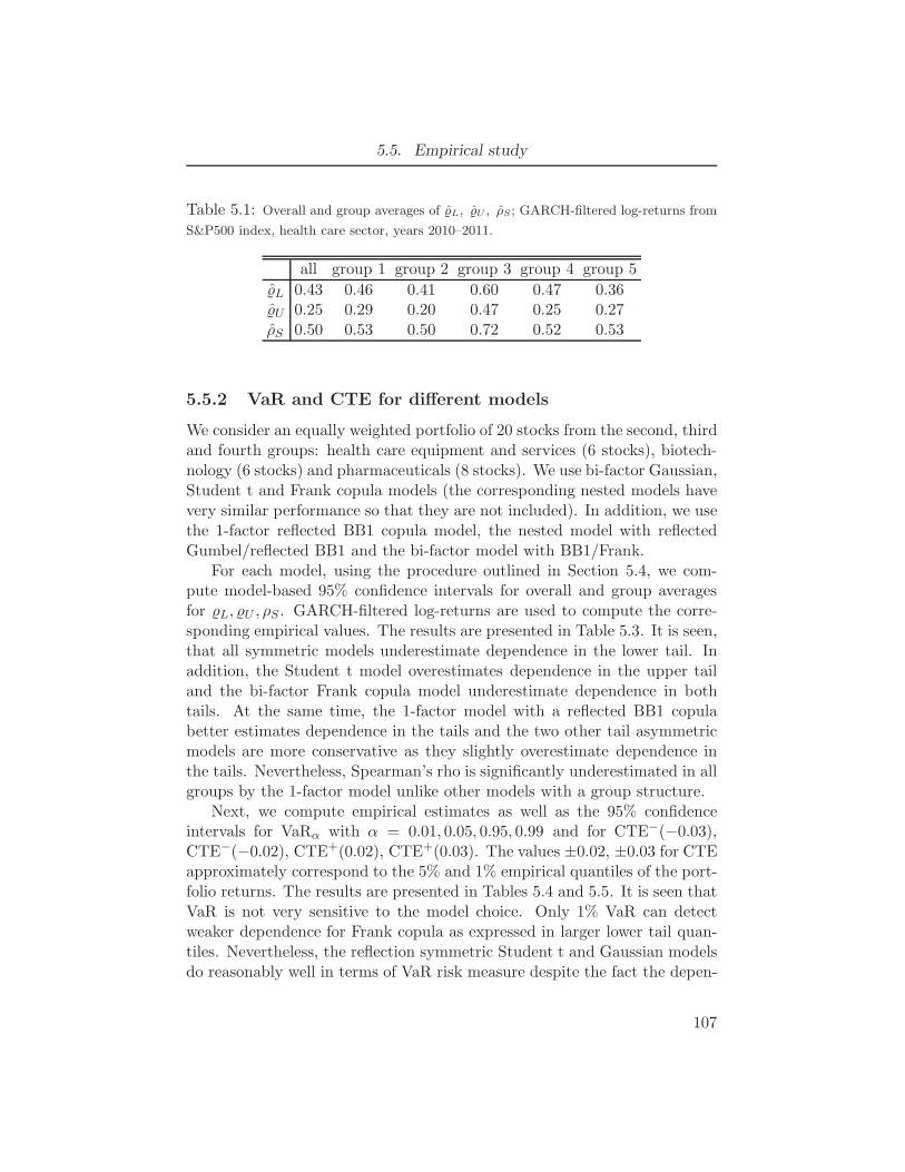
5.5. Empirical study
Table 5.1: Overall and group averages of ˆL, ˆU , ρS ; GARCH-filtered log-returns from
S&P500 index, health care sector, years 2010–2011.
all group 1 group 2 group 3 group 4 group 5
ˆL 0.43 0.46 0.41 0.60 0.47 0.36ˆU 0.25 0.29 0.20 0.47 0.25 0.27ρS 0.50 0.53 0.50 0.72 0.52 0.53
5.5.2 VaR and CTE for different models
We consider an equally weighted portfolio of 20 stocks from the second, thirdand fourth groups: health care equipment and services (6 stocks), biotech-nology (6 stocks) and pharmaceuticals (8 stocks). We use bi-factor Gaussian,Student t and Frank copula models (the corresponding nested models havevery similar performance so that they are not included). In addition, we usethe 1-factor reflected BB1 copula model, the nested model with reflectedGumbel/reflected BB1 and the bi-factor model with BB1/Frank.
For each model, using the procedure outlined in Section 5.4, we com-pute model-based 95% confidence intervals for overall and group averagesfor L, U , ρS . GARCH-filtered log-returns are used to compute the corre-sponding empirical values. The results are presented in Table 5.3. It is seen,that all symmetric models underestimate dependence in the lower tail. Inaddition, the Student t model overestimates dependence in the upper tailand the bi-factor Frank copula model underestimate dependence in bothtails. At the same time, the 1-factor model with a reflected BB1 copulabetter estimates dependence in the tails and the two other tail asymmetricmodels are more conservative as they slightly overestimate dependence inthe tails. Nevertheless, Spearman’s rho is significantly underestimated in allgroups by the 1-factor model unlike other models with a group structure.
Next, we compute empirical estimates as well as the 95% confidenceintervals for VaRα with α = 0.01, 0.05, 0.95, 0.99 and for CTE−(−0.03),CTE−(−0.02), CTE+(0.02), CTE+(0.03). The values ±0.02, ±0.03 for CTEapproximately correspond to the 5% and 1% empirical quantiles of the port-folio returns. The results are presented in Tables 5.4 and 5.5. It is seen thatVaR is not very sensitive to the model choice. Only 1% VaR can detectweaker dependence for Frank copula as expressed in larger lower tail quan-tiles. Nevertheless, the reflection symmetric Student t and Gaussian modelsdo reasonably well in terms of VaR risk measure despite the fact the depen-
107
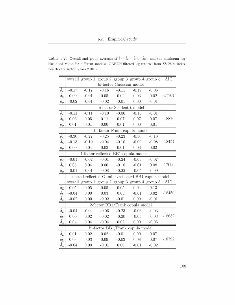
5.5. Empirical study
Table 5.2: Overall and group averages of δL, δU , |δL|, |δU |, and the maximum log-
likelihood value for different models; GARCH-filtered log-returns from S&P500 index,
health care sector, years 2010–2011.
overall group 1 group 2 group 3 group 4 group 5 AIC
bi-factor Gaussian model
δL -0.17 -0.17 -0.16 -0.11 -0.19 -0.06-17704δU 0.00 -0.01 0.05 0.02 0.03 0.02
δρ -0.02 -0.01 -0.02 -0.01 0.00 -0.01
bi-factor Student t model
δL -0.11 -0.11 -0.10 -0.06 -0.15 -0.01-18876δU 0.06 0.05 0.11 0.07 0.07 0.07
δρ 0.01 0.01 0.00 0.01 0.00 0.01
bi-factor Frank copula model
δL -0.30 -0.27 -0.25 -0.23 -0.30 -0.16-18454δU -0.13 -0.10 -0.04 -0.10 -0.09 -0.08
δρ 0.00 0.04 0.03 0.01 0.03 0.02
1-factor reflected BB1 copula model
δL -0.01 -0.02 -0.01 -0.24 -0.03 -0.07-17096δU 0.05 0.04 0.00 -0.10 -0.01 0.08
δρ -0.01 -0.01 -0.08 -0.22 -0.05 -0.09
nested reflected Gumbel/reflected BB1 copula modeloverall group 1 group 2 group 3 group 4 group 5 AIC
δL 0.05 0.05 0.05 0.05 0.04 0.13-18450δU -0.04 0.00 0.03 0.03 -0.01 0.02
δρ -0.02 0.00 -0.02 -0.01 0.00 -0.01
2-factor BB1/Frank copula model
δL -0.04 -0.04 -0.06 -0.23 -0.06 -0.03-18632δU 0.00 0.02 -0.02 -0.20 -0.05 -0.03
δρ 0.04 0.04 -0.04 0.02 0.00 -0.05
bi-factor BB1/Frank copula model
δL 0.01 0.02 0.02 -0.01 0.00 0.07-18792δU 0.03 0.03 0.09 -0.03 0.08 0.07
δρ -0.04 0.00 -0.01 0.00 -0.01 -0.02
108
5.5. Empirical study
dence structure is misspecified by these models. A possible reason is thatsmaller quantiles are required to detect weaker dependence of these modelsin the lower tail. Otherwise the inferences on VaR and CTE are mainlydominated by the fit in the middle. However, VaRα can not be empiricallyestimated well with very small or large values of α unless the sample sizeis very large. The nonsensitivity of the VaR to the copula model is alsomentioned in Section 4.1 of Brechmann (2014).
Conditional tail expectation is underestimated in the lower tail by thereflection symmetric models, but all models do reasonably well in the uppertail. However, the Student t model significantly overestimates the strengthof dependence in the upper tail according to the tail-weighted dependencemeasures, whereas the Frank copula model underestimates dependence inthe upper tail. CTE can thus still not be very sensitive to the model mis-specification.
Note that the 1-factor copula with reflected BB1 provides good estimatesfor VaR and CTE as the strength of dependence in the tails is estimatedquite well by the model. After removing the first large group of returns, themodel improves its performance, however the overall dependence is still un-derestimated as indicated by poor Spearman’s rho estimates. In conclusion,one can see that structured copula models specify both overall dependenceand dependence in the tails quite well and provide good estimates for theconsidered risk measures. The improved fit of the bi-factor copulas as seenin the AIC values matches improved model-based estimates of tail-weighteddependence measures; that is, tail-weighted dependence measures are moresensitive than portfolio VaR/CTE in differentiating models that fit less wellbased on AIC. That is, some models with incorrectly specified dependencestructure (in the middle or tails) still do reasonably well in terms of VaRand CTE. This indicates that very small (or large) values of α for VaR and,respectively, thresholds for CTE may be required to efficiently discriminatemodels with different tail properties and thus one needs a very large samplesize to get a good estimates for VaR and CTE for a model validation. On theother hand, tail-weighted dependent measures can discriminate the copulamodels without such a large sample size.
5.5.3 Comparing performance of nested copula models
In this section, we use the tail-weighted measures of dependence RTL (u6, 0.5)and RTU (u6, 0.5) to analyze a smaller data set of nine S&P500 stock returnsfrom Consumer Staples sector, and show how they can be used for modelselection and assessment of model adequacy. The time period is years 2011–
109
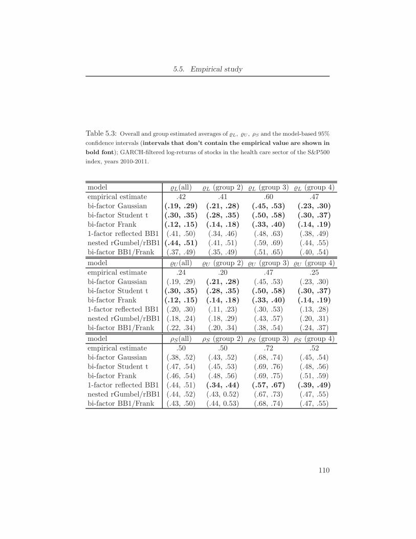
5.5. Empirical study
Table 5.3: Overall and group estimated averages of L, U , ρS and the model-based 95%
confidence intervals (intervals that don’t contain the empirical value are shown in
bold font); GARCH-filtered log-returns of stocks in the health care sector of the S&P500
index, years 2010-2011.
model L(all) L (group 2) L (group 3) L (group 4)
empirical estimate .42 .41 .60 .47bi-factor Gaussian (.19, .29) (.21, .28) (.45, .53) (.23, .30)bi-factor Student t (.30, .35) (.28, .35) (.50, .58) (.30, .37)bi-factor Frank (.12, .15) (.14, .18) (.33, .40) (.14, .19)1-factor reflected BB1 (.41, .50) (.34, .46) (.48, .63) (.38, .49)nested rGumbel/rBB1 (.44, .51) (.41, .51) (.59, .69) (.44, .55)bi-factor BB1/Frank (.37, .49) (.35, .49) (.51, .65) (.40, .54)
model U (all) U (group 2) U (group 3) U (group 4)
empirical estimate .24 .20 .47 .25bi-factor Gaussian (.19, .29) (.21, .28) (.45, .53) (.23, .30)bi-factor Student t (.30, .35) (.28, .35) (.50, .58) (.30, .37)bi-factor Frank (.12, .15) (.14, .18) (.33, .40) (.14, .19)1-factor reflected BB1 (.20, .30) (.11, .23) (.30, .53) (.13, .28)nested rGumbel/rBB1 (.18, .24) (.18, .29) (.43, .57) (.20, .31)bi-factor BB1/Frank (.22, .34) (.20, .34) (.38, .54) (.24, .37)
model ρS(all) ρS (group 2) ρS (group 3) ρS (group 4)
empirical estimate .50 .50 .72 .52bi-factor Gaussian (.38, .52) (.43, .52) (.68, .74) (.45, .54)bi-factor Student t (.47, .54) (.45, .53) (.69, .76) (.48, .56)bi-factor Frank (.46, .54) (.48, .56) (.69, .75) (.51, .59)1-factor reflected BB1 (.44, .51) (.34, .44) (.57, .67) (.39, .49)nested rGumbel/rBB1 (.44, .52) (.43, 0.52) (.67, .73) (.47, .55)bi-factor BB1/Frank (.43, .50) (.44, 0.53) (.68, .74) (.47, .55)
110
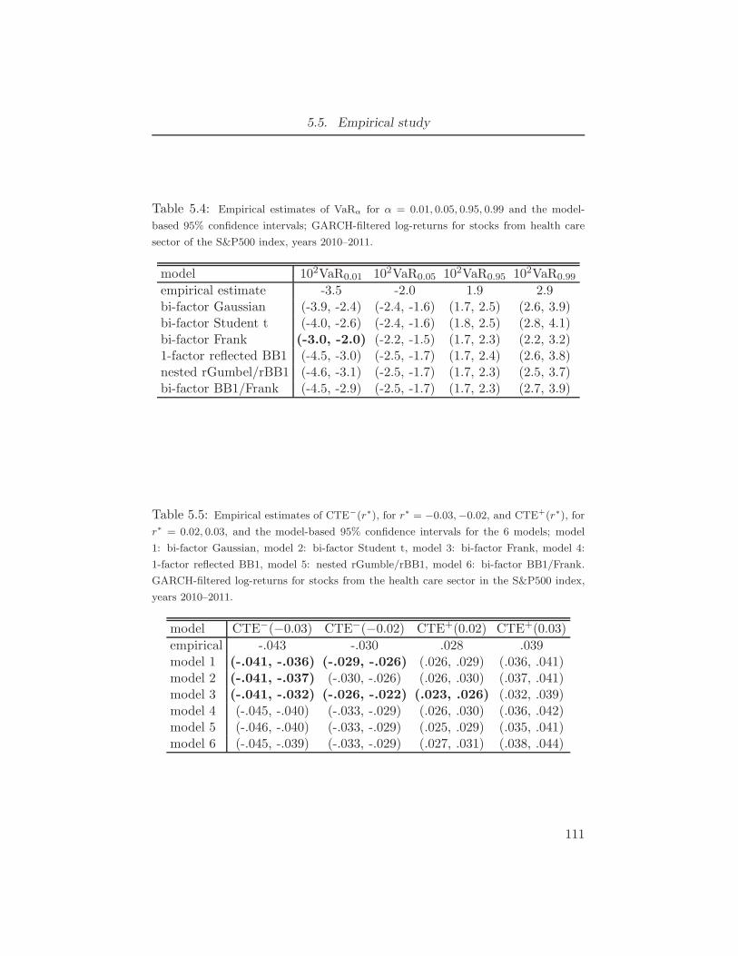
5.5. Empirical study
Table 5.4: Empirical estimates of VaRα for α = 0.01, 0.05, 0.95, 0.99 and the model-
based 95% confidence intervals; GARCH-filtered log-returns for stocks from health care
sector of the S&P500 index, years 2010–2011.
model 102VaR0.01 102VaR0.05 102VaR0.95 102VaR0.99
empirical estimate -3.5 -2.0 1.9 2.9bi-factor Gaussian (-3.9, -2.4) (-2.4, -1.6) (1.7, 2.5) (2.6, 3.9)bi-factor Student t (-4.0, -2.6) (-2.4, -1.6) (1.8, 2.5) (2.8, 4.1)bi-factor Frank (-3.0, -2.0) (-2.2, -1.5) (1.7, 2.3) (2.2, 3.2)1-factor reflected BB1 (-4.5, -3.0) (-2.5, -1.7) (1.7, 2.4) (2.6, 3.8)nested rGumbel/rBB1 (-4.6, -3.1) (-2.5, -1.7) (1.7, 2.3) (2.5, 3.7)bi-factor BB1/Frank (-4.5, -2.9) (-2.5, -1.7) (1.7, 2.3) (2.7, 3.9)
Table 5.5: Empirical estimates of CTE−(r∗), for r∗ = −0.03,−0.02, and CTE+(r∗), for
r∗ = 0.02, 0.03, and the model-based 95% confidence intervals for the 6 models; model
1: bi-factor Gaussian, model 2: bi-factor Student t, model 3: bi-factor Frank, model 4:
1-factor reflected BB1, model 5: nested rGumble/rBB1, model 6: bi-factor BB1/Frank.
GARCH-filtered log-returns for stocks from the health care sector in the S&P500 index,
years 2010–2011.
model CTE−(−0.03) CTE−(−0.02) CTE+(0.02) CTE+(0.03)
empirical -.043 -.030 .028 .039model 1 (-.041, -.036) (-.029, -.026) (.026, .029) (.036, .041)model 2 (-.041, -.037) (-.030, -.026) (.026, .030) (.037, .041)model 3 (-.041, -.032) (-.026, -.022) (.023, .026) (.032, .039)model 4 (-.045, -.040) (-.033, -.029) (.026, .030) (.036, .042)model 5 (-.046, -.040) (-.033, -.029) (.025, .029) (.035, .041)model 6 (-.045, -.039) (-.033, -.029) (.027, .031) (.038, .044)
111
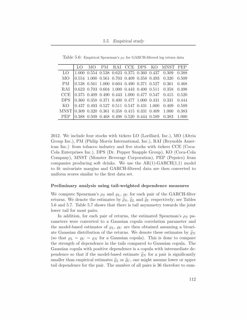
5.5. Empirical study
Table 5.6: Empirical Spearman’s ρS for GARCH-filtered log return data
LO MO PM RAI CCE DPS KO MNST PEP
LO 1.000 0.554 0.538 0.623 0.375 0.360 0.437 0.309 0.388MO 0.554 1.000 0.561 0.703 0.409 0.358 0.493 0.320 0.509PM 0.538 0.561 1.000 0.604 0.490 0.371 0.527 0.361 0.468RAI 0.623 0.703 0.604 1.000 0.443 0.400 0.511 0.358 0.498CCE 0.375 0.409 0.490 0.443 1.000 0.477 0.547 0.415 0.520DPS 0.360 0.358 0.371 0.400 0.477 1.000 0.431 0.331 0.444KO 0.437 0.493 0.527 0.511 0.547 0.431 1.000 0.409 0.589
MNST 0.309 0.320 0.361 0.358 0.415 0.331 0.409 1.000 0.383PEP 0.388 0.509 0.468 0.498 0.520 0.444 0.589 0.383 1.000
2012. We include four stocks with tickers LO (Lorillard, Inc.), MO (AltriaGroup Inc.), PM (Philip Morris International, Inc.), RAI (Reynolds Amer-ican Inc.) from tobacco industry and five stocks with tickers CCE (Coca-Cola Enterprises Inc.), DPS (Dr. Pepper Snapple Group), KO (Coca-ColaCompany), MNST (Monster Beverage Corporation), PEP (Pepsico) fromcompanies producing soft drinks. We use the AR(1)-GARCH(1,1) modelto fit univariate margins and GARCH-filtered data are then converted touniform scores similar to the first data set.
Preliminary analysis using tail-weighted dependence measures
We compute Spearman’s ρS and L, U for each pair of the GARCH-filterreturns. We denote the estimates by ρS , L and U respectively; see Tables5.6 and 5.7. Table 5.7 shows that there is tail asymmetry towards the jointlower tail for most pairs.
In addition, for each pair of returns, the estimated Spearman’s ρS pa-rameters were converted to a Gaussian copula correlation parameter andthe model-based estimates of L, U are then obtained assuming a bivari-ate Gaussian distribution of the returns. We denote these estimates by N(so that L = U = N for a Gaussian copula). This is done to comparethe strength of dependence in the tails compared to Gaussian copula. TheGaussian copula with positive dependence is a copula with intermediate de-pendence so that if the model-based estimate N for a pair is significantlysmaller than empirical estimates L or U , one might assume lower or uppertail dependence for the pair. The number of all pairs is 36 therefore to sum-
112
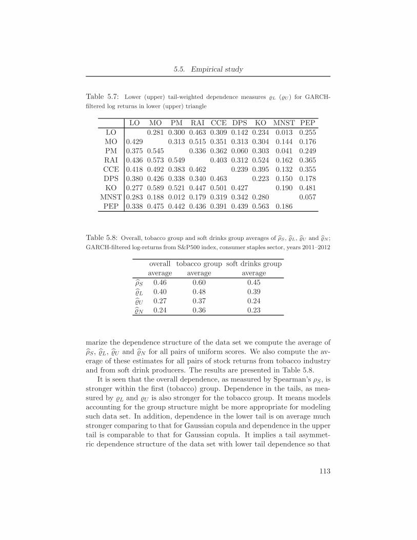
5.5. Empirical study
Table 5.7: Lower (upper) tail-weighted dependence measures L (U ) for GARCH-
filtered log returns in lower (upper) triangle
LO MO PM RAI CCE DPS KO MNST PEP
LO 0.281 0.300 0.463 0.309 0.142 0.234 0.013 0.255MO 0.429 0.313 0.515 0.351 0.313 0.304 0.144 0.176PM 0.375 0.545 0.336 0.362 0.060 0.303 0.041 0.249RAI 0.436 0.573 0.549 0.403 0.312 0.524 0.162 0.365CCE 0.418 0.492 0.383 0.462 0.239 0.395 0.132 0.355DPS 0.380 0.426 0.338 0.340 0.463 0.223 0.150 0.178KO 0.277 0.589 0.521 0.447 0.501 0.427 0.190 0.481
MNST 0.283 0.188 0.012 0.179 0.319 0.342 0.280 0.057PEP 0.338 0.475 0.442 0.436 0.391 0.439 0.563 0.186
Table 5.8: Overall, tobacco group and soft drinks group averages of ρS, L, U and N ;
GARCH-filtered log-returns from S&P500 index, consumer staples sector, years 2011–2012
overall tobacco group soft drinks groupaverage average average
ρS 0.46 0.60 0.45L 0.40 0.48 0.39U 0.27 0.37 0.24N 0.24 0.36 0.23
marize the dependence structure of the data set we compute the average ofρS , L, U and N for all pairs of uniform scores. We also compute the av-erage of these estimates for all pairs of stock returns from tobacco industryand from soft drink producers. The results are presented in Table 5.8.
It is seen that the overall dependence, as measured by Spearman’s ρS, isstronger within the first (tobacco) group. Dependence in the tails, as mea-sured by L and U is also stronger for the tobacco group. It means modelsaccounting for the group structure might be more appropriate for modelingsuch data set. In addition, dependence in the lower tail is on average muchstronger comparing to that for Gaussian copula and dependence in the uppertail is comparable to that for Gaussian copula. It implies a tail asymmet-ric dependence structure of the data set with lower tail dependence so that
113
5.5. Empirical study
using models with reflection symmetric copulas could be inappropriate.
Comparisons of different nested copula models
Next we fit different copula models and compare how well different charac-teristics of the joint distribution of returns are estimated by these models.For modeling the joint dependence of the GARCH-filtered data, we use thefollowing nested copula models:
• Model 1. Gaussian nested model. This is a model with reflectionsymmetric dependence structure and intermediate tail dependence be-tween each two stocks from the data set
• Model 2. Student t nested model: multivariate Student tν model withthe same correlation matrix as in the nested Gaussian model. Thisis a model with reflection symmetric dependence structure and taildependence between each pair of stocks.
• Model 3. Frank nested model: all linking copulas are Frank copulas.This is a model with reflection symmetric dependence structure andtail quadrant independence between each pair of stocks.
• Model 4. Reflected Gumbel/Reflected BB1 model: The reflected Gum-bel (rGumbel) copula is used to model dependence between the twogroups and the reflected BB1 (rBB1) copula is used to model depen-dence within each of the two groups. This is a model with tail asym-metric dependence structure and lower/upper tail dependence betweeneach pair of stocks.
The BB1 copula is a tail asymmetric copula with the lower and uppertail dependence; see Joe (1997) for details. Hence only the last model allowsfor asymmetric tail dependence and based on the results presented in Table5.8, first three models might be not appropriate for the data set. We next in-dicate the comparison based on negative log-likelihood and values of Akaikeinformation criterion (AIC) for the uniform-transformed GARCH-filteredlog returns. For the nested factor models based on Gaussian, Student t,Frank and rGumbel/rBB1, they are summarized in Table 5.9; the choice ofν = 15 led to the largest log-likelihood for multivariate Student t. As thepreliminary analysis based on tail-weighted dependence measures suggesttail dependence, it is not surprising that the best models based on AIC arethe two models with tail dependence.
114
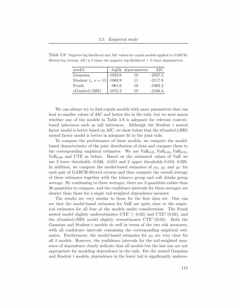
5.5. Empirical study
Table 5.9: Negative log-likelihood and AIC values for copula models applied to GARCH-
filtered log returns; AIC is 2 times the negative log-likelihood + 2 times #parameters
model -loglik #parameters AIC
Gaussian -1023.6 10 -2027.2Student tν ν = 15 -1069.9 11 -2117.8Frank -961.6 10 -1903.2rGumbel/rBB1 -1072.2 19 -2106.4
We can always try to find copula models with more parameters that canlead to smaller values of AIC and better fits in the tails, but we next assesswhether any of the models in Table 5.9 is adequate for relevant context-based inferences such as tail inferences. Although the Student t nestedfactor model is better based on AIC, we show below that the rGumbel/rBB1nested factor model is better in adequate fit to the joint tails.
To compare the performance of these models, we compute the model-based characteristics of the joint distribution of data and compare them tothe corresponding empirical estimates. We use VaR0.01,VaR0.05,VaR0.95,VaR0.99 and CTE as before. Based on the estimated values of VaR weuse 2 lower thresholds -0.026, -0.015 and 2 upper thresholds 0.016, 0.028.In addition, we compute the model-based estimates of ρS , L and U foreach pair of GARCH-filtered returns and then compute the overall averageof these estimates together with the tobacco group and soft drinks groupaverage. By condensing to these averages, there are 3 quantities rather than36 quantities to compare, and the confidence intervals for these averages areshorter than those for a single tail-weighted dependence measure.
The results are very similar to those for the first data set. One cansee that the model-based estimates for VaR are quite close to the empir-ical estimates for all four of the models under consideration. The Franknested model slightly underestimates CTE−(−0.02) and CTE+(0.02), andthe rGumbel/rBB1 model slightly overestimates CTE+(0.03). Both theGaussian and Student t models do well in terms of the two risk measures,with all confidence intervals containing the corresponding empirical esti-mates. Furthermore, the model-based estimates for ρS are very close forall 4 models. However, the confidence intervals for the tail-weighted mea-sures of dependence clearly indicate that all models but the last one are notappropriate for modeling dependence in the tails. For the nested Gaussianand Student t models, dependence in the lower tail is significantly underes-
115
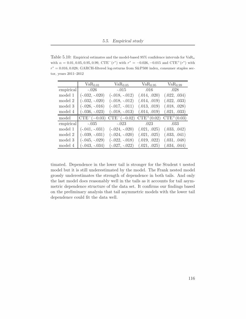
5.5. Empirical study
Table 5.10: Empirical estimates and the model-based 95% confidence intervals for VaRα
with α = 0.01, 0.05, 0.95, 0.99, CTE−(r∗) with r∗ = −0.026,−0.015 and CTE+(r∗) with
r∗ = 0.016, 0.028; GARCH-filtered log-returns from S&P500 index, consumer staples sec-
tor, years 2011–2012
VaR0.01 VaR0.05 VaR0.95 VaR0.99
empirical -.026 -.015 .016 .028model 1 (-.032, -.020) (-.018, -.012) (.014, .020) (.022, .034)model 2 (-.032, -.020) (-.018, -.012) (.014, .019) (.022, .033)model 3 (-.026, -.016) (-.017, -.011) (.013, .019) (.018, .028)model 4 (-.036, -.023) (-.018, -.013) (.014, .019) (.021, .033)
model CTE−(−0.03) CTE−(−0.02) CTE+(0.02) CTE+(0.03)
empirical -.035 -.023 .023 .033model 1 (-.041, -.031) (-.024, -.020) (.021, .025) (.033, .042)model 2 (-.039, -.031) (-.024, -.020) (.021, .025) (.033, .041)model 3 (-.045, -.029) (-.022, -.018) (.019, .022) (.031, .048)model 4 (-.043, -.034) (-.027, -.022) (.021, .025) (.034, .044)
timated. Dependence in the lower tail is stronger for the Student t nestedmodel but it is still underestimated by the model. The Frank nested modelgrossly underestimates the strength of dependence in both tails. And onlythe last model does reasonably well in the tails as it accounts for tail asym-metric dependence structure of the data set. It confirms our findings basedon the preliminary analysis that tail asymmetric models with the lower taildependence could fit the data well.
116
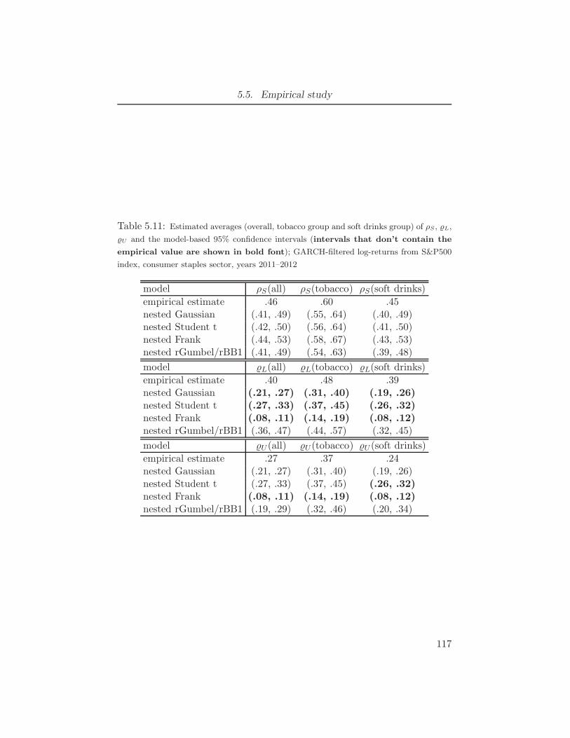
5.5. Empirical study
Table 5.11: Estimated averages (overall, tobacco group and soft drinks group) of ρS, L,
U and the model-based 95% confidence intervals (intervals that don’t contain the
empirical value are shown in bold font); GARCH-filtered log-returns from S&P500
index, consumer staples sector, years 2011–2012
model ρS(all) ρS(tobacco) ρS(soft drinks)
empirical estimate .46 .60 .45nested Gaussian (.41, .49) (.55, .64) (.40, .49)nested Student t (.42, .50) (.56, .64) (.41, .50)nested Frank (.44, .53) (.58, .67) (.43, .53)nested rGumbel/rBB1 (.41, .49) (.54, .63) (.39, .48)
model L(all) L(tobacco) L(soft drinks)
empirical estimate .40 .48 .39nested Gaussian (.21, .27) (.31, .40) (.19, .26)nested Student t (.27, .33) (.37, .45) (.26, .32)nested Frank (.08, .11) (.14, .19) (.08, .12)nested rGumbel/rBB1 (.36, .47) (.44, .57) (.32, .45)
model U (all) U (tobacco) U (soft drinks)
empirical estimate .27 .37 .24nested Gaussian (.21, .27) (.31, .40) (.19, .26)nested Student t (.27, .33) (.37, .45) (.26, .32)nested Frank (.08, .11) (.14, .19) (.08, .12)nested rGumbel/rBB1 (.19, .29) (.32, .46) (.20, .34)
117
Chapter 6
Concluding remarks
Factor copula models provide a wide range of dependence with O(d) num-ber of dependence parameters and allow for different types of tail behavior.They can be preferred over the classical factor model based on multivariatenormality when there is tail dependence or tail asymmetry, and inferencesconcerning joint tails are important. We have derived factor copula modelsas conditional independence models and shown that the classical multivari-ate normal factor models are special cases. Some properties of our versionof factor copulas can be obtained from the fact that these copula models canbe represented as the truncated C-vines rooted at the latent variables. Thelink to vines is useful for other models, with and without latent variables.
For factor models that account for sector information or other measuredfactors, Heinen and Valdesogo (2009) and Brechmann and Czado (2013)have copula models that use vines. We propose two extensions for thefactor copula models that allow the modeling of dependence for multivariatedata sets when there are several non-overlapping groups of variables withhomogeneous dependence in each group. These models are truncated regularvines and they contain bi-factor and nested Gaussian models as special cases.Tail dependence and tail asymmetry can be modeled by choosing appropriatebivariate linking copulas. The number of dependence parameters in themodels is a linear function of dimension d and, with appropriate numericalmethods, two-stage maximum likelihood estimation is efficient for d up to100. Resampling to get model-based confidence intervals is however muchmore numerically intensive.
Our proposed factor copula models are closed under marginalization,whereas truncated vine copula models are not, and this property helps ingetting starting values for numerical optimization for large d. These com-ments also apply to the structured factor models mentioned above. Thenumerical techniques of Gauss-Legendre quadrature and modified Newton-Raphson should be simpler to implement than the simulation-based esti-mation method of Oh and Patton (2012). Fast algorithms for estimatingparameters in different factor copula models and simulating data from thesemodels are implemented in R statistical software (R-Core-Team (2014)) and
118
Chapter 6. Concluding remarks
will be included to an R package along with some diagnostic tools includingthe tail-weighted measures of dependence. Some part of the code is writtenin Fortran 90 and is called from R to make computations faster. The Rpackage will be available at the web site of the book Joe (2014). The algo-rithms can be readily implemented for more flexible models with 3 factorsbut because of a large computational time that is needed to estimate param-eters in the 3-factor models, parallel computing might be needed to reducethe speed to a reasonable time. In this case, a nested copula model with 3factors model might be preferable as it has smaller number of parameterscomparing to a tri-factor copula model so that estimation should be morestable.
In addition to their theoretical plausibility, the examples given or men-tioned in this dissertation show the factor copula models to be good fitsto some financial return data sets. The choice of bivariate linking copulasis very important to correctly specify dependence structure of the data set.Therefore some preliminary analysis is required to select appropriate linkingcopulas. In this dissertation, we propose to use some tail-weighted measuresto assess the strength of dependence in the tails in pairs of variables. Evenwith a small sample size the measures can efficiently discriminate copulaswith tail dependence and copulas that are not tail dependent. The measurescan be used as summaries in addition to general concordance measures suchas Kendall’s τ and Spearman’s ρS to facilitate the choice of a model thatcould fit data well in the tails. Furthermore, the measures can be used formodel validation to assess the model adequacy of fit in the tails. Quantile-based measures, such as portfolio VaR, might not discriminate dependencemodels, and the overall dependence can be estimated fairly well by modelswith different tail properties. The tail-weighted measures of dependence canbe estimated using data in the joint tails, by putting more weight on theextremes, and thus they efficiently discriminate models with different tailorders. This is especially important for many applications in finance, insur-ance and other areas when model with misspecified tail characteristics canlead to incorrect inferences.
A model adequacy assessment for the strength of dependence in the tailsis similar to that for monotone dependence, by comparing the empirical ver-sus the model-based quantities. If discrepancies are found, then there areindications on how to improve the model in either the tail properties and/ordependence structure. Note also that conclusions about model comparisonsbased on assessment of adequacy of fit with tail-weighted dependence mea-sures could be different from conclusions based on AIC because log-likelihoodvalues are dominated by the fit in the “middle” of the data.
119
Chapter 6. Concluding remarks
Some formal tests for the model misspecification can be proposed.Schepsmeier (2014) developed a goodness-of-fit test for regular vines, andthis test could be extended for factor copula models. Nevertheless, the testdoes not provide guidance on finding an improved model and it does notaccount for variability of the estimates of univariate parameters.
The structured copula models presented in this dissertation can be ex-tended to a dynamic setting when dependence structure of the multivariatedata set can change in time. To account for dynamic dependence, copulaswith dependence parameters evolving in time can be used as in Patton (2006)or alternatively a regime switching copula can be applied; see, for example,Chollette et al. (2009). As a possible application, dynamic structured cop-ula models would allow to forecast financial portfolio returns and quantifypossible risks of the portfolio, while accounting for (i) strong dependence inthe tails and (ii) possible tail asymmetry of a multivariate distribution ofthe portfolio components. Future research includes studying the dependenceproperties of such an extended dynamic structured copula model. Based onthe model prediction, possible strategies for investors could be investigatedin order to minimize the risks of a portfolio.
Future research includes the study of multivariate extensions of the tail-weighted measures when the measure is defined for a d-dimensional randomvector with d > 2. Another research direction is the development of mea-sures of asymmetry and dependence based on the empirical copula function.These measures can be useful in detecting different types of dependencein the middle of a multivariate distribution when the use of tail-weightedmeasures of dependence is not very efficient.
120
Bibliography
Aas, K., Berg, D., 2009. Models for construction of multivariate dependence- a comparison study. European Journal of Finance 15, 639–659.
Aas, K., Czado, C., Frigessi, A., Bakken, H., 2009. Pair-copula constructionsof multiple dependence. Insurance: Mathematics and Economics 44, 182–198.
Ang, A., Chen, J., 2002. Asymmetric correlations of equity portfolios. Jour-nal of Financial Economics 63, 443–494.
Bedford, T., Cooke, R.M., 2001. Probability density decomposition for con-ditionally dependent random variables modeled by vines. Annals of Math-ematics and Artificial Intelligence 32, 245–268.
Brechmann, E.C., 2014. Hierarchical Kendall copulas: properties and infer-ence. Canadian Journal of Statistics 42, 78–108.
Brechmann, E.C., Czado, C., 2013. Risk management with high-dimensionalvine copulas: An analysis of the Euro Stoxx 50. Statistics & Risk Modeling30, 307–342.
Brechmann, E.C., Czado, C., Aas, K., 2012. Truncated regular vines inhigh dimensions with applications to financial data. Canadian Journal ofStatistics 40, 68–85.
Chollette, L., Heinen, A., Valdesogo, A., 2009. Modeling international fi-nancial returns with a multivariate regime-switching copula. Journal ofFinancial Econometrics 7, 437–480.
Clayton, D.G., 1978. A model for association in bivariate life tables andits application in epidemiological studies of familial tendency in chronicdisease incidence. Biometrika 65, 141–151.
Dißmann, J., Brechmann, E.C., Czado, C., Kurowicka, D., 2013. Selectingand estimating regular vine copulae and application to financial returns.Computational Statistics and Data Analysis 59, 52–69.
121
Bibliography
Embrechts, P., 2009. Copulas: A personal view. Journal of Risk and Insur-ance 76, 639–650.
Fermanian, J., Radulovic, D., Wegkamp, M., 2004. Weak convergence ofempirical copula processes. Bernoulli 10(5), 847–860.
Frank, M.J., 1979. On the simultaneous associativity of F (x, y) and x+ y−F (x, y). Aequationes Mathematicae 19, 194–226.
Fritsch, F.N., Carlson, R.E., 1980. Monotone piecewise cubic interpolation.SIAM Journal of Numerical Analysis 17, 238–246.
Gabbi, G., 2005. Semi-correlations as a tool of geographical and sector assetallocation. The European Journal of Finance 11(3), 271–281.
Gaenssler, P., Stute, W., 1987. Seminar on Empirical Processes. DMVSeminar. volume 9. Birkhauser, Basel.
Garralda Guillem, A.I., 2000. Structure de dependance des lois de valeursextremes bivariees. C. R. Acad. Sci. Paris 330, 593–596.
Genest, C., Neslehova, J., Quessy, J.F., 2012. Tests of symmetry for bivari-ate copulas. Ann Inst Stat Math 64, 811–834.
Genest, C., Remillard, B., Beaudoin, D., 2009. Goodness-of-fit tests for cop-ulas: a review and a power study. Insurance: Mathematics and Economics44, 199–213.
Gibbons, R., Hedeker, D., 1992. Full-information item bi-factor analysis.Psychometrika 57, 423–436.
Gumbel, E.J., 1960. Distributions des valeurs extremes en plusieurs dimen-sions. Publ. Inst. Statist. Univ. Paris 9, 171–173.
Hardy, G.H., Littlewood, J.E., Polya, G., 1952. Inequalities. CambridgeUniversity Press. 2nd edition.
Harris, C.W., Kaiser, H.F., 1964. Oblique factor analytic solutions by or-thogonal transformations. Psychometrika 29, 347–362.
Harville, D.A., 1997. Matrix Algebra from a Statisticians Perspective.Springer, New York.
Heffernan, J.E., 2000. A directory of coefficients of tail dependence. Ex-tremes 3, 279–290.
122
Bibliography
Heinen, A., Valdesogo, A., 2009. Asymmetric CAPM dependence for largedimensions: the canonical vine autoregressive model. CORE discussionpapers 2009069, Universite Catholique de Louvain, Center for OperationsResearch and Econometrics (CORE) .
Hofert, M., 2008. Sampling Archimedean copulas. Computational Statistics& Data Analysis 52, 5163–5174.
Holzinger, K.J., Swineford, F., 1937. The bi-factor method. Psychometrika2, 41–54.
Hua, L., Joe, H., 2011. Tail order and intermediate tail dependence ofmultivariate copulas. Journal of Multivariate Analysis 102, 1454–1471.
Huang, W., Prokhorov, A., 2014. A goodness-of-fit test for copulas. Econo-metric Reviews 33, 751–771.
Hull, J., White, A., 2004. Valuation of a CDO and an nth to default CDSwithout Monte Carlo simulation. Journal of Derivatives 12, 8–23.
Joe, H., 1997. Multivariate Models and Dependence Concepts. Chapman &Hall, London.
Joe, H., 2011. Tail dependence in vine copulae, in: Kurowicka, D., Joe, H.(Eds.), Dependence Modeling: Vine Copula Handbook. World Scientific,Singapore. chapter 8, pp. 165–187.
Joe, H., 2014. Dependence Modeling with Copulas. Chapman & Hall/CRC,Boca Raton, FL.
Joe, H., Hu, T., 1996. Multivariate distributions from mixtures of max-infinitely divisible distributions. Journal of Multivariate Analysis 57, 240–265.
Joe, H., Li, H., Nikoloulopoulos, A., 2010. Tail dependence functions andvine copulas. Journal of Multivariate Analysis 101, 252–270.
Johnson, R.A., Wichern, D.W., 2002. Applied Multivariate Statistical Anal-ysis. Prentice Hall, Englewood Cliffs, NJ. fifth edition.
Jondeau, E., Rockinger, M., 2006. The copula-GARCH model of condi-tional dependencies: An international stock market application. Journalof International Money and Finance 25, 827–853.
123
Bibliography
Kahaner, D., Moler, C.B., Nash, S., 1989. Numerical Methods and Software.Prentice Hall, Englewood Cliffs, NJ.
Kimeldorf, G., Sampson, A.R., 1989. A framework for positive dependence.Ann. Inst. Statist. Math. 41, 31–45.
Kluppelberg, C., Kuhn, G., 2009. Copula structure analysis. Journal ofRoyal Statistical Society B 71, 737–753.
Krupskii, P., Joe, H., 2013. Factor copula models for multivariate data.Journal of Multivariate Analysis 120, 85–101.
Krupskii, P., Joe, H., 2014a. Structural factor copula models: theory, infer-ence and computation. Working paper .
Krupskii, P., Joe, H., 2014b. Tail-weighted measures of dependence. Work-ing paper .
Kurowicka, D., Cooke, R., 2006. Uncertainty Analysis with High Dimen-sional Dependence Modelling.
Kurowicka, D., Joe, H., 2011. Dependence Modeling: Vine Copula Hand-book. World Scientific, Singapore.
Ledford, A., Tawn, J., 1996. Statistic for near independence in multivariateextreme values. Biometrica 83, 168–187.
Lee, T.H., Long, X., 2009. Copula-based multivariate GARCH model withuncorrelated dependent errors. Journal of Econometrics 150, 207–218.
Loeve, M.M., 1963. Probability theory. Van Nostrand Reinhold, New York.
McDonald, R.P., 1985. Factor Analysis and Related Methods. LawrenceErlbaum Associates, Hillsdale, NJ.
McNeil, A.J., Frey, R., Embrechts, P., 2005. Quantitative Risk Management.Princeton University Press, Princeton, NJ.
Muthen, B.O., 1994. Multilevel covariance structure analysis. SociologicalMethods & Research 22, 376–398.
Nash, J.C., 1990. Compact Numerical Methods for Computers: LinearAlgebra and Function Minimisation. Hilger, New York. second edition.
Nelsen, R.B., 2006. An Introduction to Copulas. Springer, New York. secondedition.
124
Bibliography
Nikoloulopoulos, A.K., Joe, H., 2014. Factor copula models for item responsedata. Psychometrika .
Nikoloulopoulos, A.K., Joe, H., Li, H., 2012. Vine copulas with asymmetrictail dependence and applications to financial return data. ComputationalStatistics & Data Analysis 56, 3659–3673.
Oh, D.H., Patton, A., 2012. Modeling dependence in high dimensions withfactor copulas. Submitted .
Pascual, L., Romo, J., Ruiz, E., 2006. Bootstrap prediction for returns andvolatilities in GARCH models. Computational Statistics & Data Analysis50, 2293–2312.
Patton, A., 2006. Modeling asymmetric exchange rate dependence. Inter-national Economic Review 47, 527–556.
R-Core-Team, 2014. R: A Language and Environment for Statistical Com-puting. R Foundation for Statistical Computing. Vienna, Austria.
Rosco, J., Joe, H., 2013. Measures of tail asymmetry for bivariate copulas.Statistical Papers 54, 709–726.
Salvadori, G., De Michele, C., Kottegoda, N.T., Rosso, R., 2007. Extremesin Nature. An Approach using Copulas. Springer, Dordrecht.
Schepsmeier, U., 2014. Estimating Standard Errors and Efficient Goodness-of-Fit Tests for Regular Vine Copula Models. Ph.D. thesis. TechnischeUniversitat Munchen.
Schepsmeier, U., Stoeber, J., Brechmann, E.C., 2012. VineCopula: Statis-tical inference of vine copulas. R package at http://www.r-project.org.
Schmid, F., Schmidt, R., 2007. Multivariate conditional versions of spear-mans’s rho and related measures of tail dependence. Journal of Multivari-ate Analysis 98, 1123–1140.
Shah, S., Parikh, N., 1964. Moments of single and doubly truncated standardbivariate normal distribution. Vidya (Gujarat University) 7, 82–91.
Sklar, A., 1959. Fonctions de repartition a n dimensions et leurs marges.Publ. Inst. Statist. Univ. Paris 8, 229–231.
125
Stroud, A., Secrest, D., 1966. Gaussian Quadrature Formulas. Prentice-Hall,Englewood Cliffs, NJ.
Tong, Y.L., 1980. Probability inequalities in multivariate distributions. Aca-demic Press, New York.
van der Vaart, A.W., Wellner, J.A., 1996. Weak Convergence and EmpiricalProcesses: with Applications to Statistics. Springer, New York.
126
Appendix A
Proof of Proposition 2.1,
Section 2.2
We prove the result for the measures in the lower tail TRL , RTL as the prooffor TRU , RTU is similar.
Asymptotic normality of RTL
To simplify the notation, we redefine b(u) := a(1 − u/p). In new no-tation, b(p) = 0. If bj is differentiable with bj(p) = 0, we can writebj(v) = −
∫ pv b
′j(u) du for 0 ≤ v ≤ p and j = 1, 2. Then for a bivariate
copula cdf C, after substitution of this identity and interchanging the orderof integration.
∫ p
0
∫ p
0b1(v1) b2(v2) dC(v1, v2) =
∫ p
0
∫ p
0b′1(u1) b
′2(u2)C(u1, u2) du1du2,
∫ p
0
∫ p
0b1(v1) dC(v1, v2) = −
∫ p
0b′1(u1)C(u1, p) du1,
∫ p
0
∫ p
0b2(v2) dC(v1, v2) = −
∫ p
0b′2(u2)C(p, u2) du2,
Let Cn(u1, u2) =1n
∑ni=1 I{Ri1 < u1, Ri2 < u2} be the empirical copula
for 0 < u1 < 1 and 0 < u2 < 1. The above equations also hold for Cn sothat we have:
m12 =1
n
n∑
i=1
b(Ri1) b(Ri2) I{Ri1 < p,Ri2 < p}
=
∫ p
0
∫ p
0b′(u1) b
′(u2) Cn(u1, u2) du1du2,
m1 =1
n
n∑
i=1
b(Ri1) I{Ri1 < p,Ri2 < p} = −∫ p
0b′(u1) Cn(u1, p) du1
m2 =1
n
n∑
i=1
b(Ri2) I{Ri1 < p,Ri2 < p} = −∫ p
0b′(u2) Cn(p, u2) du2.
127
Appendix A. Proof of Proposition 2.1, Section 2.2
It implies that m12 = E[m12] =∫ p0
∫ p0 b
′(u1) b′(u2)C(u1, u2) du1du2, m1 =E[m1] = −
∫ p0 b
′(u1)C(u1, p) du1, m2 = E[m2] = −∫ p0 b
′(u2)C(p, u2) du2.
Denote Gn(u1, u2) =√n(Cn(u1, u2) − C(u1, u2)). As it was shown by
Fermanian et al. (2004), Gn(u1, u2) d→ G(u1, u2), where G is a Gaussian pro-cess. As a result,
√n(m12 −m12) =
∫ p
0
∫ p
0b′(u1) b
′(u2)Gn(u1, u2) du1du2
d→∫ p
0
∫ p
0b′(u1) b
′(u2)G(u1, u2) du1du2, (A.1)
√n(m1 −m1) = −
∫ p
0b′(u1)Gn(u1, p) du1
d→ −∫ p
0b′(u1)G(u1, p) du1, (A.2)
√n(m2 −m2) = −
∫ p
0b′(u2)Gn(p, u2) du2
d→ −∫ p
0b′(u2)G(p, u2) du2. (A.3)
Similarly, we get
√n(m11 −m11)
d→ −∫ p
02b(u1) b
′(u1)G(u1, p) du1,
√n(m22 −m22)
d→ −∫ p
02b(u2) b
′(u2)G(p, u2) du2,(A.4)
where mjj = 1n
∑ni=1[b(Rij)]
2I{Ri1 < p,Ri2 < p} and mjj = E[mjj], j =1, 2.
In addition, np = 1n
∑ni=1 I{Ri1 < p,Ri2 < p} = Cn(p, p) and
√n(np −
np)d→ G(p, p), with np = C(p, p). Hence, from (A.1), (A.2), (A.3), (A.4)
we get the joint asymptotic normality of m12, m1, m2, m11, m22, np and theasymptotic normality of RTL (a, p) = (npm12−m1m2)/[(npm11−m2
1)(npm22−m2
2)]1/2 follows from the delta method and Cramer-Wold theorem. �
Asymptotic normality and the formula for the asymptotic variance of
TRL
By construction, TRL (a, p) = (m∗12 − (m∗)2)/[m∗∗ − (m∗)2], where
m∗12 =
1
nL
nL∑
i=1
a(1−R−i1) a(1−R−
i2) =
∫ 1
0
∫ 1
0a′(1− u1) a
′(1− u2)×
× (C(p)L )n(u1, u2) du1du2,
128
Appendix A. Proof of Proposition 2.1, Section 2.2
m∗ =1
nL
nL∑
i=1
b
(i− 0.5
nL
), m∗∗ =
1
nL
nL∑
i=1
b2(i− 0.5
nL
)
and (C(p)L )n(u1, u2) =
1nL
∑nLi=1 I{R−
i1 < u1, R−i2 < u2}. Denote
(G(p)L )n(u1, u2) =
√nL((C
pL)n(u1, u2) − C
(p)L (u1, u2)) and m∗
12 = E[m∗12] =∫ 1
0
∫ 10 a
′(1− u1) a′(1− u2)C
(p)L (u1, u2) du1du2. Similar to (A.1), we get:
√nL(m
∗12 −m∗
12) =
∫ 1
0
∫ 1
0a′(1− u1) a
′(1− u2) (G(p)L )n(u1, u2) du1du2
→d
∫ 1
0
∫ 1
0a′(1− u1) a
′(1− u2)G(p)L (u1, u2) du1du2. (A.5)
where G(p)L is the Gaussian process corresponding to the copula C
(p)L .
We have: m∗ =∫ 10 a(1− u)du+OP (
1n ), m
∗∗ =∫ 10 a(1− u)2du+OP (
1n ),
nLn →P C(p, p). By Slutsky’s theorem,
√n(TRL (a, p)− TRL (a, p)) →d N(0, σ2(TRL (a, p))),
where the asymptotic variance σ2(TRL (a, p)) =σ2(m∗
12)C(p,p)σ2a
and σa =∫ 10 a(1 −
u)2du−(∫ 1
0 a(1− u)du)2
. Using (A.5), we get:
σ2(TRL (a, p)) =1
C(p, p)σ2a
∫
[0,1]4a′(1−u1) a′(1−u2) a′(1−u3) a′(1−u4)×
×DpL(u1, u2, u3, u4)du1du2du3du4,
where D(p)L (u1, u2, u3, u4) = E[G(p)
L (u1, u2) · G(p)L (u3, u4)]. We have:
G(p)L (u1, u2) = B(p)
L (u1, u2)−∂C
(p)L (u1, u2)
∂u1B(p)L (u1, 1)
− ∂C(p)L (u1, u2)
∂u2B(p)L (1, u2),
where B(p)L (u1, u2) is a two-dimensional Brownian bridge and
E[B(p)L (u1, u2)B(p)
L (u3, u4)] = C(p)L (u1∧u3, u2∧u4)−C(p)
L (u1, u2)C(p)L (u3, u4).
It is seen that the formula for D(p)L (u1, u2, u3, u4) can be expanded using the
covariance function of the Brownian bridge B(p)L and therefore the variance
129
Appendix A. Proof of Proposition 2.1, Section 2.2
σ2(TRL (a, p)) can be obtained in a closed form. The formula may be usefulto avoid Monte Carlo simulations in order to estimate asymptotic varianceof the measure TRL (a, p;C) for different weighting functions a and bivariatecopulas C. �
130
Appendix B
Proof of Proposition 2.2,
Section 2.2
We start with the measure RTL and the result for TRL follows from the prooffor RTL . We use the delta method and the result of Theorem 1. Denotemj0 = (npmjj − m2
j). In case of independence copula, we get npm12 =
m1m2, m1 = m2, m11 = m22, m10 = m20 and np = p2. If we writeRTL (a, p) as a function of m12,m1,m2,m10,m20, np, we find:
RTL (a, p) =npm12 −m1m2
[m10m20]1/2,
Note that ∂L∂mj0
= 0 for j = 1, 2 so it suffices to find the asymptotic variance
of the covariance W12 = npm12 − m1m2. The gradient for W12 = npm12 −m1m2 with respect to m12,m1,m2, np is as follows:
∇W12 =
(p2, −m1, −m1,
m21
p2
)T.
Redefine b(u) := a(1−u/p). Now we find the covariance function for theGaussian process G(u1, u2) for independence copula. We have:
G(u1, u2) = B(u1, u2)−∂C(u1, u2)
∂u1B(u1, 1)−
∂C(u1, u2)
∂u2B(1, u2),
where B(u1, u2) is a two-dimensional Brownian bridge and
E[B(u1, u2)B(u3, u4)] = C(u1 ∧ u3, u2 ∧ u4)− C(u1, u2)C(u3, u4).
If C(u1, u2) = u1u2, we get:
D(u1, u2, u3, u4) = E[G(u1, u2)G(u3, u4)] = (u1 ∧ u3 − u1u3)(u2 ∧ u4 − u2u4).
Let
Σ =
σ212 v12,1 v12,2 v12,pv12,1 σ21 v1,2 v1,pv12,2 v1,2 σ22 v2,pv12,p v1,p v2,p σ2p
131
Appendix B. Proof of Proposition 2.2, Section 2.2
be the asymptotic covariance matrix of the vector M = n−1/2(m12, m1, m2,np). From (A.1), (A.2), (A.3) we find:
σ212 =
∫ p
0
∫ p
0
∫ p
0
∫ p
0b′(u1) b
′(u2) b′(u3) b
′(u4)×
× D(u1, u2, u3, u4) du1du2du3du4 = ξ2,
σ21 = σ22 =
∫ p
0
∫ p
0b′(u1) b
′(u3)D(u1, p, u3, p) du1du3 = p(1− p)ξ,
σ2p = D(p, p, p, p) = p2(1− p)2,
v12,1 = v12,2 = −∫ p
0
∫ p
0
∫ p
0b′(u1) b
′(u2) b′(u3)D(u1, u2, u3, p) du1du2du3
= (1− p)m1ξ/p,
v1,2 = v12,p =
∫ p
0
∫ p
0b′(u1) b
′(u4)D(u1, p, p, u4) du1du4 = (1− p)2m21/p
2,
v1,p = v2,p = −∫ p
0b′(u1)D(u1, p, p, p) du1 = (1− p)2m1,
where
ξ =
∫ p
0
∫ p
0b′(u1) b
′(u2)(u1 ∧ u2 − u1u2) du1du2 =m10
p3+
(1− p)m21
p3.
Using the delta method and straightforward algebraic calculations, we ob-tain the formula for the asymptotic variance σ2(W12):
σ2(W12) = (∇W12)TΣ(∇W12) = m2
10/p2
and finally, the variance of the sampling distribution of RTL is σ2(RTL ) =1/p2.
To prove the result for TRL , note that C(p)L is the independence copula
and therefore D(p)L (u1, u2, u3, u4) = (u1 ∧ u3 − u1u3)(u2 ∧ u4 − u2u4). Using
the formula for the asymptotic variance of TRL (see the proof of Proposition2.1) and the formula for ξ2 with p = 1, we get:
σ2(TRL ) =1
p2σ2a
[∫ 1
0
∫ 1
0a′(1− u1) a
′(1− u2) (u1 ∧ u2 − u1u2)du1du2
]2=
1
p2.
�
132
Appendix C
Proof of Proposition 4.5,
Section 4.3.2
The (1, 2) margin of (4.6) is:
C1,2(u, u) =
∫ 1
0
∫ 1
0C1|V2;V1(C1|V1(u|v1)|v2)·C2|V2;V1(C2|V1(u|v1)|v2) dv1dv2
= u
∫ 1
0
∫ 1/u
0C1|V2;V1(C1|V1(u|hu)|v2) · C2|V2;V1(C2|V1(u|hu)|v2) dh dv2.
Let tj(h) = limu→0Cj|V1(u|hu). This is continuous for small h > 0 from thecontinuity assumptions on Cj|V1. Since limh→0 tj(h) = tj0, for every ǫ > 0we can find h = h(ǫ) > 0 such that |tj0− tj(h)| < ǫ if h ≤ h(ǫ), j = 1, 2. Fora fixed ǫ > 0 there exists u(ǫ) > 0 such that |Cj|V1(u|h(ǫ)u) − tj(h(ǫ))| < ǫfor 0 < u ≤ u(ǫ). It implies |tj0 − Cj|V1(u|h(ǫ)u)| < 2ǫ for u ≤ u(ǫ). Dueto uniform continuity of Cj|V1 on [0, 1] × [0, 1] we can find u0 > 0, h1, h2such that h1 < h(ǫ) < h2 and |Cj|V1(u|h(ǫ)u) − Cj|V1(u|hu)| < ǫ for 0 <u ≤ u0, h1 ≤ h ≤ h2. Therefore |tj0 − Cj|V1(u|hu)| < 3ǫ for 0 < u ≤min{u0, u(ǫ)}, h1 < h ≤ h(ǫ).
For the copulas at the second level we have Cj|V2;V1(tj0|0) ≥ k0 > 0and due to uniform continuity of Cj|V2;V1 , j = 1, 2, for a fixed ǫ0 ∈ (0, k0)we get Cj|V2;V1(z|v2) ≥ (k0 − ǫ0) > 0 for some z(ǫ0) ≤ z < min{t10, t20}and 0 < v2 ≤ v2(ǫ). Let ǫ = (k0 − ǫ0)/3 and u < u(ǫ). It follows that if0 < u ≤ min{u0, u(ǫ)}, then
C1,2(u, u) ≥ u
∫ v2(ǫ)
0
∫ h(ǫ)
h1
C1|V2;V1(C1|V1(u|hu)|v2)×
C2|V2;V1(C2|V1(u|hu)|v2)dh dv2 ≥ uv2(ǫ)(h(ǫ) − h1)(k0 − ǫ0)2.
Therefore limu→0C1,2(u, u)/u ≥ v2(ǫ)(h(ǫ)− h1)(k0 − ǫ0)2 > 0 and C1,2 has
lower tail dependence. �
133
Appendix D
Proof of Proposition 4.6,
Section 4.3.2
The conditional distributions are:
Ci|V1(u1|u2) =Ci,V1(u1, u2)
u2
[Ai
(lnu2
ln(u1u2)
)+
lnu1ln(u1u2)
A′i
(lnu2
ln(u1u2)
)],
and therefore
Ci|V1(u|us) = u(s+1)Ai( ss+1)−s
[Ai
(s
s+ 1
)+
1
s+ 1A′i
(s
s+ 1
)],
0 < s <∞. (D.1)
Let u = − lnu, Bi(s) = Ai
(ss+1
)+ 1
s+1A′i
(ss+1
)for i = 1, 2 and B(s) =
B1(s)B2(s). In the 1-factor model, for the bivariate copula C1,2 we have
C1,2(u, u) =
∫ 1
0C1|V1(u|v)C2|V1(u|v)dv
= u
∫ ∞
0C1|V1(u|us)C2|V1(u|us)usds = u
∫ ∞
0uξ(s)B(s)ds, (D.2)
where
ξ(s) = (s+ 1)
[A1
(s
s+ 1
)+A2
(s
s+ 1
)]− s.
Because Ai(s/[s + 1]) ≥ s/[s + 1], then ξ(s) ≥ s; also ξ(0) = 2. Hencethe minimum ξ∗ ≤ 2 exists and C1,2(u, u) = uuξ
∗ ∫∞0 uξ(s)−ξ
∗B(s)ds. Since
−1 ≤ A′i ≤ 1 and Ai(s/[s + 1]) ≥ 1/(s + 1),
Bi(s) = Ai
(s
s+ 1
)+
1
s+ 1A′i
(s
s+ 1
)≥ 1
s+ 1
[1 +A′
i
(s
s+ 1
)]≥ 0
and since Ai is convex,
Bi(s) = Ai
(s
s+ 1
)+
(1− s
s+ 1
)A′i
(s
s+ 1
)≤ Ai(1) = 1 (D.3)
134
Appendix D. Proof of Proposition 4.6, Section 4.3.2
Therefore, 0 ≤ B(s) ≤ 1. The equality B(s) = 0 is only possible if s = 0 ors = ∞, because A′
i(t) > −1 for 0 < t < 0.5 by assumption and A′i(t) > −1
for 0.5 ≤ t < 1 by the convexity and lower bound on A′i.
The lower tail order of C1,2 cannot be larger than 2 because by theresult in Garralda Guillem (2000) bivariate extreme value copulas are SIand then by Proposition 4.1, C1,2 is PQD and satisfies C1,2(u, u) ≥ u2. If
ξ∗ = 2, C1,2(u, u) ≤ u2u{∫ 20 B(s)ds +
∫∞2 us−2ds} = u2{u
∫ 20 B(s)ds + 1}.
Hence the lower tail order of C1,2 equals 2. Next assume ξ∗ < 2. Lets∗ = argmin{ξ(s)}. Then 0 < s∗ < 2. Due to continuity and differentiabilityof ξ(s) there exist an interval (s∗l , s
∗u) containing s∗ and a constant d0 > 0
such that ξ(s) ≤ ξ∗ + d0|s − s∗| if 0 < s∗l < s < s∗u ≤ 2. Due to continuityof B(s), there exists a constant B0 > 0 such that B(s) ≥ B0 if s∗l < s < s∗u.Hence, in bounding (D.2),
C1,2(u, u) ≤ uξ∗u
(∫ ξ∗
0B(s)ds+
∫ ∞
ξ∗us−ξ
∗ds
)= uξ
∗
(u
∫ ξ∗
0B(s)ds+ 1
)
where the rightmost term with u is slowly varying in u as u→ 0, and
C1,2(u, u) ≥ B0uξ∗ u
∫ s∗u
s∗l
ud0|s−s∗|ds =
B0uξ∗
d0
(2− ud0(s
∗−s∗l ) − ud0(s∗u−s∗)
).
Therefore, the lower tail order of C1,2 equals ξ∗. �
135
Appendix E
Proof of Proposition 4.7,
Section 4.3.2
For 0 < s1 <∞, 0 < s <∞ we have:
Ci|V2;V1(us|us1) = u
(s1+s)Ai;1
(s1
s1+s
)−s1[Ai;1
(s1
s1 + s
)+
s
s1 + sA′i;1
(s1
s1 + s
)].
For i = 1, 2, let Bi;1(s1, s) = Ai;1
(s1s1+s
)+ s
s1+sA′i;1
(s1s1+s
), gi(s1, t) =
(s1+t)Ai;1
(s1s1+t
)andmi(s2) = (s2+1)Ai
(s2s2+1
)−s2+logu(Bi(s2)), and let
Bi be as defined in the proof of Proposition 4.6. From (D.1), Ci|V1(u|us2) =umi(s2) for 0 < s2 <∞, and therefore,
Ci|V2;V1(Ci|V1(u|us2)|us1) = ugi(s1,mi(s2))−s1Bi;1(s1,mi(s2)).
Let u = − lnu. For the marginal copula C1,2 of the 2-factor model, we get
C1,2(u, u) =
∫ 1
0
∫ 1
0C1|V2;V1(C1|V1(u|v1)|v2)C2|V2;V1(C2|V1(u|v1)|v2)dv1dv2
= u2∫ ∞
0
∫ ∞
0C1|V2;V1(C1|V1(u1|us1)|us2)×
× C2|V2;V1(C2|V1(u|us1)|us2)us1+s2ds1ds2
= u2∫ ∞
0
∫ ∞
0uξ2(s1,s2)B1;1(s1,m1(s2))B2;1(s1,m2(s2))ds1ds2,
where ξ2(s1, s2) = g1(s1,m1(s2)) + g2(s1,m2(s2))− s1 + s2.Now let mi(s2) = mi(s2)− logu(Bi(s2)) and then ξ2(s1, s2) =
g1(s1, m1(s2))+ g2(s1, m2(s2))− s1+ s2. For a fixed s1, the function gi(s1, t)is an increasing function of t:
∂gi(s1, t)/∂t = Ai;1
(s1
s1 + t
)− s1s1 + t
A′i;1
(s1
s1 + t
)
≥ s1s1 + t
(1−A′
i;1
(s1
s1 + t
))≥ 0.
136
Appendix E. Proof of Proposition 4.7, Section 4.3.2
Since logu(Bi(s2)) = ln(Bi(s2))/ ln u, 0 < u < 1, and 0 < Bi(s2) ≤ 1 from(D.3), we have logu(Bi(s2)) ≥ 0. It implies gi(s1, mi(s2)) ≤ gi(s1,mi(s2))and ξ2(s1, s2) ≤ ξ2(s1, s2). Note that ξ2(s1, s2) ≥ ξ2(s1, s2) ≥ s1 + s2 andBi;1(s1,mi(s2)) ≤ 1. It follows that
C1,2(u, u) ≤ uξ∗21 u
2
∫ ∞
0
∫ ∞
0uξ2(s1,s2)−ξ
∗2ds1ds2
≤ uξ∗2 u2
( ∫ ∫
s1≥0,s2≥0:s1+s2≤ξ∗2
ds1ds2 +
∫ ∫
s1≥0,s2≥0:s1+s2>ξ∗2
us1+s2−ξ∗2ds1ds2
)
= uξ∗2
(1
2(ξ∗2)
2u2 + ξ∗2u+ 1
),
where the rightmost term involving u is slowly varying in u as u→ 0.Also, due to convexity of Ai;1, we have
gi(s1,mi(s2)) ≤ (s1 +mi(s2))
[s1 + mi(s2)
s1 +mi(s2)Ai;1
(s1
s1 + mi(s2)
)+
+mi(s2)− mi(s2)
s1 +mi(s2)Ai;1(0)
]
= gi(s1, mi(s2)) + (mi(s2)− mi(s2))
= gi(s1, mi(s2)) + logu(Bi(s2)).
It implies ξ2(s1, s2) ≥ ξ2(s1, s2)− logu(B1(s2)B2(s2)).Let (s∗1, s
∗2) = argmin ξ∗2(s1, s2). Consider the case when s∗1 > 0, s∗2 > 0.
Due to continuity and differentiability of ξ2(s1, s2), there exist s∗l,i < s∗i <
s∗u,i, i = 1, 2, and d0 > 0 such that ξ2(s1, s2) ≤ ξ∗2 + d0(|s1 − s∗1|+ |s2 − s∗2|)if 0 < s∗l,i < si < s∗u,i. Since Bi(s2) > 0 and Bi;1(s1,mi(s2)) > 0 for0 < s1 < ∞, 0 < s2 < ∞, due to continuity of Bi, Bi;1, there exists aconstant B0 > 0 such that B12(s1, s2) =
∏2i=1{Bi(s2)Bi;1(s1,mi(s2))} ≥ B0
if s∗l,i < si < s∗u,i. It implies
C1,2(u, u) ≥ uξ∗2 u2
∫ s∗u,1
s∗l,1
∫ s∗u,2
s∗l,2
uξ2(s1,s2)B12(s1, s2)ds1ds2
≥ B0uξ∗2 u2
∫ s∗u,1
s∗l,1
∫ s∗u,2
s∗l,2
ud0(|s1−s∗1|+|s2−s∗2|)ds1ds2
=B0u
ξ∗2
d20
2∏
i=1
{2− ud0(s
∗i−s∗l,i) − ud0(s
∗u,i−s∗i )
}.
137
Appendix E. Proof of Proposition 4.7, Section 4.3.2
Hence, the lower tail order of C1,2 equals ξ∗2 .It is left to consider the case when ξ∗2 < 2 and s∗1s
∗2 = 0. We still can
find s∗l,i and s∗u,i, i = 1, 2, such that ξ2(s1, s2) ≤ ξ∗2 + d0(|s1 − s∗1|+ |s2 − s∗2|)
if s∗l,i < si < s∗u,i. For every 0 < ǫ < mini(s∗u,i − s∗i ), there exists a constant
B0 > 0 such that B12(s1, s2) ≥ B0 for s∗i + ǫ < si < s∗u,i. It follows that
C1,2(u, u) ≥ B0uξ∗2 u2
∫ s∗u,1
s∗1+ǫ
∫ s∗u,2
s∗2+ǫud0(|s1−s
∗1|+|s2−s∗2|)ds1ds2
=B0u
ξ∗2+d0ǫ
d20
2∏
i=1
{1− ud0(si,u−s∗i−ǫ)},
and the lower tail order of C1,2 is not greater than ξ∗2 + d0ǫ. Also, the lowertail order of C1,2 is not smaller than ξ∗2 as shown above. Hence, the lowertail order of C1,2 equals ξ∗2 . �
138
Appendix F
Parameter estimation in
factor copula models
To estimate dependence parameters in a p-factor copula model, the likeli-hood function should be maximized with respect to all these parameters.In all but the Gaussian or normal copula model the likelihood cannot beobtained in a closed form and numerical integration is required to computethe likelihood at a given parameter vector. The total number of depen-dence parameters is a linear function of dimension d and the estimationprocess can be time consuming for large d and especially for p ≥ 2 sincep-dimensional integrals must be computed numerically at each step of themaximization algorithm. Therefore we use a modified Newton-Raphson al-gorithm to reduce number of iterations. The algorithm requires the first andsecond order derivatives of the log-likelihood function. These derivatives canbe obtained numerically, however this requires multiple computations of thelog-likelihood and hence multiple computations of p-dimensional integrals.It results in a significant increase of the computation time. Nevertheless,the derivatives can be obtained analytically for the integrand function forcommonly used bivariate copula families. The details are given below forp = 1 and p = 2.
F.1 Newton-Raphson algorithm and 1-factor
copula model
Assume Cj,V (uj , v; θj), j = 1, ..., d, be bivariate linking copulas in 1-factorcopula model as before and θj denotes the vector of dependence param-eters of the copula Cj,V . As usual, small letters denote the correspond-ing copula densities. For most copula families, this parameter is a scalar,however some bivariate copula families have more then one dependence pa-rameter. Examples include the Student copula and BB1 copula families.Let {(ui1, ..., uid}ni=1 be a d-dimensional data set. The log-likelihood in the
139
F.1. Newton-Raphson algorithm and 1-factor copula model
model is then given by the formula:
l(1)n =n∑
i=1
log(L(1)in ) =
n∑
i=1
log
∫ 1
0
d∏
j=1
cj,V1(uij , v; θj)
dv
.
The first derivative of l1n with respect to θj1 is
∂l(1)n
∂θj1=
n∑
i=1
1
L(1)in
∂L(1)in
∂θj1
where
∂L(1)in
∂θj1=
∫ 1
0
∏
j 6=j1cj,V1(uij , v; θj)
∂cj1,V1(ui,j1 , v; θj1)
∂θj1
dv.
The second derivative of l(1)n with respect to θj1 is
∂2l(1)n
∂θj1∂θTj1
=n∑
i=1
(1
L(1)in
∂2L(1)in
∂θj1∂θTj1
−(
1
L(1)in
∂L(1)in
∂θj1
)(1
L(1)in
∂L(1)in
∂θTj1
))
where
∂2L(1)in
∂θj1∂θTj1
=
∫ 1
0
∏
j 6=j1cj,V1(uij , v; θj)
∂2cj1,V1(ui,j1 , v; θj1)
∂θj1∂θTj1
dv.
Lastly, the mixed second order derivative of l(1)n with respect to θj1 and θj2
(θj1 6= θj2) is
∂2l(1)n
∂θj1∂θTj2
=n∑
i=1
(1
L(1)in
∂2L(1)in
∂θj1∂θj2−(
1
L(1)in
∂L(1)in
∂θj1
)(1
L(1)in
∂L(1)in
∂θTj2
))
where
∂2L(1)in
∂θj1∂θTj2
=
∫ 1
0
{ ∏
j 6=j1,j2cj,V1(uij , v; θj)
∂cj1,V1(ui,j1 , v; θj1)
∂θj1×
× ∂cj2,V1(ui,j2 , v; θj2)
∂θTj2
}dv.
If θj are vectors, the first order derivatives are vectors and the secondorder derivative is a matrix of second order mixed derivatives. It is seen thatto implement Newton-Raphson algorithm for 1-factor copula model the firstand second order derivatives ∂cj,V1/∂θj , ∂
2cj,V1/(∂θj∂θTj ) are required for
each bivariate copula cj,V1 .
140
F.2. Newton-Raphson algorithm and 2-factor copula model
F.2 Newton-Raphson algorithm and 2-factor
copula model
Assume now, that Cj,V2;V1(uj , v; θj:1), j = 1, ..., d be bivariate linking cop-ulas for FUj |V1 and FV2|V1 in 2-factor copula model and θj;1 denotes the vec-tor of dependence parameters of the copula Cj,V2;V1 . We will use shorternotation cij,1 for cj,V1(uij, v1; θj), Cij|1 for Cj|V1(uij |v1; θj) and cij,2;1 forcj,V2;V1(Cij|1, v2; θj;1) to avoid long formulas. Denote Pid = Pid(v1, v2) =∏dj=1(cij,2;1 · cij,1). The likelihood in the model is given by the formula:
l(2)n =
n∑
i=1
log(L(2)in ) =
n∑
i=1
log
(∫ 1
0
∫ 1
0Pid dv1dv2
).
The first derivative of l(2)n with respect to a dependence parameter θ is:
∂l(2)n
∂θ=
n∑
i=1
1
L(2)in
∂L(2)in
∂θ.
If θ = θj1 is a dependence parameter of the copula Cj1,V1 , we have
∂L(2)in
∂θj1=
∫ 1
0
∫ 1
0Pid · (E1,ij1 + E2,ij1) dv1dv2
where
E1,ij1 =∂cij1,2;1/∂θj1
cij1,2;1=
D1cij1,2;1 · ∂Cij1|1/∂θj1cij1,2;1
, E2,ij1 =∂cij1,1/∂θj1
cij1,1.
Recall, Di denotes the first order derivative of a function with respect toits i-th argument and D2
i1i2denotes the mixed derivative of the function
with respect to the i1-th and i2-th arguments. Similarly, if θ = θj;1 is adependence parameter of the copula Cj,V2;V1 , we have
∂L(2)in
∂θj1;1=
∫ 1
0
∫ 1
0Pid ·
∂cij1,2;1/∂θj1;1cij1,2;1
dv1dv2.
The second derivatives can be obtained in a similar way. With θ = θj1 orθ = θj1;1, we have:
∂2l(2)n
∂θ∂θT=
n∑
i=1
(1
L(2)in
∂2L(2)in
∂θ∂θT−(
1
L(2)in
∂L(2)in
∂θ
)(1
L(2)in
∂L(2)in
∂θT
)),
141
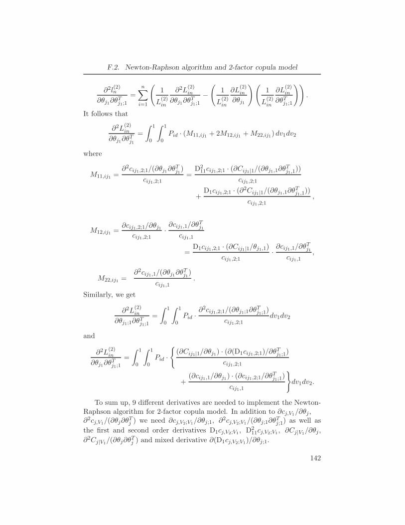
F.2. Newton-Raphson algorithm and 2-factor copula model
∂2l(2)n
∂θj1∂θTj1;1
=n∑
i=1
(1
L(2)in
∂2L(2)in
∂θj1∂θTj1;1
−(
1
L(2)in
∂L(2)in
∂θj1
)(1
L(2)in
∂L(2)in
∂θTj1;1
)).
It follows that
∂2L(2)in
∂θj1∂θTj1
=
∫ 1
0
∫ 1
0Pid · (M11,ij1 + 2M12,ij1 +M22,ij1) dv1dv2
where
M11,ij1 =∂2cij1,2;1/(∂θj1∂θ
Tj1)
cij1,2;1=
D211cij1,2;1 · (∂Cij1|1/(∂θj1,1∂θTj1,1))
cij1,2;1
+D1cij1,2;1 · (∂2Cij1|1/(∂θj1,1∂θTj1,1))
cij1,2;1,
M12,ij1 =∂cij1,2;1/∂θj1
cij1,2;1·∂cij1,1/∂θ
Tj1
cij1,1
=D1cij1,2;1 · (∂Cij1|1/θj1,1)
cij1,2;1·∂cij1,1/∂θ
Tj1
cij1,1,
M22,ij1 =∂2cij1,1/(∂θj1∂θ
Tj1)
cij1,1.
Similarly, we get
∂2L(2)in
∂θj1;1∂θTj1;1
=
∫ 1
0
∫ 1
0Pid ·
∂2cij1,2;1/(∂θj1;1∂θTj1;1
)
cij1,2;1dv1dv2
and
∂2L(2)in
∂θj1∂θTj1;1
=
∫ 1
0
∫ 1
0Pid ·
{(∂Cij1|1/∂θj1) · (∂(D1cij1,2;1)/∂θ
Tj1;1
)
cij1,2;1
+(∂cij1,1/∂θj1) · (∂cij1,2;1/∂θTj1;1)
cij1,1
}dv1dv2.
To sum up, 9 different derivatives are needed to implement the Newton-Raphson algorithm for 2-factor copula model. In addition to ∂cj,V1/∂θj ,∂2cj,V1/(∂θj∂θ
Tj ) we need ∂cj,V2;V1/∂θj;1, ∂
2cj,V2;V1/(∂θj;1∂θTj;1) as well as
the first and second order derivatives D1cj,V2;V1 , D211cj,V2;V1 , ∂Cj|V1/∂θj ,
∂2Cj|V1/(∂θj∂θTj ) and mixed derivative ∂(D1cj,V2;V1)/∂θj;1.
142
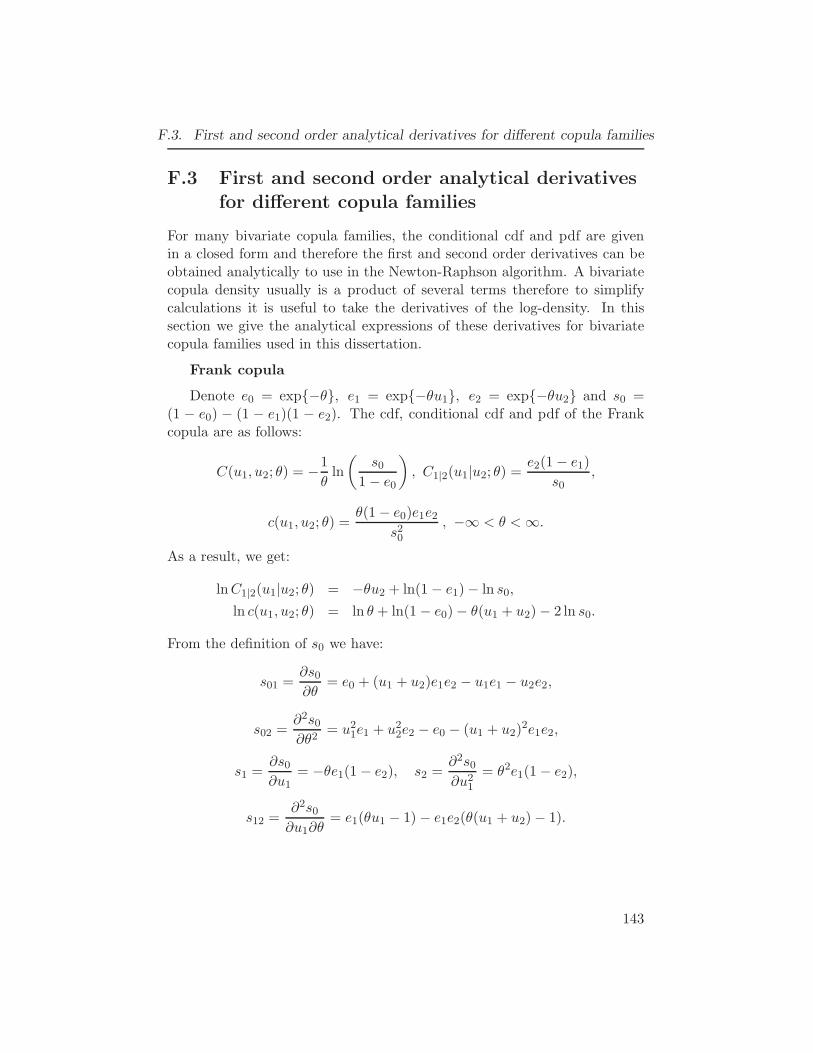
F.3. First and second order analytical derivatives for different copula families
F.3 First and second order analytical derivatives
for different copula families
For many bivariate copula families, the conditional cdf and pdf are givenin a closed form and therefore the first and second order derivatives can beobtained analytically to use in the Newton-Raphson algorithm. A bivariatecopula density usually is a product of several terms therefore to simplifycalculations it is useful to take the derivatives of the log-density. In thissection we give the analytical expressions of these derivatives for bivariatecopula families used in this dissertation.
Frank copula
Denote e0 = exp{−θ}, e1 = exp{−θu1}, e2 = exp{−θu2} and s0 =(1 − e0) − (1 − e1)(1 − e2). The cdf, conditional cdf and pdf of the Frankcopula are as follows:
C(u1, u2; θ) = −1
θln
(s0
1− e0
), C1|2(u1|u2; θ) =
e2(1− e1)
s0,
c(u1, u2; θ) =θ(1− e0)e1e2
s20, −∞ < θ <∞.
As a result, we get:
lnC1|2(u1|u2; θ) = −θu2 + ln(1− e1)− ln s0,
ln c(u1, u2; θ) = ln θ + ln(1− e0)− θ(u1 + u2)− 2 ln s0.
From the definition of s0 we have:
s01 =∂s0∂θ
= e0 + (u1 + u2)e1e2 − u1e1 − u2e2,
s02 =∂2s0∂θ2
= u21e1 + u22e2 − e0 − (u1 + u2)2e1e2,
s1 =∂s0∂u1
= −θe1(1− e2), s2 =∂2s0∂u21
= θ2e1(1− e2),
s12 =∂2s0∂u1∂θ
= e1(θu1 − 1)− e1e2(θ(u1 + u2)− 1).
143
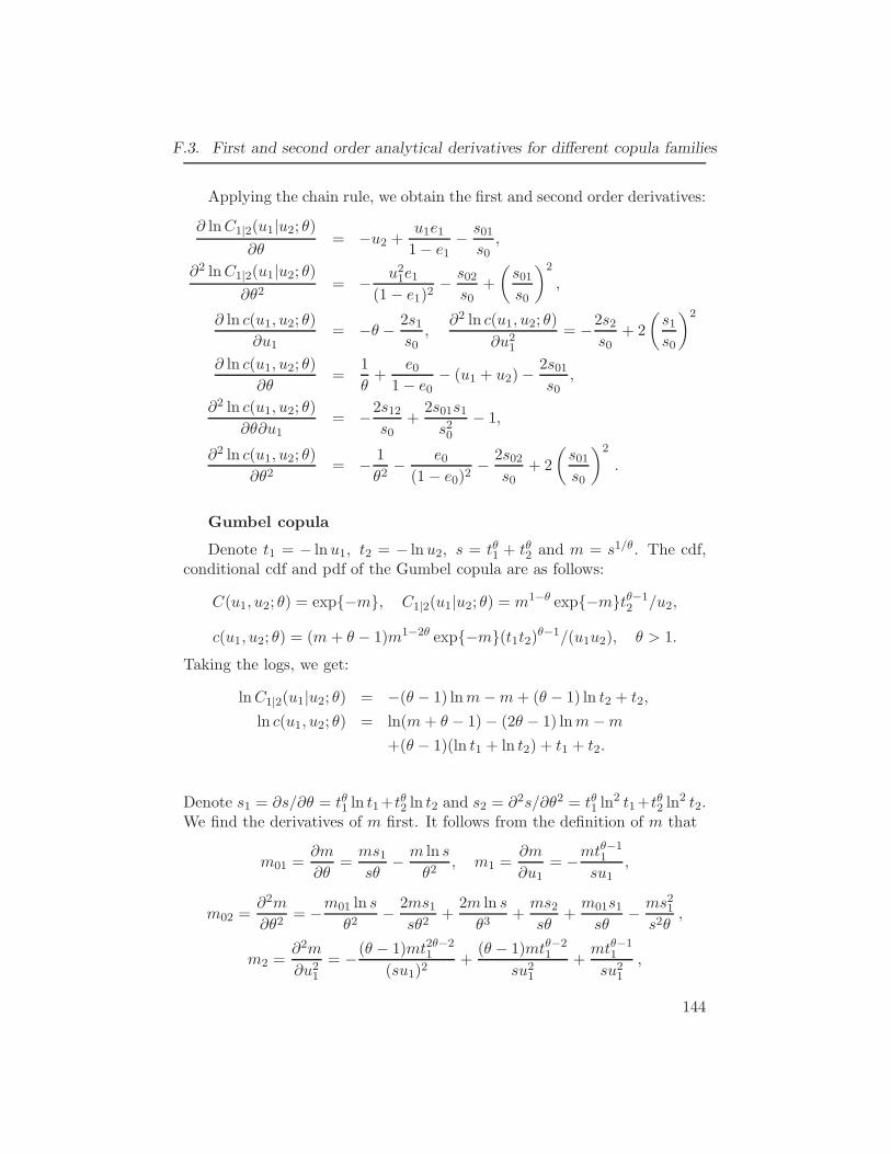
F.3. First and second order analytical derivatives for different copula families
Applying the chain rule, we obtain the first and second order derivatives:
∂ lnC1|2(u1|u2; θ)∂θ
= −u2 +u1e11− e1
− s01s0,
∂2 lnC1|2(u1|u2; θ)∂θ2
= − u21e1(1− e1)2
− s02s0
+
(s01s0
)2
,
∂ ln c(u1, u2; θ)
∂u1= −θ − 2s1
s0,
∂2 ln c(u1, u2; θ)
∂u21= −2s2
s0+ 2
(s1s0
)2
∂ ln c(u1, u2; θ)
∂θ=
1
θ+
e01− e0
− (u1 + u2)−2s01s0
,
∂2 ln c(u1, u2; θ)
∂θ∂u1= −2s12
s0+
2s01s1s20
− 1,
∂2 ln c(u1, u2; θ)
∂θ2= − 1
θ2− e0
(1− e0)2− 2s02
s0+ 2
(s01s0
)2
.
Gumbel copula
Denote t1 = − lnu1, t2 = − lnu2, s = tθ1 + tθ2 and m = s1/θ. The cdf,conditional cdf and pdf of the Gumbel copula are as follows:
C(u1, u2; θ) = exp{−m}, C1|2(u1|u2; θ) = m1−θ exp{−m}tθ−12 /u2,
c(u1, u2; θ) = (m+ θ − 1)m1−2θ exp{−m}(t1t2)θ−1/(u1u2), θ > 1.
Taking the logs, we get:
lnC1|2(u1|u2; θ) = −(θ − 1) lnm−m+ (θ − 1) ln t2 + t2,
ln c(u1, u2; θ) = ln(m+ θ − 1)− (2θ − 1) lnm−m
+(θ − 1)(ln t1 + ln t2) + t1 + t2.
Denote s1 = ∂s/∂θ = tθ1 ln t1+tθ2 ln t2 and s2 = ∂2s/∂θ2 = tθ1 ln
2 t1+tθ2 ln
2 t2.We find the derivatives of m first. It follows from the definition of m that
m01 =∂m
∂θ=ms1sθ
− m ln s
θ2, m1 =
∂m
∂u1= −mt
θ−11
su1,
m02 =∂2m
∂θ2= −m01 ln s
θ2− 2ms1
sθ2+
2m ln s
θ3+ms2sθ
+m01s1sθ
− ms21s2θ
,
m2 =∂2m
∂u21= −(θ − 1)mt2θ−2
1
(su1)2+
(θ − 1)mtθ−21
su21+mtθ−1
1
su21,
144
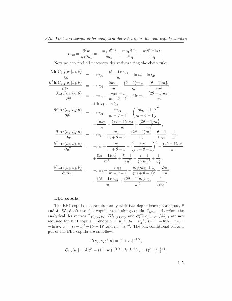
F.3. First and second order analytical derivatives for different copula families
m12 =∂2m
∂θ∂u1= −m01t
θ−11
su1+ms1t
θ−11
s2u1− mtθ−1
1 ln t1su1
.
Now we can find all necessary derivatives using the chain rule:
∂ lnC1|2(u1|u2; θ)∂θ
= −m01 −(θ − 1)m01
m− lnm+ ln t2,
∂2 lnC1|2(u1|u2; θ)∂θ2
= −m02 −2m01
m− (θ − 1)m02
m+
(θ − 1)m201
m2,
∂ ln c(u1, u2; θ)
∂θ= −m01 +
m01 + 1
m+ θ − 1− 2 lnm− (2θ − 1)m01
m+ ln t1 + ln t2,
∂2 ln c(u1, u2; θ)
∂θ2= −m02 +
m02
m+ θ − 1−(m01 + 1
m+ θ − 1
)2
−4m01
m− (2θ − 1)m02
m+
(2θ − 1)m201
m2,
∂ ln c(u1, u2; θ)
∂u1= −m1 +
m1
m+ θ − 1− (2θ − 1)m1
m− θ − 1
t1u1− 1
u1,
∂2 ln c(u1, u2; θ)
∂u21= −m2 +
m2
m+ θ − 1−(
m1
m+ θ − 1
)2
− (2θ − 1)m2
m
+(2θ − 1)m2
1
m2+θ − 1
t1u21− θ − 1
(t1u1)2+
1
u21,
∂2 ln c(u1, u2; θ)
∂θ∂u1= −m12 +
m12
m+ θ − 1− m1(m01 + 1)
(m+ θ − 1)2− 2m1
m
−(2θ − 1)m12
m+
(2θ − 1)m1m01
m2− 1
t1u1.
BB1 copula
The BB1 copula is a copula family with two dependence parameters, θand δ. We don’t use this copula as a linking copula Cj,V2;V1 therefore theanalytical derivatives D1cj,V2;V1 , D
211cj,V2;V1 and ∂(D1cj,V2;V1)/∂θj;1 are not
required for BB1 copula. Denote t1 = u−θ1 , t2 = u−θ2 , t01 = − lnu1, t02 =− lnu2, s = (t1 − 1)δ +(t2− 1)δ and m = s1/δ. The cdf, conditional cdf andpdf of the BB1 copula are as follows:
C(u1, u2; δ, θ) = (1 +m)−1/θ,
C1|2(u1|u2; δ, θ) = (1 +m)−(1/θ+1)m1−δ(t2 − 1)δ−1/uθ+12 ,
145
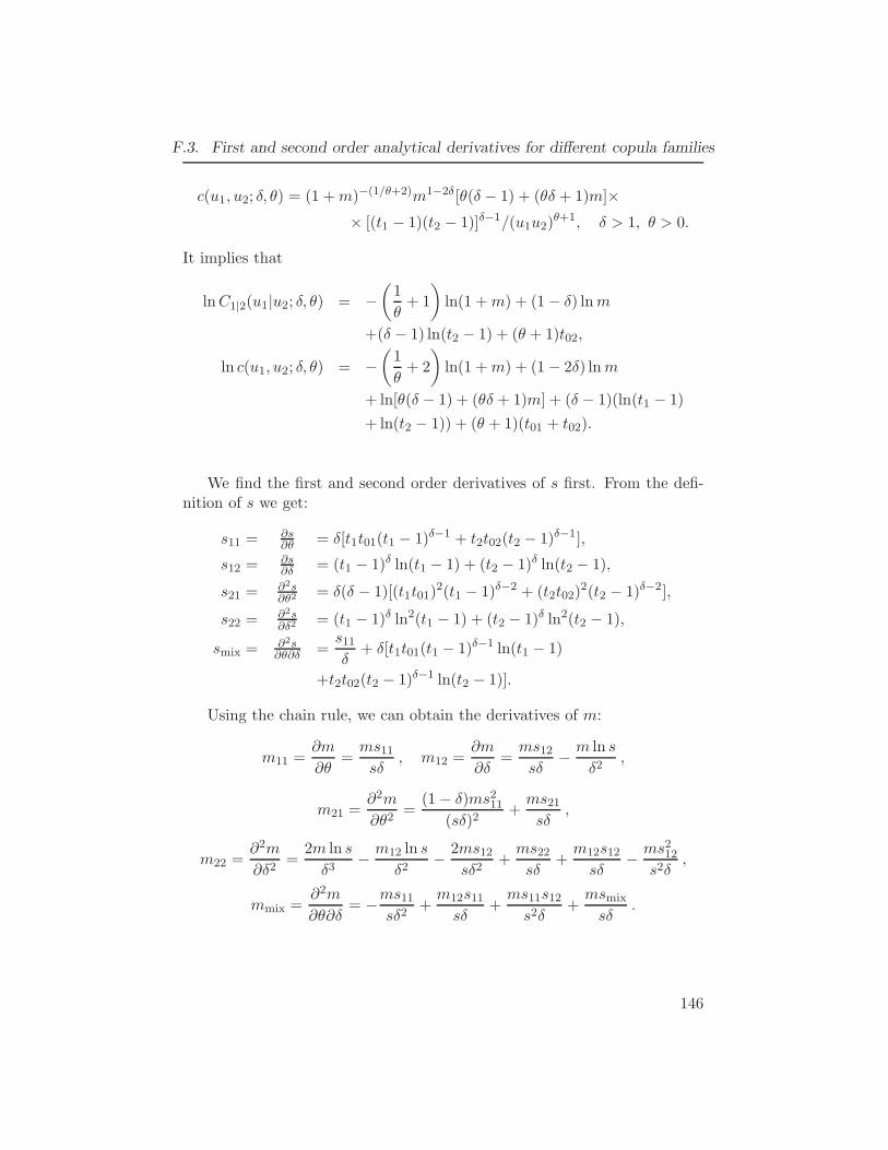
F.3. First and second order analytical derivatives for different copula families
c(u1, u2; δ, θ) = (1 +m)−(1/θ+2)m1−2δ [θ(δ − 1) + (θδ + 1)m]×× [(t1 − 1)(t2 − 1)]δ−1/(u1u2)
θ+1, δ > 1, θ > 0.
It implies that
lnC1|2(u1|u2; δ, θ) = −(1
θ+ 1
)ln(1 +m) + (1− δ) lnm
+(δ − 1) ln(t2 − 1) + (θ + 1)t02,
ln c(u1, u2; δ, θ) = −(1
θ+ 2
)ln(1 +m) + (1− 2δ) lnm
+ ln[θ(δ − 1) + (θδ + 1)m] + (δ − 1)(ln(t1 − 1)
+ ln(t2 − 1)) + (θ + 1)(t01 + t02).
We find the first and second order derivatives of s first. From the defi-nition of s we get:
s11 =∂s∂θ = δ[t1t01(t1 − 1)δ−1 + t2t02(t2 − 1)δ−1],
s12 =∂s∂δ = (t1 − 1)δ ln(t1 − 1) + (t2 − 1)δ ln(t2 − 1),
s21 =∂2s∂θ2 = δ(δ − 1)[(t1t01)
2(t1 − 1)δ−2 + (t2t02)2(t2 − 1)δ−2],
s22 =∂2s∂δ2
= (t1 − 1)δ ln2(t1 − 1) + (t2 − 1)δ ln2(t2 − 1),
smix = ∂2s∂θ∂δ =
s11δ
+ δ[t1t01(t1 − 1)δ−1 ln(t1 − 1)
+t2t02(t2 − 1)δ−1 ln(t2 − 1)].
Using the chain rule, we can obtain the derivatives of m:
m11 =∂m
∂θ=ms11sδ
, m12 =∂m
∂δ=ms12sδ
− m ln s
δ2,
m21 =∂2m
∂θ2=
(1− δ)ms211(sδ)2
+ms21sδ
,
m22 =∂2m
∂δ2=
2m ln s
δ3− m12 ln s
δ2− 2ms12
sδ2+ms22sδ
+m12s12sδ
− ms212s2δ
,
mmix =∂2m
∂θ∂δ= −ms11
sδ2+m12s11sδ
+ms11s12s2δ
+msmix
sδ.
146
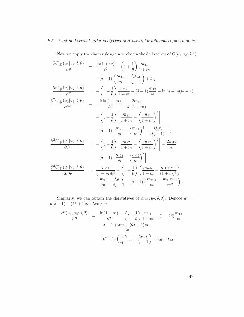
F.3. First and second order analytical derivatives for different copula families
Now we apply the chain rule again to obtain the derivatives of C(u1|u2; δ, θ):
∂C1|2(u1|u2; δ, θ)∂θ
=ln(1 +m)
θ2−(1 +
1
θ
)m11
1 +m
−(δ − 1)
(m11
m− t2t02t2 − 1
)+ t02,
∂C1|2(u1|u2; δ, θ)∂δ
= −(1 +
1
θ
)m12
1 +m− (δ − 1)
m12
m− lnm+ ln(t2 − 1),
∂2C1|2(u1|u2; δ, θ)∂θ2
= −2 ln(1 +m)
θ3+
2m11
θ2(1 +m)
−(1 +
1
θ
)[m21
1 +m−(m11
1 +m
)2]
−(δ − 1)
[m21
m−(m11
m
)2+
t202t2(t2 − 1)2
],
∂2C1|2(u1|u2; δ, θ)∂δ2
= −(1 +
1
θ
)[m22
1 +m−(m12
1 +m
)2]− 2m12
m
−(δ − 1)
[m22
m−(m12
m
)2],
∂2C1|2(u1|u2; δ, θ)∂θ∂δ
=m12
(1 +m)θ2−(1 +
1
θ
)(mmix
1 +m− m11m12
(1 +m)2
)
−m11
m+
t2t02t2 − 1
− (δ − 1)(mmix
m− m11m12
m2
).
Similarly, we can obtain the derivatives of c(u1, u2; δ, θ). Denote d∗ =θ(δ − 1) + (θδ + 1)m. We get:
∂c(u1, u2; δ, θ)
∂θ=
ln(1 +m)
θ2−(2 +
1
θ
)m11
1 +m+ (1− 2δ)
m11
m
+δ − 1 + δm+ (θδ + 1)m11
d∗
+(δ − 1)
(t1t01t1 − 1
+t2t02t2 − 1
)+ t01 + t02,
147
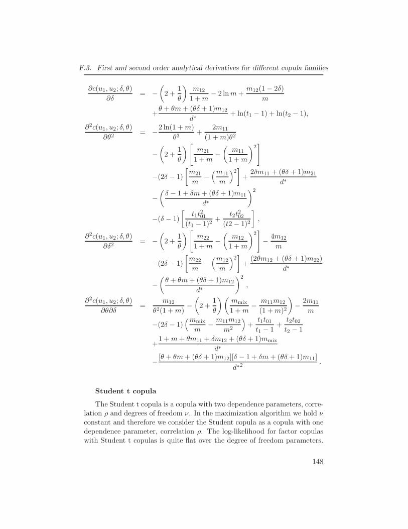
F.3. First and second order analytical derivatives for different copula families
∂c(u1, u2; δ, θ)
∂δ= −
(2 +
1
θ
)m12
1 +m− 2 lnm+
m12(1− 2δ)
m
+θ + θm+ (θδ + 1)m12
d∗+ ln(t1 − 1) + ln(t2 − 1),
∂2c(u1, u2; δ, θ)
∂θ2= −2 ln(1 +m)
θ3+
2m11
(1 +m)θ2
−(2 +
1
θ
)[m21
1 +m−(m11
1 +m
)2]
−(2δ − 1)
[m21
m−(m11
m
)2]+
2δm11 + (θδ + 1)m21
d∗
−(δ − 1 + δm+ (θδ + 1)m11
d∗
)2
−(δ − 1)
[t1t
201
(t1 − 1)2+
t2t202
(t2− 1)2
],
∂2c(u1, u2; δ, θ)
∂δ2= −
(2 +
1
θ
)[m22
1 +m−(m12
1 +m
)2]− 4m12
m
−(2δ − 1)
[m22
m−(m12
m
)2]+
(2θm12 + (θδ + 1)m22)
d∗
−(θ + θm+ (θδ + 1)m12
d∗
)2
,
∂2c(u1, u2; δ, θ)
∂θ∂δ=
m12
θ2(1 +m)−(2 +
1
θ
)(mmix
1 +m− m11m12
(1 +m)2
)− 2m11
m
−(2δ − 1)(mmix
m− m11m12
m2
)+
t1t01t1 − 1
+t2t02t2 − 1
+1 +m+ θm11 + δm12 + (θδ + 1)mmix
d∗
− [θ + θm+ (θδ + 1)m12][δ − 1 + δm+ (θδ + 1)m11]
d∗2.
Student t copula
The Student t copula is a copula with two dependence parameters, corre-lation ρ and degrees of freedom ν. In the maximization algorithm we hold νconstant and therefore we consider the Student copula as a copula with onedependence parameter, correlation ρ. The log-likelihood for factor copulaswith Student t copulas is quite flat over the degree of freedom parameters.
148
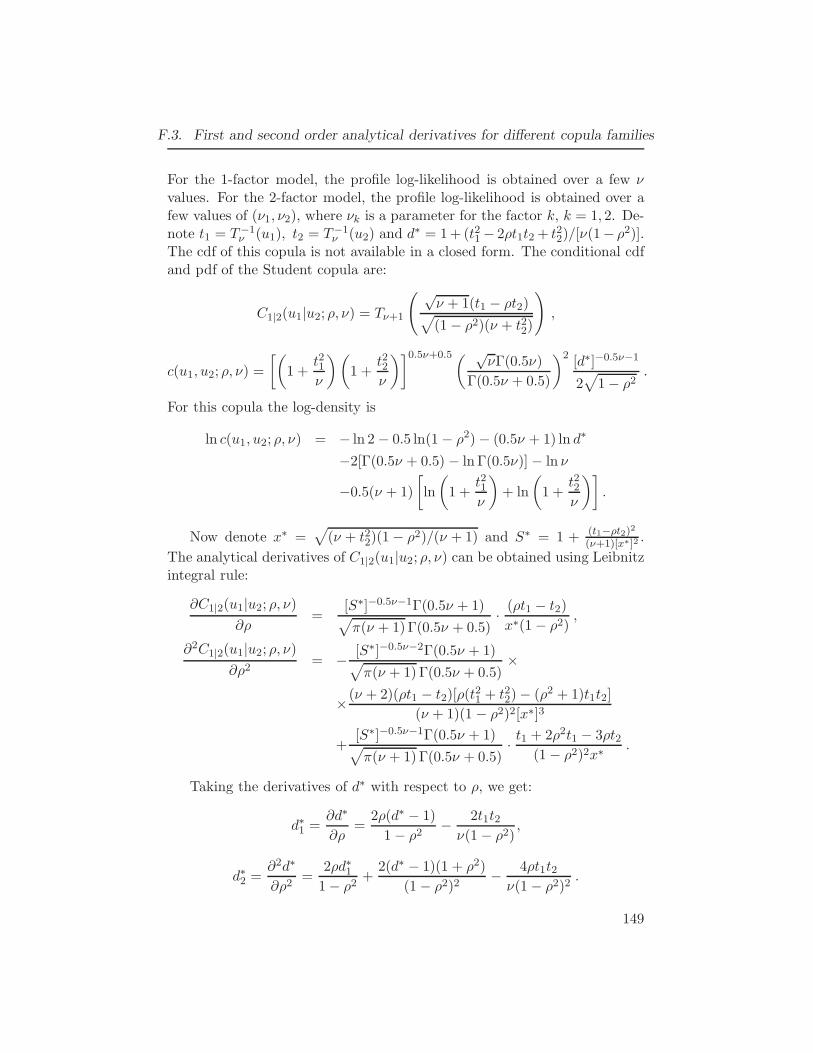
F.3. First and second order analytical derivatives for different copula families
For the 1-factor model, the profile log-likelihood is obtained over a few νvalues. For the 2-factor model, the profile log-likelihood is obtained over afew values of (ν1, ν2), where νk is a parameter for the factor k, k = 1, 2. De-note t1 = T−1
ν (u1), t2 = T−1ν (u2) and d
∗ = 1+ (t21 − 2ρt1t2 + t22)/[ν(1− ρ2)].The cdf of this copula is not available in a closed form. The conditional cdfand pdf of the Student copula are:
C1|2(u1|u2; ρ, ν) = Tν+1
( √ν + 1(t1 − ρt2)√(1− ρ2)(ν + t22)
),
c(u1, u2; ρ, ν) =
[(1 +
t21ν
)(1 +
t22ν
)]0.5ν+0.5( √νΓ(0.5ν)
Γ(0.5ν + 0.5)
)2[d∗]−0.5ν−1
2√
1− ρ2.
For this copula the log-density is
ln c(u1, u2; ρ, ν) = − ln 2− 0.5 ln(1− ρ2)− (0.5ν + 1) ln d∗
−2[Γ(0.5ν + 0.5) − ln Γ(0.5ν)] − ln ν
−0.5(ν + 1)
[ln
(1 +
t21ν
)+ ln
(1 +
t22ν
)].
Now denote x∗ =√
(ν + t22)(1− ρ2)/(ν + 1) and S∗ = 1 + (t1−ρt2)2(ν+1)[x∗]2
.
The analytical derivatives of C1|2(u1|u2; ρ, ν) can be obtained using Leibnitzintegral rule:
∂C1|2(u1|u2; ρ, ν)∂ρ
=[S∗]−0.5ν−1Γ(0.5ν + 1)√π(ν + 1)Γ(0.5ν + 0.5)
· (ρt1 − t2)
x∗(1− ρ2),
∂2C1|2(u1|u2; ρ, ν)∂ρ2
= − [S∗]−0.5ν−2Γ(0.5ν + 1)√π(ν + 1) Γ(0.5ν + 0.5)
×
×(ν + 2)(ρt1 − t2)[ρ(t21 + t22)− (ρ2 + 1)t1t2]
(ν + 1)(1 − ρ2)2[x∗]3
+[S∗]−0.5ν−1Γ(0.5ν + 1)√π(ν + 1) Γ(0.5ν + 0.5)
· t1 + 2ρ2t1 − 3ρt2(1− ρ2)2x∗
.
Taking the derivatives of d∗ with respect to ρ, we get:
d∗1 =∂d∗
∂ρ=
2ρ(d∗ − 1)
1− ρ2− 2t1t2ν(1− ρ2)
,
d∗2 =∂2d∗
∂ρ2=
2ρd∗11− ρ2
+2(d∗ − 1)(1 + ρ2)
(1− ρ2)2− 4ρt1t2ν(1− ρ2)2
.
149
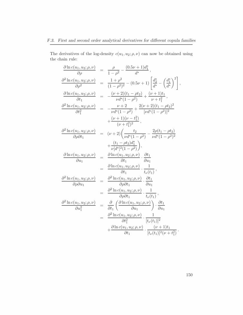
F.3. First and second order analytical derivatives for different copula families
The derivatives of the log-density c(u1, u2; ρ, ν) can now be obtained usingthe chain rule:
∂ ln c(u1, u2; ρ, ν)
∂ρ=
ρ
1− ρ2− (0.5ν + 1)d∗1
d∗,
∂2 ln c(u1, u2; ρ, ν)
∂ρ2=
1 + ρ2
(1− ρ2)2− (0.5ν + 1)
[d∗2d∗
−(d∗1d∗
)2],
∂ ln c(u1, u2; ρ, ν)
∂t1= −(ν + 2)(t1 − ρt2)
νd∗(1− ρ2)+
(ν + 1)t1ν + t21
,
∂2 ln c(u1, u2; ρ, ν)
∂t21= − ν + 2
νd∗(1− ρ2)+
2(ν + 2)(t1 − ρt2)2
[νd∗(1− ρ2)]2
+(ν + 1)(ν − t21)
(ν + t21)2
,
∂2 ln c(u1, u2; ρ, ν)
∂ρ∂t1= (ν + 2)
(t2
νd∗(1− ρ2)− 2ρ(t1 − ρt2)
νd∗(1 − ρ2)2
+(t1 − ρt2)d
∗1
ν[d∗]2(1− ρ2)
),
∂ ln c(u1, u2; ρ, ν)
∂u1=
∂ ln c(u1, u2; ρ, ν)
∂t1· ∂t1∂u1
=∂ ln c(u1, u2; ρ, ν)
∂t1· 1
tν(t1),
∂2 ln c(u1, u2; ρ, ν)
∂ρ∂u1=
∂2 ln c(u1, u2; ρ, ν)
∂ρ∂t1· ∂t1∂u1
=∂2 ln c(u1, u2; ρ, ν)
∂ρ∂t1· 1
tν(t1),
∂2 ln c(u1, u2; ρ, ν)
∂u21=
∂
∂t1
(∂ ln c(u1, u2; ρ, ν)
∂u1
)· ∂t1∂u1
=∂2 ln c(u1, u2; ρ, ν)
∂t21· 1
[tν(t1)]2
+∂ ln c(u1, u2; ρ, ν)
∂t1· (ν + 1)t1[tν(t1)]2(ν + t21)
.
150
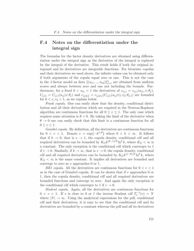
F.4. Notes on the differentiation under the integral sign
F.4 Notes on the differentiation under the
integral sign
The formulas for the factor density derivatives are obtained using differen-tiation under the integral sign as the derivative of the integral is replacedby the integral of the derivative. This result holds if both the original in-tegrand and its derivatives are integrable functions. For bivariate copulasand their derivatives we used above, the infinite values can be obtained onlyif both arguments of the copula equal zero or one. This is not the casein the 1-factor model as data {(ui1, ..., uid)}ni=1 are obtained from uniformscores and always between zero and one not including the bounds. Fur-thermore, for a fixed 0 < uij < 1 the derivatives of cij,1 = cij,1(uij , v; θj),Cij|1 = Cij,1(uij |v; θj) and cij|2;1 = cij|2;1(Cij|1(uij |v), v2; θj;1) are boundedfor 0 < v, v2 < 1, as we explain below.
Frank copula. One can easily show that the density, conditional distri-bution and all their derivatives which are required in the Newton-Raphsonalgorithm are continuous functions for all 0 ≤ v ≤ 1. The only case whichrequires some attention is θ = 0. By taking the limit of the derivative whenθ → 0 one can easily check that this limit is a continuous function for all0 ≤ v ≤ 1.
Gumbel copula. By definition, all the derivatives are continuous functionsfor 0 < v < 1. Denote v = exp{−k1/θ} where 0 < k < ∞. It followsthat if k → 0, that is v → 1, the copula density, conditional cdf and allrequired derivatives can be bounded by KGk
(θ−1)/θ ln2 k, where KG <∞ isa constant. The only exception is the conditional cdf which converges to 1if v → 0. Similarly, if k → ∞, that is v → 0, the copula density, conditionalcdf and all required derivatives can be bounded by KGk
(1−θ)/θ ln2 k, whereKG < ∞ is the same constant. It implies all derivatives are bounded andconverge to zero as v approaches 0 or 1.
BB1 copula. All the derivatives are continuous functions for 0 < v < 1as in the case of Gumbel copula. It can be shown that if v approaches 0 or1, then the copula density, conditional cdf and all required derivatives arebounded functions and converge to zero. And again the only exception isthe conditional cdf which converges to 1 if v → 0.
Student copula. Again, all the derivatives are continuous functions for0 < v < 1. If v is close to 0 or 1 the inverse Student cdf T−1
ν (v) = Nwhere |N | → ∞. Using the analytical expressions for the pdf, conditionalcdf and their derivatives, it is easy to see that the conditional cdf and itsderivatives are bounded by a constant whereas the pdf and all its derivatives
151
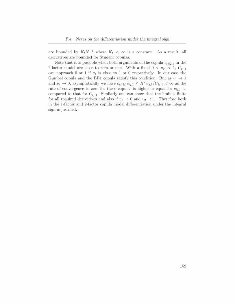
F.4. Notes on the differentiation under the integral sign
are bounded by KtN−1 where Kt < ∞ is a constant. As a result, all
derivatives are bounded for Student copulas.Note that it is possible when both arguments of the copula cij|2;1 in the
2-factor model are close to zero or one. With a fixed 0 < uij < 1, Cij|1can approach 0 or 1 if v1 is close to 1 or 0 respectively. In our case theGumbel copula and the BB1 copula satisfy this condition. But as v1 → 1and v2 → 0, asymptotically we have cij|2;1cij,1 ≤ K∗cij,1/Cij|1 < ∞ as therate of convergence to zero for these copulas is higher or equal for cij,1 ascompared to that for Cij|1. Similarly one can show that the limit is finitefor all required derivatives and also if v1 → 0 and v2 → 1. Therefore bothin the 1-factor and 2-factor copula model differentiation under the integralsign is justified.
152
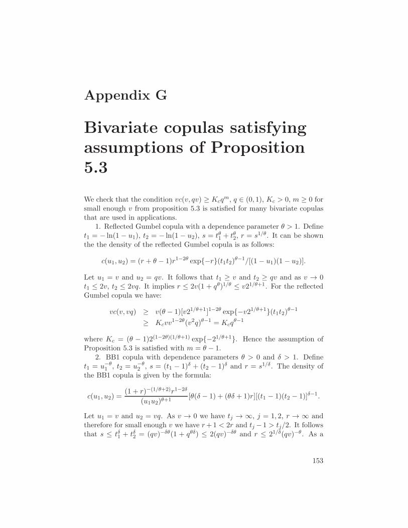
Appendix G
Bivariate copulas satisfying
assumptions of Proposition
5.3
We check that the condition vc(v, qv) ≥ Kcqm, q ∈ (0, 1), Kc > 0, m ≥ 0 for
small enough v from proposition 5.3 is satisfied for many bivariate copulasthat are used in applications.
1. Reflected Gumbel copula with a dependence parameter θ > 1. Definet1 = − ln(1 − u1), t2 = − ln(1 − u2), s = tθ1 + tθ2, r = s1/θ. It can be shownthe the density of the reflected Gumbel copula is as follows:
c(u1, u2) = (r + θ − 1)r1−2θ exp{−r}(t1t2)θ−1/[(1 − u1)(1 − u2)].
Let u1 = v and u2 = qv. It follows that t1 ≥ v and t2 ≥ qv and as v → 0t1 ≤ 2v, t2 ≤ 2vq. It implies r ≤ 2v(1 + qθ)1/θ ≤ v21/θ+1. For the reflectedGumbel copula we have:
vc(v, vq) ≥ v(θ − 1)[v21/θ+1]1−2θ exp{−v21/θ+1}(t1t2)θ−1
≥ Kcvv1−2θ(v2q)θ−1 = Kcq
θ−1
where Kc = (θ − 1)2(1−2θ)(1/θ+1) exp{−21/θ+1}. Hence the assumption ofProposition 5.3 is satisfied with m = θ − 1.
2. BB1 copula with dependence parameters θ > 0 and δ > 1. Definet1 = u−θ1 , t2 = u−θ2 , s = (t1 − 1)δ + (t2 − 1)δ and r = s1/δ . The density ofthe BB1 copula is given by the formula:
c(u1, u2) =(1 + r)−(1/θ+2)r1−2δ
(u1u2)θ+1[θ(δ − 1) + (θδ + 1)r][(t1 − 1)(t2 − 1)]δ−1.
Let u1 = v and u2 = vq. As v → 0 we have tj → ∞, j = 1, 2, r → ∞ andtherefore for small enough v we have r+1 < 2r and tj − 1 > tj/2. It followsthat s ≤ tδ1 + tδ2 = (qv)−δθ(1 + qθδ) ≤ 2(qv)−δθ and r ≤ 21/δ(qv)−θ. As a
153
Appendix G. Bivariate copulas satisfying assumptions of Proposition 5.3
result, for the BB1 copula we have:
vc(v, vq) ≥ v(2r)−(1/θ+2)r1−2δ[(θδ + 1)r](t1t2/4)δ−1(u1u2)
−θ−1
= K∗c vr
−1/θ−2δ(v2q)−θ(δ−1)−θ−1
≥ K∗c 2
−(1/(δθ)+2)v(qv)1+2θδ(v2q)−θδ−1 = Kcqθδ
where
K∗c = (θδ + 1)2−1/θ−2δ and Kc = K∗
c 2−(1/(θδ)+2) = (θδ + 1)2−(2+1/(θδ))(δ+1) .
Hence the assumption of Proposition 5.3 is satisfied with m = θδ.3. Student tν copula with dependence parameters ρ ∈ (−1; 1) and shape
parameter ν > 0. Define t1 = T−1ν (u1), t2 = T−1
ν (u2) and d∗ = 1 + (t21 −2ρt1t2 + t22)/[ν(1 − ρ2)]. The density of the Student copula is given by theformula:
c(u1, u2) =
[(1 +
t21ν
)(1 +
t22ν
)]0.5ν+0.5( √νΓ(0.5ν)
Γ(0.5ν + 0.5)
)2[d∗]−0.5ν−1
2√
1− ρ2.
Let u1 = v, u2 = vq. Using the asymptotic behavior of Student quan-tiles, as v → 0, we get −k−1 v−1/ν ≤ t1 ≤ −k+1 v−1/ν , −k−2 (vq)−1/ν ≤ t2 ≤−k+2 (vq)−1/ν for some positive constants k−1 , k
+1 , k
−2 , k
+2 . It implies d∗ ≤
1+(t1+t2)2/[ν(1−ρ2)] ≤ 1+(2t2)
2/[ν(1−ρ2)] ≤ 5t22/[ν(1−ρ2)] ≤ k3(vq)−2/ν ,
where k3 = 5(k−2 )2/[ν(1 − ρ2)]. Denote k4 =
( √νΓ(0.5ν)
Γ(0.5ν+0.5)
)21
2√
1−ρ2. For the
Student copula we have:
vc(v, vq) ≥ k4v[(t1t2)2/ν2]0.5ν+0.5[d∗]−0.5ν−1
≥ k4v[(k+1 k
+2 )
2(v2q)−2/ν/ν2]0.5ν+0.5[k3(vq)−2/ν ]−0.5ν−1
= Kcvv−2−2/νq−1−1/ν(vq)1+2/ν = Kcq
1/ν
where Kc = k4[k+1 k
+2 /ν]
ν+1k−0.5ν−13 . Hence the assumption of Proposition
5.3 is satisfied with m = 1/ν.
154
Appendix H
Derivatives of bivariate
linking copulas
In order to get the gradient and Hessian of the negative log-likelihood fornumerical minimization via a modified Newton-Raphson method, the fol-lowing derivatives are analytically needed. These derivatives are requiredwhen differentiating under the integral sign using the chain rule formula.
In a nested copula model (5.4) the following derivatives are required:
∂cVg ,V0(vg, v0; θg)
∂θg,
∂cUig ,Vg(uig, vg; ηig)
∂ηig
∂2cVg,V0(vg, v0; θg)
∂θg∂θTg,
∂2cUig,Vg(uig, vg; ηig)
∂ηig∂ηTig,
where θg, ηig are dependence parameters of the copulas CVg,V0 and CUig,Vg
respectively. In a bi-factor model (5.2) the required derivatives are as follows:
∂cUig ,V0(uij , v0; θig)
∂θig,
∂cUig ,Vg;V0(wig, vg; γig)
∂γig,
∂cUig,Vg;V0(wig, vg; γig)
∂wig,
∂CUig |V0(uig|v0; θig)∂θig
,∂2cUig,V0(uig, v0; θig)
∂θig∂θTig
,∂2cUig,Vg;V0(wig, vg; γig)
∂γig∂γTig
,
∂2cUig ,Vg;V0(wig, vg; γig)
∂w2ig
,∂2CUig|V0(uig|v0; θig)
∂θig∂θTig,
∂2cUig,Vg;V0(wig, vg; γig)
∂γig ∂wig,
where θig, γig are dependence parameters of the copula CUig,V0 and CUig,Vg;V0
respectively.For the common bivariate copula families, the density along with the
partial derivatives are available in a closed form. As such, the requiredderivatives of the cU (u) can be represented as integrals of some explicitfunctions and can be computed using numerical integration.
155
Appendix I
Correlation matrix inverse
and determinant in the
structured factor Gaussian
model
Let ϕ be a d× 1 vector of dependence parameters for copulas CUij ,V0 and γbe a d× 1 vector of dependence parameters for copulas CUig ,Vg;V0 :
ϕ = (ϕ11, . . . , ϕd11, · · · , ϕ1G, . . . , ϕdGG),
γ = (γ11, . . . , γd11, · · · , γ1G, . . . , γdGG).
The joint copula density c(u) in the model is a Gaussian copula density withan d× d correlation matrix Σ:
c(u) =φd(u;Σ)∏i,g φ(uig)
=1
|Σ|1/2 exp
−1
2
∑
k1 6=k2Σ−1k1k2
uk1uk2 +
d∑
k=1
(Σ−1k,k − 1)u2
k
(I.1)
where φd is a d-dimensional Gaussian density and u = Φ−1(u). As it followsfrom the definition, Σ = ϕϕT + ηηT where η = γ(1 − ϕ2)1/2 is a vector ofunconditional correlations. From the other hand, we can use formula (5.2) toderive the expression for c(u). In the model, CUig,V0 , CUig,Vg;V0 are Gaussiancopulas and therefore
c(u) =
∫ 1
0
G∏
g=1
Kg(v0)
∫ 1
0
dg∏
i=1
exp
{−γ2ig ξ
2ig − 2γig ξigvg + γ2igv
2g
2(1− γ2ig)
}dvg
dv0
=
∫ 1
0
G∏
g=1
Kg(v0)
∫ 1
0
dg∏
i=1
exp
{−1
2(Ag v
2g − 2Bg vg + Cg)
}dvg
dv0, (I.2)
156
Appendix I. Correlation matrix inverse and determinant in the structured factor Gaussian model
Ag =
dg∑
i=1
γ2ig1− γ2ig
, Bg =
dg∑
i=1
ξigγig1− γ2ig
, Dg =
dg∑
i=1
ξ2igγ2ig
1− γ2ig,
Kg(v0) =
dg∏
i=1
cUig,V0(uig, v0)
(1− γ2ig)1/2
,
where ξig = CUig|V0(uig|v0) and ξig = Φ−1(ξig) = (uig − ϕig v0)/(1 − ϕ2ig)
1/2.For any constants a > 0, b and c we have:
∫ ∞
−∞exp
{−1
2(av2 − 2bv + c)
}dv =
(2π
a
)1/2
exp
{b2 − ac
2a
}
and therefore∫ 1
0exp
{−1
2(Ag v
2g − 2Bgvg +Dg)
}dvg =
=
∫ ∞
−∞exp
{−1
2(Ag v
2g − 2Bg vg +Dg)
}1
(2π)1/2exp
{−v2g2
}dvg
=1
(Ag + 1)1/2exp
{B2g
2(Ag + 1)− Dg
2
}.
From (I.2) we get:
c(u) =
∫ 1
0
G∏
g=1
Kg(v0)
(Ag + 1)1/2exp
{B2g
2(Ag + 1)− Dg
2
} dv0
=1
M1/21
∫ 1
0
G∏
g=1
dg∏
i=1
cUig,V0(uig, v0)
exp
G∑
g=1
[B2g
2(Ag + 1)− Dg
2
] dv0,
(I.3)
where M1 =∏Gg=1
[(Ag + 1)
∏dgi=1(1− γ2ig)
]. We have:
G∏
g=1
dg∏
i=1
cig,V0(uig, v0) =
G∏
g=1
dg∏
i=1
1
(1− ϕ2ig)
1/2
×
×G∏
g=1
dg∏
i=1
exp
{−ϕ2igu
2ig − 2ϕiguigv0 + ϕ2
ig v20
2(1 − ϕ2ig)
}
=1
M1/22
exp
{−1
2(A0v
20 − 2B0v0 +D0)
},
157
Appendix I. Correlation matrix inverse and determinant in the structured factor Gaussian model
A0 =
G∑
g=1
dg∑
i=1
ϕ2ig
1− ϕ2ig
, B0 =
G∑
g=1
dg∑
i=1
ϕiguig1− ϕ2
ig
, D0 =
G∑
g=1
dg∑
i=1
ϕ2igu
2ig
1− ϕ2ig
,
where M2 =∏Gg=1
∏dgi=1(1 − ϕ2
ig). Combining all terms with v0 and v20 , weget:
exp
G∑
g=1
[B2g
2(Ag + 1)− Cg
2
] = exp
{−1
2(A∗v20 − 2B∗v0 +D∗)
},
A∗ =G∑
g=1
dg∑
i=1
γ2ig1− γ2ig
·ϕ2ig
1− ϕ2ig
−G∑
g=1
1
Ag + 1
dg∑
i=1
γig1− γ2ig
· ϕig
(1− ϕ2ig)
1/2
2
,
B∗ =G∑
g=1
dg∑
i=1
γ2ig1− γ2ig
· ϕiguig1− ϕ2
ig
−G∑
g=1
1
Ag + 1
dg∑
i=1
γig1− γ2ig
· uig
(1− ϕ2ig)
1/2
×
×
dg∑
i=1
γig1− γ2ig
· ϕig
(1− ϕ2ig)
1/2
,
D∗ =G∑
g=1
dg∑
i=1
γ2ig1− γ2ig
·u2ig
1− ϕ2ig
−G∑
g=1
1
Ag + 1
dg∑
i=1
γig1− γ2ig
· uig
(1− ϕ2ig)
1/2
2
.
Finally, as it follows from (I.3),
c(u) =1
(M1M2)1/2×
×∫ 1
0exp
{−1
2((A0 +A∗)v20 − 2(B0 +B∗)v0 + (C0 +C∗))
}dv0
=1
(M1M2(A+ 1))1/2exp
{B2
2(A+ 1)− D
2
}, (I.4)
158
Appendix I. Correlation matrix inverse and determinant in the structured factor Gaussian model
A =
G∑
g=1
dg∑
i=1
1
1− γ2ig·
ϕ2ig
1− ϕ2ig
−G∑
g=1
1
Ag + 1
dg∑
i=1
γig1− γ2ig
· ϕig
(1− ϕ2ig)
1/2
2
,
B =G∑
g=1
dg∑
i=1
1
1− γ2ig· uigϕig1− ϕ2
ig
−G∑
g=1
1
Ag + 1
dg∑
i=1
γig1− γ2ig
· uig
(1− ϕ2ig)
1/2
×
×
dg∑
i=1
γig1− γ2ig
· ϕig
(1− ϕ2ig)
1/2
,
D =G∑
g=1
dg∑
i=1
[1
1− γ2ig· 1
1− ϕ2ig
− 1
]u2ig−
−G∑
g=1
1
Ag + 1
dg∑
i=1
γig1− γ2ig
· uig
(1− ϕ2ig)
1/2
2
.
Denote ζ∗ig =1
1−γ2ig· ϕ2
ig
1−ϕ2ig, ζ∗∗ig =
γig1−γ2ig
· 1(1−ϕ2
ig)1/2 and ηg =
∑dgi=1 ζ
∗∗ig ϕig,
ξig =ζ∗igϕig
− ηgAgζ∗∗ig . By combining terms with ui1g1 ui2,g2 for different i1, i2, g1,
g2 and comparing the right hand sides of (I.1) and (I.4) we get:
|Σ| = (A+ 1)M1M2, (Σgg)ii =1
1− γ2ig· 1
1− ϕ2ig
−ξ2ig
A+ 1−
(ζ∗∗ig )2
Ag + 1,
(Σgg)i1i2 = −ξi1gξi2gA+ 1
−ζ∗∗i1gζ
∗∗i2g
Ag + 1, (Σg1g2)i1i2 = −ξi1g1ξi2g2
A+ 1, i1 6= i2, g1 6= g2,
where Σgg is a block of the inverse correlation matrix Σ−1 corresponding tothe correlations within the g-th group.
159