Bayesian Inference and Model Assessment for the

Analysis of Smooth Transition Autoregressive Time

Series Models

Hedibert Freitas Lopes

Graduate School of Business, University of Chicago,

1101 58th Street, Chicago, IL 60637, USA.

hedibert.lopes@gsb.uchicago.edu

and

Esther Salazar

Instituto de Matematica, Universidade Federal do Rio de Janeiro,

Av. Brigadeiro Trompowsky, Cidade Universitaria - Ilha do Fundao.

Caixa Postal 68530, 21945-970

Rio de Janeiro - RJ - Brasil

esalazar@dme.ufrj.br

1

Abstract

In this paper we propose a fully Bayesian approach to the special class of nonlinear

time series models called the logistic smooth transition autoregressive (LSTAR) model.

Initially, a Gibbs sampler is proposed for the LSTAR where the lag length, k, is kept

fixed. Then, uncertainty about k is taken into account and a novel reversible jump

Markov Chain Monte Carlo (RJMCMC) algorithm is proposed. We compared our

RJMCMC algorithm with well known information criteria, such as the AIC, the BIC,

and the DIC. Our methodology is extensively studied against simulated and real time

series.

Keywords: Markov Chain Monte Carlo, nonlinear time series model, model selection,

reversible jump MCMC, Deviance Information Criterion.

2

1 INTRODUCTION

Smooth transition autoregressive (STAR) models, initially proposed in its univariate form

by Chan and Tong (1986) and further developed by Luukkonen, Saikkonen, and Terasvirta

(1988) and Terasvirta (1994), have been extensively studied over the last twenty years in

association to the measurement, testing and forecasting of nonlinear financial time series.

The STAR model can be seen as a continuous mixture of two AR(k) models, with the weight-

ing function defining the degree of nonlinearity. In this article, we focus on an important

subclass of the STAR model, the logistic STAR model of order k, or simply the LSTAR(k)

model, where the weighting function has the form of a logistic function.

van Dijk, Terasvirta, and Franses (2002) make an extensive review of recent developments

related to the STAR model and its variants. From the Bayesian point of view, Lubrano (2000)

used weighted resampling schemes (Smith and Gelfand 1992) to perform exact posterior

inference of both linear and nonlinear parameters. Our main contribution is to propose an

MCMC algorithm that fully accounts for model order uncertainty, ie. we assume that k is

one of the parameters of the model. To this end, a reversible jump Markov chain Monte

Carlo (RJMCMC) algorithm is tailored. As a by product, we also propose a Gibbs sampler

when k is kept fixed.

The rest of the article is organized as follows. Next section defines the general LSTAR(k)

model, while Section discusses prior specification and lays down a MCMC algorithm for

posterior inference when the model order, k, is kept fixed. Uncertainty about k is treated in

Section 4, where our novel RJMCMC is introduced. Finally, Section includes several simu-

lated and real time series to substantiate our methods, with final thoughts and perspectives

listed in Section .

2 THE LOGISTIC STAR MODEL

Let yt be the observed value of a time series at time t and xt = (1, yt−1, . . . , yt−k)′ the

3

vector of regressors corresponding to the intercept plus k lagged values, for t = 1, . . . , n. The

logistic smooth transition autoregressive model of order k, or simply LSTAR(k), is defined

as follows,

yt = x′tθ1 + π(γ, c, st)x′tθ2 + εt εt ∼ N(0, σ2) (1)

with π playing the role of a smooth transition continuous function bounded between 0 and

1. In this paper we focus on the logistic transition, ie. π(γ, c, st) = {1 + exp (−γ(st − c))}−1.

Several other functions could be easily accommodated, such as the exponential or the second-

order logistic function (van Dijk, Terasvirta, and Franses 2002). The parameter γ > 0 is

responsible for the smoothness of π, while c is a location or threshold parameter and d is

the delay parameter. When γ → ∞, the LSTAR model reduces to the well known self-

exciting TAR (SETAR) model (Tong 1990) and when γ = 0 the standard AR(k) model

arises. Finally, st is called the transition variable, with st = yt−d commonly used (Terasvirta

1994). Even though we use yt−d as the transition variable throughout this paper, it is worth

emphasizing that any other linear/nonlinear functions of exogenous/endogenous variables

can be easily included with minor changes in the algorithms presented and studied in this

paper. We will also assume throughout the paper, without loss of generality, that d ≤ k

and y−k+1, . . . , y0 are known and fixed quantities. This is common practice in the time series

literature and would only marginally increase the complexity of our computation and could

easily be done by introducing a prior distribution for those missing values.

The LSTAR(k) model can be seen as model that allows smooth and continuous shifts

between two extreme regimes. More specifically, if δ = θ1 + θ2, then x′tθ1 and x′tδ represent

the conditional means under the two extreme regimes,

yt = (1− π(γ, c, yt−d))x′tθ1 + π(γ, c, yt−d)x

′tδ + εt (2)

4

or,

yt =

x′tθ1 + εt if π = 0

(1− π)x′tθ1 + πx′tδ + εt if 0 < π < 1

x′tδ + εt if π = 1

Therefore, the model (2) can be expressed as (1) with θ2 = δ2− θ1 being the contribution to

the regression of considering a second regime. We consider the following parameterization

that will be very useful in the computation of the posterior distributions:

yt = z′tθ + εt (3)

where θ′ = (θ′1, θ′2) represent the linear parameters, (γ, c) are the nonlinear parameters,

Θ = (θ, γ, c), and z′t = (x′t, π(γ, c, yt−d)x′t). The dependence of zt on γ, c and yt−d will be

made explicit whenever necessary.

3 INFERENCE

In this section we derive MCMC algorithm for posterior assessment based on two dis-

tinct prior specifications: (i) standard conditionally conjugate prior distribution, and (ii)

Lubrano’s prior. We develop inferential procedure for both linear and nonlinear parameters

and for the observable variance, σ2, so that the number of parameters to be estimated is

2k + 5. We also consider the estimation of the delay parameter d. Fully Bayesian inference

(including k) is delayed until next section.

3.1 Prior Distributions

We investigate posterior sensitivity to two funtional forms for the prior distribution. In

the first case, we adopt the following conditionally conjugate priors: θ ∼ N(mθ, σ2θI2k+2), γ ∼

G(a, b), c ∼ N(mc, σ2c ) and σ2 ∼ IG(v/2, vs2/2), with hyperparameters mθ, σ

2θ , a, b, mc, σ

2c , v

and s2 chosen to represent relatively little prior information. In the second case, we adopt

Lubrano’s (2000) prior distributions where (θ2|σ2, γ) ∼ N(0, σ2eγIk+1) and π(θ1, γ, σ2, c) ∝

5

(1 + γ2)−1σ−2 for θ1 ∈ <k+1, γ, σ2 > 0 and c ∈ [ca, cb], such that the conditional prior for

θ2 becomes more informative as γ approaches zero, relatively noninformative prior about

θ1 and γ, noninformative prior about σ2 and relatively noninformative prior about c, with

ca = F−1(0.15), cb = F−1(0.85), and F the data’s empirical cumulative distribution function.

3.2 Posterior assessment

In this section we assume that k is known. So, the posterior simulation for θ, γ, c and

σ2 is done using the MCMC algorithm. More specifically, the full conditional posterior of θ

and σ2 (non depending on the form of the prior: subjective or objective) are respectively,

normal and inverse gamma, in this case is possible to use the Gibbs sampling algorithm

(Gelfand and Smith 1990). On the other hand, the full conditional of γ and c is unknown,

in this case we use the Metropolis-Hastings algorithm (Metropolis, Rosenbluth, Rosenbluth,

Teller, and Teller (1953), Hastings (1970)). For more details about Gibbs sampling and

Metropolis-Hastings algorithms see Gilks, Richardson, and Spiegelhalter (1996) or the books

by Gamerman (1997) and Robert and Casella (1999). Below, [ξ] denoted the full conditional

distribution for the parameter ξ conditional on all the other parameters, and∑

is short for∑n

t=1.

3.2.1 Conditionally Conjugate Priors

The full conditional distributions when the conditionally conjugate prior distribution is

used are:

[θ] Combining yt ∼ N (z′tθ, σ2) with θ ∼ N(mθ, σ

2θI2k+2), it is easy to see that [θ] ∼

N(mθ, Cθ), where C−1θ = σ−2

θ I2k+2 + σ−2∑

ztz′t and mθ = Cθ{σ−2

∑ztyt + σ−2

θ mθ};

[σ2] By noticing that εt = yt−z′tθ ∼ N(0, σ2), it can be seen that [σ2] ∼ IG[(T +v)/2, (vs2+∑

ε2t )/2];

[γ, c] The joint full conditional distribution of γ and c has no known form, so we them

6

jointly by using an random-walk Metropolis step, with γ∗ ∼ G[(γ(i))2/∆γ, γ

(i)/∆γ

]

and c∗ ∼ N(c(i), ∆c) the proposal densities, where γ(i) and c(i) are the current values

of γ e c. The pair (γ∗, c∗) is accepted with probability α = min{1, A}, where

A =

∏nt=1 dN(yt|z′t∗θ, σ2)∏nt=1 dN(yt|z′tθ, σ2)︸ ︷︷ ︸likelihood ratio

dG(γ∗|a, b)dN(c∗|mc, σ2c )

dG(γ(i)|a, b)dN(c(i)|mc, σ2c )︸ ︷︷ ︸

prior ratio

× dG(γ(i)|(γ∗)2/∆γ, γ∗/∆γ)

dG(γ∗|(γ(i))2/∆γ, γ(i)/∆γ)︸ ︷︷ ︸proposal ratio

where z′t∗ = z′t(γ∗, c∗, d), dG and dN are the probability density functions of the gamma

and the normal, respectively. ∆γ and ∆c are chosen such that the acceptance proba-

bility is between 10% and 50%, for instance.

[d] Inference about the delay parameter d is rather trivial. Let p(d) be the prior probability

of d, for d in {1, . . . , dmax} and some pre-specified dmax. The posterior conditional

posterior distribution for d is, therefore, p(d|y, θ) ∝ p(y|d, θ)p(d). This way, (θ, γ, c, d)

form the new vector parameter. After the convergence of the Markov chain has been

reached, the sequence d(1), d(2), . . . , d(M) represent the marginal posterior sample of d,

i.e. P (d|y).

3.2.2 Lubrano’s Prior

The full conditional distributions when Lubrano’s prior distribution is used are:

[θ] Combining yt ∼ N(z′tθ, σ2) with (θ2|σ2, γ) ∼ N(0, σ2e−γIk+1), it is easy to see that

[θ] ∼ N(m∗θ, C

∗θ ) where C∗

θ = (∑

ztz′tσ−2 + Σ−1), m∗

θ = Σθ (∑

ztytσ−2) and,

Σ−1 =

0 0

0 σ−2e−γIk+1

(4)

[σ2] From model (3), εt = yt − z′tθ ∼ N(0, σ2), which combined with the non-informative

prior π(σ2) ∝ σ−2, leads to [σ2] ∼ IG((T + k + 1)/2, (e−γθ′2θ2 +∑

ε2t )/2).

7

[γ, c] Again, γ∗ ∼ G[(γ(i))2/∆γ, γ(i)/∆γ] and c∗ ∼ N(c(i), ∆c), truncated at the interval

[ca, cb], and γ(i) and c(i) current values of γ and c. The pair (γ∗, c∗) is accepted with

probability α = min{1, A}, where

A =

∏Tt=1 fN(ε∗t |0, σ2)∏Tt=1 fN(ε

(i)t |0, σ2)

fN(θ2|0, σ2eγ∗Ik+1)

fN(θ2|0, σ2eγ(i)Ik+1)

π(γ∗)π(c∗)π(γ(i))π(c(i))

× ×

[φ

(cb−c(i)√

∆c

)− φ

(ca−c(i)√

∆c

)]fG(γ(i)|(γ∗)2/∆γ, γ

∗/∆γ)[φ

(cb−c∗√

∆c

)− φ

(ca−c∗√

∆c

)]fG(γ∗|(γ(i))2/∆γ, γ(i)/∆γ)

where ε∗t = yt− z′t(γ∗, c∗, yt−d)θ, ε

(i)t = yt− z′t(γ

(i), c(i), yt−d)θ and φ(.) is the cumulative

distribution function of the standard normal distribution.

[d] Similar to Section 3.2.1.

4 CHOOSING THE MODEL ORDER k

In this section we started introducing the traditional information criteria, AIC (Akaike

1974) and BIC (Schwarz 1978), widely used in model selection/comparation. To this toolbox

we add the DIC (Deviance Information Criterion) that is a criterion recently developed and

widely discussed in Spiegelhalter, Best, Carlin, and Linde (2002). The second part of this

Section we adapted the Reversible Jump MCMC (RJMCMC), proposed by Green (1995),

to LSTAR(k) models, where k is unknown. Standard MCMC algorithms can not be used

since the dimension of the parameter vector is also a parameter.

4.1 Information Criteria

Traditionally, model order or model specification are compared through the computation

of information criteria, which are well known for penalizing likelihood functions of over-

parametrized models. AIC (Akaike 1974) and BIC (Schwarz 1978) are the most used ones.

For data y and parameter θ, these criteria are defined as follows: AIC = −2 ln(p(y|θ)) + 2d

8

and BIC = −2 ln(p(y|θ)) + d ln n, d is the dimension of θ, with equals d = 2k + 5 for

LSTAR(k), sample size n and maximum likelihood estimator, θ . One of the major problems

with AIC/BIC is that define k is not trivial, mainly in Bayesian Hierarchical models, where

the priors act like reducers of the effective number of parameters through its interdependen-

cies. To overcome this limitation, Spiegelhalter, Best, Carlin, and Linde (2002) developed an

information criterion that properly defines the effective number parameter by pD = D−D(θ),

where D(θ) = −2 ln p(y|θ) is the deviance, θ = E(θ|y) and D = E(D(θ)|y). As a by-product,

they proposed the Deviance Information Criterion: DIC = D(θ)+2pD = D+pD. One could

argue that the most attractive and appealing feature of the DIC is that it combines model fit

(measured by D) with model complexity (measured by pD). Besides, DICs are more attrac-

tive than Bayes Factors since the former can be easily incorporated into MCMC routines.

For successful implemenations of DIC we refer to Zhu and Carlin (2000) (spatio-temporal

hierarchical models) and Berg, Meyer, and Yu (2004) (stochastic volatility models), to name

a few.

4.2 RJMCMC in LSTAR(k) models

Proposals to incorporate k in a fully Bayesian modeling already exist in literature. For

example, Huerta and Lopes (2000) analyzed the Brazilian Industrial Production through

AR(k) model where k = 2c + s, i.e. c pairs of complex roots and s real roots, consider c and

s, and therefore k unknown. Troughton and Godsill (1997) suggest a RJMCMC algorithm

for AR(k). We generalize the work of Troughton and Godsill (1997) proposing a RJMCMC

(Green 1995) that permit the incorporation of k in the parameter vector for LSTAR(k)

models.

In LSTAR(k) models the parameter vector θ of dimension (2k + 2× 1), defined in (1), is

sampling according to the model order k. So, sampling k involve a change in dimensionality

and so in the parametric space of the model. The idea is propose a move from a parameter

space of dimension k to one of dimension k′, where φ = (γ, c, σ2, d) have the same interpre-

9

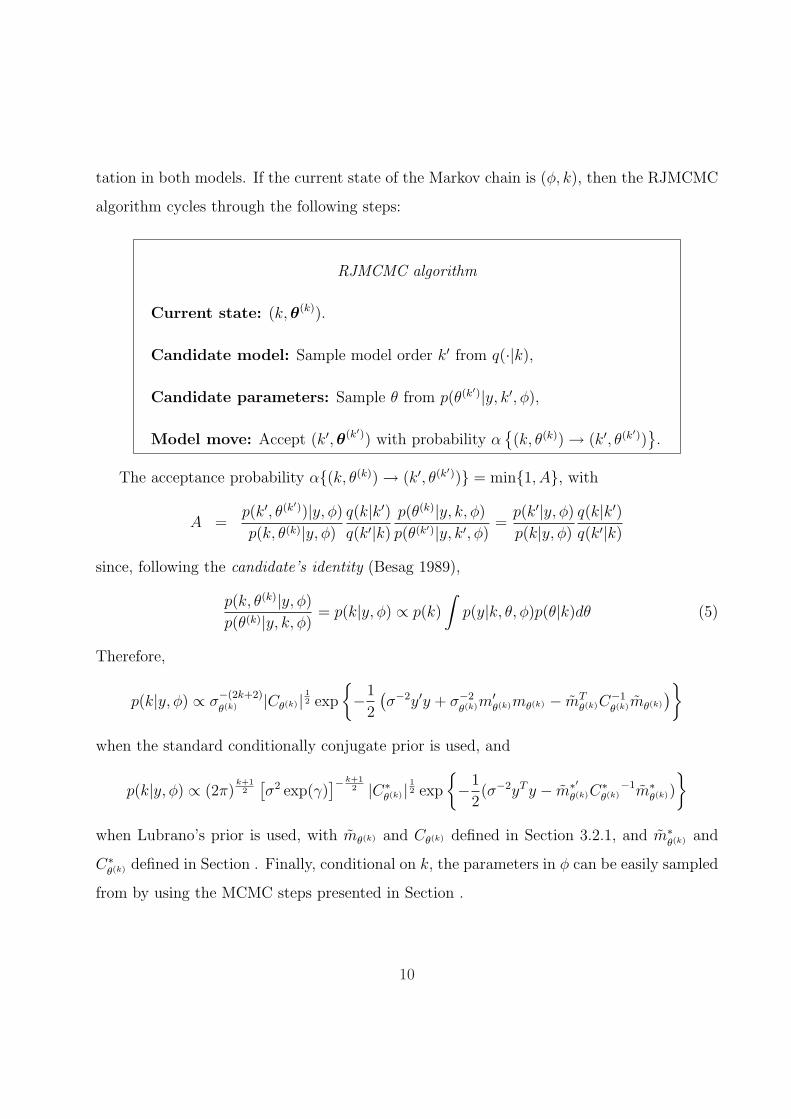
tation in both models. If the current state of the Markov chain is (φ, k), then the RJMCMC

algorithm cycles through the following steps:

RJMCMC algorithm

Current state: (k, θ(k)).

Candidate model: Sample model order k′ from q(·|k),

Candidate parameters: Sample θ from p(θ(k′)|y, k′, φ),

Model move: Accept (k′,θ(k′)) with probability α{(k, θ(k)) → (k′, θ(k′))

}.

The acceptance probability α{(k, θ(k)) → (k′, θ(k′))} = min{1, A}, with

A =p(k′, θ(k′))|y, φ)

p(k, θ(k)|y, φ)

q(k|k′)q(k′|k)

p(θ(k)|y, k, φ)

p(θ(k′)|y, k′, φ)=

p(k′|y, φ)

p(k|y, φ)

q(k|k′)q(k′|k)

since, following the candidate’s identity (Besag 1989),

p(k, θ(k)|y, φ)

p(θ(k)|y, k, φ)= p(k|y, φ) ∝ p(k)

∫p(y|k, θ, φ)p(θ|k)dθ (5)

Therefore,

p(k|y, φ) ∝ σ−(2k+2)

θ(k) |Cθ(k) | 12 exp

{−1

2

(σ−2y′y + σ−2

θ(k)m′θ(k)mθ(k) − mT

θ(k)C−1θ(k)mθ(k)

)}

when the standard conditionally conjugate prior is used, and

p(k|y, φ) ∝ (2π)k+12

[σ2 exp(γ)

]− k+12 |C∗

θ(k)| 12 exp

{−1

2(σ−2yT y − m∗′

θ(k)C∗θ(k)

−1m∗θ(k))

}

when Lubrano’s prior is used, with mθ(k) and Cθ(k) defined in Section 3.2.1, and m∗θ(k) and

C∗θ(k) defined in Section . Finally, conditional on k, the parameters in φ can be easily sampled

from by using the MCMC steps presented in Section .

10

5 APPLICATIONS

In this Section our methodology is extensively studied against simulated and real time

series. We start with an extensive simulation study, which if followed by the analysis of

two well-known dataset: (i) The Canadian Lynx series, which stands for the number of

Canadian Lynx trapped in the Mackenzie River district of North-west Canada, and (ii) The

USPI Index, which stands for the US Industrial Production Index.

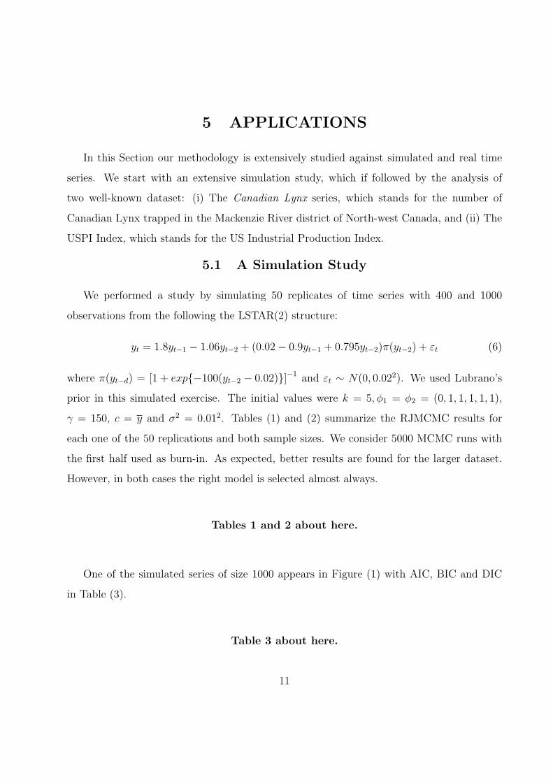
5.1 A Simulation Study

We performed a study by simulating 50 replicates of time series with 400 and 1000

observations from the following the LSTAR(2) structure:

yt = 1.8yt−1 − 1.06yt−2 + (0.02− 0.9yt−1 + 0.795yt−2)π(yt−2) + εt (6)

where π(yt−d) = [1 + exp{−100(yt−2 − 0.02)}]−1 and εt ∼ N(0, 0.022). We used Lubrano’s

prior in this simulated exercise. The initial values were k = 5, φ1 = φ2 = (0, 1, 1, 1, 1, 1),

γ = 150, c = y and σ2 = 0.012. Tables (1) and (2) summarize the RJMCMC results for

each one of the 50 replications and both sample sizes. We consider 5000 MCMC runs with

the first half used as burn-in. As expected, better results are found for the larger dataset.

However, in both cases the right model is selected almost always.

Tables 1 and 2 about here.

One of the simulated series of size 1000 appears in Figure (1) with AIC, BIC and DIC

in Table (3).

Table 3 about here.

11

Posterior means and standard deviations for the model with highest posterior model

probability are shown in Table (4).

Table 4 and Figure 1 about here.

5.2 Revisiting the Canadian Lynx Data

We analyze a Canadian Lynx series (see Figure 2) that represents logarithm of the number

of Canadian Lynx trapped in the Mackenzie River district of North-west Canada over the

period from 1821 to 1934. Some previous analyzes of this series can be found in Ozaki (1982),

Tong (1990), Terasvirta (1994), Medeiros and Veiga (2000) and Xia and Li (1999).

Figure 2 about here.

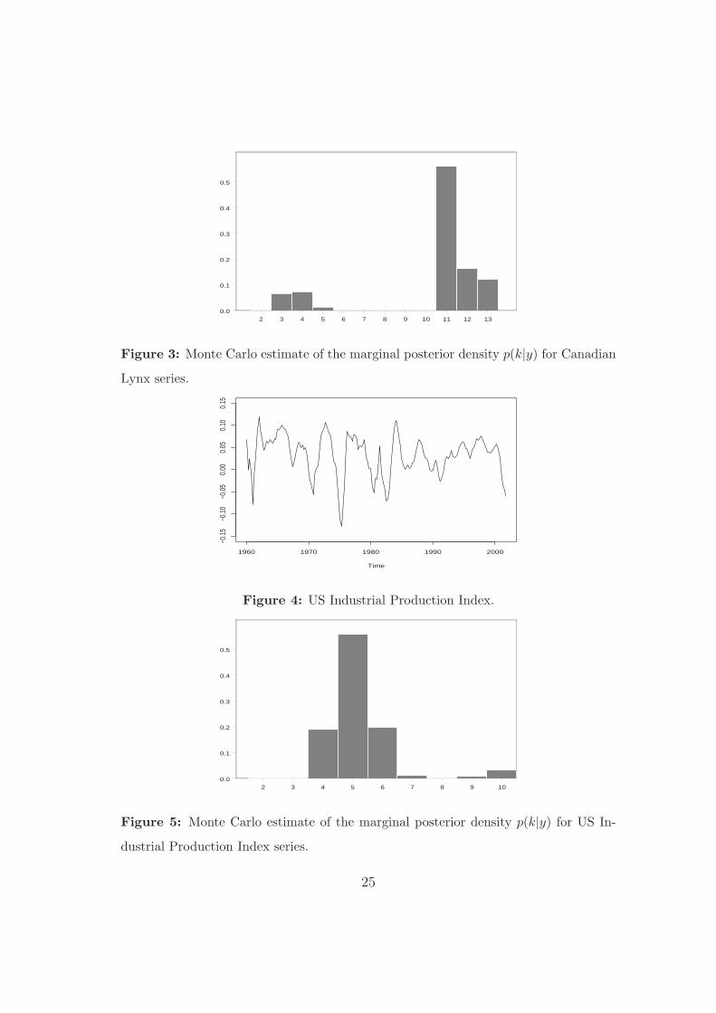
We consider the objective priors and compute the posterior model probabilities using our

RJMCMC algorithm. We run our RJMCMC algorithm for 50000 iterations and discard the

first half as burn-in. The LSTAR(11) model has the highest posterior model probability (see

the histogram on Figure 3). Note that the density of k is bimodal, which is concordance

with Medeiros and Veiga (2000) estimates, who fit an LSTAR(2) with d = 2. Terasvirta

(1994) estimates a LSTAR(11) with d = 3. The results of RJMCMC algorithm are shown

12

in table (5), where d = 3 has the highest posterior probability,

yt =(0.307)

0.987 +(0.111)

0.974 yt−1−(0.151)

0.098 yt−2−(0.142)

0.051 yt−3−(0.137)

0.155 yt−4+(0.143)

0.045 yt−5−(0.146)

0.0702 yt−6

−(0.158)

0.036 yt−7+(0.167)

0.179 yt−8+(0.159)

0.025 yt−9+(0.144)

0.138 yt−10−(0.096)

0.288 yt−11 + ((2.04)

−3.688

+(0.431)

1.36 yt−1−(0.744)

3.05 yt−2 +(1.111)

4.01 yt−3−(0.972)

2.001 yt−4+(0.753)

1.481 yt−5+(0.657)

0.406 yt−6

−(0.735)

0.862 yt−7−(0.684)

0.666 yt−8+(0.539)

0.263 yt−9+(0.486)

0.537 yt−10−(0.381)

0.569 yt−11)

×(

1 + exp{−(0.688)

11.625 (yt−3−(0.017)

3.504)})−1

+ εt, E(σ2|y) = 0.025

with posterior standard deviations in parenthesis.

Table 5 and Figure 3 about here.

5.3 Analysing the US Industrial Production Index

We analyzed the US Industrial Production Index (IPI), which can be downloaded from

the internet at www.economagic.com/sub-info/. The series comprises monthly observations

from 1960 to 2001. Following previous analysis, we converted the original series to quarterly

by averaging, after we took the fourth difference of the series in order to achieve stationarity

and remove possible seasonality. The resulting series is show in Figure (4).

Figure 4 about here.

We use the RJMCMC algorithm with objective priors to try to adjust an LSTAR model.

We consider 50000 runs and then we discarded the values from the first 25000 iterations as

burn-in. The histogram from Figure (5) and Table (6) show the posterior model probability

13

Pr(k|y), with k = 5, d = 3 the model maximal,

yt = −(0.005)

0.007 +(0.182)

0.909 yt−1−(0.214)

0.411 yt−2+(0.247)

0.51 yt−3−(0.225)

1.265 yt−4+(0.185)

0.541 yt−5 +

((0.005)

0.008 +(0.199)

0.555 yt−1−(0.261)

0.153 yt−2−(0.297)

0.412 yt−3+(0.269)

1.124 yt−4−(0.199)

0.488 yt−5)

×(

1 + exp{−(16.424)

960.58 (yt−3+(0.0029)

0.0076)})−1

+ εt, E(σ2|y) = 0.00019 (7)

with posterior standard deviations in parenthesis.

Table 6 and Figure 5 about here.

We used the LSTAR(5) with d = 3 to check the forecast performance from the first

quarter of 2002 to the second quarter of 2004. However, as can be seen from Table (6),

models with k = 4 and k = 6 alo have relatively high posterior model probability, so an

alternative is to forecast by combining the forecasts from each one of the relevant models,

a procedure that has become well known as Bayesian Model Averaging (BMA) (for more

details see Raftery, Madigan, and Hoeting (1997), Clyde (1999) and Hoeting, Madigan,

Raftery, and Volinsky (1999)). Figure (6) shows the forecasts from the LSTAR(5) with

d = 3 and from the mixture model with high posterior probabilities for k (BMA). One

could argue that the Bayesian model averaging produces more accurate forecasting for short

period, with a possible explanation for this improvement being that individual models are

over-parameterized, so suffer the curse of over-fitting and yielding poor predictions with

larger credible intervals.

Figure 6 about here.

14

6 CONCLUSIONS

In this paper we develop Markov chain Monte Carlo (MCMC) and reversible jump MCMC

(RJMCMC) algorithms for posterior inference and model selection in the broad class of

nonlinear time series models known as logistic smooth transition autoregressions, LSTAR.

Our developments are checked against simulated and real dataset with encouraging results

in favour of our RJMCMC scheme.

Even though we concentrated our computations and examples to the logistic transition

function, the algorightms we developed can be straightforwardly adapted to other functions

such as the exponential or the second-order logistic functions, or even combinations of those.

Similarly, even though we chose to work with yt−d as the transition variable and accounted

for the uncertainty about d, our findings are easily extended to situations where yt−d is

replaced by, say, s(yt−1, . . . , yt−d, α) for α and d unknown.

In this paper we focused on modelling the level of nonlinear time series. Our current

research agenda includes the adaptation of the methods proposed here to model both uni-

variate and multivariate-factor stochastic volatility problems with results to be reported

elsewhere.

All the algorithms were programmed in the student’s version of the software Ox, which

is publicly available and downloadable from www.nuff.ox.ac.uk/Users/Doornik.

References

Akaike, H. “New Look at the Statistical Model Identification.” IEEE Transactions in

Automatic Control , AC–19:716–723 (1974).

Berg, A., Meyer, R., and Yu, J. “DIC as a Model Comparison Criterion for Stochastic

Volatility Models.” Journal of Business and Economic Statistics , 22:107–120 (2004).

Besag, J. “A candidate’s formula – a curious result in Bayesian prediction.” Biometrika,

15

76(1):183 (1989).

Chan, K. S. and Tong, H. “On Estimating Thresholds in Autoregressive Models.” Journal

of Time Series Analysis , 7:179–190 (1986).

Clyde, M. “Bayesian Model Averaging and Model Search Strategies (with discussion).” In

Bernardo, J., Dawid, A., Berger, J., and Smith, A. (eds.), Bayesian Statistics 6 , 157–185.

Oxford University Press (1999).

Gamerman, D. Markov Chain Monte Carlo: Stochastic simulation for Bayesian inference.

London: Chapman & Hall (1997).

Gelfand, A. E. and Smith, A. M. F. “Sampling-based approaches to calculating marginal

densities.” Journal of the American Statiscal Asociation, 85:398–409 (1990).

Gilks, W. R., Richardson, S., and Spiegelhalter, D. J. (eds.). Markov Chain Monte Carlo in

Practice. London: Chapman & Hall, 3rd edition (1996).

Green, P. J. “Reversible Jump Markov chain Monte Carlo computation Bayesian model

determination.” Biometrika, 57(1):97–109 (1995).

Hastings, W. R. “Monte Carlo sampling methods using Markov chains and their aplications.”

Biometrika, 97–109 (1970).

Hoeting, J. A., Madigan, D., Raftery, A. E., and Volinsky, C. T. “Bayesian Model Averaging:

A Tutorial.” Statistical Science, 14:401–404 (1999).

Huerta, G. and Lopes, H. “Bayesian Forecasting and Inference in Latent Structure for the

Brazilian Industrial Production Index.” Brazilian Review of Econometrics , 20:1–26 (2000).

Lubrano, M. “Bayesian analysis of nonlinear time series models with a threshold.” (2000).

Proceedings of the Eleventh International Symposium in Economic Theory.

16

Luukkonen, R., Saikkonen, P., and Terasvirta, T. “Testing linearity against smooth transi-

tion autoregressive models.” Biometrika, 75:491–499 (1988).

Medeiros, M. C. and Veiga, A. “A Flexible Coefficient Smooth Transition Time Series

Model.” Working Paper Series in Economics and Finance 360, Stockholm School of Eco-

nomics (2000).

Metropolis, N., Rosenbluth, A. W., Rosenbluth, M. N., Teller, A. H., and Teller, E. “Equa-

tion of state calculations by fast computing machine.” Journal of Chemical Physics ,

21:1087–1091 (1953).

Ozaki, T. “The statistical analysis of perturbed limit cycle process using nonlinear time

series models.” Journal of Time Series Analysis , 3:29–41 (1982).

Raftery, A. E., Madigan, D., and Hoeting, J. A. “Bayesian model averaging for linear

regression models.” Journal of the American Statistical Association, 92:179–191 (1997).

Robert, C. and Casella, G. Monte Carlo statistical methods . Springer-Verlag (1999).

Schwarz, G. “Estimating the dimension of a model.” Annals of Statistics , 6:461–464 (1978).

Smith, A. and Gelfand, A. “Bayesian statistics without tears.” American Statistician,

46:84–88 (1992).

Spiegelhalter, D. J., Best, N. G., Carlin, B. P., and Linde, A. v. d. “Bayesian measures

of model complexity and fit (with discussion).” Journal of The Royal Statistical Society ,

64:583–639 (2002).

Terasvirta, T. “Specification, estimation, and evaluation of smooth transition autoregressive

models.” Journal of the American Statistical Association, 89(425):208–218 (1994).

Tong, H. Non-linear Time Series: A Dynamical Systems Approach, volume 6 of Oxford

Statistical Science Series . Oxford: Oxford University Press (1990).

17

Troughton, P. T. and Godsill, S. J. “A Reversible Jump Sampler for Autoregressive Time

Series, Employing Full Conditionals to Achieve Efficient Model Space Moves.” Technical

Report CUED/F-INFENG/TR.304, Department of Engineering, University of Cambrigde

(1997).

van Dijk, D., Terasvirta, T., and Franses, P. “Smooth transition autoregressive models - a

survey of recent developments.” Econometrics Reviews , 21:1–47 (2002).

Xia, Y. and Li, W. K. “On single-index coefficient regression models.” Journal of the

American Statistical Association, 94(448):1275–1285 (1999).

Zhu, L. and Carlin, B. “Comparing hierarquical models for spatio-temporally misaligned

data using the deviance information criterion.” Statistics in Medicine, 94 (2000).

18

Figure 1: Simulated series of 1000 observations from LSTAR(2).

Figure 2: Serie Canadian Lynx series.

Figure 3: Monte Carlo estimate of the marginal posterior density p(k|y) for Canadian

Lynx series.

Figure 4: US Industrial Production Index.

Figure 5: Monte Carlo estimate of the marginal posterior density p(k|y) for US Industrial

Production Index series.

Figure 6: Forecast values from 2002–1 to 2004–2 for US-IPI series using model (7) and

BMA method. The vertical line denote the start of forecasting.

19

Sample Visits Sample Visits

M1 M2 M3 M4 M5 M1 M2 M3 M4 M5

1 0 1374 3511 107 8 26 0 4622 357 15 6

2 0 3655 1140 190 15 27 0 4830 150 13 7

3 4 4725 233 30 8 28 0 4014 890 89 7

4 0 4673 315 9 3 29 0 4873 117 4 6

5 0 4710 281 1 8 30 0 4788 184 2 26

6 1 4824 157 14 4 31 0 725 3403 390 482

7 1 4676 297 17 9 32 0 4850 134 3 13

8 0 4758 213 12 17 33 0 4797 195 3 5

9 0 4516 446 32 6 34 0 4796 186 17 1

10 0 4762 224 8 6 35 0 4755 230 8 7

11 0 4912 85 2 1 36 1 4802 186 6 5

12 0 4918 73 6 3 37 0 4948 47 2 3

13 0 489 4385 113 13 38 0 4900 94 2 4

14 0 4808 181 7 4 39 0 2029 2782 165 24

15 0 4927 65 5 3 40 0 4888 89 20 3

16 0 4462 503 29 6 41 1 4789 198 3 9

17 0 4883 89 19 9 42 0 4725 245 17 13

18 0 2968 1937 90 5 43 1 4842 97 46 14

19 0 4941 47 7 5 44 0 4909 90 0 1

20 0 4245 736 17 2 45 0 1577 2976 416 31

21 10 3832 956 172 30 46 0 4925 70 4 1

22 0 4828 170 0 2 47 0 4740 251 7 2

23 0 4764 134 94 8 48 0 4460 528 8 4

24 0 4021 955 18 6 49 0 4553 411 29 7

25 0 4786 199 12 3 50 1 4666 265 64 4

Table 1: Monte Carlo experiment for 50 simulated series LSTAR(2) of size N = 400.20

Sample Visits Sample Visits

M1 M2 M3 M4 M5 M1 M2 M3 M4 M5

1 0 4921 67 11 1 26 0 4826 171 0 3

2 0 4872 123 0 5 27 0 4946 40 12 2

3 0 4944 56 0 0 28 0 4905 92 2 1

4 0 4870 117 12 1 29 0 4892 97 0 11

5 0 4963 31 2 4 30 0 4907 90 0 3

6 0 4956 43 0 1 31 0 4851 52 75 22

7 0 4868 123 6 3 32 0 4909 90 0 1

8 0 4932 62 6 0 33 0 1372 3564 58 6

9 0 4962 28 2 8 34 0 4914 82 2 2

10 0 4966 29 0 5 35 0 4890 98 10 2

11 0 4877 104 11 8 36 0 4941 56 1 2

12 0 4928 62 6 4 37 0 4943 55 0 2

13 0 4617 381 1 1 38 0 3501 1471 21 7

14 0 4827 172 1 0 39 0 4961 36 0 3

15 0 4918 78 1 3 40 0 4768 229 1 2

16 1 4973 24 0 2 41 0 4884 112 1 3

17 0 4967 32 0 1 42 0 4944 47 6 3

18 0 4919 72 5 4 43 0 4963 34 0 3

19 0 4803 193 0 4 44 1 4950 46 1 2

20 0 4933 60 0 7 45 0 4896 93 5 6

21 0 4926 60 6 8 46 0 4835 161 4 0

22 0 4555 439 4 2 47 0 4942 55 0 3

23 0 4917 77 2 4 48 0 4946 52 0 2

24 0 4956 42 1 1 49 0 4967 33 0 0

25 0 3020 25 808 1147 50 0 4965 32 2 1

Table 2: Monte Carlo experiment for 50 simulated series LSTAR(2) of size N = 1000.21

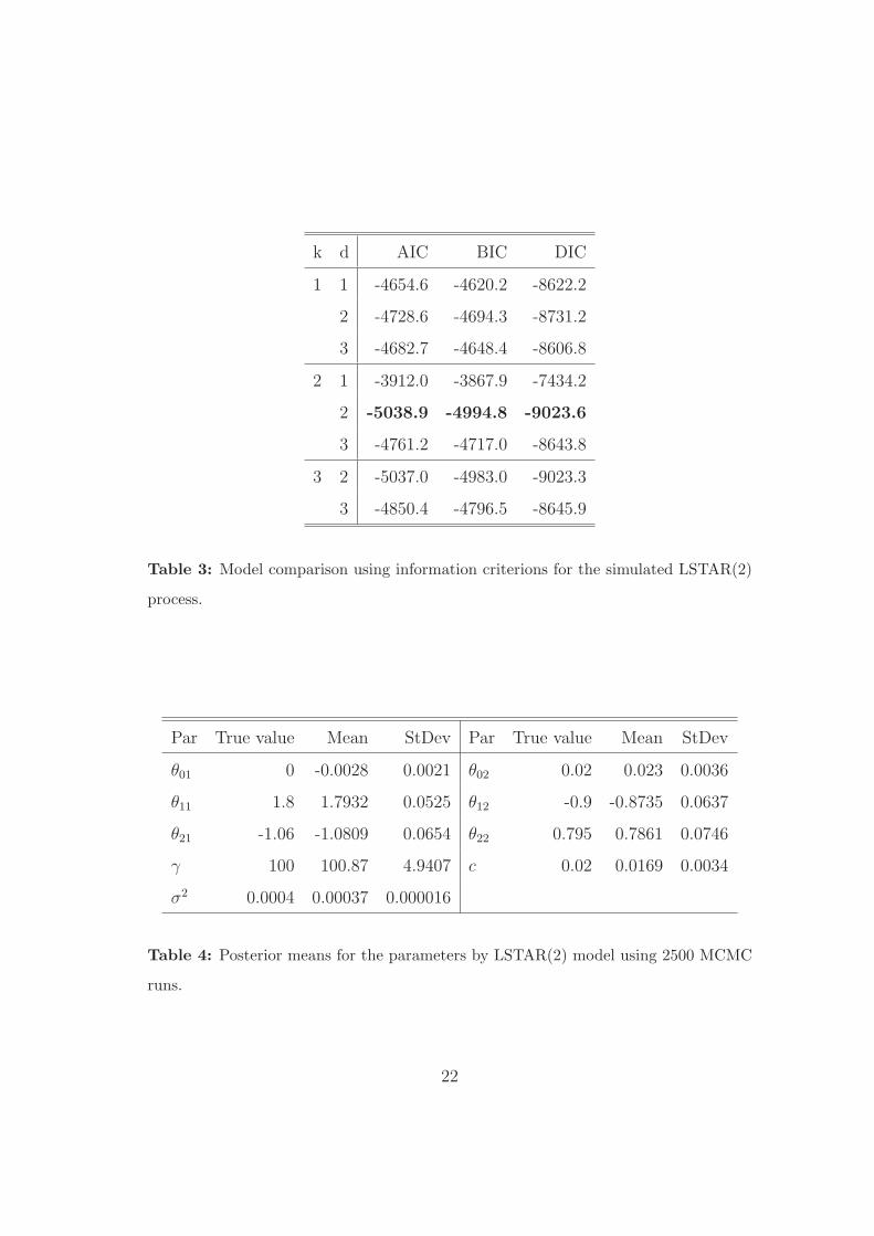
k d AIC BIC DIC

1 1 -4654.6 -4620.2 -8622.2

2 -4728.6 -4694.3 -8731.2

3 -4682.7 -4648.4 -8606.8

2 1 -3912.0 -3867.9 -7434.2

2 -5038.9 -4994.8 -9023.6

3 -4761.2 -4717.0 -8643.8

3 2 -5037.0 -4983.0 -9023.3

3 -4850.4 -4796.5 -8645.9

Table 3: Model comparison using information criterions for the simulated LSTAR(2)

process.

Par True value Mean StDev Par True value Mean StDev

θ01 0 -0.0028 0.0021 θ02 0.02 0.023 0.0036

θ11 1.8 1.7932 0.0525 θ12 -0.9 -0.8735 0.0637

θ21 -1.06 -1.0809 0.0654 θ22 0.795 0.7861 0.0746

γ 100 100.87 4.9407 c 0.02 0.0169 0.0034

σ2 0.0004 0.00037 0.000016

Table 4: Posterior means for the parameters by LSTAR(2) model using 2500 MCMC

runs.

22

d

k 1 2 3 4 p(k|y)

1 0 0 0 0 0

2 0 20 42 0 0.00124

3 6 18 3267 7 0.06596

4 0 8 3661 2 0.07342

5 0 0 658 4 0.01342

6 0 0 48 1 0.00098

7 0 0 74 6 0.00160

8 0 0 4 4 0.00016

9 0 0 34 1 0.00070

10 0 0 11 0 0.00022

11 4 0 27745 222 0.55942

12 0 0 8073 27 0.16200

13 41 0 5990 22 0.12106

Table 5: Results of the RJMCMC algorithm for Canadian Lynx series.

100 300 500 700 900

-0.2

-0.1

0.0

0.1

Figure 1: Simulated series of 1000 observations from LSTAR(2).

23

d

k 1 2 3 4 p(k|y)

1 0 0 0 0 0

2 0 0 1 2 0.00006

3 5 0 0 1 0.00012

4 134 1 9328 31 0.18988

5 81 7 27679 77 0.55688

6 246 3 9528 141 0.19836

7 8 1 531 50 0.01180

8 1 0 70 5 0.00152

9 19 0 422 7 0.00896

10 25 0 1591 5 0.03240

Table 6: Results of the RJMCMC algorithm for US-IPI series.

Time

log−

lynx

1820 1840 1860 1880 1900 1920

2.0

2.5

3.0

3.5

Figure 2: Serie Canadian Lynx series

24

2 3 4 5 6 7 8 9 10 11 12 130.0

0.1

0.2

0.3

0.4

0.5

Figure 3: Monte Carlo estimate of the marginal posterior density p(k|y) for Canadian

Lynx series.

Time

1960 1970 1980 1990 2000

−0.1

5−0

.10

−0.0

50.

000.

050.

100.

15

Figure 4: US Industrial Production Index.

2 3 4 5 6 7 8 9 100.0

0.1

0.2

0.3

0.4

0.5

Figure 5: Monte Carlo estimate of the marginal posterior density p(k|y) for US In-

dustrial Production Index series.

25

Time

1996 1998 2000 2002 2004

−0.

050.

000.

050.

10

IPI−USPrevisaoI.C. 95% Prev.Previsao MBMI.C. 95% Prev. MBM

Figure 6: Forecast values from 2002–1 to 2004–2 for US-IPI series using model (7)

and BMA method. The vertical line denote the start of forecasting.

26