SPATIAL AUTOCORRELATION AND AUTOREGRESSIVE MODELS IN ECOLOGY

445

Ecological Monographs, 72(3), 2002, pp. 445–463q 2002 by the Ecological Society of America

SPATIAL AUTOCORRELATION AND AUTOREGRESSIVE MODELSIN ECOLOGY

JEREMY W. LICHSTEIN,1,3 THEODORE R. SIMONS,1,4 SUSAN A. SHRINER,1 AND KATHLEEN E. FRANZREB2

1Cooperative Fish and Wildlife Research Unit, Department of Zoology, North Carolina State University,Raleigh, North Carolina 27695-7617 USA

2Southern Appalachian Cooperative Ecosystems Studies Unit, Department of Forestry, Wildlife, and Fisheries,University of Tennessee, Knoxville, Tennessee 37901 USA

Abstract. Recognition and analysis of spatial autocorrelation has defined a new par-adigm in ecology. Attention to spatial pattern can lead to insights that would have beenotherwise overlooked, while ignoring space may lead to false conclusions about ecologicalrelationships. We used Gaussian spatial autoregressive models, fit with widely availablesoftware, to examine breeding habitat relationships for three common Neotropical migrantsongbirds in the southern Appalachian Mountains of North Carolina and Tennessee, USA.

In preliminary models that ignored space, the abundance of all three species was cor-related with both local- and landscape-scale habitat variables. These models were thenmodified to account for broadscale spatial trend (via trend surface analysis) and fine-scaleautocorrelation (via an autoregressive spatial covariance matrix). Residuals from ordinaryleast squares regression models were autocorrelated, indicating that the assumption ofindependent errors was violated. In contrast, residuals from autoregressive models showedlittle spatial pattern, suggesting that these models were appropriate.

The magnitude of habitat effects tended to decrease, and the relative importance ofdifferent habitat variables shifted when we incorporated broadscale and then fine-scalespace into the analysis. The degree to which habitat effects changed when space was addedto the models was roughly correlated with the amount of spatial structure in the habitatvariables.

Spatial pattern in the residuals from ordinary least squares models may result fromfailure to include or adequately measure autocorrelated habitat variables. In addition, con-tagious processes, such as conspecific attraction, may generate spatial patterns in speciesabundance that cannot be explained by habitat models. For our study species, spatial patternsin the ordinary least squares residuals suggest that a scale of 500–1000 m would be ap-propriate for investigating possible contagious processes.

Key words: CAR model; habitat model; landscape effects; Moran’s I; Neotropical migrant song-birds; spatial autocorrelation; spatial autoregressive model; trend surface analysis.

INTRODUCTION

Spatial autocorrelation is frequently encountered inecological data, and many ecological theories and mod-els implicitly assume an underlying spatial pattern inthe distributions of organisms and their environment(Legendre and Fortin 1989). Typically, species abun-dances are positively autocorrelated, such that nearbypoints in space tend to have more similar values thanwould be expected by random chance. This pattern isoften driven by multiple causes that may be exogenous(e.g., autocorrelated environment, disturbance) and/orendogenous (e.g., conspecific attraction, dispersal lim-itation, demography) (Sokal and Oden 1978b, Legen-dre 1993). In addition to its ecological significance,

Manuscript received 8 November 2000; revised 9 July 2001;accepted 22 August 2001; final version received 18 October2001.

3 Current address: Laboratorio de Investigaciones Ecolo-gicas de las Yungas, Casilla de Correo 34, (4107) Yerba Bue-na, Tucuman, Argentina.

4 Author for reprints (e-mail: [email protected]).

spatial autocorrelation is problematic for classical sta-tistical tests, such as ANOVA and ordinary leastsquares (OLS) regression, that assume independentlydistributed errors (Haining 1990:161–166; Legendre1993). When the response (e.g., species abundance) isautocorrelated, the assumption of independence is ofteninvalid, and the effects of covariates (e.g., environ-mental variables) that are themselves autocorrelatedtend to be exaggerated (Gumpertz et al. 1997).

Legendre (1993) suggested two general frameworksfor incorporating space into ecological analysis. In the‘‘raw data approach,’’ species–environment relation-ships are modeled by partial regression analysis (uni-variate case for individual species) or constrained or-dination (multivariate case for community analysis;Borcard et al. 1992, Legendre and Legendre 1998); inboth cases, the effect of space is partitioned out by sitevariables or trend surface analysis. In the ‘‘matrix ap-proach,’’ species and environment data are representedby matrices of ecological distances between samplelocations, and spatial data are contained in a matrix of

446 JEREMY W. LICHSTEIN ET AL. Ecological MonographsVol. 72, No. 3

geographic distances. The correlation between speciesand environment, while controlling for space, is cal-culated by a partial Mantel test (Manly 1986, Legendreand Legendre 1998). The above methods have impor-tant limitations. For example, the raw data approachaccounts for broadscale spatial trend but not for thefine-scale autocorrelation that induces nonindependenterrors. Improvements to the methods of Legendre(1993) have been suggested by Legendre and Borcard(1994), Legendre and Legendre (1998), and Borcardand Legendre (2002), but few ecological studies to datehave incorporated fine-scale autocorrelation into spe-cies–environment analysis.

One approach to analyzing species–environment re-lationships in the presence of fine-scale autocorrelationis the class of spatial autoregressive models (Haining1990, Cressie 1993). These models can be thought ofas two-dimensional extensions of one-dimensional au-toregressive models popular in time-series analysis(Cressie 1993). Spatial autoregressive models havebeen known for decades in the statistical literature (Be-sag 1974), but have been used by ecologists in only afew studies (Pickup and Chewings 1986, Augustin etal. 1996; Klute et al., in press). Theoretically, auto-regressive models can be fit to a variety of responsedistributions, including normal (auto-Gaussian), binary(autologistic), and Poisson (auto-Poisson). However,the auto-Poisson model can only have negatively au-tocorrelated errors (Besag 1974, Cressie 1993:553–555) and is therefore of limited practical use. The au-tologistic model has been used in several ecologicalapplications (Augustin et al. 1996; Klute et al., inpress). ‘‘Pseudolikelihood’’ parameter estimates for theautologistic model can be obtained with standard lo-gistic regression software, but the standard errors tendto underestimate the true sampling variability (Gum-pertz et al. 1997). Parameter estimates for the auto-Gaussian model cannot be obtained with ordinary re-gression software, because the estimated mean functionand spatial covariance matrix interact so that an iter-ative fitting procedure is necessary (Haining 1990:128). Recent development of software for fitting auto-Gaussian models (Kaluzny et al. 1998) significantlyexpands the tools available to ecologists for analyzingautocorrelated data.

In this paper, we use auto-Gaussian models to extendthe single species raw data approach of Legendre(1993) to account for fine-scale spatial autocorrelation.We develop models of species abundance as a functionof local- and landscape-scale habitat variables usingdata from a 3-yr breeding bird study in managed forestsin the southern Appalachian Mountains, USA. This re-gion supports a diverse assemblage of Neotropical mi-gratory songbirds (Passeriformes), many of which arethought to be experiencing long-term population de-clines (Robbins et al. 1989b, Askins et al. 1990). Whiledegradation of wintering (Robbins et al. 1989b, Sherryand Holmes 1996) and migratory (Moore et al. 1995)

habitats are likely important, habitat change on thebreeding grounds remains a prominent hypothesis inexplaining population declines of Neotropical migrants(Brittingham and Temple 1983, Wilcove 1985, Templeand Cary 1988, Robinson et al. 1995). Numerousbreeding studies have documented reduced abundance(e.g., Ambuel and Temple 1983, Robbins et al. 1989a),pairing success (e.g., Gibbs and Faaborg 1990, Villardet al. 1993), or nesting success (e.g., Donovan et al.1995, Robinson et al. 1995) in highly fragmented for-ests, and the conservation of Neotropical migrant song-bird populations is thought to depend, in part, on thepreservation of large forest tracts in North America(Wilcove 1985, Donovan et al. 1995, Robinson et al.1995). Despite this widely held belief, little is knownabout nesting success or habitat use by breeding Neo-tropical migrants in large forests (Simons et al. 2000).Recent studies in both Europe and North America sug-gest that landscape structure may affect breeding song-bird habitat use even in large forested areas (e.g.,McGarigal and McComb 1995, Edenius and Elmberg1996, Jokimaki and Huhta 1996, Hagan et al. 1997,Schmiegelow et al. 1997).

The present analysis seeks an understanding of howsouthern Appalachian songbirds respond to their breed-ing habitat at local and landscape scales. Our resultsare relevant to Neotropical migratory bird conservation(Hagan and Johnston 1992, Martin and Finch 1995),as well as to the more general ecological question ofhow organisms respond to environmental variation atdifferent spatial scales (Wiens 1989). We hope that ourdiscussion of statistical methods will be valuable to themany ecologists who are currently analyzing spatiallyautocorrelated data.

METHODS

Study area

The southern Appalachians, USA, region is 70% for-ested (SAMAB 1996), including remnant old-growthstands and extensive tracts of second-growth forest thathave regrown following industrial logging from the late1800s through the 1930s (Eller 1982, Yarnell 1998).The U.S. Forest Service manages most of the publiclands in the southern Appalachians. Our study area(358409000–368079300 N, 828379300–838079300 W) en-compassed 60 000 ha of previously logged forest from380 to 1460 m elevation in the French Broad RangerDistrict of Pisgah National Forest (North Carolina) andthe Nolichucky Ranger District of Cherokee NationalForest (Tennessee). Current forest cover in the studyarea, by stand age, is: #9 yr, 5%; 10–19 yr, 4%; 20–39 yr, 5%; 40–69 yr, 27%; and $70 yr, 59% (Hermann1996). Most younger stands (,20 yr old) were createdby small (;10 ha) clearcuts, which are scatteredthroughout the landscape. The majority of the studyarea consists of deciduous mesic hardwood forests. Xe-

August 2002 447SPATIAL AUTOREGRESSIVE MODELS

TABLE 1. Habitat variables used in regression models.

Variable Description

Local habitat variablesELEVELEV2

TOPO (4)

elevation(elevation)2

topographic position (ravine, flat, slope, or ridge)EDGE (6) edge category (early-early, early-mid, early-late, mid-mid, mid-late, or late-late)RD/TR/OFF (3)RDVEG (3)CANSUBCAN

point located on road, trail, or off-roadroad bordered by Rubus, other shrub species, or no shrubspercentage of canopy coverpercentage of subcanopy cover

TALLSHLOWSHHERBDBH25–50DBH.50MAXHT

percentage of tall shrub/sapling coverpercentage of low shrub/seedling coverpercentage of herbaceous covernumber of 25–50 cm dbh trees in wedge prism samplenumber of .50 cm dbh trees in wedge prism sampleheight of tallest tree

NMDS1 NMDS axis 1: Quercus rubra and Acer saccharum (negative axis 1 scores) to Q. coccinea(positive scores)

NMDS2 NMDS axis 2: Liriodendron tulipifera (negative axis 2 scores)NMDS3 NMDS axis 3: Tsuga canadensis and Rhododendron maximum (negative axis 3 scores) to Q.

prinus (positive scores)

Landscape variablesLS#9LS#92

LSMESIC40–69LSMESIC$70

proportion of #9-yr-old forest(proportion of #9-yr-old forest)2

proportion of 40–69 yr-old mesic hardwood forestproportion of $70-yr-old mesic hardwood forest

LSCORE proportion of core area ($40-yr-old forest that is .100 m from edge with younger forest and.100 m from non-National Forest land)

LSDIV Simpson’s diversity index (1/Spi2), where pi refers to the proportion of six landcover catego-

ries (stands #9, 10–19, 20–39, 40–69, and $70 years old, and non-National Forest land)

Notes: For categorical variables, the number of categories is given in parentheses. All landscape variables were measuredwithin 250 m radius circles, centered on each sample location. Abbreviations: dbh, diameter at breast height, 1.4 m abovethe ground surface; NMDS, nonmetric multidimensional scaling.

ric hardwoods and pine (Pinus spp.) occupy dry slopesand ridges.

Bird counts

Our database consisted of 1177 point locations sam-pled from mid-May to the end of June in 1997–1999.Each point was sampled in two different years of thestudy under favorable weather conditions. Points werespaced ;200 m apart along low-traffic roads (n 5 570),hiking trails (n 5 557), and off-road transects (n 550). The location of each point was recorded with adifferentially corrected global positioning system(GPS; GeoExplorer II; Trimble Navigation, Sunnyvale,California, USA). At each point, we recorded the num-ber and identity of breeding pairs, along with a hori-zontal distance estimate from the observer, during a10-min period using the variable circular plot method(Reynolds et al. 1980). Counts were conducted betweensunrise and 10:15 h. In our analysis, we only includeddetections with distance estimates #75 m from the ob-server. Using this distance cut-off, detectability (theprobability that a present bird is detected), which wasestimated with the computer program DISTANCE(Thomas et al. 1998), was roughly equal across thedifferent habitats sampled. Additional details concern-ing bird counts can be found in Lichstein et al. (2002).

Local scale habitat

Vegetation data were recorded within 10 m radiusplots at each sample location (Table 1). Nonmetric mul-tidimensional scaling (NMDS), a robust nonparametricordination method (Minchin 1987), was used to gen-erate axes representing gradients in floristic composi-tion. Stand age was assigned to one of three succes-sional stages (early, mid, or late) for both sides of theroad or trail, yielding six edge categories: early-early,early-mid, early-late, mid-mid, mid-late, and late-late.Additional details on local habitat data can be foundin Lichstein et al. (2002).

Landscape scale habitat

Landcover maps of the southern Appalachians regionare available from the Southern Appalachian Assess-ment GIS Data Base (Hermann 1996). This databaseincludes forest stand coverages (digitized from 1:24 000 scale aerial photographs) for all National For-ests in the SAMAB (1996) assessment area. We usedARC/INFO (ESRI 1998) to quantify landscape com-position within a 250 m radius circle centered on eachsample point (Table 1). Because adjacent points wereseparated by ;200 m, landscape circles overlappedconsiderably, ensuring some spatial autocorrelation inlandscape variables. The present analysis is restricted


to simple landscape composition variables measured ata single scale. A more thorough landscape analysisdoes not qualitatively change our results (Lichstein etal. 2002).

Statistical analysis

Our general goal was to evaluate how the apparentimportance of different habitat variables changed de-pending on the scale(s) of spatial dependence account-ed for by the regression models. We began by fittingmodels that ignored both broadscale spatial trend andfine-scale autocorrelation. We then examined how thesemodels changed after accounting for broadscale trend,and we partitioned the explained variation in speciesabundance to nonspatially structured environment, spa-tially structured environment, and broadscale trend fol-lowing Legendre (1993). Finally, we examined modelsthat also accounted for fine-scale autocorrelation. Allanalyses were performed with S-PLUS (Kaluzny et al.1998, MathSoft 1999). S-PLUS codes and detailed in-structions for performing all analyses in this paper maybe found as a supplement available in ESA’s ElectronicData Archive.

Study species and preliminary analysis.—We ana-lyzed point count data for three species of Neotropicalmigrant warblers (Parulidae) that are common in ourstudy area: the Chestnut-sided Warbler (Dendroicapensylvanica), the Hooded Warbler (Wilsonia citrina),and the Black-throated Blue Warbler (Dendroica ca-erulescens). These species were selected because theyrepresent a range of habitat preferences: the Chestnut-sided Warbler is an edge/early successional specialist,the Hooded Warbler is an edge/mature forest generalist,and the Black-throated Blue Warbler is a mature forestspecialist. In addition, these species were the focus ofa concurrent nesting success study. Although patternsin bird abundance do not necessarily reflect habitatquality (Van Horne 1983), all three species reproducesuccessfully in our study area (;50% nest success rate;Weeks 2001; J. W. Lichstein, T. R. Simons, and K. E.Franzreb, unpublished data); therefore, patterns in theirabundance are likely to have some adaptive signifi-cance.

In all regression models discussed below, the re-sponse variable was the square-root-transformed count(Sokal and Rohlf 1995) for each species, summedacross the two samples at each of the 1177 point lo-cations. Quantitative explanatory variables were stan-dardized to mean zero and unit variance, and categor-ical variables were coded as zero/one dummy variables.Plots of ordinary least squares (OLS) partial residualsagainst each explanatory variable (Rawlings et al.1998:350) indicated constant variances for all threespecies. These plots suggested nonlinear responses toELEV (Hooded and Black-throated Blue Warbler) andLS#9 (Chestnut-sided Warbler), and the appropriatequadratic terms were added to these models. Frequencyhistograms of residuals and normal probability plots

(Rawlings et al. 1998:357) indicated normality for theBlack-throated Blue Warbler, while residuals for theChestnut-sided and the Hooded Warbler were not nor-mal (although both distributions were roughly sym-metric). To investigate how nonnormality would affectour results, we compared OLS models, for which clas-sical parametric tests assume normality (Rawlings etal. 1998:325), to Poisson and negative-binomial mod-els for count data using generalized linear models(McCullagh and Nelder 1989). Results from OLS, Pois-son, and negative-binomial models were qualitativelysimilar (Lichstein 2000), and we therefore proceededwith the normal errors model due to its greater flexi-bility in fitting spatial autoregressive models (Cressie1993; see Introduction).

Habitat (‘‘OLS environment’’) models.—For eachspecies, we fit OLS multiple regression models to hab-itat variables (hereafter, ‘‘OLS environment models’’),ignoring both broadscale spatial trend and fine-scaleautocorrelation. For each species, we began with amodel that included all of the habitat variables listedin Table 1 and sequentially eliminated by hand vari-ables with P . 0.01.

Habitat 1 trend (‘‘OLS trend/environment’’) mod-els.—We used trend surface analysis to model broad-scale spatial pattern in the species data. This analysishas two primary aims (Legendre 1993, Legendre andLegendre 1998): (1) to guard against false correlationsbetween species and environment, as may arise whenan unmeasured environmental factor causes a commonspatial structure in the species and in the measuredenvironmental variables; and (2) to determine if thereis a substantial amount of broadscale spatially struc-tured variation in the species data that is unexplainedby the measured environmental variables.

We fit a trend surface to bird abundance by regressingthe species data on all third-degree polynomial termsof the spatial coordinates of the sample locations:

2 2 3z 5 b 1 b x 1 b y 1 b x 1 b xy 1 b y 1 b x0 1 2 3 4 5 6

2 2 31 b x y 1 b xy 1 b y7 8 9

where z is the response variable (square-root-trans-formed species counts), b0–b9 are parameters, and x andy are the spatial coordinates of the sample locations.Prior to analysis, x and y were centered on their re-spective means to reduce collinearity with higher orderterms (Legendre and Legendre 1998:527) and stan-dardized to unit variance. Nonsignificant trend surfaceterms were removed by stepwise selection.

Following Legendre (1993), the proportion of vari-ation in the species data explained by nonspatiallystructured environment, spatially structured environ-ment, and spatial trend (independent of environment)was partitioned using partial regression analysis (Le-gendre and Legendre 1998). The total variation in thespecies data explained by trend and environment com-bined was obtained from ‘‘OLS trend/environment


models,’’ which included both the trend surface termsand the habitat variables from the OLS environmentmodels.

Habitat 1 trend 1 autocorrelation (‘‘CAR trend/environment’’) models.—Because trend surface anal-ysis only accounts for broadscale spatial pattern (Le-gendre and Borcard 1994), we next examined how OLStrend/environment models changed when we accountedfor fine-scale autocorrelation using auto-Gaussianmodels. Spatial auto-Gaussian models take on one oftwo common forms (conditional and simultaneous), de-pending on how the spatially correlated error structureis specified (Haining 1990, Cressie 1993). Cressie(1993:408) recommends the conditional autoregressive(CAR) model over the simultaneous model. We fit bothmodels, and the results were nearly identical. We reportresults for the CAR model only. The ‘‘CAR trend/en-vironment model’’ accounts for both broadscale trend(via inclusion of trend surface terms) and fine-scaleautocorrelation (via the correlated error structure; seebelow).

The difference between OLS and CAR models canbe understood by considering the expected value anddistribution of Y, the vector of observed responses. Forboth models, Y is assumed to have a multivariate nor-mal (MVN) distribution:

Y ; MVN[m, V]

where m, the vector of means, is equal to Xb (X is amatrix of independent variables, and b is a vector con-taining their slopes), and V is an n 3 n covariancematrix (n is the number of observations). In the OLSmodel, the expected value of an observation Y at alocation i is simply mi, and the covariance matrix is

2V 5 Is

where I is the identity matrix (ones on the diagonaland zeros elsewhere) and s2 is a constant. Thus, everyYi has the same variance (s2), and the covariance be-tween Yi and Yj is zero for all locations i ± j (Rawlingset al. 1998:87).

In the CAR model, the conditional expectation ofYi, given the response at all other locations, is mi plusa weighted sum of the mean-centered counts at lo-cations j:

E(Y z all Y ) 5 m 1 rS w (Y 2 m )i j±i i j±i ij j j

where r is a parameter to be estimated that determinesthe direction (positive or negative) and magnitude ofthe spatial neighborhood effect, wij are weights thatdetermine the relative influence of location j on loca-tion i, and Yj 2 mj are the mean-centered counts atlocations j (Haining 1990:88, Cressie 1993:407). Thus,CAR models, and autoregressive models in general,assume that the response is a function of both the ex-planatory variables (m in the equation above) and thevalues of the response at neighboring locations (thesummation in the equation above). In the context of

species-environment analysis, and assuming positiveautocorrelation (r . 0), the CAR model has the fol-lowing interpretation: if location i is surrounded bylocations j, which, based on the habitat at j, have higher(or lower) species abundance than expected, then i willalso tend to have higher (or lower) species abundancethan expected from the habitat at i. This framework iswell-suited for modeling the abundance of specieswhose distributions are controlled by a combination ofexogenous (e.g., habitat) and endogenous (e.g., clonalgrowth, conspecific attraction) factors. In most cases,it is reasonable to assume that distant locations willaffect each other less than nearby locations; therefore,the weights (wij) in the CAR model are typically definedto decrease with increasing distance between i and j(e.g., wij 5 1/distanceij) and are zero if i and j are notwithin each other’s spatial neighborhood (zone of in-fluence). An appropriate neighborhood size is the max-imum distance at which the residuals from an OLSmodel are autocorrelated. This distance may be judgedfrom a semivariogram or correlogram of the OLS re-siduals (Cressie 1993:557). See Haining (1990), Cres-sie (1993), and Gumpertz et al. (1997) for further dis-cussion of weight definitions.

The above expression for the expected value of Yi

in the CAR model implies the following covariancematrix:

21V 5 (I 2 rW) M

where W is an n 3 n matrix with zeros on the diagonaland the neighbor weights (wij) in the off-diagonal po-sitions, and M is an n 3 n matrix with the conditionalvariances ( ) of Y (i.e., the variances of Y2 2s ,. . . , s1 n

given the realized values of the spatial neighbors) onthe diagonal and zeros in the off-diagonal positions(Haining 1990:88, Cressie 1993:433). In contrast to theOLS model, covariances in the CAR model (off-di-agonal elements of V) are nonzero and increase thecloser locations i and j are to each other. In the presentanalysis, we assumed that the conditional variances ofY were constant (i.e., M 5 Is2), which is a specialcase of the general model described above. (See Hain-ing [1990:129] for a discussion of nonconstant vari-ances in auto-Gaussian models.) The unconditionalvariances in the CAR model (diagonal elements of V)are generally not constant and depend on r and thelocations of the spatial neighbors (see Haining 1990:Fig. 3.8), but not on the realized values of the neigh-bors.

Prior to fitting CAR models, we examined directionalcorrelograms (61808 azimuths 5 08, 458, 908, and 1358;angular tolerance 5 622.58) of OLS trend/environmentresiduals to determine if autocorrelation was isotropic(the same in all geographic directions; Haining 1990:66, Legendre and Legendre 1998:721). Anisotropy wasnot detected for any of the three species. Based oncorrelograms of OLS trend/environment residuals andempirical trials, we selected a 750 m radius spatial


neighborhood for all three species. We fit CAR modelswith three different neighbor weight definitions: wij 51, 1/distanceij, and (1/distanceij)2. We selected an ap-propriate weight function based on model fit (maxi-mized likelihood) and by how well the model accountedfor autocorrelation in the residuals. We selected wij 5(1/distanceij)2 for the Chestnut-sided Warbler and wij 51/distanceij for the Hooded and Black-throated BlueWarblers.

We calculated R2 for the CAR models using the fol-lowing formula (Nagelkerke 1991):

2R 5 1 2 exp[22/n(l 2 l )]A 0

where n is the sample size, lA is the log-likelihood ofthe model of interest, and l0 is the log-likelihood of thenull model containing only an intercept (which fits themean response and ignores autocorrelation). For OLSmodels, this formula yields the identical value as thetraditional R2 (the proportion of the mean-centered re-sponse sum of squares that is explained by the inde-pendent variables).

Habitat effects.—To provide a common ground forassessing the importance of habitat variables in OLSand CAR models, we evaluated the contribution of eachvariable to model fit with a likelihood ratio test fornested models (Haining 1990:142), with the reducedmodel containing a subset of the variables in the fullmodel:

LR 5 22(l 2 l )red full

where LR is the likelihood ratio test statistic, and lred

and lfull are the log-likelihoods of the reduced and fullmodels, respectively. Under the null hypothesis thatthe reduced and full models fit the data equally well,LR has an approximate x2 distribution with degrees offreedom equal to the number of additional parametersin the full model.

Finally, we wished to gain some insight into howspatial pattern in the habitat variables would affect theirapparent importance in the three types of regressionmodels. We assumed that the probability of observing‘‘false correlations’’ (Legendre and Legendre 1998:769) between the species and habitat data would in-crease when the two were spatially structured at similarscales. For a given habitat variable, we predicted thatthe change in its apparent importance when trend andautocorrelation were incorporated into the modelswould be related to the degree to which the habitatvariable was structured at broad and fine spatial scales,respectively. For example, if a habitat variable showedlittle broadscale trend but strong fine-scale autocorre-lation, the importance of the variable should be similarin OLS environment and OLS trend/environment mod-els, but might decrease in CAR trend/environmentmodels.

For each habitat variable, we calculated the changein its effect due to incorporating broadscale trend inthe model as:

DLR 5 LR(OLS environment)trend

2 LR(OLS trend/environment)

where LR(OLS environment) and LR(OLS trend/en-vironment) are LR statistics for a given habitat variablein OLS environment and OLS trend/environment mod-els, respectively. We predicted that DLRtrend would bepositively correlated with the degree to which eachhabitat variable was spatially structured on a broadscale. To describe the broadscale structure of the habitatvariables, we performed OLS trend surface regressions(separate regression for each habitat variable) on allthird-degree polynomial terms of the spatial coordi-nates of the sample locations. Nonsignificant trend sur-face terms were removed by stepwise selection. Weused the R2 from these trend surface models (’’ ’’)2Rtrend

as an index of broadscale structure in each habitat var-iable.

We calculated the change in the effect of each habitatvariable when fine-scale autocorrelation was added tothe model as

DLR 5 LR(OLS trend/environment)autocor

2 LR(CAR trend/environment)

where LR(OLS trend/environment) and LR(CARtrend/environment) are LR statistics for a given hab-itat variable in OLS trend/environment and CARtrend/environment models, respectively. We predictedthat DLRautocor would be positively correlated with thedegree to which the habitat variables were autocor-related on a fine scale. To describe this fine-scale au-tocorrelation, we used the residuals from the trendsurface analysis of each habitat variable to computeMoran’s I correlograms (see Spatial autocorrelationbelow). Trend surface analysis removes broadscalestructure, so any spatial pattern remaining in the re-siduals is due to fine-scale autocorrelation. For eachhabitat variable, we calculated ’’Imean,’’ the average val-ue of Moran’s Istd (standardized version of I; see Ap-pendix) out to a lag distance of 775 m (the approximatesize of the spatial neighborhood in the CAR models),as an index of fine-scale autocorrelation.

In order to calculate and Imean, categorical hab-2Rtrend

itat variables were transformed into pseudo-quantita-tive variables (see below).

Spatial autocorrelation.—We used Moran’s I cor-relograms (Sokal and Oden 1978a, Legendre and Le-gendre 1998) to evaluate spatial pattern in the (square-root-transformed) bird counts, in the residuals from thethree types of species–environment regression models,and in the residuals from the trend surface models ofthe habitat variables. Under the null hypothesis of nospatial autocorrelation, I has an expected value nearzero for large n, with positive and negative values in-dicating positive and negative autocorrelation, respec-tively. Because I does not vary strictly between 21 and11, we standardized I by dividing by its maximum


TABLE 2. Ordinary least squares (OLS) and conditional autoregressive (CAR) models of bird abundance.

Species

R2

OLSenv trend

OLStrend/env autocor

CARtrend/env r

Neighborhoodeffect

200 m† 400 m‡

Chestnut-sided WarblerHooded WarblerBlack-throated Blue Warbler

0.480.200.36

0.260.080.22

0.530.220.39

0.170.120.26

0.550.250.46

3361.617.319.0

0.250.260.29

0.060.130.14

Notes: R2 values are given for the following models: ‘‘OLS env’’ 5 habitat only; ‘‘trend’’ 5 broadscale spatial trendsurface; ‘‘OLS trend/env’’ 5 habitat 1 trend; ‘‘autocor’’ 5 fine-scale autocorrelation (conditional autoregressive [CAR]model with only intercept and r); ‘‘CAR trend/env’’ 5 habitat 1 trend 1 autocorrelation. In CAR models, neighborhoodeffects are modeled by the estimated spatial parameter, , along with the neighbor weights: wij 5 (1/distanceij)2 for therChestnut-sided Warbler and 1/distanceij for the Hooded and the Black-throated Blue Warblers. ‘‘Neighborhood effect’’ is theexpected increase in the response (square-root-transformed count) at location i where the sum of the mean-centered responsesat locations j in i’s spatial neighborhood is 13. Neighborhood effect was calculated as j±iwij(Yi 2 mj), which is therSautoregressive component of the conditional expectation of Yi in the CAR model. As an arbitrary but realistic example, weassumed that S(Yi 2 mj) 5 3 for locations j in i’s spatial neighborhood.

† Neighborhood effect was calculated assuming all j in i’s spatial neighborhood are 200 m away from i.‡ Neighborhood effect was calculated assuming all j in i’s spatial neighborhood are 400 m away from i.

attainable value to yield Istd (Haining 1990:234–235;see Appendix). Significance tests of I for raw data (i.e.,bird counts), OLS residuals, and CAR residuals aredistinct and are explained in detail in the Appendix.The first lag distance interval in the correlograms in-cluded all pairs of points separated by #250 m, andsubsequent intervals (out to a maximum distance of3100 m) were 150 m wide. All intervals contained atleast 1000 pairs of points, providing high power todetect spatial pattern.

For each lag distance, we used a randomization testwith 999 permutations (see Appendix) to determine theprobability, under the null hypothesis of no spatial au-tocorrelation, of observing a value of I as large as theobserved value (one-tailed test for positive autocor-relation; Haining 1990:231, Legendre and Legendre1998:720). For each correlogram, we tested for globalsignificance (i.e., the correlogram contains at least onepositively autocorrelated value) using a Bonferroni cor-rected a* of 0.05/20 5 0.0025 (nominal a of 0.05; 20lags; Legendre and Legendre 1998:721). Within eachcorrelogram, the significance of I for each lag distancewas assessed using the progressive Bonferroni correc-tion suggested by Legendre and Legendre (1998:671and 721–723), in which the ith lag is tested at a* 5a/i, with a 5 0.05. This procedure is appropriate whenautocorrelation is expected at the shortest lags and onewishes to know the range (maximum lag distance) ofautocorrelation (Legendre and Legendre 1998:721).

In order to calculate I, categorical habitat variables(TOPO, EDGE, RD/TR/OFF, and RDVEG; Table 1)were transformed into pseudo-quantitative variables byassigning integer values to classes ranked along eco-logical gradients: the four TOPO classes were rankedfrom driest to wettest (ridge 5 0, slope 5 1, flat 5 2,ravine 5 3); the six EDGE classes were ranked in in-creasing order of disturbance due to recent logging(late-late 5 0, mid-late 5 1, mid-mid 5 2, early-late

5 2, early-mid 5 3, early-early 5 4); the three RD/TR/OFF classes were ranked in order of increasing veg-etation disturbance (off-road 5 0, trail 5 1, road 5 2);the three RDVEG classes were ranked in increasingorder of use by early successional birds as nesting hab-itat in our study area (J. W. Lichstein, T. R. Simons,and K. E. Franzreb, unpublished data; none 5 0, shrubsother than Rubus 5 1, Rubus 5 2).

Significance tests for the presence of spatial auto-correlation require the condition of second-order sta-tionarity (Legendre and Legendre 1998:718). Broad-scale trend in the unmodeled bird counts violated sta-tionarity assumptions; significance tests of I for the rawbird counts should therefore be interpreted as testingfor the presence of spatial pattern that may reflect trendrather than fine-scale autocorrelation.

RESULTS

OLS environment models

OLS environment models explained 48, 20, and 36%of the variation in the counts for the Chestnut-sided,Hooded, and Black-throated Blue Warbler, respectively(Table 2). All models included both local- and land-scape-scale habitat variables (Fig. 1, Table 3). OLSenvironment models explained much of the broadscalespatial pattern in the counts for all three species, asseen in the overall shift in the correlograms towardszero (Fig. 2: compare correlograms for counts to thosefor OLS environment residuals). The OLS environmentmodel for the Chestnut-sided Warbler also explainedsome of the fine-scale spatial pattern in the counts, asseen in the more rapid decline in Moran’s I for the OLSenvironment residuals compared to the counts (Fig. 2).In contrast, OLS environment models explained littleof the fine-scale autocorrelation in the counts for theHooded and the Black-throated Blue Warblers: theshape of the correlograms for the counts and OLS en-


FIG. 1. Likelihood ratio (LR) statistics for habitat variables in ordinary least squares (OLS) environment, OLS trend/environment, and conditional autoregressive (CAR) trend/environment models. Larger LR values indicate a greater contri-bution to model fit. P values and parameter estimates are given in Table 3. See Table 1 for descriptions of habitat variables.

vironment residuals were similar for these two species(Fig. 2). For all three species, OLS environment resid-uals were positively autocorrelated (global Bonferronitest for correlograms significant at a* 5 0.0025), in-dicating that the assumption of independent errors wasviolated.

OLS trend/environment models

Trend surface analysis explained 26, 8, and 22% ofthe variation in the counts for the Chestnut-sided,

Hooded, and Black-throated Blue Warbler, respectively(Table 2). OLS trend/environment models, which in-cluded both the trend surface terms and the habitatvariables, explained only slightly more variation thanOLS environment models: 53, 22, and 39% for theChestnut-sided, Hooded, and Black-throated Blue War-bler, respectively (Table 2). The reason for this mar-ginal improvement is clear from the partitioning ofexplained variation due to trend, spatially structuredenvironment (‘‘trend/environment’’), and nonspatially


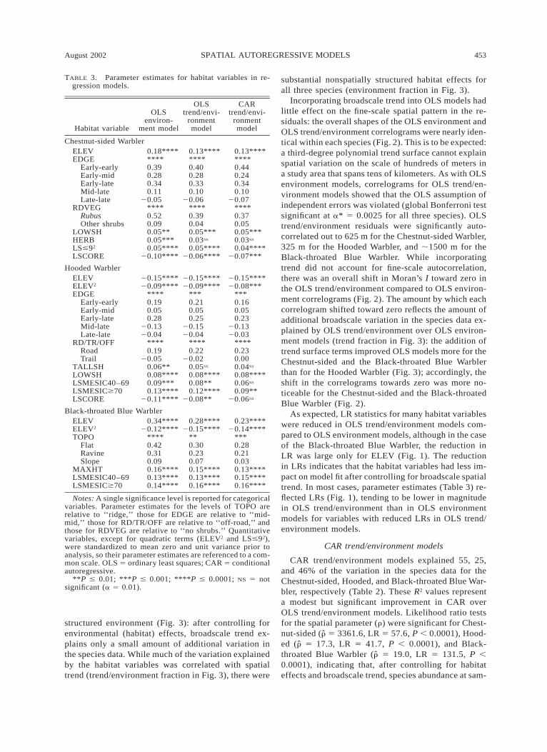
TABLE 3. Parameter estimates for habitat variables in re-gression models.

Habitat variable

OLSenviron-

ment model

OLStrend/envi-

ronmentmodel

CARtrend/envi-

ronmentmodel

Chestnut-sided WarblerELEVEDGE

Early-earlyEarly-midEarly-lateMid-lateLate-late

0.18********0.390.280.340.11

20.05

0.13********0.400.280.330.10

20.06

0.13********0.440.240.340.10

20.07RDVEG

RubusOther shrubs

****0.520.09

****0.390.04

****0.370.05

LOWSHHERBLS#92

0.05**0.05***0.05****

0.05***0.03NS

0.05****

0.05***0.03NS

0.04****LSCORE 20.10**** 20.06**** 20.07***

Hooded WarblerELEVELEV2

EDGEEarly-earlyEarly-midEarly-lateMid-lateLate-late

20.15****20.09****

****0.190.050.28

20.1320.04

20.15****20.09****

***0.210.050.25

20.1520.04

20.15****20.08***

***0.160.050.23

20.1320.03

RD/TR/OFFRoadTrail

****0.19

20.05

****0.22

20.02

****0.230.00

TALLSHLOWSHLSMESIC40–69LSMESIC$70LSCORE

0.06**0.08****0.09***0.13****

20.11****

0.05NS

0.08****0.08**0.12****

20.08**

0.04NS

0.08****0.06NS

0.09**20.06NS

Black-throated Blue WarblerELEVELEV2

TOPOFlatRavineSlope

0.34****20.12****

****0.420.310.09

0.28****20.15****

**0.300.230.07

0.23****20.14****

***0.280.210.03

MAXHTLSMESIC40–69LSMESIC$70

0.16****0.13****0.14****

0.15****0.13****0.16****

0.13****0.15****0.16****

Notes: A single significance level is reported for categoricalvariables. Parameter estimates for the levels of TOPO arerelative to ‘‘ridge,’’ those for EDGE are relative to ‘‘mid-mid,’’ those for RD/TR/OFF are relative to ‘‘off-road,’’ andthose for RDVEG are relative to ‘‘no shrubs.’’ Quantitativevariables, except for quadratic terms (ELEV2 and LS#92),were standardized to mean zero and unit variance prior toanalysis, so their parameter estimates are referenced to a com-mon scale. OLS 5 ordinary least squares; CAR 5 conditionalautoregressive.

**P # 0.01; ***P # 0.001; ****P # 0.0001; NS 5 notsignificant (a 5 0.01).

structured environment (Fig. 3): after controlling forenvironmental (habitat) effects, broadscale trend ex-plains only a small amount of additional variation inthe species data. While much of the variation explainedby the habitat variables was correlated with spatialtrend (trend/environment fraction in Fig. 3), there were

substantial nonspatially structured habitat effects forall three species (environment fraction in Fig. 3).

Incorporating broadscale trend into OLS models hadlittle effect on the fine-scale spatial pattern in the re-siduals: the overall shapes of the OLS environment andOLS trend/environment correlograms were nearly iden-tical within each species (Fig. 2). This is to be expected:a third-degree polynomial trend surface cannot explainspatial variation on the scale of hundreds of meters ina study area that spans tens of kilometers. As with OLSenvironment models, correlograms for OLS trend/en-vironment models showed that the OLS assumption ofindependent errors was violated (global Bonferroni testsignificant at a* 5 0.0025 for all three species). OLStrend/environment residuals were significantly auto-correlated out to 625 m for the Chestnut-sided Warbler,325 m for the Hooded Warbler, and ;1500 m for theBlack-throated Blue Warbler. While incorporatingtrend did not account for fine-scale autocorrelation,there was an overall shift in Moran’s I toward zero inthe OLS trend/environment compared to OLS environ-ment correlograms (Fig. 2). The amount by which eachcorrelogram shifted toward zero reflects the amount ofadditional broadscale variation in the species data ex-plained by OLS trend/environment over OLS environ-ment models (trend fraction in Fig. 3): the addition oftrend surface terms improved OLS models more for theChestnut-sided and the Black-throated Blue Warblerthan for the Hooded Warbler (Fig. 3); accordingly, theshift in the correlograms towards zero was more no-ticeable for the Chestnut-sided and the Black-throatedBlue Warbler (Fig. 2).

As expected, LR statistics for many habitat variableswere reduced in OLS trend/environment models com-pared to OLS environment models, although in the caseof the Black-throated Blue Warbler, the reduction inLR was large only for ELEV (Fig. 1). The reductionin LRs indicates that the habitat variables had less im-pact on model fit after controlling for broadscale spatialtrend. In most cases, parameter estimates (Table 3) re-flected LRs (Fig. 1), tending to be lower in magnitudein OLS trend/environment than in OLS environmentmodels for variables with reduced LRs in OLS trend/environment models.

CAR trend/environment models

CAR trend/environment models explained 55, 25,and 46% of the variation in the species data for theChestnut-sided, Hooded, and Black-throated Blue War-bler, respectively (Table 2). These R2 values representa modest but significant improvement in CAR overOLS trend/environment models. Likelihood ratio testsfor the spatial parameter (r) were significant for Chest-nut-sided ( 5 3361.6, LR 5 57.6, P , 0.0001), Hood-red ( 5 17.3, LR 5 41.7, P , 0.0001), and Black-rthroated Blue Warbler ( 5 19.0, LR 5 131.5, P ,r0.0001), indicating that, after controlling for habitateffects and broadscale trend, species abundance at sam-


FIG. 2. Moran’s Istd correlograms of (square-root transformed) bird counts, residuals from ordinary least squares (OLS)environment models, residuals from OLS trend/environment models, and residuals from conditional autoregressive (CAR)trend/environment models. Istd (I standardized to vary between 11 and 21; see Appendix) has an expected value near zerofor no spatial autocorrelation, with negative and positive values indicating negative and positive autocorrelation, respectively.Each point represents the value of Istd calculated from all possible pairs of sample locations that are separated by the lagdistance (150 m wide intervals) on the x-axis. Closed circles indicate values of Istd that are significantly larger than the valueexpected under the null hypothesis of no positive autocorrelation (one-tailed test with a 5 0.05 adjusted using progressiveBonferroni correction of Legendre and Legendre [1998:721]; see Methods: Statistical analysis: Spatial autocorrelation); opencircles are not significantly larger than the null expectation.

ple points was significantly positively correlated withabundance at nearby points. The relatively high forrthe Chestnut-sided Warbler results from defining theneighbor weights (wij) as (1/distanceij)2, as opposed to1/distanceij for Hooded and Black-throated Blue War-blers. When is adjusted for wij, the spatial neighbor-rhood effect is similar for all three species (Table 2).

To determine how much of the variation in the spe-cies data could be explained by autocorrelation alone,we fit CAR models containing only an intercept (over-all mean response) and r, where the wij were the sameas in the CAR trend/environment models. These pure

autocorrelation CAR models explained 17, 12, and 26%of the variation in the species data for the Chestnut-sided, Hooded, and Black-throated Blue Warbler, re-spectively (Table 2).

In contrast to OLS models, residuals from CARtrend/environment models showed little spatial pattern(Fig. 2), suggesting that the CAR models were appro-priate (Pickup and Chewings 1986). Of the three spe-cies, the global Bonferroni test for correlograms ofCAR residuals was significant (a* 5 0.0025) only forthe Black-throated Blue Warbler. Residuals from theCAR model for this species were positively autocor-


FIG. 3. Percentage of variation in species data in ordinaryleast squares (OLS) trend/environment models explained bynonspatially structured environment, spatially structured en-vironment (‘‘trend/environment’’), and trend (independent ofenvironment). Broadscale space was modeled by trend sur-face analysis, and the explained variation was partitionedusing partial regression analysis following Legendre (1993).The ‘‘trend’’ fraction is equal to the improvement in R2 valuesfrom OLS trend/environment models over OLS environmentmodels (Table 2). The ‘‘trend’’ and ‘‘trend/environment’’fractions combined are equal to the R2 values from the trendsurface models of species counts. The ‘‘trend/environment’’and ‘‘environment’’ fractions combined are equal to the R2

values from OLS environment models. OLS trend/environ-ment models account for broadscale trend but not for fine-scale autocorrelation.

related at several lag distances, but the degree of au-tocorrelation was greatly reduced compared to the OLStrend/environment model (Fig. 2). Because the per-mutation procedure we used to test for autocorrelationin CAR residuals is not strictly valid (see Appendix),significance tests for CAR residuals should be inter-preted with caution. Regardless, it is clear from thesmall values of I that there is little spatial pattern inthe CAR residuals (Fig. 2).

Comparison of LRs from CAR trend/environmentmodels to those from OLS trend/environment modelsshowed the same general trend as comparison of LRsfrom OLS trend/environment to OLS environmentmodels: for Chestnut-sided and Hooded Warblers, theeffect of several habitat variables were reduced whenautocorrelation was accounted for, while for the Black-throated Blue Warbler, only the effect of ELEVchanged substantially (Fig. 1). As with the comparisonof habitat parameter estimates between the two OLSmodels, the magnitude of parameter estimates in CARtrend/environment vs. OLS trend/environment models(Table 3) tended to reflect differences in LRs betweenthe two models (Fig. 1).

Habitat effects

For all three species, the relative importance of hab-itat variables shifted across the three types of models(Fig. 1). For example, EDGE was the fourth most im-portant variable in the Chestnut-sided Warbler OLSenvironment model, but was the most important vari-able in the CAR model. For the Black-throated BlueWarbler, ELEV was the single dominant variable in theOLS environment model, but was one of several im-portant variables in the CAR model. In addition toshifts in relative importance, the overall magnitude ofhabitat effects tended to decrease in spatially morecomplex models, especially for the Hooded Warbler(Fig. 1). For this species, landscape variables (LSME-SIC40–69, LSMESIC$70, and LSCORE) were highlysignificant in the OLS environment model but weremarginally significant or nonsignificant in the CARmodel (Table 3).

Residuals from trend surface models of habitat var-iables showed positive autocorrelation for all variablesincluded in regression models of bird abundance (Fig.4; global Bonferroni test significant at a* 5 0.0025 forall habitat correlograms). A few local habitat variables(ELEV, ELEV2, RD/TR/OFF, and RDVEG; Fig. 4A)and all four landscape variables (Fig. 4B) exhibitedextreme spatial patterns, with Moran’s Istd approachingone (perfect positive autocorrelation) at the shortestlags.

Scatter-plots of DLRtrend vs. the broadscale trend inhabitat variables ( ) showed positive relationships2Rtrend

for Chestnut-sided and Hooded Warblers (Fig. 5). Therelationship was weak for the Black-throated Blue War-bler and depended on a single outlier (ELEV). Scatter-plots of DLRautocor vs. the fine-scale autocorrelation inhabitat variables (Imean) showed similar patterns, witha strong positive relationship for the Hooded Warblerand noisy positive relationships for the Chestnut-sidedand Black-throated Blue Warblers (Fig. 5).

DISCUSSION

It is well known that ignoring spatial autocorrelationcan lead to overestimating environmental effects onspecies abundance (Haining 1990:166, Legendre1993), yet there are few examples in the ecologicalliterature that address this issue in the regression con-text (see Klute et al., in press). We have demonstratedhow autocorrelation can be incorporated into species–environment analysis via autoregressive models fit withwidely available software. In ordinary least squares(OLS) regression, the assumption of independent errorscan be checked by examining a correlogram of theresiduals (although raw data test procedures for Mor-an’s I are not valid in this case; see Appendix). Incontrast to OLS models, autoregressive models assumecorrelated errors, and a correlogram of the residualsprovides a check on the appropriateness of the spatialstructure of the model: if the model is appropriate, then


FIG. 4. Moran’s Istd correlograms for (A) local and (B) landscape-scale habitat variables included in regression models.Broadscale pattern was removed from habitat variables via trend surface analysis, and the residuals from the trend surfacemodels were used to calculate Istd. Closed and open circles, respectively, indicate values of Istd that are significantly differentand not different from the null expectation (one-tailed test for positive autocorrelation with progressive Bonferroni correction;see Fig. 2 legend for details). See Table 1 for descriptions of habitat variables.

the residuals should have little or no spatial pattern(Cliff and Ord 1981:197, Pickup and Chewings 1986).In this study, residuals from OLS habitat models wereautocorrelated, and incorporating spatial trend did littleto correct this statistical problem. Residuals from au-toregressive (CAR) models showed little or no auto-correlation, suggesting that these models were appro-priate and provided a reasonable picture of habitat ef-fects on bird abundance. Moreover, autoregressivemodels fit the data better than OLS models: after con-trolling for the effects of habitat variables and broad-scale trend, the spatial parameter (r) in the CAR modelswas highly significant due to the positive correlationbetween species counts at sample points located withineach other’s spatial neighborhood (zone of influence).

For all three species considered, the magnitude ofhabitat effects, as well as the relative importance ofdifferent habitat variables, shifted as we incorporateddifferent spatial scales into the analysis. Models thatignored both broadscale trend and fine-scale autocor-relation showed stronger habitat effects than modelsthat accounted for trend, and these in turn showed

stronger habitat effects than autoregressive models thataccounted for both trend and autocorrelation (Fig. 1).Habitat effects were stronger in spatially deficient mod-els because space and habitat were confounded (Gum-pertz et al. 1997). For example, trend surface modelsexplained 8–26% of the species data, but OLS trend/environment R2 values were only 2–5% higher thanOLS environment R2 values (Table 2) because the trendsurfaces were largely redundant with the habitat data.Similarly, pure autocorrelation models explained 12–26% of the species data, but CAR trend/environmentR2 values were only 2–7% higher than OLS trend/en-vironment R2 values (Table 2) because much of thevariation explained by the pure autocorrelation modelswas redundant with the variation explained by the OLStrend/environment models. If habitat, trend, and au-tocorrelation explained independent components ofvariation in the species data, then R2 values for habitat,trend, and autocorrelation models would be additive.

The extent to which habitat effects changed as spacewas added to the models was related to the degree ofspatial structure in the habitat variables (Fig. 5). How-


FIG. 5. Change in habitat effects in models of increasing spatial complexity plotted against spatial structure indices forhabitat variables. DLRtrend is the change in the importance of a given habitat variable when broadscale spatial trend was addedto regression models of bird abundance; i.e., the decrease in likelihood ratio (LR) from ordinary least squares (OLS)environment to OLS trend/environment models (see Fig. 1). (R2 from regression of each habitat variable on third-degree2Rtrend

polynomial trend surface) estimates the degree to which habitat variables were spatially structured at a broad scale. DLRautocor

is the change in the importance of a given habitat variable when fine-scale autocorrelation was added to regression modelsof bird abundance; i.e., the decrease in LR from OLS trend/environment to CAR trend/environment models (see Fig. 1). Imean

(mean of Moran’s Istd out to a lag of 775 m; see Fig. 4) estimates the degree to which habitat variables were spatially structuredon a fine scale. See Table 1 for descriptions of habitat variables.

ever, these relationships were noisy for two of the threespecies. When space (broad or fine scale) is incorpo-rated into a regression model, the importance of a spa-tially structured habitat variable will be strongly af-fected only if (1) the spatial patterns in the species andhabitat data overlap considerably and (2) this commonspatial pattern can alternatively be explained by thenew spatial terms in the model. The positive relation-ships in Fig. 5 show that the above two conditions are

more likely to hold for habitat variables with strongspatial structures. On the other hand, the scatter in Fig.5 indicates that the degree of spatial structure in a hab-itat variable is, by itself, a poor predictor for how muchthe variable’s importance will decrease when space isincorporated into the model.

Throughout this paper, we have treated trend as apotential source of false correlations between speciesand environment (Legendre and Legendre 1998:769);


e.g., when an unmeasured environmental factor causessimilar spatial patterns in species abundance and in anunimportant habitat variable that happened to be mea-sured. In this context, only the nonspatially structuredcomponent of the species–environment correlation isassumed to reflect a meaningful relationship. Two is-sues complicate this interpretation. First, the spatiallystructured component of environmental variation mayin fact be important to the species: spatial structure inthe species–environment relationship does not guar-antee the presence of a false correlation, only the pos-sibility of one. Second, what is perceived as spatiallyvs. nonspatially structured environmental variation issensitive to the degree of the polynomial trend surface.A third-degree polynomial model is often used (e.g.,Borcard et al. 1992, Legendre 1993), and Legendre andLegendre (1998:741) offer some additional guidance.However, the decision is somewhat subjective, and itwould be worthwhile to consider if one’s results arequalitatively affected by fitting a more or less complexsurface (Brownie and Gumpertz 1997). These two is-sues reflect the general problem in ecology of inter-preting correlations when, as is almost always the case,the true model is unknown. In species–environmentregression models, purely statistical criteria will sel-dom inform us if a trend surface model is needed and,if so, the appropriate level of complexity. Rather, theresearcher must make subjective decisions based on thegoals of the analysis and prior knowledge of the system(Legendre and Legendre 1998:769–770).

Following Legendre (1993), we have referred tobroadscale spatial dependence as trend and fine-scaledependence as autocorrelation. Conceptually, Legendreand Legendre (1998:11) define autocorrelation as aris-ing from interactions between responses at sites withineach other’s ‘‘zone of spatial influence,’’ as would re-sult from ‘‘contagious biotic processes such as growth,mortality, migration, and so on (Legendre 1993).’’ Incontrast, trend is defined as a spatial pattern arisingfrom the influence of spatially structured explanatoryvariables (Legendre and Legendre 1998:11). Other def-initions may be found in the geostatistical literature,where trend (or ‘‘drift’’) is considered a deterministicshift in the mean and autocorrelation the result of sto-chastic processes (e.g., Journel and Rossi 1989). Whenthe processes generating the spatial pattern are notknown, as is often the case in observational field stud-ies, trend and autocorrelation are difficult to distinguishon conceptual grounds (Legendre and Legendre 1998:724–725). Nevertheless, trend and autocorrelation maybe distinguished in the regression context by the fol-lowing practical definitions: autocorrelation refers tospatial pattern in OLS residuals that may be modeledwith a correlated error structure (e.g., CAR model inthis paper); trend refers to broadscale patterns that maybe modeled with environmental variables or trend sur-face terms. With these practical definitions in mind,what is perceived as trend vs. autocorrelation in re-

gression will depend on the size of the study area andthe proximity of sample locations. For example, in aregional-scale bird study in which sample locations areseparated by several kilometers, the trend in our datathat was not explained by habitat (trend fraction in Fig.3) would appear as autocorrelation (spatially structuredOLS residuals), and the autocorrelation in our datawould appear as nonspatially structured noise, becausethe sample locations would be spaced too far apart todetect the fine-scale spatial patterns we observed (Fig.2).

Our results have implications for designing fieldstudies. Correlograms of OLS residuals suggest that inour study, sample locations separated by 750 m werestatistically independent for Chestnut-sided and Hood-ed Warblers and nearly so for the Black-throated BlueWarbler (Fig. 2). However, spacing our points this farapart would have resulted in a considerably smallersample size due to increased travel time. While eachclosely spaced point did not represent an independentsample, there was at least some new information pro-vided by each point; i.e., Moran’s Istd did not approachone even at the shortest lag distance in correlogramsof OLS residuals. A large sample size, corrected forautocorrelation, likely provided more statistical powerto detect habitat effects than the smaller number ofindependent samples we could have collected with thesame resources. This scenario is probably common inlandscape-scale field studies.

In addition to a larger sample size, our study designallowed us to detect spatial patterns in species distri-butions that would have been overlooked by morewidely spaced sample locations. Classical regressionmodels explained, on average, only about a third of thevariation in the species data. However, some of theunexplained variation, rather than appearing as randomnoise, was spatially structured on a fine scale. Severalfactors may account for this. Mis-specifying the formof a model (e.g., assuming a linear model when thetrue relationship is nonlinear) may lead to autocorre-lated residuals, as can failing to include (or poorly mea-suring) an important explanatory variable that is itselfautocorrelated (Cliff and Ord 1981:197, 211; Haining1990:332–334). In our study, we do not think that mis-specification was a problem, because we checked therelationship between the response and all explanatoryvariables using partial residual plots (Rawlings et al.1998). We cannot rule out measurement error or miss-ing habitat variables as explanations for autocorrelationin the residuals. However, we suggest that the spatialpattern was due, at least in part, to the behavior of thebirds. Conspecific attraction results in some high-den-sity areas, while other areas of equally suitable habitatmay be underutilized (Cody 1981). This aggregationwould result in autocorrelated residuals from habitatmodels, because habitat would not fully explain thespecies’ spatial distribution (Augustin et al. 1996). Ag-gregation may give individuals more opportunities to


seek extrapair copulations (EPCs; Ramsay et al. 1999),which are known to be common in north temperatebreeding passerines (Stutchbury and Morton 1995).EPCs have been documented for Hooded (Stutchburyet al. 1994) and Black-throated Blue Warblers (Chuanget al. 1999). In addition to seeking EPCs, aggregationmay be due to dispersing animals cueing on the pres-ence of conspecifics as an indicator of habitat quality(Smith and Peacock 1990).

While the presence of conspecifics may sometimesreflect a superior habitat, bird habitat selection is inpart a stochastic process (Haila et al. 1993, 1996). Dis-persing individuals settling randomly in one of severalsuitable sites may later attract conspecifics, resultingin spatial aggregations that cannot be explained by hab-itat alone. Site fidelity in a temporally variable envi-ronment (Wiens 1985, Wiens et al. 1986), combinedwith conspecific attraction, could also generate spatialpatterns in animal abundance that are poorly explainedby habitat. However, as there was little disturbance(e.g., logging) in our study area during or several yearsprior to the study, this is an unlikely explanation forthe spatial patterns we observed. Numerous other spa-tially contagious processes could explain autocorrelat-ed species data, with predation and natal dispersal be-ing among the most obvious. However, limited datafrom nest monitoring suggests that adult mortality dur-ing the breeding season is rare in our study area (J. W.Lichstein, T. R. Simons, and K. E. Franzreb, unpub-lished data), and natal dispersal in birds in general(Greenwood and Harvey 1982), and in Hooded (EvansOgden and Stutchbury 1994) and Black-throated BlueWarblers (Holmes et al. 1992) in particular, is thoughtto be too spatially extensive to explain the fine-scaleautocorrelation we observed. While our data cannotresolve which, if any, of the above processes generatedautocorrelation in the species data, conspecific attrac-tion, for whatever reason, seems the most likely can-didate. Our results suggest 500–1000 m (i.e., the scaleof autocorrelation in the OLS regression residuals)would be an appropriate scale for future studies of pos-sible social interactions or other contagious processesin these species.

The models presented here are in accordance withour understanding of the species’ breeding ecology. Inour study area, the Chestnut-sided Warbler is foundprimarily at high elevations in regenerating stands orother recently disturbed sites. The strong correlationwith the presence of Rubus along roadsides is likelydue to the species’ frequent use of this vegetation asa nesting substrate (J. W. Lichstein, T. R. Simons, andK. E. Franzreb, unpublished data). There was also astrong correlation with the proportion of regeneratingforest in the landscape, probably due to the rarity ofthis habitat type in our study area (Andren 1994, An-dren et al. 1997). At the local scale, Hooded Warblerabundance was correlated with disturbed sites and siteswith heavy shrub cover. In our study area, Hooded

Warblers nest in thick woody undergrowth in a varietyof habitats, including roadsides, tree-fall gaps in matureforest, and Rhododendron thickets (Weeks 2001). Atthe landscape scale, Hooded Warbler abundance waspositively correlated with older forest and negativelycorrelated with the amount of core area. While thissuggests a preference for heterogeneous landscapes, thecorrelations were weak after controlling for autocor-relation. Thus, results from the CAR model imply thatthe Hooded Warbler responds primarily to local ratherthan landscape-scale habitat features in our study area.Finally, the Black-throated Blue Warbler had a strongnonlinear relationship with elevation. This species isabsent at the lowest elevations in our study area. Itsabundance increases up to ;1000 m and levels off athigher altitudes. After correcting for autocorrelation,the relative effect of other variables (e.g., canopyheight and landscape composition) increased. The im-portance of landscape scale variables was expected, asthe Black-throated Blue Warbler is considered area sen-sitive, preferring large forest patches in fragmentedlandscapes (Robbins et al. 1989a). The fact that thisspecies responded to landscape composition in ourstudy area (a large forest within a mostly forested re-gion) emphasizes the sensitivity of some forest-interiorNeotropical migrants to landscape-scale effects (Faa-borg et al. 1995, Freemark et al. 1995).

CONCLUSIONS

A prominent feature of the OLS models in this studyis the large amount of unexplained variation (Fig. 3).This variation likely consists of four components: (1)broadscale spatial structure (including that due to un-measured habitat variables or missing interactionterms), which could be explained by a more complextrend surface model; (2) fine-scale spatial structure, asseen in the autocorrelated OLS residuals (Fig. 2); (3)stochasticity in bird habitat selection (Haila et al. 1993,1996); and (4) measurement error in the response andexplanatory variables.

Our results are consistent with previous studies thatfound both local and landscape-scale effects on song-bird habitat use in large managed forests (e.g., Mc-Garigal and McComb 1995, Jokimaki and Huhta 1996,Hagan et al. 1997) and in other settings (e.g., Pearson1993, Bolger et al. 1997, Saab 1999). After controllingfor spatial autocorrelation, the abundance of Chestnut-sided and Black-throated Blue Warblers remainedstrongly correlated with landscape composition, whilethe abundance of the Hooded Warbler was only weaklycorrelated with the landscape.

Habitat variables that were highly spatially struc-tured (e.g., elevation and landscape variables) showedweaker effects in models that accounted for broadscaletrend and/or fine-scale autocorrelation. The decision toinclude trend surface terms in a species–environmentmodel is not clear-cut, nor is determining the com-plexity of the trend surface. In contrast, spatially au-


tocorrelated errors should always be accounted for ina regression model (Haining 1990:161–166), via anautoregressive framework or some other correlated er-ror structure (see Upton and Fingleton 1985:372, Hain-ing 1990:90, Brownie and Gumpertz 1997).

In OLS regression, the assumption of spatial inde-pendence can be checked by plotting a correlogram ofthe residuals. We also recommend examining corre-lograms of environmental variables as a useful step inexploratory data analysis. In this study, the overlap inGIS-derived landscape circles at adjacent sample pointscontributed to autocorrelation in landscape variables;however, these variables would have been autocorre-lated even if the circles were nonoverlapping, due tothe broad range of autocorrelation in landscape com-position (Fig. 4B). Thus, geographic separation of sam-pled landscapes does not guarantee statistical indepen-dence.

Ensuring that samples are spatially independent islogistically difficult and is a misguided goal for manyfield studies, as much can be learned from the spatialpattern in the data (Sokal and Oden 1978b, Legendreand Fortin 1989, Rossi et al. 1992). Nevertheless, it isoften the case that a researcher wishes to know thestrength of species–environment relationships aftercontrolling for autocorrelation. This paper builds onthe approach of Legendre (1993) by controlling forfine-scale autocorrelation in single-species regressionanalysis using auto-Gaussian models. Autoregressivemodels have seldom been used by ecologists, due, inpart, to the difficulty of fitting or evaluating the modelswithout appropriate software. Recently developed soft-ware makes the auto-Gaussian model accessible to abroad group of practitioners. Future software packagesthat calculate standard errors for the autologistic modelwould provide another important tool for ecologists.

Autoregressive models are intuitively appealing insituations, such as the present study, in which individ-uals are thought to interact with neighboring conspe-cifics. Numerous other spatial models could be for-mulated to test alternative hypotheses. For example,models with spatially lagged explanatory variables(Haining 1990:339, 354–357) could be specified if au-tocorrelation was suspected to result from spillover ef-fects of neighboring habitat. It is important to appre-ciate, however, that conceptually distinct models withfundamentally different interpretations (e.g., autore-gressive errors vs. lagged explanatory variables) maybe impossible to distinguish on statistical groundsalone (Haining 1990:341). As software for fitting com-plex spatial models becomes more readily available,we caution that the analytical process must be guidedby a detailed knowledge of the species’ natural history.

ACKNOWLEDGMENTS

We are especially grateful to Marcia Gumpertz, whoseguidance greatly improved this paper. Ken Pollock, GeorgeHess, Jim Saracco, Pierre Legendre, and two anonymous re-viewers also offered very helpful comments. This work would

not have been possible without assistance in the field fromKendrick Weeks, Regan Brooks, Stephen Matthews, MarcoMacaluso, Blair Musselwhite, Bonnie Parton, and SteveSchulze. Funding was provided by an NSF Graduate ResearchFellowship and a North Carolina State University AndrewsFellowship to J. W. Lichstein, USDA Cooperative Agree-ments 29-IA-97-108, 29-IA-96-065 and 33-IA-97-108 to T.R. Simons, and the North Carolina Cooperative Fish andWildlife Research Unit.

LITERATURE CITED

Ambuel, B., and S. A. Temple. 1983. Area-dependent chang-es in the bird communities and vegetation of southern Wis-consin forests. Ecology 64:1057–1068.

Andren, H. 1994. Effects of habitat fragmentation on birdsand mammals in landscapes with different proportions ofsuitable habitat: a review. Oikos 71:355–366.

Andren, H., A. Delin, and A. Seiler. 1997. Population re-sponse to landscape changes depends on specialization todifferent landscape elements. Oikos 80:193–196.

Askins, R. A., J. F. Lynch, and R. Greenberg. 1990. Popu-lation declines in migratory birds in eastern North America.Pages 1–57 in D. M. Power, editor. Current ornithology.Volume 7. Plenum Press, New York, New York, USA.

Augustin, N. H., M. A. Mugglestone, and S. T. Buckland.1996. An autologistic model for the spatial distribution ofwildlife. Journal of Applied Ecology 33:339–347.

Besag, J. 1974. Spatial interaction and the statistical analysisof lattice systems. Journal of the Royal Statistical SocietyB 36:192–236.

Bolger, D. T., T. A. Scott, and J. T. Rotenberry. 1997. Breed-ing bird abundance in an urbanizing landscape in coastalsouthern California. Conservation Biology 11:406–421.

Borcard, D., and P. Legendre. 2002. All-scale analysis ofecological data by means of principal coordinates of neigh-bour matrices. Ecological Modelling, In press.

Borcard, D., P. Legendre, and P. Drapeau. 1992. Partiallingout the spatial component of ecological variation. Ecology73:1045–1055.

Brittingham, M. C., and S. A. Temple. 1983. Have cowbirdscaused forest songbirds to decline? BioScience 33:31–35.

Brownie, C., and M. L. Gumpertz. 1997. Validity of spatialanalyses for large field trials. Journal of Agricultural, Bi-ological, and Environmental Statistics 2:1–23.

Chuang, H. C., M. S. Webster, and R. T. Holmes. 1999. Ex-trapair paternity and local synchrony in the Black-throatedBlue Warbler. Auk 116:726–736.

Cliff, A. D., and J. K. Ord. 1981. Spatial processes: modelsand applications. Pion, London, UK.

Cody, M. L. 1981. Habitat selection in birds: the roles ofvegetation structure, competitors, and productivity. Bio-Science 31:107–113.

Cressie, N. A. 1993. Statistics for spatial data. Revised edi-tion. John Wiley and Sons, New York, New York, USA.

Donovan, T. M., F. R. Thompson III, J. Faaborg, and J. R.Probst. 1995. Reproductive success of migratory birds inhabitat sources and sinks. Conservation Biology 9:1380–1395.

Edenius, L., and J. Elmberg. 1996. Landscape level effectsof modern forestry on bird communities in North Swedishboreal forests. Landscape Ecology 11:325–338.

Eller, R. D. 1982. Miners, millhands, and mountaineers: in-dustrialization of the Appalachian South, 1880–1930. Uni-versity of Tennessee Press, Knoxville, Tennessee, USA.

ESRI. 1998. ARC/INFO version 7.2.1. Environmental Sys-tems Research Institute, Redlands, California, USA.

Evans Ogden, L. J., and B. J. Stutchbury. 1994. HoodedWarbler. Pages 1–19 in A. Poole and F. Gill, editors. Thebirds of North America: life histories for the 21st century.American Ornithologists’ Union, Washington, D.C., USA.

Faaborg, J., M. Brittingham, T. Donovan, and J. Blake. 1995.


Habitat fragmentation in the temperate zone. Pages 357–380 in T. E. Martin and D. M. Finch, editors. Ecology andmanagement of Neotropical migratory landbirds: a synthe-sis and review of critical issues. Oxford University Press,New York, New York, USA.

Freemark, K. E., J. B. Dunning, S. J. Hejl, and J. R. Probst.1995. A landscape ecology perspective for research, con-servation, and management. Pages 381–427 in T. E. Martinand D. M. Finch, editors. Ecology and management of Neo-tropical migratory landbirds: a synthesis and review of crit-ical issues. Oxford University Press, New York, New York,USA.

Gibbs, J. P., and J. Faaborg. 1990. Estimating the viabilityof Ovenbird and Kentucky Warbler populations in forestfragments. Conservation Biology 4:193–196.

Greenwood, P. J., and P. H. Harvey. 1982. The natal andbreeding dispersal of birds. Annual Review of Ecology andSystematics 13:1–21.

Gumpertz, M. L., J. M. Graham, and J. B. Ristaino. 1997.Autologistic model of spatial pattern of Phytophthora ep-idemic in bell pepper: effects of soil variables on diseasepresence. Journal of Agricultural, Biological, and Envi-ronmental Statistics 2:131–156.

Hagan, J. M., III, and D. W. Johnston. 1992. Ecology andconservation of Neotropical migrant landbirds. Smithson-ian Institution Press, Washington, D.C., USA.

Hagan, J. M., P. S. McKinley, A. L. Meehan, and S. L. Grove.1997. Diversity and abundance of landbirds in a north-eastern industrial forest. Journal of Wildlife Management61:718–735.

Haila, Y., I. K. Hanski, and S. Raivio. 1993. Turnover ofbreeding birds in small forest fragments: the ‘‘sampling’’colonization hypothesis corroborated. Ecology 74:714–725.

Haila, Y., A. O. Nichols, I. K. Hanski, and S. Raivio. 1996.Stochasticity in bird habitat selection: year-to-year changesin territory locations in a boreal forest bird assemblage.Oikos 76:536–552.

Haining, R. 1990. Spatial data analysis in the social andenvironmental sciences. Cambridge University Press, Cam-bridge, UK.

Hermann, K. A., editor. 1996. The Southern AppalachiansAssessment GIS Data Base CD ROM set. Southern Ap-palachian Man and the Biosphere Program, Norris, Ten-nessee, USA.

Holmes, R. T., T. W. Sherry, P. P. Marra, and K. E. Petit. 1992.Multiple brooding and productivity of a Neotropical mi-grant, the Black-throated Blue Warbler (Dendroica caeru-lescens), in an unfragmented temperate forest. Auk 109:321–333.

Jokimaki, J., and E. Huhta. 1996. Effects of landscape matrixand habitat structure on a bird community in northern Fin-land: a multi-scale approach. Ornis Fennica 73:97–113.

Journel, A. G., and M. E. Rossi. 1989. When do we need atrend model in kriging? Mathematical Geology 21:715–739.

Kaluzny, S. P., S. C. Vega, T. P. Cardoso, and A. A. Shelly.1998. S1Spatial Stats user’s manual for Windows andUnix. Springer-Verlag, New York, New York, USA.

Klute, D. S., M. J. Lovallo, and W. M. Tzilkowski. In press.Autologistic regression modeling of American woodcockhabitat use with spatially dependent data. In J. M. Scott,P. J. Heglund, M. Morrison, M. Raphael, J. Haufler, and B.Wall, editors. Predicting species occurrences: issues ofscale and accuracy. Island Press, Covello, California, USA.

Legendre, P. 1993. Spatial autocorrelation: trouble or newparadigm? Ecology 74:1659–1673.

Legendre, P., and D. Borcard. 1994. Rejoinder. Environmen-tal and Ecological Statistics 1:57–61.

Legendre, P., and M.-J. Fortin. 1989. Spatial pattern and eco-logical analysis. Vegetatio 80:107–138.

Legendre, P., and L. Legendre. 1998. Numerical ecology.Second English edition. Elsevier Science, Amsterdam, TheNetherlands.

Lichstein, J. W. 2000. Landscape effects on breeding song-bird abundance in managed southern Appalachian forests.Thesis. North Carolina State University, Raleigh, NorthCarolina, USA.

Lichstein, J. W., T. R. Simons, and K. E. Franzreb. 2002.Landscape effects on breeding songbird abundance in man-aged forests. Ecological Applications 12: 836–857.

Manly, B. F. 1986. Randomization and regression methodsfor testing for associations with geographical, environ-mental and biological distances between populations. Re-searches on Population Ecology 28:201–218.

Martin, T. E., and D. M. Finch. 1995. Ecology and manage-ment of Neotropical migratory landbirds: a synthesis andreview of critical issues. Oxford University Press, NewYork, New York, USA.

MathSoft. 1999. S-Plus 2000 guide to statistics. Volume 1.Data Analysis Products Division, MathSoft, Seattle, Wash-ington, USA.

McCullagh, P., and J. A. Nelder. 1989. Generalized linearmodels. Second edition. Chapman and Hall, London, UK.

McGarigal, K., and W. C. McComb. 1995. Relationships be-tween landscape structure and breeding birds in the Oregoncoast range. Ecological Monographs 65:235–260.

Minchin, P. R. 1987. An evaluation of the relative robustnessof techniques for ecological ordination. Vegetatio 69:89–107.

Moore, F. R., S. A. Gauthreaux, Jr., P. Kerlinger, and T. R.Simons. 1995. Habitat requirements during migration: im-portant links in conservation. Pages 121–144 in T. E. Martinand D. M. Finch, editors. Ecology and management of Neo-tropical migratory landbirds: a synthesis and review of crit-ical issues. Oxford University Press, New York, New York,USA.

Nagelkerke, N. J. D. 1991. A note on a general definition ofthe coefficient of determination. Biometrika 78:691–692.

Pearson, S. M. 1993. The spatial extent and relative influenceof landscape-level factors on wintering bird populations.Landscape Ecology 8:3–18.

Pickup, G., and V. H. Chewings. 1986. Random field mod-eling of spatial variations in erosion and deposition in flatalluvial landscapes in arid central Australia. EcologicalModelling 33:269–296.

Ramsay, S. M., K. Otter, and L. M. Ratcliffe. 1999. Nest-site selection by female Black-capped Chickadees: settle-ment based on conspecific attraction? Auk 116:604–617.

Rawlings, J. O., S. G. Pantula, and D. A. Dickey. 1998. Ap-plied regression analysis: a research tool. Second edition.Springer-Verlag, New York, New York, USA.

Reynolds, R. T., J. M. Scott, and R. A. Nussbaum. 1980. Avariable circular-plot method for estimating bird numbers.Condor 82:309–313.

Robbins, C. S., D. K. Dawson, and B. A. Dowell. 1989a.Habitat area requirements of breeding forest birds of theMiddle-Atlantic states. Wildlife Monographs 103:1–34.

Robbins, C. S., J. R. Sauer, R. S. Greenberg, and S. Droege.1989b. Population declines in North American birds thatmigrate to the neotropics. Proceedings of the NationalAcademy of Sciences, USA 86:7658–7662.

Robinson, S. K., F. R. Thompson III, T. M. Donovan, D. R.Whitehead, and J. Faaborg. 1995. Regional forest frag-mentation and the nesting success of migratory birds. Sci-ence 267:1987–1990.

Rossi, R. E., D. J. Mulla, A. G. Journel, and E. H. Franz.1992. Geostatistical tools for modeling and interpreting


ecological spatial dependence. Ecological Monographs 62:277–314.

Saab, V. 1999. Importance of spatial scale to habitat use bybreeding birds in riparian forests: a hierarchical analysis.Ecological Applications 9:135–151.

SAMAB (Southern Appalachian Man and the Biosphere).1996. The southern Appalachian Assessment terrestrialtechnical report. Report 5 of 5. U.S. Department of Agri-culture, Forest Service, Southern Region, Atlanta, Georgia,USA.

Schmiegelow, F. K. A., C. S. Machtans, and S. J. Hannon.1997. Are boreal birds resilient to forest fragmentation?An experimental study of short-term community responses.Ecology 78:1914–1932.

Sherry, T. W., and R. T. Holmes. 1996. Winter habitat quality,population limitation, and conservation of Neotropical-Ne-arctic migrant birds. Ecology 77:36–48.

Simons, T. R., G. L. Farnsworth, and S. A. Shriner. 2000.Evaluating Great Smoky Mountains National Park as a pop-ulation source for the Wood Thrush. Conservation Biology14:1133–1144.

Smith, A. T., and M. M. Peacock. 1990. Conspecific attractionand the determination of metapopulation colonization rates.Conservation Biology 4:320–323.

Sokal, R. R., and N. L. Oden. 1978a. Spatial autocorrelationin biology: 1. Methodology. Biological Journal of the Lin-nean Society 10:199–228.

Sokal, R. R., and N. L. Oden. 1978b. Spatial autocorrelationin biology: 2. Some biological implications and four ap-plications of evolutionary and ecological interest. Biolog-ical Journal of the Linnean Society 10:229–249.

Sokal, R. R., and F. J. Rohlf. 1995. Biometry. Third edition.W. H. Freeman, New York, New York, USA.

Stutchbury, B. J., and E. S. Morton. 1995. The effects ofbreeding synchrony on extra-pair mating systems in song-birds. Behavior 132:675–690.

Stutchbury, B. J., J. M. Rhymer, and E. S. Morton. 1994.Extrapair paternity in hooded warblers. Behavioral Ecology5:384–392.

Temple, S. A., and J. R. Cary. 1988. Modeling dynamics ofhabitat-interior bird populations in fragmented landscapes.Conservation Biology 2:340–347.

Thomas, L., et al. 1998. Distance 3.5. Research unit forwildlife population assessment. University of St. Andrews,St. Andrews, UK.

Upton, G. J. G., and B. Fingleton. 1985. Spatial data analysisby example. Volume 1: Point pattern and quantitative data.John Wiley and Sons, Chichester, UK.

Van Horne, B. 1983. Density as a misleading indicator ofhabitat quality. Journal of Wildlife Management 47:893–901.

Villard, M.-A., P. A. Martin, and C. G. Drummond. 1993.Habitat fragmentation and pairing success in the Ovenbird(Seiurus aurocapillus). Auk 110:759–768.

Weeks, K. C. 2001. The foraging and nesting ecology ofBlack-throated Blue Warbler (Dendroica caerulescens) andHooded Warbler (Wilsonia citrina) in the southern Appa-lachians. Thesis. North Carolina State University, Raleigh,North Carolina, USA.

Wiens, J. A. 1985. Habitat selection in variable environ-ments: shrub-steppe birds. Pages 227–251 in M. L. Cody,editor. Habitat selection in birds. Academic Press, NewYork, New York, USA.

Wiens, J. A. 1989. Spatial scaling in ecology. FunctionalEcology 3:385–397.

Wiens, J. A., J. T. Rotenberry, and B. Van Horne. 1986. Alesson in the limitations of field experiments: shrubsteppebirds and habitat alteration. Ecology 67:365–376.

Wilcove, D. S. 1985. Nest predation in forest tracts and thedecline of migratory songbirds. Ecology 66:1211–1214.

Yarnell, S. L. 1998. The southern Appalachians: a history ofthe landscape. U.S. Department of Agriculture, Forest Ser-vice, General Technical Report SRS-18.

APPENDIX

MORAN’S I TESTS FOR AUTOCORRELATION IN RAW DATA AND REGRESSION RESIDUALS

Moran’s I for raw data is

I 5 (n /S ) w (Y 2 Y )(Y 2 Y )O Oraw o ij i mean j mean[ ]i j

24 (Y 2 Y )O i meani

where n is the number of locations, So is the sum of theweights (wij) that define the proximity (or interaction strength)between locations i and j, and Yi is the value of the variableof interest at location i (Sokal and Oden 1978a, Upton andFingleton 1985:170, Legendre and Legendre 1998:715). Toproduce a correlogram, I is calculated for a number of lagdistance intervals, with wij typically defined as one for sitepairs separated by a distance contained in the lag interval andzero otherwise; in this case So is twice the number of sitepairs in the lag interval, because the weights include both wij

and wji.Moran’s I for OLS residuals is

I 5 e9We/e9eres

where e is the vector of observed residuals and W is an n 3n matrix containing the wij (Upton and Fingleton 1985:337,Haining 1990:146). Ires yields the same value for residuals asIraw, except for the multiplier n/So (Upton and Fingleton 1985:337).

Iraw attains a maximum of (Haining 1990:234)

2

zI z 5 (n /S ) w (Y 2 Y )O Omax o ij j mean5 [ ]i j

1/2

24 (Y 2 Y ) .O i mean 6i

Ires attains the same maximum, without the multiplier n/So.After dividing by its maximum, I varies between 11 and 21and can be interpreted as a spatial autocorrelation index(Haining 1990:235). Note that the multiplier n/So cancels outif Iraw is divided by its maximum, so standardized values ofIraw and Ires are comparable.

Tests for significant departures of Iraw and Ires from theirnull expectations may be accomplished by converting to stan-dard normal deviates (see Upton and Fingleton 1985:171–173 for Iraw; Upton and Fingleton 1985:338 for Ires). Alter-natively, the significance of Iraw and Ires may be assessed bypermutation. We adopted the latter approach, which is ap-propriate for small samples (Cliff and Ord 1981:205) and doesnot assume a normal sampling distribution of I (Upton andFingleton 1985:171, 339). Tests were based on a distributionof 1000 values, which included 999 random permutations andthe reference value (the observed value for which the test isdesired; Legendre and Legendre 1998:22–25).

A permutation test for Iraw is (Upton and Fingleton 1985:174): (A) Randomly reassign the observed values Y to the nsample locations. (B) Calculate Iraw from the randomized data.


(C) Repeat steps A and B 999 times; add to these the referencevalue to generate a null distribution for Iraw.

Unlike raw data, OLS residuals cannot simply be randomlypermuted in space to test for autocorrelation, because theresiduals, by definition, are correlated (e.g., they sum to zero),even if the true, unknown errors are independent (Cliff andOrd 1981:200, Upton and Fingleton 1985:331). Therefore,the appropriate null hypothesis for OLS residuals is not spatialrandomness, but the spatial pattern expected in the residualsfrom the model of interest if it truly had independent errors.A permutation test for Ires is (Upton and Fingleton 1985:340):(A) Generate n independent values « from a normal distri-bution with mean zero and unit variance and assign them tothe n locations of the actual data. (B) Regress « on X, whereX is the design matrix (intercept plus explanatory variables)for the OLS model of interest. (C) Calculate Ires using theresiduals from step B. Note that Ires is scale independent, soany variance in step A would yield the identical results (Cliffand Ord 1981:206, Upton and Fingleton 1985:340). (D) Re-peat steps (A)–(C) 999 times; add to these the reference valueto generate a null distribution for Ires.

Testing for autocorrelation in residuals from spatial auto-regressive (e.g., CAR) models is problematic, and we areaware of no formal test (Cliff and Ord 1981:240; B. Fingleton,personal communication). In theory, one could use a per-mutation test similar to that described above for OLS resid-uals by modifying step A to generate spatially autocorrelated« according to the assumed spatial model (see Kaluzny et al.1998:144–145) and fitting the spatial model in step B. How-ever, unlike OLS models in which the error structure is de-fined, the error structure in autoregressive models is unknown(i.e., the spatial parameter, r, must be estimated from thedata). Thus, it is not clear what spatial error structure shouldbe simulated in step A of the procedure. In place of a formaltest, we used the raw data procedure for I (see above) to testfor autocorrelation in CAR residuals (Upton and Fingleton1985:347). This procedure should yield reasonable results forlarge n, where the model imposes minimal restrictions on theresiduals (Upton and Fingleton 1985:337).

Programs to perform permutation tests for Iraw and Ires areincluded in the supplementary material.

SUPPLEMENTARY MATERIAL

S-PLUS code and detailed instructions for performing all analyses in this paper are available at ESA’s Electronic DataArchive: Ecological Archives M072-007-S1.

SPATIAL AUTOCORRELATION AND AUTOREGRESSIVE MODELS IN ECOLOGY

Documents

Transcript of SPATIAL AUTOCORRELATION AND AUTOREGRESSIVE MODELS IN ECOLOGY