แนวทางส่งเสริมการเรียนรู้ตลอดชีวิตของโรงเรียนผู้สูงอายุ - DSpace ...
Upload
khangminh22Category
view
6download
0
Bayesian inference of chemical reaction networks
by
Nikhil Galagali
B.Tech., Indian Institute of Technology Madras (2007)S.M., Massachusetts Institute of Technology (2009)
Submitted to the Department of Mechanical Engineeringin partial fulfillment of the requirements for the degree of
Doctor of Philosophy in Computational Science and Engineering
at the
MASSACHUSETTS INSTITUTE OF TECHNOLOGY
June 2016
c○ Massachusetts Institute of Technology 2016. All rights reserved.
Author . . . . . . . . . . . . . . . . . . . . . . . . . . . . . . . . . . . . . . . . . . . . . . . . . . . . . . . . . . . . . . . .Department of Mechanical Engineering
February 19, 2016
Certified by. . . . . . . . . . . . . . . . . . . . . . . . . . . . . . . . . . . . . . . . . . . . . . . . . . . . . . . . . . . .Youssef M. Marzouk
Associate Professor of Aeronautics and AstronauticsThesis Supervisor
Accepted by . . . . . . . . . . . . . . . . . . . . . . . . . . . . . . . . . . . . . . . . . . . . . . . . . . . . . . . . . . .Rohan Abeyaratne
Chairman, Department Committee on Graduate Students

2
Bayesian inference of chemical reaction networks
by
Nikhil Galagali
Submitted to the Department of Mechanical Engineeringon February 19, 2016, in partial fulfillment of the
requirements for the degree ofDoctor of Philosophy in Computational Science and Engineering
Abstract
The development of chemical reaction models aids system design and optimization,along with fundamental understanding, in areas including combustion, catalysis, elec-trochemistry, and biology. A systematic approach to building reaction network modelsuses available data not only to estimate unknown parameters, but to also learn themodel structure. Bayesian inference provides a natural approach for this data-drivenconstruction of models.
Traditional Bayesian model inference methodology is based on evaluating a mul-tidimensional integral for each model. This approach is often infeasible for reactionnetwork inference, as the number of plausible models can be very large. An alternativeapproach based on model-space sampling can enable large-scale network inference, butits efficient implementation presents many challenges. In this thesis, we present newcomputational methods that make large-scale nonlinear network inference tractable.
Firstly, we exploit the network-based interactions of species to design improved“between-model” proposals for Markov chain Monte Carlo (MCMC). We then intro-duce a sensitivity-based determination of move types which, when combined withthe network-aware proposals, yields further sampling efficiency. These algorithms aretested on example problems with up to 1000 plausible models. We find that our newalgorithms yield significant gains in sampling performance, with almost two orders ofmagnitude reduction in the variance of posterior estimates.
We also show that by casting network inference as a fixed-dimensional problemwith point-mass priors, we can adapt existing adaptive MCMC methods for networkinference. We apply this novel framework to the inference of reaction models forcatalytic reforming of methane from a set of ≈ 32000 possible models and real exper-imental data. We find that the use of adaptive MCMC makes large-scale inference ofreaction networks feasible without the often extensive manual tuning that is requiredwith conventional approaches.
Finally, we present an approximation-based method that allows sampling oververy large model spaces whose exploration remains prohibitively expensive with ex-
3

act sampling methods. We run an MCMC algorithm over model indicators and foreach visited model approximate the model evidence via Laplace’s method. Limitedand sparse available data tend to produce multi-modal posteriors over the modelindicators. To perform inference in this setting, we develop a population-based ap-proximate model inference MCMC algorithm. Numerical tests on problems witharound 109 models demonstrate the superiority of our population-based algorithmover single-chain MCMC approaches.
Thesis Supervisor: Youssef M. MarzoukTitle: Associate Professor of Aeronautics and Astronautics
4

Acknowledgments
I want to firstly thank my advisor, Youssef Marzouk, for being a great mentor. His
enthusiasm for doing research and the rigor he displays in all his pursuits have been
a constant source of inspiration to me. This thesis has been shaped by his many in-
puts and I am grateful for his guidance. I would also like to thank Ahmed Ghoniem,
William Green, Pierre Lermusiaux, and Habib Najm for serving on my thesis com-
mittee. Their questions during the committee meetings made me delve deeper into
many of the ideas developed in this thesis.
I also would like to acknowledge the members of the Uncertainty Quantification
Lab for sharing a congenial atmosphere to work in. Thank you also to all the friends
I have made during stay at MIT. Spending time with friends has definitely made the
graduate school experience more enjoyable.
I am grateful for the generous financial support from KAUST Global Research
Partnership and BP through the BP-MIT Energy Conversion Program during my
graduate studies. I am also thankful to Ms. Leslie Regan for the administrative
support.
Finally, I would like to thank my parents and my brother for their love and support
over all the years I have spent away from home.
5

6

Contents
1 Introduction 17
1.1 Motivation . . . . . . . . . . . . . . . . . . . . . . . . . . . . . . . . . 17
1.2 Background on reaction network inference . . . . . . . . . . . . . . . 20
1.2.1 Non-Bayesian reaction network inference . . . . . . . . . . . . 21
1.2.2 Bayesian reaction network inference . . . . . . . . . . . . . . . 21
1.3 Thesis contributions . . . . . . . . . . . . . . . . . . . . . . . . . . . 22
2 Model inference: formulation and numerical approaches 27
2.1 Model inference . . . . . . . . . . . . . . . . . . . . . . . . . . . . . . 28
2.2 Goals of model inference . . . . . . . . . . . . . . . . . . . . . . . . . 29
2.3 Approaches for model inference . . . . . . . . . . . . . . . . . . . . . 30
2.3.1 Model selection based on estimation of prediction error . . . . 30
2.3.2 Cross validation . . . . . . . . . . . . . . . . . . . . . . . . . . 30
2.3.3 Goodness-of-fit and complexity penalty . . . . . . . . . . . . . 31
2.4 Balancing goodness-of-fit with model complexity . . . . . . . . . . . . 32
2.5 Bayesian approach to model inference . . . . . . . . . . . . . . . . . . 33
2.6 Numerical methods for Bayesian computation . . . . . . . . . . . . . 35
2.6.1 Metropolis-Hastings algorithm . . . . . . . . . . . . . . . . . . 37
2.6.2 Computing the posterior model probabilities . . . . . . . . . . 38
2.6.3 Computing the evidence via model-specific Monte Carlo simu-
lations . . . . . . . . . . . . . . . . . . . . . . . . . . . . . . . 39
7

2.6.4 Across-model Markov chain Monte Carlo . . . . . . . . . . . . 44
2.7 Model averaging . . . . . . . . . . . . . . . . . . . . . . . . . . . . . . 49
3 Network inference with adaptive MCMC 53
3.1 Reaction networks are nested . . . . . . . . . . . . . . . . . . . . . . 53
3.2 Posterior exploration by Markov chain Monte Carlo . . . . . . . . . . 57
3.2.1 Adaptive MCMC by online expectation maximization . . . . . 59
3.2.2 Random-scan AIMH for nested models . . . . . . . . . . . . . 62
3.3 Numerical demonstrations: catalytic reforming of methane . . . . . . 63
3.3.1 Stagnation flow reactor model . . . . . . . . . . . . . . . . . . 64
3.3.2 Proposed elementary reactions . . . . . . . . . . . . . . . . . . 67
3.3.3 Setup of the Bayesian model inference problem . . . . . . . . 69
3.3.4 Example 1: Steam reforming of methane with synthetic data . 73
3.3.5 Example 2: Steam reforming of methane with real data . . . . 75
3.3.6 Example 3: Dry reforming of methane with real data . . . . . 82
3.3.7 Efficiency of posterior sampling . . . . . . . . . . . . . . . . . 85
3.3.8 Posterior parameter uncertainties . . . . . . . . . . . . . . . . 89
4 Network-aware inference 91
4.1 Chemical reaction network structure . . . . . . . . . . . . . . . . . . 92
4.1.1 Reaction network elements . . . . . . . . . . . . . . . . . . . . 92
4.1.2 Effective reaction network . . . . . . . . . . . . . . . . . . . . 95
4.1.3 Determining effective networks from proposed reactions . . . . 96
4.1.4 The space of model clusters . . . . . . . . . . . . . . . . . . . 98
4.2 Reversible jump Markov chain Monte Carlo . . . . . . . . . . . . . . 98
4.2.1 Parameter proposals for RJMCMC . . . . . . . . . . . . . . . 99
4.3 Network analysis for improved sampling efficiency . . . . . . . . . . . 103
4.3.1 Constructing parameter proposals . . . . . . . . . . . . . . . . 103
4.3.2 Network-aware parameter proposals . . . . . . . . . . . . . . . 104
8
4.3.3 Sensitivity-based network-aware proposals . . . . . . . . . . . 109
4.3.4 Derandomization of conditional expectations . . . . . . . . . . 113
4.4 Results . . . . . . . . . . . . . . . . . . . . . . . . . . . . . . . . . . . 115
4.4.1 Setup of the Bayesian model inference problem . . . . . . . . 115
4.4.2 Example 1: linear Gaussian network inference . . . . . . . . . 116
4.4.3 Example 2: five-dimensional nonlinear network inference . . . 121
4.4.4 Example 3: six-dimensional nonlinear network inference . . . . 126
4.4.5 Example 4: ten-dimensional nonlinear network inference . . . 133
5 Network inference with approximation 139
5.1 Laplace’s method . . . . . . . . . . . . . . . . . . . . . . . . . . . . . 140
5.2 Large-scale approximate model inference . . . . . . . . . . . . . . . . 141
5.2.1 Setup of the Bayesian model inference problem . . . . . . . . 143
5.2.2 Example 1: 10 dimensional reaction network . . . . . . . . . . 144
5.2.3 Consistency of approximate model inference . . . . . . . . . . 146
5.3 Population-based Markov chain Monte Carlo . . . . . . . . . . . . . . 147
5.3.1 Sequence of distributions . . . . . . . . . . . . . . . . . . . . . 149
5.3.2 Population moves . . . . . . . . . . . . . . . . . . . . . . . . . 150
5.4 Population-based approximate model inference . . . . . . . . . . . . . 151
5.4.1 Example 2: 30 dimensional reaction network with a single species
observable . . . . . . . . . . . . . . . . . . . . . . . . . . . . . 153
5.4.2 Example 3: 30 dimensional reaction network with multiple
species observables . . . . . . . . . . . . . . . . . . . . . . . . 156
6 Conclusions and future work 161
6.1 Conclusions . . . . . . . . . . . . . . . . . . . . . . . . . . . . . . . . 161
6.2 Future work . . . . . . . . . . . . . . . . . . . . . . . . . . . . . . . . 163
A Online expectation-maximization for proposal adaptation 167
A.0.1 KL divergence minimization yields a maximum likelihood problem168
9
A.0.2 Classical EM algorithm . . . . . . . . . . . . . . . . . . . . . . 169
A.0.3 Online expectation maximization . . . . . . . . . . . . . . . . 170
B Reaction networks: reactions, reaction rates, and species production
rates 175
B.1 12-dimensional reaction network . . . . . . . . . . . . . . . . . . . . . 175
B.1.1 Reactions . . . . . . . . . . . . . . . . . . . . . . . . . . . . . 175
B.1.2 Reaction rates . . . . . . . . . . . . . . . . . . . . . . . . . . . 177
B.1.3 Species production rates . . . . . . . . . . . . . . . . . . . . . 178
B.1.4 Initial species concentrations . . . . . . . . . . . . . . . . . . . 179
B.2 30-dimensional reaction network . . . . . . . . . . . . . . . . . . . . . 179
B.2.1 Reactions . . . . . . . . . . . . . . . . . . . . . . . . . . . . . 181
B.2.2 Reaction rates . . . . . . . . . . . . . . . . . . . . . . . . . . . 182
B.2.3 Species production rates . . . . . . . . . . . . . . . . . . . . . 184
B.2.4 Initial species concentrations . . . . . . . . . . . . . . . . . . . 185
10
List of Figures
2-1 A process model . . . . . . . . . . . . . . . . . . . . . . . . . . . . . . 29
2-2 Bias-variance tradeoff curve . . . . . . . . . . . . . . . . . . . . . . . 32
3-1 Stagnation flow reactor; figure reproduced from [86]. . . . . . . . . . . 65
3-2 Reaction networks of the highest posterior probability models for steam
reforming of methane (Example 2), under different prior specifications.
Edge thicknesses are proportional to reaction rates calculated using
posterior mean values of the rate parameters. . . . . . . . . . . . . . 77
3-3 Posterior reaction inclusion probabilities of all reactions for the three
prior specifications in Example 2. The red line indicates the prior
reaction inclusion probability. . . . . . . . . . . . . . . . . . . . . . . 79
3-4 Reaction pathways for steam reforming of methane on rhodium (Ex-
ample 2). Pathway 1 involves both species C* and HCO*, Pathway
2 excludes HCO*, and Pathway 3 excludes C* species. All other re-
actions that are treated as uncertain and that do not involve C* and
HCO* are dotted. Reactions involving gas-phase species are shown as
regular lines. . . . . . . . . . . . . . . . . . . . . . . . . . . . . . . . . 80
3-5 Reaction networks of the highest posterior probability models for dry
reforming of methane (Example 3), under different prior specifications.
Edge thicknesses are proportional to reaction rates calculated using
posterior mean values of the rate parameters. . . . . . . . . . . . . . 84
11

3-6 Posterior reaction inclusion probabilities of all reactions for the three
prior specifications in Example 3. The red line indicates the prior
reaction inclusion probability. . . . . . . . . . . . . . . . . . . . . . . 86
3-7 Reaction pathways for dry reforming of methane on rhodium (Example
3). Pathway 1 involves both species C* and HCO*, Pathway 2 excludes
HCO*, and Pathway 3 excludes C* species. All other reactions that
are treated as uncertain and that do not involve C* and HCO* are
dotted. Reactions involving gas-phase species are shown as regular lines. 87
3-8 Autocorrelation at lag s of the log-posterior of the MCMC chains. . . 88
3-9 1-D and 2-D posterior marginals of the rate constants of the highest-
posterior-probability model for steam reforming (from Example 2), be-
ginning with the prior 𝑝(𝑘𝑖,𝑓 ) = 0.8𝛿(𝑘𝑖,𝑓 ) + 0.2𝒞(𝑘𝑖,𝑓 ). The logarithms
here are base 10. . . . . . . . . . . . . . . . . . . . . . . . . . . . . . 90
4-1 A simple reaction network . . . . . . . . . . . . . . . . . . . . . . . . 93
4-2 Common reaction network elements . . . . . . . . . . . . . . . . . . . 94
4-3 Reaction network with all reactions . . . . . . . . . . . . . . . . . . . 95
4-4 Two reaction networks with the same effective network . . . . . . . . 97
4-5 Effective reaction network . . . . . . . . . . . . . . . . . . . . . . . . 97
4-6 Efficient RJMCMC: align densities on (𝑘1, 𝑢) to (𝑘2,1, 𝑘2,2) accurately 101
4-7 Model move from network 1 to 2 and 2 to 3 in the standard approach
leads to the proposal adapting to the prior. Only the final move from
3 to 4 incorporates the likelihood function . . . . . . . . . . . . . . . 106
4-8 Two networks with different pathways . . . . . . . . . . . . . . . . . . 110
4-9 6 uncertain reactions; species 1 has non-zero initial concentration,
species 2, 3, 5, and 6 are produced in operation, and species 4 is observed.117
4-10 Variance of the eight highest posterior model probability estimates in
Example 1 . . . . . . . . . . . . . . . . . . . . . . . . . . . . . . . . . 119
12
4-11 A reaction network with 5 (reactions 3, 4, 5, 6, and 7) uncertain reac-
tions. BRaf is the observable. . . . . . . . . . . . . . . . . . . . . . . 120
4-12 MCMC trace plots for Example 2: posterior samples from models with
both pathways in orange and samples from models with only the left
pathway in blue . . . . . . . . . . . . . . . . . . . . . . . . . . . . . . 123
4-13 Variance of the eight highest posterior model probability estimates in
Example 2 . . . . . . . . . . . . . . . . . . . . . . . . . . . . . . . . . 125
4-14 MCMC trace plots for Example 2-additional: posterior samples from
models with both pathways in orange and samples from models with
only the left pathway in blue . . . . . . . . . . . . . . . . . . . . . . . 127
4-15 A reaction network with 6 (reactions 3, 5, 6, 8, 10, and 12) uncertain
reactions. BRaf is the observable. . . . . . . . . . . . . . . . . . . . . 128
4-16 MCMC trace plots for Example 3 without sensitivity-based proposals:
the generated posterior samples are only from models with both pathways129
4-17 MCMC trace plots for Example 3 with sensitivity-based proposals:
posterior samples from models with both pathways in orange and sam-
ples from models with only the left pathway in blue . . . . . . . . . . 130
4-18 Variance of the eight highest posterior model probability estimates in
Example 3 . . . . . . . . . . . . . . . . . . . . . . . . . . . . . . . . . 133
4-19 A reaction network with 10 (reactions 2–12) uncertain reactions. BRaf
is the observable. . . . . . . . . . . . . . . . . . . . . . . . . . . . . . 134
4-20 MCMC trace plots for Example 4 without sensitivity-based proposals:
the generated posterior samples are only from models with only the
left pathway . . . . . . . . . . . . . . . . . . . . . . . . . . . . . . . . 136
4-21 MCMC trace plots for Example 4 with sensitivity-based proposals:
posterior samples from models with both pathways in orange and sam-
ples from models with only the left pathway in blue . . . . . . . . . . 137
5-1 Reaction network of Example 1 . . . . . . . . . . . . . . . . . . . . . 145
13

5-2 Reaction network of Example 2 . . . . . . . . . . . . . . . . . . . . . 154
5-3 Three realizations of single-chain approximate model inference MCMC
and population-based approximate model inference MCMC algorithms
for Example 2. For the population-based algorithm, we are showing the
posterior samples for the chain corresponding to the target distribution
𝑝(𝑀 |𝒟) . . . . . . . . . . . . . . . . . . . . . . . . . . . . . . . . . . 157
5-4 Reaction network of Example 3 . . . . . . . . . . . . . . . . . . . . . 158
5-5 Three realizations of single-chain approximate model inference MCMC
and population-based approximate model inference MCMC algorithms
for Example 3. For the population-based algorithm, we are showing the
posterior samples for the chain corresponding to the target distribution
𝑝(𝑀 |𝒟) . . . . . . . . . . . . . . . . . . . . . . . . . . . . . . . . . . 159
14

List of Tables
3.1 Proposed reactions for reforming of methane . . . . . . . . . . . . . . 70
3.2 Synthetic data sets for Example 1. . . . . . . . . . . . . . . . . . . . 73
3.3 Proposed reactions for inference in Example 1. . . . . . . . . . . . . . 74
3.4 The five most probable models and their probabilities, from Example 1. 74
3.5 Experimental operating conditions for Example 2, from [86]. . . . . . 76
3.6 The ten models with highest posterior probability in Example 2, for
each choice of prior. . . . . . . . . . . . . . . . . . . . . . . . . . . . . 78
3.7 Prior and posterior pathway probabilities for steam reforming of methane,
Example 2. . . . . . . . . . . . . . . . . . . . . . . . . . . . . . . . . 81
3.8 Experimental operating conditions for Example 3 [85]. . . . . . . . . 82
3.9 The ten models with highest posterior probability in Example 3, for
each choice of prior. . . . . . . . . . . . . . . . . . . . . . . . . . . . . 83
3.10 Posterior pathway probabilities for dry reforming of methane, Example
3. . . . . . . . . . . . . . . . . . . . . . . . . . . . . . . . . . . . . . . 85
4.1 Cluster switching parameter proposals . . . . . . . . . . . . . . . . . 108
4.2 Summary statistics of MCMC simulations (Example 1). . . . . . . . . 118
4.3 Proposed reactions for Example 2 . . . . . . . . . . . . . . . . . . . . 122
4.4 Summary statistics of MCMC simulations (Example 2). . . . . . . . . 124
4.5 Proposed reactions for Example 3 . . . . . . . . . . . . . . . . . . . . 131
4.6 Summary statistics of MCMC simulations (Example 3). . . . . . . . . 131
4.7 Proposed reactions for Example 4 . . . . . . . . . . . . . . . . . . . . 135
15

4.8 Summary statistics of MCMC simulations (Example 4). . . . . . . . . 138
5.1 Proposed reactions for Example 1 . . . . . . . . . . . . . . . . . . . . 144
5.2 Summary of posterior probabilites for Example 1 by enumeration and
sampling . . . . . . . . . . . . . . . . . . . . . . . . . . . . . . . . . . 146
5.3 Consistency of posterior probability estimates . . . . . . . . . . . . . 148
5.4 Proposed reactions for Example 2 and 3 . . . . . . . . . . . . . . . . 155
16
Chapter 1
Introduction
1.1 Motivation
Detailed chemical reaction networks are a critical component of simulation tools in
a wide range of applications, including combustion, catalysis, electrochemistry, and
biology. In addition to being used as predictive tools, network models are also key
to developing an improved understanding of the complex process under study. The
development of reaction network models typically entails three tasks: selection of
participating species, identification of species interactions (refered to as reactions)
and the calibration of unknown parameter values. Combustion chemistry has a rich
history of building reaction models. Large reaction models with sometimes thou-
sands of reactions are well known [28, 67]. In other areas such as systems biology,
catalysis, and electrochemistry, the construction of network models can frequently
be extremely challenging due to the limited understanding of the operating reaction
pathways. For instance, there exist a number of competing hypotheses about H2 and
CO oxidation mechanisms for a solid-oxide fuel cell [62]. Reconstruction of biolog-
ical networks involved in cell signalling, gene regulation and metabolism is one of
the major challenges in systems biology due to the specificity of species interactions
17
[2, 17, 44, 65]. A standard approach to building models in such a case is to postulate
reaction networks and to compare them based on their ability to reproduce indirect
system-level experimental data. Data-driven approaches to network learning involve
defining a metric of fit, e.g., penalized least-squares, cross-validation, model evidence,
etc. and selecting models that optimize this metric. As such, the development of
models involves not only the identification of the right model structure, but also the
estimation of underlying parameter values given available data.
Bayesian model inference provides a rigorous statistical framework for fusing data
with prior knowledge to yield a full description of model and parameter uncertain-
ties [13, 46, 111]. The application of Bayesian model inference to reaction networks,
however, presents a significant computational challenge. Model discrimination in
Bayesian analysis is based on computing model probabilities conditioned on available
data, i.e., posterior model probabilities. Formally, the posterior model probability of
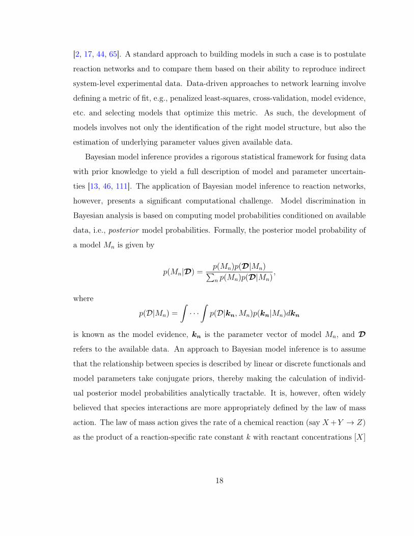
a model 𝑀𝑛 is given by
𝑝(𝑀𝑛|𝒟) =𝑝(𝑀𝑛)𝑝(𝒟|𝑀𝑛)∑𝑛 𝑝(𝑀𝑛)𝑝(𝒟|𝑀𝑛)
,
where
𝑝(𝒟|𝑀𝑛) =
∫· · ·∫𝑝(𝒟|𝑘𝑛,𝑀𝑛)𝑝(𝑘𝑛|𝑀𝑛)𝑑𝑘𝑛
is known as the model evidence, 𝑘𝑛 is the parameter vector of model 𝑀𝑛, and 𝒟
refers to the available data. An approach to Bayesian model inference is to assume
that the relationship between species is described by linear or discrete functionals and
model parameters take conjugate priors, thereby making the calculation of individ-
ual posterior model probabilities analytically tractable. It is, however, often widely
believed that species interactions are more appropriately defined by the law of mass
action. The law of mass action gives the rate of a chemical reaction (say 𝑋+𝑌 → 𝑍)
as the product of a reaction-specific rate constant 𝑘 with reactant concentrations [𝑋]
18
and [𝑌 ]:
Rate = −𝑘[𝑋][𝑌 ]. (1.1)
Under quasi-steady-state assumptions, the law of mass action produces reaction rate
expression for enzymatic reactions that are known as Michaelis-Menten functionals
[91]. The reaction rate for an enzyme 𝐸 binding to a substrate 𝑆 to produce product
𝑃 (𝐸 + 𝑆 → 𝐸 + 𝑃 ) by Michaelis Menten kinetics is given by
Rate = 𝑘𝑐𝑎𝑡[𝐸]0[𝑆]
𝑘𝑀 + [𝑆], (1.2)
where 𝑘𝑐𝑎𝑡 denotes the rate constant, [𝐸]0 is the enzyme concentration, [𝑆] the sub-
strate concentration, and 𝑘𝑀 the Michaelis constant. Using the law of mass ac-
tion to define reaction rate produces a system of differential equations such that the
parameter-to-observable map (forward model) is typically nonlinear. These equations
can be further embedded into differential equation models that describe convective
and diffusive transport, surface interactions, and other physical phenomena that af-
fect experimental observations. Rigorous computation of posterior model probabilities
then requires evaluation of a high-dimensional integral for each model. A number of
sampling-based methods exist in the literature for this purpose [26, 47, 94], but they
are computationally taxing. When the number of competing models becomes large,
the above methods actually become computationally infeasible.
Reaction network inference is particularly prone to this difficulty, since the number
of plausible models can grow exponentially with the number of proposed reactions. A
systematic approach to network inference requires appraising a combinatorially large
number of models: instead of a few model hypotheses, one might start with a list of
proposed reactions, for example, and form a collection of plausible models by consid-
ering all valid combinations of the proposed reactions. Alternatives such as Laplace’s
method and Bayesian information criterion have been suggested [21, 82, 109], but they
involve approximations of the posterior distribution. Across-model sampling offers a
19

solution in cases where the number of models is large [24, 57, 73]. These methods
work by making the sampler jump between models to explore the joint posterior dis-
tribution over models and parameters. Model probabilities are estimated from the
number of times the sampler visits each model. The prohibitively high cost of model
comparisons based on the computation of evidence for each model is avoided as the
sampler visits each model in proportion to its posterior probability. Efficient across-
model sampling, however, is challenging and require a delicate design of proposals for
between-model moves. Many practical applications of across-model sampling meth-
ods have relied on pilot posterior explorative runs to get a rough idea of the posterior
distribution, although a few automated methods do exist in literature [56, 110]. The
effective use of across-model sampling methods continues to be a challenge, especially
for problems where the parameter-to-observable map is nonlinear.
1.2 Background on reaction network inference
The general problem of network inference has been tackled in the past with various
modeling choices and inferential approaches. The modeling of species interactions has
spanned from simple Boolean networks to detailed physics-based differential equations
and stochastic models. The Boolean network approach relies on simple ON/OFF
switches and standard logic interactions to describe species interactions. Additive
linear or generalized linear models take an intermediate approach in terms of com-
plexity and reliability. The differential equations based network interactions are at
the other end of the complexity spectrum, but being rooted in mechanistic models
hold the promise of better understanding and improved predictions. From an algo-
rithmic standpoint, a large number of inference methods, both from a Bayesian and
a non-Bayesian standpoint, have been proposed. We review here a few network in-
ference approaches and refer the readers to some detailed reviews for the complete
story [44, 96, 98].
20
1.2.1 Non-Bayesian reaction network inference
Many non-Bayesian methods for network inference have been published in the chemi-
cal and biological engineering literature. Gardner et al. adopted an ODE formulation
and developed a technique known as Network Identification by Multiple Regression
(NIR) [43]. Their approach constructs a first-order model of regulatory interactions
and uses multiple linear regression to infer species interactions. Bansal et al. developed
an algorithm known as the Time Series Network Identification in which they assumed
a linear ODE model for species interactions and inferred the network topology by a
combination of interpolation and principal component analysis [10]. Bonneau et al.
use L1 shrinkage to identify transcriptional influences on genes based on the integra-
tion of genome annotation and expression data [18]. Margolin et al. have proposed
another technique called ARCANE that adopts an information-theoretic approach
in which they identify candidate interactions by estimating pairwise species mutual
information [84]. Nachman et al. utilize dynamic Bayesian network models and the
structural EM algorithm for network identification [92]. Another technique, correla-
tion metric construction, suggested by Arkin et al. is based on the calculation and
analysis of a time-lagged multivariate correlation function of a set of time-series of
chemical concentrations [7]. Burnham et al. propose a statistical technique relying
on t-statistics and 𝑅2 for the inference of chemical reaction networks governed by
ordinary differential equations [22].
1.2.2 Bayesian reaction network inference
The Bayesian approach to network inference has seen increasing applications in ar-
eas such as protein signalling modeling, gene regulation reconstruction, combustion
chemistry etc. The inference methods for signalling topologies and gene regula-
tion pathways have principally been developed with linear or discrete formulations
[40, 90, 107, 116]. Using Gaussian or multinomial likelihood functions and conjugate
priors with these formulations leads to model evidence being available in closed form.
21

In spite of the cheap analytical evaluation of evidence, the exponential explosion of
the number of networks given species and their possible interactions precludes direct
enumeration of model evidence. Thus, sampling based approaches have been devel-
oped for large-scale network inference in such contexts [37, 39]. At the same time,
ODE-based species interaction models (mass-action kinetics) are also being incorpo-
rated into inference frameworks. The use of ODE-based forward models oftentimes
results in nonlinear parameter-observable dependency—network inference then has
to be based on the computation of model evidence numerically. Xu et al. applied
Bayesian model inference with nonlinear ODEs for the elucidation of ERK signalling
pathway [118]. Braman et al. used Bayesian methodology for the comparison of
syngas chemistry models [19]. However, the methods used above for numerical com-
putation of evidence are limited to applications with a small number of hand-crafted
models. Large-scale network inference with nonlinear forward models has seen very
limited work. Oates et al. applied Bayesian model selection for the comparison of
systematically generated models derived from ODE-based species interactions [95].
They used reversible-jump Markov chain Monte Carlo algorithm, a general across-
model sampling method, for the simultaneous sampling of network topologies and
their underlying parameters. As discussed in 1.1, the use of vanilla across-model
sampling methods are generally known to perform poorly. There is a need for the
development of efficient large-scale network inference methods that would allow a
systematic comparison of exponentially large number of networks, but one that in-
corporates nonlinear forward models emerging from ODE-based species interaction
formulations.
1.3 Thesis contributions
In this thesis, we present methods for efficient large-scale Bayesian inference of non-
linear chemical reaction networks. We develop algorithms that exploit structural
22

properties of chemical reaction networks to improve exploration of posteriors over
a large number of reaction networks in comparison to existing methods. Further,
we develop a model-space sampling approach that makes approximations of the pa-
rameter posterior, and thereby allows sampling over very large model spaces whose
exploration remains intractable with exact sampling methods.
More specifically, we operate in the across-model sampling framework and make
four contributions:
1. Network inference with adaptive MCMC
The rate of a chemical reaction is given by the law of mass action and the
net species production rate a species is given by the species production rate
from all reactions [77]. The species production rates further feed into forward
models that describe convective and diffusive transport, surface interactions,
and other phenomena affecting experimental obsevations. Nevertheless, the
additive structure of the net species production rate means that reaction inclu-
sion/exclusion can be controlled by setting the rate constants to non-zero/zero
values. In spite of the overall nonlinear dependency of the observables on the
rate constants. This indirect control of network topology by assigning specific
values to the rate constants means that the plausible networks are statistically
nested. Nested models provide a natural between-model move construction.
Nested models can further allow the use of fixed-dimensional Markov chain
Monte Carlo (MCMC) algorithms. Adaptive MCMC in which the parameter
proposals adapt to posterior samples are known for fixed-dimensional MCMC
algorithms and improve sampling efficiency without manual tuning. We exploit
the nested structure of reaction network problems and develop an adaptive
MCMC algorithm for network inference. The developed algorithm is used to
learn reaction networks for steam and dry catalytic reforming of methane on
rhodium from a set of 15 proposed reactions and real experimental data.
2. Network-aware sampling
23

Chemical reaction networks can quickly become very complex [28, 108]. The
network of species interactions, however, has a special structure hidden in it.
The production/destruction of a species is directly linked to the concentration
of other species it is participating in a reaction with. Therefore, the rate of
production/destruction of a species will necessarily be zero if those other species
are absent from the system. From a data-analytic perspective, the available data
cannot inform the presence of reactions with zero reaction-rate. Many species
in a reaction network such as catalysts or enzymes play a fundamental role
in the operation of reactions, but do not get consumed. Moreover, practically
feasible experiments yield data that is sparse—data is only linked to a few of the
species. Sparsity of data and presence of catalyst/enzymes can further render
some reactions ineffective in influencing the observables. Thus, the inclusion
of these reactions is also not informed by data. We develop a network-aware
across-modeling sampling algorithm that recognizes the effective networks being
inferred and exploits this knowledge to design efficient parameter proposals for
moves between models. This translates into superior sampling performance
and low-variance posterior estimates. The recognition of effective networks also
allows derandomization of some conditional expectations and thereby yields
further variance reduction.
3. Sensitivity-based network-aware sampling
Not all reactions in a network are equally important in influencing the observ-
ables. The identification of reactions that have a sharper impact on observables
can be critical in designing improved across-model samplers. We develop a local
sensitivity-based metric to identify key reactions and use this to develop better
between-model move proposals for the reversible jump MCMC algorithm. Com-
bining the sensitivity-based proposal construction along with network-aware
sampling produces a highly improved nonlinear network inference algorithm.
We apply the algorithm for the inference of network topology from a set of 1024
24

systematically generated networks that were obtained from a subset of proposed
reactions for the activation of the extracellular signal-regulated kinase pathway
by epidermal growth factor [118].
4. Network inference with approximation
The network inference methods in Contributions 1, 2, and 3 are exact sampling
methods, i.e., they are guaranteed to converge to the correct posterior distri-
bution asymptotically as sampling proceeds. Exact inference methods over the
joint space of models and parameters are essential for consistency of poste-
rior estimates and their development is an important goal. However, for very
large model spaces, exact sampling may still be very expensive. We develop
an approximation-based network inference approach by using Laplace’s method
to approximate model evidences and using Markov chain Monte Carlo to ex-
plore the posterior distribution only over model indicators. Nonlinearity of the
forward model and limited available data results in the posterior distribution
over models being multimodal. To explore multimodal posterior distributions,
we extend the approximate posterior inference to a population-based network
inference algorithm. The developed algorithm is then used to infer signalling
networks from a space of 109 plausible networks.
This thesis is organized into 6 chapters. Following the introduction in Chapter 1,
Chapter 2 gives a detailed overview of the motivations for model inference, contrasts
different model inference approaches, highlights Bayesian model inference, and dis-
cusses existing numerical methods for Bayesian model inference. Chapters 3, 4, and 5
present the four main contributions of this thesis. We summarize and discuss future
work in Chapter 6.
25

26
Chapter 2
Model inference: formulation and
numerical approaches
An integral component of scientific research is the construction of models for the
physical process under study. Models are created for two main reasons: they enable
an easy understanding of a complex process by breaking it down into more readily
interpretable modules, and models can be used for making predictions of unobserved
quantities. Development of reliable models is often very hard because one may only
get to observe a few noisy realizations of the physical process—referred to as data.
Utilizing the available data and any background information about the process, the
job of a model developer is to construct a consistent set of equations that relate the
model inputs and model parameters to the quantities of interest. Historically, models
have been built by empiricism and experimental investigation. More recently, first-
principles calculations have also been used to aid model development in disciplines
such as chemistry and biology. However, the development of faster computers and
the availability of high-quality data has now allowed the use of rigorous statistical
techniques in the model development phase. Given a set of plausible models and
some data, tools from statistical inference can be used for a systematic evaluation
of all models to identify the “best” set of models. In this chapter, we discuss the
27

motivations for model inference, present a popular philosophy for effective learning
of models from data, outline common approaches for model inference, introduce the
Bayesian paradigm for model learning, and discuss some numerical techniques for
Bayesian model inference.
2.1 Model inference
Model inference can be defined informally as the assessment of models to ascertain
the degree to which each is supported by available data. A prerequisite for model
inference is the availability of (i) plausible models and (ii) relevant data to discriminate
among the models. Very often, we also have a great deal of background information
about the quality of competing models and the values of their underlying parameters.
This knowledge—termed as prior information—can be incorporated in the model
inference framework. It is important at this stage to distinguish model inference from
the common practice of model reduction in chemical kinetics [14, 97]. Model reduction
refers to a systematic reduction in the size of a large kinetic model so as to reproduce
model outputs within a specified tolerance. Such a procedure, however, assumes that
an accurate model (i.e., the full kinetic model) is already known and fixed. And,
crucially, it does not take experimental data into account during reduction.
A model of a physical process describes a specific collection of input-output re-
lationships. In particular, a model describes how some pre-specified quantities of
interest are related to input variables. As a result, a model may preclude the de-
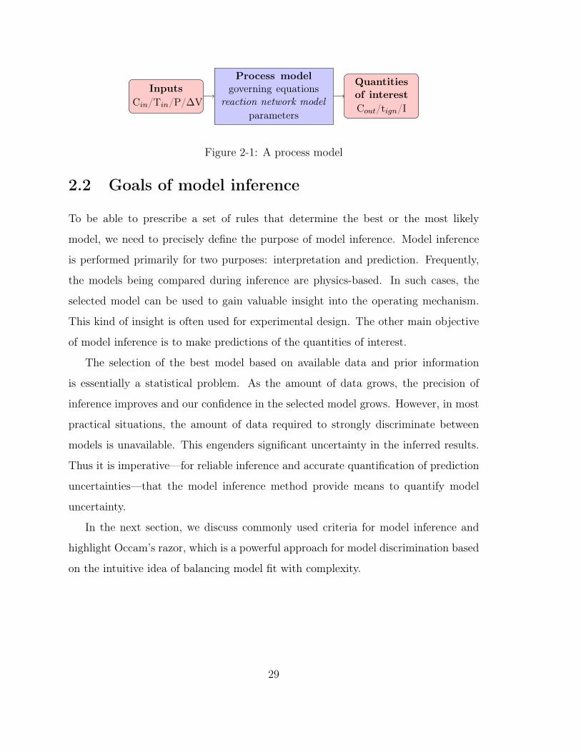
scription of quantities for which it has not been specifically built. Figure 2-1 shows a
typical process model. This model—consisting of governing equations expressing con-
servation laws, reaction network models, and thermo-kinetic parameters—may relate
inputs such as concentration 𝐶𝑖𝑛, temperature 𝑇𝑖𝑛, pressure 𝑃 , and applied voltage
∆𝑉 to observables such as concentration 𝐶𝑜𝑢𝑡, ignition delay 𝜏𝑖𝑔𝑛, and current 𝐼.
28
InputsC𝑖𝑛/T𝑖𝑛/P/ΔV
Process modelgoverning equations
reaction network modelparameters
Quantitiesof interestC𝑜𝑢𝑡/t𝑖𝑔𝑛/I
Figure 2-1: A process model
2.2 Goals of model inference
To be able to prescribe a set of rules that determine the best or the most likely
model, we need to precisely define the purpose of model inference. Model inference
is performed primarily for two purposes: interpretation and prediction. Frequently,
the models being compared during inference are physics-based. In such cases, the
selected model can be used to gain valuable insight into the operating mechanism.
This kind of insight is often used for experimental design. The other main objective
of model inference is to make predictions of the quantities of interest.
The selection of the best model based on available data and prior information
is essentially a statistical problem. As the amount of data grows, the precision of
inference improves and our confidence in the selected model grows. However, in most
practical situations, the amount of data required to strongly discriminate between
models is unavailable. This engenders significant uncertainty in the inferred results.
Thus it is imperative—for reliable inference and accurate quantification of prediction
uncertainties—that the model inference method provide means to quantify model
uncertainty.
In the next section, we discuss commonly used criteria for model inference and
highlight Occam’s razor, which is a powerful approach for model discrimination based
on the intuitive idea of balancing model fit with complexity.
29
2.3 Approaches for model inference
Having presented a few motivations for model inference, we now proceed to discuss
three approaches for model choice. Since the data we would be using to infer the
best model will necessarily be noisy, it would be incorrect to try to fit exactly to all
available data. If we maximize the quality of fit to the available data, it is the most
complex model—model with the largest degrees of freedom—which typically would
best fit the data. As we discuss in the following paragraphs, such a strategy would
be sub-optimal since the objective is to select models that peform well for all data,
not just the observed data.
2.3.1 Model selection based on estimation of prediction error
Model inference is sometimes performed in a data rich situation. In such settings, the
available data can be used to compute an estimate of prediction error known as the
empirical prediction error [64]. To begin with, the available data is split into three
parts: a training set, a validation set, and a test set. The training set is used to fit the
models; the validation set is used to estimate the prediction error for model selection;
the test set is used for the assessment of the generalization error of the final chosen
model. In a slightly data deficient situation, test set can be used to select the model
as well as estimate the prediction error. In such cases, the final chosen model will
necessarily underestimate the prediction error [64].
2.3.2 Cross validation
Cross-validation is another method that is used often to estimate the prediction error.
A 𝐾-fold cross-validation procedure begins by splitting the available data into 𝐾 sets.
Then a model is trained using data from 𝐾 − 1 sets as the training data and the
prediction error computed on the 𝐾th set as the test set. This process is repeated
for all 𝐾 sets and then the average prediction error computed. By performing these
30

operations for all 𝑀 competing models, one can select the most well supported model
or rank the competing models. Mathematically, we let 𝑠 : {1, ..., 𝑁}| → {1, ..., 𝐾} be
an indexing function that indicates the partition to which data point 𝑛 is allotted.
We denote by 𝑓−𝑠(𝑥) the fitted function, computed with the 𝑠𝑡ℎ part of the data
removed. Then the cross-validation estimate of the prediction error is
𝐶𝑉 =1
𝑁
𝑁∑𝑛=1
𝐿(𝑦𝑛, 𝑓−𝑠(𝑛)(𝑥𝑛)) (2.1)
When 𝐾 = 𝑁 , the cross-validation method is referred to as leave-one-out cross vali-
dation [64].
2.3.3 Goodness-of-fit and complexity penalty
A well known observation pertaining to the fitting of model parameters to available
data is that the goodness-of-fit generally improves as the model complexity grows.
Though the mismatch between model predictions and available data decreases as the
model complexity increases, we would not expect our future predictions to be very
accurate. This is because by increasing model complexity we begin to fit to the noise
in the data. This problem is known as the problem of overfitting in statistics. Thus,
a common strategy is to adopt a model inference criterion such that the mismatch
between model predictions and available data is agreeable and at the same time model
complexity is limited. This two-fold objective is also described by the bias-variance
tradeoff [64]. As the complexity of the model grows, the variance of the inferred
parameters would be high, and as a result, the expected prediction error of the model
tends to be high. On the contrary, simpler models tend to have higher bias, and so
fit poorly to available data and have high prediction error (Figure 2-2).
The best models tend to be ones that balance bias with variance. Therefore,
a popular approach to model selection is one that rewards good agreement with
available data, but also penalizes model complexity. This guiding principle for the
31
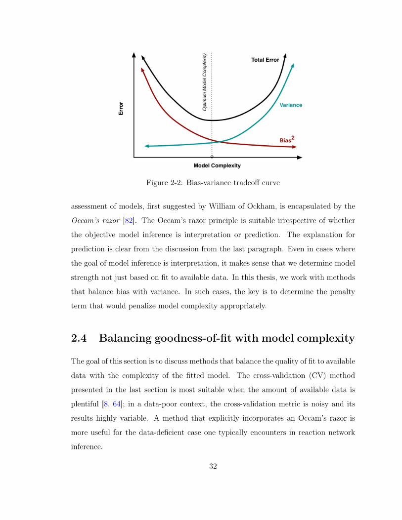
Figure 2-2: Bias-variance tradeoff curve
assessment of models, first suggested by William of Ockham, is encapsulated by the
Occam’s razor [82]. The Occam’s razor principle is suitable irrespective of whether
the objective model inference is interpretation or prediction. The explanation for
prediction is clear from the discussion from the last paragraph. Even in cases where
the goal of model inference is interpretation, it makes sense that we determine model
strength not just based on fit to available data. In this thesis, we work with methods
that balance bias with variance. In such cases, the key is to determine the penalty
term that would penalize model complexity appropriately.
2.4 Balancing goodness-of-fit with model complexity
The goal of this section is to discuss methods that balance the quality of fit to available
data with the complexity of the fitted model. The cross-validation (CV) method
presented in the last section is most suitable when the amount of available data is
plentiful [8, 64]; in a data-poor context, the cross-validation metric is noisy and its
results highly variable. A method that explicitly incorporates an Occam’s razor is
more useful for the data-deficient case one typically encounters in reaction network
inference.
32

In statistics in general, there are two main viewpoints for the identification of
likely models and their underlying parameter values from data. The frequentist ap-
proach to learning treats the models and parameters as fixed unknown quantities that
are determined by techniques that aim to produce good estimation over all possible
data sets. The Bayesian approach, in contrast, regards the models and parameters as
random variables whose distributions conditioned on available data are determined
by the consistent application of the rules of probability theory. Model selection ap-
proaches in the frequentist setting, such as 𝐶𝑝-statistic, Akaike information criterion,
etc, impose an Occam’s razor by selecting models based on the following optimization
problem:
𝑀* = arg min𝑀||𝒟 −𝐺𝑀(𝑘𝑀)||+ 𝛼|𝑀 |,
where 𝑀* is the optimal model, 𝐺𝑀 is the prediction with model 𝑀 , 𝑘𝑀 are the
parameters of model 𝑀 , 𝒟 the observed data, ||𝒟 − 𝐺𝑀(𝑘𝑀)|| is the data misfit,
|𝑀 | is the model complexity, and 𝛼 is the penalty on model complexity. The problem
with the above optimization based approaches is that they tend to be ad hoc, due to
a lack of a clear guideline about the right value for the penalty 𝛼 [12].
2.5 Bayesian approach to model inference
Bayesian statistics provides a rigorous inference framework to assimilate noisy and
indirect data, a natural mechanism to incorporate prior knowledge from different
sources, and a full description of uncertainties in parameter values and model struc-
ture. It is based on Bayes’ rule of probability:
𝑝(𝑘|𝒟) =𝑝(𝒟|𝑘)𝑝(𝑘)
𝑝(𝒟)(2.2)
33

Here, 𝑘 is the parameter being inferred, 𝑝(𝑘|𝒟) is the posterior probability den-
sity of 𝑘 conditioned on data 𝒟, 𝑝(𝒟|𝑘) is the likelihood of observing 𝒟 given the
parameter value, and 𝑝(𝑘) is the prior probability density of parameter 𝑘. 𝑝(𝒟),
commonly refered to as evidence or marginal likelihood, is the marginal distribution
of data. Sampling the posterior enables description of posterior uncertainty and the
estimation of posterior summaries such as the mean and standard deviation. Posterior
exploration by sampling is seldom directly feasible except for conjugate prior distri-
butions. For nonlinear forward models and/or non-conjugate prior distributions, one
has to rely on an indirect sampling approach, such as importance sampling or Markov
chain Monte Carlo [3, 51]. Application of Bayesian parameter inference to physical
models has received much recent interest [9, 74, 89, 113], with applications ranging
from geophysics [35, 55] and climate modeling [71] to reaction kinetics [53, 78, 99].
Applying Bayes’ rule to models 𝑀 , we get
𝑝(𝑀 |𝒟) =𝑝(𝒟|𝑀)𝑝(𝑀)
𝑝(𝒟). (2.3)
Comparing the posterior of any two models, 𝑀𝑖 and 𝑀𝑗, yields the posterior odds:
𝑝(𝑀𝑖|𝒟)
𝑝(𝑀𝑗|𝒟)=𝑝(𝒟|𝑀𝑖)𝑝(𝑀𝑖)
𝑝(𝒟|𝑀𝑗)𝑝(𝑀𝑗)(2.4)
Assuming that all models are equally probable before the observation of data, we get
𝑝(𝑀𝑖|𝒟)
𝑝(𝑀𝑗|𝒟)=𝑝(𝒟|𝑀𝑖)
𝑝(𝒟|𝑀𝑗). (2.5)
The quantity on the right-hand side of Equation 2.5 is known as Bayes factor and is
the traditional metric used to compare the probabilities of different models [13, 46,
75]. A key advantage of this Bayesian formulation is an implicit penalty on model
complexity in the model evidence—an automatic Occam’s razor that guards against
overfitting [82]. Computation of Bayes factor, however, is expensive as it relies on the
evaluation of high-dimensional integrals. Specifically,
34

𝑝(𝒟|𝑀𝑖)
𝑝(𝒟|𝑀𝑗)=
∫𝑝(𝒟|𝑘𝑖)𝑝(𝑘𝑖|𝑀𝑖)𝑑𝑘𝑖∫𝑝(𝒟|𝑘𝑗)𝑝(𝑘𝑗 |𝑀𝑗)𝑑𝑘𝑗
(2.6)
where 𝑘𝑖 and 𝑘𝑗 are model-specific multidimensional parameters. Alternatives such
as Laplace approximation method and Bayesian information criterion have been sug-
gested in the literature [21, 82, 109], but they all involve making approximations
about distributions. The standard approach presented above becomes infeasible for
an exhaustive comparison of a large number of models because of the high computa-
tional cost involved. As mentioned in Chapter 1, in this thesis, we focus on developing
tractable network inference methodologies when the number of plausible models is
large. The underlying rate parameter uncertainties would come “for free" as a natural
byproduct of the model inference results.
The Bayesian posterior model probabilities also have the advantage of being eas-
ily interpretable. Having computed the posterior probabilities of the models, it is
straightforward to understand the degree to which the different models are supported
by available data based on their posterior probabilities. The Bayesian model inference
procedure has another favorable property in that it is consistent. Consistency is a
property that if the true model is among the set of models being compared, then the
posterior probability of the true model converges to 1 in probability as the size of the
data set goes to infinity.
2.6 Numerical methods for Bayesian computation
The generation of samples from posterior distributions is a central problem in Bayesian
statistics. Integration of functions with respect to posterior distributions in high-
dimensions is most efficiently performed by Monte Carlo sampling. Formally, the
35

posterior distribution can be defined over a general state space
Θ ∈⋃𝑀
{𝑀} × 𝑘𝑀 , (2.7)
where 𝑘𝑀 ⊆ R𝑀 are parameter spaces and each parameter space 𝑘𝑀 could have a
different dimensionality. 𝑀 here acts as an indicator of the individual parameter
spaces. The posterior distribution over Θ is again given by Bayes’ rule:
𝑝(𝑀,𝑘𝑀 |𝒟) =𝑝(𝒟|𝑘𝑀 ,𝑀)𝑝(𝑀)𝑝(𝑘𝑀 |𝑀)∑
𝑀
∫𝑘𝑀
𝑝(𝒟|𝑘𝑀 ,𝑀)𝑝(𝑀)𝑝(𝑘𝑀 |𝑀). (2.8)
Note, in relation to models and parameters discussed in the previous section, 𝑀 would
correspond to model indicators and 𝑘𝑀 then are their respective parameter vectors.
The posterior distribution over 𝑀 and 𝑘𝑀 are related through a marginalization:
𝑝(𝑀 |𝒟) =
∫𝑘𝑀
𝑝(𝑀,𝑘𝑀 |𝒟) (2.9)
When the forward model is nonlinear or the prior distributions are non-conjugate,
the sampling of the posterior distribution 𝑝(Θ|𝒟) using standard Monte Carlo is
infeasible. In such cases, one has to resort to advanced Monte Carlo methods, the
most widely useful of which are a general class of algorithms known as the Markov
chain Monte Carlo methods.
In the following sections, we discuss various Monte Carlo methods that enable
computation of posterior model probabilities and in many cases also produce samples
from parameter posterior distributions. We begin with a brief discussion of an algo-
rithm used for fixed-dimensional posterior sampling known as the Metropolis-Hastings
algorithm.
36

2.6.1 Metropolis-Hastings algorithm
In many problems of interest, the model structure is assumed to be well known.
Thus the target of the inference procedure is only the posterior distribution over the
underlying parameters of the model. Sampling in such a fixed-dimensional setting,
when direct sampling is infeasible, is commonly performed using the Metropolis-
Hastings algorithm. The Metropolis-Hastings algorithm is an iterative algorithm
that produces a Markov chain whose limiting distribution is the posterior distribution
𝑝(𝑘|𝒟). At each step of the algorithm, a sample from a distribution 𝑞(𝑘|𝑘𝑛) known
as the proposal distribution is generated. The proposed sample is accepted as the
new state of the chain with a probability that depends on the posterior and proposal
distributions. If the proposed sample is rejected, the current state of the chain is
retained as the new state. The steps of the Metropolis-Hastings algorithm are given
in Algorithm 1.
Algorithm 1 The Metropolis-Hastings algorithm1: Given: Data 𝒟, prior density 𝑝(𝑘), likelihood function 𝑝(𝒟|𝑘), proposal density𝑞(𝑘|𝑘𝑛), number of steps 𝑁
2: Initialize 𝑘0
3: for 𝑛 = 0 to 𝑁 − 1 do4: Sample 𝑢 ∼ 𝒰[0,1]5: Sample 𝑘* ∼ 𝑞(𝑘|𝑘𝑡)6: if 𝑢 < 𝛼(𝑘𝑡,𝑘*) = min
{1, 𝑝(𝑘
*|𝒟)𝑞(𝑘𝑡|𝑘*)𝑝(𝑘𝑡|𝒟)𝑞(𝑘*|𝑘𝑡)
}then
7: 𝑘𝑛+1 = 𝑘*
8: else9: 𝑘𝑛+1 = 𝑘𝑛
10: end if11: end for
Under mild conditions, the above algorithm guarantees convergence of the distribution
of the Markov chain state 𝑘𝑛 to the posterior distribution and the existence of limit
theorems [105]. The sequence of Markov chain iterates yield estimates
37
𝑓 =1
𝑁
𝑁∑𝑛=1
𝑓(𝑘𝑛). (2.10)
that converges almost surely to∫𝑓(𝑘)𝑝(𝑘|𝒟)𝑑𝑘 by the strong law of large numbers.
In contrast to standard Monte Carlo sampling, the sequence of iterates produced
by the Metropolis-Hastings algorithm are correlated and thus the posterior estimates
have a higher variance. Special cases of the general Metropolis-Hastings algorithm are
obtained by considering specific choices of the proposal distribution 𝑞(𝑘|𝑘𝑛). If the
proposal is independent of the current location of the chain, we get the Independence
Metropolis-Hastings algorithm. Another very popular algorithm is obtained by con-
sidering proposals that consist of independent perturbations about the current state.
Specifically, the proposal is of the form 𝑘* = 𝑘𝑛+𝜖𝑛, where 𝜖𝑛 ∼ 𝑞 is independent of
𝑘𝑛. The resulting algorithm is then known as the random-walk Metropolis-Hastings
algorithm.
2.6.2 Computing the posterior model probabilities
The evaluation of posterior model probabilities in the Bayesian framework is often a
challenging computational problem. The computation of model evidence is seldom
analytically tractable. When the forward model is linear, the use of conjugate priors
permits closed form solutions for model evidence. However, in many practical sit-
uations, we encounter a nonlinear parameter-observable dependency. The evidence
is then obtained by resorting to numerical techniques. Formally, the objective is to
approximate the posterior model probability distribution 𝑝(𝑀 |𝒟). For any model
𝑀𝑖,
𝑝(𝑀𝑖|𝒟) ∝ 𝑝(𝒟|𝑀𝑖)𝑝(𝑀𝑖), (2.11)
where
38
𝑝(𝒟|𝑀𝑖) =
∫𝑝(𝒟|𝑘𝑖,𝑀𝑖)𝑝(𝑘𝑖|𝑀𝑖)𝑑𝑘𝑖, (2.12)
and 𝑝(𝑀𝑖) is the prior probability of model 𝑀𝑖 and 𝑘𝑖 is the vector of unknown
paramters in model 𝑀𝑖. The computation of the above multidimensional integral
is carried out by numerical methods. In low-dimensional settings, it is sometimes
efficient to compute the integral by numerical quadrature schemes [29, 48]. But for
moderate to high-dimensional integrals, sampling-based methods are necessary. We
provide a brief overview of some of the commonly used sampling-based methods for
Bayesian model inference.
2.6.3 Computing the evidence via model-specific Monte Carlo
simulations
Many existing methods in literature compute posterior model probabilities by esti-
mating the model evidence (2.12) individually for all competing models.
Standard Monte Carlo and importance sampling
A simple approach to estimating the model evidence for a model 𝑀𝑖 is to evaluate
the Monte Carlo sum by sampling from the prior distribution 𝑝(𝑘𝑖). The estimate
𝑝(𝒟|𝑀𝑖) =1
𝑁
𝑁∑𝑛=1
𝑝(𝒟|𝑘𝑛𝑖 ), (2.13)
where 𝑘𝑛𝑖 ∼ 𝑝(𝑘𝑖), is guaranteed to converge almost surely to the true model evidence
by the strong law of large numbers [105]. Although very simple, this approach is highly
inefficient as most samples are drawn from regions of the parameter space where the
likelihood tends to have a low value. Practically, this manifests into high variance in
evidence estimates.
An improvement to the above estimator is to use importance sampling. Impor-
tance sampling involves generating samples from a different distribution 𝑞(𝑘𝑖) known
39
as the proposal. Under some general conditions, a simulation consistent estimate is
given by
𝑝(𝒟|𝑀𝑖) =1
𝑁
𝑁∑𝑛=1
𝑤𝑛𝑝(𝒟|𝑘𝑛𝑖 ) (2.14)
where 𝑤𝑛 = 𝑝(𝑘𝑛𝑖 )/𝑞(𝑘𝑛𝑖 ) and 𝑘𝑛𝑖 ∼ 𝑞(𝑘𝑖) [49]. The precision of importance sampling
estimates hinges on 𝑞(𝑘𝑖) being a good approximation of 𝑝(𝑘𝑖|𝒟) and thus good
proposal distributions 𝑞(𝑘𝑖) are a priori hard to design in complex multi-dimensional
settings.
Posterior harmonic mean estimator
Newton et al. [94] suggested another importance sampling estimator for the estimation
of model evidence. In contrast to the standard importance sampling estimator (2.14),
an alternative simulation consistent importance sampling estimator is given by
𝑝(𝒟|𝑀𝑖) =
∑𝑁𝑛=1𝑤𝑛𝑝(𝒟|𝑘𝑛𝑖 )∑𝑁
𝑛=1𝑤𝑛
. (2.15)
Here again 𝑤𝑛 = 𝑝(𝑘𝑛𝑖 )/𝑞(𝑘𝑛𝑖 ) and 𝑘𝑛𝑖 ∼ 𝑞(𝑘𝑖) [49]. The advantage of this estimator
is that the proposal need only be known upto an unknown constant. Newton et al.
[94] noted that the posterior distribution 𝑝(𝑘𝑖|𝒟) is an efficient proposal distribution
and if we simulate samples approximately from the posterior, substitution into (2.15)
yields an estimate of 𝑝(𝒟|𝑀𝑖),
𝑝(𝒟|𝑀𝑖) =
{1
𝑁
𝑁∑𝑛=1
𝑝(𝒟|𝑘𝑛𝑖 )−1
}−1
, (2.16)
called the harmonic mean estimator. The simulation of posterior samples may be
performed by Markov chain Monte Carlo or sequential-importance-resampling meth-
ods [3]. It can easily be verified that the estimator (2.16) converges almost surely
to the correct model evidence. The drawback of the harmonic estimator is that it
40
can be unstable because 𝑝(𝒟|𝑘𝑖)−1 is often not square integrable with respect to the
posterior distribution.
Marginal likelihood from the Gibbs and the Metropolis-Hastings output
Another set of approaches proposed by Chib [25] and Chib et al. [26] involves expand-
ing the model evidence in terms of the likelihood, prior, and the posterior density at a
parameter value 𝑘*𝑖 and then estimating the posterior density value at 𝑘*
𝑖 using sam-
ples generated from the posterior distribution. The evidence being the normalizing
constant is given by
𝑝(𝒟|𝑀𝑖) =𝑝(𝒟|𝑘*
𝑖 )𝑝(𝑘*𝑖 )
𝑝(𝑘*𝑖 |𝒟)
. (2.17)
If 𝑝(𝑘*𝑖 |𝒟) is a posterior estimate, then the estimate of model evidence on the loga-
rithm scale is
log 𝑝(𝒟|𝑀𝑖) = log 𝑝(𝒟|𝑘*𝑖 ) + log 𝑝(𝑘*
𝑖 )− log 𝑝(𝑘*𝑖 |𝒟). (2.18)
When the posterior conditionals 𝑝(𝑘𝑖|𝒟, 𝑧) and 𝑝(𝑧|𝒟,𝑘𝑖) are available, Chib [25]
propose using the output from the Gibbs sampler {𝑘𝑛𝑖 , 𝑧𝑛}𝑁𝑛=1 to obtain a Monte
Carlo estimate of 𝑝(𝑘𝑖|𝒟) =∫𝑝(𝑘𝑖|𝒟, 𝑧)𝑝(𝑧|𝒟)𝑑𝑧 given as
𝑝(𝑘*𝑖 |𝒟) = 𝑁−1
𝑁∑𝑛=1
𝑝(𝑘*|𝒟, 𝑧𝑛). (2.19)
Chib et al. [26] extend the method to cases when full conditionals are intractable and
posterior samples are simulated using the Metropolis-Hastings algorithm. If {𝑘𝑛𝑖 }𝑁𝑛=1
are samples from the posterior 𝑝(𝑘𝑖|𝒟) and {𝑘𝑚𝑖 }𝑀𝑚=1 samples from the proposal
𝑞(𝑘𝑖|𝑘*𝑖 ,𝒟), a simulation-consistent estimate of the posterior density is
𝑝(𝑘*𝑖 |𝒟) =
𝑁−1∑𝑁
𝑛=1 𝛼(𝑘*𝑖 |𝑘𝑛𝑖 ,𝒟)𝑞(𝑘*
𝑖 |𝑘𝑛𝑖 )
𝑀−1∑𝑀
𝑚=1 𝛼(𝑘𝑚𝑖 |𝑘*𝑖 ,𝒟)
. (2.20)
41

Here
𝛼(𝑘′𝑖|𝑘𝑖,𝒟) = min
{1,𝑝(𝒟|𝑘′
𝑖)𝑝(𝑘′𝑖)𝑞(𝑘𝑖|𝑘′
𝑖,𝒟)
𝑝(𝒟|𝑘𝑖)𝑝(𝑘𝑖)𝑞(𝑘′𝑖|𝑘𝑖,𝒟)
}(2.21)
is the Metropolis-Hastings acceptance probability.
Path sampling
Methods that generalize the importance sampling algorithm by introducing a sequence
of intermediate distributions between two densities whose normalizing constants are to
be determined have existing in the computational physics literature for a few decades.
The acceptance ratio method and thermodynamic integration are routinely used in
statistical physics to compute free energies differences. More recently, Meng et al.
[87] and Gelman et al. [47] reinterpret the acceptance ratio method as an instance of
bridge sampling and more generally bridge sampling and thermodynamic integration
as instances of the path sampling algorithm. Recall that model evidence can be
written using Bayes’ rule as
𝑝(𝒟|𝑀𝑖) =𝑝(𝒟|𝑘𝑖)𝑝(𝑘𝑖)𝑝(𝑘𝑖|𝒟)
(2.22)
More generally, the normalizing constant 𝑧(𝜃) of an unnormalized density 𝑞(𝑘𝑖|𝜃) may
be written as
𝑧(𝜃) =𝑞(𝑘𝑖|𝜃)𝑝(𝑘𝑖|𝜃)
, (2.23)
where 𝑝(𝑘𝑖|𝜃) is a probability density function. Taking logarithms and then differen-
tiating both sides of (2.23) with respect to 𝜃,
𝑑
𝑑𝜃log 𝑧(𝜃) =
∫1
𝑧(𝜃)
𝑑
𝑑𝜃𝑞(𝑘𝑖|𝜃)𝜇(𝑑𝑘𝑖) (2.24)
42
= E𝜃
[𝑑
𝑑𝜃log 𝑞(𝑘𝑖|𝜃)
], (2.25)
where E𝜃 denotes the expectation with respect to 𝑝(𝑘𝑖|𝜃).
Let
𝑈(𝑘𝑖, 𝜃) =𝑑
𝑑𝜃log 𝑞(𝑘𝑖|𝜃). (2.26)
Integrating (2.25) from 0 to 1 yields
𝜆 = log
[𝑧(1)
𝑧(0)
]=
∫ 1
0
E𝜃[𝑈(𝑘𝑖, 𝜃)]𝑑𝜃. (2.27)
If we consider 𝜃 as a random variable with a uniform distribution, the right hand side
of (2.27) can be considered as the expectation of 𝑈(𝑘𝑖, 𝜃) over the joint distribution
of (𝑘𝑖, 𝜃). More generally, introducing a prior density 𝑝(𝜃) for 𝜃 ∈ [0, 1] we get
𝜆 = E[𝑈(𝑘𝑖, 𝜃)
𝑝(𝜃)
], (2.28)
where the expectation is with respect to the joint density 𝑝(𝑘𝑖|𝜃)𝑝(𝜃). Identity (2.27)
immediately suggests an unbiased estimator of 𝜆:
�� =1
𝑁
𝑁∑𝑛=1
𝑈(𝑘𝑛𝑖 , 𝜃𝑛)
𝑝(𝜃𝑛)(2.29)
using 𝑛 draws (𝑘𝑛𝑖 , 𝜃𝑛) from 𝑝(𝑘𝑖, 𝜃). The choice of the prior density 𝑝(𝜃) and the
number of discretizations of 𝜃 detemine the particular variant of importance sampling
algorithm. Bridge sampling involves a single intermediate distribution, whereas the
path sampling or thermodynmic integration involve a continuous discretization of 𝜃.
Another method which fits into the path sampling framework utilizes powers of
the posterior densities in (2.25) to yield formulas for the model evidence that make
use of MCMC sampling and numerical integration [41].
43
Annealed importance sampling
Neal [93] has presented another importance sampling based technique for the com-
putation of model evidence called the annealed importance sampling. The method
relies on using an importance proposal over a multidimensional state space with the
aid of Markov chain transition kernels with specific invariant distribution. Firstly, a
series of tempered posterior distributions
𝑓 𝑙(𝑘𝑖) = 𝑓(𝑘𝑖|𝒟)𝛽𝑙𝑓(𝑘𝑖)𝛽𝑙−1, (2.30)
where 1 = 𝛽0 > 𝛽1 > ... > 𝛽𝑛 = 0, 𝑓(𝑘𝑖|𝒟) is the unnormalized posterior probability
density and 𝑓(𝑘𝑖) is the prior probability density of 𝑘𝑖, are defined. The algorithm
starts by generating a sample 𝑘𝑛𝑖 from 𝑓(𝑘𝑖). Thereafter, starting from 𝑓𝑛−1(𝑘𝑖)
samples 𝑘𝑙𝑖 are drawn from 𝑓 𝑙(𝑘𝑖) with a Markov kernel 𝑇 𝑙(𝑘𝑖|𝑘𝑙+1𝑖 ) that keeps 𝑓 𝑙(𝑘𝑖)
invariant. These Markov kernels are constructed in the usual Metropolis-Hastings
or Gibss sampling fashion such that the detailed balance condition is satisfied. This
process is repeated 𝐽 times to generate sequence of 𝑛-dimensional samples. Let
𝑤𝑗 =𝑓𝑛−1(𝑘
𝑛−1𝑖 )
𝑓𝑛(𝑘𝑛−1𝑖 )
𝑓𝑛−2(𝑘𝑛−2𝑖 )
𝑓𝑛−1(𝑘𝑛−2𝑖 )
...𝑓1(𝑘
1𝑖 )
𝑓2(𝑘1𝑖 )
𝑓0(𝑘0𝑖 )
𝑓1(𝑘0𝑖 )
(2.31)
be importance weights. The average∑𝑤𝑗/𝑁 converges to the model evidence.The
efficiency of the algorithm increases with the number of tempered distributions.
2.6.4 Across-model Markov chain Monte Carlo
The use of the above model-specific Monte Carlo methods becomes practically infeasi-
ble when the number of possible models is large. Common examples include variable
selection problems, autoregressive time series modelling, and network inference. In
such cases, Monte Carlo methods that simultaneously traverse the space of models
and parameters are most favourable. These across-model sampling methods work by
making the MCMC sampler jump between models to explore the joint space of models
44

and parameters. Model probabilities are estimated from the number of times the sam-
pler visits each model. The prohibitively high cost of model comparisons based on the
computation of evidence for each model is avoided as the sampler visits each model
in proportion to its posterior probability. The challenge in the use of across-model
sampling schemes, however, is that the design of efficient model-switching proposal
distributions can often be hard. This thesis focuses on the across-model sampling
framework and we provide here a brief background on existing methodologies.
Product space approach
Carlin et al. [24] introduced an across-model MCMC algorithm by transforming the
transdimensional problem into one that is of constant dimension. The central idea
is that they assume complete independence of parameter vectors {𝑘𝑗}𝑀𝑗=1 given the
model indicator 𝑀𝑖 and choose ‘pseudopriors’ 𝑝(𝑘𝑗 |𝑀𝑖 =𝑗). From the conditional inde-
pendence assumptions, the joint distribution of data 𝒟 and {𝑘𝑗}𝑀𝑗=1 when the model
is 𝑀𝑖 is
𝑝(𝒟, {𝑘𝑗}𝑀𝑗=1,𝑀𝑖) = 𝑝(𝒟|𝑘𝑖,𝑀𝑖)
{ 𝑀∏𝑗=1
𝑝(𝑘𝑗 |𝑀𝑖)
}𝑝(𝑀𝑖) (2.32)
Assumming all full conditional distributions given by
𝑝(𝑘𝑗|𝑘𝑘 =𝑗 ,𝑀,𝒟) =
⎧⎪⎨⎪⎩𝑝(𝒟|𝑘𝑗 ,𝑀𝑗)𝑝(𝑘𝑗|𝑀𝑗), 𝑀 = 𝑀𝑗
𝑝(𝑘𝑗|𝑀 = 𝑀𝑗), 𝑀 = 𝑀𝑗
(2.33)
can be sampled and
𝑝(𝑀𝑗|{𝑘𝑗}𝑀𝑗=1) =
𝑝(𝒟|𝑘𝑖,𝑀𝑖)
{∏𝑀𝑗=1 𝑝(𝑘𝑗|𝑀𝑖)
}𝑝(𝑀𝑖)∑𝑀
𝑘=1 𝑝(𝒟|𝑘𝑖,𝑀𝑖)
{∏𝑀𝑗=1 𝑝(𝑘𝑗|𝑀𝑖)
}𝑝(𝑀𝑖)
(2.34)
a Gibbs sampler can be used to generate samples from the joint posterior distribution
𝑝(𝑀, {𝑘𝑗}𝑀𝑗=1). Specifically,
45
𝑝(𝑀𝑗|𝒟) =number of 𝑀𝑛
𝑗
total number of samples, j=1,...,M (2.35)
gives simulation-consistent estimates of posterior model probabilities. The drawback
of the above method is that it requires simulation from pseudopriors at each iteration
and as such the choice of pseudopriors has a direct impact on the simulation efficiency.
Carlin et al. [24] note that a good pseudoprior 𝑝(𝑘𝑗|𝑀𝑖 =𝑗) is the conditional posterior
distribution 𝑝(𝑘𝑖|𝑀𝑖). Dellaportas et al. [30] proposed a ‘Metropolised’ version of the
above approach, altering the model selection step into first proposing a move to a
model and then accepting the move with Metropolis-Hasings acceptance probability.
Reversible jump Markov chain Monte Carlo
Reversible jump MCMC (RJMCMC) is a general framework for posterior exploration
when the dimension of the state space is not constant [56, 57]. Consider the space
of candidate models ℳ = {𝑀1,𝑀2, ...,𝑀𝑁}. Each model 𝑀𝑗 has an 𝑛𝑗-dimensional
vector of unknown parameters 𝑘𝑀𝑗∈ ℛ𝑛𝑗 , where 𝑛𝑗 can different values for different
models. The reversible jump MCMC algorithm simulates a Markov chain whose in-
variant distribution is the joint model-parameter posterior distribution 𝑃 (𝑀,𝑘𝑀 |𝒟).
Each step of the algorithm consists of proposing a new vector of model-parameter
values and accepting the proposed values according to an acceptance probability that
also depends on the current model-parameter value vector. At any point of the state
space, many different proposal moves can be constructed. Generally, the moves can
be classified as between-model and within-model moves. The within model move
involves using the Metropolis-Hastings proposal. A between model move involves
proposing a move to a different model and the corresponding set of parameter values.
The necessary conditions for the reversible jump MCMC to be ergodic with the pos-
terior distribution as the invariant distribution is that the transition kernel resulting
from the chosen proposal is irreducible and aperiodic [57]. Further, ensuring that the
posterior distribution over the models and parameters is the invariant distribution of
46

the Markov chain is accomplished by satisfying the detailed balance condition. The
detailed balance condition is enforced by constructing moves between any two models
𝑀 and 𝑀 ′ according to a bijective map 𝑓 from (𝑘𝑀 ,𝑢) to (𝑘𝑀 ′ ,𝑢′), where 𝑘𝑀 and
𝑘𝑀 ′ are parameters of models 𝑀 and 𝑀 ′, 𝑢 and 𝑢′ known as dimension matching
variables are such that dim(𝑘𝑀 ′) + dim(𝑢′) = dim(𝑘𝑀) + dim(𝑢) and have densities
𝑞(𝑢) and 𝑞(𝑢′), respectively, and 𝑓 and 𝑓−1 are differentiable (i.e., 𝑓 is a diffeomor-
phism). The choice of the distribution of 𝑢 is part of the proposal construction and
in addition to an appropriate 𝑓 is key to an efficient reversible jump MCMC simu-
lation. At each step of the simulation, given the current state (𝑀,𝑘𝑀) a move to a
new model 𝑀 ′ is first proposed according to a chosen distribution 𝑞(𝑀 ′|𝑀). Next,
to move to (𝑀 ′,𝑘𝑀 ′) from (𝑀,𝑘𝑀) involves generating a sample of 𝑢 according to
𝑞(𝑢|𝑘𝑀) and accepting the proposed move with probability:
𝛼(𝑘𝑀 ,𝑘𝑀 ′) = min{1, 𝐴}, (2.36)
where
𝐴 =𝑝(𝑀 ′,𝑘𝑀 ′ |𝒟)𝑞(𝑀 |𝑀 ′)𝑞(𝑢′|𝑘𝑀 ′)
𝑝(𝑀,𝑘𝑀 |𝒟)𝑞(𝑀 ′|𝑀)𝑞(𝑢|𝑘𝑀)|det(∇𝑓(𝑘𝑀 ,𝑢))| , (2.37)
and (𝑘𝑀 ′ ,𝑢′) = 𝑓(𝑘𝑀 ,𝑢). The reverse move from (𝑘𝑀 ′ ,𝑢′) to (𝑘𝑀 ,𝑢) is performed
according to 𝑓−1 and has an acceptance probability min{1, 𝐴−1}. The complete
reversible jump MCMC algorithm we use is given in Algorithm 2.
The selection of a good map 𝑓 and the design of proposal distribution 𝑞(𝑢|𝑘𝑀)
is challenging and often chosen based on pilot runs of the reversible-jump MCMC.
The high cost and typically poor performance of the pilot-runs based RJMCMC has
prompted the development of methods for automatic proposal construction [1, 20,
36, 38, 59, 58]. All the above methods attempt to increase the acceptance rate of
between-model moves at the cost of some additional computational expense and have
shown to improve performance in a number of cases.
47

Algorithm 2 Reversible jump MCMC1: Given: A set of models 𝑀 ∈ℳ with corresponding parameter vectors 𝑘𝑀 , pos-
terior densities 𝑝(𝑀,𝑘𝑀 |𝒟), proposal for between-model move 𝑞(𝑀 ′|𝑀), pro-posal density 𝑞𝑀→𝑀 ′(𝑢|𝑘𝑀), jump-function 𝑓 , and Metropolis-Hastings proposal𝑞(𝑘′
𝑀 |𝑘𝑀).2: 𝛼 ∈ (0, 1): probability of within-model move3: Initlialize starting point (𝑀0,𝑘𝑀0)4: for 𝑛 = 0 to 𝑁𝑖𝑡𝑒𝑟 do5: Sample 𝑏 ∼ 𝒰[0,1]6: if 𝑏 ≤ 𝛼 then7: Sample 𝑝 ∼ 𝒰[0,1]8: if 𝑝 ≤ 𝐴(𝑘𝑛𝑀𝑛 → 𝑘
′
𝑀𝑛) = min{
1,𝑝(𝑀𝑛,𝑘′𝑀𝑛 |𝒟)𝑞(𝑘𝑛𝑀𝑛 |𝑘
′𝑀𝑛 )
𝑝(𝑀𝑛,𝑘𝑛𝑀𝑛 |𝒟)𝑞(𝑘′𝑀𝑛 |𝑘𝑛𝑀𝑛 )
}then
9: (𝑀𝑛+1,𝑘𝑛+1𝑀𝑛+1) = (𝑀
′,𝑘
′
𝑀 ′)10: else11: (𝑀𝑛+1,𝑘𝑛+1
𝑀𝑛+1) = (𝑀𝑛,𝑘𝑛𝑀𝑛)
12: end if13: else14: Sample 𝑀 ′ ∼ 𝑞(𝑀 ′|𝑀𝑛)15: Sample 𝑢 ∼ 𝑞𝑀𝑛→𝑀 ′(𝑢|𝑘𝑀𝑛)16: Sample 𝑝 ∼ 𝒰[0,1]17: if 𝑝 ≤ 𝐴 = min
{1,
𝑝(𝑀 ′,𝑘𝑀′ |𝒟)𝑞(𝑀𝑛|𝑀 ′)𝑞(𝑢′|𝑘𝑀′ )𝑝(𝑀𝑛,𝑘𝑀𝑛 |𝒟)𝑞(𝑀 ′|𝑀𝑛)𝑞(𝑢|𝑘𝑀𝑛 )
𝜕𝑓(𝑘𝑀𝑛 ,𝑢)𝜕(𝑘𝑀𝑛 ,𝑢)
}then
18: (𝑀𝑛+1,𝑘𝑛+1𝑀𝑛+1) = (𝑀 ′,𝑘𝑀 ′)
19: else20: (𝑀𝑛+1,𝑘𝑛+1
𝑀𝑛+1) = (𝑀𝑛,𝑘𝑛𝑀𝑛)21: end if22: end if23: end for
48
Other across-model samplers
Godsill [52] introduced a composite framework that allows interpretation of the prod-
uct space approach and the reversible jump sampler as special cases of the same
general approach. Recall that in the product space approach of Carlin et al. [24],
sampling is performed over a space {ℳ, {𝑘𝑗}𝑀𝑗=1)} of fixed dimension. The posterior
distribution 𝑝(𝑀,𝑘|𝒟) can be expressed as
𝑝(𝑀𝑖,𝑘|𝒟) =𝑝(𝒟|𝑀𝑖,𝑘𝑗)𝑝(𝑘𝑗|𝑀𝑗)𝑝(𝑘−𝑗 |𝑘𝑖,𝑀𝑖)𝑝(𝑀𝑖)
𝑝(𝒟|𝑀𝑖). (2.38)
Sampling over the fixed dimensional space {𝑀,𝑘} in a Metropolis-Hastings frame-
work using appropriate pseudopriors 𝑝(𝑘−𝑗|𝑘𝑖,𝑀𝑖) and proposal distribution 𝑞(𝑘′|𝑘),
Godsill et al. obtain the product space approach and the reversible jump sampler as
special cases.
Before the development of the reversible jump algorithm, Grenander et al. [60]
introduced a sampling method known as jump diffusion that involved between-model
jumps and within-model diffusion. This method, if corrrected by accept-reject step
like in MCMC methods would have been an example of reversible jump.
Certain trandimensional problems can be viewed as marked point processes [112].
In these problems, the variables whose number varies are regarded as marked points.
Using the birth-and-death simulation idea of Preston [100] and Ripley [103], Stephens
[112] developed a point-process approach for finite mixture analysis. Cappé et al. [23]
further extended the point-process idea to compare the reversible jump algorithm
with the continuous time birth-and-death samplers.
2.7 Model averaging
As was discussed in Section 2.2, full description of parameter and model uncertainties
is necessary for reliable decision-making and quantification of prediction uncertainties.
The Bayesian inference methodology provides a natural mechanism for the quantifica-
49
tion of all uncertainties. A direct consequence is that future predictions can be based
on all models weighted by their posterior probabilities. Making predictions based on
all models typically has the effect of lowering bias and improve predictive capability
[21]. Further, posterior predictions based on a selected model can be shown to always
underestimate prediction uncertainty [27, 102].
Consider that there is a set of M plausible models that are available for the predic-
tion of a quantity of interest ∆. Given the data 𝒟, the posterior model probabilities
of each model 𝑚, 𝑃 (𝑚|𝒟) is obtained by Bayes’s rule. Now, the posterior distribution
of the quantity of interest, ∆, is obtained by Bayesian model averaging as:
𝑝(∆|𝒟) =𝑀∑𝑖=1
𝑝(∆|𝑀𝑖,𝒟)𝑝(𝑀𝑖|𝒟). (2.39)
If we use a log-loss scoring rule, where the loss function for distribution, 𝑞(∆), is given
by:
𝐶(∆, 𝑞) = −𝐴 log 𝑞(∆) +𝐵, 𝐴 > 0, 𝐵 > 0, (2.40)
the expected loss of approximating the true posterior distribution 𝑝(∆|𝒟) with 𝑝(∆|𝑀𝑖,𝒟)
is given by −E𝑝(Δ|𝒟)[log 𝑝(∆|𝑀𝑖,𝒟)]. Since the Kullback-Leibler divergence between
any two distributions is always non-negative, it follows that
𝐷𝐾𝐿(𝑝(∆|𝒟)‖𝑝(∆|𝑀𝑖,𝒟)) ≥ 0, 𝑖 = 1, ....,𝑀 (2.41)
Consequently,
− E𝑝(Δ|𝒟)
[log
𝑀∑𝑖=1
𝑝(∆|𝑀𝑖,𝒟)𝑝(𝑀𝑖|𝒟)]≤ −E𝑝(Δ|𝒟)
[log 𝑝(∆|𝑀𝑖,𝒟)
]. (2.42)
The expected loss of approximating the uncertainty in ∆ based on any single model
is always greater than the quantifying the uncertainty by averaging over all plausible
50

models. Thus, a full description of prediction uncertainty is obtained by the posterior-
weighted-average of model predictions of the quantity of interest ∆.
51

52

Chapter 3
Network inference with adaptive
MCMC
We now present the details of a new framework for large-scale inference of chemical
reaction networks that transforms the network inference problem into a fixed dimen-
sional sampling problem and uses adaptive Markov chain Monte Carlo for improving
sampling efficiency. Viewing network inference as a fixed-dimensional problem allows
us to adapt existing fixed-dimensional adaptive MCMC algorithms for network infer-
ence. Adaptive MCMC methods adapt proposals based on previous posterior samples
and produce improved MCMC simulations without manual tuning. The material of
this chapter elaborates on one of our publications [42].
3.1 Reaction networks are nested
As we saw in Chapter 1, the law of mass action gives the rate of a chemical reaction
(say 𝑋 + 𝑌 → 𝑍) as the product of a reaction-specific rate constant 𝑘 with reactant
concentrations [𝑋] and [𝑌 ].
Rate = −𝑘[𝑋][𝑌 ]. (3.1)
53
The rate constant 𝑘 is expressed in Arrhenius form as
𝑘 = 𝐴𝑇 𝑛 exp
(− 𝐸𝑎
𝑅𝑇
), (3.2)
where 𝐴 is the pre-exponential factor, 𝐸𝑎 is the activation energy, 𝑛 is the temperature
exponent, 𝑅 is the universal gas constant, and 𝑇 is temperature. In this thesis, we
treat 𝑘 as the combined unknown parameter; it is also possible to infer 𝐴, 𝐸𝑎, and
𝑛 separately (given observations over a range of temperatures) but we leave such a
treatment for subsequent work.
In any chemically reacting process, the rates of the individual elementary reactions
in the reaction network together determine the values of the observables. And reacting
flow models are seldom linear; that is, the observables depend nonlinearly on the
elementary reaction rates and on the rate constants. Interestingly though, the net
species production rate is additive, i.e., the total production/destruction rate of a
species is the cumulative sum of the production/destruction rates of the species from
all reactions it participates in. From a statistical perspective, this implies that the
set of plausible networks given a set of proposed reactions and a noise model, are
𝑛𝑒𝑠𝑡𝑒𝑑. Specifically, a reaction can be eliminated from the network simply by setting
the corresponding rate constant to zero. The nested structure of reaction network
inference is exploited in two ways in this thesis.
First note that an across-model sampler for nested models can be constructed even
with a posterior sampler that operates over a space of fixed dimension. For example,
consider a setting where we have 𝑁 = 5 postulated elementary reactions with rate
constants 𝑘1, 𝑘2, 𝑘3, 𝑘4, and 𝑘5. Thus we wish to compare 25− 1 networks that are a
priori plausible. The key idea is to recognize that switching from a network 𝑀𝑖 (for
instance, comprising reactions 1, 2, and 5) to a network 𝑀𝑗 (for instance, comprising
reactions 3 and 4) requires that the parameter vector 𝑘 ≡ (𝑘1, 𝑘2, 𝑘3, 𝑘4, 𝑘5) change
from (𝑎, 𝑏, 0, 0, 𝑐) to (0, 0, 𝑑, 𝑒, 0), where 𝑎, 𝑏, 𝑐, 𝑑, and 𝑒 are nonzero rate constants
for each reaction. Second, the nested structure of network inference naturally leads
54
to proposing moves between networks such that the rate constants of reactions that
are common to the networks retain their parameter values.
The first step in developing a sampling scheme that assigns zero-value to rate
constants is to impose point-mass mixture priors on the rate constants 𝑘𝑖 [73, 88]. For
simplicity, in the subsequent numerical demonstrations we will take the priors to be
independent in each dimension (i.e., for each reaction), such that 𝑝(𝑘) =∏𝑁
𝑖=1 𝑝𝑖(𝑘𝑖).
We note, however, that priors can certainly be designed to reflect any additional
information, i.e., knowledge that necessitates the joint inclusion and exclusion of
reactions. In any case, a point-mass mixture prior is given by
𝑝𝑖(𝑘𝑖) = 𝑤0,𝑖𝛿(𝑘𝑖) + 𝑤1,𝑖 𝒞𝑖(𝑘𝑖), (3.3)
where 𝑤0,𝑖 and 𝑤1,𝑖 = 1 − 𝑤0,𝑖 are weights of the two prior components. 𝛿(𝑘𝑖) is
a probability atom (a point with unity probability mass) at zero and 𝒞𝑖(𝑘𝑖) is the
continuous component of the prior distribution. The continuous component of the
prior probability distribution describes any prior information about the values that the
rate constant can take and is often elicited from experts. If no such information exists,
𝒞𝑖(𝑘𝑖) may be a uniform or log-uniform distribution over all positive real numbers (an
‘uninformative’ prior). In any case, Bayesian inference and indeed our framework
allow the model developer significant flexibility in setting the prior distribution based
on his or her subjective belief or any pre-existing information. The weights 𝑤0,𝑖
and 𝑤1,𝑖 are prior beliefs about reaction 𝑖 being included or excluded, respectively,
from the inferred model. The model developer may use these weights to impose prior
information about the importance of this reaction in modeling the reacting flow model
output.
It is instructive to discuss two specific cases. First, if the model developer has
no prior preference for the inclusion or exclusion of a reaction, then an appropriate
choice for the weights is an indifference prior setting of 𝑤0,𝑖 = 𝑤1,𝑖 = 0.5. In contrast,
if the model developer believes that reaction 𝑖 should definitely be part of the inferred
55

model, then he/she can set 𝑤0,𝑖 to zero and 𝑤1,𝑖 to one. Note that if all the reactions
are assigned a prior inclusion probability of 𝑤1 = 1.0, then the model inference
framework reduces to the familiar Bayesian parameter inference problem.
Letting 𝒟 denote the available data, an application of Bayes’ rule to the parameter
vector 𝑘 yields
𝑝(𝑘|𝒟) ∝ 𝑝(𝒟|𝑘)𝑝(𝑘). (3.4)
Here 𝑝(𝒟|𝑘) is viewed as a function of 𝑘: it is the likelihood function, which reflects
the discrepancy between the data 𝒟 and the model prediction at the specified 𝑘. The
precise form of the likelihood function depends on the noise model used to describe
the data. For instance, in the examples of Section 4.4, we use an additive Gaussian
model, yielding
𝒟 = 𝐺(𝑘) + 𝜖. (3.5)
Here 𝐺(𝑘) is the prediction of the forward model (the chemically reacting flow model)
at the specified parameter value 𝑘, and 𝜖 reflects a combination of observational noise
and model errors. We assume that every component of 𝜖𝑗 of 𝜖 is independent with
mean zero and variance 𝜎2, 𝜖𝑗 ∼ 𝒩 (0, 𝜎2). Because the prior distribution on each
𝑘𝑖 is a point-mass mixture (3.3), the resulting posterior distribution of 𝑘 is also a
mixture distribution over the product space of all reactions, where each component
of the mixture contains a different set of non-zero rate constants and thus represents
a different model. Sampling the posterior distribution of 𝑘 implies visiting posterior
mixture components in proportion to their probabilities. Therefore, a scheme that
samples 𝑝(𝑘|𝒟) will not only provide a full description of uncertainties in rate constant
values, but will also yield estimates of the posterior model probabilities proportional
to the number of times each posterior mixture component is visited.
56

3.2 Posterior exploration by Markov chain Monte
Carlo
The multi-dimensional posterior distribution of the parameter vector 𝑘 obtained in
the last section cannot be sampled directly; because of the nonlinear forward model
𝐺(𝑘), the likelihood does not have a standard form and certainly is not conjugate
to the prior distribution. However, simulating posterior samples is possible using the
independence Metropolis-Hastings (MH) algorithm [105, 114]. In an independence
Metropolis-Hastings algorithm, the proposal distribution at each step is independent
of the current location of the chain. Algorithm 3 describes the independence sampler
using pseudocode. We note that another commonly-used class of MCMC algorithms,
random-walk Metropolis-Hastings, is not suitable for our problem because its chains
will tend to remain “stuck” in the point mass component of a parameter posterior
unless the support of the continuous component is very close to zero.
Algorithm 3 The independence Metropolis-Hastings algorithm1: Given: Data 𝒟, prior density 𝑝(𝑘), likelihood function 𝑝(𝒟|𝑘), proposal 𝑞(𝑘),
number of steps 𝑇2: Initialize 𝑘0
3: for 𝑡 = 0 to 𝑇 − 1 do4: Sample 𝑢 ∼ 𝒰[0,1]5: Sample 𝑘* ∼ 𝑞(𝑘*)
6: if 𝑢 < 𝒜(𝑘𝑡,𝑘*) = min{
1, 𝑝(𝑘*|𝒟)𝑞(𝑘𝑡)
𝑝(𝑘𝑡|𝒟)𝑞(𝑘*)
}then
7: 𝑘𝑡+1 = 𝑘*
8: else9: 𝑘𝑡+1 = 𝑘𝑡
10: end if11: end for
The Metropolis-Hastings algorithm’s efficiency in exploring the posterior distribution
rests on the design of an effective proposal distribution. “Efficiency” in this context
refers to how effectively the Markov chain explores the posterior—i.e., how nearly
independent its states are—which translates directly into the Monte Carlo error of
57

a sample-based posterior estimate. A good proposal distribution will require fewer
posterior density evaluations to achieve a given error. Recall that computation of
the posterior density 𝑝(𝑘|𝒟) for a proposed parameter value involves evaluating the
likelihood 𝑝(𝒟|𝑘), which in turn requires solving the forward model. Restricting the
number of forward model solves is especially important in the present application
context, because detailed models of chemically reacting flow are computationally
expensive.
Since the marginal posterior distribution of each parameter 𝑘𝑖 is a mixture of a
point mass and continuous components, the proposal distribution for each 𝑘𝑖 is taken
to be an independent point-mass mixture distribution of the form:
𝑞(𝑘𝑖;𝜓𝑖) = 𝑏𝑖,0𝛿(𝑘𝑖) +𝑀∑
𝑚=1
𝑏𝑖,𝑚𝑞𝑚(𝑘𝑖; 𝜃𝑖,𝑚). (3.6)
In the above equation, 𝛿(𝑘𝑖) is a point mass at zero, 𝑞𝑚(𝑘𝑖; 𝜃𝑖,𝑚) are continuous compo-
nents of the proposal distribution, and 𝜓 ≡ (𝑏𝑖=1:𝑁,𝑚=0:𝑀 , 𝜃𝑖=1:𝑁,𝑚=1:𝑀) comprises all
the parameters describing the proposal distribution. Recall that 𝑁 is the number of
proposed reactions, and thus the dimension of the posterior distribution. The number
of continuous components 𝑀 in each dimension is a choice left to the user. Increasing
𝑀 can potentially improve the approximation of the posterior by the proposal, espe-
cially if the continuous part of the posterior distribution is itself multimodal. This is
desirable, because a good proposal distribution for independence Metropolis-Hastings
is generally one that approximates the posterior as closely as possible. But higher
values of 𝑀 increase the number of parameters needed to describe the proposal dis-
tribution, which can affect the cost and convergence rate of the proposal adaptation
scheme discussed in Section 3.2.1. Choosing an independent proposal distribution for
each parameter 𝑘𝑖 means that the joint proposal distribution is given by
𝑞(𝑘;𝜓) =𝑁∏𝑖=1
𝑞(𝑘𝑖;𝜓𝑖). (3.7)
58

It is interesting to note that the above fixed-dimensional Metropolis-Hastings al-
gorithm is in fact a particular choice of the more general reversible jump MCMC
described in Section 2.6.4.
3.2.1 Adaptive MCMC by online expectation maximization
As noted above, efficient sampling suggests that we choose the proposal parameters
𝜓 so that (3.7) closely approximates the posterior. Of course, the true posterior
distribution is not characterized a priori; its exploration is in fact the goal of MCMC.
A useful strategy for improving sampling efficiency is, then, to continuously adapt the
proposal parameters based on past samples from the MCMC chain. Algorithms of
this kind are known as adaptive MCMC and require additional theoretical analysis to
guarantee convergence to the target distribution [105]. A commonly used adaptation
criterion is to tune the proposal parameters to minimize the Kullback-Leibler (KL)
divergence from the posterior distribution to the proposal distribution [4, 73]. We
adopt this strategy here and detail the adaptive independence Metropolis-Hastings
algorithm as follows.
Formally, the optimal proposal parameters are given by
𝜓* = arg min𝜓
𝒟𝐾𝐿
(𝑝(𝑘|𝒟)‖𝑞(𝑘;𝜓)
)= arg min
𝜓
∫𝑝(𝑘|𝒟) log
(𝑝(𝑘|𝒟)
𝑞(𝑘;𝜓)
)𝑑𝑘. (3.8)
Since this objective function involves integration over the posterior distribution 𝑝(𝑘|𝒟),
finding a solution before exploring the posterior is difficult. An effective strategy is
to use a stochastic approximation method [104, 79] that couples posterior exploration
with the solution of the minimization problem. A generic stochastic approximation
method for problem (3.8) involves iteratively (i) simulating a batch of samples from
the posterior distribution to estimate the KL divergence above, then (ii) using those
results to update the proposal parameters. Under conditions explained by [5], the
proposal parameters converge to the optimal solution of (3.8) asymptotically. Within
59

this general procedure, one could consider two possible instantiations. The first is
stochastic gradient descent: simulate a finite number of samples from the posterior
distribution and use them to compute a noisy estimate of the gradient of the objec-
tive in (3.8) with respect to 𝜓; then take a step in the negative-gradient direction
to update the parameters in each iteration. This approach is detailed in the paper
by [73]. The second approach involves solving (3.8) using a method called online
expectation maximization (EM) [4]. Online EM alternately uses posterior samples
to update estimates of the expectation of the logarithm of complete-data likelihood
(E-step) and then directly adapts the proposal parameters using analytical expres-
sions (M-step). We found the online EM approach to be more robust in practice, and
have thus adopted it for this work. (See A.0.3 for more details on the complete-data
likelihood.)
Here, we describe the expressions used to update the proposal parameters using
the online EM algorithm. A detailed derivation of the online EM algorithm applied to
point-mass mixture priors can be found in A. We consider the case where the reaction
rate parameter vector is𝑁 -dimensional, i.e., 𝑘 = (𝑘1, 𝑘2, . . . , 𝑘𝑁), where 𝑇 samples are
simulated from the posterior distribution 𝑝(𝑘|𝒟) between each proposal parameter
update, and where the 𝑀 continuous components of the proposal distribution are
Gaussian, resulting in a proposal of the form:
𝑞(𝑘𝑖;𝜓𝑖) = 𝑏𝑖,0𝛿(𝑘𝑖) +𝑀∑
𝑚=1
𝑏𝑖,𝑚𝒩𝑚(𝑘𝑖; 𝜃𝑖,𝑚). (3.9)
A non-adaptive component 𝑞 must also be added to the proposal distribution to satisfy
conditions for the convergence of the adaptive MCMC algorithm to the posterior
distribution (see A.0.3 for details). Thus, the overall proposal in each dimension is
given by
𝑞𝑠(𝑘𝑖) = 𝜆𝑖𝑞(𝑘𝑖,𝜓𝑖) + (1− 𝜆𝑖)𝑞(𝑘𝑖;𝜓𝑖), (3.10)
where 0 < 𝜆𝑖 < 1 and 𝜓𝑖 is a fixed set of proposal parameter values. At each step 𝑛
60
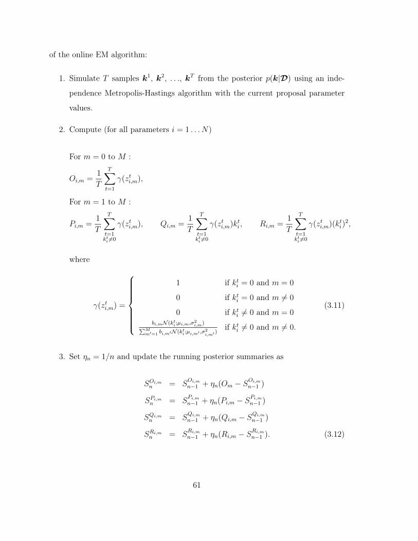
of the online EM algorithm:
1. Simulate 𝑇 samples 𝑘1, 𝑘2, . . ., 𝑘𝑇 from the posterior 𝑝(𝑘|𝒟) using an inde-
pendence Metropolis-Hastings algorithm with the current proposal parameter
values.
2. Compute (for all parameters 𝑖 = 1 . . . 𝑁)
For 𝑚 = 0 to 𝑀 :
𝑂𝑖,𝑚 =1
𝑇
𝑇∑𝑡=1
𝛾(𝑧𝑡𝑖,𝑚),
For 𝑚 = 1 to 𝑀 :
𝑃𝑖,𝑚 =1
𝑇
𝑇∑𝑡=1𝑘𝑡𝑖 =0
𝛾(𝑧𝑡𝑖,𝑚), 𝑄𝑖,𝑚 =1
𝑇
𝑇∑𝑡=1𝑘𝑡𝑖 =0
𝛾(𝑧𝑡𝑖,𝑚)𝑘𝑡𝑖 , 𝑅𝑖,𝑚 =1
𝑇
𝑇∑𝑡=1𝑘𝑡𝑖 =0
𝛾(𝑧𝑡𝑖,𝑚)(𝑘𝑡𝑖)2,
where
𝛾(𝑧𝑡𝑖,𝑚) =
⎧⎪⎪⎪⎪⎪⎪⎨⎪⎪⎪⎪⎪⎪⎩
1 if 𝑘𝑡𝑖 = 0 and 𝑚 = 0
0 if 𝑘𝑡𝑖 = 0 and 𝑚 = 0
0 if 𝑘𝑡𝑖 = 0 and 𝑚 = 0𝑏𝑖,𝑚𝒩 (𝑘𝑡𝑖 ;𝜇𝑖,𝑚,𝜎2
𝑖,𝑚)∑𝑀𝑚′=1 𝑏𝑖,𝑚′𝒩 (𝑘𝑡𝑖 ;𝜇𝑖,𝑚′ ,𝜎2
𝑖,𝑚′ )if 𝑘𝑡𝑖 = 0 and 𝑚 = 0.
(3.11)
3. Set 𝜂𝑛 = 1/𝑛 and update the running posterior summaries as
𝑆𝑂𝑖,𝑚𝑛 = 𝑆
𝑂𝑖,𝑚
𝑛−1 + 𝜂𝑛(𝑂𝑚 − 𝑆𝑂𝑖,𝑚
𝑛−1 )
𝑆𝑃𝑖,𝑚𝑛 = 𝑆
𝑃𝑖,𝑚
𝑛−1 + 𝜂𝑛(𝑃𝑖,𝑚 − 𝑆𝑃𝑖,𝑚
𝑛−1 )
𝑆𝑄𝑖,𝑚𝑛 = 𝑆
𝑄𝑖,𝑚
𝑛−1 + 𝜂𝑛(𝑄𝑖,𝑚 − 𝑆𝑄𝑖,𝑚
𝑛−1 )
𝑆𝑅𝑖,𝑚𝑛 = 𝑆
𝑅𝑖,𝑚
𝑛−1 + 𝜂𝑛(𝑅𝑖,𝑚 − 𝑆𝑅𝑖,𝑚
𝑛−1 ). (3.12)
61

4. Solve for new proposal parameters:
𝑏𝑖,𝑚 =𝑆𝑂𝑖,𝑚𝑛∑𝑀
𝑚′=0 𝑆𝑂𝑖,𝑚′𝑛
𝜇𝑖,𝑚 =𝑆𝑄𝑖,𝑚𝑛
𝑆𝑃𝑖,𝑚𝑛
𝜎2𝑖,𝑚 =
𝜇2𝑖,𝑚𝑆
𝑃𝑖,𝑚𝑛 − 2𝜇𝑖,𝑚𝑆
𝑄𝑖,𝑚𝑛 + 𝑆
𝑅𝑖,𝑚𝑛
𝑆𝑃𝑖,𝑚𝑛
. (3.13)
3.2.2 Random-scan AIMH for nested models
A straightforward application of the adaptive independence MH algorithm described
so far has one important inefficiency. In the parameter sampling step of Algorithm 3,
all the parameters are proposed jointly and then passed through an accept-reject step.
This approach can lead to a very high rate of rejection that consequently renders the
adaptation ineffective. The alternative is to use a componentwise independent MH
approach, wherein only a single component (or a small block of components) of the
parameter vector 𝑘 is proposed at a time while the other parameters are kept fixed,
and the resulting parameter vector is immediately passed through an accept-reject
step. We use a random-scan variant of the componentwise MH scheme which ran-
domly selects a block of components to be updated. Proposing to update only a few
parameter values while keeping the other parameter values fixed is a natural choice for
nested models and generally produces good exploration of the posterior distribution.
Updating only one or a few components at a time also provides the practical bene-
fit of a local search, since this amounts to making small jumps in the model space.
Algorithm 4 summarizes the overall algorithm we use to generate samples from the
posterior distribution. In implementing this algorithm for the following examples, we
choose 𝑇 = 1000 and 𝑙 = 1 or 2.
62
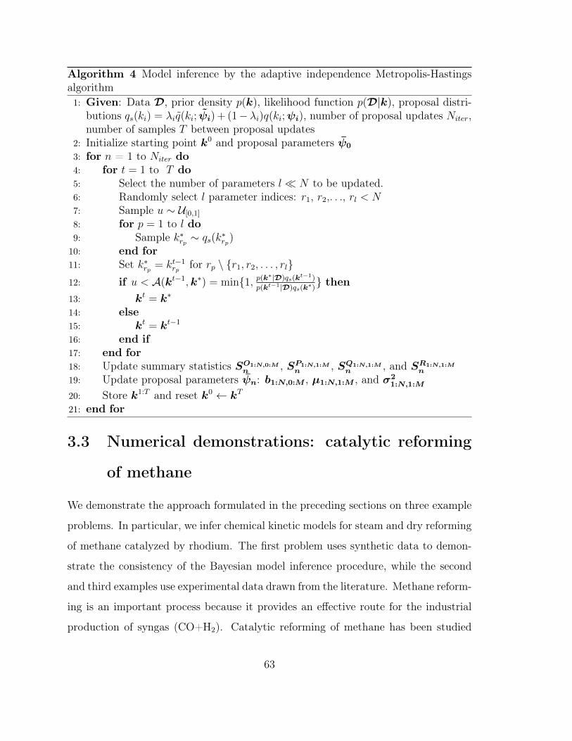
Algorithm 4 Model inference by the adaptive independence Metropolis-Hastingsalgorithm1: Given: Data 𝒟, prior density 𝑝(𝑘), likelihood function 𝑝(𝒟|𝑘), proposal distri-
butions 𝑞𝑠(𝑘𝑖) = 𝜆𝑖𝑞(𝑘𝑖;𝜓𝑖) + (1− 𝜆𝑖)𝑞(𝑘𝑖;𝜓𝑖), number of proposal updates 𝑁𝑖𝑡𝑒𝑟,number of samples 𝑇 between proposal updates
2: Initialize starting point 𝑘0 and proposal parameters 𝜓0
3: for 𝑛 = 1 to 𝑁𝑖𝑡𝑒𝑟 do4: for 𝑡 = 1 to 𝑇 do5: Select the number of parameters 𝑙≪ 𝑁 to be updated.6: Randomly select 𝑙 parameter indices: 𝑟1, 𝑟2,. . ., 𝑟𝑙 < 𝑁7: Sample 𝑢 ∼ 𝒰[0,1]8: for 𝑝 = 1 to 𝑙 do9: Sample 𝑘*𝑟𝑝 ∼ 𝑞𝑠(𝑘
*𝑟𝑝)
10: end for11: Set 𝑘*𝑟𝑝 = 𝑘𝑡−1
𝑟𝑝 for 𝑟𝑝 ∖ {𝑟1, 𝑟2, . . . , 𝑟𝑙}12: if 𝑢 < 𝒜(𝑘𝑡−1,𝑘*) = min{1, 𝑝(𝑘
*|𝒟)𝑞𝑠(𝑘𝑡−1)
𝑝(𝑘𝑡−1|𝒟)𝑞𝑠(𝑘*)} then
13: 𝑘𝑡 = 𝑘*
14: else15: 𝑘𝑡 = 𝑘𝑡−1
16: end if17: end for18: Update summary statistics 𝑆𝑂1:𝑁,0:𝑀
𝑛 , 𝑆𝑃1:𝑁,1:𝑀𝑛 , 𝑆𝑄1:𝑁,1:𝑀
𝑛 , and 𝑆𝑅1:𝑁,1:𝑀𝑛
19: Update proposal parameters 𝜓𝑛: 𝑏1:𝑁,0:𝑀 , 𝜇1:𝑁,1:𝑀 , and 𝜎21:𝑁,1:𝑀
20: Store 𝑘1:𝑇 and reset 𝑘0 ← 𝑘𝑇
21: end for
3.3 Numerical demonstrations: catalytic reforming
of methane
We demonstrate the approach formulated in the preceding sections on three example
problems. In particular, we infer chemical kinetic models for steam and dry reforming
of methane catalyzed by rhodium. The first problem uses synthetic data to demon-
strate the consistency of the Bayesian model inference procedure, while the second
and third examples use experimental data drawn from the literature. Methane reform-
ing is an important process because it provides an effective route for the industrial
production of syngas (CO+H2). Catalytic reforming of methane has been studied
63
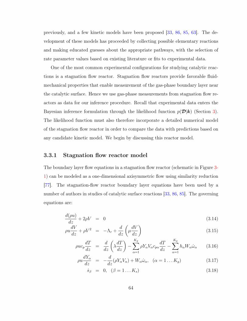
previously, and a few kinetic models have been proposed [33, 86, 85, 63]. The de-
velopment of these models has proceeded by collecting possible elementary reactions
and making educated guesses about the appropriate pathways, with the selection of
rate parameter values based on existing literature or fits to experimental data.
One of the most common experimental configurations for studying catalytic reac-
tions is a stagnation flow reactor. Stagnation flow reactors provide favorable fluid-
mechanical properties that enable measurement of the gas-phase boundary layer near
the catalytic surface. Hence we use gas-phase measurements from stagnation flow re-
actors as data for our inference procedure. Recall that experimental data enters the
Bayesian inference formulation through the likelihood function 𝑝(𝒟|𝑘) (Section 3).
The likelihood function must also therefore incorporate a detailed numerical model
of the stagnation flow reactor in order to compare the data with predictions based on
any candidate kinetic model. We begin by discussing this reactor model.
3.3.1 Stagnation flow reactor model
The boundary layer flow equations in a stagnation flow reactor (schematic in Figure 3-
1) can be modeled as a one-dimensional axisymmetric flow using similarity reduction
[77]. The stagnation-flow reactor boundary layer equations have been used by a
number of authors in studies of catalytic surface reactions [33, 86, 85]. The governing
equations are:
𝑑(𝜌𝑢)
𝑑𝑧+ 2𝜌𝑉 = 0 (3.14)
𝜌𝑢𝑑𝑉
𝑑𝑧+ 𝜌𝑉 2 = −Λ𝑟 +
𝑑
𝑑𝑧
(𝜇𝑑𝑉
𝑑𝑧
)(3.15)
𝜌𝑢𝑐𝑝𝑑𝑇
𝑑𝑧=
𝑑
𝑑𝑧
(𝜆𝑑𝑇
𝑑𝑧
)−
𝐾𝑔∑𝛼=1
𝜌𝑌𝛼𝑉𝛼𝑐𝑝𝛼𝑑𝑇
𝑑𝑧−
𝐾𝑔∑𝛼=1
ℎ𝛼𝑊𝛼��𝛼 (3.16)
𝜌𝑢𝑑𝑌𝛼𝑑𝑧
= − 𝑑
𝑑𝑧(𝜌𝑌𝛼𝑉𝛼) +𝑊𝛼��𝛼, (𝛼 = 1 . . . 𝐾𝑔) (3.17)
��𝛽 = 0, (𝛽 = 1 . . . 𝐾𝑠) (3.18)
64
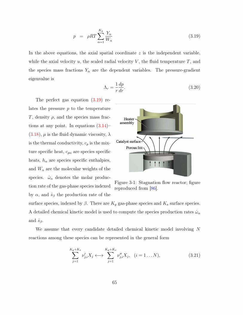
𝑝 = 𝜌𝑅𝑇
𝐾𝑔∑𝛼=1
𝑌𝛼𝑊𝛼
(3.19)
In the above equations, the axial spatial coordinate 𝑧 is the independent variable,
while the axial velocity 𝑢, the scaled radial velocity 𝑉 , the fluid temperature 𝑇 , and
the species mass fractions 𝑌𝛼 are the dependent variables. The pressure-gradient
eigenvalue is
Λ𝑟 =1
𝑟
𝑑𝑝
𝑑𝑟. (3.20)
N.E. McGuire et al. / Chemical Engineering Science 64 (2009) 5231 -- 5239 5233
Fig. 2. (a) Illustration of the stagnation-flow reactor. (b) Detail of the heated,catalytically active stagnation surface positioned above the porous frit.
catalyst geometries, such as porous-foam or channel-monolithstructures. In the technologically practical geometries, the catalystsurfaces are experimentally inaccessible. Because of small poresand narrow channels, it is not practical to experimentally probe thenear-catalyst boundary layer structure. However, the fundamentalinformation gathered from stagnation-flow experiments can beincorporated directly into models that provide quantitative designinsight for the practical configurations (Raja et al., 2000; Zhu et al.,2007).
The catalyst is coated onto a castable ceramic (Cotronics Rescor780) structure that has embedded 24-gauge Ni–Cr resistance heaters.The integrated catalyst-heater structure is bonded into a removableceramic housing (Fig. 2a). Three embedded thermocouples measurethe catalyst surface temperature. A heater controller is used to main-tain a specific catalyst surface temperature (typically between 665and 800 !C).
Hot oil (approximately 130 !C) circulates through the reactorhousing to control wall temperature. It is important to prevent wa-ter condensation on the reactor walls, especially for reforming ex-periments that incorporate high steam concentrations.
The reactor is designed to operate at slightly sub-atmosphericpressures. Reducing pressure tends to increase boundary-layer
Fig. 3. Process flow diagram of the experimental setup.
thickness, which facilitates resolving boundary-layer profiles. Theexperiments reported in this paper are conducted at pressures of40kPa (300Torr).
A microprobe (approximately 50!m opening) is used to sam-ple species-composition profiles within the boundary layer belowthe stagnation surface. As species react catalytically at the surface,the boundary-layer profiles are affected. For example, consider steamreforming of methane. Both steam and CH4 are consumed at thesurface, with H2 and CO being formed as reaction products. Becausespecies both diffuse and convect within the boundary layer, theboundary-layer profiles are affected directly by the reaction chem-istry at the surface. By measuring the profiles, a great deal can belearned about the surface chemistry. This is especially the case whencomputational models are used to assist in interpretation of the ex-perimental observations.
2.4. Boundary-layer measurements
Fig. 3 is a process flow diagram illustrating major features of theexperiment. A steady flow of reactant gases is supplied from cylin-ders at rates specified via mass-flow controllers. After mixing, wa-ter is added to the gas stream with a precision milliGAT micropumpthat dispenses water in the range of 0–100!L per minute. The fedgases pass through a heated damping reservoir that is designed todamp out any fluctuations associated with the water pump. Follow-ing water introduction, heating tape is used to maintain all lines atapproximately 135 !C. The heated lines assure that all the H2O re-mains in the vapor phase as it enters the reactor.
The quartz microprobe is used to sample gas composition withinthe boundary layer. As gases enter the probe itself, they are expandedrapidly to vacuum conditions which quench any further reaction.Water vapor is removed from the sampled gases (Drierite desiccant)before entering the mass spectrometer (SRS RGA 200).
The probe is positioned with a precision stepping motor. Be-ginning at the stagnation surface, the probe is moved downwardthrough the boundary layer. Upon arriving at each new measure-ment position, the probe is held stationary. The flow field achievessteady state conditions after approximately 2min following probemovement. Once the flow has achieved steady state, the gas-phasecomposition is measured via the mass spectrometer. A boundary-layer profile typically consists of eight measurement points, span-ning approximately 5mm below the stagnation surface.
Once a boundary-layer profile is measured for a certain setof operating parameters, the operating conditions are adjusted
Figure 3-1: Stagnation flow reactor; figurereproduced from [86].
The perfect gas equation (3.19) re-
lates the pressure 𝑝 to the temperature
𝑇 , density 𝜌, and the species mass frac-
tions at any point. In equations (3.14)–
(3.18), 𝜇 is the fluid dynamic viscosity, 𝜆
is the thermal conductivity, 𝑐𝑝 is the mix-
ture specific heat, 𝑐𝑝𝛼 are species specific
heats, ℎ𝛼 are species specific enthalpies,
and 𝑊𝛼 are the molecular weights of the
species. ��𝛼 denotes the molar produc-
tion rate of the gas-phase species indexed
by 𝛼, and ��𝛽 the production rate of the
surface species, indexed by 𝛽. There are 𝐾𝑔 gas-phase species and 𝐾𝑠 surface species.
A detailed chemical kinetic model is used to compute the species production rates ��𝛼
and ��𝛽.
We assume that every candidate detailed chemical kinetic model involving 𝑁
reactions among these species can be represented in the general form
𝐾𝑔+𝐾𝑠∑𝑗=1
𝜈 ′𝑗,𝑖𝑋𝑗 ←→𝐾𝑔+𝐾𝑠∑𝑗=1
𝜈 ′′𝑗,𝑖𝑋𝑗, (𝑖 = 1 . . . 𝑁), (3.21)
65
where 𝜈𝑗,𝑖 are integer stoichiometric coefficients and 𝑋𝑗 is the chemical name of the
𝑗th species. The molar production rates ��𝛼 and ��𝛽 are summations over all reactions:
��𝛼 =𝑁∑𝑖=1
𝜈𝛼,𝑖𝑞𝑖, ��𝛽 =𝑁∑𝑖=1
𝜈𝛽,𝑖𝑞𝑖, (3.22)
where
𝜈𝛼,𝑖 = 𝜈 ′′𝛼,𝑖 − 𝜈 ′𝛼,𝑖, (3.23)
and similarly for 𝜈𝛽,𝑖. The rate of progress 𝑞𝑖 of the 𝑖th reaction, which is assumed to
obey mass-action kinetics, is the difference between the forward and reverse reaction
rates:
𝑞𝑖 = 𝑘𝑖,𝑓
𝐾𝑔+𝐾𝑠∏𝑗=1
[𝑋𝑗]𝜈′𝑗,𝑖 − 𝑘𝑖,𝑏
𝐾𝑔+𝐾𝑠∏𝑗=1
[𝑋𝑗]𝜈′′𝑗,𝑖 . (3.24)
The form of the concentrations [𝑋𝑗] in (3.24) depends on whether the species is in
gas phase or on the surface. Also, it is known from earlier work [85] that species
production rates due to purely gas-phase reactions are negligible at normal operating
conditions. Thus we omit purely gas-phase reactions when evaluating ��𝛼 in our
differential equation model.
The species diffusion velocities are computed using a multicomponent diffusion
model as
𝑉𝛼 =1
𝑋𝛼��
𝐾𝑔∑𝑗 =𝛼
𝑊𝑗𝐷𝛼,𝑗𝑑𝑋𝑗
𝑑𝑧− 𝐷𝑇
𝛼
𝜌𝑌𝛼
1
𝑇
𝑑𝑇
𝑑𝑧. (3.25)
Here 𝑋𝛼 and 𝑋𝑗 are the species mole fractions, �� is the mean molecular weight, 𝐷𝛼,𝑗
are multicomponent diffusion coefficients, and 𝐷𝑇𝛼 are thermal diffusion coefficients.
At the reactor inlet, boundary conditions are
𝑢 = 𝑈𝑖𝑛, 𝑉 = 0, 𝑇 = 𝑇𝑖𝑛, 𝑌𝛼 = 𝑌𝛼,𝑖𝑛, (3.26)
66
and at the catalytic stagnation surface, the boundary conditions are
𝑢 = 0, 𝑉 = 0, 𝑇 = 𝑇𝑠, 𝜌𝑌𝛼𝑉𝛼 = 𝐹cg��𝛼𝑊𝛼. (3.27)
The boundary condition in (3.27) states that the gas-phase species diffusion flux at
the stagnation surface is balanced by species consumption by catalytic reactions.
The boundary condition also contains a parameter 𝐹cg, which specifies the effective
catalyst area. Since the catalyst particles are dispersed in a porous medium, the
effective catalyst area 𝐴catalyst is much greater than the geometric area 𝐴geometric of
the stagnation surface. The parameter 𝐹cg is defined as
𝐹cg =𝐴catalyst
𝐴geometric(3.28)
The steady-state stagnation flow axisymmetric boundary layer equations form a sys-
tem of ordinary differential equations. These equations are discretized using a finite
difference method and the resulting algebraic equations are solved using a combi-
nation of pseudo-time marching and Newton’s method [77]. We use the chemically
reacting flow software package Cantera 2.0.2 [54] to compute species production rates
and to solve the steady-state stagnation flow axisymmetric boundary layer equations.
3.3.2 Proposed elementary reactions
Beginning with the work of Hickman et al. [68], kinetic models for reactions of methane
on rhodium have been developed via a combination of theoretical methods, fits to
available experimental data, and previous analyses of related species. [33, 85, 63].
Activation energies for surface reactions are often estimated using the semi-empirical
unity bond index-quadratic exponential potential (UBI-QEP) method. The determi-
nation of pre-exponential factors, however, has largely relied on fits to observed data
or the assignment of nominal values. The uncertainty associated with these rate de-
termination techniques and limited understanding of the associated catalytic reaction
67

pathways make this system a good candidate for Bayesian model inference.
The set of proposed elementary reactions we use in our inference demonstrations
is taken from a comprehensive model proposed by McGuire et al. [85] recently and
is shown in Table 3.1. The reaction set consists of 42 irreversible elementary reac-
tions involving 12 surface-adsorbed species and gas-phase species. We retain the rate
parameters given by McGuire et al. [85] as base values for all reactions, except the
following two:
CO* + H* → HCO* + *
HCO* + * → CH* + O*
The pre-exponential factor of the first reaction above is changed from 5.0×10¹⁹ to 5.0×
1018, while that of the second reaction is changed from 3.7×1024 to 3.7×10²³. These
changes yield minor improvements in agreement with data at the nominal parameter
values. The pre-exponential factors were previously assigned nominal values. The
activation energies were estimated by UBI-QEP method, which has an expected error
of 1–3 kcal/mol [63].
The surface reactions shown in Table 3.1 are of two different types: adsorp-
tion/desorption of gas-phase species and reactions among surface intermediates. In
this work, we do not consider the adsorption/desorption reactions (Reactions 31–42)
to be uncertain; rather, they are included in all models inferred. In the table, the
adsorption/desorption reactions are shaded pink, while the surface reactions we con-
sider to be uncertain are shaded green. In the three examples to be presented below,
we treat the thermodynamic properties of the surface species as fixed (i.e., not un-
certain). Although the thermodynamic properties are not precisely known, they are
fixed indirectly through the individual forward and reverse rate constants. The base
values of the forward and reverse rate constants, 𝑘𝑓 and 𝑘𝑏, were originally established
to satisfy approximate thermodynamic reversibility. Therefore, with the thermody-
namic properties fixed, we need only to specify the prior distribution and apply the
68

model inference framework on the forward reactions. The reverse rate constant of
each reaction is then
𝑘𝑏 =𝑘𝑓𝐾𝑒𝑞
=𝑘*𝑏𝑘*𝑓𝑘𝑓 , (3.29)
where 𝐾𝑒𝑞, the equilibrium constant of the reaction, is a function of the thermody-
namic properties of the species participating in the reaction. In the above equations,
𝑘𝑓 and 𝑘𝑏 are the perturbed rate constants of the reactions while 𝑘*𝑓 and 𝑘*𝑏 are the
base rate constants.
3.3.3 Setup of the Bayesian model inference problem
Before discussing the three model inference examples individually, we describe the
choices we make for the likelihood function and prior distribution in our Bayesian
formulation. In the following, we use 𝑘 to refer to the rate constants of the reactions
that are treated as uncertain and 𝑘 to denote the rate constants of reactions that are
kept fixed. By “fixed,” we mean that a particular reaction is always included in the
model and that its rate constant is not a target of the inference procedure.
Likelihood function
As described in Section 3.1, evaluating the posterior probability in the Bayesian
approach requires evaluating the likelihood function 𝑝(𝒟|𝑘), where 𝒟 are the data
and 𝑘 = (𝑘, 𝑘) are the reaction parameters. We employ an i.i.d. additive Gaussian
model for the difference between model predictions and observations; thus the data
are represented as
𝒟 = 𝐺(𝑘, 𝑘) + 𝜖𝑛, (3.30)
where 𝜖𝑛 ∼ 𝒩𝑛(0, 𝜎2𝐼𝑛), 𝑛 is the number of observations, 𝐼𝑛 is an 𝑛-by-𝑛 identity
matrix, and 𝐺(𝑘, 𝑘) is the prediction of the forward model at the given value of the
reaction parameters. We let the noise standard deviation 𝜎 be 0.005. The determinis-
tic predictions 𝐺(𝑘, 𝑘) are obtained with the stagnation flow reactor model explained
69

Reaction 𝐴 𝐸𝑎 Uncertainty applied†
1 H* + O* → OH* + * 5.0× 10²² 83.7 log10 𝑘 = log10 𝑘* + 𝒰 [−2, 2]
2 H* + OH* → H2O* + * 3.0× 10²⁰ 33.5 log10 𝑘 = log10 𝑘* + 𝒰 [−2, 2]
3 OH* + OH* → H2O* + O* 3.0× 10²¹ 100.8 log10 𝑘 = log10 𝑘* + 𝒰 [−2, 2]
4 CO* + O* → CO2* + * 5.5× 10¹⁸ 121.6 log10 𝑘 = log10 𝑘* + 𝒰 [−2, 2]
5 CH4* + * → CH3* + H* 3.7× 10²¹ 61.0 log10 𝑘 = log10 𝑘* + 𝒰 [−2, 2]
6 CH3* + * → CH2* + H* 3.7× 1024 103.0 log10 𝑘 = log10 𝑘* + 𝒰 [−2, 2]
7 CH2* + * → CH* + H* 3.7× 1024 100.0 log10 𝑘 = log10 𝑘* + 𝒰 [−2, 2]
8 CH4* + O* → CH3* + OH* 1.7× 1024 80.34 log10 𝑘 = log10 𝑘* + 𝒰 [−2, 2]
9 CH3* + O* → CH2* + OH* 3.7× 1024 120.31 log10 𝑘 = log10 𝑘* + 𝒰 [−2, 2]
10 CH2* + O* → CH* + OH* 3.7× 1024 114.5 log10 𝑘 = log10 𝑘* + 𝒰 [−2, 2]
11 CH* + * → C* + H* 3.7× 10²¹ 21.0 log10 𝑘 = log10 𝑘* + 𝒰 [−2, 2]
12 CH* + O* → C* + OH* 3.7× 10²¹ 30.13 log10 𝑘 = log10 𝑘* + 𝒰 [−2, 2]
13 C* + O* → CO* + * 5.2× 10²³ 97.9 log10 𝑘 = log10 𝑘* + 𝒰 [−2, 2]
14 CO* + H* → HCO* + * 5.0× 10¹⁸ 108.9 log10 𝑘 = log10 𝑘* + 𝒰 [−2, 2]
15 HCO* + * → CH* + O* 3.7× 10²³ 59.5 log10 𝑘 = log10 𝑘* + 𝒰 [−2, 2]
16 OH* + * → H* + O* 3.0× 10²⁰ 37.7 𝑘 = 𝑘*16𝑘1/𝑘*1
17 H2O* + * → H* + OH* 5.0× 10²² 106.4 𝑘 = 𝑘*17𝑘2/𝑘*2
18 H2O* + O* → OH* + OH* 3.0× 10²¹ 171.8 𝑘 = 𝑘*18𝑘3/𝑘*3
19 CO2* + * → CO* + O* 3.0× 10²¹ 115.3 𝑘 = 𝑘*19𝑘4/𝑘*4
20 CH3* + H* → CH4* + * 3.7× 10²¹ 51.0 𝑘 = 𝑘*20𝑘5/𝑘*5
21 CH2* + H* → CH3* + * 3.7× 10²³ 44.1 𝑘 = 𝑘*21𝑘6/𝑘*6
22 CH* + H* → CH2* + * 3.7× 10²¹ 68.0 𝑘 = 𝑘*22𝑘7/𝑘*7
23 CH3* + OH* → CH4* + O* 3.7× 10²¹ 24.27 𝑘 = 𝑘*23𝑘8/𝑘*8
24 CH2* + OH* → CH3* + O* 3.7× 10²¹ 15.06 𝑘 = 𝑘*24𝑘9/𝑘*9
25 CH* + OH* → CH2* + O* 3.7× 10²¹ 36.82 𝑘 = 𝑘*25𝑘10/𝑘*10
26 C* + H* → CH* + * 3.7× 10²¹ 172.8 𝑘 = 𝑘*26𝑘11/𝑘*11
27 C* + OH* → CH* + O* 3.7× 10²¹ 136.0 𝑘 = 𝑘*27𝑘12/𝑘*12
28 CO* + * → C* + O* 2.5× 10²¹ 169.0 𝑘 = 𝑘*28𝑘13/𝑘*13
29 HCO* + * → CO* + H* 3.7× 10²¹ 0.0 𝑘 = 𝑘*29𝑘14/𝑘*14
𝜃*𝐶𝑂 50.0𝑏30 CH* + O* → HCO* + * 3.7× 10²¹ 167.5 𝑘 = 𝑘*30𝑘15/𝑘
*15
31 H2 + * + * → H* + H* 1.0× 10⁻²𝑎 0.0 -32 O2 + * + * → O* + O* 1.0× 10⁻²𝑎 0.0 -33 CH4 + * → CH4* 8.0× 10−3𝑎 0.0 -34 H2O + * → H2O* 1.0× 10−1𝑎 0.0 -35 CO2 + * → CO2* 4.8× 10−2𝑎 0.0 -36 CO + * → CO* 5.0× 10⁻¹𝑎 0.0 -37 H* + H* → H2 + * + * 3.0× 10²¹ 77.8 -38 O* + O* → O2 + * + * 1.3× 10²² 355.2 -
𝜃*𝑂 -280.0𝑏39 CH4* → CH4 + * 1.9× 10¹⁴ 25.1 -40 H2O* → H2O + * 3.0× 10¹³ 45.0 -41 CO2* → CO2 + * 4.1× 10¹¹ 18.0 -42 CO* → CO + * 3.5× 10¹³ 133.4 -
𝜃*𝐶𝑂 -15.0𝑏 -†Arrhenius rate expression for 𝑘*(base value): 𝑘* = 𝐴 exp(−𝐸𝑎/𝑅𝑇 )𝑎Sticking coefficient𝑏Coverage-dependent activation energy𝑏Forward-backward reaction pair I consists of reactions I and I+15
Table 3.1: Proposed reactions for reforming of methane
70
in Section 3.3.1. The likelihood function is thus given by
𝑝(𝒟|𝑘) = 𝒩𝑛(𝒟|𝐺(𝑘, 𝑘), 𝜎2𝐼𝑛)
=𝑛∏
𝑡=1
𝒩 (𝒟|𝐺(𝑘, 𝑘), 𝜎2)
=𝑛∏
𝑡=1
1√2𝜋𝜎2
exp
(−(𝑑𝑡 −𝐺(𝑘, 𝑘))2
2𝜎2
), (3.31)
where 𝑑𝑡 are components of the data vector 𝒟.
Prior specification
The prior distribution in Bayesian analysis should encapsulate information about
models and parameters that is available before assimilation of the data presently at
hand. Often the priors come from known scientific principles and physical constraints
on the parameters. In the context of chemical kinetics, the continuous component of
the prior distribution may also derived from previous investigations of the reactions.
Furthermore, as described in Section 3.1, priors may also be shaped by expert elic-
itation [45] or chosen to reflect relative ignorance about the rate parameter values.
In our demonstrations we will choose relatively uninformative priors by allowing the
rate constants 𝑘 to vary by two orders of magnitude above and below their base val-
ues. Other prior choices, e.g., an exponential distribution or a uniform distribution
between zero and some positive upper bound, would also be reasonable. In the same
way, prior information about model structure—applied in the form of prior weights
on reaction inclusion or exclusion—can also be designed to reflect an investigator’s
belief about the role or importance of particular reactions in the chemical process.
To illustrate the impact of the prior, we consider three different prior specifications
in our numerical demonstrations:
∙ Prior 1: 𝑝(𝑘𝑖,𝑓 ) = 0.2𝛿(𝑘𝑖,𝑓 ) + 0.8𝒞(𝑘𝑖,𝑓 ),
∙ Prior 2: 𝑝(𝑘𝑖,𝑓 ) = 0.5𝛿(𝑘𝑖,𝑓 ) + 0.5𝒞(𝑘𝑖,𝑓 ),
71

∙ Prior 3: 𝑝(𝑘𝑖,𝑓 ) = 0.8𝛿(𝑘𝑖,𝑓 ) + 0.2𝒞(𝑘𝑖,𝑓 ),
The prior distributions above are imposed identically on each reaction. Since reaction
rate constants must be positive, while their uncertainties may multiple orders of
magnitude, we take the continuous component of each prior distribution to be a
bounded uniform distribution on the logarithm of the rate constant. Specifically, we
set each 𝒞(𝑘𝑖,𝑓 ) to
𝒞(𝑘𝑖,𝑓 ) : log10 𝑘𝑖,𝑓 ∼ 𝒰(log10 𝑘*𝑖,𝑓 − 2, log10 𝑘
*𝑖,𝑓 + 2), (3.32)
where each 𝑘*𝑖,𝑓 above is the base value of the 𝑖th forward rate constant. For simplicity,
the priors used here are all of same family and width, but in general, one could
certaintly endow each of the 15 rate constants with distinct priors. One could even
encode prior correlations among the rate constants.
The three prior specifications above reflect different prior beliefs in the size and
sparsity of the reaction mechanism. Prior 1, with a weight of 0.8 on the continuous
component, has a tendency to favor kinetic models with more reactions. Prior 2 is
the indifference prior with no preference for inclusion or exclusion of reactions; it
is equivalent to a uniform prior distribution on the space of all 2𝑁 possible models,
and thus allows the data to completely determine the most probable set of reactions.
Prior 3 favors smaller models, and is an example of a sparsity-promoting prior. Such
priors introduce additional parsimony in model structure, over and above the penalty
on model complexity automatically imposed by the Bayesian Occam’s razor. By
using priors that favor reaction exclusion, the posterior distribution over models is
biased towards simpler reaction network structures; this has the potential of improving
prediction accuracy over unobserved data [64].
72
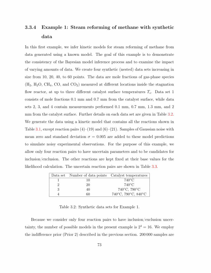
3.3.4 Example 1: Steam reforming of methane with synthetic
data
In this first example, we infer kinetic models for steam reforming of methane from
data generated using a known model. The goal of this example is to demonstrate
the consistency of the Bayesian model inference process and to examine the impact
of varying amounts of data. We create four synthetic (nested) data sets increasing in
size from 10, 20, 40, to 60 points. The data are mole fractions of gas-phase species
(H2, H2O, CH4, CO, and CO2) measured at different locations inside the stagnation
flow reactor, at up to three different catalyst surface temperatures 𝑇𝑠. Data set 1
consists of mole fractions 0.1 mm and 0.7 mm from the catalyst surface, while data
sets 2, 3, and 4 contain measurements performed 0.1 mm, 0.7 mm, 1.3 mm, and 2
mm from the catalyst surface. Further details on each data set are given in Table 3.2.
We generate the data using a kinetic model that contains all the reactions shown in
Table 3.1, except reaction pairs (4)–(19) and (6)–(21). Samples of Gaussian noise with
mean zero and standard deviation 𝜎 = 0.005 are added to these model predictions
to simulate noisy experimental observations. For the purpose of this example, we
allow only four reaction pairs to have uncertain parameters and to be candidates for
inclusion/exclusion. The other reactions are kept fixed at their base values for the
likelihood calculation. The uncertain reaction pairs are shown in Table 3.3.
Data set Number of data points Catalyst temperatures1 10 740∘C2 20 740∘C3 40 740∘C, 790∘C4 60 740∘C, 790∘C, 840∘C
Table 3.2: Synthetic data sets for Example 1.
Because we consider only four reaction pairs to have inclusion/exclusion uncer-
tainty, the number of possible models in the present example is 24 = 16. We employ
the indifference prior (Prior 2) described in the previous section. 200 000 samples are
73
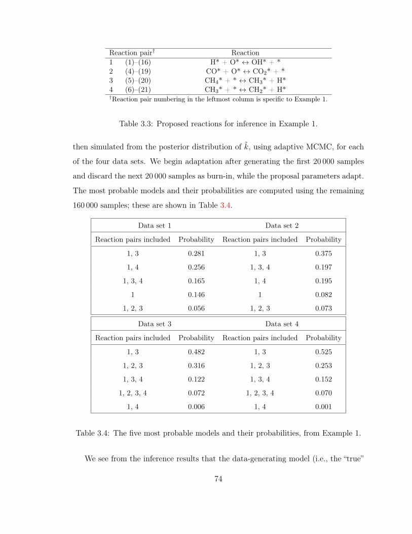
Reaction pair† Reaction1 (1)–(16) H* + O* ↔ OH* + *2 (4)–(19) CO* + O* ↔ CO2* + *3 (5)–(20) CH4* + * ↔ CH3* + H*4 (6)–(21) CH3* + * ↔ CH2* + H*†Reaction pair numbering in the leftmost column is specific to Example 1.
Table 3.3: Proposed reactions for inference in Example 1.
then simulated from the posterior distribution of 𝑘, using adaptive MCMC, for each
of the four data sets. We begin adaptation after generating the first 20 000 samples
and discard the next 20 000 samples as burn-in, while the proposal parameters adapt.
The most probable models and their probabilities are computed using the remaining
160 000 samples; these are shown in Table 3.4.
Data set 1 Data set 2
Reaction pairs included Probability Reaction pairs included Probability
1, 3 0.281 1, 3 0.375
1, 4 0.256 1, 3, 4 0.197
1, 3, 4 0.165 1, 4 0.195
1 0.146 1 0.082
1, 2, 3 0.056 1, 2, 3 0.073
Data set 3 Data set 4
Reaction pairs included Probability Reaction pairs included Probability
1, 3 0.482 1, 3 0.525
1, 2, 3 0.316 1, 2, 3 0.253
1, 3, 4 0.122 1, 3, 4 0.152
1, 2, 3, 4 0.072 1, 2, 3, 4 0.070
1, 4 0.006 1, 4 0.001
Table 3.4: The five most probable models and their probabilities, from Example 1.
We see from the inference results that the data-generating model (i.e., the “true”
74

model) is selected with highest posterior probability for every data set. Although it
is possible in principle for the true model not to be assigned the highest posterior
probability for finite data [16], we notice here that the true model is always preferred
and moreover that its probability increases with more data. This trend also demon-
strates the diminishing impact of the prior distribution as more data are included.
Indeed, Bayesian model inference is known to be asymptotically consistent, i.e., the
posterior concentrates on the true model given infinite data [12], provided that true
model is within the set of models being considered.
3.3.5 Example 2: Steam reforming of methane with real data
The second example considers inference of chemical kinetic models for steam reform-
ing of methane using real experimental data from a stagnation flow reactor apparatus
[86]. The operating conditions of the experiment are given in Table 3.5; further
specifics on the experimental data set (e.g., species and measurement locations) can
be found in [86].
In this example, we consider all three prior specifications (Section 3.3.3) imposed
on all 15 of the uncertain reaction pairs in Table 3.1. Using the adaptive MCMC
procedure of Section 3.2.1, we generate 200 000 samples from the posterior distribution
of 𝑘. Again, we begin adaptation after generating the first 20 000 samples and discard
the next 20 000 samples as burn-in. Posterior model probabilities are estimated from
the remaining 160 000 samples.
Table 3.6 shows the ten most probable models for each prior specification, and their
corresponding frequency (in a total population of 160 000 samples). As expected, the
sparsity of the most probable models increases with the weight on the 𝛿-component in
the prior. In the case of Prior 1, the model that includes all the reactions is strongly
preferred. For Prior 2, the most probable model includes all the reactions except pairs
6–21, 12–27, and 14–29. The exclusion of these three reaction pairs, particularly in
the case of an indifference prior, is an example of the Bayesian Occam’s razor in
75
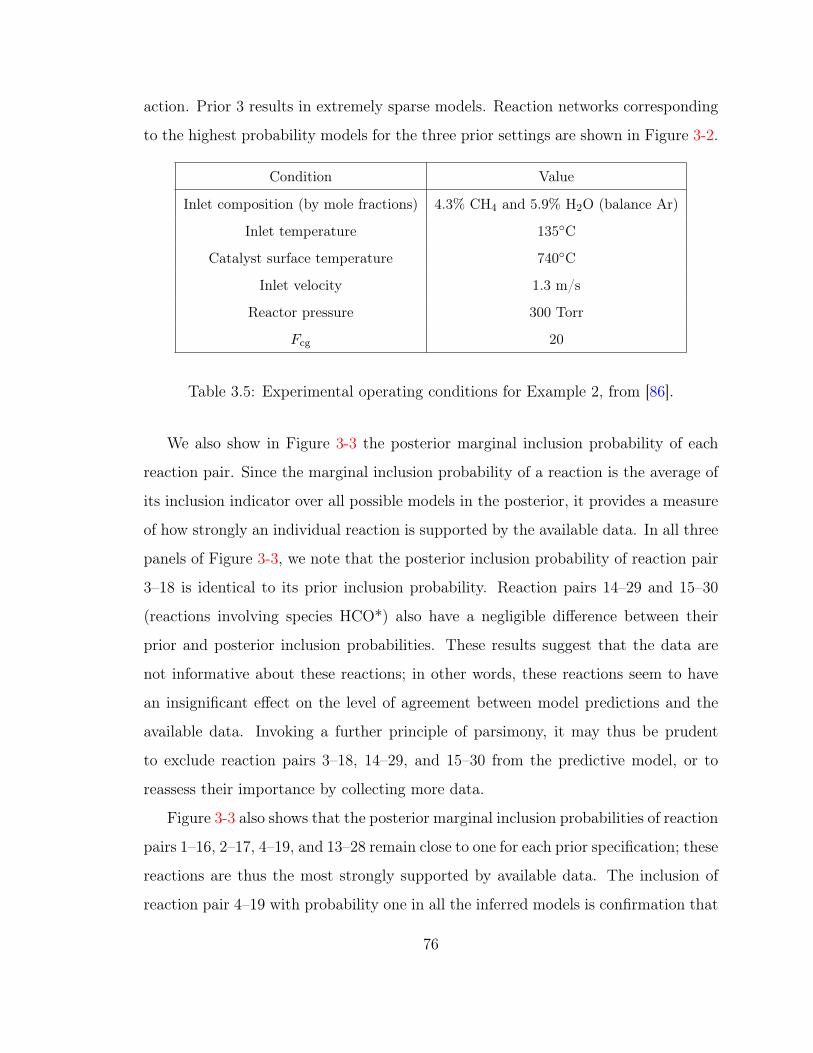
action. Prior 3 results in extremely sparse models. Reaction networks corresponding
to the highest probability models for the three prior settings are shown in Figure 3-2.
Condition Value
Inlet composition (by mole fractions) 4.3% CH4 and 5.9% H2O (balance Ar)
Inlet temperature 135∘C
Catalyst surface temperature 740∘C
Inlet velocity 1.3 m/s
Reactor pressure 300 Torr
𝐹cg 20
Table 3.5: Experimental operating conditions for Example 2, from [86].
We also show in Figure 3-3 the posterior marginal inclusion probability of each
reaction pair. Since the marginal inclusion probability of a reaction is the average of
its inclusion indicator over all possible models in the posterior, it provides a measure
of how strongly an individual reaction is supported by the available data. In all three
panels of Figure 3-3, we note that the posterior inclusion probability of reaction pair
3–18 is identical to its prior inclusion probability. Reaction pairs 14–29 and 15–30
(reactions involving species HCO*) also have a negligible difference between their
prior and posterior inclusion probabilities. These results suggest that the data are
not informative about these reactions; in other words, these reactions seem to have
an insignificant effect on the level of agreement between model predictions and the
available data. Invoking a further principle of parsimony, it may thus be prudent
to exclude reaction pairs 3–18, 14–29, and 15–30 from the predictive model, or to
reassess their importance by collecting more data.
Figure 3-3 also shows that the posterior marginal inclusion probabilities of reaction
pairs 1–16, 2–17, 4–19, and 13–28 remain close to one for each prior specification; these
reactions are thus the most strongly supported by available data. The inclusion of
reaction pair 4–19 with probability one in all the inferred models is confirmation that
76

CH4
CO2
CO2*
CH4*
CH3*
CH2*
CH*
H*
O*
CO*
OH*
CO
H2O*
H2O
C*
HCO*
H2
*
* OH*
O*
CO*
*
*
*
O*
O*
O*
*
O*O*
H*
*
H*
**
-*
-*
(a) 𝑝(𝑘𝑖,𝑓 ) = 0.2𝛿(𝑘𝑖,𝑓 ) + 0.8𝒞(𝑘𝑖,𝑓 )
CH4
CO2
CO2*
CH4*
CH3*
CH2*
CH*
H*
O*
CO*
OH*
CO
H2O*
H2O
C*
H2
*
* OH*
O*
CO*
*
*
O*
O*
O*
*
O*
H*
**
-*
-*
(b) 𝑝(𝑘𝑖,𝑓 ) = 0.5𝛿(𝑘𝑖,𝑓 ) + 0.5𝒞(𝑘𝑖,𝑓 )
CH4
CO2
CO2*
CH4*
CH3*
CH2*
CH*
H*
O*
CO*
OH*
CO
H2O*
H2O
C*
H2
*
*
O*
CO*
*
O*
O*
*
O*
H*
**
-*
-*
(c) 𝑝(𝑘𝑖,𝑓 ) = 0.8𝛿(𝑘𝑖,𝑓 ) + 0.2𝒞(𝑘𝑖,𝑓 )
Figure 3-2: Reaction networks of the highest posterior probability models for steamreforming of methane (Example 2), under different prior specifications. Edge thick-nesses are proportional to reaction rates calculated using posterior mean values of therate parameters.
77

the inference procedure is working well, in that it does not exclude reactions that
are absolutely necessary for production of the observed product species. Among all
the uncertain reaction pairs, reactions 4 and 19 are the only pair containing CO*2,
and their inclusion ensures that the model produces CO2 as one of the products. In
general, the near-unity posterior probabilities suggest that all four of these reaction
pairs are critical to explaining the steam reforming behavior of methane.
It is important to note, however, that the marginal inclusion probabilities shown
in Figure 3-3 do not capture correlations among the values of the reaction rate param-
eters or patterns of joint inclusion/exclusion. The joint posterior probability distri-
bution of the rate parameters, which we have sampled using MCMC, in fact contains
much more information. In particular, it contains information about combinations of
reactions and how well particular combinations are supported by the current data.
Reaction prior probability Reaction prior probability Reaction prior probability
0.2𝛿(𝑘𝑖,𝑓 ) + 0.8𝒞(𝑘𝑖,𝑓 ) 0.5𝛿(𝑘𝑖,𝑓 ) + 0.5𝒞(𝑘𝑖,𝑓 ) 0.8𝛿(𝑘𝑖,𝑓 ) + 0.2𝒞(𝑘𝑖,𝑓 )
Freq Excluded pairs† Freq Excluded pairs† Freq Excluded pairs†
16157 – 521 6, 12, 14 4221 3, 5, 7, 9, 12, 14, 15
4894 7 496 6, 8, 10, 12, 14 3533 3, 5, 9, 10, 12, 14, 15
4845 6 493 7, 11 3447 3, 5, 6, 7, 11, 14, 15
4545 12 477 7, 9, 11, 14 3379 3, 5, 6, 10, 11, 14, 15
4326 9 464 3, 6, 12, 14 3340 3, 5, 7, 9, 11, 14, 15
4237 10 457 3, 6, 10, 11, 14 3318 3, 5, 6, 7, 12, 14, 15
4168 11 454 6, 10, 12, 14 3153 3, 6, 8, 10, 12, 14, 15
3954 3 451 6, 12 3033 3, 7, 8, 9, 12, 14, 15
3908 15 451 7, 11, 15 2878 3, 5, 9, 10, 11, 14, 15
3902 14 441 6, 10, 11, 15 2640 3, 7, 8, 9, 11, 14, 15†Reaction pairs are denoted here by the number associated with the forward reaction
Table 3.6: The ten models with highest posterior probability in Example 2, for eachchoice of prior.
78
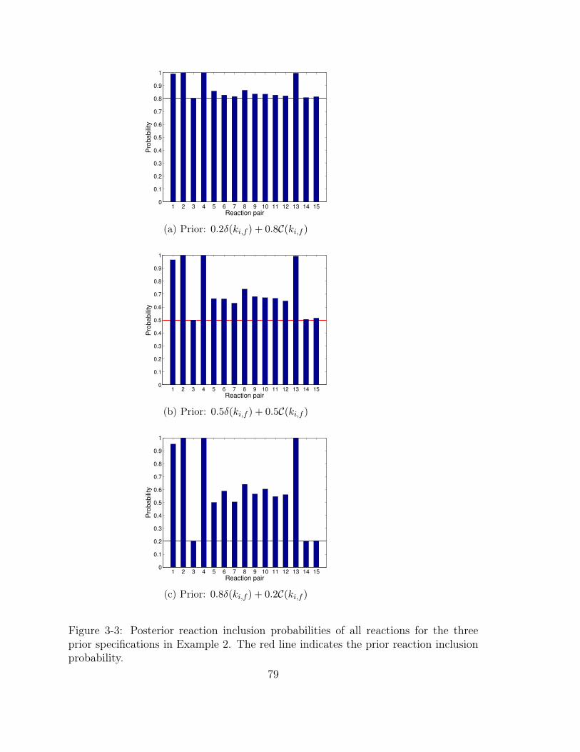
1 2 3 4 5 6 7 8 9 10 11 12 13 14 150
0.1
0.2
0.3
0.4
0.5
0.6
0.7
0.8
0.9
1
Reaction pair
Pro
babili
ty
(a) Prior: 0.2𝛿(𝑘𝑖,𝑓 ) + 0.8𝒞(𝑘𝑖,𝑓 )
1 2 3 4 5 6 7 8 9 10 11 12 13 14 150
0.1
0.2
0.3
0.4
0.5
0.6
0.7
0.8
0.9
1
Reaction pair
Pro
babili
ty
(b) Prior: 0.5𝛿(𝑘𝑖,𝑓 ) + 0.5𝒞(𝑘𝑖,𝑓 )
1 2 3 4 5 6 7 8 9 10 11 12 13 14 150
0.1
0.2
0.3
0.4
0.5
0.6
0.7
0.8
0.9
1
Reaction pair
Pro
babili
ty
(c) Prior: 0.8𝛿(𝑘𝑖,𝑓 ) + 0.2𝒞(𝑘𝑖,𝑓 )
Figure 3-3: Posterior reaction inclusion probabilities of all reactions for the threeprior specifications in Example 2. The red line indicates the prior reaction inclusionprobability.
79
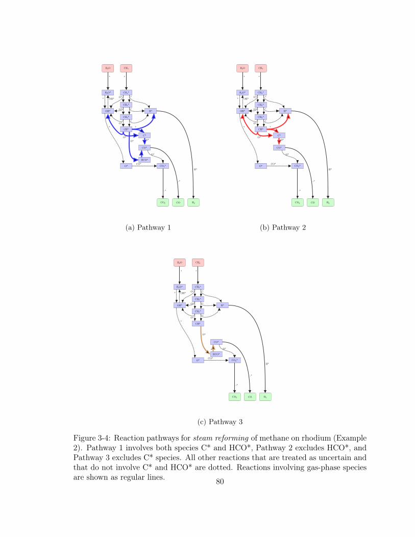
CH4
CO2
CO2*
CH4*
CH3*
CH2*
CH*
H*
O*
CO*
OH*
CO
H2O*
H2O
C*
HCO*
H2
*
* OH*
O*
CO*
*
*
*
O*
O*
O**
O*O*
*
O*
H*
**
-*
-*
(a) Pathway 1
CH4
CO2
CO2*
CH4*
CH3*
CH2*
CH*
H*
O*
CO*
OH*
CO
H2O*
H2O
C*
H2
*
* OH*
O*
CO*
*
*
*
O*
O*
O**
O*O*
H*
**
-*
-*
(b) Pathway 2
CH4
CO2
CO2*
CH4*
CH3*
CH2*
CH*
H*
O*
CO*
OH*
CO
H2O*
H2O
HCO*
H2
*
* OH*
O*
CO*
*
*
*
O*
O*
O*
*
O*
H*
**
-*
-*
(c) Pathway 3
Figure 3-4: Reaction pathways for steam reforming of methane on rhodium (Example2). Pathway 1 involves both species C* and HCO*, Pathway 2 excludes HCO*, andPathway 3 excludes C* species. All other reactions that are treated as uncertain andthat do not involve C* and HCO* are dotted. Reactions involving gas-phase speciesare shown as regular lines. 80

One way of interrogating the joint information embedded in the posterior distri-
bution is to focus attention on particular pathways in the reaction network. Looking
at the reaction network in Figure 3-2a (which contains all the proposed reactions),
it is possible to discern three clear pathways for the conversion of reactants H2O and
CH4 into products CO2, CO, and H2. The first pathway includes both C* and HCO*
species, the second pathway excludes HCO* and retains C*, and the third pathway
excludes C* but retains HCO*. The three possible reaction pathways are shown
schematically in Figure 3-4. We use samples from the joint posterior distribution to
quantify the degree to which each of these pathways is supported by available data.
The posterior probability of each pathway is obtained by computing the fraction of
posterior samples (i.e., candidate models) that contain the pathway. It is important to
note that the probabilities obtained in this fashion correctly account for uncertainties
in the other reactions (i.e., reactions not part of the pathway under consideration) by
marginalizing over them. This contrasts with a method that simply compares three
models, one corresponding to each pathway, while arbitrarily fixing or excluding all
the other reactions. Given the data produced by the steam reforming experiments
of McGuire et al. [86], the estimated posterior probabilities of the three pathways
are shown in Table 3.7. We observe that the dominant pathway is the C* pathway.
The HCO* pathway has nearly zero probability. This conclusion supports the view
commonly held in the literature that steam reforming of methane operates through
the C* pathway and that the inclusion of HCO* in the kinetic model is superfluous
[86, 85].
Pathway Prior 1 Prior 2 Prior 3Prior Posterior Prior Posterior Prior Posterior
1 (both C* and HCO* present) 0.536 0.643 0.177 0.249 0.026 0.0392 (only C* present) 0.302 0.343 0.529 0.733 0.633 0.9613 (only HCO* present) 0.162 0.010 0.294 0.012 0.340 0.000
Table 3.7: Prior and posterior pathway probabilities for steam reforming of methane,Example 2.
81
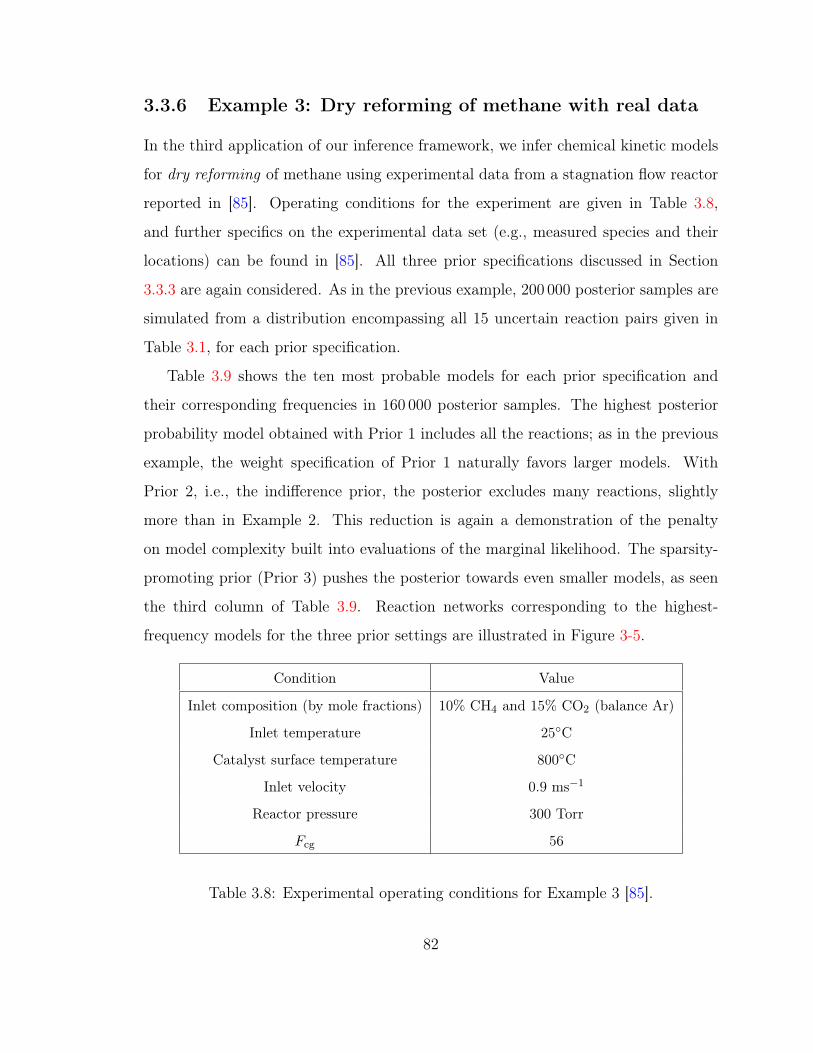
3.3.6 Example 3: Dry reforming of methane with real data
In the third application of our inference framework, we infer chemical kinetic models
for dry reforming of methane using experimental data from a stagnation flow reactor
reported in [85]. Operating conditions for the experiment are given in Table 3.8,
and further specifics on the experimental data set (e.g., measured species and their
locations) can be found in [85]. All three prior specifications discussed in Section
3.3.3 are again considered. As in the previous example, 200 000 posterior samples are
simulated from a distribution encompassing all 15 uncertain reaction pairs given in
Table 3.1, for each prior specification.
Table 3.9 shows the ten most probable models for each prior specification and
their corresponding frequencies in 160 000 posterior samples. The highest posterior
probability model obtained with Prior 1 includes all the reactions; as in the previous
example, the weight specification of Prior 1 naturally favors larger models. With
Prior 2, i.e., the indifference prior, the posterior excludes many reactions, slightly
more than in Example 2. This reduction is again a demonstration of the penalty
on model complexity built into evaluations of the marginal likelihood. The sparsity-
promoting prior (Prior 3) pushes the posterior towards even smaller models, as seen
the third column of Table 3.9. Reaction networks corresponding to the highest-
frequency models for the three prior settings are illustrated in Figure 3-5.
Condition Value
Inlet composition (by mole fractions) 10% CH4 and 15% CO2 (balance Ar)
Inlet temperature 25∘C
Catalyst surface temperature 800∘C
Inlet velocity 0.9 ms−1
Reactor pressure 300 Torr
𝐹cg 56
Table 3.8: Experimental operating conditions for Example 3 [85].
82

Marginal posterior inclusion probabilities of all reaction pairs for the three prior
specifications are shown in Figure 3-6. We see that the posterior inclusion probabilities
of all the reactions deviate from their prior inclusion probabilities, in contrast to
Example 2. This suggests that the experimental data used for this dry reforming
example is influenced by—and thus contains information about—every single reaction
pair. As in steam reforming, the inclusion of reaction pair 4–19 with probability one
confirms that the inference procedure is working well.
Reaction prior probability Reaction prior probability Reaction prior probability
0.2𝛿(𝑘𝑖,𝑓 ) + 0.8𝒞(𝑘𝑖,𝑓 ) 0.5𝛿(𝑘𝑖,𝑓 ) + 0.5𝒞(𝑘𝑖,𝑓 ) 0.8𝛿(𝑘𝑖,𝑓 ) + 0.2𝒞(𝑘𝑖,𝑓 )
Freq Excluded pairs† Freq Excluded pairs† Freq Excluded pairs†
7616 – 537 1, 2, 5, 9, 11, 14 4635 1, 3, 5, 10, 11, 12, 13
4950 6 488 1 10, 11, 12 3507 1, 2, 9, 10, 11, 14, 15
4800 5 484 1, 5, 10, 11, 14 3314 3, 5, 6, 10, 11, 12, 13
2892 7 445 1, 2, 5, 11, 14 3245 1, 2, 5, 9, 10, 11, 12, 13
2559 2, 6 401 1, 2, 5, 11 2608 1, 2, 9, 10, 11, 12, 13
2393 1 396 5, 6, 7, 14 2428 1, 2, 9, 10, 12, 14, 15
2107 12 392 5, 6, 7, 11, 14 2370 3, 5, 9, 10, 11, 12, 13
2023 15 391 5, 6, 10, 12, 15 1607 1, 3, 5, 7, 12, 14, 15
1889 9 369 5, 6, 7, 11 1511 3, 5, 6, 7, 12, 14, 15
1884 14 365 5, 6, 7, 14, 15 1448 1, 3, 7, 8, 12, 14, 15†Reaction pairs are denoted here by the number associated with the forward reaction
Table 3.9: The ten models with highest posterior probability in Example 3, for eachchoice of prior.
We also compute the posterior probabilities of the three distinct pathways shown
in Figure 3-7. Pathway 1 includes both C* and HCO*, pathway 2 excludes HCO* and
retains C*, and pathway 3 excludes C* and retains HCO*. The posterior probabilities
of the three pathways are shown in Table 3.10. Compared to the corresponding results
for steam reforming (Table 3.7), the present results suggest that the HCO* pathway
83
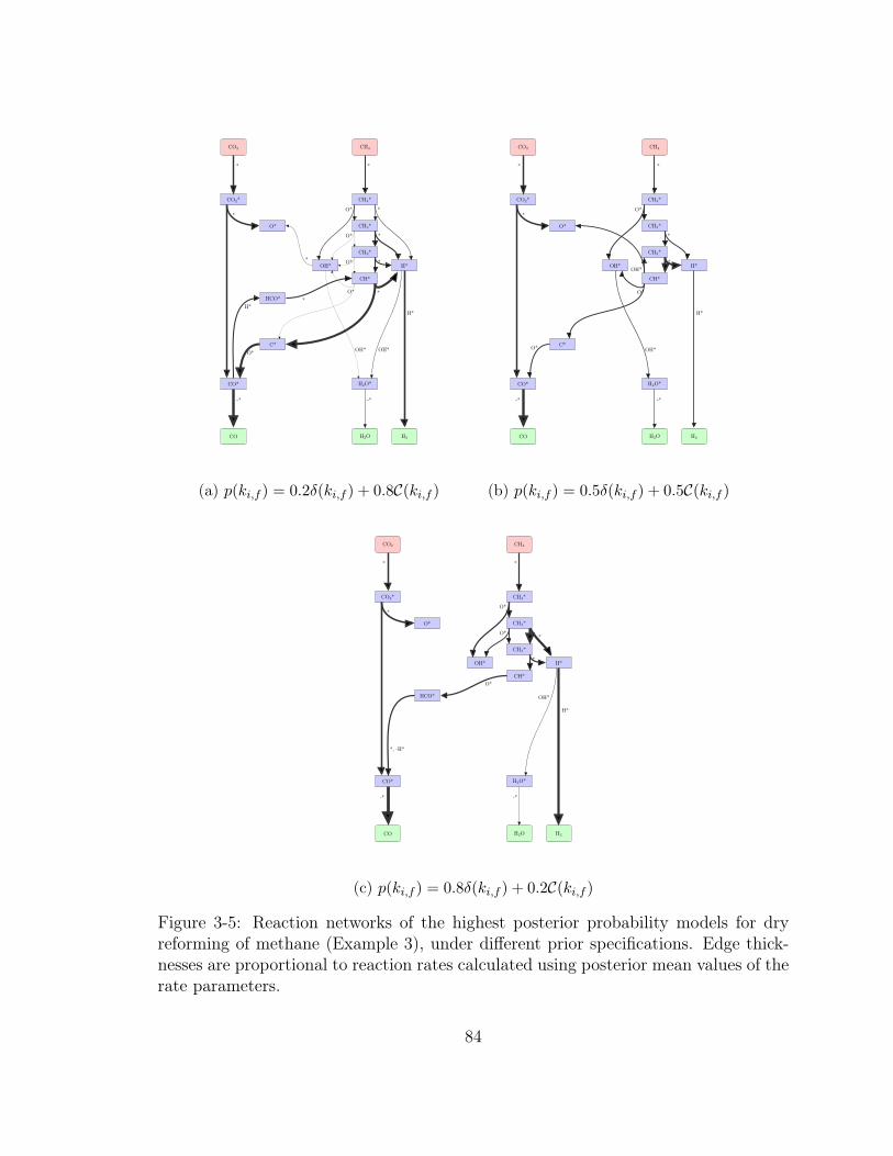
CH4CO2
CO2* CH4*
CH3*
CH2*
CH*
H*
O*
CO*
OH*
CO
H2O*
H2O
C*
HCO*
H2
*
OH*OH*
**
*
*
O*
O*
O*
*O*
O*
H**
H*
*
-*
*
-*
(a) 𝑝(𝑘𝑖,𝑓 ) = 0.2𝛿(𝑘𝑖,𝑓 ) + 0.8𝒞(𝑘𝑖,𝑓 )
CH4CO2
CO2* CH4*
CH3*
CH2*
CH*
H*
O*
CO*
OH*
CO
H2O*
H2O
C*
H2
OH*
*
*
*
O*
OH*
O*
O*
H*
*
-*
*
-*
(b) 𝑝(𝑘𝑖,𝑓 ) = 0.5𝛿(𝑘𝑖,𝑓 ) + 0.5𝒞(𝑘𝑖,𝑓 )
CH4CO2
CO2* CH4*
CH3*
CH2*
CH*
H*
O*
CO*
OH*
CO
H2O*
H2O
HCO*
H2
OH*
*
*
*
O*
O*
*, -H*
O*
H*
*
-*
*
-*
(c) 𝑝(𝑘𝑖,𝑓 ) = 0.8𝛿(𝑘𝑖,𝑓 ) + 0.2𝒞(𝑘𝑖,𝑓 )
Figure 3-5: Reaction networks of the highest posterior probability models for dryreforming of methane (Example 3), under different prior specifications. Edge thick-nesses are proportional to reaction rates calculated using posterior mean values of therate parameters.
84

is not unimportant to dry reforming. In other words, it is possible that dry reforming
of methane is realized through the generation of HCO*. With an indifference prior,
the HCO*-only pathway has a posterior probability of 8%. With a sparsity promoting
prior, the posterior probability of pathway 1 decreases dramatically and the posterior
places 23% of its mass on the HCO*-only route. That said, the C* pathway remains
very much the dominant pathway given the current data. Pathway 1 also has strong
support except in the case of the sparsity-promoting prior, which effectively forces
the posterior to “choose” between the two more parsimonious options. A clearer
conclusion can only result from collecting more data and repeating this analysis.
PathwayPrior 1 Prior 2 Prior 3
Prior Posterior Prior Posterior Prior Posterior
1 (both C* and HCO* present) 0.536 0.596 0.177 0.244 0.026 0.034
2 (only C* present) 0.302 0.347 0.529 0.677 0.633 0.732
3 (only HCO* present ) 0.162 0.056 0.294 0.080 0.340 0.234
Table 3.10: Posterior pathway probabilities for dry reforming of methane, Example3.
3.3.7 Efficiency of posterior sampling
To verify the numerical results reported in the preceding sections, we performed three
independent MCMC runs for each example problem and each prior specification, with
different initial guesses for the rate parameters 𝑘 in each case. Overall, the three repli-
cate runs yielded very similar results; the independent chains were able to identify the
high posterior probability models and accurately reproduce their probabilities. Yet
the quality of these posterior estimates, of course, depends on the number of posterior
samples employed—i.e., the length of the MCMC chains. Because the forward models
𝐺(𝑘, 𝑘) in this setting are computationally expensive, it is practically important to
85
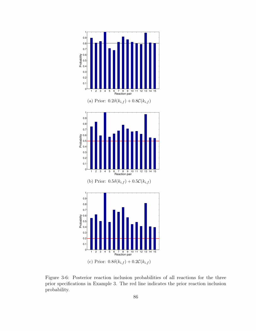
1 2 3 4 5 6 7 8 9 10 11 12 13 14 150
0.1
0.2
0.3
0.4
0.5
0.6
0.7
0.8
0.9
1
Reaction pair
Pro
babili
ty
(a) Prior: 0.2𝛿(𝑘𝑖,𝑓 ) + 0.8𝒞(𝑘𝑖,𝑓 )
1 2 3 4 5 6 7 8 9 10 11 12 13 14 150
0.1
0.2
0.3
0.4
0.5
0.6
0.7
0.8
0.9
1
Reaction pair
Pro
babili
ty
(b) Prior: 0.5𝛿(𝑘𝑖,𝑓 ) + 0.5𝒞(𝑘𝑖,𝑓 )
1 2 3 4 5 6 7 8 9 10 11 12 13 14 150
0.1
0.2
0.3
0.4
0.5
0.6
0.7
0.8
0.9
1
Reaction pair
Pro
babili
ty
(c) Prior: 0.8𝛿(𝑘𝑖,𝑓 ) + 0.2𝒞(𝑘𝑖,𝑓 )
Figure 3-6: Posterior reaction inclusion probabilities of all reactions for the threeprior specifications in Example 3. The red line indicates the prior reaction inclusionprobability.
86
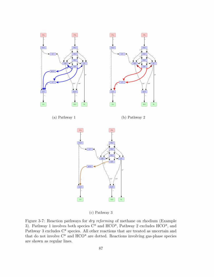
CH4CO2
CO2* CH4*
CH3*
CH2*
CH*
H*
O*
CO*
OH*
CO
H2O*
H2O
C*
HCO*
H2
*
OH*OH*
**
*
*
O*
O*
O*
*O*
O**
O*
H*
*
-*
*
-*
(a) Pathway 1
CH4CO2
CO2* CH4*
CH3*
CH2*
CH*
H*
O*
CO*
OH*
CO
H2O*
H2O
C*
H2
*
OH*OH*
**
*
*
O*
O*
O*
*O*
O*
H*
*
-*
*
-*
(b) Pathway 2
CH4CO2
CO2* CH4*
CH3*
CH2*
CH*
H*
O*
CO*
OH*
CO
H2O*
H2O
HCO*
H2
*
OH*OH*
**
*
*
O*
O*
O*
*
O*
H*
*
-*
*
-*
(c) Pathway 3
Figure 3-7: Reaction pathways for dry reforming of methane on rhodium (Example3). Pathway 1 involves both species C* and HCO*, Pathway 2 excludes HCO*, andPathway 3 excludes C* species. All other reactions that are treated as uncertain andthat do not involve C* and HCO* are dotted. Reactions involving gas-phase speciesare shown as regular lines.
87

0 50 100 150 200 250 3000
0.2
0.4
0.6
0.8
1
s (lag)
γ(s
)/γ0
Prior 1
Prior 2
Prior 3
(a) Example 2
0 100 200 300 400 500 6000
0.2
0.4
0.6
0.8
1
s (lag)
γ(s
)/γ0
Prior 1
Prior 2
Prior 3
(b) Example 3
Figure 3-8: Autocorrelation at lag s of the log-posterior of the MCMC chains.
limit the number of samples. As described in Section 3.2, the variance of a poste-
rior estimate for a fixed number of samples depends on how well the chain is mixing
[3, 105]. The adaptive MCMC scheme employed here has been shown to significantly
improve mixing over non-adaptive schemes [73], but it is nonetheless important to
assess the quality of its sampling.
A useful diagnostic for the quality of MCMC mixing is the empirical autocorre-
lation of the chain. In particular, we compute the correlation between samples as
function of lag time. A steep decay in this autocorrelation means that successive
samples are less correlated and more nearly independent. While one could compute
the empirical autocorrelation for each reaction parameter individually, we instead
summarize MCMC mixing by computing the autocorrelation of successive values of
the log-posterior density. This is reported in Figure 3-8, for Examples 2 and 3 with
all three prior specifications.
The decay of the autocorrelation is relatively good in both cases, though the
MCMC chains mix more quickly in Example 2 than in Example 3. This difference
can be ascribed to differences in posterior structure. In Example 2, the C* pathway
is largely dominant, while in the dry reforming case of Example 3, both the C* and
HCO* pathways have appreciable posterior probabilities. The MCMC chain in Exam-
ple 3 thus has to switch between pathways more frequently, and each switch requires
88
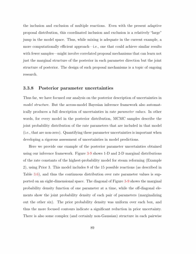
the inclusion and exclusion of multiple reactions. Even with the present adaptive
proposal distribution, this coordinated inclusion and exclusion is a relatively “large”
jump in the model space. Thus, while mixing is adequate in the current example, a
more computationally efficient approach—i.e., one that could achieve similar results
with fewer samples—might involve correlated proposal mechanisms that can learn not
just the marginal structure of the posterior in each parameter direction but the joint
structure of posterior. The design of such proposal mechanisms is a topic of ongoing
research.
3.3.8 Posterior parameter uncertainties
Thus far, we have focused our analysis on the posterior description of uncertainties in
model structure. But the across-model Bayesian inference framework also automat-
ically produces a full description of uncertainties in rate parameter values. In other
words, for every model in the posterior distribution, MCMC samples describe the
joint probability distribution of the rate parameters that are included in that model
(i.e., that are non-zero). Quantifying these parameter uncertainties is important when
developing a rigorous assessment of uncertainties in model predictions.
Here we provide one example of the posterior parameter uncertainties obtained
using our inference framework. Figure 3-9 shows 1-D and 2-D marginal distributions
of the rate constants of the highest-probability model for steam reforming (Example
2), using Prior 3. This model includes 8 of the 15 possible reactions (as described in
Table 3.6), and thus the continuous distribution over rate parameter values is sup-
ported on an eight-dimensional space. The diagonal of Figure 3-9 shows the marginal
probability density function of one parameter at a time, while the off-diagonal ele-
ments show the joint probability density of each pair of parameters (marginalizing
out the other six). The prior probability density was uniform over each box, and
thus the more focused contours indicate a significant reduction in prior uncertainty.
There is also some complex (and certainly non-Gaussian) structure in each pairwise
89
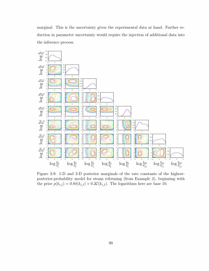
marginal. This is the uncertainty given the experimental data at hand. Further re-
duction in parameter uncertainty would require the injection of additional data into
the inference process.
−2 0 2
0.1
0.2
0.3
0.4
log
k1
k∗ 1
log
k2
k∗ 2
−2 0 2
−2
−1
0
1
2
−2 0 2
0
0.1
0.2
0.3
0.4
log
k4
k∗ 4
−2 0 2
−2
−1
0
1
2
−2 0 2
−2
−1
0
1
2
−2 0 2
0
0.2
0.4
0.6
0.8
log
k6
k∗ 6
−2 0 2
−2
−1
0
1
2
−2 0 2
−2
−1
0
1
2
−2 0 2
−2
−1
0
1
2
−2 0 2
0.1
0.2
0.3
0.4
log
k8
k∗ 8
−2 0 2
−2
−1
0
1
2
−2 0 2
−2
−1
0
1
2
−2 0 2
−2
−1
0
1
2
−2 0 2
−2
−1
0
1
2
−2 0 2
0
0.2
0.4
0.6
0.8
log
k10
k∗ 10
−2 0 2
−2
−1
0
1
2
−2 0 2
−2
−1
0
1
2
−2 0 2
−2
−1
0
1
2
−2 0 2
−2
−1
0
1
2
−2 0 2
−2
−1
0
1
2
−2 0 2
0
0.1
0.2
0.3
0.4
log
k11
k∗ 11
−2 0 2
−2
−1
0
1
2
−2 0 2
−2
−1
0
1
2
−2 0 2
−2
−1
0
1
2
−2 0 2
−2
−1
0
1
2
−2 0 2
−2
−1
0
1
2
−2 0 2
−2
−1
0
1
2
−2 0 2
0.1
0.2
0.3
0.4
log k1
k∗1
log
k13
k∗ 13
−2 0 2
−2
−1
0
1
2
log k2
k∗2
−2 0 2
−2
−1
0
1
2
log k4
k∗4
−2 0 2
−2
−1
0
1
2
log k6
k∗6
−2 0 2
−2
−1
0
1
2
log k8
k∗8
−2 0 2
−2
−1
0
1
2
log k10
k∗10
−2 0 2
−2
−1
0
1
2
log k11
k∗11
−2 0 2
−2
−1
0
1
2
−2 0 2
0.1
0.2
0.3
0.4
log k13
k∗13
Figure 3-9: 1-D and 2-D posterior marginals of the rate constants of the highest-posterior-probability model for steam reforming (from Example 2), beginning withthe prior 𝑝(𝑘𝑖,𝑓 ) = 0.8𝛿(𝑘𝑖,𝑓 ) + 0.2𝒞(𝑘𝑖,𝑓 ). The logarithms here are base 10.
90

Chapter 4
Network-aware inference
The network interaction of species in reaction models induces a special structure to
the network inference problem. The production/destruction of a species in a chemical
reaction model is directly linked to the concentrations of other species with which it
reacts. Therefore, the rate of production/consumption of a species is necessarily zero
if those other species are absent from the system. Practically, this means that by
excluding a reaction from a network, many other reactions are effectively eliminated
(i.e., have zero reaction rate). The rate constants of reactions whose rate is zero do
not affect the likelihood function and thus cannot be informed by the available data.
Another common difficulty with network inference problems is that the available
data is often sparse—data are directly linked to only a few chemical species. For
example, in applications of catalytic chemistry, only gas-phase species measurements
are practically feasible. While inferring protein signalling networks, only a few protein
concentrations may be measurable. The sparsity of data can mean that in spite
of a reaction being active (i.e., having non-zero rate), it has no influence on the
observables. Again, the rate constant values of these reactions are not informed by
data. In this chapter, we present methods that exploit the network-based species
interactions to improve the sampling efficiency of across-model network samplers.
The central theme of our network-aware MCMC methods is that the network
91

structure of species interactions can be exploited to engineer improved between-model
parameter proposals. Firstly, we analyze the reaction network given a set of proposed
reactions to identify reactions that actually impact the observables. In other words, we
identify the smallest subset of the proposed reactions that would produce an identical
value of the marginal likelihood as the proposed set of reactions. This information is
then incorporated in the design of improved proposal distributions. Identification of
networks with identical marginal likelihood further allows variance reduction through
analytical computation of some conditional expectations. The second contribution
of this chapter is due to the recognition that between-model proposals can benefit
from designing better move types. For example, proposing good moves between two
networks in many instances requires updating even the rate constants of reactions
present in both networks. We present a method to identify “key” reactions whose rate
constants are also included in the between-model parameter proposals. This step is
then combined with the first idea to further enhance sampling efficiency.
4.1 Chemical reaction network structure
4.1.1 Reaction network elements
A chemical reaction network generally consists of two different elements. Chemical
species S and the interaction between species given by reactions R. Consider a simple
reaction network shown schematically in Figure 4-1. The reaction network consists
of 6 nodes denoting the chemical species and 6 edges corresponding to reactions.
An alternative representation of the reaction network involves writing the list of all
reactions:
1. Reaction 1: 1 → 2
2. Reaction 2: 2 → 3
3. Reaction 3: 3 → 4
92

1
2
3
4
5
6
Reaction 1
Reaction 2
Reaction 3
Reaction 4
Reaction 5
Reaction 6
Figure 4-1: A simple reaction network
4. Reaction 4: 1 → 5
5. Reaction 5: 5 → 6
6. Reaction 6: 6 → 4
From a data-analytic perspective, we will classify all species into three categories.
Species initially present in the data-generating system are shown in green (Figure
4-2a), species produced only during the operation of the system are shown in blue
(Figure 4-2b), and species that are either directly observed, or are directly linked
to the observed data—referred to as observables—are shown by red nodes (Figure
4-2c). Next we discuss some common species interaction elements (reactions) present
in reaction networks.
Figure 4-2e depicts an irreversible reaction in which 𝐴 and 𝐵 are the reactants
and 𝐶 and 𝐷 are the products. Figure 4-2f shows a reversible reaction involving
with 𝐸 and 𝐹 the reactants and 𝐺 and 𝐻 the products. Figure 4-2g denotes
93

1(a) Non-zero initial concentra-tion
2(b) Zero initial concentration
3(c) Observed in experiments
(d) Species
A
B
C
D(e) Irreversible reaction
E
F
G
H(f) Reversible reaction
I J
K(g) Reaction with enzyme/catalyst I
(h) Reactions
Figure 4-2: Common reaction network elements
94
an irreversible reaction between 𝐾 and 𝐽 , with 𝐼 acting as an enzyme/catalyst.
Enzymes are chemical species that are needed for the reaction to proceed, but do not
get consumed or produced during the course of the reaction. All species interactions
(reactions) are defined by ordinary differential equations, with the corresponding rate
expressions obtained by the law of mass action or Michaelis-Menten kinetics.
4.1.2 Effective reaction network
1
2 3
4
5
6
7
89
10
11
1213
14
15
Reaction 1 Reaction 2
Reaction 3
Reaction 4Reaction 5
Reaction 6
Reaction 7
Reaction 8
Reaction 9
Reaction 10
Reaction 11
Reaction 12
Reaction 13
Figure 4-3: Reaction network with all reactions
A reaction network may contain reactions that may not be active or reactions that
are active and yet incapable of impacting the observables due to the network-based
95

interactions of all species. Consider, for example, a set of proposed reactions given
by the full reaction network in Figure 4-3. Two possible reduced reaction networks,
obtained by removing reactions 3 and 6, respectively, from the full reaction network
4-3 are shown in Figure 4-4. We define the effective network of a reaction network to
be the smallest subset of all reactions in the network that produces an identical value
of the observables as the given reaction network. This implies that the additional
reactions in a network compared to the effective network do not affect the observable
value for any parameter setting, and the reaction network has the same marginal
likelihood value as the effective reaction network. Both reduced networks shown in
Figure 4-4 have the same effective network (Figure 4-5). In reaction network 1, the
non-production of species 6 renders reactions 4, 5, 6, and 9 inactive, and thus the
value of the observable 8 is independent of their rate constant values. In case
of reaction network 2, although reactions 3, 4, 5, and 9 are active, they are linked
to the observable 8 through species 1 and 11 , which are enzymes. Recall that
catalyst/enzyme concentration is not affected by the reaction in which it participates.
Thus, the observable is again independent of the rate constants of reactions 3,4,5, and
9. Given a set of proposed reactions, one can obtain all the plausible reaction networks
and their corresponding effective networks.
4.1.3 Determining effective networks from proposed reactions
Before we begin sampling over the space of models and parameters, we first deter-
mine the effective networks of all plausible networks. If 𝑁 is the total number of
proposed reactions, the set of possible networks may be 2𝑁 , although incorporating
prior knowledge to eliminate highly unlikely models may also be a practical choice.
In either case, if the number of possible networks is very high, one may choose to
determine effective networks online only for models visited by the sampler. Our pro-
cedure to determine the effective network given a set of reactions and observables is
given by Algorithm 5. The approach we employ to determine the effective network
96

1
2 3
4
5
6
7
89
10
11
1213
14
15
Reaction 1 Reaction 2
Reaction 4Reaction 5
Reaction 6
Reaction 7
Reaction 8
Reaction 9
Reaction 10
Reaction 11
Reaction 12
Reaction 13
(a) Reaction network 1
1
2 3
4
5
6
7
89
10
11
1213
14
15
Reaction 1 Reaction 2
Reaction 3
Reaction 4Reaction 5
Reaction 7
Reaction 8
Reaction 9
Reaction 10
Reaction 11
Reaction 12
Reaction 13
(b) Reaction network 2
Figure 4-4: Two reaction networks with the same effective network
1
2 3
4
5
6
7
89
10
11
1213
14
15
Reaction 1 Reaction 2
Reaction 7
Reaction 8Reaction 10
Reaction 11
Reaction 12
Reaction 13
Figure 4-5: Effective reaction network
97

involves first identifying all reactions that are active given all species with nonzero
initial concentration and then testing all active reactions to check if they actually
influence the observables. The steps involved in checking whether a particular active
reaction influences the observables are given by Algorithm 6.
4.1.4 The space of model clusters
Given a set of proposed reactions, we can determine the effective reaction networks
for all reaction networks using the algorithm in the last section. We are now in a
position to define clusters of models. A cluster is defined as the collection of all models
with the same effective network. Thus, assuming the models have been assigned a
prior distribution 𝑝({𝑀𝑗}), the cluster prior probability is given by
𝑝(𝐶𝐾) =∑
𝑀𝑚∈𝐶𝐾
𝑝(𝑀𝑚). (4.1)
Further, the set of clusters has the following property:
𝐶𝐾 ∩ 𝐶𝐽 = ∅ for 𝐾 = 𝐽 (4.2)
and
⋃𝐾
𝐶𝐾 =ℳ, (4.3)
whereℳ is the complete space of all networks.
4.2 Reversible jump Markov chain Monte Carlo
In Chapter 3, we described a fixed-dimensional adaptive MCMC algorithm for model-
space sampling. Here we work in the more general reversible-jump MCMC (RJM-
CMC) framework which affords greater flexibility in proposal constructions. However,
98
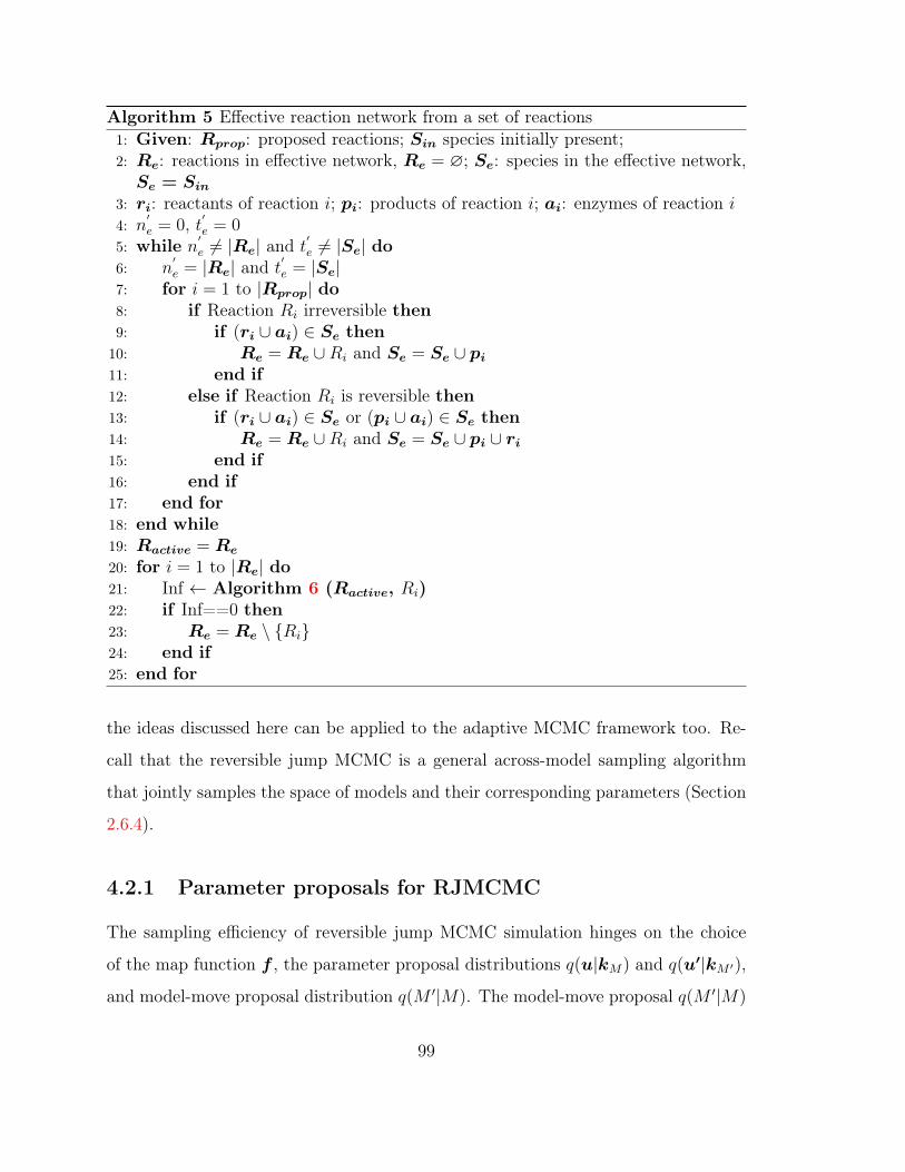
Algorithm 5 Effective reaction network from a set of reactions1: Given: 𝑅𝑝𝑟𝑜𝑝: proposed reactions; 𝑆𝑖𝑛 species initially present;2: 𝑅𝑒: reactions in effective network, 𝑅𝑒 = ∅; 𝑆𝑒: species in the effective network,𝑆𝑒 = 𝑆𝑖𝑛
3: 𝑟𝑖: reactants of reaction 𝑖; 𝑝𝑖: products of reaction 𝑖; 𝑎𝑖: enzymes of reaction 𝑖4: 𝑛
′𝑒 = 0, 𝑡′𝑒 = 0
5: while 𝑛′𝑒 = |𝑅𝑒| and 𝑡′𝑒 = |𝑆𝑒| do
6: 𝑛′𝑒 = |𝑅𝑒| and 𝑡′𝑒 = |𝑆𝑒|
7: for 𝑖 = 1 to |𝑅𝑝𝑟𝑜𝑝| do8: if Reaction 𝑅𝑖 irreversible then9: if (𝑟𝑖 ∪ 𝑎𝑖) ∈ 𝑆𝑒 then
10: 𝑅𝑒 = 𝑅𝑒 ∪𝑅𝑖 and 𝑆𝑒 = 𝑆𝑒 ∪ 𝑝𝑖11: end if12: else if Reaction 𝑅𝑖 is reversible then13: if (𝑟𝑖 ∪ 𝑎𝑖) ∈ 𝑆𝑒 or (𝑝𝑖 ∪ 𝑎𝑖) ∈ 𝑆𝑒 then14: 𝑅𝑒 = 𝑅𝑒 ∪𝑅𝑖 and 𝑆𝑒 = 𝑆𝑒 ∪ 𝑝𝑖 ∪ 𝑟𝑖15: end if16: end if17: end for18: end while19: 𝑅𝑎𝑐𝑡𝑖𝑣𝑒 = 𝑅𝑒
20: for 𝑖 = 1 to |𝑅𝑒| do21: Inf ← Algorithm 6 (𝑅𝑎𝑐𝑡𝑖𝑣𝑒, 𝑅𝑖)22: if Inf==0 then23: 𝑅𝑒 = 𝑅𝑒 ∖ {𝑅𝑖}24: end if25: end for
the ideas discussed here can be applied to the adaptive MCMC framework too. Re-
call that the reversible jump MCMC is a general across-model sampling algorithm
that jointly samples the space of models and their corresponding parameters (Section
2.6.4).
4.2.1 Parameter proposals for RJMCMC
The sampling efficiency of reversible jump MCMC simulation hinges on the choice
of the map function 𝑓 , the parameter proposal distributions 𝑞(𝑢|𝑘𝑀) and 𝑞(𝑢′|𝑘𝑀 ′),
and model-move proposal distribution 𝑞(𝑀 ′|𝑀). The model-move proposal 𝑞(𝑀 ′|𝑀)
99
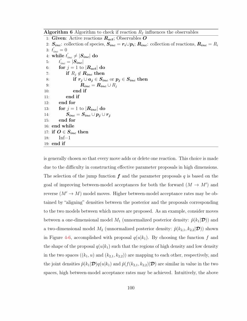
Algorithm 6 Algorithm to check if reaction 𝑅𝐼 influences the observables1: Given: Active reactions 𝑅𝑎𝑐𝑡; Observables 𝑂2: 𝑆𝑖𝑛𝑐: collection of species, 𝑆𝑖𝑛𝑐 = 𝑟𝑖∪𝑝𝑖; 𝑅𝑖𝑛𝑐: collection of reactions, 𝑅𝑖𝑛𝑐 = 𝑅𝑖
3: 𝑡′𝑖𝑛𝑐 = 0
4: while 𝑡′𝑖𝑛𝑐 = |𝑆𝑖𝑛𝑐| do5: 𝑡
′𝑖𝑛𝑐 = |𝑆𝑖𝑛𝑐|
6: for 𝑗 = 1 to |𝑅𝑎𝑐𝑡| do7: if 𝑅𝑗 ∈ 𝑅𝑖𝑛𝑐 then8: if 𝑟𝑗 ∪ 𝑎𝑗 ∈ 𝑆𝑖𝑛𝑐 or 𝑝𝑗 ∈ 𝑆𝑖𝑛𝑐 then9: 𝑅𝑖𝑛𝑐 = 𝑅𝑖𝑛𝑐 ∪𝑅𝑗
10: end if11: end if12: end for13: for 𝑗 = 1 to |𝑅𝑖𝑛𝑐| do14: 𝑆𝑖𝑛𝑐 = 𝑆𝑖𝑛𝑐 ∪ 𝑝𝑗 ∪ 𝑟𝑗15: end for16: end while17: if 𝑂 ∈ 𝑆𝑖𝑛𝑐 then18: Inf=119: end if
is generally chosen so that every move adds or delete one reaction. This choice is made
due to the difficulty in constructing effective parameter proposals in high dimensions.
The selection of the jump function 𝑓 and the parameter proposals 𝑞 is based on the
goal of improving between-model acceptances for both the forward (𝑀 → 𝑀 ′) and
reverse (𝑀 ′ →𝑀) model moves. Higher between-model acceptance rates may be ob-
tained by “aligning” densities between the posterior and the proposals corresponding
to the two models between which moves are proposed. As an example, consider moves
between a one-dimensional model 𝑀1 (unnormalized posterior density: 𝑝(𝑘1|𝒟)) and
a two-dimensional model 𝑀2 (unnormalized posterior density: 𝑝(𝑘2,1, 𝑘2,2|𝒟)) shown
in Figure 4-6, accomplished with proposal 𝑞(𝑢|𝑘1). By choosing the function 𝑓 and
the shape of the proposal 𝑞(𝑢|𝑘1) such that the regions of high density and low density
in the two spaces ((𝑘1, 𝑢) and (𝑘2,1, 𝑘2,2)) are mapping to each other, respectively, and
the joint densities 𝑝(𝑘1|𝒟)𝑞(𝑢|𝑘1) and 𝑝(𝑓(𝑘2,1, 𝑘2,2)|𝒟) are similar in value in the two
spaces, high between-model acceptance rates may be achieved. Intuitively, the above
100
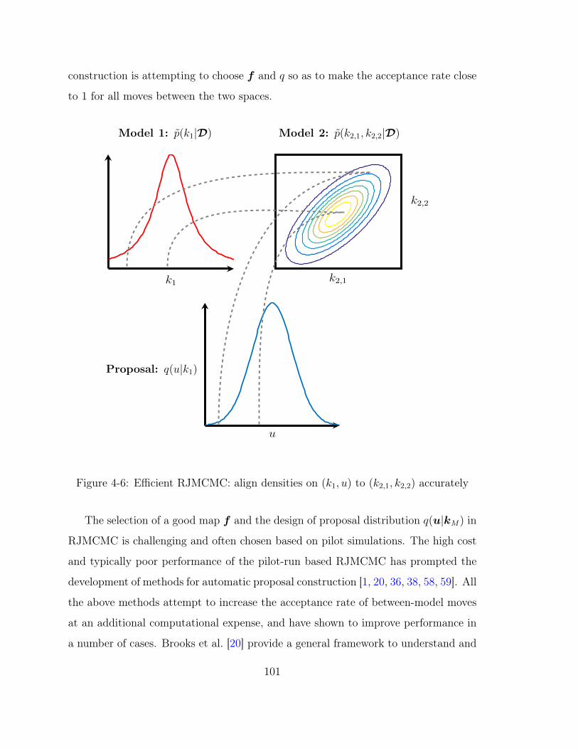
construction is attempting to choose 𝑓 and 𝑞 so as to make the acceptance rate close
to 1 for all moves between the two spaces.
𝑘1 𝑘2,1
𝑘2,2
𝑢
Model 1: 𝑝(𝑘1|𝒟) Model 2: 𝑝(𝑘2,1, 𝑘2,2|𝒟)
Proposal: 𝑞(𝑢|𝑘1)
Figure 4-6: Efficient RJMCMC: align densities on (𝑘1, 𝑢) to (𝑘2,1, 𝑘2,2) accurately
The selection of a good map 𝑓 and the design of proposal distribution 𝑞(𝑢|𝑘𝑀) in
RJMCMC is challenging and often chosen based on pilot simulations. The high cost
and typically poor performance of the pilot-run based RJMCMC has prompted the
development of methods for automatic proposal construction [1, 20, 36, 38, 58, 59]. All
the above methods attempt to increase the acceptance rate of between-model moves
at an additional computational expense, and have shown to improve performance in
a number of cases. Brooks et al. [20] provide a general framework to understand and
101

construct efficient reversible-jump proposals based on an analysis of the acceptance
probability. Our work fits in their their 𝑛𝑡ℎ-order condition proposal framework and
we briefly review it here.
Centered 𝑛𝑡ℎ-order condition based proposals
The 𝑛𝑡ℎ-order (𝑛 ≥ 1) proposal conditions of Brooks et al. [20] is based on setting a
series of derivatives (with respect to 𝑢) of the acceptance ratio 𝐴 (2.37) for proposal
moves between models 𝑀 and 𝑀 ′ to the zero vector at a specific point 𝑐𝑀→𝑀 ′(𝑘𝑀)
known as the centering point :
∇𝑛𝐴[(𝑀,𝑘𝑀), (𝑀 ′, 𝑐𝑀→𝑀 ′(𝑘𝑀))] = 0 (4.4)
The centering point 𝑐𝑀→𝑀 ′(𝑘𝑀) is taken to be the equivalent point of parameter
vector 𝑘𝑀 in model 𝑀 ′. Centering the proposal 𝑞(𝑢|𝑘𝑀) at the conditional maximum
of the posterior density 𝑝(𝑓(𝑘𝑀 ,𝑢),𝑀 ′) is one intuitive choice and aims to increase
the frequency of moves between models. In addition to the 𝑛𝑡ℎ-order condition, Brooks
et al. [20] also introduce the zeroth-order condition in which the acceptance ratio
is set to 1 at the centering point. Note the traditional random-walk Metropolis
algorithm for posterior distribution on R𝑚 satisfies the zeroth-order condition at a
central move corresponding to a step of size 0. Similarly, Langevin algorithms satisfy
both the zeroth-order and first-order conditions at the above central move. The zeroth
and 𝑛𝑡ℎ order conditions aim to adapt proposal parameters on the current state of
the chain (𝑀,𝑘𝑀), instead of relying on constant proposal parameters for all state
transitions. Brooks et al. [20] further show that for a simple two model case, the
𝑛𝑡ℎ-order conditions are optimal in terms of the capacitance of the algorithm [80].
102

4.3 Network analysis for improved sampling efficiency
We now explain how we use the effective reaction networks obtained using our Algo-
rithm 5 to design more efficient across-model samplers. We propose two methods for
performance improvement. First, we use network information to determine improved
parameter proposal densities 𝑞(𝑢|𝑘𝑀). Secondly, we demonstrate how one may use
sensitivity of observables to individual reactions to choose efficient between-model
moves. The above network-aware parameter proposals are then used along with the
sensitivity-based move types. We end by explaining how the analysis of network
structure can be used to derandomize conditional expectation calculations, leading
to further variance reduction.
4.3.1 Constructing parameter proposals
For nested models, as is the case in the reaction network inference problem, a natural
choice of the jump function 𝑓 is to choose the identity function. Thus, when proposing
a move from a lower-dimensional model 𝑀 to a higher dimensional model 𝑀 ′, the
rate constants of the newly added reactions is proposed according to 𝑞(𝑢|𝑘𝑀) and
the values of the rate constants of reactions common to the two models are kept fixed
(henceforth 1 : 𝑖). Therefore,
𝑓 := (𝑘1:𝑖𝑀 ′ ,𝑘1:𝑎
𝑀 ′ ) = (𝑘1:𝑖𝑀 ,𝑢1:𝑎
𝑀 ). (4.5)
and the acceptance probability is given by
𝛼(𝑘𝑀 ,𝑘𝑀 ′) = min{
1,𝑝(𝑀 ′,𝑘𝑀 ′ |𝒟)𝑞(𝑀 |𝑀 ′)
𝑝(𝑀,𝑘𝑀 |𝒟)𝑞(𝑀 ′|𝑀)𝑞(𝑢|𝑘𝑀)
}. (4.6)
The reverse move in this case is deterministic. Let the proposal 𝑞(𝑢|𝑘𝑀) be given by
𝑞(𝑢|𝑘𝑀) = 𝒩 (𝑢;𝜇,Σ). (4.7)
103

To improve the chance of proposal acceptance we center the proposal distribution at
the conditional mean of the posterior distribution. Next, we construct an approxima-
tion to the posterior distribution by setting the covariance of the Gaussian to be the
Hessian of the conditional posterior density. In other words, we construct a Gaussian
approximation to the conditional posterior distribution. In the framework of Brooks
et al. [20], the above construction is equivalent to the centered second-order condi-
tions. In the scheme described above, the mean vector 𝜇 is set to the conditional
maximum:
𝜇 = arg max𝑢
𝑝(𝑀 ′, (𝑘𝑀 ,𝑢)|𝒟). (4.8)
A proposal centered at the posterior conditional maximum satisfies the first order
condition:
∇ log𝐴(𝑀,𝑘𝑀 →𝑀 ′,𝑘𝑀 ′)𝜇
= ∇ [logℒ(𝒟;𝑘𝑀 ,𝑢) + log 𝑝(𝑘𝑀 ,𝑢)− log 𝑞(𝑢;𝜇,Σ)]𝜇
= 0. (4.9)
Further, setting the second-derivative of the acceptance ratio at the conditional max-
imum 0, we obtain the second order condition as:
∇2 log𝐴((𝑀,𝑘𝑀)→ (𝑀 ′,𝑘𝑀 ′)) = ∇2 [logℒ(𝒟|𝑘𝑀 ,𝑢) + log 𝑝(𝑘𝑀 ,𝑢)− log 𝑞(𝑢;𝜇,Σ)]
= 0. (4.10)
Taking ℋ to be the Hessian of the conditional posterior density at 𝜇, (4.10) yields
ℋ𝜇
+ Σ−1 = 0 =⇒ Σ = −ℋ−1𝜇. (4.11)
4.3.2 Network-aware parameter proposals
The above proposal construction for between-model moves in which the parameter
proposals adapt to conditional posterior densities typically lead to improved reversible
104

jump simulations [20, 36, 38, 52]. Effectively, the above proposal construction is
attempting to increase the chance of proposed moves between models to get accepted.
In addition, with the first and second order conditions, the idea is to make acceptance
ratio uniformly high for all transitions. However, the direct application of the centered
second-order conditions for between-model moves in the context of reaction network
inference has a major drawback. As discussed earlier, many reaction networks can
have the same effective network. In such a case, if the proposed move is between two
networks with the same effective network (i.e., the two networks belong to the same
cluster), the parameter proposal adapts to the prior distribution of the newly added
reaction (Figure 4-7). We propose a network-aware approach in which, because we
have determined the effective networks, we design parameter proposals that adapt to
the difference between the effective networks of the two networks. When the proposed
move is between two networks belonging to different clusters, we construct a proposal
that approximates the conditional posterior distribution of the rate constants of all
reactions not included in the two effective networks.
Formally, suppose that the sampler proposes a move from a lower-dimensional
model 𝑀 to a higher-dimensional model 𝑀 ′. Let the effective networks of the two
models 𝑀 and 𝑀 ′ be 𝑀𝑒 and 𝑀 ′𝑒, respectively. Following our choice of the proposal
𝑞(𝑀 ′|𝑀), dim(𝑀 ′) = dim(𝑀)+1. Suppose the proposed move is such that 𝑀 ′𝑒 = 𝑀𝑒,
i.e., the effective networks of the current and the proposed networks are different. In
our network-aware sampler, because we know the effective networks 𝑀 ′𝑒 and 𝑀𝑒 of
the two models 𝑀 ′ and 𝑀 , respectively, we construct the following proposal:
𝑓 := (𝑘1:𝑖𝑀 ′
𝑒,𝑘1:𝑎
𝑀 ′𝑒,𝑤1:𝑗
𝑀∖𝑀𝑒) = (𝑘1:𝑖
𝑀𝑒,𝑢1:𝑎
𝑀𝑒,𝑘1:𝑗
𝑀∖𝑀𝑒), (4.12)
where 𝑢1:𝑎𝑀 ∼ 𝒩 (𝜇𝑀 ,Σ𝑀) and 𝑤1:𝑗 ∼ 𝑝(𝑘1:𝑗
𝑀∖𝑀𝑒|𝑀). The proposal mean 𝜇𝑀 :
𝜇𝑀 = arg max𝑢1:𝑎
𝑝(𝑢1:𝑎|𝑘1:𝑖𝑀𝑒,𝑀 ′
𝑒,𝒟) (4.13)
105

network 1 network 2
network 3network 4
Figure 4-7: Model move from network 1 to 2 and 2 to 3 in the standard approach leadsto the proposal adapting to the prior. Only the final move from 3 to 4 incorporatesthe likelihood function
106
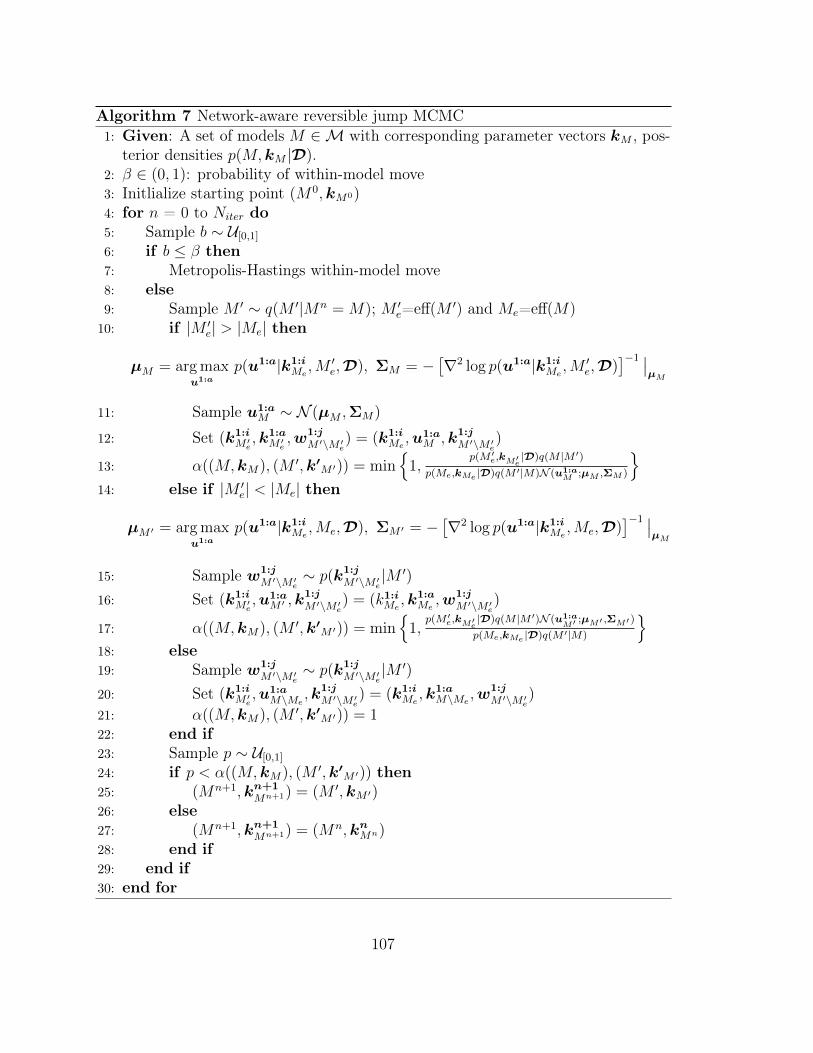
Algorithm 7 Network-aware reversible jump MCMC1: Given: A set of models 𝑀 ∈ℳ with corresponding parameter vectors 𝑘𝑀 , pos-
terior densities 𝑝(𝑀,𝑘𝑀 |𝒟).2: 𝛽 ∈ (0, 1): probability of within-model move3: Initlialize starting point (𝑀0,𝑘𝑀0)4: for 𝑛 = 0 to 𝑁𝑖𝑡𝑒𝑟 do5: Sample 𝑏 ∼ 𝒰[0,1]6: if 𝑏 ≤ 𝛽 then7: Metropolis-Hastings within-model move8: else9: Sample 𝑀 ′ ∼ 𝑞(𝑀 ′|𝑀𝑛 = 𝑀); 𝑀 ′
𝑒=eff(𝑀 ′) and 𝑀𝑒=eff(𝑀)10: if |𝑀 ′
𝑒| > |𝑀𝑒| then
𝜇𝑀 = arg max𝑢1:𝑎
𝑝(𝑢1:𝑎|𝑘1:𝑖𝑀𝑒,𝑀 ′
𝑒,𝒟), Σ𝑀 = −[∇2 log 𝑝(𝑢1:𝑎|𝑘1:𝑖
𝑀𝑒,𝑀 ′
𝑒,𝒟)]−1
𝜇𝑀
11: Sample 𝑢1:𝑎𝑀 ∼ 𝒩 (𝜇𝑀 ,Σ𝑀)
12: Set (𝑘1:𝑖𝑀 ′
𝑒,𝑘1:𝑎
𝑀 ′𝑒,𝑤1:𝑗
𝑀 ′∖𝑀 ′𝑒) = (𝑘1:𝑖
𝑀𝑒,𝑢1:𝑎
𝑀 ,𝑘1:𝑗𝑀 ′∖𝑀 ′
𝑒)
13: 𝛼((𝑀,𝑘𝑀), (𝑀 ′,𝑘′𝑀 ′)) = min
{1,
𝑝(𝑀 ′𝑒,𝑘𝑀′
𝑒|𝒟)𝑞(𝑀 |𝑀 ′)
𝑝(𝑀𝑒,𝑘𝑀𝑒 |𝒟)𝑞(𝑀 ′|𝑀)𝒩 (𝑢1:𝑎𝑀 ;𝜇𝑀 ,Σ𝑀 )
}14: else if |𝑀 ′
𝑒| < |𝑀𝑒| then
𝜇𝑀 ′ = arg max𝑢1:𝑎
𝑝(𝑢1:𝑎|𝑘1:𝑖𝑀𝑒,𝑀𝑒,𝒟), Σ𝑀 ′ = −
[∇2 log 𝑝(𝑢1:𝑎|𝑘1:𝑖
𝑀𝑒,𝑀𝑒,𝒟)
]−1 𝜇𝑀
15: Sample 𝑤1:𝑗𝑀 ′∖𝑀 ′
𝑒∼ 𝑝(𝑘1:𝑗
𝑀 ′∖𝑀 ′𝑒|𝑀 ′)
16: Set (𝑘1:𝑖𝑀 ′
𝑒,𝑢1:𝑎
𝑀 ′ ,𝑘1:𝑗𝑀 ′∖𝑀 ′
𝑒) = (𝑘1:𝑖𝑀𝑒
,𝑘1:𝑎𝑀𝑒,𝑤1:𝑗
𝑀 ′∖𝑀 ′𝑒)
17: 𝛼((𝑀,𝑘𝑀), (𝑀 ′,𝑘′𝑀 ′)) = min
{1,
𝑝(𝑀 ′𝑒,𝑘𝑀′
𝑒|𝒟)𝑞(𝑀 |𝑀 ′)𝒩 (𝑢1:𝑎
𝑀′ ;𝜇𝑀′ ,Σ𝑀′ )
𝑝(𝑀𝑒,𝑘𝑀𝑒 |𝒟)𝑞(𝑀 ′|𝑀)
}18: else19: Sample 𝑤1:𝑗
𝑀 ′∖𝑀 ′𝑒∼ 𝑝(𝑘1:𝑗
𝑀 ′∖𝑀 ′𝑒|𝑀 ′)
20: Set (𝑘1:𝑖𝑀 ′
𝑒,𝑢1:𝑎
𝑀∖𝑀𝑒,𝑘1:𝑗
𝑀 ′∖𝑀 ′𝑒) = (𝑘1:𝑖
𝑀𝑒,𝑘1:𝑎
𝑀∖𝑀𝑒,𝑤1:𝑗
𝑀 ′∖𝑀 ′𝑒)
21: 𝛼((𝑀,𝑘𝑀), (𝑀 ′,𝑘′𝑀 ′)) = 1
22: end if23: Sample 𝑝 ∼ 𝒰[0,1]24: if 𝑝 < 𝛼((𝑀,𝑘𝑀), (𝑀 ′,𝑘′
𝑀 ′)) then25: (𝑀𝑛+1,𝑘𝑛+1
𝑀𝑛+1) = (𝑀 ′,𝑘𝑀 ′)26: else27: (𝑀𝑛+1,𝑘𝑛+1
𝑀𝑛+1) = (𝑀𝑛,𝑘𝑛𝑀𝑛)28: end if29: end if30: end for
107
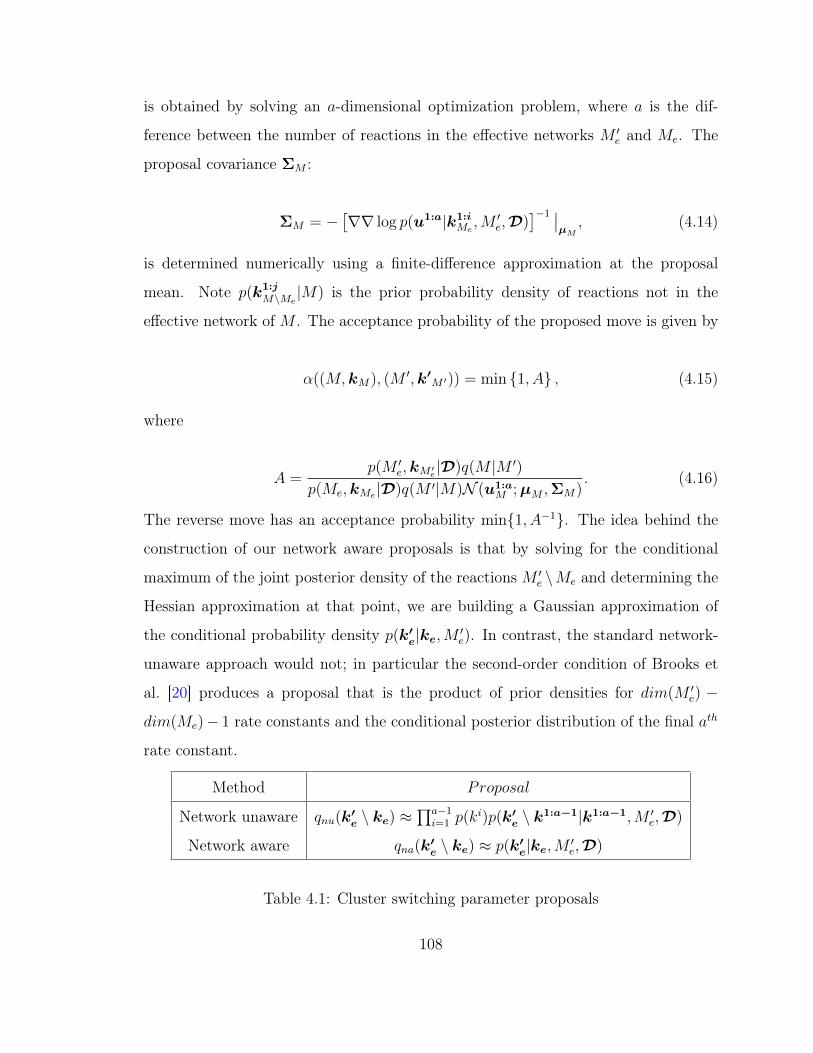
is obtained by solving an 𝑎-dimensional optimization problem, where 𝑎 is the dif-
ference between the number of reactions in the effective networks 𝑀 ′𝑒 and 𝑀𝑒. The
proposal covariance Σ𝑀 :
Σ𝑀 = −[∇∇ log 𝑝(𝑢1:𝑎|𝑘1:𝑖
𝑀𝑒,𝑀 ′
𝑒,𝒟)]−1
𝜇𝑀, (4.14)
is determined numerically using a finite-difference approximation at the proposal
mean. Note 𝑝(𝑘1:𝑗𝑀∖𝑀𝑒
|𝑀) is the prior probability density of reactions not in the
effective network of 𝑀 . The acceptance probability of the proposed move is given by
𝛼((𝑀,𝑘𝑀), (𝑀 ′,𝑘′𝑀 ′)) = min {1, 𝐴} , (4.15)
where
𝐴 =𝑝(𝑀 ′
𝑒,𝑘𝑀 ′𝑒|𝒟)𝑞(𝑀 |𝑀 ′)
𝑝(𝑀𝑒,𝑘𝑀𝑒|𝒟)𝑞(𝑀 ′|𝑀)𝒩 (𝑢1:𝑎𝑀 ;𝜇𝑀 ,Σ𝑀)
. (4.16)
The reverse move has an acceptance probability min{1, 𝐴−1}. The idea behind the
construction of our network aware proposals is that by solving for the conditional
maximum of the joint posterior density of the reactions 𝑀 ′𝑒 ∖𝑀𝑒 and determining the
Hessian approximation at that point, we are building a Gaussian approximation of
the conditional probability density 𝑝(𝑘′𝑒|𝑘𝑒,𝑀 ′
𝑒). In contrast, the standard network-
unaware approach would not; in particular the second-order condition of Brooks et
al. [20] produces a proposal that is the product of prior densities for 𝑑𝑖𝑚(𝑀 ′𝑒) −
𝑑𝑖𝑚(𝑀𝑒)− 1 rate constants and the conditional posterior distribution of the final 𝑎𝑡ℎ
rate constant.
Method 𝑃𝑟𝑜𝑝𝑜𝑠𝑎𝑙
Network unaware 𝑞𝑛𝑢(𝑘′𝑒 ∖ 𝑘𝑒) ≈
∏𝑎−1𝑖=1 𝑝(𝑘
𝑖)𝑝(𝑘′𝑒 ∖ 𝑘1:𝑎−1|𝑘1:𝑎−1,𝑀 ′
𝑒,𝒟)
Network aware 𝑞𝑛𝑎(𝑘′𝑒 ∖ 𝑘𝑒) ≈ 𝑝(𝑘′
𝑒|𝑘𝑒,𝑀 ′𝑒,𝒟)
Table 4.1: Cluster switching parameter proposals
108

Mathematically, the two proposals are shown in Table 4.1. The steps of our
network-aware reversible jump MCMC algorithm are given in Algorithm 7. If we
think of the cluster {𝑀𝑒,𝑘𝑒} as the state space, the between-model moves that pro-
pose moves within the same cluster have an acceptance probability 1 with both the
network-aware and the network-unaware approaches. However, when the proposed
move is between two distinct clusters, our network aware approach chooses a proposal
that approximates the joint conditional posterior density and hence leads to improved
alignment between the densities 𝑝(𝑘𝑒|𝒟)𝑞(𝑢|𝑘𝑒) and 𝑝(𝑘′𝑒|𝒟) of the two spaces. Here
𝑝(𝑘𝑒|𝒟) and 𝑝(𝑘𝑒|𝒟) are the unnormalized densities of the rate constants of the two
effective networks.
4.3.3 Sensitivity-based network-aware proposals
Between-model moves with deterministic reverse moves are a natural choice for nested
models. However, in many cases, MCMC mixing may be improved by adopting non-
deterministic reverse move types. In the context of reaction network inference, it is
sometimes observed that a maximum-a-posteriori rate constant value for a reaction
common to two networks differs substantially in the two networks. For example,
consider the two networks in Figure 4-8. The most likely values for the rate constant
of reaction * could differ significantly for the two networks. In such a case, keeping
the rate constant of * fixed when proposing moves between the two networks leads
to very poor acceptance rates. We propose a method to improve sampling efficiency
of the network inference problem by identifying critical reactions common to the
current and the proposed network and using a proposal distribution 𝑞 for their rate
constants in moves between the two networks. In other words, the reverse move
from a high-dimensional effective network to a low-dimensional effective network is
no longer deterministic. The move between the networks takes the following form:
(𝑘𝑀 ′𝑒,𝑢′
𝑒) = 𝑓(𝑘𝑀𝑒 ,𝑢𝑒). (4.17)
109

*
Right pathway
*
Both pathways
Figure 4-8: Two networks with different pathways
The question we answer next is how one could identify “key” reactions whose inclusion
in the proposal would improve MCMC mixing at a limited computational overhead.
Given a set of observables and the current and proposed network, a useful strategy is
to identify the reactions to which the posterior density is most sensitive. To determine
the sensitivity of the posterior density to individual reactions given a network, we em-
ploy local sensitivity analysis. Say, we have network 𝑀 with reactions 𝑅1, 𝑅2, ..., 𝑅𝑀 .
We determine the expected local sensitivity index E[
𝜕 log 𝑝(𝑘𝑖|𝒟,𝑘−𝑖)
𝜕𝑘𝑖
]of reaction 𝑖
with 𝑘*−𝑖 given nominal values and the expectation taken with respect to the prior
distribution 𝑝(𝑘𝑖|𝑀). In practice, since the expectation is usually not analytically
tractable, we settle for a noisy estimate of the expectation by evaluating the local
sensitivity at a few realizations from the prior distribution and taking their average.
Having determined the sensitivity of the log-posterior of the current and the proposed
reaction network, we select a random number of high sensitivity reactions common to
the two networks and include proposals for their rate constants in the forward and the
reverse moves. The choice of the number of reactions to be included in the proposals
is based on a Poisson distribution whose mean is kept at a small value. Choosing
110
to include only a few common rate constant into the proposal is again based on the
understanding that constructing effective proposals in high dimensions is generally
hard. Thus, as the jump function for moves between models 𝑀 and 𝑀 ′ we have
𝑓 := (𝑘1:𝑖𝑀 ′ ,𝑘1:𝑎
𝑀 ′ ,𝑘1:𝑐𝑀 ′ ,𝑢′1:𝑐) = (𝑘1:𝑖
𝑀 ,𝑢1:𝑎𝑀 ,𝑢1:𝑐,𝑘1:𝑐
𝑀 ). (4.18)
Here, {1 : 𝑖} are indices of reactions whose parameter values are kept fixed during
moves between models 𝑀 and 𝑀 ′, {1 : 𝑎} are indices of reactions that are in model
𝑀 ′ but not in 𝑀 , and {1 : 𝑐} are reactions that are present in both models but whose
rate constant values are determined according to respective proposal distributions.
Next, the parameter proposals 𝑞(𝑢1:𝑎𝑀 ,𝑢1:𝑐|𝑘1:𝑖
𝑀 ) and 𝑞(𝑢′1:𝑐|𝑘1:𝑖𝑀 ′) are again chosen
as Gaussian approximations of the conditional posteriors 𝑝(𝑘1:𝑎𝑀 ′ ,𝑘1:𝑐
𝑀 ′ |𝑘1:𝑖𝑀 ′ ,𝒟) and
𝑝(𝑘1:𝑐𝑀 |𝑘1:𝑖
𝑀 ,𝒟), respectively. Note, this construction of parameter proposals improves
alignment between densities 𝑝(𝑘1:𝑖𝑀 ′ ,𝑘1:𝑎
𝑀 ′ ,𝑘1:𝑐𝑀 ′ |𝑀 ′,𝒟)𝑞(𝑢′1:𝑐) and 𝑝(𝑘1:𝑖
𝑀 ,𝑘1:𝑐𝑀 |𝑀,𝒟)𝑞
(𝑢1:𝑎𝑀 ,𝑢1:𝑐) and produces efficient reversible jump proposals. The above construction
of reversible jump proposals satisfies the second-order conditions of Brooks et al
[20]. The foregoing discussion has focused on a network-unaware approach, where
the effective networks are not known apriori. As we discussed in Section 4.3.2 on
network-aware proposals, for the network inference problem, improved proposals that
approximate the joint posterior conditionals of the rate constants of the difference in
reactions between the current and proposed effective networks can be constructed by
determining the effective networks of proposed networks. We combine the network-
aware scheme of the previous section with the sensitivity-based determination of move
types to yield the the sensitivity-based network-aware proposals. The sequence of steps
for our sensitivity-based network-aware reversible jump MCMC algorithm are given
in Algorithm 8.
111

Algorithm 8 Sensitivity-based network-aware reversible jump MCMC1: Given: A set of models 𝑀 ∈ℳ with corresponding parameter vectors 𝑘𝑀 , posterior densities
𝑝(𝑀,𝑘𝑀 |𝒟).2: 𝛽 ∈ (0, 1): probability of within-model move3: Initlialize starting point (𝑀0,𝑘𝑀0)4: for 𝑛 = 0 to 𝑁𝑖𝑡𝑒𝑟 do5: Sample 𝑏 ∼ 𝒰[0,1]6: if 𝑏 ≤ 𝛽 then7: Metropolis-Hastings within-model move8: else9: Sample 𝑀 ′ ∼ 𝑞(𝑀 ′|𝑀𝑛 = 𝑀); 𝑀 ′
𝑒=eff(𝑀 ′) and 𝑀𝑒=eff(𝑀)10: 𝑟1 ∼ 𝑃𝑜𝑖𝑠𝑠𝑜𝑛(1.5) and 𝑟2 ∼ 𝑃𝑜𝑖𝑠𝑠𝑜𝑛(1.5)11: {1 : 𝑐}=reactions with top 𝑟1 and 𝑟2 sensitivities of 𝑀𝑒 and 𝑀 ′
𝑒, respectively, and commonto 𝑀𝑒 and 𝑀 ′
𝑒.12: if |𝑀 ′
𝑒| > |𝑀𝑒| then
𝜇𝑀𝑒= argmax
𝑢1:𝑎,𝑢1:𝑐
𝑝(𝑢1:𝑎,𝑢1:𝑐|𝑘1:𝑖𝑀𝑒,𝑀 ′
𝑒,𝒟), Σ𝑀𝑒= −
[∇2 log 𝑝(𝑢1:𝑎,𝑢1:𝑐|𝑘1:𝑖𝑀𝑒
,𝑀 ′𝑒,𝒟)
]−1 𝜇𝑀
𝜇𝑀 ′𝑒= argmax
𝑢1:𝑐
𝑝(𝑢1:𝑐|𝑘1:𝑖𝑀𝑒,𝑀𝑒,𝒟), Σ𝑀 ′
𝑒= −
[∇2 log 𝑝(𝑢1:𝑐|𝑘1:𝑖𝑀𝑒
,𝑀𝑒,𝒟)]−1
𝜇𝑀′
13: Sample 𝑢1:𝑎,𝑢1:𝑐 ∼ 𝒩 (𝜇𝑀𝑒,Σ𝑀𝑒
)
14: Set (𝑘1:𝑖𝑀 ′𝑒,𝑘1:𝑎𝑀 ′
𝑒,𝑘1:𝑐𝑀 ′
𝑒,𝑢′1:𝑐) = (𝑘1:𝑖𝑀𝑒
,𝑢1:𝑎,𝑢1:𝑐,𝑘1:𝑐𝑀𝑒)
15: else if |𝑀 ′𝑒| < |𝑀𝑒| then
𝜇𝑀𝑒= argmax
𝑢1:𝑐
𝑝(𝑢1:𝑐|𝑘1:𝑖𝑀𝑒,𝑀 ′
𝑒,𝒟), Σ𝑀𝑒= −
[∇2 log 𝑝(𝑢1:𝑐|𝑘1:𝑖𝑀𝑒
,𝑀 ′𝑒,𝒟)
]−1 𝜇𝑀
𝜇𝑀 ′𝑒= argmax
𝑢1:𝑎,𝑢1:𝑐
𝑝(𝑢1:𝑎,𝑢1:𝑐|𝑘1:𝑖𝑀𝑒,𝑀𝑒,𝒟), Σ𝑀 ′
𝑒= −
[∇2 log 𝑝(𝑢1:𝑎,𝑢1:𝑐|𝑘1:𝑖𝑀𝑒
,𝑀𝑒,𝒟)]−1
𝜇𝑀′
16: Sample 𝑢1:𝑐 ∼ 𝒩 (𝜇𝑀𝑒,Σ𝑀𝑒
)
17: Set (𝑘1:𝑖𝑀 ′𝑒,𝑢′1:𝑎,𝑢′1:𝑐,𝑘1:𝑐𝑀 ′
𝑒) = (𝑘1:𝑖𝑀𝑒
,𝑘1:𝑎𝑀𝑒,𝑘1:𝑐𝑀𝑒
,𝑢1:𝑐)
18: else 𝜇𝑀𝑒= ∅, 𝜇𝑀 ′
𝑒= ∅, Σ𝑀𝑒
= ∅, Σ𝑀 ′𝑒= ∅
19: end if20: Sample 𝑘1:𝑗𝑀 ′∖𝑀 ′
𝑒∼ 𝑝(𝑘1:𝑗𝑀 ′∖𝑀 ′
𝑒|𝑀 ′)
21: Sample 𝑝 ∼ 𝒰[0,1]
22: if 𝑝 < min{1,
𝑝(𝑀 ′𝑒,𝑘𝑀′
𝑒|𝒟)𝑞(𝑀𝑛|𝑀 ′)𝒩 (𝑢′;𝜇𝑀′
𝑒,Σ𝑀′
𝑒)
𝑝(𝑀𝑒,𝑘𝑀𝑒 |𝒟)𝑞(𝑀 ′|𝑀𝑛)𝒩 (𝑢;𝜇𝑀𝑒,Σ𝑀𝑒 )
}then
23: (𝑀𝑛+1,𝑘𝑛+1𝑀𝑛+1) = (𝑀 ′,𝑘𝑀 ′)
24: else25: (𝑀𝑛+1,𝑘𝑛+1
𝑀𝑛+1) = (𝑀𝑛,𝑘𝑛𝑀𝑛)26: end if27: end if28: end for
112

4.3.4 Derandomization of conditional expectations
The above Algorithms 7 and 8 lead to gains in sampling efficiency compared to a
reversible jump MCMC algorithm that does not use information on network structure
in designing between-model moves and parameter proposals. Identifying clusters of
models can be further used for additional variance reduction. With the knowledge
that all models belonging to the same cluster have identical model evidence, we
can compute some expectations analytically and thereby obtain posterior averages of
features with lower variances.
General formulation
Let us assume we performing model inference with 𝐹 as one the quantities of interest.
Generally, we may be interested in quantities such as the posterior model probabilities,
reaction inclusion probabilities of reactions, or pathway probabilities. The Monte
Carlo estimate of 𝐹 from posterior samples can be written as:
𝐹 = 𝑝(𝐹 = 1|𝒟)
=
∫𝑝(𝐹 = 1|𝐶)𝑝(𝐶|𝒟)𝑑𝐶
=
∫𝑝(𝐹 = 1|𝑀)𝑝(𝑀 |𝐶)𝑝(𝐶|𝒟)𝑑𝑀𝑑𝐶
=
∫E𝑝(𝑀 |𝐶) [𝑝(𝐹 = 1|𝑀)] 𝑝(𝐶|𝒟)𝑑𝐶
=1
𝑁𝑠
𝑁𝑠∑𝑖=1
E𝑝(𝑀 |𝐶𝑖) [𝑝(𝐹 = 1|𝑀)] ,
where 𝐶 refers to model clusters, 𝑁𝑠 is the number of posterior samples and 𝒟 the
available data. In the above equation, E𝑝(𝑀 |𝐶𝑖)[𝑝(𝐹 = 1|𝑀)] is the expected value of
𝑝(𝐹 = 1|𝑀) conditioned on the generated sample 𝐶𝑖. Knowing the cluster to which
each sample belongs and the dependence of the feature on the models included in
113

the cluster, the above expectation can be computed analytically and allows variance
reduction. In contrast, in the network-unaware approach, the expectation is computed
through Monte Carlo sampling.
Example: model probability estimates
Consider that the feature of interest is the probability of model 𝑚. Thus, applying
the above formula to the estimation of model probability, we get
��𝑚 = 𝑝(𝑀𝑚 = 1|𝒟)
=
∫𝑝(𝑀𝑚 = 1|𝐶)𝑝(𝐶|𝒟)𝑑𝐶
=
∫𝑝(𝑀𝑚 = 1|𝑀)𝑝(𝑀 |𝐶)𝑝(𝐶|𝒟)𝑑𝑀𝑑𝐶
=
∫E𝑝(𝑀 |𝐶)[𝑝(𝑀𝑚 = 1|𝑀)]𝑝(𝐶|𝒟)𝑑𝐶
=1
𝑁𝑠
𝑁𝑠∑𝑖=1
E𝑝(𝑀 |𝐶𝑖) [𝑝(𝑀𝑚 = 1|𝑀)]
=1
𝑁𝑠
𝑁𝑠∑𝑖=1
𝑝(𝑀𝑚|𝐶𝐾)1𝐶𝐾(𝐶𝑖), (4.19)
where 𝐾 : 1𝑀𝑚∈𝐶𝐾(𝑀𝑚) = 1 and 1 is the indicator function. In our network aware
schemes, 𝑝(𝑀𝑚|𝐶𝐾) can be computed analytically. For example, for a cluster 𝐶𝐾
with 𝑁𝐾 models, taking the prior distribution over models to be uniform, the model
probability estimate is
��𝑚 =1
𝑁𝑠
𝑁𝑠∑𝑖=1
1
𝑁𝐾
1𝐶𝐾(𝐶𝑖) (4.20)
In contrast, with a standard reversible-jump algorithm, the model probability esti-
mate is
114

��𝑚 =1
𝑁𝑠
𝑁𝑠∑𝑖=1
1𝑀𝑚(𝑀 𝑖)1𝐶𝐾(𝐶𝑖) (4.21)
4.4 Results
We present four example problems and demonstrate the efficiency of our network-
aware sampling approaches compared to the network-unaware second-order approach
of Brooks et al [20]. The observables in our examples are species concentrations
and the concentration evolution is modeled using the law of mass action/Michaelis-
Menten functionals. The resulting nonlinear system of ordinary differential equations
are solved using the multistep BDF integrator available in the SUNDIALS suite [69].
4.4.1 Setup of the Bayesian model inference problem
Before discussing the four model inference examples individually, we describe the
choices we make for the likelihood function and prior distribution in our Bayesian
formulation. In the following, we use 𝑘 to refer to the rate constants of the reactions
that are treated as uncertain and 𝑘 to denote the rate constants of reactions that are
kept fixed. By “fixed,” we mean that a particular reaction is always included in the
model and that its rate constant is not a target of the inference procedure.
Likelihood function
As described in Section 3.1, evaluating the posterior probability in the Bayesian
approach requires evaluating the likelihood function 𝑝(𝒟|𝑘), where 𝒟 are the data
and 𝑘 = (𝑘, 𝑘) are the reaction parameters. We employ an i.i.d. additive Gaussian
model for the difference between model predictions and observations; thus the data
are represented as
𝒟 = 𝐺(𝑘, 𝑘) + 𝜖𝑛, (4.22)
115
where 𝜖𝑛 ∼ 𝒩𝑛(0, 𝜎2𝐼𝑛), 𝑛 is the number of observations, 𝐼𝑛 is an 𝑛-by-𝑛 identity
matrix, and 𝐺(𝑘, 𝑘) is the prediction of the forward model at the given value of the
reaction parameters. The specific values of the noise standard deviations 𝜎 are given
later. The deterministic predictions 𝐺(𝑘, 𝑘) are obtained with the ODE integrator.
The likelihood function is thus given by
𝑝(𝒟|𝑘) = 𝒩𝑛(𝒟|𝐺(𝑘, 𝑘), 𝜎2𝐼𝑛)
=𝑛∏
𝑡=1
𝒩 (𝒟|𝐺(𝑘, 𝑘), 𝜎2)
=𝑛∏
𝑡=1
1√2𝜋𝜎2
exp
(−(𝑑𝑡 −𝐺(𝑘, 𝑘))2
2𝜎2
), (4.23)
where 𝑑𝑡 are components of the data vector 𝒟.
Prior specification
Since reaction rate constants must be positive, while their uncertainties may span
multiple orders of magnitude, we take the prior distribution to be an independent
log-normal distribution on each rate constant. That is,
𝑝(𝑘𝑖) : log10 𝑘𝑖 ∼ 𝒩 (𝜇𝑝,𝑖, 𝜎2𝑝,𝑖). (4.24)
One could even encode prior correlations among the rate constants. The model prior
distributions 𝑝(𝑀) in the following examples are uniform unless explicitly mentioned
otherwise.
4.4.2 Example 1: linear Gaussian network inference
In our first example, we consider a six-dimensional reaction network (Figure 4-9) in
which the species interactions are modeled as linear Gaussian functions, i.e.,
116

1
2
3
4
5
6
Reaction 1
Reaction 2
Reaction 3
Reaction 4
Reaction 5
Reaction 6
Figure 4-9: 6 uncertain reactions; species 1 has non-zero initial concentration, species2, 3, 5, and 6 are produced in operation, and species 4 is observed.
𝑐𝑖 =∑𝑗
𝑎𝑗𝑐𝑗 + 𝜖𝑖. (4.25)
Here, 𝑐𝑖 is the concentration of species 𝑖 and 𝑐𝑗 is the concentration of species 𝑗 that
𝑖 directly depends on. 𝑎𝑗 are the unknown rate constants. We take species 4 as
the only observable and generate 10 i.i.d. data points with {𝑎𝑖} = {0, 0, 0, 2, 1, 2}
and noise model 𝜖4 = 𝒩 (0, 2). All other variances 𝜖𝑖 are identically set to zero.
Taking a Gaussian prior distribution on {𝑎𝑗} and a Gaussian noise model 𝜖𝑖 yields
a posterior distribution on {𝑎𝑗} that is a multivariate Gaussian. In addition, the
marginal likelihood of data 𝒟 in this case is available in closed form. Specifically,
for the present example we impose independent Gaussian priors on 𝑎𝑖s with a mean
vector 𝜇𝑝 = (0, 0, 0, 0, 0, 0, 0) and variance vector 𝜎2𝑝 = (10, 10, 10, 10, 10, 10). The
noise variance for the likelihood function, as in the data generating process, is taken
117
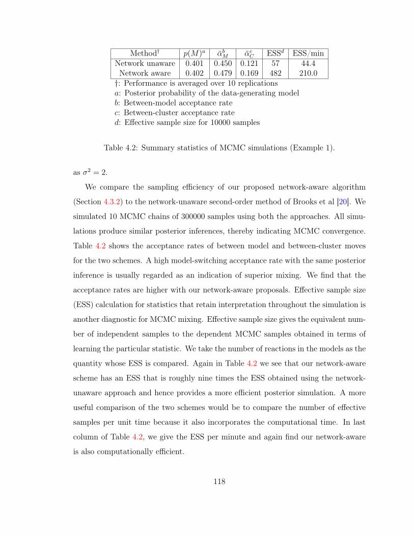
Method† 𝑝(𝑀)𝑎 ��𝑏𝑀 ��𝑐
𝐶 ESS𝑑 ESS/minNetwork unaware 0.401 0.450 0.121 57 44.4Network aware 0.402 0.479 0.169 482 210.0†: Performance is averaged over 10 replications𝑎: Posterior probability of the data-generating model𝑏: Between-model acceptance rate𝑐: Between-cluster acceptance rate𝑑: Effective sample size for 10000 samples
Table 4.2: Summary statistics of MCMC simulations (Example 1).
as 𝜎2 = 2.
We compare the sampling efficiency of our proposed network-aware algorithm
(Section 4.3.2) to the network-unaware second-order method of Brooks et al [20]. We
simulated 10 MCMC chains of 300000 samples using both the approaches. All simu-
lations produce similar posterior inferences, thereby indicating MCMC convergence.
Table 4.2 shows the acceptance rates of between model and between-cluster moves
for the two schemes. A high model-switching acceptance rate with the same posterior
inference is usually regarded as an indication of superior mixing. We find that the
acceptance rates are higher with our network-aware proposals. Effective sample size
(ESS) calculation for statistics that retain interpretation throughout the simulation is
another diagnostic for MCMC mixing. Effective sample size gives the equivalent num-
ber of independent samples to the dependent MCMC samples obtained in terms of
learning the particular statistic. We take the number of reactions in the models as the
quantity whose ESS is compared. Again in Table 4.2 we see that our network-aware
scheme has an ESS that is roughly nine times the ESS obtained using the network-
unaware approach and hence provides a more efficient posterior simulation. A more
useful comparison of the two schemes would be to compare the number of effective
samples per unit time because it also incorporates the computational time. In last
column of Table 4.2, we give the ESS per minute and again find our network-aware
is also computationally efficient.
118

Model Indicator1 2 3 4 5 6 7 8
log10Variance
-9
-8
-7
-6
-5
-4
-3
-2
-1
0
Network unawareNetwork unaware (d)Network aware
Figure 4-10: Variance of the eight highest posterior model probability estimates inExample 1
Further in Figure 4-10, we present the variance of the estimated posterior model
probabilities. The variance estimates are calculated based on 10 chains. The results of
the network-aware sampler are compared to the network-unaware approach, with and
without derandomization. Derandomization in the network-unaware approach refers
to performing the MCMC sampling without acknowledging the network structure, but
using that knowledge only as a post processing variance reduction method. We see
clear benefit in using out network-aware sampling approach compared to the standard
method with a 3–4 times reduction in variance.
119
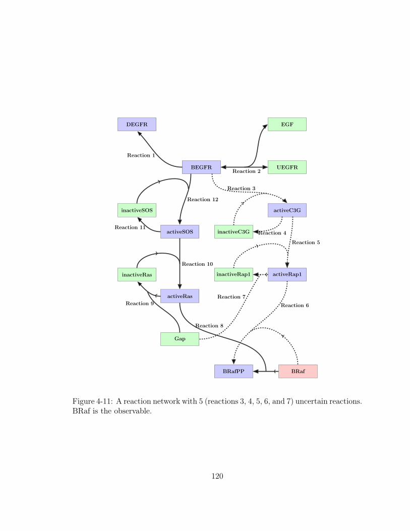
BEGFR
DEGFR EGF
UEGFR
inactiveC3G
activeC3G
activeRap1
BRafBRafPP
activeRas
Gap
inactiveRap1inactiveRas
activeSOS
inactiveSOS
Reaction 1
Reaction 2
Reaction 3
Reaction 4
Reaction 5
Reaction 6
Reaction 8
Reaction 7Reaction 9
Reaction 10
Reaction 11
Reaction 12
Figure 4-11: A reaction network with 5 (reactions 3, 4, 5, 6, and 7) uncertain reactions.BRaf is the observable.
120

4.4.3 Example 2: five-dimensional nonlinear network infer-
ence
As our second example, we consider a five-dimensional nonlinear network inference
problem where the species interactions are governed by the law of mass action (Figure
4-11). The law of mass action gives the rate of a chemical reaction (say 𝑋 + 𝑌 → 𝑍)
as the product of a reaction-specific rate constant 𝑘 with reactant concentrations [𝑋]
and [𝑌 ]:
Rate = −𝑘[𝑋][𝑌 ]. (4.26)
Under some assumptions, the law of mass action produces Michaelis-Menten reaction
rate expression
𝑅𝑎𝑡𝑒 =𝑘[𝑆]
𝑘𝑀 + [𝑆], (4.27)
or when enzyme concentration is taken into account [91]:
𝑅𝑎𝑡𝑒 = 𝑘[𝐸]0[𝑆]
𝑘𝑀 + [𝑆], (4.28)
where 𝑘 denotes the rate constant, [𝐸]0 is the enzyme concetration, [𝑆] the substrate
concentration, and 𝑘𝑀 the Michaelis constant.
In the present example, we consider a subset of reactions (15 species and 12
reactions) proposed for a protein-signalling network of the activation of extracellular
signal-regulated kinase (ERK) by epidermal growth factor (EGF) (Figure 4-11) [118].
The ODE forward model governing the evolution of species concentrations is described
in detail in Appendix B.1. We keep reactions 1, 2, 8, 9, 10, 11, and 12 fixed (denoted
by thick lines in the reaction graph 4-11 and shaded pink in Table 4.3) and thus they
are included in all the inferred models. The rate constants of all fixed reactions and
Michaelis constants of all reactions are set to their base values (Table 4.3). Reactions
121

3, 4, 5, 6, and 7 are taken to be uncertain and the concentration of BRaf is taken to
be the observable. With the above five uncertain reactions, the number of potential
models is 32. And with only BRaf as the observable, the number of clusters is 5. The
resulting problem is a nonlinear network inference problem for which the marginal
likelihood is not analytically computable.
Reaction log10 𝑘*𝑎 𝑘𝑏𝑀 Prior uncertainty
1 BEGFR → DEGFR 0.0 - −2a EGF + UEGFR → BEGFR 1.5 - −2b BEGFR → EGF + UEGFR 0.0 - −3 inactiveC3G+BEGFR → activeC3G+BEGFR 0.5 3386.3875 log10 𝑘 = 𝒩 (1.1, 0.2)4 activeC3G → inactiveC3G 2.0 - log10 𝑘 = 𝒩 (1.4, 0.2)5 inactiveRap1+activeC3G → activeRap1+activeC3G 2.0 3566 log10 𝑘 = 𝒩 (2.6, 0.2)6 BRaf+activeRap1 → BRafPP+activeRap1 0.4 17991.179 log10 𝑘 = 𝒩 (1.0, 0.2)7 activeRap1+Gap → inactiveRap1+Gap 1.0 6808.32 log10 𝑘 = 𝒩 (0.4, 0.2)8 BRaf+activeRas → BRafPP+activeRas 0.5 7631.63 −9 activeRas+Gap → inactiveRas+Gap 0.0 12457.816 −10 inactiveRas+activeSOS → activeRas+activeSOS 0.5 13.73 −11 activeSOS → inactiveSOS 4.0 9834.13 −12 inactiveSOS+BEGFR → activeSOS+BEGFR 2.5 8176.56 −𝑎 logarithm (base rate constant value)𝑏 Base value of Michaelis constant (Obtained from Xu et al. [118])
Table 4.3: Proposed reactions for Example 2
We generated 20 i.i.d. data points with noise model 𝒩 (0, 4) and rate constants
and Michaelis constants set to their base values (Table 4.3). We impose independent
Gaussian priors on the rate constants of the uncertain reactions with means and
variances as shown in Table 4.3. The above prior amounts to roughly three orders
of magnitude prior uncertainty in the rate constants. All models are assigned a
uniform prior probability. The noise variance for the likelihood function, as in the
data generating process, is taken as 𝜎2 = 4.
We compare the sampling efficiency of our network-aware algorithm (Section 4.3.2)
to the network-unaware 2𝑛𝑑 order proposal of Brooks et al [20]. We simulated 5
replications of 400000 samples using both the approaches. 30000 samples each were
discarded as burn-in. All simulations produce similar posterior inferences, thereby
indicating convergence. Figure 4-12 shows samples generated from the posterior dis-
tribution using the two approaches color coded according to the pathway they belong.
122

(a) Network-unaware proposal
(b) Network-aware proposal
Figure 4-12: MCMC trace plots for Example 2: posterior samples from models withboth pathways in orange and samples from models with only the left pathway in blue
123

Blue points are posterior samples from all models that belong to the left pathway,
i.e., models that do not contain any of reactions 3, 5, and 6. Orange points are poste-
rior samples from models that operate with both—left and right branch—pathways,
i.e., models that necessarily include reactions 3, 5, 6, 8, 10 and 12. The higher fre-
quency of moves between the left pathway models and both pathways models with
the network-aware approach is a sign of faster posterior exploration and consequently
better MCMC mixing. Table 4.4 shows the acceptance rates of between models
moves and between-cluster moves for the two approaches. High model-switching and
cluster-switching acceptance rates with the same posterior inference is an indication
of superior mixing of the network-aware approach. In Table 4.4, we also present the
ESS for the number-of-reactions-in-model statistic. The network-aware scheme has a
ten-fold higher ESS compared to the network-unaware approach. The ESS per minute
diagnostic in the last column of Table 4.4 confirms favourability of the network-aware
approach with the computational cost taken into account. The absolute value of ESS
per minute depends on the relative and absolute tolerance settings of the ODE solver.
In particular, we chose very tight tolerances, but higher ESS/min can be obtained
with loose tolerances. Nonetheless, the relative values of ESS/min demonstrate the
advantage of using the network-aware sampling approach.
Method† 𝑝(𝑀)𝑎 ��𝑏𝑀 ��𝑐
𝐶 ESS𝑑 ESS/min𝑒
Network unaware 0.7545 0.19 0.015 10 0.175Network aware 0.7544 0.22 0.034 110 0.301†: Performance is averaged over 5 simulation runs𝑎: Posterior probability of the data-generating model𝑏: Between-model move acceptance rate𝑐: Between-cluster move acceptance rate𝑑: Effective sample size for 10000 samples𝑒: The absolute values depend on the tolerances chosen for the ODE solver
Table 4.4: Summary statistics of MCMC simulations (Example 2).
Finally, in Figure 4-13, we present the variance of the estimated posterior model
124
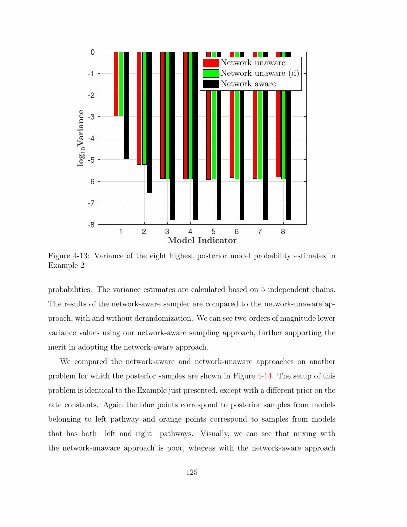
Model Indicator1 2 3 4 5 6 7 8
log10Variance
-8
-7
-6
-5
-4
-3
-2
-1
0
Network unawareNetwork unaware (d)Network aware
Figure 4-13: Variance of the eight highest posterior model probability estimates inExample 2
probabilities. The variance estimates are calculated based on 5 independent chains.
The results of the network-aware sampler are compared to the network-unaware ap-
proach, with and without derandomization. We can see two-orders of magnitude lower
variance values using our network-aware sampling approach, further supporting the
merit in adopting the network-aware approach.
We compared the network-aware and network-unaware approaches on another
problem for which the posterior samples are shown in Figure 4-14. The setup of this
problem is identical to the Example just presented, except with a different prior on the
rate constants. Again the blue points correspond to posterior samples from models
belonging to left pathway and orange points correspond to samples from models
that has both—left and right—pathways. Visually, we can see that mixing with
the network-unaware approach is poor, whereas with the network-aware approach
125

continues to be good.
4.4.4 Example 3: six-dimensional nonlinear network inference
In our third example, we consider a six-dimensional nonlinear network inference prob-
lem where species interactions are governed by law of mass action (Figure 4-15). Once
again, we consider a protein-signalling network consisting of 15 species and 12 po-
tential species interactions (Figure 4-15). The ODE forward model governing the
evolution of species concentrations is described in detail in Appendix B.1. We keep
reactions 1, 2, 4, 7, 9, and 11 fixed (denoted by thick lines in the reaction graph 4-15
and shaded pink in Table 4.5), and thus they are included in all the inferred models.
The rate constants of all fixed reactions and Michaelis constants of all reactions are
set to their base values. Reactions 3, 5, 6, 8, 10, and 12 are uncertain and the con-
centration of BRaf is again the observable. With the above six uncertain reactions,
the number of potential models is 64. However, with only BRaf as the observable,
the number of clusters is 4.
We generated 20 i.i.d. data points with noise model 𝒩 (0, 0.25) and all rate con-
stants and Michaelis constants set to their base values (Table 4.5). We impose inde-
pendent Gaussian priors on the rate constants of the uncertain reactions with means
and variances as shown in Table 4.5. The above prior amounts to roughly two orders
of magnitude prior uncertainty in the rate constants. The prior probability distribu-
tion over models is set such that all models except one are given uniform probability
and the model with all uncertain reactions included a prior probability five times the
other models. This choice is made to ensure that model with all reactions included
(thus with both pathways active) does not have insignificant posterior probability.
The noise variance for the likelihood function, as in the data generating process, is
taken as 𝜎2 = 0.25.
Samplers that did not use sensitivity-based proposals show very poor mixing.
Figure 4-16 shows samples generated (after a burn-in of 30000 samples) from the pos-
126
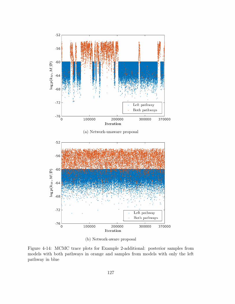
(a) Network-unaware proposal
(b) Network-aware proposal
Figure 4-14: MCMC trace plots for Example 2-additional: posterior samples frommodels with both pathways in orange and samples from models with only the leftpathway in blue
127
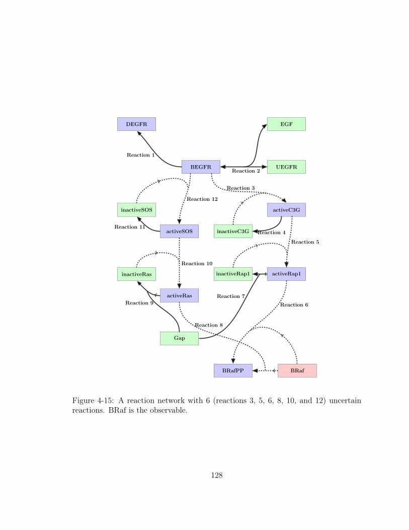
BEGFR
DEGFR EGF
UEGFR
inactiveC3G
activeC3G
activeRap1
BRafBRafPP
activeRas
Gap
inactiveRap1inactiveRas
activeSOS
inactiveSOS
Reaction 1
Reaction 2
Reaction 3
Reaction 4
Reaction 5
Reaction 6
Reaction 8
Reaction 7Reaction 9
Reaction 10
Reaction 11
Reaction 12
Figure 4-15: A reaction network with 6 (reactions 3, 5, 6, 8, 10, and 12) uncertainreactions. BRaf is the observable.
128
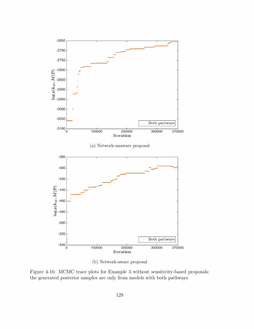
(a) Network-unaware proposal
(b) Network-aware proposal
Figure 4-16: MCMC trace plots for Example 3 without sensitivity-based proposals:the generated posterior samples are only from models with both pathways
129

(a) Sensitivity-based network-unaware proposal
(b) Sensitivity-based network-aware proposal
Figure 4-17: MCMC trace plots for Example 3 with sensitivity-based proposals: pos-terior samples from models with both pathways in orange and samples from modelswith only the left pathway in blue
130

Reaction log10 𝑘*𝑎 𝑘𝑏𝑀 Prior uncertainty
1 BEGFR → DEGFR 0.0 - −2a EGF + UEGFR → BEGFR 1.5 - −2b BEGFR → EGF + UEGFR 0.0 - −3 inactiveC3G+BEGFR → activeC3G+BEGFR 0.5 3386.3875 log10 𝑘 = 𝒩 (1.2, 0.1)4 activeC3G → inactiveC3G 2.0 - −5 inactiveRap1+activeC3G → activeRap1+activeC3G 2.0 3566 log10 𝑘 = 𝒩 (2.7, 0.1)6 BRaf+activeRap1 → BRafPP+activeRap1 0.4 17991.179 log10 𝑘 = 𝒩 (1.1, 0.1)7 activeRap1+Gap → inactiveRap1+Gap 1.0 6808.32 −8 BRaf+activeRas → BRafPP+activeRas 0.5 7631.63 log10 𝑘 = 𝒩 (0.5, 0.1)9 activeRas+Gap → inactiveRas+Gap 0.0 12457.816 −10 inactiveRas+activeSOS → activeRas+activeSOS 0.5 13.73 log10 𝑘 = 𝒩 (0.5, 0.1)11 activeSOS → inactiveSOS 4.0 9834.13 −12 inactiveSOS+BEGFR → activeSOS+BEGFR 2.5 8176.56 log10 𝑘 = 𝒩 (2.5, 0.1)𝑎 logarithm (base rate constant value)𝑏 Base value of Michaelis constant (Obtained from Xu et al. [118])
Table 4.5: Proposed reactions for Example 3
Method† 𝑝(𝑀)𝑎 ��𝑏𝑀 ��𝑐
𝐶 ESS𝑑 ESS/min𝑒
Sensitivity-based network unaware 0.022 0.236 0.0035 342 1.921Sensitivity-based network aware 0.022 0.358 0.0076 932 5.608†: Performance is averaged over 5 simulation runs𝑎: Posterior probability of the data-generating model𝑏: Between-model move acceptance rate𝑐: Between-cluster move acceptance rate𝑑: Effective sample size for 10000 samples𝑒: The absolute values depend on the tolerances chosen for the ODE solver
Table 4.6: Summary statistics of MCMC simulations (Example 3).
terior distribution using our network-aware algorithm (Section 4.3.2) and the network-
unaware 2𝑛𝑑 order proposal of Brooks et al. [20], which are color coded according to
the pathway they belong. Blue points are posterior samples from all models that
belong to the left pathway, i.e., models that do not contain any of reactions 3, 5,
and 6. Orange points are posterior samples from models that operate with both—
left and right branch—pathways, i.e., models that necessarily include reactions 3, 5,
6, 8, 10 and 12. We see that even after 400000 samples are generated, the sam-
plers remain confined to the models with both pathways without ever switching to
models belonging to the left pathway. Next, we compare the sampling efficiency of
our sensitivity-based network-aware algorithm (Section 4.3.3) to the sensitivity-based
131

network-unaware approach. We simulated 5 replications of 500000 samples using both
the approaches. 30000 samples each were discarded as burn-in. All simulations pro-
duce similar posterior inferences, thereby indicating convergence. Figure 4-17 shows
samples generated from the posterior using the two approaches color coded according
to the pathway they belong. The higher frequency of moves between the left path-
way models and both pathways models with the network-aware approach is a sign of
faster posterior exploration and consequently better MCMC mixing. Table 4.6 shows
the acceptance rates of between models moves and between-cluster moves for the two
approaches. High model-switching and cluster-switching acceptance rates with the
same posterior inference is an indication of superior mixing of the network-aware ap-
proach. In Table 4.6, we also present the ESS for the number-of-reactions-in-model
statistic. The network-aware scheme has an ESS that is roughly three times ESS of
the network-unaware approach. The ESS per minute diagnostic in the last column
of Table 4.6 confirms favourability of the network-aware approach with the computa-
tional cost taken into account. The absolute value of ESS per minute depends on the
relative and absolute tolerance settings of the ODE solver. In particular, we chose
very tight tolerances, but higher ESS/min can be obtained with loose tolerances.
Nonetheless, the relative values of ESS/min demonstrate the advantage of using the
network-aware sampling approach.
Finally, in Figure 4-18, we present the variance of the estimated posterior model
probabilities. The variance estimates are calculated based on 5 independent chains.
The results of the sensitivity-based network-aware sampler are compared to the
sensitivity-based network-unaware approach, with and without derandomization. We
can see roughly an order of magnitude lower variance values using our network-aware
sampling approach compared to the network-unaware approach with derandomiza-
tion and two orders of magnitude lower variances compared to the network-unaware
approach without derandomization.
132

Model Indicator1 2 3 4 5 6 7 8
log10Variance
-8
-7
-6
-5
-4
-3
-2
-1
0
Network unawareNetwork unaware (d)Network aware
Figure 4-18: Variance of the eight highest posterior model probability estimates inExample 3
4.4.5 Example 4: ten-dimensional nonlinear network inference
Our final example is a large scale nonlinear network inference problem with 10 uncer-
tain reactions. Once again, we consider a protein-signalling network consisting of 15
species and 12 potential species interactions (Figure 4-19). The ODE forward model
governing the evolution of species concentrations is described in detail in Appendix
B.1. We keep only reactions 1 and 2 fixed (denoted by thick lines in the reaction
graph 4-19 and shaded pink in Table 4.7) and thus they are included in all the in-
ferred models. The rate constants of all fixed reactions and Michaelis constants of
all reactions are set to their base values (Table 4.7). Reactions 3–12 are uncertain
and the concentration of BRaf is again the observable. With the above ten uncer-
tain reactions, the number of potential models is 1024. And with only BRaf as the
133
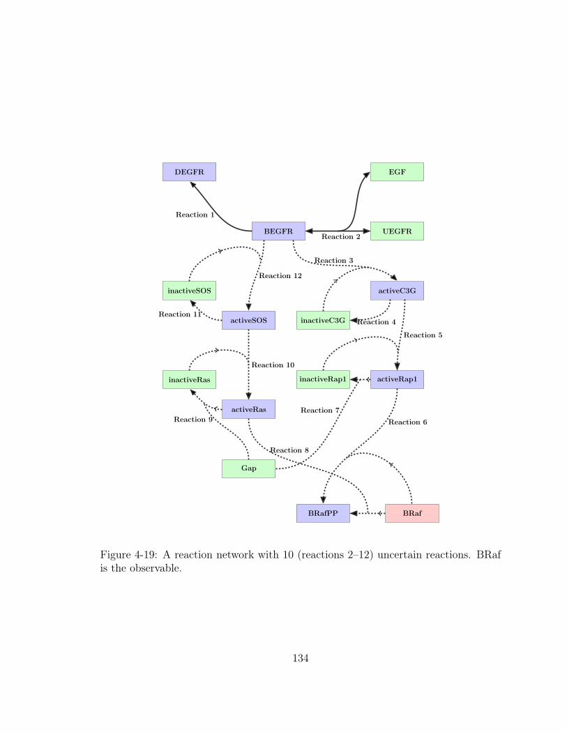
BEGFR
DEGFR EGF
UEGFR
inactiveC3G
activeC3G
activeRap1
BRafBRafPP
activeRas
Gap
inactiveRap1inactiveRas
activeSOS
inactiveSOS
Reaction 1
Reaction 2
Reaction 3
Reaction 4
Reaction 5
Reaction 6
Reaction 8
Reaction 7Reaction 9
Reaction 10
Reaction 11
Reaction 12
Figure 4-19: A reaction network with 10 (reactions 2–12) uncertain reactions. BRafis the observable.
134
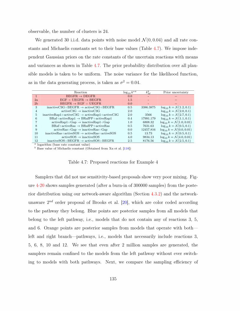
observable, the number of clusters is 24.
We generated 30 i.i.d. data points with noise model 𝒩 (0, 0.04) and all rate con-
stants and Michaelis constants set to their base values (Table 4.7). We impose inde-
pendent Gaussian priors on the rate constants of the uncertain reactions with means
and variances as shown in Table 4.7. The prior probability distribution over all plau-
sible models is taken to be uniform. The noise variance for the likelihood function,
as in the data generating process, is taken as 𝜎2 = 0.04.
Reaction log10 𝑘*𝑎 𝑘𝑏𝑀 Prior uncertainty
1 BEGFR → DEGFR 0.0 - −2a EGF + UEGFR → BEGFR 1.5 - −2b BEGFR → EGF + UEGFR 0.0 - −3 inactiveC3G+BEGFR → activeC3G+BEGFR 0.5 3386.3875 log10 𝑘 = 𝒩 (1.2, 0.1)4 activeC3G → inactiveC3G 2.0 - log10 𝑘 = 𝒩 (2.0, 0.1)5 inactiveRap1+activeC3G → activeRap1+activeC3G 2.0 3566 log10 𝑘 = 𝒩 (2.7, 0.1)6 BRaf+activeRap1 → BRafPP+activeRap1 0.4 17991.179 log10 𝑘 = 𝒩 (1.1, 0.1)7 activeRap1+Gap → inactiveRap1+Gap 1.0 6808.32 log10 𝑘 = 𝒩 (1.0, 0.01)8 BRaf+activeRas → BRafPP+activeRas 0.5 7631.63 log10 𝑘 = 𝒩 (0.5, 0.1)9 activeRas+Gap → inactiveRas+Gap 0.0 12457.816 log10 𝑘 = 𝒩 (0.0, 0.01)10 inactiveRas+activeSOS → activeRas+activeSOS 0.5 13.73 log10 𝑘 = 𝒩 (0.5, 0.1)11 activeSOS → inactiveSOS 4.0 9834.13 log10 𝑘 = 𝒩 (4.0, 0.01)12 inactiveSOS+BEGFR → activeSOS+BEGFR 2.5 8176.56 log10 𝑘 = 𝒩 (2.5, 0.1)𝑎 logarithm (base rate constant value)𝑏 Base value of Michaelis constant (Obtained from Xu et al. [118])
Table 4.7: Proposed reactions for Example 4
Samplers that did not use sensitivity-based proposals show very poor mixing. Fig-
ure 4-20 shows samples generated (after a burn-in of 300000 samples) from the poste-
rior distribution using our network-aware algorithm (Section 4.3.2) and the network-
unaware 2𝑛𝑑 order proposal of Brooks et al. [20], which are color coded according
to the pathway they belong. Blue points are posterior samples from all models that
belong to the left pathway, i.e., models that do not contain any of reactions 3, 5,
and 6. Orange points are posterior samples from models that operate with both—
left and right branch—pathways, i.e., models that necessarily include reactions 3,
5, 6, 8, 10 and 12. We see that even after 2 million samples are generated, the
samplers remain confined to the models from the left pathway without ever switch-
ing to models with both pathways. Next, we compare the sampling efficiency of
135
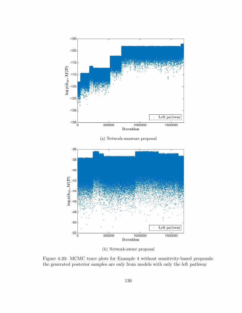
(a) Network-unaware proposal
(b) Network-aware proposal
Figure 4-20: MCMC trace plots for Example 4 without sensitivity-based proposals:the generated posterior samples are only from models with only the left pathway
136

(a) Sensitivity-based network-unaware proposal
(b) Sensitivity-based network-aware proposal
Figure 4-21: MCMC trace plots for Example 4 with sensitivity-based proposals: pos-terior samples from models with both pathways in orange and samples from modelswith only the left pathway in blue
137

our sensitivity-based network-aware algorithm (Section 4.3.3) to the sensitivity-based
network-unaware approach. We simulated 5 replications of 2 million samples using
both the approaches. 300,000 samples each were discarded as burn-in. Figure 4-21
shows samples generated from the posterior distribution using the two approaches
color coded according to the pathway they belong. We observe that the frequency
of moves between the left-pathway models and both-pathways models is higher with
the network-aware approach, indicating faster posterior exploration. Table 4.8 shows
the acceptance rates of between-model moves and between-pathway moves for the
two approaches. High model-switching and pathway-switching acceptance rates with
the same posterior inference is an indication of superior mixing of the network-aware
approach. In Table 4.8, we also present the ESS for the number-of-reactions-in-model
statistic. The network-aware approach has an ESS that is roughly three times the
ESS obtained using the network-unaware approach. The ESS per minute diagnostic
in the last column of Table 4.8 also supports the use of the network-aware approach.
Method† 𝑝(𝑀)𝑎 ��𝑏𝑀 ��𝑐
𝑃 ESS𝑑 ESS/min𝑒
Sensitivity-based network unaware 0.145 0.095 0.0013 86 3.37×10⁻³
Sensitivity-based network aware 0.157 0.145 0.0027 275 8.66×10⁻³
†: Performance is averaged over 5 simulation runs𝑎: Posterior probability of the data-generating model𝑏: Between-model move acceptance rate𝑐: Between-pathway move acceptance rate𝑑: Effective sample size for 1000000 samples𝑒: The absolute values depend on the tolerances chosen for the ODE solver
Table 4.8: Summary statistics of MCMC simulations (Example 4).
138

Chapter 5
Network inference with
approximation
In Chapters 3 and 4, we presented exact methods which converge to the true pos-
terior distribution asymptotically. Many times, however, when the number of plau-
sible models is very large (> 104), the need for also proposing parameter values for
between-model moves could render exact model-space sampling methods very ex-
pensive. In this chapter, we propose an approximation-based approach to nonlinear
network inference problems. Asymptotic inference methods such as Laplace’s method
and the Bayesian information criterion are popular alternatives to an exact Bayesian
approach [75]. By making assumptions about the structure of parameter posterior
distribution, these methods allow computationally efficient Bayesian model inference.
Specifically, the model evidence is approximated by solving a high-dimensional opti-
mization problem and evaluating a Hessian matrix for each model. If, however, the
number of models is very high, the enumeration of model evidences for all models is
again prohibitively expensive. We propose simulating a Markov chain Monte Carlo
algorithm with only the model indicator 𝑀𝑖 in the state space and for each visited
model approximating the model evidence using Laplace’s method. For linear mod-
els with conjugate priors, the Laplace approximation produces exact evidence, and
139
MCMC over model indicators is often used for variable selection and inference of
graphical models [83]. For general non-conjugate models, approximations in MCMC
simulations have been used in the past [32, 34, 61]. In particular, Guihenneuc et al.
[61] provide theory on the error induced in posterior distributions while employing
Laplace approximations in MCMC simulations.
The inference of reaction networks governed by nonlinear species interactions
(thus nonlinear parameter-to-observable maps) with limited and sparse experimental
data leads to posterior distributions that are multimodal. The standard single-chain
MCMC approach when used on multimodal posteriors has a tendency to get stuck in
one of the modes. We extend the above approximation-based network inference ap-
proach to a population-based MCMC scheme, which involves running parallel Markov
chains that exchange information among themselves to ensure all posterior modes are
adequately traversed. We show the superiority of the population-based scheme in
exploring a posterior distribution over a space of 𝑂(109) reaction networks in com-
parison to a single chain simulation. This method allows systematic exploration of
posterior distributions over nonlinear networks when exact sampling of networks is
infeasible.
5.1 Laplace’s method
Recall the application of Bayes’ rule to models {𝑀𝑖} gives
𝑝(𝑀𝑖|𝒟) =𝑝(𝒟|𝑀𝑖)𝑝(𝑀𝑖)
𝑝(𝒟). (5.1)
Here, 𝑝(𝑀𝑖|𝒟) is the posterior probability of 𝑀𝑖 conditioned on data 𝒟; 𝑝(𝒟|𝑀𝑖),
also called the model evidence, is the marginal likelihood of observing 𝒟; and 𝑝(𝑀𝑖)
is the prior probability of model 𝑀𝑖. Specifically,
140

𝑝(𝒟|𝑀𝑖) =
∫𝑝(𝒟|𝑘𝑖,𝑀𝑖)𝑝(𝑘𝑖|𝑀𝑖)𝑑𝑘𝑖, (5.2)
where 𝑘𝑖 is a model-specific multidimensional parameter. Laplace’s method ap-
proximates (5.2) by computing a Gaussian approximation to the posterior density.
Let the joint density of 𝒟 and 𝑘𝑖 conditioned on model 𝑀𝑖 be 𝑙(𝑘𝑖): 𝑙(𝑘𝑖) =
log(𝑝(𝒟|𝑘𝑖,𝑀𝑖)𝑝(𝑘𝑖|𝑀𝑖)). The Laplace’s method involves finding the posterior mode:
��𝑖 = arg max𝑘𝑖
log(𝑝(𝒟|𝑘𝑖,𝑀𝑖)𝑝(𝑘𝑖|𝑀𝑖)), (5.3)
and computing a second-order Taylor expansion of 𝑙(𝑘𝑖) about ��𝑖. Exponentiating
the quadratic yields an approximation to 𝑝(𝒟|𝑘𝑖,𝑀𝑖)𝑝(𝑘𝑖|𝑀𝑖), which has the form for
a normal density with mean ��𝑖 and covariance matrix Σ = (−∇2𝑙(��𝑖))−1. Integrating
the approximation gives
𝑝(𝒟|𝑀𝑖) = (2𝜋)𝑑/2|Σ|1/2𝑝(𝒟|𝑘𝑖,𝑀𝑖)𝑝(��𝑖|𝑀𝑖), (5.4)
where 𝑑 is the dimensionality of 𝑘𝑖. Kass et al. [76] give conditions under which
as 𝑛𝑑𝑎𝑡𝑎 → ∞, 𝑝(𝒟|𝑀𝑖) = 𝑝(𝒟|𝑀𝑖)(1 + 𝑂(𝑛−1𝑑𝑎𝑡𝑎)). Plugging 5.4 into 5.5 gives the
approximate posterior model probability:
𝑝(𝑀 |𝒟) =𝑝(𝒟|𝑀)𝑝(𝑀)
𝑝(𝒟). (5.5)
5.2 Large-scale approximate model inference
The systematic application of Laplace’s method to all models when the number of
models is very high is computationally prohibitive. Using a Markov chain Monte
Carlo scheme to explore the approximate posterior distribution over models provides
141

a simulation-consistent estimate of approximate model posteriors. Thus, we simulate
𝑀𝑛 ∼ 𝑝(𝑀 |𝒟) to get estimates of posterior model probabilities as
𝑝(𝑀𝑖|𝒟) =1
𝑁
𝑁∑𝑛=1
I𝑀𝑖(𝑀𝑛). (5.6)
Since each model has a network structure and the data may be sparse, we have
𝑝(𝒟|𝑀𝑚) =
∫· · ·∫𝑝(𝒟|𝑘𝑖,𝑀𝑖)𝑝(𝑘𝑖|𝑀𝑖)𝑑𝑘𝑖
=
∫· · ·∫𝑝(𝒟|𝑘𝑒,𝑖,𝑀𝑒,𝑖)𝑝(𝑘𝑒,𝑖|𝑀𝑒,𝑖)𝑑𝑘𝑒,𝑖,
where 𝑀𝑒,𝑖 is the effective network corresponding to 𝑀𝑖 and 𝑘𝑒,𝑖 are the parameters
of the effective network (Chapter 4). Thus, we apply Laplace’s method directly to the
effective networks. The sequence of steps in large-scale approximate model inference
are given in Algorithm 9.
Algorithm 9 Approximate model inference MCMC1: Given: A set of models {𝑀𝑖} with corresponding parameter vectors {𝑘𝑖}, likeli-
hood functions {𝑝(𝒟|𝑀𝑖,𝑘𝑖)}, parameter prior densities {𝑝(𝑘𝑖)}, and model priordistribution 𝑝(𝑀).
2: Initlialize starting point (𝑀0,𝑘𝑀0); 𝑀0𝑒 =eff (𝑀0)
3: for 𝑛 = 0 to 𝑁𝑖𝑡𝑒𝑟 do4: Sample 𝑀 ′ ∼ 𝑞(𝑀 ′|𝑀𝑛 = 𝑀); 𝑀 ′
𝑒=eff (𝑀 ′)5: Determine approximate model evidence 𝑝(𝒟|𝑀 ′
𝑒) of 𝑀 ′𝑒
6: Sample 𝑝 ∼ 𝒰[0,1]7: if 𝑝 < 𝐴(𝑀,𝑀 ′) = min{1, 𝑝(𝒟|𝑀 ′
𝑒)𝑝(𝑀′)𝑞(𝑀𝑛|𝑀 ′)
𝑝(𝒟|𝑀𝑛𝑒 )𝑝(𝑀𝑛)𝑞(𝑀 ′|𝑀𝑛)
} then8: 𝑀𝑛+1 = 𝑀 ′
9: else10: 𝑀𝑛+1 = 𝑀𝑛
11: end if12: end for
142

5.2.1 Setup of the Bayesian model inference problem
Likelihood function
We employ an i.i.d. additive Gaussian model for the difference between model pre-
dictions and observations; thus the data are represented as
𝒟 = 𝐺(𝑘) + 𝜖𝑛, (5.7)
where 𝜖𝑛 ∼ 𝒩𝑛(0, 𝜎2𝐼𝑛), 𝑛 is the number of observations, 𝐼𝑛 is an 𝑛-by-𝑛 identity
matrix, and 𝐺(𝑘) is the prediction of the forward model at the given value of the
reaction parameters. The specific values of the noise standard deviations 𝜎 are given
later. The deterministic predictions𝐺(𝑘) are obtained with the ODE integrator. The
likelihood function is thus given by
𝑝(𝒟|𝑘) = 𝒩𝑛(𝒟|𝐺(𝑘), 𝜎2𝐼𝑛)
=𝑛∏
𝑡=1
𝒩 (𝑑𝑡|𝐺𝑡(𝑘), 𝜎2)
=𝑛∏
𝑡=1
1√2𝜋𝜎2
exp
(−(𝑑𝑡 −𝐺𝑡(𝑘))2
2𝜎2
), (5.8)
where 𝑑𝑡 are components of the data vector 𝒟.
Prior specification
Since reaction rate constants must be positive, while their uncertainties may have
multiple orders of magnitude, we take the prior distribution to be a lognormal distri-
bution on the rate constant. Specifically, we set each 𝑝(𝑘𝑖) to
𝑝(𝑘𝑖) : log10 𝑘𝑖 ∼ 𝒩 (log10 𝑘*𝑖 , 𝜎
2𝑖 ), (5.9)
where each 𝑘*𝑖 above is the base value of the 𝑖th rate constant.
143

5.2.2 Example 1: 10 dimensional reaction network
We demonstrate the large-scale approximate model inference approach on a 10 dimen-
sional example with synthetic data. Consider the reaction network shown in Figure
5-1. The set of reactions shown in this network are a subset of a larger model pro-
posed for the activation of the extracellular signal-regulated kinase (ERK) pathway
by epidermal growth factor [118]. The ODE forward model governing the evolution
of species concentrations is described in detail in Appendix B.1. We keep reactions 1
and 2 fixed (denoted by thick lines in the reaction grap 5-1 and shaded pink in Table
5.1) and thus they are included in all the inferred models. The rate constants of all
fixed reactions and Michaelis constants of all reactions are set to their base values
(Table 5.1). Reactions 3–12 are taken to be uncertain and the concentration of BRaf
is taken to be the observable. With the above ten uncertain reactions, the number
of potential models is 1024. And with only BRaf as the observable, the number of
clusters is 24.
Reaction log10 𝑘*𝑎 𝑘𝑏𝑀 Prior uncertainty
1 BEGFR → DEGFR 0.0 - −2a EGF + UEGFR → BEGFR 1.5 - −2b BEGFR → EGF + UEGFR 0.0 - −3 inactiveC3G+BEGFR → activeC3G+BEGFR 0.5 3386.3875 log10 𝑘 = 𝒩 (1.2, 0.1)4 activeC3G → inactiveC3G 2.0 - log10 𝑘 = 𝒩 (2.0, 0.1)5 inactiveRap1+activeC3G → activeRap1+activeC3G 2.0 3566 log10 𝑘 = 𝒩 (2.7, 0.1)6 BRaf+activeRap1 → BRafPP+activeRap1 0.4 17991.179 log10 𝑘 = 𝒩 (1.1, 0.1)7 activeRap1+Gap → inactiveRap1+Gap 1.0 6808.32 log10 𝑘 = 𝒩 (1.0, 0.1)8 BRaf+activeRas → BRafPP+activeRas 0.5 7631.63 log10 𝑘 = 𝒩 (0.5, 0.1)9 activeRas+Gap → inactiveRas+Gap 0.0 12457.816 log10 𝑘 = 𝒩 (0.0, 0.01)10 inactiveRas+activeSOS → activeRas+activeSOS 0.5 13.73 log10 𝑘 = 𝒩 (0.5, 0.1)11 activeSOS → inactiveSOS 4.0 9834.13 log10 𝑘 = 𝒩 (4.0, 0.01)12 inactiveSOS+BEGFR → activeSOS+BEGFR 2.5 8176.56 log10 𝑘 = 𝒩 (2.5, 0.1)𝑎 logarithm (base rate constant value)𝑏 Base value of Michaelis constant (Obtained from Xu et al. [118])
Table 5.1: Proposed reactions for Example 1
We simulate 30 i.i.d. data points with additive noise model 𝒩 (0, 4) and all rate
constants and Michaelis constants set to their base values (Table 5.1). We impose
independent Gaussian priors on the logarithm of rate constants of the uncertain re-
actions with means and variances as shown in Table 5.1. The prior probability dis-
144

BEGFR
DEGFR EGF
UEGFR
inactiveC3G
activeC3G
activeRap1
BRafBRafPP
activeRas
Gap
inactiveRap1inactiveRas
activeSOS
inactiveSOS
Reaction 1
Reaction 2
Reaction 3
Reaction 4
Reaction 5
Reaction 6
Reaction 8
Reaction 7Reaction 9
Reaction 10
Reaction 11
Reaction 12
Figure 5-1: Reaction network of Example 1
145
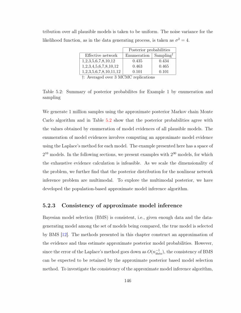
tribution over all plausible models is taken to be uniform. The noise variance for the
likelihood function, as in the data generating process, is taken as 𝜎2 = 4.
Posterior probabilitiesEffective network Enumeration Sampling†
1,2,3,5,6,7,8,10,12 0.435 0.4341,2,3,4,5,6,7,8,10,12 0.463 0.4651,2,3,5,6,7,8,10,11,12 0.101 0.101†: Averaged over 3 MCMC replications
Table 5.2: Summary of posterior probabilites for Example 1 by enumeration andsampling
We generate 1 million samples using the approximate posterior Markov chain Monte
Carlo algorithm and in Table 5.2 show that the posterior probabilities agree with
the values obtained by enumeration of model evidences of all plausible models. The
enumeration of model evidences involves computing an approximate model evidence
using the Laplace’s method for each model. The example presented here has a space of
210 models. In the following sections, we present examples with 230 models, for which
the exhaustive evidence calculation is infeasible. As we scale the dimensionality of
the problem, we further find that the posterior distribution for the nonlinear network
inference problem are multimodal. To explore the multimodal posterior, we have
developed the population-based approximate model inference algorithm.
5.2.3 Consistency of approximate model inference
Bayesian model selection (BMS) is consistent, i.e., given enough data and the data-
generating model among the set of models being compared, the true model is selected
by BMS [12]. The methods presented in this chapter construct an approximation of
the evidence and thus estimate approximate posterior model probabilities. However,
since the error of the Laplace’s method goes down as 𝑂(𝑛−1𝑑𝑎𝑡𝑎), the consistency of BMS
can be expected to be retained by the approximate posterior based model selection
method. To investigate the consistency of the approximate model inference algorithm,
146

we evaluate posterior model probabilities for the networks considered in Example 1
with steadily increasing data sets. Note Example 1 infact compares the same set of
networks as in Example 4 of Chapter 4, but with a different noise model. In order to
also compare the result we obtained using the approximate model inference approach
to the exact sampling approach of Chapter 4, we perform the consistency study with
the noise model (𝜎2 = 0.04) employed in Chapter 4. The data in each case are gener-
ated with a network consisting of all proposed reactions. The details of the size of the
data sets and the obtained posterior probabilities are presented in Table 5.3. Firstly,
we find that the results obtained for the data set with 30 points are very different using
the approximate model inference and exact sampling approaches. Specifically, we find
that the posterior probability of the data-generating model (effective network with
reactions 1–12) using the approximate model inference approach is ≈ 0.0, whereas
in Chapter 4 it was ≈ 0.15. In addition all the posterior mass is concentrated over
models with both the left and right pathways included in the approximate approach.
In contrast in Chapter 4, we found that models that only contain the left pathway of
the reaction network have sizable probability. This discrepancy between exact sam-
pling and approximate inference results is not surprising, since the inference results
with the two methods can be quite different with a small data set. As the amount of
data increases, however, we find that the posterior probability of the data-generating
model increases and ultimately converges to 1. Thus the data-generating model is
selected by the approximate model inference approach given sufficient data.
5.3 Population-based Markov chain Monte Carlo
Posterior distributions with multiple modes arise in many areas of applied statistics,
e.g., gene clustering [66] and population genetics [101], and their exploration is well
known to be a challenging sampling problem. To define multimodality in the present
context of network inference, one needs to first introduce a notion of distance metric.
147
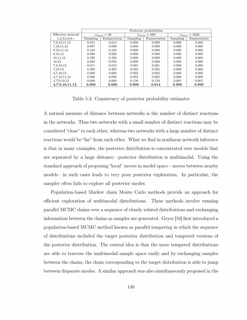
Posterior probabilitiesEffective network 𝑛𝑑𝑎𝑡𝑎 = 30 𝑛𝑑𝑎𝑡𝑎 = 880 𝑛𝑑𝑎𝑡𝑎 = 3840
1,2,3,5,6,8+ Sampling Enumeration Sampling Enumeration Sampling Enumeration7,9,10,11,12 0.013 0.013 0.000 0.000 0.000 0.0007,10,11,12 0.087 0.089 0.000 0.000 0.000 0.0009,10,11,12 0.163 0.162 0.000 0.000 0.000 0.0009,10,12 0.098 0.098 0.000 0.000 0.000 0.00010,11,12 0.238 0.236 0.000 0.000 0.000 0.00010,12 0.083 0.082 0.000 0.000 0.000 0.0007,9,10,12 0.011 0.012 0.001 0.001 0.000 0.0007,10,12 0.306 0.308 0.022 0.025 0.000 0.0004,7,10,12 0.000 0.000 0.002 0.002 0.000 0.0004,7,10,11,12 0.000 0.000 0.004 0.005 0.000 0.0004,7,9,10,12 0.000 0.000 0.156 0.159 0.001 0.0014,7,9,10,11,12 0.000 0.000 0.808 0.814 0.999 0.999
Table 5.3: Consistency of posterior probability estimates
A natural measure of distance between networks is the number of distinct reactions
in the networks. Thus two networks with a small number of distinct reactions may be
considered “close” to each other, whereas two networks with a large number of distinct
reactions would be “far” from each other. What we find in nonlinear network inference
is that in many examples, the posterior distribution is concentrated over models that
are separated by a large distance—posterior distribution is multimodal. Using the
standard approach of proposing “local” moves in model space—moves between nearby
models—in such cases leads to very poor posterior exploration. In particular, the
sampler often fails to explore all posterior modes.
Population-based Markov chain Monte Carlo methods provide an approach for
efficient exploration of multimodal distributions. These methods involve running
parallel MCMC chains over a sequence of closely related distributions and exchanging
information between the chains as samples are generated. Geyer [50] first introduced a
population-based MCMC method known as parallel tempering in which the sequence
of distributions included the target posterior distribution and tempered versions of
the posterior distribution. The central idea is that the more tempered distributions
are able to traverse the multimodal sample space easily and by exchanging samples
between the chains, the chain corresponding to the target distribution is able to jump
between disparate modes. A similar approach was also simultaneously proposed in the
148
physics literature by Hukushima et al [70]. Jasra et al. [72] review recent developments
in population-based methods. We give here a brief overview of general population-
based MCMC methods.
In order to sample from the posterior distribution 𝑝(𝜃|𝒟), a new target distribu-
tion is defined in population-based MCMC as
𝑝(𝜃1:𝑆) =𝑆∏
𝑗=1
𝑝𝑗(𝜃𝑗), (5.10)
where at least one of 𝑝𝑗(𝜃𝑗) is taken as 𝑝(𝜃|𝒟). By designing a transition kernel
that is 𝑝(𝜃1:𝑆)-irreducible, aperiodic and has 𝑝(𝜃1:𝑆) as the invariant distribution, a
population-based MCMC method is constructed. The method consists of a population
of chains, where each chain corresponds to one of the distributions 𝑝𝑗(𝜃𝑗) and the
state of the chains updated according to a set of possible move types. Many different
choices of the sequence of distributions 𝑝𝑗(𝜃𝑗) can be made. We describe two common
choices; see [72] for a complete discussion.
5.3.1 Sequence of distributions
Identical
One choice of the sequence of distributions is to take each of them to be the target
posterior distribution 𝑝(𝜃|𝒟). Although simple, the effectivity of this sequence relies
on the original single chain sampler being efficient in exploring the target distribu-
tion. This approach was used by Warnes et al. [115], where they update the state
of the chains according to a proposal that is a Gaussian approximation of the target
distribution constructed with samples from all the chains. Robert and Casella [105]
note that this approach may not work well for high-dimensional targets due to poor
density estimation in high dimensions.
149

Tempered
The tempered approach consists of taking the sequence of distributions to be tempered
versions of the target distribution [81]. Thus, one possible choice is to take
𝑝𝑗(𝜃𝑗) ∝ 𝑝(𝜃|𝒟)1𝑇𝑗 𝑝(𝜃), (5.11)
where {𝑇𝑗} is interpreted as a temperature ladder. The idea is that as the temperature
rises, the corresponding distribution becomes less peaky and the respective chain can
traverse the space faster. By defining a large number distributions in the sequence, the
chains at higher temperatures explore the state space efficiently and by exchanging
information between chains, the chains at lower temperatures can jump between
distinct modes. Note one of the chains always has 𝑇𝑗 = 1 and corresponds to the
target distribution. The choice of the temperature schedule (𝜁𝑗 = 1𝑇𝑗
) is discussed in
Jasra et al [72].
5.3.2 Population moves
At each step of the simulation, we choose among a set of possible population moves.
Move types ranging from simple Metropolis-Hastings to more non-standard moves
such as exchanging samples can performed and we give details of these here.
Mutation
The mutation population move consists of selecting one of the distributions 𝑝𝑗(𝜃𝑗)
and performing a Metropolis-Hastings move on that distribution. Formally, a chain
𝑡 ∈ {1, 2, ..., 𝑆} is selected, a proposal 𝜃′𝑡 is made according to a proposal distribution
𝑞𝑡(𝜃′𝑡|𝜃𝑡), and the proposal is accepted with probability:
𝛼𝑝𝑟𝑜𝑏(𝜃′|𝜃) = min
{1,𝑝𝑡(𝜃
′𝑡)𝑞𝑡(𝜃𝑡|𝜃′𝑡)
𝑝𝑡(𝜃𝑡)𝑞𝑡(𝜃′𝑡|𝜃𝑡)
}, (5.12)
150
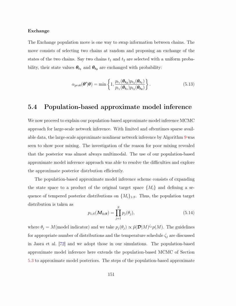
Exchange
The Exchange population move is one way to swap information between chains. The
move consists of selecting two chains at random and proposing an exchange of the
states of the two chains. Say two chains 𝑡1 and 𝑡2 are selected with a uniform proba-
bility, their state values 𝜃𝑡1 and 𝜃𝑡2 are exchanged with probability:
𝛼𝑝𝑟𝑜𝑏(𝜃′|𝜃) = min
{1,𝑝𝑡1(𝜃𝑡2)𝑝𝑡2(𝜃𝑡1)
𝑝𝑡1(𝜃𝑡1)𝑝𝑡2(𝜃𝑡2)
}. (5.13)
5.4 Population-based approximate model inference
We now proceed to explain our population-based approximate model inference MCMC
approach for large-scale network inference. With limited and oftentimes sparse avail-
able data, the large-scale approximate nonlinear network inference by Algorithm 9 was
seen to show poor mixing. The investigation of the reason for poor mixing revealed
that the posterior was almost always multimodal. The use of our population-based
approximate model inference approach was able to resolve the difficulties and explore
the approximate posterior distrbution efficiently.
The population-based approximate model inference scheme consists of expanding
the state space to a product of the original target space {𝑀𝑖} and defining a se-
quence of tempered posterior distributions on {𝑀𝑖}1:𝑆. Thus, the population target
distribution is taken as
𝑝1:𝑆(𝑀1:𝑆) =𝑆∏
𝑗=1
𝑝𝑗(𝜃𝑗), (5.14)
where 𝜃𝑗 = 𝑀(model indicator) and we take 𝑝𝑗(𝜃𝑗) ∝ 𝑝(𝒟|𝑀)𝜁𝑗𝑝(𝑀). The guidelines
for appropriate number of distributions and the temperature schedule 𝜁𝑗 are discussed
in Jasra et al. [72] and we adopt those in our simulations. The population-based
approximate model inference here extends the population-based MCMC of Section
5.3 to approximate model posteriors. The steps of the population-based approximate
151

Algorithm 10 Population-based approximate model inference MCMC1: Given: A set of models {𝑀𝑖} with corresponding parameter vectors {𝑘𝑖}, likeli-
hood functions {𝑝(𝒟|𝑀𝑖,𝑘𝑖)}, parameter prior densities {𝑝(𝑘𝑖)}, and model priordistribution 𝑝(𝑀).
2: Define a population (of size S) distribution over models: 𝑝1:𝑆(𝑀1:𝑆) =∏𝑆𝑗=1 𝑝𝑗(𝑀𝑗), where
𝑝𝑗(𝑀𝑗) ∝ 𝑝(𝒟|𝑀)𝜁𝑗𝑝(𝑀).
3: eff(M): effective network4: Initlialize starting point (𝑀0
1:𝑆,𝑘𝑀01:𝑆
); 𝑀0𝑒,1:𝑆=eff(𝑀0
1:𝑆)5: for 𝑛 = 0 to 𝑁𝑖𝑡𝑒𝑟 do6: 𝑝 ∼ U[0, 1]7: if 𝑝 ≤ 0.5 then8: Mutation move:9: Select a chain 𝑡 to update
10: Sample 𝑀 ′𝑡 ∼ 𝑞(𝑀 ′
𝑡|𝑀𝑡); 𝑀 ′𝑒,𝑡=eff(𝑀 ′
𝑒,𝑡)11: Determine approximate model evidence 𝑝(𝒟|𝑀 ′
𝑒,𝑡) of 𝑀 ′𝑒,𝑡
12: Sample 𝑝𝑝 ∼ U[0, 1]
13: if 𝑝𝑝 ≤ min{1, 𝑝(𝒟|𝑀 ′𝑒,𝑡)
𝜁𝑡𝑝(𝑀 ′𝑡)𝑞(𝑀
𝑛𝑡 |𝑀 ′
𝑡)
𝑝(𝒟|𝑀𝑒,𝑡)𝜁𝑡𝑝(𝑀𝑡)𝑞(𝑀 ′𝑡|𝑀𝑛
𝑡 )} then
14: 𝑀𝑛+1𝑡 = 𝑀 ′
𝑡
15: else16: 𝑀𝑛+1
𝑡 = 𝑀𝑛𝑡
17: end if18: else19: Exchange move:20: Select two chains 𝑡1 and 𝑡2 uniformly21: Sample 𝑝𝑝 ∼ U[0, 1]
22: if 𝑝𝑝 ≤ min{1, 𝑝(𝒟|𝑀𝑛𝑒,𝑡2
)𝜁𝑡1 𝑝(𝒟|𝑀𝑛
𝑒,𝑡1)𝜁𝑡2
𝑝(𝒟|𝑀𝑛𝑒,𝑡1
)𝜁𝑡1 𝑝(𝒟|𝑀𝑛
𝑒,𝑡2)𝜁𝑡2} then
23: 𝑀𝑛+1𝑡1 = 𝑀𝑛
𝑡2and 𝑀𝑛+1
𝑡2 = 𝑀𝑛𝑡1
24: else25: 𝑀𝑛+1
𝑡1 = 𝑀𝑛𝑡1
and 𝑀𝑛+1𝑡2 = 𝑀𝑛
𝑡2
26: end if27: end if28: end for
152

model inference method are detailed in Algorithm 10. Again focusing on the network
inference problem with possibly sparse data, we calculate approximate evidence by
first determining the effective network and then apply the Laplace’s method on the
parameters of the effective network.
5.4.1 Example 2: 30 dimensional reaction network with a sin-
gle species observable
We demonstrate our population-based approximate model inference approach on an
example with 30 proposed reactions. Consider the reaction network shown in Figure
5-2. The set of reactions shown in this network are the union of all reactions considered
to explain the activation of extracellular signal-regulated kinase (ERK) by epidermal
growth factor by Xu et al [118]. The concentration of ERK taken as the observable.
We generate 30 i.i.d. data points with the noise model 𝒩 (0, 4) and all rate constants
and Michaelis constants set to their base values (Table 5.4). We impose independent
Gaussian priors on the logarithm of the rate constants of the uncertain reactions with
means and variances as shown in Table 5.4. The prior probability distribution over
all plausible models is taken to be uniform. The noise variance for the likelihood
function, as in the data generating process, is taken as 𝜎2 = 4.
We generate 1 million samples using the single-chain approximate model inference
and the population-based approximate inference algorithms. The proposal distribu-
tion for the single-chain sampler is taken to be a Poisson distribution Pois(1.0) for
the number of reactions 𝑟 to be added/deleted, coupled with a uniform selection of
the 𝑟 reactions to be added/deleted. In case of the population-based algorithm we
take a population of 40 chains and the sequence of distributions corresponding to the
40 chains given by:
𝑝𝑗(𝜃𝑗) ∝ 𝑝(𝒟|𝑀)𝜁𝑗𝑝(𝑀), (5.15)
153

unboundEGFR
removedcRaf
removedSOS
inactiveSOS
inactiveRas
inactiveRap1
inactivePKA
inactiveEPAC
cRafPPcRaf
boundEGFR
activeSOS
activeRas
activeRap1
PKA
MEKPPMEK
ERKPPERK
EPAC
EGF
BRafPP BRaf
activeC3G
inactiveC3G
degradedEGFR
EPACA
Gap
PKAA
Cilostamide
1
2
3 4
56
7
8
9
10
11
12
13
14 1516
17
18
19
2021
22
23
24
25
26
27
28
29
30
Figure 5-2: Reaction network of Example 2
154
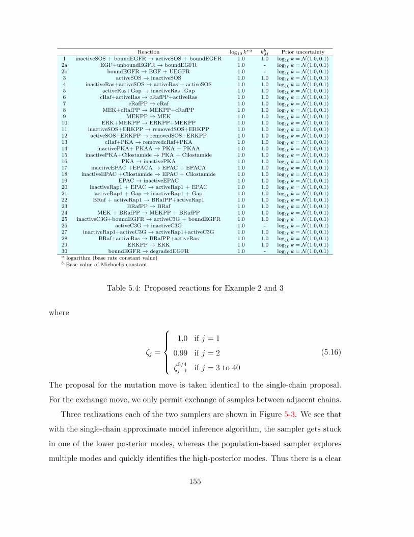
Reaction log10 𝑘*𝑎 𝑘𝑏𝑀 Prior uncertainty
1 inactiveSOS + boundEGFR → activeSOS + boundEGFR 1.0 1.0 log10 𝑘 = 𝒩 (1.0, 0.1)2a EGF+unboundEGFR → boundEGFR 1.0 - log10 𝑘 = 𝒩 (1.0, 0.1)2b boundEGFR → EGF + UEGFR 1.0 - log10 𝑘 = 𝒩 (1.0, 0.1)3 activeSOS → inactiveSOS 1.0 1.0 log10 𝑘 = 𝒩 (1.0, 0.1)4 inactiveRas+activeSOS → activeRas + activeSOS 1.0 1.0 log10 𝑘 = 𝒩 (1.0, 0.1)5 activeRas+Gap → inactiveRas+Gap 1.0 1.0 log10 𝑘 = 𝒩 (1.0, 0.1)6 cRaf+activeRas → cRafPP+activeRas 1.0 1.0 log10 𝑘 = 𝒩 (1.0, 0.1)7 cRafPP → cRaf 1.0 1.0 log10 𝑘 = 𝒩 (1.0, 0.1)8 MEK+cRafPP → MEKPP+cRafPP 1.0 1.0 log10 𝑘 = 𝒩 (1.0, 0.1)9 MEKPP → MEK 1.0 1.0 log10 𝑘 = 𝒩 (1.0, 0.1)10 ERK+MEKPP → ERKPP+MEKPP 1.0 1.0 log10 𝑘 = 𝒩 (1.0, 0.1)11 inactiveSOS+ERKPP → removedSOS+ERKPP 1.0 1.0 log10 𝑘 = 𝒩 (1.0, 0.1)12 activeSOS+ERKPP → removedSOS+ERKPP 1.0 1.0 log10 𝑘 = 𝒩 (1.0, 0.1)13 cRaf+PKA → removedcRaf+PKA 1.0 1.0 log10 𝑘 = 𝒩 (1.0, 0.1)14 inactivePKA+ PKAA → PKA + PKAA 1.0 1.0 log10 𝑘 = 𝒩 (1.0, 0.1)15 inactivePKA+Cilostamide → PKA + Cilostamide 1.0 1.0 log10 𝑘 = 𝒩 (1.0, 0.1)16 PKA → inactivePKA 1.0 1.0 log10 𝑘 = 𝒩 (1.0, 0.1)17 inactiveEPAC +EPACA → EPAC + EPACA 1.0 1.0 log10 𝑘 = 𝒩 (1.0, 0.1)18 inactiveEPAC +Cilostamide → EPAC + Cilostamide 1.0 1.0 log10 𝑘 = 𝒩 (1.0, 0.1)19 EPAC → inactiveEPAC 1.0 1.0 log10 𝑘 = 𝒩 (1.0, 0.1)20 inactiveRap1 + EPAC → activeRap1 + EPAC 1.0 1.0 log10 𝑘 = 𝒩 (1.0, 0.1)21 activeRap1 + Gap → inactiveRap1 + Gap 1.0 1.0 log10 𝑘 = 𝒩 (1.0, 0.1)22 BRaf + activeRap1 → BRafPP+activeRap1 1.0 1.0 log10 𝑘 = 𝒩 (1.0, 0.1)23 BRafPP → BRaf 1.0 1.0 log10 𝑘 = 𝒩 (1.0, 0.1)24 MEK + BRafPP → MEKPP + BRafPP 1.0 1.0 log10 𝑘 = 𝒩 (1.0, 0.1)25 inactiveC3G+boundEGFR → activeC3G + boundEGFR 1.0 1.0 log10 𝑘 = 𝒩 (1.0, 0.1)26 activeC3G → inactiveC3G 1.0 - log10 𝑘 = 𝒩 (1.0, 0.1)27 inactiveRap1+activeC3G → activeRap1+activeC3G 1.0 1.0 log10 𝑘 = 𝒩 (1.0, 0.1)28 BRaf+activeRas → BRafPP+activeRas 1.0 1.0 log10 𝑘 = 𝒩 (1.0, 0.1)29 ERKPP → ERK 1.0 1.0 log10 𝑘 = 𝒩 (1.0, 0.1)30 boundEGFR → degradedEGFR 1.0 - log10 𝑘 = 𝒩 (1.0, 0.1)𝑎 logarithm (base rate constant value)𝑏 Base value of Michaelis constant
Table 5.4: Proposed reactions for Example 2 and 3
where
𝜁𝑗 =
⎧⎪⎪⎪⎨⎪⎪⎪⎩1.0 if 𝑗 = 1
0.99 if 𝑗 = 2
𝜁5/4𝑗−1 if 𝑗 = 3 to 40
(5.16)
The proposal for the mutation move is taken identical to the single-chain proposal.
For the exchange move, we only permit exchange of samples between adjacent chains.
Three realizations each of the two samplers are shown in Figure 5-3. We see that
with the single-chain approximate model inference algorithm, the sampler gets stuck
in one of the lower posterior modes, whereas the population-based sampler explores
multiple modes and quickly identifies the high-posterior modes. Thus there is a clear
155

advantage with the population-based approximate model inference algorithm over the
standard single-chain approximate model inference algorithm. In this example, we
find that there are two effective networks with log(𝑝(𝒟|𝑀)𝑝(𝑀)) ≈ 68. All others
effective networks have log(𝑝(𝒟|𝑀)𝑝(𝑀)) < 50.
5.4.2 Example 3: 30 dimensional reaction network with mul-
tiple species observables
As our second example, we consider once again the set of proposed reactions used in
Example 2, but now with multiple observables: ERK and inactiveSOS concentrations.
We generate 30 i.i.d. data points each of ERK and inactiveSOS measurements with
the noise model 𝒩 (0, 4) and all rate constants and Michaelis constants set to their
base values (Table 5.4). We impose independent Gaussian priors on the logarithm of
rate constants, with means and variances as shown in Table 5.4. The prior probability
distribution over all plausible models is taken to be uniform. The noise variance for
the likelihood function, as in the data generating process, is taken as 𝜎2 = 4.
We generate 4 million samples using the single-chain approximate model infer-
ence and the population-based approximate model inference algorithms. We choose
the proposal distribution for the single-chain sampler to be a Poisson distribution
Pois(1.0) for the number of reactions 𝑟 to be added/deleted and uniformly select the
𝑟 reactions to added/deleted. In case of the population-based algorithm, we take a
population of 40 chains and the sequence of distributions is the same as in Example
2. The proposal for the mutation move is taken identical to the single-chain proposal.
For the exchange move, we only permit exchange of samples between adjacent chains.
Three realizations each of the two samplers are shown in Figure 5-5. The population-
based model inference samplers can be seen to have converged. We see that with the
single-chain approximate model inference algorithm, the sampler gets stuck in one
of the low posterior modes, whereas the population-based sampler explores multiple
modes and quickly identifies the high-posterior mode to which it converges. Thus
156

Iteration0 200000 400000 600000 800000 1000000
log(p
(D|M
)p(M
))
-200
-150
-100
-50
0
50
100
(a) Single-chain MCMC 1Iteration
0 200000 400000 600000 800000 1000000
log(p
(D|M
)p(M
))
-200
-150
-100
-50
0
50
100
(b) Population-based MCMC 1
Iteration0 200000 400000 600000 800000 1000000
log(p
(D|M
)p(M
))
-200
-150
-100
-50
0
50
100
(c) Single-chain MCMC 2Iteration
0 200000 400000 600000 800000 1000000
log(p
(D|M
)p(M
))
-200
-150
-100
-50
0
50
100
(d) Population-based MCMC 2
Iteration0 200000 400000 600000 800000 1000000
log(p
(D|M
)p(M
))
-200
-150
-100
-50
0
50
100
(e) Single-chain MCMC 3Iteration
0 200000 400000 600000 800000 1000000
log(p
(D|M
)p(M
))
-200
-150
-100
-50
0
50
100
(f) Population-based MCMC 3
Figure 5-3: Three realizations of single-chain approximate model inference MCMCand population-based approximate model inference MCMC algorithms for Example2. For the population-based algorithm, we are showing the posterior samples for thechain corresponding to the target distribution 𝑝(𝑀 |𝒟)
157

unboundEGFR
removedcRaf
removedSOS
inactiveSOS
inactiveRas
inactiveRap1
inactivePKA
inactiveEPAC
cRafPPcRaf
boundEGFR
activeSOS
activeRas
activeRap1
PKA
MEKPPMEK
ERKPPERK
EPAC
EGF
BRafPP BRaf
activeC3G
inactiveC3G
degradedEGFR
EPACA
Gap
PKAA
Cilostamide
1
2
3 4
56
7
8
9
10
11
12
13
14 1516
17
18
19
2021
22
23
24
25
26
27
28
29
30
Figure 5-4: Reaction network of Example 3
158

Iteration0 1000000 2000000 3000000 4000000
log(p
(D|M
)p(M
))
-200
-150
-100
-50
0
50
100
(a) Single-chain MCMC 1Iteration
0 1000000 2000000 3000000 4000000
log(p
(D|M
)p(M
))
-200
-150
-100
-50
0
50
100
(b) Population-based MCMC 1
Iteration0 1000000 2000000 3000000 4000000
log(p
(D|M
)p(M
))
-200
-150
-100
-50
0
50
100
(c) Single-chain MCMC 2Iteration
0 1000000 2000000 3000000 4000000
log(p
(D|M
)p(M
))
-200
-150
-100
-50
0
50
100
(d) Population-based MCMC 2
Iteration0 1000000 2000000 3000000 4000000
log(p
(D|M
)p(M
))
-200
-150
-100
-50
0
50
100
(e) Single-chain MCMC 3Iteration
0 1000000 2000000 3000000 4000000
log(p
(D|M
)p(M
))
-200
-150
-100
-50
0
50
100
(f) Population-based MCMC 3
Figure 5-5: Three realizations of single-chain approximate model inference MCMCand population-based approximate model inference MCMC algorithms for Example3. For the population-based algorithm, we are showing the posterior samples for thechain corresponding to the target distribution 𝑝(𝑀 |𝒟)
159
once again we find that there is a clear advantage with the population-based approx-
imate model inference algorithm over the standard single-chain approximate model
inference algorithm. For the population-based scheme, the total number of models
visited is only 160000. With ERK and inactiveSOS as the observables, the number of
effective networks visited was 12000. By employing a sampling-based approach, we
have therefore managed to characterize the posterior distribution over 109 models by
evaluating the evidence of only 12000 models. In contrast, the brute-force approach
of evaluating the evidence of all models is infeasible. In general, the combination
of approximation of model evidence with Laplace’s method and a population-based
sampling method can explore very large model spaces that is infeasible by exhaustive
evaluation of all evidences and very expensive with exact sampling methods.
160
Chapter 6
Conclusions and future work
This thesis focuses on the development of tractable numerical methods for Bayesian
inference of nonlinear chemical reaction networks. Inference of reaction network mod-
els is important in areas such as biology, combustion, and catalysis. The traditional
approach to inference of model structure in the Bayesian paradigm relies on eval-
uating a multidimensional integral for every plausible model. When the number
of models is large, however, this approach is infeasible. The inference of chemical
reaction networks can require the consideration of large model spaces since the num-
ber of plausible models grows combinatorially with the number of proposed reactions.
Across-model samplers that jointly explore the parameter spaces of all models can en-
able large-scale network inference. However, the effective use of existing across-model
samplers continues to be a challenge. In this thesis, we develop efficient across-model
samplers for large-scale inference of reaction networks.
6.1 Conclusions
In the third chapter, we presented a fixed-dimensional interpretation of the network
inference problem. Recognizing that the set of possible models in the network in-
ference problem are nested allows us to tackle the network inference problem as a
161

fixed-dimensional inference problem, and to adapt existing fixed-dimensional adap-
tive MCMC for efficient network inference. Adaptive methods allow automatic tuning
of proposals in contrast to the conventional approach of manual tuning of between-
model parameter proposals by pilot simulations. We employed our methodology to
infer reforming models of methane on rhodium with real and synthetic data. Our ex-
amples indicate that efficient large-scale nonlinear network inference is feasible with
adaptive methods even in settings where little is known about the parameter poste-
riors of the proposed models. Our general fixed-dimensional adaptive MCMC frame-
work for network inference provides myriad information, including the most probable
models, full uncertainty in parameter values, and the dominant pathways.
The network-based interaction of species in reaction networks translates into clus-
ters of networks such that networks belonging to a cluster all have identical effective
networks. We show in Chapter 4 how determining the effective networks of proposed
networks in an across-model sampler can enable the construction of more effective
between-model parameter proposals. The nonlinearity of chemical reaction networks
means that keeping the rate constants of reactions that are commmon to the cur-
rent and the proposed networks in across-model samplers can often produce poor
parameter proposals. To develop better proposals in such cases, we have further de-
veloped sensitivity-based network-aware proposals that identify critical reactions and
include a network-aware parameter proposal for their rate constants when proposing
moves between networks. The developed methods when tested on a range of exam-
ple problems show clear advantage in exploiting network topology and sensitivity of
observables to network elements while designing between-model parameter proposals.
Finally, we have developed an approach for very large-scale model inference—
settings when the number of models is so large that exact sampling methods are pro-
hibitively expensive. By incorporating a Laplace approximation for model evidence,
we run an MCMC simulation only over model indicators. Approximating the evi-
dence of all models visited by the sampler eliminates the need for developing effective
162

parameter proposals for between-model moves and thus reduces the overall cost of the
simulation. The conventional single-chain Markov chain Monte Carlo simulations over
model indicators still find it difficult to explore model posterior distributions, which
are typically multimodal. For this, we have developed a population-based approxi-
mate model inference algorithm that involves running a population of MCMC chains
which exchange information among themselves to explore the posterior distribution
over models. We applied our algorithm to network inference problems from biology
with spaces of around 109 networks. The population-based approximate model in-
ference approach is seen to outperform the single-chain approximate model inference
algorithm.
Large-scale nonlinear network inference is an important goal that could help im-
prove our fundamental understanding of many processes and enable better predictions
with quantified uncertainties. To this end, the development of efficient across-model
samplers is critical. Effective across-model samplers would allow a systematic compar-
ison of all plausible networks in contrast to the conventional approach of comparing a
few hand-crafted models or using simplified linear models. This thesis provides some
ideas on efficient across-models samplers for nonlinear network inference.
6.2 Future work
Our work in this thesis suggests some areas of future work for further development
of network inference algorithms. We outline a few ideas here:
1. Exact approximations to model evidences: A key challenge to efficient
across-model sampling that has been addressed in this thesis is the design of
good between-model parameter proposals. The ideas presented in Chapter 3 and
4 are definite improvements over existing methods, but further advancements
may be possible. One in particular is to consider using an exact approximations
of model evidence when proposing moves between models. A recent algorith-
163

mic development in the MCMC literature called pseudomarginal MCMC is one
such approach [6, 11]. The idea behind these exact approximations is to use
an ensemble of samples to approximate the evidence of the model to which a
move is proposed. As a result, the alignment of densities, which is key to good
sampling performance of the methods discussed in this thesis, is circumvented.
Note, in contrast to approximation based methods discussed in Chapter 5 of
this thesis, the exact approximation Monte Carlo converges asymptotically to
the true posterior distribution. How a good exact approximation may be con-
structed is a subject of ongoing research, but expoiting network-based species
interactions as in Chapter 4 is something that can be immediately incorporated
for network inference problems.
2. Hybrid across-model samplers: We presented adaptive MCMC methods for
network inference in Chapter 3. It is well known, however, that the performance
of adaptive MCMC methods for finite samples depends on initially having a
nonadaptive MCMC algorithm with a fairly good sampling performance. To
this end, we have developed methods that improve the performace of between-
model proposals. One interesting idea could be to combine the ideas from
Chapter 3 and 4 by using network-aware parameter proposals and adapting the
model-move proposals 𝑞(𝑀 ′|𝑀) based on previous posterior samples.
3. Network-aware forward models: The exclusion of a reaction from a net-
work has been implemented in this thesis by setting the corresponding rate
constant to zero. As a result, the forward model solve still has a computational
complexity 𝑂(𝑁𝛼𝑠 ), where 𝑁𝑠 is the total number of species in a network with
all proposed reactions, even when the actual number of species in the network
is much smaller. For large problems, superior computational performance may
be derived by turning the forward model also network aware, i.e., the forward
model need only perform computations on the species that are part of the cur-
164
rent network.
4. Limiting the size of between-model moves: The network-aware methods
of Chapter 4 design between-model parameter proposals based on the current
and proposed effective networks. Currently there is no limit on the size of
allowed difference between the effective networks. For large network inference
problem, proposed moves may often be between effective networks that differ
greatly in their sizes. As has been discussed in this thesis, in general, it is hard
to construct efficient proposals in high dimensions. Therefore, one idea that can
be incorporated in across-model samplers for network inference is to limit the
difference in sizes of the effective networks between which proposals are made.
5. Approximation-based methods with better asymptotic performance:
The Laplace’s method discussed in this thesis has an 𝑂(𝑛−1𝑑𝑎𝑡𝑎) approximation
error. Future work could look at approximation schemes that have faster asymp-
totic convergence rates. This may require considering higher-order Taylor ex-
pansions and/or incorporating more information about the structure of the net-
work inference forward models, priors, etc, into in the evidence approximation.
165

166

Appendix A
Online expectation-maximization for
proposal adaptation
Here we present a derivation of the online EM algorithm applied to a general point
mass mixture proposal:
𝑞(𝑘𝑖;𝜓𝑖) = 𝑏𝑖,0𝛿(𝑘𝑖) +𝑀∑
𝑚=1
𝑏𝑖,𝑚𝑞𝑚(𝑘𝑖; 𝜃𝑖,𝑚). (A.1)
The marginal proposal distribution 𝑞(𝑘𝑖;𝜓𝑖) shown in (A.1) can also be rewritten as
𝑞(𝑘𝑖;𝜓𝑖) =∑𝑧𝑖
𝑞(𝑘𝑖, 𝑧𝑖;𝜃𝑖), (A.2)
and taking 𝑞(𝑘𝑖;𝜓𝑖) to be independent for each 𝑘𝑖, the joint proposal distribution for
an 𝑁 -dimensional problem follows:
𝑞(��;𝜓) =∑𝑧
𝑞(��, 𝑧;𝜓) =𝑁∏𝑖=1
∑𝑧𝑖
𝑞(𝑘𝑖, 𝑧𝑖;𝜃𝑖). (A.3)
Here, 𝑧𝑖 is a latent variable that takes one of 𝑀+1 values corresponding to the 𝑀+1
components that could generate the posterior sample. 𝑞(��, 𝑧) is the joint distribution
167

of 𝑧 and �� and is referred to as the complete-data likelihood. Expanding (A.2) by
the product rule of probability gives:
𝑞(𝑘𝑖;𝜓𝑖) =∑𝑧𝑖
𝑞(𝑘𝑖|𝑧𝑖)𝑞(𝑧𝑖)
= 𝑞(𝑧𝑖 = 0)𝛿(𝑘𝑖) +𝑀∑
𝑚=1
𝑞(𝑧𝑖 = 𝑚)𝑞𝑚(𝑘𝑖|𝑧𝑖 = 𝑚; 𝜃𝑖,𝑚); (A.4)
Comparing (A.4) to (A.1), we see that
𝑞(𝑧𝑖 = 0) = 𝑏𝑖,0 and 𝑞(𝑧𝑖 = 𝑚) = 𝑏𝑖,𝑚. (A.5)
After the steps for a general point mass mixture proposal have been established,
we will obtain specific expressions for the case when the continuous components of
the above proposal distribution (3.9) are all Gaussian.
A.0.1 KL divergence minimization yields a maximum likeli-
hood problem
Recall that our goal is to update the proposal distribution 𝑞(��;𝜓) iteratively based on
samples from the posterior distribution 𝑝(��|𝒟) so as to minimize the KL divergence:
𝐷𝐾𝐿(𝑝(��|𝒟‖𝑞(��;𝜓)) =
∫𝑝(��|𝒟) log
(𝑝(��|𝒟)
𝑞(��;𝜓)
)𝑑�� (A.6)
w.r.t. the proposal parameters 𝜓. Note that minimizing the KL divergence in (A.6)
is equivalent to maximizing the cross entropy∫𝑝(��|𝒟)𝑞(��,𝜓)𝑑��. Thus the objective
function can be rewritten as
𝜓* = arg max𝜓
∫𝑝(��|𝒟) log(𝑞(��;𝜓))𝑑��. (A.7)
168
The integral in (A.7) can be approximated by a Monte Carlo sum using 𝑇 samples
from the posterior distribution 𝑝(��|𝒟) as
𝐼 =1
𝑇
𝑇∑𝑡=1
log(𝑞(��𝑡;𝜓)) =1
𝑇log
(𝑇∏𝑡=1
𝑞(��𝑡;𝜓)
). (A.8)
Now, if we think of ��𝑡=1:𝑇 as pseudo-data and 𝑞(��𝑡;𝜃) as a likelihood, cross entropy
can be interpreted as a log-likelihood under infinite data and (A.7) as a maximum
(log-)likelihood problem. Mathematically (A.7) can also be written as
𝜓* = arg max𝜓
lim𝑇→∞
1
𝑇log
(𝑇∏𝑡=1
𝑞(��𝑡;𝜓)
)(A.9)
A.0.2 Classical EM algorithm
Suppose we are given 𝑇 independent samples (��1, ��2, . . . , ��𝑇 ) distributed according
to 𝑝(��|𝒟). The solution of the maximum log-likelihood problem
𝜓* = arg max𝜓
1
𝑇
𝑇∑𝑡=1
log(𝑞(��𝑡;𝜓)
)(A.10)
can be obtained by taking the derivative of the log-likelihood and solving the resulting
nonlinear equations. The nonlinear equations thus obtained seldom have a closed-
form solution and thus are solved by numerical optimization.
An alternative known as expectation-maximization algorithm exists for the solu-
tion of the maximum log-likelihood problem [31, 15]. The EM algorithm often results
in simple analytical expressions and avoids the difficulties of gradient-based optimiza-
tion approaches. The EM algorithm consists of two steps, known as the E-step and
M-step, that are solved iteratively to obtain the optimal parameter values under mild
regularity conditions [117]. The two steps are given by
E-step
169
𝑄(𝜓,𝜓𝑛−1) =
∫log
(𝑇∏𝑡=1
𝑞(��𝑡, 𝑧𝑡;𝜓)
)(𝑇∏𝑡=1
𝑞(𝑧𝑡|��𝑡,𝜓𝑛−1)
)𝑑𝑧1 . . . 𝑑𝑧𝑇
= E𝑧1...𝑧𝑇
[log
(𝑇∏𝑡=1
𝑞(��𝑡, 𝑧𝑡;𝜓)
)](A.11)
M-step
𝜓𝑛 = arg max𝜓
𝑄(𝜓,𝜓𝑛−1) (A.12)
The E-step in the above equations evaluates the expectation of the logarithm of
the complete-data likelihood, where the expectation is taken with respect to the
latent variables conditioned on available (sampled) rate parameters. In the M-step,
an updated set of parameter values are computed by maximizing the expected log-
likelihood from the E-step. The EM algorithm as described in (A.11) and (A.12) is
applicable if all the observed samples (��𝑡=1:𝑇 ) are available a priori and the samples
are independent.
Our problem is different from the above case since we are generating samples
from 𝑝(��|𝒟) in batches. Moreover, the generated samples are not independent as
they are coming from an MCMC scheme. Thus we use a sequential variant of the EM
algorithm known as the online EM algorithm and specify conditions under which the
resulting adaptive MCMC algorithm converges to the posterior distribution, 𝑝(��|𝒟).
A.0.3 Online expectation maximization
We begin our discussion of the online EM algorithm by assuming that the proposal
distribution 𝑞(��, 𝑧;𝜓) can be represented in the form
𝑞(��, 𝑧;𝜓) = exp(⟨𝑠(��, 𝑧),𝜑(𝜓)⟩ −𝐴(𝜓)). (A.13)
Distributions that can be cast in the above form are known to belong to the expo-
nential family [13]. Here, 𝑠(��, 𝑧) is a vector of sufficient statistics, 𝜑(𝜓) refers to the
170
natural parameters, and 𝐴(𝜓) is the log base distribution. The operator ⟨·⟩ is the
standard inner product. Plugging the above expression for 𝑞(��, 𝑧) into (A.11) and
(A.12), we get
E-step:
𝑄(𝜓,𝜓𝑛−1) =
∫ 𝑇∏𝑡=1
𝑞(𝑧𝑡|��𝑡;𝜓𝑛−1)𝑇∑𝑡=1
(⟨𝑠(��𝑡, 𝑧𝑡),𝜑(𝜓)⟩ −𝐴(𝜓)
)𝑑𝑧1 . . . 𝑑𝑧𝑇 ,
(A.14)
M-step:
𝜓𝑛 = arg max𝜓
𝑄(𝜓,𝜓𝑛−1). (A.15)
The above expectation and maximization steps can be recast in terms of sufficient
statistics as
E-step:
𝑆𝑇𝑛 =1
𝑇
𝑇∑𝑡=1
E𝜓𝑇𝑛−1
[𝑠(��𝑡, 𝑧𝑡)|��𝑡
], (A.16)
M-step:
𝜓𝑇𝑛 = Γ{𝑆𝑇𝑛}, (A.17)
where Γ{𝑆𝑇𝑛} = arg max𝜓
(⟨𝑆𝑇𝑛 ,𝜑(𝜓)⟩ −𝐴(𝜓)). Letting 𝑇 → ∞, the EM iterations
are
E-step:
𝑆𝑛 = E𝑝(��|𝒟)
(E𝜓𝑛−1
[𝑠(��, 𝑧|��)
])(A.18)
M-step:
𝜓𝑛 = Γ{𝑆𝑛} (A.19)
171
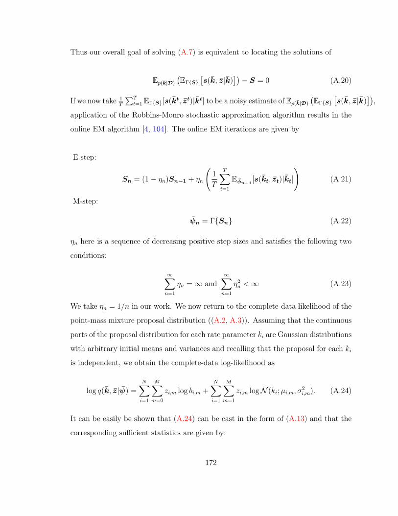
Thus our overall goal of solving (A.7) is equivalent to locating the solutions of
E𝑝(��|𝒟)
(EΓ{𝑆}
[𝑠(��, 𝑧|��)
])− 𝑆 = 0 (A.20)
If we now take 1𝑇
∑𝑇𝑡=1 EΓ{𝑆}[𝑠(��𝑡, 𝑧𝑡)|��𝑡] to be a noisy estimate of E𝑝(��|𝒟)
(EΓ{𝑆}
[𝑠(��, 𝑧|��)
]),
application of the Robbins-Monro stochastic approximation algorithm results in the
online EM algorithm [4, 104]. The online EM iterations are given by
E-step:
𝑆𝑛 = (1− 𝜂𝑛)𝑆𝑛−1 + 𝜂𝑛
(1
𝑇
𝑇∑𝑡=1
E𝜓𝑛−1[𝑠(��𝑡, 𝑧𝑡)|��𝑡]
)(A.21)
M-step:
𝜓𝑛 = Γ{𝑆𝑛} (A.22)
𝜂𝑛 here is a sequence of decreasing positive step sizes and satisfies the following two
conditions:
∞∑𝑛=1
𝜂𝑛 =∞ and∞∑𝑛=1
𝜂2𝑛 <∞ (A.23)
We take 𝜂𝑛 = 1/𝑛 in our work. We now return to the complete-data likelihood of the
point-mass mixture proposal distribution ((A.2, A.3)). Assuming that the continuous
parts of the proposal distribution for each rate parameter 𝑘𝑖 are Gaussian distributions
with arbitrary initial means and variances and recalling that the proposal for each 𝑘𝑖
is independent, we obtain the complete-data log-likelihood as
log 𝑞(��, 𝑧|𝜓) =𝑁∑𝑖=1
𝑀∑𝑚=0
𝑧𝑖,𝑚 log 𝑏𝑖,𝑚 +𝑁∑𝑖=1
𝑀∑𝑚=1
𝑧𝑖,𝑚 log𝒩 (𝑘𝑖;𝜇𝑖,𝑚, 𝜎2𝑖,𝑚). (A.24)
It can be easily be shown that (A.24) can be cast in the form of (A.13) and that the
corresponding sufficient statistics are given by:
172

For i = 1 to 𝑁
For 𝑚 = 0 to 𝑀 :
𝑂𝑖,𝑚 =1
𝑇
𝑇∑𝑡=1
𝛾(𝑧𝑡𝑖,𝑚),
For 𝑚 = 1 to 𝑀 :
𝑃𝑖,𝑚 =1
𝑇
𝑇∑𝑡=1𝑘𝑡𝑖 =0
𝛾(𝑧𝑡𝑖,𝑚) 𝑄𝑖,𝑚 =1
𝑇
𝑇∑𝑡=1𝑘𝑡𝑖 =0
𝛾(𝑧𝑡𝑖,𝑚)𝑘𝑡𝑖 𝑅𝑖,𝑚 =1
𝑇
𝑇∑𝑡=1𝑘𝑡𝑖 =0
𝛾(𝑧𝑡𝑖,𝑚)(𝑘𝑡𝑖)2
where 𝛾(𝑧𝑡𝑖,𝑚) = 𝑝(𝑧𝑡𝑖,𝑚|𝑘𝑡𝑖 ;𝜓𝑖) is given by
𝛾(𝑧𝑡𝑖,𝑚) =
⎧⎪⎪⎪⎪⎪⎪⎨⎪⎪⎪⎪⎪⎪⎩
1 if 𝑘𝑡𝑖 = 0 and 𝑚 = 0
0 if 𝑘𝑡𝑖 = 0 and 𝑚 = 0
0 if 𝑘𝑡𝑖 = 0 and 𝑚 = 0𝑏𝑖,𝑚𝒩 (𝑘𝑡𝑖 ;𝜇𝑖,𝑚,𝜎2
𝑖,𝑚)∑𝑀𝑚′=1 𝑏𝑖,𝑚′𝒩 (𝑘𝑡𝑖 ;𝜇𝑖,𝑚′ ,𝜎2
𝑖,𝑚′ )if 𝑘𝑡𝑖 = 0 and 𝑚 = 0.
(A.25)
Thus the online EM iterations consist of the following two steps
E-step:
𝑆𝑂𝑖,𝑚𝑛 = 𝑆
𝑂𝑖,𝑚
𝑛−1 + 𝜂𝑛(𝑂𝑖,𝑚 − 𝑆𝑂𝑖,𝑚
𝑛−1 )
𝑆𝑃𝑖,𝑚𝑛 = 𝑆
𝑃𝑖,𝑚
𝑛−1 + 𝜂𝑛(𝑃𝑖,𝑚 − 𝑆𝑃𝑖,𝑚
𝑛−1 )
𝑆𝑄𝑖,𝑚𝑛 = 𝑆
𝑄𝑖,𝑚
𝑛−1 + 𝜂𝑛(𝑄𝑖,𝑚 − 𝑆𝑄𝑖,𝑚
𝑛−1 )
𝑆𝑅𝑖,𝑚𝑛 = 𝑆
𝑅𝑖,𝑚
𝑛−1 + 𝜂𝑛(𝑅𝑖,𝑚 − 𝑆𝑅𝑖,𝑚
𝑛−1 ) (A.26)
173
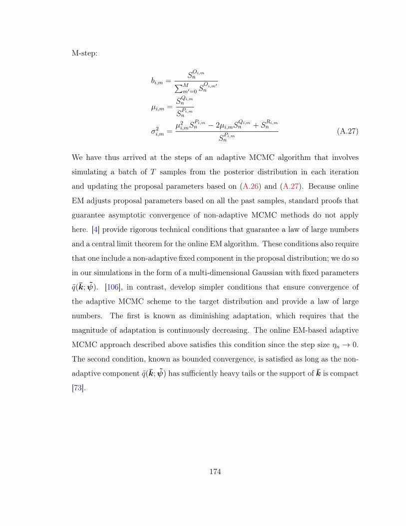
M-step:
𝑏𝑖,𝑚 =𝑆𝑂𝑖,𝑚𝑛∑𝑀
𝑚′=0 𝑆𝑂𝑖,𝑚′𝑛
𝜇𝑖,𝑚 =𝑆𝑄𝑖,𝑚𝑛
𝑆𝑃𝑖,𝑚𝑛
𝜎2𝑖,𝑚 =
𝜇2𝑖,𝑚𝑆
𝑃𝑖,𝑚𝑛 − 2𝜇𝑖,𝑚𝑆
𝑄𝑖,𝑚𝑛 + 𝑆
𝑅𝑖,𝑚𝑛
𝑆𝑃𝑖,𝑚𝑛
(A.27)
We have thus arrived at the steps of an adaptive MCMC algorithm that involves
simulating a batch of 𝑇 samples from the posterior distribution in each iteration
and updating the proposal parameters based on (A.26) and (A.27). Because online
EM adjusts proposal parameters based on all the past samples, standard proofs that
guarantee asymptotic convergence of non-adaptive MCMC methods do not apply
here. [4] provide rigorous technical conditions that guarantee a law of large numbers
and a central limit theorem for the online EM algorithm. These conditions also require
that one include a non-adaptive fixed component in the proposal distribution; we do so
in our simulations in the form of a multi-dimensional Gaussian with fixed parameters
𝑞(��;𝜓). [106], in contrast, develop simpler conditions that ensure convergence of
the adaptive MCMC scheme to the target distribution and provide a law of large
numbers. The first is known as diminishing adaptation, which requires that the
magnitude of adaptation is continuously decreasing. The online EM-based adaptive
MCMC approach described above satisfies this condition since the step size 𝜂𝑛 → 0.
The second condition, known as bounded convergence, is satisfied as long as the non-
adaptive component 𝑞(��;𝜓) has sufficiently heavy tails or the support of �� is compact
[73].
174
Appendix B
Reaction networks: reactions,
reaction rates, and species production
rates
B.1 12-dimensional reaction network
Here we present the details of the set of proposed reactions, the corresponding reaction
and species production rate ODE expressions for the 12-reaction network used in
example problems of Chapters 4 and 5 of this thesis.
B.1.1 Reactions
1. 𝑏𝑜𝑢𝑛𝑑𝐸𝐺𝐹𝑅→ 𝑑𝑒𝑔𝑟𝑎𝑑𝑒𝑑𝐸𝐺𝐹𝑅
2. 𝐸𝐺𝐹 + 𝑢𝑛𝑏𝑜𝑢𝑛𝑑𝐸𝐺𝐹𝑅↔ 𝑏𝑜𝑢𝑛𝑑𝐸𝐺𝐹𝑅
3. 𝑖𝑛𝑎𝑐𝑡𝑖𝑣𝑒𝐶3𝐺+ 𝑏𝑜𝑢𝑛𝑑𝐸𝐺𝐹𝑅→ 𝑎𝑐𝑡𝑖𝑣𝑒𝐶3𝐺+ 𝑏𝑜𝑢𝑛𝑑𝐸𝐺𝐹𝑅
4. 𝑎𝑐𝑡𝑖𝑣𝑒𝐶3𝐺→ 𝑖𝑛𝑎𝑐𝑡𝑖𝑣𝑒𝐶3𝐺
5. 𝑖𝑛𝑎𝑐𝑡𝑖𝑣𝑒𝑅𝑎𝑝1 + 𝑎𝑐𝑡𝑖𝑣𝑒𝐶3𝐺→ 𝑎𝑐𝑡𝑖𝑣𝑒𝑅𝑎𝑝1 + 𝑎𝑐𝑡𝑖𝑣𝑒𝐶3𝐺
175

BEGFR
DEGFR EGF
UEGFR
inactiveC3G
activeC3G
activeRap1
BRafBRafPP
activeRas
Gap
inactiveRap1inactiveRas
activeSOS
inactiveSOS
Reaction 1
Reaction 2
Reaction 3
Reaction 4
Reaction 5
Reaction 6
Reaction 8
Reaction 7Reaction 9
Reaction 10
Reaction 11
Reaction 12
176

6. 𝐵𝑅𝑎𝑓 + 𝑎𝑐𝑡𝑖𝑣𝑒𝑅𝑎𝑝1→ 𝐵𝑅𝑎𝑓𝑃𝑃 + 𝑎𝑐𝑡𝑖𝑣𝑒𝑅𝑎𝑝1
7. 𝑎𝑐𝑡𝑖𝑣𝑒𝑅𝑎𝑝1 +𝐺𝑎𝑝→ 𝑖𝑛𝑎𝑐𝑡𝑖𝑣𝑒𝑅𝑎𝑝1 +𝐺𝑎𝑝
8. 𝐵𝑅𝑎𝑓 + 𝑎𝑐𝑡𝑖𝑣𝑒𝑅𝑎𝑠→ 𝐵𝑅𝑎𝑓𝑃𝑃 + 𝑎𝑐𝑡𝑖𝑣𝑒𝑅𝑎𝑠
9. 𝑎𝑐𝑡𝑖𝑣𝑒𝑅𝑎𝑠+𝐺𝑎𝑝→ 𝑖𝑛𝑎𝑐𝑡𝑖𝑣𝑒𝑅𝑎𝑠+𝐺𝑎𝑝
10. 𝑖𝑛𝑎𝑐𝑡𝑖𝑣𝑒𝑅𝑎𝑠+ 𝑎𝑐𝑡𝑖𝑣𝑒𝑆𝑂𝑆 → 𝑎𝑐𝑡𝑖𝑣𝑒𝑅𝑎𝑠+ 𝑎𝑐𝑡𝑖𝑣𝑒𝑆𝑂𝑆
11. 𝑎𝑐𝑡𝑖𝑣𝑒𝑆𝑂𝑆 → 𝑖𝑛𝑎𝑐𝑡𝑖𝑣𝑒𝑆𝑂𝑆
12. 𝑖𝑛𝑎𝑐𝑡𝑖𝑣𝑒𝑆𝑂𝑆 + 𝑏𝑜𝑢𝑛𝑑𝐸𝐺𝐹𝑅→ 𝑎𝑐𝑡𝑖𝑣𝑒𝑆𝑂𝑆 + 𝑏𝑜𝑢𝑛𝑑𝐸𝐺𝐹𝑅
B.1.2 Reaction rates
1. 𝑘1[𝑏𝑜𝑢𝑛𝑑𝐸𝐺𝐹𝑅]
2. 𝑘2𝑓 [𝐸𝐺𝐹 ][𝑢𝑛𝑏𝑜𝑢𝑛𝑑𝐸𝐺𝐹𝑅]− 𝑘2𝑟[𝑏𝑜𝑢𝑛𝑑𝐸𝐺𝐹𝑅]
3.𝑘3[𝑏𝑜𝑢𝑛𝑑𝐸𝐺𝐹𝑅][𝑖𝑛𝑎𝑐𝑡𝑖𝑣𝑒𝐶3𝐺]
𝑘′3 + [𝑖𝑛𝑎𝑐𝑡𝑖𝑣𝑒𝐶3𝐺]
4. 𝑘4[𝑎𝑐𝑡𝑖𝑣𝑒𝐶3𝐺]
5.𝑘5[𝑎𝑐𝑡𝑖𝑣𝑒𝐶3𝐺][𝑖𝑛𝑎𝑐𝑡𝑖𝑣𝑒𝑅𝑎𝑝1]
𝑘′5 + [𝑖𝑛𝑎𝑐𝑡𝑖𝑣𝑒𝑅𝑎𝑝1]
6.𝑘6[𝑎𝑐𝑡𝑖𝑣𝑒𝑅𝑎𝑝1][𝐵𝑅𝑎𝑓 ]
𝑘′6 + [𝐵𝑅𝑎𝑓 ]
7.𝑘7[𝐺𝑎𝑝][𝑎𝑐𝑡𝑖𝑣𝑒𝑅𝑎𝑝1]
𝑘′7 + [𝑎𝑐𝑡𝑖𝑣𝑒𝑅𝑎𝑝1]
8.𝑘8[𝑎𝑐𝑡𝑖𝑣𝑒𝑅𝑎𝑠][𝐵𝑅𝑎𝑓 ]
𝑘′8 + [𝐵𝑅𝑎𝑓 ]
9.𝑘9[𝐺𝑎𝑝][𝑎𝑐𝑡𝑖𝑣𝑒𝑅𝑎𝑠]
𝑘′9 + [𝑎𝑐𝑡𝑖𝑣𝑒𝑅𝑎𝑠]
10.𝑘10[𝑎𝑐𝑡𝑖𝑣𝑒𝑆𝑂𝑆][𝑖𝑛𝑎𝑐𝑡𝑖𝑣𝑒𝑅𝑎𝑠]
𝑘′10 + 𝑖𝑛𝑎𝑐𝑡𝑖𝑣𝑒𝑅𝑎𝑠
11.𝑘11[𝑎𝑐𝑡𝑖𝑣𝑒𝑆𝑂𝑆]
𝑘′11 + [𝑎𝑐𝑡𝑖𝑣𝑒𝑆𝑂𝑆]
12.𝑘12[𝑏𝑜𝑢𝑛𝑑𝐸𝐺𝐹𝑅][𝑖𝑛𝑎𝑐𝑡𝑖𝑣𝑒𝑆𝑂𝑆]
𝑘′12 + [𝑖𝑛𝑎𝑐𝑡𝑖𝑣𝑒𝑆𝑂𝑆]
177
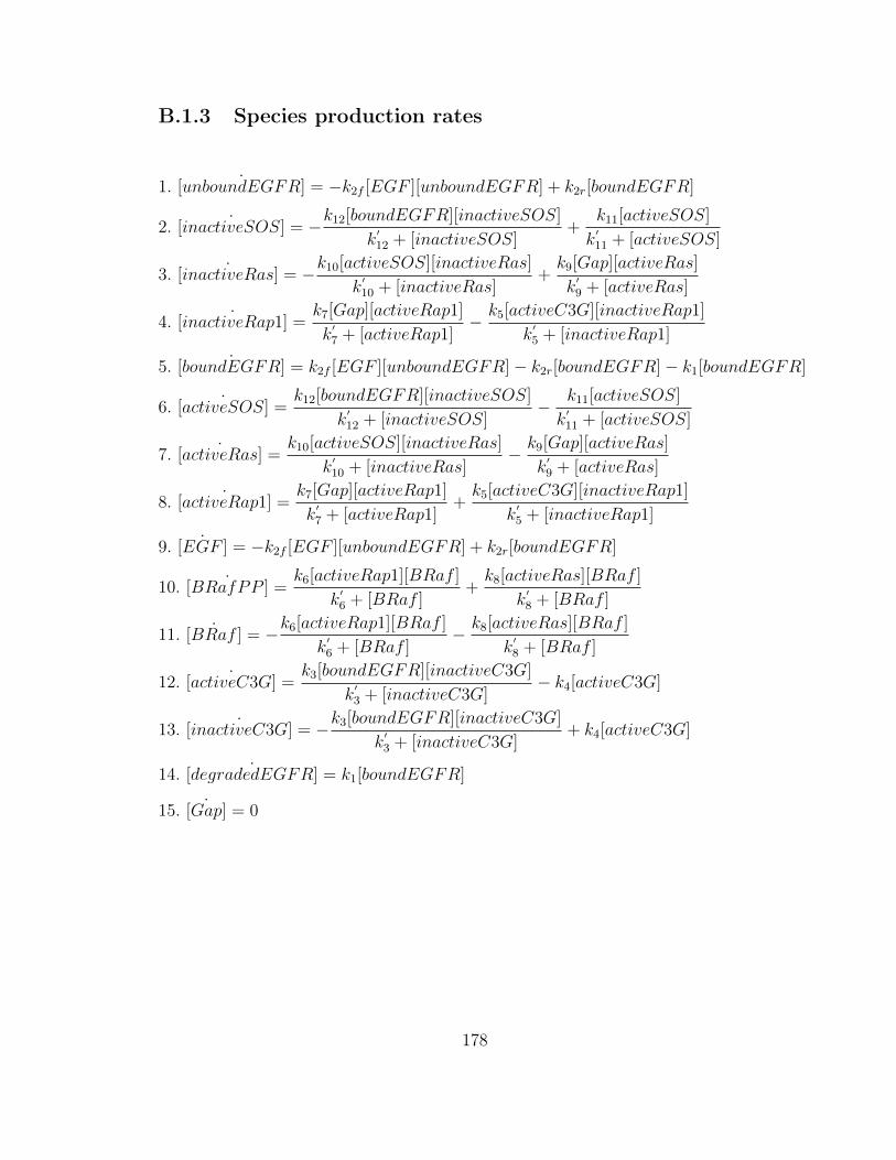
B.1.3 Species production rates
1. ˙[𝑢𝑛𝑏𝑜𝑢𝑛𝑑𝐸𝐺𝐹𝑅] = −𝑘2𝑓 [𝐸𝐺𝐹 ][𝑢𝑛𝑏𝑜𝑢𝑛𝑑𝐸𝐺𝐹𝑅] + 𝑘2𝑟[𝑏𝑜𝑢𝑛𝑑𝐸𝐺𝐹𝑅]
2. ˙[𝑖𝑛𝑎𝑐𝑡𝑖𝑣𝑒𝑆𝑂𝑆] = −𝑘12[𝑏𝑜𝑢𝑛𝑑𝐸𝐺𝐹𝑅][𝑖𝑛𝑎𝑐𝑡𝑖𝑣𝑒𝑆𝑂𝑆]
𝑘′12 + [𝑖𝑛𝑎𝑐𝑡𝑖𝑣𝑒𝑆𝑂𝑆]
+𝑘11[𝑎𝑐𝑡𝑖𝑣𝑒𝑆𝑂𝑆]
𝑘′11 + [𝑎𝑐𝑡𝑖𝑣𝑒𝑆𝑂𝑆]
3. ˙[𝑖𝑛𝑎𝑐𝑡𝑖𝑣𝑒𝑅𝑎𝑠] = −𝑘10[𝑎𝑐𝑡𝑖𝑣𝑒𝑆𝑂𝑆][𝑖𝑛𝑎𝑐𝑡𝑖𝑣𝑒𝑅𝑎𝑠]
𝑘′10 + [𝑖𝑛𝑎𝑐𝑡𝑖𝑣𝑒𝑅𝑎𝑠]
+𝑘9[𝐺𝑎𝑝][𝑎𝑐𝑡𝑖𝑣𝑒𝑅𝑎𝑠]
𝑘′9 + [𝑎𝑐𝑡𝑖𝑣𝑒𝑅𝑎𝑠]
4. ˙[𝑖𝑛𝑎𝑐𝑡𝑖𝑣𝑒𝑅𝑎𝑝1] =𝑘7[𝐺𝑎𝑝][𝑎𝑐𝑡𝑖𝑣𝑒𝑅𝑎𝑝1]
𝑘′7 + [𝑎𝑐𝑡𝑖𝑣𝑒𝑅𝑎𝑝1]
− 𝑘5[𝑎𝑐𝑡𝑖𝑣𝑒𝐶3𝐺][𝑖𝑛𝑎𝑐𝑡𝑖𝑣𝑒𝑅𝑎𝑝1]
𝑘′5 + [𝑖𝑛𝑎𝑐𝑡𝑖𝑣𝑒𝑅𝑎𝑝1]
5. ˙[𝑏𝑜𝑢𝑛𝑑𝐸𝐺𝐹𝑅] = 𝑘2𝑓 [𝐸𝐺𝐹 ][𝑢𝑛𝑏𝑜𝑢𝑛𝑑𝐸𝐺𝐹𝑅]− 𝑘2𝑟[𝑏𝑜𝑢𝑛𝑑𝐸𝐺𝐹𝑅]− 𝑘1[𝑏𝑜𝑢𝑛𝑑𝐸𝐺𝐹𝑅]
6. ˙[𝑎𝑐𝑡𝑖𝑣𝑒𝑆𝑂𝑆] =𝑘12[𝑏𝑜𝑢𝑛𝑑𝐸𝐺𝐹𝑅][𝑖𝑛𝑎𝑐𝑡𝑖𝑣𝑒𝑆𝑂𝑆]
𝑘′12 + [𝑖𝑛𝑎𝑐𝑡𝑖𝑣𝑒𝑆𝑂𝑆]
− 𝑘11[𝑎𝑐𝑡𝑖𝑣𝑒𝑆𝑂𝑆]
𝑘′11 + [𝑎𝑐𝑡𝑖𝑣𝑒𝑆𝑂𝑆]
7. ˙[𝑎𝑐𝑡𝑖𝑣𝑒𝑅𝑎𝑠] =𝑘10[𝑎𝑐𝑡𝑖𝑣𝑒𝑆𝑂𝑆][𝑖𝑛𝑎𝑐𝑡𝑖𝑣𝑒𝑅𝑎𝑠]
𝑘′10 + [𝑖𝑛𝑎𝑐𝑡𝑖𝑣𝑒𝑅𝑎𝑠]
− 𝑘9[𝐺𝑎𝑝][𝑎𝑐𝑡𝑖𝑣𝑒𝑅𝑎𝑠]
𝑘′9 + [𝑎𝑐𝑡𝑖𝑣𝑒𝑅𝑎𝑠]
8. ˙[𝑎𝑐𝑡𝑖𝑣𝑒𝑅𝑎𝑝1] =𝑘7[𝐺𝑎𝑝][𝑎𝑐𝑡𝑖𝑣𝑒𝑅𝑎𝑝1]
𝑘′7 + [𝑎𝑐𝑡𝑖𝑣𝑒𝑅𝑎𝑝1]
+𝑘5[𝑎𝑐𝑡𝑖𝑣𝑒𝐶3𝐺][𝑖𝑛𝑎𝑐𝑡𝑖𝑣𝑒𝑅𝑎𝑝1]
𝑘′5 + [𝑖𝑛𝑎𝑐𝑡𝑖𝑣𝑒𝑅𝑎𝑝1]
9. ˙[𝐸𝐺𝐹 ] = −𝑘2𝑓 [𝐸𝐺𝐹 ][𝑢𝑛𝑏𝑜𝑢𝑛𝑑𝐸𝐺𝐹𝑅] + 𝑘2𝑟[𝑏𝑜𝑢𝑛𝑑𝐸𝐺𝐹𝑅]
10. ˙[𝐵𝑅𝑎𝑓𝑃𝑃 ] =𝑘6[𝑎𝑐𝑡𝑖𝑣𝑒𝑅𝑎𝑝1][𝐵𝑅𝑎𝑓 ]
𝑘′6 + [𝐵𝑅𝑎𝑓 ]
+𝑘8[𝑎𝑐𝑡𝑖𝑣𝑒𝑅𝑎𝑠][𝐵𝑅𝑎𝑓 ]
𝑘′8 + [𝐵𝑅𝑎𝑓 ]
11. ˙[𝐵𝑅𝑎𝑓 ] = −𝑘6[𝑎𝑐𝑡𝑖𝑣𝑒𝑅𝑎𝑝1][𝐵𝑅𝑎𝑓 ]
𝑘′6 + [𝐵𝑅𝑎𝑓 ]
− 𝑘8[𝑎𝑐𝑡𝑖𝑣𝑒𝑅𝑎𝑠][𝐵𝑅𝑎𝑓 ]
𝑘′8 + [𝐵𝑅𝑎𝑓 ]
12. ˙[𝑎𝑐𝑡𝑖𝑣𝑒𝐶3𝐺] =𝑘3[𝑏𝑜𝑢𝑛𝑑𝐸𝐺𝐹𝑅][𝑖𝑛𝑎𝑐𝑡𝑖𝑣𝑒𝐶3𝐺]
𝑘′3 + [𝑖𝑛𝑎𝑐𝑡𝑖𝑣𝑒𝐶3𝐺]
− 𝑘4[𝑎𝑐𝑡𝑖𝑣𝑒𝐶3𝐺]
13. ˙[𝑖𝑛𝑎𝑐𝑡𝑖𝑣𝑒𝐶3𝐺] = −𝑘3[𝑏𝑜𝑢𝑛𝑑𝐸𝐺𝐹𝑅][𝑖𝑛𝑎𝑐𝑡𝑖𝑣𝑒𝐶3𝐺]
𝑘′3 + [𝑖𝑛𝑎𝑐𝑡𝑖𝑣𝑒𝐶3𝐺]
+ 𝑘4[𝑎𝑐𝑡𝑖𝑣𝑒𝐶3𝐺]
14. ˙[𝑑𝑒𝑔𝑟𝑎𝑑𝑒𝑑𝐸𝐺𝐹𝑅] = 𝑘1[𝑏𝑜𝑢𝑛𝑑𝐸𝐺𝐹𝑅]
15. ˙[𝐺𝑎𝑝] = 0
178
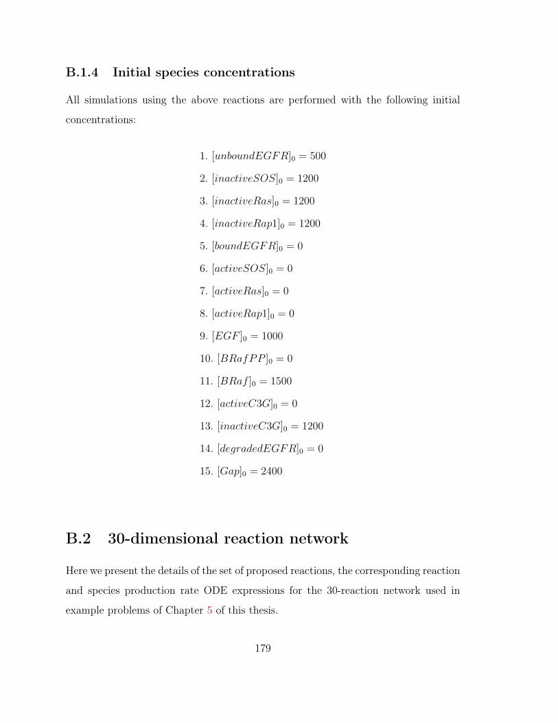
B.1.4 Initial species concentrations
All simulations using the above reactions are performed with the following initial
concentrations:
1. [𝑢𝑛𝑏𝑜𝑢𝑛𝑑𝐸𝐺𝐹𝑅]0 = 500
2. [𝑖𝑛𝑎𝑐𝑡𝑖𝑣𝑒𝑆𝑂𝑆]0 = 1200
3. [𝑖𝑛𝑎𝑐𝑡𝑖𝑣𝑒𝑅𝑎𝑠]0 = 1200
4. [𝑖𝑛𝑎𝑐𝑡𝑖𝑣𝑒𝑅𝑎𝑝1]0 = 1200
5. [𝑏𝑜𝑢𝑛𝑑𝐸𝐺𝐹𝑅]0 = 0
6. [𝑎𝑐𝑡𝑖𝑣𝑒𝑆𝑂𝑆]0 = 0
7. [𝑎𝑐𝑡𝑖𝑣𝑒𝑅𝑎𝑠]0 = 0
8. [𝑎𝑐𝑡𝑖𝑣𝑒𝑅𝑎𝑝1]0 = 0
9. [𝐸𝐺𝐹 ]0 = 1000
10. [𝐵𝑅𝑎𝑓𝑃𝑃 ]0 = 0
11. [𝐵𝑅𝑎𝑓 ]0 = 1500
12. [𝑎𝑐𝑡𝑖𝑣𝑒𝐶3𝐺]0 = 0
13. [𝑖𝑛𝑎𝑐𝑡𝑖𝑣𝑒𝐶3𝐺]0 = 1200
14. [𝑑𝑒𝑔𝑟𝑎𝑑𝑒𝑑𝐸𝐺𝐹𝑅]0 = 0
15. [𝐺𝑎𝑝]0 = 2400
B.2 30-dimensional reaction network
Here we present the details of the set of proposed reactions, the corresponding reaction
and species production rate ODE expressions for the 30-reaction network used in
example problems of Chapter 5 of this thesis.
179
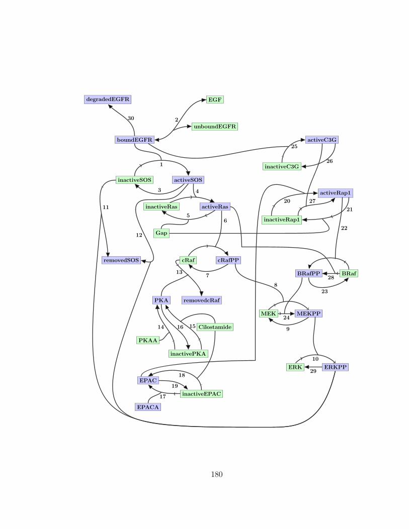
unboundEGFR
removedcRaf
removedSOS
inactiveSOS
inactiveRas
inactiveRap1
inactivePKA
inactiveEPAC
cRafPPcRaf
boundEGFR
activeSOS
activeRas
activeRap1
PKA
MEKPPMEK
ERKPPERK
EPAC
EGF
BRafPP BRaf
activeC3G
inactiveC3G
degradedEGFR
EPACA
Gap
PKAA
Cilostamide
1
2
3 4
56
7
8
9
10
11
12
13
14 1516
17
18
19
2021
22
23
24
25
26
27
28
29
30
180

B.2.1 Reactions
1. 𝑖𝑛𝑎𝑐𝑡𝑖𝑣𝑒𝑆𝑂𝑆 + 𝑏𝑜𝑢𝑛𝑑𝐸𝐺𝐹𝑅→ 𝑎𝑐𝑡𝑖𝑣𝑒𝑆𝑂𝑆 + 𝑏𝑜𝑢𝑛𝑑𝐸𝐺𝐹𝑅
2. 𝐸𝐺𝐹 + 𝑢𝑛𝑏𝑜𝑢𝑛𝑑𝐸𝐺𝐹𝑅↔ 𝑏𝑜𝑢𝑛𝑑𝐸𝐺𝐹𝑅
3. 𝑎𝑐𝑡𝑖𝑣𝑒𝑆𝑂𝑆 → 𝑖𝑛𝑎𝑐𝑡𝑖𝑣𝑒𝑆𝑂𝑆
4. 𝑖𝑛𝑎𝑐𝑡𝑖𝑣𝑒𝑅𝑎𝑠+ 𝑎𝑐𝑡𝑖𝑣𝑒𝑆𝑂𝑆 → 𝑎𝑐𝑡𝑖𝑣𝑒𝑅𝑎𝑠+ 𝑎𝑐𝑡𝑖𝑣𝑒𝑆𝑂𝑆
5. 𝑎𝑐𝑡𝑖𝑣𝑒𝑅𝑎𝑠+𝐺𝑎𝑝→ 𝑖𝑛𝑎𝑐𝑡𝑖𝑣𝑒𝑅𝑎𝑠+𝐺𝑎𝑝
6. 𝑐𝑅𝑎𝑓 + 𝑎𝑐𝑡𝑖𝑣𝑒𝑅𝑎𝑠→ 𝑐𝑅𝑎𝑓𝑃𝑃 + 𝑎𝑐𝑡𝑖𝑣𝑒𝑅𝑎𝑠
7. 𝑐𝑅𝑎𝑓𝑃𝑃 → 𝑐𝑅𝑎𝑓
8. 𝑀𝐸𝐾 + 𝑐𝑅𝑎𝑓𝑃𝑃 →𝑀𝐸𝐾𝑃𝑃 + 𝑐𝑅𝑎𝑓𝑃𝑃
9. 𝑀𝐸𝐾𝑃𝑃 →𝑀𝐸𝐾
10. 𝐸𝑅𝐾 +𝑀𝐸𝐾𝑃𝑃 → 𝐸𝑅𝐾𝑃𝑃 +𝑀𝐸𝐾𝑃𝑃
11. 𝑖𝑛𝑎𝑐𝑡𝑖𝑣𝑒𝑆𝑂𝑆 + 𝐸𝑅𝐾𝑃𝑃 → 𝑟𝑒𝑚𝑜𝑣𝑒𝑑𝑆𝑂𝑆 + 𝐸𝑅𝐾𝑃𝑃
12. 𝑎𝑐𝑡𝑖𝑣𝑒𝑆𝑂𝑆 + 𝐸𝑅𝐾𝑃𝑃 → 𝑟𝑒𝑚𝑜𝑣𝑒𝑑𝑆𝑂𝑆 + 𝐸𝑅𝐾𝑃𝑃
13. 𝑐𝑅𝑎𝑓 + 𝑃𝐾𝐴→ 𝑟𝑒𝑚𝑜𝑣𝑒𝑑𝑐𝑅𝑎𝑓 + 𝑃𝐾𝐴
14. 𝑖𝑛𝑎𝑐𝑡𝑖𝑣𝑒𝑃𝐾𝐴+ 𝑃𝐾𝐴𝐴→ 𝑃𝐾𝐴+ 𝑃𝐾𝐴𝐴
15. 𝑖𝑛𝑎𝑐𝑡𝑖𝑣𝑒𝑃𝐾𝐴+ 𝐶𝑖𝑙𝑜𝑠𝑡𝑎𝑚𝑖𝑑𝑒→ 𝑃𝐾𝐴+ 𝐶𝑖𝑙𝑜𝑠𝑡𝑎𝑚𝑖𝑑𝑒
16. 𝑃𝐾𝐴→ 𝑖𝑛𝑎𝑐𝑡𝑖𝑣𝑒𝑃𝐾𝐴
17. 𝑖𝑛𝑎𝑐𝑡𝑖𝑣𝑒𝐸𝑃𝐴𝐶 + 𝐸𝑃𝐴𝐶𝐴→ 𝐸𝑃𝐴𝐶 + 𝐸𝑃𝐴𝐶𝐴
18. 𝑖𝑛𝑎𝑐𝑡𝑖𝑣𝑒𝐸𝑃𝐴𝐶 + 𝐶𝑖𝑙𝑜𝑠𝑡𝑎𝑚𝑖𝑑𝑒→ 𝐸𝑃𝐴𝐶 + 𝐶𝑖𝑙𝑜𝑠𝑡𝑎𝑚𝑖𝑑𝑒
19. 𝐸𝑃𝐴𝐶 → 𝑖𝑛𝑎𝑐𝑡𝑖𝑣𝑒𝐸𝑃𝐴𝐶
20. 𝑖𝑛𝑎𝑐𝑡𝑖𝑣𝑒𝑅𝑎𝑝1 + 𝐸𝑃𝐴𝐶 → 𝑎𝑐𝑡𝑖𝑣𝑒𝑅𝑎𝑝1 + 𝐸𝑃𝐴𝐶
21. 𝑎𝑐𝑡𝑖𝑣𝑒𝑅𝑎𝑝1 +𝐺𝑎𝑝→ 𝑖𝑛𝑎𝑐𝑡𝑖𝑣𝑒𝑅𝑎𝑝1 +𝐺𝑎𝑝
22. 𝐵𝑅𝑎𝑓 + 𝑎𝑐𝑡𝑖𝑣𝑒𝑅𝑎𝑝1→ 𝐵𝑅𝑎𝑓𝑃𝑃 + 𝑎𝑐𝑡𝑖𝑣𝑒𝑅𝑎𝑝1
23. 𝐵𝑅𝑎𝑓𝑃𝑃 → 𝐵𝑅𝑎𝑓
181
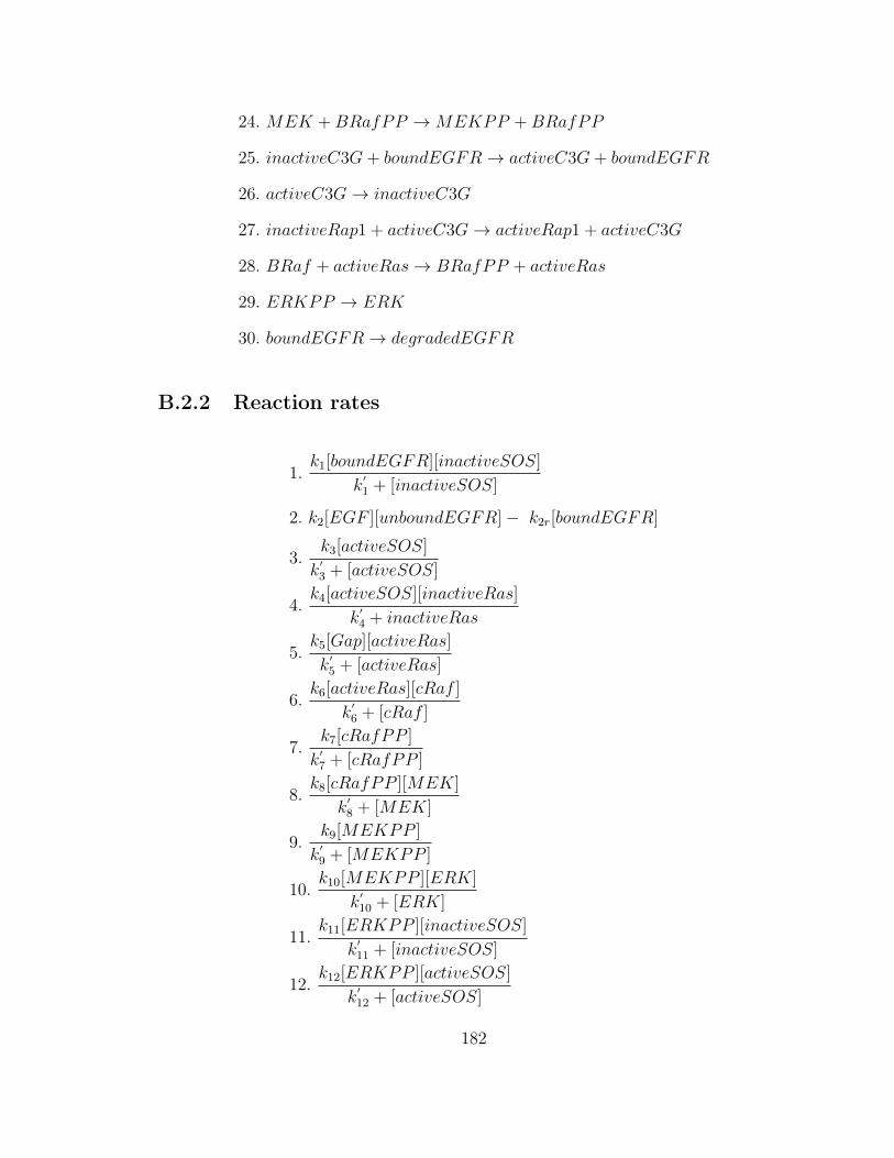
24. 𝑀𝐸𝐾 +𝐵𝑅𝑎𝑓𝑃𝑃 →𝑀𝐸𝐾𝑃𝑃 +𝐵𝑅𝑎𝑓𝑃𝑃
25. 𝑖𝑛𝑎𝑐𝑡𝑖𝑣𝑒𝐶3𝐺+ 𝑏𝑜𝑢𝑛𝑑𝐸𝐺𝐹𝑅→ 𝑎𝑐𝑡𝑖𝑣𝑒𝐶3𝐺+ 𝑏𝑜𝑢𝑛𝑑𝐸𝐺𝐹𝑅
26. 𝑎𝑐𝑡𝑖𝑣𝑒𝐶3𝐺→ 𝑖𝑛𝑎𝑐𝑡𝑖𝑣𝑒𝐶3𝐺
27. 𝑖𝑛𝑎𝑐𝑡𝑖𝑣𝑒𝑅𝑎𝑝1 + 𝑎𝑐𝑡𝑖𝑣𝑒𝐶3𝐺→ 𝑎𝑐𝑡𝑖𝑣𝑒𝑅𝑎𝑝1 + 𝑎𝑐𝑡𝑖𝑣𝑒𝐶3𝐺
28. 𝐵𝑅𝑎𝑓 + 𝑎𝑐𝑡𝑖𝑣𝑒𝑅𝑎𝑠→ 𝐵𝑅𝑎𝑓𝑃𝑃 + 𝑎𝑐𝑡𝑖𝑣𝑒𝑅𝑎𝑠
29. 𝐸𝑅𝐾𝑃𝑃 → 𝐸𝑅𝐾
30. 𝑏𝑜𝑢𝑛𝑑𝐸𝐺𝐹𝑅→ 𝑑𝑒𝑔𝑟𝑎𝑑𝑒𝑑𝐸𝐺𝐹𝑅
B.2.2 Reaction rates
1.𝑘1[𝑏𝑜𝑢𝑛𝑑𝐸𝐺𝐹𝑅][𝑖𝑛𝑎𝑐𝑡𝑖𝑣𝑒𝑆𝑂𝑆]
𝑘′1 + [𝑖𝑛𝑎𝑐𝑡𝑖𝑣𝑒𝑆𝑂𝑆]
2. 𝑘2[𝐸𝐺𝐹 ][𝑢𝑛𝑏𝑜𝑢𝑛𝑑𝐸𝐺𝐹𝑅]− 𝑘2𝑟[𝑏𝑜𝑢𝑛𝑑𝐸𝐺𝐹𝑅]
3.𝑘3[𝑎𝑐𝑡𝑖𝑣𝑒𝑆𝑂𝑆]
𝑘′3 + [𝑎𝑐𝑡𝑖𝑣𝑒𝑆𝑂𝑆]
4.𝑘4[𝑎𝑐𝑡𝑖𝑣𝑒𝑆𝑂𝑆][𝑖𝑛𝑎𝑐𝑡𝑖𝑣𝑒𝑅𝑎𝑠]
𝑘′4 + 𝑖𝑛𝑎𝑐𝑡𝑖𝑣𝑒𝑅𝑎𝑠
5.𝑘5[𝐺𝑎𝑝][𝑎𝑐𝑡𝑖𝑣𝑒𝑅𝑎𝑠]
𝑘′5 + [𝑎𝑐𝑡𝑖𝑣𝑒𝑅𝑎𝑠]
6.𝑘6[𝑎𝑐𝑡𝑖𝑣𝑒𝑅𝑎𝑠][𝑐𝑅𝑎𝑓 ]
𝑘′6 + [𝑐𝑅𝑎𝑓 ]
7.𝑘7[𝑐𝑅𝑎𝑓𝑃𝑃 ]
𝑘′7 + [𝑐𝑅𝑎𝑓𝑃𝑃 ]
8.𝑘8[𝑐𝑅𝑎𝑓𝑃𝑃 ][𝑀𝐸𝐾]
𝑘′8 + [𝑀𝐸𝐾]
9.𝑘9[𝑀𝐸𝐾𝑃𝑃 ]
𝑘′9 + [𝑀𝐸𝐾𝑃𝑃 ]
10.𝑘10[𝑀𝐸𝐾𝑃𝑃 ][𝐸𝑅𝐾]
𝑘′10 + [𝐸𝑅𝐾]
11.𝑘11[𝐸𝑅𝐾𝑃𝑃 ][𝑖𝑛𝑎𝑐𝑡𝑖𝑣𝑒𝑆𝑂𝑆]
𝑘′11 + [𝑖𝑛𝑎𝑐𝑡𝑖𝑣𝑒𝑆𝑂𝑆]
12.𝑘12[𝐸𝑅𝐾𝑃𝑃 ][𝑎𝑐𝑡𝑖𝑣𝑒𝑆𝑂𝑆]
𝑘′12 + [𝑎𝑐𝑡𝑖𝑣𝑒𝑆𝑂𝑆]
182

13.𝑘13[𝑃𝐾𝐴][𝑐𝑅𝑎𝑓 ]
𝑘′13 + [𝑐𝑅𝑎𝑓 ]
14.𝑘14[𝑃𝐾𝐴𝐴][𝑖𝑛𝑎𝑐𝑡𝑖𝑣𝑒𝑃𝐾𝐴]
𝑘′14 + [𝑖𝑛𝑎𝑐𝑡𝑖𝑣𝑒𝑃𝐾𝐴]
15.𝑘15[𝐶𝑖𝑙𝑜𝑠𝑡𝑎𝑚𝑖𝑑𝑒][𝑖𝑛𝑎𝑐𝑡𝑖𝑣𝑒𝑃𝐾𝐴]
𝑘′15 + [𝑖𝑛𝑎𝑐𝑡𝑖𝑣𝑒𝑃𝐾𝐴]
16.𝑘16[𝑃𝐾𝐴]
𝑘′16 + [𝑃𝐾𝐴]
17.𝑘17[𝐸𝑃𝐴𝐶𝐴][𝑖𝑛𝑎𝑐𝑡𝑖𝑣𝑒𝐸𝑃𝐴𝐶]
𝑘′17 + [𝑖𝑛𝑎𝑐𝑡𝑖𝑣𝑒𝐸𝑃𝐴𝐶]
18.𝑘18[𝐶𝑖𝑙𝑜𝑠𝑡𝑎𝑚𝑖𝑑𝑒][𝑖𝑛𝑎𝑐𝑡𝑖𝑣𝑒𝐸𝑃𝐴𝐶]
𝑘′18 + [𝑖𝑛𝑎𝑐𝑡𝑖𝑣𝑒𝐸𝑃𝐴𝐶]
19.𝑘19[𝐸𝑃𝐴𝐶]
𝑘′19 + [𝐸𝑃𝐴𝐶]
20.𝑘20[𝐸𝑃𝐴𝐶][𝑖𝑛𝑎𝑐𝑡𝑖𝑣𝑒𝑅𝑎𝑝1]
𝑘′20 + 𝑖𝑛𝑎𝑐𝑡𝑖𝑣𝑒𝑅𝑎𝑝1
21.𝑘21[𝐺𝑎𝑝][𝑎𝑐𝑡𝑖𝑣𝑒𝑅𝑎𝑝1]
𝑘′21 + [𝑎𝑐𝑡𝑖𝑣𝑒𝑅𝑎𝑝1]
22.𝑘22[𝑎𝑐𝑡𝑖𝑣𝑒𝑅𝑎𝑝1][𝐵𝑅𝑎𝑓 ]
𝑘′22 + [𝐵𝑅𝑎𝑓 ]
23.𝑘23[𝐵𝑅𝑎𝑓𝑃𝑃 ]
𝑘′23 + [𝐵𝑅𝑎𝑓𝑃𝑃 ]
24.𝑘24[𝐵𝑅𝑎𝑓𝑃𝑃 ][𝑀𝐸𝐾]
𝑘′24 + [𝑀𝐸𝐾]
25.𝑘25[𝑏𝑜𝑢𝑛𝑑𝐸𝐺𝐹𝑅][𝑖𝑛𝑎𝑐𝑡𝑖𝑣𝑒𝐶3𝐺]
𝑘′25 + [𝑖𝑛𝑎𝑐𝑡𝑖𝑣𝑒𝐶3𝐺]
26. 𝑘26[𝑎𝑐𝑡𝑖𝑣𝑒𝐶3𝐺]
27.𝑘27[𝑎𝑐𝑡𝑖𝑣𝑒𝐶3𝐺][𝑖𝑛𝑎𝑐𝑡𝑖𝑣𝑒𝑅𝑎𝑝1]
𝑘′27 + [𝑖𝑛𝑎𝑐𝑡𝑖𝑣𝑒𝑅𝑎𝑝1]
28.𝑘28[𝑎𝑐𝑡𝑖𝑣𝑒𝑅𝑎𝑠][𝐵𝑅𝑎𝑓 ]
𝑘′28 + [𝐵𝑅𝑎𝑓 ]
29.𝑘29[𝐸𝑅𝐾𝑃𝑃 ]
𝑘′29 + [𝐸𝑅𝐾𝑃𝑃 ]
30. 𝑘30[𝑏𝑜𝑢𝑛𝑑𝐸𝐺𝐹𝑅]
183
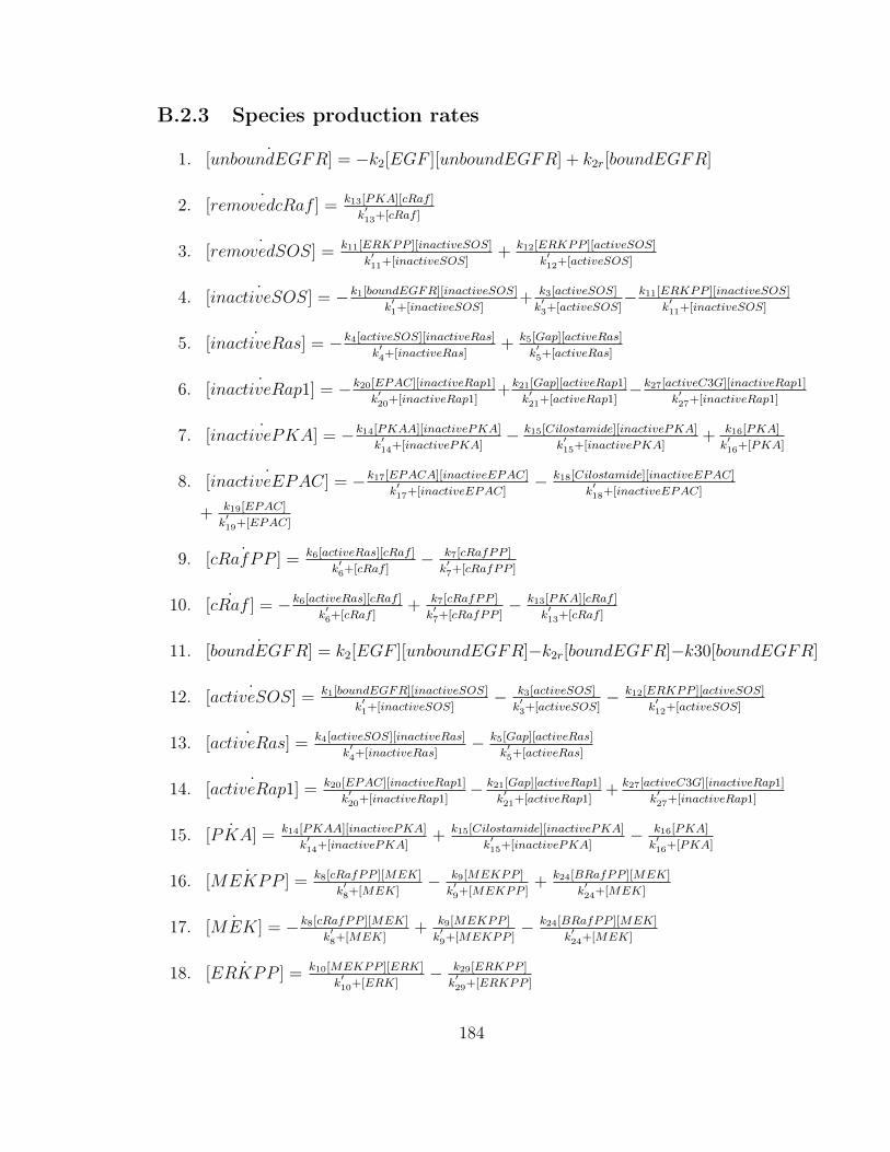
B.2.3 Species production rates
1. ˙[𝑢𝑛𝑏𝑜𝑢𝑛𝑑𝐸𝐺𝐹𝑅] = −𝑘2[𝐸𝐺𝐹 ][𝑢𝑛𝑏𝑜𝑢𝑛𝑑𝐸𝐺𝐹𝑅] + 𝑘2𝑟[𝑏𝑜𝑢𝑛𝑑𝐸𝐺𝐹𝑅]
2. ˙[𝑟𝑒𝑚𝑜𝑣𝑒𝑑𝑐𝑅𝑎𝑓 ] = 𝑘13[𝑃𝐾𝐴][𝑐𝑅𝑎𝑓 ]
𝑘′13+[𝑐𝑅𝑎𝑓 ]
3. ˙[𝑟𝑒𝑚𝑜𝑣𝑒𝑑𝑆𝑂𝑆] = 𝑘11[𝐸𝑅𝐾𝑃𝑃 ][𝑖𝑛𝑎𝑐𝑡𝑖𝑣𝑒𝑆𝑂𝑆]
𝑘′11+[𝑖𝑛𝑎𝑐𝑡𝑖𝑣𝑒𝑆𝑂𝑆]
+ 𝑘12[𝐸𝑅𝐾𝑃𝑃 ][𝑎𝑐𝑡𝑖𝑣𝑒𝑆𝑂𝑆]
𝑘′12+[𝑎𝑐𝑡𝑖𝑣𝑒𝑆𝑂𝑆]
4. ˙[𝑖𝑛𝑎𝑐𝑡𝑖𝑣𝑒𝑆𝑂𝑆] = −𝑘1[𝑏𝑜𝑢𝑛𝑑𝐸𝐺𝐹𝑅][𝑖𝑛𝑎𝑐𝑡𝑖𝑣𝑒𝑆𝑂𝑆]
𝑘′1+[𝑖𝑛𝑎𝑐𝑡𝑖𝑣𝑒𝑆𝑂𝑆]
+ 𝑘3[𝑎𝑐𝑡𝑖𝑣𝑒𝑆𝑂𝑆]
𝑘′3+[𝑎𝑐𝑡𝑖𝑣𝑒𝑆𝑂𝑆]
−𝑘11[𝐸𝑅𝐾𝑃𝑃 ][𝑖𝑛𝑎𝑐𝑡𝑖𝑣𝑒𝑆𝑂𝑆]
𝑘′11+[𝑖𝑛𝑎𝑐𝑡𝑖𝑣𝑒𝑆𝑂𝑆]
5. ˙[𝑖𝑛𝑎𝑐𝑡𝑖𝑣𝑒𝑅𝑎𝑠] = −𝑘4[𝑎𝑐𝑡𝑖𝑣𝑒𝑆𝑂𝑆][𝑖𝑛𝑎𝑐𝑡𝑖𝑣𝑒𝑅𝑎𝑠]
𝑘′4+[𝑖𝑛𝑎𝑐𝑡𝑖𝑣𝑒𝑅𝑎𝑠]
+ 𝑘5[𝐺𝑎𝑝][𝑎𝑐𝑡𝑖𝑣𝑒𝑅𝑎𝑠]
𝑘′5+[𝑎𝑐𝑡𝑖𝑣𝑒𝑅𝑎𝑠]
6. ˙[𝑖𝑛𝑎𝑐𝑡𝑖𝑣𝑒𝑅𝑎𝑝1] = −𝑘20[𝐸𝑃𝐴𝐶][𝑖𝑛𝑎𝑐𝑡𝑖𝑣𝑒𝑅𝑎𝑝1]
𝑘′20+[𝑖𝑛𝑎𝑐𝑡𝑖𝑣𝑒𝑅𝑎𝑝1]
+𝑘21[𝐺𝑎𝑝][𝑎𝑐𝑡𝑖𝑣𝑒𝑅𝑎𝑝1]
𝑘′21+[𝑎𝑐𝑡𝑖𝑣𝑒𝑅𝑎𝑝1]
−𝑘27[𝑎𝑐𝑡𝑖𝑣𝑒𝐶3𝐺][𝑖𝑛𝑎𝑐𝑡𝑖𝑣𝑒𝑅𝑎𝑝1]
𝑘′27+[𝑖𝑛𝑎𝑐𝑡𝑖𝑣𝑒𝑅𝑎𝑝1]
7. ˙[𝑖𝑛𝑎𝑐𝑡𝑖𝑣𝑒𝑃𝐾𝐴] = −𝑘14[𝑃𝐾𝐴𝐴][𝑖𝑛𝑎𝑐𝑡𝑖𝑣𝑒𝑃𝐾𝐴]
𝑘′14+[𝑖𝑛𝑎𝑐𝑡𝑖𝑣𝑒𝑃𝐾𝐴]
− 𝑘15[𝐶𝑖𝑙𝑜𝑠𝑡𝑎𝑚𝑖𝑑𝑒][𝑖𝑛𝑎𝑐𝑡𝑖𝑣𝑒𝑃𝐾𝐴]
𝑘′15+[𝑖𝑛𝑎𝑐𝑡𝑖𝑣𝑒𝑃𝐾𝐴]
+ 𝑘16[𝑃𝐾𝐴]
𝑘′16+[𝑃𝐾𝐴]
8. ˙[𝑖𝑛𝑎𝑐𝑡𝑖𝑣𝑒𝐸𝑃𝐴𝐶] = −𝑘17[𝐸𝑃𝐴𝐶𝐴][𝑖𝑛𝑎𝑐𝑡𝑖𝑣𝑒𝐸𝑃𝐴𝐶]
𝑘′17+[𝑖𝑛𝑎𝑐𝑡𝑖𝑣𝑒𝐸𝑃𝐴𝐶]
− 𝑘18[𝐶𝑖𝑙𝑜𝑠𝑡𝑎𝑚𝑖𝑑𝑒][𝑖𝑛𝑎𝑐𝑡𝑖𝑣𝑒𝐸𝑃𝐴𝐶]
𝑘′18+[𝑖𝑛𝑎𝑐𝑡𝑖𝑣𝑒𝐸𝑃𝐴𝐶]
+ 𝑘19[𝐸𝑃𝐴𝐶]
𝑘′19+[𝐸𝑃𝐴𝐶]
9. ˙[𝑐𝑅𝑎𝑓𝑃𝑃 ] = 𝑘6[𝑎𝑐𝑡𝑖𝑣𝑒𝑅𝑎𝑠][𝑐𝑅𝑎𝑓 ]
𝑘′6+[𝑐𝑅𝑎𝑓 ]
− 𝑘7[𝑐𝑅𝑎𝑓𝑃𝑃 ]
𝑘′7+[𝑐𝑅𝑎𝑓𝑃𝑃 ]
10. ˙[𝑐𝑅𝑎𝑓 ] = −𝑘6[𝑎𝑐𝑡𝑖𝑣𝑒𝑅𝑎𝑠][𝑐𝑅𝑎𝑓 ]
𝑘′6+[𝑐𝑅𝑎𝑓 ]
+ 𝑘7[𝑐𝑅𝑎𝑓𝑃𝑃 ]
𝑘′7+[𝑐𝑅𝑎𝑓𝑃𝑃 ]
− 𝑘13[𝑃𝐾𝐴][𝑐𝑅𝑎𝑓 ]
𝑘′13+[𝑐𝑅𝑎𝑓 ]
11. ˙[𝑏𝑜𝑢𝑛𝑑𝐸𝐺𝐹𝑅] = 𝑘2[𝐸𝐺𝐹 ][𝑢𝑛𝑏𝑜𝑢𝑛𝑑𝐸𝐺𝐹𝑅]−𝑘2𝑟[𝑏𝑜𝑢𝑛𝑑𝐸𝐺𝐹𝑅]−𝑘30[𝑏𝑜𝑢𝑛𝑑𝐸𝐺𝐹𝑅]
12. ˙[𝑎𝑐𝑡𝑖𝑣𝑒𝑆𝑂𝑆] = 𝑘1[𝑏𝑜𝑢𝑛𝑑𝐸𝐺𝐹𝑅][𝑖𝑛𝑎𝑐𝑡𝑖𝑣𝑒𝑆𝑂𝑆]
𝑘′1+[𝑖𝑛𝑎𝑐𝑡𝑖𝑣𝑒𝑆𝑂𝑆]
− 𝑘3[𝑎𝑐𝑡𝑖𝑣𝑒𝑆𝑂𝑆]
𝑘′3+[𝑎𝑐𝑡𝑖𝑣𝑒𝑆𝑂𝑆]
− 𝑘12[𝐸𝑅𝐾𝑃𝑃 ][𝑎𝑐𝑡𝑖𝑣𝑒𝑆𝑂𝑆]
𝑘′12+[𝑎𝑐𝑡𝑖𝑣𝑒𝑆𝑂𝑆]
13. ˙[𝑎𝑐𝑡𝑖𝑣𝑒𝑅𝑎𝑠] = 𝑘4[𝑎𝑐𝑡𝑖𝑣𝑒𝑆𝑂𝑆][𝑖𝑛𝑎𝑐𝑡𝑖𝑣𝑒𝑅𝑎𝑠]
𝑘′4+[𝑖𝑛𝑎𝑐𝑡𝑖𝑣𝑒𝑅𝑎𝑠]
− 𝑘5[𝐺𝑎𝑝][𝑎𝑐𝑡𝑖𝑣𝑒𝑅𝑎𝑠]
𝑘′5+[𝑎𝑐𝑡𝑖𝑣𝑒𝑅𝑎𝑠]
14. ˙[𝑎𝑐𝑡𝑖𝑣𝑒𝑅𝑎𝑝1] = 𝑘20[𝐸𝑃𝐴𝐶][𝑖𝑛𝑎𝑐𝑡𝑖𝑣𝑒𝑅𝑎𝑝1]
𝑘′20+[𝑖𝑛𝑎𝑐𝑡𝑖𝑣𝑒𝑅𝑎𝑝1]
− 𝑘21[𝐺𝑎𝑝][𝑎𝑐𝑡𝑖𝑣𝑒𝑅𝑎𝑝1]
𝑘′21+[𝑎𝑐𝑡𝑖𝑣𝑒𝑅𝑎𝑝1]
+ 𝑘27[𝑎𝑐𝑡𝑖𝑣𝑒𝐶3𝐺][𝑖𝑛𝑎𝑐𝑡𝑖𝑣𝑒𝑅𝑎𝑝1]
𝑘′27+[𝑖𝑛𝑎𝑐𝑡𝑖𝑣𝑒𝑅𝑎𝑝1]
15. ˙[𝑃𝐾𝐴] = 𝑘14[𝑃𝐾𝐴𝐴][𝑖𝑛𝑎𝑐𝑡𝑖𝑣𝑒𝑃𝐾𝐴]
𝑘′14+[𝑖𝑛𝑎𝑐𝑡𝑖𝑣𝑒𝑃𝐾𝐴]
+ 𝑘15[𝐶𝑖𝑙𝑜𝑠𝑡𝑎𝑚𝑖𝑑𝑒][𝑖𝑛𝑎𝑐𝑡𝑖𝑣𝑒𝑃𝐾𝐴]
𝑘′15+[𝑖𝑛𝑎𝑐𝑡𝑖𝑣𝑒𝑃𝐾𝐴]
− 𝑘16[𝑃𝐾𝐴]
𝑘′16+[𝑃𝐾𝐴]
16. ˙[𝑀𝐸𝐾𝑃𝑃 ] = 𝑘8[𝑐𝑅𝑎𝑓𝑃𝑃 ][𝑀𝐸𝐾]
𝑘′8+[𝑀𝐸𝐾]
− 𝑘9[𝑀𝐸𝐾𝑃𝑃 ]
𝑘′9+[𝑀𝐸𝐾𝑃𝑃 ]
+ 𝑘24[𝐵𝑅𝑎𝑓𝑃𝑃 ][𝑀𝐸𝐾]
𝑘′24+[𝑀𝐸𝐾]
17. ˙[𝑀𝐸𝐾] = −𝑘8[𝑐𝑅𝑎𝑓𝑃𝑃 ][𝑀𝐸𝐾]
𝑘′8+[𝑀𝐸𝐾]
+ 𝑘9[𝑀𝐸𝐾𝑃𝑃 ]
𝑘′9+[𝑀𝐸𝐾𝑃𝑃 ]
− 𝑘24[𝐵𝑅𝑎𝑓𝑃𝑃 ][𝑀𝐸𝐾]
𝑘′24+[𝑀𝐸𝐾]
18. ˙[𝐸𝑅𝐾𝑃𝑃 ] = 𝑘10[𝑀𝐸𝐾𝑃𝑃 ][𝐸𝑅𝐾]
𝑘′10+[𝐸𝑅𝐾]
− 𝑘29[𝐸𝑅𝐾𝑃𝑃 ]
𝑘′29+[𝐸𝑅𝐾𝑃𝑃 ]
184

19. ˙[𝐸𝑅𝐾] = −𝑘10[𝑀𝐸𝐾𝑃𝑃 ][𝐸𝑅𝐾]
𝑘′10+[𝐸𝑅𝐾]
+ 𝑘29[𝐸𝑅𝐾𝑃𝑃 ]
𝑘′29+[𝐸𝑅𝐾𝑃𝑃 ]
20. ˙[𝐸𝑃𝐴𝐶] = 𝑘17[𝐸𝑃𝐴𝐶𝐴][𝑖𝑛𝑎𝑐𝑡𝑖𝑣𝑒𝐸𝑃𝐴𝐶]
𝑘′17+[𝑖𝑛𝑎𝑐𝑡𝑖𝑣𝑒𝐸𝑃𝐴𝐶]
+ 𝑘18[𝐶𝑖𝑙𝑜𝑠𝑡𝑎𝑚𝑖𝑑𝑒][𝑖𝑛𝑎𝑐𝑡𝑖𝑣𝑒𝐸𝑃𝐴𝐶]
𝑘′18+[𝑖𝑛𝑎𝑐𝑡𝑖𝑣𝑒𝐸𝑃𝐴𝐶]
− 𝑘19[𝐸𝑃𝐴𝐶]
𝑘′19+[𝐸𝑃𝐴𝐶]
21. ˙[𝐸𝐺𝐹 ] = −𝑘2[𝐸𝐺𝐹 ][𝑢𝑛𝑏𝑜𝑢𝑛𝑑𝐸𝐺𝐹𝑅] + 𝑘2𝑟[𝑏𝑜𝑢𝑛𝑑𝐸𝐺𝐹𝑅]
22. ˙[𝐵𝑅𝑎𝑓𝑃𝑃 ] = 𝑘22[𝑎𝑐𝑡𝑖𝑣𝑒𝑅𝑎𝑝1][𝐵𝑅𝑎𝑓 ]
𝑘′22+[𝐵𝑅𝑎𝑓 ]
− 𝑘23[𝐵𝑅𝑎𝑓𝑃𝑃 ]
𝑘′23+[𝐵𝑅𝑎𝑓𝑃𝑃 ]
+ 𝑘28[𝑎𝑐𝑡𝑖𝑣𝑒𝑅𝑎𝑠][𝐵𝑅𝑎𝑓 ]
𝑘′28+[𝐵𝑅𝑎𝑓 ]
23. ˙[𝐵𝑅𝑎𝑓 ] = −𝑘22[𝑎𝑐𝑡𝑖𝑣𝑒𝑅𝑎𝑝1][𝐵𝑅𝑎𝑓 ]
𝑘′22+[𝐵𝑅𝑎𝑓 ]
+ 𝑘23[𝐵𝑅𝑎𝑓𝑃𝑃 ]
𝑘′23+[𝐵𝑅𝑎𝑓𝑃𝑃 ]
− 𝑘28[𝑎𝑐𝑡𝑖𝑣𝑒𝑅𝑎𝑠][𝐵𝑅𝑎𝑓 ]
𝑘′28+[𝐵𝑅𝑎𝑓 ]
24. ˙[𝑎𝑐𝑡𝑖𝑣𝑒𝐶3𝐺] = 𝑘25[𝑏𝑜𝑢𝑛𝑑𝐸𝐺𝐹𝑅][𝑖𝑛𝑎𝑐𝑡𝑖𝑣𝑒𝐶3𝐺]
𝑘′25+[𝑖𝑛𝑎𝑐𝑡𝑖𝑣𝑒𝐶3𝐺]
− 𝑘26[𝑎𝑐𝑡𝑖𝑣𝑒𝐶3𝐺]
25. ˙[𝑖𝑛𝑎𝑐𝑡𝑖𝑣𝑒𝐶3𝐺] = −𝑘25[𝑏𝑜𝑢𝑛𝑑𝐸𝐺𝐹𝑅][𝑖𝑛𝑎𝑐𝑡𝑖𝑣𝑒𝐶3𝐺]
𝑘′25+[𝑖𝑛𝑎𝑐𝑡𝑖𝑣𝑒𝐶3𝐺]
+ 𝑘26[𝑎𝑐𝑡𝑖𝑣𝑒𝐶3𝐺]
26. ˙[𝑑𝑒𝑔𝑟𝑎𝑑𝑒𝑑𝐸𝐺𝐹𝑅] = 𝑘30[𝑏𝑜𝑢𝑛𝑑𝐸𝐺𝐹𝑅]
27. ˙[𝐸𝑃𝐴𝐶𝐴] = 0
28. ˙[𝐺𝑎𝑝] = 0
29. ˙[𝑃𝐾𝐴𝐴] = 0
30. ˙[𝐶𝑖𝑙𝑜𝑠𝑡𝑎𝑚𝑖𝑑𝑒]
B.2.4 Initial species concentrations
All simulations using the above reactions are performed with the following initial
concentrations:
1. [𝑢𝑛𝑏𝑜𝑢𝑛𝑑𝐸𝐺𝐹𝑅]0 = 500
2. [𝑟𝑒𝑚𝑜𝑣𝑒𝑑𝑐𝑅𝑎𝑓 ]0 = 0
3. [𝑟𝑒𝑚𝑜𝑣𝑒𝑑𝑆𝑂𝑆]0 = 0
4. [𝑖𝑛𝑎𝑐𝑡𝑖𝑣𝑒𝑆𝑂𝑆]0 = 1200
5. [𝑖𝑛𝑎𝑐𝑡𝑖𝑣𝑒𝑅𝑎𝑠]0 = 1200
185

6. [𝑖𝑛𝑎𝑐𝑡𝑖𝑣𝑒𝑅𝑎𝑝1]0 = 1200
7. [𝑖𝑛𝑎𝑐𝑡𝑖𝑣𝑒𝑃𝐾𝐴]0 = 1000
8. [𝑖𝑛𝑎𝑐𝑡𝑖𝑣𝑒𝐸𝑃𝐴𝐶]0 = 1000
9. [𝑐𝑅𝑎𝑓𝑃𝑃 ]0 = 0
10. [𝑐𝑅𝑎𝑓 ]0 = 1500
11. [𝑏𝑜𝑢𝑛𝑑𝐸𝐺𝐹𝑅]0 = 0
12. [𝑎𝑐𝑡𝑖𝑣𝑒𝑆𝑂𝑆]0 = 0
13. [𝑎𝑐𝑡𝑖𝑣𝑒𝑅𝑎𝑠]0 = 0
14. [𝑎𝑐𝑡𝑖𝑣𝑒𝑅𝑎𝑝1]0 = 0
15. [𝑃𝐾𝐴]0 = 0
16. [𝑀𝐸𝐾𝑃𝑃 ]0 = 0
17. [𝑀𝐸𝐾]0 = 3000
18. [𝐸𝑅𝐾𝑃𝑃 ]0 = 0
19. [𝐸𝑅𝐾]0 = 10000
20. [𝐸𝑃𝐴𝐶]0 = 0
21. [𝐸𝐺𝐹 ]0 = 1000
22. [𝐵𝑅𝑎𝑓𝑃𝑃 ]0 = 0
23. [𝐵𝑅𝑎𝑓 ]0 = 1500
24. [𝑎𝑐𝑡𝑖𝑣𝑒𝐶3𝐺]0 = 0
25. [𝑖𝑛𝑎𝑐𝑡𝑖𝑣𝑒𝐶3𝐺]0 = 1200
186

26. [𝑑𝑒𝑔𝑟𝑎𝑑𝑒𝑑𝐸𝐺𝐹𝑅]0 = 0
27. [𝐸𝑃𝐴𝐶𝐴]0 = 1000
28. [𝐺𝑎𝑝]0 = 2400
29. [𝑃𝐾𝐴𝐴]0 = 1000
30. [𝐶𝑖𝑙𝑜𝑠𝑡𝑎𝑚𝑖𝑑𝑒]0 = 1000
187

188

Bibliography
[1] F. Al-Awadhi, M. A. Hurn, and C. Jennison. Improving the acceptance rateof the reversible jump MCMC proposals. Statistics and Probability Letters,69:189–198, 2004.
[2] R. Albert. Network inference, analysis, and modeling in systems biology. ThePlant Cell, 19(11):3327–3338, 2007.
[3] C. Andrieu, N. deFreitas, A. Doucet, and M. I. Jordan. An introduction toMCMC for machine learning. Machine Learning, 50:5–43, 2003.
[4] C. Andrieu and E. Moulines. On the ergodicity properties of some adaptiveMCMC algorithms. Annals of Applied Probability, 16(3):1462–1505, 2006.
[5] C. Andrieu, E. Moulines, and P. Priouret. Stability of stochastic approxi-mation under verifiable conditions. SIAM Journal Control and Optimization,44(1):283–312, 2005.
[6] C. Andrieu and G. O. Roberts. The pseudo-marginal approach for efficientMonte Carlo computations. The Annals of Statistics, 37(2):697–725, 2009.
[7] A. Arkin and J. Ross. Statistical construction of chemical reaction mechanismsfrom measured time-series. Journal of Physical Chemistry, (99):970–979, 1995.
[8] S. Arlot and A. Celisse. A survey of cross-validation procedures for modelselection. Statistics Surveys, 4:40–79, 2010.
[9] R. Asters, B. Borchers, and C. Thurber. Parameter Estimation and InverseProblems. Academic Press, 2004.
[10] M. Bansal, G. D. Gatta, and D. Bernardo. Inference of gene regulatory andcompound mode of action from time course gene expression profiles. Bioinfor-matics, 22(7):815–822, 2006.
[11] M. A. Beaumont. Estimation of population growth or decline in geneticallymonitored populations. Genetics, 164:1139–1160, 2003.
189
[12] J. Berger and L. Pericchi. Objective Bayesian methods for model selection:introduction and comparison. Model Selection (P.Lahiri, editor), IMS LectureNotes – Monograph Series, 38:135–207, 2001.
[13] J. M. Bernardo and A. F. M. Smith. Bayesian Theory. Wiley, 2000.
[14] B. Bhattacharjee, D. A. Schwer, P. I. Barton, and Jr. W. H. Green. Optimally-reduced kinetic models: reaction elimination in large-scale kinetic mechanisms.Combustion and Flame, 135(3):191–208, 2003.
[15] J. A. Bilmes. A gentle tutorial on the EM algorithm and its application toparameter estimation for Gaussian mixture and hidden Markov models, 1998.
[16] C. M. Bishop. Pattern Recognition and Machine Learning. Springer, 2007.
[17] R. Bonneau. Learning biological networks: from modules to dynamics. NatureChemical Biology, 4(11):658–662, 2008.
[18] R. Bonneau, D. J. Reiss, P. Shannon, M. Facciotti, L. Hood, N. S. Baliga, andV. Thorsson. The inferelator: an algorithm for learning parsimonious regulatorynetworks from systems-biology data sets de novo. Genome Biology, 7(5):R36,2006.
[19] K. Braman, T. A. Oliver, and V. Raman. Bayesian analysis of syngas chemistrymodels. Combustion Theory and Modelling, 17(5):858–887, 2013.
[20] S. P. Brooks, P. Giudici, and G. O. Roberts. Efficient construction of reversiblejump Markov chain Monte Carlo proposal distributions (with discussion). Jour-nal of Royal Statistical Society B, 65:3–39, 2003.
[21] K. P. Burnham and D. R. Anderson. Model Selection and Multimodal Inference:A Practical Information Theoretic Approach. Springer, 2nd edition, 2002.
[22] S. C. Burnham, D. P. Searson, M. J. Willis, and A. R. Wright. Inferenceof chemical reaction networks. Chemical Engineering Science, 63(4):862–873,2008.
[23] O. Cappé, C. P. Robert, and T. Ryden. Reversible jump, birth-and-death andmore general continuous time markov chain monte carlo samplers. Journal ofthe Royal Statistical Society B, (65):679–700, 2003.
[24] B. P. Carlin and S. Chib. Bayesian model choice via Markov chain Monte Carlomethods. Journal of the Royal Statistical Society: Series B (Methodological),57(3):473–484, 1995.
[25] S. Chib. Marginal likelihood from the Gibbs output. Journal of the AmericanStatistical Association, 90(432):1313–1321, 1995.
190

[26] S. Chib and I. Jeliazkov. Marginal likelihood from the Metropolis-Hastingsoutput. Journal of the American Statistical Association, 96(453):270–281, 2001.
[27] M. Clyde and E. I. George. Model uncertainty. Statistical Science, 19:81–94,2004.
[28] H. J. Curran, P. Gaffuri, W. J. Pitz, and C. K. Westbrook. A comprehensivemodeling study of iso-octane oxidation. Combustion and Flame, 129(3):253–280, 2002.
[29] P. J. Davis and P. Rabinowitz. Methods of Numerical Intergation. AcedemicPress, 2nd edition, 1984.
[30] P. Dellaportas, J. J. Forster, and I. Ntzoufras. On Bayesian model and variableselection using MCMC. Statistics and Computing, 12:27–36, 2002.
[31] A. P. Dempster, N. M. Laird, and D. B. Rubin. Maximum likelihood fromincomplete data via the EM algorithm. Journal of the Royal Statistical Society.Series B (Methodological), 39(1):1–38, 1977.
[32] D. G. T. Denison, B. K. Mallick, and A. F. M. Smith. Automatic Bayesiancurve fitting. Journal of the Royal Statistical Society. Series B, 60(2):333–350,1998.
[33] O. Deutschmann, R. Schwiedernoch, L. I. Maier, and D. Chatterjee. Compar-ison between calculated and experimentally determined selectivity and conver-sion for short-contact-time reactors using honeycomb monoliths. Natural GasConversion VI, Studies in surface science and catalysis, E. Iglesia, J.J. Spivey,T.H. Fleisch (eds.), Elsevier, 136:215–258, 2001.
[34] I. DiMatteo, C. R. Genovese, and R. E. Kass. Bayesian curve-fitting with free-knot splines. Biometrika, 88(4):1055–1071, 2001.
[35] Y. Efendiev, T. Y. Hou, and W. Luo. Preconditioning markov chain monte carlosimulations using coarse scale models. SIAM Journal on Scientific Computing,28:776–803, 2006.
[36] R. S. Ehlers and S. P. Brooks. Adaptive proposal construction for reversiblejump MCMC. Scandinavian Journal of Statistics, 35:677–690, 2008.
[37] B. Ellis and W. H. Wong. Learning causal Bayesian network structures from ex-perimental data. Journal of the American Statistical Association, 103(482):778–789, 2008.
[38] Y. Fan, G. W. Peters, and S. A. Sisson. Automating and evaluating reversiblejump MCMC proposal distributions. Statistics and Computing, 19:409–421,2009.
191
[39] N. Friedman and D. Koller. Being Bayesian about network structure. a Bayesianapproach to structure discovery in Bayesian networks. Machine Learning, 50:95–125, 2003.
[40] N. Friedman, M. Linial, I. Nachman, and D. Pe’er. Using Bayesian networks toanalyze expression data. Journal of Computational Biology, 7:601–620, 2000.
[41] N. Friel and A. N. Pettitt. Marginal likelihood estimation via power posteriors.Journal of the Royal Statistical Society: Series B, 70(3):589–607, 2008.
[42] N. Galagali and Y. M. Marzouk. Bayesian inference of chemical kinetic modelsfrom proposed reactions. Chemical Engineering Science, 123:170–190, 2015.
[43] T. S. Gardner, D. Bernardo, D. Lorenz, and J. J. Collins. Inferring geneticnetworks and identifying compound mode of action via expression profiling.Science, 301(5629):102–105, 2003.
[44] T. S. Gardner and J. J. Faith. Reverse engineering transcription control net-works. Physics of Life Reviews, 2(1):65–88, 2005.
[45] P. H. Garthwaite, J. B. Kadane, and A. O’Hagan. Statistical methods for elic-iting probability distributions. Journal of the American Statistical Association,100(470):680–700, 2005.
[46] A. Gelman, J. B. Carlin, H. S. Stern, and D. B. Rudin. Bayesian Data Analysis.Chapman and Hall/CRC, 2nd edition, 2004.
[47] A. Gelman and X. L. Meng. Simulating normalizing constants: from importancesampling to bridge sampling to path sampling. Statistical Science, 13(2):163–185, 1998.
[48] T. Gerstner and M. Griebel. Numerical integration using sparse grids. Numer-ical Algorithms, (18):209–232, 1998.
[49] J. Geweke. Bayesian inference in econometric models using monte carlo inte-gration. Econometrica, (57):1317–1340, 1989.
[50] C. J. Geyer. Markov chain maximum likelihood. In E. Keramigas, editor, Com-puting Science and Statistics: The 23rd Symposium on the Interface. InterfaceFoundation, Fairfax, 1991.
[51] W. R. Gilks, S. Richardson, and D. J. Spiegelhalter. Markov chain Monte Carloin Practice. Chapman and Hall/ CRC, 1996.
[52] S. J. Godsill. On the relationship between Markov chain Monte Carlo meth-ods for model uncertainty. Journal of Computational and Graphical Statistics,10(2):230–248, 2001.
192

[53] A. Golightly and D. J. Wilkinson. Bayesian inference for stochastic kineticmodels using a diffusion approximation. Biometrics, 61(3):781–788, 2005.
[54] D. Goodwin, N. Malalya, H. Moffat, and R. Speth. Cantera: An object-orientedsoftware toolkit for chemical kinetics, thermodynamics, and transport processes,version 2.0.2. available at https://code.google.com/p/cantera/, 2013.
[55] W. P. Gouveia and J. A. Scales. Resolution of seismic waveform inversion:Bayes versus occam. Inverse Problems, 13:323–349, 1997.
[56] P. Green and D. Hastie. Reversible jump MCMC. Available athttp://www.maths.bris.ac.uk/∼ mapjg/papers/. Access date: 04/24/2014,2009.
[57] P. J. Green. Reversible jump Markov chain Monte Carlo computation andmodel determination. Annals of Stat, 82(4):711–732, 1995.
[58] P. J. Green. Trans-dimensional Markov chain Monte Carlo. In P. J. Green,N. L. Hjort, and S. Richardson, editors, Highly Structures Stochastic Systems.Oxford University Press, Oxford, 2003.
[59] P. J. Green and A. Mira. Delayed rejection in reversible jump Metropolis-Hastings. Biometrika, 88:1035–1053, 2001.
[60] U. Grenander and M. I. Miller. Representations of knowledge in complex sys-tems (with discussion). Journal of the Royal Statistical Society B, (56):549–603,1994.
[61] C. Guihenneuc-Jouyaux and J. Rosseau. Laplace expansions in Markov chainMonte Carlo algorithms. Journal of Computational and Graphical Statistics,14(1):75–94, 2005.
[62] J. Hanna, W. Y. Lee, Y. Shi, and A. F. Ghoniem. Fundamentals of electro- andthermochemistry in the anode of solid-oxide fuel cells with hydrocarbon andsyngas fuels. Progress in Energy and Combustion Science, 40:74–111, 2014.
[63] M. Hartmann, L. Maier, H. D. Minh, and O. Deutschmann. Catalytic partialoxidation of iso-octane over Rhodium catalysts: An experimental, modeling,and simulation study. Combustion and Flame, 157(9):1771–1782, 2010.
[64] T. Hastie, R. Tibshirani, and J. Friedman. The Elements of Statistical Learning:Data Mining, Inference, and Prediction. Springer, 2nd edition, 2009.
[65] B. Hayete, T. S. Gardner, and J. J. Collins. Size matters: network inferencetackles the genome scale. Molecular Systems Biology, 3(77):1–3, 2007.
193

[66] N. A. Heard, C. C. Holmes, and D. A. Stephens. A quantitative study ofgene regulation involved in the immune response of anopheline mosquitoes:an application of bayesian hierarchical clustering of curves. Journal of theAmerican Statistical Association, 101:18–26, 2006.
[67] O. Herbinet, W. J. Pitz, and C. K. Westbrook. Detailed chemical kinetic oxida-tion mechanism for a biodiesel surrogate. Combustion and Flame, 154(3):507–528, 2008.
[68] D. Hickman and L. D. Schmidt. Steps in CH4 oxidation on Pt and Rh surfaces:High-temperature reactor simulations. AIChE J., 39(7):1164–1177, 1993.
[69] A. C. Hindmarsh, P. N. Brown, K. E. Grant, S. L. Lee, R. Serban, D. E.Shumaker, and C. S. Woodward. Sundials: Suite of nonlinear and differen-tial/algebraic equation solvers, 2005.
[70] K. Hukushima and K. Nemoto. Exchange monte carlo method and applicatio tospin glass simulations. Journal of the Physics Society of Japan, 65:1604–1608,1996.
[71] C. Jackson, M. K. Sen, and P. L. Stoffa. An efficient stochastic bayesian ap-proach to optimal parameter and uncertainty estimation for climate model pre-dictions. Journal of Climate, 17:2828–2841, 2004.
[72] A. Jasra, D. A. Stephens, and C. C. Holmes. On population-based simulationfor static inference. Statistics and Computing, 17:263–279, 2007.
[73] C. Ji and S. C. Schmidler. Adaptive Markov chain Monte Carlo for Bayesianvariable selection. J. Comp. and Graph. Stat., 22(3):708–728, 2013.
[74] J. Kaipio and E. Somersalo. Statistical and Computational Inverse Problems.Springer, 2005.
[75] R. E. Kass and A. E. Raftery. Bayes Factors. Journal of the American StatisticalAssociation, 90(430):773–795, 1995.
[76] R. E. Kass, L. Tierney, and J. B. Kadane. The validity of posterior asymp-totic expansions based on laplace’s method. In S. Geisser, J. S. Hodges, S. J.Press, and A. Zellner, editors, Bayesian and Likelihood Methods in Statisticsand Econometrics. North-Holland, New York, 1990.
[77] R. J. Kee, M. E. Coltrin, and P. Glarborg. Chemically Reacting Flow: Theoryand Practice. Wiley, 2003.
[78] M. Komorowski, B. Finkenstadt, C. V. Harper, and D. A. Rand. Bayesian in-ference of biochemical kinetic parameters using the linear noise approximation.BMC Bioinformatics, 10:343–352, 2009.
194

[79] H. J. Kushner and G. G. Yin. Stochastic Approximation Algorithms and Appli-cations. Springer, 2nd edition, 1997.
[80] G. Lawler and A. Sokal. Bounds on the 𝐿2 spectrum for Markov chainsand Markov processes. Transactions of the American Mathematical Society,309:557–580, 1988.
[81] F. Liang and W. H. Wong. Real parameter evolutionary monte carlo withapplications to bayesian mixture models. Journal of American Statistical As-sociation, 96:653–666, 2001.
[82] D. J. C. Mackay. Information Theory, Inference, and Learning Algorithms.Cambridge University Press UK, 2003.
[83] D. Madigan, J. York, and D. Allard. Bayesian grpahical models for discretedata. International Statistical Review, 63(2):215–232, 1995.
[84] A. A. Margolin, I. Nemenman, K. Basso, C. Wiggins, G. Stolovitzky, R. D.Favera, and A. Califano. Arcane: an algorithm for the reconstruction of generegulatory networks in a mammalian cellular context. BMC Bioinformatics,(7):(Suppl. 1),7, 2006.
[85] N. E. McGuire, N. P. Sullivan, O. Deutschmann, H. Zhu, and R. J. Kee.Dry reforming of methane in a stagnation-flow reactor using Rh supportedon strontium-substituted hexaaluminate. Applied Catalysis A: General, 394(1–2):257–265, 2011.
[86] N. E. McGuire, N. P. Sullivan, R. J. Kee, H. Zhu, A. J. Nabity, J. R. Engel,D. T. Wickham, and M. J. Kaufman. Catalytic steam reforming of methaneusing Rh supported on Sr-substituted hexaaluminate. Chemical EngineeringScience, 64(24):5231–5239, 2009.
[87] X. L. Meng and W. H. Wong. Simulating ratios of normalizing constants via asimple identity: a theoretical exploration. Statistical Sinica, (6):831–860, 1996.
[88] T. J. Mitchell and J. J. Beauchamp. Bayesian variable selection in linear re-gression. Journal of the American Statistical Association, 83(404):1023–1032,1988.
[89] A. Mohammad-Djafari. Bayesian inference for inverse problems. In Bayesian In-ference and Maximum Entropy Methods in Science and Engineering, volume 21,pages 477–496. 2002.
[90] S. Mukherjee and T. P. Speed. Network inference using informative priors.Proceedings of the National Academy of Sciences, 105(38):14313–14318, 2008.
195

[91] J. D. Murray. Mathematical Biology: I. An Introduction. Springer, 3rd edition,2002.
[92] I. Nachman, A. Regev, and N. Friedman. Inferring quantitative models ofregulatory networks from expression data. Bioinformatics, pages i248–i256,2004.
[93] R. M. Neal. Annealed importance sampling. Statistics and Computing,(11):125–139, 2001.
[94] M. A. Newton and A. E. Raftery. Approximate Bayesian inference with theweighted likelihood bootstrap. Journal of Royal Statistical Society: Series B,56(1):3–48, 1994.
[95] C. J. Oates, B. T. Hennessy, Y. Lu, G. B. Mills, and S. Mukherjee. Networkinference using steady-state data and Goldbeter-Koshland kinetics. Bioinfor-matics, 28(18):2342–2348, 2012.
[96] C. J. Oates and S. Mukherjee. Network inference and biological dynamics.Annals of Applied Statistics, 6(3):1209–1235, 2012.
[97] O. O. Oluwole, B. Bhattacharjee, J. E. Tolsma, P. I. Barton, and W. H. GreenJr. Rigorous valid ranges for optimally-reduced kinetic models. Combustionand Flame, 146(1–2):348–365, 2006.
[98] J. Omony. Biological network inference: A review of methods and assessmentof tools and techniques. Annual Research and Review in Biology, 4(4):577–601,2014.
[99] J. Prager, H. Najm, and J. Zador. Uncertainty quantification in the ab initiorate-coefficient calculation for the CH3CH(OH)CH3 + OH → CH3C(OH)CH3
+ H2O reaction. Proceedings of the Combustion Institute, 34(1):583–590, 2013.
[100] C. J. Preston. Spatial birth-and-death processes. Bulletin of the InternationalStatistical Institute, (46):371–391, 1977.
[101] J. K. Pritchard, M. Stephens, and P. Donnelly. Inference of population structureusing multilocus genotype data. Genetics, 155:945–959, 2001.
[102] A. E. Raftery, D. Madigan, and J. A. Hoeting. Bayesain model averagingfor linear regression models. Journal of the American Statistical Association,92(437):179–191, 1997.
[103] B. D. Ripley. Modelling spatial patterns (with discussion). Journal of the RoyalStatistical Society B, (39):172–212, 1977.
196

[104] H. Robbins and S. Monro. A stochastic approximation method. Annals ofMathematical Statistics, 22(3):400–407, 1951.
[105] C. P. Robert and G. Casella. Monte Carlo Statistical Methods. Springer, 2ndedition, 2004.
[106] G. O. Roberts and J. S. Rosenthal. Coupling and ergodicity of adaptive Markovchain Monte Carlo algorithms. Journal of Applied Probability, 44(1):458–475,2007.
[107] K. Sachs, D. Gifford, T. Jaakkola, P. Sorger, and D. A. Lauffenburger. Bayesiannetwork approach to cell signaling pathway modeling. Science STKE, 148:pe38,2002.
[108] B. Schoeberl, C. Eichler-Jonsson, E. D. Gilles, and G. Müller. Computationalmodeling of the dynamics of the map kinase cascade activated by surface andinternalized egf receptors. Nature Biotechnology, 20:370–375, 2002.
[109] G. E. Schwarz. Estimating the dimension of a model. Annals of Statistics,6(2):461–464, 1978.
[110] S. A. Sisson. Transdimensional markov chains: A decade of progress and futureperspectives. Journal of the American Statistical Association, 100(471):1077–1089, 2005.
[111] D. S. Sivia. Data Analysis: A Bayesian Tutorial. Oxford University Press USA,2nd edition, 2006.
[112] M. Stephens. Bayesian analysis of mixture models with an unknown numberof components - an alternative to reversible jump methods. The Annals ofStatistics, (28):40–74, 2000.
[113] A. Tarantola. Inverse Problem Theory and Methods for Model Parameter Esti-mation. SIAM, 2005.
[114] L. Tierney. Markov chains for exploring posterior distributions. Annals ofStatistics, 22(4):1701–1728, 1994.
[115] A. Warnes. The normal kernel coupler: an adaptive markov chain monte carlomethod for efficiently sampling from multimodal distributions, 2007.
[116] A. V. Werhli and D. Husmeier. Gene regulatory network reconstruction byBayesian integration of prior knowledge and/or different experimental condi-tions. Journal of Bioinformatics and Computational Biology, 6(3):543–572,2008.
197

[117] C. F. J. Wu. On the convergence properties of the EM algorithm. The Annalsof Statistics, 11(1):95–103, 1983.
[118] T.-R. Xu, V. Vyshemirsky, A. Gormand, A. von Krigsheim, M. Girolami, G. S.Baillie, D. Ketley, A. J. Dunlop, G. Milligan, M. D. Houslay, and W. Kolch. In-ferring signaling pathway topologies from multiple perturbation measurementsof specific biochemical species. Science Signaling, 3(113):ra20, 2010.
198
Copyright © 2022 FDOKUMEN