UNIVERSITY OF TARTU

Faculty of Social Sciences

School of Economics and Business Administration

Evren Yaman

TIEBOUT MODEL IN APPLICATION TO FIRMS

Master’s thesis

Supervisor: Prof. Dr. Dr. h. c. Peter Friedrich (em.)

Tartu 2017

2

Allowed for defence on …………………………….. (date) Prof. Dr. Dr. h. c. Peter Friedrich (em.) …….……………….

I have written this master's thesis independently. All viewpoints of other authors,

literary sources and data from elsewhere used for writing this paper have been

referenced.

...................................................................

3

CONTENTS 1. Introduction 2. Tiebout-model 3. Determinants of firm relocation: Literature review of a complex phenomenon 4. The Model: Graphical Analysis of Firm in Tiebout-Model 4.1. Alfred Weber’s isotims and isodapanes 4.2. Spatial margins to profitability model 4.3. Delineated arguments 4.4. Graphical analysis 5. Conclusion

4

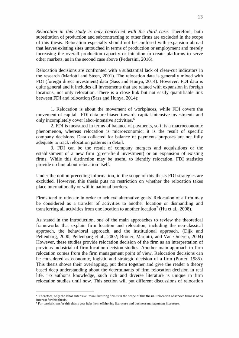
Abstract

Application of Tiebout model to firms remains unclear in previous studies. Although some research has been devoted to the firm relocation and Tiebout-model separately, rather less attention has been specifically paid to the spatial mobility of firms in Tiebout-model. This dissertation examines whether Tiebout-model can be applied to firms or not. The author uses spatial margins to profitability model as intermediate tool to derive the firm’s spatial mobility pattern on a Tiebout-model graph for the firm. In this study, graphical analysis reveals that household and firm have the same spatial mobility pattern in Tiebout-model to sustain their maximum utility or profit level. Thus, this thesis confirms that application of Tiebout-model to firm is possible, yet restrictions and assumptions should be borne in mind. The analysis also revealed the significance of moving costs. For further research investigating the effect of moving costs as well as transaction costs would contribute to a better understanding of firm relocation behavior.

5

1. Introduction

Tiebout-model’s objective was to think of a way to achieve efficient public-goods provision and to characterize the specific conditions under which it can work. Tiebout assumed that households choose where to reside only by taking into account of their utility level. According to Tiebout (1956) the utility of the households is only given by the difference between the benefits from public services they enjoy and tax burden they will bear. If there are many autonomous communities, each with a unique bundle of tax-service package, individuals will select to locate in the one that gives them the highest utility. In essence, individuals “shop”, move, between communities and “buy” the best tax-service bundle for them (Fischel, 1992). “Thus, spatial mobility provides the local public-goods counterpart to the private market’s shopping trip” (Tiebout 1956). This analogy with private markets is important because Tiebout-model avoids the preference revelation problem in public good provision and hypothesizes that individual’s preference is revealed by his mobility pattern between locations and by his decision where to reside (Cowen, 1992).

Inherently, moving between communities avoid the free-rider problem because household could get the utility from the unique services of a particular community only if he resides there. He can only use the bundles of services if he lives in that community and pays the taxes he is subject to. According to Tiebout, if a change happens and individual does not like the tax-service bundle in his current location and maximum utility is only attainable at another location, he will move there. Therefore, moving between communities will function as a revealing tool of the individual’s preference of public goods in the same way that price functions as a revealing tool of the individual’s preference for a private good in the market.

Tiebout (1956) credits nearly 11,500 citations, ranking among the most cited articles in economics. By comparison, the works related to Tiebout’s paper, Samuelson (1954) credits fewer than 6,000, while Musgrave (1959) owns around 5,000 citations (Singleton, 2015). While the main interest of these papers is contributing to public economics and specifically the problem of optimal equilibrium of allocation of public goods, this thesis instead only focuses only on the essence of Tiebout-model: Spatial mobility1 is tool to solve an economic problem.

Tiebout (1956) applies the model only on the one type of the economic agent: the household. Movement of firms has not been investigated in the original Tiebout-model. This thesis aims to fill this gap of the original paper and asks whether Tiebout model can also be applied to firms or not.

1 In this thesis, terms spatial mobility, relocation, moving, movement and migration are used interchangeably, all are meaning of a move from one location to another.

6

Firms tend to stay in their location for all their life whereas economic environment is always dynamic. There are never-ending changes in markets, preferences of consumers, environmental regulations and technological processes. Therefore, it should be that firm’s profit level is constantly changing. Thus, firms find themselves in a constant process of adjusting to new situations. If firms do not or cannot adapt to new advantages or disadvantages, it is less likely that they survive (Cowling and Lee, 2014). Instead of any other adjusting strategy, as Tiebout-model uses spatial mobility for households; thesis uses spatial mobility as only tool to solve the firm’s problem to adjust changes in its environment. This thesis founds its arguments on the fact that firm’s main motivation to adjust changes in its environment, thus motivation to relocate, is so sustain to maximum profits2. This is an exact analogy to the rationale of household’s relocation decision in the original paper –household relocates to sustain their maximum utility. Thus, the hypothesis of the thesis as follows: Every time a positive difference occurs in the profit level (revenue-costs) between firm’s current location and other locations, rather than applying other strategies, it will move to the new maximum profit location. To achieve profit maximization, this thesis finds that firm follows the cost-minimization strategy. The main aim of this paper is to investigate the movement pattern of the firm relocation decision under this hypothesis and check its applicability to Tiebout-model. To answer the main research task and hypothesis, this thesis will pursue five sub-questions: 1) What is the movement pattern of households in Tiebout-model? 2) What conditions may motivate or force firms to decide to change their location? 3) Which models can be used as an intermediate tool to introduce firm relocation decision on Tiebout-model? 4) What is the moving pattern of the firm? 5) Are moving patterns of the firm and household in Tiebout-model the same? This thesis combines Smith (1966)’s spatial margins to profitability model with Tiebout-model to show the changes in firm’s environment and its spatial mobility reaction. From the author’s point of view spatial margins to profitability model is a good tool to introduce the dynamism of the firm’s continuous maximum profit location change in the simplest way. This model is also a good base to introduce a wider set of determinants of firm relocation easily. This study, to my knowledge, thus will be the first one that gives theoretical explanatory analysis on the firm’s relocation decision in the light of Tiebout’s original paper by using the spatial margins to profitability model.3

3 Oddou (2015) discussed the firm relocation purely in the Tiebout-world, but he did it only considering the tax and expenditure patterns. Discussions in this thesis are more diverse and multidisciplinary

7

In the previous research, firms in Tiebout-model have been discussed (McGuire 1983; White, 1986; Oddou, 2015) but these discussions rather focus on general equilibrium of firm locations under governmental tax incentives. They lack focus on the firm itself. Relocation decision of a firm concerns several factors including government incentive packages, but determinants of firm relocation may go beyond the influence of these incentives (Carlsen, Langset, and Rattso, 2005; Deller, Conroy and Tsvetkova 2015). Different analytic approaches suggest different determinants to firm’s location choice. Neoclassical approach considers production factors and their costs as main determinants that affect the relocation of firms (Alkay, 2010). Institutional approach emphasizes the role of government and fiscal policy as well as the bargaining power of large firms with them. Neoclassical and institutional factors give out complementary conclusions. (Dijk and Pellenbarg, 2000) Behavioral approach suggests rather difficult to quantify factors, such as risk and uncertainity, imperfect information and decision maker’s bounded reality. (Brouer, Mariotti and Van Omeren, 2004) Investigating only the effects of governmental incentives on firm relocation decision provides the reader rather a narrow opinion on firm’s relocation behavior. This thesis follows a wider approach to firm relocation decision and collects arguments from different perspectives. To author’s knowledge, such diverse background has not been discussed in the previous research before. This thesis attributes to the firm relocation literature by putting the managerial and economical aspects of the firm theory together in one model. Thus, the contribution of the thesis to literature is twofold. First fold contributes to the firm relocation studies and second fold contributes to the firm’s mobility behavior in Tiebout-model. There have been many studies that focus on firm location but there have been few studies that focus on firm relocation. A curios follower of economics studies might argue that there is plenty of firm relocation research. Yet, big number of these studies focuses on branching or foreign direct investments rather than relocation itself (Sass and Hunya, 2014, Pedersini 2016). Event though FDI and branching studies are similar to the relocation phenomena, they are not exactly the same: they do not include complete movement of one, some or all activities of a firm from one location to another (Pedersini, 2016). FDI is rather extensions of activities at other locations.4 Thus, there is not much research on firm relocation that focus on complete transfer of firm’s activities from one place to another. This thesis also aims to fill this gap. To author’s knowledge such diverse theoretical explanation to firm relocation has not been given in any study before. This study shows that Tiebout-model is applicable to firm relocation decision, yet it is very sensitive to restriction and assumptions. The analysis of this thesis finds that firms always tend to move locations which offer least-costs however they have to consider the significant moving costs. If the perfect information assumption, the core

4 However, some aspects of the offshoring include relocation of the firm (Roza, Bosch and Volberda, 2011). Thus, aspects of offshoring, which are related with relocation, are also in the scope of this thesis.

8

of the competitive market, holds true the firm is able to compute all the moving costs. Only under perfect information condition, firms can compare the monetary benefits of moving to lower-cost location and the costs of moving, then could exactly decide either moving or staying at the current station is more profitable. If perfect information assumption does not hold and if the firm behaves with other motives than profit maximization, the application of Tiebout-model to firm relocation is not possible. The rest of the paper is organized as follows. Section 2 explains the Tiebout-model in detail. Section 3 gives an overview of the literature on the firm relocation reveals the foundations of the model of the thesis. Section 4 explains the model of the thesis and graphically analyses the firm movement pattern. It also explains what arguments are delineated in the scope of the thesis. Section 5 concludes the findings of the thesis and makes suggestions for further research. 2. Tiebout-model Tiebout-model of competition is an important and controversial one in economics (Teske et.al., 1993) In a Tiebout-world, economic activities are formed between three types of economic agents: an autonomous government of a community, households and firms. Thus a region would like to host the optimal number of households and firms to achieve a desired level of wealth. Therefore, an administration has to offer attractive opportunities to economic agents. On the other hand, if a locality realizes that it has more than the optimal number of economic agents and diseconomies are arising, then it will introduce tools to scare the current or future economic agents out of the region (White, 1986) Tiebout assumes that, for the household, locations are consisted of only of two surfaces: the tax-surface and the social expenditure-surface. In a Tiebout-world, a locality sells its social services to the household with a tax rate. Revenue for the locality comes from the taxes it collects. In return, it spends a part of this revenue back to offer services to its residents. This is called the social expenditure level of the locality. If we divide the total social expenditure level to the number of residents living there, we will get the expenditure that is assigned to a single household. For the household, tax functions like as the price. Household pays the tax to locality and in return he uses public service. Therefore, the utility of the household in the Tiebout-model is the difference between these two surfaces; the social expenditure level that is assigned to him and the tax rate he pays. Thus in Tiebout-world each locality has a unique tax and social expenditure pattern that reflects the preference of its citizens (Tiebout, 1956). For the households, the higher the difference between these two surfaces is the higher is the utility.

9

Hereby, introducing the following notations 𝑖𝑖 = 𝑙𝑙𝑜𝑜𝑜𝑜𝑜𝑜𝑙𝑙𝑖𝑖𝑜𝑜𝑜𝑜 𝑥𝑥 = ℎ𝑜𝑜𝑜𝑜𝑜𝑜𝑜𝑜ℎ𝑜𝑜𝑙𝑙𝑜𝑜 𝐸𝐸𝑥𝑥𝑥𝑥 = 𝑜𝑜𝑥𝑥𝑒𝑒𝑜𝑜𝑒𝑒𝑜𝑜𝑖𝑖𝑜𝑜𝑜𝑜𝑒𝑒𝑜𝑜 𝑒𝑒𝑜𝑜𝑒𝑒 ℎ𝑜𝑜𝑜𝑜𝑜𝑜𝑜𝑜ℎ𝑜𝑜𝑙𝑙𝑜𝑜 𝑖𝑖𝑒𝑒 𝑙𝑙𝑜𝑜𝑜𝑜𝑜𝑜𝑙𝑙𝑖𝑖𝑜𝑜𝑜𝑜 𝐸𝐸𝑎𝑎 = 𝑜𝑜𝑎𝑎𝑜𝑜𝑒𝑒𝑜𝑜𝑎𝑎𝑜𝑜 𝑜𝑜𝑥𝑥𝑒𝑒𝑜𝑜𝑒𝑒𝑜𝑜𝑖𝑖𝑜𝑜𝑜𝑜𝑒𝑒𝑜𝑜 𝑙𝑙𝑜𝑜𝑎𝑎𝑜𝑜𝑙𝑙 𝑜𝑜𝑜𝑜 𝑜𝑜𝑙𝑙𝑙𝑙 𝑙𝑙𝑜𝑜𝑜𝑜𝑜𝑜𝑙𝑙𝑖𝑖𝑜𝑜𝑖𝑖𝑜𝑜𝑜𝑜 𝑒𝑒𝑜𝑜𝑒𝑒 𝑜𝑜𝑒𝑒𝑜𝑜 ℎ𝑜𝑜𝑜𝑜𝑜𝑜𝑜𝑜ℎ𝑜𝑜𝑙𝑙𝑜𝑜 𝑜𝑜𝑥𝑥 = 𝑜𝑜𝑜𝑜𝑥𝑥 𝑒𝑒𝑜𝑜𝑜𝑜𝑜𝑜 𝑖𝑖𝑒𝑒 𝑙𝑙𝑜𝑜𝑜𝑜𝑜𝑜𝑙𝑙𝑖𝑖𝑜𝑜𝑜𝑜 𝑖𝑖 𝑜𝑜𝑎𝑎 = 𝑜𝑜𝑎𝑎𝑜𝑜𝑒𝑒𝑜𝑜𝑎𝑎𝑜𝑜 𝑜𝑜𝑜𝑜𝑥𝑥 𝑒𝑒𝑜𝑜𝑜𝑜𝑜𝑜 𝑙𝑙𝑜𝑜𝑎𝑎𝑜𝑜𝑙𝑙 𝑜𝑜𝑜𝑜 𝑜𝑜𝑙𝑙𝑙𝑙 𝑙𝑙𝑜𝑜𝑜𝑜𝑜𝑜𝑙𝑙𝑖𝑖𝑜𝑜𝑖𝑖𝑜𝑜𝑜𝑜 𝑜𝑜𝑥𝑥𝑥𝑥 = ℎ𝑜𝑜𝑜𝑜𝑜𝑜𝑜𝑜ℎ𝑜𝑜𝑙𝑙𝑜𝑜′𝑜𝑜 𝑖𝑖𝑒𝑒𝑜𝑜𝑜𝑜𝑖𝑖𝑜𝑜 𝑖𝑖𝑒𝑒 𝑙𝑙𝑜𝑜𝑜𝑜𝑜𝑜𝑙𝑙𝑖𝑖𝑜𝑜𝑜𝑜 𝑖𝑖 𝑜𝑜𝑎𝑎 = 𝑜𝑜𝑎𝑎𝑜𝑜𝑒𝑒𝑜𝑜𝑎𝑎𝑜𝑜 𝑖𝑖𝑒𝑒𝑜𝑜𝑜𝑜𝑖𝑖𝑜𝑜 𝑙𝑙𝑜𝑜𝑎𝑎𝑜𝑜𝑙𝑙 𝑜𝑜𝑜𝑜 ℎ𝑜𝑜𝑜𝑜𝑜𝑜𝑜𝑜ℎ𝑜𝑜𝑙𝑙𝑜𝑜𝑜𝑜 𝑁𝑁𝑥𝑥 = 𝑒𝑒𝑜𝑜𝑖𝑖𝑛𝑛𝑜𝑜𝑒𝑒 𝑜𝑜𝑜𝑜 𝑒𝑒𝑜𝑜𝑜𝑜𝑒𝑒𝑙𝑙𝑜𝑜 𝑖𝑖𝑒𝑒 𝑙𝑙𝑜𝑜𝑜𝑜𝑜𝑜𝑙𝑙𝑖𝑖𝑜𝑜𝑜𝑜 𝑖𝑖 𝑌𝑌𝑥𝑥 = 𝑜𝑜𝑜𝑜𝑜𝑜𝑜𝑜𝑙𝑙 𝑖𝑖𝑒𝑒𝑜𝑜𝑜𝑜𝑖𝑖𝑜𝑜 𝑖𝑖𝑒𝑒 𝑙𝑙𝑜𝑜𝑜𝑜𝑜𝑜𝑙𝑙𝑖𝑖𝑜𝑜𝑜𝑜 𝑖𝑖 𝑈𝑈𝑥𝑥𝑥𝑥 = 𝑜𝑜𝑜𝑜𝑖𝑖𝑙𝑙𝑖𝑖𝑜𝑜𝑜𝑜 𝑙𝑙𝑜𝑜𝑎𝑎𝑜𝑜𝑙𝑙 𝑜𝑜𝑜𝑜 𝑜𝑜ℎ𝑜𝑜 ℎ𝑜𝑜𝑜𝑜𝑜𝑜𝑜𝑜ℎ𝑜𝑜𝑙𝑙𝑜𝑜 𝑥𝑥 𝑖𝑖𝑒𝑒 𝑙𝑙𝑜𝑜𝑜𝑜𝑜𝑜𝑙𝑙𝑖𝑖𝑜𝑜𝑜𝑜 𝑖𝑖 From above, the expenditure per household can be reached by

𝐸𝐸𝑥𝑥𝑥𝑥 = 𝑡𝑡𝑖𝑖𝑌𝑌𝑖𝑖𝑁𝑁𝑖𝑖

(1)

And utility level for the household can be reached by 𝑈𝑈𝑥𝑥𝑥𝑥 = 𝐸𝐸𝑥𝑥𝑥𝑥 − 𝑜𝑜𝑥𝑥𝑜𝑜𝑥𝑥𝑥𝑥 (2)

by substitution of 𝐸𝐸𝑥𝑥𝑥𝑥 into the utility function, we get

𝑈𝑈𝑥𝑥𝑥𝑥 = 𝑜𝑜𝑥𝑥 �𝑌𝑌𝑖𝑖𝑁𝑁𝑖𝑖− 𝑜𝑜𝑥𝑥𝑥𝑥� (3)

To maximize their utility, in the light of the utility formula given above, individuals choose their place of residence according to a trade between local tax rates and amount of expenditure assigned. The conditions under which Tiebout believed this mechanism would work perfectly is set by the assumptions (Tiebout, 1956):

1) Consumer-voters are fully mobile and will move to that community where their preferences are best satisfied.

2) Consumer-voters are assumed to have full knowledge of differences among tax levels and expenditure patterns of communities and to react to these differences. 3) There are many communities from which to choose. 4) There are no restrictions or limitations on consumer mobility due to employment opportunities. 5) There are no spillovers of public service benefits or taxes among communities. 6) Each community, directed by a manager, attempts to attract the right size population to take advantage of scale economies –that is, to reach the minimum average cost of producing public goods. Therefore, in the light of the assumptions above, the essence of the Tiebout-model could be could be stated as: every time a positive difference occurs in utility level (tax-expenditure bundle) between household’s current location and other locations, rather than simply being dissatisfied, household will move to the new maximum utility location (Mars and Kay, 2006). Yet ‘…the costs of moving from community to community should be recognized’ (Tiebout, 1956).

10

Households may move for a variety of reasons, however, Tiebout restricts the determinants of relocation decision to only one factor: utility level change of the household –that is the change in expenditure level-tax rate level.5 The core of the Tiebout-model comes from perfectly informed and perfectly mobile households whose principal reason for moving is to maximize their utility. If we want to obtain a moving condition of a household from location i to j, then it requires

𝑈𝑈𝑥𝑥𝑥𝑥 > 𝑈𝑈𝑥𝑥𝑥𝑥 (4) then from (2) we get moving condition as

𝑈𝑈𝑥𝑥𝑥𝑥 = 𝐸𝐸𝑥𝑥 − 𝑜𝑜𝑥𝑥𝑜𝑜𝑥𝑥𝑥𝑥 > 𝑈𝑈𝑥𝑥𝑥𝑥 = 𝐸𝐸𝑥𝑥 − 𝑜𝑜𝑥𝑥𝑜𝑜𝑥𝑥𝑥𝑥 (5) or from (3) we get moving condition as

𝑜𝑜𝑥𝑥 �𝑌𝑌𝑗𝑗𝑁𝑁𝑗𝑗− 𝑜𝑜𝑥𝑥𝑥𝑥 � > 𝑜𝑜𝑥𝑥 �

𝑌𝑌𝑖𝑖𝑥𝑥− 𝑜𝑜𝑥𝑥𝑥𝑥� (6)

Under the assumption of full information households can perfectly compute average level of expenditure level (Ea) and average level of tax rate (ta) among localities and rank them according to his preference. Then he will reveal this preference simply and only by moving between locations, especially when he does not have the maximum utility with respect to his preference at the current location: There will be locations where 𝐸𝐸𝑥𝑥𝑥𝑥≥𝐸𝐸𝑎𝑎 and 𝑜𝑜𝑥𝑥≥𝑜𝑜𝑎𝑎, let’s call this Quadrant I There will be locations where 𝐸𝐸𝑥𝑥𝑥𝑥≥𝐸𝐸𝑎𝑎 and 𝑜𝑜𝑥𝑥≤𝑜𝑜𝑎𝑎, let’s call this Quadrant II There will be location where 𝐸𝐸𝑥𝑥𝑥𝑥 ≤ 𝐸𝐸𝑎𝑎and 𝑜𝑜𝑥𝑥≥𝑜𝑜𝑎𝑎, let’s call this Quadrant III There will be locations where 𝐸𝐸𝑥𝑥𝑥𝑥 ≤ 𝐸𝐸𝑎𝑎 and 𝑜𝑜𝑥𝑥≤𝑜𝑜𝑎𝑎 let’s call this Quadrant IV Graph 1: Tiebout-model graph for household 𝑇𝑇𝑜𝑜𝑥𝑥 𝐸𝐸𝑎𝑎 tax=expenditure line (zero utility line) I (Ib) IV (Ia) 𝑜𝑜𝑎𝑎 (IIIa) III II (IIIb) Expenditure *Source: Authors’s own graph 5 As Tiebout restricts the household’s motivation for mobility into one factor: utility maximization; author restricts the firm movement into one factor: profit maximization.

A

11

A careful examination of this graph will give the reader important insights. At the location A, where Ea and ta intersects each other (where Ea=ta) the household is indifferent to reside at any location. Therefore, we could get good insights about the household’s location decision between different regions if we look at the household from that neutral location. For poor household 𝑜𝑜𝑥𝑥𝑥𝑥 = 𝑜𝑜𝑥𝑥𝑥𝑥 = 0, thus from (6) the moving condition for poor household will be 𝑜𝑜𝑥𝑥(

𝑦𝑦𝑥𝑥𝑖𝑖𝑁𝑁𝑖𝑖

) > 𝑜𝑜𝑥𝑥(𝑦𝑦𝑥𝑥𝑥𝑥𝑁𝑁𝑥𝑥

) From this condition, it could be concluded that the movement pattern of the poor household would be rightwards and from this neutral point especially to quadrant I, where expenditure level and tax level is comparably higher. For a poor household, he would like to settle at locations where he would get more social expenditure to outweigh his low income. Therefore, we expect that a poor household would like to settle at quadrants where social expenditure level is comparably higher than the average. Thus, a poor household would prefer moving to quadrants I. It may come interesting to reader is that, poor households would like to move to quadrant I where taxes are high, but since they have very low income, poor households may not be so interested how much tax they pay. If they receive higher levels of social expenditure that will outweigh their low income purchase power. Therefore, in real life expect that poor people tend to cluster in quadrant I where actually higher income people who are willing to pay high taxes are living. Big cities are good examples for quadrant I. For average income household �𝑦𝑦𝑥𝑥𝑖𝑖

𝑁𝑁𝑖𝑖� = (𝑦𝑦𝑥𝑥𝑥𝑥

𝑁𝑁𝑥𝑥), thus

From (6) the moving condition for the average income will be 𝑜𝑜𝑥𝑥 �

𝑦𝑦𝑥𝑥𝑖𝑖𝑁𝑁𝑖𝑖− 𝑦𝑦𝑥𝑥𝑥𝑥

𝑁𝑁𝑥𝑥� > 𝑜𝑜𝑥𝑥(𝑦𝑦𝑥𝑥𝑥𝑥

𝑁𝑁𝑥𝑥− 𝑦𝑦𝑥𝑥𝑥𝑥

𝑁𝑁𝑥𝑥), thus simply �𝑦𝑦𝑥𝑥𝑖𝑖

𝑁𝑁𝑖𝑖� > 𝑦𝑦𝑥𝑥𝑥𝑥

𝑁𝑁𝑥𝑥

this situation for average income household is very analogical to the poor household’s situation above. Average income household’s movement pattern also will be rightwards. However, since income is higher than the poor people, he would not prefer as high tax rates as poor households. Therefore, they may tend to move to quadrant II in addition to quadrant I. Therefore, average income household’s movement pattern will may also show a downward pattern in addition to a rightward pattern. For rich households, the moving condition from following (6) will be

𝑜𝑜𝑥𝑥<𝑡𝑡𝑥𝑥(𝑦𝑦𝑥𝑥𝑥𝑥𝑁𝑁𝑥𝑥

−𝑦𝑦𝑥𝑥𝑥𝑥)

(𝑦𝑦𝑥𝑥𝑖𝑖𝑁𝑁𝑖𝑖−𝑦𝑦𝑥𝑥𝑖𝑖)

, thus simply 𝑜𝑜𝑥𝑥 < 𝑜𝑜𝑥𝑥

Rich households have high purchase power; thus they may not be so interested in social expenditure level but only in low tax rates. Since they can afford by themselves the benefits that social expenditure packages offer them, they may not be so interested in the high expenditure levels but paying less tax over their income. Therefore, rich households are expected to reside at quadrants III or II, where the tax rates are comparably lower. Thus, the movement pattern of the household will be downwards.

12

In the graph above, a careful reader might realize that quadrants I and III are divided into two-sub quadrants Ia, Ib and IIIa IIIb, respectively. The quadrants Ia and IIIa are the parts of the sub- quadrants where the taxes are higher than the expenditures. This apparently means that negative benefits. Therefore, as a utility maximizer, household would not stay at sub-quadrants Ia and IIIa as well as quadrant IV, where the taxes are higher than the expenditure level. Thus, core conclusions of the graph with respect to mobility of the households are two fold. First fold is that the household does not want reside at and move to the left side of the 45-degree zero utility (tax=expenditure) line. The second is, household’s movement pattern in Tiebout-model is rightwards and/or downwards. How about the firms? Can we expect that Tiebout-model is also applicable to firms and is it possible to come up with same insights of household’s movement pattern for the firm? To answer this question, in the next chapter some determinants of firm relocation in the previous research will be given. Literature review will give overview about the foundations of firm’s main relocation determinants and motivations. Insights from the literature review will be used in section 4 to check if Tiebout-model is compatible with these determinants and motivations. 3. Determinants of firm relocation: Literature review of a complex phenomenon Relocation of production is often treated as a straightforward issue. However, in reality it is quite a complex phenomenon. Therefore, it is better to consider relocation as a one of the effects of other dynamics instead of considering it as a process in its own. As will be revealed in the following pages, even data collection is quite difficult because transfers of firm activities are hidden in the broader data on foreign direct investment. Most discussions about relocation rely on questionnaires (Lloyd and Mason, 1978; Wissen, 2002) and not on empirical data. Therefore, this thesis does not incorporate an empirical model. It looks to the firm relocation from a theoretical point of view. Individual cases of relocation can occur in quite different situations that may be classified by three circumstances (Pedersini, 2016):

1. Production is replaced by imports from foreign competitors or from domestic producers relocated abroad (or sometimes domestic producers subcontracting to foreign firms)

2. A reorganization of company, whose production activities, as well as investments, are allocated among different plants. This kind of production relocation decisions may depend on the company structure and on the opportunities provided by local conditions. (For example, due to low sunk costs, some locations can enjoy the high concentration of the production activities in time whereas same activities can continue at pre-existing facilities in the original location in small concentrations. This can be described as production concentration interchange between different existing facilities in different locations. This decision making pattern can be applied to a company restructuring its production within national or international boundaries.

3. A decision to discontinue production at one, some or all sites and a complete transfer to a new one base at a different location.

13

Relocation in this study is only concerned with the third case. Therefore, both substitution of production and subcontracting to other firms are excluded in the scope of this thesis. Relocation especially should not be confused with expansion abroad that leaves existing sites untouched in terms of production or employment and merely increasing the overall production capacity or intention to create platforms to serve other markets, as in the second case above (Pedersini, 2016). Relocation decisions are confronted with a substantial lack of clear-cut indicators in the research (Mariotti and Steen, 2001). The relocation data is generally mixed with FDI (foreign direct investment) data (Sass and Hunya, 2014). However, FDI data is quite general and it includes all investments that are related with expansion in foreign locations, not only relocation. There is a close link but not easily quantifiable link between FDI and relocation (Sass and Hunya, 2014):

1. Relocation is about the movement of workplaces, while FDI covers the movement of capital. FDI data are biased towards capital-intensive investments and only incompletely cover labor-intensive activities.6

2. FDI is measured in terms of balance of payments, so it is a macroeconomic phenomenon, whereas relocation is microeconomic; it is the result of specific company decisions. Data collected for balance of payments purposes are not fully adequate to track relocation patterns in detail.

3. FDI can be the result of company mergers and acquisitions or the establishment of a new firm (green-field investment) or an expansion of existing firms. While this distinction may be useful to identify relocation, FDI statistics provide no hint about relocation itself. Under the notion preceding information, in the scope of this thesis FDI strategies are excluded. However, this thesis puts no restriction on whether the relocation takes place internationally or within national borders. Firms tend to relocate in order to achieve alternative goals. Relocation of a firm may be considered as a transfer of activities to another location or dismantling and transferring all activities from one location to another location7 (Hu et al., 2008). As stated in the introduction, one of the main approaches to review the theoretical frameworks that explain firm location and relocation, including the neo-classical approach, the behavioral approach, and the institutional approach. (Dijk and Pellenbarg, 2000; Pellenbarg et al., 2002; Brouer, Mariotti, and Van Omeren, 2004) However, these studies provide relocation decision of the firm as an interpretation of previous industrial of firm location decision studies. Another main approach to firm relocation comes from the firm management point of view. Relocation decisions can be considered as economic, logistic and strategic decision of a firm (Porter, 1985). This thesis shows their overlapping, put them together and give the reader a theory based deep understanding about the determinants of firm relocation decision in real life. To author’s knowledge, such rich and diverse literature is unique in firm relocation studies until now. This section will put different discussions of relocation

6 Therefore, only the labor-intensive- manufacturing firm is in the scope of this thesis. Relocation of service firms is of no interest for this thesis. 7 For partial transfer this thesis gets help from offshoring literature and business management literature.

14

literature all together and find them overlapping in one coherent consistent theoretical explanation under cost-minimizing behavior of the firm to maximize its profits. In the next chapter, this coherent theoretical explanation will be discussed on a graphical analysis and its applicability to Tiebout model will be answered. Research on firms’ relocation decisions has evolved over the past forty years. 1970s are considered as the golden age of firm relocation studies (Pellenbarg, et. al., 2002). Scholars from different disciplines investigated firm relocation under different approaches. Cost motives are often considered to be the most important driver for relocating (Anderson and Gatignon, 1986). However, other motives, such as acquiring human capital or firm growth (Dunning, 1980) are also mentioned in the literature. First of all, as firm’s internal environment driver, entrepreneurship can induce relocation decision (Brond and Pellenbarg, 2003). Research pointed out relocation as a strategy to realize growth by entering new markets (Meester, 2004). Entrepreneurship can motivate firms to attain new resource combinations beyond the existing ones (Fiet, 2001) Entrepreneurship is about carrying out new combinations and it implies the ability to identify new opportunities and to develop the resource base needed to pursue the opportunities (Phan, 2004) Entrepreneurship also reflects the desire of firms to grow, explore and expand the boundaries of the firm (Davidsson, 1989) relocating to new locations can be one of the strategies. The relocation of business functions makes it possible for firms to get closer to potential customers and other opportunities. Small firms might use relocation as entrepreneurial strategy more often than large firms. (Rothwell, 1989)8 However, relocation decision is not always within firm’’ own initiative. The relocation decision was called to adapt to dynamic changes in environments surrounding the firm in (Alkay, 2010) These changes may be external changes such in technology, production and transportation techniques. External changes may also include changes in business climate and government legislation (Deller, Conroy and Tsvetkova 2015) The competition among states and local governments to attract businesses (in an attempt to foster economic development) may also induce firms to relocate. The use of incentives to attract firms are associated with economic growth and development policy in the regional economics literature (Lowe, 2012) Incentives are in large variety: they can be reduced tax rates, labor training programs, tax credits to lower overall tax bills, aid in financing and credit programs, targeted public infrastructure investments and some other forms 9 (Deller, Conroy and Tsvetkova 2015). The theoretical foundation of use of incentives is related with neo-classic economic principle of minimizing costs in order to maximize profits. Incentives by governments are aimed at reducing costs to make a particular location more profitable over another location. Promoting lower labor costs, lower taxes, and limited regulations in the name of minimizing operating costs are so-called the pillars of a positive business climate. Policies aimed at reducing the cost of business operations by reducing taxes and regulations are said to promote a positive business climate (Glaeser, 2001).

8 Growth aims and other entrepreneurial drives of firm relocation are excluded in the model of this thesis. 9 For example, Tesla Motors was offered by State of Nevada $1.25 billion in incentives to locate its car battery manufacturing base, State of South Carolina offered a $150 million abatement to BWM and State of Alabama offered Mercedes-Benz $250 million to attract these firms (Deller, Conroy and Tsvetkova 2015)

15

Generally, regions with higher taxes and stricter regulations are said to have poorer business climates (Plaut and Pluta, 1987). Another factor related to a region’s business climate can be labor related characteristics (Pedersini, 2016) As measured by labor costs -average compensation of a manufacturer worker, union membership rates is considered to be related with the business climate. Firms will avoid locations10 with higher labor costs and union membership rates. Energy costs are also often put forward as an important component of the costs of operation and hence business climate. It is found that electricity costs are one of the few costs variables, relative to taxes or incentives consistently mentioned in location decisions of manufacturers (Carlton, 1983). Another key variable of firm relocation might be taxation and expenditure rates of local and national governments. If this point view holds true, it is expected that manufacturers will be attracted to locations with lower income taxes, lower individual income taxes, and lower property taxes. Yet, as argued by many there is a balance between the potential negative effects of taxation and the positive effect of the public goods and services that taxes pay for (Wasylenko 1981; Newman and Sullivan 1998; White 1986; Lynch 2004). Taxes pay for public education that is vital to the productivity of the workforce and pay for the transportation infrastructure that is necessary for manufacturing (Newman and Sullivan, 1998). However, some studies show that taxation and expenditure level of regions do not play important role on firm location decision especially in Tiebout-model (Bewley 1981, White 1986) The preceding paragraphs are mostly related to more to macroeconomic factors that affect firm’s relocation decision, except the entrepreneurship point of view. However, another important aspect of firm relocation is the firm itself, as a microeconomic agent. Thus far most studies have looked at the determinants of relocation without making a distinction between expansion investments and relocation decisions that involve the move of a manufacturing process from one place to another (Mucchielli and Saucier, 1997). Few studies have looked at the motives for relocation in such a strict sense. Straus-Kahn and Vives (2009) find that main reasons for the business relocation are cost savings regardless of whether the firm is a headquarter or a plant. Within a European context, Mucchielli and Saucier (1997) argue that restructuring, and flexible responses to new market conditions for innovative products are equally important motives for firm relocation. On the other hand, there may be historical, cultural and emotional as well as economic reasons for not moving one or more activities of a firm from one country to another. For example, the Swiss consumer goods company Nestle sells only two and half percent of their annual turnover in Switzerland yet maintains its headquarters in the homeland (Straus-Kahn and Vives, 2009). Global relocation takes place when a firm moves one or more business activities to a location outside its home country. When asked the firms to identify the motives for their global relocation efforts it is to pursue either low-cost strategy or differentiation strategy (Porter, 1985). Porter believes that a firm can pursue a low-cost strategy or a 10 It is not also expected that business would decide to operate at a location with higher levels of political conflict. Political conflict can add uncertainty and (Fukuyama, 1995)

16

differentiation strategy, but cannot pursue them both. If a firm chooses a low-cost strategy, then certain value chain activities will become more important in achieving this strategy. For example, a reduction in production costs may be achievable through better use of existing facilities, introduction of more advanced technologies or through relocation of activities to a lower cost (labor or other input) location. This thesis focuses only allows the latter strategy for the firm –that is relocation. The first two cost reduction strategies are excluded in the scope this thesis. Global relocation may also aid firms pursuing a differentiation strategy (Yip, 1994). Differentiation may come in various forms: better service, higher quality, advanced technology and other internal or external operation features. Relocation of certain activities may increase a firm's ability to achieve and sustain a differentiation strategy. For example, by moving marketing activities closer to final customers, firms may be able to differentiate their products or services more easily from their long distance competitors. Providing quicker delivery or service by locating closer to final users may create a differentiation advantage for the firm (Eenman and Brouthers, 1994). Finally, firms may use global relocation to take advantage of technologies developed in other countries by relocating part of their research operation to those countries that are more advanced in the competencies necessary to provide differentiation. (Porter, 1985) For example many Japanese firms are relocating their biotechnology research laboratories to the US because of the expertise already developed in that country. Similarly, many US electronics firms have relocated part of their research facilities to Japan where miniaturization technology is more advanced (Porter, 1985). Firms pursuing a differentiation strategy were expected to have motives such as quality seeking, technology seeking and reconfiguring core activities. Whereas, firms pursuing a low-cost strategy were expected to indicate motives such low cost seeking, risk reduction, or obtaining strategic flexibility (Eenman and Brouthers, 1994) The low-cost approach to global relocation research say that firms locate activities in major markets to serve those markets more economically and firms locate production activities in certain countries to obtain lower cost inputs such as labor or raw materials (Dunning, 1980; Ok and Tansel, 2007). Research found that the vast majority of relocating firms pursue a low-cost strategy. (Sleuwaegen and Pennings, 2006)11 The economic theory of global relocation is based on the rational profit-maximization assumption (Sleuwaegen and Pennings, 2006). On the other hand, the logistical (supply chain) perspectives of global relocation claim that firms have two main goals: first, firms desire to optimize the supply chain, thus obtaining inputs at the lowest possible cost. (McCormack et al., 1994) The resources firms seek at different locations may enable firms to perform activities in a cheaper way. Gaining access to personnel and technologies, for example, gives firms the opportunity to do existing things more efficient. Firm may also need to manage their growth by reaching to new resources by relocating (Jarillo, 1989). Smaller firms might search for resources relatively closely to their core activities, whereas corporate firms focus on resources more distant to their core activities as they have more possibilities to build their existing resources within their own firm. Secondly, firms want to optimize the logistical operations by minimizing transport costs to final customers –that is overall 11 Therefore, in the scope of this thesis, the analysis of differentiation strategy is not discussed. This thesis makes its analysis only on cost-reduction strategy.

17

distribution costs. Logistical (supply-chain) approach does consider the impact of relocation on corporate objectives nothing other than cost minimization. Nevertheless, logistics aspects and market demand aspects may often conflict because frequently the location of a low cost resource for a firm may be in an area which creates excessively high distribution costs because of its physical distance to final customers or because of the poor infrastructure, making physical movement of goods more expensive, in the low cost location (Min and Melachrinoudis, 1999). Still, the logistical explanation of relocation is similar to the neoclassical economic explanation in the belief that location decision is driven by a desire to maximize profits by minimizing costs. The difference between these two theories lies in the type of cost that the firm is trying to reduce: The economic theory aims to minimize the total production costs and logistical theory aims to minimize the overall (transportation) costs of inputs and outputs (Eenman and Brouthers, 1994). However, in the beginning of the twentieth century, the pioneer of the modern location theories, Alfred Weber already considered these two theories into one theory already. According to Weber (1929), total costs vary from place to mainly in accordance with transportation costs. Therefore, he assumes that the lowest-transport location for the firm is also the location where it can minimize its total costs. This point is also the optimal location for the firm where it can maximize its profits (Smith, 1966). Weber’s (1929) model is a perfect foundation to the aim of this thesis. This is due to two facts: First his model is an exact analogy with the Tiebout’s two surface economic environment: Tiebout only assumes a two-surface (tax and expenditure) economic environment for the household; and Weber only assumes a two-surface (revenue and costs) environment for the firm. Secondly the foundation of Weber’s model is based on the mainstream finding of the firm relocation studies until now: cost-minimizing behavior to maximize profits. However, Weber’s two-surface model is not enough to reply the hypothesis of the thesis because it is a static model. It does not consider the changes in the economic environment of the firm in time. Nevertheless, we need a dynamic model to investigate the spatial mobility behavior of the firm as sole reaction to the changes in its environment. Therefore, this thesis will use the Smith’s (1966) marginal spatiality to profits model that is derived from Weber’s model to graphically show the dynamism that is inherent in Tiebout-model. 4. The Model: Graphical Analysis of Firm in Tiebout-Model As is given in the literature review, since the availability of the data about firm relocation from one location to another is scarce, this model bases its model on a theoretical and graphical one. The literature review revealed that firm’s main motivation to relocate is to reach lower-cost locations to maximize profits. This thesis establishes its model on the notion that firm is profit-maximizer and has perfect information. Moreover, following the discussions in the last section, this thesis assumes that firm’s decision to change its location to maximize profits is based on the cost-minimizing behavior. All other behaviors are out of the scope of the model of this thesis.

18

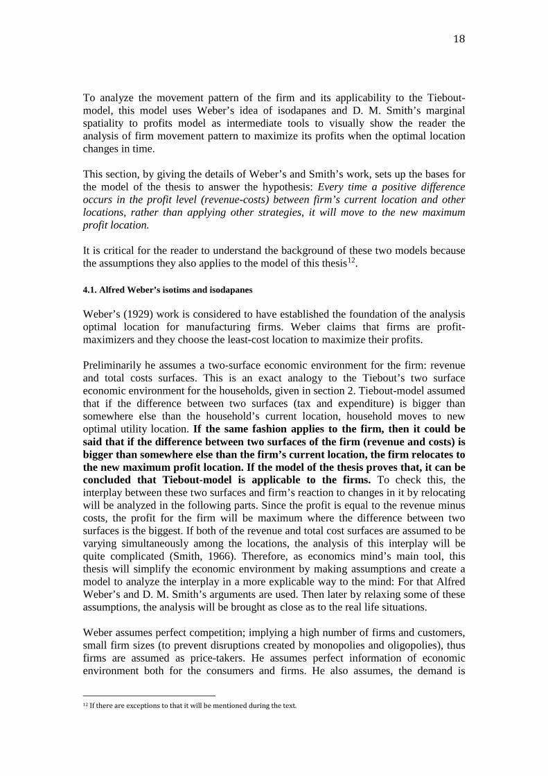
To analyze the movement pattern of the firm and its applicability to the Tiebout-model, this model uses Weber’s idea of isodapanes and D. M. Smith’s marginal spatiality to profits model as intermediate tools to visually show the reader the analysis of firm movement pattern to maximize its profits when the optimal location changes in time. This section, by giving the details of Weber’s and Smith’s work, sets up the bases for the model of the thesis to answer the hypothesis: Every time a positive difference occurs in the profit level (revenue-costs) between firm’s current location and other locations, rather than applying other strategies, it will move to the new maximum profit location. It is critical for the reader to understand the background of these two models because the assumptions they also applies to the model of this thesis12. 4.1. Alfred Weber’s isotims and isodapanes Weber’s (1929) work is considered to have established the foundation of the analysis optimal location for manufacturing firms. Weber claims that firms are profit-maximizers and they choose the least-cost location to maximize their profits. Preliminarily he assumes a two-surface economic environment for the firm: revenue and total costs surfaces. This is an exact analogy to the Tiebout’s two surface economic environment for the households, given in section 2. Tiebout-model assumed that if the difference between two surfaces (tax and expenditure) is bigger than somewhere else than the household’s current location, household moves to new optimal utility location. If the same fashion applies to the firm, then it could be said that if the difference between two surfaces of the firm (revenue and costs) is bigger than somewhere else than the firm’s current location, the firm relocates to the new maximum profit location. If the model of the thesis proves that, it can be concluded that Tiebout-model is applicable to the firms. To check this, the interplay between these two surfaces and firm’s reaction to changes in it by relocating will be analyzed in the following parts. Since the profit is equal to the revenue minus costs, the profit for the firm will be maximum where the difference between two surfaces is the biggest. If both of the revenue and total cost surfaces are assumed to be varying simultaneously among the locations, the analysis of this interplay will be quite complicated (Smith, 1966). Therefore, as economics mind’s main tool, this thesis will simplify the economic environment by making assumptions and create a model to analyze the interplay in a more explicable way to the mind: For that Alfred Weber’s and D. M. Smith’s arguments are used. Then later by relaxing some of these assumptions, the analysis will be brought as close as to the real life situations. Weber assumes perfect competition; implying a high number of firms and customers, small firm sizes (to prevent disruptions created by monopolies and oligopolies), thus firms are assumed as price-takers. He assumes perfect information of economic environment both for the consumers and firms. He also assumes, the demand is

12 If there are exceptions to that it will be mentioned during the text.

19

uniform throughout the locations, making the production level (quantity) for the firm fixed at all locations13. Hence, by making price, demand and output constant, he gets the revenue surface flat and the other surface -the cost surface- still varying. The interplay between two surfaces (revenue-cost) and the firm is easier to analyze now: Since the revenue surface is flat, firm’s profit level will only vary with the variations of cost surface. In these conditions, apparently firm’s profit will be at the location where the cost surface is the lowest. So how do costs vary from one location to another? According to Weber, costs vary from place to place largely in accordance with transportation costs (Smith, 1966). He theorizes that, firm’s least-transportation-cost-location is also its least-cost-location: this location is also the optimal location for the firm which gives the maximum profits under assumptions given above. Weber assumes an isotropic space (Becattini, 1990, Felix 2015) –that is; he assumes no variations of production costs except in transport costs: Some of the natural resources are found everywhere (ubiquitous), while some have fixed locations. Labor could only be found at some fixed locations. Transportation costs, in Weber’s model, are proportional to the weight of goods and distance covered by a raw material or a finished product. According to Weber -under these assumptions and conditions- three factors influence optimal location; transportation costs, labor costs and agglomeration economies. According to him, the firm will first find the least-transport cost location and then adjusts its location by considering labor costs and agglomeration economies. Weber considers that transportation is the most important element to decide the optimal (maximum profit) location since labor and agglomeration economies factors only have the adjustment effect.14 In order to identify points of least cost location for a manufacturing firm Weber devised a useful technique by isotim lines and isodapanes (Waugh 2002, p. 560) Isotim is a line of connecting locations of equal transportation costs. Isotim lines can be drawn to show how procurement transport costs change with distance from raw material sources at one hand and at the other hand how distribution transport costs change with distance from the market. Weber first finds the minimum transportation cost (MTC) location by using isotims. Then shows the affect of labor cost and agglomeration economies by using isodapanes. Intersecting isotims for multiple materials and products allow isodapanes to be drawn by connecting the points of intersection (Waugh 2002, p 560) Thus, an isodapane is called a line of total transport costs. The isodapanes (equal combined total transportation cost lines) progressively decrease in the direction of the optimal location, as seen in Figure 1. Weber used isodapanes is to systematically introduce the production factor and other cost factors components into firm’s location decision.

13 However, in theoretical analysis the simplifying assumption of constant demand conditions must always be borne in mind, and the possibility of spatial variations in the size of the potential market must always be considered in the interpretation of specific cases. (Smith, 1966) 14 In the scope this master thesis, I will assume that agglomeration economies do not exist. Further explanation will be given in the following parts.

20

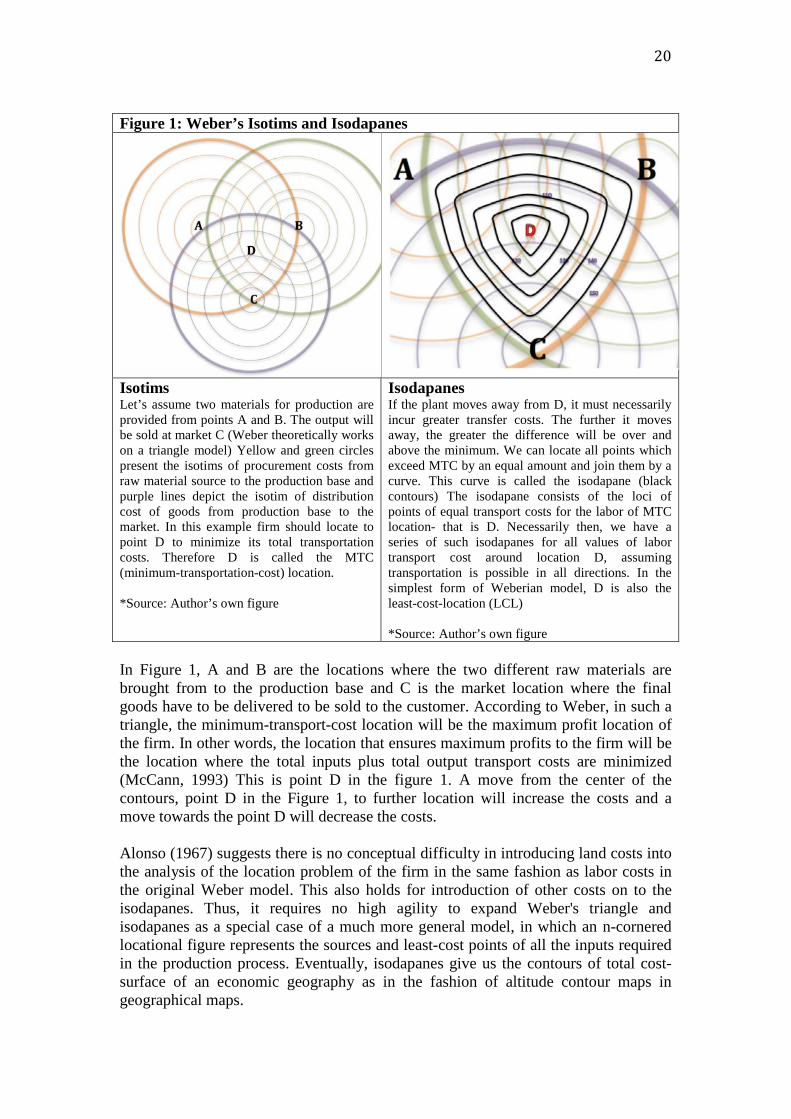
Figure 1: Weber’s Isotims and Isodapanes

Isotims Let’s assume two materials for production are provided from points A and B. The output will be sold at market C (Weber theoretically works on a triangle model) Yellow and green circles present the isotims of procurement costs from raw material source to the production base and purple lines depict the isotim of distribution cost of goods from production base to the market. In this example firm should locate to point D to minimize its total transportation costs. Therefore D is called the MTC (minimum-transportation-cost) location. *Source: Author’s own figure

Isodapanes If the plant moves away from D, it must necessarily incur greater transfer costs. The further it moves away, the greater the difference will be over and above the minimum. We can locate all points which exceed MTC by an equal amount and join them by a curve. This curve is called the isodapane (black contours) The isodapane consists of the loci of points of equal transport costs for the labor of MTC location- that is D. Necessarily then, we have a series of such isodapanes for all values of labor transport cost around location D, assuming transportation is possible in all directions. In the simplest form of Weberian model, D is also the least-cost-location (LCL) *Source: Author’s own figure

In Figure 1, A and B are the locations where the two different raw materials are brought from to the production base and C is the market location where the final goods have to be delivered to be sold to the customer. According to Weber, in such a triangle, the minimum-transport-cost location will be the maximum profit location of the firm. In other words, the location that ensures maximum profits to the firm will be the location where the total inputs plus total output transport costs are minimized (McCann, 1993) This is point D in the figure 1. A move from the center of the contours, point D in the Figure 1, to further location will increase the costs and a move towards the point D will decrease the costs. Alonso (1967) suggests there is no conceptual difficulty in introducing land costs into the analysis of the location problem of the firm in the same fashion as labor costs in the original Weber model. This also holds for introduction of other costs on to the isodapanes. Thus, it requires no high agility to expand Weber's triangle and isodapanes as a special case of a much more general model, in which an n-cornered locational figure represents the sources and least-cost points of all the inputs required in the production process. Eventually, isodapanes give us the contours of total cost-surface of an economic geography as in the fashion of altitude contour maps in geographical maps.

21

Like, Weber (1929) the earliest location theorist (Hotelling 1929, Lösch 1954 and Issard 1960) tried to explain the determinants of the location choices of industrial firms in different ways 15. However, none of these classical models hypothesizes that once the firm has analyzed its minimum cost location, settled and started operating there, it will consider the possibility of moving. According to these theories if the current chosen location of the firm is the minimum cost location, why some firms have intentions to relocate? What could be the emerging factors of relocation decision? The previous literature part has given a diverse overview to what can motivate or force firms to relocate. In the next chapter, spatial margins to profitability graph in Smith (1966) is developed from Weber (1929) and the constant change of optimal location for the firm in time is shown, which is not showed by Weber (1929). By this contribution on Smith’s spatial margins to profitability graph, the author aims to show the reader insights about firm’s location behavior when its optimal location changes. Author will also use these graphical analyses to check whether Tiebout-model is applicable to the firm relocation pattern or not. 4.2. Spatial margins to profitability model Firms are constantly changing their input suppliers and output markets in response to changes in input and output market prices. Also increases in the production capacity and changes in the production technologies are the main changes that face firms face constantly. Firms also face with the changes that are mentioned in the literature review. These changes will also imply that the optimum location of the firms given in the static model of Weber (1929) is continually changing. This situation of firm is very analogical to the condition of household in the original Tiebout-model: every time a positive difference occurs in utility level between current location and other alternative locations, rather than simply being dissatisfied, household will move to the new optimum utility location. Therefore, to test the whether firm mobility is applicable to Tiebout-model, this thesis hypothesizes: Every time a positive difference occurs in the profit level (revenue-costs) between firm’s current location and other locations, rather than applying other strategies, it will move to the new maximum profit location. The model of this thesis will use spatial margins to profitability approach as an intermediate tool to show if its hypothesis holds true: Smith (1966) used the Weber’s (1929) notion of two surfaces (revenue and cost) for the firm and developed the idea of the spatial interaction of cost and revenue as a constraint on locational choice in a series of graphic models. Smith(1966) assumed a flat revenue surface and varying cost surface as in Weber (1929). By explaining how costs vary from one location to another, he wanted to get a space(locational) cost curve applicable to the entire –manufacturing- industry –therefore to each firm. For that he had to introduce more 15 It is accepted that there are two main approaches to optimal location theory: the least cost approach and market area approach. (Balchin, Isaac and Chen, 2000) Cost minimization theories offer answers to questions such as the following: given the price and location of the market and raw materials, where does the firm relocate? On the other side, market area approach (Hotelling 1929, Lösch 1954 and Issard 1960) seeks to answer these: Given spatial distribution of demand, how firms divide up the market? In this thesis, the discussions of market area approach are excluded.

22

assumptions on Weber (1929): firms do not influence each other's location, no location is subsidized and no advantages are to be derived from economies of scale within the firm and agglomeration economies. (Non-existence of agglomeration economies is also contrast to Weber’s assumptions and thesis will follow Smith’s assumption instead of Weber’s.) Eventually, Smith (1966) used Weber’s isodapanes and then he got cost space curve by taking a cross-section of isodapanes. By taking a cross-section of isodapanes with a flat price curve, he projected the cost-revenue surfaces of an economic geography on a two-dimensional graph and shows the variations of costs in different locations with respect to distance. [Graph 2: market price, demand and output is assumed to constant over the distance as in (Weber, 1929)] Graph 2: Deriving spatial margins to profitability graph from Weber’s isodapanes

isodapanes A B revenue curve Euros costs revenuejhjhjgjgjg A t q D u y B distance(km) *Source: Author’s own graph

Locations with loss (from q to A and further, from u to B and further) Locations with profits (between q and u)

23

Graph 2 above is a reflection of Weber’s isodapanes in Figure 116. A fixed output level assumption will make the shape of the revenue and total cost curves, also the price and unit cost curves respectively. Point D represents the minimum total cost location for the firm, therefore the maximum profit location. The further the firm is away from point D; the higher costs it has. Points q and u where cost curve intersects the price curve are the locations where firm makes zero profits, R=TC (where firms only break-even). Points q and u sets the points of spatial margins where firm can operate with profits but not always maximum. Firm will produce with positive profits in localities between locations q and u (D being the maximum profit location) but by moving outwards from these locations, firm will end up at localities where it can only operate at loss. If firm starts moving from locality q with zero profits towards locality u, at localities until D, its profits will gradually increase because its costs will gradually decrease. At locality D it will have the maximum profit, being the least-cost location. If the firm continues its movement from D to u, its profit will gradually decrease because its costs will gradually increase, however still being positive. At locality u firm will again have zero profits and at further locations it will start to have losses. This move is shown on the graph of firm’s Tiebout-model Graph 3 below. This depiction sets the bases of the graphical analysis of testing the hypothesis of thesis in the following pages.

Before that, It is useful to give some theoretical, how costs may vary from place to place as seen in the Graph 2: In order to produce a given quantity of any goods, the manufacturer must assemble at one point the necessary amount of the factors of production (that are land, labor, capital -including materials and machines- and enterprise). The cost of each of these is likely to vary from place to place. In considering the cost of factors of production it is useful to distinguish between basic cost and locational cost. The basic cost is the sum that must be paid irrespective of location, e.g. the cost of a raw material at source, or the cost of labor at its cheapest point. The locational cost is the additional expenditure incurred in bringing the factor to the production base, which varies according to where the factory is situated. Just as each factor of production has its basic and locational cost, so these two elements can be distinguished in the total cost of any firm or industry.

Spatial variations in total cost and revenue impose limits to the area in which any industry can be undertaken at a profit. A careful reader would easily realize that there are various locations where firm can operate with different levels of profits within the borders of profitable area. Smith’s main aim by introducing spatial margins to profitability is to show that, unless maximum profits are sought, the individual manufacturer is free to locate anywhere where it can make profits between the profitable margins- that are between location q and u in the given example. Smith (1966) claims since optimal location will always constantly change, firms cannot always be at the optimum location. It will settle any where in the borders of spatial margins to profitability area where it can make profits, not necessarily maximum, and the entrepreneur is fine with that unless he makes loses. With those depictions, Smith’s main idea was to show that firms cannot be profit-maximizers all the time, 16 Each of the cost contours represents the locations where firm faces the same total costs (Smith, 1966)

24

therefore firms in general behave sub-optimally until they start to operate with negative profits (Smith, 1966). Smith (1966) did not pursue his discussion anymore and left the further discussions to the reader. Thesis thesis now takes forward this discussion and challanges the idea that firm may settle at sub-optimal locations: As given before, this thesis hypothesized that firm will relocate everytime a new maximum profit location arises.

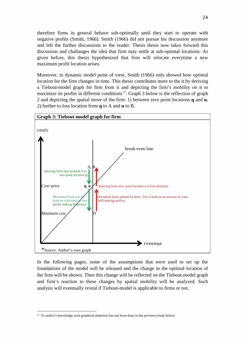
Moreover, in dynamic model point of view, Smith (1966) only showed how optimal location for the firm changes in time. This thesis contributes more to the it by deriving a Tiebout-model graph for firm from it and depicting the firm’s mobility on it to maximize its profits in different conditions17. Graph 3 below is the reflection of graph 2 and depicting the spatial move of the firm: 1) between zero point locations q and u. 2) further to loss location from q to A and u to B.

Graph 3: Tiebout-model graph for firm 𝑜𝑜𝑜𝑜𝑜𝑜𝑜𝑜𝑜𝑜 break-even line A, B (moving from loss location A to zero point location q)

Cost=price q, u (moving from zero point location u to loss location)

Movement from q to D Movement from optimal location D to u leads to an increase in costs leads to a decrease in cost (still making profits) (profit making locations) Minimum cost D 𝑒𝑒𝑜𝑜𝑎𝑎𝑜𝑜𝑒𝑒𝑜𝑜𝑜𝑜 *Source: Author’s own graph In the following pages, some of the assumptions that were used to set up the foundations of the model will be released and the change in the optimal location of the firm will be shown. Then this change will be reflected on the Tiebout-model graph and firm’s reaction to these changes by spatial mobility will be analyzed. Such analysis will eventually reveal if Tiebout-model is applicable to firms or not.

17 To author’s knowledge such graphical depiction has not been done in the previous study before.

25

Before graphical analyses it will be useful to mention assumptions and delineated arguments one more time to the reader to make the analysis clearer. 4.3. Delineated arguments Only the discussions of a small manufacturing firm’s 18 relocation decision are depicted in the graphical analysis in the next part. Relocation, in this study, only means that the firm stops its some or all production activities (if small firm grows it may have more than activities, which forces it to relocate) and transfers it to another location. Firm cannot adapt to changes by neither changing combination of its inputs nor changing its production technology at the current location; neither reducing its capacity nor applying any other alternative solutions19. In the thesis relocation is used as the only adjustment tool for adapting to the changes in monetary profit levels. To make the foundations of my model simpler, I assume that firms move only for monetary reasons20. Monetary profit is the difference between firm’s revenue and total costs. The bigger the difference is, the higher is the profit. A firm can maximize its profit in two ways 1) by cost minimizing 2) by differentiation strategy. (Porter, 1985) This thesis focuses only on the first one and neglects the discussions of second one. I assume that, the entrepreneur does not decide to move for family reasons, with altruistic intention nor for positive non-maximum profits but relocates only for maximum profits. Important notification to the reader is that the model in the thesis is not a probabilistic one. In the thesis, firm (or entrepreneur) behaves deterministically. He constantly monitors the profits levels of locations and if changes happen, he adjusts to that by either moving or not.

18 The reasons for exclusion of any service firms were given in the literature review part. The assumption of small firm comes from the competitive market assumptions of the model: there are large number of small firms, so none of them can effect the market price; thus, all firms are price-takers, making the market price same at all locations. Nevertheless, it is useful to define what is a small firm: Osteryoung and Newman (1993) states that, even though the definition of small firm changed over the time, they define small manufacturing firm has less than 250 employees. 19 For example, a firm’s current building in years could become too small to host activities of the firm. This would lead some increase in the production costs. If firm does not do any changes but continues to grow, costs will continue rising gradually and after a while firm may start to operate with loss. Therefore, the firm either has to stop growing and keep its production capacity at the same level or has to decide to continue growing. If the firm decides to continuing growing, it can increase its production activity in three ways 1) on-site expansion (adding extra space to the current facility) 2) branching (opening new plants) 3) relocating (Schemmer, 1978) On-site expansion is the easiest and cheapest solution due to low sunk and moving costs. However on-site expansion is not an optimal long-term solution. It is related with diseconomies of scale. If more production space is added on-site, the organization of the production base will still be less than optimal. It will also postpone the introduction of new production technology opportunities that could decrease the production costs. Therefore, firm will have not favorable opportunity costs by choosing to expand at the current facility. Firm might think other two alternatives: branching and relocation (Scoot and Bruce, 1987) Branching decision is taken by the firms that aim at differentiating their production at different locations by taking advantage of some localities labor skills and/or costs, favorable regulations, bigger markets providing higher demand and/or some others. This decision is generally taken by large firms to avoid overloading one plant with all the activities. Branching firms generally keep their “intelligence” –that is management, R&D activities and marketing operations- in the place of origin and relocate their production operations to locations which promise them low production costs (Ok and Lena, 2007) Firms that go to branching are mostly large-size firms. (Ok and Lena, 2007) Eventually, the third option relocation appears to be a decision generally taken locally by single small firms. Firms that choose relocation option prefer keeping their existing workforce, supplier network and market that they are known/competent (Pellenbarg, Wissen and Dijk 2002)

26

This thesis is not attempt to find a general equilibrium among firms or industry localization as some of the studies have done before, as referenced in the previous parts of the thesis. Delineation of general equilibrium discussions allows to me assume that the relocation of the firm to a new locality not having any effect on the cost structures of other firms or on the market price. There does not exist internal or external economies of scale within the firm itself or between firms in any locality. Thus, discussions of agglomeration economies are also inherently neglected. Tiebout-model is also used some scholars as foundation of regional policy studies to attract economic agents, as referenced in the previous parts of the thesis. Even though some discussions include governmental tools that change the optimal location for the firm, this thesis does not aim to give insights about governmental or administrational political studies. 4.4. Graphical analysis The main contribution of the master’s thesis comes with this analysis. Some of the assumptions that were mentioned above are relaxed in this part. With that, it is aimed to show to the reader how the cost structure and optimal location of the firm may change in time by different facts. In addition to that, the reflection of these changes is shown a Tiebout-model graph for the firm and firm’s adjustment to these changes by spatial mobility is analyzed. By these graphical analyze firm’s movement pattern in Tiebout-model is derived: Firm makes downward and rightward movements to sustain maximum utility level as a reaction to changes in the economic environment.

27

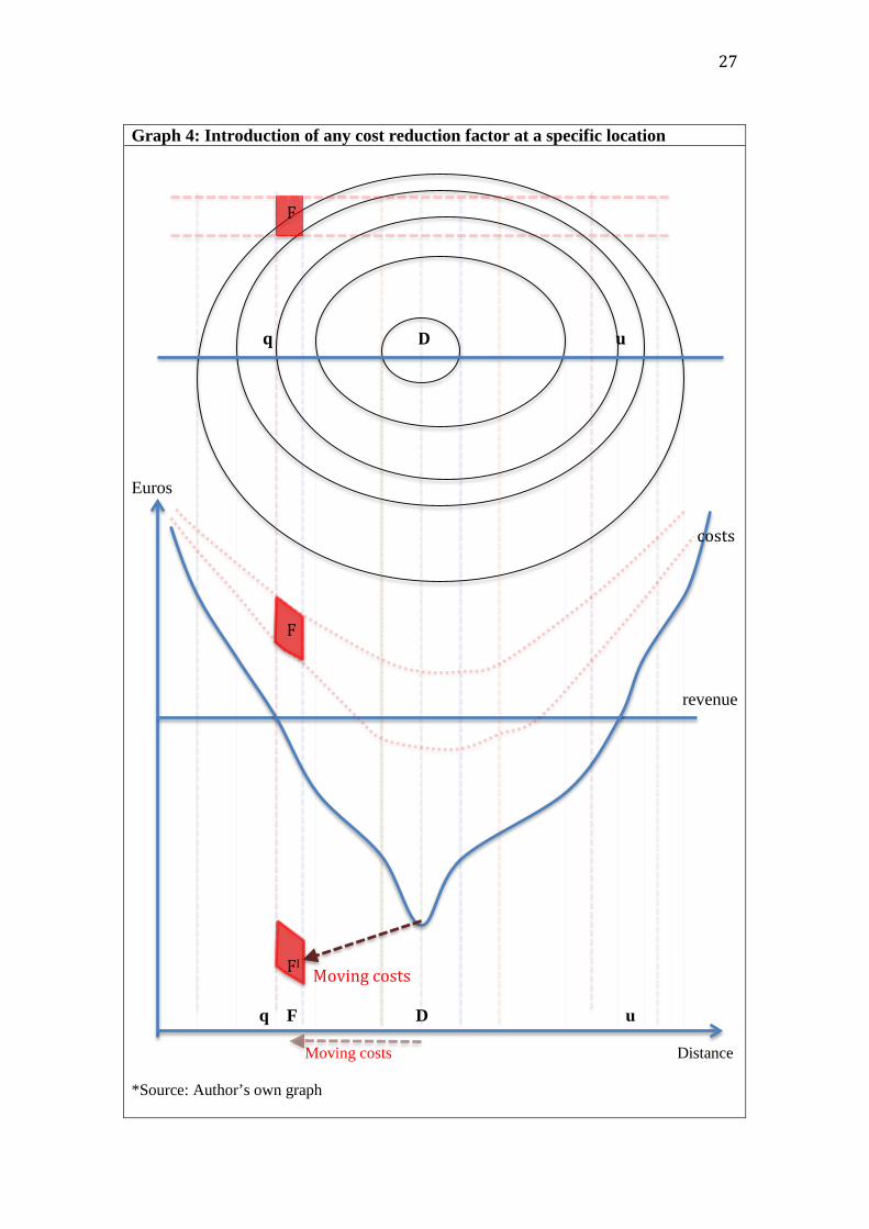
Graph 4: Introduction of any cost reduction factor at a specific location Euros

revenue q F D u

Moving costs Distance

*Source: Author’s own graph

F

F

FI Moving costs

q D u

costs

28

Graph 4a. Tiebout-model graph for firm: Introduction of any cost reduction factor at a specific location 𝑜𝑜𝑜𝑜𝑜𝑜𝑜𝑜𝑜𝑜 break-even line F

Cost=price q, u

D Minimum cost New minimum cost F Distance 𝑒𝑒𝑜𝑜𝑎𝑎𝑜𝑜𝑒𝑒𝑜𝑜𝑜𝑜 *Source: Author’s own graph

Initially The firm is located at the optimal location D. At locality F, where it was only possible to produce with losses before, some incentives (subsidy, tax abatement, energy cost discounts, etc) is introduced recently. With such incentives, total costs are now more lower than the firm’s current optimal location D. Firm’s optimal location is changed to F now. According to Tiebout’s assumptions firm has to move to the new maximum profit location; however firm has to bear moving costs. Since the firm has full information, we have tassume that firm is able to calculate exactly how much it costs for him to move. If moving costs is lower than the of the subsidy benefit offered, the firm will decide to move. The reader can extend this depiction in his mind by applying different analogies. For example at some locations some new production technologies might be innovated and usage of new technology would only be beneficial to the firm when it moves to that location (for example, the example in literature review that American firms moving to Japan for miniaturization technology and Japanese firms moving to USA for more expertised biotechnology technology) As seen above, the firms moving pattern is to make a downwards move to attain maximum profits, because new lowest-cost location went downwards.

29

Graph 5. Introduction of any cost increasing factor at a specific region Euros

revenue

Moving costs q D G u

Distance Moving costs

*Source: Author’s own graph

D

DI

G

q D G u

costs

30

Graph 5a. Tiebout-model graph for firm: Introduction of any cost increasing factor at a specific region 𝑜𝑜𝑜𝑜𝑜𝑜𝑜𝑜𝑜𝑜 break-even line Current location D after the change

Cost=price q, u moving costs New minimum cost G Minimum cost D before the change 𝑒𝑒𝑜𝑜𝑎𝑎𝑜𝑜𝑒𝑒𝑜𝑜𝑜𝑜 *Source: Author’s own graph

The firm is located at the minimum-cost location, D. Assume that location D attracted many firms with its advantageous conditionand and it exceeded the optimal number of firms. Government wants some firms to leave and introduces extra taxes or licence fees to the firm. The introduction of the higher tax rates, licence fees, strict environmental regulations may increase the cost levels of firms significantly. Such increase in the costs will change the firm’s optimal location from locality D to location G, because the current location D is not giving the lowest costs to the firm anymore. Morever, location D is not profitable anymore, it moved up to the left of 45-degree zero profit lice. According to Tiebout hypothesis, the firm has to move to new minimum-cost location location G. However, firm has to calculate the moving costs. The firm will move to the location G if moving costs are less than tax introduced. If moving costs worth more than the tax or licence fee, the firm will decide to stay still at locality D, even though it is not the maximum profit location. To move to the new maximum profit location, the fim has to make a move downwards to minimize its costs, because location D went upwards, especially to the left of 45-degree of zero profit line. If firm stays there it has to bear losses. As profit- maximizer, the firm will make a downwards move on Tiebout-model to operate at the new maximum profit location G.

31

Graph 6. The effect of cost increase on production and transportation technology towards a set of specific location Euros

revenue D

*Source:Author’s own graph

q D u

q z t u

New cost curve

costs

Distance

32

Graph 6a. Tiebout-model for graphs: Introduction of transportation costs 𝑜𝑜𝑜𝑜𝑜𝑜𝑜𝑜𝑜𝑜 new-break even line u break-even line New cost=price level q,t

Cost=price level q, u New minimum cost D

Minimum cost level D 𝑒𝑒𝑜𝑜𝑎𝑎𝑜𝑜𝑒𝑒𝑜𝑜𝑜𝑜 *Source: Author’s own graph

The firm is at the optimal location D. Assume an increase in transportation costs, the zero-profit (break-even) line moved upwards. Such increase in the costs turned the location u into a loss making locations. Now, the firm has new zero-profit locations q and t. Moreover, it now has less profit at location D now because its costs have increased. However, still location D is the maximum profit location for the firm, because only the spatial margins where firm can make profits has changed and firm’s minimum cost location point has not been changed. In this situation, firm will not change its location but it will have less profits. Thus, firm reacts to this change by not moving. In all situations given above and different conditions that the reader can come up with in his min the profit-maximizing, thus cost minimizing, firm’s movement pattern in Tiebout-model graph will be the same: The firm has to make moves downward move to minimize its costs, therefore to maximize its profits. Until now, the revenue surface is hold to be constant. If the shape of the cost curve is assumed to be staying the same and revenue is assumed to get higher at some locations, these location will fall to the right side of the graph above (the righter the location, the higher the revenue level). Therefore firm has to make a rightwards move on the Tiebout-model graph to sustain the maximum profits for the firm. Thus, the general movement pattern of the firm in Tiebout-model can be concluded as: firm makes downward and rightward movements to sustain maximum utility level as a reaction to changes in the economic environment.

33

5. Conclusion

This thesis investigated the applicability of Tiebout-model to firms under the hypothesis of: Every time a positive difference occurs in the profit level (revenue-costs) between firm’s current location and other locations, rather than applying other strategies, it will move to the new maximum profit location. The literature review revealed that the motivation for the firm to relocate is cost minimizing principle to maximize its profits. Determinants of firm relocation from different approaches converge relevantly on the aim of cost minimizing. This thesis used spatial margins to profitability model (Smith, 1966) and the idea of isodapanes (Weber, 1929) as intermediate tools to introduce different determinants of firm relocation and analyze firm’s spatial mobility pattern in Tiebout-model. The discussions of this thesis are based on theoretical insights that are derived from graphical analyses. This thesis concludes that the hypothesis only holds true under the restriction that firm is a profit-maximizer. Firm has to move downwards and/or rightwards from its current location to sustain maximum profits if a new maximum profit location arises in time. This is the same movement pattern of household in original Tiebout-model to sustain maximum utility. Another exact analogy is that firm and household cannot move to the left side of the 45-degree (zero-profit and zero utility) lines. Such condition makes both agents to locate at negative profits or negative utility. Thus, this thesis concludes that Tiebout-model is applicable to firm relocation under strict assumptions and restrictions. As original Tiebout-model, this thesis applies assumptions to use spatial mobility as sole tool to visually depict how firm adapts to changes in the change of its profit level. Non-existence of these assumptions will weaken the application of the Tiebout-model to firm. Besides that, firms have to consider the moving costs before it makes his move in Tiebout-model. The relocation process itself usually incurs very significant costs, comprising the cost of the real estate site search and acquisition, the dismantling, moving, and reconstruction of existing facilities, the construction of new facilities, and the hiring and training of new labor employed (Clark and Wrigley, 1997) In the presence of high relocation costs the firm will not move to a superior location even if the firm knows which alternative location offer higher profits. Firms will move only when the cost advantages of alternative location also compensate for these additional relocation costs. The relocation decision must smooth away difficulties involved in the existing facility and complications of physical transfer of production activities to a new location. On the other hand, where relocation costs are insignificant, the firm will be able to move to superior locations as a profit maximizing strategy. Moreover, if firm does not have perfect information, like in real life, it may not compute these costs finely and do not move very frequently. Rather, the firm will attempt to reorganize its factor allocations and activities between its current set of existing plants. The relocation of a plant, or the reorganization of multi-plant activities which involves either the closing or opening of a plant, will only be a last solution strategy (Clark and Wrigley, 1997).

34

If firm does not behave as a profit-maximizer, the graphical analysis of the thesis does not allow the firm to have a consistent moving downwards and/or rightwards pattern in Tiebout-model. The decision to relocate sometimes may be related with personal characteristics of the entrepreneur, such such as schooling of the kids, family issues tendency to move to closer but not so distant locations not to lose commercial or personal network (Hayter, 1997; Meester 2004). Such factors may result in the relocation of the firm to a sub-optimal profit location (Townroe, 1972). Thus firms may not move always downwards and/or leftwards if they behave sub-optimally. Sub-optimal behavior may make firm move upwards and/or leftwards for having less but still positive profits.

One of the important aspects to consider deciding to make the relocation move is not investigated in this study: Scholars also apply transaction cost economics to explain cost drivers of relocation (Farrell, 2005). Lower costs alone may not be enough in explaining the relocation motivation of the firm, as relocating to a longer distance increases transaction costs, which might offset savings. Transaction costs are increased by uncertainty involved in the relocation activities (Coase, 1937) Despite the fact that digitization has decreased transaction costs dramatically during the last two decades and it allowed gaining access to lower costs at long distance locations (Williamson, 1988), the reader should still bear in mind that transaction costs still significantly affect the relocation decision due to uncertainty involved (Chozora, Melkers and Kouassi, 2004). These might be called as invisible costs of relocating (Hill, 1990). For further research, a deeper investigation in transaction costs economics with respect to relocation decision will add more understanding of the firm’s mobility behavior. Another investigation that will give more insights on the firm’s spatial mobility would be the distance aspect of the firm. When richer empirical data related to firm relocation becomes more available it will be useful to test how far firms move.

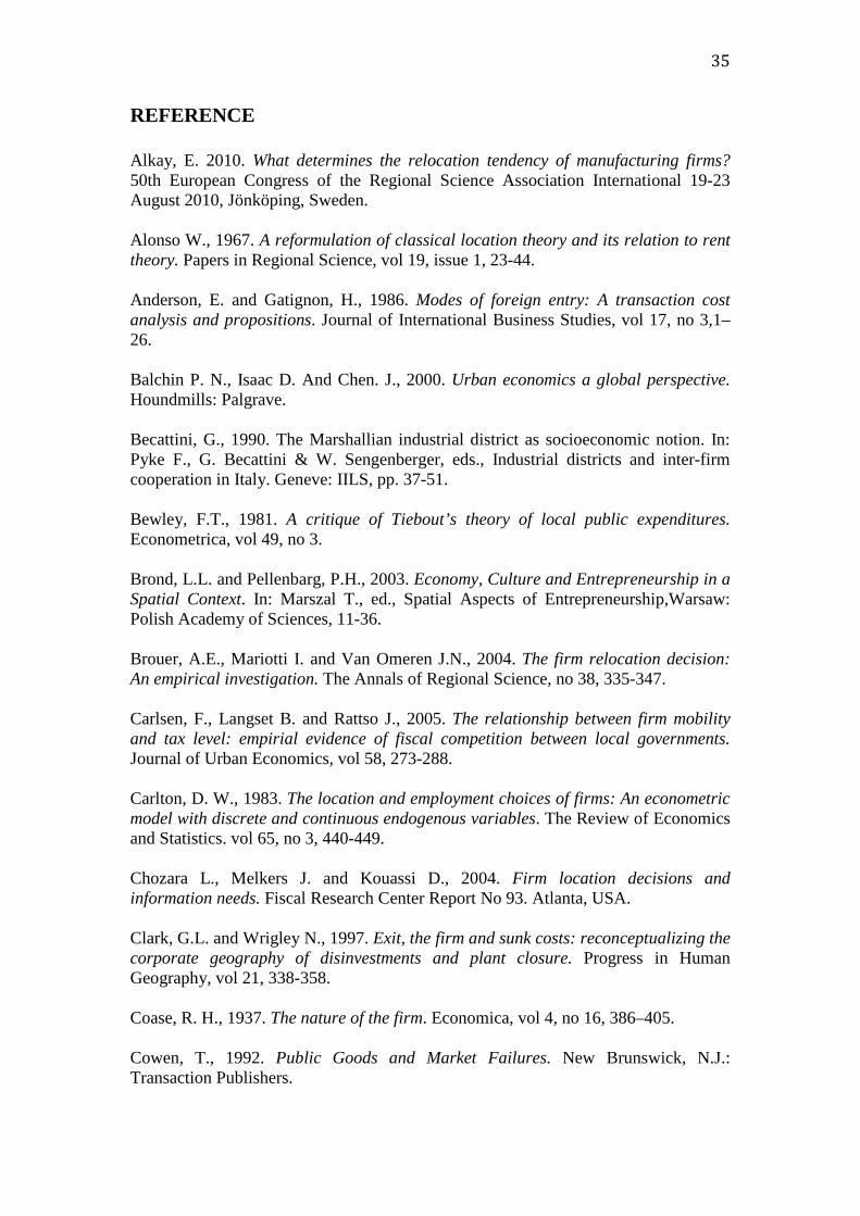
35

REFERENCE Alkay, E. 2010. What determines the relocation tendency of manufacturing firms? 50th European Congress of the Regional Science Association International 19-23 August 2010, Jönköping, Sweden. Alonso W., 1967. A reformulation of classical location theory and its relation to rent theory. Papers in Regional Science, vol 19, issue 1, 23-44. Anderson, E. and Gatignon, H., 1986. Modes of foreign entry: A transaction cost analysis and propositions. Journal of International Business Studies, vol 17, no 3,1–26. Balchin P. N., Isaac D. And Chen. J., 2000. Urban economics a global perspective. Houndmills: Palgrave. Becattini, G., 1990. The Marshallian industrial district as socioeconomic notion. In: Pyke F., G. Becattini & W. Sengenberger, eds., Industrial districts and inter-firm cooperation in Italy. Geneve: IILS, pp. 37-51. Bewley, F.T., 1981. A critique of Tiebout’s theory of local public expenditures. Econometrica, vol 49, no 3. Brond, L.L. and Pellenbarg, P.H., 2003. Economy, Culture and Entrepreneurship in a Spatial Context. In: Marszal T., ed., Spatial Aspects of Entrepreneurship,Warsaw: Polish Academy of Sciences, 11-36. Brouer, A.E., Mariotti I. and Van Omeren J.N., 2004. The firm relocation decision: An empirical investigation. The Annals of Regional Science, no 38, 335-347. Carlsen, F., Langset B. and Rattso J., 2005. The relationship between firm mobility and tax level: empirial evidence of fiscal competition between local governments. Journal of Urban Economics, vol 58, 273-288. Carlton, D. W., 1983. The location and employment choices of firms: An econometric model with discrete and continuous endogenous variables. The Review of Economics and Statistics. vol 65, no 3, 440-449. Chozara L., Melkers J. and Kouassi D., 2004. Firm location decisions and information needs. Fiscal Research Center Report No 93. Atlanta, USA. Clark, G.L. and Wrigley N., 1997. Exit, the firm and sunk costs: reconceptualizing the corporate geography of disinvestments and plant closure. Progress in Human Geography, vol 21, 338-358. Coase, R. H., 1937. The nature of the firm. Economica, vol 4, no 16, 386–405. Cowen, T., 1992. Public Goods and Market Failures. New Brunswick, N.J.: Transaction Publishers.

36

Cowling, M. and Lee, N., 2014. Do Rural Firms Perceive Different Problems? Geography, Sorting, and Barriers to Growth in UK SMEs. Environment & Planning C: Government and Policy, vol 33, no 1), 25-42. Davidsson, P., 1989. Entrepreneurship – and after – A study of growth willingness in small firms. Journal of Business Venturing, vol 4, no 3, 211–226. Deller, S., Conroy, T. And Tsvetkova, A., 2015. Factors affecting the interstate migration of manufacturong firms: Much to do about nothing? Staff Paper Series 578, University of Wisconsin, Agricultural and Applied Economics. Dijk, Van J. and Pellenbarg P.H., 2000. Firm relocation decisions in the Netherlands: An ordered Logit approach. Regional Science, vol 79, no 2, 191-219. Dunning, J. H., 1980. Toward an eclectic theory of international production: Some empirical tests. Journal of International Business Studies, vol 11, no 1, 9–31. Eenman V. F. and Brouthers K. D., 1994. Global relocation: High hopes and big risk Long Range Planning, vol 29, no 1, 84-93. Farrell, D. (2005). Offshoring: Value creation through economic change. Journal of Management Studies, vol 42, no 3, 675–683. Felix M., 2015. Von Thunen on the Bybanen: a spatial model of the commute in Bergen. Master Thesis: Norwegian School of Economics: Bergen, Norway. Fiet, J. O., 2001. The pedagogical side of entrepreneurship theory. Journal of Business Venturing, vol 16, no 2, 101–117. Fischel, William A., 1992. Property taxation and Tiebout model: Evidence from the benefit view from zoning and voting Journal of Economic Literature, vol 30, 171-177 Fukuyama, F. 1995. Trust: The Social Virtues and the Creation of Prosperity. New York: Free Press. Glaeser, E. L., 2001. The Economics of Location-Based Tax Incentives. Harvard Institute of Economic Research Discussion Papers Number 1932. Hayter, R., 1997. The dynamics of industrial location: The factory, the firm and the production system. New York: Wiley. Hill C. W. L., 1990. Cooperation, opportunism, and the invisible hand: Implications for transaction cost theory. The Academy of Management Review, vol 15, no 3, 500-513 Hotelling, H., 1929. Stability in Competition. The Economic Journal, vol 39, no 153, 41-57.

37

Hu W., Cox. J. L., Wright J. and Harris T. L., 2008 Understanding Firms’ Relocation and Expansion Decisions Using Self- Reported Factor Importance Rating The Review of Regional Studies, vol 38, no 1, 67–88. Issard, W., 1960. Location and Space-Economy, MIT press, 1960. Jarillo, J. C., 1989. Entrepreneurship and growth – The strategic use of external resources. Journal of Business Venturing, vol 4, no 2, 133–147. Lloyd, P.E. and Mason C. 1978. Manufacturing in the inner city: a case study of Greater Manchester. Transactions of the Institute of British Geographers, vol 3, 66-90. Lowe, N. J., 2012. Beyond the Deal: Using Industrial Recruitment as a Strategic Tool for Manufacturing Development. Economic Development Quarterly, vol 28, no 4, 287–299. Lösch A., 1954. The economics of location. New Haven: Yale University Press. Lynch, R.G., 2004. Rethinking Growth Strategies: How State and Local Taxes and Services Affect Economic Development. Economic Policy Institute: Washington DC. Mariotti I. and Steen, V. M., 2001. Conscious choice for organizational relocation, an application of strategic choice theories. Groeningen, Research School SOM. Mars. A, and Kay, A., 2006. Contextualizing Tiebout: Mobility, Municipalities and Methodology. Public Finance and Management, vol 6, no 1, 13-40 McCann, P., 1993. The logistics-cost location-production problem. Journal of Regional Science, vol 33, no 4, pp. 503-16. McCormack A. D., Newman L. J. and Rosenfield D. B., 1994 The New Dynamics of Global Manufacturing Site Location. Sloan Management Review, 69-80. McGuire, T., 1983. Firm location in a Tiebout-world. Journal of Regional Science, vol 23, no 2. Meester, W. J., 2004. Locational preferences of entrepreneurs. Stated Preferences in the Netherlands and Germany. Heidelberg-New York: Physica-Verlag. Min H. and Melachrinoudis E., 1999. The relocation of a hybrid manufacturing/distribution facility from supply chain perspectives: a case study. Omega, International Journal of Management and Science, vol 27, 75-85. Mucchielli J.L. and Saucier P., 1997. European industrial relocations in low-wage countries: policy and theory debates, in multinational firms and international relocation (ed . by Buckley P.J., Mucchielli J.L.), Cheltenham, Edward Elgar, 5-33. Musgrave R. A., 1959 The theory of public finance New York and. London: McGraw-Hill.

38

Newman, R.J. and Sullivan D., 1998. Econometric Analysis of Business Tax Impacts on Industrial Location: What Do We Know and How Do We Know It? Journal of Urban Economics, vol 23, 215- 234. Oddou, R., 2015. Firms location and sorting. Economics Bulletin, vol 35, issue 3. Ok, L. and Tansel E., 2007. Motives for offshoring, A qualitative case of study of Swedish Companies Bachelor Thesis Jankooping International Business School, Sweeden. Osteryoung, J. S. and Newman, D. 1993. What is a small business? The Journal of Small Business Finance, vol 2, no 3, 219-231. Pedersini R., 2016. Relocation of production and industrial relations. European Foundations for Improvement of Living and Working Conditions 2006. Pellenbarg, P.H., Van Wissen L.J.G. and Dijk, Van J., 2002. Firm Migration. In: McCann P., 2005., Industrial Location Economics., Cheltenham: Edward Elgar Publishing, 110-148. Phan, P. H., 2004. Entrepreneurship theory: Possibilities and future directions. Journal of Business Venturing, vol 19, no 5, 617–620. Plaut T.R. and Pluta J. E., 1983. Business Climate, Taxes and Expenditures, and State Industrial Growth in the United States. Southern Economic Journal, vol 50, no 1, 99-119. Porter M. E., 1985. Competitive advantage. New York: Free Press. Rothwell, R., 1989. Firm size, innovation and industrial change. Small Business Economics, vol 1, no 1, 51–64. Roza M., Van den Bosch F. A. J. and Volberda, H. W., 2011. Offshoring strategy: Motives, functions, locations, and governance modes of small, medium-sized and large firms International Business Review, vol 20, 314–323. Samuelson P.A., The Pure Theory of Public Expenditure. The Review of Economics and Statistics, vol 36, no 4, 387-389. Sass M. and Hunya G., 2014. Escaping to the east? Relocation of business activities to and from Hungary, 2003-2011 IEHAS Discussion Paper 1407, Institute of Economics, Centre for Economic and Regional Studies, Hungarian Academy of Sciences. Schemmer, R. W., 1978. The manufacturing location decision: evidence from Cincinnati and New England. Economic development research report. Washington DC: US Department of Commerce.

39

Scott M. and Bruce R., 1987. Five stages of growth in small business. Long rage Planning, vol 20, no 3, 45-52.

Singleton D. J., 2015. Sorting Charles Tiebout History of Political Economy, vol. 47, no 1, 199-226 Sleuwaegen L. and Pennings, E., 2006. International relocation of production: Where do firms go? Scottish Journal of Political Economy, vol 53, no 4. Smith, D.M., 1966. A theoretical framework for geographical studies of industrial location. Economic Geography, vol 42, issue 2, 95-113. Strauss-Kahn, V. and Vives X., 2009. Why and Where Do Headquarters Move? Regional Science and Urban Economics, vol, 39, no 2, 168–186. Teske, P., Schneider, M., Mintrom, M. and Best, S. 1993. Establishing the micro foundations of a macro theory: information, movers, and the competitive market for public goods. American Political Science Review, vol 87, 702-713. Tiebout C.M., 1956. A pure theory of local expenditures. The Journal of Political Economy, vol 64, no 5, 416-424. Townroe, P. M., 1972. Some behavioural considerations in the industrial location decision. Regional Studies, vol 6, 261-272. Wasylenko, M.J., 1981. The Location of Firms: The Role of Taxes and Fiscal Incentives. Urban Affairs Annual Review, vol 20, 339-349 Waugh, D., 2002. Geography: An integrated approach. Nelton Thornes, Cheltenham, UK. Weber, A., 1929. Theory of the Location of Industries. Chicago: University of Chicago Press. White M.J., 1986. Property taxes and firm relocation: evidence from proposition 13. NBER Studies in State and Local Public Finance, 83-112. Williamson, O. E., 1988. Technology and transaction cost economics: A reply. Journal of Economic Behaviour and Organization, vol 10, issue 3, 355-363. Wissen, Van L.J.G., 2002. Demography of the Firm: A Useful metaphor? European Journal of Population 18, pp.263-279. Yip G. S., 1994. Industry Drivers of Global Strategy and Organization. The International Executive, 529-556.

40

Non-exclusive licence to reproduce thesis and make thesis public I, Evren Yaman 1. herewith grant the University of Tartu a free permit (non-exclusive licence) to: 1.1. reproduce, for the purpose of preservation and making available to the public,

including for addition to the DSpace digital archives until expiry of the term of validity of the copyright, and

1.2. make available to the public via the web environment of the University of Tartu, including via the DSpace digital archives until expiry of the term of validity of the copyright,

TIEBOUT MODEL IN APPLICATION TO FIRMS

supervised by Prof. Dr. Dr. h. c. Peter Friedrich (em.) 2. I am aware of the fact that the author retains these rights. 3. I certify that granting the non-exclusive licence does not infringe the intellectual property rights or rights arising from the Personal Data Protection Act. Tartu, 25.05.2017