Bayesian nonparametric estimation of the spectral density of a long memory Gaussian time series

Bayesian nonparametric estimation of the spectral

density of a long memory Gaussian time series

Judith Rousseau

Universite Paris Dauphine

Brunero Liseo∗

Universita di Roma “La Sapienza”

Abstract

Let X = Xt, t = 1, 2, . . . be a stationary Gaussian random process, with mean EXt =

µ and covariance function γ(τ) = E(Xt −µ)(Xt+τ −µ). Let f(λ) be the corresponding

spectral density; a stationary Gaussian process is said to be long-range dependent, if the

spectral density f(λ) can be written as the product of a slowly varying function f(λ) and

the quantity λ−2d. In this paper we propose a novel Bayesian nonparametric approach

to the estimation of the spectral density of X. We prove that,under some specific

assumptions on the prior distribution, our approach assures posterior consistency both

when f(·) and d are the objects of interest. The rate of convergence of the posterior

sequence depends in a significant way on the structure of the prior; we provide some

general results and also consider the fractionally exponential (FEXP) family of priors

(see below). Since it has not a well founded justification in the long memory set-up,

we avoid using the Whittle approximation to the likelihood function and prefer to use

the true Gaussian likelihood. It makes the computational burden of the method quite

∗AMS 2000 subject classification: Primary 62F15, 62G07; secondary 62M15.

Key words and Phrases: Kullback-Leibler distance, fractionally exponential priors, Population Monte Carlo,

spectral analysis, Toeplitz matrices.

1

challenging. To mitigate the impact of that in finite sample computations, we propose to

use a Population Monte Carlo (PMC) algorithm, which avoids rejecting some proposed

values, as it regularly happens with MCMC algorithms. We also propose an extension

of PMC in order to deal with the case of varying dimension parameter space. We finally

present an application of our approach.

1 Introduction

Let X = Xt, t = 1, 2, . . . be a stationary Gaussian random process, with mean EXt = µ

and covariance function γ(τ) = E(Xt−µ)(Xt+τ−µ). Let f(λ) be the corresponding spectral

density, which satisfies the relation

γ(τ) =

∫ π

−πf(λ)eitλdλ (τ = 0,±1,±2, . . . ).

A stationary Gaussian process is said to be long-range dependent, if there exist a positive

number C and a value d (0 < d < 1/2) such that

limλ→0

f(λ)

Cλ−2d= 1.

Alternatively, one can define a long memory process as one such that its spectral density

f(λ) can be written as the product of a slowly varying function f(λ) and the quantity λ−2d

which causes the presence of a pole of f(λ) at the origin.

Interest in long-range dependent time series has increased enormously over the last

fifteen years; Beran (1994) provides a comprehensive introduction and the book edited by

Doukhan, Oppenheim and Taqqu (2003) explores in depth both theoretical aspects and

various applications of long-range dependence analysis in several different disciplines, from

telecommunications engineering to economics and finance, from astrophysics and geophysics

to medical time series and hydrology.2

Pioneering work on long memory process is due to Mandelbrot and Van Ness (1968),

Mandelbrot and Wallis (1969) and others. Fully parametric maximum likelihood estimates

of d were introduced in the Gaussian case by Fox and Taqqu (1986) and Dahlhaus (1989)

and they have recently been developed in much greater generality by Giraitis and Taqqu

(1999); a regression approach to the estimation of the spectral density of long memory

time series is provided in Geweke and Porter-Hudak (1983); generalised linear regression

estimates were suggested by Beran (1993). However, parametric inference can be highly

biased under mis-specification of the true model: this fact has suggested semiparametric

approaches: see for instance Robinson (1995).

Due to factorization of the spectral density f(λ) = λ−2d f(λ), a semiparametric approach to

inference seems particularly appealing in this context. One needs to estimate d as a measure

of long-range dependence while no particular modeling assumptions on the structure of the

covariance function at short ranges are necessary: Liseo, Marinucci and Petrella (2001)

consider a Bayesian approach for this problem, while Bardet, Lang, Oppenheim, Philippe,

Stoev and Taqqu (2003) provides an exhaustive review on the classical approaches.

Practically all the existing procedures either exploit the regression structure of the log-

spectral density in a reasonably small neighborhood of the origin (Robinson 1995) or use an

approximate likelihood function based on the so called Whittle’s approximation (Whittle

1962), where the original data vector Xn = (X1, X2, . . . , Xn) gets transformed into the pe-

riodogram I(λ) computed at the Fourier frequencies λj = 2π j/n, j = 1, 2, . . . , n, and the

“new” observations I(λ1), . . . , I(λn) are, under a short range dependence, approximately

independent, each I(λj)/f(λj) having an exponential distribution. This is for example the

approach taken in Choudhuri, Ghosal and Roy (2004), which develop a Bayesian nonpara-

metric analysis for the spectral density of a short memory time series. Unfortunately, the

Whittle’s approximation fails to hold in the presence of long range dependence, at least for

3

the smallest Fourier frequencies.

In this paper we propose a Bayesian nonparametric approach to the estimation of the

spectral density of the stationary Gaussian process: we avoid the use of the Whittle ap-

proximation and we deal with the true Gaussian likelihood function.

The literature on Bayesian nonparametric inference has increased tremendously in the

last decades, both from a theoretical and a practical point of view. Much of this literature

has dealt with the independent case, mostly when the observations are identically distrib-

uted. The theoretical perspective was mainly dedicated to either construction of processes

used to define the prior distribution with finite distance properties of the posterior, in par-

ticular when such a prior is conjugate, see for instance Ghosh and Ramamoorthi (2003) for

a review on this, or to consistency and rates of convergence properties of the posterior, see

for instance Ghosal, Ghosh and van der Vaart (2000) or Shen and Wasserman (2001).

The dependent case has hardly been considered from a theoretical perspective apart from

Choudhuri et al. (2004), who deal with Gaussian weakly dependent data and, in a more

general setting, Ghosal and Van der Vaart (2006). In this paper we study the asymptotic

properties of the posterior distributions for Gaussian long-memory processes, where the

unknown parameters are the spectral density and the long-memory parameter d. General

consistency results are given and a special type of prior, namely the FEXP prior as it is

based on the FEXP model, is studied. From this, consistency of Bayesian estimators of

both the spectral density and the long memory parameter are obtained. To understand

better the link between the Bayesian and the frequentist approaches we also study the rates

of convergence of the posterior distributions, first in a general setup and then in the special

case of FEXP priors. The approach considered here is similar to what is often used in

the independent and identically distributed case, see for instance Ghosal et al. (2000). In

particular we need to control prior probability on some neighborhood of the true spectral

4

density and to control a sort of entropy of the prior (see Section 3); however the techniques

are quite different due to the dependence structure of the process.

The gist of the paper is to provide a fully nonparametric Bayesian analysis of long

range dependence models. In this context there already exist many elegant and maybe

more general (in the sense of being valid even without the Gaussian assumption) classical

solutions. However we believe that a Bayesian solution would be still important because of

the following reasons.

i) By definition, our scheme allows to include in the analysis some prior information

which may be available in some applications.

ii) While classical solutions are, in a way or another, based on some asymptotic argu-

ments, our Bayesian approach relies only on the observed likelihood function (and

prior information).

iii) We are able to provide a valid approximation to the “true” posterior distribution of

the main parameters of interest in the model, namely the long memory parameter d

or the global spectral density.

Also, on a more theoretical perspective, we believe that this paper can be useful to clarify the

intertwines between Bayesian and frequentist approaches to the problem. We also present

a specific algorithm to implement the procedure, i.e. to simulate from the posterior or

approximately so. The algorithm used is a version of the Population Monte-Carlo algorithm

as devised in Douc, Guillin, Marin and Robert (2006). Although this is not the main focus

of the paper, the computation of the posterior distribution is an important issue since the

likelihood is difficult to calculate: all the details about the practical implementation of the

algorithm can be found in Liseo and Rousseau (2006).

5

The paper is organized as follows: in the next section we first introduce the necessary

notation and mathematical objects; then we provide a general theorem which states some

sufficient condition to ensure consistency of the posterior distribution. We also discuss in

detail a specific class of priors, the FEXP prior, which takes its name after the fractional

exponential model which has been introduced by Robinson1991, 1994 to model the spectral

density of a covariance stationary long-range dependent process. The FEXP model can

be seen as a generalization of the exponential model proposed by Bloomfield (1973) and

it allows for semi-parametric modeling of long range dependence; see also Beran (1994) or

Hurvich, Moulines and Soulier (2002). In Section 3 we study the rate of convergence of the

posterior distribution first in the general case and then in the case of FEXP priors and in

Section 4 we give details about computational issues. The final section is devoted to some

discussion.

2 Consistency results

We observe a set of n consecutive realizations Xn = (X1, . . . , Xn) from a Gaussian station-

ary process with spectral density f0, where f0(λ) = |λ|−2d0 f0(λ). Because of the Gaussian

assumption, the density of Xn can be written as

ϕf0(Xn) =

e−X′

nTn(f0)−1Xn/2

|Tn(f0)|1/2(2π)n/2, (1)

where Tn(f0) = [γ(j − k)]1≤j,k≤n is the covariance matrix with a Toeplitz structure. The

aim is to estimate both f0 and d0 using Bayesian nonparametric methods.

Let F = f, f symmetric on [−π, π],∫

|f | < ∞ and F+ = f ∈ F , f ≥ 0; then F+

denotes the set of spectral densities. We first define three types of pseudo-distances on F+.

6

The Kullback-Leibler divergence for finite n is defined as

KLn(f0; f) =1

n

∫

Rn

ϕf0(Xn) [log ϕf0

(Xn) − log ϕf (Xn)] dXn

=1

2n

[

tr(

Tn(f0)T−1n (f) − id

)

− log det(Tn(f0)T−1n (f))

]

where id represents the identity matrix of the appropriate order. Letting n → ∞, we can

define, when it exists, the quantity

KL∞(f0; f) =1

π

∫ π

−π

[

f0(λ)

f(λ)− 1 − log

f0(λ)

f(λ)

]

dλ.

We also define two symmetrized version of KLn, namely

hn(f0, f) = KLn(f0; f) + KLn(f ; f0); dn(f0, f) = minKLn(f0; f), KLn(f ; f0)

and their corresponding limits as n → ∞:

h(f0, f) =1

2π

∫ π

−π

[

f0(λ)

f(λ)+

f(λ)

f0(λ)− 2

]

dλ; d(f0, f) = minKL∞(f0; f), KL∞(f ; f0).

We also consider the L2 distance between the logarithms of the spectral densities, namely

ℓ(f, f ′) =

∫ π

−π(log f(λ) − log f ′(λ))2dλ. (2)

This distance has been considered in particular by Moulines and Soulier (2003). This is

quite a natural distance in the sense that it always exists, whereas the L2 distance between

f and f ′ need not, at least in the types of models considered in this paper. Let π be a prior

probability distribution on the set

F = f ∈ F , f(λ) = |λ|−2df(λ), f ∈ C0,−1

2< d <

1

2, F+ = f ∈ F+, f ≥ 0,

where C0 is the set of continuous functions on [−π, π]. Let Aε = f ∈ F+; d(f, f0) ≤ ε.

Our first goal will be to prove the consistency of the posterior distribution of f0, that is, we

want to show that

P π[Acε|Xn] → 0, f0 a.s...

7

From this, we will be able to deduce the consistency of some Bayes estimators of the

spectral density f and of the long memory parameter d. We first state and prove the strong

consistency of the posterior distribution under very general conditions both on the prior and

on the true spectral density. Then, building on these results, we will obtain the consistency

of a class of Bayes estimates of the spectral density, together with the consistency of the

Bayes estimates of the long memory parameter d. The already introduced FEXP class of

prior will be then proposed, and its use will be explored in detail.

2.1 The main result

In this section we derive the main result about consistency of the posterior distribution. We

also discuss the asymptotic behavior of the posterior point estimates of some parameter of

major interest, such as the long memory parameter d and the global spectral density.

Consider the following two subsets of F

G(d, M, m, L, ρ) = (3)

f ∈ F+; f(λ) = |λ|−2df(λ), m ≤ f(λ) ≤ M,∣

∣

∣f(x) − f(y)

∣

∣

∣≤ L|x − y|ρ

,

where −1/2 < d < 1/2, m, M, ρ > 0;

F(d, M, L, ρ) = (4)

f ∈ F ; f(λ) = |λ|−2df(λ), |f(λ)| ≤ M,∣

∣

∣f(x) − f(y)∣

∣

∣ ≤ L|x − y|ρ.

The boundedness constraint on f in the definition of G(d, M, m, L, ρ) is necessary here to

guarantee the identifiability of d, while the Lipschitz-type condition on f , in both definitions,

are actually needed to ensure that normalized traces of products of Toeplitz matrices, that

typically appear in the distances considered previously, will converge. We also consider the

following set of spectral densities, which is of interest in the study of rates of convergence:8

let

L⋆(M, m, L) = h(·) ≥ 0, 0 < m ≤ h(·) ≤ M, |h(x) − h(y)| ≤ L|x − y|(|x| ∧ |y|)−1

and

L(d, M, m, L) = f = |λ|−2df(λ), f ∈ L⋆(M, m, L).

Note that G and L are similar, with only a slight modification on the Lipschitz condition.

The set L has been considered in particular in Moulines and Soulier (2003).

We now consider the main result on the consistency of the posterior distribution

Theorem 1 Let G(t, M, m, L, ρ) = ∪0≤d≤1/2−tG(d, M, m, L, ρ), and assume that there ex-

ists (t0, M0, m0, L0) such that we have either f0 ∈ G(t, M0, m0, L0, ρ0) with 1 ≥ ρ0 > 0 or

f0 ∈ ∪0≤d≤1/2−t0L(d, M0, m0, L0). Let

F+(t, M, m) = ∪−1/2+t≤d≤1/2−tf ∈ F+, f(λ) = |λ|−2df(λ), 0 < m ≤ f ≤ M.

Let π be a prior distribution such that

i) ∀ε > 0 and for some M ′ > 0, there exists M, m, L, ρ > 0 such that if

Bε =

f ∈ G(t, M, m, L, ρ) : h(f0, f) ≤ ε, 6(d0 − d) < ρ0 ∧1

2,

∫

(f0

f− 1)3dx ≤ M ′

,

then π (Bε) > 0. For simplicity, in our notations the case

f0 ∈ ∪0≤d≤1/2−t0L(d, M0, m0, L0)

corresponds to ρ0 = 1. This simplification is also used in (ii).

ii) ∀ε > 0, small enough, there exists Fn ⊂ f ∈ F+, d(f0, fi) > ǫ, such that π(Fcn) ≤

e−nr and there exist t, M, m, C > 0 with t < ρ0/4, and a smallest possible net Hn ⊂

f ∈ F+(t, M, m); d(f, d0) > ǫ/2 such that when n is large enough, ∀f ∈ Fn, ∃fi ∈9

Hn, 0 ≤ fi − f ≤ ǫ| log ǫ|−1|λ|−2(di−t/4) and n−1 tr(

(Tn(|λ|−2di)−1Tn(fi − f0))2)

≥

B∫

(f0/fi−1)2(x)dx and n−1 tr(

(Tn(|λ|−2d0)−1Tn(fi − f0))2)

≥ B∫

(fi/f0−1)2(x)dx

Denote by Nn the logarithm of the cardinality of the smallest possible net Hn. Then,

if

Nn ≤ nc1, with c1 < ε| log ε|−2/2, 0 < δ

then

P π [Aε|Xn] → 1, f0 a.s. (5)

Proof. See Appendix B.

The above theorem is important to clarify which conditions on the prior distribution π

are really crucial in a long memory setting, where the techniques usually adopted in the

i..i.d. case, cannot be used and even the adoption of a Whittle approximation is not le-

gitimate in this setting (at least at the lowest frequencies). From a practical perspective,

however, the hardest part of the job is actually to verify whether a specific type of priors

actually meets the conditions listed in Theorem 1. Just to mention two difficulties, the con-

struction of the net Hn in the proof of Theorem 1 may be strongly dependent on the prior

we use; also it may depend, in a non trivial way, on the sample size. To be more precise,

checking the uniform bound on the terms in the form n−1 tr(

(Tn(|λ|−2di)−1Tn(fi − f0))2)

might be quite delicate. In Appendix B, we also give a more general set of conditions to

obtain consistency which is however quite cumbersome but might prove to be useful in some

situations.

We will discuss in detail these issues in the context of the FEXP prior in §2.3.

10

2.2 Consistency of estimates for some quantities of interest

We now discuss the problem of consistency for the Bayes estimates of the spectral density.

The quadratic loss function on f is not a natural loss function for this problem, since there

exist some spectral densities in F that are not square integrable (if d > 1/4). A more

reasonable loss function may be the quadratic loss on the logarithm of f , as defined by (2),

which is always integrable. The Bayes estimator of f associated with the loss ℓ and the

prior π is given by

f(λ) = expEπ[log f(λ)|Xn].

Also, in many applications, the real parameter of interest is just d, the long memory expo-

nent. It is possible to deduce, from Theorem 1, that the posterior mean of d, that is the

Bayes estimator associated with the quadratic loss on d, is actually consistent.

Corollary 1 Under the assumptions of Theorem 1, for all ǫ > 0, as n → ∞,

π[

f = |λ|−2df ; |d − d0| > ǫ|Xn

]

→ 0 f0 a.s

and d = Eπ[d|Xn] → d0, f0 a.s.

Proof. The result comes from the fact that, when |d − d0| > ǫ, both KL∞(f ; f0) and

KL∞(f0; f) are greater than some fixed value ǫ′ depending on ǫ only. Indeed, let f(λ) =

|λ|−2df(λ) and f0(λ) = |λ|−2d0 f0(λ), for all 0 < τ < π.

KL∞(f ; f0) > 2

∫ τ

0

[

f(λ)

f0(λ)λ−2(d−d0) − 1 + 2(d − d0) log λ − log (f/f0)(λ)

]

dλ

≥ 2

(

m

M(1 − 2(d − d0))τ1−2(d−d0) − τ(1 + log M/m + 2(d − d0))

+ 2(d − d0)τ log τ) ≥ ǫ′

11

where ǫ′ is based on either τ1−2(d−d0) if d > d0 or on (d0 − d)τ log 1/τ if d < d0, when τ is

small enough (but fixed, depending on ǫ, m, M). This implies that

π[Acǫ′ |X] ≥ π

[

f = |λ|−2df ; |d − d0| > ǫ|X]

→ 0, f0 a.s.

Since d is bounded, a simple application of the Jensen’s inequality gives

(d − d0)2 ≤ Eπ[(d − d0)

2|X] → 0, f0 a.s.

It is also possible to derive consistency results for the point estimate of the whole spectral

density:

Corollary 2 Under the assumptions of Theorem 1, as n → ∞,

ℓ(f0, f) → 0, f0 a.s.

Proof. The idea is to prove that for all ǫ > 0, there exists ǫ′ > 0 such that l(f, f0) > ǫ

implies that d(f, f0) > ǫ′. Indeed, when c is small enough, there exists xc < 0 (xc goes to

−∞ when c goes to 0) such that ex − 1 − x ≤ cx2. Then

KL∞(f ; f0) ≥ c

(

l(f, f0) −

∫

f/f0<exc

(log f(x) − log f0(x))2dx

)

.

Moreover,

f(x)

f0(x)= |x|−2(d−d0)

f(x)

f0(x)≥

m

Mπ−2(d−d0),

when d > d0. Hence, by choosing c small enough, the set f/f0 < exc∩d > d0 is empty.

In this case the set f/f0 < exc is a subset of |x| ≤ ac, where ac goes to zero as c goes

to zero; when c → 0,

∫

|x|≤ac

(log f(x) − log f0(x))2dx ≤ 2ac

(

4(d − d0)2(log (ac)

2 − 2 log (ac)) + (log M/m)2)

→ 0,

12

therefore by choosing c small enough there exists ǫ′ such that d(f, f0) > ǫ′. This implies

that π[

Acǫ|Xn

]

→ 0, when n goes to infinity, f0 almost surely. Using Jensen’s inequality

this implies in particular that l(f0, f) → 0, f0 a.s.

Since the conditions stated in Theorem 1 are somewhat non standard, they need to be

carefully checked for the specific class of priors one is dealing with. Here we consider the

class of Fractionally Exponential priors (FEXP), and we show that these priors actually

fulfill the above conditions.

2.3 The FEXP prior

Consider the set of the spectral densities with the form

f(λ) = |1 − eiλ|−2df(λ),

where log f(x) =∑K

j=0 θj cos(jx), and assume that the true log spectral density satisfies

log f0(x) =∑∞

j=0 θ0j cos(jx) (in other words, it is equal to its Fourier series expansion),

with

|f0(x) − f0(y)| ≤ L|x − y|

|x| ∧ |y|,∑

j

|θ0j | < ∞,

for all x and y in [−π, π]. This construction has been considered, from a frequentist per-

spective, in Hurvich et al. (2002). Note that there exists an alternative and equivalent way

of writing a FEXP spectral density in which the first coefficient of the series expansion

θ0 is explicitly expressed in terms of the variance of the process, that is σ2 = 2π eθ0 . We

will use both the parameterizations according to notational convenience. A prior distribu-

tion on f can then be expressed as a prior on the parameters (d, K, θ0, ..., θK) in the form

p(K)π(d|K)π(θ|d, K), where θ = (θ0, ..., θK), and K represents the (random) order of the

FEXP model. Usually, d is set independent of θ for given K and it is also independent

of K itself. Let π(d) > 0 on [−1/2 + t, 1/2 − t], for some t > 0, arbitrarily small. Let K13

be a priori Poisson distributed and, conditionally on K, notice that π(θ|K) needs to put

mass 1 on the set of θ’s such that∑K

j=0 |θj | ≤ A, for some value A large but finite. A

possible way to formalize it, is to assume that, for given K, the quantity SK =∑

j |θj |

has a finite support distribution; then, setting Vj = |θj |/SK , j = 1, . . . , K, one may con-

sider a distribution on the set z ∈ RK ; z = (z1, ..., zK),

∑

zi = 1, zi ≥ 0 for example:

(V1, . . . , VK) ∼ Dirichlet(α1, . . . , αK),

Since the variance of the |θj |’s should be decreasing, we may assume, for example, that,

for all j’s, αj = O((1 + j)−2). Note that if we further assume that SK has a Gamma

distribution with mean∑

j αj and variance∑

j α2j then we are approximately assuming

(modulo the truncation at A) that |θ1|, . . . , |θk| are independent Gamma(1, αj) random

variables. Alternative parameterization are also available here; for example one can assume

that (V1, · · · , Vk) follows a logistic normal distribution (Aitchison and Shen 1980), which

allows for a more flexible elicitation. Under the above conditions on the prior, the poste-

rior distribution is strongly consistent, in terms of the distance d(·, ·), the estimator f as

described in the previous section is almost surely consistent and so is the estimator d. To

prove this, we prove that the FEXP prior satisfies assumptions (i) and (ii). First, we check

assumption (i): let Kǫ be such that∑∞

j=Kǫ+1 |θ0j | ≤√

ǫ/2, then KL∞(f0; f0ǫ) ≤ ǫ/2, where

f0ǫ = |1 − eiλ|−2d0 exp

Kǫ∑

j=0

θ0j cos jλ

.

Let θ = (θ0, ..., θKǫ) be such that |θ0j−θj | ≤√

ǫ/4a|θ0j |, j = 1, . . . , Kǫ, where a =∑

j |θ0j |.

If |d − d0| < τ , with τ small enough, then k∞(f0, f) ≤ ǫ. Obviously πK(θ : |θj − θ0j | <√

ǫ/4a|θ0j |,∀j ≤ K) > 0, as soon as A >∑

j |θ0j |.

Moreover, for each f(λ) = |1− eiλ|−2d exp∑K

j=0 θj cos (jλ), provided that the parameters

14

satisfy the above constraint, one has

f0(λ)

f(λ)= |1 − eiλ|−2(d0−d) exp

∑

j

(θ0j − θj) cos (jλ) ≤ 2|1 − eiλ|−2(d0−d)

so that∫

(f0/f − 1)3dλ ≤ M ′

for some constant M ′ > 0. Now we verify assumption (ii). Let ǫ > 0 and set fk,d,θ(λ) =

|1 − e−iλ|−2d exp∑k

j=0 θj cos (jλ); consider

Fn = fk,d,θ, d ∈ [−1/2 + t, 1/2 − t], k ≤ kn,

where kn = k0n/ log n. Since π(K ≥ kn) < e−nr, for some r depending on k0, we have that

π(Fcn ≥ kn) < e−nr. Now consider spectral densities in the form,

fi(λ) = (1 − cos λ)−d−δ1 expk∑

j=0

θj cos jλ + δ2,

where 0 < δ1, δ2 < cǫ| log ǫ|−1 for some constant c > 0. We prove that if |d′ − d| < δ1/2 and

|θ′j − θj | < c′δ2[(j +1) log (j + 1)2]−1, where c′ =∑

j≥1 j−1 log j2, then f ′ = fk,d′,θ′ ≤ fi and

0 ≤ fi(λ) − f ′(λ) ≤ Cfi(λ)| log (1 − cos λ)| [δ1 + δ2] ≤ ǫ| log ǫ|−1|λ|−2di−t/2,

for some constant C > 0. To achieve the proof of assumption (ii) of Theorem 1 we need to

verify

n−1 tr(

(Tn(|λ|−2di)−1Tn(fi − f0))2)

≥ B

∫

(f0/fi − 1)2(x)dx

n−1 tr(

(Tn(|λ|−2d0)−1Tn(fi − f0))2)

≥ B

∫

(fi/f0 − 1)2(x)dx, (6)

this is proved in Appendix C. The number of such upper bounds is bounded by

CKnǫ−1

(

cǫ

Kn

)−Kn

,15

so that

Nn ≤ k0Cn

[

| log ǫ|

log n+ 1

]

≤ nc1,

by choosing k0 small enough and n large enough: this proves that the posterior distribution

associated with the FEXP prior is actually consistent.

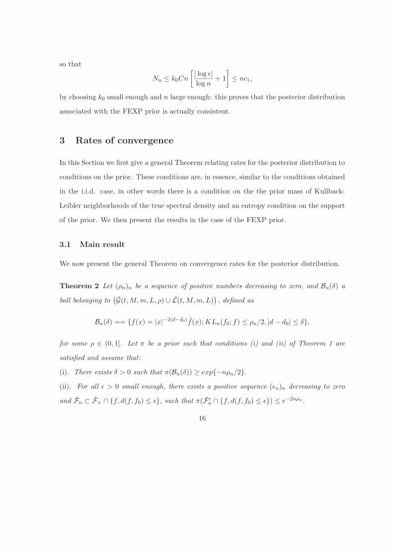
3 Rates of convergence

In this Section we first give a general Theorem relating rates for the posterior distribution to

conditions on the prior. These conditions are, in essence, similar to the conditions obtained

in the i.i.d. case, in other words there is a condition on the the prior mass of Kullback-

Leibler neighborhoods of the true spectral density and an entropy condition on the support

of the prior. We then present the results in the case of the FEXP prior.

3.1 Main result

We now present the general Theorem on convergence rates for the posterior distribution.

Theorem 2 Let (ρn)n be a sequence of positive numbers decreasing to zero, and Bn(δ) a

ball belonging to(

G(t, M, m, L, ρ) ∪ L(t, M, m, L))

, defined as

Bn(δ) == f(x) = |x|−2(d−d0)f(x); KLn(f0; f) ≤ ρn/2, |d − d0| ≤ δ,

for some ρ ∈ (0, 1]. Let π be a prior such that conditions (i) and (ii) of Theorem 1 are

satisfied and assume that:

(i). There exists δ > 0 such that π(Bn(δ)) ≥ exp−nρn/2.

(ii). For all ǫ > 0 small enough, there exists a positive sequence (ǫn)n decreasing to zero

and Fn ⊂ F+ ∩ f, d(f, f0) ≤ ǫ, such that π(Fcn ∩ f, d(f, f0) ≤ ǫ) ≤ e−2nρn.

16

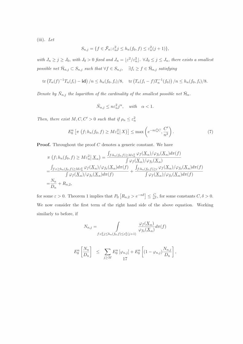
(iii). Let

Sn,j = f ∈ Fn; ε2nj ≤ hn(f0, f) ≤ ε2

n(j + 1),

with Jn ≥ j ≥ J0, with J0 > 0 fixed and Jn = ⌊ε2/ε2n⌋. ∀J0 ≤ j ≤ Jn, there exists a smallest

possible net Hn,j ⊂ Sn,j such that ∀f ∈ Sn,j , ∃fi ≥ f ∈ Hn,j satisfying

tr(

Tn(f)−1Tn(fi) − id)

/n ≤ hn(f0, fi)/8, tr(

Tn(fi − f)T−1n (f0)

)

/n ≤ hn(f0, fi)/8.

Denote by Nn,j the logarithm of the cardinality of the smallest possible net Hn.

Nn,j ≤ nε2njα, with α < 1.

Then, there exist M, C, C ′ > 0 such that if ρn ≤ ε2n

En0

[

π(

f ; hn(f0, f) ≥ Mε2n

∣

∣X)]

≤ max

(

e−nε2nC ,

C ′

n2

)

. (7)

Proof. Throughout the proof C denotes a generic constant. We have

π(

f ; hn(f0, f) ≥ Mε2n

∣

∣Xn

)

=

∫

f :hn(f0,f)≥Mε2n

ϕf (Xn)/ϕf0(Xn)dπ(f)

∫

ϕf (Xn)/ϕf0(Xn)

=

∫

f :ε≥hn(f0,f)≥Mε2n


∫


+

∫

f :hn(f0,f)≥ε ϕf (Xn)/ϕf0(Xn)dπ(f)

∫


=Nn

Dn+ Rn,2,

for some ε > 0. Theorem 1 implies that P0

[

Rn,2 > e−nδ]

≤ Cn2 , for some constants C, δ > 0.

We now consider the first term of the right hand side of the above equation. Working

similarly to before, if

Nn,j =

∫

f :ε2nj≤hn(f0,f)≤ε2

n(j+1)

ϕf (Xn)

ϕf0(Xn)

dπ(f)

En0

[

Nn

Dn

]

≤∑

j≥M

En0 [ϕn,j ] + En

0

[

(1 − ϕn,j)Nn,j

Dn

]

,

17

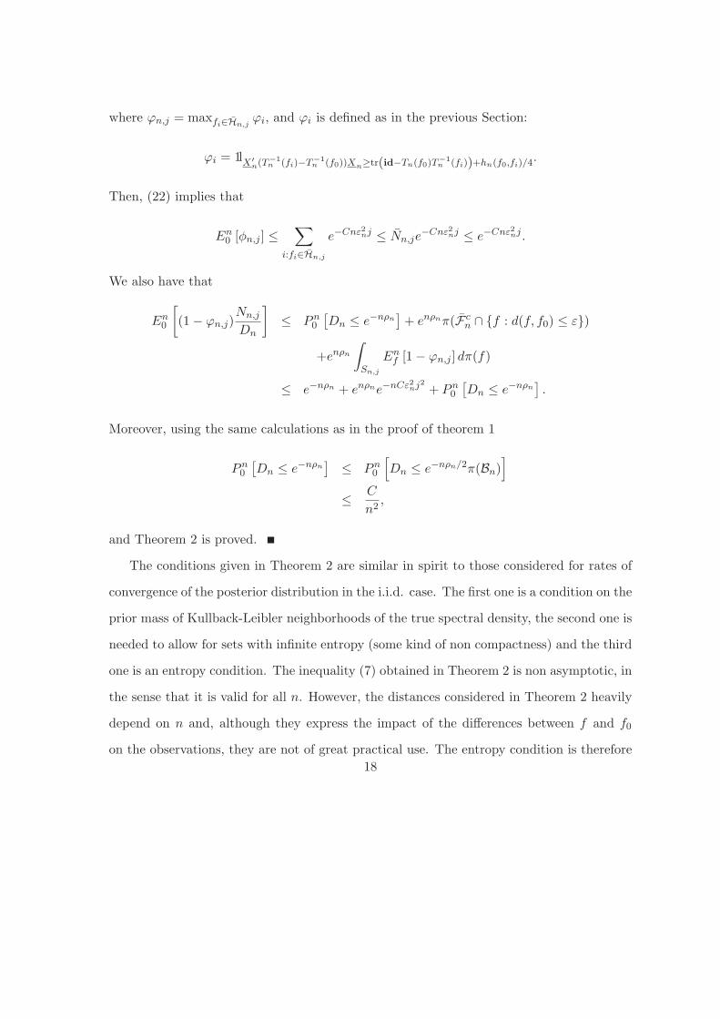
where ϕn,j = maxfi∈Hn,jϕi, and ϕi is defined as in the previous Section:

ϕi = 1lX′

n(T−1n (fi)−T−1

n (f0))Xn≥tr(id−Tn(f0)T−1n (fi))+hn(f0,fi)/4.

Then, (22) implies that

En0 [φn,j ] ≤

∑

i:fi∈Hn,j

e−Cnε2nj ≤ Nn,je

−Cnε2nj ≤ e−Cnε2

nj .

We also have that

En0

[

(1 − ϕn,j)Nn,j

Dn

]

≤ Pn0

[

Dn ≤ e−nρn]

+ enρnπ(Fcn ∩ f : d(f, f0) ≤ ε)

+enρn

∫

Sn,j

Enf [1 − ϕn,j ] dπ(f)

≤ e−nρn + enρne−nCε2nj2

+ Pn0

[

Dn ≤ e−nρn]

.

Moreover, using the same calculations as in the proof of theorem 1

Pn0

[

Dn ≤ e−nρn]

≤ Pn0

[

Dn ≤ e−nρn/2π(Bn)]

≤C

n2,

and Theorem 2 is proved.

The conditions given in Theorem 2 are similar in spirit to those considered for rates of

convergence of the posterior distribution in the i.i.d. case. The first one is a condition on the

prior mass of Kullback-Leibler neighborhoods of the true spectral density, the second one is

needed to allow for sets with infinite entropy (some kind of non compactness) and the third

one is an entropy condition. The inequality (7) obtained in Theorem 2 is non asymptotic, in

the sense that it is valid for all n. However, the distances considered in Theorem 2 heavily

depend on n and, although they express the impact of the differences between f and f0

on the observations, they are not of great practical use. The entropy condition is therefore

18

awkward and cannot be directly transformed into some more common entropy conditions.

To state a result involving distances between spectral densities that would be more useful,

we consider the special case of FEXP priors, as defined in Section 2.3. We can then obtain

rates of convergence in terms of the L2 distance between the log of the spectral densities,

l(f, f ′). The rates obtained are the optimal rates up to a logn term, at least on certain

classes of spectral densities. It is to be noted that the calculations used when working on

these classes of priors are actually more involved than those used to prove Theorem 2. This

is quite usual when dealing with rates of convergence of posterior distributions, however this

is emphasized here by the fact that distances involved in Theorem 4 are strongly dependent

on n. The method used in the case of the FEXP prior can be extended to other types of

priors.

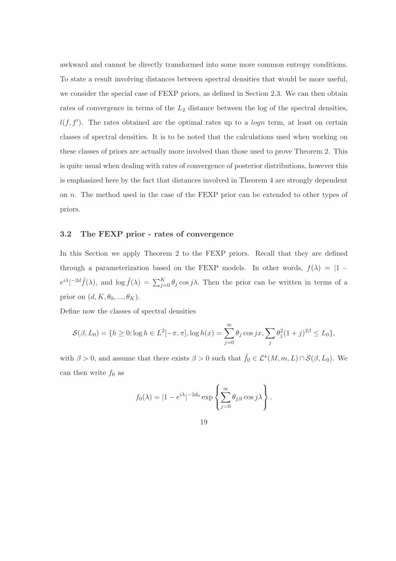
3.2 The FEXP prior - rates of convergence

In this Section we apply Theorem 2 to the FEXP priors. Recall that they are defined

through a parameterization based on the FEXP models. In other words, f(λ) = |1 −

eiλ|−2df(λ), and log f(λ) =∑K

j=0 θj cos jλ. Then the prior can be written in terms of a

prior on (d, K, θ0, ..., θK).

Define now the classes of spectral densities

S(β, L0) = h ≥ 0; log h ∈ L2[−π, π], log h(x) =∞∑

j=0

θj cos jx,∑

j

θ2j (1 + j)2β ≤ L0,

with β > 0, and assume that there exists β > 0 such that f0 ∈ L⋆(M, m, L)∩ S(β, L0). We

can then write f0 as

f0(λ) = |1 − eiλ|−2d0 exp

∞∑

j=0

θj,0 cos jλ

.

19

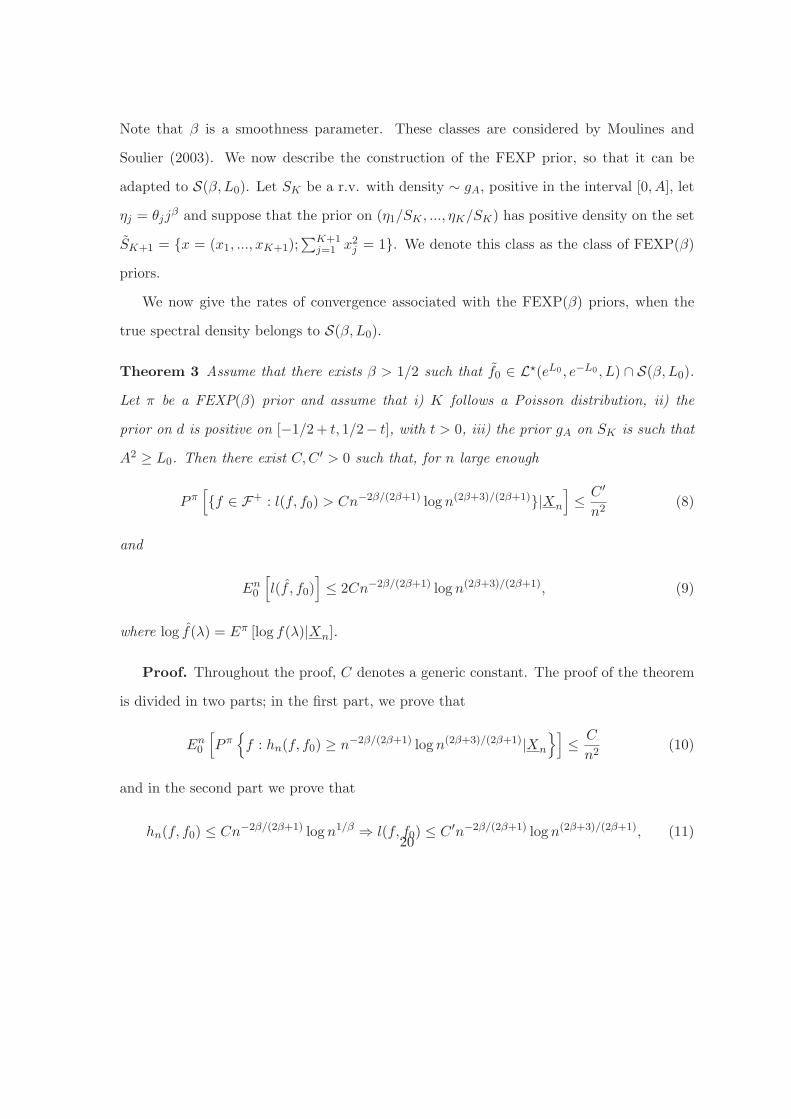
Note that β is a smoothness parameter. These classes are considered by Moulines and

Soulier (2003). We now describe the construction of the FEXP prior, so that it can be

adapted to S(β, L0). Let SK be a r.v. with density ∼ gA, positive in the interval [0, A], let

ηj = θjjβ and suppose that the prior on (η1/SK , ..., ηK/SK) has positive density on the set

SK+1 = x = (x1, ..., xK+1);∑K+1

j=1 x2j = 1. We denote this class as the class of FEXP(β)

priors.

We now give the rates of convergence associated with the FEXP(β) priors, when the

true spectral density belongs to S(β, L0).

Theorem 3 Assume that there exists β > 1/2 such that f0 ∈ L⋆(eL0 , e−L0 , L) ∩ S(β, L0).

Let π be a FEXP(β) prior and assume that i) K follows a Poisson distribution, ii) the

prior on d is positive on [−1/2 + t, 1/2− t], with t > 0, iii) the prior gA on SK is such that

A2 ≥ L0. Then there exist C, C ′ > 0 such that, for n large enough

P π[

f ∈ F+ : l(f, f0) > Cn−2β/(2β+1) log n(2β+3)/(2β+1)|Xn

]

≤C ′

n2(8)

and

En0

[

l(f , f0)]

≤ 2Cn−2β/(2β+1) log n(2β+3)/(2β+1), (9)

where log f(λ) = Eπ [log f(λ)|Xn].

Proof. Throughout the proof, C denotes a generic constant. The proof of the theorem

is divided in two parts; in the first part, we prove that

En0

[

P π

f : hn(f, f0) ≥ n−2β/(2β+1) log n(2β+3)/(2β+1)|Xn

]

≤C

n2(10)

and in the second part we prove that

hn(f, f0) ≤ Cn−2β/(2β+1) log n1/β ⇒ l(f, f0) ≤ C ′n−2β/(2β+1) log n(2β+3)/(2β+1), (11)20

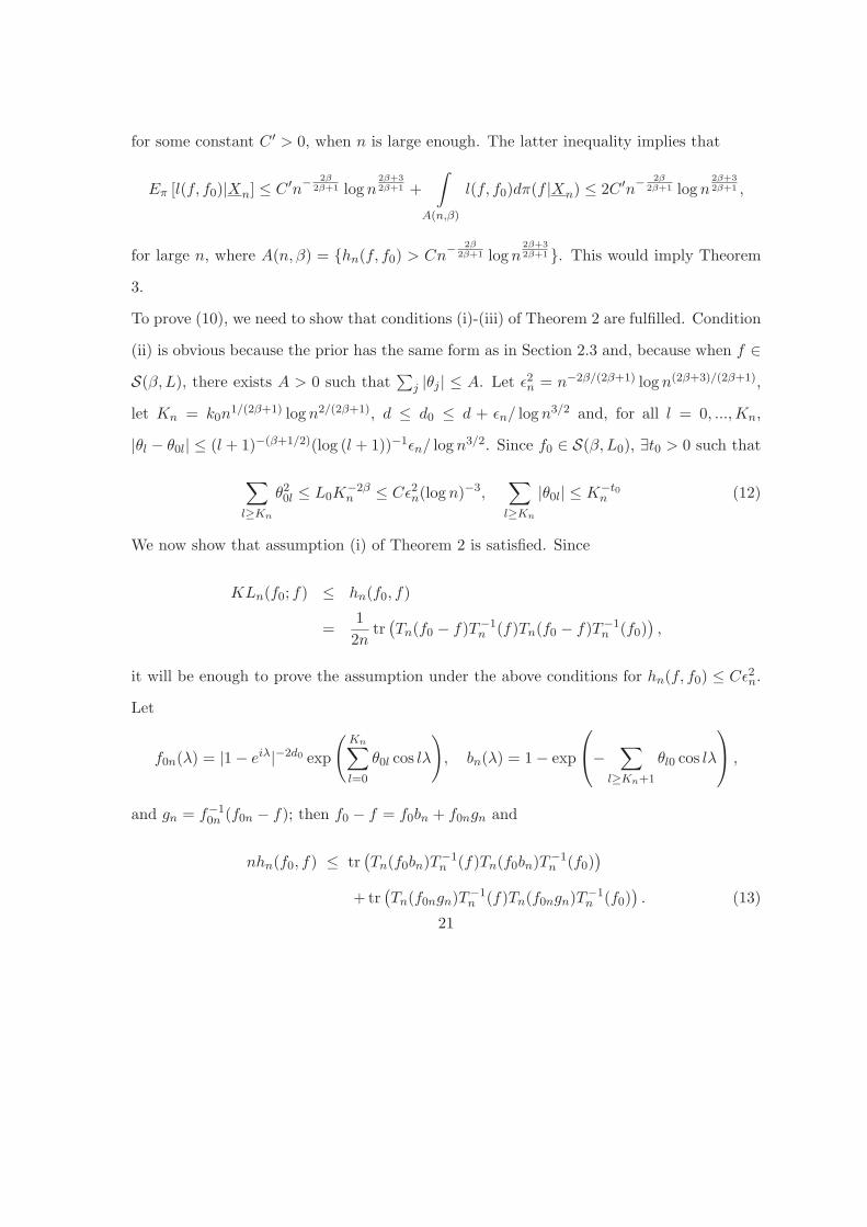
for some constant C ′ > 0, when n is large enough. The latter inequality implies that

Eπ [l(f, f0)|Xn] ≤ C ′n− 2β

2β+1 log n2β+3

2β+1 +

∫

A(n,β)

l(f, f0)dπ(f |Xn) ≤ 2C ′n− 2β

2β+1 log n2β+3

2β+1 ,

for large n, where A(n, β) = hn(f, f0) > Cn− 2β

2β+1 log n2β+3

2β+1 . This would imply Theorem

3.

To prove (10), we need to show that conditions (i)-(iii) of Theorem 2 are fulfilled. Condition

(ii) is obvious because the prior has the same form as in Section 2.3 and, because when f ∈

S(β, L), there exists A > 0 such that∑

j |θj | ≤ A. Let ǫ2n = n−2β/(2β+1) log n(2β+3)/(2β+1),

let Kn = k0n1/(2β+1) log n2/(2β+1), d ≤ d0 ≤ d + ǫn/ log n3/2 and, for all l = 0, ..., Kn,

|θl − θ0l| ≤ (l + 1)−(β+1/2)(log (l + 1))−1ǫn/ log n3/2. Since f0 ∈ S(β, L0), ∃t0 > 0 such that

∑

l≥Kn

θ20l ≤ L0K

−2βn ≤ Cǫ2n(log n)−3,

∑

l≥Kn

|θ0l| ≤ K−t0n (12)

We now show that assumption (i) of Theorem 2 is satisfied. Since

KLn(f0; f) ≤ hn(f0, f)

=1

2ntr(

Tn(f0 − f)T−1n (f)Tn(f0 − f)T−1

n (f0))

,

it will be enough to prove the assumption under the above conditions for hn(f, f0) ≤ Cǫ2n.

Let

f0n(λ) = |1 − eiλ|−2d0 exp

(

Kn∑

l=0

θ0l cos lλ

)

, bn(λ) = 1 − exp

−∑

l≥Kn+1

θl0 cos lλ

,

and gn = f−10n (f0n − f); then f0 − f = f0bn + f0ngn and

nhn(f0, f) ≤ tr(

Tn(f0bn)T−1n (f)Tn(f0bn)T−1

n (f0))

+ tr(

Tn(f0ngn)T−1n (f)Tn(f0ngn)T−1

n (f0))

. (13)

21

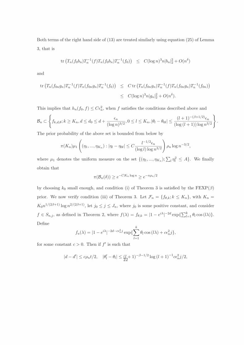
Both terms of the right hand side of (13) are treated similarly using equation (25) of Lemma

3, that is

tr(

Tn(f0bn)T−1n (f)Tn(f0bn)T−1

n (f0))

≤ C(log n)3n|bn|22 + O(nδ)

and

tr(


n (f0))

≤ C tr(


n (f0n))

≤ C(log n)3n|gn|22 + O(nδ).

This implies that hn(f0, f) ≤ Cǫ2n, when f satisfies the conditions described above and

Bn ⊂

fk,d,θ; k ≥ Kn, d ≤ d0 ≤ d +ǫn

(log n)3/2, 0 ≤ l ≤ Kn, |θl − θ0l| ≤

(l + 1)−(β+1/2)ǫn

(log (l + 1)) log n3/2

.

The prior probability of the above set is bounded from below by

π(Kn)µ1

(

(η1, ..., ηKn) : |ηl − η0l| ≤ Cl−1/2ǫn

(log l) log n3/2

)

ρn log n−3/2,

where µ1 denotes the uniform measure on the set (η1, ..., ηKn);∑

l η2l ≤ A. We finally

obtain that

π(Bn(δ)) ≥ e−CKn log n ≥ e−nρn/2

by choosing k0 small enough, and condition (i) of Theorem 3 is satisfied by the FEXP(β)

prior. We now verify condition (iii) of Theorem 3. Let Fn = fθ,k; k ≤ Kn, with Kn =

K0n1/(2β+1) log n2/(2β+1), let j0 ≤ j ≤ Jn, where j0 is some positive constant, and consider

f ∈ Sn,j , as defined in Theorem 2, where f(λ) = fθ,k = |1 − eiλ|−2d exp∑k

l=1 θl cos (lλ).

Define

fu(λ) = |1 − eiλ|−2d−cǫ2nj expk∑

l=1

θl cos (lλ) + cǫ2nj,

for some constant c > 0. Then if f ′ is such that

|d − d′| ≤ cρnt/2, |θ′l − θl| ≤ (l + 1)−β−1/2 log (l + 1)−1cǫ2nj/2,22

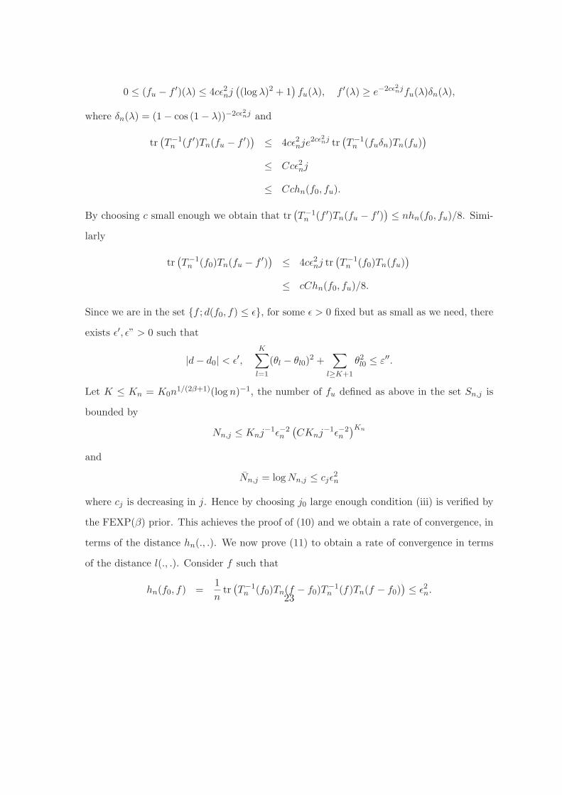
0 ≤ (fu − f ′)(λ) ≤ 4cǫ2nj(

(log λ)2 + 1)

fu(λ), f ′(λ) ≥ e−2cǫ2njfu(λ)δn(λ),

where δn(λ) = (1 − cos (1 − λ))−2cǫ2nj and

tr(

T−1n (f ′)Tn(fu − f ′)

)

≤ 4cǫ2nje2cǫ2nj tr(

T−1n (fuδn)Tn(fu)

)

≤ Ccǫ2nj

≤ Cchn(f0, fu).

By choosing c small enough we obtain that tr(

T−1n (f ′)Tn(fu − f ′)

)

≤ nhn(f0, fu)/8. Simi-

larly

tr(

T−1n (f0)Tn(fu − f ′)

)

≤ 4cǫ2nj tr(

T−1n (f0)Tn(fu)

)

≤ cChn(f0, fu)/8.

Since we are in the set f ; d(f0, f) ≤ ǫ, for some ǫ > 0 fixed but as small as we need, there

exists ǫ′, ǫ” > 0 such that

|d − d0| < ǫ′,K∑

l=1

(θl − θl0)2 +

∑

l≥K+1

θ2l0 ≤ ε′′.

Let K ≤ Kn = K0n1/(2β+1)(log n)−1, the number of fu defined as above in the set Sn,j is

bounded by

Nn,j ≤ Knj−1ǫ−2n

(

CKnj−1ǫ−2n

)Kn

and

Nn,j = log Nn,j ≤ cjǫ2n

where cj is decreasing in j. Hence by choosing j0 large enough condition (iii) is verified by

the FEXP(β) prior. This achieves the proof of (10) and we obtain a rate of convergence, in

terms of the distance hn(., .). We now prove (11) to obtain a rate of convergence in terms

of the distance l(., .). Consider f such that

hn(f0, f) =1

ntr(

T−1n (f0)Tn(f − f0)T

−1n (f)Tn(f − f0)

)

≤ ǫ2n.23

Equation (26) of Lemma 3 implies that

1

ntr(

Tn(f−10 )Tn(f − f0)Tn(f−1)Tn(f − f0)

)

≤ Cǫ2n,

leading to

1

ntr (Tn(g0)Tn(f − f0)Tn(g)Tn(f − f0)) ≤ Cǫ2n, (14)

where g0 = (1 − cos λ)d0 , g = (1 − cos λ)d.

We now prove that tr (Tn(g0(f − f0))Tn(g(f − f0))) ≤ Cǫ2n: Using the same calculations as

in the control of I2 in Appendix C,

∆ =1

ntr (Tn(g0(f − f0))Tn(g(f − f0))) −

1

ntr (Tn(g0)Tn(f − f0)Tn(g)Tn(f − f0))

= O(n6δ−1 log n3δ),

as soon as |d − d0| < δ/2, where δ is any positive constant, as small as we want. This

implies, together with (14) that

1

ntr (Tn(g0(f − f0))Tn(g(f − f0))) ≤ Cǫ2n.

To finally obtain (11), we use equation (27) in Lemma 3 which implies that

An = tr (Tn(g0(f − f0))Tn(g(f − f0))) − tr(

Tn(g0g(f − f0)2))

≤ Cn−1+δ + log n

Kn∑

l=0

l|θl|

(

∫

[−π,π]g0g(f − f0)

2(λ)dλ

)1/2

.

Moreover

Kn∑

l=1

l|θl| ≤∑

l=1

l2β+rθ2 +

Kn∑

l=1

l−r/(2β−1)

≤ CKrn + K1−r/(2β−1)

n ,

24

by choosing r = (2β − 1)/2β, An/n is of order n−(4β2+1)/(2β(2β+1)) which is negligible

compared to n−2β/(2β+2) so that if β ≥ 1/2

∫

[−π,π]g0g(f0 − f)2dλ ≤ ǫ2n,

which achieves the proof.

4 Computational issues

Any practical implementation of our nonparametric approach must take into account the

fact that the computation of the likelihood function in this context is very expensive since

both the determinant and the inverse of a large Toeplitz matrix must be computed at each

evaluation. Then one should prefer to use a Monte Carlo approximation which is as easiest

as possible to handle and with fast convergence properties. We consider several different

approaches, which are discussed in a companion paper (Liseo and Rousseau 2006). Our

final preference was for a modification of the adaptive Monte Carlo algorithm, proposed

and discussed in Douc et al. (2006), which can also be used in the presence of variable

dimension parametric spaces as is the case here. The main advantage of adaptive Monte

Carlo algorithms is that they do not rely upon asymptotic convergence of the samplers but,

rather, they should be considered as an evolution of the importance sampling schemes, with

the advantage of an on-line adaptation of the weights given to the proposal distributions,

which are allowed to be more than one. Here we briefly describe the main features of the

proposed algorithm. Further details can be found in Liseo and Rousseau (2006). Denote by

(K, ηk) our global parameter, with ηK = (θ0, ..., θk, d); here K is a positive integer which

determines the size of the parameter vector. First one has to define a set of proposal dis-

tributions, which we denote by Qh(·, ·), h = 1, . . . , H; they represent H possible different

kernels, which we assume are all dominated by the same dominating measure, as the poste-25

rior distribution πx. Denote by qh(·, ·) the corresponding densities. Then one has to perform

T different iterations of an importance sampling approximation, each based on N proposed

values. The novel feature is that, at each t, t = 1, · · · , T , the weights of the sampled values

are calibrated in terms of the previous iterations. From a practical perspective, one should

work with a large value of N , and a small value (say 5-10) of T . Douc et al. (2006) show

that, in fix dimension problems, the algorithm will converge toward the optimal mixture of

proposals, in few iterations, at least in a Kullback-Leibler distance sense.

The algorithm follows quite closely the one described in Douc et al. (2006) and will not

reported here. The only significant difference is that we have to deal with the variable di-

mension of the parameter space; then we must be able to propose a set of possible “moves”

to subspaces with a different value of k. Then, at each iteration t, (t = 1, · · · , T ) and for

each sample point j, (1 ≤ j ≤ N), we propose a new value K ′j,t from a distribution on the

set of integers, conditional on the previous value of Kj ; then, conditionally on K ′j,t and on

the value of ηj,t−1, propose a new value η(t)j,K′

j. The description of all the possible moves

is quite involved; here we sketch the ideas behind the strategy. For a fixed 1 ≤ j ≤ N ,

at the t-th iteration of the algorithm, one draws a new value K ′j,t, according the following

proposals for K ′:

Kj,t = Kj,t−1 + ξj,t, where ξj,t|Kj,t−1 ∼ p1Po(λ1) + (1 − p1)NePoKj,t−1(λ2),

where p1 ∈ (0, 1) and the symbol NePok denotes a truncated Poisson distribution over the

set −k,−(k−1), . . . , 0. At each iteration the proposed value Kj,t may be either less than,

equal to, or larger than Kj,t−1;

• If Kj,t < Kj,t−1 then θ(t)Kj,t+1 = · · · = θ

(t)Kj,t−1

= 0 and

(θ(t)0 , . . . , θ

(t)Kj,t

) = (θ(t−1)0 , . . . , θ

(t−1)Kj,t

) + εKj,t(15)

26

and εKj,tis a Kj,t-dimensional symmetric proposal.

• If Kj,t = Kj,t−1 then the new point is draw according to (15), without eliminating any

parameter.

• If Kj,t > Kj,t−1, then the first Kj,t−1 are drawn according to (15), while the latest

components are drawn from the same kernel proposal ε, although centered on an easy-to-

calculate point estimate obtained from a simplified version of the estimator presented in

Hurvich et al. (2002). Notice that, within this approach, even when the algorithm proposes

a change of dimension, one must propose a global move for all the components of the

parameter vector, in order to satisfy the positivity condition on the proposal required by

Douc et al. (2006). For the practical evaluation of the likelihood function, we have used

the approximations of the inverse matrix and of the determinant of a Toeplitz matrix, as

proposed in Chen, Hurvich and Lu (2006).

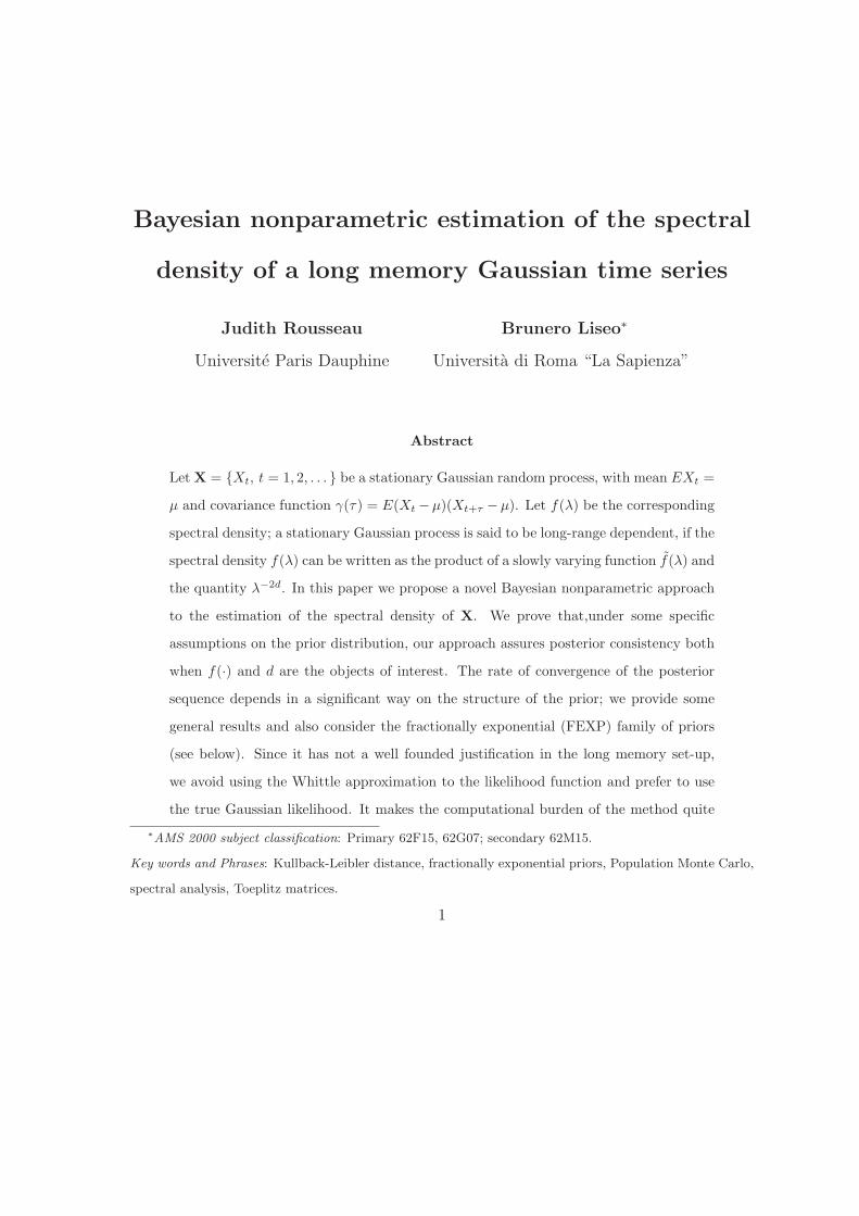
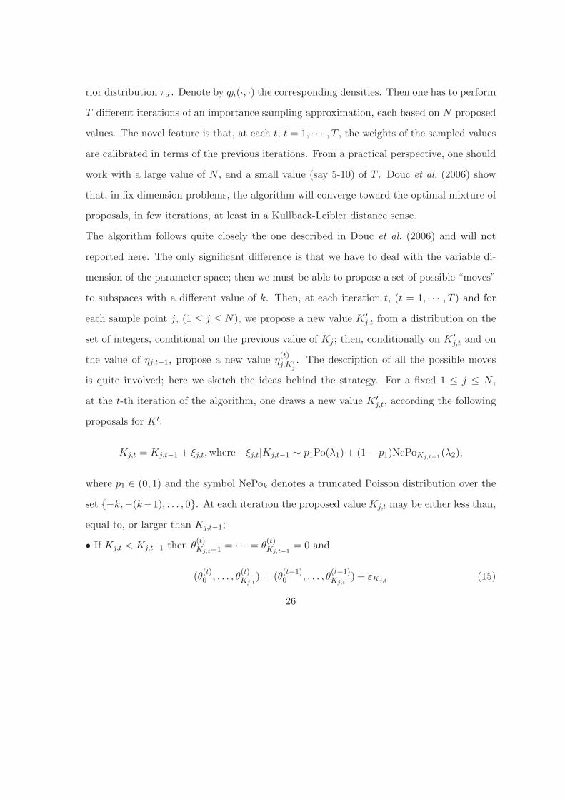
4.1 Analysis of Nile river data

Here we analyze the Nile river data that consists of the time series of annual minimum water

levels of the River Nile at the Roda Gorge; the data are available, for example, in Beran 1994,

page 237. We examined n = 512 observations corresponding to the period from 622 to

1133. A visual study (see Figure 1) of the data and the ACF reveals a strong persistence

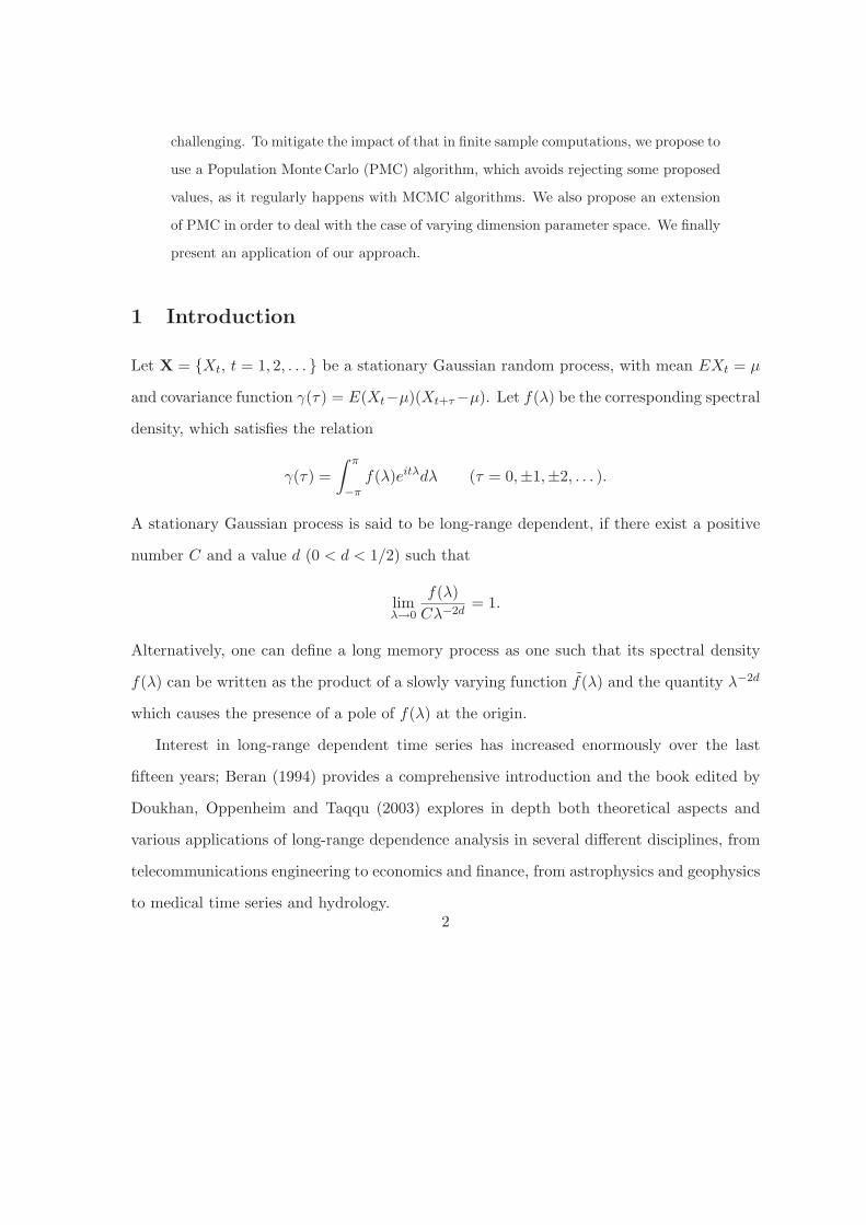
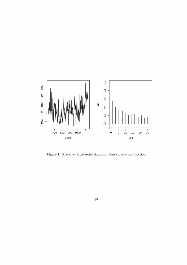
of autocorrelations; after removing the mean, we applied our procedure to produce the

corresponding spectral estimate; a point-wise 95% credible band is computed from the PMC

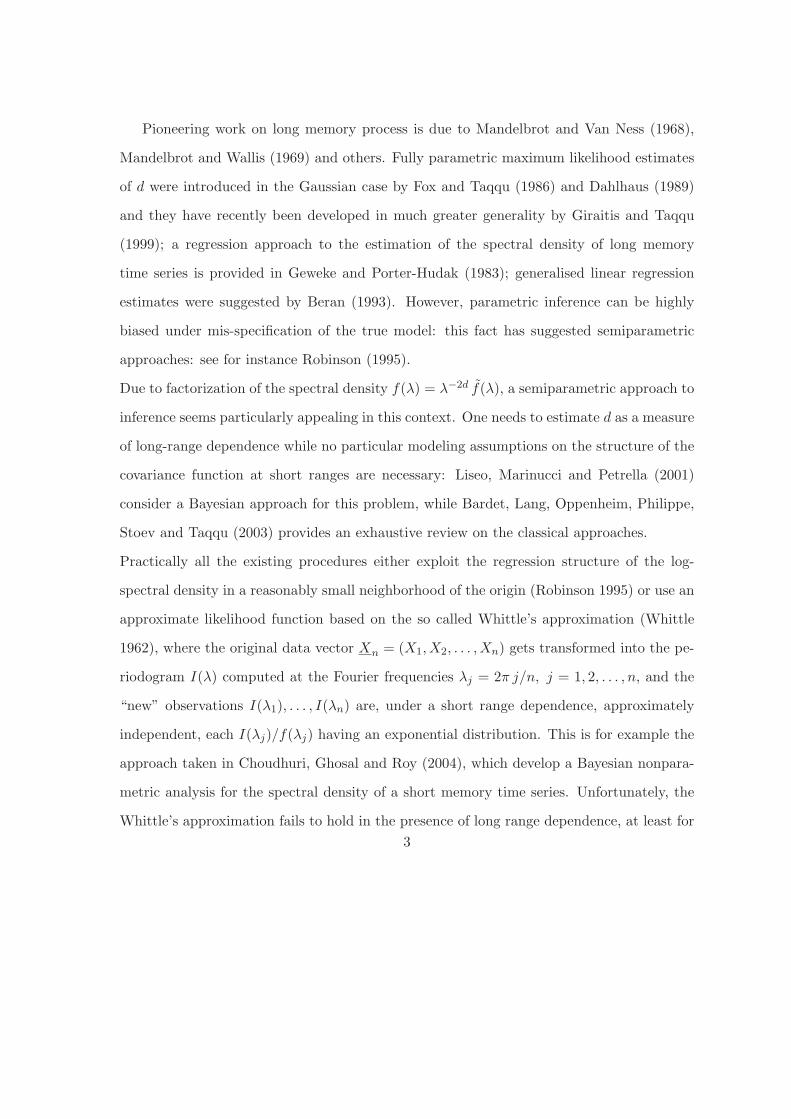
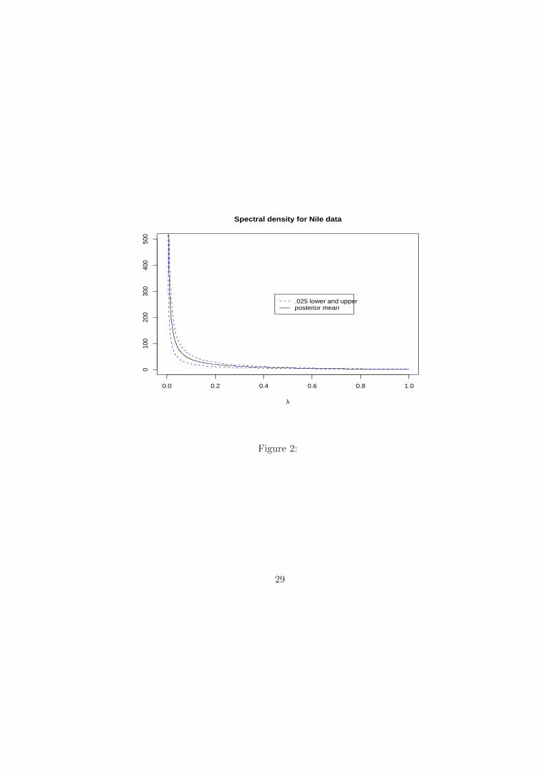
sample and is plotted in Figure 2. Figure 3 reports the PMC histogram approximation to

the posterior distribution of d. Notice that the posterior mean estimate of d is in agreement

with other proposed estimates: see, for example, Robinson (1995).

27

years

700 800 900 1000

1000

1100

1200

1300

1400

0 5 10 15 20 25

0.0

0.2

0.4

0.6

0.8

1.0

Lag

γ(k)

Figure 1: Nile river time series data and Autocorrelation function

28

0.0 0.2 0.4 0.6 0.8 1.0

010

020

030

040

050

0

Spectral density for Nile data

λ

.025 lower and upperposterior mean

Figure 2:

29

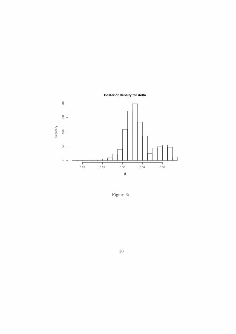
Posterior density for delta

d

Freq

uenc

y

0.26 0.28 0.30 0.32 0.34

050

100

150

200

Figure 3:

30

Appendices

A Lemmas 1 and 2

We state two technical lemmas, which are extensions of Lieberman, Rousseau and Zucker

(2003) on uniform convergence of traces of Toeplitz matrices, and which are repeatedly used

in the paper.

Lemma 1 Let t > 0, M > 0 and M a positive function on ]0, π[, let p be a positive integer,

and

˜F(d, M, M) =

f ∈ F ,∀u > 0, sup|λ|>u

df(λ)

dλ≤ M(u)

,

we have:

supp(d1+d2)≤1/2−t

fi∈˜F(d1,M,M)

gi∈˜F(d2,M,M)

∣

∣

∣

∣

∣

1

ntr

(

p∏

i=1

Tn(fi)Tn(gi)

)

− (2π)2p−1

∫ π

−π

p∏

i=1

fi(λ)gi(λ)dλ

∣

∣

∣

∣

∣

→ 0. (16)

and let L > 0 and ρ ∈ (0, 1]

supp(d1+d2)≤1/2−tfi∈F(d1,M,L,ρ)gi∈F(d2,M,L,ρ)

∣

∣

∣

∣

∣

1

ntr

(

p∏

i=1

Tn(fi)Tn(gi)

)

− (2π)2p−1

∫ π

−π

p∏

i=1

fi(λ)gi(λ)dλ

∣

∣

∣

∣

∣

→ 0. (17)

This lemma is an obvious adaptation from Lieberman et al. (2003), and the only non obvious

part is the change from the condition of continuous differentiability in that paper to the

Lipschitz condition of order ρ, considered equation 17. This different assumption affects

only equation (30) of Lieberman et al. (2003), with ηn replaced by ηρn, which does not change

the convergence results.

Lemma 2

sup2p(d1−d2)≤ρ2∧1/2−t

fi∈F(d1,M,L,ρ1)gi∈G(d2,m,M,L,ρ2)

∣

∣

∣

∣

∣

1

ntr

(

p∏

i=1

Tn(fi)Tn(gi)−1

)

−1

2π

∫ π

−π

p∏

i=1

fi(λ)

gi(λ)dλ

∣

∣

∣

∣

∣

→ 0,

31

sup2p(d1−d2)≤ρ2∧1/2−t

fi∈˜F(d1,M,M)

gi∈G(d2,m,M,L,ρ2)

∣

∣

∣

∣

∣

1

ntr

(

p∏

i=1

Tn(fi)Tn(gi)−1

)

−1

2π

∫ π

−π

p∏

i=1

fi(λ)

gi(λ)dλ

∣

∣

∣

∣

∣

→ 0.

and

sup2p(d1−d2)≤1/2−t

fi∈˜F(d1,M,M)

gi∈L(d2,m,M,L)

∣

∣

∣

∣

∣

1

ntr

(

p∏

i=1

Tn(fi)Tn(gi)−1

)

−1

2π

∫ π

−π

p∏

i=1

fi(λ)

gi(λ)dλ

∣

∣

∣

∣

∣

→ 0.

Proof. Proof of lemma 2.

In this second lemma, the uniformity result is a consequence of the first lemma, as in

Lieberman et al. (2003); The only difference is in the proof of Lemma 5.2. of Dahlhaus

(1989), i.e. in the study of terms in the form

|id − Tn(g)1/2Tn

(

(4π2g)−1)

Tn(g)1/2|.

Following Dahlhaus (1989)’s proof, we obtain an upper bound of

∣

∣

∣

∣

g(λ1)

g(λ2)− 1

∣

∣

∣

∣

which is different from Dahlhaus (1989)’s. If g ∈ G(d2, m, M, L, ρ2), the Lipschitz condition

in ρ implies that∣

∣

∣

∣

g(x)

g(y)− 1

∣

∣

∣

∣

≤ K

(

|x − y|ρ +|x − y|1−δ

|x|1−δ

)

.

Calculations using LN as in Dahlhaus (1989) imply that

|I − Tn(f)1/2Tn

(

(4π2f)−1)

Tn(f)1/2|2 = O(n1−2ρ log n) + O(nδ), ∀δ > 0.

If g ∈ L⋆(M, m, L) as defined in Section 3.2, then

∣

∣

∣

∣

f(x)

f(y)− 1

∣

∣

∣

∣

≤ K

(

|x − y|1−3δ

(|x| ∧ |y|)1−δ

)

≤ K|x − y|1−3δ

(

1

|x|1−δ+

1

|y|1−δ

)

32

and Dahlhaus (1989) Lemma 5.2 is proved, leading to a constraint in the form 4p(d1−d2) < 1

(corresponding to ρ = 1).

Then, using again Dahlhaus (1989)’s (1989) calculations we obtain that

|A − B| = 0(n2(d2−d1)n1/2−(ρ∧1/2)+δ), ∀δ > 0

and finally that

1

ntr

p∏

j=1

Aj −

p∏

j=1

Bj

=

p∑

k=1

O(n−1/2n2(p−k)(d2−d1)n2(d2−d1)n1/2−ρ)

=

p∑

k=1

O(n2(p−k+1)(d2−d1)−(ρ∧1/2))

which goes to zero when 2p(d2 − d1) < ρ ∧ 1/2.

B Proof of Theorem 1

Before giving the proof of Theorem 1, we give a more general version of assumption (ii),

namely (ii)bis, ensuring consistency of the posterior. It is quite cumbersome in its formu-

lation, but we believe that it might prove useful in some context.

Assumption [(ii)bis] For all ε > 0 there exists Fn ⊂ f ∈ F+, d(f0, fi) > ǫ, such

that π(Fcn) ≤ e−nr and there exist t, M, m > 0 with t < ρ0/4, and a smallest possible net

Hn ⊂ F+(t, M, m), d(f, f0) > ǫ/4 such that ∀f ∈ Fn, ∃fi ≥ f ∈ Hn satisfying either of

the three conditions

1. |4(d0 − di)| ≤ ρ0 ∧ 1/2 − t and

max

(

tr[Tn(f)−1Tn(fi) − id]

n,tr[Tn(fi − f)T−1

n (f0)]

n

)

≤hn(f0, fi)

8. (18)

2. 4(di − d0) > ρ0 ∧ 1/2 − t,

tr[Tn(f)−1Tn(fi) − id]/n ≤ KLn(f0; fi)/4, hn(f, fi) ≤ KLn(f0; fi)/4, (19)33

3. 4(d0 − di) > ρ0 ∧ 1/2 − t and

1

n[Tn(f)T−1

n (fi) − id − Tn(f − fi)T−1n (f0) ≤ KLn(fi; f0)/2 (20)

We also assume that ∀f ∈ Hn,

1

ntr(

(Tn(|λ|−2d)Tn(f0 − f))2)

≥ B1B(f, f0) if d ≤ d0

and

1

ntr(

(Tn(|λ|−2d0)Tn(f0 − f))2)

≥ B1B(f0, f) if d ≥ d0

Proof of Theorem 1

The proof follows the same ideas as in Ghosal et al. (2000). We can write

P π [Acε|Xn] =

∫

Acεϕf (Xn)/ϕf0

(Xn)dπ(f)∫

F+ϕf (X)/ϕf0

(Xn)dπ(f)=

Nn

Dn.

Then the idea is to bound from below the denominator using condition (i) of the Theorem

and to bound from above the numerator using a discretization of Aǫ based on the net Hn

defined in (ii) of the Theorem and on tests.

Let δ, δ1 > 0: one has

P0

[

P π [Acε|Xn] ≥ e−nδ

]

≤ Pn0

[

Dn ≤ e−nδ1]

+ Pn0

[

Nn ≥ e−n(δ+δ1)]

= p1 + p2 (21)

Also, let

Bn = f : tr (()B(f0, f)) − log det(A(f0, f)) ≤ nδ1; tr(

B(f0, f)3)

≤ M ′n,

where

• A(f0, f) = Tn(f)−1Tn(f0)34

• B(f0, f) = Tn(f0)1/2[Tn(f)−1 − Tn(f0)

−1]Tn(f0)1/2,

and M > 0 is fixed, and define

Ωn = (f, X) : −Xt[Tn(f)−1 − Tn(f0)−1]X + log (det(An)) > −2nδ1.

We then have

p1 ≤ Pn0

(∫

Ωn∩Bn

ϕf (X)

ϕf0(X)

dπ(f) ≤ e−nδ1/2 π(Bn)

2

)

≤ Pn0

(

π(Bn ∩ Ωn) ≤π(Bn)

2

)

≤ Pn0

(

π(Bn ∩ Ωcn) >

π(Bn)

2

)

≤ 2

∫

BnPn

0 [Ωcn]dπ(f)

π(Bn).

Moreover,

Pn0 [Ωc

n] = Pn0

(

Xtn[Tn(f)−1 − Tn(f0)

−1]Xn + log (det(A(f0, f))) > 2nδ1

)

= Pr[ytB(f0, f)y − tr(B(f0, f)) > 2nδ1 + log (det(A(f0, f))) − tr(B(f0, f))]

where y ∼ Nn(0, id). When f ∈ Bn, 2nδ1 + log (det(A(f0, f))) − tr (()B(f0, f)) > nδ1,

so that

Pn0 [Ωc

n] ≤ Pr[ytB(f0, f)y − tr (()B(f0, f)) > nδ1]

≤E[(ytB(f0, f)y − tr (()B(f0, f)))3]

n3.

Moreover,

E[(ytB(f0, f)y − tr (()B(f0, f)))3] = 8 tr (()B(f0, f)3) ≤ M ′n,

whenever f ∈ Bn. Hence, p1 ≤ 8M ′/n2. Besides,

Bn ⊂ f ∈ G(t, M, m, L, ρ); KL∞(f0; f) ≤δ1

2, 6(d0 − d) ≤ ρ − t,

1

2π

∫

(f0

f− 1)3dx ≤

M ′

2

35

so that assumption (i) implies that, for n large enough, π(Bn) ≥ e−nδ1/2 and

Pn0

[

Dn ≤ e−nδ1]

≤8M ′

n2.

We now consider the second term of (21), namely:

p2 = Pn0

[

Nn ≥ e−n(δ+δ1)]

≤ 2en(δ+δ1)π(Fcn) + Pn

0

[

∫

Acε∩Fn

ϕf (Xn)

ϕf0(Xn)

dπ(f) ≥ e−n(δ+δ1)/2

]

≤ e−n(r−(δ+δ1)) + p2,

take δ + δ1 < r and consider p2. Consider the following tests : let fi ∈ Hn,

φi = 1lX′(T−1n (f0)−T−1

n (fi))X≥nρi,

1. If 4(d0 − di) ≤ ρ0 − t and 4(di − d0) ≤ ρ0 − t, then if

ρi = tr(

id − Tn(f0)T−1n (fi)

)

/n + hn(f0, fi)/4,

En0 [φi] ≤ max

(

exp −nhn(f0, fi)

2

512bi, exp −n

hn(f0, fi)

32

)

, (22)

where bi = n−1 tr(

(


)2)

, and for any f ∈ F+(1−t, M, m) satisfying

f ≤ fi and

1

ntr(

Tn(f)T−1n (fi) − id

)

+1

ntr(

Tn(fi − f)T−1n (f0)

)

≤ hn(f0, fi)/4,

we have

Enf [1 − φi] ≤ max

(

exp −nhn(f0, fi)

2

16Bi, exp −n

hn(f0, fi)

4

)

,

where Bi = n−1 tr(

(id − Tn(fi)T−1n (f0))

2)

.

36

2. If 4(di − d0) > ρ0 − 4t, if ρi = tr(


)

/n + KLn(f0; fi)/2,

En0 [φi] ≤ max

(

exp −nKLn(f0; fi)

2

512bi, exp −n

hn(f0, fi)

32

)

,

and for all f ≤ fi satisfying

tr(

Tn(f)−1Tn(fi) − id)

≤ nKLn(f0; fi)/4, and hn(f, fi) ≤ KLn(f0; fi)/4,

we have

Enf [1 − φi] ≤ e−nKLn(f0;fi)/2

3. If 4(d0 − di) > ρ0 − 4t, if ρi = log det[Tn(fi)Tn(f0)−1]/n, then

En0 [φi] ≤ max

(

exp −nKLn(fi; f0)

2

8Bi, exp −n

KLn(fi; f0)

4

)

.

Moreover, for all f ∈ G(1 − t, M1, M2), satisfying f ≤ fi and

1

ntr(

Tn(f)T−1n (fi) − id − Tn(f − fi)T

−1n (f0)

)

≤ KLn(fi; f0),

we have

Enf [1 − φi] ≤ max

(

exp −nKLn(fi; f0)

2

64Bi, exp −n

KLn(fi; f0)

8

)

.

The difficulty is now to transform these conditions into a net. Using Dahlhaus’s type of

calculation (Dahlhaus (1989), pag. 1755) there exists a constant C > 0 (depending on

M, m) uniformly over the class ∪d≤d0F+(d, m, M), such that

KLn(fi; f0) ≥1

4C2

1

ntr(

(Tn(f0)−1Tn(fi) − id)2

)

(23)

for all n ≥ 1. Similarly,

KLn(f0; fi) ≥1

4C2

1

ntr(

(Tn(fi)−1Tn(f0) − id)2

)

(24)37

Since for all f ∈ Hn, associated with the long-memory parameter d,

1

ntr(

(Tn(|λ|−2d)Tn(f0 − f))2)

≥ B1B(f, f0) if d ≤ d0

and

1

ntr(

(Tn(|λ|−2d0)Tn(f0 − f))2)

≥ B1B(f0, f) if d ≥ d0

We end up with an upper bound in the form:

En0 [φi] ≤ e−ncB(fi,f0)), e−ncB(f0,fi)

Enf [1 − φi] ≤ e−ncB(fi,f0), e−ncB(f0,fi)

When d(fi, f0) > ε, up to the (2π)−1 term

B(fi, f0) =

∫ (

fi

f0− 1

)2

dx

≥ cKL∞(fi; f0)

| log KL∞(fi; f0)|

≥ c ε| log ε|−1,

for some constant c. The last inequalities comes from the fact that (fi/f0 − 1− log fi/f0) ≤

C(fi/f0 − 1)2 unless fi/f0 is close to zero (A = fi/f0 ≤ xc). On this set, we bound

∫

A(fi/f0 − 1 − log fi/f0)(λ)dλ ≤

∫

Alog f0/fi(λ)dλ

≤ (

∫

Adλ) log

(

∫

A f0/fi(λ)dλ∫

A dλ

)

≤ C ′(

∫

Adλ)

∣

∣

∣

∣

log(

∫

Adλ)

∣

∣

∣

∣

,

for some constant C ′ > 0.

Finally, in each case, we have, when n is large enough (independently of fi),

En0 [φi] ≤ e−nc ε| log ε|−1

≤ e−nε| log ε|−2

38

C Proof of inequality (6)

We show that

n−1 tr(

(Tn(|λ|−2di)−1Tn(fi − f0))2)

≥ B

∫

(f0/fi − 1)2(x)dx

when di > d0 First we prove that

n−1 tr(

(Tn(|λ|2di(fi − f0))2)

≥1

2

∫

|λ|4di(f0 − fi)2(x)dx

when d0 > di uniformly in fi ∈ Fn when n is large enough. We have,

∆ = n−1 tr(

(Tn(|λ|2di(fi − f0))2)

− n−1 tr(

(Tn(|λ|4di(fi − f0)2))

= n−1

∫

[−π,π]2g(λ1)(g(λ2) − g(λ1))∆n(λ1 − λ2)∆n(λ2 − λ1)dλ1dλ2

where

g(λ) = |λ|2di(fi − f0)(λ) = fi(λ) − |λ|2(di−d0)f0(λ).

The second term belongs to either G(t, M0, m0, L0, ρ) or ∪dL(d, M0, m0, L0), hence this

term is treated as in Appendix A. The only term that causes problem is the difference

fi(λ1) − fi(λ2) since the derivative of fi is not uniformly bounded. Note however that

|fi(λ1) − fi(λ2)| ≤ (

k∑

j=0

j|θj |)|λ1 − λ2|

in a FEXP(k) model. So that

I1 = n−1

∣

∣

∣

∣

∣

∫

[−π,π]2g(λ1)(g(λ2) − g(λ1))∆n(λ1 − λ2)∆n(λ2 − λ1)dλ1dλ2

∣

∣

∣

∣

∣

≤ n−1

k∑

j=0

j|θj |

∫

[−π,π]2|g(λ1)|Ln(λ1 − Λ2)dλ2dλ1

≤ 2π

(

∑kj=0 j|θj |

)

log nM

n.

40

In the set Fn k ≤ k0 log n/n where k0 is chosen as small as need be. Using∑k

j=0 j|θj | ≤

k0A log n/n, we obtain that

I1 ≤ δ,

where δ is chosen as small as we want, depending on k0. Now, we also have that using the

same representation of the traces:

I2 =1

n

[

tr(

(Tn(|λ|2di)Tn(fi − f0))2)

− tr(

(Tn(|λ|2di(fi − f0))2)]

≤ 2M2

n

∫

[−π,π]4|λ2 λ4|

−2(d1∨d0)∣

∣

∣|λ1|

2di − |λ2|2di

∣

∣

∣Ln(λ1 − Λ2) · · ·Ln(λ4 − Λ1)dλ1 · · · dλ4.

Using the same calculations as Dahlhaus (1989, p1760-1761), since

∣

∣

∣|λ1|

2di − |λ2|2di

∣

∣

∣≤ K

|λ1 − λ2|1−3δ

|λ2|1−2δi−δ,∀δ > 0

we have that

I2 ≤ Kn6δ−1 log n3 → 0, when δ < 1/6.

Finally consider

I3 = n−1[

tr(

(Tn(|λ|−2di)−1Tn(fi − f0))2)

− tr(

(Tn(|λ|2di(fi − f0))2)]

≤ Cnδ−1,

for any n > 0, using Dahlhaus’ proof of Theorem 5.1. (1989, p 1762). Putting all these

results together we finally obtain that

n−1 tr(

(Tn(|λ|−2di)−1Tn(fi − f0))2)

≥

∫

|λ|4di(f0 − fi)2(λ)dλ − δ + o(1)

where δ is as small as need be and comes from I1. Since

∫

|λ|4di(f0 − fi)2(λ)dλ > ǫ| log ǫ|−2

the result follows.41

D Lemma 3

Lemma 3 Let fj, j ∈ 1, 2 be such that fj(λ) = |λ|−2idj fj(λ), where dj < 1/2 and

fj ∈ S(L, β), for some constant L > 0 and consider b a bounded function on [−π, π].

Assume that hn(f1, f2) < ǫ where ǫ > 0. Then ∀δ > 0, there exists ǫ0 > 0 such that if

ǫ < ǫ0, there exists C > 0 such that

1

ntr(

Tn(f1)−1Tn(f1b)Tn(f2)

−1Tn(f1b))

≤ C(log n)3[|b|22 + C|b|2∞nδ−1|b|2∞], (25)

1

ntr(

Tn(f−11 )Tn(f1 − f2)Tn(f−1

2 )Tn(f1 − f2))

≤ Chn(f1, f2). (26)

Let gj = (1− cos λ)dj and fj = g−1j fj, where f1 ∈ S(L, β)∩L and f2 ∈ S(L, β), written

in the form log f2(λ) =∑K

l=0 θl cos lλ,

∣

∣

∣

∣

1

ntr (Tn(g1(f1 − f2))Tn(g2(f1 − f2))) − tr

(

Tn(g1g2(f1 − f2)2))

∣

∣

∣

∣

≤ Cn−1+δ + n−1 log n

Kn∑

l=0

l|θl|

(

∫

[−π,π]g1g2(f1 − f2)

2(λ)dλ

)1/2

, (27)

for any δ > 0.

Proof. Throughout the proof C denotes a generic constant. We first prove (25). To do

so, we obtain an upper bound on another quantity, namely

γ(b) =1

ntr(

Tn(f−11 )Tn(f1b)Tn(f−1

2 )Tn(f1b))

. (28)

Let ∆n(λ) =∑n

j=1 exp(−iλj) and Ln be the 2π periodic function defined by Ln(λ) = n if

|λ| ≤ 1/n and Ln(λ) = |λ|−1 if 1/n ≤ |λ| ≤ π. Then |∆n(λ)| ≤ CLn(λ) and we can express

42

traces of products of Toeplitz matrices in the following way:

γ(b) = C

∫

[−π,π]4

f1(λ1)b(λ1)f1(λ3)b(λ3)

f0(λ2)f0(λ4)×

∆n(λ1 − λ2)∆n(λ2 − λ3)∆n(λ3 − λ4)∆n(λ4 − λ1)dλ1 . . . dλ4

=C

n

∫

[−π,π]4

f1(λ1)f1(λ3)

f0(λ2)f0(λ4)

(

b(λ1)2 + b(λ1)b(λ3) − b(λ1)

2)

×∆n(λ1 − λ2)∆n(λ2 − λ3)∆n(λ3 − λ4)∆n(λ4 − λ1)dλ1 . . . dλ4

=C

ntr(

Tn(f1b2)Tn(f−1

1 )Tn(f1)Tn(f−12 ))

+C

n

∫

[−π,π]4

f1(λ1)f1(λ3)b(λ1)

f1(λ2)f2(λ4)(b(λ3) − b(λ1))

×∆n(λ1 − λ2)∆n(λ2 − λ3)∆n(λ3 − λ4)∆n(λ4 − λ1)dλ1 . . . dλ4.

On the set b(λ1) > b(λ3), 0 < b(λ1) − b(λ3) < b(λ1) and on the set b(λ3) > b(λ1), 0 <

b(λ3) − b(λ1) < b(λ3), therefore the second term of the rhs of the above inequality is

bounded by (in absolute value)

γ2(b) ≤2

n

∫

[−π,π]4

f1(λ1)f1(λ3)b(λ1)2

f1(λ2)f2(λ4)Ln(λ1 − λ2)Ln(λ2 − λ3)

×Ln(λ3 − λ4)Ln(λ4 − λ1)dλ1 . . . dλ4

≤C

n

∫

[−π,π]4b(λ1)

2 |λ1|−2d1 |λ3|

−2d1

|λ2|−2d1 |λ4|−2d2Ln(λ1 − λ2)Ln(λ2 − λ3)

×Ln(λ3 − λ4)Ln(λ4 − λ1)dλ1 . . . dλ4.

Note that∫

[−π,π]Ln(λ1 − λ2)Ln(λ2 − λ3)dλ2 ≤ C log nLn(λ1 − λ3),

43

therefore

γ2(b) ≤ C(log n)3∫

[−π,π]4b(λ)2dλ

+C

∫

[−π,π]4b(λ1)

2|λ1|−2(d1−d2)

(

|λ3|−2d1

|λ2|−2d1− 1

)(

|λ1|−2d2

|λ4|−2d2− 1

)

×Ln(λ1 − λ2)Ln(λ2 − λ3)Ln(λ3 − λ4)Ln(λ4 − λ1)dλ1 · · · dλ4

+2C

∫

[−π,π]4b(λ1)

2|λ1|−2(d1−d2)

(

|λ3|−2d1

|λ2|−2d1+

|λ1|−2d2

|λ4|−2d2− 2

)

×Ln(λ1 − λ2)Ln(λ2 − λ3)Ln(λ3 − λ4)Ln(λ4 − λ1)dλ1 · · · dλ4.

Since

∣

∣

∣

∣

|λ1|−2dj

|λ2|−2dj− 1

∣

∣

∣

∣

≤ C|λ1 − λ2|

1−δ

|λ1|1−δ, for j = 1, 2, (29)

using Dahlhaus (1989)’s (1989) calculations as in his proof of Lemma 5.2, we obtain that,

if d1 − d2 < δ/4,

∫

[−π,π]4b(λ1)

2|λ1|−2(d1−d2)

(

|λ3|−2d1

|λ2|−2d1− 1

)(

|λ1|−2d2

|λ4|−2d2− 1

)

×Ln(λ1 − λ2)Ln(λ2 − λ3)Ln(λ3 − λ4)Ln(λ4 − λ1)dλ1 · · · dλ4

≤ |b|2∞

∫

[−π,π]4|λ1|

−1+δ/2|λ4|−1+δLn(λ1−λ2)Ln(λ2−λ3)

δLn(λ3−λ4)Ln(λ4−λ1)δdλ1 · · · dλ4

≤ Cn2δ|b|2∞(log n)2,

as soon as |d1 − d2| < δ/2. By considering hn(f, f0) < ǫ with ǫ > 0 small enough, we can

impose that |d1 − d2| < δ/2, and we finally obtain that

γ(b) ≤ C|b|22(log n)3 + C|b|2∞n2δ−1(log n)2|b|2∞,

44

and (25) is proved. We now prove (26). since fj ≥ m|λ|−2dj = gj where m = e−L,

T−1n (fj) ≺ T−1

n (gj), i.e. T−1n (gj) − T−1

n (fj) is positive semi definite, and

hn(f1, f2) =1

2ntr(

Tn(f1 − f2)T−1n (f2)Tn(f1 − f2)T

−1n (f1)

)

≥1

2ntr(

Tn(f1 − f2)T−1n (f2)Tn(f1 − f2)T

−1n (g1)

)

≥1

2ntr(

Tn(f1 − f2)T−1n (f2)Tn(f1 − f2)T

−1/2n (g1)R1T

−1/2n (g1)

)

+1

2ntr

(

Tn(f1 − f2)T−1n (g2)Tn(f1 − f2)Tn

(

g−11

4π2

))

=1

2n(16π4)tr(

Tn(f1 − f2)Tn(g−12 )Tn(f1 − f2)Tn

(

g−11

))

+1

2ntr(

Tn(f1 − f2)T−1n (f2)Tn(f1 − f2)T

−1/2n (g1)R1T

−1/2n (g1)

)

+1

2n(4π2)tr(

Tn(f1 − f2)T−1/2n (g2)R2T

−1/2n (g2)Tn(f1 − f2)Tn

(

g−11

)

)

(30)

where Rj = id − T1/2n (gj)Tn(g−1

j /(4π2))T1/2n (gj). We first bound the first term of the rhs

of (30). Let δ > 0 and ǫ < ǫ0 such that, |d − d0| ≤ δ (Corollary 1 implies that there exists

such a ǫ0). Then using Lemmas 5.2 and 5.3 of Dahlhaus (1989)

∣

∣

∣tr(

Tn(f1 − f2)T−1n (f2)Tn(f1 − f2)T

−1/2n (g1)R1T

−1/2n (g1)

)∣

∣

∣

≤ 2|R1||T−1/2n (g1)Tn(f1−f2)T

−1/2n (f2)|||Tn(|f1−f2|)

1/2T−1/2n (f2)||||Tn(|f1−f2|)

1/2T−1/2n (g1)||

≤ Cn3δ|T−1/2n (g1)Tn(f1−f2)T

−1/2n (f2)|.

Since g1 ≤ Cf1,

|T−1/2n (g1)Tn(f1−f2)T

−1/2n (f2)|

2 = tr(

T−1n (g1)Tn(f1−f2)T

−1n (f2)Tn(f1−f2)

)

≤ C tr(

T−1n (f1)Tn(f1−f2)T

−1n (f2)Tn(f1−f2)

)

= Cnhn(f1, f2),

and

1

n

∣

∣

∣tr(

Tn(f1−f2)T−1n (f2)Tn(f1−f2)T

−1/2n (g1)R1T

−1/2n (g1)

)∣

∣

∣≤ Cn2δ−1/2hn(f1, f2).

45

We now bound the second term of the rhs of (30).

=

∣

∣

∣

∣

1

ntr(

Tn(f1−f2)T−1/2n (g2)R2T

−1/2n (g2)Tn(f1−f2)Tn(g−1

1 ))

∣

∣

∣

∣

≤1

n|R2||T

−1/2n (g2)Tn(f1−f2)Tn(g1)

−1/2||Tn(g1)1/2Tn(g−1

1 )Tn(|f1−f2|)T−1/2n (f2)|

≤Cnδ

√

nhn(f2, f1)

n||Tn(g1)

1/2Tn(g−11 )Tn(|f1−f2|)T

−1/2n (f2)||

≤Cnδ+1/2

√

hn(f2, f1)

n||Tn(g1)

1/2Tn(g−11 )1/2||2

×||Tn(g1)−1/2Tn(|f1−f2|)

1/2||||Tn(|f1−f2|)1/2T−1/2

n (f2)||

≤ Cn3δ−1/2hn(f1, f2),

since ||Tn(f1)1/2Tn(f−1

1 )Tn(f1)1/2|| ≤ ||id|| + |Tn(f1)

1/2Tn(f−11 )Tn(f1)

1/2 − id| ≤ Cnδ.

Therefore,

C

ntr(

Tn(f1−f2)Tn(g−12 )Tn(f1−f2)Tn(g−1

1 ))

≤ C hn(f1, f2)(1 + n−1/2+3δ),

and using the fact that g−1j > C f−1

j , for j = 1, 2 we prove (26).

The proof of (27) is similar:

A = tr (Tn(g1(f1 − f2))Tn(g2(f1 − f2))) − tr(

Tn(g1g2(f1 − f2)2))

= C

∫

[−π,π]2g1(f1−f2)(λ1)[g2(f1−f2)(λ2) − g1(f1−f2)(λ1)]∆n(λ1−λ2)...∆n(λ4−λ1)dλ

= C

∫

[−π,π]2g1(f1 − f2)(λ1)(f1 − f2)(λ2)[g2(λ2) − g2(λ1)]∆n(λ1−λ2)∆n(λ2−λ1)dλ

− C

∫

[−π,π]2g1g2(f1 − f2)(λ1)[f1(λ2) − f1(λ1)]∆n(λ1 − λ2)∆n(λ2 − λ1)dλ

+ C

∫


The first 2 terms of the right hand side are of order O(n2δ log n). We now study the last

term, here the problem is due to the fact that f2 does not necessarily belong to L. We have

46

:∫


=

∫

[−π,π]2g1g2(f1 − f2)(λ1)f2(λ2)[g

−12 (λ2) − g−1

2 (λ1)]∆n(λ1 − λ2)∆n(λ2 − λ1)dλ

+

∫

[−π,π]2g1(f1 − f2)(λ1)[f2(λ2) − f2(λ1)]∆n(λ1 − λ2)∆n(λ2 − λ1)dλ.

The first term of the above inequality is of order O(n2δ log n) since g2 belongs to L. Since

f(λ) = exp

Kn∑

l=0

θl cos lλ,

I =

∫

[−π,π]2g1(f1 − f2)(λ1)[f2(λ2) − f2(λ1)]∆n(λ1 − λ2)∆n(λ2 − λ1)dλ

≤ C

∫

[−π,π]2g1|f1 − f2|(λ1)

∣

∣

∣

∣

∣

∣

Kn∑

j=0

θl(cos (jλ2) − cos (jλ1))

∣

∣

∣

∣

∣

∣

Ln(λ1 − λ2)Ln(λ2 − λ1)dλ

≤ C log n

(

Kn∑

l=0

|θl|l

)

∫

[−π,π]g1|f1 − f2|(λ)dλ

≤ C log n

Kn∑

l=0

|θl|l

(

∫

[−π,π]g1g2(f1 − f2)

2(λ)dλ

)1/2

,

where the latter inequality holds because∫

g1/g2(λ)dλ is bounded and via an application

of Holder inequality.

References

Aitchison J. and Shen S.M. (1980) Logistic-normal distributions: some properties and uses,

Biometrika, 67, 2, 261–272.

Bardet J.M., Lang G., Oppenheim G., Philippe A., Stoev S. and Taqqu M.S. (2003) Semi-

parametric estimation of the long-range dependence parameter: a survey, in: Theory

and applications of long-range dependence, Birkhauser, Boston, MA, 557–577.47

Beran J. (1993) Fitting long-memory models by generalized linear regression, Biometrika,

80, 4, 817–822.

Beran J. (1994) Statistics for long-memory processes, volume 61 of Monographs on Statistics

and Applied Probability , Chapman and Hall, New York.

Bloomfield P. (1973) An exponential model for the spectrum of a scalar time series, Bio-

metrika, 60, 217–226.

Chen W.W., Hurvich C.M. and Lu Y. (2006) On the Correlation Matrix of the Discrete

Fourier Transform and the Fast Solution of Large Toeplitz System for Long Memory

Time Series, J. Amer. Statist. Assoc., 101, 474, 812–822.

Choudhuri N., Ghosal S. and Roy A. (2004) Bayesian estimation of the spectral density of

a time series, J. Amer. Statist. Assoc., 99, 468, 1050–1059.

Dahlhaus R. (1989) Efficient parameter estimation for self-similar processes, Ann. Statist.,

17, 4, 1749–1766.

Douc R., Guillin A., Marin J. and Robert C. (2006) Convergence of adaptive mixtures of

importance sampling schemes, Ann. Statist. (to appear).

Doukhan P., Oppenheim G. and Taqqu M.S. (Eds.) (2003) Theory and applications of long-

range dependence, Birkhauser Boston Inc., Boston, MA.

Fox R. and Taqqu M.S. (1986) Large-sample properties of parameter estimates for strongly

dependent stationary Gaussian time series, Ann. Statist., 14, 2, 517–532.

Geweke J. and Porter-Hudak S. (1983) The estimation and application of long memory time

series models, J. Time Ser. Anal., 4, 4, 221–238.

48

Ghosal S., Ghosh J.K. and van der Vaart A.W. (2000) Convergence rates of posterior

distributions, Ann. Statist., 28, 2, 500–531.

Ghosal S. and Van der Vaart A. (2006) Convergence rates of posterior distributions for non

i.i.d. observations, Ann. Statist. (to appear).

Ghosh J. and Ramamoorthi R. (2003) Bayesian nonparametrics, Springer Series in Statis-

tics, Springer-Verlag, New York.

Giraitis L. and Taqqu M.S. (1999) Whittle estimator for finite-variance non-Gaussian time

series with long memory, Ann. Statist., 27, 1, 178–203.

Hurvich C.M., Moulines E. and Soulier P. (2002) The FEXP estimator for potentially non-

stationary linear time series, Stochastic Process. Appl., 97, 2, 307–340.

Lieberman O., Rousseau J. and Zucker D.M. (2003) Valid asymptotic expansions for the

maximum likelihood estimator of the parameter of a stationary, Gaussian, strongly

dependent process, Ann. Statist., 31, 2, 586–612.

Liseo B., Marinucci D. and Petrella L. (2001) Bayesian semiparametric inference on long-

range dependence, Biometrika, 88, 4, 1089–1104.

Liseo B. and Rousseau J. (2006) Sequential importance sampling algorithm for Bayesian

nonparametric long range inference, in: Atti della XLIII Riunione Scientifica della

Societa Italiana di Statistica, Societa Italiana di Statistica, CLEUP, Padova, Italy,

43–46, vol. II.

Mandelbrot B.B. and Van Ness J.W. (1968) Fractional Brownian motions, fractional noises

and applications, SIAM Rev., 10, 422–437.

49

Moulines E. and Soulier P. (2003) Semiparametric spectral estimation for fractional

processes, in: Theory and applications of long-range dependence, Birkhauser, Boston,

MA, 251–301.

Robinson P.M. (1991) Nonparametric function estimation for long memory time series, in:

Nonparametric and semiparametric methods in econometrics and statistics (Durham,

NC, 1988), Cambridge Univ. Press, Cambridge, Internat. Sympos. Econom. Theory

Econometrics, 437–457.

Robinson P.M. (1994) Time series with strong dependence, in: Advances in econometrics,

Sixth World Congress, Vol. I (Barcelona, 1990), Cambridge Univ. Press, Cambridge,

volume 23 of Econom. Soc. Monogr., 47–95.

Robinson P.M. (1995) Gaussian semiparametric estimation of long range dependence, Ann.

Statist., 23, 5, 1630–1661.

Shen X. and Wasserman L. (2001) Rates of convergence of posterior distibutions, Annals

of Statistics, 29, 687–714.

Whittle P. (1962) Gaussian estimation in stationary time series, Bull. Inst. Internat. Statist.,

39, livraison 2, 105–129.

Acknowledgements

Part of this work was done while the second Author was visiting the Universite Paris

Dauphine, CEREMADE. He thanks for warm hospitality and financial support.

50

Judith Rousseau Brunero Liseo

ceremade Dip. studi geoeconom., linguist., statist.

Universite Paris Dauphine stor. per l’analisi regionale

Place du Marchal De Lattre, Universita di Roma “La Sapienza”

de Tassigny, 75016 Via del Castro Laurenziano, 9

Paris, France I-00161 Roma, Italia

e-mail: [email protected] e-mail: [email protected]

51

Bayesian nonparametric estimation of the spectral density of a long memory Gaussian time series

Documents

Transcript of Bayesian nonparametric estimation of the spectral density of a long memory Gaussian time series