A finite element semi-Lagrangian method with L2 interpolation
Upload
khangminh22Category
view
3download
0
Geosci. Model Dev., 13, 4379–4398, 2020https://doi.org/10.5194/gmd-13-4379-2020© Author(s) 2020. This work is distributed underthe Creative Commons Attribution 4.0 License.
Development of a semi-Lagrangian advection scheme for theNEMO ocean model (3.1)Christopher Subich, Pierre Pellerin, Gregory Smith, and Frederic DupontEnvironment and Climate Change Canada, 2121 route Transcanadienne ouest, Dorval, Québec, H9P 1J3, Canada
Correspondence: Christopher Subich ([email protected])
Received: 10 January 2020 – Discussion started: 7 April 2020Revised: 26 June 2020 – Accepted: 30 July 2020 – Published: 18 September 2020
Abstract. As resolutions of ocean circulation models in-crease, the advective Courant number – the ratio between thedistance travelled by a fluid parcel in one time step and thegrid size – becomes the most stringent factor limiting modeltime steps. Some atmospheric models have escaped this limitby using an implicit or semi-implicit semi-Lagrangian for-mulation of advection, which calculates materially conservedfluid properties along trajectories which follow the fluid mo-tion and end at prescribed grid points. Unfortunately, this for-mulation is not straightforward in ocean contexts, where theirregular, interior boundaries imposed by the shore and bot-tom orography are incompatible with traditional trajectorycalculations.
This work describes the adaptation of the semi-Lagrangianmethod as an advection module for an operational oceanmodel. We solve the difficulties of the ocean’s internalboundaries by calculating parcel trajectories using a time-exponential formulation, which ensures that all parcel tra-jectories remain inside the ocean domain despite strong ac-celerations near the boundary. Additionally, we derive thismethod in a way that is compatible with the leapfrog time-stepping scheme used in the NEMO-OPA (Nucleus for Eu-ropean Modelling of the Ocean, Océan Parallélisé) oceanmodel, and we present simulation results for a simplified testcase of flow past a model island and for 10-year free runs ofthe global ocean on the quarter-degree ORCA025 grid.
1 Introduction
Recent work by Smith et al. (2018) has shown that over themedium term (up to 7 d), a coupled forecasting system in-volving ocean, ice, and atmospheric models can significantly
improve forecasting skill over forecasts that extend initialocean and ice conditions over the atmospheric forecast pe-riod. While this is an exciting development for the futureof numerical weather prediction, coupling adds a new di-mension to the computational cost. Developing a deployableforecast system, especially with regional or ensemble com-ponents, requires exploiting every reasonable opportunity foroptimization. One straightforward optimization is to maxi-mize the admissible time step of the ocean component, andwe intend to improve the ocean time step limit by implement-ing a semi-Lagrangian advection module into the popularNEMO-OPA (Nucleus for European Modelling of the Ocean,Océan Parallélisé; Madec, 2008, version 3.1) model, used inthis coupled system. This module is intended as a drop-in re-placement for the model’s other advection modules, and inparticular it does not interfere with NEMO’s time-steppingalgorithm (leapfrog).
1.1 Time step constraints in the ocean
A numerical model with an explicit time-marching schememust generally limit its time step to satisfy a Courant–Friedrichs–Lewy (CFL) condition: information must notpropagate more than a discretization-defined maximum num-ber of cells in a single step, leading to a maximum stableCourant number. For systems such as the Euler equations (forthe atmosphere) or hydrostatic equations (as implemented byNEMO-OPA), the information propagation speeds are con-trolled by the admissible wave modes of the systems, whichbecome characteristic curves.
In the atmosphere, the most restrictive wave mode isthat corresponding to sound waves. These waves are fastcompared to atmospheric motions, and in response, atmo-spheric models generally treat sound waves either implicitly
Published by Copernicus Publications on behalf of the European Geosciences Union.
4380 C. Subich et al.: Semi-Lagrangian in NEMO
or through subcycling, especially in the most restrictive ver-tical direction. The second-most stringent restriction comesfrom simple advection by winds in the upper atmosphere.At the Canadian Meteorological Centre (CMC), the atmo-spheric forecasting system (and atmospheric component ofthe coupled forecasting system) uses the GEM (Global Envi-ronmental Multiscale; Girard et al., 2014) model, which ad-dresses this time step restriction through a semi-Lagrangiantreatment of advection (Robert, 1982).
In the ocean, the Boussinesq assumption eliminates soundwaves, but the model is left with the problem of surface grav-ity waves. Here, NEMO-OPA takes a similar approach tothat used by atmospheric models for sound waves, by eithertreating the surface pressure gradient in a time-implicit man-ner (with a linearized free surface, used in this work) or bysubcycling. The ocean lacks any direct equivalent to the at-mosphere’s strong upper-air winds, and so advection by thebackground velocity and internal gravity wave modes com-pete as the next most limiting factor for the maximum stabletime step. Lemarié et al. (2015) finds that the Courant num-ber associated with vertical advection is more limiting thanthat associated with internal (baroclinic) gravity waves at res-olutions of 1/2◦, and the Courant number associated withhorizontal advection catches up with that of gravity waves atresolutions of 1/4◦ and finer.
1.1.1 Grid stretching
In order to cover the entire ocean in a single, continuous do-main, global NEMO-OPA model configurations typically usegrids based on the ORCA “tripolar” grid (Madec and Im-bard, 1996; Murray, 1996). This grid is defined in the North-ern Hemisphere by an elliptical coordinate system, where thelatitude-like coordinate is defined by ellipses with a sharedpair of foci and the longitude-like coordinate is defined bythe hyperbolas orthogonal to these ellipses. These coordi-nates match continuously at the Equator to lines of latitudeand longitude in a Mercator projection. By placing the fociof the ellipses on land, the grid contains no singularities inthe ocean domain.
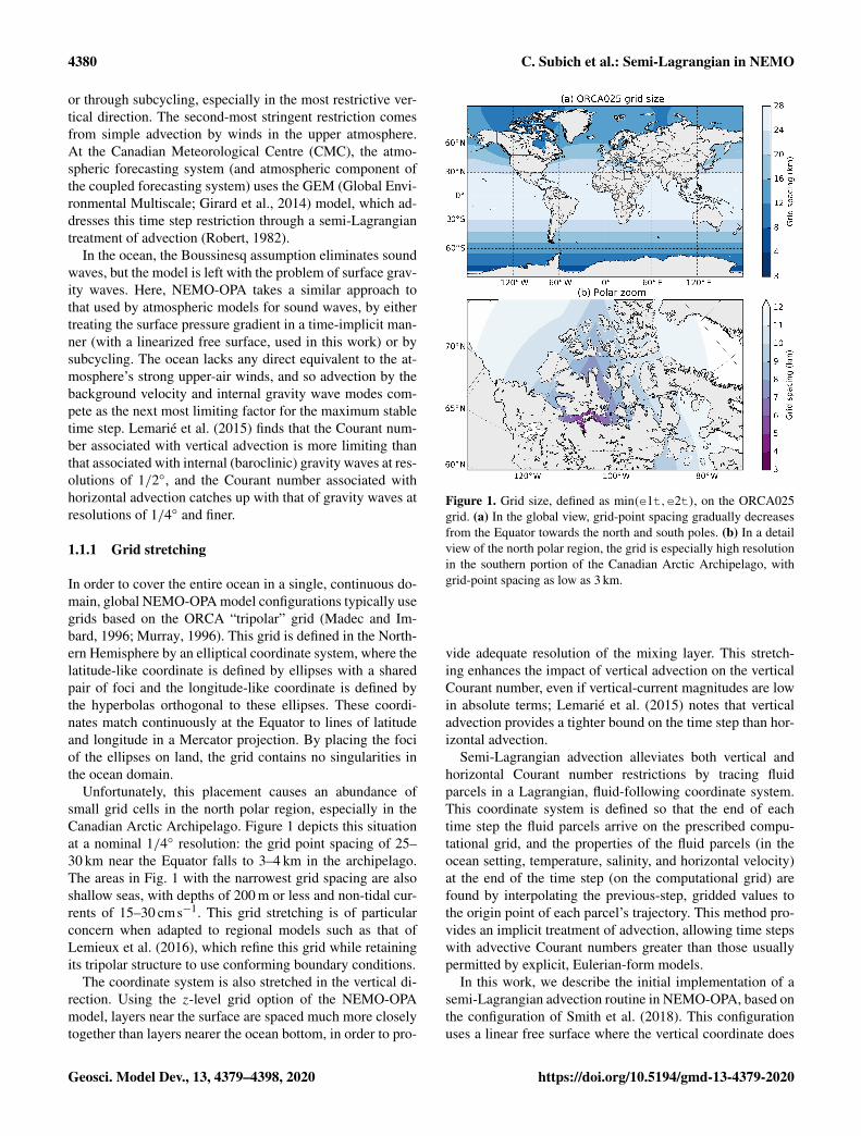
Unfortunately, this placement causes an abundance ofsmall grid cells in the north polar region, especially in theCanadian Arctic Archipelago. Figure 1 depicts this situationat a nominal 1/4◦ resolution: the grid point spacing of 25–30 km near the Equator falls to 3–4 km in the archipelago.The areas in Fig. 1 with the narrowest grid spacing are alsoshallow seas, with depths of 200 m or less and non-tidal cur-rents of 15–30 cm s−1. This grid stretching is of particularconcern when adapted to regional models such as that ofLemieux et al. (2016), which refine this grid while retainingits tripolar structure to use conforming boundary conditions.
The coordinate system is also stretched in the vertical di-rection. Using the z-level grid option of the NEMO-OPAmodel, layers near the surface are spaced much more closelytogether than layers nearer the ocean bottom, in order to pro-
Figure 1. Grid size, defined as min(e1t,e2t), on the ORCA025grid. (a) In the global view, grid-point spacing gradually decreasesfrom the Equator towards the north and south poles. (b) In a detailview of the north polar region, the grid is especially high resolutionin the southern portion of the Canadian Arctic Archipelago, withgrid-point spacing as low as 3 km.
vide adequate resolution of the mixing layer. This stretch-ing enhances the impact of vertical advection on the verticalCourant number, even if vertical-current magnitudes are lowin absolute terms; Lemarié et al. (2015) notes that verticaladvection provides a tighter bound on the time step than hor-izontal advection.
Semi-Lagrangian advection alleviates both vertical andhorizontal Courant number restrictions by tracing fluidparcels in a Lagrangian, fluid-following coordinate system.This coordinate system is defined so that the end of eachtime step the fluid parcels arrive on the prescribed compu-tational grid, and the properties of the fluid parcels (in theocean setting, temperature, salinity, and horizontal velocity)at the end of the time step (on the computational grid) arefound by interpolating the previous-step, gridded values tothe origin point of each parcel’s trajectory. This method pro-vides an implicit treatment of advection, allowing time stepswith advective Courant numbers greater than those usuallypermitted by explicit, Eulerian-form models.
In this work, we describe the initial implementation of asemi-Lagrangian advection routine in NEMO-OPA, based onthe configuration of Smith et al. (2018). This configurationuses a linear free surface where the vertical coordinate does
Geosci. Model Dev., 13, 4379–4398, 2020 https://doi.org/10.5194/gmd-13-4379-2020
C. Subich et al.: Semi-Lagrangian in NEMO 4381
not move in time, but we believe that the described methodcan be generalized.
1.2 Existing work
In the atmosphere, semi-Lagrangian advection is a standardtechnique (Robert, 1982) for the implicit treatment of ad-vection, but especially at large scales the effects of topogra-phy are relatively gentle. In particular, trajectory calculationscan proceed under the assumption that the fluid parcel doesnot experience strong boundary-related acceleration. In theocean domain this assumption is strongly violated, particu-larly for z-level vertical grids where the bathymetry changesabruptly at lateral cell boundaries.
Some attempts have been made previously to incorporatesemi-Lagrangian advection into the ocean context. The workof Casulli and Cheng (1992), which is used as part of the EL-COM lake and estuary model (Hodges and Dallimore, 2006),calculates parcel trajectories via a substepping approach,where fluid parcel trajectories are integrated via an explicitEuler method over many short steps per model time step. Thetwo-dimensional, unstructured shallow water model of Wal-ters et al. (2007) takes a similar approach, where it also musttake at least one substep per element boundary traversed bya fluid parcel.
In this work, we overcome this difficulty with an iterativetrajectory calculation which reduces in the limit to an im-plicit trapezoidal rule. In addition, we also derive the semi-Lagrangian advection scheme in a form which calculates ef-fective advective tendencies, such that the advection routinecan operate as a “plug-in” scheme for models which tradi-tionally use Eulerian fluxes. We apply this to the NEMO-OPA model, and we believe this algorithm may be usefulwhen applied to other ocean models with a structured grid.
In exchange, however, the semi-Lagrangian advection for-mulation departs from NEMO’s finite-volume interpretationof its tracer and velocity components. By tracing infinites-imal fluid parcels, semi-Lagrangian advection treats grid-point values analogously to a finite-difference method, andas a consequence the scheme does not naturally offer conser-vation guarantees. This is not a primary concern for the short-to medium-term forecasting applications that form the directtarget for this work, but extensions of the semi-Lagrangianscheme to ensure conservation (Lauritzen, 2007) may beneeded before the technique is applicable to longer-term cli-mate simulations.
Additionally, Leclair and Madec (2011) has developed an“arbitrary Lagrangian–Eulerian” vertical coordinate scheme,implemented in recent versions of NEMO. This schemesplits vertical motions into fast (high temporal frequency)and slow motions, and the former are treated by co-movingvertical coordinate surfaces with a regridding step. This co-ordinate system reduces spurious diapycnal mixing causedby the high-frequency vertical motions, and its Lagrangian
treatment of these motions relaxes the corresponding stabil-ity restriction.
1.3 Organization
We first introduce the time discretization of the semi-Lagrangian scheme in Sect. 2, in order to develop a formu-lation that remains compatible with the common leapfrogscheme. In Sect. 3, we begin to spatially discretize the semi-Lagrangian scheme by specifying the horizontal and verticalinterpolation operators, and in Sect. 4 we complete the dis-cretization by defining the trajectory calculations. We presentpreliminary numerical examples in Sect. 5, demonstratingthe stability of the advection scheme.
2 Time discretization
The first requirement of a semi-Lagrangian advectionscheme for the NEMO-OPA model is that it be consistentwith the model’s overall time-stepping approach: the advec-tion scheme is but one component of the full model.
In version 3 of NEMO-OPA, non-diffusive, non-dampingprocesses such as advection are implemented via the leapfrogscheme (Mesinger and Arakawa, 1976), where at each timestep a field f receives its new value at f A (f “after” the timestep) based on its value at the previous time step and forcingterms, which are all evaluated on the reference grid xref. Thisgives a schematic of
f A(xref)= fB(xref)+ 21tF(xref), (1)
where f A is the field calculated at time t0+1t , f B is the fieldevaluated at the known prior time t0−1t (“before”), f N isthe field at the provided time t0 (“now”), and F is the forcingoperator. The forcing operator includes advective processesat the now time level, but diffusive, damping, and hydrostaticpressure terms might be evaluated at either the before or aftertime levels.
This is an Eulerian approach to fluid motion, where tracerand momentum values are tracked along the fixed referencegrid at all times, and fluid flows through this grid.
2.1 Semi-Lagrangian advection
In contrast, the Lagrangian advection schemes consider thefluid parcel to be the fundamental unit of discretization. Inthis perspective, if f is a property of a fluid parcel that is con-served along a trajectory1, it satisfies the continuous equa-tions:
DDtf (x(t))= FL(x(t)), (2)
1This is true for temperature, salinity, and momentum providedthe ocean is treated as an incompressible fluid. This assumption issatisfied by NEMO-OPA’s adoption of the Boussinesq approxima-tion.
https://doi.org/10.5194/gmd-13-4379-2020 Geosci. Model Dev., 13, 4379–4398, 2020
4382 C. Subich et al.: Semi-Lagrangian in NEMO
where DDt = ∂t +u · ∇ is the material derivative, and FL (La-
grangian right-hand side) contains all the same forcing termsas F except those arising from tracer and momentum flux,which are included inside the material derivative.
Ordinarily, Eq. (2) is discretized so that FL is evaluatedfollowing the Lagrangian particles in the moving coordinateframe x(t), satisfying the trajectory equation:
DDt
x(t)= u(x(t)). (3)
From an Eulerian point of view, Eq. (3) is a trivial identitybased on the definition of the material derivative, but fromthe Lagrangian point of view, Eq. (3) must be solved to definex over time.
One technique for solving Eqs. (2) and (3) is the two-time-level implicit semi-Lagrangian method, used in the GEM at-mospheric model (Girard et al., 2014), among others. Here,the FL terms are evaluated with a trapezoidal rule, discretiz-ing Eqs. (2) and (3) as
f A(xref)= fN(xD)+
1t
2
(FAL(xref)+FNL (x
D))
and (4a)
xref = xD+1t
2
(uA(xref)+uN (xD)
). (4b)
The trajectory Eq. (4b) acts to implicitly define the paths ofthe traced fluid parcels, where each location on xref is associ-ated with a corresponding departure-point location xD. Overthe single time step, fluid parcels depart from xD (which ingeneral is not aligned with the grid) and arrive on the refer-ence grid.
This off-grid, departure point evaluation of u and FL isfundamental to Lagrangian and semi-Lagrangian methods,and f N(xD) (FNL (x
D)) can be written more simply as f D
(FDL) for “departure-point f (F)”. Neither the time-implicit
evaluations (generally) nor the off-grid evaluations (of non-advective forcing) are compatible with the core structureof NEMO-OPA, which considers advection to be just oneof many independent operators influencing the F term ofEq. (1).
2.2 Reconciliation
Implementing semi-Lagrangian advection in NEMO-OPArequires adopting as much of the framework of Eq. (1) aspossible, without changing the evaluation of non-advectiveforcing terms. Effectively, the semi-Lagrangian advectionroutine must ultimately supply a time trend that, from theperspective of the leapfrog time-step algorithm, is indistin-guishable from a conventional flux-form advection operator.
To effect this, consider Eq. (2) without forcing terms(FL = 0). The function f is preserved following the flow, sothis gives the simply written
f A= f D. (5)
This is approximated by taking one time step of Eq. (1)(with only advective forcing Fadv), but the latter involves in-tegrating over the whole interval from t0−1t to t0+1t .Thus, we should identify f D (and the departure points gen-erally) not with the now time level in the leapfrog schemebut rather with the before time level. Doing so and equatingEqs. (5) and (1) gives
f A= f B
+ 21tFadv = fB(xD), or (6)
Fadv =1
21t(f B− f B(xD)). (7)
Equation (7) is prescriptive, and it gives the necessarytrend for the leapfrog algorithm. Evaluating it requires fonly at the already known, before time level and calculationof the departure points xD. This calculation is further simpli-fied by basing the departure points on the time-centered ve-locities uN , and the exact algorithm for this calculation willbe discussed in more detail in Sect. 4.
2.3 Effects of the Asselin filter
To prevent decoupling of odd and even time steps (damp-ing the computational mode), NEMO-OPA is typically con-figured to use the Asselin time filter (Asselin, 1972), whichadds a small time damping proportional to ∂2
∂t2f . Using the
notation of Shchepetkin and McWilliams (2005) adapted toEq. (1), the filter extends the time-marching scheme to thesequence:
f A∗← f B
+ 21tFN∗ (8a)
f N← εf A∗
+ (1− 2ε)f N∗+ εf B (8b)
f N∗← f A∗ (8c)
f B← f N. (8d)
Equation (8a) is the direct equivalent of Eq. (1), creating aprovisional after value f A∗. Equation (8b) applies the filter(with a strength parameter ε) with this value and the previousstep’s provisional field to define a final now field, and finallyEqs. (8c) and (8d) are “bookkeeping” steps to shift field la-bels to become ready for the next time step. The forcing op-erator FN∗ is evaluated based on the provisionally definedfields.
In applying this filter with the semi-Lagrangian forcing,Eq. (7) is oblivious to the presence of the filter or the differ-ence between f N and f N∗. Substituting Eq. (7) into Eq. (8a)and applying Eqs. (8c) and (8d) to Eqs. (8a) and (8b) givesthe update equation:(f N∗
f B
)←
(f B(xD)
ε(f B(xD)+ f B(xref))+ (1− 2ε)f N∗(xref)
). (9)
In the case of one-dimensional advection by a constant ve-locity u0, the trajectory calculation is trivial, and
xD= xD
= xref− 21tu0. (10)
Geosci. Model Dev., 13, 4379–4398, 2020 https://doi.org/10.5194/gmd-13-4379-2020
C. Subich et al.: Semi-Lagrangian in NEMO 4383
Since Eq. (9) is linear, we can also take its Fourier decom-position in space and consider only a single, arbitrary wavemode, giving f = f (t)exp ikx for a time-varying coefficientf . Applying this to Eq. (9) casts the update in a matrix formas(fN∗
fB
)←
(0 exp(−2iku01t)
1− 2ε ε(1+ exp(−2iku01t))
)(fN∗
fB
). (11)
The time stability of this filter is then governed bythe eigenvalues of this matrix. Using the shorthand ω =
−ku01t , these eigenvalues are
λ1,2 =
12
(ε(1+ e(2iω))±
√ε2(1+ e(2iω))2+ (4− 8ε)e(2iω)
), (12)
and to leading order in ε, these eigenvalues have squaredmagnitudes of
|λ1,2|2= 1− 2ε± 2ε cos(ω)+O(ε2), (13)
signifying stability (|λ| ≤ 1) for all values of ω and thus allCourant numbers.
3 Interpolation
To perform the off-grid interpolations in Eq. (7) to findf B(xD), this method fits a cubic polynomial to the under-lying function. If the single departure point xd = (xd,yd,zd)
lies within2 (xa,xa+1)× (yb,yb+1)× (zc,zc+1) for integervalues of a, b, and c coinciding with grid-point locations,the full interpolation stencil consists of the grid-index cubei ∈ [a− 1,a+ 2], j ∈ [b− 1,b+ 2], and k ∈ [c− 1,c+ 2].
This grid cube contains up to 64 grid points where f (x)might be defined (subject to boundary conditions), and build-ing a complete interpolation stencil would be cumbersomeand inefficient. Instead, the interpolation procedure takes ad-vantage of the tensor-product nature of the grid to separateinterpolation along each dimension:
To effect the one-dimensional interpolations in Algo-rithm 1, we make use of the cubic Hermite polynomials
2If xd lies along an edge or corner of this interval, then at leastone of the resulting interpolations will be trivial. In that case, thechoice of which neighbouring interval xd lies “within” is arbitrary.
(Hildebrand, 1974). On the interval 0≤ χ ≤ 1, these poly-nomials are
h00(χ)= 2χ3− 3χ2
+ 1,
h01(χ)=−2χ3+ 3χ2,
h10(χ)= χ3− 2χ2
+χ , and
h01(χ)= χ3−χ2,
(14)
and a function f (χ) defined on this interval is interpolatedvia
f (χ)≈f (0)h00(χ)+ f′(0)h10(χ)+ f (1)h01(χ)
+ f ′(1)h11(χ). (15)
Here, we prefer to use the cubic Hermite polynomialsover simple Lagrange polynomial interpolation because theformer choice allows greater freedom (via Eq. 15) in im-plementation. If f ′ is approximated by a four-point finite-difference stencil, then Eq. (15) reduces to Lagrange inter-polation. However, we can also make other choices for f ′ toimpose desirable properties: restricting f ′ to have the samesign as the discrete difference imposes a type of slope limit-ing, and calculating f ′ through a three-point stencil providesfor continuous derivatives. These approaches are discussedin more detail in the following sections.
Interpolation using the above algorithm involves appropri-ately defining the interval to be scaled to [0,1] and approxi-mating f ′ at the endpoints. Because of the high aspect ratioof oceanic flows and the special character of vertical motionin a stratified ocean, these approximations differ between thehorizontal and vertical interpolations.
3.1 Horizontal interpolation
In the horizontal, the interpolation in Eq. (15) can be directlyconducted in grid-index space. Even when the underlyinggrid is mapped to the sphere, such as in the ORCA globalgrid (Madec, 2008, chap. 16), the grid generally transitionssmoothly and slowly from point to point3. The physical tra-jectory departure location xd (and yd) can be translated intoa fractional grid index offset by dividing by the appropri-ate grid scale factor, available inside the NEMO-OPA sourcecode as one of e[12][tuv].
Achieving third-order accuracy inside Eq. (15) is possible,but doing so requires an equally accurate estimate for f ′.Unfortunately, interpolating successively in one dimensionusing the above algorithm does not allow for precomputa-tion of these derivatives: after the vertical interpolation step,all of the function values need to be taken off grid, so any
3This is not necessarily the case, however, for grids that havemanually specified, non-smooth regions of enhanced resolution. Insuch cases a more nuanced treatment of interpolation would be ad-visable.
https://doi.org/10.5194/gmd-13-4379-2020 Geosci. Model Dev., 13, 4379–4398, 2020
4384 C. Subich et al.: Semi-Lagrangian in NEMO
precomputed derivatives would themselves require interpo-lation. Instead, sufficiently accurate estimates of the deriva-tive are available by applying a finite-difference formula tothe function values themselves.
3.1.1 Derivative estimates
For notational simplicity, begin with the last step of the abovealgorithm where we have f (xd,yj ,zd) and would like to es-timate f (xd,yd,zd). If yd lies between y0 and y1, then thefour-point interpolation stencil implies that we have com-puted f (xd,yj ,zd) for j =−1,0,1,2. To emphasize that thisis now a one-dimensional interpolation problem, let g(j)=f (xd,yj ,zd), such that f (xd,yd,zd)= g(j
′) for some j ′ ∈[0,1]. In this domain, g′(0) and g′(1) can be approximatedby the finite differences:
g′(0)≈−13g(−1)−
12g(0)+ g(1)−
16g(2) and (16a)
g′(1)≈16g(−1)− g(0)+
12g(1)+
13g(2), (16b)
which then substitute for the appropriate derivatives inEq. (15).
These finite differences are exact expressions for the firstderivative for polynomials up to third order in j , and their useessentially converts Eq. (15) to interpolation via Lagrangepolynomials. The Hermite polynomial form, however, allowsfor an easier imposition of boundary conditions.
3.1.2 Boundary conditions
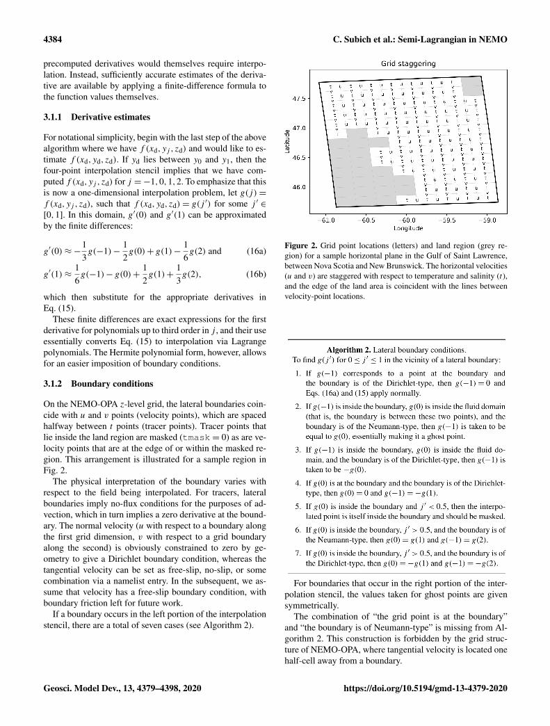
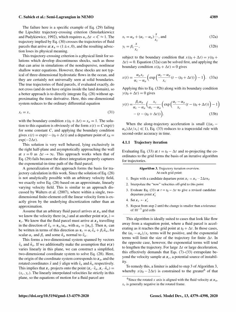
On the NEMO-OPA z-level grid, the lateral boundaries coin-cide with u and v points (velocity points), which are spacedhalfway between t points (tracer points). Tracer points thatlie inside the land region are masked (tmask= 0) as are ve-locity points that are at the edge of or within the masked re-gion. This arrangement is illustrated for a sample region inFig. 2.
The physical interpretation of the boundary varies withrespect to the field being interpolated. For tracers, lateralboundaries imply no-flux conditions for the purposes of ad-vection, which in turn implies a zero derivative at the bound-ary. The normal velocity (u with respect to a boundary alongthe first grid dimension, v with respect to a grid boundaryalong the second) is obviously constrained to zero by ge-ometry to give a Dirichlet boundary condition, whereas thetangential velocity can be set as free-slip, no-slip, or somecombination via a namelist entry. In the subsequent, we as-sume that velocity has a free-slip boundary condition, withboundary friction left for future work.
If a boundary occurs in the left portion of the interpolationstencil, there are a total of seven cases (see Algorithm 2).
Figure 2. Grid point locations (letters) and land region (grey re-gion) for a sample horizontal plane in the Gulf of Saint Lawrence,between Nova Scotia and New Brunswick. The horizontal velocities(u and v) are staggered with respect to temperature and salinity (t),and the edge of the land area is coincident with the lines betweenvelocity-point locations.
For boundaries that occur in the right portion of the inter-polation stencil, the values taken for ghost points are givensymmetrically.
The combination of “the grid point is at the boundary”and “the boundary is of Neumann-type” is missing from Al-gorithm 2. This construction is forbidden by the grid struc-ture of NEMO-OPA, where tangential velocity is located onehalf-cell away from a boundary.
Geosci. Model Dev., 13, 4379–4398, 2020 https://doi.org/10.5194/gmd-13-4379-2020
C. Subich et al.: Semi-Lagrangian in NEMO 4385
For two-dimensional interpolation, Algorithm 2 appliesindependently to each dimension. When interpolating alongx, the points f (xd,yj ,zd) will each individually be eitherin the ocean domain and valid or in the land domain andmasked, which provides the values necessary to computef (xd,yd,zd). This off-grid point itself must lie in water,which imposes a strong requirement on the trajectory cal-culations to be discussed in Sect. 4.
3.1.3 Slope limiting
As a final step, once values for the function and its derivativeat the interval endpoints are specified, the derivative valuesare limited to help prevent new maxima in the interpolatedfunction. In particular, if g(0) is a local minimum (maxi-mum) among itself, g(−1), and g(1), then g′(0) is set to zeroif the above procedure finds that it would be negative (posi-tive). A similar procedure applies symmetrically for g′(1) ifg(1) is a relative extremum.
This limiting is milder than methods derived fromBermejo and Staniforth (1992), which would strictly pre-serve positivity for any j ′, but it effectively limits excursionswhen j ′ is close to 0 or 1. Without such limiting, numericaltesting showed that semi-Lagrangian advection of tempera-ture and salinity could cause weak instabilities near the coast-line, where a locally extreme temperature or salinity couldbecome “trapped” near the coast and slowly amplified.
3.2 Vertical interpolation
Vertical motion in the NEMO-OPA model differs from hori-zontal motion in a number of respects:
– Vertical gradients of temperature and density are muchstronger than typical horizontal gradients, especiallynear the surface.
– Typical vertical grids used with NEMO-OPA arestrongly stretched, with a higher resolution near the sur-face and a lower resolution in the deep ocean.
– Vertical flow is often oscillatory, where vertical motionis driven by barotropic and baroclinic waves.
The horizontal interpolation described in Sect. 3.1 is third-order accurate; with the provided one-sided formulas forcalculating the endpoint derivatives it reduces to a four-point (cubic) Lagrangian interpolation process. However, thesmooth field implied by this interpolation process is only C0
continuous: f (xj − ε) “sees” f ′j calculated from f (xj−2)
to f (xj+1), whereas f (xj + ε) sees f ′j from f (xj−1) tof (xj+2).
We do not find this to be a practical concern for hor-izontal interpolation, since horizontal currents in most ofthe ocean tend to be dominated by relatively steady quasi-geostrophic motions. In the vertical, however, we found thateven low-amplitude oscillations caused by high-frequency
gravity waves would cause the temperature and salinity fieldsto drift. The mechanism is that a fluid parcel displaced up-wards by ε in one time step and downwards by ε in the nexttime step would see an effective diffusion proportional to thejump between the upward- and downward-looking verticalderivatives.
To maintain global accuracy, we impose C1 continuity inthe vertical direction through an alternative treatment of thevertical derivative. Instead of applying Eqs. (16), we treat thephysical depth (rather than grid index) as the relevant coor-dinate and construct a centered estimate of the derivative.
For a function f (zn) defined at the zn levels, define1f+ = f (zn+1)−f (zn), 1f− = f (zn)−f (zn−1), 1z+ =zn+1−zn, and1z− = zn−zn−1. These differences combineto give the estimated derivative:
fz(zn)≈1
1z−+1z+
(1z−
1z+1f++
1z+
1z−1f−
), (17)
which is accurate toO(1z2) for the derivative and accuratelyreproduces quadratic functions of z. In the limiting case ofa constant 1z (equispaced vertical levels), this formula re-duces to the classic centered difference.
Because vertical interpolation comes first in Algorithm 1,Eq. (17) need be evaluated only at grid points, and in fact itmay be precomputed for the entire grid for a given functionand time step. This is a key advantage of placing verticalinterpolation first in the interpolation sequence, and it avoidsduplication of work.
Whereas interpolation near the horizontal boundaries iscomplicated by the many combinations of grid staggeringand physical boundary conditions, interpolation near the ver-tical boundaries is much simpler. On the NEMO grid, tracersand horizontal velocities lie along the same vertical level, andthese levels are staggered one half-cell away from the bound-aries. Likewise, the natural vertical boundary condition forboth tracer and horizontal velocity fields is a no-flux bound-ary condition; NEMO-OPA models boundary-layer frictionin another module. Interpolation near the boundaries thenproceeds in two steps.
The first step is to define fz at the top and bottom points inthe water column, for which the central difference formulaof Eq. (17) is not directly valid. Here, we approximate thephysical no-flux condition through a fictitious ghost pointsuch that 1f− = 0 at the top boundary and 1f+ = 0 at thebottom boundary, with the respective 1z matching the layerthickness (e3t).
The second step is to define how Eq. (15) applies to the in-terval between the grid level and the physical boundary. Here,the no-flux boundary conditions reduce to even symmetry,and the derivative at the ghost points is the negative of thevertical derivative calculated for the in-boundary point. Nearthe free surface, if the interpolation point is above the level ofthe free surface (above z= 0), then it is clamped to the sur-face itself. Near the ocean bottom, if the interpolation point
https://doi.org/10.5194/gmd-13-4379-2020 Geosci. Model Dev., 13, 4379–4398, 2020
4386 C. Subich et al.: Semi-Lagrangian in NEMO
is below the level of the ocean bottom (below z= zmax) thenthe point is masked and is treated as an “inside the boundary”point for the purposes of horizontal interpolation above.
3.2.1 Treatment of partial cells
Over most of the domain, this interpolation works well. Al-though there is no guarantee of positivity in the derivativeformulation of Eq. (17), overshoots and the consequent gen-eration of spurious maxima are limited. For the tests pre-sented in Sect. 5, there was no need for slope limiting forvertical interpolation over most of the domain.
One exception to this rule is at the bottom boundary. Here,vertical levels are spaced far apart, but to better representthe ocean bottom the z-level grid of NEMO-OPA uses apartial cell configuration (Madec, 2008, sec. 5.9). For wa-ter columns where the bottom-most cell is much deeper thanits neighbours, a local (small) upwelling can cause an over-shoot of temperature or salinity that spuriously increases thelocal density but does not diminish the upwelling. Over time,the maxima-increasing trend can accumulate and cause somepoints at the bottom boundary to reach implausibly cold tem-peratures (below −10◦C, for example) or high salinities. Inthe absence of explicit horizontal diffusion (which wouldmix this maximum into more dynamically active regions),these spurious maxima do not generally corrupt the flow, al-though they obviously would corrupt whole-ocean (or whole-level) statistics such as average or extreme temperatures.
Near these boundary cells, vertical limiting is imple-mented in the simplest possible way: the interpolation ofEq. (15) is replaced with a constant, such that f (z)= f (zk)over the interval from zk downwards to the physical bound-ary.
Implementing this limiting over the whole bottom level ispossible, but that is far stronger than necessary and leadsto erroneous diffusion along gentle slopes. When the bot-tom layer is composed of partial cells of varying thickness,even interpolation along a horizontal plane (that is, withoutchanging physical depth) requires vertical interpolation ingrid space to find that constant level in adjoining columns.Imposing vertical limiting along the whole bottom level ef-fects undesired horizontal diffusion, even though the prob-lem solved by limiting is observed when adjoining cells havelarge relative thickness variations.
As a compromise between these two errors, we only applythe described limiting to vertical interpolation for cells at thebottom boundary which have a layer thickness greater than1.75 times that of their “thinnest” neighbour.
This exact threshold is empirical, and other grids mightrequire a retuning of this parameter. Ideally, the grid genera-tion itself would avoid abrupt transitions in cell-layer thick-nesses, but adding such a restriction would make this advec-tion scheme useless as a drop-in replacement for the standardadvection routines of NEMO-OPA.
3.3 A numerical example
As a simple numerical example, consider the case of a tracerbeing advected in a rectangular, two-dimensional domain byan internal wave and a background current. This tracer satis-fies the advection equation
∂σ
∂t− u(x,z, t)
∂σ
∂x−w(x,z, t)
∂σ
∂z= 0 (18)
for some prescribed velocity field (u,w).If this tracer field σ(x,z, t) would be a function of z alone,
i.e. σ (z), if not for the wave motion, then its motion is ana-lytically given by
σ(x,z, t)= σ(z− η(x− (c+ u0)t,z)
), (19)
where η(x,z) is the isopycnal displacement, u0 is the x-directed background current (uniform in z), and c is the phasespeed of the wave. Following Turkington et al. (1991), astreamfunction defined as
ψ(x,z, t)= cη(x,z, t)− u0z (20)
gives velocities
u=−ψz (21a)w = ψx, (21b)
which are exact solutions of Eq. (18) for σ(x,z, t).To give an internal wave that respects no-flux conditions
at the top and bottom of the domain, we set
η(x,z, t)= Acos(k(x− (c+ u0)t)
)sin(mz), (22)
where k and m are horizontal and vertical wavenumbers re-spectively, and A is the wave amplitude. For a domain ofsize Lx in the horizontal (periodic) and Lz in the verti-cal, k = 2π/Lx and m= π/Lz give the lowest internal wavemode, used here.
In dimensional units, we take the model domain to be achannel Lx = 1 km long and Lz = 100 m deep with a back-ground current of u0 = 1ms−1, and we set c =N/
√k2+m2
based on a mean buoyancy frequency ofN = 0.03s−1, whichcorresponds to a 1 % density change from the surface to thebottom of the channel. With a wave amplitude of A= 10 m,the maximum wave-induced current is about 10 % of u0, andthe phase speed is c ≈ 0.94ms−1.
In order to represent the pycnocline found in many oceanwaters, we choose4 σ (z)= tanh
( 12 −
110zL
−1y
).
4Since this section tests advection alone, the scaling of σ is notdynamically relevant. In fact, the wave structure of Eq. (22) cor-responds to an exact internal mode of the incompressible Navier–Stokes equations for a linear stratification.
Geosci. Model Dev., 13, 4379–4398, 2020 https://doi.org/10.5194/gmd-13-4379-2020
C. Subich et al.: Semi-Lagrangian in NEMO 4387
The domain is discretized by Nx ×Ny points, defined as
xi =−Lx
2+Lx
i− 0.5Nx
and (23a)
zj =Lz
2
(1+
αj +α3j
2
), (23b)
where i = 1,2, · · ·,Nx , j = 1,2, · · ·,Nz, and
αj = 2j − 0.5Nz
− 1. (23c)
This implements a stretched vertical coordinate that in-creases the vertical resolution in the vicinity of the pycno-cline.
3.3.1 Semi-Lagrangian advection
In integrating this system with semi-Lagrangian advection,the leapfrog method reduces to an Euler method of twicethe time step because there is no external forcing. The time-discrete equation is
σ(xi,zj , t + 21t)= σ(xd(ij),zd(ij), t), (24)
where (xd(ij),zd(ij)) is the departure point of the trajectorythat arrives at the grid point (xi,zj ), and the off-grid evalua-tion of σ proceeds via the interpolation processes describedearlier without slope limiting.
The departure points are given by the trapezoidal rule5
with a time-centered evaluation of velocity:
xi − xd(ij) =1t(u(xi,zj , t +1t
)+ u
(xd(ij),zd(ij), t +1t
))(25a)
zj − zd(ij) =1t(w(xi,zj , t +1t
)+w
(xd(ij),zd(ij), t +1t
)), (25b)
where the velocities are evaluated exactly via Eq. (21). Theoverall system Eq. (25) is solved via simple iteration, with aninitial guess given by setting (x,z)d(ij) = (x,z)ij .
This algorithm is stable for large time steps, so we testedthis system for time steps corresponding to Courant numbersof 0.2 and 2.1, with spatial grid resolutions between 40× 4and 2560× 256. The final integration time was chosen to betfin = 5Lx/u0, which allowed the wave to propagate throughthe domain several times. Since the exact solution is analyt-ically known, we recorded the maximum error experiencedover the integration, and error convergence rates are shownin Fig. 3.
5The trajectory calculation scheme of Sect. 4 could be used in-stead, but since the overall trajectory lengths are small comparedto the length scales of the velocity field (Lx and Lz), that methodwould give equivalent results to the trapezoidal rule.
3.3.2 Flux-form advection
As a control, we also integrate this system in flux form, i.e.σt −∇ · (uσ)= 0, via centered differences, with σ evaluatedat the midpoints between grid cells via a simple average,matching the central difference tracer advection scheme inNEMO-OPA.
The velocity field given by Eq. (20) is divergence free, sothis form of the equation is pointwise equivalent to Eq. (18).However, this no longer holds after discretization. In orderto eliminate the divergence error, the velocity field is de-fined by creating the streamfunction at the staggered points(xi+1/2,zj+1/2) and defining discrete velocities u and w viathe discrete equivalents to Eq. (21). With this modification,the discrete flux-form operator is equivalent to a discrete ad-vection equation.
After leapfrog discretization in time, the discretized equa-tion isσ(xi,zj , t +1t)= σ(xi,zj , t −1t)
+ 21t
1x1zj
(1zj2
(u(xi−1/2,zj , t)(σ (xi−1,zj , t)
+ σ(xi,zj , t))
− u(xi+1/2,zj , t)(σ (xi,zj , t)+ σ(xi+1,zj , t)))
+1x
2
(w(xi,zj−1/2, t)(σ (xi,zj−1, t)+ σ(xi,zj , t))
−w(xi,zj+1/2, t)(σ (xi,zj , t)+ σ(xi,zj+1, t)))),
(26)
where1zj = zj+1/2−zj−1/2 =12 (zj+1−zj−1). For the first
time step, a single Euler step is taken of size 1t with time-centered velocities (t =1t/2).
As usual, this leapfrog time-stepping algorithm is only sta-ble to a maximum Courant number of 1. With this staggeredgrid and vertical grid stretching, the Courant number can bedefined by
Cij =1t(max(ui+1/2,j ,0)−min(ui−1/2,j ,0)
1x
+max(wi,j+1/2,0)−min(wi,j−1/2,0)
1zj
). (27)
For the mode-one internal wave with background currentused in this section, the maximum Courant number is reachedat the top and bottom of the domain (where w = 0), somax(C)=max(u)/1x.
We present results for Eq. (26) at a maximum Courantnumber of 0.2, chosen to give a “small time step” for latercomparison with semi-Lagrangian results. The results are in-sensitive to the time step within the stable range, with lessthan 5 % change in maximum-norm error over the range0.2≤max(C)≤ 0.99.
3.3.3 Results
The error over time of this test case is shown in Fig. 3. Asexpected, each method achieves second-order convergence.
https://doi.org/10.5194/gmd-13-4379-2020 Geosci. Model Dev., 13, 4379–4398, 2020
4388 C. Subich et al.: Semi-Lagrangian in NEMO
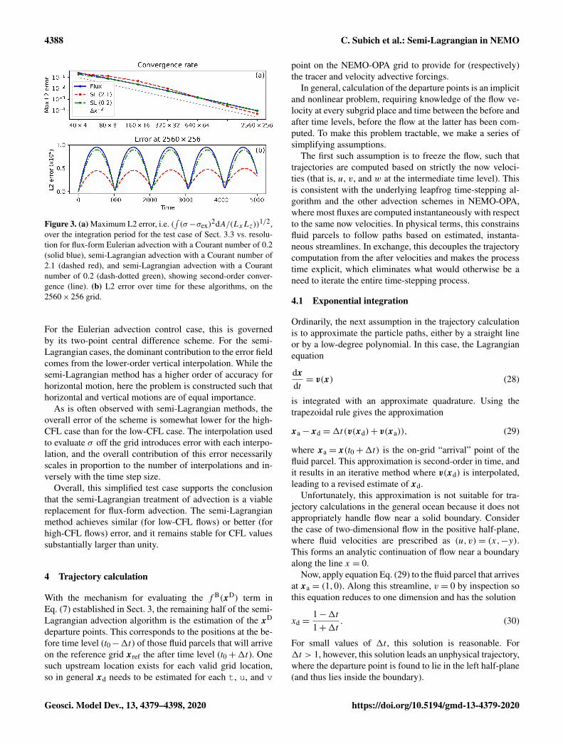
Figure 3. (a) Maximum L2 error, i.e. (∫(σ−σex)
2dA/(LxLz))1/2,over the integration period for the test case of Sect. 3.3 vs. resolu-tion for flux-form Eulerian advection with a Courant number of 0.2(solid blue), semi-Lagrangian advection with a Courant number of2.1 (dashed red), and semi-Lagrangian advection with a Courantnumber of 0.2 (dash-dotted green), showing second-order conver-gence (line). (b) L2 error over time for these algorithms, on the2560× 256 grid.
For the Eulerian advection control case, this is governedby its two-point central difference scheme. For the semi-Lagrangian cases, the dominant contribution to the error fieldcomes from the lower-order vertical interpolation. While thesemi-Lagrangian method has a higher order of accuracy forhorizontal motion, here the problem is constructed such thathorizontal and vertical motions are of equal importance.
As is often observed with semi-Lagrangian methods, theoverall error of the scheme is somewhat lower for the high-CFL case than for the low-CFL case. The interpolation usedto evaluate σ off the grid introduces error with each interpo-lation, and the overall contribution of this error necessarilyscales in proportion to the number of interpolations and in-versely with the time step size.
Overall, this simplified test case supports the conclusionthat the semi-Lagrangian treatment of advection is a viablereplacement for flux-form advection. The semi-Lagrangianmethod achieves similar (for low-CFL flows) or better (forhigh-CFL flows) error, and it remains stable for CFL valuessubstantially larger than unity.
4 Trajectory calculation
With the mechanism for evaluating the f B(xD) term inEq. (7) established in Sect. 3, the remaining half of the semi-Lagrangian advection algorithm is the estimation of the xD
departure points. This corresponds to the positions at the be-fore time level (t0−1t) of those fluid parcels that will arriveon the reference grid xref the after time level (t0+1t). Onesuch upstream location exists for each valid grid location,so in general xd needs to be estimated for each t, u, and v
point on the NEMO-OPA grid to provide for (respectively)the tracer and velocity advective forcings.
In general, calculation of the departure points is an implicitand nonlinear problem, requiring knowledge of the flow ve-locity at every subgrid place and time between the before andafter time levels, before the flow at the latter has been com-puted. To make this problem tractable, we make a series ofsimplifying assumptions.
The first such assumption is to freeze the flow, such thattrajectories are computed based on strictly the now veloci-ties (that is, u, v, and w at the intermediate time level). Thisis consistent with the underlying leapfrog time-stepping al-gorithm and the other advection schemes in NEMO-OPA,where most fluxes are computed instantaneously with respectto the same now velocities. In physical terms, this constrainsfluid parcels to follow paths based on estimated, instanta-neous streamlines. In exchange, this decouples the trajectorycomputation from the after velocities and makes the processtime explicit, which eliminates what would otherwise be aneed to iterate the entire time-stepping process.
4.1 Exponential integration
Ordinarily, the next assumption in the trajectory calculationis to approximate the particle paths, either by a straight lineor by a low-degree polynomial. In this case, the Lagrangianequation
dx
dt= v(x) (28)
is integrated with an approximate quadrature. Using thetrapezoidal rule gives the approximation
xa− xd =1t(v(xd)+ v(xa)), (29)
where xa = x(t0+1t) is the on-grid “arrival” point of thefluid parcel. This approximation is second-order in time, andit results in an iterative method where v(xd) is interpolated,leading to a revised estimate of xd.
Unfortunately, this approximation is not suitable for tra-jectory calculations in the general ocean because it does notappropriately handle flow near a solid boundary. Considerthe case of two-dimensional flow in the positive half-plane,where fluid velocities are prescribed as (u,v)= (x,−y).This forms an analytic continuation of flow near a boundaryalong the line x = 0.
Now, apply equation Eq. (29) to the fluid parcel that arrivesat xa = (1,0). Along this streamline, v = 0 by inspection sothis equation reduces to one dimension and has the solution
xd =1−1t1+1t
. (30)
For small values of 1t , this solution is reasonable. For1t > 1, however, this solution leads an unphysical trajectory,where the departure point is found to lie in the left half-plane(and thus lies inside the boundary).
Geosci. Model Dev., 13, 4379–4398, 2020 https://doi.org/10.5194/gmd-13-4379-2020
C. Subich et al.: Semi-Lagrangian in NEMO 4389
The failure here is a specific example of Eq. (29) failingthe Lipschitz trajectory-crossing criterion (Smolarkiewiczand Pudykiewicz, 1992), which requires ux1t < C ≈ 1. Thetrajectory implied by Eq. (30) crosses the trajectories of fluidparcels that arrive at xa = (1±ε,0), and the resulting advec-tion loses its physical meaning.
This trajectory-crossing criterion is a physical limit for so-lutions which develop discontinuous shocks, such as thosethat can arise in simulations of the nondispersive, nonlinearshallow water equations. However, these shocks are not typ-ical of three-dimensional hydrostatic flows in the ocean, andthey are certainly not universally seen at solid boundaries.The true trajectories of fluid parcels, if evaluated exactly, donot cross (and do not have origins inside the land domain), soa better approach is to directly integrate Eq. (28) without ap-proximating the time derivative. Here, this one-dimensionalsystem reduces to the ordinary differential equation
xt = x, (31)
with the boundary condition x(t0+1t)= xa = 1. The solu-tion to this equation is obviously of the form x(t)= C exp(t)for some constant C, and applying the boundary conditiongives x(t)= exp(t−(t0+1t)) and a departure point of xd =
exp(−21t).This solution is very well behaved, lying exclusively in
the right half-plane and asymptotically approaching the wallat x = 0 as 1t→∞. This approach works when that ofEq. (29) fails because the direct integration properly capturesthe exponential-in-time path of the fluid parcel.
A generalization of this approach forms the basis for tra-jectory calculation in this work. Since the solution of Eq. (28)is not analytically possible with an arbitrary velocity field,we exactly solve Eq. (28) based on an approximate, linearlyvarying velocity field. This is similar to an approach dis-cussed by Walters et al. (2007), where within a single, two-dimensional finite-element cell the linear velocity form is ex-actly given by the underlying discretization rather than anapproximation.
Assume that an arbitrary fluid parcel arrives at xa and thatwe know the velocity there (va) and at another point v(xc)=
vc. We know that the fluid parcel must arrive at xa travellingin the direction of va = va/αa , with αa = ‖va‖. Then vc canbe written in terms of this direction as vc = αcva+βcna , forscalar αc and βc and some na normal to va .
This forms a two-dimensional system spanned by vectorsva and na . If we additionally make the assumption that v(x)
varies linearly in this plane, we can construct a simplified,two-dimensional coordinate system to solve Eq. (28). Here,the origin of the coordinate system corresponds to xa, and therotated coordinates x and y align with va and na respectively.This implies that xc projects onto the point (xc ·va,xc ·na)=(xc,yc). The linearly interpolated velocities lie strictly in thisplane, so the equations of motion for a fluid parcel are
xt = αa + (αc−αa)x
xc, and (32a)
yt = βcx
xc, (32b)
subject to the boundary condition that x(t0+1t)= y(t0+1t)= 0. Equation (32a) can be solved first, and applying theboundary condition x(t0+1t)= 0 gives
x(t)=αaxc
αc−αa
(exp
(αc−αaxc
(t − (t0+1t)))− 1
). (33a)
Applying this to Eq. (32b) along with its boundary conditiony(t0+1t)= 0 gives
y(t)=βcαa
αc−αa
( xc
αc−αa
(exp
(αc−αaxc
(t − (t0+1t)))− 1
)− (t − (t0+1t))
). (33b)
When the along-trajectory acceleration is small (|(αc−αa)1t/xc| � 1), Eq. (33) reduces to a trapezoidal rule withsecond-order accuracy in time.
4.1.1 Trajectory iteration
Evaluating Eq. (33) at t = t0−1t and re-projecting the co-ordinates to the grid forms the basis of an iterative algorithmfor trajectories.
This algorithm is ideally suited to cases that look like flowaway from a stagnation point, where a fluid parcel is accel-erating as it reaches the grid point at t0+1t . In those cases,the (αc−αa)/xc terms will be positive, and the exponentialterms will limit the size of the trajectory for finite 1t . Inthe opposite case, however, the exponential terms will tendto lengthen the trajectory. For large 1t or large deceleration,this effectively demands that Eqs. (7)–(33) extrapolate be-yond the velocity sample at xc, a potential source of instabil-ity.
To remedy this, a limiter is added to step 3 of Algorithm 3,whereby x(t0− 21t) is constrained to the greater6 of that
6Since the rotated x axis is aligned with the fluid velocity at xa,xc is generally negative in the rotated frame.
https://doi.org/10.5194/gmd-13-4379-2020 Geosci. Model Dev., 13, 4379–4398, 2020
4390 C. Subich et al.: Semi-Lagrangian in NEMO
from Eq. (33a) and−21tmax(αa,αc). When limiting is nec-essary, it effectively reduces the time step used for the trajec-tory iteration, so for consistency a revised 1t ′ is computedby inverting Eq. (33a) with the limited x′c, which is then usedto evaluate Eq. (33b).
4.2 Underrelaxation and land boundaries
While the construction of Algorithm 3 guarantees that trajec-tories cannot converge to an out-of-boundary point, there areno guarantees that the algorithm remains in boundary dur-ing the iteration process or that the iteration converges. Theproblem of a divergent or oscillatory iteration is more likelywhen the underlying velocity field does not resemble the lin-early approximated velocity field integrated by Eq. (7), asthen each iteration might result in very different approxima-tions.
Addressing the latter point first, this work heuristicallyapplies underrelaxation when Algorithm 3 is slow to con-verge. After 10 local iterations, step 3 is replaced by xc←12 (xc+ x′c); after 20 iterations the right-hand side becomes14 (3xc+ x′c), and after 30 iterations the right-hand side be-comes 1
8 (7xc+ x′c). At 40 iterations, the trajectory is trun-cated by ending the iteration with the first in-domain pointreturned from the process; this ensures some sort of advec-tion even if the iterative process enters a limit cycle.
This underrelaxation also addresses the possibility that xcmight lie outside of the ocean domain. If xc is masked, thenthere is no valid velocity to provide via off-grid interpolation,so instead of evaluating Eq. (33), x′c is set to xa in step 3 ofAlgorithm 3. This combines with the underrelaxation after 10iterations to reduce the trajectory length until an in-boundarypoint is found, whereupon iteration resumes normally.
These values for iteration counts and underrelaxation pa-rameters are conservatively specified. In the numerical testsdiscussed in this work, the vast majority of trajectories con-verge after one or two iterations, without needing to resort tounderrelaxation or trajectory truncation.
4.3 Velocity interpolation
The trajectory algorithm requires the off-grid interpolation ofvelocities at each iteration. In principle, these velocities canbe interpolated using the interpolation process of Sect. 3. Do-ing so would be ideal for ultimate consistency with the finaloff-grid interpolation, but this process is also computation-ally expensive. In practice, it is more efficient to evaluate theoff-grid velocity field in step 2 of Algorithm 3 using trilinearinterpolation; doing so causes little change in the numericaltest cases in this work.
Trilinear interpolation proceeds with the same order of op-erations as Algorithm 1: velocities are first interpolated indepth to the (x,y) corners of the grid box at the off-grid level,then along the x direction, and finally along the y direction.Each individual interpolation respects the relevant boundary
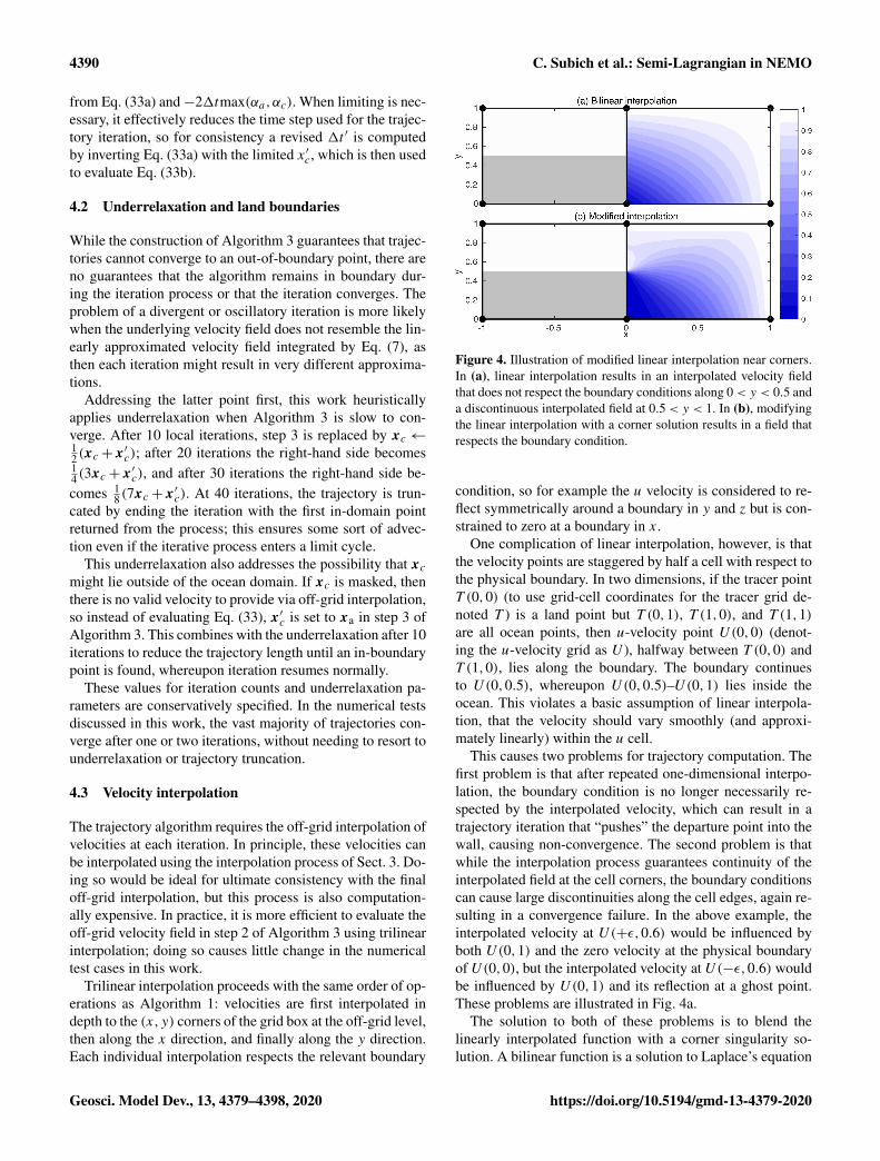
Figure 4. Illustration of modified linear interpolation near corners.In (a), linear interpolation results in an interpolated velocity fieldthat does not respect the boundary conditions along 0< y < 0.5 anda discontinuous interpolated field at 0.5< y < 1. In (b), modifyingthe linear interpolation with a corner solution results in a field thatrespects the boundary condition.
condition, so for example the u velocity is considered to re-flect symmetrically around a boundary in y and z but is con-strained to zero at a boundary in x.
One complication of linear interpolation, however, is thatthe velocity points are staggered by half a cell with respect tothe physical boundary. In two dimensions, if the tracer pointT (0,0) (to use grid-cell coordinates for the tracer grid de-noted T ) is a land point but T (0,1), T (1,0), and T (1,1)are all ocean points, then u-velocity point U(0,0) (denot-ing the u-velocity grid as U ), halfway between T (0,0) andT (1,0), lies along the boundary. The boundary continuesto U(0,0.5), whereupon U(0,0.5)–U(0,1) lies inside theocean. This violates a basic assumption of linear interpola-tion, that the velocity should vary smoothly (and approxi-mately linearly) within the u cell.
This causes two problems for trajectory computation. Thefirst problem is that after repeated one-dimensional interpo-lation, the boundary condition is no longer necessarily re-spected by the interpolated velocity, which can result in atrajectory iteration that “pushes” the departure point into thewall, causing non-convergence. The second problem is thatwhile the interpolation process guarantees continuity of theinterpolated field at the cell corners, the boundary conditionscan cause large discontinuities along the cell edges, again re-sulting in a convergence failure. In the above example, theinterpolated velocity at U(+ε,0.6) would be influenced byboth U(0,1) and the zero velocity at the physical boundaryof U(0,0), but the interpolated velocity at U(−ε,0.6) wouldbe influenced by U(0,1) and its reflection at a ghost point.These problems are illustrated in Fig. 4a.
The solution to both of these problems is to blend thelinearly interpolated function with a corner singularity so-lution. A bilinear function is a solution to Laplace’s equation
Geosci. Model Dev., 13, 4379–4398, 2020 https://doi.org/10.5194/gmd-13-4379-2020
C. Subich et al.: Semi-Lagrangian in NEMO 4391
(∇2f = 0), so it is reasonable to consider corner solutionsthat are also solutions to Laplace’s equation.
Without loss of generality, consider a grid cell definedby (x,y) ∈ [0,1]2, such that there is a solid boundary along(x = 0,y < 0.5) as depicted in Fig. 4. Treating the bound-ary as an infinite half-plane, with f (0,y)= 0 for y < 0.5and f (0,y)= f (0,1) for y > 0.5, the “corner” solution toLaplace’s equation is
fcorner(x,y)=f (0,1)
2
(1+ cos
(tan−1(y− 0.5
x
))), (34)
while bilinear interpolation would give
fbilinear(x,y)=(1− x)yf (1,0)+ x(1− y)f (0,1)
+ xyf (1,1). (35)
These two solutions are blended together, with Eq. (34)taking precedence along the solid boundary (x = 0 and 0≤y ≤ 0.5) and Eq. (35) taking precedence along the x = 1 andy = 1 boundaries of the cell. This gives
fblend(x,y)=σ(x,y)fbilinear(x,y)
+ (1− σ(x,y))fcorner(x,y), (36)
where σ =max(1− x,2(y− 0.5)).The blended function exactly respects the solid boundary
condition, and the discontinuity at the cell edges is signif-icantly reduced. Blended functions for other configurationsof the solid wall are given by applying the appropriate reflec-tions and rotations to Eq. (36).
5 Results
5.1 Flow past an island
To demonstrate the impacts of semi-Lagrangian advection ona simple test case with a lengthened time step, we first presentthe quasi-two-dimensional test case of isothermal flow pastan interposed island.
This test case consists of a 280× 70× 3 point grid, withgrid resolution 1x =1y = 5m and 1z= 10m. A 50m×50m region (10 points×10 points) is masked as land in themiddle of the domain. The inflow boundary condition is setto u= 0.03ms−1, v = 0; this was also imposed throughoutthe domain as an initial condition. The reference frame wasalso irrotational, with a Coriolis parameter of 0.
Relevant namelist parameters are given in Table 1, with pa-rameters that differ between the control and semi-Lagrangianruns highlighted. The control run used flux-form velocity ad-vection7 via the QUICKEST scheme (Leonard, 1979, 1991),whereas the semi-Lagrangian run used semi-Lagrangian ad-vection of momentum in flux form as described in Sects. 3
7This choice of velocity advection provided the best results forthe control run, of the advection models supported in NEMO ver-sion 3.1.
and 4. To emphasize the dynamical differences between theadvection schemes, both test cases were run with no explicithorizontal diffusion of momentum. Vertical mixing terms,largely irrelevant for this quasi-two-dimensional case, wereset consistently with the ORCA025 simulations in Sect. 5.2.
Both series of runs used the implicit free-surfaceformulation (enabled with the compile-time keykey_dynspg_flt), which damped the large initialsurface gravity waves caused by the imposition of theblocking island on the steady-state flow.
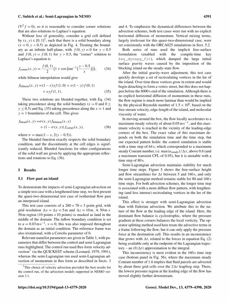
After the initial gravity-wave adjustment, this test casequickly develops a set of recirculating vortices in the lee ofthe island. Over time these vortices grow in extent and wouldbegin detaching to form a vortex street, but this does not hap-pen before the 8000 s end of the simulation. Although there isno explicit horizontal diffusion of momentum in these runs,the flow regime is much more laminar than would be impliedby the physical Reynolds number of 1.5× 10⁶, based on thefree-stream velocity, edge-length of the island, and molecularviscosity of water.
In moving around the box, the flow locally accelerates to amaximum steady velocity of about 0.05ms−1, and this max-imum velocity is reached in the vicinity of the leading-edgecorners of the box. The exact value of this maximum de-pends on both the simulation time and the time step, butour expected pattern holds: the control simulation is stablewith a time step of 64 s, which corresponded to a maximumsteady Courant number, i.e. max(usteady)/1x, above 0.6 (anda maximum transient CFL of 0.95), but it is unstable with atime step of 80 s.
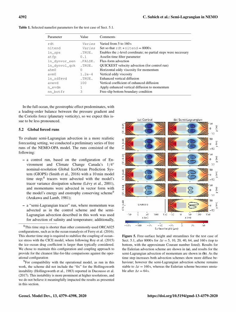
Semi-Lagrangian advection maintains stability for muchlonger time steps. Figure 5 shows the free-surface heightand flow streamlines for 1t between 5 and 160 s, and onlythe semi-Lagrangian method remains stable for 80 and 160 stime steps. For both advection schemes, the longer time stepis associated with a more diffuse flow pattern, with lengthen-ing (and less intense) recirculating vortices in the lee of theisland.
This effect is stronger with semi-Lagrangian advectionthan with Eulerian advection. We attribute this to the na-ture of the flow at the leading edge of the island. Here, thedominant flow balance is cyclostrophic, where the pressuregradient at these corners balances the local vorticity. The op-erator splitting method used here treats the advective terms ina frame following the flow, but it can only apply the pressureforce at the destination cell. This results in an inconsistencythat grows with 1t , related to the forces in equation Eq. (2)being available only at the endpoint of the Lagrangian trajec-tory – an O(1t) approximation to the integral.
This inconsistency is most evident in the 160 s time stepcase (bottom panel in Fig. 5b), where the maximum steadyCourant number of 1.6 implies that fluid parcels are advectedby about three grid cells over the 21t leapfrog step. There,the lowest pressure region at the leading edge of the flow hasmoved slightly further downstream.
https://doi.org/10.5194/gmd-13-4379-2020 Geosci. Model Dev., 13, 4379–4398, 2020
4392 C. Subich et al.: Semi-Lagrangian in NEMO
Table 1. Selected namelist parameters for the test case of Sect. 5.1.
Parameter Value Comments
rdt Varies Varied from 5 to 160 snitend Varies Set so that rdt ∗nitend= 8000sln_zps .TRUE. Enables the z-level coordinate; no partial steps were necessaryatfp 0.1 Asselin time filter parameterln_dynvor_een .FALSE. Flux-form advectionln_dynvol_qck .TRUE. QUICKEST velocity advection (for control run)ahm0 0 Horizontal eddy viscosity for momentumavm0 1.2e-4 Vertical eddy viscosityln_zdfevd .TRUE. Enhanced vertical diffusionavevd 100 Vertical coefficient of enhanced diffusionn_evdm 1 Apply enhanced vertical diffusion to momentumnn_botfr 3 Free-slip bottom boundary condition
In the full ocean, the geostrophic effect predominates, witha leading-order balance between the pressure gradient andthe Coriolis force (planetary vorticity), so we expect this is-sue to be less pronounced.
5.2 Global forced runs
To evaluate semi-Lagrangian advection in a more realisticforecasting setting, we conducted a preliminary series of freeruns of the NEMO-OPA model. The runs consisted of thefollowing:
– a control run, based on the configuration of En-vironment and Climate Change Canada’s 1/4◦
nominal-resolution Global Ice/Ocean Prediction Sys-tem (GIOPS) (Smith et al., 2016) with a 10 min modeltime step;8 tracers were advected with the model’stracer variance dissipation scheme (Lévy et al., 2001),and momentums were advected in vector form withthe model’s energy and enstrophy conserving scheme9
(Arakawa and Lamb, 1981);
– a “semi-Lagrangian tracer” run, where momentum wasadvected as in the control scheme and the semi-Lagrangian advection described in this work was usedfor advection of salinity and temperature; additionally,
8This time step is shorter than other commonly-used ORCA025configurations, such as in the ocean reanalysis of Ferry et al. (2016).This shorter time step is required to stabilize the coupling of ocean–ice stress with the CICE model, where following Roy et al. (2015)the ice–ocean drag coefficient is larger than typically considered.We chose to maintain this configuration and coupling approach toprovide for the cleanest like-for-like comparisons against the oper-ational configuration
9For compatibility with the operational model, as run in thiswork, the scheme did not include the “fix” for the Hollingsworthinstability (Hollingsworth et al., 1983) reported in Ducousso et al.(2017). This instability is more prominent at higher resolutions, andwe do not believe it meaningfully impacted the results as presentedin this section.
Figure 5. Free-surface height and streamlines for the test case ofSect. 5.1, after 8000s for 1t = 5, 10, 20, 40, 64, and 160 s (top tobottom, with the approximate Courant number listed). Results forthe Eulerian advection scheme are shown in (a), and results for thesemi-Lagrangian advection of momentum are shown in (b). As thetime step increases both advection schemes show more diffuse be-haviour; however the semi-Lagrangian advection scheme remainsstable to 1t = 160s, whereas the Eulerian scheme becomes unsta-ble after 1t = 64s.
Geosci. Model Dev., 13, 4379–4398, 2020 https://doi.org/10.5194/gmd-13-4379-2020
C. Subich et al.: Semi-Lagrangian in NEMO 4393
this run disabled horizontal diffusion of salinity andtemperature; and
– a “semi-Lagrangian momentum and tracer” run, wheremomentum as well is advected with the semi-Lagrangian scheme; the configuration was otherwisethe same as the semi-Lagrangian tracer run, save for a15 min model time step.
The runs were all initialized at 1 October 2001 on theORCA025 grid. The ocean was at rest, and temperature andsalinity were given by the 2011 World Ocean Atlas climatol-ogy (Locarnini et al., 2013; Zweng et al., 2013). Atmosphericforcing was provided at 1 h intervals from Environment andClimate Change Canada’s 1/4◦ global atmospheric refore-cast, and sea ice was modeled via coupling with version 4.0of the CICE model (Hunke and Dukowicz, 1997), with dy-namically active (moving) ice. Selected namelist parametersare provided in Table 2.
As with Sect. 5.1, the test cases used NEMO-OPA’s lin-ear free-surface with a time-implicit solver, and tidal forc-ing was not present in these configurations. In a typicaltime step, the vast majority of semi-Lagrangian trajecto-ries converged in one iteration (mean 1.004 over the semi-Lagrangian tracer run). A very small minority of cells re-quired an extended number of iterations or underrelaxationas described in Sect. 4.2, but this did not affect the overalltrajectory-calculation performance because convergence wasmeasured (and iterations limited) on a per-cell basis.
Each run continued through late 2009. For reasons ofspace efficiency, we recorded the two-dimensional seasurface height, temperature, and salinity fields for eachmodel day, and we preserved every fifth daily-mean, three-dimensional output of temperature, salinity, and horizontalocean velocity.
For short- and medium-term forecasts, the operationalcoupled forecasting systems at CMC are constrained by ob-servations and periodic re-initialization. With a focus on thisforecasting horizon, the objectives of these long free-runswere as follows:
– to provide a test of model stability with semi-Lagrangian advection, in terms of both avoiding crashesand providing plausible ocean fields;
– to check for any large-scale conservation errors, whichmight be difficult to correct given the sparsity of obser-vation data for the deep ocean; and
– to note any qualitative improvement or deterioration inthe effective resolution of the model.
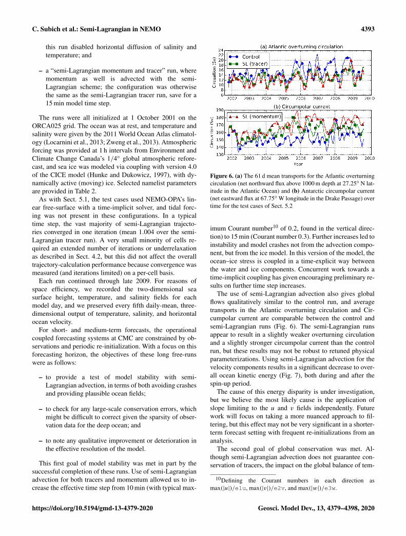
This first goal of model stability was met in part by thesuccessful completion of these runs. Use of semi-Lagrangianadvection for both tracers and momentum allowed us to in-crease the effective time step from 10 min (with typical max-
Figure 6. (a) The 61 d mean transports for the Atlantic overturningcirculation (net northward flux above 1000 m depth at 27.25◦ N lat-itude in the Atlantic Ocean) and (b) Antarctic circumpolar current(net eastward flux at 67.75◦W longitude in the Drake Passage) overtime for the test cases of Sect. 5.2
imum Courant number10 of 0.2, found in the vertical direc-tion) to 15 min (Courant number 0.3). Further increases led toinstability and model crashes not from the advection compo-nent, but from the ice model. In this version of the model, theocean–ice stress is coupled in a time-explicit way betweenthe water and ice components. Concurrent work towards atime-implicit coupling has given encouraging preliminary re-sults on further time step increases.
The use of semi-Lagrangian advection also gives globalflows qualitatively similar to the control run, and averagetransports in the Atlantic overturning circulation and Cir-cumpolar current are comparable between the control andsemi-Lagrangian runs (Fig. 6). The semi-Lagrangian runsappear to result in a slightly weaker overturning circulationand a slightly stronger circumpolar current than the controlrun, but these results may not be robust to retuned physicalparameterizations. Using semi-Lagrangian advection for thevelocity components results in a significant decrease to over-all ocean kinetic energy (Fig. 7), both during and after thespin-up period.
The cause of this energy disparity is under investigation,but we believe the most likely cause is the application ofslope limiting to the u and v fields independently. Futurework will focus on taking a more nuanced approach to fil-tering, but this effect may not be very significant in a shorter-term forecast setting with frequent re-initializations from ananalysis.
The second goal of global conservation was met. Al-though semi-Lagrangian advection does not guarantee con-servation of tracers, the impact on the global balance of tem-
10Defining the Courant numbers in each direction asmax(|u|)/e1u, max(|v|)/e2v, and max(|w|)/e3w.
https://doi.org/10.5194/gmd-13-4379-2020 Geosci. Model Dev., 13, 4379–4398, 2020
4394 C. Subich et al.: Semi-Lagrangian in NEMO
Table 2. Selected dynamical and numerical namelist parameters for the test cases of Sect. 5.2.
Parameter Value Comments
Parameters common to all runs
atfp 0.1 Asselin time filter parameterln_zps .TRUE. z-level vertical coordinate with partial (cut) cellse3zps_min 25 Absolute minimum thickness of a cut celle3zps_rat 0.2 Relative minimum thickness of a cut cellshlat 0 Free-slip lateral momentum boundary conditionnn_botfr 2 Nonlinear bottom frictionnn_bfro2 1e-3 Nonlinear bottom friction coefficientnn_bfeb2 2.5e-3 Background turbulent kinetic energy coefficientngeo_flux 0 No bottom temperature geothermal heat fluxln_dynhpg_imp .TRUE. Semi-implicit computation of the hydrostatic pressure gradientln_dynldf_bilap .TRUE. Bi-Laplacian hyperdiffusion of momentumln_dynldf_hor .TRUE. The above parameter acting in the horizontal directionahm0 -3e11 Momentum hyperviscosity coefficientsnsolv 2 Use the successive over-relaxation (SOR) free-surface solvernsol_arp 0 The above parameter with an absolute-tolerance stopping conditionnn_sstr 0 No sea surface temperature dampingnn_sssr 0 No sea surface salinity dampingndmp 0 No temperature or salinity damping in the water column
Parameters for the control run
rdt 600 Model time stepln_traadv_tvd .TRUE. Tracer variance dissipation (TVD) tracer advection schemeln_traldf_lap .TRUE. Laplacian diffusion for the tracerln_traldf_iso .TRUE. The above parameter acting in the iso-neutral directionaht0 300 Horizontal tracer diffusion coefficientln_dynadv_vec .TRUE. Vector form of the momentum advection operatorln_dynvor_een .TRUE. The above parameter using the energy- and entropy-conserving schemeresmax 1e-10 Absolute residual tolerance for the SOR free-surface solver
Parameters for the semi-Lagrangian tracer run
rdt 600 Model time stepln_traldf_lap .FALSE. No explicit horizontal tracer diffusionln_dynadv_vec .TRUE. Vector form of the momentum advection operatorln_dynvor_een .TRUE. The above parameter using the energy and enstropy conserving schemeresmax 1e-11 Absolute residual tolerance for the SOR free-surface solver
Parameters for the semi-Lagrangian momentum and tracer run
rdt 900 Model time stepln_traldf_lap .FALSE. No explicit horizontal tracer diffusionln_dynadv_vec .FALSE. Flux form of the momentum advection operatorresmax 1e-11 Absolute residual tolerance for the SOR free-surface solver
perature and salinity was small. Figure 8 shows the evolu-tion of ocean-average temperature and salinity over time inthese runs, and the effect of non-conservation attributable tothe semi-Lagrangian advection of tracers is comparable tothe magnitude of uncertainty in the global balance of atmo-spheric forcing – the imbalance seen in the control run. Eachcase saw an overall temperature drift of about 0.04K overthe simulated period, with the semi-Lagrangian cases havinga slight warming trend against the control run’s slight cool-
ing trend, and all three runs showed a very small increase inocean-average salinity, by about 0.01PSU.
The temperature change vs. depth over the simulated pe-riod is shown in Fig. 9. Both the control and semi-Lagrangianruns showed a warming trend in the surface layers, but thesemi-Lagrangian runs showed temperature stability in fluidlayers below 1000m depth, whereas the control run showeda cooling trend in these waters.
Geosci. Model Dev., 13, 4379–4398, 2020 https://doi.org/10.5194/gmd-13-4379-2020
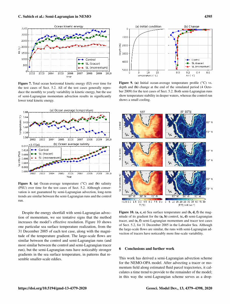
C. Subich et al.: Semi-Lagrangian in NEMO 4395
Figure 7. Total ocean horizontal kinetic energy (EJ) over time forthe test cases of Sect. 5.2. All of the test cases generally repro-duce the monthly to yearly variability in kinetic energy, but the useof semi-Lagrangian momentum advection results in significantlylower total kinetic energy.
Figure 8. (a) Ocean-average temperature (◦C) and (b) salinity(PSU) over time for the test cases of Sect. 5.2. Although conser-vation is not guaranteed by semi-Lagrangian advection, long-termtrends are similar between the semi-Lagrangian runs and the controlrun.
Despite the energy shortfall with semi-Lagrangian advec-tion of momentum, we see tentative signs that the methodincreases the model’s effective resolution. Figure 10 showsone particular sea surface temperature realization, from the31 December 2005 of each test case, along with the magni-tude of the temperature gradient. The large-scale flows aresimilar between the control and semi-Lagrangian runs (andmost similar between the control and semi-Lagrangian tracerrun), but the semi-Lagrangian runs have noticeably strongergradients in the sea surface temperature, in patterns that re-semble smaller-scale eddies.
Figure 9. (a) Initial ocean-average temperature profile (◦C) vs.depth and (b) change at the end of the simulated period (4 Octo-ber 2009) for the test cases of Sect. 5.2. Both semi-Lagrangian runsshow temperature stability in deeper waters, whereas the control runshows a small cooling.
Figure 10. (a, c, e) Sea surface temperature and (b, d, f) the mag-nitude of its gradient for the (a, b) control, (c, d) semi-Lagrangiantracer, and (e, f) semi-Lagrangian momentum and tracer test casesof Sect. 5.2, for 31 December 2005 in the Labrador Sea. Althoughthe large-scale flows are similar, the runs with semi-Lagrangian ad-vection of tracers have noticeably more fine-scale variability.
6 Conclusions and further work
This work has derived a semi-Lagrangian advection schemefor the NEMO-OPA model. After advecting a tracer or mo-mentum field along estimated fluid parcel trajectories, it cal-culates a time trend to provide to the remainder of the model;in this way the semi-Lagrangian scheme serves as a drop-
https://doi.org/10.5194/gmd-13-4379-2020 Geosci. Model Dev., 13, 4379–4398, 2020
4396 C. Subich et al.: Semi-Lagrangian in NEMO
in replacement for other tracer and (flux-form) momentumschemes.
The development of this advection module relied on sev-eral new or newly applied algorithms that might be relevantto other ocean models or other domains:
– The “semi-Lagrangian trend” form of equation Eq. (7)might be useful in other models when researcherswish to implement semi-Lagrangian advection after thefact, without disrupting the calculation of other forcingterms.
– The Hermite interpolation form in Sect. 3, especiallycombined with the C1-continuous estimate of the verti-cal derivative in Sect. 3.2 might find application in otherdomains where, as in the ocean, one dimension (the ver-tical) is more oscillatory than others.
– The exponential integration of trajectories in Eq. (4)may be useful in other applications that feature strongaccelerations over trajectories. In particular, it forbidstrajectory-crossing in one-dimensional flows, and herethat property ensures that trajectories remain inside theocean domain.
– The “corner solution” treatment of velocity for trajec-tory calculations near corners might find use in otherapplications with staggered velocity components.
Overall, we find that the semi-Lagrangian method is ef-fective at extending the realizable time step in the NEMO-OPA model. In the simple domain of Sect. 5.1, this methodresulted in a stable simulation with advective Courant num-bers in excess of 1. Although we only extended the time stepfrom 10 to 15 min for the semi-Lagrangian momentum run inSect. 5.2, this limitation was imposed by the ice model. Dis-abling ice dynamics allowed us to increase the time step to30 min, but this would have made the results incomparablewith those of the control and semi-Lagrangian tracer runs.Preliminary work with the CICE sea model and implicit cou-pling of the ice–ocean stress seems to allow us to relax theice-related time step restriction.
6.1 Performance and implementation
In spite of this increased time step, the semi-Lagrangianmethod by itself does not yet improve overall computationalperformance. The semi-Lagrangian momentum and tracerrun of Sect. 5.2 took approximately 1 h of computationaltime per 5 d of simulated time, using 128 Intel Xeon E5530processors at 2.4 GHz. With a 10 min time step, the semi-Lagrangian tracer run took approximately 50 min for thesame 5 d of simulated time, whereas the control run tookjust 30 min. We expect these results to improve with furthernumerical optimization work. In particular, we did not takegreat care to ensure that loops were vectorized where possi-ble, and it is much more difficult for compilers to automati-
cally vectorize the point-by-point semi-Lagrangian computa-tions compared to volume flux calculations in the traditionaladvection schemes.
About one-third of the additional computational costcomes from trajectory iterations, and the remainder comesfrom the cubic interpolation. This suggests that the relativecost of semi-Lagrangian advection will be lower than pre-sented here if trajectories can be reused for multiple tracerspecies (such as biogeochemical constituents). Additionally,it suggests that a further optimization may be to reuse tracertrajectories for momentum advection, at least away fromthe boundaries where interpolating (staggering) trajectoriesmight be reasonable. It seems unlikely that optimization willreduce the per-time-step penalty to the 20 % value seen byRitchie et al. (1995) for an atmospheric model – owing to thelack of three-dimensional implicit equations and expensivephysical parameterizations elsewhere in NEMO-0PA – butwe are hopeful that semi-Lagrangian advection will nonethe-less improve overall system performance.
The parallel (MPI) implementation of this algorithmwas straightforward. With the relatively modest increasein Courant number for the cases in this work, we simplyneeded to increase the interprocessor lateral halo (parametersjpreci and jprecj) to three points, which was sufficientto allow a fluid parcel arriving at a processor’s edge to applythe full interpolating stencil for the Courant numbers reachedin the presented simulations. This increase in halo size wassmall compared to the processor tile size of about 50× 260grid points for the runs in Sect. 5.2. Extending this to supportvery large horizontal Courant numbers, however (if anothersolution could be found to stabilize baroclinic waves), wouldrequire either prohibitively large halo sizes or additional in-terprocessor communication to track fluid parcels that crossMPI boundaries.
6.2 Qualitative comments on results
Although the semi-Lagrangian method does not guaranteetracer conservation, we see no evidence that its implemen-tation here leads to a degradation relevant in a weekly toseasonal forecast setting. In particular, the deep-water tem-perature stability shown in Fig. 9 is an encouraging signthat semi-Lagrangian advection will preserve the deep-waterstructure that is weakly constrained by data. Even smallimbalances, however, might become significant over thedecade-to-century timescales of climate simulations. Furtherwork will be necessary to characterize this method before wecan safely recommend semi-Lagrangian advection in suchsettings.
For the test cases in Sect. 5.2, semi-Lagrangian advectionof tracers appears to slightly increase the effective resolu-tion of the model. However, this effect is much more mixedwhen momentum is also advected with the semi-Lagrangianmethod, in part because the underlying currents differ. Bothof these differences will be the subject of future study, with
Geosci. Model Dev., 13, 4379–4398, 2020 https://doi.org/10.5194/gmd-13-4379-2020
C. Subich et al.: Semi-Lagrangian in NEMO 4397
the specific intention of assessing these effects in the settingof shorter-term forecasts. We speculate that the overall loss ofkinetic energy with semi-Lagrangian advection of momen-tum is attributable to the use of the slope limiter: limitingeach component of velocity separately may be causing un-realistic diffusion of smaller-scale structures in the presenceof background vorticity. We hope to address this issue withmore selective limiting.
6.3 Future development
Finally, the development in this paper implicitly assumes thatthe coordinate system is static with time. This is not thecase in NEMO-OPA when using its nonlinear free-surfaceoption, which necessarily implies time-varying vertical lev-els. Adapting the semi-Lagrangian method to this more gen-eral coordinate system will be a focus of future work, whichwill be required to apply this advection scheme to higher-resolution domains that require tide-permitting simulations.
Additionally, future versions of NEMO intend to move toa third-order Runge–Kutta time-stepping algorithm (Shu andOsher, 1997), which constructs a full time step as a linearcombination of forward Euler steps. We expect that the semi-Lagrangian “advective trend” of Eq. (7) can be adapted tothis framework in a straightforward manner by basing thecalculated trend on the current-step values of tracers and ve-locities, but the adaptation may require care to preserve thehigher-order temporal accuracy of the overall scheme.
Code availability. The modified NEMO (CeCILL license, version2.0) code along with scripts and data used in this paper are availableat https://doi.org/10.5281/zenodo.3905100 (Subich et al., 2020).The modified CICE 4.0 used in Sect. 5.2 is not redistributable undera free license, but it has been made available for the topical editorsand anonymous reviewers.
Author contributions. All authors were responsible for the concept.CS, PP, and FD were responsible for the necessary software devel-opment. CS contributed to the original draft preparation, and all au-thors contributed to review and editing.
Competing interests. The authors declare that they have no conflictof interest.
Acknowledgements. The authors would like to acknowledge Fran-cois Roy of Environment Canada, who provided considerable tech-nical support, especially with the forcing runs of Sect. 5.2, andJerome Chanut of Mercator Ocean, who provided helpful commentson a draft of this paper. The authors also are grateful for the peerreview provided by Florian Lemarie and Mike Bell, which greatlyimproved this paper from its original submission.
The authors also owe a debt of inspiration to the semi-Lagrangiandynamical core of MC2 (Thomas et al., 1998).
Review statement. This paper was edited by Simone Marras and re-viewed by Florian Lemarie and Mike Bell.
References
Arakawa, A. and Lamb, V. R.: A Potential Enstrophy and En-ergy Conserving Scheme for the Shallow Water Equations,Mon. Weather Rev., 109, 18–36, https://doi.org/10.1175/1520-0493(1981)109<0018:APEAEC>2.0.CO;2, 1981.
Asselin, R.: Frequency Filter for Time Integrations, Mon.Weather Rev., 100, 487–490, https://doi.org/10.1175/1520-0493(1972)100<0487:FFFTI>2.3.CO;2, 1972.
Bermejo, R. and Staniforth, A.: The Conver-sion of Semi-Lagrangian Advection Schemes toQuasi-Monotone Schemes, Mon. Weather Rev.,120, 2622–2632, https://doi.org/10.1175/1520-0493(1992)120<2622:TCOSLA>2.0.CO;2, 1992.
Casulli, V. and Cheng, R. T.: Semi-implicit finite dif-ference methods for three-dimensional shallow wa-ter flow, Int. J. Numer. Methods Fluid., 15, 629–648,https://doi.org/10.1002/fld.1650150602, 1992.
Ducousso, N., Le Sommer, J., Molines, J. M., and Bell,M.: Impact of the “Symmetric Instability of the Com-putational Kind” at mesoscale- and submesoscale-permitting resolutions, Ocean Model., 120, 18–26,https://doi.org/10.1016/j.ocemod.2017.10.006, 2017.
Ferry, N., Parent, L., Masina, S., Storto, A., Zuo, H., andBalmaseda, M.: PRODUCT USER MANUAL For GlobalOcean Reanalysis Products GLOBAL-REANALYSIS-PHYS-001-009 GLOBAL-REANALYSIS-PHYS-001-011 GLOBAL-REANALYSIS-PHYS-001-017, Tech.Rep. 2.9, Copernicus Marine Service, available at:https://resources.marine.copernicus.eu/documents/PUM/CMEMS-GLO-PUM-001-009-011-017.pdf, (last access:12 June 2020), 2016.
Girard, C., Plante, A., Desgagné, M., McTaggart-Cowan, R., Côté,J., Charron, M., Gravel, S., Lee, V., Patoine, A., Qaddouri, A.,Roch, M., Spacek, L., Tanguay, M., Vaillancourt, P. A., andZadra, A.: Staggered vertical discretization of the Canadian En-vironmental Multiscale (GEM) model using a coordinate of thelog-hydrostatic-pressure type, Mon. Weather Rev., 142, 1183–1196, 2014.
Hildebrand, F.: Introduction to Numerical Analysis: Second Edi-tion, McGraw-Hill Inc., 1974.
Hodges, B. R. and Dallimore, C.: Estuary, Lake and Coastal OceanModel: ELCOM v2.2 science manual, Tech. rep., Center for Wa-ter Research, University of Western Australia, 2006.
Hollingsworth, A., Kållberg, P., Renner, V., and Burridge, D.: Aninternal symmetric computational instability, Q. J. Roy. Meteor.Soc., 109, 417–428, 1983.
Hunke, E. C. and Dukowicz, J. K.: An elastic–viscous–plastic model for sea ice dynamics, J. Phys.Oceanogr., 27, 1849–1867, https://doi.org/10.1175/1520-0485(1997)027<1849:AEVPMF>2.0.CO;2, 1997.
Lauritzen, P. H.: A Stability Analysis of Finite-Volume AdvectionSchemes Permitting Long Time Steps, Mon. Weather Rev., 135,2658–2673, https://doi.org/10.1175/MWR3425.1, 2007.
https://doi.org/10.5194/gmd-13-4379-2020 Geosci. Model Dev., 13, 4379–4398, 2020
4398 C. Subich et al.: Semi-Lagrangian in NEMO
Leclair, M. and Madec, G.: z-Coordinate, an ArbitraryLagrangian–Eulerian coordinate separating high andlow frequency motions, Ocean Model., 37, 139–152,https://doi.org/10.1016/j.ocemod.2011.02.001, 2011.
Lemarié, F., Debreu, L., Madec, G., Demange, J., Mo-lines, J. M., and Honnorat, M.: Stability constraints foroceanic numerical models: implications for the formulation oftime and space discretizations, Ocean Model., 92, 124–148,https://doi.org/10.1016/j.ocemod.2015.06.006, 2015.
Lemieux, J.-F., Beaudoin, C., Dupont, F., Roy, F., Smith, G. C.,Shlyaeva, A., Buehner, M., Caya, A., Chen, J., Carrieres, T.,Pogson, L., DeRepentigny, P., Plante, A., Pestieau, P., Pel-lerin, P., Ritchie, H., Garric, G., and Ferry, N.: The Re-gional Ice Prediction System (RIPS): verification of forecastsea ice concentration, Q. J. Roy. Meteor. Soc., 142, 632–643,https://doi.org/10.1002/qj.2526, 2016.
Leonard, B. P.: A stable and accurate convective modelling proce-dure based on quadratic upstream interpolation, Comput. Meth-ods Appl. Mech. Eng., 19, 59–98, https://doi.org/10.1016/0045-7825(79)90034-3, 1979.
Leonard, B. P.: The ULTIMATE conservative difference schemeapplied to unsteady one-dimensional advection, Comput. Meth-ods Appl. Mech. Eng., 88, 17–74, https://doi.org/10.1016/0045-7825(91)90232-U, 1991.
Lévy, M., Estublier, A., and Madec, G.: Choice of an advectionscheme for biogeochemical models, Geophys. Res. Lett., 28,3725–3728, https://doi.org/10.1029/2001GL012947, 2001.
Locarnini, R. A., Mishonov, A. V., Antonov, J. I., Boyer, T. P., Gar-cia, H. E., Baranova, O. K., Zweng, M. M., Paver, C. R., Reagan,J. R., Johnson, D. R., Hamilton, M., and Seido, D.: World OceanAtlas 2013, Volume 1: Temperature, 2013.
Madec, G.: NEMO ocean engine, Note du Pôle de modélisation,Institut Pierre-Simon Laplace (IPSL), France, No. 27, 2008.
Madec, G. and Imbard, M.: A global ocean mesh to over-come the North Pole singularity, Clim. Dynam., 12, 381–388,https://doi.org/10.1007/BF00211684, 1996.
Mesinger, F. and Arakawa, A.: Numerical methods used in at-mospheric models, Global Atmospheric Research Programme(GARP), World Meteorological Organization, 1976.
Murray, R. J.: Explicit Generation of Orthogonal Gridsfor Ocean Models, J. Comput. Phys., 126, 251–273,https://doi.org/10.1006/jcph.1996.0136, 1996.
Ritchie, H., Temperton, C., Simmons, A., Hortal, M.,Davies, T., Dent, D., and Hamrud, M.: Implemen-tation of the Semi-Lagrangian Method in a High-Resolution Version of the ECMWF Forecast Model, Mon.Weather Rev., 123, 489–514, https://doi.org/10.1175/1520-0493(1995)123<0489:IOTSLM>2.0.CO;2, 1995.
Robert, A.: A semi-Lagrangian and semi-implicit numerical inte-gration scheme for the primitive meteorological equations, J. Me-teorol. Soc. Jpn. Ser. II, 60, 319–325, 1982.
Roy, F., Chevallier, M., Smith, G. C., Dupont, F., Garric, G.,Lemieux, J.-F., Lu, Y., and Davidson, F.: Arctic sea ice andfreshwater sensitivity to the treatment of the atmosphere-ice-ocean surface layer, J. Geophys. Res.-Oceans, 120, 4392–4417,https://doi.org/10.1002/2014JC010677, 2015.
Shchepetkin, A. F. and McWilliams, J. C.: The regional oceanicmodeling system (ROMS): a split-explicit, free-surface,topography-following-coordinate oceanic model, Ocean Model.,9, 347–404, https://doi.org/10.1016/j.ocemod.2004.08.002,2005.
Shu, C.-W. and Osher, S.: Efficient Implementation of EssentiallyNon-oscillatory Shock-Capturing Schemes, II, in: Upwind andHigh-Resolution Schemes, edited by: Hussaini, M. Y., van Leer,B., and Van Rosendale, J., Springer, Berlin, Heidelberg, 328–374, https://doi.org/10.1007/978-3-642-60543-7_14, 1997.
Smith, G., Liu, Y., Colan, D. S., Reszka, M., Roy, F., Dupont, F.,Lemieux, J.-F., Beaudoin, C., Lellouche, J.-M., Garric, G., Tes-tut, C.-E., Pellerin, P., Ritchie, H., Lu, Y., and Davidson, F.:The CMC Global Ice Ocean Prediction System v2.1, Tech. rep.,Canadian Centre for Meteorological and Environmental Pre-diction, available at: http://collaboration.cmc.ec.gc.ca/cmc/cmoi/product_guide/docs/tech_notes/technote_giops-210_e.pdf, (lastaccess: 15 September 2020), 2016.
Smith, G. C., Bélanger, J.-M., Roy, F., Pellerin, P., Ritchie, H., Onu,K., Roch, M., Zadra, A., Colan, D. S., Winter, B., Fontecilla,J.-S., and Deacu, D.: Impact of Coupling with an Ice–OceanModel on Global Medium-Range NWP Forecast Skill, Mon.Weather Rev., 146, 1157–1180, https://doi.org/10.1175/MWR-D-17-0157.1, 2018.
Smolarkiewicz, P. K. and Pudykiewicz, J. A.: A Classof Semi-Lagrangian Approximations for Fluids, J. At-mos. Sci., 49, 2082–2096, https://doi.org/10.1175/1520-0469(1992)049<2082:ACOSLA>2.0.CO;2, 1992.
Subich, C., Pellerin, P., Smith, G., and Dupont, F.: Code repositoryfor “Development of a semi-Lagrangian advection scheme forthe NEMO ocean model (3.1)”, a GMD discussion paper, Zen-odo, https://doi.org/10.5281/zenodo.3905100, 2020.
Thomas, S. J., Girard, C., Benoit, R., Desgagné, M., and Pellerin,P.: A new adiabatic kernel for the MC2 model, Atmos.-Ocean,36, 241–270, https://doi.org/10.1080/07055900.1998.9649613,1998.
Turkington, B., Eydeland, A., and Wang, S.: A Computa-tional Method for Solitary Internal Waves in a Contin-uously Stratified Fluid, Stud. Appl. Math., 85, 93–127,https://doi.org/10.1002/sapm199185293, 1991.
Walters, R. A., Lane, E. M., and Henry, R. F.: Semi-Lagrangianmethods for a finite element coastal ocean model, Ocean Model.,19, 112–124, https://doi.org/10.1016/j.ocemod.2007.06.008,2007.
Zweng, M., Reagan, J., Antonov, J., Locarnini, R., Mishonov, A.,Boyer, T., Garcia, H., Baranova, O., Johnson, D., Seidov, D., andBiddle, M.: World Ocean Atlas Volume 2: Salinity, 2013.
Geosci. Model Dev., 13, 4379–4398, 2020 https://doi.org/10.5194/gmd-13-4379-2020
Copyright © 2022 FDOKUMEN