INTERNATIONAL JOURNAL FOR NUMERICAL METHODS IN ENGINEERINGInt. J. Numer. Meth. Engng 2012; 90:1485–1507Published online 26 April 2012 in Wiley Online Library (wileyonlinelibrary.com). DOI: 10.1002/nme.3372

A finite element semi-Lagrangian method with L2 interpolation

Mofdi El-Amrani1,*,† and Mohammed Seaïd2

1Departamento de Matemática Aplicada, Universidad Rey Juan Carlos, 28933, Móstoles-Madrid, Spain2School of Engineering and Computing Sciences, University of Durham, South Road, Durham DH1 3LE, UK

SUMMARY

High-order accurate methods for convection-dominated problems have the potential to reduce the computa-tional effort required for a given order of solution accuracy. The state of the art in this field is more advancedfor Eulerian methods than for semi-Lagrangian (SLAG) methods. In this paper, we introduce a new SLAGmethod that is based on combining the modified method of characteristics with a high-order interpolatingprocedure. The method employs the finite element method on triangular meshes for the spatial discretization.An L2 interpolation procedure is developed by tracking the feet of the characteristic lines from the integra-tion nodes. Numerical results are illustrated for a linear advection–diffusion equation with known analyticalsolution and for the viscous Burgers’ equation. The computed results support our expectations for a robustand highly accurate finite element SLAG method. Copyright © 2012 John Wiley & Sons, Ltd.

Received 10 January 2011; Revised 28 October 2011; Accepted 3 November 2011

KEY WORDS: semi-Lagrangian method; finite element discretization; L2 interpolation; convection-dominated equations

1. INTRODUCTION

Modified method of characteristics or semi-Lagrangian (SLAG) method as known in the meteoro-logical community have important applications in a variety of physical and engineering areas suchas weather prediction, ocean circulation, petroleum reservoir, etc. The physical phenomena in theseareas can be modelled by transport-diffusion equations with the property that the convective termsare distinctly more important than the diffusive terms, particularly when certain nondimensionalparameters reach high values. As examples of these parameters, we mention the Peclet number forconvection–diffusion equations and the Reynolds number for incompressible Navier–Stokes equa-tions. It is well established that for large values of these parameters, the convective terms are sourcesof computational difficulties and nonphysical oscillations. On the other hand, steep fronts, shockdiscontinuities and boundary layers are among the difficulties that most Eulerian methods fail toresolve accurately [1]. It is well known that the Eulerian methods use fixed grids and incorporatesome upstream weighting in their formulations to stabilize the schemes. These Eulerian methodsinclude the Petrov–Galerkin methods, the streamline diffusion methods, discontinuous Galerkinmethods and also many other methods such as the high resolution methods from computational fluid

*Correspondence to: Mofdi El-Amrani, Departamento de Matemática Aplicada, Universidad Rey Juan Carlos, 28933,Móstoles-Madrid, Spain.

†E-mail: mofdi.elamrani@urjc.es

Copyright © 2012 John Wiley & Sons, Ltd.

1486 M. EL-AMRANI AND M. SEAÏD

dynamics, in particular, the Godunov methods and the essentially nonoscillatory methods [2,3]. Themain shortcoming of these methods is the stability conditions which impose a severe restriction onthe size of the time steps taken in numerical simulations.

The conventional SLAG method is second-order accurate in space and time provided the char-acteristic curves are exactly calculated. However, for general nonlinear convection problems, theaccuracy of the numerical scheme depends on the order of the interpolation procedure used to cal-culate the departure points and on the time integration procedure. Analysis of convergence andstability of the conventional SLAG method have been carried out in many papers, among others,in [4–7]. The main focus of our work is the development of a highly accurate SLAG method tonumerically solve the convection-dominated flow problems. The central idea in these methods is torewrite the governing equations in terms of Lagrangian coordinates as defined by the particle tra-jectories (or characteristics) associated with the problem under consideration. The time derivativeand the advection terms are combined as a directional derivative along the characteristics, lead-ing to a characteristic time-stepping procedure. The Lagrangian treatment in these methods greatlyreduces the time truncation errors in the Eulerian methods; see for example [8, 9]. Furthermore, theSLAG method offers the possibility of using time steps that exceed those permitted by the Courant–Friedrichs–Lewy (CFL) stability condition in Eulerian-based methods for convection-dominatedflows. A class of SLAG methods has been investigated in references [5–7, 10–12], among others.The authors in [13] have analyzed a SLAG method for the incompressible Navier–Stokes equationsin the finite element framework. In this reference, the solutions at characteristic feet are approxi-mated by interpolation from finite element basis functions. It should be noted that triangular finiteelements are attractive because of their flexibility for representing irregular boundaries and for localmesh refinements.

In [6], a first-order SLAG method combined with the finite element method has been analyzedfor the Navier–Stokes equations. It has been shown that the method is unconditionally stable pro-vided the characteristics are transported by a divergence-free field that is deduced from the flowvelocity. The case where the characteristics are transported by a discrete velocity field which isnot divergence-free has been studied in [7]. Analysis of a SLAG method with the use of the stan-dard finite difference discretization has been treated in [5] for convection–diffusion equations. In allthese references, the convergence and stability of the method are proven under the assumption thatall the inner products are calculated exactly. Furthermore, the evaluation of the fluid particles at thedeparture points in [5–7] is performed with the use of an L2 projection on the finite element space.However, to our best knowledge, there is a lack of computational verification of the L2 projectionin the literature. The studies reported in the references [6, 7] were devoted for the analysis of themethod, and no computational results were presented therein. The present study represents a steptowards the implementation of an L2 interpolation for the SLAG solution of convection-dominatedflow problems. We mainly focus on the algorithmic structure and outline implementational issues.The paradigm one should keep in mind is that, in the SLAG finite element context, theL2 projectionconsists of evaluating the solution at the characteristic curves using the nodal basis functions asso-ciated with the host element where the departure points are located. In the current work, we proposea new L2 interpolation using quadrature nodal points on the host element to calculate the solutionat the characteristic curves.

The aim of this paper is to develop a highly accurate SLAG method with the use of an L2 inter-polation on the finite element space. The application of this method has been demonstrated usingthree test examples including the nonlinear problem of viscous Burgers’ equation. Combining anL2 interpolation with the SLAG method, to the best of our knowledge, is reported for the first time.Numerical results presented in this study show that an interesting feature of the L2 interpolation isto allow large time steps without deteriorating the accuracy of the computed solutions. The layoutof this paper is as follows. In Section 2, we describe the finite element SLAG method for a convec-tion equation. This section includes the finite element discretization, the approximation of departurepoints and the conventional SLAG method. The proposed SLAG method using the L2 interpolationis formulated in Section 3. The extension of the new method to convection–diffusion problems isalso discussed in this section. Section 4 is devoted to numerical results and examples. Concludingremarks are summarized in Section 5.

Copyright © 2012 John Wiley & Sons, Ltd. Int. J. Numer. Meth. Engng 2012; 90:1485–1507DOI: 10.1002/nme

A FINITE ELEMENT SEMI-LAGRANGIAN METHOD WITH L2 INTERPOLATION 1487

2. FINITE ELEMENT SEMI-LAGRANGIAN METHOD

In order to describe the formulation of the considered finite element SLAG method, we consider thetwo-dimensional transport flow problem,

Dc

DtWD

@c

@tC v.x, t / � rc D 0, .x, t / 2�� .0,T /,

c.x, 0/D c0.x/, x 2�(1)

where x D .x,y/T is the space variable, rc D . @c@x

, @c@y/T is the gradient vector, � is a spatial

bounded domain in R2 with boundary @� and Œ0,T � is a time interval. Here, c.x, t / denotes theconcentration of some species, v.x, t / D .u.x, t /, v.x, t //T the velocity field assumed to dependon the solution c as well and c0.x/ a given initial function. We assume that appropriate boundaryconditions are given in such a way that the problem is well defined and has a unique solution. Notethat Dc

Dtmeasures the rate of change of the function c following the trajectories of the flow particles.

The main idea behind the SLAG method is to impose a regular grid at the new time level and tobacktrack the flow trajectories to the previous time level. At the old time level, the quantities thatare needed are evaluated by interpolation from their known values on a regular grid.

2.1. Finite element discretization

To formulate our SLAG method, we require a discretization of the space domain�. To perform thisstep, we generate a quasi-uniform partition �h �� of small elements Tj that satisfy the followingconditions:

(i) �h DNe[jD1

Tj , where Ne is the number of elements in �h.

(ii) If Ti and Tj are two different elements of �h, then

Ti \ Tj D

8<:Pij , a mesh point, or�ij , a common side, or;, empty set.

(iii) There exists a positive constant k such that for all j 2 ¹1, � � � ,Neº, Rjhj> k .hj 6 h/, where

Rj is the radius of the circle inscribed in Tj and hj is the largest side of Tj .

The conforming finite element space for the solution that we use is defined as

Vh D°ch 2 C

0.�/ W chˇ̌Tj2 P.Tj /, 8Tj 2�h

±, (2)

with

P.Tj /D°p.x/ W p.x/D Op ıF �1j .x/, Op 2 Pm. OT /

±where Op.x/ is a polynomial of degree 6m defined on the element OTj and Pm. OT / is the set of poly-nomials of degree 6m defined on the element of reference OT . Here, Fj W OT �! Tj is an invertibleone-to-one mapping.

Next, we divide the time interval into N subintervals Œtn, tnC1� with length �t D tnC1 � tn forn D 0, 1, : : : ,N . We use the notation wn to denote the value of a generic function w at time tn.Hence, we formulate the finite element solution to cn.x/ as

cnh.x/DMXjD1

C nj �j .x/ (3)

where M is the number of solution mesh points in the partition �h. The functions C nj are the cor-

responding nodal values of cnh.x/. They are defined as C nj D c

nh.xj /, where ¹xj ºMjD1 are the set of

Copyright © 2012 John Wiley & Sons, Ltd. Int. J. Numer. Meth. Engng 2012; 90:1485–1507DOI: 10.1002/nme

1488 M. EL-AMRANI AND M. SEAÏD

solution mesh points in the partition �h. In (3), ¹�j ºMjD1 are the set of global nodal basis functionsof Vh characterized by the property �i .xj /D ıij with ıij denoting the Kronecker symbol. We intro-duce ¹x1, � � � , xNd º the set of Nd node points in the element Tj . We also define ¹'j ºNdjD1 the set ofelement basis coefficients for Tj in Vh characterized by the property 'i .xj /D ıij . Hereafter, unlessotherwise stated, the subscripts h and j are used to refer to coefficients associated with the wholemesh�h and a mesh element Tj , respectively. Note that the set ¹'j ºNdjD1 is a local restriction on the

element Tj of the set of the global basis functions ¹�j ºMjD1.

2.2. Approximation of departure points

Following for example [5,14], the characteristic curves of Equation (1) are the solutions of the initialvalue problem

dXh.� I xh, tnC1/

d�D v .� ,Xh.� I xh, tnC1// , � 2 Œtn, tnC1� ,

Xh.tnC1I tnC1, xh/D xh .(4)

Note that Xh.� I xh, tnC1/ D .Xh.� I xh, tnC1/,Yh.� I xh, tnC1//T is the departure point at time � of

a particle that will arrive at xh at time tnC1. The SLAG methods do not follow the flow particlesforward in time, as the Lagrangian schemes do, instead they trace backwards the position at time tnof particles that will reach the points of a fixed mesh at time tnC1; see Figure 1 for an illustration. Bydoing so, the SLAG methods avoid the grid distortion difficulties that the conventional Lagrangianschemes have. The solutions of (4) can be expressed as

Xh.tnI xh, tnC1/D xh �Z tnC1

tn

v .� ,Xh.� I xh, tnC1// d� . (5)

To compute the departure points X nhjWD Xh.tnI xj , tnC1/, j D 1, : : : ,M , we rewrite the solution

(5) as

X nhj D xj � ˛hj (6)

where the displacement ˛hj is calculated by the successive iteration procedure

˛.0/

hjD�t

2

�3vnh

�xj�� vn�1h

�xj��

,

˛.kC1/

hjD�t

2

�3vnh

�xj �

1

2˛.k/

hj

�� vn�1h

�xj �

1

2˛.k/

hj

�, k D 0, 1, : : :

(7)

τ

j

χ

∗

χ(τ,x,tn+1)

τj

x

Fj

τ

Figure 1. A schematic diagram showing the main quantities used in the approximation of the departurepoints. Here, Tj is a fixed mesh element, T �

jis the host element where X belongs, OT is the reference

element and Fj is the affine one-to-one mapping.

Copyright © 2012 John Wiley & Sons, Ltd. Int. J. Numer. Meth. Engng 2012; 90:1485–1507DOI: 10.1002/nme

A FINITE ELEMENT SEMI-LAGRANGIAN METHOD WITH L2 INTERPOLATION 1489

where the velocity values vnh

xj � 1

2˛.k/

hj

�and vn�1

h

xj � 1

2˛.k/

hj

�are computed by a finite element

interpolation similar to (3) on the mesh element Tj where xj � 12˛.k/

hjbelongs. This procedure was

first proposed in [15] for finite difference SLAG methods and studied for finite elements in [11,13],among others. The iterations (7) are terminated when the following criteria

��˛.k/ � ˛.k�1/����˛.k�1/�� < � (8)

is fulfilled for the Euclidean norm k � k and a given tolerance �. It is also known [16] that

���˛ � ˛.k/���6 14

���˛ � ˛.k�1/��� krvk�t , k D 1, 2, : : : . (9)

Hence, a necessary condition for the convergence of iterations in (7) is that the velocity gradientsatisfies

krvk�t < 4. (10)

Note that the canonical CFL condition associated with advection problems

krvk�t

h< 1 (11)

has been relaxed to the condition (10) that allows for large time steps to be taken in simulations. Fur-thermore, the condition (10) is sufficient to guarantee that the characteristic curves do not intersectduring a time step of size �t . In our computational test examples, the iterations in (7) were contin-ued until the trajectory changed by less than � D 10�6. However, in practice, it is not recommendedto repeat the iteration process more than a few times because of efficiency considerations.

In general, the departure points Xh.tnI xh, tnC1/ do not coincide with the spatial position of agridpoint. A requirement is that the scheme to compute Xh.tnI xh, tnC1/ be equipped with a search-locate algorithm to find the host element where such point is located. Although for structured orquasi-structured grids this step can be simple as index checking or ad hoc searching, it is nontrivialfor unstructured grids. To perform this step, many algorithms have been constructed. For instance,the quadtree algorithm has been proposed in [17] for general quadrilaterals, whereas authors in [18]present searching algorithms on the basis of zone search and nearest node. In our computationspresented in Section 4, we have implemented a search-locate algorithm especially designed in [19]for the SLAG method that works for triangles, quadrilaterals, tetrahedra and hexahedra elements inunstructured discretizations.

2.3. Conventional semi-Lagrangian method

Because the departure points X nhj

would not lie on a gridpoint, the solution at the characteristicfeet cn.X n

hj/ must be obtained by interpolation from known values at the gridpoints of the element

where X nhj

belongs. In the finite elements framework, this procedure is usually performed in thehost element of departure points with the use of the finite element basis functions; see for instance[11, 13] and further references are therein.

Hence, for any .x, t / 2��Œtn, tnC1�, we integrate the Equation (1) along the characteristic curvesto obtain

cnC1.x/D cn.X .tnI x, tnC1//. (12)

Multiplying both sides of (12) by the basis function �j .x/ and integrating the resulting equationover � leads to the following equations

Copyright © 2012 John Wiley & Sons, Ltd. Int. J. Numer. Meth. Engng 2012; 90:1485–1507DOI: 10.1002/nme

1490 M. EL-AMRANI AND M. SEAÏD

Z�

cnC1.x/�j .x/ dxDZ�

cn.X .tnI x, tnC1//�j .x/ dx, j D 1, : : : ,M . (13)

Thus, the approximation cn.x/ 2 Vh at time tn is given by (3) and in matrix form CnC1.x/ isapproximated as

M�CnC1

�D R (14)

where M is the so-called mass matrix and the elementsmij of which are given byR� �i .x/�j .x/ dx,

i , j D 1, : : : ,M ,�CnC1

�D�C nC11 , : : : ,C nC1M

�Tand R D .r1, : : : , rM /

T , with ri being the right-hand side of (13). The crucial step in this approach is the evaluation of the right-hand integralsin (13). If the integrals are evaluated exactly, then it is easy to show that the SLAG method isunconditionally stable in the L2-norm. In a general framework, this cannot be done, and one has toapproximate the integral using quadrature rules.

Let us assume that for all j D 1, : : : ,M , the pairs .X nhj

, T �j /, with T �j is the mesh element wherethe characteristic foot X n

hjis located, are known. Assuming that the mesh point values ¹C nj º are

known, we compute the values ¹ OC nj º as

OC nj WD cnh.X n

hj /D

NdXkD1

C nk 'k.X nhj /. (15)

Then the solution ¹ Ocnh.x/º of the convection Equation (1) is obtained as

Ocnh.x/DMXjD1

OC nj �j .x/. (16)

Hence, the integrals in the right-hand side of (13) are evaluated as

RD

0BBBBBBBB@

Z�

cn .X / �1.x/ dxZ�

cn .X / �2.x/ dx

...Z�

cn .X / �M .x/ dx

1CCCCCCCCAD

0BBBBBBBB@

Z�

Ocn .x/ �1.x/ dxZ�

Ocn .x/ �2.x/ dx

...Z�

Ocn .x/ �M .x/ dx

1CCCCCCCCAWD

0BBBBBBBB@

r1

r2

...

rM

1CCCCCCCCA

,

where

ri D

Z�

Ocn .x/ �i .x/ dx,

D

Z�

0@ MXjD1

OC nj �j .x/

1A�i .x/ dx,

D

MXjD1

�Z�

�i .x/�j .x/ dx�OC nj WD

MXjD1

mij OCnj , (17)

which results in

RDMhOCni

,

withhOCniDOC n1 , : : : , OC nM

�T. Thus, the conventional SLAG method to solve the convection

problem (1) is carried out in the following steps:Note that several types of interpolation procedures can be used in the SLAG method but for com-

putational reasons, the most common one in practical applications is the finite elements of order

Copyright © 2012 John Wiley & Sons, Ltd. Int. J. Numer. Meth. Engng 2012; 90:1485–1507DOI: 10.1002/nme

A FINITE ELEMENT SEMI-LAGRANGIAN METHOD WITH L2 INTERPOLATION 1491

> 2. However, most of finite element interpolation procedures of degree > 2 do not preserve mono-tonicity of the approximate solutions; see [11, 20], among others. In all our simulations, we haveused quadratic elements depicted in the left plot of Figure 2.

3. AN L2 INTERPOLATION APPROACH

In transient flow problems, the convection process is repeated continuously. Thus, some artifacts thatcan be tolerated for one step might become a serious issue as the errors start building up after severalsteps. Indeed, if the solution of convection equations is expected to have sharp gradients, the numeri-cal solution obtained by the conventional SLAG method either develops spurious oscillations or it isaffected by a large artificial viscosity. Spurious oscillations and artificial viscosity often deterioratethe accuracy of the solution, so the numerical solution may become physically unacceptable. Forthis reason, in most SLAG methods, linear interpolation procedures result in oscillation-free solu-tions. However, when applied to the convection equations, a SLAG method would require higherorder interpolation for a higher accuracy. The main problem with the high-order interpolation pro-cedures is that the high degree polynomials they use might show oscillatory behaviour. In order

Figure 2. Nodal points for quadratic elements in the conventional semi-Lagrangian method (left plot) anddistribution of interpolation nodes in the L2 interpolation (right plot).

Copyright © 2012 John Wiley & Sons, Ltd. Int. J. Numer. Meth. Engng 2012; 90:1485–1507DOI: 10.1002/nme

1492 M. EL-AMRANI AND M. SEAÏD

to avoid the principal drawback of the conventional SLAG method (15), that is the failure to pre-serve monotonicity, we incorporate an L2 interpolation into our algorithm to convert the method tononoscillatory and shape preserving. The procedure consists of evaluating Ocn

hin (16) using ideas of

the quadrature rules for the approximation of integrals in the finite element discretization.In the current study, we define the solution cnC1

h2 Vh of the problem (1) such that for all vh 2 Vh�

cnC1 .x/ , vh .x/�D .cn .X .tnI x, tnC1// , vh.x// . (18)

To evaluate the inner products in (18), we proceed as follows:For all vh 2 Vh, we have

�cnC1.x/, vh.x/

�D

Z�

cnC1.x/vh.x/ dx,

D

NeXjD1

ZTjcnC1.x/vh.x/ dx.

Recall that ¹'iºNdiD1 is the set of local basis functions for the element Tj and that Nd is the numberof nodal points defining the type of the triangle. In our simulations, we used quadratic elementscorresponding to Nd D 6 as shown in the left plot of Figure 2. Thus, for vh D 'i (i D 1, : : : ,Nd )and because of the fact that

cnC1.x/

ˇ̌̌ˇ̌Tj D

NdXkD1

C nC1k

'k.x/ ,

we obtain

�cnC1.x/,'i .x/

�D

NeXjD1

ZTj

NdXkD1

C nC1k

'k.x/

!'i .x/ dx WD

NeXjD1

NdXkD1

C nC1k

mik , (19)

where

mik D

ZTj'k.x/'i .x/ dx (20)

Table I. Coordinates and weights of the nodal points used for the quadra-ture formula. Here, R denotes the radius of the circle circumscribed by the

triangle T .

g xg yg wg

1 0 0270

1200

2

p15C 1

7R 0

155�p15

1200

3�p15C 1

14R �

p15C 1

14

p3R

155�p15

1200

4�p15C 1

14R

p15C 1

14

p3R

155�p15

1200

5 �

p15� 1

7R 0

155Cp15

1200

6

p15� 1

14R �

p15� 1

14

p3R

155Cp15

1200

7

p15� 1

14R

p15� 1

14

p3R

155Cp15

1200

Copyright © 2012 John Wiley & Sons, Ltd. Int. J. Numer. Meth. Engng 2012; 90:1485–1507DOI: 10.1002/nme

A FINITE ELEMENT SEMI-LAGRANGIAN METHOD WITH L2 INTERPOLATION 1493

represent the entries of the mass matrix Mj associated with the element Tj . In our simulations, theintegrals (20) are approximated by a quadrature rule of the following form

mik D3

4

p3R2j

NqXgD1

wg'k.xg/'i .xg/CORpj

�(21)

where Rj denotes the radius of the circle circumscribed by the triangle Tj , xg D�xg ,yg

�Tis

the quadrature point and wg its associated weight. In (21), Nq is the total number of quadraturepoints in the rule and p is the order of accuracy in the quadrature rule; compare for example [21].As an example, we consider the quadrature rule depicted in the right plot of Figure 2 with thecorresponding quadrature abscissa and weights listed in Table I.

The evaluation of .cn .X .tnI x, tnC1// , vh.x// is performed similarly. We emphasize that theapproximation of these inner products in the right-hand side of (18) is the main key of the SLAGmethod using the L2 interpolation. Thus, for vh.x/D 'i .x/ and using (21), we have

.cn .X .tnI x, tnC1// ,'i .x//DZ�

cn .X .tnI x, tnC1// 'i .x/ dx WD ri (22)

where the integral (22) is approximated by the above quadrature rule as

ri D

NeXjD1

3

4

p3R2j

NqXgD1

wgcn�X�tnI xg , tnC1

��'i .xg/CO

Rpj

�. (23)

Hence, the semi-Lagrangian method using the L2 interpolation (SLAGL2) to approximate thesolution of the convection problem (1) is carried out in the following steps:It is worth remarking that Steps 3 and 4 represent the central idea of the proposed SLAGL2 algo-rithm. We should also mention that in contrast to the conventional SLAG method, the SLAGL2calculates the characteristic trajectories for all quadrature points belonging to each triangle inthe computational domain. Notice that other quadrature rules as those reported in [22] can alsobe applied.

3.1. Extension to convection–diffusion problems

In the current study, we are concerned with convection–diffusion problems where the convectiondominates the diffusion. The mathematical formulation of the problem reads

@c

@tC v.x, t / � rc � �c D f .x, t /, .x, t / 2�� .0,T /,

@c

@nD 0, .x, t / 2 @�� .0,T /,

c.x, 0/D c0.x/, x 2�

(24)

where is the diffusion (viscosity) coefficient, f is the reaction (force) source and n is the unitoutward normal to the boundary @�. A class of conventional SLAG methods have been widely usedto approximate the solution of (24), compare [4–6,14,20,23] for analysis and computational aspectsof these methods for general convection–diffusion problems. Applied to (24), the SLAG method canbe interpreted as a fractional step technique where the convective part and the diffusive part in (24)are treated separately. In the current study, the convective stage of the splitting is straightforwardlytreated by the SLAGL2 method in the same manner as described in the previous section. To dealwith the diffusive part, we consider the second-order Crank–Nicolson integration scheme along thecharacteristics. Hence, assuming the solution ch is approximated by the SLAGL2 algorithm, thenfor t 2 Œtn, tnC1�, �

Dch

Dt, vh

�� .�ch, vh/D .fh, vh/ , 8 vh 2Wh (25)

Copyright © 2012 John Wiley & Sons, Ltd. Int. J. Numer. Meth. Engng 2012; 90:1485–1507DOI: 10.1002/nme

1494 M. EL-AMRANI AND M. SEAÏD

where

Wh D

²ch 2 Vh W

@ch

@n

ˇ̌̌ˇ@�

D 0

³.

By virtue of definitions of the discrete operators given above, it follows that (25) reduces to a systemof ordinary differential equations as

M�DC

Dt

C S ŒC �DM ŒF � , t 2 Œtn, tnC1� (26)

wherehOC ni

known as initial condition at tn. In (26), ŒC � D .C1, : : : ,CM /T , M and S are sparse

symmetric matrices, the elements of which are given by

mij D

Z�

�i�j dx, i , j D 1, 2 : : : ,M

and

sij D

Z�

r�ir�j dx, i , j D 1, 2 : : : ,M ,

respectively. Applied to the semidiscrete equations (26), the Crank–Nicolson scheme results

M

"C nC1 � OC n

�t

#C1

2S�C nC1

�C1

2ShOC niD1

2M�F nC1

�C1

2MhOF ni

(27)

Copyright © 2012 John Wiley & Sons, Ltd. Int. J. Numer. Meth. Engng 2012; 90:1485–1507DOI: 10.1002/nme

A FINITE ELEMENT SEMI-LAGRANGIAN METHOD WITH L2 INTERPOLATION 1495

where all the terms with a hat are evaluated at the departure point X .tnI x, tnC1/. Note that theconsidered method requires solution of uncoupled elliptic problems such that their finite elementdiscretization leads to well-conditioned linear systems of algebraic equations for which very effi-cient solvers can be implemented. Therefore, by taking advantage of these properties we can solvethe linear systems in (27) by conjugate gradient solvers using an incomplete Cholesky factorization.This yields to an efficient method for solving this class of linear systems of algebraic equations(compare for example [12]).

4. NUMERICAL RESULTS

A number of numerical examples are selected to illustrate the accuracy of the new SLAGL2 intro-duced in the above sections. These examples range from linear passive advection of some initialconditions to nonlinear viscous Burgers’ problem. For some of these test examples, the analyticalsolution is known, so that we can evaluate the error function e at time tn as

enh D cnh � cexact.xh, tn/ (28)

x−0.5 −0.4 −0.3 −0.2 −0.1 0 0.1 0.2 0.3 0.4 0.5

−0.5

−0.4

−0.3

−0.2

−0.1

0

0.1

0.2

0.3

0.4

0.5

x

y

−0.5 −0.4 −0.3 −0.2 −0.1 0 0.1 0.2 0.3 0.4 0.5−0.5

−0.4

−0.3

−0.2

−0.1

0

0.1

0.2

0.3

0.4

0.5

x

y

−0.5 −0.4 −0.3 −0.2 −0.1 0 0.1 0.2 0.3 0.4 0.5−0.5

−0.4

−0.3

−0.2

−0.1

0

0.1

0.2

0.3

0.4

0.5

x−0.5 −0.4 −0.3 −0.2 −0.1 0 0.1 0.2 0.3 0.4 0.5

−0.5

−0.4

−0.3

−0.2

−0.1

0

0.1

0.2

0.3

0.4

0.5

x

y

−0.5 −0.4 −0.3 −0.2 −0.1 0 0.1 0.2 0.3 0.4 0.5−0.5

−0.4

−0.3

−0.2

−0.1

0

0.1

0.2

0.3

0.4

0.5

x

y

−0.5 −0.4 −0.3 −0.2 −0.1 0 0.1 0.2 0.3 0.4 0.5−0.5

−0.4

−0.3

−0.2

−0.1

0

0.1

0.2

0.3

0.4

0.5

x−0.5 −0.4 −0.3 −0.2 −0.1 0 0.1 0.2 0.3 0.4 0.5

−0.5

−0.4

−0.3

−0.2

−0.1

0

0.1

0.2

0.3

0.4

0.5

x

y

−0.5 −0.4 −0.3 −0.2 −0.1 0 0.1 0.2 0.3 0.4 0.5−0.5

−0.4

−0.3

−0.2

−0.1

0

0.1

0.2

0.3

0.4

0.5

x

y

−0.5 −0.4 −0.3 −0.2 −0.1 0 0.1 0.2 0.3 0.4 0.5−0.5

−0.4

−0.3

−0.2

−0.1

0

0.1

0.2

0.3

0.4

0.5

yy

y

Figure 3. Results for the Gaussian pulse test after 1 revolution (first row), 5 revolutions (second row) and10 revolutions (third row). Exact solutions (first column), semi-Lagrangian results (second column) and

semi-Lagrangian method using the L2 interpolation results (third column).

Copyright © 2012 John Wiley & Sons, Ltd. Int. J. Numer. Meth. Engng 2012; 90:1485–1507DOI: 10.1002/nme

1496 M. EL-AMRANI AND M. SEAÏD

where cexact.xh, tn/ and cnh

are the exact and numerical solutions, respectively, at gridpoint xh andtime tn. We also define the CFL number associated to the Equations (1) and (24) as follows

CFLx Dmaxx,yjuj�t

h, CFLy Dmax

x,yjvj�t

h, CFLD

qCFL2x CCFL2y . (29)

It should be stressed that in all our computations, the resulting algebraic system of linear equa-tions were solved using the preconditioned conjugate gradient and a tolerance of 10�6h to stop theiterations. Moreover, in all results presented in this section, the P2 element shown in Figure 2 isemployed.

4.1. A Gaussian pulse test

To ascertain the performance of the SLAGL2 algorithm, we consider the advection of rotating Gaus-sian pulse. The governing equation is of the form (1) with v D .�!y,!x/T and ! D 4. Initial andboundary conditions are taken from the analytical solution

cexact.x,y, t /D exp

��. Nx � x0/

2C . Ny � y0/2

2

�

where Nx D x cos.!t/Cy sin.4t/, Ny D�x sin.!t/Cy cos.4t/, x0 D�0.25, y0 D 0 and 2 D 0.002.The computational domain is � D Œ�0.5, 0.5� � Œ�0.5, 0.5� covered by different uniform meshes,and the time period required for one complete rotation is �

2. From (29), the CFL number associated

to this test example is !p22�th

, and it is set to different values in our simulations.In Figure 3, we illustrate 10 equidistributed contour lines of the solutions obtained by SLAGL2

and SLAG methods after 1, 5 and 10 revolutions using a CFLD �p2 and a mesh formed of 64�64

−0.5 −0.4 −0.3 −0.2 −0.1 0 0.1 0.2 0.3 0.4 0.5

0

0.1

0.2

0.3

0.4

0.5

0.6

0.7

0.8

0.9

1

Distance x

Sol

utio

n c

−0.5 −0.4 −0.3 −0.2 −0.1 0 0.1 0.2 0.3 0.4 0.5

0

0.1

0.2

0.3

0.4

0.5

0.6

0.7

0.8

0.9

1

Distance x

Sol

utio

n c

−0.5 −0.4 −0.3 −0.2 −0.1 0 0.1 0.2 0.3 0.4 0.5

0

0.1

0.2

0.3

0.4

0.5

0.6

0.7

0.8

0.9

1

Distance x

Sol

utio

n c

−0.5 −0.4 −0.3 −0.2 −0.1 0 0.1 0.2 0.3 0.4 0.5

0

0.1

0.2

0.3

0.4

0.5

0.6

0.7

0.8

0.9

1

Distance X

Sol

utio

n c

SLAGSLAGL2Exact

SLAGSLAGL2Exact

SLAGL2Exact

SLAGSLAGL2Exact

Figure 4. Cross section of the results in Figure 3 at y D 0 after one revolution (top left), 5 revolutions (topright), 10 revolution (bottom left) and 20 revolutions (bottom right).

Copyright © 2012 John Wiley & Sons, Ltd. Int. J. Numer. Meth. Engng 2012; 90:1485–1507DOI: 10.1002/nme

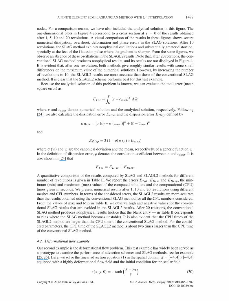
A FINITE ELEMENT SEMI-LAGRANGIAN METHOD WITH L2 INTERPOLATION 1497

nodes. For a comparison reason, we have also included the analytical solution in this figure. Theone-dimensional plots in Figure 4 correspond to a cross section at y D 0 of the results obtainedafter 1, 5, 10 and 20 revolutions. A visual comparison of the results in these figures shows severenumerical dissipation, overshoot, deformation and phase errors in the SLAG solutions. After 10revolutions, the SLAG method exhibits nonphysical oscillations and substantially greater distortion,specially at the feet of the Gaussian pulse where the gradient is sharper. From the same figures, weobserve an absence of these oscillations in the SLAGL2 results. Note that, after 20 rotations, the con-ventional SLAG method produces nonphysical results, and its results are not displayed in Figure 4.It is evident that, after one revolution, both methods give roughly similar results with some smalldifferences on the maximum value of the numerical solutions. However, by increasing the numberof revolutions to 10, the SLAGL2 results are more accurate than those of the conventional SLAGmethod. It is clear that the SLAGL2 scheme performs best for this test example.

Because the analytical solution of this problem is known, we can evaluate the total error (meansquare error) as

ETot D

Z�

.c � cexact/2 d�

where c and cexact denote numerical solution and the analytical solution, respectively. Following[24], we also calculate the dissipation error EDiss and the dispersion error EDisp defined by

EDiss D Œ .c/� .cexact/�2C .c � cexact/

2

and

EDisp D 2 .1� �/ .c/ .cexact/

where .w/ and w are the canonical deviation and the mean, respectively, of a generic function w.In the definition of dispersion error, � denotes the correlation coefficient between c and cexact. It isalso shown in [24] that

ETot DEDiss CEDisp .

A quantitative comparison of the results computed by SLAG and SLAGL2 methods for differentnumber of revolutions is given in Table II. We report the errors ETot , EDiss and EDisp , the min-imum (min) and maximum (max) values of the computed solutions and the computational (CPU)times given in seconds. We present numerical results after 1, 10 and 20 revolutions using differentmeshes and CFL numbers. In terms of the considered errors, the SLAGL2 results are more accuratethan the results obtained using the conventional SLAG method for all the CFL numbers considered.From the values of max and Min in Table II, we observe high and negative values for the conven-tional SLAG results that are avoided in the SLAGL2 results. After 20 rotations, the conventionalSLAG method produces nonphysical results (notice that the blank entry — in Table II correspondsto runs where the SLAG method becomes unstable). It is also evident that the CPU times of theSLAGL2 method are larger than the CPU time of the conventional SLAG method. For the consid-ered parameters, the CPU time of the SLAGL2 method is about two times larger than the CPU timeof the conventional SLAG method.

4.2. Deformational flow example

Our second example is the deformational flow problem. This test example has widely been served asa prototype to examine the performance of advection schemes and SLAG methods; see for example[25,26]. Here, we solve the linear advection equation (1) in the spatial domain�D Œ�4, 4�� Œ�4, 4�equipped with a highly deformational flow field and the initial condition for the scalar field

c.x,y, 0/D� tanhy � y0

ı

�(30)

Copyright © 2012 John Wiley & Sons, Ltd. Int. J. Numer. Meth. Engng 2012; 90:1485–1507DOI: 10.1002/nme

1498 M. EL-AMRANI AND M. SEAÏD

Tabl

eII

.R

esul

tsfo

rad

vect

ion

ofth

eG

auss

ian

puls

ete

staf

ter1

,10

and20

revo

lutio

nsus

ing

diff

eren

tmes

hes

and

Cou

rant

–Fri

edri

chs–

Lew

ynu

mbe

rs.T

hean

alyt

ical

max

imum

is1

and

the

com

puta

tiona

ltim

esar

egi

ven

inse

cond

s.

Aft

er1

revo

lutio

n

SLA

GSL

AG

L2

CFL

Mes

hM

inM

axETot

EDiss

EDisp

CPU

Min

Max

ETot

EDiss

EDisp

CPU

64�64

-0.041

0.441

0.0686

0.0093

0.0593

3-0

.019

0.787

0.0369

0.0038

0.0331

5�p2

4128�128

-0.047

0.740

0.0362

0.0020

0.0342

25

-0.007

0.885

0.0177

0.0006

0.0170

45

256�256

-0.011

0.932

0.0127

0.0002

0.0125

225

-0.001

0.971

0.0056

0.0001

0.0056

391

64�64

-0.016

0.695

0.0301

0.0044

0.0256

1-0

.009

0.895

0.0119

0.0014

0.0105

1.7

�p2

128�128

-0.004

0.909

0.0088

0.0007

0.0080

7-0

.001

0.954

0.0028

0.0001

0.0026

13

256�256

0.0

0.984

0.0020

0.0001

0.0019

60

0.0

0.999

0.0005

0.0000

0.0005

106

64�64

-0.010

0.854

0.0147

0.0017

0.0129

0.6

0.0

0.896

0.0064

0.0007

0.0056

1

2�p2

128�128

-0.001

0.966

0.0034

0.0003

0.0031

40.0

0.990

0.0011

0.0001

0.0010

7256�256

0.0

0.995

0.0006

0.0000

0.0006

31

0.0

0.999

0.0001

0.0000

0.0001

57

Aft

er10

revo

lutio

ns

SLA

GSL

AG

L2

CFL

Mes

hM

inM

axETot

EDiss

EDisp

CPU

Min

Max

ETot

EDiss

EDisp

CPU

64�64

——

——

——

-0.056

0.494

0.0679

0.0105

0.0574

55

�p2

4128�128

-0.079

0.345

0.0965

0.0085

0.0880

254

-0.030

0.613

0.0574

0.0032

0.0542

448

256�256

-0.114

0.638

0.0666

0.0016

0.0650

2151

-0.012

0.971

0.0360

0.0005

0.0355

3895

64�64

-3.778

0.316

0.4507

0.1462

0.3044

8-0

.037

0.573

0.0400

0.0063

0.0336

14

�p2

128�128

-0.042

0.608

0.0451

0.0049

0.0401

64

-0.015

0.743

0.0182

0.0013

0.0169

119

256�256

-0.018

0.874

0.0166

0.0007

0.0158

570

-0.001

0.990

0.0053

0.0001

0.0052

1031

64�64

-1.563

0.478

0.1885

0.0205

0.1680

4-0

.017

0.665

0.0277

0.0043

0.0233

7

2�p2

128�128

-0.025

0.765

0.0248

0.0028

0.0219

33

-0.003

0.867

0.0093

0.0010

0.0082

63

256�256

-0.004

0.947

0.0061

0.0004

0.0057

289

0.0

0.997

0.0019

0.0001

0.0017

558

Copyright © 2012 John Wiley & Sons, Ltd. Int. J. Numer. Meth. Engng 2012; 90:1485–1507DOI: 10.1002/nme

A FINITE ELEMENT SEMI-LAGRANGIAN METHOD WITH L2 INTERPOLATION 1499

Tabl

eII

.co

ntin

ued

Aft

er20

revo

lutio

ns

SLA

GSL

AG

L2

CFL

Mes

hM

inM

axETot

EDiss

EDisp

CPU

Min

Max

ETot

EDiss

EDisp

CPU

64�64

——

——

——

-0.121

0.396

0.0721

0.0133

0.0588

114

�p2

4128�128

——

——

——

-0.097

0.562

0.0665

0.0047

0.0617

937

256�256

-0.122

11.576

0.3601

0.0925

0.2675

4682

-0.054

0.871

0.0504

0.0008

0.0496

7958

64�64

——

——

——

-0.063

0.473

0.0488

0.0089

0.0399

30

�p2

128�128

——

——

——

-0.031

0.696

0.0274

0.0021

0.0252

252

256�256

-0.042

4.373

0.1341

0.0103

0.1237

1181

-0.002

0.896

0.0098

0.0002

0.0095

2024

64�64

——

——

——

-0.036

0.547

0.0374

0.0066

0.0308

16

2�p2

128�128

——

——

——

-0.015

0.787

0.0157

0.0019

0.0137

136

256�256

-0.014

1.019

0.0323

0.0001

0.0322

601

-0.001

0.991

0.0036

0.0002

0.0033

1073

Copyright © 2012 John Wiley & Sons, Ltd. Int. J. Numer. Meth. Engng 2012; 90:1485–1507DOI: 10.1002/nme

1500 M. EL-AMRANI AND M. SEAÏD

−4−2

02

4 −4−3

−2−1

01

23

4

−1

−0.5

0

0.5

1

y

Exact

x

c

−4−2

02

4 −4−3

−2−1

01

23

4

−1

−0.5

0

0.5

1

yx

c

−4−2

02

4 −4−3

−2−1

01

23

4

−1

−0.5

0

0.5

1

yx

c

Exact

x

y−4 −3 −2 −1 0 1 2 3 4

−4

−3

−2

−1

0

1

2

3

4

SLAG SLAG

x

y−4 −3 −2 −1 0 1 2 3 4

−4

−3

−2

−1

0

1

2

3

4

SLAGL2 SLAGL2

x

y−4 −3 −2 −1 0 1 2 3 4

−4

−3

−2

−1

0

1

2

3

4

Figure 5. Results for the deformational flow example at time t D 4.

where ı is the width of the front zone. The velocity field is a steady circular vortex with tangentialvelocity depending on the radius of the vortex as

VT .r/D V0sech2.r/ tanh.r/ (31)

where V0 is a value selected such that the maximum value of VT never exceeds unity. The analyticalsolution of the considered problem is defined by

cexact.x,y, t /D� tanhy � y0

ıcos .!t/�

x � x0

ısin .!t/

�(32)

Copyright © 2012 John Wiley & Sons, Ltd. Int. J. Numer. Meth. Engng 2012; 90:1485–1507DOI: 10.1002/nme

A FINITE ELEMENT SEMI-LAGRANGIAN METHOD WITH L2 INTERPOLATION 1501

−4 −3 −2 −1 0 1 2 3 4−1

−0.8

−0.6

−0.4

−0.2

0

0.2

0.4

0.6

0.8

1

Distance x

Sol

utio

n c

SLAGSLAGL2Exact

−4 −3 −2 −1 0 1 2 3 4−1

−0.8

−0.6

−0.4

−0.2

0

0.2

0.4

0.6

0.8

1

Distance y

Sol

utio

n c

−4 −3 −2 −1 0 1 2 3 4−1

−0.8

−0.6

−0.4

−0.2

0

0.2

0.4

0.6

0.8

1

Distance x

Sol

utio

n c

−4 −3 −2 −1 0 1 2 3 4−1

−0.8

−0.6

−0.4

−0.2

0

0.2

0.4

0.6

0.8

1

Distance y

Sol

utio

n c

SLAGSLAGL2Exact

SLAGSLAGL2Exact

SLAGSLAGL2Exact

Figure 6. Cross sections of the results in Figure 5 at y D 0 (left) and at x D 0 (right) using a mesh with64� 64 nodes (top) and 128� 128 nodes (bottom).

where .x0,y0/ is the centre of the vortex and ! D VTr

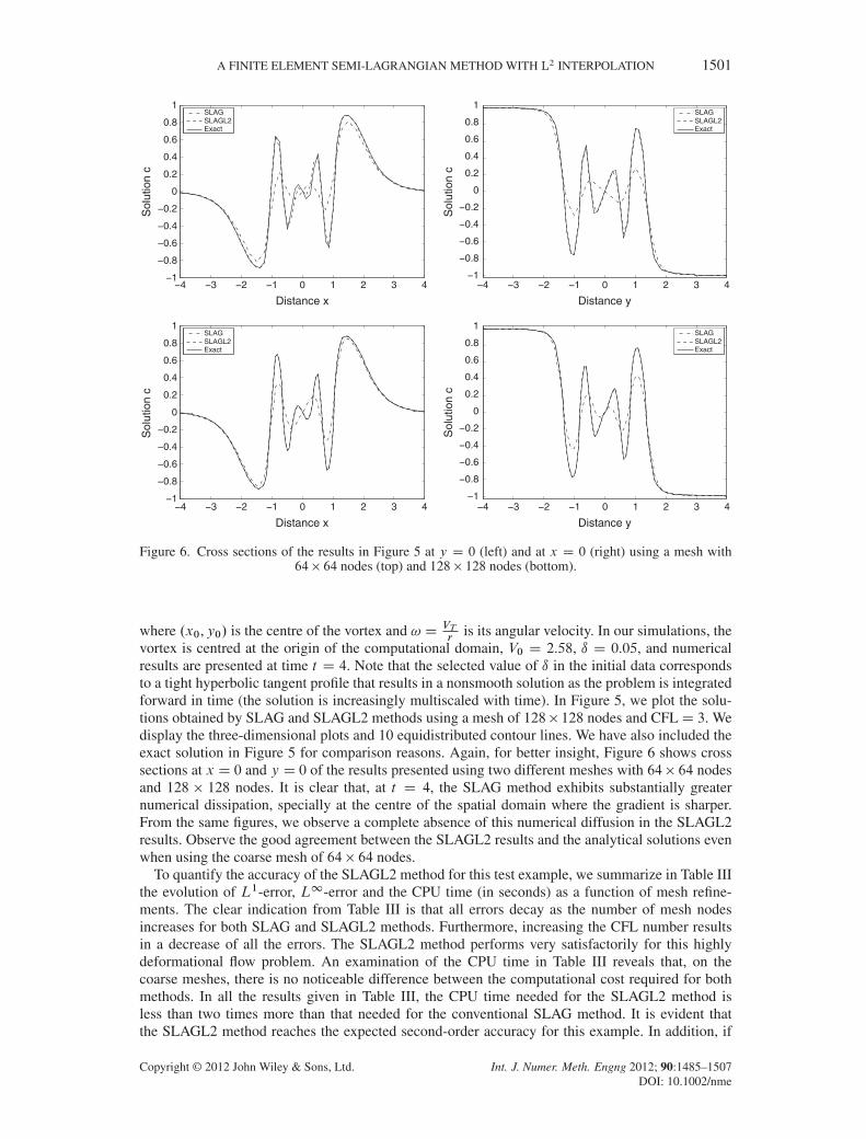
is its angular velocity. In our simulations, thevortex is centred at the origin of the computational domain, V0 D 2.58, ı D 0.05, and numericalresults are presented at time t D 4. Note that the selected value of ı in the initial data correspondsto a tight hyperbolic tangent profile that results in a nonsmooth solution as the problem is integratedforward in time (the solution is increasingly multiscaled with time). In Figure 5, we plot the solu-tions obtained by SLAG and SLAGL2 methods using a mesh of 128� 128 nodes and CFLD 3. Wedisplay the three-dimensional plots and 10 equidistributed contour lines. We have also included theexact solution in Figure 5 for comparison reasons. Again, for better insight, Figure 6 shows crosssections at x D 0 and y D 0 of the results presented using two different meshes with 64� 64 nodesand 128 � 128 nodes. It is clear that, at t D 4, the SLAG method exhibits substantially greaternumerical dissipation, specially at the centre of the spatial domain where the gradient is sharper.From the same figures, we observe a complete absence of this numerical diffusion in the SLAGL2results. Observe the good agreement between the SLAGL2 results and the analytical solutions evenwhen using the coarse mesh of 64� 64 nodes.

To quantify the accuracy of the SLAGL2 method for this test example, we summarize in Table IIIthe evolution of L1-error, L1-error and the CPU time (in seconds) as a function of mesh refine-ments. The clear indication from Table III is that all errors decay as the number of mesh nodesincreases for both SLAG and SLAGL2 methods. Furthermore, increasing the CFL number resultsin a decrease of all the errors. The SLAGL2 method performs very satisfactorily for this highlydeformational flow problem. An examination of the CPU time in Table III reveals that, on thecoarse meshes, there is no noticeable difference between the computational cost required for bothmethods. In all the results given in Table III, the CPU time needed for the SLAGL2 method isless than two times more than that needed for the conventional SLAG method. It is evident thatthe SLAGL2 method reaches the expected second-order accuracy for this example. In addition, if

Copyright © 2012 John Wiley & Sons, Ltd. Int. J. Numer. Meth. Engng 2012; 90:1485–1507DOI: 10.1002/nme

1502 M. EL-AMRANI AND M. SEAÏD

Table III. Error norms and computational times for the deformational flow problem att D 4 using different meshes and different Courant–Friedrichs–Lewy numbers.

SLAG SLAGL2

CFL Mesh L1�error L1�error CPU L1�error L1�error CPU64� 64 0.11861 0.31300 0.7 0.01822 0.04284 0.8

0.5 128� 128 0.05162 0.13718 4.8 0.00488 0.01155 6.2256� 256 0.02096 0.05889 38.0 0.00113 0.00290 57.564� 64 0.10480 0.26003 0.3 0.00961 0.02939 0.4

3 128� 128 0.03971 0.11318 1.5 0.00240 0.00787 2.5256� 256 0.01404 0.04596 9.3 0.00056 0.00196 15.864� 64 0.08600 0.22002 0.2 0.00302 0.00894 0.3

6 128� 128 0.02836 0.08337 1.1 0.00069 0.00239 1.9256� 256 0.00873 0.02947 6.3 0.00015 0.00059 11.3

instead of computing the approximate convergence rate in the SLAGL2 method between two con-secutive mesh refinings, one approximates the convergence rate between meshes of 64�64 nodes and256 � 256 nodes in the L1-norm; the results are 2.0, 2.05 and 2.16 at CFL D 0.5, 3 and 6, respec-tively. This clearly demonstrates that the L2 interpolation procedure conserves the second-orderaccuracy of the SLAG integration scheme.

4.3. Viscous Burgers’ flow example

This example solves the following viscous Burgers’ equation which evolves to a highly convectivesteady state

@u

@tC y.u�

1

2/@u

@xC x.u�

1

2/@u

@y��uD 0

where is a constant controlling the magnitude of the nonlinear convective term; see for instance[23] for further details. The boundary conditions are Dirichlet given by the exact steady statesolution

u.x,y/D1

2

�1� tanh

� xy

2

��.

The domain dimensions and the initial conditions used in our computations are depicted in Figure 7.We used the new SLAGL2 method to compute the steady state solutions for three different values

u = 1

u = 0

u = 0

-5

u = 1

+5

0

-5 0 +5

Figure 7. Domain dimension and initial conditions for the viscous Burgers’ equation. We set u D 0.5 onboth centre lines

Copyright © 2012 John Wiley & Sons, Ltd. Int. J. Numer. Meth. Engng 2012; 90:1485–1507DOI: 10.1002/nme

A FINITE ELEMENT SEMI-LAGRANGIAN METHOD WITH L2 INTERPOLATION 1503

−5

0

5

−5

0

50

0.20.40.60.8

1

Exact

−50

5

−5

0

50

0.20.40.60.8

1

SLAG

−50

5

−5

0

50

0.20.40.60.8

1

SLAGL2

−5

0

5

−5

0

50

0.2

0.4

0.6

0.8

1

−5

0

5

−5

0

50

0.2

0.4

0.6

0.8

1

−5

0

5

−5

0

50

0.2

0.4

0.6

0.8

1

−5

0

5

−5

0

50

0.2

0.4

0.6

0.8

1

−5

0

5

−5

0

50

0.2

0.4

0.6

0.8

1

−5

0

5

−5

0

50

0.2

0.4

0.6

0.8

1

Figure 8. Results for the steady-state solution of the viscous Burgers’ equation. Here, D 1 (first row), D 5 (second row) and D 10 (third row).

of namely, D 1, D 5 and D 10. For these steady state solutions, the time integration processis stopped when the inequality

��unC1 � un��kunk

6 � (33)

is satisfied. Here k�k denotes the L1-norm and � is a given tolerance fixed to 10�6�t in our compu-tations. It should be pointed out that the number of iterations to reach this tolerance depends on thevalues taken by such that for a fixed CFL number, more iterations are required for larger valuesof . For example, by setting CFLD 3 when D 1 the number of iterations is 230 and 221, respec-tively, for the SLAG method and SLAGL2 method, whereas when D 10 the number of iterationsis 3577 and 1864 for the SLAG method and SLAGL2 method, respectively. The discrepancy in thenumber of iterations in the SLAG and SLAGL2 methods can be attributed to the higher accuracyachieved in the SLAGL2 solutions compared with those computed using the SLAG method.

Figure 8 illustrates the obtained results using a mesh of 64 � 64 gridpoints and CFL D 3. InFigure 9, we plot 10 equidistributed contours of the solutions. For comparison, we have also includedanalytical steady-state solutions in these figures. It is clear that by increasing , the convective termsbecome larger and steep boundary layers are formed near the vicinity of centre lines. For low valuesof , the boundary layers are wide and diffuse in the flow domain. As increases, the boundarylayers concentrate and move towards the domain centre. It is apparent that the flow structure is ingood agreement with the previous work in [23]. These plots give a clear view of the overall flowpattern and the effect of the convection control parameter on the structure of steady boundarylayers in the cavity. It is worth remarking that the thinning of the boundary layers with increasing is evident from these plots, although the rate of this thinning is slower for the SLAG method than

Copyright © 2012 John Wiley & Sons, Ltd. Int. J. Numer. Meth. Engng 2012; 90:1485–1507DOI: 10.1002/nme

1504 M. EL-AMRANI AND M. SEAÏD

Exact

−5 −4 −3 −2 −1 0 1 2 3 4 5−5

−4

−3

−2

−1

0

1

2

3

4

5SLAG

−5 −4 −3 −2 −1 0 1 2 3 4 5−5

−4

−3

−2

−1

0

1

2

3

4

5SLAGL2

−5 −4 −3 −2 −1 0 1 2 3 4 5−5

−4

−3

−2

−1

0

1

2

3

4

5

−5 −4 −3 −2 −1 0 1 2 3 4 5−5

−4

−3

−2

−1

0

1

2

3

4

5

−5 −4 −3 −2 −1 0 1 2 3 4 5−5

−4

−3

−2

−1

0

1

2

3

4

5

−5 −4 −3 −2 −1 0 1 2 3 4 5−5

−4

−3

−2

−1

0

1

2

3

4

5

−5 −4 −3 −2 −1 0 1 2 3 4 5−5

−4

−3

−2

−1

0

1

2

3

4

5

−5 −4 −3 −2 −1 0 1 2 3 4 5−5

−4

−3

−2

−1

0

1

2

3

4

5

−5 −4 −3 −2 −1 0 1 2 3 4 5−5

−4

−3

−2

−1

0

1

2

3

4

5

Figure 9. Contours of the results in Figure 8. Here, D 1 (first row), D 5 (second row) and D 10(third row).

for the SLAGL2 method. These features clearly demonstrate the high accuracy achieved by the pro-posed SLAGL2 method for solving viscous Burgers’ problems at steady-state regimes. In addition,compared with the results published for example in [23], it can be seen that our SLAGL2 methodresolves accurately the flow structures, and the boundary layers seem to be localized in the correctplace in the flow domain.

For visualizing the comparisons, we display in Figure 10 a cross section at the main diagonalusing a mesh with 64 � 64 nodes and 128 � 128 nodes. For D 1, it is clear that the SLAG andSLAGL2 methods produce practically identical results. This can be attributed to the large physi-cal diffusion presented in the problem. However, when the value of is increased to 5 and 10, theresults computed by SLAGL2 method are more accurate than those computed by the SLAG method.Apparently, with the use of the SLAGL2 method, high resolution is achieved in those regions wherethe flow gradients are steep such as the moving fronts. Upon comparison of the results obtainedusing the considered methods, it is clear that the SLAG method produces diffusive solutions result-ing in smearing the shocks. On the other hand, this numerical diffusion has remarkably been reducedin the results computed using the SLAGL2 method. Needless to say that for convection-dominated

Copyright © 2012 John Wiley & Sons, Ltd. Int. J. Numer. Meth. Engng 2012; 90:1485–1507DOI: 10.1002/nme

A FINITE ELEMENT SEMI-LAGRANGIAN METHOD WITH L2 INTERPOLATION 1505

−5 −4 −3 −2 −1 0 1 2 3 4 50

0.1

0.2

0.3

0.4

0.5

0.6

0.7

0.8

0.9

Distance x

Sol

utio

n u

λ=1SLAGSLAGL2Exact

SLAGSLAGL2Exact

SLAGSLAGL2Exact

SLAGSLAGL2Exact

SLAGSLAGL2Exact

SLAGSLAGL2Exact

−5 −4 −3 −2 −1 0 1 2 3 4 50

0.1

0.2

0.3

0.4

0.5

0.6

0.7

0.8

0.9

Distance x

Sol

utio

n u

λ=5

−5 −4 −3 −2 −1 0 1 2 3 4 50

0.1

0.2

0.3

0.4

0.5

0.6

0.7

0.8

0.9

Distance x

Sol

utio

n u

λ=10

−5 −4 −3 −2 −1 0 1 2 3 4 50

0.1

0.2

0.3

0.4

0.5

0.6

0.7

0.8

0.9

Distance x

Sol

utio

n u

−5 −4 −3 −2 −1 0 1 2 3 4 50

0.1

0.2

0.3

0.4

0.5

0.6

0.7

0.8

0.9

Distance x

Sol

utio

n u

−5 −4 −3 −2 −1 0 1 2 3 4 50

0.1

0.2

0.3

0.4

0.5

0.6

0.7

0.8

0.9

Distance x

Sol

utio

n u

Figure 10. Cross section of the results in Figure 8 at the main diagonal using a mesh with 64 � 64 nodes(top) and 128� 128 nodes (bottom).

situation, the SLAGL2 method does not diffuse the fronts or gives spurious oscillations near thesteep gradients.

It is to be remarked that for this test example, the overall computational work in both SLAG andSLAGL2 methods increases as the value of is increased. The main part of the CPU time goes tothe preconditioned conjugate gradient algorithm for solving the resulting linear systems. We havealso observed that for the SLAGL2 method using D 10, the number of iterations required in thepreconditioned conjugate gradient solver at each time step starts at about 15–10, but it promptlydecreases to 2–3, even 1, long before the steady state is reached. This later behaviour deteriorates inthe SLAG method where the number of iterations in the preconditioned conjugate gradient solvercan increase to about 3 times more than in the SLAGL2 method.

5. CONCLUSIONS

In this paper, we have developed a new numerical method based on combining the SLAG finite ele-ment method with an L2 interpolation procedure for solving convection–diffusion equations. Thismethod exploits the interesting features offered by both techniques to construct a highly accuratealgorithm for numerical treatment of convection–diffusion problems. The important advantage ofthe new method is that the convective term that has to be treated carefully in most of Eulerian-based finite element methods has been removed from the new method with the use of the SLAGmethod to interpret the transport nature of the equation. A comparison with the conventionalSLAG finite element method demonstrates the feasibility of the present L2 interpolation to solveconvection-dominated flow problems.

A series of numerical examples including the viscous Burgers’ equation were considered to testthe accuracy of the proposed method. A comparison with the conventional SLAG finite elementmethod was also performed in the present study. The obtained results using the present L2 interpo-lation algorithm show good solution resolution and less numerical dissipation compared with theresults obtained using the conventional SLAG method. Finally, we should point out that because

Copyright © 2012 John Wiley & Sons, Ltd. Int. J. Numer. Meth. Engng 2012; 90:1485–1507DOI: 10.1002/nme

1506 M. EL-AMRANI AND M. SEAÏD

of the use of the Lagrangian coordinates, the new approach requires more implementation workthan the Eulerian methods that are relatively easy to formulate and to implement. The algorithmspresented in this paper can be highly optimized for vector computers because they do not requirenonlinear solvers and contain no recursive elements. Some difficulties arise from the fact thatfor efficient vectorization, the data should be stored contiguously within long vectors rather thantwo-dimensional arrays.

Although we have restricted our numerical computations to the case of two-dimensionalconvection–diffusion problems using structured grids, the more important implications of ourresearch concern the use of effective SLAGL2 for computational fluid dynamic problems in threespatial dimensions implemented for parallel processing and using unstructured meshes. Our currenteffort is therefore to extend these methods for the incompressible viscous flows in higher spacedimensions using unstructured meshes and multigrid algorithms to speed up the time integrationprocedure.

ACKNOWLEDGEMENTS

The authors acknowledge the support from the proyecto del plan nacional de I+D+i grant by Ministerio deciencia e innovación de España under the contract No MTM2008-03255/MTM. The authors also wish tothank the anonymous reviewers for their helpful comments on an earlier draft of the manuscript.

REFERENCES

1. Morton KW. Numerical Solution of Convection-Diffusion Problems. Chapman & Hall: London, 1996.2. Dawson CN. Godunov-mixed methods for advective flow problems in one space dimension. SIAM Journal on

Numerical Analysis 1991; 28:1282–1309.3. Shu C, Osher S. Efficient implementation of essentially non-oscillatory shock capturing schemes. Journal of

Computational Physics 1988; 77:439–471.4. Douglas J, Huang C, Pereira F. The modified method of characteristics with adjusted advection. Numerische

Mathematik 1999; 83:353–369.5. Douglas J, Russell TF. Numerical methods for convection dominated diffusion problems based on combining the

method of characteristics with finite elements or finite differences. SIAM Journal on Numerical Analysis 1982;19:871–885.

6. Pironneau O. On the transport-diffusion algorithm and its applications to the Navier–Stokes equations. NumerischeMathematik 1982; 38:309–332.

7. Süli E. Convergence and nonlinear stability of the Lagrange–Galerkin method for the Navier–Stokes equations.Numerische Mathematik 1988; 53:1025–1039.

8. Rui H, Tabata M. A mass-conservative characteristic finite element scheme for convection–diffusion problems.Journal of Scientific Computing 2010; 43:416–432.

9. Xiu D, Karniadakis GE. A semi-Lagrangian high-order method for Navier–Stokes equations. Journal of Computa-tional Physics 2001; 172:658–684.

10. El-Amrani M, Seaïd M. A semi-Lagrangian method for large-eddy simulation of turbulent flow and heat transfer.SIAM Journal on Scientific Computing 2008; 30:2734–2754.

11. El-Amrani M, Seaïd M. A finite element modified method of characteristics for convective heat transport. NumericalMethods for Partial Differential Equations 2008; 24:776–798.

12. El-Amrani M, Seaïd M. Numerical simulation of natural and mixed convection flows by semi-Lagrangian method.International Journal for Numerical Methods in Fluids 2007; 53:1819–1845.

13. El-Amrani M, Seaïd M. Convergence and stability of finite element modified method of characteristics for theincompressible Navier–Stokes equations. Journal of Numerical Mathematics 2007; 15:101–135.

14. Robert A. A stable numerical integration scheme for the primitive meteorological equations. Atmosphere-Ocean1981; 19:35–46.

15. Temperton C, Staniforth A. An efficient two-time-level semi-Lagrangian semi-implicit integration scheme. QuarterlyJournal of the Royal Meteorological Society 1987; 113:1025–1039.

16. Pudykiewicz J, Staniforth A. Some properties and comparative performance of the semi-lagrangian method of robertin the solution of advection–diffusion equation. Atmosphere-Ocean 1984; 22:283–308.

17. Giraldo FX. The Lagrange–Galerkin spectral element method on unstructured quadrilateral grids. Journal ofComputational Physics 1998; 147:114–146.

18. Kaazempur-Mofrad MR, Ethier CR. An efficient characteristic Galerkin scheme for the advection equation in 3D.Computer Methods in Applied Mechanics and Engineering 2002; 191:5345–5363.

19. Allievi A, Bermejo R. A generalized particle search-locate algorithm for arbitrary grids. Journal of ComputationalPhysics 1992; 132:157–166.

Copyright © 2012 John Wiley & Sons, Ltd. Int. J. Numer. Meth. Engng 2012; 90:1485–1507DOI: 10.1002/nme

A FINITE ELEMENT SEMI-LAGRANGIAN METHOD WITH L2 INTERPOLATION 1507

20. Seaïd M. Semi-Lagrangian integration schemes for viscous incompressible flows. Computational Methods in AppliedMathematics 2002; 4:392–409.

21. Abramowitz M, Stegun IA. Handbook of Mathematical Functions with Formulas, Graphs, and Mathematical Tables.U.S. Department of Commerce, 1972.

22. Dunavant D. High degree efficient symmetrical gaussian quadrature rules for the triangle. International Journal forNumerical Methods in Engineering 1985; 21:1129–1148.

23. Krisnamachari SV, Hayes LJ, Russel TF. A finite element alternating-direction method combined with a mod-ified method of characteristics for convection–diffusion problems. SIAM Journal on Numerical Analysis 1989;26:1462–1473.

24. Takacs LL. A two-step scheme for the advection equation with minimized dissipation and dispersion errors. MonthlyWeather Review 1985; 113:1054–1065.

25. Hólm EV. A fully two-dimensional, non-oscillatory advection scheme for momentum and scalar transport equations.Monthly Weather Review 1995; 123:536–552.

26. Nair R, Côté J, Staniforth A. Monotonic cascade interpolation for semi-Lagrangian advection. Quarterly Journal ofthe Royal Meteorological Society 1999; 125:197–212.

Copyright © 2012 John Wiley & Sons, Ltd. Int. J. Numer. Meth. Engng 2012; 90:1485–1507DOI: 10.1002/nme