Range Restricted Positivity-Preserving G1 Scattered Data Interpolation

Abd. Rahni Mt. Piah1, Azizan Saaban2, Ahmad Abd. Majid3

School of Mathematical Sciences, Universiti Sains Malaysia 11800 USM Pulau Pinang, MALAYSIA

E-mail : 1arahni@cs.usm.my, 2azizan.s@uum.edu.my, 3majid@cs.usm.my

Abstract : The construction of a range restricted bivariate G1 interpolant to scattered data is considered in which the interpolant is positive everywhere if the original data are positive. This study is motivated by earlier work in which sufficient conditions are derived on Bézier points in order to ensure that surfaces comprising quartic Bézier triangular patches are always positive and satisfy G1 continuity conditions. The gradients at the data sites are then calculated (and modified if necessary) to ensure that these conditions are satisfied. Its construction is local and easily extended to include as upper and lower constraints to the interpolating surfaces of the form z = C(x,y) where C is a polynomial of degree less or equal to 4. Moreover, G1 piecewise polynomial surfaces consisting of polynomial pieces of the form z = C(x,y) on the triangulation of the data sites are also admissible constraints. A number of examples are presented.

Keywords: Scattered data, Interpolation, Positivity, G1 continuity

1. Introduction

The properties that are most often used to quantify “shape” in shape preserving interpolation are positivity, convexity and monotonicity. The problem of positivity preserving interpolation, i.e. interpolation to positive data by a positive function, is often of interest. This problem could arise if one has data points on one side of a plane, and wishes to have an interpolating surface which is also on the same side of this plane. For instance, when the data from physical experiment are measured in the form of concentration or pressure or meteorology data such as amount of rainfall where negative values are meaningless, it is important for the interpolant to preserve positivity. This paper will propose sufficient conditions on the bivariate quartic function upon triangulation of the data in order to visualize the positive scattered data which may come from certain scientific phenomena. Various methods concerning visualization of positive data or range restricted interpolation using bivariate functions can be found in [1], [2], [8], [11], [12] and [13].

This study is motivated by previous works in [2], [13] and [15]. [2] describes the construction of range restricted bivariate C1 interpolants to scattered data where sufficient non-negativity condition on the Bézier ordinates are derived to ensure the non-negativity of a cubic Bézier triangular patch.

In [2] and [13], a C1 non-parametric surface is constructed comprising of cubic Bezier triangular patches. Each triangular patch of the interpolating surface is formed as a convex combination of three cubic Bézier triangular patches. An initial value of inner Bezier ordinates in each triangle are computed using the cubic precision method.

In this paper, we will construct bivariate G1 interpolants to scattered data using similar approach adopted in [13] but each triangular patch of the interpolating surface is formed as a single quartic Bézier triangular patch. It has been established that quartic patch is the lowest possible degree suitable for the construction of a composite G1 surface [14]. Initial values of

1

Bezier ordinates except for the values determined by gradients at vertices of each triangle are computed using the method of minimized sum of squares of principles curvartures ([7], [9]) with respect to the G1 continuity conditions [5] on each non-boundary edge over the triangular mesh using the quadratic form of an objective function [15]. We also consider the construction of range restricted bivariate G1 interpolants to the scattered data.

The sufficient conditions on Bézier ordinates which ensure the positivity of a quartic Bézier triangular patch using similar method as proposed in [13] will be described in section 2. An outline of the surface construction process is given in section 3, while section 4 presents the implementation of range-restricted interpolation. Examples are presented in section 5. Finally, the conclusions will be given in Section 6.

2. Sufficient positivity conditions for a quartic Bézier triangular patch

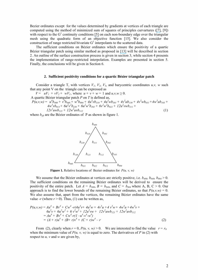
Consider a triangle T, with vertices V1, V2, V3, and barycentric coordinates u,v, w such that any point V on the triangle can be expressed as V = uV1 + vV2 + wV3 , where u + v + w = 1 and u,v,w ≥ 0. A quartic Bézier triangular patch P on T is defined as, P(u,v,w) = u4b400 + v4b040 + w4b004 + 4u3vb310 + 4u3wb301 + 4v3ub130 + 4v3wb031 +4w3ub103 + 4w3vb013 + 6u2v2b220 + 6u2w2b202 + 6v2w2b022 + 12u2vwb211 + 12v2uwb121 + 12w2uvb112 (1) where bijk are the Bézier ordinates of P as shown in figure 1. b400

b040 b004

b310

b130

b301

b103

b211

b013 b031

b220

b022

b202

b121 b112

Figure 1. Relative locations of Bezier ordinates for P(u, v, w) We assume that the Bézier ordinates at vertices are strictly positive, i.e. b400, b040, b004 > 0.

The sufficient conditions on the remaining Bézier ordinates will be derived to ensure the positivity of the entire patch. Let A = b400, B = b040, and C = b004 where A, B, C > 0. Our approach is to find the lower bounds of the remaining Bézier ordinates, so that P(u,v,w) = 0. We also assume that, apart from the vertices, the remaining Bézier ordinates have the same value -r (where r > 0). Thus, (1) can be written as, P(u,v,w) = Au4 + Bv4 + Cw4 -r(4u3v+ 4u3w + 4v3u +4 v3w + 4w3u +4w3v + 6u2v + 6u2w2 + 6 v2w2 + 12u2vw + 12v2uwb121 + 12w2uvb112 = Au4 + Bv4 + Cw4-r(1 –u4-v4-w4) = (A + r)u4 + (B+ r)v4 + (C + r)w4 – r (2)

From (2), clearly when r = 0, P(u, v, w) > 0. We are interested to find the value r = r0 when the minimum value of P(u, v, w) is equal to zero. The derivatives of P in (2) with respect to u, v and w are given by,

2

.)(4,)(4,)(4 333 wrCwPvrB

vPurA

uP

+=∂∂

+=∂∂

+=∂∂ (3)

We know that at the minimum value of P(u, v, w), 0and0 =∂∂

−∂∂

=∂∂

−∂∂

wP

uP

vP

uP .

Thus, we have wP

vP

uP

∂∂

=∂∂

=∂∂ . (4)

By substituting (3) into (4), we get rArC

wuand

rArB

vu

++

=++

= 3

3

3

3

.

Hence, 333

333 1:1:1::or1:1:1::rCrBrA

wvurCrBrA

wvu+++

=+++

= .

Since u + v + w = 1, we obtain denom

rAu

3

1+

= , denom

rBv

3

1+

= and

333

3 111where

1

rCrBrAdenom

denomrC

w+

++

++

=+

= .

Substituting these u, v and w into (2), we obtain the minimum value of P(u, v, w),

.

11

11

11

),,( 3

333

rrwvuP

rC

rB

rA

−

⎟⎟

⎠

⎞

⎜⎜

⎝

⎛

++

++

+

= (5)

We need to choose a value r = r0 so that this minimum value of P is zero. From (5) and r > 0, we know that, P(u, v, w) = 0 when

11

11

11

1333

=+

++

++ r

CrB

rA

. (6)

Let s = r1 and G(s) =

11

11

11

333 ++

++

+ CsBsAs (7)

If A, B and C are strictly positive, then s0 = 1/r0 is the solution of G(s) = 1. Now, let us describe the method to determine the value of s0 for each triangular patch.

Since A, B, C > 0, it is easy to show that for s ≥ 0, G’ (s) < 0 and G’’(s) > 0. Let M = max(A,

B, C) and N = min (A, B, C) and it can be verified that 33 1

3)(1

3+

≤≤+ Ns

sGMs

or in

particular we get .1)26(1)26( ≤≥N

GandM

G

Figure 2 shows the form of G(s), s ≥ 0 with the relative location of 26/M, 26/N and s0.

To obtain the value of s0 for given values of A, B and C, we need to find the root of (7) and G(s) = 1 that will give us a lower bound on the remaining Bézier ordinates, i.e. r0 = 1/s0 using simple iterative scheme. In choosing these scheme, we must ensure of one sided convergence of the root. This can be achieved by the method of false-position [3] with an initial estimate for the root will be the value of s for which the line joining 26/N and 26/M has the value 1. The following proposition prescribes the lower bounds for the Bézier ordinates to ensure the positivity of Bézier patch.

3

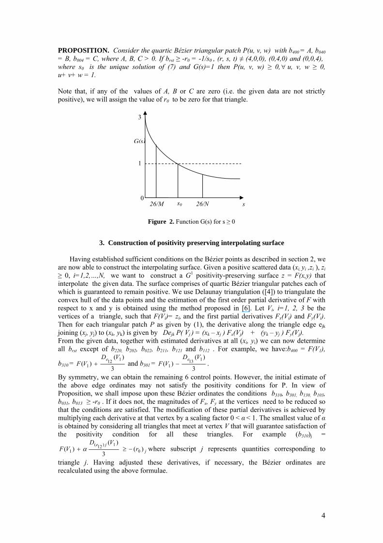
PROPOSITION. Consider the quartic Bézier triangular patch P(u, v, w) with b400 = A, b040 = B, b004 = C, where A, B, C > 0. If brst ≥ -r0 = -1/s0 , (r, s, t) ≠ (4,0,0), (0,4,0) and (0,0,4), where s0 is the unique solution of (7) and G(s)=1 then P(u, v, w) ≥ 0,∀ u, v, w ≥ 0, u+ v+ w = 1. Note that, if any of the values of A, B or C are zero (i.e. the given data are not strictly positive), we will assign the value of r0 to be zero for that triangle.

0

1

3

G(s)

26/M 26/Ns0 s

Figure 2. Function G(s) for s ≥ 0

3. Construction of positivity preserving interpolating surface

Having established sufficient conditions on the Bézier points as described in section 2, we

are now able to construct the interpolating surface. Given a positive scattered data (xi, yi ,zi ), zi ≥ 0, i=1,2,…,N, we want to construct a G1 positivity-preserving surface z = F(x,y) that interpolate the given data. The surface comprises of quartic Bézier triangular patches each of which is guaranteed to remain positive. We use Delaunay triangulation ([4]) to triangulate the convex hull of the data points and the estimation of the first order partial derivative of F with respect to x and y is obtained using the method proposed in [6]. Let Vi, i=1, 2, 3 be the vertices of a triangle, such that F(Vi)= zi, and the first partial derivatives Fx(Vi) and Fy(Vi). Then for each triangular patch P as given by (1), the derivative along the triangle edge ejk joining (xj, yj) to (xk, yk) is given by Dejk P( Vj ) = (xk – xj ) Fx(Vj) + (yk – yj ) Fy(Vj). From the given data, together with estimated derivatives at all (xi, yi) we can now determine all brst except of b220, b202, b022, b211, b121 and b112 . For example, we have:b400 = F(V1),

b310 = 3

)()(

1121

VDVF

e+ and b301 =

3

)()(

1131

VDVF

e− .

By symmetry, we can obtain the remaining 6 control points. However, the initial estimate of the above edge ordinates may not satisfy the positivity conditions for P. In view of Proposition, we shall impose upon these Bézier ordinates the conditions b310, b301, b130, b103, b031, b013 ≥ -r0 . If it does not, the magnitudes of Fx, Fy at the vertices need to be reduced so that the conditions are satisfied. The modification of these partial derivatives is achieved by multiplying each derivative at that vertex by a scaling factor 0 < α < 1. The smallest value of α is obtained by considering all triangles that meet at vertex V that will guarantee satisfaction of the positivity condition for all these triangles. For example (b310)j =

jje

rVD

VF )(3

)()( 0

1)12(1 −≥+ α where subscript j represents quantities corresponding to

triangle j. Having adjusted these derivatives, if necessary, the Bézier ordinates are recalculated using the above formulae.

4

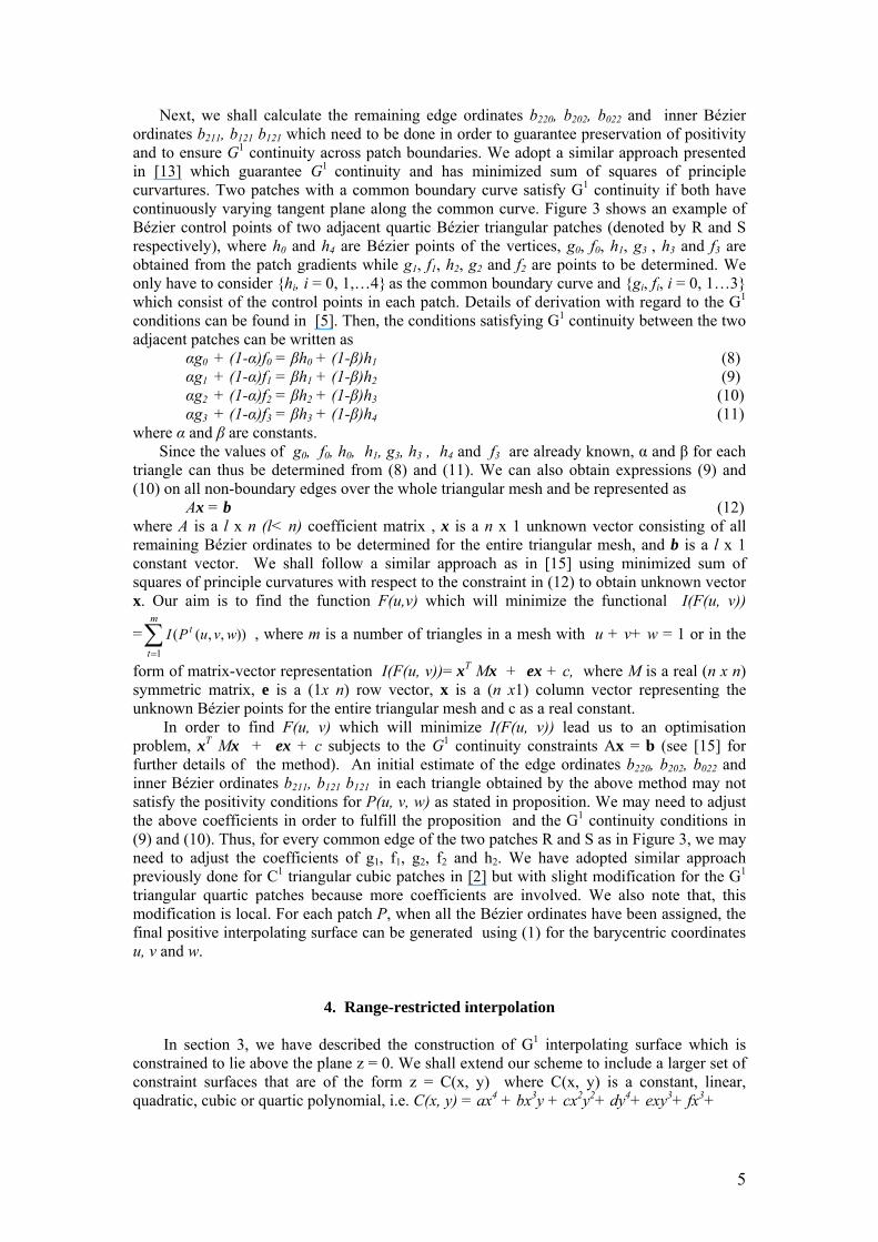
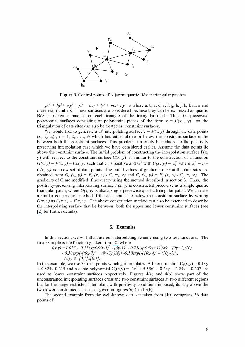
Next, we shall calculate the remaining edge ordinates b220, b202, b022 and inner Bézier ordinates b211, b121 b121 which need to be done in order to guarantee preservation of positivity and to ensure G1 continuity across patch boundaries. We adopt a similar approach presented in [13] which guarantee G1 continuity and has minimized sum of squares of principle curvartures. Two patches with a common boundary curve satisfy G1 continuity if both have continuously varying tangent plane along the common curve. Figure 3 shows an example of Bézier control points of two adjacent quartic Bézier triangular patches (denoted by R and S respectively), where h0 and h4 are Bézier points of the vertices, g0, f0, h1, g3 , h3 and f3 are obtained from the patch gradients while g1, f1, h2, g2 and f2 are points to be determined. We only have to consider {hi, i = 0, 1,…4} as the common boundary curve and {gi, fi, i = 0, 1…3} which consist of the control points in each patch. Details of derivation with regard to the G1 conditions can be found in [5]. Then, the conditions satisfying G1 continuity between the two adjacent patches can be written as αg0 + (1-α)f0 = βh0 + (1-β)h1 (8) αg1 + (1-α)f1 = βh1 + (1-β)h2 (9) αg2 + (1-α)f2 = βh2 + (1-β)h3 (10) αg3 + (1-α)f3 = βh3 + (1-β)h4 (11) where α and β are constants.

Since the values of g0, f0, h0, h1, g3, h3 , h4 and f3 are already known, α and β for each triangle can thus be determined from (8) and (11). We can also obtain expressions (9) and (10) on all non-boundary edges over the whole triangular mesh and be represented as

Ax = b (12) where A is a l x n (l< n) coefficient matrix , x is a n x 1 unknown vector consisting of all remaining Bézier ordinates to be determined for the entire triangular mesh, and b is a l x 1 constant vector. We shall follow a similar approach as in [15] using minimized sum of squares of principle curvatures with respect to the constraint in (12) to obtain unknown vector x. Our aim is to find the function F(u,v) which will minimize the functional I(F(u, v))

=∑ , where m is a number of triangles in a mesh with u + v+ w = 1 or in the

form of matrix-vector representation I(F(u, v))= x=

m

t

t wvuPI1

)),,((

T Mx + ex + c, where M is a real (n x n) symmetric matrix, e is a (1x n) row vector, x is a (n x1) column vector representing the unknown Bézier points for the entire triangular mesh and c as a real constant.

In order to find F(u, v) which will minimize I(F(u, v)) lead us to an optimisation problem, xT Mx + ex + c subjects to the G1 continuity constraints Ax = b (see [15] for further details of the method). An initial estimate of the edge ordinates b220, b202, b022 and inner Bézier ordinates b211, b121 b121 in each triangle obtained by the above method may not satisfy the positivity conditions for P(u, v, w) as stated in proposition. We may need to adjust the above coefficients in order to fulfill the proposition and the G1 continuity conditions in (9) and (10). Thus, for every common edge of the two patches R and S as in Figure 3, we may need to adjust the coefficients of g1, f1, g2, f2 and h2. We have adopted similar approach previously done for C1 triangular cubic patches in [2] but with slight modification for the G1 triangular quartic patches because more coefficients are involved. We also note that, this modification is local. For each patch P, when all the Bézier ordinates have been assigned, the final positive interpolating surface can be generated using (1) for the barycentric coordinates u, v and w.

4. Range-restricted interpolation

In section 3, we have described the construction of G1 interpolating surface which is constrained to lie above the plane z = 0. We shall extend our scheme to include a larger set of constraint surfaces that are of the form z = C(x, y) where C(x, y) is a constant, linear, quadratic, cubic or quartic polynomial, i.e. C(x, y) = ax4 + bx3y + cx2y2+ dy4+ exy3+ fx3+

5

h2

f3 f2

f1

f0

h4 h3

h1

h0

g2

g3

g1

g0

R

S

Figure 3. Control points of adjacent quartic Bézier triangular patches

gx2y+ hy3+ ixy2 + jx2 + kxy + ly2 + mx+ ny+ o where a, b, c, d, e, f, g, h, j, k, l, m, n and

o are real numbers. These surfaces are considered because they can be expressed as quartic Bézier triangular patches on each triangle of the triangular mesh. Thus, G1 piecewise polynomial surfaces consisting of polynomial pieces of the form z = C(x , y) on the triangulation of data sites can also be treated as constraint surfaces.

We would like to generate a G1 interpolating surface z = F(x, y) through the data points (xi, yi, zi) , i = 1, 2, . . ., N which lies either above or below the constraint surface or lie between both the constraint surfaces. This problem can easily be reduced to the positivity preserving interpolation case which we have considered earlier. Assume the data points lie above the constraint surface. The initial problem of constructing the interpolation surface F(x, y) with respect to the constraint surface C(x, y) is similar to the construction of a function G(x, y) = F(x, y) – C(x, y) such that G is positive and G1 with G(xi, yi) = where = z*

iz *iz i –

C(xi, yi) is a new set of data points. The initial values of gradients of G at the data sites are obtained from Gx (xi, yi) = Fx (xi, yi)- Cx (xi, yi) and Gy (xi, yi) = Fy (xi, yi)- Cy (xi, yi). The gradients of G are modified if necessary using the method described in section 3. Thus, the positivity-preserving interpolating surface F(x, y) is constructed piecewise as a single quartic triangular patch, where G(x, y) is also a single piecewise quartic triangular patch. We can use a similar construction method if the data points lie below the constraint surface by writing G(x, y) as C(x, y) – F(x, y). The above construction method can also be extended to describe the interpolating surface that lie between both the upper and lower constraint surfaces (see [2] for further details).

5. Examples

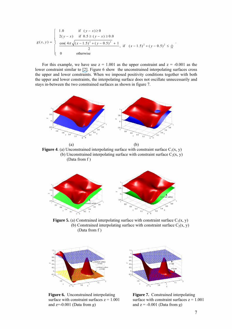
In this section, we will illustrate our interpolating scheme using two test functions. The first example is the function g taken from [2] where f(x,y) =1.025 - 0.75exp(-(6x-1)2 - (6y-1)2 - 0.75exp(-(9x+1)2/49 – (9y+1)/10) - 0.50exp(-((9x-7)2 + (9y-3)2)/4)+-0.50exp(-(10x-4)2 – (10y-7)2 , (x,y) ∈ [0,1]x[0,1]. In this example, we use 33 data points which g interpolates. A linear function C1(x,y) = 0.1xy + 0.825x-0.215 and a cubic polynomial C2(x,y) = -3x3 + 5.55x2 + 0.2xy – 2.25x + 0.207 are used as lower constraint surfaces respectively. Figures 4(a) and 4(b) show part of the unconstrained interpolating surfaces cross the two constraint surfaces at two different regions but for the range restricted interpolant with positivity conditions imposed, its stay above the two lower constrained surfaces as given in figures 5(a) and 5(b).

The second example from the well-known data set taken from [10] comprises 36 data points of

6

⎪⎪⎪

⎩

⎪⎪⎪

⎨

⎧

≤−+−+−+−

≥−≥−≥−

=

otherwise0

)5.0()5.1(if,2

1)5.0()5.1(4cos(

0.0)(5.0if)(20)(if0.1

),(16122

22

yxyx

xyxyxy

yxg π .

For this example, we have use z = 1.001 as the upper constraint and z = -0.001 as the lower constraint similar to [2]. Figure 6 show the unconstrained interpolating surfaces cross the upper and lower constraints. When we imposed positivity conditions together with both the upper and lower constraints, the interpolating surface does not oscillate unnecessarily and stays in-between the two constrained surfaces as shown in figure 7.

(a) (b) Figure 4. (a) Unconstrained interpolating surface with constraint surface C1(x, y) (b) Unconstrained interpolating surface with constraint surface C2(x, y) (Data from f )

Figure 5. (a) Constrained interpolating surface with constraint surface C1(x, y) (b) Constrained interpolating surface with constraint surface C2(x, y) (Data from f )

Figure 6. Unconstrained interpolating

surface with constraint surfaces z = 1.001 and z=-0.001 (Data from g)

Figure 7. Constrained interpolating surface with constraint surfaces z = 1.001 and z = -0.001 (Data from g)

7

6. Conclusions

In this study, we have considered the generation of non-parametric surfaces that interpolate positive scattered data. We also imposed relaxed and simpler conditions on Bézier ordinates by modifying the previous work in [13] and [15]. We also extend the problem of G1 positivity preserving interpolants to the range restricted scattered data cases similar to those considered for C1 interpolants described in [2].

References [1] K. W. Brodlie, S. Butt and P. Mashwama, Visualisation of surface data to preserve

positivity and other simple constraints, Computers and Graphics 19 (1995), 585-594. [2] E. S. Chan, and B. H. Ong, Range restricted scattered data interpolation using convex

combination of cubic Bézier triangles, J. Comp. Appl. Math. 136 (2001), 135-147. [3] S. D. Conte and C. de Boor, Elementary Numerical Analysis, Tokyo: McGraw-Hill,

1992. [4] T. P. Fang and L. A. Piegl, Algorithms for Delaunay triangulation and convex-hull

computation using a sparse matrix. Computer Aided Design, 24 (1992), 425-436. [5] G. Farin, Curves and Surfaces for Computer Aided Geometric Design-A Practical

Guide 4th Edition, San Diego: Academic Press, 1996. [6] T. N. T Goodman, H. B. Said and L. H. T. Chang, Local derivative estimation for

scattered data interpolation, Appl. Math. Comp. 80 (1994), 1-10. [7] M. Halstead, M. Kass and T. D. DeRose, Efficient fair interpolation using Catmull-

Clark surfaces, In: SIGGRAPH’93 Conference Proceedings, New York (1993), 35– 44. [8] M. Herrmann, B. Mulansky and J. W. Schmidt, Scattered data interpolation subject to

piecewise quadratic range restrictions, Journal of Computational and Applied Mathematics 73 (1996), 209 – 223.

[9] L. Kobbelt, Discrete fairing, In: Proceedings of Seventh IMA Conference on the Mathematics of Surfaces (1996), 101–131.

[10] P. Lancaster and K. Salkauskas, Curve and Surface fitting : An Introduction, San Diego: Academic Press, 1986.

[11] B. Mulansky, and J. W. Schmidt, Powell-Sabin splines in range restricted interpolation of scattered data, Computing 53 (1994), 137-154.

[12] B. H. Ong,and H. C. Wong, A C1 positivity preserving scattered data interpolation scheme, In: Advanced Topics in Multivariate Approximation, Fontanella, F. et. al. (eds)(1996), 259-274.

[13] A. R. M. Piah, K. Unsworth, and T. N. T. Goodman, Positivity preserving scattered data interpolation. In: Mathematics of Surfaces, LNCS 3604, R. Martin et. al. (eds), Springer Verlag Berlin, Heidelberg (2005) , 336-349.

[14] B. Piper, Visually smooth interpolation with triangular Bézier patches, In: Geomertic Modelling: Algorithm and New Trends, Farin. G (Ed.), SIAM Philadelphia (1987), 221-233.

[15] A. Saaban, A. R. M. Piah, A. A. Majid, and L. H. T. Chang, G1 scattered data interpolation with minimized sum of squares of principal curvatures, In: Computer Graphics, Imaging and Visualization: New Trends, Sarfraz, M. et. al. (eds), IEEE Computer Society, Los Alamitos (2005), 385-390.

[16] D. J. Walton, and D. S. Meek, A triangular G1 patch from boundary curves, Computer Aided Design 28(2)(1996), 113–123.

8