Positivity aspects of the Fantappie transform

John E. McCarthy ∗

Washington UniversitySt. Louis, Missouri 63130

mccarthy@math.wustl.edu

Mihai Putinar †

University of CaliforniaSanta Barbara, CA 93106

mputinar@math.ucsb.edu

January 27, 2005

Abstract

A Hilbert space approach to the classical Fantappie transform,based on the concept of Gel’fand triples of locally convex spaces, leadsto a novel proof of Martineau-Aizenberg duality theorem. A study ofFantappie transforms of positive measures on the unit ball in Cn re-lates ideas of realization theory of multivariate linear systems, locallyconvex duality and pluripotential theory. This is applied to obtainvon Neumann type estimates on the joint numerical range of tuples ofHilbert space operators.

0 Introduction

Let 〈z,w〉 be the Hermitian product between two vectors z,w ∈ Cn, n ≥ 1.

The Fantappie transform of a complex measure µ, in the terminology of this

article, is the analytic function

(Fµ)(z) =

∫

Cn

dµ(w)

1 − 〈z,w〉 , 〈z, supp(µ)〉 6= 1.

For instance, if supp(µ) is contained in the closure of the unit ball B, then

(Fµ)(z) is well defined for z ∈ B. Note the dimensionless character of the

∗Partially supported by National Science Foundation Grants DMS 0070639 and DMS

0322255†Partially supported by National Science Foundation Grant DMS 0100367

1

transform, and the fact that in dimension one (n = 1) it is essentially the

Cauchy transform.

The Fantappie transform is one of the basic integral operators in the

analysis of several complex variables. It was used for instance in integral

representation formulas for complex analytic functions on convex domains,

in Grothendieck-Kothe type dualities, in the study of analytic functionals

and in connection with the complex Radon transform, see [22, 3, 15, 21, 29,

14, 17].

On the other hand, in the last decade, the Hilbert function space sup-

ported by B, with reproducing kernel 11−〈z,w〉 , was the focus of several in-

vestigations contingent to operator theory, bounded analytic interpolation,

factorization, and realization theories, see [2, 5] and the references cited

there. We call this space the Drury space of the ball, in honor of the author

who first study it [10]. To put everything into a single sentence, Drury’s

space turned out to be universal for multivariate bounded analytic interpo-

lation and extension results, see [1] for the precise statement.

One of the aims of the present article is to show that there is no accident

that the Fantappie transform and the Drury space H of the ball in Cn

share the same kernel. Among other observations, we link the two in a

characterization of the images of functions in the Bergman space of the ball

via the Fantappie transform.

The same Hilbert space approach to the Fantappie transform gives a con-

ceptually simple proof of the Martineau-Aizenberg duality theorem: given

a bounded convex domain Ω ⊂ Cn, the Fantappie transform establishes a

continuous bijection between the space of analytic germs on Ω and the space

of analytic functions on the “dual” Ω = z; 〈z,Ω〉 6= 1, see [22, 3], and for

a variety of other proofs [21, 17]. The main idea behind our proof is to con-

sider a relatively compact domain Ω in the ball and the restriction operator

R between the Drury space and the Bergman space A2(Ω) of Ω. Then R is

compact and the eigenfunctions of its modulus R∗R analytically extend to

2

Ω and diagonalize the Fantappie transform on A2(Ω). In such a way we

obtain a familiar picture in the spectral theory of symmetric, unbounded

operators, namely a Gel’fand triple:

FA2(Ω) → H → A2(Ω),

where the arrows are restriction maps. Then this duality pattern carries

over to the corresponding Frechet spaces O(Ω) → H → O(Ω).

The starting point for this project was the problem of characterizing

(as much as possible in intrinsic terms) the Fantappie transforms M+(B) of

positive measures µ carried by the closed ball B. This is a moment problem

in disguise, and for some good reasons which will appear below, a simple

solution does not seem to exist. In one complex variable however, a complete

answer is given by the Riesz-Herglotz theorem and any of its many equivalent

statements, such as the spectral theorem for unitary operators.

A natural duality with respect to the Drury space inner product pairs the

convex cone M+(B) with the set of all analytic functions in the ball having

non-negative real part, or equivalently the set of non-negative pluriharmonic

functions in the ball. The latter cone, especially its geometric convexity

features, remains rather mysterious, see [20, 4]. The best one can say from

our perspective about non-negative pluriharmonic functions is a positivity

criterion found by Pfister ([26]) and Koranyi-Pukansky (see Theorem 5.3

below); or that they can be regarded, after a polarization in double the

number of complex variables, as restrictions to an n-plane of non-negative

M -harmonic functions, for which a much better understood potential theory

exists [19, 31].

The same can be said, via duality, about the class M+(B): a function f in

M+(B) can be extended to a class of analytic functions in double the number

of variables that is easier to characterize (say in terms of positive definite

sequences). To give some support for the last statement, we remark that a

Bernstein type theorem for Fantappie transforms of positive measures, in the

3

real analytic sense, was obtained by Henkin and Shananin [16]. Specifically,

the transforms∫

B

dµ(w)

1 −<〈z,w〉of positive measures µ can be characterized by Henkin and Shananin’s the-

orem.

Put in equivalent terms, the above difficulty is a reflection of the differ-

ence between characterizing the complex and real Fourier transforms of a

positive measure:

∫

B

e−i〈z,w〉dµ(w),

∫

B

e−i<〈z,w〉dµ(w).

Only the latter have the characterization given by Bochner’s theorem [17].

The recent monograph [7] by Andersson, Passare and Sigurdsson con-

tains a thorough treatment of the Fantappie transform . We recommend it

to the interested reader, along with the paper [6].

Among the duality computations around M+(B) we touch the positive

Schur class (so dear in recent times to operator theorists) and a matrix

realization idea, see Sections 6 and 7.

The last part of the article deals with the double layer type and also

Fantappie type potential

∫

B

< 1

1 − 〈z,w〉dµ(w), z ∈ B,

and an operator valued extension of it. This gives an estimate of a sym-

metrized functional calculus for systems of non-commuting operators, with

Sobolev type bounds on the joint numerical range. Similar estimates on the

numerical range of a single operator were only recently discovered [9, 28].

We would like to thank Mats Andersson for several helpful comments on

the paper.

4

Contents

0 Introduction 1

1 Notation and Formulas 5

2 The Euler operator and the Fantappie transform 7

3 The restriction operator 8

4 The dual of O(Ω) 10

5 Functions of positive real part 14

6 The Positive Schur Class 16

7 Herglotz transforms 19

8 Duality results 22

9 Functional calculus on the numerical range: The Ball 26

10 General convex sets 30

1 Notation and Formulas

We shall let B denote the unit ball in Cn. There are three Hilbert spaces

of analytic functions on B with which we shall primarily be concerned: the

Drury space H, the Hardy space H2 and the Bergman space A2. We can

define these in terms of their reproducing kernels (see e.g. [2] for a descrip-

tion of how to pass between a Hilbert function space and its reproducing

kernel):

kH(z,w) =1

1 − 〈z,w〉

kH2(z,w) =1

[1 − 〈z,w〉]n

kA2(z,w) =1

[1 − 〈z,w〉]n+1 .

We shall let α = (α1, . . . , αn) and β be multi-indices in Nn, where as

5

usual |α| = α1 + . . . + αn and α! = α1! · · ·αn!. Because

1

[1 − 〈z,w〉]d=∑

α

(|α| + d − 1)!

α!zαwα

for every positive integer d, we have (with the appropriate measure normal-

izations)

‖zα‖2H =

α!

|α|!

‖zα‖2H2 =

α!

(|α| + n − 1)!(1.1)

‖zα‖2A2 =

α!

(|α| + n)!.

Moreover, as 0 < a < b implies

1

[1 − 〈z,w〉]b− 1

[1 − 〈z,w〉]a

is a positive kernel (as can be seen by expanding

1

[1 − 〈z,w〉]b−a

in a power series and noting that all the coefficients are positive), we have

H ⊆ H2 ⊆ A2.

If f is an analytic function, we shall write fα for the coefficient of zα in

its Taylor expansion at the origin.

The Euler operator L0 is defined by

L0 =

n∏

j=1

(j +

n∑

i=1

zi∂

∂zi),

so

L0zα = (|α| + 1) . . . (|α| + n)zα.

6

The Fantappie transform of a complex measure µ is defined as:

(Fµ)(z) =

∫

B

dµ(w)

1 − 〈z,w〉 . (1.2)

If f is a function in A2, by the Fantappie transform of f , written Ff , we

mean the Fantappie transform of fV |B, where V is Lebesgue measure in Cn

normalized so that V (B) = 1. If f is a function in A2(Ω) for some Ω in B,

by Ff we mean the Fantappie transform of fV |Ω (we shall assume that the

domain Ω is clear from the context). If f(z) =∑

fαzα is in A2, then

(Ff)(z) =∑ fα

(|α| + 1) . . . (|α| + n)zα. (1.3)

Thus the Fantappie transform operator is positive and compact when

restricted to the Hardy, Bergman or similar function spaces on the ball.

Note the close connection between the Fantappie transform and the

Fourier-Laplace transform in the complex domain:

(Fµ)(z) =

∫ ∞

0(

∫

et〈z,w〉dµ(w))e−tdt,

see [7].

2 The Euler operator and the Fantappie transform

In this section we identify the inverse of the Fantappie transform on the

Bergman space with a partial differential operator, see also [3, 14] for other

formulas of inversion of the Fantappie transform. The language of un-

bounded operators is the most appropriate for our considerations.

The Euler operator L0 is a symmetric, positive, densely defined operator

on A2. Moreover, for p, q polynomials, we have

〈L0p, q〉A2 =∑

pαqαα!

|α|!= 〈p, q〉H. (2.1)

Let L be the (unique) self-adjoint extension of L0 in A2.

7

Proposition 2.2 The space H is the domain of√

L.

Proof: By (2.1), we have

‖√

Lzα‖A2 = ‖zα‖H.

So h =∑

hαzα is in Dom(√

L) iff ‖√

Lh‖A2 is finite iff ‖h‖H is finite. 2

On the other hand, let M be the self-adjoint extension of L0 on H. Then

〈Mf, f〉H =∑

(|α| + 1) . . . (|α| + n)α!

|α|! |fα|2

=∑

|(|α| + 1) . . . (|α| + n)fα|2α!

(|α| + n)!.

So f is in Dom(√

M) iff f = Fg for some g in A2 (where gα = (|α| +

1) . . . (|α| + n)fα). Summarizing, we have proved:

Proposition 2.3 The Fantappie transform is a unitary operator from A2

onto Dom(√

M) in H. We have MF = I and

〈Ff, g〉H = 〈f, g〉A2 . (2.4)

Thus Drury’s space H in n complex dimensions is a Sobolev type space of

order n/2. The Fantappie transform is a smoothing operator which restores,

roughly speaking, n radial derivatives of a function in A2.

3 The restriction operator

The restriction operator between two function spaces is better known for its

applications to approximation theory in one complex variable. We adapt

below some basic ideas of [13] with the aim of better understanding the

Fantappie transform on an arbitrary domain in Cn.

Let Ω be a domain whose closure is contained in B, and let

R : H → A2(Ω), Rf = f |Ω,

8

be the restriction operator. Because Ω ⊂⊂ B, the operator R is compact,

and so is R∗R : H → H. Let λ0 ≥ λ1 ≥ . . . be its eigenvalues, and f0, f1, . . .

be the corresponding eigenvectors, all normalized to have length 1.

Note that

R∗Rfk = λkfk

⇔ 〈R∗Rfk, g〉H = λk〈fk, g〉H ∀ g ∈ H

⇔ 〈fk, g〉A2(Ω) = λk〈fk, g〉H ∀ g ∈ H. (3.1)

In particular, letting g be the reproducing kernel at z for H, we get

λkfk(z) =

∫

Ω

fk(w)dV (w)

1 − 〈z,w〉 . (3.2)

Equation 3.2 shows in particular that each eigenfunction fk extends ana-

lytically to the connected component of the origin in Ω, which is defined

by

Ω := z : 〈z,w〉 6= 1 ∀w ∈ Ω. (3.3)

Notice too that we have

λkfk = F(fk V |Ω). (3.4)

Define a new Hilbert space H1(Ω) of holomorphic functions on Ω by asking√

λkfk to be an orthonormal basis; so

H1(Ω) = ∞∑

k=0

ak

√

λkfk :∑

|ak|2 < ∞.

By Equation 3.1, the functions 1/√

λk fk are an orthonormal basis for A2(Ω);

by Equation 3.4 we see that F maps 1/√

λkfk to√

λk fk. Thus we have:

Proposition 3.5 The Fantappie transform is an isometric isomorphism

from A2(Ω) onto H1(Ω).

Note that the monomials zα, α ∈ Nn, diagonalize as before the Fantappie

transform on a Reinhardt domain Ω.

9

In the case of a single complex variable, the eigenfunctions fk of the mod-

ulus of the restriction operator R∗R tend to have some very rigid qualitative

properties. They make the core of the so-called Fisher-Micchelli theory in

complex approximation, see e.g. [13].

4 The dual of O(Ω)

For this section, fix G ⊃⊃ B to be some convex domain that contains B.

Let Ω = G, defined by (3.3). Then Ω ⊂⊂ B ⊂⊂ G. We want to prove

the classical result (see e.g. [17]) that asserts that the Fantappie transform

establishes a duality between O(G), the Frechet space of functions holomor-

phic on G, and O(Ω), the space of functions holomorphic on a neighborhood

of O.

Notice that Ω is star-shaped with respect to the origin, but need not be

convex.

Lemma 4.1 With G and Ω as above, Ω = G.

Proof: Fix a non-zero vector ~v in Cn, and consider for what complex

numbers w does w~v lie in Ω. They are precisely the reciprocals of those

numbers z such that z~v lies in the projection of G onto the (complex) line

through ~v.

A point will lie in Ω if and only if its projection onto every line lies

in the projection of G onto that line. As G is convex, the Hahn-Banach

separation theorem shows that Ω = G. 2

Let B ⊂⊂ Gm ⊂⊂ Gm+1 be a sequence of smoothly bounded convex

domains such that⋃

m

Gm = G.

Let Ωm = Gm; this is a decreasing sequence such that

⋂

m

Ωm = Ω.

10

In Section 3 we showed the duality

A2(Ωm) × H1(Ωm) → C

(f, h) = 〈Ff, h〉H1(Ωm).

For f in H, the pairing is

(f, h) = 〈Ff, h〉H1(Ωm)

= 〈f,F−1h〉A2(Ωm)

= 〈f, h〉H.

(The last equality can be seen by expanding f and h in terms of the eigen-

functions fk). Thus, by general arguments from the theory of locally convex

spaces (see e.g. [23]), there is a duality pairing

lim→

A2(Ωm) × lim←

H1(Gm) → C.

It is immediate that

lim→

A2(Ωm) = O(Ω).

To prove that

lim←

H1(Gm) = O(G),

we shall use Lemma 4.2. We will let H∞(Ω) denote the space of bounded

analytic functions on Ω.

Lemma 4.2 For each m, we have the continuous inclusions

H∞(Gm+1) → H1(Gm) → H∞(Gm−1).

Proof: Recall that Gm−1 ⊂⊂ Gm ⊂⊂ Gm+1. First we shall prove the

inclusion H1(Gm) → H∞(Gm−1).

The space H1(Gm) is the set

∫

Ωm

f(w)dV (w)

1 − 〈z,w〉 , (4.3)

11

where f ranges over A2(Ωm). If z is in Gm−1, then the denominator in the

integrand is bounded away from 0, so (4.3) gives a function in H∞(Gm−1)

whose norm is bounded by a constant times the norm of f in A2(Ωm).

The first inclusion requires more work. Suppose h is in H∞(Gm+1)

and continuous up to the boundary. Then by the Cauchy integral formula

for convex domains with C2 boundary (see [29][Thm. IV.3.4]) h can be

represented as a Cauchy integral of its boundary values: if r is a defining

function for ∂Gm+1, then

h(z) =1

(2πi)n

∫

∂Gm+1

h(ζ)∂r(ζ) ∧ (∂∂r(ζ))n−1

〈∂r(ζ), ζ − z〉n . (4.4)

The denominator in the integrand is the nth power of the defining equation

for the tangent plane to ∂Gm+1 at ζ. Moreover, 〈∂r(ζ), ζ〉 can never be

zero on ∂Gm+1, for otherwise the tangent plane at ζ would pass through the

origin, contradicting the fact that Gm+1 is convex and 0 is in its interior.

Therefore, by approximating the integral in (4.4) by a Riemann sum, we

can uniformly approximate h on Gm by rational functions of the form

∑

i

ai1

(1 − 〈z,w(i)〉)n (4.5)

where w(i) lie in ∂Ωm+1 and∑ |ai| is uniformly bounded.

Let k(z,w) be the Bergman kernel for A2(Ωm). Then the Fantappie

transform (on Ωm) of k(z,w) is∫

Ωm

k(ζ, w)1

1 − 〈z, ζ〉dV (ζ) =1

1 − 〈z,w〉 , (4.6)

and the Fantappie transform of any partial differential operator E (in w)

applied to k(z,w) is just E applied to the right-hand side of (4.6).

In particular, let E be the Euler operator adapted to the Hardy space,

viz.

Ew =1

(n − 1)!

n−1∏

j=1

(j +

n∑

i=1

wi∂

∂wi). (4.7)

12

Then

Ew1

1 − 〈z,w〉 =1

(1 − 〈z,w〉)n .

Now, for any w in Ωm+1, all the functions Ew k(z,w) are uniformly bounded

in norm in A2(Ωm). Therefore (4.5) is the Fantappie transform of the func-

tion∑

aiEw k(z,w(i))

whose norm is controlled in A2(Ωm), so the norm of (4.5) is controlled in

H1(Gm).

Finally, the assumption that h is continuous up to the boundary of Gm+1

can be dropped by inserting another smooth convex domain Gm+ 1

2

between

Gm and Gm+1 and using (4.4) on the boundary of that domain instead. 2

We can now prove:

Theorem 4.8 With notation as above, lim←

H1(Gm) = O(G).

Proof: By Lemma 4.2, the spaces lim←

H1(Gm) and lim←

H∞(Gm) are the

same. As a set, lim←

H∞(Gm) consists of those functions whose restriction

to each Gm is bounded and holomorphic; this is exactly O(G).

The topologies are also the same: by definition, the topology on lim←

H∞(Gm)

is the weakest locally convex topology such that the restriction maps to every

H∞(Gm) are all continuous. But this is precisely the topology of uniform

convergence on compact subsets of G. 2

Thus we have proved:

Theorem 4.9 With notation as above, the dual of O(G) is O(G). The

duality is implemented, for f in O(G) and h in O(G) by choosing m suffi-

ciently large so that f is in A2(Ωm), and letting

(f, h) = 〈Ff, h〉H1(Gm);

the right-hand side is independent of m.

13

Remark 1. If we approximate G by a decreasing sequence of supersets,

the same method gives a duality between O(G) and O(G).

Remark 2. Another formulation of Theorem 4.9 is that

O(G) → H → O(Ω)

is a Gel’fand triple (a rigged triple of locally convex spaces) that diagonalizes

the Fantappie transform. See [12]. According to the computations contained

in the previous section we also have the Gel’fand triple

H1(G) → H → A2(Ω),

with orthonormal systems √

λkfk, fk, 1/√

λkfk and such that

F(1√λk

fk) =√

λkfk.

5 Functions of positive real part

We shall use O+(B) to denote the holomorphic functions of positive real

part on B:

O+(B) := f ∈ O(B) : <(f) ≥ 0

The following description is due to Koranyi and Pukansky [20].

Assume first that f is in O(B), and let

S(z,w) =1

(1 − 〈z,w〉)n

be the Szego kernel, the reproducing kernel for the Hardy space H2. Then,

letting σ denote normalized surface area measure on ∂B, we have

f(z)S(z,w) =

∫

∂B

f(u)S(u,w)S(z, u)dσ(u)

f(w)S(z,w) =

∫

∂B

f(u)S(z, u)S(u,w)dσ(u).

Hence

[f(z) + f(w)]S(z,w) = 2

∫

∂B

S(z, u)S(u,w)<f(u)dσ(u),

14

or equivalently

<f(z) =

∫

∂B

S(z, u)S(u, z)

S(z, z)<f(u)dσ(u).

The kernel

P (z, u) =|S(z, u)|2S(z, z)

is called the invariant Poisson kernel of B, and has been much studied —

see [19, 31].

For an arbitrary function f in O+(B), one considers the dilates fr(z) =

f(rz) with r increasing to 1. Then the measures <fr σ converge weak-* to

a positive measure µ such that

[f(z) + f(w)]S(z,w) = 2

∫

∂B

S(z, u)S(u,w)<f(u)dµ(u). (5.1)

Notice that the fact that each <fr(u) only has terms in powers of u and

u, with no mixed terms, means that the measure µ from (5.1) annihilates

all monomials of the form

uαuβ α 6≤ β, β 6≤ αuαuα+β [αj + βj + 1 − (|α| + |β| + n)|uj|2] 1 ≤ j ≤ nuα+βuα[αj + βj + 1 − (|α| + |β| + n)|uj|2] 1 ≤ j ≤ n.

(5.2)

The first line in (5.2) comes from the fact that there are no mixed terms in

<fr(u), and the second and third from comparing the integral∫

∂B |uα+β |2dσ(u)

with∫

∂B |uα+βuj|2dσ(u) — see Formula 1.1. See [4] for a discussion of

this point. We shall call a positive measure on ∂B that annihilates (5.2) a

Koranyi-Pukansky measure.

We summarize these observations in the following theorem, where (iii)

is obtained by letting w = 0 in (5.1).

Theorem 5.3 (Koranyi-Pukansky) Let f be in O(B). Then the follow-

ing are equivalent:

(i) The function f is in O+(B);

(ii) The kernel [f(z) + f(w)]S(z,w) is positive semi-definite;

15

(iii) There exists a Koranyi-Pukansky measure µ such that

f(z) =

∫

∂B[2S(z, u) − 1]dµ(u) + it

for some t in R.

Remark 1. If ν is an arbitrary positive measure on ∂B (i.e. not required

to annihilate (5.2)), then

U(z) =

∫

∂BP (z, u)dν(u)

is a non-negative M-harmonic function on B; the converse is also true — see

[31]. Theorem 5.3 then describes which such U are also pluriharmonic. We

note that Audibert has a different approach to testing for pluriharmonicity

[8, 30].

Remark 2. Similar results hold, mutatis mutandis, for the Bergman kernel.

6 The Positive Schur Class

In this section we shall discuss the positive Schur class of H, the class S+(B)

defined by

S+(B) := f ∈ O(B) :f(z) + f(w)

1 − 〈z,w〉 is positive semidefinite.

These functions are exactly the Cayley transforms of the functions in what is

normally called the Schur class, namely the closed unit ball of the multiplier

algebra of H. The fact that T is a contraction if and only if (I +T )(I−T )−1

has positive real part was originally observed by von Neumann [32]. We

shall derive a realization formula for S+(B).

Fix f in S+(B). Then there is a Hilbert space L and a holomorphic

function k : B → L such that

f(z) + f(w)

1 − 〈z,w〉 = 〈k(z), k(w)〉 (6.1)

16

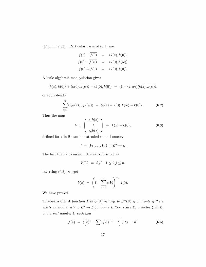
([2][Thm 2.53]). Particular cases of (6.1) are

f(z) + f(0) = 〈k(z), k(0)〉

f(0) + f(w) = 〈k(0), k(w)〉

f(0) + f(0) = 〈k(0), k(0)〉.

A little algebraic manipulation gives

〈k(z), k(0)〉 + 〈k(0), k(w)〉 − 〈k(0), k(0)〉 = (1 − 〈z,w〉)〈k(z), k(w)〉,

or equivalently

n∑

i=1

〈zik(z), wik(w)〉 = 〈k(z) − k(0), k(w) − k(0)〉. (6.2)

Thus the map

V :

z1k(z)...

znk(z)

7→ k(z) − k(0), (6.3)

defined for z in B, can be extended to an isometry

V = (V1, . . . , Vn) : Ln → L.

The fact that V is an isometry is expressible as

V ∗i Vj = δijI 1 ≤ i, j ≤ n.

Inverting (6.3), we get

k(z) =

(

I −n∑

i=1

ziVi

)−1

k(0).

We have proved

Theorem 6.4 A function f in O(B) belongs to S+(B) if and only if there

exists an isometry V : Ln → L for some Hilbert space L, a vector ξ in L,

and a real number t, such that

f(z) = 〈[

2(I −∑

ziVi)−1 − I

]

ξ, ξ〉 + it. (6.5)

17

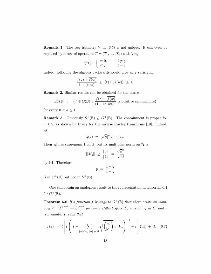
Remark 1. The row isometry V in (6.5) is not unique. It can even be

replaced by a row of operators T = (T1, . . . , Tn) satisfying

T ∗i Tj

= 0, i 6= j≤ I i = j

Indeed, following the algebra backwards would give an f satisfying

f(z) + f(w)

1 − 〈z,w〉 ≥ 〈k(z), k(w)〉 ≥ 0.

Remark 2. Similar results can be obtained for the classes

S+α (B) := f ∈ O(B) :

f(z) + f(w)

(1 − 〈z,w〉)α is positive semidefinite

for every 0 < α ≤ 1.

Remark 3. Obviously S+(B) ⊆ O+(B). The containment is proper for

n ≥ 2, as shown by Drury for the inverse Cayley transforms [10]. Indeed,

let

q(z) = [√

n]n z1 · · · zn.

Then |q| has supremum 1 on B, but its multiplier norm on H is

‖Mq‖ ≥ ‖q‖‖1‖ =

√n

n

√n!

by 1.1. Therefore

p =1 + q

1 − q

is in O+(B) but not in S+(B).

One can obtain an analogous result to the representation in Theorem 6.4

for O+(B).

Theorem 6.6 If a function f belongs to O+(B) then there exists an isom-

etry V : L2n−1 → L2n−1

for some Hilbert space L, a vector ξ in L, and a

real number t, such that

f(z) = 〈

2

I −∑

|α|≤n, |α| odd

√

(

n

|α|

)

zαVα

−1

− I

ξ, ξ〉 + it. (6.7)

18

Here we are writing V as

V =

(

L · · · LL Vα

L2n−1−1 V ′α

)

.

Proof: If f ∈ O+(B), then

[f(z) + f(w)∗]S(z,w) =f(z) + f(w)∗

(1 − 〈z,w〉)n ≥ 0,

and therefore can be factored as 〈k(z), k(w)〉 for some k with values in a

Hilbert space L. We get

〈k(z) − k(0), k(w) − k(0)〉 = (1 − (1 − 〈z,w〉)n) 〈k(z), k(w)〉.

Therefore the map

V :⊕

|α| odd

|α|≤n

(√

(

n

|α|

)

zαk(z)

)

7→ (k(z) − k(0))⊕

|α| even

0<|α|≤n

(√

(

n

|α|

)

zαk(z)

)

is an isometry. Letting ξ = k(0) we get (6.7). 2

7 Herglotz transforms

By analogy with Theorems 5.3 and 6.4, we define M+(B) to be the set of

functions f that can be represented as

f(z) =

∫

∂B

[

2

1 − 〈z, u〉 − 1

]

dµ(u) + it

for some positive Borel measure µ and some real number t. Modulo the

harmless imaginary constant, this is just the class of Herglotz transforms of

positive measures, where the Herglotz transform of µ is

(Hµ)(z) =

∫

∂B

1 + 〈z, u〉1 − 〈z, u〉dµ(u).

Proposition 7.1 The set M+(B) is contained in S+(B).

19

Proof: Fix a positive measure µ on ∂B. Then

(Hµ)(z) + (Hµ)(w)

1 − 〈z,w〉 = 2

∫

∂B

1

1 − 〈z, u〉1 − 〈z, u〉〈u,w〉

1 − 〈z,w〉1

1 − 〈u,w〉 dµ(u).

The middle factor is positive semi-definite because for every u in B, the map

z 7→ 〈z, u〉

is in the closed unit ball of the multiplier algebra of H. Therefore the whole

expression is positive, as required. 2

Thus we have

M+(B) ⊆ S+(B) ⊆ O+(B).

For n = 1, all three sets are equal, by the Riesz-Herglotz theorem. For

n > 1, the second inclusion is strict as was remarked in Section 6. The main

result of this section is that the first inclusion is also strict.

Theorem 7.2 For n ≥ 2, we have M+(B) ( S+(B).

Proof: By definition, f is in M+(B) iff there exists µ ≥ 0 such that

1

2

[

f(z) + f(0)]

=

∫

∂B

dµ(u)

1 − 〈z, u〉 (7.3)

=∑

α∈Nn

zα |α|!α!

∫

∂Buαdµ(u). (7.4)

By Theorem 6.4, g is in S+(B) iff there exists an isometry V : Ln → Land ξ ∈ L such that

1

2

[

g(z) + g(0)]

= 〈(I − zV )−1ξ, ξ〉 (7.5)

=∞∑

j=0

〈(zV )jξ, ξ〉

=∑

α∈Nn

zα〈(zα)s(V )ξ, ξ〉 |α|!α!

. (7.6)

20

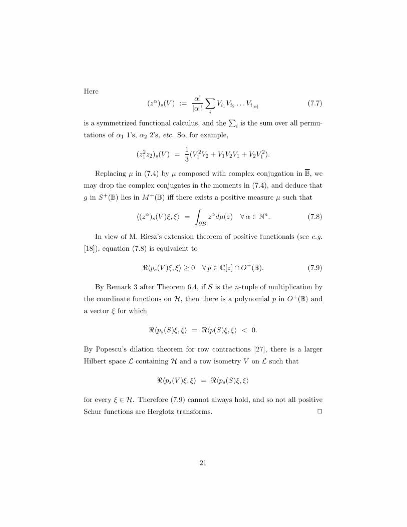
Here

(zα)s(V ) :=α!

|α|!∑

i

Vi1Vi2 . . . Vi|α|(7.7)

is a symmetrized functional calculus, and the∑

i is the sum over all permu-

tations of α1 1’s, α2 2’s, etc. So, for example,

(z21z2)s(V ) =

1

3(V 2

1 V2 + V1V2V1 + V2V21 ).

Replacing µ in (7.4) by µ composed with complex conjugation in B, we

may drop the complex conjugates in the moments in (7.4), and deduce that

g in S+(B) lies in M+(B) iff there exists a positive measure µ such that

〈(zα)s(V )ξ, ξ〉 =

∫

∂Bzαdµ(z) ∀α ∈ Nn. (7.8)

In view of M. Riesz’s extension theorem of positive functionals (see e.g.

[18]), equation (7.8) is equivalent to

<〈ps(V )ξ, ξ〉 ≥ 0 ∀ p ∈ C[z] ∩ O+(B). (7.9)

By Remark 3 after Theorem 6.4, if S is the n-tuple of multiplication by

the coordinate functions on H, then there is a polynomial p in O+(B) and

a vector ξ for which

<〈ps(S)ξ, ξ〉 = <〈p(S)ξ, ξ〉 < 0.

By Popescu’s dilation theorem for row contractions [27], there is a larger

Hilbert space L containing H and a row isometry V on L such that

<〈ps(V )ξ, ξ〉 = <〈ps(S)ξ, ξ〉

for every ξ ∈ H. Therefore (7.9) cannot always hold, and so not all positive

Schur functions are Herglotz transforms. 2

21

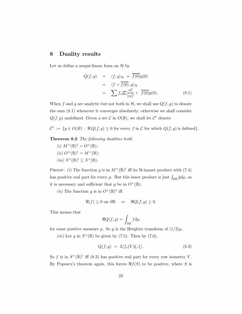
8 Duality results

Let us define a sesqui-linear form on H by

Q(f, g) = 〈f, g〉H + f(0)g(0)

= 〈f + f(0), g〉H=

∑

fαgαα!

|α|! + f(0)g(0). (8.1)

When f and g are analytic but not both in H, we shall use Q(f, g) to denote

the sum (8.1) whenever it converges absolutely; otherwise we shall consider

Q(f, g) undefined. Given a set C in O(B), we shall let C† denote

C† := g ∈ O(B) : <Q(f, g) ≥ 0 for every f in C for which Q(f, g) is defined.

Theorem 8.2 The following dualities hold:

(i) M+(B)† = O+(B);

(ii) O+(B)† = M+(B);

(iii) S+(B)† ⊆ S+(B).

Proof: (i) The function g is in M+(B)† iff its H-innner product with (7.4)

has positive real part for every µ. But this inner product is just∫

∂B gdµ, so

it is necessary and sufficient that g be in O+(B).

(ii) The function g is in O+(B)† iff

<(f) ≥ 0 on ∂B ⇒ <Q(f, g) ≥ 0.

This means that

<Q(f, g) =

∫

∂Bfdµ

for some positive measure µ. So g is the Herglotz transform of (1/2)µ.

(iii) Let g in S+(B) be given by (7.5). Then by (7.6),

Q(f, g) = 2〈fs(V )ξ, ξ〉. (8.3)

So f is in S+(B)† iff (8.3) has positive real part for every row isometry V .

By Popescu’s theorem again, this forces <f(S) to be positive, where S is

22

the n-tuple of multiplication by the coordinate functions on H. Therefore f

must be in S+(B). 2

Theorem 8.2 gives another proof that the three classes are distinct. We

do not know if the inclusion (iii) is proper.

Question 8.4. Is S+(B)† = S+(B)?

Let E be as in (4.7):

Ez =1

(n − 1)!

n−1∏

j=1

(j +

n∑

i=1

zi∂

∂zi). (8.5)

Then we can give two further characterizations of the set of Herglotz trans-

forms of positive measures.

Theorem 8.6 With notation as above,

M+(B) = f : <[∫

(Ef)dµ

]

≥ 0 ∀ Koranyi − Pukansky µ(8.7)

= f : Ez(f(z)) = v(z, 0) for some non−negative

M−harmonic v(z, z). (8.8)

Proof: (8.7): When calculating Q, there is no loss of generality in assuming

f(0) and g(0) are real, and we shall assume this below. Let g be in O+(B);

by Theorem 5.3, there is some Koranyi-Pukansky measure µ such that

g(z) + g(0) =

∫

∂B

dµ(u)

(1 − 〈z, u〉)n . (8.9)

So f is in M+(B) = O+(B)† iff the H inner product of f with (8.9) always

has positive real part (here the inner product is evaluated formally on power

series). But, assuming f is regular enough,

〈f(z),

∫

∂B

dµ(u)

(1 − 〈z, u〉)n 〉H = 〈f(z), Ez

∫

∂B

dµ(u)

1 − 〈z, u〉 〉H

=

∫

∂B〈Ezf(z),

1

1 − 〈z, u〉 〉Hdµ(u)

=

∫

∂B(Ef)(u)dµ(u).

23

Therefore (8.7) holds.

(8.8): Let

v(z, z) :=

∫

S(z, u)S(u, z)

S(z, z)dµ. (8.10)

Then if f is given by (7.3), we find

Ez[f(z) + f(0)] = 2v(z, 0).

Conversely, given v, let µ be defined by (8.10). Then f given by (7.3) satisifes

(8.8).

2

Example. By direct calculation,

Ezzα =

(

n + |α| − 1

n − 1

)

zα. (8.11)

So if f is the sum of a function fd homogeneous of degree d and a constant

f0, then

Ezf(z) = f0 +

(

n + |d| − 1

n − 1

)

fd(z) = f(rz),

where

r =

(

n + |d| − 1

n − 1

)1/d

.

A sufficient condition for (8.7) to hold is that

<f |B(0,r) ≥ 0.

As M+(B) ( S+(B) ( O+(B), any function f in M+(B) must have

realizations as in Theorems 6.4 and 5.3. How are they related?

Assume f is in M+(B), and =f(0) = 0 for convenience. Then f is

the Herglotz transform of some positive measure µ on ∂B. Therefore, if

N = (N1, . . . , Nn) is the normal n-tuple of multiplication by the coordinate

functions in L2(µ), we have

f(z) = 〈[2(I − z · N)−1 − I]1, 1〉. (8.12)

24

As NN∗ =∑

NiN∗i = I, N is a co-isometry, and therefore a row contrac-

tion. Let V be Popescu’s row isometric dilation of N [27]. Then replacing

N by V in (8.12) we get the same function; this is the realization of f in

Theorem 6.4.

The connection with O+(B) is less clear. If g is a matrix or scalar valued

analytic function on B with <g ≥ 0, then the weak-* limit of the measures

<g(rz)dσ(z) is a positive operator valued Koranyi-Pukansky measure E on

∂B satisfying g(z) =∫

(2S(z, u)−1)dE(u). By Naimark’s dilation theorem

[11], E has a dilation to a spectral measure, and so if M is the normal n-

tuple corresponding to this spectral measure, and P is the projection onto

the range of E, we have

g(z) = P (2(I − z · M)−n − I) P. (8.13)

Notice that if T is any row contraction, then

2<(I − z · T )−1 − I ≥ 0.

So if we let g(z) = 2(I − z · T )−1 − 1, then (8.13) applied to g(z) + g(0)∗

gives

(I − z · T )−1 = P (I − z · M)−nP. (8.14)

Therefore, a function f ∈ M+(B) admits three different realizations,

reflecting the inclusions M+(B) ( S+(B) ( O+(B):

1

2(f(z) + f(0)) = 〈(I − z · N)−1ξ, ξ〉 =

〈(I − z · V )−1ξ, ξ〉 = 〈(I − z · M)−nξ, ξ〉.

Above N and M are commuting tuples of normal operators, acting on dif-

ferent spaces, both with joint spectrum on the sphere. The row isometric

dilation of N is denoted by V , while M is a dilation of V in the sense of

(8.14). We could invoke Theorem 6.6 to linearize the last realization, but

this seems less important.

25

9 Functional calculus on the numerical range: The

Ball

Let R be an operator on a Hilbert space L. Its numerical range, denoted

W (R), is the set

W (R) := 〈Rξ, ξ〉 : ‖ξ‖ = 1.

By a classical Theorem of Hausdorff and Toeplitz, the numerical range

of an operator is a convex set that contains in its closure the spectrum.

Recently, B. and F. Delyon proved that for any R, its numerical range is an

M -spectral set for some M [9], i.e.

‖p(R)‖ ≤ M‖p‖W (R) ∀ polynomials p. (9.1)

For an alternative proof, with an analysis of the best M , see [28]. In this

section, we shall extend (9.1) to n-tuples with numerical range in the ball.

Let T = (T1, . . . , Tn) be an n-tuple of operators on a Hilbert space L.

We do not assume that the operators commute with each other. We shall

say the numerical range of T is contained in B, written W(T ) ⊆ B, if for

every u in B,

W (uT ) = W (u1T1 + . . . + unTn) ⊆ D. (9.2)

Our standing assumption throughout this section will be that W(T ) ⊆ B.

Lemma 9.3

<(I − uT )−1 ≥ 0 ∀u ∈ B.

Proof: Note that

(I − uT )−1 + (I − uT ∗)−1 = (I − uT )−1 [2 − uT − uT ∗] (I − uT ∗)−1.

The quantity in brackets is positive iff <uT ≤ I; this holds for all u iff

W(T ) ⊆ B. 2

26

Consider the measures <(I − ruT )−1dσ(u). These are all positive by

Lemma 9.3, and have total mass 1. Therefore the positive operator valued

measure

dµT (u) := weak∗ − limr1

<(I − ruT )−1dσ(u) (9.4)

exists and is well-defined. Define

Ξ : C[z] → B(L)

p 7→∫

∂Bp dµT .

If <p ≥ 0 on ∂B, then <[Ξ(p)] ≥ 0.

To understand Ξ better, let us consider the scalar case. Define

Λp(z) :=

∫

∂B

1

2

[

1

1 − 〈u, z〉 +1

1 − 〈z, u〉

]

p(u)dσ(u)

=1

2F(pdσ) +

1

2p(0).

Then

Λ : zα 7→

12

1(|α|+1)···(|α|+n−1)z

α α 6= 0

1 α = 0.

Note that

Ξ(p) = [Λp]s (T ), (9.5)

where the subscript means the symmetrized functional calculus from (7.7).

By direct calculation on monomials, the operator

Γ : p 7→ 2(n − 1)!Ez [p − p(0)] + p(0) (9.6)

is the inverse to Λ.

By Naimark’s dilation theorem [11], the positive operator valued measure

µT has a dilation to a spectral measure on ∂B, whose values are projections

in a Hilbert space K ⊇ L. If P is projection from K onto L, then

∫

pdµT = Pp(N)P

27

where N is the normal n-tuple of multiplication by the coordinate functions.

By (9.5), for any polynomial p,

Ξ(Γ p) = [ΛΓ p]s (T ) = ps(T ).

Therefore

ps(T ) =

∫

Γ p dµT = PΓp(N)P. (9.7)

The above argument goes through unchanged if p is matrix-valued. If p(z) =∑

Aαzα, with the coefficients Aα d × d matrices, then ps(T ) is the d × d

operator valued matrix with (i, j) entry [pij ]s(T ), and Γp is likewise obtained

by applying Γ entrywise.

We have proved

Theorem 9.8 Let T have W(T ) ⊆ B, and let Γ be defined by (9.6). Then,

for any polynomial p, scalar or matrix valued, we have

‖ps(T )‖ ≤ ‖Γp‖B.

Example 1. Let p be homogeneous of degree d. Then

Γp = 2(d + 1) . . . (d + n − 1)p,

so

‖ps(T )‖ ≤ 2(d + 1) . . . (d + n − 1)‖p‖B.

Example 2. In one complex variable (n = 1) Theorem 9.8 gives

‖p(T )‖ ≤ ‖2p − p(0)‖D

≤ 3‖p‖D

whenever W (T ) ⊆ D. This was first obtained in [9] and [28]. Note that the

last inequality says that T is completely polynomially bounded, since there

is one constant that works for all matrix valued polynomials. Therefore by

Paulsen’s theorem [24] any operator with numerical range in the closed unit

disk is similar to a contraction.

28

In light of (9.7), it is natural to ask what conditions on p make <(Γp)

non-negative. As Λ is the inverse of Γ, this is equivalent to asking when p

is in Λ(O+(B)).

Now, q is in O+(B) iff H[<q dσ] is in M+(B). By comparing the formulas

for H and Λ, we get

2Λ[q] = H[<q dσ] + i=q(0) + q(0).

Therefore p is Λ(q) for some q in O+(B) if and only if

p − 1

2<p(0) − i=p(0) ∈ M+(B). (9.9)

Corollary 9.10 Suppose W(T ) ⊆ B and p satisfies (9.9). Then <ps(T ) ≥0.

Alternatively, one can work directly with Γp, which is easily calculated

when p is decomposed into homogeneous pieces.

Corollary 9.11 Let p = p0 + p1 + . . . + pd be the decomposition of p into

homoegeneous polynomials. If

1

2Γp =

1

2p0 +

n!

1!p1 + . . . +

(n + d − 1)!

d!pd

has positive real part on B, then <ps(T ) ≥ 0 for every T with W(T ) ⊆ B.

Example 3. Suppose T2 = T ∗1 , and the numerical radius of T is at most

1/√

2 (the numerical radius is the supremum of the moduli of the numbers

in the numerical range). Then W(T1, T2) ⊆ B2. Let n = 2, and, for m ≥ 2,

let

p(z1, z2) =2m + 1

2m−1− zm

1 zm2 .

Then

Γp (z1, z2) =2m + 1

2m−1− 2(2m + 1) zm

1 zm2 ,

29

which is nonnegative on B2. Therefore (zm1 zm

2 )s(T ), which is the average of

all(2m

m

)

ways of writing m copies of T1 and m copies of T ∗1 , is less than or

equal to (2m + 1)/2m−1 times the identity:

(zm1 zm

2 )s(T1, T∗1 ) ≤ 2m + 1

2m−1I. (9.12)

When m = 1, inequality (9.12) is worse than the trivial one obtained from

the observation that ‖T1‖ is at most twice the numerical radius. For m ≥ 2,

the inequality is better than this trivial one.

If T1 =

(

0√

20 0

)

, then only two terms in the whole sum are non-zero.

One obtains the inequality

(

2m

m

)

≥ 22m−1

2m + 1.

Example 4. Let T = (T1, . . . , Tn) be a commuting n-tuple, with W(T ) ⊆Bn. Assume also that the operators are jointly nilpotent, in the sense that

there is some integer N such that Tα = 0 whenever |α| > N . Then there

is some constant CN such that if p(z) =∑

Aαzα is a matrix valued

polynomial, then∑

|α|≤N

‖Aα‖ ≤ CN‖p‖Bn.

Therefore

‖Γp‖ ≤ 2(N + 1) · · · (N + n − 1)CN‖p‖Bn.

Therefore the n-tuple T is completely polynomially bounded, and so it is

similar to an n-tuple that has a normal dilation to ∂Bn by [25, Thm 9.1].

10 General convex sets

Let Ω be a closed convex set in Cn with 0 in the interior. Assume that Ω is

circular, i.e. whenever z is in Ω, then so is eiθz for all θ ∈ [0, 2π]. Let Ω

30

be defined by (3.3). Let T = (T1, . . . , Tn) be an n-tuple of not necessarily

commuting operators. Then we say W(T ) ⊆ Ω if

W (u1T1 + . . . unTn) ⊆ D ∀u ∈ Ω.

Fix some n-tuple T with W(T ) ⊆ Ω. Let ω be a circularly symmetric

probability measure on Ω. As in Section 9, we can define the positive

operator valued measure µT on ∂Ω by

dµT (u) := weak∗ − limr1

<(I − ruT )−1dω(u).

Define Ξ and Λ by

Ξ(p) =

∫

p dµT

Λp =1

2F(p ω) +

1

2p(0).

If Ω is Reinhardt (i.e. invariant under rotation of each coordinate sep-

arately) and if ω is also invariant under rotations, then the monomials are

orthogonal, and

F(uαω)(z) =

[ |α|!α!

∫

∂Ω

|uα|2dω(u)

]

zα.

So Γ = Λ−1 exists and is diagonalized by the orthogonal basis of the mono-

mials.

Even if Ω is not Reinhardt, it is invariant under the action of the cir-

cle group by hypothesis. Therefore in L2(ω), homogeneous polynomials of

different degrees are orthogonal. Let Pd denote the homogeneous polyno-

mials of degree d. Then Λ : Pd → Pd. Moreover, Λ has no kernel, because

Λp = 0 implies p is orthogonal to every power of u, and so∫

|p|2dω = 0.

Therefore, as Pd is finite dimensional, Γ = Λ−1 exists and maps Pd onto Pd.

We can therefore repeat the argument of Theorem 9.8, and get:

Theorem 10.1 With notation as above, let T satisfy W(T ) ⊆ Ω. Then, for

any polynomial p, we have

‖ps(T )‖ ≤ ‖Γp‖Ω .

31

Example Let Ω be the bidisk, and let dω = dθ1dθ2dr1 on Ω. Then for

any pair T = (T1, T2) with numerical range in the closed bidisk, we get the

inequality

‖(zm1 zm

2 )s(T )‖ ≤ C (m + 1).

References

[1] J. Agler and J.E. McCarthy. Complete Nevanlinna-Pick kernels. J.

Funct. Anal., 175(1):111–124, 2000.

[2] J. Agler and J.E. McCarthy. Pick Interpolation and Hilbert Function

Spaces. American Mathematical Society, Providence, 2002.

[3] L.A. Aizenberg. The general form of a linear continuous functional in

spaces of functions holomorphic in convex domains in Cn. Soviet Math.

Doklady, pages 198–202, 1966.

[4] L.A. Aizenberg and Sh.A. Dautov. Holomorphic functions of several

complex variables with nonnegative real part. Traces of holomorphic

and pluriharmonic functions on the Shilov boundary. Mat. USSR

Sbornik, 99:342–355, 1976.

[5] C. Ambrozie, M. Englis, and V. Muller. Operator tuples and analytic

models over general domains in Cn. J. Operator Theory, 47:287–302,

2002.

[6] M. Andersson. Cauchy-Fantappie-Leray formulas and the inverse Fan-

tappie transform. Bull. Soc. Math. France, 120:113–128, 1990.

[7] M. Andersson, M. Passare, and R. Sigurdsson. Complex convexity and

analytic functionals. Birkhauser, Basel, 2004.

[8] T. Audibert. Operateurs differentielles sur la sphere de Cn car-

acterisant les restrictions des fonctions pluriharmoniques. PhD thesis,

Universite de Provence, 1977.

32

[9] B. Delyon and F. Delyon. Generalizations of von Neumann’s spectral

sets and integral representations of operators. Bull. Soc. Math. France,

127:25–41, 1999.

[10] S.W. Drury. A generalization of von Neumann’s inequality to the com-

plex ball. Proc. Amer. Math. Soc., 68:300–304, 1978.

[11] P.A. Fillmore. Notes on operator theory. Van Nostrand-Reinhold, New

York, 1970.

[12] I.M. Gel’fand and N.Ya. Vilenkin. Generalized Functions, Vol. 4. Ap-

plications of Harmonic Analysis. Academic Press, New York, 1964.

[13] B. Gustafsson, M. Putinar, and H.S. Shapiro. Restriction operators,

balayage, and doubly orthogonal systems of analytic functions. J.

Funct. Anal., 199:332–378, 2003.

[14] G.M. Henkin. The method of integral representations in complex anal-

ysis. In A.G. Vitushkin, editor, Several Complex Variables I, pages

19–116, 1990.

[15] G.M. Henkin and J. Leiterer. Theory of Functions on Complex Mani-

folds. Birkhauser, Basel, 1984.

[16] G.M. Henkin and A.A. Shananin. The Bernstein theorems for the Fan-

tappie indicatrix and their applications to mathematical economics.

In Geometry and complex variables (Bologna 1988/1990), Lect. Notes.

Math. 132, pages 221–227, New York, 1991. Dekker.

[17] L. Hormander. Notions of convexity. Birkhauser, Amsterdam, 1994.

[18] P. Koosis. The logarithmic integral. Cambridge University Press, Cam-

bridge, 1988.

[19] A. Koranyi. The Poisson integral for generalized half-planes and

bounded symmetric domains. Ann. of Math., 82:332–350, 1965.

33

[20] A. Koranyi and L. Pukansky. Holomorphic functions with positive real

part on polycylinders. Trans. Amer. Math. Soc., 108:449–456, 1963.

[21] P. Lelong and L. Gruman. Entire Functions of Several Complex Vari-

ables. Springer, Berlin, 1986.

[22] A. Martineau. Sur les fonctionnelles analytiques et la transformation

de Fourier-Borel. J. Analyse Math., XI:1–164, 1963.

[23] L. Narici and E. Beckenstein. Topological Vector Spaces. Marcel Dekker,

New York, 1985.

[24] V.I. Paulsen. Every completely polynomially bounded operator is sim-

ilar to a contraction. J. Funct. Anal., 55:1–17, 1984.

[25] V.I. Paulsen. Completely bounded maps and operator algebras. Cam-

bridge University Press, Cambridge, 2002.

[26] A. Pfister. Uber das Koeffizientenproblem der beschrankten Funktionen

von Zwei Veranderlichen. Math. Ann., 146:249–262, 1962.

[27] G. Popescu. Isometric dilations for infinite sequences of noncommuting

operators. Trans. Amer. Math. Soc., 316:523–536, 1989.

[28] M. Putinar and S. Sandberg. A normal dilation on the numerical range

of an operator. Math. Ann., 2004. DOI: 10.1007/s00208-004-0585-3

(electronic version).

[29] R.M. Range. Holomorphic functions and integral representations in

several complex variables. Springer Verlag, New York, 1986.

[30] W. Rudin. Function Theory in the unit ball of Cn. Springer-Verlag,

Berlin, 1980.

[31] M. Stoll. Invariant Potential Theory on the unit ball of Cn. Cambridge

University Press, Cambridge, 1994.

34

[32] J. von Neumann. Eine Spektraltheorie fur allgemeine Operatoren eines

unitaren Raumes. Math. Nachr., 4:258–281, 1951.

35