IMAGE INTERPOLATION

IMAGE INTERPOLATION Francesca Pizzorni Ferrarese

1

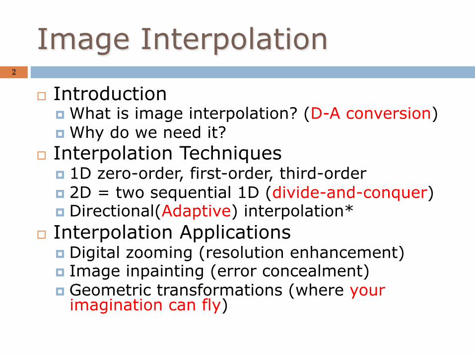
Image Interpolation 2

  Introduction  What is image interpolation? (D-A conversion)  Why do we need it?

  Interpolation Techniques  1D zero-order, first-order, third-order  2D = two sequential 1D (divide-and-conquer)  Directional(Adaptive) interpolation*

  Interpolation Applications  Digital zooming (resolution enhancement)   Image inpainting (error concealment)  Geometric transformations (where your

imagination can fly)

Introduction 3

  What is image interpolation?  An image f(x,y) tells us the intensity values

at the integral lattice locations, i.e., when x and y are both integers

 Image interpolation refers to the “guess” of intensity values at missing locations, i.e., x and y can be arbitrary

 Note that it is just a guess (Note that all sensors have finite sampling distance)

A Sentimental Comment 4

  Haven’t we just learned from discrete sampling (A-D conversion)?

  Yes, image interpolation is about D-A conversion

  Recall the gap between biological vision and artificial vision systems  Digital: camera + computer  Analog: retina + brain

Engineering Motivations 5

  Why do we need image interpolation?  We want BIG images

 When we see a video clip on a PC, we like to see it in the full screen mode

 We want GOOD images  If some block of an image gets damaged during

the transmission, we want to repair it  We want COOL images

 Manipulate images digitally can render fancy artistic effects as we often see in movies

Scenario I: Resolution Enhancement

6

Low-Res.

High-Res.

Scenario II: Image Inpainting 7

Non-damaged Damaged

Scenario III: Image Warping 8


•  Introduction – What is image interpolation? – Why do we need it?

•  Interpolation Techniques – 1D linear interpolation (elementary algebra) – 2D = 2 sequential 1D (divide-and-conquer) – Directional(adaptive) interpolation*

•  Interpolation Applications – Digital zooming (resolution enhancement) –  Image inpainting (error concealment) – Geometric transformations

Upsampling

  This image is too small for this screen:   How can we make it 10 9mes as big?   Simplest approach: repeat each row and column 10 9mes

  (“Nearest neighbor interpola9on”)

Image interpola9on

Recall how a digital image is formed

•  It is a discrete point-‐sampling of a con9nuous func9on •  If we could somehow reconstruct the original func9on, any new

image could be generated, at any resolu9on and scale

1 2 3 4 5

Adapted from: S. Seitz

d = 1 in this example

Image interpola9on

1 2 3 4 5


Recall how a digital image is formed

•  It is a discrete point-‐sampling of a con9nuous func9on •  If we could somehow reconstruct the original func9on, any new

image could be generated, at any resolu9on and scale


Image interpola9on

1 2 3 4 5 2.5

1

•  Convert to a con9nuous func9on:

•  Reconstruct by convolu9on with a reconstruc)on filter, h

•  What if we don’t know ? •  Guess an approxima9on: •  Can be done in a principled way: filtering



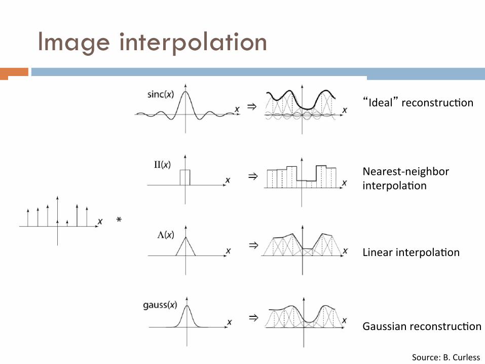
“Ideal” reconstruc9on

Nearest-‐neighbor interpola9on

Linear interpola9on

Gaussian reconstruc9on

Source: B. Curless

Image interpolation

Ideal reconstruction 15

Nearest-‐neighbor interpola9on Bilinear interpola9on Bicubic interpola9on

Original image: x 10

Image interpolation

1D Zero-order (Replication) 19

n f(n)

x

f(x)

1D First-order Interpolation (Linear) 20

n f(n)

x

f(x)

Linear Interpolation Formula 21

a 1-a

f(n)

f(n+1) f(n+a)

f(n+a)=(1-a)×f(n)+a×f(n+1), 0<a<1

Heuristic: the closer to a pixel, the higher weight is assigned Principle: line fitting to polynomial fitting (analytical formula)

Note: when a=0.5, we simply have the average of two

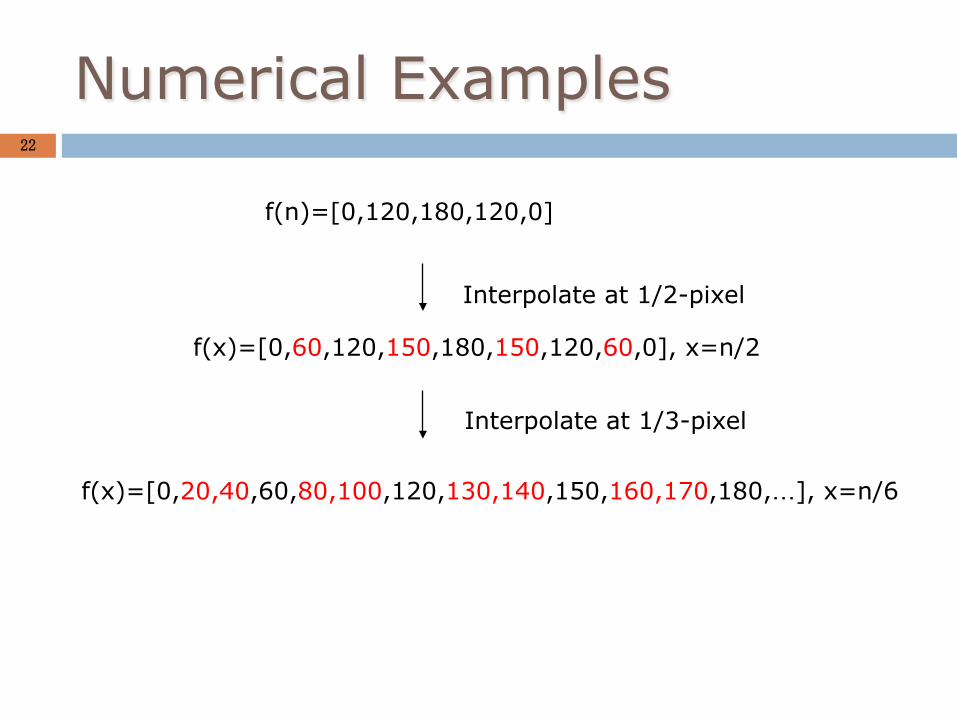
Numerical Examples 22

f(n)=[0,120,180,120,0]

f(x)=[0,60,120,150,180,150,120,60,0], x=n/2

f(x)=[0,20,40,60,80,100,120,130,140,150,160,170,180,…], x=n/6

Interpolate at 1/2-pixel

Interpolate at 1/3-pixel

1D Third-order Interpolation (Cubic)* 23

n

x

f(n)

f(x)

Cubic spline fitting

http://en.wikipedia.org/wiki/Spline_interpolation

From 1D to 2D 24

•  Engineers’ wisdom: divide and conquer •  2D interpolation can be decomposed into two sequential

1D interpolations. • The ordering does not matter (row-column = column-row) • Such separable implementation is not optimal but enjoys low

computational complexity “If you don’t know how to solve a problem, there must be a related but easier problem you know how to solve. See if you can reduce the problem to the easier one.” - rephrased from G. Polya’s “How to Solve It”

Graphical Interpretation of Interpolation at Half-pel

25

row column

f(m,n) g(m,n)

Numerical Examples 26

a b c d

a a b b a a b b c c d d c c d d

zero-order

first-order

a (a+b)/2 b (a+c)/2 (a+b+c+d)/4 (b+d)/2 c (c+d)/2 d

Numerical Examples (Con’t) 27

X(m,n) row m

row m+1

Col n Col n+1

X(m,n+1)

X(m+1,n+1) X(m+1,n)

Y a 1-a

b

1-b

Q: what is the interpolated value at Y? Ans.: (1-a)(1-b)X(m,n)+(1-a)bX(m+1,n) +a(1-b)X(m,n+1)+abX(m+1,n+1)

Bicubic Interpolation* 28

http://en.wikipedia.org/wiki/Bicubic_interpolation

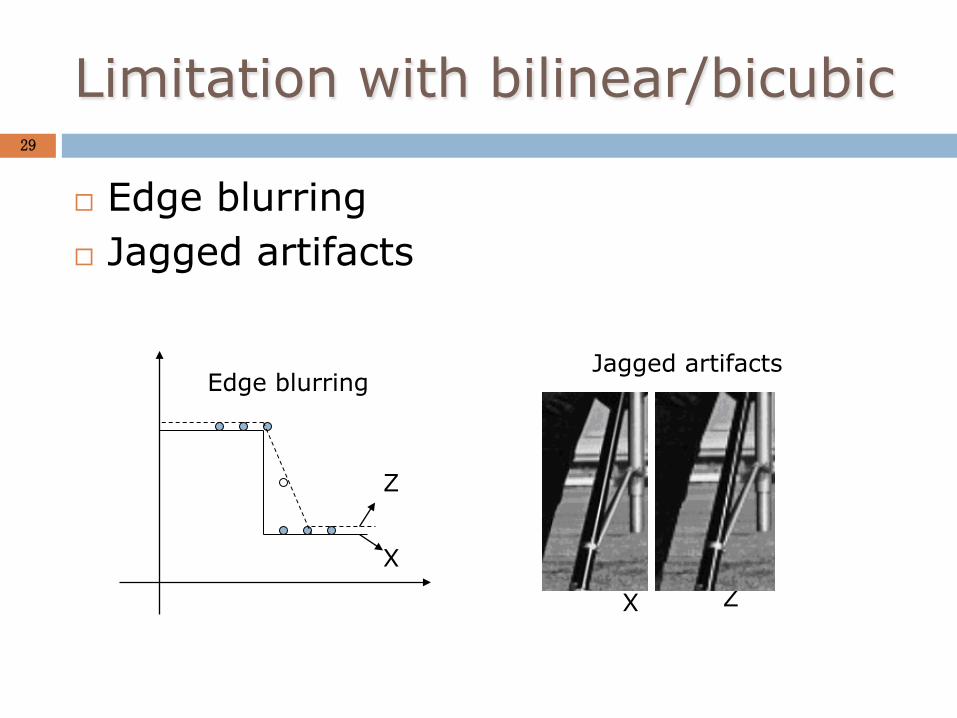
Limitation with bilinear/bicubic 29

  Edge blurring   Jagged artifacts

X Z

Jagged artifacts

X

Z

Edge blurring

Edge-Sensitive Interpolation 30

Step 1: interpolate the missing pixels along the diagonal

black or white?

Step 2: interpolate the other half missing pixels

a b

c d

Since |a-c|=|b-d| x

x has equal probability of being black or white

a

b

c

d Since |a-c|>|b-d|

x=(b+d)/2=black

x


•  Introduction •  Interpolation Techniques

– 1D zero-order, first-order, third-order – 2D zero-order, first-order, third-order – Directional interpolation*

•  Interpolation Applications – Digital zooming (resolution enhancement) –  Image inpainting (error concealment) – Geometric transformations (where your

imagination can fly)

Pixel Replication 32

low-resolution image (100×100)

high-resolution image (400×400)

Bilinear Interpolation 33



Bicubic Interpolation 34



Edge-Directed Interpolation (Li&Orchard’2000)

35



Image Demosaicing (Color-Filter-Array Interpolation)

36

Bayer Pattern

Image Example 37

Ad-hoc CFA Interpolation Advanced CFA Interpolation

Error Concealment* 38

damaged interpolated

Image Inpainting* 39

Image Mosaicing* 40

Geometric Transformation 41

MATLAB functions: griddata, interp2, maketform, imtransform

Basic Principle 42

  (x,y) → (x’,y’) is a geometric transformation

  We are given pixel values at (x,y) and want to interpolate the unknown values at (x’,y’)

  Usually (x’,y’) are not integers and therefore we can use linear interpolation to guess their values

MATLAB implementation: z’=interp2(x,y,z,x’,y’,method);

Rotation 43

⎥⎦

⎤⎢⎣

⎡⎥⎦

⎤⎢⎣

⎡

−=⎥

⎦

⎤⎢⎣

⎡

yx

yx

θθ

θθ

cossinsincos

''

x

y

x’

y’

θ

MATLAB Example 44

% original coordinates [x,y]=meshgrid(1:256,1:256);

z=imread('cameraman.tif');

% new coordinates a=2; for i=1:256;for j=1:256; x1(i,j)=a*x(i,j); y1(i,j=y(i,j)/a; end;end % Do the interpolation z1=interp2(x,y,z,x1,y1,'cubic');

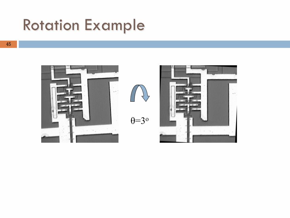
Rotation Example 45

θ=3o

Scale 46

⎥⎦

⎤⎢⎣

⎡⎥⎦

⎤⎢⎣

⎡=⎥

⎦

⎤⎢⎣

⎡

yx

aa

yx

/100

''

a=1/2

Affine Transform 47

⎥⎦

⎤⎢⎣

⎡+⎥⎦

⎤⎢⎣

⎡⎥⎦

⎤⎢⎣

⎡=⎥

⎦

⎤⎢⎣

⎡

y

x

dd

yx

aaaa

yx

2221

1211

''

square parallelogram

Affine Transform Example 48

⎥⎦

⎤⎢⎣

⎡+⎥⎦

⎤⎢⎣

⎡⎥⎦

⎤⎢⎣

⎡

−=⎥

⎦

⎤⎢⎣

⎡

10

25.15.

''

yx

yx

Shear 49

⎥⎦

⎤⎢⎣

⎡+⎥⎦

⎤⎢⎣

⎡⎥⎦

⎤⎢⎣

⎡=⎥

⎦

⎤⎢⎣

⎡

y

x

dd

yx

syx

101

''

square parallelogram

Shear Example 50

⎥⎦

⎤⎢⎣

⎡+⎥⎦

⎤⎢⎣

⎡⎥⎦

⎤⎢⎣

⎡=⎥

⎦

⎤⎢⎣

⎡

10

15.01

''

yx

yx

Projective Transform 51

1'

87

321

++

++=

yaxaayaxa

x

1'

87

654

++

++=

yaxaayaxay

quadrilateral square

A B

C D

A’

B’

C’

D’

Projective Transform Example 52

[ 0 0; 1 0; 1 1; 0 1] [-4 2; -8 -3; -3 -5; 6 3]

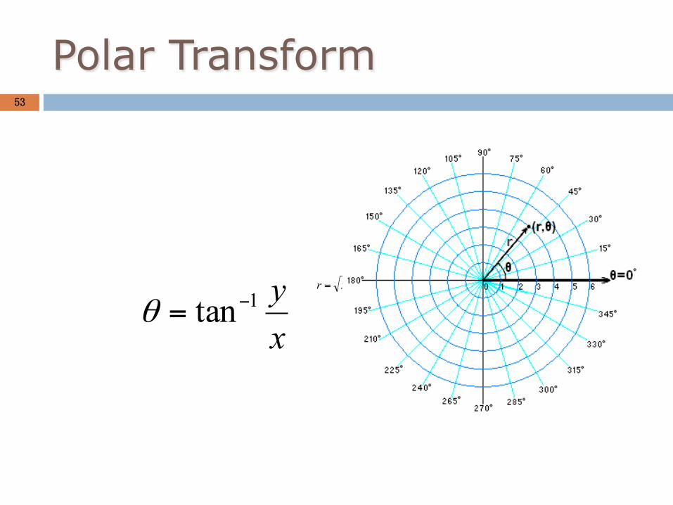
Polar Transform 53

22 yxr +=

xy1tan−=θ

Iris Image Unwrapping 54

r

θ

Use Your Imagination 55

r -> sqrt(r)

http://astronomy.swin.edu.au/~pbourke/projection/imagewarp/ �

Free Form Deformation 56

Seung-Yong Lee et al., “Image Metamorphosis Using Snakes and Free-Form Deformations,”SIGGRAPH’1985, Pages 439-448

Application into Image Metamorphosis

57

Summary of Image Interpolation

58

  A fundamental tool in digital processing of images: bridging the continuous world and the discrete world

  Wide applications from consumer electronics to biomedical imaging

  Remains a hot topic after the IT bubbles break

IMAGE INTERPOLATION

Documents

Transcript of IMAGE INTERPOLATION