Linear Algebra and its Applications 422 (2007) 526–539www.elsevier.com/locate/laa

Interpolation algorithm for computing Drazin inverseof polynomial matrices

Marko D. Petkovic∗, Predrag S. Stanimirovic

University of Niš, Department of Mathematics, Faculty of Science, Višegradska 33,18000 Niš, Serbia and Montenegro

Received 24 August 2005; accepted 8 November 2006Available online 17 January 2007

Submitted by V. Mehrmann

Abstract

In this paper we introduce an interpolation method for computing the Drazin inverse of a given poly-nomial matrix. This method is an extension of the known method from [A. Schuster, P. Hippe, Inversionof polynomial matrices by interpolation, IEEE Trans. Automat. Control 37 (3) (1992) 363–365], applicableto usual matrix inverse. Also, we improve our interpolation method, using a more effective estimation ofdegrees of polynomial matrices generated in Leverrier–Faddeev method. Algorithms are implemented andtested in the symbolic package MATHEMATICA.© 2006 Elsevier Inc. All rights reserved.

AMS classification: 15A09; 68Q40

Keywords: Drazin inverse; Interpolation; MATHEMATICA; Leverrier–Faddeev method; Polynomial matrices; Symboliccomputation

1. Introduction

Let R be the set of real numbers, Rm×n be the set of m × n real matrices, and Rm×nr =

{X ∈ Rm×n : rank(X) = r}. As usual, R[s] (resp. R(s)) denotes the polynomials (resp. rationalfunctions) with real coefficients in the indeterminate s. The m × n matrices with elements in R[s](resp. R(s)) are denoted by R[s]m×n (resp R(s)m×n).

∗ Corresponding author.E-mail addresses: dexter_of_nis@neobee.net (M.D. Petkovic), pecko@pmf.ni.ac.yu (P.S. Stanimirovic).

0024-3795/$ - see front matter ( 2006 Elsevier Inc. All rights reserved.doi:10.1016/j.laa.2006.11.011

M.D. Petkovic, P.S. Stanimirovic / Linear Algebra and its Applications 422 (2007) 526–539 527

For any matrix A ∈ Rn×n the Drazin inverse of A is the unique matrix, denoted by AD , andsatisfying the following equations in X:

(1) AkXA = Ak, (2) XAX = X, (3) AX = XA.

An algorithm for computing the Drazin inverse of a constant real matrix A(s) ≡ A0 ∈ Rn×n

by means of the Leverrier–Faddeev algorithm (also called Souriau–Frame algorithm) is proposedin [4]. Hartwig in [7] continues investigation of this algorithm. The method for computing A−1(s)

of the polynomial matrix A(s) = A1s + A0, det(A(s)) /= 0 is presented in [3]. A representationand corresponding algorithm for computing the Drazin inverse of a nonregular polynomial matrixof an arbitrary degree is introduced in [8] and [16]. Corresponding algorithm for two-variablepolynomial matrix and its implementation in the programming language MATLAB is presentedin [1]. Similar algorithms for symbolic computation of the Moore–Penrose and Drazin inverse ofone-variable rational and polynomial matrix are presented in [10–12]. Corresponding algorithmfor two-variable rational and polynomial matrix and the Moore–Penrose is introduced in [13].Also, an effective version of given algorithm is presented in the paper [1]. This algorithm is efficientwhen elements of the input matrix are sparse polynomials with only few nonzero addends. On theother hand, the interpolation method presented in our paper possesses better performances whenmatrices A(s), Bj (s) and Aj(s) are dense and their elements are dense polynomials.

In [15] Schuster and Hippe generalize known polynomial interpolation methods to polynomialmatrices in order to compute the ordinary inverse of the polynomial (non-singular) matrices.Generalizing the idea of interpolation from [15] we made an algorithm for calculating the Dra-zin inverse of one-variable polynomial matrices. A background for interpolation methods forcomputing generalized inverses can be found in [2]. Also in [5,6,17] it is used the interpolationpolynomial of the function f (x) = 1/x to construct an iterative method for computing Moore–Penrose inverse. In our approach we have been using interpolation to compute polynomial andmatrix polynomial required by the last step of Leverrier–Faddeev method.

Also, different methods for computing Drazin inverse, based neither on the Leverrier–Faddeevmethod nor the interpolation, are given in [9,18,19].

In the second section we restate the Leverrier–Faddeev method for one variable rational matri-ces from [8,16], and present a complexity analysis of this algorithm in the case when the input isa polynomial matrix.

In the third section, an algorithm for computing the Drazin inverse of one-variable polynomialmatrices, based on the interpolation techniques is presented. We use the Leverrier–Faddeev methodto compute constant generalized inverses into selected base points, and the Newton interpolationmethod to generate interpolating polynomial. Also, complexity analysis of new algorithm is given.

In the fourth section we showed a small improvement of previous algorithm based on animproved estimating the degrees of matrices which appear in the Leverrier–Faddeev method.Implementation of algorithms in symbolic programming language MATHEMATICA and the expe-rience with the program are shown in the last section.

2. Drazin inverse of one-variable polynomial matrices

In this section complexity analysis of the Leverrier–Faddeev algorithm for both polynomialand constant matrices is being investigated. The following algorithm is restated from [16,8] forthe polynomial matrix case, and it is also applicable to rational matrices.

Algorithm 2.1. Input: Polynomial matrix A(s) ∈ R[s]n×n with respect to unknown s.

528 M.D. Petkovic, P.S. Stanimirovic / Linear Algebra and its Applications 422 (2007) 526–539

Step 1. Set initial values B0(s) = In, a0(s) = 1.Step 2. For j = 1, . . . , n perform the following three steps:

Step 2.1. Calculate Aj(s) = A(s)Bj−1(s).

Step 2.2. Calculate aj (s) = − tr(Aj (s))

j.

Step 2.3. Calculate Bj (s) = Aj(s) + aj (s)In.Step 3. Let

k = max{l|al(s) /= 0}, t = min{l|Bl(s) = 0}, r = t − k.

The Drazin inverse is given by:

A(s)D = (−1)r+1ak(s)−r−1A(s)rBk−1(s)

r+1.

In the rest of the paper we use the following notion:

Definition 2.1. For a given polynomial matrix A(s) ∈ R[s]n×m its maximal degree is defined asthe maximal degree of its elements:

deg A(s) = max{dg(A(s))ij |1 � i � n, 1 � j � m}.

Further we denote by kA, tA, aAi and BA

i , respectively, values of k, t , ai and Bi in Algorithm2.1 when its input is a polynomial or constant matrix A. Also we use simpler notations aA = aA

kA

and BA = BAkA−1

. Next lemma can be easily proved by mathematical induction, but it will bevery useful in the next considerations.

Lemma 2.1. Let A be real n × n matrix. Then holds:

(a) BAtA+i

= 0 for all i = 0, . . . , n − tA − 1,

(b) BAkA+i−1

= Ai−1(ABA + aAIn) for all i = 1, . . . , tA − kA,

(c) aAtA+i

= 0 for each i = 0, . . . , n − tA, or equivalently kA � tA.

(d) If A = A(s) then also holds degBi(s) � i · deg A(s) and dgai(s) � i · deg A(s) for alli = 0, . . . , n.

In Step 2.1 we need to multiply two matrices of the order n × n. This multiplication canbe done in time O(n3) when A is a constant matrix, but in the polynomial case correspondingcomplexity is O(n3 · deg A(s) · degBj−1(s)). If we denote by d = deg A(s), then in accordanceto the part (d) of Lemma 2.1, the required time for Step 2.1 is O(n3 · j · d2). Similarly one canverify that the required time for Step 2.2 as well as for Step 2.3 is O(n · j · d). This is much lessthan the time required for Step 2.1, so the total time for Steps 2.1, 2.2 and 2.3 for a fixed value j isapproximately O(n3 · j · d2). We need to evaluate Steps 2.1, 2.2 and 2.3 for each j = 1, 2, . . . , n,so the complexity of complete Algorithm 2.1 is:

O

⎛⎝ n∑

j=1

n3 · j · d2

⎞⎠ = O(n5 · d2) (2.1)

In most cases, the complexity of Algorithm 2.1 is smaller than (2.1) (not all elements of matricesBj (s), Aj(s) and A(s) has the maximal degree).

M.D. Petkovic, P.S. Stanimirovic / Linear Algebra and its Applications 422 (2007) 526–539 529

It can be shown that complexity of Leverrier–Faddeev algorithm for constant matrices isO(n3 · n) = O(n4).

3. Inversion of polynomial matrices by interpolation

It is well known that there is one and only one polynomial f (s) of degree q � n which assumesthe values f (s0), f (s1), . . . , f (sn) at distinct base points s0, s1, . . . , sn. The polynomial is calledthe qth degree interpolation polynomial. Three important interpolation methods are [15]:

(i) the direct approach using Vandermonde’s matrix,(ii) Newton interpolation,

(iii) Lagrange’s interpolation.

In the case of finding inverses of polynomial matrices (and also in many other applications) itis suitable to use the Newton interpolation polynomial [14].

In the following theorem a sufficient number of interpolation points to determine the valueskA(s), tA(s) and polynomials BA(s), aA(s) is being investigated. We use the notation κ = kA(s),τ = tA(s) and d = deg A(s).

Theorem 3.1. Let A(s) ∈ R[s]n×n and values kA(s), aA(s) and BA(s) are defined from Algorithm2.1. Let d = degA(s) and si, i = 0, . . . , n · d be any pairwise different real numbers. Then thefollowing statements are valid:

(a) For f (j) = max{tA(si )|i = 0, . . . , j · d}, j = 1, . . . , n, τ is the unique number satisfyingτ = f (τ), and also holds τ = f (n).

(b) κ = max{kA(si )|i = 0, . . . , τ · d}.(c) Polynomial matrix BA(s) and polynomial aA(s) can be computed using the set of constant

matrices BA(si ) and values aA(si ), i = 0, . . . , κ · d respectively.

Proof. (a) From Lemma 2.1 we have BAi = 0 ⇐⇒ i � tA.

First, we will prove that f (j) � τ for each j = 1, . . . , n. Assume that f (j0) > τ for somej0 ∈ {1, . . . , n}. Since there exists 0 � i0 � d such that tA(si0 ) = f (j0) and tA(si0 ) is minimal,

we have BA(s)τ (si0) = B

A(si0 )τ /= 0. This implies B

A(s)τ /= 0, which is a contradiction. Since 0 �

τ � n, we have f (τ) � τ .Now we prove the opposite inequality. Assume now t ′ = f (τ) < τ . Then from t ′ � tA(si ) we

have BA(s)

t ′ (si) = BA(si )

t ′ = 0 for i = 0, . . . , t ′ · d . From Lemma 2.1 we have degBA(s)

t ′ � t ′ · d <

t ′ · d + 1, so we can conclude that BA(s)

t ′ = 0, which is a contradiction with definition of τ (τ isminimal). So, f (τ) = τ .

In the rest of this part of the proof we show the uniqueness of τ : If for any 1 � t0 � n holds t0 =f (t0), show that t0 = τ . From the definition of t0 we have t0 � tA(si ) for all i = 0, . . . , t0 · d. Alsofrom the definition of tA(si ), and from Lemma 2.1 we have B

A(s)t0

(si) = BA(si )t0

= 0, i = 0, . . . ,

t0 · d. Again from Lemma 2.1 we have degBA(s)t0

� t0 · d, so we can conclude that BA(s)t0

= 0.This proves that τ � t0. We already proved the statement t0 = f (t0) � τ , so this completes theproof of t0 = τ . Since f (j) � τ , for each j = 1, . . . , n, we immediately conclude τ � f (n).From the definition of f , we have f (i) � f (j) for i > j . Then τ � f (n) � f (τ) � τ impliesτ = f (n) = f (τ).

530 M.D. Petkovic, P.S. Stanimirovic / Linear Algebra and its Applications 422 (2007) 526–539

(b) Let k′ = max{kA(si )|i = 0, . . . , τ · d}. We will show that k′ = κ .Assume that a

A(s)κ (si) = 0 for all i = 0, . . . , τ · d . According to Lemma 2.1, the degree of

polynomial aA(s)κ (s) is limited by κ · d . Since κ · d � τ · d, we have a

A(s)κ (s) = 0, which is con-

tradiction with the definition of κ . Then we obtain

(∃i0 � τ · d)(a

A(si0 )κ = aA(s)

κ (si0) /= 0)

,

which implies κ � kA(si0 ) � k′.On the other hand, by definition of κ we have a

A(s)κ+j (s) = 0 for all t = 1, . . . , n − κ . Since

the equality aA(si )κ+j = a

A(s)κ+j (si) = 0 is satisfied for all i = 0, . . . , τ · d, it can be concluded that

aA(si )κ+j = 0. This means kA(si ) � κ for all i = 0, . . . , τ · d, and we obtain k′ � κ . This completes

this part of the proof.(c) From Lemma 2.1, for each i = 0, . . . , κ · d we have

BA(s)(si) = BA(si )κ−1 =

{A(si)

κ−kA(si )−1(A(si)BA(si ) + aA(si )In), κ > κi

BA(si ), κ = κi

and

aA(s)(si) ={aA(si ), kA(si ) = κ,

0, kA(si ) < κ.

Now we know values of polynomials BA(s) and aA(s) in κ · d + 1 different points. After anotherapplication of Lemma 2.1, the last statement of the theorem is proved. �

Previous theorem gives the main idea for the following interpolation algorithm. First choosedifferent real numbers si , i = 0, . . . , n · d , and find τ = tA(s) and κ = kA(s) from statements (a)and (b) of Theorem 3.1. Next calculate values B

A(si )κ−1 and a

A(si )κ for i = 0, . . . , κ · d using part (c)

of Lemma 2.1, and find polynomial matrix BA(s)κ−1 and polynomial a

A(s)κ using the interpolation.

Finally compute the Drazin inverse using Step 3 of Algorithm 2.1.

Algorithm 3.1. Input: a polynomial matrix A(s) of the order n × n.

Step 1. Initial calculationsStep 1.1. Compute d = deg A(s) and d ′ = n · d .Step 1.2. Select distinct base points s0, s1, . . . , sd ′ ∈ R.

Step 2. Set i = 0. Perform the following: **Step 2.1. Calculate the constant matrix Ai = A(si),Step 2.2. Compute values κi = kAi , τi = tAi , B ′

i = BAi

κi−1 and a′i = a

Aiκi

applying Algorithm2.1 on the input matrix Ai .

Step 2.3. Set τ ′ = max{τj |j = 0, . . . , i}.Step 2.4. If i = τ ′ · d or i = d ′ then go to the Step 3 else set i = i + 1 and go the Step 2.1.

Step 3. Set τ = τ ′ and κ = kA(s) = max{κi |i = 0, . . . , τ · d}.If κ = 0 then return AD(s) = 0.Otherwise, for each i = 0, . . . , κ · d perform the following:

Step 3.1. Compute:

BA(s)κ−1 = Bi =

{A

κ−κi−1i (AiB

′i + a′

iIn), κ > κi

B ′i κ = κi

M.D. Petkovic, P.S. Stanimirovic / Linear Algebra and its Applications 422 (2007) 526–539 531

Step 3.2. If κ > κi then set ai = 0 else set ai = a′i .

Step 4. Interpolate polynomial aA(s)κ and matrix polynomial BA(s)

κ−1 using pairs (si, ai) and (si, Bi),i = 0, . . . , κ · d as base points, respectively. Let us mention that we perform the inter-polation of the polynomial matrix B

A(s)κ−1 by interpolating each of its elements (B

A(s)κ−1 )pq

using values (Bi)pq , i = 0, . . . , κ · d .Step 5. Compute r = τ − κ and return the Drazin inverse:

A(s)D = (−1)r+1(aA(s)(s))−r−1A(s)r (BA(s)(s))r+1.

Now we will make a complexity analysis of Algorithm 3.1. First, we have a loop which repeatsκ · d + 1 times (Step 2). In every cycle we compute values ai, Bi , κi and τi using Algorithm 2.1 forconstant matrices Ai . The complexity of Algorithm 2.1 for constant matrices is O(n4). Therefore,the complexity of the exterior loop is O(n4 · d ′) = O(n5 · d) (d = deg A(s)). In Step 3 we arecalculating matrices Bi in time O(n · n3 · log(κ − κi) − 1) = O(n4 · log(n · d)), which is lessthan the complexity of the previous step. We assumed that matrix degrees are calculating in timeO(log(m)) using recursive formulae A2l = (Al)2 and A2l+1 = (Al)2A. These formulae are alsoused in Step 4. Finally, complexity of the last step (interpolation) is O(n2 · d ′2) = O(n4 · d2)

when we are using Newton interpolation method. So, the complexity of whole algorithm isO(n4 · d2 + n5 · d).

Shown complexity is better (but not so much) than the complexity of Algorithm 2.1 for poly-nomial matrices. But as we will show in the last section, in practice Algorithm 3.1 is much betterthan Algorithm 2.1 especially for dense matrices. Also, both algorithms usually do not achievetheir maximal complexity, which will be also shown in the next section.

4. Estimating degrees of polynomials BA(s)i

, aA(s)i

In the previous section we stated inequality degBA(s)j � j · deg A(s), and we used this (and

related) relations for complexity analysis. In practice, this bound is not usually achieved, becausesome elements of matrix A (and other matrices) does not have maximal degree. In this sectionwe will try to improve this bound.

Definition 4.1. The degree matrix corresponding to A(s) ∈ R[s]n×n is the matrix defined bydgA(s) = [dgA(s)ij ]m×n.

Next lemma shows some properties of degree matrices.

Lemma 4.1. Let A(s), B(s) ∈ R[s]n×n and a(s) ∈ R[s]. The following facts are valid for eachi, j = 1, . . . , n:

(a) dg(A(s)B(s))ij = max{dgA(s)ik + dgB(s)kj |1 � k � n}.(b) dg(A(s) + B(s))ij � max{dgA(s)ij , dgB(s)ij }.(c) dg(a(s)A(s))ij = dgA(s)ij + dg(a(s)).

Proof. (a) From the definition of the matrix product, and using simple formulae

dg(p(s) + q(s)) � max{dg(p(s)), dg(q(s))}, dg(p(s)q(s)) = dg(p(s)) + dg(q(s))

for every p(s), q(s) ∈ R(s) we conclude:

532 M.D. Petkovic, P.S. Stanimirovic / Linear Algebra and its Applications 422 (2007) 526–539

dg(A(s)B(s))ij = dg((A(s)B(s))ij ) � max{dgA(s)ik + dgB(s)kj |k = 1, . . . , n}.This completes the proof of part (a).

The other two parts can be similarly verified. �

Using Lemma 4.1, we construct the following algorithm for estimating the upper bounds DBi

and DAi corresponding to matrices B

A(s)i and A

A(s)i respectively, as well as the upper bound di

corresponding to polynomial ai(s).

Algorithm 4.1. Estimating degree matrix dgBA(s)l (s) and degree of polynomial dga

A(s)l for a

given matrix A(s), 0 � l � n · deg A(s).

Step 1. Set (DB0 )ii = 0, i = 1, . . . , n and (DB

0 )ij = −∞ for all i = 1, . . . , n, j = 1, . . . , n, i /=j . Also denote Q = dgA(s), d0 = 0.

Step 2. For l = 1, . . . , n perform the following:Step 2.1. Calculate (DA

l )ij = max{Qik + (DBl−1)kj , k = 1, . . . , n} for i = 1, . . . , n, j =

1, . . . , n.Step 2.2. Calculate dl = max{(DA

l )ii|i = 1, . . . , n}.

Step 2.3. Calculate (DBl )ii =max{(DA

l )ii , dl} and (DBl )ij =(DA

l )ij for all i = 1, . . . , n, j =1, . . . , n, i /= j .

Step 3. Return {DBl }0�l�n and {dl}0�l�n.

Consequently, the required number of interpolation points used in the reconstruction of poly-nomial (B

A(s)l )ij is equal to (DB

l )ij and for aA(s)l is dl .

5. Implementation

Algorithms 2.1, 3.1 and 4.1 are implemented in symbolic programming language MATHE-MATICA. About the package MATHEMATICA see, for example, [20] and [21].

Function GeneralInv[A] implements Algorithm 2.1.

GeneralInv[A_] :=Module[{e, n, m, t, l, h, a, A1, B, k, at, Btm1, Btm2, AA, ID, av, Bv, vkk},

{n, m} = Dimensions[A];ID = IdentityMatrix[n];B = IdentityMatrix[n]; k = 0; l = −1; a = 1; t = n;at = 0; Btm2 = 0 ∗ B;Btm1 = B;For [h = 1, h <= n, h + +,

A1 = Expand[A.B];a = Expand[−1/h ∗ Tr[A1]];If [a =! = 0, k = h; at = a; Btm2 = B; ];Btm1 = B;B = Expand[A1 + a ∗ ID];If [B === 0 ∗ IdentityMatrix[n], t = h; Break[]; ];

M.D. Petkovic, P.S. Stanimirovic / Linear Algebra and its Applications 422 (2007) 526–539 533

];

Return[{k, t, Expand[at], Expand[Btm2]}];];

For the input matrix A ∈ Rn×m, it returns the list with elements kA, tA, aA and BA respectively.Function works for both polynomial (it is used for the first and second step of Algorithm 2.1) andconstant matrices (used for Step 2.2 of Algorithm 3.1).

Function DegreeEstimator[A, i, var] implements Algorithm 4.1 and estimates (gives anupper bound) for the degree of polynomial a

A(s)i and the matrix degree of B

A(s)i−1 .

DegreeEstimator[A_, i_, var_] :=Module[{h, j, k, l, m, d1, d2, Bd, ad, AA, Ad, Btm1d, Btm2d, atd, td, IDd},

{d1, d2} = Dimensions[A];Ad = MatrixDg[A, var];Ad = MultiplyDG[Ad, Transpose[Ad]];Bd = MatrixDg[IdentityMatrix[d1], var];IDd = Bd; td = −1; l = −1; ad = −\[Infinity];For [h = 1, h <= i, h + +,

A1d = MultiplyDG[Ad, Bd];ad = Max[Table[A1d[[j, j]], j, d1]];td = h; atd = ad; Btm2d = Bd;Btm1d = Bd;Bd = A1d;For [j = 1, j <= d1, j + +,

Bd[[j, j]] = Max[Bd[[j, j]], ad];];

];

Return[{atd, Btm2d}];];

The main loop in this function (with respect to variable h) implements Step 2 of Algorithm4.1. This function uses two temporary functions: MatrixDg[A, var] which computes the matrixdegree of matrix A and MultiplyDG[Ad,Bd] which computes upper bound for matrix degree ofproduct of matrices A and B whose degrees are Ad and Bd. Both functions are based on Lemma4.1.

Function GeneralInvPoly[A, var] implements Algorithm 3.1.

GeneralInvPoly[A_, var_] :=Module[{AA, dg, tg, deg, n, m, x, tm, i, h, p, Ta, TB, A1, a, B, t, at,

Btm1, k1, k, degA, Deg, k2, t1, n1, Tk},{n, m} = Dimensions[A];degA = MatrixPolyDegree[A, s];p = n ∗ degA + 1;

534 M.D. Petkovic, P.S. Stanimirovic / Linear Algebra and its Applications 422 (2007) 526–539

x = Table[i, {i, 1, p}];t = −1; k = −1; n1 = n ∗ degA + 1;Ta = Table[0, {i, 1, n1}]; TB = Ta; Tk = Ta;For [h = 1, h <= n1, h + +,

A1 = ReplaceAll[A, var− > x[[h]]];{k1, t1, a, B} = GeneralInv[A1];Tk[[h]] = k1;If [t1 > t, t = t1]; If [k1 > k, k = k1]; p = k ∗ degA + 1;If [h > t1 ∗ degA + 1, Break[]];Ta[[h]] = {x[[h]], a}; TB[[h]] = {x[[h]], B};

];

If [k == 0, Return[{0, t, 0, 0 ∗ B}; ]]For [h = 1, h <= p, h + +,

If [Tk[[h]] < k,

A1 = ReplaceAll[A, var− > x[[h]]];B = A1.TB[[h, 2]] + Ta[[h, 2]] ∗ IdentityMatrix[n];TB[[h, 2]] = MatrixPower[A1, k − 1 − Tk[[h]]].B;Ta[[h, 2]] = 0;

];

];

{deg, Deg} = DegreeEstimator[A, k, var];at = SimpleInterpolation[Ta, deg, var];Btm1 = AdvMatrixMinInterpolation[TB, Deg, var];Return[{k, t, Expand[at], Expand[Btm1]}];];

In this function the input is polynomial matrix A(s) with respect to variable var. The firstand second dimension of A(s) are equal to n and m, respectively. It returns the list with elementsκ = kA(s), τ = tA(s), a

A(s)κ and B

A(s)κ−1 (k1, t1, a and B in function). Also in this implementation,

we used si = i for interpolation points. With these interpolation points, function is fastest (wealso tried si = − [

n2

] + i, si = in

, etc.).In the second loop, it computes κi , τi , ai and Bi , defined in Algorithm 3.1 using function

GeneralInv[A] for constant matrix A(si) (denoted by A1). The computed values are stored inarrays Ta and TB. After that, we are estimating the upper bounds of degrees of a

A(s)κ and B

A(s)κ−1

using function DegreeEstimator[A, n, var].Finally, inside the function GeneralInvPoly we are using our temporary functions

SimpleInterpolation[Ta, deg, var] and

AdvMatrixMinInterpolation[TB, Deg, var]

M.D. Petkovic, P.S. Stanimirovic / Linear Algebra and its Applications 422 (2007) 526–539 535

which provides interpolation of polynomials aA(s)κ and B

A(s)κ−1 respectively, through calculated data.

Both functions are using built-in MATHEMATICA function InterpolatingPolynomial[T,var] based on Newton interpolation method.

Remark 5.1. When we have fixed maximum degree of the polynomial matrix we want to inter-polate, we can use Lagrange method with precalculated coefficients

Li(s) =∏n

j=0,j /=i (s − sj )∏nj=0,j /=i (si − sj )

.

In this method, we only need to sum all data matrices multiplied with corresponding coeffi-cient Li(s). This can be also done (as in case of Newton method) in O(d2) where d is degreeof interpolated polynomial. In our case, this method was several times slower because built-infunction InterpolatingPolynomial[T, var] is much faster than our function implementedin MATHEMATICA.

6. Testing experience

We tested implementations of Algorithm 2.1 and Algorithm 3.1 improved with Algorithm 4.1on test cases from [22] and some random generated test cases. In the next table we presentedtimings of functions GeneralInv (based on the Algorithm 2.1) and GeneralInvPoly (based onAlgorithm 3.1) on test cases from [22].

Matrix Alg 2.1 Alg 3.1

V2 0.015 0.015V3 0.032 0.078V4 0.218 1.047S5 0.093 0.188S10 0.875 1.594S15 3.687 6.688S20 10.86 22.37

These matrices are very sparse, so Algorithm 3.1 (GeneralInvPoly) is slower than Algorithm2.1 (GeneralInv).

Example 6.1. Let us consider test matrix Sn(t) of the format (2n + 1) × (2n + 1) from [22]:

Sn(t) =

⎛⎜⎜⎜⎜⎜⎜⎜⎜⎜⎝

1 + t t t · · · t t 1 + t

t −1 + t t · · · t t t

t t −1 + t · · · t t t...

......

. . ....

......

t t t · · · −1 + t t t

t t t · · · t −1 + t t

1 + t t t · · · t t 1 + t

⎞⎟⎟⎟⎟⎟⎟⎟⎟⎟⎠

.

536 M.D. Petkovic, P.S. Stanimirovic / Linear Algebra and its Applications 422 (2007) 526–539

The following relations are true:

kSn(t) = 2n, tSn(t) = 2n + 1, aSn(t) = (−1)n · 2,

BSn(t) =

⎛⎜⎜⎜⎜⎜⎜⎜⎜⎜⎜⎜⎝

2nt −t t · · · t −t −1 − (2n − 1)t

−t 2 + 2t −2t · · · −2t 2t −t

t −2t −2 + 2t · · · 2t −2t t

......

.... . .

......

...

t −2t 2t · · · −2 + 2t −2t t

t 2t −2t · · · −2t 2 + 2t −t

−1 − (2n − 1)t −t −t · · · t −t 2nt

⎞⎟⎟⎟⎟⎟⎟⎟⎟⎟⎟⎟⎠

.

As we can see, only 2n + 3 elements of matrix BSn(t) have all non-zero coefficients but otherelements have only one. That is why our algorithm is slower than Algorithm 2.1 on test matricesSn(t).

For presenting test results on random matrices, let us consider the following two definitions.

Definition 6.1. For given matrix A(s) (polynomial or constant), define the first sparse numbersp1(A) as ratio of the total number of non-zero elements and total number of elements in A(s).In the case when A(s) has the format m × n, then

sp1(A) = |{(i, j)|aij /= 0}|mn

.

First sparse number represents density of non-zero elements and it is between 0 and 1.

Definition 6.2. For a given polynomial matrix A(s) ∈ R[s]m×n define the second sparse numbersp2(A) as the following ratio:

sp2(A(s)) = |{(i, j, k)|Coef(aij (s), sk) /= 0}|

deg A · mn,

where Coef(P (s), sk) denotes coefficient corresponding to sk in polynomial P(s). The secondsparse number represents density of non-zero coefficients contained in non-zero elements Aij (s),and it is also between 0 and 1.

These two numbers determine sparsity of matrix A. As it will be shown, these sparsity numbershave the influence on timings of Algorithms 2.1 and 3.1. Our function RandomMatrix[n, deg,prob1, prob2, rank, var] generates a random An×n polynomial matrix of variable var,whose rank and degree are equal to rank and deg. Sparse numbers (sp1(A) and sp2(A)) ofgenerated matrix are equal to prob1 and prob2. Average timings (average required time inseconds for 20 randomly generated different test matrices of the same type) for both algorithmsare presented in next tables.

M.D. Petkovic, P.S. Stanimirovic / Linear Algebra and its Applications 422 (2007) 526–539 537

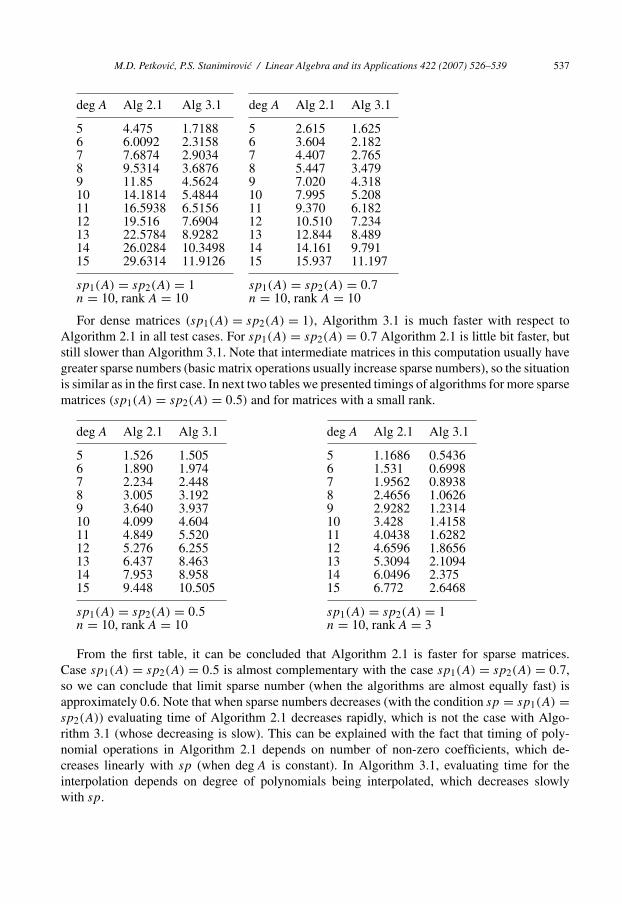
deg A Alg 2.1 Alg 3.1

5 4.475 1.71886 6.0092 2.31587 7.6874 2.90348 9.5314 3.68769 11.85 4.562410 14.1814 5.484411 16.5938 6.515612 19.516 7.690413 22.5784 8.928214 26.0284 10.349815 29.6314 11.9126

deg A Alg 2.1 Alg 3.1

5 2.615 1.6256 3.604 2.1827 4.407 2.7658 5.447 3.4799 7.020 4.31810 7.995 5.20811 9.370 6.18212 10.510 7.23413 12.844 8.48914 14.161 9.79115 15.937 11.197

sp1(A) = sp2(A) = 1 sp1(A) = sp2(A) = 0.7n = 10, rank A = 10 n = 10, rank A = 10

For dense matrices (sp1(A) = sp2(A) = 1), Algorithm 3.1 is much faster with respect toAlgorithm 2.1 in all test cases. For sp1(A) = sp2(A) = 0.7 Algorithm 2.1 is little bit faster, butstill slower than Algorithm 3.1. Note that intermediate matrices in this computation usually havegreater sparse numbers (basic matrix operations usually increase sparse numbers), so the situationis similar as in the first case. In next two tables we presented timings of algorithms for more sparsematrices (sp1(A) = sp2(A) = 0.5) and for matrices with a small rank.

deg A Alg 2.1 Alg 3.1

5 1.526 1.5056 1.890 1.9747 2.234 2.4488 3.005 3.1929 3.640 3.93710 4.099 4.60411 4.849 5.52012 5.276 6.25513 6.437 8.46314 7.953 8.95815 9.448 10.505

deg A Alg 2.1 Alg 3.1

5 1.1686 0.54366 1.531 0.69987 1.9562 0.89388 2.4656 1.06269 2.9282 1.231410 3.428 1.415811 4.0438 1.628212 4.6596 1.865613 5.3094 2.109414 6.0496 2.37515 6.772 2.6468

sp1(A) = sp2(A) = 0.5 sp1(A) = sp2(A) = 1n = 10, rank A = 10 n = 10, rank A = 3

From the first table, it can be concluded that Algorithm 2.1 is faster for sparse matrices.Case sp1(A) = sp2(A) = 0.5 is almost complementary with the case sp1(A) = sp2(A) = 0.7,so we can conclude that limit sparse number (when the algorithms are almost equally fast) isapproximately 0.6. Note that when sparse numbers decreases (with the condition sp = sp1(A) =sp2(A)) evaluating time of Algorithm 2.1 decreases rapidly, which is not the case with Algo-rithm 3.1 (whose decreasing is slow). This can be explained with the fact that timing of poly-nomial operations in Algorithm 2.1 depends on number of non-zero coefficients, which de-creases linearly with sp (when deg A is constant). In Algorithm 3.1, evaluating time for theinterpolation depends on degree of polynomials being interpolated, which decreases slowlywith sp.

538 M.D. Petkovic, P.S. Stanimirovic / Linear Algebra and its Applications 422 (2007) 526–539

The second table shows that rank of the matrix A has great influence on timings of bothalgorithms. Algorithm 3.1 is also faster than Algorithm 2.1 for the matrices with a small rank.Let us now consider two cases where sparse numbers are not equal:

deg A Alg 2.1 Alg 3.1

5 0.404 1.27710 0.658 2.50115 0.794 3.375

sp1(A) = 0.1, sp2(A) = 1n = 10, rank A � 10

deg A Alg 2.1 Alg 3.1

5 1.166 1.2767 1.781 2.22910 3.150 4.182

sp1(A) = 1, sp2(A) = 0.1n = 10, rank A � 10

n Alg 2.1 Alg 3.1

5 0.398 0.3476 1.027 0.6997 2.257 1.3128 4.582 2.2109 8.437 3.60110 14.656 5.59311 23.750 8.42512 37.499 12.030

sp1(A) = 1, sp2(A) = 1deg A = 10, rank A = n

When one of the sparse number is small, Algorithm 2.1 is also faster than Algorithm 3.1. Notethat time of Algorithm 2.1 reduces rapidly when either sp1(A) or sp2(A) is small. In the caseof interpolation (Algorithm 3.1) sp2(A) almost does not influence on timing which is not thecase with sp1(A). When sp1(A) is small, degree matrix dgA(s) has large number of elementsequal to −∞. Also the same holds for output matrix of Algorithm 4.1 (function DegreeEstima-tor[A, i, var]), but this number is smaller. This accelerates the matrix interpolation (functionAdvMatrixMinInterpolation[TB, Deg, var]).

In the last table we showed the timings of both algorithms for n = 5, . . . , 12. Using the linearinterpolation in log–log scale we established approximate complexities: O(n5.19) and O(n4.06) forAlgorithm 2.1 and Algorithm 3.1 respectively. This confirms validity of theoretically establishedcomplexities. Also we used the similar method for estimating the complexities as a function ofd = degA. All tables gave approximately equal complexities O(d1.7) for both algorithms. Thisalso proves theoretically established complexities at the end of sections 2 and 3. At the end of thissection, the final complexities of Algorithm 2.1 and Algorithm 3.1 can be stated again: O(n5 · d2)

and O(n4 · d2) respectively.

7. Conclusion

We compared two algorithms for computing the Drazin inverse of polynomial matrix A(s).The first algorithm is the extension of the Leverrier–Faddeev method and it is restated from [8]and [16]. The second one uses the polynomial interpolation, arising from the corresponding oneintroduced in [15].

Both algorithms are implemented in symbolic programming language MATHEMATICA andtested on several classes of test examples which proved established complexities. In practice, theinterpolation algorithm was faster on dense matrices.

M.D. Petkovic, P.S. Stanimirovic / Linear Algebra and its Applications 422 (2007) 526–539 539

References

[1] F. Bu, Y. Wei, The algorithm for computing the Drazin inverses of two-variable polynomial matrices, Appl. Math.Comput. 147 (2004) 805–836.

[2] S.L. Campbell (Ed.), Recent Applications of Generalized Inverses, Pitman, London, 1982.[3] G. Fragulis, B.G. Mertzios, A.I.G. Vardulakis, Computation of the inverse of a polynomial matrix and evaluation of

its Laurent expansion, Int. J. Control 53 (1991) 431–443.[4] T.N.E. Grevile, The Souriau–Frame algorithm and the Drazin pseudoinverse, Linear Algebra Appl. 6 (1973)

205–208.[5] C.W. Groetsch, Representation of the generalized inverse, J. Math. Anal. Appl. 49 (1975) 154–157.[6] C.W. Groetsch, Generalized Inverses of Linear Operators, Marcel Dekker, Inc., New York and Basel, 1977.[7] R.E. Hartwig, More on the Souriau–Frame algorithm and the Drazin inverse, SIAM J. Appl. Math. 31 (1) (1976)

42–46.[8] J. Ji, A finite algorithm for the Drazin inverse of a polynomial matrix, Appl. Math. Comput. 130 (2002) 243–251.[9] J. Ji, An alternative limit expression of Drazin inverse and its application, Appl. Math. Comput. 61 (1994) 151–156.

[10] J. Jones, N.P. Karampentakis, A.C. Pugh, The computation and application of generalized inverse via Maple, J.Symbolic Comput. 25 (1998) 99–124.

[11] N.P. Karampentakis, Computation of generalized inverse of polynomial matrix and applications, Linear AlgebraAppl. 252 (1997) 35–60.

[12] N.P. Karampentakis, S. Vologianidis, DFT calculation of generalized and Drazin inverse of polynomial matrix,Appl.Math. Comput. 143 (2003) 501–521.

[13] N.P. Karampetakis, Generalized inverses of two-variable polynomial matrices and applications, Circuits Syst. SignalProcess. 16 (1997) 439–453.

[14] W.H. Press, S.A. Teukolsky, W.T. Wetterling, B.P. Flannery, Numerical Receipts in C, Cambridge University Press,Cambridge (MA), 1992.

[15] A. Schuster, P. Hippe, Inversion of polynomial matrices by interpolation, IEEE Trans. Automat. Control 37 (3)(1992) 363–365.

[16] P.S. Stanimirovic, M.B. Tasic, Drazin inverse of one-variable polynomial matrices, Filomat, Niš 15 (2001) 71–78.[17] G. Wang, Y. Wei, S. Qiao, Generalized Inverses: Theory and Computations, Science Press, Beijing/New York, 2004.[18] Y. Wei, H. Wu, The representation and approximation for Drazin inverse, J. Comput. Appl. Math. 126 (2000)

417–432.[19] Y. Wei, Index splitting for the Drazin inverse and the singular linear system,Appl. Math. Comput. 95 (1998) 115–124.[20] S. Wolfram, Mathematica Book, Version 3.0, Wolfram Media and Cambridge University Press, 1996.[21] S. Wolfram, The Mathematica Book, fourth ed., Wolfram Media/Cambridge University Press, 1999.[22] G. Zielke, Report on test matrices for generalized inverses, Computing 36 (1986) 105–162.