Polynomial and Radonal Functions
98
x3 VI and Internet tide answers to amulative Tests. Pre-Tests (that ;pts covered in :hapter Post- re randomly diagnostic Polynomial and Radonal Functions 2.1 Quadratic Functions 2.5 The Fundamental Theorem of Algebra 2.2 Polynomial Functions of Higher Degree 2.6 Rational Functions and Asymptotes 2,3 Real Zeros of Polynomial Functions 2.7 Graphs of Rational Functions 2.4 Complex Numbers In this chapter you will learn how to lj sketch and analyze graphs of quadratic and polynomial functions. use long division and synthetic division to divide polynomials by other polynomials. o determine the number of rational and real i N zeros of polynomial functions, and find them. C - J perform operations with complex num- bers and plot cokaplex numbers in the complex plane. CI determine the domain, find asymptotes, and sketch the graphs of rational functions. U.S. wheat production increased from 2183 million bushels in 1995 to 2527 million bushels in 1997, while the price per bushel dropped from S4.55 to 83.45. (Source: US. Department of Agriculture) Important Vocabulary As you encounter each new vocabulary term in this chapter, add the term and its definition to your notebook glossary. • polynomial function (p. 136) • constant function (p. 136) • linear function (p. 136) • quadratic function (p. 136) • parabola (p. 136) • axis of symmetry (p. 137) • vertex (p. 137) • continuous (p. 147) • Leading Coefficient Test (p. 149) • extrema (p. 150) • repeated zero (p. 152) • multiplicity (p. 152) • complex plane (p. 178) • imaginary axis (p. 178) • real axis (p. 178) • Fundamental Theorem of Algebra (p. 182) • Linear Factorization Theorem (p. 182) • rational function (p. 189) • vertical asymptote (p. 190) • horizontal asymptote (p. 190) • slant (or oblique) asymptote (p. 202) • Intermediate Value Theorem (p. 154) • long division of polynomials (p. 160) • Division Algorithm (p. 161) • synthetic division (p. 163) • Remainder Theorem (p. 164) • Factor Theorem (p. 164) • Rational Zero Test (p. 166) • upper bound (p. 168) • lower bound (p. 168) • imaginary unit i (p. 174) • complex number (p. 174) • complex conjugates (p. 177) / Resources Text-specific additional resources are available to help you do well in this course. See page xvi for details. 135
-
Upload
khangminh22 -
Category
Documents
-
view
1 -
download
0
Transcript of Polynomial and Radonal Functions

x3
VI and Internet tide answers to amulative Tests. Pre-Tests (that ;pts covered in :hapter Post-re randomly diagnostic
Polynomial and Radonal Functions 2.1
Quadratic Functions 2.5 The Fundamental Theorem of Algebra
2.2 Polynomial Functions of Higher Degree 2.6 Rational Functions and Asymptotes
2,3 Real Zeros of Polynomial Functions 2.7 Graphs of Rational Functions
2.4 Complex Numbers
In this chapter you will learn how to
lj sketch and analyze graphs of quadratic and polynomial functions. use long division and synthetic division to divide polynomials by other polynomials.
o determine the number of rational and real iN zeros of polynomial functions, and find
them. C-J perform operations with complex num-
bers and plot cokaplex numbers in the complex plane.
CI determine the domain, find asymptotes, and sketch the graphs of rational functions.
U.S. wheat production increased from 2183 million bushels in 1995 to 2527 million bushels in 1997,
while the price per bushel dropped from S4.55 to 83.45. (Source: US. Department of Agriculture)
Important Vocabulary As you encounter each new vocabulary term in this chapter, add the term and its definition to your notebook glossary.
• polynomial function (p. 136) • constant function (p. 136) • linear function (p. 136) • quadratic function (p. 136) • parabola (p. 136) • axis of symmetry (p. 137) • vertex (p. 137) • continuous (p. 147) • Leading Coefficient Test (p. 149) • extrema (p. 150) • repeated zero (p. 152) • multiplicity (p. 152)
• complex plane (p. 178) • imaginary axis (p. 178) • real axis (p. 178) • Fundamental Theorem of Algebra
(p. 182) • Linear Factorization Theorem (p. 182) • rational function (p. 189) • vertical asymptote (p. 190) • horizontal asymptote (p. 190) • slant (or oblique) asymptote (p. 202)
• Intermediate Value Theorem (p. 154) • long division of polynomials (p. 160) • Division Algorithm (p. 161) • synthetic division (p. 163) • Remainder Theorem (p. 164) • Factor Theorem (p. 164) • Rational Zero Test (p. 166) • upper bound (p. 168) • lower bound (p. 168) • imaginary unit i (p. 174) • complex number (p. 174) • complex conjugates (p. 177)
/ Resources Text-specific additional resources are available to help you do well in this course. See page xvi for details.
135

136 Chapter 2 • Polynomial and Rational Functions
You Should Learn:
All parabol or simply t1
ola is the Ire
a is positivt and if the h a parabola 1
The Graph of a Quadratic Function
In this and the next section, you will study the graphs of polynomial functions.
Definition of Polynomial Function
Let n be a nonnegative integer and let an, . . . , a2, a1, ac, be real numbers with an 0. The function
f(x) = anxn an-ixn-1 + • • • + a2x2 + ai x + aa
is called a polynomial function of x with degree n.
Polynomial functions are classified by degree. For instance, the polynomial function
f(x) = a, a 0 0 Constant function
has degree 0 and is called a constant function. In Chapter P, you learned that the graph of this type of function is a horizontal line. The polynomial function
f(x) = mx + b, m 0 0 Linear function
has degree 1 and is called a linear function. You also learned in Chapter P that the graph of the linear function f(x) = mx + b is a line whose slope is m and whose y-intercept is (0, b). In this section you will study second-degree polyno-mial functions, which are called quadratic functions.
Definition of Quadratic Function
Let a, b, and c be real numbers with a 0 0. The function
f(x) = ax 2 + bx + c Quadratic function
is called a quadratic function.
• How to analyze graphs of quadratic functions
• How to write quadratic functions in standard form and use the results to sketch graphs of functions
• How to use quadratic functions to model and solve real-life problems
Axis
Opens
You Should Learn It:
Quadratic functions can be uset to model data to analyze con-sumer behavior. For instance, Exercise 78 on page 146 shows how a quadratic function can model VCR usage in the Unite( States. The simplesi
f(x) =
Its graph is 2 point on the shown in Fii
Figure 2.1
c "40
Often real-life data can be modeled by quadratic functions. For instance, the table shows height h (in feet) of a projectile fired from a height of 6 feet with an initial velocity of 256 feet per second at any time t (in seconds). A quadratic model for the data in the table is h(t) = —16t2 + 256t + 6 for 0 t 16.
t 0 2 4 6 8 10 12 14 16
h 6 454 774 966 1030 966 774 454 6
The graph of a quadratic function is a special type of U-shaped curve called a parabola. Parabolas occur in many real-life applications—especially those involving reflective properties, such as satellite dishes or flashlight reflectors. You will study these properties in Section 10.1.
Figure 2.2
When sketc as a referer graph of y ' the graph o strated agai

1111111111111111111111111/1
earn:
;raphs of ns tdratic lard form ts to sketch us ratic el and solve
larn It:
can be used tlyze con-instance, 146 shows
ction can n the United
Opens upward
Vertex is low point
Figure 2.1
Use a graphing utility to graph the parabola
y - ax 2
for a = —3, —2, —1, 1, 2, and 3. What can you conclude about
I
Ahe parabola when a < 0? When - a > 0?
Library of Functions The graph of a quadratic function is called a parabola. Graph y1 = x2 and y2 = 'xi in the same viewing window. Zoom in near the origin and compare the shape of the two graphs. Which graph grows faster as x gets larger and larger? Why does the definition of a quadratic function require that a 0 0?
Consult the Library of Functions Summary inside the front cover for a description of the quadratic function.
2.1 • Quadratic Functions 137
All parabolas are symmetric with respect to a line called the axis of symmetry, rrnply the axis of the parabola. The point where the axis intersects the parab-
s or is the vertex of the parabola, as shown in Figure 2.1. If the leading coefficient la o
a is positive, the graph of f(x) = ax2 + bx + c is a parabola that opens upward; A if the leading coefficient a is negative, the graph of f(x) = ax 2 + bx + c is art,.
a parabola that opens downward.
Opens downward
The simplest type of quadratic function is
f(x)
Its graph is a parabola whose vertex is (0, 0). If a > 0, the vertex is the minimum point on the graph; and if a < 0, the vertex is the maximum point on the graph, as shown in Figure 2.2.
-3 -2 -1 -1
3
Minimum: (0, 0) -2 -
Figure 2.2
sWhen
a sketching the graph of f(x) =- ax2, it is helpful to use the graph of y = x 2
a reference, as discussed in Section 1.3. There you saw that when a > 1, the graph of y af (x) is a vertical stretch of the graph of y = f(x). When 0 < a < 1, the graph of y = af (x) is a vertical shrink of the graph of y = f (x) . This is demon-strated again in Example 1.

y = x2] 7 F.L.(x). 1)_,-,x21 7 [g(x) = 2x2
6 6 6 6
=
= f(- 4
Reflection in x-axis
Reflection in y-axis
y = f(x ± c) Horizontal shift
y = f(x) ± c Vertical shift
138 Chapter 2 • Polynomial and Rational Functions
EXAMPLE 1 Graphing Simple Quadratic Functions
Describe how the graph of each function is related to the graph of y = x2.
1 a. f(x) = —
3 x2 b. g(x) = 2x2
c. h(x) = —x2 + 1 d. k(x) = (x + 2)2 — 3
Solution a. Compared with y = x2, each output of f "shrinks" by a factor of 1. The result
is a parabola that opens upward and is broader than the parabola represented by y = x2, as shown in Figure 2.3(a).
b. Compared with y = x2, each output of g "stretches" by a factor of 2, creating a narrower parabola, as shown in Figure 2.3(b).
c. With respect to the graph of y = x2, the negative coefficient in h(x) = —x2 + 1 reflects the graph downward and the positive constant term shifts the vertex up one unit. The graph of h is shown in Figure 2.3(c).
d. With respect to the graph of y = x2, the graph of k(x) -= (x + 2)2 — 3 is obtained by a horizontal shift two units to the left and a vertical shift three units down, as shown in Figure 2.3(d).
(a) (b)
y = x2
-7 1 '
(-2, -3 -4
(c)
Figure 2.3
Recall from Section 1.3 that the graphs of y = f(x ± c), y = f(x) ± c, y = —f(x), and y = f(-4 are rigid transformations of the graph of y = f(x).
(d)
The Interactive CD-ROM and Internet versions of this text show every example, with its solution; clicking on the Try It! button brings up similar problems. Guided Examples and Integrated Examples show step-by-step solutions to additional examples. Integrated Exampl are related to several concepts in the section.
In Example 1, note that the coefficient a determines how widely the parabola given by f(x) = ax2 opens. If lal is small, the parabola opens more widely than if lal is large.
STUDY TIP
A

• ‘ Exploration Use a graphing utility to grap y = ax2 with a = —2, —1, —0.5, 0.5, 1, and 2. How does the value of a affect the graph?
Use a graphing utility to graph y = (x — h)2 with h= —4, —2, 2, and 4. How does the value of h affect the
,graph? Use a graphing utility to
graph y = x2 + k with k = — —2, 2, and 4. How does the value of k affect the graph?
2.1 • Quadratic Functions 139
f(x)= 2x + 8x + 7 //—
'OP
that the Lines how given by lal is small,
more widely
4 and Internet v every example
on the Try It! problems. tegrated step solutions to ;grated Examples icepts in the
The Standard Form of a Quadratic Function
The equation in Example 1(d) is written in the standard form
f(x) = a(x — h)2 + k.
This form is especially convenient for sketching a parabola because it identifies
tile vertex of the parabola as (h, k).
Standard Form of a Quadratic Function
The quadratic function
f(x) = a(x — h)2 + k, a * 0
is said to be in standard form. The graph of f is a parabola whose axis is the vertical line x = h and whose vertex is the point (h, k). If a > 0, the parabola
opens upward, and if a < 0, the parabola opens downward.
EXAMPLE 2 Identifying the Vertex of a Quadratic Function
Describe the graph of
f(x) = 2x2 + 8x + 7
and identify the vertex.
Solution Write the quadratic function in standard form by completing the square. Recall that the first step is to factor out any coefficient of x2 that is different from 1.
f(x) = 2x2 + 8x + 7
= 2(x2 + 4x) + 7
= 2(x2 + 4x + 4 — 4) + 7
I t
(D2 = 2(x2 + 4x + 4) — 2(4) + 7 Regroup terms.
= 2(X + 2)2 — 1 Write in standard form.
From the standard form, you can see that the graph of f is a parabola that opens upward with vertex (-2, —1), as shown in Figure 2.4.
Write original function.
Factor 2 out of x-terms.
Because b = 4, add and subtract (b/2)2 = 4 within parentheses.
3
—2 Figure 2.4
140 Chapter 2 • Polynomial and Rational Functions
To find the x-intercepts of the graph of f(x) = ax2 + bx + c, solve the equation ax 2 + bx + c = 0. If ax 2 + bx + c does not factor, you can use the Quadratic Formula to find the x-intercepts, or a graphing utility to approximate the x-intercepts. Remember, however, that a parabola may have no x-intercept.
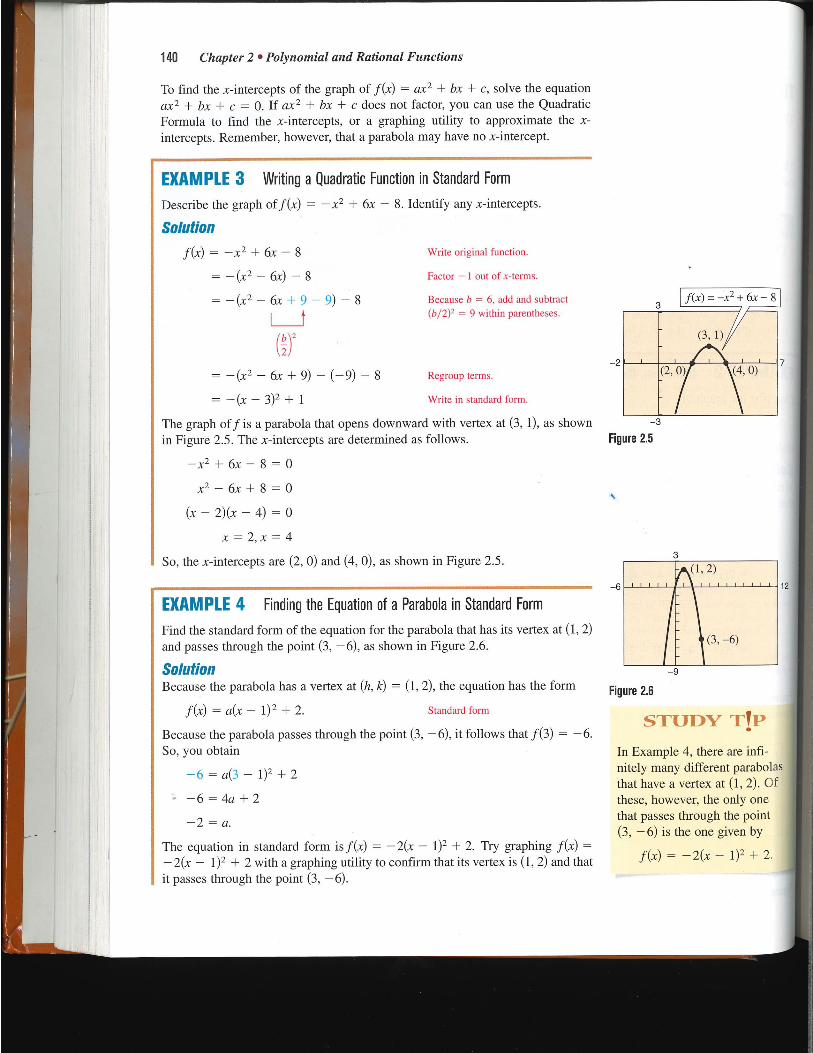
EXAMPLE 3 Writing a Quadratic Function in Standard Form
Describe the graph of f(x) = —x2 + 6x — 8. Identify any x-intercepts.
Solution
f(x) = -x 2 + 6x — 8
Write original function.
= —(x2 — 6x) — 8
Factor — 1 out of x-terms.
= —(x2 — 6x + 9 — 9) — 8 Because b = 6, add and subtract
I
(b/2)2 = 9 within parentheses.
(b2)2
= —(x2 — 6x + 9) — (-9) — 8 Regroup terms.
= —(x — 3)2 + 1
Write in standard form.
The graph off is a parabola that opens downward with vertex at (3, 1), as shown in Figure 2.5. The x-intercepts are determined as follows.
—x2 + 6x — 8 = 0
x2 — 6x + 8 = 0
(x — 2)(x — 4) = 0
x = 2, x = 4
So, the x-intercepts are (2, 0) and (4, 0), as shown in Figure 2.5.
EXAMPLE 4 Finding the Equation of a Parabola in Standard Form
Find the standard form of the equation for the parabola that has its vertex at (1, 2) and passes through the point (3, —6), as shown in Figure 2.6.
Solution Because the parabola has a vertex at (h, = (1, 2), the equation has the form
f(x) = a(x — 1) 2 + 2. Standard form
Because the parabola passes through the point (3, —6), it follows that f(3) = —6. So, you obtain
— 6 = a(3 — 1)2 + 2
— 6 = 4a + 2
— 2 = a.
The equation in standard form is f(x) = —2(x — 1)2 + 2. Try graphing f(x) = —2(x — 1)2 + 2 with a graphing utility to confirm that its vertex is (1, 2) and that it passes through the point (3, —6).
3 f(x) = - + 6x -
2
—3
Figure 2.5
(1,2) I I I I I I I
(3,-6)
Figure 2.6
STUDY TtP
In Example 4, there are infi-nitely many different parabola that have a vertex at (1, 2). Of these, however, the only one that passes through the point (3, —6) is the one given by
f(x) = —2(x — 1)2 + 2

Ng draic Solution
For his quadratic function, you have
r(x) = ax 2 + bx + c
= -0.0032x2 + x + 3
which implies that a = -0.0032 and b = 1. Because the Unction has a maximum when x = - b1(2a), you :;an conclude that the baseball reaches its maxi-mum height when
- -
2a
2(- 0.0032)
= 156.25 feet
from home plate. At this distance, the maximum height is
(l56.25) = _0.0032(!56.25)2 + 156.25 + 3
= 81.125 feet.
2.1 • Quadratic Functions 141
Applications
2. I
many applications involve finding the maximum or minimum value of a quad-ratic function. By writing the quadratic function f(x) = ax2 + bx + c in stan-
dard form,
f(x) a( b2
x + --) + ( b2
c - — 2a 4a
:;an see that the vertex occurs at x = -b/(2a), which implies the following.
' a > 0, f has a minimum that occurs at
x =- 2a
you
1. I
STUDY 11P
To obtain the standard form at the left, you can complete the square of the form
f(x) = ax2 + bx + C.
Try verifying this computation.
a < 0, f has a maximum that occurs at
x = 2a
EXAMPLE 5 The Maximum Height of a Baseball
A baseball is hit 3 feet above ground at a velocity of 100 feet per second and at an angle of 45 degrees with respect to level ground. The path of the baseball is given by the function f(x) = - 0.0032x2 + x + 3, where f(x) is the height of the baseball (in feet) and x is the horizontal distance from home plate (in feet). What is the maximum height reached by the baseball? (See Example 7 in Section 1.1.)
A computer simulation of this example appears in the Interactive CD-ROM and Internet versions of this text.
r TIP
3 are infi-nt parabolas it (1, 2). Of only one the point
given by
- 1)2 + 2.
12
Graphical Solution
Use a graphing utility to graph y = - 0.0032x2 + x + 3 so that you can see the important features of the parabola. In Figure 2.7 the graph appears to have a maximum near x = 150. Use the maximum feature of the graphing utility or the zoom and trace features to approximate the maximum height on the graph to be y 81.125 feet at x 156.25. Note that when using the zoom and trace features of a graph-ing utility, you might have to change the y-scale in order to avoid a graph that is "too flat."
y = —0.0032x2 + x + 3
100 200 300 400
Distance (in feet)
Figure 2.7
-6)
100
80
60
40
43 20

6
0 5 a)
4
t' 3 a) c.) 2 a)
1 Minimum X=54.607148 Y=1.6802839.1
20 40 60 80 100 120
Income (in thousands of dollars)
The parabola in the figure below has an equation of the form
y = ax2 + bx — 4.
Find the equation for this parabola in two different ways, by hand and with technology (graphing utility or computer software). Write a paragraph de-scribing the methods you used and comparing the results of the two methods.
- (2,2)
_ —12
7
142 Chapter 2 • Polynomial and Rational Functions
EXAMPLE 6 Charitable Contributions
According to a survey conducted by Independent Sector, the percent of their income that Americans give to charities is related to their household income. For families with an annual income of $100,000 or less, the percent is approximately
P = 0.0014x2 — 0.1529x + 5.855, 5 x 100
where P is the percent of annual income given and x is the annual income (in thousands of dollars). According to this model, what income level corresponds to the minimum percent of charitable contributions?
Graphical Solution
Use a graphing utility to graph
yi = 0.0014x2 — 0.1529x + 5.855
for 5 x 100, as shown in Figure 2.8. The graph appears to have a minimum near x = 55. Use the minimum feature of the graphing utility or the zoom and trace features to approximate the minimum point of the parabola to be x 54.6, So, the minimum point corresponds to an income level of about $54,600.
Figure 2.8
Algebraic Solution
Use the fact that the minimum point of the parabola occurs when x = — b1(2a). For this function, you have a = 0.0014 and b = —0.1529. So,
x = --
2a
—0.1529 2(0.0014)
54.6.
From this x-value, you can con-clude that the minimum percent corresponds to an income level of about $54,600.

16. f(x) = 16 -
18. f(x) = (x - 6)2 + 3 20. g(x) = x 2 + 2x + 1
22. f(x) = x2 + 3x +
24. f(x) = -x2 - 4x + 1
26. f(x) = 2x2 - x + 1
8 15. f(x) = - 4
17. f(x) = (x + 4)2 - 3
19. h(x) = x2 - 8x + 16
21. f(x) = x2 - x +
23. f(x) = -x2 + 2x + 5
25. h(x) = 4x2 - 4x + 21
4 4 -5
-3
5 (d) (c)
8
(f) (e) 6
3 4 -5
11. (a) y = (x - 1)2
(C) y = (x - 3)2
12. (a) y - - 12-(x 2)2 + 1
(c) y = + 2)2 - 1
(b) y = (x + 1)2
(d) y = (x + 3)2
(b) y =1(x - 2)2 + 1
(d) y = + 2)2 - 1
35. Exploration In Exercises 9-12, use a graphing util-ity to graph each equation. Describe how the graph of each equation is related to the graph of y = x 2.
9. (a) y = x 2 (b) y = _ x2
(C) y = x 2 (d) y = -3x2 10. (a) y = x2 ± 1 (b) y = x2 - 1
(c) y = x2 + 3 (d) y = x2 - 3
MI6 r . • CACIUlbeb
In Exercises 1-8, match the quadratic function with the correct graph. [The graphs are labeled (a), (b), (c), (d), (e), (f), (g), and (h).]
(a) 3 (b)
5 In Exercises 13-26, sketch the graph of the quadratic function. Identify the vertex and intercepts. Use a graphing utility to verify your results.
13. f(x) = 25 - x2 14. f(x) = x2 - 7
In Exercises 27-34, use a graphing utility to graph the
6 quadratic function. Identify the vertex and intercepts. Then check your results alrbraically by completing the square.
(g) 5 (h) 4
27. f(x) = - (x2 + 2x - 3)
28. f(x) = -(x2 + x - 30)
-4
5 29. g(x) = x2 + 8x + 11 30. f(x) = x2 + 10x + 14
3
6
31. f(x) = 2x2 - 16x + 31
-2
32. f(x) = -4x2 + 24x - 41 1. f(x) = (x - 2)2 2. f(x) = (x + 4)2
33. g(x) = (x 2 + 4x - 2) 34. f(x) = i(x2 + 6x - 5) 3. f(x) =- x2 - 2 4. f(x) = 3 - x2
5. f(x) = 4 - (x - 2)2 6. f(x) = (x + 1)2 - 2
In Exercises 35-38, find an equation for the parabola.
7. f(x) = x2 + 3 8. f(x) = - (x - 4)2
Use a graphing utility to graph the equation and verify your result.
we a minimum - the zoom and to be x 54.6. $54,600.
® The Interactive CD-ROM and Internet versions of this text contain step-by-step solutions to all odd-numbered Section and Review Exercises. They also provide Tutorial Exercises, which link to Guided Examples for additional help.
3
-3
-5
5
2.1 • Quadratic Functions 143
144 Chapter 2 • Polynomial and Rational Functions
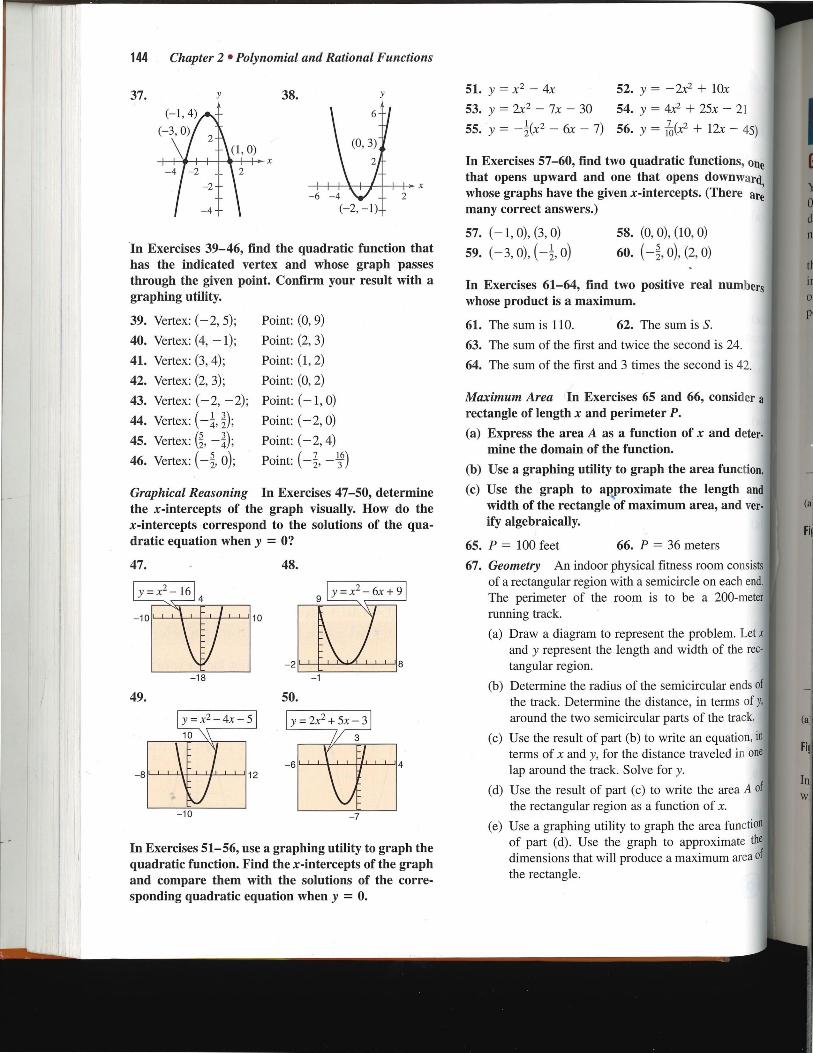
37. Y 38. (-1, 4)
(-3,0) (1,0)
In Exercises 39-46, find the quadratic function that has the indicated vertex and whose graph passes through the given point. Confirm your result with a graphing utility.
39. Vertex: (-2, 5);
40. Vertex: (4, —1);
41. Vertex: (3, 4);
42. Vertex: (2, 3);
43. Vertex: (-2, —2);
44. Vertex:(—, );
45. Vertex: (, —i);
46. Vertex: (-3, 0);
Point: (0, 9)
Point: (2, 3)
Point: (1,2)
Point: (0, 2)
Point: (-1,0)
Point: (-2, 0)
Point: (-2,4) 7 16 Point: (—
Graphical Reasoning In Exercises 47-50, determine the x-intercepts of the graph visually. How do the x-intercepts correspond to the solutions of the qua-dratic equation when y = 0?
47. 48.
Y = — 16
10
9 y = x2 — 6x + 9
III —2 8
' '10
-1 -1
49. 50.
y = x2 — 4x —5 10
—10
12 8 I I 1 I I
In Exercises 51-56, use a graphing utility to graph the quadratic function. Find the x-intercepts of the graph and compare them with the solutions of the corre-sponding quadratic equation when y = 0.
51. y = x2 — 4x 52. y = 2x2 + 10x
53. y = 2x2 — 7x — 30 54. y = 4x2 + 25x — 21
55. y =(x 2 — 6x — 7) 56. y = Ii(x2 + 12x — 4
In Exercises 57-60, find two quadratic functions, 0fle that opens upward and one that opens downward, whose graphs have the given x-intercepts. (There are many correct answers.)
57. (— 1, 0), (3, 0)
59. (-3, 0), ( —1, 0)
58. (0, 0), (10, 0)
60. ( 0), (2, 0)
In Exercises 61-64, find two positive real numb whose product is a maximum.
61. The sum is 110. 62. The sum is S.
63. The sum of the first and twice the second is 24.
64. The sum of the first and 3 times the second is 42
Maximum Area In Exercises 65 and 66, conside rectangle of length x and perimeter P.
(a) Express the area A as a function of x and det mine the domain of the function.
Fil
In
(b) Use a graphing utility to graph the area function.
(c) Use the graph to approximate the length and width of the rectangle of maximum area, and ver- (a
ify algebraically. Fl!
65. P = 100 feet 66. P = 36 meters
67. Geometry An indoor physical fitness room consists of a rectangular region with a semicircle on each end. The perimeter of the room is to be a 200-mete running track.
(a) Draw a diagram to represent the problem. Let and y represent the length and width of the rec-tangular region.
(b) Determine the radius of the semicircular ends of
the track. Determine the distance, in terms of y
around the two semicircular parts of the track. (a
(c) Use the result of part (b) to write an equation, in terms of x and y, for the distance traveled in one
lap around the track. Solve for y.
(d) Use the result of part (c) to write the area A the rectangular region as a function of x.
(e) Use a graphing utility to graph the area function
of part (d). Use the graph to approximate the
dimensions that will produce a maximum area of the rectangle.

2.1 • Quadratic Functions 145
68. Numerical, Graphical, and Analytical Analysis A rancher has 200 feet of fencing to enclose two adja-cent rectangular corrals. Use the following methods to determine the dimensions that will produce a maximum enclosed area.
mime ..,..70099.,,,, ............--...1A. .... ....71........
t,....1... ....1....-44 Af
......po # ....... rem vv. ......
(a) Complete six rows of a table such as the one below. (The first two rows are shown.)
x y Area
2 [200 — 4(2)] 2xy = 256
4 1[200 — 4(4)] ay .---- 491
(b) Use a graphing utility to generate additional rows of the table in part (a). Use the table to estimate the dimensions that will produce the maximum enclosed area.
(c) Write the area A as a function of x.
(d) Use a graphing utility to graph the area function. Use the graph to approximate the dimensions that will produce the maximum enclosed area.
(e) Write the area function in standard form to find algebraically the dimensions that will produce the maximum area.
(f) Compare your results from parts (b), (d), and (e).
69. Business A manufacturer of lighting fixtures has daily production costs of
C = 800 — 10x + 0.25x2
where C is the total cost (in dollars) and x is the number of units produced. How many fixtures should be produced each day to yield a minimum cost?
70. Business A textile manufacturer has daily produc-tion Costs of
C = 10,000 — 110x + 0.45x2
where C is the total cost (in dollars) and x is the number of units produced. How many units should be produced each day to yield a minimum cost?
71. Business The profit P (in dollars) for a company is
P = —0.0002x2 + 140x — 250,000
where x is the number of units sold. What sales level will yield maximum profit?
72. Business The profit P (in hundreds of dollars) that a company makes depends on the amount x (in hun-dreds of dollars) the company spends on advertising according to the model
P = 230 + 20x — 0.5x2.
What expenditure for advertising results in the max-imum profit?
73. Trajectory of a Ball The height y (in feet) of a ball thrown by a child is
y = + 2x + 4
where x is the horizontal distance (in feet) from where the ball is thrown.
(a) Use a graphing utility to graph the path of the ball.
(b) How high is the ball when it leaves the child's hand? (Hint: Find y when x = 0.)
(c) How high is the ball when it is at its maximum height?
(d) How far from the child does the ball strike the ground?
74. Maximum Height of a Dive The path of a diver is
12 y = 2 24x +
where y is the height (in feet) and x is the horizontal distance (in feet) from the end of the diving board. What is the maximum height of the dive? Verify your answer using a graphing utility.

146 Chapter 2 • Polynomial and Rational Functions
75. Forestry The number of board feet V in a 16-foot log is approximated by the model
V = 0.77x2 — 1.32x — 9.31, 5 x 40
where x is the diameter (in inches) of the log at the small end. (One board foot is a measure of volume equivalent to a board that is 12 inches wide, 12 inch-es long, and 1 inch thick.)
(a) Use a graphing utility to graph the function.
(b) Estimate the number of board feet in a 16-foot log with a diameter of 16 inches. Use a graphing utility to verify your answer.
(c) Estimate the diameter of a 16-foot log that scaled 500 board feet when the lumber was sold. Use a graphing utility to verify your answer.
76. Automobile Aerodynamics The number of horse-power y required to overcome wind drag on a certain automobile is approximated by
y = 0.002s2 + 0.005s — 0.029, 0 s 100
where s is the speed of the car in miles per hour.
(a) Use a graphing utility to graph the function.
(b) Graphically estimate the maximum speed of the car if the power required to overcome wind drag is not to exceed 10 horsepower. Verify your result algebraically.
77. Graphical Analysis For certain years from 1950 to 1990, the average annual per capita consumption C of cigarettes by Americans (18 and older) can be modeled by C = 3248.89 + 108.64t — 2.97t2 for 0 t < 40, where t is the year, with t = 0 corre-sponding to 1950. (Source: U.S. Department of Agriculture)
(a) Use a graphing utility to graph the model.
(b) Use the graph of the model to approximate the maximum average annual consumption. Beginning in 1966, all cigarette packages were required by law to carry a health warning. Do you think the warning had any effect? Explain.
(c) In 1960, the U.S. population (18 and over) was 116,530,000. Of those, about 48,500,000 were smokers. What was the average annual cigarette consumption per smoker in 1960? What was the average daily cigarette consumption per smoker?
78. Data Analysis The number y (in millions) of VCRs in use in the United States for the years 1987 through 1996 are shown in the table. The variable t represents time (in years), with t = 7 corresponding to 1987.
t 7 8 9 10 11 12 13 14 15 16
y 43 51 58 63 67 69 72 74 77 79
(Source: Television Bureau of Advertising, Inc.)
(a) Use a graphing utility to sketch a scatter plot of the data.
(b) Use the regression capabilities of a graphing utility to fit a quadratic model to the data.
(c) Use a graphing utility to graph the model in the same viewing window as the scatter plot.
(d) Do you think the model can be used to estimate VCR utilization in the year 2005? Explain.
Synthesis
True or False? In Exercises 79 and 80, determine whether the statement is true or false. Justify your answer.
79. The function f(x) = —12x2 — 1 has no x-intercepts.
80. The graphs of f(x) = —4x2 — 10x + 7 and g(x) = 12x2 + 30x + 1 have the same axis of symmetry.
81. Think About It The profits P (in millions of dol-lars) for a company are modeled by a quadratic func-tion of the form P = at2'+ bt + c, where t repre-sents the year. If you were president of the company, which of the models would you prefer? Explain your reasoning.
(a) a is positive and t —b/(2a).
(b) a is positive and t —b/(2a).
(c) a is negative and t —b/(2a).
(d) a is negative and t —b/(2a).
Review
In Exercises 82-85, determine algebraically any points of intersection of the graphs of the equations. Verify your results using the intersect feature of a graphing utility.
82. x + y = 8 83. y = 3x — 10 2 1 y = 6 y = 74,x + 1
84. y = 9 — x2 85. y = + 2x — 1
y = x + 3 y = —2x + 15
In Exercises 86-89, decide whether the equation represents y as a function of x.
86. 3x — 4y = 12 87. y2 = x2 — 9
88. y = ,/x + 3 89. x2 + y2 — 6x + 8y = 0

• How to use transformations to sketch graphs of polynomial functions
• How to use the Leading Coefficient Test to determine the end behavior of graphs of polynomial functions
• How to find and use zeros of polynomial functions to sketch their graphs
• How to use the Intermediate Value Theorem to help locate zeros of polynomial functions
You Should Learn It:
You can use polynomial functions to model various aspects of nature, such as the growth of a red oak tree, as shown in Exercise 98 on page 158._
(b) Graphs of polynomial functions cannot have sharp turns.
2.2 • Polynomial Functions of Higher Degree 147
+ 10x
25x — 21
+ 12x — 45)
unctions, one s downward, s. (There are
0)
, 0)
vat numbers
S S.
rid is 24.
cond is 42.
6, consideR a
x and deter-
rea function.
length and rea, and ver-
eters
room consists on each end. a 200-meter
roblem. Let x lth of the rec-
rcular ends of in terms of y, )f the track.
n equation, in •aveled in one
the area A of of x.
area function roximate the imum area of
Graphs of Polynomial Functions
you should be able to sketch accurate graphs of polynomial functions of degrees 0, 1, and 2. The graphs of polynomial functions of degree greater than 2 are more
difficult to sketch by hand. However, in this section you will learn how to recog-
nize some of the basic features of the graphs of polynomial functions.
The graph of a polynomial function is continuous. Essentially, this means graph of a polynomial function has no breaks, holes, or gaps, as shown that the
in Figure 2.9. Another feature of the graph of a polynomial function is that it has only smooth, rounded turns, as shown in Figure 2.10(a). It cannot have a sharp,
pointed turn such as the one shown in Figure 2.10(b).
(a) Polynomial functions have continuous (b) Functions with graphs that are not graphs. continuous are not polynomial functions.
Figure 2.9
x
(a) Polynomial functions have smooth, rounded graphs.
Figure 2.10
Informally, you can say that a function is continuous if its graph can be drawn With a perrcil without lifting the pencil from the paper.
You Should Learn:

(a)
Figure 2.12
-3
f(x) = -x5
(0,0)
-2
3
—3
(b)
3 4
(c)
h(x) = (x + 1)4
(-2, 1)
(-1,0)
3
2
(0, 1)
148 Chapter 2 • Polynomial and Rational Functions
The polynomial functions that have the simplest graphs are monomials of the form f(x) = _V', where n is an integer greater than zero.
y = x91 ly=t5Trx 3 1 2
(1, 1)
I
If II IS even, the graph of y = x If n is odd, the graph of y = x crosses the
touches the fildS at the x-intercept, axis at the x-intercept
Figure 2.11
In Figure 2.11, you can see that when n is even the graph is similar to the graph of f(x) = x 2, and when n is odd the graph is similar to the graph of f(x) = x3. Moreover, the greater the value of n, the flatter the graph is on the interval (— 1, 1).
EXAMPLE 1 Sketching Transformations of Polynomial Functions
Sketch the graph of each polynomial function.
a. f(x) = — x5 b. g(x) = x4 + 1 c. h(x) = (x + 1)4
Solution a. Because the degree of f(x) = —x5 is odd, the graph is similar to the graph of
y = x3. Moreover, the negative coefficient reflects the graph in the x-axis, as shown in Figure 2.12(a).
b. The graph of g(x) = x4 + 1 is an upward shift, by one unit, of the graph of y = x4, as shown in Figure 2.12(b).
c. The graph of h(x) = (x + 1)4 is a left shift, by one unit, of the graph of y = x4, as shown in Figure 2.12(c).
Use a graphing utility to graph ity = xn with n = 2, 4, and 8.
(Use the viewing window —1.5 x 1.5 and —1 y 5_ 6.) Compare the graphs. In the interval (— 1, 1), which graph is on the bottom? Outside the interval (— 1, 1), which graph is, on the bottom?
Use a graphing utility to graph y = xn with n = 3, 5, and 7. (Use the viewing window —1.5 x 1.5 and — 4 y 5.. 4.) Compare the
Pgraphs. In the intervals (-00, —1) and (0, 1), which graph is on the bottom? In the intervals (-1, 0) and (1, oo), which graph is on the bottom
-3 3
Ate Interactive CD-ROM and Internet versions of this text offer a built-in graphing calculator, which can be used with the Examples, Explorations, and Exercises.

X
f(x) I as x --> 00
as x
f(x) as x
•""
or As , moves without bound to the left or to the right, the graph of the polyno-mial function f(x) = an xn + • • • + ax + ae eventually rises or falls in the following manner.
1. When n is odd:
ding Coefficient Test
If the leading coefficient is positive (an > 0), the graph falls to the left and rises to the right.
When n is even:
If the leading coefficient is positive (an > 0), the graph ises to the left and right.
If the leading coefficient is negative (an < 0), the graph rises to the left and falls to the right.
Note that the dashed portions of the graphs indicate that the test determines only the right and left behavior of the graph.
If the leading coefficient is negative (an < 0), the graph falls to the left and right.
For each function, identify the degree of the function and whether the degree of the func-tion is even or odd. Identify the leading coefficient and note whether the leading coefficient is positive or negative. Use a graphing utility to graph each function. Describe the relation-ship between the degree and leading coefficient of the func-tion and the behavior of the ends of the graph of the function.
a. y = x3 — 2x2 — x + 1
b. y = 2x5 + 2x2 — 5x + 1
c. y = —2x5 — x2 + 5x + 3
d. y = —x3 + 5x — 2
e. y = 2x2 + 3x — 4
f. y = x 4 — 3x2 + 2x — 1
g. y = —x2 + 3x + 2
h. y = —x6 — x2 — 5x + 4
2.2 • Polynomial Functions of Higher Degree 149
ity to graph 4, and 8. indow
ware the a1(-1, 1),
he bottom? (— 1, 1),
he bottom? utility to
z = 3, 5, and window
[pare the rals 1), which Dm? In the d (1, oo), le bottom?
I and Internet a built-in
:h can be used mations, and
—1 2
The Leading Coefficient Test
in Example 1, note that all three graphs eventually rise or fall without bound as x
moves to the right. Whether the graph of a polynomial eventually rises or falls can be determined by the function's degree (even or odd) and by its leading coeffi-
cient, as indicated in the Leading Coefficient Test.
Library of Functions The graphs of polynomials of degree 1 are lines, and those of degree 2 are parabolas. The graphs of polynomials of higher degree are smooth and continu-ous. The graphs eventually rise or fall without bound as x moves to the right (or left).
Consult the Library of Functions Summary inside the front cover for a description of the polyno-mial function.

150 Chapter 2 • Polynomial and Rational Functions
EXAMPLE 2 Applying the Leading Coefficient Test
Use the Leading Coefficient Test to determine the left and right behavior of the graph of each polynomial function.
a. f(x) =-- —x3 + 4x b. f(x) = x4 — 5x2 + 4 c. f(x) = x5 — x
Solution a. Because the degree is odd and the leading coefficient is negative, the graph
rises to the left and falls to the right, as shown in Figure 2.13(a).
b. Because the degree is even and the leading coefficient is positive, the graph rises to the left and right, as shown in Figure 2.13(b).
c. Because the degree is odd and the leading coefficient is positive, the graph falls to the left and rises to the right, as shown in Figure 2.13(c).
-2
(c) (a)
Figure 2.13
In Example 2, note that the Leading Coefficient Test only tells you whether the graph eventually rises or falls to the right or left. Other characteristics of the graph, such as intercepts and minimum and maximum points, must be determined by other tests.
Zeros of Polynomial Functions It can be shown that for a polynomial function f of degree n, the following statements are true.
1. The graph of f has at most n real zeros. (This result is discussed in detail in Section 2.5.)
2. The function f has at most n — 1 relative extrema (relative minimums or maximums).
Recall that a zero of a function f is a number x for which f(x) = 0. Finding the zeros of polynomial functions is one of the most important problems in algebra. You have already seen that there is a strong interplay between graphical and alge-braic approaches to this problem. Sometimes you can use information about the graph of a function to help find its zeros. In other cases you can use information about the zeros of a function to find a good viewing window.
-4 -3
(b)
For each of the graphs in Figure 2.13, count the number of zeros of the polynomial function ard the number of relative extrema, and compare these numbers with the degree of the polyno-mial. What do you observe?

EXAMPLE 3 Finding Zeros of a Polynomial Function
Find all real zeros of f(x) = x3 — x2 — 2x.
Algebraic Solution
f(x) = x 3 — x 2 — 2x
0 = x3 — x2 — 2x
= .k(x2 — x — 2)
= x(x — 2)(x + 1)
So, the real zeros are x = 0, x = 2, corresponding x-intercepts are (0, 0),
Check
(o)3 — (0)2 — 2(0) = o x = 0 is a zero.
(2)3 — (2)2 — 2(2) = o x = 2 is a zero.
(-1)3 — (-1)2 — 2(-1) = o x= — I is a zero.
Graphical Solution
Use a graphing utility to graph y = x3 — x2 — 2x. In Figure 2.14, the graph appears to have the x-intercepts (0, 0), (2, 0), and (-1, 0). Use the zero or root feature, or the zoom and trace features, of the graphing utility to verify these intercepts. Note that this third-degree polynomial has two relative extrema.
y = x3 — x 2 — 2
(-1, 0) \ (0, 0)
\
—3
Figure 2.14
—2
Write original function.
Substitute 0 for f(x).
Remove common monomial factor.
Factor completely.
and x = —1, and the (2, 0), and (— 1, 0).
3
1
2
in Figure ber of zeros mction and ye extrema, lumbers he polyno-kserve?
2.2 • Polynomial Functions of Higher Degree 151
as l polynomial th ol:nomial function and a is a real number, e following statements
ros of Polynomial Functions
gf i a are equivalent.
1. x = a is a zero of the function f
2. x = a is a solution of the polynomial equation f(x) = 0.
3. (x — a) is a factor of the polynomial f(x).
4. (a, 0) is an x-intercept of the graph of f
Finding zeros of polynomial functions is closely related to factoring and finding
x-intercepts, as demonstrated in Examples 3, 4, and 5.
EXAMPLE 4 Analyzing a Polynomial Function
Find all real zeros and relative extrema of f(x) = — 2x4 + 2x2.
Solution
f(x) = —2x4 + 2x 2
o = —2x4 + 2x2
= — 2x2(x2 — 1)
— 2x2(x — 1)(x + 1)
So, the real zeros are x = 0, x = 1, and x = —1, and the corresponding x-intercepts are (0, 0), (1, 0), and (— 1, 0), as shown in Figure 2.15. Using the minimum and maximum features of a graphing utility, you can approximate the three relative extrema to be (-0.7071, 0.5), (0, 0), and (0.7071, 0.5).
STUDY TIP
Some graphing utilities have two features that analyze the graph of a function: (1) the root feature or the zero feature for finding zeros of a function, and (2) the minimum and maximum features for finding the relative extrema. If your graphing utility has these features, use them to confirm the results in Examples 3 and 4.
(-0.7071,0.5) (0.7071, 0.5)
,
0)
—2
f(x) = —2x4 2x2
Figure 2.15
Write original function.
Substitute 0 for f(x). 2
Remove common monomial factor.
Factor completely.
2
152 Chapter 2 • Polynomial and Rational Functions
In Example 4, the real zero x = 0 arising from — 2x2 = o is a repeated zero. In general, a factor of (x — a)k yields a repeated zero x = a of multiplicity k. If k is odd, the graph crosses the x-axis at x = a. If k is even, the graph touches (but does not cross) the x-axis at x = a, as shown in Figure 2.15.
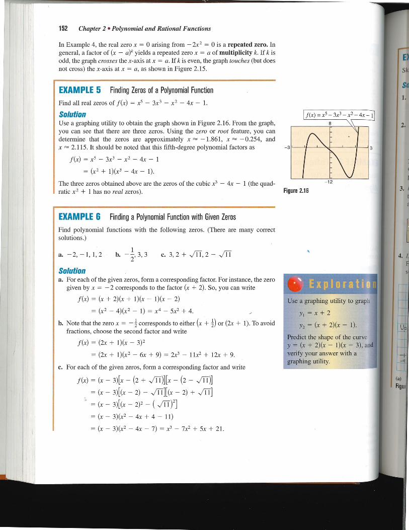
EXAMPLE 5 Finding Zeros of a Polynomial Function
Find all real zeros of f(x) = x5 — 3x3 — x2 — 4x — 1.
Solution Use a graphing utility to obtain the graph shown in Figure 2.16. From the graph, you can see that there are three zeros. Using the zero or root feature, you can determine that the zeros are approximately x — 1.861, x —0.254, and x 2.115. It should be noted that this fifth-degree polynomial factors as
f(x) = x5 — 3x3 — x2 — 4x — 1
= (x2 + 1)(x3 — 4x — 1).
The three zeros obtained above are the zeros of the cubic x3 — 4x — 1 (the quad-ratic x2 + 1 has no real zeros).
EXAMPLE 6 Finding a Polynomial Function with Given Zeros
Find polynomial functions with the following zeros. (There are many correct solutions.)
1 a. —2,-1,1,2 b. —,3,3 c. 3, 2 + , 2 —
Solution a. For each of the given zeros, form a corresponding factor. For instance, the zero
given by x = —2 corresponds to the factor (x + 2). So, you can write
f(x) = (x + 2)(x + 1)(x — 1)(x — 2)
= (x2 — 4)(x2 — 1) = x4 — 5x2 + 4.
b. Note that the zero x = — corresponds to either (x + 1) or (2x + 1). To avoid fractions, choose the second factor and write
f(x) = (2x + 1)(x — 3)2
= (2x + 1)(x2 — 6x + 9) = 2x3 — 11x2 + 12x + 9.
c. For each of the given zeros, form a corresponding factor, and write
f(x) = (x — 3)[x — (2 + „/1-1-)] [x — (2 —
=(x- 3)[(x — 2) — -,/TI][(x — 2) + -1-ff]
=(x— 3)[(x — 2)2 —(-,/il)2]
= (x — 3)(x2 — 4x + 4 — 11)
= (x — 3)(x2 — 4x —7) = x3 — 7x2 + 5x + 21.
4110 - §se i graphing utility to graph 41
y1 = x + 2
Y2 = (x + 2)(x — 1). i
Predict the shape of the curve ill Ui_
= (x + 2)(x — 1)(x — 3), and verify your answer with a raphing utility.
I (a) Figu

-5 - 14
artner Activity Multiply 3, or 5 distinct linear factors to obtain the equation of a polyno-mial fanction that has a degree of 3, 4, or 5. Exchange equa-tions with your partner and sketch, by hand, the graph of the
t equation that your partner wrote. When you are finished, use a graphing utility to check each other's work.
STUDY TIP
It is easy to make mistakes when entering functions into a graph-ing utility. So, it is important to have an understanding of the basic shapes of graphs and to be able to graph simple polynomials by hand. For example, suppose you had entered the function in Example 7 as y = 3x5 - 4x3. By looking at the graph, what mathematical principles would alert you to the fact that you had made a mistake?
2.2 • Polynomial Functions of Higher Degree 153
- x2 - 4x- 1
ty to graph
the curve i(x - 3), and with a
3
ExAIRAPLE 7 Sketching the Graph of a Polynomial Function
Sketch the graph of f(x) = 3x4 - 4x3 by hand
Solution
1. Apply Leading Coefficient Test. Because the leading coefficient is positive and the degree is even, you know that the graph eventually rises to the left and
to the right [see Figure 2.17(a)].
2. Find the Zeros of the Polynomial. By factoring
f (x) = 3x4 - 4x3
= x3(3x - 4)
you can see that the zeros of f are x = 0 (of odd multiplicity 3) and x = (of
odd multiplicity 1). So, the x-intercepts occur at (0, 0) and (, 0). Add these points to your graph, as shown in Figure 2.17(a).
3. Plot a Few Additional Points. To sketch the graph by hand, find a few addi-tional points, as shown in the table. Be sure to choose points between the zeros and to the left and right of the zeros. Then plot the points [see Figure 2.17(b)].
x - 1 0.5 1 1.5
f (x) 7 - 0.3125 -1 1.6875
4. Draw the Graph. Draw a continuous curve through the points, as shown in Figure 2.17(b). If you are unsure of the shape of the portion of the graph, plot some additional points.
x f̀ A A
7
6
3 —
-4
UP to le I
Up to right
• 7
(x)
= 3
5 1.1
x3
(a) Figure 2.17
(b)

154 Chapter 2 • Polynomial and Rational Functions
EXAMPLE 8 Sketching the Graph of a Polynomial Function
6 —
Sketch the graph of f(x) = — 2x3 + 6x2 — x.
5 —
Solution
4 —
Up to left 3 — Down to right 1. Apply Leading Coefficient Test. Because the leading coefficient is negative
and the degree is odd, you know that the graph eventually rises to the left and falls to the right [see Figure 2.18(a)].
2
(0, 0)
—
• 1 • 1 I
-4 -3 -2 -1 1 2 3 4 2. Find the Zeros of the Polynomial. By factoring
f(x) = —2x3 + 6x2 — = — ix(4x2 — 12x + 9) = —1x(2x — 3)2
-1
-2 —
—
you can see that the zeros of f are (a) 3 x = 0 (of odd multiplicity 1) and x = (of even multiplicity 2).
So, the x-intercepts occur at (0, 0) and 0). Add these points to your graph, as shown in Figure 2.18(a).
3. Plot a Few Additional Points. To sketch the graph by hand, find a few addi-tional points, as shown in the table. Then plot the points [see Figure 2.18(b)].
f(x) = -2x3 + 6x2 - -
32
x —0.5 0.5 1 2
f(x) 4 —1 —0.5 —1
4. Draw the Graph. Draw a continuous curve through the points, as shown in Figure 2.18(b). Notice that the graph crosses the x-axis at (0, 0) and touches (but does not cross) the x-axis at (, 0).
The Intermediate Value Theorem The Intermediate Value Theorem concerns the existence of real zeros of polynomial functions. The theorem states that if (a, f (a)) and (b, f (b)) are two points on the graph of a polynomial function such that f (a) 0 f (b), then for any number d between f (a) and f (b) there must be a number c between a and b such that f (c) = d. (See Figure 2.19.)
(b)
Figure 2.18
Intermediate Value Theorem
Let a and b be real numbers such that a < b. If f is a polynomial function such that f (a) f (b), then in the interval [a, b], f takes on every value between f (a) and f (b)
f(b)
f(c)= d
f(a)
This theorem helps locate the real zeros of a polynomial function in the follow-ing way. If you can find a value x = a where a polynomial function is positive, and another x = b where it is negative, you can conclude that the function has at least one real zero between these two values. For example, the function f(x) = x3 + x2 + 1 is negative when x = —2 and positive when x = —1. Therefore, it follows from the Intermediate Value Theorem that f must have a real zero somewhere between —2 and —1.
a
Figure 2.19

(a)
1.
rI
( (x) = — x3
(b)
2. f(x) = —x3 + 4x 3. f(x) = x3
x
(c) (d)
4. f(x) = x3 — 4x
vn to right
0) \ x
2 3 4
3 + 6x2 —
\ 3 4
2.2 • Polynomial Functions of Higher Degree 155
EXAMPLE 9 Approximating the Zeros of a Function
Find three intervals of length 1 in which the polynomial
f(x) 12x3 — 32x2 + 3x + 5
is guaranteed to have a zero.
Graphical Solution
Use a graphing utility to graph
y = 12x3 — 32 + 3x + 5
as shown in Figure 2.20.
Numerical Solution
Use the table feature of a graphing utility to create a table that shows the function values for —20 x 20 as shown in Figure 2.21.
X Y1
-2 -225
-1 -42
o 5
1 -12
2 -21
il 50
4 273
X=3
Figure 2.21
Scroll through the table looking for consecutive function values that differ in sign. For instance, from the table you can see that f(— 1) and f(0) differ in sign. So, you can conclude from the Intermediate Value Theorem that the function has a zero between —1 and 0. Similarly, f(0) and f(1) differ in sign, so the function has a zero betweerk 0 and 1. Likewise, f(2) and f(3) differ in sign, so the function has a zero between 2 and 3. So, you can conclude that the function has zeros in the intervals (— 1, 0), (0, 1), and (2, 3).
= 12x — 32x2 + 3x + 5
-4
Figure 2.20
From the figure, you can see that the graph crosses the x-axis three times—between —1 and 0, between 0 and 1, and another between 2 and 3. Sb, you can conclude that the function has zeros in the intervals (-1,0), (0, 1), and (2, 3).
Mg About Math The Graphs of Cubic Polynomials 11.111. The graphs of cubic polynomials can be categorized according to the four basic shapes below. Match the graph of each function with one of the basic shapes and write a short paragraph describing how you reached your conclu-sion. Is it possible for a polynomial of odd degree to have no real zeros? Explain.

5
5
1111 1 111111
10 (a) (b)
5 10 10
4 5
(c) (d) 4
5
9
5
6
6 4
(e) (f)
4 6 III Ijj
II
-5
-6
-10
5
-5
-6 5
-3
1. f(x) = -2x + 3
3. f(x) = -2x2 - 5x
5. f(x) = + 3x2
7. f(x) = x 4 + 2x3
-4
5
-5
2. f(x) = x 2 - 4x
4. f(x) = 2x3 - 3x + 1
6. f(x) = 4C3 ± X2 -
8. f(x) = .x• 5 - 2x3 +
7 3
In Exercises 9-12, sketch the graphs of y = x" and each specified transformation.
9. y = x3
(a) f(x) = (x - 2)3 (b) f(x) = x3 - 2
(c) f(x) = - 1X 3 (d) f(x) = (x - 2)3 - 2
10. y = x5
(a) f(x) = (x + 3)5 (b) f(x) = x 5 + 3
(c) f(x) = 1 - (d) f(x) = (x + 1)5
156 Chapter 2 • Polynomial and Rational Functions
Exercises
In Exercises 1-8, match the polynomial function with its graph. [The graphs are labeled (a) through (h).]
11. y = x4
(a) f(x) = (x + 5)4 (b) f(x) = x4 - 5
(c) f(x) = 4 - x4 (d) f(x) = - 1)4
12. y = x6
(a) f(x) = -1x6 (b) f(x) = x6 - 4
(c) f(x) = + 1 (d) f(x) = + 2)6 - 4
Graphical Analysis In Exercises 13-16, use a graph. ing utility to graph the functions f and g in the same viewing window. Zoom out sufficiently far to show that the right-hand and left-hand behavior off and g
appear identical. Show the graphs.
13. f(x) = 3x3 - 9x + 1, g(x) = 3x3
14. f(x) = - (x - 3x + 2), g(x) = tX3
15. f(x) = -(x4 - 4x 3 + 16x), g(x) = -x 4
16. f(x) = 3x4 - 6x2, g(x) = 3x 4
In Exercises 17-26, use the Leading Coefficient Test to determine the right-hand and left-hand behavior of the graph of the polynomial function. Verify your result by using a graphing utility to graph the function.
17. f(x) = 2x2 - 3x + 1 18. f(x) = 131x3 + 5x
19. g(x) = 5 - - 3x2 20. h(x) = 1 - x6
21. f(x) = -2.1x5 + 4x3 - 2
22. f(x) = 2x5 - 5x + 7.5
23. f(x) = 6 - 2x + 4x2 - 5x3
24. f(x) = 3x4 -2x + 5 4
25. h(t) = - 5t + 3)
26. f(s) = + 52 - 7s + 1)
In Exercises 27-36, find all the real zeros of the polynomial function. Verify your result by using a graphing utility to graph the function.
27. f(x) = x2 - 25 28. f(x) = 49 - x2
29. h(t) = t 2 - 6t + 9 30. f(x) = X2 + 10x + 25
31. f(x) = x2 + x - 2 32. f(x) = 2x - 14x + 2
33. f(t) = t 3 - 4t2 + 4f 34. f(x) = x4 - X3 - 20X
35. f(x) = 1X 2 - 36. f(x) = 1,12

Graphical Analysis In Exercises 37-48, (a) use a graphing utility to graph the function, (b) use the
graph to approximate any zeros, and (c) find the
zeros algebraically.
37. f(x) 3x2 - 12x + 3
38. g(x) = 5(x 2 - 2x - 1)
39. g (t) 2114
41. f(x) = + - 6x
40. y = -,1-1x 3(x 2 - 9)
42. g(t) = t 5 - 6t 3 + 9t
43. f(x) 2x4 - 2x2 - 40
44. f(x) = 5x 4 + 15x2 + 10
45. f(x) = x 3 - 4x 2 - 25x + 100
46. y 4x3 +4x2 - 7x+ 2
47. y 4x3 - 20x2 + 25x 48. y = x 5 - 5x 3 + 4x
2.2 • Polynomial Functions of Higher Degree 157
In Exercises 49-52, use a graphing utility to graph the function and approximate (accurate to three decimal places) any relative extrema.
49. f(x) = 2x4 - 6x2 + 1
50. f(x) = - 3x3 - 4x2 + x - 3
51. f(x) = x5 + 3x3 - x + 6
52. f(x) -= - - x3 + 2x2 + 5
In Exercises 53-64, find a polynomial function that has the given zeros. (There are many correct answers.)
53. 0, 12
54. 0,-8
55. 2, -6
56. -4,5
57. 0, -4, -3
58. 0, 2, 7
59. 4, -3, 3, 0
60. - 2, -1, 0, 1, 2
61. 1 + 1 - 62. 6 + 6 -
63. 2, 4 + ,/3, 4 - 64. 4, 2 + -,/7, 2 -
In Exercises 65-78, sketch the graph of the function by (a) applying the Leading Coefficient Test, (b) find-ing the zeros of the polynomial, (c) plotting sufficient solution points, and (d) drawing a continuous curve through the points.
65. f(x) = x3 - 9x 66. g(x) = x4 - 4x2 67. f(t) = lz(t 2 - 2t + 15) 68. g(x) = - x2 ± 10X 16 69. f(x) = x3 3x2
70. f(x) = 1 - x3
71. f(x) = 3x3 - 15x2 + 18x
72. f(x) = -4x3 + 4x2 + 15x
73. f(x) = -x3 - 5x2 74. f(x) = 3x4 - 48x2 75. f(x) = x2(x - 4)
76. h(x) = lx3(x - 4)2
77. g(t) = -(t - 2)2(t + 2)2
78. g(x) = x + 1)2(x - 3)2
In Exercises 79-82, (a) use the Intermediate Value Theorem and a graphing utility to find intervals of length 1 in which the polynomial function is guaran-teed to have a zero, (b) use the root or zero feature of a graphing utility to approximate the zeros of the function, and (c) verify your answers in part (a) by using the table feature of a graphing utility.
79. f(x) = x3 - 3x2 + 3
80. f(x) = 0.11x3 - 2.07x2 + 9.81x - 6.88
81. g(x) = 3x 4 + 4x 3 - 3
82. h (x) = x4 - 10x2 +2
In Exercises 83-86, use a graphing utility to graph the function. Describe a viewing window that gives a good view of the basic characteristics of the graph. (There are many correct answers.)
83. f(x) =
84. h(x) = - 3
85. f(t) = (t2 - 4t + 21)
86. g(x) = -x2 + 9x - 14
In Exercises 87-94, use a graphing utility to graph the function. Identify any symmetry with respect to the x-axis, y-axis, or origin. Determine the number of x-intercepts of the graph.
87. f(x) = x 2(x + 6)
88. h(x) = x 3(x - 4)2
89. g(t) = A(t - 4)2(t + 4)2
90. g(x) = (x + 1)2(x - 3)3
91. f(x) = x3 - 4x
92. f(x) = x4 - 2x2
93. g(x) = (x + 1)2(x - 3)(2X - 9)
94. h(x) = x + 2)2(3x - 5)2
4_ 5
_ 1)4
6_ 4
e + 2)6 - 4
use a graph. in the same far to show ur of f and g
x 3
Ancient Test nd behavior Verify your graph the
zeros of the t by using a
- x2
+ 10X ± 25
- 14x + 24
- x3 - 20x2
+ -

36— 2x
350 300
a) a
250 g 0 a 0 200
a` 3 150 100
50
— — — — —
158 Chapter 2 • Polynomial and Rational Functions
95. Numerical and Graphical Analysis An open box is to be made from a square piece of material 36 centimeters on a side by cutting equal squares from the corners and turning up the sides.
(a) Complete four rows of a table like the one below.
Height Width Volume
1 36 — 2(1) 1[36 — 2(1)]2 = 1156
2 36 — 2(2) 2[36 — 2(2)]2 = 2048
(b) Use a graphing utility to generate additional rows of the table. Use the table to estimate a range of dimensions within which the maximum volume is produced.
(c) Verify that the volume of the box is V(x) = x(36 — 242. Determine the domain of the function.
(d) Use a graphing utility to graph V, and use the range of dimensions from part (b) to find the x-value for which V(x) is maximum.
96. Geometry An open box with locking tabs is to be made from a square piece of material 24 inches on a side. This is done by cutting equal squares from the corners and folding along the dashed lines, as shown in the figure.
(a) Show that the volume of the box is
V(x) = 8x(6 — 4(12 —
(b) Determine the domain of the function V.
(c) Sketch the graph of the function and estimate the value of x for which V(x) is maximum.
1-4— 24 in.
X X
97. Business The total revenue R (in millions of1 C dollars) for a company is related to its advertising expense by the function
1 R = ( x3 + 600x 2), 0 x 400
100,000
where x is the amount spent on advertising (in tens of thousands of dollars). Use the graph of the function shown in the figure to estimate the point on the graph at which the function is increasing most rapidly. This point is called the point of diminishing returns because any expense above this amount will yield less return per dollar invested in advertising.
100 200 300 400
Advertising expense (in tens of thousands of dollars)
98. Environment The growth of a red oak tree is approximated by the function
G = —0.003t3 + 0.137t2 + 0.458t — 0.839
where G is the height of the tree (in feet) and t (2 t 34) is its age (in years). Use a graphing utility to graph the function and estimate the age of the tree when it is growing most rapidly. This point is called the point of diminishing returns because the increase in growth will be less with each addi-tional year. (Hint: Use a viewing window in which —10 5_ x 45 and —5 y 60.)
99. Data Analysis The vertical deflection y of a 4- A meter beam is measured in 1-meter intervals x. The measurements are given by the following ordered pairs.
(0, 0), (0.5, 0.06), (1, 0.11), (1.5, 0.15), (2, 0.16), (2.5, 0.15), (3, 0.11), (3.5, 0.06), (4,0)
1(

t 3 4 5 6 7 8
yi 82.2 88.6 103.3 125 140 149
Y2 70.9 72 75 80.2 88 92
t 9 10 11 12 13
y1 159.6 159 155.9 169 162.6
Y2 96.4 99 100 105.5 115
t 14 15 16 17
y1 169 180 186 190
Y2 116.9 124.5 126.2 129.6
(a) Use the regression capabilities of a graphing utility to fit a cubic model to the median prices of homes in the Northeast.
(b) Use the regression capabilities of a graphing utility to fit a cubic model to the median prices of homes in the South.
(c) Use the graphs of the models in parts (a) and (b) to write a short paragraph about the relationship between the median prices of homes in the two regions.
millions of s advertising
mg (in tens of F the function t on the graph rapidly. This
iing returns int will yield ising.
n feet) and t ;e a graphing ate the age of ly. This point urns because th each addi-low in which
on y of a 4-
tervals x. The wing ordered
, (2, 0.16),
0.839
(a) Use the regression capabilities of a graphing utility to fit a quartic (fourth-degree polyno-mial) equation to the data.
(b) Use a graphing utility to graph the data and 5 400 the regression equation in the same viewing
window. How do they compare?
(c) Because y = 0 when x = 0, what should the constant term in the model be? Does your answer agree with the result of part (a)? Explain.
100. Data Analysis The table gives the median values of new privately owned U.S. homes for 1983 through 1997. In the table, t is the time (in years), with t = 3 corresponding to 1983, and y1 and y2 are the median prices (in thousands of dollars) in the Northeast and the South, respectively. (Sources: U.S. Bureau of the Census; U.S. Department of Housing and Urban Development)
oak tree is
2.2 • Polynomial Functions of Higher Degree 159
Synthesis
True or False? In Exercises 101 and 102, determine whether the statement is true or false. Justify your answer.
101. A fourth-degree polynomial can have four turning points.
102. The graph of the function
f(x) = 2 + x _ x2 + xa _ x4 + x5 + x6 _ x7
rises to the left and falls to the right.
103. Graphical Reasoning Use a graphing utility to graph the function f(x) = x4. Explain how the graph of g differs (if it does) from the graph of f and confirm your result with a graphing utility. Determine whether g is odd, even, or neither.
(a) g(x) = f(x) + 2 (b) g(x) = f(x + 2)
(c) g(x) = f (- (d) g(x) = -f(x)
(e) g(x) =- f(x) (f) g(x) = f(x)
(g) g(x) = f(x3/4) (h) g(x) = (f f)(x)
Review
In Exercises 104-109, let f(x) = 14x - 3, and g(x) = 8x2. Find the indicated value.
104. (f g)(-4) 105. (g -f)(3)
106. (fg)(-;) 107. (1)(- 1.5)
108. (f a- 1) 109. (g f)(0)
In Exercises 110-113, solve the inequality and sketch the solution on the real number line. Use a graphing utility to verify your solution graphically.
110. 3(x - 5) < 4x - 7 111. 2x2 - x 1
5x - 2 112.
4 113. Ix + 81 - 1 15 < x - 7
In Exercises 114-117, find the quadratic function that has the indicated vertex and whose graph passes through the given point.
114. Vertex: (3, -6); Point: (- 1, 2)
115. Vertex: (0, -8); Point: (5, 9)
116. Vertex: (4, -4); Point: (1, 10)
117. Vertex: (-5, -2); Point: (0, 3)
x 400
llars)

160 Chapter 2 • Polynomial and Rational Functions
iii 0 You Should Learn:
In E; the 1( prodi you ( Long Division of Polynomials
Consider the graph of
f(x) = 6x3 — 19x2 + 16x — 4.
Notice in Figure 2.22 that x = 2 appears to be a zero off. Because f(2) = 0, you know that x = 2 is a zero of the polynomial function f, and that (x — 2) is a factor of f(x). This means that there exists a second-degree polynomial q(x) such that f(x) = (x — 2) • q(x). To find q(x), you can use long division of polynomials.
) = 6x — 19x z+ 16x — 0.5
2.5
-0.5
Figure 2.22
EXAMPLE 1 Long Division of Polynomials
Divide f(x) = 6x3 — 19x2 + 16x — 4 by t — 2, and use the result to factor the function f completely.
Solution
Partial quotients
6x2 — 7x + 2
x — 2 ) 6x3 — 19x2 + 16x —4
6x3 — 12x2 Multiply: 6x2(x — 2).
—7x2 + 16x Subtract.
—7x2 + 14x Multiply: —7x(x — 2).
2x —4 Subtract.
2x — 4 Multiply: 2(x — 2).
Subtract.
You can see that
6x3 — 19x2 + 16x — 4 = (x — 2)(6x2 — 7x + 2)
= (x — 2)(2x — 1)(3x — 2).
Note that this factorization agrees with the graph of f (Figure 2.22) in that the three x-intercepts occur at x = 2, x = and x =
-0.5
You Should Learn It:
7ro ynomial division can help yc rewrite polynomials that are use to model i•eal-life problems. Fot
How to use long division to divide polynomials by other polynomials How to use synthetic divisic to divide polynomials by binomials of the form (x - -
• How to use the Remainder Theorem and the Factor Theorem
• How to use the Rational Zei Test to determine possible rational zeros of polynorri, al functions
• How to determine upper anc lower bounds for zeros of polynomial functions
0
This
which Algor
In fra
instance, Exercise 87 on page 172, shows how polynomial division can be used to model the avera monthly rates for cable televisk in the United States from 1988 through 1997.

Divisor Remainder
t I t 1 idend Quotient
2.3 • Real Zeros of Polynomial Functions 161
PI114 ii..............0 Learn: division to
als by other
hetic division mials by form (x — k) emainder Factor
Zational Zero e possible 1 polynomial
, ie upper and r zeros of tions
earn It: i can help y ,ti that are used
70blems. Fo 7 on page 172 lial division 1 the average
tble television from 1988
In Example 1, x — 2 is a factor of the polynomial 6x3 — 19x2 + 16x — 4, and
tile long division process produces a remainder of zero. Often, long division will produce a nonzero remainder. For instance, if you divide x2 + 3x + 5 by x + 1,
you obtain the following.
x + 2 Quotient
Divisor => X + 1 ) x2 + 3x + 5 Dividend
x2 + x
2x + 5
2x + 2
3 Remainder
In fractional form, you can write this result as follows.
Remainder Dividend
Quotient
x2 + 3x + 5 3 = x + 2 +
x + 1
Divisor Divisor
This implies that
x2 + 3x + 5 = (x + 1)(x + 2) + 3
which illustrates the following well-known theorem called the Division Algorithm.
The Division Algorithm If f(x) and d(x) are polynomials such that d(x) 0, and the degree of d(x) is less than or equal to the degree of f(x), there exist unique polynomials q(x) and r(x) such that
f(x) = d(x)q(x) + r(x)
x+ 1
Div
where r(x) = 0 or the degree of r(x) is less than the degree of d(x). If the remainder r(x) is zero, d(x) divides evenly into f(x).
The Division Algorithm can also be written as
f(x) r(x) d(x)
q(x)
In the Disiision Algorithm, the rational expression f(x)/d(x) is improper because the degree of f(x) is greater than or equal to the degree of d(x). On the other hand, the rational expression r(x)Id(x) is proper because the degree of r(x) is less than the degree of d(x).

162 Chapter 2 • Polynomial and Rational Functions
No
a p!
EX
Use
Sof You ing
—3
Ther plyir
You can check the result of a division problem by multiplying. For instance, in Example 2, try checking that
(x — 1)(x2 + x + 1) = x3 — 1.
EXAMPLE 3 Long Division of Polynomials
Divide 2x4 + 4x3 — 5x 2 + 3x — 2 by x2 + 2x — 3.
Solution
2x2 +1
X2 ± 2x — 3 ) 2x4 + 4x3 — 5x2 +3x —2
2x4 + 4x3 — 6x2
x2 + 3x — 2 2 X -r zx 3
x + 1
A computer animation of this example appears in the Interactive CD-ROM an Internet versions of this text.
Note that the first subtraction eliminated two terms from the dividend. When this happens, the quotient skips a term. You can write the result as
2x4 + 4x3 — 5x2 + 3x — 2 x + 1 = 2x2 + 1 +
x2 + 2x — 3 x2 + 2x — 3.
EXAMPLE 2 Long Division of Polynomials
Divide x3 — 1 by x — 1.
Solution Because there is no x2-term or x-term in the dividend, you need to line up the sub-traction by using zero coefficients (or leaving spaces) for the missing terms.
x2+ X + 1
X 1 ) X3 + OX 2 OX — 1
X3 - X2
X2
X2 - X
x - 1
X 1
0
So, x — 1 divides evenly into x3 — 1, and you can write
x3 — 1 = x2 + x + 1, x 1.
x — 1

b d Vertical pattern: Add terms. c Diagonal pattern: Multiply by k.
k
@ 0 0
Remainder
Coefficients of quotient
So, you have
x4 — 10x2 — 2x + 4 1 x+ 1+
x + 3 x+ 3
2.3 • Real Zeros of Polynomial Functions 163
Synthetic Division There is a nice shortcut for long division of polynomials by divisors of the form x _ k. The shortcut is called synthetic division. The pattern for synthetic divi-
sion of a cubic polynomial is summarized as follows. (The pattern for higher-degree polynomials is similar.)
synthetic Division (of a Cubic Polynomial)
To Jivide ax3 + bx2 + cx + d by x — k, use the following pattern.
Note that synthetic division works only for divisors of the form x — k. [Remember that x + k = x — (— k).] You cannot use synthetic division to divide a polynomial by a quadratic such as x2 — 3.
this example CD-ROM and
ext.
EXAMPLE 4 Using Synthetic Division
Use synthetic division to divide x4 — 101.2 — 2x + 4 by x + 3.
Solution You should set up the array as follows. Note that a zero is included for each miss-ing term in the dividend.
—3 ;I; 0-10 —2 4
Then, use the synthetic division pattern by adding terms in columns and multi-plying the results by —3.
Divisor: x + 3 Dividend: x4 — 10x2 — 2x + 4
—3 1 0 — 10 —2 4
—3 9 3 —3
1 — 3 — 1 1 11
Remainder: 1
Quotient: x 3 — 3x 2 — x + 1
A computer animation of this example appears in the Interactive CD-ROM and Internet versions of this text.

The Remainder Theorem
If a polynomial f(x) is divided by x — k, the remainder is
r f (k).
The Factor Theorem
A polynomial f (x) has a factor (x — k) if and only if f (k) = 0.
164 Chapter 2 • Polynomial and Rational Functions
The Remainder and Factor Theorems
The remainder obtained in the synthetic division process has an important inter-pretation, as described in the Remainder Theorem. (A proof of this theorem is given in Appendix A.)
The Remainder Theorem tells you that synthetic division can be used to evaluate a polynomial function. That is, to evaluate a polynomial function f(x) when x = k, divide f(x) by x — k. The remainder will be f (k), as illustrated in Example 5.
EXAMPLE 5 Using the Remainder Theorem
Use the Remainder Theorem to evaluate the following function at x = — 2.
f(x) = 3x3 + 8x2 + 5x — 7
Solution Using synthetic division, you obtain the following.
—2 3 8 5 —7
—6 —4 —2
3 2 1 —9
Because the remainder is r = — 9, you can conclude that
f (— 2) = —9.
This means that (-2, —9) is a point on the graph of f You can check this by substituting x = — 2 in the original function.
Check
f( —2) = 3(-2)3 + 8(-2)2 + 5(-2) — 7
= 3( — 8) + 8(4) — 10 —7
= —24 + 32 — 10 — 7
= —9
Another important theorem is the Factor Theorem, which is stated below. This theorem states that you can test to see whether a polynomial has (x — k) as a factor by evaluating the polynomial at x = k. If the result is 0, — k) is a factor. For a proof of the Factor Theorem, see Appendix A.

From Figure 2.23, you can see that the graph appears to cross the x-axis in two other places, near x = —1 and
3 1 x = Use the zero or root feature or the zoom and trace features to approximate the other two intercepts to be x= —1 and x = —I So, the factors of f are
(x —2), (x + 3), (x + i), and (x + 1). You can rewrite
the factor (x + i) as (2x + 3), so the complete factor-
ization of f is f(x) = (x — 2)(x + 3)(2x + 3)(x + 1).
Graphical Solution
The graph of a polynomial with factors of (x — 2) and (x + 3) has x-intercepts at x = 2 and x = —3. Use a graphing utility to graph
y = 2x4 + 7x3 — 4x2 — 27x — 18.
Figure 2.23
4
_ _
_ I
I 1
_
_
_
Zero
X=-3 Y;13
y = 2x4 + 7x3 — 4x2 — 27x — 18
—12
6
3
2.3 • Real Zeros of Polynomial Functions 165
EXAMPLE 6 Factoring a Polynomial: Repeated Division
Show that (x — 2) and (x + 3) are factors of
f(x) 2x4 + 7x3 — 4x2 — 27x — 18.
Then find the remaining factors of f(x).
Algebraic Solution
Using synthetic division with 2 and —3 repeatedly, you
obtain the following.
2 2
7 4
—4 —27 22 36
—18 18
2
11 18 9
0 .1010 0 remainder
(x — 2) is a factor.
—3
2 11 18 9
—6 —15 —9
2 5 3 0
aii> 0 remainder
(x + 3) is a factor.
Because the resulting quadratic factors as
2x 2 + 5x + 3 = (2x + 3)(x + 1)
the complete factorization of f(x) is
f(x) = (x — 2)(x + 3)(2x + 3)(x + 1).
LEFT-1g the Remainder in Synthetic Division In summary, the remainder r, obtained in the synthetic division of f(x) by x — k, provides the following information.
1. The remainder r gives the value of f at x = k. That is, r = f(k). 2. If r= 0,(x — k) is a factor of f(x).
3. If r = 0, (k, 0) is an x-intercept of the graph of f.
Throughout this text, the importance of developing several problem-solving strategies has been emphasized. In the exercises for this section, try using more than one strategy to solve several of the exercises. For instance, if you find that
— k divides evenly into f(x), try sketching the graph of f. You should find that (k, 0) is an x-intercept of the graph.

3
If th, zeroq sevei
1. A
2. A
3. 11 rat
Findh piffle(
EXAI
Find t
SOM The le.
Pc
Fa Fa
By syn
1
, (x
•f
STUDY Tfil
Graph the polynomial y = x3 — 53x2 + 103x — 51 in the standard viewing windov, From the graph alone, it appears that there is only one zero. From the Leading Coefficient Test, you know that because the degree of the polynomial is odd and the leading coefficient is positive, the graph falls to the left and rises to the right. So, the function must have another zerc From the Rational Zero Test, you know that ±51 might be zeros of the function. If you zoom out several times, you wil see a more complete picture of the graph. Your graph should confirm that x = 51 is a zero of f.
and yo as shov
4 f(x
3
-2
Figure 2.24
Figure 2.
166 Chapter 2 • Polynomial and Rational Functions
The Rational Zero Test The Rational Zero Test relates the possible rational zeros of a polynomial (having integer coefficients) to the leading coefficient and to the constant term of the polynomial.
The Rational Zero Test
If the polynomial
f(x) = ax n + a_ 1x'' + • • • + a 2x 2 + aix + a0
has integer coefficients, every rational zero of f has the form
Rational zero = —
where p and q have no common factors other than 1, p is a factor of the constant term /20, and q is a factor of the leading coefficient an.
To use the Rational Zero Test, first list all rational numbers whose numerators are factors of the constant term and whose denominators are factors of the leading coefficient.
factors of constant term Possible rational zeros —
factors of leading coefficient
Now that you have formed this list of possible rational zeros, use a trial-and-error method to determine which, if any, are actual zeros of the polynomial. Note that when the leading coefficient is 1, the possible rational zeros are simply the fac-tors of the constant term. This case is illustrated in Example 7.
EXAMPLE 7 Rational Zero Test with Leading Coefficient of 1
Find the rational zeros of f(x) = x3 + x + 1.
Solution Because the leading coefficient is 1, the possible rational zeros are simply the factors of the constant term.
Possible Rational Zeros: ±1
By testing these possible zeros, you can see that neither works.
f(1) = (1)3 + 1 + 1 = 3
f(— 1) = (— 1)3 + (-1) + 1 = — 1
So, the potynomial has no rational zeros. Note from the graph off in Figure 2.24 thatf does have one real zero (between — 1 and 0). However, by the Rational Zero Test, you know that this real zero is not a rational number.

'TIP
[al 03x — 51 ing window. re, it appears e zero. From ient Test, use the omial is odd fficient is 'ails to the right. So, the another zero. '.,ero Test, might be n. If you nes, you will e picture of ph should
is a zero
-4 2
f(x)= 2x3 + 3x2 — 8x + 3 16
2.3 • Real Zeros of Polynomial Functions 167
if the leading coefficient of a polynomial is not 1, the list of possible rational zeros can increase dramatically. In such cases the search can be shortened in several ways.
1. A programmable calculator can be used to speed up the calculations.
2. A graphing utility can give a good estimate of the locations of the zeros.
3. The Factor Theorem and synthetic division can be used to test the possible rational zeros.
Finding the first zero is often the most difficult part. After that, the search is sim-plified by working with the lower-degree polynomial obtained in synthetic division.
EXAMPLE 8 Using the Rational Zero Test
Find the rational zeros of
f(x) = 2x3 + 3x 2. — 8x + 3.
Solution The leading coefficient is 2 and the constant term is 3.
Possible Rational Zeros:
Factors of 3 ±1, +3 — ±1 +3 +-
1 3 +—
Factors of 2 ±1, +2
2' — 2
By synthetic division, you can determine that x = 1 is a zero.
1 2 3 —8 3
2 5 —3
2 5 —3 0
So, f (x) factors as
f(x) = (x — 1)(2x2 + 5x — 3)
= (x — 1)(2x— 1)(x + 3)
1 and you can conclude that the rational zeros of f are x = 1, x = —2, and x = — 3,
as shown in Figure 2.25.
Figure 2.25 -2
3
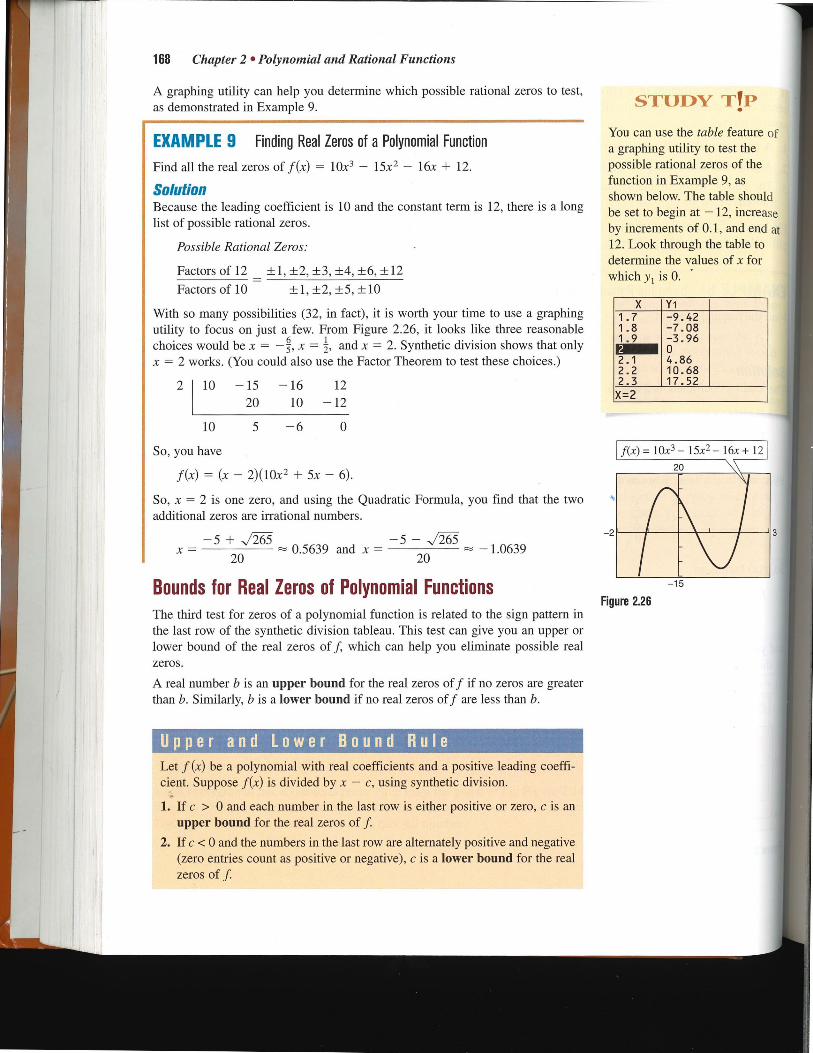
STUDY 11P
You can use the table feature of a graphing utility to test the possible rational zeros of the function in Example 9, as shown below. The table should be set to begin at — 12, increase by increments of 0.1, and end at 12. Look through the table to determine the values of x for which y1 is 0.
X Yi
1.7 -9.42
1.8 -7.08
1.9 -3.96
2 0
2.1 4.86
2.2 10.68
2.3 17.52
X=2
f(x)=10x3 — 15x —16x + 12 20
-15
Figure 2.26
168 Chapter 2 • Polynomial and Rational Functions
A graphing utility can help you determine which possible rational zeros to test, as demonstrated in Example 9.
EXAMPLE 9 Finding Real Zeros of a Polynomial Function
Find all the real zeros of f(x) = 10x3 — 15x2 — 16x + 12.
Solution Because the leading coefficient is 10 and the constant term is 12, there is a long list of possible rational zeros.
Possible Rational Zeros:
Factors of 12 ±1, ±2, ±3, ±4, ±6, ±12 Factors of 10 ±1, ±2, ±5, ±10
With so many possibilities (32, in fact), it is worth your time to use a graphing utility to focus on just a few. From Figure 2.26, it looks like three reasonable choices would be x = x = 1, and x = 2. Synthetic division shows that only x = 2 works. (You could also use the Factor Theorem to test these choices.)
2 10 —15 —16 12
20 10 —12
10 5 —6 0
So, you have
f(x) = (x — 2)(10x2 + 5x — 6).
So, x = 2 is one zero, and using the Quadratic Formula, you find that the two additional zeros are irrational numbers.
— 5 + ./265 — 5 — 2/ X =
20 — 0.5639 and x =
20 1.0639
Bounds for Real Zeros of Polynomial Functions
The third test for zeros of a polynomial function is related to the sign pattern in the last row of the synthetic division tableau. This test can give you an upper or lower bound of the real zeros of f, which can help you eliminate possible real zeros.
A real number b is an upper bound for the real zeros of f if no zeros are greater than b. Similarly, b is a lower bound if no real zeros of f are less than b.
Upper and Lower Bound Rule
Let f (x) be a polynomial with real coefficients and a positive leading coeffi-cient. Suppose f(x) is divided by x — c, using synthetic division.
1. If c > 0 and each number in the last row is either positive or zero, c is an upper bound for the real zeros of f.
2. If c < 0 and the numbers in the last row are alternately positive and negative (zero entries count as positive or negative), c is a lower bound for the real zeros of f.

TIP
le feature of test the
ros of the e 9, as able should 12, increase 1, and end at le table to s of x for
— 16x+ 12
Use a graphing utility to graph
yi = 6x3 — 4x2 + 3x — 2.
Notice that the graph intersects the x-axis at the point 0). How does this relate to the real zero found in Example 10? Use a graphing utility to graph
y2 = x4 — 5x3 + *3x2 + x.
IN How many times does the graph intersect the x-axis? How many real zeros does y2 have?
• ` Exploration
Use a graphing utility to graph
y = x3 + 4.9x2 — 126x + 382.5
in the standard viewing window. From the graph, what do the real zeros appear to be? Discuss how the mathematical tools of this section might help you real-ize that the graph does not show all the important features of the polynomial function. Now use the zoom feature to find all the zeros of this function.
A computer animation of this concept appears in the Interactive CD-ROM and Internet versions of this text.
2.3 • Real Zeros of Polynomial Functions 169
suomm.•••••
EXAMPLE 10 Finding the Zeros of a Polynomial Function
Find the real zeros of f(x) = 6x3 — 4x2 + 3x — 2.
Solution The possible real zeros are as follows.
Factors of 2
± 1, ±2
— +1, 1
+— 1
+— 1
+— 2
+— +2 Factors 0f6 ± 1, +2, +3, +6
2' 3' 6' 3'
Trying x = 1 produces the following.
1 6 —4 3 —2
6 2 5
6 2 5 3
So, x = 1 is not a zero, but because the last row has all positive entries, you know
that x = 1 is an upper bound for the real zeros. Therefore, you can restrict the search to zeros less than 1. By testing the possible rational zeros less than 1, you
can determine that x = is a zero. So,
f(x) = — —23 )(6x2 + 3).
Because 6x2 + 3 has no real zeros, it follows that x = is the only real zero.
Before concluding this section, two additional hints that can help you find the real zeros of a polynomial are listed below.
1. If the terms of f(x) have a common monomial factor, it should be factored out before applying the tests in this section. For instance, by writing
f(x) = x4 — 5x3 + 3x2 + x = x(x3 — 5x2 + 3x + 1)
you can see that x = 0 is a zero of f and that the remaining zeros can be obtained by analyzing the cubic factor.
2. If you are able to find all but two zeros of f(x), you can always use the Quadratic Formula on the remaining quadratic factor. For instance, if you succeeded in writing
f(x) = x4 — 5x3 + 3x 2 + x = x(x — 1)(x 2 — 4x — 1)
you can apply the Quadratic Formula to x2 — 4x — 1 to conclude that the two remaining zeros are x = 2 + -,,/3 and x = 2 —
alriting About Math Finding Patterns in Polynomial Division
Complete the following polynomial divisions.
a. X 2 - 1
x — 1 b. = c.
x3 — 1 x4 — 1 x — 1 x — 1
Write a brief description of the pattern that you obtain, and use your result to find a formula for the polynomial division (xn — 1)/(x — 1). Create a numerical example to test your formula.

48.
49. , 50.
In E, all p( f shly
51. f
54. Ax
-2
170 Chapter 2 • Polynomial and Rational Functions
fu, yoi (d) by Graphical Analysis In Exercises 1-6, use a graphing
utility to graph the two equations in the same viewing window. Use the graphs to verify that the expressions are equivalent. Verify the results algebraically.
4x 4 Y2 = 4 x - 1
3x - 5 4 x - 3 Y2 = 3 x - 3
x2 4 y2 = x 2 +
x + 2' x + 2
x4 - 3x2 - 1 39 x2 + 5 ' Y2 = X 2 8 +
x2 + 5
x5 - 3x3 4x , y2 = x3 4x +
x2 + 1 x2 + 1
x3 - 2x2 + 5 2(x + 4) x2 + x + 1 ' Y2 = X 3 + x2 + x + 1
In Exercises 7-18, divide using long division.
7. Divide 2x2 + 10x + 12 by x + 3. 8. Divide 5x2 - 17x - 12 by x - 4. 9. Divide 4x3 - 7x2 - llx + 5 by 4x + 5.
10. Divide x4 + 5x3 + 6x2 - x - 2 by x + 2. 11. Divide 7x + 3 by x + 2. 12. Divide 8x - 5 by 2x + 1. 13. (6x3 + 10x2 + x + 8) + (2x2 + 1) 14. (x3 - 9) + (x2 + 1)
x4 + 3x2 + 1 15.
x2 + 3
2x3 - 4x2 - 15x + 5 17.
(x - 1)2
x3 + 512 x3 - 729 25. 26.
x + 8 x - 9
4x3 + 16x2 - 23x - 15 3x3 - 4x2 + 27. 28.
x+ 2
In Exercises 29-34, express the function in the form A f(x) = (x - k)q(x) + r (x) for the given value of k. Use a graphing utility to demonstrate that f(k) = r.
Function Value of k 29. f(x) = x3 - x2 - 14x + 11 k = 4 30. f(x) = 15x4 + 10x3 - 6x2 + 14 k =
31. f(x) = x3 + 3x2 - 2x - 14 k=
32. f(x) = x3 + 2x2 - 5x - 4 k = -
33. f(x) = 4x3 - 6x2 - 12x - 4 k= 1 -
34. f(x) = -3x3 + 8x2 + 10x - 8 k = 2 +
In Exercises 35-38, use synthetic division to find each function value. Use a graphing utility to verify your result.
35. f(x) = 4x3 - 13x + 10
(a) f(1) (b) (c) f() (d) f(8)
36. g(x) =x6 - 4x4 + 3x2 + 2 (a) g(2) (b) g(-4) (c) g(3) (d) g(-1)
37. h(x) = 3x3 + 5x2 - 10x + 1 (a) h(3) (b) h(- ) (c) h (- 2) (d) h(-5)
38. f(x) = 0.4x4 - 1.6x3 + 0.7x2 - 2 (a) f(1) (b) f(-2) (c) f(s) (d) f(-I0)
In Exercises 39-44, use synthetic division to show that x is a solution of the third-degree polynomial equation, and use the result to factor the polynomial completely, List all the real zeros of the function.
1. y1 =
2. y1 =
3. .Y1 =
4. y1
45.
46.
47.
52. f(
-4
53.
-3
In Exercises 19-28, divide using synthetic division. Polynomial Equation
19. (3x3 - 10x2 + 12x - 22) + (x - 4) 39. x3 - 7x + 6 = 0
20. (2x3 6x2 - 14x + 9) + (x - 1) 40. x3 - 28x - 48 = 0
21. (6x3 + 7x2 - x + 26) + (x - 3) 41. 2x3 - 15x2 + 27x - 10 = 0 22. (2x3 + 14x2 - 20x + 7) + (x + 6) 42. x3 + 2x2 - 3x - 6 = 0
23. (9x3 - 18x2 - 16x + 32) + (x - 2) 43. x3 + 2x2 - 2x - 4 = 0
24. (5x3 + 6x + 8) + (x + 2) 44. x3 - x2 - 13x - 3 = 0
Value of x
x = 2 x = -4 x= X = -2 x = -2 x = - 3
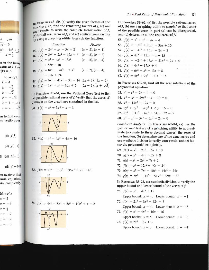
2.3 • Real Zeros of Polynomial Functions 171
Ii*i 4
'3 - 729
in Exercises 45-50, (a) verify the given factors of the
function f, (b) find the remaining factors of f, (c) use your results to write the complete factorization of f, (d) list all real zeros off, and (e) confirm your results
by using a graphing utility to graph the function.
- 10x + 24
49. f(x) = 6x3 + 41x2 - 9x - 14 (2x + 1), (3x - 2)
50. f(x) = 2x3 - x2 - 10x + 5 (2x - 1), +
In Exercises 51-54, use the Rational Zero Test to list all possible rational zeros off. Verify that the zeros of f shown on the graph are contained in the list.
51. f(x) = x3 + 3x2 - x - 3 5
-5
52. f(x) = x3 - 4x 2 - 4x + 16 18
4
-6
53. f(x) = 2x4 - 17x3 + 35x2 + 9x - 45 20
7
-50
54. f(x) = 4x5 - 8x4 - 5x3 + 10x2 + x - 2 2
-7
In Exercises 55-62, (a) list the possible rational zeros off, (b) use a graphing utility to graph f so that some of the possible zeros in part (a) can be disregarded, and (c) determine all the real zeros off.
55. f(x) = x3 + x 2 - 4x - 4 56. f(x) = -3x3 + 20x2 - 36x + 16 57. f(x) = -4x3 + 15x2 - 8x - 3 58. f(x) = 4x3 - 12x2 - x + 15 59. f(x) = - 2x4 + 13x3 - 21x2 + 2x + 8 60. f(x) = 4x4 - 17x2 + 4
61. f(x) = 6x3 - x2 - 13x + 8
62. f(x) = 4x3 + 7x2 - 1 lx - 18
In Exercises 63-68, find all the real solutions of the polynomial equation.
63. z4 - z3 - 2z - 4 = 0 64. x4 - x3 - 29x2 - x - 30 = 0 65. x4 - 13x 2 - 12x = 0
66. 2y4 + 7y 3 - 26y2 + 23y - 6 = 0 67. 2x4 - 11x3 - 6x2 + 64x + 32 = 0 68. x5 - x4 3x3 5x2 2x = 0
Graphical Analysis In Exercises 69-74, (a) use the zero or root feature of a graphing utility to approxi-mate (accurate to three decimal places) the zeros of the function, (b) determine one of the exact zeros and use synthetic division to verify your result, and (c) fac-tor the polynomial completely.
69. f(x) = x3 - 2x2 - 5x + 10
70. g(x) = x3 - 4x 2 - 2x + 8
71. h(t) = t3 - 2t 2 - 7t + 2
72. f(s) = s3 - 12s2 + 40s - 24
73. h(x) = x5 - 7x4 + 10x3 + 14x2 - 24x
74. g(x) = 6x4 - 11x3 - 51x2 + 99x - 27
In Exercises 75-78, use synthetic division to verify the upper bound and lower bound of the zeros off.
75. f(x) = x4 - 4x3 + 15
Upper bound: x = 4; Lower bound: x = -1 76. f(x) = 2x3 - 3x2 - 12x + 8
Upper bound: x = 4; Lower bound: x = -3 77. f(x) = x4 - 4x3 + 16x - 16
Upper bound: x = 5; Lower bound: x = -3 78. f(x) = 2x4 - 8x + 3
Upper bound: x = 3; Lower bound: x = -4
Value of k
k = 4
k=
k
k= -
k = 1 -
k = 2 +
m to find each to verify your
(d) f (8)
(d) g(-1
(d) h(-5)
(d) f (-10)
m to show that nnial equation, tial completely.
blue of x
= 2
= -4
x = 2
x = -2
x = -2
x = -3
x - 9 Function Factors
Ix3 - 4x2 + 5 45. f(x) 2x3 + x2 - 5x + 2 (x + 2), (x - 1) 3 -
X 46. f(x) = 3x3 + 2x2 - 19x + 6 (x + 3), (x - 2)
n in the form value of k. Use
47. f(x) = x4 - 4x3 - 15x2
+ 58x - 40
- 5), (x + 4)
'(k) = r. 48. f(x) = 8x4 - 14x3 - 71x2 (x + 2), (x - 4)
-6 4
6
3
2 4

172 Chapter 2 • Polynomial and Rational Functions
In Exercises 79-82, find the rational zeros of the polynomial function.
79. P(x) = x4 — x 2 + 9 = i.(4x4 — 25x2 + 36)
80. f(x)= x3 — ir.X 2 -21-X ± 6 = (2x3 — 3x2 — 23x +12)
81. f(x) = x3 — — x + = i(4x3 — x2 — 4x + 1)
82. f(z) = z3 + — = (6z3 + liz2 - 3z —2)
In Exercises 83-86, match the cubic function with the correct number of rational and irrational zeros. (a) Rational zeros: 0; Irrational zeros: 1 (b) Rational zeros: 3; Irrational zeros: 0 (c) Rational zeros: 1; Irrational zeros: 2 (d) Rational zeros: 1; Irrational zeros: 0
83. f(x) = x3 — 1 84. f(x) = x3 — 2
85. f(x) = x3 — x 86. f(x) = x3 — 2x
87. Data Analysis The average monthly basic rates R for cable television in the United States for the years 1988 through 1997 are given in the table, where t represents the time (in years), with t = 0 corre-sponding to 1990. (Source: Paul Kagan Associates, Inc.)
—2 —1 0 1 2
R 13.86 15.21 16.78 18.10 19.08
3 4 5 6 7
R 19.39 21.62 23.07 24.41 26.48
(a) Use a graphing utility to sketch a scatter plot of the data.
(b) Use the regression capabilities of a graphing utility to find a cubic model for the data. Then graph the model in the same viewing window as the scatter plot. Compare the model with the data.
(c) Use a graphing utility and the model to create a table of estimated values of R. Compare the estimated values with the actual data.
(d) Use the Remainder Theorem to evaluate the model for the year 2002. Even though the model is relatively accurate for estimating the given data, do you think it is accurate to predict future cable rates? Explain.
88. Data Analysis The number of United States military personnel M (in thousands) on active duty for the years 1989 through 1996 is shown in the table, where t represents the time (in years), with t = 0 corre, sponding to 1990. (Source: U.S. Department of Defense)
t —1 0 1 2
M 2130 2044 1986 1807
t 3 4 5 6 •
M 1705 1611 1518 1472
(a) Use a graphing utility to sketch a scatter plot the data.
(b) Use the regression capabilities of a graphing utility to find a cubic model for the data. Then graph the model in the same viewing window as the scatter plot. Compare the model with the data.
(c) Use a graphing utility and the model to create a table of estimated values of M. Compare the estimated values with the actual data.
(d) Use the Reinainder Theorem to evaluate the model for the year 2001. Even though the model is relatively accurate for estimating the given data, would you use this model to predict the number of military personnel in the future9 Explain.
89. Geometry An open box is to be made from a rectangular piece of material 15 centimeters by 9 centimeters by cutting equal squares from the corners and turning up the sides.
(a) Let x represent the length of the sides of the squares. Draw a diagram showing the squares removed from the original piece of material and the resulting dimensions of the open box.
(b) Use the diagram in part (a) to write the volume V of the box as a function of x. Determine the domain of the function.
(c) Use a graphing utility to graph the function and
approximate the dimensions of the box that yield maximum volume.
(d) Find values of x such that V = 56. Which of these values is a physical impossibility in the construction of the box? Explain.

Synthesis
True or False? In Exercises 93-95, determine whether the statement is true or false. Justify your answer.
93. If (7x + 4) is a factor of some polynomial function f, then 1. is a zero of f
94. The rational expression x3 + 2x2 — 13x + 10
is x2 - 4x — 12
improper.
95. (2x — 1) is a factor of the polynomial
6x6 + x5 — 92x4 + 45x3 + 184x2 + 4x — 48.
Think About It In Exercises 96 and 97, perform the division by assuming that n is a positive integer.
xi" 9x2" + 27xn + 27 96.
xn + 3
97.x3n 3x2n 5xn _ 6
98. Think About It What does it mean for a divisor to divide evenly into a dividend?
99. Writing Write a short paragraph explaining how you can check polynomial division. Give an example.
Review
In Exercises 100-103, find (a) f og and (b) g of.
100. f(x) = x2, g(x) = x + 4
101. f(x) = 2x — 5, g(x) = x2 + 1
102. f(x) = Ix' + 2, g(x) = x — 3
103. f(x) = g(x) = 4x + x2
In Exercises 104-107, find a polynomial function that has the given zeros.
104. 0,-12 105. 1, — 3, 8
106. 0, — 1, 2, 5 107. 2 + 2 —
2.3 • Real Zeros of Polynomial Functions 173
States military duty for the
le table, where t = 0 Corr.
)epartment of
scatter plot of
of a graphing the data. Then .,wing window riodel with the
)del to create a Compare the
data.
o evaluate the m though the estimating the iodel to predict I in the future?
made from a ltimeters by 9 tres from the
le sides of the ng the squares of material and Ten box.
rite the volume Determine the
ie function and f the box that
56. Which of
,ssibility in the
90. Geometry A rectangular package sent by a delivery service can have a maximum combined length and girth (perimeter of a cross section) of
120 inches.
(a) Show that the volume of the package is
V(x) = 4x2(30 — x).
(b) Use a graphing utility to graph the function and approximate the dimensions of the package that yield a maximum volume.
(c) Find values of x such that V = 13,500. Which of these values is a physical impossibility in the construction of the package? Explain.
X
91. Automobile Emissions The number of parts per million of nitric oxide emissions y from a certain car engine is approximated by the model
y= — 5.05x3 + 3857x — 38,411.25, 13 5 x 5 18
where x is the air-fuel ratio.
(a) Use a graphing utility to graph the emissions function.
(b) It is observed from the graph that two air-fuel ratios produce 2400 parts per million of nitric oxide, with one being 15. Use the graph to approximate the second air-fuel ratio.
(c) Algebraically approximate the second air-fuel ratio that produces 2400 parts per million of nitric oxide. (Hint: Because you know that an air-fuel ratio of 15 produces the specified nitric oxide emission, you can use synthetic division.)
92. Advertising Costs A company that manufactures bicycles estimates that the profit for selling a partic-ular model is
P = 45x3 + 2500x2 — 275,000, 0 5_ x 50
where P is the profit (in dollars) and x is the adver-tising expense (in tens of thousands of dollars). According to this model, find the smaller of two advertising amounts that yield a profit of $800,000.

Definition of a Complex Number
If a and b are real numbers, the number a + bi is a complex number, and it is said to be written in standard form. If b = 0, the number a + bi = a is a real number. If b 0 0, the number a + bi is called an imaginary number. A number of the form bi, where b 0, is called a pure imaginary number.
Equality of Complex Numbers
Two complex numbers a + bi and c + di, written in standard form, are equal to each other
a + bi = c + di Equality of two complex numbers
if and only if a = c and b = d.
174 Chapter 2 • Polynomial and Rational Functions
The Imaginary Unit i Some quadratic equations have no real solutions. For instance, the quadratic equation x2 + 1 = 0 has no real solution because there is no real number x that can be squared to produce —1. To overcome this deficiency, mathematicians created an expanded system of numbers using the imaginary unit i, defined as
i = Imaginary unit
where i2 = — 1. By adding real numbers to real multiples of this imaginary unit, you obtain the set of complex numbers. Each complex number can be written in the standard form a + bi. For instance, the standard form of the complex number 9 — 5 is —5 + 3i because
— 5 = 1) — 5 = —5 = —5 + 3i.
In the standard form a + bi, the real number a is called the real part of the complex number and the number bi (where b is a real number) is called the imag-inary part of the complex number.
You Should Learn:
• How to use the imaginary uni i to write complex numbers
• How to add, subtract, and multiply complex numbers
• How to use complex conju-gates to divide complex numbers How to plot complex numbq in the complex plane
To
The the ber c
So,:
You Should Learn It:
Complex numbers are used to iinodel numerous aspects of the 1 natural world, such as the imped-ance of an electrical circuit, as shown in Exercise 83 on page 181.
EX
a. (
The set of real numbers is a subset of the set of complex numbers, as shown in Figure 2.27. This is true because every real number a can be written as a complex number using b = 0. That is, for every real number a, you can write a = a + Oi. b. 2,
Real numbers
Complex numbers
c. 3
Imaginary numbers
Figure 2.27 d.

Operations with Complex Numbers
2.4 • Complex Numbers 175
Carl Friedrich Gauss (1777-1855) proved that all the
;1 roots of any algebraic equation are "numbers" of the form a + bi, where a and b are real numbers and i is the square root of — 1. These "numbers" are called complex.
earn:
naginary unit x numbers ract, and
numbers )1ex conju-nnplex
plex numbers lane
larn It:
ke used to ects of the
the impec-circuit, as 3 on page
To add (or subtract) two complex numbers, you add (or subtract) the real and
imaginary parts of the numbers separately.
Addition and Subtraction of Complex Numbers
If I + bi and c + di are two complex numbers written in standard form, their
SW] -1 and difference are defined as follows.
Sum: (a + bi) + (c + di) = (a +c) +(b + d)i
Difference: (a + bi) — (c + di) = (a — + (b — d)i
The additive identity in the complex number system is zero (the same as in the real number system). Furthermore, the additive inverse of the complex num-ber a + bi is
kr — (a + bi) = — a — bi. Additive inverse
SO, you have
II (a + bi) + (— a — bi) = 0 + Oi = 0.
EXAMPLE 1 Adding and Subtracting Complex Numbers
a. (3 — i) + (2 + 3i) = 3 — i + 2 + 3i
= 3 + 2— i + 3i
= (3 + 2) + (-1 + 3)i
= 5 + 2i
b. 2i + (-4 — 2i) = 2i — 4 — 2i
= —4 + 2i — 2i
= —4
Remove parentheses.
Group like terms.
Write in standard form.
Remove parentheses.
Group like terms.
Write in standard form.
c. 3 — (-2 + 3i) + (-5 + i) = 3 + 2 — 3i — 5 + i
= 3 + 2 — 5 — 3i + i
= 0 — 2i
= —2i
d. (3 + 2i) + (4 — i) — (7 + = 3 + 2i + 4 — i — 7 — i
= 3 + 4 — 7 + 2i — i — i
= 0 + Oi
=0
In Examples 1(b) and 1(d) note that the sum of complex numbers can be a real number.

What pattern do you see? Write a brief description of how you would find i raised to any po tive integer power.
16)
STUDY TIP
Note in Example 2(b) that
.,41 • 16 0 -,/(— 4)(—
=
= 8.
+ 2i)(3 — 2i) = 9 — 6i + 6i — 4i2
= 9 — 4(— 1)
= 9 + 4
= 13
176 Chapter 2 • Polynomial and Rational Functions
Many of the properties of real numbers are valid for complex numbers as well. Here are some examples.
Associative Property of Addition and Multiplication Commutative Property of Addition and Multiplication Distributive Property of Multiplication over Addition
Notice how these properties are used when two complex numbers are multiplied.
(a + bi)(c- + di) = a(c + di) + bi(c + di) Distributive Property
= ac + (ad)i + (bc)i + (bd)i 2 Distributive Property
= ac + (ad)i + (bc)i + (bd)(— 1) i 2 = —1
= ac — bd + (ad)i + (bc)i Commutative Property
= (ac — bd) + (ad + bc)i Distributive Property
Rather than trying to memorize this multiplication rule, you should simply remember how the distributive property is used to multiply two complex num-bers. The procedure is similar to multiplying two polynomials and combining like terms (as in the FOIL Method).
EXAMPLE 2 Multiplying Complex Numbers
a. (i)(-3i) = —3i 2
= — 3(— 1)
=3
b. • = (20(40
= 8i2
= 8(—l)
= —8
c. (2 — i)(4 + 3i) = 8 + 6i — 4i — 3i2
= 8 + 6i — 4i — 3(— 1)
= 8 + 3 + 6i — 4i
= 11 + 2i
d. (3
e. (3 + 2i)2 = 9 + 6i+ 6i + 4i2
= 9 + 4(— 1) + 12i
= 9 — 4 + 12i
= 5 + 12i
Multiply.
i 2 = — 1
Simplify.
Write each factor in standard form.
Multiply.
i2 = _1
Simplify.
Product of binomials
i 2 = —1
Group like terms.
Write in standard form.
Product of binomials
i 2 = 1
Simplify.
Write in standard form.
Product of binomials
i 2 = — I
Simplify.
Write in standard form.

Multiply numerator and denominator by conjugate of denominator.
Expand.
i2 = _ 1
Simplify.
Write in standard form.
Multiply numerator and denominator by conjugate of denominator.
EXAMPLE 3 Dividing Complex Numbers
2 + 3i 2 + 3i(4 + 2i) 4 — 2i 4 — 2A4 + 2i)
8 + 4i + 12i + 6i2 16 — 4i2
8 — 6 + 16i 16 + 4
(2 + 160 20
= —1
+ —4
i 10 5
Expand.
i2 = - 1
Simplify.
Write in standard form.
Dmplex Conjugates and Division
',Duce in Example 2(d) that the product of two complex numbers can be a real number. This occurs with pairs of complex numbers of the form a + bi and a — bi, called complex conjugates.
(a + bi)(a — bi)= a2 — abi + abi — b2i 2
= a2 b2(-1)
= a2 b2
To find the quotient of a + bi and c + di where c and d are not both zero, multiply the numerator and denominator by the conjugate of the denominator to
obtain
a + bi a + bi( c — di)
c + di c + di\c — di)
(ac + bd) + (bc — ad)i c2 + d2
a see? Writ A how you to any posi
1 1 (1— i
1 + i 1 + Al — i)
2
2.4 • Complex Numbers 177
TIP
b) that
4)(— 16
STUDY TIP
Some graphing utilities can perform operations with complex numbers. For instance, on some graphing utilities, to divide 2 + 3i by 4 — 2i, enter
M 2 2 3 ID M 2
El4B201=1
The display will be as follows.
1 4 .1 + .8i or —
10 +
Consult your user's manual for specific instructions on performing operations with complex numbers.
ENTER
EXAMPLE 4 Dividing Complex Numbers

4 Real axis
Imaginary axis
b
(a, b) a •
a
Figure 2.28
Imaginary axis
2 + 3i
—1 + 2i 41- - —
—3i
Figure 2.29
0
178 Chapter 2 • Polynomial and Rational Functions
Applications Most applications involving complex numbers are either theoretical or very tech-nical, and are therefore not appropriate for inclusion in this text. However, to give you some idea of how complex numbers can be used in applications, we give a general description of their use in fractal geometry.
To begin, consider a coordinate system called the complex plane. Just as every real number corresponds to a point on the real number line, every complex number corresponds to a point in the complex plane, as shown in Figure 2.28. In this figure, note that the vertical axis is the imaginary axis and the horizontal axis is the real axis. The point that corresponds to the complex number a + bi is (a, b).
EXAMPLE 5 Plotting Complex Numbers
Plot each complex number in the complex plane.
a. 2 + 3i b. —1 + 2i
c. 4 d. — 3i
Solution a. To plot the complex number 2 + 3i, move (from the origin) two units to the
right on the real axis and then three units up, as shown in Figure 2.29. In other words, plotting the complex number 2 + 3i in the complex plane is compara-ble to plotting the point (2, 3) in the Cartesian plane.
b. The complex number —1 + 2i corresponds to the point (-1, 2), as shown in Figure 2.29.
c. The complex number 4 corresponds to the point (4, 0), as shown in Figure 2.29.
d. The complex number — 3i corresponds to the point (0, 3), as shown in Figure 2.29.
In the hands of a person who understands fractal geometry, the complex plane can become an easel on which stunning pictures, called fractals, can be drawn. The most famous such picture is called the Mandelbrot Set, named after the Polish-born mathematician Benoit Mandelbrot. To draw the Mandelbrot Set, consider the following sequence of numbers.
c, c2 c,
(c2 c)2 c,
[(c2 c)2 c,
The behavior of this sequence depends on the value of the complex number c. For some values of c this sequence is bounded, which means that all elements in the sequence are less than some fixed number N. For other values it is unbounded, which means that the elements in the sequence become infinitely large. If the sequence is bounded, the complex number c is in the Mandelbrot Set; if the sequence is unbounded, the complex number c is not in the Mandelbrot Set.
.0
Fig
To thE On
apj pa'
fra

(a, b) <—> a + bi
I Real I
axis 7
+ 3i
4 Real • ax's
b.
C.
Figure 2.31
Figure 2.32 A Fractal Fern
2.4 • Complex Numbers 179
EXAMPLE 6 Members of the Mandelbrot Set
The complex number —2 is in the Mandelbrot Set because for c = —2,
the corresponding Mandelbrot sequence is —2, 2, 2, 2, 2, 2,. . . , which is bounded.
The complex number i is also in the Mandelbrot Set because for c = i, the corresponding Mandelbrot sequence is
—1 + i, —i, —1 1 + i, —i, —1 1 +
which is bounded.
The complex number 1 + i is not in the Mandelbrot Set because for c = 1 + i, the corresponding Mandelbrot sequence is
1 + j, 1 + 3i, —7 + 7i, 1 — 97i, —9407 — 193i,
88454401 + 3631103i,
which is unbounded.
With this definition, a picture of the Mandelbrot Set would have only two colors:
one color for points that are in the set (the sequence is bounded), and one for points that are outside the set (the sequence is unbounded). Figure 2.30 shows a black and yellow picture of the Mandelbrot Set. The points that are black are in the Mandelbrot Set and the points that are yellow are not.
Imaginary axis
To add more interest to the picture, computer scientists discovered that the points that are not in the Mandelbrot Set can be assigned a variety of colors, depending on "how quickly" their sequences diverge. Figure 2.31 shows three different appendages of the Mandelbrot Set. (The black portions of the picture represent Points that are in the Mandelbrot Set.)
Figure 2.32 shows another type of fractal. From this picture, you can see why fractals have fascinated people since their discovery (around 1980). The fractal shown was produced on a graphing calculator.

Real I I axi
-
-
-3
180 Chapter 2 • Polynomial and Rational Functions
1111LExercises In Exercises 1-4, solve for a and b.
1. a + bi = -9 + 4i 2. a + bi = 12 + 5i 3. (a - 1) + (b + 3)i = 5 + 8i 4. (a + 6) + 2bi = 6 - 5i
In Exercises 5-14, write in standard form.
5. 4 + 6. 3 + 7. 12 8. 42 9. -5i + i2 10. -3i2 + i
11. (-../- -is) 12. - 7
13. -,/-0.09 14. ,/-0.0004
In Exercises 15-24, perform the addition or subtrac-tion and write the result in standard form.
15. (4 + 0 + (7 - 2i) 16. (11 - 2i) + (-3 + 6i) 17. (-1 + + (8 - 18. (7 + ,/-18) - (3 + 19. 13i - (14 - 7i) 20. 22 + (-5 + 8i) + 10i 21. -(i + + + 22. 23. (1.6 + 3.2i) + (-5.8 + 4.3i) 24. -(-3.7 - 12.80 - (6.1 - ,/-24.5)
In Exercises 25-36, perform the operation and write the result in standard form.
25. -,[2 6 • 26. • 27. (-\/ 7:- -10)2 28. (-,/-75)2 29. (1 + i)(3 - 2i) 30. (6 - 2i)(2 - 3i) 31. 645 - 2i) 32. -8i(9 + 4i) 33. („/T4 + -,/T3i)(„/T4 - ,/17)i) 34. (3 + - 35. (4 + 502 36. (1 - 202 - (1 + 202
37. Error Analysis Describe the error.
= -,/(- 6)(-6) = = 6 X
38. Error Analysis Describe the error.
- 1) = - 1) X
= -4i2 - i
= 4 - i
In Exercises 39-46, find the product of the number and its conjugate.
39. 4 + 3i 40. 8 - 12i
41. -6 - 42. -3 +
43. 22i 44.
45. 3 - 46. 1 + 8
In Exercises 47-58, perform the operation and write the result in standard form.
5 47. -
6 48.
4 3 49. 50.
4 - Si 1 - i
51. 2 + i 52. 8 - 7i 2 - i 1 - 2i
6 - 7i 8 + 20i 53. 54.
i 2i 1
56: (2 - 30(50
55. (4 - 502 2 + 3i
2 3 2i 5 57. 58. +
1 + i 1 - i 2 + i 2 - i
In Exercises 59-66, simplify the complex number and write it in standard form.
59. -6i3 + i 2 60. 4i2 - 2i3
61. -5i5 62. (-03
63. (-./-75)3 64. (-,/,) 6
65. 1 66. (203
1
In Exercises 67-70, determine the complex number shown in the complex plane.
67. Imaginary 68. Imaginary axis axis
4 - 1 -
3
2 -
1 - Real
1 2 3 axis
-•
69. in
In Exe comple
71. 4 - 73. - E
Fractal in the f
C, c 2 +
From t numbei reasoni:
75. c 77. c
79. c =
81. Cut (a)
82. Rai (a)
83. hnj cal a p equ
wh(
tabl cuit wa the

(a) (b) 3 SI
4 II
Synthesis
True or False? In Exercises 84-86, determine whether the statement is true or false. Justify your answer.
ImagniarY axis
6• 5 - 4 - 3 --
2 --
1 ---
-- 1 I I I > 1 2 3 4 5 6
70. Imaginary axis
the number Real axis
3 4 axis Real
In Exercises 71-74, plot the complex number in the complex plane.
71. 4 - 5i 72. 3i
73. -6 74. -7 + 2i
-8
ion and write
2.4 • Complex Numbers 181
2 - i
number °and
3
tplex number
laginary axis
1 - Real
1 axis
3 -
Fractals In Exercises 75-80, find the first six terms
in the following sequence.
c , e 2 C, (C 2 + C)2 [(c2 c)2
From these terms, do you think the given complex number is in the Mandelbrot Set? Explain your reasoning.
75. c = 0 76. c = 2
77. c=i 78. c = - i
79. c = 1 80. c = -1
81. Cube each complex number. What do you notice?
(a) 2 (b) -1 + (c) -1 -
82. Raise each number to the fourth power.
(a) 2 (b) -2 (c) 2i (d) -2i
83. Impedance The opposition to current in an electri-cal circuit is called its impedance. The impedance in a parallel circuit with two pathways satisfies the equation
1 1 1 - = - + - z Z1 Z2
when z1 is the impedance (in ohms) of pathway 1 and Z2 is the impedance (in ohms) of pathway 2. Use the table to determine the impedance of each parallel cir-cuit. (Hint: You can find the impedance of each path-way by adding the impedance of each component in the pathway.)
Resistor Inductor Capacitor
Symbol
-/VV\i-
a Si -'060'
b n HI-
c 11
Impedance a hi -ci
84. There is no complex number that is equal to its conjugate.
85. -i-,/6 is a solution of x4 - x2 + 14 = 56.
86. i44 ± 050 _ i74 _ 009 + i61 = 1
87. Express each of the following powers of i as i, - i, 1, or -1. (a) i40 (b) i25 (c) i 5° (d) i67
88. Prove that the sum of a complex number a + hi and its conjugate is a real number, and that the difference of a complex number a + hi and its conjugate is an imaginary number.
89. Prove that the product of a complex number a + hi and its conjugate is a real number.
Review
In Exercises 90 and 91, write an equation of the line through the point (a) parallel to the given line and (b) perpendicular to the line.
90. (3, -2) 5x - 4y = 8
91. (- 8,3) 2x + 3y = 5
In Exercises 92-95, find the x- and y-intercepts of the graph of the equation.
92. y = -x2 + 6 93. y = x2 + Zr - 8
94. y = lx - 41 + 1 95. Y = Ix' - 1
96. Mixture Problem A 5-liter container contains a mixture with a concentration of 50%. How much of this mixture must be withdrawn and replaced by 100% concentrate to bring the mixture up to 60% concentration?

The Fundamental Theorem of Algebra
If f(x) is a polynomial of degree n, where n > 0, f has at least one zero in the complex number system.
Linear Factorization Theorem
If f(x) is a polynomial of degree n where n > 0, f has precisely n linear factors
f(x) = an(x — c 1)(x — c2) • • • (x — cn)
where cl, c2, . . . , cn are complex numbers.
182 Chapter 2 • Polynomial and Rational Functions
The Fundamental Theorem of Algebra
You have been using the fact that an nth-degree polynomial can have at most n real zeros. In the complex number system, this statement can be improved. That is, in the complex number system, every nth-degree polynomial function has pre-cisely n zeros. This important result is derived from the Fundamental Theorem of Algebra, first proved by the famous German mathematician Carl Friedrich Gauss (1777-1855).
EXA
a. TI You Should Learn:
• How to use the Fundamenta Theorem of Algebra to deter. mine the number of zeros. o polynomial functions
• How to find all zeros of p01 nomial functions, including complex zeros
• How to find conjugate pairs of complex zeros
• How to find zeros of poly mials by factoring
ha 2..
b. TI
ha Fi
Exam; Ratio pyn
l
You Should Learn It:
Using the Fundamental Theorem of Algebra and the equivalence of zeros and fac-tors, you obtain the Linear Factorization Theorem. EXAI
Write
as the
Being able to find zeros of poly-nomial functions is an importar part of modeling real-life prob-lems. For instance, Exercise 65 on page 188 shows how to dete mine whether a ball thrown wit a given velocity can reach a certain height.
(A proof of the Linear Factorization Theorem is found in Appendix A.) Note that neither the Fundamental Theorem of Algebra nor the Linear
Factorization Theorem tells you how to find the zeros or factors of a polynomial. Such theorems are called existence theorems. To find the zeros of a polynomial function, you still must rely on other techniques.
Remember that the n zeros of a polynomial function can be real or complex, and they may be repeated. Examples 1 and 2 illustrate several cases.
SO/1/1 The p 2.34 i zero I-
C repeat
By fa(
you o
which
Note I that al
EXAMPLE 1 Real Zeros of Polynomial Functions
a. The first-degree polynomial f(x) = x — 2 has exactly one zero: x = 2.
b. Counting multiplicity, the second-degree polynomial function
f(x) = x2 — 6x + 9 = (x — 3)(x — 3)
has exactly two zeros: x = 3 and x = 3.
Note in Example 1 that you can use a graphing utility to verify graphically the zeros of the polynomial functions.

2
b. T
f(x) = x3 + 4x = x(x2 + 4) = x(x — 2i)(x + 2i)
is exactly three zeros: x = 0, x = 2i, and x = —2i. In the graph in Figure 33(a), only the real zero x = 0 appears as an intercept.
le fourth-degree polynomial function
f(x) = x4 — 1 = (x — 1)(x + 1)(x — i)(x + i)
is exactly four zeros: x = 1, x = —1, x = i, and x = — i. In the graph in
gure 2.33(b), only the real zeros x = — 1 and x = 1 appear as x-intercepts.
as th
f(x) = x5 + x3 + 2x — 12x + 8
product of linear factors, and list all of its zeros.
;
0
.111° L1
Learn:
Fundamental ebra to det(J.-r of zeros of tions zeros of poly_ s, including
tjugate pans
os of polyno-ng
Barn It:
eros of pol an important al-life prob Exercise 65 how to deter-thrown with reach a
2.5 • The Fundamental Theorem of Algebra 183
EXAMPLE 2 Real and Complex Zeros of Polynomial Functions
a. The third-degree polynomial function
Example 3 shows how to use the methods described in Sections 2.2 and 2.3 (the
Rational Zero Test, synthetic division, and factoring) to find all the zeros of a
polynomial function, including complex zeros.
EXAMPLE 3 Finding the Zeros of a Polynomial Function
Writ
Solution The possible rational zeros are ± 1, ±2, ±4, and ±8. The graph shown in Figure 2.34 indicates that 1 and —2 are good guesses, and that 1 is possibly a repeated zero because it touches the x-axis.
Using synthetic division, you can determine that —2 is a zero and 1 is a repeated zero off. So, you have
f (x) = x5 + x3 + 2x2 — 12x + 8
= (x — 1)(x — 1)(x + 2)(x2 + 4).
By factoring x2 + 4 as
c2 — (-4) = — + = (x — 2i)(x + 2i)
you obtain
F(x) = (x — 1)(x— 1)(x + 2)(x — 2i)(x +
which gives the following five zeros off.
1, —2, 2i, and —2i
Note from the graph off shown in Figure 2.34 that the real zeros are the only ones that appear as x-intercepts.
6
f(x) =
-6
6
f(x)= x4
-6
(b)
Figure 2.33
4x
f(x)= x5 + x3 + 2x2 — 12x -F
16 \
- 4
Figure 2.34
9
(a)
9

184 Chapter 2 • Polynomial and Rational Functions
Conjugate Pairs
In Example 3, note that the two complex zeros are conjugates. That is, they are of the form a + bi and a — bi.
Complex Zeros Occur in Conjugate Pairs
Let f(x) be a polynomial function that has real coefficients. If a + bi, where b 0, is a zero of the function, the conjugate a — bi is also a zero of the function.
A quad sure yo exampl
X2
js irredi the qua
x2
is irrech
Be sure you see that this result is true only if the polynomial function has real coefficients. For instance, the result applies to the function f(x) = x2 + 1, but not to the function g(x) = x — i.
EXAMPLE 4 Finding a Polynomial with Given Zeros
Find a fourth-degree polynomial function, with real coefficients, that has —1, —1, and 3i as zeros.
Solution Because 3i is a zero and the polynomial is stated to have real coefficients, you know that the conjugate — 3i must also be a zero. So, from the Linear Factorization Theorem, f(x) can be written as
f(x) = a(x + 1)(x + 1)(x — 3i)(x + 3i).
For simplicity, let a = 1, to obtain
f(x) = (x2 + 2x + 1)(x2 + 9)
= x4 + 2x3 + 10x2 + 18x + 9.
Factoring a Polynomial
The Linear Factorization Theorem shows that you can write any nth-degree polynomial as the product of n linear factors.
f(x) = a(x — c 1)(x — c2)(x — c3) • • • (x — cn)
However, this result includes the possibility that some of the values of ci are complex. The following theorem says that even if you do not want to get involved with "complex factors," you can still write f(x) as the product of linear and/or quadratic factors.
Factors of a Polynomial
Every polynomial of degree n > 0 with real coefficients can be written as the product of linear and quadratic factors with real coefficients, where the qua-dratic factors have no real zeros.
(For a proof of this theorem, see Appendix A.)
Jean Le Rond d'Alembert (1717-1783) worked indepen-dently of Carl Gauss trying to
kprove the Fundamental Theore of Algebra. His efforts were such that in France, the
IF' undamental Theorem of Algebra is frequently known as the Theorem of d'Alembert.
STUDY Tly
EXAM
Write d
a. as if
b. as ti the r
C. in cc
S011Ith a. Begi
poly
Some graphing utilities can fin both real and complex zeros ol function. For instance, to find all the zeros of
Both
b. By f
f(x) = x4 — 3x3 + 6x2
+ 2x — 60
use the graphing utility's solve feature. If your graphing utility can find complex zeros, you w obtain the following solutions.
x = 1 + 3i, x = 1 — 3i,
x = 3, x = — 2
Exar polynor'
Thr term,
ould h because
f(x
are pre(
an;
whe
C. In et

lembert d indepen-s trying to ital Theoren irts were the
em of iy known as lembert.
T,P
ities can find lex zeros of a ice, to find
+ 6x2
- 60
dity's solve thing utility .ros, you will solutions.
= 1 - 3i.
-2
2.5 • The Fundamental Theorem of Algebra 185
factor with no real zeros is said to be irreducible over the reals. Be A Oadratic
e you see that this is not the same as being irreducible over the rationals. For stir eXELrnple, the quadratic
x2 4- 1 = (X' — i)(X i)
rreducible over the reals (and therefore over the rationals). On the other hand, quadratic
is i
the x2 - 2 +
rreducible over the rationals, but reducible over the reals.
EXAMPLE 5 Factoring a Polynomial
Write the polynomial
f(x) = x4 - x2 - 20
a. as the product of factors that are irreducible over the rationals,
b. as the product of linear factors and quadratic factors that are irreducible over
the reals, and
C. in completely factored form.
Solution a. Begin by factoring the polynomial into the product of two quadratic
polynomials.
x4 - x2 - 20 = (x2 - 5)(x2 + 4)
Both of these factors are irreducible over the rationals.
b. By factoring over the reals, you have
x4 - x2 - 20 =(x+ ,/3)(x - -A(x2 + 4)
where the quadratic factor is irreducible over the malls.
c. In completely factored form, you have
x4 _ x2 _ 20 - + /)(x-- ,Z3)(x - 2i)(x + 2i).
In Example 5, notice from the completely factored form that the fourth-degree polynomial has four zeros.
Throughout this chapter, the results and theorems have basically been stated in terms of zeros of polynomial functions. Be sure you see that the same results could have been stated in terms of solutions of polynomial equations. This is true because the zeros of the polynomial function
z
is i
f (x) = axn ± an- 1xn-1 + • • • + a2x2 + a1x + ao
are precisely the solutions of the polynomial equation
ax n + an _ i xn-1 + • • • + a2x2 + aix + ao = 0.
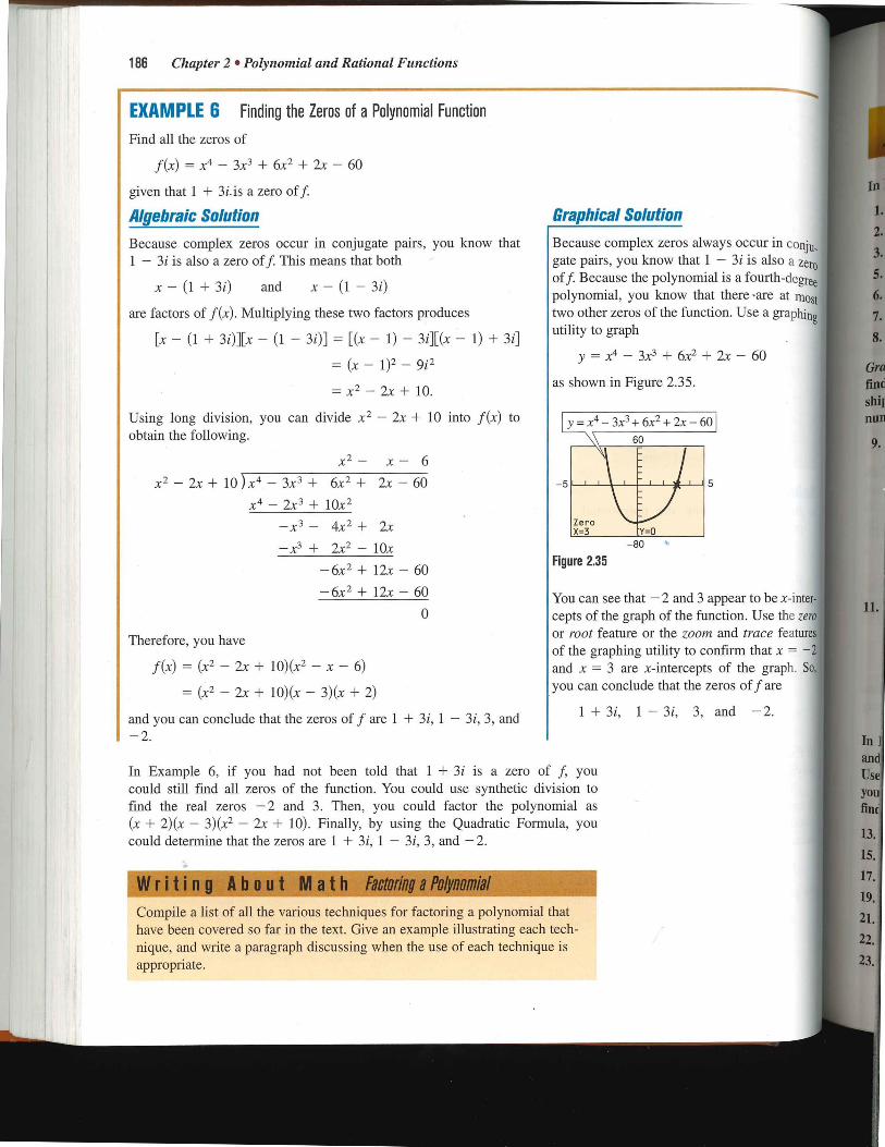
t0.1/11# a lid ..Lgai"..4MIE Compile a list of all the various techniques for factoring a polynomial that have been covered so far in the text. Give an example illustrating each tech-nique, and write a paragraph discussing when the use of each technique is appropriate.
EXAMPLE 6 Finding the Zeros of a Polynomial Function
Find all the zeros of
f(x) = x4 — 3x3 + 6x2 + 2x — 60
given that 1 + 3i,is a zero off
Algebraic Solution
Because complex zeros occur in conjugate pairs, you know that 1 — 3i is also a zero off. This means that both
x — (1 + 3i) and x — (1 — 3i)
are factors of f(x). Multiplying these two factors produces
[x — (1 + 30][x — (1 — 3i)] = [(x — 1) — 3i][(x — 1) + 3i]
= (x — 1)2 — 9i2
= X2 — 2x + 10.
Using long division, you can divide x2 — 2x + 10 into f(x) to obtain the following.
x2 — x — 6
x2 — 2x + 10 )x4 — 3x3 + 6x2 + 2x — 60
x4 — 2x3 + 10x2
—x 3 — 4x2 + 2x
— x3 + 2X2 — 10X
- 6X2 ± 12x — 60
— 6x2 + 12x — 60
0
Therefore, you have
f(x) = (x2 — 2x + 10)(x2 — x — 6)
= (x2 — 2x + 10)(x — 3)(x + 2)
and you can conclude that the zeros of f are 1 + 3i, 1 — 3i, 3, and —2.
13.
15.
17.
19.
21.
22.
23.
186 Chapter 2 • Polynomial and Rational Functions
11.
1 + 3i, 1 — 3i, 3, and —2.
In and
In Example 6, if you had not been told that 1 + 3i is a zero of f, you Use could still find all zeros of the function. You could use synthetic division to you find the real zeros —2 and 3. Then, you could factor the polynomial as fin( (x + 2)(x — 3)(x2 — 2x + 10). Finally, by using the Quadratic Formula, you could determine that the zeros are 1 + 3i, 1 — 3i, 3, and —2.
Graphical Solution
Because complex zeros always occur in conjo, gate pairs, you know that 1 — 3i is also a zero off. Because the polynomial is a fourth-degree polynomial, you know that there are at most two other zeros of the function. Use a graphing utility to graph
y = x4 — 3x3 + 6x2 + 2x — 60
as shown in Figure 2.35.
You can see that —2 and 3 appear to be x-inte cepts of the graph of the function. Use the zero or root feature or the zoom and trace features of the graphing utility to confirm that x = —2 and x = 3 are x-intercepts of the graph. So, you can conclude that the zeros off are
Figure 2.35
—5
y = x4 — 3x3 + 6x2 +a— 60
ill i 1 1 1
Zero
—80
60
5
Gra rind shir nun
In
1.
2.
3.
5.
6.
7.
8.
9.
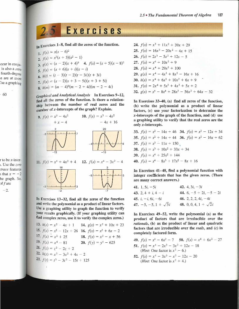
2.5 • The Fundamental Theorem of Algebra 187
xercise
in Exercises 1-8, find all the zeros of the function.
1. f(x) = x(x - 6)2
2.f(x) x2(x 3)(x2 _ 1 )
3. g(x)(X - 2)(x ± 4)3 4. f(x) = (x + 5)(x - 8)2
5. f(x) + 6)(x + i)(x - i)
6. h(t) = (t 3)(t - 2)(t - 3i)(t + 3i)
7. f(x) = (x - 2)(x+ 3_ 5i)(x + 3 + 5i)
8. h(m) = (m - 4)2(m - 2 + 4i)(m - 2 - 4i)
Graphical and Analytical Analysis In Exercises 9-12,
find all the zeros of the function. Is there a relation-ship between the number of real zeros and the number of x-intercepts of the graph? Explain.
9. f(x) = x3 - 4x2 10. f(x) = x3 - 4x2
+ x - 4 - 4x + 16
2 20
-3
-13 -10
11. f(x) = x4 + 4x2 + 4 12. f(x) = x4 - 3x2 - 4
18 3
-3
In Exercises 13-32, find all the zeros of the function and write the polynomial as a product of linear factors. Use a graphing utility to graph the function to verify your results graphically. (If your graphing utility can find complex zeros, use it to verify the complex zeros.)
13. h(x) = x2 - 4x + 1 14. g(x) = x 2 + 10x + 23
15. f(x) --- x2 - 12x + 26 16. f(x) = x2 + 6x - 2
17. f(x) = x2 + 25 18. f(x) = x2 - x + 56
19. f(x) = x 4 - 81 20. f(y) = y4 - 625
21. f (z) z2 - 2z + 2 22. h(x) x 3 - 3x 2 + 4x - 2
23. f (t) = t 3 - 3t 2 - 1St + 125
24. f(x) = x3 + 11x2 + 39x + 29 25. f(x) = 16x3 - 20x 2 - 4x + 15
26. f(s) = 2s3 - 5s2 + 12s - 5
27. f(x) = x4 + 10x2 + 9
28. f(x) =x4 + 29x2 + 100
29. g(x) = x 4 - 4x3 + 8x2 - 16x + 16
30. h(x) = x4 + 6x3 + 10x2 + 6x + 9
31. f(x) = 2x4 + 5x3 + 4x2 + 5x + 2
32. g(x) = x5 - 8x4 + 28x3 - 56x2 + 64x - 32
In Exercises 33-40, (a) find all zeros of the function, (b) write the polynomial as a product of linear factors, (c) use your factorization to determine the x-intercepts of the graph of the function, and (d) use a graphing utility to verify that the real zeros are the only x-intercepts.
33. f(x) = x2 - 14x + 46 34. f(x) = x2 - 12x + 34
35. f(x) = x2 + 14x + 44 36. f(x) = x2 - 16x + 62
37. f(x) = x3 - 1 lx + 150
38. f(x) = x3 + 10x2 + 33x + 34
39. f(x) = x4 + 25x2 + 144
40. f(x) = x4 - 8x3 + 17x2 - 8x + 16
In Exercises 41-48, find a polynomial function with integer coefficients that has the given zeros. (There are many correct answers.)
41. 1,5i, -5i 42. 4, 3i, -3i
43. 2, 4 + i, 4 - i 44. 6, -5 + 2i, -5 - 2i
45. i, -i, 6i, -6i 46. 2, 2, 2, 4i, -4i
47. -5, -5, 1 + 48. 0, 0,4, 1 +
In Exercises 49-52, write the polynomial (a) as the product of factors that are irreducible over the rationals, (b) as the product of linear and quadratic factors that are irreducible over the reals, and (c) in completely factored form.
49. f(x) = x4 - 6x2 - 7 50. f(x) = x4 + 6x2 - 27
51. f(x) = x4 - 2x3 - 3x2 + 12x - 18 (Hint: One factor is x2 - 6.)
52. f(x) = x4 - 3x3 - x2 - 12x - 20 (Hint: One factor is x2 + 4.)
ccur in conju. is also a zero fourth-degree e are at most Jse a graphing
- 60
r to be x-inter-
L. Use the zero trace features that x = -2
he graph. So, )f f are
-2.
7
6
-4
3
-2

ide our
ion
In Exercises 73-76, sketch the graph of the function. Identify the vertex and any intercepts. Use a graphing utility to verify your results.
73. f(x) = x2 — 7x — 8 74. f(x) = —x2 + x + 6
75. f(x) = 6x2 + 5x — 6
76. f(x) = 4x2 + 2x — 12
+4
the ues sfy any
69
ffi-s a
m-
s a
ex .f(
Nol tras. of .;
-4
Figur
188 Chapter 2 • Polynomial and Rational Functions
In Exercises 53-60, use the given zero to find all the zeros of the function.
Function Zero
53. f(x) = 2x3 + 3x2 + 50x + 75 5i
54. f(x) = 2x4 — x3 + 7x2 — 4x — 4 2i
55. g(x) = x 3 — 7x2 — x + 87 5 + 2i
56. g(x) = 4x3 + 23x2 + 34x — 10 —3 + i
57. h(x) = 3x3 — 4x2 + 8x + 8 1 —
58. f(x) = x3 + 4x2 + 14x + 20 —1 — 3i
59. h(x) = 8x3 — 14x2 + 18x — 9 1(1 —
60. f(x) = 25x3 — 55x2 — 54x — 18 2 +
Graphical Analysis In Exercises 6164, (a) use the zero or root feature of a graphing utility to approxi-mate the zeros of the function accurate to three decimal places, (b) determine one of the exact zeros and use synthetic division to verify your result, and (c) find the exact values of the remaining zeros.
61. f(x) = x4 + 3x3 — 5x2 — 21x + 22
62. f(x) = x3 + 4x2 + 14x + 20
63. h(x) = 8x3 — 14x2 + 18x — 9
64. f(x) = 25x3 — 55x2 — 54x — 18
65. Maximum Height A baseball is thrown upward from ground level with an initial velocity of 48 feet per second, and its height h (in feet) is
h = —16t 2 + 48t, 0 t 3
where t is the time (in seconds). Suppose you are told that the ball reaches a height of 64 feet. Is this possible? Explain.
66. Profit The demand equation for a microwave is
p = 140 — 0.0001x
where p is the unit price (in dollars) of the microwave and x is the number of units produced and sold. The cost equation for the microwave is
C = 80x + 150,000
where C is the total cost (in dollars) and xis the num-ber of units produced. The total profit obtained by producing and selling x units is
P = R — C = xp — C.
Suppose you are working in the marketing depart-ment that produces this microwave, and you are asked to determine a price p that would yield a profit of 9 million dollars. Is this possible? Explain.
Synthesis
True or False? In Exercises 67 and 68, de( whether the statement is true or false. Justify y answer.
67. It is possible for a third-degree polynomial func with integer coefficients to have no real zeros.
68. If x = 4 + 3i is a zero of the function f(x x4 — 7x3 — 13x2 + 265x —750, then x = —3i must also be a zero of f.
69. Exploration Use a graphing utility to graph function f(x) = x4 — 4x2 + k for different val of k. Find values of k such that the zeros of f sat the specified characteristics. (Some parts have m correct answers.)
(a) Four real zeros
(b) Two real zeros each of multiplicity 2
(c) Two real zeros and two complex zeros
(d) Four complex zeros
70. Think About It Will the answers to Exercise change for the function g?
(a) g(x) = f (x — 2) (b) g(x) = f (2x)
71. Find a quadratic function f (with integer coc cients) that has ±,j9i as zeros. Assume that b positive integer.
72. Find a quadratic function f (with integer cue cients) that has a -± hi as zeros. Assume that b positive integer.
Review
In Exercises 77-80, perform the operations and vvl ite
the result in standard form.
77. 12 — (-7 + 5i) + (-2 + 3i)
78. —8i — + 3i)
— i 79. (-3 — 802 80.
16 — 4/

You Should Learn:
2.6 • Rational Functions and Asymptotes 189
68, decide Justify your
mial functioil 1 zeros.
ction f(x) r = — 3i + 4
to graph the ferent values
of f satisfy ts have many
2
ros
Exercise 69
Lteger coeffi-le that b is a
aeger coeffi-le that b is a
he function. e a graphing
introduction to Rational Functions
A rational function can be written in the form
N(x) f(x) = mx)
where N(x) and D(x) are polynomials and D(x) is not the zero polynomial. In this section it is assumed that N(x) and D(x) have no common factors.
In general, the domain of a rational function of x includes all real numbers except x-values that make the denominator zero. Much of the discussion of ratio-nal functions will focus on their graphical behavior near these x-values.
EXAMPLE 1 Finding the Domain of a Rational Function
Find the domain of f(x) = 1/x and discuss the behavior of f near any excluded x-values.
Solution Because the denominator is zero when x = 0, the domain off is all real numbers except x = 0. To determine the behavior off near this excluded value, evaluate f(x) to the left and right of x = 0, as indicated in the following tables.
x —1 —0.5 —0.1 —0.01 —0.001 0
f(x) —1 — 2 —10 —100 —1000 —> — co
x 0 0.001 0.01 0.1 0.5 1
f(x) co <— 1000 100 10 2 1
• How to find domains of ratio-nal functions
• How to find horizontal and vertical asymptotes of graphs of rational functions
• How to use rational functions to model and solve real-life problems
11,4p You Should Learn It:
Rational functions are convenient in modeling a wide variety of real-life problems, such as envi-ronmental scenarios. For instance, Exercise 31 on page 196 shows how to determine the cost of removing pollutants from aim
Note that as x approaches 0 from the left, f(x) decreases without bound. In con-trast, as x approaches 0 from the right, f(x) increases without bound. The graph of f is shown in Figure 2.36.
1 f(x) = 7 - 7
as and write
-4 5
-3
Figure 2.36
3

Library of Functions A rational function f(x) is the quotient of two polynomials, f(x) = N(x)/D(x). A rational function is not defined at points x for which D(x) = 0. Near these points, the graph of the rational function may increase or decrease without bound.
Consult the Library of Functions Summary inside the front cover for a description of the rational functions.
wl
1.
2.
EX
a. T
190 Chapter 2 • Polynomial and Rational Functions
Horizontal and Vertical Asymptotes
In Example 1, the behavior of f(x) = 1/x near x = 0 is denoted as follows.
f(x) — cc as x—> f (x) —> oo as x —> 0+
f(x) decreases without bound as 1(x) increases without bound as x approaches 0 from the left. x approaches 0 from the right.
The line x = 0 is a vertical asymptote of the graph off as shown in Figure 2.37. The graph off also has a horizontal asymptote—the line y = 0. This means the values of f(x) = x approach zero as x increases or decreases without bound.
f(x) —> 0 as x —> — cc f(x) 0 as x —*00
1(x) approaches 0 as x f(x) approaches 0 as x decreases without bound. increases without bound.
• ‘ Explorat
Use a graphing utility to grap g(x) = (3x2) / (x2 + 2) in a standard viewing window. G: ip g(x) again, using a viewing win-
dow in which —100 x 00, Graph g(x) a third time, usin a viewing window in which — 1000 x 1000. Desch' ,e the left and right behavior of the graphs Complete the table.
Vertical asymptote: y-axis — N\
\3
—3 Horizontal asymptote: x-axis
Figure 2.37
f(x) = -
Definition of Vertical and Horizontal Asymptotes
1. The line x = a is a vertical asymptote of the graph of f if f(x) oo or f(x) —> — oo as x —> a, either from the right or from the left.
2. The line y = b is a horizontal asymptote of the graph of f if f(x) b as x—> oo or — oo.
Eventually (as x —> oo or x—> — cc), the distance between the horizontal asymp-tote and the points on the graph must approach zero. Figure 2.38 shows the horizontal and vertical asymptotes of the graphs of three rational functions.
g(x)
s the x-values become very 'arge or very small, what do values of g(x) approach? Wha is the horizontal asymptote of the graph of g?
2 f(x) = x - 1 2
10
— 10
Vertical asymptote: x
2.
b. T
ha th th nu
C. TI-
ha
A 1 t ht e
h
' asym asym, Vertical
asymptote: x = —1 Figure 2.38
Horizontal asymptote: y =0
Horizontal asymptote: y 0

rtical ymptote: x =
f(x) is the 'nomials, , rational ed at points x Near these
the rational se or decrease
of Functions front cover
.he rational
ty to graph 2) in a ndow. Graph riewing win-
x 100. me, using a which D. Describe aavior of the e table.
1000
DO -1000
ome very what do the )ach? What rmptote of
rizontal mptote: y =
Use a graphing utility to com-pare the graphs of y1 and y2.
3x3 - 5x2 + 4x - 5 y1=
2x2 - 6x + 7 3x3
y2 2x2
Start with a viewing window in which -5 x .5 and -10 y 10, then zoom out. Write a convincing argument that the shape of the graph of a rational function eventually behaves like the graph of y = anxn/binxm, where anxn is the leading term of the numera-tor and knei is the leading term of the denominator.
2
EXAMPLE 2 Finding Horizontal Asymptotes
a. The graph of
2x f (x) =
3x 2 + 1
has the line y = 0 (the x-axis) as a horizontal asymptote, as shown in Figure 2.39(a). Note that the degree of the numerator is less than the degree of the denominator.
b. The graph of 2x 2
g(x) = 3x 2 + 1
has the line y = as a horizontal asymptote, as shown in Figure 2.39(b). Note that the degree of the numerator is equal to the degree of the denominator, and the horizontal asymptote is given by the ratio of the leading coefficients of the numerator and denominator.
C. The graph of
1.5
3x2 + 1
Horizontal _ asymptote:
y = 0 -1 5
3
g(x)-2x2 Horizontal
asymptote: y= 2
3x2 + 1
1.5
2
(a)
-2
(b)
2
2
2x3 h(X) =
3x2 +
1
has no horizontal asymptote because the degree of the numerator is greater than the degree of the denominator. See Figure 2.39(c).
Although the graph of the function in part (c) does not have a horizontal asymptote, it does have a slant asymptote—the line y = ix. You will study slant asymptotes in the next section. (c)
Figure 2.39
-2
-1 5
2.6 • Rational Functions and Asymptotes 191
As mptotes of R'ationa Function
Let f be the rational function
N(x) f (x) - D(x)
ax " + an _ ix" 1 + . • + ax + 61 0
bine' + lx"2-1 + • • • + bix + bo
where N(x) and D(x) have no common factors.
1. The graph of f has vertical asymptotes at the zeros of D(x).
2. The graph of f has at most one horizontal asymptote determined by com-paring the degrees of N(x) and D(x).
a. If n < m, the line y = 0 (the x-axis) is a horizontal asymptote.
b. If n = m, the line y = anIbm is a horizontal asymptote.
c. If n> m, the graph of f has no horizontal asymptote.

X Y1
1 12
10 -0.9267
100 -0.7675
1000 -0.7518
10000 -0.7502
x=
X Y1
-1 0.66667
-10 -0.5738
-100 -0.7325
-1000 -0.7482
-10000 -0.7498
MM.
'X=
192 Chapter 2 • Polynomial and Rational Functions
..4.81,3C41, T=1.
EXAMPLE 3 Finding a Function's Domain and Asymptotes
For the function f, find (a) the domain of f, (b) the vertical asymptote of f, and (c) the horizontal asymptote of f.
3x3 + 7x2 + 2 f(x) =
—4x3 + 5
Algebraic Solution
a. Because the denominator is zero when — 4x3 + 5 = 0, solve this equation to determine that the domain of f is all real numbers except x =
b. Because the denominator of f has a zero at x = and et is not a zero of the numerator, the g9..ph of f has the vertical asymptote
x = 1.08, as shown in Figure 2.40.
c. Because the degrees of the numerator and denom-inator are the same, the horizontal asymptote is given by the ratio of the leading coefficients.
leading coefficient of numerator = 3 Y= leading coefficient of denominator 4
The horizontal asymptote of f, y = is shown in Figure 2.40.
Numerical Solution
a. Because the denominator is zero when — 4x3 + 5 = 0, so] this equation to determine that the domain of f is all
numbers except x =
b. Because the denominator of f has a zero at x =
graph of f has the vertical asymptote x = 1.08, shown in Figure 2.40.
c. You can create tables like those shown in Figure 2.41 estimate that the graph of f has a horizontal asymptote y = —4. because the values of f(x) become closer and do!
3 to —4 as x becomes increasingly large or small.
3 4
f(x):=_ 3x3 + 7x2 +2 —4x3 + 5
x Increases Without Bound
Figure 2.41 x Oecreases Without Bound
6
Figure 2.40
0(111111131JE 41 A Graph with Two Horizontal Asymptotes
A function that is not rational can have two horizontal asymptotes—one to the left and one to the right. For instance, the graph of
f(x) x + 10
[xl ± 2
is shown in Figure 2.42. It has the line y = — 1 as a horizontal asymptote to the left and the line y = 1 as a horizontal asymptote to the right. You can confirm this by rewriting the function as follows.
x + 10 f(x) = lx1+ 2
20 i
x + 10 —x + 2'
f(x) = x + 10 x + 2
x < 0 = — x for x < 0
X > 0 xl= x for x O
Y=
Figure 2.42
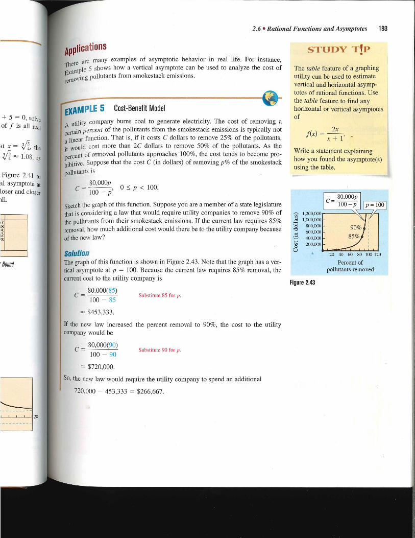
p = 100
2.6 • Rational Functions and Asymptotes 193
Applications
liere are many examples of asymptotic behavior in real life. For instance, xampie 5 shows how a vertical asymptote can be used to analyze the cost of
removing pollutants from smokestack emissions.
EXAMPLE 5 Cost-Benefit Model
Autility company burns coal to generate electricity. The cost of removing a
certain
percent of the pollutants from the smokestack emissions is typically not function. That is, if it costs C dollars to remove 25% of the pollutants, a n
it would cost more than 2C dollars to remove 50% of the pollutants. As the
percent of removed pollutants approaches 100%, the cost tends to become pro-
hibitive. Suppose that the cost C (in dollars) of removing p% of the smokestack
100 — p
Sketch the graph of this function. Suppose you are a member of a state legislature
that is considering a law that would require utility companies to remove 90% of
the pollutants from their smokestack emissions. If the current law requires 85% removal, how much additional cost would there be to the utility company because of the new law?
Solution The graph of this function is shown in Figure 2.43. Note that the graph has a ver-tical asymptote at p = 100. Because the current law requires 85% removal, the current cost to the utility company is
100 — 85
$453,333.
If the new law increased the percent removal to 90%, the cost to the utility company would be
c 80,000(90) 100 — 90
= $720,000.
So, the new law would require the utility company to spend an additional
720,000 — 453,333 = $266,667.
pollutants is
80,000p C = , 0 p < 100.
80,000(85) C = Substitute 85 for p.
Substitute 90 for p.
+ 5 = 0, solve of f is all real
it X = the
1.08, as
Figure 2.41 to al asymptote at loser and closer
Baud
Figure 2.43
80' 000p C — 100 —p
7 8 5 2 8
STUDY TIP
The table feature of a graphing utility can be used to estimate vertical and horizontal asymp-totes of rational functions. Use the table feature to find any horizontal or vertical asymptotes of
2x f(x) =
x+ 1.
Write a statement explaining how you found the asymptote(s) using the table.
20 40 60 80 100 120
Percent of pollutants removed
1,200,000 1,000,000
800,000 600,000 400,000 200,000
Cos
t (i
n do
llars
)
90% 85%

In Exer mine ti function
194 Chapter 2 • Polynomial and Rational Functions
Algebraic Solution
When x = 1000,
_c =
0.5(1000) + 5000 = $5.50.
1000
When x = 5000,
_ 0.5(5000) + 5000 = $1.50.
5000
When x = 10,000,
z, 0.5(10,000) + 5000 =
10,000
When x = 90,000,
_c —
0.5(90,000) + 5000 $0.56.
90,000
Because the degree of the numerator and denominator are the same for
—c =
0.5x + 5000
Graphical Solution
Using a graphing utility to graph the function
0.5x + 5000 0.99
0.999
using a viewing window similar to the graph shown in Figure 2.4 Then use the trace or value feature to approximate the following.
When x = 1000, y1 = $5.50. When x = 5000, y1 = $1.50.
When x = 10,000, y = $1.00. When x = 90,000, y1 = $0.5
Continue to use the trace or value feature to approximate values 0 f(x) for larger and larger values of x. From this, you can estimate the horizontal asymptote to be y = $0.50. This line represents the least possible cost for the product.
5
4
3
2
1
EXAMPLE 6 Average Cost of Producing a Product
A business has a cost function of C = 0.5x + 5000, where C is measured in dollars and x is the number of units produced. The average cost per unit is
C 0.5x + 5000 C — —
Find the average cost per unit when x = 1000, 5000, 10,000, and 100,000. What is the horizontal asymptote for this function, and what does it represent?
=
5
10
100
1000
the horizontal asymptote is given by the ratio of the leading coefficients of the numerator and denominator. So, the graph has the line r = $0.50 as a horizontal asymptote. This line represents the least possible unit cost for the product.
Number of units
Figure 2.44
Writing About Math Common Factors in the Numerator and Denominator
— Consider thejunction f(x) =
x(x 1) which has a common factor of x in
the numerator and denominator. Use a graphing utility to graph this function. Use the zoom and trace features to decide whether the function has a vertical asymptote at x = 0. Then write a short paragraph explaining why you should check for common factors in the numerator and denominator when graphing a rational function.

in Figure 2.44. following.
y1 = $1.50.
D, Y1 = $0.56.
mate values of an estimate the ;sents the least
16 9
5 5 5 5
10 10 5
4x 6. f(x) —
x2 — 1
5
2.6 • Rational Functions and Asymptotes 195
•
Jo Exercises mine the function,
vertical and
f(x)
1-6,
(c) fmd
(a) complete each and horizontal
the domain of
table, (b) deter-asymptotes of the
the function.
In [The
(a)
Exercises 7-12, match graphs are labeled
5
(a), (b),
(b)
the function with its graph. (c), (d), (e), and (f).]
f(x)
0.5
1.5
7
3 -4
I I 10
0.9
1.1
0.99
1.01
-5
-8
0.999
1.001
(c) (d)
f (x)
9
5
f(x)
2 —5
8
5
-5 5
—10
10
-5
100
—100
(e) (f)
1000
—1000
5
5
1. f(x) 1
2. f(x) 5x
5 II II I I II 5 9
= x — 1
= x— 1
5
5
-5
-5
-5
5 -8
2 7. f =
2
8. f(x) = 1
x + 2 x — 3
9. f(x) = 4x + 1
10. f(x)
-5 -5
1 —x
x =
3. f(x) 3x
= 4. f(x) 3
=
11. f(x) = x — 2
12. f(x) x + 2
Ix — 11 — ii
x — 4 =
x + 4
In Exercises 13-18, (a) find the domain of the func-tion, (b) identify any horizontal and vertical asymp-totes, and (c) verify your answer to part (a) both graphically by using a graphing utility and numeri-cally by creating a table of values.
1 3 13. f(x) — 14. f(x) =
x2 - 2)3
15. f(x) =3
16. f (x) = 2 ± — x
2x3 3X2 + 1 17. f(x) = 2 1 18. f (x) =
x2 +
x + 9
X -
-4 -5

f(x)
g(x)
4 30. h(x) = 6 +
x 2 + 2
25,000p x — 5 C 100 = , 0 5_ p < 100 .
— p
2
x 0 1 2 3 4 5 6
f(x)
g(x)
Exploration In Exercises 23-26, determine the value the function f approaches as the magnitude of x increases. Is f(x) greater than or less than this func-tional value when x is positive and large in magni-tude? What about when x is negative and large in magnitude?
23. f(x) = 4 —! 24. f(x) = 2 + 1
x — 3
2x — 1 2x — 1 x
25. f(x) = 3 26. f(x) = x2
±
(a) Find the cost of giving bins to 15% of the pops lation.
Find the cost of giving bins to 50% of the pops lation.
(b)
(c) Find the cost of giving bins to 90% of the po lation.
(d) Use a graphing utility to graph the cost functt Be sure to choose an appropriate viewing dow. Explain why you chose the values that used in your viewing window.
(e) According to this model, would it be possib supply bins to 100% of the residents? Exp
196 Chapter 2 • Polynomial and Rational Functions
Analytical and Numerical Explanation In Exercises 19-22, (a) determine the domain of f and g, (b) find any vertical asymptotes of f, (c) complete the table, and (d) explain what your results suggest.
x2 — 4 19. f(x) =
—4 —3 —2.5 —2 —1.5 0
x2(x — 3) 20. f(x) = g(x) = x
x2 — 3x'
x — 1 0 1 2 3 3.5 4
f(x)
g(x)
21. f(x) = x
2 _ 3x'
x — 3 g(x) = —
1
x — 1 —0.5 0 0.5 2 3 4
f(x)
g(x)
2x — 8 22. f(x) = x2 — 9x + 20' g(x)
In Exercises 27-30, find the zeros (if any) of t rational function. Use a graphing utility to verify yo answer.
x2 — 9 x3 — 8 27. g(x) = 28. g(x) =
x2 + 4
x + 1
2 29. f(x) = 1
x — 5
31. Pollution The cost (in millions of dollars) for removing p% of the industrial and municipal pollutants discharged into a river is
255p
100 — p
(a) Find the cost of removing 10% of the pollutan
(b) Find the cost of removing 40% of the pollutants,
(c) Find the cost of removing 75% of the pollutants,
(d) Use a graphing utility to graph the cost function, Be sure to choose an appropriate viewing window. Explain why you chose the values that you used in your viewing window.
(e) According to this model, would it be possible to remove 100% of the pollutants? Explain.
32. Recycling In a pilot project, a rural township wa given recycling bins for separating and storing recy-clable products. The cost (in dollars) for supplyin bins to p% of the population is
x + 2 g(x) = x — 2

Near point
• Far
point
20(5 + 3t) N — 1 + 0.04t
50 100 150 200 250
Time (in years)
Dee
r po
pula
tion
1600 1400 1200 1000 800 600 400 200
2.6 • Rational Functions and Asymptotes 197
' any) of the to verify your
3 8
r2 d_ 4
4 5 +
JC2 + 2
f dollars) fur nd munic i pa]
the pollutants.
the pollutants.
the pollutants.ii
cost function! rate viewing the values that
be possible to xplain.
township was storing recy-
for supplying
7'0 of the popu
/0 of the popu
/0 of the popu-
cost function. viewing win-
ulues that you
be possible to its? Explain.
33. Data Analysis Consider a physics laboratory experiment designed to determine an unknown mass. A flexible metal meter stick is clamped to a table
with 50 centimeters overhanging the edge. Known masses M ranging from 200 grams to 2000 grams are attached to the end of the meter stick. For each mass, the meter stick is displaced vertically and then
allowed to oscillate. The average time t in seconds of
one oscillation for each mass is recorded in the table.
M 200 400 600 800 1000
t 0.450 0.597 0.721 0.831 0.906
M 1200 1400 1600 1800 2000
t 1.003 1.088 1.168 1.218 1.338
%-4-50 cm-
A model for the data is
38M + 16,965 t =
10(M + 5000)•
(a) Use a graphing utility to create a table showing the estimated time based on the model for each of the masses shown in the table. What can you conclude?
(b) Use the model to approximate the mass of an object if the average for one oscillation is 1.056 seconds.
34. Data Analysis The endpoints of the interval over which distinct vision is possible are called the near point and far point of the eye. With increasing age these points normally change. The table gives the approximate near points y in centimeters for various ages x.
x 10 20 30 40 50
y 7 10 14 22 40
Object Object Object blurry clear blurry
(a) Fit a rational model to the data. Take the recipro-cals of the near points to generate the points (x, 1/y). Use the regression capabilities of a graphing utility to fit a line to this data. The resulting line has the form
—1
= ax + b.
Solve for y.
(b) Use a graphing utility to create a table giving the predicted near point based on the model for each of the ages in the given table.
(c) Do you think the model can be used to predict the near point for a person who is 60 years old? Explain.
35. Deer Population The ,game commission intro-duces 100 deer into newly acquired state game lands. The population of the herd is
N = 20(5 + 3t), t 0 1 + 0.04t
where t is the time (in years).
(a) Find the population when t is 5, 10, and 25.
(b) What is the limiting size of the herd as time increases? Explain your reasoning.

Synthesis
True or False? In Exercises 38 and 39, determin whether the statement is true or false. Justify you answer.
38. A rational function can have infinitely many vertical asymptotes.
39. f(x) = x3 - 2x2 - 5x + 6 is a rational function.
The Grap
sketch ti
1.568x - 0.001 6.360x + 1
Foo
d ea
ten
(in
mg)
0.30 0.25 0.20 0.15 0.10 0.05
Let f(x) = factors.
1. Find an
2. Set the solutior
3. Set the i solu nor dashed
Find an horizon
Plot at 1 vertical
Use sm asympt
Testing for s example, th( the graph of,
Graph if have vertica not suppose
f(x) =
Notice that of x -= 2 an try changinl is that the g! curve, as sh
f(x)
(a) Connect( Fign e 2.45
PIP"
198 Chapter 2 • Polynomial and Rational Functions
36. Insects A biology class performs an experiment comparing the quantity of food consumed by a cer-tain kind of moth with the quantity supplied. The model for their experimental data is
1.568x - 0.001 Y = x > 0
6.360x + 1
where x is the quantity (in milligrams) of food supplied and y is the quantity (in milligrams) eaten. At what level of consumption will the moth become satiated?
0.25 0.50 0.75 1.0 1.25
Food supplied (in mg)
37. Military The number of United States military reserve personnel M (in thousands) for the years 1990 through 1997 is shown in the table. (Source: U.S. Department of Defense)
Year 1990 1991 1992 1993
M 1671 1786 1883 1867
Year 1994 1995 1996 1997
M 1805 1659 1550 1461
A model for the data is
1671.92 + 130.21' Y - 1 - 0.02t + 0.02t2
where t is time (in years), with t = 0 corresponding to 1990.
(a) Use a graphing utility to plot the data and graph the model in the same viewing window.
(b) Use the model to estimate the number of military reserve personnel in 2002.
(c) Would this model be useful for estimating the number of military reserve personnel for future years? Explain.
Think About It In Exercises 40-43, write a rational function f having the specified characteristics. (There are many correct answers.)
40. Vertical asymptotes: x = -2, x = 1
41. Vertical asymptote: None
Horizontal asymptote: y = 0
42. Vertical asymptote: None
Horizontal asymptote: y = 2
43. Vertical asymptotes: x = 0, x =
Horizontal asymptote: y = -3
Review
In Exercises 44-49, find all solutions of the equati
44. 225x - 50x3 = 0
45. x(10 - = 25
46. 2z2 - 3z - 35 = 0 47. t3 - 50t = 0
48. 27x3 - 147x = 0
49. x4 - 225 = 0
In Exercises 50-53, divide using synthetic division.
50. (x2 + 5x + 6) + (x - 4)
51. (x2 - 10x + 15) + (x - 3)
52. (2x2 + x - 11) + (x + 5)
53. (4x2 + 3x - 10) + (x + 6)
In Exercises 54-57, find a polynomial with integer coefficients that has the given zeros. (There are many
correct answers.)
54. 8, 5i, -5i 55. -2, 6i, -6i
56. 6, 3 + i, 3 - i 57. 1, -3 + 2i, -3 --
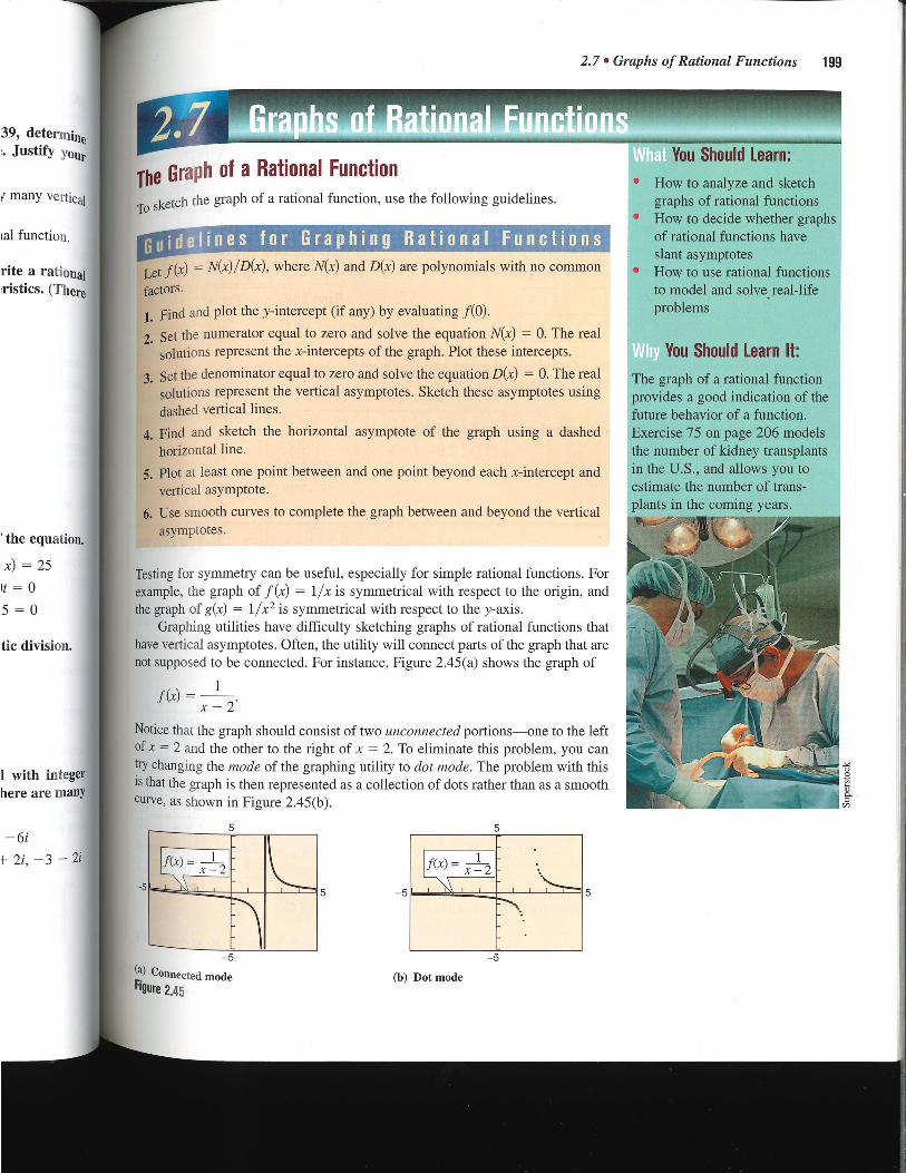
The Graph of a Rational Function
To sketch the graph of a rational function, use the following guidelines.
'delines for Graphing Rational Functions
Let .f(x) = N(x)/D(x), where N(x) and D(x) are polynomials with no common
factors.
1. Find and plot the y-intercept (if any) by evaluating f(0).
2. Set the numerator equal to zero and solve the equation N(x) = 0. The real solutions represent the x-intercepts of the graph. Plot these intercepts.
3. Set the denominator equal to zero and solve the equation D(x) = 0. The real solutions represent the vertical asymptotes. Sketch these asymptotes using dashed vertical lines.
4. Find and sketch the horizontal asymptote of the graph using a dashed horizontal line.
5. Plot at least one point between and one point beyond each x-intercept and vertical asymptote.
6. Use smooth curves to complete the graph between and beyond the vertical asymptotes.
Testing for symmetry can be useful, especially for simple rational functions. For example, the graph of f(x) = 11x is symmetrical with respect to the origin, and the graph of g(x) = 11x 2 is symmetrical with respect to the y-axis.
Graphing utilities have difficulty sketching graphs of rational functions that have vertical asymptotes. Often, the utility will connect parts of the graph that are not supposed to be connected. For instance, Figure 2.45(a) shows the graph of
f(x) = 1
5 5
x — 2.
Notice that the graph should consist of two unconnected portions—one to the left of x = 2 and the other to the right of x = 2. To eliminate this problem, you can try changing the mode of the graphing utility to dot mode. The problem with this is that the graph is then represented as a collection of dots rather than as a smooth curve, as shown in Figure 2.45(b).
-5 5 -5 5
2.7 • Graphs of Rational Functions 199
39, deterrojue . Justify your
many vertical
al function.
rite a rational ristics. (There
You Should Learn:
• How to analyze and sketch graphs of rational functions
• How to decide whether graphs of rational functions have slant asymptotes
• How to use rational functions to model and solve real-life problems
You Should Learn It:
The graph of a rational function provides a good indication of the future behavior of a function. Exercise 75 on page 206 models the number of kidney transplants in the U.S., and allows you to estimate the number of trans-clantik the coming years.
' the equation.
= 25
= 0
5 = 0
tic division.
with integer here are many
—6i
2i, —3 — 2i
-5 (a) connected mode Figtire 2.45
(b) Dot mode
-5

•VII•
EXAN
Sketch
SO/Util By fact(
f(x;
y-Interce
x-Interce
Vertical
Horizon
Additiont
The grapll
EXAM
Sketch tht
Solution By factori
f(x)
y-Intercepi
.r-Intercepi
Vertical As
Horizontal
SYmmeny:
Additional
200 Chapter 2 • Polynomial and Rational Functions
EXAMPLE 1 Sketching the Graph of a Rational Function
Sketch the graph of g(x) = x —
3 2
by hand.
(0, —i), because g(0) =
None, because 3 0.
x = 2, zero of denominator
y = 0, degree of N(x) < degree of D(x)
x —4 1 3 5
g(x) — 0.5 —j 3 1
Solution y-Intercept:
x-Intercept:
Vertical Asymptote:
Horizontal Asymptote:
Additional Points:
By plotting the intercepts, asymptotes, and a few additional points, you can obtain the graph shown in Figure 2.46. Confirm this with a graphing utility.
Note that the graph of g in Example 1 is a vertical stretch and a right shift of the graph of
because
g(x) = 3 = 3 x — 2 (x —1 2) = 3f (x 2).
11111•111111111111,111111111
LEMBEIN1111111111/111111 EMESP1111111.111111111 P2M1111111M11111111 111111111111101111111111101111 1111111M111111111111•111111a1 10:511111111.1111/1111111'
111111EINIVONINFOR111 mmiumweeina
Figure 2.46
EXAMPLE 2 Sketching the Graph of a Rational Function
— Sketch the graph of f(x)
2x 1x
by hand.
None, because x = 0 is not in the domain.
(, 0), because 2x — 1 = 0, or x =
x = 0, zero of denominator
y = 2, degree of N(x) = degree of D(x)
x —4 —1 i 4
f(x) 2.25 3 —2 1.75
Solution y-Intercept:
x-Intercept:
Vertical Asymptote:
Horizontal Asymptote:
Additional Points:
By plotting the intercepts, asymptotes, and a few additional points, you can obtain the graph shown in Figure 2.47. Confirm this with a graphing utility. Figure 2.47
f(x) = te
The graph

Use a graphing utility to graph
f(x) = 1 + 1.
x — —x
1
Set the graphing utility to dot mode and use a decimal viewing window. Use the trace feature to find three "holes" or 'breaks" in the graph. Do all three holes represent zeros of the denominator
1 x — —
x?
xplain.
A X — X — a Vert ical
5
—5 —if 3 5
e: Horizonta asymptote:
Y= I I
3 a
te:
ert ical asymp,ot x=
a5yrnp = —
Figure 2.48
M111111111111151MINIIIIMEN
1111111111111111111MINIM11111111111111 11111111111111111111101111111111111=111 EIMINIM1111111111110E231
IEFEE111111111111111111111112E1111111
ICE11111111111111111111Milial
1111111111111111111111111E11111111 M1111111111111111111111MINIIIIII NMI
Figure 2.49
(x+ 1)(x — 2)•
(0, 0), because f (0) = 0.
(0, 0)
x = —1, x = 2, zeros of denominator
y = 0, degree of N(x) < degree of D(x)
x —3 —0.5 1 3
f(x) — 0.3 0.4 —0.5 0.75
y-Intereept:
x-Intercept:
Vertical Asymptotes:
Horizontal Asymptote:
Additional Points:
The graph is shown in Figure 2.48.
2.7 • Graphs of Rational Functions 201
EXAMPLE 3 Sketching the Graph of a Rational Function
Sketch the graph of f(x) = X 2 - X -
SONtiOn By factoring the denominator, you have
f (x) — x — 2
EXAMPLE 4 Sketching the Graph of a Rational Function
Sketch the graph of f(x) = 2(x2 — 9)
x2 — 4
Solution By factoring the numerator and denominator, you have
2(x2 — 9) f(x) =
x2 — 4
2(x — 3)(x + 3)
(x — 2)(x + 2)
(0, !), because f (0) =
(-3,0), (3,0)
x = —2, x = 2, zeros of denominator
y = 2, degree of N(x) = degree of D(x)
With respect to y-axis, because f(— = f(x).
x 0.5 2.5 6
f(x) 4.67 —2.44 1.69
The graph is shown in Figure 2.49.
C) A computer animation of this example appears in the Interactive CD-ROM ,ind Internet versions of this text.
y-Intercept:
x-Intercepts:
Vertical Asymptotes:
Horizontal Asymptote:
Symmetry:
Additional Points:
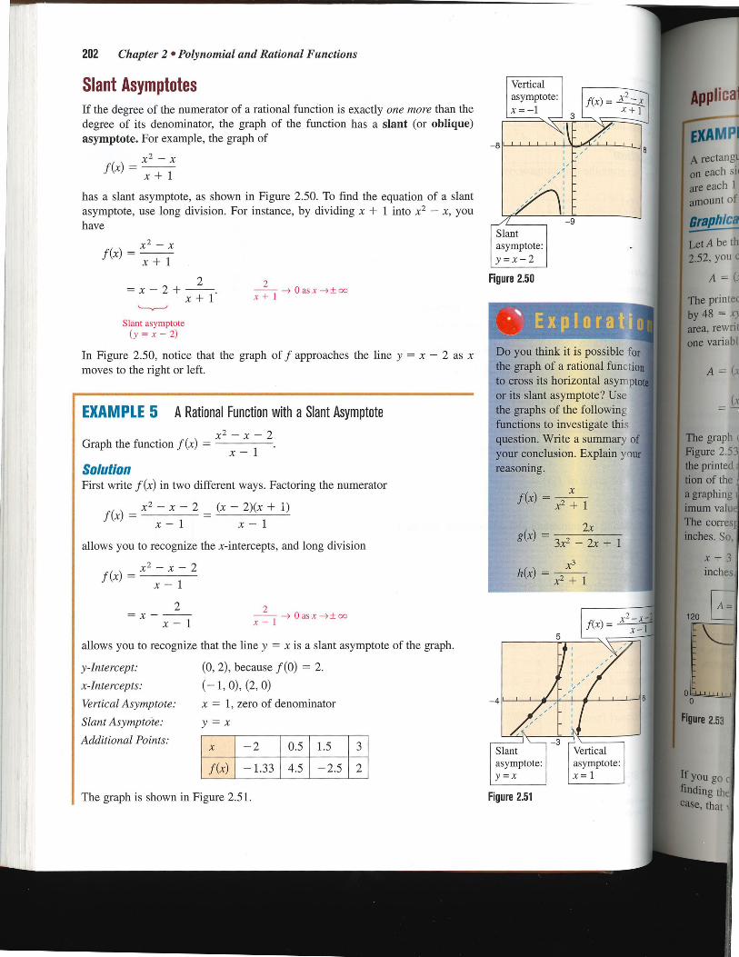
—> 0 a s x —> oo x + 1
2
y = x
x —2 0.5 1.5 3
f(x) — 1.33 4.5 —2.5 2
202 Chapter 2 • Polynomial and Rational Functions
Slant Asymptotes If the degree of the numerator of a rational function is exactly one more than the degree of its denominator, the graph of the function has a slant (or oblique) asymptote. For example, the graph of
x2 — x f(x) =
x + 1
has a slant asymptote, as shown in Figure 2.50. To find the equation of a slant asymptote, use long division. For instance, by dividing x + 1 into x2 — x, you have
f(x) =
2 x + 1*
Slant asymptote (y = x — 2)
In Figure 2.50, notice that the graph of f approaches the line y = x — 2 as x moves to the right or left.
EXAMPLE 5 A Rational Function with a Slant Asymptote
x2 — x — 2 Graph the function f(x) =
x — 1
Solution First write f(x) in two different ways. Factoring the numerator
x2 — x — 2 (x — 2)(x + 1) f(x) =
x — 1 x — 1
allows you to recognize the x-intercepts, and long division
f(x) =
2 —> 0 as x -->± co
x — 1
allows you to recognize that the line y = x is a slant asymptote of the graph.
X2 — X
x+ 1
x 2 — x — 2 x — 1
2 = x
x— 1
Applical
Slant asymptote: y =x — 2
Figure 2.50
8
Do you think it is possible for the graph of a rational func lion to cross its horizontal asymptote or its slant asymptote? Use the graphs of the following functions to investigate this question. Write a summary of your conclusion. Explain your
asoning.
x2 + 1
The graph Figure 2.53 the printed, tion of the a graphing imum value The con-esr inches. So,
x + 3 inches
EXAM P1
A rectangu on each sic
are each 1 amount of
GraPhiC8
Let A be thi
2.52, you c
A=
The printec by 48 = Xy
area, rewrit one variabli
A =(x
A= 120
y-Intercept: (0, 2), because f (0) = 2.
x-Intercepts: (-1, 0), (2, 0)
Vertical Asymptote: x = 1, zero of denominator
Slant Asymptote:
Additional Points: Slant asymptote: y =x
The graph is shown in Figure 2.51. Figure 2.51
0 -I-LLL in _Li 0
Figure 2.53
If You go c finding the Case, that

x > 0 (x + 3)(48 + 2x)
(x) =
ossible for la.1 function al asympt te? Use llowing ;ate this immary of 'plain your
+ 1
Kx) . x2 - x -
x - 1
ical nptote: 1
48 )A = (x + 3)(-- + 2
2.7 • Graphs of Rational Functions 203
A ctan gular page is designed to contain 48 square inches of print. The margins re
on each side of the page are each 11. inches. The margins at the top and bottom
are each 1 inch. What should the dimensions of the page be so that the minimum
amount of paper is used?
11 in.
Figure 2.52
graphical Solution
Let A be the area to be minimized. From Figure
2,52, you can write
A = (x + 3)(y + 2).
The printed area inside the margins is modeled
by 48 = xy or y = 48/x. To find the minimum
area, rewrite the equation for A in terms of just
one variable by substituting 48/x for y.
The graph of this rational function is shown in Figure 2.53. Because x represents the width of the printed area, you need consider only the por-tion of the graph for which x is positive. Using a graphing utility, you can approximate the min-imum value of A to occur when x 8.5 inches. The corresponding value of y is 48/8.5 5.6 inches. So, the dimensions should be
+ 3 11.5 inches by y + 2 7.6 inches.
Figure 2.53
0
120
24
If You go on to take a course in calculus, you will learn an analytic technique for finding the exact value of x that produces a minimum area in Example 6. In this case, that value is x = 8.485.
Application
EXAMPLE 6 Finding a Minimum Area
Numerical Solution
1 in.
1 in.
(x + 3)(48 + 2x) x > 0
Let A be the area to be minimized. From Figure 2.52, you can write
A = (x + 3)(y + 2).
The printed area inside the margins is modeled by 48 = xy or y = 48/x. To find the minimum area, rewrite the equation for A in terms of just one variable by substituting 48/x for y.
(x + 3)(48 + 2x) A - (x + 3)(L18 + 2) , = x > 0
Use the table feature of a graphing utility to create a table of values (x + 3)(48 + 2x)
for the function y1 = beginning at x = 1, as
shown in Figure 2.54.
X Y1
6 90
7 88.571
8 88
9 88
10 88.4
11 89.091
12 90
Y1=88
Figure 2.54
From the table, you can see that the minimum value of y1 occurs when x is somewhere between 8 and 9. To approximate the minimum value of y1 to one decimal place, change the table to begin at 8 with an increment of 0.1. The minimum value of y1 occurs when x 8.5, as shown in Figure 2.55. The corresponding value of y is 48/8.5 5.6 inches. So, the dimensions should be x + 3 11.5 inches by y + 2 7.6 inches.
X Y1
8.2 87.961
8.3 87.949
8.4 87.943
8.5 87.941
8.6 87.944
8.7 87.952
8.8 87.964
Y1=87.9411764706
Figure 2.55

- 2)2
25. g(x) - 4(x + 1)
26. h(x) - 2
x(x - 4) x 2(x - 2)
x' 24. f(x) - 1
20x 1 39. f(x) =
- x2 +1 X
40. f(x) = 5(x
1 4
28. f(x) - 2x
x2 + x - 2
4 5
5- - 29. f(x) =
3 - x 32. f(x)
2 - x
x- 2 34. h(x) =
x - 3
36. g(x) = -(x -
x 2)
x + 4 X2 -I- X -
38. f(x) =
204 Chapter 2 • Polynomial and Rational Functions
liaLExercises In Exercises 1-4, use a graphing utility to graph f(x) = 2/x and the function g in the same viewing window. Describe the relationship between the two graphs.
1. g(x) = f(x) + 1 2. g(x) = f(x - 1)
3. g(x) = -f(x) 4. g(x) = If(x -F 2)
In Exercises 5-8, use a graphing utility to graph f(x) = 242 and the function g in the same viewing window. Describe the relationship between the two graphs.
5. g(x) = f(x) - 2 6. g(x) = -f(x)
7. g(x) = f(x - 2) 8. g(x) = if(x)
In Exercises 9-12, use a graphing utility to graph f(x) = 4/x3 and the function g in the same viewing window. Describe the relationship between the two graphs.
9. g(x) = f(x + 2) 10. g(x) = f(x) + 1
11. g(x) = -f(x) 12. g(x) = lf(x)
In Exercises 13-30, sketch the graph of the rational function by hand. As sketching aids, check for inter-cepts, symmetry, vertical asymptotes, and horizontal asymptotes. Use a graphing utility to verify your graph.
1 1 13. f(x) = 14. f(x) =
x + 2 x - 5
5 + 2x 1 - 3x 15. C(x) = 16. P(x) =
1 + x 1 - x
17. g(x) = 1
+ 2 18. f(t) = 1 - 2t
x + 2
x2 19. f(x) = 2 - -
3 20. h(x) =
X2 X2 - 9
X2 X 21. f(x) =
x2- 4 22. g(x) -
x2- 9
3x 27. f(x) -
x2 - x - 2
30. f(x) = 2 + 8
3x -
In Exercises 31-40, use a graphing utility to obtain the graph of the function. Give its domain and identi, fy any vertical or horizontal asymptotes.
2 + x 31. f(x) =
1 - x
3t + 1 33. f(t)
= 4 35. h(t)
t2 + 1
x+ 1 37. f(x) =
x2 - x - 6
Exploration In Exercises 41-46, use a graphing util. ity to obtain the graph of the function. What do you observe about its asymptotes?
6x 41. h(x) =
x2 + 1 42. f(x) =
j
41x - 21 44. f(x) =
813 + A 43. g(x) =
x + 1 x - 2
= 4(x - 1)2 3x4 - 5x + 3 46. g(x) = 45. f(x) x2 - 4x + 5 x4 + 1
In Exercises 47-54, sketch the graph of the rational function. As sketching aids, check for intercepts, sy metry, vertical asymptotes, and slant asymptotes
x2 + 1 48. g(x) =
x2 X3 50. f(x) =
x2 - 1
x2 - 1 52. f(x) -
x2 + 4
2x2 5x -1 54. f(x) =
x _2
1
2x2 1 47. f (x) =
49. h(x) - x- 1
X3 51. g(x) - 2x2 8
x3 + 2x2 + 4 53' f(x) = 2x2 + 1
Graphical graph to function g equation t
55. v = x
1 57. y = - -
x
In Exercises rational fun identify anyl that the gra
2x ' 59. y
Graphical R graphing uti any x-interc( ing equation

btajo der,
ifility to a lain and ii es.
_ 3 — x 2 — x
x— 2 1
57. Y
2x 56. y =
—3 x — 3 +1
8 8 12
20
'20 20
-213
hical Reasoning In Exercises 55-58, (a) use the GraP „rap!' to estimate any x-intercepts of the rational
% a nd (b) set y = 0 and solve the resulting ffleti °11
equatiOn to confirm your result in part (a).
55. 2 X
10
5 x — 3
6
-10
58. y = x — 3 + —2
:2+ 8
3x -
x — 2
3x4 — 5x +
x4 +
al
[ntercepts, sym• icvmntotes.
tinr of the ra
X2 — 1
X2 — 1 X2 + 4
2x2 — 5x
x — 2
In Exercises 59-62, use a graphing utility to graph the rational function. Give the domain of the function and Identify any asymptotes. Then zoom out far enough so that the graph appears as a line. Identify the line.
2.7 • Graphs of Rational Functions 205
(b) Determine the domain of the function on the basis of the physical constraints of the problem.
(c) Use a graphing utility to graph the function. As the tank is filled, what happens to the rate at which the concentration of brine increases? How close to the horizontal asymptote is the graph of C when the tank is full?
68. Geometry A rectangular region of length x and width y has an area of 500 square meters.
(a) Express the width y as a function of x. (b) Determine the domain of the function on the
basis of the physical constraints of the problem.
(c) Sketch a graph of the function and determine the width of the rectangle if x = 30 meters.
69. Page Design A page that is x inches wide and y inches high contains 30 square inches of print. The margins at the top and bottom are 2 inches and the margins on each side are 1 inch.
a graphing ut 1. What do you
2x 2 ± x
X2 ± 5x + 8 59. y = 60. Y= +1 x + 3
61. y — 1 + 3x2 — x3
62. Y 12 — 2x — x2
x2 2(4+x)
Graphical Reasoning In Exercises 63-66, (a) use a graphing utility to graph the function and determine any x-intercepts, and (b) set y = 0 and solve the result-ing equation to confirm your result in part (a).
64. y = 20( 2 3) x + 1 x
6 9 66. y = x — —
x x — 1
67. Concentration of a Mixture A 1000-liter tank con-tains 10 liters of a 25% brine solution. You add x liters Of a 75% brine solution to the tank.
(a) Show that the concentration C of the final mix-ture is
(a) Show that the total area A of the page is
2x (2x + 11) A=
x — 2
(b) Determine the domain of the function on the basis of the physical constraints of the problem.
(c) Use a graphing utility to graph the area function and approximate the page size such that the min-imum amount of paper will be used. Verify your answer numerically using the table feature of a graphing utility.
70. Minimum Area A right triangle is formed in the first quadrant by the x-axis, the y-axis, and a line segment through the point (3, 2).
6 (0, y) 5
4
3
2
1 4 63. y = 5 x
65.
4-5 c =r. 3x + 10
4(x + 10)•
(3,2)
(a, 0)
1 2 3 4 5 6
30 35 40 45 50 55 60
Year 1992 1993 1994 1995 1996
K 10,231 11,020 11,392 11,891 12,0
1111 (c)
206 Chapter 2 • Polynomial and Rational Functions
74. Numerical and Graphical Analysis A driver aver, aged 50 miles per hour on the round trip between home and a city 100 miles away. The average speeds for going and returning were x and y miles per hour respectively.
(a) Show that an equation of the line segment is
2(a — x) Y = a — 3
0 < x a.
a — 3'
(c) Use a graphing utility to graph the area function and estimate the value of a that yields a mini-mum area. Estimate the minimum area. Verify your answer numerically using the table feature of a graphing utility.
71. Ordering and Transportation Cost The ordering and transportation cost C for the components used in manufacturing a certain product is
C = 100Hx2
x +301
200 x x > 1
where C is measured in thousands of dollars and x is the order size (in hundreds). Use a graphing utility to obtain the graph of the cost function and, from the graph, estimate the order size that minimizes cost.
72. Average Cost The cost ofrqlucing x units of a product is C = 0.2x2 + 10X--+- 5, and therefore the average cost per unit is
C 0.2x2 +x10x + 5
-C- , x > 0. = =
Sketch the graph of the average cost function, and estimate the number of units that should be produced to minimize the average cost per unit.
73. Medicine The concentration of a certain chemical in the bloodstream t hours after injection into muscle tissue is
3t 2 + t C =
t3 50' t O.
(a) Determine the horizontal asymptote of the func-tion and interpret its meaning in the context of the problem.
(b) Use a graphing utility to graph the function and approximate the time when the bloodstream con-centration is greatest.
(c) Use a graphing utility to determine when the concentration is less than 0.345.
a2 (b) Show that the area of the triangle is A =
(a) Show that y = 25x
x — 25.
(b) Determine the vertical and horizontal totes of the function.
(c) Use a graphing utility to complete the table. What do you observe?
asymp,
76. Co of for tab] Coi
For with
17
(d) Use a graphing utility to graph the function.
(e) Is it possible to average 20 miles per hour in one direction and still average 50 miles per hour the round trip? Explain.
75. Comparing Models The number of kidney transplants K in the United States from 1987 through 1996 is shown in the table. (Sources: U Department of Health and Human Services; Unit Network for Organ Sharing)
(b)
(a)
Year 1987 1988 1989 1990 1991
K 8967 9123 8890 9877 10,122
For each of the following, let t be the time (in ye with t = 7 corresponding to 1987.
(a) A model for the data is
K8116.17 — 280t
= 1 — 0.0447t
Use a graphing utility to plot the data points graph the model in the same viewing window
(b) Use the regression capabilities of a grap utility to fit a line to the data.
(c) Use the regression capabilities of a grap utility to fit a parabola to the data.
(d) Which of the three models would you rec mend as an estimator of the number of kit transplants for the years following 19 Explain your reasoning.
True or whether answer.
77. If th asyri with,
78. A rai totes
Snit&

A driver aver, id trip between average speeds miles per hour,
izontal asymp,
ilete the table.
1991
10,122
)95 1996
1,891 12,080
time (in years),
x2 + x - 2
x - 1 80. g(x) -
True or False? In Exercises 77 and 78, determine whether the statement is true or false. Justify your answer.
77. If the graph of a rational function f has a vertical asymptote at x = 5, it is possible to sketch the graph Without lifting your pencil from the paper.
78. A rational function can never cross one of its asymp-totes.
In Exercises 92-95, use a graphing utility to graph the function and find its domain and range.
92. f(x) = + x2 93. f(x) = -,/121 - x2
94. f(x) = - lx + 91 95. f(x) = -x2 + 9
data points and ring window.
of a grap
of a graphing
id you reconi-
nber of kidneY lowing 1996?
2.7 • Graphs of Rational Functions 207
Le function.
per hour in one les per hour on
of kidney es from 1987 (Sources: U.S
ervices; Unit
6 ornparing Models The number N (in thousands) /. C of insured commercial banks in the United States
for the years 1988 through 1997 is shown in the table. (Source: U.S. Federal Deposit Insurance Corporation)
ir 1988 1989 1990 1991 1992
13.1 12.7 12.3 11.9 11.5
Year 1993 1994 1995 1996 1997
N 11.0 10.5 9.9 9.5 9.1
For each of the following, let t be the time (in years), with t = 8 corresponding to 1988.
(a) Use the regression capabilities of a graphing util-ity to fit a line to the data. Use a graphing utility to plot the data points and graph the model in the same viewing window.
(b) Fit a rational model to the data. Take the recip-rocal of N to generate the points (t, 1/N). Use the regression capabilities of a graphing utility to fit a line to this data. The resulting line has the form
-1
= at + b.
Solve for N. Use a graphing utility to plot the data points and graph the rational model in the same viewing window.
(c) Use a graphing utility to create a table showing the predicted number of banks based on each model for each of the years in the given table. Which model do you prefer? Why?
Sytithesis
Think About It In Exercises 79 and 80, use a graph-ing utility to obtain the graph of the function. Explain why there is no vertical asymptote when a superficial examination of the function may indicate that there should be one.
79. h(x) - 6 - 2x 3 - x
81. Writing Write a paragraph discussing whether every rational function has a vertical asymptote.
Think About It In Exercises 82-85, write a rational function satisfying the following criteria.
82. Vertical asymptote: x = 2
Slant asymptote: y = x + 1
Zero of the function: x = -2
83. Vertical asymptote: x = -4
Slant asymptote: y = x - 2
Zero of the function: x = 3
84. Vertical asymptote: x = -1
Horizontal asymptote: y = 2
Zero of the function: x = 3
85. Vertical asymptote: x = 3
Horizontal asymptote: y = -2
Zero of the function: x = -6
Review
In Exercises 86-91, sketch a graph of the equation by hand. Use a graphing utility to verify your graph.
86. -y + 3x + 8 = 0 87. 4x + Sy - 2 = 0
88. 7x + 3 = 0
89. 4y - 10 = 0
90. x - y - 1 = 0
91. -7 + 8x - 2y = 0
55 60
Ye

208 Chapter 2 • Polynomial and Rational Functions
Gr, a graphi viewing from the
1. (a) I. (c) y
!. (a) Y (c) y
Exerct Inaction.
3. f(x)
5. f(x) 6. f(x)
In Exercis has the Ihrough t
7.Vertex
8.Vertex
In Exercis altie of th
9.g(x)
11. f(x) =
13. f(t) = -
IS, h(x) = A
!7. Numerit rectang1( x-axis, tl
1_ -
-2-
What did you learn?
Section 2.1 Review Exercises O How to analyze graphs of quadratic functions 1,2
El How to write quadratic functions in standard form and graph them 3-16
O How to use quadratic functions to model and solve real-life problems 17, 18
Section 2.2 O How to use transformations to sketch graphs of polynomial functions 19-22
El How to use the Leading Coefficient Test to determine the end behavior of 23-28 graphs of polynomial functions
El How to find and use zeros of polynomial functions to sketch their graphs 29-36
O How to use the Intermediate Value Theorem to help locate zeros of 37-40 polynomial functions
Section 2.3 O How to use long division and synthetic division to divide polynomials 41-52
O How to use the Remainder Theorem and the Factor Theorem 53-56
El How to use the Rational Zero Test to determine possible rational zeros 57-62
O How to determine upper and lower bounds for zeros of polynomial functions 63,64
Section 2.4 El How to use the imaginary unit i to write complex numbers 65-68
O How to add, subtract, multiply, and divide complex numbers 69-80
O How to plot complex numbers in the complex plane 81-84
Section 2.5 El How to use the Fundamental Theorem of Algebra to determine the number
of zeros of polynomial functions 85-88
O How to find all zeros of polynomial functions, including complex zeros 89-94
El How to find conjugate pairs of complex zeros 95-98
El How to find zeros of polynomials by factoring 99,100
Section 2.6 O How to find domains of rational functions 101-104
El How to find horizontal and vertical asymptotes of graphs of rational functions 105-110
El How fo use rational functions to model and solve real-life problems 111,112
Section 2.7 O How to analyze and sketch graphs of rational functions 113-120
El How to decide whether graphs of rational functions have slant asymptotes 121-126
El How to use rational functions to model and solve real-life problems 127

• Review Exercises 209
ra Graphical Reasoning In Exercises 1 and 2, use
a graphing utility to graph each equation in the same viewing window. Describe how each graph differs
from the graph of y = x2.
1. (a) Y = 2x2 (b) y = —2x2
(c) y = x + 2 (d) y = (x + 2)2
2. (a) y = x 2 - 4 (b) y = 4 — x2
(c) y = (x — 3)2 (d) y = x2 - 1
In Exercises 3-6, sketch the graph of the quadratic function. Identify the vertex and the intercepts.
3.f(x) + D2 ± 1 4. f(x) = (x — 4) 2 — 4
5. f(x) = 1(x2 + 5x — 4)
6. f(x) = 3x2 — 12x + 11
In Exercises 7 and 8, find the quadratic function that has the indicated vertex and whose graph passes through the given point.
7. Vertex: (1, —4); Point: (2, —3)
8. Vertex: (2, 3); Point: (— 1, 6)
In Exercises 9-16, find the maximum or minimum value of the quadratic function.
9. g(x) = x2 — 2x 10. f(x) = x2 + 8x + 10
11. f(x) = 6x — x2 12. h(x) = 3 + 4x — x2
13. At) = — 2t2 + 4t + 1 14. h(x) = 4x2 + 4x + 13
15. h(x) = x2 + 5x — 4 16. f(x) = 4x2 + 4x + 5
17. Numerical, Graphical, and Analytical Analysis A lib rectangle is inscribed in the region bounded by the
x-axis, the y-axis, and the graph of x + 2y — 8 = 0.
(a) Complete six rows of a table like the one below.
x y
Area
1 4 — .1(1) (1)[4 — 1(1)] =
2 4 — 1(2) (2)[4 — (2)] = 6
(b) Use a graphing utility to generate additional rows of the table. Use the table to estimate the dimensions that will produce the maximum area.
(c) Write the area A as a function of x. Determine the domain of the function in the context of the problem.
(d) Use a graphing utility to graph the function. Use the graph to approximate the dimensions that will produce the maximum area.
(e) Write the area function in standard form to find algebraically the dimensions that will produce the maximum area.
18. Maximum Profit Let x be the amount (in hundreds of dollars) a company spends on advertising, and let P be the profit, where
P = 320 + 15x — 1.r2.
(a) Use a graphing utility to graph the function.
(b) Use the zoom and trace features of a graphing utility to estimate the vertex of the function.
(c) Verify your answer in part (b) both algebraically and numerically by creating a table of values.
(d) Explain what the vertex represents.
Ea In Exercises 19-22, sketch the graphs of y = xri and the specified transformations.
19. y = x4
(a) f(x) = (x + 5)4 (b) f(x) = x4 — 4
(c) f(x) = 3 + x4 (d) f(x) = — 2)4
20. y = x5
(a) f(x) = (x + 4)5 (b) f(x) = 6 + x5
(c) f(x) = 3 — 1x5 (d) f(x) = 2(x + 3)5
21. y = x6
(a) f(x) = x6 — 2 (b) f(x) = -14.X6
(C) f(X) = AX6 - 5 (d) f(x) = — (x + 7)6 — 5

Vait4 rva4
goat, t trea, ros of.
2, use fl tile
that est its
5
In tha use all
55. 56.
In of./ of' det
57.
58.
59.
60.1
61.
62.1
In the
63.
64.
algebraically.
X 2
Y1 = X 2 9 Y2
4 = x + 2 +
x - 2 41.
x4 ± 1
5 Y2 = X2 2+ 42. v .,= 1 x2+ 2 ' .7C2 ± 2
In Exercises 43-48, divide by long division.
24x2 - x - 8 4x + 7 43. 44.
3x - 2 3x - 2
x4 - 3x2 + 2 3x4 45. .
x2 - 1 46 x2 - 1
x4 + x3 - x2 + 2x
x2 +.2x
48. 6x4 + 10x3 + 13x2 - 5x + 2
2x2 - 1
47.
65
67
In tho
69
70
71 73 75
7"
210 Chapter 2 • Polynomial and Rational Functions
22. y = 1'
(a) f(x) = -x7 + 4 (b) f(x) = (x + 2)7 - 1
(c) f(x) = - + 1 (d) f(x) = -(x + 8)7
In Exercises 23-26, determine the right-hand and left-hand behavior of the graph of the polynomial function.
23. f(x) = -x2 + 6x + 9
24. f(x) = + 2x
25. g(x) = i(x4 + 3x 2 + 2)
26. h(x) = -x 5 - 7x 2 + 10x
Graphical Analysis In Exercises 27 and 28, use a graphing utility to graph the functions l and g in the same viewing window. Zoom out far enough so that the right-hand and left-hand behavior of f and g appear identical.
27. f(x) = ix3 - 2x + 1, g(x) =
28. f(x) = - x4 2X3, g(x) = _x4
In Exercises 29-34, (a) find the zeros of the function and (b) sketch its graph.
29. g(x) = x4 - x 3 - 2x 2
30. h(x) = -2x3 - x2 + x
31. f(t) = t3 - 3t 32. f(x) = - (x + 6)3 - 8
33. f(x) = x(x + 3) 2 34. f(t) = t4 - 4t2
35. Volume A rectangular package can have a maxi-mum combined length and girth (perimeter of a cross section) of 216 centimeters.
(a) Write the volume V as a function of x.
(b) Use a graphing utility to graph the volume function, and then use the graph to estimate the dimensions of the package of maximum volume.
,
36. Volume Rework Exercise 35 for a cylindrical pack-age. (The cross sections are circular.)
In Exercises 37-40, (a) use the Intermediate Theorem and a graphing utility to find open int, of length 1 in which the polynomial function is anteed to have a zero, and (b) use the zero or ro( ture of a graphing utility to approximate the ze the function.
37. f(x) = x3 + 2x2 - x - 1
38. f(x) -= 0.24x3 - 2.6x - 1.4
39. f(x) = x4 - 6x2 - 4
40. f(x) = 2x4 + - 2
En Graphical Analysis In Exercises 41 and 4 a graphing utility to graph the two equations same viewing window. Use the graphs to verif: the expressions are equivalent. Verify your r
In Exercises 49-52, divide by synthetic divisie
49. (0.25x4 - 4x3) + (x + 2)
50. (0.1x3 + 0.3x2 - 0.5) + (x - 5)
51. (6x4 - 4x3 - 27x2 + 18x) + -
52. (2x3 + 2x2 - x + 2) + -
In Exercises 53 and 54, use synthetic division to fl
each function value. Use a graphing utility to your result.
53. f(x) = 2x3 + 3x2 - 20x - 21
(a) f(4) (b) f(- 1)
(c) f(-) (d) f(0)

2
division.
ivision to find tility to verify
mediate Va open inter nction is gu gm or root I ite the zero
41 and 42, use illations in the to verify that
v your results
hie als at, ea, of
20x4 + 9x3 - 14x2 - 3x
l) (b) .f(i) f(0) (d) f(1)
57. f(x)
58. f(x)
59. f(x)
60. f(x)
61. f(x)
62. f(x)
4x3 - 11x2 + 10x - 3
= 10x 3 + 21x2 - x - 6
= 6x3 - 5x2 + 24x - 20
= 10x3 - 13x2 - 17x + 6
= 6x4 - 25x3 + 14x2 + 27x - 18
= 5x4 + 126x2 + 25
la Exercises 55 and 56, use synthetic division to show that x is a solution of the polynomial equation, then
use the result to factor the polynomial completely. List
all real zeros of the function.
55.2x 11x2 - 20x + 12 = 0, x = -3 4 5x3
56. 3x3 + 2x2 - 15x - 10 = 0, x =
La Exercises 57-62, (a) list the possible rational zeros
of f, (b) use a graphing utility to graph f so that some
of the possible zeros in (a) can be disregarded, and (c)
determine all the real zeros of the function.
In Exercises 63 and 64, use synthetic division to verify the upper bound and lower bound of the zeros off.
63. f(x) = 4x3 - 3x2 + 4x - 3
Upper bound: x = 1; Lower bound: x =
64. f(x) = 2x3 - 5x2 - 14x + 8
Upper bound: x = 8; Lower bound: x = -4
Exercises 65-68, write in standard form.
66. - 12 + 3
68. -i 2 - 4i
In Exercises 69-80, perform the operations and write the result in standard form.
69. (7 + + (-4 + 2i)
7A. ( --
.) - " - 2 2 2 2
72. (1 + 60(5 - 2i)
74. i(6 + 0(3 - 2i)
76. (4 - - (4 +
3 78.
+ 2i 5 + i
• Review Exercises 211
4 1 79. 80.
-3i (2 + 04
In Exercises 81-84, plot the complex number in the complex plane.
81. 2 - 5i 82. - 1 + 4i
83. -6i 84. 7i
ElE1 In Exercises 85-88, use a graphing utility to (a) graph the function, (b) determine the number of real zeros of the function, and (c) approximate the real zeros of the function to the nearest hundredth.
85. f(x) = x4 + 2x + 1
86. g(x) = x3 - 3x 2 + 3x + 2
87. h (x) = x3 - 6x2 + 12x- 10
88. f(x) = x5 + 2x3 - 3x - 20
In Exercises 89-94, find all the zeros of the function and write the polynomial as a product of linear fac-tors. Use a graphing utility to verify your answer.
89. f(x) = x3 - 4x2 + 6x - 4
90. f(x) = x3 - 5x2 - 7x + 51
91. f(x) = x3 + 6x2 + 1 lx,+ 12
92. f(x) = 2x3 - 9x2 + 22x - 30
93. f(x) = x4 + 34x2 + 225
94. f(x) = x4 + 10x3 + 26x2 + 10x + 25
In Exercises 95-98, find a polynomial function with integer coefficients that has the given zeros. (There are many correct answers.)
95. -2, -2, -5i 96. 1, -4, -3 + 5i
97. -,-1,3 + 98. -4,-4,1 +
In Exercises 99 and 100, write the polynomial (a) as the product of factors that are irreducible over the ra-tionals, (b) as the product of linear and quadratic factors that are irreducible over the reals, and (c) in completely factored form.
99. f(x) = x4 - x3 - x2 + 5x - 20
(Hint: One factor is x2 - 5.)
100. f(x) = x4 - 4x3 + 3x2 + 8x - 16
(Hint: One factor is x2 - x - 4.)
In
65. 6 + 67. - 2 +
71. 5i(1
73. (10 75. (3 .4.
6 + 77,
3 - 8i) - 80(2 - 3i) - 702 + (3 - 702

212 Chapter 2 • Polynomial and Rational Functions
find the domain of the horizontal and vertical
2x - 1 113. = 114. f(x) = Ea In Exercises 101-104,
function and identify any f(x)
x - 5 asymptotes. 2x
x - 8 5x 116. f(x) = 115. f(x) =
x2+ 4
2 101. f(x) =
x 102. f(x) =
x + 12
2 2x2 + 3 118. f(x) = 117. f(x) - (x + 1)2
103. f(x) = x2 _ 3x - 18 104. f(x) =
x2 ±
x 3
2x
120. f(x) = 119. f(x) = x2 + x - 12
In Exercises 105-110, determine the horizontal asymptotes of the function.
105. f(x) = 7 + x 7 - x
106. f(x) = 7c2
6x 1
4x2 2x3 107. f(x) = 2x2 _ 3 108. f(x) =
x2 ±
a 8
x - 2 2x 10⁹. f(x) -= 110. f(x) =
lx1 ± 2 12x - 11
111. Average Cost A business has a cost of C = 0.5x + 500 for producing x units. The average cost per unit is
z,. C 0.5x + 500 , x > O.
(a) Use a graphing utility to graph the function.
(b) Find the average cost of producing x = 50, 100, 1000, and 10,000 units.
(c) Determine the average cost per unit as x increases without bound. (Find the horizontal asymptote.)
112. Seizure of Illegal Drugs The cost in millions of dollars for the U.S. govemment to seize p% of a certain illegal drug as it enters the country is
528p C =
100 - p, 0 p < 100.
(a) Find the cost of seizing 25%. (b) Find the cost of seizing 50%. (c) Find the cost of seizing 75%. (d) Use a graphing utility to graph the function. (e) According to this model, would it be possible to seize 100% of the drug?
Es In Exercises 113-120, sketch the graph of the rational function. As a sketching aid, check for inter-cepts, symmetry, vertical asymptotes, and horizontal asymptotes. Use a graphing utility to verify your graph.
2 2 2
x2 - 4
3x - 1
+ 5x
In Exercises 121-126, sketch the graph of the ra. tional function. As a sketching aid, check for inter, cepts, symmetry, vertical asymptotes, horizontal asymptotes, and slant asymptotes. Use a graphing utility to verify your graph.
2x3 121. f(x) =
x2 + 1
1 123. f(x) =
x 3 + 2
x2 - x+1 125. f(x) =
x - 3
127. Population of Fish The Parks and Wildlife Commission introduces 80,000 fish into a large human-made lake. The population of the fish in thousands is
20(4 + 30 N= t 0
1 + 0.05t
where t is time in years.
(a) Sketch the graph of the function by hand. Use a graphing utility to verify your graph.
(b) Find the populations when t is 5, 10, and 25
(c) What is the maximum number of fish in the lake as time increases? Explain your reasoning.
Synthesis
True or False? In Exercises 128 and 129, deterrni whether the statement is true or false. Justify your answer.
2x3 128. The graph of f(x) = has a slant asymptote
x + 1
129. The graphs of f(x) = (3x2 - 10)/x2 and f(x (3x2 - 10)/1x2 I are the same, with both havin horizontal asymptote at x = 3.
x3 122. f(x) -
3x2 - 6
5x 124. f(x) =
x2- 4
7x 126. f(x) -
2x2 +
x + 1
13 1
You can intersect
In this p given by
x 2 -
a. Begit tions
b. Use dow, to est
-9 LL.
Figure
Que 1. us,
1.8 am Th. (ac of SCI
2. At tio tio eq
(a'
(b

oter Project Finding Points of Intersection
you o n use the zoom feature of a graphing utility to approximate the points of
intersection of the graphs of equations.
In this project you will find the points of intersection of the circle and parabola
given by
x2 + 2 - 3x + 5y — 11 = 0 and y = x 2 — 4x + 5.
Begin by writing the circle as the union of two functions. Identify the func-
tions that represent the top half and the bottom half of the circle.
Use a graphing utility to graph all three functions in the same viewing win-
dow, as shown in Figure 2.56. Use the intersect feature of the graphing utility
to estimate the points of intersection.
4
a.
b.
9 -9
-8
Figure 2.56
• Chapter Project 213
x — 3 x — 2
2x2
X2 - 4
4
ph of the Ea. lieck for inter. es, horizontal se a graphing
X3
3X2 - 6
5x
x2 — 4
2x2 + 7x + 3 - x + 1„
and Wildlife di into a large of the fish in
by hand. Use a raph.
i, 10, and 25.
• of fish in the your reasoning
1.29, determine !. Justify your
int asymptote.
(x2 and f(x)
both having a
Questions for Further Exploration
1. Using a window setting of 1.05 x 1.06 and 1.89 5_ y 5_ 1.90, graph the top half of the circle and the parabola in the example on the same screen. Then use the trace or value feature to approximate (accurate to three decimal places) the y-coordinate of the point of intersection that is shown on the screen.
2. Another method for finding the points of intersec-tion is to substitute x2 — 4x + 5 for y in the equa-tion of the circle to get a fourth-degree polynomial equation. Graph this polynomial function.
(a) Find a setting that allows you to approximate the solution x 1.055 of the polynomial equation to two more decimal places.
(b) Find a setting that allows you to approximate the solution x 2.841 to two more decimal places.
3. Use a graphing utility to find the points of intersection of the circle and the parabola given by
X2 + y2 ...._ 5x + 4y — 13 = 0
y = x2 — 3x + 2.
4. Market Equilibrium The market equilibrium of a commodity is the quantity (and corresponding price) at which the supply of the commodity and the demand for the commodity are equal. The supply and demand curves for a business dealing with wheat are
Supply: p = 1.45 + 0.00014x2
Demand: p = (2.388 — 0.00742
where p is the price (in dollars) per bushel and x is the quantity (in bushels per day). Use a graphing utility to graph the supply and demand equations and find the market equilibrium. (Hint: The market equi-librium is the point of intersection of the graphs for x> 0.)

214 Chapter 2 • Polynomial and Rational Functions
Take this test as you would take a test in class. After you are done, check your work against the answers in the back of the book.
1. Describe how the graph of g differs from the graph of f(x) = x2.
(a) g(x) = 2 — x2 (b) g(x) = — 3)2
2. Identify the vertex and intercepts of the graph of y = x2 + 4x + 3.
3. Find an equation for the parabola shown at the right.
4. The path of a ball is given by y = ± 3x + 5, where y is the height in feet and x is the horizontal distance in feet.
(a) Find the maximum height of the ball.
(b) Which term determines the height at which the ball was thrown? Does changing this term change the coordinates of the maximum height of the ball? Explain.
5. Divide using long division: (3x3 + 4x — 1) + (x2 + 1).
6. Divide using synthetic division: (2x4 _ 5x2 _ 3) + (x — 2).
In Exercises 7 and 8, list all the possible rational zeros of the function. Use a graphing utility to graph the function and find all the rational zeros.
7. g(t) = 2t4 — 3t3 + 16t — 24 8. h(x) = 3x5 + 2x4 — 3x — 2
In Exercises 9-12, perform the operation.
9. (— 8 — 3i) + (-1 — 15i)
11. (2 + i)(6 — i) 12. 6 — i
In Exercises 13 and 14, use the zero or root feature of a graphing utility to approximate (accurate to three decimal places) the real zeros of the function.
13. f(x) = x4 — x3 — 1 14. f(x) = 3x5 + 2x4 — 12x — 8
In Exercises 15-17, find a polynomial function with integer coefficients that has the given zeros.
15. 0, 3, 3 + i, 3 — i 16. 1 — 2,2 17. 0, —5, 1 + i
In Exercises 18-20, sketch the graph of the rational function. As a sketching aid, check for intercepts, symmetry, vertical asymptotes, horizontal asymptotes, and slant asymptotes. Use a graphing utility to verify your graph.
18. h(x) = —4
— 1 x 2
21. The average age of the groom in a wedding for a given age of the bride can be approximated by the model y = —0.00428x2 + 1.442x — 3.136, 20 x 55, where y is the age of the groom and x is the age of the bride. For what age of the bride is the average age of the groom 30? (Source: U.S. National Center for Health Statistics)
x2 + 2 19. g(x) =
x — 1 2x2 + 9
20. f(x) = 5x2 + 2
3.1
3.2
3.3
FIGURE FOR 3
The Interactive CD-ROM and Internet versions of this text provide answers to the Chapter Tests and Cumulative Test! They also offer Chapter Pre-Tests (that test key skills and concepts covered in previous chapters) and Chapter Post-Tests, both of which have randomly generated exercises with diagnostic capabilities.
Penn 'neon Ennui
In As
• a • ti • e
• n • n • Ic
Add

1 4. (a) f(x) =
(b) Reflection in y-axis and a horizontal shift 7 units to the left
(c)
6
6
Answers to Odd-Numbered Exercises and Tests A65
(c) 18. f -1(x) = — 8 19. No inverse
20. f -1(x) = @x)213, x > 0
21. A = —x2 + 50x, 0 < x < 50
A
30 10 20 40 50
700
600
500
400
300
200
100
(25,625)
Maximum area = 625 square inches (c)
12-
10-
8-
6-
4-
-16-14-12-10 -8 -6 -4 -2
-4-
5. (a) f(x) = lx1
(b) Reflection in y-axis (no effect), vertical stretch, and vertical shift 7 units downward
1
Vertical shrink
(b) 1 11111
-7
Vertical shrink and reflection in the x-axis
6 6
S. (a) f(x) =
(b) Horizontal shift 3 units to the right and a reflection in the x-axis, followed by a vertical shift 5 units upward
(c)
(c)
6
7
Vertical stretch
;ction in x-axis,
3 units upward 1
2
7. (a) x2 — — x, (— co, 2] (b) ( °°,
2)
(c) 2 — x, (— co, 2] (d) 2 _x2, [ow)
(d) 6
-7
Vertical stretch and reflection in the x-axis
Chapter 2
Section 2.1 (page 143)
1. (g) 3. (b) 5. (f) 7. (e)
9. (a) 7
6 6
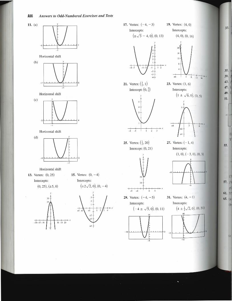
11111117
21. Vertex: (I, 1)
Intercept: (0, i)
23. Vertex: (1, 6)
Intercepts:
(1 ± 0), (0,
17. Vertex: (-4, —3) 19. Vertex: (4, 0)
Intercepts: Intercepts:
(±-1 — 4, 0), (0, 13) (4,0), (0, 16)
Horizontal shift
13. Vertex: (0, 25)
Intercepts:
(0, 25), (±5, 0)
9
3
15. Vertex: (0, —4)
Intercepts:
(±2-,/, 0), (0, —4)
5 -
4 -
1 1 1 I -2 -1 1 2 3
25. Vertex: 20)
Intercept: (0, 21)
27. Vertex: (-1,4)
Intercepts:
(1, 0), (— 3, 0), (0
5
Horizontal shift
(d) 7
9
3
A66 Answers to Odd-Numbered Exercises and Tests
7
Horizontal shift 7
Horizontal shift
5 7
7
29. Vertex: (-4, —5) 31. Vertex: (4, —1)
Intercepts: Intercepts:
(-4 ± 0), (0, 11) (4 ± 0), (0,
-6
14
11. (a)
(b)
Pill I
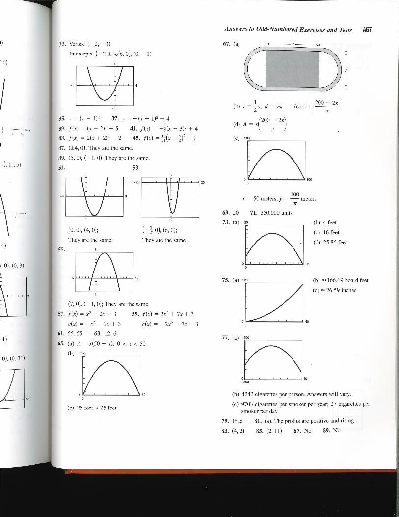
67. (a)
Answers to Odd-Numbered Exercises and Tests A67
33. Vertex: (-2, —3)
Intercepts: (-2 ± 0), (0, —1)
4
-8 4
-4
35. y = (x — 1)2 37. y = —(x + 1)2 + 4
39. f(x) = x + 2)2 + 5 41. f(x) = — 3)2 + 4
43. f(x) = 2(x + 2)2 — 2 45. f(x) = le(x — 1)2 —
47. (±4, 0); They are the same.
49. (5, 0), (— 1, 0); They are the same.
51. 53. 4
20
4
(0, 0), (4, 0);
They are the same.
55. 8
-4
(7, 0), (-1, 0); They are the same.
57. f(x) = x2 — 2x — 3 59. f(x) = 2x2 + 7x + 3
g(x) = —x2 + 2x + 3 g(x) = — 2x2 — 7x — 3
61. 55, 55 63. 12, 6
65. (a) A = x(50 — 0 < x < 50
(b) 700
1 200 — 2x (b) r = —2
y; d = (c) y — ir
(d) A (200_ 2x)
)
(e) 20
1
02_
(b) 166.69 board feet
(c) 26.59 inches
40
40
(b) 4242 cigarettes per person. Answers will vary.
(c) 9703 cigarettes per smoker per year; 27 cigarettes per smoker per day
79. True 81. (a). The profits are positive and rising.
83. (4,2) 85. (2, 11) 87. No 89. No
8 12 16
o), (o, 5)
0), (0, 31)
-6 12
i
12
100
100 x = 50 meters, y = — meters
IT
20
26
(b) 4 feet
(c) 16 feet
(d) 25.86 feet
69. 20 71. 350,000 units
73. (a) 20
I)
16)
8
-4
5
-40
They are the same.
0
(c) 25 feet x 25 feet
50

A68 Answers to Odd-Numbered Exercises and Tests
Section 2.2 (page 156)
1. (f) 3. (c) 5. (e) 7. (g)
9. (a) (b)
17. Rises to the left. 19. Falls to the left.
Rises to the right. Falls to the right 21. Rises to the left. 23. Rises to the left.
Falls to the right. Falls to the righi
25. Falls to the left. 27. ±5 29. 3
Falls to the right.
31. 1, —2 33. 2, 0 35. —5 ±
2
37. (a) 2
7 1111111 111111 11
(c) (d)
A
4 -
3 -
2
1 I 1 1 I 1 x -4 -3 -2 2 3 4
-10
(b) Answers will vary. (c) (2 — 0), (2
39. (a) 6
6 6 „u 11. (a) (b)
-2
1 1 1 1 III , x -7 -6 -5 -4 -3 -2 -1 I 2 3
-4 —
(c) (d)
(b) Answers will vary. (-1, 0), (1, 0)
41. (a) 4
II 6 6
-4
(b) Answers will vary. (c) (0, 0), (— 0)
43. (a) 10
5 10
- 45 ii
13. 15.
(b) Answers will vary. (c) (— (3), (-./3.,
45. (a) 130
12
8
12
6 6
-10
-8 -20 (b) Answers will vary. (c) (4, 0), (-5, 0), (!
5:
5!
61
6'
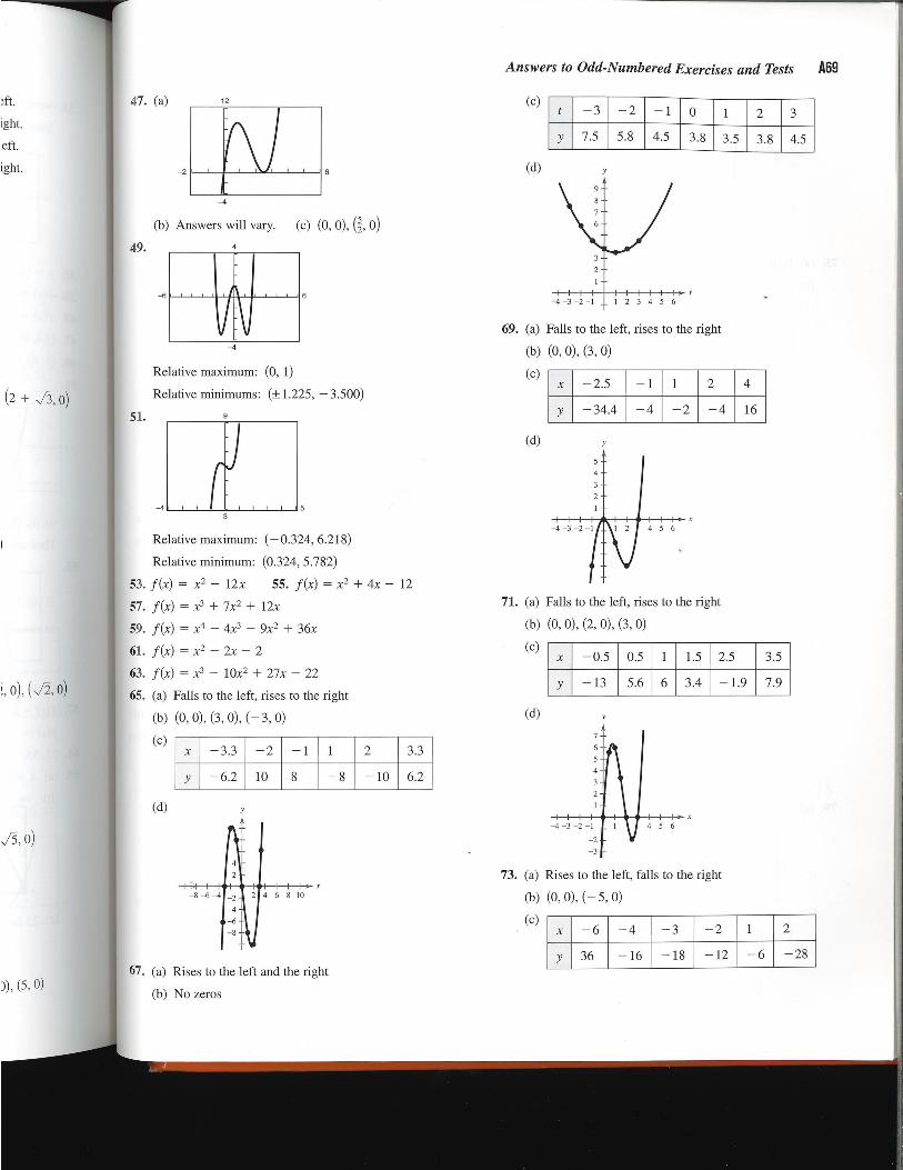
Answers to Odd-Numbered Exercises and Tests A69
;ft.
Lght.
eft.
Lght.
12 47. (a) (c) t -3 -2 -1 0 1 2 3
y 7.5 5.8 4.5 3.8 3.5 3.8 4.5
-2 (d) 6
-4
(b) Answers will vary.
4
(c) (o, 0), o)
49. lu 3
2
1
1 1 1 1 1 1 1 1 1 1-
-4-3-2-1 1 2 3 4 5 6 6 -6
69. (a) Falls to the left, rises to the right -4
Relative maximum: (0, 1)
Relative minimums: (±1.225, -3.500)
51. 9
(b) (0, 0), (3, 0)
(c) x -2.5 - 1 1 2 4
y -34.4 -4 -2 -4 _16
(d)
-4 5
71. (a) Falls to the left, rises to the right
(b) (0, 0), (2, 0), (3, 0)
(c) x -0.5 0.5 1 1.5 2.5 3.5
y -13 5.6 6 3.4 -1.9 7.9 !, 0), (2, 0)
3
Relative maximum: (-0.324, 6.218)
Relative minimum. (0.324, 5.782)
53. f(x) = x2 - 12x 55. f(x) = x2 + 4x - 12
57. f(x) = x3 + 7x2 + 12x
59. f(x) = x4 - 4x3 - 9x2 + 36x
61. f(x) = x2 - 2x - 2
63. f(x) = x3 - 10x2 + 27x - 22
65. (a) Falls to the left, rises to the right
(b) (0,0), (3, 0), (-3,0)
(c)
(d)
x -3.3 -2 -1 1 2 3.3
y -6.2 10 8 -8 -10 6.2
(d)
0)
73. (a) Rises to the left, falls to the right -8 -6 -4 4 6810 (b) (0, 0), (-5, 0)
(c) x -6 -4 -3 -2 1 2
y 36 -16 -18 -12 -6 -28
)), (5, 0) 67. (a) Rises to the left and the right
(b) No zeros

II
97.
99..
101.
103
87. 35
10 10
-6 -6
9
12
(d)
A70 Answers to Odd-Numbered Exercises and Tests
75. (a) Falls to the left, rises to the right
(b) (0, 0), (4, 0)
(c)
(d)
77. (a) Falls to the left and right
t —4 —3 —1 0 1 3
y —36 —6.3 —2.3 —4 —2.3 —6.3
(d)
(b) —0.879, 1.347,
2.532
7
(b) (-2, 0), (2, 0)
(c)
79. (a)
Symmetric to the origin Three x-intercec
Three x-intercepts
1111
5
-3
(— 1, 0), (1,2), (2,3)
5
-150
Symmetric to the y-axis
Two x-intercepts
91. 93. 6 14
5
x —2 —1 1 2 3 5
y —24 —5 —3 —8 —9 25
3
6 6
83.
4 4
Xmin = -4 Xmax =4 Xscl = 1 Ymin = -3 Ymax = 1 Yscl = 1 -3
(-2, —1), (0, 1)
81. (a) (b) — 1.585, 0
85. 16
14 - 10
Xmin = -10 Xmax = 14 Xscl = 2 Ymin =0 Ymax = 16 Yscl = 2
-5
Two x-intercepts
89. 10
-10 10
11111 11 111111
I I
.

1. 3.
A -2 -1 0 1 2
-32-24-16-8 0 8 16
21
10
-21
6
Answers to Odd-Numbered Exercises and Tests A71
95. (a) and (b)
Height Width Volume
1 36 - 2(1) 1[36 - 2(1)]2 = 1156
2 36 - 2(2) 2[36 - 2(2)]2 = 2048
3 36 - 2(3) 3[36 - 2(3)]2 = 2700
4 36 - 2(4) 4[36 - 2(4)]2 = 3136
5 36 - 2(5) 5[36 - 2(5) 2 = 3380
6 36 - 2(6) 6[36 - 2(6)]2 = 3456
7 36 - 2(7) 7[36 - 2(7)]2 = 3388
5 < x < 7
(c) Answers will vary. Domain: 0 < x < 18
(d) 3600 X = 6
105. 33 107. -1 -1.3 109. 72
111. x x > 1 113. x -24, x > 8
115. f(x) = x2 - 8 117. f(x) = (x + 5)2 - 2
Section 2.3 (page 170)
-2
5.
6 6
4
i85, 0.779
-4
97. (200, 160)
99. (a) 0.002983x4 - 0.02386x3 + 0.0194x2 + 0.113x
(b) o.2 (c) O. Yes
5
The model fits well.
101. False. It can have at most three turning points.
03.
-6
(a) Vertical shift of two units; even
(b) Horizontal shift of two units; neither even nor odd
(c) Reflection in the y-axis; even
(d) Reflection in the x-axis; even
(e) Vertical shrink; even (f) Vertical shrink; even
(g) g(x) = x3; odd (h) g(x) = x16; even
7. 2x + 4 9. x2 - 3x + 1 11. 7
2x - 3 13. 3x + 5 2x2 1
21. 6x2 + 25x + 74 + 248
23. 9x2 - 16 x - 3
25. x2 - 8x.+ 64 27. 4x2 + 14x - 30
29. f(x) = (x - 4)(x2 + 3x - 2) + 3, f(4) = 3
31. f(x) = - + (3 + „Mx + 312] - 8,
33. f(x) = - 1 + ./-314x2 - (2 + 413-)x - (2 +
35. (a) 1 (b) 4 (c) 4 (d) 1954
37. (a) 97 (b) (c) 17 (d) -199
39. (x - 2)(x + 3)(x - 1) 41. (2x - 1)(x - 5)(x - 2)
Zeros: 2, -3, 1 Zeros: 1, 5, 2
43. (x - ,/2)(x + ,/2)(x + 2)
Zeros: ± -2
45. (a) Answers will vary. (b) (2x - 1)
(c) (x + 2)(x - 1)(2x - 1) (d) -2, 1,-f
J.
0 4
6
-17
18
nercepts
11 x + 2
17. 2x x2 - 2x + 1
2x - 11 15. x2 + 2x + 4 +
19. 3x2 + 2x + 20 + 58
x - 4 17x - 5
X 2 2x ± 3

t —2 —1 0 1 _
2
R 13.84 15.37 16.68 17.86 18.98
t 3 4 5 6 7
R 20.12 21.37 22.8 24.49 26.53
(c) 41. 41
49. zj
55. —
61. —.
69. 6i
71.
-3 -
1.82 x 5.36 x 11.36
(d) 8; 8 is not in the domain of V.
91. (a) 2700 (b) 16.89
(c) 16.89 12 L 1 1 1 1 1 1 1 1 1 1 I
—5 ± (c) 1,
12 (b) 15
I I I I I I I I I I -12
(c) —2,-1,2
-7
57. (a) ±1, +3, +.1, +i, +i
(b) (c) —,l,3
I I I I I I I I I 12 12
59. (a) ±1, ±2, ±4, ±8, 16 (b)
4
-8
61. (a) ±1, +2, ±4, +8, ±-1, ±1, ±i,
(c) —,1,2,4
(b) 6
A72 Answers to Odd-Numbered Exercises and Tests
47. (a) Answers will vary. (b) (x — 1), (x — 2)
(c) (x — 5)(x + 4)(x — 1)(x — 2) (d) —4, 1, 2, 5
49. (a) Answers will vary. (b) (x + 7)
(c) (2x + 1)(3x — 2)(x + 7) (d) —7, —
51. ±1,±3
53. ±1, ±3, +5, +9, +15, +45, 4 ±1 +3, +3, ±1, 55. (a) ±1, ±2, ±4
75. and 77. Answers will vary.
83. (d) 85. (b)
87. (a) and (b)
35
79. ±2, +i 81.
89. (a)
-2 10
R = 0.01326t3 — 0.0677t2 + 1.231t + 16.68 The model is a good fit.
1--1
(b) V = x(9 — 24(15 — 24; Domain: 0 <x <
(C) 125
(d) R(12) = 44.62. No; the model will turn sharply upward.
-
F.1- 15 -01
7
5
63. — 1, 2 65. 0, —1, —3, 4 67. —2,—,4
69. (a) — 2.236, 2, 2.236 (b) 2
(c) f(x) = — 2)(x — 13)(x + -13)
71. (a) — 2, 0.268, 3.732 (b) —2
(c) h(t) = (t + 2)(t — 2 + -,A(t — 2 —
73. (a) 0, 3,4, — 1.414, 1.414 (b) 0, 3,4
(c) h(x) = x(x — 3)(x — 4)(x + -A(x — -1fl
13 0
93. False. —1 is the zero derived from (7x + 4).
95. True 97. x2" — x^ + 3
99. Multiply the divisor and the quotient to obtain the dividend
101. (a) 2x2 — 3 (b) 4x2 — 20x + 26
18
-7
—0.1
79. No.
81. (a) 8
83. (a) 3.
87. (a) 11
89. Answ

81. ±
- 16.68
2
18.98
7
26.53
starply upwar
Answers to Odd-Numbered Exercises and Tests A73
103. (a) (b) + 1 91. (a) 2x + 3y + 7 = 0 (b) 3x - 2y + 30 = 0
4x + x2 x x2 93. (-4, 0), (2, 0), (0, -8) 95. (-1, 0), (1, 0), (0, -1)
16.89
16.89
1).
in the dividend.
105. f(x) = x3 - 6x2 - 19x + 24 107. f(x) = x2 - 4x + 1
Section 2.4 (page 180)
1. a = -9, b = 4 3. a = 6, b = 5 5. 4 + 5i
7. 12 9. -1 - 5i 11. -75 13. 0.3i
15. 11 - i 17. 7 - i 19. -14 + 20i
21. + 76- i 23. -4.2 + 7.5i 25.
27. -10 29. 5 + i 31. 12 + 30i
33. 24 35. -9 + 40i
37. = i = 6i2 = -6 39. 25
41. 41 43. 484 45. 11 47. -6i
49. Ili + i 51. + i 53. -7 - 6i
55. - + 1if 57. - i 59. - 1 + 6i
61. -Si 63. -375-,5i 65. i 67. 4 + 3i
69. 6i
71. Imaginary axis
3 :-
2 - I -
Real
axis
•
73.
5 4
3 2
-7 -6 -5 -4 -3 -2 -1 I 2 3 1401111 I I Real
axis
-2
-3 -4 -5
75. Yes. 0, 0, 0, 0, 0, 0
77. Yes.
0.5i, -0.25 + 0.5i, -0.1875 + 0.25i, -0.0273 + 0.4063i,
- 0.1643 + 0.4778i, -0.2013 + 0.3430i
79. No. 1, 2, 5, 26, 677, 458,330
81. (a) 8 (b) 8 (c) 8
83. (a) 3.12 - 0.97i (b) 12.82 + 5.28i 85. True
87. (a) 1 (b) i (c) -1 (d)
89. Answers will vary.
Section 2.5 (page 187)
1. 0, 6, 6 3. 2, -4, -4, -4 5. -6, i, - i
7. 2, -3 + 5i, -3 - 5i
9. Zeros: 4, - i, i. One real zero; same
11. Zeros: -,/D, --ID. No real zeros; same
13. 2 ±
- 2 - - 2 + .5)
15. 6 ±
6 - ./T.0)(x - 6 +
17. ±5i 19. ±3,±3i
(x + 50(x - 5i) (x + 3)(x - 3)(x + 3i)(x - 3i)
21. 1 ± i
- 1 + i)(z - 1 -
23. -5, 4 ± 3i
(t + 5)(t - 4 + 30(t - 4 - 3i)
25. 1 +
(4x + 3)(x - 1 - Ii)(x - 1+ i)
27. ±i, ±3i
+ i)(x - i)(x + 3i)(x - 3i)
29. 2, 2, ±2i
(x - 2)2(x + 2i)(x - 2i)
31. -2, -1, ±i
+ 2)(2x + 1)(x - i)(x +
33. (a) 7 ± -,5 (b) - 7 - -.5)(x - 7 +
(c) (7 ± 0)
35. (a) -7 ± -13 (b) + 7 - -13)(x + 7 + -13)
(c) (-7 ± -13, 0)
37.(a) -6, 3 ± 4i (b) (x + 6)(x - 3 - 4i)(x - 3 + 4i)
(c) (-6,0)
39. (a) ±4i, ±3i (b) (x + 4i)(x - 4i)(x + 3i)(x - 3i)
(c) None
41. x3 - x2 + 25x - 25 43. x3 - 10x2 + 33x - 34
45. x4 + 37x2 + 36 47. x4 + 8x3 + 9x2 - 10x + 100
49. (a) (x2 + 1)(x2 -7) (b) (x2 + 1)(x + -17)(x - 1 77)
(c) (x + i)(x - 0(x + ,r7)(x - -177)
51. (a) (x2 - 6)(x2 - 2x + 3)
(b) + .,/g)(x ,/6)(x2 - 2x + 3)
(c) + - -,./3)(x - 1 - -,/2i)(x - 1 + -1D)
- 4 -
<x<
Imaginary axis

69. (a) 0 < k < 4 (b) k = 4 (c) k < 0 (d) k > 4
71. f(x) = x2 + b
73. , 75.
Section 2.6 (page 195)
x f(x) A. f(x)
0.5 -2 1.5 2
0.9 -10 1.1 10
0.99 -100 1.01 100
0.999 -1000 1.001 1000
x f(x) x f(x)
5 0.25
-5
10 0.T -10 -0.-0
100 0.(7 -100
-0.0099
1410 0.001 -1000
-0.000999
1. (a)
x f(x) x f(x)
0.5 3 1.5 9
0.9 27 1.1 33
0.99 297 1.01 303
0.999 2997 1.001 3003
x f(x) x f (x)
5 3.75 -5 -2.5
10 3.-n -10 -2.727
100 3.0 -100 -2.97
1000 3.003 -1000 -2.997
3. (a)
x f(x) x f(x)
5 3.125 -5 3.125
10 3.0 -10 3.0
100
-100
3.0003 3.0003
1000 3 -1000 3.000003
x f(x) x f(x)
0.5 -1 1.5 5.4
0.9 -12.79 1.1 17.29
0.99 -147.8 1.O1 152.3
0.999 -1498 1.001 1502.3
(b) Vertical asymptote: x = 1
Horizontal asymptotes: y = ±3
(c) Domain: all x 0 1
5. (a)
A74 Answers to Odd-Numbered Exercises and Tests
53. -1 -F5i 55. -3, 5 + 2i 57. 1 ±
59. 1(1 ±
61. (a) 1.000, 2.000 (b) 1, 2 (c) 1, 2, -3 ±
3 3 1 63. (a) 0.750
(b) (c) ±
65. No. Setting h = 64 and solving the resulting equation yields imaginary roots.
67. False. A polynomial can only have an even number of complex zeros, so one of the zeros of a third-degree poly-nomial must be real.
Vertex: (3.5, -20.25) Vertex: -72+4)
Intercepts: Intercepts:
(-1,0), (8, 0), (0, -8) (-1 0), (, 0), (0, -6)
77. 17 - 21 79. -55 + 48i
(b) Vertical asymptote: x = 1
Horizontal asymptote: y = 0
(c) Domain: all x 1
(b) Vertical asymptotes x = ±1
Horizontal asymptote: y = 3
(c) Domain: all x ± 1
7. (a) 9. (c) 11. (b)
13. (a) Domain: all x 0
(b) Vertical asymptote: x = 0
Horizontal asymptote: y = 0
15. (a) Domain: all x 0 3
(b) Vertical asymptote: x = 3
Horizontal asymptote: y = -1
17. (a) Domain: all x i ± 1
(b) Vertical asymptotes: x = ± 1
19
23.
25.
27.
31.
32.
35, (

(b)
a
1900
1400
37. (a)
6
-4
6 6
(b) $170 million
23. 4; Less than; Greater than
25. 2; Greater than; Less than
27. ±3 29. 7
31. (a) $28.33 million
(c) $765 million
(d) 2000
19. (a) Domain off all x 0 -2
Domain of g: all real numbers
(b) Vertical asymptote: None
x -4 -3 -2.5 -2 -1.5 -1 0
f(x) - 6 -5 -4.5 Undef. -3.5 -3 -2
g(x) - 6 -5 -4.5 -4 -3.5 -3 -2
(d) Values differ only where f is undefined.
21. (a) Domain off all x 0, 3; Domain of g: all x * 0
(b) Vertical asymptote: x = 0
(c)
(d) Values differ only where f is undefined and g is defined.
100
Answers will vary.
(e) No. The function is undefined at the 100% level.
33. (a)
M 1200 1400 1600 1800 2000
t 1.009 1.096 1.178 1.255 1.328
The greater the mass, the more time required per oscillation.
(b) M = 1306 grams
35. (a) 333 deer, 500 deer, 800 deer
(b) 1500. Because the degrees of the numerator and the denominator are equal, the limiting size is the ratio of the leading coefficients, 60/0.4 = 1500.
(c)
x -1 -0.5 0 0.5 2 3 4
f(x) -1 - 2 Undef. 2
Undef.
g(x) -1 -2 Undef. 2 I 2 3 1 4
M 200 400 600 800 1000
t 0.472 0.596 0.710 0.817 0.916
Answers to Odd-Numbered Exercises and Tests A75
(c) Not likely. The graph of the model dips quite low in the future.
39. True. Can be written as
N(x) x3 - 2x2 - 5x + 6 D(x) 1
-3(x + 1)2 41. f(x) - 1 +1 x2 43. f(x) =
x(x -
45. x = 5 47. t = 0, ±5-I2
49. x = , ± / T. i 51. x 7 6
x - 3
53. 4x - 21 + 116
55. x3 + 2x2 + 36x + 72 x + 6
57. x3 + 5x2 + 7x - 13
Section 2.7 (page 204)
1. 3. 4 4
Vertical shift
5. 4
-4
Reflection in the x-axis
6 -6
Horizontal shift
11. 4
6 6
-4
Reflection in the x-axis
Vertical shift
9. 4
-4
Horizontal shift

33. 35. 15. 13.
Y
21. 23.
17. 19.
9
4-L-
s
A76 Answers to Odd-Numbered Exercises and Tests
---- ••••11114
r
29. 31.
7
—4
Domain: (—on, 1), (1, cc)
x = 1, y = —1
—15
—10
Domain: (—on, 0), (0, on)
x = 0, y = 0
41.
12
There are two horizontal asymptotes, y = 6 and y =
43. 16
—16
There are two horizontal asymptotes, y = 4 and y
and one vertical asymptote, x = —1.
24 24
y 7
Domain: (—cc, 0), (0, co)
x = 0, y -= 3
6
—2
Domain: (— co, 00)
y=o
6 6
6
-6
Domain: (—on, —2), (-2, 3), (3, co)
x = —2, x = 3,y = 0
39. 10
37.
—9
4
27. 25.
Y
8
12
— 8
1 1 1 1 1 1 L, ,
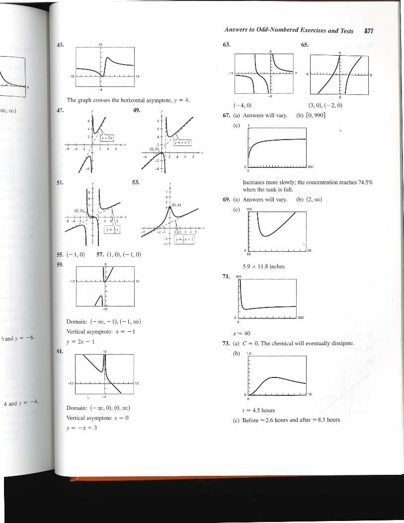
11
4
2
51. 53.
2 4 6
o
o
Answers to Odd-Numbered Exercises and Tests A77
63. 65. 6
-6
(— 4, 0)
67. (a) Answers will vary.
(c) 1
950 o
Increases more slowly; the concentration reaches 74.5% when the tank is full.
69. (a) Answers will vary. (b) (2, co)
(c) 100
20 50
5.9 x 11.8 inches
71. 300 -12 12
-10
Domain: (—cc, —1), (-1, oo)
Vertical asymptote: x = —1
y = 2x — 1
300 [ 5 and y = —
12 61.
x ..-- 40
73. (a) C = 0. The chemical will eventually dissipate.
(b) 10
12 -12
- 10
-4
4 and y =---- — , t --,--• 4.5 hours
(c) Before =--•• 2.6 hours and after =---. 8.3 hours
Domain: (—cc, 0), (0, co)
Vertical asymptote: x = 0
y = —x + 3
55. (— 1, 0) 57. (1, 0), (— 1, 0)
59. 6
12
-4
The graph crosses the horizontal asymptote, y = 4.
oo, co) 47. y 49.
10 14
6
7 9 9
-6
(3, 0), (— 2, 0)
(b) [0, 990]
45.

A78 Answers to Odd-Numbered Exercises and Tests
91.
20
(b) y = 384.5x + 5938
15,000
93. 95. 15 10
-15 15
20 GTTT 8,000 15 -15
(c) y = 14.87x2 + 42.5x + 7781 -5
15,000 - Domain: —11 5_ x 11
Range: 0 y 11
Domain: (- 00, oo)
Range: y 9
Review Exercises
20 1. (a)
(page 209)
(b) 6 6
(d) Answers will vary. The rational model seems to start climbing too fast. The quadratic model may fit the data a little better than the linear model, is easy to use, and would be most useful.
9 9 9
77. False. A graph with a vertical asymptote is not continuous.
79. -6
4 -6
Vertical stretch Vertical stretch an reflection in the x-
axis -6
(d) (c) 6
-4
9 -9 The denominator is a factor of the numerator.
81. No. (Discussions will vary.)
± 2x — 15
-9
85. f(x) = -6 -6 83. f(x) = x + 4
—2x — 12 x — 3
87. Vertical shift 89.
3.
Horizontal shift
Vertex: (- -1, 1)
Intercept: (0, )
III I I I I -5 -4 -3 -2 -1 1 2 3 4 5
IS x
-7
-4-
5 - 4 - 3 - 2 -

15
11, Maximum: (3, 9) 13. Maximum: (1, 3) 41 15. minimum: ( —
(b) x = 4, y = 2
(d) 9
-6
shift
1 23
Answers to Odd-Numbered Exercises and Tests A79
(c) (d)
1 1 1 1 1 1 1 1 1 Irs -5 -4 -3 -2 -1 _ 1 2 3 4 5 -5 -4 -3 -2 -1 1 2 3 4 5
-2
is
10
- 00, 00)
9
etch and n the x-axis
6
17. (a)
7. f(x) = (x - 1)2 - 4 9. Minimum: (1, -1)
Vertex: (-2' 5
41\)1 - 2
Intercepts: (0, 43), ( -5 ± -12-11 0 2
x y
Area
1 4 - 1(1) (1)[4 - 1(1)] = 1
2 4 - 1(2) (2)[4 - 1(2)] = 6
3 4 - 1(3) (3)[4 - 1(3)] = 121
4 4 - 1(4) (4)[4 - 1(4)] = 8
5 4 - 1(5) (5)[4 - 1(5)] = 1
6 4 - 1(6) (6)[4 - 1(6)] = 6
- (c) A = x (8
2 x), 0 < x < 8
x = 4, y = 2
(b) Y
5 - 4 - 3 - 2 - 1 -
1 1 1 1 1 1 1 1 ), -5 -4 -3 -2 fr _ 2 3 4 5
-4-
(d)
-8-6-4-2 _ 2 4 6 8 10
-4-
-6-
-8 - -10 - -12 -
25. Rises to the left.
Rises to the right.
21. (a)
(c)
10
23. Falls to the left.
Falls to the right.
27. 12
tIJ 1 1 1 1 1
-8 -6 -4 -2 _ 2 1 1 46
-4
Ii'
1 x 11111 11111 ,,
18 18
-12
29. (a) x= -1,0,2 (b)
31. (a) t = 0, ±-,/ (b)
(e) A = -1(x - 4)2 + 8
). (a) (b)
1 1 1 1 -7 -6 -5 -4 -3 -2 -1 _
-4-

95. f(
97. f(
99. (
103. D
Ve
(b)
6 6
(c) 1
+ 4
1 I _I 1 1 50
81. Imaginary axis
4 — 3 — 2 — 1 —
IIIII 1 1 1 1 1 —5 —4 —3 —2 —1 — 1 2 3 4 5
A80 Answers to Odd-Numbered Exercises and Tests
35. (a) V = x2(216 — 4x)
(b) 100,000
00
x = 36 centimeters, y = 72 centimeters
37. (a) (-3, —2), (-1,0), (0, 1)
(b) (-2.247,0), (-0.555, 0), (0.802, 0)
39. (a) (-3, —2), (2,3) (b) (-2.570,0), (2.570,0)
2 41. 14 43. 8x + 5 + v
—16
—10
45. x2 — 2, x ±1 47. x2 — x + 1, x 0, —2
36 49. —1x3 — —9x2 + 9x — 18 +
4 2 x + 2
51. 6x3 — 27x, x
53. (a) 75 (b) 0 (c) 0 (d) —21
55. 2(x + 3)(x + 2)(x — i)(x — 2)
—3, —2,,2 13 3 1 57. (a) ±T, ±3, ±74, ±1
—4
20
6
10
—100
59. (a) +V, +1, +10, +20, +i, ±5, ±i,
+4, +I-, +4, +1
(b) loo (c)
10
33. (a) x= —3,0 (b)
30 (C) —1 2 3: ' 3, 2
5
(b)
5
—30
63. Answers will vary. 65. 6 + 5i 67. 2 + 71
69. 3 + 7i 71. 40 + 65i 73. —4 — 46i
75. —80 77. 1 — 6i
Imaginary axis
2 — I —
I 1'111 1111 —5 —4 —3 —2 —1 — I 2 3 4
12 —6
-4-
-5-- •
7
—1
85. (a)
6
(b) Two
(c) —1, —0.54
87. (a) 4
—8
89. 2, 1± i
(x — 2)(x— 1— i)(x — 1+1)
(b) One
(c) 3.26
3x —2
79.
83.
Real

2 J", -±3, +2,
,
32-> 3
Answers to Odd-Numbered Exercises and Tests A81
121. 123.
—7 —6 —5 —4
125.
18 16 14 12 10
8 6 4
6810 12 18
—10
—6 —4 —2 4 (1 l A —4
`') —6 —8
—10
10 8 6 4 '5_ 2
4
91. —4, —1 ±
+ 4)(x + 1 + -,/2i)(x + 1 - -JD)
93. ±3i,±5i
(x — 3i)(x + 3i)(x — 50(x +
95. f(x) = x4 + 4x3 + 29x2 + 100x + 100
97. f(x) = 3x4 — 13x3 + 5x2 + 43x + 22
99. (a) (x2 — 5)(x2 — x + 4)
(b) — -10(x + ,/3)(x2 — x + 4)
(c) — -,./3)(x + ./3)(x 1 ± ./1.3i)(x 1 —
2 2
101. Domain: all x 1
Vertical asymptote: x = 1
Horizontal asymptote: y = —1
103. Domain: all x 6, —3
Vertical asymptotes: x = 6, x = —3 . 2 + 7i Horizontal asymptote: y = 0 [6i 105. y = —1 107. y = 2
111. (a) 300
I I I I I> 1 2 3 4 5
0 0
127. (a) 800
g 700
"rg 600 tga 500
a, .g acio 300
100 1 1 1 I 5 10 15 20 25
Time (in years)
109. y = ±1
50
(b) 10.5, 5.5, 1, 0.55 (c) 0.5
13. y 115.
1 I I
117. 119.
(b) 304,000; 453,333; 702,222
(c) 1,200,000, because N has a horizontal asymptote at y = 1,200,000.
129. True
o) Chapter Test (page 214)
1 2 3 1. (a) Reflection in the x-axis followed by a vertical shift
(b) Horizontal shift
2. Vertex: (-2, — 1)
Intercepts: (0, 3), (-3,0), (-1,0)
3. y = (x — 3)2 — 6
4. (a) 50 feet
(b) 5. Changing the constant term results in a vertical shift of the graph and therefore changes the maximum height.
x — 1 6. 2x3 + 4x2 + 3x + 6 +
9 X2 + 1 X — 2
6 8 10 12 14 -1 —
3 —
2
1 —
One
3.26
I I I I,

.1
A82 Answers to Odd-Numbered Exercises and Tests
7. ±1, ±2, ±3, ±4, ±6, ±8, ±12, ±24, ±i,
5
10 10
-35
-2,
8. +1, +2, +1,
111111111
1111111
-9 9
+1, -
9. -9 - 18i 10. 6 + (2-,/3 +
11. 13 + 4i 12. V. + gi 13. -0.819, 1.380
14. - 1.414, -0.667, 1.414
15. f (x) = x4 - 9x3 + 28x2 - 30x
16. f (x) = x4 - 6x3 + 16x2 - 24x + 16
17. f(x) = x4 + 3x3 - 8x2 + 10x
18. 19.
-9 -8 -7-
x
f(x)
9 21 -
7 - 6 - 5 - 4 - 3 -
- -I F -I 2
20.
21. 24.8 years
x -1 0 1 2 3
f (x) 0.4 1 2.5 6.3 15.6
35.
Chapter 3 Section 3.1 (page 225)
1. 4112.033 3. 77,494.076 5. 19.568
9. 9897.129 11. f(x) = h(x)
13. f(x) = g(x) = h(x) 15. (c) 17. (e)
21. (a) 23. Right shift of 5 units
25. Left shift of 4 units and reflection in x-axis
27. 29.
7. 1.649
19 (g)
37.
f(x)
39.
f(x)
-7 -6 -5 -4 3
2
I I 2 3 4
(a) y = 0
(b) (0, I)
(c)Decreasing
33.
2
-2 -3 -4
(a) y = 0
(b) (0, 1)
(c) Increasing
31.
4
(a) y = 0
(b) (o,11 )
(c) Increasing
(a) y = -3
(b) (0, -2), (-0.6
(c) Decreasing
41.
f(x)
83,
43.