Local Polynomial Modeling
13
196 4. Minimum Roughness Filters 0 5 10 15 20 25 30 35 40 45 50 0 0.5 1 1.5 Robust smoothing, N it = 0 time samples, t outliers outliers desired smoothed noisy 0 5 10 15 20 25 30 35 40 45 50 0 0.5 1 1.5 Robust smoothing, N it = 1 time samples, t desired smoothed noisy adjusted 0 5 10 15 20 25 30 35 40 45 50 0 0.5 1 1.5 Robust smoothing, N it = 2 time samples, t desired smoothed noisy adjusted 0 5 10 15 20 25 30 35 40 45 50 0 0.5 1 1.5 Robust smoothing, N it = 4 time samples, t desired smoothed noisy adjusted Fig. 4.5.3 Robust smoothing with outliers. n1=10; n2=25; m = [-1 0 1 3]; % outlier indices relative to n1 and n2 y(n1+m+1)=1; y(n2+m+1)=0; % outlier values Nit=4; K=4; x = rlpfilt(y,N,d,s,Nit,K); % robust LP filtering plot(t,x0,’--’, t,y,’o’, t,x,’-’, n1+m,x(n1+m+1),’.’, n2+m,x(n2+m+1),’.’); 4.6 Problems 4.1 Using binomial identities, prove the equivalence of the three expressions in Eq. (4.4.14) for the maximally-flat filters. Then, show Eq. (4.4.15) and determine the proportionality con- stants indicated as (const.). 5 Local Polynomial Modeling 5.1 Weighted Local Polynomial Modeling The methods of weighted least-squares local polynomial modeling and robust filtering can be generalized to unequally-spaced data in a straightforward fashion. Such methods provide enough flexibility to model a wide variety of data, including surfaces, and have been explored widely in recent years [188–231]. For equally-spaced data, the weighted performance index centered at time n was: J n = M m=−M ( y n+m − p(m) ) 2 w(m)= min , p(m)= d r=0 c i m r (5.1.1) The value of the fitted polynomial p(m) at m = 0 represents the smoothed estimate of y n , that is, ˆ x n = c 0 = p(0). Changing summation indices to k = n + m, Eq. (5.1.1) may be written in the form: J n = n+M k=n−M ( y k − p(k − n) ) 2 w(k − n)= min , p(k − n)= d r=0 c i (k − n) r (5.1.2) For a set of N unequally-spaced observations t k , y(t k ) , k = 0, 1,...,N − 1, we wish to interpolate smoothly at some time instant t, not necessarily coinciding with one of the observation times t k , but lying in the interval t 0 ≤ t ≤ t N−1 . A generalization of the performance index (5.1.2) is to introduce a t-dependent window bandwidth h t , and use only the observations that lie within that window, |t k − t|≤ h t , to perform the polynomial fit: J t = |t k −t|≤h t ( y(t k )−p(t k − t) ) 2 w(t k − t)= min , p(t k − t)= d r=0 c r (t k − t) r (5.1.3) The estimated/interpolated value at t will be ˆ x t = c 0 = p(0), and the estimated first derivative, ˆ ˙ x t = c 1 = ˙ p(0), and so on for the higher derivatives, with r! c r representing the rth derivative. As illustrated in Fig. 5.1.1, the fitted polynomial, p(x − t)= d r=0 c r (x − t) r , t − h t ≤ x ≤ t + h t 197
-
Upload
khangminh22 -
Category
Documents
-
view
0 -
download
0
Transcript of Local Polynomial Modeling

196 4. Minimum Roughness Filters
0 5 10 15 20 25 30 35 40 45 50
0
0.5
1
1.5Robust smoothing, Nit = 0
time samples, t
outliers
outliers
desired smoothed noisy
0 5 10 15 20 25 30 35 40 45 50
0
0.5
1
1.5Robust smoothing, Nit = 1
time samples, t
desired smoothed noisy adjusted
0 5 10 15 20 25 30 35 40 45 50
0
0.5
1
1.5Robust smoothing, Nit = 2
time samples, t
desired smoothed noisy adjusted
0 5 10 15 20 25 30 35 40 45 50
0
0.5
1
1.5Robust smoothing, Nit = 4
time samples, t
desired smoothed noisy adjusted
Fig. 4.5.3 Robust smoothing with outliers.
n1=10; n2=25; m = [-1 0 1 3]; % outlier indices relative to n1 and n2
y(n1+m+1)=1; y(n2+m+1)=0; % outlier values
Nit=4; K=4; x = rlpfilt(y,N,d,s,Nit,K); % robust LP filtering
plot(t,x0,’--’, t,y,’o’, t,x,’-’, n1+m,x(n1+m+1),’.’, n2+m,x(n2+m+1),’.’);
4.6 Problems
4.1 Using binomial identities, prove the equivalence of the three expressions in Eq. (4.4.14) forthe maximally-flat filters. Then, show Eq. (4.4.15) and determine the proportionality con-stants indicated as (const.).
5Local Polynomial Modeling
5.1 Weighted Local Polynomial Modeling
The methods of weighted least-squares local polynomial modeling and robust filteringcan be generalized to unequally-spaced data in a straightforward fashion. Such methodsprovide enough flexibility to model a wide variety of data, including surfaces, and havebeen explored widely in recent years [188–231]. For equally-spaced data, the weightedperformance index centered at time n was:
Jn =M∑
m=−M
(yn+m − p(m)
)2w(m)= min , p(m)=d∑r=0
cimr (5.1.1)
The value of the fitted polynomial p(m) atm = 0 represents the smoothed estimateof yn, that is, xn = c0 = p(0). Changing summation indices to k = n +m, Eq. (5.1.1)may be written in the form:
Jn =n+M∑k=n−M
(yk − p(k− n)
)2w(k− n)= min , p(k− n)=d∑r=0
ci(k− n)r (5.1.2)
For a set of N unequally-spaced observations{tk, y(tk)
}, k = 0,1, . . . ,N − 1, we
wish to interpolate smoothly at some time instant t, not necessarily coinciding with oneof the observation times tk, but lying in the interval t0 ≤ t ≤ tN−1. A generalizationof the performance index (5.1.2) is to introduce a t-dependent window bandwidth ht,and use only the observations that lie within that window, |tk − t| ≤ ht, to perform thepolynomial fit:
Jt =∑
|tk−t|≤ht
(y(tk)−p(tk − t)
)2w(tk − t)= min , p(tk − t)=d∑r=0
cr(tk − t)r (5.1.3)
The estimated/interpolated value at t will be xt = c0 = p(0), and the estimated firstderivative, ˆxt = c1 = p(0), and so on for the higher derivatives, with r! cr representingthe rth derivative. As illustrated in Fig. 5.1.1, the fitted polynomial,
p(x− t)=d∑r=0
cr(x− t)r , t − ht ≤ x ≤ t + ht
197

198 5. Local Polynomial Modeling
is local in the sense that it fits the observations only within the local window [t−ht, t+ht].The quantity yk = p(tk − t) represents the estimated value of the kth observation ykwithin that window.
Fig. 5.1.1 Local polynomial modeling.
The weighting function w(tk − t) is chosen to have bandwidth ±ht. This can beaccomplished by using a functionW(u) with finite support over the standardized range−1 ≤ u ≤ 1, and setting u = (tk − t)/ht:
w(tk − t)=W(tk − tht
)(5.1.4)
Some typical choices for W(u) are as follows [224]:
1. Tricube, W(u)= (1− |u|3)3
2. Bisquare, W(u)= (1− u2)2
3. Triweight, W(u)= (1− u2)3
4. Epanechnikov, W(u)= 1− u2
5. Gaussian, W(u)= e−α2u2/2
6. Exponential, W(u)= e−α|u|7. Rectangular, W(u)= 1
(5.1.5)
where all types have support |u| ≤ 1 and vanish for |u| > 1. A typical value forα in thegaussian and exponential cases is α = 2.5. The curve shown in Fig. 5.1.1 is the tricubefunction; because it vanishes at u = ±1, the observations that fall exactly at the edgesof the window do not contribute to the fit. The MATLAB function locw generates theabove functions at any vector of values of u:
W = locw(u,type); % local polynomial weighting functions W(u)
where type takes the values 1–7 as listed in Eq. (5.1.5). The bisquare, triweight, andEpanechnikov functions are special cases of the more general W(u)= (1− u2)s, whichmay be thought of as the large-M limit of the Henderson weights; in the limit s → ∞they tend to a gaussian, as in the Krawtchouk case. The various window functions aredepicted in Fig. 5.1.2.
5.1. Weighted Local Polynomial Modeling 199
−1 −0.5 0 0.5 10
0.2
0.4
0.6
0.8
1Window Functions
u
W(u
)
tricube bisquare triweight epanechnikov gaussian exponential
Fig. 5.1.2 Window functions.
Because of the assumed finite extent of the windows, the summation in Eq. (5.1.3)can be extended to run over all N observations, as is often done in the literature:
Jt =N−1∑k=0
(y(tk)−p(tk − t)
)2w(tk − t)= min , p(tk − t)=d∑r=0
cr(tk − t)r (5.1.6)
We prefer the form of Eq. (5.1.3) because it emphasizes the local nature of the fittingwindow. LetNt be the number of observations that fall within the interval [t−ht, t+ht].We may cast the performance index (5.1.3) in a compact matrix form by defining theNt×1 vector of observations yt, theNt×(d+1) basis matrix St, and theNt×Nt diagonalmatrix of weights by
yt = [· · · , y(tk), · · · ]T , for t − ht ≤ tk ≤ t + ht
St =
⎡⎢⎢⎢⎣
......
......
1 (tk − t) · · · (tk − t)r · · · (tk − t)d...
......
...
⎤⎥⎥⎥⎦ =
⎡⎢⎢⎢⎣
...uT(tk − t)
...
⎤⎥⎥⎥⎦
Wt = diag([· · · ,w(tk − t), · · · ]
)(5.1.7)
where uT(tk− t) is the k-th row of St, defined in terms of the (d+1)-dimensional vectoruT(τ)= [1, τ, τ2, . . . , τd]. For example, if t−ht < t3 < t4 < t5 < t6 < t+ht, thenNt = 4and for a polynomial order d = 2, we have:
yt =
⎡⎢⎢⎢⎣y(t3)y(t4)y(t5)y(t6)
⎤⎥⎥⎥⎦ , St =
⎡⎢⎢⎢⎣
1 (t3 − t) (t3 − t)2
1 (t4 − t) (t4 − t)2
1 (t5 − t) (t5 − t)2
1 (t6 − t) (t6 − t)2
⎤⎥⎥⎥⎦
Wt =
⎡⎢⎢⎢⎣w(t3 − t) 0 0 0
0 w(t4 − t) 0 00 0 w(t5 − t) 00 0 0 w(t6 − t)
⎤⎥⎥⎥⎦
200 5. Local Polynomial Modeling
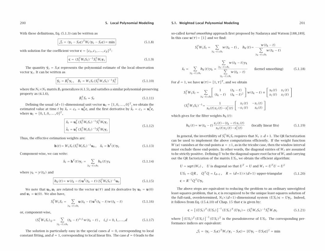
With these definitions, Eq. (5.1.3) can be written as
Jt = (yt − Stc)TWt(yt − Stc)= min (5.1.8)
with solution for the coefficient vector c = [c0, c1, . . . , cd]T:
c = (STt WtSt)−1STt Wtyt (5.1.9)
The quantity yt = Stc represents the polynomial estimate of the local observationvector yt. It can be written as
yt = BTt yt , Bt =WtSt(STt WtSt)−1STt (5.1.10)
where theNt×Nt matrixBt generalizes (4.1.5), and satisfies a similar polynomial-preservingproperty as (4.1.6),
BTt St = St (5.1.11)
Defining the usual (d+1)-dimensional unit vector u0 = [1,0, . . . ,0]T, we obtain theestimated value at time t by xt = c0 = uT0 c, and the first derivative by ˆxt = c1 = uT1 c,where u1 = [0,1,0, . . . ,0]T,
xt = uT0 (STt WtSt)−1STt Wtyt
ˆxt = uT1 (STt WtSt)−1STt Wtyt(5.1.12)
Thus, the effective estimation weights are:
h(t)=WtSt(STt WtSt)−1u0 , xt = hT(t)yt (5.1.13)
Component-wise, we can write:
xt = hT(t)yt =∑
|tk−t|≤hthk(t)yk (5.1.14)
where yk = y(tk) and
hk(t)= w(tk − t)uT(tk − t)(STt WtSt)−1u0 (5.1.15)
We note that u0,u1 are related to the vector u(τ) and its derivative by u0 = u(0)and u1 = u(0). We also have,
STt WtSt =∑
|tk−t|≤htu(tk − t)uT(tk − t)w(tk − t) (5.1.16)
or, component-wise,
(STt WtSt)ij=∑
|tk−t|≤ht(tk − t)i+j w(tk − t) , i, j = 0,1, . . . , d (5.1.17)
The solution is particularly easy in the special cases d = 0, corresponding to localconstant fitting, and d = 1, corresponding to local linear fits. The case d = 0 leads to the
5.1. Weighted Local Polynomial Modeling 201
so-called kernel smoothing approach first proposed by Nadaraya and Watson [188,189].In this case u(τ)= [1] and we find:
STt WtSt =∑
|tk−t|≤htw(tk − t) , hk(t)= w(tk − t)∑
|tk−t|≤htw(tk − t)
xt =∑
|tk−t|≤hthk(t)yk =
∑|tk−t|≤ht
w(tk − t)yk∑
|tk−t|≤htw(tk − t)
(kernel smoothing) (5.1.18)
For d = 1, we have u(τ)= [1, τ]T, and we obtain
STt WtSt =∑
|tk−t|≤ht
[1 (tk − t)
(tk − t) (tk − t)2
]w(tk − t)≡
[s0(t) s1(t)s1(t) s2(t)
]
(STt WtSt)−1= 1
s0(t)s2(t)−s21(t)
[s2(t) −s1(t)−s1(t) s0(t)
]
which gives for the filter weights hk(t):
hk(t)= w(tk − t)s2(t)−(tk − t)s1(t)s0(t)s2(t)−s2
1(t)(locally linear fits) (5.1.19)
In general, the invertibility of STt WtSt requires thatNt ≥ d+1. The QR factorizationcan be used to implement the above computations efficiently. If the weight functionW(u) vanishes at the end-points u = ±1, as in the tricube case, then the window intervalmust exclude those end-points. In other words, the diagonal entries ofWt are assumedto be strictly positive. DefiningU to be the diagonal square root factor ofWt and carryingout the QR factorization of the matrix USt, we obtain the efficient algorithm:
U = sqrt(Wt) , U is diagonal so that UT = U and Wt = UTU = U2
USt = QR , QTQ = Id+1 , R = (d+1)×(d+1) upper-triangular
c = R−1QTUyt
(5.1.20)
The above steps are equivalent to reducing the problem to an ordinary unweightedleast-squares problem, that is, c is recognized to be the unique least-squares solution ofthe full-rank, overdetermined, Nt×(d+1)-dimensional system (USt)c = Uyt. Indeed,it follows from Eq. (15.4.10) of Chap. 15 that c is given by:
c = [(USt)T(USt)
]−1(USt)T(Uyt)= (STt WtSt)−1STt Wtyt (5.1.21)
where[(USt)T(USt)
]−1(USt)T is the pseudoinverse of USt. The corresponding per-formance indices are equivalent:
Jt = (yt − Stc)TWt(yt − Stc)= ‖Uyt −UStc‖2 = min
202 5. Local Polynomial Modeling
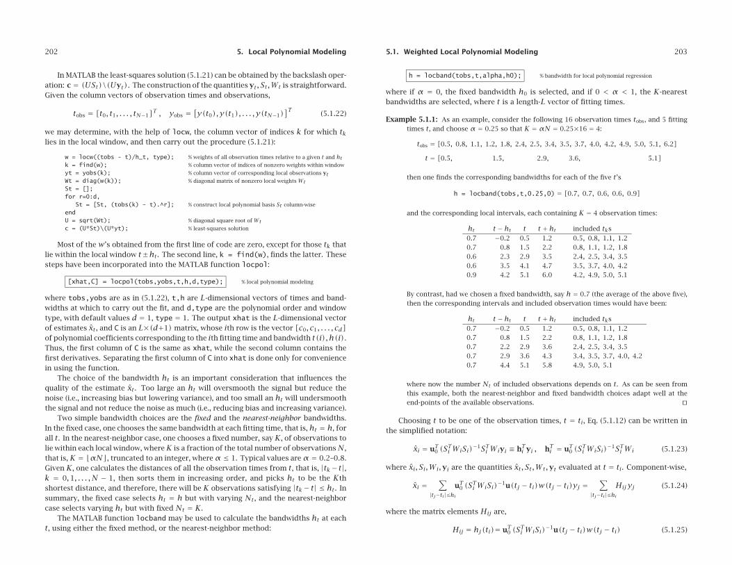
In MATLAB the least-squares solution (5.1.21) can be obtained by the backslash oper-ation: c = (USt)\(Uyt). The construction of the quantities yt, St,Wt is straightforward.Given the column vectors of observation times and observations,
tobs = [t0, t1, . . . , tN−1]T , yobs =[y(t0), y(t1), . . . , y(tN−1)
]T(5.1.22)
we may determine, with the help of locw, the column vector of indices k for which tklies in the local window, and then carry out the procedure (5.1.21):
w = locw((tobs - t)/h_t, type); % weights of all observation times relative to a given t and htk = find(w); % column vector of indices of nonzero weights within window
yt = yobs(k); % column vector of corresponding local observations ytWt = diag(w(k)); % diagonal matrix of nonzero local weights WtSt = [];for r=0:d,
St = [St, (tobs(k) - t).^r]; % construct local polynomial basis St column-wise
endU = sqrt(Wt); % diagonal square root of Wtc = (U*St)\(U*yt); % least-squares solution
Most of thew’s obtained from the first line of code are zero, except for those tk thatlie within the local window t±ht. The second line, k = find(w), finds the latter. Thesesteps have been incorporated into the MATLAB function locpol:
[xhat,C] = locpol(tobs,yobs,t,h,d,type); % local polynomial modeling
where tobs,yobs are as in (5.1.22), t,h are L-dimensional vectors of times and band-widths at which to carry out the fit, and d,type are the polynomial order and windowtype, with default values d = 1, type = 1. The output xhat is the L-dimensional vectorof estimates xt, and C is an L×(d+1)matrix, whose ith row is the vector [c0, c1, . . . , cd]of polynomial coefficients corresponding to the ith fitting time and bandwidth t(i), h(i).Thus, the first column of C is the same as xhat, while the second column contains thefirst derivatives. Separating the first column of C into xhat is done only for conveniencein using the function.
The choice of the bandwidth ht is an important consideration that influences thequality of the estimate xt. Too large an ht will oversmooth the signal but reduce thenoise (i.e., increasing bias but lowering variance), and too small an ht will undersmooththe signal and not reduce the noise as much (i.e., reducing bias and increasing variance).
Two simple bandwidth choices are the fixed and the nearest-neighbor bandwidths.In the fixed case, one chooses the same bandwidth at each fitting time, that is, ht = h, forall t. In the nearest-neighbor case, one chooses a fixed number, sayK, of observations tolie within each local window, whereK is a fraction of the total number of observationsN,that is,K = �αN, truncated to an integer, whereα ≤ 1. Typical values areα = 0.2–0.8.Given K, one calculates the distances of all the observation times from t, that is, |tk− t|,k = 0,1, . . . ,N − 1, then sorts them in increasing order, and picks ht to be the Kthshortest distance, and therefore, there will be K observations satisfying |tk− t| ≤ ht. Insummary, the fixed case selects ht = h but with varying Nt, and the nearest-neighborcase selects varying ht but with fixed Nt = K.
The MATLAB function locband may be used to calculate the bandwidths ht at eacht, using either the fixed method, or the nearest-neighbor method:
5.1. Weighted Local Polynomial Modeling 203
h = locband(tobs,t,alpha,h0); % bandwidth for local polynomial regression
where if α = 0, the fixed bandwidth h0 is selected, and if 0 < α < 1, the K-nearestbandwidths are selected, where t is a length-L vector of fitting times.
Example 5.1.1: As an example, consider the following 16 observation times tobs, and 5 fittingtimes t, and choose α = 0.25 so that K = αN = 0.25×16 = 4:
tobs = [0.5, 0.8, 1.1, 1.2, 1.8, 2.4, 2.5, 3.4, 3.5, 3.7, 4.0, 4.2, 4.9, 5.0, 5.1, 6.2]
t = [0.5, 1.5, 2.9, 3.6, 5.1]
then one finds the corresponding bandwidths for each of the five t’s
h = locband(tobs,t,0.25,0) = [0.7, 0.7, 0.6, 0.6, 0.9]
and the corresponding local intervals, each containing K = 4 observation times:
ht t − ht t t + ht included tks0.7 −0.2 0.5 1.2 0.5, 0.8, 1.1, 1.20.7 0.8 1.5 2.2 0.8, 1.1, 1.2, 1.80.6 2.3 2.9 3.5 2.4, 2.5, 3.4, 3.50.6 3.5 4.1 4.7 3.5, 3.7, 4.0, 4.20.9 4.2 5.1 6.0 4.2, 4.9, 5.0, 5.1
By contrast, had we chosen a fixed bandwidth, say h = 0.7 (the average of the above five),then the corresponding intervals and included observation times would have been:
ht t − ht t t + ht included tks0.7 −0.2 0.5 1.2 0.5, 0.8, 1.1, 1.20.7 0.8 1.5 2.2 0.8, 1.1, 1.2, 1.80.7 2.2 2.9 3.6 2.4, 2.5, 3.4, 3.50.7 2.9 3.6 4.3 3.4, 3.5, 3.7, 4.0, 4.20.7 4.4 5.1 5.8 4.9, 5.0, 5.1
where now the number Nt of included observations depends on t. As can be seen fromthis example, both the nearest-neighbor and fixed bandwidth choices adapt well at theend-points of the available observations. �
Choosing t to be one of the observation times, t = ti, Eq. (5.1.12) can be written inthe simplified notation:
xi = uT0 (STi WiSi)−1STi Wiyi ≡ hTi yi , hTi = uT0 (S
Ti WiSi)−1STi Wi (5.1.23)
where xi, Si,Wi,yi are the quantities xt, St,Wt,yt evaluated at t = ti. Component-wise,
xi =∑
|tj−ti|≤hiuT0 (S
Ti WiSi)−1u(tj − ti)w(tj − ti)yj =
∑|tj−ti|≤hi
Hij yj (5.1.24)
where the matrix elements Hij are,
Hij = hj(ti)= uT0 (STi WiSi)−1u(tj − ti)w(tj − ti) (5.1.25)

204 5. Local Polynomial Modeling
Similarly, one may express STi WiSi and STi Wiyi as,
STi WiSi =∑
|tj−ti|≤hiu(tj − ti)uT(tj − ti)w(tj − ti)
STi Wiyi =∑
|tj−ti|≤hiu(tj − ti)w(tj − ti)yj
(5.1.26)
Because the factor w(tj − ti) vanishes outside the local window ti ± hi, the sum-mations in (5.1.24) and (5.1.26) over tj can be extended to run over all N observations.Defining theN-dimensional vectors x = [x0, x1, . . . , xN−1]T and y = [y0, y1, . . . , yN−1]T,we may write (5.1.24) in the compact matrix form:
x = Hy (5.1.27)
The filtering matrix H is also known as the “hat” matrix or the “smoothing” matrix.Its diagonal elementsHii play a special role in bandwidth selection, where w0 = w(0),†
Hii = hi(ti)= w0 uT0 (STi WiSi)−1 u0 (5.1.28)
5.2 Bandwidth Selection
There exist various automatic schemes for choosing the bandwidth. Such schemes mayat best be used as guidelines. Ultimately, one must rely on one’s judgment in makingthe final choice.
A popular bandwidth selection method is the so-called cross-validation criterion thatselects the bandwidth h that minimizes the sum of squared prediction errors:
CV(h)= 1
N
N−1∑i=0
(yi − x−i )2= min (5.2.1)
where x−i is the estimate or prediction of the sample xi = x(ti) obtained by deleting theith observation yi and basing the estimation on the remaining observations, where weare assuming the usual additive-noise model y(ti)= x(ti)+v(ti)with x(ti) representingthe desired signal to be extracted from y(ti). We show below that the predicted estimatex−i is related to the estimate xi based on all observations by the relationship:
x−i =xi −Hii yi
1−Hii (5.2.2)
where Hii is given by (5.1.28). It follows from (5.2.2) that the corresponding estimationerrors will be related by:
yi − x−i =yi − xi1−Hii (5.2.3)
†w0 = 1 for all the windows in Eq. (5.1.5), but any other normalization can be used.
5.2. Bandwidth Selection 205
and therefore, the CV index can be expressed as:
CV(h)= 1
N
N−1∑i=0
(yi − x−i )2= 1
N
N−1∑i=0
(yi − xi1−Hii
)2
= min (5.2.4)
A related selection criterion is based on the generalized cross-validation index, whichreplaces Hii by its average over i, that is,
GCV(h)= 1
N
N−1∑i=0
(yi − xi1− H
)2
= min , H = 1
N
N−1∑i=0
Hii = 1
Ntr(H) (5.2.5)
If the bandwidth is to be selected by the nearest-neighbor method, then, the CVand GCV indices may be regarded as functions of the fractional parameter α and min-imized. Similarly, one could consider minimizing with respect to the polynomial orderd, although in practice d is usually chosen to be 1 or 2.
Eq. (5.2.2) can be shown as follows. If the tj = ti observation is deleted fromEq. (5.1.23), the corresponding optimum polynomial coefficients and optimum estimatewill be given by
c− = (STi WiSi)−1− (STi Wiyi)− , x−i = uT0 c−
where the minus subscripts indicate that the tj = ti terms are to be omitted. It followsfrom Eq. (5.1.26) that
STi WiSi = (STi WiSi)−+w0u0uT0
STi Wiyi = (STi Wiyi)−+w0u0yi(5.2.6)
and then,c− =
[STi WiSi −w0u0uT0 ]−1[STi Wiyi −w0u0yi
](5.2.7)
Setting Fi = STi WiSi and noting that c = F−1i S
Ti Wiyi or STi Wiyi = Fic, we may write,
c− =[Fi −w0u0uT0 ]−1[Fi c−w0u0yi
]Using the matrix inversion lemma, we have,
[Fi −w0u0uT0 ]−1= F−1
i + w0F−1i u0uT0F
−1i
1−w0uT0F−1i u0
(5.2.8)
Noting that Hii = w0uT0F−1i u0, we obtain,
c− =[F−1i + w0F−1
i u0uT0F−1i
1−Hii
][Fi c−w0u0yi
]
=[I + w0F−1
i u0uT01−Hii
][c−w0F−1
i u0yi]
= c−w0F−1i u0yi + w0F−1
i u0[uT0 c−w0uT0F
−1i u0yi
]1−Hii
and since xi = uT0 c, we find,
c− = c−w0F−1i u0yi + w0F−1
i u0[xi −Hiiyi
]1−Hii = c+w0F−1
i u0xi − yi1−Hii

206 5. Local Polynomial Modeling
from which we find for x−i = uT0 c−,
x−i = xi +Hii(xi − yi)
1−Hii = xi −Hiiyi1−Hii (5.2.9)
In practice, the CV and GCV indices are evaluated over a certain range of the smooth-ing parameter h or α to look for a minimum. The MATLAB function locgcv evaluatesthese indices at any vector of parameter values:
[GCV,CV] = locgcv(tobs,yobs,d,type,b,btype); % CV and GCV evaluation
where type is the window type, b is either a vector of hs or a vector of αs at whichto evaluate CV and GCV, and the string btype takes the values ’f’ or ’nn’ specifyingwhether the parameter vector b corresponds to a fixed or nearest-neighbor bandwidth.
5.3 Local Polynomial Interpolation
The primary advantage of local polynomial modeling is its flexibility and ease of smooth-ing unequally-spaced data. Its main disadvantage is the potentially high computationalcost, that is, the calculations (5.1.12) must be performed for each t, and generally adense set of such t’s might be required in order to get a visually smooth curve.
One way to cut down the cost is to evaluate the smoothed values xt at a less densegrid of ts, and then interpolate smoothly between the computed points. This is akinto what plotting programs do by connecting the dots by straight-line segments (linearlyinterpolating)—the result being a visually continuous curve. But here, we can do betterthan just connecting the dots because we have available the slopes at each grid point.These slopes are contained in the second column of the fitting matrix C resulting fromlocpol, assuming of course that d ≥ 1.
Consider two time instants t1, t2 at which the fitted signal values are a1, a2 withcorresponding slopes b1, b2, as shown below. The lowest-degree polynomial P(t) inter-polating between the two points t1, t2 that matches the fitted values and their slopes att1 and t2 is a cubic polynomial—the method being known as cubic Hermite interpolation.The four polynomial coefficients are fixed uniquely by the four conditions:
P(t1) = a1 , P(t1)= b1
P(t2) = a2 , P(t2)= b2
which result into the cubic polynomial, where T = t2 − t1,
P(t)=(t − t2T
)2 [a1 + (Tb1 + 2a1)
(t − t1T
)]
+(t − t1T
)2 [a2 + (Tb2 − 2a2)
(t − t2T
)] (5.3.1)
5.3. Local Polynomial Interpolation 207
For local-polynomial orders d ≥ 1, we use Eq. (5.3.1) to interpolate at a denser gridof points between the less dense grid of fitted points. For the special case, d = 0, theslopes are not available and we can only use linear interpolation, that is,
P(t)= a1 + (a2 − a1)(t − t1T
)(5.3.2)
The MATLAB function locval takes the output matrix C from locpol correspondingto a grid of fitting points t, and computes the interpolated points ygrid at the denser gridof points tgrid:
ygrid = locval(C,t,tgrid); % interpolating local polynomial fits
The auxiliary function locgrid helps establish a uniform grid between the t points:
tgrid = locgrid(t, Ngrid); % uniform grid with respect to t
which is simply a shorthand for,
tgrid = linspace(min(t), max(t), Ngrid);
Example 5.3.1: The motorcycle acceleration dataset [231] has served as a benchmark in manystudies of local polynomial modeling and spline smoothing. The ordinate represents headacceleration (in units of g) during impact, and the abscissa is the time (in msec).
Fig. 5.3.1 shows a plot of the GCV index as a function of the nearest-neighbor fractionalparameter α on the left, and as a function of the fixed bandwidth h on the right, for thetwo polynomial orders d = 1,2.
0.1 0.2 0.3 0.4 0.5300
400
500
600
700
800GCV score
NN parameter, α
d = 1 d = 2
2 4 6 8 10300
400
500
600
700
800GCV score
bandwidth, h
d = 1 d = 2
Fig. 5.3.1 GCV score for nearest-neighbor (left) and fixed bandwidths (right).
The “optimal” values of these parameters that minimize the GCV (and indicated by dotson the graphs) are as follows, where the subscripts indicate the value of d:
α1 = 0.16 , α2 = 0.33 , h1 = 3.9 , h2 = 7.8
The graphs (for d = 1) were produced by the MATLAB code:
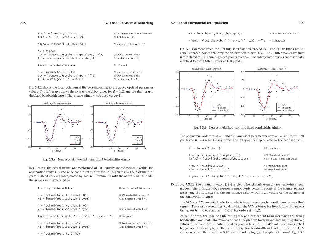
208 5. Local Polynomial Modeling
Y = loadfile(’mcyc.dat’); % file included in the OSP toolbox
tobs = Y(:,1); yobs = Y(:,2); % 133 data points
alpha = linspace(0.1, 0.5, 51); % vary over 0.1 ≤ α ≤ 0.5
d=1; type=1;gcv = locgcv(tobs,yobs,d,type,alpha,’nn’); % GCV as function of α[F,i] = min(gcv); alpha1 = alpha(i); % minimum at α = α1
figure; plot(alpha,gcv); % left graph
h = linspace(2, 10, 51); % vary over 2 ≤ h ≤ 10
gcv = locgcv(tobs,yobs,d,type,h,’f’); % GCV as function of h[F,i] = min(gcv); h1 = h(i); % minimum at h = h1
Fig. 5.3.2 shows the local polynomial fits corresponding to the above optimal parametervalues. The left graph shows the nearest-neighbor cases for d = 1,2, and the right graph,the fixed bandwidth cases. The tricube window was used (type=1).
0 10 20 30 40 50 60−150
−100
−50
0
50
100motorcycle acceleration
t (msec)
data d = 1 d = 2
0 10 20 30 40 50 60−150
−100
−50
0
50
100motorcycle acceleration
t (msec)
data d = 1 d = 2
Fig. 5.3.2 Nearest-neighbor (left) and fixed bandwidths (right).
In all cases, the actual fitting was performed at 100 equally-spaced points t within theobservation range tobs and were connected by straight-line segments by the plotting pro-gram, instead of being interpolated by locval. Continuing with the above MATLAB code,the graphs were generated by
t = locgrid(tobs,101); % equally-spaced fitting times
h = locband(tobs, t, alpha1, 0); % NN bandwidths at each tx1 = locpol(tobs,yobs,t,h,1,type); % fit at times t with d = 1
h = locband(tobs, t, alpha2, 0);x2 = locpol(tobs,yobs,t,h,2,type); % fit at times t with d = 2
figure; plot(tobs,yobs,’.’, t,x1,’-’, t,x2,’--’); % left graph
h = locband(tobs, t, 0, h1); % fixed bandwidths at each tx1 = locpol(tobs,yobs,t,h,1,type); % fit at times t with d = 1
h = locband(tobs, t, 0, h2);
5.3. Local Polynomial Interpolation 209
x2 = locpol(tobs,yobs,t,h,2,type); % fit at times t with d = 2
figure; plot(tobs,yobs,’.’, t,x1,’-’, t,x2,’--’); % right graph
Fig. 5.3.3 demonstrates the Hermite interpolation procedure. The fitting times are 20equally-spaced points spanning the observation interval tobs. The 20 fitted points are theninterpolated at 100 equally-spaced points over tobs. The interpolated curves are essentiallyidentical to those fitted earlier at 100 points.
0 10 20 30 40 50 60−150
−100
−50
0
50
100motorcycle acceleration
t (msec)
data fit points interpolated
0 10 20 30 40 50 60−150
−100
−50
0
50
100motorcycle acceleration
t (msec)
data fit points interpolated
Fig. 5.3.3 Nearest-neighbor (left) and fixed bandwidths (right).
The polynomial order was d = 1 and the bandwidth parameters wereα1 = 0.21 for the leftgraph and h1 = 4.4 for the right one. The left graph was generated by the code segment:
tf = locgrid(tobs,21); % fitting times
h = locband(tobs, tf, alpha1, 0); % NN bandwidths at tf
[xf,C] = locpol(tobs,yobs,tf,h,1,type); % fitted values and derivatives
tint = locgrid(tf,101); % interpolation times
xint = locval(C, tf, tint); % interpolated values
figure; plot(tobs,yobs,’.’, tf,xf,’o’, tint,xint,’-’);
Example 5.3.2: The ethanol dataset [230] is also a benchmark example for smoothing tech-niques. The ordinate NOx represents nitric oxide concentrations in the engine exhaustgases, and the abscissa E is the equivalence ratio, which is a measure of the richness ofthe ethanol/air mixture.
The GCV and CV bandwidth selection criteria tend sometimes to result in undersmoothedsignals. This can be seen in Fig. 5.3.4 in which the GCV criterion for fixed bandwidth selectsthe values h1 = 0.039 and h2 = 0.058, for orders d = 1,2.
As can be seen, the resulting fits are jagged, and can benefit form increasing the fittingbandwidth somewhat. The minima of the GCV plot are fairly broad and any neighboringvalues of the bandwidth would be just as good in terms of the GCV value. A similar effecthappens in this example for the nearest-neighbor bandwidth method, in which the GCVcriterion selects the value α = 0.19 corresponding to jagged graph (not shown). Fig. 5.3.5

210 5. Local Polynomial Modeling
0.02 0.04 0.06 0.080
0.1
0.2
0.3GCV score
bandwidth, h
d = 1 d = 2
0.6 0.8 1 1.20
1
2
3
4
5ethanol data, h1 = 0.038, h2 = 0.058
E
NO
x
data d = 1 d = 2
Fig. 5.3.4 GCV and local polynomial fits with d = 1,2.
0.6 0.8 1 1.20
1
2
3
4
5ethanol data, d = 1, h = 0.08
E
NO
x
0.6 0.8 1 1.20
1
2
3
4
5ethanol data, d = 1, α = 0.3
E
NO
x
Fig. 5.3.5 Fits with fixed (left) and nearest-neighbor (right) bandwidths.
shows the fits when the fixed bandwidth is increased to h = 0.08 and the nearest-neighborone to α = 0.3. The resulting fits are much smoother.
The MATLAB code for generating the graphs of Fig. 5.3.4 is as follows:
Y = loadfile(’ethanol.dat’); % file available in OSP toolbox
tobs = Y(:,1); yobs = Y(:,2); % data
t = locgrid(tobs,101); % uniform grid of 101 fitting points
h = linspace(0.02, 0.08, 41); % vary h over 0.02 ≤ h ≤ 0.08
gcv1 = locgcv(tobs,yobs,1,1,h,’f’); % GCV as function of hgcv2 = locgcv(tobs,yobs,2,1,h,’f’);
figure; plot(h,gcv1,’-’, h,gcv2,’--’); % left graph
h = locband(tobs, t, 0, h1); % fixed bandwidths at tx1 = locpol(tobs,yobs,t,h,1,1); % fit with d = 1 and tricube window
h = locband(tobs, t, 0, h2);
5.4. Variable Bandwidth 211
x2 = locpol(tobs,yobs,t,h,2,1); % fit with d = 2 and tricube window
figure; plot(tobs,yobs,’.’, t,x1,’-’, t,x2,’--’); % right graph
The MATLAB code for generating Fig. 5.3.5 is as follows:
h0 = 0.08; h = locband(tobs, t, 0, h0); % fixed bandwidth case
x1 = locpol(tobs,yobs,t,h,1,1); % order d = 1, tricube window
figure; plot(tobs,yobs,’.’, t,x1,’-’); % left graph
alpha = 0.3; h = locband(tobs, t, alpha, 0); % nearest-neighbor bandwidth case
x1 = locpol(tobs,yobs,t,h,1,1); x1 = C(:,1); % order d = 1, tricube windowmfigure; plot(tobs,yobs,’.’, t,x1,’-’); % right graph
Fig. 5.3.6 shows a fit at 10 fitting points and interpolated over 101 points. The fittingparameters are as in the right graph of Fig. 5.3.5. The following code generates Fig. 5.3.6:
tf = locgrid(tobs,10); % fitting points
alpha = 0.3; h = locband(tobs, tf, alpha, 0); % nearest-neighbor bandwidths
[xf,C] = locpol(tobs,yobs,tf,h,1,1); % order 1, tricube window
ti = locgrid(tf,101); yi = locval(C,tf,ti); % interpolated points
figure; plot(tobs,yobs,’.’, ti,yi,’-’, tf,xf,’o’);
0.6 0.8 1 1.20
1
2
3
4
5ethanol data, d = 1, α = 0.3
E
NO
x
data interp fitted
Fig. 5.3.6 Interpolated fits.
5.4 Variable Bandwidth
The issue of selecting the right bandwidth has been studied extensively, with approachesranging from finding an optimum bandwidth that minimizes a selection criterion such asthe GCV to using a locally-adaptive criterion that allows the bandwidth to automaticallyadapt to the local nature of the signal with different bandwidths being used in differentparts of the signal [188–231].

212 5. Local Polynomial Modeling
There is no selection criterion that is universally successful or universally agreedupon and one must use one’s judgment and visual inspection to decide how muchsmoothing is satisfactory. The basic idea is always to reduce the bandwidth in regionswhere the curvature of the signal is high in order not to oversmooth.
The function locpol can accept a different bandwidth ht for each fitting time t. Aswe saw in the above examples, the function locband generates such bandwidths forinput to locpol. However, locband generates either fixed or or nearest-neighbor band-widths and is not adaptive to the local nature of the signal. One could manually, dividethe range of the signal in non-overlapping regions and use a different fixed bandwidthin each region. In some cases, as in the Doppler example below, this is possible but inother cases a more automatic way of adapting is desirable.
A naive, but as we see in the examples below, quite effective way is to estimate thecurvature, sayκt, of the signal and define the bandwidth in terms of a suitable decreasingfunction ht = f(κt). We may define the curvature in terms of the estimate of the secondderivative of the signal and normalize it to its maximum value:
κt = |ˆxt|maxt|ˆxt| (5.4.1)
The second derivative ˆxt can be estimated by performing a local polynomial fit withpolynomial order d ≥ 2 using a fixed bandwidth h0 or a nearest-neighbor bandwidth α.If one could determine a bandwidth range [hmin, hmax] such that hmax would providean appropriate amount of smoothing in certain parts of the signal and hmin would beappropriate in regions where the signal appears to have larger curvature, then one maychoose hmin ≤ h0 ≤ hmax, with h0 = hmax as an initial trial value. An ad hoc but verysimple choice for the bandwidth function f(κt) then could be
ht = hmax
(hmin
hmax
)κt(5.4.2)
Other simple choices are possible, for example,
ht = hmaxhmin
hmin + (hmax − hmin)κpt
for some power p. Since κt varies in 0 ≤ κt ≤ 1, these choices interpolate between hmax
at κt = 0 when the curvature is small, and hmin at κt = 1 when the curvature is large.We illustrate the use of (5.4.2) with the three examples in Figs. 5.4.1–5.4.3, and we
make a different bandwidth choice for Fig. 5.4.4. All four examples have been usedas benchmarks in studying wavelet denoising methods [821] and we will be discussingthem again in that context in Sec. 10.7.
In all cases, we use a second-order polynomial to determine the curvature, and thenperform a locally linear fit (d = 1) using the variable bandwidth. Fig. 5.4.1 illustratesthe test function “bumps” defined by
s(t)=11∑i=1
ai[1+ |t − ti|/wi
]4 , 0 ≤ t ≤ 1
5.4. Variable Bandwidth 213
0 0.2 0.4 0.6 0.8 1
0
10
20
30
40
50
t
noise free
0 0.2 0.4 0.6 0.8 1
0
10
20
30
40
50
t
noisy signal
0 0.2 0.4 0.6 0.8 10
0.2
0.4
0.6
0.8
1
t
curvature, κt
0 0.2 0.4 0.6 0.8 1
0
10
20
30
40
50
t
smoothed with adaptive bandwidth
0 0.2 0.4 0.6 0.8 1
0
10
20
30
40
50
t
smoothed with fixed bandwidth, hmax
0 0.2 0.4 0.6 0.8 10
0.2
0.4
0.6
0.8
1
t
adaptive bandwidth, ht /hmax
Fig. 5.4.1 Bumps function.
with the parameter values:
ti = [10,13,15,23,25,40,44,65,76,78,81]/100
ai = [40,50,30,40,50,42,21,43,31,51,42]·1.0523
wi = [5,5,6,10,10,30,10,10,5,8,5]/1000
The function s(t) is sampled at N = 2048 equally-spaced points tn in the interval[0,1) and zero-mean white gaussian noise of variance σ2 = 1 is added so that the noisysignal is yn = sn+vn, where sn = s(tn). The factor 1.0523 in the amplitudes ai ensuresthat the signal-to-noise ratio has the standard benchmark value σs/σv = 7, where σsis the standard deviation of sn, that is, σs = std(s). The bandwidth range is definedby hmax = 0.01 and hmin = 0.00025. The value for hmax was chosen so that the flatportions of the signal between peaks are adequately smoothed.
The curvature κt, estimated using the bandwidth h0 = hmax, is shown in the upperright graph. The corresponding variable bandwidth ht derived from Eq. (5.4.2) is shownin the bottom-right graph. The bottom-left graph shows the resulting local linear fitusing the variable bandwidth ht, while the bottom-middle graph shows the fit usingthe fixed bandwidth hmax. Although hmax is adequate for smoothing the valleys of thesignal, it is too large for the peaks and results in broadened peaks of reduced heights. Onthe other hand, the variable bandwidth preserves the peaks fairly well, while achievingcomparable smoothing of the valleys. The MATLAB code for this example was as follows:
N=2048; t=linspace(0,1,N); s=zeros(size(t));F = inline(’1./(1 + abs(t)).^4’); % bumps function

214 5. Local Polynomial Modeling
ti = [10 13 15 23 25 40 44 65 76 78 81]/100;ai = [40,50,30,40,50,42,21,43,31,51,42] * 1.0523;wi = [5,5,6,10,10,30,10,10,5,8,5]/1000;
for i=1:length(ai), % construct signal
s = s + ai(i)*F((t-ti(i))/wi(i));end
hmax=10e-3; hmin=2.5e-4; h0=hmax; % bandwidth limits
seed=2009; randn(’state’,seed); % noisy signal
y = s + randn(size(t));
d=2; type=1; % fit with d = 2 and tricube window
[x,C] = locpol(t,y,t,h0,d,type); % using fixed bandwidth h0
kt = abs(C(:,3)); kt = kt/max(kt); % curvature, κtht = hmax * (hmin/hmax).^kt; % bandwidth, ht
d=1; type=1; % fit with d = 1
xv = locpol(t,y,t,ht,d,type); % use variable bandwidth htxf = locpol(t,y,t,h0,d,type); % use fixed bandwidth h0
figure; plot(t,s); figure; plot(t,y); figure; plot(t,kt); % upper graphs
figure; plot(t,xv); figure; plot(t,xf); figure; plot(t,ht/hmax); % lower graphs
Fig. 5.4.2 shows the “blocks” function defined by
s(t)=11∑i=1
aiF(t − ti) , F(t)= 1
2(1+ sign t) , 0 ≤ t ≤ 1
with the same delays ti as above and amplitudes:
ai = [40,−50,30,−40,50,−42,21,43,−31,21,−42]·0.3655
The noisy signal is yn = sn + vn with zero-mean unit-variance white noise. Theamplitude factor 0.3655 in ai is adjusted to give the same SNR as above, std(s)/σ = 7.The MATLAB code generating the six graphs is identical to the above, except for the partthat defines the signal and the bandwidth limits hmax = 0.03 and hmin = 0.0015:
N=2048; t=linspace(0,1,N); s=zeros(size(t));
ti = [10 13 15 23 25 40 44 65 76 78 81]/100;ai = [40,-50,30,-40,50,-42,21,43,-31,21,-42] * 0.3655;
for i=1:length(ai),s = s + ai(i) * (1 + sign(t - ti(i)))/2; % blocks signal
end
hmax=0.03; hmin=0.0015; h0=hmax; % bandwidth limits
We observe that the flat parts of the signal are smoothed equally well by the variableand fixed bandwidth choices, but in the fixed case, the edges are smoothed too much.The “HeaviSine” signal shown in Fig. 5.4.3 is defined by
s(t)= [4 sin(4πt)−sign(t − 0.3)−sign(0.72− t)] · 2.357 , 0 ≤ t ≤ 1
5.4. Variable Bandwidth 215
0 0.2 0.4 0.6 0.8 1−10
−5
0
5
10
15
20
25
t
noise free
0 0.2 0.4 0.6 0.8 1−10
−5
0
5
10
15
20
25
t
noisy signal
0 0.2 0.4 0.6 0.8 10
0.2
0.4
0.6
0.8
1
t
curvature, κt
0 0.2 0.4 0.6 0.8 1−10
−5
0
5
10
15
20
25
t
smoothed with adaptive bandwidth
0 0.2 0.4 0.6 0.8 1−10
−5
0
5
10
15
20
25
t
smoothed with fixed bandwidth, hmax
0 0.2 0.4 0.6 0.8 10
0.2
0.4
0.6
0.8
1
t
adaptive bandwidth, ht /hmax
Fig. 5.4.2 Blocks function.
where the factor 2.357 is adjusted to give std(s)= 7. The graphs shown in Fig. 5.4.3 areagain generated by the identical MATLAB code, except for the parts defining the signaland bandwidths:
s = (4*sin(4*pi*t)-sign(t-0.3)-sign(0.72-t))*2.357; % HeaviSine signal
hmax=0.035; hmin=0.0035; h0=hmax; % bandwidth limits
We note that the curvature κt is significantly large—and the bandwidth ht is signif-icantly small—only near the discontinuity points. The fixed bandwidth case smoothesthe discontinuities too much, whereas the variable bandwidth tends to preserve themwhile reducing the noise equally well in the rest of the signal.
In the “doppler” example shown in Fig. 5.4.4, noticing that the curvature κt is sig-nificantly large only in the range 0 ≤ t ≤ 0.2, we have followed a simpler strategy todefine a variable bandwidth (although the choice (5.4.2) still works well). We took a fixedbut small bandwidth over the range 0 ≤ t ≤ 0.2 and transitioned gradually to a largerbandwidth for 0.2 ≤ t ≤ 1. The signal is defined by
s(t)= 24√t(1− t) sin
(2.1πt + 0.05
), 0 ≤ t ≤ 1
The auxiliary unit-step function ustep was used to define the two-step bandwidthwith a given rise time. The MATLAB code generating the six graphs was as follows:
N = 2048; t = linspace(0,1,N);
s = 24*sqrt(t.*(1-t)) .* sin(2.1*pi./(t+0.05)); % doppler signal

216 5. Local Polynomial Modeling
0 0.2 0.4 0.6 0.8 1−20
−15
−10
−5
0
5
10
15
t
noise free
0 0.2 0.4 0.6 0.8 1−20
−15
−10
−5
0
5
10
15
t
noisy signal
0 0.2 0.4 0.6 0.8 10
0.2
0.4
0.6
0.8
1
t
curvature, κt
0 0.2 0.4 0.6 0.8 1−20
−15
−10
−5
0
5
10
15
t
smoothed with adaptive bandwidth
0 0.2 0.4 0.6 0.8 1−20
−15
−10
−5
0
5
10
15
t
smoothed with fixed bandwidth, hmax
0 0.2 0.4 0.6 0.8 10
0.2
0.4
0.6
0.8
1
t
adaptive bandwidth, ht /hmax
Fig. 5.4.3 HeaviSine function.
seed=2009; randn(’state’,seed); % noisy signal
y = s + randn(size(t));
0 0.2 0.4 0.6 0.8 1−15
−10
−5
0
5
10
15
t
noise free
0 0.2 0.4 0.6 0.8 1−15
−10
−5
0
5
10
15
t
noisy signal
0 0.2 0.4 0.6 0.8 10
0.2
0.4
0.6
0.8
1
t
curvature, κt
0 0.2 0.4 0.6 0.8 1−15
−10
−5
0
5
10
15
t
smoothed with adaptive bandwidth
0 0.2 0.4 0.6 0.8 1−15
−10
−5
0
5
10
15
t
smoothed with fixed bandwidth, hmax
0 0.2 0.4 0.6 0.8 10
0.1
0.2
0.3
0.4
0.5
0.6
0.7
0.8
0.9
1
t
variable bandwidth, ht /hmax
Fig. 5.4.4 Doppler function.
5.5. Repeated Observations 217
hmax=0.02; hmin=0.002; h0=hmax; % bandwidth limits
d=2; type=1; % fit with d = 2 and tricube window
[x,C] = locpol(t,y,t,h0,d,type); % using fixed bandwidth h0
kt = abs(C(:,3)); kt = kt/max(kt); % curvature, κtht = hmin + (hmax-hmin) * ustep(t-0.2, 0.1); % two-step bandwidth, ht
% ustep is in the OSP toolbox
d=1; type=1;xv = locpol(t,y,t,ht,d,type); % fixed bandwidth h0
xf = locpol(t,y,t,h0,d,type); % fixed bandwidth h0
figure; plot(t,s); figure; plot(t,y); figure; plot(t,kt); % upper graphs
figure; plot(t,xv); figure; plot(t,xf); figure; plot(t,ht/hmax); % lower graphs
The local polynomial fitting results from these four benchmark examples are verycomparable with the wavelet denoising approach discussed in Sec. 10.7.
5.5 Repeated Observations
Until now we had implicitly assumed that the observations were unique, that is, oneobservation y(tk) at each time tk. However, in experimental data one often has repeatedobservations at a given tk, all of which are listed as part of the data set. This is in facttrue of both the motorcycle and the ethanol data sets. For example, in the motorcycledata, we have six repeated observations at t = 14.6,
k tk yk...
......
22 14.6 −13.323 14.6 −5.424 14.6 −5.425 14.6 −9.326 14.6 −16.027 14.6 −22.8
......
...
and there other similar instances within the data set. In fact, among the 133 givenobservations, only 94 correspond to unique observation times.
To handle repeated observations one possibility is to simply keep one and ignore therest—but which one? A better possibility is to allow all of them to be part of the least-squares performance index. It is easy to see that this is equivalent to replacing eachgroup of repeated observations by their average and modifying the weighting functionby the corresponding multiplicity of the group.
Let nk denote the multiplicity of the observations at time tk, that is, let yi(tk), i =1,2, . . . , nk be the observation values that are given at the unique observation time tk.Then, the performance index (5.1.3) must be modified to include all of the yi(tk):
Jt =∑
|tk−t|≤ht
nk∑i=1
[yi(tk)−uT(tk − t)c
]2w(tk − t)= min (5.5.1)

218 5. Local Polynomial Modeling
Setting the gradient with respect to c to zero, gives the normal equations:
∑|tk−t|≤ht
nk∑i=1
w(tk − t)u(tk − t)uT(tk − t) c =∑
|tk−t|≤htw(tk − t)u(tk − t)
nk∑i=1
yi(tk)
Defining the average of the nk observations,
y(tk)= 1
nk
nk∑i=1
yi(tk)
and noting that the left-hand side has no dependence on i, we obtain:
∑|tk−t|≤ht
nkw(tk − t)u(tk − t)uT(tk − t)c =∑
|tk−t|≤htnkw(tk − t)u(tk − t)y(tk) (5.5.2)
This is recognized to be the solution of an equivalent least-squares local polyno-mial fitting problem in which each unique tk is weighted by nkwk(tk − t) with the kthobservation replaced by the average y(tk), that is,
Jt =∑
|tk−t|≤ht
[y(tk)−uT(tk − t)c
]2nkw(tk − t)= min (5.5.3)
Internally, the function locpol calls the function avobs, which takes in the raw datatobs,yobs and determines the unique observation times ta, averaged observations ya,and their multiplicities na:
[ta,ya,na] = avobs(tobs,yobs); % average repeated observations
For example, if
tobs = [ 1 1 1 3 3 5 5 3 4 7 9 9 9 9];yobs = [20 22 21 11 12 13 15 19 21 25 28 29 31 32];
the function first sorts the ts in increasing order,
tobs = [ 1 1 1 3 3 3 4 5 5 7 9 9 9 9];yobs = [20 21 22 11 12 19 21 13 15 25 28 29 31 32];
and then returns the output,
ta = [ 1 3 4 5 7 9];ya = [21 14 21 14 25 30];na = [ 3 3 1 2 1 4];
5.6 Loess Smoothing
Loess, which is a shorthand for local regression, is a method proposed by Cleveland[192] for handling data with outliers. A version of it was discussed in Sec. 4.5. Themethod carries out a local polynomial regression using a nearest-neighbor bandwidthand the tricube window function, and then uses the resulting error residuals to iterativelyreadjust the window weights giving less importance to the outliers.
5.6. Loess Smoothing 219
The method is described as follows [192]. Given theN-dimensional vectors of obser-vation times and observations tobs, yobs, the nearest-neighbor bandwidth parameter α,and the polynomial order d, the method begins by performing a preliminary fit to all theobservation times. For example, in the notation of the locband and locpol functions:
h = locband(tobs, tobs,α,0); (find local bandwidths at tobs)
x = locpol(tobs, yobs, tobs, h, d,1); (perform fit at all tobs)(5.6.1)
where the last argument of locpol designates the use of the tricube window. From theresulting N-dimensional signal xk, k = 0,1, . . . ,N − 1, we calculate the correspondingerror residuals ek and use their median to calculate “robustness” weights rk:
ek = yk − xk , k = 0,1, . . . ,N − 1
μ = median0≤k≤N−1
(|ek|)
rk =W(ek6μ
) (5.6.2)
where W(u) is the bisquare function defined in (5.1.5). The local polynomial fitting isnow repeated at all observation points tobs, but instead of using the weights w(tk −tobs) for the kth observation’s contribution to the fit, one uses the modified weightsrkw(tk − tobs). The new residuals are then computed as in (5.6.2) and the process isrepeated a few more times or until convergence (i.e., until the estimated signal xk nolonger changes).
After the final iteration resulting in the final values of the rks, one can carry out thefit at any other time point t, but again using weights rkw(tk− t) for the contribution ofthe kth observation, that is, the weight matrix Wt in Eq. (5.1.7) is replaced by
Wt = diag([· · · , rkw(tk − t), · · · ])
The MATLAB function loess implements these steps:
[xhat,C] = loess(tobs,yobs,t,alpha,d,Nit); % Loess smoothing
where t are the final fitting times and xhat and C have the same meaning as in locpol.This function is similar in spirit to the robust local polynomial filtering function rlpfiltthat was discussed in Sec. 4.5.
Example 5.6.1: Fig. 5.6.1 shows the same example as that of Fig. 4.5.3, with nearest-neighborbandwidth parameter α = 0.4 and an order-2 polynomial. The graphs show the results ofNit = 0,2,4,6 iterations—the first one corresponding to ordinary fitting with no robust-ness iterations. The MATLAB code for the top two graphs was:
t = (0:50); x0 = (1 - cos(2*pi*t/50))/2; % desired signal
seed=2005; randn(’state’,seed);y = x0 + 0.1 * randn(size(x0)); % noisy signal
m = [-1 0 1 3]; % outlier indices
n0=25; y(n0+m+1) = 0; % outlier values
n1=10; y(n1+m+1) = 1;

220 5. Local Polynomial Modeling
0 5 10 15 20 25 30 35 40 45 50
0
0.5
1
1.5Loess smoothing, Nit = 0
time samples, t
outliers
outliers
desired noisy smoothed
0 5 10 15 20 25 30 35 40 45 50
0
0.5
1
1.5Loess smoothing, Nit = 2
time samples, t
outliers
outliers
desired noisy smoothed
0 5 10 15 20 25 30 35 40 45 50
0
0.5
1
1.5Loess smoothing, Nit = 4
time samples, t
outliers
outliers
desired noisy smoothed
0 5 10 15 20 25 30 35 40 45 50
0
0.5
1
1.5Loess smoothing, Nit = 6
time samples, t
outliers
outliers
desired noisy smoothed
Fig. 5.6.1 Loess smoothing with d = 2, α = 0.4, and different iterations.
alpha=0.4; d=2; % bandwidth parameter and polynomial order
Nit=0; x = loess(t,y,t,alpha,d,Nit); % loess fit at tfigure; plot(t,x0,’--’, t,y,’.’, t,x,’-’); % left graph
Nit=2; x = loess(t,y,t,alpha,d,Nit); % loess fit at tfigure; plot(t,x0,’--’, t,y,’.’, t,x,’-’); % right graph
The loess fit was performed at all t. We observe how successive iterations gradually di-minish the distorting influence of the outliers. �
5.7 Problems
5.1 Prove the matrix inversion lemma identity (5.2.8). Using this identity, show that
Hii = H−ii
1+H−ii, where H−
ii = w0uT0 F−i u0 , F−i = (STi WiSi)−
then, argue that 0 ≤ Hii ≤ 1.
6Exponential Smoothing
6.1 Mean Tracking
lThe exponential smoother, also known as an exponentially-weighted moving average
(EWMA) or more simply an exponential moving average (EMA) filter is a simple, effective,recursive smoothing filter that can be applied to real-time data. By contrast, the localpolynomial modeling approach is typically applied off-line to a block a signal samplesthat have already been collected.
The exponential smoother is used routinely to track stock market data and in fore-casting applications such as inventory control where, despite its simplicity, it is highlycompetitive with other more sophisticated forecasting methods [232–279].
We have already encountered it in Sec. 2.3 and compared it to the plain FIR averager.Here, we view it as a special case of a weighted local polynomial smoothing problemusing a causal window and exponential weights, and discuss some of its generalizations.Both the exponential smoother and the FIR averager are applied to data that are assumedto have the typical form:
yn = an + vn (6.1.1)
where an is a low-frequency trend component, representing an average or estimate ofthe local level of the signal, and vn a random, zero-mean, broadband component, suchas white noise. If an is a deterministic signal, then by taking expectations of both sideswe see that an represents the mean value of yn, that is, an = E[yn]. If yn is stationary,then an is a constant, independent of n.
The output of either the FIR or the exponential smoothing filter tracks the signal an.To see how such filters arise in the context of estimating the mean level of a signal, con-sider first the stationary case. The mean m = E[yn] minimizes the following varianceperformance index (e.g., see Example 1.3.5):
J = E[(yn − a)2] = min ⇒ aopt =m = E[yn] (6.1.2)
with minimized value Jmin = σ2y . This result is obtained by setting the gradient with
respect to a to zero:∂J∂a
= −2E[yn − a]= 0 (6.1.3)
221