CONJUNCTION ASSESSMENT USING POLYNOMIAL CHAOS EXPANSIONS

Brandon A. Jones(1), Alireza Doostan(2), and George Born(3)

(1)(3)Colorado Center for Astrodynamics Research, University of Colorado Boulder, UCB 431,Boulder, Colorado, 80309, 303-735-4490, brandon.jones@colorado.edu,

george.born@colorado.edu(2)Department of Aerospace Engineering Sciences, University of Colorado Boulder, UCB 429,

Boulder, Colorado, 80309, 303-492-7572, alireza.doostan@colorado.edu

Abstract: This paper presents the application of polynomial chaos expansions (PCEs) to estimatethe probability of collision between two spacecraft. Common methods of collision risk assessmentuse either Monte Carlo analyses or assume a Gaussian probability distribution function (pdf). PCEsprovide a means for approximating the solution to a large set of stochastic ordinary differentialequations, which includes orbit propagation. When compared to Monte Carlo methods, sampling-based, non-intrusive PCE techniques greatly reduce the number of orbit propagations requiredto approximate the a posteriori pdf. Additionally, PCEs make no assumption that the propagateddistribution will be Gaussian or that the state pdfs are uncorrelated for two spacecraft. This paperconsiders two cases where these assumptions are no longer valid. Results demonstrate that morethan 100,000 Monte Carlo trials are required to estimate the collision probability, but accurateestimates may be achieved with less than 300 orbit propagations by performing most of the analysisvia PCE evaluations.

Keywords: conjunction assessment, uncertainty propagation, polynomial chaos

1. Introduction

As the space in low-Earth and geosynchronous orbit becomes increasingly congested, rigorousmethods of estimating the risk of collision between any two objects becomes increasingly important.Such methods must be highly accurate to both identify possible collisions and minimize the numberof false alarms that waste fuel and disrupt satellite operations. This paper considers a new applicationof polynomial chaos (PC) expansions for the quantification of collision risks in scenarios wherealready established methods no longer apply.

Several methods of conjunction assessment already exist and are used for satellite operations today.The most commonly discussed methods [1–3] share several assumptions, including, but not limitedto:

1. the probability density function (pdf) describing the position state is a multivariate Gaussiandistribution,

2. the uncertainties for the two objects are uncorrelated.

This paper considers situations where at least one of these conditions is not satisfied. Recent researchdemonstrates that assumption (1) is not strictly true in astrodynamics [4–10], with various methodssuggested for non-Gaussian uncertainty propagation. Assumption (2) is valid for most scenarios,and almost surely true for orbital debris. However, given the increasing interest in formation flyingand fractionated spacecraft, the inclusion of relative measurements in their orbit determinationcreates correlated uncertainties between the satellites.

1

Conjunction assessment based on Monte Carlo (MC) methods provides the most accurate, butcomputationally expensive, estimate of the collision risk. Such methods reduce the assumptions,and are only limited by the accuracy of the propagator, the initial uncertainty, and computationtime. However, the computation time requirements pose a major limitation in adoption of suchmethods [11–13]. Several tools exist to reduce the long computation times associated with MonteCarlo methods, with these tools leveraging off of both improvements in computation capabilitiesand theories developed to reduce the number of MC trials. Sabol, et al. [11] demonstrate the useof the supercomputer capabilities to perform Monte Carlo analyses within seconds per satellite.Dolado et al. [12] consider importance sampling to reduce the number of orbit propagations requiredto quantify collision probability. Garmier et al. [13] reduce the overall computation time by filteringout scenarios with a sufficiently low probability of collision, thereby limiting the total number ofMonte Carlo trials for a given space object catalog. The PC-based methods discussed in this papershare similarities with Monte Carlo, but use polynomial surrogates to reduce the total number oforbit propagations.

Polynomial chaos expansions (PCEs) allow for the approximation of the solution to a stochasticdifferential equation that is square-measurable, possibly non-Gaussian, with respect to the inputuncertainties [14–25]. PC-based methods use a projection of the stochastic solution onto a basis oforthogonal polynomials in stochastic variables that is dense in the space of finite-variance randomvariables. Using this polynomial basis, these PC methods provide a response surface in the space ofthe random inputs, thereby allowing for the generation of realizations at a future point in time whengiven random inputs at the initial time. In generating these realizations, no additional evaluationsof the orbit propagator are required, thereby reducing the computation time. The current authorsalready demonstrated the use of PC for propagating orbit uncertainty over relatively long durations(10 days), and results demonstrate the ability to accurately approximate a non-Gaussian pdf at thefinal time [4]. This research considers the use of PC, specifically the generated response surfaces, toconduct conjunction assessment. As discussed later, the collision assessment assumptions listedabove do not apply when using PC-based methods.

The rest of this paper is organized as follows. Section 2 provides an overview of polynomial chaos.Section 3 then discusses how methods based on PC may be employed to estimate the probabilityof collision. The test cases used to demonstrate the benefits of PC are then described in Section 4,with the test results presented in Section 5. Section 6 then concludes the paper.

2. Polynomial Chaos

Methods based on polynomial chaos provide a means for generating an approximation to thesolution of a stochastic system by projecting it onto a basis of spectral polynomials. Wiener [26]first proposed this type of approximation, with methods based on Hermite chaos expansions firstestablished [14–17] and later generalized to non-Gaussian input uncertainties [18]. The generatedPCE represents the stochastic solution as a linear expansion of multi-variate polynomials that arefunctions of the input uncertain variables ξ ∈ Rd where d is the stochastic dimension of the system.Solving for the PCE means estimating the coefficients, or weights, of the expansion. PC-basedmethods provide a computationally efficient means to represent any square-measurable, possiblynon-Gaussian distribution, and have already been demonstrated for orbit propagation [4].

2

Let (S,F ,P) be a probability space with the sample space S and the probability measure P onσ-algebra F . The d random inputs to the system are ξ ∈ Rd : S → Γd ⊆ Rd on (S,F ,P),where these elements are independent and identically distributed (iid) and characterize the inputuncertainties. Additionally, we denote the set of ordinary differential equations (ODEs) that, for thepresent case case, describe the temporal evolution of a satellite’s state, as

A(t, ξ) = 0, (t, ξ) ∈ [t0, tf ]× Γd, P − a.s. in S (1)

where A is a stochastic ordinary differential operator and t ∈ [t0, tf ] is the temporal variable. Thiswork considers the propagation of orbit state uncertainty using PC with the goal of performingconjunction assessment. Let X(t0) be the orbit state at time t0 with uncertainty that may berepresented by the probability space (S,F ,P). For this discussion, assume X ∈ Rd, i.e., thenumber of state variables equals the number of stochastic inputs to the system. PC-based methodsare then used to generate a solution to the stochastic operator A that describes the space of possiblesolutionsX(tf ) at any future time tf .

In the context of PCEs, the orbit solutionX(t, ξ) may be approximated by the finite series

X(t, ξ) =∑

α∈Λp,d

cα(t)ψα(ξ) (2)

where X is the approximate solution to the true value X , Λp,d := (α1, . . . , αd) : ‖α‖1 ≤p, ‖α‖0 ≤ d is the set of multi-indices of size d defined on the non-negative integers, ψα are themulti-variate polynomials of maximum degree p,

ψα(ξ) = ψα1(ξ1)ψα2(ξ2) · · ·ψαd(ξd), (3)

serve as the basis functions for the approximation, and the vector of coefficients cα(t) yields thePCE solution. In other words, the multivariate polynomials (of maximum degree p) are simply theproduct of univariate polynomials, and the degree of each polynomial is defined by the index αi.We note that a vector representation for cα effectively allows for the simulataneous representationof d PCEs, i.e. one for each element of the vectorX ∈ Rd. The number of terms in Eq. (2) is

P :=(p+ d)!

p!d!. (4)

For PC methods to apply, the basis ψα must be orthonormal with respect to the random inputs ξ∫Γd

ψα(ξ)ψβ(ξ)ρ(ξ) dξ = δαβ (5)

where δα,β is the Kronecker delta function. Eq. (5) specifies that the random inputs ξ and theirprobability function ρ(ξ) determines the polynomials ψα in Eq. (3). The current paper onlyconsiders ξ ∈ N (0, Id), i.e., the random inputs are multivariate Gaussian with zero mean andunit variance. Hence, ψα are Hermite polynomials [18]. Although ξ are Gaussian distributed, theuncertainty ofX(t0) is not necessarily Gaussian.

3

The PCE in Eq. (2) provides a method for generating a solution X when given a random inputξ, i.e., it describes the response of X(tf ) to the realizations ξi. In this way, the PCE yields asolution to a stochastic system, as opposed to propagating the a priori state pdf. Information on thea posteriori pdf may then be inferred from the stochastic solution. Given sufficient accuracy of cα,the polynomial surrogates also provide a means for bypassing an ODE solver and approximatingthe Monte Carlo results using the computationally inexpensive polynomial evaluation. This latterproperty allows for conjunction assessment using PC, which is described further in Section 3.

2.1. PCE Solution Methods

This study only considers non-intrusive methods to generate a global PCE approximating thestochastic solution of the propagated orbit at time tf . Such methods treat already existing ODEsolvers as a black box, and require no alterations to existing orbit propagation software. This allowsus to wrap current software to propagate the state uncertainty and perform CA. The algorithmbehind the non-intrusive methods may be summarized by:

1. Generate MPC realizations ξi. For the current paper, these samples are based on a randomsampling of the distribution N (0, Id).

2. For each of the MPC random vectors, use the initial uncertainty in X(t0, ξi) to generate arealization based on the random input ξi. For example, a Cholesky decomposition may beused with the covariance matrix P and initial mean X .

3. PropagateX(t0, ξi) to tf using the existing ODE solver, and perform this process for each ofthe MPC realizations.

4. Solve for the PC coefficients cα(tf ) based onX(tf , ξi) and the method of choice. This yieldsa PCE X(tf , ξ).

Several things should be noted about this procedure. First, solutions at intermediate steps, e.g. inte-gration time steps, may be easily generated using the same samples at those times. More samples areonly required if p increases at the intermediate time ti. Hence, cα(t) may be generated at multipletimes using the same samples. Second, there are many methods of generating a non-intrusive PCEsolution, including, but not limited to: regression, pseudo-spectral collocation, and compressivesampling [24, 25, 27]. Each of these methods have several advantages and disadvantages which willnot be discussed here. The current study considers solutions based on regression. Ongoing studiesat CCAR consider other methods, but those either do not apply to the current cases or are not yetfully developed. The next section provides a brief overview of the regression methods.

2.1.1. PCE Solutions via Regression

The method to solve for cα based on regression uses random samples ξi from the density functionρ(ξ). Given the MPC propagated states, one solution for the coefficients cα minimizes the costfunction

J(cα) =1

2

MPC∑i=1

εTi εi (6)

4

whereεi = X(t, ξi; cα)−X(t, ξi). (7)

Eq. (6) is simply the cost function of the least squares estimator. Upon inspection of Eq. (2), wemay represent the PCE as a linear system

ψα1(ξ1) ψα2(ξ1) · · · ψαP(ξ1)

ψα1(ξ2) ψα2(ξ2) · · · ψαP(ξ2)

...... . . . ...

ψα1(ξMPC) ψα2(ξMPC) · · · ψαP(ξMPC)

cTα1

cTα2...cTαP

=

XT (t, ξ1)XT (t, ξ2)

...XT (t, ξMPC)

. (8)

Instead, one may writeHC = Y (9)

whereH is the MPC×P sensitivity matrix on the left hand side of Eq. (8), C is the matrix of PCEcoefficients, and Y is comprised of the propagated states at tf . Given this formulation,

C = (HTH)−1HTX, (10)

which is the normal equation solution to the least squares estimator. This method of solving for thePCE coefficients requires MPC ≥ P measurements. Also, assuming the same samples are used at alltimes,H does not change as a function of t. Hence, (HTH)−1HT remains constant, and solvingfor cα(ti) at different ti only requires assembling Y and evaluating a single matrix multiplication.Such operations may be parallelized to minimize computation time.

2.2. PCE Coordinate System Selection Considerations

As demonstrated in the literature, orbit elements provide a better coordinate system for propagatingorbit uncertainty since the pdf remains Gaussian for longer time periods [4–6, 9]. Hence, to reduced, the PCEs used here represent the orbit state as an element set, e.g., the equinoctial elements. Thisreduces the number of samples required to generate a PCE.

However, element sets pose a difficulty in performing CA: the mapping from elements to Cartesianposition is not injective. Specifically, two distinct element set may describe a satellite state atthe same position but with different velocities. This results from the fact that all six elements arerequired to represent a point in R3, while the Cartesian representation only requires three. Hence,there is an inherent ambiguity in the representation of position. For this reason, when generatingthe PC-based realizations using Eq. (2), the output is then converted to Cartesian coordinates forcalculation of the probability of collision, Pc.

3. Collision Assessment Using PC

3.1. Estimation of Pc

The methods employed for estimating the probability of collision Pc using PC are similar to MonteCarlo techniques, but rely on the polynomial surrogates to reduce the overall computation time. The

5

following discussion begins with a description of Monte Carlo methods, which then serves as aframework for presenting the PC-based methods.

For the state vector

Xl(t0) =

[r(t0)r(t0)

](11)

let Xl(t0) be the mean at time t0 for satellite l with covariance matrix Pl. In a Monte Carlo test,MMC trials are generated using, for example,

Xl(t0, ξi) = Xl(t0) +Llξi (12)

whereLl is the lower-triangular Cholesky decomposition ofPl, i = 1, . . . ,MMC, and ξi ∼ N (0, Id).Each trial Xl(t0, ξi) is then propagated to some time tk to yield Xl(tk, ξi). This procedure isconducted for any number of satellites, each with unique ξi. Given two satellites, denoted bysubscripts 1 and 2, their separation at time tk is

s(tk, ξi, ξ′i) =

√∆r12(tk, ξi, ξ′i) ·∆r12(tk, ξi, ξ′i) (13)

where∆r12(tk, ξi, ξ

′i) = r1(tk, ξi)− r2(tk, ξ

′i), (14)

and the prime on ξ′i is only meant to indicate a different set of samples from ξi. The empiricalprobability of collision is then

Pc =count(s(tk, ξi, ξ′i) ≤ R)

MMC(15)

where R is a given collision cross-section radius, and the count() operator indicates the numberof true results of the argument over i = 1, . . . ,MMC. Given MMC samples for each satellite, thereare up to M2

MC possible combinations available for evaluating Eqs. (13)-(15). However, not everycomparison will be independent.

Estimating Pc via PC differs slightly from the above procedure in that using a polynomial surrogaterequires the propagation of significantly fewer samples. Instead, when using regression methodsto solve for the coefficients cα, MPC training samples are generated using Eq. (12). Each of thesesamples are propagated, and the coefficient cα(tk) are then generated using Eq. (10). As mentionedearlier, this yields a response surface to generate solutions at tk when given ξi. Hence, MMC

evaluations of Eq. (2) with each PCE generates the needed Monte Carlo trials. Eqs. (13)-(15) arethen used with the PCE output to estimate Pc. In other words, evaluations of the orbit propagatorare substituted with the more computationally efficient evaluation of a set of polynomials, therebygreatly reducing the computation time of computing Pc. In general, orbit propagation may takeseconds of computer processing time per evaluation, but these polynomial evaluations are on thescale of thousands of evaluations per second.

Of course, the accuracy of Pc is then limited by the accuracy of the PCE. Methods exist to accountfor errors in the PCE when calculating a rare failure probability, e.g., satellite collision, by combiningPCE evaluations with additional Monte Carlo orbit propagations [28, 29]. However, we do not yet

6

add these techniques to the current method. Additionally, this work assumes the propagation tool isaccurate, and does not account for modeling errors, etc. These elements have been identified asfuture work.

3.2. Probability of Collision Confidence Interval

Several techniques exist for generating a 1σ confidence interval σPc . When using Monte Carlomethods, the most accurate, but computationally expensive, method requires repeating a MonteCarlo test N times. To clarify, a single Monte Carlo test consists of MMC trials. Each test yieldsa single Pc, and the empirical standard deviation of these N estimates provides σPc . Specifically,given N tests,

σ2Pc

=N∑j=1

(P(j)c − Pc

)2

N − 1(16)

where the superscript (j) indicates a value produced via Monte Carlo test j and Pc is the mean of alltests. Of course, this is more computationally expensive and requires MMC×N orbit propagations.Other methods exist to lower the computation cost while computing a confidence interval, butreduce the accuracy of the solution statistics. For example, bootstrap methods use a number ofsamples, e.g., 2MMC, and then randomly select MMC trials (with replacement) to serve as a MonteCarlo test. This process is conducted N times to estimate σPc while reducing the computation cost,but may yield optimistic confidence intervals. Additionally, assuming Pc is small, i.e., it representsa rare failure probability, then

σPc ≈Pc(1− Pc)MMC

(17)

The studies of [12, 13] use this final method to approximate σPc .

In the following sections, the PC-based σPc relies on bootstrap techniques to generate N PCE-basedestimates of Pc. In this process, a collection of training points are propagated forward in time tothe point of interest. These propagated realizations serve as a bank of samples, from which MPC

trials are randomly selected with replacement. This process is repeated N times to yield a collectionof PCEs. Each of these PCEs are individually sampled to generate P(j)

c , and then the confidenceinterval is approximated using Eq. (16).

4. Simulation Methods

4.1. Test Descriptions

The following sections describe tests for two principle scenarios: (A) two satellites in formation withcorrelated initial uncertainty, and (B) a potential collision between two satellites in low-Earth orbit(LEO) with a non-Gaussian posteriori pdf. The first case, based on the Magnetospheric Multiscale(MMS) mission [30], considers two satellites in a highly eccentric orbit with a relatively smallinitial uncertainty. Case B demonstrates the application of PC to a scenario more commensuratewith current collision avoidance. Initial conditions for these two cases are described in Tab. 1, andthe a priori uncertainties are discussed further in the following sections.

7

Table 1. Initial Conditions in Classical Orbital Elements

Orbit Element Case A Case BSat 1 Sat 2 Molniya LEO

a (km) 41545.517 41545.487 26462.0 7441.128e 0.82043 0.82043 0.741 0.06

ι (deg) 27.60 27.61 63.4 119.34Ω (deg) 10.182 10.181 90.0 265.20ω(deg) 81.17 81.18 -90.0 204.79ν (deg) 147.901 147.902 0.0 86.94

4.1.1. Case A: Correlated Satellites with Long Dwell Time

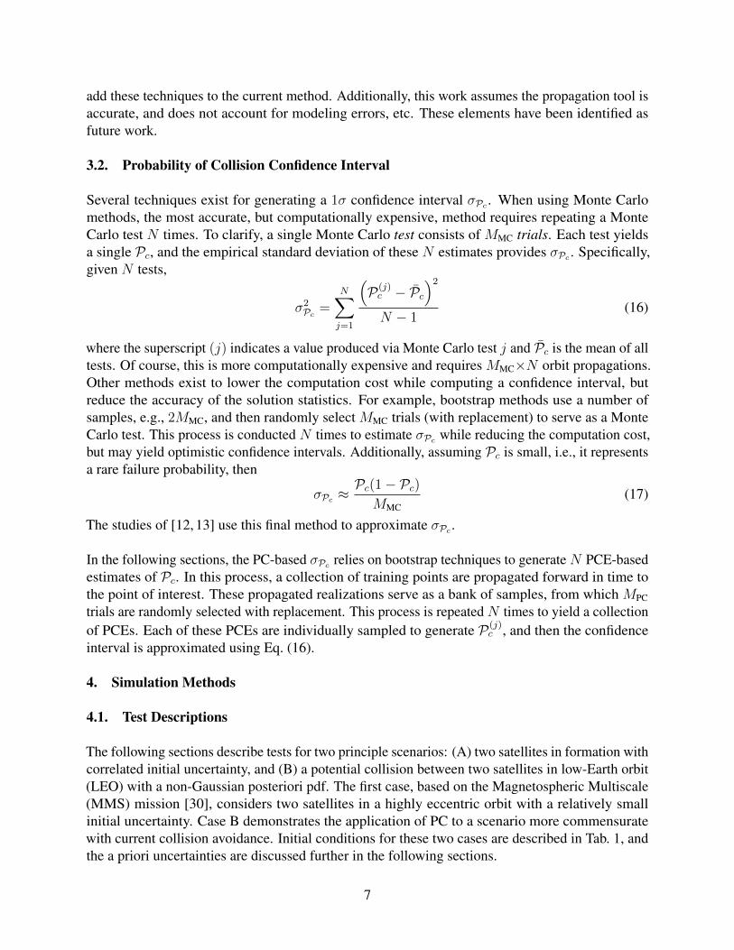
This case considers two satellites flying in formation with a correlated a priori covariance matrix.This correlation violates the assumption that the uncertainties in the two colliding satellites areindependent. A histogram of the correlation coefficients for the 12×12 covariance matrix may befound in Fig. 1. The mean correlation coefficient is 0.19 with a maximum value of approximately0.85. The position and velocity uncertainties in each Cartesian direction are approximately 1 m and10−4 m/s, respectively, at t0. These are commensurate with the expected navigation uncertaintiesfor the MSS mission at a similar point in the orbit1. For this case,R is 20 m, which differs from the120 m used for MMS [31]. The current study considers a smaller collision radius to reduce Pc toapproximately 10−4, i.e., the maneuver decision threshold for MMS.

−0.6 −0.4 −0.2 0.0 0.2 0.4 0.6 0.8 1.0Correlation Coefficients

0

2

4

6

8

10

12

14

16

18

Figure 1. Histogram of correlation coefficients for the Case A satellites.

4.1.2. Case B: Non-Gaussian Conjunction Assessment

This case considers the possible collision of a Molniya and a low-Earth orbit (LEO) satellite. Forthe Molniya, the case considered in [4] is duplicated. As demonstrated in that work, after a 10-daypropagation, the orbit uncertainty in both the Cartesian and Poincare elements is non-Gaussian.To generate a test case using the already available data, the velocity of the mean Molniya orbit atits perigee at the ten-day mark is rotated about the velocity vector by 180. This is intended to

1Personal correspondence with Dan Mattern, a.i. solutions

8

simulate a nearly head-on collision between satellites represented by the mean states. To constrainthe second satellite to LEO, the velocity vector is rescaled to approximately 7.5 km/s (averagevelocity of a LEO satellite). The position and velocity vector are propagated backwards in time toTCA−36 hours, which yields the initial mean state. A Gaussian distribution with a RSS 1σ positionuncertainty ellipsoid radius of 20 m is then selected for the initial state uncertainty, and matchesthat of the Molniya orbit [4]. With the mean and covariance now defined for the LEO satellite, theuncertainty is propagated using the PCE methods discussed previously.

4.2. Orbit Propagation Methods

The CU-TurboProp [32] orbit propagation suite serves as the principle orbit simulation tool forthis study. It provides a suite of orbit propagation capabilities using both a collection of high- andlow-fidelity models of the forces acting on a satellites. Both cases consider the same forces, althoughwith potentially different fidelities appropriate for the given orbit. A description of the force modelsused may be found in Tab. 2. For Case A, a low-fidelity gravity field is allowed given the highaltitude and eccentricity of the orbit. Conversely, the LEO orbit requires a higher degree and ordergravity expansion due to the lower altitude. All propagations employ the Dormand-Prince 8(7) [33]integration method implemented in CU-TurboProp with a relative tolerance of 10−13. For allsatellites, A/m is 0.01 m2/kg.

Table 2. Test Case Force Models

Force Case A Case BGravity Perturbations GGM02C, 4×4 GGM02C, 200×200Sun/Moon Ephemeris DE405Atmospheric Density U.S. Standard 1976, CD = 2.2

Solar Radiation Pressure Cannonball, CR = 1.8

5. Collision Assessment Results

5.1. Case A Results

This section describes the result for calculating Pc and σPc for Case A. As mentioned previously,this test considers a scenario with two satellites in formation. Pc is computed via the algorithmdescribed in Section 3.1. To compute σPc , the bootstrap analysis described in Section 3.2 isconducted to generate 100 PCEs from 300 training samples. To generate each PCE, 26 samplesare randomly selected from the training sample pool. The PCEs for this case are expressed inCartesian coordinates. As discussed below, an orbit element representation is not required for thiscase. For comparison purposes, MMC = 106 Monte Carlo samples are also generated. Since theinitial uncertainties are coupled and ξi ∈ R12 is used to compute r for both spacecraft, we may notanalyze M2

MC combinations.

Figure 2 illustrates the position pdf for the two satellites at TCA. The realizations used to illustratethe pdf are based on 105 Monte Carlo propagations. Given the relatively small standard deviations

9

1.0 1.2 1.4 1.6 1.8 2.0Y (km) +1.6837e4

−0.9

−0.8

−0.7

−0.6

−0.5

−0.4

−0.3

−0.2

−0.1

Z (

km

)

−3.262e3

0.0

0.3

0.6

0.9

1.2

1.5

1.8

2.1

2.4

Nu

mb

er o

f Realiza

tion

s (1

0x

)

Figure 2. Position and uncertainty for Case A at TCA in the Y -Z plane. The ellipsoids indicate thestate uncertainty propagated via the unscented transformation.

10-1010-810-610-410-2100102104

X

10-1210-1010-810-610-410-2100

Xdeg = 2deg = 1

deg = 0

10-810-610-410-2100102104

Y

10-1210-1010-810-610-410-2100

Y

0 20 40 60 80Index Number

10-810-610-410-2100102104

Z

0 20 40 60 80Index Number

10-1210-1010-810-610-410-2100

Z

Figure 3. cα terms for the second satellite in Case A and ordered by polynomial degree.

at t0, the propagated pdf at TCA is approximately Gaussian. For this reason, p = 1 for the PCEsin Case A will likely be sufficient to calculated Pc. To confirm this, Fig. 3 demonstrates the rapiddecay of the cα terms for the second satellite. Terms of degree two are 11 orders of magnitudesmaller than the degree-zero coefficient. This indicates that they provide little contribution to thestochastic solution. Given their small magnitude, they are likely within the noise of the propagator.Although they are not provided in the interest of brevity, results are similar for the first satellite. Forthese reasons, the PCEs in the remainder of this section only include terms of degree zero and one.A PCE with p = 1 also indicates that the pdf describing the posteriori solution is Gaussian, which iscommensurate with Fig. 2.

Figure 4 describes the accuracy of the PCEs generated for Case A. These errors compare the106 Monte Carlo realizations to the values generated using the polynomial surrogates with the

10

0.0

0.1

0.2

0.3

0.4

0.5

0.6

Satellite 1

0 1 2 3 4 5RSS Position Error (cm)

0.0

0.1

0.2

0.3

0.4

0.5

0.6

0.7

Satellite 2

Figure 4. Normalized histogram of evaluation errors for the PCEs of Case A.

same input values ξi. The errors are on the order of centimeters, which is almost three orders ofmagnitude less thanR. The χ2 distribution is expected for range when the error for each componentis approximately Gaussian. Since these errors are small compared toR, they are not considered aprinciple factor when assessing the accuracy of Pc for this case.

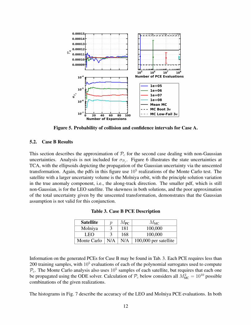
The values for Pc and σPc as a function of the number of PCE evaluations and the number ofPCE expansions N may be found in Fig. 5. For this test, the number of samples MMC providedto the polynomial surrogates was varied from 105 to 108 by factors of 10. It is noted that MMC isnot the number of training samples for the PCE, but the number of evaluations of the polynomialsurrogate. The top left plot describes the convergence of Pc as a function ofN , with a correspondingillustration of σPc in the bottom left plot. As described by the bottom left image, the confidence inthe solution is driven more by MMC, i.e., the number of evaluations of the PCE. The top right plotcompares the values determined via PC to those of 100,000 Monte Carlo trials (independent of theMPC training samples), and provides the computed Pc (solid black line) and 3σ error bars. The 3σMonte Carlo confidence intervals represent those determined by (a) 10,000 bootstrap samples of the106 available trials, and (b) the low-failure probability approximation given by Eq. (17). Althoughthe performance of the Monte Carlo tests will improve with more samples, these results demonstratethat the PCE-determined statistics lie within 3σ of the current Monte Carlo solution. With 108

samples, the PCE-determined value for Pc, is within the 3σ range [1.004×10−4, 1.064×10−4].Given a requirement to maneuver if Pc > 10−4, this indicates a need for a collision avoidancemaneuver. The Monte Carlo solution still exhibits ambiguity in the decision, which is illustrated inthe top right image of Fig. 5.

11

0.00009

0.00010

0.00011

0.00012

0.00013

0.00014

0.00015

P c

0 20 40 60 80 100Number of Expansions

10-7

10-6

10-5

10-4P c

105 106 107 108

Number of PCE Evaluations

1e+051e+061e+071e+08Mean MCMC Boot 3

MC Low-Fail 3

Figure 5. Probability of collision and confidence intervals for Case A.

5.2. Case B Results

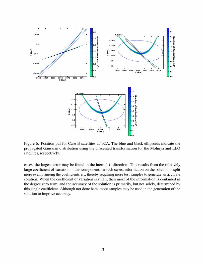
This section describes the approximation of Pc for the second case dealing with non-Gaussianuncertainties. Analysis is not included for σPc . Figure 6 illustrates the state uncertainties atTCA, with the ellipsoids depicting the propagation of the Gaussian uncertainty via the unscentedtransformation. Again, the pdfs in this figure use 105 realizations of the Monte Carlo test. Thesatellite with a larger uncertainty volume is the Molniya orbit, with the principle solution variationin the true anomaly component, i.e., the along-track direction. The smaller pdf, which is stillnon-Gaussian, is for the LEO satellite. The skewness in both solutions, and the poor approximationof the total uncertainty given by the unscented transformation, demonstrates that the Gaussianassumption is not valid for this conjunction.

Table 3. Case B PCE Description

Satellite p MPC MMC

Molniya 3 181 100,000LEO 3 168 100,000

Monte Carlo N/A N/A 100,000 per satellite

Information on the generated PCEs for Case B may be found in Tab. 3. Each PCE requires less than200 training samples, with 105 evaluations of each of the polynomial surrogates used to computePc. The Monte Carlo analysis also uses 105 samples of each satellite, but requires that each onebe propagated using the ODE solver. Calculation of Pc below considers all M2

MC = 1010 possiblecombinations of the given realizations.

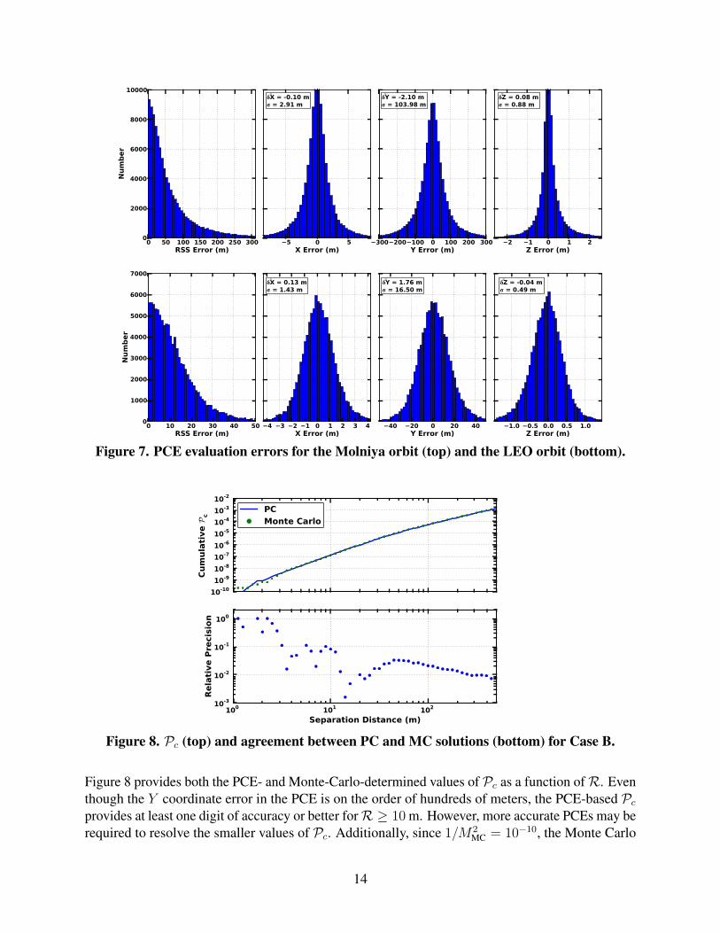
The histograms in Fig. 7 describe the accuracy of the LEO and Molniya PCE evaluations. In both

12

3062 3064 3066 3068 3070 3072 3074X (km)

−300

−200

−100

0

100

Y (

km

)

0.0

0.4

0.8

1.2

1.6

2.0

2.4

2.8

Nu

mb

er o

f Realiza

tion

s (1

0x

)

3062 3064 3066 3068 3070 3072 3074X (km)

−3.5

−3.0

−2.5

−2.0

−1.5

−1.0

Z (

km

)

−6.129e3

0.0

0.3

0.6

0.9

1.2

1.5

1.8

2.1

2.4

2.7N

um

ber o

f Realiza

tion

s (1

0x

)

−300 −200 −100 0 100Y (km)

−3.5

−3.0

−2.5

−2.0

−1.5

−1.0

Z (

km

)

−6.129e3

0.0

0.3

0.6

0.9

1.2

1.5

1.8

2.1

2.4

2.7

Nu

mb

er o

f Realiza

tion

s (1

0x

)

Figure 6. Position pdf for Case B satellites at TCA. The blue and black ellipsoids indicate thepropagated Gaussian distribution using the unscented transformation for the Molniya and LEOsatellites, respectively.

cases, the largest error may be found in the inertial Y direction. This results from the relativelylarge coefficient of variation in this component. In such cases, information on the solution is splitmore evenly among the coefficients cα, thereby requiring more test samples to generate an accuratesolution. When the coefficient of variation is small, then most of the information is contained inthe degree zero term, and the accuracy of the solution is primarily, but not solely, determined bythis single coefficient. Although not done here, more samples may be used in the generation of thesolution to improve accuracy.

13

0 50 100 150 200 250 300RSS Error (m)

0

2000

4000

6000

8000

10000

Nu

mb

er

−5 0 5X Error (m)

δX = -0.10 mσ = 2.91 m

−300−200−100 0 100 200 300Y Error (m)

δY = -2.10 mσ = 103.98 m

−2 −1 0 1 2Z Error (m)

δZ = 0.08 mσ = 0.88 m

0 10 20 30 40 50RSS Error (m)

0

1000

2000

3000

4000

5000

6000

7000

Nu

mb

er

−4 −3 −2 −1 0 1 2 3 4X Error (m)

δX = 0.13 mσ = 1.43 m

−40 −20 0 20 40Y Error (m)

δY = 1.76 mσ = 16.50 m

−1.0 −0.5 0.0 0.5 1.0Z Error (m)

δZ = -0.04 mσ = 0.49 m

Figure 7. PCE evaluation errors for the Molniya orbit (top) and the LEO orbit (bottom).

10-10

10-9

10-8

10-7

10-6

10-5

10-4

10-3

10-2

Cu

mu

lati

ve P

c

PCMonte Carlo

100 101 102

Separation Distance (m)

10-3

10-2

10-1

100

Rela

tive P

recis

ion

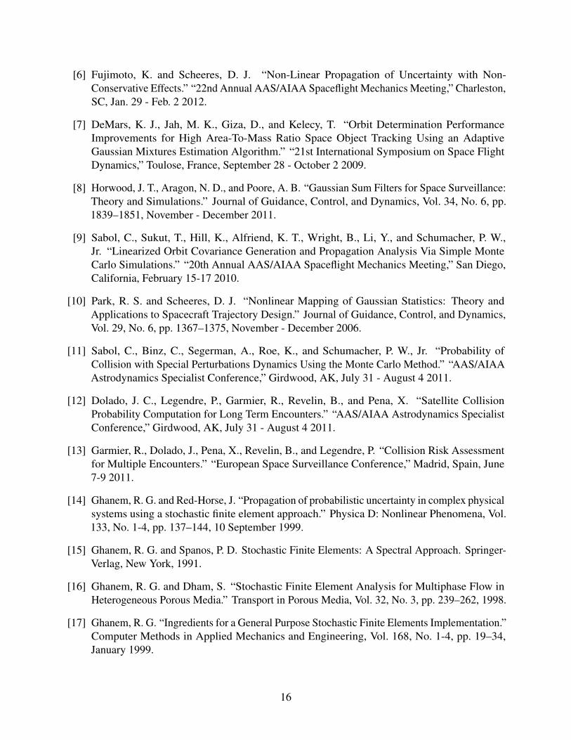
Figure 8. Pc (top) and agreement between PC and MC solutions (bottom) for Case B.

Figure 8 provides both the PCE- and Monte-Carlo-determined values of Pc as a function ofR. Eventhough the Y coordinate error in the PCE is on the order of hundreds of meters, the PCE-based Pcprovides at least one digit of accuracy or better forR ≥ 10 m. However, more accurate PCEs may berequired to resolve the smaller values of Pc. Additionally, since 1/M2

MC = 10−10, the Monte Carlo

14

solution for Pc ∼ O(10−10) is likely also inaccurate. The accuracy of the PCE may be improved byusing additional training samples. However, methods exist to improve the accuracy of rare failureprobability calculation using a hybrid of polynomial surrogates and additional evaluations of theODE solver [28, 29], and such techniques may be employed to limit the number of additional orbitpropagations required.

6. Conclusions

This paper demonstrated the use of polynomial chaos expansions (PCEs) for conjunction assessment.The PCE provides a polynomial surrogate to map random inputs at the initial time to generatea realized state at some future time. This allows for Monte-Carlo-like conjunction assessmentusing polynomial evaluations instead of computationally expensive orbit propagations. This workconsidered two test cases designed to demonstrate the use of PCEs in situations where semi-analyticmethods of estimating the probability of collision are not applicable. For both of these test cases,the PCEs provided a probability of collision with enough accuracy to make an informed maneuveravoidance decision. Additionally, each individual PCE required less than 300 evaluations of theorbit propagation tool, which is at least a factor of 330 less than the Monte Carlo results presented.The accuracy of the collision probability may be improved with a careful selection of additionalorbit propagations, with methods identified and designated as future work.

7. Acknowledgements

The authors wish to thank Russell Carpenter (NASA/GSFC), Geoff Wawrzyniak, and Dan Mattern(a.i. solutions) for helping to understand the MMS mission, which served as the basis for Case A.Discussions with them also helped in refining the presentation of polynomial chaos to make it morereadily accessible to those not familiar with the subject. This work was partially funded by theNASA GSFC through a.i. solutions.

8. References

[1] Alfriend, K. T., Akella, M. R., Frisbee, J., Foster, J. L., Lee, D.-J., and Wilkins, M. “Probabilityof Collision Error Analysis.” Space Debris, Vol. 1, No. 1, pp. 21–35, 1999.

[2] Patera, R. P. “General Method for Calculating Satellite Collision Probability.” Journal ofGuidance, Control, and Dynamics, Vol. 24, No. 4, pp. 716–722, July-August 2001.

[3] Alfano, S. “A Numerical Implementation of Spherical Object Collision Probability.” TheJournal of the Astronautical Sciences, Vol. 53, No. 1, pp. 103–109, January - March 2005.

[4] Jones, B. A., Doostan, A., and Born, G. H. “Nonlinear Propagation of Orbit Uncertainty UsingNon-Intrusive Polynomial Chaos.” Journal of Guidance, Control, and Dynamics, accepted,2012.

[5] Fujimoto, K., Scheeres, D. J., and Alfriend, K. T. “Analytical Nonlinear Propagation ofUncertainty in the Two-Body Problem.” Journal of Guidance, Control, and Dynamics, Vol. 35,No. 2, pp. 497–509, March-April 2012.

15

[6] Fujimoto, K. and Scheeres, D. J. “Non-Linear Propagation of Uncertainty with Non-Conservative Effects.” “22nd Annual AAS/AIAA Spaceflight Mechanics Meeting,” Charleston,SC, Jan. 29 - Feb. 2 2012.

[7] DeMars, K. J., Jah, M. K., Giza, D., and Kelecy, T. “Orbit Determination PerformanceImprovements for High Area-To-Mass Ratio Space Object Tracking Using an AdaptiveGaussian Mixtures Estimation Algorithm.” “21st International Symposium on Space FlightDynamics,” Toulose, France, September 28 - October 2 2009.

[8] Horwood, J. T., Aragon, N. D., and Poore, A. B. “Gaussian Sum Filters for Space Surveillance:Theory and Simulations.” Journal of Guidance, Control, and Dynamics, Vol. 34, No. 6, pp.1839–1851, November - December 2011.

[9] Sabol, C., Sukut, T., Hill, K., Alfriend, K. T., Wright, B., Li, Y., and Schumacher, P. W.,Jr. “Linearized Orbit Covariance Generation and Propagation Analysis Via Simple MonteCarlo Simulations.” “20th Annual AAS/AIAA Spaceflight Mechanics Meeting,” San Diego,California, February 15-17 2010.

[10] Park, R. S. and Scheeres, D. J. “Nonlinear Mapping of Gaussian Statistics: Theory andApplications to Spacecraft Trajectory Design.” Journal of Guidance, Control, and Dynamics,Vol. 29, No. 6, pp. 1367–1375, November - December 2006.

[11] Sabol, C., Binz, C., Segerman, A., Roe, K., and Schumacher, P. W., Jr. “Probability ofCollision with Special Perturbations Dynamics Using the Monte Carlo Method.” “AAS/AIAAAstrodynamics Specialist Conference,” Girdwood, AK, July 31 - August 4 2011.

[12] Dolado, J. C., Legendre, P., Garmier, R., Revelin, B., and Pena, X. “Satellite CollisionProbability Computation for Long Term Encounters.” “AAS/AIAA Astrodynamics SpecialistConference,” Girdwood, AK, July 31 - August 4 2011.

[13] Garmier, R., Dolado, J., Pena, X., Revelin, B., and Legendre, P. “Collision Risk Assessmentfor Multiple Encounters.” “European Space Surveillance Conference,” Madrid, Spain, June7-9 2011.

[14] Ghanem, R. G. and Red-Horse, J. “Propagation of probabilistic uncertainty in complex physicalsystems using a stochastic finite element approach.” Physica D: Nonlinear Phenomena, Vol.133, No. 1-4, pp. 137–144, 10 September 1999.

[15] Ghanem, R. G. and Spanos, P. D. Stochastic Finite Elements: A Spectral Approach. Springer-Verlag, New York, 1991.

[16] Ghanem, R. G. and Dham, S. “Stochastic Finite Element Analysis for Multiphase Flow inHeterogeneous Porous Media.” Transport in Porous Media, Vol. 32, No. 3, pp. 239–262, 1998.

[17] Ghanem, R. G. “Ingredients for a General Purpose Stochastic Finite Elements Implementation.”Computer Methods in Applied Mechanics and Engineering, Vol. 168, No. 1-4, pp. 19–34,January 1999.

16

[18] Xiu, D. and Karniadakis, G. E. “The Wiener-Askey Polynomial Chaos for Stochastic Dif-ferential Equations.” SIAM Journal of Scientific Computing, Vol. 24, No. 2, pp. 619–644,2002.

[19] Xiu, D. and Karniadakis, G. E. “Modeling Uncertainty in Flow Simulations Via GeneralizedPolynomial Chaos.” Journal of Computational Physics, Vol. 187, pp. 137–167, 2003.

[20] Le Maıtre, O. P., Najm, H. N., Ghanem, R. G., and Knio, O. M. “Multi-resolution analysis ofWiener-type uncertainty propagation schemes.” Journal of Computational Physics, Vol. 197,No. 2, pp. 502–531, 1 July 2004.

[21] Babuska, I., Tempone, R., and Zouraris, G. E. “Galerkin Finite Element Approximationsof Stochastic Elliptic Partial Differential Equations.” SIAM Journal on Numerical Analysis,Vol. 42, No. 2, pp. 800–825, 2005.

[22] Wan, X. and Karniadakis, G. E. “An adaptive multi-element generalized polynomial chaosmethod for stochastic differential equations.” Journal of Computational Physics, Vol. 209,No. 2, pp. 617–642, 1 November 2005.

[23] Xiu, D. “Fast Numerical Methods for Stochastic Computations: A Review.” Communicationsin Computational Physics, Vol. 5, No. 2-4, pp. 242–272, February 2009.

[24] Xiu, D. Numerical Methods for Stochastic Computations: A Spectral Method Approach.Princeton University Press, Princeton, New Jersey, 2010.

[25] Le Maıtre, O. P. and Knio, O. M. Spectral Methods for Uncertainty Quantification withApplications to Computational Fluid Dynamics. Springer, 2010.

[26] Wiener, N. “The Homogeneous Chaos.” American Journal of Mathematics, Vol. 60, No. 4, pp.897–936, October 1938.

[27] Doostan, A. and Owhadi, H. “A Non-adapted Sparse Approximation of PDEs with StochasticInputs.” Journal of Computational Physics, Vol. 230, No. 8, pp. 3015–3034, 20 April 2011.

[28] Li, J. and Xiu, D. “Evaluation of failure probability via surrogate models.” Journal ofComputational Physics, Vol. 229, No. 23, pp. 8966–8980, November 20 2010.

[29] Li, J., Li, J., and Xiu, D. “A efficient surrogate-based method for computing rare failureprobability.” Journal of Computational Physics, Vol. 230, No. 24, pp. 8683–8697, October 12011.

[30] Sharma, A. S. and Curtis, S. A. “Magnetospheric Multiscale Mission.” “NonequilibriumPhenomena in Plasmas,” Vol. 321 of Astrophysics and Space Science Library, pp. 179–195.Springer Netherlands, 2005.

[31] Carpenter, J. R., Markley, F. L., Alfriend, K. T., Wright, C., and Arcido, J. “SequentialProbability Ratio Test for Collision Avoidance Maneuver Decisions Based on a Bank ofNorm-Inequality-Constrained Epoch-State Filters.” “AAS/AIAA Astrodynamics SpecialistConference,” Girdwood, AK, July 31 - August 4 2011.

17

[32] Hill, K. and Jones, B. A. TurboProp Version 4.0. Colorado Center for Astrodynamics Research,May 2009.

[33] Prince, R. J. and Dormand, J. R. “High order embedded Runge-Kutta formulae.” Journal ofComputational and Applied Mathematics, Vol. 7, No. 1, pp. 67–75, March 1981.

18