HAL Id: hal-02963147https://hal-unilim.archives-ouvertes.fr/hal-02963147v2

Submitted on 9 Apr 2021

HAL is a multi-disciplinary open accessarchive for the deposit and dissemination of sci-entific research documents, whether they are pub-lished or not. The documents may come fromteaching and research institutions in France orabroad, or from public or private research centers.

L’archive ouverte pluridisciplinaire HAL, estdestinée au dépôt et à la diffusion de documentsscientifiques de niveau recherche, publiés ou non,émanant des établissements d’enseignement et derecherche français ou étrangers, des laboratoirespublics ou privés.

Deterministic computation of the characteristicpolynomial in the time of matrix multiplication

Vincent Neiger, Clément Pernet

To cite this version:Vincent Neiger, Clément Pernet. Deterministic computation of the characteristic polynomialin the time of matrix multiplication. Journal of Complexity, Elsevier, 2021, 67, pp.101572.�10.1016/j.jco.2021.101572�. �hal-02963147v2�

Deterministic computation of the characteristic polynomialin the time of matrix multiplication

Vincent Neiger

Univ. Limoges, CNRS, XLIM, UMR 7252, F-87000 Limoges, France

Clement Pernet

Universite Grenoble Alpes, Laboratoire Jean Kuntzmann, CNRS, UMR 5224700 avenue centrale, IMAG - CS 40700, 38058 Grenoble cedex 9, France

Abstract

This paper describes an algorithm which computes the characteristic polynomial of a matrix overa field within the same asymptotic complexity, up to constant factors, as the multiplication of twosquare matrices. Previously, this was only achieved by resorting to genericity assumptions orrandomization techniques, while the best known complexity bound with a general deterministicalgorithm was obtained by Keller-Gehrig in 1985 and involves logarithmic factors. Our algorithmcomputes more generally the determinant of a univariate polynomial matrix in reduced form,and relies on new subroutines for transforming shifted reduced matrices into shifted weak Popovmatrices, and shifted weak Popov matrices into shifted Popov matrices.

Keywords: Characteristic polynomial, polynomial matrices, determinant, fast linear algebra.

1. Introduction

The last five decades witnessed a constant effort towards computational reductions of linearalgebra problems to matrix multiplication. It has been showed that most classical problems arenot harder than multiplying two square matrices, such as matrix inversion, LU decomposition,nullspace basis computation, linear system solving, rank and determinant computations, etc. [7][25] [8, Chap. 16]. In this context, one major challenge stands out: designing a similar reductionto matrix multiplication for the computation of characteristic polynomials and related objectssuch as minimal polynomials and Frobenius forms. For the characteristic polynomial, significantprogress was achieved by Keller-Gehrig [31], and more recently by Pernet and Storjohann [39]who solved the problem if one allows randomization. This paper closes the problem by providinga deterministic algorithm with the same asymptotic complexity as matrix multiplication.

The characteristic polynomial of a square matrix over a field K, say M ∈ Km×m, is defined asdet(xIm −M). Specific algorithms exist for sparse or structured matrices; here we consider theclassical, dense case. In this paper the complexity of an algorithm is measured as an upper boundon its arithmetic cost, that is, the number of basic field operations it uses to compute the output.

Theorem 1.1. Let K be a field. Using a subroutine which multiplies two matrices in Km×m inO(mω) field operations for some ω > 2, the characteristic polynomial of a matrix in Km×m canbe computed deterministically in O(mω) field operations.

Outline. The rest of this introduction gives more details about our framework for complexitybounds (Section 1.1), summarizes previous work (Section 1.2), describes our contribution onpolynomial matrix determinant computation (Section 1.3), gives an overview of our approachand of new tools that we designed to avoid logarithmic factors (Sections 1.4 and 1.5), and finallylists a few perspectives (Section 1.6). Section 2 introduces the notation, main definitions, andbasic properties used in this paper. Then Section 3 presents the main algorithm of this paper alongwith a detailed complexity analysis. This algorithm uses two new technical tools described inSections 4 and 5: the transformation of reduced forms into weak Popov forms and of weak Popovforms into Popov forms, in the case of shifted forms.

1.1. Framework for complexity bounds

In this paper, K is any field and we seek upper bounds on the complexity of algorithms whichoperate on objects such as matrices and polynomials over K. We consider the arithmetic cost ofthese algorithms, i.e. the number of basic operations in K that are used to compute the outputfrom some input of a given size. The basic operations are addition, subtraction, multiplication,and inversion in the field, as well as testing whether a given field element is zero.

As already highlighted in Theorem 1.1, in this paper we fix any 2 < ω ≤ 3 as well as anyalgorithm which multiplies matrices in Km×m using O(mω) operations in K: this algorithm isassumed to be the one used as a black box for all matrix multiplications arising in the algorithmswe design. The current best known cost bounds ensure that any ω > 2.373 is feasible [33].In practice, one often considers a cubic algorithm with ω = 3 or Strassen’s algorithm withω = log2(7) [47]. Our results hold with the only assumption that 2 < ω ≤ 3.

In the computer algebra literature, this setting is classical and often implicit; we still em-phasize it because here, and more generally when one studies the logarithmic factors in the costbound of some algorithm, this clarification of how the underlying matrix multiplications are per-formed is of the utmost importance. Indeed, if one were allowed to use any matrix multiplicationsubroutine, then the question of logarithmic factors becomes void: for any exponent ω known tobe feasible at the time of writing, it is known that ω− ε is feasible as well for a sufficiently smallε > 0; then one might rather rely on this faster subroutine, and apply Keller-Gehrig’s algorithmto obtain the characteristic polynomial in O(mω−ε log(m)) operations in K, which is in O(mω).

Similarly, we consider a nondecreasing function d 7→ M(d) and an algorithm which multipliestwo polynomials in K[x] of degree at most d using at most M(d) operations in K; our algorithmsrely on this subroutine for polynomial multiplication. Here d is any nonnegative real number; itwill often be a fraction D/m of positive integers; we assume that M(d) = 1 for 0 ≤ d < 1, so thatM(d) ≥ 1 for all d ≥ 0. To help derive complexity upper bounds, we also consider the followingassumptionsHsl,Hsm, andHω.Hsl: 2 M(d) ≤ M(2d) for all d ≥ 1 (superlinearity).Hsm: M(d1d2) ≤ M(d1) M(d2) for all d1, d2 ≥ 0 (submultiplicativity).Hω: M(d) ∈ O(dω−1−ε) for some ε > 0.

The first assumption is customary, see e.g. [19, Sec. 8.3]; note that it implies M(d) ≥ d forall d ≥ 1. The second and last assumptions are commonly made in complexity analyses fordivide and conquer algorithms on polynomial matrices [45, 23]: we refer to [45, Sec. 2] forfurther comments on these assumptions. They are satisfied by the cost bounds of polynomialmultiplication algorithms such as the quasi-linear algorithm of Cantor and Kaltofen [9] and, forsuitable fields K, the quasi-linear algorithm of Harvey and van der Hoeven and Lecerf [24],and most of Toom-Cook subquadratic algorithms [50, 10]. For the latter only Hω might not

2

be satisfied, depending on ω and on the number of points used. Note that with the currentestimates having ω > 2.373, an order 5 Toom-Cook multiplication (requiring a field with at least9 points) has exponent log(9)/ log(5) ≈ 1.365 < ω−1; thus for such exponents ω all Toom-Cookalgorithms of order 5 or more satisfy all the above assumptions.

Following [45, 23], we also define a function d 7→ M′(d) related to the cost of divide andconquer methods such as the half-gcd algorithm: M′(d) =

∑0≤i≤dlog2(d)e 2i M(2−id) for d ≥ 1, and

M′(d) = 1 for 0 ≤ d ≤ 1. By definition one has M′(d) ≥ M(d) ≥ 1 for all d ≥ 0, and the identityM′(2d) = 2 M′(d) + M(2d) for d ≥ 1 ensures that M′(d) is superlinear: 2 M′(d) ≤ M′(2d) forall d ≥ 1. Assuming Hsl yields the asymptotic bound M′(d) ∈ O(M(d) log(d)) where the log(d)factor only occurs if a quasi-linear polynomial multiplication is used; in particular, Hsl and Hω

imply M′(d) ∈ O(dω−1−ε) for some ε > 0. Furthermore, if one assumes Hsl and Hsm, then M′(·)is submultiplicative as well: M′(d1d2) ≤ M′(d1) M′(d2) for all d1, d2 ≥ 0.

In what follows we assume that two polynomial matrices in K[x]m×m of degree at most d ≥ 0can be multiplied in O(mω M(d)) operations in K. This is a very mild assumption: it holds assoon as M(d) corresponds to one of the above-mentioned polynomial multiplication algorithms,and it also holds if the chosen matrix multiplication algorithm defining ω supports matrices overa commutative ring using only the operations {+,−,×} (so that one can use it to multiply m × mmatrices over K[x]/(x2d+1)). Note still that this bound O(mω M(d)) is slightly worse than thebest known ones [9, 24]; for example, Cantor and Kaltofen’s algorithm performs polynomialmatrix multiplication in O(mωd log(d) + m2d log(d) log(log(d))) field operations, which is finerthan the bound O(mω M(d)) with M(d) = Θ(d log(d) log(log(d))) in that case. This simplificationis frequent in the polynomial matrix literature, and it is made here for the sake of presentation,to improve the clarity of our main complexity results and of the analyses that lead to them.

1.2. Previous work

Previous algorithms based on linear algebra over K for computing the characteristic polyno-mial of M ∈ Km×m mainly fall in three types of methods.

Traces of powers: combining the traces of the first n powers of the input matrix using theNewton identities reveals the coefficients of the characteristic polynomial. Known as theFaddeev-LeVerrier algorithm, it was introduced in [34], refined and rediscovered in [43,16, 18], and used in [11] to prove that the problem is in theNC2 parallel complexity class.

Determinant expansion formula: introduced in [41] and improved in [6], this approach doesnot involve division, and is therefore well suited for computing over integral domains.Later developments in this field include [1, 30], the latter reaching the best known costbound of O(m2.6973 log(m)c) ring operations using a deterministic algorithm, for some con-stant c > 0.

Krylov methods: based on sequences of iterates of vectors under the application of the matrix:(v,Mv,M2v, . . .). These methods rely on the fact that the first linear dependency betweenthese iterates defines a polynomial which divides the characteristic polynomial. Some al-gorithms construct the Krylov basis explicitly [31, 20, 14], while others can be interpretedas an implicit Krylov iteration with structured vectors [12, 39].

Methods based on traces of powers use O(m4) or O(mω+1) field operations, and are mostly com-petitive for their parallel complexity. Methods based on determinant expansions use O(m4) orO(mω+1) field operations and are relevant for division-free algorithms. Lastly, the Krylov meth-ods run in O(m3) [12, 14] or O(mω log m) [31] field operations with deterministic algorithms, orin O(mω) field operations with the Las Vegas randomized algorithm in [39].

3

Note that the characteristic polynomial of M cannot be computed faster than the determinantof M, since the latter is the constant coefficient of the former. Furthermore, under the model ofcomputation trees, the determinant of m×m matrices cannot be computed faster than the productof two m × m matrices [8, Sec. 16.4], a consequence of Baur and Strassen’s theorem [2].

Another type of characteristic polynomial algorithms is based on operations on matrices overK[x], called polynomial matrices in what follows. Indeed the characteristic polynomial may beobtained by calling a determinant algorithm on the characteristic matrix xIm −M, which is inK[x]m×m. Existing algorithms, which accept any matrix in K[x]m×m of degree d as input, include• the evaluation-interpolation method, which costs O(mω+1d + m3 M′(d)) field operations,

requires that the field K is large enough, and mainly relies on the computation of about mddeterminants of matrices in Km×m;• the algorithm of Mulders and Storjohann [36] based on weak Popov form computation,

which uses O(m3d2) field operations;• retrieving the determinant as the product of the diagonal entries of the Smith form, itself

computed by a Las Vegas randomized algorithm in O(mω M′(d) log(m)2) field operations[45, Prop. 41], assuming M′(d) ∈ O(dω−1);• the algorithm based on unimodular triangularization in [32], which is deterministic and

uses O(mωd log(d)a log(m)b) field operations for some constants a, b ∈ Z>0.In the last two items the cost bound is, up to logarithmic factors, the same as the cost of multiply-ing matrices K[x]m×m of degree d by relying on both fast linear algebra over K and fast arithmeticin K[x], as showed in [9]. The last two of these cost bounds do involve factors logarithmic in m,whereas the first two have an exponent on m which exceeds ω.

In summary, the fastest characteristic polynomial algorithms either are randomized or have acost a logarithmic factor away from the lower bound. This paper, with Theorem 1.1, bridges thisgap by proposing the first deterministic algorithm with cost O(mω).

1.3. A more general result: determinant of reduced polynomial matricesOur algorithm falls within the category of polynomial matrix determinant computation. Yet

unlike the above-listed approaches ours is tailored to a specific family of polynomial matrices,which contains the characteristic matrix xIm −M: the family of row reduced matrices [52, 29].Restricting to such matrices provides us with good control of the degrees in computations; asa typical example, it is easy to predict the degree of a vector-matrix product v(xIm − M) byobserving the degrees in v, without actually computing the product. As we explain below, thisdegree control allows us to avoid searches of degree profiles, which would add logarithmic termsto the cost. Although the characteristic matrix has other properties besides row reducedness (ithas degree 1, and is in Popov form [40] hence column reduced), we do not exploit them.

When appropriate, the average row degree D/m, where D is the sum of the degrees of the rowsof the matrix, is chosen as a measure of the input degree which refines the matrix degree d usedabove. This gives cost bounds more sensitive to the input degrees and also, most importantly,leverages the fact that even if the algorithm starts from a matrix with uniform degrees such asxIm −M, it may end up handling matrices with unbalanced row degrees in the process.

Theorem 1.2. Assuming Hsl, Hsm, and Hω (hence in particular ω > 2), there is an algorithmwhich takes as input a row reduced matrix A ∈ K[x]m×m and computes its determinant using

O(mω M′(D/m)

)⊆ O

(mω M′

(deg(A)

))operations in K, where D = deg(det(A)) is equal to the sum of the degrees of the rows of A.

4

The fact that deg(det(A)) is the sum of row degrees is a consequence of row reducedness [29],and the cost bound inclusion follows from deg(det(A)) ≤ m deg(A). Taking A = xIm −M forM ∈ Km×m, Theorem 1.1 is a direct corollary of Theorem 1.2. The only assumption needed inTheorem 1.1 is ω > 2, since it implies the existence of a polynomial multiplication algorithmsuch thatHsl,Hsm, andHω hold, such as Cantor and Kaltofen’s algorithm [9].

Previous polynomial matrix determinant algorithms with costs of the order of mω deg(A), upto logarithmic factors, have been listed above: a randomized one from [45], and a deterministicone from [32]. To our knowledge, this paper gives the first description of an algorithm achievingsuch a cost involving no factor logarithmic in m. Our approach partially follows the algorithm of[32], but also substantially differs from it in a way that allows us to benefit from the reducednessof A. The cost bound O(mω M′(deg(A))) has been obtained before in [21, Sec. 4.2.2] in theparticular case of a “sufficiently generic1” matrix A. In that case, both the algorithm of [32] andthe one here coincide and become the algorithm of [21, Sec. 4.2.2]; when A is the characteristicmatrix xIm −M, this also relates to the fast algorithm in [31, Sec. 6] for a generic M.

1.4. Approach, and existing toolsFor the sake of presentation, suppose m is a power of 2. Writing A = [ A1 A2

A3 A4] with the Ai’s of

dimensions (m/2) × (m/2), the algorithm of [32] is based on the block triangularization[∗ ∗

K1 K2

] [A1 A2A3 A4

]=

[R ∗

0 B

]where the entries “∗” are not computed, B = K1A2 + K2A4, and R and [K1 K2] are computedfrom [ A1

A3] as a row basis and a kernel basis, respectively (see Section 2.2 for definitions). Then

the leftmost matrix in the above identity is unimodular [32, Lem. 3.1] and thus, up to a constantfactor, det(A) can be computed recursively as det(R) det(B).

A first observation is that neither the kernel basis computation nor the matrix multiplicationgiving B is an obstacle towards a cost which is free of log(m). (The fastest known method formultiplying matrices with unbalanced degrees, such as in B = K1A2 + K2A4, splits the com-putation into O(log(m)) multiplications of smaller matrices with balanced degrees [58, Sec. 3.6],suggesting that its cost may involve a log(m) factor.) Indeed we show that, under the above as-sumptions on M(·), the cost of these operations is in O(mω M(D/m)) and O(mω M′(D/m)), thusonly involving factors logarithmic in D/m. In previous work, cost bounds either hide logarith-mic factors [58] or they are derived without assuming Hsm and have the form O(mω−1 M(D))and O(mω−1 M′(D)) [27], thus resulting in factors logarithmic in D. Proving this observation isstraightforward from the analyses in [58, 27] (see Section 2.5). This is a first key towards ourmain result: the characteristic matrix has D = m, and O(mω M(1)) is the same as O(mω) whereasO(mω−1 M(m)) involves factors logarithmic in m.

However, the computation of the row basis R remains an obstacle which prevents the algo-rithm of [32] from being a candidate for Theorem 1.2. Indeed, among the row basis algorithmswe are aware of, only one has a cost bound which fits into our target up to logarithmic factors: theone of [56]. It relies on three kernel bases computations, and while one of them is similar to thecomputation of [K1 K2] and is handled via the algorithm of [58], the two others have differentconstraints on the input and were the subject of a specific algorithm described in [56, Sec. 4].

1Precisely, if the upper triangular, row-wise Hermite normal form of A has diagonal entries (1, . . . , 1, λ det(A)), forsome λ ∈ K \ {0} making λ det(A) monic.

5

In this reference, cost bounds were given without showing logarithmic factors; our own analysisrevealed the presence of a factor logarithmic in m. The algorithm has a loop over Θ(log(m))iterations, each of them calling [55, Algo. 2] for minimal approximant bases with unbalanced in-put. This approximant basis algorithm may spend a logarithmic number of iterations for findingsome degree profile of the output basis, in a way reminiscent of Keller-Gehrig’s algorithm in [31,Sec. 5] which finds the lengths of Krylov sequences (the link between the two situations becomesmore explicit for approximant bases at small orders, see [27, Sec. 7]).

Our attempts at accelerating the row basis algorithm of [56] having not succeeded, the algo-rithm in this paper follows an approach which is more direct at first: remove the obstacle. Insteadof computing a row basis R and relying on the identity det(A) = det(R) det(B) (up to a constant),keep the first block row of A: [

Im/2 0K1 K2

] [A1 A2A3 A4

]=

[A1 A20 B

](1)

and rely on the identity det(A) = det(A1) det(B)/ det(K2). The nonsingularity of A1 and K2 iseasily ensured thanks to the assumption that A is reduced, as discussed in Section 1.5.

This leads to an unusual recursion scheme: we are not aware of a similar scheme being usedin the literature on computational linear algebra. The algorithm uses three recursive calls with(m/2) × (m/2) matrices whose determinant has degree at most D/2 for two of them and at mostD for the third; our complexity analysis in Section 3.3 shows that such a recursion gives the costin Theorem 1.2. Precisely, if deg(det(A1)) ≤ D/2 then degree properties of minimal kernel basesimply that deg(det(K2)) ≤ D/2, yielding the two calls in half the degree; otherwise the algorithmuses inexpensive row and column operations on A to reduce to the case deg(det(A1)) ≤ D/2.

Although this approach removes the obstacle of row basis computation which arises in [32],it adds a requirement: all recursive calls must take input matrices that are reduced. In the nextsection we discuss how to ensure the reducedness of A1 and B thanks to a straightforward gener-alization of [42, Sec. 3], and we describe a new algorithm which handles the more involved caseof K2.

1.5. New tools, and ensuring reduced form in recursive calls

When outlining the approach of our determinant algorithm via the identity in Eq. (1), weimplicitly assumed that the matrices used as input in recursive calls, i.e. A1 and K2 and B, dosatisfy the input requirement of row reducedness: this is not necessarily the case, even if startingfrom a reduced matrix A.

Concerning A1, one may locate such a reduced submatrix of A and then permute rows andcolumns of A (which only affects the sign of det(A)) to make this submatrix become the leadingprincipal submatrix A1. This is a classical operation on reduced matrices which suggests usinga form slightly stronger than reduced form called weak Popov form [36] (see Section 2.4). As-suming that A has this form ensures that its leading principal submatrix A1 has it as well. Thisassumption is acceptable in terms of complexity since one can transform a reduced A into a weakPopov P by means of fast linear algebra in a cost negligible compared to our target [42, Sec. 3];note that A and P have the same determinant up to an easily found constant (see Algorithm 1).

Next, the cases of K2 and B are strongly linked. First, we will not discuss K2 but the wholekernel basis [K1 K2]. The fastest known algorithm for computing such a basis is that of [58],and for best efficiency it outputs a matrix in shifted reduced form, which is a generalization ofreducedness involving degree weights given by a tuple s ∈ Zm called a shift (see Sections 2.3

6

and 2.4 for definitions); the non-shifted case is for s = 0. As in the determinant algorithm of [32],here the shift for [K1 K2] is taken as the list of row degrees of A, denoted by s = rdeg(A); for thecharacteristic matrix one has s = (1, . . . , 1) but non-uniform shifts may arise in recursive calls.We want [K1 K2] to be not only s-reduced, but in s-weak Popov form: a direct consequence isthat B is in weak Popov form, and is thus suitable input for a recursive call.

To obtain [K1 K2] we use the kernel basis algorithm of [58] and transform its output intos-weak Popov form. A minor issue is that the fastest known algorithm for such transformationswas written in [42, Sec. 3] for non-shifted forms; yet it easily extends to shifted forms as weshow in Section 4, obtaining the next result.

Theorem 1.3. There is an algorithm ReducedToWeakPopov which takes as input a matrix A ∈K[x]m×n with m ≤ n and a shift s ∈ Zn such that A is in s-reduced form, and returns an s-weakPopov form of A using O(mω−2nD + mω−1n) operations in K, where D = |rdegs(A)| −m ·min(s).

Here, following usual notation recalled in Section 2.1, |rdegs(A)| is the sum of the s-degrees ofthe rows of A. This result extends [42, Thm. 13] since for s = 0 the quantity D is the sum of therow degrees of A and in particular D ≤ m deg(A), leading to the cost bound O(mω−1n deg(A)).

To summarize, at this stage we have outlined how to ensure, without exceeding our targetcost bound, that A1 and B are valid input for recursive calls, i.e. are in weak Popov form. Havingdet(A1) and det(B), it remains to find det(K2) and then the sought det(A) follows. We noted that,to ensure the form of B but also for efficiency reasons, the kernel basis [K1 K2] is computedin s-weak Popov form for the shift s = rdeg(A). This causes the main difficulty related to ourmodification of the determinant algorithm of [32]: K2 is not valid input for a recursive call sinceit is in v-weak Popov form for some shift v, a subtuple of s which is possibly nonzero.

A first idea is to extend our approach to the shifted case, allowing recursive calls with sucha v-reduced matrix: this is straightforward but gives an inefficient algorithm. Indeed, along therecursion the shift drifts away from its initial value and becomes arbitrarily large and unbalancedwith respect to the degrees of the input matrices of recursive calls. For example, as mentionedabove the sum of row degrees of the initial non-shifted m × m matrix A is D = deg(det(A)),whereas for the v-shifted (m/2) × (m/2) matrix K2 we only have the same bound D instead ofone related to deg(det(K2)) itself, which is known to be at most D/2 in our algorithm. This gap,here between D and D/2, will only grow as the algorithm goes down the tree of recursive calls,meaning that degrees in matrices handled recursively are not sufficiently well controlled.

Another idea is to compute a 0-reduced matrix which has the same determinant as K2. Find-ing a 0-reduced form of K2 within our target cost seems to be a difficult problem. The best knownalgorithms for general 0-reduction involve log(m) factors, either explicitly [23] or implicitly [38](in the latter approach one starts by using the above-discussed triangularization procedure of [32]which we are modifying here to avoid log(m) factors). More specific algorithms exploit the formof K2, interpreting the problem as a change of shift from v to 0; yet at the time of writing efficientchanges of shifts have only been achieved when the target shift is larger than the origin shift [27,Sec. 5], a fact that offers degree control for the transformation between the two matrices. Anotherpossibility is to compute the so-called v-Popov form P of K2, since its transpose PT is 0-reducedby definition (see Section 2.4), and det(PT) = det(P) is det(K2) up to a constant. However thissuffers from the same issue, as computing P is essentially the same as changing the shift v intothe nonpositive shift −δ, where δ is the list of diagonal degrees of K2 [42, 26].

To circumvent these issues, we use the property that the transpose KT2 of a v-reduced matrix

is in −d-reduced form where d = rdegv(K2). This fact naturally comes up here since det(K2) =

7

det(KT2 ), but seems otherwise rarely exploited in polynomial matrix algorithms: in fact we did

not find a previous occurrence of it apart from related degree considerations in [56, Lem. 2.2].Transposing the above two approaches using KT

2 instead of K2, we observe that computinga 0-reduced form of KT

2 is a change of shift from −d to 0, and computing the −d-Popov form Pof KT

2 is essentially a change of shift from −d to −δ. In both cases the target shift is larger thanthe origin shift, implying that the kernel-based change of shift of [27, Sec. 5] involves matricesof well-controlled degrees. Still, this is not enough to make this change of shift efficient as such,the difficulty being now that the average row degree of KT

2 may not be small: only its averagecolumn degree, which corresponds to the average row degree of K2, is controlled.

Our solution uses the second approach, computing the −d-Popov form P, because it offers thea priori knowledge that the column degrees of P are exactly δ. We exploit this degree knowledgeto carry out partial linearization techniques, originally designed for approximant bases [46, 28],which we extend here to kernel bases. These techniques allow us to reduce our problem to akernel basis computation where the matrix entries have uniformly small degrees, implying thatit can be efficiently handled via the minimal approximant basis algorithm PM-Basis from [21].The next result summarizes the new algorithmic tool developed in Section 5 for finding P.

Theorem 1.4. Let s ∈ Zm, let A ∈ K[x]m×m be in −s-weak Popov form, let δ ∈ Zm≥0 be the

−s-pivot degree of A, and assume that s ≥ δ. There is an algorithm WeakPopovToPopov whichtakes as input (A, s) and computes the −s-Popov form of A by

• performing PM-Basis at order less than |s|/m + 4 on an input matrix of row dimension atmost 6m and column dimension at most 3m,• multiplying the inverse of a matrix in Km×m by a matrix in K[x]m×m of column degree δ,• and performing O(m2) extra operations in K.

Thus, computing the −s-Popov form of A can be done in O(mω M′(|s|/m)) operations in K.

This theorem is a generalization of [42, Sec. 4] to shifted forms, for shifts −s that satisfy theassumption s ≥ δ. Indeed, if A is 0-weak Popov, then one recovers [42, Thm. 20] by takings = (deg(A), . . . , deg(A)) in the above theorem. For comparison, the naive generalization of [42,Sec. 4] to shifted forms runs in O(mω M′(max(s))), which exceeds our target complexity as soonas max(s) � |s|/m. Hence the use of partial linearization techniques, which were not needed inthe non-shifted case featuring max(s) = |s|/m = deg(A).

As mentioned above, our Algorithm WeakPopovToPopov is based on the computation of akernel basis with a priori knowledge of the degree profile of the output. This kernel problem isvery close to the one handled in [56, Sec. 4], except that in this reference one only has upperbounds on the output degrees, implying a certain number—possibly logarithmic in m—of callsto PM-Basis to recover the output and its actual degrees. In the same spirit but in the context ofapproximant bases, [28, Sec. 5] uses partial linearization techniques to reduce an arbitrary inputwith known output degrees to essentially one call to PM-Basis, whereas [55, Algo. 2] assumesweaker output degree information and makes a potentially logarithmic number of calls to PM-Basis.

1.6. PerspectivesWe plan to implement our characteristic polynomial algorithm in the LinBox ecosystem [48,

49]. First prototype experiments suggest that, for large finite fields, it could be competitivewith the existing fastest-known implementation, based on the randomized algorithm of [39].The native support for small fields of our algorithm should outperform the algorithm of [39]

8

which requires expensive field extensions. Another perspective stems from the remark that ouralgorithm resorts to fast polynomial multiplication (see assumption Hω), while previous onesdid not [31, 39]: we woud like to understand whether the same cost can be achieved by a purelylinear algebraic approach. Finally, perhaps the most challenging problem related to characteristicpolynomial computation is to compute Frobenius forms deterministically in the time of matrixmultiplication, the current best known complexity bound being O(mω log(m) log(log(m))) [44];and more generally computing Smith forms of polynomial matrices with a cost free of factorslogarithmic in the matrix dimension.

2. Preliminaries on polynomial matrices

In this section we present the notation as well as basic definitions and properties that will beused throughout the paper.

2.1. Notation

Tuples of integers will often be manipulated entry-wise. In particular, for tuples s, t ∈ Zn ofthe same length n, we write s + t for their entry-wise sum, and the inequality s ≤ t means thateach entry in s is less than or equal to the corresponding entry in t. The concatenation of tuplesis denoted by (s, t). We write |t| for the sum of the entries of t. The tuple of zeros is denoted by0 = (0, . . . , 0); its length is understood from the context.

For an m × n matrix A over some ring, we write Ai, j for its entry at index (i, j). We extendthis to submatrices: given sets I ⊆ {1, . . . ,m} and J ⊆ {1, . . . , n} of row and column indices, wewrite AI,J for the submatrix of A formed by its entries indexed by I × J. Besides, AI,∗ stands forthe submatrix of A formed by its rows with index in I, and we use the similar notation A∗,J . Thetranspose of A is denoted by AT. The identity matrix of size n is denoted by In, while the n × nmatrix with 1 on the antidiagonal and 0 elsewhere is denoted by Jn. In particular, when writingsJn for a tuple s = (s1, . . . , sn) ∈ Zn, we mean the reversed tuple sJn = (sn, . . . , s1).

Now consider A with polynomial entries, i.e. A ∈ K[x]m×n. The degree of A is denoted bydeg(A) and is the largest of the degrees of its entries, or −∞ if A = 0. The row degree of A isthe tuple rdeg(A) ∈ (Z≥0 ∪ {−∞})m whose ith entry is max1≤ j≤n(deg(Ai, j)). More generally, for atuple s = (s1, . . . , sn) ∈ Zn, the s-row degree of A is the tuple rdegs(A) ∈ (Z ∪ {−∞})m whose ithentry is max1≤ j≤n(deg(Ai, j) + s j). In this context, the tuple s is commonly called a (degree) shift[4]. The (shifted) column degree of A is defined similarly.

We write Xs for the n×n diagonal matrix diag(xs1 , . . . , xsn ) which is over the ring K[x, x−1] ofLaurent polynomials over K. Note that, hereafter, Laurent polynomials will only arise in proofsand explanations, more specifically in considerations about shifted degrees: they never arise inalgorithms, which for the sake of clarity only involve polynomials in K[x]. The usefulness ofthis matrix Xs will become clear in the definition of leading matrices in the next subsection.

The next lemma gives a link between shifted row degrees and shifted column degrees. Wewill mostly use the following particular case of it: the column degree of A is at most d ∈ Zn

≥0(entry-wise) if and only if the −d-row degree of A is nonpositive.

Lemma 2.1 ([56, Lemma 2.2]). Let A be a matrix in K[x]m×n, d be a tuple in Zn, and t be atuple in Zm. Then, cdegt(A) ≤ d if and only if rdeg−d(A) ≤ −t.

9

2.2. Bases of modules, kernel bases and approximant basesWe recall that any K[x]-submodule M of K[x]1×n is free, and admits a basis formed by r

elements of K[x]1×n, where r ≤ n is called the rank ofM [see e.g. 15]. Such a basis can thus berepresented as an r × n matrix B over K[x] whose rows are the basis elements; this basis matrixB has rank r.

For a matrix A ∈ K[x]m×n, its row space is the K[x]-submodule {pA,p ∈ K[x]1×m} of K[x]1×n,that is, the set of all K[x]-linear combinations of its rows. If B ∈ K[x]r×n is a basis of this rowspace, then B is said to be a row basis of A; in particular, r is the rank of B and of A.

The left kernel of A, denoted byK(A), is the K[x]-module {p ∈ K[x]1×m | pA = 0}. A matrixK ∈ K[x]k×m is a left kernel basis of A if its rows form a basis of K(A), in which case k = m − r.Similarly, a right kernel basis of A is a matrix K ∈ K[x]n×(n−r) whose columns form a basis ofthe right kernel of A.

Given positive integers γ = (γ1, . . . , γn) ∈ Zn>0 and a matrix F ∈ K[x]m×n, the set of approxi-

mants for F at order γ [see e.g. 51, 3] is the K[x]-submodule of K[x]1×m defined as

Aγ(F) = {p ∈ K[x]1×m | pF = 0 mod Xγ }.

The identity pF = 0 mod Xγ means that pF∗, j = 0 mod xγ j for 1 ≤ j ≤ n. Since all m rows ofthe matrix xmax(γ)Im are inAγ(F), this module has rank m.

2.3. Leading matrices and reduced forms of polynomial matricesWe will often compute with polynomial matrices that have a special form, called the (shifted)

reduced form. It corresponds to a type of minimality of the degrees of such matrices, and alsoprovides good control of these degrees during computations as illustrated by the predictabledegree property [17] [29, Thm. 6.3-13] which we recall below. In this section, we introduce thenotion of row reducedness; to avoid confusion, we will not use the similar notion of columnreducedness in this paper, and thus all further mentions of reducedness refer to row reducedness.

For shifted reduced forms, we follow the definitions in [4, 5]. Let A ∈ K[x]m×n and s ∈ Zn,and let t = (t1, . . . , tm) = rdegs(A). Then, the s-leading matrix of A is the matrix lms(A) ∈ Km×n

whose entry (i, j) is the coefficient of degree ti − s j of the entry (i, j) of A, or 0 if ti = −∞.Equivalently, lms(A) is the coefficient of degree zero of X−t AXs , whose entries are in K[x−1].The matrix A is said to be in s-reduced form if its s-leading matrix has full row rank. In particular,a matrix in s-reduced form must have full row rank.

For a matrix M ∈ K[x]k×m, we have rdegs(MA) ≤ rdegt(M) and this is an equality when nocancellation of leading terms occurs in this left-multiplication. The predictable degree propertystates that A is s-reduced if and only if rdegs(MA) = rdegt(M) holds for any M ∈ K[x]k×m. Hereis a useful consequence of this characterization.

Lemma 2.2. Let s ∈ Zn, let A ∈ K[x]m×n, and let t = rdegs(A). If A is s-reduced, then theidentity lms(MA) = lmt(M)lms(A) holds for any M ∈ K[x]k×m.

Proof. Let d = rdegs(MA). By definition, lms(MA) is the coefficient of degree 0 of the matrixX−d MAXs = X−d MXt X−t AXs , whose entries are in K[x−1]. Besides, since rdegs(A) = t andsince the predictable degree property gives rdegt(M) = d, the matrices X−d MXt and X−t AXs

are over K[x−1] and their coefficients of degree 0 are lmt(M) and lms(A), respectively.

Another characterization of matrices in s-reduced form is that they have minimal s-row de-gree among all matrices which represent the same K[x]-module [53, Def. 2.13]; in this paper, wewill use the following consequence of this minimality.

10

Lemma 2.3. LetM be a submodule of K[x]1×n of rank m, let s ∈ Zn, and let t ∈ Zm be the s-rowdegree of some s-reduced basis ofM. Without loss of generality, assume that t is nondecreasing.Let B ∈ K[x]m×n be a matrix of rank m whose rows are inM, and let d ∈ Zm be its s-row degreesorted in nondecreasing order. If d ≤ t, then B is an s-reduced basis ofM, and d = t.

Proof. Up to permuting the rows of B, we assume that rdegs(B) = d without loss of generality.Let A ∈ K[x]m×n be an s-reduced basis ofM such that rdegs(A) = t. Since the rows of B are inM, there exists a matrix U ∈ K[x]m×m such that B = UA; and U is nonsingular since B and Ahave rank m. Since A is s-reduced, the predictable degree property applies, ensuring that

d = rdegs(B) = rdegs(UA) = rdegt(U).

This means that deg(Ui, j) ≤ di − t j for all 1 ≤ i, j ≤ m.Now, assume by contradiction that d = t does not hold. Thus, dk < tk for some 1 ≤ k ≤ m.

Then, for i ≤ k and j ≥ k we have di ≤ dk < tk ≤ t j, hence deg(Ui, j) < 0. Thus, the submatrixU{1,...,k},{k,...,m} is zero, which implies that U is singular; this is a contradiction, hence d = t.

Since t is nondecreasing, the inequality deg(Ui, j) ≤ ti − t j implies that U is a block lowertriangular matrix whose diagonal blocks have degree 0; hence these blocks are invertible matricesover K, and U is unimodular [see 42, Lemma 6 for similar degree considerations, starting fromstronger assumptions on A and B]. Thus, B is a basis ofM.

Furthermore, it is easily observed that lmd(U) ∈ Km×m is block lower triangular with the sameinvertible diagonal blocks as U; hence lmd(U) is invertible. On the other hand, Lemma 2.2 statesthat lms(B) = lmd(U)lms(A). Thus lms(B) has rank m = rank(lms(A)), and B is s-reduced.

2.4. Pivots and weak Popov forms of polynomial matrices

For algorithmic purposes, it is often convenient to work with reduced forms that satisfy someadditional requirements, called weak Popov forms. These are intrinsically related to the notionof pivot of a polynomial matrix.

For a nonzero vector p ∈ K[x]1×n and a shift s ∈ Zn, the s-pivot of p is its rightmost entry p j

such that deg(p j)+ s j = rdegs(p) [4, 36]; it corresponds to the rightmost nonzero entry of lms(p).The index j = π and the degree deg(pπ) = δ of this entry are called the s-pivot index and s-pivotdegree, respectively. For brevity, in this paper the pair (π, δ) is called the s-pivot profile of p. Byconvention, the zero vector in K[x]1×n has s-pivot index 0 and s-pivot degree −∞. These notionsare extended to matrices A ∈ K[x]m×n by forming row-wise lists. For example, the s-pivot indexof A is π = (π1, . . . , πm) ∈ Zm

>0 where πi is the s-pivot index of the row Ai,∗. The s-pivot degree δand the s-pivot profile (πi, δi)1≤i≤m of A are defined similarly.

Then, A is said to be in s-weak Popov form if it has no zero row and π is strictly increasing;and A is said to be in s-unordered weak Popov form if it is in s-weak Popov form up to rowpermutation, i.e. the entries of π are pairwise distinct. Furthermore, a matrix is in s-Popov formif it is in s-weak Popov form, its s-pivots are monic, and each of these s-pivots has degree strictlylarger than the other entries in the same column. For a given K[x]-submodule M of K[x]1×n,there is a unique basis ofM which is in s-Popov form [4].

For a given matrix B, the matrix A is said to be an s-reduced (resp. s-weak Popov, s-Popov)form of B if A is a row basis of B and A is in s-reduced (resp. s-weak Popov, s-Popov) form.

Like for s-reducedness, the property of a matrix A ∈ K[x]m×n to be in s-weak Popov formdepends only on its s-leading matrix lms(A) ∈ Km×n, namely on the fact that it has a staircaseshape. Indeed, A is in s-weak (resp. s-unordered weak) Popov form if and only if lms(A) has no

11

zero row and Jmlms(A)Jn is in row echelon form (resp. in row echelon form up to row permu-tation); this was used as a definition by Beckermann et al. [4, 5]. In particular, for any constantmatrix C ∈ Km×n, we have lm0(C) = C and therefore C is in 0-weak (resp. 0-unordered weak)Popov form if and only if it has no zero row and JmCJn is in row echelon form (resp. in rowechelon form up to row permutation). Taking C = lms(A), the next lemma follows.

Lemma 2.4. Let A ∈ K[x]m×n and let s ∈ Zn. Then, A is in s-weak (resp. s-unordered weak)Popov form if and only if lms(A) is in 0-weak (resp. 0-unordered weak) Popov form.

Furthermore, if A is in s-weak Popov form and ( j1, . . . , jm) is the list of indices of pivotcolumns in the row echelon form Jmlms(A)Jn (in other words, this list is the column rank profileof that matrix), then the s-pivot index of A is equal to (n + 1 − jm, . . . , n + 1 − j1). This leadsto the following lemma which states that the s-pivot profile is an invariant of left-unimodularlyequivalent s-weak Popov forms [29, 4, 5], generalizing the fact that for matrices over K the setof indices of pivot columns is an invariant of left-equivalent row echelon forms.

Lemma 2.5. Let s ∈ Zn and let A ∈ K[x]m×n be in s-unordered weak Popov form with s-pivotprofile (πi, δi)1≤i≤m. Then, the s-pivot profile of the s-Popov form of A is (πσ(i), δσ(i))1≤i≤m, whereσ : {1, . . . ,m} → {1, . . . ,m} is the permutation such that (πσ(i))1≤i≤m is strictly increasing.

Proof. Without loss of generality we assume that A is in s-weak Popov form, implying alsoσ(i) = i for 1 ≤ i ≤ m. Let P ∈ K[x]m×n be the s-Popov form of A: we want to prove that A andP have the same s-pivot index and the same s-pivot degree. Let U be the unimodular matrix suchthat P = UA; then Lemma 2.2 yields lms(P) = lmt(U)lms(A), where t = rdegs(A). Since bothlms(P) and lms(A) have full row rank, lmt(U) ∈ Km×m is invertible. Then

Jmlms(P)Jn = Jmlmt(U)JmJmlms(A)Jn

holds, and thus the row echelon forms Jmlms(P)Jn and Jmlms(A)Jn have the same pivot columnssince Jmlmt(U)Jm ∈ Km×m is invertible. It follows from the discussion preceding this lemma thatP has the same s-pivot index as A.

As a consequence, P has the same s-pivot degree as A if and only if rdegs(P) = rdegs(A).Suppose by contradiction that there exists an index i such that rdegs(Pi,∗) < rdegs(Ai,∗). Then,build the matrix B ∈ K[x]m×n which is equal to A except for its ith row which is replaced byPi,∗. By construction, B has rank m (since it is in s-weak Popov form) and its rows are in the rowspace of A. Writing d for the tuple rdegs(B) sorted in nondecreasing order, and u for the tuple tsorted in nondecreasing order, we have d ≤ u and d , u, which contradicts Lemma 2.3. Hencethere is no such index i, and since this proof by contradiction is symmetric in A and P, there isno index i such that rdegs(Ai,∗) < rdegs(Pi,∗) either. Thus rdegs(A) = rdegs(P).

We will also use the following folklore fact, which is a corollary of Lemma 2.2, and hasoften been used in algorithms for approximant bases or kernel bases in order to preserve thereducedness of matrices during the computation.

Lemma 2.6. Let A ∈ K[x]m×n and B ∈ K[x]k×m, and let s ∈ Zn and t = rdegs(A) ∈ Zm. Then,

• if A is s-reduced and B is t-reduced, then BA is s-reduced;• if A is in s-weak Popov form and B is in t-weak Popov form, then BA is in s-weak Popov

form.

12

Proof. Since A is s-reduced, Lemma 2.2 states that lms(BA) = ML where L = lms(A) ∈ Km×n

and M = lmt(B) ∈ Kk×m. The first item then follows from the fact that if M has rank k and Lhas rank m, then ML has rank k. Similarly, the second item reduces to prove that, assuming Mand L are in row echelon form with full row rank, then ML is also in row echelon form. Let(a1, . . . , ak) (resp. (b1, . . . , bm)) be the pivot indices of M (resp. L). Then the ith row of ML is anonzero multiple of row ai of L combined with multiples of rows of L of index greater than ai.Consequently, the pivot indices of the rows of ML are ba1 < · · · < bak , which proves that ML isin row echelon form.

Finally, under assumptions that generalize the situation encountered in our determinant algo-rithm below, we show that the pivot entries of a kernel basis [K1 K2] are located in its rightmostcolumns, that is, in K2.

Lemma 2.7. Let t ∈ Zn, let F ∈ K[x]n×n be in t-weak Popov form, and let u = rdegt(F). LetG ∈ K[x]m×n and v ∈ Zm be such that v ≥ rdegt(G), and let K = [K1 K2] ∈ K[x]m×(m+n) be a(u, v)-weak Popov basis ofK([ F

G ]), where K1 and K2 have m and n columns, respectively. Then,the (u, v)-pivot entries of K are all located in K2; in particular, K2 is in v-weak Popov form.

Proof. Since the (u, v)-pivot entry of a row is the rightmost entry of that row which reaches the(u, v)-row degree, it is enough to prove that rdegv(K2) ≥ rdegu(K1). First, from v ≥ rdegt(G), weobtain rdegv(K2) ≥ rdegrdegt (G)(K2). Now, by definition, rdegrdegt (G)(K2) ≥ rdegt(K2G). Sincethe rows of K are in K([ F

G ]), we have K2G = −K1F, hence rdegt(K2G) = rdegt(K1F). SinceF is t-reduced, we can apply the predictable degree property: rdegt(K1F) = rdegu(K1). Thisproves the sought inequality. For the last point, note that the (u, v)-pivot entries of [K1 K2]located in K2 correspond to v-pivot entries in K2. Thus, since [K1 K2] is in (u, v)-weak Popovform with all (u, v)-pivot entries in K2, it follows that the v-pivot index of K2 is increasing.

2.5. Basic subroutines and their complexity

To conclude these preliminaries, we recall known fast algorithms for three polynomial matrixsubroutines used in our determinant algorithm: multiplication with unbalanced degrees, minimalapproximant bases, and minimal kernel bases; we give the corresponding complexity estimatesadapted to our context and in particular using our framework stated in Section 1.1.

Unbalanced multiplication. Polynomial matrix algorithms often involve multiplication with ma-trix operands whose entries have degrees that may be unbalanced but still satisfy properties thatcan be exploited to perform the multiplication efficiently. Here we will encounter products ofreduced matrices with degree properties similar to those discussed in [58, Sec. 3.6], where anefficient approach for computing such products was given.

Lemma 2.8. There is an algorithm UnbalancedMultiplication which takes as input a matrixB ∈ K[x]k×m with k ≤ m, a matrix A ∈ K[x]m×n with n ≤ m, and an integer D greater than orequal to both the sum of the positive entries of rdeg0(A) and that of rdegrdeg0(A)(B), and returnsthe product BA using O(mω M(D/m)) operations in K, assumingHsm andHω.

Proof. Zhou et al. [58, Sec. 3.6] gave such an algorithm, yet with a cost analysis which hideslogarithmic factors; because these factors are our main concern here we will rely on the versionin [27, Sec. 4]. In this reference, Algorithm UnbalancedMultiplication was described for squarematrices. One could adapt it to the case of rectangular A and B as in the statement above.

13

However, for the sake of conciseness and with no impact on the asymptotic cost bound, weconsider the more basic approach of forming the square m×m matrices D = [ B

0 ] and C = [A 0],computing DC using the above-cited algorithm, and retrieving BA from it. Now, by construction,both the sum of the positive entries of rdeg0(C) and that of rdegrdeg0(A)(D) are at most D, hence[27, Prop. 4.1] applies: defining m and d as the smallest powers of 2 greater than or equal to m andD/m, it states that the computation of DC costs O(

∑0≤i≤log2(m) 2i(2−im)ω M(2id)) operations in K.

UsingHsm andHω, which ensure respectively that M(2id) ≤ M(2i) M(d) and M(2i) ∈ O(2i(ω−1−ε))for some ε > 0, we obtain that this bound is in O(mω M(d)

∑0≤i≤log2(m) 2−iε) ⊆ O(mω M(d)). This

is in O(mω M(D/m)), since m ∈ Θ(m) and d ∈ Θ(1 + D/m).

Minimal approximant basis. The second basic tool we will use is approximant bases computa-tion; for this, we will use the algorithm PM-Basis, originally described in [21]. Precisely, werely on the slightly modified version presented in [28] which ensures that the computed basis isin shifted weak Popov form.

Lemma 2.9. There is an algorithm PM-Basis which takes as input a tuple γ ∈ Zn>0, a matrix

F ∈ K[x]m×n with cdeg(F) < γ, and a shift s ∈ Zm, and returns a basis ofAγ(F) in s-weak Popovform using O((m + n)mω−1 M′(max(γ))) operations in K.

Proof. The algorithm is [28, Algo. 2]; to accommodate non-uniform order γ, it is called withinput order Γ = max(γ) and input matrix FX(Γ,...,Γ)−γ as explained in [28, Rmk. 3.3]. According to[28, Prop. 3.2], this costs O((1+ n

m )∑

0≤i≤dlog2(Γ)e 2imω M(2−iΓ)) operations in K, which is preciselythe claimed bound by definition of M′(·).

Minimal kernel basis. We will make use of the algorithm of Zhou et al. [58], which itself relieson unbalanced products and approximant bases, and returns a kernel basis in shifted reducedform efficiently for input matrices with small average row degree.

Lemma 2.10. There is an algorithm KernelBasis which takes as input a full column rank matrixF ∈ K[x]m×n with m ≥ n and m ∈ O(n), and a shift s ∈ Zm

≥0 such that s ≥ rdeg0(F), and returns abasis ofK(F) in s-reduced form using O(mω M′(D/m)) operations in K, assumingHsl,Hsm,Hω.Here D is the sum of the entries of s, and the sum of the s-row degree of this basis is at most D.

Proof. The algorithm of Zhou et al. [58] computes an s-reduced basis K ∈ K[x]k×m of K(F);precisely, this reference is about computing a basis of the right kernel in column reduced form,yet this naturally translates into left kernels and row reduced forms by taking suitable transposes.Furthermore, the last claim in the lemma follows from [58, Thm. 3.4], which states that any suchbasis K is such that |rdegs(K)| ≤ |s| = D. For the complexity, we rely on the analysis in [27,Prop. B.1] which shows that, defining m and d as the smallest powers of 2 greater than or equalto m and D/m, this computation costs

O

log2(m)∑j=0

2 j

log2(2− jm)∑i=0

2i(2−i− jm)ω M(2i+ jd

)+

log2(2 jd)∑i=0

2i(2− jm)ω M(2 j−id

)

operations in K. Now the same analysis as in the proof of Lemma 2.8 shows that, assumingHsm and Hω, the first inner sum is in O((2− jm)ω M(2 jd)), and by definition of M′(·) the secondinner sum is in O((2− jm)ω M′(2 jd)). Thus the total cost is in O(

∑0≤ j≤log2(m) 2 j(2− jm)ω M′(2 jd)),

which is in O(mω M′(d)∑

0≤ j≤log2(m) 2 j(1−ω) M′(2 j)) since Hsl and Hsm ensure that M′(·) is sub-multiplicative. Similarly to the proof of Lemma 2.8, this bound is in O(mω M′(D/m)) thanks toHω.

14

3. Determinant algorithm for reduced matrices

In this section, we present the main algorithm in this paper, which computes the determinantof a matrix in reduced form using the subroutines listed in Section 2.5 as well as the algorithmsReducedToWeakPopov and WeakPopovToPopov from Theorems 1.3 and 1.4. Taking for grantedthe proof of these theorems in Sections 4 and 5, here we prove the correctness of our determinantalgorithm in Section 3.2 and analyse its complexity in Section 3.3, thus proving Theorem 1.2.

3.1. Two properties of determinants of reduced matrices

Leading coefficient of the determinant. All bases of a given submodule of K[x]1×n of rank n havethe same determinant up to a constant factor, i.e. up to multiplication by an element of K \ {0}.Many algorithms operating on polynomial matrices such as PM-Basis and KernelBasis computesuch bases, so that their use in a determinant algorithm typically leads to obtaining the soughtdeterminant up to a constant factor; then finding the actual determinant requires to efficientlyrecover this constant [see e.g. 32, Sec. 4]. Since in this paper we seek determinants of matricesin reduced form, this issue is easily handled using the next result.

Lemma 3.1. Let s ∈ Zn and A ∈ K[x]n×n. If A is in s-reduced form, the leading coefficientof det(A) is det(lms(A)). In particular, if A is in s-weak Popov form, the leading coefficient ofdet(A) is the product of the leading coefficients of the diagonal entries of A.

Proof. The second claim is a direct consequence of the first, since for A in s-weak Popov form,lms(A) is lower triangular with diagonal entries equal to the leading coefficients of the diagonalentries of AXs , which are the leading coefficients of the diagonal entries of A. For the first claimin the case s = 0, we refer to [29, Sec. 6.3.2], and in particular Eq. (23) therein. Now, for anarbitrary s and A in s-reduced form, we consider the nonnegative shift t = s−(min(s), . . . ,min(s))and observe that lms(A) = lm0(AXt ), hence AXt is 0-reduced, and thus the leading coefficientof det(AXt ) = det(A) det(Xt ) (which is the same as that of det(A)) is equal to det(lm0(AXt )) =

det(lms(A)).

From shifted to non-shifted. In Section 1.5, we explained that one step of our algorithm consistsin finding det(K) for a matrix K in v-weak Popov form, and that it achieves this by computing the−d-Popov form of KT, which is already in −d-weak Popov form. The next lemma substantiatesthis; note that in Section 1.5 we had left out the reversal matrix Jn for the sake of exposition.

Lemma 3.2. Let v ∈ Zn, let K ∈ K[x]n×n, and let d = rdegv(K).(a) if lmv(K) has no zero column, then lm−d(KT) = lmv(K)T and rdeg−d(KT) = −v;(b) if K is in v-reduced form, then KT is in −d-reduced form;(c) if K is in v-weak Popov form, then JnKTJn is in −dJn-weak Popov form;(d) if furthermore P is the −dJn-Popov form of JnKTJn, then PT is in 0-weak Popov form and

det(K) = det(lmv(K)) det(PT).

Proof. By definition, lmv(K)T is the coefficient of degree 0 of (X−d KXv )T = Xv KTX−d , whichis a matrix over K[x−1]. The assumption on lmv(K) implies that this coefficient of degree 0 hasno zero row. It follows that rdeg−d(KT) = −v and that this coefficient of degree 0 is lm−d(KT).Item (b) follows from Item (a) by definition of shifted reduced forms.

From now on, we assume that K is in v-weak Popov form. Then lmv(K) is invertible andlower triangular, and in particular lm−d(KT) = lmv(K)T. Since Jn is a permutation matrix, we

15

obtain lm−dJn (JnKTJn) = Jnlm−d(KT)Jn = Jnlmv(K)TJn, which is invertible and lower triangular.Hence JnKTJn is in −dJn-weak Popov form.

For Item (d), since P is n × n and in −dJn-Popov form, we have lm0(PT) = In, hence PT is in0-weak Popov form. Furthermore, since JnKTJn is unimodularly equivalent to P, its determinantis det(K) = det(JnKTJn) = λ det(P) for some λ ∈ K \ {0}. Applying Lemma 3.1 to P showsthat det(P) is monic, hence λ is the leading coefficient of det(K); applying the same lemma to Kyields λ = det(lmv(K)).

3.2. Algorithm and correctnessOur main determinant algorithm is DeterminantOfWeakPopov (Algorithm 2), which takes

as input a matrix in 0-weak Popov form and computes its determinant using recursive calls onmatrices of smaller dimension. Then, we compute the determinant of a 0-reduced matrix by firstcalling ReducedToWeakPopov to find a 0-weak Popov matrix which has the same determinantup to a nonzero constant, and then calling the previous algorithm on that matrix. This is detailedin Algorithm 1.

Algorithm 1 DeterminantOfReduced(A)Input: a matrix A ∈ K[x]m×m in 0-reduced form.Output: the determinant of A.

1: P ∈ K[x]m×m ← ReducedToWeakPopov(A, 0)2: ∆← DeterminantOfWeakPopov(P); `∆ ∈ K \ {0} ← leading coefficient of ∆

3: return det(lm0(A)) ∆/`∆

The correctness of Algorithm 1 is obvious: according to Theorem 1.3 and Proposition 3.3, Pis a 0-weak Popov form of A, and ∆ is the determinant of P up to multiplication by some elementof K \ {0}. Thus det(A) = `∆ for some ` ∈ K \ {0}, and Lemma 3.1 yields ` = det(lm0(A))/`∆.

Concerning the cost bound, Theorem 1.3 states that the first step uses O(mω(1 + D/m))operations in K, where D = |rdeg0(A)|; since A is 0-reduced, this is D = deg(det(A)) [29,Sec. 6.3.2]. In the last step, the determinant computation costs O(mω) operations, while scal-ing ∆ by a constant costs O(D) operations. The second step uses O(mω M′(D/m)) operationsaccording to Proposition 3.3, under the assumptionsHsl,Hsm, andHω.

We now describe the main algorithm of this paper (Algorithm 2) and focus on its correctness.We also mention cost bounds for all steps of the algorithm that are not recursive calls, but wedefer the core of the complexity analysis to Section 3.3.

Proposition 3.3. Algorithm 2 is correct, and assuming that Hsl, Hsm, and Hω hold (hence inparticular ω > 2), it uses O(mω M′(D/m)) operations in K.

Proof of correctness. The fact that A is in 0-weak Popov form has two consequences on the tuples computed at Line 1: first, it is the 0-pivot degree of A (i.e. its diagonal degrees), and second,the sum D = |s| is equal to the degree of the determinant of A [29, Sec. 6.3.2].

The main base case of the recursion is when m = 1 and is handled at Line 2; it uses nooperation in K. We use a second base case at Line 3: if D = 0, then A is an m × m matrix overK. Since it is in 0-weak Popov, it is invertible and lower triangular, hence det(A) is the productof its diagonal entries, which is computed in O(m) multiplications in K. This base case is notnecessary for obtaining the correctness and the cost bound in Proposition 3.3; still, not using itwould incur a cost of O(mω) operations in the case D = 0.

16

Algorithm 2 DeterminantOfWeakPopov(A)Input: a matrix A ∈ K[x]m×m in 0-weak Popov form.Output: the determinant of A, up to multiplication by some element of K \ {0}.

1: s = (s1, . . . , sm) ∈ Zm≥0 ← rdeg0(A); D← s1 + · · · + sm . D = degree of det(A)

2: if m = 1 then return the polynomial f such that A = [ f ] . base case: 1 × 1 matrix3: if D = 0 then return the product of diagonal entries of A . base case: matrix over K4: if D < m then . handle constant rows to reduce to dimension ≤ D5: B← A lm0(A)−1 from which rows and columns with indices in {i | si = 0} are removed6: return DeterminantOfWeakPopov(B)7: if s1 + · · · + sbm/2c > D/2 then return DeterminantOfWeakPopov(JmA lm0(A)−1Jm)8: Write A = [ A1 A2

A3 A4], with A1 of size bm/2c × bm/2c and A4 of size dm/2e × dm/2e

9: K ∈ K[x]dm/2e×m ← KernelBasis([ A1A3

], s)10: [K1 K2] ∈ K[x]dm/2e×m ← ReducedToWeakPopov(K, s), where K2 is dm/2e × dm/2e11: B← UnbalancedMultiplication([K1 K2], [ A2

A4],D) . B = K1A2 + K2A4

12: ∆1 ← DeterminantOfWeakPopov(B) . first recursive call13: ∆2 ← DeterminantOfWeakPopov(A1) . second recursive call14: P←WeakPopovToPopov(Jdm/2eKT

2 Jdm/2e, rdeg(sbm/2c+1,...,sm)(K2)Jdm/2e)15: ∆3 ← DeterminantOfWeakPopov(PT) . third recursive call16: return ∆1∆2/∆3

For the recursion, we proceed inductively: we assume that the algorithm correctly computesthe determinant for all 0-weak Popov matrices of dimension less than m, and based on this weshow that it is also correct for any 0-weak Popov matrix A of dimension m.

Case 1: D < m. Then A has at least one constant row; using linear algebra we reduce to thecase of a matrix B of dimension at most D with all rows of degree at least 1. Since s = rdeg0(A),we can write A = Xs lm0(A) + R for a matrix R ∈ K[x]m×m such that rdeg0(R) < s. Since A is0-reduced, lm0(A) is invertible and A lm0(A)−1 = Xs + R lm0(A)−1 with rdeg0(R lm0(A)−1) < s,which implies lm0(A lm0(A)−1) = Im. In particular, A lm0(A)−1 is in 0-weak Popov form, andfor each i such that the row Ai,∗ is constant, i.e. si = 0, the ith row of A lm0(A)−1 is the ith rowof the identity matrix. Therefore the matrix B at Line 5 is in 0-weak Popov form, has the samedeterminant as A up to a constant, and has dimension #{i | si , 0} ≤ D. Hence the correctnessin this case. In terms of complexity, computing B essentially amounts to computing the productA lm0(A)−1, which is done by row-wise expanding A into a (m + D) × m matrix over K, right-multiplying by lm0(A)−1, and compressing the result back into a polynomial matrix: this costsO(mω(1 + D/m)) ⊆ O(mω) operations.

Case 2: s1 + · · ·+ sbm/2c > D/2. Then we modify the input A so as to reduce to Case 3. As wehave seen above, lm0(A lm0(A)−1) = Im. We now reverse the diagonal entries by reversing theorder of rows and columns: let B = JmAlm0(A)−1Jm. Then lm0(B) = Jmlm0(Alm0(A)−1)Jm = Im,hence B is in 0-weak Popov form: Line 7 calls the algorithm on this matrix to obtain det(B) upto a constant, and this yields det(A) since it is equal to det(lm0(A)) det(B). To conclude the proofof correctness in that case (assuming correctness in Case 3), it remains to observe that B has thesame matrix dimension m as A, and that the matrix B has degrees such that calling the algorithmwith input B does not enter Case 2 but Case 3. Indeed, we have rdeg0(B) = sJm, hence the sumof the first bm/2c entries of the tuple rdeg0(B) is sm + · · · + sdm/2e+1 = D − (s1 + · · · + sdm/2e),which is at most D/2 by assumption. In terms of complexity, the main step is to compute the

17

product A lm0(A)−1, which costs O(mω(1 + D/m)) operations as we have seen above; this is inO(mω M′(D/m)).

Case 3: s1 + · · · + sbm/2c ≤ D/2. Then, Line 7 performs no action, and Line 8 definessubmatrices of A. By construction, [ A1

A3] has full column rank and s ≥ rdeg0([ A1

A3]) holds. Thus,

according to Lemma 2.10, Line 9 uses O(mω M′(D/m)) operations to compute an s-reduced basisK of K([ A1

A3]), with |rdegs(K)| ≤ D. Then, Theorem 1.3 states that Line 10 transforms K into

an s-weak Popov basis [K1 K2] of this kernel at a cost of O(mω(1 + D/m)) operations, since|rdegs(K)| ≤ D and min(s) ≥ 0. Since all s-reduced bases ofK(F) have the same s-row degree upto permutation, |rdegs([K1 K2])| ≤ D holds, hence the assumptions of Lemma 2.8 are satisfiedand Line 11 uses O(mω M(D/m)) operations to compute B = K1A2 + K2A4.

The important observation at this stage is the identity[Idm/2e 0K1 K2

] [A1 A2A3 A4

]=

[A1 A20 B

](2)

which, provided that K2 is nonsingular, implies det(A) = det(B) det(A1)/ det(K2). We are goingto show that this is the formula used in Line 16 to compute det(A).

First, A1 has dimension less than m and, being a principal submatrix of the 0-weak Popovmatrix A, it is also in 0-weak Popov form. Hence the recursive call at Line 13 is sound and ∆2 isequal to det(A1) up to a constant.

Since A is in 0-weak Popov form and [ Idm/2e 0K1 K2

] is in rdeg0(A)-weak Popov form, their product[ A1 A2

0 B ] is in 0-weak Popov form; see Lemma 2.6, or note that lm0([ A1 A20 B ]) is invertible and lower

triangular according to Lemma 2.2. It follows that B is in 0-weak Popov form and has dimensionless than m: Line 12 recursively computes ∆1, equal to det(B) up to a constant.

It remains to prove that ∆3 computed at Lines 14 and 15 is equal to det(K2) up to a constant.Let v = rdeg0(A4) = (sbm/2c+1, . . . , sm) be the shift used at Line 14, and let d = rdegv(K2) =

rdegs([K1 K2]). Applying Lemma 2.7 (with F = A1, G = A3, t = 0, and v as above) showsthat [K1 K2] has all its s-pivot entries in K2, and in particular K2 is in v-weak Popov form. Letδ ∈ Zn

≥0 be the v-pivot degree of K2, where n = dm/2e, and note that d = δ + v ≥ δ since v ≥ 0.Then, Lemma 3.2 states that JnKT

2 Jn is in −dJn-weak Popov form; its −dJn-pivot degree is thelist of degrees of its diagonal entries, that is, δJn. Since dJn ≥ δJn, we can apply Theorem 1.4,which implies that Line 14 computes the −dJn-Popov form P of JnKT

2 Jn using O(mω M′(|d|/m))operations; as we have seen above, |d| = |rdegs([K1 K2])| ≤ D. Then, from the last itemof Lemma 3.2, PT is in 0-weak Popov form and det(K) = det(lmv(K)) det(PT), hence Line 15correctly computes det(K) up to a constant.

To conclude this presentation of our determinant algorithm, we note that it would be benefi-cial, in a practical implementation, to add an early exit. Precisely, just after computing det(B) atLine 12, one could perform the following action before (possibly) proceeding to the next steps:

12b: if deg(∆1) = D then return ∆1 . early exit

Indeed, recall that ∆1 is det(B) up to a constant; furthermore we claim that• for a generic A, we have deg(∆1) = D,• if deg(∆1) = D (i.e. deg(det(B)) = D), then det(B) is det(A) up to a constant.

It follows that for a generic matrix A, then ∆1 is det(A) up to a constant, hence the correctnessof this early exit (see also [21, Sec. 4.2.2] for similar considerations). To prove the above claim,

18

first note that since [K1 K2] is a kernel basis, it has unimodular column bases [22, Lem. 2.2],and thus it can be completed into a unimodular matrix U = [ U1 U2

K1 K2] ∈ K[x]m×m [57, Lem. 2.10].

Therefore

UA =

[U1 U2K1 K2

] [A1 A2A3 A4

]=

[B1 B20 B

]where [B1 B2] = [U1 U2]A. Since det(U) is in K \ {0}, det(A) is det(B1) det(B) up to a constant.For the second item of the claim, deg(∆1) = D implies deg(det(B)) = D = deg(det(A)), hencedet(B1) is in K \ {0}. The first item follows from the fact that B1 is a row basis of [ A1

A3] [56,

Lem. 3.1]; since the latter matrix has more rows than columns, if A1 and A3 have generic entries,then such a row basis B1 is unimodular which means det(B1) ∈ K \ {0} and thus deg(∆1) = D.

3.3. Complexity analysisWe have seen above that all computations in Algorithm 2 other than recursive calls have an

arithmetic cost in O(mω M′(D/m)) operations in K; here, we complete the proof of the cost boundin Proposition 5.14. In this section, we use the assumptions Hsl, Hsm, and Hω as well as theirconsequences stated in Section 1.1.

Let C(m,D) denote the arithmetic cost of Algorithm 2; recall that D is the degree of thedeterminant of the input, which is also the sum of its row degrees. First consider the case m ≤ D.If s1 + · · · + sbm/2c > D/2, the reduction to the case s1 + · · · + sbm/2c ≤ D/2 with the same mand D performed at Line 7 costs O(mω(1 + D/m)). Once we are in the latter case, there are threerecursive calls with input matrices having the following dimensions and degrees:• At Line 12, the matrix B is dm/2e × dm/2e, and applying the predictable degree property

on Eq. (2) gives in particular rdeg0(B) = rdegs([K1 K2]), hence |rdeg0(B)| ≤ D.• At Line 13, the matrix A1 is bm/2c×bm/2c and the sum of its row degrees is s1 +· · ·+ sbm/2c,

which is at most D/2 by assumption.• At Line 15, the matrix PT is dm/2e×dm/2e and its 0-pivot degree is rdeg0(PT) = δJm. Recall

indeed that this is the list of diagonal degrees of PT, which is the same as that of P, andthus the same as that of JnKT

2 Jn according to Lemma 2.5. Now, from |δ+ v| = |δ|+ |v| ≤ Dand the assumption |v| = sbm/2c+1 + . . . + sm > D/2, we obtain |rdeg0(PT)| = |δ| ≤ D/2.

We assume without loss of generality that m is a power of 2. If it is not, a given input matrixcan be padded with zeros, and ones on the main diagonal, so as to form a square matrix withdimension the next power of two and the same determinant. According to the three items above,the cost bound then satisfies:

C(m,D) ≤ 2C(m/2, bD/2c) + C(m/2,D) + O(mω M′(D/m)

).

Letting the O(·) term aside, we illustrate this recurrence relation in Fig. 1.Let µ = log2(m) and let K be the constant of the O(·) term above. Recalling that m ≤ D and

bbD/2 jc/2c = bD/2 j+1c, unrolling this recurrence to the ith recursion level for 0 ≤ i ≤ µ yields

C(m,D) ≤i∑

j=0

ai, jC

(m2i ,

⌊ D2 j

⌋)+ K

i−1∑k=0

k∑j=0

ak, j

( m2k

)ωM′

(D/2 j

m/2k

)

≤

i∑j=0

ai, jC

(m2i ,

⌊ D2 j

⌋)+ Kmω M′

(Dm

) i−1∑k=0

k∑j=0

ak, j2−kω M′(2k− j

) ,19

m,D

m/2,D m/2, bD/2c

m/4,D m/4, bD/2c m/4, bD/4c

m/8,D m/8, bD/2c m/8, bD/4c m/8, bD/8c

1,D . . . 1, bD/2 jc . . . 1, bD/2µc

1

1 2

1 4 4

1 6 12 8

12 j

(µj

)2µ

1 2

1 2 2 4

1 2 4 8 4 8

Figure 1: Directed acyclic graph of recursive calls, of depth µ = log2(m). Each boxed node shows the matrix dimensionsand the determinantal degree of a recursive call. Beginning with one call in dimension and determinantal degree (m,D),for a given node the number above it indicates the number of times a recursive call corresponding to this node is made,and the numbers of recursive sub-calls this node generates are indicated on both arrows starting from this node.

where the last inequality comes from the submultiplicativity of M′(·) and the coefficients ai, j

satisfy ai,0 = 1,ai,i = 2i,ai, j = ai−1, j + 2ai−1, j−1 for 0 < j < i.

In Fig. 1, one can observe the similarity between Pascal’s triangle and the number of calls withparameters (m/2i,D/2 j). This translates as a connection between the ai, j’s and the binomialcoefficients: one can prove by induction that ai, j = 2 j

(ij

).

Now, by assumption M′(d) ∈ O(dω−1−ε) for some ε > 0; for such an ε > 0, let K be a constantsuch that M′(d) ≤ Kdω−1−ε for all d ≥ 0. Then

i−1∑k=0

k∑j=0

ak, j2−kω M′(2k− j

)≤ K

i−1∑k=0

2−(1+ε)kk∑

j=0

ak, j

2 j(ω−1−ε) ≤ Ki−1∑k=0

2−(1+ε)kk∑

j=0

(kj

)= K

i−1∑k=0

2−εk

and, defining the constant K = KK∑+∞

k=0 2−εk, for i = µ we obtain

C(m,D) ≤µ∑

j=0

aµ, jC(1,

⌊ D2 j

⌋)+ Kmω M′

(Dm

).

As we have seen above, parameters (1, d) for any d ∈ Z≥0 correspond to base cases with a 1 × 1matrix, and they incur no arithmetic cost (one might want to consider them to use O(1) operations

20

each; then the total cost of these base cases is bounded asymptotically by∑µ

j=0 aµ, j ≤ mlog2(3)).Thus we obtain C(m,D) = O(mω M′(D/m)), under the assumption m ≤ D.

For the case D < m handled at Line 4, Section 3.2 showed that C(m,D) = C(m,D) + O(mω)where m is the number of non-constant rows of the input matrix. Since m ≤ D, our proof aboveshows that C(m,D) is in O(mω M′(D/m)). Now our assumptions on M(·) imply in particularthat M′(·) is subquadratic, hence this bound is in O(mω(D/m)2) = O(mω−2D2) ⊆ O(mω). Thisconcludes the complexity analysis.

4. Shifted forms: from reduced to weak Popov

This section proves Theorem 1.3 by generalizing the approach of [42, Sec. 2 and 3], whichfocuses on the non-shifted case s = 0. It first uses Gaussian elimination on the 0-leading matrixof A to find a unimodular matrix U such that UA is in 0-weak Popov form, and then exploits thespecific form of U to compute UA efficiently. Here we extend this approach to arbitrary shiftsand show how to take into account the possible unbalancedness of the row degree of A.

First, we generalize [42, Lem. 8] from s = 0 to an arbitrary s, by describing how U can beobtained by computing a 0-weak Popov form of the s-leading matrix of A.

Lemma 4.1. Let s ∈ Zn and let A ∈ K[x]m×n be s-reduced with rdegs(A) nondecreasing. Thereexists an invertible lower triangular T ∈ Km×m which can be computed in O(mω−1n) operationsin K and is such that T lms(A) is in 0-unordered weak Popov form. For any such matrix T,

• U = Xt TX−t has polynomial entries and is unimodular, where t = rdegs(A),• rdegs(UA) = rdegs(A) and lms(UA) = T lms(A),• UA is in s-unordered weak Popov form.

Proof. Consider the matrix lms(A)Jn and its generalized Bruhat decomposition lms(A)Jn = CPRas defined in [35]: C ∈ Km×m is in column echelon form, R ∈ Km×n is in row echelon form, andP ∈ Km×m is a permutation matrix. Therefore JmRJn is in 0-weak Popov form (see the paragraphbefore Lemma 2.4 in Section 2.4), and PRJn is in 0-unordered weak Popov form. Since lms(A)has full row rank, C is lower triangular and invertible, hence PRJn = C−1lms(A) which provesthe existence of T = C−1. Computing the decomposition costs O(mω−1n) operations [13, Cor. 25]while inverting C costs O(mω) operations. Alternatively, [42, Sec. 3] shows how to compute Twithin the same cost bound using an LUP decomposition with a modified pivoting strategy.

For any such matrix T, write T = (Ti j)i j and t = (ti)i. Then the entry (i, j) of U is Ti jxti−t j .Thus, U is lower triangular in K(x)m×m with diagonal entries in K \ {0}, and since t = rdegs(A)is nondecreasing, U is a unimodular matrix in K[x]m×m.

Now, consider the nonnegative shift u = t − (min(t), . . . ,min(t)) ∈ Zm≥0, and note that U =

Xu TX−u . (The introduction of u is to circumvent the fact that we have not defined the rowdegree of a matrix over the Laurent polynomials, a notion which would be needed if we used Xt

rather than Xu in Eq. (4).) Since A is in s-reduced form, the predictable degree property yields

rdegs(UA) = rdegt(U) = rdegu(U) + (min(t), . . . ,min(t)). (3)

On the other hand,

rdegu(U) = rdeg0(UXu ) = rdeg0(Xu T) = u = rdegs(A) − (min(t), . . . ,min(t)), (4)

where the third equality follows from the fact that T is a constant matrix with no zero row. Then,from Eqs. (3) and (4), we obtain rdegs(UA) = rdegs(A) = t.

21

Then, lms(UA) is formed by the coefficients of nonnegative degree of

X−rdegs(UA) UAXs = X−t UAXs = TX−t AXs .

Since T is constant and lms(A) is formed by the coefficients of nonnegative degree of X−t AXs ,we obtain that lms(UA) = T lms(A). The third item then directly follows from Lemma 2.4.

Knowing T, and therefore U, the remaining difficulty is to efficiently compute UA. For this,in the case s = 0, the approach in [42] has a cost bound which involves the maximum degreed = deg(A) = max(rdeg0(A)) [42, Thm. 13], and uses the following steps:• first compute xdX−rdeg0(A) UA = T(X(d,...,d)−rdeg0(A) A);• then scale the rows via the left multiplication by x−dXrdeg0(A) .

While the scaling does not use arithmetic operations, the first step asks to multiply the constantmatrix T by an m × n polynomial matrix of degree d: this costs O(mω−1nd) operations in K.Such a cost would not allow us to reach our target bound for the computation of characteristicpolynomials, since d may be too large, namely when A has unbalanced row degrees.

Below, we refine the approach to better conform with the row degrees of A. This leads toan improvement of the above cost bound to O(mω−1n(1 + D/m)) where D = |rdeg0(A)|, thusinvolving the average row degree of A instead of its maximum degree d. For this, we follow thestrategy of splitting the rows of A into subsets having degrees in prescribed intervals; when theseintervals get further away from the average row degree of A, the corresponding subset containsa smaller number of rows. Earlier works using a similar strategy such as [54], [58, Sec. 2.6], and[22, Sec. 4], are not directly applicable to the problem here. Furthermore, we exploit the fact thatA has nondecreasing row degree and that T has a lower triangular shape to avoid logarithmicfactors in the cost bound. This results in Algorithm 3.

Algorithm 3 ReducedToWeakPopov(A, s)Input: a matrix A ∈ K[x]m×n, a shift s ∈ Zn such that A is in s-reduced form.Output: an s-weak Popov form of A.

1: . Step 1: Ensure nonnegative shift and nondecreasing s-row degree /2: s ∈ Zn

≥0 ← s − (min(s), . . . ,min(s))3: (B, t) ∈ K[x]m×n × Zm

≥0 ← matrix B obtained from A by row permutation such that the tuplet = rdegs(B) is nondecreasing

4: . Step 2: Compute the factor T in the unimodular transformation U = Xt TX−t /5: L ∈ Km×n ← lms(B), that is, the entry (i, j) of L is the coefficient of degree ti − s j of the

entry (i, j) of B, where s = (s1, . . . , sn) and t = (t1, . . . , tm)6: T ∈ Km×m ← invertible lower triangular matrix such that TL is in 0-unordered weak Popov

form . can be computed via a generalized Bruhat decomposition, see Lemma 4.17: . Step 3: Compute the product P = UB /8: D← t1 + · · · + tm; K ← blog2(mtm/D)c + 1 . K = min{k ∈ Z>0 | tm < 2kD/m}9: i0 ← 0; ik ← max{i | ti < 2kD/m} for 1 ≤ k ≤ K . 0 = i0 < i1 ≤ · · · ≤ iK−1 < iK = m

10: P← zero matrix in K[x]m×n

11: for k from 1 to K do12: R ← {ik−1 + 1, . . . ,m}; C ← {ik−1 + 1, . . . , ik}; θ ← tik = max(tC)13: PR,∗ ← PR,∗ + XtR−(θ,...,θ) TR,C X(θ,...,θ)−tC BC,∗14: return the row permutation of P which has increasing s-pivot index

22

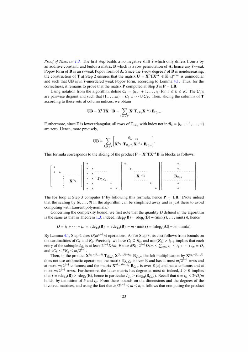
Proof of Theorem 1.3. The first step builds a nonnegative shift s which only differs from s byan additive constant, and builds a matrix B which is a row permutation of A; hence any s-weakPopov form of B is an s-weak Popov form of A. Since the s-row degree t of B is nondecreasing,the construction of T at Step 2 ensures that the matrix U = Xt TX−t ∈ K[x]m×m is unimodularand such that UB is in s-unordered weak Popov form, according to Lemma 4.1. Thus, for thecorrectness, it remains to prove that the matrix P computed at Step 3 is P = UB.

Using notation from the algorithm, define Ck = {ik−1 + 1, . . . , ik} for 1 ≤ k ≤ K. The Ck’sare pairwise disjoint and such that {1, . . . ,m} = C1 ∪ · · · ∪ CK . Then, slicing the columns of Taccording to these sets of column indices, we obtain

UB = Xt TX−t B =∑

1≤k≤K

Xt T∗,Ck X−tCk BCk ,∗.

Furthermore, since T is lower triangular, all rows of T∗,Ck with index not in Rk = {ik−1 +1, . . . ,m}are zero. Hence, more precisely,

UB =∑

1≤k≤K

[0ik−1×n

XtRk TRk ,Ck X−tCk BCk ,∗

].

This formula corresponds to the slicing of the product P = Xt TX−t B in blocks as follows:

∗

∗ ∗

XtRk

∗

∗ ∗

∗ ∗

∗ ∗ TRk ,Ck

∗ ∗ ∗

∗ ∗ ∗ ∗

∗

∗

X−tCk

∗

∗

∗

∗

BCk ,∗

∗

∗

.

The for loop at Step 3 computes P by following this formula, hence P = UB. (Note indeedthat the scaling by (θ, . . . , θ) in the algorithm can be simplified away and is just there to avoidcomputing with Laurent polynomials.)

Concerning the complexity bound, we first note that the quantity D defined in the algorithmis the same as that in Theorem 1.3; indeed, rdegs(B) = rdegs(B) − (min(s), . . . ,min(s)), hence

D = t1 + · · · + tm = |rdegs(B)| = |rdegs(B)| − m ·min(s) = |rdegs(A)| − m ·min(s).

By Lemma 4.1, Step 2 uses O(mω−1n) operations. As for Step 3, its cost follows from bounds onthe cardinalities of Ck and Rk. Precisely, we have Ck ⊆ Rk, and min(Rk) > ik−1 implies that eachentry of the subtuple tRk is at least 2k−1D/m. Hence #Rk ·2k−1D/m ≤

∑i∈Rk

ti ≤ t1 + · · ·+ tm = D,and #Ck ≤ #Rk ≤ m/2k−1.

Then, in the product XtRk−(θ,...,θ) TRk ,Ck X(θ,...,θ)−tCk BCk ,∗, the left multiplication by XtRk−(θ,...,θ)

does not use arithmetic operations; the matrix TRk ,Ck is over K and has at most m/2k−1 rows andat most m/2k−1 columns; and the matrix X(θ,...,θ)−tCk BCk ,∗ is over K[x] and has n columns and atmost m/2k−1 rows. Furthermore, the latter matrix has degree at most θ: indeed, s ≥ 0 impliesthat t = rdegs(B) ≥ rdeg0(B), hence in particular tCk ≥ rdeg0(BCk ,∗). Recall that θ = tik ≤ 2kD/mholds, by definition of θ and ik. From these bounds on the dimensions and the degrees of theinvolved matrices, and using the fact that m/2k−1 ≤ m ≤ n, it follows that computing the product

23

XtRk−(θ,...,θ) (TRk ,Ck (X(θ,...,θ)−tCk BCk ,∗)) uses O((m/2k−1)ω−1n(θ+1)) ⊆ O((m/2k−1)ω−1n(2kD/m+1))operations in K. Thus, since ω > 2, the cost of Step 3 is

O

∑1≤k≤K

( m2k−1

)ω−1n(

2kDm

+ 1) ⊆ O

mω−2nD

∑1≤k≤K

2k(2−ω)

+ mω−1n

∑1≤k≤K

2k(1−ω)

⊆ O(mω−2nD + mω−1n

).

5. Shifted forms: from weak Popov to Popov

This section culminates in Section 5.5 with the description of Algorithm WeakPopovToPopovand a proof of Theorem 1.4. Based on [42, Lem. 14] (which extends to the shifted case), the resultin Theorem 1.4 can easily be used to solve the same problem in the rectangular case with an m×nmatrix A; while this is carried out in Algorithm WeakPopovToPopov, it is out of the main scopeof this paper and thus for conciseness we only give a cost analysis in the case m = n.

Our approach is to obtain the −s-Popov form of A from a shifted reduced kernel basis ofsome matrix F built from A. This fact is substantiated in Section 5.1, which also proves that wehave precise a priori information on the degrees of this sought kernel basis.

A folklore method for kernel basis computation is to find an approximant basis at an ordersufficiently large so that it contains a kernel basis as a submatrix. More precisely, assuming weknow a list of bounds s such that there exists a basis of K(F) with column degree bounded by s,the following algorithm computes such a kernel basis which is furthermore −s-reduced:• γ← cdegs(F) + 1;• M← basis ofAγ(F) in −s-reduced form;• return the submatrix of M formed by its rows with nonpositive −s-degree.

The idea is that any row p of M is such that pF = 0 mod Xγ , and if it further satisfies cdeg(p) ≤ sthen cdeg(pF) ≤ cdegs(F) < γ, so that pF = 0 holds. Here the complexity mainly depends on|s| and |cdegs(F)|, quantities that are often large in which case the algorithm of Zhou et al. [58]is more efficient. Nevertheless there are cases, such as the one arising in this section, where bothsums are controlled, and elaborating over this approach leads to an efficient algorithm.

In order to propose Algorithm KnownDegreeKernelBasis in Section 5.4, efficiently comput-ing the kernel basis using essentially a single call to PM-Basis, we transform the input into onewith a balanced shift and a balanced order. Here and in what follows, for a nonnegative tuplet ∈ Zn

≥0, we say that t is balanced if max(t) ∈ O(|t|/n), meaning that the maximum entry in t isnot much larger than the average of all entries of t. Section 5.2 deals with the shifts by describinga transformation of the input inspired from [46, Sec. 3], allowing us to reduce to the case of ashift s whose entries are balanced. Section 5.3 deals with balancing the order γ by performingthe overlapping partial linearization of [46, Sec. 2].

For the latter transformation, as noted above, we assume that there exists a basis of the consid-ered kernel whose column degree is bounded by s, or equivalently that −s-reduced kernel baseshave nonpositive −s-row degree. On the other hand, for the first transformation we must ensurethat −s-reduced kernel bases have nonnegative −s-row degree. Thus our algorithm works underthe requirement that −s-reduced bases of K(F) have −s-row degree exactly 0, hence its name.This is a restriction compared to [56, Algo. 1] which only assumes that −s-reduced bases ofK(F)have nonpositive −s-row degree and has to perform several approximant basis computations to

24

recover the whole kernel basis, as outlined in the introduction. In short, we have managed to ex-ploit the fact that we have better a priori knowledge of degrees in kernel bases than in the contextof [56], leading to a faster kernel computation which, when used in our determinant algorithm,brings no logarithmic factor in the complexity.

5.1. Normalization via kernel basis computation

We normalize the matrix A into its −s-Popov form P using a kernel basis computation, an ap-proach already used in a context similar to ours in the non-shifted case in [42, Lem. 19]. Roughly,this stems from the fact that the identity UA = P with a unimodular U can be rewritten as

[U P

] [ A−Im

]= 0;

and that, for a well-chosen shift, one retrieves [U P] as a shifted reduced kernel basis. The nextstatement gives a choice of shift suited to our situation, and describes the degree profile of suchkernel bases. The focus on the shift −δ comes from the fact that any −δ-reduced form R of A isonly a constant transformation away from being the −s-Popov form P of A [see 26, Lem. 4.1].

Lemma 5.1. Let s ∈ Zm, let A ∈ K[x]m×m be in −s-weak Popov form, let δ ∈ Zm≥0 be the −s-

pivot degree of A, and assume that s ≥ δ. Let R be a −δ-weak Popov form of A and let U be theunimodular matrix such that UA = R. Let further d = (s−δ, δ) ∈ Z2m and F =

[A−Im

]∈ K[x]2m×m.

Then,

• the −d-pivot profile of [U R] is (m + j, δ j)1≤ j≤m,• [U R] is in −d-weak Popov form with rdeg−d([U R]) = 0 and cdeg([U R]) ≤ d,• [U R] is a basis of K(F).

Proof. First, we prove that R has −δ-pivot degree δ; note that this implies rdeg−δ(R) = 0 andcdeg(R) = δ since R is in −δ-weak Popov form. Lemma 2.5 shows that the −s-Popov formP of A has the same −s-pivot degree as A, that is, δ. Hence, by definition of Popov forms,cdeg(P) = δ. Then, [26, Lem. 4.1] states that P is also in −δ-Popov form. Since R is a −δ-weakPopov form of P, by Lemma 2.5 it has the same −δ-pivot degree as P, that is, δ.

Now, by the predictable degree property and since rdeg−s(A) = −s + δ,

rdeg−s+δ(U) = rdeg−s(UA) = rdeg−s(R) ≤ rdeg−δ(R) = 0,

where the inequality holds because −s ≤ −δ. Thus, by choice of d, the −d-pivot entries of [U R]are the −δ-pivot entries of its submatrix R; this proves the first item.

Then, the second item follows: the matrix [U R] is in −d-weak Popov form since its −d-pivot index is increasing; its −d-row degree is equal to the −δ-row degree of R which is 0; andrdeg−d([U R]) = 0 implies cdeg([U R]) ≤ d by Lemma 2.1.

Let [K1 K2] ∈ K[x]m×2m be a basisK(F) (it has m = 2m−m rows since F is 2m×m and hasrank m). Since UA = R, the rows of [U R] are in this kernel. As a result, there exists a matrixV ∈ K[x]m×m such that [U R] = V[K1 K2]. In particular, U = VK1, and since U is unimodular,this implies that V is unimodular as well. Thus, the basis [K1 K2] is unimodularly equivalent to[U R], and the latter matrix is also a basis of K(F).

One may note similarities with [27, Lem. 5.1], which is about changing the shift of reducedforms via kernel basis computations. Here, we consider A in −s-reduced form and are interested

25

in its −δ-reduced forms R: we change −s into −δ = −s + (s − δ), with a nonnegative differences − δ ≥ 0. Still, the above lemma does not follow from [27] since here the origin shift −s isnonpositive and thus we cannot directly incorporate it in the matrix F by considering AX−s .

The next corollary uses notation from Lemma 5.1 and shows how to obtain the −s-Popovform of A via a −d-reduced basis of the kernel of F. Then Sections 5.2 to 5.4 focus on theefficient computation of such a kernel basis.

Corollary 5.2. Let [U R] ∈ K[x]m×2m be a −d-reduced basis of K(F). Then, R is a −δ-reducedform of A, and P = (lm−δ(R))−1R is the −s-Popov form of A.

Proof. It suffices to prove that R is a −δ-reduced form of A; then, the conclusion follows from[26, Lem. 4.1]. Both matrices [U R] and [U R] are −d-reduced and thus have the same −d-rowdegree up to permutation. Lemma 5.1 yields rdeg−d([U R]) = 0, hence rdeg−d([U R]) = 0. Inparticular, since −d = (δ − s,−δ), we have rdeg−δ(R) ≤ 0.

We conclude by applying Lemma 2.3 to the row space of A, which has rank m, and whichhas a basis R in −δ-reduced form with −δ-row degree 0. From UA = R, we obtain that the rowsof R are in this row space. This identity also implies that R has rank m, otherwise there wouldexist a nonzero vector in the left kernel of R, which would also be in the left kernel of U sinceA is nonsingular, hence it would be in the left kernel of the full row rank matrix [U R]. Theassumptions of the lemma are satisfied, and thus R is a −δ-reduced form of A.

5.2. Reducing to the case of balanced pivot degree

Here, we show that the output column partial linearization, used previously in algorithms forapproximant bases and generalizations of them [46, Sec. 3], [55, 26], can be applied to kernelcomputations when the sought kernel basis has nonnegative shifted row degree. The main effectof this transformation is to make the shift and output degrees more balanced, while preservingmost other properties of (s,F). The transformation itself, defined below, is essentially a column-wise xδ-adic expansion for a well-chosen integer parameter δ.

Definition 5.3. Let s = (s1, . . . , sm) ∈ Zm≥0, and let δ ∈ Z>0. For 1 ≤ j ≤ m, write s j =

(α j − 1)δ + β j with α j = ds j/δe and 1 ≤ β j ≤ δ if s j , 0, and α j = 1 and β j = 0 if s j = 0. Definem = α1 + · · · + αm, and the expansion-compression matrix E ∈ K[x]m×m as

E =

1xδ...

x(α1−1)δ

. . .

1xδ...

x(αm−1)δ

.

Define alsos = ( δ, . . . , δ, β1︸ ︷︷ ︸

α1

, . . . , δ, . . . , δ, βm︸ ︷︷ ︸αm

) ∈ Zm≥0.

In this context, for a matrix K ∈ K[x]k×m, we define the column partial linearization of K as theunique matrix K ∈ K[x]k×m such that K = KE and all the columns of K whose index is not in{α1 + · · · + α j, 1 ≤ j ≤ m} have degree less than δ.

26

We use the notation in this definition in all of Section 5.2. More explicitly, K = [K1 · · · Km]where K j ∈ K[x]k×α j is the unique matrix such that

K∗, j = K j

1xδ...

x(α j−1)δ

and the first α j − 1 columns of K j have degree less than δ.

This construction originates from [46, Sec. 3], where it was designed for approximant basiscomputations, in order to make the shift more balanced at the cost of a small increase of thedimension; this is stated in Lemma 5.4. As mentioned above, several slightly different versionsof this column partial linearization have been given in the literature: each version requires someminor adaptations of the original construction to match the context. Here, in order to benefit fromproperties proved in [28, Sec. 5.1], we follow the construction in [28, Lem. 5.2]: one can checkthat Definition 5.3 is a specialization of the construction in that reference, for the shift −s ∈ Zm

≤0and taking the second parameter to be t = max(−s) so that t = −s −max(−s) + t = −s.

Lemma 5.4. The entries of s are in {0, 1, . . . , δ}. Furthermore, if δ ≥ |s|/m, then m ≤ m ≤ 2m.

Proof. The first remark is obvious. For the second one, note that 1 ≤ α j ≤ 1 + s j/δ holds byconstruction, for 1 ≤ j ≤ m. Hence m ≤ m ≤ m + |s|/δ ≤ 2m.

Importantly, this column partial linearization behaves well with respect to shifted row degreesand shifted reduced forms.

Lemma 5.5. Let K ∈ K[x]k×m with rdeg−s(K) ≥ 0, and let K ∈ K[x]k×m be its column partiallinearization. Then, row degrees are preserved: rdeg−s(K) = rdeg−s(K). Furthermore, if K is in−s-weak Popov form, then K is in −s-weak Popov form.

Proof. We show that this follows from the second item in [28, Lem. 5.2]; as noted above, theshift t = (t1, . . . , tm) in that reference corresponds to −s = (−s1, . . . ,−sm) here. Let (πi, δi)1≤i≤k

denote the −s-pivot profile of K. By definition of the −s-pivot index and degree, rdeg−s(K) =

(δi − sπi )1≤i≤k, hence our assumption rdeg−s(K) ≥ 0 means that δi ≥ sπi for 1 ≤ i ≤ k. Thus, wecan apply [28, Lem. 5.2] to each row of K, from which we conclude that K has −s-pivot profile(α1 + · · · + απi , δi − sπi + βπi )1≤i≤k.

First, since the entry of −s at index α1 + · · · + απi is −βπi , this implies that

rdeg−s(K) = (δi − sπi + βπi − βπi )1≤i≤k = (δi − sπi )1≤i≤k = rdeg−s(K).

Furthermore, if K is in −s-weak Popov form, then (πi)1≤i≤k is increasing, hence (α1+· · ·+απi )1≤i≤k

is increasing as well and K is in −s-weak Popov form.

Remark 5.6. One may further note the following properties:

• Writing lm−s(K) = [L∗,1 · · · L∗,m] ∈ Kk×m, we have

lm−s(K) = [ 0 · · · 0 L∗,1︸ ︷︷ ︸α1

· · · 0 · · · 0 L∗,m︸ ︷︷ ︸αm

] ∈ Kk×m.

27

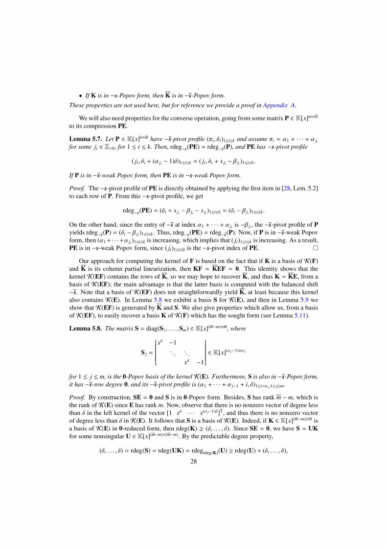
• If K is in −s-Popov form, then K is in −s-Popov form.

These properties are not used here, but for reference we provide a proof in Appendix A.

We will also need properties for the converse operation, going from some matrix P ∈ K[x]m×m

to its compression PE.

Lemma 5.7. Let P ∈ K[x]k×m have −s-pivot profile (πi, δi)1≤i≤k and assume πi = α1 + · · · + α jifor some ji ∈ Z>0, for 1 ≤ i ≤ k. Then, rdeg−s(PE) = rdeg−s(P), and PE has −s-pivot profile

( ji, δi + (α ji − 1)δ)1≤i≤k = ( ji, δi + s ji − β ji )1≤i≤k.

If P is in −s-weak Popov form, then PE is in −s-weak Popov form.

Proof. The −s-pivot profile of PE is directly obtained by applying the first item in [28, Lem. 5.2]to each row of P. From this −s-pivot profile, we get

rdeg−s(PE) = (δi + s ji − β ji − s ji )1≤i≤k = (δi − β ji )1≤i≤k.

On the other hand, since the entry of −s at index α1 + · · · + α ji is −β ji , the −s-pivot profile of Pyields rdeg−s(P) = (δi − β ji )1≤i≤k. Thus, rdeg−s(PE) = rdeg−s(P). Now, if P is in −s-weak Popovform, then (α1 + · · ·+α ji )1≤i≤k is increasing, which implies that ( ji)1≤i≤k is increasing. As a result,PE is in −s-weak Popov form, since ( ji)1≤i≤k is the −s-pivot index of PE.

Our approach for computing the kernel of F is based on the fact that if K is a basis of K(F)and K is its column partial linearization, then KF = KEF = 0. This identity shows that thekernel K(EF) contains the rows of K, so we may hope to recover K, and thus K = KE, from abasis of K(EF); the main advantage is that the latter basis is computed with the balanced shift−s. Note that a basis of K(EF) does not straightforwardly yield K, at least because this kernelalso contains K(E). In Lemma 5.8 we exhibit a basis S for K(E), and then in Lemma 5.9 weshow that K(EF) is generated by K and S. We also give properties which allow us, from a basisof K(EF), to easily recover a basis K of K(F) which has the sought form (see Lemma 5.11).

Lemma 5.8. The matrix S = diag(S1, . . . ,Sm) ∈ K[x](m−m)×m, where

S j =

xδ −1

. . .. . .

xδ −1

∈ K[x](α j−1)×α j

for 1 ≤ j ≤ m, is the 0-Popov basis of the kernelK(E). Furthermore, S is also in −s-Popov form,it has −s-row degree 0, and its −s-pivot profile is (α1 + · · · + α j−1 + i, δ)1≤i<α j,1≤ j≤m.

Proof. By construction, SE = 0 and S is in 0-Popov form. Besides, S has rank m − m, which isthe rank ofK(E) since E has rank m. Now, observe that there is no nonzero vector of degree lessthan δ in the left kernel of the vector [1 xδ · · · x(α j−1)δ]T, and thus there is no nonzero vectorof degree less than δ in K(E). It follows that S is a basis of K(E). Indeed, if K ∈ K[x](m−m)×m isa basis of K(E) in 0-reduced form, then rdeg(K) ≥ (δ, . . . , δ). Since SE = 0, we have S = UKfor some nonsingular U ∈ K[x](m−m)×(m−m). By the predictable degree property,

(δ, . . . , δ) = rdeg(S) = rdeg(UK) = rdegrdeg(K)(U) ≥ rdeg(U) + (δ, . . . , δ),

28

hence U is constant. Thus U is unimodular, and S is a basis of K(E).Now consider j such that α j > 1, and write t = (−δ, . . . ,−δ,−β j) ∈ Zα j . Then, the definition

of α j and β j, notably the fact that −β j < 0, ensures that S j is in t-Popov form with t-pivot degree(δ, . . . , δ) and t-pivot index (1, . . . , α j − 1). The conclusion about S follows.

Lemma 5.9. Let F ∈ K[x]m×n. The following properties hold.

(i) Column degrees are preserved: cdegs(EF) = cdegs(F).(ii) The kernels of F and EF are related by K(EF)E = K(F).

(iii) Let K ∈ K[x]k×m be a basis of K(F) (hence k = m − rank(F)), and let K ∈ K[x]k×m be anymatrix such that K = KE. Then,

B =

[KS

]∈ K[x](k+m−m)×m (5)

is a basis of K(EF), where S is the matrix defined in Lemma 5.8.(iv) Assume that rdeg−s(K) ≥ 0 and that K is the column partial linearization of K. Then,

rdeg−s(B) = (rdeg−s(K), 0), and if K is in −s-weak Popov form, then B is in −s-unorderedweak Popov form.

Proof. (i) By definition, cdegs(EF) = cdeg(Xs EF) and cdegs(F) = cdeg(Xs F). Since the matrix

Xs E =

Xδ

...X(α1−1)δ

Xs1

. . .Xδ

...X(αm−1)δ

Xsm

has column degree s and contains Xs as a subset of its rows, we get cdeg(Xs EF) = cdeg(Xs F).

(ii) For any vector p ∈ K(EF), we have pEF = 0, which means pE ∈ K(F). Conversely,from any p ∈ K(F) we can construct q ∈ K[x]1×m such that qE = p since E has the identity as asubset of its rows; then, qEF = pF = 0, which means q ∈ K(EF).

(iii) We recall that, by Lemma 5.8, S is a basis of K(E). The rows of B are in K(EF), sinceSEF = 0 and KEF = KF = 0. Now, we want to prove that any u ∈ K(EF) is a K[x]-linearcombination of the rows of B. By Item (ii), uE ∈ K(F); thus uE = vK = vKE for somev ∈ K[x]1×k. Therefore u − vK ∈ K(E), and it follows that u − vK = wS for some w ∈ K[x]1×m.This yields u = [v w]B.

(iv) Since rdeg−s(K) ≥ 0, we can apply Lemma 5.5, which yields rdeg−s(K) = rdeg−s(K),hence rdeg−s(B) = (rdeg−s(K), 0). Now, if K is in −s-weak Popov form, then Lemma 5.5 showsthat K is in −s-weak Popov form and that all entries of its −s-pivot index are in {α1 + · · ·+αi, 1 ≤i ≤ m}. Besides, by Lemma 5.8, S is in −s-Popov form with a −s-pivot index which is disjointfrom {α1 + · · · + αi, 1 ≤ i ≤ m}. Hence B is in −s-unordered weak Popov form.

Remark 5.10. Similarly to Item (iv), one may observe that if K is in −s-reduced form, then Bis in −s-reduced form; and that if K is in −s-Popov form, then B is in −s-Popov form up to rowpermutation. These points will not be used here; for reference a proof is given in Appendix A.

29

Finally, we combine the above results to show that one can compute a basis of K(F) bycomputing a −s-weak Popov basis of K(EF) and taking a submatrix of it.

Lemma 5.11. Let F ∈ K[x]m×n and let r = m − rank(F) be the rank of K(EF). Assume that−s-reduced bases of K(F) have nonnegative −s-row degree. Let Q ∈ K[x]r×m be a −s-weakPopov basis of K(EF). Let P ∈ K[x]k×m be the submatrix of the rows of Q whose −s-pivot indexis in {α1 + · · · + α j, 1 ≤ j ≤ m}. Then, PE is a −s-weak Popov basis of K(F).

Proof. We first prove that the number of rows of PE is the rank ofK(F), that is, k = m− rank(F).Indeed, by Item (iv) of Lemma 5.9, the −s-pivot index of the −s-Popov basis of K(EF) containsthe −s-pivot index of S. By Lemma 5.8, the latter is the tuple formed by the integers in the set{1, . . . ,m} \ {α1 + · · · + α j, 1 ≤ j ≤ m} sorted in increasing order. Since P is the submatrix of therows of Q whose −s-pivot index is not in this set, P has k = r − (m − m) = m − rank(F) rows.

Now, by construction, P is in −s-weak Popov form and its −s-pivot index has entries in{α1 + · · ·+αi, 1 ≤ i ≤ m}. Thus we can apply Lemma 5.7; it ensures that PE is in −s-weak Popovform and that rdeg−s(PE) = rdeg−s(P).

It remains to prove that PE is a basis of K(F). Let K ∈ Kk×m be the −s-Popov basis ofK(F), and let K ∈ Kk×m be its column partial linearization. Let d = rdeg−s(K), which hasnonnegative entries by assumption. Then, according to Lemma 5.5, K is in −s-weak Popov form,and rdeg−s(K) = d. Then, we define B ∈ K(k+m−m)×m as in Eq. (5); by Item (iv) of Lemma 5.9,the matrix B is a −s-unordered weak Popov basis of K(EF).

Then, Lemma 2.5 shows that Q has the same −s-pivot profile as the row permutation of Bwhich is in −s-weak Popov form. Since P (resp. K) is the submatrix of the rows of Q (resp. B)whose −s-pivot index is in {α1 + · · · + α j, 1 ≤ j ≤ m}, and since both P and K are in −s-weakPopov form, it follows that P and K have the same −s-pivot profile. In particular, we haverdeg−s(P) = rdeg−s(K) = d, from which we get rdeg−s(PE) = d. According to Lemma 2.3, sincethe rows of PE are in K(F), this implies that PE is a basis of K(F).

5.3. Reducing to the case of a balanced orderNow we apply the overlapping partial linearization of [46, Sec. 2], more precisely the version

in [28, Sec. 5.2] which supports arbitrary γ as showed in the definition below that we recall forcompleteness. In the next lemma, we will show that the sought kernel basis can be retrieved as asubmatrix of an approximant basis for the transformed problem.

Definition 5.12 ([46, 28]). Let γ = (γ1, . . . , γn) ∈ Zn>0, let F ∈ K[x]m×n with cdeg(F) < γ, and

let µ ∈ Z>0. Then, for 1 ≤ i ≤ n, let γi = αiµ + βi with αi =⌈γiµ− 1

⌉and 1 ≤ βi ≤ µ. Let also

n = max(α1 − 1, 0) + · · · + max(αn − 1, 0), and define

Lµ(γ) = (γ1, . . . , γn) ∈ Zn+n>0 ,

where γi = (2µ, . . . , 2µ, µ+βi) ∈ Zαi>0 if αi > 1 and γi = γi otherwise. Considering the ith column

of F, we write its xµ-adic representation as

F∗,i = F(0)∗,i + F(1)

∗,i xµ + · · · + F(αi)∗,i xαiµ

where cdeg([F(0)∗,i F(1)

∗,i · · · F(αi)∗,i ]) < (µ, . . . , µ, βi).

If αi > 1, we define

F∗,i =[F(0)∗,i + F(1)

∗,i xµ F(1)∗,i + F(2)

∗,i xµ · · · F(αi−1)∗,i + F(αi)

∗,i xµ]∈ K[x]m×αi

30

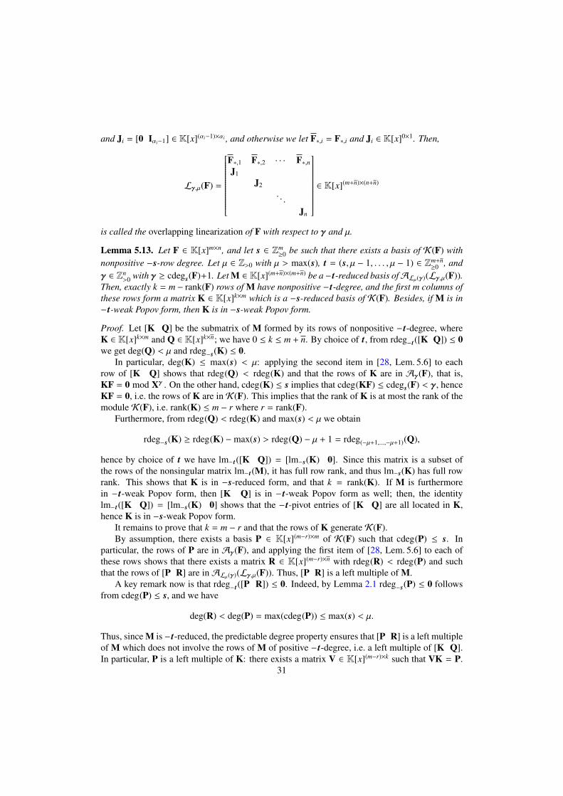
and Ji = [0 Iαi−1] ∈ K[x](αi−1)×αi , and otherwise we let F∗,i = F∗,i and Ji ∈ K[x]0×1. Then,

Lγ,µ(F) =

F∗,1 F∗,2 · · · F∗,nJ1

J2. . .

Jn

∈ K[x](m+n)×(n+n)

is called the overlapping linearization of F with respect to γ and µ.

Lemma 5.13. Let F ∈ K[x]m×n, and let s ∈ Zm≥0 be such that there exists a basis of K(F) with

nonpositive −s-row degree. Let µ ∈ Z>0 with µ > max(s), t = (s, µ − 1, . . . , µ − 1) ∈ Zm+n≥0 , and

γ ∈ Zn>0 with γ ≥ cdegs(F)+1. Let M ∈ K[x](m+n)×(m+n) be a −t-reduced basis ofALµ(γ)(Lγ,µ(F)).

Then, exactly k = m − rank(F) rows of M have nonpositive −t-degree, and the first m columns ofthese rows form a matrix K ∈ K[x]k×m which is a −s-reduced basis of K(F). Besides, if M is in−t-weak Popov form, then K is in −s-weak Popov form.

Proof. Let [K Q] be the submatrix of M formed by its rows of nonpositive −t-degree, whereK ∈ K[x]k×m and Q ∈ K[x]k×n; we have 0 ≤ k ≤ m + n. By choice of t, from rdeg−t([K Q]) ≤ 0we get deg(Q) < µ and rdeg−s(K) ≤ 0.

In particular, deg(K) ≤ max(s) < µ: applying the second item in [28, Lem. 5.6] to eachrow of [K Q] shows that rdeg(Q) < rdeg(K) and that the rows of K are in Aγ(F), that is,KF = 0 mod Xγ . On the other hand, cdeg(K) ≤ s implies that cdeg(KF) ≤ cdegs(F) < γ, henceKF = 0, i.e. the rows of K are in K(F). This implies that the rank of K is at most the rank of themodule K(F), i.e. rank(K) ≤ m − r where r = rank(F).

Furthermore, from rdeg(Q) < rdeg(K) and max(s) < µ we obtain

rdeg−s(K) ≥ rdeg(K) −max(s) > rdeg(Q) − µ + 1 = rdeg(−µ+1,...,−µ+1)(Q),

hence by choice of t we have lm−t([K Q]) = [lm−s(K) 0]. Since this matrix is a subset ofthe rows of the nonsingular matrix lm−t(M), it has full row rank, and thus lm−s(K) has full rowrank. This shows that K is in −s-reduced form, and that k = rank(K). If M is furthermorein −t-weak Popov form, then [K Q] is in −t-weak Popov form as well; then, the identitylm−t([K Q]) = [lm−s(K) 0] shows that the −t-pivot entries of [K Q] are all located in K,hence K is in −s-weak Popov form.

It remains to prove that k = m − r and that the rows of K generate K(F).By assumption, there exists a basis P ∈ K[x](m−r)×m of K(F) such that cdeg(P) ≤ s. In

particular, the rows of P are in Aγ(F), and applying the first item of [28, Lem. 5.6] to each ofthese rows shows that there exists a matrix R ∈ K[x](m−r)×n with rdeg(R) < rdeg(P) and suchthat the rows of [P R] are inALµ(γ)(Lγ,µ(F)). Thus, [P R] is a left multiple of M.

A key remark now is that rdeg−t([P R]) ≤ 0. Indeed, by Lemma 2.1 rdeg−s(P) ≤ 0 followsfrom cdeg(P) ≤ s, and we have

deg(R) < deg(P) = max(cdeg(P)) ≤ max(s) < µ.

Thus, since M is −t-reduced, the predictable degree property ensures that [P R] is a left multipleof M which does not involve the rows of M of positive −t-degree, i.e. a left multiple of [K Q].In particular, P is a left multiple of K: there exists a matrix V ∈ K[x](m−r)×k such that VK = P.

31

Since P has rank m − r, we obtain k ≥ m − r, hence k = m − r. On the other hand, since therows of K are in K(F), there exists a matrix W ∈ K[x]k×k such that WP = K. It follows thatP = VWP, and since P has full row rank this implies VW = Ik. This means that P and K are leftunimodularly equivalent, hence K is a basis of K(F), which concludes the proof.

5.4. Computing kernel bases with known pivot degree

After applying the transformations presented in Sections 5.2 and 5.3, we are left with thecomputation of an approximant basis for a balanced order Lµ(γ) and a balanced shift −s: this isdone efficiently by PM-Basis, designed in [21] as an improvement of [3, Algo. SPHPS]. Here,we use the version in [28, Algo. 2] which ensures that the output basis is in −s-weak Popov form.

Algorithm 4 KnownDegreeKernelBasis(F, s)Input: a matrix F ∈ K[x]m×n, and a nonnegative shift s ∈ Zm

≥0.Requirement: −s-reduced bases of K(F) have −s-row degree 0.Output: a −s-weak Popov basis of K(F).

1: . Step 1: Output column partial linearization /2: δ← dD/me ∈ Z>0, where D = max(|s|, |cdegs(F)|, 1)3: Apply Definition 5.3 to (s, δ) to obtain the parameters and expansion-compression matrix:

(α1, . . . , αm) ∈ Zm>0, m ∈ Z>0, s ∈ Zm

≥0, E ∈ K[x]m×m

4: . Step 2: Overlapping partial linearization /5: γ← cdegs(F) + 1 ∈ Zn

>0 . order for approximation, equal to cdegs(EF) + 16: Apply Definition 5.12 to (γ,EF, δ + 1) to obtain the order Lδ+1(γ) ∈ Zn+n

>0 and the matrixLγ,δ+1(EF) ∈ K[x](m+n)×(n+n)

7: . Step 3: Compute −t-weak Popov basis ofALδ+1(γ)(Lγ,δ+1(EF)) /8: t ← (s, δ, . . . , δ) ∈ Zm+n

≥09: Γ← max(Lδ+1(γ)); G = Lγ,δ+1(EF)X(Γ,...,Γ)−Lδ+1(γ) . use uniform order (Γ, . . . ,Γ)

10: M ∈ K[x](m+n)×(m+n) ← PM-Basis(Γ,G,−t)11: . Step 4: Deduce first −s-weak Popov basis of K(EF), then −s-weak Popov basis of K(F) /

12: Q ∈ K[x]k×m ← first m columns of the rows of M which have nonpositive −t-degree13: P ∈ K[x]k×m ← the rows of Q whose −s-pivot index is in {α1 + · · · + α j, 1 ≤ j ≤ m}14: return PE

Proposition 5.14. Algorithm 4 is correct. Let D = max(|s|, |cdegs(F)|, 1). Then, assuming m ≥ nand using notation from the algorithm, its cost is bounded by the sum of:

• the cost of performing PM-Basis at order at most 2dD/me + 2 on an input matrix of rowdimension m + n ≤ 3m and column dimension n + n ≤ 2m;• O(m2) extra operations in K.

Thus, Algorithm 4 uses O(mω M′(D/m)) operations in K.

Proof. Using the assumption that −s-reduced bases of K(F) have −s-row degree 0 along withItem (iv) of Lemma 5.9 shows that the −s-reduced bases of K(EF) have −s-row degree 0. Thus,we can apply Lemma 5.13 to (EF, s, µ,γ) with µ = δ + 1 > max(s) and γ = cdegs(EF) + 1,which is γ = cdegs(F) + 1 according to Item (i) of Lemma 5.9. Note that M is a −t-weak Popovbasis ofA(Γ,...,Γ)(G) = ALδ+1(γ)(Lγ,δ+1(EF)) (see e.g. [28, Rmk. 3.3] for this approach to make theorder uniform). Then, Lemma 5.13 states that the matrix Q at Line 12 has k = m − rank(EF) =

32

m − rank(F) rows and is a −s-weak Popov basis of K(EF). Then, by Lemma 5.11, PE is a−s-weak Popov basis of K(F), hence the correctness.

For the cost analysis, we assume m ≥ n, and we start by summarizing bounds on the dimen-sions and degrees at play. Lemma 5.4 yields m ≤ m ≤ 2m, while Item (i) of Lemma 5.9 ensurescdegs(EF) = cdegs(F). Each entry of Lδ+1(γ) is at most 2(δ+ 1) = 2dD/me+ 2, by construction.Writing γ = (γ1, . . . , γn), by Definition 5.12 we have

n = max(⌈

γ1

δ + 1− 1

⌉, 0

)+ · · · + max

(⌈γn

δ + 1− 1

⌉, 0

)≤

γ1

δ + 1+ · · · +

γn

δ + 1=|γ|

δ + 1.

Since |γ| = |cdegs(F)| + n ≤ D + m, and since δ + 1 ≥ (D + m)/m, it follows that n ≤ m. Besides,rdeg−s(P) ≤ 0 by construction, so that cdeg(P) ≤ s by Lemma 2.1.

The only steps that involve operations in K are the call to PM-Basis at Line 10 and themultiplication PE at Line 14. The construction of E and the inequality cdeg(P) ≤ s imply thatthe product PE mainly involves concatenating vectors of coefficients; concerning operations inK, there are m − m columns of P for which we may add the constant term of that column tothe term of degree δ of the previous column. Therefore Line 14 has cost bound O(mk); sincem ≤ 2m and k ≤ m this is in O(m2). At Line 10, we call the approximant basis subroutine PM-Basis discussed in Section 2.5; since Γ = max(Lδ+1(γ)) is at most 2dD/me + 2 ∈ O(1 + D/m),Lemma 2.9 states that this call uses

O((m + n + n + n)(m + n)ω−1 M′(D/m)

)operations in K. Since n + n ≤ m + n ≤ 3m, this yields the claimed cost bound.

5.5. Proof of Theorem 1.4

Algorithm 5 WeakPopovToPopov(A, s)Input: a matrix A ∈ K[x]m×n, a shift s ∈ Zn such that A is in −s-weak Popov form.Requirement: sπ ≥ δ, where (π, δ) is the −s-pivot profile of A.Output: the −s-Popov form of A.

1: . Step 1: Find unimodular transformation and −δ-reduced form of A∗,π /2: (π, δ)← the −s-pivot profile of A

3: [U R] ∈ K[x]m×2m ← KnownDegreeKernelBasis([

A∗,π−Im

], (sπ − δ, δ)

)4: . Step 2: Deduce −s-Popov form of A /5: P← zero matrix in K[x]m×n

6: P∗,π ← lm−δ(R)−1R7: P∗,{1,...,n}\π ← lm−δ(R)−1U A∗,{1,...,n}\π8: return P

For proving Theorem 1.4, we describe Algorithm WeakPopovToPopov (Algorithm 5) and wefocus on the square case, m = n. Then, by definition of the −s-weak Popov form, δ is the tupleof degrees of the diagonal entries of A, and π = (1, . . . ,m). Furthermore, in this case, sπ = s,A∗,π = A, and P∗,π = P; in particular, we can discard the step at Line 7 since the submatrices itinvolves are empty.

First note that the shift d = (sπ − δ, δ) = (s − δ, δ) used at Line 3 is nonnegative. Besides,Lemma 5.1 shows that −d-reduced bases of K(F) have −d-row degree 0. Thus the requirements

33

of Algorithm KnownDegreeKernelBasis are met, and Proposition 5.14 shows that the matrix[U R] computed at Line 3 is a −d-weak Popov basis of K(F). Then, Corollary 5.2 shows thatthe matrix P = P∗,π = lm−δ(R)−1R computed at Line 6 is the −s-Popov form of A. This provesthat Algorithm 5 is correct.

Concerning the cost bound, we focus on the case |s| > 0. Indeed, since s ≥ δ ≥ 0, if |s| = 0,then s = δ = 0. In this case, no computation needs to be done: the −s-Popov form of A is Im, theunique matrix in Popov form whose pivot degree is 0.

The cost of Line 6 is that of multiplying lm−δ(R)−1 ∈ Km×m by R ∈ K[x]m×m, which hascolumn degree δ as explained in Section 5.1; this computation corresponds to the second item inTheorem 1.4. This multiplication can be done by first performing a column linearization of Rinto a m × (m + |δ|) matrix R over K, computing lm−δ(R)−1R, and finally compressing the resultback into a polynomial matrix. This uses O(mω(1 + |δ|/m)) operations in K.

Concerning Line 3, we rely on Proposition 5.14. Here, the matrix we give as input to Al-gorithm KnownDegreeKernelBasis has dimensions 2m × m, hence the dimensions in Proposi-tion 5.14 satisfy m ≤ 4m and n ≤ 2m (the latter bound comes from the proof of that proposition).Then, Proposition 5.14 states that Line 3 costs:• O(m2) operations in K, which is the third item in Theorem 1.4,• one call to PM-Basis on a matrix of row dimension m + n ≤ 6m, column dimension

m + n ≤ 3m, and at order at most 2dD/(2m)e + 2, where D = max(|d|, |cdegd(F)|, 1) and Fis the input matrix [AT − Im]T.

Besides, Proposition 5.14 also implies that Line 3 uses O(mω M′(D/m)) operations in K.We are going to prove that D = |s|, which concludes the proof. Indeed, the previous paragraph

then directly gives the overall cost bound O(mω M′(|s|/m)) in Theorem 1.4, and using

2⌈ D2m

⌉+ 2 < 2

( D2m

+ 1)

+ 2 = |s|/m + 4,

the previous paragraph also gives the first item in that theorem.To observe that D = |s|, we first use the definition of d to obtain |d| = |s − δ| + |δ| = |s|.

Since |s| ≥ 1, this gives D = max(|s|, |cdegd(F)|). Now, cdegd(F) is the entry-wise maximum ofcdegs−δ(A) and cdegδ(−Im) = δ. Since A is in −s-row reduced form with rdeg−s(A) = −s + δ,Lemma 3.2 ensures that AT is in s − δ-reduced form with cdegs−δ(A) = rdegs−δ(AT) = s. Then,since s ≥ δ we obtain cdegd(F) = s, and thus D = |s|. This concludes the proof of Theorem 1.4.

As for the rectangular case m < n, the correctness of Algorithm 5 follows from the aboveproof in the square case, which shows that the algorithm correctly computes the −sπ-Popov formP∗,π of A∗,π, and from [37, Lem. 5.1] concerning the computation of P∗,{1,...,n}\π and the fact thatlm−δ(R)−1U is the unimodular matrix which transforms A into P. The cost bound can be derivedusing the degree bounds on rectangular shifted Popov forms given in [5, 37] (we do not detailthis here since this would add technical material unrelated to the main results of this article).

Appendix A.

In this appendix, we give proofs for Remarks 5.6 and 5.10. We use notation from Section 5.2:a shift s ∈ Zm

≥0, an integer δ ∈ Z>0, and a matrix F ∈ K[x]m×n are given; K ∈ K[x]k×m is abasis of K(F); (α j, β j)1≤ j≤m and s ∈ Zm

≥0 and K ∈ K[x]k×m are as described in Definition 5.3.Following the context of Remarks 5.6 and 5.10, we assume rdeg−s(K) ≥ 0, hence in particularrdeg−s(K) = rdeg−s(K) (see Lemma 5.5). We start with the claims in Remark 5.6.

34

Lemma A.1. Writing lm−s(K) = [L∗,1 · · · L∗,m] ∈ Kk×m, we have

lm−s(K) = [ 0 · · · 0 L∗,1︸ ︷︷ ︸α1

· · · 0 · · · 0 L∗,m︸ ︷︷ ︸αm

] ∈ Kk×m.

If K is in −s-Popov form, then K is in −s-Popov form.

Proof. For given i ∈ {1, . . . , k} and j ∈ {1, . . . ,m}, we rely on the definition of a leading matrix(see Section 2.3): the entry (i, j) of lm−s(K) is the coefficient of degree di + s j of Ki, j, wheredi = rdeg−s(Ki,∗) = rdeg−s(Ki,∗) ≥ 0. First consider the case j < {α1 + · · · + απ, 1 ≤ π ≤ m}.Then the jth entry of s is s j = δ, and by definition of the output column partial linearization Ki, j

has degree less than δ, hence its coefficient of degree di + δ ≥ δ must be zero. This proves thatall columns of lm−s(K) with index not in {α1 + · · · + απ, 1 ≤ π ≤ m} are indeed zero. It remainsto prove that in the case j = α1 + · · · + απ for some 1 ≤ π ≤ m, then the entry (i, j) of lm−s(K)is equal to Li,π. This holds, since in this case we have s j = βπ, and by construction of K thecoefficient of degree di +βπ of Ki, j is equal to the coefficient of degree di + (απ−1)δ+βπ = di + sπof Ki,π, which itself is equal to Li,π by definition of a leading matrix.

Now assume K is in −s-Popov form. We have showed in Lemma 5.5 that K is in −s-weakPopov form and that the row Ki,∗ has its −s-pivot at index α1 + · · · + απi where πi is the −s-pivotindex of Ki,∗. By construction, the column K∗,α1+···+απi

is the part of nonnegative degree of thecolumn x−(απi−1)δK∗,πi = x−sπi +βi K∗,πi . It follows first that the −s-pivot entry Ki,α1+···+απi

is monicsince it is a high degree part of the (monic) −s-pivot entry Ki,πi ; and second that Ki,α1+···+απi

hasdegree strictly larger than all other entries in the column K∗,α1+···+απi

since Ki,πi has degree strictlylarger than all other entries in the column K∗,πi . Hence K is in −s-Popov form.

Now we prove the claims in Remark 5.10 concerning variants of Item (iv) of Lemma 5.9,using further notation from Section 5.2: S is the basis of K(E) described in Lemma 5.8 and B =

[ KS ] ∈ K[x](k+m−m)×m is the basis ofK(EF) given in Eq. (5). As above we assume rdeg−s(K) ≥ 0,

and therefore rdeg−s(B) = (rdeg−s(K), 0) as stated in Item (iv) of Lemma 5.9.

Lemma A.2. With the above notation and assumptions,

• If K is in −s-reduced form, then B is in −s-reduced form.• If K is in −s-Popov form, then B is in −s-Popov form up to row permutation.

Proof. Suppose first that K is in −s-reduced form. We apply Lemma A.1:

lm−s(K) = [ 0 · · · 0 L∗,1 · · · 0 · · · 0 L∗,m]

where lm−s(K) = [L∗,1 · · · L∗,m] ∈ Kk×m. The latter matrix has full rank, since K is in−s-reduced form. On the other hand, for matrices such as the diagonal blocks of S we have

lm(−δ,...,−δ,−β)

xδ −1

. . .. . .

xδ −1

=

1 0

. . .. . .

1 0

35

for any integer β ≥ 1. As a result,

lm−s(B) =

[lm−s(K)lm−s(S)

]=

| |

L∗,1 · · · L∗,m| |

1. . .

1. . .

1. . .

1

has full rank as well, which means that B is in −s-reduced form.

Now, assume further that K is in −s-Popov form. Then Lemma A.1 states that K is in −s-Popov form, and the above description of lm−s(B) shows that K and S have disjoint −s-pivotindices, and that all their −s-pivots are monic. Hence B is in −s-unordered weak Popov formwith monic −s-pivots. It remains to show that each of these −s-pivots has degree strictly largerthan the other entries in the same column. Each row of the submatrix S of B has −s-pivot entryxδ and the other entries in the same column of B are either −1, which has degree 0 < δ, or are ina column of K whose index is not in {α1 + · · · + α j, 1 ≤ j ≤ m}, which has degree less than δ bydefinition of the column partial linearization. The jth row of the submatrix K of B has −s-pivotindex α1 + · · · + α j and strictly positive −s-pivot degree since rdeg−s(K) ≥ 0 and the entry of −sat index α1 + · · ·+α j is −β j < 0. This concludes the proof since the column S∗,α1+···+α j has degree0, and since K is in −s-Popov form.

References

[1] Abdeljaoued, J., Malaschonok, G.I., 2001. Efficient algorithms for computing the characteristic polynomial in adomain. Journal of Pure and Applied Algebra 156, 127–145. doi:10.1016/S0022-4049(99)00158-9.

[2] Baur, W., Strassen, V., 1983. The complexity of partial derivatives. Theoretical computer science 22, 317–330.doi:10.1016/0304-3975(83)90110-X.

[3] Beckermann, B., Labahn, G., 1994. A uniform approach for the fast computation of matrix-type Pade approximants.SIAM J. Matrix Anal. Appl. 15, 804–823. doi:10.1137/S0895479892230031.

[4] Beckermann, B., Labahn, G., Villard, G., 1999. Shifted normal forms of polynomial matrices, in: ISSAC’99,ACM. pp. 189–196. doi:10.1145/309831.309929.

[5] Beckermann, B., Labahn, G., Villard, G., 2006. Normal forms for general polynomial matrices. J. SymbolicComput. 41, 708–737. doi:10.1016/j.jsc.2006.02.001.

[6] Berkowitz, S.J., 1984. On computing the determinant in small parallel time using a small number of processors.Information Processing Letters 18, 147–150. doi:10.1016/0020-0190(84)90018-8.

[7] Bunch, J.R., Hopcroft, J.E., 1974. Triangular factorization and inversion by fast matrix multiplication. Mathematicsof Computation 28, 231–236. doi:10.2307/2005828.

[8] Burgisser, P., Clausen, M., Shokrollahi, A., 1997. Algebraic Complexity Theory. 1st ed., Springer-Verlag BerlinHeidelberg. doi:10.1007/978-3-662-03338-8.

[9] Cantor, D.G., Kaltofen, E., 1991. On fast multiplication of polynomials over arbitrary algebras. Acta Inform. 28,693–701. doi:10.1007/BF01178683.

[10] Cook, S.A., 1966. On the minimum computation time of functions. Ph.D. thesis.[11] Csanky, L., 1975. Fast parallel matrix inversion algorithms, in: 16th Annual Symposium on Foundations of

Computer Science (sfcs 1975), pp. 11–12. doi:10.1109/SFCS.1975.14.[12] Danilevskij, A.M., 1937. The numerical solution of the secular equation. Matem. Sbornik 44, 169–171. In Russian.

36

[13] Dumas, J.G., Pernet, C., Sultan, Z., 2017. Fast computation of the rank profile matrix and the generalized Bruhatdecomposition. J. Symbolic Comput. 83, 187–210. doi:10.1016/j.jsc.2016.11.011.

[14] Dumas, J.G., Pernet, C., Wan, Z., 2005. Efficient computation of the characteristic polynomial, in: ISSAC’05,ACM. pp. 140–147. doi:10.1145/1073884.1073905.

[15] Dummit, D.S., Foote, R.M., 2004. Abstract Algebra. John Wiley & Sons.[16] Faddeev, D., Sominskii, I., 1949. Collected Problems in Higher Algebra, Problem n°979.[17] Forney, Jr., G.D., 1975. Minimal Bases of Rational Vector Spaces, with Applications to Multivariable Linear

Systems. SIAM Journal on Control 13, 493–520. doi:10.1137/0313029.[18] Frame, J., 1949. A simple recurrent formula for inverting a matrix (abstract). Bull. of Amer. Math. Soc. 55, 1045.[19] Gathen, J.v.z., Gerhard, J., 2013. Modern Computer Algebra (third edition). Cambridge University Press. doi:10.

1017/CBO9781139856065.[20] Giesbrecht, M., 1995. Nearly optimal algorithms for canonical matrix forms. SIAM Journal on Computing 24,

948–969. doi:10.1137/S0097539793252687.[21] Giorgi, P., Jeannerod, C.P., Villard, G., 2003. On the complexity of polynomial matrix computations, in: ISSAC’03,

ACM. pp. 135–142. doi:10.1145/860854.860889.[22] Giorgi, P., Neiger, V., 2018. Certification of minimal approximant bases, in: ISSAC’18, ACM. pp. 167–174.

doi:10.1145/3208976.3208991.[23] Gupta, S., Sarkar, S., Storjohann, A., Valeriote, J., 2012. Triangular x-basis decompositions and derandomization

of linear algebra algorithms over K[x]. J. Symbolic Comput. 47, 422–453. doi:10.1016/j.jsc.2011.09.006.[24] Harvey, D., Van Der Hoeven, J., Lecerf, G., 2017. Faster polynomial multiplication over finite fields. J. ACM 63.

doi:10.1145/3005344.[25] Ibarra, O.H., Moran, S., Hui, R., 1982. A generalization of the fast LUP matrix decomposition algorithm and

applications. Journal of Algorithms 3, 45–56. doi:10.1016/0196-6774(82)90007-4.[26] Jeannerod, C.P., Neiger, V., Schost, E., Villard, G., 2016. Fast computation of minimal interpolation bases in Popov

form for arbitrary shifts, in: ISSAC’16, ACM. pp. 295–302. doi:10.1145/2930889.2930928.[27] Jeannerod, C.P., Neiger, V., Schost, E., Villard, G., 2017. Computing minimal interpolation bases. J. Symbolic

Comput. 83, 272–314. doi:10.1016/j.jsc.2016.11.015.[28] Jeannerod, C.P., Neiger, V., Villard, G., 2020. Fast computation of approximant bases in canonical form. J.

Symbolic Comput. 98, 192–224. doi:10.1016/j.jsc.2019.07.011.[29] Kailath, T., 1980. Linear Systems. Prentice-Hall.[30] Kaltofen, E., Villard, G., 2005. On the complexity of computing determinants. Computational Complexity 13,

91–130. doi:10.1007/s00037-004-0185-3.[31] Keller-Gehrig, W., 1985. Fast algorithms for the characteristic polynomial. Theoretical Computer Science 36,

309–317. doi:10.1016/0304-3975(85)90049-0.[32] Labahn, G., Neiger, V., Zhou, W., 2017. Fast, deterministic computation of the Hermite normal form and determi-

nant of a polynomial matrix. J. Complexity 42, 44–71. doi:10.1016/j.jco.2017.03.003.[33] Le Gall, F., 2014. Powers of tensors and fast matrix multiplication, in: ISSAC’14, ACM. pp. 296–303. doi:10.

1145/2608628.2608664.[34] Le Verrier, U., 1840. Sur les variations seculaires des elements elliptiques des sept plantetes principales. Journal

des Mathematiques Pures et Appliquees 5, 220–254.[35] Manthey, W., Helmke, U., 2007. Bruhat canonical form for linear systems. Linear Algebra Appl. 425, 261–282.

doi:10.1016/j.laa.2007.01.022.[36] Mulders, T., Storjohann, A., 2003. On lattice reduction for polynomial matrices. J. Symbolic Comput. 35, 377–401.

doi:10.1016/S0747-7171(02)00139-6.[37] Neiger, V., Rosenkilde, J., Solomatov, G., 2018. Computing Popov and Hermite Forms of Rectangular Polynomial

Matrices, in: ISSAC’18, ACM. pp. 295–302. doi:10.1145/3208976.3208988.[38] Neiger, V., Vu, T.X., 2017. Computing canonical bases of modules of univariate relations, in: ISSAC’17, ACM.

pp. 357–364. doi:10.1145/3087604.3087656.[39] Pernet, C., Storjohann, A., 2007. Faster Algorithms for the Characteristic Polynomial, in: ISSAC’07, ACM. pp.

307–314. doi:10.1145/1277548.1277590.[40] Popov, V.M., 1972. Invariant description of linear, time-invariant controllable systems. SIAM Journal on Control

10, 252–264. doi:10.1137/0310020.[41] Samuelson, P.A., 1942. A method of determining explicitly the coefficients of the characteristic equation. Annals

of Mathematical Statistics 13, 424–429.[42] Sarkar, S., Storjohann, A., 2011. Normalization of row reduced matrices, in: ISSAC’11, ACM. pp. 297–304.

doi:10.1145/1993886.1993931.[43] Souriau, J.M., 1948. Une methode pour la decomposition spectrale et l’inversion des matrices. Comptes-Rendus

de l’Academie des Sciences 227, 1010–1011.[44] Storjohann, A., 2001. Deterministic computation of the frobenius form, in: Proceedings 42nd IEEE Symposium

37

on Foundations of Computer Science, pp. 368–377. doi:10.1109/SFCS.2001.959911.[45] Storjohann, A., 2003. High-order lifting and integrality certification. J. Symbolic Comput. 36, 613–648. doi:10.

1016/S0747-7171(03)00097-X.[46] Storjohann, A., 2006. Notes on computing minimal approximant bases, in: Challenges in Symbolic Computation

Software. URL: http://drops.dagstuhl.de/opus/volltexte/2006/776.[47] Strassen, V., 1969. Gaussian elimination is not optimal. Numer. Math. 13, 354–356. doi:10.1007/BF02165411.[48] The FFLAS-FFPACK Group, 2019. FFLAS-FFPACK: Finite Field Linear Algebra Subroutines / Package, version

2.4.3. http://github.com/linbox-team/fflas-ffpack.[49] The LinBox Group, 2019. Linbox: Linear algebra over black-box matrices, version 1.6.3. https://github.

com/linbox-team/linbox/.[50] Toom, A.L., 1963. The complexity of a scheme of functional elements realizing the multiplication of integers.

Soviet Mathematics Doklady 3, 714–716.[51] Van Barel, M., Bultheel, A., 1992. A general module theoretic framework for vector M-Pade and matrix rational

interpolation. Numer. Algorithms 3, 451–462. doi:10.1007/BF02141952.[52] Wolovich, W.A., 1974. Linear Multivariable Systems. volume 11 of Applied Mathematical Sciences. Springer-

Verlag New-York. doi:10.1007/978-1-4612-6392-0.[53] Zhou, W., 2012. Fast Order Basis and Kernel Basis Computation and Related Problems. Ph.D. thesis. University

of Waterloo. URL: http://hdl.handle.net/10012/7326.[54] Zhou, W., Labahn, G., 2009. Efficient computation of order bases, in: ISSAC’09, ACM. pp. 375–382. doi:10.

1145/1576702.1576753.[55] Zhou, W., Labahn, G., 2012. Efficient algorithms for order basis computation. J. Symbolic Comput. 47, 793–819.

doi:10.1016/j.jsc.2011.12.009.[56] Zhou, W., Labahn, G., 2013. Computing column bases of polynomial matrices, in: ISSAC’13, ACM. pp. 379–386.

doi:10.1145/2465506.2465947.[57] Zhou, W., Labahn, G., 2014. Unimodular completion of polynomial matrices, in: ISSAC’14, ACM. pp. 413–420.

doi:10.1145/2608628.2608640.[58] Zhou, W., Labahn, G., Storjohann, A., 2012. Computing minimal nullspace bases, in: ISSAC’12, ACM. pp.

366–373. doi:10.1145/2442829.2442881.

38