Solving Polynomial Equations and Applications

Simon Telen

August 31, 2022

AbstractThese notes accompany an introductory lecture given by the author at the workshop

on solving polynomial equations & applications at CWI Amsterdam in the context of the2022 fall semester programme on polynomial optimization & applications. We introducesystems of polynomial equations and the main approaches for solving them. We alsodiscuss applications and solution counts. The theory is illustrated by many examples.

1 Systems of polynomial equationsLet K be a field with algebraic closure K. The polynomial ring with n variables and coef-ficients in K is R = K[x1, . . . , xn]. We abbreviate x = (x1, . . . , xn) and use variable namesx, y, z rather than x1, x2, x3 when n is small. Elements of R are polynomials, which we thinkof as functions f : K

n → K of the form

f(x) =∑α∈Nn

c(α1,...,αn) xα11 · · ·xαn

n =∑α∈Nn

cα xα,

with finitely many nonzero coefficients cα ∈ K. A system of polynomial equations is

f1(x) = · · · = fs(x) = 0, (1)

where f1, . . . , fs ∈ R. By a solution of (1) we mean a point x ∈ Kn satisfying all of these s

equations. Solving usually means finding coordinates for all solutions. This makes sense onlywhen the set of solutions is finite, which typically happens when s ≥ n. However, systemswith infinitely many solutions can be ‘solved’ too, in an appropriate sense [40]. We point outthat one is often mostly interested in solutions x ∈ Kn over the ground field K. The reasonfor allowing solutions over the algebraic closure K is that many solution methods, like thosediscussed in Section 4, intrinsically compute all such solutions. Here are some examples.

Example 1.1 (Univariate polynomials: n = 1). When n = s = 1, solving the polynomialsystem defined by f = c0 + c1x + · · · + cdx

d ∈ K[x], with cd = 0, amounts to finding theroots of f(x) = 0 in K. These are the eigenvalues of the d× d companion matrix

Cf =

−c0/cd

1 −c1/cd. . . ...

1 −cd−1/cd

(2)

1

Figure 1: Algebraic curves in the plane (n = 2) and an algebraic surface (n = 3).

of f , whose characteristic polynomial is det(x · id− Cf ) = c−1d · f . ⋄

Example 1.2 (Linear equations). When fi =∑n

j=1 aij xj − bi are given by affine-linearfunctions, (1) is a linear system of the form Ax = b, with A ∈ Ks×n, b ∈ Ks. ⋄

Examples 1.1 and 1.2 show that, after a trivial rewriting step, the univariate and affine-linear cases are reduced to a linear algebra problem. Here, we are mainly interested in thecase where n > 1, and some equations are of higher degree in the variables x. Such systemsrequire tools from nonlinear algebra [34]. We proceed with an example in two dimensions.

Example 1.3 (Intersecting two curves in the plane). Let K = Q and n = s = 2. We workin the ring R = Q[x, y] and consider the system of equations f(x, y) = g(x, y) = 0 where

f = −7x− 9y − 10x2 + 17xy + 10y2 + 16x2y − 17xy2,

g = 2x− 5y + 5x2 + 5xy + 5y2 − 6x2y − 6xy2.

Geometrically, we can think of f(x, y) = 0 as defining a curve in the plane. This is the redcurve shown in Figure 1. The curve defined by g(x, y) = 0 is shown in blue. The set ofsolutions of f = g = 0 consists of points (x, y) ∈ Q2 satisfying f(x, y) = g(x, y) = 0. Theseare the intersection points of the two curves. There are seven such points in Q2, of whichtwo lie in Q2. These are the points (0, 0) and (1, 1). Note that all seven solutions are real.replacing Q by K = R, we count as many solutions over K as over K = C. ⋄

The set of solutions of the polynomial system (1) is called an affine variety. We denotethis by VK(f1, . . . , fs) = {x ∈ K

n | f1(x) = · · · = fs(x) = 0}, and replace K by K in thisnotation to mean only the solutions over the ground field. Examples of affine varieties arethe red curve VK(f) and the set of black dots VK(f, g) in Example 1.3. In the case of VK(f),Figure (1) only shows the real part VK(f) ∩ R2 of the affine variety.

2

Example 1.4 (Surfaces in R3). Let K = R and consider the affine variety V = VC(f) where

f = 81(x3 + y3 + z3)− 189(x2y + x2z + y2x+ y2z + xz2 + yz2) + 54xyz

+ 126(xy + xz + yz)− 9(x2 + y2 + z2)− 9(x+ y + z) + 1.(3)

Its real part VR(f) is the surface shown in the right part of Figure 1. The variety V is calledthe Clebsch surface. It is a cubic surface because it is defined by an equation of degree three.Note that f is invariant under permutations of the variables, i.e. f(x, y, z) = f(y, x, z) =f(z, y, x) = f(x, z, y) = f(z, x, y) = f(y, z, x). This reflects in symmetries of the surfaceVR(f). Many polynomials from applications have similar symmetry properties. Exploitingthis in computations is an active area of research, see for instance [28]. ⋄

More pictures of real affine varieties can be found, for instance, in [16, Chapter 1, §2],or in the algebraic surfaces gallery hosted at https://homepage.univie.ac.at/herwig.hauser/bildergalerie/gallery.html.

We now briefly discuss commonly used fields K. In many engineering applications, thecoefficients of f1, . . . , fs live in R or C. Computations in such fields use floating pointarithmetic, yielding approximate results. The required quality of the approximation dependson the application. Other fields show up too: polynomial systems in cryptography oftenuse K = Fq, see for instance [39]. Equations of many prominent algebraic varieties haveinteger coefficients, i.e. K = Q. Examples are determinantal varieties (e.g. the variety ofall 2× 2 matrices of rank ≤ 1), Grassmannians in their Plücker embedding [34, Chapter 5],discriminants and resultants [44, Sections 3.4, 5.2] and toric varieties obtained from monomialmaps [45, Section 2.3]. In number theory, one is interested in studying rational pointsVQ(f1, . . . , fs) ⊂ VQ(f1, . . . , fs) on varieties defined over Q. Recent work in this directionfor del Pezzo surfaces can be found in [35, 17]. Finally, in tropical geometry, coefficientscome from valued fields such as the p-adic numbers Qp or Puiseux series C{{t}} [32]. Solvingover the field of Puiseux series is also relevant for homotopy continuation methods, see [44,Section 6.2.1]. We end the section with two examples highlighting the difference betweenVK(f1, . . . , fs) and VK(f1, . . . , fs).

Example 1.5 (Fermat’s last theorem). Let k ∈ N \ {0} be a positive integer and considerthe equation f = xk + yk − 1 = 0. For any k, the variety VQ(f) has infinitely many solutionsin Q2. For k = 1, 2, there are infinitely many solutions in Q2. For k ≥ 3, the only solutionsin Q2 are (1, 0), (0, 1) and, when k is even, (−1, 0), (0,−1). ⋄

Example 1.6 (Computing real solutions). The variety VC(x2 + y2) consists of the two lines

x+√−1 ·y = 0 and x−

√−1 ·y = 0 in C2. However, the real part VR(x

2+y2) = {(0, 0)} hasonly one point. If we are interested only in this real solution, we may replace x2 + y2 by thetwo polynomials x, y, which have the property that VR(x

2 + y2) = VR(x, y) = VC(x, y). Analgorithm that computes all complex solutions will still recover only the interesting solutions,after this replacing step. It turns out that such a ‘better’ set of equations can always becomputed. The new polynomials generate the real radical ideal associated to the originalequations [34, Section 6.3]. For recent computational progress, see for instance [1]. ⋄

3

2 ApplicationsPolynomial equations appear in many fields of science and engineering. Some examples aremolecular biology [22], computer vision [29], economics and game theory [42, Chapter 6],topological data analysis [9] and partial differential equations [42, Chapter 10]. For anoverview and more references, see [14, 10]. In this section, we present a selection of otherapplications in some detail. Much of the material is taken from [44, Section 1.2].

2.1 Polynomial optimization

In the spirit of the semester programme on polynomial optimization & applications, let us con-sider the problem of minimizing a polynomial objective function g(x1, . . . , xk) ∈ R[x1, . . . , xk]over the real affine variety VR(h1, . . . , hℓ) ⊂ Rk, with h1, . . . , hℓ ∈ R[x1, . . . , xk]. That is, weconsider the polynomial optimization problem [31]

minx∈Rk

g(x1, . . . , xk),

subject to h1(x1, . . . , xk) = · · · = hℓ(x1, . . . , xk) = 0.(4)

Introducing new variables λ1, . . . , λℓ we obtain the Lagrangian L = g − λ1h1 − · · · − λℓhℓ,whose partial derivatives give the optimality conditions

∂L

∂x1

= · · · = ∂L

∂xk

= h1 = · · · = hℓ = 0. (5)

This is a polynomial system with n = s = k+ ℓ, and our field is K = R. Only real solutionsare candidate minimizers. The methods in Section 4 compute all complex solutions andselect the real ones among them. The number of solutions over C is typically finite.

Example 2.1 (Euclidean distance degree). Given a general point y = (y1, . . . , yk) ∈ Rk, weconsider the (squared) Euclidean distance function g(x1, . . . , xk) = ∥x− y∥22 = (x1 − y1)

2 +· · ·+ (xk − yk)

2. Let Y be the real affine variety defined by h1, . . . , hℓ ∈ R[x1, . . . , xk]:

Y = {x ∈ Rk | h1 = · · · = hℓ = 0}.

Consider the optimization problem (4) given by these data. The solution x∗ is the point onY that’s closest to y. The number of complex solutions of (5) is called the Euclidean distancedegree of Y [19]. For a summary and examples, see [43, Section 2]. ⋄

Example 2.2 (Parameter estimation for system identification). System identification is anengineering discipline that aims at constructing models for dynamical systems from measureddata. A model explains the relation between input, output, and noise. It depends on a set ofmodel parameters, which are selected to best fit the measured data. A discrete time, single-input single-output linear time invariant system with input sequence u : Z → R, outputsequence y : Z → R and white noise sequence e : Z → R is often modeled by

A(q) y(t) =B1(q)

B2(q)u(t) +

C1(q)

C2(q)e(t).

4

Here A,B1, B2, C1, C2 ∈ C[q] are unknown polynomials of a fixed degree in the backwardshift operator q, acting on s : Z → R by qs(t) = s(t − 1). The model parameters are thecoefficients of these polynomials, which are to be estimated. Clearing denominators gives

A(q)B2(q)C2(q)y(t) = B1(q)C2(q)u(t) +B2(q)C1(q)e(t). (6)

Suppose we have measured u(0), . . . , u(N), y(0), . . . , y(N). Then we can find algebraic rela-tions among the coefficients of A,B1, B2, C1, C2 by writing (6) down for t = d, d + 1, . . . , Nwhere d = max(dA+dB2 +dC2 , dB1 +dC2 , dB2 +dC1) and dA, dB1 , dB2 , dC1 , dC2 are the degreesof our polynomials. The model parameters are estimated by solving

minΘ∈Rk

e(0)2 + . . .+ e(N)2 subject to (6) is satisfied for t = d, . . . , N

where Θ consists of e(0), . . . , e(N) and the coefficients of A,B1, B2, C1, C2. We refer to [3,Section 1.1.1] for a worked out example and more references. ⋄

2.2 Chemical reaction networks

The equilibrium concentrations of the chemical species occuring in a chemical reaction net-work satisfy algebraic relations. Taking advantage of the algebraic structure of these net-works has led to advances in the understanding of their dynamical behaviour. We refer theinterested reader to [18, 13] and references therein. The network below involves 4 speciesA,B,C,D and models T cell signal transduction (see [18]).

A+Bκ12κ

21

C

κ 31

Dκ23

The parameters κ12, κ21, κ31, κ23 ∈ R>0 are the reaction rate constants. Let xA, xB, xC , xD

denote the time dependent concentrations of the species A,B,C,D respectively. The law ofmass action gives the relations

fA =dxA

dt= −κ12xAxB + κ21xC + κ31xD, fB =

dxB

dt= −κ12xAxB + κ21xC + κ31xD,

fC =dxC

dt= κ12xAxB − κ21xC − κ23xC , fD =

dxD

dt= κ23xC − κ31xD.

The set {(xA, xB, xC , xD) ∈ (R>0)4 | fA = fB = fC = fD = 0} is called the steady state

variety of the chemical reaction network. By the structure of the equations, for given initialconcentrations, the solution (xA, xB, xC , xD) cannot leave its stoichiometric compatibilityclass, which is an affine subspace of (R>0)

4. Adding the affine equations of the stoichiometriccompatibility class to the system, we get the set of all candidate steady states. In thisapplication, we are interested in positive solutions, rather than real solutions. It is importantto characterize parameter values for which there is a unique positive solution, see [37].

5

Figure 2: The two configurations of a robot arm are the intersection points of two circles.

2.3 Robotics

We present a simple example of how polynomial equations arise in robotics. Consider aplanar robot arm whose shoulder is fixed at the origin (0, 0) in the plane, and whose two armsegments have fixed lengths L1 and L2. Our aim is to determine the possible positions ofthe elbow (x, y), given that the hand of the robot touches a given point (a, b). The situationis illustrated in Figure 2. The Pythagorean theorem gives the identities

x2 + y2 − L21 = (a− x)2 + (b− y)2 − L2

2 = 0, (7)

which is a system of s = 2 equations in n = 2 variables x, y. The plane curves correspondingto these equations (see Example 1.3) are shown in blue and orange in Figure 2. Their inter-section points, i.e. the solutions to the equations, correspond to the possible configurations.One easily imagines more complicated robots leading to more involved equations, see [51].

3 Number of solutionsIt is well known that a univariate polynomial f ∈ C[x] of degree d has at most d roots in C.Moreover, d is the typical number of roots, in the following sense. Consider the family

F(d) = {a0 + a1x+ · · ·+ adxd | (a0, . . . , ad) ∈ Cd+1} ≃ Cd+1 (8)

of polynomials of degree at most d. There is an affine variety ∇d ⊂ Cd+1, such that allf ∈ F(d) \ ∇d have precisely d roots in C. Here ∇d = VC(∆d), where ∆d is a polynomial inthe coefficients ai of f ∈ F(d). Equations for small d are

∆1 = a1,

∆2 = a2 · (a21 − 4 a0a2),

∆3 = a3 · (a21a22 − 4 a0a32 − 4 a31a3 + 18 a0a1a2a3 − 27 a20a

23),

∆4 = a4 · (a21a22a23 − 4 a0a32a

23 − 4 a31a

33 + 18 a0a1a2a

33 + · · ·+ 256 a30a

34).

6

Notice that ∆d = ad · ∆d, where ∆d is the discriminant for degree d polynomials. Thereexist similar results for families of polynomial systems with n > 1, which bound the numberof isolated solutions from above by the typical number. This section states some of theseresults. The field K = K is algebraically closed throughout the section.

3.1 Bézout’s theorem

Let R = K[x] = K[x1, . . . , xn]. A monomial in R is a finite product of variables: xα =xα1 · · ·xαn , α ∈ N. The degree of the monomial xα is deg(xα) =

∑ni=1 αi, and the degree of a

polynomial f =∑

α cαxα is deg(f) = max{α : cα =0} deg(x

α). We define the vector subspaces

Rd = {f ∈ R : deg(f) ≤ d}, d ≥ 0.

For an n-tuple of degrees (d1, . . . , dn), we define the family of polynomial systems

F(d1, . . . , dn) = Rd1 × · · · ×Rdn .

That is, F = (f1, . . . , fn) ∈ F(d1, . . . , dn) satisfies deg(fi) ≤ di, i = 1, . . . , n, and representsthe polynomial system F = 0 with s = n. We leave the fact that F(d1, . . . , dn) ≃ KD, withD =

∑ni=1

(n+din

), as an exercise to the reader. Note that this is a natural generalization of

(8). The set of solutions of F = 0 is denoted by VK(F ) = VK(f1, . . . , fn), and a point inVK(F ) is isolated if it does not lie on a component of VK(F ) with dimension ≥ 1.

Theorem 3.1 (Bézout). For any F = (f1, . . . , fn) ∈ F(d1, . . . , dn), the number of isolatedsolutions of f1 = · · · = fn = 0, i.e., the number of isolated points in VK(F ), is at mostd1 · · · dn. Moreover, there exists a proper subvariety ∇d1,...,dn ⊊ KD such that, when F ∈F(d1, . . . , dn) \ ∇d1,...,dn, the variety VK(F ) consists of precisely d1 · · · dn isolated points.

The proof of this theorem can be found in [21, Theorem III-71]. As in our univariateexample, the variety ∇d1,...,dn can be described using discriminants and resultants. See forinstance the discussion at the end of [44, Section 3.4.1]. Theorem 3.1 is an important resultand gives an easy way to bound the number of isolated solutions of a system of n equationsin n variables. The bound is almost always tight, in the sense that the only systems withfewer solutions lie in ∇d1,...,dn . Unfortunately, many systems coming from applications lieinside ∇d1,...,dn . For instance, the system (7) with K = C lies in ∇2,2, by the fact that thetwo real solutions seen in 2 are the only complex solutions, and 2 < d1 · d2 = 4. One alsochecks that for f, g as in Example 1.3, we have (f, g) ∈ ∇3,3 ⊂ F(3, 3) (use K = Q).

Remark 3.2. Bézout’s theorem more naturally counts solutions in projective space PnK , and

it accounts for solutions with multiplicity > 1. More precisely, if fi ∈ H0(PnK ,OPn

K(di)) is a

homogeneous polynomial in n + 1 variables of degree di, and f1 = · · · = fn = 0 has finitelymany solutions in Pn

K , the number of solutions (counted with multiplicity) is always d1 · · · dn.We encourage the reader who is familiar with projective geometry to check that (7) definestwo solutions at infinity, when each of the equations is viewed as a global section of OP2

C(2).

7

3.2 Kushnirenko’s theorem

An intuitive consequence of Theorem 3.1 is that random polynomial systems given by poly-nomials of fixed degree always have the same number of solutions. Looking at f and g fromExample 1.3, we see that they do not look so random, in the sense that some monomialsof degree ≤ 3 are missing. For instance, x3 and y3 do not appear. Having zero coefficientsstanding with some monomials in F(d1, . . . , dn) is sometimes enough to conclude that thesystem lies in ∇d1,...,dn . That is, the system is not random in the sense of Bézout’s theorem.

The (monomial) support supp(f) of f =∑

α cαxα is the set of exponents appearing in f :

supp

(∑α

cαxα

)= {α : cα = 0} ⊂ Nn.

This subsection considers families of polynomial systems whose equations have a fixed sup-port. let A ⊂ Nn be a finite subset of exponents in Nn of cardinality |A|. We define

F(A) = { (f1, . . . , fn) ∈ Rn : supp(fi) ⊂ A, i = 1, . . . , n } ≃ K n·|A|.

Kushnirenko’s theorem counts the number of solutions for systems in the family F(A). Itexpresses this in terms of the volume Vol(A) =

∫Conv(A)

dα1 · · · dαn of the convex polytope

Conv(A) =

{∑α∈A

λα · α : λα ≥ 0,∑α∈A

λα = 1

}⊂ Rn. (9)

The normalized volume vol(A) is defined as n! · Vol(A).

Theorem 3.3 (Kushnirenko). For any F = (f1, . . . , fn) ∈ F(A), the number of isolatedsolutions of f1 = · · · = fn = 0 in (K \ {0})n, i.e., the number of isolated points in VK(F ) ∩(K \ {0})n, is at most vol(A). Moreover, there exists a proper subvariety ∇A ⊊ K n·|A| suchthat, when F ∈ F(A) \ ∇A, VK(F ) ∩ (K \ {0})n consists of precisely vol(A) isolated points.

For a proof, see [30]. The theorem necessarily counts solutions in (K \ {0})n ⊂ Kn, asmultiplying all equations with a monomial xα may change the number of solutions in thecoordinate hyperplanes (i.e., there may be new solutions with zero-coordinates), but it doesnot change the normalized volume vol(A). The statement can be adapted to count solutionsin Kn, but becomes more involved [27]. We point out that, with the extra assumption that0 ∈ A, one may replace (K \ {0})n by Kn in Theorem 3.3.

Example 3.4 (Kushnirenko VS Bézout). If A = {α ∈ Nn : deg(xα) ≤ d}, we have F(A) =F(d, . . . , d) and dn = vol(A). Theorem 3.3 recovers Theorem 3.1 for d1 = · · · = dn. ⋄

Example 3.5 (Example 1.3 continued). The polynomial system f = g = 0 from Example1.3 belongs to the family F(A) with A = {(1, 0), (0, 1), (2, 0), (1, 1), (0, 2), (2, 1), (1, 2)}. Theconvex hull Conv(A) is a hexagon in R2, see Figure 3. Its normalized volume is vol(A) =n! ·Vol(A) = 2! · 3 = 6. Theorem 3.3 predicts 6 solutions in (Q \ {0})2. These are six out ofthe seven black dots seen in the left part of Figure 1: the solution (0, 0) is not counted. Wehave a chain of inclusions ∇A ⊂ F(A) ⊂ ∇3,3 ⊂ F(3, 3) and (f, g) ∈ F(A) \ ∇A. ⋄

8

x

xy

xy2

y

y2

x2

x2y

Figure 3: The polytope Conv(A) from Example 3.5 is a hexagon.

Remark 3.6. The analogue of Remark 3.2 for Theorem 3.3 is that vol(A) counts solutions onthe projective toric variety XA associated to A. It equals the degree of XA in its embeddingin P|A|−1

K (after multiplying with a lattice index). When A is as in Example 3.4, we haveXA = Pn. A toric proof of Kushnirenko’s theorem and examples are given in [45, Section 3.4].

Remark 3.7. The convex polytope Conv(supp(f)) is called the Newton polytope of f . Itsimportance goes beyond counting solutions: it is dual to the tropical hypersurface definedby f , which is a combinatorial shadow of VK(f) ∩ (K \ {0})n [32, Proposition 3.1.6].

3.3 Bernstein’s theorem

There is a generalization of Kushnirenko’s theorem which allows different supports for thepolynomials f1, . . . , fn. We fix n finite subsets of exponents A1, . . . ,An with respectivecardinalities |Ai|. These define the family of polynomial systems

F(A1, . . . ,An) = { (f1, . . . , fn) ∈ Rn : supp(fi) ⊂ Ai, i = 1, . . . , n } ≃ KD,

where D = |A1|+ · · ·+ |An|. The number of solutions is characterized by the mixed volumeof A1, . . . ,An, which we now define. The Minkowski sum S + T of two sets S, T ⊂ Rn is{s+ t : s ∈ S, t ∈ T}, where s+ t is the usual addition of vectors in Rn. For a nonnegativereal number λ, the λ-dilation of S ⊂ Rn is λ · S = {λ · s : s ∈ S}, where λ · s is the usualscalar multiplication in Rn. Each of the supports Ai gives a convex polytope Conv(Ai) asin (9). The function Rn

≥0 → R≥0 given by

(λ1, . . . , λn) 7−→ Vol(λ1 · Conv(A1) + · · · + λn · Conv(An) )

is a homogeneous polynomial of degree n, meaning that all its monomials have degree n [15,Chapter 7, §4, Proposition 4.9]. The mixed volume MV(A1, . . . ,An) is the coefficient of thatpolynomial standing with λ1 · · ·λn. Note that MV(A, . . . ,A) = vol(A).

Theorem 3.8 (Bernstein-Kushnirenko). For any F = (f1, . . . , fn) ∈ F(A1, . . . ,An), thenumber of isolated solutions of f1 = · · · = fn = 0 in (K \ {0})n, i.e., the number of isolatedpoints in VK(F ) ∩ (K \ {0})n, is at most MV(A1, . . . ,An). Moreover, there exists a proper

9

Figure 4: The green area counts the solutions to equations with support in P1, P2.

subvariety ∇A1,...,An ⊂ KD such that, when F ∈ F(A1, . . . ,An)\∇A1,...,An, VK(F )∩(K\{0})nconsists of precisely MV(A1, . . . ,An) isolated points.

This theorem was originally proved by Bernstein for K = C in [6]. The proof by Kush-nirenko in [30] works for algebraically closed fields. Several alternative proofs were found byKhovanskii. Theorem 3.8 is sometimes called the BKK theorem, after the aforementionedmathematicians. Like Kushnirenko’s theorem, Theorem 3.8 can be adapted to count rootsin Kn rather than (K \ {0})n [27], and if 0 ∈ Ai for all i, one may replace (K \ {0})n by Kn.

Example 3.9. When A1 = · · · = An = A, we have F(A1, . . . ,An) = F(A), and whenAi = {α ∈ Nn : deg(xα) ≤ di}, we have F(A1, . . . ,An) = F(d1, . . . , dn). Hence, all familieswe have seen before are of this form, and Theorem 3.8 generalizes Theorems 3.1 and 3.3. ⋄

Example 3.10. A useful formula for n = 2 is MV(A1,A2) = Vol(A1 + A2) − Vol(A1) −Vol(A2). For instance, the following two polynomials appear in [44, Example 5.3.1]:

f = a0 + a1x3y + a2xy

3, g = b0 + b1x2 + b2y

2 + b3x2y2.

The system f = g = 0 is a general member of the family F(A1,A2) ≃ K7, where A1 ={(0, 0), (3, 1), (1, 3)} and A2 = {(0, 0), (2, 0), (0, 2), (2, 2)}. The Newton polygons, togetherwith their Minkowski sum, are shown in Figure 4. By applying the formula for MV(A1,A2)seen above, we find that the mixed volume for the system f = g = 0 is the area of thegreen regions in the right part of Figure 4, which is 12. Note that the Bézout bound(Theorem 3.1) is 16. and Theorem 3.3 also predicts 12 solutions, with A = A1 ∪A2. HenceF(A1,A2) ⊂ F(A) ⊂ ∇4,4 ⊂ F(4, 4) and F(A1,A2) ⊂ ∇A. ⋄

Theorem 3.8 provides an upper bound on the number of isolated solutions to any systemof polynomial equations with n = s. Although it improves significantly on Bézout’s bound formany systems, it still often happens that the bound is not tight for systems in applications.That is, one often encounters systems F ∈ ∇A1,...,An . Even more refined root counts exist,such as those based on Khovanskii bases. In practice, with today’s computational methods(see Section 4), we often count solutions reliably by simply solving the system. Certificationmethods provide a proof for a lower bound on the number of solutions [11]. The actualnumber of solutions is implied if one can match this with a theoretical upper bound.

10

4 Computational methodsWe give a brief introduction to two of the most important computational methods for solvingpolynomial equations. The first method uses normal forms, the second is based on homotopycontinuation. We keep writing F = (f1, . . . , fs) = 0 for the system we want to solve. Werequire s ≥ n, and assume finitely many solutions over K. All methods discussed herecompute all solutions over K, so we will assume that K = K is algebraically closed. Animportant distinction between normal forms and homotopy continuation is that the formerworks over any field K, while the latter needs K = C. If the coefficients are contained ina subfield (e.g. R ⊂ C), a significant part of the computation in normal form algorithmscan be done over this subfield. Also, homotopy continuation is most natural when n = s,whereas s > n is not so much a problem for normal forms. However, if K = C and n = s,continuation methods are extremely efficient and can compute millions of solutions.

4.1 Normal form methods

Let I = ⟨f1, . . . , fs⟩ ⊂ R = K[x1, . . . , xn] be the ideal generated by our polynomials. Forease of exposition, we assume that I is radical, which is equivalent to all points in VK(I) =VK(f1, . . . , fs) having multiplicity one. In other words, the Jacobian matrix (∂fi/∂xj), eval-uated at any of the points in VK(I), has rank n. Let us write VK(I) = {z1, . . . , zδ} ⊂ Kn

for the set of solutions, and R/I for the quotient ring obtained from R by the equiva-lence relation f ∼ g ⇔ f − g ∈ I. The main observation behind normal form methods isthat the coordinates of zi are encoded in the eigenstructure of the K-linear endomorphismsMg : R/I → R/I given by [f ] 7→ [g · f ], where [f ] is the residue class of f in R/I.

We will now make this precise. First, we show that dimK R/I = δ. We define evi :R/I → K as evi([f ]) = f(zi), and combine these to get

ev = ( ev1, . . . , evδ ) : R/I −→ K δ, given by ev([f ]) = ( f(z1), . . . , f(zδ) ).

By Hilbert’s Nullstellensatz [16, Chapter 4], a polynomial f ∈ R belongs to I if and only iff(zi) = 0, i = 1, . . . , δ. In other words, the map ev is injective. It is also surjective: thereexist Lagrange polynomials ℓi ∈ K[x] satisfying ℓi(zj) = 1 if i = j and ℓi(zj) = 0 for i = j [44,Lemma 3.1.2]. We conclude that ev establishes the K-vector space isomorphism R/I ≃ Kδ.

The following statement makes our claim that the zeros z1, . . . , zδ are encoded in theeigenstructure of Mg concrete.

Theorem 4.1. The left eigenvectors of the K-linear map Mg are the evaluation functionalsevi, i = 1, . . . , δ. The eigenvalue corresponding to evi is g(zi).

Proof. We have (evi ◦Mg)([f ]) = evi([g · f ]) = g(zi)f(zi) = g(zi) · evi([f ]), which shows thatevi is a left eigenvector with eigenvalue g(zi). Moreover, ev1, . . . , evδ form a complete set ofeigenvectors, since ev : R/I → Kδ is a K-vector space isomorphism.

We encourage the reader to check that the residue classes of the Lagrange polynomials[ℓi] ∈ R/I form a complete set of right eigenvectors. We point out that, after choosing abasis of R/I, the functional evi is represented by a row vector w⊤

i of length δ, and Mg is a

11

δ × δ matrix. Such matrices are called multiplication matrices. The eigenvalue relation inthe proof of Theorem 4.1 reads more familiarly as w⊤

i Mg = g(zi) ·w⊤i . Theorem 4.1 suggests

to break up the task of computing VK(I) = {z1, . . . , zδ} into two parts:

(A) Compute multiplication matrices Mg and

(B) extract the coordinates of zi from their eigenvectors or eigenvalues.

For step (B), let {[b1], . . . , [bδ]} be a K-basis for R/I, with bj ∈ R. The vector wi is explicitlygiven by wi = (b1(zi), . . . , bδ(zi)). If the coordinate functions x1, . . . , xn are among the bj,one reads the coordinates of zi directly from the entries of wi. If not, some more processingmight be needed. Alternatively, one can choose g = xj and read the j-th coordinates of thezi from the eigenvalues of Mxj

. There are many things to say about these procedures, inparticular about their efficiency and numerical stability. We refer the reader to [44, Remark4.3.4] for references and more details, and do not elaborate on this here.

We turn to step (A), which is where normal forms come into play. Suppose a ba-sis {[b1], . . . , [bδ]} of R/I is fixed. We identify R/I with the K-vector space B =spanK(b1, . . . , bδ) ⊂ R. For any f ∈ R, there are unique constants cj(f) ∈ K such that

f −δ∑

j=1

cj(f) · bj ∈ I. (10)

These are the coefficients in the unique expansion of [f ] =∑δ

j=1 cj(f) · [bj] in our basis. TheK-linear map N : R → B which sends f to

∑δj=1 cj(f) · bj is called a normal form. Its key

property is that N projects R onto B along I, meaning that N ◦N = N (N|B is the identity),and kerN = I. The multiplication map Mg : B → B is simply given by Mg(b) = N (g · b).More concretely, the i-th column of the matrix representation of Mg contains the coefficientscj(g · bi), j = 1, . . . , δ of N (g · bi). Here is a familiar example.

Example 4.2. Let I = ⟨f⟩ = ⟨c0+ c1x+ · · ·+ cdxd⟩ be the ideal generated by the univariate

polynomial f ∈ K[x] in Example 1.1. For general ci, there are δ = d roots with multiplicityone, hence I is radical. The dimension dimK K[x]/I equals d, and a canonical choice of basisis {[1], [x], . . . , [xd−1]}. Let us construct the matrix Mx in this basis. That is, we set g = x.We compute the normal forms N (x · xi−1), i = 1, . . . , d:

N (xi) = xi, i = 1, . . . , d− 1 and N (xd) = −c−1d (c0 + c1x+ · · ·+ cd−1x

d−1).

One checks this by verifying that xi−N (xi) ∈ ⟨f⟩. The coefficient vectors cj(xi), j = 1, . . . , dof the N (xi) are precisely the columns of the companion matrix Cf . We conclude thatMx = Cf and Theorem 4.1 confirms that the eigenvalues of Cf are the roots of f . ⋄

Computing normal forms can be done using linear algebra on certain structured matrices,called Macaulay matrices. We illustrate this with an example from [47].

Example 4.3. Consider the ideal I = ⟨f, g⟩ ⊂ Q[x, y] given by f = x2 + y2 − 2, g = 3x2 −y2 − 2. The variety VQ(I) = VQ(I) consists of four points {(−1,−1), (−1, 1), (1,−1), (1, 1)},

12

as predicted by Theorem 3.1. We construct a Macaulay matrix whose rows are indexed byf, xf, yf, g, xg, yg, and whose columns are indexed by all monomials of degree at most 3:

M =

x3 x2y xy2 y3 x2 y2 1 x y xy

f 1 1 −2xf 1 1 −2yf 1 1 −2g 3 −1 −2xg 3 −1 −2yg 3 −1 −2

.

The first row reads f = 1 · x2 +1 · y2 − 2 · 1. A basis for Q[x, y]/I is {[1], [x], [y], [xy]}. Thesemonomials index the last four columns. We now invert the leftmost 6 × 6 block and applythis inverse from the left to M :

M =

x3 x2y xy2 y3 x2 y2 1 x y xy

x3−x 1 −1x2y−y 1 −1xy2−x 1 −1y3−y 1 −1x2−1 1 −1y2−1 1 −1

.

The rows of M are linear combinations of the rows of M, so they represent polynomials inI. The first row reads x3 − 1 · x ∈ I. Comparing this with (10), we see that we have foundthat the normal form of x3 is x. Using the information in M we can construct Mx and My:

Mx =

[x] [x2] [xy] [x2y]

[1] 0 1 0 0[x] 1 0 0 0[y] 0 0 0 1[xy] 0 0 1 0

, My =

[y] [xy] [y2] [xy2]

[1] 0 0 1 0[x] 0 0 0 1[y] 1 0 0 0[xy] 0 1 0 0

. ⋄

Remark 4.4. The entries of a Macaulay matrix M are the coefficients of the polynomialsf1, . . . , fs. An immediate consequence of the fact that normal forms are computed usinglinear algebra on Macaulay matrices, is that when the coefficients of fi are contained in asubfield K ⊂ K, all computations in step (A) can be done over K. That is assuming thepolynomials g for which we want to compute Mg have coefficients in K.

As illustrated in Example 4.3, to compute the matrices Mg it is sufficient to determinethe restriction of the normal form N : R → B to a finite dimensional K-vector space V ⊂ R,containing g · B. The restriction N|V : V → B is called a truncated normal form, see [46]and [44, Chapter 4]. The dimension of the space V counts the number of columns of theMacaulay matrix.

Usually, one chooses the basis elements bj of B to be monomials, and g to be a coordinatefunction xi. The basis elements may arise, for instance, as standard monomials from aGröbner basis computation. We briefly discuss this important concept.

13

4.1.1 Gröbner bases.

Gröbner bases are a powerful tool for symbolic computations in algebraic geometry. Wesuppose a monomial order ⪯ is fixed on R and write LT(f) for the leading term of f withrespect to ⪯. The reader who is not familiar with monomial orders can consult [16, Chapter2, §2]. The basis elements b1, . . . , bδ of B are the δ ⪯–smallest monomials which are linearlyindependent modulo our ideal I. They are also called standard monomials.

A Gröbner basis of any ideal I (no finiteness of VK(I) or radicality required) is a finiteset of polynomials g1, . . . , gk ∈ I such that the leading terms LT(g1), . . . ,LT(gk) generatethe leading term ideal ⟨LT(f) : f ∈ I⟩. This key property ensures that the gi are a basisfor I. Moreover, in our setting, we have that for any f ∈ R, there exist q1, . . . , qk ∈ R and aunique polynomial h ∈ B such that f = q1 g1+ · · ·+qk gk+h. The qi and h are computed bythe multivariate Euclidean division algorithm [16, Chapter 9, §3, Theorem 3]. Since h ∈ Band [f ] = [h] ∈ R/I, we conclude that h = N (f). This justifies the following claim:

taking remainder upon Euclidean division by a Gröbner basis is a normal form.

Computing a Gröbner basis g1, . . . , gk from the input polynomials f1, . . . , fs can be inter-preted as Gaussian elimination on a Macaulay matrix [23]. Once this has been done, multipli-cation matrices are computed via taking remainder upon Euclidean division by {g1, . . . , gk}.

On a sidenote, we point out that Gröbner bases are often used for elimination of variables.For instance, if g1, . . . , gk form a Gröbner basis of any ideal I with respect to a lex monomialorder for which x1 ≺ x2 ≺ · · · ≺ xn, we have for j = 1, . . . n that the j-th elimination ideal

Ij = I ∩K[x1, . . . , xj] = ⟨gi : gi ∈ K[x1, . . . , xj]⟩

is generated by those elements of our Gröbner basis which involve only the first j variables,see [16, Chapter 3, §1, Theorem 2]. In our case, a consequence is that one of the gi isunivariate in x1, and its roots are the x1-coordinates of z1, . . . , zδ. The geometric counterpartof computing the j-th elimination ideal is projection onto a j-dimensional coordinate space:the variety VK(Ij) ⊂ Kj is obtained from VK(I) ⊂ Kn by forgetting the final n−j coordinates(x1, . . . , xn) 7→ (x1, . . . , xj) and taking the closure of the image. Here are two examples.

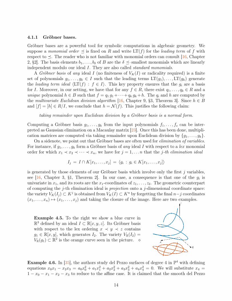
Example 4.5. To the right we show a blue curve inR3 defined by an ideal I ⊂ R[x, y, z]. Its Gröbner basiswith respect to the lex ordering x ≺ y ≺ z containsg1 ∈ R[x, y], which generates I2. The variety VR(I2) =VR(g1) ⊂ R2 is the orange curve seen in the picture. ⋄

Example 4.6. In [35], the authors study del Pezzo surfaces of degree 4 in P4 with definingequations x0x1 − x2x3 = a0x

20 + a1x

21 + a2x

22 + a3x

23 + a4x

24 = 0. We will substitute x4 =

1 − x0 − x1 − x2 − x3 to reduce to the affine case. It is claimed that the smooth del Pezzo

14

surfaces of this form are those for which the parameters a0, . . . , a4 lie outside the hypersurfaceH = {a0a1a2a3a4(a0a1 − a2a3) = 0}. This hypersurface is the projection of the variety{

(a, x) ∈ Q5 ×Q4 : x0x1 − x2x3 =3∑

i=0

aix2i + a4

(1−

3∑i=0

xi

)2= 0 and rank(J) < 2

}

onto Q5. Here J is the 2 × 4 Jacobian matrix of our two equations with respect to the 4variables x0, x1, x2, x3. The defining equation of H is computed in Macaulay2 [24] as follows:

R = QQ[x_0..x_3,a_0..a_4]x_4 = 1-x_0-x_1-x_2-x_3I = ideal( x_0*x_1-x_2*x_3 , a_0*x_0^2 + a_1*x_1^2 + a_2*x_2^2 + a_3*x_3^2 + a_4*x_4^2 )M = submatrix( transpose jacobian I , 0..3 )radical eliminate( I+minors(2,M) , {x_0,x_1,x_2,x_3} )

The work behind the final command is a Gröbner basis computation. ⋄

Remark 4.7. In a numerical setting, it is better to use border bases or more general basesto avoid the amplification of rounding errors. Border bases use basis elements bi for B whoseelements satisfy a connectedness property, see for instance [36] for details. They do notdepend on a monomial order. For a summary and comparison between Gröbner bases andborder bases, see [44, Sections 3.3.1, 3.3.2]. Recently, in truncated normal form algorithms,bases are selected adaptively by numerical linear algebra routines, such as QR decompositionwith optimal column pivoting or singular value decomposition. This often yields a significantimprovement in terms of accuracy. See for instance Section 7.2 in [47].

4.2 Homotopy Continuation

The goal of this subsection is to briefly introduce the method of homotopy continuationfor solving polynomial systems. For more details, we refer to the standard textbook[41], and to the lecture notes and exercises from the 2021 Workshop on Software andApplications of Numerical Nonlinear Algebra, available at https://github.com/PBrdng/Workshop-on-Software-and-Applications-of-Numerical-Nonlinear-Algebra.

We set K = C and n = s. We think of F = (f1, . . . , fn) ∈ R as an element of afamily F of polynomial systems. The reader can replace F by any of the families seenin Section 3. A homotopy in F with target system F ∈ F and start system G ∈ F is acontinuous deformation of the map G = (g1, . . . , gn) : Cn → Cn into F , in such a way thatall systems obtained throughout the deformation are contained in F . For instance, WhenF ∈ F(d1, . . . , dn) as in Section 3.1 and G is any other system in F(d1, . . . , dn), a homotopyis H(x; t) = t ·F (x)+ (1− t) ·G(x), where t runs from 0 to 1. Indeed, for any fixed t∗ ∈ [0, 1]the degrees of the equations remain bounded by (d1, . . . , dn), hence H(x; t∗) ∈ F(d1, . . . , dn).

The method of homotopy continuation for solving the target system f1 = · · · = fn = 0assumes that a start system g1 = · · · = gn = 0 can easily be solved. The idea is thattransforming G continuously into F via a homotopy H(x; t) in F transforms the solutionsof G continuously into those of F . The following example appears in [48].

15

00.5

1

−5051015

−10

−5

0

5

10

t

Re(x)

Im(x

)

Figure 5: The twelfth roots of unity travel to 1, . . . , 12 along continuous paths.

Example 4.8 (n = s = 1,F = F(12)). Let f = (x− 1)(x− 2) · · · (x− 12) be the Wilkinsonpolynomial of degree 12. We view f = 0 as a member of F(12) and choose the start systemg = x12 − 1 = 0. The start solutions, i.e. the solutions of g = 0, are the twelfth roots ofunity. The solutions of H(x; t) = t · f(x) + (1− t) · g(x) travel from these roots of unity tothe integers 1, . . . , 12 as t moves from 0 to 1. This is illustrated in Figure 5. ⋄

More formally, if H(x; t) = (h1(x; t), . . . , hn(x; t)) is a homotopy with t ∈ [0, 1], thesolutions describe continuous paths x(t) satisfying H(x(t); t) = 0. Taking the derivativewith respect to t gives the Davidenko differential equation

dH(x(t), t)

dt= Jx · x(t) +

∂H

∂t(x(t), t) = 0, with Jx =

(∂hj

∂xi

)j,i

. (11)

Each start solution x∗ of g1 = · · · = gn = 0 gives an initial value problem with x(0) = x∗,and the corresponding solution path x(t) can be approximated using any numerical ODEmethod. This typically leads to a discretization of the solution path, see the blue dots inFigure 5. The solutions of the target system f1 = · · · = fn = 0 are obtained by evaluatingthe solution paths at t = 1. The following are important practical remarks.

Avoid the discriminant. Each of the families seen in Section 3 has a subvariety ∇F ⊂ Fconsisting of systems with non-generic behavior in terms of their number of solutions. Thissubvariety is sometimes referred to as the discriminant of F , for reasons alluded to in thebeginning of Section 3. When the homotopy H(x; t) crosses ∇F , i.e. H(x; t∗) ∈ ∇F for somet∗ ∈ [0, 1), two or more solution paths collide at t∗, or some solution paths diverge. Thisis not allowed for the numerical solution of (11). Fortunately, crossing ∇F can be avoided.The discriminant ∇F has complex codimension at least one, hence real codimension at leasttwo. Since the homotopy t 7→ H(x; t) describes a one-real-dimensional path in F , it is alwayspossible to go around the discriminant. See for instance [41, Section 7]. When the targetsystem F belongs to the discriminant, end games are used to deal with colliding/divergingpaths at t = 1 [41, Section 10]. Note that this discussion implies that the number of paths

16

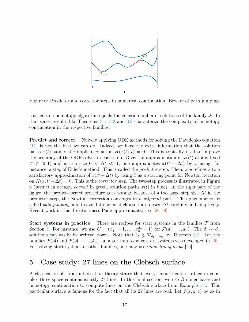
Figure 6: Predictor and corrector steps in numerical continuation. Beware of path jumping.

tracked in a homotopy algorithm equals the generic number of solutions of the family F . Inthat sense, results like Theorems 3.1, 3.3 and 3.8 characterize the complexity of homotopycontinuation in the respective families.

Predict and correct. Naively applying ODE methods for solving the Davidenko equation(11) is not the best we can do. Indeed, we have the extra information that the solutionpaths x(t) satisfy the implicit equation H(x(t), t) = 0. This is typically used to improvethe accuracy of the ODE solver in each step. Given an approximation of x(t∗) at any fixedt∗ ∈ [0, 1) and a step size 0 < ∆t ≪ 1, one approximates x(t∗ + ∆t) by x using, forinstance, a step of Euler’s method. This is called the predictor step. Then, one refines x to asatisfactory approximation of x(t∗ +∆t) by using x as a starting point for Newton iterationon H(x, t∗+∆t) = 0. This is the corrector step. The two-step process is illustrated in Figure6 (predict in orange, correct in green, solution paths x(t) in blue). In the right part of thefigure, the predict-correct procedure goes wrong: because of a too large step size ∆t in thepredictor step, the Newton correction converges to a different path. This phenomenon iscalled path jumping, and to avoid it one must choose the stepsize ∆t carefully and adaptively.Recent work in this direction uses Padé approximants, see [48, 49].

Start systems in practice. There are recipes for start systems in the families F fromSection 3. For instance, we use G = (xd1

1 − 1, . . . , xdnn − 1) for F(d1, . . . , dn). The d1 · · · dn

solutions can easily be written down. Note that G /∈ ∇d1,...,dn by Theorem 3.1. For thefamilies F(A) and F(A1, . . . ,An), an algorithm to solve start systems was developed in [26].For solving start systems of other families, one may use monodromy loops [20].

5 Case study: 27 lines on the Clebsch surfaceA classical result from intersection theory states that every smooth cubic surface in com-plex three-space contains exactly 27 lines. In this final section, we use Gröbner bases andhomotopy continuation to compute lines on the Clebsch surface from Example 1.4. Thisparticular surface is famous for the fact that all its 27 lines are real. Let f(x, y, z) be as in

17

(3). A line in R3 parameterized by (a1+ t · b1, a2+ t · b2, a3+ t · b3) is contained in our Clebschsurface if and only if f(a1 + t · b1, a2 + t · b2, a3 + t · b3) ≡ 0. The left hand side evaluates toa cubic polynomial in t with coefficients in the ring Z[a1, a2, a3, b1, b2, b3] = Z[a, b]:

f ( a1 + t · b1, a2 + t · b2, a3 + t · b3 ) = f1(a, b) · t3 + f2(a, b) · t2 + f3(a, b) · t+ f4(a, b).

The lines contained in the Clebsch surface satisfy

f1(a, b) = f2(a, b) = f3(a, b) = f4(a, b) = 0. (12)

We further reduce this to a system of s = 4 equations in n = 4 unknowns by removingthe redundancy in our parameterization of the line: we may impose a random affine-linearrelation among the ai and among the bi. We choose to substitute

a3 = −(7 + a1 + 3a2)/5, b3 = −(11 + 3b1 + 5b2)/7.

Implementations of Gröbner bases are available, for instance, in Maple [33] and in msolve

[7], which can be used in julia via the package msolve.jl. This is also available in thepackage Oscar.jl [38]. The following snippet of Maple code constructs our system (12) andcomputes a Gröbner basis with respect to the graded lexicographic monomial ordering witha1 ≻ a2 ≻ b1 ≻ b2. This basis consists of 23 polynomials g1, . . . , g23.

> f := 81*(x^3 + y^3 + z^3) - 189*(x^2*y + x^2*z + x*y^2 + x*z^2 + y^2*z + y*z^2)+ 54*x*y*z + 126*(x*y + x*z + y*z) - 9*(x^2 + y^2 + z^2) - 9*(x + y + z) + 1:

> f := expand(subs({x = t*b[1] + a[1], y = t*b[2] + a[2], z = t*b[3] + a[3]}, f)):> f := subs({a[3] = -(7 + a[1] + 3*a[2])/5, b[3] = -(11 + 3*b[1] + 5*b[2])/7}, f):> ff := coeffs(f, t):> with(Groebner):> GB := Basis({ff}, grlex(a[1], a[2], b[1], b[2]));> nops(GB); ----> output: 23

The set of standard monomials is the first output of the command NormalSet. It consistsof 27 elements, and the multiplication matrix with respect to a1 in this basis is constructedusing MultiplicationMatrix:

> ns, rv := NormalSet(GB, grlex(a[1], a[2], b[1], b[2])):> nops(ns); ----> output: 27> Ma1 := MultiplicationMatrix(a[1], ns, rv, GB, grlex(a[1], a[2], b[1], b[2])):

This is a matrix of size 27× 27 whose eigenvectors reveal the solutions (Theorem 4.1).We now turn to julia and use msolve to compute the 27 lines on {f = 0} as follows:

using OscarR,(a1,a2,b1,b2) = PolynomialRing(QQ,["a1","a2","b1","b2"])I = ideal(R, [-189*b2*b1^2 - 189*b2^2*b1 + 27*(11 + 3*b1 + 5*b2)*b1^2 + ...A, B = msolve(I)

The output B contains 4 rational coordinates (a1, a2, b1, b2) of 27 lines which approximatethe solutions. To see them in floating point format, use for instance

18

Figure 7: Two views on the Clebsch surface with three of its 27 lines.

[convert.(Float64,convert.(Rational{BigInt},b)) for b in B]

We have drawn three of these lines on the Clebsch surface in Figure 7 as an illustration. Othersoftware systems supporting Gröbner bases are Macaulay2 [24], Magma [8] and Singular [25].

Homotopy continuation methods provide an alternative way to compute our 27 lines.Here we use the julia package HomotopyContinuation.jl [12].

using HomotopyContinuation@var x y z t a[1:3] b[1:3]f = 81*(x^3 + y^3 + z^3) - 189*(x^2*y + x^2*z + x*y^2 + x*z^2 + y^2*z + y*z^2)

+ 54*x*y*z + 126*(x*y + x*z + y*z) - 9*(x^2 + y^2 + z^2) - 9*(x + y + z) + 1fab = subs(f, [x;y;z] => a+t*b)E, C = exponents_coefficients(fab,[t])F = subs(C,[a[3];b[3]] => [-(7+a[1]+3*a[2])/5; -(11+3*b[1]+5*b[2])/7])R = solve(F)

The output is shown in Figure 8. There are 27 solutions, as expected. The last line indicatesthat a :polyhedral start system was used. In our terminology, this means that the systemwas solved using a homotopy in the family F(A1, . . . ,A4) from Section 3.3. The numberof tracked paths is 45, which is the mixed volume MV(A1, . . . ,A4) of this family. Thediscrepancy 27 < 45 means that our system F lies in the discriminant ∇A1,...,A4 . The 18‘missing’ solutions are explained in [4, Section 3.3]. The output also tells us that all solutionshave multiplicity one (this is the meaning of non-singular) and all of them are real.

Figure 8: The julia output when computing 27 lines on the Clebsch surface.

Other software implementing homotopy continuation are Bertini [2] and PHCpack [50].Numerical normal form methods are used in EigenvalueSolver.jl [5].

19

AcknowledgementsThe author was supported by a Veni grant from the Netherlands Organisation for ScientificResearch (NWO).

References[1] L. Baldi and B. Mourrain. Computing real radicals by moment optimization. In Proceedings of the 2021

on International Symposium on Symbolic and Algebraic Computation, pages 43–50, 2021.

[2] D. J. Bates, A. J. Sommese, J. D. Hauenstein, and C. W. Wampler. Numerically solving polynomialsystems with Bertini. SIAM, 2013.

[3] K. Batselier. A numerical linear algebra framework for solving problems with multivariate polynomials.PhD thesis, Faculty of Engineering, KU Leuven (Leuven, Belgium), 2013.

[4] M. Bender and S. Telen. Toric eigenvalue methods for solving sparse polynomial systems. Mathematicsof Computation, 91(337):2397–2429, 2022.

[5] M. R. Bender and S. Telen. Yet another eigenvalue algorithm for solving polynomial systems. arXivpreprint arXiv:2105.08472, 2021.

[6] D. N. Bernstein. The number of roots of a system of equations. Functional Analysis and its applications,9(3):183–185, 1975.

[7] J. Berthomieu, C. Eder, and M. Safey El Din. msolve: A library for solving polynomial systems. InProceedings of the 2021 on International Symposium on Symbolic and Algebraic Computation, pages51–58, 2021.

[8] W. Bosma, J. Cannon, and C. Playoust. The Magma algebra system. I. The user language. J. SymbolicComput., 24(3-4):235–265, 1997. Computational algebra and number theory (London, 1993).

[9] P. Breiding. An algebraic geometry perspective on topological data analysis. arXiv preprintarXiv:2001.02098, 2020.

[10] P. Breiding, T. Ö. Çelik, T. Duff, A. Heaton, A. Maraj, A.-L. Sattelberger, L. Venturello, and O. Yürük.Nonlinear algebra and applications. arXiv preprint arXiv:2103.16300, 2021.

[11] P. Breiding, K. Rose, and S. Timme. Certifying zeros of polynomial systems using interval arithmetic.arXiv preprint arXiv:2011.05000, 2020.

[12] P. Breiding and S. Timme. HomotopyContinuation.jl: A package for homotopy continuation in Julia.In International Congress on Mathematical Software, pages 458–465. Springer, 2018.

[13] C. Conradi, E. Feliu, M. Mincheva, and C. Wiuf. Identifying parameter regions for multistationarity.PLoS computational biology, 13(10):e1005751, 2017.

[14] D. A. Cox. Applications of polynomial systems, volume 134. American Mathematical Soc., 2020.

[15] D. A. Cox, J. B. Little, and D. O’Shea. Using algebraic geometry, volume 185. Springer Science &Business Media, 2006.

[16] D. A. Cox, J. B. Little, and D. O’Shea. Ideals, varieties, and algorithms: an introduction to compu-tational algebraic geometry and commutative algebra. Springer Science & Business Media, correctedfourth edition edition, 2018.

[17] J. Desjardins and R. Winter. Density of rational points on a family of del Pezzo surfaces of degree one.Advances in Mathematics, 405:108489, 2022.

[18] A. Dickenstein. Biochemical reaction networks: An invitation for algebraic geometers. In Mathematicalcongress of the Americas, volume 656, pages 65–83. Contemp. Math, 2016.

20

[19] J. Draisma, E. Horobeţ, G. Ottaviani, B. Sturmfels, and R. R. Thomas. The euclidean distance degreeof an algebraic variety. Foundations of computational mathematics, 16(1):99–149, 2016.

[20] T. Duff, C. Hill, A. Jensen, K. Lee, A. Leykin, and J. Sommars. Solving polynomial systems viahomotopy continuation and monodromy. IMA Journal of Numerical Analysis, 39(3):1421–1446, 2019.

[21] D. Eisenbud and J. Harris. The geometry of schemes, volume 197. Springer Science & Business Media,2006.

[22] I. Z. Emiris and B. Mourrain. Computer algebra methods for studying and computing molecularconformations. Algorithmica, 25(2):372–402, 1999.

[23] J.-C. Faugère. A new efficient algorithm for computing Gröbner bases (F4). Journal of pure and appliedalgebra, 139(1-3):61–88, 1999.

[24] D. R. Grayson and M. E. Stillman. Macaulay2, a software system for research in algebraic geometry.Available at http://www.math.uiuc.edu/Macaulay2/.

[25] G.-M. Greuel, G. Pfister, and H. Schönemann. Singular—a computer algebra system for polynomialcomputations. In Symbolic computation and automated reasoning, pages 227–233. AK Peters/CRCPress, 2001.

[26] B. Huber and B. Sturmfels. A polyhedral method for solving sparse polynomial systems. Mathematicsof computation, 64(212):1541–1555, 1995.

[27] B. Huber and B. Sturmfels. Bernstein’s theorem in affine space. Discrete & Computational Geometry,17(2):137–141, 1997.

[28] E. Hubert and E. Rodriguez Bazan. Algorithms for fundamental invariants and equivariants. Mathe-matics of Computation, 91(337):2459–2488, 2022.

[29] Z. Kukelova, M. Bujnak, and T. Pajdla. Automatic generator of minimal problem solvers. In EuropeanConference on Computer Vision, pages 302–315. Springer, 2008.

[30] A. G. Kushnirenko. Newton polytopes and the Bézout theorem. Functional analysis and its applications,10(3):233–235, 1976.

[31] M. Laurent. Sums of squares, moment matrices and optimization over polynomials. In Emergingapplications of algebraic geometry, pages 157–270. Springer, 2009.

[32] D. Maclagan and B. Sturmfels. Introduction to tropical geometry, volume 161. American MathematicalSociety, 2021.

[33] Maplesoft, a division of Waterloo Maple Inc.. Maple.

[34] M. Michałek and B. Sturmfels. Invitation to nonlinear algebra, volume 211. American MathematicalSoc., 2021.

[35] V. Mitankin and C. Salgado. Rational points on del Pezzo surfaces of degree four. arXiv preprintarXiv:2002.11539, 2020.

[36] B. Mourrain. A new criterion for normal form algorithms. In International Symposium on AppliedAlgebra, Algebraic Algorithms, and Error-Correcting Codes, pages 430–442. Springer, 1999.

[37] S. Müller, E. Feliu, G. Regensburger, C. Conradi, A. Shiu, and A. Dickenstein. Sign conditions forinjectivity of generalized polynomial maps with applications to chemical reaction networks and realalgebraic geometry. Foundations of Computational Mathematics, 16(1):69–97, 2016.

[38] Oscar – open source computer algebra research system, version 0.9.0, 2022.

[39] M. Sala. Gröbner bases, coding, and cryptography: a guide to the state-of-art. In Gröbner Bases,Coding, and Cryptography, pages 1–8. Springer, 2009.

21

[40] A. J. Sommese, J. Verschelde, and C. W. Wampler. Numerical decomposition of the solution sets ofpolynomial systems into irreducible components. SIAM Journal on Numerical Analysis, 38(6):2022–2046, 2001.

[41] A. J. Sommese, C. W. Wampler, et al. The Numerical solution of systems of polynomials arising inengineering and science. World Scientific, 2005.

[42] B. Sturmfels. Solving systems of polynomial equations. Number 97. American Mathematical Soc., 2002.

[43] B. Sturmfels. Beyond linear algebra. arXiv preprint arXiv:2108.09494, 2021.

[44] S. Telen. Solving Systems of Polynomial Equations. PhD thesis, KU Leuven, Leuven, Belgium, 2020.available at https://simontelen.webnode.page/publications/.

[45] S. Telen. Introduction to toric geometry. arXiv preprint arXiv:2203.01690, 2022.

[46] S. Telen, B. Mourrain, and M. Van Barel. Solving polynomial systems via truncated normal forms.SIAM Journal on Matrix Analysis and Applications, 39(3):1421–1447, 2018.

[47] S. Telen and M. Van Barel. A stabilized normal form algorithm for generic systems of polynomialequations. Journal of Computational and Applied Mathematics, 342:119–132, 2018.

[48] S. Telen, M. Van Barel, and J. Verschelde. A robust numerical path tracking algorithm for polynomialhomotopy continuation. SIAM Journal on Scientific Computing, 42(6):A3610–A3637, 2020.

[49] S. Timme. Mixed precision path tracking for polynomial homotopy continuation. Advances in Compu-tational Mathematics, 47(5):1–23, 2021.

[50] J. Verschelde. Algorithm 795: Phcpack: A general-purpose solver for polynomial systems by homotopycontinuation. ACM Transactions on Mathematical Software (TOMS), 25(2):251–276, 1999.

[51] C. W. Wampler and A. J. Sommese. Numerical algebraic geometry and algebraic kinematics. ActaNumerica, 20:469–567, 2011.

Author’s address:

Simon Telen, CWI Amsterdam simon.telen@cwi.nl

22